Embed Size (px)
Citation preview
Estimating the consequential cost of
bovine TB incidents on cattle farmers in
the High Risk & Edge Areas of England &
High and Intermediate TB Areas of Wales
Final Report for Defra
June 2020
Prepared by
Andrew Barnes1, Andrew Moxey2, Sarah Brocklehurst3, Alyson Barratt1, Iain McKendrick3, Giles Innocent3, Bouda Ahmadi4
1 Scotland's Rural College 2 Pareto Consulting 3 Biomathematics & Statistics Scotland, part of the James Hutton Institute 4 Food and Agriculture Organization
The project was led by SRUC working with Biomathematics and Statistics Scotland
(BioSS, part of the James Hutton Institute), Pareto Consulting (an agricultural
economics consultant) and Pexel (a market research company).
The project team wishes to record its gratitude for the support of various public and
private organisations in helping to complete this project, but especially to the
individual farmers who contributed to the questionnaire design and participated in the
survey: their willingness to revisit what were often traumatic experiences was the
essential basis for the project’s results.
Contents
Executive Summary ............................................................................................................... i
1.0 Introduction .................................................................................................................... 1
2.0 Rapid Literature Review .................................................................................................. 1
3.0 Sampling Frame design ................................................................................................. 4
4.0 Questionnaire design ..................................................................................................... 6
5.0 Survey implementation ................................................................................................... 7
6.0 Data processing and Statistical Methods ...................................................................... 11
6.1 Preliminary Survey Data Processing ......................................................................... 11
6.2 APHA data and further Survey Data Processing ....................................................... 12
6.3 Derivation of Test Load Coefficient ........................................................................... 13
6.4 Statistical Analysis Methods for the Results .............................................................. 14
7.0 Results ......................................................................................................................... 16
7.1 Headline results ........................................................................................................ 16
7.2 Distribution of Costs by Key Sampling Categories .................................................... 22
7.3 Impacts beyond the end of the breakdown ............................................................... 36
8.0 Conclusions ................................................................................................................. 38
8.1 Cost variation and drivers ......................................................................................... 38
8.2 Comparison with other estimates .............................................................................. 39
8.3 Reliance on self-reporting ......................................................................................... 40
8.4 Longer-term effects .................................................................................................. 41
8.5 Reflective recommendations ..................................................................................... 42
9 References ..................................................................................................................... 44
Annex A: Rapid Literature Review....................................................................................... 45
Annex B: Proposed Approach to Sampling ......................................................................... 58
Annex C: Telephone questionnaire & letter ......................................................................... 68
Annex D: Tables determining the pool for contacts letters and the fine and course grouping
for target quotas .................................................................................................................. 80
Annex E: Sources used to convert physical to financial values ........................................... 96
Annex F: Updated data provided to project by APHA – Oct 2019 ........................................ 97
Parish Area Table ............................................................................................................ 97
ParishTestingInterval Table ............................................................................................. 97
HerdData Table ............................................................................................................... 98

HerdTestingData Table ................................................................................................... 99
BreakdownData Table ................................................................................................... 101
Annex G: Data linked or derived from APHA data ............................................................. 106
i
Executive Summary
A bovine tuberculosis (bTB) breakdown has a number of direct and indirect impacts on cattle
farms. Whereas direct impacts, in the form of slaughtered animals, are routinely monitored
and compensated for, other costs arising as a consequence of a breakdown are not.
A small number of previous studies have attempted to identify and quantify these
'consequential' costs. However, no such study has been undertaken recently and there is a
need to update available cost estimates. Defra, the Welsh Government and the Scottish
Government jointly commissioned this project, led by SRUC, to conduct a large-scale
telephone survey of a statistically representative sample of farms.
The main focus of the survey was on generating estimates for the uncompensated and within-
breakdown costs arising from having to comply with policy requirements. Although the
experience of a bTB breakdown can impose mental health costs, these were not within the
remit of this study. Similarly, whilst lingering effects on production and management can
extend costs beyond the end-date of a breakdown, quantification of these impacts was also
beyond this study. Nevertheless, some qualitative insights were gleaned into wider impacts,
and these suggest possible topics for future studies.
The questionnaire used for the survey was based on a literature review, expert opinion and
valuable feedback provided by farmers via a focus group and iterative piloting of draft versions
of the questionnaire. Importantly, this process revealed that questions about costs needed to
explicitly ask about different cost items (e.g. labour, feed, bedding) and about different events
causing them (e.g. testing, isolating, movement restrictions). That is, the questionnaire had to
be structured to help respondents think-through how they had been affected. In addition,
farmers were given prior written notification of the types of questions they would be asked,
and encouraged to refer to farm records (they were subsequently asked if they had done so,
and how confident they were in their answers).
We employed data provided by the Animal and Plant Health Agency (APHA) to design a
sampling frame based on a six-way classification of breakdowns, which was then used to
collect data on farms that had suffered a bTB breakdown between the periods 1st January
2012 and 31st October 2018. The survey was administered between August and October
2019. This led to a final sample achieved of 1,604 farmers located in the High Risk and Edge
areas of England and the High (HTBA) and Intermediate (ITBA) TB areas of Wales. An
updated augmented data set was subsequently provided by APHA which was further analysed
and processed extensively to get additional variables of interest for all breakdowns from 1st
January 2012, such as estimation of a test load coefficient and variables relating to isolating
inconclusive reactors and reactors. This was then linked into the survey data to obtain a final
data set for analyses.
The results show that the composition and magnitude of consequential costs vary greatly
across breakdowns. Mainly this is due to a) farm characteristics, such as type and size of
business, and b) timing, size and duration of these outbreaks. The mean is a very misleading
summary statistic to use when the data are skewed, as it will be highly influenced by large
values. We instead present the median as well as the mean, as this provides a more accurate
picture of costs for such skewed data. Moreover, we would recommend focusing on median
values of costs across different classifications.
Total costs of a breakdown had a median value of c.£6,600 with an interquartile range of
c.£20,800 across all farms in the survey. This illustrates the wide variance in costs found
across the survey sample. In particular, not all farms experience all categories of cost, and
costs increase with herd size (reflecting the scale effects of handling and maintaining more
animals), breakdown duration (reflecting the increasing effort both of complying with testing
and of coping with movement restrictions) and with the number of animals compulsorily
slaughtered (reflecting disruption to planned production). For example, across England and
Wales median total costs for large herds (>300 cattle) are c.£18,600 whilst those for very small
herds (1-50 cattle) are c.£1,700; median total costs for long breakdowns (>273 days) are
c.£16,000, those for very short breakdowns (≤150 days) are c.£4,600. On average, testing,
movement restrictions and output losses account for almost two-thirds of total costs. Whilst
such costs are not surprising, by generating estimates from a large and statistically
representative sample, the survey has updated but also improved upon previous estimates of
consequential costs.
The questionnaire was mostly quantitative in nature and focused on within-breakdown costs.
However, some qualitative insights were gleaned into longer-term consequences of a
breakdown. These tended to emphasise the significant psychological or emotional burden
from a breakdown, but also the implications on future ambitions for growth of the beef or dairy
enterprise, in terms of loss of productivity. Whilst quantifying these additional costs was not
within the remit of this work, we recommend further research on this to help compose a more
comprehensive picture of breakdown impacts.
Feedback during the process of devising the questionnaire and from presenting survey
findings to stakeholders indicated some concern about the reliance of this methodology on
self-reporting of costs. Specifically, there was some concern that not all farmers will
necessarily have a good understanding or records of actual costs incurred. Although the large
sample size and the care taken in designing and administering the questionnaire should
reduce the proportion of farmers falling into this category whose data are included, thus
mitigating any effect on the overall results, these concerns are valid. Greater confidence in
estimates may require more routine, on-going monitoring of costs. For example, perhaps

independent recording/auditing of costs in real-time for a proportion of breakdowns as they
unfold. This could, however, entail significant effort.
1
1.0 Introduction
A bovine tuberculosis (bTB) breakdown has a number of direct and indirect cost impacts on
affected cattle farms. Whereas direct impacts in the form of culled animals are routinely
monitored and compensated for, other costs arising as a consequence of a breakdown are
not. For example, the need for additional labour, feed and bedding needed to isolate animals
reacting to the skin test and/or for animals to be kept longer due to movement restrictions.
A small number of previous studies have attempted to identify and quantify these
'consequential' costs (e.g. Bennett et al., 2004; Butler et al., 2010). The majority of these
studies have been commissioned by Defra (formerly MAFF). However, no such study has
been undertaken recently and there is an on-going need to update available estimates of
consequential costs. Hence Defra, the Welsh Government and Scottish Government jointly
commissioned a project to conduct a telephone survey of a statistically representative sample
of farms that have suffered a bTB breakdown.
Undertaking the survey involved using data held by the Animal and Plant Health Agency
(APHA) on bTB breakdowns to design a sampling frame, designing a questionnaire suitable
to be administered by telephone, and then applying appropriate analytical techniques to the
combined APHA data and survey results. The remainder of this report summarises the
methodology followed and findings generated. Some supporting material is contained in
Annexes to the report. In addition a 'cost-calculator' was developed based on these data.
This will allow government analysts to query the survey data structured by various strata based
on classifications of key APHA variables, such as herd size and type.
The main focus of the survey was on generating estimates for the uncompensated and within-
breakdown costs arising from having to comply with policy requirements. Although the
experience of a bTB breakdown can impose mental health costs, these were not within the
remit of this study. Similarly, whilst lingering effects on production and management can
extend costs beyond the end-date of a breakdown, quantification of these impacts was also
beyond this study. Nevertheless, some qualitative insights were gleaned into wider impacts,
and these suggest possible topics for future studies.
2.0 Rapid Literature Review
To inform design of both the sampling frame and the telephone questionnaire, a rapid literature
review was undertaken to identify key cost variables (see Annex A). This was based on using
a set of keywords to search various on-line databases for relevant academic and grey
literature. The resulting short-list of reports and papers of specific interest generated a range
of cost categories, the completeness and relevance of which were validated by consultation
with a number of national and international experts.
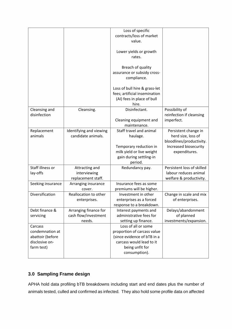
Table 1 summarises the compiled categories from the literature, listing discrete events within
a breakdown and their cost consequences over both the short-term and the longer-term.
The longer-term includes a variety of ways in which farming systems are forced to move away
from their pre-breakdown configurations. For example, switching to lower and more volatile
spot markets rather than forward contracts, persistent changes to the size and productivity of
herds due to difficulties in finding suitable replacement animals and/or having to carry
additional stock to ensure maintenance of the breeding herd, and difficulties in maintaining
productivity due to enforced staffing changes. All of these effects are noted in the literature,
but are acknowledged as difficult to quantify.
Shorter-term, within-breakdown costs are easier (but still not necessarily straightforward) to
quantify and fall into three types: staff time (labour) spent on arranging and undertaking
additional tasks; additional expenditure on other inputs, notably feed and bedding, as a
consequence of having to comply with breakdown requirements; and loss of output value as
a result of either producing less and/or receiving lower prices.
Each of these types of costs may arise from one or more event categories experienced over
the course of the breakdown. For example, some farms report significant costs from additional
labour effort to arrange testing and handling of animals, as well as costs around isolating
reactors and replacing animals. Similarly, if movement restrictions delay the timing of animal
sales, maintenance of animals on-farm for longer than planned necessarily incurs additional
labour and other inputs costs. Movement restrictions can also disrupt planned patterns of
buying and selling animals, leading to changes in both production volumes and prices
received, and therefore output losses.
Other event categories include cleansing and disinfection, but also arranging and servicing
(but not repaying the capital element of) additional debt finance incurred because of the
breakdown, and having to manage the laying-off and/or hiring of new staff. In all cases, the
counterfactual is one of no breakdown, and hence the focus is on costs that would not
otherwise have been incurred in the absence of the breakdown.
Importantly, not all farms will necessarily incur all types of costs during a given breakdown.
Moreover, previous studies highlight the heterogeneity of costs which can vary dramatically
according to circumstances, e.g. by size, timing and duration of breakdown plus endogenous
factors such as herd size, farming system, and trading pattern. This means that it is important
to present both the breakdown of different costs and the full distribution of cost estimates, not
simply global averages.
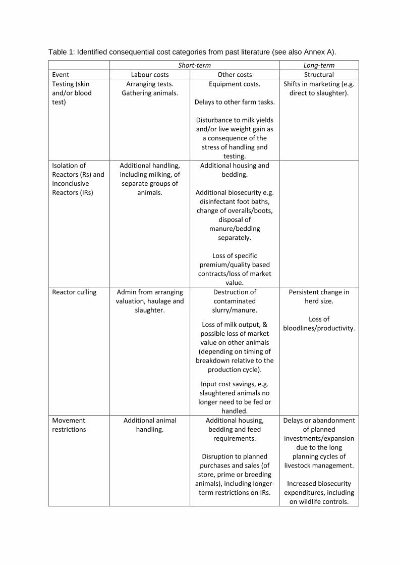
Table 1: Identified consequential cost categories from past literature (see also Annex A).
Short-term Long-term
Event Labour costs Other costs Structural
Testing (skin and/or blood test)
Arranging tests. Gathering animals.
Equipment costs.
Delays to other farm tasks.
Disturbance to milk yields and/or live weight gain as
a consequence of the stress of handling and
testing.
Shifts in marketing (e.g. direct to slaughter).
Isolation of Reactors (Rs) and Inconclusive Reactors (IRs)
Additional handling, including milking, of separate groups of
animals.
Additional housing and bedding.
Additional biosecurity e.g.
disinfectant foot baths, change of overalls/boots,
disposal of manure/bedding
separately.
Loss of specific premium/quality based contracts/loss of market
value.
Reactor culling Admin from arranging valuation, haulage and
slaughter.
Destruction of contaminated slurry/manure.
Loss of milk output, & possible loss of market value on other animals
(depending on timing of breakdown relative to the
production cycle).
Input cost savings, e.g. slaughtered animals no longer need to be fed or
handled.
Persistent change in herd size.
Loss of
bloodlines/productivity.
Movement restrictions
Additional animal handling.
Additional housing, bedding and feed
requirements.
Disruption to planned purchases and sales (of
store, prime or breeding animals), including longer-
term restrictions on IRs.
Delays or abandonment of planned
investments/expansion due to the long
planning cycles of livestock management.
Increased biosecurity
expenditures, including on wildlife controls.
Loss of specific contracts/loss of market
value.
Lower yields or growth rates.
Breach of quality
assurance or subsidy cross-compliance.
Loss of bull hire & grass-let fees; artificial insemination
(AI) fees in place of bull hire.
Cleansing and disinfection
Cleansing. Disinfectant.
Cleaning equipment and maintenance.
Possibility of reinfection if cleansing imperfect.
Replacement animals
Identifying and viewing candidate animals.
Staff travel and animal haulage.
Temporary reduction in milk yield or live weight gain during settling-in
period.
Persistent change in herd size, loss of
bloodlines/productivity. Increased biosecurity
expenditures.
Staff illness or lay-offs
Attracting and interviewing
replacement staff.
Redundancy pay. Persistent loss of skilled labour reduces animal welfare & productivity.
Seeking insurance Arranging insurance cover.
Insurance fees as some premiums will be higher.
Diversification Reallocation to other enterprises.
Investment in other enterprises as a forced
response to a breakdown.
Change in scale and mix of enterprises.
Debt finance & servicing
Arranging finance for cash flow/investment
needs.
Interest payments and administrative fees for
setting up finance.
Delays/abandonment of planned
investments/expansion.
Carcass condemnation at abattoir (before disclosive on-farm test)
Loss of all or some proportion of carcass value (since evidence of bTB in a
carcass would lead to it being unfit for consumption).
3.0 Sampling Frame design
APHA hold data profiling bTB breakdowns including start and end dates plus the number of
animals tested, culled and confirmed as infected. They also hold some profile data on affected
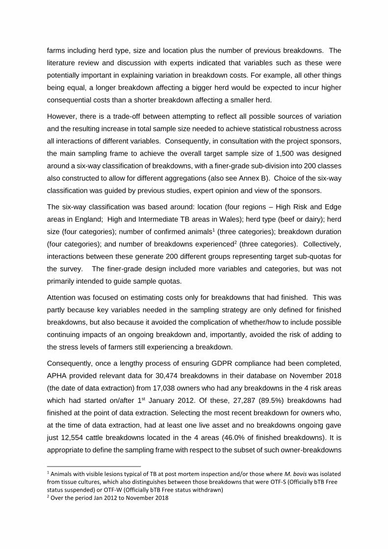
farms including herd type, size and location plus the number of previous breakdowns. The
literature review and discussion with experts indicated that variables such as these were
potentially important in explaining variation in breakdown costs. For example, all other things
being equal, a longer breakdown affecting a bigger herd would be expected to incur higher
consequential costs than a shorter breakdown affecting a smaller herd.
However, there is a trade-off between attempting to reflect all possible sources of variation
and the resulting increase in total sample size needed to achieve statistical robustness across
all interactions of different variables. Consequently, in consultation with the project sponsors,
the main sampling frame to achieve the overall target sample size of 1,500 was designed
around a six-way classification of breakdowns, with a finer-grade sub-division into 200 classes
also constructed to allow for different aggregations (also see Annex B). Choice of the six-way
classification was guided by previous studies, expert opinion and view of the sponsors.
The six-way classification was based around: location (four regions – High Risk and Edge
areas in England; High and Intermediate TB areas in Wales); herd type (beef or dairy); herd
size (four categories); number of confirmed animals1 (three categories); breakdown duration
(four categories); and number of breakdowns experienced2 (three categories). Collectively,
interactions between these generate 200 different groups representing target sub-quotas for
the survey. The finer-grade design included more variables and categories, but was not
primarily intended to guide sample quotas.
Attention was focused on estimating costs only for breakdowns that had finished. This was
partly because key variables needed in the sampling strategy are only defined for finished
breakdowns, but also because it avoided the complication of whether/how to include possible
continuing impacts of an ongoing breakdown and, importantly, avoided the risk of adding to
the stress levels of farmers still experiencing a breakdown.
Consequently, once a lengthy process of ensuring GDPR compliance had been completed,
APHA provided relevant data for 30,474 breakdowns in their database on November 2018
(the date of data extraction) from 17,038 owners who had any breakdowns in the 4 risk areas
which had started on/after 1st January 2012. Of these, 27,287 (89.5%) breakdowns had
finished at the point of data extraction. Selecting the most recent breakdown for owners who,
at the time of data extraction, had at least one live asset and no breakdowns ongoing gave
just 12,554 cattle breakdowns located in the 4 areas (46.0% of finished breakdowns). It is
appropriate to define the sampling frame with respect to the subset of such owner-breakdowns
1 Animals with visible lesions typical of TB at post mortem inspection and/or those where M. bovis was isolated from tissue cultures, which also distinguishes between those breakdowns that were OTF-S (Officially bTB Free status suspended) or OTF-W (Officially bTB Free status withdrawn) 2 Over the period Jan 2012 to November 2018
within well classified Beef and Dairy herds which are still live, classified as OTF-S, or OTF-W,
that started on or after 1st January 2014; this specification allowed identification of a potential
sampling frame of 9,978 owner-breakdowns. Although we were only sampling from these
owners with no ongoing breakdowns it is appropriate to include latest finished breakdowns for
1,853 other owners with ongoing breakdowns in the weighting of the sample, as these are
more likely to be owners with persistent breakdowns.
So, 7,992 breakdowns were selected from the 9,978, randomly sampled subject to quotas
required to be filled which were weighted based on a slightly larger subset of 11,831
breakdowns in the APHA dataset. Once exclusions were made to remove recent participants
in other surveys, this set reduced to 7,547 from which owners were sampled to be sent contact
letters.
This approach contrasts with previous published studies which were either explicitly case-
study based or relied on relatively small convenience samples.
4.0 Questionnaire design
Development of the survey questionnaire was a multi-stage iterative process, designed to
formulate a set of questions able to capture meaningful data from farmers during a telephone
call of around 20 to 25 minutes duration. Importantly, this process revealed that questions
about costs needed to explicitly ask about different cost items (e.g. labour, feed, bedding) and
about different events causing them (e.g. testing, isolating, movement restrictions). That is,
the questionnaire had to be structured to help respondents think through how they had been
affected.
First, a set of draft questions based on findings from the rapid literature review was presented
for discussion to a focus group of farmers. The focus group was held on 15th October 2018 at
Welshpool mart with the invaluable assistance of local NFU and NFU Cymru staff, particularly
in recruiting a cross-section of 12 farmers with experience of bTB breakdowns.
Discussions confirmed that the types of cost identified by the literature review were
appropriate, but that questions needed to be relatively simple and structured in such a way as
to help farmers think through how their businesses had been affected. In addition, it was made
clear that answering questions over the telephone would be easier if farmers had prior sight
of the questions and were encouraged to refer to farm records.
Second, in consultation with the project sponsors, a revised set of questions was devised and
circulated for comment to members of the focus group. Feedback from individual participants
confirmed that the revisions were an improvement and that the questionnaire was ready to be
tested over the phone.
Third, the revised questionnaire was administered by Pexel to eight volunteer farmers with
experience of bTB breakdowns. The volunteers were representative of a cross-section of
farming systems and were recruited via a variety of industry contacts, albeit subject to GDPR
constraints which slowed the process down considerably. Telephone interviews were
conducted during January and February 2019, with five of the volunteers agreeing to a follow-
up call to discuss how the questionnaire could be further improved. Participants were sent a
copy of the questions in advance together with background information on the project.
Feedback from Pexel and from participants confirmed that the questions were relevant and
mostly phrased and structured appropriately, although a few issues with the wording and the
order of questions were noted. More problematically, interviews took about twice as long as
had been hoped. Some concern was expressed about the ability of all farmers to accurately
answer all questions. Consequently, again in consultation with the project sponsors, individual
questions were edited slightly to improve clarity and prioritised to allow non-essential ones to
be dropped in order to shorten the overall questionnaire. For example, some attitudinal
questions intended to allow more detailed analysis were removed, as were questions about
the effects of breakdowns on neighbouring farms. In addition, whilst recognising that a bTB
breakdown exposes farmers to considerable stress, after consultation with project sponsors,
no attempt was made to explore mental health impacts.
The shortened questionnaire version was then formally piloted with 100 farms drawn from the
APHA-derived sampling frame. Farmers were sent a letter alerting them to their selection for
(voluntary) interview, explaining the purpose of the survey, how information would be used
and recommending/requesting that they review relevant farm records. Drafting of the letter
was itself an iterative process, partly due to uncertainty about GDPR requirements. The
questionnaire and contact letter were made available in both English and Welsh.
Pilot interviews were conducted during May 2019, with a final response of 32 completed
questionnaires achieved. This was judged to be a reasonable response rate (from a sample
of 100), and feedback from Pexel (plus listening to a selection of recorded interviews)
confirmed that farmers were able to engage confidently with the process, giving reassurance
that they would be able to provide reliable answers. Importantly, the average interview length
was now 23 minutes. On this basis, the questionnaire was judged as being ready to be
administered across the full survey (see Annex C for the questionnaire and the letter alerting
farmers to the project).
5.0 Survey implementation
A key criterion specified by Defra was that, due to the sensitive nature of the survey, all farmers
who received a letter about the project had to be phoned and offered the opportunity to actually
participate. This is in contrast to other surveys where, once sample quotas had been
achieved, calls to potential respondees would cease. Formally, rather than treating the group
of farmers with the correct characteristics who, having been contacted, did not opt-out as a
sampling frame from which a sample could be derived, it was necessary to treat this group as
the sample. To avoid over-sampling, which would not only increase project costs but also
reduce the remaining pool of farms available for other survey work (because once surveyed
for one purpose, farms are excluded from other government surveys for a period of time, to
reduce their survey burden), sampling consequently had to proceed cumulatively over iterated
stages.
This process entailed i) sending letters to an initial set of farmers, allowing sufficient time for
letters to arrive and be read, ii) attempting to contact all letter-recipients to arrange and then
conduct interviews, and iii) collating responses to identify how much progress towards sample
quotas had been achieved before repeating the cycle with another set of letters to a different
set of farmers. Three cycles of sampling were required, which added some complexity and
time delays to implementing the survey.
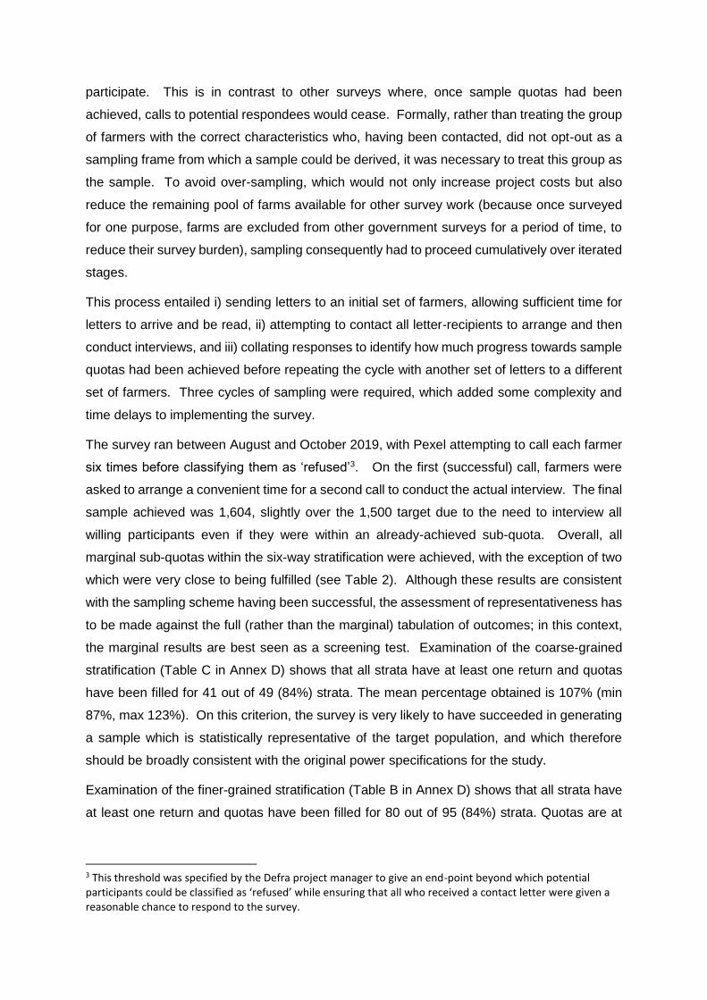
The survey ran between August and October 2019, with Pexel attempting to call each farmer
six times before classifying them as ‘refused’3. On the first (successful) call, farmers were
asked to arrange a convenient time for a second call to conduct the actual interview. The final
sample achieved was 1,604, slightly over the 1,500 target due to the need to interview all
willing participants even if they were within an already-achieved sub-quota. Overall, all
marginal sub-quotas within the six-way stratification were achieved, with the exception of two
which were very close to being fulfilled (see Table 2). Although these results are consistent
with the sampling scheme having been successful, the assessment of representativeness has
to be made against the full (rather than the marginal) tabulation of outcomes; in this context,
the marginal results are best seen as a screening test. Examination of the coarse-grained
stratification (Table C in Annex D) shows that all strata have at least one return and quotas
have been filled for 41 out of 49 (84%) strata. The mean percentage obtained is 107% (min
87%, max 123%). On this criterion, the survey is very likely to have succeeded in generating
a sample which is statistically representative of the target population, and which therefore
should be broadly consistent with the original power specifications for the study.
Examination of the finer-grained stratification (Table B in Annex D) shows that all strata have
at least one return and quotas have been filled for 80 out of 95 (84%) strata. Quotas are at
3 This threshold was specified by the Defra project manager to give an end-point beyond which potential participants could be classified as ‘refused’ while ensuring that all who received a contact letter were given a reasonable chance to respond to the survey.

least 75% full for 94 out of 95 (99%) strata and the mean percentage achieved is 107% (min
64%, max 147%). Again, these results indicate that the sample is robust.
Table 2. Counts for each of the classifiers used to form the 6-way strata, comparing number obtained (completed questionnaires only, n=1,604) to the target population and quotas.
Classifier Class counts in target
population
relative percent in
target population
counts needed
in survey sample
number obtained
percent of quota obtained
(quotas)
bTB risk area
E HRA 8361 70.67 1060 1131 106.7
W HTBA 1872 15.82 237 247 104.2
E Edge 1215 10.27 154 174 113.0
W ITBA4 383 3.24 49 52 106.1
herd type Beef 7452 62.99 945 1006 106.5
Dairy 4379 37.01 555 598 107.8
VSmall 2972 25.12 377 377 100.0
herd size Small 2948 24.92 374 402 107.5
Medium 2964 25.05 376 408 108.5
Large 2947 24.91 374 417 111.5
confirmed animals5
0 3949 33.38 501 523 104.4
1 4242 35.85 538 588 109.3
2-3 1998 16.89 253 264 104.4
>3 1642 13.88 208 229 110.1
duration
VShort 3081 26.04 391 377 96.4
Short 2852 24.11 362 402 111.1
Medium 2940 24.85 373 408 109.4
Long 2958 25 375 417 111.2
number of breakdowns for owner
1 4704 39.76 596 588 98.7
2 3754 31.73 476 532 111.8
>2 3373 28.51 428 433 101.2
Note1. For confirmed animals, 0 is OTF-S (Officially bTB Free status suspended) and >0 is OTF-W (Officially bTB Free status withdrawn). Note2: For the purposes of optimising survey sample representativeness, classifications for herd size and durations were derived in order to result in equal number of individuals in each class in the target population: For herd size, the category thresholds were <=56 (vsmall), 57-128 (small), 129-263 (medium), >=264(large). For duration, the category thresholds were <=150 (vshort), 150-184 (short), 186-273 (medium), >=273 (long). Note3. The number of breakdowns for the owner from 1st Jan 2012 up to and including the sampled breakdown.
4 EHRA (England High Risk Area); W HTBA (Wales High TB Area); E EDGE (England Edge Area); W ITBA (Wales Intermediate TB Area) 5 Animals with visible lesions typical of TB at post mortem inspection and/or those where M. bovis was isolated from tissue cultures
6.0 Data processing and Statistical Methods
6.1 Preliminary Survey Data Processing
Once the survey had been completed and responses linked to some key APHA breakdown
data variables, a complex and labour-intensive process of data cleansing and validation was
implemented. This involved a number of tasks, including identification and checking of outliers
and the conversion of physical units to financial values.
Outliers, responses to a given question that appear inconsistent with prior expectations and/or
other responses, may capture genuine answers but could alternatively reflect inadvertent
misinterpretation by respondents and/or data entry errors. Outliers were initially flagged via
both manual inspection and exploratory statistical analysis including preliminary statistical
modelling of all raw data columns against key explanatory variables; these were referred back
to Pexel, who reviewed interview recordings for data entry errors. Possible errors were where
answers were recorded for a different question or a decimal place was mis-positioned. Where
errors in recording were found, the outlier (for that question) was corrected, if possible, or
removed (i.e. recorded as a missing value), but where no error was identified, the value
remained in the dataset.
Furthermore, although survey participants were asked to give financial values for costs, where
they had experienced a cost but were unable to express it in financial terms they were invited
to answer in physical units. Examples include hours of labour or tonnes of feed. Use of such
information in the subsequent analysis required that it first be converted into financial values.
To do this, recourse was made to various published indices and/or industry sources for the
prices of cattle, labour, feed and chemical inputs (see Annex E) with values at the time of the
mid-point of the breakdown used to convert physical to estimated financial values. Finally, in
order to make them comparable over time all actual and estimated financial values were
converted to 2018 real-term values with conversion based on the year of the mid-point of the
breakdown.
Given that indices give only an average value, applying them to individual farms can introduce
some errors. For example, a given farm may normally achieve cattle prices above or below
the all-industry average. However, not using answers given in physical units would disregard
some information gathered by the survey, giving rise to larger biases. Moreover, converted
values are identified as such in the survey database, and hence the analysis can compare
their values to those recorded as financial values to identify any bias.
6.2 APHA data and further Survey Data Processing
A further data set (see Annex F) was supplied by APHA for all 34,1136 breakdowns that started
from 1st January 2012 which included additional variables to those that had been supplied for
the design of the sampling strategy. This included more information on previous owner
breakdowns, age and sex distribution of animals slaughtered, and the detailed production type
at the time of the breakdown. Most importantly, the herd testing data associated with all the
breakdowns were supplied, including some fields specially compiled by APHA for the project
relating to isolation of animals. The herd testing data were needed to estimate the ‘test load
coefficient’ - a multiplier to be used to estimate the full testing costs over the breakdown based
on the costs for the first test collected in the survey data.
Extensive processing and exploratory analysis of the data from the different data tables
(parish, herd, herd testing, breakdown) was carried out and pertinent variables (some derived)
were linked with the breakdown data (see Annex G) so that all the final data variables for
analysis were each a single measurement per breakdown. This data processing included
summarising the herd testing per breakdown in intuitive ways such as summing the number
of test intervals and test days over the breakdown, and so on. More complex calculations
included estimation, from the data provided by APHA in the herd testing data on isolation, of
the number of days during the breakdown when the herd needed to accommodate
inconclusive reactors (IRs) and the mean number of those animals on those days over the
breakdown. Similar estimates were made for reactors (Rs). The test load coefficient was also
calculated for each breakdown (see Section 6.3 below). For the purposes of subsequent
analysis, classifications of all continuous variables were formed based on the full APHA data
set of 31,127 finished breakdowns, by subdividing this population into 4 equal subsets (i.e.
quartiles). Where the data was too sparse for this, alternative classifications were derived. In
addition, for herd size variables the standard classifications used by Defra were derived. All of
these calculations were carried out for the full population of 34,113 breakdowns.
A subset of this dataset with all raw and derived data for each breakdown was then linked to
the survey data. A number of further variables were derived, including quantities representing
the extent of the overlap of calving, selling and buying-in with the breakdown (see Annex G).
A data processing program was written and run on the combined data set in order to calculate
the aggregated costs for all cost categories at the various levels of the categorisation hierarchy
(e.g. ‘time spent arranging animals for testing’, ‘all testing costs’, ‘all costs’ are three
categorisation levels, from ‘lower’ to ‘higher’ respectively). The indices used for converting
6 This is larger than the number cited in Section 3 due to these data being extracted at a later date and therefore covering a longer time period.
physical answers to financial costs and the conversion to 2018 real-term values were based
on the mid date of each breakdown. For all aggregates an index was also calculated which
indicated the proportion of missing data that contributed to the aggregate. This is to facilitate
any decision to omit these costs before subsequent analysis where this proportion is large.
For example, if all data is missing, this proportion will be 1, but the cost recorded in the data
set will be 0. This 0 can easily be identified and removed. All costs with this proportion>0.5,
regardless of value, are removed from the data used in exploratory analyses presented in the
Results section of this report and from the modelling exercise to derive the test load coefficient
(Section 6.3). The analysis presented in this report focuses on just the highest level of
aggregation– the total cost and the cost in the main categories – testing, movement
restrictions, outputs and so on, in which all financial and physical costs are combined.
However, all the detailed data that lead to these aggregates have been retained for possible
subsequent analysis.
Finally, a novel statistical approach to identifying any remaining outliers was applied to the
completed survey dataset. This was an iterative method which involved repeatedly fitting
linear mixed models (LMM) to each separate cost variable on a standardised log scale against
key APHA data. Fixed effects included in the LMM were herd type (diary, beef), status of the
breakdown (suspended, withdrawn),herd size (log transformed) and breakdown duration (log
transformed) and their interactions (these are implicitly assumed to be error-free) and
interactions up to 3 way, and random effect county used as a simple approach to modelling
spatial variation. The iterative process stopped when the resulting residuals were all below a
pre- specified threshold. This approach facilitated identification of some clearly erroneous
values and statistical outliers remaining in the data. These values have been removed from
the exploratory analyses presented in the Results section of this report and from the modelling
work to derive the test load coefficient.
The initial master data file for the survey data and APHA data was compiled in MS Excel 2016.
All survey and APHA data were processed and linked using bespoke programs written in
Genstat 18th Edition. Exploratory statistical analysis and modelling were carried out using
Genstat 18th Edition.
6.3 Derivation of Test Load Coefficient
Derivation of the method to calculate the test load coefficient first involved a pre-run of much
of the data processing described above. This was in order to calculate the aggregates for the
cost of first testing. Key APHA variables at the breakdown level were linked with the herd
testing data and used to work out which of the herd testing data rows corresponded to the ‘first
test’ or ‘testing interval’ and also how subsequent herd testing data rows could be combined
into a sequence of similarly defined discrete testing intervals. A number of variables were then
derived for the data rows for the first testing interval, e.g. total number of test data rows, total
test days (‘parts’), total number of cattle tested, for all tests or just for skin tests. This was then
linked to the cost data for the first test from the survey.
Extensive exploratory statistical analysis was carried out using LMMs of the relationship
between the first test cost reported from the survey and the potential explanatory variables
associated with herd testing as well as key APHA variables. It is overwhelmingly likely that
both the number of days on which tests take place and the number of cows tested will impact
on test costs, so various metrics associated with these terms, derived from the herd testing
data, were investigated and the impact of alternative approaches and these candidate
variables for number of days on which tests take place and the number of cows associated
with the first test was assessed. Linear mixed models (LMM) were fitted to the first test cost
(on the log scale). LMMs with different sets of covariates were investigated, with key APHA
variables such as herd size and herd type included prior to inclusion of candidate variables for
the number of days and number of cattle tested in order to explore the effects of ‘number of
test days’ and ‘number of animals tested’ after allowing for variation explained by the key
APHA variables.
The number of cattle tested was highly confounded with herd size but in deriving the test load
coefficient there is no interest in explaining variability in costs between breakdowns in different
herds; the test load coefficient is just intended to estimate the variability in costs within a herd,
within a single breakdown, between the first test and subsequent tests. Therefore in order to
reduce the effect of between herd breakdown variation, the test load coefficient was derived
from the LMM in which test days and number of cattle tested were fitted to the residuals
derived from the (previously fitted) LMM with key breakdown variables included (herd type and
maximum herd size over the period of the breakdown). That is to say, the ‘costs’ used to
calculate the test load coefficient were adjusted for herd type and herd size.
From the coefficients estimated from this model for the number of first day tests and cattle
tested, together with the number of test days and cattle tested for the first and for all
subsequent test intervals, the test load coefficient was calculated for each breakdown. This
coefficient was then multiplied by the cost of the first test to estimate the test costs over the
whole breakdown.
6.4 Statistical Analysis Methods for the Results
Basic exploratory analysis based on summary statistics and graphs is reported here for the
total financial costs and financial costs for the 9 different categories from the 1604 surveys
with APHA variables (raw and derived) linked in. Any total aggregated costs or any aggregated
costs for the 9 different categories judged to be gross outliers on the basis of application of
linear mixed models for detecting outliers (see above) were excluded prior to this analysis as
were aggregated costs for which the data entries in the survey that lead to them was more
than 50% missing (see above).
Summary statistics calculated over the breakdowns (owner/farmer) include quartiles (25th, 50th
and 75th percentiles) and the interquartile range, as well as the percentage (after exclusions)
of missing values and of zero costs. Means and standard deviations (SDs) are also presented
for completeness, but as the cost data are very skewed these can be misleading and less
helpful than the median (50th percentile) and the interquartile range, respectively. These
summary statistics are presented for the total financial cost and for financial costs for the 9
different categories. For total costs these summary statistics are also shown in tables and box-
plots classified by key variables that characterise the herd or the breakdown. The box-plot is
a modification of the box-and-whisker diagram for which the box spans the interquartile range
of the values, so that the middle 50% of the data lie within the box, with a line indicating the
median. The whiskers extend only to the most extreme data values within the inner "fences",
which are at a distance of 1.5 times the interquartile range beyond the quartiles, or the
maximum (minimum) value if that is smaller (larger). Individual outliers (any points outside
whiskers) are either plotted with a green cross or "far" outliers, beyond the outer "fences" (at
a distance of three times the interquartile range beyond the quartiles), are plotted with a red
cross. Note that as the data are very skewed and we have already eliminated gross outliers,
these remaining ‘outliers’ shown on the box-plots are considered to be plausible values.
Spearman’s rank correlations (ρ) were examined between all of the data associated with costs
(including all contributory components) and the APHA data variables. This statistic was chosen
as it is robust where data are skewed and will not be unduly influenced by outliers. For each
survey with no missing costs for the categories, the percentage that each cost category
contributed to the total costs was calculated and the average percentages are shown in a pie
chart. Pie charts were also shown for each decile of the total cost in order to show which cost
categories were dominant with varying overall cost.
7.0 Results
This section presents a series of Tables and Charts summarising different aspects of the results from the survey. The figures reported are per
breakdown, per business and include both selected percentiles and the mean whilst variation across the data is shown using both the inter-
quartile range and the standard deviation, as being relevant to the median and mean figures respectively. The percentage of missing values in
the data are also reported, to indicate how complete the data are. In addition, the last column shows the percentage of survey breakdowns
reporting zero costs for a given category.
7.1 Headline results
Tables 3, 4 and 5 below present some headline figures for the estimated costs of a breakdown. Table 3 summarises costs by category. For
example, the median cost of cleansing and disinfecting was £127 and the mean was £299. Significant variation across the sample is apparent,
seen both in the inter-quartile ranges and standard deviations, which, relative to the median or mean, are consistently large for all categories.
For example, the inter-quartile range for cleansing and disinfecting was £219 and the standard deviation was £593.
The values in each column of Table 3 cannot simply be summed to give an estimate of overall Total Costs. This is partly because of variation in
the number of missing values in each row but also because the percentile ranking of observations varies across the different rows, since the
ranking process is carried out independently for each cost category. Table 4 avoids these complications by simply presenting figures for the
overall total costs. For example, the median is £6,554 and the mean is £23,636. Again, there is considerable variation around these averages,
with an inter-quartile range of £20,768 and standard deviation of £52,233, reflecting differences across the sample in terms of farm and breakdown
characteristics. This variation is explored further in later Tables and Charts (boxplots) for different classifications within the dataset, such as herd
size and breakdown duration.
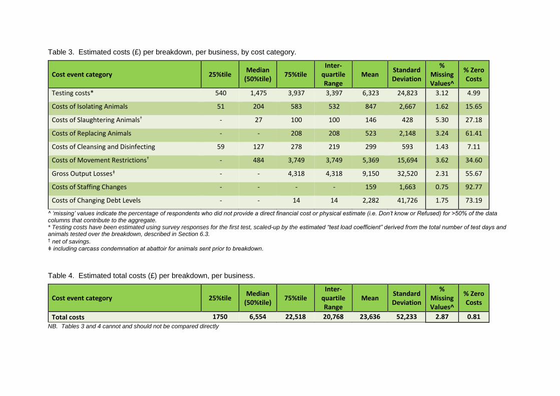
Table 3. Estimated costs (£) per breakdown, per business, by cost category.
Cost event category 25%tile Median
(50%tile) 75%tile
Inter-quartile Range
Mean Standard Deviation
% Missing Values^
% Zero Costs
Testing costs* 540 1,475 3,937 3,397 6,323 24,823 3.12 4.99
Costs of Isolating Animals 51 204 583 532 847 2,667 1.62 15.65
Costs of Slaughtering Animals† - 27 100 100 146 428 5.30 27.18
Costs of Replacing Animals - - 208 208 523 2,148 3.24 61.41
Costs of Cleansing and Disinfecting 59 127 278 219 299 593 1.43 7.11
Costs of Movement Restrictions† - 484 3,749 3,749 5,369 15,694 3.62 34.60
Gross Output Lossesǂ - - 4,318 4,318 9,150 32,520 2.31 55.67
Costs of Staffing Changes - - - - 159 1,663 0.75 92.77
Costs of Changing Debt Levels - - 14 14 2,282 41,726 1.75 73.19
^ ‘missing’ values indicate the percentage of respondents who did not provide a direct financial cost or physical estimate (i.e. Don’t know or Refused) for >50% of the data columns that contribute to the aggregate. * Testing costs have been estimated using survey responses for the first test, scaled-up by the estimated “test load coefficient” derived from the total number of test days and animals tested over the breakdown, described in Section 6.3. † net of savings.
ǂ including carcass condemnation at abattoir for animals sent prior to breakdown.
Table 4. Estimated total costs (£) per breakdown, per business.
Cost event category 25%tile Median
(50%tile) 75%tile
Inter-quartile Range
Mean Standard Deviation
% Missing Values^
% Zero Costs
Total costs 1750 6,554 22,518 20,768 23,636 52,233 2.87 0.81
NB. Tables 3 and 4 cannot and should not be compared directly
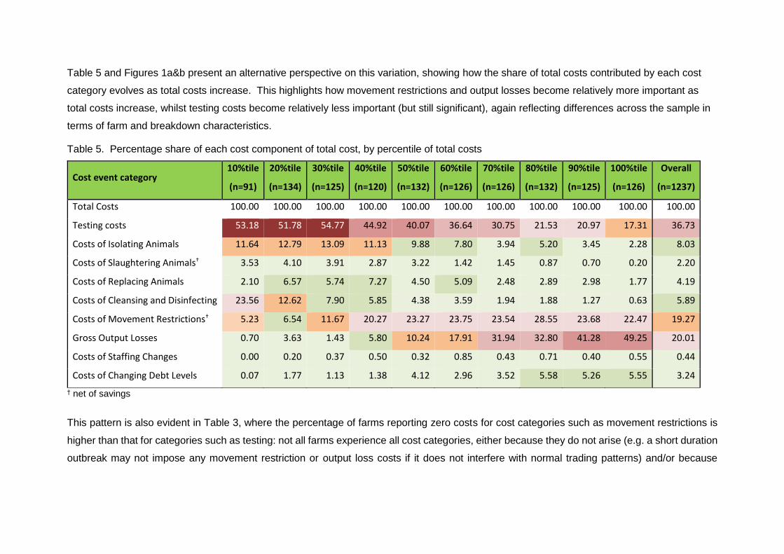
Table 5 and Figures 1a&b present an alternative perspective on this variation, showing how the share of total costs contributed by each cost
category evolves as total costs increase. This highlights how movement restrictions and output losses become relatively more important as
total costs increase, whilst testing costs become relatively less important (but still significant), again reflecting differences across the sample in
terms of farm and breakdown characteristics.
Table 5. Percentage share of each cost component of total cost, by percentile of total costs
Cost event category 10%tile
(n=91)
20%tile
(n=134)
30%tile
(n=125)
40%tile
(n=120)
50%tile
(n=132)
60%tile
(n=126)
70%tile
(n=126)
80%tile
(n=132)
90%tile
(n=125)
100%tile
(n=126)
Overall
(n=1237)
Total Costs 100.00 100.00 100.00 100.00 100.00 100.00 100.00 100.00 100.00 100.00 100.00
Testing costs 53.18 51.78 54.77 44.92 40.07 36.64 30.75 21.53 20.97 17.31 36.73
Costs of Isolating Animals 11.64 12.79 13.09 11.13 9.88 7.80 3.94 5.20 3.45 2.28 8.03
Costs of Slaughtering Animals† 3.53 4.10 3.91 2.87 3.22 1.42 1.45 0.87 0.70 0.20 2.20
Costs of Replacing Animals 2.10 6.57 5.74 7.27 4.50 5.09 2.48 2.89 2.98 1.77 4.19
Costs of Cleansing and Disinfecting 23.56 12.62 7.90 5.85 4.38 3.59 1.94 1.88 1.27 0.63 5.89
Costs of Movement Restrictions† 5.23 6.54 11.67 20.27 23.27 23.75 23.54 28.55 23.68 22.47 19.27
Gross Output Losses 0.70 3.63 1.43 5.80 10.24 17.91 31.94 32.80 41.28 49.25 20.01
Costs of Staffing Changes 0.00 0.20 0.37 0.50 0.32 0.85 0.43 0.71 0.40 0.55 0.44
Costs of Changing Debt Levels 0.07 1.77 1.13 1.38 4.12 2.96 3.52 5.58 5.26 5.55 3.24
† net of savings
This pattern is also evident in Table 3, where the percentage of farms reporting zero costs for cost categories such as movement restrictions is
higher than that for categories such as testing: not all farms experience all cost categories, either because they do not arise (e.g. a short duration
outbreak may not impose any movement restriction or output loss costs if it does not interfere with normal trading patterns) and/or because
farmers do not perceive any additional burden (e.g. if routine cleansing would have occurred anyway). Table 4 shows, however, that less than
1% of farms reported zero total costs.
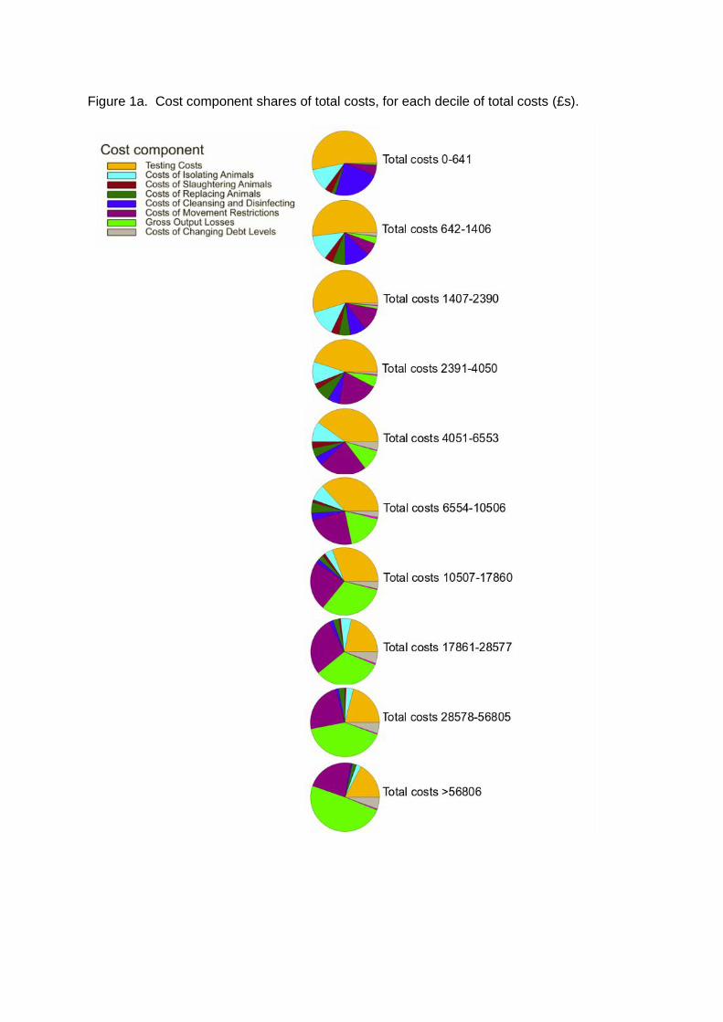
Figure 1a. Cost component shares of total costs, for each decile of total costs (£s).
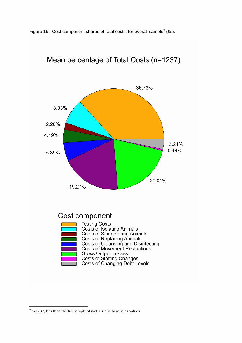
Figure 1b. Cost component shares of total costs, for overall sample7 (£s).
7 n=1237, less than the full sample of n=1604 due to missing values
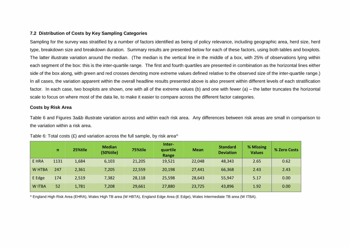
7.2 Distribution of Costs by Key Sampling Categories
Sampling for the survey was stratified by a number of factors identified as being of policy relevance, including geographic area, herd size, herd
type, breakdown size and breakdown duration. Summary results are presented below for each of these factors, using both tables and boxplots.
The latter illustrate variation around the median. (The median is the vertical line in the middle of a box, with 25% of observations lying within
each segment of the box: this is the inter-quartile range. The first and fourth quartiles are presented in combination as the horizontal lines either
side of the box along, with green and red crosses denoting more extreme values defined relative to the observed size of the inter-quartile range.)
In all cases, the variation apparent within the overall headline results presented above is also present within different levels of each stratification
factor. In each case, two boxplots are shown, one with all of the extreme values (b) and one with fewer (a) – the latter truncates the horizontal
scale to focus on where most of the data lie, to make it easier to compare across the different factor categories.
Costs by Risk Area
Table 6 and Figures 3a&b illustrate variation across and within each risk area. Any differences between risk areas are small in comparison to
the variation within a risk area.
Table 6: Total costs (£) and variation across the full sample, by risk area^
n 25%tile Median
(50%tile) 75%tile
Inter-quartile Range
Mean Standard Deviation
% Missing Values
% Zero Costs
E HRA 1131 1,684 6,103 21,205 19,521 22,048 48,343 2.65 0.62
W HTBA 247 2,361 7,205 22,559 20,198 27,441 66,368 2.43 2.43
E Edge 174 2,519 7,382 28,118 25,598 28,643 55,947 5.17 0.00
W ITBA 52 1,781 7,208 29,661 27,880 23,725 43,896 1.92 0.00
^ England High Risk Area (EHRA), Wales High TB area (W HBTA), England Edge Area (E Edge), Wales Intermediate TB area (W ITBA).
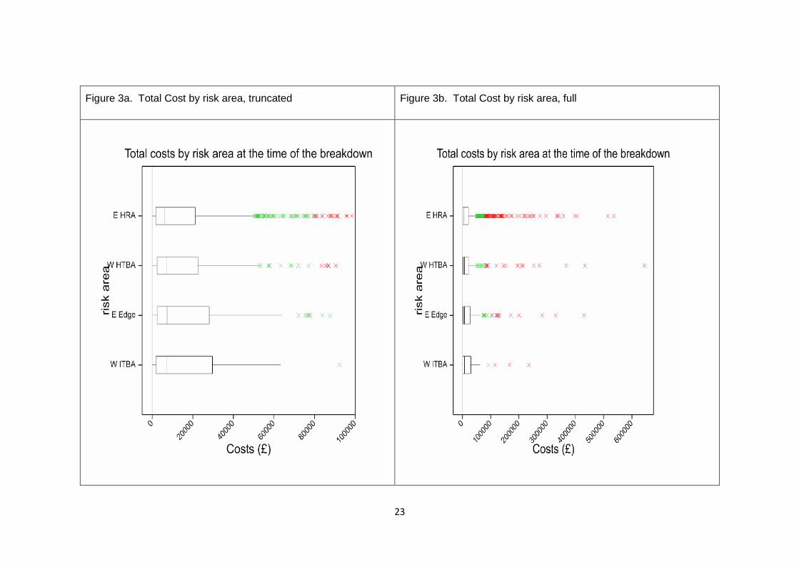
23
Figure 3a. Total Cost by risk area, truncated Figure 3b. Total Cost by risk area, full
24
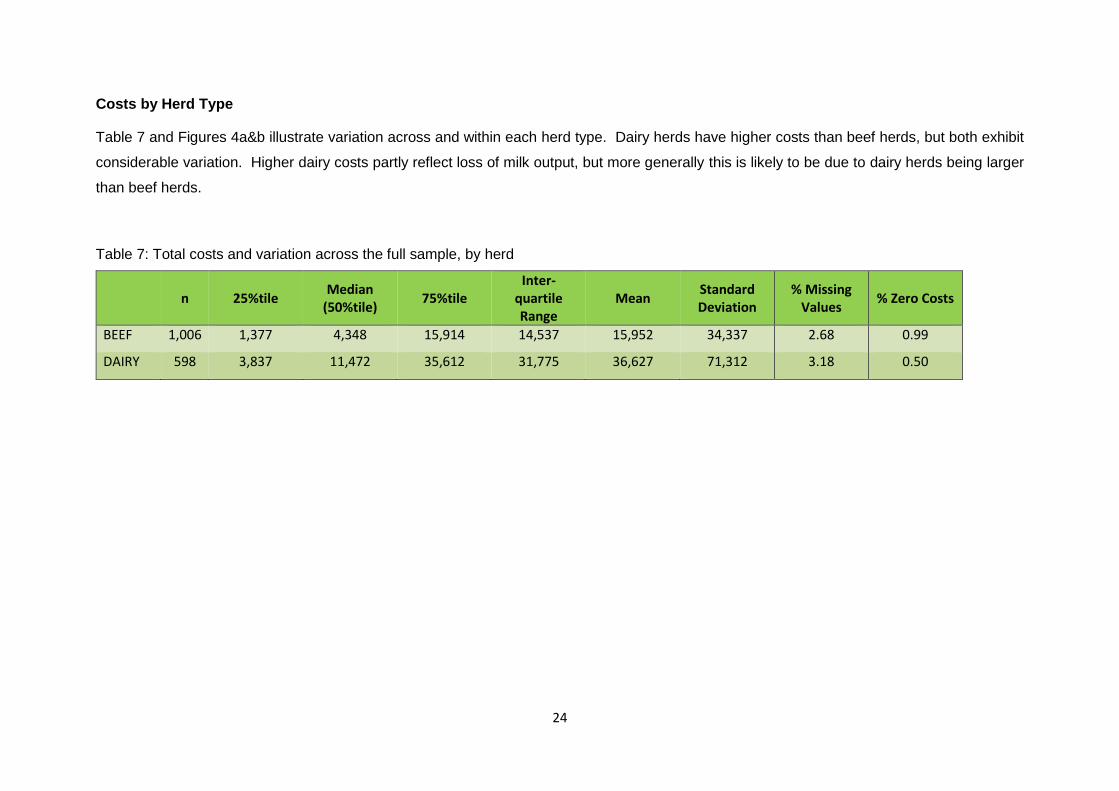
Costs by Herd Type
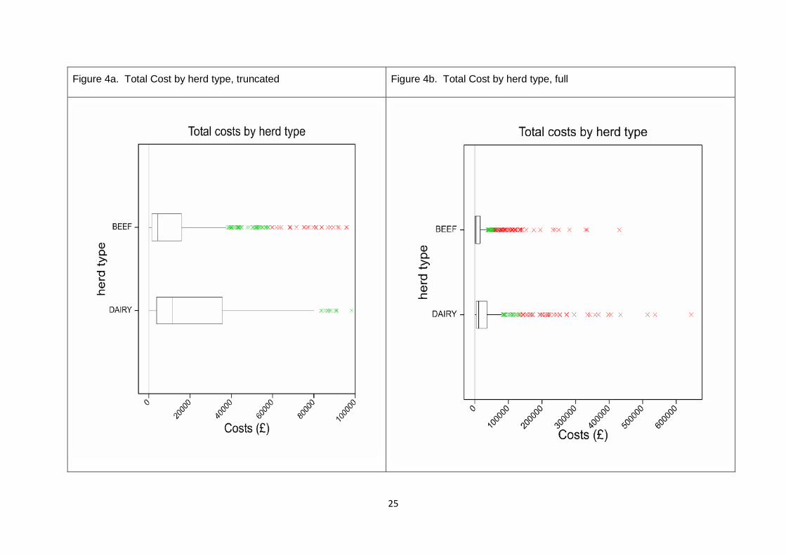
Table 7 and Figures 4a&b illustrate variation across and within each herd type. Dairy herds have higher costs than beef herds, but both exhibit
considerable variation. Higher dairy costs partly reflect loss of milk output, but more generally this is likely to be due to dairy herds being larger
than beef herds.
Table 7: Total costs and variation across the full sample, by herd
n 25%tile Median
(50%tile) 75%tile
Inter-quartile Range
Mean Standard Deviation
% Missing Values
% Zero Costs
BEEF 1,006 1,377 4,348 15,914 14,537 15,952 34,337 2.68 0.99
DAIRY 598 3,837 11,472 35,612 31,775 36,627 71,312 3.18 0.50
25
Figure 4a. Total Cost by herd type, truncated Figure 4b. Total Cost by herd type, full
26
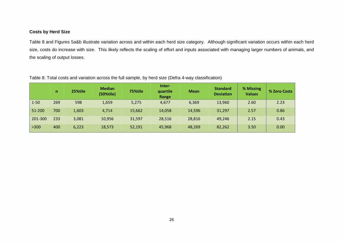
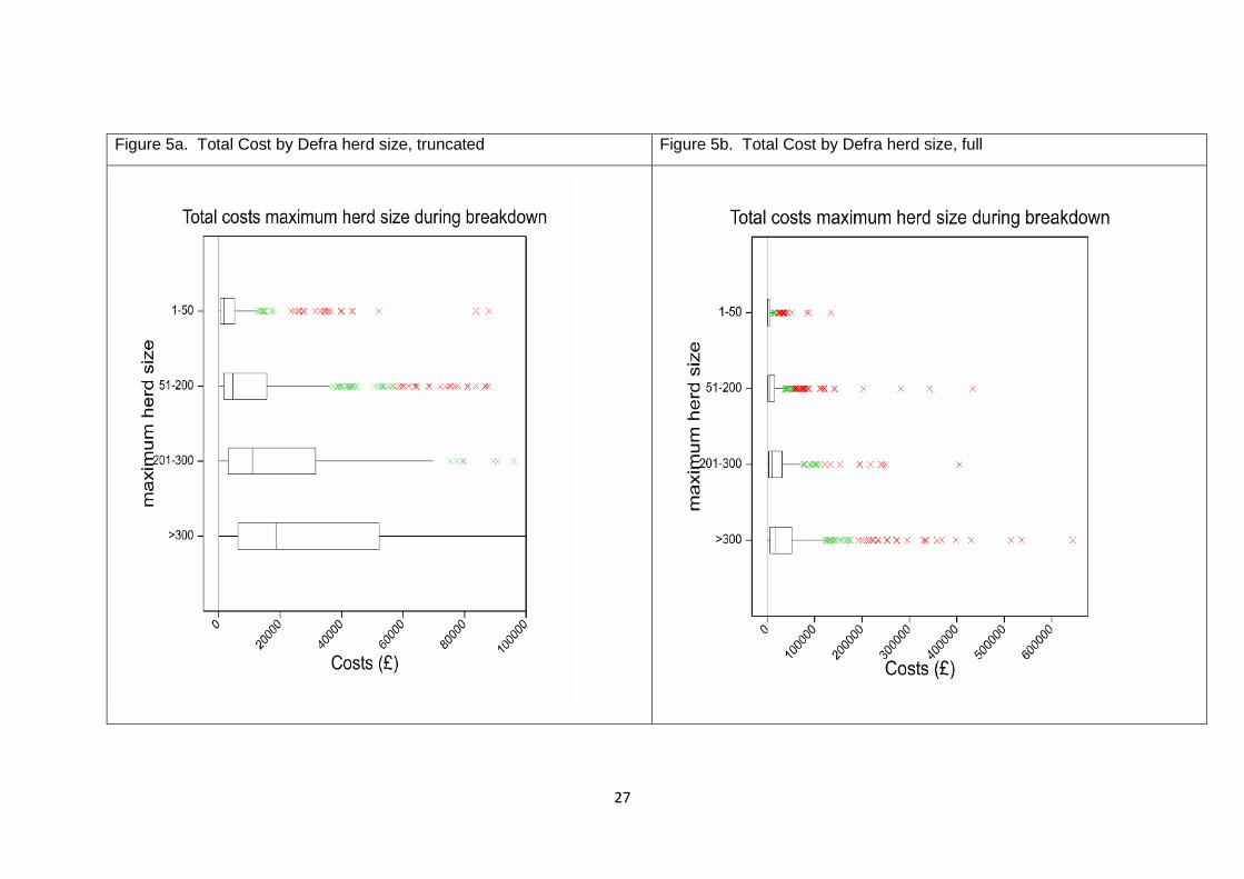
Costs by Herd Size
Table 8 and Figures 5a&b illustrate variation across and within each herd size category. Although significant variation occurs within each herd
size, costs do increase with size. This likely reflects the scaling of effort and inputs associated with managing larger numbers of animals, and
the scaling of output losses.
Table 8: Total costs and variation across the full sample, by herd size (Defra 4-way classification)
n 25%tile Median
(50%tile) 75%tile
Inter-quartile Range
Mean Standard Deviation
% Missing Values
% Zero Costs
1-50 269 598 1,659 5,275 4,677 6,369 13,960 2.60 2.23
51-200 700 1,603 4,714 15,662 14,058 14,596 31,297 2.57 0.86
201-300 233 3,081 10,956 31,597 28,516 28,816 49,246 2.15 0.43
>300 400 6,223 18,573 52,191 45,968 48,269 82,262 3.50 0.00
27
Figure 5a. Total Cost by Defra herd size, truncated Figure 5b. Total Cost by Defra herd size, full
28
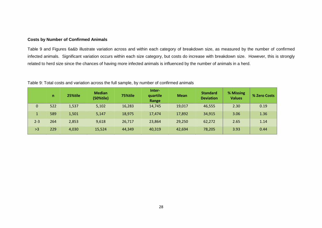
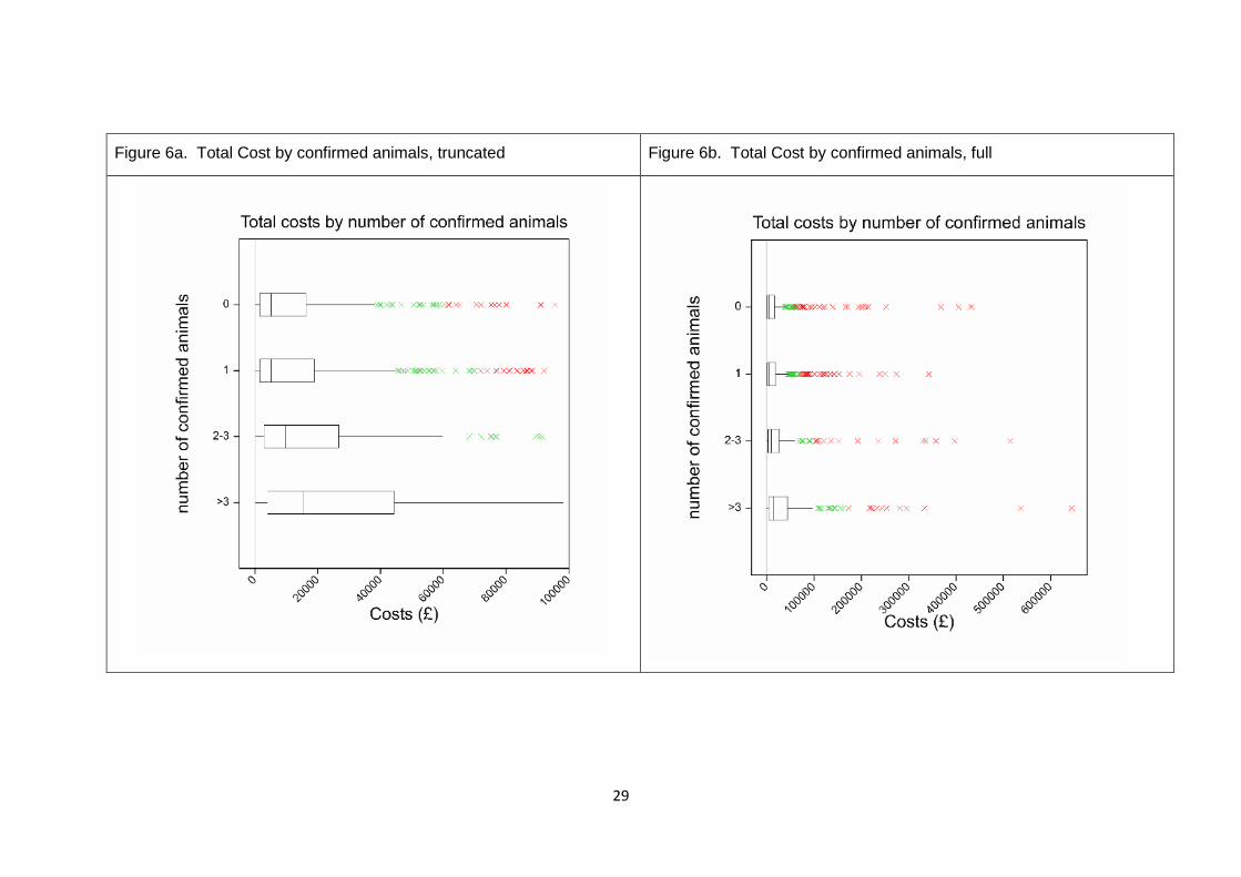
Costs by Number of Confirmed Animals
Table 9 and Figures 6a&b illustrate variation across and within each category of breakdown size, as measured by the number of confirmed
infected animals. Significant variation occurs within each size category, but costs do increase with breakdown size. However, this is strongly
related to herd size since the chances of having more infected animals is influenced by the number of animals in a herd.
Table 9: Total costs and variation across the full sample, by number of confirmed animals
n 25%tile Median
(50%tile) 75%tile
Inter-quartile Range
Mean Standard Deviation
% Missing Values
% Zero Costs
0 522 1,537 5,102 16,283 14,745 19,017 46,555 2.30 0.19
1 589 1,501 5,147 18,975 17,474 17,892 34,915 3.06 1.36
2-3 264 2,853 9,618 26,717 23,864 29,250 62,272 2.65 1.14
>3 229 4,030 15,524 44,349 40,319 42,694 78,205 3.93 0.44
29
Figure 6a. Total Cost by confirmed animals, truncated Figure 6b. Total Cost by confirmed animals, full
30
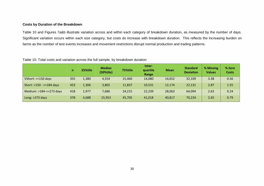
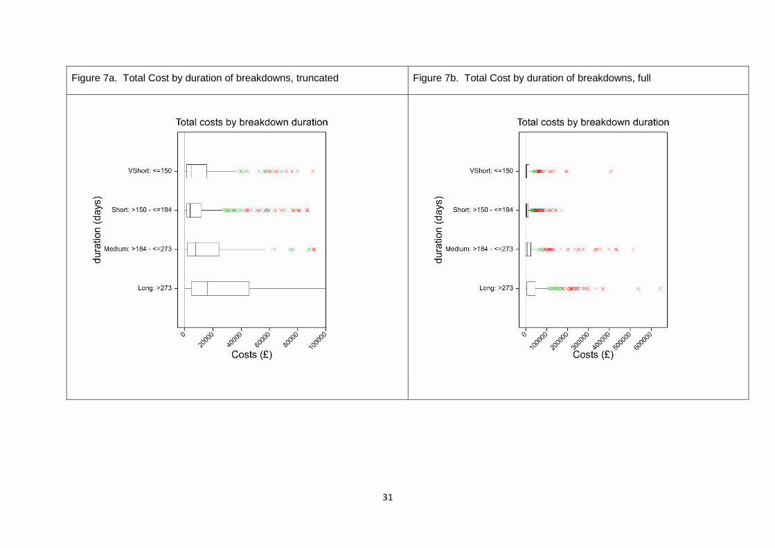
Costs by Duration of the Breakdown
Table 10 and Figures 7a&b illustrate variation across and within each category of breakdown duration, as measured by the number of days.
Significant variation occurs within each size category, but costs do increase with breakdown duration. This reflects the increasing burden on
farms as the number of test events increases and movement restrictions disrupt normal production and trading patterns.
Table 10: Total costs and variation across the full sample, by breakdown duration
n 25%tile Median
(50%tile) 75%tile
Inter-quartile Range
Mean Standard Deviation
% Missing Values
% Zero Costs
VShort: <=150 days 355 1,380 4,554 15,460 14,080 14,652 32,109 3.38 0.56
Short: >150 - <=184 days 453 1,306 3,805 11,837 10,531 12,174 22,131 2.87 1.55
Medium: >184-<=273 days 418 1,977 7,686 24,215 22,239 28,063 64,094 2.63 0.24
Long: >273 days 378 4,688 15,953 45,705 41,018 40,817 70,234 2.65 0.79
31
Figure 7a. Total Cost by duration of breakdowns, truncated Figure 7b. Total Cost by duration of breakdowns, full
32
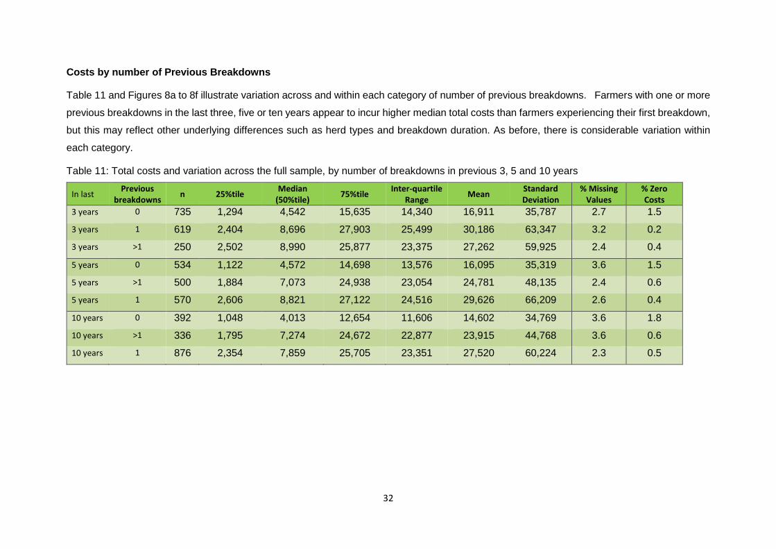
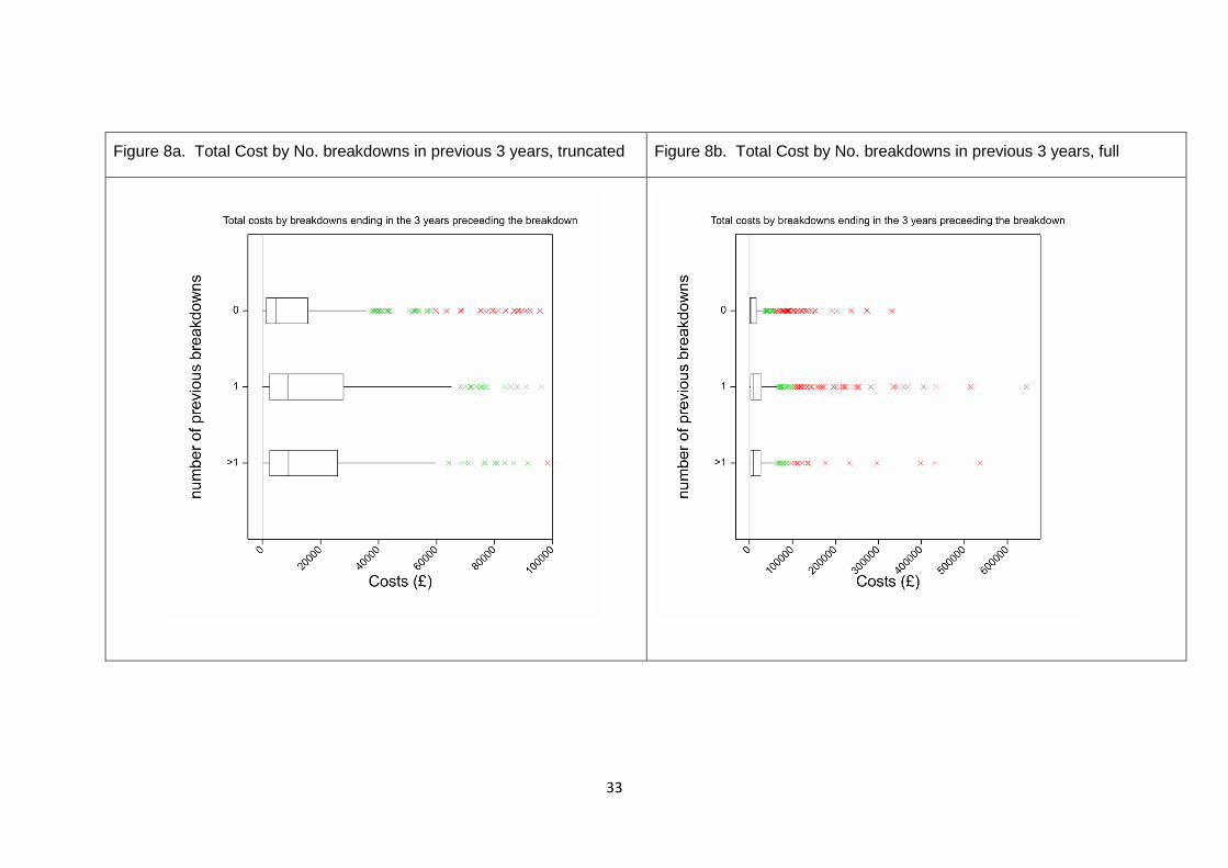
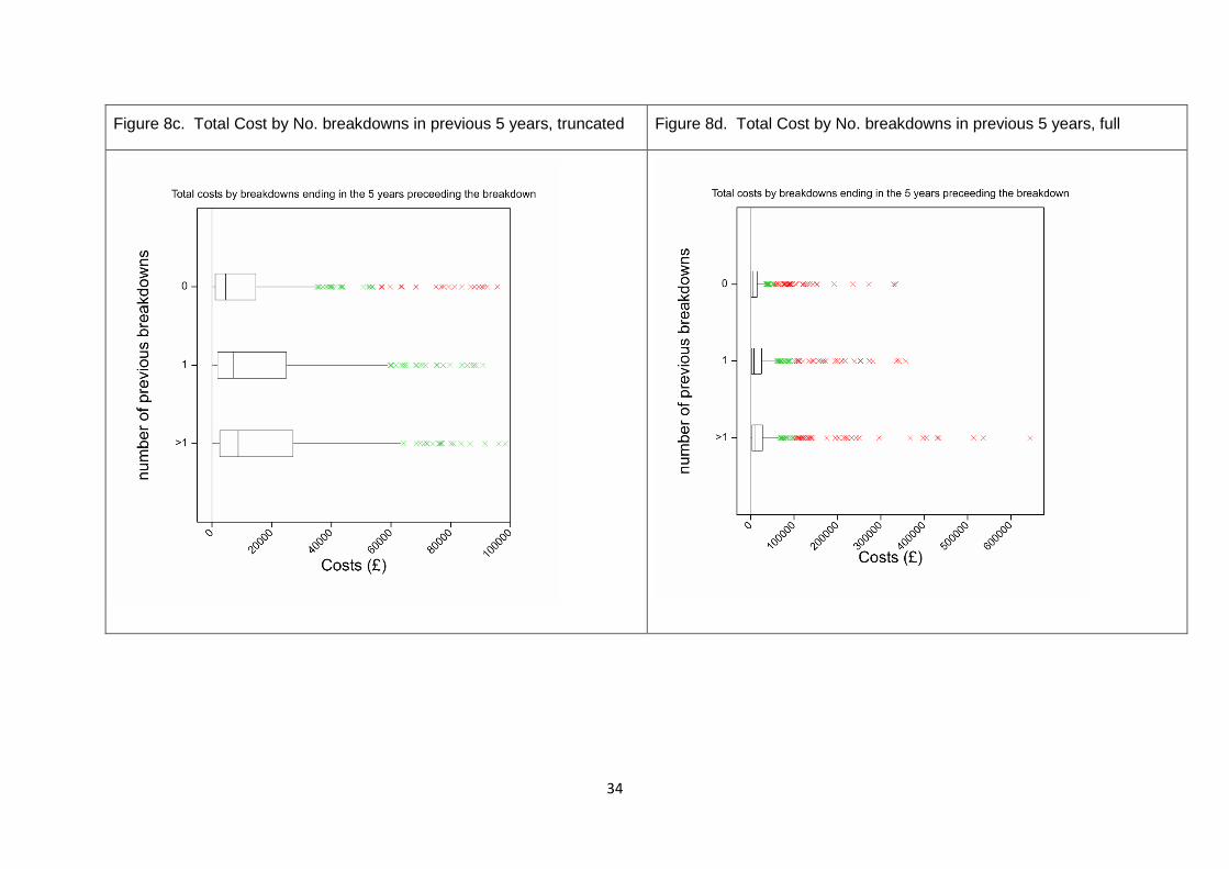
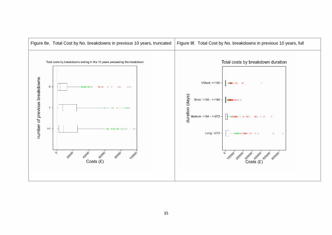
Costs by number of Previous Breakdowns
Table 11 and Figures 8a to 8f illustrate variation across and within each category of number of previous breakdowns. Farmers with one or more
previous breakdowns in the last three, five or ten years appear to incur higher median total costs than farmers experiencing their first breakdown,
but this may reflect other underlying differences such as herd types and breakdown duration. As before, there is considerable variation within
each category.
Table 11: Total costs and variation across the full sample, by number of breakdowns in previous 3, 5 and 10 years
In last Previous
breakdowns n 25%tile
Median (50%tile)
75%tile Inter-quartile
Range Mean
Standard Deviation
% Missing Values
% Zero Costs
3 years 0 735 1,294 4,542 15,635 14,340 16,911 35,787 2.7 1.5
3 years 1 619 2,404 8,696 27,903 25,499 30,186 63,347 3.2 0.2
3 years >1 250 2,502 8,990 25,877 23,375 27,262 59,925 2.4 0.4
5 years 0 534 1,122 4,572 14,698 13,576 16,095 35,319 3.6 1.5
5 years >1 500 1,884 7,073 24,938 23,054 24,781 48,135 2.4 0.6
5 years 1 570 2,606 8,821 27,122 24,516 29,626 66,209 2.6 0.4
10 years 0 392 1,048 4,013 12,654 11,606 14,602 34,769 3.6 1.8
10 years >1 336 1,795 7,274 24,672 22,877 23,915 44,768 3.6 0.6
10 years 1 876 2,354 7,859 25,705 23,351 27,520 60,224 2.3 0.5
33
Figure 8a. Total Cost by No. breakdowns in previous 3 years, truncated Figure 8b. Total Cost by No. breakdowns in previous 3 years, full
34
Figure 8c. Total Cost by No. breakdowns in previous 5 years, truncated Figure 8d. Total Cost by No. breakdowns in previous 5 years, full
35
Figure 8e. Total Cost by No. breakdowns in previous 10 years, truncated Figure 8f. Total Cost by No. breakdowns in previous 10 years, full
Examining components of cost, total costs were most highly correlated with movement
restrictions (Spearman’s ρ=0.66), all testing costs (ρ=0.64) and outputs (ρ=0.61), and less so
with isolation (ρ=0.45) and debt (ρ=0.42). Correlations with the other components of costs
were more marginal (cleaning: ρ=0.37; culling: ρ=0.32; replacement: ρ=0.26; staffing: ρ=0.21).
These correlations should be interpreted with caution, since the total costs do include each of
the other components; they are best looked at in conjunction with Table 5.
Examining associations with APHA data, total costs are correlated with the maximum herd
size at the time of the breakdown (ρ=0.46) as are all testing costs (ρ=0.57). Correlations of
costs due to isolating animals and movement restrictions with herd size are more marginal
(ρ=0.27, ρ=0.26, respectively). Correlations with breakdown duration are lower than those
seen with herd size (total costs: ρ=0.28; all testing costs ρ=0.36; isolation ρ=0.13; outputs
ρ=0.14).
Correlations with the number of previous breakdowns are also fairly marginal (e.g. correlation
with number of breakdowns with the last 20 years; total costs: ρ=0.17; all testing costs:
ρ=0.24; isolation: ρ=0.13) and generally decrease with the time period over which numbers of
breakdowns are counted (e.g. correlation with number of breakdowns with the last 2 years;
total costs: ρ=0.13; all testing costs: ρ=0.17; isolation: ρ=0.09) although this is probably, at
least in part, because there will be less variation in these observations across the population,
and hence less scope to observe any correlation.
7.3 Impacts beyond the end of the breakdown
Although the main focus of the survey was on within-breakdown costs, a simple question was
asked to allow farmers to report types of longer-term impacts that were experienced beyond
the end of the breakdown. Responses are summarised in Figure 8.
37
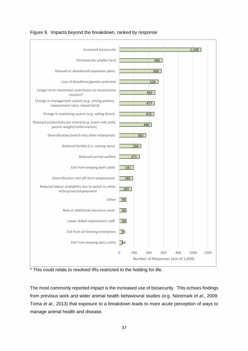
Figure 9. Impacts beyond the breakdown, ranked by response
* This could relate to resolved IRs restricted to the holding for life.
The most commonly reported impact is the increased use of biosecurity. This echoes findings
from previous work and wider animal health behavioural studies (e.g. Nöremark et al., 2009;
Toma et al., 2013) that exposure to a breakdown leads to more acute perception of ways to
manage animal health and disease.
44
55
93
95
95
165
185
191
271
294
362
440
472
477
483
526
569
583
1,109
0 200 400 600 800 1000 1200
Exit from keeping dairy cattle
Exit from all farming enterprises
Lower skilled replacement staff
New or additional insurance cover
Other
Reduced labour availability due to switch to otherenterprises/employment
Diversification into off-farm employment
Exit from keeping beef cattle
Reduced animal welfare
Reduced fertility (i.e. calving rates)
Diversification/switch into other enterprises
Reduced productivity per animal (e.g. lower milk yield,poorer weight/conformation)
Change in marketing system (e.g. selling direct)
Change in management system (e.g. calving pattern,replacement rates, closed-herd)
Longer-term movement restrictions on inconclusivereactors*
Loss of bloodlines/genetic potential
Delayed or abandoned expansion plans
Permanently smaller herd
Increased biosecurity
Number of Responses (out of 1,604)
38
Other reported effects show impacts on growth in term of business potential and productivity.
For example, loss of better-quality breeding stock (including health status), reductions in herd
size and carrying more young stock to hedge against losing some breeding replacements, but
also more extreme examples such as exiting from beef or dairy enterprises as a whole. A
small number (95) stated other effects. These included psychological and emotional stress of
the outbreak, more pessimism within the enterprises but also more working on non-farm
enterprises.
8.0 Conclusions
This final section offers some further summary discussion of the results, followed by some
reflective recommendations for future research.
8.1 Cost variation and drivers
The survey results confirm findings reported in the literature and expert opinion that both the
composition and magnitude of consequential costs vary greatly across breakdowns, reflecting
heterogeneity both in the circumstances of the farm and in the timing, size and duration of
breakdowns. This wide variation makes it difficult to characterise a “typical” cost - a few farms
incur very high costs, most suffer more modest ones.
Total costs of a breakdown had a median value of c.£6,600 with an interquartile range of
c.£20,800. This illustrates the wide variance in costs found across the survey population, due
to variation both in which categories of cost are experienced by individual farms, but also in
how badly a given cost is incurred when it is experienced. For example, over 95% of farms
report testing costs and over 65% report movement restriction costs, but only 44% report
output losses; the inter-quartile ranges for these categories are respectively c.£3,400,
c.£3,750 and c.£4,300.
In-keeping with the findings of the literature review, it is possible to identify some key drivers
of cost to explain this variation. In particular, all other things being equal, costs increase with
herd size (reflecting the scale effects of handling and maintaining more animals) and
breakdown duration (reflecting the increasing effort both of complying with testing and of
coping with movement restrictions).
For example, median total costs for large herds (>300 cattle) are c.£18,600 whilst those for
very small herds (1-50 cattle) are c.£1,700; median total costs for long breakdowns (>273
days) are c.£16,000, those for very short breakdowns (<150 days) are c.£4,600. Such
relationships are not surprising.
39
However, the main univariate analysis presented here needs to be interpreted with a little
caution due to possible confounding between different aspects of breakdown characteristics
and farm characteristics. For example, whilst the results suggest that total median costs are
higher for dairy herds relative to beef herds, this may at least partly reflect the fact that dairy
herds are typically larger than beef herds rather than that dairy herds are necessarily being
more affected for some other reason (although loss of milk output is a likely difference).
Similarly, it is possible that breakdown duration is affected by herd type and/or size, and that
the apparent absence of cost variation across different risk areas is actually due to the
masking effect of other factors.
Investigation of effects of multiple related explanatory variables on the costs was not feasible
within the lifetime of this study, but could be implemented using the assembled database for
further research.
8.2 Comparison with other estimates
Direct comparisons with results from previous empirical studies are hampered by variation in
their presentational style, but also by their vintage, given that farming practices and structures
have changed over time, as have policy measures (hence why an update of cost estimates
was commissioned).
Nevertheless, the broad magnitudes and patterns of how costs vary as shown by results here
are consistent with previous studies and the drivers identified in the literature review. For
example, Bennett et al. (2004) report total costs varying between about £300 and £143,000,
with the distribution being highly skewed around medians of about £7,000 for dairy farms and
£3,750 for beef farms; Sheppard and Turner (2005) report total costs of up to £162,000, but
with two-thirds of farms suffering less than £27,000 and the medians for dairy and beef farms
being around £10,000 and £2,700 respectively.
Similarly, for specific component costs, Sheppard & Turner (2005) report testing costs per
farm per breakdown of up to £15,000 for dairy farms and up to £6,750 for beef farms, but with
medians of £1,350 and £800 respectively, and costs of movement restrictions of up to £180,00
per breakdown, but around a median of zero for both farm types. Bennett et al. (2004) report
testing costs of up to £11,000 per breakdown, but also with medians of £1,350 and £800 for
dairy and beef farms respectively, and costs of isolating animals of up to £6,000 per
breakdown, but around a median of about £200.
Separately, it was also possible to compare more detailed costings for a small number of farms
that had experienced breakdowns whilst participating in the badger vaccine pilot. Unlike other
farms, if these pilot participants suffered a breakdown they were entitled to full compensation,
40
including for consequential costs. As a result, Defra was able to provide anonymised claim
forms providing independently-verified details on how five individual farms had incurred
consequential costs. The cost profiles of these farms were similar to those reported by
surveyed farms exhibiting similar size and type characteristics and experiencing breakdowns
of similar intensity and duration. For example, in terms of labour devoted to testing, additional
expenditure on feed and bedding for isolated animals, output losses arising from movement
restrictions, and cleaning and disinfection costs.
The apparent general consistency with the shape and size of estimates available from other
sources provides some reassurance that the survey results presented here are indicative of
recent consequential costs. However, there are some issues around reliance on farmers’ self-
reporting of data.
8.3 Reliance on self-reporting
As with previous surveys and case-studies of bTB costs on UK farms (e.g. Bennet et al., 2004;
Butler et al., 2010) this study relied upon self-reporting by farmers. Pragmatically, this was
unavoidable within the time and budget constraints available. However, it does lead to the
possibility of inaccuracies in results.
First, some or all survey respondents could deliberately exaggerate their reported costs if they
believed that doing so would somehow benefit them. For example, through higher
compensation payments or other favourable policy shifts. Such strategic misrepresentation
could have been encouraged by statements made in the invitation letter and the questionnaire
preamble which made explicit that the purpose of the survey was to inform policy decisions.
However, such statements were judged necessary to encourage survey participation and also
to comply with GDPR requirements to make clear the purpose of an exercise using personal
data.
Moreover, although the potential for abuse has to be acknowledged, there is no evidence of
systematic exaggeration in this case, or indeed other surveys of UK farmers. Rather, whilst it
is possible that some individual respondents may deliberately misreport, the presumption is
that the majority participate in good faith to the best of their ability. This was certainly the
impression gained throughout the process of designing and administering the questionnaire.
The large sample size, sampling design and exclusion of statistical outliers using a formal
statistical method will also have helped to mitigate the effects of any exaggeration by a few
individual farmers.
Second, however, the accuracy of self-reporting may be undermined more commonly by flaws
in farm records and/or farmers’ recollections. In particular, it is possible that some farmers do
41
not keep fully accurate (or indeed any) formal records and/or are imperfectly aware of how
bTB has affected specific costs. Whilst attempts were made to address the latter concern by
careful structuring and wording of questions, to help respondents think about how they had
been affected, any answers drawing from inaccurate records or recollections will still be
potentially incorrect. For example, some farmers may systematically under-record time
actually devoted to bTB testing or use inappropriate comparators to estimate price and/or
volume losses from disrupted trading patterns.
Unfortunately, it is not possible to conclusively judge the degree to which inaccurate self-
reporting may or may not affect the validity of estimates presented here. For example,
although the pattern and magnitude of variation of reported figures is consistent with those
from previous studies, these previous investigations were also reliant on self-reporting.
Equally, checks for internal consistency within an individual respondent’s answers cannot
detect basic inaccuracies, nor, given the wide variation in circumstances, can comparisons
between the figures for respondents indicating recourse to formal records (59.4% of sample)
and/or confidence (81.9% of sample) in their answers against figures for those not indicating
recourse or confidence. As such, whilst the estimates presented here are plausible and the
best available, they are subject to some uncertainty.
If the risk of inaccuracies arising from self-reporting is deemed to be unacceptably large, any
future attempts at estimating bTB costs will need to deploy some form of independent scrutiny.
One possibility for this would be to require a proportion of all future breakdowns to be subject
to active third-party monitoring as they unfold. The TB Advisory Service may be well placed
to play such as role. Collecting cost data via a standardised proforma and in close to real-
time would address concerns about imperfect record keeping and faulty recollections, whilst
independent observation would deter exaggeration. However, such an approach would be
labour intensive (and hence expensive) and might be regarded by farmers as intrusive.
Moreover, defining the counterfactual of no breakdown would still require an element of
judgement and some recourse to pre-breakdown records, which could still be inaccurate
(unless all farmers were under a more general obligation to keep accurate records).
8.4 Longer-term effects
Due to constraints on what could be explored within a c.20-minute telephone interview, this
study focused primarily upon within-breakdown costs. Nevertheless, indicative, qualitative
responses were also sought on longer-term impacts. Of answers received these revealed
significant structural changes – including reductions in herd sizes, exiting from keeping cattle,
or indeed exiting from farming. Others related to changes in managerial practices and/or
productivity – including loss of valuable breeding bloodlines and experienced staff.
42
Such impacts are consistent with findings reported in the literature, and highlight that longer-
term effects merit further exploration. However, as reported by Butler et al. (2010), identifying
and quantifying longer-term impacts is somewhat challenging, even using an intensive case-
study approach. Again, it may be that routine recourse to third-party scrutiny could be used
to track the performance of at least some businesses affected by bTB beyond the end of a
breakdown.
Separately, by far the most commonly reported change beyond the end of a breakdown was
an increase in biosecurity. Although previous studies (e.g. Nöremark et al., 2009; Toma et al.,
2013) have shown that exposure to a disease can prompt greater attention to biosecurity
measures, the indicative responses gathered here are insufficient to offer detailed insights into
the level and types of changes adopted, nor the baseline to which they apply. For example,
how diligent or lax biosecurity was prior to the breakdown, and in what form and for how long
any extra diligence was observed.
In addition, whilst the costs estimated from this study are conditional upon a farm suffering a
breakdown, biosecurity efforts would be expected to affect the likelihood of a breakdown.
Hence, although beyond the scope of this study, future research could attempt to explore the
endogenous relationship between prior biosecurity efforts and subsequent impacts.
8.5 Reflective recommendations
In pursuing further research on bTB costs, a number of issues should be considered in
planning any similar future exercises:
• First, the advent of GDPR caused additional complexities and delays to obtaining
necessary permissions to access and share relevant data. This affected volunteer
recruitment for the initial focus group and pre-pilot testing of the questionnaire, but also
more significantly in relation to access to the contact details and breakdown data held
by APHA. Whilst some of the issues may be attributed to this being an early instance
of trying to conduct a survey under the GDPR regimen, with all parties facing a steep
learning-curve, confusion also arose from different institutional interpretations of what
was and what was not permissible. To avoid such issues in future, it would be
advisable for project sponsors to have clear policies in advance and for researchers to
understand the stance of their institutional information officers.
• Second, survey complexity was increased by the twin requirements for all farmers to
be sent an initial letter to be offered an interview and, also, that the number of recipients
sent letters be minimised. Consequently, it would be helpful if such requirements were
made explicit in invitations to tender, so the costs could be budgeted for in the tender.
43
• Third, whilst the survey successfully gathered information on a number of key financial
costs, it was clear that farmers perceive there to be appreciable non-financial impacts,
particularly on mental health. This may merit further investigation.
• Fourth, due to the constraint of keeping the telephone interview to a reasonable length,
the focus of the questionnaire was almost exclusively on short-term impacts. Yet the
(limited) qualitative responses recorded confirm findings from the literature that longer-
term impacts (including adoption of biosecurity measures) can be important. Hence,
they too may merit further investigation.
• Fifth, peer review comments plus feedback during the process of devising the
questionnaire and from presenting survey findings to stakeholders suggest some valid
concerns about relying on self-reporting of costs. Achieving more confidence in
estimates may require some routine, on-going monitoring of costs, such as
independent recording/auditing of costs in real-time for a proportion of breakdowns as
they unfold.
• Sixth, qualitative responses and feedback from farmers throughout the study reveal a
strong desire for greater, on-going engagement with government officials, to engender
greater mutual understanding of issues, constraints and opportunities. One way of
achieving this might be explicitly to include farmer representatives or other industry
stakeholders on the steering group(s) of any future research project(s). This would
help to improve mutual understanding of issues, constraints and potential solutions.
• Seventh, APHA hold additional data on farms and farm breakdowns. For example,
data is recorded on the patterns of livestock movements before, during and after a
breakdown, and on the manner in which movement restrictions are
applied/relaxed/lifted. Use of such data, rather than the more aggregate
approximations used in this project, could permit more sophisticated analysis to help
inform policy analysis needs, for example in the development of risk-based trading.
• Eighth, the combined APHA and survey data represent the outcome of significant data
collection, integration and processing efforts and offer the opportunity for further
modelling analysis to tease-out effects on costs due to multiple related potential
explanatory variables. For example, investigation of costs attributable to herd size,
herd type and breakdown duration.
• Ninth, the time and effort entailed in data processing should not be under-estimated.
In particular, the final results are dependent on careful matching of data from different
sources and on successful identification of errors and outliers. Similarly, meaningful
analysis and presentation requires an understanding of relationships within the data.
44
9 References
Bennett, R.M. (2009) Farm costs associated with pre-movement testing for bovine
tuberculosis. Veterinary Record, v164, 74-79.
Butler, Allan; Lobley, M. & Winter, M. (2010) Economic Impact Assessment of Bovine
Tuberculosis in the South West of England. CRPR Research Paper No 30. University of
Exeter.
Nöremark, M., Lindberg, A., Vågsholm, I., Sternberg Lewerin, S. (2009). Disease
awareness, information retrieval and change in biosecurity routines among pig farmers in
association with the first PRRS outbreak in Sweden, Preventive Veterinary Medicine 90, 1-9.
Toma, L., Stott, A.W., Heffernan,C., Ringrose, S., Gunn, G.J. (2013). Determinants of
biosecurity behaviour of British cattle and sheep farmers—A behavioural economics
analysis, Preventive Veterinary Medicine 108, 321-333
45
Annex A: Rapid Literature Review
Estimating the economic cost of
bovine TB incidents on cattle
farmers in England and Wales
WS1: Rapid Literature Review
Andrew Moxey, Andrew Barnes & Bouda Vosough Ahmadi
October 2018
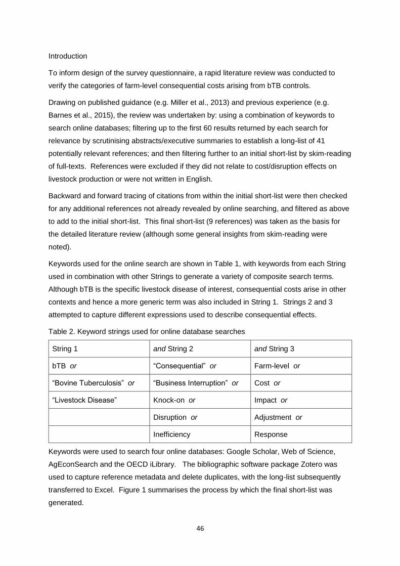
46
Introduction
To inform design of the survey questionnaire, a rapid literature review was conducted to
verify the categories of farm-level consequential costs arising from bTB controls.
Drawing on published guidance (e.g. Miller et al., 2013) and previous experience (e.g.
Barnes et al., 2015), the review was undertaken by: using a combination of keywords to
search online databases; filtering up to the first 60 results returned by each search for
relevance by scrutinising abstracts/executive summaries to establish a long-list of 41
potentially relevant references; and then filtering further to an initial short-list by skim-reading
of full-texts. References were excluded if they did not relate to cost/disruption effects on
livestock production or were not written in English.
Backward and forward tracing of citations from within the initial short-list were then checked
for any additional references not already revealed by online searching, and filtered as above
to add to the initial short-list. This final short-list (9 references) was taken as the basis for
the detailed literature review (although some general insights from skim-reading were
noted).
Keywords used for the online search are shown in Table 1, with keywords from each String
used in combination with other Strings to generate a variety of composite search terms.
Although bTB is the specific livestock disease of interest, consequential costs arise in other
contexts and hence a more generic term was also included in String 1. Strings 2 and 3
attempted to capture different expressions used to describe consequential effects.
Table 2. Keyword strings used for online database searches
String 1 and String 2 and String 3
bTB or “Consequential” or Farm-level or
“Bovine Tuberculosis” or “Business Interruption” or Cost or
“Livestock Disease” Knock-on or Impact or
Disruption or Adjustment or
Inefficiency Response
Keywords were used to search four online databases: Google Scholar, Web of Science,
AgEconSearch and the OECD iLibrary. The bibliographic software package Zotero was
used to capture reference metadata and delete duplicates, with the long-list subsequently
transferred to Excel. Figure 1 summarises the process by which the final short-list was
generated.
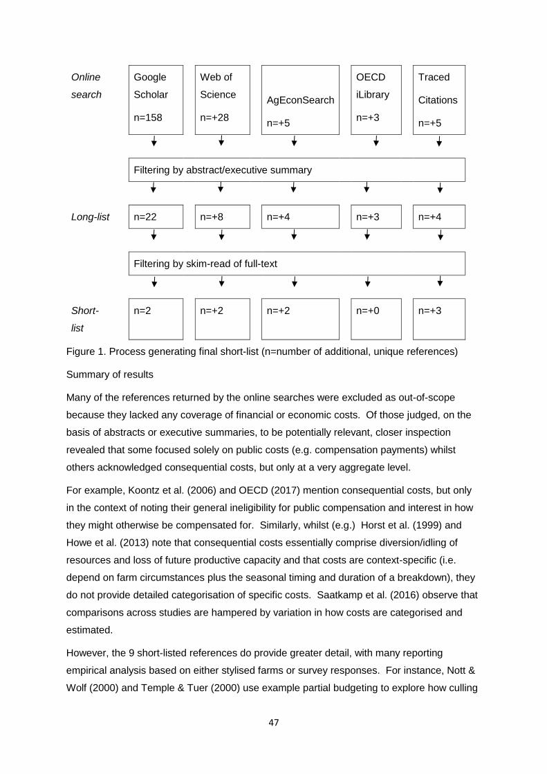
47
Online
search
Scholar
n=158
Web of
Science
n=+28
AgEconSearch
n=+5
OECD
iLibrary
n=+3
Traced
Citations
n=+5
Filtering by abstract/executive summary
Long-list n=22 n=+8 n=+4 n=+3 n=+4
Filtering by skim-read of full-text
Short-
list
n=2 n=+2 n=+2 n=+0 n=+3
Figure 1. Process generating final short-list (n=number of additional, unique references)
Summary of results
Many of the references returned by the online searches were excluded as out-of-scope
because they lacked any coverage of financial or economic costs. Of those judged, on the
basis of abstracts or executive summaries, to be potentially relevant, closer inspection
revealed that some focused solely on public costs (e.g. compensation payments) whilst
others acknowledged consequential costs, but only at a very aggregate level.
For example, Koontz et al. (2006) and OECD (2017) mention consequential costs, but only
in the context of noting their general ineligibility for public compensation and interest in how
they might otherwise be compensated for. Similarly, whilst (e.g.) Horst et al. (1999) and
Howe et al. (2013) note that consequential costs essentially comprise diversion/idling of
resources and loss of future productive capacity and that costs are context-specific (i.e.
depend on farm circumstances plus the seasonal timing and duration of a breakdown), they
do not provide detailed categorisation of specific costs. Saatkamp et al. (2016) observe that
comparisons across studies are hampered by variation in how costs are categorised and
estimated.
However, the 9 short-listed references do provide greater detail, with many reporting
empirical analysis based on either stylised farms or survey responses. For instance, Nott &
Wolf (2000) and Temple & Tuer (2000) use example partial budgeting to explore how culling
48
and movement restrictions impose costs through additional labour and feed requirements
plus loss of output, whilst Bennett et al. (2004), Garforth et al. (2005) and Turner et al.
(2008) draw on survey responses to provide detailed cost categorisations.
The main points of each short-listed reference are summarised below, with Table 2 (and
Annex A) listing the various cost categories identified. Importantly, the sensitivity of costs to
when in the farming year a breakdown occurs (e.g. relative to calving patterns and planned
movements) and to the adjustment flexibility of farming businesses and households (e.g.
resource base, other farm enterprises, off-farm employment opportunities) is highlighted
repeatedly by several studies. Table 3 summarises the range of reported cost estimates.
Impacts on the physical or mental health of farm labour are outwith the scope of this study
and hence are not covered in detail here.
Temple & Tuer (2000)
This is a report prepared for the Ministry of Agriculture, Farming and Fisheries (MAFF) by
the Agricultural Development and Advisory Service (ADAS), relating to bTB in England.
Three sources of consequential cost are identified: restrictions on cattle movements on and
off farm; repeat testing; and compulsory cleaning and disinfection. Of these, it is asserted
that costs arising from movement restrictions are the most significant, comprising changes
to: livestock sales and purchases; revenue from output and subsidies; quota usage (no
longer applicable); and inputs costs, especially feed and labour.
The effects of movement restrictions are explored for five different dairy and beef systems
(e.g. heifer-rearing vs. bought-in heifers), across three different herd sizes, three different
durations of restriction, and three different scales of breakdown (i.e. number of cows
slaughtered). Descriptive explanations of why costs arise are accompanied by numerical
illustrations based on industry-standard unit costs and revenues.
For example, movement restrictions mean that dairy calves either need to be killed on-farm
or reared on-farm. The former avoids additional labour, feed costs and housing costs but
forgoes sales revenue whilst the latter preserves revenue but incurs costs. Retention for
rearing is typically feasible for short periods, but less so for long-duration movement
restrictions - although timing relative to calving periods affects this. Similarly, inability to
buy-in replacement heifers for culled reactors means that either herd size will be reduced for
a period of time, leading to foregone milk revenue (but also some avoided costs), and/or
sales revenue from surplus heifers will be foregone as heifers are retained for breeding
instead. Again, timing of breakdown and removal of reactors relative to production cycles
affects actual impacts.
49
For beef systems, finisher-only systems relying on bought-in animals can find it difficult to
source calves and/or delay marketing of mature animals, incurring costs and possibly losing
value if cattle go out of spec. The latter also applies to breeder-finisher systems. Breeder-
only systems are forced to either retain suckled calves for longer (incurring additional costs)
or to kill on-farm (foregoing revenue). Many suckler herds lack the resources to retain
calves for longer. As with dairy herds, herd size may also be affected for a while if
replacement animals cannot be bought-in, and/or revenue lost by having to retain more
heifers for breeding.
Wolf, Harsh & Lloyd (2000)
This is a Staff Working Paper from Michigan State University, focusing on farm-level impacts
of bTB on dairy farms in Michigan. Example partial budgeting is used to explore impacts for
two different systems – although the heterogeneity of farms is acknowledged and it is
stressed that the values presented are purely illustrative. The description of impacts is not
as detailed as in Temple & Tuer, but essentially covers the same considerations, including
the importance of breakdown timing within production cycles. Consideration is also given
to the possibility of temporarily depressed milk yields for replacement animals due to
stress/settling-in.
Nott & Wolf (2000)
This is another Staff Working Paper from Michigan State University, focusing on farm-level
impacts of bTB on dairy farms in Michigan. Example partial budgeting is used to explore a
choice between complete herd culling (depopulation) and partial culling for two different herd
sizes. Full depopulation avoids movement restriction costs but foregoes all revenues whilst
partial culling retains some revenues but incurs additional costs. The approach is similar to
that in Wolf et al. (above), but excludes consideration of the age profile of the herd.
However, mention is made of effects on cashflow/working capital plus the possibility of not
being able to sell any contaminated feedstuffs, manure and/or other crops.
Bennett, Cooke & Upelaar (2004)
This is a report by the University of Reading to Defra, using a combination of workshops, a
survey of 151 farms (drawn from VetNet) and spreadsheet modelling to explore the costs of
different bTB control strategies. Consequential costs are considered explicitly, although
much of the report extends beyond the farm-level to consider aggregate impacts and policy
choices. Helpfully, the farm survey questionnaire is presented in an Appendix, as is an
example of the spreadsheet model used to simulate farm-level costs for different severities
and duration of breakdowns, and a useful timeline of different stages of a breakdown.
50
As well as those arising from movement restrictions (as above), cost categories considered
include those associated with testing, retesting and isolation of reactors – essentially
additional labour effort, separate bedding/housing and (although now compensated)
arranging valuation and removal of reactors – plus disinfection/cleansing. The possibility of
long-term impacts due to (e.g.) forced changes in herd size or loss of bloodlines is noted, as
is the risk of farmers double-counting across categories. Heterogeneity across farms is
highlighted as important, both in terms of systems but also the severity, duration and repeat
of breakdowns – all of which influence costs incurred. The authors note that some farms
apparently received compensation in excess of total costs incurred.
Garforth, Rehman, McKemey, & Rana (2005)
This is a report by the University of Reading for Defra, considering the use of private
insurance to cover consequential costs from notifiable diseases (not only bTB). It draws on
a survey of 106 cattle, pig and sheep farms plus (for comparative purposes) 53 potato
farmers, to discuss cost categories and attitudes towards insurance (although it is noted that
cover is not necessarily actually available).
A high proportion of respondents reported suffering impacts from either an outbreak on their
own farm or on neighbouring farms. Beyond loss of culled stock, the most frequently
reported impacts were on cash flow and income, with loss of breeding stock and market
access plus movement restriction costs all mentioned. Current uptake of consequential loss
insurance (itself a consequential cost) was low, and attitudes towards it somewhat variable.
Sheppard & Turner (2005)
This is a report by the University of Exeter for the South West of England Rural Development
Agency. It presents results of a face-to-face survey of 61 farms of which seven are reported
in greater detail as case studies, plus a telephone survey of a further 50 farms (and a survey
of 41 other stakeholders).8 The farm survey questionnaires were based on that used by
Bennett et al. (2004, above), and indeed were administered by staff from the University of
Reading with results being deliberately presented in the same style. The questionnaires are
presented in Appendices.
Perhaps unsurprisingly, the results largely echo those of Bennett et al. (2004) in terms of
revealing considerable heterogeneity of costs incurred according to farm-specific
circumstances and covering similar cost categories. However, effects on cash flow and debt
were also noted, as were effects on cancelling or postponing business investments and
expansion plus non-financial effects of stress on household members and diversification
8 The sampling frame is not specified.
51
away from cattle enterprises. The authors also note that some farms apparently received
compensation in excess of total costs incurred, but farms with few reactors yet long
movement restrictions typically suffered the greatest net losses. The survey of other
stakeholders suggested bTB breakdown effects on the wider rural economy were minimal,
although some individual firms (e.g. valuers) gained and some (e.g. engineering firms) lost.
Turner, Temple, Howe, Jeanes, Boothby, & Watts (2008)
This is a report by the University of Exeter and ADAS for Defra, exploring longer-term effects
of bTB breakdowns over months and years rather than more immediately during the
breakdown. The focus is on both human health (e.g. stress) and business impacts (e.g.
viability), with evidence presented on costs drawing on a literature review, analysis of Farm
Business Survey (FBS) data, a face-to-face survey of 152 farmers (drawn from VetNet) and
a stakeholder consultation.
Longer term economic impacts are identified as arising from short-term disruptions which
force changes in the size and/or mix of farm enterprises. For example, forced herd size
reduction or cash flow requirements leading to shifts towards non-cattle enterprises (as
noted by both Bennet et al. and Sheppard & Turner, above) that subsequently endure after
the breakdown has ended. The average frequency of different cost categories and their
relative financial significance is reported. However, it is noted that attributing structural
changes solely to a bTB breakdown is difficult due to the influence of other factors, including
the often low profitability of some livestock enterprises, the presence or absence of a farm
successor and household confidence. Long-term impacts are relatively minor for farms
experiencing small and short-duration breakdowns but can be significant for farms
experiencing large and/or sustained/repeated breakdowns. Given that most farms
experience only small and/or short breakdowns, the long-term impacts are restricted to a
minority of breakdown farms but are typically difficult to estimate.
Bennett (2009)
This paper reports on a study by the University of Reading, sponsored by the Royal
Association of British Dairy Farmers. It presents estimates of farm-level costs incurred
through compliance with requirements for bTB pre-movement testing, based on a face-to-
face survey of 60 farms.
Farm labour required for gathering and testing animals, plus associated administrative tasks,
is reported as the dominant form of additional costs, with slightly higher machinery, housing
and feed costs also incurred. Some farmers reported avoiding pre-movement testing by
adjusting farm practices. For example, sending animals direct to slaughter or using an
exempt market, which may have cost and/or revenue implications. Similarly, a proportion of
52
farmers reported suffering general business disruption and injuries to staff or animals,
although none of these categories were costed.
Butler, Lobley & Winter (2010)
This is a report by the University of Exeter, sponsored by the NFU, Devon County Council,
and SW Sustainable Farming and Food Board. It complements Sheppard & Turner (2005,
above) by adopting a case-study approach (of eight farms) to provide greater detail
(including a useful flowchart presentation). It also draws on stakeholder interviews.
The results indicate variability in the level and composition of costs across different farm
circumstances, including size and nature of herds but also the spatial configuration of
businesses e.g. farms with multiple holdings face additional movement restriction issues.
Costs of testing can include knock-ons for other farming activities (e.g. delays in silage
making), livestock productivity (e.g. lower milk yield or liveweight gain due to stress) and
administrative tasks. Similarly, sourcing replacements for culled animals incurs labour effort
in researching and travelling to view cattle, plus their haulage costs. Movement restrictions
can lead to over-stocking, which may breach quality assurance and cross-compliance
requirements, whilst ability to fulfil specific contracts timings and/or volumes may lead to
price penalties or loss of contracts. Echoing Turner et al. (2008), the possibility of long-term
impacts is acknowledged (e.g. higher debts, postponement of investments, household
stress), as are difficulties of estimating them.
Discussion
Despite consequential costs being acknowledged widely in livestock disease literature,
references providing the level of detail required to inform design of a survey questionnaire
are apparently somewhat scarce. Moreover, most of those revealed by online searching
relate to previous studies of bTB in England, conducted by staff at the Universities of Exeter
and/or Reading. Nonetheless, the range of cost categories reported in the literature is
consistent with the list offered in the ITT specification for this project9 and the more general
principles outlined in economic frameworks. As such, the categories summarised above and
below in Table 2 should be adequate.10
9See Appendix for this. 10 A draft of Table 2 was shared with academic experts in Europe and North America, who confirmed the identified categories and the need to distinguish between different farm types (e.g. dairy vs. beef) but also suggested inclusion of labour retention/recruitment and carcass condemnation, plus the need to avoid double-counting across categories. Cost categories used for compensation of infected farmers within Defra’s research projects on the Badger Vaccine Deployment Project & long-term trials at Woodchester Park were also consistent with those in Table 2 (adding loss of hiring-out fees for bulls & AI fees in-place of hiring-in).
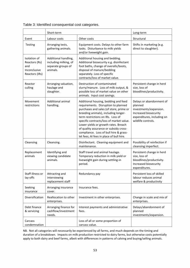
53
Table 3: Identified consequential cost categories.
Short-term Long-term
Event Labour costs Other costs Structural
Testing Arranging tests, gathering animals.
Equipment costs. Delays to other farm tasks. Disturbance to milk yields and/or liveweight gain.
Shifts in marketing (e.g. direct to slaughter).
Isolation of Reactors (Rs) and Inconclusive Reactors (IRs)
Additional handling, including milking, of separate groups of animals.
Additional housing and bedding. Additional biosecurity e.g. disinfectant foot baths, change of overalls/boots, disposal of manure/bedding separately. Loss of specific contracts/loss of market value.
Reactor culling
Arranging valuation, haulage and slaughter.
Destruction of contaminated slurry/manure. Loss of milk output, & possible loss of market value on other animals. Input cost savings.
Persistent change in herd size, loss of bloodlines/productivity.
Movement restrictions
Additional animal handling.
Additional housing, bedding and feed requirements. Disruption to planned purchases and sales (of store, prime or breeding animals), including longer-term restrictions on IRs. Loss of specific contracts/loss of market value. Lower yields or growth rates. Breach of quality assurance or subsidy cross-compliance. Loss of bull hire & grass-let fees; AI fees in place of bull hire.
Delays or abandonment of planned investments/expansion. Increased biosecurity expenditures, including on wildlife controls.
Cleansing Cleansing. Disinfectant. Cleaning equipment and maintenance.
Possibility of reinfection if cleansing imperfect.
Replacement animals
Identifying and viewing candidate animals.
Staff travel and animal haulage. Temporary reduction in milk yield or liveweight gain during settling-in period.
Persistent change in herd size, loss of bloodlines/productivity. Increased biosecurity expenditures.
Staff illness or lay-offs
Attracting and interviewing replacement staff
Redundancy pay Persistent loss of skilled labour reduces animal welfare & productivity
Seeking insurance
Arranging insurance cover.
Insurance fees.
Diversification Reallocation to other enterprises.
Investment in other enterprises. Change in scale and mix of enterprises.
Debt finance & servicing
Arranging finance for cashflow/investment needs.
Interest payments and administrative fees.
Delays/abandonment of planned investments/expansion.
Carcass condemnation
Loss of all or some proportion of carcass value.
NB. Not all categories will necessarily be experienced by all farms, and much depends on the timing and duration of a breakdown. Impacts on milk production restricted to dairy farms, but otherwise costs potentially apply to both dairy and beef farms, albeit with differences in patterns of calving and buying/selling animals.
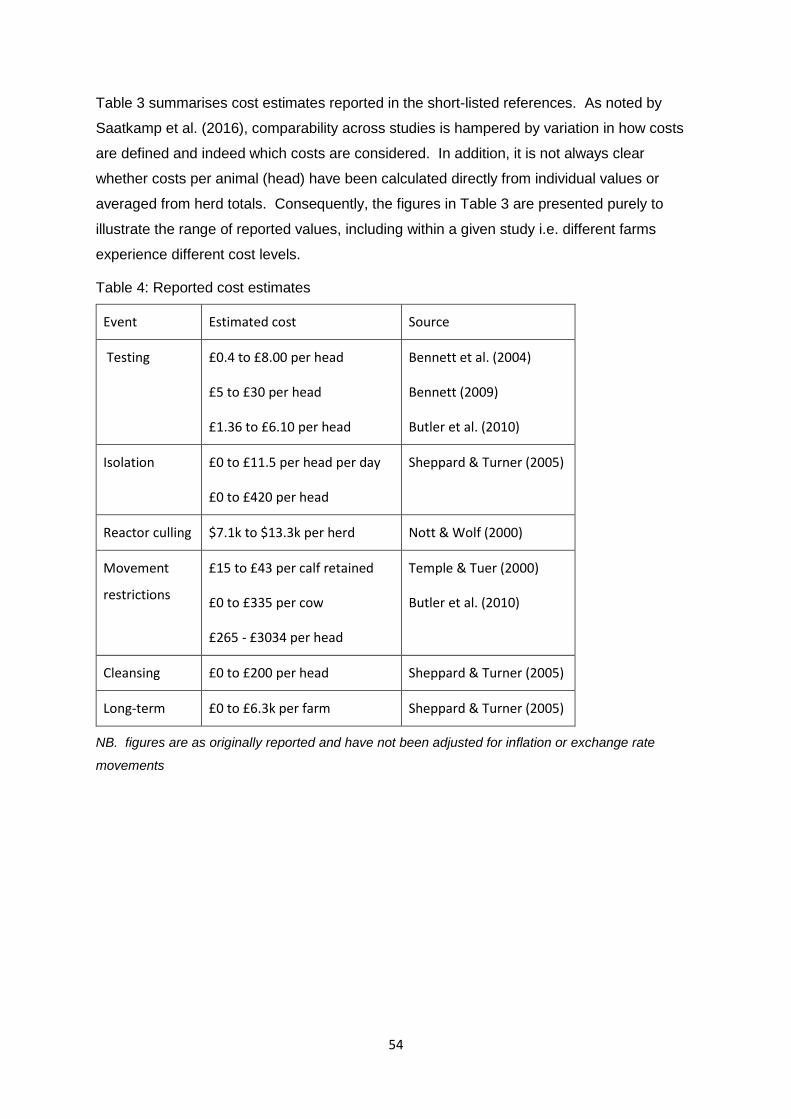
54
Table 3 summarises cost estimates reported in the short-listed references. As noted by
Saatkamp et al. (2016), comparability across studies is hampered by variation in how costs
are defined and indeed which costs are considered. In addition, it is not always clear
whether costs per animal (head) have been calculated directly from individual values or
averaged from herd totals. Consequently, the figures in Table 3 are presented purely to
illustrate the range of reported values, including within a given study i.e. different farms
experience different cost levels.
Table 4: Reported cost estimates
Event Estimated cost Source
Testing £0.4 to £8.00 per head
£5 to £30 per head
£1.36 to £6.10 per head
Bennett et al. (2004)
Bennett (2009)
Butler et al. (2010)
Isolation £0 to £11.5 per head per day
£0 to £420 per head
Sheppard & Turner (2005)
Reactor culling $7.1k to $13.3k per herd Nott & Wolf (2000)
Movement
restrictions
£15 to £43 per calf retained
£0 to £335 per cow
£265 - £3034 per head
Temple & Tuer (2000)
Butler et al. (2010)
Cleansing £0 to £200 per head Sheppard & Turner (2005)
Long-term £0 to £6.3k per farm Sheppard & Turner (2005)
NB. figures are as originally reported and have not been adjusted for inflation or exchange rate
movements
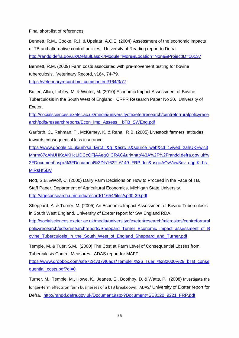
55
Final short-list of references
Bennett, R.M., Cooke, R.J. & Upelaar, A.C.E. (2004) Assessment of the economic impacts
of TB and alternative control policies. University of Reading report to Defra.
http://randd.defra.gov.uk/Default.aspx?Module=More&Location=None&ProjectID=10137
Bennett, R.M. (2009) Farm costs associated with pre-movement testing for bovine
tuberculosis. Veterinary Record, v164, 74-79.
https://veterinaryrecord.bmj.com/content/164/3/77
Butler, Allan; Lobley, M. & Winter, M. (2010) Economic Impact Assessment of Bovine
Tuberculosis in the South West of England. CRPR Research Paper No 30. University of
Exeter.
http://socialsciences.exeter.ac.uk/media/universityofexeter/research/centreforruralpolicyrese
arch/pdfs/researchreports/Econ_Imp_Assess__bTB_SWEng.pdf
Garforth, C., Rehman, T., McKemey, K. & Rana. R.B. (2005) Livestock farmers’ attitudes
towards consequential loss insurance.
https://www.google.co.uk/url?sa=t&rct=j&q=&esrc=s&source=web&cd=1&ved=2ahUKEwic3
Mnrm87cAhUHKcAKHcLIDCcQFjAAegQICRAC&url=http%3A%2F%2Frandd.defra.gov.uk%
2FDocument.aspx%3FDocument%3Dls1622_6149_FRP.doc&usg=AOvVaw3ov_dgpfK_bs_
MlRsHf5BV
Nott, S.B. &Wolf, C. (2000) Dairy Farm Decisions on How to Proceed in the Face of TB.
Staff Paper, Department of Agricultural Economics, Michigan State University.
http://ageconsearch.umn.edu/record/11654/files/sp00-39.pdf
Sheppard, A. & Turner, M. (2005) An Economic Impact Assessment of Bovine Tuberculosis
in South West England. University of Exeter report for SW England RDA.
http://socialsciences.exeter.ac.uk/media/universityofexeter/research/microsites/centreforrural
policyresearch/pdfs/researchreports/Sheppard_Turner_Economic_impact_assessment_of_B
ovine_Tuberculosis_in_the_South_West_of_England_Sheppard_and_Turner.pdf
Temple, M. & Tuer, S.M. (2000) The Cost at Farm Level of Consequential Losses from
Tuberculosis Control Measures. ADAS report for MAFF.
https://www.dropbox.com/s/fe72rcv37vt6adz/Temple_%26_Tuer_%282000%29_bTB_conse
quential_costs.pdf?dl=0
Turner, M., Temple, M., Howe, K., Jeanes, E., Boothby, D. & Watts, P. (2008) Investigate the
longer-term effects on farm businesses of a bTB breakdown. ADAS/ University of Exeter report for
Defra. http://randd.defra.gov.uk/Document.aspx?Document=SE3120_9221_FRP.pdf
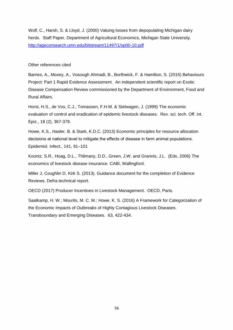
56
Wolf, C., Harsh, S. & Lloyd, J. (2000) Valuing losses from depopulating Michigan dairy
herds. Staff Paper, Department of Agricultural Economics, Michigan State University.
http://ageconsearch.umn.edu/bitstream/11497/1/sp00-10.pdf
Other references cited
Barnes, A., Moxey, A., Vosough Ahmadi, B., Borthwick, F. & Hamilton, S. (2015) Behaviours
Project: Part 1 Rapid Evidence Assessment. An independent scientific report on Exotic
Disease Compensation Review commissioned by the Department of Environment, Food and
Rural Affairs.
Horst, H.S., de Vos, C.J., Tomassen, F.H.M. & Stelwagen, J. (1999) The economic
evaluation of control and eradication of epidemic livestock diseases. Rev. sci. tech. Off. int.
Epiz., 18 (2), 367-379.
Howe, K.S., Hasler, B. & Stark, K.D.C. (2013) Economic principles for resource allocation
decisions at national level to mitigate the effects of disease in farm animal populations.
Epidemiol. Infect., 141, 91–101
Koontz, S.R., Hoag, D.L., Thilmany, D.D., Green, J.W. and Grannis, J.L. (Eds, 2006) The
economics of livestock disease insurance. CABI, Wallingford.
Miller J, Coughlin D, Kirk S. (2013). Guidance document for the completion of Evidence
Reviews. Defra technical report.
OECD (2017) Producer Incentives in Livestock Management. OECD, Paris.
Saatkamp, H. W.; Mourits, M. C. M.; Howe, K. S. (2016) A Framework for Categorization of
the Economic Impacts of Outbreaks of Highly Contagious Livestock Diseases.
Transboundary and Emerging Diseases. 63, 422-434.
57
Appendix: ITT specification listing of example cost categories
• The productivity loss as a result of a whole herd skin test (which is required every 60 days
after a breakdown). This will require farmers to prepare the cattle for testing and they may
need to hire additional labour, facilities, etc.
• The inability to move animals on or off the farm (except under licence and to a much
reduced range of approved outlets)
• The delay in replacing compulsorily slaughtered animals
• The value of lost milk production and cattle bloodlines/germplasm
• The economic cost of stress caused to animals
• The cost of keeping infected (test-positive and any direct contact) animals isolated until
slaughter, such as feed
• Cleansing and disinfection of farm buildings following the removal of infected animals to
slaughter, etc.
• Cattle carcases condemned during routine meat inspection at slaughterhouse due to
lesions typical of TB.11
• Whether insurance was purchased/ available to protect against bovine TB prior to a
breakdown
11 This was not reported in the literature (but was suggested by one academic expert) and emphasized in Defra feedback on a draft of this report.
58
Annex B: Proposed Approach to Sampling
(Note this is a copy of an early report sent to Defra to justify our proposed approach to
designing the survey; some details may have changed in the final report. It was sent
primarily to argue the case that we needed access to lots of owners in order to achieve the
quotas needed for our target sample size of 1,500. An earlier report was sent to Defra which
contains more detailed information on the APHA data set on which the sampling strategy
was designed but it is too large to include here).
Sarah Brocklehurst (BioSS), Iain J. McKendrick (BioSS), Andrew Moxey (Pareto Consulting)
Summary
• Sampling will be from, and in proportion to, the 10K latest finished breakdowns that
started on or after 1st January 2014 (which does not preclude weighted extrapolation
of estimates from subsequent statistical analyses to alternative populations, such as
all finished breakdowns).
• Sampling is to be carried out using strata based on risk area, herd type and size,
breakdown duration and severity, and the number of previous breakdowns per herd
(owner).
• Using fewer than the identified 10K as the Operational Sampling Frame (those sent
opt-out letters) means excluding some breakdowns (e.g. 25% if using 7.5K). Doing this
by design rather than randomly helps to mitigate the impact on likely sample
representativeness and coverage, but is not straightforward due to the varying size of
different strata (groups) and their interactions within the sampling frame. Use of the
smaller Operational Sampling Frame necessitates selective and unequal adjustments
to membership of each strata within the sampling frame, and merging of some strata.
• For the target Sample of 1.5K, strata will be chosen to optimise the trade-offs between
representativeness of the population in terms of coverage (which is better if
more/smaller strata are used), representativeness in terms of maintaining a relatively
consistent sampling fraction (for which fewer/larger strata are needed so as to avoid
low counts) and maximising the probability of sufficiently achieving the quota for all
strata (which increases if fewer/larger strata are used).
• The probability of sufficiently achieving the sampling fraction for all strata depends on
the number of strata, the distribution of quotas for the strata, the overall response rate,
and the sampling fraction (which for 1.5K out of 7.5K is 1:5). Fulfilling quotas for all
strata is much harder than achieving the sample size overall with no stratified sampling.
• Regardless of whether the overall response rate ranges from 20%-40%, sampling from
just 5K is likely to lead to a substantially increased risk of not sufficiently fulfilling quotas
for the survey when compared to sampling from 7.5K. Sampling piecemeal based on
59
sending opt-out letters to 5K followed by 2.5K later if needed is likely to result in a
survey that is not as representative in terms of coverage of the population as sampling
based on sending opt-out letters to 7.5K initially.
1 Overall Approach
The full dataset received from APHA contained c.30K breakdowns. However, some of these
are still ongoing (and so final costs have yet to be incurred), some were older (and hence
possibly less easily remembered and relating to different market conditions), some were
repeat breakdowns from the same owner, and some had data anomalies (such as conflicting
information on herd details). Excluding these categories yielded a sub-set of 9,976
breakdowns, encompassing a wide range of support over key covariates, which was judged
suitable as the basis for the survey.
We propose to sample from the 9,976 (~10K) latest (most recent) concluded breakdowns
that started on or after 1st January 2014 associated with herds that have no ongoing
breakdown at the time the data was extracted. We have classified this 10K data set by 6 key
categorical variables listed here in order of importance.
• bTB risk area (E HRA, W HTBA, E Edge, W ITBA)
• herd type (beef, dairy)
• herd size (4 classes)
• number of confirmed animals (0, 1, 2, >3) (note: 0 is status suspended, ≥1 is status
withdrawn)12
• duration of breakdown (4 classes)
• number of breakdowns since 1st January 2012 (1, 2, >2).
The current 6-way classification of counts for the 10K has 1536 cells, about 1/3 of which
have 0 counts, and about 2/3 that have counts that are too small to be represented
proportionately by even 1 survey in the target sample of 1,500. We propose to stratify the
sample using a simplification of this 6-way classification by merging cells with lower numbers
of counts (see sections 2 and 3 below).
We introduce the following terminology:
Population (the set of units about which we want to find out) contains, as a subset:
12 animals with visible lesions typical of TB at post mortem inspection and/or those where M. bovis was isolated from tissue cultures
60
Potential Sampling Frame (a well-defined population with the right attributes, but for which
we only potentially have contact information), which contains, as a subset:
Operational Sampling Frame (the subset of the potential sampling frame who receive the
opt-out letter), which contains, as a subset:
Potential Sample (the subset of the Operational Sampling Frame that does not opt-out at any
stage), which contains, as a subset:
Sample (the 1500 records that we actually contact and collect).
The 10K grouping is, in this terminology, the Potential Sampling Frame. The linkages
between these different datasets are wholly under our control, with the important exception
of the step between the Operational Sampling Frame and the Potential Sample, which
depends on the response rate, an unknown parameter. The Operational Sampling Frame
will be a stratified random subset of the Potential Sampling Frame, with records selected at
random without replacement from within each stratum. The Sample will be a stratified
random subset of the Potential Sample, with records selected at random without
replacement from within each stratum. The stratification to be used at these two stages will
differ.
We propose to sample in proportion to the 10K data set for several reasons including:
a) The key variables are associated, and disproportionate sampling to achieve more
consistency in error estimates when estimating means across the full range of the values
of covariates such as herd size and duration, will likely result in gross over-representation
of rarely occurring subsets of the 10K population, and less precise estimates of costs
when averaged across the entire population.
b) There are clearly several populations for which mean cost estimates would be of potential
interest: specifically all 30K breakdowns and the set of latest breakdowns per owner; the
10K broadly corresponds to the latter and there are good reasons for thinking that costs
for a population defined relative to the owner (i.e. with the owner as the primary sampling
unit) are of as much/possibly more interest than those for the whole population of
breakdowns.
c) Covariates of key interest relating to the severity of breakdowns (i.e. duration and number
of confirmed animals) are important and are only defined for finished breakdowns. Hence
membership of the sampling frames has to be restricted to those with finished
breakdowns.
d) In order both to maximise use of the information in the 6 key variables and maximise the
chances of achieving our target sampling quotas per group, we should keep the sampling
61
fraction (ratio of [target for each group in the Survey]/[numbers in Operational Sampling
Frame for each group]) constant for all groups (i.e. sampling in proportion to the 10K is
optimal, given that the actual sampling fraction is going to be broadly consistent across
the groups). This is because, if we decrease these ratios in some groups while
maintaining the same overall size of sampling frame, the ratios will have to increase in
other groups, diminishing the chances of obtaining all required quotas. Note that if opt-
out letters are sent to 7.5K owners, this ratio is 1/5.
As stated earlier, the step between the Operational Sampling Frame and the Potential
Sample (and thus Sample) is not under our control. There is a high risk that within many
strata the target number of responses for the Sample will not be reached, since the pool of
names in the Operational Sampling Frame for those strata will be exhausted though opt-out
before hitting the target. There is also a risk that in some strata no samples will be collected
at all. These risks can be mitigated by use of a larger Operational Sampling Frame (hence
our preference for use of the 10K grouping), and/or the use of fewer strata, with
correspondingly larger pools of potential contacts in each stratum. Note that there is a trade-
off between the urge to promote use of more strata, to increase representativeness, and the
need for fewer, to increase the available pool in each stratum.
The classifications for herd size and duration of breakdown have been thresholded such that
there are equal numbers of the 10K in each of the 4 classes. This will allow maximum
information in the 6 key categorical variables to be utilised in forming our stratified groups
and so maintain representativeness of the 10K population. This is because other choices
that result in imbalances between these 4 classes will in turn increase the frequency of lower
counts in the 6 way table meaning that more simplification will be needed of the 6 way table.
Regardless of the detail of how this sampling is done, for the information extracted from
Sam, we have actual covariate values and proportions in different classes for all populations
of interest (e.g. all finished breakdowns, latest finished breakdowns, etc.). Therefore,
providing we obtain enough data for the statistical modelling of costs against these
covariates, we should be able to use the distribution of covariates in alternative populations
of interest to make pertinent weighted estimates (for example for all 30K breakdowns since
1st January 2012), so long as the covariates can be used to fully characterise the different
populations. Similarly, we would be able to give estimates using any specified classification
of covariates (such as classifications of herd size commonly used in analyses/publications),
provided that coverage of the covariate in each class in our 1.5K Sample is sufficient to do
this. If coverage in a class were to be insufficient, this outcome would suggest that the class,
although perhaps commonly used in other contexts, occurs rarely in our population of
interest and hence the classification is not particularly relevant to the needs of this project.
62
2 Selecting Owners to be Sent Opt-Out Letters
In order to obtain a representative Operational Sampling Frame (say of 7.5K) to which to
send out opt-out letters, the 6 way classification of the 10K needs to be simplified in such a
way as to maintain a relatively consistent sampling fraction in selection of the 7.5K from the
10K, whilst maximising the number of groups. The process to do this is exactly the same,
albeit less constrained, as for obtaining the Sample of 1.5K and is discussed in more detail
below. Once we have the required groups and the counts in each group, owner-breakdowns
can be randomly selected from the 10K Potential Sampling Frame for each group in order to
achieve the 7.5K Operational Sampling Frame of owners to which to send out opt-out letters.
If we were to aim to send out opt-out letters to 5K owners, the numbers would not be able to
support the same degree of stratification, and so more simplification (a lower number of
groups) will be needed. Hence a 7.5K Operational Sampling Frame of owners is likely to be
more representative of the target population than a 5K set.
3 Selection of Partitioning for Sampling Quotas During Survey
In order to obtain a representative Sample of 1.5K for the survey, the 6-way classification of
the 10K needs to be simplified in such a way as to maintain a relatively consistent sampling
fraction in selection of the 1.5K from the 10K. This has to be balanced against the need to
maximise the number of groups (to get best representativeness) while also maintaining a
reasonable number of contacts in each group in the Operational Sampling Frame. We need
to take into account the ratio of [target for each group in the Survey]/[numbers in Operational
Sampling Frame for each group], as this will also impact on the chances of obtaining target
quotas for all groups. The larger this ratio, the larger the stratification group quotas (and
hence fewer groups) will be required.
Fulfilling quotas for all strata is much harder than achieving the sample size overall with no
stratified sampling, and, for a given set of stratification groups, the probability of sufficiently
fulfilling quotas will be maximised if we send opt-out letters to 10K owners regardless of the
overall response rate. If we send out opt-out letters to 7.5K then we have a ratio of 1 to 5
and we will inevitably need larger quotas to compensate, and thus a smaller number of
groups and so a less representative survey will likely be achieved than if we have access to
10K. If we send out opt-out letters to 5K with the aim of achieving the 1.5K survey, we will
need to reduce the number of groups even more and the resulting survey Sample is likely to
be even less representative.
Because of concerns about the high ratio of [target for each group in the Survey]/[numbers in
Operational Sampling Frame for each group] it has been agreed with Pexel that for the 1.5K
63
Sample two partitionings will be produced: one fine partitioning with a larger number of
groups and smaller quota sizes, and a coarser partitioning that will only be used where
quotas for the finer option cannot be achieved. In this way we will mitigate the risk of
exhausting individual strata by using larger groups, but only where this is necessary,
hopefully thus maintaining better representativeness of the Sample in the rest of the survey.
Formally, the protocol will switch to a coarser stratification to maintain a consistent sampling
fraction, but will only do this when necessary.
4 Simplification to Obtain Partitioning for Operational Sampling Frame and Sample
The process of simplifying the table of counts cannot be automated, but will be carried out
with strict adherence to the importance of the 6 key variables and their associated levels. It
is necessary that the different partitionings: opt-out letter partitioning, fine survey Sample
partitioning, and coarse survey Sample partitioning, form a nested hierarchy and so this is
best carried out by simplifying the 6 way table of counts first to form the opt-out letter
partitioning, then simplifying further to form the fine partitioning, and then further still to form
the coarse partitioning.
In simplifying to form the partitioning for the opt out letters (Operational Sampling Frame), we
wish to retain as many groups as possible, but we need to combine those groups with lower
counts in order to ensure that the resulting proportions in each strata is a reasonable match
to the proportions in the 10K population. This can be done by, where needed, first combining
adjacent levels of the least important variables first; for example:
• for the number of breakdowns since 1st January 2012 (1, 2, >2), combining 2 with >2,
• then combining duration classes VShort with Shortl, Medium with Long
• then for number of confirmed animals13 (0, 1, 2, >3), combining classes 1, 2, >3 (so that
OTF-Withdrawn are still distinguished from OTF-Suspended) and so on.
In some parts of the 6-way table where all the counts are quite high, little or no simplification
will be needed whilst in other parts much simplification will be required, and so some of the
less important variables (e.g. the number of breakdowns since 1st January 2012, duration)
may be dropped altogether.
The process of further simplification to obtain the fine partitioning for the survey Sample is
carried out on a similar basis, keeping as many groups as possible, but nevertheless
reducing the number of groups until the resulting proportion in each strata is a reasonable
13 animals with visible lesions typical of TB at post mortem inspection and/or those where M. bovis was isolated from tissue cultures
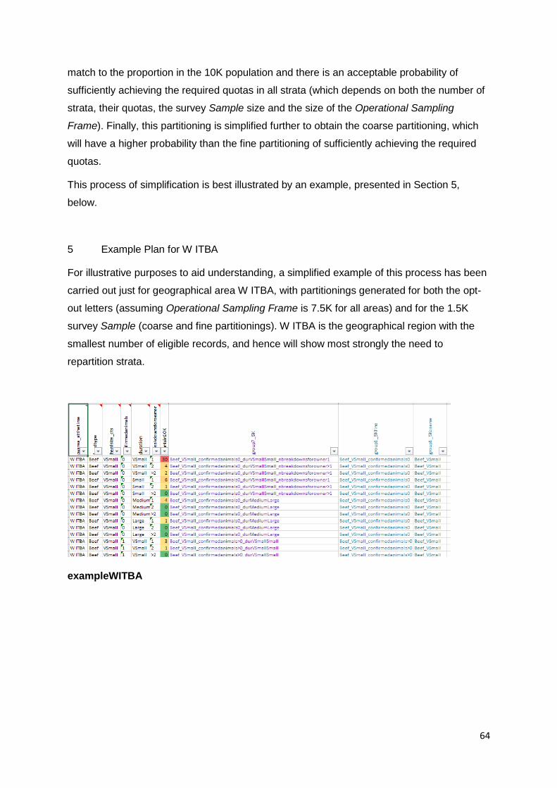
64
match to the proportion in the 10K population and there is an acceptable probability of
sufficiently achieving the required quotas in all strata (which depends on both the number of
strata, their quotas, the survey Sample size and the size of the Operational Sampling
Frame). Finally, this partitioning is simplified further to obtain the coarse partitioning, which
will have a higher probability than the fine partitioning of sufficiently achieving the required
quotas.
This process of simplification is best illustrated by an example, presented in Section 5,
below.
5 Example Plan for W ITBA
For illustrative purposes to aid understanding, a simplified example of this process has been
carried out just for geographical area W ITBA, with partitionings generated for both the opt-
out letters (assuming Operational Sampling Frame is 7.5K for all areas) and for the 1.5K
survey Sample (coarse and fine partitionings). W ITBA is the geographical region with the
smallest number of eligible records, and hence will show most strongly the need to
repartition strata.
exampleWITBA
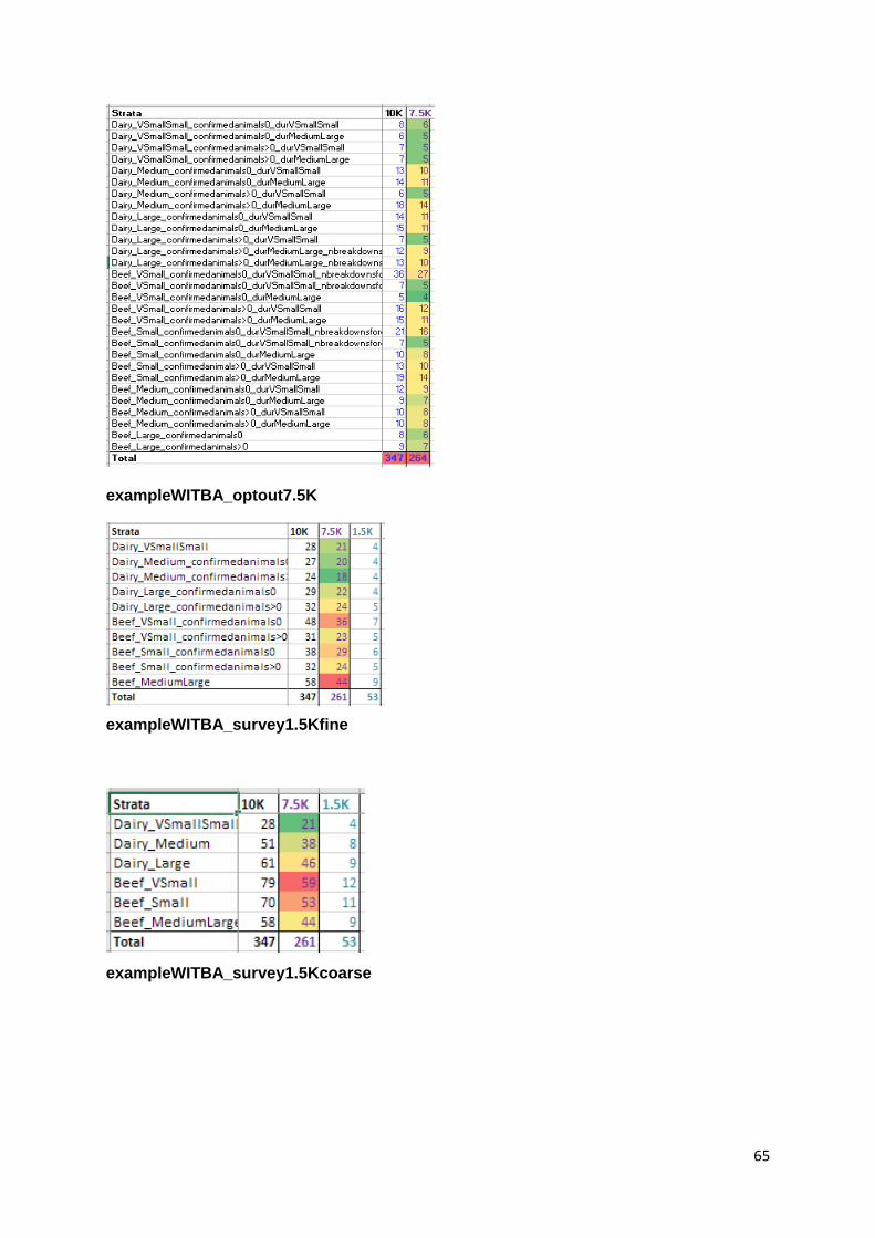
65
exampleWITBA_optout7.5K
exampleWITBA_survey1.5Kfine
exampleWITBA_survey1.5Kcoarse
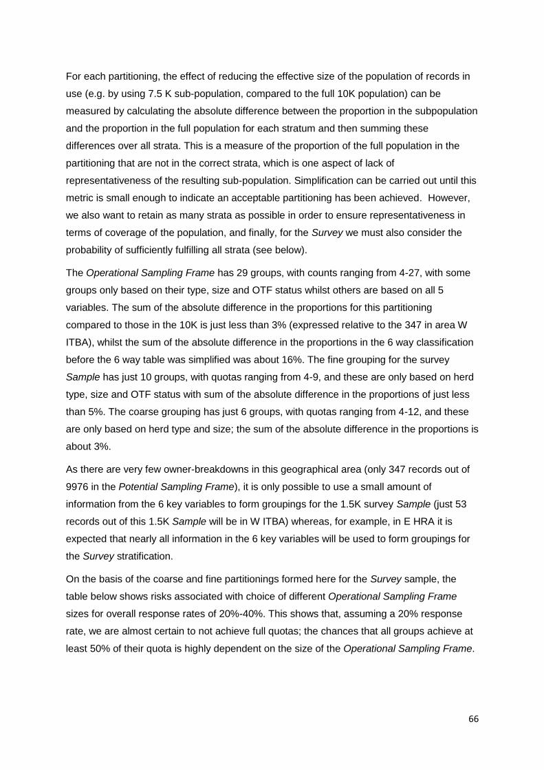
66
For each partitioning, the effect of reducing the effective size of the population of records in
use (e.g. by using 7.5 K sub-population, compared to the full 10K population) can be
measured by calculating the absolute difference between the proportion in the subpopulation
and the proportion in the full population for each stratum and then summing these
differences over all strata. This is a measure of the proportion of the full population in the
partitioning that are not in the correct strata, which is one aspect of lack of
representativeness of the resulting sub-population. Simplification can be carried out until this
metric is small enough to indicate an acceptable partitioning has been achieved. However,
we also want to retain as many strata as possible in order to ensure representativeness in
terms of coverage of the population, and finally, for the Survey we must also consider the
probability of sufficiently fulfilling all strata (see below).
The Operational Sampling Frame has 29 groups, with counts ranging from 4-27, with some
groups only based on their type, size and OTF status whilst others are based on all 5
variables. The sum of the absolute difference in the proportions for this partitioning
compared to those in the 10K is just less than 3% (expressed relative to the 347 in area W
ITBA), whilst the sum of the absolute difference in the proportions in the 6 way classification
before the 6 way table was simplified was about 16%. The fine grouping for the survey
Sample has just 10 groups, with quotas ranging from 4-9, and these are only based on herd
type, size and OTF status with sum of the absolute difference in the proportions of just less
than 5%. The coarse grouping has just 6 groups, with quotas ranging from 4-12, and these
are only based on herd type and size; the sum of the absolute difference in the proportions is
about 3%.
As there are very few owner-breakdowns in this geographical area (only 347 records out of
9976 in the Potential Sampling Frame), it is only possible to use a small amount of
information from the 6 key variables to form groupings for the 1.5K survey Sample (just 53
records out of this 1.5K Sample will be in W ITBA) whereas, for example, in E HRA it is
expected that nearly all information in the 6 key variables will be used to form groupings for
the Survey stratification.
On the basis of the coarse and fine partitionings formed here for the Survey sample, the
table below shows risks associated with choice of different Operational Sampling Frame
sizes for overall response rates of 20%-40%. This shows that, assuming a 20% response
rate, we are almost certain to not achieve full quotas; the chances that all groups achieve at
least 50% of their quota is highly dependent on the size of the Operational Sampling Frame.
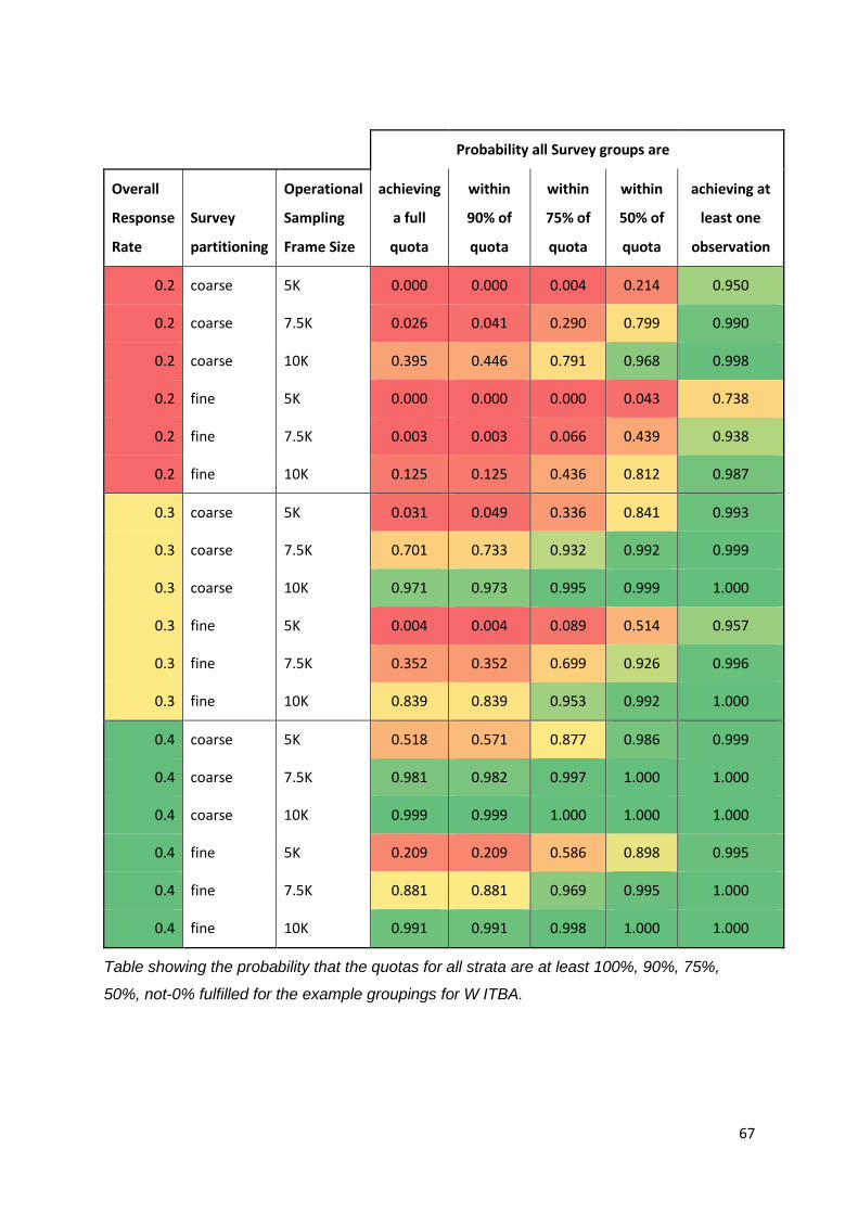
67
Probability all Survey groups are
Overall
Response
Rate
Survey
partitioning
Operational
Sampling
Frame Size
achieving
a full
quota
within
90% of
quota
within
75% of
quota
within
50% of
quota
achieving at
least one
observation
0.2 coarse 5K 0.000 0.000 0.004 0.214 0.950
0.2 coarse 7.5K 0.026 0.041 0.290 0.799 0.990
0.2 coarse 10K 0.395 0.446 0.791 0.968 0.998
0.2 fine 5K 0.000 0.000 0.000 0.043 0.738
0.2 fine 7.5K 0.003 0.003 0.066 0.439 0.938
0.2 fine 10K 0.125 0.125 0.436 0.812 0.987
0.3 coarse 5K 0.031 0.049 0.336 0.841 0.993
0.3 coarse 7.5K 0.701 0.733 0.932 0.992 0.999
0.3 coarse 10K 0.971 0.973 0.995 0.999 1.000
0.3 fine 5K 0.004 0.004 0.089 0.514 0.957
0.3 fine 7.5K 0.352 0.352 0.699 0.926 0.996
0.3 fine 10K 0.839 0.839 0.953 0.992 1.000
0.4 coarse 5K 0.518 0.571 0.877 0.986 0.999
0.4 coarse 7.5K 0.981 0.982 0.997 1.000 1.000
0.4 coarse 10K 0.999 0.999 1.000 1.000 1.000
0.4 fine 5K 0.209 0.209 0.586 0.898 0.995
0.4 fine 7.5K 0.881 0.881 0.969 0.995 1.000
0.4 fine 10K 0.991 0.991 0.998 1.000 1.000
Table showing the probability that the quotas for all strata are at least 100%, 90%, 75%,
50%, not-0% fulfilled for the example groupings for W ITBA.
68
Annex C: Telephone questionnaire & letter
Survey on the consequential cost of bovine TB incidents on cattle farms14
Scotland’s Rural College (SRUC) is conducting research on behalf of Defra into the
type and level of uncompensated business costs arising as a consequence of bovine
TB incidents. For example, additional labour, feed and bedding requirements and/or
reduced output levels, but not the value of culled animals for which compensation
payments are made. You were previously sent a letter inviting you to participate in a
survey about these costs, together with a version of this questionnaire. Participation
in the survey is voluntary and the telephone interview should take about 30 minutes
to complete, but will require reference to your farm records.
We appreciate that recalling the experience of a stressful bTB breakdown can be
difficult, but this is an opportunity for you to help improve Defra’s understanding of
bTB impacts, to influence future policy decisions. You are free to stop the interview
at any time and are not obliged to answer any question that you do not want to. We
emphasise that all information given will be totally anonymous in any subsequent
reports or publications, that you and your farm will never be individually identifiable,
and that the data will be stored and handled in accordance with the General Data
Protection Regulation 2016/679.
(Blue text only read-out if interviewee needs more help).
(Red text are additional items after piloting)
Q1. Please confirm your consent to continue with the
interview
Yes No
Q2. Please confirm you have previously seen the question types and have access to farm records to
help answer questions.
Yes No If No, try to reschedule for when they will have
14 This letter was slightly different for Wales to cover administrative requirements.
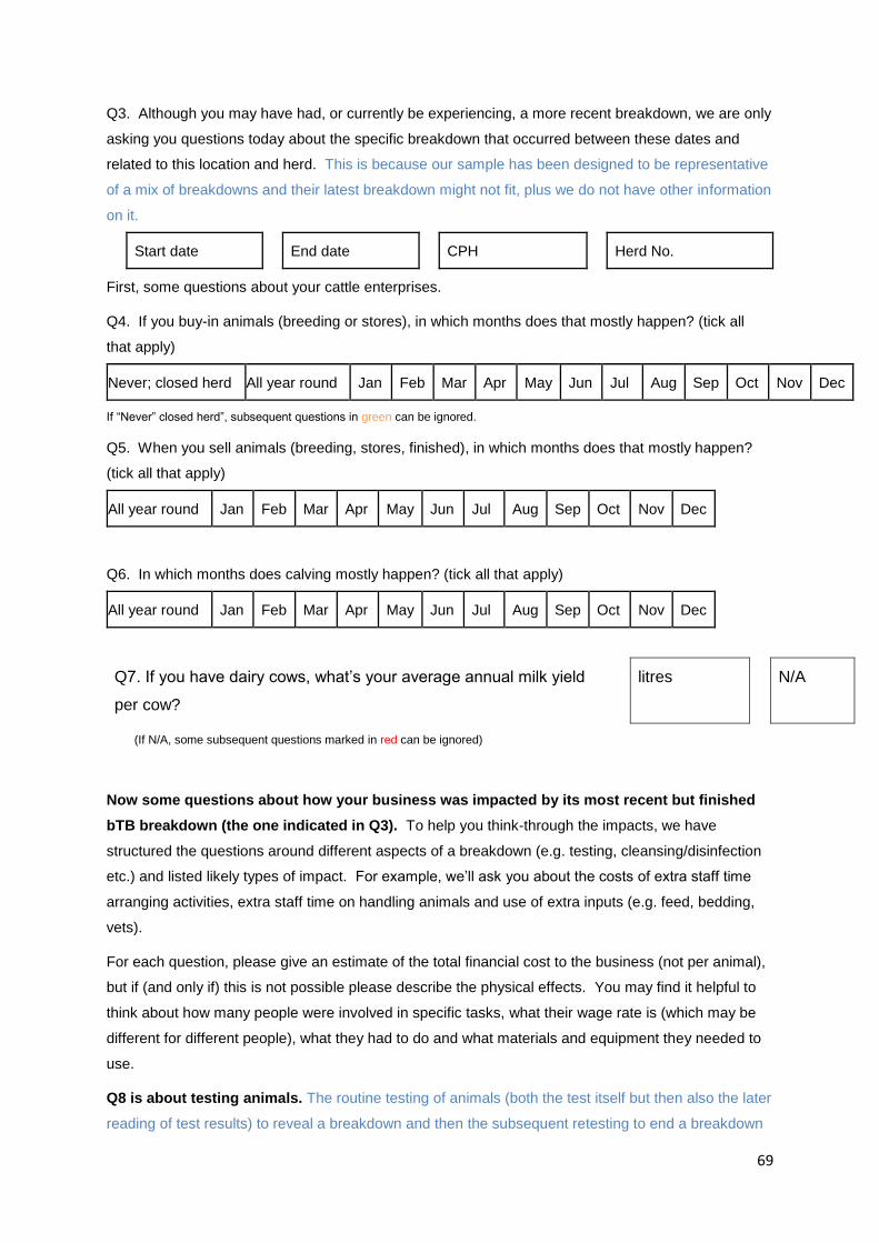
69
Q3. Although you may have had, or currently be experiencing, a more recent breakdown, we are only
asking you questions today about the specific breakdown that occurred between these dates and
related to this location and herd. This is because our sample has been designed to be representative
of a mix of breakdowns and their latest breakdown might not fit, plus we do not have other information
on it.
Start date End date CPH Herd No.
First, some questions about your cattle enterprises.
Q4. If you buy-in animals (breeding or stores), in which months does that mostly happen? (tick all
that apply)
Never; closed herd All year round Jan Feb Mar Apr May Jun Jul Aug Sep Oct Nov Dec
If “Never” closed herd”, subsequent questions in green can be ignored.
Q5. When you sell animals (breeding, stores, finished), in which months does that mostly happen?
(tick all that apply)
All year round Jan Feb Mar Apr May Jun Jul Aug Sep Oct Nov Dec
Q6. In which months does calving mostly happen? (tick all that apply)
All year round Jan Feb Mar Apr May Jun Jul Aug Sep Oct Nov Dec
Q7. If you have dairy cows, what’s your average annual milk yield
per cow?
litres N/A
(If N/A, some subsequent questions marked in red can be ignored)
Now some questions about how your business was impacted by its most recent but finished
bTB breakdown (the one indicated in Q3). To help you think-through the impacts, we have
structured the questions around different aspects of a breakdown (e.g. testing, cleansing/disinfection
etc.) and listed likely types of impact. For example, we’ll ask you about the costs of extra staff time
arranging activities, extra staff time on handling animals and use of extra inputs (e.g. feed, bedding,
vets).
For each question, please give an estimate of the total financial cost to the business (not per animal),
but if (and only if) this is not possible please describe the physical effects. You may find it helpful to
think about how many people were involved in specific tasks, what their wage rate is (which may be
different for different people), what they had to do and what materials and equipment they needed to
use.
Q8 is about testing animals. The routine testing of animals (both the test itself but then also the later
reading of test results) to reveal a breakdown and then the subsequent retesting to end a breakdown
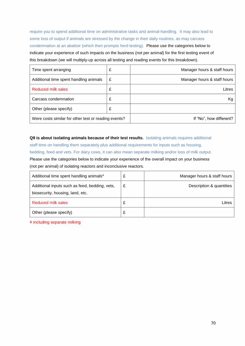
70
require you to spend additional time on administrative tasks and animal-handling. It may also lead to
some loss of output if animals are stressed by the change in their daily routines, as may carcass
condemnation at an abattoir (which then prompts herd testing). Please use the categories below to
indicate your experience of such impacts on the business (not per animal) for the first testing event of
this breakdown (we will multiply-up across all testing and reading events for this breakdown).
Time spent arranging £ Manager hours & staff hours
Additional time spent handling animals £ Manager hours & staff hours
Reduced milk sales £ Litres
Carcass condemnation £ Kg
Other (please specify) £
Were costs similar for other test or reading events? If “No”, how different?
Q9 is about isolating animals because of their test results. Isolating animals requires additional
staff time on handling them separately plus additional requirements for inputs such as housing,
bedding, feed and vets. For dairy cows, it can also mean separate milking and/or loss of milk output.
Please use the categories below to indicate your experience of the overall impact on your business
(not per animal) of isolating reactors and inconclusive reactors.
Additional time spent handling animalsǂ £ Manager hours & staff hours
Additional inputs such as feed, bedding, vets,
biosecurity, housing, land, etc.
£ Description & quantities
Reduced milk sales £ Litres
Other (please specify) £
ǂ including separate milking
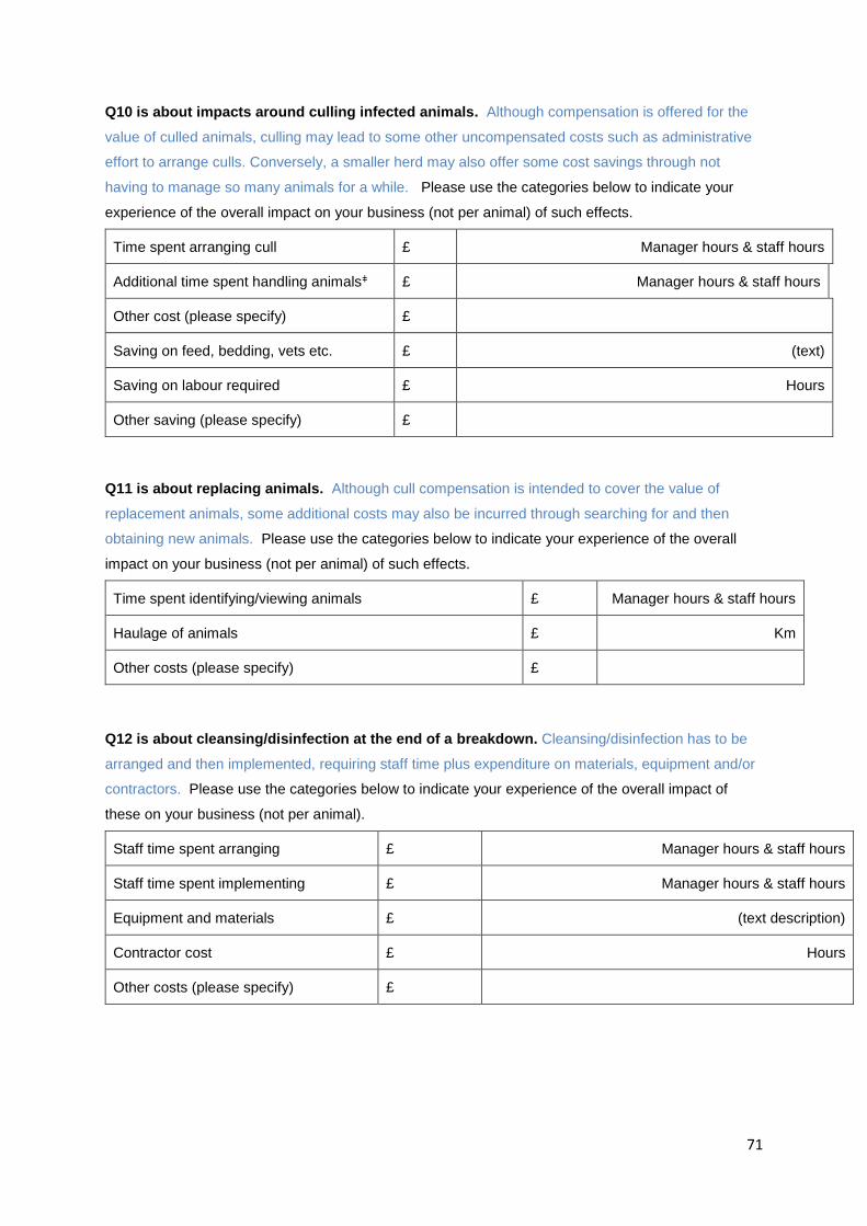
71
Q10 is about impacts around culling infected animals. Although compensation is offered for the
value of culled animals, culling may lead to some other uncompensated costs such as administrative
effort to arrange culls. Conversely, a smaller herd may also offer some cost savings through not
having to manage so many animals for a while. Please use the categories below to indicate your
experience of the overall impact on your business (not per animal) of such effects.
Time spent arranging cull £ Manager hours & staff hours
Additional time spent handling animalsǂ £ Manager hours & staff hours
Other cost (please specify) £
Saving on feed, bedding, vets etc. £ (text)
Saving on labour required £ Hours
Other saving (please specify) £
Q11 is about replacing animals. Although cull compensation is intended to cover the value of
replacement animals, some additional costs may also be incurred through searching for and then
obtaining new animals. Please use the categories below to indicate your experience of the overall
impact on your business (not per animal) of such effects.
Time spent identifying/viewing animals £ Manager hours & staff hours
Haulage of animals £ Km
Other costs (please specify) £
Q12 is about cleansing/disinfection at the end of a breakdown. Cleansing/disinfection has to be
arranged and then implemented, requiring staff time plus expenditure on materials, equipment and/or
contractors. Please use the categories below to indicate your experience of the overall impact of
these on your business (not per animal).
Staff time spent arranging £ Manager hours & staff hours
Staff time spent implementing £ Manager hours & staff hours
Equipment and materials £ (text description)
Contractor cost £ Hours
Other costs (please specify) £
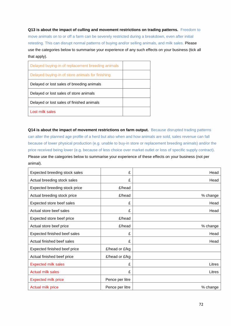
72
Q13 is about the impact of culling and movement restrictions on trading patterns. Freedom to
move animals on to or off a farm can be severely restricted during a breakdown, even after initial
retesting. This can disrupt normal patterns of buying and/or selling animals, and milk sales. Please
use the categories below to summarise your experience of any such effects on your business (tick all
that apply).
Delayed buying-in of replacement breeding animals
Delayed buying-in of store animals for finishing
Delayed or lost sales of breeding animals
Delayed or lost sales of store animals
Delayed or lost sales of finished animals
Lost milk sales
Q14 is about the impact of movement restrictions on farm output. Because disrupted trading patterns
can alter the planned age profile of a herd but also when and how animals are sold, sales revenue can fall
because of lower physical production (e.g. unable to buy-in store or replacement breeding animals) and/or the
price received being lower (e.g. because of less choice over market outlet or loss of specific supply contract).
Please use the categories below to summarise your experience of these effects on your business (not per
animal).
Expected breeding stock sales £ Head
Actual breeding stock sales £ Head
Expected breeding stock price £/head
Actual breeding stock price £/head % change
Expected store beef sales £ Head
Actual store beef sales £ Head
Expected store beef price £/head
Actual store beef price £/head % change
Expected finished beef sales £ Head
Actual finished beef sales £ Head
Expected finished beef price £/head or £/kg
Actual finished beef price £/head or £/kg
Expected milk sales £ Litres
Actual milk sales £ Litres
Expected milk price Pence per litre
Actual milk price Pence per litre % change
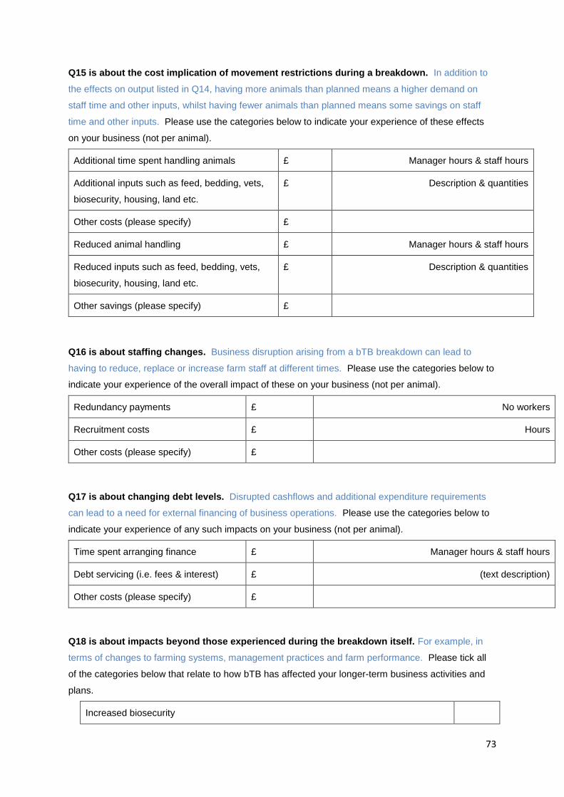
73
Q15 is about the cost implication of movement restrictions during a breakdown. In addition to
the effects on output listed in Q14, having more animals than planned means a higher demand on
staff time and other inputs, whilst having fewer animals than planned means some savings on staff
time and other inputs. Please use the categories below to indicate your experience of these effects
on your business (not per animal).
Additional time spent handling animals £ Manager hours & staff hours
Additional inputs such as feed, bedding, vets,
biosecurity, housing, land etc.
£ Description & quantities
Other costs (please specify) £
Reduced animal handling £ Manager hours & staff hours
Reduced inputs such as feed, bedding, vets,
biosecurity, housing, land etc.
£ Description & quantities
Other savings (please specify) £
Q16 is about staffing changes. Business disruption arising from a bTB breakdown can lead to
having to reduce, replace or increase farm staff at different times. Please use the categories below to
indicate your experience of the overall impact of these on your business (not per animal).
Redundancy payments £ No workers
Recruitment costs £ Hours
Other costs (please specify) £
Q17 is about changing debt levels. Disrupted cashflows and additional expenditure requirements
can lead to a need for external financing of business operations. Please use the categories below to
indicate your experience of any such impacts on your business (not per animal).
Time spent arranging finance £ Manager hours & staff hours
Debt servicing (i.e. fees & interest) £ (text description)
Other costs (please specify) £
Q18 is about impacts beyond those experienced during the breakdown itself. For example, in
terms of changes to farming systems, management practices and farm performance. Please tick all
of the categories below that relate to how bTB has affected your longer-term business activities and
plans.
Increased biosecurity
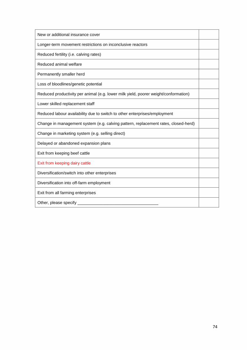
74
New or additional insurance cover
Longer-term movement restrictions on inconclusive reactors
Reduced fertility (i.e. calving rates)
Reduced animal welfare
Permanently smaller herd
Loss of bloodlines/genetic potential
Reduced productivity per animal (e.g. lower milk yield, poorer weight/conformation)
Lower skilled replacement staff
Reduced labour availability due to switch to other enterprises/employment
Change in management system (e.g. calving pattern, replacement rates, closed-herd)
Change in marketing system (e.g. selling direct)
Delayed or abandoned expansion plans
Exit from keeping beef cattle
Exit from keeping dairy cattle
Diversification/switch into other enterprises
Diversification into off-farm employment
Exit from all farming enterprises
Other, please specify ___________________________________
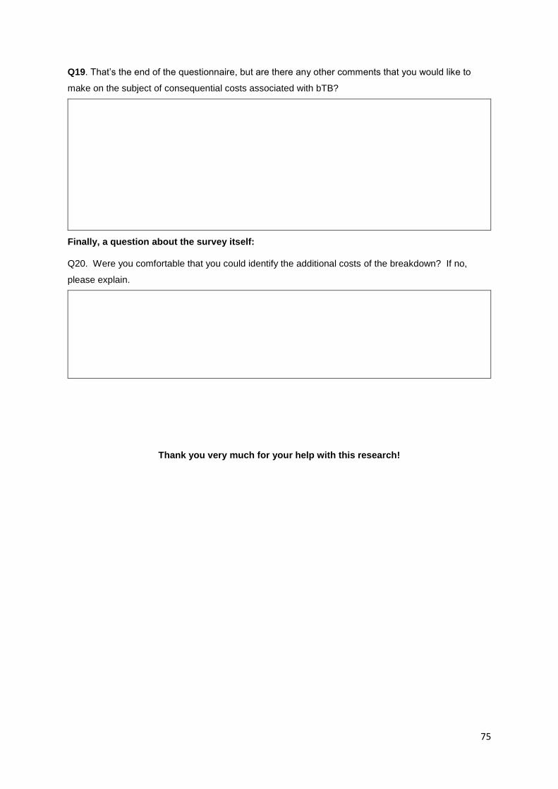
75
Q19. That’s the end of the questionnaire, but are there any other comments that you would like to
make on the subject of consequential costs associated with bTB?
Finally, a question about the survey itself:
Q20. Were you comfortable that you could identify the additional costs of the breakdown? If no,
please explain.
Thank you very much for your help with this research!
XXX Bovine TB Programme
XXX Nobel House,
XXX 17 Smith Square,
XXX London,
XXX SW1P 3JR
Dear <>
Bovine TB research invitation and privacy notice
This letter invites you to contribute to a research project investigating the uncompensated
costs of bovine tuberculosis (bTB) across different farm situations. For example, by farm
type, production system and severity of breakdown. Costs arise as a consequence of testing
and isolating animals plus coping with any movement restrictions and changes to the size
and/or age profile of a herd. Information on such costs will improve understanding of how
bTB is affecting the economics of individual farms and the industry as a whole, and will
contribute to the development of future Government policy.
Details on who has commissioned the project and who is undertaking the research are
provided in Appendix A to this letter, along with an explanation of how data will be used. The
public interest in the economics and sustainability of farming and of controlling livestock
disease means that this research can be conducted using existing data on bTB breakdowns,
and that contact details for farms suffering breakdowns can be used to seek further
information via a telephone survey.
In the first instance, we are writing to notify you that you may be telephoned and asked to
answer a series of questions relating to your herd <herdmark> and holding <CPH> and the
bTB breakdown you experienced between <start date> and <end date>. Not all farmers will
be contacted, but if you are called it will be during the next two months.
If you are called, but do not wish to participate in the research, you can decline at that point:
we understand that bTB is a difficult and emotive topic. However, better information is key to
understanding impacts and improving policy, and can only be obtained by asking farmers
directly about their experiences. Your participation in the project is important and will be
greatly appreciated.
Yours sincerely,

Appendix A: Project partners and research details
The project has been commissioned by the Department for the Environment Food and Rural Affairs (Defra),
the Welsh Government (WG) and the Scottish Government (SG); and supported by the Animal and Plant
Health Agency (APHA). It is being conducted in accordance with APHA’s published Privacy Notice on how
data they hold may be used for research purposes (see
https://assets.publishing.service.gov.uk/government/uploads/system/uploads/attachment_data/file/741423/aph
a-privacy-notice.pdf). The project is being led by SRUC (Scotland’s Rural College, with involvement from
Pexel (a market research company), BioSS (Biomathematics and Statistics Scotland, which is part of the
James Hutton Institute) and Pareto Consulting (an agricultural economics consultancy). Contact addresses
for each project partner are presented in Appendix B. APHA provided your contact details, so we could send
you this letter.
Pexel will initially call to arrange a date and time for the interview, and then (if you agree) subsequently call
again to ask questions about your herd management and how the bTB breakdown affected this. For example,
how much extra labour, feed and bedding was required to cope with isolating animals and movement
restrictions or how production levels were affected by not being able to buy and sell animals as planned.
Appendix C to this letter lists the types of question topics that will be covered, with the whole interview taking
around 30 minutes.
To keep the interview as short as possible, it will be helpful if you can refer to farm records when answering
questions. Hence, the initial call from Pexel to arrange the time & date for answering questions will encourage
you to retrieve and consult such records in advance (but please do not do so simply on receipt of this letter
since you may not be called).
Once Pexel has completed all telephone interview calls, the survey data will be passed to BioSS to be merged
with existing farm-level data on bTB breakdowns. For example, the number of animals tested, isolated and
culled. Using these existing data, which have been provided by APHA, avoids us having to ask you for such
information. Before the survey data are passed across to BioSS, your contact details will be deleted such that
they are not seen by BioSS.
Once BioSS has merged the survey and existing data, and completed quality checks on the dataset, your herd
number and county-parish-holding (CPH) numbers will also be deleted. This will anonymise the final dataset,
which will then be used for statistical and economic analysis by BioSS, SRUC and Pareto Consulting. The
anonymised data will also be provided to APHA, Defra, the Welsh Government and the Scottish Government.
Any enquiries about the project should be directed to SRUC in the first instance.
Neither you nor your farm will be identifiable in any reports or publications arising from the research, and you
have the right to request access to or deletion of any personal information supplied. If you wish to exercise
this right, please contact Pexel. You also have the right to complain to the Information Commissioner’s Office
(ICO) if you think that the General Data Protection Regulation (GDPR) has been breached. Your personal
data will be held securely by BioSS, Pexel and SRUC until the anonymised, combined dataset has been

created and validated (estimated to be September 2019), at which point all personal data held for this project
will be permanently destroyed as no longer required.
Appendix B: Contact addresses and GDPR role of project partners
APHA, Data Controller of English breakdown data; Joint Data Controller of Welsh Breakdown
data
bTB survey, Bovine TB R&D Programme, Area 2A, APHA, Nobel House, 17 Smith Square, London,
SW1P 3JR.
Defra. Data Controller and Ministerial Body to which APHA is accountable
bTB survey, Bovine TB Programme, Area 5D, Nobel House, 17 Smith Square, London SW1P 3JR.
BioSS, Data Processor (of breakdown data and survey data)
bTB survey, BioSS, JCMB, The King's Buildings, Peter Guthrie Tait Road, Edinburgh, EH9 3FD.
Pexel, Data Processor (of names, addresses & farm identifiers)
bTB Survey, Pexel Ltd, 28 Elderpark Workspace, 100 Elderpark Street, Glasgow G51 3TR.
SRUC, Data Processor (of breakdown data and survey data)
bTB survey, REES Group, SRUC, West Mains Road, Edinburgh EH9 3JG. [email protected]
Pareto Consulting. Will only see anonymised project data.
bTB survey, Pareto Consulting, 29 Redford Avenue, Edinburgh EH13 0BX.
Welsh Government. Joint Data Controller of Welsh breakdown data.
bTB survey, TB Team, Welsh Government, Cathays Park, Cardiff, CF10 3NQ.
Appendix C: bTB survey topic guide
To help you think through the consequences of your bTB breakdown, the telephone questionnaire
will be structured by splitting the breakdown into a number of stages to help estimate the total
financial cost to the business (not per animal). The stages are:
• testing animals;
• isolating animals;
• culling animals;
• replacing animals;
• cleansing premises;
• staff recruitment/redundancy;
• arranging and servicing additional finance; and
• coping with management restrictions.
At each stage, you may have experienced costs in the form of actual spending on additional inputs
and/or additional time and effort required. On the other hand, you may have saved costs in some
instances. You will be asked about these possibilities for each breakdown stage in turn. For
example:
• additional administrative costs for time spent making arrangements;
• additional labour costs for handling animals; and
• additional expenditure on inputs (e.g. feed, bedding, housing, haulage, debt servicing).
You may also have experienced lower physical output and/or lower prices as a result of culling
and/or movement restrictions. For example:
• lower production of store, breeding or finished animals;
• lower prices for cattle sold;
• lower milk output; and
• lower milk prices.
In each case, you will be asked to provide £ figures. If (and only if) you are unable to give a £ figure,
you will be asked to describe impacts in physical terms (e.g. extra hours of management labour,
extra hours of staff labour, kg of additional feed, change in number of animals sold etc.).
Feedback from farmers who helped to test the questionnaire before the full survey was launched
highlighted that it is much easier and quicker to answer the questions if farm records are readily to
hand. Hence it will be helpful if you can please retrieve, and ideally consult, such records before the
agreed interview time.
You will also be asked a few questions to help us understand your farming system. For example:
• when you typically buy or sell cattle;
• when you typically calve;
• any longer-term impacts lasting beyond the end of the breakdown.
Please note, the focus of the survey is on uncompensated consequential costs rather than the
cost of culled animals for which compensation is available. Also, if you have experienced more
than one breakdown, please note that the interviewer will only be asking about the breakdown
specified in the main letter.
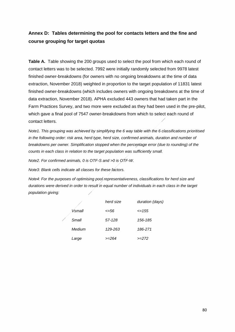
80
Annex D: Tables determining the pool for contacts letters and the fine and
course grouping for target quotas
Table A. Table showing the 200 groups used to select the pool from which each round of
contact letters was to be selected. 7992 were initially randomly selected from 9978 latest
finished owner-breakdowns (for owners with no ongoing breakdowns at the time of data
extraction, November 2018) weighted in proportion to the target population of 11831 latest
finished owner-breakdowns (which includes owners with ongoing breakdowns at the time of
data extraction, November 2018). APHA excluded 443 owners that had taken part in the
Farm Practices Survey, and two more were excluded as they had been used in the pre-pilot,
which gave a final pool of 7547 owner-breakdowns from which to select each round of
contact letters.
Note1. This grouping was achieved by simplifying the 6 way table with the 6 classifications prioritised
in the following order: risk area, herd type, herd size, confirmed animals, duration and number of
breakdowns per owner. Simplification stopped when the percentage error (due to rounding) of the
counts in each class in relation to the target population was sufficiently small.
Note2. For confirmed animals, 0 is OTF-S and >0 is OTF-W.
Note3: Blank cells indicate all classes for these factors.
Note4: For the purposes of optimising pool representativeness, classifications for herd size and
durations were derived in order to result in equal number of individuals in each class in the target
population giving:
herd size duration (days)
Vsmall <=56 <=155
Small 57-128 156-185
Medium 129-263 186-271
Large >=264 >=272
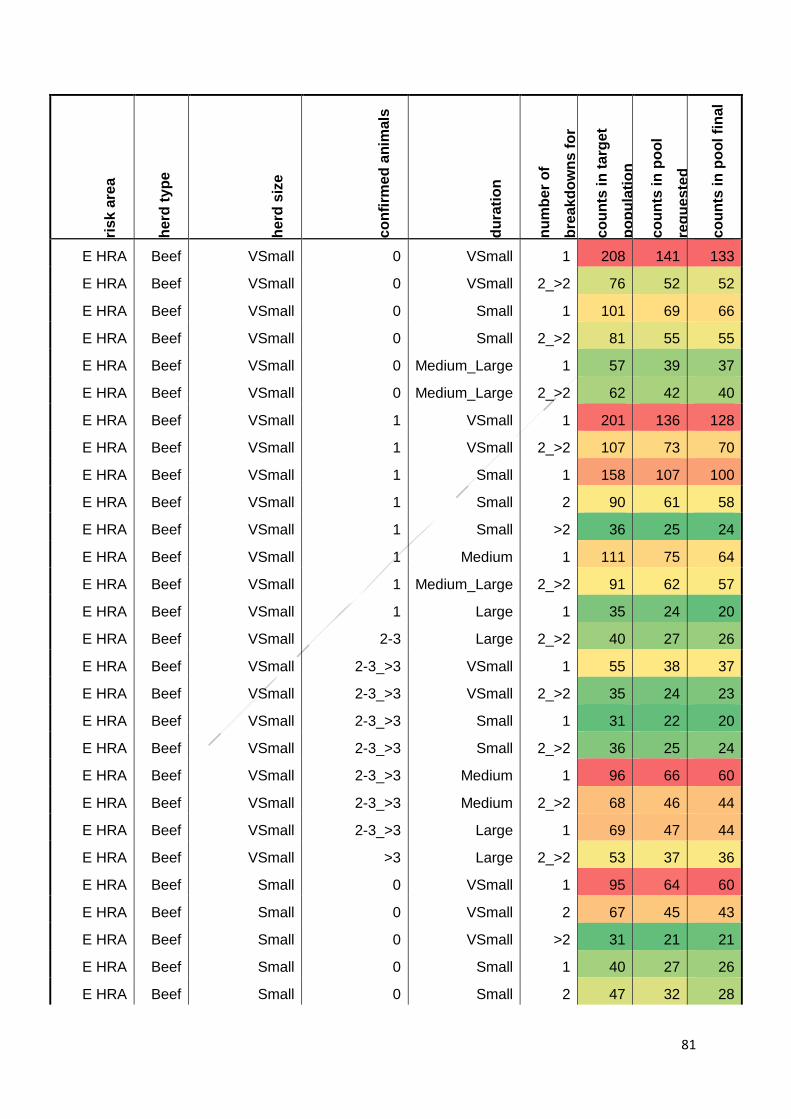
81
ris
k a
rea
herd
ty
pe
herd
siz
e
co
nfi
rme
d a
nim
als
du
rati
on
nu
mb
er
of
bre
ak
do
wn
s f
or
ow
ne
r c
ou
nts
in
ta
rget
po
pu
lati
on
co
un
ts in
po
ol
req
ue
ste
d
co
un
ts in
po
ol fi
nal
E HRA Beef VSmall 0 VSmall 1 208 141 133
E HRA Beef VSmall 0 VSmall 2_>2 76 52 52
E HRA Beef VSmall 0 Small 1 101 69 66
E HRA Beef VSmall 0 Small 2_>2 81 55 55
E HRA Beef VSmall 0 Medium_Large 1 57 39 37
E HRA Beef VSmall 0 Medium_Large 2_>2 62 42 40
E HRA Beef VSmall 1 VSmall 1 201 136 128
E HRA Beef VSmall 1 VSmall 2_>2 107 73 70
E HRA Beef VSmall 1 Small 1 158 107 100
E HRA Beef VSmall 1 Small 2 90 61 58
E HRA Beef VSmall 1 Small >2 36 25 24
E HRA Beef VSmall 1 Medium 1 111 75 64
E HRA Beef VSmall 1 Medium_Large 2_>2 91 62 57
E HRA Beef VSmall 1 Large 1 35 24 20
E HRA Beef VSmall 2-3 Large 2_>2 40 27 26
E HRA Beef VSmall 2-3_>3 VSmall 1 55 38 37
E HRA Beef VSmall 2-3_>3 VSmall 2_>2 35 24 23
E HRA Beef VSmall 2-3_>3 Small 1 31 22 20
E HRA Beef VSmall 2-3_>3 Small 2_>2 36 25 24
E HRA Beef VSmall 2-3_>3 Medium 1 96 66 60
E HRA Beef VSmall 2-3_>3 Medium 2_>2 68 46 44
E HRA Beef VSmall 2-3_>3 Large 1 69 47 44
E HRA Beef VSmall >3 Large 2_>2 53 37 36
E HRA Beef Small 0 VSmall 1 95 64 60
E HRA Beef Small 0 VSmall 2 67 45 43
E HRA Beef Small 0 VSmall >2 31 21 21
E HRA Beef Small 0 Small 1 40 27 26
E HRA Beef Small 0 Small 2 47 32 28
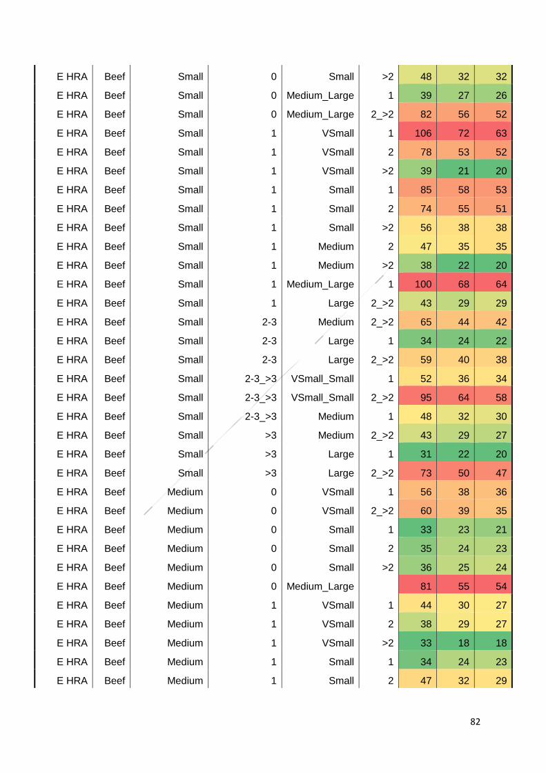
82
E HRA Beef Small 0 Small >2 48 32 32
E HRA Beef Small 0 Medium_Large 1 39 27 26
E HRA Beef Small 0 Medium_Large 2_>2 82 56 52
E HRA Beef Small 1 VSmall 1 106 72 63
E HRA Beef Small 1 VSmall 2 78 53 52
E HRA Beef Small 1 VSmall >2 39 21 20
E HRA Beef Small 1 Small 1 85 58 53
E HRA Beef Small 1 Small 2 74 55 51
E HRA Beef Small 1 Small >2 56 38 38
E HRA Beef Small 1 Medium 2 47 35 35
E HRA Beef Small 1 Medium >2 38 22 20
E HRA Beef Small 1 Medium_Large 1 100 68 64
E HRA Beef Small 1 Large 2_>2 43 29 29
E HRA Beef Small 2-3 Medium 2_>2 65 44 42
E HRA Beef Small 2-3 Large 1 34 24 22
E HRA Beef Small 2-3 Large 2_>2 59 40 38
E HRA Beef Small 2-3_>3 VSmall_Small 1 52 36 34
E HRA Beef Small 2-3_>3 VSmall_Small 2_>2 95 64 58
E HRA Beef Small 2-3_>3 Medium 1 48 32 30
E HRA Beef Small >3 Medium 2_>2 43 29 27
E HRA Beef Small >3 Large 1 31 22 20
E HRA Beef Small >3 Large 2_>2 73 50 47
E HRA Beef Medium 0 VSmall 1 56 38 36
E HRA Beef Medium 0 VSmall 2_>2 60 39 35
E HRA Beef Medium 0 Small 1 33 23 21
E HRA Beef Medium 0 Small 2 35 24 23
E HRA Beef Medium 0 Small >2 36 25 24
E HRA Beef Medium 0 Medium_Large 81 55 54
E HRA Beef Medium 1 VSmall 1 44 30 27
E HRA Beef Medium 1 VSmall 2 38 29 27
E HRA Beef Medium 1 VSmall >2 33 18 18
E HRA Beef Medium 1 Small 1 34 24 23
E HRA Beef Medium 1 Small 2 47 32 29
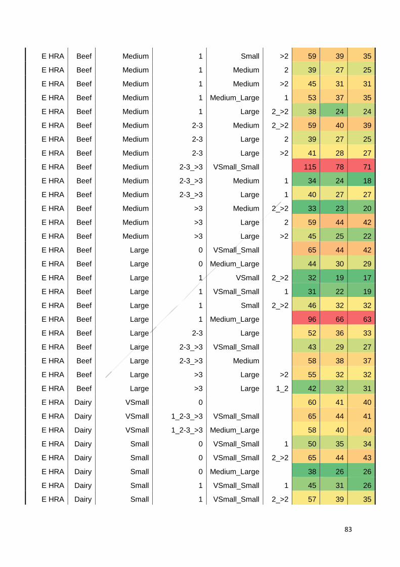
83
E HRA Beef Medium 1 Small >2 59 39 35
E HRA Beef Medium 1 Medium 2 39 27 25
E HRA Beef Medium 1 Medium >2 45 31 31
E HRA Beef Medium 1 Medium_Large 1 53 37 35
E HRA Beef Medium 1 Large 2_>2 38 24 24
E HRA Beef Medium 2-3 Medium 2_>2 59 40 39
E HRA Beef Medium 2-3 Large 2 39 27 25
E HRA Beef Medium 2-3 Large >2 41 28 27
E HRA Beef Medium 2-3_>3 VSmall_Small 115 78 71
E HRA Beef Medium 2-3_>3 Medium 1 34 24 18
E HRA Beef Medium 2-3_>3 Large 1 40 27 27
E HRA Beef Medium >3 Medium 2_>2 33 23 20
E HRA Beef Medium >3 Large 2 59 44 42
E HRA Beef Medium >3 Large >2 45 25 22
E HRA Beef Large 0 VSmall_Small 65 44 42
E HRA Beef Large 0 Medium_Large 44 30 29
E HRA Beef Large 1 VSmall 2_>2 32 19 17
E HRA Beef Large 1 VSmall_Small 1 31 22 19
E HRA Beef Large 1 Small 2_>2 46 32 32
E HRA Beef Large 1 Medium_Large 96 66 63
E HRA Beef Large 2-3 Large 52 36 33
E HRA Beef Large 2-3_>3 VSmall_Small 43 29 27
E HRA Beef Large 2-3_>3 Medium 58 38 37
E HRA Beef Large >3 Large >2 55 32 32
E HRA Beef Large >3 Large 1_2 42 32 31
E HRA Dairy VSmall 0 60 41 40
E HRA Dairy VSmall 1_2-3_>3 VSmall_Small 65 44 41
E HRA Dairy VSmall 1_2-3_>3 Medium_Large 58 40 40
E HRA Dairy Small 0 VSmall_Small 1 50 35 34
E HRA Dairy Small 0 VSmall_Small 2_>2 65 44 43
E HRA Dairy Small 0 Medium_Large 38 26 26
E HRA Dairy Small 1 VSmall_Small 1 45 31 26
E HRA Dairy Small 1 VSmall_Small 2_>2 57 39 35
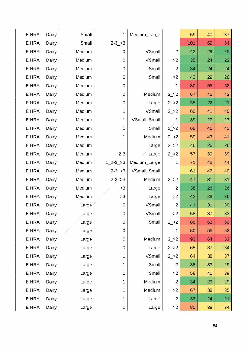
84
E HRA Dairy Small 1 Medium_Large 59 40 37
E HRA Dairy Small 2-3_>3 101 69 64
E HRA Dairy Medium 0 VSmall 2 43 29 25
E HRA Dairy Medium 0 VSmall >2 35 24 22
E HRA Dairy Medium 0 Small 2 34 24 24
E HRA Dairy Medium 0 Small >2 42 29 26
E HRA Dairy Medium 0 1 80 55 52
E HRA Dairy Medium 0 Medium 2_>2 67 45 42
E HRA Dairy Medium 0 Large 2_>2 35 22 21
E HRA Dairy Medium 1 VSmall 2_>2 60 41 40
E HRA Dairy Medium 1 VSmall_Small 1 39 27 27
E HRA Dairy Medium 1 Small 2_>2 68 46 42
E HRA Dairy Medium 1 Medium 2_>2 59 43 41
E HRA Dairy Medium 1 Large 2_>2 46 26 26
E HRA Dairy Medium 2-3 Large 2_>2 57 39 39
E HRA Dairy Medium 1_2-3_>3 Medium_Large 1 71 48 44
E HRA Dairy Medium 2-3_>3 VSmall_Small 61 42 40
E HRA Dairy Medium 2-3_>3 Medium 2_>2 47 31 31
E HRA Dairy Medium >3 Large 2 38 26 26
E HRA Dairy Medium >3 Large >2 42 28 26
E HRA Dairy Large 0 VSmall 2 41 31 30
E HRA Dairy Large 0 VSmall >2 58 37 33
E HRA Dairy Large 0 Small 2_>2 86 63 60
E HRA Dairy Large 0 1 80 55 52
E HRA Dairy Large 0 Medium 2_>2 93 64 62
E HRA Dairy Large 0 Large 2_>2 65 37 34
E HRA Dairy Large 1 VSmall 2_>2 64 38 37
E HRA Dairy Large 1 Small 2 38 33 29
E HRA Dairy Large 1 Small >2 58 41 39
E HRA Dairy Large 1 Medium 2 34 29 29
E HRA Dairy Large 1 Medium >2 67 38 35
E HRA Dairy Large 1 Large 2 33 24 21
E HRA Dairy Large 1 Large >2 80 38 34
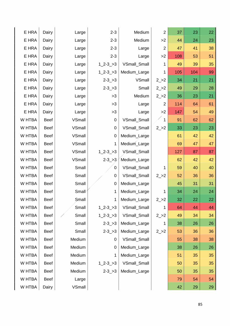
85
E HRA Dairy Large 2-3 Medium 2 37 23 22
E HRA Dairy Large 2-3 Medium >2 44 24 23
E HRA Dairy Large 2-3 Large 2 47 41 38
E HRA Dairy Large 2-3 Large >2 108 53 51
E HRA Dairy Large 1_2-3_>3 VSmall_Small 1 49 39 35
E HRA Dairy Large 1_2-3_>3 Medium_Large 1 105 104 99
E HRA Dairy Large 2-3_>3 VSmall 2_>2 34 21 21
E HRA Dairy Large 2-3_>3 Small 2_>2 49 29 28
E HRA Dairy Large >3 Medium 2_>2 36 23 21
E HRA Dairy Large >3 Large 2 114 64 61
E HRA Dairy Large >3 Large >2 147 54 49
W HTBA Beef VSmall 0 VSmall_Small 1 91 62 62
W HTBA Beef VSmall 0 VSmall_Small 2_>2 33 23 23
W HTBA Beef VSmall 0 Medium_Large 61 42 42
W HTBA Beef VSmall 1 Medium_Large 69 47 47
W HTBA Beef VSmall 1_2-3_>3 VSmall_Small 127 87 87
W HTBA Beef VSmall 2-3_>3 Medium_Large 62 42 42
W HTBA Beef Small 0 VSmall_Small 1 59 40 40
W HTBA Beef Small 0 VSmall_Small 2_>2 52 36 36
W HTBA Beef Small 0 Medium_Large 45 31 31
W HTBA Beef Small 1 Medium_Large 1 34 24 24
W HTBA Beef Small 1 Medium_Large 2_>2 32 22 22
W HTBA Beef Small 1_2-3_>3 VSmall_Small 1 64 44 44
W HTBA Beef Small 1_2-3_>3 VSmall_Small 2_>2 49 34 34
W HTBA Beef Small 2-3_>3 Medium_Large 1 38 26 26
W HTBA Beef Small 2-3_>3 Medium_Large 2_>2 53 36 36
W HTBA Beef Medium 0 VSmall_Small 55 38 38
W HTBA Beef Medium 0 Medium_Large 38 26 26
W HTBA Beef Medium 1 Medium_Large 51 35 35
W HTBA Beef Medium 1_2-3_>3 VSmall_Small 50 35 35
W HTBA Beef Medium 2-3_>3 Medium_Large 50 35 35
W HTBA Beef Large 79 54 54
W HTBA Dairy VSmall 42 29 29
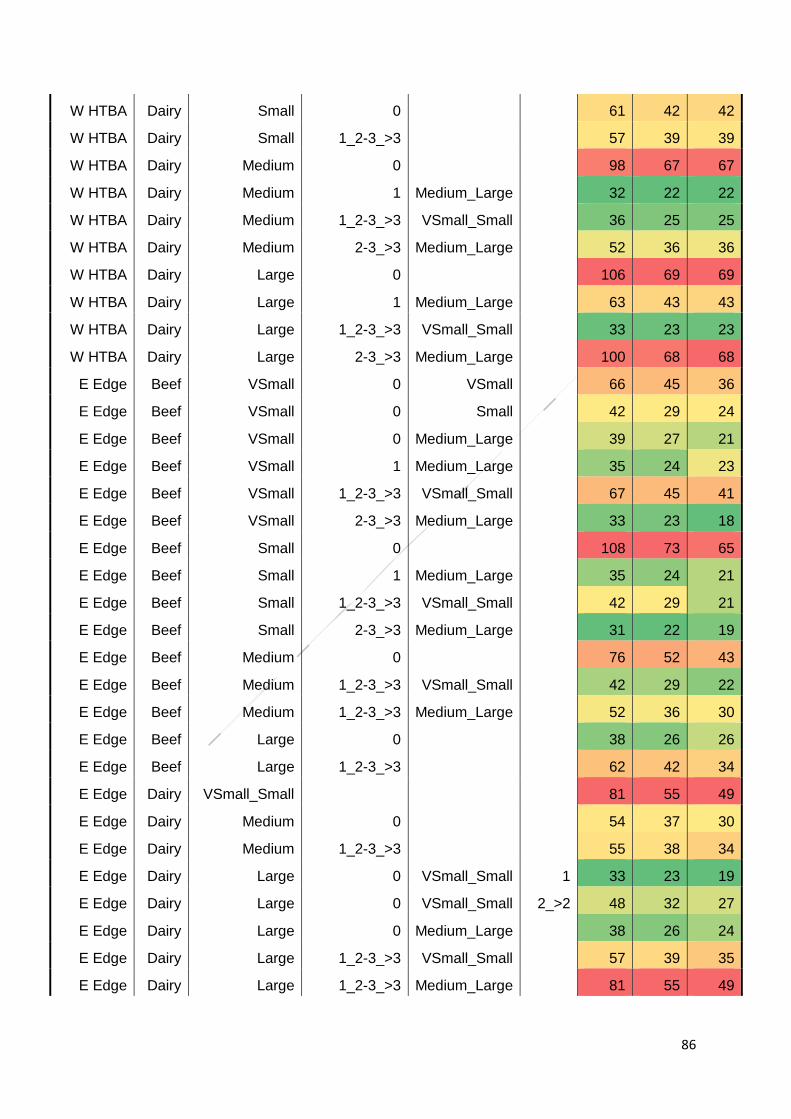
86
W HTBA Dairy Small 0 61 42 42
W HTBA Dairy Small 1_2-3_>3 57 39 39
W HTBA Dairy Medium 0 98 67 67
W HTBA Dairy Medium 1 Medium_Large 32 22 22
W HTBA Dairy Medium 1_2-3_>3 VSmall_Small 36 25 25
W HTBA Dairy Medium 2-3_>3 Medium_Large 52 36 36
W HTBA Dairy Large 0 106 69 69
W HTBA Dairy Large 1 Medium_Large 63 43 43
W HTBA Dairy Large 1_2-3_>3 VSmall_Small 33 23 23
W HTBA Dairy Large 2-3_>3 Medium_Large 100 68 68
E Edge Beef VSmall 0 VSmall 66 45 36
E Edge Beef VSmall 0 Small 42 29 24
E Edge Beef VSmall 0 Medium_Large 39 27 21
E Edge Beef VSmall 1 Medium_Large 35 24 23
E Edge Beef VSmall 1_2-3_>3 VSmall_Small 67 45 41
E Edge Beef VSmall 2-3_>3 Medium_Large 33 23 18
E Edge Beef Small 0 108 73 65
E Edge Beef Small 1 Medium_Large 35 24 21
E Edge Beef Small 1_2-3_>3 VSmall_Small 42 29 21
E Edge Beef Small 2-3_>3 Medium_Large 31 22 19
E Edge Beef Medium 0 76 52 43
E Edge Beef Medium 1_2-3_>3 VSmall_Small 42 29 22
E Edge Beef Medium 1_2-3_>3 Medium_Large 52 36 30
E Edge Beef Large 0 38 26 26
E Edge Beef Large 1_2-3_>3 62 42 34
E Edge Dairy VSmall_Small 81 55 49
E Edge Dairy Medium 0 54 37 30
E Edge Dairy Medium 1_2-3_>3 55 38 34
E Edge Dairy Large 0 VSmall_Small 1 33 23 19
E Edge Dairy Large 0 VSmall_Small 2_>2 48 32 27
E Edge Dairy Large 0 Medium_Large 38 26 24
E Edge Dairy Large 1_2-3_>3 VSmall_Small 57 39 35
E Edge Dairy Large 1_2-3_>3 Medium_Large 81 55 49
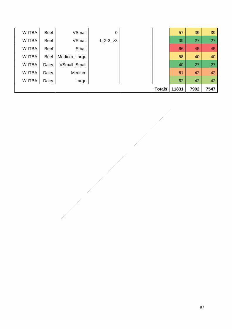
87
W ITBA Beef VSmall 0 57 39 39
W ITBA Beef VSmall 1_2-3_>3 39 27 27
W ITBA Beef Small 66 45 45
W ITBA Beef Medium_Large 58 40 40
W ITBA Dairy VSmall_Small 40 27 27
W ITBA Dairy Medium 61 42 42
W ITBA Dairy Large 62 42 42
Totals 11831 7992 7547
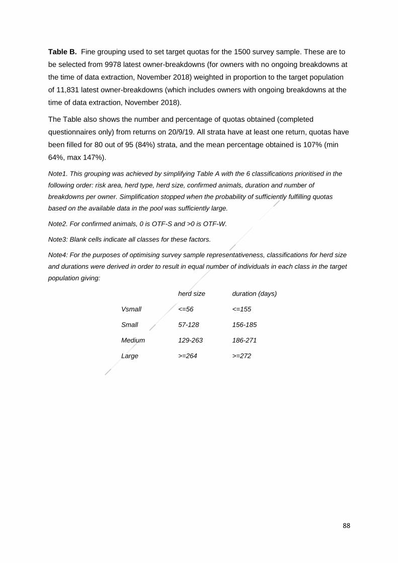
88
Table B. Fine grouping used to set target quotas for the 1500 survey sample. These are to
be selected from 9978 latest owner-breakdowns (for owners with no ongoing breakdowns at
the time of data extraction, November 2018) weighted in proportion to the target population
of 11,831 latest owner-breakdowns (which includes owners with ongoing breakdowns at the
time of data extraction, November 2018).
The Table also shows the number and percentage of quotas obtained (completed
questionnaires only) from returns on 20/9/19. All strata have at least one return, quotas have
been filled for 80 out of 95 (84%) strata, and the mean percentage obtained is 107% (min
64%, max 147%).
Note1. This grouping was achieved by simplifying Table A with the 6 classifications prioritised in the
following order: risk area, herd type, herd size, confirmed animals, duration and number of
breakdowns per owner. Simplification stopped when the probability of sufficiently fulfilling quotas
based on the available data in the pool was sufficiently large.
Note2. For confirmed animals, 0 is OTF-S and >0 is OTF-W.
Note3: Blank cells indicate all classes for these factors.
Note4: For the purposes of optimising survey sample representativeness, classifications for herd size
and durations were derived in order to result in equal number of individuals in each class in the target
population giving:
herd size duration (days)
Vsmall <=56 <=155
Small 57-128 156-185
Medium 129-263 186-271
Large >=264 >=272
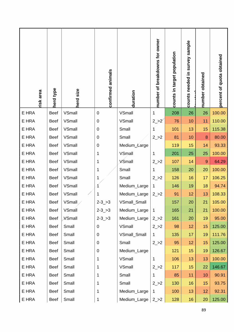
89
ris
k a
rea
herd
ty
pe
herd
siz
e
co
nfi
rme
d a
nim
als
d
ura
tio
n
nu
mb
er
of
bre
ak
do
wn
s f
or
ow
ner
co
un
ts in
ta
rget
po
pu
lati
on
c
ou
nts
ne
ed
ed
in
su
rve
y s
am
ple
(qu
ota
s)
nu
mb
er
ob
tain
ed
p
erc
en
t o
f q
uo
ta o
bta
ine
d
E HRA Beef VSmall 0 VSmall 1 208 26 26 100.00
E HRA Beef VSmall 0 VSmall 2_>2 76 10 11 110.00
E HRA Beef VSmall 0 Small 1 101 13 15 115.38
E HRA Beef VSmall 0 Small 2_>2 81 10 8 80.00
E HRA Beef VSmall 0 Medium_Large 119 15 14 93.33
E HRA Beef VSmall 1 VSmall 1 201 25 25 100.00
E HRA Beef VSmall 1 VSmall 2_>2 107 14 9 64.29
E HRA Beef VSmall 1 Small 1 158 20 20 100.00
E HRA Beef VSmall 1 Small 2_>2 126 16 17 106.25
E HRA Beef VSmall 1 Medium_Large 1 146 19 18 94.74
E HRA Beef VSmall 1 Medium_Large 2_>2 91 12 13 108.33
E HRA Beef VSmall 2-3_>3 VSmall_Small 157 20 21 105.00
E HRA Beef VSmall 2-3_>3 Medium_Large 1 165 21 21 100.00
E HRA Beef VSmall 2-3_>3 Medium_Large 2_>2 161 20 19 95.00
E HRA Beef Small 0 VSmall 2_>2 98 12 15 125.00
E HRA Beef Small 0 VSmall_Small 1 135 17 19 111.76
E HRA Beef Small 0 Small 2_>2 95 12 15 125.00
E HRA Beef Small 0 Medium_Large 121 15 19 126.67
E HRA Beef Small 1 VSmall 1 106 13 13 100.00
E HRA Beef Small 1 VSmall 2_>2 117 15 22 146.67
E HRA Beef Small 1 Small 1 85 11 10 90.91
E HRA Beef Small 1 Small 2_>2 130 16 15 93.75
E HRA Beef Small 1 Medium_Large 1 100 13 12 92.31
E HRA Beef Small 1 Medium_Large 2_>2 128 16 20 125.00
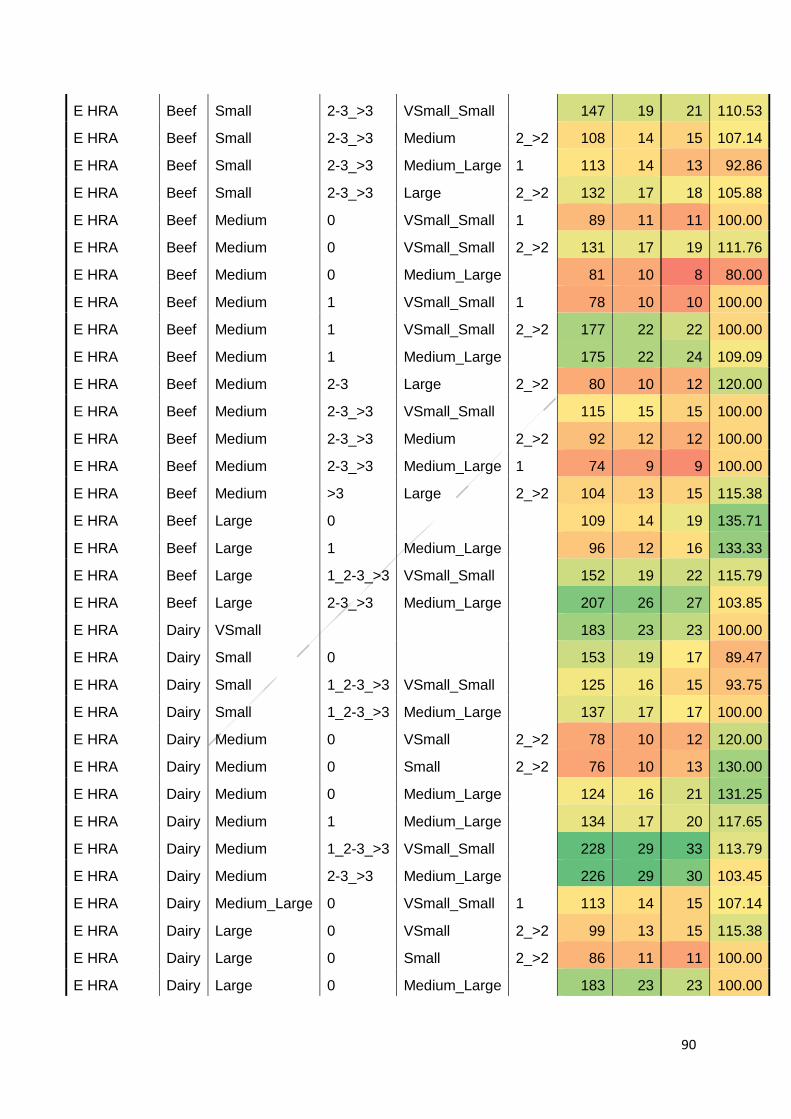
90
E HRA Beef Small 2-3_>3 VSmall_Small 147 19 21 110.53
E HRA Beef Small 2-3_>3 Medium 2_>2 108 14 15 107.14
E HRA Beef Small 2-3_>3 Medium_Large 1 113 14 13 92.86
E HRA Beef Small 2-3_>3 Large 2_>2 132 17 18 105.88
E HRA Beef Medium 0 VSmall_Small 1 89 11 11 100.00
E HRA Beef Medium 0 VSmall_Small 2_>2 131 17 19 111.76
E HRA Beef Medium 0 Medium_Large 81 10 8 80.00
E HRA Beef Medium 1 VSmall_Small 1 78 10 10 100.00
E HRA Beef Medium 1 VSmall_Small 2_>2 177 22 22 100.00
E HRA Beef Medium 1 Medium_Large 175 22 24 109.09
E HRA Beef Medium 2-3 Large 2_>2 80 10 12 120.00
E HRA Beef Medium 2-3_>3 VSmall_Small 115 15 15 100.00
E HRA Beef Medium 2-3_>3 Medium 2_>2 92 12 12 100.00
E HRA Beef Medium 2-3_>3 Medium_Large 1 74 9 9 100.00
E HRA Beef Medium >3 Large 2_>2 104 13 15 115.38
E HRA Beef Large 0 109 14 19 135.71
E HRA Beef Large 1 Medium_Large 96 12 16 133.33
E HRA Beef Large 1_2-3_>3 VSmall_Small 152 19 22 115.79
E HRA Beef Large 2-3_>3 Medium_Large 207 26 27 103.85
E HRA Dairy VSmall 183 23 23 100.00
E HRA Dairy Small 0 153 19 17 89.47
E HRA Dairy Small 1_2-3_>3 VSmall_Small 125 16 15 93.75
E HRA Dairy Small 1_2-3_>3 Medium_Large 137 17 17 100.00
E HRA Dairy Medium 0 VSmall 2_>2 78 10 12 120.00
E HRA Dairy Medium 0 Small 2_>2 76 10 13 130.00
E HRA Dairy Medium 0 Medium_Large 124 16 21 131.25
E HRA Dairy Medium 1 Medium_Large 134 17 20 117.65
E HRA Dairy Medium 1_2-3_>3 VSmall_Small 228 29 33 113.79
E HRA Dairy Medium 2-3_>3 Medium_Large 226 29 30 103.45
E HRA Dairy Medium_Large 0 VSmall_Small 1 113 14 15 107.14
E HRA Dairy Large 0 VSmall 2_>2 99 13 15 115.38
E HRA Dairy Large 0 Small 2_>2 86 11 11 100.00
E HRA Dairy Large 0 Medium_Large 183 23 23 100.00
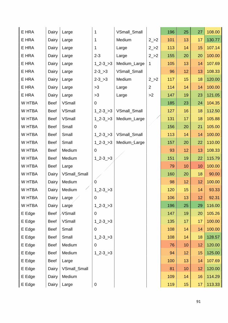
91
E HRA Dairy Large 1 VSmall_Small 196 25 27 108.00
E HRA Dairy Large 1 Medium 2_>2 101 13 17 130.77
E HRA Dairy Large 1 Large 2_>2 113 14 15 107.14
E HRA Dairy Large 2-3 Large 2_>2 155 20 20 100.00
E HRA Dairy Large 1_2-3_>3 Medium_Large 1 105 13 14 107.69
E HRA Dairy Large 2-3_>3 VSmall_Small 96 12 13 108.33
E HRA Dairy Large 2-3_>3 Medium 2_>2 117 15 18 120.00
E HRA Dairy Large >3 Large 2 114 14 14 100.00
E HRA Dairy Large >3 Large >2 147 19 23 121.05
W HTBA Beef VSmall 0 185 23 24 104.35
W HTBA Beef VSmall 1_2-3_>3 VSmall_Small 127 16 18 112.50
W HTBA Beef VSmall 1_2-3_>3 Medium_Large 131 17 18 105.88
W HTBA Beef Small 0 156 20 21 105.00
W HTBA Beef Small 1_2-3_>3 VSmall_Small 113 14 14 100.00
W HTBA Beef Small 1_2-3_>3 Medium_Large 157 20 22 110.00
W HTBA Beef Medium 0 93 12 13 108.33
W HTBA Beef Medium 1_2-3_>3 151 19 22 115.79
W HTBA Beef Large 79 10 10 100.00
W HTBA Dairy VSmall_Small 160 20 18 90.00
W HTBA Dairy Medium 0 98 12 12 100.00
W HTBA Dairy Medium 1_2-3_>3 120 15 14 93.33
W HTBA Dairy Large 0 106 13 12 92.31
W HTBA Dairy Large 1_2-3_>3 196 25 29 116.00
E Edge Beef VSmall 0 147 19 20 105.26
E Edge Beef VSmall 1_2-3_>3 135 17 17 100.00
E Edge Beef Small 0 108 14 14 100.00
E Edge Beef Small 1_2-3_>3 108 14 18 128.57
E Edge Beef Medium 0 76 10 12 120.00
E Edge Beef Medium 1_2-3_>3 94 12 15 125.00
E Edge Beef Large 100 13 14 107.69
E Edge Dairy VSmall_Small 81 10 12 120.00
E Edge Dairy Medium 109 14 16 114.29
E Edge Dairy Large 0 119 15 17 113.33
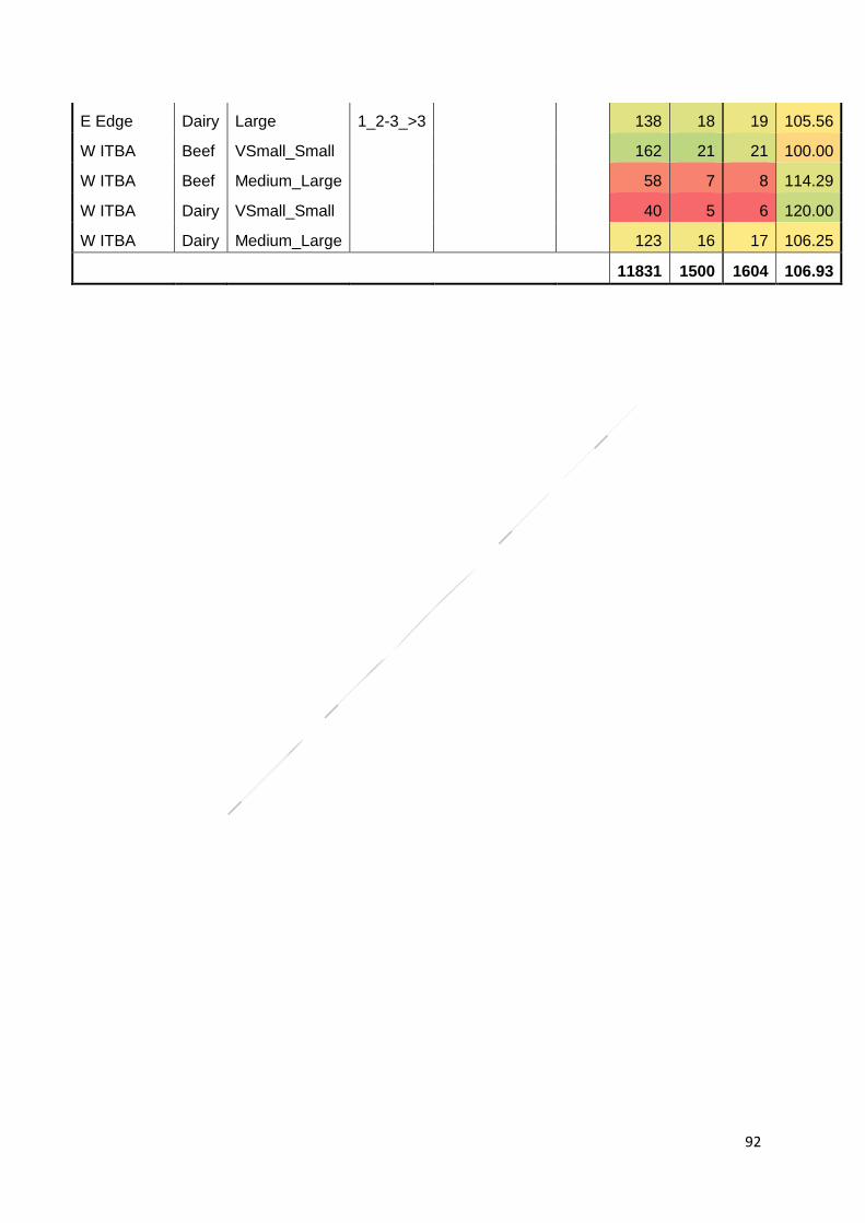
92
E Edge Dairy Large 1_2-3_>3 138 18 19 105.56
W ITBA Beef VSmall_Small 162 21 21 100.00
W ITBA Beef Medium_Large 58 7 8 114.29
W ITBA Dairy VSmall_Small 40 5 6 120.00
W ITBA Dairy Medium_Large 123 16 17 106.25
11831 1500 1604 106.93
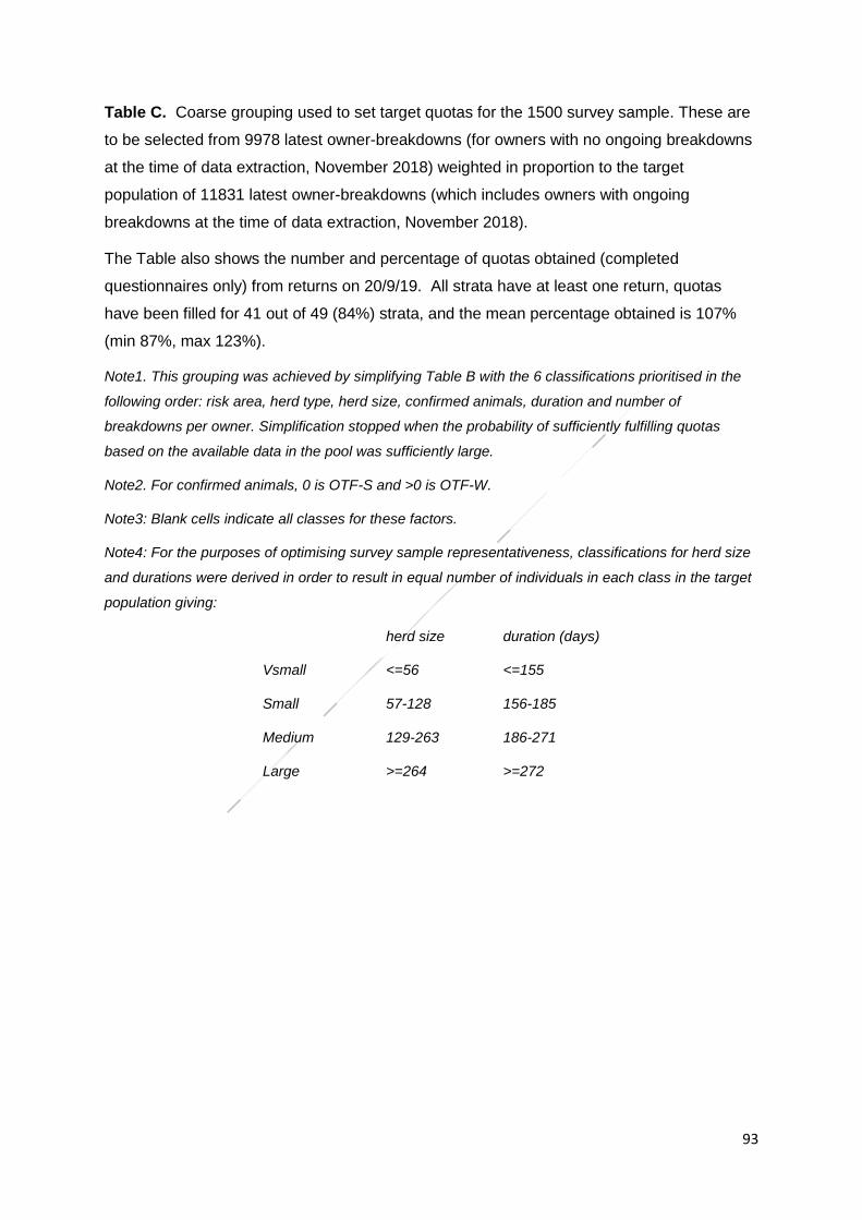
93
Table C. Coarse grouping used to set target quotas for the 1500 survey sample. These are
to be selected from 9978 latest owner-breakdowns (for owners with no ongoing breakdowns
at the time of data extraction, November 2018) weighted in proportion to the target
population of 11831 latest owner-breakdowns (which includes owners with ongoing
breakdowns at the time of data extraction, November 2018).
The Table also shows the number and percentage of quotas obtained (completed
questionnaires only) from returns on 20/9/19. All strata have at least one return, quotas
have been filled for 41 out of 49 (84%) strata, and the mean percentage obtained is 107%
(min 87%, max 123%).
Note1. This grouping was achieved by simplifying Table B with the 6 classifications prioritised in the
following order: risk area, herd type, herd size, confirmed animals, duration and number of
breakdowns per owner. Simplification stopped when the probability of sufficiently fulfilling quotas
based on the available data in the pool was sufficiently large.
Note2. For confirmed animals, 0 is OTF-S and >0 is OTF-W.
Note3: Blank cells indicate all classes for these factors.
Note4: For the purposes of optimising survey sample representativeness, classifications for herd size
and durations were derived in order to result in equal number of individuals in each class in the target
population giving:
herd size duration (days)
Vsmall <=56 <=155
Small 57-128 156-185
Medium 129-263 186-271
Large >=264 >=272
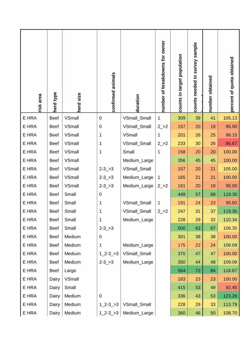
ris
k a
rea
herd
ty
pe
herd
siz
e
co
nfi
rme
d a
nim
als
d
ura
tio
n
nu
mb
er
of
bre
ak
do
wn
s f
or
ow
ner
co
un
ts in
ta
rget
po
pu
lati
on
c
ou
nts
ne
ed
ed
in
su
rve
y s
am
ple
(qu
ota
s)
nu
mb
er
ob
tain
ed
p
erc
en
t o
f q
uo
ta o
bta
ine
d
E HRA Beef VSmall 0 VSmall_Small 1 309 39 41 105.13
E HRA Beef VSmall 0 VSmall_Small 2_>2 157 20 19 95.00
E HRA Beef VSmall 1 VSmall 1 201 26 25 96.15
E HRA Beef VSmall 1 VSmall_Small 2_>2 233 30 26 86.67
E HRA Beef VSmall 1 Small 1 158 20 20 100.00
E HRA Beef VSmall Medium_Large 356 45 45 100.00
E HRA Beef VSmall 2-3_>3 VSmall_Small 157 20 21 105.00
E HRA Beef VSmall 2-3_>3 Medium_Large 1 165 21 21 100.00
E HRA Beef VSmall 2-3_>3 Medium_Large 2_>2 161 20 19 95.00
E HRA Beef Small 0 449 57 68 119.30
E HRA Beef Small 1 VSmall_Small 1 191 24 23 95.83
E HRA Beef Small 1 VSmall_Small 2_>2 247 31 37 119.35
E HRA Beef Small 1 Medium_Large 228 29 32 110.34
E HRA Beef Small 2-3_>3 500 63 67 106.35
E HRA Beef Medium 0 301 38 38 100.00
E HRA Beef Medium 1 Medium_Large 175 22 24 109.09
E HRA Beef Medium 1_2-3_>3 VSmall_Small 370 47 47 100.00
E HRA Beef Medium 2-3_>3 Medium_Large 350 44 48 109.09
E HRA Beef Large 564 72 84 116.67
E HRA Dairy VSmall 183 23 23 100.00
E HRA Dairy Small 415 53 49 92.45
E HRA Dairy Medium 0 336 43 53 123.26
E HRA Dairy Medium 1_2-3_>3 VSmall_Small 228 29 33 113.79
E HRA Dairy Medium 1_2-3_>3 Medium_Large 360 46 50 108.70
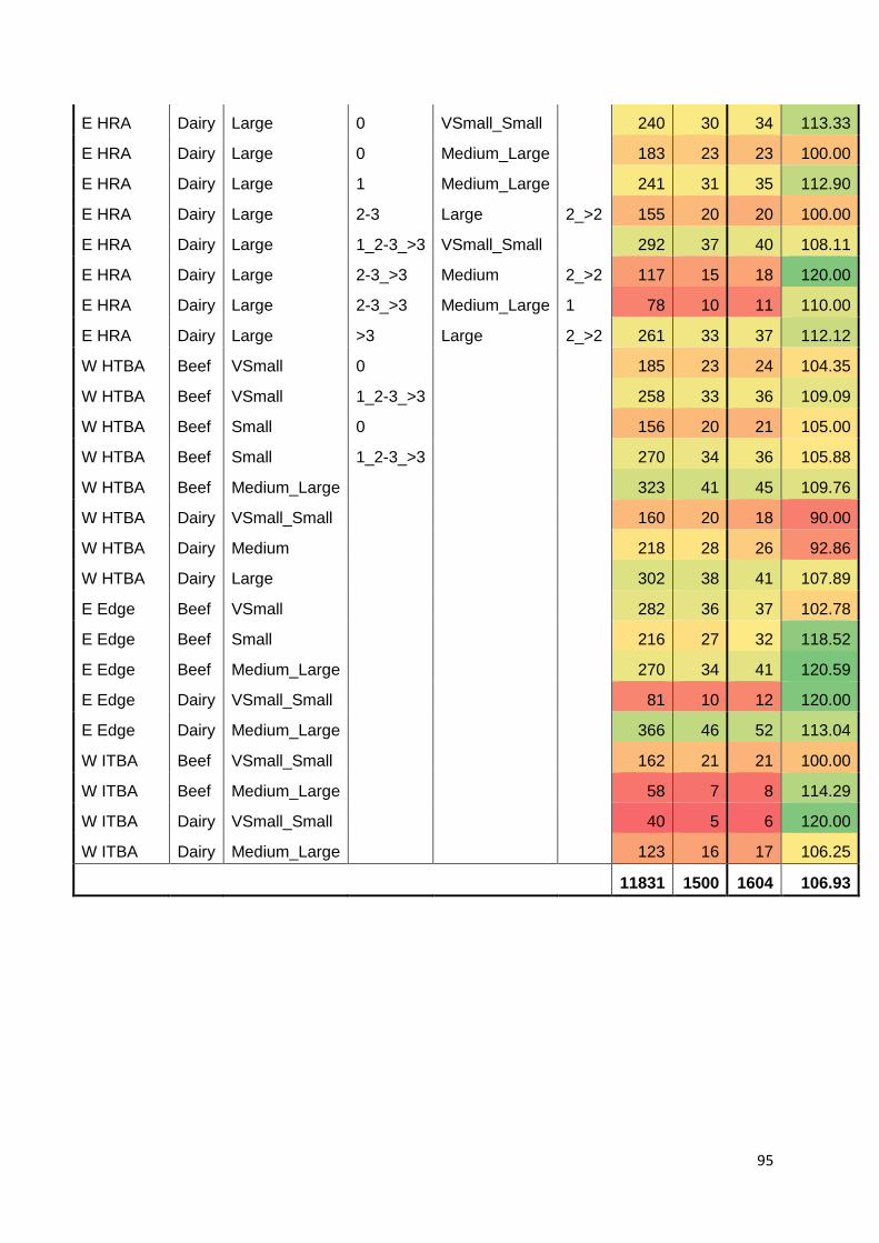
95
E HRA Dairy Large 0 VSmall_Small 240 30 34 113.33
E HRA Dairy Large 0 Medium_Large 183 23 23 100.00
E HRA Dairy Large 1 Medium_Large 241 31 35 112.90
E HRA Dairy Large 2-3 Large 2_>2 155 20 20 100.00
E HRA Dairy Large 1_2-3_>3 VSmall_Small 292 37 40 108.11
E HRA Dairy Large 2-3_>3 Medium 2_>2 117 15 18 120.00
E HRA Dairy Large 2-3_>3 Medium_Large 1 78 10 11 110.00
E HRA Dairy Large >3 Large 2_>2 261 33 37 112.12
W HTBA Beef VSmall 0 185 23 24 104.35
W HTBA Beef VSmall 1_2-3_>3 258 33 36 109.09
W HTBA Beef Small 0 156 20 21 105.00
W HTBA Beef Small 1_2-3_>3 270 34 36 105.88
W HTBA Beef Medium_Large 323 41 45 109.76
W HTBA Dairy VSmall_Small 160 20 18 90.00
W HTBA Dairy Medium 218 28 26 92.86
W HTBA Dairy Large 302 38 41 107.89
E Edge Beef VSmall 282 36 37 102.78
E Edge Beef Small 216 27 32 118.52
E Edge Beef Medium_Large 270 34 41 120.59
E Edge Dairy VSmall_Small 81 10 12 120.00
E Edge Dairy Medium_Large 366 46 52 113.04
W ITBA Beef VSmall_Small 162 21 21 100.00
W ITBA Beef Medium_Large 58 7 8 114.29
W ITBA Dairy VSmall_Small 40 5 6 120.00
W ITBA Dairy Medium_Large 123 16 17 106.25
11831 1500 1604 106.93
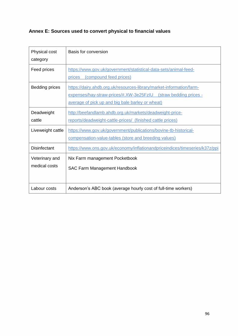
96
Annex E: Sources used to convert physical to financial values
Physical cost
category
Basis for conversion
Feed prices https://www.gov.uk/government/statistical-data-sets/animal-feed-
prices (compound feed prices)
Bedding prices https://dairy.ahdb.org.uk/resources-library/market-information/farm-
expenses/hay-straw-prices/#.XW-3e25FzIU (straw bedding prices -
average of pick up and big bale barley or wheat)
Deadweight
cattle
http://beefandlamb.ahdb.org.uk/markets/deadweight-price-
reports/deadweight-cattle-prices/ (finished cattle prices)
Liveweight cattle https://www.gov.uk/government/publications/bovine-tb-historical-
compensation-value-tables (store and breeding values)
Disinfectant https://www.ons.gov.uk/economy/inflationandpriceindices/timeseries/k37z/ppi
Veterinary and
medical costs
Nix Farm management Pocketbook
SAC Farm Management Handbook
Labour costs Anderson’s ABC book (average hourly cost of full-time workers)
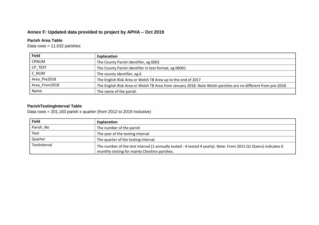
Annex F: Updated data provided to project by APHA – Oct 2019
Parish Area Table
Data rows = 11,632 parishes
Field Explanation
CPNUM The County Parish identifier, eg 6001
CP_TEXT The County Parish identifier in text format, eg 06001
C_NUM The county identifier, eg 6
Area_Pre2018 The English Risk Area or Welsh TB Area up to the end of 2017
Area_From2018 The English Risk Area or Welsh TB Area from January 2018. Note Welsh parishes are no different from pre-2018.
Name The name of the parish
ParishTestingInterval Table
Data rows = 201,183 parish x quarter (from 2012 to 2019 inclusive)
Field Explanation
Parish_No The number of the parish
Year The year of the testing interval
Quarter The quarter of the testing interval
TestInterval The number of the test interval (1-annually tested - 4-tested 4 yearly). Note: From 2015 Q1 0(zero) indicates 6 monthly testing for mainly Cheshire parishes.
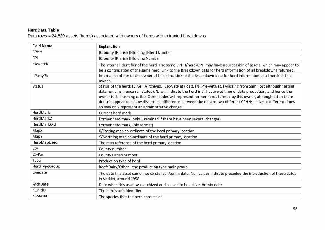
98
HerdData Table
Data rows = 24,820 assets (herds) associated with owners of herds with extracted breakdowns
Field Name Explanation
CPHH [C]ounty [P]arish [H]olding [H]erd Number
CPH [C]ounty [P]arish [H]olding Number
hAssetPK The internal identifier of the herd. The same CPHH/herd/CPH may have a succession of assets, which may appear to be a continuation of the same herd. Link to the Breakdown data for herd information of all breakdowns returned.
hPartyPk Internal identifier of the owner of this herd. Link to the Breakdown data for herd information of all herds of this owner.
Status Status of the herd: [L]ive, [A]rchived, [E]x-VetNet (lost), [N]:Pre-VetNet, [M]issing from Sam (lost although testing data remains, hence reinstated). 'L' will indicate the herd is still active at time of data production, and hence the owner is still farming cattle. Other codes will represent former herds farmed by this owner, although often there doesn't appear to be any discernible difference between the data of two different CPHHs active at different times so may only represent an administrative change.
HerdMark Current herd mark
HerdMark2 Former herd mark (only 1 retained if there have been several changes)
HerdMarkOld Former herd mark, (old format)
MapX X/Easting map co-ordinate of the herd primary location
MapY Y/Northing map co-ordinate of the herd primary location
HerpMapUsed The map reference of the herd primary location
Cty County number
CtyPar County Parish number
Type Production type of herd
HerdTypeGroup Beef/Dairy/Other - the production type main group
Livedate The date this asset came into existence. Admin date. Null values indicate preceded the introduction of these dates in VetNet, around 1998
ArchDate Date when this asset was archived and ceased to be active. Admin date
hUnitID The herd's unit identifier
hSpecies The species that the herd consists of
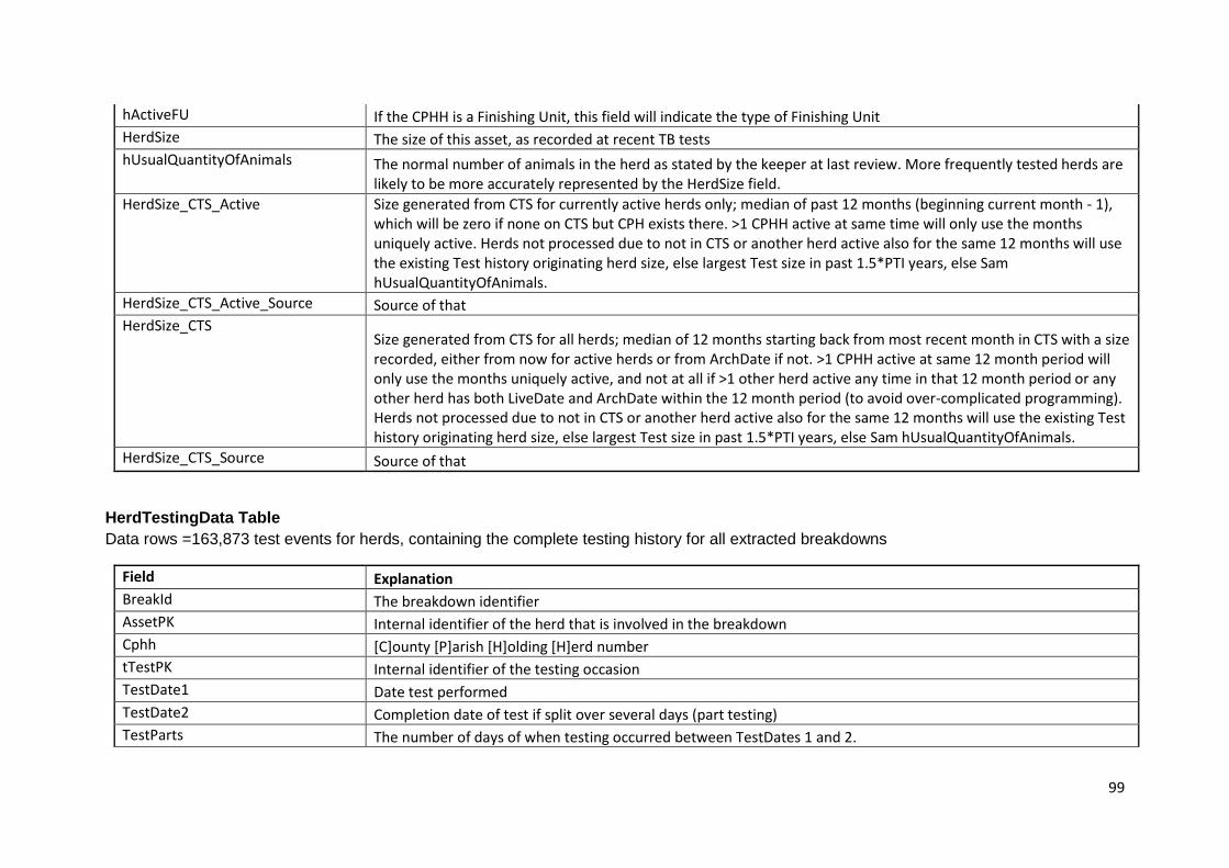
99
hActiveFU If the CPHH is a Finishing Unit, this field will indicate the type of Finishing Unit
HerdSize The size of this asset, as recorded at recent TB tests
hUsualQuantityOfAnimals The normal number of animals in the herd as stated by the keeper at last review. More frequently tested herds are likely to be more accurately represented by the HerdSize field.
HerdSize_CTS_Active Size generated from CTS for currently active herds only; median of past 12 months (beginning current month - 1), which will be zero if none on CTS but CPH exists there. >1 CPHH active at same time will only use the months uniquely active. Herds not processed due to not in CTS or another herd active also for the same 12 months will use the existing Test history originating herd size, else largest Test size in past 1.5*PTI years, else Sam hUsualQuantityOfAnimals.
HerdSize_CTS_Active_Source Source of that
HerdSize_CTS Size generated from CTS for all herds; median of 12 months starting back from most recent month in CTS with a size recorded, either from now for active herds or from ArchDate if not. >1 CPHH active at same 12 month period will only use the months uniquely active, and not at all if >1 other herd active any time in that 12 month period or any other herd has both LiveDate and ArchDate within the 12 month period (to avoid over-complicated programming). Herds not processed due to not in CTS or another herd active also for the same 12 months will use the existing Test history originating herd size, else largest Test size in past 1.5*PTI years, else Sam hUsualQuantityOfAnimals.
HerdSize_CTS_Source Source of that
HerdTestingData Table
Data rows =163,873 test events for herds, containing the complete testing history for all extracted breakdowns
Field Explanation
BreakId The breakdown identifier
AssetPK Internal identifier of the herd that is involved in the breakdown
Cphh [C]ounty [P]arish [H]olding [H]erd number
tTestPK Internal identifier of the testing occasion
TestDate1 Date test performed
TestDate2 Completion date of test if split over several days (part testing)
TestParts The number of days of when testing occurred between TestDates 1 and 2.
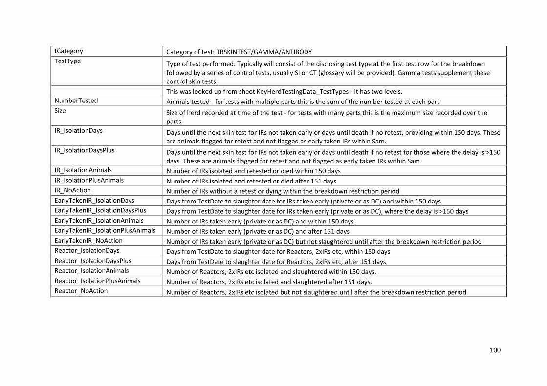
100
tCategory Category of test: TBSKINTEST/GAMMA/ANTIBODY
TestType Type of test performed. Typically will consist of the disclosing test type at the first test row for the breakdown followed by a series of control tests, usually SI or CT (glossary will be provided). Gamma tests supplement these control skin tests.
This was looked up from sheet KeyHerdTestingData_TestTypes - it has two levels.
NumberTested Animals tested - for tests with multiple parts this is the sum of the number tested at each part
Size Size of herd recorded at time of the test - for tests with many parts this is the maximum size recorded over the parts
IR_IsolationDays Days until the next skin test for IRs not taken early or days until death if no retest, providing within 150 days. These are animals flagged for retest and not flagged as early taken IRs within Sam.
IR_IsolationDaysPlus Days until the next skin test for IRs not taken early or days until death if no retest for those where the delay is >150 days. These are animals flagged for retest and not flagged as early taken IRs within Sam.
IR_IsolationAnimals Number of IRs isolated and retested or died within 150 days
IR_IsolationPlusAnimals Number of IRs isolated and retested or died after 151 days
IR_NoAction Number of IRs without a retest or dying within the breakdown restriction period
EarlyTakenIR_IsolationDays Days from TestDate to slaughter date for IRs taken early (private or as DC) and within 150 days
EarlyTakenIR_IsolationDaysPlus Days from TestDate to slaughter date for IRs taken early (private or as DC), where the delay is >150 days
EarlyTakenIR_IsolationAnimals Number of IRs taken early (private or as DC) and within 150 days
EarlyTakenIR_IsolationPlusAnimals Number of IRs taken early (private or as DC) and after 151 days
EarlyTakenIR_NoAction Number of IRs taken early (private or as DC) but not slaughtered until after the breakdown restriction period
Reactor_IsolationDays Days from TestDate to slaughter date for Reactors, 2xIRs etc, within 150 days
Reactor_IsolationDaysPlus Days from TestDate to slaughter date for Reactors, 2xIRs etc, after 151 days
Reactor_IsolationAnimals Number of Reactors, 2xIRs etc isolated and slaughtered within 150 days.
Reactor_IsolationPlusAnimals Number of Reactors, 2xIRs etc isolated and slaughtered after 151 days.
Reactor_NoAction Number of Reactors, 2xIRs etc isolated but not slaughtered until after the breakdown restriction period
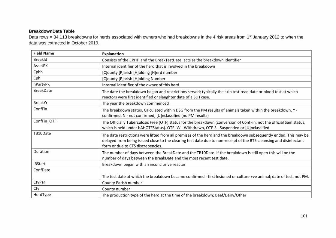
101
BreakdownData Table
Data rows = 34,113 breakdowns for herds associated with owners who had breakdowns in the 4 risk areas from 1st January 2012 to when the
data was extracted in October 2019.
Field Name Explanation
BreakId Consists of the CPHH and the BreakTestDate; acts as the breakdown identifier
AssetPK Internal identifier of the herd that is involved in the breakdown
Cphh [C]ounty [P]arish [H]olding [H]erd number
Cph [C]ounty [P]arish [H]olding Number
hPartyPK Internal identifier of the owner of this herd.
BreakDate The date the breakdown began and restrictions served; typically the skin test read date or blood test at which reactors were first identified or slaughter date of a SLH case.
BreakYr The year the breakdown commenced
ConfFin The breakdown status. Calculated within DSG from the PM results of animals taken within the breakdown. Y - confirmed, N - not confirmed, [U]nclassified (no PM results)
ConfFin_OTF The Officially Tuberculosis Free (OTF) status for the breakdown (conversion of ConfFin, not the official Sam status, which is held under bAHOTFStatus). OTF- W - Withdrawn, OTF-S - Suspended or [U]nclassified
TB10Date The date restrictions were lifted from all premises of the herd and the breakdown subsequently ended. This may be delayed from being issued close to the clearing test date due to non-receipt of the BT5 cleansing and disinfectant form or due to CTS discrepencies.
Duration The number of days between the BreakDate and the TB10Date. If the breakdown is still open this will be the number of days between the BreakDate and the most recent test date.
IRStart Breakdown began with an inconclusive reactor
ConfDate
The test date at which the breakdown became confirmed - first lesioned or culture +ve animal; date of test, not PM.
CtyPar County Parish number
Cty County number
HerdType The production type of the herd at the time of the breakdown; Beef/Dairy/Other
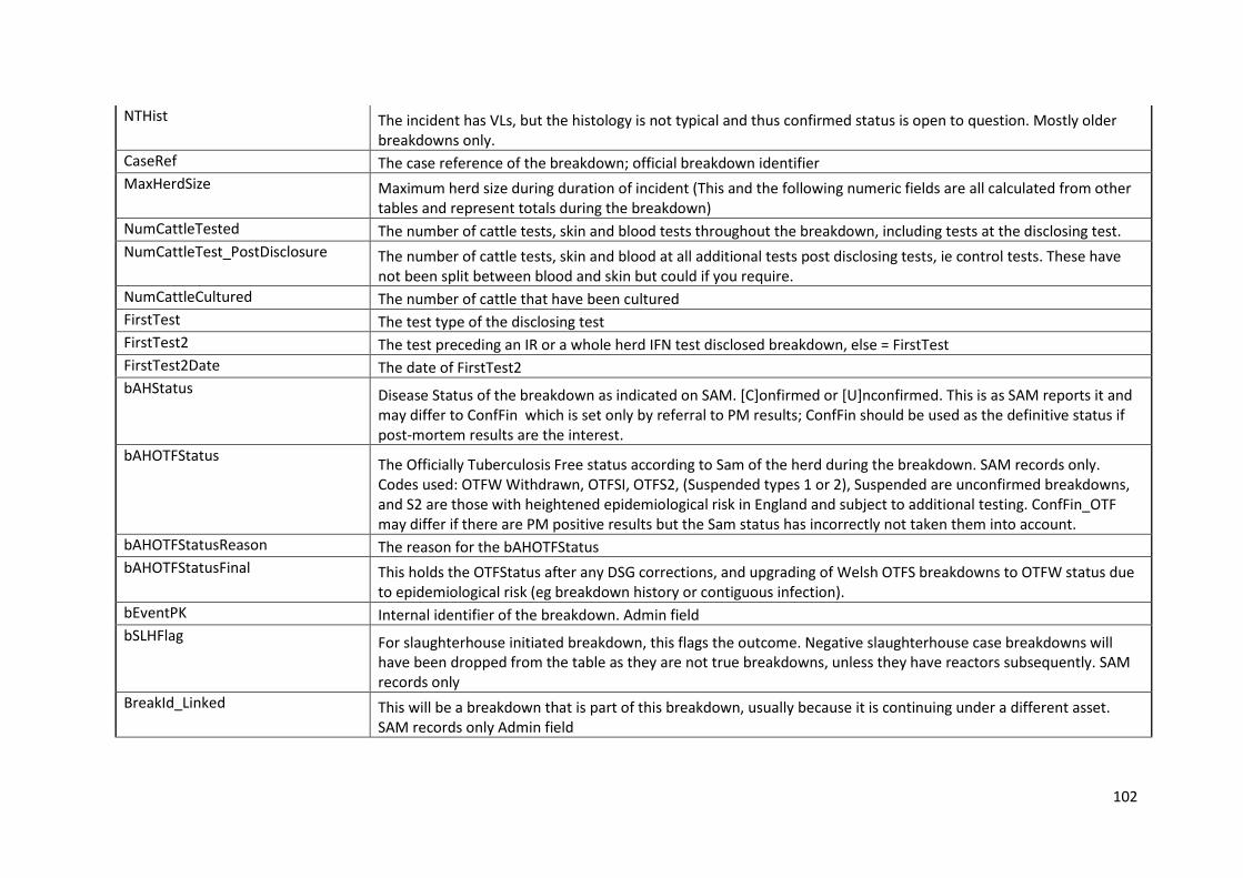
102
NTHist The incident has VLs, but the histology is not typical and thus confirmed status is open to question. Mostly older breakdowns only.
CaseRef The case reference of the breakdown; official breakdown identifier
MaxHerdSize Maximum herd size during duration of incident (This and the following numeric fields are all calculated from other tables and represent totals during the breakdown)
NumCattleTested The number of cattle tests, skin and blood tests throughout the breakdown, including tests at the disclosing test.
NumCattleTest_PostDisclosure The number of cattle tests, skin and blood at all additional tests post disclosing tests, ie control tests. These have not been split between blood and skin but could if you require.
NumCattleCultured The number of cattle that have been cultured
FirstTest The test type of the disclosing test
FirstTest2 The test preceding an IR or a whole herd IFN test disclosed breakdown, else = FirstTest
FirstTest2Date The date of FirstTest2
bAHStatus Disease Status of the breakdown as indicated on SAM. [C]onfirmed or [U]nconfirmed. This is as SAM reports it and may differ to ConfFin which is set only by referral to PM results; ConfFin should be used as the definitive status if post-mortem results are the interest.
bAHOTFStatus The Officially Tuberculosis Free status according to Sam of the herd during the breakdown. SAM records only. Codes used: OTFW Withdrawn, OTFSI, OTFS2, (Suspended types 1 or 2), Suspended are unconfirmed breakdowns, and S2 are those with heightened epidemiological risk in England and subject to additional testing. ConfFin_OTF may differ if there are PM positive results but the Sam status has incorrectly not taken them into account.
bAHOTFStatusReason The reason for the bAHOTFStatus
bAHOTFStatusFinal This holds the OTFStatus after any DSG corrections, and upgrading of Welsh OTFS breakdowns to OTFW status due to epidemiological risk (eg breakdown history or contiguous infection).
bEventPK Internal identifier of the breakdown. Admin field
bSLHFlag For slaughterhouse initiated breakdown, this flags the outcome. Negative slaughterhouse case breakdowns will have been dropped from the table as they are not true breakdowns, unless they have reactors subsequently. SAM records only
BreakId_Linked This will be a breakdown that is part of this breakdown, usually because it is continuing under a different asset. SAM records only Admin field
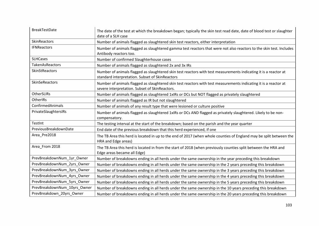
103
BreakTestDate The date of the test at which the breakdown began; typically the skin test read date, date of blood test or slaughter date of a SLH case
SkinReactors Number of animals flagged as slaughtered skin test reactors, either interpretation
IFNReactors Number of animals flagged as slaughtered gamma test reactors that were not also reactors to the skin test. Includes Antibody reactors too.
SLHCases Number of confirmed Slaughterhouse cases
TakenAsReactors Number of animals flagged as slaughtered 2x and 3x IRs
SkinStReactors Number of animals flagged as slaughtered skin test reactors with test measurements indicating it is a reactor at standard interpretation. Subset of SkinReactors
SkinSeReactors Number of animals flagged as slaughtered skin test reactors with test measurements indicating it is a reactor at severe interpretation. Subset of SkinReactors.
OtherSLIRs Number of animals flagged as slaughtered 1xIRs or DCs but NOT flagged as privately slaughtered
OtherIRs Number of animals flagged as IR but not slaughtered
ConfirmedAnimals Number of animals of any result type that were lesioned or culture positive
PrivateSlaughtersIRs Number of animals flagged as slaughtered 1xIRs or DCs AND flagged as privately slaughtered. Likely to be non-compensatory.
TestInt The testing interval at the start of the breakdown; based on the parish and the year quarter
PreviousBreakdownDate End date of the previous breakdown that this herd experienced, if one
Area_Pre2018 The TB Area this herd is located in up to the end of 2017 (when whole counties of England may be split between the HRA and Edge areas)
Area_From 2018 The TB Area this herd is located in from the start of 2018 (when previously counties split between the HRA and Edge areas became all Edge)
PrevBreakdownNum_1yr_Owner Number of breakdowns ending in all herds under the same ownership in the year preceding this breakdown
PrevBreakdownNum_2yrs_Owner Number of breakdowns ending in all herds under the same ownership in the 2 years preceding this breakdown
PrevBreakdownNum_3yrs_Owner Number of breakdowns ending in all herds under the same ownership in the 3 years preceding this breakdown
PrevBreakdownNum_4yrs_Owner Number of breakdowns ending in all herds under the same ownership in the 4 years preceding this breakdown
PrevBreakdownNum_5yrs_Owner Number of breakdowns ending in all herds under the same ownership in the 5 years preceding this breakdown
PrevBreakdownNum_10yrs_Owner Number of breakdowns ending in all herds under the same ownership in the 10 years preceding this breakdown
PrevBreakdown_20yrs_Owner Number of breakdowns ending in all herds under the same ownership in the 20 years preceding this breakdown
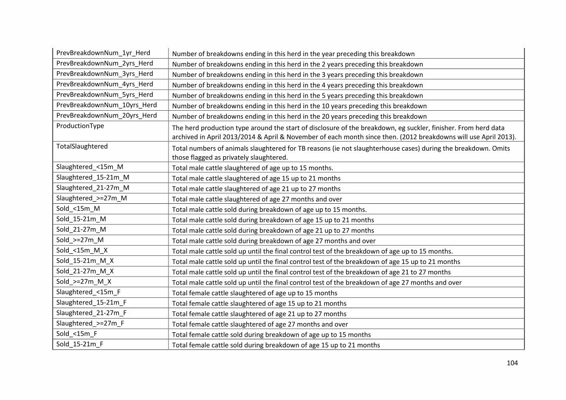
104
PrevBreakdownNum_1yr_Herd Number of breakdowns ending in this herd in the year preceding this breakdown
PrevBreakdownNum_2yrs_Herd Number of breakdowns ending in this herd in the 2 years preceding this breakdown
PrevBreakdownNum_3yrs_Herd Number of breakdowns ending in this herd in the 3 years preceding this breakdown
PrevBreakdownNum_4yrs_Herd Number of breakdowns ending in this herd in the 4 years preceding this breakdown
PrevBreakdownNum_5yrs_Herd Number of breakdowns ending in this herd in the 5 years preceding this breakdown
PrevBreakdownNum_10yrs_Herd Number of breakdowns ending in this herd in the 10 years preceding this breakdown
PrevBreakdownNum_20yrs_Herd Number of breakdowns ending in this herd in the 20 years preceding this breakdown
ProductionType The herd production type around the start of disclosure of the breakdown, eg suckler, finisher. From herd data archived in April 2013/2014 & April & November of each month since then. (2012 breakdowns will use April 2013).
TotalSlaughtered Total numbers of animals slaughtered for TB reasons (ie not slaughterhouse cases) during the breakdown. Omits those flagged as privately slaughtered.
Slaughtered_<15m_M Total male cattle slaughtered of age up to 15 months.
Slaughtered_15-21m_M Total male cattle slaughtered of age 15 up to 21 months
Slaughtered_21-27m_M Total male cattle slaughtered of age 21 up to 27 months
Slaughtered_>=27m_M Total male cattle slaughtered of age 27 months and over
Sold_<15m_M Total male cattle sold during breakdown of age up to 15 months.
Sold_15-21m_M Total male cattle sold during breakdown of age 15 up to 21 months
Sold_21-27m_M Total male cattle sold during breakdown of age 21 up to 27 months
Sold_>=27m_M Total male cattle sold during breakdown of age 27 months and over
Sold_<15m_M_X Total male cattle sold up until the final control test of the breakdown of age up to 15 months.
Sold_15-21m_M_X Total male cattle sold up until the final control test of the breakdown of age 15 up to 21 months
Sold_21-27m_M_X Total male cattle sold up until the final control test of the breakdown of age 21 to 27 months
Sold_>=27m_M_X Total male cattle sold up until the final control test of the breakdown of age 27 months and over
Slaughtered_<15m_F Total female cattle slaughtered of age up to 15 months
Slaughtered_15-21m_F Total female cattle slaughtered of age 15 up to 21 months
Slaughtered_21-27m_F Total female cattle slaughtered of age 21 up to 27 months
Slaughtered_>=27m_F Total female cattle slaughtered of age 27 months and over
Sold_<15m_F Total female cattle sold during breakdown of age up to 15 months
Sold_15-21m_F Total female cattle sold during breakdown of age 15 up to 21 months
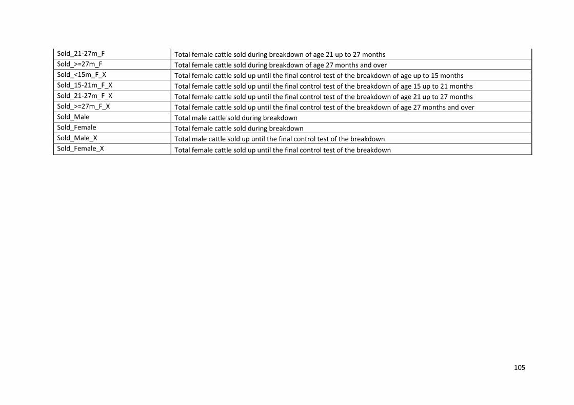
105
Sold_21-27m_F Total female cattle sold during breakdown of age 21 up to 27 months
Sold_>=27m_F Total female cattle sold during breakdown of age 27 months and over
Sold_<15m_F_X Total female cattle sold up until the final control test of the breakdown of age up to 15 months
Sold_15-21m_F_X Total female cattle sold up until the final control test of the breakdown of age 15 up to 21 months
Sold_21-27m_F_X Total female cattle sold up until the final control test of the breakdown of age 21 up to 27 months
Sold_>=27m_F_X Total female cattle sold up until the final control test of the breakdown of age 27 months and over
Sold_Male Total male cattle sold during breakdown
Sold_Female Total female cattle sold during breakdown
Sold_Male_X Total male cattle sold up until the final control test of the breakdown
Sold_Female_X Total female cattle sold up until the final control test of the breakdown
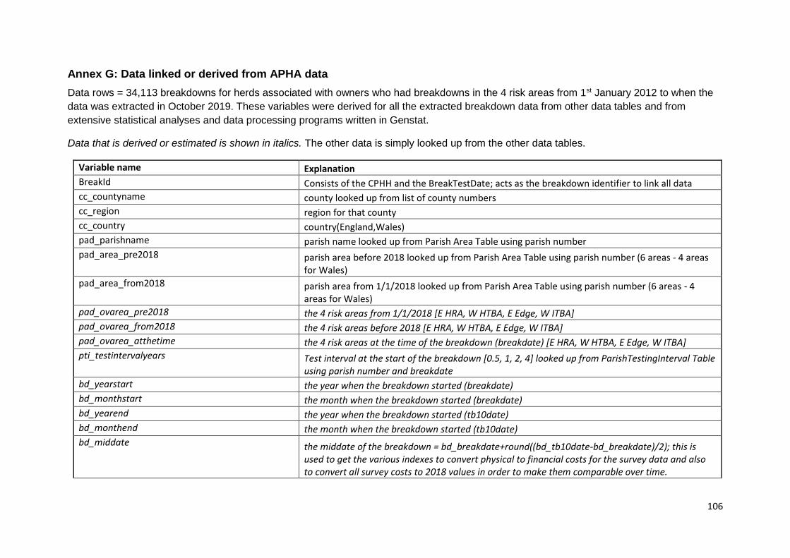
106
Annex G: Data linked or derived from APHA data
Data rows = 34,113 breakdowns for herds associated with owners who had breakdowns in the 4 risk areas from 1st January 2012 to when the
data was extracted in October 2019. These variables were derived for all the extracted breakdown data from other data tables and from
extensive statistical analyses and data processing programs written in Genstat.
Data that is derived or estimated is shown in italics. The other data is simply looked up from the other data tables.
Variable name Explanation
BreakId Consists of the CPHH and the BreakTestDate; acts as the breakdown identifier to link all data
cc_countyname county looked up from list of county numbers
cc_region region for that county
cc_country country(England,Wales)
pad_parishname parish name looked up from Parish Area Table using parish number
pad_area_pre2018 parish area before 2018 looked up from Parish Area Table using parish number (6 areas - 4 areas for Wales)
pad_area_from2018 parish area from 1/1/2018 looked up from Parish Area Table using parish number (6 areas - 4 areas for Wales)
pad_ovarea_pre2018 the 4 risk areas from 1/1/2018 [E HRA, W HTBA, E Edge, W ITBA]
pad_ovarea_from2018 the 4 risk areas before 2018 [E HRA, W HTBA, E Edge, W ITBA]
pad_ovarea_atthetime the 4 risk areas at the time of the breakdown (breakdate) [E HRA, W HTBA, E Edge, W ITBA]
pti_testintervalyears Test interval at the start of the breakdown [0.5, 1, 2, 4] looked up from ParishTestingInterval Table using parish number and breakdate
bd_yearstart the year when the breakdown started (breakdate)
bd_monthstart the month when the breakdown started (breakdate)
bd_yearend the year when the breakdown started (tb10date)
bd_monthend the month when the breakdown started (tb10date)
bd_middate the middate of the breakdown = bd_breakdate+round((bd_tb10date-bd_breakdate)/2); this is used to get the various indexes to convert physical to financial costs for the survey data and also to convert all survey costs to 2018 values in order to make them comparable over time.
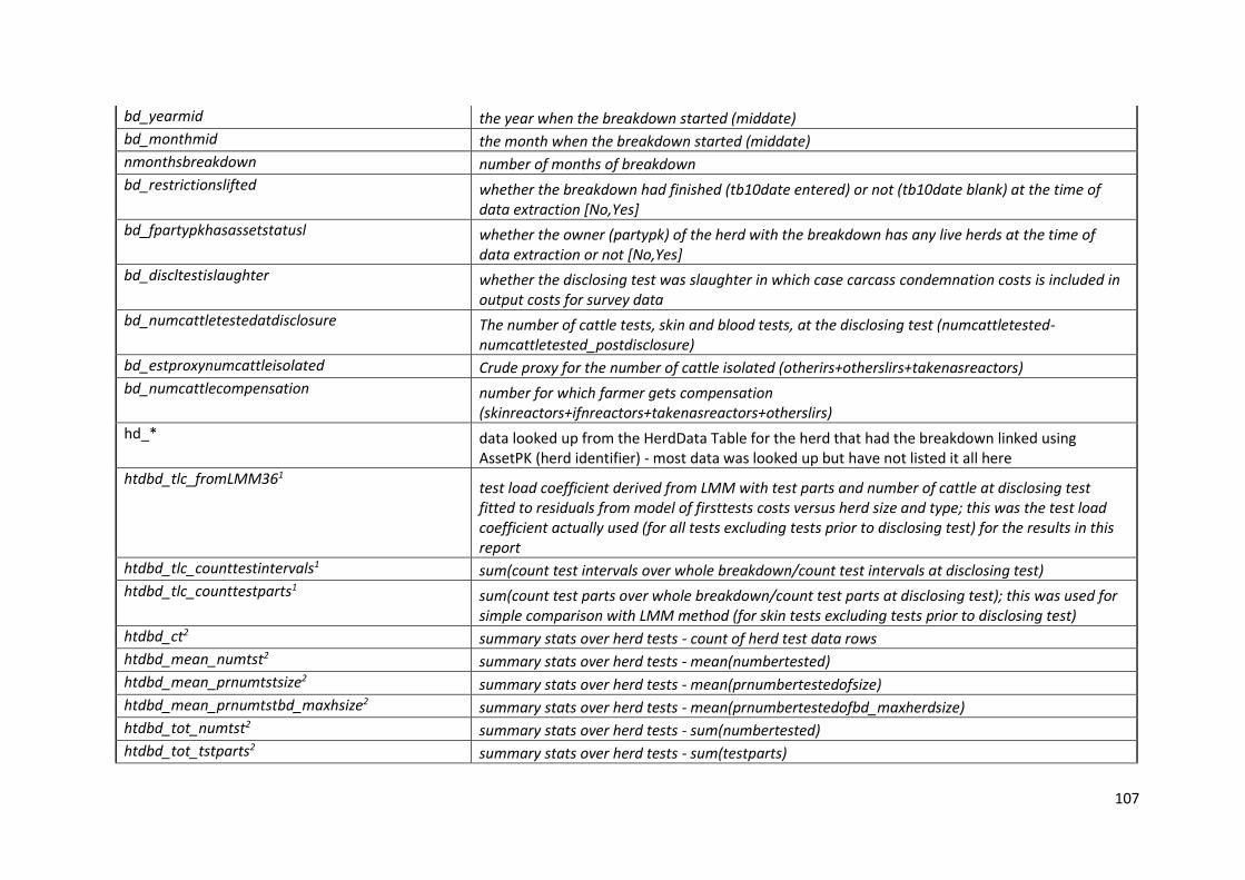
107
bd_yearmid the year when the breakdown started (middate)
bd_monthmid the month when the breakdown started (middate)
nmonthsbreakdown number of months of breakdown
bd_restrictionslifted whether the breakdown had finished (tb10date entered) or not (tb10date blank) at the time of data extraction [No,Yes]
bd_fpartypkhasassetstatusl whether the owner (partypk) of the herd with the breakdown has any live herds at the time of data extraction or not [No,Yes]
bd_discltestislaughter whether the disclosing test was slaughter in which case carcass condemnation costs is included in output costs for survey data
bd_numcattletestedatdisclosure The number of cattle tests, skin and blood tests, at the disclosing test (numcattletested-numcattletested_postdisclosure)
bd_estproxynumcattleisolated Crude proxy for the number of cattle isolated (otherirs+otherslirs+takenasreactors)
bd_numcattlecompensation number for which farmer gets compensation (skinreactors+ifnreactors+takenasreactors+otherslirs)
hd_* data looked up from the HerdData Table for the herd that had the breakdown linked using AssetPK (herd identifier) - most data was looked up but have not listed it all here
htdbd_tlc_fromLMM361 test load coefficient derived from LMM with test parts and number of cattle at disclosing test fitted to residuals from model of firsttests costs versus herd size and type; this was the test load coefficient actually used (for all tests excluding tests prior to disclosing test) for the results in this report
htdbd_tlc_counttestintervals1 sum(count test intervals over whole breakdown/count test intervals at disclosing test)
htdbd_tlc_counttestparts1 sum(count test parts over whole breakdown/count test parts at disclosing test); this was used for simple comparison with LMM method (for skin tests excluding tests prior to disclosing test)
htdbd_ct2 summary stats over herd tests - count of herd test data rows
htdbd_mean_numtst2 summary stats over herd tests - mean(numbertested)
htdbd_mean_prnumtstsize2 summary stats over herd tests - mean(prnumbertestedofsize)
htdbd_mean_prnumtstbd_maxhsize2 summary stats over herd tests - mean(prnumbertestedofbd_maxherdsize)
htdbd_tot_numtst2 summary stats over herd tests - sum(numbertested)
htdbd_tot_tstparts2 summary stats over herd tests - sum(testparts)
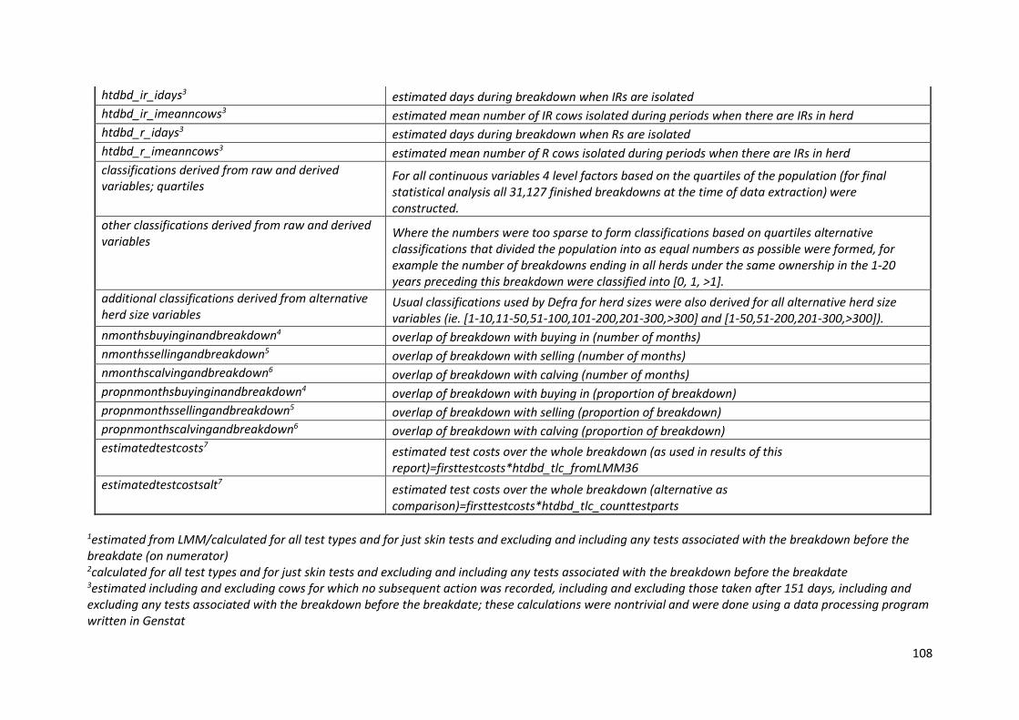
108
htdbd_ir_idays3 estimated days during breakdown when IRs are isolated
htdbd_ir_imeanncows3 estimated mean number of IR cows isolated during periods when there are IRs in herd
htdbd_r_idays3 estimated days during breakdown when Rs are isolated
htdbd_r_imeanncows3 estimated mean number of R cows isolated during periods when there are IRs in herd
classifications derived from raw and derived variables; quartiles
For all continuous variables 4 level factors based on the quartiles of the population (for final statistical analysis all 31,127 finished breakdowns at the time of data extraction) were constructed.
other classifications derived from raw and derived variables
Where the numbers were too sparse to form classifications based on quartiles alternative classifications that divided the population into as equal numbers as possible were formed, for example the number of breakdowns ending in all herds under the same ownership in the 1-20 years preceding this breakdown were classified into [0, 1, >1].
additional classifications derived from alternative herd size variables
Usual classifications used by Defra for herd sizes were also derived for all alternative herd size variables (ie. [1-10,11-50,51-100,101-200,201-300,>300] and [1-50,51-200,201-300,>300]).
nmonthsbuyinginandbreakdown4 overlap of breakdown with buying in (number of months)
nmonthssellingandbreakdown5 overlap of breakdown with selling (number of months)
nmonthscalvingandbreakdown6 overlap of breakdown with calving (number of months)
propnmonthsbuyinginandbreakdown4 overlap of breakdown with buying in (proportion of breakdown)
propnmonthssellingandbreakdown5 overlap of breakdown with selling (proportion of breakdown)
propnmonthscalvingandbreakdown6 overlap of breakdown with calving (proportion of breakdown)
estimatedtestcosts7 estimated test costs over the whole breakdown (as used in results of this report)=firsttestcosts*htdbd_tlc_fromLMM36
estimatedtestcostsalt7 estimated test costs over the whole breakdown (alternative as comparison)=firsttestcosts*htdbd_tlc_counttestparts
1estimated from LMM/calculated for all test types and for just skin tests and excluding and including any tests associated with the breakdown before the breakdate (on numerator) 2calculated for all test types and for just skin tests and excluding and including any tests associated with the breakdown before the breakdate 3estimated including and excluding cows for which no subsequent action was recorded, including and excluding those taken after 151 days, including and excluding any tests associated with the breakdown before the breakdate; these calculations were nontrivial and were done using a data processing program written in Genstat
109
4derived for survey breakdowns only using information on buying in given in survey 5derived for survey breakdowns only using information on selling given in survey 6derived for survey breakdowns only using information on calving given in survey 7derived for survey breakdowns only using information given on the disclosing test in the survey


![Bovine TB infection status in cattle inGreat Britain in 2018 · • Scotland remained Officially TB Free, with 36 incidents (0.7 TB incidents per 100 herd-years at risk [HYR]) detected](https://img.pdfslide.net/doc/110x75/5ecebf0debc4355d0440ba18/bovine-tb-infection-status-in-cattle-ingreat-britain-in-2018-a-scotland-remained.jpg)