Research ArticleEstimating the Effect of Fractal Dimension on RepresentativeElementary Volume of Randomly Distributed RockFracture Networks

Jing Zhang, Liyuan Yu , Hongwen Jing, and Richeng Liu

State Key Laboratory for Geomechanics and Deep Underground Engineering, China University of Mining and Technology,Xuzhou 221116, China

Correspondence should be addressed to Liyuan Yu; yuliyuancumt@126.com

Received 1 June 2018; Accepted 9 August 2018; Published 29 October 2018

Academic Editor: Baojun Bai

Copyright © 2018 Jing Zhang et al. This is an open access article distributed under the Creative Commons Attribution License,which permits unrestricted use, distribution, and reproduction in any medium, provided the original work is properly cited.

The effect of fractal dimension (Df ) on the determination of representative elementary volume (REV) was investigated throughnumerical experimentations, in which a new method was adopted to extract submodels that have different length-width ratiosfrom original discrete facture networks (DFNs). Fluid flow in 1610 DFNs with different geometric characteristics of fracturesand length-width ratios was simulated, and the equivalent permeability was calculated. The results show that the averageequivalent permeability (KREV) at the REV size for DFNs increases with the increase in Df . The KREV shows a downward trendwith increasing length-width ratio of the submodel. A strong exponent functional relationship is found between the REV sizeand Df . The REV size decreases with increasing Df . With the increment of the length-width ratio of submodels, the REV sizeshows a decreasing trend. The effects of length-width ratio and Df on the REV size can be negligible when Df ≥ 1 5, but aresignificant when Df < 1 5.

1. Introduction

Fractures play a dominating role in the mechanical andhydraulic properties of rock masses and are sources ofdiscontinuity, anisotropy, and heterogeneity. Therefore, toanalyze the performance of structure characteristics infractured rock masses, it is important to accurately selectan appropriate model volume to determine the relevantrock properties. In recent years, numerical simulationtechniques such as the Monte Carlo method have beendeveloped for modeling fluid flow in models containingcomplex fracture systems [1–5]. It is definite that the per-meability of a fractured rock mass changes significantlydepending on the size of the model [6]. Beyond a certainsample size (area in two dimensions and/or volume inthree dimensions), the average permeability tends to attaina critical value and the variation in permeability will bevery small and can be negligible. In such a situation, thissize can be termed as REV size for a fractured rock masswith respect to fluid flow behavior [1, 6].

The previous works have documented the effectiveness offracture geometry parameters and average strength in deter-mining REV [1, 7, 8]. The REV size decreases with increasingjoint density and joint size [1]. The permeability change atlow stress levels is more sensitive to model size than at highstress levels due to the nonlinear fracture normal stress-displacement relation [2, 7]. The determination of REVbecomes more difficult for fracture network models subjectedto a lower stress environment. The application of the com-posite element method can greatly facilitate the preprocessand enable a large number of stochastic tests for the fracturedrock samples [9]. The existence of REV is illustrated bychanging the sizes and orientations of the samples. TheREV is used to overcome the obstacle that small modelscontain only a few joints while the large models containhundreds of joints that lead to impractical computation runtime [10]. The REV designation embeds a sufficient numberof joints in REV-size models. These innovations can reducecomputation time by two orders of magnitude fromhundreds of hours to a few hours.

HindawiGeofluidsVolume 2018, Article ID 7206074, 13 pageshttps://doi.org/10.1155/2018/7206074

The studies of REV in three dimensions have previ-ously been performed. A new method that gives throughthorough consideration to the fracture features of rockmasses was proposed based on models of 3D fracture net-works [11]. Subsequently, the REV size was determined byvolumetric joint count calculation. The specimens, whichare generated by collecting structure data, were introducedinto a 3D particle flow code (PFC3D) to create syntheticrock mass (SRM) samples. A series of T-tests and F-testswere carried out to determine the REV size, in whichthe T-test was used to assess the difference of samplesand the F-test was used to describe the calculated variance[12]. The basic assumptions were that the rock matrix isimpermeable and linearly elastic and that the fluid flowsonly in fractures [7].

Fractal characterization of complex fracture networkshas been proven to be effective through statistical analysisof natural geological rock masses [13, 14]. The index offracture density, which is fractal and often scale-invariant,can be predicted through fractal geometry [15]. Theanalytical expression for gas permeability is derived basedon dual-porosity media [16]. In the dual porosity, theoriginal channel diameter of embedded fractal-like treenetworks follows a fractal distribution. A percolation term(ρ′ − ρc′) was obtained using a series of geometric propertiesof fracture networks and had a high correlation coefficientbetween the actual and the predicted equivalent fracturenetwork permeability.

However, most of the previous studies on REV arefocused on square submodels in both 2D and 3D. Few of thestudies consider the relationship between fractal dimensionand REV. A method is presented to compute the equivalentpermeability of submodels extracted from original discretefracture networks (DFNs) that are generated using theMonteCarlo method. Finally, the relationship between fractaldimension and REV size is established, considering differentmodel length-width ratios.

2. Theory

Fractures in DFNs are typically treated as parallel plates, inwhich the flow rate is proportional to the cube of aperture,as follows [17]:

Q = ρge3

12μΔhLf

W, 1

where Q is the flow rate, e is the hydraulic aperture of afracture, μ is the dynamic viscosity, g is the gravitationalacceleration, Δh is the hydraulic head difference, Lf is thelength of a fracture, and W is the aperture of a fracture.

In the deep fractured rock masses, the fluid flow is com-monly in the linear regime and obeys the cubic law, which is akind of Darcy’s flow [18–21]. Therefore, we just calculatedthe laminar flow and did not consider turbulent flow. Thepermeability of the rock matrix can be negligible whencomparing to the permeability of fractures in tight rockmasses, i.e., granite and basalt. The fractal dimension Df

can be calculated using gauge method and grid method. Afractal permeability model for bi-dispersed porous media isdeveloped based on the fractal characteristics of pores inthe media, and a series of functions are derived to establishthe fractal permeability model [22]. Besides, many studieshave successfully proven that the fracture length distributionfollows the fractal scaling law ([23–25]; Miao et al. 2015). Thetotal number of fractures, N t, can be calculated as follows:

N t L ≥ lmin = lmaxlmin

D f /2, 2

where N t is the cumulative number of fractures, lmin is theminimum fracture length, and lmax is the maximum fracturelength. In addition, lmin ≪ lmax is the necessary condition forthe fracture length distribution to follow the fractal scalinglaw. lmin/lmax ≪ 10−3 is used in the present study. The lengthof the ith fracture can be calculated as:

li =lmin

1 − Ri2/D f

, 3

where li is the length of the ith fracture, i = 1, 2, 3,… ,N t, N tis the total number which has been obtained from (2), and Riis a uniformly distributed random number that varies from 0to 1. Based on a series of assumptions and derivations, theformula of new total number of fractures corresponding toany side length Ln of DFNs can be expressed as [24, 25]:

N t =1 73N tL

2nD

7 14f

∑N t

i=1li

4

After updating the total number of fractures from N tto N t′, the fractal length distribution of fractures in anyLn of a DFN model can be generated using (3). Thus, aseries of stochastic DFNs are generated using the MonteCarlo method and fluid flow is modeled by solving thecubic law (see (1)).

3. Generation of DFNs

3.1. Fracture System Description. Stochastic models providevalidate ways for representing fracture networks based onavailable structural data. It was noted that fracture systemmodels can be treated as an entity to represent rock massgeometry [26]. They further described the Orthogonal,Baecher, Veneziano, Dershowitz, and Mosaic Tessellationmodels. The paper [27] suggested an incrementally linearelastic, orthotropic constitutive model to represent theequivalent continuum prefailure mechanical behavior ofthe jointed rock masses.

In general, two fundamental approaches are suggestedfor modeling fluid flow through fractured rock masses:[28] equivalent continuum flow model [17, 29–32] and[13] discrete fracture flow model ([20]; Oda 1985; [28,33]). The first approach assumes that the combined

2 Geofluids

hydraulic effect of fractures and rock matrix can be repre-sented by an equivalent continuum model. The secondapproach treats fractures as separate elements havingsignificantly higher hydraulic conductivity compared tothat of the rock matrix. The former model is used to sim-ulate fractures of small size and having a great quantity,while the latter is applicable for large-scale fractures [9].More reasonable models such as continuum-discrete cou-pling model are also explored. This approach takes thepermeability of fractures and capillary in the matrix intoaccount. This model is close to reality, but the workloadof numerical simulation is commonly unavailable.

In most cases, fracture locations are stochasticallydistributed and fracture length is specified directly or indi-rectly [1, 12, 18, 24, 34]. Many models can accommodatea large quantity of fractures that are intersected and/orterminated in rock masses. A number of fractures can be

located in the same plane in 2D. Some sophisticatedmodels can exhibit not only geometric characteristics butalso geological structures [35].

The previous studies have shown that the permeabilitypredicted using the 2D model is slightly less than thatpredicted using the 3D model, i.e., less than one order ofmagnitude [36, 37]. Besides, although the 3D model cancharacterize the spatial distributions of geometric parametersof fractures, these parameters are difficult to obtain becausethe fractures are buried in rock masses and are nonvisual.In contrast, the 2D model can use the data from outcropsto calculate parameters such as fracture length, aperture,and orientation. Therefore, the 2D model is currently widelyaccepted by engineers and hydrologists.

3.2. Discrete Fracture Network Generation. The Monte Carlosimulation technique is used for the generation of the DFNs.

Table 1: Two sides of rectangular submodels compared to the length of square submodels with the same area when Df = 1.6.

Length-width ratio (rectangular models)Lx Ly = 1 1 Lx Ly = 1 2 Lx Ly = 1 1 5 Lx Ly = 1 5 1 Lx Ly = 2 1Lx = Ly (m) Lx (m) Ly (m) Lx (m) Ly (m) Lx (m) Ly (m) Lx (m) Ly (m)

0.25 0.177 0.354 0.204 0.306 0.306 0.204 0.354 0.177

0.5 0.354 0.707 0.408 0.612 0.612 0.408 0.707 0.354

1 0.707 1.414 0.816 1.224 1.224 0.816 1.414 0.707

2 1.414 2.828 1.632 2.449 2.449 1.632 2.828 1.414

3 2.121 4.242 2.449 3.674 3.674 2.449 4.242 2.121

4 2.828 5.569 3.265 4.898 4.898 3.265 5.569 2.828

5 3.535 7.071 4.082 6.123 6.123 4.082 7.071 3.535

6 4.243 8.485 4.898 7.348 7.348 4.898 8.485 4.243

7 4.949 9.899 5.715 8.573 8.573 5.715 9.899 4.949

10 mm

10 m

(a) Extraction of submodels from an original

DFNs

1:21:1.5

2:1

1.5:1

(b) Submodels that have different length-width ratios

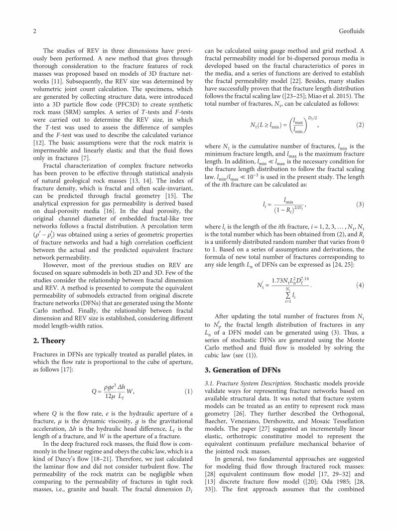
Figure 1: Schematic view of the generation of submodels.

3Geofluids

The theory and technique of the issue have been well studiedand presented in previous studies [27, 38–40]. The process ofgeneration includes the following steps:

(1) Several parameters, such as lmin, lmax, Df , and Ln,should be determined before DFNs are generated.lmin and lmax are set to be 0.5 and 500m, respectively,which satisfies the necessary condition for the sizedistribution of fracture length to follow the fractal

Table 2: Comparison of the values of a and achievements inprevious studies.

Authors Year Value of a

Dverstop and Anderson 1989 1.7

Tsang et al. 1996 3.0

Bour and Davy 1997 1.0–3.0

De Dreuzy 2001 0.0–3.5

Richeng Liu 2016 1.17–3.39

Present study 2018 0.96–1.29

(a) Lx : L

y = 1 : 2 (b) L

x : L

y = 1 : 1.5

(c) Lx : L

y = 1.5 : 1 (d) L

x : L

y = 2 : 1

Impermeable

Impermeable

P1 P2

Impermeable

Impermeable

P1 P2

Impermeable

Impermeable

P1

Impermeable

Impermeable

P1 P2P2

X

Y

0

Figure 2: Hydraulic boundary conditions.

0 2 4 6 8 10

0

1000

2000

3000

4000

Frac

ture

num

ber

Fracture length (m)

Df = 1.3Df = 1.4Df = 1.5Df = 1.6Df = 1.7

y = 1510x−1.19 R2 = 0.96268y = 1107x−1.26 R2 = 0.97167y = 695x−1.29 R2 = 0.96967y = 586x−1.33 R2 = 0.97626y = 437x−0.96 R2 = 0.93612

Figure 3: Correlation between fracture number and fracture length.

4 Geofluids

scaling law. The fractures with lengths that aresmaller than 0.5m contribute negligibly to the flowrate with respect to long fractures. The location offractures can be determined by setting the centerpoint, orientation, and fracture length. The fractureorientation and center point distribution areassumed to be uniformly and randomly distributedin order to focus on the effects of fractal lengthdistribution. Original square DFNs having sidelengths (Ln) of 50m, 25m, 15m, 10m, 8m, and4m are generated when Df = 1 3, 1.4, 1.5, 1.6,and 1.7, respectively. Ln decreases with the increase

in Df . If a large Ln (i.e., 50m) is adopted when Dfis large (i.e., Df = 1 7), there would be many frac-tures generated, which may cost a longer time forsolving fluid flow, comparing with that with asmaller Df (i.e., Df = 1 3).

(2) The value of N t can be calculated using (1). Thelength of the ith fracture can be calculated using(3) after generating N t random numbers. N t′ canbe obtained by calculating (4). After that, thelengths of all fracture with a number of N t′ canbe generated using (3).

0 5 10 15 20 25 30 35 400.0

3.0 × 10−14

6.0 × 10−14

9.0 × 10−14

1.2 × 10−13

Kp (

m2 )

Ln (m)

Simulation resultKavgKmax

KminVK

(a) Lx Ly = 1 2

0.2

0.4

0.6

0.8

RMS

0 5 10 15 20 25 30 35 40Ln (m)

(b) Lx Ly = 1 2

Kp (m

2 )

2.0 × 10−14

4.0 × 10−14

6.0 × 10−14

8.0 × 10−14

1.0 × 10−13

0 5 10 15 20 25 30 35 40Ln (m)

Simulation resultKavgKmax

KminVK

(c) Lx Ly = 1 1 5

0.2

0.4

0.6

0.8

RMS

0 5 10 15 20 25 30 35 40Ln (m)

(d) Lx Ly = 1 1 5K

p (m

2 )

1.0 × 10−14

2.0 × 10−14

3.0 × 10−14

4.0 × 10−14

0 5 10 15 20 25 30 35 40Ln (m)

Simulation resultKavgKmax

KminVK

(e) Lx Ly = 1 5 1

0.2

0.4

0.6

0.8

RMS

0 5 10 15 20 25 30 35 40Ln (m)

(f) Lx Ly = 1 5 1

Kp (

m2 )

0.0

1.0 × 10−14

2.0 × 10−14

3.0 × 10−14

0 5 10 15 20 25 30 35 40Ln (m)

Simulation resultKavgKmax

KminVK

(g) Lx Ly = 2 1

0.2

0.4

0.6

0.8

RMS

0 5 10 15 20 25 30 35 40Ln (m)

(h) Lx Ly = 2 1

Figure 4: Variations in Kp and RMS with different Ln when Df = 1 3.

5Geofluids

(3) The DFNs are established using a DEM (discreteelement method) code based on a 2D open sourcesoftware (OSS) UDEC (Itasca Consulting GroupInc. 2004), in which the fractures are representedwith line segments.

(4) Rectangular submodels are inserted into UDEC tocalculate REV with different Df . The submodels,whose area is the square of Ln, are extracted fromoriginal large models with Ln = 5~45m, 1~20m,0.5~10m, 0.25~7m, and 0.25~4m, correspondingto Df = 1 3, 1.4, 1.5, 1.6, and 1.7, respectively. The

aperture for each fracture is a constant (65μm) inorder to study the effect of fracture length on thepermeability. Here, we take Df = 1 6 as an example toshow the details of generation of original DFNs andextraction of submodels as shown in Figure 1.Figure 1(a) shows the process of extracting submodelsfrom an original DFN with Ln = 10m and Lx Ly =1 5 1, in which Lx and Ly represent the length andwidth of the submodels, respectively. Figure 1(b)exhibits the extraction of submodels that have differ-ent length-width ratios while maintaining the same

0.0

1.5 × 10−13

3.0 × 10−13

4.5 × 10−13

0 2 4 6 8 10 12 14 16 18 20

Kp (m

2 )

Ln (m)

Simulation resultKavgKmax

KminVK

(a) Lx Ly = 1 2

0 2 4 6 8 10 12 14 16 18 20

0.2

0.0

0.4

0.6

0.8

RMS

Ln (m)

(b) Lx Ly = 1 2

0.0

4.0 × 10−14

8.0 × 10−14

1.2 × 10−13

0 2 4 6 8 10 12 14 16 18 20

Kp

(m2 )

Ln (m)

Simulation resultKavgKmax

KminVK

(c) Lx Ly = 1 1 5

0 2 4 6 8 10 12 14 16 18 20

0.2

0.0

0.4

0.6

0.8

RMS

Ln (m)

(d) Lx Ly = 1 1 5

0.0

4.0 × 10−14

8.0 × 10−14

1.2 × 10−13

0 2 4 6 8 10 12 14 16 18 20

Kp (m

2 )

Ln (m)

Simulation resultKavgKmax

KminVK

(e) Lx Ly = 1 5 1

0 2 4 6 8 10 12 14 16 18 20

0.2

0.0

0.4

0.6

0.8

RMS

Ln (m)

(f) Lx Ly = 1 5 1

0.0

2.0 × 10−14

4.0 × 10−14

6.0 × 10−14

8.0 × 10−14

0 2 4 6 8 10 12 14 16 18 20

Kp (m

2 )

Ln (m)

Simulation resultKavgKmax

KminVK

(g) Lx Ly = 2 1

0 2 4 6 8 10 12 14 16 18 20

0.2

0.0

0.4

0.6

0.8

RMS

Ln (m)

(h) Lx Ly = 2 1

Figure 5: Variations in Kp and RMS with different Ln when Df = 1 4.

6 Geofluids

area. Table 1 shows the two sides of rectangular sub-models compared to the length of square submodelswith the same area whenDf = 1.6.

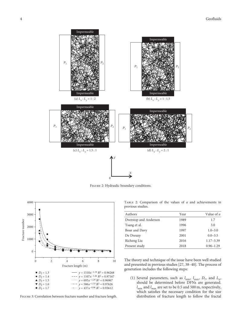
(5) Constant hydraulic head boundary conditions areapplied, as shown in Figure 2, to numericallycalculate the permeability (Kp) along the direction

of the hydraulic gradient when fluid flow is in thesteady state. The upper and bottom sides are imper-meable, and the horizontal flow from the left side to

the right side is set for the calculation. The hydraulicpressure gradient is 10 kPa/m for each DFN.

When the geometric parameters such as fracture length,aperture, and orientation are available, our model can simu-late the fluid flow in real situations. However, characterizingthese parameters is not a simple work, especially for the 3Dmodel. Generally, for simplification, some functions are usedto generate fracture parameters. For example, fracture lengthdistribution follows a power law function [41, 42]; fracture

0 2 4 6 8 100.0

2.0 × 10−13

4.0 × 10−13

6.0 × 10−13

Ln (m)

Simulation resultKavgKmax

KminVK

Kp (m

2 )

(a) Lx Ly = 1 2

0 2 4 6 8 10Ln (m)

0.2

0.0

0.4

0.6

0.8

RMS

(b) Lx Ly = 1 2

0.0

4.0 × 10−14

8.0 × 10−14

1.2 × 10−13

1.6 × 10−13

2.0 × 10−13

0 2 4 6 8 10Ln (m)

Simulation resultKavgKmax

KminVK

Kp (m

2 )

(c) Lx Ly = 1 1 5

0 2 4 6 8 10Ln (m)

0.2

0.0

0.4

0.6

0.8

RMS

(d) Lx Ly = 1 1 5

0.0

2.0 × 10−13

4.0 × 10−13

6.0 × 10−13

0 2 4 6 8 10Ln (m)

Simulation resultKavgKmax

KminVK

Kp (m

2 )

(e) Lx Ly = 1 5 1

0 2 4 6 8 10Ln (m)

0.2

0.0

0.4

0.6

0.8

RMS

(f) Lx Ly = 1 5 1

0.0

2.0 × 10−13

4.0 × 10−13

6.0 × 10−13

8.0 × 10−13

0 2 4 6 8 10Ln (m)

Simulation resultKavgKmax

KminVK

Kp (m

2 )

(g) Lx Ly = 2 1

0 2 4 6 8 10Ln (m)

0.2

0.0

0.4

0.6

0.8

RMS

(h) Lx Ly = 2 1

Figure 6: Variations in Kp and RMS with different Ln when Df = 1 5.

7Geofluids

aperture is correlated with fracture length [18, 19]; and frac-ture orientation follows the Fisher distribution [2, 8]. Bydoing so, the calculated results (i.e., permeability) are stillclose to the in situ results.

3.3. Discrete Fracture Network Validation. A fundamentalconcern is whether the generated DFNs are representativeof observed field conditions. This is often difficult toquantify due to the limited available field data. This canbe overcome by comparing the statistical information ofgenerated fracture length distribution with those reportedin literature. The feasibility and effectiveness of fractal

length distribution of fractures are illustrated. Figure 3shows the results of the relationship between the lengthand numbers of fractures. It is obvious that each set oflength–number relationship corresponding to each Dffollows a power law function that can be expressed by:

n l, 0 5 = αl−a, 5

where α is the proportional coefficient, a is the power lawexponent, and n l, 0 5 represents the fracture numberwith lengths in the range of l − 0 5, l + 0 5 .

0 1 2 3 4 5 6

0.0

4.0 × 10−13

8.0 × 10−13

1.2 × 10−12

Kp (m

2 )

Ln (m)

Simulation resultKavgKmax

KminVK

(a) Lx Ly = 1 2

0 1 2 3 4 5 6Ln (m)

0.2

0.0

0.4

0.6

0.8

RMS

(b) Lx Ly = 1 2

0.0

2.0 × 10−13

4.0 × 10−13

6.0 × 10−13

8.0 × 10−13

1.0 × 10−12

0 1 2 3 4 5 6

Kp (m

2 )

Ln (m)

Simulation resultKavgKmax

KminVK

(c) Lx Ly = 1 1 5

0 1 2 3 4 5 6Ln (m)

0.2

0.0

0.4

0.6

0.8

RMS

(d) Lx Ly = 1 1 5

0.0

1.5 × 10−13

3.0 × 10−13

4.5 × 10−13

0 1 2 3 4 5 6

Kp (m

2 )

Ln (m)

Simulation resultKavgKmax

KminVK

(e) Lx Ly = 1 5 1

0 1 2 3 4 5 6Ln (m)

0.2

0.0

0.4

0.6

0.8

RMS

(f) Lx Ly = 1 5 1

0.0

1.0 × 10−13

2.0 × 10−13

3.0 × 10−13

0 1 2 3 4 5 6

Kp (m

2 )

Ln (m)

Simulation resultKavgKmax

KminVK

(g) Lx Ly = 2 1

0 1 2 3 4 5 6Ln (m)

0.2

0.0

0.4

0.6

0.8

RMS

(h) Lx Ly = 2 1

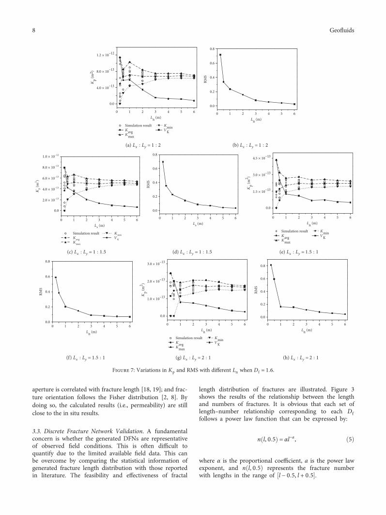
Figure 7: Variations in Kp and RMS with different Ln when Df = 1 6.

8 Geofluids

When Df varies from 1.3 to 1.7, a is in the range of0 96, 1 29 , which fits well with the values reported inprevious studies as shown in Table 2. This verifies thevalidity of (2) and (3), and indirectly verifies the validityof the generated DFNs. In practice, the choice of themodel depends on how it can be correlated to the avail-able field data and to be engineering needs of the project.Therefore, the validity of the generated models still needsfurther verification using in situ data collected from differ-ent scales and different rock types.

4. Results and Analysis

4.1. Determinations of Equivalent Permeability and REV Size.Using the abovementioned methods, the flow rates areobtained under a fixed hydraulic pressure gradient formodels that have different Df . Next, the equivalent perme-ability is back-calculated using Darcy’s law, as follows:

K f =μQA∇P

, 6

0.0 0.5 1.0 1.5 2.0 2.5 3.0 3.5

5.0 × 10−13

1.0 × 10−12

1.5 × 10−12

2.0 × 10−12

2.5 × 10−12

Kp (m

2 )

Ln (m)

Simulation resultKavgKmax

KminVK

(a) Lx Ly = 1 2

0.1

0.2

0.3

0.4

0.0 0.5 1.0 1.5 2.0 2.5 3.0 3.5Ln (m)

RMS

(b) Lx Ly = 1 2

4.0 × 10−13

8.0 × 10−13

1.2 × 10−12

1.6 × 10−12

2.0 × 10−12

0.0 0.5 1.0 1.5 2.0 2.5 3.0 3.5

Kp (m

2 )

Ln (m)

Simulation resultKavgKmax

KminVK

(c) Lx Ly = 1 1 5

0.1

0.2

0.3

0.4

0.0 0.5 1.0 1.5 2.0 2.5 3.0 3.5Ln (m)

RMS

(d) Lx Ly = 1 1 5

Simulation resultKavgKmax

KminVK

2.0 × 10−13

4.0 × 10−13

6.0 × 10−13

8.0 × 10−13

0.0 0.5 1.0 1.5 2.0 2.5 3.0 3.5

Kp (m

2 )

Ln (m)

(e) Lx Ly = 1 5 1

0.1

0.2

0.3

0.4

0.0 0.5 1.0 1.5 2.0 2.5 3.0 3.5Ln (m)

RMS

(f) Lx Ly = 1 5 1

1.5 × 10−13

3.0 × 10−13

4.5 × 10−13

6.0 × 10−13

0.0 0.5 1.0 1.5 2.0 2.5 3.0 3.5

Kp (m

2 )

Ln (m)

Simulation resultKavgKmax

KminVK

(g) Lx Ly = 2 1

0.1

0.2

0.3

0.4

0.0 0.5 1.0 1.5 2.0 2.5 3.0 3.5Ln (m)

RMS

(h) Lx Ly = 2 1

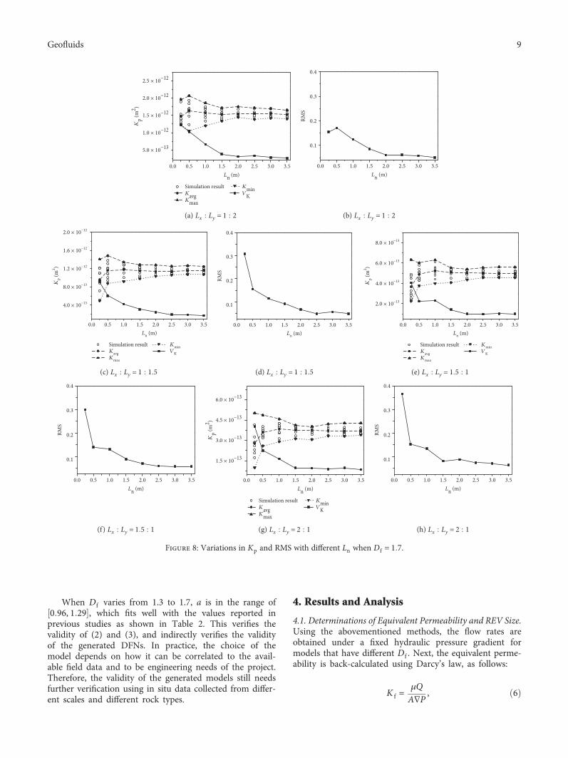
Figure 8: Variations in Kp and RMS with different Ln when Df = 1 7.

9Geofluids

where μ is the fluid viscosity, Q is the total flow rate, A isthe cross section of percolation, and ∇P is the hydraulicpressure gradient that equals 10 kPa/m. For each DFN,the average width of the cross section is assumed to be1.0m because the DFN model is two-dimensional andthus A equals the side length of the inlet boundary.

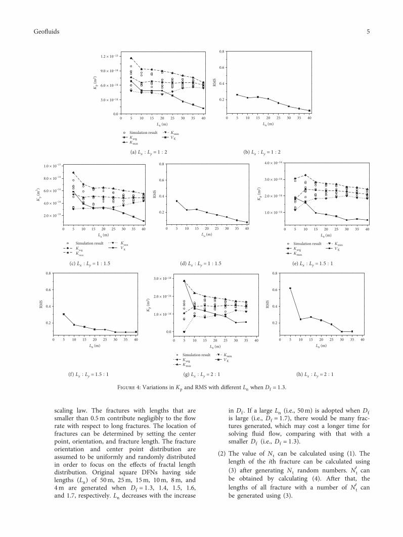
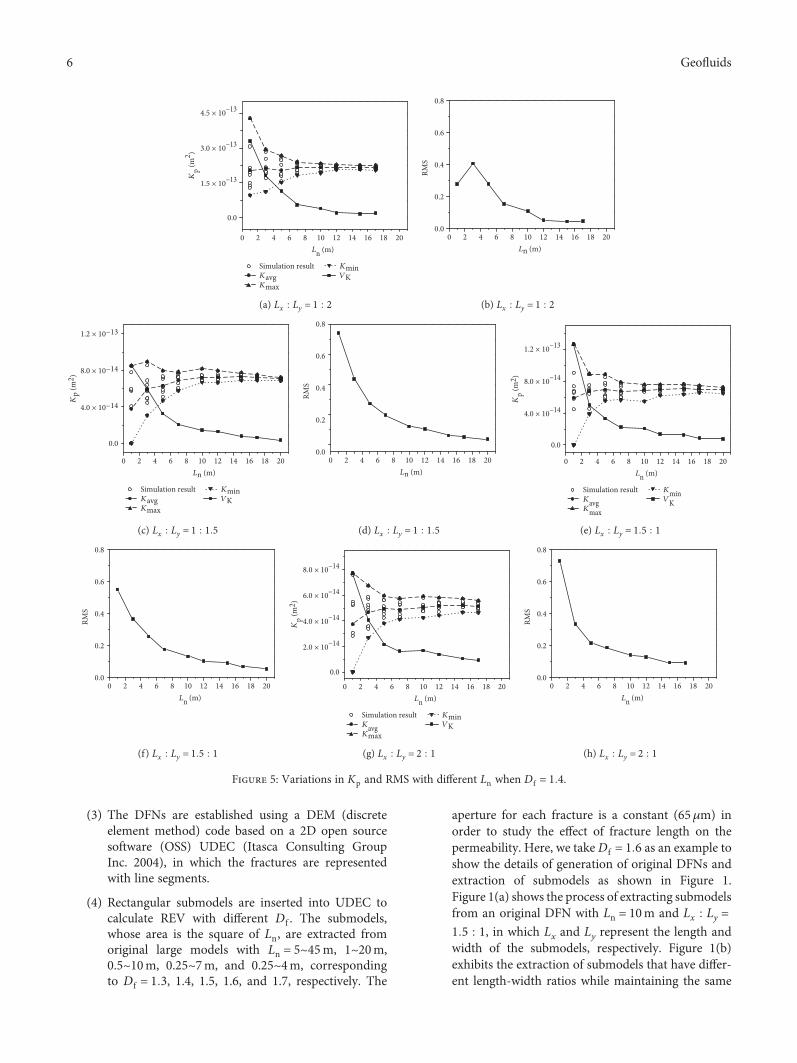
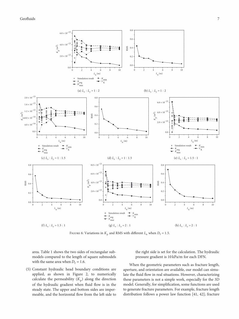
Based on the extracted DFNs with different length-widthratios as shown in Section 3.2, the variations in K f and corre-sponding root mean square (RMS) are plotted in Figures 4–8.For each Df and each length-width ratio, 10 DFNs are gener-ated using 10 sets of random numbers. Then, K f and its meanvalue of the 10 DFNs are calculated. K f tends to stabilize withincreasing model size. Before the curve stabilizes, the perme-ability of the models depends on the connectivity of the frac-tures. The REV can be defined theoretically as the size beyondwhich the permeability varies in a sufficiently small range. Inpractice, the correspondingmodel scale, in which Ln increasesto a critical value and the change in K f is sufficiently slight,can be regarded as the REV size. VK and RMS decrease withthe increment of Ln. Here, VK is defined as the difference inequivalent permeability between the maximum and mini-mum values. The RMS is determined by the ratio of standarddeviation of simulation results to the mean value of themaximum and minimum equivalent permeability.

The RMS is introduced to quantify whether two datasetsagree well with each other [3], defined as:

RMS =2 1

n〠n

1Kavg − Ksim

2

Kmax + Kmin, 7

where Kmax is the maximum equivalent permeability, Kmin isthe minimum equivalent permeability, Kavg is the averageequivalent permeability, and Ksim is the simulation result.

Taking the case of Df = 1 6 in Figure 6(a) for an example,Kp ranges from 8.5E−14 to 5.5E−13m2 when Ln = 0 5m,while for Ln = 10m, Kp ranges from 3.5E−13 to 3.1E−13m2.Besides, VK decreases from 4.95E−13 to 4E−14 and RMSdecreases from 0.443 to 0.032, indicating that the connec-tivity of the fractures tends to be homogeneous. However,when the length-width ratio of submodels changes, thenumber of connected fractures will change, and so doesthe Kp of submodels with the same area.

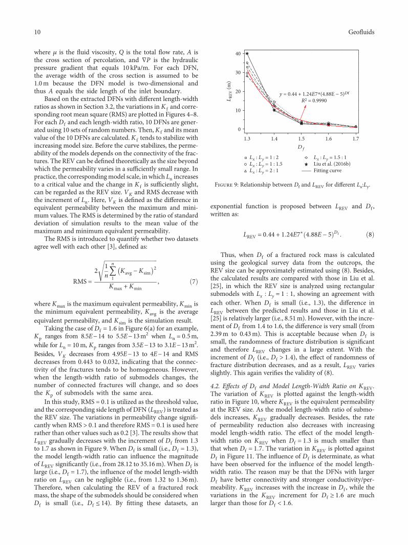
In this study, RMS = 0 1 is utilized as the threshold value,and the corresponding side length of DFN (LREV) is treated asthe REV size. The variations in permeability change signifi-cantly when RMS > 0 1 and therefore RMS = 0 1 is used hererather than other values such as 0.2 [3]. The results show thatLREV gradually decreases with the increment of Df from 1.3to 1.7 as shown in Figure 9. When Df is small (i.e., Df = 1 3),the model length-width ratio can influence the magnitudeof LREV significantly (i.e., from 28.12 to 35.16m). When Df islarge (i.e., Df = 1 7), the influence of the model length-widthratio on LREV can be negligible (i.e., from 1.32 to 1.36m).Therefore, when calculating the REV of a fractured rockmass, the shape of the submodels should be considered whenDf is small (i.e., Df ≤ 14). By fitting these datasets, an

exponential function is proposed between LREV and Df ,written as:

LREV = 0 44 + 1 24E7∗ 4 88E − 5 D f 8

Thus, when Df of a fractured rock mass is calculatedusing the geological survey data from the outcrops, theREV size can be approximately estimated using (8). Besides,the calculated results are compared with those in Liu et al.[25], in which the REV size is analyzed using rectangularsubmodels with Lx Ly = 1 1, showing an agreement witheach other. When Df is small (i.e., 1.3), the difference inLREV between the predicted results and those in Liu et al.[25] is relatively larger (i.e., 8.51m). However, with the incre-ment of Df from 1.4 to 1.6, the difference is very small (from2.39m to 0.43m). This is acceptable because when Df issmall, the randomness of fracture distribution is significantand therefore LREV changes in a large extent. With theincrement of Df (i.e., Df > 1 4), the effect of randomness offracture distribution decreases, and as a result, LREV variesslightly. This again verifies the validity of (8).

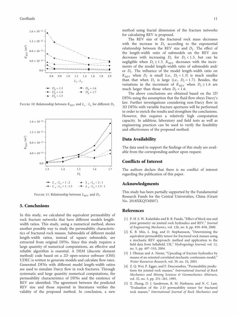
4.2. Effects of Df and Model Length-Width Ratio on KREV.The variation of KREV is plotted against the length-widthratio in Figure 10, where KREV is the equivalent permeabilityat the REV size. As the model length-width ratio of submo-dels increases, KREV gradually decreases. Besides, the rateof permeability reduction also decreases with increasingmodel length-width ratio. The effect of the model length-width ratio on KREV when Df = 1 3 is much smaller thanthat when Df = 1 7. The variation in KREV is plotted againstDf in Figure 11. The influence of Df is determinate, as whathave been observed for the influence of the model length-width ratio. The reason may be that the DFNs with largerDf have better connectivity and stronger conductivity/per-meability. KREV increases with the increase in Df , while thevariations in the KREV increment for Df ≥ 1 6 are muchlarger than those for Df < 1 6.

1.3 1.4 1.5 1.6 1.7

0

10

20

30

40

LRE

V (m

)

Df

y = 0.44 + 1.24E7⁎(4.88E − 5)Df

R2 = 0.9990

Lx : Ly = 1.5 : 1Liu et al. (2016b)Fitting curve

Lx : Ly = 1 : 2Lx : Ly = 1 : 1.5Lx : Ly = 2 : 1

Figure 9: Relationship between Df and LREV for different Lx:Ly.

10 Geofluids

5. Conclusions

In this study, we calculated the equivalent permeability ofrock fracture networks that have different models length-width ratios. This study, using a numerical method, showsanother possible way to study the permeability characteris-tics of fractured rock masses. Submodels of different modellength-width ratios, instead of square submodels, areextracted from original DFNs. Since this study requires alarge quantity of numerical computations, an effective andreliable algorithm is essential. A DEM (discrete elementmethod) code based on a 2D open-source software (OSS)UDEC is written to generate models and calculate flow rates.Generated DFNs with different model length-width ratiosare used to simulate Darcy flow in rock fractures. Throughsystematic and large quantity numerical computations, thepermeability characteristics of DFNs and the existence ofREV are identified. The agreement between the predictedREV size and those reported in literatures verifies thevalidity of the proposed method. In conclusion, a new

method using fractal dimension of the fracture networksfor calculating REV is proposed.

The REV size of the fractured rock mass decreaseswith the increase in Df according to the exponentialrelationship between the REV size and Df . The effect ofthe length-width ratio of submodels on the REV sizedecreases with increasing Df for Df < 1 5, but can benegligible when Df ≥ 1 5. KREV decreases with the incre-ments of the model length-width ratio of submodels and/or Df . The influence of the model length-width ratio onKREV when Df is small (i.e., Df = 1 3) is much smallerthan that when Df is large (i.e., Df = 1 7). Besides, thevariations in the increment of KREV when Df ≥ 1 6 aremuch larger than those when Df < 1 6.

The above conclusions are obtained based on the 2DDFNs using the assumption that the fluid flow obeys Darcy’slaw. Further investigations considering non-Darcy flow in3D DFNs with variable fracture apertures will be performedin order to enrich the results and strengthen the conclusions.However, this requires a relatively high computationcapacity. In addition, laboratory and field tests as well asengineering practices can be used to verify the feasibilityand effectiveness of the proposed method.

Data Availability

The data used to support the findings of this study are avail-able from the corresponding author upon request.

Conflicts of Interest

The authors declare that there is no conflict of interestregarding the publication of this paper.

Acknowledgments

This study has been partially supported by the FundamentalResearch Funds for the Central Universities, China (GrantNo. 2018XKQYMS07).

References

[1] P. H. S. W. Kulatilake and B. B. Panda, “Effect of block size andjoint geometry on jointed rock hydraulics and REV,” Journalof Engineering Mechanics, vol. 126, no. 8, pp. 850–858, 2000.

[2] K. B. Min, L. Jing, and O. Stephansson, “Determining theequivalent permeability tensor for fractured rock masses usinga stochastic REV approach: method and application to thefield data from Sellafield, UK,” Hydrogeology Journal, vol. 12,no. 5, pp. 497–510, 2004.

[3] J. Öhman and A. Niemi, “Upscaling of fracture hydraulics bymeans of an oriented correlated stochastic continuum model,”Water Resources Research, vol. 39, no. 10, 2003.

[4] Z. Q. Wei, P. Egger, and F. Descoeudres, “Permeability predic-tions for jointed rock masses,” International Journal of RockMechanics and Mining Sciences & Geomechanics Abstracts,vol. 32, no. 3, pp. 251–261, 1995.

[5] X. Zhang, D. J. Sanderson, R. M. Harkness, and N. C. Last,“Evaluation of the 2-D permeability tensor for fracturedrock masses,” International Journal of Rock Mechanics and

1.3 1.4 1.5 1.6 1.7

0.0

4.0 × 10−13

8.0 × 10−13

1.2 × 10−12

1.6 × 10−12

KRE

V (m

2 )

Df

L x : Ly = 1.5 : 1L x : Ly = 2 : 1L x : Ly = 1 : 2

L x : Ly = 1 : 1.5

Figure 11: Relationship between LREV and Df .

0.6 0.8 1.0 1.2 1.4 1.6 1.8 2.0

0.0

4.0 × 10−13

8.0 × 10−13

1.2 × 10−12

1.6 × 10−12

KRE

V (m

2 )

Lx : Ly

Dp = 1.3Dp = 1.4Dp = 1.5

Dp = 1.6Dp = 1.7

Figure 10: Relationship between KREV and Lx Ly for different Df .

11Geofluids

Mining Sciences & Geomechanics Abstracts, vol. 33, no. 1,pp. 17–37, 1996.

[6] B. B. Panda and P. H. S. W. Kulatilake, “Effect of joint geome-try and transmissivity on jointed rock hydraulics,” Journal ofEngineering Mechanics, vol. 125, no. 1, pp. 41–50, 1999.

[7] A. Baghbanan and L. Jing, “Stress effects on permeability in afractured rock mass with correlated fracture length andaperture,” International Journal of Rock Mechanics and Min-ing Sciences, vol. 45, no. 8, pp. 1320–1334, 2008.

[8] K. B. Min, J. Rutqvist, C. F. Tsang, and L. Jing, “Stress-depen-dent permeability of fractured rock masses: a numericalstudy,” International Journal of Rock Mechanics and MiningSciences, vol. 41, no. 7, pp. 1191–1210, 2004.

[9] S.-H. Chen, X.-M. Feng, and S. Isam, “Numerical estimation ofREV and permeability tensor for fractured rock masses bycomposite element method,” International Journal for Numer-ical and Analytical Methods in Geomechanics, vol. 32, no. 12,pp. 1459–1477, 2008.

[10] W. G. Pariseau, S. Puri, and S. C. Schmelter, “A new model foreffects of impersistent joint sets on rock slope stability,” Inter-national Journal of Rock Mechanics and Mining Sciences,vol. 45, no. 2, pp. 122–131, 2008.

[11] Y. An and Q. Wang, “Analysis of representative elementvolume size based on 3D fracture network,” Rock and SoilMechanics, vol. 33, pp. 3775–3780, 2012.

[12] K. Esmaieli, J. Hadjigeorgiou, and M. Grenon, “Estimatinggeometrical and mechanical REV based on synthetic rockmass models at Brunswick mine,” International Journal ofRock Mechanics and Mining Sciences, vol. 47, no. 6, pp. 915–926, 2010.

[13] C. C. Barton and E. Larsen, “Fractal geometry of two-dimensional fracture networks at Yucca Mountain, southwest-ern Nevada: proceedings,” Office of Scientific & TechnicalInformation Technical Reports, 1985.

[14] Y. Zhao, Z. Feng, W. Liang, D. Yang, Y. Hu, and T. Kang,“Investigation of fractal distribution law for the trace numberof random and grouped fractures in a geological mass,”Engineering Geology, vol. 109, no. 3-4, pp. 224–229, 2009.

[15] P. R. la Pointe, “A method to characterize fracture density andconnectivity through fractal geometry,” International Journalof Rock Mechanics and Mining Sciences & GeomechanicsAbstracts, vol. 25, no. 6, pp. 421–429, 1988.

[16] Q. Zheng and B. Yu, “A fractal permeability model for gas flowthrough dual-porosity media,” Journal of Applied Physics,vol. 111, no. 2, article 024316, 2012.

[17] J. Bear, Dynamics of Fluids in Porous Media, Elsevier, NewYork, 1972.

[18] A. Baghbanan and L. Jing, “Hydraulic properties of fracturedrock masses with correlated fracture length and aperture,”International Journal of Rock Mechanics and Mining Sciences,vol. 44, no. 5, pp. 704–719, 2007.

[19] C. Klimczak, R. A. Schultz, R. Parashar, and D. M. Reeves,“Cubic law with aperture-length correlation: implications fornetwork scale fluid flow,” Hydrogeology Journal, vol. 18,no. 4, pp. 851–862, 2010.

[20] J. C. S. Long, J. S. Remer, C. R. Wilson, and P. A. Witherspoon,“Porous media equivalents for networks of discontinuousfractures,” Water Resources Research, vol. 18, no. 3, pp. 645–658, 1982.

[21] Z. Zhao, B. Li, and Y. Jiang, “Effects of fracture surface rough-ness on macroscopic fluid flow and solute transport in fracture

networks,” Rock Mechanics and Rock Engineering, vol. 47,no. 6, pp. 2279–2286, 2014.

[22] B. Yu and P. Cheng, “A fractal permeability model for bi-dispersed porous media,” International Journal of Heat andMass Transfer, vol. 45, no. 14, pp. 2983–2993, 2002.

[23] R. Liu, Y. Jiang, B. Li, and X. Wang, “A fractal model forcharacterizing fluid flow in fractured rock masses based onrandomly distributed rock fracture networks,” Computersand Geotechnics, vol. 65, pp. 45–55, 2015.

[24] R. Liu, B. Li, and Y. Jiang, “A fractal model based on a new gov-erning equation of fluid flow in fractures for characterizinghydraulic properties of rock fracture networks,” Computersand Geotechnics, vol. 75, pp. 57–68, 2016.

[25] R. Liu, Y. Jiang, B. Li, and L. Yu, “Estimating permeability ofporous media based on modified Hagen–Poiseuille flow intortuous capillaries with variable lengths,” Microfluidics andNanofluidics, vol. 20, no. 8, p. 120, 2016.

[26] W. S. Dershowitz and H. H. Einstein, “Characterizing rockjoint geometry with joint system models,” Rock Mechanicsand Rock Engineering, vol. 21, no. 1, pp. 21–51, 1988.

[27] Q. Wu and P. H. S. W. Kulatilake, “REV and its properties onfracture system and mechanical properties, and an orthotro-pic constitutive model for a jointed rock mass in a dam sitein China,” Computers and Geotechnics, vol. 43, no. 3,pp. 124–142, 2012.

[28] J. Andersson and B. Dverstorp, “Conditional simulations offluid flow in three-dimensional networks of discrete fractures,”Water Resources Research, vol. 23, no. 10, pp. 1876–1886,1987.

[29] P. A. Hsieh and S. P. Neuman, “Field determination of thethree-dimensional hydraulic conductivity tensor of aniso-tropic media: 1. Theory,” Water Resources Research, vol. 21,no. 11, pp. 1655–1665, 1985.

[30] C. Louis, Rock Hydraulic in Rock Mechanics, L. Muller, Ed.,Springer, Vienna, 1974.

[31] G. DeMarsily, “Flow and transport in fractured rocks: connec-tivity and scale effect,” in International Symposium on theHydrogeology of Rocks of Low Permeability, pp. 267–277, Inter-national Association of Hydrogeologists, Tucson, AZ, USA,1985.

[32] A. E. Scheidegger, “The physics of flow through porousmedia,” Soil Science, vol. 86, no. 6, p. 355, 1958.

[33] S. Segan and K. Karasaki, “TRINET: a flow and transport codefor fracture networks-user’s manual and tutorial,” LawrenceBerkely Laboratory, Berkely Laboratory, LBL-34834, Berkeley,CA, USA, 1993.

[34] G. Rong, J. Peng, X. Wang, G. Liu, and D. Hou, “Permeabilitytensor and representative elementary volume of fractured rockmasses,” Hydrogeology Journal, vol. 21, no. 7, pp. 1655–1671,2013.

[35] V. M. Ivanova, Geologic and Stochastic Modeling of FractureSystems in Rocks, Massachusetts Institute of Technology,1998.

[36] N. Huang, Y. Jiang, R. Liu, and B. Li, “Estimation of permeabil-ity of 3-D discrete fracture networks: an alternative possibilitybased on trace map analysis,” Engineering Geology, vol. 226,pp. 12–19, 2017.

[37] C. T. O. Leung and R. W. Zimmerman, “Estimating thehydraulic conductivity of two-dimensional fracture networksusing network geometric properties,” Transport in PorousMedia, vol. 93, no. 3, pp. 777–797, 2012.

12 Geofluids

[38] R. Parashar and D. M. Reeves, “On iterative techniques forcomputing flow in large two-dimensional discrete fracturenetworks,” Journal of Computational and Applied Mathemat-ics, vol. 236, no. 18, pp. 4712–4724, 2012.

[39] X.-H. Tan, J.-Y. Liu, X.-P. Li, L.-H. Zhang, and J. Cai, “Asimulation method for permeability of porous media basedon multiple fractal model,” International Journal of Engineer-ing Science, vol. 95, pp. 76–84, 2015.

[40] W. Wei, J. Cai, X. Hu, and Q. Han, “An electrical conductivitymodel for fractal porous media,” Geophysical Research Letters,vol. 42, no. 12, pp. 4833–4840, 2015.

[41] J. R. De Dreuzy, P. Davy, and O. Bour, “Hydraulic propertiesof two-dimensional random fracture networks following apower law length distribution: 1. Effective connectivity,”Water Resources Research, vol. 37, no. 8, pp. 2065–2078, 2001.

[42] J. R. De Dreuzy, P. Davy, and O. Bour, “Hydraulic propertiesof two-dimensional random fracture networks following apower law length distribution: 2. Permeability of networksbased on lognormal distribution of apertures,” WaterResources Research, vol. 37, no. 8, pp. 2079–2095, 2001.

13Geofluids

Hindawiwww.hindawi.com Volume 2018

Journal of

ChemistryArchaeaHindawiwww.hindawi.com Volume 2018

Marine BiologyJournal of

Hindawiwww.hindawi.com Volume 2018

BiodiversityInternational Journal of

Hindawiwww.hindawi.com Volume 2018

EcologyInternational Journal of

Hindawiwww.hindawi.com Volume 2018

Hindawiwww.hindawi.com

Applied &EnvironmentalSoil Science

Volume 2018

Forestry ResearchInternational Journal of

Hindawiwww.hindawi.com Volume 2018

Hindawiwww.hindawi.com Volume 2018

International Journal of

Geophysics

Environmental and Public Health

Journal of

Hindawiwww.hindawi.com Volume 2018

Hindawiwww.hindawi.com Volume 2018

International Journal of

Microbiology

Hindawiwww.hindawi.com Volume 2018

Public Health Advances in

AgricultureAdvances in

Hindawiwww.hindawi.com Volume 2018

Agronomy

Hindawiwww.hindawi.com Volume 2018

International Journal of

Hindawiwww.hindawi.com Volume 2018

MeteorologyAdvances in

Hindawi Publishing Corporation http://www.hindawi.com Volume 2013Hindawiwww.hindawi.com

The Scientific World Journal

Volume 2018Hindawiwww.hindawi.com Volume 2018

ChemistryAdvances in

Scienti�caHindawiwww.hindawi.com Volume 2018

Hindawiwww.hindawi.com Volume 2018

Geological ResearchJournal of

Analytical ChemistryInternational Journal of

Hindawiwww.hindawi.com Volume 2018

Submit your manuscripts atwww.hindawi.com