Embed Size (px)
Citation preview

Estimation in the Regression Discontinuity Model∗
Jack PorterHarvard University
Department of EconomicsLittauer Center 121
Cambridge, MA [email protected]
May 7, 2003
Abstract
The regression discontinuity model has recently become a commonly applied framework forempirical work in economics. Hahn, Todd, and Van der Klaauw (2001) provide a formal devel-opment of the identification of a treatment effect in this framework and also note the potentialbias problems in its estimation. This bias difficulty is the result of a particular feature of theregression discontinuity treatment effect estimation problem that distinguishes it from typicalsemiparametric estimation problems where smoothness is lacking. Here, the discontinuity is notsimply an obstacle to overcome in estimation; instead, the size of discontinuity is itself the objectof estimation interest. In this paper, I derive the optimal rate of convergence for estimation ofthe regression discontinuity treatment effect. The optimal rate suggests that with appropriatechoice of estimator the bias difficulties are no worse than would be found in the usual non-parametric conditional mean estimation problem (at an interior point of the covariate support).Two estimators are proposed that attain the optimal rate under varying conditions. One newestimator is based on Robinson’s (1988) partially linear estimator. The other estimator useslocal polynomial estimation and is optimal under a broader set of conditions.
Keywords: Regression Discontinuity Design, Optimal Convergence Rate, Asymptotic Bias
JEL Classification: C13, C14
∗I am grateful to Gary Chamberlain, Michael Murray, Whitney Newey, numerous seminar participants, andespecially Guido Imbens for comments and suggestions. I thank the National Science Foundation for research supportunder grant SES-0112095. This paper has also circulated under the title “Asymptotic Bias and Optimal ConvergenceRates for Semiparametric Kernel Estimators in the Regression Discontinuity Model.”
1

1 Introduction
The regression discontinuity [RD] design has recently become a commonly applied framework for
identification of treatment effects in economics. The RD design can be useful when there is a
“cut-off” point in treatment assignment or in the probability of treatment assignment. Under weak
smoothness conditions, the assignment near the cut-off behaves almost as if random. Regression
discontinuity models typically use only the information very close to the shift to identify the treat-
ment effect of interest without reliance on functional form assumptions. For example, Van der
Klaauw (1996) examined the effect of a university’s scholarship offer on the probability of an appli-
cant choosing to attend that university. The scholarship amount offered was based on an underlying
index of various individual characteristics observable to the econometrician. Cut-off points in the
index were used by the college to group applicants into categories, and scholarship offers were given
depending on the applicant category. This admissions procedure led to discontinuous shifts in the
scholarship amount with respect to the index at the cut-off points. Van der Klaauw used the data
near the discontinuities to estimate the causal effect of the scholarship amount on the probability
of acceptance. The empirical literature applying the RD design in other contexts where a disconti-
nuity in the treatment assignment exists includes Angrist and Lavy (1999), Battistin and Rettore
(2002), Black (1999), Chay and Greenstone (1998), Lee (2001), and Pence (2002). The formal
theoretical work in the econonometrics literature on identification and estimation in the RD model
is apparently limited to the work of Hahn, Todd, and Van der Klaauw (2001). The present paper
proposes two new estimators, derives the optimal convergence rate for semiparametric estimation
of the treatment effect identified in the RD model, and finds that the proposed estimators attain
the bound under varying conditions.
The lack of smoothness inherent in the RD model is not simply an obstacle to overcome in esti-
mation; instead, the size of discontinuity itself is the object of interest. Semiparametric estimation
of the discontinuity size is akin to estimation of a conditional expectation at two boundary points
and differencing the results. Given this connection to boundary estimation, it is not surprising to
2

find that a nonparametric estimator, such as the Nadaraya-Watson estimator, for the RD treatment
effect has poor asymptotic bias behavior. This poor bias behavior forces the bandwidth to shrink
at a fast rate and hence leads to a slow convergence rate. Hahn, Todd, and Van der Klaauw (2001)
suggest dealing with the bias by using a local linear estimator for the RD treatment effect and
provide the associated distributional results.
In this paper, I establish that the optimal convergence rate for estimation of the treatment
effect in the RD model is the same as Stone’s (1980) optimal rate for estimation of a conditional
expectation at an interior point of the covariate support. This result suggests that the apparent
bias difficulties are completely surmountable. I propose two optimal kernel-based semiparametric
estimators: a new estimator based on Robinson’s (1988) partially linear estimator, and a local
polynomial estimator that is the natural extension of the local linear estimator covered in Hahn,
Todd, and Van der Klaauw (2001). While the usual intuition motivating Robinson’s estimator
in the partially linear model breaks down in the RD model, it still turns out that this estimator
achieves the optimal rate of convergence for estimation of the RD treatment effect under a particular
smoothness condition (namely, that the derivatives of the conditional expectation have identical
right and left-hand limits at the discontinuity point). Moreover, the local polynomial estimator
attains the optimal convergence rate even more generally. These estimators not only improve the
asymptotic bias to the order of typical conditional expectation estimators at an interior point
of the support, but in some cases actually exhibit further unexpected bias reductions. Both of
these estimators are familiar from their use in other nonparametric settings, but their limiting
distributions in the RD context are different than in previously studied models.
Section 2 discusses RD treatment effect identification results relevant to our semiparametric
estimation problem and formally demonstrates that estimation of treatment effects in RD models
is equivalent to estimation of the size of a discontinuity in a conditional expectation. In particular,
given a dependent variable y and a scalar covariate x, the jump size is given by
α = limx↓x
E(y|x)− limx↑x
E(y|x) (1)
where x is the known discontinuity point of the conditional expectation E(y|x). No finite parametriza-
3
tion of the conditional expectation is assumed, just smoothness away from the discontinuity, so
estimating the jump size requires nonparametric techniques.
The connection to the conditional expectation boundary problem in nonparametric estimation
is clear from equation (1).1 The usual bias issues in the boundary problem carry over to the RD
case. Also, equation (1) makes apparent that only data near the discontinuity will be useful in
estimating α. Data far from the discontinuity could only contribute to estimation in the limit if
more is known about the functional form of E(y|x) thus violating the nonparametric assumption.
From this intuition, we should expect a slower than parametric√n-rate for estimation of α. This
intuition is confirmed in sections 3 and 4. In section 3, we find that, under certain conditions,
the partially linear and the local polynomial estimators have bias behavior like the difference of
a conditional expectation at two interior points of support, where the differencing results in still
further bias reduction. Due to this bias behavior, the limiting distribution of the local polynomial
estimator does not follow from known results on the limiting distribution of such estimators at a
boundary point (Fan and Gijbels 1996, Ruppert and Wand 1994). The new asymptotic distribution
theory is given given in section 3. The asymptotic behavior of the partially linear estimator in the
RD model is wholly different than its behavior in the canonical partially linear model (Robinson
1988). The new limiting distribution theory for this estimator is also covered in section 3.
In section 4, the optimal convergence rates are derived under a strong and weak set of smooth-
ness conditions. The optimal rate is attained by the partially linear and local polynomial estimators.
The relation of these results on best rates to the literature on optimal nonparametric conditional
mean estimation, especially, optimal estimation at boundaries is also described in section 4. Sec-
tion 5 discusses extending the results to more general RD models with multivariate covariates or
unknown cut-off point. Section 6 concludes.
2 Regression Discontinuity Models
The theoretical connections between the regression discontinuity model and the treatment effect
literature have been formally established in Hahn, Todd, and Van der Klaauw (2001). From1see Hardle and Linton (1994) for further discussion of the nonparametric boundary problem.
4

its inception in Thistlewaite and Campbell (1960), the regression discontinuity model has been
termed “quasi-experimental”, reflecting its intuitive connection to purely randomized experimental
methods. Trochim (1984) distinguishes between two different incarnations of the discontinuity
model, depending on whether the treatment assignment is related to the observed variable by a
deterministic function (sharp design) or a stochastic function (fuzzy design).
If treatment assignment is given by the indicator variable D ∈ {0, 1}, then the sharp design can
be characterized by D ={
1 if Z ≥ Z0 if Z < Z
where Z is observed and the cut-off point Z is known.
Let Y1 and Y0 be the potential outcomes corresponding to the two treatment assignments, and as
usual, Y = DY1 +(1−D)Y0 is the observed outcome. Then under the smoothness assumption that
E(Yj |Z) is continuous at Z for j = 0, 1, the expected causal effect of the treatment on the outcome
is identified at the discontinuity point. In particular
α = E(Y1 − Y0|Z)
= E(Y1|Z)− E(Y0|Z)
= limZ↓Z
E(Y1|Z)− limZ↑Z
E(Y0|Z)
= limZ↓Z
E(Y |Z)− limZ↑Z
E(Y |Z).
Hence, the discontinuity in treatment assignment at Z provides an opportunity to observe the
average difference in potential outcomes from points just on either side of the discontinuity. In the
limit, this average difference represents the expected causal effect evaluated at the discontinuity,
Z = Z. Identification is achieved assuming only smoothness in expected potential outcomes at the
discontinuity (and a positive density in a neighborhood of the discontinuity) without any parametric
functional form restrictions.
In the fuzzy design, E(D|Z) is discontinuous at Z. Hahn, Todd, and Van der Klaauw (2001)
discusses conditions under which the expected causal effect at Z is identified. For instance, the
assumption that Y1 − Y0 is independent of D conditional on Z is sufficient for identification.2
2Hahn, Todd, and Van der Klaauw (2001) and Battistin and Rettore (2002) also discuss the case where D(Z) isa deterministic function that varies by individual, see Imbens and Angrist (1994). If (Yi,1 − Yi,0, Di(Z)) is jointlyindependent of Zi for all Z, Di(Z) is discontinuous at Z for some i, and treatment assignment is monotone in Z,then the local average treatment effect (LATE) is identified at the discontinuity. Importantly, this set of identify-
5

In this case, we obtain E(Y1 − Y0|Z = Z) = [limZ↓Z E(Y |Z) − limZ↑Z E(Y |Z)] /[limZ↓Z E(D|Z)
− limZ↑Z E(D|Z)]. The key point for our estimation purposes is that in all cases the causal effect is
identified from an expression involving only the sizes of discontinuities in conditional expectations.
A special case of both sharp and fuzzy designs is the common treatment effects model, where
Yi,1 − Yi,0 = α is constant across individuals.3 In this case identification of the treatment effect is
achieved for sharp and fuzzy designs by only assuming smoothness in expected potential outcomes
at Z = Z. This case is important because with common treatment effects smoothness in expected
potential outcomes translates directly into smoothness of m(·) in the corresponding estimation
model (3) below (e.g. equal right and left hand side derivatives) at the discontinuity.
From the above expressions it is clear that the regression discontinuity approach only identifies
a causal effect at the discontinuity. Without some additional functional form assumptions (e.g.
common treatment effects) or additional discontinuity points, the result does not generalize to
identify the average effect or effects at other values of Z. Nevertheless, the regression discontinuity
model provides a useful framework for certain applications, and the above theoretical developments
show where the regression discontinuity model fits into the treatment evaluation literature.
3 Semiparametric Kernel Estimators
For the purposes of the current work, the key point to take from the previous section is the finding
that for each set of identifying assumptions, estimation of the RD treatment effect is equivalent to
the problem of estimating the jump size of a discontinuity in a conditional expectation. We focus
on estimation in the simplest RD model where the observed index in which the discontinuity occurs
is scalar and no additional covariates are included. Below three different kernel-based approaches
to semiparametric estimation are discussed. Since estimation in the RD model is analogous to
nonparametric estimation at a boundary, where bias problems have received some attention, special
consideration is given to the asymptotic bias behavior of each estimator. In particular, two proposed
ing assumptions also lead to an expression for the treatment effect in terms of just discontinuities in conditionalexpectations.
3Note that a local common treatment effects assumption would also be sufficient for these results. That is, it issufficient that the common treatment effect assumption only hold for observations in a neighborhood of Z.
6

discontinuity jump size esimators are based on partially linear and local polynomial estimators
which are often applied in different nonparametric models. The asymptotic bias of each of these
two jump size estimators will be different than what would be expected from their limiting behavior
in other nonparametric settings. These new asymptotic results are important for inference in RD
applications. In the next section, an additional reason for emphasizing the partially linear and local
polynomial estimators will be presented when obtaining optimal rates of convergence.
3.1 Assumptions
Before discussing the semiparametric kernel estimators in the following subsections, we introduce
the main assumptions necessary to derive the limiting distributions for the estimators.
The first assumption concerns the choice of kernel for estimation:
Assumption 1 (a) k(·) is a symmetric, bounded, Lipschitz function, zero outside a bounded set;∫k(u)du = 1.
(b) For positive integer s,∫k(u)ujdu = 0, 1 ≤ j ≤ s− 1.
This assumption is fairly standard, allowing for higher-order bias-reducing kernels (an sth order
kernel above). For s ≥ 3, the function k(·) is necessarily somewhere negative to satisfy condition (b).
By assuming that the kernel has a bounded support set, the remaining assumptions on the model
only need to describe behavior local to the discontinuity, and the need for a trimming function is
avoided.4
The second assumption concerns the RD model itself. Let f0 denote the marginal density of x
and m(x) denote the conditional expectation of y given x minus the discontinuity. Formally, m(x)
= E(y|x) −α1{x ≥ x}.
Assumption 2 Suppose the data (yi, xi)i=1,...,n is i.i.d. and α is defined by equation (1).
(a) For some compact interval N of x with x ∈ int(N ), f0 is lf times continuously differentiable
and bounded away from zero; m(x) is lm times continuously differentiable for x ∈ N\{x}, and m4Alternatively one could have an unbounded kernel support and trimming that becomes negligible as the sample
size increases, as in Robinson (1988).
7

is continuous at x with finite right and left-hand derivatives to order lm.
(b) Right and left-hand derivatives of m to order lm are equal at x.
Assumption 2(a) assures sufficient smoothness on either side of the discontuity, but allows for
unequal right and left-hand derivatives of m (equivalently E(y|x)) at x. Assumption 2(b) imposes
more smoothness in m at x. This part of the assumption will not affect the limiting distribution
result for the Nadaraya-Watson estimator below, but will play an important role in the asymptotic
bias of subsequent estimators. Part (b) would be implied by, for instance, smoothness in the
derivatives of E(Y0|X) to order lm and a common treatment effect assumption for observations in a
neighborhood of x. Bounding the density away from zero in a neighborhood of x assures that there
is positive density near the discontinuity and thus sufficient data for estimating the jump size. It
also allows us to avoid the technical problems of a near-zero denominator.
The third assumption concerns the behavior of the moments of the outcome variable. Define
ε = y − E(y|x) = y −m(x)− α1{x ≥ x}.
Assumption 3 (a) σ2(x) = E(ε2|x) is continuous for x 6= x, x ∈ N , and the right and left-hand
limits at x exist.
(b) For some ζ > 0, E[|ε|2+ζ |x] is uniformly bounded on N .
This assumption places no restrictions on the unconditional moments. Instead, only the behav-
ior of conditional moments evaluated near the discontinuity is restricted. Part (b) of the assumption
bounds the moments so that a central limit theorem can be applied to derive the limit distribution
of the different estimators. Part (a) simply allows us to write the asymptotic variance expressions
in a tractable form.
3.2 Nadaraya-Watson Estimation
The simplest kernel estimator of the discontinuity jump takes a kernel weighted average of obser-
vations on each side of the discontinuity and differences. Such an estimator is referred to as a
Nadaraya-Watson estimator and is discussed in Hahn, Todd, and Van der Klaauw (2001). Here we
briefly cover this estimator to formally establish the bias difficulty in estimation of the discontinuity
8

���
-�
6
x
rr
m(x)
m(x) + dα
m(x)
m(x) + α
x
Figure 1
jump size. Our discussion then serves as a point of reference for the subsequent estimators with
improved bias properties.
Usual Nadaraya-Watson estimation of α would proceed from a sample version of equation (1).
To estimate the first term in the difference, one would average the values of y corresponding to the
observations with the x’s just to the right of the discontinuity. The second term in the difference
would be estimated similarly, and then the estimate of α would be given by the difference of the
estimated first and second terms. The idea of using local averages to estimate the desired conditional
expectations is captured by kernel regression. A specific kernel version of the estimation method
just described follows. Given data (yi, xi)i=1,...,n, let
α =1n
∑i kh(x− xi)yidi
1n
∑j kh(x− xj)dj
−1n
∑i kh(x− xi)yi(1− di)
1n
∑j kh(x− xj)(1− dj)
(2)
where di = 1{xi ≥ x}, 1{A} is an indicator for the event A, kh(·) = 1hk( ·
h
), k(·) is a kernel function,
and h denotes a bandwidth that controls the size of the local neighborhood to be averaged over.
The first term in α is a weighted average of the dependent variable values for data just to the right
of the discontinuity, where the weights depend on the distance from the discontinuity (x− xi), the
bandwidth h, and the kernel k. Similarly, the second term estimates the left-hand side limit of the
conditional expectation at the discontinuity.
Such an estimator is subject to the problems of many nonparametric methods at a boundary.
Here, the bias at the boundary is O(h), where h is the bandwidth, whereas typical kernel regression
9
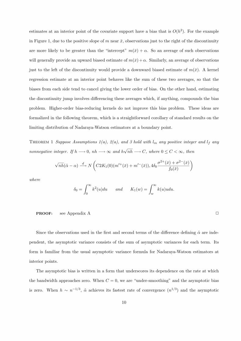
estimates at an interior point of the covariate support have a bias that is O(h2). For the example
in Figure 1, due to the positive slope of m near x, observations just to the right of the discontinuity
are more likely to be greater than the “intercept” m(x) + α. So an average of such observations
will generally provide an upward biased estimate of m(x)+α. Similarly, an average of observations
just to the left of the discontinuity would provide a downward biased estimate of m(x). A kernel
regression estimate at an interior point behaves like the sum of these two averages, so that the
biases from each side tend to cancel giving the lower order of bias. On the other hand, estimating
the discontinuity jump involves differencing these averages which, if anything, compounds the bias
problem. Higher-order bias-reducing kernels do not improve this bias problem. These ideas are
formalized in the following theorem, which is a straightforward corollary of standard results on the
limiting distribution of Nadaraya-Watson estimators at a boundary point.
Theorem 1 Suppose Assumptions 1(a), 2(a), and 3 hold with lm any positive integer and lf any
nonnegative integer. If h −→ 0, nh −→∞ and h√nh −→ C, where 0 ≤ C <∞, then
√nh(α− α) d−→ N
(C2K1(0)(m′+(x) +m′−(x)), 4δ0
σ2+(x) + σ2−(x)f0(x)
)where
δ0 =∫ ∞
0k2(u)du and K1(w) =
∫ ∞
wk(u)udu.
PROOF: see Appendix A 2
Since the observations used in the first and second terms of the difference defining α are inde-
pendent, the asymptotic variance consists of the sum of asymptotic variances for each term. Its
form is familiar from the usual asymptotic variance formula for Nadaraya-Watson estimators at
interior points.
The asymptotic bias is written in a form that underscores its dependence on the rate at which
the bandwidth approaches zero. When C = 0, we are “under-smoothing” and the asymptotic bias
is zero. When h ∼ n−1/3, α achieves its fastest rate of convergence (n1/3) and the asymptotic
10

bias term is non-negligible. From this formula, we see formally that the bias of α is of order
O(h). If Assumptions 1(b) and 2(b) are added to the conditions of Theorem 1, the asymptotic
distribution does not change. That is, higher-order bias-reducing kernels do not affect the order
of the asymptotic bias, so that s does not enter into the limiting distribution.5 Also, equality or
inequality of the right and left-hand derivatives of m at x does not affect the order of the asymptotic
bias (unless the sum of the right and left-hand derivatives happened to exactly equal zero).
The bias behavior of the Nadaraya-Watson estimator follows from the form of the RD treatment
effect in equation (1). It is exactly what one would expect from taking the difference of two boundary
estimates. This expected order O(h) asymptotic bias will serve as a basis for comparison with the
estimators discussed next.
3.3 Partially Linear Estimation
The discontinuous conditional expectation given in (1) can be rewritten in a slightly different form,
y = m(x) + dα+ ε, where E(ε|x, d) = 0 and d = 1{x ≥ x}. (3)
Assuming m(·) is continuous at x, α represents the jump size of the discontinuity at x. Written
in this form, the model appears to be of the usual partially linear type, as considered by Engle,
Granger, Rice, and Weiss (1986), where the discontinuity jump corresponds to the linear parametric
component. Estimation of partially linear models has been considered in Chen (1988), Heckman
(1986), Rice (1986), Robinson (1988), and Speckman (1988). Stock (1989) applied these semi-
parametric techniques. Estimation in the partially linear model is one of the prime successes of
semiparametrics. In particular, despite the presence of a nonparametric component, the paramet-
ric component can be estimated at a√n-rate. Below we focus on Robinson’s (1988) estimation
method. We will first point out that the model in (3) differs from the traditional partially linear
model in important ways, making the use of Robinson’s partially linear estimator questionable.
The partially linear estimator is motivated by subtracting the conditional expectation with5The kernel could be modified to achieve higher-order type bias reduction. In particular, if the kernel is symmetric
and satisfies∫k(u)|u|jdu = 0 for 1 ≤ j < s, then boundary bias reduction occurs to order s. Such kernels are called
boundary kernels.
11

respect to x from both sides of (3),
y − E(y|x) = α(d− E(d|x)) + ε (4)
This partialling out idea is the natural nonparametric extension of the same idea in the fully linear
model. The intuition for the partially linear estimator is to first use nonparametric regression to
estimate the conditional expectations and form the residuals ηi = yi−E(y|xi) and νi = di−E(d|xi).
Then apply least squares to the residuals to obtain an estimate of α, α = [∑
i νiν′i]−1∑
i νiηi.
Robinson shows that the fact that the conditional expectations in the partially linear analog of
(4) are estimated before applying least squares does not affect the limiting distribution of the
estimator. That is, the limiting distribution of α is the same as the least squares estimate from (4)
with known E(y|x) and E(d|x). Under certain regularity conditions, Robinson provides a necessary
and sufficient condition for√n-consistency with asymptotic normality.
√n(α− α) d−→ N(0, σ2E[(d− E(d|x))2]−1) 6
if and only if
E[(d− E(d|x))2] is positive definite.
The specification (3), and in particular the condition d = 1{x ≥ x}, present some problems with
this approach that ultimately lead to failure of the necessary and sufficient positive definiteness con-
dition in the RD model. First, E(d|x) is discontinuous and so violates the smoothness assumption
needed for consistent nonparametric estimation. As a result, the usual nonparametric regression
estimator E(d|x) would be inconsistent at the discontinuity point x, which would appear to be a
stumbling block in estimation of α. Second, d is a deterministic function of x (d = 1(x ≥ x)), and
so d−E(d|x) = 0. Thus we lose the intuition from the partialling out equation (4), which can now
be written more simply as y − E(y|x) = ε. Partialling out with respect to x completely partials
out the linear (parametric) term too. If we proceeded with partialling out, the residuals (ν) would
be d− E(d|x) = [d− E(d|x)] +[E(d|x)− E(d|x)] = E(d|x)− E(d|x). In the usual partially linear
framework, E(d|x)− E(d|x) is small enough that the residual, ν, is mostly approximating the term6For notational convenience and to match Robinson’s result exactly, I’ve assumed homoskedasticity for the mo-
ment.
12

d − E(d|x). In the discontinuity model, d − E(d|x) = 0 so the residual, ν = E(d|x) − E(d|x), is
just the error in estimating a discontinuous conditional expectation by nonparametric regression.
Stated differently, d− E(d|x) is simply a noisy estimate of 0 = d−E(d|x). Moreover, note that the
necessary and sufficient condition (positive definiteness of E(d−E(d|x))2) in Robinson’s asymptotic
normality result for the partially linear estimator fails in the discontinuity model (3).
The partially linear estimator is known for obtaining root-n consistent estimates of the param-
eter of the linear component. In the discontinuity model, α is the parameter of the linear part.
From the earlier intuition that only data near the discontinuity is useful in estimation of α, it’s
clear that α is only estimable at a nonparametric rate. In section 4, this intuition is formalized by
providing results on optimal rates of convergence for estimation of α.
We now turn to a different intuition for estimating α from (3) which will lead to an alternative
motivation for using Robinson’s approach in the RD model. Consider rewriting (3) as (y − dα) =
m(x) + ε, and treating y = (y − dα) as the dependent variable. If we knew α, then nonparametric
estimation of m using y would be a standard exercise. And the resulting estimate m of m could
then be used to provide a least squares estimate of α by subtracting that estimate from y and
choosing the estimate of α to minimize the squared difference between y − m(x) and dα. Clearly
this procedure is infeasible since we do not know α to start with. But we can follow basically the
same approach for unknown α, essentially using a profiled estimator. More specifically, estimate α
by finding the value that minimizes the average squared deviation between the dependent variable
(y− dα) and the nonparametric estimate of m(·) (using (y− dα) as the dependent variable). Then
our estimate of α comes from the following optimization problem.
minα
n∑i=1
[yi − αdi −n∑
j=1
wij(yj − αdj)]2 (5)
where wij =
kh(xi − xj)∑nl=1 kh(xi − xl)
A closer look at the individual terms in the objective function’s sum reveals the intuition behind
this estimator. First, we seek which terms in the sum are most important to the optimization, i.e.
have more weight in the sum. Let f+(x) = 1n
∑nj=1 kh(x−xj)dj and f−(x) = 1
n
∑nj=1 kh(x−xj)(1−
13
dj). Then the kernel density estimate at x is f0(x) = f+(x) + f−(x), and f+(x) is the part of the
density estimate that comes from data to the right of the discontinuity and f−(x) is the part that
comes from the left. So if x is very close to the discontinuity point x, then we would expect f+(x)
and f−(x) to be close in magnitude. On the other hand, if x >> x, then we would expect f+(x)
>> f−(x). The ratio of f+(x) and f−(x) determines the import of individual terms in the objective
function sum. From the objective function (5), consider the portion of the deviation affected by
the choice of α: (di −∑
j wijdj)α =
(di
11+(f+(x)/f−(x))
− (1− di) 11+(f−(x)/f+(x))
)α. So if di = 1,
i.e. xi > x, then the weight on observation i is small if f+(x)/f−(x) is large, i.e. xi >> x. If
di = 1 and xi is close to x, then f+(x)/f−(x) is small and the weight on observation i is relatively
larger. Similarly, if di = 0, the observations with xi very close to x have the greatest weight in the
sum. Just as α is defined by the limiting behavior of the conditional expectation on either side
of the discontinuity, the estimator defined in (5) is mostly determined by the data closest to the
discontinuity.
If the true value of α were known, then we could let yi = yi− diα, and m(xi) =∑
j wij yj would
be a consistent Nadaraya-Watson kernel regression estimate of m(xi). Thus in each term of the
sum in (5),∑
j wij(yj − djα) is close to m(xi) for appropriately chosen α. Note here that the data
from both sides of the discontinuity is used in regression estimation at each data point, in contrast
to the Nadaraya-Watson estimator of α given in 3.2. In fact, from above we know that the data
closest to the discontinuity will have the most weight and such points will make most use of data
from the other side of the discontinuity. The whole term [yi − diα −∑
j wij(yj − djα)] then gives
the deviation of yi − diα from an estimate of m(xi) where α is chosen to make this difference as
small as possible.
14

Finally, of course, the objective function (5) has an analytic solution.
α =
∑i
(di −∑
j
wijdj)2
−1∑i
[(di −∑
j
wijdj)(yi −
∑j
wijyj)] (6)
=
[∑i
(dif2−(xi)
f20 (xi)
+ (1− di)f2+(xi)
f20 (xi)
)]−1∑i
(dif−(xi)
f0(xi)− (1− di)
f+(xi)
f0(xi)
)yi −∑
j
wijyj
= α+
[∑i
(dif2−(xi)
f20 (xi)
+ (1− di)f2+(xi)
f20 (xi)
)]−1∑i
(dif−(xi)
f0(xi)− (1− di)
f+(xi)
f0(xi)
)yi −∑
j
wij yj
α− α =
[1nh
∑i
(dif2−(xi)
f20 (xi)
+ (1− di)f2+(xi)
f20 (xi)
)]−1
(7)
· 1nh
∑i
[(dif−(xi)
f0(xi)− (1− di)
f+(xi)
f0(xi)
)[εi − (m(xi)−m(xi))]
]
From (6), it’s clear that α is the partially linear estimator for the model (3) treating diα as
the linear part and partialling out with respect to the nonparametric part, m(xi). The Robinson
estimator allows one to partial out with respect to the additive nonparametric part and still esti-
mate the parametric part at a n1/2-rate. In the present setting, the discontinuity jump cannot be
estimated at a parametric rate, yet the same partialling out method still allows us to estimate the
jump at a nonparametric rate. This result is perhaps unexpected, since we are able to nonparamet-
rically partial out on the right hand side of equation (3) despite the fact that E(d|x) is identically
equal to d and thus is discontinuous at x.
The expression in (7) suggests that α has reasonable asymptotic properties. The numerator of
the expression contains a weighted average of εi − (m(xi)−m(xi)), which should approach zero if
appropriately normalized. Next we formalize this intuition with an asymptotic normality result for
α.
Theorem 2 Suppose Assumptions 1 and 3 hold, and assume s ≥ 2 and nζ
2+ζ hln n −→∞.
(a) If Assumption 2(a) holds with lf ≥ s, lm ≥ 2, and h2√nh −→ Ca, where 0 ≤ Ca <∞, then
√nh(α− α) d−→ N
(Caba, vk
σ2+(x) + σ2−(x)4f0(x)
)
15
(b) Let Is = 1{s odd}. If Assumption 2 holds with lf ≥ s+Is, lm ≥ s+1+Is, and hs+1+Is√nh −→
Cb, where 0 ≤ Cb <∞, then
√nh(α− α) d−→ N
(Cbbb, vk
σ2+(x) + σ2−(x)4f0(x)
)
where
vk =(∫ ∞
0K2
0 (w)dw)−2 ∫ ∞
0(K0(w) + L(w)− L(−w))2dw,
ba =(
2f0(x)∫ ∞
0K2
0 (w)dw)−1 ∫ ∞
0
[2K2
1 (v)µ1 −K0(v)(K2(0)−K2(v))(µ0 + 2µ1)
−2vK0(v)K1(v)(µ0 + 3µ1) + v2K20 (v)(µ0 + 2µ1)
]dv,
bb = 2Ks+Is(0)(f0(x)
∫ ∞
0K2
0 (w)dw)−1 [f ′0(x)
f0(x)gs+Is(x)
∫ ∞
0K1(v)dv
−g′s+Is(x)∫ ∞
0K0(v)vdv
],
Kj(w) =∫ ∞
wk(u)ujdu and L(w) =
∫ ∞
0K0(u)k(u+ w)du,
µ0 = f0(x)(m′′+(x)−m′′−(x)) and µ1 = f ′0(x)(m′+(x)−m′−(x)), and
gt(x) =t∑
j=1
m(j)(x)f (t−j)0 (x)
j!(t− j)!.
PROOF: see Appendix A 2
This asymptotic normality result for α will be complemented by a consistent variance estimator
in section 3.5 to provide the basic tools for inference. Formally, the rate conditions above provide
no practical guide to bandwidth choice (only a rate condition). While this theorem does not
incorporate data-determined bandwidth choices, one could imagine using a leave-one-out cross-
validation criterion evaluated at points outside a bandwidth neighborhood of the discontinuity.
The resulting bandwidth could be used as a guide for bandwidth choice.
While we’ve shown that the estimator α is the partially linear estimator, it is important to
notice that the asymptotic variance in Theorem 2 differs from the corresponding expression for
Robinson’s estimator for the parametric component in the traditional partially linear model.
16

Look first at the denominator in (6). In the usual partially linear model, the analogous denom-
inator would converge in probability to E[(d − E(d|x))2]. In the discontinuity case, d = E(d|x),
so E[(d − E(d|x))2] = 0 corresponding to the slower than√n-rate in this model. Here, 1
nh
∑i
(di −∑
j wijdj)2 = 2f0(x)
∫∞0 (∫∞w k(t)dt)2dw +op(1). In the numerator of the expression (6) for
√nh(α − α), we have 1√
nh
∑i (di −
∑j w
ijdj) [εi − (m(xi) −m(xi))]. In Robinson’s partially lin-
ear case, the latter part of the expression m(xi) − m(xi) makes no contribution to the influence
function. In the discontinuity case, both terms εi and m(xi) −m(xi), contribute to the influence
function. In the numerator, the difference from the usual partially linear case is the leading term
in the product, di −∑
j wijdj . Again in the discontinuity case this term converges slowly to zero,
so that as the sample size increases the influence of any fixed data point shrinks to zero (and more
weight is given to new data points closer to the discontinuity) which leads to the nonparametric
convergence rate.
To prove Theorem 2, I linearize the numerator of (7) and use the uniform convergence results
of Appendix B to show the remainder (“quadratic”) terms are asymptotically negligible.7 Andrews
(1995) notes that√n-consistent semiparametric estimators often require uniform convergence re-
sults of the form n1/4 supx |f0(x)−f0(x)| = op(1). However, in the regression discontinuity context,
the slower rate of convergence would seem to analogously require the much stronger result that(nh
)1/4 supx |f0(x)−f0(x)| = op(1). In fact, the assumptions of Theorem 2 need not be so strong and
only the weaker uniform convergence condition, explored by Andrews (1995) for the√n-consistent
semiparametric case, is needed here. The reason that only the weaker result is required here is that
the averages in these remainder terms are only taken over observations i with xi in a shrinking
neighborhood of the cut-off x. As a result, these averages are Op(h) (rather than Op(1) as in the√n-rate semiparametric cases), so that only the less stringent uniform convergence rate result is
needed in Theorem 2.8
7The lemmas of Appendix B contain apparently new boundary uniform convergence results and a uniform con-vergence result for regression functions that only assumes bounds on conditional moments.
8The mathematical details of this argument are given following equation (14) in the proof in Appendix A.
17

Bias
Since the asymptotic variance expression is the same in parts (a) and (b) of Theorem 2, the order
of the asymptotic bias determines the fastest convergence rate for the partially linear estimator. In
part (b) of the theorem, continuity of the derivatives of m at x is assumed (Assumption 2(b)), while
in part (a) it is not assumed. The order of the bias depends crucially on this condition. When
smoothness of the derivatives of m at x is not assumed, as in part (a), the order of the bias is
O(h2). Higher-order bias-reducing kernels do not affect this rate. Comparing this rate to the order
of bias for the Nadaraya-Watson estimator from Theorem 1, O(h), the partially linear estimator
already shows an improvement. That is, while the Nadaraya-Watson estimator behaves as one
would expect from a boundary estimation problem, the partially linear estimator achieves an order
of bias commensurate with kernel regression at an interior point of support, without higher-order
kernels or derivative continuity in m at x.
When continuity in the derivatives of m at x is assumed in part (b) of the theorem, the bias
behavior becomes more interesting. In this case, the higher-order kernels are effective in reducing
the bias further. In fact, given enough smoothness, the order of bias is reduced beyond what
would be expected from a given higher-order kernel. If an sth-order kernel is used in a typical
interior point kernel regression problem, the asymptotic bias is of order O(hs). In the discontinuity
problem, if s is even, the partially linear estimator yields a bias of order O(hs+1). If s is odd, the
order of the bias is further improved at O(hs+2). Since symmetry of the kernels is assumed, for
odd s,∫k(u)usdu = 0. So it is not surprising that an order s (odd) kernel achieves the same bias
reduction as an s+1-order kernel given sufficient smoothness in m. However, in the next section on
local polynomial estimation, it will be seen that similar odd/even bias reduction behavior occurs
even without higher-order kernels.
Using the Nadaraya-Watson estimator to estimate the discontinuity jump, the bias can be
characterized as in a boundary point estimation problem. On the other hand, if the derivatives of
m are continuous at x, the bias of the partially linear estimator behaves quite differently. In the
model (3), observations with x ≥ x provide data on m(x) + α + ε, while observations with x < x
provide data on m(x) + ε. Hence, observations to the right of the discontinuity can be used to
18

estimate m(x) + α and observations to the left of x can be used to estimate m(x). Now consider a
different model, where for some η ∈ (0, 1)
y = m(x) + dα(x) + ε, where E(ε|x, d) = 0 and Pr(d = 1|x) ∈ [η, 1− η] for all x. (8)
Now suppose the parameter of interest is α(x). In this model, observations on m(x) + α(x) + ε
are available for x’s to the right and left of the discontinuity, and similarly for m(x) + ε. The
observations with d = 1 can then be used to provide an interior point Nadaraya-Watson kernel
regression estimate of m(x) + α(x), and the d = 0 observations can be used to estimate m(x).
Each of these estimators would have the asymptotic bias associated with a typical interior support
point kernel regression problem. Under certain conditions, when the estimators are differenced
to obtain an estimator of α(x), the leading bias terms from each estimator cancel to yield a bias
improvement over the interior point kernel regression estimators. The partially linear estimator
in the discontinuity problem mimics the bias behavior of the Nadaraya-Watson kernel regression
estimator in the above setup. That is, instead of inheriting the poor bias behavior of a boundary
problem, the bias of the partially linear estimator behaves more like there’s data available to
estimate both m(x) +α and m(x) on both sides of the discontinuity. The partially linear estimator
achieves this performance by actually using data on both sides of the discontinuity to estimate
each point of the regression function. This use of the data allows the higher-order kernels to be
effective in bias reduction. In the next subsection, it is seen that the local polynomial estimator,
like the Nadaraya-Watson estimator, uses the data on each side of the discontinuity separately and
then differences the level estimates. Yet, the local polynomial estimator achieves the same order
of bias reduction as the partially linear estimator under Assumption 2(b) and improves on the
partially linear bias performance when Assumption 2(b) does not hold. Next, a more mathematical
description of the bias reduction for the partially linear estimator is provided.
From (7), the bias is approximately proportional to 1h E
[d f−(x)
f0(x) (m(x) − m(x))]− 1
h E[(1 −
di)f+(xi)f0(xi)
(m(x)−m(x))], where m(x) = (f0(x))−1
∫1hk(
x−uh )f0(u)m(u)du, f+(x) =
∫d(u) 1
hk(x−u
h )
f0(u)du, and f−(x) =∫
(1 − d(u)) 1hk(
x−uh )f0(u)du. Importantly, this bias expression involves the
difference in the bias in estimates of m(·) at an interior point, in contrast to the Nadaraya-Watson
19

estimator of α which involves the nonparametric bias at a boundary. This advantage for α comes
from the use of data on both sides of the discontinuity in estimation of m(·). As n gets large the
weights (1 − di)f+(xi)f0(xi)
and dif−(xi)f0(xi)
, on each term favor points closer to the discontinuity, and so
these weights on each side tend to be close to a half. If the kernel regression bias m(x) − m(x)
is smooth in a neighborhood of the discontinuity, then this difference can be approximated by a
Taylor expansion. The leading, linear term of this expansion is zeroed out by the symmetry of the
kernel, and the quadratic terms cancel in the differencing of the two bias terms. Thus without the
use of higher-order bias-reducing kernels, the order of the bias for α−α is O(h3). Considering that
the usual Nadaraya-Watson estimator α has bias of order O(h) due to the boundary, the result that
α not only improves the bias to the usual order for kernel regression at an interior point (O(h2))
but actually improves upon that order is rather remarkable.
3.4 Local Polynomial Estimation
Local polynomial estimators (Fan 1992) are known for their nice boundary behavior (Fan and
Gijbels 1996, Ruppert and Wand 1994). A direct application of local polynomial estimation to the
regression discontinuity setting would simply estimate the level of the conditional expectation on
each side of the boundary and subtract, as in Nadaraya-Watson estimation. However, by accounting
for the polynomial type behavior of the conditional expectation near the boundary, the estimate of
the level at the boundary is free of the biases associated with Nadaraya-Watson estimation. The
bias reduction here is not accomplished by higher-order bias-reducing kernels, but by the polynomial
“correction.”
The order p local polynomial estimator can be defined as follows. Suppose (αp+, βp+) is the
solution to the following minimization problem.
mina,b1,...,bp
1n
n∑i=1
kh(xi − x)di[yi − a− b1(xi − x)− · · · − bp(xi − x)p]2 (9)
Similarly (αp−, βp−) minimizes the analogous criterion with 1− di replacing di. Then
αp = αp+ − αp−.
Notice that if p = 0, then this estimator (with no local polynomial correction) is identical to the
20

Nadaraya-Watson estimator. We, then, will focus on the cases with p ≥ 1. Even when p ≥ 1,
the local polynomial estimator is very similar to the Nadaraya-Watson estimator in that αp+ (and
analogously αp−) is simply a weighted average of the dependent variable from data just to one side
of the discontinuity.
For our purposes, the polynomial term coefficients will be treated as nuisance parameters. Still
it is worth pointing out that the optimal value βp−,j of bj from (9) estimates the jth order right-
hand derivative of m at x. It is in this sense that local polynomial estimation directly accounts for
the shape of the conditional expectation when estimating its level.
Hahn, Todd, and Van der Klaauw (2001) provide asymptotic distribution results for p = 1 (local
linear estimation) under Assumption 2(a) and a slightly different set of rate and moment conditions.
The theorem below describes the asymptotic distribution for the local polynomial estimator, αp,
with p ≥ 1. In the next section, it is shown that by considering “higher-order” polynomials, αp can
achieve the optimal rate of convergence. Also, the asymptotic bias results for the local polynomial
estimator in Theorem 3 provide an interesting comparison to the higher-order kernel results for the
partially linear estimator in Theorem 2.
Theorem 3 Suppose Assumptions 1(a) and 3 hold.
(a) If Assumption 2(a) holds with lf nonnegative, lm ≥ p + 1, and nh −→ ∞, hp+1√nh −→ Ca,
where 0 ≤ Ca <∞, then
√nh(αp − α) d−→ N
(Ba,
σ2+(x) + σ2−(x)f0(x)
e1′Γ−1∆Γ−1e1
)
(b) If p is odd, Assumption 2 holds with lf a positive integer, lm ≥ p + 2, and nh3 −→ ∞,
hp+2√nh −→ Cb, where 0 ≤ Cb <∞, then
√nh(αp − α) d−→ N
(Bb,
σ2+(x) + σ2−(x)f0(x)
e1′Γ−1∆Γ−1e1
)
21
where
Ba =Ca
(p+ 1)![m(p+1)+(x)− (−1)p+1m(p+1)−(x)
]e1′Γ−1
γp+1...
γ2p+1
,
Bb = 2Cb
(m(p+1)(x)(p+ 1)!
f0′(x)
f0(x)+m(p+2)(x)(p+ 2)!
)e1′Γ−1
γp+2...
γ2p+2
−2Cb
m(p+1)(x)(p+ 1)!
f0′(x)
f0(x)e1′Γ−1Γ(+1)Γ
−1
γp+1...
γ2p+1
,
and
Γ =
γ0 · · · γp...
...γp · · · γ2p
,Γ(+1) =
γ1 · · · γp+1...
...γp+1 · · · γ2p+1
, and ∆ =
δ0 · · · δp...
...δp · · · δ2p
,e1 = (1, 0, . . . , 0)′, γj =
∫ ∞
0k(u)ujdu and δj =
∫ ∞
0k2(u)ujdu.
PROOF: see Appendix A 2
The asymptotic variance in this result is of the same form as in usual local polynomial estimation
for conditional means. The part of the limiting distribution that is special to RD treatment effects
is the asymptotic bias. From Theorem 3, we see the identical convergence rate behavior as in
Theorem 2(b) which characterizes the partially linear estimator. That is, when Assumption 2(b)
holds giving continuity in the derivatives of m at x, the local polynomial estimator also achieves
an unexpectedly low order of asymptotic bias. For usual conditional expectation estimation, an
order p local polynomial has an asymptotic bias of oder O(hp). For the RD model, which would
appear to have a problematic bias problem due to its boundary-like features, a local polynomial
of order p with p even has improved asymptotic bias of order O(hp+1). Under Assumption 2(b),
when p is odd, the bias is O(hp+2), just as for the pth-order kernel partially linear estimator from
Theorem 2(b).
The results in Theorem 3(a) present a different picture. Whereas the partially linear estimator
has bias of order O(h2) when Assumption 2(b) fails, the order p local polynomial estimator has
22

bias of order O(hp+1). Thus even without continuity in the derivatives of m at x, the local polyno-
mial estimator improves on the bias behavior familiar from interior point conditional expectation
estimation with local polynomials. That is, regardless of whether Assumption 2(b) is presumed to
hold, the bias of the local polynomial estimator behaves analogous to kernel regression estimation
of α(x) in the smooth version of model (8), as described in 3.3. In section 4, it will be seen that
due to this bias behavior, the local polynomial estimator can be used to attain the optimal rate of
convergence regardless of whether Assumption 2(b) holds or not.
Note that under Assumption 2(b), the local polynomial estimator could be modified to con-
strain the derivative estimates to be the same on either side of the discontinuity. In that case, an
alternative estimator would be the solution for a from the following optimization problem.9
minc,a,b1,...,bp
1n
n∑i=1
kh(xi − x)[yi − c− dia− b1(xi − x)− · · · − bp(xi − x)p]2 (10)
If Assumption 2(b) holds, this estimator might be preferred over αp since it uses the information
contained in the derivative restriction in that assumption. However, like the partially linear estima-
tor, this estimator will not have the dramatic bias reductions achieved by αp when Assumption 2(b)
does not hold.
3.5 Variance Estimation
To perform inference using any of the estimators covered above, consistent estimates of the expres-
sions in the limiting distribution are often desired. The asymptotic bias expressions in Theorems 1,
2, and 3 involve complicated functionals of the kernel and the derivatives of f0 and m at x. Con-
sistent estimation of the levels and derivatives of f0 and m (or the right and left-hand limits and
derivatives) is a straightforward nonparametric exercise, see Hardle (1990) or Pagan and Ullah
(1999). As mentioned in 3.4, the relevant estimates for the derivatives of m are a byproduct of the
optimization in (9).
The only parts of the asymptotic variance expressions from Theorems 1, 2, and 3 that have to be
estimated are σ2+(x), σ2−(x), and f0(x). The remaining part of each asymptotic variance expression
is a functional of the kernel and can be calculated exactly. The density at the discontinuity, f0(x) can9A formal limiting distribution result for this case (analogous to Theorem 3) is available from the author.
23

be estimated consistently by kernel density estimation, as in Silverman (1992). The right and left-
hand limits of the variance of the residual at the discontinuity can be estimated straightforwardly.
Next a plug-in estimator is given for variance estimation that can be used with any of the RD
estimators discussed above or others.
Suppose α is a consistent estimator for α. Define right and left-hand variance estimators by
σ2+(x) =1n
∑ni=1
1hk(
x−xih
)diε
2i
12 f0(x)
and σ2−(x) =1n
∑ni=1
1hk(
x−xih
)(1− di)ε2i
12 f0(x)
where
εi = yi − m(xi)− diα and
m(x) =1n
∑nj=1
1hk(
x−xj
h
)(yj − djα)
f0(x).
Theorem 4 Suppose Assumptions 1(a), 2(a), and 3 with lf and lm positive integers and ζ ≥ 2. If√
nh2
ln n −→∞ and αp−→ α, then σ2+(x)
p−→ σ2+(x) and σ2−(x)p−→ σ2−(x).
PROOF: see Appendix A 2
This result requires a more stringent moment condition (since ζ ≥ 2) than required for the
limiting distribution results for estimators of α in the previous subsections, but otherwise presumes
only the minimal parts of Assumptions 1, 2, and 3. In particular, this variance estimator and the
above consistency theorem do not require continuity in the derivatives of m at the discontinuity, as
in Assumption 2(b), or the higher-order kernels of Assumption 1(b). Hence, this variance estimator
is applicable under any of the conditions given in Theorems 1, 2, and 3. Further, α could be set
equal to any of the estimators discussed in subsections 3.2 - 3.4, since it is simply required to be
some consistent estimator of α.
3.6 Fuzzy Design
From the discussion in section 2, estimation of the RD treatment effect in the sharp design is exactly
equivalent to estimation of α in (1). Hence, the estimators discussed above are directly applicable
24

to the sharp design case. In the fuzzy design, the causal effect of interest can be expressed as the
ratio of the discontinuity jumps in the conditional expectations of the outcome (y) and treatment
(t). The discontinuity jump in the conditional expectation of the treatment is given by β in
t = j(x) + dβ + η, where E(η|x) = 0. If α and β denote these two discontinuity jump sizes, then
taking the quotient of estimates of α and β gives an estimate of the fuzzy design RD treatment effect
α/β. The asymptotic distribution of any such estimator can then be computed straightforwardly
by application of the Delta Method. Let α and β be estimators of α and β.
Proposition 1 If ( √nh(α− α)√nh(β − β)
)d−→ N
((Bα
Bβ
),
(Vα Cαβ
Cαβ Vβ
)),
then√nh
(α
β− α
β
)d−→ N
(1βBα −
α
β2Bβ,
1β2Vα − 2
α
β3Cαβ +
α2
β4Vβ
).
PROOF: By the Delta Method. 2
If α and β are estimated using one of the estimators from 3.2 - 3.4, then Theorem 1, 2, or 3 can
be used to provide the limiting marginal distributions for√nh(α − α) and
√nh(β − β). Hence,
analytic expressions for Bα, Bβ, Vα, and Vβ are given by the appropriate theorem. To complete
the description of the limiting distribution for the RD treatment effect in the fuzzy design as given
by√nh(
αβ− α
β
)in Proposition 1, the joint limiting distribution of
√nh(α − α) and
√nh(β − β)
is required. It follows that only the asymptotic covariance Cαβ remains to be specified for each of
the RD estimators.
Corollary 1 Suppose σεη(x) = E(εη|x) is continuous for x 6= x, x ∈ N , and the right and left-
hand limits at x exist.
(a) If α and β are Nadaraya-Watson estimators and the conditions of Theorem 1 (along with the
analogous conditions for the treatment t) are satisfied, then
Cαβ = 4δ0σ+
εη(x) + σ−εη(x)f0(x)
25

(b) If α and β are partially linear estimators and the conditions of Theorem 2(a) or (b) (along with
the analogous conditions for the treatment t) are satisfied, then
Cαβ = vk
σ+εη(x) + σ−εη(x)
4f0(x)
(c) If α and β are local polynomial estimators and the conditions of Theorem 3(a) or (b) (along
with the analogous conditions for the treatment t) are satisfied, then
Cαβ =σ+
εη(x) + σ−εη(x)f0(x)
e1′Γ−1∆Γ−1e1.
PROOF: In each case, the Cramer-Wold device can be used to establish the joint limiting
distribution of√nh(α− α) and
√nh(β − β) following closely the scalar derivation in the proof of
the corresponding theorem. The derivations of the covariance expressions follow derivations of the
expressions for Vα in the proof of the corresponding theorem. 2
This result is written to incorporate whatever convergence rates are called for by the smoothness
and moments conditions of the relevant theorem. Note that covariance estimation proceeds just as
variance estimation in 3.5. One could also imagine using different estimators for α and β, and their
limiting joint distribution could then be derived from the influence functions given in the proofs of
the corresponding theorems.
4 Optimal Rates of Convergence
The asymptotic results of the previous section seem to confirm the intuition that α can only be
estimated at a slower than parametric√n-rate. In this section, we derive the optimal rate of
convergence, under Stone’s (1980) definition, for estimation of the discontinuity jump size.
Efficient nonparametric estimation of a conditional mean at an interior point of support has been
studied extensively and corresponding optimal rates for a given smoothness class are well known.
Conditional mean boundary estimation is considered in Cheng, Fan, and Marron (1997). Their
efficiency criteria is minimaxity with respect to mean-squared-error risk over linear smoothers.10
10Cheng, Fan, and Marron (1997) also develop optimal kernel choices in this context.
26

This criteria allows them to characterize both best rates and best constants (and show the efficiency
of local polynomial estimation at the boundary). Their efficiency results might be extended beyond
the class of linear estimators by the modulus of continuity approach developed in Donoho and Liu
(1987, 1991). Below we consider best rates as defined by Stone (1980). Stone rates do not depend
on a choice of loss function and are established relative to all estimators (not just linear smoothers).
They are essentially the rate at which a best test has nondegenerate local power.
Note that the Cheng-Fan-Marron best rate for conditional mean boundary point estimation
among linear smoothers yields a lower bound for the corresponding Stone rate. On the other hand,
optimal rates for estimation of a conditional mean at an interior point yields an upper bound on
the optimal rate at the boundary. That is, for estimation purposes, an interior point could be
treated as if it were a boundary point, so that boundary point estimators are included in the class
of interior point estimators. Finally, note that these upper and lower bounds are equal, so the
optimal rate for estimating a regression function at a boundary point of support is the same as the
optimal rate at an interior point.
Below we derive results on best rates for estimation of a discontinuity jump size. From (1),
the jump size can be expressed as the difference of conditional mean boundary points. Hence, the
optimal rate for conditional mean boundary point estimation provides a lower bound on the optimal
rate for jump size estimation and, in turn, for RD treatment effects. Theorem 5 below shows that
even under Assumption 2(b), giving continuity in the derivatives of the regression function at the
discontinuity point, this lower bound is tight. It follows that the partially linear and local estimators
are, in fact, optimal as described below.
Stone (1980) establishes the optimal convergence rate for estimation of a conditional mean at a
point. The best rate depends on the smoothness of the conditional mean (as well as the dimension of
the conditioning variable). Define θ(x) = m(x)+α1{x ≥ x} and α(θ) = limx↓x θ(x)− limx↑x θ(x) =
α, where the last equality assumes continuity of m at x. Then the optimal rate for estimation of
α will depend on the class of allowable functions Θ. Stone defines r as an upper bound to the rate
27
of convergence if for every sequence of estimators {αn},
lim infn−→∞
supθ∈Θ
Pθ(|αn − α(θ)| > cn−r) > 0 for all c > 0 (11)
and
limc−→0
lim infn−→∞
supθ∈Θ
Pθ(|αn − α(θ)| > cn−r) = 1. (12)
If r is an upper bound to the rate of convergence and there exists an estimator αn such that
limc−→∞
lim supn−→∞
supθ∈Θ
Pθ(|αn − α(θ)| > cn−r) = 0, (13)
then r is also an optimal rate of convergence. We will find that under Assumption 2(b), continuity in
the derivatives of m at x, the partially linear estimator and the local polynomial estimator achieve
the optimal rate of convergence. Moreover, when Assumption 2(b) fails, the local polynomial
estimator still achieves the optimal rate, while the partially linear estimator generally does not.
However, the order of the local polynomial estimator used to achieve optimality depends on whether
Assumption 2(b) holds or not.
Let Cp denote the class of p times continuously differentiable functions on N . Suppose m0 is
a fixed continuous function; α0 is a fixed real number; and θ0(x) = m0(x) +α01{x ≥ x}. Define
Θ = {θ0 + θ : θ(x) = g(x) + γ1{x ≥ x}, g ∈ Cp, γ ∈ R}. Given that θ is an unknown element of Θ,
the problem is to estimate α(θ).
For the case when Assumption 2(b) fails, we also define Cp to be the class of continuous functions
onN and p times continuously differentiable at x ∈ N\{x} with finite right and left-hand derivatives
to order p at x. Correspondingly, let Θ = {θ0 + θ : θ(x) = g(x) + γ1{x ≥ x}, g ∈ Cp, γ ∈ R}.
Given these definitions, optimal convergence rates for α are determined by equations (11), (12),
and (13) for each of the two classes, Θ and Θ, of allowable conditional expectation functions.
For each of the limiting distribution results in section 3, conditions are given on the conditional
distribution of y given x that generates the observed data. To obtain an optimal rate result, a
class of potential distributions indexed by θ must be considered. The next assumption specifies the
manner in which the conditional distribution of y given x may depend on θ.
28

Assumption 4 (a) The conditional distribution of y given x can be written as f(y|x, θ(x)).11 If
N is a neighborhood of x as in Assumption 2, let T denote an open interval containing {θ(x) :
θ ∈ Θ and x ∈ N}. Suppose f(y|x, t) is positive and twice continuously differentiable in t on the
support for y and N×T , and∫supt∈T | ∂
∂tf(y|x, t)|dy and∫supt∈T | ∂2
∂t2f(y|x, t)|dy are finite.
(b) For some positive constants τ0 and C, there is a function M(y|x, t) such that on T , |l′′(y|x, t+τ)|
≤M(y|x, t) for |τ | ≤ τ0 and∫M(y|x, t)f(y|x, t)dy ≤ C.
The first part of this assumption assures that the order of integration and differentiation can be
interchanged in the equation∫f(y|x, t)dy = 1 to yield
∫∂∂tf(y|x, t)dy = 0 and
∫∂2
∂t2f(y|x, t)dy = 0.
These equations in conjunction with part (b) of the assumption will allow us to bound the first
order term in a Taylor expansion of the likelihood function via the Cauchy-Schwarz Inequality and
the information matrix equality. With Assumption 4 in hand, an optimal convergence rate result
can now be stated.
The proof of the following result follows the approach outlined in Stone (1980). Given a true
θ ∈ Θ, one constructs a sequence θn ∈ Θ that approaches θ. If θ and θn are difficult to distinguish
using a best test, then typically αn − α is bounded below by |α(θn) − α(θ)|/2. For appropriate
choice of a “least favorable” sequence θn, a meaningful upper bound to the rate of convergence
is established. It then remains to show that some estimator achieves this upper rate to prove
optimality of the rate.
Theorem 5 Suppose x is absolutely continuous and its density f0 and σ2(x) = V ar(y|x) are
bounded away from zero and infinity on int(N ).
(a) If θ ∈ Θ and the distribution of (y, x) satisfies Assumption 4, then the optimal rate of conver-
gence for estimation of α(θ) is p2p+1 ;
(b) If θ ∈ Θ and the distribution of (y, x) satisfies Assumption 4, then the optimal rate of conver-
gence for estimation of α(θ) is p2p+1 .
11More formally, we could let the conditional distribution be f(y|x, θ(x))ψ(dy) for some measure ψ on R. As usual,for notational simplicity, we’ll suppress ψ and understand that subsequent integrals with respect to y are taken overa given measure that does not need to be Lebesgue (and could include discrete distributions).
29
PROOF: see Appendix A 2
These optimal rates are the same as those established by Stone for estimation of a conditional
expectation at an interior point of the support. Both partially linear and local polynomial estimators
achieve the optimal rate of part (a) of Theorem 5, while the partially linear estimator does not
generally achieve the optimal rate under the conditions in (b). What this theorem does not reveal
is the interesting way in which these estimators achieve the rate in part (a). Specifically, from
Theorem 2, the partially linear estimator with bias-reducing kernels of order only p − 1 (or only
p− 2 if p is odd) achieve the optimal rate. Similarly, the local polynomial estimator only requires
polynomials of order p − 1 (or p − 2 if p is odd). In contrast, from Stone (1980), to achieve the
above rates in estimation of a conditional mean at an interior point of support, one uses either
bias-reducing kernels of order p (using the Nadaraya-Watson estimator) or polynomials of order p.
To attain the rate in part (b) of this theorem, the local polynomial estimator still only requires use
of a polynomial of order p− 1.
Note that the optimal convergence rate result of Theorem 5 can be extended naturally to the
case of higher-dimensional covariates. In these cases, the optimal rate depends on the form of the
discontinuity frontier.
5 Extensions
This paper has concentrated exclusively on the univariate RD model. The results here naturally ex-
tend to the multivariate model, where the covariate space is partitioned by a discontinuity frontier.
The goal would be to estimate the size of the discontinuity jump in a conditional expectation along
the frontier. The appropriate estimator would depend on the variation in the jump size along the
frontier. When the discontinuity jump is not constant along the frontier, the size of the jump can be
estimated at any point along the frontier. The local polynomial estimator extends straightforwardly
to this case by simply using a multivariate local polynomial in estimation. On the other hand, the
partially linear estimator naturally extends to the constant discontinuity frontier case. The same
partially linear estimator as above can be used with a multivariate kernel and d now denoting an
30

indicator for one part of the covariate space bounded by the discontinuity frontier. In both of these
cases, the additional bias reductions seen in some of the univariate settings would require symmetry
around the point or frontier where estimation occurs.12 Another natural extension to the partially
linear estimator occurs when the additional covariate dimensions enter the conditional expectation
in the form of an additively separable linear (or parametric) term. Then, estimation of the linear
component at a parametric rate would not affect the limiting distribution of the discontinuity size
estimates.
Another extension is the model with unknown discontinuity point (or frontier). As in the time
series break point problem, estimators of the cut-off point have a faster convergence rate than the
estimators of the discontinuity size and so do not affect the limiting distribution results given here.
Results in this case would allow empirical applications of the RD design to the common case where
the cut-off point is unknown.
6 Conclusion
As a semiparametric problem, estimation in the RD model differs from the typical case found in
econometrics. Here the inherent non-smoothness given by the discontinuity is itself the object
of estimation interest. Because nonparametric boundary estimation commonly encounters bias
problems, RD estimation might be expected face bias difficulties, too. I find RD estimation can
suffer bias problems, but we can overcome these problems by an appropriate choice of estimator.
In particular, I propose two estimators that attain the optimal convergence rate under varying
conditions. Following the approach of Stone (1980), we establish upper bounds on the rate of
convergence for estimation of the RD treatment effect under two sets of conditions. One set of
conditions assumes smoothness in the derivatives of the conditional expectation at the discontinuity
point, while under the other set of conditions, that smoothness assumption is relaxed. When the
smoothness in the derivatives at the discontinuity holds, the upper bound can be attained using a
partially linear estimator. The order of the bias-reducing kernel used in the partially linear estimator12The interested reader may obtain from the author multivariate results circulated in an earlier draft of this paper
under the title “Semiparametric Estimation of Regression Discontinuity Models.”
31

to achieve a given order of bias reduction is actually lower than the order of the kernel required
for the same bias reduction in the typical nonparametric problem of estimating a conditional mean
at an interior point of the covariate support. Similar bias-reduction properties are enjoyed by the
local polynomial estimator. In fact, the local polynomial estimator attains the upper bound on the
rate of convergence under either set of smoothness conditions, making it a potentially more robust
estimator.
32

A Proofs
In the proofs below, let C denote a generic positive constant. Also, given N as defined in Assump-
tion 2, let N0 be a compact interval such that x ∈ int(N0) and N0 ⊂ int(N ). In accordance with
Assumption 1(a), suppose the support of the kernel k is [−M,M ].
PROOF OF THEOREM 1: As stated in section 3, the conclusion of Theorem 1 follows from
standard results in nonparametric kernel estimation, as follows.
√nh(α− α) =
1√nh
∑i k(
x−xih
)di[m(xi)−m(x) + εi]
1n
∑j
1hk(
x−xj
h
)dj
−1√nh
∑i k(
x−xih
)(1− di)[m(xi)−m(x) + εi]
1n
∑j
1hk(
x−xj
h
)(1− dj)
First consider the denominator of the first term. Show (nh)−1∑
j k((x−xj)/h)djp−→ f0(x)/2.
Var(1n
∑j
1hk
(x− xj
h
)dj) ≤ 1
nh2E
[k2
(x− x
h
)d
]
=1nh
∫ M
0k2(u)f0(x+ uh)du
= O
(1nh
)= o(1).
Then, by Chebyshev’s Inequality,
1n
∑j
1hk
(x− xj
h
)dj = E
[1hk
(x− x
h
)d
]+ op(1)
= f0(x)∫ M
0k(u)du + op(1)
=12f0(x) + op(1)
Similarly, (nh)−1∑
j k((x− xj)/h)(1− dj)p−→ f0(x)/2.
33
Next verify Liapunov’s condition. For large enough n,
∑i
E
∣∣∣∣ 1√nhk
(x− xi
h
)diεi
∣∣∣∣2+ζ
=1
(nh)ζ/2E
[1h
∣∣∣∣k( x− x
h
)∣∣∣∣2+ζ
dE(|ε|2+ζ |x)
]
≤ 1(nh)ζ/2
[supx∈N
E(|ε|2+ζ |x)] ∫ M
0|k(u)|2+ζf0(x+ uh)du
= o(1).
Thus the CLT can be applied. Derive the asymptotic variance,
∑j
Var(
1√nhk
(x− xj
h
)djεj
)= E
[1hk2
(x− x
h
)dσ2(x)
]
=∫ M
0k2(u)σ2(x+ uh)f0(x+ uh)du
= σ2+(x)f0(x)∫ M
0k2(u)du + o(1).
Then by Liapunov’s CLT,
1√nh
∑i k(
x−xih
)diεi
1n
∑j
1hk(
x−xj
h
)dj
−1√nh
∑i k(
x−xih
)(1− di)εi
1n
∑j
1hk(
x−xj
h
)(1− dj)
d−→ N
(0, 4
σ2+(x) + σ2−(x)f0(x)
∫ M
0k2(u)du
).
Finally, consider the bias of the estimator.
Var
(1√nh
∑i
k
(x− xi
h
)di[m(xi)−m(x)]
)≤ 1
hE
[k2
(x− x
h
)d[m(x)−m(x)]2
)
≤
[sup
v∈[0,M ]|m(x+ vh)−m(x)|
]2 ∫ M
0k2(u)f0(x+ uh)du
= o(1).
So again by Chebyshev’s Inequality,
1√nh
∑i k(
x−xih
)di[m(xi)−m(x)]
1n
∑j
1hk(
x−xj
h
)dj
−1√nh
∑i k(
x−xih
)(1− di)[m(xi)−m(x)]
1n
∑j
1hk(
x−xj
h
)(1− dj)
=2
f0(x)
√n
h
(E
[k
(x− x
h
)d[m(x)−m(x)]
]− E
[k
(x− x
h
)(1− d)[m(x)−m(x)]
])+ op(1)
=2√nh
f0(x)
∫ M
0k(u) {[m(x+ uh)−m(x)]f0(x+ uh)− [m(x− uh)−m(x)]f0(x− uh)} du + op(1)
=√nh
2f0(x)
{h(m′+(x) +m′−(x))f0(x)
∫ M
0k(u)udu + o(h)
}+ op(1).
The conclusion of the theorem follows. 2
34
PROOF OF THEOREM 2:
From (7),
√nh(α− α) =
[1nh
∑i
(dif2−(xi)
f20 (xi)
+ (1− di)f2+(xi)
f20 (xi)
)]−1
· 1√nh
∑i
[(dif−(xi)
f0(xi)− (1− di)
f+(xi)
f0(xi)
)[εi − (m(xi)−m(xi))]
].
For the numerator, take an expansion to linearize.
1√nh
∑i
[(dif−(xi)
f0(xi)− (1− di)
f+(xi)
f0(xi)
)[εi − (m(xi)−m(xi))]
]
=1√nh
∑i
[diεif0(xi)
(f−(xi)− f−(xi))−(1− di)εif0(xi)
(f+(xi)− f+(xi))]
+1√nh
∑i
{(dif−(xi)f0(xi)
− (1− di)f+(xi)f0(xi)
)(−εif0(xi)
(f0(xi)− f0(xi)) (14)
+m(xi)f0(xi)
(f0(xi)− f0(xi))−1
f0(xi)(r(xi)− r(xi)) + εi
)}+Qn.
Since d(x)f−(x) = 0 if x 6∈ [x, x+Mh], di can be replaced everywhere in the above expression by
1{x ≤ xi ≤ x +Mh}. Similarly, 1 − di can be replaced by 1{x −Mh ≤ xi < x}. Qn denotes the
quadratic terms in the expansion,
Qn =1√nh
∑i
{(dif−(xi)− (1− di)f+(xi)
) [(εif0(xi)−m(xi)(f0(xi) + f0(xi)))
f20 (xi)f2
0 (xi)
·(f0(xi)− f0(xi))2 +f0(xi) + f0(xi)
f20 (xi)f2
0 (xi)(r(xi)− r(xi))(f0(xi)− f0(xi))
]+
1
f0(xi)f0(xi)[(m(xi)− εi)(f0(xi)− f0(xi))− (r(xi)− r(xi))]
·[di(f−(xi)− f−(xi))− (1− di)(f+(xi)− f+(xi))]},
for r(x) = 1nh
∑j k(
x−xj
h )yj and r(x) = m(x)f0(x). Here f+(x) [f−(x)] is linearized around f+(x)
[f−(x)] rather than its limit, since for fixed x < x [x ≥ x], the limit is zero.
Show Qn = op(1). Note that supx∈N0|1/f0(x)| = Op(1) since f0 is uniformly consistent on
N0 by Lemmas B1 and B4 and f0 is bounded away from zero on N by Assumption 2. Also, by
boundedness of k and f0, there exists C <∞ such that |d(x)f−(x)| < C and |(1− d(x))f+(x)| < C
35

for all x. For some C <∞ and n large enough (h small enough),
1hE [|ε|1{x ≤ x ≤ x+Mh}] ≤ 1
h
[supx∈N
E(|ε||x)]E1{x ≤ x ≤ x+Mh}
=[supx∈N
E(|ε||x)] ∫ M
0f0(x+ uh)du
< C
The last inequality follows by Assumptions 2(a) and 3(b). So, by Markov’s Inequality, 1nh
∑i |εi|
1{x ≤ xi ≤ x+Mh} = Op(1). Similarly, 1nh
∑i 1{x ≤ xi ≤ x+Mh} = Op(1).
First consider the quadratic terms (in Qn) that include the difference r(xi) − r(xi). The con-
vergence of such terms differs under the assumptions of parts (a) and (b) of the theorem. Let r(x)
= Er(x) =∫
1hk(
x−uh )r(u)du. Under the assumptions of part (a), for n large enough,∣∣∣∣ 1√
nh
∑i
dif−(xi)(f0(xi) + f0(xi))
f20 (xi)f2
0 (xi)(r(xi)− r(xi))(f0(xi)− f0(xi))
∣∣∣∣ (15)
≤√nh
[sup
x|df−(x)|
][supx∈N0
∣∣∣∣∣ f0(x) + f0(x)
f20 (x)f2
0 (x)
∣∣∣∣∣] [
supx∈N0
|r(x)− r(x)|+ supx≤x≤x+Mh
|r(x)− r(x)|
]
·[
supx∈N0
|f0(x)− f0(x)|]
1nh
∑i
1{x ≤ xi ≤ x+Mh}
=√nh Op(1) Op
(√lnnnh
+ h
)Op
(√lnnnh
+ hs
)
= Op
(lnn√nh
+ h√
lnn+√nh2s+3
)The first equality follows by Lemmas B1 - B4, and this quadratic term is op(1) under the bandwidth
rate conditions in part (a). The other terms in Qn that include the difference r(xi)− r(xi) follow
similarly under the assumptions of part (a) of the theorem.
If the conditions of part (b) hold, then by Lemma B4, supx∈N |r(x)−r(x)| = Op(hs). With this
modification, the above argument can be used to show that the quadratic term examined above in
(15) is Op(lnn/√nh +hs
√lnn +
√nh4s+1), which is op(1) under the rate conditions of part (b).
The other terms in Qn that include the difference r(xi)− r(xi) follow similarly.
The argument for convergence of the remaining quadratic terms is the same under the assump-
36
tions of part (a) or (b) of the theorem. Take a typical term, for n large enough,∣∣∣∣ 1√nh
∑i
diεif−(xi)
f20 (xi)f0(xi)
(f0(xi)− f0(xi))2∣∣∣∣
≤√nh
[supx∈N0
1
f20 (x)f0(x)
] [sup
x|dif−(xi)|
] [supx∈N0
|f0(x)− f0(x)|]2 1nh
∑i
|εi|1{x ≤ xi ≤ x+Mh}
= Op
(lnn√nh
+ hs√
lnn+√nh4s+1
).
The last equality follows by uniform convergence of the kernel density estimator on N0 from Lem-
mas B1 and B4. The rate conditions in both parts (a) and (b) imply that this term is op(1). The
remaining quadratic terms are shown op(1) similarly.
Next a U-statistic projection is applied to the first two terms of the linearization in (14) to
show that they are op(1). Let zi = (xi, εi). Then 1√nh
∑i
diεif0(xi)
f−(xi) =√
nh
1n2
∑i,j bn(zi, zj),
where bn(zi, zj) = diεi
f0(xi)1hk(
xi−xj
h )(1 − dj). Note that bn(zi, zi) = 0 so that this term is a U-
statistic. By Assumptions 1(a), 2(a), and 3(b), E(bn(zi, zj)2) =∫M0
∫ −w−M
σ2(x+wh)f0(x+wh) k
2(u)f0(x+wh+
uh)dudw < ∞. Then by standard U-statistic projection results, see Serfling (1980) section 5.3,
1√nh
∑i
diεif0(xi)
(f−(xi)− f−(xi)) =√
nhOp(
[E(bn(zi,zj)2)]1/2
n ) = Op(1/√nh) = op(1). The second term
follows similarly.
Now consider the next term in (14). Show 1√nh
∑i
(di
f−(xi)f0(xi)
− (1− di)f+(xi)f0(xi)
)(−εi
f0(xi)(f0(xi)− f0(xi))
)= op(1). Let bn(zi, zj) = di
f−(xi)εi
f20 (xi)
1hk(
xi−xj
h ). Then 1√nh
∑i di
f−(xi)εi
f20 (xi)
f0(xi) =√
nh
1n2
∑i,j bn(zi, zj).
As above, E(bn(zi, zj)2) <∞. Also,
E|bn(zi, zi)| = E
∣∣∣∣dif−(xi)εif20 (xi)
1hk(0)
∣∣∣∣≤
[supx∈N
E(|ε||x)] [
supx|d(x)f−(x)|
] [supx∈N
1f20 (xi)
]|k(0)|1
hE1{x ≤ x ≤ x+Mh}
< ∞
for all n large enough. By a V-statistic projection theorem, as in Newey and McFadden (1994)
Lemma 8.4, 1√nh
∑i di
f−(xi)εi
f20 (xi)
(f0(xi)− f0(xi)) =√
nh Op(
[E(bn(zi,zj)2)]1/2
n +E|bn(zi,zj)|n ) = Op( 1√
nh)
= op(1). Next note that
E
[dif−(xi)εif20 (xi)
(f0(xi)− f0(xi))]
= 0
37

and
V
(1√nh
∑i
dif−(xi)εif20 (xi)
(f0(xi)− f0(xi))
)
=1hE
[diσ2(xi)f2
−(xi)f40 (xi)
(f0(xi)− f0(xi))2]
≤[
supx∈N0
|f0(x)− f0(x)|]2 ∫ M
0
σ2(x+ wh)f30 (x+ wh)
(∫ −w
−Mk(u)f0(x+ wh+ uh)du
)2
dw
= O(h2s) = o(1)
Then by Chebyshev’s Inequality, 1√nh
∑i di
f−(xi)εi
f20 (xi)
(f0(xi) − f0(xi)) = op(1). Similarly for the
remaining part of the expression.
Another application of V-statistic projections and Chebyshev’s Inequality leads to
1√nh
∑i
[(dif−(xi)
f0(xi)− (1− di)
f+(xi)
f0(xi)
)[εi − (m(xi)−m(xi))]
]
=√n
hEx
[(d(x)
f−(x)f20 (x)
− (1− d(x))f+(x)f20 (x)
)[m(x)(f0(x)− f0(x))− (r(x)− r(x))
]]+
1√nh
∑i
(dif−(xi)f0(xi)
− (1− di)f+(xi)f0(xi)
)εi +Bn + op(1).
where
Bn =√n
hEx
[(d(x)
f−(x)f20 (x)
− (1− d(x))f+(x)f20 (x)
)[m(x)(f0(x)− f0(x))− (r(x)− r(x))
]].
Here f0 and r are treated as fixed functions inside the expectation. The term Bn composes the
bias, which will be considered later. Note that√
nhEx
[(d(x) f−(x)
f20 (x)
− (1 − d(x)) f+(x)f20 (x)
)m(x)f0(x)
]= 1√
nh
∑i δ1h(xi), where δa
1h(z) = Ex
[(d(x) f−(x)
f20 (x)
)m(x) 1
hk(x−z
h )], δb
1h(z) = Ex
[((1 − d(x)) f+(x)
f20 (x)
)m(x) 1
hk(x−z
h )], and δ1h(z) = δa
1h(z) − δb1h(z). Similarly, let δa
2h(z) = Ex
[(d(x) f−(x)
f20 (x)
)1hk(
x−zh )],
δb2h(z) = Ex
[((1− d(x)) f+(x)
f20 (x)
)1hk(
x−zh )], and δ2h(z) = δa
2h(z)− δb2h(z). So,
1√nh
∑i
[(dif−(xi)
f0(xi)− (1− di)
f+(xi)
f0(xi)
)·[εi − (m(xi)−m(xi))
]]=
1√nh
∑i
[δ1h(xi)− δ2h(xi)yi +
(dif−(xi)f0(xi)
− (1− di)f+(xi)f0(x)
)εi]
(16)
− 1√nh
∑i
[E(δ1h(xi))− E(δ2h(xi)yi)] +Bn + op(1).
38
A limiting distribution for (16) can be derived using the Liapunov Central Limit Theorem (along
with the limit for the bias term Bn to be derived subsequently). To apply the Liapunov CLT, it
suffices that for some ζ > 0,∑
iE∣∣ 1√
nh
[δ1h(xi)−δ2h(xi)yi +
(di
f−(xi)f0(x) − (1−di)
f+(xi)f0(x)
)εi]∣∣2+ζ −→ 0.
This expression is bounded above by C∑
i
[E∣∣ 1√
nhδa1h(xi)
∣∣2+ζ + · · · + E∣∣ 1√
nh(1 − di)
f+(xi)f0(x) εi
∣∣2+ζ].Then,
∑i
E
∣∣∣∣ 1√nh
(1− di)f+(xi)f0(x)
εi
∣∣∣∣2+ζ
≤ 1(nh)ζ/2
[supx∈N
E(|ε|2+ζ |x)] [
supx|(1− d(x))f+(x)|2+ζ
][supx∈N
1
f2+ζ0 (x)
]1hE1{x−Mh ≤ x ≤ x}
≤ O
(1
(nh)ζ/2
)= o(1).
The other terms are bounded similarly, so the Liapunov condition is satisfied.
The asymptotic variance can be derived directly from (16). For instance, since 1√hE(δa
1h(xi))
= O(√h),
1h
Var(δa1h(xi))
=1hE(δa
1h(xi)2) + o(1)
=1h
∫ [∫d(x)
f−(x)f0(x)
m(x)1hk(x− z
h)dx]2
f0(z)dz + o(1)
=∫ [∫ M
0
m(x+ uh)f0(x+ uh)
k(u− w)(∫ −u
−Mk(t)f0(x+ uh+ th)dt
)du
]2
f0(x+ wh)dw + o(1)
= m2(x)f0(x)∫ [∫ M
0k(u− w)
(∫ −u
−Mk(t)dt
)du
]2
dw + o(1),
where the last equality follows by continuity of m and f0 near x, the dominated convergence
theorem, f0 bounded away from zero on N , and the conditions on k in Assumption 1. The
variances and covariances of the other terms can be similarly derived. Hence,
39

Var
(1√nh
∑i
[δ1h(xi)− δ2h(xi)yi +
(dif−(xi)f0(xi)
− (1− di)f+(xi)f0(x)
)εi
])
= 2m2(x)f0(x)∫ [∫ ∞
0k(u− w)
(∫ −u
−∞k(t)dt
)du
]2
dw
+(2m2(x) + σ2+(x) + σ2−(x))f0(x)∫ [∫ ∞
0k(u− w)
(∫ −u
−∞k(t)dt
)du
]2
dw
+(σ2+(x) + σ2−(x))f0(x)∫ ∞
0
(∫ −u
−∞k(t)dt
)2
du
−2m2(x)f0(x)∫ [∫ ∞
0k(u− w)
(∫ −u
−∞k(t)dt
)du
]·[∫ 0
−∞k(v − w)
(∫ ∞
−vk(z)dz
)dv
]dw
−(2m2(x) + σ2+(x) + σ2−(x))f0(x)∫ [∫ ∞
0k(u− w)
(∫ −u
−∞k(t)dt
)du
]·[∫ 0
−∞k(v − w)
(∫ ∞
−vk(z)dz
)dv
]dw
+4m2(x)f0(x)∫ [∫ ∞
0k(u− w)
(∫ −u
−∞k(t)dt
)du
]·[∫ 0
−∞k(v − w)
(∫ ∞
−vk(z)dz
)dv
]dw
+2(σ2+(x) + σ2−(x))f0(x)∫ ∞
0
[∫ 0
−∞k(v − w)
(∫ ∞
−vk(z)dz
)dv
](∫ −w
−∞k(t)dt
)dw
−4m2(x)f0(x)∫ [∫ ∞
0k(u− w)
(∫ −u
−∞k(t)dt
)du
]2
dw
−2(σ2+(x) + σ2−(x))f0(x)∫ ∞
0
[∫ ∞
0k(u− w)
(∫ −u
−∞k(t)dt
)du
](∫ −w
−∞k(z)dz
)dw
+ o(1)
= (σ2+(x) + σ2−(x))f0(x)∫ ∞
0(K0(w) + L(w)− L(−w))2dw + o(1)
where
Kj(w) =∫ ∞
wk(u)ujdu and L(w) =
∫ 0
−∞K0(−u)k(u− w)du.
Next consider the bias term, Bn. Under the assumptions of part (a),
40

√nh
1hE
[df−(x)f20 (x)
(m(x)f0(x)− r(x)
)]−√nh
1hE
[(1− d)f+(x)
f20 (x)
(m(x)f0(x)− r(x)
)]= −
√nh
∫ M
0
1f0(x+ vh)
(∫ −v
−Mk(u)f0(x+ uh+ vh)du
)·∫ M
−Mk(w)f0(x+ vh+ wh)[m(x+ vh+ wh)−m(x+ vh)]dwdv
+√nh
∫ 0
−M
1f0(x+ vh)
(∫ M
−vk(u)f0(x+ uh+ vh)du
)·∫ M
−Mk(w)f0(x+ vh+ wh)[m(x+ vh+ wh)−m(x+ vh)]dwdv
= −√nhhf0(x)
∫ M
0
(∫ −v
−Mk(u)du
)[(∫ M
−vk(w)wdw
)m′+(x)
+∫ −v
−Mk(w)[m′−(x)w + (m′−(x)−m′+(x))v]dw
]dv
+√nhhf0(x)
∫ 0
−M
(∫ M
−vk(u)du
)[∫ M
−vk(w)[m′+(x)w + (m′+(x)−m′−(x))v]dw
+(∫ −v
−Mk(w)wdw
)m′−(x)
]dv
−√nhh2
∫ M
0
{(∫ −v
−Mk(u)du
)[∫ M
−vk(w)[f0(x)m′′+(x)
(vw +
w2
2
)+f ′0(x)m
′+(x)(vw + w2)]dw +∫ −v
−Mk(w)[f0(x)m′′−(x)
(vw +
w2
2
)+f0(x)(m′′−(x)−m′′+(x))
v2
2+ f ′0(x)m
′−(x)(vw + w2)
+f ′0(x)(m′−(x)−m′+(x))(v2 + vw)]dw
]+(∫ −v
−Mk(u)udu
)[(∫ M
−vk(w)wdw
)f ′0(x)m
′+(x)
+∫ −v
−Mk(w)[f ′0(x)m
′−(x)w + f ′0(x)(m′−(x)−m′+(x))v]dw
]}dv
+√nhh2
∫ 0
−M
{(∫ M
−vk(u)du
)[∫ M
−vk(w)[f0(x)m′′+(x)
(vw +
w2
2
)+f0(x)(m′′+(x)−m′′−(x))
v2
2+ f ′0(x)m
′+(x)(vw + w2)
+f ′0(x)(m′+(x)−m′−(x))(v2 + vw)]dw
+∫ −v
−Mk(w)[f0(x)m′′−(x)
(vw +
w2
2
)+ f ′0(x)m
′−(x)(vw + w2)]dw]
+(∫ M
−vk(u)udu
)[∫ M
−vk(w)[f ′0(x)m
′+(x)w + f ′0(x)(m′+(x)−m′−(x))v]dw
+(∫ −v
−Mk(w)wdw
)f ′0(x)m
′−(x)]}dv + o(h2)
41

=√nhh2
∫ M
0
{(∫ M
vk(u)du
)(∫ M
vk(w)wdw
)v[2f0(x)(m′′−(x)−m′′+(x))
+6f ′0(x)(m′−(x)−m′+(x))
]+[(∫ M
vk(u)du
)(∫ v
0k(w)w2dw
)−(∫ M
vk(u)du
)2
v2
]·[f0(x)(m′′−(x)−m′′+(x)) + 2f ′0(x)(m
′−(x)−m′+(x))]
+(∫ M
vk(u)udu
)2 [2f ′0(x)(m
′+(x)−m′−(x))]}dv + o(h2)
Let gt(x) =∑t
j=1m(j)(x)f (t−j)
0 (x)/(j!(t− j)!). Under the assumptions of part (b) for s even,
√nh
1hE
[df−(x)f20 (x)
(m(x)f0(x)− r(x)
)]−√nh
1hE
[(1− d)f+(x)
f20 (x)
(m(x)f0(x)− r(x)
)]= −
√nh
∫ M
0
1f0(x+ vh)
(∫ −v
−Mk(u)f0(x+ uh+ vh)du
)·{h
[(∫k(w)wdw
)f0(x+ vh)m′(x+ vh)
]+ h2
[(∫k(w)w2dw
)·g2(x+ vh)
]+ · · ·+ hs
[(∫k(w)wsdw
)gs(x+ vh)
]+hs+1
[(∫k(w)ws+1dw
)gs+1(x+ vh)
]+O(hs+2)
}dv
+√nh
∫ 0
−M
1f0(x+ vh)
(∫ M
−vk(u)f0(x+ uh+ vh)du
)·{h
[(∫k(w)wdw
)f0(x+ vh)m′(x+ vh)
]+ h2
[(∫k(w)w2dw
)·g2(x+ vh)
]+ · · ·+ hs
[(∫k(w)wsdw
)gs(x+ vh)
]+hs+1
[(∫k(w)ws+1dw
)gs+1(x+ vh)
]+O(hs+2)
}dv
= hs
(∫k(w)wsdw
){∫ M
0
(∫ M
vk(u)du
)[gs(x− vh)− gs(x+ vh)]dv
+h∫ M
0
(∫ M
vk(u)udu
)[f ′0(x+ vh)f0(x+ vh)
gs(x+ vh) +f ′0(x− vh)f0(x− vh)
gs(x− vh)]dv
}+o(hs+1)
= hs+1
(∫k(w)wsdw
)[2f ′0(x)f0(x)
gs(x)∫ M
0
(∫ M
vk(u)udu
)dv
−2g′s(x)∫ M
0
(∫ M
vk(u)du
)dv
]+ o(hs+1)
The bias under the assumptions of part (b) for s odd is similarly derived.
42

Finally, for the denominator in (7), expand to linearize.
1nh
∑i
(dif2−(xi)
f20 (xi)
+ (1− di)f2+(xi)
f20 (xi)
)
=1nh
∑i
(dif2−(xi)f20 (xi)
+ (1− di)f2+(xi)f20 (xi)
)
+1nh
∑i
[dif−(xi) + f−(xi)
f20 (xi)
(f−(xi)− f−(xi)) + (1− di)f+(xi) + f+(xi)
f20 (xi)
(f+(xi)− f+(xi))
]
− 1nh
∑i
(f0(xi) + f0(xi))
f20 (xi)f2
0 (xi)
[dif
2−(xi)(f0(xi)− f0(xi)) + (1− di)f2
+(xi)(f0(xi)− f0(xi))]
Use the uniform convergence results in Lemmas B1 and B4 to show the linear terms are op(1).
Take one such term,∣∣∣∣∣ 1nh
∑i
dif−(xi) + f−(xi)
f20 (xi)
(f−(xi)− f−(xi))
∣∣∣∣∣≤
[supx∈N0
1
f20 (x)
] [supx∈N0
d(x)|f−(x)− f−(x)|+ 2 supx|d(x)f−(x)|
] [supx∈N0
d(x)|f−(x)− f−(x)|]
· 1nh
∑i
1{x ≤ xi ≤ x+Mh}
= Op
(√lnnnh
)= op(1).
The other linear terms are shown op(1) similarly.
By Assumptions 1 and 2,
Var
(1nh
∑i
[dif2−(xi)f20 (xi)
+ (1− di)f2+(xi)f20 (xi)
])
≤ 1nh2
E
[dif4−(xi)f40 (xi)
+ (1− di)f4+(xi)f40 (xi)
]=
1nh
∫ M
0
1f30 (x+ wh)
(∫ −w
−Mk(u)f0(x+ wh+ uh)du
)4
dw
+1nh
∫ 0
−M
1f30 (x+ wh)
(∫ M
−wk(u)f0(x+ wh+ uh)du
)4
dw
= O
(1nh
)= o(1).
Then by Chebyshev’s Inequality,
1nh
∑i
(dif2−(xi)
f20 (xi)
+ (1− di)f2+(xi)
f20 (xi)
)=
1hE
[dif2−(xi)f20 (xi)
+ (1− di)f2+(xi)f20 (xi)
]+ op(1)
= 2f0(x)∫ M
0K2
0 (w)dw + op(1)
43

using the dominated convergence theorem. The theorem follows. 2
PROOF OF THEOREM 3:
Begin by noting
√nh(α+ − α− − α) =
√nh[(α+ − (m(x) + α))− (α− −m(x))]
= e1′Dn+
{1√nh
∑i
(k
(xi − x
h
)diZiy
+i − E
[k
(xi − x
h
)diZiy
+i
∣∣xi
])}(17)
+ e1′Dn+
√nh
{1n
∑i
1hE
[k
(xi − x
h
)diZiy
+i
∣∣xi
]− E
[1n
∑i
1hk
(xi − x
h
)diZiy
+i
]}(18)
+ e1′Dn+
√nh
{E
[1n
∑i
1hk
(xi − x
h
)diZiy
+i
]− hp+1Bn+
}(19)
− e1′Dn−
{1√nh
∑i
(k
(xi − x
h
)(1− di)Ziy
−i − E
[k
(xi − x
h
)(1− di)Ziy
−i
∣∣xi
])}(20)
− e1′Dn−
√nh
{1n
∑i
1hE
[k
(xi − x
h
)(1− di)Ziy
−i
∣∣xi
]
−E
[1n
∑i
1hk
(xi − x
h
)(1− di)Ziy
−i
]}(21)
− e1′Dn−
√nh
{E
[1n
∑i
1hk
(xi − x
h
)(1− di)Ziy
−i
]− hp+1Bn−
}(22)
+ e1′Dn+
√nhhp+1Bn+ − e1
′Dn−√nhhp+1Bn− (23)
where
e1 = (1, 0, . . . , 0)′, Zi =(
1,xi − x
h, . . . ,
(xi − x
h
)p)′Dn+ =
[1n
n∑i=1
1hk(xi − x
h)diZiZi
′
]−1
, Dn− =
[1n
n∑i=1
1hk(xi − x
h)(1− di)ZiZi
′
]−1
y+i = m(xi)−m(x)−m′+(x)(xi − x)− · · · − 1
p!m(p)+(x)(xi − x)p + εi
y−i = m(xi)−m(x)−m′−(x)(xi − x)− · · · − 1p!m(p)−(x)(xi − x)p + εi
We will proceed by applying a CLT to terms (17) and (20). Term (23) is the bias term, and
its limit depends on whether the conditions of part (a) or (b) are assumed to hold. The remaining
terms (18), (19), (21), and (22) are shown to be asymptotically negligible. The proof for each term
will again differ under the assumptions of part (a) or part (b). The terms Bn+ and Bn− will be
defined below (and will be defined differently based on whether we are assuming the conditions of
44

part (a) or (b) hold).13 They are sucscripted by n to allow for (non-stochastic) sequences, which is
useful when part (b) conditions are assumed.
First, we establish the probability limit for the denominator termsDn+ andDn−. ShowDn+p−→
1f0(x)Γ
−1+ , where Γ+ is the (p+ 1)× (p+ 1) matrix with (j, l) element Γj+l−2 for j, l = 1, . . . , p+ 1.
Similarly, [Γ−]j,l = (−1)j+lΓj+l−2. Define Γj =∫∞0 k(u)ujdu. By the dominated convergence
theorem, E[n−1∑
i kh(xi − x)di
(xi−x
h
)l] =∫M0 k(u)ulf0(x + uh)du −→ f0(x)
∫M0 k(u)uldu. Also,
V (n−1∑
i kh(xi− x)di
(xi−x
h
)l) ≤ 1nh
∫M0 k2(u)u2lf0(x+uh)du −→ 0 by the dominated convergence
theorem. Continuity of matrix inversion completes the argument. Similarly Dn−p−→ 1
f0(x)Γ−1− .
Terms (17) and (20):
Show 1√nh
∑i
(k(
xi−xh
)diZiy
+i − E
[k(
xi−xh
)diZiy
+i |xi
]) d−→ N(0, f0(x)σ2+(x)∆+), where [∆+]j,l =
δj+l−2 and δj =∫∞0 k2(u)ujdu. The Cramer-Wold device will be applied to derive the asymp-
totic normality, so let λ be a nonzero, finite vector and define Uni = k(
xi−xh
)diλ
′Ziεi/√nh.
E[Uni] = 0. h−1E[k2(
x−xh
)dε2
(x−x
h
)j ] −→ f0(x)σ2+(x)δj by the dominated convergence theo-
rem, so∑
j V (Unj) −→ f0(x)σ2+(x)λ′∆λ. For ζ > 0 and constants C,C ′ > 0,
∑i
E|Uni|2+ζ =∑
i
(1nh
)ζ/2 1nhE
[∣∣∣∣k(xi − x
h
)∣∣∣∣2+ζ
di|λ′Zi|2+ζ |εi|2+ζ
]
≤ C
(1nh
)ζ/2 1hE
∣∣∣∣k(x− x
h
)∣∣∣∣2+ζ
dE(|ε|2+ζ |x
) p∑l=0
∣∣∣∣∣λl
(x− x
h
)l∣∣∣∣∣2+ζ
≤ C ′(
1nh
)ζ/2 [supx∈N
E(|ε|2+ζ |x
)]∫ M
0|k(u)|2+ζ f0(x+ uh)
p∑l=0
∣∣∣λlul∣∣∣2+ζ
du
= O
(1
(nh)ζ/2
)= o(1)
Application of Liapunov’s CLT and the Cramer-Wold device completes the argument. The limit
distribution of 1√nh
∑i
(k(
xi−xh
)(1− di)Ziy
−i − E
[k(
xi−xh
)(1− di)Ziy
−i |xi
])follows similarly.
Define ∆− by [∆−]j,l = (−1)j+lδj+l−2 for j, l = 1, . . . , p + 1 and note that e′1Γ−1− ∆−Γ−1
− e1
= e′1Γ−1+ ∆+Γ−1
+ e1. Then,
(17) + (20) d−→ N
(0,σ2+(x) + σ2−(x)
f0(x)e′1Γ
−1+ ∆+Γ−1
+ e1
)13Actually, the definitions of Bn+ and Bn− under part (b) could be used under part (a) as well, but the higher
order terms would simply drop out asymptotically.
45

Terms (18) and (21) (under part (a)):
Show n−1∑
iE[kh(xi − x)diZiy
+i |xi
]= E
[n−1
∑i kh(xi − x)diZiy
+i
]+op(hp+1). Let µj,+(x) =
m(x) −[m(x) +m′+(x)(x− x) + · · · +m(j)+(x)(x− x)j/(j!)]. For l = 0, . . . , p,
V
(1
nhp+1
∑i
E
[1hk
(xi − x
h
)di
(xi − x
h
)l
y+i |xi
])
≤ C1
nh2(p+1)E
1h2k2
(x− x
h
)d
(x− x
h
)2lµ2
p+1,+(x) +
(m(p+1)+(x)
(p+ 1)!
)2
(x− x)2(p+1)
≤ C
1nh2(p+1)
[supx∈N
µ2p+1,+(x)
]E
[1h2k2
(x− x
h
)d
(x− x
h
)2l]
+C
(m(p+1)+(x)
(p+ 1)!
)21nE
[1h2k2
(x− x
h
)d
(x− x
h
)2(l+p+1)]
≤ C1nh
[1
hp+1supx∈N
|µp+1,+(x)|]2 ∫ M
0k2(u)u2lf0(x+ uh)du
+C
(m(p+1)+(x)
(p+ 1)!
)21nh
∫ M
0k2(u)u2(l+p+1)f0(x+ uh)du
= o
(1nh
)+O
(1nh
)by the dominated convergence theorem
= o(1)
The result follows by Chebyshev’s Inequality. The analogous result for (21) holds similarly, so that
(18) +(21) = op(√nh hp+1).
Terms (19) and (22) (under part (a)):
Show h−(p+1)E[n−1
∑i kh (xi − x) diZiy
+i
]−Bn+ = o(1), whereBn+ = m(p+1)+(x)
(p+1)! f0(x) (Γp+1, . . . ,Γ2p+1)′.
For l = 0, . . . , p,
46
∣∣∣∣∣ 1hp+1
E
[1n
∑i
1hk
(xi − x
h
)di
(xi − x
h
)l
y+i
]− m(p+1)+(x)
(p+ 1)!f0(x)Γl+p+1
∣∣∣∣∣≤
∣∣∣∣∣E[
1hk
(x− x
h
)d
(x− x
h
)l+p+1 m(p+1)+(x)(p+ 1)!
]− m(p+1)+(x)
(p+ 1)!f0(x)Γl+p+1
∣∣∣∣∣+
∣∣∣∣∣ 1hp+1
E
[1hk
(x− x
h
)d
(x− x
h
)l
µp+1,+(x)
]∣∣∣∣∣≤
∣∣∣∣∣m(p+1)+(x)(p+ 1)!
∫ M
0k(u)ul+p+1f0(x+ uh)du− m(p+1)+(x)
(p+ 1)!f0(x)Γl+p+1
∣∣∣∣∣+
1hp+1
[supx∈N
|µp+1,+(x)|] ∫ M
0|k(u)|ulf0(x+ uh)du
= o(1) by the dominated convergence theorem
The analogous result for (22) holds similarly.
Assume the conditions of part (b) also hold. Terms (17) and (20) converge in distribution as
above.
Terms (18) and (21) (under part (b)):
Show n−1∑
iE[kh(xi − x)diZiy
+i |xi
]= E
[n−1
∑i kh(xi − x)diZiy
+i
]+op(hp+2). Let µj(x) =
m(x) −[m(x) +m′(x)(x− x) + · · · +m(j)(x)(x− x)j/(j!)]. For l = 0, . . . , p,
V
(1
nhp+2
∑i
E
[1hk
(xi − x
h
)di
(xi − x
h
)l
y+i |xi
])
≤ C1
nh2(p+2)E
[1h2k2
(x− x
h
)d
(x− x
h
)2l
·
µ2p+2(x) +
(m(p+1)(x)(p+ 1)!
)2
(x− x)2p+2 +
(m(p+2)(x)(p+ 2)!
)2
(x− x)2p+4
≤ C
1nh
[1
hp+2supx∈N
µp+2(x)]2
E
[1hk2
(x− x
h
)d
(x− x
h
)2l]
+C1nh3
(m(p+1)(x)(p+ 1)!
)2
E
[1hk2
(x− x
h
)d
(x− x
h
)2(l+p+1)]
+C1nh
(m(p+2)(x)(p+ 2)!
)2
E
[1hk2
(x− x
h
)d
(x− x
h
)2(l+p+2)]
47

= o
(1nh
)+O
(1nh3
)+O
(1nh
)by the dominated convergence theorem
= o(1)
Apply Chebyshev’s Inequality and proceed as above.
Terms (19) and (22) (under part (b)):
Show h−(p+1)E[n−1
∑i kh (xi − x) diZiy
+i
]−Bn+ = o(h), whereBn+ = m(p+1)(x)
(p+1)! f0(x) (Γp+1, . . . ,Γ2p+1)′
+h(m(p+1)(x)(p+1)! f ′(x) +m(p+2)(x)
(p+2)! f0(x)) (Γp+2, . . . ,Γ2p+2)′. For l = 0, . . . , p,∣∣∣∣∣ 1hp+1
E
[1n
∑i
1hk
(xi − x
h
)di
(xi − x
h
)l
y+i
]− m(p+1)(x)
(p+ 1)!f0(x)Γl+p+1
−h
(m(p+1)(x)(p+ 1)!
f ′(x) +m(p+2)(x)(p+ 2)!
f0(x)
)Γl+p+2
∣∣∣∣∣≤
∣∣∣∣∣E[
1hk
(x− x
h
)d
{(x− x
h
)l+p+1 m(p+1)(x)(p+ 1)!
+ h
(x− x
h
)l+p+2 m(p+2)(x)(p+ 2)!
}]
−m(p+1)(x)
(p+ 1)!f0(x)Γl+p+1 − h
(m(p+1)(x)(p+ 1)!
f ′(x) +m(p+2)(x)(p+ 2)!
f0(x)
)Γl+p+2
∣∣∣∣∣+
∣∣∣∣∣ 1hp+1
E
[1hk
(x− x
h
)d
(x− x
h
)l
µp+2(x)
]∣∣∣∣∣≤
∣∣∣∣∣m(p+1)+(x)(p+ 1)!
∣∣∣∣∣∣∣∣∣∫ M
0k(u)ul+p+1[f0(x) + f ′(xu)uh]du− f0(x)Γl+p+1 − hf ′(x)Γl+p+2
∣∣∣∣+h
∣∣∣∣∣m(p+2)+(x)(p+ 2)!
∣∣∣∣∣∣∣∣∣∫ M
0k(u)ul+p+2f0(x+ uh)du− f0(x)Γl+p+2
∣∣∣∣+h
1hp+2
[supx∈N
|µp+2(x)|] ∫ M
0|k(u)|ulf0(x+ uh)du
= o(h) by the dominated convergence theorem
where xu is a mean-value between x and x+uh. The analogous result for (22) holds similarly with
Bn− =m(p+1)(x)(p+ 1)!
f0(x)((−1)p+1Γp+1, . . . , (−1)2p+1Γ2p+1)′
+h(m(p+1)(x)(p+ 1)!
f ′(x) +m(p+2)(x)(p+ 2)!
f0(x))((−1)p+2Γp+2, . . . , (−1)2p+2Γ2p+2)′.
48
Term (23) (under part (b)):
Show Dn+ − ( 1f0(x)Γ
−1+ + hG+) = op(h), where
G+ = − f′(x)
f2(x)Γ−1
+
Γ1 · · · Γp+1...
...Γp+1 · · · Γ2p+1
Γ−1+ and
G− = − f′(x)
f2(x)Γ−1−
−Γ1 · · · (−1)p+1Γp+1...
...(−1)p+1Γp+1 · · · (−1)2p+1Γ2p+1
Γ−1− .
For j = 0, . . . , 2p,
V
(1nh
∑i
1hk
(xi − x
h
)di
(xi − x
h
)j)
≤ 1nh3
E
[1hk2
(x− x
h
)d
(x− x
h
)2j]
= o(1)[f0(x)
∫ M
0k2(u)u2jdu+ o(1)
]= o(1)
1h
∣∣∣∣∣E[
1hk
(x− x
h
)d
(x− x
h
)j]− f0(x)Γj − hf ′(x)Γj+1
∣∣∣∣∣=
1h
∣∣∣∣∫ M
0k(u)uj(f0(x+ uh)− f0(x))du− hf ′(x)Γj+1
∣∣∣∣=
∣∣∣∣∫ M
0k(u)uj+1(f ′(xu)− f ′(x))du
∣∣∣∣= o(1)
Then Lemma B5 gives the result and similarly the corresponding result, Dn− − ( 1f0(x)Γ
−1− + hG−)
= op(h).
Finally, note
e1′Dn+
1hBn+ − e1
′Dn−1hBn−
= e1′Dn+
1h
m(p+1)(x)(p+ 1)!
f0(x)
Γp+1...
Γ2p+1
+ h
(m(p+1)(x)(p+ 1)!
f ′(x) +m(p+2)(x)(p+ 2)!
f0(x)
) Γp+2...
Γ2p+2
−e1′Dn−1h
m(p+1)(x)(p+ 1)!
f0(x)
(−1)p+1Γp+1...
(−1)2p+1Γ2p+1
+h
(m(p+1)(x)(p+ 1)!
f ′(x) +m(p+2)(x)(p+ 2)!
f0(x)
) (−1)p+2Γp+2...
(−1)2p+2Γ2p+2
49

=1h
m(p+1)(x)(p+ 1)!
e1′Γ−1+
Γp+1...
Γ2p+1
− e1′Γ−1−
(−1)p+1Γp+1...
(−1)2p+1Γ2p+1
+
(m(p+1)(x)(p+ 1)!
f ′(x)f0(x)
+m(p+2)(x)(p+ 2)!
)e1′Γ−1+
Γp+2...
Γ2p+2
− e1′Γ−1−
(−1)p+2Γp+2...
(−1)2p+2Γ2p+2
+m(p+1)(x)(p+ 1)!
f0(x)
e1′G+
Γp+1...
Γ2p+1
− e1′G−
(−1)p+1Γp+1...
(−1)2p+1Γ2p+1
+h
(m(p+1)(x)(p+ 1)!
f ′(x) +m(p+2)(x)(p+ 2)!
f0(x)
)e1′G+
Γp+2...
Γ2p+2
− e1′G−
(−1)p+2Γp+2...
(−1)2p+2Γ2p+2
= 2
(m(p+1)(x)(p+ 1)!
f ′(x)f0(x)
+m(p+2)(x)(p+ 2)!
)e1′Γ−1
+
Γp+2...
Γ2p+2
+2
m(p+1)(x)(p+ 1)!
f0(x)e1′G+
Γp+1...
Γ2p+1
+ o(1)
which complees the proof. 2
PROOF OF THEOREM 4:
σ2+(x) =1n
∑i
1hk(
x−xih
)diε
2i
12 f0(x)
.
Consider the numerator,
1n
∑i
1hk
(x− xi
h
)diε
2i
=1n
∑i
1hk
(x− xi
h
)diε
2i
+1n
∑i
1hk
(x− xi
h
)di
(m(xi)−r(xi)
f0(xi)
)2
+f2−(xi)
f20 (xi)
(α− α)2
(24)
+21n
∑i
1hk
(x− xi
h
)diεi
[(m(xi)−
r(xi)
f0(xi)
)− f−(xi)
f0(xi)(α− α)
]
−21n
∑i
1hk
(x− xi
h
)dif−(xi)
f0(xi)(α− α)
(m(xi)−
r(xi)
f0(xi)
)
50
We show the last three terms are op(1). By Lemmas B1, B2, B3, and B4 (with s = 1),
supx∈N0
|df−(x)| ≤ supx∈N0
d|f−(x)− Ef−(x)|+ supx∈N0
|df−(x)| = Op(1)
supx∈N0
|f0(x)− f0(x)| ≤ supx∈N0
|f0(x)− f0(x)|+ supx∈N0
|f0(x)− f0(x)| = op(1)
supx≤x≤x+Mh
|r(x)− r(x)| ≤ supx∈N0
|r(x)− r(x)|+ supx≤x≤x+Mh
|r(x)− r(x)| = op(1)
supx≤x≤x+Mh
∣∣∣∣∣m(x)− r(x)
f0(x)
∣∣∣∣∣ ≤ supx∈N0
∣∣∣∣∣m(x)
f0(x)
∣∣∣∣∣ · supx∈N0
|f0(x)− f0(x)|
+ supx∈N0
∣∣∣∣∣ 1
f0(x)
∣∣∣∣∣ · supx≤x≤x+Mh
|r(x)− r(x)| = op(1).
Also,
Var
(1n
∑i
∣∣∣∣1hk(x− xi
h
)diεi
∣∣∣∣)
≤ 1nh2
E
[k2
(x− x
h
)dσ2(x)
]=
1nh
∫ M
0k2(u)σ(x+ uh)f0(x+ uh)du
= o(1).
Similarly, Var(n−1∑
i |kh(x − xi)di|) = op(1). Thus by Chebyshev’s Inequality, the uniform con-
vergence results above, and the assumption that α − α = op(1), the last three terms in (24) are
op(1).
The conclusion that σ2+(x)p−→ σ2+(x) follows by another application of Chebyshev’s Inequality
to the first term of (24) using supN E(ε4|x) < ∞. The other conclusion of the theorem follows
similarly. 2
PROOF OF THEOREM 5: The proof method below follows Stone (1980). First we define a
sequence of functions θn ∈ Θ that approach θ0. The sequence is chosen to be difficult to distinguish
from θ0 given a sample of size n in the sense that the Bayes risk can be bounded away from zero.
Then the Bayes risk of a decision rule that takes its action based on an estimator α of α is also
bounded below. By appropriate choice of such a decision rule such a bound can be re-written to
show (11) holds. Equation (12) holds by a modification of this argument. Without loss of generality,
we’ll take x = 0. Let Pθ denote the distribution of the observation (x, y) under θ with marginal
density for x, fx.
51

Suppose φ(x) is an infinitely differentiable function such that φ(x) = 0 for x ≤ K < 0 and
φ(x) = ζ > 0 for x ≥ K > 0. For δ ∈ (0, 1] and N > 0, define
gn,δ(x) = −δNpn− p
2p+1φ
(n
12p+1x
N
)+ δNpn
− p2p+1 ζ1{x ≥ 0}.
Then a sequence of functions is defined θn,δ = θ0 + gn,δ ∈ Θ.
Now note for n large enough,
nEg2n,1(x) = n
∫ 0
Nn−1
2p+1 KN2pn
−2p2p+1φ2
(n
12p+1x
N
)fx(x)dx
+n∫ Nn
−12p+1 K
0N2pn
−2p2p+1
(ζ − φ
(n
12p+1x
N
))2
fx(x)dx
= nN2pn−2p2p+1Nn
−12p+1
[∫ 0
Kφ2(u)fx(Nn−
12p+1u)du+
∫ K
0(ζ − φ(u))2fx(Nn−
12p+1u)du
]
≤ N2p+1
[sup
K≤u≤0φ2(u) + sup
0≤u≤K
(r − φ(u))2] [
supx∈N
fx(x)]
(K −K)
< C <∞
Also, gn,δ = δgn,1, so for the same constant C as above, nEg2n,δ(x) < δ2C. Then, for any fixed
δ ∈ (0, 1],
lim supn
nEg2n,δ(x) <∞ (25)
and
limδ−→0
lim supn
nEg2n,δ(x) = 0 (26)
Let µn and νn denote the joint distribution of (x1, y1), . . . , (xn, yn) under Pθ0 and Pθn . Let
Ln = dνn/dµn (the Radon-Nikodym derivative) and ln = lnLn. Next show that
lim supn
Eθ0 |ln| <∞ (27)
and
limδ−→0
lim supn
Eθ0 |ln| = 0. (28)
Since φ is (uniformly) continuous on [K, K] and supx 6∈[K,K] |φ(x)| = ζ, there exists a constant
A > 0 such that max{|φ|, |ζ − φ|} ≤ A. Choose n large enough that δNpn−p
2p+1A < τ0.
52

If U is an open neighborhood of the origin, one can choose n large enough that {Nn−1
2p+1x|x ∈
[K, K]} ⊂ U . Then gn,δ = 0 on U c.
Now a Taylor expansion of ln gives an expression in terms of gn,δ, so that (25) and (26) can be
used to prove (27) and (28). Let l′ and f ′ denote the partial derivatives of l(y|x, t) and f(y|x, t)
with respect to t (and similarly for l′′ and f ′′).
ln =∑
i
[l(yi|xi, θ0(xi) + gn,δ(xi))− l(yi|xi, θ0(xi))]
=∑
i:xi∈U
gn,δ(xi)l′(yi|xi, θ0(xi)) +12
∑i:xi∈U
g2n,δ(xi)l′′(yi|xi, θ0(xi) + τi)
for some τi with |τi| ≤ τ0.
The expectation of the second term in the summand above can be bounded directly,
Eθ0
∣∣∣∣∣∣12∑
i:xi∈U
g2n,δ(xi)l′′(yi|xi, θ0(xi) + τi)
∣∣∣∣∣∣ ≤ Eθ0
12
∑i:xi∈U
g2n,δ(xi)M(yi|xi, θ0(xi))
≤ Cn
2E[g2
n,δ(x)]
By assumption, ∫l′(y|x, t)f(y|x, t)ψ(dy) =
∫f ′(y|x, t)dy = 0.
So,
Eθ0
∑i:xi∈U
gn,δ(xi)l′(yi|xi, θ0(xi))
= 0
As in the proof of the information matrix equality,∫(l′(y|x, t))2f(y|x, t)dy =
∫f ′′(y|x, t)dy −
∫l′′(y|x, t)f(y|x, t)dy
≤∫|l′′(y|x, t)|f(y|x, t)dy
≤∫|M(y|x, t)|f(y|x, t)dy
≤ C.
53

Thus,
Eθ0
∣∣∣∣∣∣∑
i:xi∈U
gn,δ(xi)l′(yi|xi, θ0(xi))
∣∣∣∣∣∣ ≤
Eθ0
∑i:xi∈U
gn,δ(xi)l′(yi|xi, θ0(xi))
21/2
=[nE(g2n,δ(x)Eθ0 [(l
′(y|x, θ0(x))2|x, θ0(x)])]1/2
≤[CnEg2
n,δ(x)]1/2
Then,
Eθ0 |ln| ≤[CnEg2
n,δ(x)]1/2 +
Cn
2E[g2
n,δ(x)].
Hence, equations (27) and (28) follow by (25) and (26).
By (27), for some 0 < B < ∞, lim supnEθ0 | lnLn| < B. Choose ε ∈ (0, 12) such that ε
1−ε
< e−2B. By Markov’s Inequality,
lim supn
µn
({Ln >
1− ε
ε
}∪{Ln <
ε
1− ε
})≤ lim sup
nµn(| lnLn| > 2B)
≤ 12B
lim supn
Eθ0 | lnLn|
<12.
It follows that lim infn µn
(ε
1−ε ≤ Ln ≤ 1−εε
)> 1
2 , so choose n large enough that
µn
(ε
1− ε≤ Ln ≤
1− ε
ε
)>
12.
Now consider the decision problem corresponding to a test of a simple hypothesis between θn
and θ0. The above inequality will be used to derive a lower bound on the Bayes’ risk of Bayes’ rule.
Any other rule based on estimators of θ will necessarily have greater Bayes’ risk, which provides
the desired upper bound on the rate of convergence.
Define the following loss function as follows,
L(θ, a) ={
1 if θ 6= a0 if θ = a
.
Let (xn, yn) denote the first n data points (x1, y1), . . . , (xn, yn). Given a prior
π(θ) ={
12 if θ = θn12 if θ = θ0
54

the Bayes risk of a decision rule a(xn, yn) is half the sum of the error probabilities
B(π, a(xn, yn)) =12Pθn(a(xn, yn) = θ0) +
12Pθ0(a(x
n, yn) = θn).
The posterior is
P (θ = θn|xn, yn) =Pθn(xn, yn)π(θn)
Pθn(xn, yn)π(θn) + Pθ0(xn, yn)π(θ0)=
Ln
Ln + 1.
Then, Bayes’ Rule is
b(xn, yn) ={θn if Ln
Ln+1 >12
θ0 otherwise={θn if Ln > 1θ0 otherwise
and the corresponding Bayes risk can be bounded below, as follows
B(π, b(xn, yn)) =12Pθn(Ln ≤ 1) +
12Pθ0(Ln > 1)
≥ 12εPθn
(ε
1− ε≤ Ln ≤ 1
)+
12Pθ0
(1− ε
ε≥ Ln > 1
)=
12εPθn
(ε
1− ε≤ Ln ≤ 1
)+
12
∫1> 1
Ln≥ ε
1−ε
1Ln
dPθn
≥ 12εPθn
(ε
1− ε≤ Ln ≤ 1
)+
12ε
∫1> 1
Ln≥ ε
1−ε
dPθn
=12εµn
(ε
1− ε≤ Ln ≤
1− ε
ε
)>
ε
4.
Now consider a decision rule based on some estimator αn:
a(xn, yn) ={θn if αn ≥ α(θ0)+α(θn)
2θ0 otherwise
Since Bayes’ rule minimizes Bayes’ risk,
ε
4<
12Pθn
(αn <
α(θ0) + α(θn)2
)+
12Pθ0
(αn ≥
α(θ0) + α(θn)2
)≤ 1
2Pθn
(|αn − α(θn)| > α(θn)− α(θ0)
2
)+
12Pθ0
(|αn − α(θ0)| ≥
α(θn)− α(θ0)2
)≤ sup
θ∈ΘPθ
(|αn − α(θ)| ≥ α(θn)− α(θ0)
2
)Since N can be chosen arbitrarily large and
α(θn)− α(θ0)2
=α+ δNpn
−p2p+1 ζ − α
2= cn
−p2p+1 ,
55

(11) holds, as desired.
Next show (12). Below it will be shown that
lim infn
supθ∈Θ
Pθ
(|αn − α(θ)| ≥ δNpζ
2(J − 1)n
−p2p+1
)≥ 1− 2
J(29)
Given 0 < η < 1, choose J large enough that 2J < η and C = δNpζ
4(J−1) . Then for all c ≤ C ≤ δNpζ2(J−1) ,
lim infn
supθ∈Θ
Pθ(|αn − α(θ)| > cn−p
2p+1 ) ≥ lim infn
supθ∈Θ
Pθ
(|αn − α(θ)| > δNpζ
2(J − 1)n
−p2p+1 )
)> 1− η.
Hence, showing (29) will be sufficient to prove (12).
Given J above, let ξ = 18J3 . From (26), δ > 0 can be chosen small enough that
lim supn
Eθ0 |ln| ≤[CnEg2
n,δ(x)]1/2 +
Cn
2E[g2
n,δ(x)] < −ξ ln(1− ξ).
Then for j = 1, . . . , J , set
θnj = θ0 +j − 1J − 1
gn,δ.
If νnj denotes the joint distribution of (xn, yn) under Pθnj, let Lnj denote the Radon-Nikodym
derivative dνnj/dνn1 and set lnj = lnLnj .
By the same arguments as above,
Eθ0 |lnj | ≤j − 1J − 1
[CnEg2
n,δ(x)]1/2 +
Cn
2E
[(j − 1J − 1
)2
g2n,δ(x)
]< −ξ ln(1− ξ).
Hence, for j = 1, . . . , J ,
lim infn
µn
(1− ξ ≤ Lnj ≤
11− ξ
)≥ 1− lim sup
nµn(| lnLnj | > − ln(1− ξ))
≥ 1− lim supn
1− ln(1− ξ)
Eθ0 |lnj |
> 1− ξ.
Choose n large enough that Pθ0
(1− ξ ≤ Lnj ≤ 1
1−ξ
)> 1− ξ for all j.
56
Then for j 6= k and j > 1,
Pθnk
((1− ξ)2 ≤
Lnj
Lnk
≤ 1(1− ξ)2
)≥ Pθnk
(1− ξ ≤ Lnj ≤
11− ξ
⋂1− ξ ≤ Lnk
≤ 11− ξ
)=
∫1−ξ≤Lnj≤
11−ξ
1{1− ξ ≤ Lnk≤ 1
1− ξ}Lnk
dPθ0
≥ (1− ξ)Pθ0
(1− ξ ≤ Lnj ≤
11− ξ
)> (1− ξ)2 ≥ 1− 3ξ.
Similarly,
Pθnk
((1− ξ)2 ≤ 1
Lnk
≤ 1(1− ξ)2
)> (1− ξ)3 ≥ 1− 3ξ.
Given a prior π(θ) ={
1J if θ = θnj
0 otherwise, the posterior is P (θ = θnj |xn, yn) =
Lnj∑Jk=1 Lnk
, where
Ln1 = 1.
Now for j 6= k and k > 1,
Pθnk
(1− 4ξJ
≤ P (θ = θnj |xn, yn) ≤ 1(1− 4ξ)J
)
≥ Pθnk
(1− ξ)2
1 + (J − 1) 1(1−ξ)2
≤Lnj
Lnk
1 +∑
i6=kLniLnk
≤1
(1−ξ)2
1 + (J − 1)(1− ξ)2
≥ Pθnk
⋂i6=k
{(1− ξ)2 ≤ Lni
Lnk
≤ 1(1− ξ)2
}≥
∑i6=k
Pθnk
((1− ξ)2 ≤ Lni
Lnk
≤ 1(1− ξ)2
)− (J − 2)
≥ (J − 1)(1− 3ξ)− (J − 2) = 1− 3ξ(J − 1).
By similar arguments,
Pθnk
(1− 4ξJ
≤ P (θ = θnk|xn, yn) ≤ 1
(1− 4ξ)J
)≥ 1− 3ξ(J − 1)
Pθ0
(1− 4ξJ
≤ P (θ = θnk|xn, yn) ≤ 1
(1− 4ξ)J
)≥ 1− 3ξ(J − 1), and
Pθ0
(1− 4ξJ
≤ P (θ = θ0|xn, yn) ≤ 1(1− 4ξ)J
)≥ 1− 3ξ(J − 1).
Using the same loss function as before, a lower bound for the Bayes’ risk can now be established.
Consider a decision rule a(xn, yn) = θnj with probability qj(xn, yn) for j = 1, . . . , J . Let P (xn, yn)
57
=∑J
j=1 Pθnj(xn, yn)π(θnj ).
B(π, a(xn, yn))
=J∑
j=1
π(θnj )∫L(θnj , a(x
n, yn))Pθnj(xn, yn)d(xn, yn)
=∫ J∑
j=1
(1− qj(xn, yn))P (θ = θnj |xn, yn)
P (xn, yn)d(xn, yn)
≥(
1− 4ξJ
)∫∩J
i=1{1−4ξ
J≤P (θ=θni |xn,yn)≤ 1
J(1−4ξ)}
J∑j=1
(1− qj(xn, yn))
P (xn, yn)d(xn, yn)
=1J
(1− 4ξ)(J − 1)P(∩J
i=1{1− 4ξJ
≤ P (θ = θni |xn, yn) ≤ 1J(1− 4ξ)
})
≥ (1− 4ξ)(
1− 1J
) J∑i=1
J∑j=1
1JPθnj
(1− 4ξJ
≤ P (θ = θni |xn, yn) ≤ 1J(1− 4ξ)
)− (J − 1)
= (1− 4ξ)
(1− 1
J
)(J(1− 3ξ(J − 1))− (J − 1))
≥ 1− 2J
Consider the following decision rule based on an estimator αn:
a(xn, yn) =
θ0 if αn <
α(θ0)+α(θn2 )2
θnj ifα(θnj−1 )+α(θnj )
2 ≤ αn <α(θnj )+α(θnj+1 )
2 and 2 ≤ j ≤ J − 1
θnJ if αn ≥α(θnJ−1
)+α(θnJ)
2
Note that for j = 2, . . . , J ,
α(θnj )− α(θnj−1)2
=δNpζ
2(J − 1)n
−p2p+1 .
So,
1− 2J
≤ 1JPθ0
(αn ≥
α(θ0) + α(θn2)2
)+
1JPθnJ
(αn <
α(θnJ−1) + α(θnJ )2
)+
J−1∑j=2
1JPθnj
({αn <
α(θnj−1) + α(θnj )2
}⋃{αn ≥
α(θnj ) + α(θnj+1)2
})
≤J∑
j=1
1JPθnj
(|αn − α(θnj )| ≥
δNpζ
2(J − 1)n
−p2p+1
)
≤ supθ∈Θ
Pθ
(|αn − α(θnj )| ≥
δNpζ
2(J − 1)n
−p2p+1
)
58

which proves (29) and leads to (28) as described before. Thus p2p+1 is an upper bound to the
rate of convergence. From Theorem 2(b) and Theorem 3, the partially linear estimator and local
polynomial estimator satisfy (13). Part (a) of Theorem 5 follows.
Since Θ ⊂ Θ,
supθ∈Θ
Pθ
(|αn − α(θnj )| ≥
δNpζ
2(J − 1)n
−p2p+1
)≥ sup
θ∈ΘPθ
(|αn − α(θnj )| ≥
δNpζ
2(J − 1)n
−p2p+1
)and p
2p+1 is an upper bound to the rate of convergence for part (b) too. From Theorem 3, the
partially linear estimator satisfies (13). Part (b) of the theorem is thus proven. 2
B Lemmas
The first four lemmas contain uniform convergence results. Let N1 and N0 be compact intervals
such that x ∈ int(N0) and N0 ⊂ int(N1). Define N1−= (−∞, x] ∩ N1, N1+ = [x,∞) ∩ N1,
N0−= (−∞, x] ∩ N0, and N0+ = [x,∞) ∩ N0.
Lemma B1 Suppose the kernel k is bounded, symmetric, zero outside of a bounded set M and
Lipschitz, and f0 is continuous on N1. If nh/ lnn −→ ∞, then supx∈N0− |f+(x) − Ef+(x)| =
Op
(√ln nnh
), supx∈N0+
|f−(x)−Ef−(x)| = Op
(√ln nnh
), and supx∈N0
|f(x)−Ef(x)| = Op
(√ln nnh
).
PROOF: By k Lipschitz, sup|x−z|<n−3 |f+(x)− f+(z)| ≤ Cn−3h−2. Compact N0−can be covered
by J open balls with centers xj,n and radii n−3. There exists B > 0 such that J ≤ Bn3. Let xj,n(x)
denote the center of a ball containing x.
supx∈N0−
|f+(x)− Ef+(x)| ≤ supx∈N0−
|f+(x)− f+(xj,n(x))|+ supx∈N0−
E|f+(x)− f+(xj,n(x))|
+ supx∈N0−
|f+(xj,n(x))− Ef+(xj,n(x))|
≤ C ′1
n3h2+ sup
j|f+(xj,n)− Ef+(xj,n)|
Note that 2nV (kh(xj,n−xi)di) ≤ 2(n/h)∫M k2(u)f0(xj,n +uh)du ≤ C(n/h) for n large enough.
Also, M√
lnn/(nh) −C ′n−3h−2 ≥ (M/2)√
lnn/(nh) for n large enough. Hence, using Bernstein’s
59

inequality,
Pr
(supN0−
∣∣∣f+(x)− Ef+(x)∣∣∣ > M
√lnnnh
)≤ Pr
(sup
j
∣∣∣f+(xj,n)− Ef+(xj,n)∣∣∣ > M
2
√lnnnh
)
≤J∑
j=1
Pr
(∣∣∣∣∣n∑
i=1
[1hk
(xj,n − xi
h
)di − E
[1hk
(xj,n − xi
h
)di
]]∣∣∣∣∣ > nM
2
√lnnnh
)
≤ (Bn3)2 exp
−M2
4 n2 ln nnh
2nV(
1hk(
xj,n−xi
h
)di
)+ 2
3Ch n
M2
√ln nnh
≤ Cn3−C′M2
= o(1) for M large enough,
where the last inequality follows by noting that for n large enough M3
√ln nnh ≤ 1
2 . The remaining
results hold analogously. 2
The next lemma is a modification of Newey (1994) Lemma B.1 that only bounds a conditional
moment of y, and the proof follows Newey’s.
Lemma B2 Suppose the kernel k is bounded, symmetric, zero outside of a bounded set M and
Lipschitz, f0 is continuous on N1, supx∈N1E[|y|2+ζ |x] < ∞ for some ζ > 0, and nζ/(2+ζ)h/(lnn)
−→∞. Then supx∈N0|r(x)− Er(x)| = Op
(√ln nnh
).
PROOF: Note r(x) = n−1∑
i kh(x−xi)yi and define ˜r(x) = n−1∑
i kh(x−xi)yi,n, where yi,n = yi
if |yi| ≤ Pn1/(2+ζ); yi,n = Pn1/(2+ζ) if yi > Pn1/(2+ζ); yi,n = −Pn1/(2+ζ) if yi < −Pn1/(2+ζ). For
any M0 > 0 and n large enough,
Pr
(supN0
√nh
lnn|˜r(x)− r(x)| > M0
)≤ Pr(˜r(x) 6= r(x) for some x ∈ N0)
≤ Pr(yi,n 6= yi and xi ∈ N1 for some i)
≤ nPr(yi,n 6= yi and xi ∈ N1)
≤ nPr(yi,n 6= yi| xi ∈ N1)
≤ 1P 2+ζ
E[|yi|2+ζ |xi ∈ N1]. (30)
The last inequality holding by conditional Markov’s inequality
60

For large enough n, if Pr(xi ∈ N1) = 0, then |E ˜r(x) − Er(x)| = 0 for x ∈ N0almost surely;
otherwise,
supx∈N0
√nh
lnn
∣∣E ˜r(x)− Er(x)∣∣ (31)
≤ supx∈N0
√nh
lnn
∣∣∣∣∣E[
1nh
∑i
k
(x− xi
h
)(yi − yi,n)
]∣∣∣∣∣≤ sup
x∈N0
√nh
lnn
∣∣∣∣E [E(yi − yi,n|xi)1hk
(x− xi
h
) ∣∣∣∣xi ∈ N1
]∣∣∣∣Pr(xi ∈ N1)
≤ supx∈N0
√nh
lnnE
[E
[(|yi|
Pn1
2+ζ
)1+ζ
|yi||xi
] ∣∣∣∣1hk(x− xi
h
) ∣∣∣∣∣∣∣∣xi ∈ N1
]Pr(xi ∈ N1)
≤ C
√nh
lnn1
n(1+ζ)/(2+ζ)P p−1supx∈N0
E
[∣∣∣∣k(x− xi
h
)∣∣∣∣ ∣∣∣∣xi ∈ N1
]Pr(xi ∈ N1)
≤ C ′
√h
nζ
2+ζ lnnsupx∈N0
∫M|k(u)|f0(x+ uh)du
= o(1). (32)
Cover compact N0 by J open balls (intervals) with centers xj,n and radii n−3. There exists
B > 0 such that J ≤ Bn3. Let xj,n(x) denote the the center of the ball containing x. Since k is
Lipschitz, sup|x−z|<n−3 |˜r(x)− ˜r(z)| ≤ Cn−3+1/(2+ζ)h−2. Then,
supx∈N0
|˜r(x)− E ˜r(x)| ≤ supx∈N0
|˜r(x)− ˜r(xj,n(x))|+ supx∈N0
E|˜r(x)− ˜r(xj,n(x))|
+ supx∈N0
|˜r(xj,n(x))− E ˜r(xj,n(x))|
≤ C ′n
12+ζ
−3
h2+ sup
j|˜r(xj,n)− E ˜r(xj,n)|
Note that 2nV (kh(xj,n − xi)yi,n) ≤ 2nh−2E[k2((xj,n − xi)/h)y2i ] ≤ 2(n/h) supxi∈N1
E(y2i |xi)∫
M k2(u)f0(xj,n + uh)du ≤ C(n/h). Also, M√
lnn/(nh) −Cn−3+1/(2+ζ)h−2 ≥ (M/2)√
lnn/(nh)
for n large enough. Similarly, we can choose n large enough that Mn1/(2+ζ)√
lnn/(nh) < .5 by
supposition. Hence, using Bernstein’s inequality,
61

Pr
(supN0
∣∣˜r(x)− E ˜r(x)∣∣ > M
√lnnnh
)≤ Pr
(sup
j
∣∣˜r(xj,n)− E ˜r(xj,n)∣∣ > M
2
√lnnnh
)
≤J∑
j=1
Pr
(∣∣∣∣∣n∑
i=1
[1hk
(xj,n − xi
h
)yi,n − E
[1hk
(xj,n − xi
h
)yi,n
]]∣∣∣∣∣ > nM
2
√lnnnh
)
≤ (Bn3)2 exp
−M2
4 n2 ln nnh
2nV(
1hk(
xj,n−xi
h
)yi,n
)+ 2
31hPn
1/(2+ζ)nM2
√ln nnh
≤ Cn3−C′M2
= o(1) for M large enough. (33)
where the last inequality follows by the rate condition giving M3 Pn
1/(2+ζ)√
ln nnh < C
2 for large
enough n.
Given ε > 0, choose P such that P−(2+ζ)E(|yi|2+ζ |xi ∈ N1) < ε/2. In turn, P deter-
mines ˜r. From (32), (33), and the triangle inequality, supN0|˜r(x) − Er(x)| = Op(
√lnn/(nh)).
So, there exists M > 0 such that Pr(√nh/ lnn supN0
|˜r(x) − Er(x)| > M/2) < ε/2 for large
enough n. By (30), Pr(√nh/ lnn supN0
|˜r(x) − r(x)| > M/2) < ε/2. By the triangle inequality,
Pr(√nh/ lnn supN0
|r(x)− Er(x)| > M) < ε, and the conclusion follows. 2
Lemma B3 Suppose the kernel k is bounded, symmetric, zero outside of a bounded set [−M,M ].
On N1, f0 is continuously differentiable; m(x) is continuously differentiable for x 6= x, x ∈ N1, and
m is continuous at x with finite right and left-hand derivatives. Then supx∈[x,x+Mh] |Er(x)− r(x)|
= O(h).
PROOF: For large enough n,
supx∈[x,x+Mh]
|Er(x)− r(x)|
= supx∈[x,x+Mh]
∣∣∣∣ ∫ x−xh
−Mk(u)[r(x+ uh)− r(x)− (r(x)− r(x))]du
+∫ M
x−xh
k(u)(r(x+ uh)− r(x))du∣∣∣∣
62

≤ supx∈[x,x+Mh]
[sup
z∈N1−
|r′−(z)|+ supz∈N1+
|r′+(z)|]|x− x|
∫ x−xh
−M|k(u)|du
+h supz∈N1−
|r′−(z)|∫ x−x
h
−M|k(u)u|du+ h sup
z∈N1+
|r′+(z)|∫ M
x−xh
|k(u)u|du
= O(h)
2
Lemma B4 Suppose the kernel k is bounded, symmetric, zero outside of a bounded set [−M,M ]
and∫M−M k(u)ujdu = 0 for 1 ≤ j < s. If f0 and m are continuously differentiable to order s on N1,
then supx∈N0|Ef0(x)− f0(x)| = Op(hs) and supx∈N0
|Er(x)− r(x)| = Op(hs).
PROOF: For large enough n, and some mean value xu between x and x+ uh, supN0|Ef0(x)−
f0(x)| = supN0|∫M k(u)f (s)
0 (xu)ushs/s!du ≤ supN1|f (s)
0 (x)/s!|∫M k(u)usdu = O(hs) and similarly
for the second conclusion. 2
Lemma B5 If {Bn} is a bounded sequence of matrices with |det(Bn)| ≥ ε ∀n ≥ N for some N and
ε > 0 and rn(An − Bn) = op(1) for a sequence rn −→ ∞ as n −→ ∞, then rn[(A−1n ) − (B−1
n )]
= op(1).
PROOF: For bounded sequences, addition and multiplication preserve rates, so rn(det(An) −
det(Bn)) = op(1) and rn(det(Ajln ) − det(Bjl
n )) = op(1) for cofactors Ajln and Bjl
n . Using lower case
letters to denote scalars, suppose rn(an − αn) = op(1) and rn(dn − δn) = op(1). If additionally
|δn| ≥ ε for n ≥ N and {αn} and {δn} are bounded sequences, then∣∣∣∣rn(an
dn− αn
δn
)∣∣∣∣ ≤ 1|dnδn|
[|δn||rn(an − αn)|+ |αn||rn(dn − δn)|] = Op(1)1εCop(1) = op(1)
So, rn(
det(Ajln )
det(An) −det(Bjl
n )det(Bn)
)= op(1). 2
63
References
Andrews, D. (1995): “Nonparametric Kernel Estimation for Semiparametric Models,” Econo-
metric Theory, 11, 560–596.
Angrist, J., and V. Lavy (1999): “Using Maimonides’ Rule to Estimate the Effect of Class Size
on Scholastic Achievement,” Quarterly Journal of Economics, 114, 533–576.
Battistin, E., and E. Rettore (2002): “Testing for Programme Effects in a Regression Discon-
tinuity Design with Imperfect Compliance,” Journal of the Royal Statistical Society, Series A,
165, 39–57.
Black, S. (1999): “Do Better Schools Matter? Parental Valuation of Elementary Eduction,”
Quarterly Journal of Economics, 114, 577–599.
Chay, K., and M. Greenstone (1998): “Does Air Quality Matter? Evidence from the Housing
Market,” NBER Working Paper 6826.
Chen, H. (1988): “Convergence Rates for Parametric Components in a Partly Linear Model,”
Annals of Statistics, 16, 136–146.
Cheng, M., J. Fan, and J. Marron (1997): “On Automatic Boundary Corrections,” Annals of
Statistics, 25, 1691–1708.
Donoho, D., and R. Liu (1987): “Geometrizing Rates of Convergence, I,” Discussion Paper 137,
UC Berkeley, Department of Statistics.
Engle, R., C. Granger, J. Rice, and A. Weiss (1986): “Semiparametric Estimates of the
Relationship Between Weather and Electricity Sales,” Journal of the American Statistical Asso-
ciation, 81, 310–320.
Fan, J. (1992): “Design Adaptive Nonparametric Regression,” Journal of the American Statistical
Association, 87, 998–1004.
64

Fan, J., and I. Gijbels (1996): Local Polynomial Modelling and its Applications. Chapman &
Hall, New York.
Hahn, J., P. Todd, and W. Van der Klaauw (2001): “Identification and Estimation of
Treatment Effects with a Regression-Discontinuity Design,” Econometrica, 69, 201–209.
Hardle, W. (1990): Applied Nonparametric Regression. Cambridge University Press, New York.
Hardle, W., and O. Linton (1994): “Applied Nonparametric Methods,” in Handbook of Econo-
metrics, Vol. 4, ed. by R. Engle, and D. McFadden, pp. 2295–2339. New York: North-Holland.
Heckman, N. (1986): “Spline Smoothing in a Partly Linear Model,” Journal of the Royal Statis-
tical Society, Series B, 48, 244–248.
Imbens, G., and J. Angrist (1994): “Identification of Local Average Treatment Effects,” Econo-
metrica, 62, 467–475.
Lee, D. (2001): “The Electoral Advantage to Incumbency and Voters’ Valuation of Politicans’
Experience: A Regression Discontinuity Analysis of Elections to the U.S. House,” NBER Working
Paper 8441.
Newey, W., and D. McFadden (1994): “Estimation and Inference in Large Samples,” in Hand-
book of Econometrics, Vol. 4, ed. by R. Engle, and D. McFadden, pp. 2111–2245. New York:
North-Holland.
Pagan, A., and A. Ullah (1999): Nonparametric Econometrics. Cambridge University Press,
New York.
Pence, K. (2002): “Foreclosing on Opportunity: State Laws and Mortgage Credit,” manuscript,
Federal Reserve Board of Governors.
Rice, J. (1986): “Convergence Rates for Partially Splined Models,” Statistics and Probability
Letters, 4, 203–208.
65

Robinson, P. (1988): “Root-N-Consistent Semiparametric Regression,” Econometrica, 56, 931–
954.
Ruppert, D., and M. Wand (1994): “Multivariate Weighted Least Squares Regression,” Annals
of Statistics, 22, 1346–1370.
Serfling, R. (1980): Approximation Theorems of Mathematical Statistics. Wiley, New York.
Silverman, B. (1992): Density Estimation for Statistics and Data Analysis. Chapman and Hall,
New York.
Speckman (1988): “Kernel Smoothing in Partial Linear Models,” Journal of the Royal Statistical
Society, Series B, 50, 413–436.
Stock, J. (1989): “Nonparametric Policy Analysis,” Journal of the American Statistical Associa-
tion, 84, 567–576.
Stone, C. (1980): “Optimal Rates of Convergence for Nonparametric Estimators,” The Annals of
Statistics, 8, 1348–1360.
Thistlewaite, D., and D. Campbell (1960): “Regression-Discontinuity Analysis: An Alterna-
tive to the Ex Post Facto Experiment,” Journal of Educational Psychology, 51, 309–317.
Trochim, W. (1984): Research Design for Program Evaluation: The Regression Discontinuity
Approach. Sage Publications, Beverly Hills.
Van der Klaauw, W. (1996): “A Regression-Discontinuity Evaluation of the Effect of Financial
Aid Offers on College Enrollment,” manuscript, New York University.
66