Embed Size (px)
Citation preview

Unclassified DSTI/SU/SC(2015)12/FINAL Organisation de Coopération et de Développement Économiques Organisation for Economic Co-operation and Development 09-Jun-2017
___________________________________________________________________________________________
_____________ English - Or. English DIRECTORATE FOR SCIENCE, TECHNOLOGY AND INNOVATION
STEEL COMMITTEE
EVALUATING THE FINANCIAL HEALTH OF THE STEEL INDUSTRY
Contact: Mr. Filipe Silva, Tel. + 31 (1) 45 24 92 12, E-mail: [email protected]
JT03415722
Complete document available on OLIS in its original format
This document, as well as any data and map included herein, are without prejudice to the status of or sovereignty over any territory, to the
delimitation of international frontiers and boundaries and to the name of any territory, city or area.
DS
TI/S
U/S
C(2
015)1
2/F
INA
L
Un
classified
En
glish
- Or. E
ng
lish

DSTI/SU/SC(2015)12/FINAL
2
FOREWORD
OECD Steel Committee delegates discussed a draft of this report at the Steel Committee meeting on
30 November and 1 December 2015. Delegates agreed to declassify the report in January 2016. The report
will be made available on the Steel Committee website: http:/oe.cd/steel.
© OECD/OCDE, 2016
This document and any map included herein are without prejudice to the status of or sovereignty over any
territory, to the delimitation of international frontiers and boundaries and to the name of any territory, city
or area.
You can copy, download or print OECD content for your own use, and you can include excerpts from
OECD publications, databases and multimedia products in your own documents, presentations, blogs,
websites and teaching materials, provided that suitable acknowledgment of OECD as source and copyright
owner is given. All requests for commercial use and translation rights should be submitted to

DSTI/SU/SC(2015)12/FINAL
3
EVALUATING THE FINANCIAL HEALTH OF THE STEEL INDUSTRY
Filipe Silva, Anthony de Carvalho
OECD Paris
ABSTRACT
Concerns have been raised about the current health of the steel industry, amidst a context of global
excess steelmaking capacity. This paper shows that, notwithstanding considerable firm-level heterogeneity,
the steel industry’s financial situation is on average weaker than it has been in years, worse than during the
last steel crisis of the late 1990s. Even though the industry has experienced crises in the past, the current
downturn is of particular concern given its depth and length. Further deterioration in steel demand
prospects along with continued capacity expansions are likely to place additional pressure on the financial
sustainability of the steel industry. The complex financial situation of the industry and mounting trade
disputes calls for immediate action to address underlying imbalances in the steel market.
Keywords: Steel; Firm performance; Finance; Crisis; Capacity
JEL Classification: L61; L250; G30

DSTI/SU/SC(2015)12/FINAL
4
TABLE OF CONTENTS
FOREWORD ................................................................................................................................................... 2
ACKNOWLEDGEMENTS ............................................................................................................................ 5
EVALUATING THE FINANCIAL HEALTH OF THE STEEL INDUSTRY .............................................. 6
1. Introduction .............................................................................................................................................. 6 2. The evolution of the global steel industry’s main financial indicators .................................................... 7 3. A comparison of recent steel downturns ................................................................................................ 17
3.1 Brief background .............................................................................................................................. 17 3.1 Financial performance of the steel sector: 1997-2002 and 2009-2014 ............................................ 19
4. Linking financial performance to capacity utilisation ........................................................................... 24 5. Conclusion ............................................................................................................................................. 26
NOTES .......................................................................................................................................................... 28
REFERENCES .............................................................................................................................................. 29
ANNEX 1. DATA AND METHODOLOGICAL CONSIDERATIONS ..................................................... 31
A1. Dataset ................................................................................................................................................. 31 A2. Methodological challenges ................................................................................................................. 31 A3. Variable definitions ............................................................................................................................. 33
ANNEX 2. SELECTED ADDITIONAL CHARTS ...................................................................................... 36
TECHNICAL NOTE: HOW TO INTERPRET THE CHARTS AND STATISTICS .................................. 39

DSTI/SU/SC(2015)12/FINAL
5
ACKNOWLEDGEMENTS
The authors are extremely grateful to Naoki Sekiguchi and Sonal Jain for invaluable statistical
assistance. Comments and suggestions on previous versions of this paper by national delegates to the
OECD Steel Committee are also greatly appreciated. The authors would also like to thank Nick Johnstone
for his insight and guidance, Dirk Pilat, Laurent Daniel, and Matej Bajgar for useful discussions and input,
as well as Florence Hourtouat, Robin Cay, for editorial support. The authors retain all responsibilities for
remaining errors and omissions in this document.

DSTI/SU/SC(2015)12/FINAL
6
EVALUATING THE FINANCIAL HEALTH OF THE STEEL INDUSTRY
1. Introduction
Excess capacity, the economic health of the steel industry, and steel market openness are closely
inter-linked. Recent discussions by the Steel Committee have shown that developments across these three
dimensions are raising concerns. That is, global crude steelmaking excess capacity has reached record
levels and continues to grow, the industry’s financial situation has been weak for an extended period of
time, and trade actions are escalating. Along with the slowdown in global steel demand and falling prices,
many steel producers are facing significant economic difficulties.
Given the seriousness of the problems, in 2013, the OECD Secretariat was asked to examine how the
current financial situation of the steel industry compares to the previous steel crisis of the late 1990s/early
2000s, just before governments decided to initiate high-level talks at the OECD on policies to reduce
capacity and to work towards strengthening the rules on government support measures (OECD, 2013b).
Analysing a large-scale data set of steel-producing firms, that study made three broad conclusions: i) it
found that the financial performance of the global steel industry had deteriorated to levels not seen since
the steel crisis of the late 1990s, ii) that there was a statistically significant relationship between excess
capacity and the industry’s profitability, and iii) that the industry’s profitability was expected to remain
weak due to continued excess capacity, though the future evolution of many other factors that also
determine profitability (such as input prices) was highly uncertain.
This document provides an update of the current financial performance of the steel industry and
presents some thoughts about ways to improve the analysis of the statistical relationship between the
capacity utilisation and profitability of steel companies. This paper confirms the conclusions of the
previous study that recent trends in key financial indicators, such as profitability and indebtedness, indicate
that the global steel industry remains in a very difficult economic and financial situation. Measures of
aggregated free cash-flows for the global steel industry have been negative or barely positive in recent
years, indicating that the steel industry is in need of external funds to cover any investment or even to
maintain operational activities. As a consequence, debt ratios are rising and, for instance, the ratio of debt
to earnings before interest, taxes, depreciation and amortisation (EBITDA) is at such high levels that bring
into question the solvency of many companies. Moreover, markets are sending a clear signal that
investment opportunities are scarce, if existent at all. Nevertheless, this paper also shows that there is a
considerable degree of heterogeneity across companies; while the majority of steelmaking companies are
experiencing difficulties, few seem to be performing rather well.
The findings of this paper are relevant for the Steel Committee’s work on investment projects and
related government support. Recent research conducted internally at the OECD (OECD, 2015d; OECD,
2015e) shows that some governments are incentivising new investments in the steel sector, by supporting
lending for projects or through various fiscal measures. Governments influencing commercial decisions in
the steel sector – whether for economic development purposes or to meet other policy objectives – can lead
to inappropriate investment decisions and increase the challenges facing the global steel sector, particularly
when they contradict market signals. In the context of global excess steelmaking capacity, any additional
capacity expansions supported by governments should be halted or, at least, fully scrutinised and barriers

DSTI/SU/SC(2015)12/FINAL
7
to the closure of the least successful plants should be removed as they may be harming the entire industry
by limiting the scope for reallocation of resources towards the most successful firms.
The size of some steelmaking companies and the financial links they feature could mean that
bankruptcy and/or closures might have serious direct consequences in terms of (localised) job losses as
well as indirect costs related to the robustness of the financial sector in some economies. However,
signalling that large steelmaking companies have a “safety net” may result in moral hazard issues and
provide disincentives for companies to make needed structural changes. On the international front, it is
crucial to ensure that investment and trade distortions are removed, so that companies from different
economies can compete on a level playing field.
The structure of the paper is as follows. Section 2 tracks the evolution of major financial indicators for
the steel industry over the past 23 years, highlighting meaningful trends that may help in understanding the
seriousness of the current situation facing the steel industry. Section 3 provides an introduction to the two
steel downturns (the current one and the crisis of 1997-2002), and notes some similarities and differences
between the two episodes. Section 4 discusses some possible extensions to the work that links excess
capacity to the industry’s profitability, followed by an overall conclusion in Section 5.
2. The evolution of the global steel industry’s main financial indicators
Concerns have been raised about the current health of the steel industry, amidst a context of global
excess steelmaking capacity (OECD, 2015b). This section tracks the evolution of major financial indicators
for the past 23 years, highlighting meaningful trends that may help in understanding the current financial
situation of the steel industry. The analysis required constructing a large dataset of financial indicators at
the firm level, with around 70 basic variables covering more than 800 steelmaking companies over
23 years. A detailed description of the dataset, which could also be matched with other firm- and
plant-level data and used in projects to be developed in the future, is available in Annex 1 of this paper.
The financial data overviewed in this section suggests that:
After a period of robust financial strength during the mid-2000s, the financial performance of the
steel industry has been deteriorating rapidly in recent years.
The industry’s financial performance has reached very weak levels, to some extent close to those
of the late 1990s and early 2000s.
Average operating profitability is well below sustainable levels, and companies appear to be
increasingly relying on short-term debt.
Financial performance varies significantly across companies. While most companies are not
performing well, a small number of firms remain resilient.
Investment has been slowing and, according to financial markets, there is hardly any room for
expansion.
Steel is a cyclical industry and, as a consequence, steelmakers’ share prices should react more to
macroeconomic downturns and upturns. The relative market value of steelmaking companies compared to
total market capitalisation provides a broad indication of the performance of the steel industry relative to
other industries (Figure 1). This share has been declining significantly since reaching a peak in 2009. The
relative market value in 2014 was at a higher level (0.68%) than the record low of the last two decades
(0.33% in 2000). Nevertheless, since 2009, the industry has been losing market value at a much faster pace

DSTI/SU/SC(2015)12/FINAL
8
than other sectors; steelmakers’ market value declined 40.9% compared to an increase in total market
capitalisation of 37.1%. As a result, the total loss of market value since the pre-crisis level in 2007 has
amounted to 55.4% for steelmaking companies, while the overall market has already recovered to pre-
crisis levels.
Although the relative market capitalisation of the steel industry was lower in the late-1990s, this was
more of a reflection of the rapid growth of other sectors. Indeed, perhaps due to the boom in the
information and communication technology sector, total market capitalisation at that time was increasing
much faster than the market value of the steel industry — total capitalisation more than doubled (it
increased by 230.1%) between 1992 and 1999 while for the steel industry it increased by 5%, leading to a
combined relative loss of 68.2%. Therefore, the current steel market situation appears to be having a more
severe effect on steelmaking companies’ valuations, compared to the steel crisis of the late 1990s.
Figure 1. Steel industry’s market value relative to total world market capitalisation between 1992 and 2014, %
Source: OECD calculations based on data from Factset.
Financial performance provides a good indication of how strong and successful a company and an
industry is. Financial performance indicators can be derived from the income statements of publicly traded
companies (financial accounting) or from the national accounts aggregated at the sector level. EBITDA
(earnings before interest, taxes, depreciation, and amortization) gives an indication of the operational profit
of a company, as it takes into account sales and operating costs but ignores changes in working capital,
capital expenditures, taxes, and interest. EBITDA/sales reveals firms’ core operational profitability and is a
widely used indicator when assessing the operational performance of a company. National accounts data
can provide an indication of the overall profitability of an industry by comparing gross operational
surpluses to total output (see Box 1 for more on the two approaches).
0.0%
0.2%
0.4%
0.6%
0.8%
1.0%
1.2%
1.4%
1.6%
1.8%
Average

DSTI/SU/SC(2015)12/FINAL
9
Box 1. Financial performance indicators
National accounts data provide an indication of the overall financial performance of a sector by taking the ratio of gross operating surplus to production. The corresponding profitability indicator in financial accounting is computed as earnings before interest, taxes, depreciation and amortisation (EBITDA) as a share of total sales. However, the perspectives and accounting principles used in national accounts and financial accounting are substantially different (Rassier, 2013). For example, when comparing gross operating surplus with EBITDA, it is important to acknowledge differences between i) intermediate consumption (national accounts) and the cost of sales (financial accounting), as well as ii) compensation and taxes on production less subsidies (national accounts) and operating expenses (financial accounting). Moreover, while consumption of fixed capital is based on current cost, depreciation and amortization is based on historical cost. For this reason the comparison between, for example, net operating surplus (which is gross operating surplus minus the consumption of fixed capital, according to the national accounts) and earnings before interest and taxes (EBIT, from company income statements) can be problematic. Therefore, while gross operating margin (national accounts) and EBITDA on sales (income statements) are two related indicators, they are not directly comparable.
Panel A of Figure 2 depicts the evolution of aggregate profitability across different industries between
1980 and 2014, according to national accounts data. It shows that the financial performance of the steel
industry has been worse than that of several other industries and the overall manufacturing sector,
particularly since the financial crisis in 2009, though less so relative to the non-ferrous basic metal sector.
Information collected from the income statements of publicly traded companies in selected sectors also
suggests that steelmaking companies have underperformed when compared to companies in other
industries in recent years (Panel B of Figure 2).
The steel industry’s underperformance compared to other industries warrants further study of its
causes. Excess capacity in the steel industry likely plays an important role in the industry’s profitability.
Innovation and productivity issues are also important. Productivity is one of many factors that determine
profits. Recent research suggests that productivity developments in the steel sector have been weak, which
may reflect high exit barriers that prevent a reallocation of resources to the most productive firms and
hinder the growth prospects of more innovative firms (OECD, 2015c).
Figure 2. Evolution of profitability across selected industries
A. Gross operating margin, 1980-2014 B. EBITDA/Sales, 1992-2014
Source: IHS (gross operating margins) and OECD calculations based on Factset (EBITDA on Sales).
Although the average profitability of the steel industry, measured by EBITDA on sales, has been
below 10% for the last four years, it has recovered slightly over the last two years after reaching a low of
only 7.7% in 2012 (Figure 3). In 2014, profitability stood at 9.5%, thus still raising concerns regarding how
5%
10%
15%
20%
Chemicals Plastics Shipbuilding
Steel Manufacturing Non-Ferrous
0%
5%
10%
15%
20%
25%
Chemicals Plastics Shipbuilding Steel

DSTI/SU/SC(2015)12/FINAL
10
much longer the industry can withstand such low profitability levels.1 Figure 3 also shows that average
EBITDA on sales has been very close to the third quartile of the profitability distribution (upper dashed
line) for the last few years. This suggests that while there are a few companies that are doing very well
(increasing the average), most companies are experiencing difficulties. Indeed, Figure 3 shows that the first
quartile of the distribution (lower dashed line) has been very close to zero since 2009, which means that
25% of the companies in the sample are barely making profits at all. In 2014, profitability levels for 25%
of the companies in the sample were below 2.2% and 75% of the sample exhibited profitability levels
below 10%.
Figure 3. Ratio of EBITDA to sales between 1992 and 2014, %, steel industry
Note: The dashed lines provide information on the distribution of operating profitability across the firms in the sample: 25% of the companies have operating profitability below (above) the first (third) quartile line. The heavy line depicts the industry average operating profitability.
Source: OECD calculations based on data from Factset.
Looking more closely at the profitability distribution, Figure 4 below shows the evolution of
profitability through time. While it is clear that there is a shift in the distribution towards the left (i.e. lower
profitability) between 1992-2002 and 2003-2014 (Panel A), Figure 4 also shows that the left tail of the
distribution became slightly heavier — in other words, there are now more firms with lower profitability
levels. Interestingly, the far right tail of the distribution in recent years seems to remain rather similar. By
looking at some individual years since 2001 (Panel B), it is clear that that the reduction in average
profitability shown in Figure 3 is driven by profitable firms, but not those at the top of the distribution.
Indeed, a small number of companies remain highly profitable as indicated by the circled area in Panel B.
0%
5%
10%
15%
20%
25%
Average Quartiles 1&3

DSTI/SU/SC(2015)12/FINAL
11
Figure 4. Evolution of the distribution of EBITDA to sales
A. Distribution of EBITDA on sales: 1992-02 and 2003-14 B. Distribution of EBITDA on sales in selected years
Note: These figures plot the distributions of the ratio of EBITDA on sales in different periods (Panel A) or years (Panel B) using kernel density estimates. The kernel density estimate gives an approximation of the probability density function of a given distribution — up to a given point x in the horizontal axis, the area under this function provides the percentage of observations that have values that are lower or equal to x. The total area below the curve for each year equals one.
Source: OECD calculations based on data from Factset.
Compared to the steel crisis of the late 1990s/early 2000s, the recent profitability decline is much
more pervasive across the publicly traded steel companies present in the sample. Although average
profitability levels are only a little lower than those experienced during the late 1990s and early 2000s,
when values remained above 9%, more companies today are performing below the average. The figures for
EBIT on sales, which take into account depreciation and amortisation, show a similar picture (Annex 2).
In line with this low profitability development, steelmaking companies find themselves with low
availability of cash. The steel industry’s free cash-flow on sales was generally positive between 1999 and
2009, with slightly negative values in 2001 and 2008 (Figure 5).2 However, in recent years free cash-flow
has fallen to very low, negative levels. Taking into account the cash used for investments and replacing
capital, the available cash to pay out as dividends or to keep as retained earnings has averaged -1% of sales
since 2009, even taking into account a slight improvement in 2014. This implies that companies
increasingly have to resort to external funds to cover investment or even operational activities.

DSTI/SU/SC(2015)12/FINAL
12
Figure 5. Free cash-flow on sales between 1992 and 2014, %, steel industry
Note: The dashed lines provide information on the distribution of free cash flow across the firms in the sample: 25% of the companies have free cash flow below (above) the first (third) quartile line. The heavy line depicts the industry average free cash flow.
Source: OECD calculations based on data from Factset.
As cash flows directly affect the need for resorting to external funds (debt), another trend observed
recently is increasing indebtedness among steelmaking companies. Debt levels on total assets amounted to
34% in 2014, having increased from 25% in 2004 (Figure 6, Panel A). Nevertheless, the current level of
indebtedness still remains below the 1999 peak of 39%. When compared to several other industries,
steelmaking companies appear to have relatively high levels of indebtedness (Figure 6, Panel B). Even
though debt can be a valuable source of funds for investment activity, it can also become a drag on
profitability through increased interest expenses. In fact, the share of interest expenses on total assets for
steelmaking companies has increased by 34% since 2007.

DSTI/SU/SC(2015)12/FINAL
13
Figure 6. Share of debt on total assets between 1992 and 2014, %, steel industry
A. Steel industry
B. Steel and selected industries, average
Note: The dashed lines in panel A provide information on the distribution of debt on total assets across the firms in the sample: 25% of the companies have debt on total assets below (above) the first (third) quartile line. The heavy line depicts the industry average debt on total assets.
Source: OECD calculations based on data from Factset.
These results raise an important question: How have steel companies been able to sustain such high
levels of indebtedness and for how long can they continue to do so? Should steelmaking companies
continue to experience low profitability levels, it is unlikely that they can continue to service their debts.
The industry average debt-on-EBITDA ratio is well above the recommended levels of three times
operating profit levels in one year. The ratio reached 4.6 in 2014, having remained above 3 since the onset
of the global financial crisis (Figure 7).
0%
5%
10%
15%
20%
25%
30%
35%
40%
45%
50%
Average Quartiles 1&3
0%
5%
10%
15%
20%
25%
30%
35%
40%
45%
Chemicals Plastics Shipbuilding Steel

DSTI/SU/SC(2015)12/FINAL
14
Figure 7. Ratio of debt to EBITDA between 1992 and 2014, steel industry
Source: OECD calculations based on data from Factset.
An interesting feature observed recently is an increasing reliance on short-term debt (Figure 8).
Although the average short-term debt as a share of total debt has remained relatively stable at around 40%,
an increasing number of firms are resorting to short term liabilities, as indicated by the quartile
distributions in Figure 8 (the dashed lines that represent the top and bottom 25% companies). In 2014,
short-term debt accounted for 38.4% of total debt for more than 75% of steelmaking companies and 25%
of these companies had ratios above 95.6%. The increasing preponderance of short-term debt in total debt
suggests that either firms are facing difficulties in obtaining long-term loans for investment purposes — in
line with recent general trends (OECD, 2013c) — or are using debt (e.g. bank overdraft) to cover their
operational activities. The comparison of distributions across periods (in the next section) provides a
clearer picture of this increased focus on short-term financing.
Figure 8. Share of short-term debt in total debt between 1992 and 2014, %, steel industry
Note: The dashed lines provide information on the distribution of short to long-term debt across the firms in the sample: 25% of the companies have short to long-term debt below (above) the first (third) quartile line. The heavy line depicts the industry average short to long-term debt.
Source: OECD calculations based on data from Factset.

DSTI/SU/SC(2015)12/FINAL
15
Investment opportunities are increasingly scarce in the steel industry, as indicated by recent industry
price-to-book figures (Figure 9).3 Price-to-book ratios reveal markets’ expectations about companies. In
2012, this ratio was 0.94, but has since hovered near a value of one. Values below one suggest that the
market values a company below its total asset value. This is often regarded as a signal that companies are
earning poor (or negative) returns on assets and should not commit to new investments.
Figure 9. Price-to-book ratio between 1992 and 2014
Note: The dashed lines provide information on the distribution of price-to-book ratio across the firms in the sample: 25% of the companies have price-to-book ratio below (above) the first (third) quartile line. The heavy line depicts the industry average price-to-book ratio.
Source: OECD calculations based on data from Factset.
Even though recent price-to-book values are slightly higher than those observed during the early
2000s, it is interesting to note that low investment opportunities are more persistent in steel than in other
industries. Table 1 below summarises the persistence of low price-to-book ratios across selected industries.
Between 2009 and 2014, more than 30% of steelmaking companies in the sample continued to have
price-to-book ratios below unity after three years, the highest percentage amongst the selected industries.
At the end of the period, the perceptions of the markets regarding steelmaking companies continued to be
very low for almost 7% of the steelmaking companies in the sample.

DSTI/SU/SC(2015)12/FINAL
16
Table 1. Persistence of low investment opportunities
2009-2014
Industry
Percentage of firms with low investment opportunities in consecutive years after…
1 Year 2 Years 3 Years 4 Years 5 Years
Chemicals 62.5% 41.6% 25.7% 13.7% 5.9%
Plastics 68.0% 46.1% 29.0% 16.3% 6.4%
Shipbuilding 62.4% 39.8% 23.5% 11.1% 4.9%
Steel 70.2% 48.1% 30.3% 16.4% 6.9%
Note: Low investment opportunities are defined as a price-to-book (Q) ratio below unity for each year. Industries are defined at the 3-digit NACE Rev. 2. Persistence is measured in consecutive years with low investment opportunities. Some firms may well exhibit low Q in one year, Q above unity in the next year and then Q below unity again one (or more) year later — these are not taken into account here.
Source: OECD calculations based on data from Factset.
Despite low profitability and few investment opportunities, it is interesting to note that investments in
physical capital are still being made. Investment figures are nevertheless relatively low, with 75% of
steelmaking companies investing less than 6.3% of their assets, compared to 9.7% in 2008 (the top dashed
line in Figure 10). Conversely, 75% of the steelmaking companies in the sample were still investing more
than 1% of their assets in 2014 and the average investment on assets was 4.6% in 2014, higher than that in
2002 (4.0%). Given still weak prospects for steel demand growth (OECD, 2015a), the extent to which any
of this investment feeds into new capacity additions can further deteriorate the already challenging global
excess capacity situation (OECD, 2015b).
Figure 10. The share of investment on total assets between 1992 and 2014, %, steel industry
Note: The dashed lines provide information on the distribution of investment on total assets across the firms in the sample: 25% of the companies have investment on total assets below (above) the first (third) quartile line. The heavy line depicts the industry average investment on total assets.
Source: OECD calculations based on data from Factset.

DSTI/SU/SC(2015)12/FINAL
17
Theory predicts that investment should be relatively highly correlated with the price-to-book ratio
(e.g. Hayashi, 1982; Chirinko, 1993), if not fully explained by the ratio (see Annex 1, A3). Figure 11,
however, shows that the correlation is quite lagged when it comes to the steel sector. Investment often
continues to increase for some time despite falling price-to-book ratios, a situation that occurred in the
early /mid-1990s and again in the aftermath of the global financial crisis. Investments in the steel sector
have been thus very slow to react to a steep decline in the price-to-book ratio.
Figure 11. Price-to-book ratio and investment/assets in the steel sector
Source: OECD calculations based on data from Factset.
Overall, the evolution of the financial performance of steelmaking companies over the past 21 years
has been irregular. The mid-2000s period of financial strength in the industry was preceded and followed
by periods of lower profitability, higher debt and sluggish investment. Two important features should be
highlighted in recent developments. First, the shift towards short-term debt hints at external financing
challenges. Second, the assessment of future opportunities by financial markets clearly signals that new
investment, if any, should be carefully considered.
Fears that the steel industry is in a new crisis of the scale seen in the late 1990s and early 2000s have
been raised. The analysis in this section points to some potential similarities. Profitability and indebtedness
have recently reached serious levels, close to or even past the levels observed before. A more detailed
analysis comparing the two periods may unveil additional features that deserve due consideration.
3. A comparison of recent steel downturns
3.1 Brief background
Several steel crises have been observed over the past several decades, with at least one crisis having
recurred every decade since the 1970s. These crises have been associated with broader regional or global
economic recessions. While the internal structural problems of the industry are usually at the origin of steel
crises, external events usually trigger them, resulting in severe and protracted downturns in the sector.
During these crises, the industry typically experiences unstable and deteriorating conditions, while trade
measures proliferate to protect domestic industries from unfair trade practices.
The Asian financial crisis is often seen as triggering the steel industry crisis of the late 1990s.
However, an earlier event – the breakdown of the Soviet Union and associated decline in investment and
industrial activity across the Commonwealth of Independent States (CIS) region – set the background. The
severe economic contraction in the CIS region in the 1990s led to a shift in some countries away from

DSTI/SU/SC(2015)12/FINAL
18
industry towards agriculture and services. The economic decline persisted until the late 1990s, and had a
profound impact on the global steel industry. As steel consumption in these economies collapsed, their
exports increased significantly throughout the 1990s, even amidst declining steel production. Previously
net importing countries in the 1980s, the CIS economies became the world’s largest net exporters by the
end of the 1990s, with net exports amounting to around 50 million metric tonnes (mmt) by the end of the
decade.
The Asian economic crisis, which began in 1997, intensified the situation and added to trade tensions.
The economic crisis led to a collapse in the region’s demand for steel, with demand for steel in Southeast
Asia falling by some 35-40 million tonnes in 1998 (accounting for approximately 5% of global
consumption that year) but by smaller amounts in subsequent years. On the supply side, large investments
in greenfield steel projects had been made in the region just prior to the crisis, supported by the perception
that regional demand would grow strongly in the future. Although some projects were eventually
withdrawn as demand declined and the crisis deepened, the region’s excess capacity grew significantly and
steelmakers increasingly turned to export markets to sell their output.
As a result of these economic shocks, global trade flows underwent significant fluctuation during the
1990s and trade actions escalated. Stronger economic growth in the United States and the EU translated
into a strong influx of steel products into these economies particularly from East Asia and the CIS region.
A series of antidumping and countervailing duty cases were filed, which eventually culminated in a
number of safeguard actions in 2001-2003. Although the escalation of trade remedies in the late 1990s
involved a wide range of steel products, hot-rolled flat products accounted for much of the friction. More
than half of the cases during this period were filed by the United States, the EU, Canada, Mexico, and
Argentina, and the remainder by a number of emerging and developing economies in South America,
Africa and East Asia. Many of the filing countries were also accused of dumping hot-rolled steel in foreign
markets.
The steel industry downturn that began in 2008 was also triggered by an economic and financial
shock, but one that was broader than the external shocks observed in the 1990s. Although indications of a
steel market slowdown were already emerging in some OECD countries prior to the onset of the financial
crisis in the autumn of 2008, on a global level the market remained buoyant owing to continued growth in
steel demand in emerging economies. The financial market shock, however, brought demand growth even
in emerging economies to a complete halt towards the end of 2008, as many countries experienced a sharp
decline in exports of manufactured goods, and thus also in their demand for intermediate inputs such as
steel.
The immediate reaction by steel producers differed to some extent from previous market downturns.
In late 2008 and early 2009, production was curbed sharply, which helped bring supply much closer in line
with demand and thus prevented a steeper decline in prices. At that time, increased global consolidation
and the past restructuring of the industry were cited as factors that had helped the industry adjust better to
the global crisis. Indeed, in many of the previous cyclical downturns, steel producers had tried to maintain
operations at a level of low average costs in hopes of finding new demand at lower prices on domestic and
foreign markets. But, because too many producers pursued these incentives, the end result was typically
excess supply and, as a consequence, sharp price declines.
Global demand for steel began to recover in late 2009, but this was supported mainly by a stimulus-
led recovery in China while many economies continued to suffer from deep recessions. The recovery in
steel demand has since been uneven. In addition to China, major players such as Brazil, India, Korea,
Russia, and Turkey saw demand return to pre-crisis levels relatively quickly, i.e. within one to three years
following the crisis. On the other hand, recovery in the European Union, Japan and the United States has
been slower.4 To make matters worse, the economic slowdown in China (which accounts for more than
DSTI/SU/SC(2015)12/FINAL
19
50% of global apparent steel use) and in several other emerging economies are leading to renewed
weakness in steel demand since 2014 (see OECD, 2015a).
As described in the preceding section, the financial situation of steelmakers has rapidly deteriorated
over the last few years. Recent developments suggest that the steel market has further deteriorated during
2015.5 The situation is critical and perhaps even worse than the economic challenges faced during the early
2000s. A formal comparison of key financial indicators between the two steel downturns (1997-2002 and
2009-2014) is discussed below.
3.1 Financial performance of the steel sector: 1997-2002 and 2009-2014
The steel industry is currently facing significant challenges. This section provides a more formal
comparison of the two periods (1997-2002 versus 2009-2014) and unveils a number of similarities and
differences between these periods. In particular, the financial data analysed suggest that
The recent years (2009-2014) are different from the period 1997-2002 in many respects (e.g.
profitability, indebtedness, R&D investment).
The overall financial performance of steelmaking companies as a whole is now worse than it was
during the 1997-2002 crisis.
A number of factors raise some concerns about the short-term performance of steel companies,
these include: i) lower operating profitability levels; ii) an increasing focus (either voluntary or
not) on short-term credit; and iii) very low levels of investments in R&D, despite relatively
similar levels of physical capital investment.
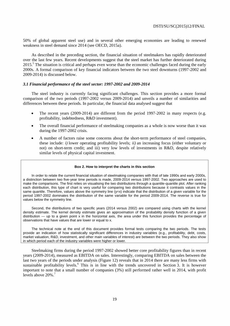
Box 2. How to interpret the charts in this section
In order to relate the current financial situation of steelmaking companies with that of late 1990s and early 2000s, a distinction between two five-year time periods is made, 2009-2014 versus 1997-2002. Two approaches are used to make the comparisons. The first relies on visualising the two distributions through a quantile-quantile plot. After ranking each distribution, this type of chart is very useful for comparing two distributions because it contrasts values in the same quantile. Therefore, values above the symmetry line (y=x) indicate that the distribution of a given variable for the period 1997-2002 dominates the distribution of the same variable for the period 2009-2014. The reverse is true for values below the symmetry line.
Second, the distributions of two specific years (2014 versus 2002) are compared using charts with the kernel density estimate. The kernel density estimate gives an approximation of the probability density function of a given distribution — up to a given point x in the horizontal axis, the area under this function provides the percentage of observations that have values that are lower or equal to x.
The technical note at the end of this document provides formal tests comparing the two periods. The tests provide an indication of how statistically significant differences in industry variables (e.g., profitability, debt, costs, market valuation, R&D, investment, and other main variables of interest) are between the two periods. They also show in which period each of the industry variables were higher or lower.
Steelmaking firms during the period 1997-2002 showed better core profitability figures than in recent
years (2009-2014), measured as EBITDA on sales. Interestingly, comparing EBITDA on sales between the
last two years of the periods under analysis (Figure 12) reveals that in 2014 there are many less firms with
sustainable profitability levels.6 This is in line with the trends uncovered in Section 3. It is however
important to note that a small number of companies (3%) still performed rather well in 2014, with profit
levels above 20%.7

DSTI/SU/SC(2015)12/FINAL
20
Figure 12. Comparison of profitability levels between the two periods
A. EBITDA on sales, 1997-02 and 2009-14 B. Distribution of EBITDA on sales
Note: Quantile-quantile plots for EBITDA on Sales and cash-flow on total assets, as well as the kernel density estimates for EBITDA on Sales in 2002 and 2014.
Source: OECD calculations based on data from Factset.
Lower profitability in 2014 has been associated with higher costs, especially in terms of the variable
cost component. Figure 13 clearly shows higher variable costs for the recent years. A remarkable feature
that can be observed from the comparison between 2002 and 2014 is a shift in the whole variable cost
distribution towards higher levels. This means that the increase in variable costs was felt across the board,
affecting not only the least but also the most cost-effective companies. Part of the increase in variable costs
might result from increases in raw material prices (notably between 2009 and 2012), whereas in the past
changes in raw material prices did not seem to affect variable costs to the same extent. A comparison of the
evolution of variable costs and raw material prices is provided in Annex 2.
-1
-.5
0
.5
19
97
-20
02
-1 -.5 0 .52009-2014
EBITDA_SALES
02
46
8
f(x)
-1 -.5 0 .5x
2002 2014
Distribution of EBITDA_SALES in 2002 & 2014

DSTI/SU/SC(2015)12/FINAL
21
Figure 13. Comparison of cost levels between periods
A. Total costs, 1997-02 and 2009-14 B. Distribution of total costs
C. Variable costs, 1997-02 and 2009-14 D. Distribution of variable costs
Source: OECD calculations based on data from Factset.
Even though steelmaking companies were slightly more indebted during the 1997-2002 crisis
(Figure 14, Panel A), they now rely more on short term debt than they used to (Panel C). This evolution is
likely to reflect difficulties in obtaining longer-term debt. Tighter credit conditions for steel companies
than before would be in line with the conditions facing the broader economy, especially with regards to
access to long-term financing.8
0
1
2
3
4
19
97
-20
02
0 1 2 3 42009-2014
COST_ASSETS
0.5
11.5
f(x)
0 1 2 3 4x
2002 2014
Distribution of COST_ASSETS in 2002 & 2014
.4
.6
.8
1
1.2
1.4
19
97
-20
02
.4 .6 .8 1 1.2 1.42009-2014
COST_VAR_SALES
01
23
45
f(x)
.4 .6 .8 1 1.2 1.4x
2002 2014
Distribution of COST_VAR_SALES in 2002 & 2014

DSTI/SU/SC(2015)12/FINAL
22
Figure 14. Comparison of indebtedness between periods
A. Total debt, 1997-02 and 2009-14 B. Distribution of total debt
C. Short-term debt, 1997-02 and 2009-14 D. Distribution short-term debt
Source: OECD calculations based on data from Factset.
The market’s assessment of steelmaking companies relative to assets (price-to-book ratio) is now
higher than in 1997-2002 (Figure 15). However, panel A of Figure 15 also suggests that this effect was
more pronounced in firms at the higher end of the distribution. In addition, companies exhibited high ratios
during the years 2009 and 2010, reverting to unity or below in the years after (c.f. Figure 12 in the previous
section). The latest data for 2014 (Figure 15, Panel B) shows that the majority of steelmaking companies
are now valued by the market below the value of their assets (52%, the same as in 2002). It is nevertheless
of concern the financial markets’ assessment of good investment opportunities for a significant number of
steelmaking companies, given the current excess capacity situation.
There are no visible differences between investment expenditures in 1997-2002 and 2009-2014, nor
between 2002 and 2014, even though the formal tests available in the Technical Note (row 10 of the
corresponding table) suggest higher value in the former period. Nevertheless, when it comes to efforts to
introduce innovation, the two periods are very different (Figure 16). Even though there is no clear-cut
differences in R&D investments between the selected years 2002 and 2014 (Panel B), between 2009 and
2014 steelmaking companies invested much less in R&D than they did in 1997-2002 (Panel A). This is
interesting as R&D investment can be an important driver of productivity growth (OECD, 2013d; OECD,
0
.5
1
19
97
-20
02
0 .5 12009-2014
DEBT_ASSETS
0.5
11.5
2
f(x)
0 .5 1x
2002 2014
Distribution of DEBT_ASSETS in 2002 & 2014
0
20
40
60
80
100
19
97
-20
02
0 20 40 60 80 1002009-2014
STLT_DEBT
.005
.01
.015
f(x)
0 20 40 60 80 100x
2002 2014
Distribution of STLT_DEBT in 2002 & 2014

DSTI/SU/SC(2015)12/FINAL
23
2015c) and is important for the steel industry to move towards increased energy efficiency and
environmental performance in the future (IEA, 2015).It is however important to note that, during
downturns when short-term cash needs are more pressing, firms may decide to reduce investments into
R&D, notably if the returns on such investments (e.g. gains in efficiency or cost reductions) are only
accrued over the longer run.
Figure 15. Comparison of investment opportunities between periods
A. Price-to-book ratio during 1997-2002 and 2009-2014 B. Distribution of price-to-book ratio, 2014
Note: The red line depicts the threshold (value of one), above which a company could and/or should increase its assets, thus is a proxy for investment opportunities. Ratios below 1 (to the left of the red line) indicate that, if a company would sell all its assets, it would not even meet the market value. Please refer to Annex 1, Section A3 for further details on the interpreting this variable.
Source: OECD calculations based on data from Factset.
Figure 16. Comparison of R&D investment levels between periods
A. R&D investments during 1997-2002 and 2009-2014 B. Distribution of R&D investments, 2002 and 2014
Source: OECD calculations based on data from Factset.
The storage of inputs and production outputs may be particularly advantageous if markets (and prices)
are very volatile as they work as a buffer. Interestingly, inventories are substantially higher in the recent
period than they were in 1997-2002 (Figure 17, Panel A). This is particularly true with respect to
0
2
4
6
8
10
19
97
-20
02
0 2 4 6 8 102009-2014
PBK
0 0.5
1 1.5
2 2.5
3
Distribution PBK 2014

DSTI/SU/SC(2015)12/FINAL
24
inventories of raw materials (Figure 17, Panel C). A possible explanation for this relates to the changes in
the way raw material prices are set — especially with regards to the change from contract-based to spot
iron-ore prices — and increase in prices (Annex 2).
Figure 17. Comparison of inventories between periods
A. Inventories, 1997-02 and 2009-14 B. Distribution of inventories
C. Inventories raw materials, 1997-02 and 2009-14 D. Distribution of inventories raw materials
Source: OECD calculations based on data from Factset.
4. Linking financial performance to capacity utilisation
Steel production has not been keeping up with increases in capacity, resulting in a declining trend in
the global capacity utilisation rate (CUR) since 2006, despite some recovery in 2010 and 2011. This has
occurred while the industry’s aggregate operational profitability, measured as EBITDA on sales, has
declined (Figure 18). With the exception of the period 2003-2007 characterised by a rapid increase in steel
demand and booming raw material markets, Figure 17 suggests that CUR and profitability move more or
less in line.9This raises the question as to what extent global excess capacity affects the operational
profitability of steel producers. The question is not new and has been addressed at previous OECD Steel
Committee meetings.

DSTI/SU/SC(2015)12/FINAL
25
Figure 18. Profitability and Capacity Utilisation Rate (%)
Source: OECD calculations based on data from Factset.
Excess capacity affects profitability through a number of channels. Two main channels are costs and
prices. For example, in periods of low capacity utilisation, economies of scale are not fully exploited and
thus costs are higher and profits lower. Prices also tend to be lower during periods of low capacity
utilisation, thereby directly impacting profits. At the global level, the effects of excess capacity are
transmitted through trade; excess capacity can lead to export surges, leading to price declines and market
share losses for import-competing domestic producers. Preliminary analysis discussed at previous Steel
Committee sessions suggests that there is a strong relationship between the global capacity utilisation rate
and the operating profitability of firms (OECD, 2013b). However, that analysis also found that profitability
is driven by a vast and heterogeneous group of factors, from global trends to firm-level behaviour and
characteristics.
The OECD Secretariat is currently examining ways to improve the analysis of the impact of capacity
utilisation on profitability. Changes in the global capacity utilisation rate may affect profitability through a
number of channels, as discussed above, including firms’ ability to adjust to changes in the global steel
market. Even though during challenging market periods — notably in the presence of import surges — all
firms suffer significantly, companies might be more or less flexible to accommodate shocks depending on
the steelmaking technology they employ as well as their exposure to international markets. For example,
differences between EAF and BOF technologies may have implications upon their flexibility to adjust
production. Compared to BOF, the EAF route tends to provide companies with a higher degree of
flexibility in setting their production, which in turn allows them to better cope with volatile steel demand
and supply shocks.
As a result, profitability is also likely to be affected by the production technology employed, i.e. by
the degree of flexibility to adjust production. To illustrate this argument, assume that there are two steel
plants with distinct technologies (EAF and BOF) facing a negative demand shock. While a BOF plant will
mostly be affected by price (because quantity adjustments may be more difficult in the short term), an EAF
plant will be affected by price but can adjust quantity. Should prices fall below marginal cost, the EAF
plant would stop (or reduce) production to save on variable costs, but the BOF plant might carry on with
losses because they have a larger share of fixed (or semi-fixed) costs. Figure 19 presents annual changes in
the capacity utilisation of EAF and BOF steelmakers using plant-level information. While the data are not
fully representative of the population of steel plants, they generally do indicate greater variation in the
60
65
70
75
80
85
90
95
100
0%
5%
10%
15%
20%
25%
EBITDA/SALES (left scale) CUR (right scale)

DSTI/SU/SC(2015)12/FINAL
26
capacity utilisation rates of EAF plants in response to changes in the market, relative to BOF plants, at
least since the previous market downturn in the late 1990s.
Figure 19. Annual changes in capacity utilisation rate by steelmaking technology
Note: The plant-level data are not fully representative of the population of steel plants.
Source: OECD calculations based on data provided by James King.
Matching profitability data with production technology at the firm level through time is however
challenging. Further efforts are needed to collect data that matches financial performance, capacity and
technology at the firm level in order to provide robust estimates of the effect that changes in the global
steel market situation, notably in terms of capacity utilisation, may have upon the financial health of the
industry.
5. Conclusion
In the context of excess steelmaking capacity, the steel industry’s financial situation is weaker than it
has been in years. Even though the steel industry has experienced crises in the past, the current downturn is
of particular concern given its depth and length. This report suggests that financial performance of the
industry is perhaps worse now than during the crisis of the late 1990s. Moreover, recent trends in key
financial indicators raise serious concerns and suggest that the global industry is in a very difficult
economic and financial situation. Nevertheless, financial performance is heterogeneous, as some firms
appear to be resilient and are performing rather well. Further work is needed to better understand why this
is the case and identify strategies that can be used to increase the performance of steelmaking companies.
A further deterioration in steel demand prospects along with continued capacity expansions are likely
to place further pressure on the financial sustainability of the steel industry. The complex financial
situation of the industry and mounting trade disputes calls for immediate action to address underlying
imbalances in the steel market. Governments should be aware of the financial risks facing the sector when
considering policies that promote new capacity expansions and should work to facilitate the closure and/or
restructuring of inefficient producers, while mitigating associated social costs. In addition, private and
government-related financial institutions facilitating capacity expansion projects in the steel sector should
take into further consideration existing supply-demand imbalances, as newly installed steel capacities
could face serious short- to medium-term financial sustainability risks and further amplify the extent of the
capacity challenge.
-15.0
-10.0
-5.0
0.0
5.0
10.01
99
8
19
99
20
00
20
01
20
02
20
03
20
04
20
05
20
06
20
07
20
08
20
09
20
10
20
11
20
12
20
13
20
14
percentage points
BOF
EAF
DSTI/SU/SC(2015)12/FINAL
27
Further research is, however, still needed to explain the differences in performance between different
industries and more specifically across steelmaking companies, as well as to analyse policy options to
promote a more efficient and viable steel industry. Further efforts are also needed to collect and combine
firm-level data and policy indicators, in order to provide robust evidence in this and other areas of steel
related policymaking.

DSTI/SU/SC(2015)12/FINAL
28
NOTES
1 A presentation by McKinsey at the 1-2 July 2013 OECD Steel Committee meeting suggested that 16% is
the sustainability threshold for steel companies.
2 Free cash-flow to sales is an additional profitability indicator. This variable provides information on firms’
capacity to generate cash after investments and covering costs of replacing capital (depreciation and
amortisation). Free cash flow is the amount of cash that a firm generates and is available for either paying
out dividends to shareholders or retaining as cash holdings for use in future periods (revealing expectations
about the future state of the market).
3 The price-to-book ratio indicates how the market evaluates a firm, relative to its assets. If the ratio is
above 1, it suggests that a company can and/or should increase its assets, i.e. it is a proxy for investment
opportunities. Ratios below 1 indicate that if a company would sell all its assets, it would not even meet the
market value.
4. Please note that in some of these regions, significant efforts have been made to close down production
capacity, amidst the demand slowdown. For data on steelmaking capacity developments, please refer to the
OECD Steelmaking Capacity Portal, available at: http://oe.cd/steelcapacity.
5. Steel market developments during 2015 suggest that the financial situation is rapidly deteriorating, leading
to bankruptcy events, closures of steel plants across the world and mounting trade disputes. For additional
information on recent market steel market developments, please visit the dedicated OECD Steel webpage
available at: http://oe.cd/stlmktdev.
6 A presentation by McKinsey at the 1-2 July 2013 OECD Steel Committee suggested that 16% is the
sustainability threshold for steel companies. This threshold is, according to McKinsey, the amount of
EBITDA no sales required to cover debt, taxes, equity and capital expenditure. This estimate, however,
may be subject to different views.
7 For comparison purposes, 14% of the companies in the sample had profits above 20% in 2007; 9% of the
sample had profits above 20% in 2001.
8 The World Economic Forum compiles data on the ease of access to loans by country (e.g. Schwab, 2012).
Access to loans was shown to have significantly decreased since the financial crisis (see OECD 2013c,
pp. 200 for a comparison). The OECD has also developed substantial work on long-term investment,
available at: www.oecd.org/finance/lti.
9. In periods of rapid demand growth, capacity increases may not be sufficient to accommodate the expected
growth in demand because capacity is slow to build up. In such circumstances prices (and ultimately
profitability) may increase quite rapidly — the steel market experienced a situation alike during the run up
to the financial crisis — this is corroborated by internal OECD research (OECD, 2014).

DSTI/SU/SC(2015)12/FINAL
29
REFERENCES
Chirinko, R. S. (1993). “Business Fixed Investment Spending: Modeling Strategies, Empirical Results, and
Policy Implications”. Journal of Economic Literature, 31(4): 1875-1911.
Hayashi, F. (1982). “Tobin's Marginal q and Average q: A Neoclassical Interpretation”. Econometrica,
50(1): 213-24.
Morgan Stanley (2013), “Global steel industry, steeling for oversupply”, 22 May 2013.
OECD (2010), “Climate change policy and iron and steel industry 2010”, internal working document,
Directorate for Science, Technology and Industry, DSTI/SU/SC(2010)17.
OECD (2012a), “Excess capacity in the steel industry: an examination of the global and regional extent of
the challenge”, internal working document, Directorate for Science, Technology and Industry,
DSTI/SU/SC(2012)15.
OECD (2012b), “Market developments and trends in key steel-using industries”, internal working
document, Directorate for Science, Technology and Industry, DSTI/SU/SC(2012)5.
OECD (2012c) “The future of the steel industry: selected trends and policy issues”, internal working
document, Directorate for Science, Technology and Industry, DSTI/SU/SC(2012)12.
OECD (2012d), “State Ownership in the Steel Industry: Issues for Consideration”, internal working
document, Directorate for Science, Technology and Industry, DSTI/SU/SC(2012)6.
OECD (2013a) “Evaluating the current state of the steel industry: Work in progress”, internal working
document, Directorate for Science, Technology and Industry, DSTI/SU/SC(2013)19.
OECD (2013b), “The viability of the steel industry: An attempt to analyse steelmakers’ economic and
financial performance”, internal working document, Directorate for Science, Technology and
Industry, DSTI/SU/SC(2013)2.
OECD (2013c), OECD Science, Technology and Industry Scoreboard 2013: Innovation for Growth,
OECD Publishing. doi: 10.1787/sti_scoreboard-2013-en.
OECD (2013d), Supporting Investment in Knowledge Capital, Growth and Innovation, OECD Publishing.
doi: 10.1787/9789264193307-en.
OECD (2014), “Proposal for measuring effective capacity”, internal working document, Directorate for
Science, Technology and Industry, DSTI/SU/SC(2014)17.
OECD (2015a), Steel Market Developments: 2nd
Quarter 2015, OECD Publishing, Paris, available at:
www.oecd.org/sti/ind/1-Steel-market-developments-2015Q2.pdf.
OECD (2015b), "Excess Capacity in the Global Steel Industry and the Implications of New Investment
Projects", OECD Science, Technology and Industry Policy Papers, No. 18, OECD Publishing, Paris.
DOI: http://dx.doi.org/10.1787/5js65x46nxhj-en.

DSTI/SU/SC(2015)12/FINAL
30
OECD (2015c) “R&D, innovation and Productivity growth in the steel sector: Preliminary draft”, internal
working document, Directorate for Science, Technology and Industry, DSTI/SU/SC(2015)5.
OECD (2015d) “Public financial support to new investments in the global steel industry: Work in
progress”, internal working document, Directorate for Science, Technology and Industry,
DSTI/SU/SC(2015)2/REV1.
OECD (2015e) “Government support to steel sector: Study on sector-specific investment incentive
policies”, internal working document, Directorate for Science, Technology and Industry,
DSTI/SU/SC(2015)13.
Pauliuk, S., Milford, R., Müller, D. and Allwood, J., The steel scrap age, main document and
supplementary information, Environmental Science and Technology, 2012.
Rassier (2013), “Accounting for Intellectual Property Products: International Guidelines for National
Economic Accounting and U.S. Rules for Financial Accounting”.
Schwab, K. (2012), “The Global Competitiveness Report 2012–13”, Geneva: World Economic Forum.
Tobin, J. (1969). “A General Equilibrium Approach to Monetary Theory”. Journal of Money, Credit and
Banking, 1(1): 15-29.

DSTI/SU/SC(2015)12/FINAL
31
ANNEX 1. DATA AND METHODOLOGICAL CONSIDERATIONS
A1. Dataset
This paper employs a new, very broad, and rich dataset that includes, inter alia, financial information,
market valuation, ownership structure, mergers and acquisitions, and R&D investment for steelmaking
companies. It includes over 70 basic variables covering more than 800 steelmaking companies over
23 years.
The information to build this database was obtained from Factset, a commercial data provider. The
financial information obtained from this database is provided on a standardised basis and is therefore
comparable. Information from company filings was taken as given and was not validated, implying that
any results from the analysis should be taken with some caution. When necessary, the information was
complemented with further research done by the OECD Secretariat.
Most of the variables analysed were only available since 1992. Therefore, the sample of steelmaking
companies covers the period 1992-2014 (23 years), which is sufficient to allow comparisons of the current
situation with that in the late 1990s and early 2000s.
An important limitation of this dataset is the reduced availability of information for firms that are not
listed in stock markets (e.g. privately-owned and subsidiary firms). Even if non-listed firms are observed in
the data, country coverage is reduced and information is usually very incomplete.
Additionally, during the period 1992-2014, some firms were created or became publicly traded, on the
one hand, or were liquidated, merged or became private on the other. This implies that the same firm might
not be observed over the full time span. The panel of firms is thus unbalanced and screening out the exact
motives for entry\exit of the sample still remains a challenge.
The data thus far includes all companies that are either classified as “Steel” in Factset (code 1105) or
their activity belongs to SIC codes 3312, 3316, and 3317. This raw sample includes 982 companies over
the 23 year period, resulting in 11 527 firm-year observations.10
However, this sample includes companies
that have major mining activities. As the analysis was intended to focus on steel companies, some
companies whose operations were heavily focussed on mining had to be excluded. To do so, cleaning
procedures were applied. For example, companies with mines and no steel activity were excluded, as well
as companies that did not have the terms “steel” or “metal” in their names or their business descriptions,
but did have “iron ore”, “mining”, and/or “minerals”.
Given the characteristics of the dataset, and after undertaking the above-mentioned cleaning
procedures, the final dataset results in an unbalanced panel of 890 firms covering the period 1992-2014,
corresponding to a total of 10 611 firm-year observations.
A2. Methodological challenges
Sample representativeness: Ensuring the representativeness of smaller steelmaking companies is
challenging. Nevertheless, the approach followed consisted in constructing weights based on Sales, which
allow for a correction of biases in trend and econometric analysis (Sections 3 and 5.1, respectively). The

DSTI/SU/SC(2015)12/FINAL
32
OECD Secretariat is confident that this approach minimises the impact of sample biases. Full
representativeness by country, region and size is not guaranteed, meaning that results should always be
taken with a grain of salt. Nevertheless, this is, to date, the most comprehensive sample of financial
information for steelmaking companies available.
Ownership, control and SOE definition: Ownership links are complex. Entities can own companies
through direct and indirect ownership positions. Additionally, it is not clear if a given percentage
ownership actually results in control. In fact there might be some degree of dissociation between
ownership and control. For example, the government could have substantial influence, without necessarily
holding a majority of shares. Definitions of SOEs vary across countries and might not cover the full extent
of state control. This report relies on data from both Factset to obtain state-ownership shares as well as
ownership links. SOEs were defined in this study as firms that are owned by the government either through
direct or combined indirect ownership links. Ownership is defined as holding more than a 50% share in a
given company. The definition is based on the ultimate parent company, i.e. ownership is traced back,
through the different ownership links, to the company/agency that ultimately owns the target steel
company. Ownership by a government related agency is identified by searching a number of keywords in
the ultimate parent company name. Keywords include "Gov" "Province" "City" "State". Nevertheless, a
number of government related agencies and/or companies might still not be captured, thus ownership by a
government related agency might be underrepresented. In 2014, 22 companies out of a total of 609
companies in operation were identified as SOEs and had a combined market share of 17.68%. China
accounts for an important share of SOEs in the sample (82%) followed by Egypt, India and Indonesia (5%
each).
Groups and consolidated accounts: Many firms are part of a larger group and, normally, the only
accounts available are consolidated. It is therefore challenging to disentangle the financial performance of
subsidiary companies. This is particularly relevant if there is high variation of profitability levels across the
different firms that make up the group, especially if these firms operate in distinct industries. A company
may also operate in mining sectors or produce other types of metals and products. It is therefore important
but also challenging to isolate the different operations. Given that the dataset available does not cover all
subsidiary firms, the analysis of financial performance focuses only on firms/groups for which
consolidated financial information is made available.
Localisation: Data collection can be rather challenging due to differences between the country where
the steelmaker operates and the country where the firm or the corresponding parent firm/group is legally
registered. Increased cross-border investment activity and the existence of multiple foreign subsidiaries
impose additional challenges to country identification. For simplification purposes the company
headquarters is taken as a measure of localisation and assign the corresponding country to that firm.
Results are nevertheless presented at the global level.
Privately held companies: Financial information on privately help companies is very scarce. These
companies do not have the same information disclosure requirements as firms listed in stock markets. This
is particularly the case for ownership and certain financial variables that involve market valuation such as
share price or earnings per share. Please note that while publicly traded companies are required to disclose
a large number of financial data, this is not the case for privately owned companies.
Business cycles, nominal values and deflators: Ideally, the effects of cycles should be filtered
taking into account both fluctuations across countries and industries. In this analysis only global
fluctuations are explicitly controlled for. Fluctuations at the macro-regional level are captured through year
and region dummies. Price changes might also impose some difficulties and require the use of deflators.
However, since selected variables for analysis are constructed as ratios (see Annex 1, Section A3), it is
assumed that the relative price is constant, thus no deflators are used.

DSTI/SU/SC(2015)12/FINAL
33
A3. Variable definitions
The choice of financial performance indicators followed two principles. First, indicators should be
informative about either the profitability or indebtedness of a firm. Second, indicators should be available
in Factset, for the maximum number of firms in our sample. This implies that some variables (e.g. industry
metrics, number of employees) are not necessarily included in this analysis to avoid any biases resulting
from underrepresentation.
EBITDA_SALES: Ratio between earnings before interest, tax, depreciation and amortization
(EBIDA) and total revenue. EBITDA indicates a firm’s operating profitability. Provides a good measure of
core profitability because it excludes depreciation and amortization. The ratio to total revenue allows for
comparability of core profitability between firms. Below zero, companies are making losses.
A presentation by McKinsey at the 1-2 July 2013 OECD Steel Committee suggests that 16% is the
sustainability threshold for Steel companies. This threshold is, according to McKinsey, the amount of
EBITDA to sales required to cover debt, taxes, equity and capital expenditure. This estimate, however,
may be subject to different views.
EBIT_SALES: EBIT/Sales is an alternative measure of operational profitability that takes into
account depreciation and amortization
CF_ASSETS: Cash-flow scaled by total assets is a measure of profitability that takes into account
depreciation and amortization as well as taxes. Along with EBITDA, this gives insights into how a
company finances short-term capital.
CF_FREE_SALES: Free Cash-flow to sales is an additional profitability indicator. This variable
provides information of firms’ capacity to generate cash after investments and covering costs with
replacing capital (depreciation and amortisation). Free cash flow is the amount of cash that a firm generates
and is available for either paying out dividends to shareholders or retaining as cash holdings for use in
future periods (revealing expectations about future states of the market).
CS_ASSETS: Cash stocks scaled by total assets. This is an indicator of firm’s immediate liquidity.
Firms may have higher cash stocks to face expected negative shocks in the future or to take advantage of
future investment opportunities (if external finance is difficult to obtain).
DEBT_EBITDA: Debt to EBITDA reveals firms’ ability to service debt. Healthy firms should have a
ration below 3. The indicator is only meaningful for positive values of EBITDA, thus for all companies
making losses this indicator is not computed. An alternative indicator was constructed as the ratio between
average DEBT and average EBITDA over all firms for a given year. This avoids difficulties with negative
EBITDA figures that are diluted when the average across firms is taken. This alternative indicator is used
in the time trend analysis.
DEBT_ASSETS: Debt to assets. Ratio between total debt and total assets. Indicates the percentage of
a company’s assets that have been financed through debt. Accordingly, it measures the degree of leverage
of a firm. Incudes both short-term and long-term debt.
STLT_DEBT: The share of short-term debt in total debt indicates whether a company is focusing on
financing for operational issues. The ratio varies between zero and one and will depend on the extent to
which firms are investing or not. The difference to unity will provide the share of long-term liabilities.
PBK: Price-to-Book ratio indicates how the market evaluates a firm, relative to its assets. If the ratio
is above 1, it suggests that a company could and\or should increase its assets — proxying investment
opportunities. Ratios below 1 indicate market doesn't recognise enough value in company's books. In other

DSTI/SU/SC(2015)12/FINAL
34
words, if a company would sell all its assets, it would not even meet the market value. In the economics
literature, this ratio is also known as “average Q”, an approximation to the theoretical marginal Tobin’s Q
(Tobin 1969; Hayashi, 1982). If not summarising all relevant information for a firm’s investment decision,
this indicator should, at least, be highly correlated with investment.
I_ASSETS: Investment in fixed assets normalised by total assets. Investment is defined as additions to
plant, property and equipment.
TRADE_CREDIT: Difference between accounts payable and accounts receivable. A positive value
indicates that the company is a net receiver of trade credit, negative values indicate that a company is a net
provider of trade credit. For analysis purposes, this indicator is scaled by total assets
(TRD_CREDIT_ASSETS)
RD: R&D expenses provides an indication of whether a firm is making efforts to innovate. Missing
R&D values are assumed to be 0. For analysis purposes, R&D investments are also scaled by total assets
(RD_ASSETS). R&D investments as a percentage of total investments, which proxy firms’ propensity to
invest in R&D (RD_INVEST_PERCENT) is also analysed.
AGE: Constructed as the difference of current date to founding date plus one. The construction of this
variable is rather challenging due to the large number of mergers and acquisitions (M&As) in the past.
DIV_ASSETS: Dividend payments scaled by total assets. Dividend payments signal that a firm is
being able to generate enough cash to pay shareholders. Conditional on investment and cash holdings
figures, it reveals a strategic preference for paying out dividends instead of investing or retaining profits.
COST: Total cost is calculated as the sum of variable costs (proxied by costs of sales) and fixed costs
(proxied by depreciation and amortization). The variable is scaled by total assets.
COST_VAR_SALES: Variable costs are costs of goods sold minus depreciation and amortisation
expenses.
SLOPE: Slope of the variable cost curve. The cost curve is calculated by ranking all firms in a given
year by their variable costs and then adding up their sales on a cumulative basis. The slope is calculated
through a simple OLS regression of variable costs on cumulative sales and reflects the increase in cost per
additional output sold. The evolution of the slope indicates how different steelmaking companies in their
production efficiency are. The steeper the curve, the more heterogeneous are companies. This curve also
provides an approximation of the theoretical supply curve in the global steel market. This approach is used
by some consultancies to assess the profitability of steelmaking companies.
INVENT_ASSETS: Inventories scaled by total assets. Changes in inventories are highly dependent
upon upstream (inputs, e.g. raw materials) and downstream (output, e.g. automotive sector) market
conditions. Additionally, inventories can work as a buffer during periods of high market volatility.
INVENT_RM_PERCENT: Percentage of Raw Materials inventories in total inventories. This
provides an indication of whether steelmaking companies are hoarding raw materials, which would signal
expectations on future raw material prices.
SOE: Binary indicator of whether a company is an SOE. When used in time trend or regression
analysis, this variable is scaled by the number of firms in the sample, providing a proxy for the percentage
of state ownership in a given year. In this paper, SOEs are defined as firms that are owned by the
government either through direct or combined indirect ownership links. Ownership is defined as holding
more than a 50% share in a given company.

DSTI/SU/SC(2015)12/FINAL
35
GROUP: Binary indicator of whether a company belongs to a group. When used in time trend or
regression analysis, this variable is scaled by the number of firms in the sample, providing a proxy for the
percentage of firms belonging to a group in each year.
REGION: Information on company headquarters (by country) is aggregated into the following
regions: Western European, Eastern European, North America, South America, India, China, Turkey
MENA, Southeast Asia, Asia-Pacific. This variable does not take into account that firms headquartered in
one country may have operations in a different country. However, the aggregation into regions minimises
this issue to some extent.
M&As: Information from Factset on mergers and acquisitions (M&As) was retrieved in order to build
an indicator of concentration in the global steelmaking industry. Only M&As that have been completed
between 1992 and 2012 are considered. The indicator is constructed as the natural logarithm of sum of all
M&As in a given year. M&As should be able to provide an indication of restructuring in the steel industry.
CUR: Capacity utilization ratio is defined here as the ratio, for a given year, of global crude steel
production, provided by the World Steel Association, to the level of global crude steelmaking capacity in
nominal terms, provided by the OECD.
MKT_VAL: Market value reflects the market capitalisation of each company obtained from Factset.
For each year, total steelmakers’ market capitalisation is constructed as the sum of companies’ market
value. For the purpose of trend analysis (Section 3), this value is scaled by total market capitalisation
(World Bank, 2013) and reflects the weight of steelmaking companies in stock markets. Annex 2. Selected
additional charts

DSTI/SU/SC(2015)12/FINAL
36
ANNEX 2. SELECTED ADDITIONAL CHARTS
According to data from Factset, the number of M&As in the steel industry have significantly
increased over the years up to 2007 (Figure A2.1). After a sharp decrease in 2008 possibly associated with
the financial crisis, industry restructuring activity appears to have stabilised.
Figure A2.1: Number of M&As in the steel industry
Source: OECD calculations based on data from Factset.
Figure A2.2 depicts the evolution of the estimated slope of the cost curve (see Annex 1, A3 for a
detailed description of this variable). The slope seems to have significantly decreased and remained at
lower levels after a height during the early 2000s. This suggests that nowadays steelmaking companies are
more homogenous in terms of their production efficiency than they used to be.
Figure A2.2. Evolution of the slope of the cost curve Index, 2001=100
Source: OECD calculations based on data from Factset.

DSTI/SU/SC(2015)12/FINAL
37
Figure A2.3 shows the annual evolution of EBIT on sales. In comparison with EBITDA on sales, this
ratio takes into account amortisation and depreciation. The evolution of this indicator supports the decline
in profitability since 2007, as discussed in Section 3. From 12.2% in 2007, average EBIT on sales reached
3.1% in 2012 and then improving to 4.7% however higher than the levels reached in 2001 (2.8%).
Figure A2.3: Annual evolution of EBIT on sales between 1992 and 2014
Source: OECD calculations based on data from Factset.
Figure A2.4 compares the annual evolution of variable costs against the evolution of raw material
prices. This figure suggests that during the 1990s variable costs were not so affected by changes in raw
material prices — both in levels (panel A) and growth rates (Panel B). After reaching a share of 87% of
sales, the weight of variable costs on sales has steeply decreased until 2004. During the second half of the
2000s, the increase in raw material prices was accompanied by a significant increase in the weight of
variable costs. In 2014, the share of variable costs was almost 90% (87.2%). This indicates both a shift in
the steelmaking production process, where fixed costs have become less important and raw materials
appear to have an increasingly preponderant role.

DSTI/SU/SC(2015)12/FINAL
38
Figure A2.4: The evolution of variable costs and raw material prices
Source: OECD calculations based on data from Factset and raw material prices obtained from American Metal Market, CUR Monitor and SBB.

DSTI/SU/SC(2015)12/FINAL
39
TECHNICAL NOTE: HOW TO INTERPRET THE CHARTS AND STATISTICS
In order to relate the current financial situation of steelmaking companies with that of late 1990s and
early 2000s, a distinction of time periods is made, on a six year window. The distribution of relevant
financial variables during the period 2009-2014 is compared against the distribution of the same variable
over the period 1997-2002.
Two approaches are followed. The first relies on visualising the two distributions through a quantile-
quantile plot. After ranking each distribution, this type of chart is very useful for comparing two
distributions because it contrasts values in the same quantile. Therefore, values above the symmetry line
(y=x) indicate that the distribution of a given variable for the period 1997-2002 dominates the distribution
of the same variable for the period 2009-2014. The reverse is true for values below the symmetry line. In
the example below, given that most of the values stand above the symmetry line, it is possible to argue that
the profitability distribution during 1997-2002 dominates that of 2009-2014.
Example of quantile-quantile plot
Second, two formal nonparametric tests (Kolmogorov-Smirnov and Fligner-Policello tests) are
performed in order to provide additional evidence on the relationship between the two periods (see Table
below). The advantage of using non-parametric test is avoiding complications with the likely non-
normality of distributions and unequal variances that classical tests may not account for. In the table below,
columns (1) and (3) contain the test statistics for the Kolmogorov-Smirnov and Fligner-Policello tests,
respectively. Columns (2) and (4) provide the corresponding p-values that allow identifying whether the
distribution of each variable during 2009-2014 is statistically different from that in 1997-2002. For
example if the if the p-value is lower than 0.01 for a given variable, the two periods can be considered
statistically different with a level of confidence of 99%. In addition, the sign of values in column (3) also
indicates whether the values of a variable during the 2009-2014 period were higher (positive) or lower
(negative) than during 1997-2002.
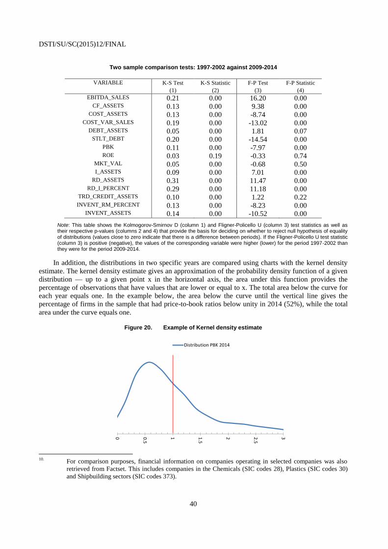
DSTI/SU/SC(2015)12/FINAL
40
Two sample comparison tests: 1997-2002 against 2009-2014
VARIABLE K-S Test K-S Statistic F-P Test F-P Statistic
(1) (2) (3) (4)
EBITDA_SALES 0.21 0.00 16.20 0.00
CF_ASSETS 0.13 0.00 9.38 0.00
COST_ASSETS 0.13 0.00 -8.74 0.00
COST_VAR_SALES 0.19 0.00 -13.02 0.00
DEBT_ASSETS 0.05 0.00 1.81 0.07
STLT_DEBT 0.20 0.00 -14.54 0.00
PBK 0.11 0.00 -7.97 0.00
ROE 0.03 0.19 -0.33 0.74
MKT_VAL 0.05 0.00 -0.68 0.50
I_ASSETS 0.09 0.00 7.01 0.00
RD_ASSETS 0.31 0.00 11.47 0.00
RD_I_PERCENT 0.29 0.00 11.18 0.00
TRD_CREDIT_ASSETS 0.10 0.00 1.22 0.22
INVENT_RM_PERCENT 0.13 0.00 -8.23 0.00
INVENT_ASSETS 0.14 0.00 -10.52 0.00
Note: This table shows the Kolmogorov-Smirnov D (column 1) and Fligner-Policello U (column 3) test statistics as well as their respective p-values (columns 2 and 4) that provide the basis for deciding on whether to reject null hypothesis of equality of distributions (values close to zero indicate that there is a difference between periods). If the Fligner-Policello U test statistic (column 3) is positive (negative), the values of the corresponding variable were higher (lower) for the period 1997-2002 than they were for the period 2009-2014.
In addition, the distributions in two specific years are compared using charts with the kernel density
estimate. The kernel density estimate gives an approximation of the probability density function of a given
distribution — up to a given point x in the horizontal axis, the area under this function provides the
percentage of observations that have values that are lower or equal to x. The total area below the curve for
each year equals one. In the example below, the area below the curve until the vertical line gives the
percentage of firms in the sample that had price-to-book ratios below unity in 2014 (52%), while the total
area under the curve equals one.
Figure 20. Example of Kernel density estimate
10.
For comparison purposes, financial information on companies operating in selected companies was also
retrieved from Factset. This includes companies in the Chemicals (SIC codes 28), Plastics (SIC codes 30)
and Shipbuilding sectors (SIC codes 373).
0 0.5
1 1.5
2 2.5
3
Distribution PBK 2014