Embed Size (px)
Citation preview

Evaluation of a Mesoscale Short-Range Ensemble Forecasting System
over the Northeast United States
Matt Jones & Brian A. Colle
NROW, 2004
Institute for Terrestrial and Planetary AtmospheresStony Brook UniversityStony Brook, New York

OUTLINE
Verification Method- Northeast- Seasonal view- Multiple parameters
Results Conclusions

Verification Method
SUMMER = May – September 2003WINTER = October 2003 – March 2004
Scalar Measures:
Contingency-based Measures:
Prob.-based Measures:
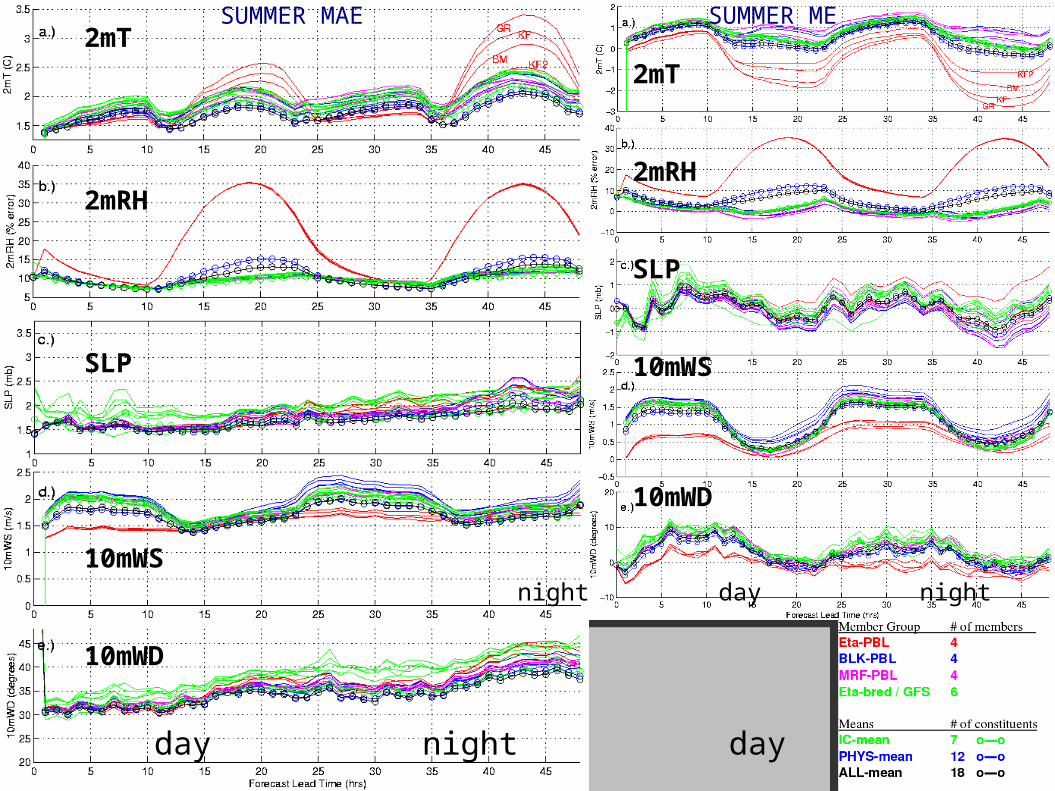
SUMMER MESUMMER MAE2mT
2mRH
SLP
10mWS
10mWD
2mT
2mRH
SLP
10mWS
10mWD
night day night day
night day night day

Near-Surface T
Lowest level cloud water (~3K ft.)
Warm
Cool
Moist
Dry
Example of PHYS-member spread – Eta-PBL 2mT

WINTER MEWINTER MAE
NCEP BREDS
GFS
2mT
2mRH
SLP
10mWS
10mWD
2mT
2mRH
SLP
10mWS
10mWD
night day night day
night day night day

21zEta-1 21zEta-2 21zEta+1 21zEta+2 21zEta-CTL
00zEta 00zGFS IC MEAN
PHYS MEAN
L992
L
2004102200 f48

SUMMER MAE SUMMER MAE2mT
2mRH
SLP
10mWS
10mWD
night day night day
2mT
2mRH
SLP
10mWS
10mWD
night day night day
0000UTC Eta0000UTC ensemble mean0000UTC 4-km MM5
1200UTC 4-km MM50000UTC ensemble mean
Can the ensemble-mean beat 4km MM5 and Eta
determinitistic forecasts?

WINTER MAE WINTER MAE
Can the ensemble-mean beat 4km MM5 and Eta
determinitistic forecasts?
2mT
2mRH
SLP
10mWS
10mWD
night day night day
night day night day
2mT
2mRH
SLP
10mWS
10mWD
0000UTC 4-km MM5 1200UTC 4-km MM50000UTC ensemble mean
0000UTC Eta 0000UTC ensemble mean

0.1 0.2 0.3 0.4 0.5 0.6 0.7 0.8 0.9 1.0
0.8
0.9
1.0
1.1
1.2
1.3
1.4
1.5
Threshold (inches above, centimeters below)
BIA
S
0.1 0.2 0.3 0.4 0.5 0.6 0.7 0.8 0.9 1.0
0.05
0.10
0.15
0.20
0.25
0.30
0.35
0.40
0.45
0.50
0.55
Threshold (inches above, centimeters below)
Equi
tabl
e Thre
at Sco
re
0.1 0.2 0.3 0.4 0.5 0.6 0.7 0.8 0.9 1.0
0.8
0.9
1.0
1.1
1.2
1.3
1.4
1.5
Threshold (inches above, centimeters below)
BIA
S
0.1 0.2 0.3 0.4 0.5 0.6 0.7 0.8 0.9 1.0
0.05
0.10
0.15
0.20
0.25
0.30
0.35
0.40
0.45
0.50
0.55
Threshold (inches above, centimeters below)
Equi
tabl
e Thre
at Sco
re
SUMMER 24HP BIAS WINTER 24HP BIAS
SUMMER 24HP ETS WINTER 24HP ETS
Better
Worse
Over Pred.
Under Pred.
PHYS IC ALL

Verification Rank Histogram
All solutions of ensemble should be equally likely.Observation should appear no different than any ensemble member.Not a measure of skill; a necessary, but not sufficient condition for a good ensemble.
Perfect
“flat”
“U-shaped” “N-shaped” “L-shaped”
Under-dispersed Over-Dispersed Biased
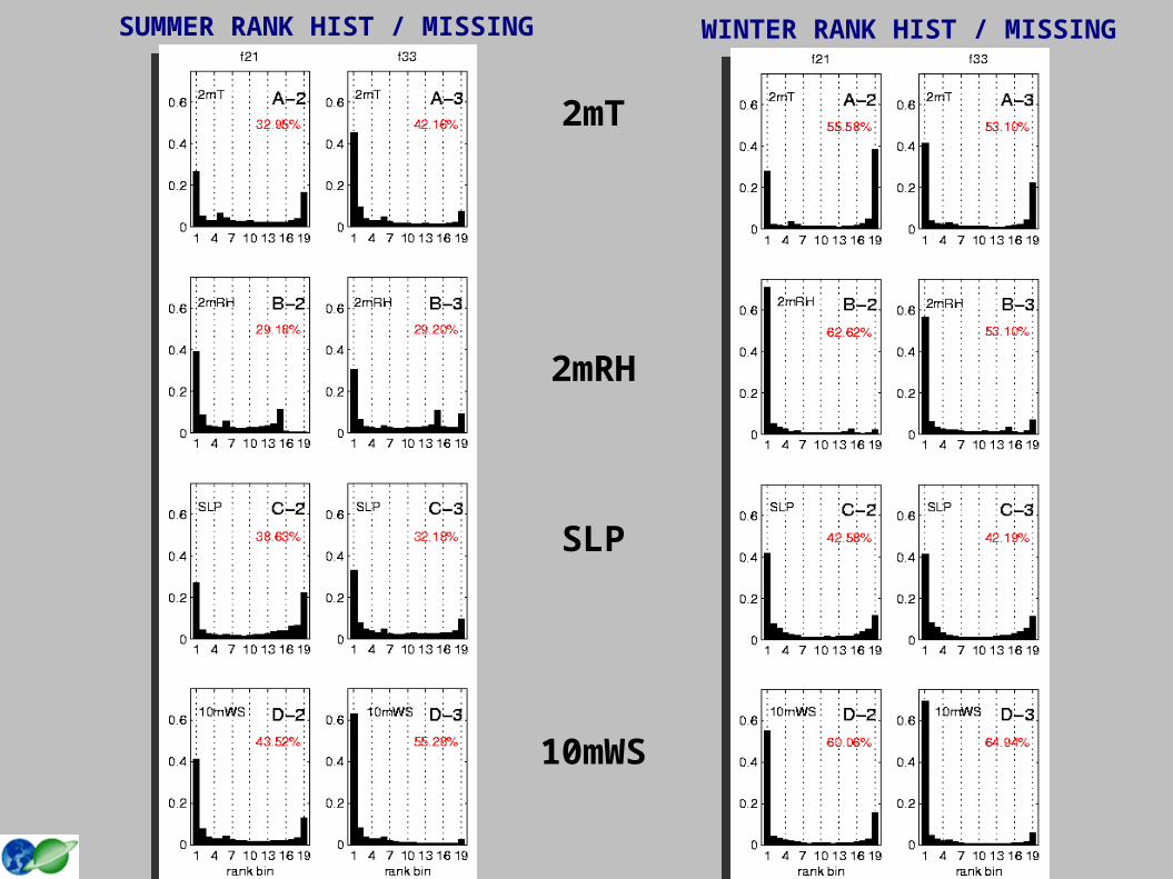
SUMMER RANK HIST / MISSING RATES WINTER RANK HIST / MISSING RATES
2mT
2mRH
SLP
10mWS

SUMMER MAE-VAR WINTER MAE-VAR
2mT
2mRH
SLP
10mWS
10mWD
Corr. Coeff.
MA
E
VAR
MA
E
VAR
C.C
.
C.C
.

Probabilistic Precipitation
Brier Score:
REL = Reliability
RES = Resolution (event discrimination)
UNC = Uncertainty (dependent only on obs.)fi = forecast probability
oi = observed probability (=1 for occurrence, =0 for non-
occurrence)N
t = number of forecast/event pairs for threshold, t
m = number of ensemble members (m+1 probability categories)
Skill
Perfect ReliabilityNo skillNo resolution

SUMMER 24HPReliability Diagrams
PHYSIC
ALLSample SUMMER 24h MPC

WINTER 24HPReliability Diagrams
PHYSIC
ALLSample WINTER 24h MPC

Ensemble Post-processing
Due to model imperfections, significant bias is retained even after ensemble averaging.
Day-15 Day-14 Day-13 Day-12 Day-11 Day-10 Day-9 Day-8 TODAY Day-7 Day-6 Day-5 Day-4 Day-3 Day-2 Day-1
Use previous 14 complete forecasts to correct forecasts starting 0000UTC today

SUMMER MISSING RATE IMPROVEMENT WINTER MISSING RATE IMPROVEMENT
2mT
2mRH
SLP
10mWS
UncalibratedCalibrated

The ensemble-mean is more skillful than component members on average for daytime 2mT/10mWS, SLP, and 10mWD. Persistent biases among component members reduce the skill advantage of the ensemble-mean during other periods (e.g. nighttime 2mT/10mWS).
The ensemble-mean can outperform the deterministic Eta model, and can equal the skill of a high-resolution deterministic MM5 initialized 12 hours later.
The PHYS ensemble is more beneficial for forecasting surface parameters during the warm season due to greater variation among component members.
The GFS initial condition leads to a superior SLP forecast compared to the poorly skilled NCEP Eta-bred members, especially during the cool season. The GFS member outperforms the ensemble-mean for SLP and 10mWD in the cool season.
The ensemble has some ability to predict forecast skill and estimate the uncertainty of a forecast through ensemble spread-error correlation, especially for 10mWD. Persistent biases among component members and ensemble underdispersion for other surface parameters reduce the spread-error correlation (e.g. 2mT, 10mWS).
Conclusions (1)

In warm season, low POPs have reliability for low threshold precip. events. High POPs have reliability for all thresholds.
In cool season, low POPs have poor reliability for all precip. event thresholds. High POPs have reliability all precip. event thresholds.
The PHYS (IC) ensemble is more skillful in POPs during the warm (cool) season. In the warm season, the Hybrid ensemble has the greatest POP skill.
A 14-day bias calibration can reduce much of the bias for most parameters, improving ensemble MRs.
Conclusions (2)

http://fractus.msrc.sunysb.edu/mm5rte
18-mbr Ens output
Ensemble Stats
Ensemble Verif.
REALTIME SBU-SREF PRODUCTS
Acknowledgments●Eric Grimit – University of Washington●NWS – OKX●ITPA – SBU
Website●http://fractus.msrc.sunysb.edu/mm5rte
Publication●Jones, M.S., and B. A. Colle, 2004: Evaluation of a mesoscale short-range ensemble forecasting system over the Northeast United States. Wea. Forecasting, in preparation.

OUTLINE
Verification Method Results Conclusions Future Work
Investigate for which synoptic regimes ensemble variance is most/least useful.
Investigate for which synoptic regimes a post-processing technique is most beneficial (MOS vs. historical bias calibration).
Reduce the inequality of skill among members by removing poorly-performing members / replacing with multiple models, multiple analysis initial conditions.
Investigate alternative ensemble quantities (trimmed mean/variance, modal quantile value).
Continue efforts in improving presentation of forecast uncertainty/ensemble confidence.
Future Work

Verification Rank Histogram
●All solutions of ensemble should be equally likely.●Observation should appear no different than any ensemble member.●Not a measure of skill; a necessary, but not sufficient condition for a good ensemble.
MR =Summation of Extreme Ranks
MR exp =2
M ƒ 1=
2
6
MR adj = MR MR exp
MR = “Missing Rate” Perfect
“flat”
“U-shaped” “N-shaped” “L-shaped”
Under-dispersed Over-Dispersed Biased

Usability of Ensemble Variance
●The variance of a properly dispersed ensemble is a good representation of forecast uncertainty.●Ensemble variance should be correlated with ensemble error, leading to an ability of the ensemble to predict ensemble skill (Houtekamer 1993).
High skillLow spread
Low skillHigh spread

Ensemble Probability Forecasts
●An ensemble distribution should present what is most probable and what is least probable, reducing the “element of surprise” (Brooks and
Doswell 1993).

SUMMER MAE REDUCTION WINTER MAE REDUCTION
PHYSIC
ALL
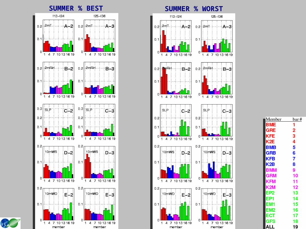
SUMMER % BEST SUMMER % WORST

2mT
24HP
2003081000 CASENear-Surface T
Lowest level cloud water (~3K ft.)
Composite “moist” case Composite “dry” case 2003081000 case KF2KFBMGR
Warm
Cool
Moist
Dry


![Eric Prié & Aaron Summerscale - Colle & Anti-Colle [D02-05]](https://img.pdfslide.net/doc/110x75/55cf97e3550346d033943939/eric-prie-aaron-summerscale-colle-anti-colle-d02-05.jpg)