Embed Size (px)
Citation preview

EVALUATION PARAMETERS FOR
COMPUTER AIDED DESIGN OF
IRRIGATION SYSTEMS
MATODES
APRIL 1987
Thesis submitted to Department of Civil Engineering,
University of Cape Town, in fulfillment of the require
ments for the Degree of Doctor ofPhilosophy.
'->r~
, . "" (1 ;1
: . '

To my wife, Melanie
An unfailing source of support and inspiration
;
SYNOPSIS
SYNOPSIS
The research has entailed the formulation and coding of computer models for the design of
pressurized irrigation systems. Particular emphasis has been given to the provision of
routines for the evaluation of the expected performance from a designed system. Two
separate sets of models have been developed, one for the block or in-field system and one for
file mainline netWork.
·The thesis is presented in three seelions asfollows :
* Basic theory, in which the general background to the research is covered.
* The models, which includes detailed descriptions of both the design models and the
.. computer programs.
* Applications, in which several test casesof both sets of models are reported.
SECTlON 1: BASIC THEORY.
This seelion contains three chapters as follows :
Chapter 1 : Rationale. The general nature of the design problem is discussed and
shortcomings of current manuel design procedures are identified. A motivation for the
research is proposed. Particular reference is made to philosophies .of computer aided design
and the way in which these concepts can enhance the design process.
Chapter 2 : Systems analysis of the design process. A systematic review is presented of
the process required for the complete design of an irrigation system. The components of an
irrigation system are categorized in terms of hardware and system characteristics. The design
process, which entails the establishing of these characteristics for a given set of conditions, is
structured into three distinct modules. viz :
* Preliminary design;
.* Block design; and
* Mainline design.
Specific aspects of the design problem relating to each of these modules are discussed.
Chapter 3 : Review of irrigation quality analysis. A review of the literature relating to the
evaluation of operating irrigation systems is presented, with a view to the formulation of
suitable evaluation parameters for the computer design models. A preliminary structure for
the proposed evaluation model is outlined.
iii

SYNOPSIS
SECTION 3: APPUCAnONS.
Once again three chapters are presented. as follows :
Chapter 7 : Applications of the block design and evaluation models. A single apple
orchard is used as a test case for a number of altemative designs. Some sensitivity analyses
of the design parameters are carried out using the evaluation model to provide an analysis of
the various results.
Chapter 8 : Applications of the mainline design model. A series of different applications of
the mainline design model are presented. The examples show the variety of applications that
are possible with the design model, and also examine the efficacy of the procedures.
Chapter 9 : Summary and conclusions. A summary is given of the principal contributions of
the research. Conclusions are drawn about the applicability of the design models and about
the nature of the CAD process incorporated into the programs.
v

ACKNOWLEDGEMENTS
ACKNOVVLEDGEMENTS
I would like to express my gratitude to a number of people, and organizations, for their
assistance throughout the completion of this research:
My supervisor, Professor John Lazarus, for his patient guidance and direction over the past..twoyears.
Francois Korb, who was responsible for much of the computer code and considerable
inspiration; and from whom I learnt a lot more than just PASCAL
The Directors, my coneagues and friends at Messrs. Murray Biesenbach and Badenhorst
Inc., who provided financial assistance, a perfect working environment and the benefit of
tapping a large body of experience in irrigation design,whenever I needed help.
I was singularly fortunateto have received formal training in the field of Irrigation Engineering
in the Department of Agricultural Engineering at the Technion-Israel Institute of
Technology. In particular, Professor David Karmeli and Dr. Gideon Peri were my mentors
dUring this period, and assisted me greatly during the initial formulation of the ideas for this
Thesis.
Messrs Compustat Pty Ud have generously provided me with open '!ccess to their technical
facilities for the typing and production of this Thesis.
Whilst in the Department of Civil Engineering at UCT, I received financial assistance in the
form of a bursary from the Council for Scientific and Industrial Research.
The research for this Thesis was undertaken as part of the work for a project funded and
commissioned by the Water Research Commission.
vi

CONTENTS
Synopsis
Acknowledgements
Part 1: BASIC THEORY
CHAPTER 1 RATIONAlE
1.1 Introduction1.2 Design of irrigations systems1.3 Shortcomings of existing design procedures1.4 Computers in engineering design1.5 Basis for the research
CHAPTER 2 SYSTEMS ANALYSIS OF THE DESIGN PROCESS
2.1 Introduction·2.2 Requirements of the design process2.3 The design process2.4 Design of design software
CHAPTER 3 REVIEW OF IRRIGATION QUAUTY ANAlYSIS
3.1 Introduction3.2 Waler distribution functions3.3 Efficiency3A Uniformity3.5 Appropriate evaluation parameters for design
Part 2 : THE MODELS
CHAPTER 4 BLOCK DESIGN
4.1 Introduction4.2 Pipe alignments4.3 Determination of pipe sizes4.4 The computer programs
CHAPTER 5 EVALUATION OF BLOCK DESIGN
5.1 Introduction5.2 Basic model structure5.3 Yield estimation5.4 Economic calculations5.5 Operating point5.6 Comparison with other models5.7 The computer programs
CHAPTER 6 MAlNUNE DESIGN
6.1 Introduction6.2 Network layout6.3 Valvesequencing6.4 Pump and pipe sizing6.5 The computer programs
Page iii
vi
..
1.11.21.81.121.14
2.12.22.42.9
3.13.33.163.193.21
4.14.14.44.8
5.15.25.65.135.175.235.29
6.16.16.46.126.25

Part 3: APPUCATIONS
CHAPTER 7 APPUCATIONS OF THE BLOCK DESIGN AND EVALUATION MODELS
7.1 Introduction7.2 Basic design7.3 Evaluation7.4 Sensitivity analysis7.5 Accuracy ofthe hydraulic models7.6 Conclusions
-CHAPTER 8 APPUCATIONS OF THE MAINUNE DESIGN MODEL
8.1 The sequencing algorithm8.2 The design optimization procedure8.3 Example of an application on a new design8.4 The use of booster pumps8.5 The design model as an aid to network operation8.6 Conclusions
CHAPTER 9 SUMMARY AND CONCLUSIONS
9.1 Principal results9.2 Applications of the design models
. 9.3 Development of the computer models9.4 Indications for further work
APPENDIX 1
Synoptic maps of the computer design models
APPENDIX 2
PASCAL listings of computer programs
APPENDIX 3
Glossary and notation
7.17.37.97,127.1f!7.17
8.18.58.78.108.128.15
9.19.59.59.7
AU
A2.1
A3.1

, .
PART 1 :
BASIC THEORY
.. .'
1, RATIONALE
1. RATIONALE
1.1 Introduction..
: ."
, Th~ design of irrigation systems is a multi-faceted, multi-objectiv8 problem. Different facets of
the problem include: , '
* selecting emitters to meet the irrigation requirements of the specific design case.
* the laying out and sizing of pipelines on the basis of various hydraulic considerations;
* selecting pumps to meet the hydraulic requirements of the system; and
* determining irrigation operating schedules on the basis of hydraulic, agronomic and
climatic considerations.
Objectives of the design problem can range from trying to maximize crop yield per unit of land
or per unit of water used, to stabilizing food production and/or social development in a
particular region.
System design is normally carried out in a series of independent steps, each dealing with a
separate aspect of the design problem. The design process at each stage is based on
various criteria that have been established over time, through experimentation and
observation. In other words the derivation of these criteria ha~, been empirical. The work
described herein relates to research that has been carried out into the design of irrigation
systems, aimed at the development of an integrated set of design procedures incorporating
rationalized rather than purely empirical design criteria.
A methodology has been proposed for the design of irrigation systems utilizing computer
based models. The major objective in developing the computer models has been to provide
the designer with access to measures describing the expected quality of irrigation that will be
obtained from the designed system. These measures provide the designer with a set of
parameters for making a rational evaluation of the effects of various decisions made in the
course of the design process. They are therefore referred to as "evaluation parameters".
For example, perhaps the best known design criterion is the so called "20% rule": by which
the allowed pressure variation in a network of pipes delivering water to a single field is limited
to a maximum of 20% of a predefined nominal pressure value. This value of 20% allowable
pressure variation is based on an expected resultant discharge variation within the field of
10%, which is considered to be within "acceptable" limits. The acceptability of this degree of
variation has been established over time through experience rather than through any
1.1
1. RATIONAlE
analytical process. " Furthermore, the 20% rule, is based on an assumed square' root
relationship between the, emitter operating pressure and, its discharge.: However, some"
recently developed pressure compensating emitters provide discharges which are less
sensitive to pressure variation, and the 20% rule may therefore be inappropriate .for these
emitters. The proposed computer models have been structured to enable rapid evaluation of
the effects of, ,!arying the allowable pressure variation for a given design situation. By, so
, doing, the designer is able to make a rational decision as to what degree of pressure variation
should be allowed in the system, on the basis of the results of the evaluation.
This chapter presents an overall rationale for the research. An overview of the design process
is presented and some of the shortcomings of current design practices are discussed. This is
followed bya review of the impact that computer aided design (CAD) has had in the
engineering design process. Finally, the underlying philosophy of the proposed design
,models is discussed, with particular reference to the aims of incorporating the principles of
computer aided design.
1.2 Design of Irrigation Systems
Any engineering project will typically undergo three main phases in its development, namely:
* Planning
* Design
* Implementation
In the case of an irrigated agricultural development project, these phases are defined
more specifically as follows :
Planning. Once a potential site for the development of irrigated' agriculture has been
identified, decisions have to be made as to what crops will be planted and to which areas
each crop will be allocated. These decisions will be based on an analysis of the available
resources in,relation to the project objectives. The resources to be considered in this
analysis include soils, water, energy, labour, management and capital. The objectives will
generally concern a maximizing of economic returns from the project, but will usually also
include social and ecological objectives such as regional development, food production,
creation of employment, distribution of incomes and soil conservation.
1.2

,.~. r'''' " ::.1 •. RATIONALE
Design. Once the primary planning decisions have been made, the irrigation system has to
be designed. This includes selecting the type of irrigation to be applied and the operating
regime, as well as designing the actualsystem hardware.
:
Implementation. With regard to the irrigation system, the implementation phase consists of
installation and commissioning of the system and the establishing of reai time operating
procedures. These procedures include both management practices such as opening and
closing valves, moving pipes and flushing filters, as well as irrigation scheduling practices
such as evaporation and soil moisture measurement and water balance calculations•. '. , . .
The research described in this report has been concerned with the design phase of a project,
as defined above.
1.2.1 Elements in the Design of Irrigation Systems
The design of an irrigation system involves determining the characteristics of the specific
system which will deliver water to the plant in the field. In order to design the system, the
following factors would havebeen established dUringthe planning phase of the project :
* the exact geometry and topography of the field;
* the nature of the soils;
* the proposed cropping programme;
* the location and capacities of the water and energy sources;
* the estimated plant water requirements during the season.
The design process then involves the determination of the various system components,
which include both the'actual hardware and the system characteristics. These two sets of
components can be broken down as follows :
Hardware
Q The emitters.
Ii) The in-field or block network, which transports water from the supply pipes to the
emitters. This netWork consists of lateral and manifold or branch line pipes.
iii) The mainline or conveyance network, which transports water from the source to the
block network. This network consists of main and submain pipelines.
Iv) The control components such asvalves, regulators, controllers and sensors.
v) .The pumps (water and fertilizer injection).
The hierarchical nature of the hardware in an irrigation system is illustrated diagrammatically
in figure 1.1.
1.3

..• 1•.· RATIONALE·
FELD BORIJ[R
.y
BLOCK BOIlDfR;;', :
RIVER--~
fRS (' .~ VAL.VE AND PRESSURE RfGULATDR/1'\... ' ,I: I
I I: ,
ALS ;.
I I IOlD =t= ~ +
.[HLINEI - .- - .-I- - I- --
• I • I • I •I I I
---1--+-'---+-->--+_.->---• I • I • I •
.: I II I
IN 'i E~fUERS. VALVES. PlETERS
.....-.
EPIITT
BLOCKPN-F[LDI LATERNrTWORK
;',' . I "~
t. . ,,!,:'
", .~ .
Figure 1.1 Diagramatic representation of a typical Irrigation system
System Characteristics
I) Capacity, which is defined by the discharge rate, the flow and pressure distributions
and the gross application quantities.
ii) Layout and alignments of both the block and mainline networlls.
iii) The nature of the control system (types and locations of the control elements, levels of
automation).
iv) The operating regime, which is defined by the length (time) of an irrigation, the
irrigation cycle time and the irrigation programmes.
v) The pumping requirements.
vi) The system performance, which relates to the extent to which the design meets the
original objectives.
1.2.2 The Generalized existing Design Procedure
Although specific design procedures vary between different designers, from case-to-case and
most Significantly for different methods of irrigation, it is possible to classify a generalized
1.4
1. RATIONAlE
procedure which is widely applied. This procedure, which is discussed at length in several
texts (notably Jensen -1981 and Walker-1978), is summarized below.
All water measurements of rainfall, crop water requirements, soil moisture and irrigation
applications are usually specified in terms of volume per unit area; which is exp~ed as
"depth" and is normally given in millimeters. The equivalent volumes can be computed by
multiplying these depths by the area over which they apply.' On the basis of these units.' the
design procedure involves the following five steps :
(I) Establish operating constraints
If:
RAW = the readily available water that can be extracted by a plant from a soil that
is wet to field capacity (mm);
Et = the peak daily evapotranspiration (mm/day)
Then the maximum irrigation interval (71..,.) is given by :
Tl_ = RAWIEt (days) (1.1)
And given:
&9 = the gross application efficiency of the irrigation system ('lEo); being a
measure of the portion of the total water application that becomes
available to the plant, rather than being lost through evaporation or deep
percolation in the soil
Then the maximum peak application per irrigation due to agro-climatic constraints (£4-1 is
given by:
(1.2)
Rnally,lf:
Nb = the number of blocks to be irrigated in a given field; each block being
irrigated separaJely in one irrigation set, so that there are Nb irrigation sets
in a complete irrigation cycle.
Td = the time aVailable per day for irrigation (hrs).
Then the maximum system application rate (.4R...,J is given by :
AR_ = (NbxlA-JI(I1_xTd) (mrn/h)
1.5
(1.3)

1. RATIONAlE .:
This value of ARmax must also be checked against the maximum infiltration rate of the soil,
ie. ARmax < maximum infiltration rate.
. .~"
(2) Select Emitter (Establish Actual Operating Characteristics) :
Given the operating constraints established in step (1), based on soil, crop and field
considerations, the designer now considers the irrigation system itself in order to deterrnine
the actual operating characteristics. The first step is to select an emitter and the emitter
spacings in the field. This is normally done on the basis of experience and trial and error,
with reference to manufacturers' recommendations and tables of emitter operating
characteristics.
If:
qnOlll = the emitter discharge althe intended operating pressure (m3/h or/ph)
sl = the spacing of the emitters along the lateral (m)
sb = the spacing between laterals (m)
Then the actual irrigation system application rate (AR.ct) is given by : .
AR.ct = (qoomx lOOO)/(slxsb) (mm/h)
Where qnOlll is given in m 3/h.
. The condition ARact < ARmax must be checked.
And if:
AT = the total area of the field being irrigated (m 2)
Als = the area irrigated per irrigation set =AT/Nb (m2)
(1.4)
Then the number of emitters operating slrnultaaeously dUring each irrigation set (Ne) is :
Ne = Als/(slxsb)
And the discharge capacity of the system (Qcap) is :
Qcap = Nexqnom (m3/h)
(1.5)
(1.6)
(3) Block Design
The next step is the design of the block network. Alignments, layouts lengths and
diameters of laterals and manifolds have to be established. Layout and alignment are
normally established on the basis of experience and trial and error, pipe sizes are
established on the basis of hydraulic calculations relating to the loss of pressure due to
friction and emitter discharge along the pipelines. Consideration has to be given to :
1.6

1. RATIONALE
*, the area to b.e covered per irrigation set (AIS>. .s :
* the number of irrigation sets per cycle (/Vb).
* , the proposed method of shifting laterals (or other relevant operating units) between
irrigations. , "
* maintaining uniformity of discharge throughoutthe field. The variation in discharge is
normally restricted to a maximum of 10%, which translates to 20% pressure variation
(the20% rule) for non pressure compensating emitters.
(4) Mainline design '.,., -._ " ", . ,
Once the block design is complete, the pressure and flow requirements at each block valve
are known. Mainline design entails establishing the layout and sizes of the pipes
connecting each block valve to the water source. Design considerations are principally the
same as those for the block design. '
(5) Establish pump and control systems
Rnally the designer selects pumps to meet the system supply requirements (head and
discharge duty), and establishes the type and positioning of various control elements such
as valves, regulators, booster pumps and automatic controllers.
1.2.3 Design Criteria
The procedure outlined in the live steps described above is an iterative one. The designer
will normally shift back and forth from step to step in establishing the hardware and system
characteristics.
When considering various pipe sizes for alternative network layouts, the respective system
discharges are known. Thus the basic consideration is one of establishing the pressure
distributions on the basis of the 20% rule. Also, the primary decisions of emitter size and
spacing are constrained by the results of the set of calculations in step (1). The value of Nb,
the number of sub-areas or blocks, is determined on the basis of the designer's experience of
how many irrigations can feasibly be ,executed per day and the number of irrigating days per
cycle.
Throughout the design process, the principal considerations are generally to maintain costs
as low as possible, whilst aiming to achieve the highest possible yield in each specific case.
1.7

Thus the criteria used in the design process can be summarized as follows :
* Minimum system and operating costs.
* Maximum yield. • t •
* Uniformity of application defined by adherance to the 20% rule.
* Constraints on the operating regime defined by > pre-determined soil, plant and
field-geometry characteristics.
1.3 Shortcomings of Existing Design Procedures
The principal shortcoming of existing design procedures is that they do not have a "systems
analysis" orientation. Design methods have evolved over time, together with the
development of various irrigation technologies. As such, no thorough rationalization of the
various design parameters has been carried out in order to relate design practice to a set of
clearlystated objectives. This is manifested in the following problem areas :
(1) Minimum Cost and Maximum Yield. Perhaps the most well recognized problem is the
use of the minimum cost criterion, rather than one of maximum profits. A trade-off exists
between cost and the performance of the system, which implies a trade-off between cost and
expected returns. Ideally an optimal design will be one ln.whlch the marginal costs of
improving the system are equal to the marginal revenue from the crop yield. This is illustrated
in figure 1.2 (English et al, 1983), which shows generalized curves relating applied water to.
income and cost respectively.
Curve #1 illustrates the response of crop yield to water applied from an irrigation system,
which can also be equivalenced to gross income since crop yield is directly proportional to> -
income. Crop yield has been shown in a number of studies to be more or less linearly related
to plant consumptive use of water. As consumptive use increases however, the amount of
applied water lost to evaporation and deep percolation also increases, hence the curvilinear
shape of the curve. Once maximum yield has been achieved, excess water can actually have
a negative effect on crop yield, through factors such as deteriorating soil structure due to
waterlogging, reduced nitrification and constrained movement of nutrients in the soil. This
results in the downward slope of the curve beyond the maximum yield position.
1.8

T, RATIONALE
·'.i
$MAXtlUH mo
NET HOME
. 111. GROSS HOM[ CURVE
~Zl PfIDDIJCTlDH COSTrt1Ill:, (lIIacit,5,.1..1 .
1.311'RDllUtllDM tOSTtDlficit Clpacit,5,11..,
IIIIIIIIIIII
WATER APPlIED
;
Figure 1.2 Generalized applied water vs cost and Income curves for Irrigation systems
The relationship between production costs and applied water is a complex one. In its
generalized form shown in curves #2 and #3 in figure 1.2, th'e starting point on the vertical
axis represents the the capital and other fixed costs of a system. The total operating costs
then increase as the water application increases up to a point representing the maximum
capacity of the irrigation system. The solid line (curve #2) illustrates this for normal design
practice, in which the irrigation system capacity equals the application required for maximum
yield. However, as can be seen in figure 1.2, maximum yield does not necessarily imply
maximum nett income (the difference betweEl(\ the two curves at any given applied water
value). The dashed line (curve #3) illustrates the potential advantages that can be achieved
through so called "defidt irrigation", whereby a system is deliberately designed to have a
•capacity that is less than that required to achieve maximum yield. By so doing, savings in
both the capital and operating costs of the system can be affected, with a resulting increase in
the nett income achieved.
These curves illustrate an idealized state, and optimization on this basis is difficult Firstly, the
existing design process is not structured to yield an assessment of the cost versus
performance relationship of the system being designed. Secondly the cost structure that has
to be incorporated into the optimization procedure is complex. As well as the total capital and
operating costs ofthe system,.the marginal cost calculations should also include estimates of
r 1.9

1. RATIONALE
the additional costs incurred in harvesting and marketing the improved yields. And finally,
reliable information on the yield response to water (irrigation) is difficult to establish.
(2) Design Objectives. The design' problem, like the planning problem, is ge':!erally' Iimulti-objective one. Rydzewski (1978) proposed the following list of possible social and
economic objectives, a selection of which may be included in both the planning and design
framework of an irrigation project: ' "
1. Maximizing the retum per unit of capital invested. '
2. Maximizing the retum per unit of project area.
3. Maximizing the retum per unit of water.
4. Maximizing the value of the agricultural output.
5. Maximizing the output of food products.
6. Reaching a target output of food' products (possibly linked with National
self-sufficiency).
7. Maximizing output of export crops.
,8. Maximizing farm-family net income.
9. Maximizing the number of families settled on a project (i.e. minimizing the cost per
family settled).
10. Maximizing job creation, at a specified level of skill, for a given expenditure.
11. Minimizing the use of foreign currency in project operations.
12. Maximizing Govemment revenue (from taxation etc.).
13. Minimizing public expenditure (i.e. encouraging private sector investment).
14. Achieving a re-distribution of income in the region.
'15. Generating maximum economic activity in the project area.
16. Settling previously nomadic communities so as to place them within reach of the
instruments of social advancement
17. Establishing social stability.
18. Satisfying political ideals.
Loucks, at at, (1981) have formulated an objective oriented irrigation planning model, in
which they have made provision for multiple socio-economic objectives in the objective
function. However, while the irrigation system designer may consider his client's objectives
implicitly in designing the system, existing design procedures do not incorporate any explicit
formulation of objectives, nor any evaluation of the extent to which the system meets these
objectives.
1.10

1•.. RATIONALE
Thus the designer is unable to fully rationalize, either for himself or his client, his
recommendations In regard to the generation and selection of alternative designs. As can be
seen from the above list of possible objectives, any explicit formulation of the objectives
which may pertain to a specific design. situation may well incorporate some conflicting
objectives. This is not an uncommon situation, and is addressed through the. use of. .
multi-objective analyses which assistthe decision maker to.select a "best compromise" solution.
(3) System Performance. Underlying both of the points discussed above is the fact that the
existing design process does not incorporate performance related design criteria. The 20%
.rule is a surrogate criterion which ensures some unspecified (in terms of irrigation
performance) rnlnlrm-m standard. After completing. a design, the designer and his client, who
is the decision maker, generally know the costs and layout of the proposed system, the
energy, labour and water requirements, the operating. regime and the pressure and flow
distributions within the system. However, they do not have any definite measure of the quality
of the irrigation to be expected from the system.
Furthermore. with the development of increasingly sophisticated pressure and flow regulation
mechanisms, in particular pressure compensating emitters, the 2()oA, rule is becoming
inappropriate, and the need for considerations based on rationalized cost/benefit trade-offs is
becoming increasingly critical.
(4) Trade-otis. The design process is characterized by a number of trade-offs, some of which
are listed below:
1. Cost vs. performance. As discussed above, greater uniformity of application implies
improved crop yields. However it also implies larger pipe diameters and hence greater
system costs.. Similarly, several other decisions, such as the emitter spacing and the
operating regime, are related to a trade-off Between overall costs and performance.
2. System vs. operating costs. Smaller pipe sizes, which imply lower system costs. result in
.greater pressure losses and hence greater pumping requirements. which in tum imply
greater operating costs. Similarly, designing towards "solid set" (permanent) systems
implies more hardware in the field and greater system 'costs, to be offset by reduced
operating requirements and simpler system management Included in this classification
is the perennial question of labour Intensive versus automated systems.
3. Block (In-field) network vs. mainline network. The costs of the block system can be
reduced through the use of shorter laterals, with smaller discharges enabling smaller
1.11

1. RATIONALE
diameters e . However, this implies a more ramified mainline network and hence greater
costs. , '
;4. Network geometry. Several trade-offs are required in establishing the various network
configurations. For example,. a network can often be laid out to exploit the prevailing
topography in orderto offset pressure losses due to friction, thus enabling the use of
smaller diameter pipes. However this will often also imply greater lengths of the various
network sections, and hence the trade-off.
5. Flexibility ofoperation. The designer is always faced with the question of how much
flexibility to allow his client in the operation of the system. This flexibility manifests in the
ability to rearrange operating schedules to suit changing cropping pattems and
cultivation practices. However, provision of this flexibility naturally requires a degree of
overdesign in aspects such as the system capacity and the pressure and flow
distributions in the networks.
Notwithstanding the extent of these trade-offs in the design of irrigation systems, only limited
mechanisms have been established in current design procedures for sensitivity analysis of
the various relationships. As a result, the designer is required to incorporate a great deal of
intuition into the design process.
1.4 Computers In Engineering Design
The rapid development, in recent years, of micro-computer technology has lead to the
incorporation of computers into many aspects of our daily lives: This technology has been
one of the comerstones of what Toffler (1980) has termed the "Third Wave". He believes that
solid state electronics and computer based technology have largely contributed to the
catapulting of Mankind into a third social revolution, following the Agricultural and Industrial
revolutions respectively.
For the design engineer, this has manifested itself in the development of Computer Aided
Design (CAD) or more generically, Computer Aided Engineering (CAE). CAD systems
enable the engineedo work interactively with the computer by projecting onto the screen
multi-dimensional representations of the system being designed. ~y sitting in front of this
s~enamj' manipulating these ~rojectionsthe~"gine'e;' is able to contemplate and
investigate design aspects that were previously beyond his capabilities and may even have
been beyond his cOgnition.
1.12

'"' .
1. RATIONAlE
James and Robinson (1981) have written that •....It Is important to realize that the Civil
.Engineering profession Is currently experiencing a major revolution In design, brought about
,by advances In computer hardware (I.e., equipment) and software (i.e.; programming
techniques). Four phases may be identified In this revolution:. ' '.;
1. more "number aunching.· where limited access to batch-oriented mainframes allowed
more calculations (·number crunching·), of the same type, than could previously be
carried out on more elementary machines;
. 2. better "number aunching, • where new programs incorporating advances in techniques of
numerical analysis allowed more design options to be explored, typically In' a
'remote-batch environment, ~Sin9 for example, design-office terminals;
3. new kinds of "number crunching. • where widespread access to inexpensive minicomputers
- allowed wholly different problems to be investigated and solved; new programs,
techniques and machines increased the scope of engineering design; computing
became an essential and naturally accepted basis for design;
4. much more than "number crunching" where entirely new approaches to the design
problem have taken root; for example, where communication with comprehensive,models Is through interactive color graphics that allow the design engineer to focus on
difficult problem areas using a single keystroke on the terminal.••••
In describing the extent of the enhanced design capabilities that can be achieved with CAD,
Preiss (1982) has used the analogy of Man's progression from solely oral communication to
the development of written communication. This development provided, through paper
based information systems, a medium which facilitated conceptual or abstract thinking.
Preiss believes that inasmuch as the computer overcomes many of the limitations of the
paper based information systems, such as analysis in more than two dimensions. the
identifying and notifying of errors and the affecting of corrections and alterations, it represents
a quantum leap forward that Is comparable to the- development of written communication. In
discussing the implications of future CAD systems, Preiss believes that they ••••will have a
capability of checking interrelations between data, and will be able to check implications of
proposed decisions, to a degree which is difficult to grasp today.·
Thus, using CAD the engineer is able to develop greater understanding and evEln new
perceptions of the system he is designing. The full implications of the effect of CAD on
engineering design has been the subject of considerable debate, which is beyond the scope
of this report. The interested reader Is referred to Cooley (1980). However the nature of CAD
systems Is discussed in more detail below, in order to illustrate how irrigation systems design
can be structured for CAD.
1.13

1. :RA110NALE '
Preiss has classified two generations of CAD systems. The first generation systems are
characterized by 2-dimensional drawings that are merely representations In the machine of
what used to be on paper. Man/machine interaction is directed and actuated by the user; and
the software is "deterministic", in that on receiving input it will either calculate a given output
or fail because of the nature of the input The second generation of systems have an
interpretive capability that enables them to generate their own data and to lead the desIgner
through solutions in an interactive "conversation". In these systems the machine can display .
to the designer, and maintain within its own processor, 3-dimensional representations of the
system being designed. It is therefore able to carry out solid geometric modelling which, for
example, will identify and preclude infeasible interactions between solid objects.
These second generation systems are imbued with "artificial intelligence" through
non-deterministic software. This software has alternatively been termed "knowledge based"
and "problem solving". Starling with the initial state, which is the input data, the programs
apply a series of rules to transform the data through several intermediate states to a final
output slate.. These rules are governed by a number of logical preconditions which test the
current state of the data and enable a decision on which rule to apply on the basis of specified
criteria. The dynamic properties of the software emerge from the hierarchical structure of the
rules and preconditions. In order to evaluate the preconditions for a specific rule, other rules
may be used, which in tum trigger the use of additional rules, and so on recursively. Also,
there can be rules to change the preconditions depending on th~ current state of the data.
Thus the user will not generally know, apriori, to which state the application of rules will drive
the computation. This class of software has been used for the development of applications
such as computer chess players" language interpretation, robotics and medical diagnosis.
The nature of the CAD system that has been developed for irrigation design is discussed
further in section 1;5 below.
1.5 Basis for the Research
The basic motivation for the research has been to utilize CAD technology to develop a more
rationalized approach to the design of irrigation systems. In order to do this, two distinct sets
of work havebeen undertaken.
Rrstly, as stated in the introduction of this chapter, the work has attempted to develop a set
of appropriate performance parameters to be used as evaluation tools In the design
process. Much work has been reported in the literature, relating to the development of
1.14

1. RATIONAlE
performance parameters to evaluate operating systems in the field. This work has been
. used as a basis for the development of the proposed design parameters, and is therefore
reviewed in chapter three of this report•.
Secondly, the work has attempted to develop an Integrated approach to the overall design
process. A considerable amount of work has been done over the years in the development
of optimization routines for individual aspects of the design process. This work has been
Incorporated into the proposed model wherever Considered appropriate, and is consequently
reviewed In the relevant chapters. .The proposed model has been predicated upon a
thorough ·systems analysis· of irrigation systems themselves•. This is described In chapter
two.
1.5.1 Structure of the proposed model
The proposed model can be used to generate alternative systems, which can then be
evaluated in terms of prestated objectives using the various performance criteria. On the
basis of this evaluation new alternatives may be generated. By this process, the designer Is
able to thoroughly Investigate the effects of the various trade-offs that have to be made, and
.finally to select the design which best meets his objectives.
Thus in terms of classic modelling theory, the proposed model may be classified as :
* an event based ~e. deterministic rather than probabilistic) si'!1ulation model;
* with an Isomorphic and iterative (multi-directionally) internal structure (ie. it attempts to
model the exact processes of cause and effect in irrigation systems, these processes
being multidirectional rather than having a fixed path from start to end);
* and its function Is predictive (heuristic) rather than purely descriptive.
The computer programs can been seen as a hybrid first and second generation CAD
package. Inasmuch as the design process is not yet fully rationalized (analytical), it is still
directed by the designer. Nevertheless the level of interaction with the computer is high and
considerable flexibility is provided in the directing of this interaction. It is hoped that in the
future, as experience Is gained in using the CAD based model, and insights into the
interactions of the various irrigation system components are developed, algorithms for
knowledge based software will also be developed.
1.15

1. RATIONALE ..
1.5.2 Summary
In summary, the contribution of the reported research to the current state of the art In
irrigation systems design is seen to be: .r
:1. The carrying out of a comprehensive "systems analysis" of the process of design of
Irrigation systems, leading to a proposed detailed structuring of the design problem.
This Includes: a listing of all of the Irrigation system components to be designed: the
formulation of three distinct design modules and the Individual routines contained
within these modules: and identification of the links goveming components and design
parameters within and between each module (chapter 2).
2. The formulation of measurable performance and quality of irrigation related design
criteria, to be used in the design process for "on-line" evaluation and selection of
alternatives (chapters3, 5 and 6).
3. The development of a suite of programs for a computer based irrigation design model.
The programs have been structured to enable the user to carry out an interactive
dialogue with the computer, thereby building up experience with the effectiveness of
the various evaluation parameters. It is hoped that this will lead in Mure to the
development of more knowledge based algorithms (chapters 4 - 8).
1.16

., I'· ., . "..,
'.
1.: RATIONALE . , ~~. - .~. '
References ' ' t- , _,I' ,, ,
" '.1. Cooley, M.J.E., Some Social Implications ofCAD, Ch. 2 in CAD in Medium and Small
Sized Industries, European Conference on CAD,Ed. J. Mermet, Paris, 1980. ., .
2. English, M.J., A.G. Nelson. B.C. Nakamura. !C.C. Nielson and G.S. Nuss. Economic
Optimization of Irrigation, Water Resources Research Institute Publication' WRRI-BO,
Oregon StateUniversity, Corvallis, March 1983.
3. James, W. and M.A. Robinson, Interactive Processors for Design Use ofLarge Program
Packages, Canadian Jou~al of CMI Engineering, V9 No 3, pp 449-451,1982•
. 4. Jensen. M.E., Ed, of Design and Operation ofFarm Irrigation Systems, American Society
of Irrigation Engineers, Michigan U.S.A.,September 1981.
5. Loucks, D.P., J.R. Stedinger and D.A. Haith, Water Resource Systems Planning and
Analysis, Prentice Hall, New Jersey U.S.A.,1981.
6. Preiss, !C.,Future CADSystems. CAD/CAMDigest, V4 No 1, July 1982.
1. Rydzewski, J.R., Irrigation Project Monitoring: A feedback for Planners and Management,
the Civil Engineer in South Africa, V20 No 12, December 1918.
8. Toffler, A., The Third Wave, Collins, England, 1980.
9. Walker, W.R., Design and Evaluation of Pressurized Irrigation Systems, Department of
Agricultural and Chemical Engineering, Colorado Stale University, Colorado U.S.A.
1918.
. , 1.17
· 2. SYSTEMS ANAlYSIS OF THEDESIGN PROCESS
2. SYSTEMS ANALYSIS OFTHEDESIGN PROCESS, ."'.
2.1 IntroductIon
The systems approach to engineering problems has developed from work in the disciplines
of engineering science, operations research, management science and cybemetics. It is a
philosophy that perceives processes as systems, consisting of •••• a goal-directed collection
of interrelated, interdependent parts existing in an environment, w'JIh boundaries that are
dependent on the purposes of the person defining the system" (Duffy and Assad, 1980). In
order to study the interrelationships between the various parts of a system, as well as those
between the system and its environment, techniques have been developed for the
construction of models which can simulate the operation of a system. These models are
normally conceptual, rather than physical, and are constructed using various analytical
procedures.
In the above context, systems analysis can have two distinct meanings. The first refers to
the techniques employed, as part of the system model, for the analysis of a given situation.
These techniques are often malhematical, and typically include optimization procedures such
as linear and dynamic programming. The second meaning refers to a systematic analysis of a
particular process, that is carried out in order to identify and characterize the individual parts
of the system being analysed. Such an analysis is normally carried out in order to facilitate
construction of the system model. It is this latter meaning that is implied in the title of this
chapter (note that in the context of computer science, systems analysis has yet another
meaning).
Thus, this chapter provides a detailed review of the design process. The requirements of the
process are discussed, with partlcular reference to identification of the design parameters.
This is followed by a presentation of the proposed design procedure, with discussion
focussing on the specific design problems in each part of the process. Rna/ly, a review is
given of the principles employed in the design of the computer models.
2.2 Requirements of the Design Process
The -maln purpose of the design process is to establish the irrigation system components.
These components can be classified into two groups, namely :
2.1

a .SYSTEMS ANALYSIS OFTIlE DESIGN PROCESS
* Hardware. This includes all the physical elements of the irrigation system, such as
pipes, emitters and accessories. The design involves determining the type and size of
these elements, as well as the quantity of each element to be used in the system.
' .. '"
* System Characteristics. This includes all of the non-physlcal attributes of the system
that are established during the design process. • .
The design process involves establishing these components, for a given set of prevailing
physiographic conditions and on the basis of a number of predefined objectives. In order to
achieve this, a number of different procedures are used for different sets of components.
Each of these procedures utilizes a specific set of design parameters.
2.2.1 Components
Table 2.1 shows a list of all of the system components that have to be designed. The actual
design requirements in each case are listed under the respective component The right-hand
column of the table shows the parameters which affect the design of each component
As can be seen from the table, there is a considerable degree of interaction and
inter-dependence between components and their associated parameters. This is examined
further in the description of the actual design procedure (section 2.3).
2.2.2 Design objectives
As discussed in chapter one, existing design procedure normally entails the following
objectives:
* maximum yield; and
* minimum cost
The proposed computer based procedures developed in this research however, attempt to
incorporate an orientation towards:
* maximum profit.
In the case of private ownership under ideal conditions, for which economic return is the
primary objective and there are no other constraining factors, the abovementioned objectives
may be adequate for design purposes. However, there may often be certain limiting factors
which require the incorporation of other objectives. For example, if water is limited then the
design might be aimed at producing the maximu~ return per unit of water. Alternatively, in
the case of a development agency project, certain social objectives, such as maximum job
creation, will have to be incorporated into the design. Such objectives may conflict with those
2.2

.2. SYSTEMS ANAlYSIS OFlHE DESIGN PROCESS
Table 2.1 System components and associated design parameters
Component·
I. Emitters-type.
I. Block network-lateral pipe diameters- manKold diameters
Iii. Mainrlne network•pipe diameters
Iv. Controlelements•valves : type, size:-now end pressure regulators:
Kneeded. type.size- meters: Kneeded. type. size- automation equipment:
Kneeded,type- fitters: Kneeded. type, size
v. Pumps- main pump size- boosterpump sizes- IerlJlizer injection equipment:
Kneeded. type,size
Design Parameters
Hardware
Spacing; Nominal operatingpressure; Costs;Pressure/discharge relationship; Operating regime;
Hydraunc gradeDne; Allowablepressurevariation;Coefficient 01 unKormify; Pipeefignments;Topography;Pipecosts;
Hydrau6c gradenne; Pipecosts; .Energy costs; Flowend pressurerequirements;
Aowend pressurerequirements; Hydraunc gradeDne;Discharge volumes; Waterqualify; Costs;
HydrauDc gradeDne; Dischargevolumes;Flow and pressure requirements; Costs;
System characteristics
I.
i.
Capacity- maximum system discharge-now and pressure distribution- system application rate- maximum appDcstion depth
Layout and aUgnments- dMsion 01 fieldinto blocks- emitter spacings- orientation01 laterals- positioning 01 manKold-location 01 blockvalves- configuration 01 mainDne
network
Pump size; Pipesizes;Emitterdischarge;Max.block size;Emitterpressure;Emitterspacings; Irrigation set time;
Operating regime; System app6cstion rate;Pressure andflow requirements of emitters:Maximum lengthof a singleor double diameterpipe;Topography;Pressure end now requirements 01 valves;
Iii. Controlsystem-location of controlelements- degree 01automation
Iv. Operating regime- irrigation settime- irrigation cycle length- timing of irrigation sets
O.e.1imes of the day, days01the week)
- sequencing01 blocikvalves- fitterflushingprogramme- lertiJizer Injection programme
v. Pumping requirements- maximum pumping capabifilies- the pumping regime, Including
operation 01 booster pumps
vi. Perlonnance- coellicient 01 unKormily- appUcation endrequlnement
efficiencies-capitaland operatingcosts- return on Investment
Readily avefiable sol moisture;Peak daDy Irrigation requirement;Number01 Irrigation blocks; System capacily;SystemappDcstion rate;Degree01 automation;
System capacily; Operating regime;Hydraufic gradeline;Flow requirements;
AD design components

2. SYSTEMS ANALYSIS OFTHEDESIGN PROCESS
aimed at generating maximum economic retum from the project. In this case, the onus Is on
the designer to establish a best compromise design. A list of possible objectives is shown in
chapter one.
The proposed design models have been structured to provide a full economic evaluation,
thereby enabling the designer to assess the performance of a given design ~n terms of its
specific economic objectives.
2.3 The Design Process
The overall design process incorporates three distinct phases, as shown diagrammaticallly in
figure 2.1.These are respectively, basic input; design and final output.
BASIC [INPUT
DESIGN
FiNAl [OUTPUT
Physlo- ' r-- Graphicgraphic InputData
r-r- -PreliminaryDesign
BlockDesign
Mainline-. Design -
Bm.ol r-- DrawingsOuanlilies
Figure 2.1 : Phases in the Design Process
Basic Input. This phase involves the accumulation of all relevant physiographic data, which
includes the prevailing soil, plant and climatic characterisflcs, as well as the field topography.
The topographic data may be incorporated into the computer models either digitally from the
keyboard, or via a graphics tablet using computer aided draughting techniques.
2.4
'.."..-'
.2. SYSTEMS ANALYSIS OFTHEDESIGN PROCESS
Design. This phase incorporates three modules, namely preliminary design, block design
and mainline design. As indicated In figure 2.1, the design process involves considerable
iteration between all three modules until the design is complete.
Final output. To complete the design process a bill of quantities, together'with a set of
drawings to be used for Installation and future management of the system, are needed."
Three design modules are discussed in more detail below. this discussion alms to Identify
the individual design problems within each module: to provide a perspective on the
relationships between these problems within the overall design process; and to Introduce the
basic approaches to soMng each of the individual problems. Figure 2.2 shows the main
elements of each module. The required input data for each module are shown on the left of
each respective block, and the components that are designed in each module are listed on
the right of each block.
The research has concentrated on the block and mainline design modules.
2.3.1 Preliminary Design
This module centres around three principal design problems, namely: establishing the
operating· regime: selecting the emitter on the basis of r~quired operating pressure,
discharge and spacings; and sub-division of the field into blocks.
The first step of the process entails calculating the basic soil/plant/water relationships from
the input data. These include the soil moisture holding capacity and infiltration rates and the
plant water requirements. These relationships are then used as constraints in the ensuing
trial and error process for emitter selection and determination of the operating regime. A set
of required operating and capacity characteristics is calculated; a number of emitters are
then considered and their performance in relation to the required characteristics is examined.
This process is repeated for several sets of required characteristics and in this way a matrix of
possible emitters and related operating characteristics is developed. The designer is then
able to make a selection that best suits the prevailing circumstances.
Division of the field into blocks is carried out principally on the basis of the designer's
intuition, with due consideration of the following factors :
* the chosen operating characteristics limit the maximum number of blocks that can be
irrigated within the complete irrigation cycle;
2.5

...."..: . ..-
2. SYSTEMS ANALYSIS OFTHEDESIGN PROCESS
" INPUT .. MODULE, ' OUTPUT .
~. ,"
* SolI, climatic, .crop data
'., * Emitter operatlng
characteristics
* . Topography,fieldsize,operatingregime
PRELIMINARY DESIGN
* Calculate soil/planl/waterconstraints
• Select emitter
• Calculate operatingcharacteristics
• Subdivide the fieldinto blocks
• Operating regime:~rrig. cyclelength~g, settime-timingof sets
• layout:-divisioninto blocks-ernitter spacing
* Emitters:-type
-nominal discharge
• Capacity:-system applic. rate-max, applic. depth
!
BLOCKDESIGN
* Same for manffold diameters
• Determine pipe-networkalignments
• Block Network:-pipe diameters
• Capacity:-pressure & flowrequirements
* Performance:-all values
* Control:-vaJve sizes &locations
• Layout:-alignments oflaterals&manifold
* Operating regime:-operating point
Calc.system performance*
* Carryout hydraunccalculations to determinelateral pipe diameters
Crop yield &economic data
Pipealignments,topography,allowed head loss
*
'.
• SequencetheYa~es
* Establish the layout• Valve pressure&nowrequirements,topography, .energy costs
•
*
MAINLINE DESIGN
Optimize diameterselection& pumpingrequirements
Estabnsh control elements
* Mainline Network. :-pipediameters
• Pumping:-main & boosterpumpsizes-pumping regime
• Operating Regime:-valve sequencing
• Capacity:-max. discharge inthe system
* layout:-rnalnline
configuration* Control:
-allelements
Figure 2.2: The Design Modules
2.6

2. SYSTEMS ANALYSIS OFTHEDESIGN PROCESS .
*' the size of each block determines the flow requirement for the block, which must be .
, "practicable in terms of the availablesupply;
* the block dimensions determine the block pipe-networ\< dimensions, which must be
economical.
2.3.2 Block Design
This module entails:
*' determination of the block pipe-networ\< alignments:
* determination of the pipe diameters; and
* an assessment of the system performance for the block being designed.
This is carried out for each irrigation block in tum.
: . '
Pipe alignments. The lateral pipes are aligned parallel to the planted rows. The position of
the manifold, which transects each of the laterals, is then established on the basis of both
practical convenience and hydraulic considerations. These hydraulic considerations arise out
of the fact that the manifold divides the laterals into two sets, lying on either side of the
manifold. Ideally, the manifold should be positioned such that the lengths of the laterals
running'uphill away from the manifold are maximized, within the constraints of the allowable
pressure loss in the system.
Pipe diameters. The pipe diameters are established using the allowed pressure variation in
the system as a design parameter. The general procedure for a given pipe involves first of all
establishing an allowed pressure envelope, defined by the topographic elevations along the
length of the pipe and the allowable pressure variation within the pipe. The upper and lower
limits of the envelope represent the maximum and minimum allowable hydraulic grade lines
respectively along the pipe being designed. Then, starting at the furthest end of the pipe with
the smallest available diameter, the pressure head in the pipe is calculated for points along its
length, working back towards its inlel This pressure head will increase exponentially as the
flow in the pipe increases, because more and more outlets are included along the length
being considered. Considering this curve in the other direction (i.e. in the direction of flow in .
the pipe), the exponential shape represents the decreasing rate of head loss due to friction,
per unit length, as the flow in the pipe decreases. As soon as the actual hydraulic grade line
for the diameter of pipe being considered rises steeply towards the upper limit of the allowed
envelope, the pipe is replaced by a larger diameter, thereby reducing the rate of pressure
loss due to friction. The process is continued until the inlet is reached. The pipe will then
.have been designed with the smallest possible diameters (and therefore the cheapest) that
will keep the pressure variation within the.allowable limits. A more detailed discussion of this
design process is given in chapter 4.
2.7

2. SYSlEMS ANALYSIS OF THE DESIGN PROCESS
This process Is carried out for each lateral in tum, and then using the results from the lateral
design, it is repeated for the manifold.·. At the end of this process, the pressure and flow
required at the block valve, for irrigation of the block, are known.
Evaluation. The last step of the block design process involves a calculation of various
performance parameters for the designed block. These parameters include Indices of both
the quality of the irrigation that will be applied by the designed system, and the eXpected
economic benefits that will result from the use of the system.
,",
The system is designed for a pre-specified capacity, which depends on the expected crop
water requirements. However it may in fact be operated at different levels of intensity up to a
maximum level defined by its capacity. Maximum benefits may not necessarily accrue from
operating the system at its full capacity, which implies always providing all of the plant water
requirement. In some cases, the nett benefits may be increased by operating the system
below capacity, thereby providing the plant with less than its full requirement (so called
deficit irrigation). The evaluation process includes an analysis of the effects of operating the
designed system at different levels of intensity. A procedure for determining the optimal level
of operation of the system by dynamic programming has been developed and is discussed in
chapterS.
2.3.3 Mainline Design
This module entails the following design problems:
* establishing the pipeline layout;
* establishing the operating sequence of the valves (irrigation blocks) within the irrigation
cycle;
* determining the diameters of the pipes; and
* establishing the pumping requirements for tJ:Ie system.
Layout. The routing of the pipelines from the water source to the block valves is
straightforward to achieve, but difficult to optimize. Since there are normally an infinite,number of alternative routes, anyone of them will generally satisfy the requirements of the
problem. However, it is difficult to establish which of these routes involves the minimum cost
in terms of both capital and operating expenses. For example, the topography of the site may
be such that minimizing the total length of pipes results in the need for larger diameter pipes
In order to avoid excessive pressure loss due to friction. In addition, there may be certain
practical considerations which influence the route of the pipelines. For example, in an
established farm it may be preferable to align the main pipelines alongside the existing roads
rather than through already planted fields.
2.8
2. SYSTEMS ANALYSIS OFTHEDESIGN PROCESS
required function; it is essential that these programs should operate efficiently and accurately.
Structuring of the computer programs has therefore constituted an important aspect of the
research effort.
Three components to this problem can be identified. Firstly, the actual analysis roirtlnes,.• which cany out the mathematical design procedures, have to be formulated. The success of
these routines is measured by the speed and accuracy with which they generate results.
Accuracy in this sense is determined by their ability to handle all design problems, including
those of an irregular nature, without resulting in a software failure.
Secondly, routines have to be designed for the validation of the input data, prior to analysis.
'Once the required data have been supplied by the user, they should be checked by the
computer to ensure that they conform to both the format and the limits that can be handled by
the analysis routines. This prevents the generation of unnecessary errors during computation•
. The third aspect of the software structuring problem relates to the nature of the user-machine
Interaction. The development of so called demand-mode computing has enabled the user to
interact with the computer, during the design process, via a specifically designed dialogue.
The most appropriate nature of this dialogue, for specific problems, has been the subject of a
considerable amount of study, much of which is summarised by James and Robinson (1982).
They believe that the importance of formulating a good man-machine dialogue cannot be
over-emphasized. Newstead and Wynne (1976), and Roy (1980), found that suitably
designed interactive procedures can assist the user in making the judgements necessary for
the solution of multl-objective problems by providing more complete information. However,
James and Robinson believe that •...if the method of communicating with the computer is
complicated and exacting, or the dialogue ambiguous, the positive aspects of computing will
be nullified.·
The interactive dialogue has two principal functions, firstly to assist the user to input the .
required data for the model, and secondly to guide the user through the design process. In
this latter regard the interaction should not be an inflexible step by step process, whereby the
user's role is a passive one of merely inputting the data and then reading the results of the
analysis. Since ultimately all design decisions should be made by the designer, the
interactive procedure should ensure that the user receives full information regarding all
options in a multi-objectlve problem, and in such a form that he is able to make a correct and
well informed decision.
2.10
2. SYSTEMS ANALYSIS OFTHEDESIGN PROCESS
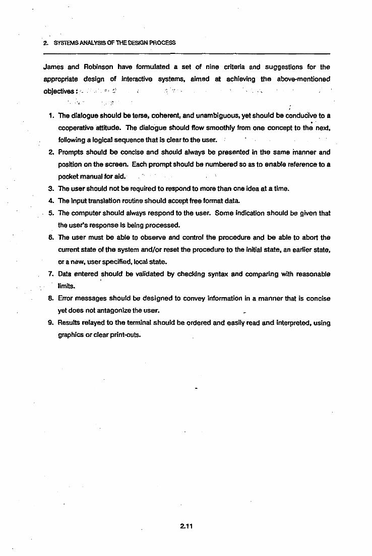
James and Robinson have formulated a set of nine criteria and suggestions for the
appropriate design of interactive systems, aimed at achieving the above-mentioned
objectives: ", ~' "
1. The dialogue should be terse, coherent, and unambiguous, yet should be conduCive to a. '
cooperative attitude. The dialo'gue should flow smoothly from one concept to the next,
following a logical sequence that is clear to the user.
2. Prompts should be concise and should always be presented in the same manner and
position on the screen. Each prompt should be numbered so as to enable reference to a
pocket manual for aid.
3. The user should not be required to respond to more than one idea at a time.
4. The input translation routine should accept free format data.
5. The computer should always respond to the user. Some indication should be given that
the user's response is being processed.
6. The user must be able to observe and control the procedure and be able to abort the
current state of the system and/or reset the procedure to the initial state, an earlier state,
or a new, user specified, local state.
7. Data entered should be validated by checking syntax and comparing with reasonable
limits.
8. Error messages should be designed to convey information in a manner that is concise
yet does not antagonize the user.
9. Results relayed to the terminal should be ordered and easily read and interpreted, using
graphics or clear print-outs.
2.11

2. SYS1"EMS ANALYSIS OFTHEDESIGN PROCESS .
References ,,",.-' ~,~' :",.~.,
1. Duffy, N.M. and M.G. Assad, Information Ma/lllgement: An Executive Approach, Oxford
University Press, 1980.
2. James, W. and M.A. Robinson, Interactive Processors for Design Use ofLarge ;Program
Packages, Canadian Joumal of Civil Engineering, Vol 9 No 3, pp 449-457,1982. ,
3. Newstead, P.R. and B.E. Wynne, Augmenting Man's Judgement with Interactive Computer
Systems, Intemational Joumal of Man-Machine Studies, Vol 8, pp 29-59, 1976.
4. Roy, G.G, A Man-Machine Approach to Multicriteria Decision Making, Intemational Joumal
of Man-Machine Studies, Vol 12, pp 203-215, 1980.
2.12

3. REVIEW OFIRRIGATION atJALI1YANAlYSIS'
", .
3.
3.1 IntroductIon
REVIEW OF IRRIGATION QUAUTY ANALYSIS.',. "
..
Since one of the primary objectives of the research relates to the development of evaluation
parameters for ,incorporation into the design process, it is necessary to review the current '
state of the art.
A substantial amount of work has been done in establishing methods to measure and
evaluate the performance of irrigation systems. Meriam etal. (1981) have identified four
. purposes for this work as follows :
1. To determine the efficiency of the system as it is being used.
2. To determine how effectively the system can be operated and whether it can be
improved.
3. To obtain information that will assist engineers in designing other systems.
4. To obtain information for comparing various methods, systems and operating procedures
. as a basis for economic decisions.
As can be seen from these purposes, the orientation of this work has been In the evaluation of
existing systems, rather than In the design of new systems. The various performance
parameters that have been'proposed in the literature have been determined in each case
from field measurements made on operating systems. Notwithstanding this, several authors
(Karmeli etal., 1978 and Walker, 1979) have identified the potential advantages of
incorporating these performance concepts into the design process. This chapter therefore
presents a review of past approaches to the evaluation of irrigation system performance,
together with discussion on the possible adaptation of these approaches for use in the design
process.
In order to evaluate an irrigation system, some measure of the quality of the irrigation
delivered by the system is needed. Ultimately, since the purpose of irrigating is to improve
production. this quality must be measured in tenns of the yield attained from the crop. In
other words. some measure of the extent to which the irrigation has influenced the yield is
needed. Considerable experimental and theoretical research has been done in investigating
yield/water relationships for various crops. This work has focused on the relationships
between the amount of water supplied to the crop and the resullant yield, and also on the
effect of various irrigation scheduling practices on the yield. However, these relationships are
3.1
3. REVIEW OFIRRIGATION QUAUTY ANAlYSIS .
3. REVIEW OF IRRIGATION QUAUTY ANALYSIS
3.1 Introduction
Since one of the primlllY objectives of the research relates to the development of evaluation
parameters for .incorporation into the design process, it is necessary to review the current"
state of the art.
A substantial amount of work has been done in establishing methods to measure and
evaluate the periormance of irrigation systems. Meriam et.a1. (1981) have identified four
. purposes for this work as follows :
1. To determine the efficiency of the system as it is being used.
2. To determine how effectively the system can be operated and whether it can be
improved.
3. To obtain information that will assist engineers in designing other systems.
4~ To obtain information for comparing various methods, systems and operating procedures
as a basis for economic decisions.:
As can be seen from these purposes, the orientation of this work has been in the evaluation of
existing systems, rather than in the design of new systems. The various performance
parameters that have been proposed in the literature have been determined in each case
from field measurements made on operating systems. Notwithstanding this, several authors
(Karmeli etal., 1978 and Walker, 1979) have identified the potential advantages of
incorporating these performance concepts into the design process. This chapter therefore
presents a review of past approaches to the evaluation of irrigation system performance,
together with discussion on the possible adaptation of these approaches for use in the design
process.
In order to evaluate an irrigation system, some measure of the quality of the irrigation
delivered by the system is needed. Ultimately, since the purpose of irrigating is to improve
production, this quality must be measured in terms of the yield attained from the crop. In
other words, some measure of the extent to which the irrigation has influenced the yield is
needed. Considerable experimental and theoretical research has been done in investigating
yield/water relationships for various crops. This work has focused on the relationships
between the amount of water supplied to the crop and the resultant yield, and also on the
effect of various irrigation scheduling practices on the yield. However, these relationships are
3.1

3. REVIEW OFIRRIGATION QUALITY ANALYSIS
difficult to establish since they are also dependent on several other prevailing factors, such as
the climate, the soil, cultivation practices and crops varieties. These other factors are not
easily Isolated, so that control experiments are difficult to set up. Notwithstanding this, some
general relationships have been developed for a number of crops, and models relating these
relationships to the Irrigation system have been proposed.
Since the disperSion of water from an irrigation system Is not uniform, the general approach In
the design of systems Is to attempt to supply ••••an adequate average irrigation depth, ••• with
reasonably high uniformity ••• in order to minimize the reduction in crop yield as a consequence ofthe
non-uniformity of the irrigation' (Chaudhry 1978). However, improved uniformity implies
increased system and operating costs, and therefore an optimal system is not necessarily
one in which uniformity Is maximised. Ideally, in order to establish a profit maximising
objective function for the design of irrigation systems, the relationship between the costs of
the system and the expected yield Is required. This aspect of system design is discussed
further in chapter 5.
Given the difficulties inherent in determining the abovementioned relationships, past work
has concentrated on the definition of parameters which measure certain aspects of the water
dispersion in the field. Once the amount of irrigation water required in the field has been
established on the basis of knowledge of the plant evapotranspiration and the moisture
condition of the soil, the irrigation quality can be defined in terms of the extent to which it
meets this requirement. For any point in the field the requirement (depth) at the time of
irrigation, and the amount of water applied (depth) during irrigation can be measured. Thus
the extent to which the given point has been over or under irrigated Can also be calculated. If
this measurement is integrated over the whole field, then the following parameters can be
determined:
1. The extent (area) of the field which was under irrigated (deficit);
2. The extent (area) of the field which was over irrigated (excess);
3. The respective deficit and excess water volumes.
If it were required, it would also be possible to identify the specific regions in the field which
are respectively in deficit or excess. However, in the overall evaluation of the irrigation this Is
generally not done. Instead the data are aggregated and expressed in the form of the
cumulative depth versus area irrigated relationship, which Is discussed in section 3.2.3 of this
chapter. From this relationship several different quality parameters can be defined. These
can be classified into two principal groups:
3.2

3. REVIEW OF IRRIGATION QUALITY ANAlYSIS
1. Efficiency measures which give an indication of the extent to which the irrigation has
been usefully utilised. These measures.are based on the extent and volume of the
deficit and the excess.
2. Uniformity measures which give an indication of the evenness with which the irrigation
was applied in the field. These measures are based on the extent to which the
application depths varyfrom the overall average application depth.
This chapter consists of firstly a review of the various methods which have been used to
describe the distribution of water resulting from an irrigalion; followed by a review of the
numerous efficiency and uniformity measures respectively that have been developed in the
• literature. Finally some discussion is presented of the appropriateness and possible
adaptation ofthese measuresfor use in the design process.
3.2 Water Distribution Functions
3.2.1 Single Emitter
The description of the overall field distribution begins with the analysis of the distribution from
a single emitter. Three possible situations can be identified:
1. A sprinkler or sprayer that is stationary during the irrigation;
2. A sprinkler or sprayer that moves during irrigation;
3. A stationary drip (trickle) irrigation emitter.
Stationary sprinkler
In order to be able to analyze and compare distributions of water obtained from single
stationary sprinklers. the American Society of Agricultural Engineers (ASAE) (1969)
established a standard testing procedure. This procedure entails the definition of a square
grid matrix which is superimposed over the sprinkler being tested. "Catch cans" are then
placed in the field at the nodes of the grid to meas.ure the precipitation resulting from the
operating sprinkler over a given period of time.
The results of this testing procedure provide point values on a square pattem of the depth of
water being spread from the sprinkler in a given time. The size of intervals on the grid is not
specified in the ASAE standard. and is therefore selected by the tester. and will naturally
depend on the purpose of the test. A sprinkler manufacturer wanting to test the operation of
one of his sprinklers would probably select a relatively fine grid. whereas a farmer evaluating
his system in the field would probably utilize a more coarse grid in which the intervals were
some whole fraction of the sprinkler spacing of his system.
3.3

3•. REVIEW OFIRRIGAnON QUAlITYANALYSIS .
Other salient aspects of the testing procedure include rigorous measurements of the
prevailing operating conditions, such as the sprinkler flow rate and pressure, the general
climatic conditions at the time of the test and wind measurements.
Alternatively, simple geometric shapes which will approximate the distribution pattern
expected from a single sprinkler have been proposed. Instead of the point measurements
obtained from the testing procedure, mathematical expressions can be derived from the
assumed shapes for the precipitation expected from an operating sprinkler at any point within
its circular distribution pattern. Bittenger and Longenbaugh (1962) developed analyses for
both triangular and elliptical distributions as shown in Figure 3.1.
In the figure, r is the wetted radius of the sprinkler and h is the precipitation rate (mrn/h) at the
sprinkler. Considering a point p at a distance s from the sprinkler, then the precipitation rate,
PP' at this point is given by:
Pp = h[(r-s)/r] (mm/h)
for the triangular pattern, and
(3.1)
(mm/h) (3.2)
for the elliptical pattern.
Moving sprinkler
With the development of mechanical irrigation systems in which- the sprinkler moves
continuously during irrigation, appropriate methods for describing the distribution hav6 had to
be developed. Special test conditions can be set up in order to make field measurements.
However, this is not as practicable as in the case of the stationary sprinkler. For the moving
systems, the mathematical analyses developed by Bittenger and Longenbaugh have proved
to be more useful than the experimental methods, in describing the distribution patterns.
Heermann and Hein (1968) found that both the triangular and the elliptical models gave
ligures which were not significantly different from those obtained experimentally in tests on
two different center-pivot systems.
Equations 3.1 and 3.2 can be extended for both lateral-move systems (straight line path of
sprinkler) and center-pivot systems (circular path of sprinkler) as follows :
a) Lateral-move systems. With reference to Figure 3.2a, s is given by :
(3.3)
3.4
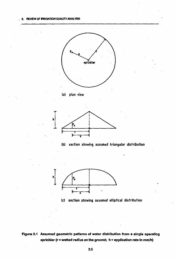
\ 3. REVIEW Of IlRIGAnON QlJA1.JTY ANALVSIS
la) plan view
s
Ib) section showing assumed triangular distribution
hI
s
Ie) section showing assumed elliptical distribution
Figure 3.1 Assumed geometric patterns of water distribution from a single operating
sprinkler (r =welled radius on the ground; h =application rate In mm/h)
3.5

3.. REVIEWOFIlRIGATION QUALITY ANAl.VSIS ~
< ,•••"
r
".
Figure 3.2(a) Analysis of distribution pattern for a moving sprinkler: lateral move
And if the travel speed of the sprinkler is v, and it takes time t to move from its present
position to a point perpendicular to Po then:
y = vt (3.4)
By substitution in equations 3.1 and 3.2, the precipitation rate at point p and time t after
thesprinkler was perpendicular to p, is given by :
Pp = h [r- (m2r2 +v2t2)"' l fr (mm}h)
for the triangular pattem, and
Pp = h[rL(m2r2+v2t 2)J"'lr ""(mm}h)
for the elliptical pattem.
(3.5)
(3.6)
Thus. if the sprinkler takes time T to move from a point perpendicular to p to a point
where p Is on the circumference of the wetted circle formed by the sprinkler, then the
total depth of precipitation,DI" at point pfor a single pass of the sprinkler is :
T
D p = 2 JPpdt (mm)
o3.6
(3.7)

~ • I' "./.
s.. REVIEW OFIRRIGATION QUAUTY ANAl.YSIS
-, Substituting equations 3.5 and 3.6 respectively Into equation 3.7 and solving, gives :
.. ' " ,.'
] hrlv (3.8)
for the triangular pattern. and .
Dp = (l-m 2)DrI2v
'for the elliptical pattern.
(3.9)
It can be seen that hr/v and fChrl2v give the depth of precipitation along the sprinkler's
path of travel for the triangular and elliptical patterns respectively. Thus the terms in the
brackets of equations 3.8 and 3.9 are dimensionless. and represent the fraction of the
maximum depth which is received along a path which is fraction m of the wetted radius r
t1:N8y from the sprinkler's path.
b) . Center-pivot systems. With reference to figure 3.2b. s is given by :
(3.10)
Bysubstituting equation 3.10 Into equations 3.1 and 3.2 respectively. and each of these
. into equation 3.7. relatively complex expressions for the depth of application at point p
are obtained. Nevertheless. these expressions are readily evaluated using numerical
methods and hence lend themselves to solution by computer. ..
\\( pith of trlyel .\
Isprinkler I,
III
I,I
Figure 3.2(b) Analysis of distribution pattern for a moving sprinkler: center-pivot.
3.7

(3.11)
3. REVIEW OFIRRIGATlON QUALITY ANALYSIS
Singhi dripper
The emitters lit a drip Irrigation system provide a point source for water, which Infiltrates
directly Into the soil at the point of emission. Any lateral spreading of the wetted area on the
soil surface Is due to forces within the soil matrix, rather than forces imparted by the emitter.
Thus in assessing the distribution characteristics of drip irrigation systems, measurements of
the application depth of various points over the irrigated area are no longer meaningful. The
principal parameter related to distribution, from the point of view of the actual emitter, Is its
discharge rate, which Is in tum dependent on the physical characteristics of the emitter and
on the operating pressure, -Kanneli and Keller (1975) conducted extensive. analysis of the
discharge characteristics of individual drippers. They classified the emitters in tenns of the
generalized flow/pressure relation:
qe = kpx
Where qe = the emitter flow (lph).
." = a proportionality factor, characteristic of each emitter.
P = the operating pressure head (m).
x = the emitter discharge exponent, characteristic of the water flow regime
within the emitter.
The lower the value of x, the less the discharge will be affected by pressure variations in the
irrigation system. For laminar flow x =1.0, wheras for fully turbulent flow In the emitter,
x = 0.5. In practice, for the most common long path emitters, x Is somewhere between 0.5
and 1.0. Some pressure-compensating emitters have been developed, for which x < 0.5. In
fully compensating emitters, the discharge will be constant regardless of the pressure
variations, Implying a value of x = 0.0.
In designing drip irrigation systems it is important to have an assessment of the water
distribution pattem In the soil profile. As the water Infiltrates the soil, it spreads to fonn a
'wetted bulb' radiating from the source. Eventually a steady flow situation is reached In the
relevant area around the emitter. The zone immedia:tely around the source is saturated and
the dimensions of the wetted bulb are constant. The extent of this bulb depends on the
discharge rate and on the soil characteristics. In general, the higher the discharge rate and
the lower the infiltrability of the soil, the larger the wetted area. Also, the higher the discharge
rate, the greater the affect of gravity, resulting in an elongation of the bulb in the vertical
direction (i.e. deeper area of wetling) together with a narrowing In the horizontal direction.
3.2.2 Field distribution pattern
The assessments of the distributions from Individual emitters are used to develop overall
3.8

3.' REVIEW OFIRRIGATION QUALITY ANALVSIS
patterns of the irrigation distribution in the field. Once again three different situations can be
identified. These are loosely classified in terms of dimensions as follows:
1. .Three-dimensional distribution in which the welled area is continuous throughout the
.'. . field. This is normally associated with closely planted field crops under sprinkler
irrigation.
2. Two-dimensional distribution in which the welling pattern consists of continuous rows,
with a dry area between each row. This is normally associated with wider spaced "row
crops" such as some vegetables and orchards. In these cases the most common
irrigation systems are drip or micro-jet (sprayer) with the lateral lines running parallel to
the rows•.
3. One-dimensional distribution in which individual plants are irrigated and only the area
around the plant is welled. This occurs in orchards with large planting distances, and
is normally associated with drip systems, but may also occur with sprayer or even
sprinkler systems.
In order to develop an overall field distribution pattern, measurements can be taken over the
whole area, in the same way as was described for single emitters. Alternatively, the pallems
can be built up using a simple overlapping procedure developed by Hart and Heerman
(1976). This procedure assumes that the distribution pallem obtained from a single emitter is
replicable for the other emitters in the field. Thus, starling with the point values on the grid
matrix for the single emitter, the matrix is shifted left and right, and up and down, sufficienUy
to provide a new, composite pallern with the sprinkler position repeated at the appropriate
spacing. The sprinkler spacing must be some whple integer multiple of the grid intervals, so
that the values on the grid 01 each sprinkler coincide with each other in the area where they
overlap. Then the overall pallern is developed by simply adding together all the values
occurring at each point of the new composite grid.
This process can be described mathematically :
Given an m x n matrix consisting of elements ars describing the distribution from an
individual emiller
Then within the p x q matrix describing the composite distribution pallem within the
rectangle described by the four positions of adjacent sprinklers in the field the elements bkJ
are given by :
• n
bkl = I I arsr=k s=l
3.9
(3.12)
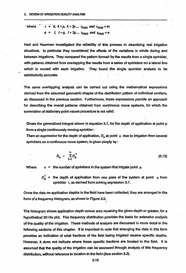
3. REVIEW OF IRRIGATION QUALfIY ANAlYSIS
r = k; k: +P. k + 2P-: r~ lIIId r~< m
S = ~ l+q, 1+2q ••• Smax lIIId smax<n
Hart and Heerman Investigated the reliability of this process in describing real Irrigation
situations. In particular they considered the effects of the variations In winds during and
between irrigations. They compared the pattem formed by the results from a single sprinkler,
with pattems obtained from overlapping the results from a series of sprinklers on a lateral line
which Is moved with each irrigation. They found the single sprinkler analysis to be
satisfactorily accurate•
. The same overlapping analysis can be carried out using the mathematical expressions
derived from the assumed geometric shapes of the distribution pattem of individual emitters.
es discussed in the previous section. Furthermore. these expressions provide an approach
for describing the overallpatterns obtained from continuous move systems, for which the
summation of stationary point values procedure is not valid.
Given the generalized Integral shown in equation 3.7, for the depth of application at point p
from a single continuously moving sprinkler:
Then an expression for the depth of application, D. at point p due to irrigation from several
sprinklers on a continuous move system, Is given simply by :
Where
n 1D. = !Dp
1=1
n = the number of sprinklers in the system that irrigate point p.
(3.13)
D~ = the depth of application from one pass of the system at point p from
sprinkler I, as derived from solving expression 3.7.
Once the data on application depths in the field have been collected, they are arranged In the
form of a frequency histogram, as shown in Figure 3.3.
The histogram shows application depth versus area receiving the given depth or greater, for a
hypotheticat 20 Ha plot. This frequency distribution provides the basis for extensive analysis
of the quality of the irrigation. These methods of analysis are discussed in more detail in the
following sections of this chapter. It is important to note that arranging the data in this form
provides an indication of what fractions of the field being irrigated receive specific depths.
However, it does not indicate where these specific fractions are located in the field. It is
assumed that the quality of the irrigation can be assessed through analysis of this frequency
distribution, without reference to location in the field (See section 3.3).
3.10

3. REVIEW OFIRRIGAnON QUAUTY ANALYSIS
I•
-~
~
~
f-
lo.
0
20
- 40EE-~ 60
.!!-.. 80...:::AA~ 100-co.&. 120-A..c
140
160
2
Area receiving ~ depth , CHal
46810121416 18 20
Figure 3.3 Example of an applicatIon depth vs area IrrIgated hIstogram for a 20Ha plot.
3.2.3 Functional fonns of the distribution pattern
The arrangement of the distribution pattern data in the form of a frequency histogram lends
itself to the development of mathematical functions to descnbe the distribution. From these
functions, several parameters that describe the distribution pattern and provide a measure of
the quality of the irrigation can then be Identified.
The first steP in this process is to form the nermallzed dimensionless distribution curve shown
in Figure 3.4 by dividing each spplication depth by the average depth, and each area by the
total area. The curve is then drawn by joining the midpoints of each frequency in the
histogram. Note that the average depth of appliCation is 1.0 on the new scale and that the
total area bound by the two axes and the curve is equal to 1.0. This latterproperty implies that
anyfunclion,f(x), used to describe this distribution curve will be a normalized density function.
Several functional forms have been proposed. Howell (1964) suggested the process of
determining as many moments as possible to characterize the distribution. However Hart and
Heerman (1976) have shown that the first two moments (i.e. the mean and variance of the
distribution) are sufficient for most purposes, particularly when a standardized function is
used.
3.11

3. REVIEW OFIlRIGATION QUALJ1Y ANALVSlS
"«.•., " ,
-I:-...D-
O.."D..Do 0.3..tS 0.6-0c:
0.9J!.......... U==£D- 15..c..
U....-j2.1
J 2.4
~ '"
Area IS I friction of the total area
0.1 0.2 0.3 0.4 0.5 0.6 0.7 0.8 0.9 1.0
Figure 3.4 Normalized dimensionless distribution curve
Since the application depth frequency curve generally approximates an ·S· shape, Hart
(1961) proposed a normal distribution model to describe the distribution pattem. Once the
mean and standard deviation of the dsta are known, then the distribution is completely
defined by the"expression:
..Q(y) = (l/S'K,f2) Jup [·J.{(Y·y)/s}2]dy
y"
(3.14)
Where Q(y) = The area under the normal distribution curve from y to .., which in this
case represents the fraction of !he area which receives dimensionless
application depth y or greater;
s = The standard deviation of the application depths;
y = The average application depth;
Y = The dimensionless depth for which the following holds:y =< Y =< ..
The coefficient of variation" = Illy provides an indication of the uniformity of the distribution. A
small value of " implies a highly uniform irrigation, characterized by a concentration of the
application depths around the mean, and hence a frequency distribution curve tending
towards the horizontai.
3.12
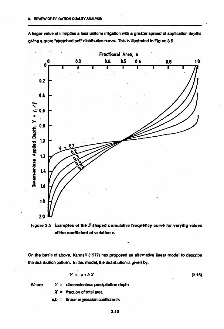
So REVIEW OF IRRIGATION QUALITY ANALYSIS
A larger value 0111 Implies a less uniform Irrigation with a greater spread 01 application depths
giving a more ·stretched out· distribution curve. This Is Illustrated In Agure 3.5.
0.2
0.4.....,;: 0.6•>-.zf 0.1-tc"a 1.0:!t< 1.2
i1 1.4i~ 1.6
1.8
2.0
0.2Frlctionll Arel. X
G.It 0.5 0.6 0.1 1.0
Agure 3.5 Examples of the S shaped cumulative frequency curve for varying values
of the coefficient of variation II.
On the basis 01 above. Karmali (1977) has proposed an alternative linear model to describe
the distribution pattern. In this model. the distribution is given by:
Where
Y = a+bX
Y = dimensionless precipitation depth
X = fraction of total area
a,b = linear regression coefficients
3.13
(3.15)

Where 1(r) =•fer) =
r =
c, =ta =
3. REVIEW OF IRRIGATION QUALITY ANALYSIS
The constants a and b are detennined by least squares regression. Kanneli argues that for
distributions where v is large, the linear model provides a better fit than the nonnal
distribution model, since the errors at both extremes of the frequency curve will be smaller for
the linear model. Also, whereas the normal model might be expected to provide a better fit
than the linear model in cases where v Is small, in fact the linear model should provide a good
flt since in these cases most of the values are concentrated around the mean and therefore
the errors at each extreme of the curve will be limited.
Karmeli calibrated his model for several different distribution patterns, with a wide range of
values of v. The regressions yielded intuitively sound models with highly significant
goodness-ol-fit statistics in each case, indicating most satisfactory models. the principal
advantage of Karmeli's model is its simplicity, particularly in developing the irrigation quality
parameters which are discussed in the following sections.
The gamma and beta distribution models
Several variations of these two basic models have been proposed. Chaudhry (197B)
examined the effects of the skewness of observed distribution patterns, together with the
exclusion of negative observations, on the fit of the normal model. He proposed an
alternative gamma distribution model, which can account for the observed skewness and
eliminates the negative observations. It also provides more accurate evaluations, than the
normal model, of some of the irrigation quality parameters discussed in the following
sections. By this model the area fraction, a,which receives depthYa or greater is given by:
a = 1- [1 r.::-:-::rt (r)/f(r)) (3.16)o/"a+ T
the incomplete gamma function.
the complete gamma function.
the parameter of the gamma distribution, which in this case is 4/C:.
the coefficient of skewness =[I (Yi -Y J3 ] I s3N
[ya-y]ls
Elliot et aI (1980) proposed an alternative beta distribution model which they believed was
more flexible than the gamma distribution in modelling any skewness of the application depth
data. They calibrated the model using a simple transfonnation to constrain the dimensionless
depth values between 0 and 1, and method-of-moments estimates to calculate the
parameters a and p. They compared the fils of normal, linear and beta models on 2 450
different over1apped sprinkler patterns, using the RMS error statistic as a means of
comparison. They found that the beta model consistently gave a better fit than the other two
models. However they concluded that the normal and linear models are more practical than
3.14
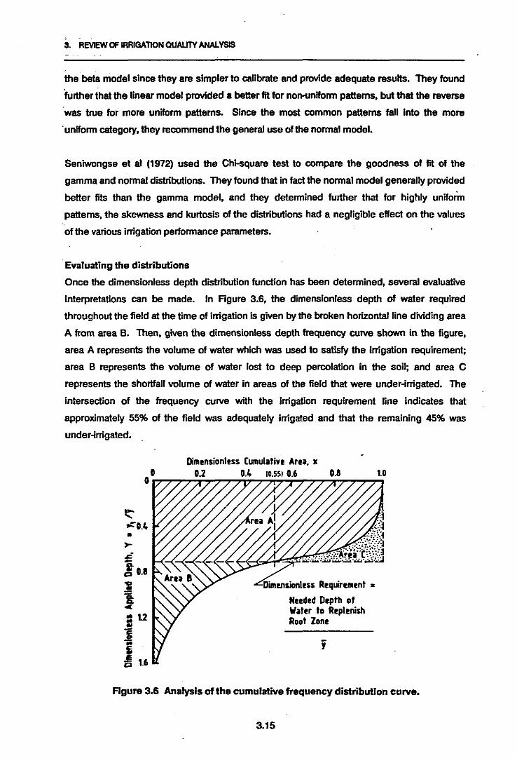
"
3. REVIEW OF IRRlGA1l0N QUALITY ANALVSlS
the beta model since they are simpler to calibrate and provide adequate results. They found
further that the linear model provided a better fit for non-unlform pattems, but that the reverse
'was true for more uniform pattems. Since the most common patterns fall Into the more
'uniform category, they recommend the general use of the nonnal model.
Seniwongse et al (1972) used the Chi-square test to compare the goodness of fit 01 the
gamma and normal distributions. They found that in fact the normal model generally provided
better fits than the gamma model, and they determined further that for highly uniform
patterns, the skewness and kurtosis of the distributions had a negligible effect on the values
of the various irrigation performance parameters.
Evaluating the distributions
Once the dimensionless depth distribution function has been determined. several evaluative
Interpretations can be made. In Figure 3.6, the dimensionless depth of water required
throughout the field at the time of irrigation is given by the broken horizontal line dMding area
A from area B. Then, given the dimensionless depth frequency CUNe shown in the figure,
area A represents the volume of water which was used to satisfy the irrigation requirement;
area B represents the volume of water lost to deep percolation in the soil; and area C
represents the shortfall volume of water in areas of the field that were under-irrigated. The
intersection of the frequency CUNe with the irrigation requirement line indicates that
approximately 55% of the field was adequately irrigated and that the remaining 45% was
under-irrigated.
1.0
:~,:,t
,~.~ddi
3. REVIEW OFIRRIGATION OUALllY ANALYSIS
On the basis of these analyses several parameters measuring the efficiency of the Irrigation
can be calculated. Furthermore. the shape of the frequency curve provides a measure of the
uniformity of the distribution. These parameters are discussed further In the following
sections.
3.3 Efficiency
In the engineering context, the term "ef]idency" generally refers to the ratio of output to input.
This context is applied to irrigation. where the inputs and outputs are quantities of water.
Numerous different efficiencies have been defined in the literature. differing from each other
on the basis of what each of the inputs and outputs represent
Bos and Nugteren (1974) defined a set of efficiencies based on the four basic water quantities
as shown schematically in Figure 3.7. These efficiencies were used to evaluate irrigation data
form several different countries with greatly varying crops. climatic and other physiographic
conditions and irrigation methods. The set proved to be adequate for developing a
composite picture of the elliciency of different irrigation methods over a wide range of
operating conditions. However. this elliciency was measured in terms of overall water
utilization. rather than actual irrigation elliciency.
- .
Vn,f VI. Vf. Vt a WItter voh.mes" • crop ~reMent at ti_ of irrigation
Pe • effective rainfalle• • application efficiencyq, • fara ditcll efficiency
ec :It water cCll"lVe'YllnCe efficiencyed • distribution efficiencyef • fara efficiency~ • .,..,r.lI project efficiency
Figure 3.7 Set of efficiencies defined by Bos 3< Nugteren (1974)
3.16

3. REVIEW OFIRRIGATION QUALITY ANAlYSIS
Several investigators have developed measures of litigation efficiency by defining a fifth basic
water quantity, viz. the quantity of water which is beneficially used during one ilTigation cycle.
Although this Is a more difficult parameter to measure or determine than the other four, it
does enable a more rigorous analysis of the ilTigation performance than the set defined by
Bos and Nugteren.
Many of the efficiency measures are very similar to each other, but are defined in the literature
slightly differently and may therefore have different names. A list of the principal parameters
is provided on the following pages on the basis of the terms that will be adopted for this
chapter. In .cases where alternative terms have been used for these parameters in the
literature, these terms are listed together with their respective sources.
The following measures are expressed in terms of depths and volumes defined in figure 3.8 :
Maximum and average deficit (Hart and Reynolds 1965)
The average deficit is given by Volume-A/a, and the maximum deficit by HR- H..;".
Application efficiency (Hart and Heerman 1976; Karmell et al 1978; Walker 1979;
Chaudhry 1978)
This is the fraction of the total application that is made available to the plant, as given by
Volume-BNolume-D. lt has been a1tematively referred to as :
Water storage efficiency (Hart and Reynolds 1965)
Effective water application (Howell 1964)
Deep percolation efficiency (Hart, Peri and Skogerboe 1979)
Requirement efficiency (Walker 1979)
Defined as the fraction of the total requirement that is met, as given by Volume-BNolume-E. lt
has been alternatively referred to as :
AVailability factor (Hart and Reynolds 1965; Chaudhry 1978)
Storage efficiency (Karmeli et al 1978; Hart et aI 1979)
1 - deficiency coefficient (Peri and Skogerboe 1978)
Delivery efficiency (Hart et al 1979)
If we have a measure of losses, other than deep percolation, due to factors such as wind drift,
evaporation and runoff, then this parameter is defined as the fraction of the total volume of
3.17

3. REVIEW OFIRRIGATION QUALITY ANALYSIS
•I
1rri,ltltl Ar••,IIII
a
•
A,
".. -.-------------,-----~-...,o:"lI
w.tr H,Daptll
!
a K area of the field which Is deficiently Irrigated_AT K total Irea of the field
"-in K .inioua application depth"-ax K ..,.ioua application depth
HI • requirement It the tille of irrigationHT ••.erage application depthIto • a.erlge del i.ery depth
The I"ILIJbers below refer to points on the 8bove diagr_. end the .reaa theyenclose designate wlunes lIS follows :
Voluoe-A K 12,7,8,12 (deficit wluoe)Voluoe-B • 4,5,6,7,12,4 (wluse recei.ed bY the plant)Vo\u.e·C c 2,4,12,11,2 (excess volu.e)Voluoe-O .2,5,6,7,12,11,2 (total applied wluoe)Voluoe-E • 4,5,6,8,4 (required voluoe)Voluoe-F • 1,5,6,10,1 (total deli.ered wluoe)
Figure 3.8 Cumulative depth ys Irrigated area curve, showing measurements defining
the various efficiency and unlfonnity parameters.
3.18

3; REVIEW OFIRRIGATION QUAUlYANAlYSIS
water delivered that is effective in the irrigation. It is given by Volume-DNolume-F and has
been alternatively referred to as : ' ,
, TaUwaterefficiency or 1 • proportion of tailwater (Karmeli et al 1978)
Fraction of deep percolation (Karmeli et a11978)
This the fraction of the total application which is lost to deep percolation, and is given by
Volume-CNolume-D., ,
Application ratio (Chaudhry 1978)
This is the ratio of the average application depth to the required depth, as given by HyIHR• It
has been alternatively referred to as :
, The application coefficient (Peri and Skogerboe 1978)
The distribution coefficient (Hart and Reynolds 1965)
Delivery coefficient (perl and Skogerboe 1978)
This is the ratio of the delivery depth to the required depth, as given by HrlHR-
3.4 Uniformity
Similarly, numerous concepts of uniformity have been defined, and these are reviewed below
(summarised in Karmeli et al 1978 and Hart and Heermann 1976).
Christiansen Uniformity Concept - UCC (Christiansen 1942)
Christiansen first suggested a uniformity coefficient which gave the absolute mean deviation
of the various application depths from the average depth, over the whole field, expressed as a
fraction of this average depth. It was expressed mathematically as follows :
Where N=
X=
the number of observations Xi.•
the average application depth.
(3.17)
Wilcox and Swailes - UCW (1947)
Wilcox and Swailes replaced the absolute mean deviation from the mean, with the standard
deviation (sum of squares deviation from the mean), to give the following formula:
uew = 100(I-siX)
3.19
(3.18)

3. REVIEW OF IRRIGATION QUALITY ANAlYSIS
Where s = the standard deviation.
Hawaiian Sugar Planters Association - UCH (Hart 1961)
If the distribution in the field is normal. then the absolute mean deviation from the mean is
equal to ./2/ff.s = 0.79&. Thus Hart proposed the following uniformity coefficient:
UCH = 100 (1- 0.789s/X) (3.19)
Karmeli et. al. (1978) - UCL
In the linear model proposed by Karmeli et at, the slope of the regression line (coefficient b in
Figure 3.9) gives an indication of the uniformity of the irrigation. The smaller the value of b.
the more uniform the irrigation. For the dimensionless model. as shown in Figure 3.9. the
average deviation from the mean is given by 2[0.5 x 0.5 x (ymax -1')]/1. And since YRlaX - Y =
O.5b. this average deviation is given by 0.25bll.
Thus since the average dimensionless depth = 1. Karmeli et al. have proposed a uniformity
coefficient (UCL). equivalent to UCc. given by:
UCL = l-o.251bl
•fraction X ottowa,,,,, irigaled --+
U
(3.20)
to
DimensionlessWater Depth
Y
III
-----------~-----------III------------r---I
YR K dimensionless required irigation depthV K dimensionless average application depth
Figure 3.9 Dimensionless linear model of cumulative depth vs area irrigated
(after Karmeli et. al. 1978)
3.20

3. REVIEW OFIRRIGATION QUALITY ANAlYSIS
Benaml and Hare (1964)-A
These authors proposed an alternative coefficient which considers deviations of observations
greater than the mean separately from deviations of observations less than the mean. Their
. coefficient is given as : .
A :Xb- (Ilx;.b-XbIJINb
1.66 X. - (I Ix; •• -x.I)iN.. (3.21)
Where Subscript • refers to observations greater than the mean.
Subscript b refers to observations less than the mean.
X; •• ' X;.b are the individual observations.
X•• Xb are the means of the two groups.
N•• N b are the number of observations in each group.
Pattern Efficiency - PEU (The USDA; Criddle et. al. 1956)
The United States Department of Agriculture proposed a pattern efficiency coefficient which
expressed the average of the lowest 25% of the observations as a fraction of the overall
average. This is expressed mathematically as :
Where
PEU : XX;.ql NqX
XX· = the sum of lowest 25% of the observations.1.q
Nq = the number of observations in this group.
X = the mean of all observations
(3.22)
Hart and Heermann (1976) showed that given a normal distribution of depths in the field, an
equivalent pattern efficiency can be calculated as follows: .
PEH : 1- 1.27(sIX)
3.5 Appropriate evaluation parameters for design
(3.23)
3.5.1 Qualitative analysis
In order to utilize some of the measures of irrigation quality for design purposes, the multitude
of parameters described above must be screened in order to arrive at the most appropriate
ones to provide a composite picture of the irrigation performance. and to reflect the eflects of
the changes made to the design.
As far as efficiency is concemed, it can be seen that all of the parameters listed above can be
derived from six basic measurements, viz :
3.21
3. REVIEW OFIRRIGATION QUALITY ANAlYSIS
1. The total volume of water delivered by the system.
2. The total volume of water usefully applied to the field.
3. The total crop requirement at the time of irrigation.
4. The volume ofthe deficit.
5. The volume of the excess (deep percolation).
6. The minimum depth of application.
Hart et al 1979 showed further that all of the parameters described above. apart from the
maximum and average deficits, can be readily derived from the three basic parameters. viz.:
* Water application efficiency
* Water requirement efficiency
* Delivery efficiency
The delivery efficiency is principally a measure of the effect of factors related to the actual
operation of the system in the field. Typical losses that reduce the delivery efficiency are
those due to wind drift, evaporation! runoff and leakage. Thus. whilst delivery efficiency is
affected to some extent by design decisions such as irrigating at night and relating the
emitter spacing to expected wind conditions, it is difficult to measure a priori on the basis of
an assumed distribution pattem. For design purposes, an average, empirically established
value is usually assumed for the whole field. This value will generally be the same for all
design altematives of a given method of irrigation. This implies that for the purpose of
evaluating a design. the irrigation efficiency can be adequately characterized by the
application and requirement coefficients.
As far as uniformity is concerned, each of the parameters described above expresses some
measure of the deviation of parts of the distribution from the mean. In considering the pattem
efficiencies (pEU and PER) it is obvious that any number of parameters can be derived by
simply defining different fractions of the distribution. In this sense, the parameters of
Christiansen, Wilcox and Swailes. Hart and Karmeli respectively must be considered as being
the most general, since they all give a measure of the deviation of the total distribution.
Benami and Hore (1964) believe that their coefficient (A) is more sensitive than others,
because it stresses the deviations of deficient observations and also because it is more
sensitive to the larger deviations from the mean than other parameters. Hart and Reynolds
(1976) however. have shown that both of these assumptions are not necessarily correct.
They showed further that for a given sample data set, a simple linear relationship expressing
A in terms of UCC could be established by least squares regression. yielding a correlation
3.22

3. REVIEW OFIRRIGATION QUAlITYANALYSIS
coefficient of 0.883. They concluded that there appeared to be no apparent advantage in
usingA rather than any of the other parameters. '
The parameters UCe, UCH and UCL' all purport to measure the mean deviation of
observations from the overall mean. The latter two assume different functional forms of the
. distribution. Several researchers (notably Hart and Heerman 1979, Seniwongse et al 1972
and Karmeli et al 1978) have invesligated the correlation between these parameters. for
numerous different sets of data. In all cases high correlation was obtained for simple linear
relationships between any two of the parameters. Furthermore, it can be seen from the
delinitions of UCH and uew that a simple linear relationship exists between these two
parameters. Thus it can be seen that all the uniformity parameters discussed above are very
much equivalent to each other. In the case of computer-based design procedures the
distribution data will be generated in the computer from calculated discharge rates at each
emitter. In this case there is no point in assuming any functional relationship to represent the
distribution, since the uniformity can be calculated directly from these numerical data, using
the formulation for uce.
A composite picture of the irrigation performance can therefore be developed for altemative
designs from the application and requirement efficiencies and the Christiansen uniformity
coefficient. As long as either the required depth or the average application depth are given,
then these parameters fully characterize the irrigation. (Note: Chaudhry 1978 believes that
the skewness coefficient should also be added as a measure of the extent to which the
distribution is not normal],
The uniformity coefficient is dependent only on the shape of the cumulative frequency curve,
and is independent of the actual depths applied. In other words, it is independent of the
vertical alignment of the point HI on the "water depth- axis in Figure 3.8. In this sense, the
uniformity coefficient is independent of the two efficiency coefficients. These efficiency
parameters however, are determined both by the-uniformity (shape of the cumulative
frequency curve) and by the application ratio.
Hansen (1960) and Hart et aI (1979) have illustrated this for three different cases asshown in
Figure 3.10. If HI is greater than H_ (Rgure 3.10a), then regardless of the uniformity there
will be no deep seepage, and the application efficiency will therefore be 100%. However, in
this case the requirement efficiency will be the inverse of the application ratio. Alternatively, if
the required depth is less than H.in (Figure 3.10b), then the requirement efficiency will be
100% and the application efficiency will be equal to the application ratio. In
3.23

3. REVIEW OFIRRIGATION QUAUTY ANAlYSIS
Ea • 100·;'
E, • HT/ H"
U • 11_ eh.ded .... )
"T
I
, ':At••~
Hu x"' 1------------1
HT
lal H. >"-
HT
• Atu-+I
• ""/HyEa
E, = 100%
U = (1_ Ih_ a... )HT
lbl H. < H...
Ea •
E, •
"II - ehadod area....... "IIHT
"II - 1hadId ........... "II"II
u .U......d ... )HT
1•
HT
Iloplh
J.
Figure 3.10 Cumulative frequency curves In three extreme cases illustrating the
relationship between application efficiency, requirement efficiency and
uniformity (symbols as defined In figure 3.8 and the text)
3.24

3. REVIEW OFIRRIGATION QUALITY ANALYSIS
between these two extremes, when the required depth is greater than H min but less than Hr
(Figure 3.10c), which is the most common situation in practice, then the requirement
efficiency can be increased either by improving the uniformity or by increasing the application
ratio.
Conversely, once the uniformity and average application depth are established, then a given
value of either of the.efficiencies will also determine the application ratio. This implies that Jf
predetermined minimum acceptable values of the efficiencies are specified, then for a given
uniformity the application ratio can be determined. In other words, for a given distribution
pattem in the field (which fixes the uniformity) the application ratio can be established by
specifying the required values of the efficiencies.
.Thus it can be seen that these three parameters can be used to provide a complete
description of an irrigation. Hart and Reynolds (1965) produced a complete table of feasible
values of these parameters, thereby characterising all possible irrigations within this feasible
range. Hart et aI (1979) illustrated this characterisation graphically for a given uniformity.
Walker (1979) and Chaudhry (1978) developed analytical solutions for the relationships
characterizing an irrigation. Both of these models also yield the size of the area which will be
deficiently irrigated.
3.5.2 Economic analysis
Whereas a number of researchers have investigated the inter-relationships between all cit the
abovementioned parameters, in order to characterize an irrigation qualitatively, limited work
has been done to investigate their use in any economic evaluation of irrigation performance.
Hart et aI. (1979) have proposed the possible formulation of a composite objective function Q
given by:
(3.24)
where E. , Ea and Ed are the requirement, application and delivery efficiencies. respectively,
Ud is the uniformity coefficient and C, ... C4 are weighting factors giving the relative
importance of each quality parameter in the overall evaluation. These weights reflect the
economic factors related to each of the parameters. Hart et aI. have suggested that C, and
C4 are both related to crop yield and water quantity and the associated eamings and costs; Czis related to the cost of deep percolation; and C3 is related to the cost of distribution losses.
They have not however, suggested how Q can be evaluated, nor how it can be related to any
absolute measure of irrigation quality.
3.25
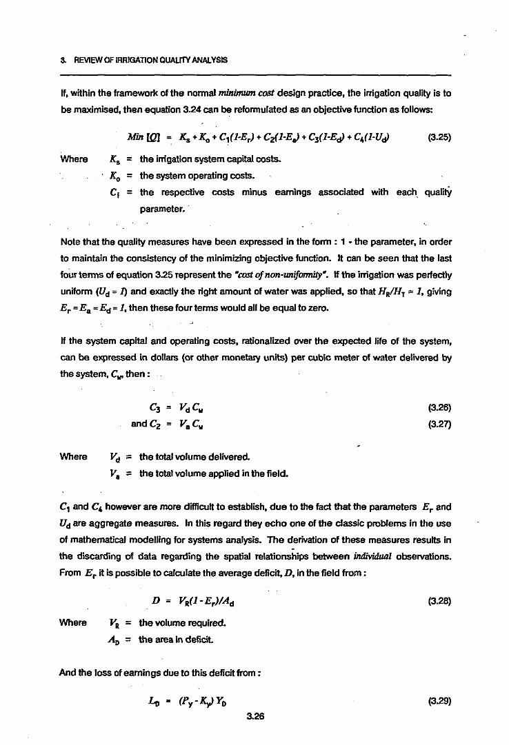
3. REVIEW OF IRRIGATION QUAlI1Y ANALYSIS
If, within the framework of the normal minimumcostdesign practice, the irrigation quality is to
be maximised, then equation 3.24 can be reformulated as an objective function as follows:
Where
Min [Q] ~ K., +K" + C,(1-Er) + Cz(1-E,) + C3(1-E,} + C4(1-U,} (3.25)
X. = the irrigation system capital costs.
K" = the system operating costs.
Cj = the respective costs minus earnings associated with each qualitY
parameter.:
Note that the quality measures have been expressed in the form : 1 - the parameter. in order
to maintain the consistency of the minimizing objective function. It can be seen that the last
four terms of equation 3.25 represent the 'costofnon-uniformity". If the irrigation was perfectly
uniform (Ud =1) and exactly the right amount of water was applied. so that HR/HT =1, giving
E; =Ea =Ed= 1. then these four terms would all be equal to zero.
If the system capital and operating costs, rationalized over the expected life of the system,
can be expressed in dollars (or other monetary units) per cubic meter of water delivered by
the system, CII' then:
Where
C3 = VdCw
andCz = VaCw
Vd ;: the total volume delivered.
V. = the total volume applied in the field.
(3.26)
(3.27)
C, and C, however are more difficult to establish, due to the fact that the parameters Er and
Ud are aggregate measures. In this regard they echo one of the classic problems in the use
of mathematical modelling for systems analysis. The derivation of these measures results in
the discarding of data regarding the spatial relationships between intlivi4ual observations.
From E r it is possible to calculate the average deficit, D, in the field from :
Where VR ;: the volume requlred,
AD = the area in deficit.
(3.28)
And the loss of earnings due to this deficit from :
3.26
(3.29)

·3. REVIEW OF IRRIGATION QUAlITY ANAlVSIS
Where 1.0 = loss of earnings/unit area/unit depth of deficit
Py = price eamed/unit of yield.
ICy = production cost/unit of yield.
Yo = loss of yield/unit area/unit depth of deficit.
> .!'
Then the constant C, in the objective function is given by :
(3.30)
Hart and Reynolds (1965) proposed a similar model to calculate the expected eamings from
an Irrigation characterized by E r•
Similarly, for C4 , Seginer (1978) has proposed a model giving the relationship between crop
yield and hence net earnings on the one hand and irrigation uniformity on the other. The
model is based on the assumptions that:
1. The yield/water function can be divided into two linear segments, with no loss of yield
due to excess irrigation.
2. The irrigation distribution can be represented by Kanneli's linear model.
3. The cost of water is independent of the unlfonnity, i.e. that an increase In unifonnity does
not imply an increase in water cost due to the increase in system cost
Ideally, given a yield/water function, y(i), which expresses the yield per unit area achieved as
a function of the irrigation depth i for the crop being considered, then ayrofit-maximizing design
objectivefunction can be derived as shown below:
Given the frequency distribution function of irrigation depths for a given irrigation, I(i), then
the expected total yield, Y, for a field of AreaAT is given by the integral:
!max
Y = AT IY(i)f(i)di
lilin
(3.31)
When a design alternative is simulated by computer, the irrigation depths throughout the field
are generated as part of the design. In this case integral 3.31 can be solved numerically,
without any explicit evaluation ofl(i).
The profit-maximizing objective function, is given by :
Max: [NE] = Y(Py - ICy) - Va C..
3.27
(3.32)

3. REVIEW OFIRRIGATION QUALITY ANALYSIS
Where HE = The Net Eamings achieved through irrigation.
V. = The total volume of water applied.
All other terms areas defined previously.'. ,
The constraints required to formulate the full optimization problem consist of the complex set
of functions determining the costewand the volume V. together with the integral 3.31 above..
The most significant problem related to the models expressed in equations 3.25 and 3.31
respectively is the obtaining of sufficiently accurate yield/water functions. It is believed,
however that with the ongoing research and development of these relationships, various
adaptations of these models will increasingly be incorporated into the design process.
Several papers relating to the solution of equation 3.31 are analysed further in chapter 5,
leading to the proposed evaluation model Whichhas been formulated as part of this research.
3.28

3. REVIEW OFIRRIGATION auAUTYANAlYSIS
References
1. A.S.A.E., Soil and water division standards committee, Recommendation :
A.S.A.E. R330, Procedure for sprinkler distribution testing for research purposes, Michigan,
December 1969.
2. Benami, A. and F.R. Hore. A new irrigation-sprinkler distribution coefficient, Trans.
ASAE,7(2) : pp 157-158, 1964
3. Bittinger, M.W. and R.A. Longenbaugh, Theoretical distribution ofwaterfrom a-moving
irrigation sprinkler, TransASAE, 5(1): pp 26-30, 1962-
4. Bos, M.G. and J. Nugteren, On irrigation efficienaes, Intemational Inst for land
Reclamationand Improvement, Publ. 19, Wageningen, Netherlands, 1974.
5. Chaudhry, F.H., Non uniform sprinkler irrigation application ejJidency, Joumal of the
Irrigation and Drainage Division, Proc. Paper 13802, ASCE 104 (IR2) : pp 165-178,
1978.
6. Christiansen, J.E., lnigation by sprinkling, C.alifomia Agric. Experimental Station
Bulletin 570, 1942.
7. Criddle, W.D., S. Davis, C.H. Pair and D.G. Shockley, Methodsfor evaluating irrigation
systems, Soil conservation Service Agricultural Handbook 82, USDA,Washington D.C.,
1954.
8. Elliot, R.L, J.C. Nelson, J.C. loftis, and W.E. Hart, Comparison ofsprinkler unifonnity
models, Journal of the Irrigation and Drainage Division, ASCE 106 (IR4) : pp 321-330,
December 1980.
9. Hansen, V.E., New concept in irrigation efficiency, Trans of the ASAE, 3(1) : pp 55-57,
1960
10. Hart, W.E. Overhead irrigation pattem parameters, Agric. Engineering, 42(7) : pp
354-355,1961.
11. Hart, W.E. and D.F. Heerman, Evaluating water distributions of sprinkler irrigation
systems, Colorado StateUniversity Experiment Station Bulletin 128, 1976.
12. Hart, W.E., G. Peri and G.V. Skogerboe, lnigatiun performance:an evaluation, Joumal
of the Irrigation and Drainage Division, Proc Paper 14827, ASCE, 105(IR3) : pp
275-288, September 1979.
13. Hart, W.E. and W.N. Reynolds, Analytical design of sprinkler systems. Trans. of the
ASCE,8(1) : pp 83-85,89, 1965.
14. Heermann, D.F. and P.R. Hein, Performance charactenstics ofself-propelled center-pivot
sprinkler irrigation systems, Trans oftheASAE 11(1): pp 11-15, 1968.
15. Howell, D.T., Sprinkler non-unifonnitycharacteristics and yield, Journal of the Irrigation
and Drainage Division, Proc. of the ASCE,90 (IR3) : pp 55-67, September 1964.
3.29

3. REVIEW OFIRRIGAllON QUALITY ANAlVSIS
16. Karmell, D., Waterdistn1Jution patterns for sprinkler and swface irrigation systems. Proc.
National Conference on Irrigation Return Flow Quality Management, Colorado State
University, Colorado, pp 233-251, 1977.
17. Karmeli D. and J. Keller, Trickle irrigation design, Rainbird Sprinkler Manufacturing
Corp., Glendora USA,1975.
18. Karmeli, D., LJ. Salazar and W.R., Walker, Assessing the spatialvariability of irrigation
waterapplications, EPA-600/2-78-ll41, Oklahoma USA,March 1978.
19. Merriam, J.L N.M. Shearer and C.M. Burt, Evaluating irrigation systems and practices,
Ch. 17 of Design and operation of farm irrigation systems. ASAE Monograph No.3,
December 1980.
20. Peri, G. and G.V. Skogerboe, Evaluation 0{ irrigation systems. Unpublished Report
prepared for Colorado State University, 1978.
21. Seginer, I., A note on the economic significance 0{ uniform water application, Irrigation
Science 1 : pp 19-25,1978.
22. Seniwongse, C., J.P."Wu and W.N. Reynolds, Skewnes and kurtosis influence on
unifonnity coefficient; and application to sprinkler irrigation design, Trans. of the ASAE,
15(2): pp 266-271, 1972.
23. Walker, E.R., Explicit sprinkler irrigation unifonnity: effidency model, Journal of Irrigation
and Drainage Division. proc. paper 14508, ASCE,105(IR2) : pp 129-136,June 1979.
24. Wilcox, J.C. and G.E. Swailes, Unifonnity of water distn"bution by some under-tree
orchardsprinklers, Scientific Agric., 27(11) : pp 565-583,1974.
3.30

' ..
~ • >
. ~,-,,!
, ( .
". '
PART 2 :
THE MODELS
4. BLOCK DESIGN
4. . BLOCK DESIGN
4.1 Introduction
An irrigation block consists of the components of the system that operate downstream of the
valve; it is a1tematively known as the in-field system because it is usually located above
ground in the actual field being irrigated. as opposed to the mainline which is normally .
underground and conveys water from the source to the field. The principal hardware
components of the block system are the emitters. the lateral pipes and the manifold, as
shown in figure 1.1 in chapter 1 and discussed further in chapter 2.
The block design process consists of three distinct phases, viz:
* Establishing the pipe alignments;
* Sizing of the pipes; and
* Detailed eValuation of the expected system performance.
As shown in figure 2.2, the output from the block design process consists of :
* The lengths and diameters of all pipes in the block;
* The specifications needed for the layout of the block system;
* The pressure and flow requirements at the valve;
* The required size of the valve; and
* An assessment of the expected costs and benefits that will result from the use of the
system.
This chapter presents a detailed analysis of the first two phases of the block design process,
namelypipe alignment and pipe sizing; the third (evaluation) phase is discussed in chapter 5.
4.2 Pipe Alignments
This aspect of the design process is influenced largely by local conditions which affect the
block layout on a case-by-case basis. Consequently, it is normally done by trial and error,
based on the designer's experience. Two distinct aspects of the design problem can be
identified:
* Establishing the block dimensions; and
* Establishing the pipe layout within the block.
4.1

4. BLOCKDeSIGN
4.2.1 Block dimensions
This aspect of the design problem is strongly related to the preliminary design process, since
the size of the block'is determined by constraints reiated to the operating regime, the emitter
selection and the available water supply, as follows:
• The operating regime determines the number of irrigation shifts in a complete cycle; the
area to be irrigated in each shift is then given by the total area divided by the number of
shifts per cycle.
• The emitter selection determines the irrigation application rate and thus establishes the
relationship between block size and associated discharge requirement The total '
discharge required in each shift is given by the product of the area to be irrigated per
shift and the application rate.
• The maximum available water discharge may be limited by a number of factors such as
existing pumps and pipelines, borehole capacities or regulations goveming extraction
rates from irrigation schemes or public rivers. The total discharge required per shift must
not exceed the available maximum.
• In addition, practical considerations related to the most economical valve sizes also limit
the available supply rate to each block. This maximum available supply determines the
maximum block size; the total discharge required per shift, divided by the maximum
available block supply, gives the number of blocks to be irrigated per shift and hence the
total number of blocks required for the whole scheme.
Once the block sizes have been established, the actual dimensions are related to the
following factors :
• the maximum allowable lengths of the lateral and manifold pipes, which in tum are
related to hydraulic factors such as the maximum allowable pressure losses in the pipes;
• the economical trade-off between lateral length and manifold length, which is not easy to
establish; and most importantly
• the constraints of the preVailing land geometry.
Oron and Walker (1981) have proposed an algorithm based on non-linear, mixed-integer
mathematical programming techniques, for the optimization of the block dimensions. This
procedure assumes a regular, rectangularly shaped field and determines the optimum length
to width ratios for all blocks, in the field. However, in practice irrigation fields are often
irregularty shaped and the block dimensions are influenced by a number of other factors such
as existing farm infrastructure, the location of the water source and peculiarities in the local
topography. For these reasons, as mentioned above, the block dimensions are probably best
determined by trial and error based on experience.
4.2

4. BLOCKDESIGN
4.2.2 Pipe layouts
Once the boundaries of the block have been determined. then the alignments of the pipes
can be established. This is also normally done on the basis of the designer's intuition.
The laterals are positioned parallel to the planted rows and the manifold then transects the
laterals. The exact positioning of the manifold requires further consideration, since it may
split the laterals into two sets lying on either side of il Ideally, the manifold should be
positioned such that the lengths of the laterals running uphill away from the manifold are
maximized, within the constraints of the allowable pressure loss in the system, as shown in
figure 4.1 below. However, once again, local conditions may mitigate in favour of alternative
alignments. For example, if the block has a natural ridge running through it, then it may be
desirable to position the manifold along the ridge so that the laterals run downhill on either
side of the manifold.
Iliteriis
Down SlopeIi Q •
..........--block boundllry
~ngth of uphill Iiteriisto be Illllximized
Figure 4.1 Layout of laterals and manifold
The positioning of the valve is often determined by the layout of an existing mainline.
However, if its position can be determined quite freely, then similar considerations to those
governing the positioning of the manifold apply to the positioning of the valve; in other words,
the valve may split the manifold in two, in which case this should be done such that the length
of the uphill section is maximized.
The computer programs developed through the research incorporate a pop-up "maximum
length calculator", which is a rapidly accessed utility enabling calculation of the maximum
4.3

4. BLOCK DESIGN
allowable length of one or two diameter pipes on given slopes with given emitter
characteristics and predefined allowable pressure losses. This utility can be used as an aid to
establishing the valve and manifold positions for a current design (see section 4.4).
4.3 Determination of Pipe Sizes
This aspect of the design problem is currently perceived as constituting the core of the whole
irrigation systems design process. It involves working with each pipe in tum and selecting
diameters that maintain the variation in pressure, and hence discharge, along the length of
the pipe within predetermined limits.
Calculation of the pressure losses in the pipe is done by anyone of a number of empirical
relationships that have been developed for the different pipe materials operating under
various flow conditions. The most general form of these relationships is given by :
J = a(QlciD1 (4.1)
Where J =Q =D =
a,~,c,1 =
the headloss per unit length of pipe;
the flow rate in the pipe;
the diameter of the pipe; and
parameters dependent on the pipe material, the flow regime in the pipe
and the units of measurement of the variables.
The relationship between the pressure head in the pipe, H, and the emitter discharqe, q, is
given by:
q = kJiX
Where k and x are constants dependent on the emitter type and the units of q and H.
(4.2)
Several different design procedures have been proposed in. the literature, and these are
reviewed in section 4.3.1 below.
4.3.1 Existing manual solution procedures
The general principles of each of these methods are similar:
* A trial and error procedure is used for selecting either feasible pipe diameters for a given
lateral length, or a feasible length for given diameters.
4.4

4. BLOCK DESIGN
* For a given diameter, over a specified length of the pipe, the decreasing discharge from
the pipe and hence the flow in the pipe are known. The headloss due to friction in the
pipe over the specified length can therefore be calculated (equation 4.1) and the
hydraulic grade line established.
* The variation in pressure and/or discharge along the length of the pipe is used as an
indicator to test and modify the diameter or length selection.
* In each case the main objective is to establish a minimum cost set of diameters that
meet the requirements regarding the maximum allowable variation of the discharge
along the pipe.
The different solution procedures can be classified broadly into two main groups:
Design nomographs. The first set of procedures were proposed in a series of papers by Wu
and Gitlin (1974, 1975, 1983) and Wu et al (1979). They are based on the determination of four
dimensionless parameters, shown in figure 4.2 and defined as follows :
* the friction loss ratio tJf;ltJf
* the slope ratio t.Zilt.Z
* the total dimensionless friction loss tJflH, and
* the total dimensionless slope t.ZIH
Where tJf; = the friction loss in the pipe from the inlet to point along the length of
the pipe;
tJf = the total friction loss over the full length of the pipe;
t.Z; = the head gain or loss due to land slope from the inlet up to point I;
t.Z = the total headloss or gain due to slope over the full length of the pipe;
H = a known fixed pressure head, either the pressure at the pipe inlet or the
emitter nominal design pressure.
"z
""" n.t-~~:;;"--------:;-------+--lrtftrence"tUlIe HJ
prUSl.rt _ad lossdult to friction
Figure 4.2 The parameters defined for irrigation pipe design nomographs
4.5

4. BLOCKDESIGN
The four parameters can be derived from equation 4.1 and from information on the prevailing
topography. They can be calibrated for a series of different operating conditions (l.e, pipe
lengths and diameters. total discharge requirements and land slopes); and can then be used
to characterize either the pressure or the flow variations (by incorporating the emitter
pressure/discharge relationship - equation 4.2) for various combinations of the operating
conditions. The designer can then test selected pipe diameters or lengths against the
resultant pressure or flow variations or associated irrigation performance values related to
these variations.
Wu et aI developed a set of design charts based on calculations of the dimensionless
parameters relating different operating conditions to :
* the coefficient of uniformity (equation 3.17);
* the maximum percentage pressure variation;
* the maximum percentage discharge variation;
* the irrigation application efficiency expressed as qm;n / qavecage; and
* possible variation of the emitter pressure/discharge exponent ( x in equation 4.2) for
given values of the total discharge variation.
Perold (1977) proposed an iterative solution procedure based on the four dimensionless
parameters. that can be applied using a programmable pocket calculator. The procedure
entails the use of the coefficient of uniformity as the criterion for acceptability of trial designs.
It is applicable for the single diameter pipe/uniform slope case. However modem systems.
particularly those designed for micro-sprayer emitters. generally incorporate telescopic
(multi-diameter) pipes and they are often installed on sites with varying topography. Wu et al
showed how their design charts can be adapted for the multi-diameter and non-uniform slope
cases.
The "poly-plot" procedure. The major limitation of the procedures described above is that
they do not incorporate an explicit algorithm for determining the lengths of successive
diameters in a multi-diameter pipe. that will satisfy the design requirements at minimum cost.
The widely used poly-plot procedure. proposed by Herbert (1971). is a graphical method
which overcomes this limitation. The principles of the method are as follows:
* The criterion for acceptable design is set as a chosen value of the maximum pressure
variation along the pipe. Then for a given nominal design pressure the maximum
variation defines the maximum and minimum allowable pressure heads in the pipe
respectively. These values can in tum be used together with the prevailing topographic
4.6

4. BLOCKDESIGN
data to define an allowable pressure envelope along the length of the pipe. The upper
and lower boundaries of this envelope are the maximum and minimum hydraulic grade
lines respectively. A sectional representation of this is shown in figure 4.3(b).
* The pressure headless due to friction in a pipe with a series of emitters along its length is
a function of: firstly the size and type of emitter and its spacing along the pipe, and
secondly the diameter of the pipe. If the discharge from each emitter is assumed to be
constant along the length of the pipe. then the emitter size and spacing determine the
specific discharge rate (SOR). which is defined as the discharge through the emitters
per unit length of the pipe.For example. a 50l/h sprayer operating at 2m spacing along
the lateral has an SOA of 251/h/m. For any given SOA and pipe diameter, a characteristic
headloss curve can be produced. It will typically have an exponential shape,
representing the decreasing rate of headloss per unit length in the direction of the flow,
as the flow along the pipe decreases down to zero at the end.
Herbert produced several sets of curves for different SOR's. Each set consisted of a
curve for each different available pipe diameter, for the given SOA. Typical curves for an
SORof 301/h/m are shown in figure"4.3(a).
* The design procedure entails drawing the allowable pressure envelope on transparent
paper and then aligning it over the headloss curves for the appropriate SOA. The
envelope is shifted vertically until the characteristic headloss curve fits within the
boundaries of the pressure envelope.
The designer normally starts with the smallest available diameter, working progressively
from the closed end of the pipe back towards the pipe inlet. The envelope is shifted until
the bottom of the headloss curve is tangential with the lower boundary of the pressure
envelope. This ensures that the longest possible length of the smallest diameter is used
before its headloss curve moves above the allowable pressure envelope. At a point
where the headloss curve moves steeply up towards the upper boundary, it is replaced
by the curve for the next bigger diameter. which is flatter at this point. The point of
intersection of the two curves gives the length of the small diameter pipe that will be
used. This procedure is continued until the inlet is reached, as shown in figure 4.3(b).
Jobling (1972) simplified the procedure by producing a single universal set of curves that
could be used, together with a key diagram indicator to the appropriate curve, for all SDR and
diameter values. Wu (1985) proposed a uni-plot procedure, based on the poly-plot principle,
which fits a feasible energy grade line within the allowable pressure envelope, and then
calculates the pipe diameter associated with the energy grade line from equation 4.1.
4.7
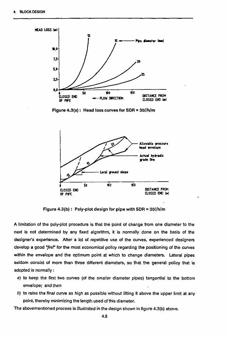
4. BLOCKDESIGN
I£All LOSS '-I
12
DlSTAIIC£ FROtIQ.OSED EIiD 1111
150100
- flO"! ORECTVJll
o.oJ-~~;;;;;;;;;;::::;:::::=---r-----• SOQ.OSED £IllOf Pl'E
Figure 4.3{a): Head loss curves for SDR =30l/h/m
DlSTAIIC£ FROIIQ.OSED £Ill IIlI
A11."lllle prusurelIoad ..ftIOlIe
150100
-t-"""',..ol!==---- Aetuol hydraulicFIllt Ih
"1---- Loa! ground &lope.,-,-
• SOQ.OSED £IllOf Pl'E
Figure 4.3(b): Poly-plot design for pipe with SDR =301/h/m
A limitation of the polyoplot procedure is that the point of change from one diameter to the
next is not determined by any fixed algorithm. it is normally done on the basis of the
designer's experience. After a lot of repetitive use of the curves, experienced designers
develop a good "leer for the most economical policy regarding the positioning of the curves
within the envelope and the optimum point at which to change diameters. Lateral pipes
seldom consist of more than three different diameters, so that the general policy that is
adopted is normally:
a) to keep the first two curves (of the smaller diameter pipes) tangential to the bottom
envelope; and then
b) to raise the final curve as high as possible without lifting it above the upper limit at any
point, thereby minimizing the length used of this diameter.
The abovementioned process is illustrated in the design shown in figure 4.3(b) above.
4.8

4. BLOCKDESIGN
Pleban et al (1984) proposed a more rigorous mathematical optimization procedure for
determining a least cost design within the constraints of the allowable pressure envelope.
The solution utilizes the method of Lagrange Multipliers, and has been programmed for
execution by computer. It is however limited to the uniform slope case.
A further limitation of all of the methods described above is that they are based on an
assumption of constant discharge from the outlets along the pipe. In other words, the
exponent x in equation 4.2 is assumed to be zero. The rationale for this assumption is that if
the maximum pressure variation is kept within acceptable limits, then the error in assuming
constant discharge will be small. A widely accepted industry standard for the allowable
pressure variation is 20%. This is based on a typical x exponent of 0.5, which, when applied in
equation 4.2, will result in a discharge variation of approximately 10%. The extent of the
possible error due to this assumption is in fact very small, as shown in chapter 7 using results
from the computerized design procedure described below.
4.3.2 The proposed computer based algorithm for pipe sizing.
The proposed computerized solution procedure which has been developed as part of this
research is based directly on the poly-plot algorithm; with the exception that the pipe
hydraulics are calculated on a step by step basis incorporating calculation of the varying
discharge along the length of the pipe, rather than assuming a constant SDR.
Development of the algorithm for the computer programs entailed formalizing the rules
governing the graphical poly-plot process. In other words, the conditions for shifting a
headless curve up or down within the allowed envelope had to be stated mathematically. In
addition, an algorithm for establishing the point of change-over from one diameter to another
had to be developed.
Computer algorithms for this process were originally proposed by Perold (1979), and these
algorithms have been adopted for this research. As experience was gained in using the
algorithms, some modifications were developed to overcome specific cases that were found
to cause the design process to break down. These modifications related to the adjustments
after a shift or change of diameter, and the handling of the cycling condition. In addition, the
process was adapted to incorporate a pressure/discharge relationship for each designed
lateral In the manifold design process.
The Pascal listing of the computer routines for lateral design is given in Appendix 2a, and the
full algorithm is described on the following pages.
4.9

4. BLOCKDESIGN
Basic hydraulic calculations. The emitters in the pipe are numbered from 1 at the inlet
through to 1. the last emitter at the closed end of the pipe. The hydraulic calculations are
carried out on a step-by-step basis. starting at the last emitter and working back towards the
pipe inlet in steps of one emitter at a time. See figure 4.4
The calculations are initiated with an assumed value of the pressure head. HI' at the last
emitter. At each subsequent step the pressure at the current emitter. Hi' is known from the
calculations of the previous step. The discharge from the current emitter. qj. is calculated
from equation 4.2; the flow along the pipe in the next section towards the inlet from the
current emitter. Q i. is calculated from the flow along the previous section by :
Qi = Qi+l+qj (4.3)
and finally the headloss due to friction. liHlj • in the next pipe section is calculated using
equation 4.1.
e.itters
Pipe inlet
-------------Mi-1-- Hj
Figure 4.4: Elements in the basic hydraulic calculation procedure
of the computer design algorithm
The change in elevation between the current emitter.zj. and the next emitter. Zj-l. gives the
loss or gain of head due to slope:
liHJg. = z· 1 -z,1 1· 1
4.10
(4.4)

4. BLOCKDESIGN
over section i. And hence the pressure at the next emitter is given by :
(4.5)
In this way. the headloss curve along the length of the pipe is gradually established, from the
closed end back towards the inlet. At certain points during this procedure the curve must be
shifted vertically, in the same way as is done in the poly-plot process.
Shift routine. A vertical shift of the headless curve is carried out in order to move the curve
to a position where it is tangential to one of the envelope boundaries, thereby ensuring that it
can continue through as far as possible before a change in diameter is needed. This is
illustrated in figure 4.5. where:
* curve 1 is in the initial position,
* curve 2 shows the result of a downwards shift, and
* curve 3 shows the result of a subsequent upwards shift.
::::::::::::==:pUpshift indicated
Downshift indicated
Figure 4.5: The basic shift procedure
The point of tangency is determined by the difference between sm, and oHgi • For example,
if the headless due to friction at emitter ; is less than the head gain due to the slope
(l.e, sm, < oHgi ) , then the headloss curve is moving towards the lower boundary. As the
flow in the pipe increases, the headloss due to friction will increase. At a certain point it will
be equal to the head gain due to the slope and thereafter will exceed it. At the point where
oHli = oHg;, the headloss curve is parallel to the pressure envelope. If the headloss curve is
shifted down, it will touch the lower envelope boundary tangentially at this point, as shown in
figure 4.5 for the shift from curve 1 to curve 2.
4.11
4. BLOCKDESIGN
Similarly, if the curve is moving up towards the upper boundary (SHl; > SHg j ) and there is a
sudden sharp increase in the ground slope such that beyond this point oHg; > oHl;, then if
the curve is shifted up it will touch the upper envelope boundary tangentially at the point of
the sharp change in the ground slope. This is shown in figure 4.5 for the shift from curve 2 to
curve 3.
In the computer algorithm, the amount of any shift is constrained by the fact that the starting
point of a curve (i.e. the point nearest the closed end of the pipe) that is being shifted must
coincide with the position of an emitter, since the hydraulic calculations are carried out in
steps of one emitter spacing at a time. If the curve being shifted is not the first curve, in other
words it does not start at the closed end of the pipe, then the pressure at the starting point of
the curve is determined by the pressure at the end of the previous curve. This means that the
starting point of any curve can only be shifted to the emitter on the previous curve that results
in the shifted curve being still within the envelope and as close as possible, but not
necessarily exactly tangential, to the envelope boundary. This effect can be seen in figure 4.6
and is discussed further below.
Perold identified two so called "modes" of operation, defined by the envelope boundary (upper
or lower) to which the current headloss curve will be shifted, and four different shift situations
as shown in figure 4.6 :
a) Calculations in the down mode and the current diameter larger than the previous
one. In this case, the amount of the required shift is indicated by the arrow at the end of
curve 2; the starting point of curve 2 is shifted down by this amount and then the curve is
calculated in the reverse direction (curve 3) until it intersects curve 1: the starting point
becomes the first emitter after the point of intersection, and curve 4 is calculated on from
this point.
b) Calculations in the down mode and the current diameter smaller than the previous
one. As in the previous case, the amount of the down shift is indicated by the arrow at
the end of curve 2; the starting point of curve 2 is shifted GOwn by this amount and in this
case the curve is calculated forwards (curve 3) to the point of intersection of an
extension of curve 1; the starting point is taken as the first emitter before the point of
intersection, and curve 4 is calculated on from this point
c) Calculations in the up mode and the current diameter larger than the previous one.
This is similar to case b, except that the shift is up instead of down.
d) Calculations in the up mode and the current diameter smaller than the previous
one. This is similar to case a, except that the shift is up instead of down.
4.12

4. BLOCKDESIGN
~) b)
1
c}
t
d)
a) Down mode, larger diameterC) Up axx:!e, larger diameter
b) Down mode, smaller diameterd) Up mode, smaller diameter
Figure 4.6: The shift cases (after Perold 1979)
Change diameter routine. The design routine is initiated with the smallest available
diameter. Two specific cases for the subsequent changes of diameter can be identified:
oj Change to larger diameter. This occurs when the calculations are in the up mode and
the headloss curve reaches the upper boundary before a shift up is indicated.
b) Change to smaller diameter. This occurs when the calculations are in the down mode
and the headloss curve reaches the lower boundary before a shift down is indicated.
Once again the constraint relating to the calculations being carried out in steps of one emitter
at a time applies to the point of change· of diameter. It will always be at the emitter which is
closest to the envelope boundary on the previous curve.
4.13

4. BLOCKDESIGN
Change of calculating mode. The design process is initiated with a value of HI which is
assumed to be equal to the maximum allowed pressure. In other words, the first headloss
curve starts from the upper boundary, at the last emitter. The calculations begin in the down
mode.
Aller a down shift, the calculating mode is set to up; similarly after an up shift the mode
reverts to down.
Aller a change to a larger diameter the calculations continue in the down mode; alter a
change to a smaller diameter the calculations continue in the up mode.
Adjustments. Three distinct sets of adjustments may be required at various stages during
the design process :
Firstly, alter any vertical shift of the headloss curve the new curve will not be exactly parallel to
the previous curve because the discharge from each emitter is dependent on the pressure
(eq.4.2). Since the pressure at each emitter is either increased or decreased after a shift, the
discharge from each emitter will change accordingly and hence the flow in the pipe and the
headloss due to friction will also be different in each section. In the up shift case the
increased pressures will result in greater headlosses and hence a steeper headloss curve
than before; in the down shift case the reduced pressures will result in lower headlosses and
hence a flatter headloss curve than before. This means that in both cases the amount of the
shift should have been reduced to account for this effect. The extent of this effect is directly
proportional to the size of the shift and the value of the x coefficient. in the emitter
pressure/discharge relationship (eq. 4.2). Thus whenever a shift is indicated, the size of the
shift is adjusted by a factor, F, given by :
(4.6)
This is an arbitrarily determined correction factor, but it is regulated by the second adjustment
case discussed below.
Secondly if the amount of a shift has still been overestimated (even after application of the
first adjustment factor), then the curve may move outside of the envelope boundary before
getting to the previously determined point of tangency. Also, after a diameter change the
new curve may move immediately outside of the envelope boundary at which the change was
made before getting a chance to be shifted. In either of these cases, the starting point of the
affected curve is adjusted one position forward or back, depending on the case as defined in
figure 4.6, and the calculations are re-started from this new point
4.14

4. BLOCKDESIGN
The third adjustment is made on the final curve after the pipe inlet has been reached. If the
pressure at the inlet is less than the maximum allowable pressure, then the final curve is
shifted up so that the inlet pressure is as close as possible to the maximum. This reduces the
length of the last diameter and increases the length of the previous smaller and hence
cheaper diameter.
Minimum length. It is not practical to use short lengths of several different diameters for a
lateral or manifold. Designers generally have a minimum practical length for any section,
determined mainly through experience. The algorithm includes provision for this constraint.
Whenever a change of diameter is indicated, the length of the previous section is checked. If
it is less than the specified minimum, then it is discarded and the new diameter is moved
across to start at the starting point of the previous diameter.
A similar check is done after a shift up or down, and after an adjustment, since these may
have reduced the length of a previous section to below the minimum.
Cycling. In the case of a very narrow tolerance band, particularly for manifold design, the
curve may get into a repetitive loop whereby: a change to a larger diameter is indicated but
this takes the curve immediately below the lower boundary; and changing back to the smaller
diameter takes the curve above the upper boundary, as shown in figure 4.7. In this case the
width of the envelope is temporarily increased by 5% until the curve has moved beyond this
point.
Figure 4.7: The cycling condition (Perold 1979)
4.3.3 The overall computer based solution procedure.
The overall block design procedure incorporates the diameter design procedure as detailed
above, together with the following additional algorithms that enable the complete design of
the block:
4.15

4. BLOCKDESIGN
The pressure envelope. The maximum and minimum allowable pressures within the block
are normally expressed in terms of a percentage allowable tolerance around the nominal
design pressure. The computer algorithm allows the designer to specify the tolerance above
and below the nominal value as two separate design parameters.
A second decision is required to establish the split of the total allowable headloss between
the manifold and the laterals. This will vary from case to case and depends mainly on the
slopes of the respective pipes. The manifold is most often on a steeper slope than the
laterals and this slope can therefore compensate for headloss to a greater extent in the
manifold than in the laterals. For this reason the split is normally set to around 20% /80% for
manifolds and laterals respectively; based purely on experience. The computer algorithm
allowsthis split to be specified as a separate design parameter.
lateral vs. manifold design. The design process described in section 4.3.2 above relates
principally to the laterals, where the variation in discharge with pressure at the emitters is
given by equation 4.2. In the case of the manifold, the design process is a similar one with
the laterals taking the place of the emitters along the pipe length. However, the
discharge/pressure relationship for each lateral will vary with the lateral length and the type of
emitters. An equivalent relationship to that of equation 4.2 cannot be established a priori. The
computer algorithm deals with this problem in the following way:
prnsere envelope
later.linlet
!IPz.0.21
2 l~terill design pressure curvesE~
Hinimum allolted~pressure
..""",.",.,.
Overall m~ximum _ - _- -allo'o/ed pressureE:- ---6H »>
. -H~xlmum alloltedI~teral inld pressure
Figure 4.8: Calculation of the lateral pressure/discharge relationship
4.16
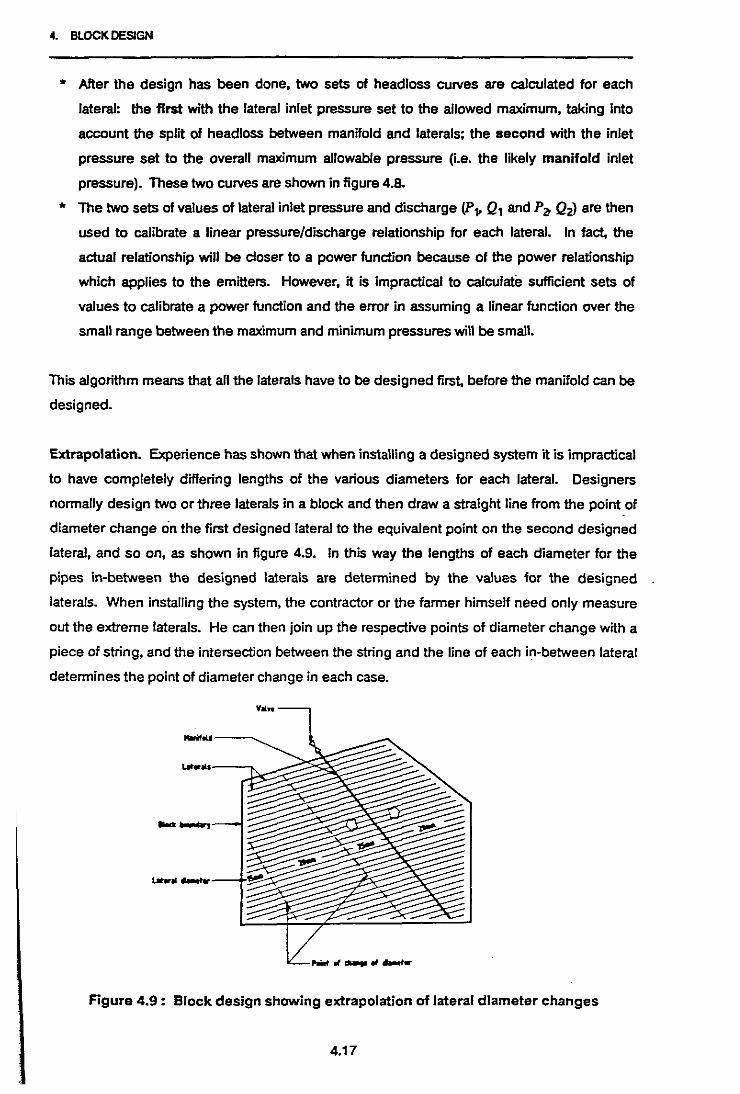
4. BLOCKDESIGN
* After the design has been done, two sets of headloss curves are calculated for each
lateral: the first with the lateral inlet pressure set to the allowed maximum, taking into
account the split of headloss between manifold and laterals; the second with the inlet
pressure set to the overall maximum allowable pressure (i.e. the likely manifold inlet
pressure). These two curves are shown in figure 4.8.
* The two sets of values of lateral inlet pressure and discharge (P... Ql and P"l! Qzl are then
used to calibrate a linear pressure/discharge relationship for each lateral. In fact, the
actual relationship will be closer to a power function because of the power relationship
which applies to the emitters. However, it is impractical to calculate sufficient sets of
values to calibrate a power function and the error in assuming a linear function over the
small range between the maximum and minimum pressures will be small.
This algorithm means that all the laterals have to be designed first, before the manifold can be
designed.
Extrapolation. Experience has shown that when installing a designed system it is impractical
to have completely differing lengths (If the various diameters for each lateral. Designers
normally design two or three laterals in a block and then draw a straight line from the point of
diameter change on the first designed lateral to the equivalent point on the second designed
lateral, and so on, as shown in figure 4.9. In this way the lengths of each diameter for the
pipes in-between the designed laterals are determined by the values for the designed
laterals. When installing the system, the contractor or the farmer himself need only measure
out the extreme laterals. He can then join up the respective points of diameter change with a
piece of string, and the intersection between the string and the line of each in-between lateral
determines the point of diameter change in each case.
-...--........
--
Figure 4.9: Block design showing extrapolation of lateral diameter changes
4.17

4. BLOCKDESIGN
The computer algorithm allows for this by incorporating an extrapolate function. The
designer specifies any two extreme laterals that have already been designed and then the
computer extrapolates the lengths of each diameter for the intermediate laterals. The
extrapolation is done linearly between lengths of like diameters. This means that if the length
of any particular diameter is greater than zero on one of the laterals and equal to zero on the
other one, then the lengths of this diameter on the intermediate laterals will gradually
decrease down to zero.
4.4 The Computer Programs
The computer models for block design have been written in Turbo-PascaJ (Borland Int. 1985)
for Ms-DOS (Microsoft Inc. 1983) based personal computers. They incorporate a number of
different functions that have been integrated into a single package, as shown in Appendix ta,
The package is menu driven and consists of four different modules, viz :
* data base maintenance;
* the layout module;
* the design module; and
* the evaluation module.
The first three of these modules are discussed in sections 4.4.1, 4.4.2 and 4.4.3 respectively.
The evaluation module is discussed in chapter 5.
In addition, four utility functions have been programmed to operate as so called pop-up
windows. These are windows that can be popped onto the screen temporarily over any
current screen and then popped down, leaving the screen as it was preViously. These utilities
include:
* Pipe data base look-up table;
* Emitter data base look-up tables;
* a program help facility; and
* a maximum length calculator.
These utilities are discussed further in section 4.4.4 below.
4.4.1 Data base maintenance.
Maintenance of the data base is carried out via on-screen editing of the input tables for both
the pipes and the emitters.
4.18

4. BLOCKDESIGN
Pipes. The pipe data base consists of two different tables :
* A general table listing:
• all the available pipe materials;
• the available classes for each material; and
- the values ofthe four parameters in the headloss formula (eq. 4.1) for each material.
* Aset of tables, one for each pipe material, showing:
• the nominal diameters that are available;
And for each available class for each of these nominal values :
• the internal diameter; and
• current list price per meter length.
Emitters. The emitter data base consists of a single 'page" display for each emitter, as shown
in the lower right comer of figure 4.14. The user can page through this data base using the
'Pg Up" and "Pg On" keys on the computer keyboard. The display for each emitter shows :
• an identification code;
- the manufacturer;
- the emitter name;
- its size;
- the k:and x coefficient values for the pressure/discharge equation (eq. 4.2);
- the list price of the emitter; and finally
- five sets of pressure/discharge operating points taken from information supplied by the
manufacturers.
Functions at the bottom of the emitter display page enable the user to :
* calibrate the k and x values from a minimum of three operating points;
* calculate the pressure value from any given discharge, or vice versa, using the calibrated
k and x values;
* store the emitter information in the data base; and
* delete the currently displayed emitter from the data base.
4.4.2 Layout.
The layout module enables the user to specify the details about the system alignments that
are required for the actual design. These include:
* the emitter and lateral spacings;
* the lengths of each lateral and the manifold; and
* the elevations of the pipes.
Provision is made for the possible layout of two laterals per row ("tramlines") and for the
possible installation of two emitters per tree in orchards.
4.19

4. BLOCKDESIGN
Figure 4.10: Table of results of the lateral design process
4.4.3 Design.
This module controls the pipe designs. based on the algorithms described in section 4.3
above. The module is presented on two main display pages, one for lateral design and one
for manifold design.
The lateral design page is shown In figure 4.10 above. It shows a window of up to eight
laterals at a time. for each of which a table of the lengths (len) and equivalent number of
emitters (#Em) of up to five different diameters is shown. The three rightmost columns of the
table show totals of the length, number of emitters and cost of each lateral.
The lateral design process is operated from a pop-up menu which presents the following
functions :
4.20

4. BLOCKDESIGN
* Select a quadrant. Any block may be divided into up to four quadrants, depending on
the locations of the valve and manifold within the block. This function enables the
designer to specify which quadrant he is working in at anyone time.
* Design parameters. Selection of this function presents a pop-up window on top of the
design page, in which the user specifies the following parameters :
- the emitter, extracted from the data base;
- the nominal operating pressure. in which case the
nominal operating discharge will be displayed, or vice versa;
- the upper percentage tolerance on the nominal pressure. in which case the
maximum allowable pressure will be displayed, or vice versa;
- the lower percentage tolerance on the nominal pressure. in which case the
minimum allowable pressure will be displayed, or vise versa;
- the maximum lateral inlet pressure, which establishes the split of the allowable
headloss between the laterals and the manifold;
- the lateral pipe material, class, minimum diameter and minimum length per
diameter;
- the manifold pipe material, class, minimum diameter and minimum length per
diameter; and finally
- the discount on the list prices stored in the data base that the designer expects to be
able to obtain.
* Edit diameters. The designer will have specified a minimum allowable diameter in the
list of design parameters discussed above. The computer then selects the minimum
diameter plus the next four diameters in the data base for use in the design process.
These are displayed at the top of the display table. as shown in figure 4.10. The user is
however free to select the edit diameters function which enables him to change any of
the five diameters to alternative values, if so desired.
* Edit table. This function enables the designer to move.the cursor into the main display
table and make manual changes to any of the lateral designs. Any change that is made
to the designed values of a lateral will result in an automatic adjustment of the other
values for the changed lateral, such that the total length remains correct. All the other
displayed totals are also automatically updated.
Whilst operating in this function, the user is able to scroll the display window up or down
in order to display any particular lateral in the set that was defined in the layout phase.
4.21

4. BLOCKDESIGN
i,i ~t~li~i~l~~/;i{~isth .. ;;,i~~~f~i~~~~r"head...;~ ""'~Lj. '~<Q~ j,;j";tia<iC>-~i.iadd:."-'---.......,;.;...-"-'-..:..:..-..:-~-_....:......:......:......:..---.
do~oo.'.' iili.ao., oii.rio
00.00>00.00
, '.. '.', .j'a~· No•. 3 ...., . <froot 0 .fle" 96;S><!o 13 . <Jev: 94.2>: <Slope: 5.8X>
,i;'~~C~;·:..}~;~H~~;" ',···.'.MaxHCm) ..<; rn;~iH~~) ···'.'infitCCnL3/h) > ..
.,'. :: .. <125· 12.7> '.··~iO:4 ~ 11.0> ·<13:6·' 14'.h·· '<13~6 '·14.1>· <1.245 • 1.546>·
Figure 4.11 : Table showing design results for lateral 3
* Design. On selecting the design function, an input box appears below the main table
(see figure 4.11). The designer specifies the lateral number that is to be designed. He
can then either calculate the hydraulic characteristics (pressure and flow distribution in
the lateral) for a prespecified set of diameter lengths, or design the lateral from scratch.
The results of the design are displayed in three different forms:
0) A summary of the flows and pressures is given in the design box (figure 4.11) for the
two design curves, as discussed in section 4.3.3. This includes:
- the pressure at the end of the lateral;
- the minimum pressure in the lateral;
- the maximum pressure in the lateral;
- the pressure at the lateral inlet; and
- the flow requirement at the lateral inlet.
4.22
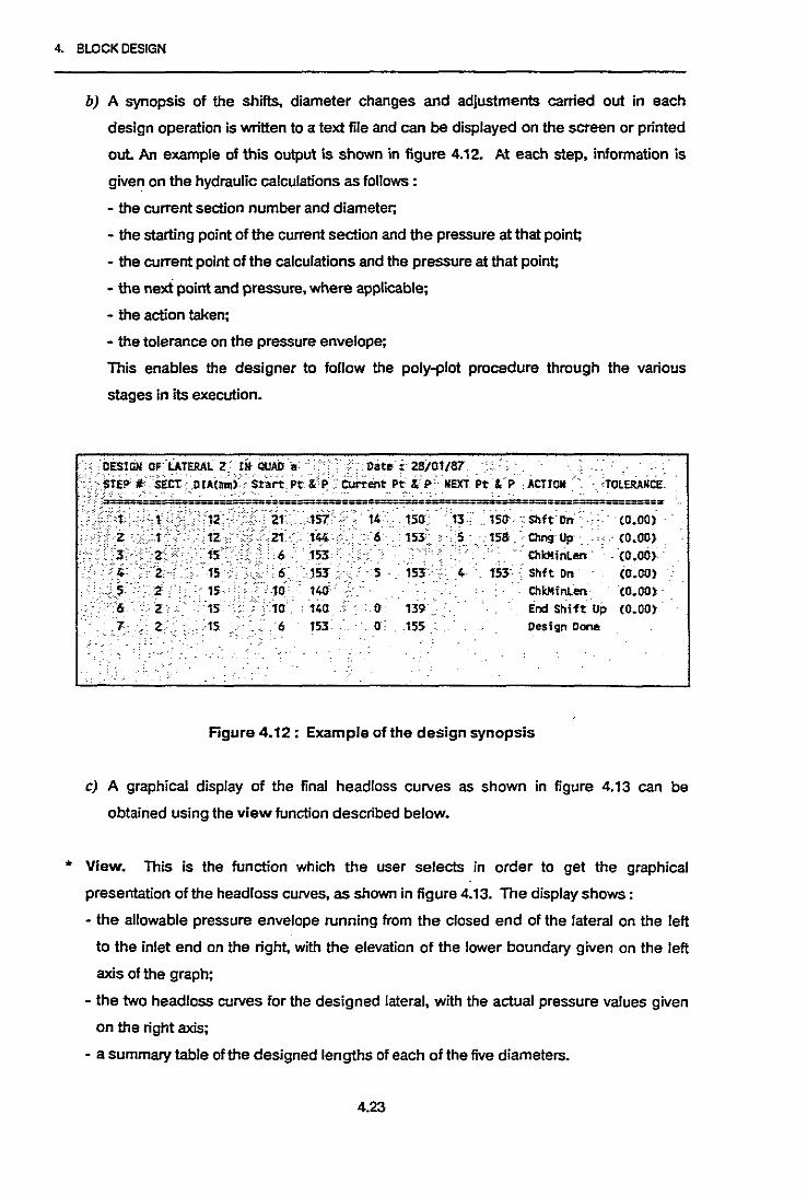
'0 139·,... 0: ,155"
4. BLOCK DESIGN
b) A synopsis of the shills, diameter changes and adjustments carried out in each
design operation is written to a text file and can be displayed on the screen or printed
out. An example of this output is shown in figure 4.12. At each step, information is
given on the hydraulic calculations as follows :
- the current section number and diameter;
- the starting point of the current section and the pressure at that point;
- the current point of the calculations and the pressure at that point;
- the next point and pressure, where applicable;
- the action taken;
- the tolerance on the pressure envelope;
This enables the designer to follow the poly-plot procedure through the various
stages in its execution.
··..0ES1Gl10FLATERAl z liHlUAil i1(llate: 2a/0t/sr: ...... STEP ~smo IA(";'; si~rt Pt I. ~ Current Pt & P NEXT Pt n ACTlOll'TOLERANI:C
~: :~..: =;:;;:;_ - ~=::;:~__,;: ==':--::lI==~==== =a"
IIi 150.13 .. 150 Sbft 01>< (0.00) ..
.6, 153:. <S'15S·Chn9Up (0.00) ... .' •.;. ,. . ChkMinLen· .. ·(0.00) .
, . 5 . ·153<' :4 :. ·153·. Shft Dn· (D.OO)
. CbkMfnLer, ·(0.00) .
End Shift Up (0.00)Design Done-
Figure 4.12: Example ofthe design synopsis
c) A graphical display of the final head loss curves as shown in figure 4.13 can be
obtained using the view function described below.
* View. This is the function which the user selects in order to get the graphical
presentation of the headloss curves, as shown in figure 4.13. The display shows:
- the allowable pressure envelope running from the closed end of the lateral on the left
to the inlet end on the right, with the elevation of the lower boundary given on the left
axis of the graph;
- the two headloss curves for the designed lateral, with the actual pressure values given
on the right axis;
- a summary table of the designed lengths of each of the five diameters.
4.23

4. BLOCKDESIGN
b) A synopsis of the shifts, diameter changes and adjustments carried out in each
design operation is written to a text file and can be displayed on the screen or printed
out An example of this output is shown in figure 4.12. At each step, information is
given on the hydraulic calculations as follows :
- the current section number and diameter;
- the starling point of the current section and the pressure at that point;
- the current point of the calculations and the pressure at that point;
- the next point and pressure, where applicable;
- the action taken;
• the tolerance on the pressure envelope;
This enables the designer to follow the poly-plot procedure through the various
stages in its execution.
'OESlGII· OF LATERAL , .. Iii QuAaa . '" .:. Oat.. : ·,8/0t/87 ..•.., .':·STf? ~?sEci' oiii,m,i 'Start Pt &; 'PCurrMf 'Pt .& P .., NriT Pt' & p. ACTION. TOLERANCf
I.t·. y .. 12 .:> ..i4
,.1' : 21 151 .. .. 150 .. i3 150 Shh. On (0.00), .. .. ..it .,. t· f ..·.•.12·· ·.,21 144 6· 15J . 5 .. 158 ChngUp (0.00)
,'2). ,
.... 3: ..15· 6
,153 '.
..ChkMinLen· (0.00).. ,
,".. , , ,
4 it .. 15 ·6 153 5 ,153· 4 15J Shft On (0.00), ,. .,;..;" ,
i..
146 ChkMinLen5 ... .. 15. 10 (0.00)6.'·
.., ., ..t5 10 140 0 ·n9 End Shift Up (0.00)
7 a .., t5 6 153 (I 155 Design Done
Figure 4.12: Example of the design synopsis
c) A graphical display of the final headloss curves as shown in figure 4.13 can be
obtained using the view function described below.
* View. This is the function which the user selects in order to get the graphical
presentation of the headloss curves, as shown in figure 4.13. The display shows :
• the allowable pressure envelope running from the closed end of the lateral on the left
to the inlet end on the right, with the elevation of the lower boundary given on the left
axis olthe graph;
• the two headloss curves for the designed lateral, with the actual pressure values given
on the right axis;
• a summary table of the designed lengths of each of the five diameters.
4.23

4. BLOCKDESIGN
....
.........
.....
..-.- .-
.-."
! ....... _"M ...... l """5
..". -.• •• _ ••• 0-
..........
Il
Figure 4.13: Graphical plot olthe pressure profile
resulting from the lateral design process
* Extrapolate. Selection of this function enables the designer to extrapolate the design of
a set of laterals using the results of two previously designed laterals, as discussed in
section 4.3.3.
The manifold design programs ,are similar to those for lateral design, the only differences
being the display of up to ten different diameters for the manifold and the absence of an
extrapolate function.
4.4.4 The pop-up utilities.
The four pop-up utilities are accessed from function keys on the computer keyboard, as
follows :
* F1.Help. This is an on line help facility which gives several pages of information and
assistance in working the program. On selecting this function. the page which discusses
the current activity on the screen will be popped up. The user can then scroll through
the other pages using the 'Pg Up' and 'Pg On' keys.
4.24
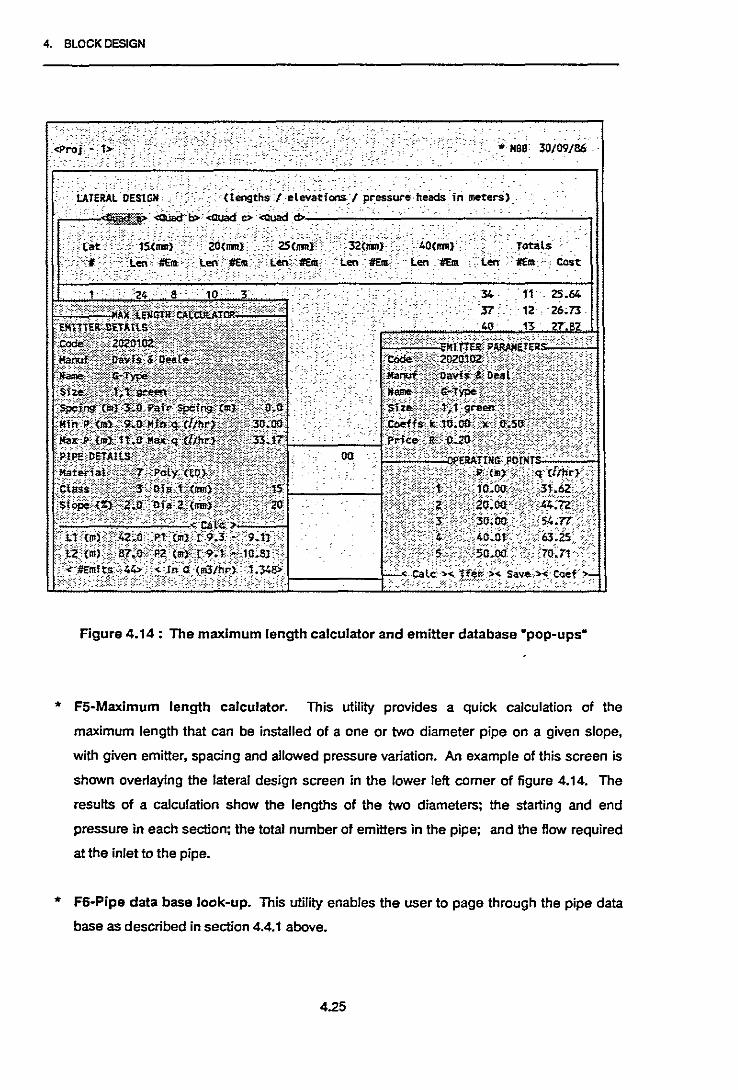
4. BLOCKDESIGN
.•. '''MBS 30i09/86·.•
.···.·(iengt~}~;i;~j~·,Pressur;headsj;;~~urs) •..•
;;.1:!'~~f~~,]'i®I' ;l~r' .;:~. a.::::'·~,..... 34 .. 11 . 2S.i54
";rr '.: .'12 . '26;73 .. 4\1' 13 27·.B
.00
Figure 4.14: The maximum length calculator and emitter database "pop-ups"
* F5-Maximum length calculator. This utility provides a quick calculation of the
maximum length that can be installed of a one or two diameter pipe on a given slope.
with given emitter. spacing and allowed pressure variation. An example of this screen is
shown overlaying the lateral design screen in the lower left comer of figure 4.14. The
results of a calculation show the lengths of the two diameters; the starting and end
pressure in each section; the total number of emitters in the pipe; and the flow required
at the inlet to the pipe.
* F6-Pipe data base look-up. This utility enables the user to page through the pipe data
base as described in section 4.4.1 above.
4.25

4. BLOCKDESIGN
* F7-Emitter data base look-up. This utility enables the user to page through the emitter
data base as described in section 4.4.1 above. An example of the display is shown
overlaying the lateral design screen simultaneously with the maximum length calculator
in figure 4.14.
Both the emitter and pipe pop-up tables have a transfer facility, which enables the designer to
select a required component and then transfer this selection to either the maximum length
calculator or the table of design parameters.
4.26

4. BLOCKDESIGN
References
1. Borland International, Publishers of Turbo-Pascal programming language for
personal computers, Ver 3.0, 1985.
2. Herbert, E., Hydraulic design : the useofPoiyplot; Trickle Irrigation, Australia, 1971.
3. Jobling, GA, Graphical design for pipelines with flow decreasing uniformly to zero,
Agricultural Engineering Australia, 3(3), 1972.
4. Oron, G. and W.R. Walker, Optimaldesign and operation ofpermanent irrigation systems,
Water Resources Research, 17(1) : pp 11-17,1981.
5. Microsoft lne., Publishers of MS-DOS disk operating system for personal computers,
Ver 2.1,1984.
6. Perold, P.R., Design of irrigation pipe laterals with multiple outlets, Journal of the
Irrigation and Drainage Division, ASeE, 103(IR2) : pp 179-195, 1977.
7. Perold, P.R., Computer design of micro-irrigation pipe systems, Journal of the Irrigation
and Drainage Division, ASCE, 105(IR4): pp 403-417,1979.
8. Wu, I-P., A uniplot for drip irrigation lateral and .submain design, Transactions of the
ASAE, 28(2) : pp 522-528, 1985.
9. Wu, I-P. and H.P. Gitlin, Dripirrigation design based on uniformity, Transactions of the
ASAE, 17(3): pp 429-432, 1974.
10. Wu, I-P. and H.P. Gitlin, Energy gradient line for drip irrigation laterals, Journal of
Irrigation and Drainage Division, ASCE, 101(IR4) : pp 323-326, 1975.
11. Wu, I-P. and H.P. Gitlin, Sprinkler irrigation design for uniformity on slopes, Transactions
ofthe ASAE, 26(6) : pp 1698-1703, 1983.
12. Wu, I-P., TA Howell and E.A. Hiller, Hydraulic design of drip irrigation systems,
Technical Bulletin No. 105, Hawaii Agricultural Experiment Station, University of
Hawaii, 1979.
4.27
5. EVALUAllON
5. EVALUATION OF BLOCK DESIGN
5.1 Introduction
Evaluation is carried out once the design has been completed, in order to assess the
expected performance of the irrigation system. The aim of the evaluation process is to give
the designer some measure of the quality of the design, in order to :
a) Consider possible improvements through changing one or more of the values of the
various design parameters; and
b) Provide the farmer with an assessment of the expected retum on his investment.
During the development of the systems analysis of the design process (chapter 2) the
evaluation was initially considered as a separate module, coming after completion of all the
blocks and the mainline design. However it was found that this rendered the process
inflexible when working with individual blocks within a large system. In order for the designer
to evaluate and then modify a single block it would be necessary to first complete the initial
design of all the other blocks and the mainline. In addition, testing of any changes made to a
single block would entail re-evaluation of the whole system.
Therefore, since the mainline evaluation can readily be separated from the block evaluation, it
was decided to incorporate the block evaluation model as the last step in the block design
process, to be applied as an integral part of the design of each block. This means that if the
mainline has not yet been designed then some estimates have to be made of the costs and
operating characteristics of the mainline in order to carry out the block evaluation process. If
these estimates prove to be too inaccurate, then an iterative process between the block and
mainline designs may ensue.
The block evaluation model has been formulated principally on the basis of the work that was
reviewed in chapter 3. In addition, it also includes further analysis relating to the level ofoperation of the system in the field. Once an irrigation system has been installed, it can be
operated to apply any irrigation depth ranging from zero up to the system capacity. However
it will not always be most economical to operate the system at full capacity. The evaluation
process therefore includes an analysis of the operating point of the system, which is defined
as the depth of application applied by the system in response to the varying plant requirement
during the season. One of the results of the evaluation process is a calculation of the
5.1

5. EVALUATION
optimum operating point; both an overall seasonal value and values for individual applications
during the season.
This chapter presents a detailed analysis of the model structure, together with a review of
some additional relevant literature. This is followed by a description of the computer
programs.
5.2 Basic Model Structure
The proposed evaluation model is divided into two distinct phases. The first looks at the
water distribution patterns that result from the designed system in a given block and the
second carries out an economic cost/benefit analysis of the system. An outline of the basic
input and output in each of these analyses is shown in figure 5.1.
5.2.1 Water distribution analysis.
This analysis entails calculation of the parameters listed under the "OUTPUT" column in figure
5.1. Several different procedures for the calculation of these parameters from field data are
shown in chapter 3. Since it is impractical to measure the discharge of every emitter in an
operating system in the field, the calculation procedures are based on assumed statistically
determined distribution functions. In the case of the evaluation model however, it is not
necessary to assume any mathematical function for the distribution pattern since the•
discharge at each emitter can be calculated directly. Hence each of the evaluation
parameters can be calculated numerically from the emitter discharge values•.
The coefficient of uniformity is calculated as the Christiansen coefficient, given by equation
3.17 :
Where
ace = 100[ 1 - ( :l: Ix; -XIJINX]
N = the number of observations X; •
X = the average application depth.
(3.17)
It should be noted that the Christiansen coefficient was originally formulated as a measure of
the water distribution in the field, determined on the basis of the variation in spread around
each sprinkler (the "within emitter variationj. In this case however, it represents a measure
of the variation in discharge from each emitter (the "between emitter discharge" variation).
It has been used interchangeably in the literature and has become commonly accepted as
representing both of these concepts, even though they have quite different applications.
5.2

5. EVALUATION
The maximum discharge. minimum discharge and percentage variation also provide an
indication of the efficiency of the design algorithm. The percentage discharge variation, Var,
is given by:
(5.1)
Where qmax = the maximum emitter discharge in the system;
qm;n = the minimum emitter discharge in the system;
qav = the average discharge.
The final parameter that is determined by the distribution analysis is a list of any lateral
containing one or more emitters operating at a pressure value that is outside of the limits
defined for the pressure envelope. This enables the designer to identify any specific areas in
the field which might be inadequately designed, possibly as a result of having been
established by using the extrapolate function rather than the actual design function.
Atter completing the block design, the required pressure at the valve will be known. However
for a number of reasons related to the nature of the system and the prevailing topography, the
designer may wish to operate the block valve at a different pressure, which will affect the
performance of the system. The evaluatlcn model therefore calculates all the
abovementioned parameters for a series of different operating pressures. Four sets of values
are presented, being respectively 0.8, 1.0, 1.2 and 1.4 times the design value. The designer
may also specify any other valve pressure for which he might want to calculate the evaluation
. parameters.
Comparison of the results for the different operating pressures provides an indication of the
sensitivity of the system to either over or under-pressure operation. These effects can be
further considered by studying the results of the economic analysis for each different
operating pressure. In this way the designer is able to make a rational decision on the most
appropriate operating pressures in the system and the extent to which any pressure
regulation may be required in the mainline.
5.2.2 Economic cost benefit analysis.
Once the water distribution analysis has been completed the designer must specify a valve
operating pressure for which the ensuing economic analysis will be carried out.
This analysis entails estimating the yield that will result from the designed system and then
comparing the income resulting from the yield with the various costs involved in generating
this yield. The evaluation is carried out on the basis of the economic return, both per unit of
5.4

5. EVALUATION
cultivated area and per unit of water used. The specific parameters generated by the analysis
are shown in figure 5.1.
The main measure of financial return generated by the analysis is the equivalent annual
worth (EAW) of the project, which is established as follows: A conventional Nett Present
Worth (NPW) analysis of the system is calculated using different inflation rates for energy
costs, other production costs, and producer prices respectively. The EAW is then
obtained by converting the NPW value back to an annual figure using a capital recovery
calculation with the preVailing project discount rate, which reflects the overall cost of money.
Thus the EAW value represents a measure in current financial terms of the average annual
return that will be obtained from the system over its expected lifespan.
The input required for the model includes:
* the emitter discharge values;
* a breakdown of the expected seasonal plant water requirements;
* the price earned for the produce per unit of yield;
* details of the capital costs of the system, which include the cost of the all the
block-system elements and the value of the mainline which can be apportioned to the
block being evaluated;
* details of the operating costs of the irrigation system;
* a breakdown of other non irrigation-l'etated operating costs, separated into yield
dependent and yield independent components;
* prevailing rates of inflation for the producer price, energy costs, production costs and the
overall market rate; and the project discount rate.
A more detailed mathematical derivation of the model is given in section 5.4 below.
5.2.3 System operation.
In order to carry out the economic analysis, the depth of water to be applied by the system (its
"operatingpOint") during the season must be known. It has previously been common practice,
for the purpose of this type of analysis, to assume that the average application depth is always
equal to the expected plant requirement However, the system can in fact be operated to
apply any depth between zero and the maximum design capacity. If the distribution
uniformity of the system is low, then it may be desirable to generally over-irrigate in order to
ensure that as much of the field as possible obtains the amount of water required for
maximum yield. Alternatively, it may be more economical to deliperately under-irrigate in
order to reduce operating costs and/or conserve water.
5.5

5. EVAlUATION
This latter practice. which is known as deficit irrigation. has been increasingly considered in
recent years. It entails a trade-off of reduced yield and hence reduced earnings for a
reduction in the operating costs and a saving in water usage. If the system is deliberately
designed for deficit irrigation practice, then its maximum capacity can be reduced and this
may also generate a reduction in the capital costs of the system.
The evaluation model includes an analysis of this aspect of the design problem. A dynamic
programming algorithm has been developed to determine the optimal seasonal operating
point for the designed system. based on the expected water requirement in individual periods
during the season. The mathematical derivation of the optimization model is shown in section
5.5 below.
5.2.4 Application oftha model
Thus by using the model described above. the designer is able to evaluate a given design in
terms of its expected distribution and economic performance characteristics. Through
iterative use of the model, it will be possible to generate a three dimensional sensitivity
analysis of EAW vs UCC vs operating point.
Similarly. the relationships between any of the design parameters and the expected system
performance can also be investigated. One of the most commonly considered of these
relationships is that between allowed pressure variation and UCC. The results of some of
these investigations are shown in chapter 7•.
5.3 Yield Estimation
The core of the economic evaluation model is the yield estimation equation that was given in
chapter 3 :
Where
i lllllX
Y = AT Jy(i) f(i) Iii
fmin
Y = the expected total yield from a field of areaAt ;
y(i) = the yield per unit area as a function of the irrigation depth, i;
f(i) = the frequency distribution function of irrigation depths
(3.31)
In order to evaluate this integral, both the frequency distribution of irrigation depths function,
f(i). and the water/yield function. y(i), must be known. As discussed above, f(i) can be
5.6
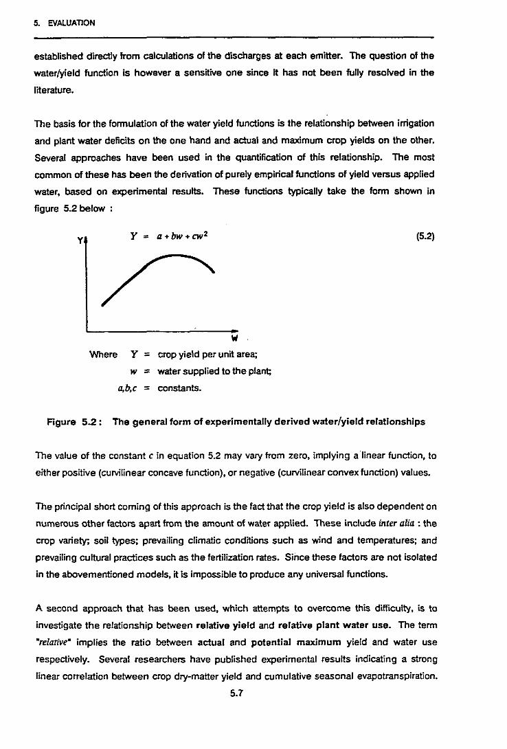
5. EVALUATION
established directly from calculations of the discharges at each emitter. The question of the
water/yield function is however a sensitive one since it has not been fully resolved in the
literature.
The basis for the formulation of the water yield functions is the relationship between irrigation
and plant water deficits on the one hand and actual and maximum crop yields on the other.
Several approaches have been used in the quantification of this relationship. The most
common of these has been the derivation of purely empirical functions of yield versus applied
water, based on experimental results. These functions typically take the form shown in
figure 5.2 below :
y
W
Where Y = crop yield per unit area;
w = water supplied to the plant;
ab,c = constants.
(5.2)
Figure 5.2: The general form of experimentally derived water/yield relationships
The value of the constant c in equation 5.2 may vary from zero, implying a"linear function, to
either positive (curvilinear concave function), or negative (curvilinear convex function) values.
The principal short coming of this approach is the fact that the crop yield is also dependent on
numerous other factors apartfrom the amount of water applied. These include inter alia: the
crop variety; soil types; prevailing climatic conditions such as wind and temperatures; and
prevailing cultural practices such as the fertilization rates. Since these factors are not isolated
in the abovementioned models, it is impossible to produce any universal functions.
A second approach that has been used, which attempts to overcome this difficulty, is to
investigate the relationship between relative yield and relative plant water use. The term
"relative" implies the ratio between actual and potential maximum yield and water use
respectively. Several researchers have published experimental results indicating a strong
linear correlation between crop dry-matter yield and cumulative seasonal evapotranspiration.
5.7
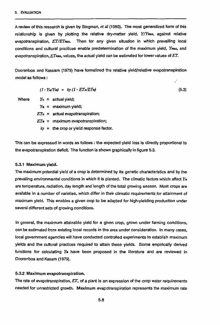
5. EVAlUATION
A review of this research is given by Stegman, et at (1980). The most generalized form of this
relationship is given by plotting the relative dry-matter yield, Y/Ymax, against relative
evapotranspiration, ET/ETmax. Then for any given situation in which prevailing local
conditions and cultural practices enable predetermination of the maximum yield, Ymax, and
evapotranspiration, ETmax, values, the actual yield can be estimated for lower values of ET.
Doorenbos and Kassam (1979) have formalized the relative yield/relative evapotranspiration
model as follows :/
(l-Ya/Ym) = ley (1- ETa/ETm) (5.3)
Where Ya = actual yield;
Y,. = maximum yield;
ETa = actual evapotranspiration;
ET,. = maximum evapotranspiration;
ley = the crop or yield response factor.
This can be expressed in words as follows: the expected yield loss is directly proportional to
the evapotranspiration deficit The function is shown graphically in figure 5.3.
5.3.1 Maximum yield.
The maximum potential yield of a crop is determined by its genetic characteristics and by the
prevailing environmental conditions in which it is planted. The climatic factors which affect Ym
are temperature, radiation, day length and length of the total growing season. Most crops are
available in a number of varieties, which differ in their climatic requirements for attainment of
maximum yield. This enables a given crop to be adapted for high-yielding production under
several different sets of growing conditions.
In general, the maximum attainable yield for a given crop, grown under farming conditions,
can be estimated from existing local records in the area under consideration. In many cases,
local government agencies will have conducted controlled experiments to establish maximum
yields and the cultural practices required to attain these yields. Some empirically derived
functions for calculating Y,. have been proposed in the literature and are reviewed in
Doorenbos and Kasam (1979).
5.3.2 Maximum evapotranspiration.
The rate of evapotranspiration, ET, of a plant is an expression of the crop water requirements
needed for unrestricted growth. Maximum evapotranspiration represents the maximum rate
5.8

5. EVAlUATION
of transpiration of a healthy crop grown in a large field under ideal agronomic conditions and
in particular with adequate water. Determination of ET. is an important aspect of the design
problem since it is equivalent to the plant water requirement and hence determines a number
of factors relating to the capacity of the system. A general function for ET. is given by :
ET. = koETa (mm/day) (5.4)
Where ETa = the reference evapotranspiration;
ko = a crop factor.
The reference evapotranspiration, ETa, represents the rate of evapotranspiration, under the
given climatic conditions, of an extended surface of an 8 to 15 cm tall green grass cover,
actively growing with adequate water supply and completely shading the ground. There are
several methods for the calculation of ETa. The "Penman" and "radiation" methods provide
accurate calculation of ETa from measurements of climatic data including vapour pressure,
wind speeds, temperature, sunshine duration and radiation. The more commonly used "pan
evaporation" method is simple and adequately accurate for most farming requirements. By
this method, ETa is calculated from:
ETa = kpEp (mm/day) (5.5)
Where Ep = the evaporation from an unscreened class A evaporation pan (mm/day):
kp = the pan coefficient which can be obtained from reference tables (see
Doorenbos and Kassam) for given estimations of the prevailing wind,
relative humidity and surrounding ground cover conditions.
The crop factor, ke, varies with the stage of growth of the plant and is dependent on the
humidity and wind conditions under which the crop is being grown. General values for most
crops are readily available in a number of references (Doorenbos and Kassam) and more
specific values for local conditions are usually published by government agencies.
5.3.3 Actual evapotranspiration.
The crop water demand, ETa, must be met by the available water in the soil, via the root
system of the plant The actual rate of water uptake by the plant plus evaporation, ETa, is
determined by the level of available water in the soil.
The amount of water that can be stored in the soil and then extracted by the plant is
dependent principally on the physical properties of the soil and also on the type of crop under
consideration. A model that has been widely accepted for estimating ETa is as follows :
5.9
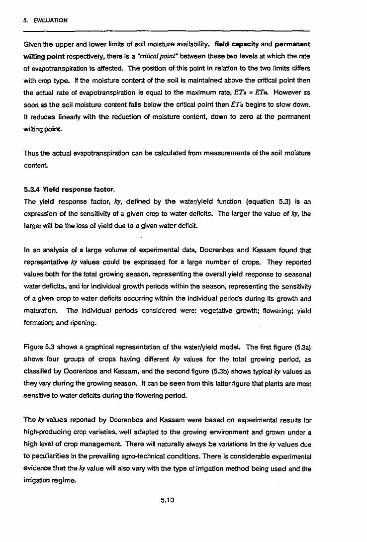
5. EVALUATION
Given the upper and lower limits of soil moisture availability, field capacity and permanent
wilting point respectively, there is a "critkalpoint" between these two levels at which the rate
of evapotranspiration is affected. The position of this point in relation to the two limits differs
with crop type. If the moisture content of the soil is maintained above the critical point then
the actual rate of evapotranspiration is equal to the maximum rate, ETa =ETm. However as
soon as the soil moisture content falls below the critical point then ETa begins to slow down.
It reduces linearly with the reduction of moisture content, down to zero at the permanent
wilting point.
Thus the actual evapotranspiration can be calculated from measurements of the soil moisture
content
5.3.4 Yield response factor.
The yield response factor, ky, defined by the water/yield function (equation 5.3) is an
expression of the sensitivity of a given crop to water deficits. The larger the value of ky, the
larger will be the loss of yield due to a given water deficit
In an analysis of a large volume of experimental data, Doorenbos and Kassam found that
representative ky values could be expressed for a large number of crops. They reported
values both for the total growing season, representing the overall yield response to seasonal
water deficits, and for individual growth periods within the season, representing the sensitivity
of a given crop to water deficits occurring within the individual periods during its growth and
maturation. The individual periods considered were: vegetative growth; flowering; yield
formation; and ripening.
Rgure 5.3 shows a graphical representation of the water/yield model. The first figure (5.3a)
shows four groups of crops having different fey values for the total growing period, as
classified by Doorenbos and Kassam, and the second figure (5.3b) shows typical fey values as
they vary during the growing season. It can be seen from this latter figure that plants are most
sensitive to water deficits during the flowering period.
The ky values reported by Doorenbos and Kassam were based on experimental results for
high-producing crop varieties, well adapted to the growing environment and grown under a
high level of crop management. There will naturally always be variations in the ky values due
to peculiarities in the prevailing agro-technical conditions. There is considerable experimental
evidence that the ky value will also vary with the type of irrigation method being used and the
irrigation regime.
5.10
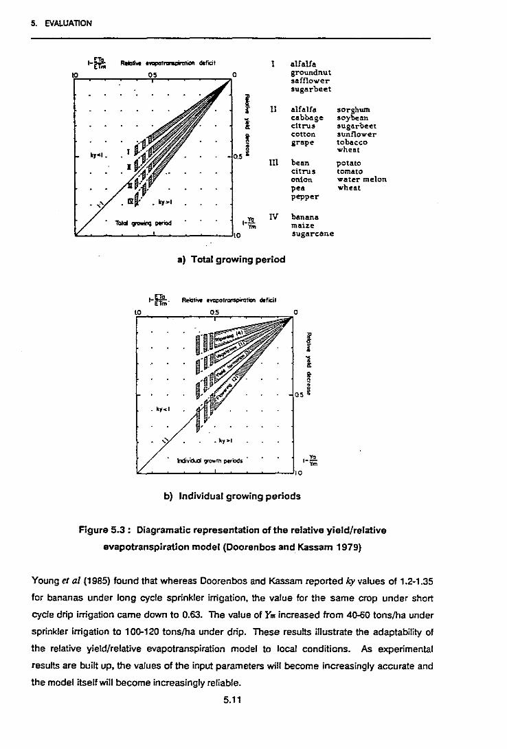
5. EVAlUATION
I-ffi; RtIotive tvapOttarllElinrtiOft defcit I alfalfaEmgroundnuttosarnoW'ersugarbeet
I11 alfalfa sorghumr
icabbage soybeancitrus auger-beer
i cotton aunf'lcwer-grape tobacco
0.5 i wheatItJcl p
JJI bean potatocitrus tomatoonion water melonpea "heatpepper
"I-I! IV banana1lltoI_ period
Ym maizeto sugarcane
a) Total growing period
m. Rebtive tvacolranspirotiM defic:j'f- ETm"
to 05
ill!l:i
1~0•Q
05 ~
. k1<1
" • \p"
hivQ.d 'I"O"'lh perixts 1-!2.Ym10
b) Individual growing periods
Figure 5.3: Diagramatic: representation of the relative yield/relative
evapotranspiration model (Doorenbos and Kassam 1979)
Young et al (1985) found that whereas Doorenbos and Kassam reported k.y values of 1.2-1.35
for bananas under long cycle sprinkler irrigation, the value for the same crop under short
cycle drip irrigation came down to 0.63. The value of Ym increased from 40-60 tons/ha under
sprinkler irrigation to 100-120 tons/ha under drip. These results illustrate the adaptability of
the relative yield/relative evapotranspiration model to local conditicns. As experimental
results are built up, the values of the input parameters will become increasingly accurate and
the model itself will become increasingly reliable.
5.11

5. EVAlUATION
5.3.5 Actual yield and applied water.
It can be seen that the expected yield loss can readily be calculated for given values of ETa,
ET. and ky, and that if a value of the maximum potential yield, Y. is known for the crop under
consideration, then the expected actual yield, Yo, can be established. YIIl ET. and ky are
dependent on the crop and prevailing soil and cultural conditions, and are therefore constant
for a given design situation. ETa is dependent on the soil moisture condition; which in tum is
directly related to the gross water supply, consisting of (I) the initial soil moisture content at
the start of the season, (ii) the water added to the soil due to natural rainfall and (m) the water
applied by irrigation, M.
Thus if a relationship could be established between ETa and M then the expected yield could
be estimated from the irrigation application. In fact, a number of researchers have proposed a
one-to-one relationship between ET. and M on the basis that the water applied by irrigation
directly replaces the water evapotranspired by the plant. This implies a linear relative
yield/relative irrigation application model, equivalent to the relative yield/relative
evapotranspiration relationship:
(l-YalYm) = ky(l-WET.l (5.6)
In terms of this model, the expected yield will increase linearly with the amount of water
applied by irrigation up to a maximum, Y.. alter which it will remain constant. This model is
supported by a large volume of research, some of which is reviewed by Warrick and Gardener
(1983) in defense of the linear model. Shalhevet et oJ (1976) calibrated a number of linear
regression models of yield versus applied water, for several different crops. The models were
based on experimental results and gave good goodness-of-fit statistics, thereby supporting
the linear response hypothesis.
It has been found that the maximum yield level is maintained for considerable levels of
over-irrigation, above which the yield may begin to come down in conditions of poor drainage
and excessive nutrient leaching. The model has therefore been considered valid for the type
of analysis required for the design problem, where optimal irrigation levels will not be greatly
in excess of that required for maximum yield.
5.3.6 Yield loss.
Thus for a given irrigation requirement to achieve maximum yield, JR, and average
application, M, the expected yield loss can be calculated as follows :
5.12

5. EVAlUATION
For each emitter an application factor is calculated by :
AI; = (q;!q•..,). (lAIIR)AI; = 1
(5.7)
Where AI; = the application factor at emitter ;;
q i = the discharge from emitter ;;
q.v = the average emitter discharge.
Then the yield loss for each emitter, YL;. is given by:
YL; = ley(I-A!;) Y,.
And the total yield loss for the block, YLb is given by :
YLb = Y,. (IYL; )1 n; (tons/Ha);
(5.8)
(5.9)
Where n; = the total number of emitters in the block.
5.4 Economic calculations
5.4.1 Inflation.
Inflation can have a significant effect on the viability of a development project. particularly
when it is evaluated over a long period. The lifespan of irrigation development projects is
typically taken as between 10 and 20 years. Furthermore, the economics of agricultural
projects are affected by several different cost and income parameters, each of which might be
inflating at a different rate. These parameters can be grouped as follows:
* production costs;
* energy costs;
* general cost of money; and
* the producer price (the price paid to the farmer for his produce).
The economic evaluation model incorporates four different inflation rates, one for each of the
abovementioned factors, as input variables to be specified by the designer.
A number of different approaches have been proposed to account for the effects of inflation.
in the economic evaluation of development projects. The method used in the proposed
model has been modified from Hanke et al (1975) and is given by :
5.13

5. EVAlUATION
(l-t) = (l+l)j(l+r) (5.10)
Where i = the rate of interest to be used in ensuing discounted cash flow analyses;
I = the rate of inflation;
r = the discount rate.
5.4.2 Discount rate.
The discount rate is the rate used in the discounted cash flow analyses to relate future worth
to present value. The question of the most appropriate rate to use for agricultural
development projects is a complex one. For most commercial projects of a private nature, the
opportunity cost of the investment represents a reasonable measure for calculating the
economic worth of the project. In other words, the discount rate can be taken as being equal
to the rate that could be earned from an alternative investment, commonly the prevailing bank
rate. However, there is varying opinion with regard to the evaluation of agricultural projects.
On the one hand, experience has shown that farmers do not generally perceive the
opportunity costs of a project as being important They are often strongly motivated by the
desire to develop the land as fully· as possible, so as to foster a feeling of permanent
ownership and stability. In other words, they take a long tenn view of their operation, and any
proposed development cannot therefore be evaluated purely in terms of the immediate return
on investment that will accrue. Also, farmers are inclined to attach more weight to capital
costs which require immediate expenditure. than to future operating costs. even when these
operating costs fonn the dominant portion of the total costs. This is because capital
expenditure normally has a greater impact on the farmer's cash-flow situation than operating
costs. These factors all mitigate for a low discount rate to be used.
Similarly, in the case of agricultural projects that are initiated by development agencies the
need for a rapid return on investment is often supplanted by the aim of stimulating rural
development This also mitigates for a lower than nonnal discount rate.
On the other hand, Keller (1983) argues that agricultUral development projects are naturally of
a high risk nature, and economic evaluations of these projects should therefore reflect this
through the use of a discount rate in the region of 10% higher than the prevailing interest
rates.
It can be seen therefore that the value of the discount rate to be used in the analysis should
be decided subjectively to reflect the preferences and objectives of the developer. It is
therefore incorporated into the evaluation model as a user specified variable.
5.14

5. EVALUATION
5.4.3 Costs.
The different cost elements incorporated into the model are as follows :
* FIXed costs. These include:
• equipment and installation costs of both the block and a portion of the mainline equal to
the ratio of the block area to the total scheme area.
• system maintenance costs, again for both the block and a representative portion of the
mainline.
• fixed production costs, representing those costs of production other than direct
irrigation costs, that are fixed and not related to the size of the yield. These typically
include tractor and machinery costs, land preparation costs, chemicals, labour and
interest on operating finance.
* Yield related production costs, which typically include items such as harvesting,
packing and in some cases fertilization.
* System operating costs, which include energy and direct water costs.
The cost of water has two possible components. Rrstly the basic cost of the actual water
used for irrigation. This may be charged directly to the farmer, in which case it is straight
forward to calculate. In some cases however, the water supply may be subsidized and then
the rate to be included in the calculations depends on the purpose of the analysis.
The second water cost component is an opportunity cost which may be applicable when the
available water supply is limited and there are a number of altemative uses competing for the
water. It represents the potential additional benefits that could be realized by using the water
elsewhere. The opportunity cost of water is particularly relevant in the case of deficit
irrigation, where reduced application will result in a saving of water.
5.4.4 Return on investment calculations.
The equivalent annual worth, EAW, is derived in the following steps:
1) Present value factors for the four groups of parameters discussed above are calculated
using the conventional present value formulation:
PVF = [(l+iYV-1j/i(l+iYV
Where PVF = the present value factor;
i = the interest rate (%/100);
N = the period of analysis (years).
5.15
(5.11)

5. EVAlUATION
The value of the interest rate, i, is calculated for each factor from equation 5.10, using the
different inflation rates. Four present value factors are calculated, being respectively:
"PVF.J1rod"for production costs;
"PVF_energy" for energy costs;
"PVF earning" for the producer price;
"PVFJeneral" for the general cost of money.
2) The cost elements are then calculated as follows :
k...fixed = tot_captI_costs + (tot_ maint_costs +fixed.J1rod_costs) • PVF"'prod (R/Ha) (5.12)
(R/ton) (5.13)
= [(tot energy cost. PVF energy) +- - -«water_bose_cast+ water_apport_cost) .PVFJeneral)}*Ab .Eag.1O (R/mm) (5.14)
Where k...fixed = the fixed costs over the life of the project, ammortized to present
value terms;
k.Yield = the yield related operating costs over the life of the project,
ammortized to present value terms;
k:_operat = the non yield related operating costs over the life of the project,
ammortized to present value terms;
tot_captl_casts, tot_rnaint_costs andfixed"'prod_casts are the equipment, maintenance
and fIXed production costs respectively, as defined in section 5.4.2;
yield.J1rod_costs are the yield related production costs given in R/ton of produce;
tot_energy_cost = the total energy cost per cubic meter of water
= base_energy..Jate .Xl'1367 .0.75 (R/m3 of water);
base_energy-fate is given in R/kWhr;
Xl' = the pump operating head (m);
water_bose_cost and water_apport_cost are given in R/m3 of water;
Ab = the area of the block (Ha);
Eag = the gross efficiency of the system, reflecting losses in the system and
to the atmosphere.
3) The present value of nett earnings from production, nett_earn, is given by:
nett_earn = (prod"'price. PVF_earning) - k:.Yield
Where prod...price = the producer price paid to the farmer (R/ton).
5.16
(Rlton) (5.15)
5. EVALUATION
4) For a given average irrigation application, L4, the expected yield loss, nb, in tons/ha is
calculated from equation 5.9. And the present value cost of this loss is given by :
NPV_cost = (nett_earn. nb .Ab) + (L4 .k_operat)
5) Thus the nett present worth of the project is given by :
NPW = nett_earn .Ym.Ab-NPV_Cost
(R)
(R)
(5.16)
(5.17)
6) Finally, a capital recovery factor, CRF, is calculated using the conventional formulation
(the inverse of the PW expression in equation 5.11) with the interest rate equal to the
project discount rate. And the equivalent annual worth is then given by:
EAW = NPW.CRF (5.15)
A sample set of all the input parameters required for the economic evaluation model is given
in table 5.1.
5.5 Operating Point
The economic analysis described above was specified for an average irrigation application,
L4. As discussed in section 5.2 above, this average application can be varied between zero
and the maximum system capacity in response to the plant requirement It is therefore
necessary to determine the optimal operating point (i.e. the optimal L4) corresponding to a
given seasonal requirement, JR. The value of L4/JR is termed the "application ratio (ar)", as
defined in chapter 3.
Furthermore, since the requirement varies during the season, the optimal application ratio
may also vary. For example, in the case of a period of low irrigation requirement it will be
feasible to raise the application ratio so that all or most of the field receives the required
application. This will not be possible during the peak requirement period since the upper limit
of the ratio will be constrained by the system capacity. The optimum point in each period will
depend on the economic factors affecting the evaluation model. For example, if the yield
response factor, ky, varies during the growing season, then it would intuitively make sense to
raise the application ratio during the period when the ky value is highest (the crop is most
sensitive to water deficits). However there is a trade-off with the higher operating costs that
ensue from a higher application.
If the total available seasonal water supply is limited but may be allocated in any way during
5.17

5. EVAlUATION
Table 5.1 Sample set of the input parameters for the economic evaluation model
Design Data1) Capacity/Ooerating regime:
Average emiller discharge *(48.6Iph) Gross application rate (6.9mm/h)
Emitter spacing (2.0 x3.5m) Gross system efficiency 96%
TotaJavailablewater 600mm Nett application rate (6.7mm/h)
Maximum irrigating time/set 6hrs
Maximum application/cycle (4Omm)
2) Area:Area of block (O.2Ha) Area of scheme 5Ha
3) Agronomic data:Maximum crop yield 53tons!Ha
Period NovlDee Dec/Jan Feb March Total
Crop water requirement (mm!cycle) 25 40 30 20 (590)Duration of period (cycles) 6 6 4 4 (20)ky value for each period 0.8 0.8 0.8 0.8
4) AppJication fractions for operation point optimization: 0.90 1.00 1.05 1.10 1.15
Economic Data1) Cap~al costs:
Material costs
-block piping and ernillers-otherblock materials
-estimated mainline costInstallation costs
-block
-mainfineOther cap~ ltems (fees,etc)
TotaJcapital costs
3) Fixed production costs:
5) Ope<atingcosts:
Energy cost
Estimated headloss In mainline
Pump deflVery pressure
Overall energy cost
Water base cost
Water opportunity cost
7) Producer price to fanner :
(R 343.07)
R 34.30
R 2500.00
R 100.00
R 500.00
R 50.00
(R 3162.54/Ha)
R 2500/Ha/yr
5c/kWh200kPa
(362kPa)
(O.66c/m3)
10c/m30c/m3
R 253.00/ton
2) Maintenancecosts:
Block 5% (R 91.66/Ha/yr)
Mainrll1e 3% (R 15.00/Ha/yr)
4) Yield relafed production costs:
R 75.00/ton
6) Discounted cash lIow analysis:
Period 15years
Discount rate 13%
Inflation rates
-energy 18%
-production costs 18%
-earnings 14%
iler1eraJ 19%
*All values within ( ) are calculated by the computer from the design and other Input data.
the season, as is typically the case when the supply comes from a storage dam, then there is
a further problem to allocate the operating points during the season in such a way that the
overall return on investment is optimized.
5.18
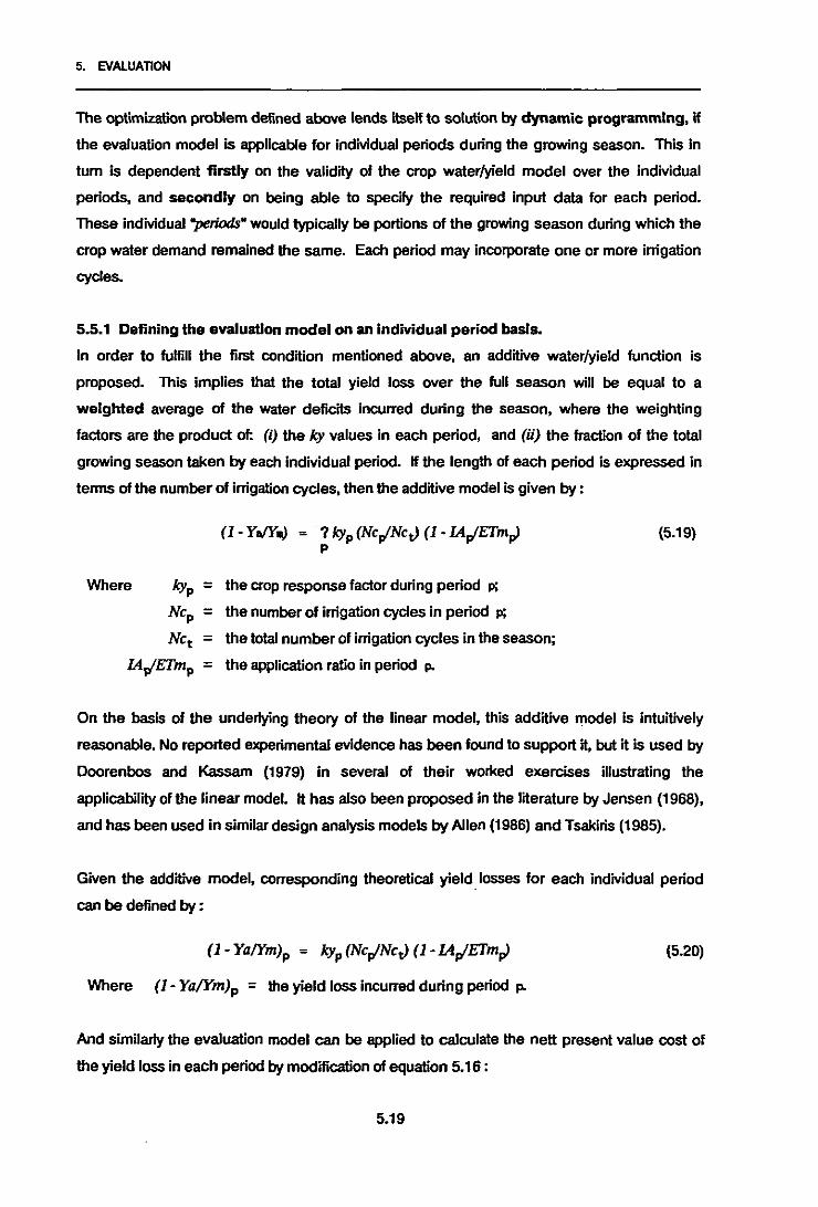
5. EVALUATION
The optimization problem defined above lends itself to solution by dynamic programming, if
the evaluation model is applicable for individual periods during the growing season. This in
tum is dependent firstly on the validity 01 the crop water/yield model over the individual
periods, and secondly on being able to specify the required input data for each period.
These individual "periods" would typically be portions of the growing season during which the
crop water demand remained the same. Each period may incorporate one or more irrigation
cycles.
5.5.1 Defining the evaluation model on an Individual period basis.
In order to fulfill the first condition mentioned above, an additive water/yield function is
proposed. This implies that the total yield loss over the full season will be equal to a
weighted average of the water deficits incurred during the season, where the weighting
factors are the product of: (i) the Icy values in each period, and (ii) the fraction 01the total
growing season taken by each individual period. If the length of each period is expressed in
terms olthe number of irrigation cycles, then the additive model is given by:
(1- YoIY-> =? kyp (Nepl'NeJ (1- IApI'ETmplp
Where kyp = the crop response factor during period p;
Nep = the number of irrigation cycles in period p;
Net = the total number 01 irrigation cycles in the season;
IApI'ETmp = the application ratio in period p.
(5.19)
On the basis of the underlying theory 01 the linear model, this additive model is intuitively
reasonable. No reported experimental evidence has been found to support it, but it is used by
Doorenbos and Kassam (1979) in several of their worked exercises illustrating the
applicability 01 the linear model. It has also been proposed in the literature by Jensen (1968),
and has been used in similar design analysis models by Allen (1986) and Tsakiris (1985).
Given the additive model, corresponding theoretical yield. losses for each individual period
can be defined by :
(5.20)
Where (1- Ya/Ym)p = the yield loss incurred during period p.
And similarly the evaluation model can be applied to calculate the nell present value cost 01
the yield loss in each period by modification of equation 5.16 :
5.19

5. EVAlUATION
(R) (5.21)
Where the terms of equation 5.21 are the same as those defined for equation 5.16 with the
subscript p referring to an individual period in the growing season.
The second condition stated above for the applicability of the evaluation model to individual
periods in the growing season was the availability of data on an individual period basis. The
specific parameters needed for this are shown in table 5.1, viz: the crop water requirement in
each period, the number of fixed irrigation cycles (of equal length) in each period and the
corresponding ky value for the period.
The crop water requirement is normally estimated from daily evaporation data, and it is fairly
common practice to group the data into periods of the same average daily requirement
These are typically, but not necessarily, monthly periods. Thus there should not be any
difficulty in defining the crop requirement for a number of different periods during the growing
season. The length of each period will also be known.
The most difficult parameter to establish for each period is the crop response factor, kyo
Doorenbos and Kassam have defined factors for a number of different crops for four different
growth periods in the plant cycle: "vegetative", "flowering", "yield formation" and "ripening". If
these are available for the crop under consideration and they can be correlated to the periods
defined by the varying water requirement, then the corresponding ky values can be used. If
no individual ky values are available then the total seasonal value can be used for each period.
5.5.2 The proposed dynamic programming model
On the basis of the foregoing, the proposed dynamic programming (OP) solution to the
problem of optimizing the system operating point is derived as follows :
The stages of the OP are the periods defined during the growing season, and the decision
variable is the operating point, or application, in each period, Up" The solution is best derived
from a backward-moving OP. In other words the solution procedure starts by calculating the
cost function at the last period in the season and then continues by working back through
each stage to the first period. The cost component of each stage is a function of the decision
variable given by :
(5.22)
5.20

5. EVALUATION
And the objective function is then: Min ['Yo Rp(lArJ ]
subject to: 'Yo lAp < Q
Where Q = the total available water supply.
The state variable, sp' represents the amount of water remaining out of the initial total, at
stage p. It is determined from the sum of the allocations in each period from the last, back
to p. For any feasible state in period p a function of the cumulative cost up to the current
stage,fp(srJ. is given by:
(5.23)
Where fl""l(SI""V = the cumulative cost up to the previous stage. which was at
period 1""1.
And then if the notation,!p(spJ, is used to denote the minimum cumulative cost at stage p for
state Spo then the recursive equation of the DP is given by :
(5.24)
Thus by calculating!p for each stage working back to period 1, the value of !1(SI)=!I(Q)
gives the total NPV_cost, and the optimal operating point at each stage can be found by
following the optimal allocation policy through the DP solution.
Both the decision variable, and consequently the state variable, are continuous over the
range of feasible operating points. In other words. literally any depth of water can be applied
by the irrigation system, within the limits of the system capacity. This implies an infinite
number of feasible values of the decision variable and a corresponding infinite number of
values of the state variable. In order to set up the DP it is therefore necessary to specify a
series of discrete values within the feasible range of the decision variable, for each stage of
the CP. This in tum will generate a limited number of feasible states at each stage. This
discretization is achieved by specifying a constant set of application ratios, from which the
actual applications can be calculated for each period.
5.5.3 Example of the DP application.
A hypothetical example is presented in order to illustrate the selling up of the CP and the
calculations carried out at each stage:
5.21
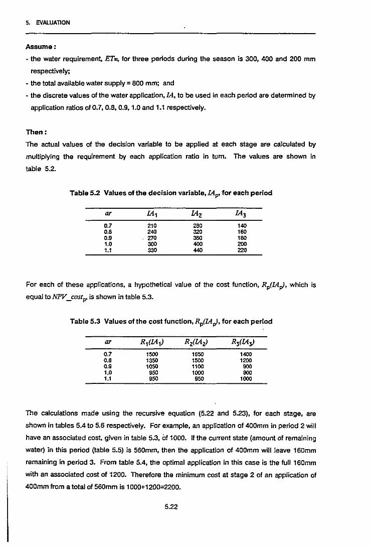
5. EVAlUATION
Assume:
- the water requirement, ETm, for three periods during the season is 300, 400 and 200 mm
respectively;
• the total available water supply =800 mm; and
- the discrete values of the water application, IA, to be used in each period are determined by
application ratios of 0.7,0.8,0.9,1.0 and 1.1 respectively.
Then:
The actual values of the decision variable to be applied at each stage are calculated by
multiplying the requirement by each application ratio in tum. The values are shown in
table 5.2.
Table 5.2 Values of the decision variable, IA p' for each period
ar IA 1 IA2 IA3
0.7 210 280 1400.8 240 320 1600.9 270 360 1801.0 300 400 2001.1 330 440 220
For each of these applications, a hypothetical value of the cost function, Rp(IA~, which is
equal to NPV_costp' is shown in table 5.3.
Table 5.3 Values of the cost function, Rp(IA~, for each period
ar R 1(IA 1) R 2(IA2) R3(IA~
0.7 1500 1650 14000.8 1350 1500 12000.9 1050 1100 9001.0 950 1000 9001.1 950 950 1000
The calculations made using the recursive equation (5.22 and 5.23), for each stage, are
shown in tables 5.4 to 5.6 respectively. For example, an application of 400mm in period 2 will
have an associated cost, given in table 5.3, of 1000. If the current state (amount of remaining
water) in this period (table 5.5) is 560mm, then the application of 400mm will leave 160mm
remaining in period 3. From table 5.4, the optimal application in this case is the full 160mm
with an associated cost of 1200. Therefore the minimum cost at stage 2 of an application of
400mm from a total of 560mm is 1000+1200=2200.
5.22

5. EVALUATION
Similarly, an application of 300mm in period 1 has a cost of 950. This leaves 500mm
remaining in period 2, for which the optimal application is 320mm at a cumulative cost of 2400
(1500 from applying 320mm in period 2 and 900 from applying 180mm in period 3). The total
cost of this strategy is therefore 3350.
Once the calculations are complete, the optimum strategy can be identified by working
through the results. From table 5.6, the minimum cost for this system is 3300, and this is
incurred from applying 240mm, 360mm and 200mm in periods 1, 2 and 3 respectively.
Table 5.4 Values of the functionf3{s~
State R3{IA~
s3 IA3: 140 160 180 200 220 ~3{S~ IA*3
140 1400 1400 140160 1400 1200 1200 160180 1400 1200 900 900 180200 1400 1200 900 850 850 200·220 1400 1200 900 850 1000 850 200
Table 5.5 Values of the functionfz{sz>
State R 2{IAz>
s2 IA2: 280 320 360 400 440 ~2{SZ> IA*2
470 2550 2900 2550 280500 2500 2400 2500 2400 320530 2500 2350 2300 2300 360560 2500 2350 1950 2200 1950 360·590 2500 2350 1950 1900 2350 1900 400
Table 5.6 Values ofthe functionf1{S1)
State R 1{IA 1)
sl IA1: 210 240 270 300 330 ~1{S,) IA*1
800 3400 3300 3350 3350 3500 3300 240·
5.6 Comparison With Other Models
Several researchers have proposed models to solve the yield-distribution integral (equation
3.31) with the specific purpose of considering system design rather than in-field evaluation.
Some of these are reviewed below for the sake of comparison with the proposed model.
5.23

5. EVALUATION
The following papers are reviewed:
Allen (1896);
English et oJ (1983);
Hill and Keller (1980);
A series of three papers by Peri, Norum and Hart published with each author listed first, in
tum (1979, 1979, 1980);
Seginer (1978);
Tsakiris (1985);
Warrick and Gardner (1983).
5.6.1 Water distribution function.
All of the abovementioned authors, with the exception of Allen, have used a functional
analysis of the water distribution pattem. In other words, they have assumed that the
distribution pattem can be adequately represented by a statistically derived mathematical
function. There is however, considerable disparity between the functions and solution
procedures that have been used.
Allen does not consider the water distribution function directly In his model, he simply
designs for acceptable limits of pressure variation within the system.
English et al use the analysis of Hart and Heerman (1976) that was discussed in chapter 3,
with the assumption of a normal distribution of the watering pattem. Their analysis requires
estimation of the mean and variance of the ETo/ET. ratio, on the basis of assumed values of
the coefficient of uniformity and the requirement and application efficiencies.
Hill and Keller present an analysis for three different irrigation systems, viz : sprinkler, drip and
furrow. A normal distribution characterized by the coefficient of uniformity is assumed for the
sprinkler system; similarly a normal distribution characterized by the emission uniformity
(Karmeli and Keller 1975) is assumed for the drip system; and empirical formulae for the water
time advance and infiltration respectively are used for the furrow system. Statistical analysis,
published by Hart and Reynolds (1955), relating irrigation depth received per increment of
area to the uniformity coefficient is used for the sprinkler system.
5.24

5. EVAlUATION
Peri et oJ develop their own analytical solutions to the yield-distribution integral for both
normal and linear functions of the water distribution pattern. Similarty, Seginer develops a
solution based on an assumed uniform distribution function. Warrick and Gardner show
mathematical formulations for live different statistical functions, in which they include
consideration of the effects of both the non-uniformity due to the system design and that due
to the heterogeneity of the soil.
Tsakiris, in part 1 of his paper, formulates three "applU:ation patternparameters" to characterize
the distribution pattern. These parameters are calibrated from experimental catch-can
measurements of the spread of water from a single sprinkler. In part 2 of his work, an
alternative analysis is presented using both normal and Pearson type 3 distributions. A
graphical (numerical) solution procedure is used to relate the coefficient of variation to the
relative mean deficit for varying application ratios.
5.6.2 Water/yleld function.
Several different approaches to the water/yield function are also reported.
Warrick and Gardner, Allen, Tsakiris and English et al all use the linear relative yield/relative
evapotranspiration model formalized by Doorenbos and Kassam. English et oJ use the
specific curve for winter-wheat, which in fact has a correction term for apparent non-linearity of
the response curve close to the maximum point Tsakiris discusses the validity of the model
in estimating the seasonal evapotranspiration deficit from data on the deficit at each irrigation
during the season. He considers both the additive and multiplicitive models.
Allen uses an additive form of the linear water yield function for individual periods of the
growing season. His model is mathematically equivalent to the model proposed in this
research (equation 5.19), but excludes the second weighting factor (ie. fraction of the total
growing season taken by each period). Also, he does not use a direct relationship between
ETa and L4. He proposes rather, multiple linear regression equations expressing ETa for
each period p as a function of L4p and the antecedent soil moisture content at the start of
each period.
Seginer uses a linear function of similar shape to the Doorenbos and Kassam function, but
with absolute values of yield and seasonal water application rather than the dimensionless
(relative) values.
5.25

5. EVAlUATION
Hill and Keller use a graphical curvilinear plot 01 experimental data relaling absolute yield to
seasonal infiltrated water depth.
Peri et al present an analysis that is essentially independent 01the water/yield function. They
postulate parameters a and b representing the economic loss incurred due to areas receiving
deficit irrigation and excess irrigation respectively. Their analysis is based on the ratio bfa,
and on the assumption that the magnitudes 01 these cost parameters are directly proportional
to the amount 01the deficit, or excess respectively. In their third paper they do present a case
specific analysis based on a quadratic absolute yield/seasonal water application function.
5.6.3 Operating point.
All 01 the authors consider the operating point as a decision variable, however they relate to it
in dillerent ways. Only Allen considers the possibility 01 varying the operating point during the
season. Peri, Tsakiris, and English et al make a stated assumption that the application ratio
remains constant throughout the season.
Allen uses the ellective irrigation application rate as a measure 01 the operating point It is
expressed as a series 01 decision variables, one lor each identified growing period in the
season. These variables are evaluated within a linear objective function which is solved by
conventional linear programming methods.
English et al, Tsakiris, and Warrick and Gardner all do not consider the question 01 optimizing
the operating point, but rather incorporate it as a decision variable that is established on a
case-by-ease basis as part 01 the input data. English et al specifically examine the feasibility
01deficit irrigation.
The analyses of Peri et aI are based entirely on optimizing the operating point; whilst both
Seginer, and Hill and Keller present methods 01finding the optimal operating point as part of
their overall analyses.
5.6.4 Model structure and solution procedure.
Only three 01the seven papers present a full economic analysis including consideration 01
complete system designs. These are the papers 01 Allen, English et al, and Hill and Keller.
5.26

5. EVAlUATION
Allen derives a single Unear objective function of "expected equivalent annual net after-tax
profit" for an irrigation development project, which is maximized by standard linear
programming. The decision variables are the capital, energy and labour requirements of the
system; expected yield; production costs; and the effective irrigation application rates for
different periods in the growing season. The model is based on linearized expressions of
various costs and labour and energy requirements versus the application rate. These
expressions are in tum derived by linear regression from a series of simulated hydraulic
designs for given system configurations. The hydraulic designs are carried out by a "critical
branch approach" for blocks and "life cycle cosIing" for mainlines. The model is best suited
to coarse level design of very large projects. The example shown by Allen in his paper is a
2 700ha. multi-crop development
Hill and Keller consider the irrigation of a single field of sugar cane to be irrigated alternatively
by a sprinkler, a drip and a gravity (furrow) system. For each alternative method, a series of
designs are developed for a range of uniformities. The capital costs associated with each of
these uniformities are identified. Then for each design, the expected yield and hence profit
are catculated using the functions discussed above with an assumed seasonal depth of
application. A search technique to find the optimal seasonal application depth is described.
The process, which is similar to that of the model proposed in this research, entails evaluating
the model for discrete increments of the application depth between prespecified limits; as the
application depth appears to be approaching the optimum, the size of the increments is
decreased. The profit calculation is done by amortizing the capital costs using a capital
recovery factor based on a fixed discount rate and zero inflation. The results are presented in
tabular form for each system, for varying uniformities, pumping requirements and producer
prices.
English et al present a case study on a field of winter-wheat to be irrigated by a moving lateral
system. Two alternative designs are presented. one for full irrigation and the other for
deliberate deficit irrigation. For each design, a system uniformity coefficient and operating
point are assumed and the expected yield is determined analytically using the models
discussed above. The water supply is from wells, so that the total supply is limited by the
capacity of the wells. The water savings realized for the deficit design are utilized by irrigating
a larger area than is possible under full irrigation. The economic analysis incorporates
equivalent annual worth calculations using two different inflation rates, 15% for energy costs
5.27
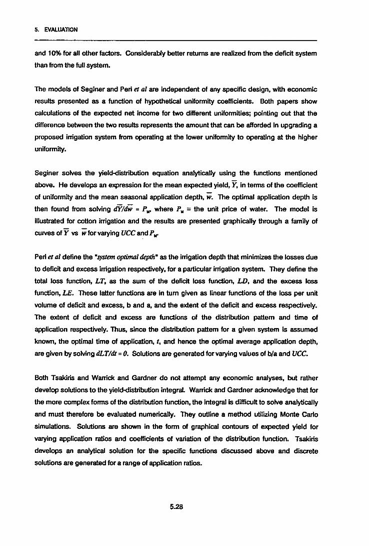
5. EVALUATION
and 10% for all other factors. Considerably better returns are realized from the deficit system
than from the full system.
The models of Seginer and Peri et al are independent of any specific design, with economic
results presented as a function of hypothetical uniformity coefficients. Both papers show
calculations of the expected net income for two different uniformities; pointing out that the
difference between the two results represents the amount that can be afforded in upgrading a
proposed irrigation system from operating at the lower uniformity to operating at the higher
uniformity.
Seginer solves the yield-distribution equation analytically using the functions mentioned
above. He develops an expression for the mean expected yield, Y, in terms of the coefficient
of uniformity and the mean seasonal application depth. w. The optimal application depth is
then found from solving dY/dw = POI' where Pw = the unit price of water. The model is
illustrated for cotton irrigation and the results are presented graphically through a family of- -
curves of Y vs w for varying UCC and p...
Peri et al define the "system optimal depth" as the irrigation depth that minimizes the losses due
to deficit and excess irrigation respectively, for a particular irrigation system. They define the
total loss function, LT, as the sum of the deficit loss function, W, and the excess loss
function, LE. These latter functions are in tum given as linear functions of the loss per unit
volume of deficit and excess, b and a, and the extent of the deficit and excess respectively.
The extent of deficit and excess are functions of the distribution pattem and time of
application respectively. Thus, since the distribution pattem for a given system Is assumed
known, the optimal time of application, t, and hence the optimal average application depth,
are given by solving tiLT/tit = O. Solutions are generated for varying values of bla and UCC.
Both Tsakiris and Warrick and Gardner do not attempt any economic analyses, but rather
develop solutions to the yield-distribution integral. Warrick and Gardner acknowledge that for
the more complex forms of the distribution function, the integral is difficult to solve analytically
and must therefore be evaluated numerically. They outline a method utilizing Monte Carlo
simulations. Solutions are shown in the form of graphical contours of expected yield for
varying application ratios and coefficients of variation of the distribution function. Tsakiris
develops an analytical solution for the specific functions discussed above and discrete
solutions are generated for a range of application ratios.
5.28
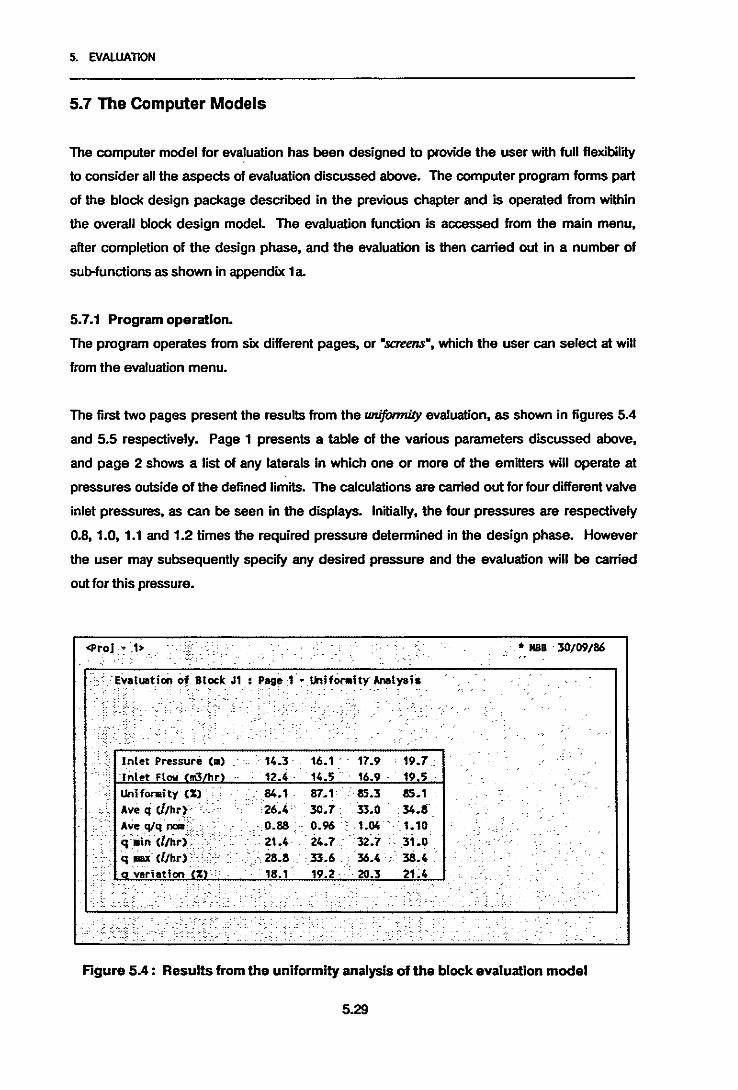
5. EVAlUAnON
5.7 The Computer Models
The computer model for evaluation has been designed to provide the user with full flexibility
to consider all the aspects of evaluation discussed above. The computer program forms part
of the block design package described in the previous chapter and is operated from within
the overall block design model. The evaluation function is accessed from the main menu,
after completion of the design phase, and the evaluation is then carried out in a number of
sub-functions as shown in appendix 1a.
5.7.1 Program operation.
The program operates from six different pages, or "screens", which the user can select at will
from the evaluation menu.
The first two pages present the results from the uniformity evaluation, as shown in figures 5.4
and 5.5 respectively. Page 1 presents a table of the various parameters discussed above,
and page 2 shows a list of any laterals in which one or more of the emitters will operate at
pressures outside of the defined limits. The calculations are carried out for four different valve
inlet pressures, as can be seen in the displays. Initially, the four pressures are respectively
0.8,1.0,1.1 and 1.2 times the required pressure determined in the design phase. However
the user may subsequently specify any desired pressure and the evaluation will be carried
out for this pressure.
<ProJ.: ·.t> ..
.·Evaluation of Block Jl : Pas,,": IKIlfo....lty Analvais
• MBa . 3()/09/M
Inlet P~ssure (m)
'Ini.t flow ni3 h.Uniforaity (:1:) , : :
Ave q (1/hr~ .Ave qlq rxoOi:' ..' '.qlii~ Cl/hr,< '•..q r8aX Cl/hr) ,', .
verhtfon .
14.3' 1&.1" 17.9 19.7 :12.4· 14.5' 16.9' 19 5 .
.. 84., 87.1'" 85.3 85.1'26.4 3().1 33.0'.34.110.88 .. 0.96 .. 1.04 -, '.1.10
.. 21.4 . 24.1..32.1 31.0. 28.8 ,'.D.& .' 36.4 38.4. 18." 19.2 '20.3 2\;4
Figure 5A: Results from the unHormity analysis of the block evaluation model
5.29

5. EVAlUAllON
Figure 5.5: Results from the uniformity analysis of the block evaluation model
The remaining four pages relate to the economic evaluation. On initiating this function, the
user will have either page 1 or page 2 displayed on the screen and will be requested to
specify which of the four displayed inlet pressures should be used for the ensuing
calculations. All the input parameters required for the economic evaluation, as listed in table
5.1, must then be specified. This is done in paqes 3, 4 and 5. Anyof these parameters which
are determined by the de5ign process or the uniformity evaluation, such as the block
equipment costs, the layout characteristics and the average emitter discharge, are carried
through and displayed on the relevant pages automatically. On initiating page 6, the
computer checks that all the required data have been supplied and then carries out the
economic evaluation. The results are displayed in both tabular and graphical format, as
shown in figure 5.6.
Atany stage intheprocess, the usermay move interactively frompage to page.
5.30
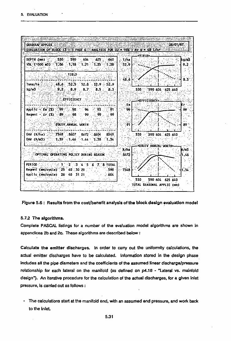
5. EVALUATION
ImJ .';,4li
530 ~9D 604 625 640;T6YALSEASONAL APPlIC loin)
.' ...'
.... ;.,
'...• il/~.
'llPTIHAl·Ol>w.n~G .POll CY DURING SEisON .'.."';:>8672
RP~t" .•·(l:'<""I·.:".·.1:23 4 567< 8.'r."5090T~l.~._. "... ,_ ·,'25 "'4D .:.30 '20 .'
Apl)Uc~~cyt;t.j 26 4D 3; 21 ;:604
85491.34 ..
' ..;;~ ..,9.2.··.
Figure 5.6: Results from the cost/benefit analysis of the block design evaluation model
5.7.2 The algorithms.
Complete PASCAL listings for a number of the evaluation model algorithms are shown In
appendices 2b and 2c. These algorithms are described below :
Calculate the emitter discharges. In order to carry out the uniformity calculations, the
actual emitter discharges have to be calculated. Information stored in the design phase
includes all the pipe diameters and the coefficients of the assumed linear discharge/pressure
relationship for each lateral on the manifold (as defined on p4.16 - "lateral VB. mainfold
design"). An iterative procedure for the calculation of the actual discharges, for a given inlet
pressure, is carried out as follows :
- The calculations start at the manifold end, with an assumed end pressure, and work back
to the inlel
5.31

5. EVAlUATION
- For the given lateral inlet pressure, the expected lateral inlet flows are calculated from
the discharge/pressure relationship. The actual emitter pressures, and hence
discharges, are calculated in tum from the lateral inlet to its end, using the given lateral
inlet pressure and inflow, the known emitter pressure/discharge relationship and a point
to point calculation of the head losses in the lateral pipes.
- On reaching the end of the lateral, the calculated remaining lateral flow is checked to
ensure that it is equal to zero. If not, then the estimated inlet flow is adjusted, and the
calculation is repeated.
- Once these calculations are satisfactorily concluded, the head loss in the manifold up to
the next lateral is calculated, using the corrected lateral inflows. This in tum enables
calculation of the inlet pressure at the next lateral.
- The process is repeated for each lateral in tum, working back to the manifold inlet A
cumulative total of the manifold flow and its pressure at the current lateral are maintained
throughout the calculations.
- Once the valve is reached, the calculated pressure at this point is compared with the
specified inlet pressure for which the calculations are being done. If the calculated
pressure is not within 1% of the specified pressure, then the end pressure that was used
to initiate the calculations is adjusted by the amount of the error minus a correction for
the non-parallel effect The whole process is repeated until the correct inlet pressure is
reached.
Calculate the uniformity parameters. The uniformity parameters are calculated by looping
through the emitter discharges in a two-pass process. The first is used to calculate the
average emitter discharge, as well as the maximum and minimum values; and the laterals in
which one or more emitters operate outside the design limits. The second pass uses the
average value to calculate the mean deviation from the mean (coefficient of uniformity). as
well as the maximum percentage variation.
Perform the dynamic programming optimization. Prior to initiating the economic
evaluation, the inputted irrigation requirement values are all rounded to the nearest 5mm. and
all subsequent calculations are carried out using 5mm increments. The DP is evaluated in
three phases :
- The cost matrix for each stage of the DP and each possible application (table 5.2 in the
example presented in section 5.5) is calculated. The program loops through each
emitter discharge and calculates the expected yield loss; this is then used to calculate
the associated NPV_cost.
5.32
5. EVAlUATION
- Maximum and minimum feasible states (remaining available water) are then calculated
for each stage, by subtracting the minimum and maximum applications respectively,
starting from the initial total at stage one. Then the cumulative cost matrices at each
stage of the DP (tables 5.3 - 5.5 of the example) are calculated for each possible state, in
5mm increments, between the established feasible maximum and minimum limits. This
is done working back from the last period to the first.
- Finally, the DP results are determined from the matrices, and the economic evaluation
parameters are calculated,
5.33

5. EVAlUAllON
REFERENCES
1. Allen. R.G••Sprinkler irrigl1lioll project design withproduction functions, Joumal of Irrigation
and Drainage Engineering, ASCE, 112(4}. 1986.
2. Doorenbos, J. and A.H. Kassam. Yield response to water. FAO Irrigation and Drainage
Paper 33. Rome. 1979.
3. English. M.J••A.G. Nelson. B.C. Nakamura, K.C. Nielson and G.S. Nuss. Economic
optimization of irrigation, Research Report PB83-265140, Water Resources Research
Institute. Oregon State University, 1983.
4. Hanke. S.H•• P.H. Carver and P. Bugg. Project evaluation during inflation, Water
Resources Research. 11(4), pp 511-514.1975.
5. Hart, W.E. and D.F. Heerman, Evaluating waterdistributions ofsprinkler irrigation systems,
Colorado StateUniversity Experimental Station Bulletin No. 128, 1976.
6. Hart, W.E., 0.1. Norum and G. Perl. Optimal seasonal irrigation application analysis,
Joumal of the Irrigation and Drainage Division ASCE, 106(1R3}, pp 221-235, 1980.
7. Hart, W.E. and W.M. Reynolds,Anao/ticai design ofsprinklersystems, Transactions of the
ASAE, 9(1}, pp 83-85,1965.
8. Hill. R.W. and J. Keller. Irrigation system selection for maximum crop Profit, Transactions
of the ASAE, 23(2}, pp 366-372, 1980.
9. Jensen. M.E.. Water consumption by agricuItural plants. In Water Deficits and Plant
Growth (T.T. Kozlowski - Ed.), Academic Press. 11(1), 1968.
10. Karmeli. D. and J. Keller. Trickle irrigation design, RainBird Sprinkler Manufacturing
Corp., Glendora Ca. USA, 1975.
11. Keller. J. Chapter 11: Sprinkler Irrigation, In SCS National Engineering Handbook,
Section 15 - Irrigation, Ch Press. 1983.
12. Norum. 0.1•• G. Perl and W.E. Hart, Application ofsystem optimaldepth concept, Joumal
of the Irrigation and Drainage Division ASCE, 105(IR4},pp 357-366, 1978.
13. Perl. G•• W.E. Hart and 0.1. Norum. Optimal irrigl1lioll depths • a method of analysis,
Joumal of the Irrigation and Drainage Division ASCE, 105(IR4}, pp 341-355, 1979.
14. Seginer. I•• A note on the economic signifit:ilIIa of uniform water application. Irrigation
Science. Vol 1, pp 19-25, 1978.
15. Shalhevet, J.• A. Mantell. H. Bieloral and D. Shimshl. Irrigl1lioll of field and orchard
crops undersemi-arid conditions. mc Pub! No 1. Volcani Center, Israel, 1976.
16. Stegman. E.C., J.T. Musiek and J.I. Stewart, Irrigation water maJllJgement. In Design
and Operation of Fann Irrigation Systems (M.E. Jensen - Ed.), ASAE Monograph No 3.,
1980.
5.34

5. EVALUATION
17. Tsakiris, G.P., Evaluating the effect ofnon-lI1Iiform and deficient irrigation - PartsI and Il,
Adv. Water Resources. Vol 8. June 1985.
18. Warrick, A.W. and W.R. Gardner, Crop yield as affected by spatial variations ofsoil and
irrigation, Water Resources Research. 19(1).pp 181-186. 1983.
19. Young, S.C.H., T.W. Sammis and I.P. Wu, BfUIIlJUl yieldasaffected bydeficit irrigation and
pattern oflatera/layouts. Transactions of the ASAE,28(2). pp 507-510.516. 1985.
5.35
6. MAINLINEDESIGN
6. MAINLINE DESIGN
6.1 Introduction
The mainline is the pipe network that distributes water from the source to the block valves. It
consists of the pipes themselves which may ramify from a single main into several sub-mains,
as shown in figure 6.1, and various control elements such as pumps, filters, fertilizer injectors
and pressure regulating valves. In general, irrigation networks have a branching structure,
implying that the network branches out from the source without ever joining back up with
itself; unlike urban water supply networks which are normally looping. This branching
structure simplifies the design problem as is shown further on in this chapter.
At the start of the mainline design process the location and operating requirements
(discharge and pressure) of each block valve are known. In most cases, the location of the
pumps (water source) is also known. The design problem consists of three distinct elements:
* determining the network layout;
* establishing the sequencing (or scheduling) of the block valves during operation; and
* sizing of the pumps and pipes.
These three problems are inter-dependent, so that the solution to anyone of them will affect
the results of the other two. It is therefore difficult to establish a gl.obally optimal solution
procedure for the whole design. For this reason, the approach adopted has been to develop
locally optimized solutions for each module. If necessary, each solution can then be modified
by a manually directed iterative process, based on the results obtained for each of the other
design modules.
This chapter provides a detailed description of each of the three solution processes, together
with a description of the computer programs that have been developed to generate these
solutions.
6.2 Network Layout
6.2.1 The design problem
The layout problem consists of establishing the lowest cost arrangement of pipes that will link
the water source to each of the block valves.
6.1

II. MAlNUNE DESIGN
F..ld border
tioM ofnVlrd grOl.ll'ld 5top.
•
-, - Dirac:dow
-, !'\~
I--
~sour,
Subllain pipes
Rgure 6.1: Schematic example of • mainline layout
In its simplest form, the solution to this problem might be seen to be the layout for which the
total length of piping is minimized. However, there are trade-offs in the pipe sizing problem
which involve exploiting the prevailing topography to offset pressure losses due to pipe
friction. These may mitigate against selecting the shortest path. For example. in the network
shown in figure 6.1 the length of the main pipe could be reduced by leading it up to the
sub-mains directly above the water source. However, this would result in the water in the
sub-mains having to be pumped up against the slope. The current arrangement allows for the
headloss due to friction in part of the sub-mains to be offset by the gain due to topography.
This means that a higher headloss can be tolerated in the sub-main sections below the main
pipe, which in tum means that smaller diameter pipes can be used over these sections.
A further consideration in determining the network layout is the operating sequence of the
block valves. In general this sequence is established in conjunction with the network layout
in such a way as to distribute the flow in the network as widely as pOSSible. In this way the
maximum discharge carried by any single branch of the network is minimized, and hence the
diameters required are also minimized.
Thus it can be seen that the optimal layout is one for which both the capital costs of the pipes
and the energy requirements for operation are minimized. A practical optimization procedure
has proved difficult to establish, since the number of possible layouts for any given situation is
theoretically infinite. Stephenson (1984) has proposed the following solution: For a given
6.2

6. MAlNUNEDESIGN
situation, a full "grid" network is defined incorporating all of the valves and the source. The
network will contain multiple loops and will generally be over-specified for the requirements of
the irrigation system. However it will incorporate a large number of alternative layouts. The
network is then trimmed by solving a linear programming problem given by :
NMin [Iq;L;]
;=1(6.1)
subject to for all j (6.2)
Where q; = the flow in each section; of the network;
L; = the length of each section ; of the network;
N = the total number of pipe sections defined for the network;
};q. L. = the sum of flows in all sections ; leading water directly into or out of valveI.)
or intersection j of the network;
Qj = the discharge flow out of the network at point j.
Thus the decision variables in this formulation are the flows in each pipe section. Any flow
that is set to zero in the solution implies that the section carrying that flow can be discarded.
The product q;L; represents an expression for the "cost" of the pipe section in terms of its
flow volume and length, so that the minimization gives a minimum cost solution. In order to
solve this problem, assumptions must be made of the flow directions in any sections that form
part of a loop. Also the solution does not consider the trade-offs related to the prevailing
topography, that were discussed above.
Buras and Schweig (1969) proposed a dynamic programming procedure for the optimal
routing of an aqueduct planned for installation in Iran. However their solution is specific to
various unique features of the design case, in particular the "herring bone" structure of the
network.
6.2.2 Proposed solution procedure
Notwithstanding the potentially infinite number of layouts for any given system, most networks
will generally have a rectangular, or close to rectangular, alignment that will facilitate the
formulation of alternative layouts. For example, in the system shown in figure 6.1, once the
direction of the sub-mains has been decided (east-west rather than north-south) then
altemative layouts are generated by moving the alignment of the connecting main. Thus if a
method for rapid evaluation of each alternative layout can be developed, then the designer
can work interactively with the computer generating a number of alternative layouts to be
6.3

6. MAlNUNE DESIGN
compared on the basis of the evaluation criterion. In this case it is important that the
alternative layouts can be specified simply and quickly on the computer, and that the
evaluation is also produced quickly, without requiring lengthy computer time.
The proposed evaluation criterion is a preliminary cost estimate, established as follows :
* An acceptable average headloss for the network (say 2% in terms of length) will be
preselected by the designer. This is used to calculate the expected headloss in the
network from each valve back to the source. This in tum enables estimates of the
required pipe-class at each section, the required pumping head for each valve, and the
pump duty.
* A first estimate of the pipe diameter at each section is then established on the basis of
the flow velocity in each section. Experience has shown that flow velocities in optimally
designed irrigation networks vary between a narrow range of to.9 to tl.8 mIs,
depending on the size of the flow and the slope of the pipe section. Thus the values
used for the diameter estimates have been set as follows :
• Flow less than 50m 3!iu: uphill 0.9m/s; downhill1.2m/s
- Flow between 50-150m3/hr: uphilll.0m/s; downhill 1.3m/s
- Flow greater than 150m 3/hr: uphilll.3m/s; downhill 1.8m/s
For sections at the ends of each branch of the network, these allowable velocities are
increased by 67%. Thus for each section the maximum flow is used to calculate the
velocity that would result from the various available diameters in the class of pipe
established in the first step described above. The smallest diameter that results in a
velocity not exceeding the allowed velocity is selected as the first estimate.
In this way the estimated cost of the network, including both the capital costs of the pipes and
the operating costs, can be calculated. The optimal layout is then the one with the lowest
expected cost.
This layout evaluation model acts as a form of screening model, before the application of a
more rigorous optimization model for the sizing of the pipes and pumps. In fact, it provides a
starting point for the optimization model, as discussed in section 6.4.4.
6.3 Valve Sequencing
Any given network will contain a number of block valves. Since it is uneconomical to design
the network for all the valves to operate simultaneously. the irrigation cycle is divided into a
number of irrigation ·shifts· (or 'sets') and each valve is allocated to operate in one of these
6.4

6. MAlNUNE DESIGN
shifts. The valves must be operated in a specified schedule, such that the hydraulic
characteristics of the network are maintained within the limits of its capacity.
The number of shifts within an irrigation cycle is established during the preliminary design
phase, and the valve operating schedule consists of a specification of which valves operate
together in each shift. It can be seen that for each alternative layout the designer will have to
specify the valve operating sequence in order to calculate the flows throughout the network.
6.3.1 The design problem
The valve sequencing problem therefore entails allocating the irrigation of each block to be
done in one of a given number of available shifts. The optimal schedule will be one for which:
aj the energy required in each shift is minimized; and
b) the maximum flow in each pipe section is minimized.
The second of these optimization objectives relates to the minimization of the capital costs of
the pipes through minimizing the required diameters. It implies spreading the required flow
in each shift aswidely as possible throughout the network.
This is a difficult optimization problem, which is not readily solved by any known techniques.
Although there has been considerable work done in optimizing real-time responses to the
operating requirements of urban water networks, very little work has been reported on the
irrigation valve sequencing problem as it is defined above.
The two sets of problems are quite different On the one hand, urban domestic water
networks tend to be multi-sourced and multi-looped. The optimization procedure revolves
around establishing the hydraulic characteristics of the network using a computer-based
network solver and then developing operating strategies for differing operating requirements.
In particular, the real-time nature of the problem implies that the network is already designed,
and therefore the second of the abovementioned optimization criteria does not apply. The
emphasis of the problem relates to optimizing the operation of the network.
Irrigation networks on the other hand are generally single-sourced and branching. Also, the
different valve pressure requirements are usually constrained within a narrow range, and the
duty point on the pump characteristic curve remains fixed during each shift. This enables
certain simplifying assumptions to be made. The emphasis of the problem shifts to one of
optimizing the design of the network.
6.5

6. MAINUNE DESIGN
Sabbagh (1986) has proposed an optimization model for the real-time case, in which an
objective of minimizing the overall energy consumption of the system is formulated, and the
pressure and flow requirements of the valves form the constraints. The model uses a network
solver and standard curve fitting techniques to calibrate the pump and system characteristic
curves. A search algorithm is then used to establish the optimal operating strategy.
Gofman and Rodeh (1978) also formulated the valve sequencing problem in terms of the
single minimum energy objective. They concluded that in this form the problem is equivalent
to the so called "independent task schedulingproblem", which has been shown (Garey et a11978)
to be NP-complete for more than two valves. This is a condition implying that no efficient
algorithm for solving the optimization problem is known or ever likely to be discovered. They
conclude therefore that the problem is best tackled by using an "approximation algorithm",
which in mathematical terms is considered satisfactory if it generates solutions that are
guaranteed to be close to the optimum.
Their proposed solution procedure employs a computer based hydraulic network solver for
interactive use in constructing the valve sequencing schedules. The user plays an important
role in directing a search for admissible schedules. Once the system has been defined, the
approximation algorithm generates a trial solution on the following basis: An upper bound, B,
is set on the total discharge allowed in a single shift. The valves are then scheduled by the
first fit decreasing method. This method treats the valves in order of decreasing discharges,
assigning each valve in tum to the earliest shift in which it will not cause the total discharge to
exceed B. For a particular value of B the algorithm will either succeed or fail. Binary search
techniques are used to find the smallest possible value of B and the algorithm has been
proved to be highly computationally efficient
6.3.2 The proposed solution procedure
The proposed solution procedure addresses both of the two abovementioned objectives (Le.
energy and pipe flow minimization). The energy requirements of the network are a function of
the pressure and discharge requirements of the valves. However, in single source irrigation
networks the operating pressure at the pump is normally determined by the maximum valve
pressure requirement, and the system sizing is optimized on this basis. In this case the
energy minimization objective can be simplified by expressing it in terms of discharge only.
And since the total discharge over all shifts is fixed, minimizing the discharge in each shift
implies minimizing the deviation of the discharge in each shift from the average discharge per
shift The two design objectives can then be formulated as follows :
6.6

6. MAINLINEDESIGN
a) for all J (6.3)
Where DJ = the deviation of the discharge in shift
shift;
from the average discharge per
vQJ ::: (I q) / I = the average discharge per shift;
v=1
v = the total number of valves;
I ::: the number of shifts per cycle;
qv ::: the discharge from valve v;
vf J ::: all valves v that operate in shift J.
b) Min [Qk.I·]::: I qk~ _ .vV<IkfFPv
for all k.J (6.4)
Where Qk.J :::
qk.v :::
FPv =
the flow in pipe section k during shift J;
the flow in pipe section k due to valve v;
the flow path in the network from the source to valve v.
As mentioned above, the second objective stems from consideration of the pipe sizing
problem. In the solution to the valve sequencing problem it is incorporated as a constraint
which facilitates the formulation of a successful approximation algorithm.
The algorithm works incrementally with each shift in tum. A tolerance level, oJ, for the
maximum allowable deviation of the total shift discharge from the average discharge is set for
shift oJ' Valves are then allocated to this shift on a basis that attempts to minimize the flows
in each section and simultaneously bring the total shift discharge to within OJ% of the
average. The value of [)J is initially set to 5%. If this tolerance cannot be satisfied, then it is
increased iteratively until the lowest value that can be satisfied is established.
When a valve is being considered for allocation to a specific shift, the algorithm calculates a
measure which has been termed the 'degree of coincidence" of the valve under
consideration with all other valves that have already been allocated to the shift. This is a
measure of the extent to which the valve under consideration will add to the maximum flows
in the network pipe sections. It is defined as follows :
6.7

6. MAINUNEDESIGN
For each section there is a minimum flow that will be required, irrespective of the valve
sequencing programme. This is determined by the largest discharge requirement of all
valves whose flow paths include the section in question. The degree of coincidence is
calculated as the product of the length of a section times the flow in that section in excess of
the established minimum flow. summed over all sections in the network. This is expressed
algebraically as follows :
(6.5)
Where vE j = the valves thus far allocated to shift j. plus the valve under
consideration for addition to the shift.
The excess flow in each section, EF~,j. is calculated as:
EFk,j = 0EFk j' = Qk j' - Qmin k. , ,
Where Qmin,k = the minimum flow in section k.
forQk,j <= Qmin,kfor Qk j' > Qmin k, , (6.6)
Then the degree of coincidence. DCv, j' of valve v in shift j is:
DC . =V,J
KX (EFk J' x L k>
1c.=1 '(6.7)
Where K = the total number of sections in the network;
L k = the length of section k,
The algorithm follows a series of steps which are described below:
1. The valvewith the largest discharge requirement is allocated to the first shift.
2. For each remaining valve its degree of coincidence with the allocated valve is calculated
and these valves are then ranked in order of increasing coincidence.
3. One valve is allocated to each remaining shift. starting from the valve that has the highest
coincidence with the allocated valve and working down in decreasing order of
coincidence.
An iterative procedure is now followed, starting with the first shift and then working with
each shift in tum :
4. The tolerance, Sj' by which the total discharge in shift j may deviate from the average
shift discharge is set to 0.05 (i.e. 5%).
6.8

8. MAlNUNE DESIGN
5. The degree of coincidence of each of the remaining unallocated valves with the valves
already allocated to shift j is calculated and the valves are ranked in order of increasing
coincidence.
6. An allocation is attempted on the basis of :
Working from lowest to highest coincidence;
Keeping the total shift discharge less than (1 + 0j) x the average shift discharge.
7. If no allocation was possible, then the value of OJ is increased by 0.05, and the process
returns to step 5.
Alternatively if an allocation was made and j>l, then a backwards checking function is
performed as follows :
For each valve already allocated to a previously completed shift, the possibility is
examined of improving the allocations by swapping with the valve that was allocated to
shift j in step 6. A swap is made if:
* the discharges in each shift after the swap remain within the respective allowed
tolerances of the average; and
* the combined degrees of coincidence of the swapped valves with the other valves
in the respective shifts is less than for the swapped valves in their original shifts.
If a swap is made, the backwards checking function continues through the remaining
allocated valves, with the last swapped valve in shift j as the candidate for the next
swap.
8. If the discharge in shift j is now greater than (1 - 0j) x the average, then the shift is fully
allocated. The algorithm returns to step 4 and continues for the next shift. If the shift is
not yet complete, then the algorithm returns to step 5 and the process is repeated.
The whole process continues until all the valves are allocated.
Although this algorithm yields a good approximation of the optimum as defined by the
abovementioned objectives, the design problem is exacerbated by the fact that practical
considerations may often override the results of the solution procedure. For example, it may
be required to have blocks of the same soil type grouped together in each schedule.
A1temativety, the schedule may be dictated by a pesticide spraying program which has an
associated drying-off requirement. In the case of manually operated systems, it may not be
practical to have valves at distal ends of the network operating together due to the distances
between them. In this case it will be preferable to group the valve schedules on a
geographical basis, which conflicts with the objective of trying to spread the flow as widely as
possible throughout the network.
Consequently it is important to provide the designer with a facility to either allocate the valve
schedules himself from scratch, or to manually overide the schedules established by the
6.9
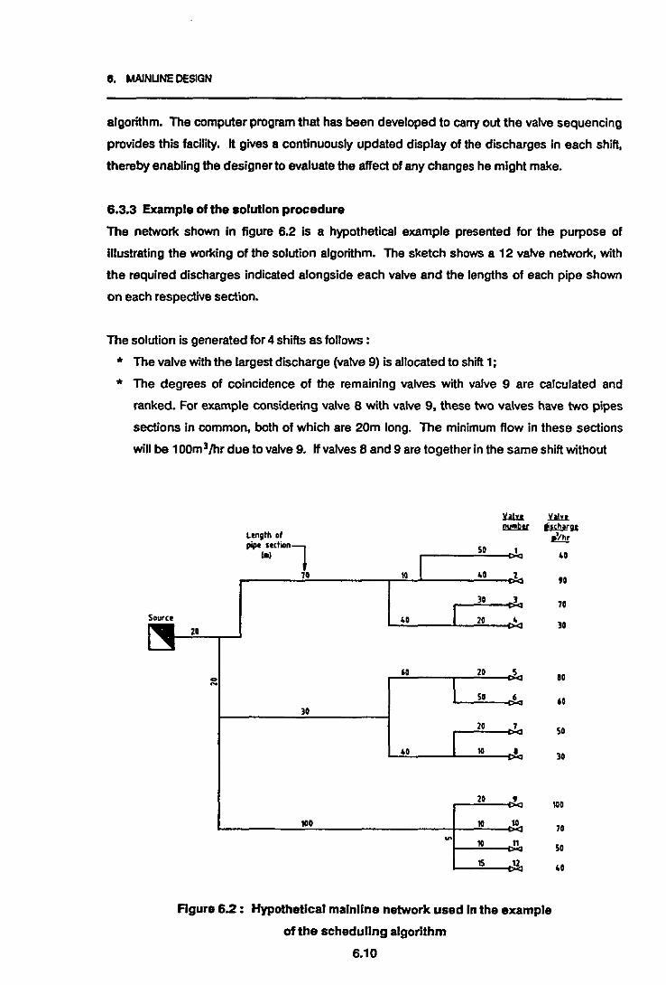
e. MAlNUNE DESIGN
algorithm. The computer program that has been developed to carry out the valve sequencing
provides this facility. It gives a continuously updated display of the discharges In each shift.
thereby enabling the designer to evaluate the affect of any changes he might make.
6.3.3 Example of the solution procedure
The network shown in figure 6.2 is a hypothetical example presented for the purpose of
illustrating the working of the solution algorithm. The sketch shows a 12 valve network. with
the required discharges indicated alongside each valve and the lengths of each pipe shown
on each respective section.
The solution is generated for 4 shifts as follows :
* The valve with the largest discharge (valve 9) is allocated to shift 1;
* The degrees of coincidence of the remaining valves with valve 9 are calculated and
ranked. For example considering valve 8 with valve 9, these two valves have two pipes
sections in common, both of which are 20m long. The minimum flow In these sections
will be 100m3/hr due to valve9. "valves 8 and 9 are together in the same shift without
70
)0
'0
ao
30
so
70
SO
60
soLtngth ofpipe "'tio°
lloll
10 I70 .0 2
)0 ]
Source '0 20 •20
60 20 S0N
SO 6
3Q
20 7
.0 10 •
2Q ,100 10 10
~
10 n
15 U
Rgure 6.2: Hypothetical mainline network used In the example
of the scheduling algorithm
6.10

8. MAINLINEDESIGN
any other valves, then the flow In these sections will be 30m3/hr greater than the
minimum, and the flows in all other sections will be equal to or less than the minimum.
The degree of coincidence is therefore (30x20)+(30x20)=1200;
* Working from highest to lowest coincidence, allocations to the remaining shifts are made
as follows:
shift 2 : valve 10
shift 3 : valve 11
shift 4 : valve 12
The total system discharge is 71Om 3/hr, which gives an average of 177.5m3/hr for each shift.
* Starting with shift 1, the allocations made on the basis of minimizing the coincidence
level are valves 4 and 1 respectively. At this stage the discharge in shift 1 is 170m3/hr,
which is within 5% of the average, so the allocation is complete.
* In shift 2, valves 8 and 3 are allocated before the shift is full, and after each allocation no
improving swaps are found with the valves in shift 1.
* In shift 3, valve 7 is allocated, leaving valves 6, 5 and 2 unallocated. From the point of
view of spreading the flow in the network, valve 2 would be the best allocation from these
remaining valves. However this would bring the total shift discharge to 190m3/hr, which
is more than 5% greater than the average. The next best allocation, in terms of the flow
minimization objective, is valve 6, which has a lower discharge requirement than valve 5.
This would bring the shift discharge to 160m3/hr. Although this is not within 5% of the
average, it is less then 5% greater than the average and so passes the second condition
of step 6, described above, and the allocation is therefore made. No improving swap can
be found.
* The allocation to shift 3 is not yet complete, since the discharge is still less than (1 • cS) x
the average. If either of the two remaining unallocated valves are added to shift 3
however, the total discharge will exceed (1 + cS) x the average. No allocation is therefore
possible at the current cS level. cS is increased to 10%, which then means that the
existing allocation is within (1 - cS) x the average and the shift is considered fully
allocated.
* This leaves the overall allocation at this stage as follows :
shift 1 : valves 9, 4, 1; Q = 170m3/hr;
shift 2: valves 10, 8, 3; Q = 170m3/hr;
shift3:valves11, 7, 6; Q=160m3/hr;
shift 4 : valves 12, 5, 2; Q = 210m3/hr;
which is not a particularly well optimized allocation, in terms of minimizing shift
6.11

6. MAINLINE DESIGN
discharge (shill 4). However, in making the allocations to shill 4, the algorithm finds
suitable swaps, which improve the overall allocation. These are valve 10 for valve 5, and
valve 6 for valve2 respectively, leaving the final allocation as follows :
shift 1 : valves 9, 4, 1; Q =170m3/hr;
shift 2 : valves 5, 8, 3; Q =180m3/hr;
shift 3: valves11, 7, 2; Q =190m3/h r;
shift 4 : valves12, 10, 6; Q =170m3/hr;
This example illustrates how the algorithm tends to utilize the smaller discharges to fill the
first few shifts, leaving the larger discharges, and hence a less flexible situation, for the filling
of the last shifts. This is a classic problem with allocation algorithms which can only be
alleviated to some extent by the backward seeking function. The algorithm has been tested
on a number of real networks, with favourable results, as reported in chapter 8.
6.4 Pump and Pipe Sizing
A trade-off exists in establishing the pipe and pump sizes. The higher the pump pressure
(higherpumping costs), the greater the amount of pressure that can be lost through friction in
the pipes, and hence the smaller the diameters ( and the cheaper the cost) of the pipes
needed in the network. By carrying out a present value analysis on the cost of pumping over
the expected life of the system, the energy costs can be expressed in terms of current Rands
per meter of pumping head supplied at the source. The cost of the pipes is a capital item,
which can be expressed in terms of current Rands per meter length of each diameter used in
each pipe section. The design problem can then be formulated as an optimization problem,
with several altemative methods for its solution. These solution procedures are reviewed
below.
6.4.1 Generalized formulation of the optimization problem
In order to discuss the optimization routines further; it is necessary first to outline the
conventions that havebeen developed forthe mathematical representation of pipe networks.
Networks are represented mathematically by defining a series of links and nodes. The links
represent the pipelines which connect one node to another, and the nodes represent
specifically defined points in the network. These may be points at which the network
branches, or other points such as reservoirs, pumps, valves or outlets. Each link Is
characterized by the change in head (energy per unit weight) of the water along its length.
6.12
6. MAINLINEDESIGN
Several empirical formulae have been established to determine the loss of head due to
friction in a pipe. A generalized form of these relationships is given in chapter 4 (equation
4.1). Each node is characterized by the flow entering or leaving it, either along the various
links attached to the node, or due to inputs and consumptions at the node.
Thus, for a network operating at a given time under steady-state flow, for which a fIXed set of
boundary conditions can be specified (I.e. inflows, outflows and fixed heads at specific
nodes), two basic types of equations can be formulated to define the flow, viz node and link
equations. The node equations are given by the conservation of flow law:
For node j : (6.8)
Where Qij = theflowfromnode to node j (foraflowfromnode jtonode i, Q;j
will be negative);
I j = input or consumption (i.e. negative input) at node j;
}; = all nodes ; linked directly (i.e.via a single link) to node j.
The link equations express the total difference in head between the end nodes of a path (brJ
in the network as the sum of head gains and losses (liR; j) in each of the links along the path:
For path p: (6.9)
These equations represent a set of simultaneous non-linear equations expressing the flow
and pressure distribution throughout the network. They can be solved iteratively using
techniques such as the Hardy-Cross and Newton-Raphson algorithms.
Solution ofthese equations enables a full specification of a given flow condition in a network.
The solution techniques form the basis of computer "network solvers" that have become
increasingly widely available. These solvers utilize rapidly converging algorithms (e.g. a
modified Newton-Raphson method employing sparse-malrix solution procedures as
described by Brailovsky and Rodeh - 1978, and Gofman and Rodeh - 1980), which enable
large networks to be solved very rapidly on relatively small computers. The solvers are useful
for monitoring and adapting existing networks, however they do not provide a process for
explicit optimization of the network design.
Several different design optimization procedures have been proposed in the literature,
utilizing both linear and non-linear methods.
6.13

6. MAINLINE DESIGN
Mandl (1981) formulated a generalized linear optimization model for the design problem,
which reduces to the "trans-shipment problem" for typical pressurized pipe networks. The
decision variables are the capacities of each link and external source, as shown below:
The objective function is given by :
(6.10)
Subject to the following constraints :
(6.12)
(6.13)
(6.14)
(6.11)for all jfA
jfA
jfA
for all
for all
* The conservation law: 7Pij Qij + QP j a = IIQjl + oSj
(i,jlEA (j,llEA
for all (i,jlEA* Qij>=O
* QP· >=0Ja
* oSj >=0
Where Qij = the flow into node j through pipe I,j (equivalenttoitscapacity);
QP j a = the flow generated at node j (e.g. by a pump);
Q j I = the flow from node j through pipe j ,I (equivalentto its capacity);
oS j = the flow consumed at node j (e.g. at a sprinkler outlet);
Ci j = the unit cost of producing flow in pipe i,j;
Cj a = the unit cost of generating flow at node j;
A = the set of all nodes in the network;
0< Pi j <= 1 = the fraction of water that is not lost on its way through pipe I,j. Typically =
1 in pressurized networks.
Shamir (1974) has proposed a generalized non-linear optimization procedure for the
design and operation of water distribution networks. incorporating a vector of decision
variables which may include either design factors such as pipe diameters or control factors
such as heads and flows in the networks :
The objective function is given by:
LMin [F(d, u,x, s) = f(d) + I wlcl(d, u l, xl. sl)]
1=1(6.15)
Subject to the following constraints :
* d ED (6.16)
* u l E ut for all I (6.17)
* [GI(d, u l, xl, sl) I 0 for all I (6.18)
* xl = {x/[GI(d, u l, xl, sl) I = O} E xI for all I (6.19)
6.14
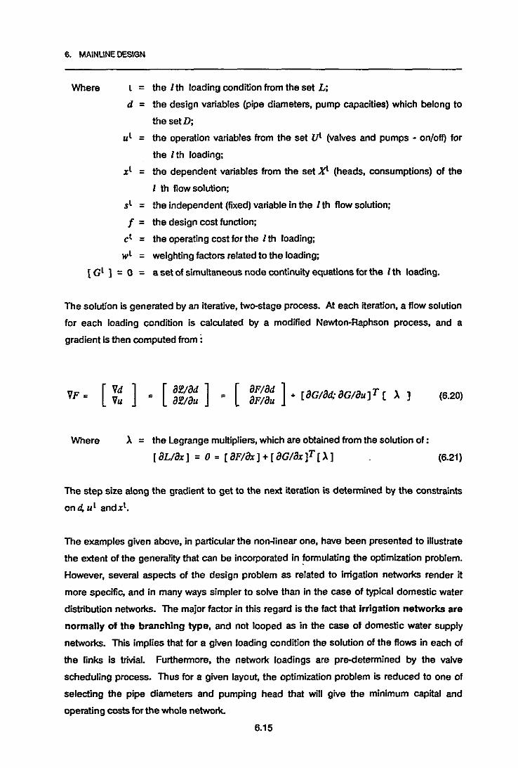
6. MAINUNE DESIGN
Where =d =
Ul =
xl =
Sl =f=
Cl =wI =
[GI ] =0 =
the lth loading condition from the set L;
the design variables (pipe diameters, pump capacities) which belong to
the setD;
the operation variables from the set vt (valves and pumps • on/off) for
the I th loading;
the dependent variables from the set xL (heads, consumptions) of the
I th flow solution;
the independent (fIXed) variable in the I th flow solution;
the design cost function;
the operating cost for the I th loading;
weighting factors related to the loading;
a set of simultaneous node continuity equations for the I th loading.
The solution is generated by an iterative, two-stage process. At each iteration, a flow solution
for each loading condition is calculated by a modified Newton-Raphson process, and a
gradient Is then computed from:
VF = 8ff./8d ]8f/8u (6.20)
Where A = the Legrange multipliers, which are obtained from the solution of:
[8L/8x] =0 = [8F/8x 1+ [8G/8x IT[AI (6.21)
The step size along the gradient to get to the next iteration is determined by the constraints
on d; u l and xl.
The examples given above, in particular the non-linear one, have been presented to illustrate
the extent of the generality that can be incorporated in formulating the optimization problem.
However, several aspects of the design problem as related to irrigation networks render it
more specific, and in many ways simpler to solve than in the case of typical domestic water
distribution networks. The major factor in this regard is the fact that Irrigation networks are
normally of the branching type, and not looped as in the case of domestic water supply
networks. This implies that for a given loading condition the solution of the flows in each of
the links is trivial. Furthermore, the network loadings are pre-determined by the valve
scheduling process. Thus for a given layout, the optimization problem is reduced to one of
selecting the pipe diameters and pumping head that will give the minimum capital and
operating costs for the whole network.
6.15

6. MAINLINEDESIGN
Both linear and dynamic programming solutions have been proposed for this problem. and
these are reviewed below.
6.4.2 The linear programming (LP) solution
The LP solution to the network design optimization problem has been presented In slightly
different forms by Karmeli et, al, (1968). Gupta (1969), and Kinney and Moncrief (1980). It is
derived as follows :
The links of a network are defined by the upstream node, t , and the downstream node, J,
respectively. Then for each link i} in the network being designed, a set of candidate
diameters, m, is to be considered. One set of decision variables is given by the length of
pipe for each of the candidate diameters to be used in each link i}. These lengths are
expressed as Xi}m and they have associated costs given by Ci}m per unit length.
A second set of decision variables is given by the operating head of the pump at the source of
the network. for each different loading condition, I. These operating heads are expressed as
XP(I). The discharge at the pump for loading I is QP(I), and ko(1} is the present value of the
operating cost of the pump per unit of head and discharge that it delivers. multiplied by : (a)
coefficients reflecting the units in which the head and discharge are expressed; (b) the
efficiency of the pump; and (e) the fraction of the total pumping time during which loading I
is operative. The cost of operating the pump during loading I is given by [ko(1} XP(I) QP(I) ].
Similarly. assuming that the capital cost of a pump is directly proportional to its maximum
operating head. XPM, the overall cost of the pump at the source is given by [ kc XPM ].
where k c is the capital cost per unit of head produced by the pump.
These variables are illustrated for a hypothetical network in figure 6.3.
The objective function of the LP is given by :
Minimize [K] = ~_ I Ci}mXijm + Iko(I)XP(l) QP(I) + kcXPMlJ M l
Where I = the summation of all loadings 1;I
I = the summation of all candidate pipe diameters m in link i};..I = the summation of all links i} in the network;i}
K = the total (present value) cost of the system.
6.16
(6.22)

6. MAINLINEDESIGN
• 3' 100 ..3'h'Q)
£3'160 ..
£!iISOoo
'7' ZOO..3,,,,
e
OISClWlG[••Z' 100 ..3,,,,
,~
£Z'130 ..
d :120m'/hr
" ........... @£,,' 133..
','330..3, ,,,
'®£,'113 ..
Pipe CostLink Length Candidate Diameter Dia Cost
ij (m) I 2 3 (rom) (Rim)
12 1000 500 4SO 400 100 1623 1000 250 200 ISO 200 2324 1000 4SO 400 3SO 250 3245 1000 300 250 200 300 SO46 1000 4SO 400 3SO 3SO 6067 1000 300 250 200 400 .90
4SO 130
Examples of LP variables: 500 170
(i) X2A) = the length of candidate diameter 3 (350 mm diameter) that will be usedin link 24.
(ill <;.) = The cost of this diameter = ROO/m.
(iii) The network has only one loading, t = I, for which QP(I). = I 120 m)/hr andXPM = OOm.
(iv) PumpinC costs:Capital;say kc = R2OO/ m of pumping head.Therefore capital cost = R200 x XPM = RJ2000
Operating:say 4c/Kwhr; 2 000 hrs/year; I m'/hr raised I m is 0.004 Kwhrs and presentvalue factor for 25 years at 12% is 7.843.
Therefore ko(/) = 0.04 x 2 000 x 0.004 x 7.843= R2,51 per m per m'/hr'
So operating cost = 2.51 X I 120 = R2 811 X XP (I)
(v) If the pressure at node 5 must be ;::: 30 Ill, then its head loss constraint is given by
180$210-IJI2m X 12m - IJ2... X2... - IJ.s.. Xos.... m m
(vi) The length constraint for link 12 isgiven by
XI2I +X,22 +XID = I 000 m.
Figure 6.3 A hypothetical network Illustrating the variables and constraints
used in the linear programming solution procedure
6.17

6. MAlNUNEDESIGN
Four sets of constraints can be be derived for the LP problem as follows :
1. The non-negativity constraint. The decision variables must be non-negative, so that a
set of constraints can be stated as :
Xi"m >= 0xpll) >= 0 forall ij, l (6.23)
2. The headloss constraint. Assume that the head at a specific reference node, s, is
fixed and known for loading l, and that either the maximum or minimum (or both)
allowable heads at a second node, n, downstream of the reference node are also known
for loading l, Then the total headloss in the network along the path from the reference
node to the second node, must not result in the head at the second node being either
greater than the allowable maximum, or less than the allowable minimum. This is
expressed by :
HMINn(l) <= Hs(l) ± "~ X Jijm(l)Xijm <= HMAXn(t) forall 1 (6.24)'J m
Where Hsfl)
HMINn(l): HMAXn(l)
};Xij m
= the head plus elevation at the reference node, s, for loading 1;
= the minimum and maximum allowable head plus elevation at
the second node, n,for loading t;
= the headloss (or gain depending on the direction of flow) per
unit length of pipe of diameter min link i j under load (flow) l,
This is calculated using one of the empirical headloss formulae;
= the summation of all segments Xi jon inall links i j along the
path from node s to node n.
3. The length constraint. The lengths of each diameter of pipe selected for a given link
must add up to the length of the link. This is stated by :
Where
z z.. = L,'J'm IJm
LiJ = the length of link i j
for all ij (6.25)
4. The pumping constraint. Since the operating head of the pump for each loading is a
decision variable in the LP, it must be constrained not to exceed the maximum possible
head that the pump is capable of producing, XPM. This is stated by :
XP(t) <=XPM
6.18
for all t (6.26)
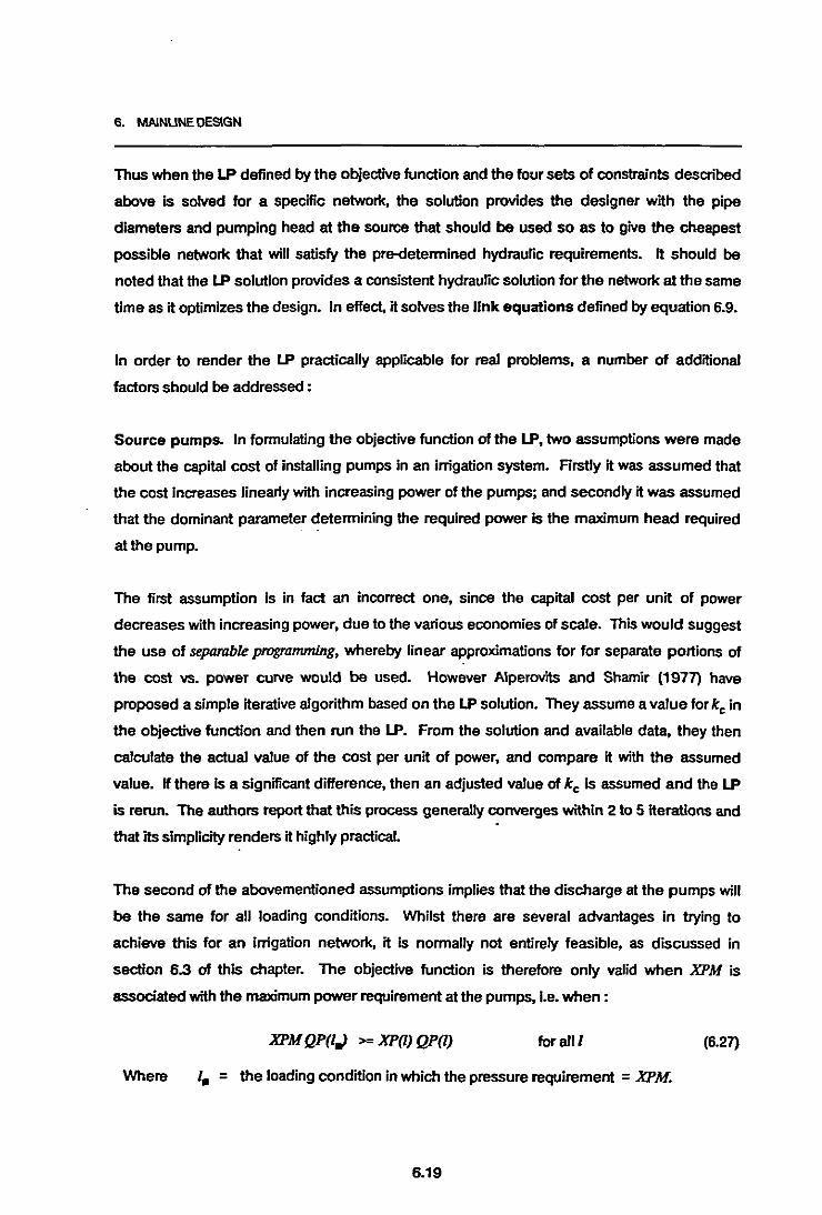
6. MAlNUNEDESIGN
Thus when the LP defined by the objective function and the four sets of constraints described
above is solved for a specific network, the solution provides the designer with the pipe
diameters and pumping head at the source that should be used so as to give the cheapest
possible natwork that will satisfy the pre-determined hydraulic requirements. It should be
noted that the LP solution provides a consistent hydraulic solution for the network at the same
time as it optimizes the design. In effect, it solves the link equations defined by equation 6.9.
In order to render the LP practically applicable for real problems, a number of additional
factors should be addressed:
Source pumps. In formulating the objective function of the LP, two assumptions were made
about the capital cost of installing pumps in an irrigation system. Firstly it was assumed that
the cost increases linearly with increasing power of the pumps; and secondly it was assumed
that the dominant parameter determining the required power is the maximum head required
at the pump.
The first assumption is in fact an incorrect one, since the capital cost per unit of power
decreases with increasing power, due to the various economies of scale. This would suggest
the use of separable programming, whereby linear approximations for for separate portions of
the cost vs. power curve would be used. However A1perovits and Shamir (1977) have
proposed a simple iterative algorithm based on the LP solution. They assume a value for lee in
the objective function and then run the LP. From the solution and available data, they then
calculate the actual value of the cost per unit of power, and compare it with the assumed
value. If there is a significant difference, then an adjusted value of lee is assumed and the LP
is rerun. The authors report that this process generally converges within 2 to 5 iterations and
that its simplicity renders it highly practical.
The second of the abovementioned assumptions implies that the discharge at the pumps will
be the same for all loading conditions. Whilst there are several advantages in trying to
achieve this for an irrigation network, it is normally not entirely feasible, as discussed in
section 6.3 of this chapter. The objective function is therefore only valid when XPM is
associated with the maximum power requirement at the pumps, i.e. when:
XPM QP(l.) >= XP{l) QP{l} for all 1 (6.27)
Where 1. = the loading condition in which the pressure requirement =XPM.
6.19
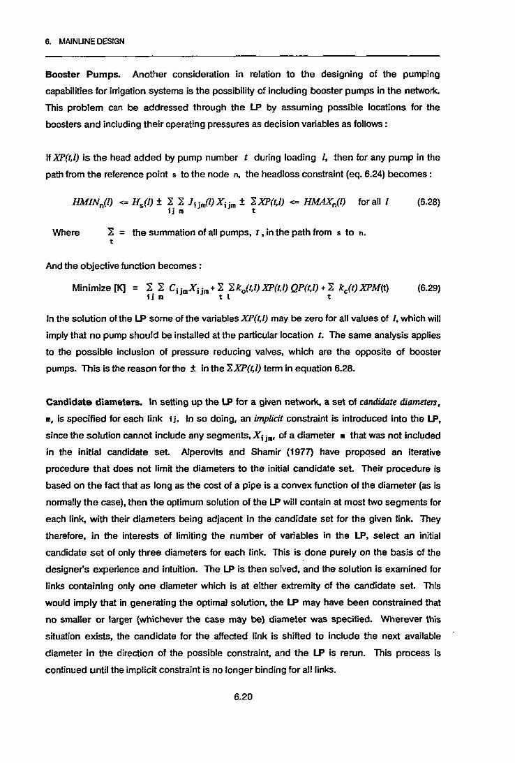
6. MAINUNE DESIGN
Booster Pumps. Another consideration in relation to the designing of the pumping
capabilities for irrigation systems is the possibility of including booster pumps in the network.
This problem can be addressed through the LP by assuming possible locations for the
boosters and including their operating pressures as decision variables as follows :
If XP(~/) is the head added by pump number t during loading I, then for any pump in the
path from the reference point s to the node n, the headloss constraint (eq. 6.24) becomes:
HMINn(l) <= Hs(l) ± ~. ~ Jijm(l) X i jm ± ~XP(~/) <= HMAXn(l) for all I (6.28)lJ m t
Where ~ = the summation of all pumps, t, in the path from s to n.t
And the objective function becomes:
Minimize[K] = ~ ~ CijmXijm+~ ~ko(~/)XP(~/)QP(~/)+~ kc(t)XPM(t) (6.29)ijm tl t
In the solution of the LP some of the variables XP(t,l) may be zero for all values of I, which will
imply that no pump should be installed at the particular location t. The same analysis applies
to the possible inclusion of pressure reducing valves, which are the opposite of booster
pumps. This is the reason for the ± in the ~XP(~/) term in equation 6.28.
Candidate diameters. In setting up the LP for a given network, a set of candidate diameters,
e, is specified for each link ij. In so doing, an implicit constraint is introduced into the LP,
since the solution cannot include any segments, Xi jm' of a diameter • that was not included
in the initial candidate set A1perovits and Shamir (1977) have proposed an iterative
procedure that does not limit the diameters to the initial candidate set. Their procedure is
based on the fact that as long as the cost of a pipe is a convex function of the diameter (as is
normally the case), then the optimum solution of the LP will contain at most two segments for
each link, with their diameters being adjacent in the candidate set for the given link. They
therefore, in the interests of limiting the number of variables in the LP, select an initial
candidate set of only three diameters for each link. This is done purely on the basis of the
designer's experience and intuition. The LP is then solved, and the solution is examined for
links containing only one diameter which is at either extremity of the candidate set This
would imply that in generating the optimal solution, the LP may have been constrained that
no smaller or larger (whichever the case may be) diameter was specified. Wherever this
situation exists. the candidate for the affected link is shifted to include the next available
diameter in the direction of the possible constraint, and the LP is rerun. This process is
continued until the implicit constraint is no longer binding for all links.
6.20

6. MAINLINE DESIGN
6.4.3 The dynamic programming (OP) solution
An aRemative dynamic programming optimization procedure for the design of branching
mainline networks has been proposed by Karmeli et.al. (1968), Kally (1969) and Uang (1971).
It is derived as follows :
As was the case for the LP, the decision variables are the pipe diameters in each segment and
the pump capacities. The state variables are the heads at the nodes, and the stages of the OP
are the nodes themselves. For a pipe of diameter D k in segment k between nodes j and
j+1, where j+1 is upstream of j, the cost of the pipe is given by g(Dk ) . If a link contains a
pump which raises the head from H j +1, at its intake to H j at its outlet, then the capital and
operating costs of the pump can be expressed as a function of these heads, g( H j +...Hs},
Now for a given head at node j+1, H j +1, the head at node j, H j , can easily be calculated for
a known flow Qk and for a selected pipe diameter Dk• Thus if we express the minimum cost of
the portion of the network downstream of node j, for different discrete levels of the head H j ,
as F*j(Hj), then the recursive equation olthe OP is given by:
(6.30)
The minimization is generally carried out for all possible diameters, D k, for a set of discrete
values of H j +1 within the admissible range for node j+1. Whenever H j = f (Hj+1, Q", DiJ is
outside the admissible range for node j, then the examined Dk is discarded. In the case of a
pump between nodes j+1 and j, the minimization is carried out over a set of discrete values
ofHj •
Shamir (1979) considers the OP solution to be "free of certain shortcomings present in the LP
procedure". In particular, it enables, through adequate investigation of alternative Dk's, an
optimization encompassing the class and type of pipe to be used, as well as the diameter.
However, Shamir points out that the generalized formulation is computationally more
involved, and hence less computer-efficient, than the LP, particularly when a highly ramified
network is considered.
6.4.4 The proposed solution procedure
In view of the foregoing discussion, the LP solution procedure has been adopted for the
proposed design model. A number of modifications to the process described above have
been incorporated into the model, and these are discussed on the following pages:
6.21

6. MAlNUNE DESIGN
6.4.3 The dynamic programming (OP)solution
An alternative dynamic programming optimization procedure for the design of branching
mainline networks has been proposed by Karmeli et.at, (1968), Kally (1969) and Uang (1971).
It is derived as follows :
As was the case for the LP, the decision variables are the pipe diameters in each segment and
the pump capacities. The state variables are the heads at the nodes, and the stages of the OP
are the nodes themselves. For a pipe of diameter Dk in segment k between nodes j and
j+1, where j+1 is upstream of j, the cost of the pipe is given by g(Dk). If a link contains a
pump which raises the head from H j +1, at its intake to H j at its outlet, then the capital and
operating costs of the pump can be expressed as a function of these heads, g( H j+"H j) .
Now for a given head at node j+1, H j +1, the head at node j, H j , can easily be calculated for
a known flow Qk and for a selected pipe diameter Dk• Thus if we express the minimum cost of
the portion of the network downstream of node j, for different discrete levels of the head H j ,
asF* j(HjJ, then the recursive equation of the OP is given by :
(6.30)
The minimization is generally carried out for all possible diameters, Dk, for a set of discrete
values of H j +1within the admissible range for node j-t, Whenever H j = f (H j +1, Q", DJ is
outside the admissible range for node j, then the examined Dk is discarded. In the case of a
pump between nodes j+1 and J, the minimization is carried out over a set of discrete values
ofHj •
Shamir (1979) considers the OPsolution to be "free of certain shortcomings present in the LP
procedure", In particular, it enables, through adequate investigation of altemative Dk's, an
optimization encompassing the class and type of pipe to be used, as well as the diameter.
However, Shamir points out that the generalized formulation is computationally more
involved, and hence less computer-efficient, than the LP,. particularly when a highly ramified
network is considered.
6.4.4 The proposed solution procedure
In view of the foregoing discussion, the LP solution procedure has been adopted for the
proposed design model. A number of modifications to the process described above have
been incorporated into the model, and these are discussed on the following pages:
6.21
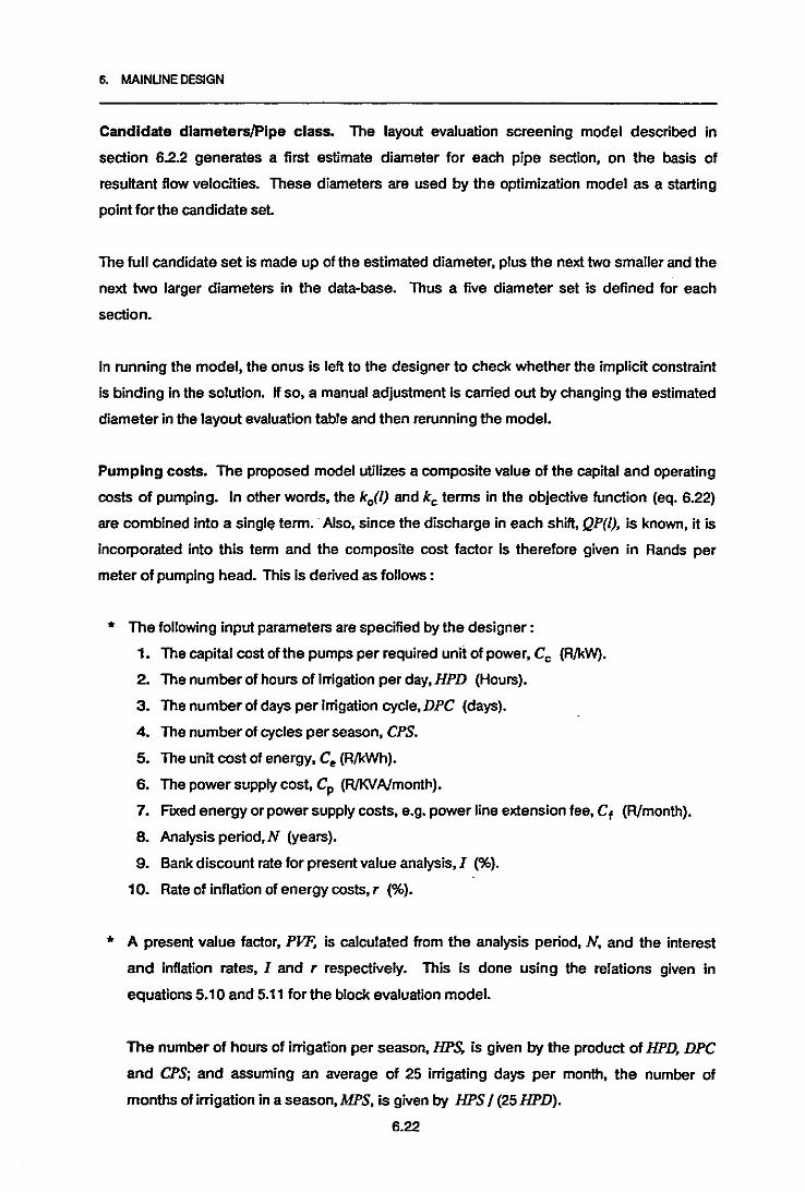
6. MAlNUNE DESIGN
Candidate diameters/Pipe class. The layout evaluation screening model described in
section 6.2.2 generates a first estimate diameter for each pipe section, on the basis of
resultant flow velocities. These diameters are used by the optimization model as a starting
point for the candidate set.
The full candidate set is made up of the estimated diameter, plus the next two smaller and the
next two larger diameters in the data-base. Thus a five diameter set is defined for each
section.
In running the model, the onus is left to the designer to check whether the implicit constraint
is binding in the solution. If so, a manual adjustment is carried out by changing the estimated
diameter in the layout evaluation table and then rerunning the model.
Pumping costs. The proposed model utilizes a composite value of the capital and operating
costs of pumping. In other words, the ko(l) and kc terms in the objective function (eq. 6.22)
are combined into a singh~ term.: Also, since the discharge in each shift, QP(l), is known, it is
incorporated into this term and the composite cost factor is therefore given in Rands per
meter of pumping head. This is derived as follows :
* The following input parameters are specified by the designer:
1. The capital cost of the pumps per required unit of power, Cc (R/kW).
2. The number of hours of irrigation per day, HPD (Hours).
3. The number of days per irrigation cycle, DPC (days).
4. The number of cycles per season, CPS.
5. The unit cost of energy, C. (R/kWh).
6. The power supply cost, Cp (R/KVNmonth).
7. FIXed energy or power supply costs, e.g. power line extension fee, Cf (R/month).
8. Analysis period, N (years).
9. Bank discount rate for present value analysis, I (%).
10. Rate of inflation of energy costs, r (%).
* A present value factor, PVF, is calculated from the analysis period, N, and the interest
and inflation rates, I and r respectively. This is done using the relations given in
equations 5.10 and 5.11 for the block evaluation model.
The number of hours of inrigation per season, lIPs, is given by the product of lIPD, DPC
and CPS; and assuming an average of 25 irrigating days per month, the number of
months of inrigalion in a season, MPS, is given by lIPS / (25 lIPD).
6.22

6. MAlNUNE DESIGN
For each shift, a load faelor,/f(l), is defined, representing the fraction of the total irrigation'
time dUringwhich shift I is operative.
* The discharge required at the pump for each irrigation shift, QP(I), is known; and the
pumping head required for each valve has been estimated by the layout evaluation
process described in seelion 6.2.2. The estimatedpumping head for each shift, XP' (I),
can therefore be taken as the maximum of the required pumping heads for each valve in
the given shift. If QP(I) is given in cubic meters per hour, and XP I (I) in meters, then the
estimated power requirement for each shift, P' (I), is given by:
Where
P'W = QPWXP'W~67n (k~
n = the efficiency of the pump
(6.31)
And maximum power requirement, MAXP is given by Max [ P' (I) ] for all I. This
represents the estimated power rating required at the pump.
* The operating cost component, kil), is calculated as follows: The estimated seasonal
energy consumption for sh1ft l; EPS' (I), is given by:
EPS' (I) = (/f(I) HrPS) P I (I) (kWh/season) (6.32)
And cost of this energy, kil), is:
kil) = C. EPS' (I) (R/season) (6.33)
The "fixed energy costs, Ct" are assumed to be levied for a lull 12 months of the year;
whereas the "power supply costs, Cp• are levied on the basis of the maximum power..load, MAXP, each month during the irrigation season. Thus the sum of these two cost
factors, for each shift, kll), is given by:
ksW = /f(I) [(MPS MAXI' CpJ + (12 Cf» (R/season) (6.34)
And finally, the present value of the full operating cost for shift I, over the analysis period,
ko(I), is given by :
ko(l) = PVF [kil) + ks(l» / [QP(I) XP' (I» (R/m/m3ph) (6.35)
* The capital cost component apportioned to each shift, kcW, is calculated as follows:
ke(l) = 1[(1) c;MAXI' / XP I (I) (R/m)
6.23
(6.35)

6. MAlNUNE DESIGN
* The composite cost factor, K(l), is then given by:
K(l) = [ko(l) Q}'(l)] + kc(l) (RIm) (6.37)
The objective function therefore has a single term relating to pumping costs, and the full
function is given by :
Minimize [I<] = ~. I Ci ImX; jm + I K(l) XP(l)lJ m l
(6.38)
Possible error in the composite cost factor stems from the following:
- the assumed linear relationship between pump capital cost and power rating, as
discussed in section 6.4.2 above;
- the difference between the estimated pumping heads in each shift, XP I (1), and the final
optimal values, XP(l), determined by the LP;
- the difference between the estimated maximum power requirement, MAXP, and the
actual value.
These errors affect the capital cost component and the load cost portion of the operating
costs. Since the errors due to each of these factors are expected to be small, and the capital
cost is generally a small portion of the total pumping cost (typically less than 10%), it is felt
that the total error will not significantly affect the results of the LP process.
In the case of booster pumps, the costs are more difficult to establish since no prior estimate
of the pumping head of the boosters is available. The booster cost factor is assumed to be
directly proportional to the sum of the composite cost factor for all shifts, weighted by the shift
load factor 1!(1); with the proportionality constant being the product of (I) the ratio of the
maximum flow through the booster pump to the maximum discharge through the source
pump, and (il) the fraction of the total irrigating time during which the booster will operate.
This assumption implies that the principal component of the total pumping costs is the
operating cost. This is considered to be valid since the Capital costs are typically only a small
traction of the total pumping costs and this will be particularly true for booster pumps which
are normally relatively small and therefore do not require expensive installation structures.
Pump optimization. In the case of irrigation networks, the source pump installation often
consists of one or more centrifugal pumps connected in parallel, and therefore with limited
flexibility of operating pressure. It is therefore common design practice to assume a constant
operating pressure in all shifts (determined by the maximum requirement) and to design the
6.24

6. MAlNUNE DESIGN
pipelines accordingly. For this reason the optimization model has been structured to operate
in two alternative modes:
* Either optimizing the pumping head separately for each irrigation shift. This is done
using the objective function as defined in equation 6.38, where each loading 1represents
an irrigation shift.
* Or optimizing on the basis of a fixed pumping head which is the same for each shift. In
this case the objective function becomes:
Where
Minimize [I<] = ~.:z C;jmXijm +KtXPtI) m
Kt = :z K(l) If(l)l
XPt = the fixed source pump delivery head.
(6.39)
(6.40)
The head loss constraint. The relation given in 6.24 is simplified by removing the maximum
pressure condition (RHS of the relation) thereby reducing it to a single constraint The
reference node is taken as the source and each valve in tum is taken as the downstream
node. Thus the set of headloss constraints is given by :
XP(l) - ~ :z lijm(l)X;jm <= VPn-AZs,nI) m
forall n e l (6.41)
Where VPn = the minimum pressure required at valve n;
AZs n = the elevation at the source minus the elevation at valve n;,
6.5 The Computer Programs
The computer programs for mainline design have been written in standard BASIC for use on
Ms-DOS or PC-DOSdriven personal computers. The programs have been structured into fIVe
different modules as follows :
1. Layout specification, in which the alternative layouts are specified.
2. Valve sequencing, which carries out the valve sequencing algorithm.
3. Layout evaluation, which perfonns the rapid layout evaluation and simultaneously
establishes the candidate diameters and pumping costs for the optimization model.
4. Optimization, which sets up the input matrix for the LP procedure and then solves it.
5. Result Interpretation, which converts the results from the LP solution into a
meaningful fonnat and then enables the designer to consider the affect of alterations to
these results.
6.25

6. MAlNUNE DESIGN
The programs are operated interactively from a series of menus. Appendix 1b shows a
synoptic map of these menus, illustrating the logical flow of the program operation.
Layout specification. This is done on three separate tables, viz :
* Valves. Each valve is listed together with its topographic elevation and the required
discharge and pressure.
* Nodes. These are all points, otherthan the valves, at which the network branches, or at
which there is some other change in the network characteristics. The node number is
listed together with its elevation.
* Unks. The input required for each link in the network includes: the start and end points
(node and/or valve numbers) ; the length of the link; and the pipe material. An additional
column allows for optional specification of the pipe class. If the class is left unspecified
then it will be determined during the layout evaluation calculations.
The tables can be displayed on the screen in any sequence and edited freely by moving the
cursor around within the diplay.
Valve sequencing. The valve sequencing option can only be initiated if the layout has been
fully specified. At the start of the sequencing process the user will be asked to input the
number of shifts into which the valves are to be scheduled. The scheduling algorithm is then
initiated and the results are displayed in a table which lists each valve together with the shifts
in which it operates. The bottom of the table shows a summary of the total discharge in each
shift.
This table can then be edited by the user. In other words, any of the schedules can be
changed manually. The summary table showing the shift discharges is automatically updated
as any changes are made.
Layout evaluation. The layout evaluation can only be selected if the layout is fully specified
and the valve sequencing has been completed. The evaluation is done in two phases.
namely calculation of the capital costs and then calculation of the pumping costs.
On initialing the evaluation function, the pipe class and diameter esttmation calculations are
carried out. The results are displayed in a table showing, for each section:
- the start and end points;
- the section length;
- the pipe material and class;
- the maximum flow in the pipe;
6.26

6. MAlNUNE DESIGN
ctess( DI'": (om) ..
. ,Cost(i).
t,0211.0 10 486.17
Figure 6.4: Results of the layout evaluation process In mainline design
(Estimated pipe costs)
- the estimated maximum pressure head in the pipe;
- the selected diameter; and
- the pipe cost.
An example of this table is shown in figure 6.4. The total length of the network and the
estimated cost of the piping are shown at the bottom of the table. The class and diameter
values for each section can be edited manually by the user, and the changes in cost due to
any such editing will be displayed automatically.
6.27

6. MAlNUNE DESIGN
Once this is complete, the user then initiates the pumping cost calculations. The results of
this are displayed in a table showing, for each shift :
- the load factor If(f);
- the estimated pump operating efficiency;
- the estimated power requirementP I (f);
- the estimated seasonal energy requirement EPS' (f);
- the annual cost of this energy at current prices; and
- the product of the operating cost component and the shift discharge (kif) QP(f) ) in
Rands per meter pumping head.
An example ofthis table is shown in figure 6.5.
.:~:.,.::: 7 :...
',6
....,.,
T~A( {IWU: " '.", ',', 7,CAPITAl/PRES.VAl~,COST'U} Z ,148 '
"4m4 2Z7
, 9059 ' '
149158
, 29710563
OiSOOLf1ted Cost(RIm)
1n163
315 '
Figure 6.5: Results of layout evaluation process in mainline design
(Estimated energy costs)
6.28
6. MAlNUNE DESIGN
The totals at the bottom of the table include:
- the ~value;
- the total seasonal energy requirement;
• the total seasonal cost at current prices;
- the total capital cost of the pump;
- the total present value cost of pumping over the full analysis period; and
- the total present value cost of pumping per meter head of pumping.
A second table showing each of the ten pumping cost parameters is displayed beneath the
main results table.
The load factors and the estimated pump efficiencies can be edited in the main table. and all
of the cost parameters can be edited. The costs are automatically recalculated as soon as
any changes are made.
Optimization. The optimization can only be initiated once the layout evaluation has been
completed.
At the start of the process the user is asked to specify whether the pumping head is to be
optimized on a per schedule basis. or on the basis of a fixed head for all shifts. An input table
is then provided for specifying the booster pump data.
Once this is complete. the computer continues. without input from t~e user. preparing the
initial solution matrix for the LP and then solving the LP.
Result Interpretation. Once the LP process is complete. the computer translates the results
from the solution matrix into a more meaningful format. The results are displayed in two
tables. The first table shows for each section. the selected diameters and their
corresponding lengths and costs. Totals are given for each section and for the whole
network. A subsidiary table provides a summary of the pipe costs by diameter. The second
table shows a summary of the operating pressures at each valve. in each shift.
The length and diameter selections can be edited manually by the user. If any changes are
made. the various totals and the pressures table are updated automatically.
6.29

6. MAINUNE DESIGN
References
1. Alperovits, E. and U. ShamJr, Design of optimal water distribution systems, Water
Resources Research, 13(6), pp 885-900, 1977.
2. BraiJovsky, M. and M. Rodeh, An improved hydraulic network solver, TR065, IBM-Israel
Scientific Centre, Haifa, Israel, 1978.
3. Buras, N. and Z Schweig, Aqueductroute optimization by dynamic programming, Proc of
the ASCE (HY5),pp 1615-1631, 1969.
5. Garey, M.R., R.L Graham and D.S. Johnson, Performance guarantees for scheduling
algorithms, Operations Research, 26(1),pp 3-21, 1978.
6. Gofman, E. and M. Rodeh, An interactive aid for constructing irrigation time tables, TR068,
IBM-Israel Scientific Centre, Haifa, Israel, 1978.
7. Gupta, I.; Linearprogramming analysis ofa water supply system, AilE Transactions, 1(1), pp
55-61, 1969.
8. Kally, E., Pipeline planning by dynamic computer programming, Journal AWWA, 61(3), pp
114-118, 1969.
9. Karmeli, D., Y.Gadish and S.Myres, Design ofoptimal waterdistribution networks, Proc of
the ASCE, 94(PL1), pp 1-10, 1968.
10. Karmeli, D., Y.Gadish and S.Myres, Design of optimal water distribution systems by
dynamic programming, Technion-Israel Institute of Technology, Faculty of Agricultural
Engineering, Publ 51, Haifa, Israel, 1968.
11. Kinney, LA. and M.R. Moncrief, &onomical pipe sizing for irrigation systems, Source
unknown, 1980.
12. Uang, T., Design ofconduit systems by dynamic programming, Proc of the ASCE, 97(HY3),
pp 383-393, 1971.
13. Mandl, C.E.•A survey ofmathematical optimization modelsand algorithms for designing and
extending irrigation and wastewater networks, Water Resources Research, 17(4), 1981.
14. Sabbagh, E., Optimal real-time control of pumping stations in irrigation systems, MSc
Thesis, Faculty of Agricultural Engineering, Technion-Israel Institute of Technology,
Haifa, Israel, 1986.
15. Shamir, U., Optimization in water distribution systems engineering, Mathematical
Programming Study, 11, pp 65-84, 1979.
16. Shamir. U., Optimal design and operation of water distribution systems, Water Resources
Research,10(1), 1974.
17. Stephenson, D., Pipeflow analysis, Vol 19 in Developments in Water Science, Elsevier,
Amsterdam, 1984.
6.30

PART 3 :
APPLICATIONS

7. APPUCATIONS OFTHEBLOCKDESIGN ANDEVALUATION MODELS
7. APPUCATIONS OFTHE BLOCK DESIGN AND EVALUATION MODELS
7.1 Introduction
Agure 7.1 shows a O.2Ha apple orchard in the Grabouw region (Western Cape, South Africa).
that has been used as a test case for the design and evaluation models. A number of
different design cases are analysed in order to demonstrate the capabilities of the design
models.
The orchard is on a hill-side. and has been laid out with the manifold running down a steep
ridge (27% slope). and the laterals. on either side of the manifold. running down more gentle
slopes (±4% in Quad a and ±B%in Quad b). Irrigation is by micro-sprayers. with a spacing of
2m along the laterals and 3.5m between the laterals.
Most of the rain in the area falls in winter. with highly variable rainfall occurring during the
summer growing season. The average seasonal irrigation requirement is 490mm. However.
in a year of one standard deviation less than average rainfall. the irrigation requirement
increases to 740mm. Consequently, irrigation systems in this area are generally designed for
a higher peak requirement than the average, but the question of the most appropriate
design peak is unresolved.
The farmer irrigates the entire farm on a weekly cycle. using four 6-hour shifts per day. six
days per week. All the orchards on the farm have- been standardised on a sprayer delivering
49lph at 150kPa pressure. with full wetting. For the given spacings, this implies a gross
application rate of 7mm/h. giving a maximum gross application of 42mm in a 6-hour shift. The
irrigation system is operated by a time-based automatic controller.
Irrigation scheduling is normally done on the basis of well tried rules of thumb. for various
periods in the growing season. The farmer knows that each 1mm of required irrigation needs
a setting of 8.5 minutes on the controller. The forthcoming week's requirement is set
accordingly. every Monday. Efforts have been made to improve scheduling practices in the
region through experimentation to produce appropriate, local crop factors for use with weekly
climatic data from a centrally located weather station.
7.1

1' ~
:. <'-~ 1"~" .~~,~~,' ".", ' ""
".'
~
n
"..II
II
..
A,.••, Modo • IlH.L.t.1I. Ifadt\t • l.511E-Ilt......... I ....
""'. "l
,/'
"'.
",
.,' ,.","
,;"
,t:,
. ~ ~.
.~..
~,.....
....'., U s»
, ~"~ t·
LflDll
I1aIIl 11M
_oW
L.t ...
" ............... ' t.......SCALf Al'PIlOX, l' I I"
:'I'
~~i!il~
~I~
~~z
~
Figure 7.1 Layout of micro irrigation scheme on Grabouw Orchard

7. APPLICATIONS OFTHEBLOCK DESIGN AND EVAlUATION MODELS
7.2 Basic Design
In a moderately dry year, the average weekly irrigation requirement throughout the season,
based on historical climatic data, can generally be categorized into four periods as shown in
table 7.1 below. It can be seen that if evaporation losses are around 5%, then the existing
42mm/week gross system capacitywill supply exactly the 40mm nett requirement.
Table 7.1 Irrigation requirements for apples In Grabouw (South Africa)(in a moderately dry rainfall season) ,
Weedy requirement (nvn)Totaller period (nvn)
NovlDec(6 weeks)
25150
Dec/Jan(6 weeks)
40
240
Feb(4 weeks)
30120
March
(4 weeks)
20
eo
Total(20weeks)
590
The design was carried out on the computer as follows :
7.2.1 Design Parameters
The base set of design parameterswas as shown in table 7.2 below:
Table 7.2 Design parameters for Grabouw apple orchard
Type
CoefficIents 01pressurelow relationship:
EmittersD & D 1.1nvnGT-JETmiao sprayerk.ll.34 x=O.54
NominalUpperlo1erancelower tolerance
Maximum lateralinletpressure
MaterialMinimum diameterMinimum length/section
MalerialMinimum diameterMinimum length/section
Operating Flows and Pressures49lph @ 151kPa10% (167kPa)10% (l36kPa)157kPa
lateral Pipinglow denslly polyethylene, cia.. 312nvn'
Om
Manifold Pipinglow densitypolyethylene. class 320nvnOm
As can be seen in the above table, the allowable pressure variation was specified as the
traditional 20%, which gave an absolute allowable variation of 167-136=31kPa. This was
divided roughly 2/3 in the lateralsand 113 (10kPa) in the manifold.
7.3

7. APPUCATlONSOFTHE BLOCK DESIGN AND EVALUATlON MODELS
7.2.2 Design results
The results of this design, as produced by the computer, are shown in table 7.3 below:
Table 7.3 Results of design of Grabouw apple orchard(20% allowed pressure variation)
Lateral lengths (m) Costl.at# 12mm 15mm (A)
Quad a1 15.0 7.752 17.0 8.753 21.0 10.754 24.0 3.0 14.205 22.0 9.0 17.106 22.0 11.0 18.407 20.0 17.0 21.308 18.0 21.0 22.909 14.0 29.0 26.10
Quadb1 28.0 13.0 22.702 28.0 13.0 22.703 26.0 15.0 23.004 28.0 9.0 20.105 26.0 7.0 17.806 28.0 3.0 16.207 26.0 3.0 15.208 27.0 13.759 27.0 13.75
Totals417.0 153.0 312.45
Man~old lengths (m) (Om min length/section) Cost
20mm 25mm 32mm 40mm 32mm 40mm (R)
7.0 7.0 3.5 5.0 3.5 5.5 3129
Graphical plots produced by the computer as part of the design process, are. shown in figure
7.2. The figure shows the pressure profiles for one of the designed laterals and for the
manifold design in two different cases, which are discussed further below.
As discussed in chapter 4 (section 4.3.3), two design curves are established for each lateral,
in order to calculate coefficients of the pressure/discharge relationship for use in the manifold
design. The two curves for lateral 5 in Quad a can be seen in figure 7.2a. the second curve is
established by moving the end pressure up by an amount equal to the width of the manifold
pressure variation envelope (10kPa in this case) and calculating the pressures on a point to
point basis back to the inlet. The fact that the second curve moves up above the upper
envelope boundary as it gets towards the inlet, as seen in the figure, is indicative of the
difference in head losses in the two curves due to the different operating pressures of the
emitters. This gives an indication of the error in assuming a constant discharge from each
emitter along the lateral.
7.4

7. APPlICATIONS OF THE BLOCK DESIGN ANDEVALUATION MODELS
I~t-.___ •
l-.r.l' 0 I0
.~w -- ..~w ww
l ..•••·•.•·.·~0
...-........ ...... d......-.
W
_:. • • --I ••....C__
I
I - - * •• ZSI.1 ~. In. u Ii ••• ..
a) lateral design
I"....... lMt.... "" no ...11 ~ I
'Ww -- .._ww
Ow
-~.
•0
w
.>................::. :::.:::...... .
w.......-
r
• •I "W ,........ili._lU I
I- .... ..... - - "0- * • o. N. N••... ... d.' U •.. ... ... .. ..• ..I"...... Jcr_ ,......... I
c) manifold design
( 10m min. length/section)
"....... i_.... ,.. _'''1iI ••
::'"1 .....-. ww
j .,...... •.. , .... ......0
.'.'.. . '
.........'.,
.'.,..' ..,
.-.' ..., ...>: ....
..'.... .'
.'
;
~•
I J,... ,..._1."•._ .... I
i "'.0 ow. ~.. _.0 .0- -. ..-00- ....0 --I ... " ... ... u ... ... ... .. ...!"..., .... Scr_ ,.....-. I
b) manifold design
( Om min. length/section)
Figure 7.2 Graphical output of results from the computer design model
7.5

7. APPUCAllONS OFTHE BLOCK DESIGNAND EVAlUATION MODElS
The design of the manifold is of interest, since it is representative of a number of notoriously
difficult factors. Firstly. manifolds are generally more difficult to design than laterals because
of their narrower allowable pressure envelopes; secondly this manifold is on a particularly
steep slope; and thirdly the hydraulic grade line has a characteristic "kink' between outlets 2
and 3 due to this section being on a steeper gradient than the rest of the manifold (see figure
7.2 b & c).
It can be seen from the results that the designed manifold starts at the inlet with a 40mm
diameter pipe. and then decreases to a 32mm 'choke' over the steeper section between
inlets 2 and 3. in order to counteract the effects of increased head gain due to the steeper
topography. As the manifold flattens out, the diameter is increased back to 4Omm. and it then
"telescopes' normally down to 20mm at the last outlet
It can be seen further in figure 7.2b and c that the manifold pressure moves out of the
envelope boundaries over part of its length. This is a typical result for manifolds on steep
slopes, caused when the design routine falls into the cycling condition described in section
4.3.2 of chapter 4. In order to resolve the cycling problem, the design algorithm temporarily
widens the pressure envelope by defining a tolerance amount by which the curve may move
beyond the envelope boundaries. Once the cycling has been bypassed. the tolerance is
reset to zero.
During the design process, each step of the algorithm is summarized in the synopsis file. as.discussed in section 4.4.3 of chapter 4. This file is written onto the computer data disk, so
that it does not interfere with the results seen on the screen. However, if the designer wishes
. to·review-the file, itcan be popped-up over the design screen orprinted out Table 7.4 shows
extracts from this file for the manifold design.
Case 1 in this table shows the design described in tables 7.2 and 7.3 and shown in figure
7.2b. With reference to table 7.4. the steps of the design process are as follows :
* Starting in step 1, with section 1, a 20mm pipe. at outlet number 9 (the closed end of the
manifold) and an assumed pressure of 167kPa (the top envelope boundary value). N.
outlet 8, in step 1. the pressure is 162kPa, and at the next point the pressure goes back up
to 167kPa. A 'down shlft" is indicated;
* The process starts again in step 2. after the shift, with a starting pressure of 162kPa. This
time the calculations go through to outlet 7, where the pressure has come back up to
162kPa. The pressure at the next point will be 180kPa. Since this is above ttle upper
envelope limit, a change to a larger diameter ('Chng Up') is indicated;
7.6

7. APPLICATIONS OFTHE BLOCK DESIGN ANDEVALUATION MODELS
" Step 3 shows that a 25mm pipe has been selected for section 2, and the calculations
continue from point 7, where the previous section ended. The first action is to check that
the previous section is longer than the specified minimum length;
" Step 4 shows that the new section runs out of the top boundary almost immediately, so
that an adjustment is indicated;
" The curve for section 2 is moved back 1 outlet, to outlet 8, which means that section 1
must be re-checked for the minimum length criterion (step 5);
Table 7.4 Extracts from the design synopsis file
Case 1 : Om minimum length/sectionOESIGH OF MAIIIFOUl alb Date : 28/01/87STEP 1/ SECT OIA(nm) Start Pt & P Current Pt & P NEXT Pt & P ACTION TOLERANCE
1 1 20 9 167 8 162 7 167 Shft On (D.DD)2 1 20 9 162 7 162 6 180 Chng Up (0.00)3 2 25 7 162 ChkHinLen (0.00)4 2 25 7 162 6 163 5 171 Adjust (0.00)5 2 25 8 157 ChkHinLen (O.DD)6 2 25 8 157 8 157 7 153 Chng On (0.00)7 3 20 8 157 ChkHinLen (O.DD)
IIinlon failed: length z 0.08 1 20 9 167 8 162 7 167 Shft On (0.05)9 1 20 9 162 7 162 6 180 Chng Up (0.05)
11 2 25 7 162 5 171 4 187 Chng Up (0.00)
17 4 40 4 168 3 165 2 152 Chng On (0.00)18 5 32 3 165 ChkHinLen (0.00)19 5 32 3 165 2 160 1 169 Chng Up (0.00)20 6 40 2 160 ChkHinLen (0.00)
_.21 6- 4D 2 160- 0 161 Design Done (0.00)
Case 2: 10m minimum length/sectionDESIGN OF MANIFOLD alb Date : 28/01/87STEP 1/ SECT DIA(am) Start Pt & P Current Pt & P NEXT Pt & P ACTION TOLERANCE= a::aZ===-ZS-===:hl
13 2 32 5 165 4 162 3 167 Chng Up (0.00)14 3 4D 4 162 ChkHinLen (0.00)
IIinlon failed: length z 3.515 2 4D 5 165 4 157 3 155 Chng On (D.DD)16 3 32 4 157 ChkHinLen (0.00)
IIinlon failed: length = 3.517 2 32 5 165 4 162 3 167 Shft On (0.05)18 2 32 5 165 3 167 2 162 Shft Up (0.00)19 2 32 5 165 2 162 1 170 Shft On (0.00)20 2 32 5 165 2 162 1 170 Chng Up (0.00)
7.7

· 7. APPlICATIONS OFTHE BLOCK DESIGN ANDEVALUATION MODELS
*
*
*
*
*
*
From outlet 8, the curve for section 2 runs straight out below the bottom envelope,
indicating a change back to a smaller diameter (step 6);
The 20mm pipe is therefore re-introduced at outlet 8 for section 3. Section 2 is checked
against minimum length and fails since its length is actually zero (step 7);
The process is back at the same point that it was at in the first step and a cycling
condition has occurred. The tolerance is set at 5% and the process starts over from the
point of cycling (step 8);
Steps 8, 9 and 10 are a repeat of steps 1. 2 and 3. However. in step 11, section 2 now
gets through to outlet 5 because of the tolerance which allows the curve to move 5%
above the upper boundary. The tolerance is reset to 0, and the process continues with a
change up to a larger diameter;
Steps 17 to 20 show the process of inserting the 32mm choking section between outlets
2 and 3;
The process ends at step 21, when the calculations get to the pipe inlet within the
pressure envelope.
The manifold was designed a second time with a stipulated minimum length of 10m for any
section. The result of this design is shown in figure 7.2c and in table 7.5 below:
Table 7.5 Alternative manifold design of Grabouw apple orchard
Manijold lengths (m) (10m min. length/section) Cost20mm 25mm 32mm 40mm 32mm 40mm (R)
14.0 12.0 5.5 30.62
As expected. in this case the design algorithm rejects the 20mm section at the end of the
manifold and starts with a 25mm section. The envelope is opened 5% at the start of the
process in order to get through with 14m of the 25mm pipe. At this stage the process cycles
again, this time over outlets 5 to 3 with 32mm and 40mm pipe sections. as shown in case 2 in
table 7.4 (steps 13 -16). The tolerance is set to 5% and the 32mm section then gets through
to outlet 2. Note that the curve for the 32mm pipe is sufficiently steep going through outlets 3
and 2 so as to obviate the need for the choking section. Step 18 shows that a shift up was
indicated as the curve came into the kink at outlet 3. This is equivalent to case c in figure 4.3
of chapter 4. This is followed by a shift down at the end of the kink in step 19 (case b in figure
4.3). In both these cases however, the envelope was so narrow that any shift would have
taken the curve outside of the envelope. and consequently no actual shift was affected.
7.8
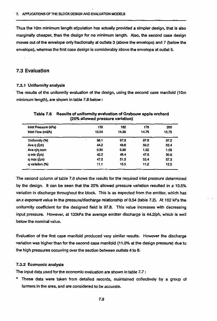
7. APPUCATIONS OFTHEBLOCKDESIGN ANDEVALUATION MODELS
Thus the 10m minimum length stipulation has actually provided a simpler design, that is also
marginally cheaper, than the design for no minimum length. Also. the second case design
moves out of the envelope only fractionally at outlets 3 (above the envelope) and 7 (below the
envelope), whereas the first case design is considerably above the envelope at outlet 5.
7.3 Evaluation
7.3.1 Uniformity analysis
The results of the unifonnity evaluation of the design, using the second case manifold (10m
minimum length), are shown in table 7.6 below:
Table 7.6 Results of uniformity evaluation of Grabouw apple orchard(20% allowed pressure variation)
Inlet Pressure (!<Pa) 130 162 178 200Inlet Flow(m3Ih) 13.04 14.30 14.75 15.75
Uniformity (%) 98.1 97.8 97.6 972Aveq (lph) 442 48.6 502 53.4Avea/qnom 0.90 0.99 1.02 1.09q min (lph) 42.2 48.4 47.6 50.6qrnax (lph) 47.3 51.5 53.4 57.3q variation (%) 11.1 10.5 112 12.5
The second column of table 7.6 shows the results for the required inlet pressure detennined
by the design. It can be seen that the 20% allowed pressure variation resulted in a 10.5%
variation in discharge throughout the block. This is as expected from the emitter, which has
an·J: exponent value in the pressure/d"lScharge relationship of 0.54 (table 7.2). At 162 kPa the
unifonnity coefficient for the designed field is 97.8. This value increases wilh decreasing
input pressure. However, at 130kPa the average emitter discharge is 44.21ph, which is well
below the nominal value.
Evaluation of the first case manifold produced very similar results, However the discharge
variation was higher than for the second case manifold (11.6% at the design pressure) due to
the high pressures occurring over the section between outlels 4 to 6.
7.3.2 Economic analysis
The input data used for the economic evaluation are shown in table 7.7 :
.. These data were taken from detailed records, maintained collectively by a group of
farmers in the area, and are considered to be accurate.
7.9

7. APPUCATIONS OFTHE BLOCK DESIGN ANDEVALUATION MODELS
* The capital costs of the overall irrigation system are R 3162.54/Ha. of which about 2/3 are
actual in-field system material costs (including an estimated additional 10% for 'other
materials' e.g. fittings). Note that all manifold costs are apportioned on a per hectare
basis.
Table 7.7 Summary of the input parameters for the economic evaluation ofGrabouw apple farm
Design Data
1) Capacity/Operating regime:Averageemitterdischarge *(48.6Iph) Gross appfocation rate (6.9mm/h)Emitterspacing (2.0x 3.5m) Gross systemefficiency 96%Total available water BOOmm Nell app6cation rate (6.7mm/h)
Maximumirrigatingtime/set 6hrsMaximJmapp6cation/cycle (4Omm)
2) Area:
AreaaIblock (O.2Ha) Areaof scheme 5Ha
3) Aaronomic data :
MaximJm aop yield 53lonsIHa
Period NovtPec Dec/Jan Feb March TotalCrop water requirement (mm/cycle) 25 40 30 20 (590)Duration of period (cycles) 6 6 4 4 (20)Icy valuefor each period 0.8 0.8 0.8 0.8
4) AppJieation fractions for operation pointoptimization: 0.90 1.00 1.05 1.10 1.15
Economic Data
1) Capfial costs : 2) Maintenance costs:
Material costs Block 5% (R 91.68/Ha/yr)-block piping and emitters (R 343.07) Mainrme 3% (R 15.oo/Ha/yr)-other block materials R 34.30
. -es1imated mainDnecost R 2500.00Installationcosts
-block R 100.00.;nainDne R 500.00
Other capital fiern. (f....,etc) R 50.00
Total capital costs (R 3162.54/Ha)
3) FIXed production cost. : R 25OO/Ha/yr 4) Yieldrelated production cost. :
R 75.oo/lon
5) Operatino costs : 6) DI'counted cash ~ow analysis:Energy cost sc.1<Wh Period 15yearsEstimatedheadloss in mainrme 200kPa Discount rate 13%Pump delivery pressure (362kPa) In~tion rates
Overa6energycost (0.66c1m3) -energy 18%-production costs 18%
Water base cost 1Oc/m3 -earnings 14%
Water opportunity cost Oc/m3 -general 19%
7) Producer price to farmer: R 253.00/100
* AD values wfthin ( ) are caJaJlated by the computer from the design and other input data.
7.10

7. APPlICATIONS OF'THE BLOCKDESIGN ANDEVALUATION MODELS
* Water for the farm.is drawn from a storage scheme developed jointly by the fanners of the
region, for which they are paying interest and redemption on capital loans. Hence the
relatively highcost of the water which completely over shadows the energy costs.
* Over the past 4-5 years,. the farmers have experienced a rapid escalation in production
costs, that has not been matched by equivalent rises in eamings. Their predicament is .
reflected in the rates used for the discounted cash flow analysis.
* In the absence of any detailed information about the yieldMater relationship for apples
over individual periods in the growing season, a constant value of the crop response factor
(ky) has been assumed throughout the season.
The results of this analysis are shown in figure 7.3 below.
a;3
590604 : 6Z5 640530... '<c.............,......L_L.-...L.....L-'-J
un1.44
.~~ !.~••/ ;..,. ; ; ~ :;
Appl Ie- •. Ea c%)"~,, . 9a 96 ..•. 93 ". 91R""",t .» ir ex) :::89':,' 9a. 99. 99.",'.99
EAW. C~/ha)·'·.'n4i( , 1l607£All (R/II13) 1.39" .. 1.'46
.. ,.
i1.-_-'-_-:;-_-'-__-:- .,...,-_--'-'. : ll/h:
..un
PERlOo ,.... -"1,':·2 3' 4 5 .,6 '7' 8 TOTAL
~""",i: t';"Cycl.)25 '·40 30 ZO ". 590
Awl ; ~ (';""cyclei '·26 40 31 ZI604~. . ... ~.
1m31'.46 .
1.34 .
Figure 7.3: Results of economic analysis of Grabouw apple farm
7.11

7. APPlICATIONS OFTHEBLOCKDESIGN ANDEVALUATION MODELS
The following conclusions can be drawn from these results :
" The main table of results shows five different seasonal applications. The column with the
depth equal to the optimal depth, shows results for an irrigating regime based on the
optimal policy determined from the the solution of the dynamic programming exercise and
shown in the second table, below the main table. The other four columns show results for
irrigating at a fixed application ratio (AR) throughout the season, unless this ratio entails
exceeding the maximum system application. Thus for example, the 604mm seasonal
application shown in column three is derived from applications of 26, 40, 31 and 21
mm/cycle during each of the four periods respectively, whereas the 530mm application is
derived from a constant AR of 0.9 throughout the season. The 625mm result is derived
fromAR=1.10 for periods 1, 3 and 4, andAR=1.00 (i.e. the maximum possible) in period 2.
" The yield per unit of land increases as the application is increased. up to a maximum of
52.9 tons/Ha. This is reached when the requirement efficiency is 100% in periods 1, 3 and
4 (at AR=1.10 for these periods). The maximum possible yield of 53 tonslHa cannot be
attained with this system in a moderately dry year since the peak requirement of
40mm/week during December/January cannot be exceeded by the system. The yield per
unit of water decreases exponentially as the seasonal application is increased.
" The return on investment is maximal at a seasonal application of 604mm. However the
maximum return per unit of water occurs at an operating point of 590mm/season. It is
interesting to note that the maximum return is not derived from operating the system to
produce maximum yield. The marginal costs of increasing the seasonal application from
.604mm to625mrrroutweiglr the extra income from the increased yield. .
7.4 Sensitivity Analysis
A number of a1temative economic analyses were generated by varying selected parameters.
The results of these analyses are summarized in table 7.8, and can be grouped as follows :
a) specific variations of the data-input parameters, and
b) variations of the design parameters.
In each case, only the specified parameters were changed, and all other parameters were
restored to their original base case values.
7.12

7. APPLICATIONS OFTHEBLOCK DESIGN ANDEVALUATION MODELS
7.4.1 Alternative Data-Input Parameters
* Operating and production costs. These affect the irrigation system in two ways. Firstly,
the overall profitability of the scheme is dependent on the ratio between yield related
production costs (e.g. packaging) and income, and the rate at which this ratio is either
increasing or decreasing. Secondly, the optimal operating depth is dependent on the
marginal costs of increasing the yield through increased water application. These two
aspects were examined in alternatives 1 and 2 in table 7.8 :
1) The producer price was reduced by 10% to R228/ton; the yield related production
costs were increased by 10% to R82.50!ton; and the difference between the rate of
inflation of production costs versus the rate of inflation of earnings was increased from
4 to 6 percentage points. This resulted in a negative EAW at all depths, the minimum
loss being R89/Ha at a seasonal depth of 604mm. This depth also coincided with the
depth at which the loss per cubic meter of water was minimized.
2) The most sensitive of the operating costs was found to be the water cost. An analysis
was therefore run considering the situation if, for example, the farmer had an a1temative
use for the water which paid him a premium of 15c1m3 over and above the purchase
price. This was input into the model by specifying the 15c1m3 as a water opportunity
cost. In this case the operating point giving a maximum EAWIHa came down to
596mm, thus narrowing the gap between operating for maximum EAWIHa and
operating for maximum EAWlm 3• The result implies that for any application greater
than 596mm, the marginal return would be less than could be realised through using
the required water for the alternative purpose.
* System capacity.
-. 3) This analysis considered the question of what the optimum depth would be if the
system, as designed. could apply more than 4Omm/week. This was done by increasing
the time available per irrigation shift to 8 hours. thereby increasing the capacity of the
system to 53mm/week. The results in table 7.8 show that under these circumstances,
the maximum return per unit of land is reached when the maximum yield is attained
(requirement efficiency is 100%). This is achieved through a constant AR of 1.05
throughout the season. The increase in EAWfrom the base case is R18/Ha. which is
equivalent to a nett present value of R120/Ha. This represents the amount that can
profitably be spent on the irrigation system in order to increase its capacity to meet the
required 42mm/week.
* The water/yield relationship. As discussed in chapter 5. the yield response factor (ky)
varies during the growing season. Four distinct periods during the season can be
7.13

7. APPUCAilONS OFTHE BLOCK DESIGN AND EVALUAilON MODELS
identified, viz. vegetative growth, flowering, yield formation and ripening. Typical ley
values for each of these periods would be 0.6, 1.1, 0.7 and 0.2 respectively. In other
words, the plant is typically more sensitive to water deficits during flowering and yield
formation than during the other two periods.
4) The model was rerun using the abovementioned leyvalues, on the assumption that the
four periods defined for the Grabouw region correspond to the four growing periods.
The results for this alternative have the optimum seasonal application reduced to
600mm with only a small reduction in the EAW compared with the base case. This is
due to the low ley value during the last period. It implies that the loss of yield due to
under-irrigation in this period is small, and consequently the 5% excess irrigation
during this period, suggested in the base model, is no longer economically
advantageous.
* Total available water.
5) The model was then rerun using the new ley values, but this time with only 550mm total
available water. In other words, the system was forced to operate under deficit (93%)
irrigation conditions. This situation can occur in the area since the total water allocation
from the storage scheme is limited and most of the farmers have their own
supplementary storage, for which they rely on good winter rains. This condition
provides the truest test of the dynamic programming model as an allocation
optimization process. The results show that a yield of 51.0 tons/Ha can be achieved,
giving an EAWof RB171/Ha. The optimal operating policy maintained a full irrigation in
period 2 and only a slight reduction in period 3. As expected the greatest reduction in
the application was allocated to period 4.
. "- . . .: . .....
For comparison, the model was run with a forced constantAR =0.93. This resulted in a
yield of 50.6 tons/Ha and an EAWof RB030/Ha. Thus the regime proposed by the
optimization model does give an improvement over the fixedAR regime.
* Irrigation requirement. The final analysis in this group was done for an assumption of
the system, as designed, operating in an average rainfall season. The total seasonal
requirement in this case is 490mm, made up from peak requirements of 20, 35, 25 and
15mm for each of the four periods respectively.
6) The results for this case are similar to those of case 3. The optimum operation under
these circumstances is with a constant AR of 1.05, in order to produce the full 53
tons/Ha. This results in a maximum EAW of R9061/Ha, which is considerably higher
than the maximum in the base case, due to the reduced water requirement. The
reduced requirement also has the affect that the application for maximum EAW/m3
coincides with the application for maximum EAW/Ha.
7.14

7. APPUCATIONS OFTHE BLOCK DESIGN AND EVALUATION MODELS
Table 7.8 Summary of results of sensitivity analyses on the evaluation
OpL Opertng.PI. OpL Opertng.PaRcyDepthUnn. Captl.
Coe! Cost Depth Yield EAW mrnIweek/period for Max
('llo) (R/Ha) (mm) (!/Ha) (R/Ha) 1 2 3 4 EAW/m3
BASECASERESULTS: 97.8 3163 604 52.8 8672 26 40 31 21 590
ALlERNATIVEDATA-INPUT PARAMElERS:1. Higher cost/earning ratio 604 52.8 -69 26 40 31 21 604
2. 15c/m3water apparLcost 596 52.7 5566 26 40 30 20 590
3. 53mrnlweekcapacity 618 53.0 8890 26 42 31 21 590
4. Changed ky values 600 52.8 8659 26 40 31 20 590
5. Limitedavailablewater 550 51.0 8171 23 40 26 15 5506. Averagerequirement 516 53.0 9061 21 37 26 18 518
ALlERNATIVEDESIGN PARAMElERS:7. Smallersystem, d1yyear 97.4 3092 582 37.1 2789 26 35 33 21 5828. Smallersystem, ave.year 97.4 3092 504 51.3 8478 21 35 26 16 504
Analysis over 15 years:9. 40% pressure variation 96.1 3063 604 52.7 8633 26 40 31 21 590
1O. 3O'lIo pressure variatlon 96.8 3113 604 52.7 8652 26 40 31 21 590
11. 10%pressure variatlon 96.6 3242 604 52.9 8673 26 40 31 21 590
Analysis over 5 years :12. 40% pressure variatlon 687113. 3O'lIo pressure variation 687914. 20%variation(basecase) 688515. 10%pressure variation 6872
7.4.1 Alternative Design Parameters
* System capacity. The possibility of designing· the system for a lower capacity was
considered, the rationale being that the resultant loss of production might be offset by the
reduced capital cost of the system. This was done by specifying a sprayer that delivers
431ph at 150kPa (also with full wetting), giving a maximum nett application in 6 hours of
35mm.
7) The new system was designed and then evaluated for the base set of input parameters.
The results show that the saving in the capital cost of the system was only 2%; and that
in a moderately dry year, the loss in production and subsequent eamings will be
substantial.
8) An alternative evaluation of the designed system was carried out using the irrigation
requirements in an average year (as specified for case 6). Under these circumstances
the system gives reasonably good results, but the EAW/Ha is still less than that
achieved from the larger system.
7.15
7. APPUCATIONS OFTHEBLOCKDESIGN ANDEVALUATION MODELS
* Allowable pressure variation. The question of the most appropriate allowable pressure
variation to be used for design (the 20% rule debate), was analysed by designing and
evaluating a number of systems using different values of this parameter.
9) 40%total allowable pressure variation;
10) 30% total allowable pressure variation;
11) 10%total allowable pressure variation.
Note that the base case was designed using 20% allowable variation.
The results show that as the allowable pressure variation was decreased, the uniformity
and the capital cost of each system increased accordingly, as expected. The maximum
EAW/Ha obtained from the system also increased in each case, implying that the
10%-system is the optimal one, notwithstanding its higher capital cost. However, the
additional return from the 10%-system over the 20%-system is small and considerations of
cash-flow might mitigate in favour of the cheaper system.
The four designs (40%, 30%, 20% and 10% allowable pressure variation respectively)
were re-evaluated using a 5 year write off period, rather than the 15 year period used in the
first set of evaluations. The results are shown in cases 12to 15. It can be seen that in this
case, the maximum return from the 10%-system was less than that from the 20%-system, so
that the 20% rule is in fact an optimal one under these circumstances.
7.5 Accuracy of the Hydraulic Calculations
The widely used poly-plot graphical design procedure is based on an assumed constant
emitter discharge, regardless of any variation in pressure. The extent of the error in this
assumption was investigated using the computer programs in the following way:
*
*
*
A fictitious emitter was defined in the data-base, giving a constant 49lph at all pressures
(r exponent in the pressure/discharge relationship = 0).
This emitter was then used to design the system, with all the other design parameters
set to the same value that was specified for the base case described above.
The original, real emitter was then respecified, before carrying out the evaluation of the
designed system. This is necessary since running the evaluation using the fictitious
emitter gives an erroneous uniformity of 100%.
The results of this analysis are shown in table 7.9
7.16
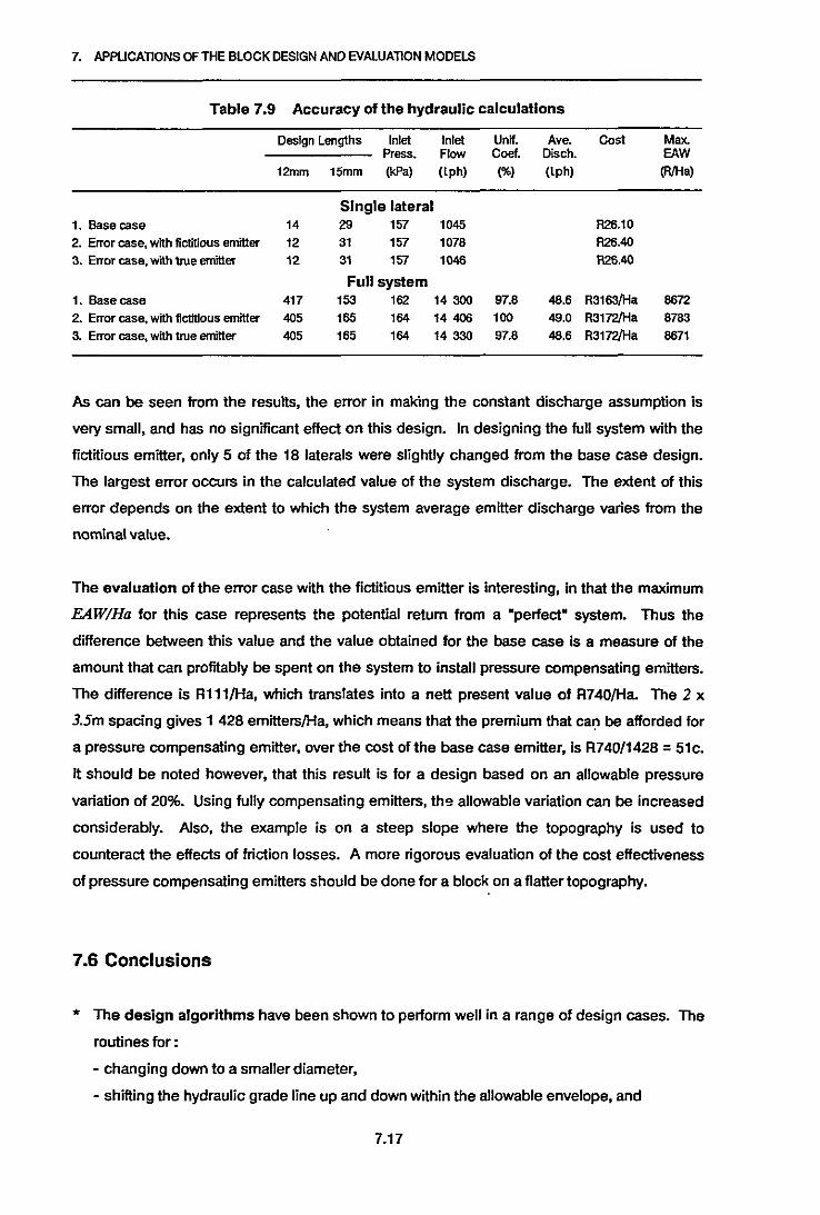
7. APPUCATIONS OFTHEBLOCKDESIGN ANDEVALUATION MODELS
Table 7.9 Accuracy of the hydraulic calculations
Design Lengths Inlet Inlet Unn. Ave. Cost Max.Press. Flow Coel. Disch. EAW
12mm 15mm (kPa) (lph) (%) (I ph) (R/Ha)
Single lateral1. Base case 14 29 157 1045 R26.10
2. Error case, with fictitious emitter 12 31 157 1078 R26.40
3. Error case,with 'trueemitter 12 31 157 1046 R26.40
Full system1. Basecase 417 153 162 14300 97.8 48.6 R3163/Ha 8672
2. Error case. with fictitious emitter 405 165 164 14406 100 48.0 R3172/Ha 87633. Error case, with true emitter 405 165 164 14330 97.8 48.6 R3172/Ha 8671
As can be seen from the results, the error in making the constant discharge assumption is
very small, and has no significant effect on this design. In designing the full system with the
fictitious emitter, only 5 of the 18 laterals were slightly changed from the base case design.
The largest error occurs in the calculated value of the system discharge. The extent of this
error depends on the extent to which the system average emitter discharge varies from the
nominal value.
The evaluation of the error case with the fictitious emitter is interesting, in that the maximum
EAW/Ha for this case represents the potential return from a "perfect" system. Thus the
difference between this value and the value obtained for the base case is a measure of the
amount that can profitably be spent on the system to install pressure compensating emitters.
The difference is R111/Ha, which translates into a nett present value of R740/Ha. The 2 x
35m spacing gives 1 428 emitters/Ha, which means that the premium that can be afforded for
a pressure compensating emitter, over the cost of the base case emitter, is R740/1428 =51c.
It should be noted however, that this result is for a design based on an allowable pressure
variation of 20%. Using fully compensating emitters, the allowable variation can be increased
considerably. Also, the example is on a steep slope where the topography is used to
counteract the effects of friction losses. A more rigorous evaluation of the cost effectiveness
of pressure compensating emitters should be done for a block on a flatter topography.
7.6 Conclusions
* The design algorithms have been shown to perform well in a range of design cases. The
routines for :
- changing down to a smaller diameter,
- shifting the hydraulic grade line up and down within the allowable envelope, and
7.17

7. APPUCATIONS OFTHEBLOCKDESIGN ANDEVALUATION MODELS
- widening the allowable envelope in order to move out of a cycling condition
all operated appropriately and effectively where required. In particular, the often
encountered problem of steep slope design (>20%), was successfully overcome.
* The evaluation program successfully met the stated objective of providing a basis for
formulating and evaluating altemative designs. In this respect it was shown to be highly
flexible in accommodating changes to the input data. It was effectively used to :
- assess the expected performance resulting from a given design, under varying
economic and farm related conditions; and
- evaluate different designs, generated by changing specific design parameters. An
example of this was the investigation undertaken of the most appropriate value of the
allowable pressure variation parameter.
* In the investigation of the most appropriate allowable pressure variation, the 20% rule
was shown to be optimal for the given case.
* All the computer design models require an explicit statement of all values used for the
design parameters. This requirement is an important benefit of the models, because it
enables the designer to consider aspects of the design problem that have been
addressed up till now through unproven rules of thumb. For instance, the question of the
optimal split of the allowable pressure variation between the manifold and the laterals is a
"grey area" that has never been tested. It is believed that in time, as experience is gained
from the use of the programs, tested values for such parameters will be developed.
* Important components of the success of the programs are their ease of use and quick
run times:
- the design parameters can be changed almost instantaneously while designing, by
calling the parameters table as a pop-up window onto the screen;
- entering the layout data for the Grabouw orchard, from the plan, took approximately
5 minutes;
- once the layout had been tully specified, each complete redesign of all the laterals and
the manifold took 4-5 minutes of computer time;
- design of a single lateral or manifold took 10-15 seconds computer time;
- the initial uniformity evaluation was the longest of the computer processes, taking
10 minutes for the Grabouw orchard;
- each run of the economic evaluation took 20-30 seconds.
7.18

8. APPLICATIONS OFMAlNUNE DESIGN
8. APPLICATIONS OF THE MAINLINE DESIGN MODEL
Four different farm irrigation mainline networks have been analysed, in order to test both the
efficiency of the design routines and the range of different types of applications for which the
models can be used.
8.1 The Sequencing algorithm
The efficiency of the sequencing algorithm was tested on a network of the Ciskei Agricultural
Corporation at Ncera. The network supplies a 22Ha. vegetable farm from 24 valves, as shown
in figure 8.1.
The network was designed to be operated in 12 irrigation shills. Both the valve operation
schedules that were proposed as part of the original design, and the schedules that were
produced by the computer model, are shown in table 8.1.
Table 8.1 Valve operation schedules for the Ncera Network (fig 8.1)
Original Schedules ComputerSchedules
Shill No. OpenValves Tala/Flow Openvalves TotaIAow
(m3/h) (m3/h)
1 3& 4 60 6&20 882 1 & 2 51 5. 7 & 19 993 13&20 84 2.11 & 13 1044 9&24 108 4& 9 875 15&21 105 1 &17 836 10&22 100 3&18 787 11 &23 102 8& 15 988 14&18 107 12& 14 919 18&19 95 10&23 99
10 12&17 94 18&21 10311 5& 7 53 22 5312 6& 8 102 24 58
The two schedules can be compared in terms of three sets of criteria, as follows:
Row dispersion in the network. Inspection of the two sets of schedules shows that the
computer generated schedules appear to be more widely distributed than the original
schedules, thereby resulting in a more dispersed flow through the network during its operation.
8.1

8. APPLICATIONS OFMAINLINE DESIGN
If i I II:
: I r, !!..>
>I
11 t1) I~'"
:
.>l..0
!IICII.=cOJE.:u
=' II0'..
10D-C.2-coCl-.:~....IIUZ
...eDII..::>Clii:
8.2

8. APPLICATIONS OFMAlNUNE DESIGN
The original design has valves clustered together in the following shifts :
(1): valves 3 and 4;
(2): valves 1 and 2;
(3): valves 13 and 20;
(5): valves 21 and 15;
(8): valves 14 and 16; and
(9): valves 18 and 19.
Whereas the only clustering in the computer schedules occurs in shift (10): valves 18 and 21.
This is borne out further by considering the maximum flows in each section, as generated in
the output of the quick evaluation procedure. Table 8.2 shows these flows. It can be seen
that the flows are reduced in the computer generated schedules in 8 out of the 29 pipe
sections, constituting 463m out of a total of 1764m of piping. The flows in the remaining 21
sections are the same for both sets of schedules.
Variation In flow demand at the pump. The discharge required from the pump, in each
schedule, is shown in table 8.1. The average flow in both cases is 86.7m3/h. The average
deviation from this mean is 19.9m3/h for the original design and 12.8m3/h for the computer
design. Thus the flow requirements for the computer design are more evenly re.g.ulated than
those for the original design.
Affect on optimum design. The pipeline was designed using the optimizing procedure. with
both the original and the computer generated schedules. The results. using PVC/class 4
piping. are shown in table 8.2.
It can be seen that the computer generated schedules yielded a design with a net saving on
total costs. of Rl 273.29 over that for the original schedules.
General notes
In general. the scheduling algorithm has been found to give good results. In some instances,
when a schedule has been allocated up to a flow level which is close to the current W%
tolerance level and the remaining unallocated valves all have relatively large discharges. then
the algorithm tends to make illogical selections. However the backward seeking mechanism
described in Chapter 6 tends to be self correcting in this regard.
In addition to the computer scheduling algorithm, the program provides the user with the
facility to alter the schedules manually once they have been displayed on the screen. An
updated display of the total flow requirement in each schedule is maintained on the screen
8.3

8. APPUCATIONS OFMAlNUNEDESIGN
during this process. This facility has proved to be most useful in incorporating the designer's
preferences, to correct or modify computer generated schedules. It should be noted that the
computer algorithm does not incorporate cognizance of any practical, non hydraulic. factors
that may affect the schedules. These may include. for example, the need to schedule
together blocks with similar precipitation rates or similar soil types. Or. alternatively, the need
to keep the physical distances between valve operations (opening and closing) In each
schedule within reasonable limits. The manual adjustment facility enables the designer to
incorporate these considerations.
Table 8.2 Optimized design of the Neara network (fig 8.1)
Original SChedules ComputerSChedules
1) Pipes:Pipe Max Flow Diameter Max Flow Diameter
Sectlon (m3/h ) (mm) (m 3/h) (mm)
1 108 200 104 2002 60 160 35 1403 25 125 25 1254 25 125 25 1255 35 00/75 35 00/758 102 140 1i7 1257 1i7 110/90 57 008 1i7 00 1i7 110/909 45 110/90 45 110/90
10 45 00 45 0011 108 160 103 14012 49 110 49 0013 49 110/90 49 110/9014 39 00/75 39 00/7515 107 160/140 103 14018 52 110/90 52 00/7517 32 75/63 32 75/6318 95 140 55 11019 95 140 55 11020 95 140 55 11021 44 00 44 00/7522 55 110/90 55 0023 50 00 50 110/9024 58 125/110 58 125/11025 52 00/75 52 0028 32 75/63 32 75/6327 53 00 53 11028 52 00 52 110/9029 58 110/90 58 00/75
Totel pipingcosts: R15373.95 R14538.20
2) Energy:
Operatingpressure (m) 24.8 24.8Seasonal energyreqmnt (kWh) 18759 18608Presentvaluecost R41992.52 R41443.98
Total netwoc1< costs R1i7258.47 R55983.18
8.4
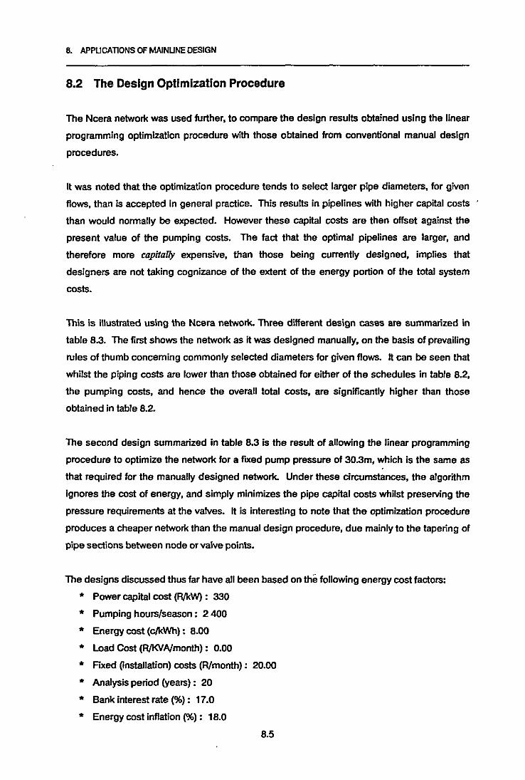
8. APPLICATIONS OFMAINLINE DESIGN
8.2 The Design Optimization Procedure
The Ncera network was used further, to compare the design results obtained using the linear
programming optimization procedure with those obtained from conventional manual design
procedures.
It was noted that the optimization procedure tends to select larger pipe diameters, for given
flows, than is accepted in general practice. This results in pipelines with higher capital costs
than would normally be expected. However these capital costs are then offset against the
present value of the pumping costs. The fact that the optimal pipelines are larger, and
therefore more capitally expensive, than those being currently designed, implies that
designers are not taking cognizance of the extent of the energy portion of the total system
costs.
This is illustrated using the Ncera network. Three different design cases are summarized in
table 8.3. The first shows the network as it was designed manually, on the basis of prevailing
rules of thumb conceming commonly selected diameters for given flows. It can be seen that
whilst the piping costs are lower than those obtained for either of the schedules in table 8.2,
the pumping costs, and hence the overall total costs, are significantly higher than those
obtained in table 8.2.
The second design summarized in table 8.3 is the result of allowing the linear programming
procedure to optimize the network for a fixed pump pressure of 30.3m, which is the same as
that required for the manually designed network. Under these circumstances, the algorithm
ignores the cost of energy, and simply minimizes the pipe capital costs whilst preserving the
pressure requirements at the valves. It is interesting to note that the optimization procedure
produces a cheaper network than the manual design procedure, due mainly to the tapering of
pipe sections between node or valve points.
The designs discussed thus far have all been based on the following energy cost factors:
* Power capital cost (R/kW): 330
* Pumping hours/season: 2400
* Energy cost (clkWh): 8.00
* Load Cost (RIKVA/month): 0.00
* FIXed (installation) costs (R/month): 20.00
* Analysis period (Years): 20
* Bank interest rate (%): 17.0
* Energy cost inflation (%): 18.0
8.5

8. APPUCATIONS OFMAlNUNE DESIGN
These values of the energy cost parameters resulted in a present value cost of R1 690 per
meter pumping head.
Table 8.3: Further design of the Ncera network
Original Optimized for Optimized for
Design FIxed Pressure 10% Inftatlon
Head
1) Pipes:Pipe Diameter Diameter Diameter
section No. (mm) (mm) (mm)
1 160 160 1602 110 110 1103 90 75 1104 75 90/75 1105 75 75/63 90/756 160 140 1107 90 110 1108 90 75 90/759 90 90 110/90
10 90 75 9011 160 140 14012 90 125 12513 90 110 11014 75 75/63 75/6315 160 140 14016 90 90 9017 75 63 75/6319 110 140 12519 110 140 11020 110 140 11021 90 75 7522 90 110. 11023 90 90/75 110/9024 90 110 11025 90 90 9026 75 63 75/6327 90 125 12526 90 90/75 110/9029 90 90/75 • 90/75
Totalpiping costs R13515.68 R13230.55 R13990.00
2) Energy:Operating pressure (m) 30.3 30.3 252seasonalenergy reqmnt 22919 22919 19061
(kWh)Present value eest R51207.00 R51207.00 R23307.68
Totalnetworkcosts R64722.68 R64437.55 R37297.68
The third design shown in table 8.3 summarizes the results of a full optimization using the
computer generated schedules. for which the expected rate of inflation was reduced from
18% to 10% per annum. This change resulted in the energy cost being reduced from R1 690
down to R916 per meter of pumping head. As a result, the optimum design used some
smaller pipes. bringing the capital cost down from R14 539.20 to R13 990.00; and the
pressure head required at the pump was increased from 24.6 to 25.2 meters. The pipe costs
8.6
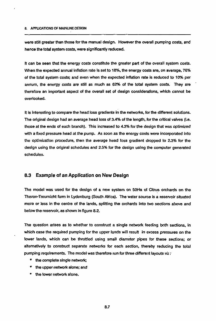
8. APPUCATIONS OF MAlNUNE DESIGN
were still greater than those for the manual design. However the overall pumping costs, and
hence the total system costs, were significantly reduced.
It can be seen that the energy costs constitute the greater part of the overall system costs.
When the expected annual inflation rate is set to 1B%, the energy costs are, on average, 76%
of the total system costs; and even when the expected Inflation rate is reduced to 10% per
annum, the energy costs are still as much as 62% of the total system costs. They are
therefore an important aspect of the overall set of design considerations, which cannot be
overlooked.
It is interesting to compare the head loss gradients in the networks, for the different solutions.
The original design had an average head loss of 3.4% of the length, for the critical valves (i.e.
those at the ends of each branch). This increased to 4.3% for the design that was optimized
with a fixed pressure head at the pump. As soon as the energy costs were incorporated into
the optimization procedure, then the average head loss gradient dropped to 2.3% for the
design using the original schedules and 2.5% for the design using the computer generated
schedules.
8.3 Example of an Application on New Design
The model was used for the design of a new system on 50Ha of Citrus orchards on the
Theron-Treurnicht fann in Lydenburg (South Africa). The water source is a reservoir situated
more or less in the centre of the lands, splitting the orchards into two sections above and
below the reservoir, as shown in figure 8.2.
The question arises as to whether to construct a single network feeding both sections, in
which case the required pumping for the upper lands will result in excess pressures on the
lower lands. which can be thrOllled using small diameter pipes for these sections; or
alternatively to construct separate networks for each section, thereby reducing the total
pumping requirements. The model was therefore run for three different layouts viz :
* the complete single network;
* the upper network alone; and
* the lower network alone.
8.7

8. APPlICAlIONS OFMAlNUNE DESIGN
8.8
~..~ClD.5C"iiEco1iiDl;:.=:.E...l!:Ii:uC..,.~c2lD
~
NcOf,.Dlii:

B. APPUCATIONS OF MAlNUNE DESIGN
The energy cost parameter values for each of these cases were as follows:
Parameter Complete Network Upper Network Lower NetworkAlone Alone
Power cost (R/kW) 120 120 120
Pumping hours per
season 2016 1368 662
Energy cost (R/kWh) 2.40 2.40 2.40
Load cost (R/KVNmonth) 13.00 13.00 13.00
FIXed costs(R/month) 250.00 170.00 80.00
Analysis period (years) 20 20 20
Interest rate (%) 14.0 14.0 14.0
Inflation rate (%) 10.0 10.0 10.0
In each case, computer generated schedules were used. The results are summarized in
table 8.4.
Thus, although the capital costs are lower for the single network than they are for the two
separate networks, the energy costs are considerably higher; and hence the option of two
separate networks is economically better.
It should be noted that the significant difference in the energy requirements between the two
options is masked by the high fixed costs that were specified in the energy cost parameters.
Although the separate-networks option requires only 67% as much energy as the single
network option, this only yields a saving in energy costs of 8.9%. This is because the flxed
costs, which are made up principally of an ESCOM (power authority) installation fee, are
constant irrespective of the energy being used and constitute over 75% of the total energy
cost. The full R250 per month has been apportioned to the two separate networks in the ratio
of their respective pumping hours per season.
8.9
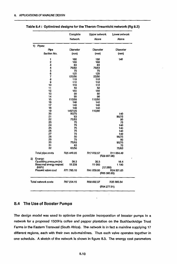
8. APPUCATlONS OF MAlNUNE DESIGN
Table 8.4: Optimized designs for the Theron-Treurnicht network (fig 8.2)
Complete Upper network Lower network
Network Alone Alone
1) Pipes:
Pipe Diameter Diameter DiameterSection No. (mm) (mm) (mm)
1 160 160 1402 160 1603 63 634 75/63 75/635 75 756 125 1257 125/90 25/908 110 1109 110 110
10 110 11011 50 5012 160 15013 90 9014 90 9015 110/90 110}9016 140 14017 140 14018 140 14019 140/125 110/9020 90/75 14021 "63 90/7522 75/63 9023 75 7524 75 14025 75 14026 75 14027 75 14026 50 90/7529 75 9030 75/63 90/7531 63 7532 63/50 75/63
Total pipe costs R25449.05 R17932.57 Rll064.49(R28 897.06)
2) Energy:Operating pressure (m) 36.3 36.3 16.4Seasonal energy reqmnt 18208 11 080 1190
(kWh) (12260)Present value cost R71785.10 R41059.80 R24321.05
(R65 380.85)
Total network costs R97234.15 R58892.37 R35365.54
(R94 277.91)
8.4 The Use of Booster Pumps
The design model was used to optimize the possible incorporation of booster pumps in a
network for a proposed 1500Ha coffee and pepper plantation on the Bushbuckridge Trust
Farms in the Eastern Transvaal (South Africa). The network is in fact a mainline supplying 17
different regions, each with their own sub-mainlines. Thus each valve operates together in
one schedule. A sketch of the network is shown in figure 8.3. The energy cost parameters
8.10

!"
,,{II ) ~."
SCALE _x. l:ll ...
~2!o?;oiii!il~zCZm
~
Plpl I..Hotl
Vol"
l[IPD(i)
-","'.11_____......__ T""".._ ...._
I_I
V~_
..YO
'""'"'m
n,
121 _
11'-
.~
!:II......
Figure 8.3: Bushbuckrldge Trust farms, Irrigation mainline network

•
8. APPUCATIONS OF MAlNUNE DESIGN
were the same as those used for the Theron-Treumicht network described in section 8.3
above.
The network was optimized twice, once with no booster pumps specified, and once with
booster pumps in sections 2,4,6,8,12 and 13 respectively. The results are summarized in
table 8.5.
Table 8.5: Optimized design of the Bushbuckrldge network (fig 8.3)
PipecostsRequiredpump pressures (m) :
At sourceBooster (2)Booster (4)Booster (6)Booster (8)Booster (12)Booster (13)
Total seasonal energyrequirements (kWh)
Presentvalue of energy _costs
Tolal system costs
Wrthoul Boosters
R389062.60
172.3
1236729
R847640.4O
R1 236 703.00
WrthBoosters
R303444.20
84.117.451.545.114.525.80.0
954 740
R654196.60
R957641.00
The pipe diameters for the two networks were principally the same, however the booster
pumps resulted in considerably lower pressures in the pipes and hence enabled the use of
lower class pipes,which yielded the savings shown in table 8.5.
The booster pumps resulted in a significant saving in the total energy requirement; and in this
case this saving is reflected equally significantly in the total costs, since unlike the case
described in section 8.3, the fixed costs are now overshadowed by the direct energy costs.
The list of pressures required at the booster pumps indicates that the booster specified in
section 13 is redundant, but that each of the other boosters contributes to reducing the total
system costs.
8.5 The Design Model as an Aid to Network Operation
The final application of the mainline design model to be described in this chapter relates to
the use of the model to assist in the operation of an existing network. The network is on the
Beyers Trust Farms at Riviersonderend in the Westem Cape. A dam situated on a hill above
the irrigated lands supplies 31 separate orchards covering a total of 140Ha,as shown in figure
8.4.
8.12

8. APPLICATIONS OFMAINLINE DESIGN
IoS
i :I ~
.lIl:..0
• ! .~ .~i
.,I!
~> c.,.!:
;; C"iiEc
:I 0;:;..Cl"i:~
riii E....
~f...'ill:l
~.....,>0-
;.,
m;,; ;;;§ ;:;: m'ItcO.,
i!..e
~Cl
I w I tat m ii:
~ ~ ;:g;
;---
8.13

8. APPLICATIONS OFMAlNUNE DESIGN
The existing pipeline was installed over several years, without ever having been fully
designed with the whole system taken into consideration. Until some racent expansions to
the system, the network operated adequately under gravity. No pumping was needed.
However, the current system is heavily loaded and the farmer has experienced difficulty in
obtaining adequate pressures at the valves. The possibility of adding a pump to the system
was considered.
The design model was used to establish operating schedules that would require the
minimum amount of pumping pressure, if any pumping was needed at all. This was done as
follows :
The layout was specified with the existing pipes. The scheduling algorithm was then run to
establish operating schedules for 9 irrigation shifts. This was the maximum possible number
of schedules, taking into account the required time for each schedule, the total available time
and the time required for an altemative use of the network to irrigate large pastures. The
optimization procedure was then" run to find the minimum pumping requirement for these
schedules.
As discussed in chapter 6, the design procedure allows optimization on the basis of two
different specifications of the required pumping pressure. The first is a single overall
pressure which will be the same in each schedule. The rationale for this being that the
pressure operating point of a centrifugal pump can not normally be varied over a very large
range, and it is preferable to have a constant operating point for all schedules. The second
possible specification is for a separate optimum pressure in each schedule, which enables
the designer to establish the extent to which the requirements in each schedule are
unbalanced; and sometimes to design a bank of pumps that will meet the varying network
requirements. For the Beyers network, the latter case was specified, so that if only some of
the schedules required pumping, then they could be identified.
The resulting valve operation schedules are shown in table 8.6.
The results of the optimization showed that the required pressures at the valves could be met
in all schedules with zero pressure head at the pump. In other words, there was no need for
any pumping. In fact, the pressures at all valves, except for valve number 1, were at least 4m
greater than the required minimum of 15m. The available pressure at valve 1 was exactly
15m, which means that any undue pressure losses in the pipeline will cause valve 1 to
operate below the required pressure.
8.14

8. APPUCAllONS OF MAlNUNE DESIGN
Table 8.6: Valve operation schedules for the Beyers Network (fig 8.4)
ShiftNo.
123456789
8.6 Conclusions
Operatingvalves
7&289,23,25, &3010,17,24 &291,11,22 &26
6,20 &212,31 &19
8,15,18 &273,12 &14
4,5,13 &18
Total flow
(m3/ h)
215218218207203198221185233
The mainline design model has been shown to provide good results in a number of different
applications. Specifically, it has been used to :
* provide efficient valve operating schedules;
* optimize the pipe diameters and pumping requirements of complete networks;
* enable rational decision making regarding altemative network layouts and structures;
* investigate and optimize the incorporation of booster pumps into a mainline design;
and finally to,
* assist in planning the operation of an existing network.
The experience gained in using the model showed it to be flexible in the formulation of
altemative designs, and relatively fast in generating solutions to each altemative. Once the
basic data had been fed into the computer, then the approximate run times required to
complete each alternative design, for each of the examples described above, were as follows:
1. The Ncera network (24valves) :
Valve sequencing - 4 minutes;
Optimized design - 9 minutes.
2. The Theron-Treumicht network (31 valves) :
Valvesequencing - 6 minutes;
Optimized design of the full network - 14 minutes.
3. The Bushbuckridge network (16 valves) :
Optimized design with 6 boosters - 8 minutes.
4. The Beyers network (31 valves) :
Valvesequencing - 5 minutes;
Pump optimization - 2 minutes.
8.15

8. APPUCATIONS OF MAINLINE DESIGN
These "tum around" times enable a designer to investigate numerous altematives relatively
painlessly in the same time that it would take him to complete a single design by conventional
manual methods.
Experience showed further that it is important for the user to have a good understanding of
both the structure of the computer programs and the solution algorithms they employ. The
programs do not provide a 'black box' for use by unqualified designers.
The results obtained from a number of applications indicate that current design practice tends
to underestimate the effect of energy costs on the total system costs, in favour of lower capital
costs. Several designers. when spoken to about this, felt that the reason for it was that their
clients (the farmers) were more concemed about the immediate cashttow effects of any
development, than the longer term minimization of expenditure. It would be useful to use the
design model to build up a series of recommended head loss gradients to be applied in the
design of mainlines under varying circumstances.
In general, the tendency with existing manual techniques has been to design mainline
networks with only a single diameter pipe in each section. One of the strengths of the LP
procedure is that it can determine the optimal lengths for up to two diameters in a given
section. In some cases, if a particular section is extremely long, it may be advantageous to
specify a dummy node at some suitable point (e.g. at a sudden change in topography, or at
the mid point) along the length of the section, so that more than two diameters can be
calculated for the section.
A number of areas for Mure improvement of the programs have been identified:
* The data input routines should be streamlined. The whole layout, including valves,
nodes and pipe sections could be specified in one table.
* The results of the optimization routine should include a fuller specification of the
resulting energy and hydraulic characteristics of the network.
* The candidate diameter constraint currently has to be investigated by the user, and
rectified manually in the layout evaluation table, prior to re-optimization. A routine to
automate this process should be developed.
* The diameter selection criterion for the layout evaluation appears to work well, since
few cases requiring candidate diameter adjustment were experienced. Nevertheless, it
would be useful if the limiting velocities used for establishing the first estimate diameter
were user specified (with the currently set values as defaults). This would enable the
user to develop a "feel' for the most appropriate values under different circumstances.
8.16
9. CONCLUSIONS
9. CONCLUSIONS
9.1 Principal Results
The main aim of the work reported in this thesis has been to develop a functional set of
computer programs for the design of irrigation systems. It is felt that in achieving this goal,
the principal results of the research have been as follows :
9.1.1 Structuring of the design process
The research has resulted in a complete and formal specification of the irrigation systems
design process, viz :
* Classification of the requirements of the design process into system and hardware
characteristics, and identification of the individual components within these two groups;
* Formulation of three main design modules (preliminary, block and mainline)
incorporating all ofthe required components;
* Identification of the specific design routines within each module;
* Specification of the input, output, design parameters and design objectives involved
in the execution of each routine; and
* Identification of the links between various routines and the inter-dependence between
various design components.
An overview of this structure is provided in table 2.1 and figures 2.1 and 2.2 in chapter 2,
together with the synoptic maps of the computer models in Appendix 1. Documenting this
structure provides a reference wherein each element of the design process is placed in its full
context; as such it formed an essential first step in the development of the complete design
model.
9.1.2 Comprehensive evaluation models
In developing the computer based design models, a principal objective has been to
incorporate on-line evaluation procedures that enable the designer to focus his attention on
the expected performance of the designed system and the exlent to which it meels the
prevailing requirements. Both the mainline design and the block design modules contain
comprehensive evaluation processes which enable the designer:
* to assess the extent to which the design satisfies his objectives;
* to generate alternative designs; and then
* to compare these alternative designs.
9.1

9. CONCLUSIONS
Appropriate use of these evaluation models will provide the designer with an insight into the
performance of the irrigation system that has not been practically attainable using current
manual design procedures.
The evaluation procedures are based on a thorough study of the state of the art in measuring
irrigation performance, leading to the formulation of a set of performance parameters which
have been incorporated into the models. These parameters are discussed in detail in
Chapters 3, 5 and 6.
The main evaluation model at the end of the block design process provides the designer with
information on :
- the uniformity of distribution that will result from the designed system;
- the expected yield per unit area and per unit of water applied, that will be attained using
the system;
• the requirement and application efficiencies that will be achieved by the system;
- the estimated cost of the system and the financial return on Investment per unit area and
per unit of water applied, that will be achieved; and
- Information on the optimal application depths during the irrigation season.
It is important to note further that the principle of evaluation has been incorporated into the
whole design process. Thus, apart from the main evaluation model described above, more
general evaluation is carried out continuously throughout the design process. The models
have been structured so that whenever the designer wants to investigate the effects of
possible adjustments to the design, he is able to consider these effects in terms of
immediately updated evaluation parameters. For example:
* In the lateral and manifold design routines of the block design module, the designer
has the choice of (a) letting the computer carry out the design, either by the poly-plot
routine or by extrapolation of results obtained from previously designed pipes, or (b) he
may specify the design himself, by inputting the required lengths and diameters. Once
the design is complete, the table in which the design details are listed (figure 4.10) is
updated withstatistics on :
- the cost of the pipe being designed;
- the total cost of the whole block;
- the total length of the pipe being designed; and
- the total lengths, for the whole block, of each diameter of pipe being used.
•
9.2

9. CONCLUSIONS
If the designer now wishes to change the design, for example by altering the length of
one of the pipe sections used for a specific lateral, he will immediately be able to see the
effect of this change on the cost of the lateral and on the overall block costs.
Furthermore, having made the change, he can then obtain a graphical plot or a numeric
listing of the pressure envelope, and thereby investigate the hydraulic effects of this
change.
* In the valve sequencing routine of the mainline design module, once again the
designer has the choice of either letting the computer determine the schedules or of
specifying his own schedules. Once the valves have been fully allocated, the resulting
schedules are displayed in a table which also lists a summary of the flow required in
each shift. If the designer decides to alter any of the schedules, the table is updated as
soon as any change is made and the designer is therefore able to monitor the extent to
which the flow requirements in each shift are balanced.
* In the quick evaluatIon of layouts routine of the mainline design module, the results of
this evaluation are presented in two tables. The first lists the estimated capital costs of
the mainline, based on "first shot" pipe diameter selections (figure 6.4). The second lists
the estimated operating costs, based on prevailing energy cost tariffs, the expected
efficiency of the pumping system and the rates used for the present value analysis
(figure 6.5).
Both of these tables can be edited by the designer and the effects of any changes will be
updated immediately. Thus for example, he can investigate the sensitivity of the overall
network cost to changes in any ofthe selected pipe diameters. A1tematively, he can test
the sensitivity of the operating costs to changes in the energy tariffs or interesl/inflation
rates.
* Similarly, the linear programming routine of the mainline module presents the results of
the optimization in two tables; one showing the optimum pipe diameters and their
associated lengths for each section of the network, and the second showing the
resulting pressures at each valve and at the pump.
The designer may change any of the selected pipe diameters or their lengths, and the
effects of such changes will be shown in the cost summaries and in the pressures table.
9.3

9. CONCLUSIONS
9.1.3 Design algorithms.
The research did not attempt specifically to develop new design procedures, but rather
wherever possible to adapt well established methods into a workable format for the type of
Interactive computing that was being strived for. This was achieved In the following
algorithms:
'" the routines for lateral and manifold design. The mathematical specification of the
graphical poly-plot procedure was a continuation of the work of Perold (1979 • ref. 7 in
chapter 4). Several modifications were developed in order to render the process
efficient and stable for common design situations; as well as to incorporate accurate
point-to-point calculation of the pipe and emitter hydraulics, for both laterals and
manifolds.
'" the linear programming routine for optimization of the mainline pipe diameters and
pumping requirements. MOdifications to established algorithms include the generation
of the candidate diameters, the calculation of the pumping costs and the allowed option
for generating either an overall optimized pumping head or an optimum for each shift.
In addition, a number of new procedures for the design of various parts of the overall process
have been proposed. These include:
- the valve sequencing algorithm in the mainline design;
• the layout evaluation process in the mainline design;
- the dynamic programming algorithm for optimizing the system operating point which
forms part of the block design evaluation process.
9.1.4 Rationalization of the design process
Although the design model does not provide a completely rationalized solution to the design
problem at this stage (as discussed in Chapter 1), it does enable the designer to carry out a
quantitative study of the various trade-offs involved in the design process. For example:
'" the suitability of the 20% allowable head loss criterion can be investigated on a case by
case basis;
'" the maximum yieldcriterion can be modified to a maximumprofit criterion, which allows for
rationalconsideration of the possibility of deficit irrigation; and
'" the ratios of cost vs performance, system vs operating costs and block network vs
mainline network costs can also be investigated.
9.1.5 Computer aided design (CAD)
The computer programs have been designed to exploit, to the fullest possible extent, the
impact of computer aided design (as opposed to computer aided draughting) on the general
"Engineering Design" process. Experience gained during the course of the research showed
9.4

9. CONCLUSIONS
that both the on-line availability of the various evaluation facilities. and the user friendly and
interactive man/computer dialogue. encouraged the designer to undertake a more broadly
based and investigative approach to the design problem than was practically feasible in the
past. As such, the Author believes that the programs constitute a significant contribution to
the state of the art of CAD In the field of Irrigation Engineering.
In particular, a specific objective of the work was that the programs should be applicable to
real on-farm situations. To this end they were developed for use in a design office
environment on personal computers with locally developed databases, rather than on any
remote main-frame facility with hypothetical data.
9.2 Applications of the design models
The computer based design models have been tested on a number of different design
problems. The results of these tests, on both block design and mainline design cases, are
reported in chapters 7 and 8 respectively.
In general, the models were found to perform well, providing rapid calculation times and good
operating flexibility. More specific conclusions regarding the performance of the computer
models in specific design circumstances are drawn at the end of each of the abovementioned
chapters.
9.3 Development of the computer programs
The structuring and design of the computer programs played an important part In the
successful development of the design models. The programs evolved in three distinct
phases, as experience was gained in the use of computer aided design techniques. These
phases can be characterized by the nature of the man/machine interface In each case :
9.3.1 Phase 1 : Initial Individual design routines
These programs employed a consecutive input dialogue. followed by a unidirectional operating
procedure. This meant that the required data was input on a line by line basis. and the
designer then sat back while the computer carried out the calculations. Once the design was
complete the designer could study the results In order to decide on any changes he might
want to investigate further. These changes would then be incorporated into a new set of Input
data and the programs would be rerun from the start, using the new data.
9.5
9. CONCLUSIONS
The rigidity of this structure precluded the type of continuous evaluation throughout the
design process described In section 9:1.2 above.
9.3.2 Phase 2 : The BASIC programs for mainline design, written on the IBM-PC
These programs employ a tabular input dialogue and a multidirectional operating procedure.
This implies that the data are input through fully editable tables. The designer can make any
additions or corrections he wants to the tables, before continuing with the various calculation
routines. The results of the calculation procedures are also presented in tables on the
computer screen, and the designer can once again edit these result tables for use in any on
going calculations. Furthermore, the designer does not have to run the program in a fixed
order of steps, but can rather move between the various routines at will.
Thus the use of the programs is no longer based on individual 'runs' of the design routines,
but rather on extended "work sessions' in which the designer and the computer work
together to investigate numerous alternatives on the way to optimizing the final results.
These programs incorporated the continuous evaluation principles discussed above.
Another aspect of the programs that was developed during this phase was the incorporation
of on-line routines for immediate validation of the data input This means that the data is
checked as far as possible for its general feasibility, while It Is being entered Into the
computer, rather than allowing the program to fail while performing the calculations.
9.3.3 Phase 3: The PASCALprograms for block design, written on the I~M-PC
These programs are operated by similar processes to those of the phase 2 programs.
However, they are considerably more flexible in their ability to move between different
routines. The prevailing philosophy Is one of lelling the user determine the path followed
through the program, rather than the program directing the user. All procedures are
accessed through displayed menu functions.
Also, greater accessibility to various reference facilities (e.g. the databases and the maximum
length calculator) is achieved through the use of the "pop-up Windows'. Attention has been
given to details such as a uniform screen layout, constant use of prompts which are always
displayed in the same place on the screen, and the use of graphics to illustrate results. It has
been found that these aspects greatly enhance the operation of the programs.
9.6

9. CONCLUSIONS
9.4 Indications for further work
It Is felt that continued research on the subject of this thesis could follow two main directions:
* Once the results of more applications have been acquired, they can be used to develop
a set of design norms that could form the basis of a code of practice. For example,
recommendations could be formulated on the following:
- The most appropriate overall system coefficients ofuniforrnity, under different conditions;
- Expected application andrequirement efficiencies under different operating conditions.
- Allowable pressure variation within a system;
- Appropriate ratios of block versus mainline and hardware versus operating costs;
- The most economical pipe sizes to be used In mainlines, with due consideration to the
cost of energy in the overall cost of the system•
• One of the most interesting parameters in this category, Is an Investigation of the
potential for deficit irrigation under varying conditions.
* Continued development of the models themselves. This would entail :
- Development of a preliminary design module, and integration of all three modules
(preliminary, block and mainline) into a single package utilizing shared data input and
output routines and similar operating procedures;
- Interfacing the design package with one of the commercially available computer aided
draughting packages in order to enable graphical data input and results output ;
- The development of a complete irrigation equipment database to be used as a master
bill for interfacing with the design process and subsequent detail specification of bills of
quantities. This specification would be linked to the output of the design model.
9.7

APPENDICES
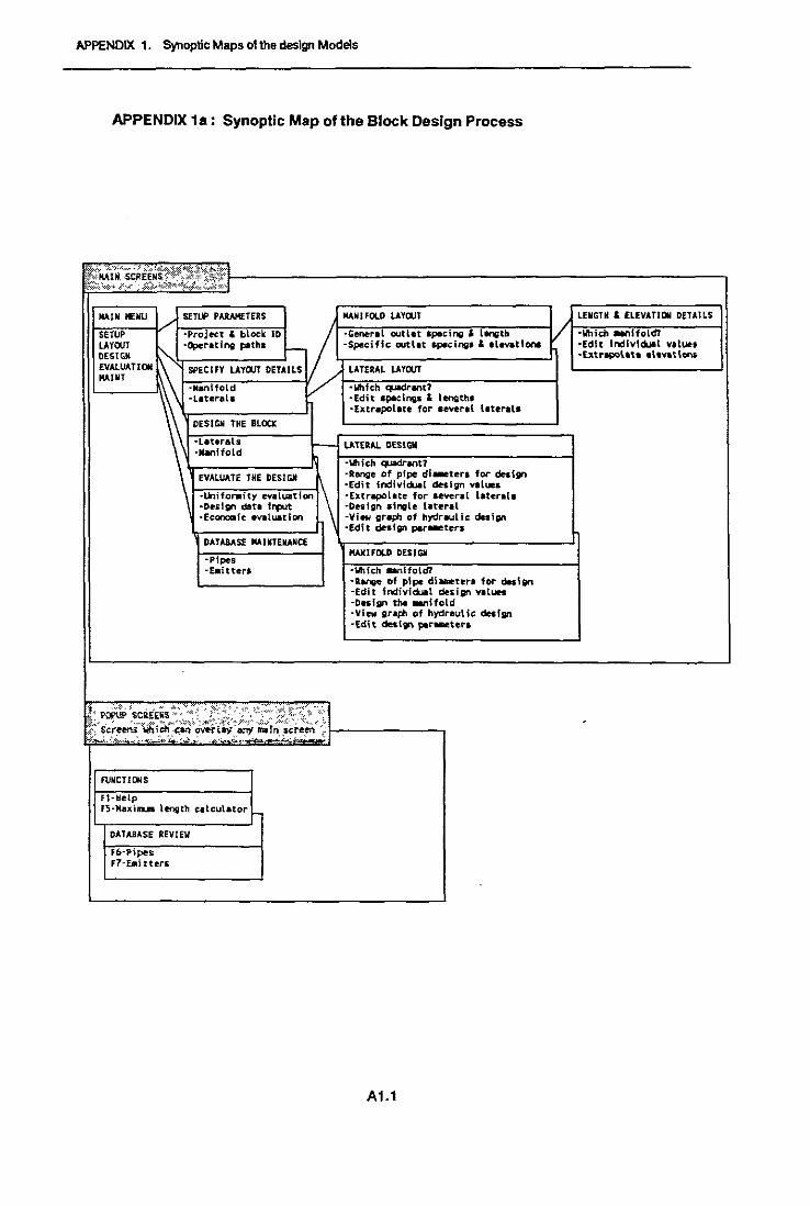
APPENOIX 1. Synoptic Maps 01 tho designModels
APPENDIX 1a: Synoptic Map of the Block DesIgn Process
LENGTH &. ELEVATION DETAILS
-Which .,-alfold?-Edit Indlvfc»ll value.-btnpo,""••"'vattent
LATERAL LAYQJT
-Which quadrant?-Edit sPIcing. " len;th.-extrapolate for several lIter.la
LATERAl DESIGN
-"IIich ~t"lnt1
-Range of pipe di..tere fOl" design-Edit indivlciJIIl ~i;n values-ExtrapoLue for HVeral Latenl,-Design .lngLe lateral-View Graph of hydrauL te duijn-Edit design par..eter.
MA,N1FOLO UYaJT
-General outlet apecil"lQ " lqth-SpecifIc outlet r.pecil"lSl' &. elavatfClnl
f--!--,-,..,...,..-=-"......,.,---------l
EVALUATE THE DESIGN
-Unifo,..ity evaluation \-Design data trpJt-EcClnCIIic eVIlu.tion
MAIN MENU /" SETUP PAlAMETERS
SETUP -srejeee I block ID Ih==r::=:::-==::""''''=~---l/IJ.==:-::===-----1LAYOOT -, -aperatin; p'thl ~OESlCiM . '- ... ....1
EVALUATIott ~ SPECIFY UYCl.IT DETAILS
MAUlT -Manifold yf-'"'"''""'""-,..,.-'''"---------1\\ -Laural.
\' DESIGN THE BLOCX
\ -Laterals\ \ -Manifold
DATABASE MAINTElWICE
-stsee-Eaitters,
MA1UFQUl DESIGN
-Which aanftold?,aa''l8e of pipe d'i.-nr. for design-Edit fndividJIl design values-Design tha ...,Uold-View Graph of hydraulic: design-Edit de"'gn p.r.-ten
FUNCTIONS
fl-Helpf5-MaxillUll length ealculator
DATABASE REVIEW
fb-Pipes;F7-ElIIitters
AU
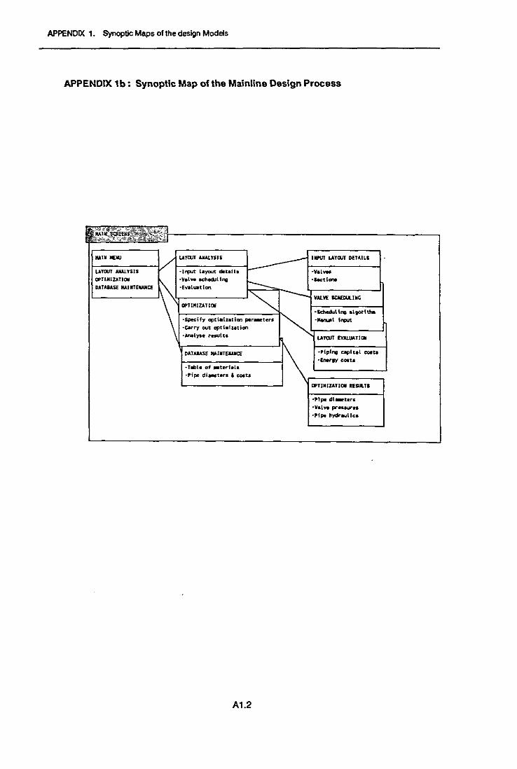
APPENDIX 1. Synoptic Maps of the design Models
APPENDIX 1b: Synoptic Map of the Mainline Design Process
Ifl~eJ'~(~~f!''l»"," ,:.;.*~ ,~. >ok
RA11II..,
/LAYClIT AltALYSIS --- IIPlJT UoYOJT DETAILS
LAYOUT ANALYSIS 'J~ layout detail, -V.IVHOPHMlZATJOll
~·V.l.... leheclJU", :-- "SKtlorw.
OATAIASE MAI,rEIlANCE -EV8llMtlon.
<, --- VALVE ICNEDUlIMGCFJlMIZAT101l
-Sche6.lUn; s\pht.-Specify opti_lzatfon plr_teu •....t I,..n:-car.-y out cptl.;ution·~tYH ".-utn LATM EVALlJATUIi
CATAlASE ",IMTEIWlCE 1\ ·'ipl"lil apftat CQltl
-Ene'-Y COits-riMIt. of _terfat,
-Pipe di.,tarl & ~u.
El'TlMIZATICil IfSlJL1S
.p'pe dl_terl·v.l .... prftaurn-Pipe hydr.....t tee
A1.2
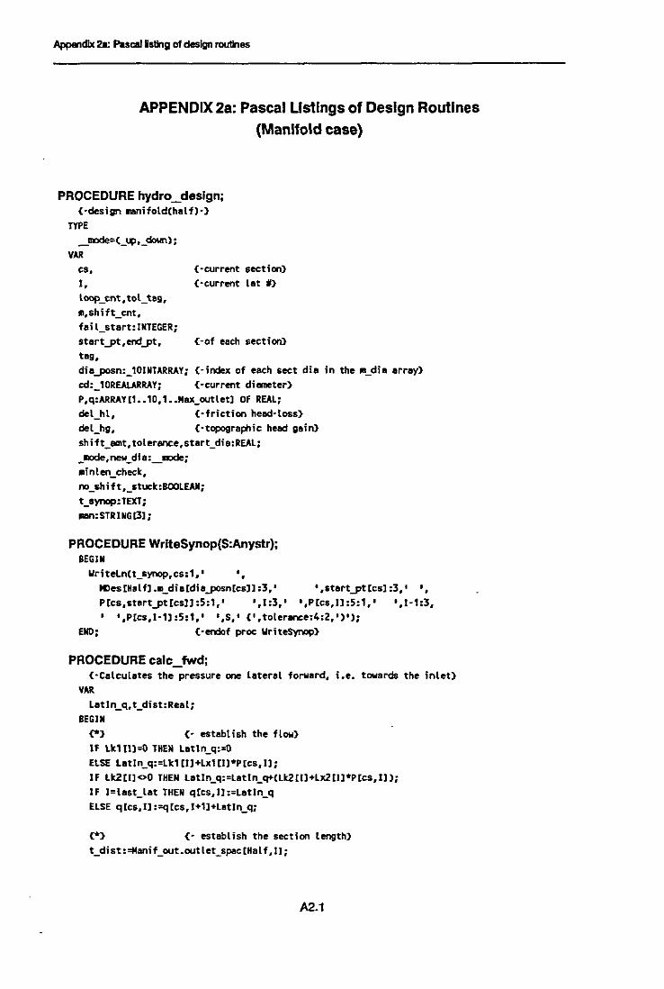
(-of each section>
<·current section><-current lat j}
Appendix 2&: Pascallsting DI design routines
APPENDIX2a: Pascal Listings of Design Routines
(Manifold case)
PROCEDUREhydro_design;{-design nanifold(halfl-}
TYPE_1OOde=(_tJP,_down) ;
YAHcs,
I,loop_cnt,tol_t 89.",shift_cot,fail_start:INTEGERistartJ>t,endJJt,tI!Ig.dia-PQsn:_'OINTARRAYi (-index of each sect die in the __die .rray)cd:_'OREALARRAY; <~current diameter>P,q:ARRAYll •• l0,l ••Mox_outletl OF REAL;del_hi, {·friction head-loss}del_hg, {-topographic head gain}shift_arnt,tolerence,start_dia:REAL;_1IIOde, new_di 8:_1JClde;
.inlen_check.,no_shift,_stuck:BOOLEAN;t_synop:TEXT;...n:STRlNG[3I;
PROCEDUREWriteSynop(S:Anystr);BEGIN
Yrheln(t_synop,cs:1,' "lI)es [Half] .m_di a[di 8-POSn[csl] :3, I • ,Itart...pt [es] :3, I I I
P[cs,stertJ)ttcslJ:5:1,' ',1:3,' ',Ptcs,Il:5:1,' ',1-1:3,',P[cs,[-U:5:1,' ',5,· C',tolerance:4:2,')');
END; {-endof proc IIriteSynop}
PROCEDURE calc_fwd;(-Calculates the pressure one lateral forward, i.e. towanda the inlet)
VARLatl"_q,t_dist:Real;
BEGIN{*} {- estoblish the flow}
IF Lkll11:O THEH Latln_q:=OELSE Latln_q:=Lkll1l+Lx1[I)*Plcs,ll;IF Lk2l1l<>O THEN Latln_q:=Latln_q+(Lk2l1l+Lx2l1l*Plcs.1l I;IF I=last_lat THEN qlcs.I):=Latln_qELSE q [cs, 1] :=q[cs, t+1J+Latln_q;
{*} (- establ ish the section length)t_dist:=Hanif_out.outlet_spac[Hal f,n;
A2_1

• )i
Appendix2a: Pascal IstIng01design routines
<*> (- headloss r. elev.tlon eh-. celes>del_hI :*IExp(LnIHlplll )+Hlp[2]*Lnlq[es.Il/11000*Hlp[41», +Hlp13]*Lnlcd[cs]>l*t_dist);del_hg:oM.nif_out.outlet_elev[H.lf.l-l]-H.nif_out.outlet_elev[H.lf.ll;Plco.l-l] :.p [ts. Il+del_hl-del_hg;
(* -trece used for debugging purposes, now connented out:
gotoxy(42,8);write('latinq, P, del_hl, del_hg, lk', Ix1, lk2, lx2 I ) ;
gotoxyI42.91;writell.tin_q:8:3.P[cs.i]:8:2.del_hl:8:2.del_hg:8:2);gotoxyC42. lO);writel lkl [i] :8:2.lxlli] ,8:2.1k21i] :8:2.lx2li] :8:2);pause; *)
ENll; {-of prot. C.le_fwd>
PROCEDURE calc_back;(-Calculates the pressure one lateral back., i ..e .. away frOlll the i.nlet)
VAlLatln_q,t_dist,t_hl,t_hg:Real;
BEGIN{*> (- establish the flow>IF Lkl [1]=0 THEN Latln_q:=OELSE L.t1n_q:'Lkl 1I]+Lxl Ill*P[cs.ll;IF Lk2[1]<>O THEN L.t1n_q:'Latln_q+ILk2Ill+Lx2I1]*P[cs.Il);qlcs,l+11 :=qtcs,n "latln_qi
{*> {- establ ish the section length>t_dist:#Manif_DUt.outlet_spec[Half,J+1l:
<*> (- headless r. elevation eh.nge calcs>t_h1 :=IExp(LnCHlp[l] )+Hlp[2]*Lnlqlcs.I+1l1l1000*Hlp[4]»
+Hlp13]*LnCcd[es] >l*t_distl;t_hg:=Manif_out.outlet_elev[H.lf.I]-Menlf_out.outlet_elev[H.lf.l+l];P[c5,1+13 :zP[cs, n-t_h L+t_hg;
ENll; (-of prot cele_beck>
PROCEDURE stuck(X:lnteger);{-Hendles the verious stuck situations>
VAlBeason:STRlNG130];J,jj:lnteger:MsgString:~tr;
_llStr:Anystr;BEGIN_Stuck.:~True;
"..iteSynopCt
<*> {- establish BIOSs.ge >IF X=1 THEN Reason::!:' (in en Ihift loop)';IF Xz:Z THEM Reason:=' (need. larger dial';IF X=3 THEN Reason: z ' (need a UII!Iller dil)';IF X=4 THEN Reason: c ' (.in dia>all dies in list)':IF X=5 THEN Reason:=' (in a change diems loop)l;
{-beep r. write. IISg}
Beep;MsgString:=I':MsgString:='Design stuck It die. I;Strlllles [H.l f].__die [die.JlOSn[es]] :3.SIl81IStr);
A2.2
AppencflX 2a: Pucallsllng 01 design routines
MsgStrlng:aMsgStrlng+soaIIStr;MsgString:-MsgString+', emitter' ';StrCl :3._IIStrl;MsgStrlng:zMsgString+smeIIStr;MsgStrfng:~s"Strin;+Reason;
InstrCMsgString+' •• hit any key');WriteLn(t_aynop,MsgString);Pause;
{*> c- estsbl ish the plotJlts ->WITH MOeslHalf] DO
BEGINFOIl J:zl TO cs DO
FOR jj:zstartJltIJ] DOWHTO endJltlJ] DO.Jllot[jj] :zPIJ.jj];
__desi;ned:zFalse;END;
WritePlotFile(Halfl;
{- updote col totals &exit>Fill_.enif_descrip;
END; {-of proc. stuclc}
PROCEDURE change_dla(nn:_mode);{-Chan;e diaMeter when pressure profile reaches envelope boI..ndarfesJ
YAKaa:lntegeq
BEGINWITH MOeslHalf] DO
BEGINnD_sbift:af.tse;ca:=ca+1;
startJPt[csl:~r;end-pt[c.·,]:zl+';
Plcs,n :cP[cs-',Jl;qlcs,'+'] :&q{cs·', 1+11;IF _1IOde=_"" THEN _DOCIe:z_downELSE _ax:Ie:=_14»;.inlen_checlt:ll:True;IF endJltlcs-ll>startJltlcs-l] THEN endJltlcs-ll:zstartJltlcs-ll;tag [csJ :_1;diaJPOS"lcs]:=dlaJPOS"lcs-ll+l;
{*> {-change to a larser dil..eter >IF m=_"" THEN
BEGINIF dia-P08"lcs]>10 THEN diaJPOS"lcs]:z10;WHILE (M_dialdiaJ'OSnlcsll<=m_dla[diaJ'OSnlcs-llll
AHO (dlaJlOS"lcsl<10l DO diaJ'OSnlcsl:=dlaJlO8nlcsl+l;IF ._dia[dlaJ'OSnlcsll<.._dialdia-P08"lcs-lll THEN stuck(Zl;IF NOT _Stuck THEN
BEGINnew_dia:=_'4);cdlcs]:==
Mat_Detai1.lnt_dla [_classlndex••_dla_inclex[dlaJlOsn[csl]l ;END;
ENDELSE

Appenclx 2a: Pascallsting 01design routines
(*) {-change to • &moIler diameter>IF ,."._down THEN
BEGINIF d;aJlO5nlesl>IO THEN d;aJlOsnlesl,"O;
WHILE (o_dialdiaJlO5nles]].<m_dilldiaJlOSnles-']]lAND (diaJlO5nles].1) DO diaJlO5nlesl :adiaJlO5nlesl -I;
IF (o_dia IdiaJlOSnlesll <dJlllr...~__lf_dial
OR (o_dialdiaJlO5nlesll ..._dialdisJlOsnles·Illl THEN stuc.(3l;IF NOT _Stuck THEN
BEGINneN_di.:-=_doIm;celtcs] ,=
Mat_Detai 1. int_die [_classJnclex••_dia_inclex[diayosn[csl)];END;
END;END;
END;
PROCEDURE Shift_up;{-Shifts the current pressure cur-ve ~ to meet the top of the envelope}
BEGINno_shift:=false;tag [cs] :=1;
shi ft_cnt:=shift_cnt+1;.inlen_check:=True;shift_aot:=dJlllr".~JPMax·Ples,ll;
_-=de:=_down:IF shift_oat.O THEN
BEGINI :••tart-pt [esl j
PIes,I] ,ap tes, U+( (I ·sh; ft_oat/dJlIIr...q,JPM;nl+sh; ft_oatl;
ENDELSE BEGIN
no_shift:ztrue;.inlen_check:zfatle;
END;
IF (c"'l AND (NOT no_shift) THENBEGIN
IF new_dis=_up THENBEGINqlcs,l+l]:=q[cs,I+I]+('+shift_aat/dJlllr".~JPMinl;
WHILE (P[es.Il.=P[es·'.lll AND (Ples·'.lloDl
AIID (Plcs·'.Il<dJ>llr...~JPMaxl DO
BEGINcalc_fwd;l:zJ-';
END; (-of while)
IF (Ples,ll<Plcs·'.lll OR (P[cs-'.Il00l OR
(P[cs-l.Il>dJlllr".~JPMaxl THEN 1:=[+';ENO
ELSEIF new_dis=_down THEN
BEGIN
q[cs,ll:=q[cs.ll+('+shift_aat/d-p"r".~JPMinl;
WH[LE (Plcs,Il.=Ples·',l]l AND (l<=start..ptlcs-lllAND (Pla-',Il.p[cs·'.I+ll) DO
A2.4

Appenclx 2a: Pascallsllng 01 deslgn routines
IEGINcalc_beck;1:-1+':
EIID; {-of whHe}
IF (Plcs,ll<Ple'-',Il> DR (I>otartJ't1es-n>THEN 1:=1-';
END;IF 1••tartJ't[csJ THEN
BEGINno_shift:ctrue;.inlen_check:=false:
ENDELSE
BEGIN.tartjptlcs]:=l;endJ'tlcs-'l:=I+';IF endJ'tlcs-'l>startJ'tles-'l THEN endJ'tlcs-'l:·.tartJ'tles-'I;
END;Pres, J] :-9 tes-j , 1];q [cs, l+1] :-=q[cs-', 1+1];
END;EIID; {-of prot Shift_",,>
PROCEDURE Shift_down;{-Shifts the current pressure curve down to leet the bottcu of the envelope}
VARbackcnt : INTEGER;
BEGINno_shfft:af.lae;tag[ca]:-·ibeet.cnt::EO;ahift_cnt: ashift_cnt+1;
.inlen_check:cTrue:shift_BOt:=Plcs,ll-dJlOr...dp_I8XJ'lnlet;_aode:._~;
IF shlft_-.t>D THEN
BEGINl:=startJPt[cs]iPles,IJ:=Plcs,IJ-«1-ohift_emt/dJlOr...dp-FM in)*.hlft_BDt);
EIIDELSE BEGIN
no_shift:atrue;.inlen_check:afelse;
Ell);
IF (e5>1) AJI) (IIOT no_shift> THENBEGIN
IF new_dlll=_"" THENBEGIN
qlcs,ll:-qICl,ll+(1·shift_BDt/dJlOr...dp-FM i n>;IIHILE (Ples,Il_les-',Il> AND (I<=stsrtJ't1es-1])
AJI) (Ples-1,Il>Ples-',I+']) AND (qles,Il>O)AJI) (beckcnt<taglcsl+2> 00
{-the lest eon:litlon ensures that we dent go back too farif we .ight get to the end >BEGIN
calc_beck;A2.5

Appencllx 2a: Pascal Isling 01 design rouIi1es
J:-1+';beckent:-succ(beckcnt):
END; (-of while}IF (Plcs,Il.P[es·t,ll) OR (\.start..pt[cs-t]) OR
(q[cs.J]<-O) THEN 1:-.-';END
ELSE IF new_dia=_dOwn THENBEGIN
q[cs,l+tl:=q[es,l+ll*(I·shift_amt/d"poram.dpjPMin);IIlIILE (Plcs,ll<=Plcl-t,ll) AJll) (Plcs·l,lloD) DO
BEGINcalc_fwd;1:-.·';
END; (-of while}IF (Plcs,II.P[cs-t,ll) OR (P[es-t,II-O) THEN 1:=1+1;
END;IF .astart-pt[csl THEN
BEGINno_6hift:~true;
ainlen_check:afalse;END
ELSEBEGIN
.tart....Pt[csl :c[:endJPttcs-1l: c ]+' ;IF end..pt[cs-ll.start..pt[cs-tl THEN end..pt[cI·ll :=start..pt[cs-ll;
END;Ptcs, n :ap[cs-1 ..I) ;
qtcs.I+1l :cq[cs-'.J+1];END;
END; (-of proc. Shift_doi«l>
PROCEDURE adjust;{-Adust the start-pt of the current dia,If after a shift the pressure lOVes outllde the envelope}
BEGIN
ainler'Lcbeck:=True;IF t.glcsl.1 THEN tag [csl :=1;IF _-.de=_down THEN
BEGIN
IF co·t THENIF P[CI,lt.rt..pt[csll =d..POr....dp_IIOX..Plnlet THEN
BeGIN
I:-.tart-Ptlcs]iWrite5ynop(' Adj e1mg Up • >;P[CI,II:=d"poram.dpjPM8x;_-=de:=_up;
ch-"_dl·Cup>;Exit;
ENDELSE
BeGIN
I :=start--pt [csl;PIes, I] :~.995·P[cslJ);
IF P[cs,Il<d"poram.dp_IlOX"plnlet THENPlcs,II:=d-PBram.dp_IlOX"plnlet;
END;A2.6

Appenclx 2a: Pasc:allstklg of design roulkles
IF (CP1) AIID (new_di.._up) THENIF Plcs-l,&tartJltlcsl+l1<Plcs-l,startJltlcsll THEN
JEGIHstart....pt tal :sstartJtttcs]+';l:astartJtttcsl;endJltlcs-1J :-1+1;Plcs,n :<Plcs-l,n;qtcs"1+1] :-qtcs·',l+ll;
EIlDELSE
SEGIHIIriteSynop(' Adj ClIIlll Up ');
_1IOde:=_1.4>;Change_diaUJP);Exit;
END;IF (C5>1) AND (new_dia=_dcwn) THEN
IF Plcs-l,startJltlcsl-l1>dJllram.dp_ImXJllnlet THENJEGIN
start-pt[csl:=start-pt[cs]·';I :zstartJ't [es];endJltlcs-l1:=I+l;Pres, I] :=Ptes-t, 11;qtcs,l+ll :=q[cs- 1,,1+1];
EMl
ELSEJEGIN
IIriteSynopl' Adj Chllll Up ');
_.xIe:c_~;
Change_diaCup);Exit;
END;END;
IF _-_up THENSEGIN
IF cs=1 THENIF Plcs,startJltlcsllodJllram.dpjPKaX THEN
SEGIN
1:astllrtJ'tlcsl;YriteSynop< I Adj Chng Dn I):
Plcs,ll:odJllraa.dp-PMi n;_-=de:-_dot«1;c:hBlllle_diaCdown);Exit;
EMl
ELSE JEGINI :=start..pt [cs];Ptes.n :-, .005*P tcs, Jl;IF Plcs,ll>dJllraa.dpjPKaX THEN
Plcs,ll:=dJllraa.dpjPKaX;END;
IF (cpl) AIID (new_die:_up) THEN
IF Plcs-l,startJltlcsl-1J>Plcs-l,startJltlcsll THENSEGIN
startJ>tlcsl:=startJltlcsl-l;I :astart...Pt [es];endJltlcs-1J :=1+1;
1>2..7
)

Appenclx 28: Pascallslk1g of design rou1tIos
P[el, Il:-P[CI- 1. J];
qrcl,l+ll :cqlci-' ,1+11;END
ELSE
BEGINlI,iteSynop(' Adj CIu-4l Dn ');
_.oe:-_dcM1;Chlnlle_diaCdown);
Exit;END;
IF (co>1) AND (new_dia=_down) THEN
IF Plca-1.lta,tjptlcll+1l>d-p",am.dp_lmXjplnlet THEN
BEGIN
It.rt-ptlcsl:astartJPtlcs]+';I:cstartJPt[cs]:endjptlcl-1l:=1+1;
P res, J1 :=P tes-j,n;qlcs,l+1] :aqlcs-', 1+11;
END
ELSE
BEGIN"riteSynop(' Adj Chng On I);
_mde:=_cIoI«1;Change_di aCdown);
Exit:END;
END;END; (-of peee, adjust)
FUNcnON Inlt_hydro_des:Boolean;(·tnitiate variables at the stert of the design)
BEGINInit_hydro_des:-True;_Stuek:aFalse;IIITH MDeslHllfl DO
BEGIN
FOR ca:.1 TO 10 DO
BEGIN
Itl,tjpt[col :oO;endjpt[col :00;
teglcol:oO;
cdlcol:oO;__len[cs]:cD;__nooflcl]:zO:
FOR 1:·1 TO Max_outlet DO
BEGIN
PIes, n :=O;qlcl, I] :-=0;END;
END;_aode:=_cIow1;cs:c';diajPOSn[cs]:c';IIHILE __dialdiaJPOSfllcsll<d-p",••dp_Enif_dia DO
BEGIN
diaJPOSfllcal:=diajpOSnlcsl+1;
IF diljpOSnlcsl=11 THENBEGIN
stuck(4);
Init_hydro_des:=False;A2.8

(-of with)(-of proe. Inlt_hydro_des)
Appenclx2a: PucIJ Ialilg of design routines
END;ENIl; (-of while)
IF NOT _Stuc:k THEN
IEGINno_lhift:cfalse;J:lI:last_lat;atart..pt[cs] :_1;tag[cs] :-1;toL_tag:-.:fai l_start:El;loop_cnt:a:O:toler.-.ce:=O;l1eW_dia: z _Lp;
ahift_cnt:=O;Plcs.I]:adJPOram.dP-PMax;.inlen_check:=false;cdlcs] :-
Mat_Detel 1. int_di II [_classIndex,._dia_tndex [diayosn[csl)];.t.rt_di.:~[cs];
END;END;
END;
PROCEDURE Check_min_length;{-Check that Length of previous diameter is not less than stipulated .iniaun>
VARf i: Integer;Len:Reali
BEGINWriteSynopCI ChlcMi....en "i
len: =0;.inlen_check:~F.tle;
IF endjptlcs-1]>ltortjptlcl] THEN
BEGINFOR H:astortjptlcl-1] DOoIHTO endJ'tlcs-ll DO
len:clen+Manif_out.outlet_spec[Half,iil;END;
IF (len<dJPOr_.dP_lIOIlif_lIlnLen) OR (len=0) THENBEGIN
cs:=cs-';1:'&start...ptrcsl;teg res] :zl;start-pt[cs+11:=O;IF cs=1 THEN Plcs.lI:adJPOram.dP.JPllox;cdlcl] :=cdlcl+1];cdlcs+1] :cO;ahift_cnt:=O;di0.JP05nlcs]:adi0.JPOSnlcs+11;dio.JP05nlcs+11 :=0;_.:de:=_dowI:new_die:.:_\4):Writeln(t_synop,'Minlen failed: length :',Len:5:1):
{*} {Now check for loopi"ll - three conditions: }IF (cs>1) AND «cd[cll-cdlcs-11)<:O.D01) THEN
BEGINcs::ces·1;
A2.9

Appenclx 2a: Pucella1lng ofdesign routiles
1:••t8rt-ptlcsl;taglesl:-1:start-pt[c8+11:aO:IF _1 THEM PIcs,ll :-d.Jlllr ....dpJllax:cdlcs+lI :-0;tolerance:c toLerance+O.05:loop_cnt:csucc( loop_ent);
ElillELSE IF «cs") AND (cdlcsl<stort_dio»
OR «c5>l) AND (I=foil_stort» THENBEGIN
toleranee:=to\erance+O.05:loop_cnt:asucc(loop_cnt>:
END;atart_dia:&Cd[csJ;fat l_stllrt:sl;
END;END; (-of proc. Check__in_let'lllth)
PROCEDURE Open_synopsis;VAR
tt_cnt,t_cnt:tnte;er:line:ARRAY[1 •• '001 OF STRlNGI!OI;
BEGINt_cnt:EQ;IF Exist(DATAPATK+SYNOP) THEN
BEGINAssign(t_synop,DATAPATH+SYNOP);Resetlt_synop);IIIlllE IIOT seek£oflt_synop) DO
BEGIMIF t_tnt<'OO THEN
BEGINt_cnt:sSUCc(t_cnt):Reedl.ntt_synop,llnelt_cntJ ):
ENDELSE
BEGINFOR it_cnt:"TD 99 DO Iinellt_cntl:.lineltt_tnt+lI;ReodLn(t_synop,linel'OOI);
00;00;
Closett_synop);Erase(t_lynop);
END;Assigntt_synop,DATAPATH+SYNOP);Rewrite(t_lynop):IF t_cnt>D THEN FOR It_tnt:., TO t_cnt DO
Writeln(t_lynop,linelit_cnt);END; (-of Open_synopsis)
PROCEDURE Phase1;BEGIN (·..in procedure)
Open_synopsis;WriteLn(t_synop):IF Holf=' THEN oen:='a/b' ELSE oen:='c/d';WritelnCt_synDp, 'DESIGN OF MAJlIF • , ...., I Date' ,DateString);
A2.10

Appenclx 2a: PuC81lsting of deslgn routkles
IIriteLn(t__• 'SECT DiAl...) Stort Pt & P CUrrent Pt & P NEXT Pt & PACTION TOLERANCE' );
IF Inlt_hydro_des TIlENIEGIN
<_0> <--.In loop lI'ltll designed}REPEAT
IF ahlft_cnt>10 THENIEGIN
stuclr.(1);Exit;
£11>:
IF loop_cnt>5 THENBEGIN
Ituclr.(5);
"Exit;END;
IF I<tol_teg THEN tol_teg:=l:calc_fwd;
{ .•} (··set LP cases)IF _1Ilde=_down THEN
IF (P[cs.I-11>(1+tolerance)*d-POram.dpjPMax)AND (1<lt8rtjpt[cII) THENIEGIN
IF P[cs.[+1]<P[cs..Il THEN 11:-1
ElSE .:=2;END
ElSE IF P[cs.I-11>-(1-tolerance)*d-POr...dp_lBXjplnlet THEN.:8:2
ELSE IF P[cs.I-11«1-tolerance)*d-POr...dp_lBXjplnlet THEN.:-3;
IF _1Ilde=_"" THENIF (P[cs.I-11«1·toleronce)*d-POr...dp_lBXjplnlet)
AND (I <st8rtjptCcsl ) THEN .:-1ElSE IF P[cs.I-1I<o(1+toleronce)*d-POr...dpjPMax THEN .:04ElSE IF P[cs.I-11>(1+tolerance)*d-POrBl.dpjPMax THEN .:<5;
{*> ( •.- I",,'.-nt the ceoes >CASE • OF
l:IF no_shift THEN 1:-1-1ELSE
BEGINWriteSynop(' Adjust ');edjust;
£)1);
2:IF (I>-tllll[CS]) OR (del_hl<=del_hg) THEN 1:-1·1ELSE
BEGINWrite5ynop( I Shft Dn I);
IF (I<tag[CI]) AIID (del_hl>del_hg) THEN ShIfUlown;END;
A2.11

Appendix 2a: PucoJ •.,..g 01des9I routines
3:IF (no_Mitt) AND (I>teg[••]) THEN [:*1-'
ELSEBEGIN
hD_lhift:-falleiWrlteSynop(' Chng On ');
c:IIonge_dioC-');Ell);
':IF (I>-teg[cs]) OR (del_hl>adel_hg) THEN 1:-1-'
ELSEBEGIN
WriteSynop(' Shft Up ');
IF (I<tog[••]) AND (del_hl<del_hg) THEN Shift_up;
END;
5:IF (no_Mitt) AND (I>lOg[••]) THEN 1:-[-'
ELSEBEGIN
wrlteSynop(' Chng Up ');
c:II""lIe_di oCup);
END;END; (·of case)
IF _Stuck THEN Exit;IF (.inlen_c:IIeck) AND ( es>1) THEN Check_.ln_length;
IF (tolerenee>O) AND (I<tol_teg) THEN tolerenee:aO;
UNTIL laO;END;
END; (-endof Pho.e'>
PROCEDURE Phase2;BEGIN
IF _Stuck THEN EXit;(_a> (--now shitt lost die>
IF (P[cs.Il<o.99*dJlOrllll.~J:IIex) AlCD (new_di .._up)
AND C-_up) THEN
BEGINWriteSynop(' End Shft Up ');
Shift_up;WH[LE 100 00
BEGIN
calc_fwd;1:=Pred(l);
END;Wrltesynop<' Design Done I);
EIlIl
ELSE VriteSynop(' Design Done ');
endJ>tl.s] :-';(-*) (--now set up lengths C no-of ..Itterss>WITH MDes[Holf] 00
BEGIN
FOR .:*, TO co DOBEGIN
IF (..1) AND (die...JlOS"OO<dieJlOSnr.-ll) THENBEGIN
A2.12

Appendix 2&:Pascollslng 01 design routines
FOR 1:.'0 D<MITO dloJlOS"[II-1]+2 00__dla[/] :._dlo[l-1];
__dloldloJlOS"[II-1]+1] :._dio ldloJlOS" 00 I ;
dlaJlOS"!Ill :odloJ'Cl5n[11-1] +';IF _s THEN
FOR I :_, TO co 00
BEGINIF dla.JlOSn[/]>odl0J'Cl5n[I(J THEN
dl0.JlOSnlll:odio-POSnlll+';IF dlo-POSn11]>5 THEN
BEGINcs:EJ.';stuck(2l;EXit;
END;END;(-of For J)
Up:Iate_dia_cost:END;
__!lOOf ldla-POS"!Ill] :=stort..pt 00 -end..pt !Ill+';
FOR l:.stsrt..pt/Jlll DOWIITO end..ptOO 00__lenldio-POSn/Jllll :.._lenldlo-POS"/JIIl]+
Manif_out.outlet_spec[Half,I];END; {-of for 10
{-update design counter}__designed:=True;
END; {-of with Des}END; {-phase2l
BEGIN {-main procedure}JnstrC'Designing the .enifold••••• ·);Phase';Phase2:Close(t_synopl;
END;
A2.13
Appendix 2b: Pascal Istilg of unWormIly cala.JlaIIon routines
APPENDIX 2b: Pascal Listings of Uniformity Calculation Routines
PROCEDURE Unlfonnlty_calc(J:lnteger);{ calculate the unifoMlity poraoeters for uniflj).lnletP )
VARllne:Anystr;
.,b, Lat,e_cnt ,quad, pass, n_emits,
lnoof_cnt.l_cnt,~f_cnt••_cnt:[nteger;dia,t_dist,eait_q,HL,Slope,Q_tot,Q_curr,P_curr,EndP,JnP:Real;InCl:ARRAYl' ••21 OF Real;
InP_edjust, InQ_adjust,early_adjust, lat_fLeg:BooLean;hI fstr:STRINGl3];
qdstr:STRINGl1J;
PROCEDURE SetVals;BEGIN
IIITH uni flJ] DO
IEGIN
IF poso=' THEN
BEGIN
Av_q:=Av_qln_emitsiGLvorlance:='OO*(GLIBX-GL·inl/Av_q;
AYGL~ratlo:cAv_q/dJl8r••~_qNe-;
IF noof_hlghl-eJ THEN
IEGIN
noof_highlow:.';
highlow_laterala[1l:·'none'iEND;
END
ELSE IF poss=2 THEN
BEGIN
uni f_coaf: =uni f_coefI(n_..I to-Av_ql;
unif_coaf:=(,-unif_coefl-'OO;
END;END;
END; { endof setVah )
PROCEDURE CalcStets;(~calcul.te the stltistics, once the discharges are established)VAR
t_VIIl:Real;BEGIN
IIITH uni flJ] DO
BEGIN
FOR ~:=, TO 4 00
BEGIN
IF Eyal_gen.noof...JqJadlcp.JadloO THEN
BEGIN
IF quad<=2 THEN Half:=' ELSE Half:=2;
FOR lat:=' TO Evol_gen.last_laUHalfJ 00
BEGIN
lat_flag:=False;A2.14

Appenclx 2b: Pucallsting 01unllormlly cak:uIatIon routines
e_cnt:.';CASE quad OF
l:t_vol:aqv.llAIL.t,e_cntl;
2:t_~l:-qV.l2A[L.t,e_cnt]:
3:t_vol:aqv.13AIL.t,e_cntl;
4:t_val:cqVaL4A[lat,e_cntli
END:\IIIILE (t_vol<>o) AIIll (e_cnt<oIIax_outlet) 00
BEGINIF pes.:' TREN
BEGIN"_e.its:-Suec("_emits);IF t_vIl<qL_in THEN ~.in:=t_~l;
IF t_v.I~1BX THEN GLIBX:.t_vol;IF (t_v.l>Exp(Ln(dJPOram·dP_k)+dJPOr"·dP_x*Ln(dJPOram·dP-PM.x»)OR (t_v.l<Exp(Ln(dJPOr".dP_k)+dJPOr".dP_x*Ln(dJPOram·dP-PMin»)THEN
IF NOT l.t_flog THENBEGIN
Lat_fLeg:cTrue:noof_highlow:'Succ(noof_highlow);( * }{ _ke • otril1ll of l.t no I quad )
Str(L.t:3.h;ghlow_l.ter.I.~f_h;ghlowl);
CASE quad OFl:h;ghlow_l.ter.lo~f~ighlowl:·
highlow_l.ter.lo~f~lghlowl+·.·;
2:highlow_l.ter.lo~f~lghlowl:'
hlghlow_l.ter.lo~f_highlcoa+·b·;
3:hlghlow_l.ter.lo~f~ighlowl:·
hlghlow_l.ter.lo~f~lghlowl+·c·;
4:hlghlow_l.ter.lo~f_highlowl:·
h;ghlow_l.ter.lo~f_h;ghlowl+·d·;
END;
END:Av_q:aAv_q+t_vol;
ENDELSE IF peso'2 THEN
Un; f_coef:-Un; f_coof+Abll(t_vet-Av_q);e_cnt:-SUCc(e_c:nt);CASE quad OF
l:t_val:.qvallA[lat,e_cnt):
2:t_vol:aqv.12A[L.t,e_cntl;
3:t_vol:oqY.13A[L.t,e_cntl;
4:t_Yal:cqval4A[Lat,e_cntl;
END;EIIl;{ endof \IIIILE t_vol )
GoToXl(3.21);IF H.lf-l THEN hlf.tr:,·./b· ELSE hlfotr:"c/d';IF quadFl THEN qdstr:.·.·;IF quadF2 THEN qdstr:"b';IF quadF3 THEN qdstr:.·c·;IF quad=4 THEN qdstr:"d';Write('<Half I,hlfstr,', Quad ',qdstr,', Pass '.pass:'," lateral ',lat:2,'> I);
A2.15

Appenclx 21>: Puc.l b&1g of unlIormIIy caIallation routines
EIID;{ endof FOR lot cnt }EIID; { endof IF tot_noof__ltoQ }
EIID; { endof FOR~ cnt }END; { endof WITH }
EIID; { endof ColcStots }
PROCEDURE Check_lnP_Adjust;( check for odjuotlllent of IrjI o;olnst InletP )
BEGINIF Abs(lnP-l»iftJl.InletP»O.~H[Jl.InletP THEN
BEGINLat:sEval_gen.last_lat [Hal f]:GetLateral(Half,Lat);EncP:-EncP- l(lnP-Unif [Jl.lnletP)*11-IAbsllrjl·unif[Jl.lnletP»/Unif[Jl.lnletP»;
ENDELSE
BEGINuniflJl.lnletQ:-uniflJl.lnlet__tot;InP_adjust:aFalse;
END;EIID; { endof Check_lrjI_Acljust }
PROCEDURE SetNextLat;{ establish IrjI &InQ for next loterol }
BEGINOioIPipeldjplr...qp_oenif_code);{ * } { get the heod l05s por_ }FOR 1:.1 TO 4 DO
Hlp[ll:-Mat_toble[d-POr...dp_oonlf_codel.heodl..o[ll;
t_diot:oManlf_out.outlet_spoc[Holf.Lotl;Slope:=Monlf_out.outlet_elev[Hllf.Lot-l1
-Manlf_out.outlet_elev[Holf.Lltl;dio:oMot_OOtlil.lnt_dil
D4Des[11.a_cl..s_lndex.MDes[Hllfl.a_dio_lndex[o_cntll;
HL:.IIExp<LnIHlpm )+Hlp[2]*LnlQ_tot/(1000*Hlp[41»+Hlp[3]"Lnldio»)"t_di at) - lSlope);
1~:-=Jri>+Hl;
GoTOXYl3.21);IF Half-' THEN hlfatr:a'a/b' ELSE hlfatr:a'c/d';IF quad=1 THEN qdstr: a ' . ' ;
IF quad=2 THEN qdstr:"b';IF quadF3 THEN qdstr:c'c';IF quad=4 THEN qdstr:.'d';Urfte(I<Half ',hifstr,', Quad ',qdstr,', lateral ',lat-1:2,
I, Inlet PntSlure ',lnP:6:2,'>');
IF Lotol THENBEGIN
Lat:=Lat-';GetLateral(Half,Lat>;
A2.16

Appenclx 2b: Puc.! Islilg 01unWonrlty coIaJlalion routiles
InQraJ :.LDes [al .1_coef[1]+LDes raJ •l_coe1[2]*1"";InQ[b1:.LDes[bl.l_cooHlI+LDes[bl.l_coof [2]*1"";
~f_cnt:...-.oof_cnt+';
IF on:>of_cnt>llles[H.lfl.a_noof[JI_cntl THEN
BEGIN-.001_cnt :a';__cnt:-SuccCa_cnt)i
IIHILE lIles[H.lfl.a_nooHI,-cntlaO DO a_cnt:'SUCcla_cnt);END;
ENDELSE lat:~Lat·';
END; { endof SetNextL.t }
PROCEDURE LateralCale;(-Calculate the discharges in the current lateral)VAR
emitq:RealiBEGIN
InCI_acjjust:=True;
REPEAT { ..,til Inll_adjust=fal.e }P_curr:s:lnP;Q_curr:zInQ [CfJIIdJ;
l_cnt:~;
IIHILE LDes[quad].1_noofU_cntl=O DOl_cnt:=Predll_cnt);
lnoof_cnt:E(I;earLy_acfjust:cFalse;OlalPlpeldjP8r...dp_l.t_code);
{ * } { get the head I_ par.... }FOR 1:.1 TO 4 DO
HlpUI :_t_table[djP8r••dp_lat_codel.headlos. [II;
{ * } { at.rt the In-lateral loop }FOR e_ent:.l TO Lat_gen.noof_..IUquad] DO
BEGINIF Q_curr>o THEN
BEGINlnoof_cnt:alnoof_cnt+';IF lnoof_ent>LDeo[quad] .1_noofU_cntl THEN
BEGINlnoof_cnt:=1;l_cnt:-Predl l_cnt);IIHILE LDes[quaclJ.l_noaf[l_cntlaO DO l_cnt:=Predll_cnt);
END;dia:_t_Oet.ll.lnt_dla[odia 1<p.Jad] ._cl••••odla [<p.Jad] ._olndex [l_cntll;
{ * } { t_diot }IF le_cnt<>l) AND IL.t_llOf1.pr_ealt_op<tC[quad]>O) THEN
BEGINIF HOT Oddle_cntl THEN t_dl.t:=Lat_gen.pr_..lt_op<tClquad]ELSE
t_dlot:'L.t_geIl...1t_opac[quad] -Lat_;en.pr_..It_opac [<p.Jad];
ENDELSE IF "_entol THEN t_dlst:.L.t_gen...it_opac[quad];IF e_ent=1 THEN t_dist:=L.t_gen.First_eIIit[~;
A2.17

Appenclx 2b: PasCII islIng 01 unIIormIIy Cl!<:ulatlon routines
( * ) ( slope )
If e_cnt<>1 THENSlope:...1[cpod.e_cnt·lI·el [quad.e_cnt]
ELSE If e_cntz1 THENSlope:=Manif_out.outlet_elev[Half.Lat]·el[cpod.e_cnt];
( * ) ( head loss )HL:z((Exp(Ln(Hlp[1] )+Hlp[Z]*Ln(Q_currJ(1000*Hlp[4]])
+H lp [3]*Ln(dia» )*t_di st)· (S lope);P eurr:=P curr-HL-- - ...itq:=Exp(Ln(dJPOr...dp_k)+dJPOr...dp_X"Ln(P_CUrr»;CASE quad Of
1:qVal1"[Lat,e_cntl :-sitq;2:qValZA[Lat,e_cntl:ceai tq:3:qVal3"[Lat,e_cnt]:aemftq:4:qVal4"[Lat,e_cntl:=emitq:
END:Q_curr:=Q_curr-emitq;
EII1lELSE early_edjust:=True;
EII1l; ( endof e_cnt fOR loop )
{*> {-test for satisfactory zero Q tl!llll!lining in pipe }If (Abs(Q_curr)<O.1*(emitq»AND (NOT early_adjust) THEN [nQ_adjust:zfalse
ELSEBEGIN
If early_edjust THEN InQ[cpdl :z[nQ[cpdl*1.05ELSE InQ[cpdl :zlnQ[cpdl·(Q_curr*O.95);
END;
UNTIL InQ_BCfjusts:Felse;
EII1l; ( endof Lateraltalc )
PROCEDURE StartUp;BEGIN
InstrC'Starting up... f):__cnt:=1;
I/IIILE Illes [HalfJ ••_nooflJI_cnt]=0 00 ._cnt:zSucc(a•.cnt);
WlOOf_cnt: s 1;Q_tot:=O;
IrI' : zErd';InQ[a] :=LDes[a] .1_coef[1]+LDes[a] • I_coef[Z]*lrI';InQ£b] :zLD.. [bJ .1_coef[1]+LDes£b].I_coef[Z]*lrI';
END; ( endof StartUp )
PROCEDURE FlndLastLat;( establ ish posn of last lateral on aanif & Initial encI' )
BEGINInstrC'Finding last later.l..... '>;Lat:=Oes_hist.outlets £halfJ;Eval_geM.last_lat[Half]:<O;REPEAT
Gettateral(Half,Lat):If (Lat_llO".noof_..it[a]<>O) OR (Lat_Ben.noof_..it£b]<>O) THEN
Eval_llO".last_lat[Half]:zLat
A2.18

Appenclx 2b: Pascal IalIng 01 unllormllycaJculation 1llUlkl""
ELSE Lot:oPredCLotl;UNTIL Evot_gen.to.t_totOlotfl<>O;EndP:OMDesIHotfl.__EndP+CunlfIJI.lnletP·MOesIHotfl.__lnPl;IrI'__ijust:KTNe:
ENO; ( endOf FlndLo.tLot )
PROCEDUREF1uBhqVals;(-flush the _ry an the heop )
VAR~,l_t,Eait:lntege~;
t_"tr:STRING 131;__"tr:STRINGll01;
BEGINFOR ~:~1 TO 4 DO
FOR L_t:al TO Max_outlet DOBEGIN
str(quad:3,t_str);__str:a'(l+t_str+',';
str(L_t:3,t_str)i__Itr: str+t_atr+')';
Instr(IFlushing qvals on the heap for lateral '''_Itr);FOR ~lt:~l TO Max_outlet DO
BEGINIF quodzl THEN qvotlAIL_t.~itl:~;
IF quod;Z THEN qvoIZA[L_t.E_itl:=O;IF quod;3 THEN qvoI3A[L_t.~itl:~;
IF quodz4 THEN qvol4A[L_t.~ltl:~;
END;END;
uni f [JI.lnletQ:~;ENO; ( endOf Flushqvoll )
BEGIN {main Uniformity Calc procedure}IF .JlIIge<>T THEN
BEGIN..,J::teDe:E1;LoadScreen(rnl1screen);FOIl tJlSn:~l TO 4 DO flll.JllllleCl.tJlSnl;
END;_COff5cn(Truel;
IIITH un! fiJI DOBEGIN
InatrC'lkIiforllity I'V8luation in progress •••••_Inverse;TexttolorCO+Blinkl;TextBockgrounc!(7);
GoToXYCx.J>I.Jlllge.JI.Y.J>[.JlIIgel1;IIrlteClnletP:4:11;
_Inverse:
( * ) ( .- begin the .in calc)FlushqVol.;FOIl Holf:~l TO Z DO
BEGINIF HoIfal THEN
BEGINA2.19
.):

Appendix 2b: Pascal Isting of unlfonnlly Cllculallon routines
a:.';b:-2;END
ELSE
BEGINa:c3;b:-4;
END;IF CEval_gen.noofJlClUOdlal<>O>OIl CEval_gen.noofJlClUOdlbloO> THEN
BEGINfindlaatlat;REPEAT < loop until InletP ..tch.. unif[jl.lnletP }
startUp;Jnstr('C8lculating the e.itter di.ch.rges.... I):
REPEAT{ loop with each lat until ..nif Inlet reached }FOIl cpld:=a TO b DO( do current lateral In each cpld }
IF lat_aen.noof_entit[quad]<>Q THEN Later.Leele;SetNextLat;
UNTIL Lat=O; <all laterals done }
check_lnP_Adjust;UNTIL InP_adjust=False; < now InP ..tch.. Unlf[jl.lnletP }
END; < endof IF holf exists}END; <endof FOR hoIf }
< * > { now calc the unifo~ity statistics}InstrC'Caleulating the unifo~ity peremeters.... .>;'l-.ln:~.O;
'l-EX:-o.O;"_e111tl:-o;Av_q:-G;FOIl pass:.1 TO 2 00
BEGINC8lcStetsjsetVals;
END;
( * ) ( restore the screen & save the di .charge values • qVala >IF~1 THEN
line:.-ELSE
1F JlIlges2 THl:NLfne:zlLaterall with Pressure Proffles Beyond Allowable Li.ftc';
GoTdXY(3,5);Write(Line);GoTOXY(3,20);WriteC":60);GoTOXTC3.21>;~rlteC··:60>;
SoveqFileCJ>;END; <endof ~; th }
__COffScnCFals.>;END; { .ndof Uniformity calc}
A2.20

Appenclx2c: Pascallsli>g of econonic evaluation lOU1k1es
APPENDIX 2c: Pascal LIstIngs of EconomIc Evaluation RoutInes
PROCEDURE get_eeon_eval;<corry out the eeon<lIIlc evaluation & display the results on pege 6)
VAREccnFHe:F1lE Of ecen_wsl_type;Te:Chlr;Period,Frac,t_frlC,~,lat,e_cnt.H.lf,applfc_rem,
1,ltate_cnt,applic_cnt,prev_ltete:lnteger;CRF ,PVF"'prod,PVF_energy ,PVF_eaming,PYf_general,k_fixed,k_yield,k_operat,nett_earn,yield_ratio,yield_loss,inca.e,~-yield:Real;
NPV_cost,re<t.eff:ARRAYl1 ••8.I •• 5] OF leol;oppllc:ARRAHI ••8.1 •• 5] OF Integer;CUI_cost:ARRAYl1 ••S] OF lesl;fel!lsib_st.te:ARRAY(1~..8,1 •• 23 OF Integer;.in_CUR_cost:ARRAY[1... 8,O••3001 OF Reali
opt_oppl ic:ARRAY[1 •• 8.0••300] OF Integer;<- put on heep??? .)opt_flag:Booleon;ee:Char;
PROCEDURE Setup_Costs;(-caleulate CRF, PVFI. & cost factors)
FUNCTION PVF_colcClnflst:leol):leal;VAR
rate,power_rate:RealiBEGIN
IF inflst=O THEN rste:.l+CpegeS_vora.PV_lnterest/l00)ELSE rste:.Cl+Cpege5_vars.PV_lnterest/l00»/Cl+Clnflat/l00»;power_rste:=Exp(pege5_vora .PVJ'Oriod*LnC rste»;IF rateel THEN PVF_calc:zpege5_vars.PVJ>l!rlodELSE PVF_calc:a(power_rate-1)/«rate-1,*power_rate);
END;
BEGINCRF:zl/PVF_colcCO);PVF..Prod:_F_co lcCpagoS_vars.PV_I nf lotyod);
PVF_energy:=PVF_colcCpegeS_vara.PV_Inflat_engy);PVF_eanning:.pyF_calc(pege5_vars.PV_fnflet_eenn):PVF_general :=PVF_co lcCpogeS_vara.PV_Inf lot_gnr l);
k_fixed: =pagel._vars. totol_f ixed_costs+«page4_V8rl.total_.mint_costs+page4_vors.fl xedJ>rod_cosU)*PVFyod); O/Ha)
k_operst :zCCpageS_vara. tot_energy_cost*PVF_energy)
+CCpage5_vora.water_bese_cost+pageS_vara.water_opport_cost)*PVFJlI"od»*C10*pa;e3_vora.bloek_orea/l00)*Cl00/page3_vars.gross_efflc); O/mm>
A2.21

Appenclx2c: Pascallstklg of economic ovWallonrouUnes
GoTOXY(5, 7):Wrlte( 'PVF...,Productic::n-' ,PVFyod:5:2,' PVf_energy.t ,PVF_energy:5:Z)iGoTOXY(S,.8):Write( 'PVF_umtn;a .',PVf_urning:5:2,· PVF_general.· ,PVF_veneral:5:Z)jGoTOXY(S,9)iWrite('CRFc',CRF:5:2):GoTOXY(5,10):WriteC'PYof fixed cocta • R',k_fixed:7:2,·/H.');GoTOXY(5,1')iWrite('PV of yield~production ca.ta • R',k_yield:7:2,'/ton'):GolOXY(S,1Z):Wrfte('PV of operating coats • R',k_operet:7:Z,'/.m·);
END:
PROCEOURECmcDP_m~~
{·colc applicotlon (In units of Som). yield loss& loss_cost _trixl
VAKt_val:Real;t_MX:!nteger;
BEGINFOIl Period:-' TO pago3_vors.noJlOriods DO
BEGINFOIl Froc:.' TO S DO
BEGINre<t.eff [Period, Fracl :=0;
<·Cale totL application in each perfod for each frac,to nearest 5l1li. Ca/YK)t exceed eex .ysteaa capecity .)
appllc[Period. Freel :'Tn.nc(O.5+IEvol..ven.appllc_free[Freel*pago3_vara.ReqIIlt [perlodl*pego3_¥llra.cycles [Perl odl »;
t_..,.: """go3_vor••..,._appllc*pege3_vors .cycles [Perlodl ;IF applic[period,frecl>t_.ex THEN applic[pe:riod,frecl:at_.x;
appt1c_r_:-applic:lPeriod,Fr.c] MOO 5;If applic_rs<3 TNENepplic:[Period,Frac:):aapplfclPeriod,Frec:]·~lfc_~
ElSfoppllc[Perlod.Freel:aoppllc[Perlod.Freel+(S·oppllc_r..);
{·establlsh yield I"". , ...ocl.ted cost _trlx·>yield_loss:,",,;FOIl q.Jlld:., TO 4 DO
BEGlNIF quod<=2 THEN Holf:-' ELSE Holf:'2;IF Evol_gen.noofJXlUlld[~OO TNEN
BEGINFOIl lot:=l TO Evol_gen.lut_lot[H.lfl DO
BEGIN
e_cnt:c1j
CASE "* OF1:t_val :cqVal,A [Lat,e_Cfltl;2:t_vol:-qvoI2A[lot.e_cntJ;
3:t_vol:oqvoI3A[l.t.e_cntJ;
4:t_vaL:cqVal4A[Lat,e_Cfltl;
END;IIIIllE (t_voloO) AIIO (e_cnt<=Ma,,-outlet) 00
BEGIN1'12.22
Appendix 2c: PuC8I bllng of ecanorric evIIuaIIon roulk1es
yield r.tio:(t_VlI/Eval_gen.AYqLa.lect)*(applle[P.rlod.Frsclf(pege3_vara.Reqmt[P.rlod!*page3_vsrs.cycl... [p.rlod! »;
IF yl.ld_r.tlo>l THEN yi.ld_r.tlo:-l;
MOqL.ff[P.rlod.Fracl:r~eff(Period.frael+y'eld_r.t;o:
yi.ld_losa:ayl.ld_l06a+«I-yl.ld_r.tlo)*poge3_Vlra.Ky[P.rlocD*(poge3_v.rs.cycleslP.rlocDfpage3_vara.total_cycles»;
e_cnt:=Succ(e_cnt);CASE CJllld OF
, :t_YIIl :=qVal ,A[let,e_tnt];
2:t_val:zqVal2A(Lat,e_cntli
3:t_v.l:=qv.13'[L.t••_cntl;4:t_val:-qVal4"(L.t,e_cntl;
END;END;{·WHILE t_vsl>
END;{'endof FOR I.t cnt>END;{-endof IF noof.JlC'.l'ldOO>
END; {'endof FOR CJllld ent>
yl.ld_loss:=yleld_lossfpoge3_vsrs.tot.l_noof;rect...eff[Period, Fracl :cr~efflPerlod.Frsclfpoge3_vsrs.tot.l_noof;
. IIPV_costCPeriod,fracl:.(nett_earn*yield_10$s*poge3_vsrs...._erop_yl.ld*page3_vsrs.block_.r••)+[appllelP.riod. Frael*k_oper.t>;
GoTCXY(5,13+frec)iWrite('Period ',Period:','; ·,100*Eva1-aen.applic_fr-e[Frecl:4:0,'x application; Yield lossc',100*yield_losl:5:2,'X');
END;(W;
END;
{'endof FOR frae cnt>{-endof FOR period cnt>(-endof talcDP__trill)
PROCEDURE PerformDP;{-dynMie _r_ln; algorlt"-l
BEGIN{-establish rang. of posslbl. avail ...tor levela .t each period>FOR 1:=1 TO B 00
BEG[NIF I-I THEN
BEGINfeasib_st.te[J,1]:=pege3_vars.8YBil_water~;
feasfb_statel!,21:=pege3_vars.avafl_water :END;
IF ([>1) AND (l<pege3_vars.nojpOrlods+l) THENBEGIN
{.... at.t.>f••slb_st.t.[I.ll:=f••slb_at.t.[I-'.ll·applle[l-l.ll;
A2.23

Appendix 2c: PasC81~g of econonic evaluation l'OUI>les
(-.in atate)
fe..lb_atate[I.21,·feaalb_atate[l-l.21-appllc[l-l.51:END;
IF l>pogV_vara.noJlOrlods THENBEGIN
feaslb_atate[l.ll.-D:felsib_stlteU,2l :aO:
END:IF feasib_atate[l.ll<O THEN feasib_state[l.ll:-D;IF feaslb_stateU.21<O THEN feaslb_stateU.21 :=0;
END;
(~now do cost eates for elch possible lvail ...ter stateIn each period)
FOR Perlod:-page3_wra.noJlOrlods DOIIIITO 1 DOBEGIN
(-establish CUI. cost for each frae of each ItateNote: 1. only CUI costs for period 1 ..ill be Sived
2. atlte_cnt in single integer. -)
FOR state_cnt:=feasib_stateCPeriod,2J DIY 5 TOfeaslb_state[perlod.1J DIY 5 DOBEGIN
FOR Free:=1 TO 5 DOBEGIN
IF Perlod<page3_wra.noJlOriods THENBEGIN
prov_atate"state_cnt-(applic[Perlod.Fracl DIY 5);IF applic[Period.FrKI>atate_cnt*S THEN
CWI_cost [Freel :c10000*NPY_coct [Period, freelELSE
CUI_cost{Frael :=IIPV_eo&t!Period,Freel"i"_a.l_coct [Period+1,prev_stltel;
END:IF Perlod=pege3_wrs.noJlOriods THEN
BEGINIF appllc[Perlod.FrKI>atate_cnt*5 THEN
CUll_cost[Freel :=10000*NPY_coat [Period. FreelELSE cu-_cost[Frac]:.NPY_cost[Peri~,Fr.cl;
END;
<-establ ish .in CUI cost &. associated frae for eachstlte ->
IF Frac=1 THENBEGIN
.in_CUl_cost[Period,ltlte_cnt):-cu._costlfracl;opt_applic[Perfod,ltate_cntl:cFrac;
END;If (CUI_cost [Fracl CIIin_Cla_cost CPeriod,stlte_cntl) THEN
BEGINain_cua_costIPeriod,state_cntl:=cu._cost[Frecl;opt_applic [Period,state_cntl :aFrac;
END;END; (-endof FOR free cnt)
END; {·endof FOR state_cnt}END; (-endof FOR period cnt)
END; {-endof PerfondlP}
A2.24

Appenclx2c: Pascal Isllng D1l1C011onic evWation rou!kIes
PROCEDURE SortDepth;(-.ort the five depth... e••ocleted r..ult. Into Incre••lng order)vart,J:Jnteger;
PROCEDlIlE _SveI>;(-.'"'1' 2 aet. using t_vora)var
t_depth:lnt_r;t_vol.t_yleld-PHa.t_yleld~'leal;
t_apptic_effic,t_reqmnt_effic:lnteger;t_eaw....PIe, t_eewJW3:Real;
BEGIN
WITH ECOf1_vers DObegin
(-depth)t_depth:-depthlil;depthtn ,-depth rn ;depthIj] ,at_depth;
(-vol)
t_vol:=vollil;volliJ :"Vollj];vol [j] :=t_vol:
(-yield-PHa)t_yieldJ'lla:=yieldJ'lla[i] ;yield-PHalll:oyieldJPHa[jl;yieldJPHa[j] :=t_yieldJPHa;
(-yleld~)
t-yleld.J>l5:oyleld~[ll;
yleld.J>l5[ll:oyleld~[jl;
yleld.JlD3[jl:·t_yield.JlD3;(-applic_effic)
t_llI'Pllc_effic'_l ic_efficli);IlI'Plic_effic[il:=appllc_effic[jl;IlI'Plfc_effic[jl:=t_llI'Pllc_effic;
(·roqont_effic)t_roqont_effic:=reqont_effic[il;reqont_effic[il,=reqont_effic[j);reqont_effic[jl'=t_reqont_efflc;
(·e...Jlha)t_eawJlh.,=e"'Jlh.[i) ;....Jlh. [i] :=e"'Jlh.Ij];....Jlh.[jl'=t_....Jlh.;
(-e ~)
t_ ~,_~[f];
e ~ [i) ,=eaw~Ij];....~[j] '=t_e....JID3;
end;EIID;(-endof _Swap)
(-sort aeon_Vlra.depth ancI friencls on key--depth)BEGIN
for 1,=1 to 4 dofor j,=i+1 to 5 do
If lCon_v.rs.depth[i]>econ_var•• depth[jl then _.wap;EIID;(-endof SortDepth)
A2.25

Appendix2c: Pascall~g ofeconomicevaluation routines
{- Now GetilP_resul ts proclJc...
o>the results for each yield fraetlen, .sUllng oppllcfraetlen to be ccnstont In each period, except for theoptlml frae In period 1 which then follows the optlmlpath through the DP .tric...
blthe optiml opersting depths In esch perlod.-}
PROCEDURE GetDP_results;{-calculate results of DP}
VARyldloss_cost,t_reqeff:Resl;
BEGINWITH EcoILva,... DO
BEGINFOR I :-1 TO a DO opt_oppllcJlCYclem .=0;opt_oppllc_total :-0;
FOR FrlC:.1 TO 5 DOBEGIN
{-1st perlod-}stete_cnt:cpege3_vers.avail_W8ter_Bn DIY 5;opt_flag:=(Frac--opt_oppllcll,stste_cntll;depth[Frac):ceppLic[1,Fracl;IF opt_flag THEN
BEGINopt_appllcjPCyclelll.=
trunc(O.5+(sppllcll,Frael/pege3_vsrs.cycleslllll;cpt_~lic_tot.l:.
Copt_appllcJlCYclelll*pege3_vsrs.cycl..llll;00;
t_frac:-Fr8C;t_reqeff.=r<qLeffll,Frael*ps;e3_vars.cycl.. lll;yldloss_cost:cNPV_cost[',Fracl;
{-each other perlod-}FOR Period:c2 TO pege3_vars.no~riods DO
BEGINItate_cnt:-.tate_cnta(epplic[Perfod·1,t_fracl DIV 5);t_frec:copt_eppLic[Perfod,ltate_cntliIF opt_flllll THEN
BEGINopt_appllcJlCYclelPerlod! :=
trunc(D.5+(appllclPerlod, t_fraellpage3_vsrs.cycl.. [period! »;opt_8PPllc_total.=opt_appllc_totll+
Copt_appllcJlCYclelperlodl*pege3_vsrl_cycl.. [perlodl l;t_reqeff:=t_reqeff+(r<qLefflPerlod,t_frael*
pege3_vlrs.cycleslPerlodl l;END
ELSEBEGIN~thIFracl:~thIFrael+appllclPerlod,Fracl;
tJeqeff:=t_reqeff+( r<qLeff lPerl od,Fracl*page3_vsrs.cyclesIPerlodll;
yldloss_cost.=yldloss_cost+NPV_costlPerlod,Fracl;END;
END.IF opt_flag THEN
A2.26

Appendix 2c: Pascal b1iIg of economic evaluation routi>es
BEGINclepth[frocl :-opt_eppllc_tot.l;yldloss_cost :"ClB_cost IfrlCl;
END:
(-now establish the volues-)volIFr.cl:-depthIFr.cl*pege3_vors.block_.r••*10;state_cnt:=pege3_V8fs.avail_WBter_.. DIY 5;
fnccae:-(nett_eam*pe!le3_varS.MX_crop_yield*pege3_vars.block_area'-(yldloss_cost)-(k_flxedOpege3_v.rs.block_.rea);
EAWjPHa[Fracl:aincome*CRF/pege3_YBfS.block_area;
EAW~[Frac]:.income*CRF/vol[Fracl;
lIIX_yi.ld:_;e3_v.ro.lIIX_crclp....Y1.Id*pege3_v.rs.block_.re.;yield_loss:lI=
(yldloss_cost-(clepthIFrlCl*k_oper.t»/nett_e.rn;yl.ld-PHaIFracl:=
(..._yi.ld-yl.ld_loss)/pege3_vors.block_.rea;yield~IFrocl:'l000*(IIIX-yield·yleld_loss)/volIFracl;
recpll"lt_effic [Freel :~Trunc(l00*t_reqeff/pege3_voro.tot.l_CVCles);
eppllc_efflclFracl :=Trunc( (pege3_voro. tot.lJecp1t/clepth [Frocl)
*reqmnt_effic[Frae]);IF oppllc_efflc[Frocl>l00 THEN oppllc_efflc[Frocl:.l00;
END:SOl"tDepth;
END;Etm;
(-endof FOR frlC)
(-endof WITH)(-endof GetDPJosul to)
BEGIN { main procedure }IF (IIOT ReadPage6) OR (IIOT Evol_;en.econ_OYIl_exlsto) THEN
BEGINloadScreen(EvoI6Screen);set~_Costl;
cal COP__trix:;
Perfor'ICP;GetOP_results;SlvePage6;EvaL_Qen.econ_eval_exists:=True;
END;END; { of proc }
A2.27

APPENDIX 3. Glossary and Notation
Appendjx 3: Glossary and Notation
Application rate. The rate of application of water to the plant from an operating irrigation
system. Normally expressed in mm/hr.
Block. An area of land commanded from a single point in the irrigation system and irrigated
together in one irrigation set. The command point is normally a valve and the block or in-field
irrigation system consists of a manifold pipe from the valve, distributing into several lateral
pipes along the manifold.
Depth of irrigation. Represents the amount of water applied to the plant.
quantities are normally expressed in terms of volume per unit area or "depth".
expressed in mm.
Irrigation
Usually
Design process. The series of procedures whereby the irrigation system components are
established.
Design criteria. Values of the various design parameters by which the adequacy of the
design is measured.
Design objectives. A predefined set of values used as the basic aims of the design
process.
Design parameters. Factorswhich are used as pivots in the design process in order to
establish the various system components.
Evaluation. The process of determining the expected performance of the designed
system. See chapter 3.
Irrigation quality. A generic term representing the extent to which an irrigation satisfies
the plant requirements. Measured in terms of several parameters such the coefficient of
uniformity and the various efficiency values. See chapter 3 for a full discussion.
Performance. A generic term representing the extent to which the designed system
meets the design objectives. See chapter 3.
Efficiency. A measure of the extent to which water applied by an irrigation system is
effectively used by the plant:
Application efficiency. The fraction of the total volume of water applied during an
irrigation that becomes available to the plant rather than being lost through evaporation
or deep percolation in the soil. Normally expressed as a percentage.
A3.1
APPENDIX 3. Glossary and Notation
Requirement efficiency. The fraction of the total plant water requirement that is met by
the water that becomes available to the plantafter an irrigation.
Emitters. The devices through which water is discharged from the irrigation system, to the
plant environment. They may be sprinklers, micro-sprayers or drippers, and are located on
the lateral pipes.
Emitter spacing. Two dimensions representing the spacing of emitters olong the lateral
and between laterals respectively.
Evaluation. See under "design process".
Evapotranspiration. Represents the combined rate of transpiration and evaporation of water
from the plant environment. It can be considered as an expression of the crop water
requirements needed for growth. Normally expressed in mm/day.
Actual evapotranspiration. The actual rate of transpiration of a specified crop grown
under specified agronomic conditions whichmayor may not include adequate water.
Maximum evapotranspiration. The maximum rate of transpiration of a healthy crop
grown in a large field under ideal agronomic conditions and in particular with adequate
water.
Irrigation.
Cycle. The period of time between irrigations on a particular block. Thus each irrigation
is intended to apply enough water to last forthe duration of the cycle period.
Set. The length of time of a single irrigation on a particular block, i.e. the duration of a
single water application.
Shift. The same as a "set". There are normally several shifts within a cycle, and different
blocks are irrigated in each shift.
Laterals. The pipes which run parallel to each other at regular intervals in a field and onto
which the emitters are attached, also at regular intervals. The laterals are connected to the
"manifold" or "branchline",
Mainline. The network of pipes, usually buried, which carry water from the source to all the
block command points. These command points are usually valves which control delivery to
the manifolds.
A3.2

APPENDIX 3. Glossary and Notation
Manifold or Branchline. The pipe running from the block command point (usually a valve)
and distributing water to the laterals, which are attached to the manifold at regular intervals
along its length.
Objectives. See under "design process".
Performance. See under "design process".
Quality of irrigation. See under "design process".
Soil.
Moisture holding capacity. The amount of water that can be stored by the soil and
made available to the plant.
Infiltration rate. The rate at which the soil can absorb water from its surface. Normally
expressed in mm/hr.
Soil/plant/water relationships. A generic term which refers to the various relationships
governing the interactions between water, the soil, the plant and the atmosphere respectively.
These relationships determine firstly the plant water requirements and secondly the
availability of the water to the plant
System components.
Hardware. The physical elements of an irrigation system, such as the pipes, the
emitters and the accessories (pumps, valves, fillings, etc.)
System characteristics. All of the non-physical attributes of an irrigation system, such
as the operating regime, the pumping requirements and the capacity of the system.
See chapter 2 for a full discussion.
Valve.
Sequencing. The order in which the irrigation block valves are operated within an
irrigation cycle. The cycle is divided into a number of ·shifts·, and the valves which are to
be grouped together to operate in each shift must be determined.
Schedules. The list of valves in each shift are refered to as "operating schedules", and the
sequencing operation is sometimes termed "valve scheduling".
A3.3
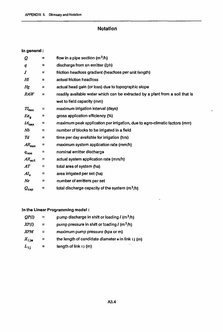
APPENDIX 3. Glossary and Notation
Notation
In general:
Q =q =J =In =Hg =RAW =
l1max =Ea g =L4max =Nb =Td =ARmax =qnom =AReet =AT =AIs =Ne =Qeep =
flow in a pipe section (m3/h)
discharge from an emitter (lph)
friction head/ass gradient (head/ass per unit length)
actual friction headloss
actual head gain (or loss) due to topographic slope
readily available water which can be extracted by a plant from a soil that is
wet to field capacity (mm)
maximum irrigation interval (days)
gross application efficiency (%)
maximum peak application per irrigation, due to agro-climatic factors (mm)
number of blocks to be irrigated in a field
time per day available for irrigation (hrs)
maximum system application rate (mm/h)
nominal emitter discharge
actual system application rate (mm/h)
total area of system (ha)
area irrigated per set (ha)
number of emitters per set
total discharge capacity of the system (m3/h)
In the Unear Programming model:
QP(I) = pump discharge in shift or loading I (m3th)
XP(I) = pump pressure in shift or loading I (m 3/h)
XPM = maximum pump pressure (kpa or m)
X; jll = the length of candidate diameter min link i j (m)
L; j = length of link; j (m)
A3.4

APPENDIX 3. Glossaryand Notation
In the Evaluation model:
Ya = actual yield/unit area (tons/ha)
Ym = maximum potential yield/unit area (tons/ha)
Eta = actual evapotranspiration (mm)
Etm = maximum potential evapotranspiration (mm)
ky = yield response factor
IA = average irrigation application depth (mm)
IR = irrigation requirement for maximum yield (mm)
Ai; = application factor for emitter;
YL; = yield loss for emitter;
YLb = yield loss for block
ar = application ratio
A3.5
- r
- 8 FEB 1QRR


![Evaluation ofhydrologic parameters in a semiarid rangeland ... · Evaluation ofhydrologic parameters in a semiarid rangeland using remotely sensed spectral data ... [Rosema, 1990],](https://img.pdfslide.net/doc/110x75/5b365c827f8b9a6b548e6079/evaluation-ofhydrologic-parameters-in-a-semiarid-rangeland-evaluation-ofhydrologic.jpg)