Embed Size (px)
Citation preview
EXCEL ESSENTIALS (INTERMEDIATE) VERSION: 20_10A
DIGITAL DISTRIBUTION COPY
This manual was supplied in digital form exclusively for Mobile MOUSe student usage.
Under no circumstances may you distribute or make copies of this manual (in whole or in part) to any
other entity, person, party or organization.
This manual may not be printed or reproduced in any form without express permission from Mobile
MOUSe.
IF YOU FEEL THAT THIS DOCUMENT HAS BEEN TAMPERED WITH OR REPRODUCED ILLEGALLY, WE ASK
THAT YOU KINDLY INFORM US OF ANY IMPROPRIETY.
This manual was supplied in digital form for Mobile MOUSe student usage exclusively. Under no circumstances may you copy or distribute this
document (in whole or in part) to any entity, person, party or organization. This manual may not be printed or reproduced in any form without
express permission from Mobile MOUSe.
ABOUT THIS COURSE…
Microsoft Excel is the spread sheet application included with Microsoft Office. In this course you
will learn about customizing Microsoft Excel as well as critical aspects (theory and practical)
regarding designing successful and efficient spread sheets in Microsoft Excel. In this courseware
you will learn how to master the advanced features of this powerful spread sheet application,
increasing your productivity, efficiency and overall spread sheet skills.
DOWNLOAD THE PRACTICE FILES…
In addition to the exercises you will complete in class, there are also exercises in this workbook.
These workbook exercises can only be completed in conjunction with your Mobile MOUSe practice
files. In order to locate your Mobile MOUSe Practice Files visit:
www.mobilemouse.com.au/downloads.php
CHAPTERS IN THE WORKBOOK…
PART 1 : WORKING WITH EXCEL
PART 2 : NAMES, FORMULAS & HYPERLINKS
PART 3 : LISTS AND MANAGEMENT
PART 4 : CHARTS, GRAPHS AND SPARKLINES
WHAT YOU WILL NEED…
IN ORDER TO COMPLETE THE EXERCISES IN THIS WORKBOOK, THE FOLLOWING IS REQUIRED…
1. A desktop computer (or laptop) running Microsoft Windows
2. Microsoft Excel Desktop Application
3. A set of Mobile MOUSe Practice Files
MOS CERTIFICATION
If you are considering attempting the MOS certification (Microsoft Office Specialist), please note
that this workbook addresses a majority of the concepts and skills required in order to obtain this
certification. However, there may be other fundamental skills and requirements of this certification
note included in this manual (as they either relate to Basic or Advanced Concepts, which are
addressed in our appropriate courseware).
As Microsoft are continually updating the elements for certification, we also highly recommend you
visit the Microsoft web site regarding MOS certification: https://www.microsoft.com/learning/en-
au/mos-certification.aspx
This manual was supplied in digital form for Mobile MOUSe student usage exclusively. Under no circumstances may you copy or distribute this
document (in whole or in part) to any entity, person, party or organization. This manual may not be printed or reproduced in any form without
express permission from Mobile MOUSe.
HOW TO USE THIS MANUAL
WHEN YOU SEE… IT MEANS…
Important Notes… You MUST read this, because it could have an effect on the
final outcome of an action you perform.
Useful Tips… This is optional to read, but these tips often point out
quicker ways of doing things, or alternative methods or
usages.
Exercise Time… You are about to start an exercise in the workbook.
Bold Text
Objects that you click on, like buttons, tabs or menus are
often listed in Bold. Files, Locations and folders are also
listed in Bold.
Type any text that you see this way!! Type the text that is formatted this way...
F+G+L
Keyboard shortcuts are displayed like this. In this example
you would press and hold CTRL, hold SHIFT and then press
ESC once (while still holding CTRL and SHIFT).
This is an example of a more detailed
explanation for the reasoning behind your
actions.
Paragraphs that are formatted like this usually contain
explanations and reasoning behind the actions you are
being instructed to perform.
Home > Copy Click the Home tab, click the Copy button
“Find this text and then click within this here paragraph...”
This is existing typed text in a document you are currently
working on.
This manual was supplied in digital form for Mobile MOUSe student usage exclusively. Under no circumstances may you copy or distribute this
document (in whole or in part) to any entity, person, party or organization. This manual may not be printed or reproduced in any form without
express permission from Mobile MOUSe.
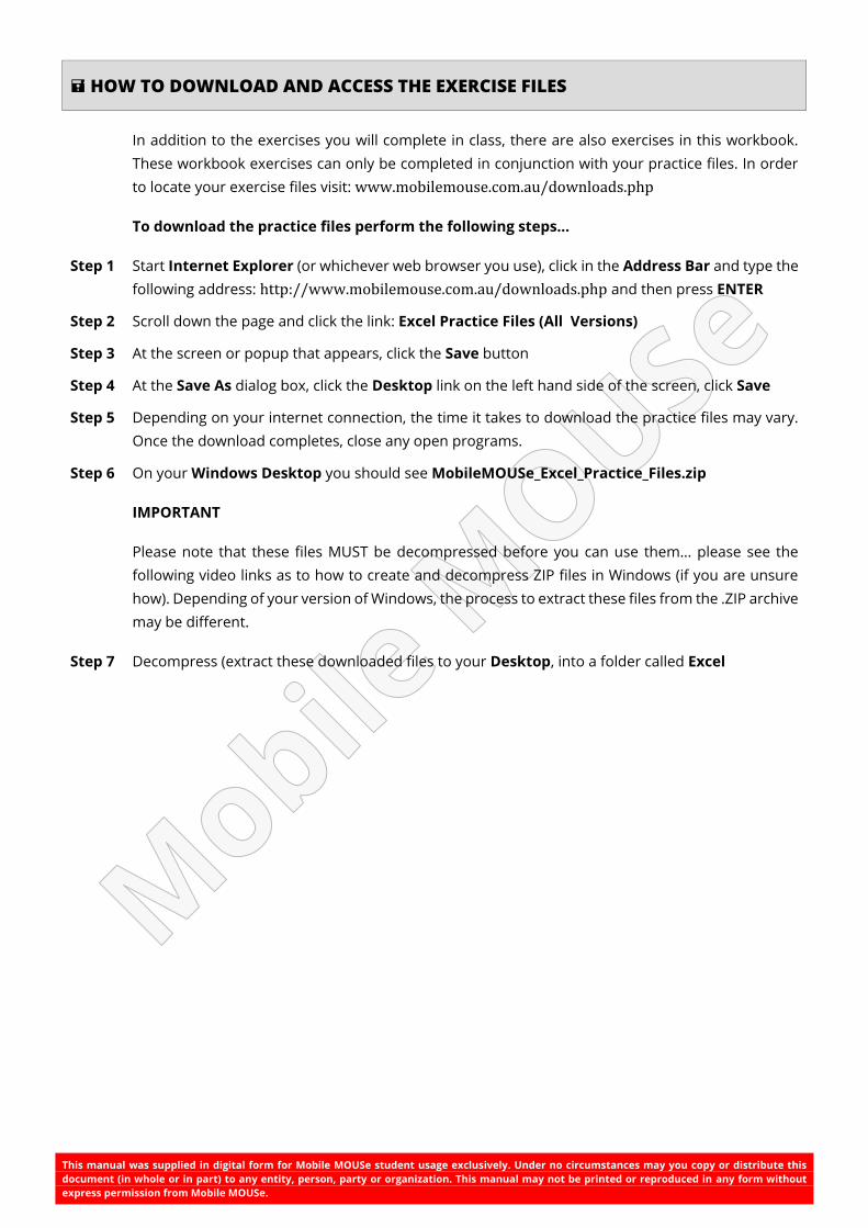
HOW TO DOWNLOAD AND ACCESS THE EXERCISE FILES
In addition to the exercises you will complete in class, there are also exercises in this workbook.
These workbook exercises can only be completed in conjunction with your practice files. In order
to locate your exercise files visit: www.mobilemouse.com.au/downloads.php
To download the practice files perform the following steps...
Step 1 Start Internet Explorer (or whichever web browser you use), click in the Address Bar and type the
following address: http://www.mobilemouse.com.au/downloads.php and then press ENTER
Step 2 Scroll down the page and click the link: Excel Practice Files (All Versions)
Step 3 At the screen or popup that appears, click the Save button
Step 4 At the Save As dialog box, click the Desktop link on the left hand side of the screen, click Save
Step 5 Depending on your internet connection, the time it takes to download the practice files may vary.
Once the download completes, close any open programs.
Step 6 On your Windows Desktop you should see MobileMOUSe_Excel_Practice_Files.zip
IMPORTANT
Please note that these files MUST be decompressed before you can use them… please see the
following video links as to how to create and decompress ZIP files in Windows (if you are unsure
how). Depending of your version of Windows, the process to extract these files from the .ZIP archive
may be different.
Step 7 Decompress (extract these downloaded files to your Desktop, into a folder called Excel
This manual was supplied in digital form for Mobile MOUSe student usage exclusively. Under no circumstances may you copy or distribute this
document (in whole or in part) to any entity, person, party or organization. This manual may not be printed or reproduced in any form without
express permission from Mobile MOUSe.
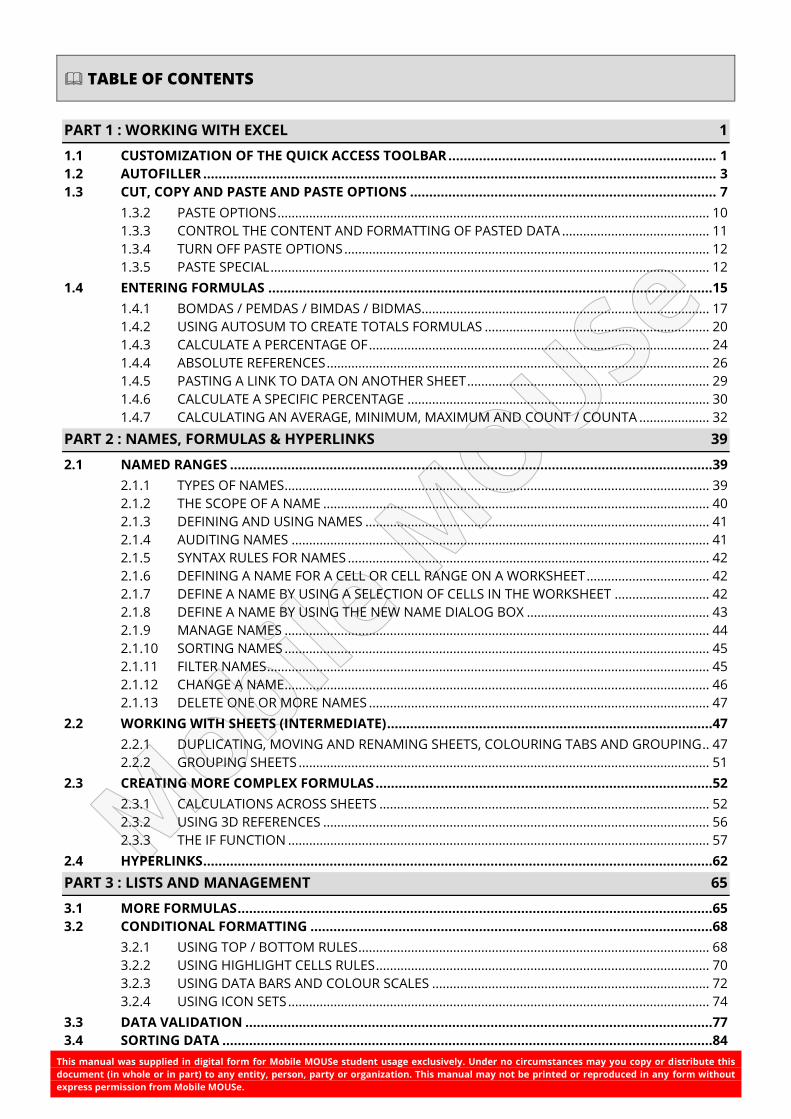
TABLE OF CONTENTS
PART 1 : WORKING WITH EXCEL 1
1.1 CUSTOMIZATION OF THE QUICK ACCESS TOOLBAR ...................................................................... 1 1.2 AUTOFILLER ...................................................................................................................................... 3 1.3 CUT, COPY AND PASTE AND PASTE OPTIONS ................................................................................ 7
1.3.2 PASTE OPTIONS ........................................................................................................................... 10 1.3.3 CONTROL THE CONTENT AND FORMATTING OF PASTED DATA .......................................... 11 1.3.4 TURN OFF PASTE OPTIONS ........................................................................................................ 12 1.3.5 PASTE SPECIAL ............................................................................................................................. 12
1.4 ENTERING FORMULAS ....................................................................................................................15
1.4.1 BOMDAS / PEMDAS / BIMDAS / BIDMAS .................................................................................. 17 1.4.2 USING AUTOSUM TO CREATE TOTALS FORMULAS ................................................................ 20 1.4.3 CALCULATE A PERCENTAGE OF ................................................................................................. 24 1.4.4 ABSOLUTE REFERENCES ............................................................................................................. 26 1.4.5 PASTING A LINK TO DATA ON ANOTHER SHEET ..................................................................... 29 1.4.6 CALCULATE A SPECIFIC PERCENTAGE ...................................................................................... 30 1.4.7 CALCULATING AN AVERAGE, MINIMUM, MAXIMUM AND COUNT / COUNTA .................... 32
PART 2 : NAMES, FORMULAS & HYPERLINKS 39
2.1 NAMED RANGES ..............................................................................................................................39
2.1.1 TYPES OF NAMES ......................................................................................................................... 39 2.1.2 THE SCOPE OF A NAME .............................................................................................................. 40 2.1.3 DEFINING AND USING NAMES .................................................................................................. 41 2.1.4 AUDITING NAMES ....................................................................................................................... 41 2.1.5 SYNTAX RULES FOR NAMES ....................................................................................................... 42 2.1.6 DEFINING A NAME FOR A CELL OR CELL RANGE ON A WORKSHEET ................................... 42 2.1.7 DEFINE A NAME BY USING A SELECTION OF CELLS IN THE WORKSHEET ........................... 42 2.1.8 DEFINE A NAME BY USING THE NEW NAME DIALOG BOX .................................................... 43 2.1.9 MANAGE NAMES ......................................................................................................................... 44 2.1.10 SORTING NAMES ......................................................................................................................... 45 2.1.11 FILTER NAMES .............................................................................................................................. 45 2.1.12 CHANGE A NAME ......................................................................................................................... 46 2.1.13 DELETE ONE OR MORE NAMES ................................................................................................. 47
2.2 WORKING WITH SHEETS (INTERMEDIATE) .....................................................................................47
2.2.1 DUPLICATING, MOVING AND RENAMING SHEETS, COLOURING TABS AND GROUPING .. 47 2.2.2 GROUPING SHEETS ..................................................................................................................... 51
2.3 CREATING MORE COMPLEX FORMULAS ........................................................................................52
2.3.1 CALCULATIONS ACROSS SHEETS .............................................................................................. 52 2.3.2 USING 3D REFERENCES .............................................................................................................. 56 2.3.3 THE IF FUNCTION ........................................................................................................................ 57
2.4 HYPERLINKS .....................................................................................................................................62
PART 3 : LISTS AND MANAGEMENT 65
3.1 MORE FORMULAS ............................................................................................................................65 3.2 CONDITIONAL FORMATTING .........................................................................................................68
3.2.1 USING TOP / BOTTOM RULES .................................................................................................... 68 3.2.2 USING HIGHLIGHT CELLS RULES ............................................................................................... 70 3.2.3 USING DATA BARS AND COLOUR SCALES ............................................................................... 72 3.2.4 USING ICON SETS ........................................................................................................................ 74
3.3 DATA VALIDATION ..........................................................................................................................77 3.4 SORTING DATA ................................................................................................................................84
This manual was supplied in digital form for Mobile MOUSe student usage exclusively. Under no circumstances may you copy or distribute this
document (in whole or in part) to any entity, person, party or organization. This manual may not be printed or reproduced in any form without
express permission from Mobile MOUSe.
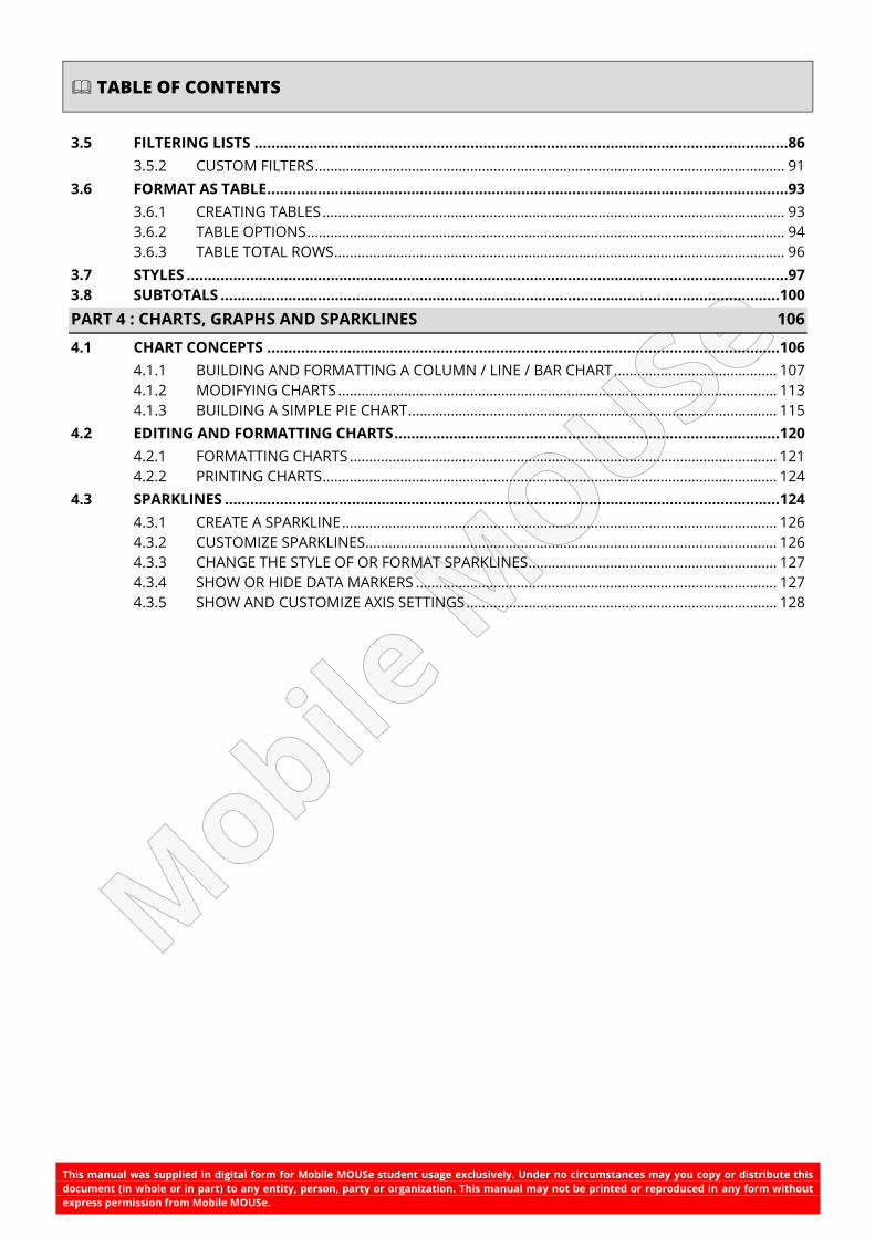
TABLE OF CONTENTS
3.5 FILTERING LISTS ..............................................................................................................................86
3.5.2 CUSTOM FILTERS ......................................................................................................................... 91
3.6 FORMAT AS TABLE ...........................................................................................................................93
3.6.1 CREATING TABLES ....................................................................................................................... 93 3.6.2 TABLE OPTIONS ........................................................................................................................... 94 3.6.3 TABLE TOTAL ROWS .................................................................................................................... 96
3.7 STYLES ..............................................................................................................................................97 3.8 SUBTOTALS .................................................................................................................................... 100
PART 4 : CHARTS, GRAPHS AND SPARKLINES 106
4.1 CHART CONCEPTS ......................................................................................................................... 106
4.1.1 BUILDING AND FORMATTING A COLUMN / LINE / BAR CHART .......................................... 107 4.1.2 MODIFYING CHARTS ................................................................................................................. 113 4.1.3 BUILDING A SIMPLE PIE CHART ............................................................................................... 115
4.2 EDITING AND FORMATTING CHARTS ........................................................................................... 120
4.2.1 FORMATTING CHARTS .............................................................................................................. 121 4.2.2 PRINTING CHARTS ..................................................................................................................... 124
4.3 SPARKLINES ................................................................................................................................... 124
4.3.1 CREATE A SPARKLINE ................................................................................................................ 126 4.3.2 CUSTOMIZE SPARKLINES .......................................................................................................... 126 4.3.3 CHANGE THE STYLE OF OR FORMAT SPARKLINES ................................................................ 127 4.3.4 SHOW OR HIDE DATA MARKERS ............................................................................................. 127 4.3.5 SHOW AND CUSTOMIZE AXIS SETTINGS ................................................................................ 128
This manual was supplied in digital form for Mobile MOUSe student usage exclusively. Under no circumstances may you copy or distribute this
document (in whole or in part) to any entity, person, party or organization. This manual may not be printed or reproduced in any form without
express permission from Mobile MOUSe.
LIST OF TABLES
TABLE 1-1: ADDITIONAL AUTOFILL OPTIONS ............................................................................................................. 6
TABLE 1-2: PASTE OPTIONS EXPLAINED ................................................................................................................... 11
TABLE 1-3: CELL SELECTION PASTE SPECIAL OPTIONS .......................................................................................... 13
TABLE 1-4: PASTE SPECIAL MATHEMATICAL OPERATION ...................................................................................... 15
TABLE 1-5: PASTE SPECIAL ADDITIONAL ACTIONS ................................................................................................. 15
TABLE 1-6: MATHEMATICAL AND LOGICAL OPERATIONS AND THE SYMBOL(S) USED ...................................... 16
TABLE 1-7: MICROSOFT EXCEL AUTOSUM OPTIONS (BELOW) .............................................................................. 20
TABLE 2-1: NAMED RANGE EXAMPLES ..................................................................................................................... 39
TABLE 2-2: METHODS OF NAMING RANGES ............................................................................................................ 41
TABLE 2-3: METHODS AND TECHNIQUES OF USING NAMED RANGES ................................................................ 41
TABLE 2-4: FILTERING NAMES .................................................................................................................................... 46
TABLE 3-1: DATA VALIDATION CHOICES ................................................................................................................... 77
TABLE 3-2: ERROR ALERT STYLES .............................................................................................................................. 80
TABLE 3-3: SUBTOTAL SUMMARY FUNCTIONS ..................................................................................................... 101

This manual was supplied in digital form for Mobile MOUSe student usage exclusively. Under no circumstances may you copy or distribute this
document (in whole or in part) to any entity, person, party or organization. This manual may not be printed or reproduced in any form without
express permission from Mobile MOUSe.
QUICK NOTES
..................................................................................................................................................................................................................................................
..................................................................................................................................................................................................................................................
..................................................................................................................................................................................................................................................
..................................................................................................................................................................................................................................................
..................................................................................................................................................................................................................................................
..................................................................................................................................................................................................................................................
..................................................................................................................................................................................................................................................
..................................................................................................................................................................................................................................................
..................................................................................................................................................................................................................................................
..................................................................................................................................................................................................................................................
..................................................................................................................................................................................................................................................
..................................................................................................................................................................................................................................................
..................................................................................................................................................................................................................................................
..................................................................................................................................................................................................................................................
..................................................................................................................................................................................................................................................
..................................................................................................................................................................................................................................................
..................................................................................................................................................................................................................................................
..................................................................................................................................................................................................................................................
..................................................................................................................................................................................................................................................
..................................................................................................................................................................................................................................................
..................................................................................................................................................................................................................................................
..................................................................................................................................................................................................................................................
..................................................................................................................................................................................................................................................
..................................................................................................................................................................................................................................................
..................................................................................................................................................................................................................................................
..................................................................................................................................................................................................................................................
..................................................................................................................................................................................................................................................
..................................................................................................................................................................................................................................................
..................................................................................................................................................................................................................................................
..................................................................................................................................................................................................................................................
..................................................................................................................................................................................................................................................
..................................................................................................................................................................................................................................................
..................................................................................................................................................................................................................................................
..................................................................................................................................................................................................................................................
..................................................................................................................................................................................................................................................

This manual was supplied in digital form for Mobile MOUSe student usage exclusively. Under no circumstances may you copy or distribute this
document (in whole or in part) to any entity, person, party or organization. This manual may not be printed or reproduced in any form without
express permission from Mobile MOUSe.
QUICK NOTES
..................................................................................................................................................................................................................................................
..................................................................................................................................................................................................................................................
..................................................................................................................................................................................................................................................
..................................................................................................................................................................................................................................................
..................................................................................................................................................................................................................................................
..................................................................................................................................................................................................................................................
..................................................................................................................................................................................................................................................
..................................................................................................................................................................................................................................................
..................................................................................................................................................................................................................................................
..................................................................................................................................................................................................................................................
..................................................................................................................................................................................................................................................
..................................................................................................................................................................................................................................................
..................................................................................................................................................................................................................................................
..................................................................................................................................................................................................................................................
..................................................................................................................................................................................................................................................
..................................................................................................................................................................................................................................................
..................................................................................................................................................................................................................................................
..................................................................................................................................................................................................................................................
..................................................................................................................................................................................................................................................
..................................................................................................................................................................................................................................................
..................................................................................................................................................................................................................................................
..................................................................................................................................................................................................................................................
..................................................................................................................................................................................................................................................
..................................................................................................................................................................................................................................................
..................................................................................................................................................................................................................................................
..................................................................................................................................................................................................................................................
..................................................................................................................................................................................................................................................
..................................................................................................................................................................................................................................................
..................................................................................................................................................................................................................................................
..................................................................................................................................................................................................................................................
..................................................................................................................................................................................................................................................
..................................................................................................................................................................................................................................................
..................................................................................................................................................................................................................................................
TH IS MANUAL W AS PREPARED EX CLUSIVE LY FOR MOBILE MOUSe ST UDE NT USAGE
PAGE 1 EXCEL ESSENTIALS (INTERMEDIATE) MOBILE MOUSe
PAGE 1 MOBILE MOUSe
COPYRIGHT © 2018 MOBILE MOUSE. NO PART OF THIS MANUAL MAY BE DISTRIBUTED, REPRODUCED, COPIED OR MODIFIED WITHOUT THE EXPRESS PERMISSION OF
MOBILE MOUSe. IF YOU FEEL THAT THIS DOCUMENT HAS BEEN TAMPERED WITH OR REPRODUCED ILLEGALLY, KINDLY INFORM US OF ANY IMPROPRIETY.
PART 1 : WORKING WITH EXCEL In this session...
• Cells and Ranges
• Selecting, Entering and Editing Data
• Using the AutoFiller to copy data or make patterns
• Moving and Copying Data with Advanced Paste Options
• Creating and Editing Formulas
• Customization of the Quick Access Toolbar
1.1 CUSTOMIZATION OF THE QUICK ACCESS TOOLBAR
MICROSOFT OFFICE CERTIFICATION
This concept addresses the Personalize environment by using Backstage
competency of the Microsoft Office Specialist Certification (Exam 77-420).
PLEASE NOTE: This training resource does not necessarily cover all of the
requirements of this exam objective as this objective may include but is not
limited to: Manipulate the Quick Access Toolbar, manipulate the ribbon tabs
and groups, manipulate Excel default settings, import data to Excel, import
data from Excel, demonstrate how to manipulate workbook properties,
manipulate workbook files and folders. Apply different name and file formats
for different uses by using save and save as features.
Visit http://www.microsoft.com/learning/en/us/mos-certification.aspx for the
latest Microsoft Office Certification requirements.
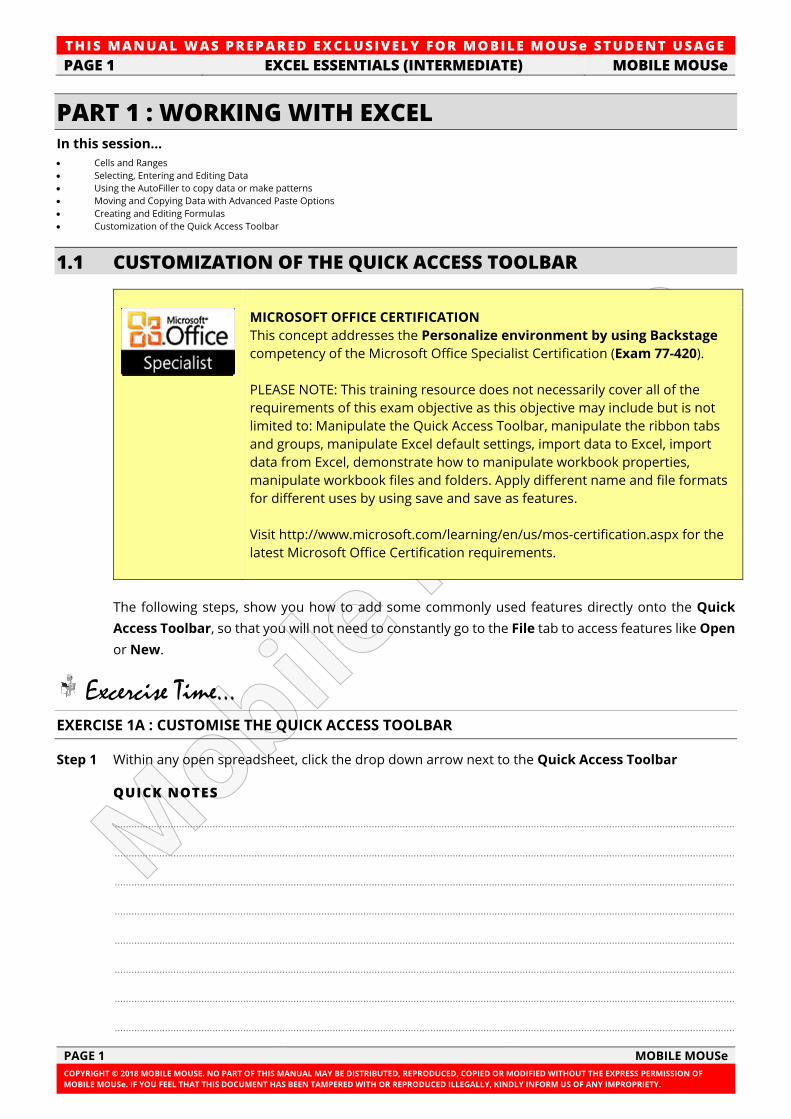
The following steps, show you how to add some commonly used features directly onto the Quick
Access Toolbar, so that you will not need to constantly go to the File tab to access features like Open
or New.
Excercise Time... EXERCISE 1A : CUSTOMISE THE QUICK ACCESS TOOLBAR
Step 1 Within any open spreadsheet, click the drop down arrow next to the Quick Access Toolbar
QUICK NOTES
..............................................................................................................................................................................................................................
..............................................................................................................................................................................................................................
..............................................................................................................................................................................................................................
..............................................................................................................................................................................................................................
..............................................................................................................................................................................................................................
..............................................................................................................................................................................................................................
..............................................................................................................................................................................................................................
..............................................................................................................................................................................................................................
TH IS MANUAL W AS PREPARED EX CLUSIVE LY FOR MOBILE MOUSe ST UDE NT USAGE
MOBILE MOUSe EXCEL ESSENTIALS (INTERMEDIATE) PAGE 2
MOBILE MOUSe PAGE 2
COPYRIGHT © 2018 MOBILE MOUSE. NO PART OF THIS MANUAL MAY BE DISTRIBUTED, REPRODUCED, COPIED OR MODIFIED WITHOUT THE EXPRESS PERMISSION OF
MOBILE MOUSe. IF YOU FEEL THAT THIS DOCUMENT HAS BEEN TAMPERED WITH OR REPRODUCED ILLEGALLY, KINDLY INFORM US OF ANY IMPROPRIETY.
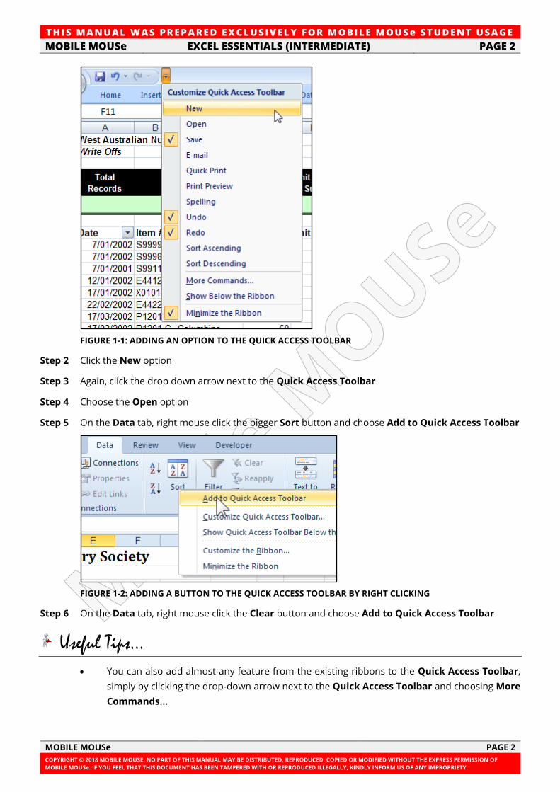
FIGURE 1-1: ADDING AN OPTION TO THE QUICK ACCESS TOOLBAR
Step 2 Click the New option
Step 3 Again, click the drop down arrow next to the Quick Access Toolbar
Step 4 Choose the Open option
Step 5 On the Data tab, right mouse click the bigger Sort button and choose Add to Quick Access Toolbar
FIGURE 1-2: ADDING A BUTTON TO THE QUICK ACCESS TOOLBAR BY RIGHT CLICKING
Step 6 On the Data tab, right mouse click the Clear button and choose Add to Quick Access Toolbar
Useful Tips...
• You can also add almost any feature from the existing ribbons to the Quick Access Toolbar,
simply by clicking the drop-down arrow next to the Quick Access Toolbar and choosing More
Commands...
TH IS MANUAL W AS PREPARED EX CLUSIVE LY FOR MOBILE MOUSe ST UDE NT USAGE
PAGE 3 EXCEL ESSENTIALS (INTERMEDIATE) MOBILE MOUSe
PAGE 3 MOBILE MOUSe
COPYRIGHT © 2018 MOBILE MOUSE. NO PART OF THIS MANUAL MAY BE DISTRIBUTED, REPRODUCED, COPIED OR MODIFIED WITHOUT THE EXPRESS PERMISSION OF
MOBILE MOUSe. IF YOU FEEL THAT THIS DOCUMENT HAS BEEN TAMPERED WITH OR REPRODUCED ILLEGALLY, KINDLY INFORM US OF ANY IMPROPRIETY.
1.2 AUTOFILLER
MICROSOFT OFFICE CERTIFICATION
This concept addresses the Apply AutoFill competency of the Microsoft Office
Specialist Certification (Exam 77-420).
PLEASE NOTE: This training resource does not necessarily cover all of the
requirements of this exam objective as this objective may include but is not
limited to: Copy data using AutoFill, fill series using AutoFill, copy or preserve
cell format with AutoFill, select from drop-down list.
Visit http://www.microsoft.com/learning/en/us/mos-certification.aspx for the
latest Microsoft Office Certification requirements.
A very handy feature in Excel is AutoFill, which allows you to automatically fill cells with pre-set data.
If you need to add the months of the year or the days of the week to your spreadsheets, you can do
so using AutoFill.
It is also possible to customize the lists of data that work with AutoFill so that you can easily add data
that you use frequently. If you regularly add the same department names or part numbers to your
spreadsheets you can add these names to the AutoFill feature making it easier to enter them when
needed.
Excercise Time... EXERCISE 1B : THE AUTOFILLER
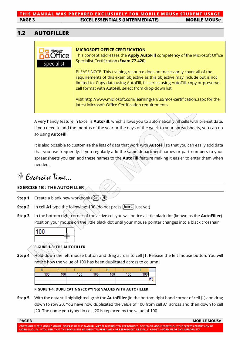
Step 1 Create a blank new workbook (F+N)
Step 2 In cell A1 type the following: 100 (do not press I just yet)
Step 3 In the bottom right corner of the active cell you will notice a little black dot (known as the AutoFiller).
Position your mouse on the little black dot until your mouse pointer changes into a black crosshair
FIGURE 1-3: THE AUTOFILLER
Step 4 Hold down the left mouse button and drag across to cell J1. Release the left mouse button. You will
notice how the value of 100 has been duplicated across to column J
FIGURE 1-4: DUPLICATING (COPYING) VALUES WITH AUTOFILLER
Step 5 With the data still highlighted, grab the AutoFiller (in the bottom right hand corner of cell J1) and drag
down to row 20. You have now duplicated the value of 100 from cell A1 across and then down to cell
J20. The name you typed in cell J20 is replaced by the value of 100
TH IS MANUAL W AS PREPARED EX CLUSIVE LY FOR MOBILE MOUSe ST UDE NT USAGE
MOBILE MOUSe EXCEL ESSENTIALS (INTERMEDIATE) PAGE 4
MOBILE MOUSe PAGE 4
COPYRIGHT © 2018 MOBILE MOUSE. NO PART OF THIS MANUAL MAY BE DISTRIBUTED, REPRODUCED, COPIED OR MODIFIED WITHOUT THE EXPRESS PERMISSION OF
MOBILE MOUSe. IF YOU FEEL THAT THIS DOCUMENT HAS BEEN TAMPERED WITH OR REPRODUCED ILLEGALLY, KINDLY INFORM US OF ANY IMPROPRIETY.
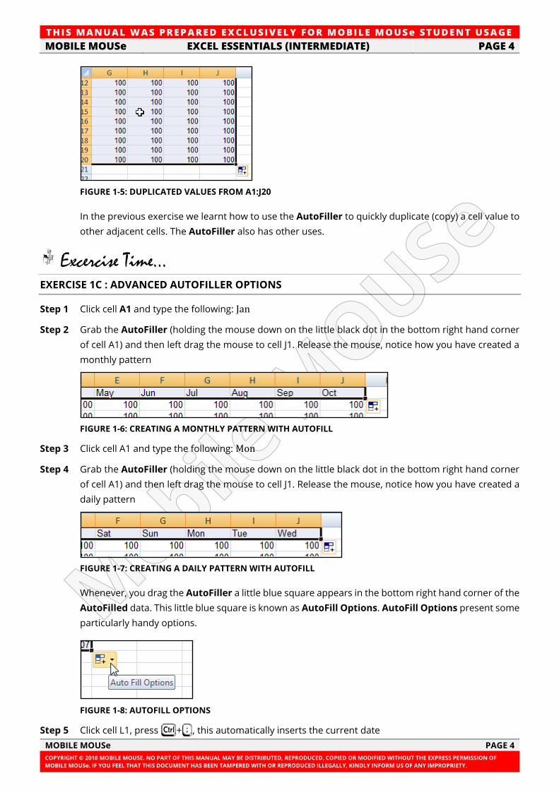
FIGURE 1-5: DUPLICATED VALUES FROM A1:J20
In the previous exercise we learnt how to use the AutoFiller to quickly duplicate (copy) a cell value to
other adjacent cells. The AutoFiller also has other uses.
Excercise Time... EXERCISE 1C : ADVANCED AUTOFILLER OPTIONS
Step 1 Click cell A1 and type the following: Jan
Step 2 Grab the AutoFiller (holding the mouse down on the little black dot in the bottom right hand corner
of cell A1) and then left drag the mouse to cell J1. Release the mouse, notice how you have created a
monthly pattern
FIGURE 1-6: CREATING A MONTHLY PATTERN WITH AUTOFILL
Step 3 Click cell A1 and type the following: Mon
Step 4 Grab the AutoFiller (holding the mouse down on the little black dot in the bottom right hand corner
of cell A1) and then left drag the mouse to cell J1. Release the mouse, notice how you have created a
daily pattern
FIGURE 1-7: CREATING A DAILY PATTERN WITH AUTOFILL
Whenever, you drag the AutoFiller a little blue square appears in the bottom right hand corner of the
AutoFilled data. This little blue square is known as AutoFill Options. AutoFill Options present some
particularly handy options.
FIGURE 1-8: AUTOFILL OPTIONS
Step 5 Click cell L1, press F+;, this automatically inserts the current date
TH IS MANUAL W AS PREPARED EX CLUSIVE LY FOR MOBILE MOUSe ST UDE NT USAGE
PAGE 5 EXCEL ESSENTIALS (INTERMEDIATE) MOBILE MOUSe
PAGE 5 MOBILE MOUSe
COPYRIGHT © 2018 MOBILE MOUSE. NO PART OF THIS MANUAL MAY BE DISTRIBUTED, REPRODUCED, COPIED OR MODIFIED WITHOUT THE EXPRESS PERMISSION OF
MOBILE MOUSe. IF YOU FEEL THAT THIS DOCUMENT HAS BEEN TAMPERED WITH OR REPRODUCED ILLEGALLY, KINDLY INFORM US OF ANY IMPROPRIETY.
Step 6 Grab the AutoFiller (by holding the mouse down on the little black dot in the bottom right hand corner
of cell L1) and then left drag the mouse to cell L20. Release the mouse, notice how you have created
a daily pattern
Important Notes...
• If after performing step 6 above, you receive a series of ####### symbols in certain cells, this
means that you column is not wide enough to accommodate the dates. You will need to widen
column L by dragging the “crack” between column headings L and M further to the right. Better
still you could double click the “crack” to the right of heading L to automatically fit (AutoFit)
column L to the widest value in that column. If you have had to do this, repeat step 6 again.
Step 7 Click the AutoFill Options square, from the list of options, choose Fill Weekdays. Notice how the
weekend dates are excluded and only dates for Mondays through Fridays are entered
Step 8 Click the AutoFill Options square, from the list of options, choose Fill Months. Notice how the
monthly value is incremented
Step 9 Click the AutoFill Options square, from the list of options, choose Fill Years. Notice how the yearly
value is incremented
Step 10 Click the AutoFill Options square, from the list of options, choose Copy Cells. Notice how the date
value is simply repeated
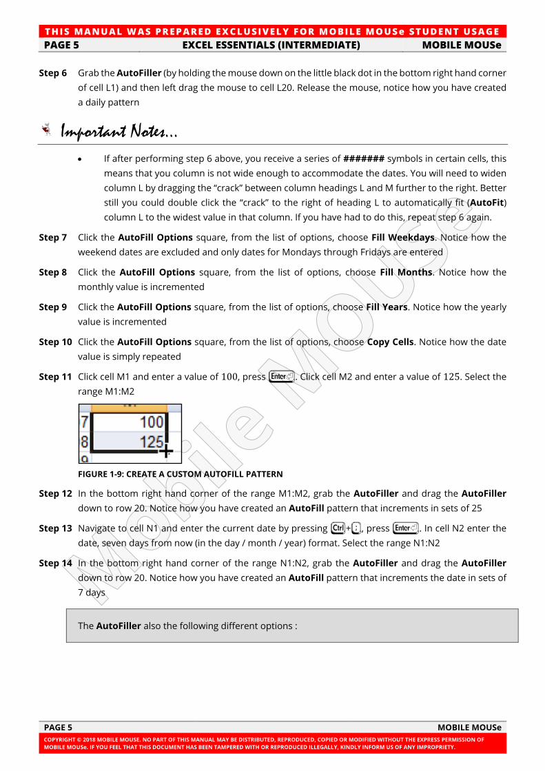
Step 11 Click cell M1 and enter a value of 100, press I. Click cell M2 and enter a value of 125. Select the
range M1:M2
FIGURE 1-9: CREATE A CUSTOM AUTOFILL PATTERN
Step 12 In the bottom right hand corner of the range M1:M2, grab the AutoFiller and drag the AutoFiller
down to row 20. Notice how you have created an AutoFill pattern that increments in sets of 25
Step 13 Navigate to cell N1 and enter the current date by pressing F+;, press I. In cell N2 enter the
date, seven days from now (in the day / month / year) format. Select the range N1:N2
Step 14 In the bottom right hand corner of the range N1:N2, grab the AutoFiller and drag the AutoFiller
down to row 20. Notice how you have created an AutoFill pattern that increments the date in sets of
7 days
The AutoFiller also the following different options :
TH IS MANUAL W AS PREPARED EX CLUSIVE LY FOR MOBILE MOUSe ST UDE NT USAGE
MOBILE MOUSe EXCEL ESSENTIALS (INTERMEDIATE) PAGE 6
MOBILE MOUSe PAGE 6
COPYRIGHT © 2018 MOBILE MOUSE. NO PART OF THIS MANUAL MAY BE DISTRIBUTED, REPRODUCED, COPIED OR MODIFIED WITHOUT THE EXPRESS PERMISSION OF
MOBILE MOUSe. IF YOU FEEL THAT THIS DOCUMENT HAS BEEN TAMPERED WITH OR REPRODUCED ILLEGALLY, KINDLY INFORM US OF ANY IMPROPRIETY.
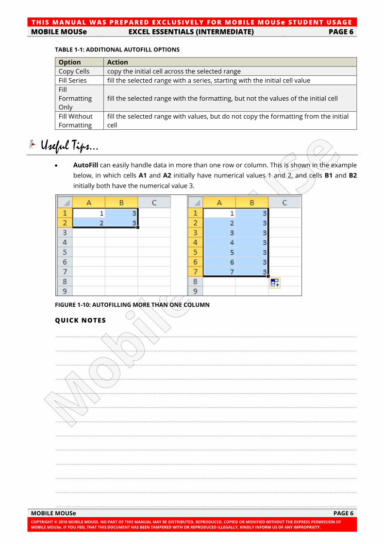
TABLE 1-1: ADDITIONAL AUTOFILL OPTIONS
Option Action
Copy Cells copy the initial cell across the selected range
Fill Series fill the selected range with a series, starting with the initial cell value
Fill
Formatting
Only
fill the selected range with the formatting, but not the values of the initial cell
Fill Without
Formatting
fill the selected range with values, but do not copy the formatting from the initial
cell
Useful Tips...
• AutoFill can easily handle data in more than one row or column. This is shown in the example
below, in which cells A1 and A2 initially have numerical values 1 and 2, and cells B1 and B2
initially both have the numerical value 3.
FIGURE 1-10: AUTOFILLING MORE THAN ONE COLUMN
QUICK NOTES
..............................................................................................................................................................................................................................
..............................................................................................................................................................................................................................
..............................................................................................................................................................................................................................
..............................................................................................................................................................................................................................
..............................................................................................................................................................................................................................
..............................................................................................................................................................................................................................
..............................................................................................................................................................................................................................
..............................................................................................................................................................................................................................
..............................................................................................................................................................................................................................
..............................................................................................................................................................................................................................
..............................................................................................................................................................................................................................
..............................................................................................................................................................................................................................
..............................................................................................................................................................................................................................
TH IS MANUAL W AS PREPARED EX CLUSIVE LY FOR MOBILE MOUSe ST UDE NT USAGE
PAGE 7 EXCEL ESSENTIALS (INTERMEDIATE) MOBILE MOUSe
PAGE 7 MOBILE MOUSe
COPYRIGHT © 2018 MOBILE MOUSE. NO PART OF THIS MANUAL MAY BE DISTRIBUTED, REPRODUCED, COPIED OR MODIFIED WITHOUT THE EXPRESS PERMISSION OF
MOBILE MOUSe. IF YOU FEEL THAT THIS DOCUMENT HAS BEEN TAMPERED WITH OR REPRODUCED ILLEGALLY, KINDLY INFORM US OF ANY IMPROPRIETY.
1.3 CUT, COPY AND PASTE AND PASTE OPTIONS
MICROSOFT OFFICE CERTIFICATION
This concept addresses the Construct Cell Data competency of the Microsoft Office Specialist
Certification (Exam 77-420).
PLEASE NOTE: This training resource does not necessarily cover all of the requirements of this
exam objective as this objective may include but is not limited to: using paste special (formats,
formulas, values, preview icons, transpose rows and columns, operations, comments, validation,
paste as a link), and cutting, moving, and select cell data
Visit http://www.microsoft.com/learning/en/us/mos-certification.aspx for the latest Microsoft
Office Certification requirements.
Within Microsoft Excel as with every other Windows application (program) there are two methods for
moving or copying data around. These two techniques are...
• Cut, Copy, Paste
• Drag and Drop
You can cut a selection to move it and Paste a cut selection to place it. Microsoft Excel makes use of
the Microsoft Office clipboard, which can hold up to 24 Cut / Copy operations.
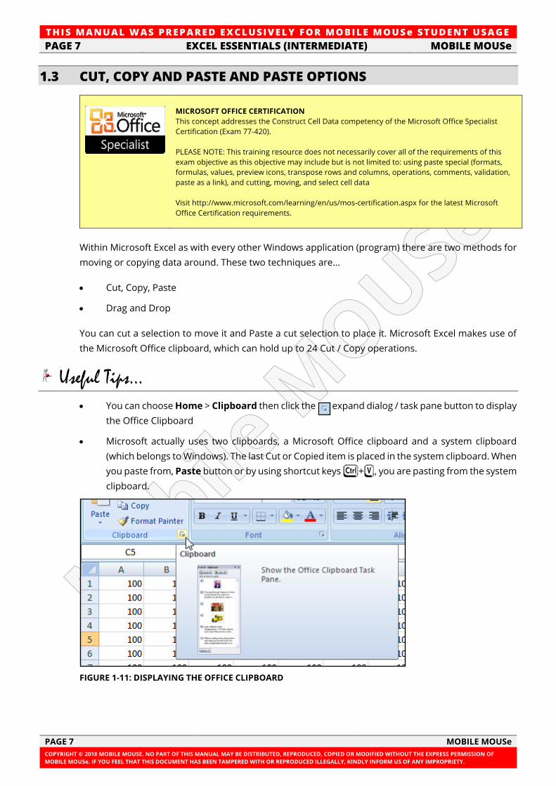
Useful Tips...
• You can choose Home > Clipboard then click the expand dialog / task pane button to display
the Office Clipboard
• Microsoft actually uses two clipboards, a Microsoft Office clipboard and a system clipboard
(which belongs to Windows). The last Cut or Copied item is placed in the system clipboard. When
you paste from, Paste button or by using shortcut keys F+V, you are pasting from the system
clipboard.
FIGURE 1-11: DISPLAYING THE OFFICE CLIPBOARD
TH IS MANUAL W AS PREPARED EX CLUSIVE LY FOR MOBILE MOUSe ST UDE NT USAGE
MOBILE MOUSe EXCEL ESSENTIALS (INTERMEDIATE) PAGE 8
MOBILE MOUSe PAGE 8
COPYRIGHT © 2018 MOBILE MOUSE. NO PART OF THIS MANUAL MAY BE DISTRIBUTED, REPRODUCED, COPIED OR MODIFIED WITHOUT THE EXPRESS PERMISSION OF
MOBILE MOUSe. IF YOU FEEL THAT THIS DOCUMENT HAS BEEN TAMPERED WITH OR REPRODUCED ILLEGALLY, KINDLY INFORM US OF ANY IMPROPRIETY.
Cut, Copy, Paste works well just about all the time, whilst Drag and Drop is most efficient for short
moves and copies. The traditional method of moving and copying text is to use the Cut, Copy and
Paste features on the Home tab. You can move or copy any object or text by performing the following
steps.
Step 1 Select the object (cell, row, column etc…) using any of the selection techniques illustrated earlier
Step 2 Click the Cut button (or press F+X) if you want to move the selection or the Copy button (or press
F+C) if you want to copy the selection
Step 3 Click on the location where you want the selection to appear
Step 4 Click the Paste button (or press F+V)
There are three common ways to access the Cut and Copy commands,
• Click the Cut / Copy button in the Clipboard group of the Home tab
• Press F+X to cut or press F+C to copy
• Right click the selection and choose Cut or choose Copy from the shortcut menu
There are four common ways to paste data in Microsoft Excel,
• Click the Paste button on the Home tab
• Press F+V to paste
• Right click the destination cell(s) and choose Paste from the shortcut menu
• Pressing I (This only works if done directly after choosing Cut or Copy. By pasting using
I; this signifies to Microsoft Excel that this is the last of the current Paste operations. You
will not be able to paste again, until you Copy or Cut once more)
Useful Tips...
• In addition to the Cut, Copy and Paste features you can also move and copy your selection by
using Drag and Drop. It is important to note that the drag and drop method works best when
you can see both the source (the location of the original selection) as well as the destination
(the place that you want the moved or copied selection to appear).
• When you use the left mouse button to drag and drop the selected text or object, Microsoft
Excel moves the selection to the new location with no questions asked. If you want to copy the
selection by using the left mouse button, you should hold down the F key before dropping
the text.
It is important to note the minor differences between the Cut, Copy and Paste operations of Microsoft
Word and Microsoft Excel.
TH IS MANUAL W AS PREPARED EX CLUSIVE LY FOR MOBILE MOUSe ST UDE NT USAGE
PAGE 9 EXCEL ESSENTIALS (INTERMEDIATE) MOBILE MOUSe
PAGE 9 MOBILE MOUSe
COPYRIGHT © 2018 MOBILE MOUSE. NO PART OF THIS MANUAL MAY BE DISTRIBUTED, REPRODUCED, COPIED OR MODIFIED WITHOUT THE EXPRESS PERMISSION OF
MOBILE MOUSe. IF YOU FEEL THAT THIS DOCUMENT HAS BEEN TAMPERED WITH OR REPRODUCED ILLEGALLY, KINDLY INFORM US OF ANY IMPROPRIETY.
Important Notes...
• In Excel, if you paste cells on top of existing data, the existing data will be overwritten. Before
pasting, make sure that there are enough free blank cells to accommodate the selection you
want to paste. As an example, if you wanted to move the contents of column E to the right of
column A, you would be well advised to insert a new column between column A and column B
in order to prevent overwriting the data in column B.
• When you cut a cell in Microsoft Excel it is placed in the clipboard and will only be removed from
its current location when it has been placed into its new location by Pasting.
• When you are getting ready to paste, simply click the first cell, row or column where you want
your pasted cells to appear. If you select more than one cell to paste into, that selection must
be exactly the same size as the range that is coming from the clipboard.
• Even if you plan to paste only once, there is a reason for rather using the Paste option than
using the I key to paste your data. Whenever you paste data, Microsoft Excel will display a
Paste Options button at the bottom of the pasted selection. Clicking this button allows you to
choose from other options such as pasting numbers without the underlying formulas (values)
or transposing the copied data or pasting data without it’s formatting or pasting formatting
without the data (and many more useful options).
Excercise Time... EXERCISE 1D : MOVING CELLS WITH CUT AND PASTE
Step 1 Select the range A1:J1 and press F+X to cut the cell contents. In the status bar the following text
appears “Select destination and press enter or choose Paste”. A moving border “marching ants” also
appears around the cut selection, the data remains in the cell
Step 2 Click cell A21, press F+V to move the contents of A1:J1 to A21:J21
Step 3 Leave the workbook open
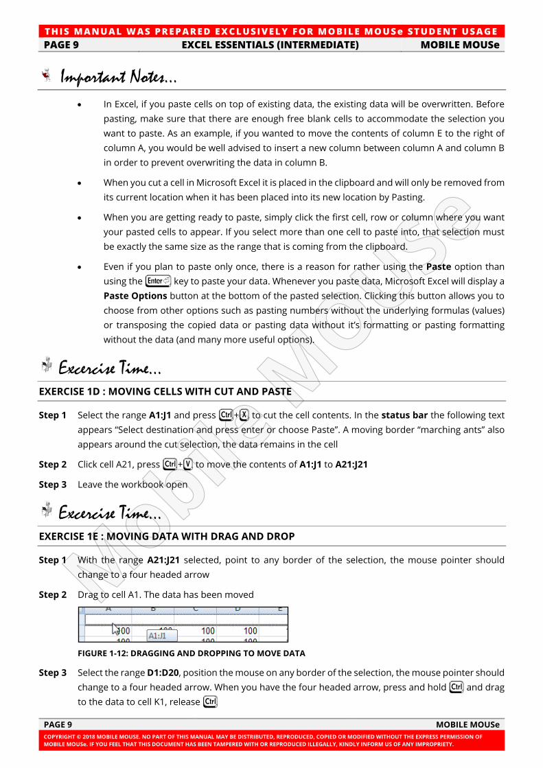
Excercise Time... EXERCISE 1E : MOVING DATA WITH DRAG AND DROP
Step 1 With the range A21:J21 selected, point to any border of the selection, the mouse pointer should
change to a four headed arrow
Step 2 Drag to cell A1. The data has been moved
FIGURE 1-12: DRAGGING AND DROPPING TO MOVE DATA
Step 3 Select the range D1:D20, position the mouse on any border of the selection, the mouse pointer should
change to a four headed arrow. When you have the four headed arrow, press and hold F and drag
to the data to cell K1, release F
TH IS MANUAL W AS PREPARED EX CLUSIVE LY FOR MOBILE MOUSe ST UDE NT USAGE
MOBILE MOUSe EXCEL ESSENTIALS (INTERMEDIATE) PAGE 10
MOBILE MOUSe PAGE 10
COPYRIGHT © 2018 MOBILE MOUSE. NO PART OF THIS MANUAL MAY BE DISTRIBUTED, REPRODUCED, COPIED OR MODIFIED WITHOUT THE EXPRESS PERMISSION OF
MOBILE MOUSe. IF YOU FEEL THAT THIS DOCUMENT HAS BEEN TAMPERED WITH OR REPRODUCED ILLEGALLY, KINDLY INFORM US OF ANY IMPROPRIETY.
Step 4 Close the worksheet, by clicking the File tab > Close (or click the second X in the top right hand corner
of the window), or you can also press F+W. When asked if you want to save your changes click No.
This closes your workbook. Because we chose not to save the data, all work done so far is now lost
(don’t worry, that is what we want in this case ☺).
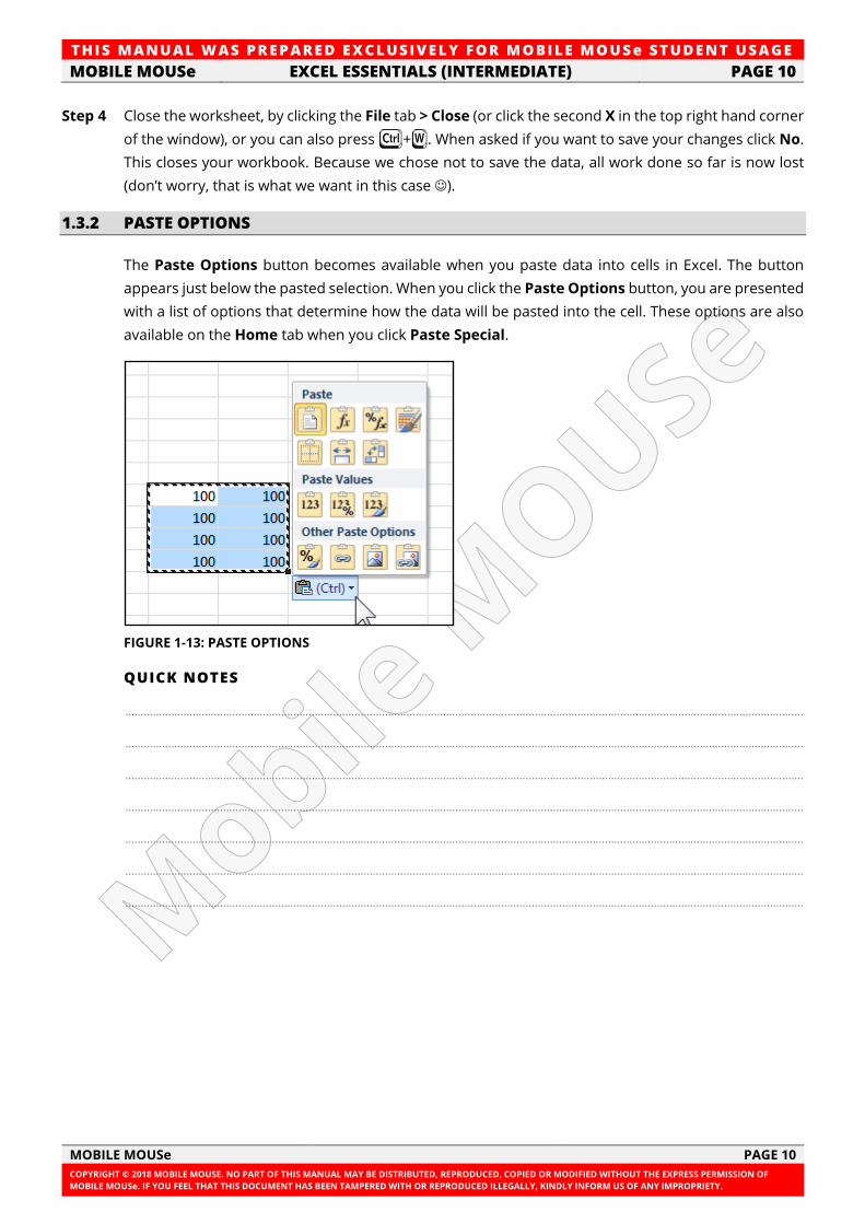
1.3.2 PASTE OPTIONS
The Paste Options button becomes available when you paste data into cells in Excel. The button
appears just below the pasted selection. When you click the Paste Options button, you are presented
with a list of options that determine how the data will be pasted into the cell. These options are also
available on the Home tab when you click Paste Special.
FIGURE 1-13: PASTE OPTIONS
QUICK NOTES
..............................................................................................................................................................................................................................
..............................................................................................................................................................................................................................
..............................................................................................................................................................................................................................
..............................................................................................................................................................................................................................
..............................................................................................................................................................................................................................
..............................................................................................................................................................................................................................
..............................................................................................................................................................................................................................
TH IS MANUAL W AS PREPARED EX CLUSIVE LY FOR MOBILE MOUSe ST UDE NT USAGE
PAGE 11 EXCEL ESSENTIALS (INTERMEDIATE) MOBILE MOUSe
PAGE 11 MOBILE MOUSe
COPYRIGHT © 2018 MOBILE MOUSE. NO PART OF THIS MANUAL MAY BE DISTRIBUTED, REPRODUCED, COPIED OR MODIFIED WITHOUT THE EXPRESS PERMISSION OF
MOBILE MOUSe. IF YOU FEEL THAT THIS DOCUMENT HAS BEEN TAMPERED WITH OR REPRODUCED ILLEGALLY, KINDLY INFORM US OF ANY IMPROPRIETY.
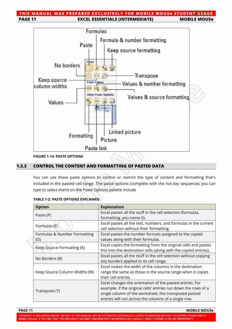
FIGURE 1-14: PASTE OPTIONS
1.3.3 CONTROL THE CONTENT AND FORMATTING OF PASTED DATA
You can use these paste options to control or restrict the type of content and formatting that's
included in the pasted cell range. The paste options (complete with the hot key sequences you can
type to select them) on the Paste Options palette include
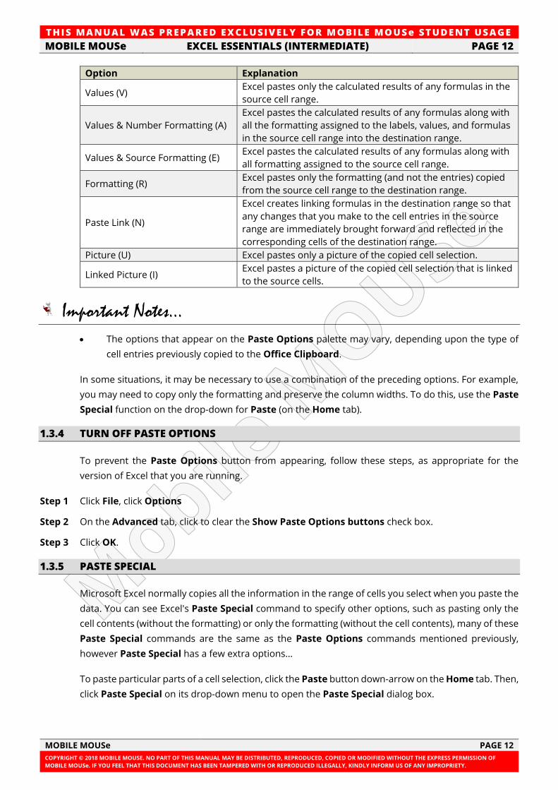
TABLE 1-2: PASTE OPTIONS EXPLAINED
Option Explanation
Paste (P) Excel pastes all the stuff in the cell selection (formulas,
formatting, you name it).
Formulas (F) Excel pastes all the text, numbers, and formulas in the current
cell selection without their formatting.
Formulas & Number Formatting
(O)
Excel pastes the number formats assigned to the copied
values along with their formulas.
Keep Source Formatting (K) Excel copies the formatting from the original cells and pastes
this into the destination cells (along with the copied entries).
No Borders (B) Excel pastes all the stuff in the cell selection without copying
any borders applied to its cell range.
Keep Source Column Widths (W)
Excel makes the width of the columns in the destination
range the same as those in the source range when it copies
their cell entries.
Transpose (T)
Excel changes the orientation of the pasted entries. For
example, if the original cells' entries run down the rows of a
single column of the worksheet, the transposed pasted
entries will run across the columns of a single row.
TH IS MANUAL W AS PREPARED EX CLUSIVE LY FOR MOBILE MOUSe ST UDE NT USAGE
MOBILE MOUSe EXCEL ESSENTIALS (INTERMEDIATE) PAGE 12
MOBILE MOUSe PAGE 12
COPYRIGHT © 2018 MOBILE MOUSE. NO PART OF THIS MANUAL MAY BE DISTRIBUTED, REPRODUCED, COPIED OR MODIFIED WITHOUT THE EXPRESS PERMISSION OF
MOBILE MOUSe. IF YOU FEEL THAT THIS DOCUMENT HAS BEEN TAMPERED WITH OR REPRODUCED ILLEGALLY, KINDLY INFORM US OF ANY IMPROPRIETY.
Option Explanation
Values (V) Excel pastes only the calculated results of any formulas in the
source cell range.
Values & Number Formatting (A)
Excel pastes the calculated results of any formulas along with
all the formatting assigned to the labels, values, and formulas
in the source cell range into the destination range.
Values & Source Formatting (E) Excel pastes the calculated results of any formulas along with
all formatting assigned to the source cell range.
Formatting (R) Excel pastes only the formatting (and not the entries) copied
from the source cell range to the destination range.
Paste Link (N)
Excel creates linking formulas in the destination range so that
any changes that you make to the cell entries in the source
range are immediately brought forward and reflected in the
corresponding cells of the destination range.
Picture (U) Excel pastes only a picture of the copied cell selection.
Linked Picture (I) Excel pastes a picture of the copied cell selection that is linked
to the source cells.
Important Notes...
• The options that appear on the Paste Options palette may vary, depending upon the type of
cell entries previously copied to the Office Clipboard.
In some situations, it may be necessary to use a combination of the preceding options. For example,
you may need to copy only the formatting and preserve the column widths. To do this, use the Paste
Special function on the drop-down for Paste (on the Home tab).
1.3.4 TURN OFF PASTE OPTIONS
To prevent the Paste Options button from appearing, follow these steps, as appropriate for the
version of Excel that you are running.
Step 1 Click File, click Options
Step 2 On the Advanced tab, click to clear the Show Paste Options buttons check box.
Step 3 Click OK.
1.3.5 PASTE SPECIAL
Microsoft Excel normally copies all the information in the range of cells you select when you paste the
data. You can see Excel's Paste Special command to specify other options, such as pasting only the
cell contents (without the formatting) or only the formatting (without the cell contents), many of these
Paste Special commands are the same as the Paste Options commands mentioned previously,
however Paste Special has a few extra options…
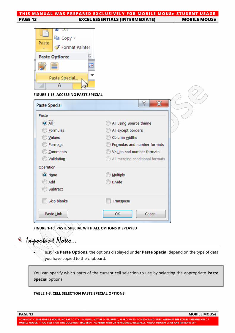
To paste particular parts of a cell selection, click the Paste button down-arrow on the Home tab. Then,
click Paste Special on its drop-down menu to open the Paste Special dialog box.
TH IS MANUAL W AS PREPARED EX CLUSIVE LY FOR MOBILE MOUSe ST UDE NT USAGE
PAGE 13 EXCEL ESSENTIALS (INTERMEDIATE) MOBILE MOUSe
PAGE 13 MOBILE MOUSe
COPYRIGHT © 2018 MOBILE MOUSE. NO PART OF THIS MANUAL MAY BE DISTRIBUTED, REPRODUCED, COPIED OR MODIFIED WITHOUT THE EXPRESS PERMISSION OF
MOBILE MOUSe. IF YOU FEEL THAT THIS DOCUMENT HAS BEEN TAMPERED WITH OR REPRODUCED ILLEGALLY, KINDLY INFORM US OF ANY IMPROPRIETY.
FIGURE 1-15: ACCESSING PASTE SPECIAL
FIGURE 1-16: PASTE SPECIAL WITH ALL OPTIONS DISPLAYED
Important Notes...
• Just like Paste Options, the options displayed under Paste Special depend on the type of data
you have copied to the clipboard.
You can specify which parts of the current cell selection to use by selecting the appropriate Paste
Special options:
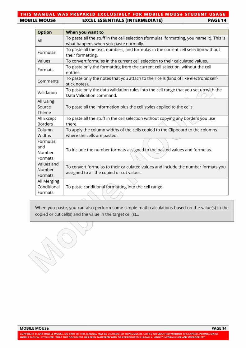
TABLE 1-3: CELL SELECTION PASTE SPECIAL OPTIONS
TH IS MANUAL W AS PREPARED EX CLUSIVE LY FOR MOBILE MOUSe ST UDE NT USAGE
MOBILE MOUSe EXCEL ESSENTIALS (INTERMEDIATE) PAGE 14
MOBILE MOUSe PAGE 14
COPYRIGHT © 2018 MOBILE MOUSE. NO PART OF THIS MANUAL MAY BE DISTRIBUTED, REPRODUCED, COPIED OR MODIFIED WITHOUT THE EXPRESS PERMISSION OF
MOBILE MOUSe. IF YOU FEEL THAT THIS DOCUMENT HAS BEEN TAMPERED WITH OR REPRODUCED ILLEGALLY, KINDLY INFORM US OF ANY IMPROPRIETY.
Option When you want to
All To paste all the stuff in the cell selection (formulas, formatting, you name it). This is
what happens when you paste normally.
Formulas To paste all the text, numbers, and formulas in the current cell selection without
their formatting.
Values To convert formulas in the current cell selection to their calculated values.
Formats To paste only the formatting from the current cell selection, without the cell
entries.
Comments To paste only the notes that you attach to their cells (kind of like electronic self-
stick notes).
Validation To paste only the data validation rules into the cell range that you set up with the
Data Validation command.
All Using
Source
Theme
To paste all the information plus the cell styles applied to the cells.
All Except
Borders
To paste all the stuff in the cell selection without copying any borders you use
there.
Column
Widths
To apply the column widths of the cells copied to the Clipboard to the columns
where the cells are pasted.
Formulas
and
Number
Formats
To include the number formats assigned to the pasted values and formulas.
Values and
Number
Formats
To convert formulas to their calculated values and include the number formats you
assigned to all the copied or cut values.
All Merging
Conditional
Formats
To paste conditional formatting into the cell range.
When you paste, you can also perform some simple math calculations based on the value(s) in the
copied or cut cell(s) and the value in the target cell(s)…
TH IS MANUAL W AS PREPARED EX CLUSIVE LY FOR MOBILE MOUSe ST UDE NT USAGE
PAGE 15 EXCEL ESSENTIALS (INTERMEDIATE) MOBILE MOUSe
PAGE 15 MOBILE MOUSe
COPYRIGHT © 2018 MOBILE MOUSE. NO PART OF THIS MANUAL MAY BE DISTRIBUTED, REPRODUCED, COPIED OR MODIFIED WITHOUT THE EXPRESS PERMISSION OF
MOBILE MOUSe. IF YOU FEEL THAT THIS DOCUMENT HAS BEEN TAMPERED WITH OR REPRODUCED ILLEGALLY, KINDLY INFORM US OF ANY IMPROPRIETY.
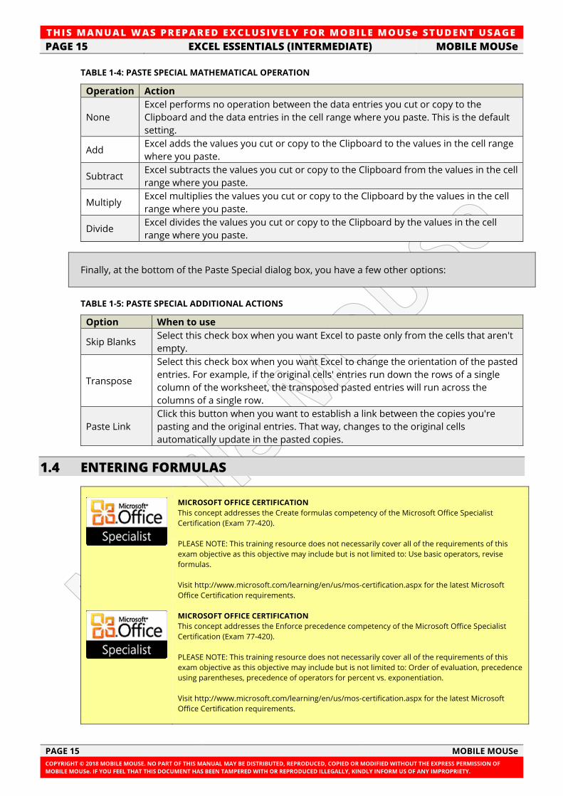
TABLE 1-4: PASTE SPECIAL MATHEMATICAL OPERATION
Operation Action
None
Excel performs no operation between the data entries you cut or copy to the
Clipboard and the data entries in the cell range where you paste. This is the default
setting.
Add Excel adds the values you cut or copy to the Clipboard to the values in the cell range
where you paste.
Subtract Excel subtracts the values you cut or copy to the Clipboard from the values in the cell
range where you paste.
Multiply Excel multiplies the values you cut or copy to the Clipboard by the values in the cell
range where you paste.
Divide Excel divides the values you cut or copy to the Clipboard by the values in the cell
range where you paste.
Finally, at the bottom of the Paste Special dialog box, you have a few other options:
TABLE 1-5: PASTE SPECIAL ADDITIONAL ACTIONS
Option When to use
Skip Blanks Select this check box when you want Excel to paste only from the cells that aren't
empty.
Transpose
Select this check box when you want Excel to change the orientation of the pasted
entries. For example, if the original cells' entries run down the rows of a single
column of the worksheet, the transposed pasted entries will run across the
columns of a single row.
Paste Link
Click this button when you want to establish a link between the copies you're
pasting and the original entries. That way, changes to the original cells
automatically update in the pasted copies.
1.4 ENTERING FORMULAS
MICROSOFT OFFICE CERTIFICATION
This concept addresses the Create formulas competency of the Microsoft Office Specialist
Certification (Exam 77-420).
PLEASE NOTE: This training resource does not necessarily cover all of the requirements of this
exam objective as this objective may include but is not limited to: Use basic operators, revise
formulas.
Visit http://www.microsoft.com/learning/en/us/mos-certification.aspx for the latest Microsoft
Office Certification requirements.
MICROSOFT OFFICE CERTIFICATION
This concept addresses the Enforce precedence competency of the Microsoft Office Specialist
Certification (Exam 77-420).
PLEASE NOTE: This training resource does not necessarily cover all of the requirements of this
exam objective as this objective may include but is not limited to: Order of evaluation, precedence
using parentheses, precedence of operators for percent vs. exponentiation.
Visit http://www.microsoft.com/learning/en/us/mos-certification.aspx for the latest Microsoft
Office Certification requirements.
TH IS MANUAL W AS PREPARED EX CLUSIVE LY FOR MOBILE MOUSe ST UDE NT USAGE
MOBILE MOUSe EXCEL ESSENTIALS (INTERMEDIATE) PAGE 16
MOBILE MOUSe PAGE 16
COPYRIGHT © 2018 MOBILE MOUSE. NO PART OF THIS MANUAL MAY BE DISTRIBUTED, REPRODUCED, COPIED OR MODIFIED WITHOUT THE EXPRESS PERMISSION OF
MOBILE MOUSe. IF YOU FEEL THAT THIS DOCUMENT HAS BEEN TAMPERED WITH OR REPRODUCED ILLEGALLY, KINDLY INFORM US OF ANY IMPROPRIETY.
MICROSOFT OFFICE CERTIFICATION
This concept addresses the Apply cell references in formulas competency of the Microsoft Office
Specialist Certification (Exam 77-420).
PLEASE NOTE: This training resource does not necessarily cover all of the requirements of this
exam objective as this objective may include but is not limited to: Relative, absolute.
Visit http://www.microsoft.com/learning/en/us/mos-certification.aspx for the latest Microsoft
Office Certification requirements.
MICROSOFT OFFICE CERTIFICATION
This concept addresses the Apply cell ranges in formulas competency of the Microsoft Office
Specialist Certification (Exam 77-420).
PLEASE NOTE: This training resource does not necessarily cover all of the requirements of this
exam objective as this objective may include but is not limited to: Enter a cell range definition in
the formula bar, define a cell range using the mouse, and define a cell range using a keyboard
shortcut.
Visit http://www.microsoft.com/learning/en/us/mos-certification.aspx for the latest Microsoft
Office Certification requirements.
Whenever you want to perform a calculation in Microsoft Excel you use a formula or a combination
of formulas. Microsoft Excel uses standard computer operator symbols to denote mathematical and
logical operations.
TABLE 1-6: MATHEMATICAL AND LOGICAL OPERATIONS AND THE SYMBOL(S) USED
Mathematical Operation Symbol used
Addition + (plus)
Subtraction - (minus)
Multiplication * (asterisk)
Division / (forward slash)
Exponentials (Power of) ^ (carat)
Precedence (Do this first) - enclose the
argument in parenthesis ( ) (round brackets)
Percentage % (percentage)
Equal to = (equals)
Not equal to < > (less than greater than)
Greater than > (greater than)
Less than < (less than)
There are three ways to create simple formulas in Microsoft Excel:
• Point and Click
• Typing the formula using cell addresses
• Copying / filling in a formula from another cell
Important Notes...
• It is very important to note that every calculation created in Microsoft Excel must begin with an
operator. It is common and good practice to use the = (equals) operator to begin most
calculations in Excel.
TH IS MANUAL W AS PREPARED EX CLUSIVE LY FOR MOBILE MOUSe ST UDE NT USAGE
PAGE 17 EXCEL ESSENTIALS (INTERMEDIATE) MOBILE MOUSe
PAGE 17 MOBILE MOUSe
COPYRIGHT © 2018 MOBILE MOUSE. NO PART OF THIS MANUAL MAY BE DISTRIBUTED, REPRODUCED, COPIED OR MODIFIED WITHOUT THE EXPRESS PERMISSION OF
MOBILE MOUSe. IF YOU FEEL THAT THIS DOCUMENT HAS BEEN TAMPERED WITH OR REPRODUCED ILLEGALLY, KINDLY INFORM US OF ANY IMPROPRIETY.
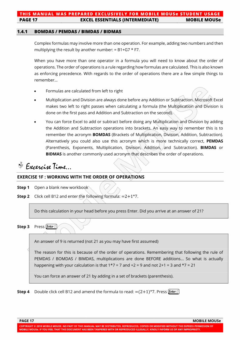
1.4.1 BOMDAS / PEMDAS / BIMDAS / BIDMAS
Complex formulas may involve more than one operation. For example, adding two numbers and then
multiplying the result by another number: = B1+G7 * F7.
When you have more than one operator in a formula you will need to know about the order of
operations. The order of operations is a rule regarding how formulas are calculated. This is also known
as enforcing precedence. With regards to the order of operations there are a few simple things to
remember…
• Formulas are calculated from left to right
• Multiplication and Division are always done before any Addition or Subtraction. Microsoft Excel
makes two left to right passes when calculating a formula (the Multiplication and Division is
done on the first pass and Addition and Subtraction on the second).
• You can force Excel to add or subtract before doing any Multiplication and Division by adding
the Addition and Subtraction operations into brackets. An easy way to remember this is to
remember the acronym BOMDAS (Brackets of Multiplication, Division, Addition, Subtraction).
Alternatively you could also use this acronym which is more technically correct, PEMDAS
(Parenthesis, Exponents, Multiplication, Division, Addition, and Subtraction). BIMDAS or
BIDMAS is another commonly used acronym that describes the order of operations.
Excercise Time... EXERCISE 1F : WORKING WITH THE ORDER OF OPERATIONS
Step 1 Open a blank new workbook
Step 2 Click cell B12 and enter the following formula: =2+1*7.
Do this calculation in your head before you press Enter. Did you arrive at an answer of 21?
Step 3 Press I
An answer of 9 is returned (not 21 as you may have first assumed)
The reason for this is because of the order of operations. Remembering that following the rule of
PEMDAS / BOMDAS / BIMDAS, multiplications are done BEFORE additions... So what is actually
happening with your calculation is that 1*7 = 7 and +2 = 9 and not 2+1 = 3 and *7 = 21
You can force an answer of 21 by adding in a set of brackets (parenthesis).
Step 4 Double click cell B12 and amend the formula to read: =(2+1)*7. Press I

TH IS MANUAL W AS PREPARED EX CLUSIVE LY FOR MOBILE MOUSe ST UDE NT USAGE
MOBILE MOUSe EXCEL ESSENTIALS (INTERMEDIATE) PAGE 18
MOBILE MOUSe PAGE 18
COPYRIGHT © 2018 MOBILE MOUSE. NO PART OF THIS MANUAL MAY BE DISTRIBUTED, REPRODUCED, COPIED OR MODIFIED WITHOUT THE EXPRESS PERMISSION OF
MOBILE MOUSe. IF YOU FEEL THAT THIS DOCUMENT HAS BEEN TAMPERED WITH OR REPRODUCED ILLEGALLY, KINDLY INFORM US OF ANY IMPROPRIETY.
This time by forcing (2+1) to be calculated first (because of the brackets) you will get an answer of 21...
(2+1) = 3 and 3 * 7 = 21.
Step 5 Double click cell B12 and amend the formula to read =(2+1)*7 – 5 – 4. Press I
You should get an answer of 12, because (2+1) = 3 and 3 * 7 = 21, then 21 – 5 = 16 and 16 – 4 = 12. The
subtractions are done last due to the order of operations.
Step 6 Double click cell B12 and make the following change to the formula...
=(2+1)*7 –(5 – 4). Press I
This time you arrive at an answer of 20, because (2+1) = 3 and (5-4) = 1... Remember brackets are
always calculated before anything else... therefore 3 * 7 = 21 and 21 – 1 = 20
Important Notes...
• Exponential operations ^ (to the power of) are performed after anything in Parenthesis
(brackets) and before Multiplication, Division, Addition or Subtraction.
• When it comes to Multiplications and Divisions, whichever occurs first in the formula (from left
to right) is calculated first.
• When it comes to Additions and Subtractions, whichever occurs first in the formula (from left to
right) is calculated first.
Step 7 Click cell B12 and press V on the keyboard to clear the contents in the cell
We will look at some other examples of this theory of mathematics at a later stage. For now, let’s
continue on and look at some other simple formulae.
Excercise Time... EXERCISE 1G : USING POINT AND CLICK FORMULAS
Step 1 Open the file named Chapter_1G.xlsx in the Desktop \ Excel \ Essentials folder
To begin with, we will be adding up a majority of the numbers on this spread sheet.
Step 2 Click cell F5 where the result of the first calculation is going to appear
Step 3 Type an equal sign: =
Step 4 Click the first cell you want to include in the formula (in this case click cell B5)
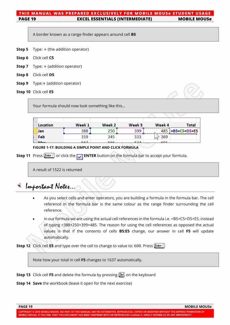
TH IS MANUAL W AS PREPARED EX CLUSIVE LY FOR MOBILE MOUSe ST UDE NT USAGE
PAGE 19 EXCEL ESSENTIALS (INTERMEDIATE) MOBILE MOUSe
PAGE 19 MOBILE MOUSe
COPYRIGHT © 2018 MOBILE MOUSE. NO PART OF THIS MANUAL MAY BE DISTRIBUTED, REPRODUCED, COPIED OR MODIFIED WITHOUT THE EXPRESS PERMISSION OF
MOBILE MOUSe. IF YOU FEEL THAT THIS DOCUMENT HAS BEEN TAMPERED WITH OR REPRODUCED ILLEGALLY, KINDLY INFORM US OF ANY IMPROPRIETY.
A border known as a range finder appears around cell B5
Step 5 Type: + (the addition operator)
Step 6 Click cell C5
Step 7 Type: + (addition operator)
Step 8 Click cell D5
Step 9 Type:+ (addition operator)
Step 10 Click cell E5
Your formula should now look something like this…
FIGURE 1-17: BUILDING A SIMPLE POINT AND CLICK FORMULA
Step 11 Press I or click the ENTER button on the formula bar to accept your formula.
A result of 1522 is returned
Important Notes...
• As you select cells and enter operators, you are building a formula in the formula bar. The cell
reference in the formula bar is the same colour as the range finder surrounding the cell
reference.
• In our formula we are using the actual cell references in the formula i.e. =B5+C5+D5+E5, instead
of typing =388+250+399+485. The reason for using the cell references as opposed the actual
values is that if the contents of cells B5:E5 change, our answer in cell F5 will update
automatically.
Step 12 Click cell E5 and type over the cell to change to value to: 600. Press I
Note how your total in cell F5 changes to 1637 automatically.
Step 13 Click cell F5 and delete the formula by pressing V on the keyboard
Step 14 Save the workbook (leave it open for the next exercise)
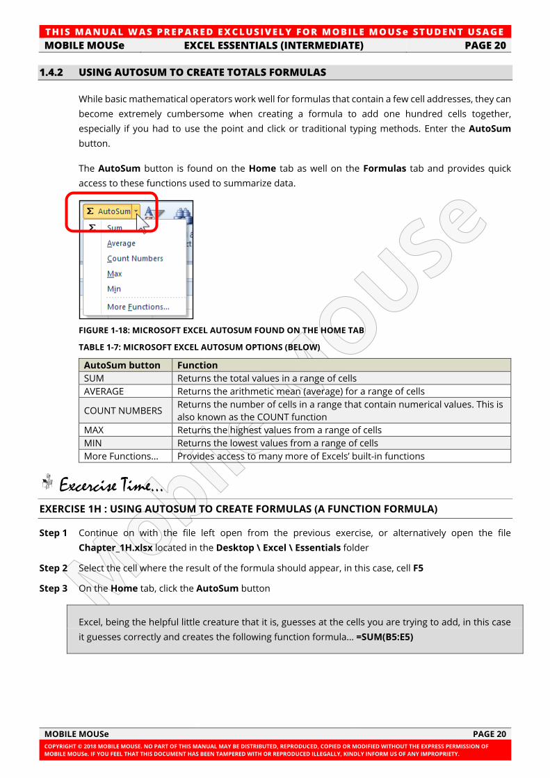
TH IS MANUAL W AS PREPARED EX CLUSIVE LY FOR MOBILE MOUSe ST UDE NT USAGE
MOBILE MOUSe EXCEL ESSENTIALS (INTERMEDIATE) PAGE 20
MOBILE MOUSe PAGE 20
COPYRIGHT © 2018 MOBILE MOUSE. NO PART OF THIS MANUAL MAY BE DISTRIBUTED, REPRODUCED, COPIED OR MODIFIED WITHOUT THE EXPRESS PERMISSION OF
MOBILE MOUSe. IF YOU FEEL THAT THIS DOCUMENT HAS BEEN TAMPERED WITH OR REPRODUCED ILLEGALLY, KINDLY INFORM US OF ANY IMPROPRIETY.
1.4.2 USING AUTOSUM TO CREATE TOTALS FORMULAS
While basic mathematical operators work well for formulas that contain a few cell addresses, they can
become extremely cumbersome when creating a formula to add one hundred cells together,
especially if you had to use the point and click or traditional typing methods. Enter the AutoSum
button.
The AutoSum button is found on the Home tab as well on the Formulas tab and provides quick
access to these functions used to summarize data.
FIGURE 1-18: MICROSOFT EXCEL AUTOSUM FOUND ON THE HOME TAB
TABLE 1-7: MICROSOFT EXCEL AUTOSUM OPTIONS (BELOW)
AutoSum button Function
SUM Returns the total values in a range of cells
AVERAGE Returns the arithmetic mean (average) for a range of cells
COUNT NUMBERS Returns the number of cells in a range that contain numerical values. This is
also known as the COUNT function
MAX Returns the highest values from a range of cells
MIN Returns the lowest values from a range of cells
More Functions... Provides access to many more of Excels’ built-in functions
Excercise Time... EXERCISE 1H : USING AUTOSUM TO CREATE FORMULAS (A FUNCTION FORMULA)
Step 1 Continue on with the file left open from the previous exercise, or alternatively open the file
Chapter_1H.xlsx located in the Desktop \ Excel \ Essentials folder
Step 2 Select the cell where the result of the formula should appear, in this case, cell F5
Step 3 On the Home tab, click the AutoSum button
Excel, being the helpful little creature that it is, guesses at the cells you are trying to add, in this case
it guesses correctly and creates the following function formula... =SUM(B5:E5)
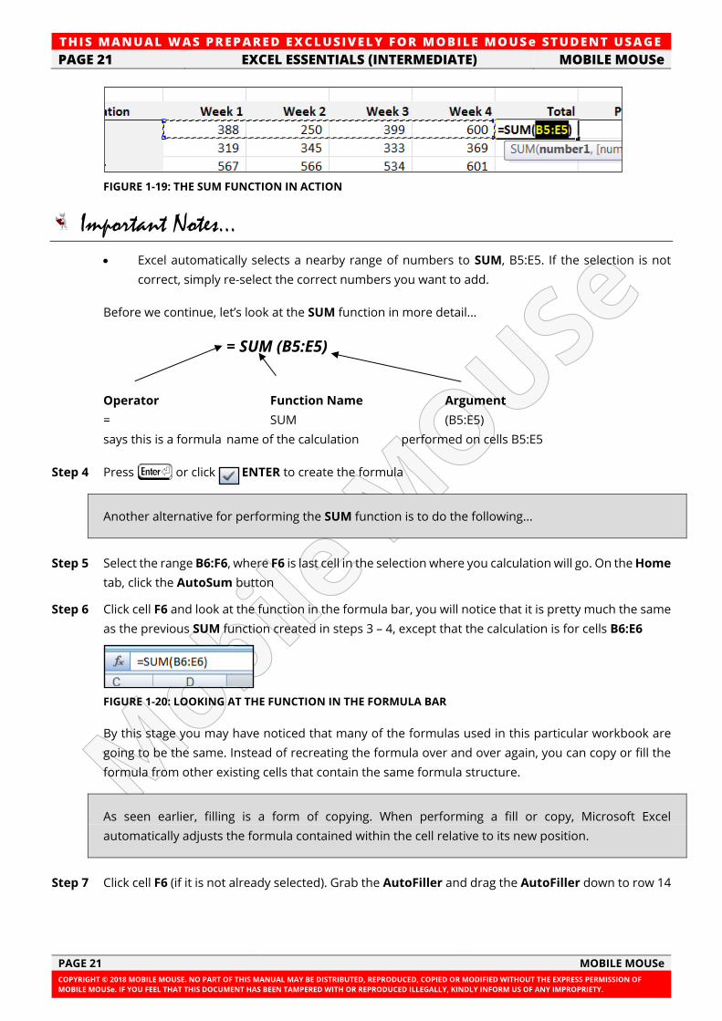
TH IS MANUAL W AS PREPARED EX CLUSIVE LY FOR MOBILE MOUSe ST UDE NT USAGE
PAGE 21 EXCEL ESSENTIALS (INTERMEDIATE) MOBILE MOUSe
PAGE 21 MOBILE MOUSe
COPYRIGHT © 2018 MOBILE MOUSE. NO PART OF THIS MANUAL MAY BE DISTRIBUTED, REPRODUCED, COPIED OR MODIFIED WITHOUT THE EXPRESS PERMISSION OF
MOBILE MOUSe. IF YOU FEEL THAT THIS DOCUMENT HAS BEEN TAMPERED WITH OR REPRODUCED ILLEGALLY, KINDLY INFORM US OF ANY IMPROPRIETY.
FIGURE 1-19: THE SUM FUNCTION IN ACTION
Important Notes...
• Excel automatically selects a nearby range of numbers to SUM, B5:E5. If the selection is not
correct, simply re-select the correct numbers you want to add.
Before we continue, let’s look at the SUM function in more detail...
= SUM (B5:E5)
Operator Function Name Argument
= SUM (B5:E5)
says this is a formula name of the calculation performed on cells B5:E5
Step 4 Press I or click ENTER to create the formula
Another alternative for performing the SUM function is to do the following...
Step 5 Select the range B6:F6, where F6 is last cell in the selection where you calculation will go. On the Home
tab, click the AutoSum button
Step 6 Click cell F6 and look at the function in the formula bar, you will notice that it is pretty much the same
as the previous SUM function created in steps 3 – 4, except that the calculation is for cells B6:E6
FIGURE 1-20: LOOKING AT THE FUNCTION IN THE FORMULA BAR
By this stage you may have noticed that many of the formulas used in this particular workbook are
going to be the same. Instead of recreating the formula over and over again, you can copy or fill the
formula from other existing cells that contain the same formula structure.
As seen earlier, filling is a form of copying. When performing a fill or copy, Microsoft Excel
automatically adjusts the formula contained within the cell relative to its new position.
Step 7 Click cell F6 (if it is not already selected). Grab the AutoFiller and drag the AutoFiller down to row 14
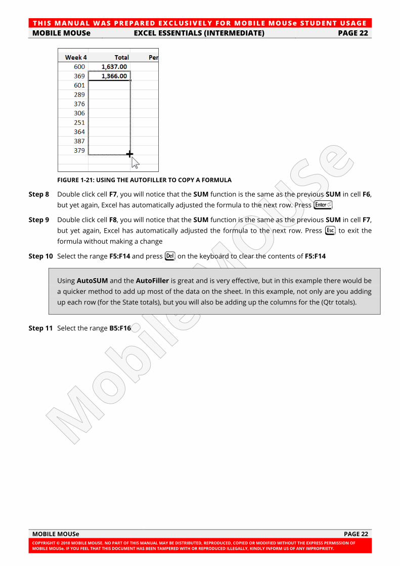
TH IS MANUAL W AS PREPARED EX CLUSIVE LY FOR MOBILE MOUSe ST UDE NT USAGE
MOBILE MOUSe EXCEL ESSENTIALS (INTERMEDIATE) PAGE 22
MOBILE MOUSe PAGE 22
COPYRIGHT © 2018 MOBILE MOUSE. NO PART OF THIS MANUAL MAY BE DISTRIBUTED, REPRODUCED, COPIED OR MODIFIED WITHOUT THE EXPRESS PERMISSION OF
MOBILE MOUSe. IF YOU FEEL THAT THIS DOCUMENT HAS BEEN TAMPERED WITH OR REPRODUCED ILLEGALLY, KINDLY INFORM US OF ANY IMPROPRIETY.
FIGURE 1-21: USING THE AUTOFILLER TO COPY A FORMULA
Step 8 Double click cell F7, you will notice that the SUM function is the same as the previous SUM in cell F6,
but yet again, Excel has automatically adjusted the formula to the next row. Press I
Step 9 Double click cell F8, you will notice that the SUM function is the same as the previous SUM in cell F7,
but yet again, Excel has automatically adjusted the formula to the next row. Press L to exit the
formula without making a change
Step 10 Select the range F5:F14 and press V on the keyboard to clear the contents of F5:F14
Using AutoSUM and the AutoFiller is great and is very effective, but in this example there would be
a quicker method to add up most of the data on the sheet. In this example, not only are you adding
up each row (for the State totals), but you will also be adding up the columns for the (Qtr totals).
Step 11 Select the range B5:F16
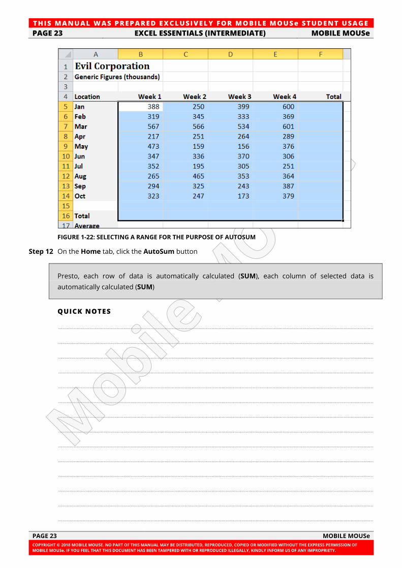
TH IS MANUAL W AS PREPARED EX CLUSIVE LY FOR MOBILE MOUSe ST UDE NT USAGE
PAGE 23 EXCEL ESSENTIALS (INTERMEDIATE) MOBILE MOUSe
PAGE 23 MOBILE MOUSe
COPYRIGHT © 2018 MOBILE MOUSE. NO PART OF THIS MANUAL MAY BE DISTRIBUTED, REPRODUCED, COPIED OR MODIFIED WITHOUT THE EXPRESS PERMISSION OF
MOBILE MOUSe. IF YOU FEEL THAT THIS DOCUMENT HAS BEEN TAMPERED WITH OR REPRODUCED ILLEGALLY, KINDLY INFORM US OF ANY IMPROPRIETY.
FIGURE 1-22: SELECTING A RANGE FOR THE PURPOSE OF AUTOSUM
Step 12 On the Home tab, click the AutoSum button
Presto, each row of data is automatically calculated (SUM), each column of selected data is
automatically calculated (SUM)
QUICK NOTES
..............................................................................................................................................................................................................................
..............................................................................................................................................................................................................................
..............................................................................................................................................................................................................................
..............................................................................................................................................................................................................................
..............................................................................................................................................................................................................................
..............................................................................................................................................................................................................................
..............................................................................................................................................................................................................................
..............................................................................................................................................................................................................................
..............................................................................................................................................................................................................................
..............................................................................................................................................................................................................................
..............................................................................................................................................................................................................................
..............................................................................................................................................................................................................................
..............................................................................................................................................................................................................................
..............................................................................................................................................................................................................................
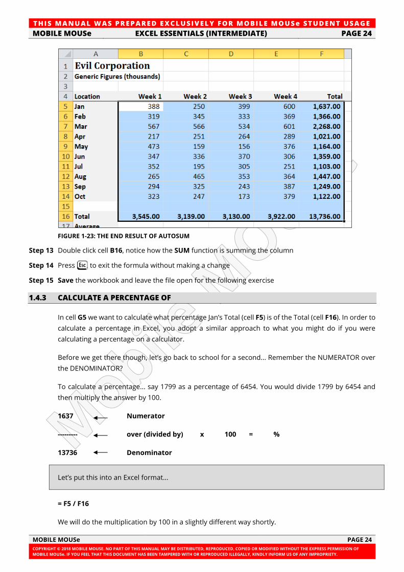
TH IS MANUAL W AS PREPARED EX CLUSIVE LY FOR MOBILE MOUSe ST UDE NT USAGE
MOBILE MOUSe EXCEL ESSENTIALS (INTERMEDIATE) PAGE 24
MOBILE MOUSe PAGE 24
COPYRIGHT © 2018 MOBILE MOUSE. NO PART OF THIS MANUAL MAY BE DISTRIBUTED, REPRODUCED, COPIED OR MODIFIED WITHOUT THE EXPRESS PERMISSION OF
MOBILE MOUSe. IF YOU FEEL THAT THIS DOCUMENT HAS BEEN TAMPERED WITH OR REPRODUCED ILLEGALLY, KINDLY INFORM US OF ANY IMPROPRIETY.
FIGURE 1-23: THE END RESULT OF AUTOSUM
Step 13 Double click cell B16, notice how the SUM function is summing the column
Step 14 Press L to exit the formula without making a change
Step 15 Save the workbook and leave the file open for the following exercise
1.4.3 CALCULATE A PERCENTAGE OF
In cell G5 we want to calculate what percentage Jan’s Total (cell F5) is of the Total (cell F16). In order to
calculate a percentage in Excel, you adopt a similar approach to what you might do if you were
calculating a percentage on a calculator.
Before we get there though, let’s go back to school for a second... Remember the NUMERATOR over
the DENOMINATOR?
To calculate a percentage... say 1799 as a percentage of 6454. You would divide 1799 by 6454 and
then multiply the answer by 100.
1637 Numerator
--------- over (divided by) x 100 = %
13736 Denominator
Let’s put this into an Excel format...
= F5 / F16
We will do the multiplication by 100 in a slightly different way shortly.
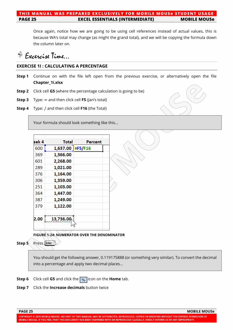
TH IS MANUAL W AS PREPARED EX CLUSIVE LY FOR MOBILE MOUSe ST UDE NT USAGE
PAGE 25 EXCEL ESSENTIALS (INTERMEDIATE) MOBILE MOUSe
PAGE 25 MOBILE MOUSe
COPYRIGHT © 2018 MOBILE MOUSE. NO PART OF THIS MANUAL MAY BE DISTRIBUTED, REPRODUCED, COPIED OR MODIFIED WITHOUT THE EXPRESS PERMISSION OF
MOBILE MOUSe. IF YOU FEEL THAT THIS DOCUMENT HAS BEEN TAMPERED WITH OR REPRODUCED ILLEGALLY, KINDLY INFORM US OF ANY IMPROPRIETY.
Once again, notice how we are going to be using cell references instead of actual values, this is
because WA’s total may change (as might the grand total), and we will be copying the formula down
the column later on.
Excercise Time... EXERCISE 1I : CALCULATING A PERCENTAGE
Step 1 Continue on with the file left open from the previous exercise, or alternatively open the file
Chapter_1i.xlsx
Step 2 Click cell G5 (where the percentage calculation is going to be)
Step 3 Type: = and then click cell F5 (Jan’s total)
Step 4 Type: / and then click cell F16 (the Total)
Your formula should look something like this...
FIGURE 1-24: NUMERATOR OVER THE DENOMINATOR
Step 5 Press I.
You should get the following answer, 0.119175888 (or something very similar). To convert the decimal
into a percentage and apply two decimal places…
Step 6 Click cell G5 and click the icon on the Home tab.
Step 7 Click the Increase decimals button twice
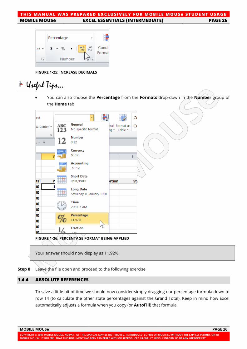
TH IS MANUAL W AS PREPARED EX CLUSIVE LY FOR MOBILE MOUSe ST UDE NT USAGE
MOBILE MOUSe EXCEL ESSENTIALS (INTERMEDIATE) PAGE 26
MOBILE MOUSe PAGE 26
COPYRIGHT © 2018 MOBILE MOUSE. NO PART OF THIS MANUAL MAY BE DISTRIBUTED, REPRODUCED, COPIED OR MODIFIED WITHOUT THE EXPRESS PERMISSION OF
MOBILE MOUSe. IF YOU FEEL THAT THIS DOCUMENT HAS BEEN TAMPERED WITH OR REPRODUCED ILLEGALLY, KINDLY INFORM US OF ANY IMPROPRIETY.
FIGURE 1-25: INCREASE DECIMALS
Useful Tips...
• You can also choose the Percentage from the Formats drop-down in the Number group of
the Home tab
FIGURE 1-26: PERCENTAGE FORMAT BEING APPLIED
Your answer should now display as 11.92%.
Step 8 Leave the file open and proceed to the following exercise
1.4.4 ABSOLUTE REFERENCES
To save a little bit of time we should now consider simply dragging our percentage formula down to
row 14 (to calculate the other state percentages against the Grand Total). Keep in mind how Excel
automatically adjusts a formula when you copy (or AutoFill) that formula.
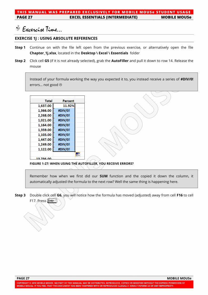
TH IS MANUAL W AS PREPARED EX CLUSIVE LY FOR MOBILE MOUSe ST UDE NT USAGE
PAGE 27 EXCEL ESSENTIALS (INTERMEDIATE) MOBILE MOUSe
PAGE 27 MOBILE MOUSe
COPYRIGHT © 2018 MOBILE MOUSE. NO PART OF THIS MANUAL MAY BE DISTRIBUTED, REPRODUCED, COPIED OR MODIFIED WITHOUT THE EXPRESS PERMISSION OF
MOBILE MOUSe. IF YOU FEEL THAT THIS DOCUMENT HAS BEEN TAMPERED WITH OR REPRODUCED ILLEGALLY, KINDLY INFORM US OF ANY IMPROPRIETY.
Excercise Time... EXERCISE 1J : USING ABSOLUTE REFERENCES
Step 1 Continue on with the file left open from the previous exercise, or alternatively open the file
Chapter_1j.xlsx, located in the Desktop \ Excel \ Essentials folder
Step 2 Click cell G5 (if it is not already selected), grab the AutoFiller and pull it down to row 14. Release the
mouse
Instead of your formula working the way you expected it to, you instead receive a series of #DIV/0!
errors... not good
FIGURE 1-27: WHEN USING THE AUTOFILLER, YOU RECEIVE ERRORS?
Remember how when we first did our SUM function and the copied it down the column, it
automatically adjusted the formula to the next row? Well the same thing is happening here.
Step 3 Double click cell G6, you will notice how the formula has moved (adjusted) away from cell F16 to cell
F17. Press I
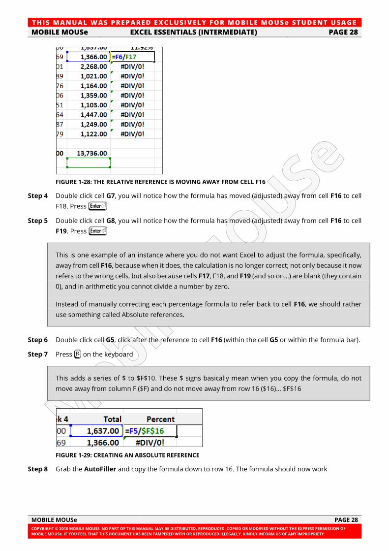
TH IS MANUAL W AS PREPARED EX CLUSIVE LY FOR MOBILE MOUSe ST UDE NT USAGE
MOBILE MOUSe EXCEL ESSENTIALS (INTERMEDIATE) PAGE 28
MOBILE MOUSe PAGE 28
COPYRIGHT © 2018 MOBILE MOUSE. NO PART OF THIS MANUAL MAY BE DISTRIBUTED, REPRODUCED, COPIED OR MODIFIED WITHOUT THE EXPRESS PERMISSION OF
MOBILE MOUSe. IF YOU FEEL THAT THIS DOCUMENT HAS BEEN TAMPERED WITH OR REPRODUCED ILLEGALLY, KINDLY INFORM US OF ANY IMPROPRIETY.
FIGURE 1-28: THE RELATIVE REFERENCE IS MOVING AWAY FROM CELL F16
Step 4 Double click cell G7, you will notice how the formula has moved (adjusted) away from cell F16 to cell
F18. Press I
Step 5 Double click cell G8, you will notice how the formula has moved (adjusted) away from cell F16 to cell
F19. Press I
This is one example of an instance where you do not want Excel to adjust the formula, specifically,
away from cell F16, because when it does, the calculation is no longer correct; not only because it now
refers to the wrong cells, but also because cells F17, F18, and F19 (and so on…) are blank (they contain
0), and in arithmetic you cannot divide a number by zero.
Instead of manually correcting each percentage formula to refer back to cell F16, we should rather
use something called Absolute references.
Step 6 Double click cell G5, click after the reference to cell F16 (within the cell G5 or within the formula bar).
Step 7 Press 4 on the keyboard
This adds a series of $ to $F$10. These $ signs basically mean when you copy the formula, do not
move away from column F ($F) and do not move away from row 16 ($16)... $F$16
FIGURE 1-29: CREATING AN ABSOLUTE REFERENCE
Step 8 Grab the AutoFiller and copy the formula down to row 16. The formula should now work
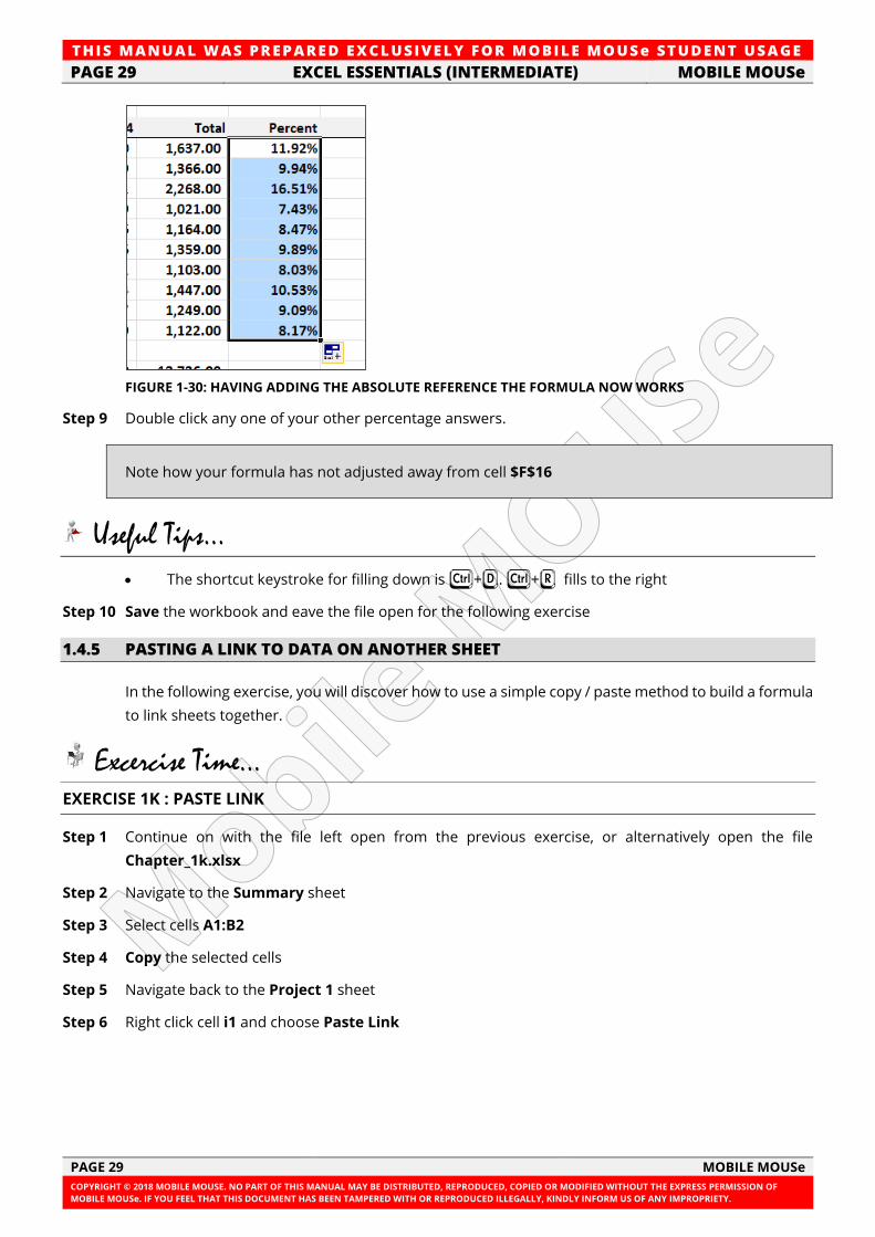
TH IS MANUAL W AS PREPARED EX CLUSIVE LY FOR MOBILE MOUSe ST UDE NT USAGE
PAGE 29 EXCEL ESSENTIALS (INTERMEDIATE) MOBILE MOUSe
PAGE 29 MOBILE MOUSe
COPYRIGHT © 2018 MOBILE MOUSE. NO PART OF THIS MANUAL MAY BE DISTRIBUTED, REPRODUCED, COPIED OR MODIFIED WITHOUT THE EXPRESS PERMISSION OF
MOBILE MOUSe. IF YOU FEEL THAT THIS DOCUMENT HAS BEEN TAMPERED WITH OR REPRODUCED ILLEGALLY, KINDLY INFORM US OF ANY IMPROPRIETY.
FIGURE 1-30: HAVING ADDING THE ABSOLUTE REFERENCE THE FORMULA NOW WORKS
Step 9 Double click any one of your other percentage answers.
Note how your formula has not adjusted away from cell $F$16
Useful Tips...
• The shortcut keystroke for filling down is F+D. F+R fills to the right
Step 10 Save the workbook and eave the file open for the following exercise
1.4.5 PASTING A LINK TO DATA ON ANOTHER SHEET
In the following exercise, you will discover how to use a simple copy / paste method to build a formula
to link sheets together.
Excercise Time... EXERCISE 1K : PASTE LINK
Step 1 Continue on with the file left open from the previous exercise, or alternatively open the file
Chapter_1k.xlsx
Step 2 Navigate to the Summary sheet
Step 3 Select cells A1:B2
Step 4 Copy the selected cells
Step 5 Navigate back to the Project 1 sheet
Step 6 Right click cell i1 and choose Paste Link
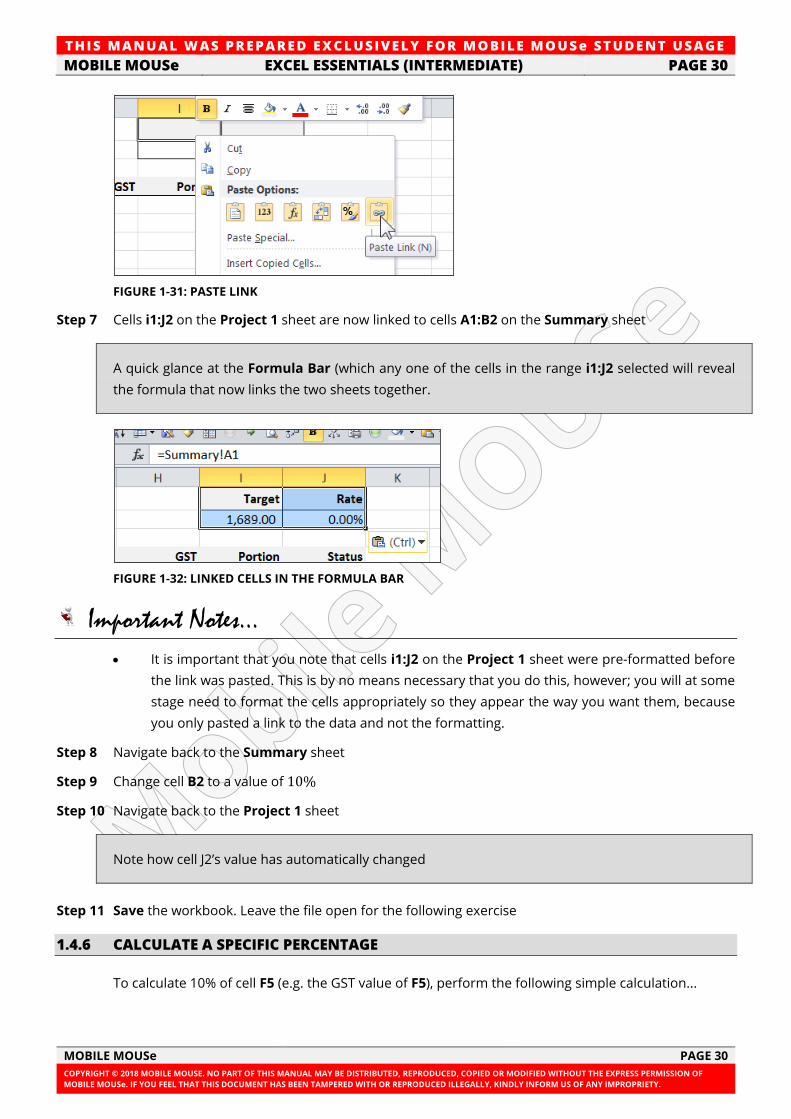
TH IS MANUAL W AS PREPARED EX CLUSIVE LY FOR MOBILE MOUSe ST UDE NT USAGE
MOBILE MOUSe EXCEL ESSENTIALS (INTERMEDIATE) PAGE 30
MOBILE MOUSe PAGE 30
COPYRIGHT © 2018 MOBILE MOUSE. NO PART OF THIS MANUAL MAY BE DISTRIBUTED, REPRODUCED, COPIED OR MODIFIED WITHOUT THE EXPRESS PERMISSION OF
MOBILE MOUSe. IF YOU FEEL THAT THIS DOCUMENT HAS BEEN TAMPERED WITH OR REPRODUCED ILLEGALLY, KINDLY INFORM US OF ANY IMPROPRIETY.
FIGURE 1-31: PASTE LINK
Step 7 Cells i1:J2 on the Project 1 sheet are now linked to cells A1:B2 on the Summary sheet
A quick glance at the Formula Bar (which any one of the cells in the range i1:J2 selected will reveal
the formula that now links the two sheets together.
FIGURE 1-32: LINKED CELLS IN THE FORMULA BAR
Important Notes...
• It is important that you note that cells i1:J2 on the Project 1 sheet were pre-formatted before
the link was pasted. This is by no means necessary that you do this, however; you will at some
stage need to format the cells appropriately so they appear the way you want them, because
you only pasted a link to the data and not the formatting.
Step 8 Navigate back to the Summary sheet
Step 9 Change cell B2 to a value of 10%
Step 10 Navigate back to the Project 1 sheet
Note how cell J2’s value has automatically changed
Step 11 Save the workbook. Leave the file open for the following exercise
1.4.6 CALCULATE A SPECIFIC PERCENTAGE
To calculate 10% of cell F5 (e.g. the GST value of F5), perform the following simple calculation...
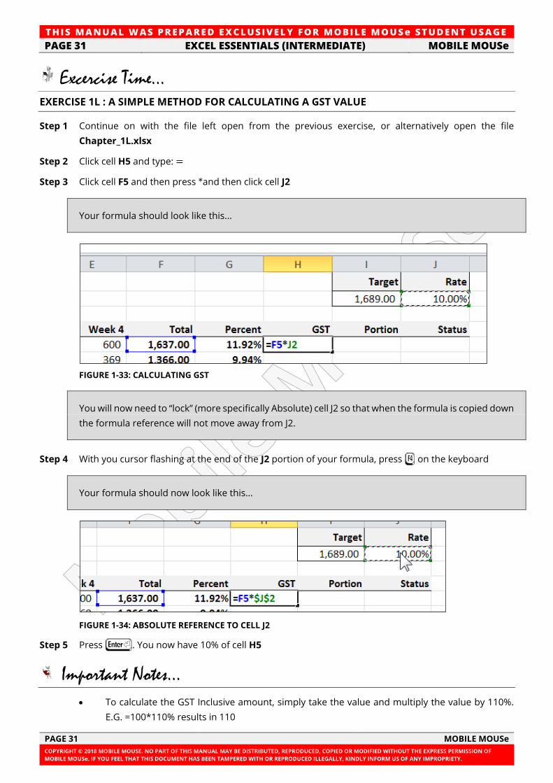
TH IS MANUAL W AS PREPARED EX CLUSIVE LY FOR MOBILE MOUSe ST UDE NT USAGE
PAGE 31 EXCEL ESSENTIALS (INTERMEDIATE) MOBILE MOUSe
PAGE 31 MOBILE MOUSe
COPYRIGHT © 2018 MOBILE MOUSE. NO PART OF THIS MANUAL MAY BE DISTRIBUTED, REPRODUCED, COPIED OR MODIFIED WITHOUT THE EXPRESS PERMISSION OF
MOBILE MOUSe. IF YOU FEEL THAT THIS DOCUMENT HAS BEEN TAMPERED WITH OR REPRODUCED ILLEGALLY, KINDLY INFORM US OF ANY IMPROPRIETY.
Excercise Time... EXERCISE 1L : A SIMPLE METHOD FOR CALCULATING A GST VALUE
Step 1 Continue on with the file left open from the previous exercise, or alternatively open the file
Chapter_1L.xlsx
Step 2 Click cell H5 and type: =
Step 3 Click cell F5 and then press *and then click cell J2
Your formula should look like this...
FIGURE 1-33: CALCULATING GST
You will now need to “lock” (more specifically Absolute) cell J2 so that when the formula is copied down
the formula reference will not move away from J2.
Step 4 With you cursor flashing at the end of the J2 portion of your formula, press n on the keyboard
Your formula should now look like this…
FIGURE 1-34: ABSOLUTE REFERENCE TO CELL J2
Step 5 Press I. You now have 10% of cell H5
Important Notes...
• To calculate the GST Inclusive amount, simply take the value and multiply the value by 110%.
E.G. =100*110% results in 110
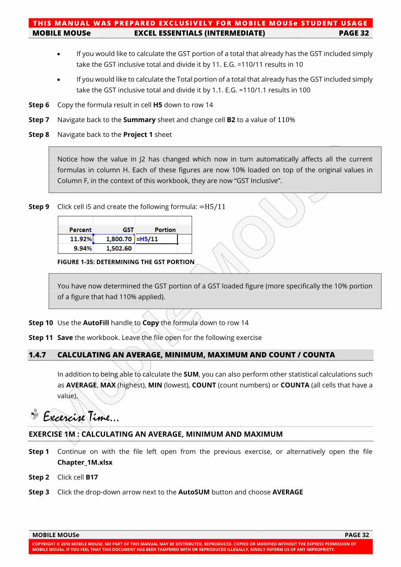
TH IS MANUAL W AS PREPARED EX CLUSIVE LY FOR MOBILE MOUSe ST UDE NT USAGE
MOBILE MOUSe EXCEL ESSENTIALS (INTERMEDIATE) PAGE 32
MOBILE MOUSe PAGE 32
COPYRIGHT © 2018 MOBILE MOUSE. NO PART OF THIS MANUAL MAY BE DISTRIBUTED, REPRODUCED, COPIED OR MODIFIED WITHOUT THE EXPRESS PERMISSION OF
MOBILE MOUSe. IF YOU FEEL THAT THIS DOCUMENT HAS BEEN TAMPERED WITH OR REPRODUCED ILLEGALLY, KINDLY INFORM US OF ANY IMPROPRIETY.
• If you would like to calculate the GST portion of a total that already has the GST included simply
take the GST inclusive total and divide it by 11. E.G. =110/11 results in 10
• If you would like to calculate the Total portion of a total that already has the GST included simply
take the GST inclusive total and divide it by 1.1. E.G. =110/1.1 results in 100
Step 6 Copy the formula result in cell H5 down to row 14
Step 7 Navigate back to the Summary sheet and change cell B2 to a value of 110%
Step 8 Navigate back to the Project 1 sheet
Notice how the value in J2 has changed which now in turn automatically affects all the current
formulas in column H. Each of these figures are now 10% loaded on top of the original values in
Column F, in the context of this workbook, they are now “GST Inclusive”.
Step 9 Click cell i5 and create the following formula: =H5/11
FIGURE 1-35: DETERMINING THE GST PORTION
You have now determined the GST portion of a GST loaded figure (more specifically the 10% portion
of a figure that had 110% applied).
Step 10 Use the AutoFill handle to Copy the formula down to row 14
Step 11 Save the workbook. Leave the file open for the following exercise
1.4.7 CALCULATING AN AVERAGE, MINIMUM, MAXIMUM AND COUNT / COUNTA
In addition to being able to calculate the SUM, you can also perform other statistical calculations such
as AVERAGE, MAX (highest), MIN (lowest), COUNT (count numbers) or COUNTA (all cells that have a
value).
Excercise Time... EXERCISE 1M : CALCULATING AN AVERAGE, MINIMUM AND MAXIMUM
Step 1 Continue on with the file left open from the previous exercise, or alternatively open the file
Chapter_1M.xlsx
Step 2 Click cell B17
Step 3 Click the drop-down arrow next to the AutoSUM button and choose AVERAGE
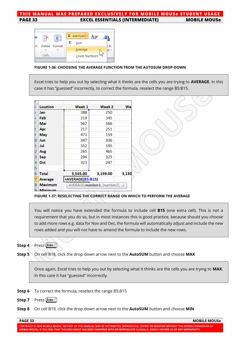
TH IS MANUAL W AS PREPARED EX CLUSIVE LY FOR MOBILE MOUSe ST UDE NT USAGE
PAGE 33 EXCEL ESSENTIALS (INTERMEDIATE) MOBILE MOUSe
PAGE 33 MOBILE MOUSe
COPYRIGHT © 2018 MOBILE MOUSE. NO PART OF THIS MANUAL MAY BE DISTRIBUTED, REPRODUCED, COPIED OR MODIFIED WITHOUT THE EXPRESS PERMISSION OF
MOBILE MOUSe. IF YOU FEEL THAT THIS DOCUMENT HAS BEEN TAMPERED WITH OR REPRODUCED ILLEGALLY, KINDLY INFORM US OF ANY IMPROPRIETY.
FIGURE 1-36: CHOOSING THE AVERAGE FUNCTION FROM THE AUTOSUM DROP-DOWN
Excel tries to help you out by selecting what it thinks are the cells you are trying to AVERAGE. In this
case it has “guessed” incorrectly, to correct the formula, reselect the range B5:B15.
FIGURE 1-37: RESELECTING THE CORRECT RANGE ON WHICH TO PERFORM THE AVERAGE
You will notice you have extended the formula to include cell B15 (one extra cell). This is not a
requirement that you do so, but in most instances this is good practice, because should you choose
to add more rows e.g. data for Nov and Dec, the formula will automatically adjust and include the new
rows added and you will not have to amend the formula to include the new rows.
Step 4 Press I
Step 5 On cell B18, click the drop-down arrow next to the AutoSUM button and choose MAX
Once again, Excel tries to help you out by selecting what it thinks are the cells you are trying to MAX.
In this case it has “guessed” incorrectly.
Step 6 To correct the formula, reselect the range B5:B15
Step 7 Press I
Step 8 On cell B19, click the drop-down arrow next to the AutoSUM button and choose MIN
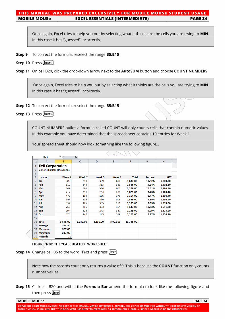
TH IS MANUAL W AS PREPARED EX CLUSIVE LY FOR MOBILE MOUSe ST UDE NT USAGE
MOBILE MOUSe EXCEL ESSENTIALS (INTERMEDIATE) PAGE 34
MOBILE MOUSe PAGE 34
COPYRIGHT © 2018 MOBILE MOUSE. NO PART OF THIS MANUAL MAY BE DISTRIBUTED, REPRODUCED, COPIED OR MODIFIED WITHOUT THE EXPRESS PERMISSION OF
MOBILE MOUSe. IF YOU FEEL THAT THIS DOCUMENT HAS BEEN TAMPERED WITH OR REPRODUCED ILLEGALLY, KINDLY INFORM US OF ANY IMPROPRIETY.
Once again, Excel tries to help you out by selecting what it thinks are the cells you are trying to MIN.
In this case it has “guessed” incorrectly.
Step 9 To correct the formula, reselect the range B5:B15
Step 10 Press I
Step 11 On cell B20, click the drop-down arrow next to the AutoSUM button and choose COUNT NUMBERS
Once again, Excel tries to help you out by selecting what it thinks are the cells you are trying to MIN.
In this case it has “guessed” incorrectly.
Step 12 To correct the formula, reselect the range B5:B15
Step 13 Press I
COUNT NUMBERS builds a formula called COUNT will only counts cells that contain numeric values.
In this example you have determined that the spreadsheet contains 10 entries for Week 1.
Your spread sheet should now look something like the following figure...
FIGURE 1-38: THE “CALCULATED” WORKSHEET
Step 14 Change cell B5 to the word: Text and press J
Note how the records count only returns a value of 9. This is because the COUNT function only counts
number values.
Step 15 Click cell B20 and within the Formula Bar amend the formula to look like the following figure and
then press J
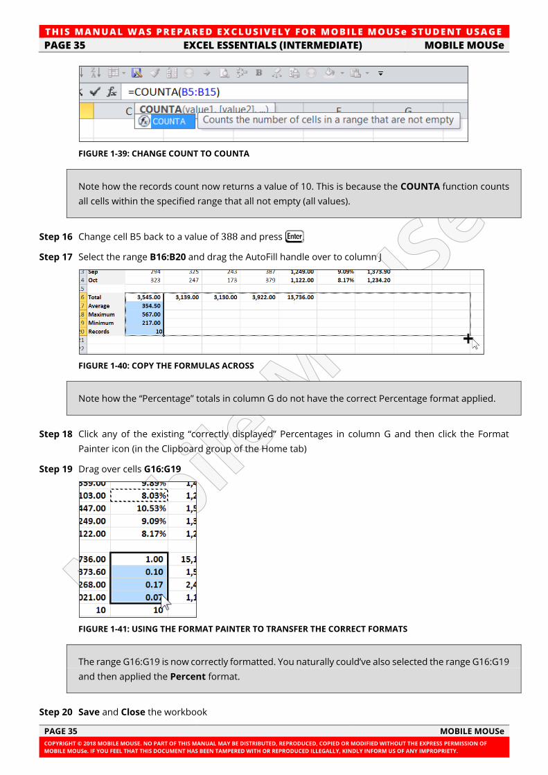
TH IS MANUAL W AS PREPARED EX CLUSIVE LY FOR MOBILE MOUSe ST UDE NT USAGE
PAGE 35 EXCEL ESSENTIALS (INTERMEDIATE) MOBILE MOUSe
PAGE 35 MOBILE MOUSe
COPYRIGHT © 2018 MOBILE MOUSE. NO PART OF THIS MANUAL MAY BE DISTRIBUTED, REPRODUCED, COPIED OR MODIFIED WITHOUT THE EXPRESS PERMISSION OF
MOBILE MOUSe. IF YOU FEEL THAT THIS DOCUMENT HAS BEEN TAMPERED WITH OR REPRODUCED ILLEGALLY, KINDLY INFORM US OF ANY IMPROPRIETY.
FIGURE 1-39: CHANGE COUNT TO COUNTA
Note how the records count now returns a value of 10. This is because the COUNTA function counts
all cells within the specified range that all not empty (all values).
Step 16 Change cell B5 back to a value of 388 and press J
Step 17 Select the range B16:B20 and drag the AutoFill handle over to column J
FIGURE 1-40: COPY THE FORMULAS ACROSS
Note how the “Percentage” totals in column G do not have the correct Percentage format applied.
Step 18 Click any of the existing “correctly displayed” Percentages in column G and then click the Format
Painter icon (in the Clipboard group of the Home tab)
Step 19 Drag over cells G16:G19
FIGURE 1-41: USING THE FORMAT PAINTER TO TRANSFER THE CORRECT FORMATS
The range G16:G19 is now correctly formatted. You naturally could’ve also selected the range G16:G19
and then applied the Percent format.
Step 20 Save and Close the workbook
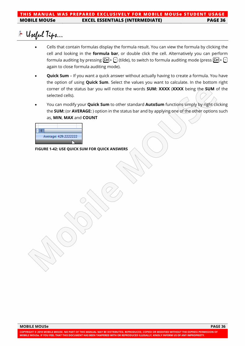
TH IS MANUAL W AS PREPARED EX CLUSIVE LY FOR MOBILE MOUSe ST UDE NT USAGE
MOBILE MOUSe EXCEL ESSENTIALS (INTERMEDIATE) PAGE 36
MOBILE MOUSe PAGE 36
COPYRIGHT © 2018 MOBILE MOUSE. NO PART OF THIS MANUAL MAY BE DISTRIBUTED, REPRODUCED, COPIED OR MODIFIED WITHOUT THE EXPRESS PERMISSION OF
MOBILE MOUSe. IF YOU FEEL THAT THIS DOCUMENT HAS BEEN TAMPERED WITH OR REPRODUCED ILLEGALLY, KINDLY INFORM US OF ANY IMPROPRIETY.
Useful Tips...
• Cells that contain formulas display the formula result. You can view the formula by clicking the
cell and looking in the formula bar, or double click the cell. Alternatively you can perform
formula auditing by pressing F+ ~ (tilde), to switch to formula auditing mode (press F+ ~
again to close formula auditing mode).
• Quick Sum – If you want a quick answer without actually having to create a formula. You have
the option of using Quick Sum. Select the values you want to calculate. In the bottom right
corner of the status bar you will notice the words SUM: XXXX (XXXX being the SUM of the
selected cells).
• You can modify your Quick Sum to other standard AutoSum functions simply by right clicking
the SUM: (or AVERAGE: ) option in the status bar and by applying one of the other options such
as, MIN, MAX and COUNT
FIGURE 1-42: USE QUICK SUM FOR QUICK ANSWERS
TH IS MANUAL W AS PREPARED EX CLUSIVE LY FOR MOBILE MOUSe ST UDE NT USAGE
PAGE 37 EXCEL ESSENTIALS (INTERMEDIATE) MOBILE MOUSe
PAGE 37 MOBILE MOUSe
COPYRIGHT © 2018 MOBILE MOUSE. NO PART OF THIS MANUAL MAY BE DISTRIBUTED, REPRODUCED, COPIED OR MODIFIED WITHOUT THE EXPRESS PERMISSION OF
MOBILE MOUSe. IF YOU FEEL THAT THIS DOCUMENT HAS BEEN TAMPERED WITH OR REPRODUCED ILLEGALLY, KINDLY INFORM US OF ANY IMPROPRIETY.
QUICK NOTES
..................................................................................................................................................................................................................................................
..................................................................................................................................................................................................................................................
..................................................................................................................................................................................................................................................
..................................................................................................................................................................................................................................................
..................................................................................................................................................................................................................................................
..................................................................................................................................................................................................................................................
..................................................................................................................................................................................................................................................
..................................................................................................................................................................................................................................................
..................................................................................................................................................................................................................................................
..................................................................................................................................................................................................................................................
..................................................................................................................................................................................................................................................
..................................................................................................................................................................................................................................................
..................................................................................................................................................................................................................................................
..................................................................................................................................................................................................................................................
..................................................................................................................................................................................................................................................
..................................................................................................................................................................................................................................................
..................................................................................................................................................................................................................................................
..................................................................................................................................................................................................................................................
..................................................................................................................................................................................................................................................
..................................................................................................................................................................................................................................................
..................................................................................................................................................................................................................................................
..................................................................................................................................................................................................................................................
..................................................................................................................................................................................................................................................
..................................................................................................................................................................................................................................................
..................................................................................................................................................................................................................................................
..................................................................................................................................................................................................................................................
..................................................................................................................................................................................................................................................
..................................................................................................................................................................................................................................................
..................................................................................................................................................................................................................................................
..................................................................................................................................................................................................................................................
..................................................................................................................................................................................................................................................
..................................................................................................................................................................................................................................................
..................................................................................................................................................................................................................................................
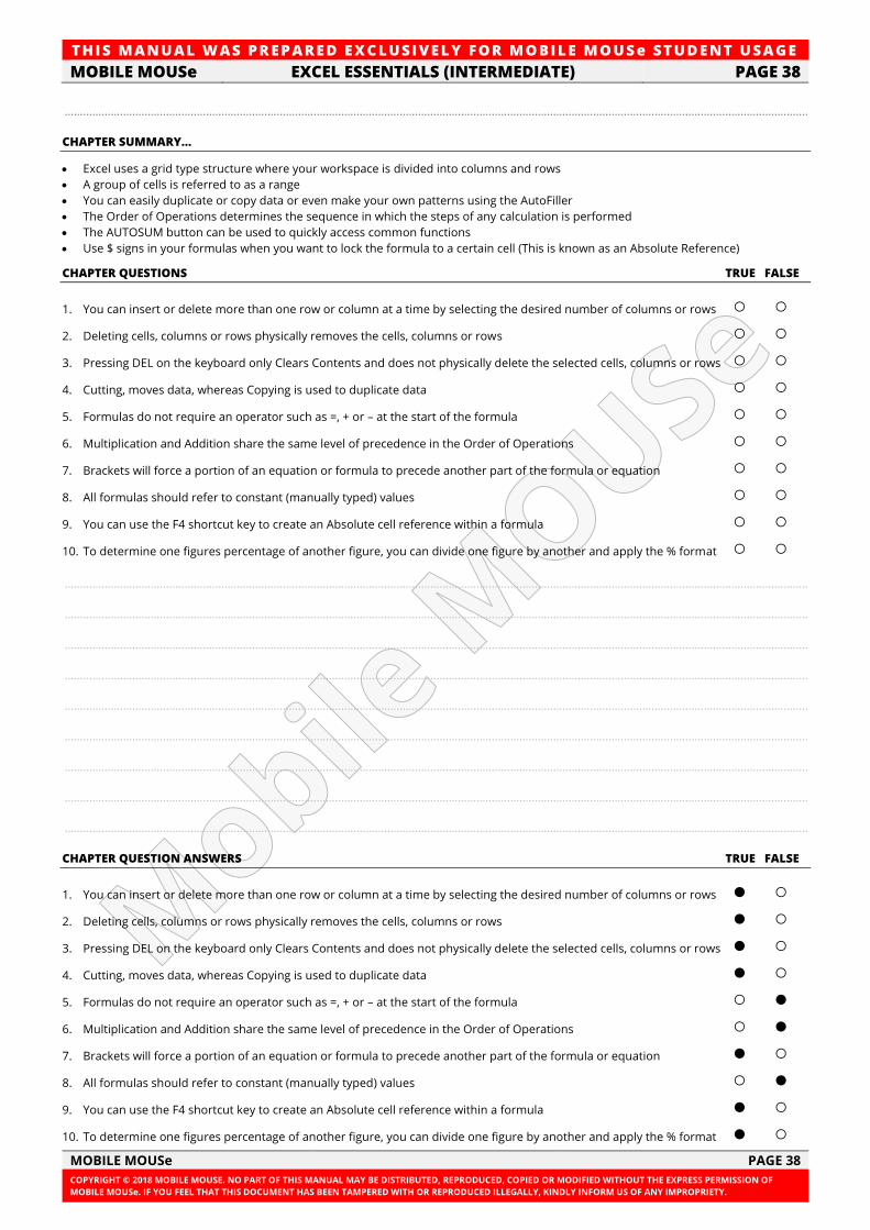
TH IS MANUAL W AS PREPARED EX CLUSIVE LY FOR MOBILE MOUSe ST UDE NT USAGE
MOBILE MOUSe EXCEL ESSENTIALS (INTERMEDIATE) PAGE 38
MOBILE MOUSe PAGE 38
COPYRIGHT © 2018 MOBILE MOUSE. NO PART OF THIS MANUAL MAY BE DISTRIBUTED, REPRODUCED, COPIED OR MODIFIED WITHOUT THE EXPRESS PERMISSION OF
MOBILE MOUSe. IF YOU FEEL THAT THIS DOCUMENT HAS BEEN TAMPERED WITH OR REPRODUCED ILLEGALLY, KINDLY INFORM US OF ANY IMPROPRIETY.
..................................................................................................................................................................................................................................................
CHAPTER SUMMARY…
• Excel uses a grid type structure where your workspace is divided into columns and rows
• A group of cells is referred to as a range
• You can easily duplicate or copy data or even make your own patterns using the AutoFiller
• The Order of Operations determines the sequence in which the steps of any calculation is performed
• The AUTOSUM button can be used to quickly access common functions
• Use $ signs in your formulas when you want to lock the formula to a certain cell (This is known as an Absolute Reference)
CHAPTER QUESTIONS TRUE FALSE
1. You can insert or delete more than one row or column at a time by selecting the desired number of columns or rows ○ ○
2. Deleting cells, columns or rows physically removes the cells, columns or rows ○ ○
3. Pressing DEL on the keyboard only Clears Contents and does not physically delete the selected cells, columns or rows ○ ○
4. Cutting, moves data, whereas Copying is used to duplicate data ○ ○
5. Formulas do not require an operator such as =, + or – at the start of the formula ○ ○
6. Multiplication and Addition share the same level of precedence in the Order of Operations ○ ○
7. Brackets will force a portion of an equation or formula to precede another part of the formula or equation ○ ○
8. All formulas should refer to constant (manually typed) values ○ ○
9. You can use the F4 shortcut key to create an Absolute cell reference within a formula ○ ○
10. To determine one figures percentage of another figure, you can divide one figure by another and apply the % format ○ ○
..................................................................................................................................................................................................................................................
..................................................................................................................................................................................................................................................
..................................................................................................................................................................................................................................................
..................................................................................................................................................................................................................................................
..................................................................................................................................................................................................................................................
..................................................................................................................................................................................................................................................
..................................................................................................................................................................................................................................................
..................................................................................................................................................................................................................................................
..................................................................................................................................................................................................................................................
CHAPTER QUESTION ANSWERS TRUE FALSE
1. You can insert or delete more than one row or column at a time by selecting the desired number of columns or rows ● ○
2. Deleting cells, columns or rows physically removes the cells, columns or rows ● ○
3. Pressing DEL on the keyboard only Clears Contents and does not physically delete the selected cells, columns or rows ● ○
4. Cutting, moves data, whereas Copying is used to duplicate data ● ○
5. Formulas do not require an operator such as =, + or – at the start of the formula ○ ●
6. Multiplication and Addition share the same level of precedence in the Order of Operations ○ ●
7. Brackets will force a portion of an equation or formula to precede another part of the formula or equation ● ○
8. All formulas should refer to constant (manually typed) values ○ ●
9. You can use the F4 shortcut key to create an Absolute cell reference within a formula ● ○
10. To determine one figures percentage of another figure, you can divide one figure by another and apply the % format ● ○
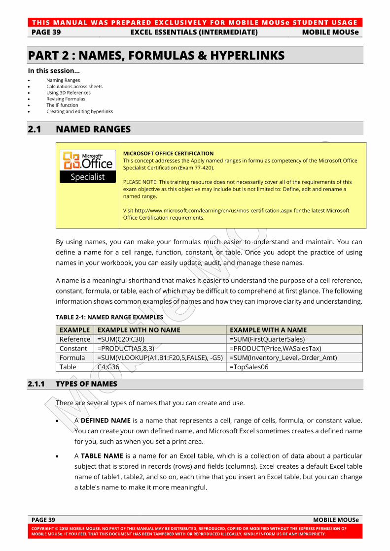
TH IS MANUAL W AS PREPARED EX CLUSIVE LY FOR MOBILE MOUSe ST UDE NT USAGE
PAGE 39 EXCEL ESSENTIALS (INTERMEDIATE) MOBILE MOUSe
PAGE 39 MOBILE MOUSe
COPYRIGHT © 2018 MOBILE MOUSE. NO PART OF THIS MANUAL MAY BE DISTRIBUTED, REPRODUCED, COPIED OR MODIFIED WITHOUT THE EXPRESS PERMISSION OF
MOBILE MOUSe. IF YOU FEEL THAT THIS DOCUMENT HAS BEEN TAMPERED WITH OR REPRODUCED ILLEGALLY, KINDLY INFORM US OF ANY IMPROPRIETY.
PART 2 : NAMES, FORMULAS & HYPERLINKS In this session...
• Naming Ranges
• Calculations across sheets
• Using 3D References
• Revising Formulas
• The IF function
• Creating and editing hyperlinks
2.1 NAMED RANGES
MICROSOFT OFFICE CERTIFICATION
This concept addresses the Apply named ranges in formulas competency of the Microsoft Office
Specialist Certification (Exam 77-420).
PLEASE NOTE: This training resource does not necessarily cover all of the requirements of this
exam objective as this objective may include but is not limited to: Define, edit and rename a
named range.
Visit http://www.microsoft.com/learning/en/us/mos-certification.aspx for the latest Microsoft
Office Certification requirements.
By using names, you can make your formulas much easier to understand and maintain. You can
define a name for a cell range, function, constant, or table. Once you adopt the practice of using
names in your workbook, you can easily update, audit, and manage these names.
A name is a meaningful shorthand that makes it easier to understand the purpose of a cell reference,
constant, formula, or table, each of which may be difficult to comprehend at first glance. The following
information shows common examples of names and how they can improve clarity and understanding.
TABLE 2-1: NAMED RANGE EXAMPLES
EXAMPLE EXAMPLE WITH NO NAME EXAMPLE WITH A NAME
Reference =SUM(C20:C30) =SUM(FirstQuarterSales)
Constant =PRODUCT(A5,8.3) =PRODUCT(Price,WASalesTax)
Formula =SUM(VLOOKUP(A1,B1:F20,5,FALSE), -G5) =SUM(Inventory_Level,-Order_Amt)
Table C4:G36 =TopSales06
2.1.1 TYPES OF NAMES
There are several types of names that you can create and use.
• A DEFINED NAME is a name that represents a cell, range of cells, formula, or constant value.
You can create your own defined name, and Microsoft Excel sometimes creates a defined name
for you, such as when you set a print area.
• A TABLE NAME is a name for an Excel table, which is a collection of data about a particular
subject that is stored in records (rows) and fields (columns). Excel creates a default Excel table
name of table1, table2, and so on, each time that you insert an Excel table, but you can change
a table's name to make it more meaningful.
TH IS MANUAL W AS PREPARED EX CLUSIVE LY FOR MOBILE MOUSe ST UDE NT USAGE
MOBILE MOUSe EXCEL ESSENTIALS (INTERMEDIATE) PAGE 40
MOBILE MOUSe PAGE 40
COPYRIGHT © 2018 MOBILE MOUSE. NO PART OF THIS MANUAL MAY BE DISTRIBUTED, REPRODUCED, COPIED OR MODIFIED WITHOUT THE EXPRESS PERMISSION OF
MOBILE MOUSe. IF YOU FEEL THAT THIS DOCUMENT HAS BEEN TAMPERED WITH OR REPRODUCED ILLEGALLY, KINDLY INFORM US OF ANY IMPROPRIETY.
2.1.2 THE SCOPE OF A NAME
All names have a scope, either to a specific worksheet (also called the local worksheet level) or to the
entire workbook (also called the global workbook level). The scope of a name is the location within
which the name is recognized without qualification. For example:
If you have defined a name, such as Budget_FY08, and its scope is Sheet1, that name (if not qualified)
is recognized only in Sheet1, but cannot be recognized in other sheets without qualification.
To use a local worksheet name in another worksheet, you can qualify it by preceding it with the
worksheet name, as the following example shows:
Sheet1!Budget_FY08
If you have defined a name, such as Sales_Dept_Goals, and its scope is limited to the workbook, that
name is recognized for all worksheets in that workbook, but not for any other workbook.
A name must always be unique within its scope. Excel prevents you from defining a name that is not
unique within its scope. However, you can use the same name in different scopes. For example, you
can define a name, such as GrossProfit, that is scoped to Sheet1, Sheet2, and Sheet3 in the same
workbook. Although each name is the same, each name is unique within its scope. You might do this
to ensure that a formula that uses the name, GrossProfit, is always referencing the same cells at the
local worksheet level.
You can even define the same name, GrossProfit, for the global workbook level, but again the scope
is unique. In this case, however, there can be a name conflict. To resolve this conflict, by default, Excel
uses the name that is defined for the worksheet because the local worksheet level takes precedence
over the global workbook level. If you want to override the precedence and you want to use the
workbook name, you can disambiguate the name by prefixing the workbook name, as the following
example shows:
WorkbookFile!GrossProfit
You can override the local worksheet level for all worksheets in the workbook, with the exception of
the first worksheet, which always uses the local name if there is a name conflict and cannot be
overridden.
QUICK NOTES
..............................................................................................................................................................................................................................
..............................................................................................................................................................................................................................
..............................................................................................................................................................................................................................
..............................................................................................................................................................................................................................
..............................................................................................................................................................................................................................
..............................................................................................................................................................................................................................
..............................................................................................................................................................................................................................
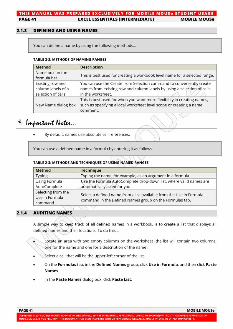
TH IS MANUAL W AS PREPARED EX CLUSIVE LY FOR MOBILE MOUSe ST UDE NT USAGE
PAGE 41 EXCEL ESSENTIALS (INTERMEDIATE) MOBILE MOUSe
PAGE 41 MOBILE MOUSe
COPYRIGHT © 2018 MOBILE MOUSE. NO PART OF THIS MANUAL MAY BE DISTRIBUTED, REPRODUCED, COPIED OR MODIFIED WITHOUT THE EXPRESS PERMISSION OF
MOBILE MOUSe. IF YOU FEEL THAT THIS DOCUMENT HAS BEEN TAMPERED WITH OR REPRODUCED ILLEGALLY, KINDLY INFORM US OF ANY IMPROPRIETY.
2.1.3 DEFINING AND USING NAMES
You can define a name by using the following methods…
TABLE 2-2: METHODS OF NAMING RANGES
Method Description
Name box on the
formula bar This is best used for creating a workbook level name for a selected range.
Existing row and
column labels of a
selection of cells
You can use the Create from Selection command to conveniently create
names from existing row and column labels by using a selection of cells
in the worksheet.
New Name dialog box
This is best used for when you want more flexibility in creating names,
such as specifying a local worksheet level scope or creating a name
comment.
Important Notes...
• By default, names use absolute cell references.
You can use a defined name in a formula by entering it as follows…
TABLE 2-3: METHODS AND TECHNIQUES OF USING NAMED RANGES
Method Technique
Typing Typing the name, for example, as an argument in a formula.
Using Formula
AutoComplete
Use the Formula AutoComplete drop-down list, where valid names are
automatically listed for you.
Selecting from the
Use in Formula
command
Select a defined name from a list available from the Use in Formula
command in the Defined Names group on the Formulas tab.
2.1.4 AUDITING NAMES
A simple way to keep track of all defined names in a workbook, is to create a list that displays all
defined names and their locations. To do this…
• Locate an area with two empty columns on the worksheet (the list will contain two columns,
one for the name and one for a description of the name).
• Select a cell that will be the upper-left corner of the list.
• On the Formulas tab, in the Defined Names group, click Use in Formula, and then click Paste
Names.
• In the Paste Names dialog box, click Paste List.
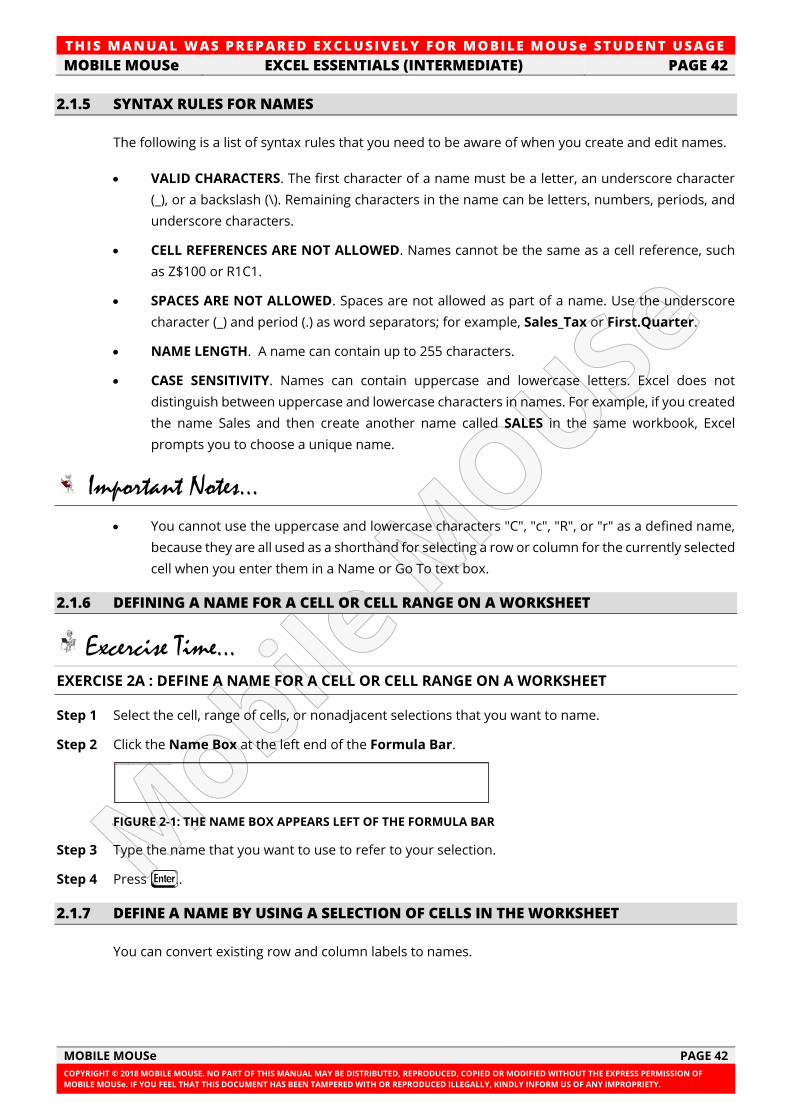
TH IS MANUAL W AS PREPARED EX CLUSIVE LY FOR MOBILE MOUSe ST UDE NT USAGE
MOBILE MOUSe EXCEL ESSENTIALS (INTERMEDIATE) PAGE 42
MOBILE MOUSe PAGE 42
COPYRIGHT © 2018 MOBILE MOUSE. NO PART OF THIS MANUAL MAY BE DISTRIBUTED, REPRODUCED, COPIED OR MODIFIED WITHOUT THE EXPRESS PERMISSION OF
MOBILE MOUSe. IF YOU FEEL THAT THIS DOCUMENT HAS BEEN TAMPERED WITH OR REPRODUCED ILLEGALLY, KINDLY INFORM US OF ANY IMPROPRIETY.
2.1.5 SYNTAX RULES FOR NAMES
The following is a list of syntax rules that you need to be aware of when you create and edit names.
• VALID CHARACTERS. The first character of a name must be a letter, an underscore character
(_), or a backslash (\). Remaining characters in the name can be letters, numbers, periods, and
underscore characters.
• CELL REFERENCES ARE NOT ALLOWED. Names cannot be the same as a cell reference, such
as Z$100 or R1C1.
• SPACES ARE NOT ALLOWED. Spaces are not allowed as part of a name. Use the underscore
character (_) and period (.) as word separators; for example, Sales_Tax or First.Quarter.
• NAME LENGTH. A name can contain up to 255 characters.
• CASE SENSITIVITY. Names can contain uppercase and lowercase letters. Excel does not
distinguish between uppercase and lowercase characters in names. For example, if you created
the name Sales and then create another name called SALES in the same workbook, Excel
prompts you to choose a unique name.
Important Notes...
• You cannot use the uppercase and lowercase characters "C", "c", "R", or "r" as a defined name,
because they are all used as a shorthand for selecting a row or column for the currently selected
cell when you enter them in a Name or Go To text box.
2.1.6 DEFINING A NAME FOR A CELL OR CELL RANGE ON A WORKSHEET
Excercise Time... EXERCISE 2A : DEFINE A NAME FOR A CELL OR CELL RANGE ON A WORKSHEET
Step 1 Select the cell, range of cells, or nonadjacent selections that you want to name.
Step 2 Click the Name Box at the left end of the Formula Bar.
FIGURE 2-1: THE NAME BOX APPEARS LEFT OF THE FORMULA BAR
Step 3 Type the name that you want to use to refer to your selection.
Step 4 Press J.
2.1.7 DEFINE A NAME BY USING A SELECTION OF CELLS IN THE WORKSHEET
You can convert existing row and column labels to names.
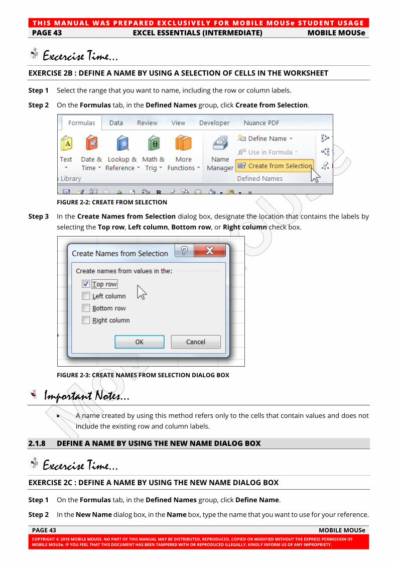
TH IS MANUAL W AS PREPARED EX CLUSIVE LY FOR MOBILE MOUSe ST UDE NT USAGE
PAGE 43 EXCEL ESSENTIALS (INTERMEDIATE) MOBILE MOUSe
PAGE 43 MOBILE MOUSe
COPYRIGHT © 2018 MOBILE MOUSE. NO PART OF THIS MANUAL MAY BE DISTRIBUTED, REPRODUCED, COPIED OR MODIFIED WITHOUT THE EXPRESS PERMISSION OF
MOBILE MOUSe. IF YOU FEEL THAT THIS DOCUMENT HAS BEEN TAMPERED WITH OR REPRODUCED ILLEGALLY, KINDLY INFORM US OF ANY IMPROPRIETY.
Excercise Time... EXERCISE 2B : DEFINE A NAME BY USING A SELECTION OF CELLS IN THE WORKSHEET
Step 1 Select the range that you want to name, including the row or column labels.
Step 2 On the Formulas tab, in the Defined Names group, click Create from Selection.
FIGURE 2-2: CREATE FROM SELECTION
Step 3 In the Create Names from Selection dialog box, designate the location that contains the labels by
selecting the Top row, Left column, Bottom row, or Right column check box.
FIGURE 2-3: CREATE NAMES FROM SELECTION DIALOG BOX
Important Notes...
• A name created by using this method refers only to the cells that contain values and does not
include the existing row and column labels.
2.1.8 DEFINE A NAME BY USING THE NEW NAME DIALOG BOX
Excercise Time... EXERCISE 2C : DEFINE A NAME BY USING THE NEW NAME DIALOG BOX
Step 1 On the Formulas tab, in the Defined Names group, click Define Name.
Step 2 In the New Name dialog box, in the Name box, type the name that you want to use for your reference.
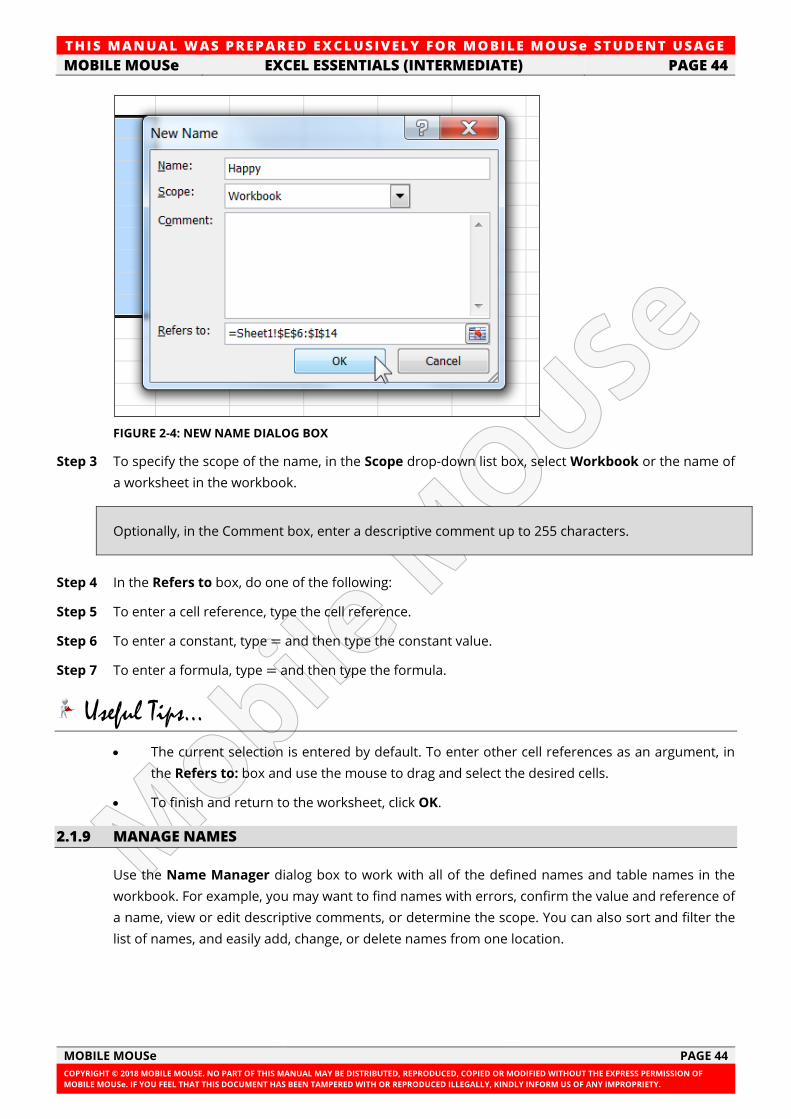
TH IS MANUAL W AS PREPARED EX CLUSIVE LY FOR MOBILE MOUSe ST UDE NT USAGE
MOBILE MOUSe EXCEL ESSENTIALS (INTERMEDIATE) PAGE 44
MOBILE MOUSe PAGE 44
COPYRIGHT © 2018 MOBILE MOUSE. NO PART OF THIS MANUAL MAY BE DISTRIBUTED, REPRODUCED, COPIED OR MODIFIED WITHOUT THE EXPRESS PERMISSION OF
MOBILE MOUSe. IF YOU FEEL THAT THIS DOCUMENT HAS BEEN TAMPERED WITH OR REPRODUCED ILLEGALLY, KINDLY INFORM US OF ANY IMPROPRIETY.
FIGURE 2-4: NEW NAME DIALOG BOX
Step 3 To specify the scope of the name, in the Scope drop-down list box, select Workbook or the name of
a worksheet in the workbook.
Optionally, in the Comment box, enter a descriptive comment up to 255 characters.
Step 4 In the Refers to box, do one of the following:
Step 5 To enter a cell reference, type the cell reference.
Step 6 To enter a constant, type = and then type the constant value.
Step 7 To enter a formula, type = and then type the formula.
Useful Tips...
• The current selection is entered by default. To enter other cell references as an argument, in
the Refers to: box and use the mouse to drag and select the desired cells.
• To finish and return to the worksheet, click OK.
2.1.9 MANAGE NAMES
Use the Name Manager dialog box to work with all of the defined names and table names in the
workbook. For example, you may want to find names with errors, confirm the value and reference of
a name, view or edit descriptive comments, or determine the scope. You can also sort and filter the
list of names, and easily add, change, or delete names from one location.
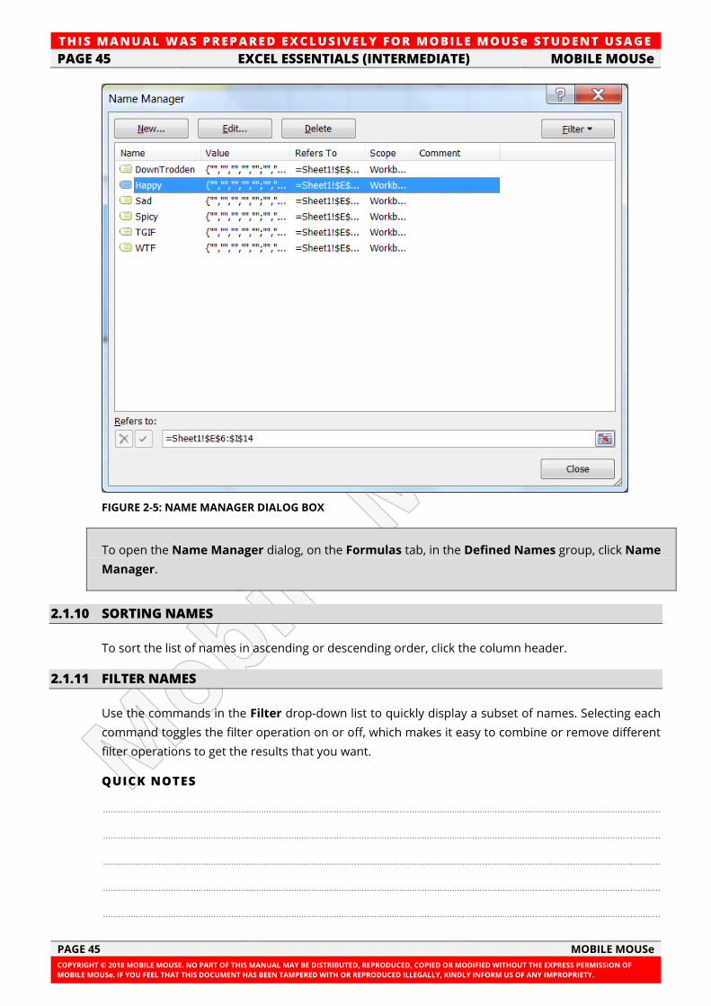
TH IS MANUAL W AS PREPARED EX CLUSIVE LY FOR MOBILE MOUSe ST UDE NT USAGE
PAGE 45 EXCEL ESSENTIALS (INTERMEDIATE) MOBILE MOUSe
PAGE 45 MOBILE MOUSe
COPYRIGHT © 2018 MOBILE MOUSE. NO PART OF THIS MANUAL MAY BE DISTRIBUTED, REPRODUCED, COPIED OR MODIFIED WITHOUT THE EXPRESS PERMISSION OF
MOBILE MOUSe. IF YOU FEEL THAT THIS DOCUMENT HAS BEEN TAMPERED WITH OR REPRODUCED ILLEGALLY, KINDLY INFORM US OF ANY IMPROPRIETY.
FIGURE 2-5: NAME MANAGER DIALOG BOX
To open the Name Manager dialog, on the Formulas tab, in the Defined Names group, click Name
Manager.
2.1.10 SORTING NAMES
To sort the list of names in ascending or descending order, click the column header.
2.1.11 FILTER NAMES
Use the commands in the Filter drop-down list to quickly display a subset of names. Selecting each
command toggles the filter operation on or off, which makes it easy to combine or remove different
filter operations to get the results that you want.
QUICK NOTES
..............................................................................................................................................................................................................................
..............................................................................................................................................................................................................................
..............................................................................................................................................................................................................................
..............................................................................................................................................................................................................................
..............................................................................................................................................................................................................................
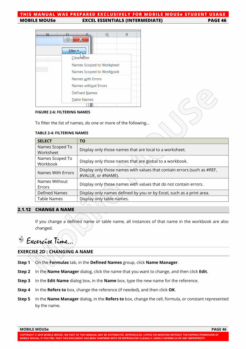
TH IS MANUAL W AS PREPARED EX CLUSIVE LY FOR MOBILE MOUSe ST UDE NT USAGE
MOBILE MOUSe EXCEL ESSENTIALS (INTERMEDIATE) PAGE 46
MOBILE MOUSe PAGE 46
COPYRIGHT © 2018 MOBILE MOUSE. NO PART OF THIS MANUAL MAY BE DISTRIBUTED, REPRODUCED, COPIED OR MODIFIED WITHOUT THE EXPRESS PERMISSION OF
MOBILE MOUSe. IF YOU FEEL THAT THIS DOCUMENT HAS BEEN TAMPERED WITH OR REPRODUCED ILLEGALLY, KINDLY INFORM US OF ANY IMPROPRIETY.
FIGURE 2-6: FILTERING NAMES
To filter the list of names, do one or more of the following…
TABLE 2-4: FILTERING NAMES
SELECT TO
Names Scoped To
Worksheet Display only those names that are local to a worksheet.
Names Scoped To
Workbook Display only those names that are global to a workbook.
Names With Errors Display only those names with values that contain errors (such as #REF,
#VALUE, or #NAME).
Names Without
Errors Display only those names with values that do not contain errors.
Defined Names Display only names defined by you or by Excel, such as a print area.
Table Names Display only table names.
2.1.12 CHANGE A NAME
If you change a defined name or table name, all instances of that name in the workbook are also
changed.
Excercise Time... EXERCISE 2D : CHANGING A NAME
Step 1 On the Formulas tab, in the Defined Names group, click Name Manager.
Step 2 In the Name Manager dialog, click the name that you want to change, and then click Edit.
Step 3 In the Edit Name dialog box, in the Name box, type the new name for the reference.
Step 4 In the Refers to box, change the reference (if needed), and then click OK.
Step 5 In the Name Manager dialog, in the Refers to box, change the cell, formula, or constant represented
by the name.
TH IS MANUAL W AS PREPARED EX CLUSIVE LY FOR MOBILE MOUSe ST UDE NT USAGE
PAGE 47 EXCEL ESSENTIALS (INTERMEDIATE) MOBILE MOUSe
PAGE 47 MOBILE MOUSe
COPYRIGHT © 2018 MOBILE MOUSE. NO PART OF THIS MANUAL MAY BE DISTRIBUTED, REPRODUCED, COPIED OR MODIFIED WITHOUT THE EXPRESS PERMISSION OF
MOBILE MOUSe. IF YOU FEEL THAT THIS DOCUMENT HAS BEEN TAMPERED WITH OR REPRODUCED ILLEGALLY, KINDLY INFORM US OF ANY IMPROPRIETY.
To cancel unwanted or accidental changes, click Cancel, or press L.
Step 6 To save your changes, click Commit, or press J.
Important Notes...
• The Close button only closes the Name Manager dialog. Clicking Close is not required to
commit changes that have already been made.
2.1.13 DELETE ONE OR MORE NAMES
Excercise Time... EXERCISE 2E : DELETING A NAMED RANGE
Step 1 On the Formulas tab, in the Defined Names group, click Name Manager.
Step 2 In the Name Manager dialog, click the name that you want to change.
Step 3 Select one or more names by doing one of the following:
Step 4 To select a name, click it.
Step 5 To select more than one name in a contiguous group, click and drag the names, or press G and
click the mouse button for each name in the group.
Step 6 To select more than one name in a non-contiguous group, press F and click the mouse button for
each name in the group.
Step 7 Click Delete. You can also press the V key.
Step 8 Click OK to confirm the deletion.
2.2 WORKING WITH SHEETS (INTERMEDIATE)
MICROSOFT OFFICE CERTIFICATION
This concept addresses the Create and format worksheets competency of the Microsoft Office
Specialist Certification (Exam 77-420).
PLEASE NOTE: This training resource does not necessarily cover all of the requirements of this
exam objective as this objective may include but is not limited to: Insert worksheets, delete
worksheets, copy, reposition, copy and move, rename, grouping, apply colouring to worksheet
tabs, hiding worksheet tabs, and Unhiding worksheet tabs.
Visit http://www.microsoft.com/learning/en/us/mos-certification.aspx for the latest Microsoft
Office Certification requirements.
2.2.1 DUPLICATING, MOVING AND RENAMING SHEETS, COLOURING TABS AND GROUPING
Worksheets are like documents within a workbook. In Microsoft Excel, you can rename the
worksheets, giving them useful names that describe their contents.
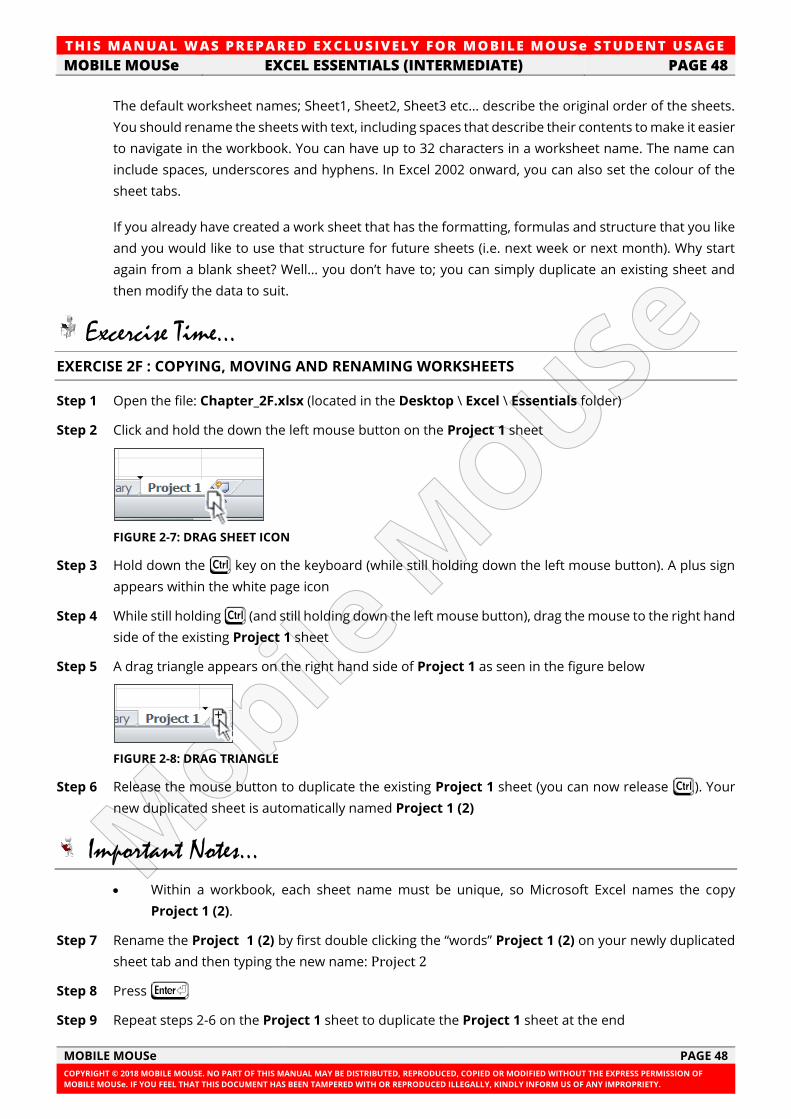
TH IS MANUAL W AS PREPARED EX CLUSIVE LY FOR MOBILE MOUSe ST UDE NT USAGE
MOBILE MOUSe EXCEL ESSENTIALS (INTERMEDIATE) PAGE 48
MOBILE MOUSe PAGE 48
COPYRIGHT © 2018 MOBILE MOUSE. NO PART OF THIS MANUAL MAY BE DISTRIBUTED, REPRODUCED, COPIED OR MODIFIED WITHOUT THE EXPRESS PERMISSION OF
MOBILE MOUSe. IF YOU FEEL THAT THIS DOCUMENT HAS BEEN TAMPERED WITH OR REPRODUCED ILLEGALLY, KINDLY INFORM US OF ANY IMPROPRIETY.
The default worksheet names; Sheet1, Sheet2, Sheet3 etc… describe the original order of the sheets.
You should rename the sheets with text, including spaces that describe their contents to make it easier
to navigate in the workbook. You can have up to 32 characters in a worksheet name. The name can
include spaces, underscores and hyphens. In Excel 2002 onward, you can also set the colour of the
sheet tabs.
If you already have created a work sheet that has the formatting, formulas and structure that you like
and you would like to use that structure for future sheets (i.e. next week or next month). Why start
again from a blank sheet? Well... you don’t have to; you can simply duplicate an existing sheet and
then modify the data to suit.
Excercise Time... EXERCISE 2F : COPYING, MOVING AND RENAMING WORKSHEETS
Step 1 Open the file: Chapter_2F.xlsx (located in the Desktop \ Excel \ Essentials folder)
Step 2 Click and hold the down the left mouse button on the Project 1 sheet
FIGURE 2-7: DRAG SHEET ICON
Step 3 Hold down the F key on the keyboard (while still holding down the left mouse button). A plus sign
appears within the white page icon
Step 4 While still holding F (and still holding down the left mouse button), drag the mouse to the right hand
side of the existing Project 1 sheet
Step 5 A drag triangle appears on the right hand side of Project 1 as seen in the figure below
FIGURE 2-8: DRAG TRIANGLE
Step 6 Release the mouse button to duplicate the existing Project 1 sheet (you can now release F). Your
new duplicated sheet is automatically named Project 1 (2)
Important Notes...
• Within a workbook, each sheet name must be unique, so Microsoft Excel names the copy
Project 1 (2).
Step 7 Rename the Project 1 (2) by first double clicking the “words” Project 1 (2) on your newly duplicated
sheet tab and then typing the new name: Project 2
Step 8 Press I
Step 9 Repeat steps 2-6 on the Project 1 sheet to duplicate the Project 1 sheet at the end
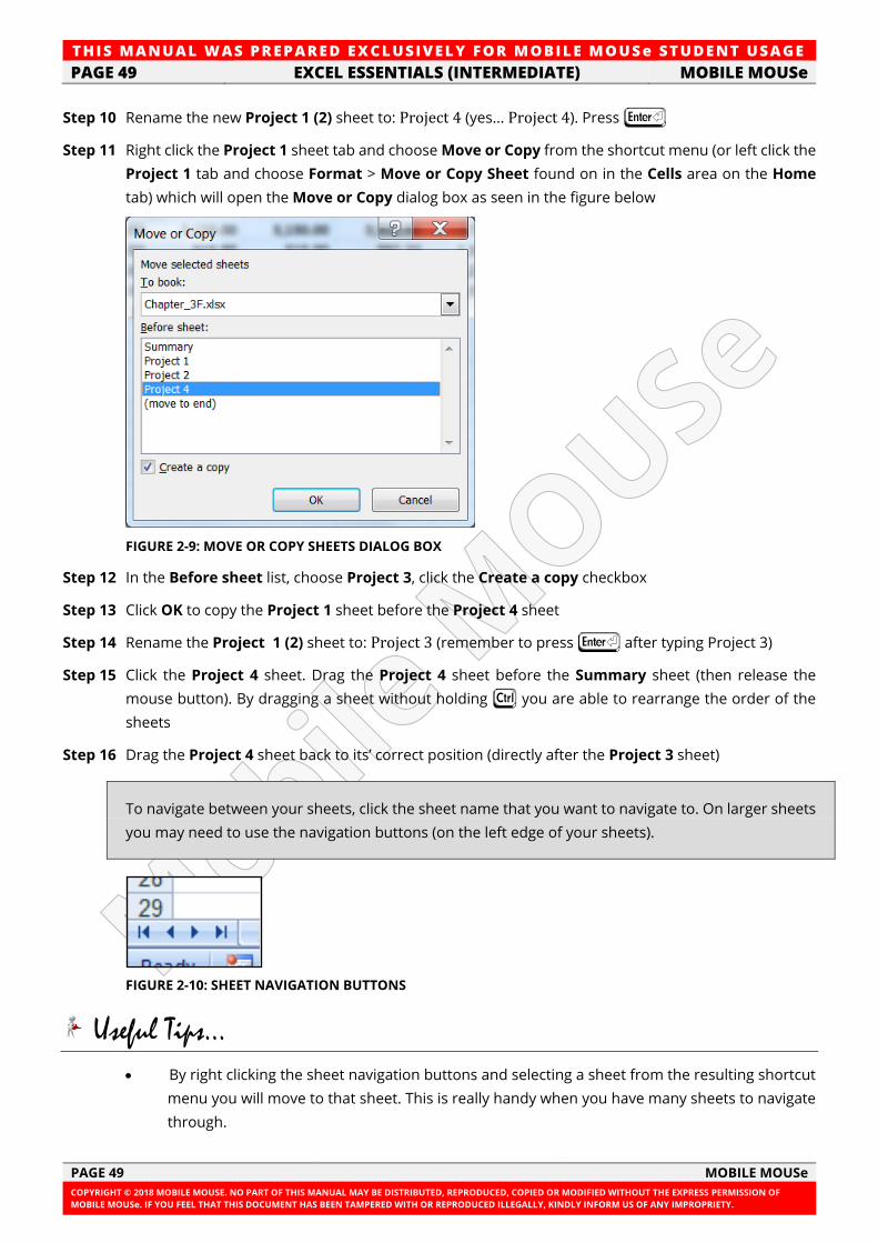
TH IS MANUAL W AS PREPARED EX CLUSIVE LY FOR MOBILE MOUSe ST UDE NT USAGE
PAGE 49 EXCEL ESSENTIALS (INTERMEDIATE) MOBILE MOUSe
PAGE 49 MOBILE MOUSe
COPYRIGHT © 2018 MOBILE MOUSE. NO PART OF THIS MANUAL MAY BE DISTRIBUTED, REPRODUCED, COPIED OR MODIFIED WITHOUT THE EXPRESS PERMISSION OF
MOBILE MOUSe. IF YOU FEEL THAT THIS DOCUMENT HAS BEEN TAMPERED WITH OR REPRODUCED ILLEGALLY, KINDLY INFORM US OF ANY IMPROPRIETY.
Step 10 Rename the new Project 1 (2) sheet to: Project 4 (yes... Project 4). Press I
Step 11 Right click the Project 1 sheet tab and choose Move or Copy from the shortcut menu (or left click the
Project 1 tab and choose Format > Move or Copy Sheet found on in the Cells area on the Home
tab) which will open the Move or Copy dialog box as seen in the figure below
FIGURE 2-9: MOVE OR COPY SHEETS DIALOG BOX
Step 12 In the Before sheet list, choose Project 3, click the Create a copy checkbox
Step 13 Click OK to copy the Project 1 sheet before the Project 4 sheet
Step 14 Rename the Project 1 (2) sheet to: Project 3 (remember to press I after typing Project 3)
Step 15 Click the Project 4 sheet. Drag the Project 4 sheet before the Summary sheet (then release the
mouse button). By dragging a sheet without holding F you are able to rearrange the order of the
sheets
Step 16 Drag the Project 4 sheet back to its’ correct position (directly after the Project 3 sheet)
To navigate between your sheets, click the sheet name that you want to navigate to. On larger sheets
you may need to use the navigation buttons (on the left edge of your sheets).
FIGURE 2-10: SHEET NAVIGATION BUTTONS
Useful Tips...
• By right clicking the sheet navigation buttons and selecting a sheet from the resulting shortcut
menu you will move to that sheet. This is really handy when you have many sheets to navigate
through.
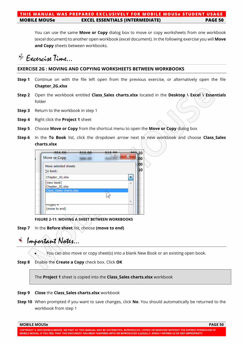
TH IS MANUAL W AS PREPARED EX CLUSIVE LY FOR MOBILE MOUSe ST UDE NT USAGE
MOBILE MOUSe EXCEL ESSENTIALS (INTERMEDIATE) PAGE 50
MOBILE MOUSe PAGE 50
COPYRIGHT © 2018 MOBILE MOUSE. NO PART OF THIS MANUAL MAY BE DISTRIBUTED, REPRODUCED, COPIED OR MODIFIED WITHOUT THE EXPRESS PERMISSION OF
MOBILE MOUSe. IF YOU FEEL THAT THIS DOCUMENT HAS BEEN TAMPERED WITH OR REPRODUCED ILLEGALLY, KINDLY INFORM US OF ANY IMPROPRIETY.
You can use the same Move or Copy dialog box to move or copy worksheets from one workbook
(excel document) to another open workbook (excel document). In the following exercise you will Move
and Copy sheets between workbooks.
Excercise Time... EXERCISE 2G : MOVING AND COPYING WORKSHEETS BETWEEN WORKBOOKS
Step 1 Continue on with the file left open from the previous exercise, or alternatively open the file
Chapter_2G.xlsx
Step 2 Open the workbook entitled Class_Sales charts.xlsx located in the Desktop \ Excel \ Essentials
folder
Step 3 Return to the workbook in step 1
Step 4 Right click the Project 1 sheet
Step 5 Choose Move or Copy from the shortcut menu to open the Move or Copy dialog box
Step 6 In the To Book list, click the dropdown arrow next to new workbook and choose Class_Sales
charts.xlsx
FIGURE 2-11: MOVING A SHEET BETWEEN WORKBOOKS
Step 7 In the Before sheet list, choose (move to end)
Important Notes...
• You can also move or copy sheet(s) into a blank New Book or an existing open book.
Step 8 Enable the Create a Copy check box. Click OK
The Project 1 sheet is copied into the Class_Sales charts.xlsx workbook
Step 9 Close the Class_Sales charts.xlsx workbook
Step 10 When prompted if you want to save changes, click No. You should automatically be returned to the
workbook from step 1
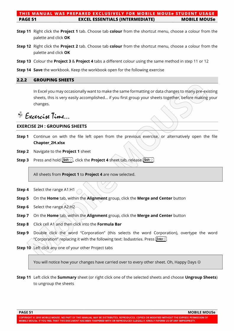
TH IS MANUAL W AS PREPARED EX CLUSIVE LY FOR MOBILE MOUSe ST UDE NT USAGE
PAGE 51 EXCEL ESSENTIALS (INTERMEDIATE) MOBILE MOUSe
PAGE 51 MOBILE MOUSe
COPYRIGHT © 2018 MOBILE MOUSE. NO PART OF THIS MANUAL MAY BE DISTRIBUTED, REPRODUCED, COPIED OR MODIFIED WITHOUT THE EXPRESS PERMISSION OF
MOBILE MOUSe. IF YOU FEEL THAT THIS DOCUMENT HAS BEEN TAMPERED WITH OR REPRODUCED ILLEGALLY, KINDLY INFORM US OF ANY IMPROPRIETY.
Step 11 Right click the Project 1 tab. Choose tab colour from the shortcut menu, choose a colour from the
palette and click OK
Step 12 Right click the Project 2 tab. Choose tab colour from the shortcut menu, choose a colour from the
palette and click OK
Step 13 Colour the Project 3 & Project 4 tabs a different colour using the same method in step 11 or 12
Step 14 Save the workbook. Keep the workbook open for the following exercise
2.2.2 GROUPING SHEETS
In Excel you may occasionally want to make the same formatting or data changes to many pre-existing
sheets, this is very easily accomplished... if you first group your sheets together, before making your
changes.
Excercise Time... EXERCISE 2H : GROUPING SHEETS
Step 1 Continue on with the file left open from the previous exercise, or alternatively open the file
Chapter_2H.xlsx
Step 2 Navigate to the Project 1 sheet
Step 3 Press and hold G, click the Project 4 sheet tab, release G
All sheets from Project 1 to Project 4 are now selected.
Step 4 Select the range A1:H1
Step 5 On the Home tab, within the Alignment group, click the Merge and Center button
Step 6 Select the range A2:H2
Step 7 On the Home tab, within the Alignment group, click the Merge and Center button
Step 8 Click cell A1 and then click into the Formula Bar
Step 9 Double click the word “Corporation” (this selects the word Corporation), overtype the word
“Corporation” replacing it with the following text: Industries. Press I
Step 10 Left click any one of your other Project tabs
You will notice how your changes have carried over to every other sheet. Oh, Happy Days ☺
Step 11 Left click the Summary sheet (or right click one of the selected sheets and choose Ungroup Sheets)
to ungroup the sheets
TH IS MANUAL W AS PREPARED EX CLUSIVE LY FOR MOBILE MOUSe ST UDE NT USAGE
MOBILE MOUSe EXCEL ESSENTIALS (INTERMEDIATE) PAGE 52
MOBILE MOUSe PAGE 52
COPYRIGHT © 2018 MOBILE MOUSE. NO PART OF THIS MANUAL MAY BE DISTRIBUTED, REPRODUCED, COPIED OR MODIFIED WITHOUT THE EXPRESS PERMISSION OF
MOBILE MOUSe. IF YOU FEEL THAT THIS DOCUMENT HAS BEEN TAMPERED WITH OR REPRODUCED ILLEGALLY, KINDLY INFORM US OF ANY IMPROPRIETY.
Useful Tips...
• When creating Headers and Footers they are normally only applied to the sheet you are
currently working on. By using grouping, you can easily apply the same Headers and Footers to
many sheets at once.
Step 12 You can also select all sheets, by right clicking any existing sheet tab and then choosing Select All
Sheets.
Step 13 You can also use grouping to duplicate or delete many sheets at once.
Step 14 You can make multiple copies of sheets (or move multiple sheets) or even delete multiple sheets by
using grouping… e.g. If you have three sheets selected and you Move or Copy you will either end up
with three additional sheets (if you copied), or you will move three sheets.
Important Notes...
• You can use click, G, click to select from one sheet to another (including every sheet in-
between). Remember to keep your finger down on the G key.
• Use click, F, click to select multiple random sheets. Remember to keep your finger down on
the F key until you are finished clicking the various sheets.
• Remember to Ungroup the sheets once you have finished performing your changes or
additions.
Step 15 Save the workbook. Leave the file open for the following exercise
2.3 CREATING MORE COMPLEX FORMULAS
Microsoft Excel formulas can be simple formulas that add one cell to another or they can be more
complicated formulas that use cell contents from several worksheets as well as statistical, financial
and other functions. In this session, we will create advanced formulas using more advanced cell
references and functions.
2.3.1 CALCULATIONS ACROSS SHEETS
It is a common requirement in Excel that you be able to extract values from other sheets and use
them in your calculations. In the following exercise, you will extract values from across sheets. Later
on you will add-up values across sheets.
Excercise Time... EXERCISE 2I : REFERENCING VALUES FROM OTHER SHEETS
Step 1 Continue on with the file left open from the previous exercise, or alternatively open the file
Chapter_2i.xlsx (located in the Desktop \ Excel \ Essentials folder)
Step 2 If it is not already selected, click cell A5
Step 3 Type the words: Project 1
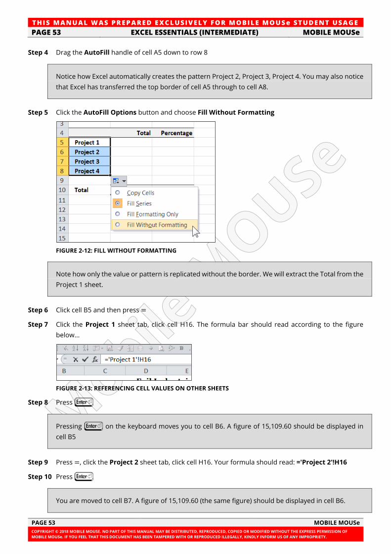
TH IS MANUAL W AS PREPARED EX CLUSIVE LY FOR MOBILE MOUSe ST UDE NT USAGE
PAGE 53 EXCEL ESSENTIALS (INTERMEDIATE) MOBILE MOUSe
PAGE 53 MOBILE MOUSe
COPYRIGHT © 2018 MOBILE MOUSE. NO PART OF THIS MANUAL MAY BE DISTRIBUTED, REPRODUCED, COPIED OR MODIFIED WITHOUT THE EXPRESS PERMISSION OF
MOBILE MOUSe. IF YOU FEEL THAT THIS DOCUMENT HAS BEEN TAMPERED WITH OR REPRODUCED ILLEGALLY, KINDLY INFORM US OF ANY IMPROPRIETY.
Step 4 Drag the AutoFill handle of cell A5 down to row 8
Notice how Excel automatically creates the pattern Project 2, Project 3, Project 4. You may also notice
that Excel has transferred the top border of cell A5 through to cell A8.
Step 5 Click the AutoFill Options button and choose Fill Without Formatting
FIGURE 2-12: FILL WITHOUT FORMATTING
Note how only the value or pattern is replicated without the border. We will extract the Total from the
Project 1 sheet.
Step 6 Click cell B5 and then press =
Step 7 Click the Project 1 sheet tab, click cell H16. The formula bar should read according to the figure
below...
FIGURE 2-13: REFERENCING CELL VALUES ON OTHER SHEETS
Step 8 Press I
Pressing I on the keyboard moves you to cell B6. A figure of 15,109.60 should be displayed in
cell B5
Step 9 Press =, click the Project 2 sheet tab, click cell H16. Your formula should read: ='Project 2'!H16
Step 10 Press I
You are moved to cell B7. A figure of 15,109.60 (the same figure) should be displayed in cell B6.
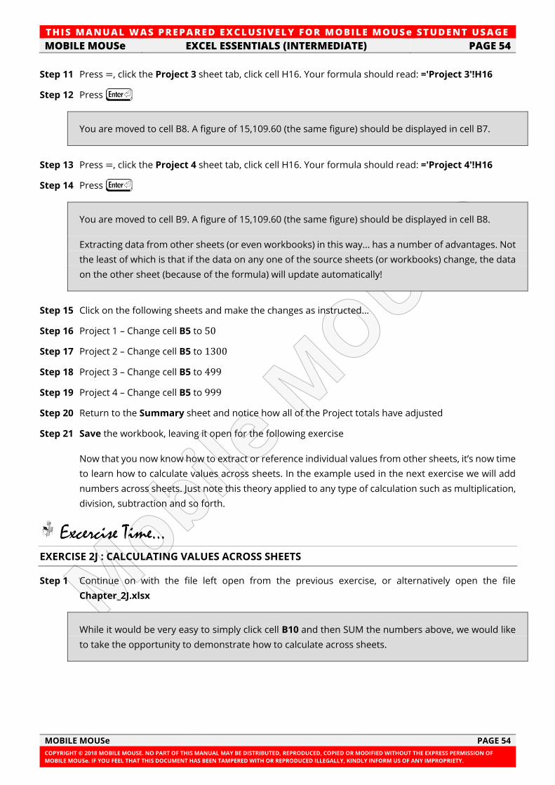
TH IS MANUAL W AS PREPARED EX CLUSIVE LY FOR MOBILE MOUSe ST UDE NT USAGE
MOBILE MOUSe EXCEL ESSENTIALS (INTERMEDIATE) PAGE 54
MOBILE MOUSe PAGE 54
COPYRIGHT © 2018 MOBILE MOUSE. NO PART OF THIS MANUAL MAY BE DISTRIBUTED, REPRODUCED, COPIED OR MODIFIED WITHOUT THE EXPRESS PERMISSION OF
MOBILE MOUSe. IF YOU FEEL THAT THIS DOCUMENT HAS BEEN TAMPERED WITH OR REPRODUCED ILLEGALLY, KINDLY INFORM US OF ANY IMPROPRIETY.
Step 11 Press =, click the Project 3 sheet tab, click cell H16. Your formula should read: ='Project 3'!H16
Step 12 Press I
You are moved to cell B8. A figure of 15,109.60 (the same figure) should be displayed in cell B7.
Step 13 Press =, click the Project 4 sheet tab, click cell H16. Your formula should read: ='Project 4'!H16
Step 14 Press I
You are moved to cell B9. A figure of 15,109.60 (the same figure) should be displayed in cell B8.
Extracting data from other sheets (or even workbooks) in this way... has a number of advantages. Not
the least of which is that if the data on any one of the source sheets (or workbooks) change, the data
on the other sheet (because of the formula) will update automatically!
Step 15 Click on the following sheets and make the changes as instructed…
Step 16 Project 1 – Change cell B5 to 50
Step 17 Project 2 – Change cell B5 to 1300
Step 18 Project 3 – Change cell B5 to 499
Step 19 Project 4 – Change cell B5 to 999
Step 20 Return to the Summary sheet and notice how all of the Project totals have adjusted
Step 21 Save the workbook, leaving it open for the following exercise
Now that you now know how to extract or reference individual values from other sheets, it’s now time
to learn how to calculate values across sheets. In the example used in the next exercise we will add
numbers across sheets. Just note this theory applied to any type of calculation such as multiplication,
division, subtraction and so forth.
Excercise Time... EXERCISE 2J : CALCULATING VALUES ACROSS SHEETS
Step 1 Continue on with the file left open from the previous exercise, or alternatively open the file
Chapter_2J.xlsx
While it would be very easy to simply click cell B10 and then SUM the numbers above, we would like
to take the opportunity to demonstrate how to calculate across sheets.
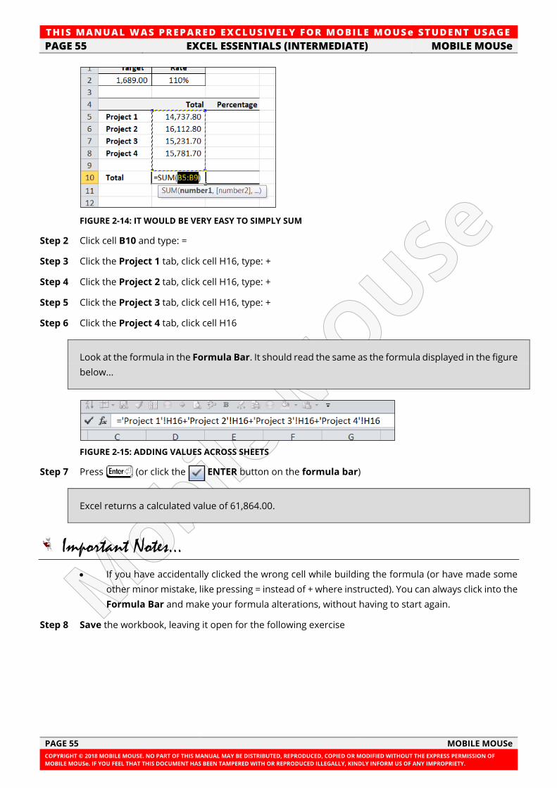
TH IS MANUAL W AS PREPARED EX CLUSIVE LY FOR MOBILE MOUSe ST UDE NT USAGE
PAGE 55 EXCEL ESSENTIALS (INTERMEDIATE) MOBILE MOUSe
PAGE 55 MOBILE MOUSe
COPYRIGHT © 2018 MOBILE MOUSE. NO PART OF THIS MANUAL MAY BE DISTRIBUTED, REPRODUCED, COPIED OR MODIFIED WITHOUT THE EXPRESS PERMISSION OF
MOBILE MOUSe. IF YOU FEEL THAT THIS DOCUMENT HAS BEEN TAMPERED WITH OR REPRODUCED ILLEGALLY, KINDLY INFORM US OF ANY IMPROPRIETY.
FIGURE 2-14: IT WOULD BE VERY EASY TO SIMPLY SUM
Step 2 Click cell B10 and type: =
Step 3 Click the Project 1 tab, click cell H16, type: +
Step 4 Click the Project 2 tab, click cell H16, type: +
Step 5 Click the Project 3 tab, click cell H16, type: +
Step 6 Click the Project 4 tab, click cell H16
Look at the formula in the Formula Bar. It should read the same as the formula displayed in the figure
below...
FIGURE 2-15: ADDING VALUES ACROSS SHEETS
Step 7 Press I (or click the ENTER button on the formula bar)
Excel returns a calculated value of 61,864.00.
Important Notes...
• If you have accidentally clicked the wrong cell while building the formula (or have made some
other minor mistake, like pressing = instead of + where instructed). You can always click into the
Formula Bar and make your formula alterations, without having to start again.
Step 8 Save the workbook, leaving it open for the following exercise
TH IS MANUAL W AS PREPARED EX CLUSIVE LY FOR MOBILE MOUSe ST UDE NT USAGE
MOBILE MOUSe EXCEL ESSENTIALS (INTERMEDIATE) PAGE 56
MOBILE MOUSe PAGE 56
COPYRIGHT © 2018 MOBILE MOUSE. NO PART OF THIS MANUAL MAY BE DISTRIBUTED, REPRODUCED, COPIED OR MODIFIED WITHOUT THE EXPRESS PERMISSION OF
MOBILE MOUSe. IF YOU FEEL THAT THIS DOCUMENT HAS BEEN TAMPERED WITH OR REPRODUCED ILLEGALLY, KINDLY INFORM US OF ANY IMPROPRIETY.
2.3.2 USING 3D REFERENCES
In Microsoft Excel formulas, you can refer to ranges of cells that occur in the same cell or group of
cells on one or two or more worksheets with a single reference. A good way to think of a 3D reference
is as follows. Imagine a five story building with the same floor plan on each floor. The building would
relate to the workbook and each floor is a worksheet. Each room on each floor is a cell. If you were to
refer to the room in the North East corner of the building on the fifth floor, you may use a reference
similar to 5NE. However if you wanted to refer to the North East corner room on all floors you may
use a reference similar to 1-5NE. This is what is known as a 3D reference.
In the workbook we have been using thus far, the four Project worksheets have exactly the same
layout. As we now know, the Summary worksheet summarizes the figures from the various Project
worksheets.
Because all four Project worksheets have exactly the same layout, you can total all the worksheets at
once with formulas that use 3D references. For example, the formula currently in cell B10 in the
Summary worksheet refers to cell H16 in all the other worksheets: In other words...
The sum of cell H16 for the Project 1 tab through to the Project 4 tab. You are adding the same cell
but on different sheets. In the following exercise you will create 3D cell references to add the same
cell button different worksheets.
Excercise Time... EXERCISE 2K : CREATING 3D REFERENCES FORMULAS
Step 1 Continue on with the file left open from the previous exercise, or alternatively open the file
Chapter_2K.xlsx
Step 2 Click cell B10 on the Summary worksheet
Admittedly in this example, we could simply SUM the column to achieve the respective Totals (because
we already have the numbers to SUM above. But, for the purposes of this exercise we will use a
different example.
Step 3 Click the Home tab, Click the AutoSum button to create a SUM formula
Step 4 Click the Project 1 sheet tab. Click cell H16
Step 5 Hold G and click the Project 4 tab
This selects the Project 1, Project 2, Project 3 and Project 4 worksheets (similar to grouping)
The formula in the formula bar should now read: =SUM('Project 1:Project 4'!H16)
Step 6 Press I to accept the formula
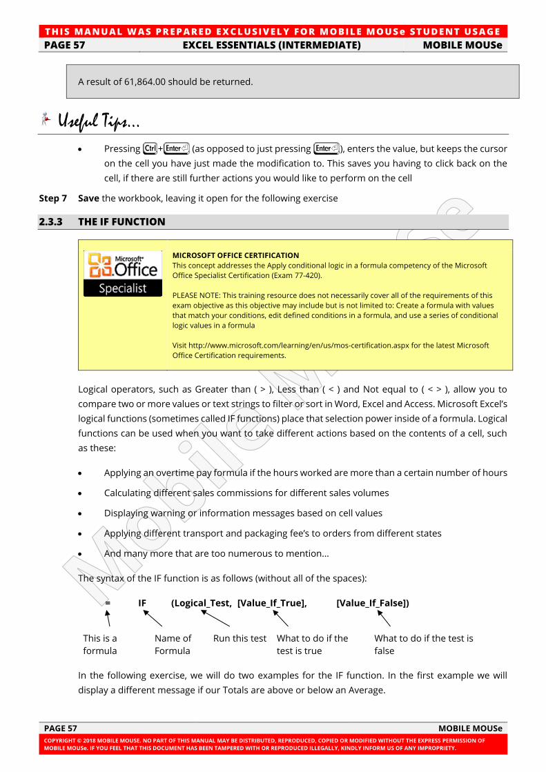
TH IS MANUAL W AS PREPARED EX CLUSIVE LY FOR MOBILE MOUSe ST UDE NT USAGE
PAGE 57 EXCEL ESSENTIALS (INTERMEDIATE) MOBILE MOUSe
PAGE 57 MOBILE MOUSe
COPYRIGHT © 2018 MOBILE MOUSE. NO PART OF THIS MANUAL MAY BE DISTRIBUTED, REPRODUCED, COPIED OR MODIFIED WITHOUT THE EXPRESS PERMISSION OF
MOBILE MOUSe. IF YOU FEEL THAT THIS DOCUMENT HAS BEEN TAMPERED WITH OR REPRODUCED ILLEGALLY, KINDLY INFORM US OF ANY IMPROPRIETY.
A result of 61,864.00 should be returned.
Useful Tips...
• Pressing F+I (as opposed to just pressing I), enters the value, but keeps the cursor
on the cell you have just made the modification to. This saves you having to click back on the
cell, if there are still further actions you would like to perform on the cell
Step 7 Save the workbook, leaving it open for the following exercise
2.3.3 THE IF FUNCTION
MICROSOFT OFFICE CERTIFICATION
This concept addresses the Apply conditional logic in a formula competency of the Microsoft
Office Specialist Certification (Exam 77-420).
PLEASE NOTE: This training resource does not necessarily cover all of the requirements of this
exam objective as this objective may include but is not limited to: Create a formula with values
that match your conditions, edit defined conditions in a formula, and use a series of conditional
logic values in a formula
Visit http://www.microsoft.com/learning/en/us/mos-certification.aspx for the latest Microsoft
Office Certification requirements.
Logical operators, such as Greater than ( > ), Less than ( < ) and Not equal to ( < > ), allow you to
compare two or more values or text strings to filter or sort in Word, Excel and Access. Microsoft Excel’s
logical functions (sometimes called IF functions) place that selection power inside of a formula. Logical
functions can be used when you want to take different actions based on the contents of a cell, such
as these:
• Applying an overtime pay formula if the hours worked are more than a certain number of hours
• Calculating different sales commissions for different sales volumes
• Displaying warning or information messages based on cell values
• Applying different transport and packaging fee’s to orders from different states
• And many more that are too numerous to mention...
The syntax of the IF function is as follows (without all of the spaces):
= IF (Logical_Test, [Value_If_True], [Value_If_False])
This is a
formula
Name of
Formula
Run this test What to do if the
test is true
What to do if the test is
false
In the following exercise, we will do two examples for the IF function. In the first example we will
display a different message if our Totals are above or below an Average.
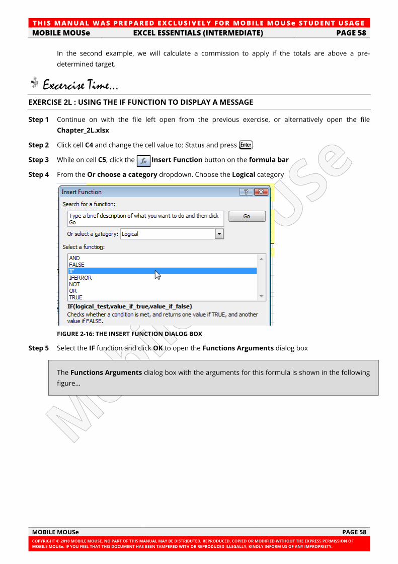
TH IS MANUAL W AS PREPARED EX CLUSIVE LY FOR MOBILE MOUSe ST UDE NT USAGE
MOBILE MOUSe EXCEL ESSENTIALS (INTERMEDIATE) PAGE 58
MOBILE MOUSe PAGE 58
COPYRIGHT © 2018 MOBILE MOUSE. NO PART OF THIS MANUAL MAY BE DISTRIBUTED, REPRODUCED, COPIED OR MODIFIED WITHOUT THE EXPRESS PERMISSION OF
MOBILE MOUSe. IF YOU FEEL THAT THIS DOCUMENT HAS BEEN TAMPERED WITH OR REPRODUCED ILLEGALLY, KINDLY INFORM US OF ANY IMPROPRIETY.
In the second example, we will calculate a commission to apply if the totals are above a pre-
determined target.
Excercise Time... EXERCISE 2L : USING THE IF FUNCTION TO DISPLAY A MESSAGE
Step 1 Continue on with the file left open from the previous exercise, or alternatively open the file
Chapter_2L.xlsx
Step 2 Click cell C4 and change the cell value to: Status and press J
Step 3 While on cell C5, click the Insert Function button on the formula bar
Step 4 From the Or choose a category dropdown. Choose the Logical category
FIGURE 2-16: THE INSERT FUNCTION DIALOG BOX
Step 5 Select the IF function and click OK to open the Functions Arguments dialog box
The Functions Arguments dialog box with the arguments for this formula is shown in the following
figure...
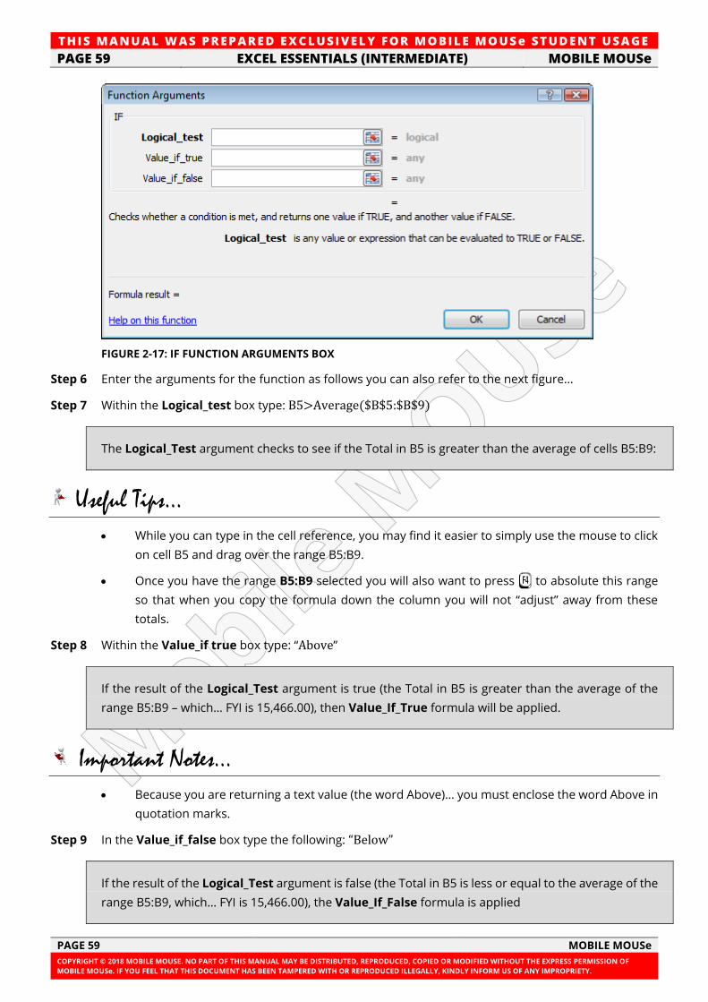
TH IS MANUAL W AS PREPARED EX CLUSIVE LY FOR MOBILE MOUSe ST UDE NT USAGE
PAGE 59 EXCEL ESSENTIALS (INTERMEDIATE) MOBILE MOUSe
PAGE 59 MOBILE MOUSe
COPYRIGHT © 2018 MOBILE MOUSE. NO PART OF THIS MANUAL MAY BE DISTRIBUTED, REPRODUCED, COPIED OR MODIFIED WITHOUT THE EXPRESS PERMISSION OF
MOBILE MOUSe. IF YOU FEEL THAT THIS DOCUMENT HAS BEEN TAMPERED WITH OR REPRODUCED ILLEGALLY, KINDLY INFORM US OF ANY IMPROPRIETY.
FIGURE 2-17: IF FUNCTION ARGUMENTS BOX
Step 6 Enter the arguments for the function as follows you can also refer to the next figure...
Step 7 Within the Logical_test box type: B5>Average($B$5:$B$9)
The Logical_Test argument checks to see if the Total in B5 is greater than the average of cells B5:B9:
Useful Tips...
• While you can type in the cell reference, you may find it easier to simply use the mouse to click
on cell B5 and drag over the range B5:B9.
• Once you have the range B5:B9 selected you will also want to press n to absolute this range
so that when you copy the formula down the column you will not “adjust” away from these
totals.
Step 8 Within the Value_if true box type: “Above”
If the result of the Logical_Test argument is true (the Total in B5 is greater than the average of the
range B5:B9 – which… FYI is 15,466.00), then Value_If_True formula will be applied.
Important Notes...
• Because you are returning a text value (the word Above)... you must enclose the word Above in
quotation marks.
Step 9 In the Value_if_false box type the following: “Below”
If the result of the Logical_Test argument is false (the Total in B5 is less or equal to the average of the
range B5:B9, which… FYI is 15,466.00), the Value_If_False formula is applied
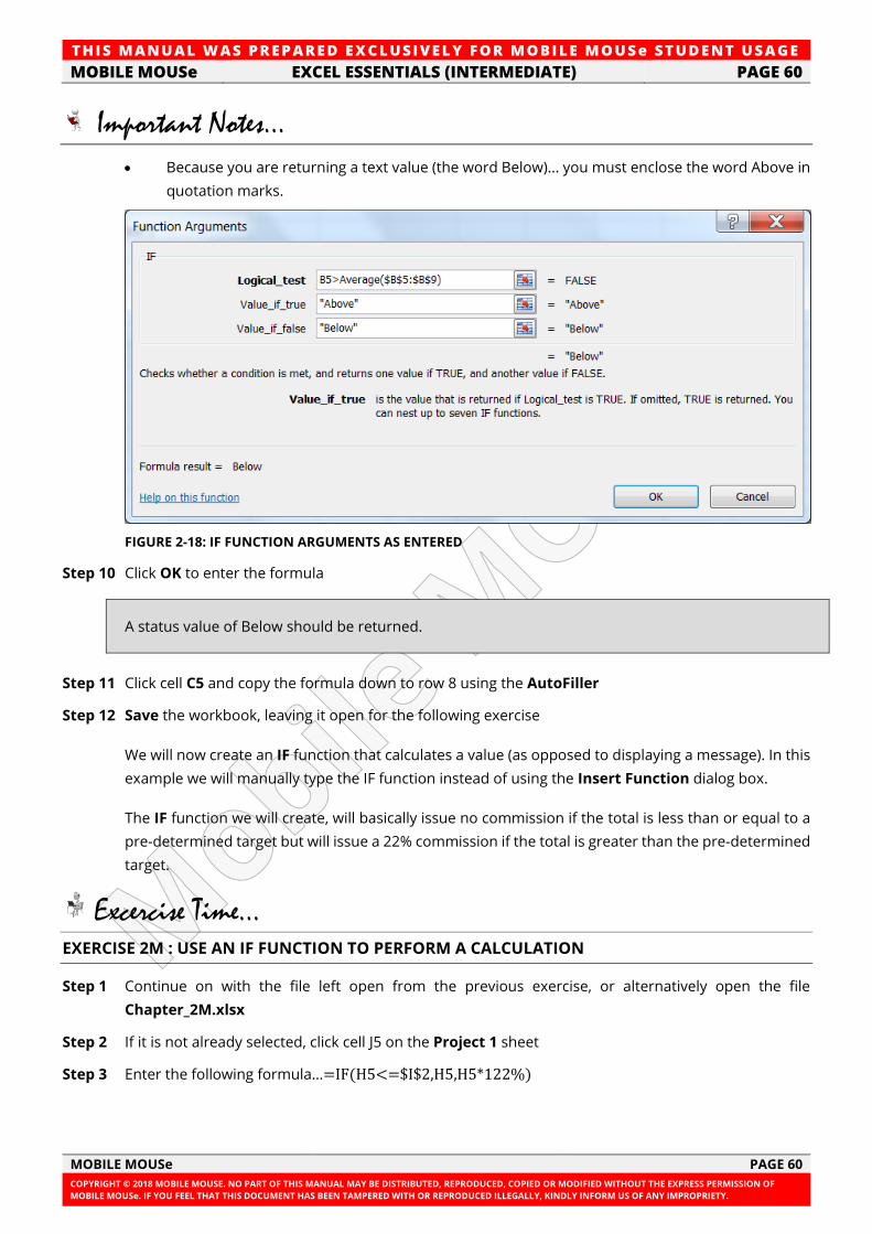
TH IS MANUAL W AS PREPARED EX CLUSIVE LY FOR MOBILE MOUSe ST UDE NT USAGE
MOBILE MOUSe EXCEL ESSENTIALS (INTERMEDIATE) PAGE 60
MOBILE MOUSe PAGE 60
COPYRIGHT © 2018 MOBILE MOUSE. NO PART OF THIS MANUAL MAY BE DISTRIBUTED, REPRODUCED, COPIED OR MODIFIED WITHOUT THE EXPRESS PERMISSION OF
MOBILE MOUSe. IF YOU FEEL THAT THIS DOCUMENT HAS BEEN TAMPERED WITH OR REPRODUCED ILLEGALLY, KINDLY INFORM US OF ANY IMPROPRIETY.
Important Notes...
• Because you are returning a text value (the word Below)... you must enclose the word Above in
quotation marks.
FIGURE 2-18: IF FUNCTION ARGUMENTS AS ENTERED
Step 10 Click OK to enter the formula
A status value of Below should be returned.
Step 11 Click cell C5 and copy the formula down to row 8 using the AutoFiller
Step 12 Save the workbook, leaving it open for the following exercise
We will now create an IF function that calculates a value (as opposed to displaying a message). In this
example we will manually type the IF function instead of using the Insert Function dialog box.
The IF function we will create, will basically issue no commission if the total is less than or equal to a
pre-determined target but will issue a 22% commission if the total is greater than the pre-determined
target.
Excercise Time... EXERCISE 2M : USE AN IF FUNCTION TO PERFORM A CALCULATION
Step 1 Continue on with the file left open from the previous exercise, or alternatively open the file
Chapter_2M.xlsx
Step 2 If it is not already selected, click cell J5 on the Project 1 sheet
Step 3 Enter the following formula…=IF(H5<=$I$2,H5,H5*122%)
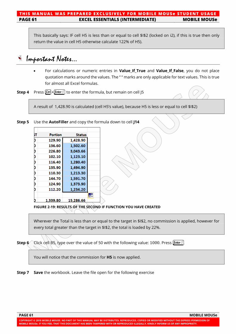
TH IS MANUAL W AS PREPARED EX CLUSIVE LY FOR MOBILE MOUSe ST UDE NT USAGE
PAGE 61 EXCEL ESSENTIALS (INTERMEDIATE) MOBILE MOUSe
PAGE 61 MOBILE MOUSe
COPYRIGHT © 2018 MOBILE MOUSE. NO PART OF THIS MANUAL MAY BE DISTRIBUTED, REPRODUCED, COPIED OR MODIFIED WITHOUT THE EXPRESS PERMISSION OF
MOBILE MOUSe. IF YOU FEEL THAT THIS DOCUMENT HAS BEEN TAMPERED WITH OR REPRODUCED ILLEGALLY, KINDLY INFORM US OF ANY IMPROPRIETY.
This basically says: IF cell H5 is less than or equal to cell $I$2 (locked on i2), if this is true then only
return the value in cell H5 otherwise calculate 122% of H5).
Important Notes...
• For calculations or numeric entries in Value_If_True and Value_If_False, you do not place
quotation marks around the values. The “ “ marks are only applicable for text values. This is true
for almost all Excel formulas.
Step 4 Press F+I to enter the formula, but remain on cell J5
A result of 1,428.90 is calculated (cell H5’s value), because H5 is less or equal to cell $I$2)
Step 5 Use the AutoFiller and copy the formula down to cell J14
FIGURE 2-19: RESULTS OF THE SECOND IF FUNCTION YOU HAVE CREATED
Wherever the Total is less than or equal to the target in $I$2, no commission is applied, however for
every total greater than the target in $I$2, the total is loaded by 22%.
Step 6 Click cell B5, type over the value of 50 with the following value: 1000. Press I
You will notice that the commission for H5 is now applied.
Step 7 Save the workbook. Leave the file open for the following exercise
TH IS MANUAL W AS PREPARED EX CLUSIVE LY FOR MOBILE MOUSe ST UDE NT USAGE
MOBILE MOUSe EXCEL ESSENTIALS (INTERMEDIATE) PAGE 62
MOBILE MOUSe PAGE 62
COPYRIGHT © 2018 MOBILE MOUSE. NO PART OF THIS MANUAL MAY BE DISTRIBUTED, REPRODUCED, COPIED OR MODIFIED WITHOUT THE EXPRESS PERMISSION OF
MOBILE MOUSe. IF YOU FEEL THAT THIS DOCUMENT HAS BEEN TAMPERED WITH OR REPRODUCED ILLEGALLY, KINDLY INFORM US OF ANY IMPROPRIETY.
2.4 HYPERLINKS
MICROSOFT OFFICE CERTIFICATION
This concept addresses the Apply and manipulate hyperlinks competency of the Microsoft Office
Specialist Certification (Exam 77-420).
PLEASE NOTE: This training resource does not necessarily cover all of the requirements of this
exam objective as this objective may include but is not limited to: Create a hyperlink in a cell,
modify hyperlinks, modify hyperlinked-cell attributes, and remove a hyperlink.
Visit http://www.microsoft.com/learning/en/us/mos-certification.aspx for the latest Microsoft
Office Certification requirements.
Hyperlinks are essentially links to other cells, sheets, documents and workbooks. You can also
hyperlink to webpage addresses and email addresses.
You can create four types of hyperlinks in Excel. Hyperlinks in Excel allow you to link to the following:
• An existing file or web page
• A range in the current workbook
• A new workbook
• An e-mail address
Excel creates links to web URLs and e-mail addresses automatically. When you type an e-mail address
(for example, [email protected]) or a web address (www.mobilemouse.com.au),
Excel automatically converts the text to a hyperlink.
Excercise Time... EXERCISE 2N : CREATING HYPERLINKS
Step 1 Continue on with the file left open from the previous exercise, or alternatively open the file
Chapter_2N.xlsx
Step 2 Click cell E1. Type your email address
Step 3 If you do not have an email address type the following email address: [email protected]
Step 4 Press I
Excel colours the text blue and underlines it. You have now created a hyperlink.
Step 5 Right click cell B5, from the shortcut menu that appears, choose Hyperlink...
Step 6 Within the Insert Hyperlink dialog box, click the option on the left that says, Place in this document
Step 7 Within the Or select a place in this document area, click Project 1
Step 8 Within the Type the cell reference box, type: H16.
Step 9 Click the ScreenTip button
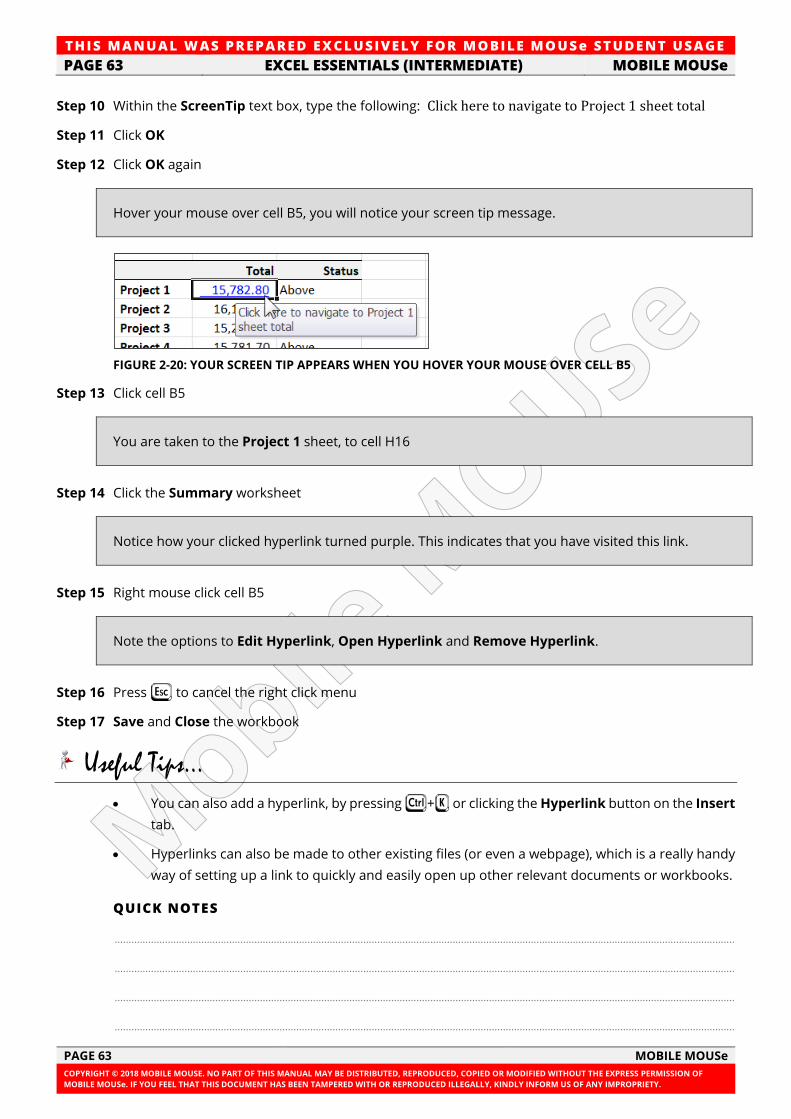
TH IS MANUAL W AS PREPARED EX CLUSIVE LY FOR MOBILE MOUSe ST UDE NT USAGE
PAGE 63 EXCEL ESSENTIALS (INTERMEDIATE) MOBILE MOUSe
PAGE 63 MOBILE MOUSe
COPYRIGHT © 2018 MOBILE MOUSE. NO PART OF THIS MANUAL MAY BE DISTRIBUTED, REPRODUCED, COPIED OR MODIFIED WITHOUT THE EXPRESS PERMISSION OF
MOBILE MOUSe. IF YOU FEEL THAT THIS DOCUMENT HAS BEEN TAMPERED WITH OR REPRODUCED ILLEGALLY, KINDLY INFORM US OF ANY IMPROPRIETY.
Step 10 Within the ScreenTip text box, type the following: Click here to navigate to Project 1 sheet total
Step 11 Click OK
Step 12 Click OK again
Hover your mouse over cell B5, you will notice your screen tip message.
FIGURE 2-20: YOUR SCREEN TIP APPEARS WHEN YOU HOVER YOUR MOUSE OVER CELL B5
Step 13 Click cell B5
You are taken to the Project 1 sheet, to cell H16
Step 14 Click the Summary worksheet
Notice how your clicked hyperlink turned purple. This indicates that you have visited this link.
Step 15 Right mouse click cell B5
Note the options to Edit Hyperlink, Open Hyperlink and Remove Hyperlink.
Step 16 Press L to cancel the right click menu
Step 17 Save and Close the workbook
Useful Tips...
• You can also add a hyperlink, by pressing F+K or clicking the Hyperlink button on the Insert
tab.
• Hyperlinks can also be made to other existing files (or even a webpage), which is a really handy
way of setting up a link to quickly and easily open up other relevant documents or workbooks.
QUICK NOTES
..............................................................................................................................................................................................................................
..............................................................................................................................................................................................................................
..............................................................................................................................................................................................................................
..............................................................................................................................................................................................................................
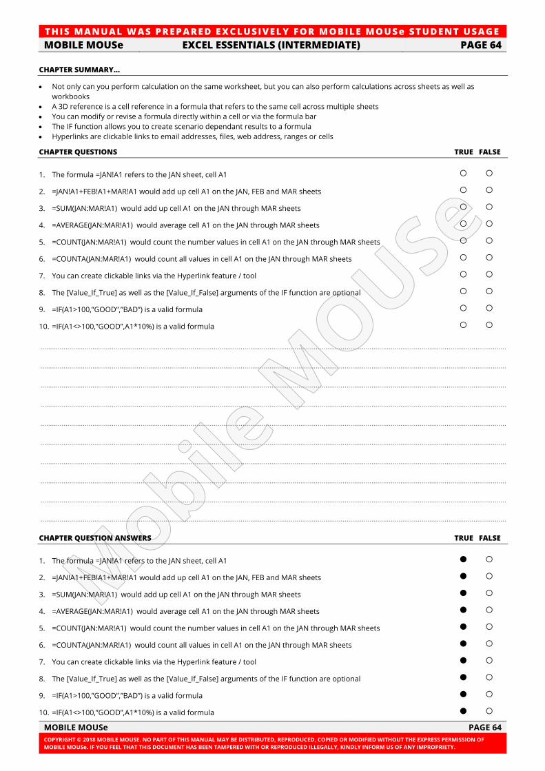
TH IS MANUAL W AS PREPARED EX CLUSIVE LY FOR MOBILE MOUSe ST UDE NT USAGE
MOBILE MOUSe EXCEL ESSENTIALS (INTERMEDIATE) PAGE 64
MOBILE MOUSe PAGE 64
COPYRIGHT © 2018 MOBILE MOUSE. NO PART OF THIS MANUAL MAY BE DISTRIBUTED, REPRODUCED, COPIED OR MODIFIED WITHOUT THE EXPRESS PERMISSION OF
MOBILE MOUSe. IF YOU FEEL THAT THIS DOCUMENT HAS BEEN TAMPERED WITH OR REPRODUCED ILLEGALLY, KINDLY INFORM US OF ANY IMPROPRIETY.
CHAPTER SUMMARY…
• Not only can you perform calculation on the same worksheet, but you can also perform calculations across sheets as well as
workbooks
• A 3D reference is a cell reference in a formula that refers to the same cell across multiple sheets
• You can modify or revise a formula directly within a cell or via the formula bar
• The IF function allows you to create scenario dependant results to a formula
• Hyperlinks are clickable links to email addresses, files, web address, ranges or cells
CHAPTER QUESTIONS TRUE FALSE
1. The formula =JAN!A1 refers to the JAN sheet, cell A1 ○ ○
2. =JAN!A1+FEB!A1+MAR!A1 would add up cell A1 on the JAN, FEB and MAR sheets ○ ○
3. =SUM(JAN:MAR!A1) would add up cell A1 on the JAN through MAR sheets ○ ○
4. =AVERAGE(JAN:MAR!A1) would average cell A1 on the JAN through MAR sheets ○ ○
5. =COUNT(JAN:MAR!A1) would count the number values in cell A1 on the JAN through MAR sheets ○ ○
6. =COUNTA(JAN:MAR!A1) would count all values in cell A1 on the JAN through MAR sheets ○ ○
7. You can create clickable links via the Hyperlink feature / tool ○ ○
8. The [Value_If_True] as well as the [Value_If_False] arguments of the IF function are optional ○ ○
9. =IF(A1>100,”GOOD”,”BAD”) is a valid formula ○ ○
10. =IF(A1<>100,”GOOD”,A1*10%) is a valid formula ○ ○
..................................................................................................................................................................................................................................................
..................................................................................................................................................................................................................................................
..................................................................................................................................................................................................................................................
..................................................................................................................................................................................................................................................
..................................................................................................................................................................................................................................................
..................................................................................................................................................................................................................................................
..................................................................................................................................................................................................................................................
..................................................................................................................................................................................................................................................
..................................................................................................................................................................................................................................................
..................................................................................................................................................................................................................................................
CHAPTER QUESTION ANSWERS TRUE FALSE
1. The formula =JAN!A1 refers to the JAN sheet, cell A1 ● ○
2. =JAN!A1+FEB!A1+MAR!A1 would add up cell A1 on the JAN, FEB and MAR sheets ● ○
3. =SUM(JAN:MAR!A1) would add up cell A1 on the JAN through MAR sheets ● ○
4. =AVERAGE(JAN:MAR!A1) would average cell A1 on the JAN through MAR sheets ● ○
5. =COUNT(JAN:MAR!A1) would count the number values in cell A1 on the JAN through MAR sheets ● ○
6. =COUNTA(JAN:MAR!A1) would count all values in cell A1 on the JAN through MAR sheets ● ○
7. You can create clickable links via the Hyperlink feature / tool ● ○
8. The [Value_If_True] as well as the [Value_If_False] arguments of the IF function are optional ● ○
9. =IF(A1>100,”GOOD”,”BAD”) is a valid formula ● ○
10. =IF(A1<>100,”GOOD”,A1*10%) is a valid formula ● ○
TH IS MANUAL W AS PREPARED EX CLUSIVE LY FOR MOBILE MOUSe ST UDE NT USAGE
PAGE 65 EXCEL ESSENTIALS (INTERMEDIATE) MOBILE MOUSe
PAGE 65 MOBILE MOUSe
COPYRIGHT © 2018 MOBILE MOUSE. NO PART OF THIS MANUAL MAY BE DISTRIBUTED, REPRODUCED, COPIED OR MODIFIED WITHOUT THE EXPRESS PERMISSION OF
MOBILE MOUSe. IF YOU FEEL THAT THIS DOCUMENT HAS BEEN TAMPERED WITH OR REPRODUCED ILLEGALLY, KINDLY INFORM US OF ANY IMPROPRIETY.
PART 3 : LISTS AND MANAGEMENT In this session...
• Reporting or Extracting Data with Filters
• Sorting Data
• Creating Shortcuts to your commonly used features
• Creating and editing more formulae
• Using the Format as table feature
• Automatically format cells based on their values using Conditional Formatting
• Control what data is able to be entered into cells using Data Validation
• Subtotalling
3.1 MORE FORMULAS
In the following exercise we will make some more modifications to an existing spreadsheet using
some of the formula concepts learned this far and we will learn one or two new functions.
Excercise Time... EXERCISE 3A : MORE FORMULAE
Step 1 Open the file: Chapter_3A.xlsx (located in the Desktop \ Excel \ Essentials folder)
Step 2 Click cell B4 and enter the following formula: =today() and press J
The TODAY function returns the current date.
Step 3 In cell B5 enter the following function: =now() and press J
The NOW function returns the current date and time.
Step 4 In the Home tab (in the Number group), change the number format to Time
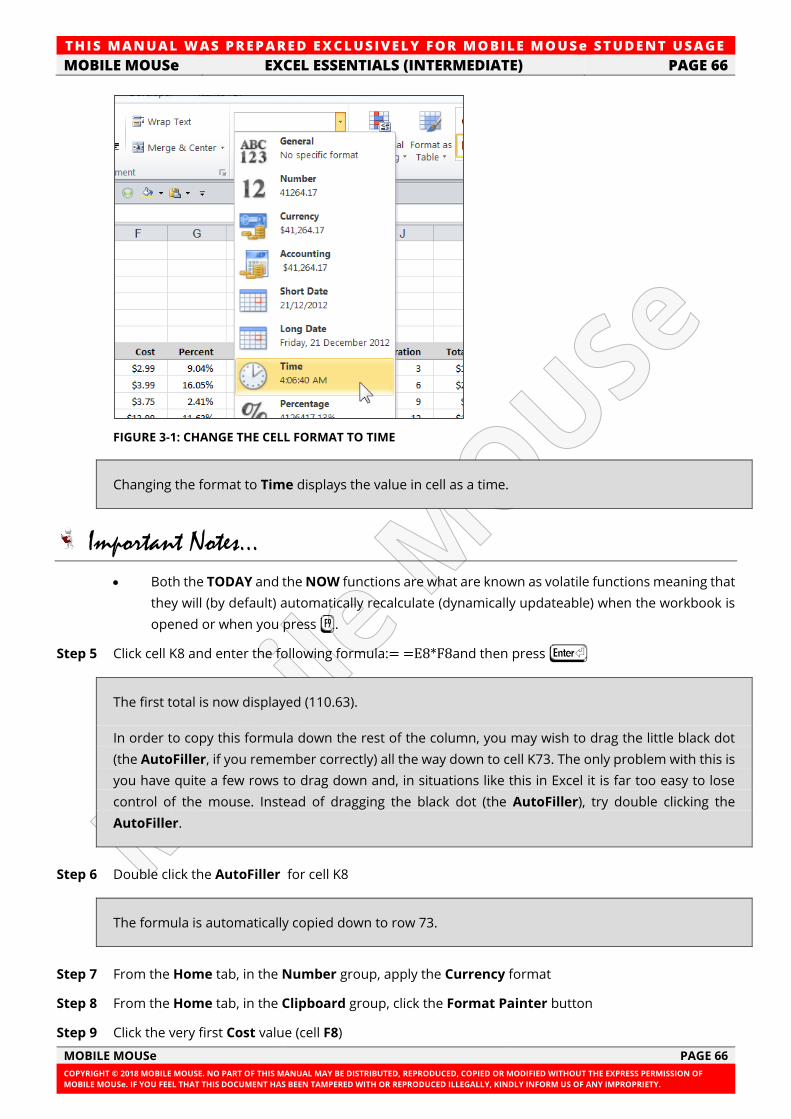
TH IS MANUAL W AS PREPARED EX CLUSIVE LY FOR MOBILE MOUSe ST UDE NT USAGE
MOBILE MOUSe EXCEL ESSENTIALS (INTERMEDIATE) PAGE 66
MOBILE MOUSe PAGE 66
COPYRIGHT © 2018 MOBILE MOUSE. NO PART OF THIS MANUAL MAY BE DISTRIBUTED, REPRODUCED, COPIED OR MODIFIED WITHOUT THE EXPRESS PERMISSION OF
MOBILE MOUSe. IF YOU FEEL THAT THIS DOCUMENT HAS BEEN TAMPERED WITH OR REPRODUCED ILLEGALLY, KINDLY INFORM US OF ANY IMPROPRIETY.
FIGURE 3-1: CHANGE THE CELL FORMAT TO TIME
Changing the format to Time displays the value in cell as a time.
Important Notes...
• Both the TODAY and the NOW functions are what are known as volatile functions meaning that
they will (by default) automatically recalculate (dynamically updateable) when the workbook is
opened or when you press s.
Step 5 Click cell K8 and enter the following formula:= =E8*F8and then press I
The first total is now displayed (110.63).
In order to copy this formula down the rest of the column, you may wish to drag the little black dot
(the AutoFiller, if you remember correctly) all the way down to cell K73. The only problem with this is
you have quite a few rows to drag down and, in situations like this in Excel it is far too easy to lose
control of the mouse. Instead of dragging the black dot (the AutoFiller), try double clicking the
AutoFiller.
Step 6 Double click the AutoFiller for cell K8
The formula is automatically copied down to row 73.
Step 7 From the Home tab, in the Number group, apply the Currency format
Step 8 From the Home tab, in the Clipboard group, click the Format Painter button
Step 9 Click the very first Cost value (cell F8)
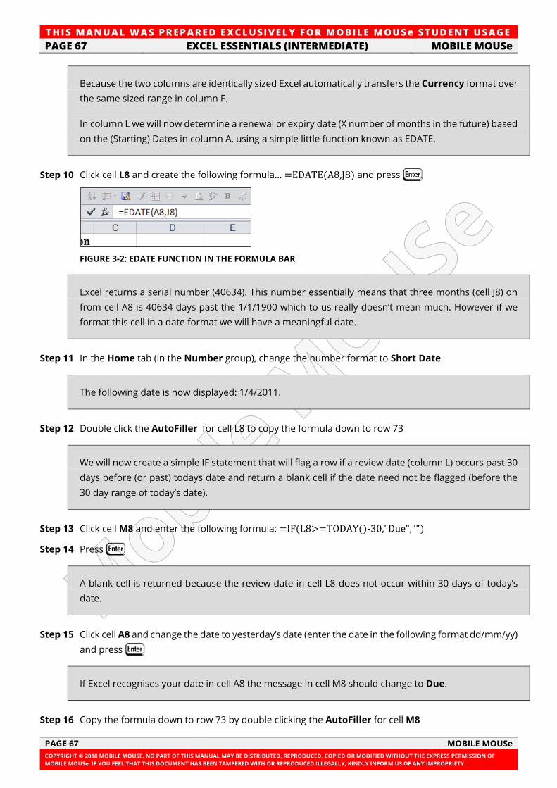
TH IS MANUAL W AS PREPARED EX CLUSIVE LY FOR MOBILE MOUSe ST UDE NT USAGE
PAGE 67 EXCEL ESSENTIALS (INTERMEDIATE) MOBILE MOUSe
PAGE 67 MOBILE MOUSe
COPYRIGHT © 2018 MOBILE MOUSE. NO PART OF THIS MANUAL MAY BE DISTRIBUTED, REPRODUCED, COPIED OR MODIFIED WITHOUT THE EXPRESS PERMISSION OF
MOBILE MOUSe. IF YOU FEEL THAT THIS DOCUMENT HAS BEEN TAMPERED WITH OR REPRODUCED ILLEGALLY, KINDLY INFORM US OF ANY IMPROPRIETY.
Because the two columns are identically sized Excel automatically transfers the Currency format over
the same sized range in column F.
In column L we will now determine a renewal or expiry date (X number of months in the future) based
on the (Starting) Dates in column A, using a simple little function known as EDATE.
Step 10 Click cell L8 and create the following formula… =EDATE(A8,J8) and press J
FIGURE 3-2: EDATE FUNCTION IN THE FORMULA BAR
Excel returns a serial number (40634). This number essentially means that three months (cell J8) on
from cell A8 is 40634 days past the 1/1/1900 which to us really doesn’t mean much. However if we
format this cell in a date format we will have a meaningful date.
Step 11 In the Home tab (in the Number group), change the number format to Short Date
The following date is now displayed: 1/4/2011.
Step 12 Double click the AutoFiller for cell L8 to copy the formula down to row 73
We will now create a simple IF statement that will flag a row if a review date (column L) occurs past 30
days before (or past) todays date and return a blank cell if the date need not be flagged (before the
30 day range of today’s date).
Step 13 Click cell M8 and enter the following formula: =IF(L8>=TODAY()-30,"Due","")
Step 14 Press J
A blank cell is returned because the review date in cell L8 does not occur within 30 days of today’s
date.
Step 15 Click cell A8 and change the date to yesterday’s date (enter the date in the following format dd/mm/yy)
and press J
If Excel recognises your date in cell A8 the message in cell M8 should change to Due.
Step 16 Copy the formula down to row 73 by double clicking the AutoFiller for cell M8
TH IS MANUAL W AS PREPARED EX CLUSIVE LY FOR MOBILE MOUSe ST UDE NT USAGE
MOBILE MOUSe EXCEL ESSENTIALS (INTERMEDIATE) PAGE 68
MOBILE MOUSe PAGE 68
COPYRIGHT © 2018 MOBILE MOUSE. NO PART OF THIS MANUAL MAY BE DISTRIBUTED, REPRODUCED, COPIED OR MODIFIED WITHOUT THE EXPRESS PERMISSION OF
MOBILE MOUSe. IF YOU FEEL THAT THIS DOCUMENT HAS BEEN TAMPERED WITH OR REPRODUCED ILLEGALLY, KINDLY INFORM US OF ANY IMPROPRIETY.
Step 17 Save the workbook leaving it open for the following exercise
3.2 CONDITIONAL FORMATTING
MICROSOFT OFFICE CERTIFICATION
This concept addresses the Apply conditional formatting competency of the Microsoft Office
Specialist Certification (Exam 77-420).
PLEASE NOTE: This training resource does not necessarily cover all of the requirements of this
exam objective as this objective may include but is not limited to: Apply conditional formatting to
cells, use the Rule Manager to Apply Conditional Formats, use the IF Function and Apply
Conditional Formatting, icon sets, data bars, clear rules.
Visit http://www.microsoft.com/learning/en/us/mos-certification.aspx for the latest Microsoft
Office Certification requirements.
With conditional formatting, you can apply formats to selected cells based on a condition. With
conditional formatting, formatting is automatically applied, changed or removed as specific cell values
change.
In Excel, you can use conditional formatting to visually annotate your data for both analytical and
presentation purposes. To easily find exceptions and to spot important trends in your data, you can
implement and manage multiple conditional formatting rules that apply rich visual formatting in the
form of gradient colours, data bars, and icon sets to data that meets those rules. Conditional formats
are also easy to apply—in just a few clicks; you can see relationships in your data that you can use for
your analysis purposes.
Conditional formatting in Excel is one of the features that have been greatly improved over previous
versions of Excel. Conditional formatting can contain up to sixty-four rules, but in earlier versions of
Excel, only three rules are supported.
You can apply font attributes, borders, or patterns to cells based on whether the condition is true or
false to emphasize, (for example) above-average or below par performance or on dates occurring
outside a specific range and now in addition to simple colours, you can also easily apply data bars,
and icon sets to cells.
Important Notes...
• Conditional formatting overrides other formatting of the same type within a cell. For example,
a custom format that includes colours will be replaced with the colours specified in a conditional
format (if and when the specified condition is met).
3.2.1 USING TOP / BOTTOM RULES
In the following exercise, you will use Top / Bottom Rules to format the highest three quantities as
well as the lowest three quantities.
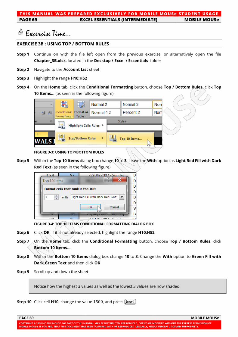
TH IS MANUAL W AS PREPARED EX CLUSIVE LY FOR MOBILE MOUSe ST UDE NT USAGE
PAGE 69 EXCEL ESSENTIALS (INTERMEDIATE) MOBILE MOUSe
PAGE 69 MOBILE MOUSe
COPYRIGHT © 2018 MOBILE MOUSE. NO PART OF THIS MANUAL MAY BE DISTRIBUTED, REPRODUCED, COPIED OR MODIFIED WITHOUT THE EXPRESS PERMISSION OF
MOBILE MOUSe. IF YOU FEEL THAT THIS DOCUMENT HAS BEEN TAMPERED WITH OR REPRODUCED ILLEGALLY, KINDLY INFORM US OF ANY IMPROPRIETY.
Excercise Time... EXERCISE 3B : USING TOP / BOTTOM RULES
Step 1 Continue on with the file left open from the previous exercise, or alternatively open the file
Chapter_3B.xlsx, located in the Desktop \ Excel \ Essentials folder
Step 2 Navigate to the Account List sheet
Step 3 Highlight the range H10:H52
Step 4 On the Home tab, click the Conditional Formatting button, choose Top / Bottom Rules, click Top
10 Items… (as seen in the following figure)
FIGURE 3-3: USING TOP/BOTTOM RULES
Step 5 Within the Top 10 Items dialog box change 10 to 3. Leave the With option as Light Red Fill with Dark
Red Text (as seen in the following figure)
FIGURE 3-4: TOP 10 ITEMS CONDITIONAL FORMATTING DIALOG BOX
Step 6 Click OK, if it is not already selected, highlight the range H10:H52
Step 7 On the Home tab, click the Conditional Formatting button, choose Top / Bottom Rules, click
Bottom 10 Items…
Step 8 Within the Bottom 10 Items dialog box change 10 to 3. Change the With option to Green Fill with
Dark Green Text and then click OK
Step 9 Scroll up and down the sheet
Notice how the highest 3 values as well as the lowest 3 values are now shaded.
Step 10 Click cell H10, change the value 1500, and press I
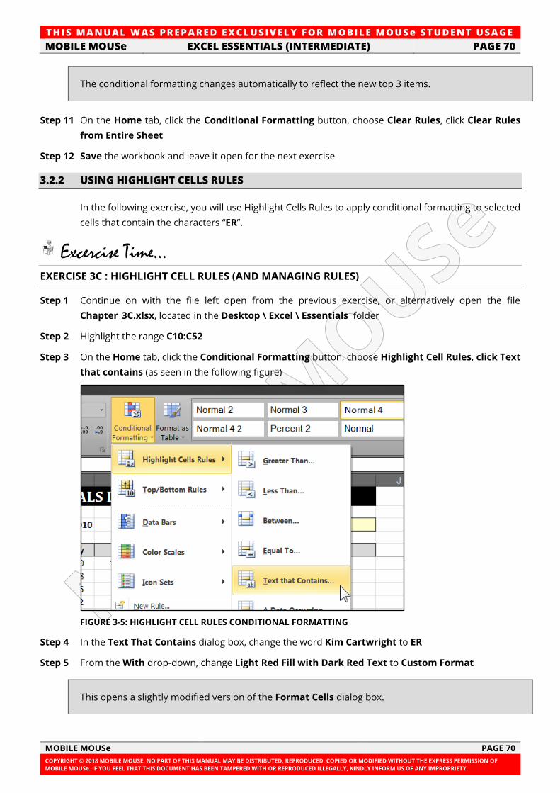
TH IS MANUAL W AS PREPARED EX CLUSIVE LY FOR MOBILE MOUSe ST UDE NT USAGE
MOBILE MOUSe EXCEL ESSENTIALS (INTERMEDIATE) PAGE 70
MOBILE MOUSe PAGE 70
COPYRIGHT © 2018 MOBILE MOUSE. NO PART OF THIS MANUAL MAY BE DISTRIBUTED, REPRODUCED, COPIED OR MODIFIED WITHOUT THE EXPRESS PERMISSION OF
MOBILE MOUSe. IF YOU FEEL THAT THIS DOCUMENT HAS BEEN TAMPERED WITH OR REPRODUCED ILLEGALLY, KINDLY INFORM US OF ANY IMPROPRIETY.
The conditional formatting changes automatically to reflect the new top 3 items.
Step 11 On the Home tab, click the Conditional Formatting button, choose Clear Rules, click Clear Rules
from Entire Sheet
Step 12 Save the workbook and leave it open for the next exercise
3.2.2 USING HIGHLIGHT CELLS RULES
In the following exercise, you will use Highlight Cells Rules to apply conditional formatting to selected
cells that contain the characters “ER”.
Excercise Time... EXERCISE 3C : HIGHLIGHT CELL RULES (AND MANAGING RULES)
Step 1 Continue on with the file left open from the previous exercise, or alternatively open the file
Chapter_3C.xlsx, located in the Desktop \ Excel \ Essentials folder
Step 2 Highlight the range C10:C52
Step 3 On the Home tab, click the Conditional Formatting button, choose Highlight Cell Rules, click Text
that contains (as seen in the following figure)
FIGURE 3-5: HIGHLIGHT CELL RULES CONDITIONAL FORMATTING
Step 4 In the Text That Contains dialog box, change the word Kim Cartwright to ER
Step 5 From the With drop-down, change Light Red Fill with Dark Red Text to Custom Format
This opens a slightly modified version of the Format Cells dialog box.
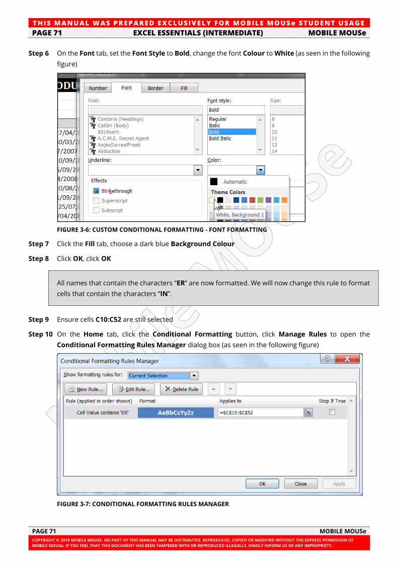
TH IS MANUAL W AS PREPARED EX CLUSIVE LY FOR MOBILE MOUSe ST UDE NT USAGE
PAGE 71 EXCEL ESSENTIALS (INTERMEDIATE) MOBILE MOUSe
PAGE 71 MOBILE MOUSe
COPYRIGHT © 2018 MOBILE MOUSE. NO PART OF THIS MANUAL MAY BE DISTRIBUTED, REPRODUCED, COPIED OR MODIFIED WITHOUT THE EXPRESS PERMISSION OF
MOBILE MOUSe. IF YOU FEEL THAT THIS DOCUMENT HAS BEEN TAMPERED WITH OR REPRODUCED ILLEGALLY, KINDLY INFORM US OF ANY IMPROPRIETY.
Step 6 On the Font tab, set the Font Style to Bold, change the font Colour to White (as seen in the following
figure)
FIGURE 3-6: CUSTOM CONDITIONAL FORMATTING - FONT FORMATTING
Step 7 Click the Fill tab, choose a dark blue Background Colour
Step 8 Click OK, click OK
All names that contain the characters “ER” are now formatted. We will now change this rule to format
cells that contain the characters “IN”.
Step 9 Ensure cells C10:C52 are still selected
Step 10 On the Home tab, click the Conditional Formatting button, click Manage Rules to open the
Conditional Formatting Rules Manager dialog box (as seen in the following figure)
FIGURE 3-7: CONDITIONAL FORMATTING RULES MANAGER
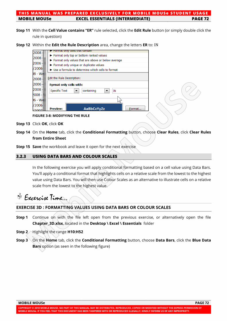
TH IS MANUAL W AS PREPARED EX CLUSIVE LY FOR MOBILE MOUSe ST UDE NT USAGE
MOBILE MOUSe EXCEL ESSENTIALS (INTERMEDIATE) PAGE 72
MOBILE MOUSe PAGE 72
COPYRIGHT © 2018 MOBILE MOUSE. NO PART OF THIS MANUAL MAY BE DISTRIBUTED, REPRODUCED, COPIED OR MODIFIED WITHOUT THE EXPRESS PERMISSION OF
MOBILE MOUSe. IF YOU FEEL THAT THIS DOCUMENT HAS BEEN TAMPERED WITH OR REPRODUCED ILLEGALLY, KINDLY INFORM US OF ANY IMPROPRIETY.
Step 11 With the Cell Value contains “ER” rule selected, click the Edit Rule button (or simply double click the
rule in question)
Step 12 Within the Edit the Rule Description area, change the letters ER to: IN
FIGURE 3-8: MODIFYING THE RULE
Step 13 Click OK, click OK
Step 14 On the Home tab, click the Conditional Formatting button, choose Clear Rules, click Clear Rules
from Entire Sheet
Step 15 Save the workbook and leave it open for the next exercise
3.2.3 USING DATA BARS AND COLOUR SCALES
In the following exercise you will apply conditional formatting based on a cell value using Data Bars.
You’ll apply a conditional format that highlights cells on a relative scale from the lowest to the highest
value using Data Bars. You will then use Colour Scales as an alternative to illustrate cells on a relative
scale from the lowest to the highest value.
Excercise Time... EXERCISE 3D : FORMATTING VALUES USING DATA BARS OR COLOUR SCALES
Step 1 Continue on with the file left open from the previous exercise, or alternatively open the file
Chapter_3D.xlsx, located in the Desktop \ Excel \ Essentials folder
Step 2 Highlight the range H10:H52
Step 3 On the Home tab, click the Conditional Formatting button, choose Data Bars, click the Blue Data
Bars option (as seen in the following figure)
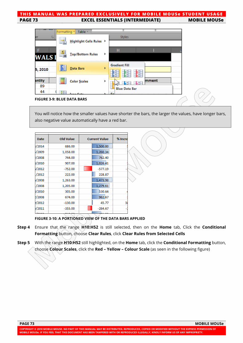
TH IS MANUAL W AS PREPARED EX CLUSIVE LY FOR MOBILE MOUSe ST UDE NT USAGE
PAGE 73 EXCEL ESSENTIALS (INTERMEDIATE) MOBILE MOUSe
PAGE 73 MOBILE MOUSe
COPYRIGHT © 2018 MOBILE MOUSE. NO PART OF THIS MANUAL MAY BE DISTRIBUTED, REPRODUCED, COPIED OR MODIFIED WITHOUT THE EXPRESS PERMISSION OF
MOBILE MOUSe. IF YOU FEEL THAT THIS DOCUMENT HAS BEEN TAMPERED WITH OR REPRODUCED ILLEGALLY, KINDLY INFORM US OF ANY IMPROPRIETY.
FIGURE 3-9: BLUE DATA BARS
You will notice how the smaller values have shorter the bars, the larger the values, have longer bars,
also negative value automatically have a red bar.
FIGURE 3-10: A PORTIONED VIEW OF THE DATA BARS APPLIED
Step 4 Ensure that the range H10:H52 is still selected, then on the Home tab, Click the Conditional
Formatting button, choose Clear Rules, click Clear Rules from Selected Cells
Step 5 With the range H10:H52 still highlighted, on the Home tab, click the Conditional Formatting button,
choose Colour Scales, click the Red – Yellow – Colour Scale (as seen in the following figure)
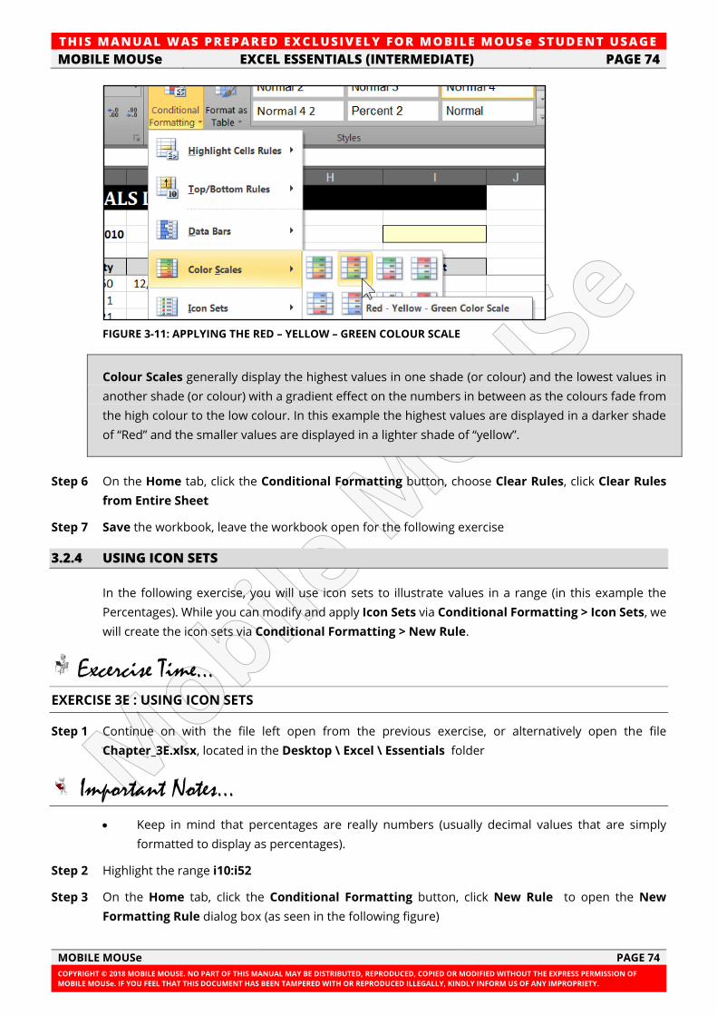
TH IS MANUAL W AS PREPARED EX CLUSIVE LY FOR MOBILE MOUSe ST UDE NT USAGE
MOBILE MOUSe EXCEL ESSENTIALS (INTERMEDIATE) PAGE 74
MOBILE MOUSe PAGE 74
COPYRIGHT © 2018 MOBILE MOUSE. NO PART OF THIS MANUAL MAY BE DISTRIBUTED, REPRODUCED, COPIED OR MODIFIED WITHOUT THE EXPRESS PERMISSION OF
MOBILE MOUSe. IF YOU FEEL THAT THIS DOCUMENT HAS BEEN TAMPERED WITH OR REPRODUCED ILLEGALLY, KINDLY INFORM US OF ANY IMPROPRIETY.
FIGURE 3-11: APPLYING THE RED – YELLOW – GREEN COLOUR SCALE
Colour Scales generally display the highest values in one shade (or colour) and the lowest values in
another shade (or colour) with a gradient effect on the numbers in between as the colours fade from
the high colour to the low colour. In this example the highest values are displayed in a darker shade
of “Red” and the smaller values are displayed in a lighter shade of “yellow”.
Step 6 On the Home tab, click the Conditional Formatting button, choose Clear Rules, click Clear Rules
from Entire Sheet
Step 7 Save the workbook, leave the workbook open for the following exercise
3.2.4 USING ICON SETS
In the following exercise, you will use icon sets to illustrate values in a range (in this example the
Percentages). While you can modify and apply Icon Sets via Conditional Formatting > Icon Sets, we
will create the icon sets via Conditional Formatting > New Rule.
Excercise Time... EXERCISE 3E : USING ICON SETS
Step 1 Continue on with the file left open from the previous exercise, or alternatively open the file
Chapter_3E.xlsx, located in the Desktop \ Excel \ Essentials folder
Important Notes...
• Keep in mind that percentages are really numbers (usually decimal values that are simply
formatted to display as percentages).
Step 2 Highlight the range i10:i52
Step 3 On the Home tab, click the Conditional Formatting button, click New Rule to open the New
Formatting Rule dialog box (as seen in the following figure)
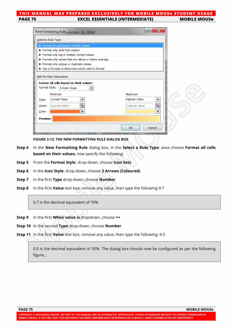
TH IS MANUAL W AS PREPARED EX CLUSIVE LY FOR MOBILE MOUSe ST UDE NT USAGE
PAGE 75 EXCEL ESSENTIALS (INTERMEDIATE) MOBILE MOUSe
PAGE 75 MOBILE MOUSe
COPYRIGHT © 2018 MOBILE MOUSE. NO PART OF THIS MANUAL MAY BE DISTRIBUTED, REPRODUCED, COPIED OR MODIFIED WITHOUT THE EXPRESS PERMISSION OF
MOBILE MOUSe. IF YOU FEEL THAT THIS DOCUMENT HAS BEEN TAMPERED WITH OR REPRODUCED ILLEGALLY, KINDLY INFORM US OF ANY IMPROPRIETY.
FIGURE 3-12: THE NEW FORMATTING RULE DIALOG BOX
Step 4 In the New Formatting Rule dialog box, in the Select a Rule Type: area choose Format all cells
based on their values, now specify the following:
Step 5 From the Format Style: drop-down, choose Icon Sets
Step 6 In the Icon Style: drop-down, choose 3 Arrows (Coloured)
Step 7 In the first Type drop-down, choose Number
Step 8 In the first Value text box, remove any value, then type the following 0.7
0.7 is the decimal equivalent of 70%
Step 9 In the first When value is dropdown, choose >=
Step 10 In the second Type drop-down, choose Number
Step 11 In the first Value text box, remove any value, then type the following: 0.5
0.5 is the decimal equivalent of 50%. The dialog box should now be configured as per the following
figure…
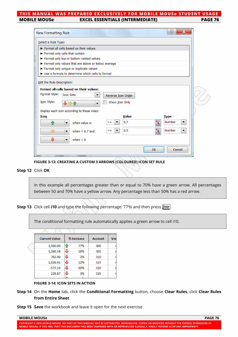
TH IS MANUAL W AS PREPARED EX CLUSIVE LY FOR MOBILE MOUSe ST UDE NT USAGE
MOBILE MOUSe EXCEL ESSENTIALS (INTERMEDIATE) PAGE 76
MOBILE MOUSe PAGE 76
COPYRIGHT © 2018 MOBILE MOUSE. NO PART OF THIS MANUAL MAY BE DISTRIBUTED, REPRODUCED, COPIED OR MODIFIED WITHOUT THE EXPRESS PERMISSION OF
MOBILE MOUSe. IF YOU FEEL THAT THIS DOCUMENT HAS BEEN TAMPERED WITH OR REPRODUCED ILLEGALLY, KINDLY INFORM US OF ANY IMPROPRIETY.
FIGURE 3-13: CREATING A CUSTOM 3 ARROWS (COLOURED) ICON SET RULE
Step 12 Click OK
In this example all percentages greater than or equal to 70% have a green arrow. All percentages
between 50 and 70% have a yellow arrow. Any percentage less than 50% has a red arrow.
Step 13 Click cell i10 and type the following percentage: 77% and then press J
The conditional formatting rule automatically applies a green arrow to cell i10.
FIGURE 3-14: ICON SETS IN ACTION
Step 14 On the Home tab, click the Conditional Formatting button, choose Clear Rules, click Clear Rules
from Entire Sheet
Step 15 Save the workbook and leave it open for the next exercise
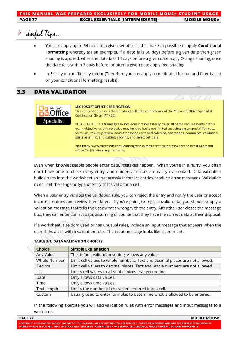
TH IS MANUAL W AS PREPARED EX CLUSIVE LY FOR MOBILE MOUSe ST UDE NT USAGE
PAGE 77 EXCEL ESSENTIALS (INTERMEDIATE) MOBILE MOUSe
PAGE 77 MOBILE MOUSe
COPYRIGHT © 2018 MOBILE MOUSE. NO PART OF THIS MANUAL MAY BE DISTRIBUTED, REPRODUCED, COPIED OR MODIFIED WITHOUT THE EXPRESS PERMISSION OF
MOBILE MOUSe. IF YOU FEEL THAT THIS DOCUMENT HAS BEEN TAMPERED WITH OR REPRODUCED ILLEGALLY, KINDLY INFORM US OF ANY IMPROPRIETY.
Useful Tips...
• You can apply up to 64 rules to a given set of cells, this makes it possible to apply Conditional
Formatting whereby (as an example), if a date falls 30 days before a given date then green
shading is applied, when the date falls 14 days before a given date apply Orange shading, once
the date falls within 7 days before (or after) a given date apply Red shading.
• In Excel you can filter by colour (Therefore you can apply a conditional format and filter based
on your conditional formatting results).
3.3 DATA VALIDATION
MICROSOFT OFFICE CERTIFICATION
This concept addresses the Construct cell data competency of the Microsoft Office Specialist
Certification (Exam 77-420).
PLEASE NOTE: This training resource does not necessarily cover all of the requirements of this
exam objective as this objective may include but is not limited to: using paste special (formats,
formulas, values, preview icons, transpose rows and columns, operations, comments, validation,
paste as a link), and cutting, moving, and select cell data.
Visit http://www.microsoft.com/learning/en/us/mos-certification.aspx for the latest Microsoft
Office Certification requirements.
Even when knowledgeable people enter data, mistakes happen. When you’re in a hurry, you often
don’t have time to check every entry, and numerical errors are easily overlooked. Data validation
builds rules into the worksheet so that grossly incorrect entries produce error messages. Validation
rules limit the range or type of entry that’s valid for a cell.
When a user entry violates the validation rule, you can reject the entry and notify the user or accept
incorrect entries and review them later. If you’re going to reject invalid data, you should supply a
validation message that tells the user what’s wrong with the entry. After the user closes the message
box, they can enter correct data, assuming of course that they have the correct data at their disposal.
If a worksheet is seldom used or has unusual rules, include an input message that appears when the
user clicks a cell with a validation rule. The input message looks like a comment.
TABLE 3-1: DATA VALIDATION CHOICES
Choice Simple Explanation
Any Value The default validation setting. Allows any value.
Whole Number Limit cell values to whole numbers. Text and decimal places are not allowed.
Decimal Limit cell values to decimal places. Text and whole numbers are not allowed.
List Limits cell values to a list of choices that you define.
Date Only allows data values.
Time Only allows time values.
Text Length Limits the number of characters entered into a cell.
Custom Usually used to enter formulas to determine what is allowed to be entered.
In the following exercise you will add validation rules with error messages and input messages to a
workbook.
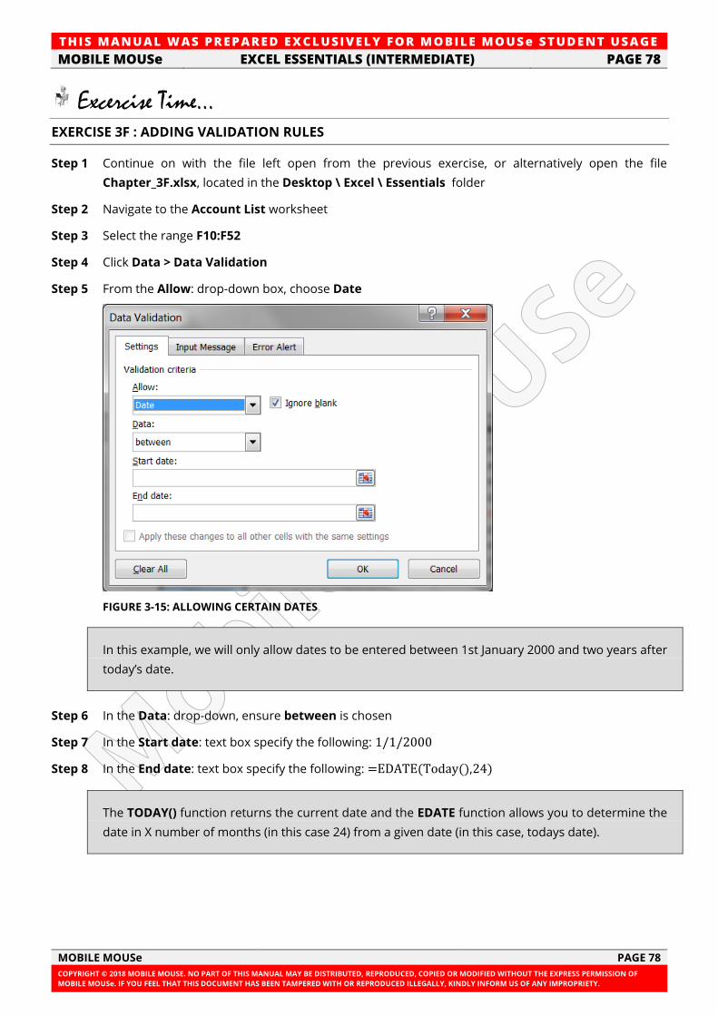
TH IS MANUAL W AS PREPARED EX CLUSIVE LY FOR MOBILE MOUSe ST UDE NT USAGE
MOBILE MOUSe EXCEL ESSENTIALS (INTERMEDIATE) PAGE 78
MOBILE MOUSe PAGE 78
COPYRIGHT © 2018 MOBILE MOUSE. NO PART OF THIS MANUAL MAY BE DISTRIBUTED, REPRODUCED, COPIED OR MODIFIED WITHOUT THE EXPRESS PERMISSION OF
MOBILE MOUSe. IF YOU FEEL THAT THIS DOCUMENT HAS BEEN TAMPERED WITH OR REPRODUCED ILLEGALLY, KINDLY INFORM US OF ANY IMPROPRIETY.
Excercise Time... EXERCISE 3F : ADDING VALIDATION RULES
Step 1 Continue on with the file left open from the previous exercise, or alternatively open the file
Chapter_3F.xlsx, located in the Desktop \ Excel \ Essentials folder
Step 2 Navigate to the Account List worksheet
Step 3 Select the range F10:F52
Step 4 Click Data > Data Validation
Step 5 From the Allow: drop-down box, choose Date
FIGURE 3-15: ALLOWING CERTAIN DATES
In this example, we will only allow dates to be entered between 1st January 2000 and two years after
today’s date.
Step 6 In the Data: drop-down, ensure between is chosen
Step 7 In the Start date: text box specify the following: 1/1/2000
Step 8 In the End date: text box specify the following: =EDATE(Today(),24)
The TODAY() function returns the current date and the EDATE function allows you to determine the
date in X number of months (in this case 24) from a given date (in this case, todays date).
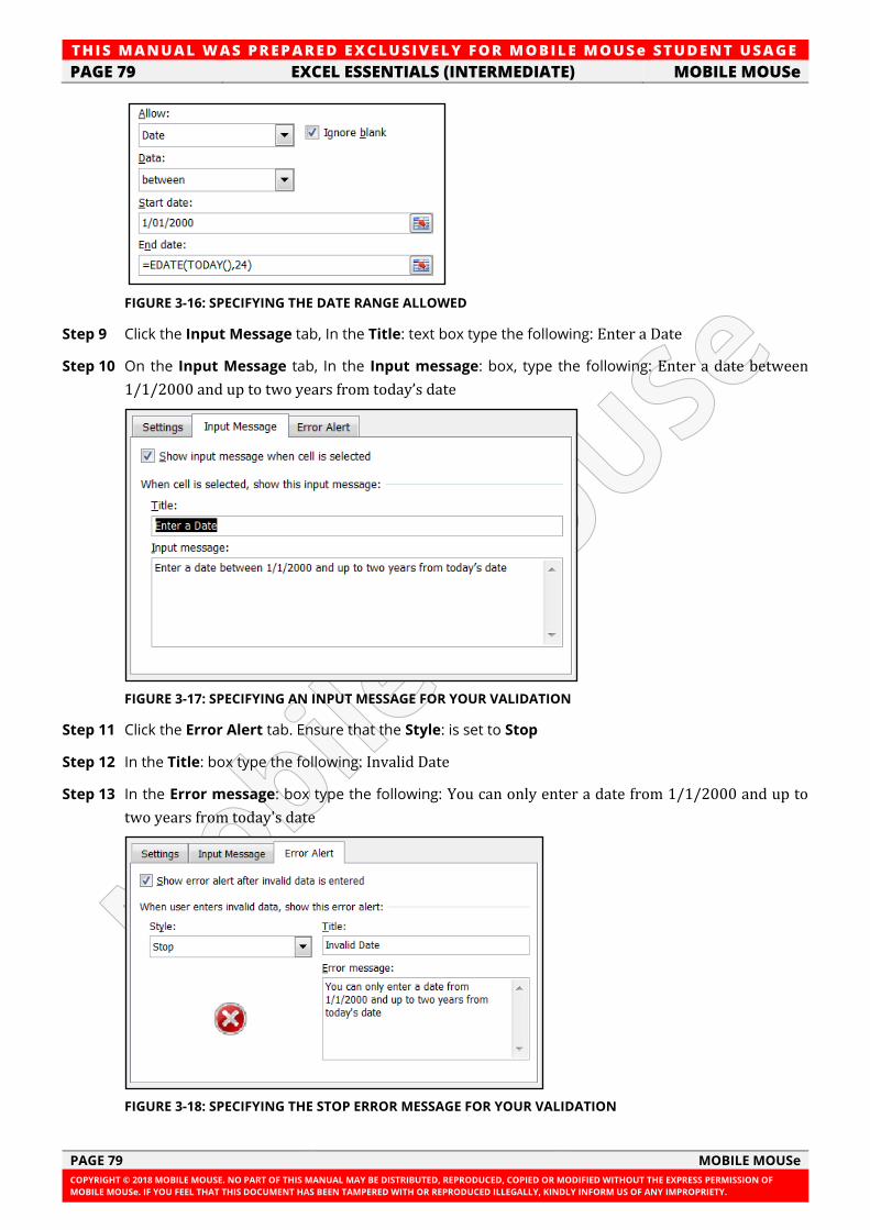
TH IS MANUAL W AS PREPARED EX CLUSIVE LY FOR MOBILE MOUSe ST UDE NT USAGE
PAGE 79 EXCEL ESSENTIALS (INTERMEDIATE) MOBILE MOUSe
PAGE 79 MOBILE MOUSe
COPYRIGHT © 2018 MOBILE MOUSE. NO PART OF THIS MANUAL MAY BE DISTRIBUTED, REPRODUCED, COPIED OR MODIFIED WITHOUT THE EXPRESS PERMISSION OF
MOBILE MOUSe. IF YOU FEEL THAT THIS DOCUMENT HAS BEEN TAMPERED WITH OR REPRODUCED ILLEGALLY, KINDLY INFORM US OF ANY IMPROPRIETY.
FIGURE 3-16: SPECIFYING THE DATE RANGE ALLOWED
Step 9 Click the Input Message tab, In the Title: text box type the following: Enter a Date
Step 10 On the Input Message tab, In the Input message: box, type the following: Enter a date between
1/1/2000 and up to two years from today’s date
FIGURE 3-17: SPECIFYING AN INPUT MESSAGE FOR YOUR VALIDATION
Step 11 Click the Error Alert tab. Ensure that the Style: is set to Stop
Step 12 In the Title: box type the following: Invalid Date
Step 13 In the Error message: box type the following: You can only enter a date from 1/1/2000 and up to
two years from today's date
FIGURE 3-18: SPECIFYING THE STOP ERROR MESSAGE FOR YOUR VALIDATION
TH IS MANUAL W AS PREPARED EX CLUSIVE LY FOR MOBILE MOUSe ST UDE NT USAGE
MOBILE MOUSe EXCEL ESSENTIALS (INTERMEDIATE) PAGE 80
MOBILE MOUSe PAGE 80
COPYRIGHT © 2018 MOBILE MOUSE. NO PART OF THIS MANUAL MAY BE DISTRIBUTED, REPRODUCED, COPIED OR MODIFIED WITHOUT THE EXPRESS PERMISSION OF
MOBILE MOUSe. IF YOU FEEL THAT THIS DOCUMENT HAS BEEN TAMPERED WITH OR REPRODUCED ILLEGALLY, KINDLY INFORM US OF ANY IMPROPRIETY.
TABLE 3-2: ERROR ALERT STYLES
Icon Type Use to
Stop Prevent users from entering invalid data in a cell. A Stop alert message has
two options: Retry or Cancel.
Warning
Warn users that the data they entered is invalid, without preventing them
from entering it. When a Warning alert message appears, users can click Yes
to accept the invalid entry, No to edit the invalid entry, or Cancel to remove
the invalid entry.
Information
Inform users that the data they entered is invalid, without preventing them
from entering it. This type of error alert is the most flexible. When an
Information alert message appears, users can click OK to accept the invalid
value or Cancel to reject it.
Step 14 Click OK
Step 15 Click cell F11, type the following date: 29/4/1976 press J.
You receive the following error…
FIGURE 3-19: INVALID DATE ERROR ALERT
Step 16 Click Cancel
Step 17 Select the range K10:K52
We will now create a validation rule for our voucher column, which will display a warning message for
any invalid data, but still allow the data to be entered.
Step 18 Choose Data > Data Validation
Step 19 Click the Settings tab
Step 20 In the Allow: drop-down list, choose Whole Number
Step 21 In the Data: drop-down list, choose Greater than or equal to
Step 22 In the Minimum: box specify: 47300
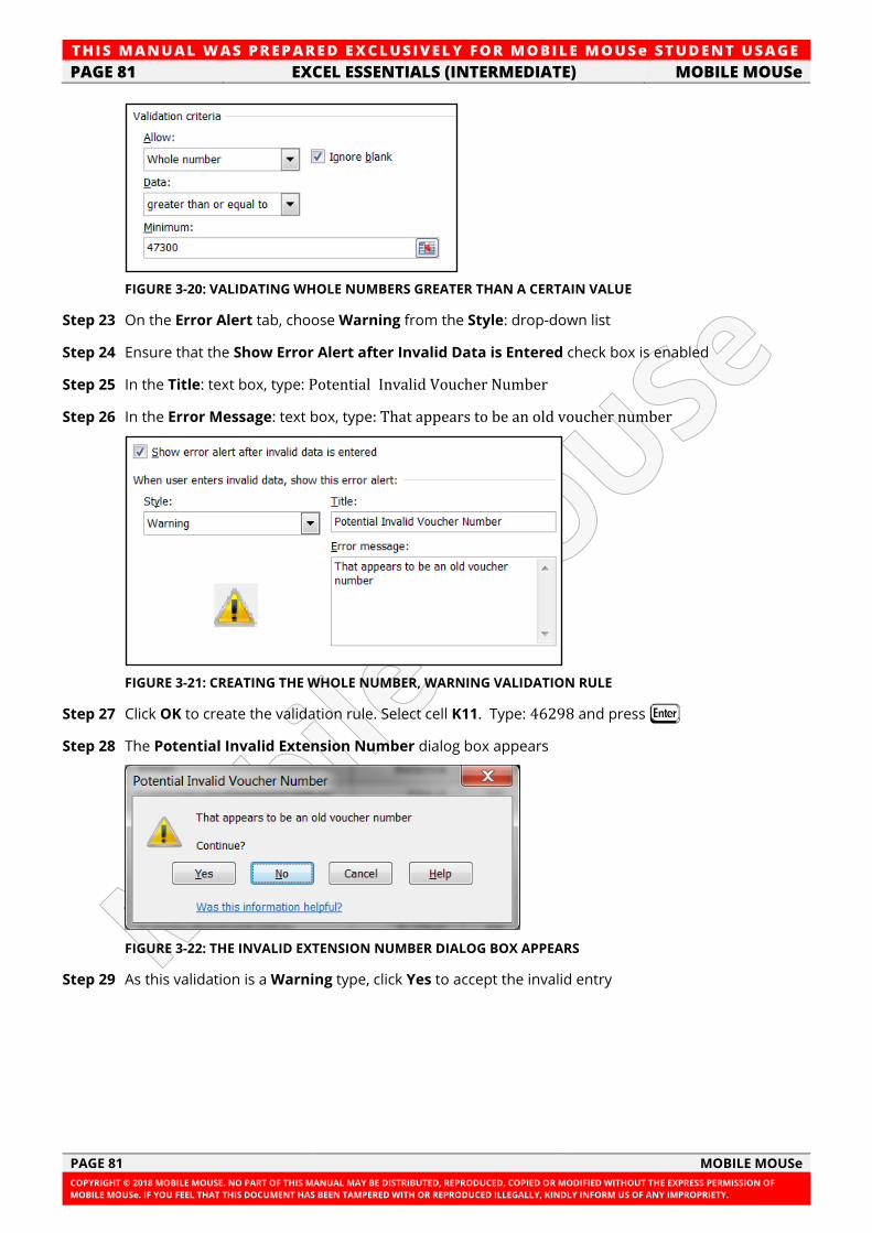
TH IS MANUAL W AS PREPARED EX CLUSIVE LY FOR MOBILE MOUSe ST UDE NT USAGE
PAGE 81 EXCEL ESSENTIALS (INTERMEDIATE) MOBILE MOUSe
PAGE 81 MOBILE MOUSe
COPYRIGHT © 2018 MOBILE MOUSE. NO PART OF THIS MANUAL MAY BE DISTRIBUTED, REPRODUCED, COPIED OR MODIFIED WITHOUT THE EXPRESS PERMISSION OF
MOBILE MOUSe. IF YOU FEEL THAT THIS DOCUMENT HAS BEEN TAMPERED WITH OR REPRODUCED ILLEGALLY, KINDLY INFORM US OF ANY IMPROPRIETY.
FIGURE 3-20: VALIDATING WHOLE NUMBERS GREATER THAN A CERTAIN VALUE
Step 23 On the Error Alert tab, choose Warning from the Style: drop-down list
Step 24 Ensure that the Show Error Alert after Invalid Data is Entered check box is enabled
Step 25 In the Title: text box, type: Potential Invalid Voucher Number
Step 26 In the Error Message: text box, type: That appears to be an old voucher number
FIGURE 3-21: CREATING THE WHOLE NUMBER, WARNING VALIDATION RULE
Step 27 Click OK to create the validation rule. Select cell K11. Type: 46298 and press J
Step 28 The Potential Invalid Extension Number dialog box appears
FIGURE 3-22: THE INVALID EXTENSION NUMBER DIALOG BOX APPEARS
Step 29 As this validation is a Warning type, click Yes to accept the invalid entry
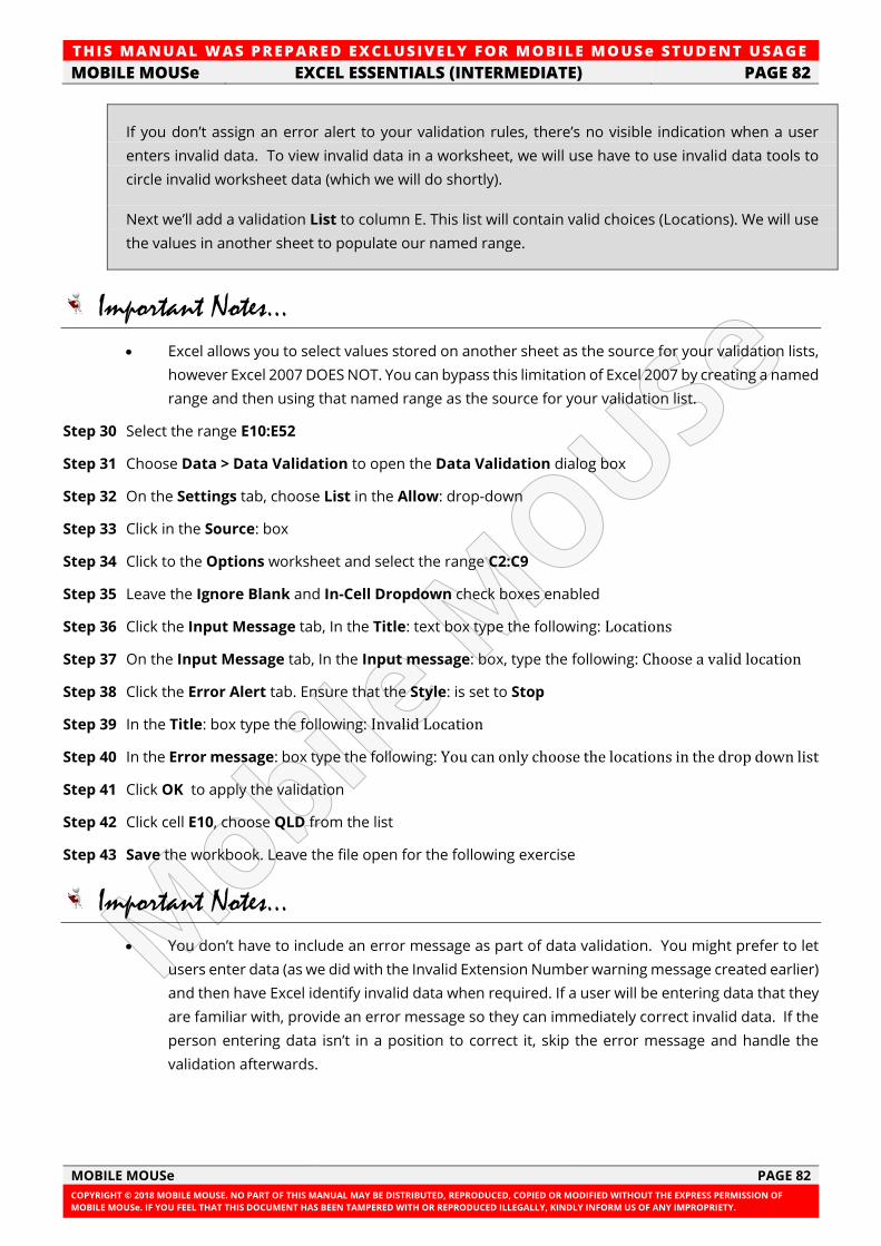
TH IS MANUAL W AS PREPARED EX CLUSIVE LY FOR MOBILE MOUSe ST UDE NT USAGE
MOBILE MOUSe EXCEL ESSENTIALS (INTERMEDIATE) PAGE 82
MOBILE MOUSe PAGE 82
COPYRIGHT © 2018 MOBILE MOUSE. NO PART OF THIS MANUAL MAY BE DISTRIBUTED, REPRODUCED, COPIED OR MODIFIED WITHOUT THE EXPRESS PERMISSION OF
MOBILE MOUSe. IF YOU FEEL THAT THIS DOCUMENT HAS BEEN TAMPERED WITH OR REPRODUCED ILLEGALLY, KINDLY INFORM US OF ANY IMPROPRIETY.
If you don’t assign an error alert to your validation rules, there’s no visible indication when a user
enters invalid data. To view invalid data in a worksheet, we will use have to use invalid data tools to
circle invalid worksheet data (which we will do shortly).
Next we’ll add a validation List to column E. This list will contain valid choices (Locations). We will use
the values in another sheet to populate our named range.
Important Notes...
• Excel allows you to select values stored on another sheet as the source for your validation lists,
however Excel 2007 DOES NOT. You can bypass this limitation of Excel 2007 by creating a named
range and then using that named range as the source for your validation list.
Step 30 Select the range E10:E52
Step 31 Choose Data > Data Validation to open the Data Validation dialog box
Step 32 On the Settings tab, choose List in the Allow: drop-down
Step 33 Click in the Source: box
Step 34 Click to the Options worksheet and select the range C2:C9
Step 35 Leave the Ignore Blank and In-Cell Dropdown check boxes enabled
Step 36 Click the Input Message tab, In the Title: text box type the following: Locations
Step 37 On the Input Message tab, In the Input message: box, type the following: Choose a valid location
Step 38 Click the Error Alert tab. Ensure that the Style: is set to Stop
Step 39 In the Title: box type the following: Invalid Location
Step 40 In the Error message: box type the following: You can only choose the locations in the drop down list
Step 41 Click OK to apply the validation
Step 42 Click cell E10, choose QLD from the list
Step 43 Save the workbook. Leave the file open for the following exercise
Important Notes...
• You don’t have to include an error message as part of data validation. You might prefer to let
users enter data (as we did with the Invalid Extension Number warning message created earlier)
and then have Excel identify invalid data when required. If a user will be entering data that they
are familiar with, provide an error message so they can immediately correct invalid data. If the
person entering data isn’t in a position to correct it, skip the error message and handle the
validation afterwards.
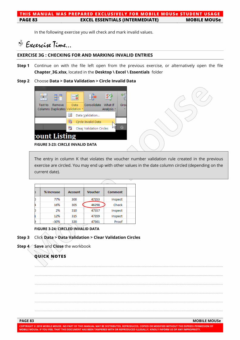
TH IS MANUAL W AS PREPARED EX CLUSIVE LY FOR MOBILE MOUSe ST UDE NT USAGE
PAGE 83 EXCEL ESSENTIALS (INTERMEDIATE) MOBILE MOUSe
PAGE 83 MOBILE MOUSe
COPYRIGHT © 2018 MOBILE MOUSE. NO PART OF THIS MANUAL MAY BE DISTRIBUTED, REPRODUCED, COPIED OR MODIFIED WITHOUT THE EXPRESS PERMISSION OF
MOBILE MOUSe. IF YOU FEEL THAT THIS DOCUMENT HAS BEEN TAMPERED WITH OR REPRODUCED ILLEGALLY, KINDLY INFORM US OF ANY IMPROPRIETY.
In the following exercise you will check and mark invalid values.
Excercise Time... EXERCISE 3G : CHECKING FOR AND MARKING INVALID ENTRIES
Step 1 Continue on with the file left open from the previous exercise, or alternatively open the file
Chapter_3G.xlsx, located in the Desktop \ Excel \ Essentials folder
Step 2 Choose Data > Data Validation > Circle Invalid Data
FIGURE 3-23: CIRCLE INVALID DATA
The entry in column K that violates the voucher number validation rule created in the previous
exercise are circled. You may end up with other values in the date column circled (depending on the
current date).
FIGURE 3-24: CIRCLED INVALID DATA
Step 3 Click Data > Data Validation > Clear Validation Circles
Step 4 Save and Close the workbook
QUICK NOTES
..............................................................................................................................................................................................................................
..............................................................................................................................................................................................................................
..............................................................................................................................................................................................................................
..............................................................................................................................................................................................................................
..............................................................................................................................................................................................................................
..............................................................................................................................................................................................................................
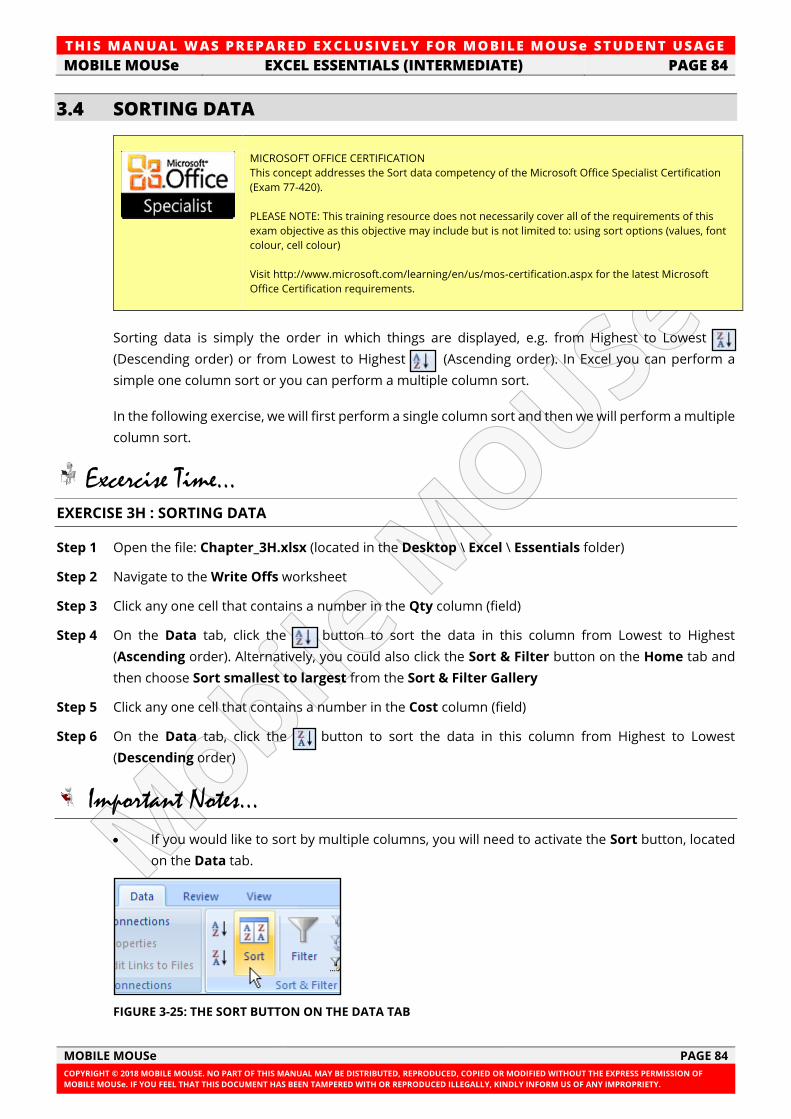
TH IS MANUAL W AS PREPARED EX CLUSIVE LY FOR MOBILE MOUSe ST UDE NT USAGE
MOBILE MOUSe EXCEL ESSENTIALS (INTERMEDIATE) PAGE 84
MOBILE MOUSe PAGE 84
COPYRIGHT © 2018 MOBILE MOUSE. NO PART OF THIS MANUAL MAY BE DISTRIBUTED, REPRODUCED, COPIED OR MODIFIED WITHOUT THE EXPRESS PERMISSION OF
MOBILE MOUSe. IF YOU FEEL THAT THIS DOCUMENT HAS BEEN TAMPERED WITH OR REPRODUCED ILLEGALLY, KINDLY INFORM US OF ANY IMPROPRIETY.
3.4 SORTING DATA
MICROSOFT OFFICE CERTIFICATION
This concept addresses the Sort data competency of the Microsoft Office Specialist Certification
(Exam 77-420).
PLEASE NOTE: This training resource does not necessarily cover all of the requirements of this
exam objective as this objective may include but is not limited to: using sort options (values, font
colour, cell colour)
Visit http://www.microsoft.com/learning/en/us/mos-certification.aspx for the latest Microsoft
Office Certification requirements.
Sorting data is simply the order in which things are displayed, e.g. from Highest to Lowest
(Descending order) or from Lowest to Highest (Ascending order). In Excel you can perform a
simple one column sort or you can perform a multiple column sort.
In the following exercise, we will first perform a single column sort and then we will perform a multiple
column sort.
Excercise Time... EXERCISE 3H : SORTING DATA
Step 1 Open the file: Chapter_3H.xlsx (located in the Desktop \ Excel \ Essentials folder)
Step 2 Navigate to the Write Offs worksheet
Step 3 Click any one cell that contains a number in the Qty column (field)
Step 4 On the Data tab, click the button to sort the data in this column from Lowest to Highest
(Ascending order). Alternatively, you could also click the Sort & Filter button on the Home tab and
then choose Sort smallest to largest from the Sort & Filter Gallery
Step 5 Click any one cell that contains a number in the Cost column (field)
Step 6 On the Data tab, click the button to sort the data in this column from Highest to Lowest
(Descending order)
Important Notes...
• If you would like to sort by multiple columns, you will need to activate the Sort button, located
on the Data tab.
FIGURE 3-25: THE SORT BUTTON ON THE DATA TAB
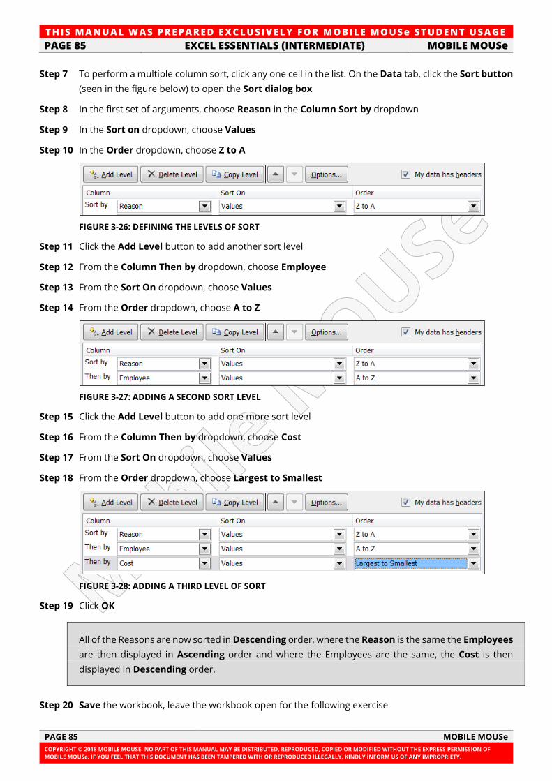
TH IS MANUAL W AS PREPARED EX CLUSIVE LY FOR MOBILE MOUSe ST UDE NT USAGE
PAGE 85 EXCEL ESSENTIALS (INTERMEDIATE) MOBILE MOUSe
PAGE 85 MOBILE MOUSe
COPYRIGHT © 2018 MOBILE MOUSE. NO PART OF THIS MANUAL MAY BE DISTRIBUTED, REPRODUCED, COPIED OR MODIFIED WITHOUT THE EXPRESS PERMISSION OF
MOBILE MOUSe. IF YOU FEEL THAT THIS DOCUMENT HAS BEEN TAMPERED WITH OR REPRODUCED ILLEGALLY, KINDLY INFORM US OF ANY IMPROPRIETY.
Step 7 To perform a multiple column sort, click any one cell in the list. On the Data tab, click the Sort button
(seen in the figure below) to open the Sort dialog box
Step 8 In the first set of arguments, choose Reason in the Column Sort by dropdown
Step 9 In the Sort on dropdown, choose Values
Step 10 In the Order dropdown, choose Z to A
FIGURE 3-26: DEFINING THE LEVELS OF SORT
Step 11 Click the Add Level button to add another sort level
Step 12 From the Column Then by dropdown, choose Employee
Step 13 From the Sort On dropdown, choose Values
Step 14 From the Order dropdown, choose A to Z
FIGURE 3-27: ADDING A SECOND SORT LEVEL
Step 15 Click the Add Level button to add one more sort level
Step 16 From the Column Then by dropdown, choose Cost
Step 17 From the Sort On dropdown, choose Values
Step 18 From the Order dropdown, choose Largest to Smallest
FIGURE 3-28: ADDING A THIRD LEVEL OF SORT
Step 19 Click OK
All of the Reasons are now sorted in Descending order, where the Reason is the same the Employees
are then displayed in Ascending order and where the Employees are the same, the Cost is then
displayed in Descending order.
Step 20 Save the workbook, leave the workbook open for the following exercise
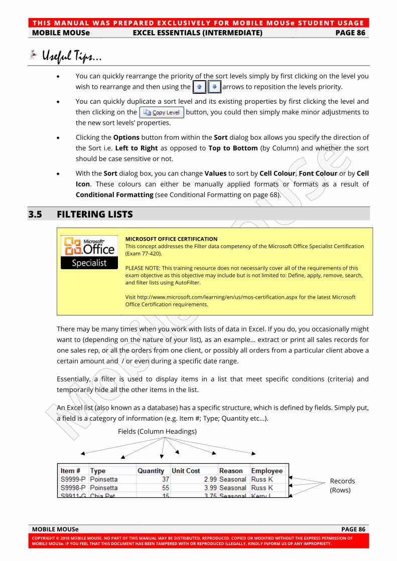
TH IS MANUAL W AS PREPARED EX CLUSIVE LY FOR MOBILE MOUSe ST UDE NT USAGE
MOBILE MOUSe EXCEL ESSENTIALS (INTERMEDIATE) PAGE 86
MOBILE MOUSe PAGE 86
COPYRIGHT © 2018 MOBILE MOUSE. NO PART OF THIS MANUAL MAY BE DISTRIBUTED, REPRODUCED, COPIED OR MODIFIED WITHOUT THE EXPRESS PERMISSION OF
MOBILE MOUSe. IF YOU FEEL THAT THIS DOCUMENT HAS BEEN TAMPERED WITH OR REPRODUCED ILLEGALLY, KINDLY INFORM US OF ANY IMPROPRIETY.
Useful Tips...
• You can quickly rearrange the priority of the sort levels simply by first clicking on the level you
wish to rearrange and then using the arrows to reposition the levels priority.
• You can quickly duplicate a sort level and its existing properties by first clicking the level and
then clicking on the button, you could then simply make minor adjustments to
the new sort levels’ properties.
• Clicking the Options button from within the Sort dialog box allows you specify the direction of
the Sort i.e. Left to Right as opposed to Top to Bottom (by Column) and whether the sort
should be case sensitive or not.
• With the Sort dialog box, you can change Values to sort by Cell Colour, Font Colour or by Cell
Icon. These colours can either be manually applied formats or formats as a result of
Conditional Formatting (see Conditional Formatting on page 68).
3.5 FILTERING LISTS
MICROSOFT OFFICE CERTIFICATION
This concept addresses the Filter data competency of the Microsoft Office Specialist Certification
(Exam 77-420).
PLEASE NOTE: This training resource does not necessarily cover all of the requirements of this
exam objective as this objective may include but is not limited to: Define, apply, remove, search,
and filter lists using AutoFilter.
Visit http://www.microsoft.com/learning/en/us/mos-certification.aspx for the latest Microsoft
Office Certification requirements.
There may be many times when you work with lists of data in Excel. If you do, you occasionally might
want to (depending on the nature of your list), as an example... extract or print all sales records for
one sales rep, or all the orders from one client, or possibly all orders from a particular client above a
certain amount and / or even during a specific date range.
Essentially, a filter is used to display items in a list that meet specific conditions (criteria) and
temporarily hide all the other items in the list.
An Excel list (also known as a database) has a specific structure, which is defined by fields. Simply put,
a field is a category of information (e.g. Item #; Type; Quantity etc…).
Fields (Column Headings)
Records
(Rows)
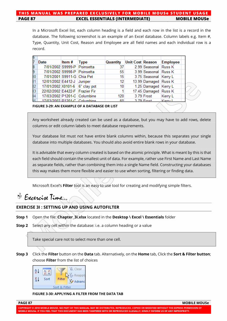
TH IS MANUAL W AS PREPARED EX CLUSIVE LY FOR MOBILE MOUSe ST UDE NT USAGE
PAGE 87 EXCEL ESSENTIALS (INTERMEDIATE) MOBILE MOUSe
PAGE 87 MOBILE MOUSe
COPYRIGHT © 2018 MOBILE MOUSE. NO PART OF THIS MANUAL MAY BE DISTRIBUTED, REPRODUCED, COPIED OR MODIFIED WITHOUT THE EXPRESS PERMISSION OF
MOBILE MOUSe. IF YOU FEEL THAT THIS DOCUMENT HAS BEEN TAMPERED WITH OR REPRODUCED ILLEGALLY, KINDLY INFORM US OF ANY IMPROPRIETY.
In a Microsoft Excel list, each column heading is a field and each row in the list is a record in the
database. The following screenshot is an example of an Excel database. Column labels e.g. Item #,
Type, Quantity, Unit Cost, Reason and Employee are all field names and each individual row is a
record.
FIGURE 3-29: AN EXAMPLE OF A DATABASE OR LIST
Any worksheet already created can be used as a database, but you may have to add rows, delete
columns or edit column labels to meet database requirements.
Your database list must not have entire blank columns within, because this separates your single
database into multiple databases. You should also avoid entire blank rows in your database.
It is advisable that every column created is based on the atomic principle. What is meant by this is that
each field should contain the smallest unit of data. For example, rather use First Name and Last Name
as separate fields, rather than combining them into a single Name field. Constructing your databases
this way makes them more flexible and easier to use when sorting, filtering or finding data.
Microsoft Excel’s Filter tool is an easy to use tool for creating and modifying simple filters.
Excercise Time... EXERCISE 3I : SETTING UP AND USING AUTOFILTER
Step 1 Open the file: Chapter_3i.xlsx located in the Desktop \ Excel \ Essentials folder
Step 2 Select any cell within the database: i.e. a column heading or a value
Take special care not to select more than one cell.
Step 3 Click the Filter button on the Data tab. Alternatively, on the Home tab, Click the Sort & Filter button;
choose Filter from the list of choices
FIGURE 3-30: APPLYING A FILTER FROM THE DATA TAB
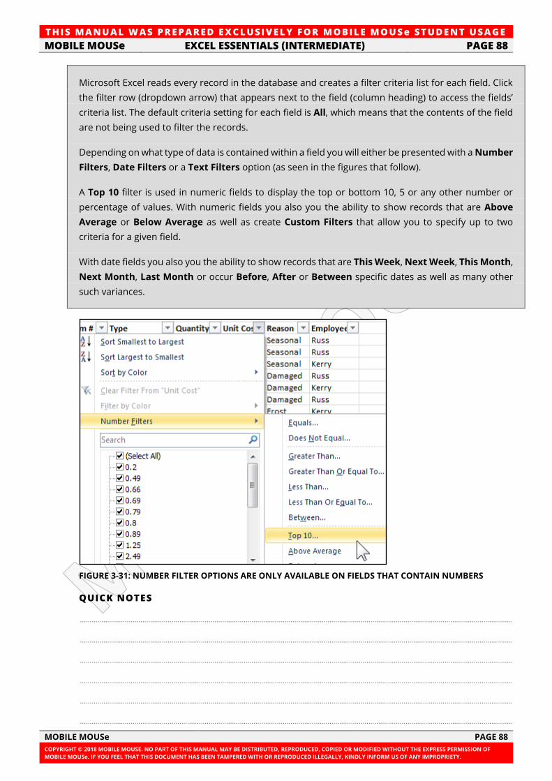
TH IS MANUAL W AS PREPARED EX CLUSIVE LY FOR MOBILE MOUSe ST UDE NT USAGE
MOBILE MOUSe EXCEL ESSENTIALS (INTERMEDIATE) PAGE 88
MOBILE MOUSe PAGE 88
COPYRIGHT © 2018 MOBILE MOUSE. NO PART OF THIS MANUAL MAY BE DISTRIBUTED, REPRODUCED, COPIED OR MODIFIED WITHOUT THE EXPRESS PERMISSION OF
MOBILE MOUSe. IF YOU FEEL THAT THIS DOCUMENT HAS BEEN TAMPERED WITH OR REPRODUCED ILLEGALLY, KINDLY INFORM US OF ANY IMPROPRIETY.
Microsoft Excel reads every record in the database and creates a filter criteria list for each field. Click
the filter row (dropdown arrow) that appears next to the field (column heading) to access the fields’
criteria list. The default criteria setting for each field is All, which means that the contents of the field
are not being used to filter the records.
Depending on what type of data is contained within a field you will either be presented with a Number
Filters, Date Filters or a Text Filters option (as seen in the figures that follow).
A Top 10 filter is used in numeric fields to display the top or bottom 10, 5 or any other number or
percentage of values. With numeric fields you also you the ability to show records that are Above
Average or Below Average as well as create Custom Filters that allow you to specify up to two
criteria for a given field.
With date fields you also you the ability to show records that are This Week, Next Week, This Month,
Next Month, Last Month or occur Before, After or Between specific dates as well as many other
such variances.
FIGURE 3-31: NUMBER FILTER OPTIONS ARE ONLY AVAILABLE ON FIELDS THAT CONTAIN NUMBERS
QUICK NOTES
..............................................................................................................................................................................................................................
..............................................................................................................................................................................................................................
..............................................................................................................................................................................................................................
..............................................................................................................................................................................................................................
..............................................................................................................................................................................................................................
..............................................................................................................................................................................................................................
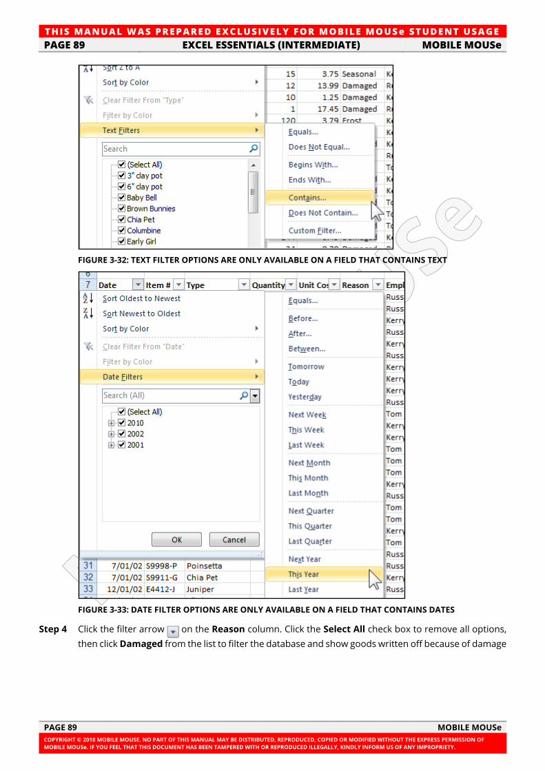
TH IS MANUAL W AS PREPARED EX CLUSIVE LY FOR MOBILE MOUSe ST UDE NT USAGE
PAGE 89 EXCEL ESSENTIALS (INTERMEDIATE) MOBILE MOUSe
PAGE 89 MOBILE MOUSe
COPYRIGHT © 2018 MOBILE MOUSE. NO PART OF THIS MANUAL MAY BE DISTRIBUTED, REPRODUCED, COPIED OR MODIFIED WITHOUT THE EXPRESS PERMISSION OF
MOBILE MOUSe. IF YOU FEEL THAT THIS DOCUMENT HAS BEEN TAMPERED WITH OR REPRODUCED ILLEGALLY, KINDLY INFORM US OF ANY IMPROPRIETY.
FIGURE 3-32: TEXT FILTER OPTIONS ARE ONLY AVAILABLE ON A FIELD THAT CONTAINS TEXT
FIGURE 3-33: DATE FILTER OPTIONS ARE ONLY AVAILABLE ON A FIELD THAT CONTAINS DATES
Step 4 Click the filter arrow on the Reason column. Click the Select All check box to remove all options,
then click Damaged from the list to filter the database and show goods written off because of damage
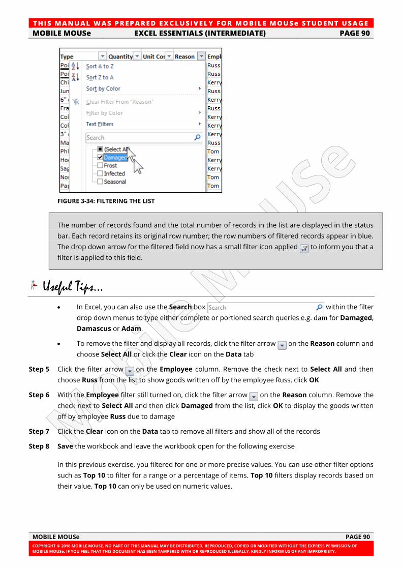
TH IS MANUAL W AS PREPARED EX CLUSIVE LY FOR MOBILE MOUSe ST UDE NT USAGE
MOBILE MOUSe EXCEL ESSENTIALS (INTERMEDIATE) PAGE 90
MOBILE MOUSe PAGE 90
COPYRIGHT © 2018 MOBILE MOUSE. NO PART OF THIS MANUAL MAY BE DISTRIBUTED, REPRODUCED, COPIED OR MODIFIED WITHOUT THE EXPRESS PERMISSION OF
MOBILE MOUSe. IF YOU FEEL THAT THIS DOCUMENT HAS BEEN TAMPERED WITH OR REPRODUCED ILLEGALLY, KINDLY INFORM US OF ANY IMPROPRIETY.
FIGURE 3-34: FILTERING THE LIST
The number of records found and the total number of records in the list are displayed in the status
bar. Each record retains its original row number; the row numbers of filtered records appear in blue.
The drop down arrow for the filtered field now has a small filter icon applied to inform you that a
filter is applied to this field.
Useful Tips...
• In Excel, you can also use the Search box within the filter
drop down menus to type either complete or portioned search queries e.g. dam for Damaged,
Damascus or Adam.
• To remove the filter and display all records, click the filter arrow on the Reason column and
choose Select All or click the Clear icon on the Data tab
Step 5 Click the filter arrow on the Employee column. Remove the check next to Select All and then
choose Russ from the list to show goods written off by the employee Russ, click OK
Step 6 With the Employee filter still turned on, click the filter arrow on the Reason column. Remove the
check next to Select All and then click Damaged from the list, click OK to display the goods written
off by employee Russ due to damage
Step 7 Click the Clear icon on the Data tab to remove all filters and show all of the records
Step 8 Save the workbook and leave the workbook open for the following exercise
In this previous exercise, you filtered for one or more precise values. You can use other filter options
such as Top 10 to filter for a range or a percentage of items. Top 10 filters display records based on
their value. Top 10 can only be used on numeric values.
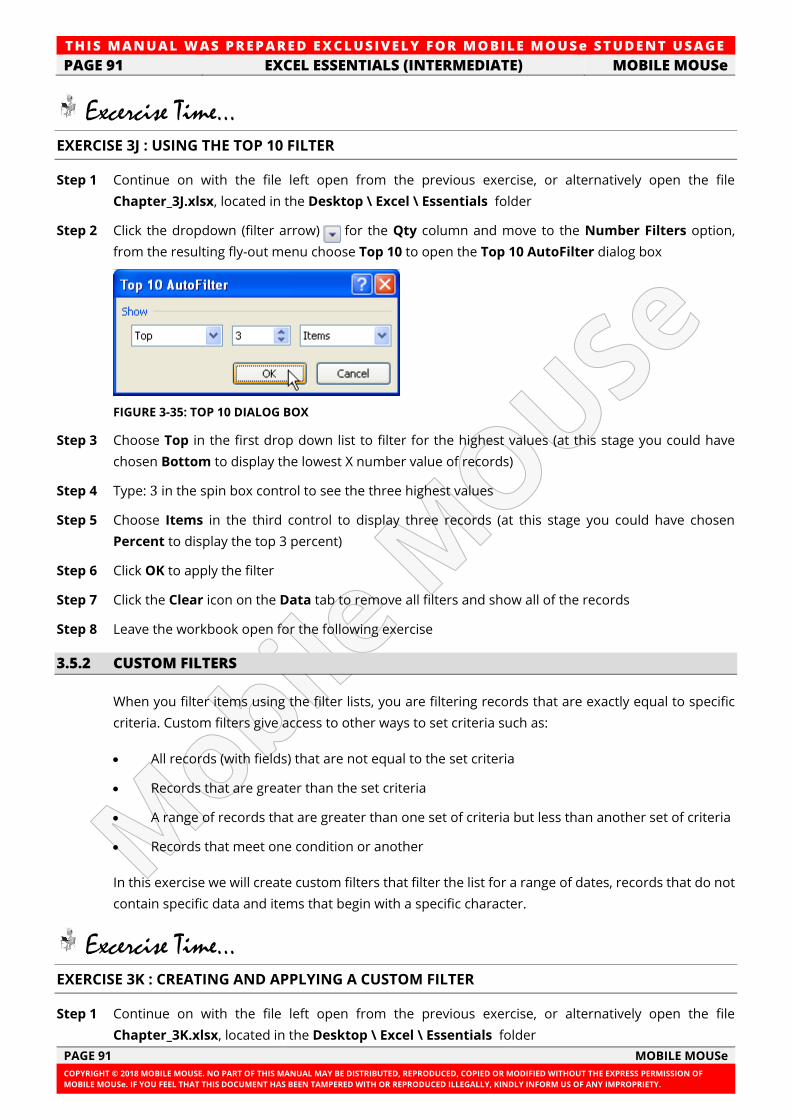
TH IS MANUAL W AS PREPARED EX CLUSIVE LY FOR MOBILE MOUSe ST UDE NT USAGE
PAGE 91 EXCEL ESSENTIALS (INTERMEDIATE) MOBILE MOUSe
PAGE 91 MOBILE MOUSe
COPYRIGHT © 2018 MOBILE MOUSE. NO PART OF THIS MANUAL MAY BE DISTRIBUTED, REPRODUCED, COPIED OR MODIFIED WITHOUT THE EXPRESS PERMISSION OF
MOBILE MOUSe. IF YOU FEEL THAT THIS DOCUMENT HAS BEEN TAMPERED WITH OR REPRODUCED ILLEGALLY, KINDLY INFORM US OF ANY IMPROPRIETY.
Excercise Time... EXERCISE 3J : USING THE TOP 10 FILTER
Step 1 Continue on with the file left open from the previous exercise, or alternatively open the file
Chapter_3J.xlsx, located in the Desktop \ Excel \ Essentials folder
Step 2 Click the dropdown (filter arrow) for the Qty column and move to the Number Filters option,
from the resulting fly-out menu choose Top 10 to open the Top 10 AutoFilter dialog box
FIGURE 3-35: TOP 10 DIALOG BOX
Step 3 Choose Top in the first drop down list to filter for the highest values (at this stage you could have
chosen Bottom to display the lowest X number value of records)
Step 4 Type: 3 in the spin box control to see the three highest values
Step 5 Choose Items in the third control to display three records (at this stage you could have chosen
Percent to display the top 3 percent)
Step 6 Click OK to apply the filter
Step 7 Click the Clear icon on the Data tab to remove all filters and show all of the records
Step 8 Leave the workbook open for the following exercise
3.5.2 CUSTOM FILTERS
When you filter items using the filter lists, you are filtering records that are exactly equal to specific
criteria. Custom filters give access to other ways to set criteria such as:
• All records (with fields) that are not equal to the set criteria
• Records that are greater than the set criteria
• A range of records that are greater than one set of criteria but less than another set of criteria
• Records that meet one condition or another
In this exercise we will create custom filters that filter the list for a range of dates, records that do not
contain specific data and items that begin with a specific character.
Excercise Time... EXERCISE 3K : CREATING AND APPLYING A CUSTOM FILTER
Step 1 Continue on with the file left open from the previous exercise, or alternatively open the file
Chapter_3K.xlsx, located in the Desktop \ Excel \ Essentials folder
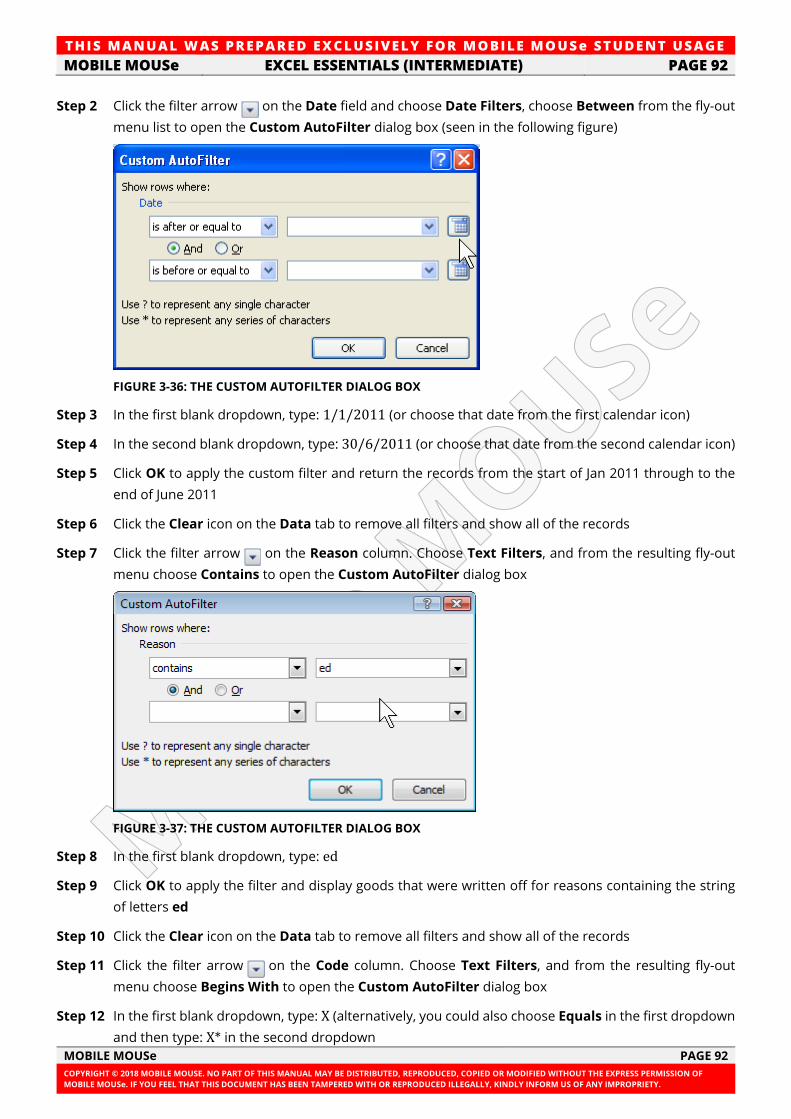
TH IS MANUAL W AS PREPARED EX CLUSIVE LY FOR MOBILE MOUSe ST UDE NT USAGE
MOBILE MOUSe EXCEL ESSENTIALS (INTERMEDIATE) PAGE 92
MOBILE MOUSe PAGE 92
COPYRIGHT © 2018 MOBILE MOUSE. NO PART OF THIS MANUAL MAY BE DISTRIBUTED, REPRODUCED, COPIED OR MODIFIED WITHOUT THE EXPRESS PERMISSION OF
MOBILE MOUSe. IF YOU FEEL THAT THIS DOCUMENT HAS BEEN TAMPERED WITH OR REPRODUCED ILLEGALLY, KINDLY INFORM US OF ANY IMPROPRIETY.
Step 2 Click the filter arrow on the Date field and choose Date Filters, choose Between from the fly-out
menu list to open the Custom AutoFilter dialog box (seen in the following figure)
FIGURE 3-36: THE CUSTOM AUTOFILTER DIALOG BOX
Step 3 In the first blank dropdown, type: 1/1/2011 (or choose that date from the first calendar icon)
Step 4 In the second blank dropdown, type: 30/6/2011 (or choose that date from the second calendar icon)
Step 5 Click OK to apply the custom filter and return the records from the start of Jan 2011 through to the
end of June 2011
Step 6 Click the Clear icon on the Data tab to remove all filters and show all of the records
Step 7 Click the filter arrow on the Reason column. Choose Text Filters, and from the resulting fly-out
menu choose Contains to open the Custom AutoFilter dialog box
FIGURE 3-37: THE CUSTOM AUTOFILTER DIALOG BOX
Step 8 In the first blank dropdown, type: ed
Step 9 Click OK to apply the filter and display goods that were written off for reasons containing the string
of letters ed
Step 10 Click the Clear icon on the Data tab to remove all filters and show all of the records
Step 11 Click the filter arrow on the Code column. Choose Text Filters, and from the resulting fly-out
menu choose Begins With to open the Custom AutoFilter dialog box
Step 12 In the first blank dropdown, type: X (alternatively, you could also choose Equals in the first dropdown
and then type: X* in the second dropdown
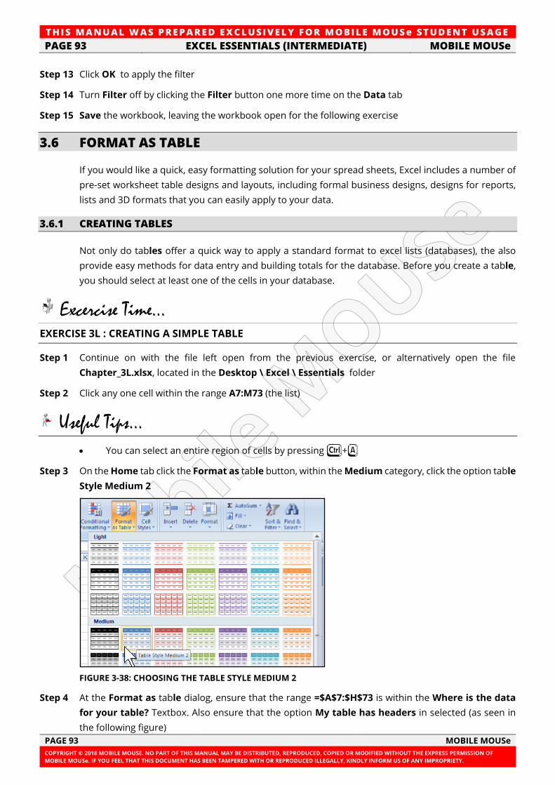
TH IS MANUAL W AS PREPARED EX CLUSIVE LY FOR MOBILE MOUSe ST UDE NT USAGE
PAGE 93 EXCEL ESSENTIALS (INTERMEDIATE) MOBILE MOUSe
PAGE 93 MOBILE MOUSe
COPYRIGHT © 2018 MOBILE MOUSE. NO PART OF THIS MANUAL MAY BE DISTRIBUTED, REPRODUCED, COPIED OR MODIFIED WITHOUT THE EXPRESS PERMISSION OF
MOBILE MOUSe. IF YOU FEEL THAT THIS DOCUMENT HAS BEEN TAMPERED WITH OR REPRODUCED ILLEGALLY, KINDLY INFORM US OF ANY IMPROPRIETY.
Step 13 Click OK to apply the filter
Step 14 Turn Filter off by clicking the Filter button one more time on the Data tab
Step 15 Save the workbook, leaving the workbook open for the following exercise
3.6 FORMAT AS TABLE
If you would like a quick, easy formatting solution for your spread sheets, Excel includes a number of
pre-set worksheet table designs and layouts, including formal business designs, designs for reports,
lists and 3D formats that you can easily apply to your data.
3.6.1 CREATING TABLES
Not only do tables offer a quick way to apply a standard format to excel lists (databases), the also
provide easy methods for data entry and building totals for the database. Before you create a table,
you should select at least one of the cells in your database.
Excercise Time... EXERCISE 3L : CREATING A SIMPLE TABLE
Step 1 Continue on with the file left open from the previous exercise, or alternatively open the file
Chapter_3L.xlsx, located in the Desktop \ Excel \ Essentials folder
Step 2 Click any one cell within the range A7:M73 (the list)
Useful Tips...
• You can select an entire region of cells by pressing F+A
Step 3 On the Home tab click the Format as table button, within the Medium category, click the option table
Style Medium 2
FIGURE 3-38: CHOOSING THE TABLE STYLE MEDIUM 2
Step 4 At the Format as table dialog, ensure that the range =$A$7:$H$73 is within the Where is the data
for your table? Textbox. Also ensure that the option My table has headers in selected (as seen in
the following figure)
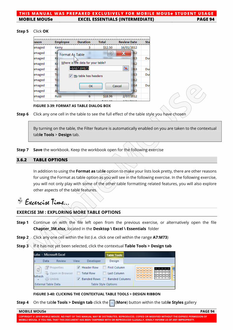
TH IS MANUAL W AS PREPARED EX CLUSIVE LY FOR MOBILE MOUSe ST UDE NT USAGE
MOBILE MOUSe EXCEL ESSENTIALS (INTERMEDIATE) PAGE 94
MOBILE MOUSe PAGE 94
COPYRIGHT © 2018 MOBILE MOUSE. NO PART OF THIS MANUAL MAY BE DISTRIBUTED, REPRODUCED, COPIED OR MODIFIED WITHOUT THE EXPRESS PERMISSION OF
MOBILE MOUSe. IF YOU FEEL THAT THIS DOCUMENT HAS BEEN TAMPERED WITH OR REPRODUCED ILLEGALLY, KINDLY INFORM US OF ANY IMPROPRIETY.
Step 5 Click OK
FIGURE 3-39: FORMAT AS TABLE DIALOG BOX
Step 6 Click any one cell in the table to see the full effect of the table style you have chosen
By turning on the table, the Filter feature is automatically enabled on you are taken to the contextual
table Tools > Design tab.
Step 7 Save the workbook. Keep the workbook open for the following exercise
3.6.2 TABLE OPTIONS
In addition to using the Format as table option to make your lists look pretty, there are other reasons
for using the Format as table option as you will see in the following exercise. In the following exercise,
you will not only play with some of the other table formatting related features, you will also explore
other aspects of the table features.
Excercise Time... EXERCISE 3M : EXPLORING MORE TABLE OPTIONS
Step 1 Continue on with the file left open from the previous exercise, or alternatively open the file
Chapter_3M.xlsx, located in the Desktop \ Excel \ Essentials folder
Step 2 Click any one cell within the list (i.e. click one cell within the range A7:M73)
Step 3 If it has not yet been selected, click the contextual Table Tools > Design tab
FIGURE 3-40: CLICKING THE CONTEXTUAL TABLE TOOLS > DESIGN RIBBON
Step 4 On the table Tools > Design tab click the (More) button within the table Styles gallery
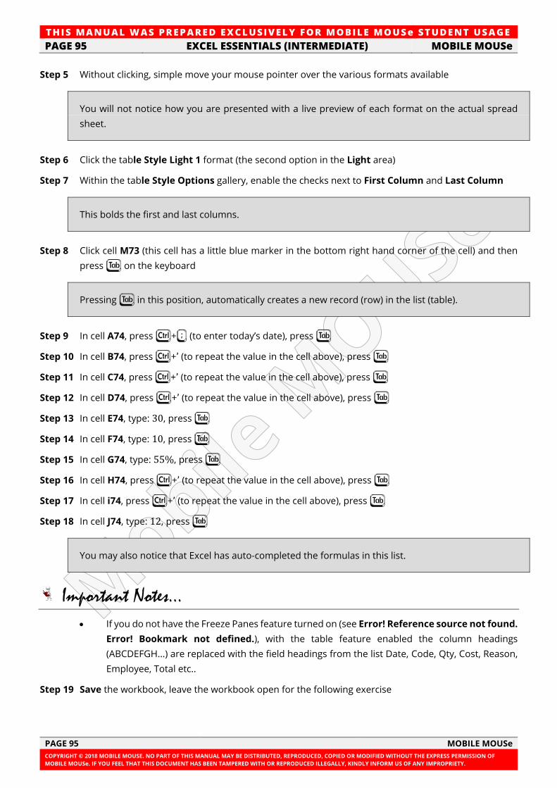
TH IS MANUAL W AS PREPARED EX CLUSIVE LY FOR MOBILE MOUSe ST UDE NT USAGE
PAGE 95 EXCEL ESSENTIALS (INTERMEDIATE) MOBILE MOUSe
PAGE 95 MOBILE MOUSe
COPYRIGHT © 2018 MOBILE MOUSE. NO PART OF THIS MANUAL MAY BE DISTRIBUTED, REPRODUCED, COPIED OR MODIFIED WITHOUT THE EXPRESS PERMISSION OF
MOBILE MOUSe. IF YOU FEEL THAT THIS DOCUMENT HAS BEEN TAMPERED WITH OR REPRODUCED ILLEGALLY, KINDLY INFORM US OF ANY IMPROPRIETY.
Step 5 Without clicking, simple move your mouse pointer over the various formats available
You will not notice how you are presented with a live preview of each format on the actual spread
sheet.
Step 6 Click the table Style Light 1 format (the second option in the Light area)
Step 7 Within the table Style Options gallery, enable the checks next to First Column and Last Column
This bolds the first and last columns.
Step 8 Click cell M73 (this cell has a little blue marker in the bottom right hand corner of the cell) and then
press N on the keyboard
Pressing N in this position, automatically creates a new record (row) in the list (table).
Step 9 In cell A74, press F+; (to enter today’s date), press N
Step 10 In cell B74, press F+’ (to repeat the value in the cell above), press N
Step 11 In cell C74, press F+’ (to repeat the value in the cell above), press N
Step 12 In cell D74, press F+’ (to repeat the value in the cell above), press N
Step 13 In cell E74, type: 30, press N
Step 14 In cell F74, type: 10, press N
Step 15 In cell G74, type: 55%, press N
Step 16 In cell H74, press F+’ (to repeat the value in the cell above), press N
Step 17 In cell i74, press F+’ (to repeat the value in the cell above), press N
Step 18 In cell J74, type: 12, press N
You may also notice that Excel has auto-completed the formulas in this list.
Important Notes...
• If you do not have the Freeze Panes feature turned on (see Error! Reference source not found.
Error! Bookmark not defined.), with the table feature enabled the column headings
(ABCDEFGH...) are replaced with the field headings from the list Date, Code, Qty, Cost, Reason,
Employee, Total etc..
Step 19 Save the workbook, leave the workbook open for the following exercise
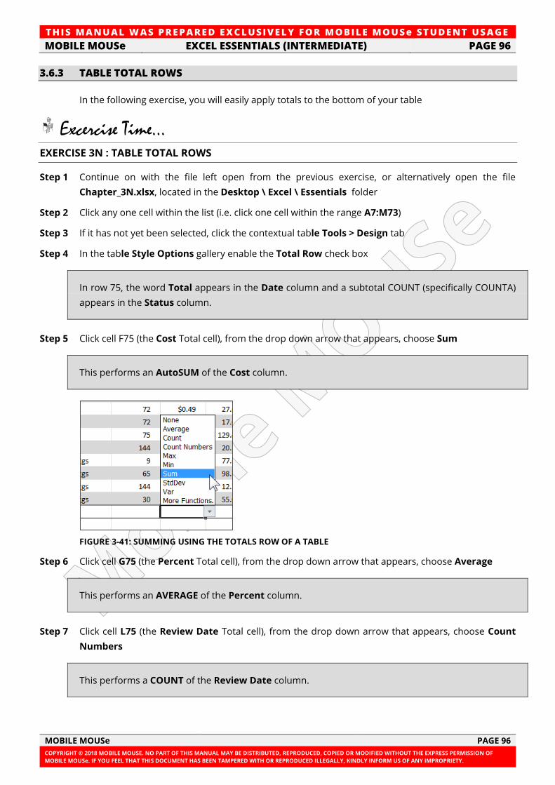
TH IS MANUAL W AS PREPARED EX CLUSIVE LY FOR MOBILE MOUSe ST UDE NT USAGE
MOBILE MOUSe EXCEL ESSENTIALS (INTERMEDIATE) PAGE 96
MOBILE MOUSe PAGE 96
COPYRIGHT © 2018 MOBILE MOUSE. NO PART OF THIS MANUAL MAY BE DISTRIBUTED, REPRODUCED, COPIED OR MODIFIED WITHOUT THE EXPRESS PERMISSION OF
MOBILE MOUSe. IF YOU FEEL THAT THIS DOCUMENT HAS BEEN TAMPERED WITH OR REPRODUCED ILLEGALLY, KINDLY INFORM US OF ANY IMPROPRIETY.
3.6.3 TABLE TOTAL ROWS
In the following exercise, you will easily apply totals to the bottom of your table
Excercise Time... EXERCISE 3N : TABLE TOTAL ROWS
Step 1 Continue on with the file left open from the previous exercise, or alternatively open the file
Chapter_3N.xlsx, located in the Desktop \ Excel \ Essentials folder
Step 2 Click any one cell within the list (i.e. click one cell within the range A7:M73)
Step 3 If it has not yet been selected, click the contextual table Tools > Design tab
Step 4 In the table Style Options gallery enable the Total Row check box
In row 75, the word Total appears in the Date column and a subtotal COUNT (specifically COUNTA)
appears in the Status column.
Step 5 Click cell F75 (the Cost Total cell), from the drop down arrow that appears, choose Sum
This performs an AutoSUM of the Cost column.
FIGURE 3-41: SUMMING USING THE TOTALS ROW OF A TABLE
Step 6 Click cell G75 (the Percent Total cell), from the drop down arrow that appears, choose Average
This performs an AVERAGE of the Percent column.
Step 7 Click cell L75 (the Review Date Total cell), from the drop down arrow that appears, choose Count
Numbers
This performs a COUNT of the Review Date column.
TH IS MANUAL W AS PREPARED EX CLUSIVE LY FOR MOBILE MOUSe ST UDE NT USAGE
PAGE 97 EXCEL ESSENTIALS (INTERMEDIATE) MOBILE MOUSe
PAGE 97 MOBILE MOUSe
COPYRIGHT © 2018 MOBILE MOUSE. NO PART OF THIS MANUAL MAY BE DISTRIBUTED, REPRODUCED, COPIED OR MODIFIED WITHOUT THE EXPRESS PERMISSION OF
MOBILE MOUSe. IF YOU FEEL THAT THIS DOCUMENT HAS BEEN TAMPERED WITH OR REPRODUCED ILLEGALLY, KINDLY INFORM US OF ANY IMPROPRIETY.
Step 8 On the table Tools > Design tab within the table Style Options gallery, uncheck the Total Row check
box
Step 9 Click any one cell within the table (the range A7:M74), within the Tools group (on the table Tools >
Design tab), click the Convert to Range button
Step 10 At the dialog box that appears, click Yes to convert the list to a conventional range
Step 11 Save the workbook, leave the workbook open for the following exercise
3.7 STYLES
MICROSOFT OFFICE CERTIFICATION
This concept addresses the Create and apply cell styles competency of the Microsoft Office
Specialist Certification (Exam 77-420).
PLEASE NOTE: This training resource does not necessarily cover all of the requirements of this
exam objective as this objective may include but is not limited to: Apply cell styles, construct new
cell styles.
Visit http://www.microsoft.com/learning/en/us/mos-certification.aspx for the latest Microsoft
Office Certification requirements.
Styles are simply pre-set formats that can be easily applied to cells. In the following exercise you will
create and apply styles.
Excercise Time... EXERCISE 3O : CREATING AND APPLYING STYLES
Step 1 Continue on with the file left open from the previous exercise, or alternatively open the file
Chapter_3O.xlsx, located in the Desktop \ Excel \ Essentials folder
Step 2 Select the range A7:M7 (the heading row of your list)
Step 3 On the Home tab click the Cell Styles button within the Styles gallery
From the series of choices presented, move your mouse over various choices, again notice how you
are presented with a live preview of the formatting.
Step 4 Click the Heading 3 style
QUICK NOTES
..............................................................................................................................................................................................................................
..............................................................................................................................................................................................................................
..............................................................................................................................................................................................................................
..............................................................................................................................................................................................................................
..............................................................................................................................................................................................................................
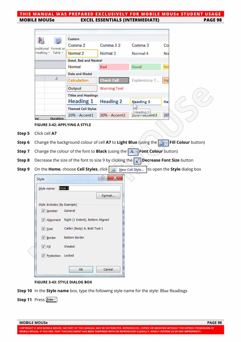
TH IS MANUAL W AS PREPARED EX CLUSIVE LY FOR MOBILE MOUSe ST UDE NT USAGE
MOBILE MOUSe EXCEL ESSENTIALS (INTERMEDIATE) PAGE 98
MOBILE MOUSe PAGE 98
COPYRIGHT © 2018 MOBILE MOUSE. NO PART OF THIS MANUAL MAY BE DISTRIBUTED, REPRODUCED, COPIED OR MODIFIED WITHOUT THE EXPRESS PERMISSION OF
MOBILE MOUSe. IF YOU FEEL THAT THIS DOCUMENT HAS BEEN TAMPERED WITH OR REPRODUCED ILLEGALLY, KINDLY INFORM US OF ANY IMPROPRIETY.
FIGURE 3-42: APPLYING A STYLE
Step 5 Click cell A7
Step 6 Change the background colour of cell A7 to Light Blue (using the Fill Colour button)
Step 7 Change the colour of the font to Black (using the Font Colour button)
Step 8 Decrease the size of the font to size 9 by clicking the Decrease Font Size button
Step 9 On the Home, choose Cell Styles, click to open the Style dialog box
FIGURE 3-43: STYLE DIALOG BOX
Step 10 In the Style name box, type the following style name for the style: Blue Headings
Step 11 Press I
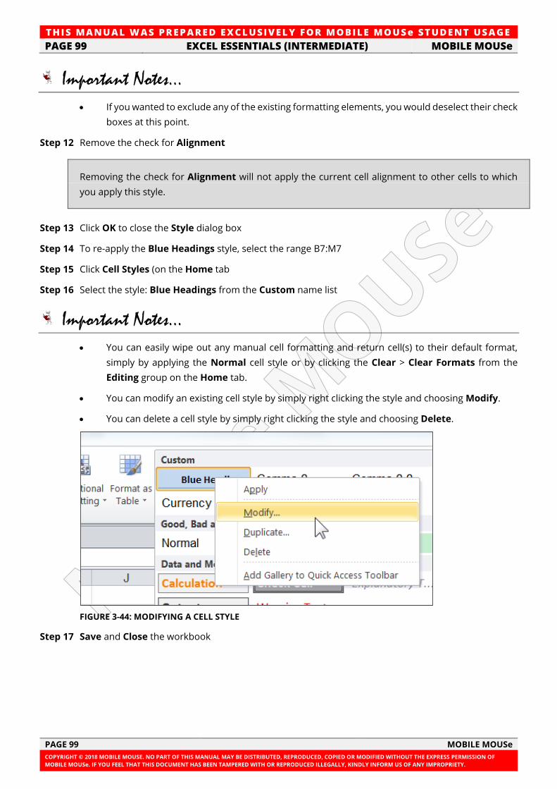
TH IS MANUAL W AS PREPARED EX CLUSIVE LY FOR MOBILE MOUSe ST UDE NT USAGE
PAGE 99 EXCEL ESSENTIALS (INTERMEDIATE) MOBILE MOUSe
PAGE 99 MOBILE MOUSe
COPYRIGHT © 2018 MOBILE MOUSE. NO PART OF THIS MANUAL MAY BE DISTRIBUTED, REPRODUCED, COPIED OR MODIFIED WITHOUT THE EXPRESS PERMISSION OF
MOBILE MOUSe. IF YOU FEEL THAT THIS DOCUMENT HAS BEEN TAMPERED WITH OR REPRODUCED ILLEGALLY, KINDLY INFORM US OF ANY IMPROPRIETY.
Important Notes...
• If you wanted to exclude any of the existing formatting elements, you would deselect their check
boxes at this point.
Step 12 Remove the check for Alignment
Removing the check for Alignment will not apply the current cell alignment to other cells to which
you apply this style.
Step 13 Click OK to close the Style dialog box
Step 14 To re-apply the Blue Headings style, select the range B7:M7
Step 15 Click Cell Styles (on the Home tab
Step 16 Select the style: Blue Headings from the Custom name list
Important Notes...
• You can easily wipe out any manual cell formatting and return cell(s) to their default format,
simply by applying the Normal cell style or by clicking the Clear > Clear Formats from the
Editing group on the Home tab.
• You can modify an existing cell style by simply right clicking the style and choosing Modify.
• You can delete a cell style by simply right clicking the style and choosing Delete.
FIGURE 3-44: MODIFYING A CELL STYLE
Step 17 Save and Close the workbook
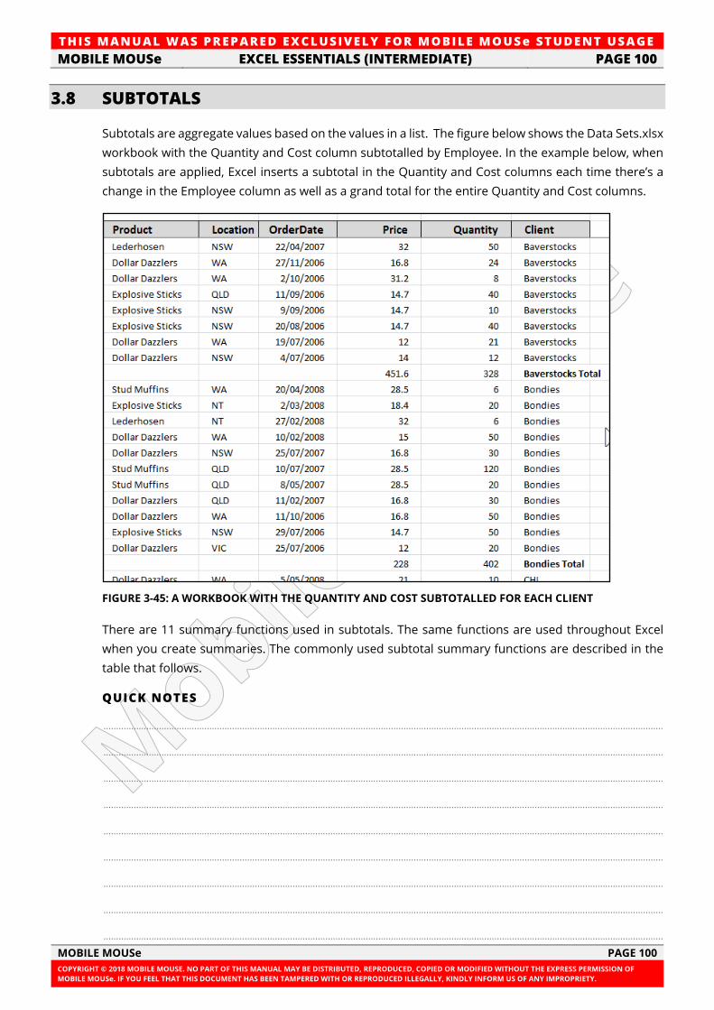
TH IS MANUAL W AS PREPARED EX CLUSIVE LY FOR MOBILE MOUSe ST UDE NT USAGE
MOBILE MOUSe EXCEL ESSENTIALS (INTERMEDIATE) PAGE 100
MOBILE MOUSe PAGE 100
COPYRIGHT © 2018 MOBILE MOUSE. NO PART OF THIS MANUAL MAY BE DISTRIBUTED, REPRODUCED, COPIED OR MODIFIED WITHOUT THE EXPRESS PERMISSION OF
MOBILE MOUSe. IF YOU FEEL THAT THIS DOCUMENT HAS BEEN TAMPERED WITH OR REPRODUCED ILLEGALLY, KINDLY INFORM US OF ANY IMPROPRIETY.
3.8 SUBTOTALS
Subtotals are aggregate values based on the values in a list. The figure below shows the Data Sets.xlsx
workbook with the Quantity and Cost column subtotalled by Employee. In the example below, when
subtotals are applied, Excel inserts a subtotal in the Quantity and Cost columns each time there’s a
change in the Employee column as well as a grand total for the entire Quantity and Cost columns.
FIGURE 3-45: A WORKBOOK WITH THE QUANTITY AND COST SUBTOTALLED FOR EACH CLIENT
There are 11 summary functions used in subtotals. The same functions are used throughout Excel
when you create summaries. The commonly used subtotal summary functions are described in the
table that follows.
QUICK NOTES
..............................................................................................................................................................................................................................
..............................................................................................................................................................................................................................
..............................................................................................................................................................................................................................
..............................................................................................................................................................................................................................
..............................................................................................................................................................................................................................
..............................................................................................................................................................................................................................
..............................................................................................................................................................................................................................
..............................................................................................................................................................................................................................
..............................................................................................................................................................................................................................
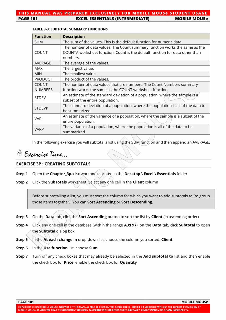
TH IS MANUAL W AS PREPARED EX CLUSIVE LY FOR MOBILE MOUSe ST UDE NT USAGE
PAGE 101 EXCEL ESSENTIALS (INTERMEDIATE) MOBILE MOUSe
PAGE 101 MOBILE MOUSe
COPYRIGHT © 2018 MOBILE MOUSE. NO PART OF THIS MANUAL MAY BE DISTRIBUTED, REPRODUCED, COPIED OR MODIFIED WITHOUT THE EXPRESS PERMISSION OF
MOBILE MOUSe. IF YOU FEEL THAT THIS DOCUMENT HAS BEEN TAMPERED WITH OR REPRODUCED ILLEGALLY, KINDLY INFORM US OF ANY IMPROPRIETY.
TABLE 3-3: SUBTOTAL SUMMARY FUNCTIONS
Function Description
SUM The sum of the values. This is the default function for numeric data.
COUNT
The number of data values. The Count summary function works the same as the
COUNTA worksheet function. Count is the default function for data other than
numbers.
AVERAGE The average of the values.
MAX The largest value.
MIN The smallest value.
PRODUCT The product of the values.
COUNT
NUMBERS
The number of data values that are numbers. The Count Numbers summary
function works the same as the COUNT worksheet function.
STDEV An estimate of the standard deviation of a population, where the sample is a
subset of the entire population.
STDEVP The standard deviation of a population, where the population is all of the data to
be summarized.
VAR An estimate of the variance of a population, where the sample is a subset of the
entire population.
VARP The variance of a population, where the population is all of the data to be
summarized.
In the following exercise you will subtotal a list using the SUM function and then append an AVERAGE.
Excercise Time... EXERCISE 3P : CREATING SUBTOTALS
Step 1 Open the Chapter_3p.xlsx workbook located in the Desktop \ Excel \ Essentials folder
Step 2 Click the SubTotals worksheet. Select any one cell in the Client column
Before subtotalling a list, you must sort the column for which you want to add subtotals to (to group
those items together). You can Sort Ascending or Sort Descending.
Step 3 On the Data tab, click the Sort Ascending button to sort the list by Client (in ascending order)
Step 4 Click any one cell in the database (within the range A3:F97), on the Data tab, click Subtotal to open
the Subtotal dialog box
Step 5 In the At each change in drop-down list, choose the column you sorted; Client
Step 6 In the Use function list, choose Sum
Step 7 Turn off any check boxes that may already be selected in the Add subtotal to list and then enable
the check box for Price, enable the check box for Quantity
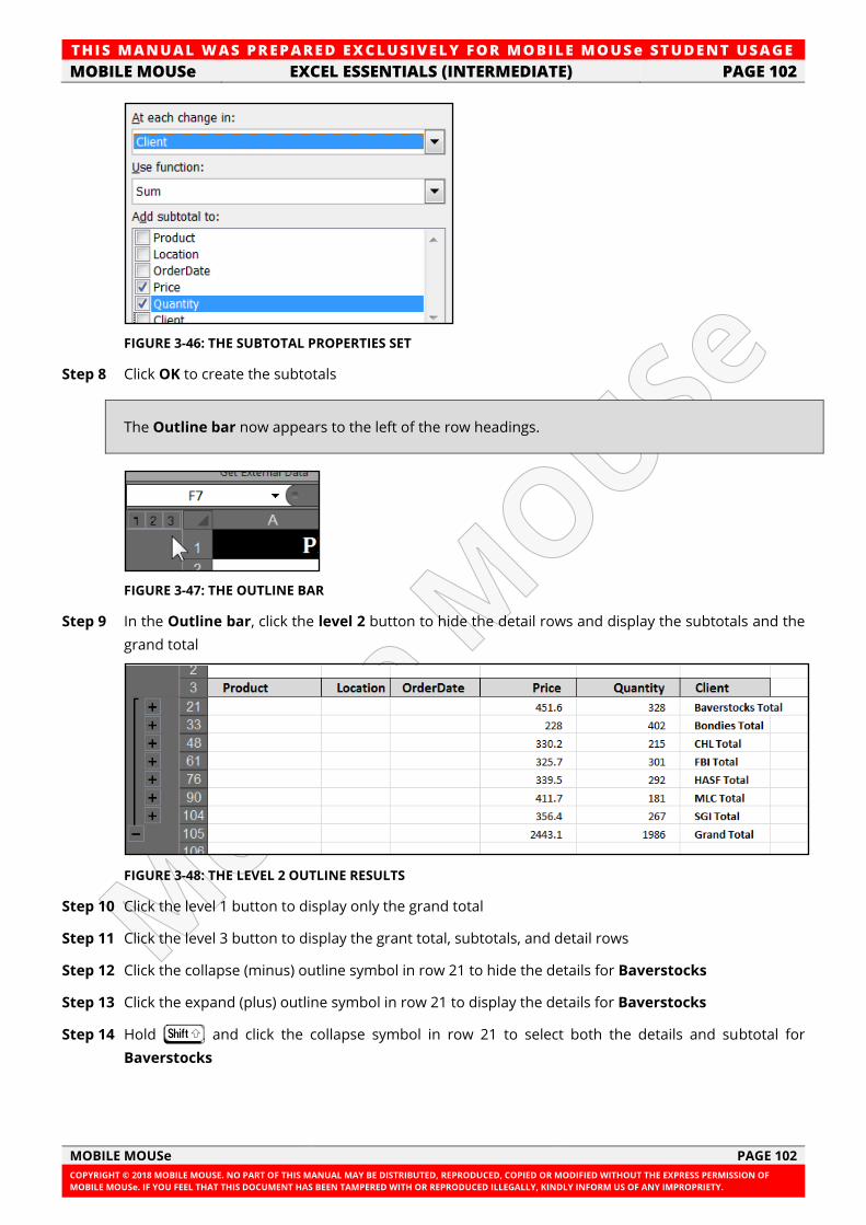
TH IS MANUAL W AS PREPARED EX CLUSIVE LY FOR MOBILE MOUSe ST UDE NT USAGE
MOBILE MOUSe EXCEL ESSENTIALS (INTERMEDIATE) PAGE 102
MOBILE MOUSe PAGE 102
COPYRIGHT © 2018 MOBILE MOUSE. NO PART OF THIS MANUAL MAY BE DISTRIBUTED, REPRODUCED, COPIED OR MODIFIED WITHOUT THE EXPRESS PERMISSION OF
MOBILE MOUSe. IF YOU FEEL THAT THIS DOCUMENT HAS BEEN TAMPERED WITH OR REPRODUCED ILLEGALLY, KINDLY INFORM US OF ANY IMPROPRIETY.
FIGURE 3-46: THE SUBTOTAL PROPERTIES SET
Step 8 Click OK to create the subtotals
The Outline bar now appears to the left of the row headings.
FIGURE 3-47: THE OUTLINE BAR
Step 9 In the Outline bar, click the level 2 button to hide the detail rows and display the subtotals and the
grand total
FIGURE 3-48: THE LEVEL 2 OUTLINE RESULTS
Step 10 Click the level 1 button to display only the grand total
Step 11 Click the level 3 button to display the grant total, subtotals, and detail rows
Step 12 Click the collapse (minus) outline symbol in row 21 to hide the details for Baverstocks
Step 13 Click the expand (plus) outline symbol in row 21 to display the details for Baverstocks
Step 14 Hold G and click the collapse symbol in row 21 to select both the details and subtotal for
Baverstocks
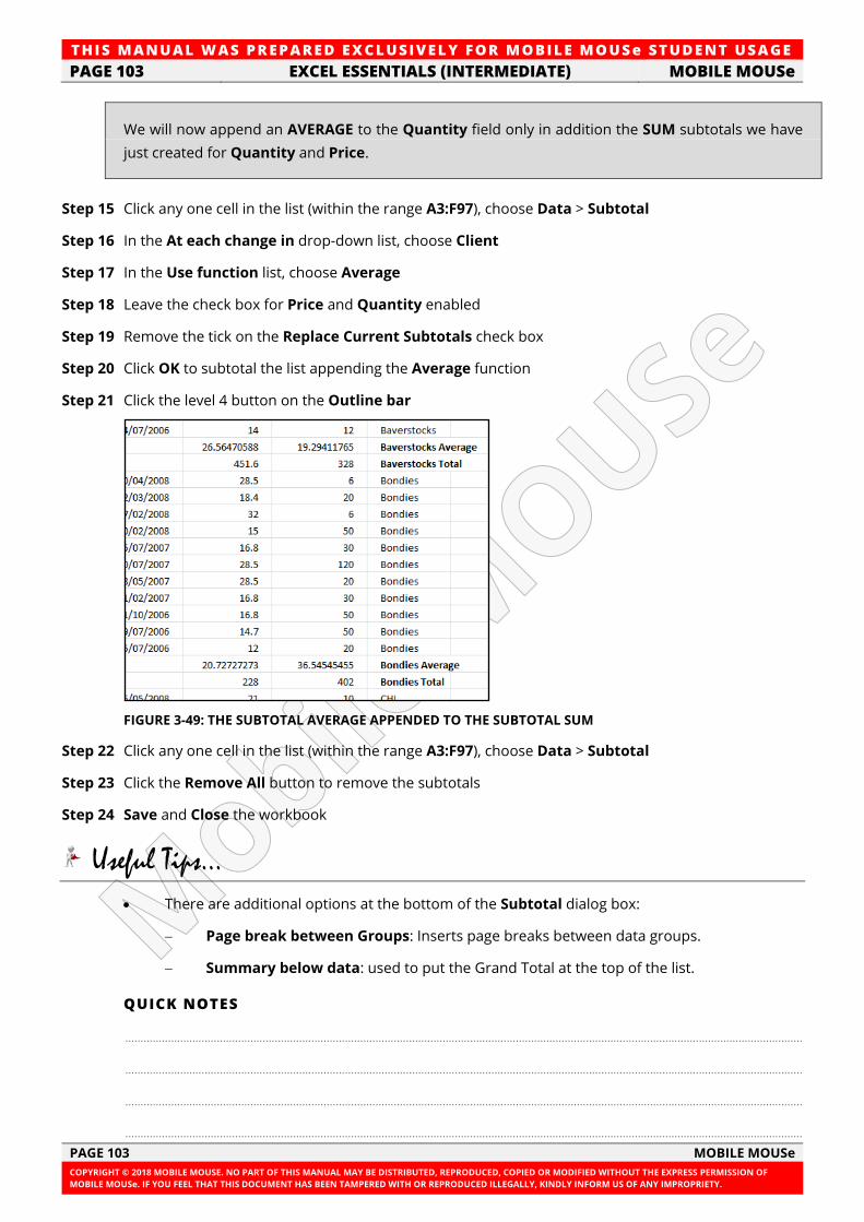
TH IS MANUAL W AS PREPARED EX CLUSIVE LY FOR MOBILE MOUSe ST UDE NT USAGE
PAGE 103 EXCEL ESSENTIALS (INTERMEDIATE) MOBILE MOUSe
PAGE 103 MOBILE MOUSe
COPYRIGHT © 2018 MOBILE MOUSE. NO PART OF THIS MANUAL MAY BE DISTRIBUTED, REPRODUCED, COPIED OR MODIFIED WITHOUT THE EXPRESS PERMISSION OF
MOBILE MOUSe. IF YOU FEEL THAT THIS DOCUMENT HAS BEEN TAMPERED WITH OR REPRODUCED ILLEGALLY, KINDLY INFORM US OF ANY IMPROPRIETY.
We will now append an AVERAGE to the Quantity field only in addition the SUM subtotals we have
just created for Quantity and Price.
Step 15 Click any one cell in the list (within the range A3:F97), choose Data > Subtotal
Step 16 In the At each change in drop-down list, choose Client
Step 17 In the Use function list, choose Average
Step 18 Leave the check box for Price and Quantity enabled
Step 19 Remove the tick on the Replace Current Subtotals check box
Step 20 Click OK to subtotal the list appending the Average function
Step 21 Click the level 4 button on the Outline bar
FIGURE 3-49: THE SUBTOTAL AVERAGE APPENDED TO THE SUBTOTAL SUM
Step 22 Click any one cell in the list (within the range A3:F97), choose Data > Subtotal
Step 23 Click the Remove All button to remove the subtotals
Step 24 Save and Close the workbook
Useful Tips...
• There are additional options at the bottom of the Subtotal dialog box:
− Page break between Groups: Inserts page breaks between data groups.
− Summary below data: used to put the Grand Total at the top of the list.
QUICK NOTES
..............................................................................................................................................................................................................................
..............................................................................................................................................................................................................................
..............................................................................................................................................................................................................................
..............................................................................................................................................................................................................................
TH IS MANUAL W AS PREPARED EX CLUSIVE LY FOR MOBILE MOUSe ST UDE NT USAGE
MOBILE MOUSe EXCEL ESSENTIALS (INTERMEDIATE) PAGE 104
MOBILE MOUSe PAGE 104
COPYRIGHT © 2018 MOBILE MOUSE. NO PART OF THIS MANUAL MAY BE DISTRIBUTED, REPRODUCED, COPIED OR MODIFIED WITHOUT THE EXPRESS PERMISSION OF
MOBILE MOUSe. IF YOU FEEL THAT THIS DOCUMENT HAS BEEN TAMPERED WITH OR REPRODUCED ILLEGALLY, KINDLY INFORM US OF ANY IMPROPRIETY.
QUICK NOTES
..................................................................................................................................................................................................................................................
..................................................................................................................................................................................................................................................
..................................................................................................................................................................................................................................................
..................................................................................................................................................................................................................................................
..................................................................................................................................................................................................................................................
..................................................................................................................................................................................................................................................
..................................................................................................................................................................................................................................................
..................................................................................................................................................................................................................................................
..................................................................................................................................................................................................................................................
..................................................................................................................................................................................................................................................
..................................................................................................................................................................................................................................................
..................................................................................................................................................................................................................................................
..................................................................................................................................................................................................................................................
..................................................................................................................................................................................................................................................
..................................................................................................................................................................................................................................................
..................................................................................................................................................................................................................................................
..................................................................................................................................................................................................................................................
..................................................................................................................................................................................................................................................
..................................................................................................................................................................................................................................................
..................................................................................................................................................................................................................................................
..................................................................................................................................................................................................................................................
..................................................................................................................................................................................................................................................
..................................................................................................................................................................................................................................................
..................................................................................................................................................................................................................................................
..................................................................................................................................................................................................................................................
..................................................................................................................................................................................................................................................
..................................................................................................................................................................................................................................................
..................................................................................................................................................................................................................................................
..................................................................................................................................................................................................................................................
..................................................................................................................................................................................................................................................
..................................................................................................................................................................................................................................................
..................................................................................................................................................................................................................................................
..................................................................................................................................................................................................................................................
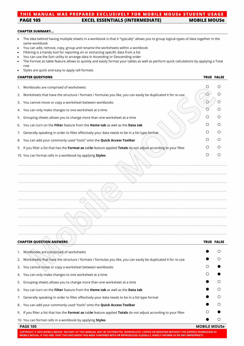
TH IS MANUAL W AS PREPARED EX CLUSIVE LY FOR MOBILE MOUSe ST UDE NT USAGE
PAGE 105 EXCEL ESSENTIALS (INTERMEDIATE) MOBILE MOUSe
PAGE 105 MOBILE MOUSe
COPYRIGHT © 2018 MOBILE MOUSE. NO PART OF THIS MANUAL MAY BE DISTRIBUTED, REPRODUCED, COPIED OR MODIFIED WITHOUT THE EXPRESS PERMISSION OF
MOBILE MOUSe. IF YOU FEEL THAT THIS DOCUMENT HAS BEEN TAMPERED WITH OR REPRODUCED ILLEGALLY, KINDLY INFORM US OF ANY IMPROPRIETY.
CHAPTER SUMMARY…
• The idea behind having multiple sheets in a workbook is that it “typically” allows you to group logical types of data together in the
same workbook
• You can add, remove, copy, group and rename the worksheets within a workbook
• Filtering is a handy tool for reporting on or extracting specific data from a list
• You can use the Sort utility to arrange data in Ascending or Descending order
• The Format as table feature allows to quickly and easily format your tables as well as perform quick calculations by applying a Total
row
• Styles are quick and easy to apply cell formats
CHAPTER QUESTIONS TRUE FALSE
1. Workbooks are comprised of worksheets ○ ○
2. Worksheets that have the structure / formats / formulas you like, you can easily be duplicated it for re-use ○ ○
3. You cannot move or copy a worksheet between workbooks ○ ○
4. You can only make changes to one worksheet at a time ○ ○
5. Grouping sheets allows you to change more than one worksheet at a time ○ ○
6. You can turn on the Filter feature from the Home tab as well as the Data tab ○ ○
7. Generally speaking in order to filter effectively your data needs to be in a list type format ○ ○
8. You can add your commonly used “tools” onto the Quick Access Toolbar ○ ○
9. If you filter a list that has the Format as table feature applied Totals do not adjust according to your filter ○ ○
10. You can format cells in a workbook by applying Styles ○ ○
..................................................................................................................................................................................................................................................
..................................................................................................................................................................................................................................................
..................................................................................................................................................................................................................................................
..................................................................................................................................................................................................................................................
..................................................................................................................................................................................................................................................
..................................................................................................................................................................................................................................................
..................................................................................................................................................................................................................................................
..................................................................................................................................................................................................................................................
..................................................................................................................................................................................................................................................
CHAPTER QUESTION ANSWERS TRUE FALSE
1. Workbooks are comprised of worksheets ● ○
2. Worksheets that have the structure / formats / formulas you like, you can easily be duplicated it for re-use ● ○
3. You cannot move or copy a worksheet between workbooks ○ ●
4. You can only make changes to one worksheet at a time ○ ●
5. Grouping sheets allows you to change more than one worksheet at a time ● ○
6. You can turn on the Filter feature from the Home tab as well as the Data tab ● ○
7. Generally speaking in order to filter effectively your data needs to be in a list type format ● ○
8. You can add your commonly used “tools” onto the Quick Access Toolbar ● ○
9. If you filter a list that has the Format as table feature applied Totals do not adjust according to your filter ○ ●
10. You can format cells in a workbook by applying Styles ● ○
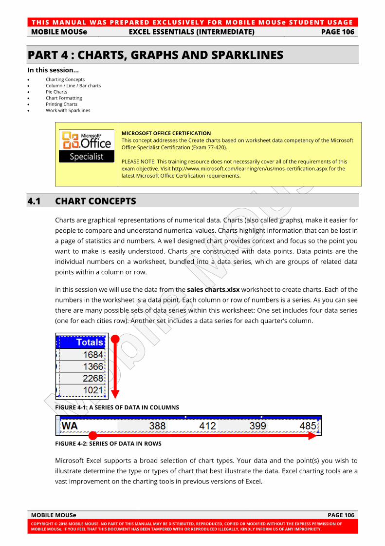
TH IS MANUAL W AS PREPARED EX CLUSIVE LY FOR MOBILE MOUSe ST UDE NT USAGE
MOBILE MOUSe EXCEL ESSENTIALS (INTERMEDIATE) PAGE 106
MOBILE MOUSe PAGE 106
COPYRIGHT © 2018 MOBILE MOUSE. NO PART OF THIS MANUAL MAY BE DISTRIBUTED, REPRODUCED, COPIED OR MODIFIED WITHOUT THE EXPRESS PERMISSION OF
MOBILE MOUSe. IF YOU FEEL THAT THIS DOCUMENT HAS BEEN TAMPERED WITH OR REPRODUCED ILLEGALLY, KINDLY INFORM US OF ANY IMPROPRIETY.
PART 4 : CHARTS, GRAPHS AND SPARKLINES In this session...
• Charting Concepts
• Column / Line / Bar charts
• Pie Charts
• Chart Formatting
• Printing Charts
• Work with Sparklines
MICROSOFT OFFICE CERTIFICATION
This concept addresses the Create charts based on worksheet data competency of the Microsoft
Office Specialist Certification (Exam 77-420).
PLEASE NOTE: This training resource does not necessarily cover all of the requirements of this
exam objective. Visit http://www.microsoft.com/learning/en/us/mos-certification.aspx for the
latest Microsoft Office Certification requirements.
4.1 CHART CONCEPTS
Charts are graphical representations of numerical data. Charts (also called graphs), make it easier for
people to compare and understand numerical values. Charts highlight information that can be lost in
a page of statistics and numbers. A well designed chart provides context and focus so the point you
want to make is easily understood. Charts are constructed with data points. Data points are the
individual numbers on a worksheet, bundled into a data series, which are groups of related data
points within a column or row.
In this session we will use the data from the sales charts.xlsx worksheet to create charts. Each of the
numbers in the worksheet is a data point. Each column or row of numbers is a series. As you can see
there are many possible sets of data series within this worksheet: One set includes four data series
(one for each cities row). Another set includes a data series for each quarter’s column.
FIGURE 4-1: A SERIES OF DATA IN COLUMNS
FIGURE 4-2: SERIES OF DATA IN ROWS
Microsoft Excel supports a broad selection of chart types. Your data and the point(s) you wish to
illustrate determine the type or types of chart that best illustrate the data. Excel charting tools are a
vast improvement on the charting tools in previous versions of Excel.
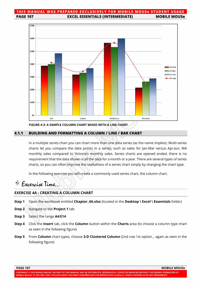
TH IS MANUAL W AS PREPARED EX CLUSIVE LY FOR MOBILE MOUSe ST UDE NT USAGE
PAGE 107 EXCEL ESSENTIALS (INTERMEDIATE) MOBILE MOUSe
PAGE 107 MOBILE MOUSe
COPYRIGHT © 2018 MOBILE MOUSE. NO PART OF THIS MANUAL MAY BE DISTRIBUTED, REPRODUCED, COPIED OR MODIFIED WITHOUT THE EXPRESS PERMISSION OF
MOBILE MOUSe. IF YOU FEEL THAT THIS DOCUMENT HAS BEEN TAMPERED WITH OR REPRODUCED ILLEGALLY, KINDLY INFORM US OF ANY IMPROPRIETY.
FIGURE 4-3: A SAMPLE COLUMN CHART MIXED WITH A LINE CHART
4.1.1 BUILDING AND FORMATTING A COLUMN / LINE / BAR CHART
In a multiple series chart you can chart more than one data series (as the name implies). Multi-series
charts let you compare the data points in a series, such as sales for Jan-Mar versus Apr-Jun, WA
monthly sales compared to Victoria’s monthly sales. Series charts are opened ended, there is no
requirement that the data shown is all the data for a month or a year. There are several types of series
charts, so you can often improve the usefulness of a series chart simply by changing the chart type.
In the following exercise you will create a commonly used series chart, the column chart.
Excercise Time... EXERCISE 4A : CREATING A COLUMN CHART
Step 1 Open the workbook entitled Chapter_4A.xlsx (located in the Desktop \ Excel \ Essentials folder)
Step 2 Navigate to the Project 1 tab
Step 3 Select the range A4:E14
Step 4 Click the Insert tab, click the Column button within the Charts area (to choose a column type chart
as seen in the following figure)
Step 5 From Column chart types, choose 3-D Clustered Column (2nd row 1st option... again as seen in the
following figure)
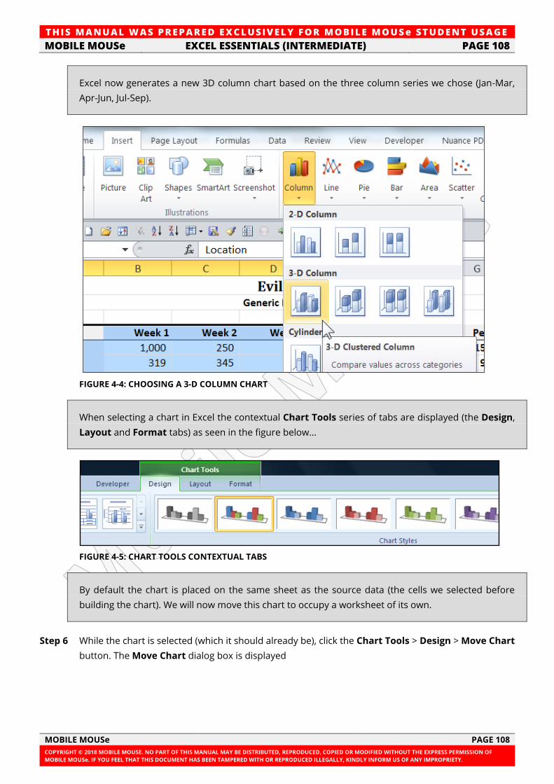
TH IS MANUAL W AS PREPARED EX CLUSIVE LY FOR MOBILE MOUSe ST UDE NT USAGE
MOBILE MOUSe EXCEL ESSENTIALS (INTERMEDIATE) PAGE 108
MOBILE MOUSe PAGE 108
COPYRIGHT © 2018 MOBILE MOUSE. NO PART OF THIS MANUAL MAY BE DISTRIBUTED, REPRODUCED, COPIED OR MODIFIED WITHOUT THE EXPRESS PERMISSION OF
MOBILE MOUSe. IF YOU FEEL THAT THIS DOCUMENT HAS BEEN TAMPERED WITH OR REPRODUCED ILLEGALLY, KINDLY INFORM US OF ANY IMPROPRIETY.
Excel now generates a new 3D column chart based on the three column series we chose (Jan-Mar,
Apr-Jun, Jul-Sep).
FIGURE 4-4: CHOOSING A 3-D COLUMN CHART
When selecting a chart in Excel the contextual Chart Tools series of tabs are displayed (the Design,
Layout and Format tabs) as seen in the figure below...
FIGURE 4-5: CHART TOOLS CONTEXTUAL TABS
By default the chart is placed on the same sheet as the source data (the cells we selected before
building the chart). We will now move this chart to occupy a worksheet of its own.
Step 6 While the chart is selected (which it should already be), click the Chart Tools > Design > Move Chart
button. The Move Chart dialog box is displayed
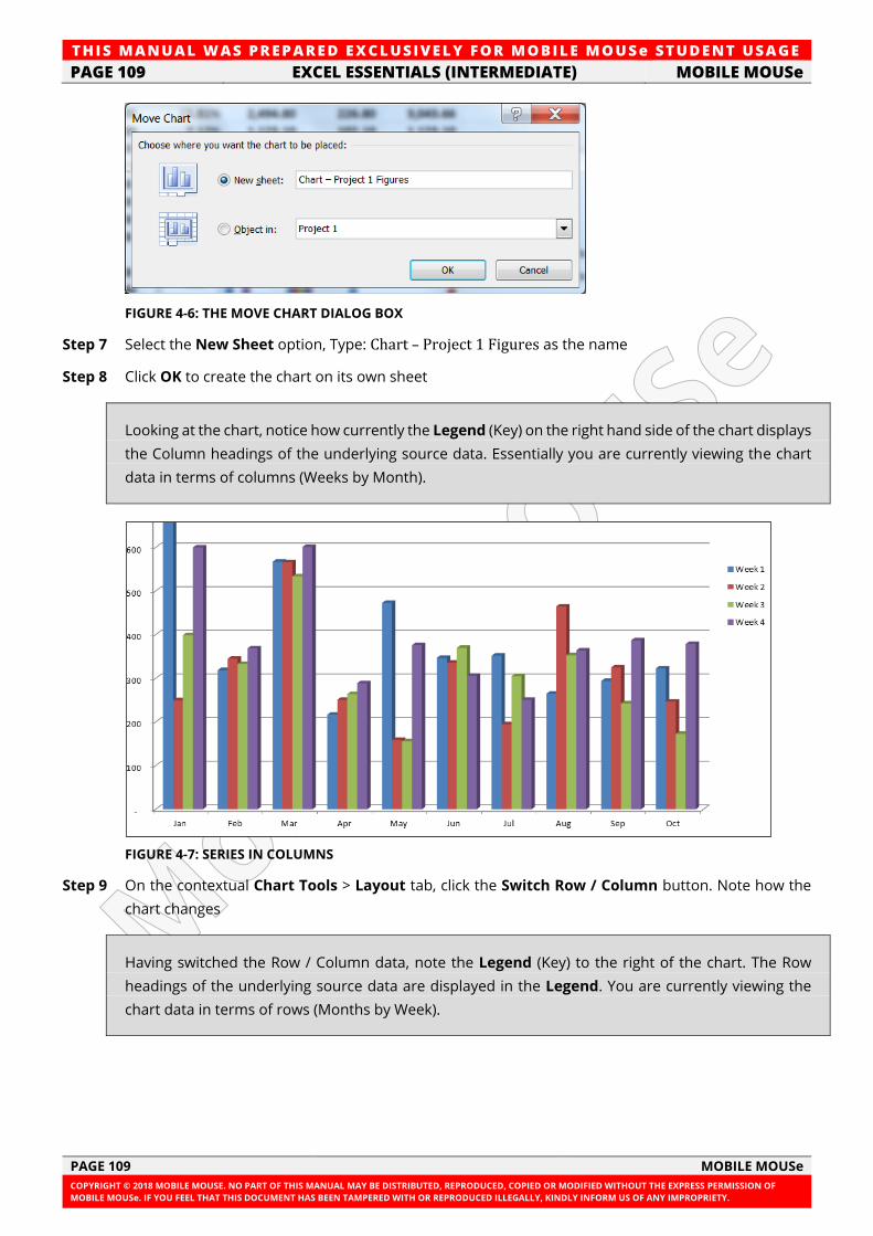
TH IS MANUAL W AS PREPARED EX CLUSIVE LY FOR MOBILE MOUSe ST UDE NT USAGE
PAGE 109 EXCEL ESSENTIALS (INTERMEDIATE) MOBILE MOUSe
PAGE 109 MOBILE MOUSe
COPYRIGHT © 2018 MOBILE MOUSE. NO PART OF THIS MANUAL MAY BE DISTRIBUTED, REPRODUCED, COPIED OR MODIFIED WITHOUT THE EXPRESS PERMISSION OF
MOBILE MOUSe. IF YOU FEEL THAT THIS DOCUMENT HAS BEEN TAMPERED WITH OR REPRODUCED ILLEGALLY, KINDLY INFORM US OF ANY IMPROPRIETY.
FIGURE 4-6: THE MOVE CHART DIALOG BOX
Step 7 Select the New Sheet option, Type: Chart – Project 1 Figures as the name
Step 8 Click OK to create the chart on its own sheet
Looking at the chart, notice how currently the Legend (Key) on the right hand side of the chart displays
the Column headings of the underlying source data. Essentially you are currently viewing the chart
data in terms of columns (Weeks by Month).
FIGURE 4-7: SERIES IN COLUMNS
Step 9 On the contextual Chart Tools > Layout tab, click the Switch Row / Column button. Note how the
chart changes
Having switched the Row / Column data, note the Legend (Key) to the right of the chart. The Row
headings of the underlying source data are displayed in the Legend. You are currently viewing the
chart data in terms of rows (Months by Week).
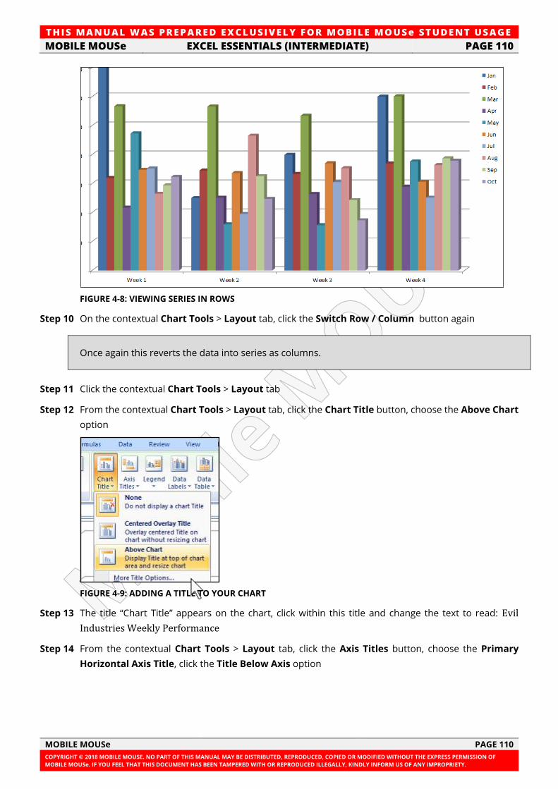
TH IS MANUAL W AS PREPARED EX CLUSIVE LY FOR MOBILE MOUSe ST UDE NT USAGE
MOBILE MOUSe EXCEL ESSENTIALS (INTERMEDIATE) PAGE 110
MOBILE MOUSe PAGE 110
COPYRIGHT © 2018 MOBILE MOUSE. NO PART OF THIS MANUAL MAY BE DISTRIBUTED, REPRODUCED, COPIED OR MODIFIED WITHOUT THE EXPRESS PERMISSION OF
MOBILE MOUSe. IF YOU FEEL THAT THIS DOCUMENT HAS BEEN TAMPERED WITH OR REPRODUCED ILLEGALLY, KINDLY INFORM US OF ANY IMPROPRIETY.
FIGURE 4-8: VIEWING SERIES IN ROWS
Step 10 On the contextual Chart Tools > Layout tab, click the Switch Row / Column button again
Once again this reverts the data into series as columns.
Step 11 Click the contextual Chart Tools > Layout tab
Step 12 From the contextual Chart Tools > Layout tab, click the Chart Title button, choose the Above Chart
option
FIGURE 4-9: ADDING A TITLE TO YOUR CHART
Step 13 The title “Chart Title” appears on the chart, click within this title and change the text to read: Evil
Industries Weekly Performance
Step 14 From the contextual Chart Tools > Layout tab, click the Axis Titles button, choose the Primary
Horizontal Axis Title, click the Title Below Axis option
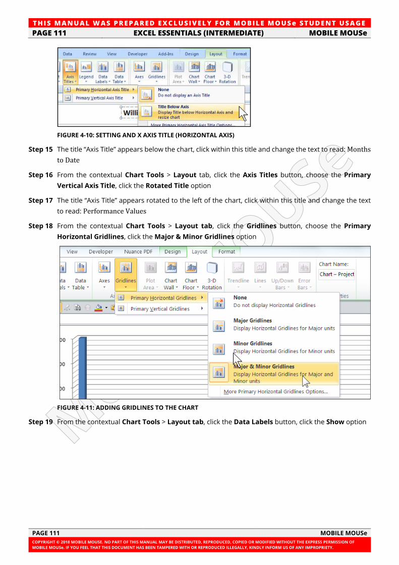
TH IS MANUAL W AS PREPARED EX CLUSIVE LY FOR MOBILE MOUSe ST UDE NT USAGE
PAGE 111 EXCEL ESSENTIALS (INTERMEDIATE) MOBILE MOUSe
PAGE 111 MOBILE MOUSe
COPYRIGHT © 2018 MOBILE MOUSE. NO PART OF THIS MANUAL MAY BE DISTRIBUTED, REPRODUCED, COPIED OR MODIFIED WITHOUT THE EXPRESS PERMISSION OF
MOBILE MOUSe. IF YOU FEEL THAT THIS DOCUMENT HAS BEEN TAMPERED WITH OR REPRODUCED ILLEGALLY, KINDLY INFORM US OF ANY IMPROPRIETY.
FIGURE 4-10: SETTING AND X AXIS TITLE (HORIZONTAL AXIS)
Step 15 The title “Axis Title” appears below the chart, click within this title and change the text to read: Months
to Date
Step 16 From the contextual Chart Tools > Layout tab, click the Axis Titles button, choose the Primary
Vertical Axis Title, click the Rotated Title option
Step 17 The title “Axis Title” appears rotated to the left of the chart, click within this title and change the text
to read: Performance Values
Step 18 From the contextual Chart Tools > Layout tab, click the Gridlines button, choose the Primary
Horizontal Gridlines, click the Major & Minor Gridlines option
FIGURE 4-11: ADDING GRIDLINES TO THE CHART
Step 19 From the contextual Chart Tools > Layout tab, click the Data Labels button, click the Show option
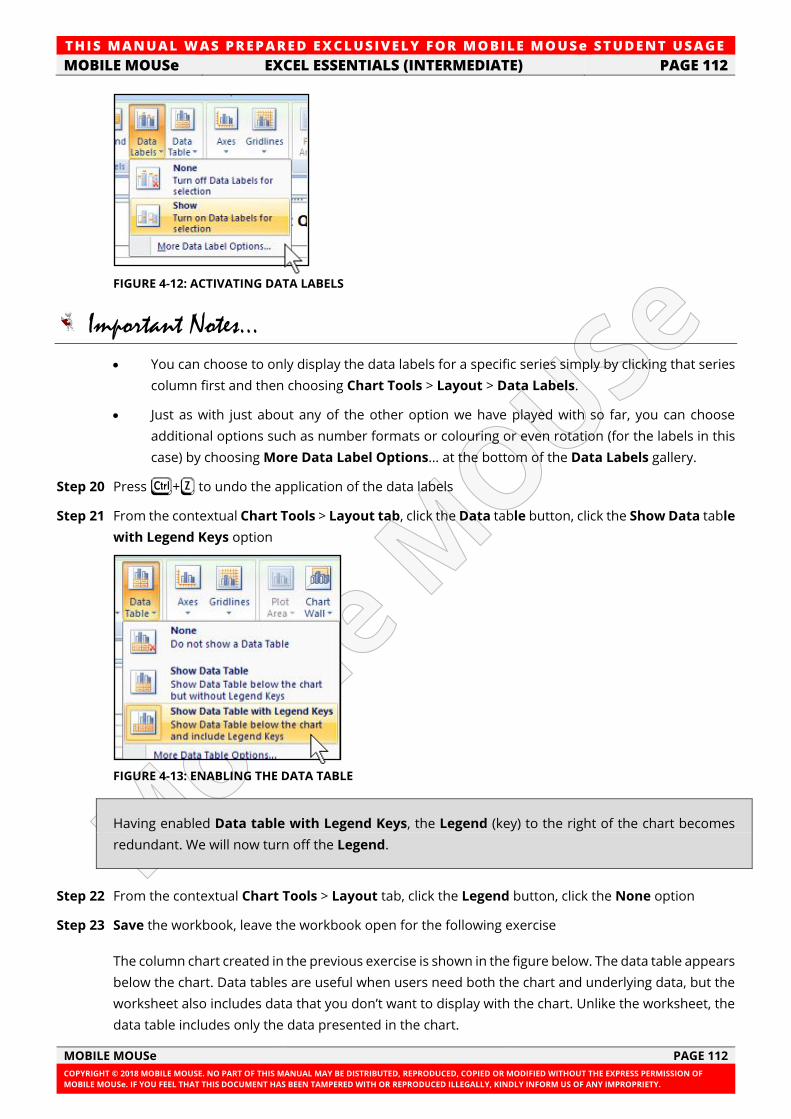
TH IS MANUAL W AS PREPARED EX CLUSIVE LY FOR MOBILE MOUSe ST UDE NT USAGE
MOBILE MOUSe EXCEL ESSENTIALS (INTERMEDIATE) PAGE 112
MOBILE MOUSe PAGE 112
COPYRIGHT © 2018 MOBILE MOUSE. NO PART OF THIS MANUAL MAY BE DISTRIBUTED, REPRODUCED, COPIED OR MODIFIED WITHOUT THE EXPRESS PERMISSION OF
MOBILE MOUSe. IF YOU FEEL THAT THIS DOCUMENT HAS BEEN TAMPERED WITH OR REPRODUCED ILLEGALLY, KINDLY INFORM US OF ANY IMPROPRIETY.
FIGURE 4-12: ACTIVATING DATA LABELS
Important Notes...
• You can choose to only display the data labels for a specific series simply by clicking that series
column first and then choosing Chart Tools > Layout > Data Labels.
• Just as with just about any of the other option we have played with so far, you can choose
additional options such as number formats or colouring or even rotation (for the labels in this
case) by choosing More Data Label Options... at the bottom of the Data Labels gallery.
Step 20 Press F+Z to undo the application of the data labels
Step 21 From the contextual Chart Tools > Layout tab, click the Data table button, click the Show Data table
with Legend Keys option
FIGURE 4-13: ENABLING THE DATA TABLE
Having enabled Data table with Legend Keys, the Legend (key) to the right of the chart becomes
redundant. We will now turn off the Legend.
Step 22 From the contextual Chart Tools > Layout tab, click the Legend button, click the None option
Step 23 Save the workbook, leave the workbook open for the following exercise
The column chart created in the previous exercise is shown in the figure below. The data table appears
below the chart. Data tables are useful when users need both the chart and underlying data, but the
worksheet also includes data that you don’t want to display with the chart. Unlike the worksheet, the
data table includes only the data presented in the chart.
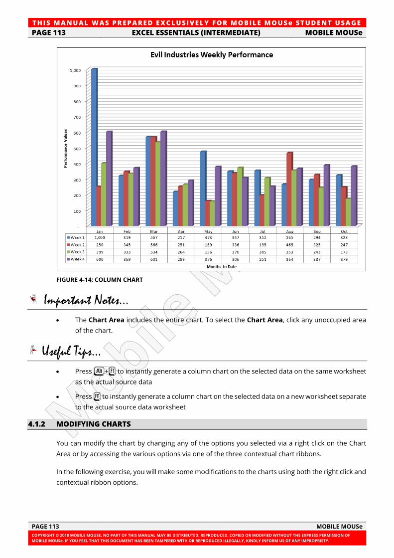
TH IS MANUAL W AS PREPARED EX CLUSIVE LY FOR MOBILE MOUSe ST UDE NT USAGE
PAGE 113 EXCEL ESSENTIALS (INTERMEDIATE) MOBILE MOUSe
PAGE 113 MOBILE MOUSe
COPYRIGHT © 2018 MOBILE MOUSE. NO PART OF THIS MANUAL MAY BE DISTRIBUTED, REPRODUCED, COPIED OR MODIFIED WITHOUT THE EXPRESS PERMISSION OF
MOBILE MOUSe. IF YOU FEEL THAT THIS DOCUMENT HAS BEEN TAMPERED WITH OR REPRODUCED ILLEGALLY, KINDLY INFORM US OF ANY IMPROPRIETY.
FIGURE 4-14: COLUMN CHART
Important Notes...
• The Chart Area includes the entire chart. To select the Chart Area, click any unoccupied area
of the chart.
Useful Tips...
• Press E+1 to instantly generate a column chart on the selected data on the same worksheet
as the actual source data
• Press ! to instantly generate a column chart on the selected data on a new worksheet separate
to the actual source data worksheet
4.1.2 MODIFYING CHARTS
You can modify the chart by changing any of the options you selected via a right click on the Chart
Area or by accessing the various options via one of the three contextual chart ribbons.
In the following exercise, you will make some modifications to the charts using both the right click and
contextual ribbon options.
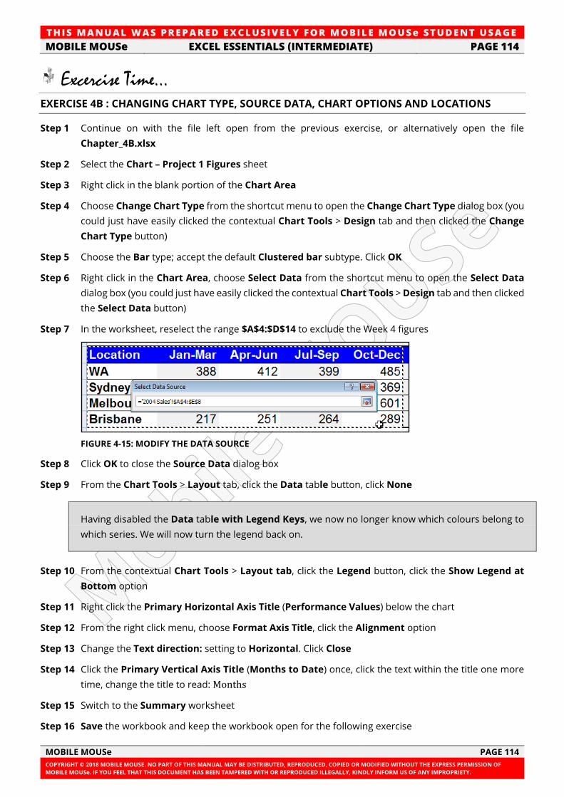
TH IS MANUAL W AS PREPARED EX CLUSIVE LY FOR MOBILE MOUSe ST UDE NT USAGE
MOBILE MOUSe EXCEL ESSENTIALS (INTERMEDIATE) PAGE 114
MOBILE MOUSe PAGE 114
COPYRIGHT © 2018 MOBILE MOUSE. NO PART OF THIS MANUAL MAY BE DISTRIBUTED, REPRODUCED, COPIED OR MODIFIED WITHOUT THE EXPRESS PERMISSION OF
MOBILE MOUSe. IF YOU FEEL THAT THIS DOCUMENT HAS BEEN TAMPERED WITH OR REPRODUCED ILLEGALLY, KINDLY INFORM US OF ANY IMPROPRIETY.
Excercise Time... EXERCISE 4B : CHANGING CHART TYPE, SOURCE DATA, CHART OPTIONS AND LOCATIONS
Step 1 Continue on with the file left open from the previous exercise, or alternatively open the file
Chapter_4B.xlsx
Step 2 Select the Chart – Project 1 Figures sheet
Step 3 Right click in the blank portion of the Chart Area
Step 4 Choose Change Chart Type from the shortcut menu to open the Change Chart Type dialog box (you
could just have easily clicked the contextual Chart Tools > Design tab and then clicked the Change
Chart Type button)
Step 5 Choose the Bar type; accept the default Clustered bar subtype. Click OK
Step 6 Right click in the Chart Area, choose Select Data from the shortcut menu to open the Select Data
dialog box (you could just have easily clicked the contextual Chart Tools > Design tab and then clicked
the Select Data button)
Step 7 In the worksheet, reselect the range $A$4:$D$14 to exclude the Week 4 figures
FIGURE 4-15: MODIFY THE DATA SOURCE
Step 8 Click OK to close the Source Data dialog box
Step 9 From the Chart Tools > Layout tab, click the Data table button, click None
Having disabled the Data table with Legend Keys, we now no longer know which colours belong to
which series. We will now turn the legend back on.
Step 10 From the contextual Chart Tools > Layout tab, click the Legend button, click the Show Legend at
Bottom option
Step 11 Right click the Primary Horizontal Axis Title (Performance Values) below the chart
Step 12 From the right click menu, choose Format Axis Title, click the Alignment option
Step 13 Change the Text direction: setting to Horizontal. Click Close
Step 14 Click the Primary Vertical Axis Title (Months to Date) once, click the text within the title one more
time, change the title to read: Months
Step 15 Switch to the Summary worksheet
Step 16 Save the workbook and keep the workbook open for the following exercise
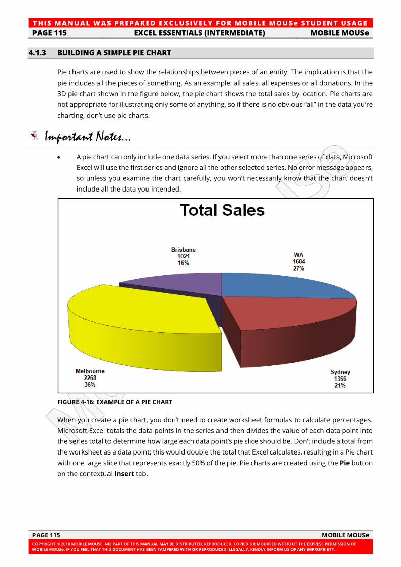
TH IS MANUAL W AS PREPARED EX CLUSIVE LY FOR MOBILE MOUSe ST UDE NT USAGE
PAGE 115 EXCEL ESSENTIALS (INTERMEDIATE) MOBILE MOUSe
PAGE 115 MOBILE MOUSe
COPYRIGHT © 2018 MOBILE MOUSE. NO PART OF THIS MANUAL MAY BE DISTRIBUTED, REPRODUCED, COPIED OR MODIFIED WITHOUT THE EXPRESS PERMISSION OF
MOBILE MOUSe. IF YOU FEEL THAT THIS DOCUMENT HAS BEEN TAMPERED WITH OR REPRODUCED ILLEGALLY, KINDLY INFORM US OF ANY IMPROPRIETY.
4.1.3 BUILDING A SIMPLE PIE CHART
Pie charts are used to show the relationships between pieces of an entity. The implication is that the
pie includes all the pieces of something. As an example: all sales, all expenses or all donations. In the
3D pie chart shown in the figure below, the pie chart shows the total sales by location. Pie charts are
not appropriate for illustrating only some of anything, so if there is no obvious “all” in the data you’re
charting, don’t use pie charts.
Important Notes...
• A pie chart can only include one data series. If you select more than one series of data, Microsoft
Excel will use the first series and ignore all the other selected series. No error message appears,
so unless you examine the chart carefully, you won’t necessarily know that the chart doesn’t
include all the data you intended.
FIGURE 4-16: EXAMPLE OF A PIE CHART
When you create a pie chart, you don’t need to create worksheet formulas to calculate percentages.
Microsoft Excel totals the data points in the series and then divides the value of each data point into
the series total to determine how large each data point’s pie slice should be. Don’t include a total from
the worksheet as a data point; this would double the total that Excel calculates, resulting in a Pie chart
with one large slice that represents exactly 50% of the pie. Pie charts are created using the Pie button
on the contextual Insert tab.
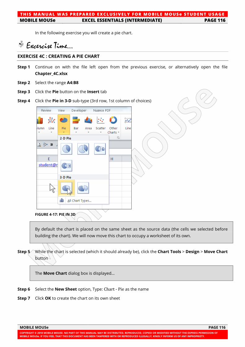
TH IS MANUAL W AS PREPARED EX CLUSIVE LY FOR MOBILE MOUSe ST UDE NT USAGE
MOBILE MOUSe EXCEL ESSENTIALS (INTERMEDIATE) PAGE 116
MOBILE MOUSe PAGE 116
COPYRIGHT © 2018 MOBILE MOUSE. NO PART OF THIS MANUAL MAY BE DISTRIBUTED, REPRODUCED, COPIED OR MODIFIED WITHOUT THE EXPRESS PERMISSION OF
MOBILE MOUSe. IF YOU FEEL THAT THIS DOCUMENT HAS BEEN TAMPERED WITH OR REPRODUCED ILLEGALLY, KINDLY INFORM US OF ANY IMPROPRIETY.
In the following exercise you will create a pie chart.
Excercise Time... EXERCISE 4C : CREATING A PIE CHART
Step 1 Continue on with the file left open from the previous exercise, or alternatively open the file
Chapter_4C.xlsx
Step 2 Select the range A4:B8
Step 3 Click the Pie button on the Insert tab
Step 4 Click the Pie in 3-D sub-type (3rd row, 1st column of choices)
FIGURE 4-17: PIE IN 3D
By default the chart is placed on the same sheet as the source data (the cells we selected before
building the chart). We will now move this chart to occupy a worksheet of its own.
Step 5 While the chart is selected (which it should already be), click the Chart Tools > Design > Move Chart
button
The Move Chart dialog box is displayed…
Step 6 Select the New Sheet option, Type: Chart - Pie as the name
Step 7 Click OK to create the chart on its own sheet
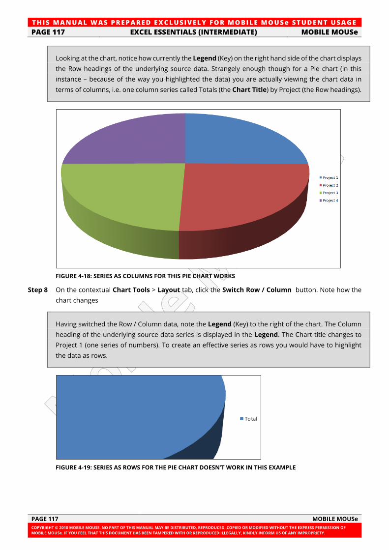
TH IS MANUAL W AS PREPARED EX CLUSIVE LY FOR MOBILE MOUSe ST UDE NT USAGE
PAGE 117 EXCEL ESSENTIALS (INTERMEDIATE) MOBILE MOUSe
PAGE 117 MOBILE MOUSe
COPYRIGHT © 2018 MOBILE MOUSE. NO PART OF THIS MANUAL MAY BE DISTRIBUTED, REPRODUCED, COPIED OR MODIFIED WITHOUT THE EXPRESS PERMISSION OF
MOBILE MOUSe. IF YOU FEEL THAT THIS DOCUMENT HAS BEEN TAMPERED WITH OR REPRODUCED ILLEGALLY, KINDLY INFORM US OF ANY IMPROPRIETY.
Looking at the chart, notice how currently the Legend (Key) on the right hand side of the chart displays
the Row headings of the underlying source data. Strangely enough though for a Pie chart (in this
instance – because of the way you highlighted the data) you are actually viewing the chart data in
terms of columns, i.e. one column series called Totals (the Chart Title) by Project (the Row headings).
FIGURE 4-18: SERIES AS COLUMNS FOR THIS PIE CHART WORKS
Step 8 On the contextual Chart Tools > Layout tab, click the Switch Row / Column button. Note how the
chart changes
Having switched the Row / Column data, note the Legend (Key) to the right of the chart. The Column
heading of the underlying source data series is displayed in the Legend. The Chart title changes to
Project 1 (one series of numbers). To create an effective series as rows you would have to highlight
the data as rows.
FIGURE 4-19: SERIES AS ROWS FOR THE PIE CHART DOESN’T WORK IN THIS EXAMPLE
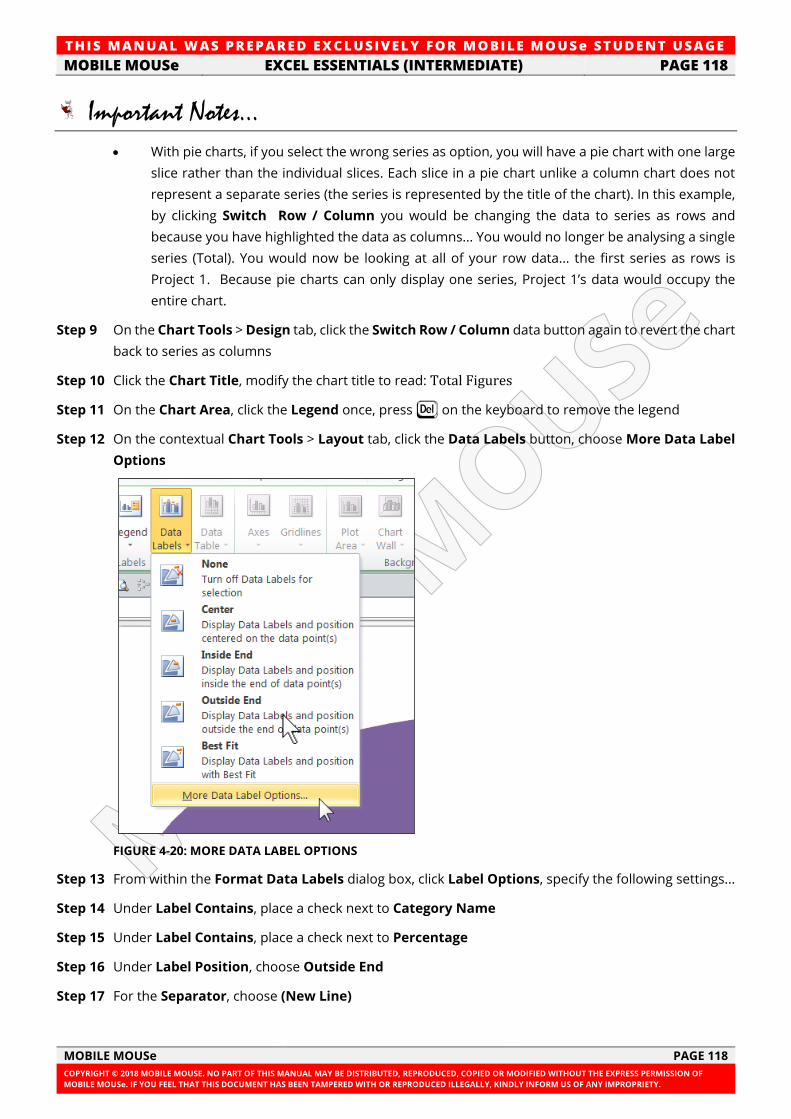
TH IS MANUAL W AS PREPARED EX CLUSIVE LY FOR MOBILE MOUSe ST UDE NT USAGE
MOBILE MOUSe EXCEL ESSENTIALS (INTERMEDIATE) PAGE 118
MOBILE MOUSe PAGE 118
COPYRIGHT © 2018 MOBILE MOUSE. NO PART OF THIS MANUAL MAY BE DISTRIBUTED, REPRODUCED, COPIED OR MODIFIED WITHOUT THE EXPRESS PERMISSION OF
MOBILE MOUSe. IF YOU FEEL THAT THIS DOCUMENT HAS BEEN TAMPERED WITH OR REPRODUCED ILLEGALLY, KINDLY INFORM US OF ANY IMPROPRIETY.
Important Notes...
• With pie charts, if you select the wrong series as option, you will have a pie chart with one large
slice rather than the individual slices. Each slice in a pie chart unlike a column chart does not
represent a separate series (the series is represented by the title of the chart). In this example,
by clicking Switch Row / Column you would be changing the data to series as rows and
because you have highlighted the data as columns... You would no longer be analysing a single
series (Total). You would now be looking at all of your row data... the first series as rows is
Project 1. Because pie charts can only display one series, Project 1’s data would occupy the
entire chart.
Step 9 On the Chart Tools > Design tab, click the Switch Row / Column data button again to revert the chart
back to series as columns
Step 10 Click the Chart Title, modify the chart title to read: Total Figures
Step 11 On the Chart Area, click the Legend once, press V on the keyboard to remove the legend
Step 12 On the contextual Chart Tools > Layout tab, click the Data Labels button, choose More Data Label
Options
FIGURE 4-20: MORE DATA LABEL OPTIONS
Step 13 From within the Format Data Labels dialog box, click Label Options, specify the following settings...
Step 14 Under Label Contains, place a check next to Category Name
Step 15 Under Label Contains, place a check next to Percentage
Step 16 Under Label Position, choose Outside End
Step 17 For the Separator, choose (New Line)
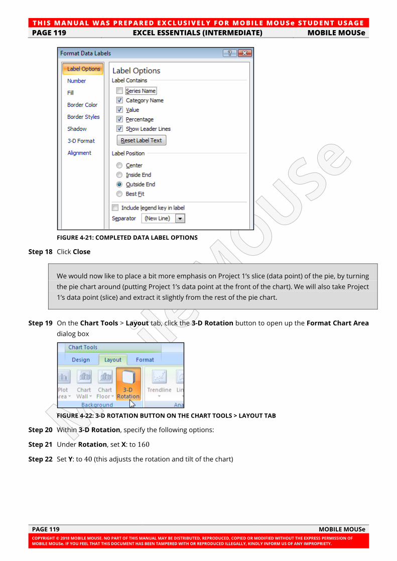
TH IS MANUAL W AS PREPARED EX CLUSIVE LY FOR MOBILE MOUSe ST UDE NT USAGE
PAGE 119 EXCEL ESSENTIALS (INTERMEDIATE) MOBILE MOUSe
PAGE 119 MOBILE MOUSe
COPYRIGHT © 2018 MOBILE MOUSE. NO PART OF THIS MANUAL MAY BE DISTRIBUTED, REPRODUCED, COPIED OR MODIFIED WITHOUT THE EXPRESS PERMISSION OF
MOBILE MOUSe. IF YOU FEEL THAT THIS DOCUMENT HAS BEEN TAMPERED WITH OR REPRODUCED ILLEGALLY, KINDLY INFORM US OF ANY IMPROPRIETY.
FIGURE 4-21: COMPLETED DATA LABEL OPTIONS
Step 18 Click Close
We would now like to place a bit more emphasis on Project 1’s slice (data point) of the pie, by turning
the pie chart around (putting Project 1’s data point at the front of the chart). We will also take Project
1’s data point (slice) and extract it slightly from the rest of the pie chart.
Step 19 On the Chart Tools > Layout tab, click the 3-D Rotation button to open up the Format Chart Area
dialog box
FIGURE 4-22: 3-D ROTATION BUTTON ON THE CHART TOOLS > LAYOUT TAB
Step 20 Within 3-D Rotation, specify the following options:
Step 21 Under Rotation, set X: to 160
Step 22 Set Y: to 40 (this adjusts the rotation and tilt of the chart)
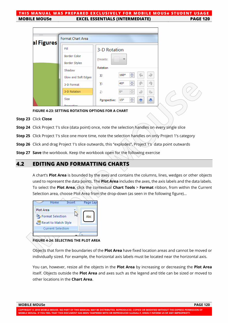
TH IS MANUAL W AS PREPARED EX CLUSIVE LY FOR MOBILE MOUSe ST UDE NT USAGE
MOBILE MOUSe EXCEL ESSENTIALS (INTERMEDIATE) PAGE 120
MOBILE MOUSe PAGE 120
COPYRIGHT © 2018 MOBILE MOUSE. NO PART OF THIS MANUAL MAY BE DISTRIBUTED, REPRODUCED, COPIED OR MODIFIED WITHOUT THE EXPRESS PERMISSION OF
MOBILE MOUSe. IF YOU FEEL THAT THIS DOCUMENT HAS BEEN TAMPERED WITH OR REPRODUCED ILLEGALLY, KINDLY INFORM US OF ANY IMPROPRIETY.
FIGURE 4-23: SETTING ROTATION OPTIONS FOR A CHART
Step 23 Click Close
Step 24 Click Project 1’s slice (data point) once, note the selection handles on every single slice
Step 25 Click Project 1’s slice one more time, note the selection handles on only Project 1’s category
Step 26 Click and drag Project 1’s slice outwards, this “explodes”, Project 1’s data point outwards
Step 27 Save the workbook. Keep the workbook open for the following exercise
4.2 EDITING AND FORMATTING CHARTS
A chart’s Plot Area is bounded by the axes and contains the columns, lines, wedges or other objects
used to represent the data points. The Plot Area includes the axes, the axis labels and the data labels.
To select the Plot Area, click the contextual Chart Tools > Format ribbon, from within the Current
Selection area, choose Plot Area from the drop-down (as seen in the following figure)...
FIGURE 4-24: SELECTING THE PLOT AREA
Objects that form the boundaries of the Plot Area have fixed location areas and cannot be moved or
individually sized. For example, the horizontal axis labels must be located near the horizontal axis.
You can, however, resize all the objects in the Plot Area by increasing or decreasing the Plot Area
itself. Objects outside the Plot Area and axes such as the legend and title can be sized or moved to
other locations in the Chart Area.
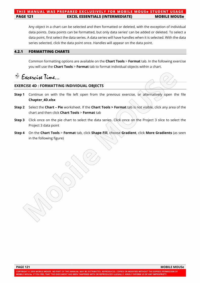
TH IS MANUAL W AS PREPARED EX CLUSIVE LY FOR MOBILE MOUSe ST UDE NT USAGE
PAGE 121 EXCEL ESSENTIALS (INTERMEDIATE) MOBILE MOUSe
PAGE 121 MOBILE MOUSe
COPYRIGHT © 2018 MOBILE MOUSE. NO PART OF THIS MANUAL MAY BE DISTRIBUTED, REPRODUCED, COPIED OR MODIFIED WITHOUT THE EXPRESS PERMISSION OF
MOBILE MOUSe. IF YOU FEEL THAT THIS DOCUMENT HAS BEEN TAMPERED WITH OR REPRODUCED ILLEGALLY, KINDLY INFORM US OF ANY IMPROPRIETY.
Any object in a chart can be selected and then formatted or deleted, with the exception of individual
data points. Data points can be formatted, but only data series’ can be added or deleted. To select a
data point, first select the data series. A data series will have handles when it is selected. With the data
series selected, click the data point once. Handles will appear on the data point.
4.2.1 FORMATTING CHARTS
Common formatting options are available on the Chart Tools > Format tab. In the following exercise
you will use the Chart Tools > Format tab to format individual objects within a chart.
Excercise Time... EXERCISE 4D : FORMATTING INDIVIDUAL OBJECTS
Step 1 Continue on with the file left open from the previous exercise, or alternatively open the file
Chapter_4D.xlsx
Step 2 Select the Chart – Pie worksheet. If the Chart Tools > Format tab is not visible, click any area of the
chart and then click Chart Tools > Format tab
Step 3 Click once on the pie chart to select the data series. Click once on the Project 3 slice to select the
Project 3 data point
Step 4 On the Chart Tools > Format tab, click Shape Fill, choose Gradient, click More Gradients (as seen
in the following figure)
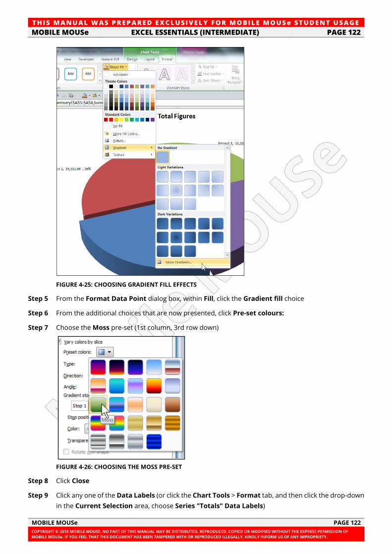
TH IS MANUAL W AS PREPARED EX CLUSIVE LY FOR MOBILE MOUSe ST UDE NT USAGE
MOBILE MOUSe EXCEL ESSENTIALS (INTERMEDIATE) PAGE 122
MOBILE MOUSe PAGE 122
COPYRIGHT © 2018 MOBILE MOUSE. NO PART OF THIS MANUAL MAY BE DISTRIBUTED, REPRODUCED, COPIED OR MODIFIED WITHOUT THE EXPRESS PERMISSION OF
MOBILE MOUSe. IF YOU FEEL THAT THIS DOCUMENT HAS BEEN TAMPERED WITH OR REPRODUCED ILLEGALLY, KINDLY INFORM US OF ANY IMPROPRIETY.
FIGURE 4-25: CHOOSING GRADIENT FILL EFFECTS
Step 5 From the Format Data Point dialog box, within Fill, click the Gradient fill choice
Step 6 From the additional choices that are now presented, click Pre-set colours:
Step 7 Choose the Moss pre-set (1st column, 3rd row down)
FIGURE 4-26: CHOOSING THE MOSS PRE-SET
Step 8 Click Close
Step 9 Click any one of the Data Labels (or click the Chart Tools > Format tab, and then click the drop-down
in the Current Selection area, choose Series "Totals" Data Labels)
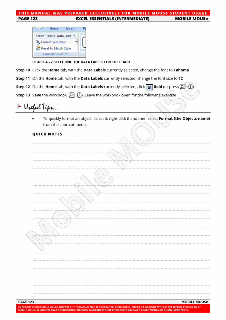
TH IS MANUAL W AS PREPARED EX CLUSIVE LY FOR MOBILE MOUSe ST UDE NT USAGE
PAGE 123 EXCEL ESSENTIALS (INTERMEDIATE) MOBILE MOUSe
PAGE 123 MOBILE MOUSe
COPYRIGHT © 2018 MOBILE MOUSE. NO PART OF THIS MANUAL MAY BE DISTRIBUTED, REPRODUCED, COPIED OR MODIFIED WITHOUT THE EXPRESS PERMISSION OF
MOBILE MOUSe. IF YOU FEEL THAT THIS DOCUMENT HAS BEEN TAMPERED WITH OR REPRODUCED ILLEGALLY, KINDLY INFORM US OF ANY IMPROPRIETY.
FIGURE 4-27: SELECTING THE DATA LABELS FOR THE CHART
Step 10 Click the Home tab, with the Data Labels currently selected, change the font to Tahoma
Step 11 On the Home tab, with the Data Labels currently selected, change the font size to 12
Step 12 On the Home tab, with the Data Labels currently selected, click Bold (or press F+B)
Step 13 Save the workbook (F+S). Leave the workbook open for the following exercise
Useful Tips...
• To quickly format an object, select it, right click it and then select Format (the Objects name)
from the shortcut menu.
QUICK NOTES
..............................................................................................................................................................................................................................
..............................................................................................................................................................................................................................
..............................................................................................................................................................................................................................
..............................................................................................................................................................................................................................
..............................................................................................................................................................................................................................
..............................................................................................................................................................................................................................
..............................................................................................................................................................................................................................
..............................................................................................................................................................................................................................
..............................................................................................................................................................................................................................
..............................................................................................................................................................................................................................
..............................................................................................................................................................................................................................
..............................................................................................................................................................................................................................
..............................................................................................................................................................................................................................
..............................................................................................................................................................................................................................
..............................................................................................................................................................................................................................
..............................................................................................................................................................................................................................
..............................................................................................................................................................................................................................
..............................................................................................................................................................................................................................
..............................................................................................................................................................................................................................
TH IS MANUAL W AS PREPARED EX CLUSIVE LY FOR MOBILE MOUSe ST UDE NT USAGE
MOBILE MOUSe EXCEL ESSENTIALS (INTERMEDIATE) PAGE 124
MOBILE MOUSe PAGE 124
COPYRIGHT © 2018 MOBILE MOUSE. NO PART OF THIS MANUAL MAY BE DISTRIBUTED, REPRODUCED, COPIED OR MODIFIED WITHOUT THE EXPRESS PERMISSION OF
MOBILE MOUSe. IF YOU FEEL THAT THIS DOCUMENT HAS BEEN TAMPERED WITH OR REPRODUCED ILLEGALLY, KINDLY INFORM US OF ANY IMPROPRIETY.
4.2.2 PRINTING CHARTS
In the following exercise you will Preview and then print a chart.
Excercise Time... EXERCISE 4E : PRINTING CHARTS
Step 1 Continue on with the file left open from the previous exercise, or alternatively open the file
Chapter_4E.xlsx
Step 2 Click the Print Preview button under the File tab (or press F+2).
In the Preview window, note that the chart prints when the chart is selected
Step 3 Within Print Preview, click the Print button. Click OK
Step 4 Save the workbook (F+S). Close (F+W) the workbook
Important Notes...
• If you placed your chart as an object within the current worksheet, you can still print it separately
by clicking on the chart itself. When the worksheet is selected, the worksheet and the objects
on it print. When the chart object is selected, only the chart object prints.
4.3 SPARKLINES
MICROSOFT OFFICE CERTIFICATION
This concept addresses the Apply Sparklines competency of the Microsoft Office Specialist
Certification (Exam 77-420).
PLEASE NOTE: This training resource does not necessarily cover all of the requirements of this
exam objective as this objective may include but is not limited to: using Line, Column, and
Win/Loss chart types, creating a Sparkline chart, customizing a Sparkline, formatting a Sparkline,
and showing or hiding data markers.
Visit http://www.microsoft.com/learning/en/us/mos-certification.aspx for the latest Microsoft
Office Certification requirements.
Important Notes...
• Sparklines are only available to Excel 2010 onwards.
A sparkline is a tiny chart in a worksheet cell that provides a visual representation of data. Use
sparklines to show trends in a series of values, such as seasonal increases or decreases, economic
cycles, or to highlight maximum and minimum values. Position a sparkline near its data for greatest
impact.
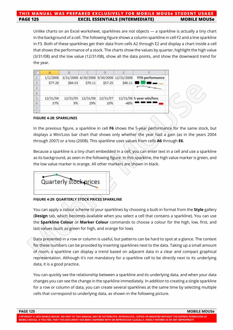
TH IS MANUAL W AS PREPARED EX CLUSIVE LY FOR MOBILE MOUSe ST UDE NT USAGE
PAGE 125 EXCEL ESSENTIALS (INTERMEDIATE) MOBILE MOUSe
PAGE 125 MOBILE MOUSe
COPYRIGHT © 2018 MOBILE MOUSE. NO PART OF THIS MANUAL MAY BE DISTRIBUTED, REPRODUCED, COPIED OR MODIFIED WITHOUT THE EXPRESS PERMISSION OF
MOBILE MOUSe. IF YOU FEEL THAT THIS DOCUMENT HAS BEEN TAMPERED WITH OR REPRODUCED ILLEGALLY, KINDLY INFORM US OF ANY IMPROPRIETY.
Unlike charts on an Excel worksheet, sparklines are not objects — a sparkline is actually a tiny chart
in the background of a cell. The following figure shows a column sparkline in cell F2 and a line sparkline
in F3. Both of these sparklines get their data from cells A2 through E2 and display a chart inside a cell
that shows the performance of a stock. The charts show the values by quarter, highlight the high value
(3/31/08) and the low value (12/31/08), show all the data points, and show the downward trend for
the year.
FIGURE 4-28: SPARKLINES
In the previous figure, a sparkline in cell F6 shows the 5-year performance for the same stock, but
displays a Win/Loss bar chart that shows only whether the year had a gain (as in the years 2004
through 2007) or a loss (2008). This sparkline uses values from cells A6 through E6.
Because a sparkline is a tiny chart embedded in a cell, you can enter text in a cell and use a sparkline
as its background, as seen in the following figure. In this sparkline, the high value marker is green, and
the low value marker is orange. All other markers are shown in black.
FIGURE 4-29: QUARTERLY STOCK PRICES SPARKLINE
You can apply a colour scheme to your sparklines by choosing a built-in format from the Style gallery
(Design tab, which becomes available when you select a cell that contains a sparkline). You can use
the Sparkline Colour or Marker Colour commands to choose a colour for the high, low, first, and
last values (such as green for high, and orange for low).
Data presented in a row or column is useful, but patterns can be hard to spot at a glance. The context
for these numbers can be provided by inserting sparklines next to the data. Taking up a small amount
of room, a sparkline can display a trend based on adjacent data in a clear and compact graphical
representation. Although it's not mandatory for a sparkline cell to be directly next to its underlying
data, it is a good practice.
You can quickly see the relationship between a sparkline and its underlying data, and when your data
changes you can see the change in the sparkline immediately. In addition to creating a single sparkline
for a row or column of data, you can create several sparklines at the same time by selecting multiple
cells that correspond to underlying data, as shown in the following picture.
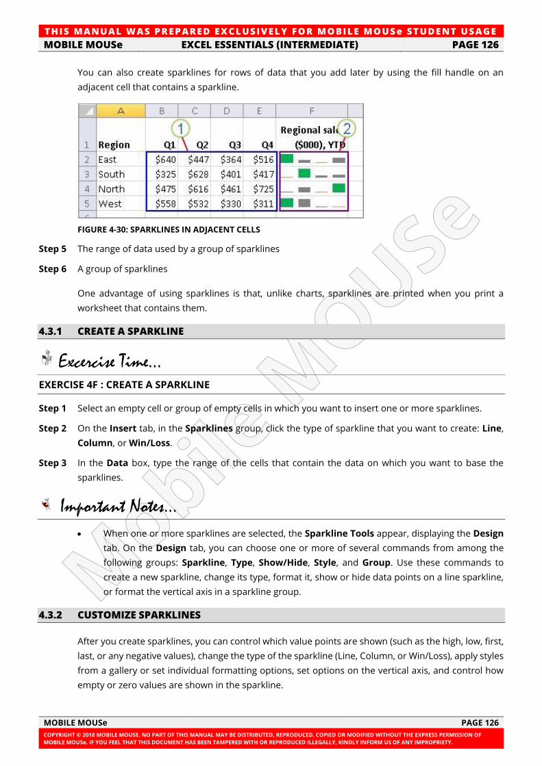
TH IS MANUAL W AS PREPARED EX CLUSIVE LY FOR MOBILE MOUSe ST UDE NT USAGE
MOBILE MOUSe EXCEL ESSENTIALS (INTERMEDIATE) PAGE 126
MOBILE MOUSe PAGE 126
COPYRIGHT © 2018 MOBILE MOUSE. NO PART OF THIS MANUAL MAY BE DISTRIBUTED, REPRODUCED, COPIED OR MODIFIED WITHOUT THE EXPRESS PERMISSION OF
MOBILE MOUSe. IF YOU FEEL THAT THIS DOCUMENT HAS BEEN TAMPERED WITH OR REPRODUCED ILLEGALLY, KINDLY INFORM US OF ANY IMPROPRIETY.
You can also create sparklines for rows of data that you add later by using the fill handle on an
adjacent cell that contains a sparkline.
FIGURE 4-30: SPARKLINES IN ADJACENT CELLS
Step 5 The range of data used by a group of sparklines
Step 6 A group of sparklines
One advantage of using sparklines is that, unlike charts, sparklines are printed when you print a
worksheet that contains them.
4.3.1 CREATE A SPARKLINE
Excercise Time... EXERCISE 4F : CREATE A SPARKLINE
Step 1 Select an empty cell or group of empty cells in which you want to insert one or more sparklines.
Step 2 On the Insert tab, in the Sparklines group, click the type of sparkline that you want to create: Line,
Column, or Win/Loss.
Step 3 In the Data box, type the range of the cells that contain the data on which you want to base the
sparklines.
Important Notes...
• When one or more sparklines are selected, the Sparkline Tools appear, displaying the Design
tab. On the Design tab, you can choose one or more of several commands from among the
following groups: Sparkline, Type, Show/Hide, Style, and Group. Use these commands to
create a new sparkline, change its type, format it, show or hide data points on a line sparkline,
or format the vertical axis in a sparkline group.
4.3.2 CUSTOMIZE SPARKLINES
After you create sparklines, you can control which value points are shown (such as the high, low, first,
last, or any negative values), change the type of the sparkline (Line, Column, or Win/Loss), apply styles
from a gallery or set individual formatting options, set options on the vertical axis, and control how
empty or zero values are shown in the sparkline.
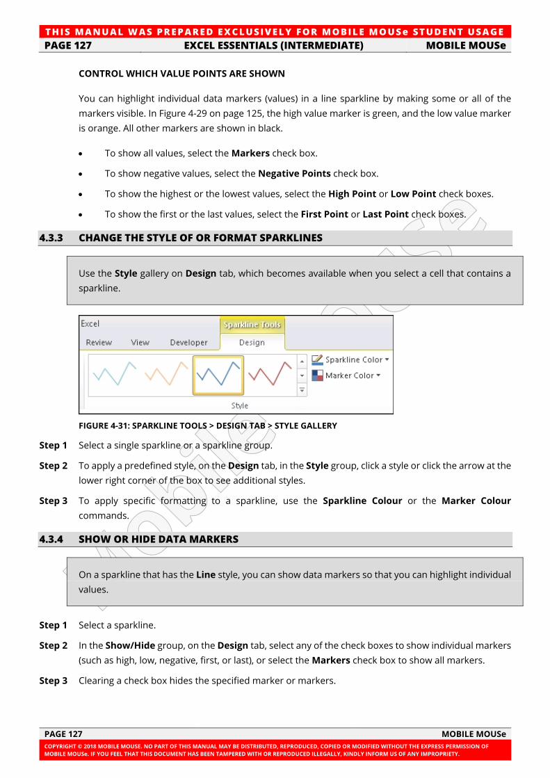
TH IS MANUAL W AS PREPARED EX CLUSIVE LY FOR MOBILE MOUSe ST UDE NT USAGE
PAGE 127 EXCEL ESSENTIALS (INTERMEDIATE) MOBILE MOUSe
PAGE 127 MOBILE MOUSe
COPYRIGHT © 2018 MOBILE MOUSE. NO PART OF THIS MANUAL MAY BE DISTRIBUTED, REPRODUCED, COPIED OR MODIFIED WITHOUT THE EXPRESS PERMISSION OF
MOBILE MOUSe. IF YOU FEEL THAT THIS DOCUMENT HAS BEEN TAMPERED WITH OR REPRODUCED ILLEGALLY, KINDLY INFORM US OF ANY IMPROPRIETY.
CONTROL WHICH VALUE POINTS ARE SHOWN
You can highlight individual data markers (values) in a line sparkline by making some or all of the
markers visible. In Figure 4-29 on page 125, the high value marker is green, and the low value marker
is orange. All other markers are shown in black.
• To show all values, select the Markers check box.
• To show negative values, select the Negative Points check box.
• To show the highest or the lowest values, select the High Point or Low Point check boxes.
• To show the first or the last values, select the First Point or Last Point check boxes.
4.3.3 CHANGE THE STYLE OF OR FORMAT SPARKLINES
Use the Style gallery on Design tab, which becomes available when you select a cell that contains a
sparkline.
FIGURE 4-31: SPARKLINE TOOLS > DESIGN TAB > STYLE GALLERY
Step 1 Select a single sparkline or a sparkline group.
Step 2 To apply a predefined style, on the Design tab, in the Style group, click a style or click the arrow at the
lower right corner of the box to see additional styles.
Step 3 To apply specific formatting to a sparkline, use the Sparkline Colour or the Marker Colour
commands.
4.3.4 SHOW OR HIDE DATA MARKERS
On a sparkline that has the Line style, you can show data markers so that you can highlight individual
values.
Step 1 Select a sparkline.
Step 2 In the Show/Hide group, on the Design tab, select any of the check boxes to show individual markers
(such as high, low, negative, first, or last), or select the Markers check box to show all markers.
Step 3 Clearing a check box hides the specified marker or markers.
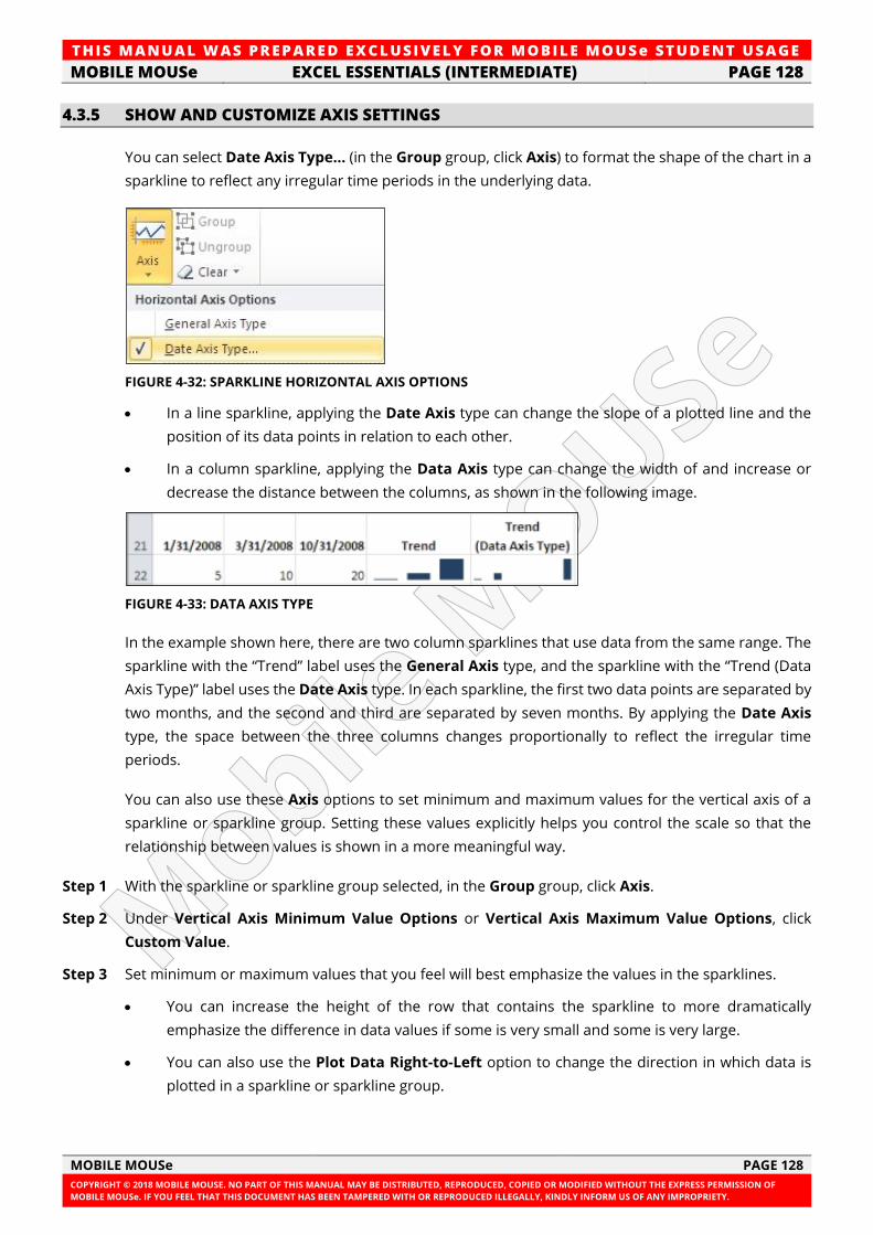
TH IS MANUAL W AS PREPARED EX CLUSIVE LY FOR MOBILE MOUSe ST UDE NT USAGE
MOBILE MOUSe EXCEL ESSENTIALS (INTERMEDIATE) PAGE 128
MOBILE MOUSe PAGE 128
COPYRIGHT © 2018 MOBILE MOUSE. NO PART OF THIS MANUAL MAY BE DISTRIBUTED, REPRODUCED, COPIED OR MODIFIED WITHOUT THE EXPRESS PERMISSION OF
MOBILE MOUSe. IF YOU FEEL THAT THIS DOCUMENT HAS BEEN TAMPERED WITH OR REPRODUCED ILLEGALLY, KINDLY INFORM US OF ANY IMPROPRIETY.
4.3.5 SHOW AND CUSTOMIZE AXIS SETTINGS
You can select Date Axis Type… (in the Group group, click Axis) to format the shape of the chart in a
sparkline to reflect any irregular time periods in the underlying data.
FIGURE 4-32: SPARKLINE HORIZONTAL AXIS OPTIONS
• In a line sparkline, applying the Date Axis type can change the slope of a plotted line and the
position of its data points in relation to each other.
• In a column sparkline, applying the Data Axis type can change the width of and increase or
decrease the distance between the columns, as shown in the following image.
FIGURE 4-33: DATA AXIS TYPE
In the example shown here, there are two column sparklines that use data from the same range. The
sparkline with the “Trend” label uses the General Axis type, and the sparkline with the “Trend (Data
Axis Type)” label uses the Date Axis type. In each sparkline, the first two data points are separated by
two months, and the second and third are separated by seven months. By applying the Date Axis
type, the space between the three columns changes proportionally to reflect the irregular time
periods.
You can also use these Axis options to set minimum and maximum values for the vertical axis of a
sparkline or sparkline group. Setting these values explicitly helps you control the scale so that the
relationship between values is shown in a more meaningful way.
Step 1 With the sparkline or sparkline group selected, in the Group group, click Axis.
Step 2 Under Vertical Axis Minimum Value Options or Vertical Axis Maximum Value Options, click
Custom Value.
Step 3 Set minimum or maximum values that you feel will best emphasize the values in the sparklines.
• You can increase the height of the row that contains the sparkline to more dramatically
emphasize the difference in data values if some is very small and some is very large.
• You can also use the Plot Data Right-to-Left option to change the direction in which data is
plotted in a sparkline or sparkline group.
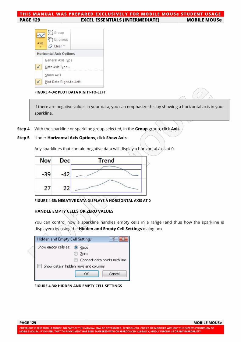
TH IS MANUAL W AS PREPARED EX CLUSIVE LY FOR MOBILE MOUSe ST UDE NT USAGE
PAGE 129 EXCEL ESSENTIALS (INTERMEDIATE) MOBILE MOUSe
PAGE 129 MOBILE MOUSe
COPYRIGHT © 2018 MOBILE MOUSE. NO PART OF THIS MANUAL MAY BE DISTRIBUTED, REPRODUCED, COPIED OR MODIFIED WITHOUT THE EXPRESS PERMISSION OF
MOBILE MOUSe. IF YOU FEEL THAT THIS DOCUMENT HAS BEEN TAMPERED WITH OR REPRODUCED ILLEGALLY, KINDLY INFORM US OF ANY IMPROPRIETY.
FIGURE 4-34: PLOT DATA RIGHT-TO-LEFT
If there are negative values in your data, you can emphasize this by showing a horizontal axis in your
sparkline.
Step 4 With the sparkline or sparkline group selected, in the Group group, click Axis.
Step 5 Under Horizontal Axis Options, click Show Axis.
Any sparklines that contain negative data will display a horizontal axis at 0.
FIGURE 4-35: NEGATIVE DATA DISPLAYS A HORIZONTAL AXIS AT 0
HANDLE EMPTY CELLS OR ZERO VALUES
You can control how a sparkline handles empty cells in a range (and thus how the sparkline is
displayed) by using the Hidden and Empty Cell Settings dialog box.
FIGURE 4-36: HIDDEN AND EMPTY CELL SETTINGS
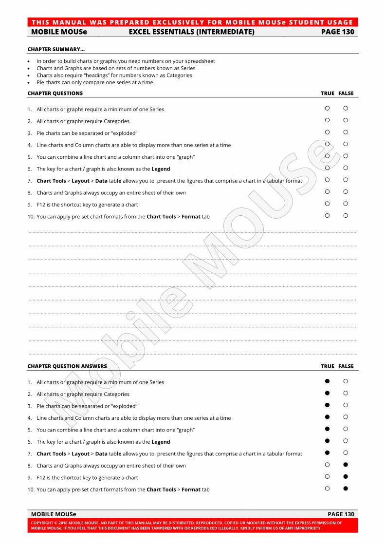
TH IS MANUAL W AS PREPARED EX CLUSIVE LY FOR MOBILE MOUSe ST UDE NT USAGE
MOBILE MOUSe EXCEL ESSENTIALS (INTERMEDIATE) PAGE 130
MOBILE MOUSe PAGE 130
COPYRIGHT © 2018 MOBILE MOUSE. NO PART OF THIS MANUAL MAY BE DISTRIBUTED, REPRODUCED, COPIED OR MODIFIED WITHOUT THE EXPRESS PERMISSION OF
MOBILE MOUSe. IF YOU FEEL THAT THIS DOCUMENT HAS BEEN TAMPERED WITH OR REPRODUCED ILLEGALLY, KINDLY INFORM US OF ANY IMPROPRIETY.
CHAPTER SUMMARY…
• In order to build charts or graphs you need numbers on your spreadsheet
• Charts and Graphs are based on sets of numbers known as Series
• Charts also require “headings” for numbers known as Categories
• Pie charts can only compare one series at a time
CHAPTER QUESTIONS TRUE FALSE
1. All charts or graphs require a minimum of one Series ○ ○
2. All charts or graphs require Categories ○ ○
3. Pie charts can be separated or “exploded” ○ ○
4. Line charts and Column charts are able to display more than one series at a time ○ ○
5. You can combine a line chart and a column chart into one “graph” ○ ○
6. The key for a chart / graph is also known as the Legend ○ ○
7. Chart Tools > Layout > Data table allows you to present the figures that comprise a chart in a tabular format ○ ○
8. Charts and Graphs always occupy an entire sheet of their own ○ ○
9. F12 is the shortcut key to generate a chart ○ ○
10. You can apply pre-set chart formats from the Chart Tools > Format tab ○ ○
..................................................................................................................................................................................................................................................
..................................................................................................................................................................................................................................................
..................................................................................................................................................................................................................................................
..................................................................................................................................................................................................................................................
..................................................................................................................................................................................................................................................
..................................................................................................................................................................................................................................................
..................................................................................................................................................................................................................................................
..................................................................................................................................................................................................................................................
..................................................................................................................................................................................................................................................
..................................................................................................................................................................................................................................................
CHAPTER QUESTION ANSWERS TRUE FALSE
1. All charts or graphs require a minimum of one Series ● ○
2. All charts or graphs require Categories ● ○
3. Pie charts can be separated or “exploded” ● ○
4. Line charts and Column charts are able to display more than one series at a time ● ○
5. You can combine a line chart and a column chart into one “graph” ● ○
6. The key for a chart / graph is also known as the Legend ● ○
7. Chart Tools > Layout > Data table allows you to present the figures that comprise a chart in a tabular format ● ○
8. Charts and Graphs always occupy an entire sheet of their own ○ ●
9. F12 is the shortcut key to generate a chart ○ ●
10. You can apply pre-set chart formats from the Chart Tools > Format tab ○ ●

This manual was supplied in digital form for Mobile MOUSe student usage exclusively. Under no circumstances may you copy or distribute this
document (in whole or in part) to any entity, person, party or organization. This manual may not be printed or reproduced in any form without
express permission from Mobile MOUSe.
QUICK NOTES
..................................................................................................................................................................................................................................................
..................................................................................................................................................................................................................................................
..................................................................................................................................................................................................................................................
..................................................................................................................................................................................................................................................
..................................................................................................................................................................................................................................................
..................................................................................................................................................................................................................................................
..................................................................................................................................................................................................................................................
..................................................................................................................................................................................................................................................
..................................................................................................................................................................................................................................................
..................................................................................................................................................................................................................................................
..................................................................................................................................................................................................................................................
..................................................................................................................................................................................................................................................
..................................................................................................................................................................................................................................................
..................................................................................................................................................................................................................................................
..................................................................................................................................................................................................................................................
..................................................................................................................................................................................................................................................
..................................................................................................................................................................................................................................................
..................................................................................................................................................................................................................................................
..................................................................................................................................................................................................................................................
..................................................................................................................................................................................................................................................
..................................................................................................................................................................................................................................................
..................................................................................................................................................................................................................................................
..................................................................................................................................................................................................................................................
..................................................................................................................................................................................................................................................
..................................................................................................................................................................................................................................................
..................................................................................................................................................................................................................................................
..................................................................................................................................................................................................................................................
..................................................................................................................................................................................................................................................
..................................................................................................................................................................................................................................................
..................................................................................................................................................................................................................................................
..................................................................................................................................................................................................................................................
..................................................................................................................................................................................................................................................
..................................................................................................................................................................................................................................................
..................................................................................................................................................................................................................................................
..................................................................................................................................................................................................................................................
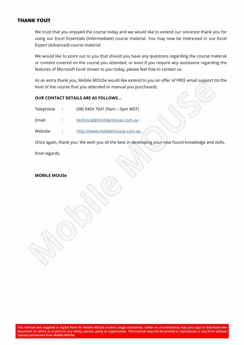
This manual was supplied in digital form for Mobile MOUSe student usage exclusively. Under no circumstances may you copy or distribute this
document (in whole or in part) to any entity, person, party or organization. This manual may not be printed or reproduced in any form without
express permission from Mobile MOUSe.
THANK YOU!!
We trust that you enjoyed the course today and we would like to extend our sincerest thank you for
using our Excel Essentials (Intermediate) course material. You may now be interested in our Excel
Expert (Advanced) course material.
We would like to point out to you that should you have any questions regarding the course material
or content covered on the course you attended, or even if you require any assistance regarding the
features of Microsoft Excel shown to you today, please feel free to contact us.
As an extra thank you, Mobile MOUSe would like extend to you an offer of FREE email support (to the
level of the course that you attended or manual you purchased).
OUR CONTACT DETAILS ARE AS FOLLOWS…
Telephone : (08) 9404 7041 (9am – 5pm WST)
Email : [email protected]
Website : http://www.mobilemouse.com.au
Once again, thank you. We wish you all the best in developing your new found knowledge and skills.
Kind regards,
MOBILE MOUSe
This manual was supplied in digital form for Mobile MOUSe student usage exclusively. Under no circumstances may you copy or distribute this
document (in whole or in part) to any entity, person, party or organization. This manual may not be printed or reproduced in any form without
express permission from Mobile MOUSe.
DOCUMENT INDEX
ANSWERS
PART 1 ................................................................................................................................................................................. 39
PART 2 ................................................................................................................................................................................. 65
PART 3 ............................................................................................................................................................................... 106
PART 4 ............................................................................................................................................................................... 131
AutoFiller
Copy a Formula .................................................................................................................................................................. 23
Introduction ......................................................................................................................................................................... 3
Charts
Axis Titles .......................................................................................................................................................................... 111
Change Source Data ........................................................................................................................................................ 114
Chart Area ........................................................................................................................................................................ 114
Chart Title ......................................................................................................................................................................... 111
Column ............................................................................................................................................................................. 108
Concepts ........................................................................................................................................................................... 107
Data Labels ....................................................................................................................................................................... 112
Data Table ........................................................................................................................................................................ 113
Editing and Formatting ................................................................................................................................................... 121
Gridlines ........................................................................................................................................................................... 112
Legend .............................................................................................................................................................................. 113
More Data Label Options ............................................................................................................................................... 119
Moving .............................................................................................................................................................................. 110
Pie ...................................................................................................................................................................................... 116
Printing ............................................................................................................................................................................. 125
Rotating 3D Charts .......................................................................................................................................................... 120
Select Data ........................................................................................................................................................................ 115
Series ................................................................................................................................................................................. 107
Shortcut Keys ................................................................................................................................................................... 114
Switch Row / Column ...................................................................................................................................................... 110
Clipboard ............................................................................................................................................................. 8
Conditional Formatting ................................................................................................................................... 69
Clear Rules from Entire Sheet .......................................................................................................................................... 73
ClearRules from Selected Cells ........................................................................................................................................ 74
Data Bars and Colour Scales ............................................................................................................................................ 73
Editing ................................................................................................................................................................................. 73
Highlight Cells Rules .......................................................................................................................................................... 71
Icon Sets ............................................................................................................................................................................. 75
Limits ................................................................................................................................................................................... 69
Managing ............................................................................................................................................................................ 73
Top / Bottom Rules ............................................................................................................................................................ 69
Customizing the Quick Access Toolbar ............................................................................................................ 1
Cut, Copy and Paste ........................................................................................................................................... 8
Data Validation ................................................................................................................................................. 78
Circle Invalid Data .............................................................................................................................................................. 84
Date ..................................................................................................................................................................................... 79
Error Alert Styles ................................................................................................................................................................ 81
Error Message .............................................................................................................................................................. 80, 83
Input Message.................................................................................................................................................................... 80
List ....................................................................................................................................................................................... 83
Whole Number .................................................................................................................................................................. 81
Filtering ............................................................................................................................................................. 87
Clear .................................................................................................................................................................................... 91
Custom ................................................................................................................................................................................ 92
Dates ................................................................................................................................................................................... 90
This manual was supplied in digital form for Mobile MOUSe student usage exclusively. Under no circumstances may you copy or distribute this
document (in whole or in part) to any entity, person, party or organization. This manual may not be printed or reproduced in any form without
express permission from Mobile MOUSe.
Search ................................................................................................................................................................................. 91
Formulas ............................................................................................................................................................ 16
3D References .................................................................................................................................................................... 57
Absolute References ......................................................................................................................................................... 27
AUTOSUM ........................................................................................................................................................................... 21
AVERAGE ....................................................................................................................................................................... 21, 33
Calculate a Specific Percentage ....................................................................................................................................... 32
Calculating a Percentage .................................................................................................................................................. 25
Calculations Across Sheets ............................................................................................................................................... 53
Copy with AutoFiller .......................................................................................................................................................... 23
COUNT ................................................................................................................................................................................ 21
COUNTA .............................................................................................................................................................................. 21
IF .......................................................................................................................................................................................... 58
MAX ............................................................................................................................................................................... 21, 33
MIN ................................................................................................................................................................................ 21, 33
Operators ........................................................................................................................................................................... 17
Order of Operations .......................................................................................................................................................... 18
Quick Calc ........................................................................................................................................................................... 37
Relative References ........................................................................................................................................................... 22
Hyperlinks ......................................................................................................................................................... 63
Paste Options .................................................................................................................................................... 10
QUESTIONS
PART 1 ................................................................................................................................................................................. 39
PART 2 ................................................................................................................................................................................. 65
PART 3 ............................................................................................................................................................................... 106
PART 4 ............................................................................................................................................................................... 131
Sheets
Copying Sheets .................................................................................................................................................................. 49
Grouping Sheets ................................................................................................................................................................ 52
Moving or Copying between Workbooks ....................................................................................................................... 51
Navigating Sheets .............................................................................................................................................................. 50
Renaming Sheets ............................................................................................................................................................... 49
Sorting ............................................................................................................................................................... 85
Styles.................................................................................................................................................................. 99
Subtotals ......................................................................................................................................................... 101
Functions .......................................................................................................................................................................... 102
SUMMARY
PART 1 ................................................................................................................................................................................. 39
PART 2 ................................................................................................................................................................................. 65
PART 3 ............................................................................................................................................................................... 106
PART 4 ............................................................................................................................................................................... 131
Tables
Format as Table ................................................................................................................................................................. 94
Options ............................................................................................................................................................................... 95
Total Row ............................................................................................................................................................................ 97
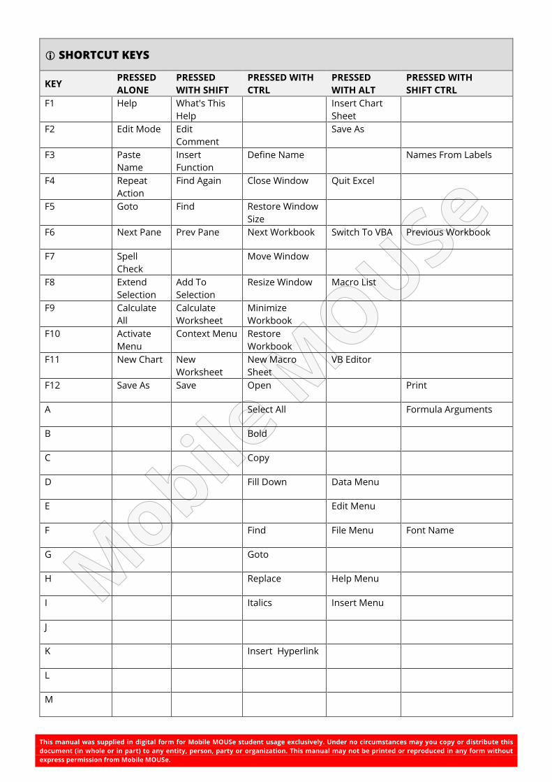
This manual was supplied in digital form for Mobile MOUSe student usage exclusively. Under no circumstances may you copy or distribute this
document (in whole or in part) to any entity, person, party or organization. This manual may not be printed or reproduced in any form without
express permission from Mobile MOUSe.
SHORTCUT KEYS
KEY PRESSED
ALONE
PRESSED
WITH SHIFT
PRESSED WITH
CTRL
PRESSED
WITH ALT
PRESSED WITH
SHIFT CTRL
F1 Help What's This
Help
Insert Chart
Sheet
F2 Edit Mode Edit
Comment
Save As
F3 Paste
Name
Insert
Function
Define Name Names From Labels
F4 Repeat
Action
Find Again Close Window Quit Excel
F5 Goto Find Restore Window
Size
F6 Next Pane Prev Pane Next Workbook Switch To VBA Previous Workbook
F7 Spell
Check
Move Window
F8 Extend
Selection
Add To
Selection
Resize Window Macro List
F9 Calculate
All
Calculate
Worksheet
Minimize
Workbook
F10 Activate
Menu
Context Menu Restore
Workbook
F11 New Chart New
Worksheet
New Macro
Sheet
VB Editor
F12 Save As Save Open
A Select All Formula Arguments
B Bold
C Copy
D
Fill Down Data Menu
E
Edit Menu
F
Find File Menu Font Name
G Goto
H Replace Help Menu
I Italics Insert Menu
J
K
Insert Hyperlink
L
M
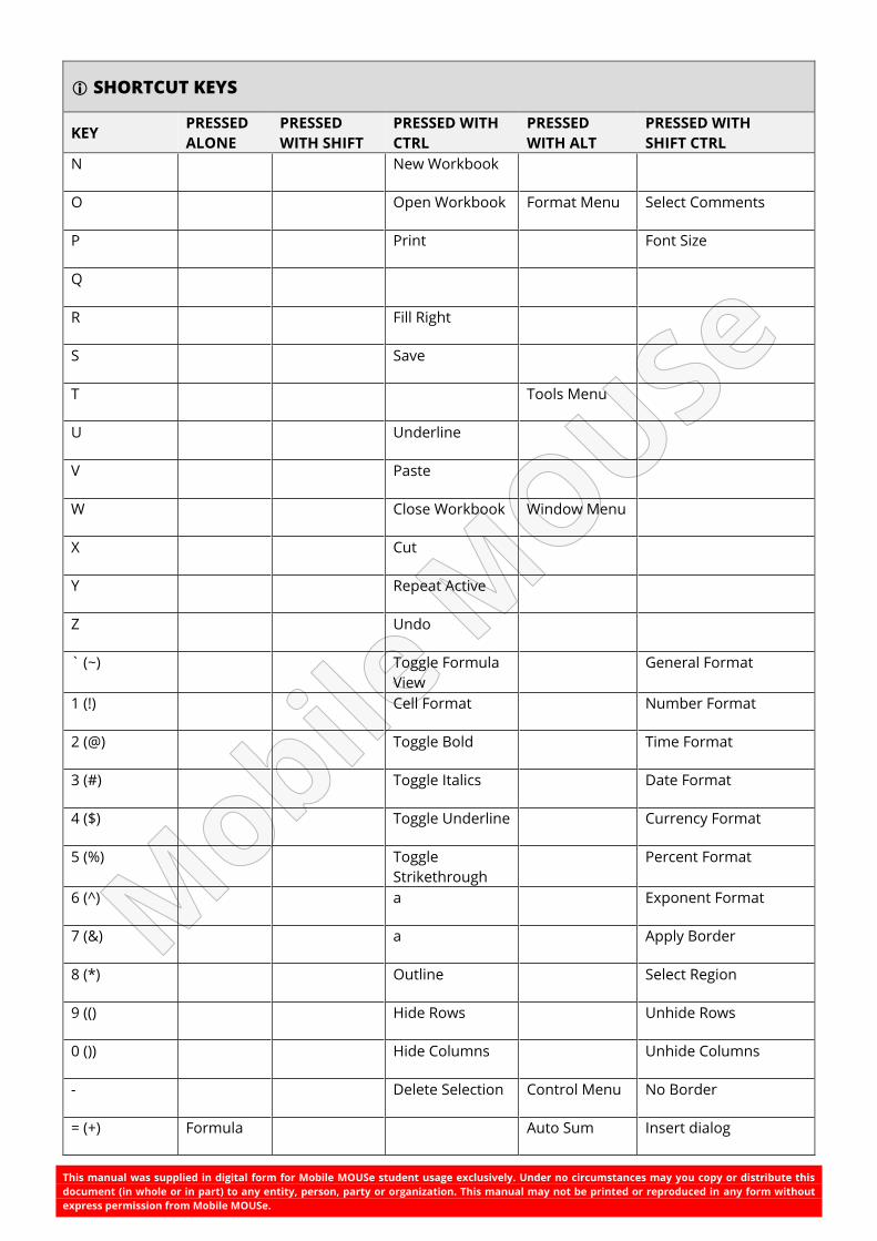
This manual was supplied in digital form for Mobile MOUSe student usage exclusively. Under no circumstances may you copy or distribute this
document (in whole or in part) to any entity, person, party or organization. This manual may not be printed or reproduced in any form without
express permission from Mobile MOUSe.
SHORTCUT KEYS
KEY PRESSED
ALONE
PRESSED
WITH SHIFT
PRESSED WITH
CTRL
PRESSED
WITH ALT
PRESSED WITH
SHIFT CTRL
N New Workbook
O Open Workbook Format Menu Select Comments
P
Font Size
Q
R
Fill Right
S Save
T Tools Menu
U Underline
V
Paste
W
Close Workbook Window Menu
X
Cut
Y Repeat Active
Z Undo
` (~) Toggle Formula
View
General Format
1 (!)
Cell Format
Number Format
2 (@)
Toggle Bold
Time Format
3 (#)
Toggle Italics
Date Format
4 ($) Toggle Underline Currency Format
5 (%) Toggle
Strikethrough
Percent Format
6 (^) a Exponent Format
7 (&)
a
Apply Border
8 (*)
Outline
Select Region
9 (()
Hide Rows
Unhide Rows
0 ()) Hide Columns Unhide Columns
- Delete Selection Control Menu No Border
= (+) Formula Auto Sum Insert dialog
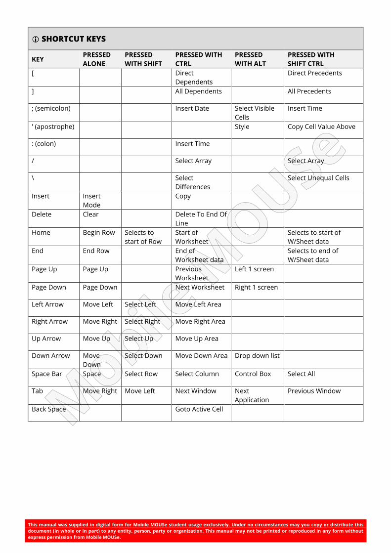
This manual was supplied in digital form for Mobile MOUSe student usage exclusively. Under no circumstances may you copy or distribute this
document (in whole or in part) to any entity, person, party or organization. This manual may not be printed or reproduced in any form without
express permission from Mobile MOUSe.
SHORTCUT KEYS
KEY PRESSED
ALONE
PRESSED
WITH SHIFT
PRESSED WITH
CTRL
PRESSED
WITH ALT
PRESSED WITH
SHIFT CTRL
[
Direct
Dependents
Direct Precedents
]
All Dependents
All Precedents
; (semicolon)
Insert Date Select Visible
Cells
Insert Time
' (apostrophe) Style Copy Cell Value Above
: (colon) Insert Time
/ Select Array Select Array
\
Select
Differences
Select Unequal Cells
Insert Insert
Mode
Copy
Delete Clear
Delete To End Of
Line
Home Begin Row Selects to
start of Row
Start of
Worksheet
Selects to start of
W/Sheet data
End End Row
End of
Worksheet data
Selects to end of
W/Sheet data
Page Up Page Up Previous
Worksheet
Left 1 screen
Page Down Page Down
Next Worksheet Right 1 screen
Left Arrow Move Left Select Left Move Left Area
Right Arrow Move Right Select Right Move Right Area
Up Arrow Move Up Select Up Move Up Area
Down Arrow Move
Down
Select Down Move Down Area Drop down list
Space Bar Space Select Row Select Column Control Box Select All
Tab Move Right Move Left Next Window Next
Application
Previous Window
Back Space Goto Active Cell