Excel 2016 Formatting Beyond the Basics 

training@health.ufl.edu

Updated 10/25/2016 

Excel 2016: Formatting Beyond the Basics 1.5 hours 

In this workshop we will learn to use conditional formatting to have Excel automatically format our data sets based on the cell contents; how to use tables which provide filters and automatic alternating row colors; apply themes to change the color schemes associated within our workbook; create comments to make notes within the cells; and protect the worksheets and workbooks. This intermediate workshop assumes prior experience with Microsoft Excel.  

Conditional Formatting ................................................................................................................... 1 Finding Duplicates ....................................................................................................................... 1 

Top and Bottom Values ............................................................................................................... 2 

Data Bars ..................................................................................................................................... 2 

Color Scales ................................................................................................................................. 2 

Icon Sets ...................................................................................................................................... 3 

Custom Rule – Dates past due ..................................................................................................... 3 

Tables............................................................................................................................................... 4 Create a Table structure .............................................................................................................. 4 

Removing the Table structure (Convert to range) ....................................................................... 5 

Adding/Deleting Rows in Tables ................................................................................................. 5 

Doing Math in Tables .................................................................................................................. 6 

Protecting Worksheets/Workbooks ................................................................................................ 6 Protect Sheet ............................................................................................................................... 7 

Comments ....................................................................................................................................... 7 Themes ............................................................................................................................................ 8 Numbers Exercises .......................................................................................................................... 8 

Customize Color Scales ................................................................................................................ 8 

Find Min, Max, and Average with Conditional Formatting ......................................................... 9 

Too Much Data to Chart .............................................................................................................. 9 

Sparklines ...................................................................................................................................... 10 Quick Totals ............................................................................................................................... 10 

More about Custom Conditional Formatting ................................................................................ 11 More about Excel Tables ............................................................................................................... 12 More about Sparklines .................................................................................................................. 13 

  

 

Pandora Rose Cowart   Education/Training Specialist   UF Health IT Training    

 C3‐013 Communicore   (352) 273‐5051 PO Box 100152  prcowart@ufl.edu  Gainesville, FL 32610‐0152  http://training.health.ufl.edu   

 

1 

Conditional Formatting 

Using criteria, a set of rules, we can have Excel format the cells that match. The following exercises will walk us through some of these powerful formatting aides. This tool works best if you select the cells you want to format before you set any rules. Finding Duplicates 

1. Open Customers 

2. Select Column A (Last) 

3. On the Home Tab, in the Styles group, choose Conditional Formatting 

4. Select Highlight Cell Rules, and then Duplicate Values… 

5. In the Duplicate Values Window, leave the light red fill setting and, click OK 

6. Scroll down to see the M's 

7. Joe and John Jinks are different records, but Marge and Marjorie look to be the same. 

 

 

8. Clear the formatting rules.  

‐ Open the Conditional Formatting menu again. 

‐ Choose Clear Rules, and choose Clear Rules from Entire Sheet. 

 

 

2 

Top and Bottom Values We can sort the Balance column to find the top and bottom values listed, or we can have Excel format the cells to help them pop out. 

1. Select Column G (balance) 

2. From Conditional Formatting choose Top/Bottom Rules 

3. Choose Top 10 Items 

‐ Notice you can change the number of items to be the top 3 or any number between 1 and 1000. 

4. Leave the default settings of 10 items, with a Light Red Fill. Click OK. 

5. Go back to the Conditional Formatting, choose Top/Bottom Rules 

6. Choose Bottom 10 Items 

7. Change the color setting to Green Fill and click OK. 

   

8. Clear the formatting rules from the Conditional Formatting menu 

 Data Bars 

1. Select Column G (Balance)  

2. From Conditional Formatting choose Data Bars 

3. Hover over the different options to see a live preview of the embedded bar chart in the cells. The larger the number, the longer the bar. 

‐ You can widen the column as much as you want, and the bars will stretch with your column width. 

4. Choose one that you like 

‐ Set the number format to general to see them without the $ and decimals. 

 Color Scales 

1. Select Column G (Balance) 

2. From Conditional Formatting choose Color Scales 

3. Hover over the different options to see a live preview of the shading. Notice the data bars are still showing. 

4. Clear all Conditional Formatting 

5. Try the color scales again. 

6. Sort the column to see the shading in action 

7. Undo the sort and Conditional Formatting 

   

 

3 

Icon Sets 1. Select Column G (Balance) 2. From Conditional Formatting choose Icon Sets 3. Hover over the different options to see a live preview of the icons 

‐ As with the data bars and color scales these icons are relative to the data in the entire column. Up arrows are above average, sideways arrows are near average and down arrows are below average.  

4. Clear the formatting rules from the Conditional Formatting menu 

 Custom Rule – Dates past due There are date rules available in the Conditional Formatting, Highlight Cell Rules, you can choose A Date Occurring…  However, the rules here are limited. What I would like us to find is all the records (rows) where the date is past due.  

1. Select Column H (Due Date) 2. From Conditional Formatting choose New Rule… 3. From the top of the New Formatting Rule window, 

choose Format only cells that contain  ‐ Change the second drop down list to less than 

‐ In the third box type:  =Today() 

‐ Don't forget the equal sign and the parentheses 

4. Click the Format button ‐ Set the format to be Bold, with an Outline border, and a light grey fill 

‐ Click OK to accept the format, and click OK to accept the rule. 

5. Leave this format      

 

4 

Tables We can format Excel ourselves using the tools found in the Font group. There are font styles, fill colors, and borders. When we set up the format ourselves, we sometimes have to be careful about moving cells around. It's very easy to lose a border format, or shade in the wrong color. If you need a formatted structure with consistent colors, you may fall in love with Tables. Create a Table structure 

1. Return to Cell A1 (Ctrl Home) 

2. From the Home tab, next to the Conditional Formatting button, choose Format as Table 

3. Choose an option that has alternating colors for each row.  

 

 

4. Excel should pick up the entire dataset. We have titles, headers, so we'll leave that option checked. Click OK to see the result. 

5. Our conditional formatting remains on the Due Dates. 

6. We now have a new tab in the ribbon to help us modify the Design of the table. 

7. Try the different table style options and table styles to see how it changes the format of our table. One of the best features is the Total Row. 

‐ With the total row turned on, scroll to the bottom of the dataset. The 77 represents how many records we have. Click inside the Total for the Balance column and change it to Sum. 

 

5 

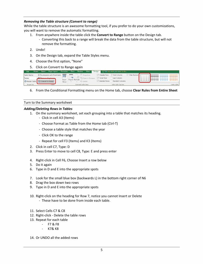
Removing the Table structure (Convert to range) While the table structure is an awesome formatting tool, if you prefer to do your own customizations, you will want to remove the automatic formatting. 

1. From anywhere inside the table click the Convert to Range button on the Design tab. ‐ Converting this back to a range will break the data from the table structure, but will not remove the formatting. 

2. Undo! 

3. On the Design tab, expand the Table Styles menu. 

4. Choose the first option, "None" 

5. Click on Convert to Range again 

 

 

 

6. From the Conditional Formatting menu on the Home tab, choose Clear Rules from Entire Sheet 

 

Turn to the Summary worksheet 

Adding/Deleting Rows in Tables 1. On the summary worksheet, set each grouping into a table that matches its heading. 

‐ Click in cell A3 (Items) 

‐ Choose Format as Table from the Home tab (Ctrl‐T) 

‐ Choose a table style that matches the year 

‐ Click OK to the range 

‐ Repeat for cell F3 (Items) and K3 (Items) 

2. Click in cell C7, Type: D 3. Press Enter to move to cell C8, Type: E and press enter 

 4. Right‐click in Cell F6, Choose Insert a row below 5. Do it again 6. Type in D and E into the appropriate spots 

 7. Look for the small blue box (backwards L) in the bottom right corner of N6 8. Drag the box down two rows 9. Type in D and E into the appropriate spots 

 10. Right‐click on the heading for Row 7, notice you cannot Insert or Delete 

‐ These have to be done from inside each table. 

 11. Select Cells C7 & C8 12. Right‐click ‐ Delete the table rows 13. Repeat for each table 

‐ F7 & F8 ‐ K7& K8 

 14. Or UNDO all the added rows   

 

6 

Doing Math in Tables 1. In Cell D4 press the equal sign ( = ) 

2. Click in cell B4 (123) 

‐ Excel doesn't say B4, it says: =[@Price] 

3. Type the multiply sign, the asterisk ( * ) 

4. Click in Cell C4 (812) 

‐ =[@Price]*[@Qty] 

5. Press Enter to accept. All the equations are filled in 

6. Turn on the totals row 

7. Repeat for the other two tables 

8. Since these are such small tables, you may consider turning off the Filter Buttons as well. 

 

Protecting Worksheets/Workbooks If you would like to restrict people from making changes, including yourself, you may consider protecting it. You'll find the option on the Review tab in the Changes group. From here you can decide what users, including yourself, are allowed to do within this sheet.  You do not have to set a password unless you want one.   

Once you have protected the sheet, the button will change to say Unprotect Sheet, use this option to release the control.   

If you would like to allow edits to specific cells, choose those cells and change their protection "lock cell" option from the Format Cell menu, or Format Cell Window.   Locking a worksheet helps prevent 

edits, and formatting, inserting/deleting columns and rows and cells.  

Locking a workbook helps prevent changes to the workbook structure, like inserting/deleting worksheets.  

If you forget the password, there is no recovery. Either don't use a password, or DON'T FORGET IT! 

   

 

7 

Protect Sheet 1. From the Review tab, choose Protect Sheet 

2. Leave the defaults and click OK 

3. Click in cell C4 to and try to change the Qty 

4. From the Review tab, choose Unprotect Sheet 

5. Select all the Qty cells C4:C6; H4:H6, M4:M6 

‐ Use your control key, or do each section one at a time 

6. Open the format cells window 

‐ Right‐click in the selection, or press Ctrl 1 

7. Turn to the Protection tab 

8. Uncheck the Locked option and click OK 

9. From the Review tab, choose Protect Sheet 

10. Leave the defaults and click OK 

11. Click in cell C4 to and try to change the Qty 

‐ No Problem! 

Comments A comment is a way to leave a subtle note within the worksheet. In this case let's put a note with the 2018 Price title reminding people if they need to change the price, they will have to unprotect the sheet. Comments can be printed by choosing the option in the Page Setup on the sheet tab.  

1. Unprotect sheet 

2. Click in Cell L3 (Price) 

3. From the Review tab choose New Comment 

4. Type your comment into the comment box 

5. Click outside of the box and it will disappear 

6. Notice the small red triangle in the upper right corner of the box. That's our visual cue there is a comment in that cell. 

7. Hover over your mouse over cell L3 to see the comment appear. If you can't see all the text, you can click on the Edit Comment button that has taken the place of the New Comment button. 

‐ Click inside the cell, Click Edit Comment, Resize the box, click outside the comment 

 

8 

Themes A theme is a preset list of default formatting for the workbook. This includes the Fonts, Colors, and Effects. We typically stay with the Office theme and choose custom colors when we want them, but this is a way to change everything at once.  

1. From the Page Layout tab, choose Themes 

2. Hover over each theme to see it change the fonts and colors of your tables ‐ Notice there is a scroll bar! More than you can see. Either scroll down, or grab the corner ( ) to stretch the window. 

3. Return to the Office Theme at the top of the list 

4. Click on the Colors option ‐ This setting will change the colors and not the fonts and effects 

5. Return to the Office color choices ‐ Remember your choices here will change the sheets in the workbook. 

 

Turn to the Numbers worksheet 

Numbers Exercises Customize Color Scales 

1. Select Dataset from the Name Box 

2. Choose a Color Scale from the Conditional Formatting menu 

3. Choose Mange Rules from the Conditional Formatting menu 

 

4. Click on the Edit Rule button 

‐ If needed change to a 2 color scale 

5. Pick two colors 

‐ I recommend something light 

6. Click OK to accept your changes 

7. Click OK to leave the Rules Manager 

8. Clear all Conditional Formatting from sheet 

 

 

9 

Find Min, Max, and Average with Conditional Formatting 1. Click in the Name Box to see a pre‐named range of Dataset 

2. Choose Dataset (B2:Z27) 

3. Create the functions for the small grouping in column AE 

‐ In cell AE1 type: =Min(Dataset) 

‐ In cell AE2 type: =Max(Dataset) 

‐ In cell AE3 type: =Average(Dataset) 

4. Select Dataset from the Name Box 

5. Set a Conditional Format to find the min values 

‐ Turn to the Home Tab  

‐ Choose Conditional Formatting 

‐ Choose Highlight Cells Equal To 

‐ Click in Cell AE1 

‐ Leave the formatting Light Red Fill… 

6. Set a Conditional Format to find the max values 

‐ Equal to Cell AE2, Green Fill … 

7. Set a Conditional Format to find the Avg values 

‐ Equal to Cell AE3, Yellow Fill  

8. Clear all Conditional Formatting from sheet 

 Too Much Data to Chart 

1. Return to the top of the sheet (Ctrl Home) 

2. From the Insert tab choose Recommended Charts 

3. Click on each Recommended Chart to see the messy outcome 

‐ Each item or date may need to be charted separately or by quarter 

4. Change to the All Charts tab to see other possible previews. 

5. Cancel the Insert Chart window. 

6. Select Dataset from Name Box 

7. Return to the Home tab and set a Conditional Format with Data Bars for an embedded bar chart 

8. Set a Conditional Format with a Ratings Icons to see an embedded pie‐like chart 

9. Clear all Conditional Formatting 

 

10 

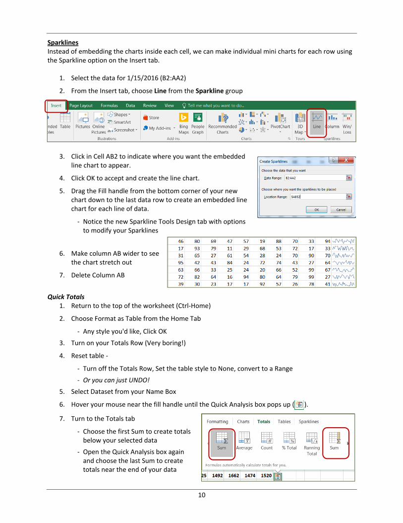
Sparklines Instead of embedding the charts inside each cell, we can make individual mini charts for each row using the Sparkline option on the Insert tab.  

1. Select the data for 1/15/2016 (B2:AA2)  

2. From the Insert tab, choose Line from the Sparkline group 

 3. Click in Cell AB2 to indicate where you want the embedded 

line chart to appear. 

4. Click OK to accept and create the line chart. 

5. Drag the Fill handle from the bottom corner of your new chart down to the last data row to create an embedded line chart for each line of data. 

‐ Notice the new Sparkline Tools Design tab with options to modify your Sparklines 

 

6. Make column AB wider to see the chart stretch out 

7. Delete Column AB 

 Quick Totals 

1. Return to the top of the worksheet (Ctrl‐Home) 

2. Choose Format as Table from the Home Tab 

‐ Any style you'd like, Click OK 

3. Turn on your Totals Row (Very boring!) 

4. Reset table ‐  

‐ Turn off the Totals Row, Set the table style to None, convert to a Range 

‐ Or you can just UNDO! 

5. Select Dataset from your Name Box 

6. Hover your mouse near the fill handle until the Quick Analysis box pops up ( ). 

7. Turn to the Totals tab 

‐ Choose the first Sum to create totals below your selected data 

‐ Open the Quick Analysis box again and choose the last Sum to create totals near the end of your data 

 

11 

More about Custom Conditional Formatting (Modified from the Office Help) To more easily find specific cells within a range of cells, you can format those specific cells based on a comparison operator.   

Quick formatting  

1. Select one or more cells in a range, table, or PivotTable report. 

2. On the Home tab, in the Style group, click the arrow next to Conditional Formatting, and then click Highlight Cells Rules. 

 

3. Select the command that you want such as Between, Equal To Text that Contains, or A Date Occurring. 

4. Enter the values that you want to use, and then select a format.  

Advanced formatting  

1. Select one or more cells in a range, table, or PivotTable report. 

2. On the Home tab, in the Styles group, click the arrow next to Conditional Formatting, and then click Manage Rules. 

The Conditional Formatting Rules Manager dialog box is displayed. 

3. Do one of the following: 

o To add a conditional format, click New Rule. 

o To change a conditional format, do the following: 

i. Select the rule, and then click Edit rule. 

4. Under Select a Rule Type, click Format only cells that contain. 

5. Under Edit the Rule Description, in the Format only cells with list box, do one of the following: 

o Format by number, date, or time ‐ Select Cell Value, select a comparison operator, and then enter a number, date, or time.  If you enter a formula, start it with an equal sign (=). Invalid formulas result in no formatting being applied. It's a good idea to test the formula to make sure that it doesn't return an error value. 

o Format by text ‐ Select Specific Text, choose a comparison operator, and then enter text. Quotes are included in the search string, and you may use wildcard characters. The maximum length of a string is 255 characters. 

o Format by date ‐ Select Dates Occurring, and then select a date comparison.  

o Format cells with blanks or no blanks ‐ Select Blanks or No Blanks.  A blank value is a cell that contains no data and is different from a cell that contains one or more spaces (spaces are considered as text). 

o Format cells with error or no error values ‐ Select Errors or No Errors. Error values include: #####, #VALUE!, #DIV/0!, #NAME?, #N/A, #REF!, #NUM!, and #NULL!. 

6. To specify a format, click Format. ‐ The Format Cells dialog box is displayed. 

7. Select the number, font, border, or fill format that you want to apply when the cell value meets the condition, and then click OK.  The formats that you select are displayed in the Preview box. 

 

12 

More about Excel Tables (Modified from the Office Help) 

To make managing and analyzing a group of related data easier, you can turn a range of cells into a Microsoft Office Excel table (previously known as an Excel list). A table typically contains related data in a series of worksheet rows and columns that have been formatted as a table. By using the table features, you can then manage the data in the table rows and columns independently from the data in other rows and columns on the worksheet.  Elements of an Excel table A table can include the following elements: 

Header row ‐ By default, a table has a header row. 

Every table column has filtering enabled in the 

header row so that you can filter or sort your 

table data quickly.  

Banded rows ‐ By default, alternate shading or 

banding has been applied to the rows in a table to 

better distinguish the data.  

Calculated columns ‐ By entering a formula in one 

cell in a table column, you can create a calculated 

column in which that formula is instantly applied 

to all other cells in that table column.  

Total row ‐ You can add a total row to your table 

that provides access to summary functions (such 

as the AVERAGE, COUNT, or SUM). A dropdown 

list appears in each total row cell so that you can 

quickly calculate the totals that you want.  

Sizing handle ‐ A sizing handle in the lower‐right 

corner of the table allows you to drag the table to 

the size that you want.  

 Managing data in an Excel table 

Inserting and deleting table rows and columns ‐ You can use one of several ways to add rows 

and columns to a table. You can quickly add a blank row at the end of the table, include adjacent 

worksheet rows or worksheet columns in the table, or insert table rows and table columns 

anywhere that you want. You can delete rows and columns as needed. You can also quickly 

remove rows that contain duplicate data from a table.  

Using a calculated column ‐ To use a single formula that adjusts for each row in a table, you can 

create a calculated column. A calculated column automatically expands to include additional 

rows so that the formula is immediately extended to those rows.  

Displaying and calculating table data totals ‐ You can quickly total the data in a table by 

displaying a totals row at the end of the table and then using the functions that are provided in 

drop‐down lists for each totals row cell.  

 

13 

More about Sparklines Sparklines are little charts embedded in your cells to show the trend of your data. You'll find the tools on the Insert tab, in their own group next to Charts.     Line  Column 

  

Create Sparklines You can select the data range at any time, but if you do so before you choose the Sparkline option, your selection will autofill into the Data Range.   You can create the Sparkline for one cell and then fill down the pattern and Excel will create the Sparkline for each row's data. If you want to do all the rows at once, be sure to place the same number of cells in the Location Range.  

Modify Sparklines Click inside an existing Sparkline to see the Design tab. 

  Use the Edit Data drop down to change the range of your Sparkline data and location. You can do the full group or the individual series.  The Show options put markers or color variations within the charts to help points stand out.  The Style options are used to make the charts look better.  

‐ Use the Sparkline Color option to change the color and weight (thickness) of the lines.  

‐ The Marker Color option allows you to customize each of the markers.  By default, each Sparkline has its own axis range. Among many other things, the Axis option allows you to set Same for All Sparklines so the charts are easier to compare across multiple ranges. Notice there is a minimum and maximum.  As you change the format, all of the Sparklines change. If you want to modify them independently you can Ungroup the Sparklines. This allows you to format each one, but if you decide to Group later, all the Sparklines will have the same format.