Embed Size (px)
Citation preview
Louisiana State UniversityLSU Digital Commons
LSU Historical Dissertations and Theses Graduate School
1995
Experimental and Numerical-Modeling Studies ofa Field-Scale Hazardous Waste Rotary KilnIncinerator.Allen Lee JakwayLouisiana State University and Agricultural & Mechanical College
Follow this and additional works at: https://digitalcommons.lsu.edu/gradschool_disstheses
This Dissertation is brought to you for free and open access by the Graduate School at LSU Digital Commons. It has been accepted for inclusion inLSU Historical Dissertations and Theses by an authorized administrator of LSU Digital Commons. For more information, please [email protected].
Recommended CitationJakway, Allen Lee, "Experimental and Numerical-Modeling Studies of a Field-Scale Hazardous Waste Rotary Kiln Incinerator." (1995).LSU Historical Dissertations and Theses. 6110.https://digitalcommons.lsu.edu/gradschool_disstheses/6110
INFORMATION TO USERS
This manuscript has been reproduced from the microfilm master. UMI
films the text directly from the original or copy submitted. Thus, some
thesis and dissertation copies are in typewriter face, while others may be
from any type of computer printer.
The quality of this reproduction is dependent upon the quality of the
copy submitted. Broken or indistinct print, colored or poor quality
illustrations and photographs, print bleedthrough, substandard margins,
and improper alignment can adversely affect reproduction.
In the unlikely event that the author did not send UMI a complete
manuscript and there are missing pages, these will be noted. Also, if
unauthorized copyright material had to be removed, a note will indicate
the deletion.
Oversize materials (e.g., maps, drawings, charts) are reproduced by
sectioning the original, beginning at the upper left-hand comer and
continuing from left to right in equal sections with small overlaps. Each
original is also photographed in one exposure and is included in reduced
form at the back of the book.
Photographs included in the original manuscript have been reproduced
xerographically in this copy. Higher quality 6” x 9” black and white
photographic prints are available for any photographs or illustrations
appearing in this copy for an additional charge. Contact UMI directly to
order.
UMIA Bell & Howell Information Company
300 North Zed) Road, Ann Arbor MI 48106-1346 USA 313/761-4700 800/521-0600
Reproduced with permission of the copyright owner. Further reproduction prohibited without permission.

Reproduced with permission of the copyright owner. Further reproduction prohibited without permission.
EXPERIMENTAL AND NUMERICAL-MODELING STUDIES OF A FIELD-SCALE HAZARDOUS WASTE
ROTARY KILN INCINERATOR
A Dissertation
Submitted to the Graduate Faculty of the Louisiana State University and
Agricultural and Mechanical College in partial fulfillment of the
requirements for the degree of Doctor of Philosophy
in
The Department of Mechanical Engineering
byAllen Lee Jakway
B.S., University of New Orleans, 1985 December 1995
Reproduced with permission of the copyright owner. Further reproduction prohibited without permission.

UMI Number: 9618300
UMI Microform 9618300 Copyright 1996, by UMI Company. All rights reserved.
This microform edition is protected against unauthorized copying under Title 17, United States Code.
UMI300 North Zeeb Road Ann Arbor, MI 48103
Reproduced with permission of the copyright owner. Further reproduction prohibited without permission.
ACKNOWLEDGMENTS
The author would like to express his gratitude to a cast o f people who made
this research possible. First, the author is grateful to Dr. Vic A. Cundy whose
invaluable guidance, determination, encouragement, and personal sacrifice were
instrumental in making this project possible. Dr. Arthur M. Sterling also provided
clear direction and meaningful advice throughout the author’s research effort. Finally,
the author’s graduate committee, composed of Drs. Robert W. Cornier (who helped
bring him to L.S.U.), Dimitris E. Nikitopoulos, Tryfon T. Charalampopoulos, and
Robert Hammer, has contributed suggestions and advice to enhance the quality of
this research.
Additionally, the author would like to thank several other people at L. S. U.
for their contributions to this research. First, the friendship, support and technical
expertise given by co-workers and co-authors Dr. Christopher B. Leger, Dr. Charles
A. Cook, and Mr. Alfred N. Montestruc, are appreciatively acknowledged. Second,
the author is extremely grateful for the very capable assistance in assembling and
executing research experiments generously supplied by Mr. Rodger Conway, Mr.
Daniel Farrell, and Ms. Jodi Roszell. Third, use of computer facilities made available
through the Advanced Workstation Laboratory, headed by Dr. Robert Mcllhenny
and run by Mr. George Ohrberg, is greatly appreciated. Fourth, computer support
lent by Ms. Gabriela Segarra, Mr. Alaric Haag, Mr. Myles Prather, and Dr. David
Koonce was essential to the completion of this project. Finally, the support offered
by Dr. Louis J. Thibodeaux, Director of the Hazardous Substance Research Center
South and Southwest at Louisiana State University, is appreciated.
ii
Reproduced with permission of the copyright owner. Further reproduction prohibited without permission.
The author is also grateful to several other specialists outside of the L.S.U.
community for their support of this combustion and modeling research. First, the
author's brief, but highly educational, pilot-scale kiln research effort at the University
of Utah was made possible and fruitful by Dr. Warren D. Owens, Dr. David W.
Pershing, Dr. JoAnn S. Lighty, and Mr. David Wagner. Second, Drs. Christopher B.
Leger of Praxair, Inc. and Joseph D. Smith of The Dow Chemical Company provided
insight to the research through their vast experience in modeling rotary kilns. Third,
Drs. Louis A. Gritzo, Sheldon R. Tieszen, Russell D. Skocypec, and Mr. Jaime L.
Moya of Sandia National Laboratories and Dr. Tim Tong (Arizona State University)
hosted a summer internship in Albuquerque N. M. during which the author received a
crash course in soot modeling, among other combustion topics, relevant to this
research. Fourth, the author gratefully acknowledges the assistance and cooperation
of both the Michigan and Louisiana Divisions of The Dow Chemical Company and
several of its employees, namely Mr. Tony Brouillette, Mr. Jonathan Huggins, Mr.
Scott Mancroni, Mr. J. J. Hiemenz, and Mr. Chuck Lipp, who facilitated the field
testing portions of this work.
Of course, none of this research would have been possible without financial
resources. Funding of this research was provided by The State of Louisiana Board of
Regents, the Department of Mechanical Engineering, The Dow Chemical Company,
and The Louisiana Mining and Mineral Resources Research Institute.
Most importantly, the author is grateful to his family and friends for their
encouragement, support, and patience while he focused on obtaining the degree
associated with this dissertation. This is especially true of Ms. Jennifer Savoie.
Reproduced with permission of the copyright owner. Further reproduction prohibited without permission.
TABLE OF CONTENTS
ACKNOWLEDGMENTS ............................................................. ii
NOMENCLATURE .................................................................................................vii
ABSTRACT .............................................................................................................. xi
CHAPTER1 INTRODUCTION .................................................................................. 1
Establishing Common Ground .................................................................1Why Incinerate Waste: The Hierarchy of Waste Handling ...................4Description of General Incineration Facilities .........................................7
2 LITERATURE REVIEW .......................................................................11Numerical Modeling: An Overview ..................................................... 11Numerical Kiln Models ..........................................................................15
Zonal Models ..............................................................................16Navier-Stokes Solvers ................................................................. 19Summary of Numerical Models ..................................................25
Field-Scale Incineration: Experimental Studies ....................................26Introduction .................................................................................26Review of literature .................................................................... 28Summary of Experimental Field-Scale Incineration Studies ......37
3 RESEARCH GOALS AND OBJECTIVES ...................................... 38Overall Program Goals ...........................................................................38Specific Research Objectives .................................................................40
Field-Scale Experimental Objectives ..........................................40Numerical Modeling Objectives .................................................41
4 IN SITU VELOCITY MEASUREMENTS FROM AN INDUSTRIAL ROTARY KILN INCINERATOR ............................ 42Implications ............................................................................................42Introduction ............................................................................................42Background ............................................................................................ 43
iv
Reproduced with permission of the copyright owner. Further reproduction prohibited without permission.
Apparatus Overview ...............................................................................46Velocity Probe ............................................................................. 46Pressure Transducer ....................................................................48Suction Pyrometer ....................................................................... 48Boom ............................................................................................48Boom Positioning Rack ...............................................................50
Experimental Method ............................................................................. 51Results ..................................................................................................... 52
Mean Velocity and Temperature Data ....................................... 52Mass Flow Study ........................................................................ 59Numerical Model ......................................................................... 63
Summary ................................................................................................. 64
5 T H R E E -D IM E N S IO N A L N U M E R IC A L M O D E L IN G O F A F IE L D -S C A L E R O T A R Y K IL N IN C IN E R A T O R 67Introduction ............................................................................................. 67Physical System ......................................................................................68Numerical Kiln Model ............................................................................. 71
Solution Method ...........................................................................71Geometry Details ........................................................................ 72Grid Details ................................................................................. 74Fluid Physical Properties ............................................................76Radiation .......................................................................................76Chemical Reactions ......................................................................78Boundary Conditions .................................................................. 81
Results ..................................................................................................... 83Model Verification ................................................................................. 88
Validation I - Comparisons with Experiment (Leger et al.,1991a, 1993a, 1993b) and the Predecessor Model(Leger etal., 1993c) ..................................................................... 90Validation II - Comparisons with experiment Jakway et al.(1995a, 1995b) ............................................................................. 93Validation III - Grid Dependency Study ................................... 95
Parametric and Sensitivity Studies .........................................................99Distribution of Unmetered Infiltration Air ................................. 99Effects of Radiation, Soot, and Adiabatic Walls ......................103
Summary ............................................................................................... 105
6 SUMMARY, CONCLUSIONS, AND RECOMMENDATIONS ................................................................... 107Summary ............................................................................................... 107
Experimental Velocity and Temperature Measurements ....... 107Numerical Model of Rotary Kiln Incinerator.............................. 109
Conclusions ........................................................................................... 110
v
Reproduced with permission of the copyright owner. Further reproduction prohibited without permission.
Recommendations For Further Work .................................................. I l lExperimental................................................................................. 112Numerical Modeling..................................................................... 112
BIBLIOGRAPHY ....................................................................................................115
APPENDICES ......................................................................................................... 123A PUBLISHING INFORMATION ON CHAPTER 4 ................... 123
Publishing Permission Letters .........................................................123Reviewers Comments ...................................................................... 126
B PROBE BOOM CONSTRUCTION ........................................... 128
C BOOM POSITIONER ...................................................................139
D DETAILED REVIEW OF MODELING BY LEGER ETAL.(1993C) ............................................................................................140
E KILN WALL HEAT LOSS CALCULATIONS .......................... 146
F COMPUTER CODE FOR RADIATION USERSUBROUTINE ............................................................................... 147
G GOVERNING DIFFERENTIAL EQUATIONS USED INTHE NUMERICAL MODEL ........................................................179
H NUMERICAL MODEL BOUNDARY CONDITIONS ANDMISCELLANEOUS SOLUTION INFORMATION...... .............182Key For The Listing of The Numerical Model Specifications ......1821) TA-on, coarse grid, data from Jakway et al.
(1995a, 1995b) ........................................................................1822) TA-on, refined grid, data from Jakway et al.
(1995a, 1995b) ........................................................................ 1963) TA-off, coarse grid, data from Jakway et al.
(1995a, 1995b) ........................................................................2034) TA-on, coarse grid, data from Leger et al.
(1991a, 1993a, 1993b) ........................................................... 2065) TA-off, coarse grid, data from Leger et al.
(1991a, 1993a, 1993b) ........................................................... 209
VITA .........................................................................................................................212
vi
Reproduced with permission of the copyright owner. Further reproduction prohibited without permission.
NOMENCLATURE
ROMAN SYMBOLS
c calibration coefficient for velocity probe
D inside diameter of kiln
Da Damkohler number
fv volume fraction
F kiln bed depth
Lm mean beam length (length)
lo characteristic length of large eddies
M molecular weight
n a Avogadro’s number
P static gas pressure
AP differential = dynamic pressure
R universal gas constant
Si laminar flame speed
T temperature
U fluid mean velocity
U ’ fluctuating component of velocity
V total gas velocity
Vp volume of a typical soot particle
X mole fraction of soot particles
Reproduced with permission of the copyright owner. Further reproduction prohibited without permission.
GREEK SYMBOLS
Oac absorption coefficient
a absorptivity
CXg absorptivity of gas only
a p absorptivity of soot particle only
Si characteristic length of large eddies
e rate of K dissipation
characteristic chemical reaction time
Tm characteristic mixing time
e angle between gas glow and velocity instrument
p gas density
K turbulent kinetic energy
CHEMICAL FORMULAS
C12C2H2 dichloromethane
c h 4 methane
CxHy various combinations of carbon and hydrogen
C6H5CH3 toluene
CO carbon monoxide
C 02 carbon dioxide
CCI4 carbon tetrachloride
h 2o water
n 2 nitrogen
NOx various oxides of nitrogen
O2 oxygen
S02 sulfur dioxide
viii
Reproduced with permission of the copyright owner. Further reproduction prohibited without permission.
ABBREVIATIONS
atm atmosphere
BDAT Best Demonstrated Available Technology
BFC Body Fitted Coordinate (grid)
CFD Computational Fluid Dynamics
COV Coefficient of Variation
CPU Central Processing Unit
DTRM Discrete Transfer Radiation Model
DRE Destruction and Removal Efficiency
FID Flame Ionizing Detector
GC Gas Chromatography
Hz Hertz
LSU Louisiana State University
MS Mass Spectrograph
MW Mega Watts
NTS Not (drawn) to Scale
OD Outside Diameter
PDE Partial Differential Equation
PDF Probability Density Function
ppm parts per million
RCRA Resource Conservation and Recovery Act
r.m.s root mean square
rpm revolutions per minute
SCMH Standard Cubic Meters per Hour
SIMPLEC Semi-Implicit Method for Pressure-Linked Equations Consistent
TDMA Thomas TriDiagonal-Matrix Algorithm
Reproduced with permission of the copyright owner. Further reproduction prohibited without permission.
tpd tons per day
THC Total Hydrocarbon
TA-on Turbulence Air on (off)
USEPA United States Environmental Protection Agency
VOST Volatile Organic Sampling Train
WBPM Wide Band Property Model
WSGG Weighted Sum of Grey Gases
X
Reproduced with permission of the copyright owner. Further reproduction prohibited without permission.
ABSTRACT
A comprehensive study of rotary kiln incineration is ongoing at Louisiana
State University. Through experimentation at all levels and numerical modeling, the
underlying physical processes are searched out and studied with the intent to
improve the understanding o f how rotary kiln incinerators process waste with the
eventual goal of creating a fully predictive numerical model.
The experimental work presented here focuses on mapping combustion gas
temperature and, for the first time, velocity fields of a field-scale, industrial
incinerator. Measurements are made at multiple points across an upper quadrant of
the kiln near its exit using a bidirectional pressure probe, suction pyrometer, and a
newly designed, lighter yet stiffer, positioning boom. The kiln is directly fired using
natural gas in a steady state mode without waste processing. Results indicate
insignificant horizontal variation, but strong vertical stratification, with the highest
values of temperature and velocity corresponding to the top of the kiln. Access
restraints prevented the lower region from being mapped. Operating conditions were
varied by adjusting the amount of ambient air added to the front o f the kiln.
Increasing this air flow reduced temperatures as expected, but did not have as
significant an effect on velocities. The quality of the results is examined by
performing mass balances and by comparing with an existing numerical model. Both
methods indicate that the experimental results are reasonable.
A new steady state numerical model for the rotary kiln segment of this
incinerator is then presented. This model builds on previous LSU work by including
radiation and soot in the heat transfer analysis, switching to an adiabatic kiln wall
xi
Reproduced with permission of the copyright owner. Further reproduction prohibited without permission.
boundary condition, and including a more accurate geometry and better fitting grid.
These changes improve agreement with data taken from this rotary kiln by up to two
orders of magnitude compared with previously developed models at LSU. In most
instances, prediction is within repeatability limits of the experiments. Grid
dependency is demonstrated near the kiln front where gradients are very steep. Near
the exit, however, where experimental data are available, both grids produce very
similar results. Parametric and sensitivity studies using the developed model are
reported.
xii
Reproduced with permission of the copyright owner. Further reproduction prohibited without permission.
I
CHAPTER 1
INTRODUCTION
ESTABLISHING COMMON GROUND
Research in this dissertation centers on the incineration o f hazardous wastes.
A common ground consisting o f both terms and concepts will first be established,
allowing the reader to understand better the nature of this work, using a series of
questions, along with answers, often asked of scientists. The first question to answer
is: "What is waste?" Waste can be defined as anything unwanted and considered
worthless by an individual. Under this general definition, grass cuttings may be
waste. However, while cuttings may be waste to one person, these cuttings may be a
valuable addition to another person's compost pile. Therefore, one must be careful in
defining hazardous wastes to avoid these ambiguities.
Today, the regulatory definition of hazardous waste in common use is much
more specific than the previous example of grass cuttings. Only materials containing
manufactured chemicals that are useless to the owner, and hazardous or toxic to
humans, aie considered hazardous waste. Further, the limits of the hazardous part of
the definition include only wastes which exhibit well defined (CFR, 1991a)
characteristic traits o f reactivity, ignitibility (i.e. a flash point below 60° C),
leachability, corrosivity under ambient conditions, or toxicity.
Issues concerning the management and disposal of hazardous wastes must also
be discussed, for the public is becoming more conscious o f and knowledgeable about
environmental management issues and problems. The most fundamental question
1
Reproduced with permission of the copyright owner. Further reproduction prohibited without permission.
2
asked by the public is: "Why is there waste?" An answer to this question lies in the
first o f the four natural laws of hazardous waste defined by Thibodeaux (1990) who
states the first law as "I am, therefore I pollute." The basis o f this statement is that
the transformation of any raw material into products creates some residuals or waste.
This law holds for chemical manufacturers, food processors, and any other
manipulator or transformer of chemical materials, including the human body. Thus,
every activity ranging from the obvious production of modem chemicals to preparing
a meal produces waste by virtue of changing raw materials into desired products.
Other questions often asked of scientists and industry are: "W here does the
waste come from ?" and "W here does this waste go?" Indeed, Congress and the
Environmental Protection Agency have reacted to both of these questions by passing
legislation from which regulations such as the Community Right-To-Know Act (CFR,
1991b) were developed during the late 1980's. This act requires manufacturers to
disclose information regarding storage, treatment, and disposal of chemical materials,
including hazardous wastes, to the public. This annual reporting process provides the
most comprehensive tracking of quantities, sources, and final fates of wastes ever
required in this country.
Because the public is keenly aware of the ultimate fate o f wastes, the next
question commonly asked is: "Why don’t we just recycle all wastes?" The second
natural law of hazardous waste, which states that "complete waste recycling is
impossible," addresses this question (Thibodeaux, 1990). The impossibility of
complete waste recycling is a clear consequence of Thibodeaux’s first law, that is,
some waste is always produced by transforming a material (the waste in this case)
into a usable product. Thibodeaux likens the possibility o f "one hundred percent
recycling" to that of a perpetual motion machine, the existence of which would violate
Reproduced with permission of the copyright owner. Further reproduction prohibited without permission.
3
the second law o f thermodynamics. Therefore, waste generation can be reduced by
recycling, but not eliminated.
Thibodeaux's second law, then, leads to the obvious question: "W hat should
be done with the remaining wastes?” His third natural law answers this, in a
fundamental sense, by stating that, "proper disposal o f hazardous wastes entails
conversion of offensive substances to environmentally compatible or earthen-like
materials." The principal idea conveyed by this law is that wastes must be properly
and correctly converted into forms that are non-toxic to life. Through regulation, the
federal government provides a less philosophical answer to the question through the
land disposal bans (CFR, 1991c) promulgated in the late 1980's. Disposal of many
hazardous chemicals by landfill, land-farming, and deep-well injection methods was
banned by this act, forcing chemical manufacturers to turn to incineration as the only
legally acceptable means of waste disposal remaining for certain streams.
Finally, since the first, second, and third laws of hazardous waste suggest that
even treatment processes which generate earthen-like, non-toxic materials must
generate some wastes, the remaining question which must be addressed by the fourth
law is: "C an some wastes be returned to the environment without harm ing
it?" The fourth natural law of hazardous waste states that, "small waste leaks are
unavoidable and acceptable." During the 1980's, President Reagan stated that, "Trees
pollute." Trees do indeed pollute as do all living organisms; however, nature has
successfully assimilated these pollutants since the dawn of time because these wastes
are typically dilute and are released slowly. Similarly, nature can absorb man-made
hazardous wastes as long as the concentrations and/or quantities are low. Scientific
efforts to determine the acceptable limits of chemical concentrations that can be
naturally degraded without imposing health risks to the public are underway and will
be greatly expanded and incorporated into new regulations issued during the 1990's.
Reproduced with permission of the copyright owner. Further reproduction prohibited without permission.
4
In summary, fundamental questions concerning waste generation and waste
management are commonly asked by a concerned public. The questions raised
address serious problems like why wastes are generated, the inability to completely
recycle waste, and the poorly understood assimilative capacity of the environment to
manage wastes that are returned to nature. The following discussion addresses the
available ways in which wastes, once generated, are best managed and in particular,
why incineration is often the preferred method of waste treatment.
WHY INCINERATE WASTE: The Hierarchy of Waste Handling
Once a material has been identified as a hazardous waste, there are four
primary options for handling this substance. The hierarchy o f these four options
serves as the basis of the Resource Conservation and Recovery Act (RCRA) passed
by Congress in 1976. These management options regarding waste minimization
activities are identified in guidance documents published by the United States
Environmental Protection Agency (USEPA) (Federal Register, 1993).
First, re-use of the waste as a raw material in some other process is the most
desirable waste management choice. An example of this re-use would be a process in
which hydrogen chloride is first produced as waste, but then re-used as a raw material
in a process to produce calcium chloride, a salable product.
A second alternative is to recover and recycle the portions of the material that
still retain some value in the original process. An example of this alternative follows.
For a process that generates a waste stream still containing significant concentrations
o f a usable raw or intermediate material, distillation, evaporation, or other unit
operation processes can be applied to the waste stream to separate the valuable
fraction from the residuals in the waste stream. The portion that is recovered could
then be recycled into the production process, and the residuals subsequently treated
and/or disposed. Both of these recycle and re-use activities permit the generator to
Reproduced with permission of the copyright owner. Further reproduction prohibited without permission.
5
capitalize on the valuable aspects of the waste stream while decreasing the amount of
residuals which must be treated and disposed.
Two options remain for management o f wastes: treatment and disposal.
Treatment, the third option for waste handling includes, but is not limited to,
incineration, biological degradation, carbon adsorption, and wet air oxidation. These
treatment processes remove or chemically change the waste stream pollutants into
more innocuous substances which can potentially be released into the environment.
The USEPA has further defined various treatment technologies (CFR, 199Id) as the
best demonstrated available technology (BDAT) for certain waste streams based on
their treatment and residual characteristics. State and federal regulations require many
wastes to be treated using the BDAT to meet stringent concentration standards prior
to disposal.
For management of wastes, the least preferred option is disposal with or
without prior treatment. This option is necessary when all other waste management
alternatives have been exhausted or have been dismissed because o f technical
infeasibility or in some cases, economic unreasonableness. Disposal options include
land-farming, deepwell injection, or placement in a secure landfill or salt dome. Under
current environmental regulations, use of these disposal options typically requires
prior treatment or stabilization of pollutants.
Therefore, several different ways to manage wastes exist, but for any one
particular waste there may only be a few methods which are viable or allowable under
modem environmental laws. From a performance perspective, incineration is
commonly viewed as a state-of-the-art treatment strategy because it is typically
capable of delivering 99.99 mass percent or greater conversion of organic pollutants.
Also, technical confidence in incinerator design and performance of new units is high,
based on many years of safe and effective operation of existing units. Finally,
Reproduced with permission of the copyright owner. Further reproduction prohibited without permission.
6
incineration is explicitly required by the USEPA as the BDAT for many specific
hazardous waste streams.
In summary, any comprehensive study of hazardous waste management must
address a fundamental set of questions such as: "What is waste?", "Why is there
waste?", and "What should be done with the waste?" In the current regulatory sense,
hazardous waste typically includes discarded chemical manufactured products that
are considered useless to the owner or generator because these streams contain non-
recyclable or non-reusable components or exhibit undesirable physical characteristics.
As defined by Thibodeaux (1990), the four natural laws of hazardous waste dictate
that such wastes and their treatments must result from: (1) human existence; (2) the
impossibility o f absolutely complete recycling; (3) the need to render wastes
ecologically compatible; and (4) phenomena which produce small, acceptable amounts
of waste that are assimilated in natural processes. Once wastes are generated, the
USEPA often requires that such wastes be incinerated under current environmental
regulations which are influenced, in part, by a general public that is becoming more
conscious of and knowledgeable about environmental issues. As such, it is important
to study incineration to further improve upon performance, to increase cost
effectiveness, and to answer many questions that the public may have concerning the
design, operation, safety, and environmental impact of incineration units.
A need to study incineration for treatment and disposal of hazardous wastes
has now been established. In the next section, incinerator design is discussed.
Although there are many different variations in design of incinerators, this dissertation
focuses on the treatment of hazardous waste in a rotary kiln incinerator. Descriptions
of a general rotary kiln incineration facility as well as a more detailed look at the
rotary kiln component follow.
Reproduced with permission of the copyright owner. Further reproduction prohibited without permission.
7
DESCRIPTION OF GENERAL INCINERATION FACILITIES
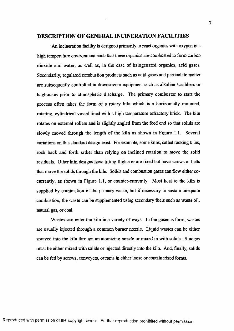
An incineration facility is designed primarily to react organics with oxygen in a
high temperature environment such that these organics are combusted to form carbon
dioxide and water, as well as, in the case o f halogenated organics, acid gases.
Secondarily, regulated combustion products such as acid gases and particulate matter
are subsequently controlled in downstream equipment such as alkaline scrubbers or
baghouses prior to atmospheric discharge. The primary combustor to start the
process often takes the form of a rotary kiln which is a horizontally mounted,
rotating, cylindrical vessel lined with a high temperature refractory brick. The kiln
rotates on external rollers and is slightly angled from the feed end so that solids are
slowly moved through the length of the kiln as shown in Figure 1.1. Several
variations on this standard design exist. For example, some kilns, called rocking kilns,
rock back and forth rather than relying on inclined rotation to move the solid
residuals. Other kiln designs have lifting flights or are fixed but have screws or belts
that move the solids through the kiln. Solids and combustion gases can flow either co-
currently, as shown in Figure 1.1, or counter-currently. Most heat to the kiln is
supplied by combustion o f the primary waste, but if necessary to sustain adequate
combustion, the waste can be supplemented using secondary fuels such as waste oil,
natural gas, or coal.
Wastes can enter the kiln in a variety of ways. In the gaseous form, wastes
are usually injected through a common burner nozzle. Liquid wastes can be either
sprayed into the kiln through an atomizing nozzle or mixed in with solids. Sludges
must be either mixed with solids or injected directly into the kiln. And, finally, solids
can be fed by screws, conveyers, or rams in either loose or containerized forms.
Reproduced with permission of the copyright owner. Further reproduction prohibited without permission.
8
WasteFeed
Secondary Fuel Support Burners
Stack
'JAfterburnerChamber
Rotarv Kiln
Kiln Support Rollers Ash
Air PollutionControlEquipment
Induced Draft Fan
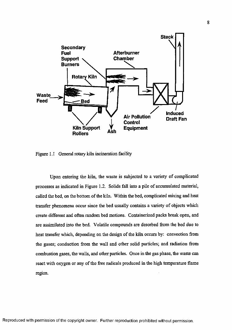
Figure 1.1 General rotary kiln incineration facility
Upon entering the kiln, the waste is subjected to a variety of complicated
processes as indicated in Figure 1.2. Solids fall into a pile of accumulated material,
called the bed, on the bottom of the kiln. Within the bed, complicated mixing and heat
transfer phenomena occur since the bed usually contains a variety of objects which
create different and often random bed motions. Containerized packs break open, and
are assimilated into the bed. Volatile compounds are desorbed from the bed due to
heat transfer which, depending on the design of the kiln occurs by: convection from
the gases; conduction from the wall and other solid particles; and radiation from
combustion gases, the walls, and other particles. Once in the gas phase, the waste can
react with oxygen or any of the free radicals produced in the high temperature flame
region.
Reproduced with permission of the copyright owner. Further reproduction prohibited without permission.
9
Spray and Droplet
Flame-ModeKinetics
Buoyant,TurbulentFlowfield
Air Infiltration
GasesTo
Afterbumei
Natural Gas/ Waste/Air Burner =
SolidsFeeder
Convection Thermal Radiation
Barrel Waste Collapses Evolution
BumoutWaste Barrel Enters Kiln
Bed Mixing and DesorptionMulti-Mode Heat
Transfer and Fluid Mechanics
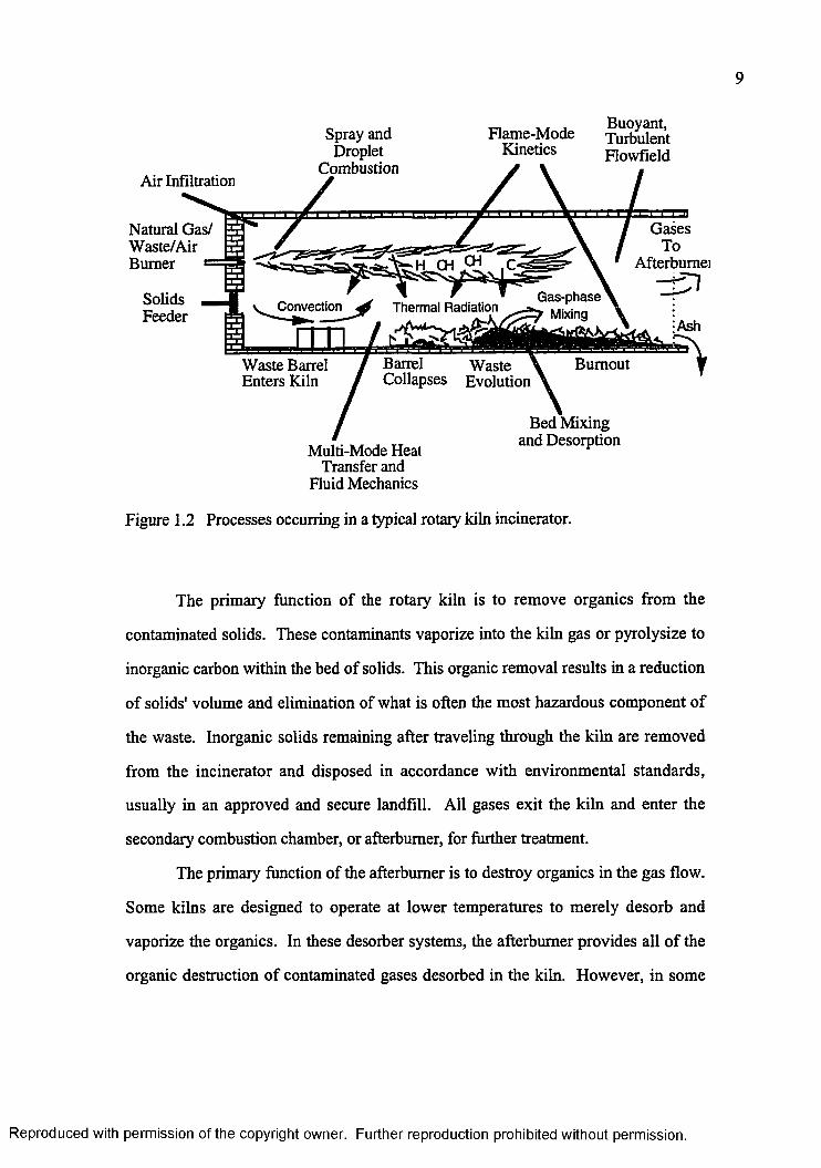
Figure 1.2 Processes occurring in a typical rotary kiln incinerator.
The primary function of the rotary kiln is to remove organics from the
contaminated solids. These contaminants vaporize into the kiln gas or pyroiysize to
inorganic carbon within the bed of solids. This organic removal results in a reduction
of solids' volume and elimination of what is often the most hazardous component of
the waste. Inorganic solids remaining after traveling through the kiln are removed
from the incinerator and disposed in accordance with environmental standards,
usually in an approved and secure landfill. All gases exit the kiln and enter the
secondary combustion chamber, or afterburner, for further treatment.
The primary function of the afterburner is to destroy organics in the gas flow.
Some kilns are designed to operate at lower temperatures to merely desorb and
vaporize the organics. In these desorber systems, the afterburner provides all o f the
organic destruction of contaminated gases desorbed in the kiln. However, in some
Reproduced with permission of the copyright owner. Further reproduction prohibited without permission.
10
cases, rather than being combusted in an afterburner, the organics and other hazardous
compounds are separated from the gas stream by methods such as carbon absorption
and partial liquefaction.
Gas and liquid wastes can also be sprayed directly into afterburners. For
processes that only produce liquid or gas waste streams, the incinerator often does
not have a rotary kiln segment. Incineration facilities that include a rotary kiln,
however, provide maximum versatility since these units are able to process gases,
liquids, sludges, and solids in bulk or containerized forms. Gases leaving the
afterburner are usually quenched in a water spray and then enter downstream gas
purification equipment such as wet or dry alkaline scrubbers, electrostatic
precipitators, cyclones, or baghouses all of which are designed to remove particulate
and/or neutralize acid gas emissions.
Treated gases are drawn through an induced draft fan and out the stack. These
fans maintain the entire incinerator train under a slight vacuum to prevent leakage of
hazardous vapor contaminants from the facility into the environment. This negative
pressure results in air infiltrating into the incineration facility where small gaps exist.
Gases discharged from the stack are typically free of 99.99 percent to 99.9999
percent (hence terms such as "four nines" and "six nines") of the original organic mass
fed to the incinerator unit. Flue gases discharged from hazardous waste incinerators
also must currently meet Federal particulate standards of 0.08 grains per dry standard
cubic foot of gas (CFR 1991e).
Reasons why waste creation is inevitable have been reviewed along with an
overview o f incineration strategy, which can be used to treat selected waste streams.
Next, an examination of the background or history of research in the field of rotary
kiln incineration and related areas will be presented in the form of a literature review.
Reproduced with permission of the copyright owner. Further reproduction prohibited without permission.
CHAPTER 2
LITERATURE REVIEW
This chapter presents a review of literature relevant to the research presented
in this dissertation. This review is divided into sections concerning numerical
modeling of rotary kiln incinerators and experimental studies of field-scale incinerators
since the proposed work will include both experimental and numerical components.
Included are works that have elements incorporated directly into the current research
or are important in the developmental history of a related area.
NUMERICAL MODELING: AN OVERVIEW
Jones and Whitelaw (1982) present an excellent overview of numerical
modeling while focusing on calculation methods for turbulent, reacting flows. They
note that turbulence models existing at the time did not correctly predict certain
flows. Some examples of flows incorrectly predicted by the then current turbulence
models were cases o f high temperature re-laminarization of turbulent flows, up-
gradient diffusion, and a jet discharging into a quiescent chamber. The authors further
note that due to the very nonlinear nature of reaction rates with respect to
temperature and species concentration, using mean values of these variables in
turbulent fluctuating conditions can lead to errors in reaction rates of up to three
orders of magnitude. Probability density functions (PDF) were suggested as a good
way to account for fluctuations about the mean, but the authors noted their
considerable consumption of computer memory and run time.
11
Reproduced with permission of the copyright owner. Further reproduction prohibited without permission.
12
The differences between finite rate and "fast" chemistry assumptions for
diffusion flames are also reviewed by Jones and Whitelaw (1982). Finite rate
chemistry can account for the rate of a global reaction being controlled by different
elementary reactions depending on the temperature, pressure, and species
concentrations present. To precisely model the chemistry, a complete set of
elementary reactions and corresponding kinetic information making up the global
reaction (activation energy, pre-exponential factor, and temperature dependence) is
needed. However, acquiring this information is not trivial. According to Westbrook
and Dryer (1984), the number of elementary steps can approach 100 even for the
relatively simple combustion of methane in air. To add even more complexity, the
steps used and the corresponding kinetic information for even simple reactions often
vary greatly from one researcher to the next. This is pointed out by Westbrook and
Dryer (1984) with the following comparison regarding the heat of formation of the
formyl radical. The 1971 version of the JANAF Thermochemical Tables (Stull and
Prophet, 1971) altered the heat o f formation value for the formyl radical from -2.9
kcal/mole (published in the previous edition) to 10.4 kcal/mole. Then in 1976,
Benson published a value of 7.2 kcal/mole for the same radical.
Fast chemistry assumptions are divided into either the equilibrium or
irreversible reaction cases (Jones and Whitelaw, 1982). Neither case requires kinetic
information. The irreversible case requires the user to input a reaction sequence for
each reactant, usually a simplified one-step global reaction, specifying the
stoichiometry for each reaction step. Whenever all the reactants for a particular
reaction are together in one control volume, the reaction is assumed to instantly and
irreversibly proceed to completion. Reactants are then created as specified by a
particular reaction stoichiometry. In contrast, the equilibrium case requires no formal
input of reaction sequences or stoichiometry because a library of thermodynamic and
Reproduced with permission of the copyright owner. Further reproduction prohibited without permission.
13
species information is accessed. This database, used in combination with information
on the control volume pressure, temperature and quantities o f individual atoms
present, can then determine which molecular species and concentrations are present to
minimize the Gibbs free energy of the control volume. Both fast chemistry
assumptions falter when reaction rates are slow. In the irreversible case, the global
reaction assumption ignores sometimes important reaction intermediates.
Jones and Whitelaw (1982) also present several reaction models for premixed
flames including the eddy break-up model. This model uses the rate of turbulent
mixing rather than kinetics as the reaction rate controller. The authors stress that the
eddy break-up model is inappropriate for diffusion flames. Several models that
attempt to cover both premixed and diffusion flames are presented but all seem non-
workable or valid in only restricted cases. A large number of examples and references
are provided throughout the text. In one example, using a PDF to model the mixture
fraction, the discrepancy between experimental data and model is traced to
insufficient radial turbulent mixing. An attempt to "fix" this by dropping the
turbulent Schmidt number to 0.2 was cited as "unjustified" and a failure.
Boris (1989) discusses current directions in Computational Fluid Dynamics
(CFD) research. Initially he states that
algorithms for solving partial differential equations (PDE) have reached the point of diminishing returns in terms of trading off computational cost for accuracy. It is now more effective to increase the number of grid points to improve spatial resolution and hence accuracy than to seek greater accuracy through higher-order algorithms. Even increasing the complexity of turbulence and physical sub-models is now less important than resolution improvements.
Boris divides current research into three areas: representational models of the fluid
state, algorithms for solving the resulting PDEs, and the computer hardware to run the
Reproduced with permission of the copyright owner. Further reproduction prohibited without permission.
14
algorithms. New fluid state models include cellular-automata, hybrid-cellular-
automata, and molecular-dynamics. Also discussed are new approaches for
discretizing continuous functions and approaches to decimating the fluid-dynamic
equations to a few dynamically significant degrees of freedom.
Algorithmic extensions and new directions discussed include adaptive and
unstructured grids, spectral elements, and fully Lagrangian algorithms. On evolving
hardware, Boris states that application o f CFD technology is and always will be
limited by the speed and size of available computers. The speed of single processors
is limited by the speed of light and the current requirements o f generality. New
advances will come in using parallelism, pipelines, and building processors to do
specific tasks. An interesting observation is that nature "solves" fluid problems in a
fully parallel manner. He notes that to fully utilize the new directions in hardware
will require redesigning many of the current solution algorithms.
In discussions related to the research presented in this proposal, Boris states
that "fluid-dynamic convection in the absence of strong physical diffusion effects is
the most difficult flow process to simulate." Major weaknesses in CFD are the
detailed representation and simulation o f turbulence and chemical reactions. To
resolve small-scale turbulence or full chemical kinetic systems in a multidimensional
CFD model imposes unacceptable costs, if it can be done at all. Flows can be solved
with either complex geometry and simple physics or with complex physics in
relatively simple geometry, but not with both. The example is given: a realistic
chemical-reaction mechanism contains many chemical species and perhaps hundreds
o f reaction rates linking them. Integrating the stiff ordinary differential equations for
the evolution of the individual species and fluid temperature in a multidimensional
CFD code is theoretically possible. However, two faster and currently usable
alternatives exist. First, use the detailed reaction mechanism to calculate bulk
Reproduced with permission of the copyright owner. Further reproduction prohibited without permission.
15
properties, such as final temperatures and pressures across broad zones. Or second,
use generalized reaction mechanisms to calculate temperature, pressure and species on
a fine spatial resolution. The difference between these two simplifications is the basis
for the division o f most CFD codes into one o f two categories. The first category
involves CFD codes that solve relatively inclusive sub-models over coarse zones
returning bulk properties called zonal models. The second category of CFD codes are
called Navier-Stokes solvers because they solve the Navier-Stokes equations resulting
in great flow detail; however, simplified sub-models are usually required. The
numerical modeling work presented in Chapter 5 of this dissertation emphasizes
analysis of the flow field; therefore, this work utilizes a Navier-Stokes type model
code.
NUMERICAL KILN MODELS
Presently, there are two main types of numerical models for incinerator flow
fields: those that solve the Navier-Stokes equations and those that divide the flow
field into multiple zones, avoiding direct solution of the flow field. The latter uses
various models for each zone and does not usually attempt formal solution of the
Navier-Stokes equations. Solution of the Navier-Stokes equations is needed for the
exact solution of the flow field. However, except for very simple situations, the
PDEs are coupled, nonlinear, and very difficult to solve. The zonal models represent
the first successful attempts to numerically solve complicated flow fields and are still
in wide use today due to their greater flexibility and proven performance. The full
Navier-Stokes equation set is still directly solvable for only simple cases, but, by
approximating certain terms in the equations through the use o f sub-models, the
equations can be simplified enough to be solved. An example of this simplification is
the K-e model to evaluate the Reynolds stress term in the time-averaged momentum
equations. Also, ingenious methods have been developed to allow the sequential,
Reproduced with permission of the copyright owner. Further reproduction prohibited without permission.
16
though iterative, solution of coupled equations. An example of this is the Semi-
Implicit Method of Pressure-Linked Equations or SIMPLE (Patankar, 1980).
Although there are a large number of zonal models available, only a few will be
presented because the focus o f this research uses a Navier-Stokes solver. However, a
limited presentation of zonal models follows because these models utilize many of the
same sub-models as the Navier-Stokes solvers and provide good insight into the
history of numerical flow simulation.
Zonal Models
Jenkins and Moles (1981) present an axisymmetric zonal model to predict gas
and refractory temperature profiles in a directly-fired rotary kiln. The authors use a
zonal radiation model with exchange areas. Emissivity of the gas is approximated
using a three spectral band model consisting of two gray bands and one clear band.
The separate effects of soot and other airborne particles on gas emissivity are also
included in a three band model. The velocity field is predicted using empirical
correlations. The heat release distribution from gas phase reactions is accounted for
by analyzing measured gas concentrations of CO and CO2 in the kiln (see also
reference to this work in the experimental section of this literature review) and
predicting the amount of reaction required to produce those concentrations. Next, the
gas and axial wall temperature profiles are predicted. Model results are then
compared with data from a 1 0 0 ton per day (tpd) directly heated, coal-fired, cement
kiln. Discrepancies in the comparison are explained by the fact that the model does
not handle gas phase recirculation, which is calculated as being strong in several
regions, nor does it account for CO2 production and heat transfer from the bed
reactions. This approach seems impractical because exact measurements of gas
concentrations, which are very difficult to obtain, are needed throughout the kiln in
Reproduced with permission of the copyright owner. Further reproduction prohibited without permission.
17
order to predict refractory and gas temperature profiles which are typically easier to
measure.
Clark et al. (1984) present a model for predicting the destruction performance
of an incinerator. Analysis includes both the afterburner and stack regions and is
compared to a coaxial liquid waste kiln. A zone method coupled with a Monte Carlo
technique is used to predict radiant heat transfer. Mixing is handled as macro-scale
mass exchange between well-stirred zones. The flow field is obtained by either actual
measurement or by estimation techniques using empirical correlations for specific
burner types. A large number of possible paths through the system are evaluated,
yielding a time/temperature history for each path and a percentage possibility of each
path being used. Simple, one-step, first-order Arrhenius kinetics are applied to all
paths, giving a fractional decomposition for each path. These results are then
averaged over a large number of paths to obtain an average destruction efficiency. The
authors claimed that the model correctly predicts trends in destruction efficiency even
though it may deviate from measured values by several orders of magnitude. Due to
the poor agreement and the sparse experimental data, the results appear inconclusive.
Clark and Seeker (1986) present another model designed to predict the
ultimate destruction of waste. This model again assumes complete combustion of
waste with no intermediates. Single temperatures for the gas and walls of the kiln as
well as the secondary combustion chamber are calculated and used. Plug flow is
assumed, and mean residence times are computed. Inputs include the heating value
for the fuel and waste. Two percent of the volatile carbon is assumed to become soot,
which the authors site as typical, but no references or experimental studies were
provided. The radiation model uses a speckled wall approach along with a
composition and temperature dependent grey gas. The results match two different
kiln data sets fairly well, but both kilns have incomplete operating data. One kiln
Reproduced with permission of the copyright owner. Further reproduction prohibited without permission.
required the addition of unreported leak air amounting to more than half of the total
air entering the incinerator. A big advantage is that the model code can be run in less
than 30 seconds on a personal computer having only 256 k bytes of memory.
Owens et al. (1991) compare their model to data from a directly-fired, pilot-
scale rotary kiln. The experimental study focused on four independent variables
including bed fill fraction; kiln rotation rate; kiln wall temperature, which was fixed by
the natural gas firing rate; and water content of the clay sorbent. The kiln is operated
in a batch mode, that is, solids do not flow axially through the system. For their
model, a one dimensional approximation is made by dividing the kiln ipto axial zones
within which the gas and solids are assumed to be well mixed and isothermal. Heat
transfer is modeled by a thermal resistance network for an indirectly-fired kiln which
is assumed to approximate the conditions o f low temperature operation in their
directly fired kiln. Heat transfer between zones is neglected. The mean beam length
radiation model is used along with a grey gas and wall approximation. The model
calculates the transient heating of the bed including the effects of bed slumping rates.
Solids heating is treated in three stages: initial heating to the boiling point of water,
isothermal vaporization of the water, and final heating of the bed above the boiling
point after all the water has evolved from the bed. Scaling laws are presented, but
different laws are required depending on whether radiation or convection is assumed
to dominate the heat transfer or if moisture is present. Wall and gas temperatures are
treated as constants and must be inserted to the program before solution can begin.
This is a major weakness of their model in that a prior knowledge of the combustion
gas and kiln wall temperatures are required.
Chen and Lee (1994) present a one-dimensional, steady state model of a
rotary kiln incinerator. A single burner support flame is modeled as a uniform
temperature cylinder. Solid pelletized waste is included and allowed to combust via a
Reproduced with permission of the copyright owner. Further reproduction prohibited without permission.
surface area, Arrhenius-style pyrolytic reaction. Inert and reactive components of the
waste are included, and the pellets are allowed to shrink in size; however, the waste is
never named. A surface flame is assumed to exist on top of the bed of solids.
Equations are solved using an iterative process coupled to a Newton-Raphson
method. The authors state as one o f their primary items of focus “to fit all
experimental data exactly”; however, neither experimental data nor percent error is
ever shown or discussed in the whole work. No kiln details are given with all
analyses conducted on a dimensionless basis. Sensitivity studies are carried out on
surface emissivity, feed particle size, and the surface flame. A study is performed on
radiation indicating that interactions between axial zones can be very important;
however, the authors claim that with mole fractions o f CO2 and H2O in the gas
stream less than 1 0 percent, radiation transfer to adjacent zones will only be reduced
by 2 0 percent, and as a result, radiation exchange with the gas phase can be neglected.
They add, however, that in large scale kilns (greater than 2.4 m) or a soot laden kiln,
radiation exchange with the gas phase becomes much more important.
Navier-Stokes Solvers
Gillis and Smith (1988) present a three-dimensional numerical model for
predicting flow in industrial furnaces. The SIMPLE algorithm and a vectorized
Thomas algorithm are used to solve the Navier-Stokes equations. The model can only
be utilized in Cartesian or polar coordinates. Perhaps the biggest limitation of the
model is that it does not include chemical reactions. The authors compare three
turbulence models and examine the assumption of constant eddy diffusivity, the
Prandtl mixing length model, and the k - e model. The K -e turbulence model uses
transport equations for "k ," the turbulent kinetic energy, as well as "e," the
dissipation rate o f turbulent kinetic energy. The model was compared to what the
authors describe as a "proven" 2-D axisymmetric numerical model and to a l/20th
Reproduced with permission of the copyright owner. Further reproduction prohibited without permission.
20
scale pilot testing facility. Because the model does not handle reactions, only air is
flowed through the test facility. The K -e turbulence model is shown to be superior in
matching the actual non-reacting furnace flow field. The experimental flow field was
not matched exactly, but the model did correctly predict some of the measured flow
features and produced a logical flow field. A grid dependence study was executed by
examining grids of 17,500; 48,125; and 102,375 nodes. The solution from the grid
consisting of the least nodes is greatly different from the others. The two larger cases
are closer, but the largest showed several small eddies not developed in the middle
case near the highly turbulent burner inlet area. This suggests that further grid
refinement may produce more changes in the calculated flow field.
Wang, Chen, and Farmer (1989) apply a finite difference type solution to the
Navier-Stokes equations to solve the flow field of a reactive ramjet dump combustor.
A term is added to an extended K -E turbulence model to include the effect of
temperature on eddy breakup. Kinetics for an Arrhenius form, finite rate, one step,
global reaction of hydrogen and oxygen are generated from the results of a 28 step
reaction model. The resulting source term equations are modified by an algorithm
called PARASOL (Pade1 Rational Solution) before the species equations are solved.
Modifications to the solution procedure are designed to allow for solutions across
shock waves and in hypersonic flows. The final system of linear algebraic equations
are solved by a modified Stone's method using a Cray XMP computer. Even though
the reaction scheme seems to work well, the authors caution that global kinetic rate
constants such as used in this study are only valid for conditions which have been
validated with experimental data. The model matches well for this axisymmetric
problem, but it is unclear if this model can be used for three-dimensional problems.
Smith, Sowa, and Hedman (1990) use a comprehensive two dimensional coal
combustion model called Pulverized Coal Gasification and Combustion (PCGC-2). A
Reproduced with permission of the copyright owner. Further reproduction prohibited without permission.
21
k—e model is used that is modified to account for the presence of particles. Reaction
rates are assumed to be limited by molecular scale mixing. Probability density
functions are used to account for the turbulent fluctuation about the mean values.
Radiation is accounted for by a six-flux model that includes anisotropic and multiple
scattering from the particles. The usefulness of the model is summarized by the
authors as being:
...capable of predicting qualitative information in the combustion and gasification applications that are used as case studies in this paper. In most cases sufficient quantitative information is predicted within the measurable accuracy of the data to justify engineering decisions based on the simulation.
Nasserzadeh et al. (1991) used a commercially available code, FLUENT V
2.95 to model a 500 tonne/day municipal solid-waste incinerator. Modeling was
divided into two geometric parts. The first part included the moving grate incinerator
which consisted of hoppers, six rollers, and the refuse bed on top of the rollers with a
7,980 node three-dimensional grid. Symmetry was sited to allow only one half of the
geometry to be modeled; however, the use of Cartesian coordinates required sloped
surfaces to be modeled with a stepped wall approximation. Results from this model
were used as boundary conditions for the 10,260 node grid of the other half of the
furnace and the shaft and boiler sections. Symmetry was again cited to cut the
modeling effort in half. Still, modeled geometry had to be simplified and stair-stepped
walls were utilized. Gases were assumed ideal, turbulence was resolved using the k - e
model, and reaction rates were determined by the limiting choice between Arrhenius
kinetics and a turbulent eddy-dissipation model. A two step reaction mechanism was
employed with CxHy and air as reactants, CO as the intermediate, and CO2 and H2O
as the products. The values of refuse density, molecular weight, heat o f combustion,
stoichiometric ratio, viscosity (gas), and heat capacity that are used as boundary
Reproduced with permission of the copyright owner. Further reproduction prohibited without permission.
22
conditions are given. The amounts of raw refuse and amounts gasified on top o f each
roller were patched into the calculations based on experiments conducted at the
facility (see this reference in the experimental section of this chapter). No other
model details were given or referred to and no facility dimensions were provided. The
resulting flow field is said to be nearly two-dimensional. Predicted velocities range
from 0 m/s to 7 m/s with temperatures up to 2,000 K. Predicted temperatures leaving
the boiler are in the 800 K to 900 K range, very close to the measured values of
around 950 K. This is interesting because radiation modeling is never mentioned.
Explanation of presented data and model results is incomplete, making comparisons
difficult. Gas speciation data were recorded at the exit of air pollution equipment
which is downstream of the boiler. The solution domain o f the model ends at the
boiler exit and therefore does not include the sampling location. The authors state
that the CO prediction is low, but their figures appear to show it more than an order
o f magnitude high. A “mismatch of conditions” is mentioned but not explained as a
partial reason for differences between experimental and model results. Even so, the
authors state “the two-step kinetic model, for the prediction of CO formation, has
performed well.” The possibility of grid dependence of the solution is not mentioned.
Nasserzadeh et al. (1994) uses the above model to examine residence times in
the incinerator. Fluent V 2.95 is again used. The only change is that tracking of
particles using a Lagrangian type model is included. Neutrally buoyant particles are
injected at several locations of the incinerator and tracked. Results show the existence
of several recirculation zones. Residence time distributions are calculated showing
residence times ranging from 1.6 to 3.4 seconds for entrance from a secondary air inlet
to 45 to 70 seconds for entrance from roller number six. No discussion of model
validity is made though the authors state that any “possible errors in the results ... are
likely to be due to” among other things “the possible existence of some computational
Reproduced with permission of the copyright owner. Further reproduction prohibited without permission.
23
dead time on the small difference cell.” The authors go on to state “Nevertheless, the
modeling results obtained here, are generally satisfactory.” Proposed design
modifications to improve residence times by eliminating or reducing recirculation
regions are tested. Model predictions showed that a proposed baffle addition would
nearly double gas residence times. Model predicted improvements are also cited for
changing the way secondary air is injected into the incinerator, but no quantification is
offered.
Leger et al. (1993c) used FLUENT V 3.0 to examine the flow field inside a
field-scale rotary kiln. This incineration facility is detailed in Cundy et al. (1989a)
and Montestruc (1989) and is briefly described in both the “Background” section of
Chapter 4 and the “Physical System” section o f Chapter 5 o f this dissertation. Leger
created a three-dimensional grid of 17 x 20 x 36 (12,240) control volumes. Air was
assumed to infiltrate the kiln through the two kiln rotary seals and the solids loading
chute door. Air infiltrating through the rotary seals was included by modeling all of
the front and rear kiln-wall perimeter control volumes as inlets. Each burner inlet to
the kiln was represented by only a single control volume. Due to the coarseness of
the grid and the use o f uniform grid spacing, the areas of the burners, solids loading
door, and external mixing air inlets did not match the actual areas. To account for this,
the inlet velocities were adjusted to maintain the correct mass flow rates. Radiation
was not included, and the walls were modeled as isothermal at 800 K. Ideal gas was
assumed, and gas composition was included in the specific heat calculations. A more
complete description o f the model used in Leger et al. (1993c) is given in “Appendix
D” of this dissertation. The primary finding by Leger et al. (1993c) was the
importance of buoyancy in creating the characteristic, vertically stratified temperature
and species profiles observed in experimental data at the kiln exit. The highly three-
dimensional nature o f the flow field is pointed out as is the unexpected existence of a
Reproduced with permission of the copyright owner. Further reproduction prohibited without permission.
recirculation zone in the lower region of the kiln’s exit. Quantitative agreement with
experimental data is off by as much as two orders of magnitude; however the authors
suggest that the model generates reasonable results in spite of the many “gross”
underlying assumptions, rough grid, and crude sub-models that are used. Leger et al.
suggest that the model is a useful tool for formulating rough comparisons of different
kiln operating conditions and design modifications.
Khan et al. (1993) also used FLUENT V 3.0 to examine the same field-scale
kiln on which the work of Leger et al. (1993c) and this dissertation are based. Only
the major differences between Khan et al. (1993) and Leger et al. (1993c) are
discussed here. Khan used a 27 x 30 x 40 control volume grid, (32,400 total nodes)
and then checked for grid dependence using a 30 x 33 x 75 grid (74,250 total nodes).
Each burner inlet to the kiln was modeled using four inlet control volumes. Again, the
modeled areas of the burners, door, and air inlets did not match the actual areas
because of the coarse grid and uniform grid spacing used. To compensate for this, the
inlet velocities o f the burners and air inlet nozzles were reduced to maintain the
correct mass flow rates. The velocity of air infiltrating through the door was
calculated to be 14.4 m/s using the inviscid Bernoulli equation with a pressure drop of
0.124 kPa. Rotary seal infiltration air was assumed to have an inlet velocity of 1.5
m/s. With the control volume size and leak air inlet velocities fixed, the mass flow of
leak air into the kiln could only be controlled by altering the number of control
volumes designated as inlets. This means that the physical inlet geometry was
artificially altered in order to account for the different leak air rates at each different
operating condition. Two different heat transfer wall boundary conditions were
studied: an adiabatic wall and a constant heat flux wall at 1400 W/m2 (about 5 percent
of the combustion energy). Turbulence was accounted for by the K - e turbulence
Reproduced with permission of the copyright owner. Further reproduction prohibited without permission.
model, and the specific heat was assumed to be that of air. Three conspicuous
differences between the model setup and the field-scale facility are:
1. The burners are placed on the wrong side of the kiln;
2. Infiltration air from the loading chute door is placed too low in the kiln;
and
3. Metered air for both the kiln and afterburner is input through the kiln
burners.
The results of interest are that the maximum temperature at the kiln exit was
2,344 K, the flow field was virtually unaffected by the difference of adiabatic versus
constant heat flux wall boundary conditions, the solution was grid dependent, and
recirculation existed in the top rather than the bottom of the kiln as in Leger et al.
(1993c). Khan et al. (1993) compared these methane only (no waste) modeling
results to experiments in which methane, along with liquid carbon tetrachloride (CCI4)
waste, was continuously burned, as published in Cundy et al. (1989a, 1989b, 1989c).
The results o f the model qualitatively match the field results to the extent that the
model correctly shows the existence of vertical stratification at the kiln exit, with little
to no stratification in the other two planes.
Summary of Numerical Models
Numerical models using Navier-Stokes solvers are relatively new and are
quickly improving; however, the zonal models are still in wide use due to their proven
performance and greater adaptability. Navier-Stokes solvers are not yet able to
handle situations involving vastly different phenomena in the same problem, such as
solids mixing in a bed along with full spectrally dependent radiation in the gas flow
field above the bed. Zonal models, which handle various detailed sub-models
Reproduced with permission of the copyright owner. Further reproduction prohibited without permission.
26
relatively well, only calculate bulk flow properties, have trouble with large property
discontinuities at boundaries between zones, and rely on the assumption that
properties are uniform within zones. All of the models reviewed are limited to steady
state operation and depend on the ability to make simplifying assumptions such as
plug flow of solids and/or gases. For both solver types, sub-model development is
needed. In particular, turbulence and radiation sub-models need improvement.
Currently no model correctly predicts the quantitative aspects of an incinerator flow
field.
FIELD-SCALE INCINERATION: EXPERIMENTAL STUDIES
Introduction
Every facility that bums waste must first acquire a permit from the USEPA or
state/local regulatory agencies. To obtain a permit, proof of the incinerator's ability to
achieve required performance standards must be established and documented. This
proof is obtained by presenting satisfactory results from a "trial bum" for
incinerators, cement kilns, and boilers that bum hazardous wastes. Facilities
processing non hazardous wastes must submit results from a similar, but slightly less
stringent, "compliance test". Although the results of these trial bums are available to
the general public through facility permit applications, these documents are not
usually helpful to researchers for several reasons. First, information about results of
pre-trial tests and any design changes that may have been made to achieve the final
test bum results are not ordinarily included in public documents. Rather, public test
bum documents usually contain data about the final feed, operating conditions, and
stack exhaust measurements and only minimal information about the kiln or
afterburner regions. Second, permits containing the final test results are lengthy,
contain much extraneous information, and are difficult to read. A typical example is
the Trial Bum Report submitted by Eastman Kodak in 1985 that contained 1,800
Reproduced with permission of the copyright owner. Further reproduction prohibited without permission.
27
pages of documentation in eight volumes (Bastian and Wood, 1987). Such
information from the public record is generally of little value to researchers and the
scientific community.
Very few non-trial bum, scientific studies of field-scale incinerators have been
undertaken. Although there are several reasons for this void, the primary reason is
that researchers generally cannot gain access to incinerators that are suitably designed
and fitted for detailed studies. To further exacerbate the situation, current regulations
discourage post-trial bum modifications such as installing extra inlets or additional
access ports that could be useful for sampling and/or viewing. Finally, many
incinerator facilities are just not accessible for testing because o f the placement of
equipment and utilities, and large incineration facilities are too expensive to build
solely for experimentation purposes.
The two main groups of owners of hazardous waste incinerators are the
private sector and the federal government. The federal government and many private
companies generally will not allow details of their proprietary processes published
for reasons o f competitiveness, national security, and/or public reaction which is
increasingly set against incineration. Additionally, academic research at privately
owned hazardous waste incinerators is usually not conducted because business
demands dictate that unit downtime to conduct research experiments is economically
unreasonable. For example, one facility 'roughly' estimated that for twelve hours of
experimental tests, costs in excess of $60,000 were incurred, not including lost
revenues (Lipp, 1992).
Another reason for the lack of useful experimental data at the field-scale is the
large amount of manpower generally necessary to safely and expediently complete a
test run. For example, field-scale tests conducted by Louisiana State University
researchers typically require ten workers in addition to five plant personnel (Huggins,
Reproduced with permission of the copyright owner. Further reproduction prohibited without permission.
28
1994). Even pilot-scale facilities tend to require four or more people to conduct tests.
Finally, the difficulty and sometimes unavailability of methods to extract data from
various points within a large rotating kiln with temperatures in the 600° C to 2,000°
C range contribute to the lack o f experimental data found in the literature.
Given these reasons, it is not surprising that only a few groups have done
experimental work with field-scale incineration units. The first group to present data
on field-scale units was Jenkins and Moles (1981) with data from a 100 tpd cement
kiln. Next, R. W. Wood (1987) presents detailed results from a hazardous waste
incinerator trial bum. Then, Nasserzadeh et al. (1991) present data from a 500
tonne/day municipal solid-waste incinerator. Finally, a group at Louisiana State
University has been studying a directly fired hazardous waste kiln since 1986. Each
of these studies are reviewed next.
Review of Literature
Jenkins and Moles (1981) present data taken from the 100 tpd cement kiln at
the Bamstone Works in Nottinghamshire. The kiln is 1.7 m in diameter by 45.7 m
long and directly heated by coal. The authors explain that gas samples were collected
"... through water-cooled probes using an integral sample cooling unit which rotated
with the kiln." Highly detailed two-dimensional axial contour plots were constructed
for CO2 , CO, O2 , and temperature fields along with an axial wall temperature profile.
Gas temperatures as high as 2,000° C were measured. Gas temperatures were
measured using both suction pyrometers and venturi-pneumatic pyrometers, while
wall temperatures were gathered using sheathed thermocouples. Clinkering and
decarbonizing reactions took place in the solids bed during data collection.
Recirculation of the gases was observed in the kiln and a Craya-Curtet parameter, m,
equal to 3.5 was calculated indicating stronger recirculation than claimed as the1
industry average; m = 0.8 to 1.6. The Craya-Curtet parameter indicates the onset of
Reproduced with permission of the copyright owner. Further reproduction prohibited without permission.
29
recirculation areas in systems with a primary jet issuing into a larger area, and ranges
from zero to infinity. Modeling work presented in Jenkins and Moles (1981) is
discussed in the modeling section of this chapter.
Although most public information, such as trial bum and permit application
information, is usually not useful for research purposes, R. W. Wood (1987) presents
a rare summary of a trial bum report that includes the pre-trial bum data and resultant
operational modifications suggested by those tests. This trial bum report is the
culmination of tests performed from 1980 to 1984 on Eastman Kodak's rotary kiln
incinerator located at the Kodak Park film, paper, and chemical manufacturing site in
Rochester, New York. Data recorded during the tests include temperature from a
single point at the kiln exit and the middle of the afterburner, O2 level in the
afterburner, CO concentration and GC/MS/FID analysis of the stack gas. Operating
parameters measured during the tests included type of waste and waste feed
container, kiln temperature, rate of rotation, and air inlet rates. The general finding of
these tests was that longer residence times at higher operating temperatures improve
the destruction and removal efficiency (DRE) of the wastes under study in this
incinerator. To achieve longer residence time and higher temperatures which in turn
lead to higher DREs, it was necessary to reduce the rate of air infiltrating the kiln. A
new kiln exit seal was installed resulting in a temperature drop between the kiln exit
and the quench of 100° F compared to the previous 400° F temperature drop.
Nasserzadeh et al. (1991) present data from the 30MW, 500 tonne/day
municipal solid-waste incinerator located in Sheffield, England. The incinerator is
designed to handle 10 tonne/hr of raw waste in each of the facilities’ two grates, and
its boiler provides heat for 10,000 homes. A typical analysis of the Sheffield refuse is
broken down into 8 categories by both weight and volume with the two largest
categories being paper and vegetable putrescent matter. Temperatures recorded at a
Reproduced with permission of the copyright owner. Further reproduction prohibited without permission.
point in the boiler exit range from 875° C to 1,025° C over 40 minutes. A water-
cooled probe was used to gather speciation data at the exit o f the electrostatic
precipitator located downstream of the boiler. Measured CO ranged from 110 to 190
ppm, while O2 ranged from 8 to 12 volume percent. Data is also presented for NOx,
SO2 , and CO2 .
The group located at Louisiana State University is continuing research started
in 1986 on a hazardous waste, rotary kiln incinerator located at Dow Chemical
Company in Plaquemine, Louisiana. This incineration facility is detailed in Cundy et
al. (1989a) and Montestruc (1989) and is briefly described in both the “Background”
section of Chapter 4 and the “Physical System” section o f Chapter 5 o f this
dissertation. Initial studies on this kiln consisted of three sets of experiments (Cundy
1989a, 1989b, 1989c), each carried out on a different day. For all experiments, liquid
CCI4 was directly injected, along with natural gas and air, through one burner nozzle,
while natural gas and air were injected through another nozzle. To the greatest extent
possible, the operating parameters were kept constant over all three test days.
In the first paper, Cundy et al. (1989a) discuss insights gained by studying
incineration practices in Germany, and then details the incinerator facility under
study, including its geometry and operation, along with sampling methods and
locations. Data were obtained from the exit of the rotary kiln using a 7.8 m long
stainless steel, circulating water-cooled probe, detailed in the paper. Gas temperature
was measured by a suction pyrometer protected by a ceramic radiation shield at the
end of the probe. The gases from the suction pyrometer were analyzed for CO2 and
O2 . A shorter 3.8 m probe, otherwise identical in design, was used to extract the
same type o f data from the middle of the afterburner.
At the kiln exit only horizontal traverses were possible. Relatively little
variation was observed moving from the kiln centerline to near the burner side o f the
Reproduced with permission of the copyright owner. Further reproduction prohibited without permission.
31
kiln: 1.4 percent increase in O2 , 16.7 percent decrease in CO2, and 3.7° C decrease in
temperature. With the addition of extra mixing air supplied at the burner face, the
above values increased to 10.3 percent, 46.7 percent, and 17.4° C respectively. Axial
variation was also minimal with no change in O2 concentration, a 33 percent increase
in CO2 concentration, and a 15° C temperature decrease at the downstream location.
Gas samples were collected in glass bottles for later GC/MS analysis. The
experiment was duplicated so that data could be recorded first in the kiln and then in
the afterburner.
In the next experiments, Cundy et al. (1989b) took simultaneous
measurements at fixed locations in the kiln, afterburner, and stack. Stack testing
included volatile organic sampling train (VOST) analysis recorded over 20 minute
intervals along with batch sampling. Continuous total hydrocarbon (THC) data were
recorded only at the kiln. A new access port allowed measurements to be obtained
from the previously inaccessible upper region of the kiln; hence, vertical profiles were
obtained for the first time. These data were compared to previous data (Cundy et al.,
1989a) taken in the lower kiln region. Separate test days were required for data
collection from the top and bottom regions of the kiln. These experiments showed
the presence of a strong vertical stratification at the kiln exit that was greater than
expected and greater than stratification in the horizontal plane. Specifically, in the
upper kiln as compared to the lower kiln region the O2 mole fraction was 360 percent
less, the CO2 mole fraction was 3,150 percent greater, and the temperature increased
by 570° C. The addition of mixing air at the burner face of the kiln reduced these
differences.
In the final paper of the series, Cundy et al. (1989c) present data from another
experimental set while providing a summary of the two previous test sets (Cundy et
al., 1989a, 1989b). This newest set involved taking data at five locations in a section
Reproduced with permission of the copyright owner. Further reproduction prohibited without permission.
32
of the transition between the kiln and the afterburner. Because this location was an
expansion, recirculation region, few hypotheses could be inferred from the data. This
test did demonstrate, however, the relatively uniform conditions that occur in such an
expansion recirculation region.
Experiments conducted by the Louisiana State University team after the
steady CCI4 feed experiments focused on batch feed waste processing. The
complexity of these experiments increases dramatically as the number and type of
data collected per experiment increases.
In Cundy et al. (1989d) the first batch waste processing experiments are
presented along with some preliminary data. Before the run, 18.9 liters o f toluene
(C6H5CH3) were poured into 53 liter (3.2 kg) polyethylene packs containing 22.7 kg
of montmorillonite clay granules, with an average diameter o f 0.635 cm. One pack
was inserted into the kiln by a hydraulic ram every five minutes. Continuous THC
and temperature data, measured at 30 second intervals, are presented only for the
upper kiln location at several operating conditions. When the pack was inserted into
the kiln, the kiln exit temperature dropped initially, due to the opening of the loading
chute doors leading into the kiln, and then a double peak in temperature occurred
before the profile gradually returned to baseline values. The authors relate these
peaks to the initial pack breakdown and bed motion. As expected, the THC
concentration measured at the exit of the kiln showed an opposite behavior, that is,
the THC increased during drops in temperature. Addition of external mixing air
increased the magnitude of the excursions from baseline. Visual observations indicate
that periods of high THC correspond to periods in which the kiln is obscured by
highly-luminous, particle-laden flames. Conversely, periods of low THC correspond
to improved visibility, often to the front of the kiln. A large part of this paper
discusses complementary work using pilot-scale facilities at the University of Utah.
Reproduced with permission of the copyright owner. Further reproduction prohibited without permission.
33
These pilot-scale studies confirmed trends observed at the field-scale and indicated
that the multiple spikes in various parameters were associated with toluene evolution
resulting from pack break-up and bed motion dynamics. The paper recaps the
continuous data from Cundy et al. (1989a, 1989b, 1989c) and discusses several
numerical models of kiln processes under development. Several innovative methods
of approximating CCI4 reaction rates are also presented.
Lester et al. (1990) continue the discussion on the toluene batch runs
introduced in Cundy et al. (1989d). Data recorded in the transition section
downstream from the kiln exit and closest to the back wall had a temperature 300° C
less than that in the upper kiln. This point was theorized to be in the streamline from
the bottom of the kiln. For the first time, VHS video data were recorded
simultaneously from the lower port in the transition section, with a view of the front
face of the kiln, while the probe was inserted in the upper port. Several color
reproductions taken from this recording are presented showing periods of intense
sooting, large turbulent flame zones, and the general non uniformities that exist in the
flow. Several pictures include the natural gas support flame which radiates a bright
yellow-orange. The pictures indicate the intense changes that can occur in a matter of
seconds in the flow field during pack break-up and subsequent toluene evolution. The
authors also learned from the video data that even after five minutes, pack combustion
was not complete. Efforts to demonstrate repeatability were only partially
successful due largely to the randomness of initial pack break-up and subsequent
mixing with the existing bed.
In Cundy et al. (1991a) information on batch processing of packs is presented
similar to Lester et al. (1990) and Cundy et al. (1989d), except the packs contained
xylene instead o f toluene. Using information gained from the previous experiment
(Lester et al., 1990), one pack was inserted every ten minutes to ensure the complete
Reproduced with permission of the copyright owner. Further reproduction prohibited without permission.
34
processing of each pack before introduction of the next pack. The experiments were
performed on two different days to allow sampling from both the lower and upper
areas of the kiln exit. Four to eight packs were inserted for each combination of the
independent variables which were rotation rate at 0.25 or 0.1 rpm and external mixing
air injection (on or off). Continuous CO2 , CO, O2 , temperature, and THC were
recorded for the first time at the kiln exit. These data were recorded once per second.
To reduce the effect of instrument noise and to consolidate the large number of data
points in the presentation, ten second "boxcar" (Willard et al., 1981) averages were
applied. Within each operating condition, the random effects of bed motion and pack
break-up resulted in differences between each pack's combustion. These random
variations within a set operating mode made it hard to compare between different
operating conditions. To reduce this randomness effect, the data were ensemble
averaged for all runs conducted at the same operating conditions. Vertical
stratification was again noted between the upper and lower kiln sampling locations.
No THC was detected in the lower kiln while peaks over 150 ppm were recorded in
the upper kiln. The O2 concentration dipped as low as 9 percent in the upper region
versus a minimum of 15 percent in the lower region. Similarly, temperature peaks
were 300° C higher, and CO peaks were almost an order of magnitude greater in the
upper kiln. Material balances on carbon showed 90 percent mass closure with
external mixing air on and 50 percent mass closure when the external air was off.
Color pictures from VHS data are presented and correlated with the continuous data.
In Cundy et al. (1991b), data from batch processing o f dichloromethane
(CI2 C2H2 ) are presented for the lower and upper regions o f the kiln exit, and these
data are compared to the xylene runs discussed above in Cundy et al. (1991a). In
addition to the CO2 , CO, O2 , temperature, and THC data recorded continuously, grab
sample data from the kiln are also presented for both xylene and dichloromethane
Reproduced with permission of the copyright owner. Further reproduction prohibited without permission.
35
processing. The O2 and CO2 concentrations, along with the temperature showed
similar profiles; however, the temperature response was flatter and did not show
short duration excursions as clearly as the O2 and CO2 concentrations. Peaks in THC
coincided very closely with peaks in the CO trace. Deviations from baseline kiln O2,
CO2 , and temperature values during waste combustion were much larger for xylene
than dichloromethane. These differences were related to the different reaction
stoichiometry and thermodynamics of the two wastes.
In the next series of papers, Leger et al. (1991a, 1993a, 1993b) present the
most complete set of data taken by this research group. For the first time, continuous
CO2 , CO, O2 , THC, and temperature measurements were simultaneously recorded at
the kiln exit and afterburner along with continuous CO, O2 and THC data at the stack.
Several permanent facility temperature and pressure readings were continuously
recorded, and gas batch samples were taken for GC/MS analysis. Toluene, inserted
via packs at ten minute intervals, was the test waste. Experiments were again
performed on different days to obtain data from both the upper and lower kiln exit
locations. Video data was not recorded during data collection from the lower kiln
since only the lower port offered a good view o f the kiln and the probe and camera
could not both fit in the lower access port. A summary o f these papers follows.
Leger et al. (1991a), the first paper in the series, sets the stage for the other
papers by listing the experimental matrix, showing the sampling locations, the kiln
operational parameters and instruments used to gather data. Continuous, unaveraged
oxygen data are presented for all packs at all locations to highlight the randomness and
similarities between packs. Individual excursions were traced from the kiln to the
stack with only minimal smoothing due to axial flow mixing. A large flow of air,
infiltrating around the hydraulic ram during pack insertion, is noted by observing
blowing debris during pack feeding. The argument is made that even though the
Reproduced with permission of the copyright owner. Further reproduction prohibited without permission.
36
magnitudes of the individual responses at the two kiln sampling locations were greatly
different, their trends were the same. The authors further suggest that this indicates
that measurements taken at only one point in the kiln exit may be a good qualitative
indicator of events or phenomena occurring elsewhere in the kiln.
In Leger et al. (1993a) all the data, including the previously presented oxygen
data (Leger et al., 1991a), is presented in ensemble averaged form. GC analysis are
overlaid with continuous data. The two data sets matched well about half the time,
and the error for the other half was attributed to a possible sampling leak causing
dilution in the sample bottles used for the GC analysis. A thermocouple was inserted
into the bed in the front (loading) area of the kiln, but the positioning pipe became
bent by the kiln's rotaiy motion. This caused uncertainty regarding whether or not
the thermocouple was in the bed. Video data, not presented, indicated that the bed
was in a slipping rather than the usual slumping motion. This different bed motion
was attributed possibly to the presence of the thermocouple probe in the bed. No
difference between "fast" and "slow" data was observed, and this was thought to be
due to the slipping bed motion. This result suggested the interesting possibility that
bed motion, and thereby evolution rates, could be controlled by placing objects in the
bed.
In Leger et al. (1993b) the previously presented data, Leger et al. (1991a,
1993a), are manipulated generating leak air rates, evolution curves, mass closure
calculations, and characteristic times for evolution. The amount of air infiltrating into
the incinerator was calculated to be between 2.8 and 3.5 times the amount of metered
air which is in the range estimated from previous experiments. Mass closure was
calculated to be 0.88 with a standard deviation of 0.18 over 32 values, which is very
good for a large industrial system.
Reproduced with permission of the copyright owner. Further reproduction prohibited without permission.
37
Summary of Experimental Field-Scale Incineration Studies
The study by Jenkins and Moles (1981) presented several highly detailed
contour maps of CO2 , CO, O2 , and temperature inside a coal-fired cement kiln.
However, Jenkins and Moles did not present a parametric study nor was any waste
incineration involved. Wood (1987) presented a rare summary of a trial bum report
which included the pre-trial results and resulting operational modifications from these
early tests. However, the only variable recorded for this kiln is the temperature at
only one point just past the kiln's exit. For both o f the above groups, no recent
experimental data has been published. Nasserzadeh et al. (1991) present a large array
o f data, but the waste feed is not uniform and all the data is taken downstream of the
boiler. The research team at Louisiana State University has been consistently
publishing detailed information on field-scale, rotary kiln incinerators. No
information on the velocity fields inside a full size rotary kiln, necessary to validate
numerical models, exists today.
In the preceding literature review several gaps or shortcomings in the
collection of published work on incineration have been pointed out. The next section
entitled "Research Goals and Objectives" will indicate which areas were researched to
fill in some of the aforementioned gaps in incineration knowledge. The last part of the
goals section pinpoints what was done in each of the general areas of research by
delineating itemized research objectives.
Reproduced with permission of the copyright owner. Further reproduction prohibited without permission.
CHAPTER 3
RESEARCH GOALS AND OBJECTIVES
OVERALL PROGRAM GOALS
The overall objective of the Louisiana State University incineration group is to
develop a rudimentary, but reliable predictive capability for rotary kiln incineration.
This ultimate goal cannot be achieved in a single step. The components of the group's
research include:
A) Collecting data from bench-scale, pilot-scale, and field-scale facilities.
B) Developing sub-models to describe observed phenomena.
C) Evaluating sub-models against experimental data.
D) Combining sub-models into a rudimentary global model capable of
predicting the gross aspects of system performance.
The overall project organization structure and the associated project objectives
incorporate the components listed above and are shown in Figure 3.1.
Although development of a single comprehensive model is outside o f the
scope of this research, this dissertation does present the results of investigation in the
areas o f numerical modeling and field-scale experimentation that have contributed
toward achievement o f the group's overall goals. Chronologically, pilot-scale studies
were carried out first. Since the model is attempting to match a field-scale kiln and
38
Reproduced with permission of the copyright owner. Further reproduction prohibited without permission.
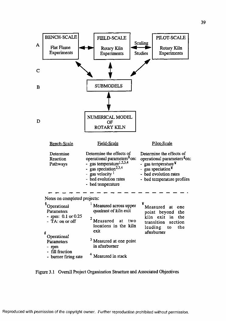
39
B
BENCH-SCALE FIELD-SCALE PILOT-SCALE
Flat FlameScaling
Rotary Kiln ----- ► Rotary KilnExperiments Experiments Studies Experiments
\ ) /
D
SUBMODELS
NUMERICAL MODEL OF
ROTARY KILN
Bench-Scale
DetermineReactionPathways
Field-Scale
Determine the effects of operational parameters5 on:- gas temperature1,2’3,4- gas speciation2,3’4- gas velocity 1- bed evolution rates- bed temperature
Pilot-Scale
Determine the effects of operational parameters £on:- gas temperature ¥- gas speciation¥- bed evolution rates- bed temperature profiles
Notes on completed projects:1 Measured across upper
quadrant of kiln exitOperationalParameters- rpm: 0.1 or 0.25- TA: on or off
OperationalParameters- rpm- fill fraction- burner firing rate
M easured at two locations in the kiln exit
3 Measured at one point in afterburner
4 Measured in stack
M easured at one point beyond the kiln exit in the transition section lead ing to the afterburner
Figure 3.1 Overall Project Organization Structure and Associated Objectives
Reproduced with permission of the copyright owner. Further reproduction prohibited without permission.
4 0
proven scaling laws do not exist, pilot-scale data cannot be used directly. However,
the pilot-scale studies are needed to provide information to guide the much more
expensive and involved field-scale experiments. Pilot-scale work that this author
participated in includes the following: Owens et al., 1990a, 1990b, 1991,1992; Silcox
et al., 1990. The field-scale effort presented in this dissertation is aimed at providing
information on velocity and temperature fields in an incinerator. Field-scale research
that this author participated in, but preceding the work presented in this dissertation,
includes the following: Cundy et al., 1989e, 1990, 1991a, 1991b, 1991c, 1991d;
Sterling et al., 1990a, 1990b; Lester et al., 1991; Cook et al., 1992; Leger et al., 1991a,
1991b, 1993a, 1993b. Research in these two areas of field and pilot-scale
experimentation is required to provide data needed to support the numerical modeling
effort. Numerical modeling research not presented here includes Jakway et al., 1993a,
1993b, 1995a. The central focus of the modeling research is development of a
rudimentary three-dimensional numerical model of a field-scale rotary kiln incinerator.
The new research presented here centers on obtaining field-scale data and using this
data to develop and validate a numerical model of a field-scale unit. The general
objectives of the field-scale experimentation and numerical modeling research are
explicitly enumerated in the following section.
SPECIFIC RESEARCH OBJECTIVES
Field-Scale Experimental Objectives
1. To design, build, and test a probe capable of measuring the temperature and, for
the first time, velocity inside a directly fired rotary kiln incinerator;
2. To design a test procedure and matrix which will provide an accurate map o f the
velocity and temperature fields at a cross-sectional plane at the exit of the kiln for
various operating conditions;
Reproduced with permission of the copyright owner. Further reproduction prohibited without permission.
41
3. To perform experimental tests on a field-scale facility while recording continuous
data from the kiln for several different operating cases;
4. To create velocity and temperature maps of the cross-section of the kiln exit;
5. To determine the effects of turbulence air addition on the temperature and
velocity fields.
Numerical Modeling Objectives
6 . To further develop the Leger et al. (1993c) numerical model of a directly-fired,
field-scale rotary kiln by:
A) more accurately matching the geometry of the kiln and its inlets
B) improving the geometrical representation of the transition section
C) improving the numerical grid
D) accounting for radiation effects
E) adding soot to the radiation model
7. To compare the kiln exit flow field predicted by the numerical model with
experimentally measured flow field data.
The following two chapters detail the methodologies used to achieve the
objectives listed above. Chapter 4 presents the design work and results of the field-
scale experiments. Chapter 5 presents the numerical model and compares results to
data from Chapter 4 and previous experimental work. Chapter 6 summarizes results
given in this dissertation, presents conclusions, and offers recommendations for future
endeavors.
Reproduced with permission of the copyright owner. Further reproduction prohibited without permission.
CHAPTER 4
IN SITU VELOCITY MEASUREMENTS FROM AN INDUSTRIAL ROTARY KILN INCINERATOR*
IMPLICATIONS
Previous experimental work has shown that incinerator flows can be highly stratified
in both temperature and chemical species. This latest work shows that the exit of a
rotary kiln incinerator can also be highly stratified in velocity and presents evidence
that regions of reverse flow may exist. It is, therefore, important to consider the
general velocity field when interpreting other measurements taken from the rotary kiln
section of an incinerator. This is particularly important if single point sampling is
used to characterize the incineration process, so that stagnant areas and regions of
reverse flow can be identified. This work presents a device and methodology for
measuring velocities in high-temperature, particulate-laden turbulent flows.
INTRODUCTION
At Louisiana State University, an ongoing research program is focused toward
obtaining a better understanding and characterization of the physical and chemical
processes associated with rotary kiln incineration. In this particular study,
temperatures and, for the first time, velocities were mapped over a significant portion
o f the exit region of a directly-fired, field-scale, rotary kiln incinerator under
* Reprinted with permission from The Journal o f the Air and Waste Management Association. November 1995. AH Rights Reserved.
42
Reproduced with permission of the copyright owner. Further reproduction prohibited without permission.
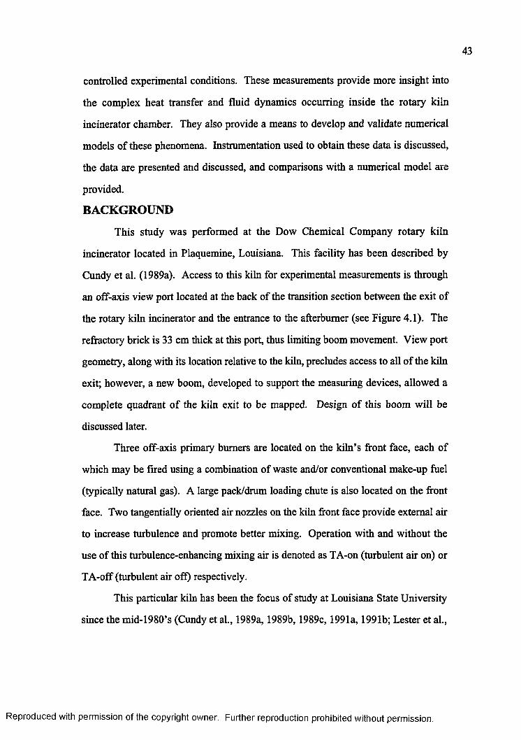
43
controlled experimental conditions. These measurements provide more insight into
the complex heat transfer and fluid dynamics occurring inside the rotary kiln
incinerator chamber. They also provide a means to develop and validate numerical
models o f these phenomena. Instrumentation used to obtain these data is discussed,
the data are presented and discussed, and comparisons with a numerical model are
provided.
BACKGROUND
This study was performed at the Dow Chemical Company rotary kiln
incinerator located in Plaquemine, Louisiana. This facility has been described by
Cundy et al. (1989a). Access to this kiln for experimental measurements is through
an off-axis view port located at the back of the transition section between the exit of
the rotary kiln incinerator and the entrance to the afterburner (see Figure 4.1). The
refractory brick is 33 cm thick at this port, thus limiting boom movement. View port
geometry, along with its location relative to the kiln, precludes access to all of the kiln
exit; however, a new boom, developed to support the measuring devices, allowed a
complete quadrant o f the kiln exit to be mapped. Design of this boom will be
discussed later.
Three off-axis primary burners are located on the kiln’s front face, each of
which may be fired using a combination of waste and/or conventional make-up fuel
(typically natural gas). A large pack/drum loading chute is also located on the front
face. Two tangentially oriented air nozzles on the kiln front face provide external air
to increase turbulence and promote better mixing. Operation with and without the
use of this turbulence-enhancing mixing air is denoted as TA-on (turbulent air on) or
TA-ofF (turbulent air off) respectively.
This particular kiln has been the focus of study at Louisiana State University
since the mid-1980’s (Cundy et al., 1989a, 1989b, 1989c, 1991a, 1991b; Lester et al.,
Reproduced with permission of the copyright owner. Further reproduction prohibited without permission.
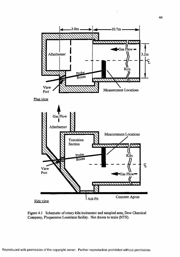
-3.8m, ^ I 4 ■10.7m
I O v \ \ \ \ X \ \ \ \ X \ X - | KXXXX
■^»-Gas FlowAfterburner
xv^ v^ xxx^ ^ xx^
ViewPort
Plan view
\Measurement Locations
Gas Flow
Afterburner
Measurement LocationsTransitionSection
Kiln
ViewPort fas Flow1
Concrete ApronAsh PitSide view
Figure 4.1 Schematic of rotary kiln incinerator and sampled area; Dow Chemical Company, Plaquemine Louisiana facility. Not drawn to scale (NTS).
Reproduced with permission of the copyright owner. Further reproduction prohibited without permission.
45
1990; Leger et al., 1991a, 1993a, 1993b; Cook et al., 1992). Gas temperatures and
compositions have been obtained from inside the kiln, afterburner, and stack.
Experiments have been conducted under a variety of operating and feed conditions.
The significant vertical gradients in temperature and chemical composition at this
kiln’s exit, characterized by a highly reactive combustion region (high temperatures
and high levels o f combustion products) in the upper kiln and a less reactive
environment (low temperatures and chemical compositions close to that of ambient
air) in the lower kiln, have been discussed at length. The gradients were observed in
both steady waste feed experiments and transient pack feed runs, persisting even
when the turbulence-enhancing mixing air was added.
Leger et al. (1993c) developed a fully three-dimensional numerical model of
the flow field inside this rotary kiln incinerator. The model reproduced the
experimentally-observed vertical stratification and further predicted the existence of a
recirculation region in the lower area of the kiln exit. A parametric study using the
model showed that the location and quantity of unmetered air infiltrating the kiln have
a major influence on the flow inside the kiln. Overall, the study demonstrated that a
relatively simple numerical model of a rotary kiln incinerator can provide valuable
insight into the process, especially when used in conjunction with experimental data.
Results of these experimental and numerical studies have helped to provide a
better picture of the incineration process in this rotary kiln incinerator; however, the
picture is far from complete. A velocity map with corresponding temperatures at the
kiln exit is needed to improve understanding of the flow dynamics, and to assist both
in interpreting past data and further development of the model. This is also an
important step in generalizing results from the kiln under study to other rotary kiln
incinerators.
Reproduced with permission of the copyright owner. Further reproduction prohibited without permission.
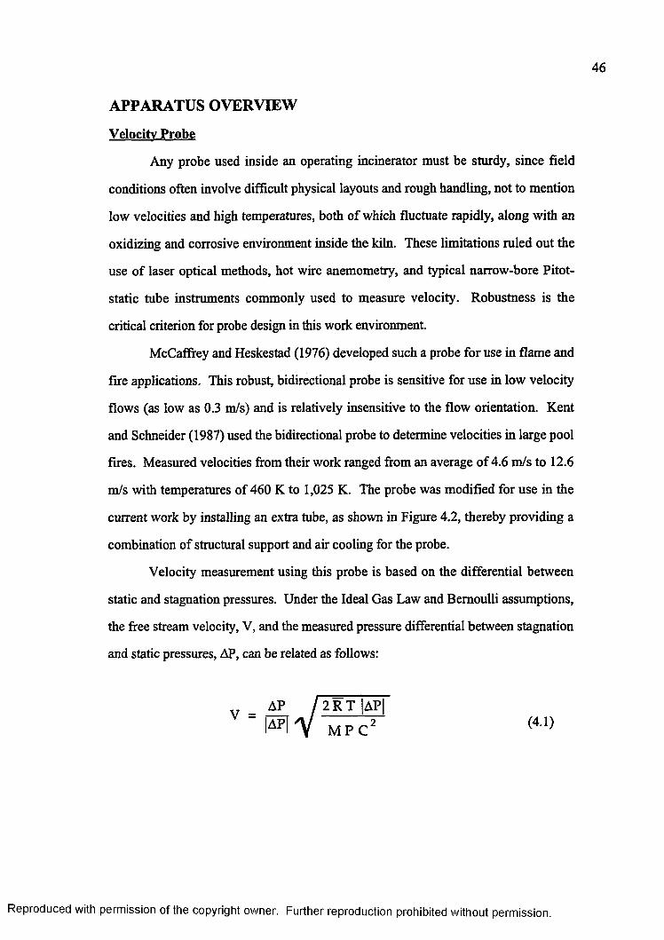
4 6
APPARATUS OVERVIEW
Velocity Probe
Any probe used inside an operating incinerator must be sturdy, since field
conditions often involve difficult physical layouts and rough handling, not to mention
low velocities and high temperatures, both of which fluctuate rapidly, along with an
oxidizing and corrosive environment inside the kiln. These limitations ruled out the
use of laser optical methods, hot wire anemometry, and typical narrow-bore Pitot-
static tube instruments commonly used to measure velocity. Robustness is the
critical criterion for probe design in this work environment.
McCaffrey and Heskestad (1976) developed such a probe for use in flame and
fire applications. This robust, bidirectional probe is sensitive for use in low velocity
flows (as low as 0.3 m/s) and is relatively insensitive to the flow orientation. Kent
and Schneider (1987) used the bidirectional probe to determine velocities in large pool
fires. Measured velocities from their work ranged from an average of 4.6 m/s to 12.6
m/s with temperatures of 460 K to 1,025 K. The probe was modified for use in the
current work by installing an extra tube, as shown in Figure 4.2, thereby providing a
combination of structural support and air cooling for the probe.
Velocity measurement using this probe is based on the differential between
static and stagnation pressures. Under the Ideal Gas Law and Bernoulli assumptions,
the free stream velocity, V, and the measured pressure differential between stagnation
and static pressures, AP, can be related as follows:
(4.1)
Reproduced with permission of the copyright owner. Further reproduction prohibited without permission.
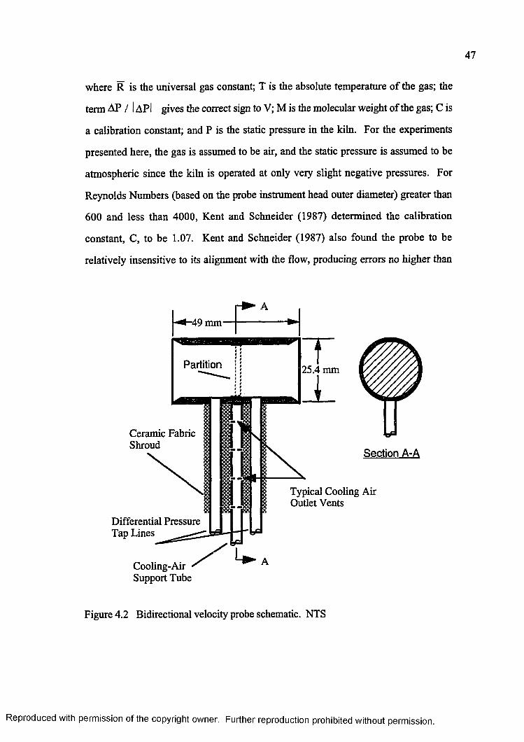
47
where R is the universal gas constant; T is the absolute temperature of the gas; the
term AP / 1 API gives the correct sign to V; M is the molecular weight of the gas; C is
a calibration constant; and P is the static pressure in the kiln. For the experiments
presented here, the gas is assumed to be air, and the static pressure is assumed to be
atmospheric since the kiln is operated at only very slight negative pressures. For
Reynolds Numbers (based on the probe instrument head outer diameter) greater than
600 and less than 4000, Kent and Schneider (1987) determined the calibration
constant, C, to be 1.07. Kent and Schneider (1987) also found the probe to be
relatively insensitive to its alignment with the flow, producing errors no higher than
Ceramic Fabric Shroud
Differential Pressure Tap Lines
Cooling-Air Support Tube
25.4 mm
49 mm
Partition
Section A-A
Typical Cooling Air Outlet Vents
Figure 4.2 Bidirectional velocity probe schematic. NTS
Reproduced with permission of the copyright owner. Further reproduction prohibited without permission.
10 percent for angles up to ± 50° (where 0° represents probe alignment parallel to
flow streamlines).
Pressure Transducer
The pressure differential, AP, was measured using an MKS Instruments Inc.
model 220CO-00001A2BS pressure transducer. This instrument is rated from 0.0
inch to 0.5 inches water column (0.0 cm to 1.27 cm), with an accuracy of ± 0.005
inches water column (± 0.13 mm) and was factory calibrated.
Suction Pyrom eter
To minimize radiation-induced error, a suction pyrometer was used to
measure gas temperatures. The pyrometer is a 1.59 mm diameter, sheathed and
grounded, type K thermocouple housed in a 9.53 mm OD Monel tube. This
pyrometer was attached to the boom and placed in close proximity to the velocity
probe, but not so close as to affect the ffee-stream velocity. Gas flow through the
pyrometer was provided by an eductor using high pressure air for the driver. A
suction flow rate of approximately 2.3 standard cubic meters per hour (SCMH) was
maintained throughout the test program. Exhaust gas from the eductor was routed
back into the incinerator downstream of the kiln exit.
Boom
The boom supports the velocity probe and suction pyrometer in the kiln and
protects the associated tubing from the kiln’s environment. The access port to the
kiln is located 3.8 m downstream from the exit of the rotary kiln incinerator (see
Figure 4.1). Hence, a relatively long and stiff boom was required in order to reach into
the incinerator while maintaining confidence in the measurement location. A
circulating-water-cooled boom used in previous experiments (Cundy et al., 1989a,
1989b, 1989c, 1991a, 1991b; Lester etal., 1990; Leger etal., 1991a, 1993a, 1993b;
Cook et al., 1992) was considered for use in this study; however, because of the large
Reproduced with permission of the copyright owner. Further reproduction prohibited without permission.
4 9
droop associated with the previous boom design and the inability to easily modify the
boom to accommodate the velocity instrument head and associated tubing, this was
ruled out. Consequently, we designed a light, stiff, and robust boom cooled with
circulating water. A schematic of this boom is shown in Figure 4.3. The new boom
design incorporates the following improvements:
• A removable probe-tip plate allows the boom to be used with different probes
• Two concentric aluminum jackets direct water flow and provide stiffness to
the boom
• An air annulus between the inner and outer aluminum water jackets reduces
the weight of the boom and isolates the hot return water from the cooler
supply water
• The use of aluminum on all parts which are not directly exposed to the kiln
environment reduces the weight of the boom
• A thicker walled tube incorporated along the base o f the boom provides added
support where the bending moment is highest
The velocity probe tip was aligned as close to co-axial with the expected kiln
flow as possible. Tip deflection was measured outside the kiln to be 11.4 cm when
the boom was filled with water and cantilevered. This same deflection was assumed
to occur when the boom was fully inserted into the kiln, as the return cooling water,
in general, was heated only 17° C, exiting the boom around 33° C. Construction
details of this boom and a comparisons to the previous boom are given in “Appendix
B” of this dissertation.
Reproduced with permission of the copyright owner. Further reproduction prohibited without permission.
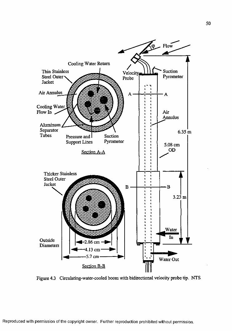
50
Cooling Water Return
Thin Stainless Steel Outer Jacket
Air Annulus
Cooling Water Flow In
Aluminum Separator Tubes
/Velocity^ Probe
Pressure and Support Lines
SuctionPyrometer
Section A-A
Thicker Stainless Steel Outer Jacket
OutsideDiameters
2.86 cm
4.13 cm5.7 cm
^ Suction Pyrometer
AirAnnulus
6.35 m
5.08 cm OD
T■B
3.23 m
Section B-B
Water
Water Out
Figure 4.3 Circulating-water-cooled boom with bidirectional velocity probe tip. NTS
Reproduced with permission of the copyright owner. Further reproduction prohibited without permission.
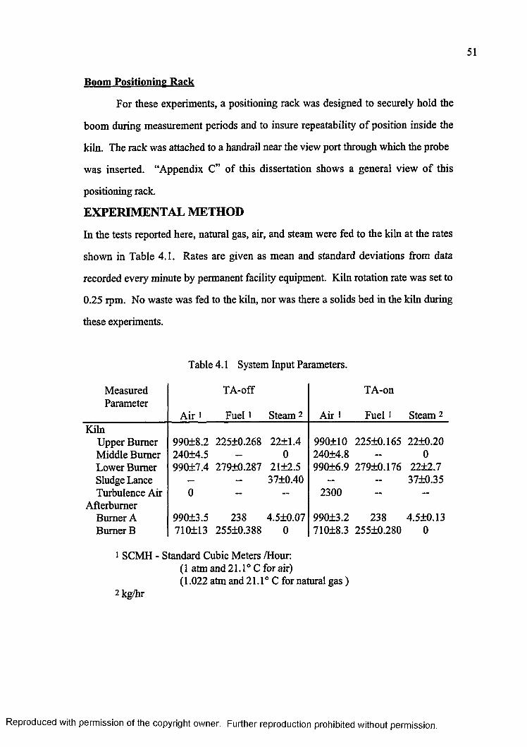
51
Boom Positioning Rack
For these experiments, a positioning rack was designed to securely hold the
boom during measurement periods and to insure repeatability o f position inside the
kiln. The rack was attached to a handrail near the view port through which the probe
was inserted. “Appendix C” of this dissertation shows a general view o f this
positioning rack.
EXPERIMENTAL METHOD
In the tests reported here, natural gas, air, and steam were fed to the kiln at the rates
shown in Table 4.1. Rates are given as mean and standard deviations from data
recorded every minute by permanent facility equipment. Kiln rotation rate was set to
0.25 rpm. No waste was fed to the kiln, nor was there a solids bed in the kiln during
these experiments.
Table 4.1 System Input Parameters.
MeasuredParameter
Air i
TA-off
Fuel i Steam 2 Air i
TA-on
Fuel i Steam 2Kiln
Upper Burner 990±8.2 225±0.268 22±1.4 990±10 225±0.165 22±0.20Middle Burner 240±4.5 — 0 240±4.8 — 0Lower Burner 990±7.4 279±0.287 21+2.5 990+6.9 279±0.176 22+2.1Sludge Lance — -- 37+0.40 — — 37±0.35Turbulence Air 0 — — 2300 — —
AfterburnerBurner A 990±3.5 238 4.5±0.07 990±3.2 238 4.5±0.13Burner B 710+13 255+0.388 0 710±8.3 255±0.280 0
1 SCMH - Standard Cubic Meters /Hour:(1 atmand21.1° C for air)(1.022 atm and 21.1° C for natural gas)
2 kg/hr
Reproduced with permission of the copyright owner. Further reproduction prohibited without permission.
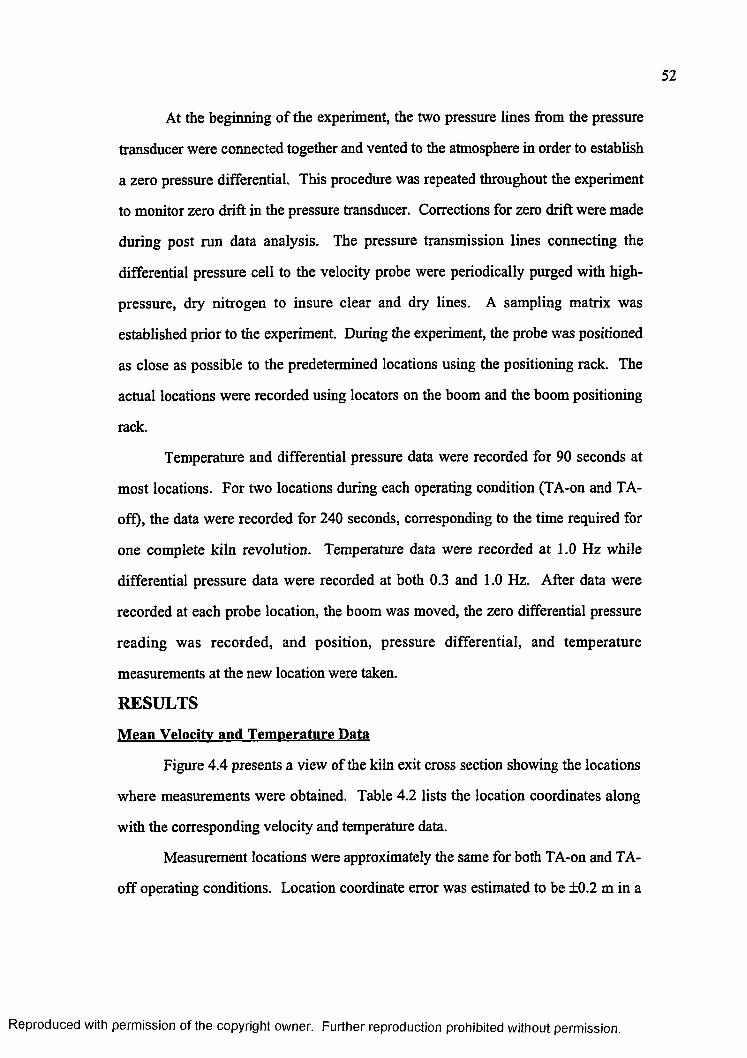
52
At the beginning of the experiment, the two pressure lines from the pressure
transducer were connected together and vented to the atmosphere in order to establish
a zero pressure differential. This procedure was repeated throughout the experiment
to monitor zero drift in the pressure transducer. Corrections for zero drift were made
during post run data analysis. The pressure transmission lines connecting the
differential pressure cell to the velocity probe were periodically purged with high-
pressure, dry nitrogen to insure clear and dry lines. A sampling matrix was
established prior to the experiment. During the experiment, the probe was positioned
as close as possible to the predetermined locations using the positioning rack. The
actual locations were recorded using locators on the boom and the boom positioning
rack.
Temperature and differential pressure data were recorded for 90 seconds at
most locations. For two locations during each operating condition (TA-on and TA-
off), the data were recorded for 240 seconds, corresponding to the time required for
one complete kiln revolution. Temperature data were recorded at 1.0 Hz while
differential pressure data were recorded at both 0.3 and 1.0 Hz. After data were
recorded at each probe location, the boom was moved, the zero differential pressure
reading was recorded, and position, pressure differential, and temperature
measurements at the new location were taken.
RESULTS
Mean Velocity and Temperature Data
Figure 4.4 presents a view of the kiln exit cross section showing the locations
where measurements were obtained. Table 4.2 lists the location coordinates along
with the corresponding velocity and temperature data.
Measurement locations were approximately the same for both TA-on and TA-
off operating conditions. Location coordinate error was estimated to be ±0.2 m in a
Reproduced with permission of the copyright owner. Further reproduction prohibited without permission.
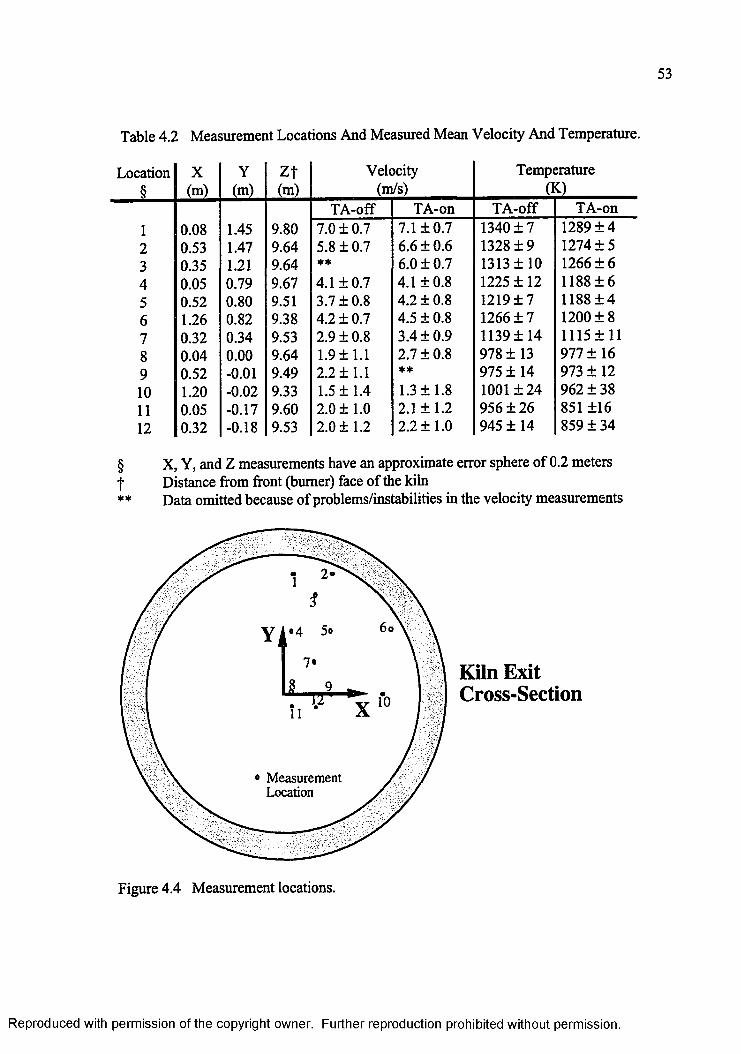
53
Table 4.2 Measurement Locations And Measured Mean Velocity And Temperature.
Location X Y z t Velocity Temperature§ (m) (m) (m) (m/s) a Q
TA-off TA-on TA-off TA-on1 0.08 1.45 9.80 7.0 ± 0.7 7.1 ±0.7 1340 ± 7 1289 ± 42 0.53 1.47 9.64 5.8+ 0.7 6.6 ±0.6 1328 ± 9 1274 ± 53 0.35 1.21 9.64 ** 6.0 ±0.7 1313 ±10 1266 ± 64 0.05 0.79 9.67 4.1 ±0.7 4.1 ±0.8 1225 ± 12 1188 ± 65 0.52 0.80 9.51 3.7 ±0.8 4.2 ± 0.8 1219 ± 7 1188 ± 46 1.26 0.82 9.38 4.2 ± 0.7 4.5 ± 0.8 1266 ± 7 1200 ± 87 0.32 0.34 9.53 2.9 ± 0.8 3.4 ±0.9 1139 ±14 1115 ±118 0.04 0.00 9.64 1.9 ±1.1 2.7 ± 0.8 978 ± 13 977 ± 169 0.52 -0.01 9.49 2.2 ±1.1 ** 975 ± 14 973 ± 1210 1.20 -0.02 9.33 1.5 ±1.4 1.3 ±1.8 1001 ±24 962 ± 3811 0.05 -0.17 9.60 2.0 ±1.0 2.1 ±1.2 956 ±26 851 ±1612 0.32 -0.18 9.53 2.0 ±1.2 2.2 ±1.0 945 ± 14 859 ± 34
§ X, Y, and Z measurements have an approximate error sphere of 0.2 meters| Distance from front (burner) face of die kiln** Data omitted because of problems/instabilities in the velocity measurements
Kiln Exit Cross-Section
Figure 4.4 Measurement locations.
• Measurement Location
Reproduced with permission of the copyright owner. Further reproduction prohibited without permission.
54
sphere surrounding the boom tip. Plans were to map a greater portion of the kiln exit;
however, slag build-up in the access window hindered boom movement. Still, a
complete quadrant of the upper kiln exit was mapped. Temperatures shown are
average values from the 1 Hz data. Velocities were calculated at 1 second intervals
using a factory calibration of the pressure transducer, the recorded zero drift, and the
velocity equation (Equation 4.1). A velocity mean and standard deviation were then
calculated for each location. Small-scale, turbulent fluctuations were not measurable
due to the characteristic slow response time and insensitivity to flow orientation
associated with the velocity probe. Raw velocity and temperature data are presented
in Figure 4.5 for the operating condition of TA-on at three different locations along
with a typical zero reading. In this figure, location 2 illustrates the relatively low
fluctuations about the mean, common in the upper region of the kiln, while locations
10 and 12 demonstrate the wider fluctuations typically observed close to the center of
the kiln. Location 10 presents conditions suggestive of intermittent regions of reverse
flow. Difficulties with the velocity instrumentation were encountered at two
locations—location 3 during TA-off operation and location 9 during TA-on
operation—and therefore, the data associated with these locations are not reported.
Probe-based Reynolds Numbers ranged from 1000 in the upper region to 300 near the
centerline. Calibration work by Kent and Schneider (1987) shows a drop in the
calibration constant from -1.07 to -1.02 between Reynolds Numbers of 600 to 300
along with an increase in uncertainty. However, the resulting error in calculated
velocities near the centerline, up to 5 percent, was ignored in the present study.
Figures 4.6 and 4.7 show the velocity and temperature data as a function of
vertical position along with fitted lines (to be discussed later). Strong vertical
stratification is evident in temperature and velocity during both TA-on and TA-off
operating conditions. Velocities and temperatures increase significantly from kiln
Reproduced with permission of the copyright owner. Further reproduction prohibited without permission.
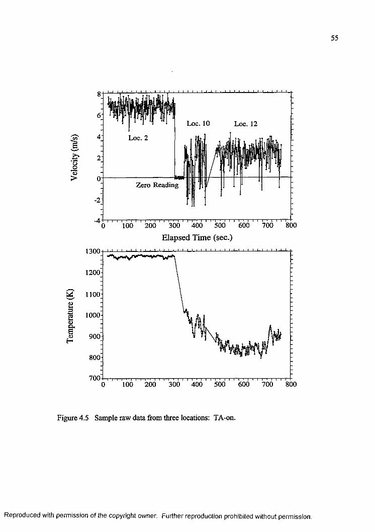
55
- 4 I i i i i r - r ~r i i i i i i i i i i i i i i i i i i i i r i i i i i i ' i i i i I0 100 200 300 400 500 600 700 800
Elapsed Time (sec.)1300
1200 -
1100 -
1000 -
<DI*CD
H 900-
800-
700100 200 300 400 500 600 700 8000
Figure 4.5 Sample raw data from three locations: TA-on.
Reproduced with permission of the copyright owner. Further reproduction prohibited without permission.
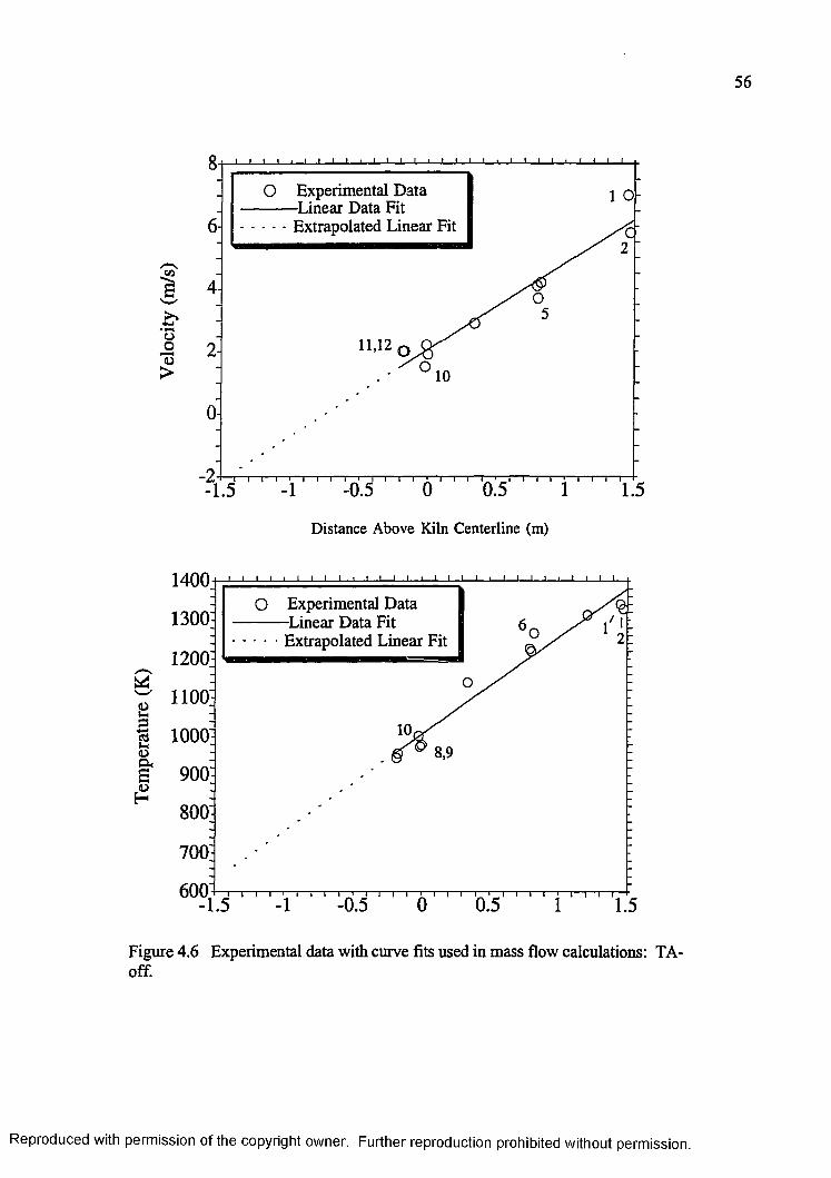
Tem
pera
ture
(K
)
O Experimental Data Linear Data Fit- - - Extrapolated Linear Fit
11,12<L>>
0.5 1.5-1.5
Distance Above Kiln Centerline (m)
1400O Experimental Data Linear Data Fit• • • Extrapolated Linear Fit
1300-
1200;
1100'
1000
900
800-
700-
6001-0.5 0.5-1.5
Figure 4.6 Experimental data with curve fits used in mass flow calculations: TA- off.
Reproduced with permission of the copyright owner. Further reproduction prohibited without permission.
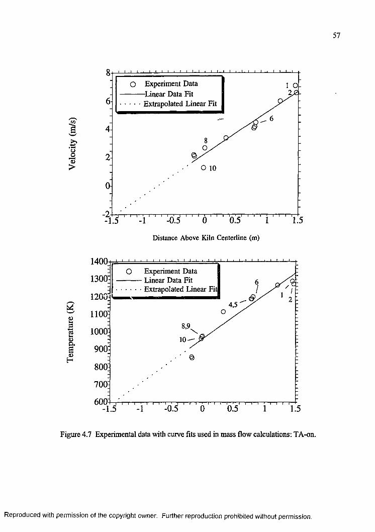
Tem
pera
ture
(K
) Ve
locit
y (m
/s)
O Experiment Data Linear Data Fit• - • Extrapolated Linear Fit
O 10
0.5 1.5
Distance Above Kiln Centerline (m)
1400O Experiment Data Linear Data Fit- - - - Extrapolated Linear Fit
1300-
1 2 0 0 j4.5
1100'
1000-
900-
800-
700-
6001-0.5 0.5 1.51.5
Figure 4.7 Experimental data with curve fits used in mass flow calculations: TA-on.
Reproduced with permission of the copyright owner. Further reproduction prohibited without permission.
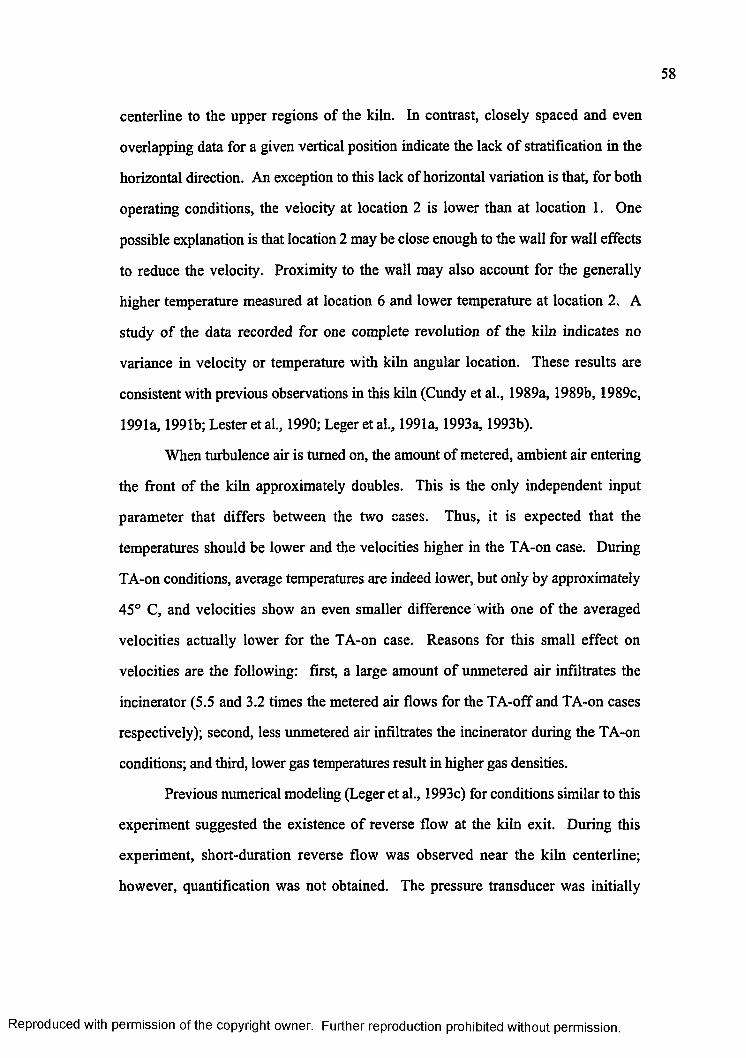
centerline to the upper regions of the kiln. In contrast, closely spaced and even
overlapping data for a given vertical position indicate the lack of stratification in the
horizontal direction. An exception to this lack of horizontal variation is that, for both
operating conditions, the velocity at location 2 is lower than at location 1. One
possible explanation is that location 2 may be close enough to the wall for wall effects
to reduce the velocity. Proximity to the wall may also account for the generally
higher temperature measured at location 6 and lower temperature at location 2. A
study o f the data recorded for one complete revolution of the kiln indicates no
variance in velocity or temperature with kiln angular location. These results are
consistent with previous observations in this kiln (Cundy et al., 1989a, 1989b, 1989c,
1991a, 1991b; Lester etal., 1990; Leger etal., 1991a, 1993a, 1993b).
When turbulence air is turned on, the amount of metered, ambient air entering
the front of the kiln approximately doubles. This is the only independent input
parameter that differs between the two cases. Thus, it is expected that the
temperatures should be lower and the velocities higher in the TA-on case. During
TA-on conditions, average temperatures are indeed lower, but only by approximately
45° C, and velocities show an even smaller difference with one of the averaged
velocities actually lower for the TA-on case. Reasons for this small effect on
velocities are the following: first, a large amount o f unmetered air infiltrates the
incinerator (5.5 and 3.2 times the metered air flows for the TA-off and TA-on cases
respectively); second, less unmetered air infiltrates the incinerator during the TA-on
conditions; and third, lower gas temperatures result in higher gas densities.
Previous numerical modeling (Leger et al., 1993c) for conditions similar to this
experiment suggested the existence o f reverse flow at the kiln exit. During this
experiment, short-duration reverse flow was observed near the kiln centerline;
however, quantification was not obtained. The pressure transducer was initially
Reproduced with permission of the copyright owner. Further reproduction prohibited without permission.
59
calibrated to read only positive pressure differences. We planned to interchange the
pressure taps when reverse flow was encountered, so that a positive pressure
difference could be maintained, thus allowing quantification o f any reverse flow. This
swapping was accomplished by changing valve settings on a five-valve manifold, a
process that took 15 to 30 seconds. Unfortunately, the reverse flow had a shorter
than expected duration (typically 5 seconds or less) and was infrequent. After the
experiment, it was determined that the instrument remained linear into the near
reverse pressure range. This information was used to calculate the negative velocities
shown in Figure 4.5. Combining the trend of decreasing velocity with elevation
together with the appearance o f short periods o f reverse flow at some o f the lower
sampling points suggests that, had lower regions been sampled, substantial reverse
flow may have been detected.
Mass Flow Study
This paper presents, for the first time, velocities measured inside an operating
incinerator using the bidirectional probe assembly of Figure 4.3. Since this is the first
time the probe has been used in a confined combustion environment, the data obtained
need to be examined and checked for reasonableness. This check is accomplished by
comparing the mass flow at the exit plane of the incinerator calculated in two ways.
The first technique uses the measured velocities and temperatures to calculate the
mass flow, while the second method is based on a mass balance across the kiln. The
mass balance method uses the metered inputs along with an estimate o f unmetered air
infiltrating into the system. Since the second method does not involve the measured
velocities, it provides an independent check of the experimental data.
I - Kiln Mass Flow from Experimental Velocity and Temperature Measurements
To calculate a kiln mass flow rate using the measured data, the individual point
values of temperature and velocity shown in Table 4.1, and graphed in Figures 4.6 and
Reproduced with permission of the copyright owner. Further reproduction prohibited without permission.
4.7, were first transformed into smooth surface functions. Because of the lack of
horizontal variation, the surface equations were assumed to vary with "y" only,
where "y" is the vertical direction measured from kiln centerline. Utilizing linear
approximations for the y-dependency of temperature and velocity along with the
ideal gas approximation, the local mass flux was calculated. By integrating this local
mass flux over the area of the kiln's upper quadrant, where the experimental values
were taken (29 percent of the total cross-sectional area), the total mass flow rate
through this region of the kiln was obtained. Results o f these calculations indicate
mass flow rates of 2.5 kg/s and 2.9 kg/s for the TA-off and TA-on conditions
respectively. If the lack of horizontal variation observed in this quadrant of the kiln is
true o f the other upper quadrant as well, then the above calculated flows can be
doubled to yield the mass flow in the entire upper 58 percent of the kiln: 5.0 kg/s and
5.7 kg/s for the TA-off and TA-on conditions respectively.
To determine the total mass flow through the rotary kiln incinerator, the linear
curve fits to the temperature and velocity data are assumed to extend to the bottom of
the kiln. These straight-line extrapolations are shown as dashed lines in Figures 4.6
and 4.7 (Note that this extrapolation implies the existence of reverse flow in the lower
region o f the kiln.) Using this approximation, along with horizontal symmetry, the
total net mass flow out of the kiln was calculated to be 4.5 kg/s and 5.2 kg/s for the
TA-off and TA-on conditions respectively.
The assumption that the velocity and temperature data trends extend linearly
to the bottom of the kiln is rather bold. Preliminary numerical modeling suggests,
however, that linear extrapolation is usually appropriate. If this linear extrapolation
method is indeed valid, the resulting net mass flow rates across the entire exit plane
(4.5 kg/s and 5.2 kg/s for the TA-off and TA-on respectively) being less than the net
mass flows out the upper half of the exit plane (5.0 kg/s and 5.7 kg/s for the TA-off
Reproduced with permission of the copyright owner. Further reproduction prohibited without permission.
61
and TA-on respectively) indicates that there must be recirculation in the lower region
of the kiln, and that the majority of the flow out of the kiln takes place in the upper
region, as expected.
IT - Kiln Mass Flow from Mass Balance
The mass flow rate calculated from the experimental data can be compared
with that found from a mass balance on the system. To perform a mass balance, all
inlet and exit flows need to be quantified. Information on all metered inlets to the
incinerator is available and has previously been presented in Table 4.1. However,
there is also a considerable amount of unmetered air infiltrating the incinerator. This
infiltration results from the operation of the incinerator at a slight vacuum (1.1 cm
negative water column during TA-off operation and 1.0 cm negative water column
during TA-on operation), which is done to prevent fugitive emissions. This
unmetered air infiltration rate must be determined in order to complete the mass
balance.
Unmetered air infiltrates this system from the front and rear rotary seals of
the kiln, around the perimeter of the solids loading chute at the front face of the kiln,
and through the pressure relief hatch near the front of the incinerator. Additional air
infiltrates the system through various instrumentation ports and other small openings.
Although the amount of unmetered air entering through any one o f these sources is
not known, their combined effect can be calculated in two different ways. The first
way, termed the Oxygen Method, uses the metered flow rates into the incinerator, the
measured dry oxygen concentration at the stack (13.3 percent for TA-off and 13.5
percent for TA-on operation), and the assumption that the natural gas is pure
methane which reacts completely to water vapor and carbon dioxide (Cook et al.,
1992; Leger et al., 1993b).
Reproduced with permission of the copyright owner. Further reproduction prohibited without permission.
62
A second way of calculating the unmetered air infiltration rate, the Mass
Balance Method, involves performing a mass balance across the whole incinerator on
a dry basis. Performing the mass balance on a dry basis allows use of the measured
stack flow rate (24,551 SCMH for TA-off and 24,755 SCMH for TA-on operation),
which was recorded on a dry basis. Again using the assumptions of pure methane
completely combusting to water vapor and carbon dioxide, the unmetered air
infiltration rate can be determined (Cook et al., 1992; Leger et al., 1993b). Results of
these calculations are shown in Table 4.3.
Table 4.3 Calculated incinerator air infiltration, (SCMH).
TA-off TA-onOxygen Method 21,400 19,890Mass Balance Method 21,630 19,550
This table shows that the two methods of calculating unmetered infiltrating air
compare very favorably. An average is used in subsequent calculations. Comparison
of these data to those in Table 4.1 also shows that the unmetered air infiltrating the
incinerator can be as much as 5.5 times the amount o f metered air fed into the
incinerator. This in-leakage is commonly included when calculating the amount of
metered air needed to insure complete combustion in an incinerator.
The problem now reduces to one o f proportioning the unmetered infiltration
air in order to determine the mass flow in the rotary kiln incinerator. Obviously, this
is a difficult process requiring a considerable degree of estimation. Leger et al. (1993c)
reasoned that 55 percent of the total unmetered air infiltrating this system entered at
the front face of the kiln. Using this estimate, the mass flow leaving the exit plane of
the kiln was calculated to be 5.1 kg/s for the TA-off case and 5.5 kg/s for the TA-on
case.
Reproduced with permission of the copyright owner. Further reproduction prohibited without permission.
63
These mass flow values differ by 13 and 8 percent respectively from the
values calculated above using the experimentally determined temperature and velocity.
Thus, the data appear reasonable.
Numerical Model
A second way to examine the reasonableness o f the experimental data is by
comparison to a numerical model. Leger et al. (1993c) constructed a three-
dimensional numerical model of the same rotary kiln incinerator studied in this work.
The model is a finite difference type utilizing the SIMPLEC algorithm. The main
weakness o f this model is that radiation heat transfer is not included. While Leger et
al. (1993c) modeled the same incineration facility utilized in the present study, the
model inputs do not exactly match the present experimental conditions. For TA-off,
the modeled kiln inputs differ from the operating conditions (previously presented in
Table 4.1) in the following ways: the kiln natural gas flow was 27 percent lower, the
metered air to the afterburner was 8 percent higher, and the unmetered infiltrating air
was 25 percent lower. However, incinerator operating conditions for the TA-on case
were nearly identical to those of the present study. Given the similarity between the
model inputs and the operating conditions of this paper, useful comparisons can be
made between the modeling and experimental results.
As an expected result o f the omission of radiation heat transfer, the
temperatures are over predicted for both the TA-off and TA-on cases. Model
predicted velocities at the kiln exit for the TA-off case ranged from a high of 7.7 m/s
at the top, to 0.7 m/s at centerline, to - 1.5 m/s at the bottom of the kiln, in an
approximately linear fashion. For the TA-on case, velocities were 8.6 m/s at the top,
1.0 m/s at centerline, and - 1.3 m/s at the bottom of the kiln, again varying in an
approximately linear fashion.
Reproduced with permission of the copyright owner. Further reproduction prohibited without permission.
64
These modeled velocities are close to the measured values, but are slightly
higher at the top of the kiln and marginally lower at the centerline of the kiln. The
model also confirms the uniformity of the flow field in the horizontal direction. At a
distance one quarter from the top, the maximum deviation from the predicted mean
values of velocity and temperature taken horizontally across the kiln are respectively
10 and 14 percent for TA-off, and 13 and 1.2 percent for TA-on operation. The
small size o f these deviations predicted by the model improves confidence in the
assumption that the lack o f horizontal variation of velocity and temperature in the
quadrant sampled extends to the other quadrants of the kiln exit.
SUMMARY
A new device for measuring velocities and temperatures inside a directly-fired,
full-scale, rotary kiln incinerator has been developed, constructed, and tested.
Temperatures and, for the first time, velocities were mapped across an upper
quadrant of a rotary kiln incinerator during steady state burning of natural gas. The
experimental results and ensuing analysis provide the following conclusions.
• Stratification of both temperature and velocities is evident in the vertical but not
horizontal direction.
• The highest velocities and temperatures were recorded at the top of the kiln.
• The effect of the turbulent air jets on velocities and temperatures at the exit o f the
rotary kiln incinerator is largely mitigated by the large amount of unmetered air
infiltrating at the front of the kiln.
• Temperature values and data stratification trends generated by this new device
agree with previous experimental findings on the same incinerator under similar
operating conditions.
Reproduced with permission of the copyright owner. Further reproduction prohibited without permission.
65
• Mass flow rates calculated using the experimental results compare favorably with
mass flow rates calculated by a mass balance across the kiln.
• Numerical modeling also produces results that compare favorably with those
generated by the new experimental device.
• The need to sample a complete vertical traverse of the rotary kiln incinerator to
determine the amount of air infiltrating at the front of the kiln and the possible
existence of reverse flow at the exit of the kiln is reinforced.
Prior to obtaining the velocity and temperature data reported in this paper,
there were virtually no means to quantify the mass flow inside rotary kilns. This led
to uncertainty about the distribution of unmetered infiltration air and the flow
dynamics at the locations of previous sampling efforts. Because the limited access of
this incinerator did not allow a complete mapping of the kiln exit, the amount of
unmetered air entering the kiln is still uncertain. However, the results do help to
provide confidence that the estimated infiltration air distribution of Leger et al.
(1993c) is realistic. Further, the results indicate that, with adequate access, this probe
assembly could completely characterize the mass flow field o f this rotary kiln
incinerator or other similar combustion devices. Limitations include material
compatibility with kiln environment, pressure transducer limitations, and calibration
constant applicability limits (not a theoretical limit, but so far determined only for the
Reynolds Number range of 300 to 4000 according to Kent and Schneider (1987). In
addition, the relatively good agreement between the measured and calculated kiln mass
flow rates suggests that the experimental techniques used and the assumptions
imposed (horizontal symmetry at the exit region of the kiln, along with linear velocity
and temperature profiles) are reasonable. While this may seem a circular argument, it
should be noted that, primarily due to the complexity of the system, never before has
Reproduced with permission of the copyright owner. Further reproduction prohibited without permission.
66
the flow field of an operating rotary kiln incinerator been quantified. With each piece
of new information, the picture of what takes place inside a rotary kiln incinerator
becomes clearer, and the ability to test previous assumptions becomes possible.
While the measurements reported in this paper only covered a portion of the kiln exit
region, they have added considerably to our understanding of the complicated process
of rotary kiln incineration.
Reproduced with permission of the copyright owner. Further reproduction prohibited without permission.
CHAPTER 5
THREE-DIMENSIONAL NUMERICAL MODELING OF A FIELD- SCALE ROTARY KILN INCINERATOR
INTRODUCTION
The second-generation numerical model of a field-scale, direct-fired, rotary kiln
incinerator presented in this paper represents a continuation of work initiated by
Leger et al. (1993c), hereafter referred to as Leger’s model. The work is part of a
comprehensive rotary kiln incineration research program undertaken over the past ten
years at Louisiana State University. The overall goal of this program is to obtain a
better understanding of hazardous waste incineration in rotary kiln facilities.
Leger et al. (1993c) have provided a comprehensive overview of recent
attempts to model rotary kiln incineration processes. This overview points out that
incinerators are typically over designed and operated far below capacity, and that
there is a scarcity of field-scale data, proven numerical models, or empirical relations
for design or optimization studies. The lack of experimental data is due, in part, to
strict incineration regulations requiring field-scale units to operate within a narrow
range of previously established compliance conditions with virtually zero tolerance
for excursion from these limits. Recent modeling studies conducted at LSU have,
therefore, aimed toward development of a comprehensive and reliable numerical model
of rotary kiln incineration. This model can then be used to investigate, among other
issues, the effects of system geometry, overall configuration, and waste composition
67
Reproduced with permission of the copyright owner. Further reproduction prohibited without permission.
68
as well as optimal operating parameters, and failure modes, all currently nearly
impossible to do in the field.
The approach taken by Louisiana State University has been to develop this
model in stages, relying on experimental data to characterize and verify predicted kiln
behavior under various operating conditions. The current stage of model development
focuses only on the rotary kiln section of the incinerator during operation without
waste processing. This stage, a second generation model which is presented here,
builds on its predecessor (Leger et al., 1993c) by providing a more accurate
representation of the facility geometry and including the effects of radiation and soot
in the heat transfer analysis. A grid dependency study is provided for the first time,
and sensitivity and parametric studies are also presented. Waste is not yet included in
the model because even baseline conditions (operation with natural gas support flames
only in the kiln) have yet to be fully understood and modeled. Even so, the model in
its current stage of development, can be used for limited design and operation studies
as demonstrated in the following sections.
PHYSICAL SYSTEM
The incinerator under study (Figure 5.1a shows a general skematic) is owned
and operated by The Dow Chemical Company. It is a direct-fired, hazardous waste,
rotary kiln incinerator located in Plaqucmine, Louisiana. A more complete description
of the facility is available elsewhere (Cundy et al., 1989a; Montestruc, 1989; Jakway
et al., 1995a, 1995b); only a brief description is provided here.
The kiln is 10.7 m in length and its inside diameter is 3.2 m. Gases exiting the
cylindrical kiln pass into a rectangular transition section which directs the flow into a
vertical afterburner. Gasses then pass through air pollution control systems and the
stack. As shown in Figure 5.1b, the front face of the kiln is highly non-symmetric,
Reproduced with permission of the copyright owner. Further reproduction prohibited without permission.
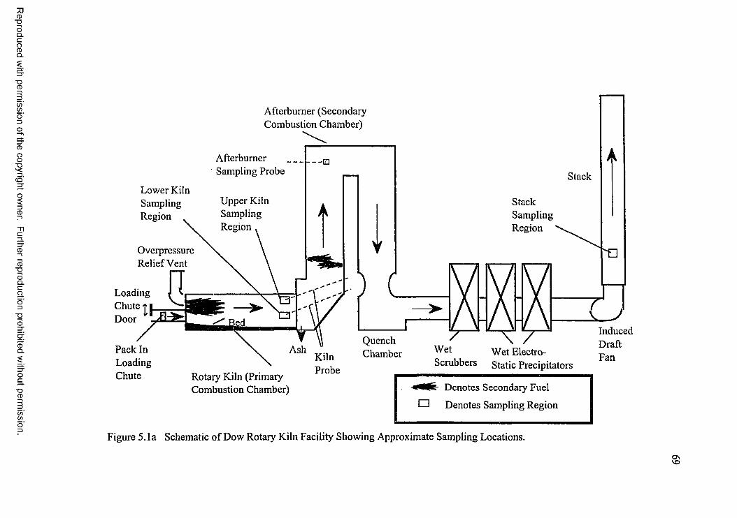
Reproduced
with perm
ission of the
copyright ow
ner. Further
reproduction prohibited
without
permission.
Lower Kiln Sampling Region
Overpressure Relief Vent
LoadingChute 1 1Door
Pack InLoadingChute
Afterburner (Secondary Combustion Chamber)
Afterburner Sampling Probe
Upper Kiln Sampling Region
Stack Sampling Region
QuenchChamber Wet
ScrubbersProbeRotary Kiln (Primary
Combustion Chamber)
TWet Electro- Static Precipitators
Denotes Secondary Fuel
Denotes Sampling Region
InducedDraftFan
Figure 5.1a Schematic of Dow Rotary Kiln Facility Showing Approximate Sampling Locations.
CT\v©
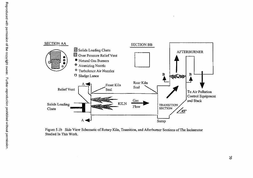
Reproduced
with perm
ission of the
copyright ow
ner. Further
reproduction prohibited
without
permission.
SECTION AA SECTION BB0 Solids Loading Chute ^ Over Pressure Relief Vent ® Natural Gas Burners ® Atomizing Nozzle ° Turbulence Air Nozzles E Sludge Lance B
Relief Vent
Solids Loading Chute
Front Kiln Rear Kiln
AFTERBURNER
t B
IKILN TRANSITION
SECTION
To Air Pollution Control Equipment and Stack
Sump
Figure 5.1b Side View Schematic of Rotary Kiln, Transition, and Afterburner Sections of The Incinerator Studied In This Work.
-jo
71
with an off-axis solids loading chute as well as off-axis and angled natural gas burners
and secondary air nozzles (termed turbulence air nozzles). Turbulence air nozzles are
designed to assist combustion by introducing a je t o f high velocity ambient air,
thereby increasing turbulence and mixing in the kiln. The system is designed to
operate with (TA-on) or without (TA-off) secondary turbulence air.
The kiln is operated at a slight vacuum to prevent fugitive emissions; this also
allows substantial amounts o f unmetered air to infiltrate into the system. Infiltration
is known to occur at the front and rear kiln rotary seals, around the edges of the solids
loading door and pressure relief hatch, and through various instrument ports.
Infiltration amounts have been calculated as high as 5.5 times the metered air flowing
into the incinerator system (Leger et al., 1993b; Jakway et al., 1995a, 1995b). A fuel-
rich mixture of natural gas and air is typically injected from the upper and lower kiln
burners, which also have a low steam feed to cool the burners.
NUMERICAL KILN MODEL
The model described here contains a number of improvements and new features not
contained in Leger’s model. In this section the general solution method is presented,
followed by brief discussions of the geometry, the grid, and methods used to calculate
important physical properties. Radiation (added for the first time) and the chemical
reaction rate mechanism are then discussed. This section concludes with a discussion
of boundary conditions.
Solution Method
The commercial software package, FLUENT version 4.25, produced by Fluent
Inc. (Fluent, 1993), is used as the primary source code for the model. This package
employs a control-volume-based, fmite-difference solution technique to allow full
characterization of the flow field. The Reynolds-averaged Navier-Stokes equations
coupled with the Reynolds-averaged governing differential equations o f continuity,
Reproduced with permission of the copyright owner. Further reproduction prohibited without permission.
energy, and species (listed in “Appendix G” of this dissertation) are solved in a
discritized form. The standard K-e turbulence model is employed. To obtain values
at control volume interfaces needed for flux calculations, the power law interpolation
scheme is utilized. The pressure-linked continuity and momentum equations are
solved using the Semi-Implicit Method for Pressure-Linked Equations Consistent
(SIMPLEC) solution algorithm. Specific details regarding convergence parameters
such as multigrid and underrelaxation factors are available in “Appendix H” of this
dissertation.
Geometry Details
The model focuses on, and is considered valid only for, the rotary kiln segment
o f the incinerator. However, the section immediately downstream of the rotary kiln
(the transition section, Figure 5.1) must be included in the model because it exchanges
radiation with the kiln, shifts the flow centerline horizontally by 0.7 m, and, for
modeling purposes, prevents influx of undefined material at the outlet boundary
which would otherwise occur due to recirculation at the kiln exit. This second
generation model represents the transition section geometry more accurately than the
previous attempt (Leger et al., 1993c), which did not include the horizontal flow shift
or the 45° inclination (shown in Figure 5.1).
The outflow boundary condition used in this model requires the flow leaving
the solution domain to be fully developed; however, the flow leaving the transition
section is far from fully developed. To remedy this situation, a fictitious chimney
was added at the exit o f the transition section having the same cross-section as the
afterburner shown in Figure 5.1. To reduce the height needed to achieve a fully
developed exit flow from the solution domain, the chimney’s exit area was reduced or
"necked" (see Figure 5.2), eliminating a region where recirculation tended to form. The
necked chimney results in a nearly fully developed flow field, without inflow, at the
Reproduced with permission of the copyright owner. Further reproduction prohibited without permission.
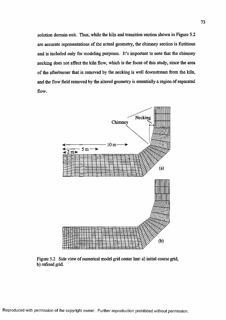
73
solution domain exit. Thus, while the kiln and transition section shown in Figure 5.2
are accurate representations of the actual geometry, the chimney section is fictitious
and is included only for modeling purposes. It’s important to note that the chimney
necking does not affect the kiln flow, which is the focus of this study, since the area
of the afterburner that is removed by the necking is well downstream from the kiln,
and the flow field removed by the altered geometry is essentially a region of separated
flow.
Figure 5.2 Side view of numerical model grid center line: a) initial coarse grid, b) refined grid.
NeckingChimney
Reproduced with permission of the copyright owner. Further reproduction prohibited without permission.
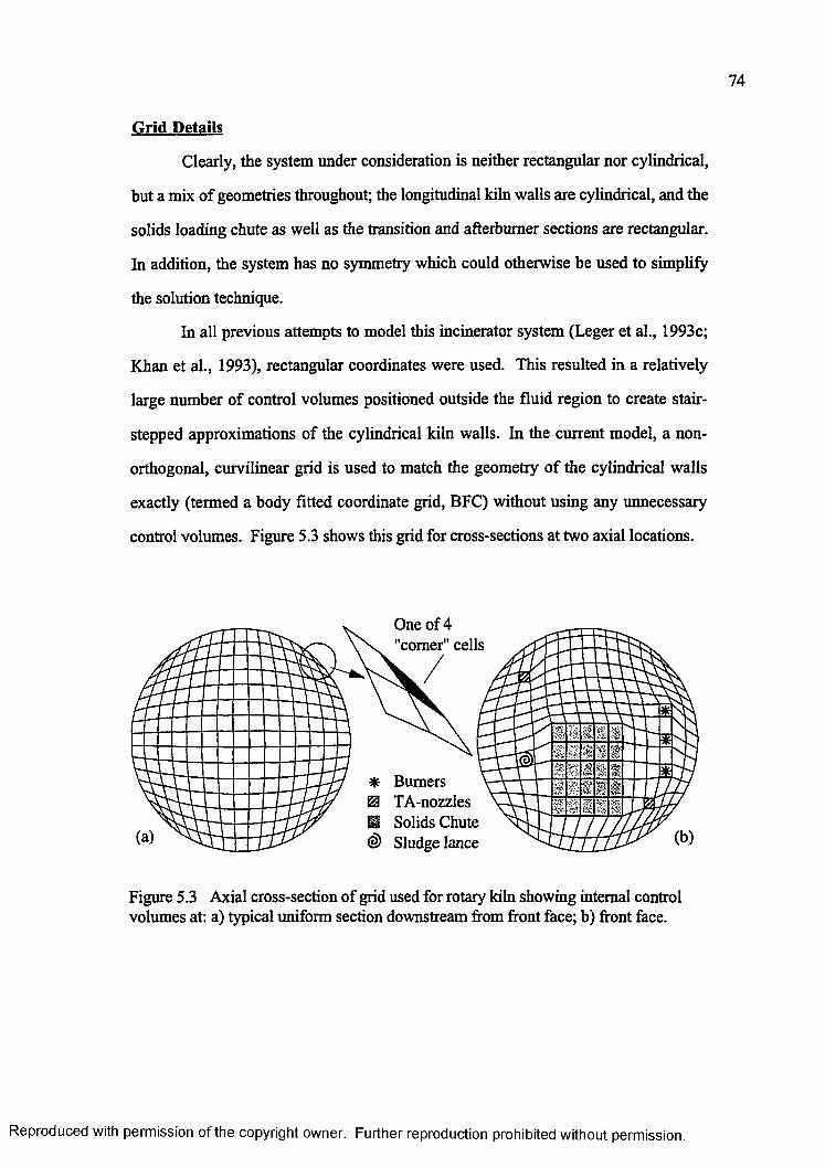
74
Grid Details
Clearly, the system under consideration is neither rectangular nor cylindrical,
but a mix of geometries throughout; the longitudinal kiln walls are cylindrical, and the
solids loading chute as well as the transition and afterburner sections are rectangular.
In addition, the system has no symmetry which could otherwise be used to simplify
the solution technique.
In all previous attempts to model this incinerator system (Leger et al., 1993c;
Khan et al., 1993), rectangular coordinates were used. This resulted in a relatively
large number of control volumes positioned outside the fluid region to create stair-
stepped approximations of the cylindrical kiln walls. In the current model, a non-
orthogonal, curvilinear grid is used to match the geometry o f the cylindrical walls
exactly (termed a body fitted coordinate grid, BFC) without using any unnecessary
control volumes. Figure 5.3 shows this grid for cross-sections at two axial locations.
One of 4 "comer" cells
Burners TA-nozzIes Solids Chute Sludge lance
Figure 5.3 Axial cross-section o f grid used for rotary kiln showing internal control volumes at: a) typical uniform section downstream from front face; b) front face.
Reproduced with permission of the copyright owner. Further reproduction prohibited without permission.
75
In the previous modeling attempts (Leger et al., 1993c; Khan et al., 1993), the
coarseness of the grid and the use of uniform grid spacing required the position of inlet
streams (natural gas, steam, and mixing air) to be slightly shifted from actual locations.
In addition, the nozzle flow areas were also different from actual areas found in the
field; hence, gas velocities differed from known values so that the mass flow rates
would match. The non-uniform grid spacing utilized in the current model alleviates
this problem thereby allowing gas inlets to be placed and sized precisely. The only
exception is the rotary seal gaps at the front and rear of the kiln which are too small to
be correctly sized with the coarse grid employed.
The grid used in the model consists of 17 x 17 control volumes per axial cross-
section (15 x 15 internal control volumes and a boundary control volume at the ends
of each row and column of internal control volumes). There are 34 grid cross-sections
in the axial flow direction for a total of 9,826 control volumes. Figure 5.3b shows the
grid used at the front face of the kiln and highlights the grid distortions used to
position and size the inlets accurately. Because of the limited number of control
volumes, burners and turbulence air nozzles are represented by single square control
volumes. Perimeter cells on the kiln front face are set as inlet cells to account for air
infiltrating through the front rotary seal. Two intermediate grid cross-sections are
used to make the transition from the distortions of the front face (Figure 5.3b) to the
uniform cross-sections shown in Figure 5.3a.
A side view of the centerline grid is shown in Figure 5.2a. This figure also
illustrates the necked chimney, which, when combined with the elongation o f the
chimney control volumes in the flow direction, significantly reduces the total number
of control volumes necessary to satisfy the exit boundary condition. Figure 5.2b is a
refined version of the grid discussed in a later section.
Reproduced with permission of the copyright owner. Further reproduction prohibited without permission.
Fluid Physical Properties
Natural gas feeding the support flames contains a minimum of 95 percent
methane by volume and, therefore, is modeled as pure methane. Fluid physical
properties are calculated as indicated in Leger et al. (1993c), with the exception of the
pure component heat capacities. These are calculated using third order polynomials
(listed in “Appendix H” of this dissertation) in temperature fit to data from the
JANAF tables (Stull and Prophet, 1971). Maximum error in the resulting heat
capacity polynomials is 2.6 percent over the range of 300 K to 3,000 K.
Radiation
Radiation heat transfer is calculated by the Discrete Transfer Radiation Model
(DTRM) discussed by Murthy and Choudhury (1992). Heat transfer in the DTRM
is accomplished by following the path of radiation as it travels from one surface to
another. Eight paths are traced from each surface control volume. Increasing the
number of paths to sixteen changed the maximum gas temperature by only 0.3
percent; however, both CPU time and computer storage requirements were
significantly increased. As the path from one surface to another is traced, adsorption
and emission from participating media are included.
In all experiments that Louisiana State University conducted at this facility,
the support flames in the kiln have been orange colored (Lester et al., 1990) and fuel
rich, with equivalence ratios at the burners ranging from 2.2 to 2.9 on a molar basis.
Therefore, it was concluded that a substantial amount of soot was formed near the
burners. As the majority of radiation from flames laden with soot originates from
soot particles (J. De Ris, 1978), it is important to include soot in the heat transfer
model. Fluent, however, does not currently account for the radiation effects o f soot;
instead, a special version of the Fluent software was obtained which allowed
modification of certain subroutines, including the calculation of absorption
Reproduced with permission of the copyright owner. Further reproduction prohibited without permission.
77
coefficients. The remainder of this sub-section focuses on the subroutines developed
to include the radiation effects of soot by modifying the absorption coefficients used
in the standard Fluent software package. The numerical codes for the subroutines are
given in “Appendix F” of this dissertation.
Effects o f gas composition and soot particles on absorptivity, a , are calculated
separately and then combined using the technique of Felske and Charalampopoulos
(1982):
a = a p + a g - a p a g (5.1)
where a p is the absorptivity of soot particles alone with no participating gas media,
and a g is the absorptivity of gases alone without soot. The Weighted Sum of Gray
Gasses, (WSGG) model is used to calculate otp, with values for the coefficients given
by Felske and Charalampopoulos (1982). In calculating a g, the spectral nature of the
gas absorptivity is included using the Wide Band Property Model (WBPM) of
Edwards (1981). This model also accounts for arbitrary concentrations of carbon
dioxide and water vapor, and compensates for overlapping radiation bands.
The absorption coefficient, a ac, is related to absorptivity, a , and the mean
beam length, Lm, on the basis of Beer’s Law (Incropera and DeWitt, 1985):
a = 1 - exp(- otac Lm) (5.2)
The source temperature used in the WBPM is calculated as the volume-based average
of all gas-domain control volumes in the upper two thirds of the kiln, as experimental
measurements and the model indicate that this is where the majority of the carbon
dioxide, water vapor and soot are located. To calculate Lm, the relation of Gorog et al.
Reproduced with permission of the copyright owner. Further reproduction prohibited without permission.
78
(1981) is used. This relation is valid for an infinite circular cylinder of diameter D
radiating to its walls and a bed o f materials in the bottom o f a cylinder o f depth F,
through a gas of finite optical thickness.
Lm = 0.95(1-F/D)D (5.3)
For this work, the bed depth is set to zero, so that Lm is 0.95D.
Chemical Reactions
I - Reaction Rate Limits
To determine the reaction rate limit, the Damkohler number, Da, defined as the
ratio o f the characteristic mixing time, Tm, to the characteristic chemical reaction time,
t c, is calculated as follows (Glassman, 1987):
° a " TC ~ U7 (5-4)
where 1q is the characteristic length of large eddies, Si is the laminar flame speed, U ' is
the magnitude of turbulent fluctuations, and Si is characteristic thickness o f the
premixed flame. Several assumptions are required to make this calculation. The inside
diameter of the burner chorals, 0.25 m, is used for 10, and Glassman (1987)
recommends 40 cm/s for Si. Thus Tm is approximately 0.4 s. To calculate U ', the
relation U - U*(U'/U) is used, where U is the fluid mean velocity in the flame region,
typically 7 m/s as estimated by the current numerical model, and U7U is the turbulent
intensity, estimated at 10 percent. Glassman (1987) uses typical hydrocarbon flame
lengths, 8 i5 on the order of 1 mm. These values combine to yield t c at approximately
0.003 s.
Reproduced with permission of the copyright owner. Further reproduction prohibited without permission.
79
Because the characteristic time of chemical reaction is much less than the
characteristic time of mixing (Damkohler Number approximately 130) the rate of
reaction for this work is assumed to be turbulent mixing rate limited. Consequently,
the eddy break-up model of Magnussen and Hjertager (1977) was chosen to determine
the reaction rate.
II - Methane Reaction Model
Methane combustion is modeled by the one step global reaction (Leger et al.,
Ill - Soot Reaction Model
The simple methane reaction model does not allow for soot formation;
however, calculation of soot absorptivity detailed earlier requires the soot volume
fraction, fv. Therefore, for modeling purposes soot is assumed to enter the kiln at the
burner nozzles. Soot is added at the expense of N2 instead of CH4 in order to
maintain the correct overall flow rate and heat input to the incinerator. Bard and Pagni
(1981) have shown that between 0.5 and 3.1 percent o f the volatile carbon is
converted to soot in a variety of fuels; Clark et al. (1986) use a value of two percent
for all fuels in their modeling work. While there is a degree of uncertainty, a value of
one percent soot conversion was chosen for this modeling work. In the highly
turbulent flame zone, soot is assumed to flow with the local gases. The soot volume
fraction, defined as the volume of soot per unit of gas volume, can be calculated as:
1993c):
CH4 + 2 O2 --------> C 02 + 2H2 0 . (5.5)
_ Vp Na X P v R T
(5.6)
Reproduced with permission of the copyright owner. Further reproduction prohibited without permission.
80
where Vp is the volume o f each soot particle, Na is Avogadro's number, R is the
universal gas constant, X is the mole fraction of soot particles, and P is the control
volume pressure which is assumed atmospheric. To calculate the volume of a soot
particle, some assumptions about shape and size must be invoked. Even though as
soot agglomerates it can take a variety of shapes such as clusters, straight chains, or
irregular, random structures (Charalampopoulos and Chang, 1991), soot is often
assumed spherical for modeling purposes. Bard and Pagni (1981) give values ranging
from 27 nm to 47 nm for the mean radius o f soot in pool fires generated from a variety
o f fuels; Wagner (1981) suggests a radii in the range o f 20 nm to 30 nm;
Charalampopoulos and Chang (1988) graph soot radii as a function of height above a
flat flame burner, with values ranging from 16 nm to 36 nm for premixed propane in
oxygen with an equivalence ratio of 1.8. A 25 nm spherical radius was chosen for the
present work.
An average soot particle contains 106 carbon atoms (Wagner, 1981) and only
one percent of the fuel carbon atoms are assumed to contribute to soot production.
Hence, soot particle mole fractions are typically very small. This is important since
transport equations in Fluent are solved in terms of mole fractions using single
precision FORTRAN variables. To circumvent precision problems, the transport
equations are solved in terms of the mole fraction of individual carbon atoms which
form the soot particle, termed “soot carbon atoms,” rather than the entire soot
particle. The mole fraction of soot needed for Equation 6 can then be accurately
calculated from the mole fraction of soot carbon atoms within the double precision
code developed for this work, rather than the primary, single precision Fluent code.
For the present modeling work, the soot carbon atoms are assigned a molecular weight
o f 12 and a specific heat for carbon atoms in the solid phase. The specific heat used is
Reproduced with permission of the copyright owner. Further reproduction prohibited without permission.
81
third order in temperature, calculated from curve fits given in Gardner (1984) for the
temperature range o f 300 K to 2,500 K. Because of their minimal importance in the
overall flow field calculations, the gas thermal conductivity and molecular viscosity
terms are not altered to reflect the presence of soot.
No mechanism for soot combustion is included. Instead, soot downstream of
the first one-third of the rotary kiln is assigned an absorptivity of zero (corresponding
to soot burnout). This distance is based on typical visual observations at the
incinerator facility (Lester et al., 1990). Radiation exchange with carbon dioxide and
water vapor is included throughout the incinerator.
Boundary Conditions
Since 1987, the incineration research group at Louisiana State University has
performed a number of field-scale tests using this incinerator (Jakway et al., 1995b).
Several of these tests will be used to verify the model (Leger et al., 1991a, 1993a,
1993b; Jakway et al., 1995a, 1995b). Operational conditions recorded during these
tests are used to determine the inlet boundary conditions for the model. A complete
list of conditions used in the current work, including inlet speciation, temperature, and
three-component velocities are provided in “Appendix H” of this dissertation.
The refractory brick walls of the kiln, transition, and chimney sections are
assigned an emissivity o f 0.8 (Gorog et al., 1983), and the surfaces of all inlets to the
rotary kiln are assigned emissivities of 0.01. The maximum rotation rate during field-
scale testing was 0.25 rpm, generating a velocity at the inner wall of 0.042 m/s. Since
this wall velocity is very small, it is believed to have a negligible effect on the flow
field in the kiln; hence, the simulated kiln walls do not rotate. Previous modeling by
Leger et al. (1993c) assumed that the 33 cm thick refractory brick walls of the rotary
kiln behave isothermally. However, a heat balance shows that an adiabatic condition
Reproduced with permission of the copyright owner. Further reproduction prohibited without permission.
82
is more realistic, with less than one percent of the heat generated within the kiln lost
to the atmosphere. More detail available in “Appendix E” of this dissertation.
The large amount of unmetered infiltration air creates unique challenges when
modeling this kiln system. While the total amounts of air infiltrating the incinerator
have been calculated (Montestruc, 1989; Leger et al., 1993b; Jakway et al., 1995a,
1995b), neither the amount nor the temperature of the individual sources o f the
infiltrating air are known. Therefore, values are assumed using general reasoning found
in Leger et al. (1993c). Table 5.1 shows the assumed distribution, as percent of total
infiltration, and entering temperature of the infiltration air. Inlet locations listed in
Table 5.1 are shown in Figure 5.1. The row labeled "X Kiln Front" represents the
total percentage of infiltration air thought to enter at the kiln front face: the sum of air
infiltrating at the solids loading chute, the over pressure relief vent, and the kiln front
seal. A major departure from distributions used in the previous model (Leger et al.,
1993c) is the addition of the inlet location labeled "downstream of sump" which
includes all infiltration that takes place from the afterburner to the stack. The BASE
distribution refers to the most likely air infiltration distribution. The other
Table 5.1 Temperature and Division of Infiltration Air.
Inlet Location
Base
(%)
Mass Distribution
Front- Front+ Sump- (%) (%) (%)
SUMP+
Temp(K)
Solids Loading Chute 30 15 40 30 40 400ReliefVent 5 0 15 5 10 400Front Kiln Seal 23 10 25 23 25 500
X Kiln Front 58% 25% 80% 58% 75% -
Rear Kiln Seal 18 18 10 18 5 500Sump Area 10 10 5 0 15 350Downstream of Sump 14 47 5 24 5 -
Reproduced with permission of the copyright owner. Further reproduction prohibited without permission.
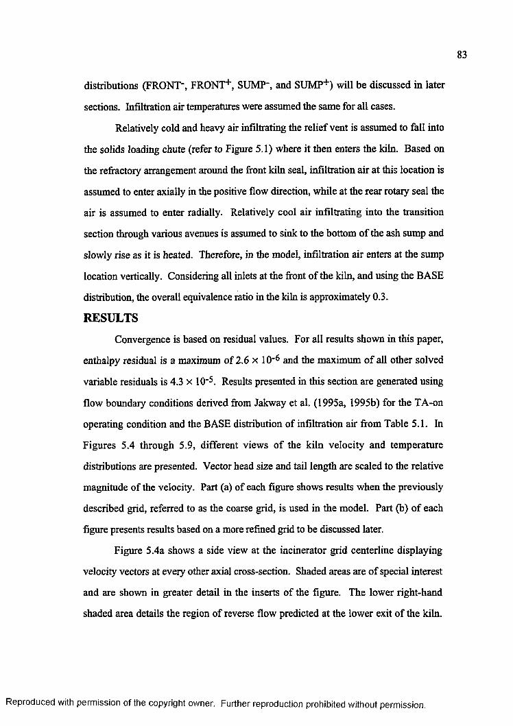
83
distributions (FRONT", FRONT+, SUMP", and SUMP+) will be discussed in later
sections. Infiltration air temperatures were assumed the same for all cases.
Relatively cold and heavy air infiltrating the relief vent is assumed to fall into
the solids loading chute (refer to Figure 5.1) where it then enters the kiln. Based on
the refractory arrangement around the front kiln seal, infiltration air at this location is
assumed to enter axially in the positive flow direction, while at the rear rotary seal the
air is assumed to enter radially. Relatively cool air infiltrating into the transition
section through various avenues is assumed to sink to the bottom of the ash sump and
slowly rise as it is heated. Therefore, in the model, infiltration air enters at the sump
location vertically. Considering all inlets at the front of the kiln, and using the BASE
distribution, the overall equivalence ratio in the kiln is approximately 0.3.
RESULTS
Convergence is based on residual values. For all results shown in this paper,
enthalpy residual is a maximum of 2 .6 x 1 0 '6 and the maximum of all other solved
variable residuals is 4.3 x 10⁻⁵. Results presented in this section are generated using
flow boundary conditions derived from Jakway et al. (1995a, 1995b) for the TA-on
operating condition and the BASE distribution of infiltration air from Table 5.1. In
Figures 5.4 through 5.9, different views of the kiln velocity and temperature
distributions are presented. Vector head size and tail length are scaled to the relative
magnitude of the velocity. Part (a) of each figure shows results when the previously
described grid, referred to as the coarse grid, is used in the model. Part (b) of each
figure presents results based on a more refined grid to be discussed later.
Figure 5.4a shows a side view at the incinerator grid centerline displaying
velocity vectors at every other axial cross-section. Shaded areas are o f special interest
and are shown in greater detail in the inserts of the figure. The lower right-hand
shaded area details the region of reverse flow predicted at the lower exit of the kiln.
Reproduced with permission of the copyright owner. Further reproduction prohibited without permission.
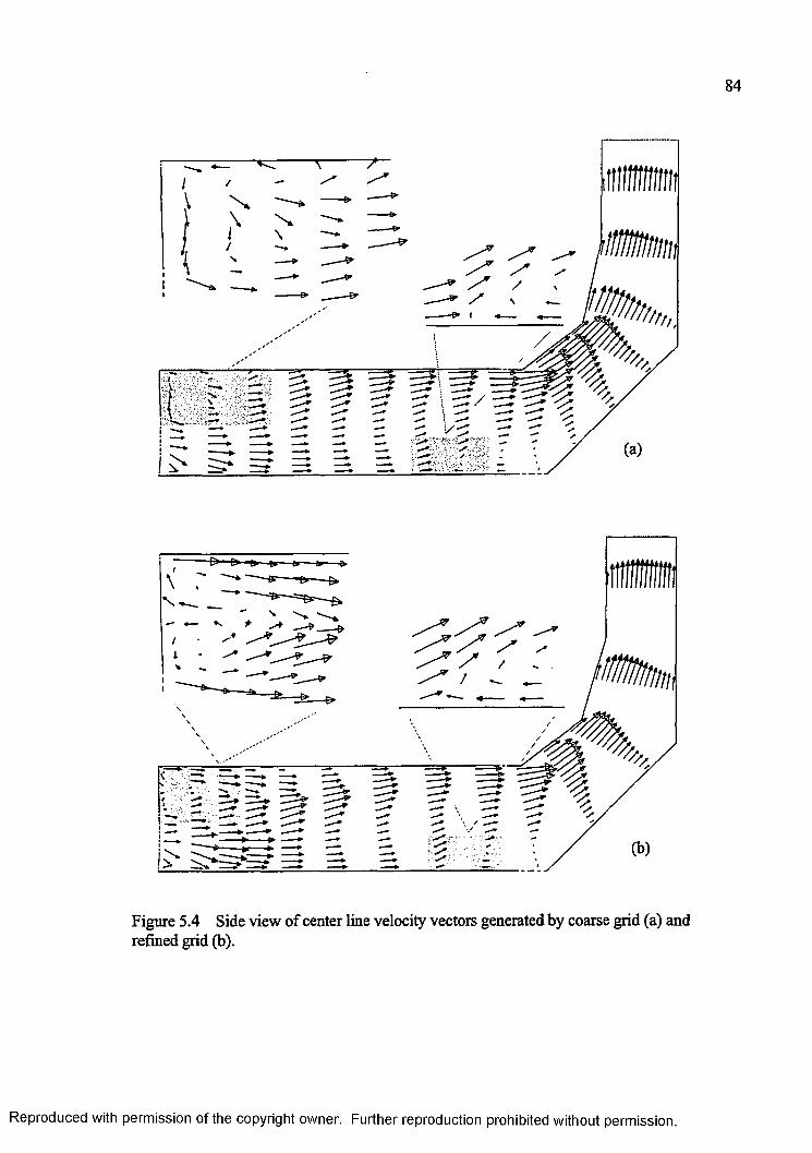
84
X
Figure 5.4 Side view of center line velocity vectors generated by coarse grid (a) and refined grid (b).
Reproduced with permission of the copyright owner. Further reproduction prohibited without permission.
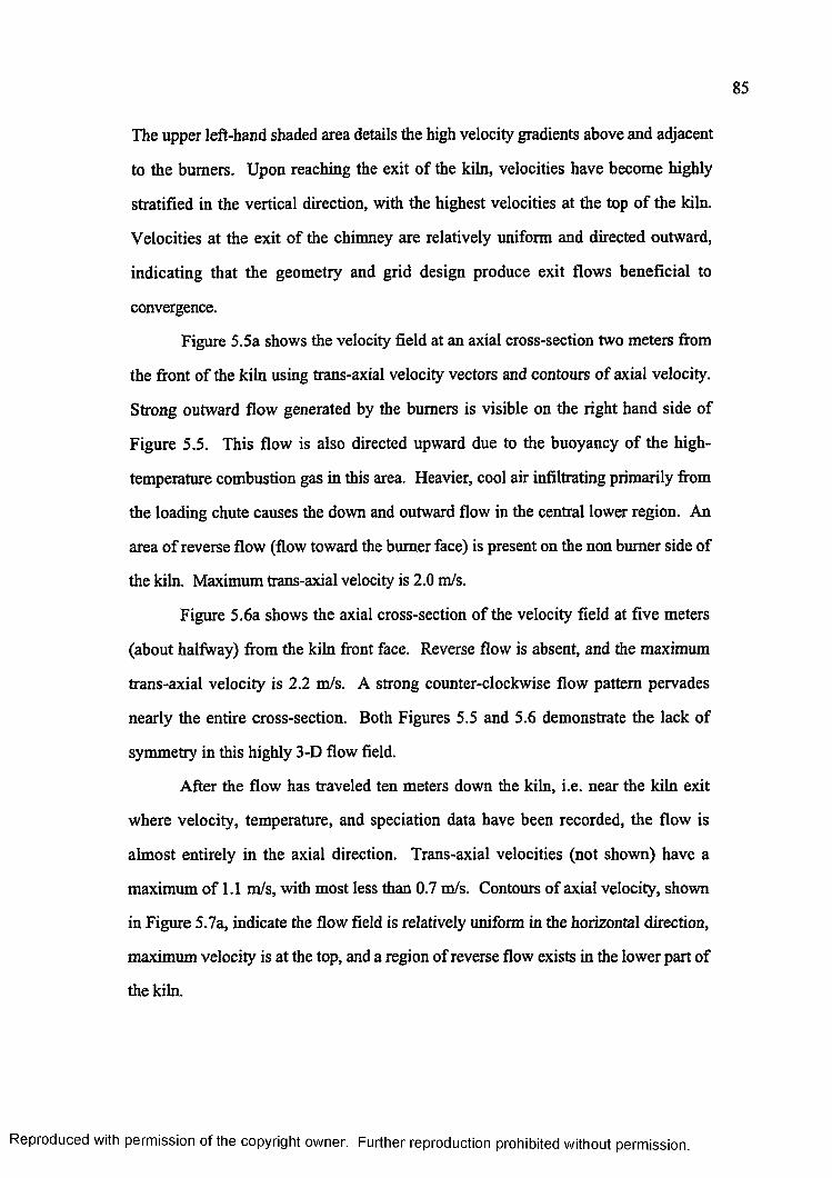
85
The upper left-hand shaded area details the high velocity gradients above and adjacent
to the burners. Upon reaching the exit o f the kiln, velocities have become highly
stratified in the vertical direction, with the highest velocities at the top of the kiln.
Velocities at the exit of the chimney are relatively uniform and directed outward,
indicating that the geometry and grid design produce exit flows beneficial to
convergence.
Figure 5.5a shows the velocity field at an axial cross-section two meters from
the front of the kiln using trans-axial velocity vectors and contours o f axial velocity.
Strong outward flow generated by the burners is visible on the right hand side of
Figure 5.5. This flow is also directed upward due to the buoyancy of the high-
temperature combustion gas in this area. Heavier, cool air infiltrating primarily from
the loading chute causes the down and outward flow in the central lower region. An
area o f reverse flow (flow toward the burner face) is present on the non burner side of
the kiln. Maximum trans-axial velocity is 2.0 m/s.
Figure 5.6a shows the axial cross-section of the velocity field at five meters
(about halfway) from the kiln front face. Reverse flow is absent, and the maximum
trans-axial velocity is 2.2 m/s. A strong counter-clockwise flow pattern pervades
nearly the entire cross-section. Both Figures 5.5 and 5.6 demonstrate the lack of
symmetry in this highly 3-D flow field.
After the flow has traveled ten meters down the kiln, i.e. near the kiln exit
where velocity, temperature, and speciation data have been recorded, the flow is
almost entirely in the axial direction. Trans-axial velocities (not shown) have a
maximum of 1.1 m/s, with most less than 0.7 m/s. Contours of axial velocity, shown
in Figure 5.7a, indicate the flow field is relatively uniform in the horizontal direction,
maximum velocity is at the top, and a region of reverse flow exists in the lower part of
the kiln.
Reproduced with permission of the copyright owner. Further reproduction prohibited without permission.
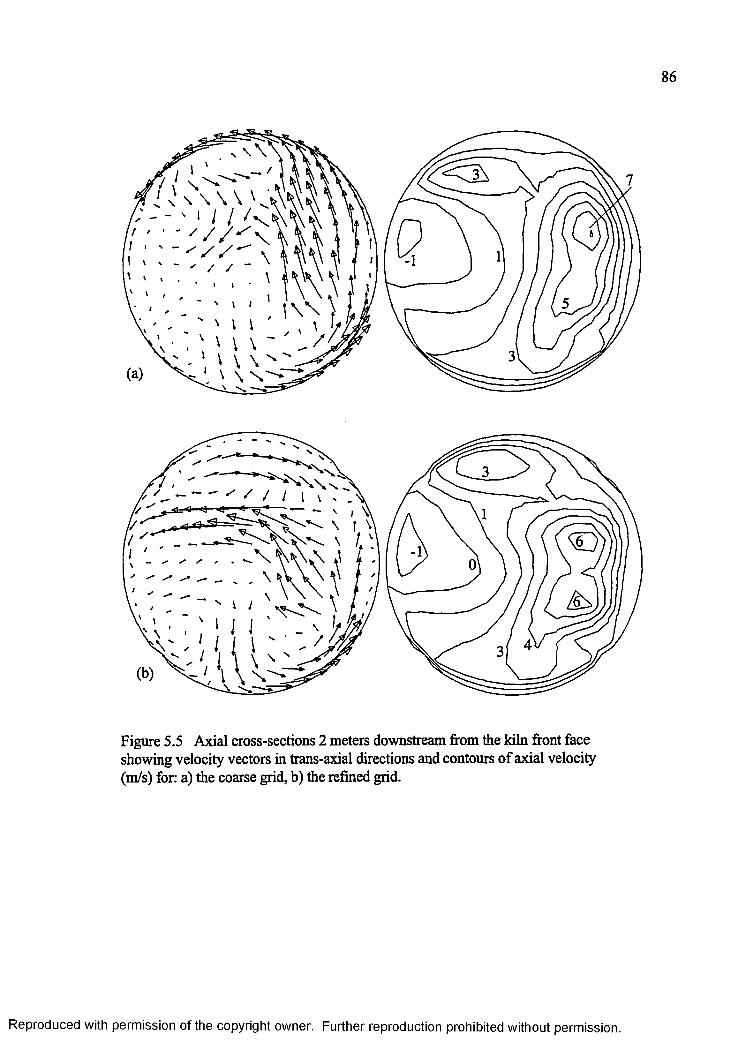
86
' \ \ I V ‘ \
✓/
/
Figure 5.5 Axial cross-sections 2 meters downstream from the kiln front face showing velocity vectors in trans-axial directions and contours of axial velocity (m/s) for: a) the coarse grid, b) the refined grid.
Reproduced with permission of the copyright owner. Further reproduction prohibited without permission.
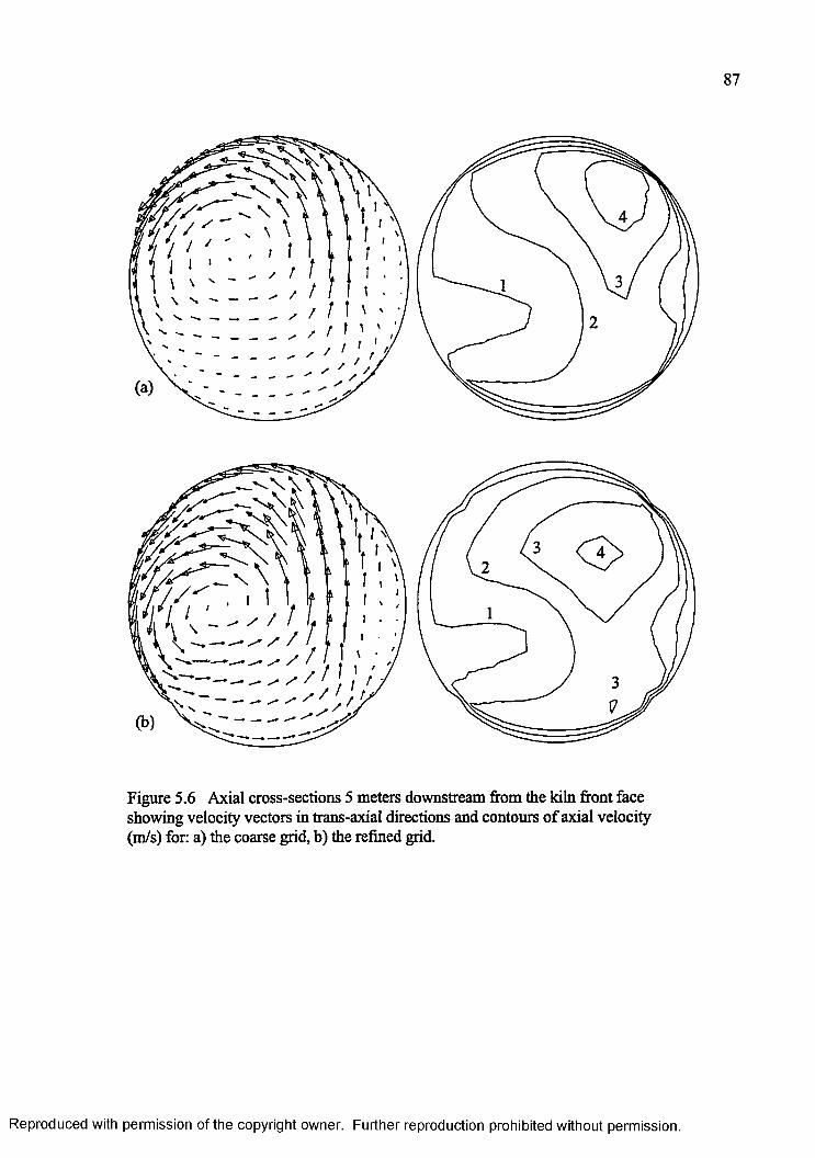
87
Figure 5.6 Axial cross-sections 5 meters downstream from the kiln front face showing velocity vectors in trans-axial directions and contours o f axial velocity (m/s) for: a) the coarse grid, b) the refined grid.
Reproduced with permission of the copyright owner. Further reproduction prohibited without permission.
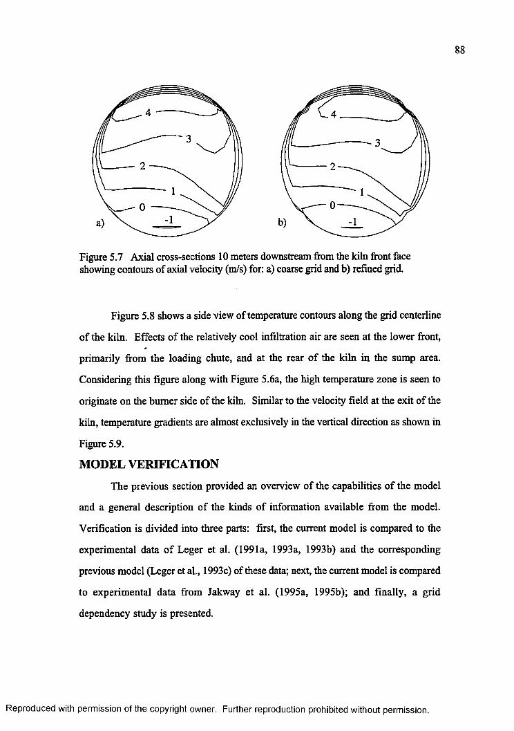
88
Figure 5.7 Axial cross-sections 10 meters downstream from the kiln front face showing contours of axial velocity (m/s) for: a) coarse grid and b) refined grid.
Figure 5.8 shows a side view of temperature contours along the grid centerline
o f the kiln. Effects o f the relatively cool infiltration air are seen at the lower front,
primarily from the loading chute, and at the rear o f the kiln in the sump area.
Considering this figure along with Figure 5.6a, the high temperature zone is seen to
originate on the burner side of the kiln. Similar to the velocity field at the exit of the
kiln, temperature gradients are almost exclusively in the vertical direction as shown in
Figure 5.9.
MODEL VERIFICATION
The previous section provided an overview of the capabilities of the model
and a general description o f the kinds of information available from the model.
Verification is divided into three parts: first, the current model is compared to the
experimental data o f Leger et al. (1991a, 1993a, 1993b) and the corresponding
previous model (Leger et al., 1993c) of these data; next, the current model is compared
to experimental data from Jakway et al. (1995a, 1995b); and finally, a grid
dependency study is presented.
Reproduced with permission of the copyright owner. Further reproduction prohibited without permission.
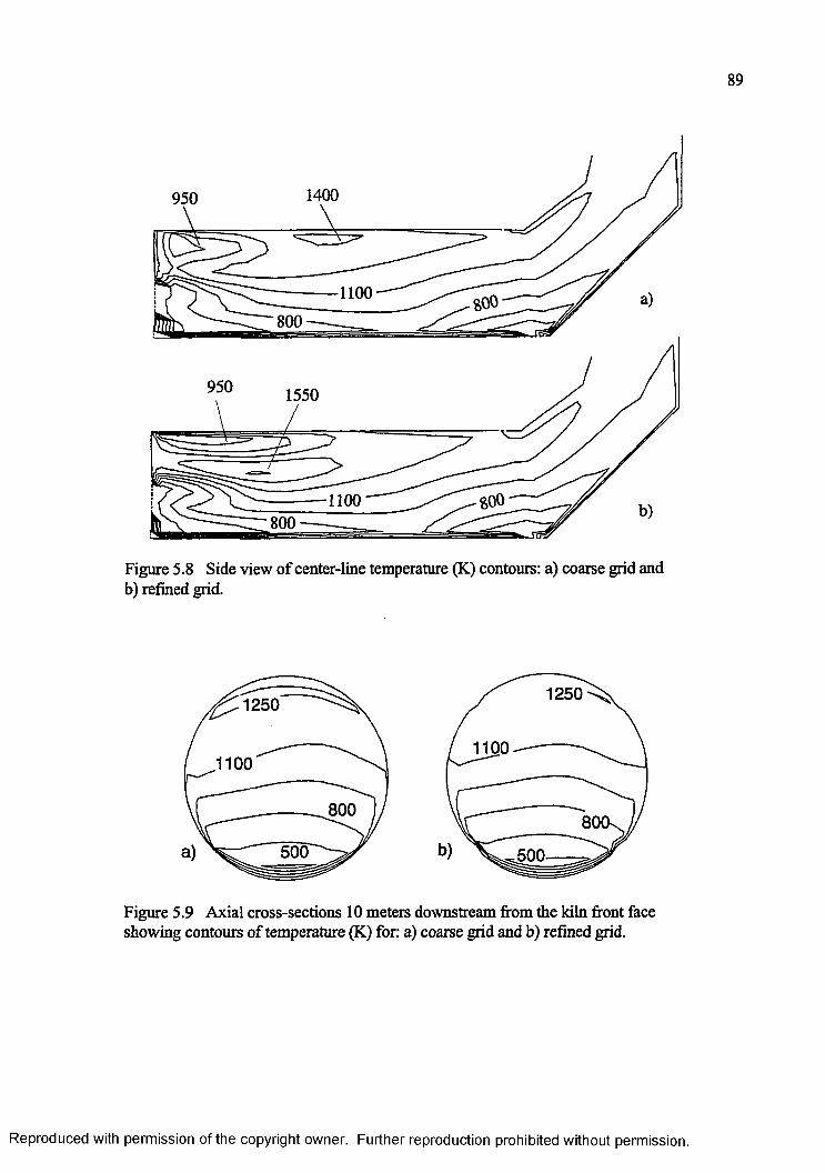
89
1400950
1100800
950 1550
8001100800
Figure 5.8 Side view of center-line temperature (K) contours: a) coarse grid and b) refined grid.
1250
1100
500
.1100
800
500
Figure 5.9 Axial cross-sections 10 meters downstream from the kiln front face showing contours of temperature (K) for: a) coarse grid and b) refined grid.
Reproduced with permission of the copyright owner. Further reproduction prohibited without permission.
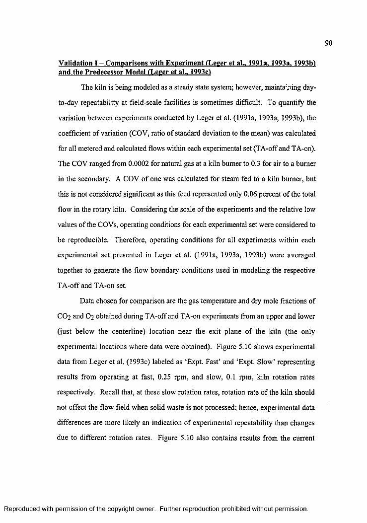
90
Validation I - Comparisons with Experiment (Leger et al.. 1991a. 1993a. 1993bl and the Predecessor Model (Leger et al.. 1993c1
The kiln is being modeled as a steady state system; however, maintaining day-
to-day repeatability at field-scale facilities is sometimes difficult. To quantify the
variation between experiments conducted by Leger et al. (1991a, 1993a, 1993b), the
coefficient of variation (COV, ratio of standard deviation to the mean) was calculated
for all metered and calculated flows within each experimental set (TA-off and TA-on).
The COV ranged from 0.0002 for natural gas at a kiln burner to 0.3 for air to a burner
in the secondary. A COV of one was calculated for steam fed to a kiln burner, but
this is not considered significant as this feed represented only 0.06 percent of the total
flow in the rotary kiln. Considering the scale of the experiments and the relative low
values of the COVs, operating conditions for each experimental set were considered to
be reproducible. Therefore, operating conditions for all experiments within each
experimental set presented in Leger et al. (1991a, 1993a, 1993b) were averaged
together to generate the flow boundary conditions used in modeling the respective
TA-off and TA-on set.
Data chosen for comparison are the gas temperature and dry mole fractions of
CO2 and O2 obtained during TA-off and TA-on experiments from an upper and lower
(just below the centerline) location near the exit plane of the kiln (the only
experimental locations where data were obtained). Figure 5.10 shows experimental
data from Leger et al. (1993c) labeled as ‘Expt. Fast’ and ‘Expt. Slow’ representing
results from operating at fast, 0.25 rpm, and slow, 0.1 rpm, kiln rotation rates
respectively. Recall that, at these slow rotation rates, rotation rate of the kiln should
not effect the flow field when solid waste is not processed; hence, experimental data
differences are more likely an indication of experimental repeatability than changes
due to different rotation rates. Figure 5.10 also contains results from the current
Reproduced with permission of the copyright owner. Further reproduction prohibited without permission.
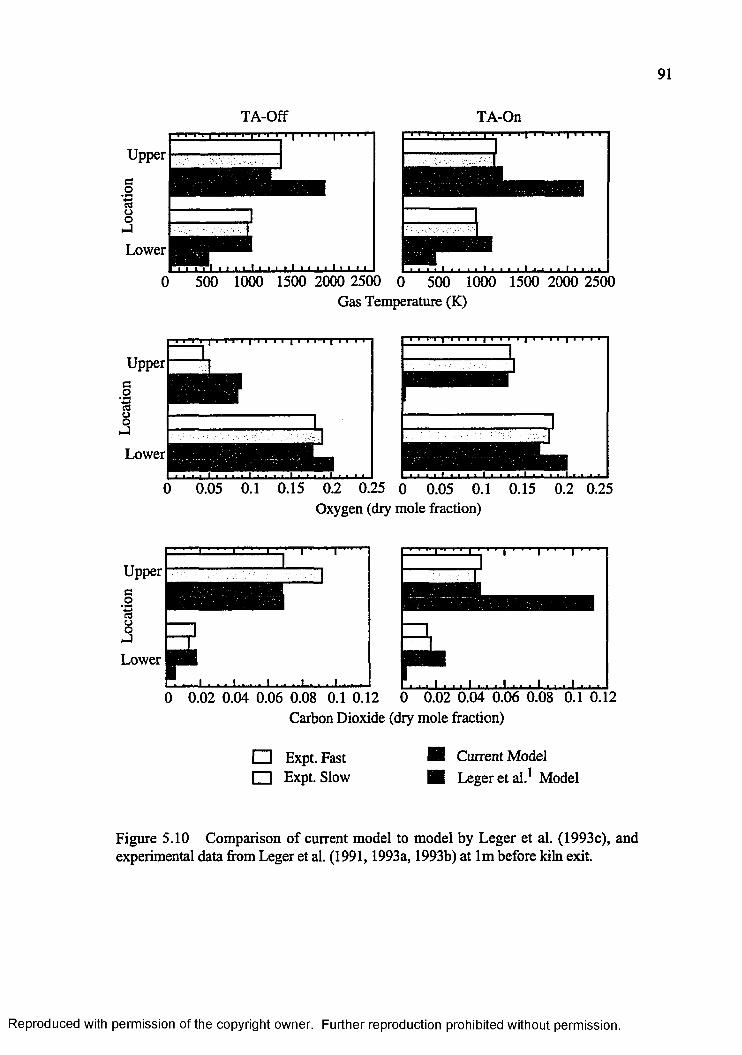
0 500 1000 1500 2000 2500 0 500 1000 1500 2000 2500Gas Temperature (K)
Upperco13oo
Lower
0 0.05 0.1 0.15 0.2 0.25 0 0.05 0.1 0.15 0.2 0.25Oxygen (dry mole fraction)
Upperao**-»COuO
hJ
Lower
0 0.02 0.04 0.06 0.08 0.1 0.12 0 0.02 0.04 0.06 0.08 0.1 0.Carbon Dioxide (dry mole fraction)
EU Expt. Fast I I Expt. Slow
Current Model Leger e ta l . 1 Model
Figure 5.10 Comparison of current model to model by Leger et al. (1993c), and experimental data from Leger et al. (1991,1993a, 1993b) at lm before kiln exit.
Reproduced with permission of the copyright owner. Further reproduction prohibited without permission.
92
model and Leger’s model. The remainder of this discussion focuses on a comparison
between the two models, and how each compares to the experimental data.
For TA-off operation, model improvement is most marked in the prediction of
temperature. Compared to experimental data, Leger’s model over predicted
temperature at the upper location by 550 K, and under predicted temperature at the
lower location by 500 K. The current model improves these predictions greatly with
the upper temperature under predicted by only 110 K and the lower temperature over
predicted by only 30 K. Both models predict the O2 dry mole fraction to be nearly
twice as high as that measured in the upper kiln; in the lower kiln, both predictions
nearly match the experimental data. Both models predict CO2 concentrations equally
well at the upper location; however, at the lower location, Leger et al. (1993c) under
predict the value by a factor of three, and the current model over predicts
experimental measurements by only 2 0 percent.
Even larger improvements are noted during TA-on operation. Leger’s model
over predicted the upper location temperature by 1,090 K (nearly twice the measured
value), while it under predicted the lower location temperature by 500 K (nearly half
the measured value). In comparison, the current model over predicts temperatures by
only 90 K and 180 K at the upper and lower kiln exit locations respectively. Leger’s
model under predicted the dry O2 mole fraction in the upper kiln by nearly two
orders of magnitude; similarly, the dry CO2 mole fraction was over predicted in the
upper kiln by nearly a factor of 3. The current model closely matches experimental
data for both O2 and CO2 . In the lower kiln, both the current model and Leger’s
model reasonably match the measured O2 mole fraction; however, Leger’s model
under predicted CO2 by nearly an order o f magnitude, whereas the value predicted by
the current model is only 1.5 times the observed value.
Reproduced with permission of the copyright owner. Further reproduction prohibited without permission.
Improvement over Leger’s model in temperature prediction is attributed to the
combination of treating the wall as adiabatic rather than isothermal and including
radiation with participating CO2 , water vapor, and soot. Better agreements with
experiment in species concentrations are most likely due to an increase in vertical
mixing induced by a less-stratified temperature distribution in the current model.
Predictions by the current model in all cases, except the upper region TA-off O2
prediction, are within the repeatability limits of the experiments. Whereas Leger’s
model was capable of only qualitative predictions, the current model quantitatively
predicts accurate results at the kiln exit when no waste is processed.
Validation Test II - Comparisons with experiment Jakwav et al. 11995a. 1995bl
Although Jakway et al. (1995a, 1995b) do not report gas speciation, a
mapping o f the velocity and temperature distribution near the same exit location of
the kiln is presented. Data were obtained at 12 locations across an upper quadrant
axial cross-section of the kiln, about one meter before the kiln exit. For these
experiments, turbulence air was the only parameter varied. Maximum metered and
calculated flow COV for Jakway et al. (1995a, 1995b) over a time of 2 horns was 0.3,
again for steam to one of the afterburner burners. Non steam COV’s ranged from
0.0006 for natural gas to the lower kiln burner to 0 .1 for the total stack dry air flow
rate.
Model results are compared to experimental data in Figures 5.11, TA-off, and
5.12, TA-on. In both Figures, solid lines represent predicted velocity and
temperature distributions; experimental velocity and temperature data are graphed as
open circles. All data are plotted against vertical distance from the center-line of the
kiln. Multiple data points for an elevation indicate values from different horizontal
locations. The lack of horizontal gradients measured at this location supports the
Reproduced with permission of the copyright owner. Further reproduction prohibited without permission.
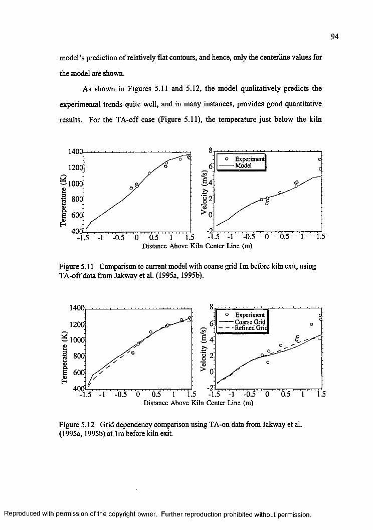
9 4
model’s prediction of relatively flat contours, and hence, only the centerline values for
the model are shown.
As shown in Figures 5.11 and 5.12, the model qualitatively predicts the
experimental trends quite well, and in many instances, provides good quantitative
results. For the TA-off case (Figure 5.11), the temperature just below the kiln
1400ExperimentModel
o-1200
1000
800
£ 600
4001.5
Distance Above Kiln Center Line (m)
Figure 5.11 Comparison to current model with coarse grid lm before kiln exit, using TA-off data from Jakway et al. (1995a, 1995b).
1400° Experiment — Coarse Grid - • Refined Grid1200
1000
800'
£ 600
4001.5
Distance Above Kiln Center Line (m)
Figure 5.12 Grid dependency comparison using TA-on data from Jakway et al. (1995a, 1995b) at lm before kiln exit.
Reproduced with permission of the copyright owner. Further reproduction prohibited without permission.
95
centerline is under predicted by 5 percent, and over predicted by only 3 percent near
the top of the kiln. For the TA-on case (Figure 5.12), the temperature is over
predicted near the kiln centerline by about 8 percent. Model-predicted velocities
match well for the TA-off case (Figure 5.11) except at the uppermost location where
the error is 24 percent. Most of the predicted velocities tend to be slightly lower than
experimental values when the turbulence air is activated (Figure 5.12) reaching a
maximum difference of 31 percent, again at the very top of the kiln. The discrepancy
between predicted and experimental data at the upper locations is, as yet,
unexplained.
Validation Test III - Grid Dependency Study
To examine the effect of the grid on the numerical results, the same general
geometry was fitted to a grid of 12,427 control volumes, a 27 percent increase over
the baseline course grid used in all model results presented thus far. The only change
in the geometry was to increase necking of the chimney, thereby further reducing the
cross-sectional area by 10 percent and improving the solution domain exit flow. The
new control volumes are added as 9 extra axial cross-sections. Perhaps more
important than the addition of control volumes is their placement. While the cross-
sections of the baseline coarse grid are uniformly spaced in the axial direction, the
refined grid makes use of non-uniform spacing to concentrate the axial grid cross-
sections at the front of the kiln where spatial gradients in the flow variables are the
greatest. This dense grid is gradually expanded to a less dense spacing at the kiln exit
as shown in Figure 5.2b. The grid used on the axial cross-sections is unchanged;
however, to achieve final convergence, one control volume in each of the four
“comers” (highlighted in Figure 5.3a) is changed from an interior volume to a volume
in the kiln wall. This is necessary because of the high degree o f skew (departure from
orthogonal intersections) present in these control volumes. Resulting reduction in the
Reproduced with permission of the copyright owner. Further reproduction prohibited without permission.
cross-sectional area of the internal kiln is only 0.026 m2 or 0.33 percent; therefore,
effects on the flow field are assumed negligible.
Comparison between the coarse and fine grids of Figure 5.2 is performed using
TA-on flow boundary conditions derived from the experimental data of Jakway et al.
(1995a, 1995b). Part (b) of Figures 5.4 through 5.9 contain data generated by the
model using the refined grid which can be compared to Parts (a) of each figure,
representing the baseline coarse grid results. Consider first Figure 5.4, where a side
view of the velocity vectors are shown. For clarity, vectors are shown at every other
axial cross-section in Figure 5.4(a) and every third axial cross-section in Figure 5.4(b).
Again, the highlighted regions show areas where more complex flow patterns develop.
The primary differences between the velocities generated by the two grids appears in
the upper highlighted zone near the front of the kiln. The refined grid produces a flow
structure resembling a pair o f counter-rotating eddies at the front wall of the kiln,
which is not present in the coarse grid results. Otherwise this figure indicates that the
two grids produce very similar velocity fields.
Cross-sectional views o f the developing velocity fields are compared in
Figures 5.5, 5.6, and 5.7, again comparing parts (a) for the baseline coarse grid with
parts (b) for the fine grid. At 2 m from the front face, axial velocity contours are very
similar for both grids as are the trans-axial velocities in lower half of Figure 5.5.
However, major differences in trans-axial velocities are visible in the upper region. A
primary difference is that, just above the centerline, the refined grid generates a strong
right-to-left flow not present in the coarse grid solution. Maximum trans-axial
velocity is 2.3 m/s for the refined grid. Interestingly, despite the major trans-axial
velocity differences noted above near the front of the kiln, Figure 5.6 indicates that at
5 m from the kiln front face the flows generated by both grids are very similar.
Maximum trans-axial velocity is 1.3 m/s for the refined grid. At 10 m from the kiln
Reproduced with permission of the copyright owner. Further reproduction prohibited without permission.
front face (Figure 5.7), both grids generate nearly identical velocity fields with the
refined grid predicting a maximum trans-axial velocity of only 0 .6 m/s.
Temperature contours can be compared by referring to Figure 5.8. Similar to
the velocities, the greatest difference in temperature fields occurs in the upper part of
the front half o f the kiln. The zone inside the 1,550 K contour o f the fine grid
solution corresponds to a region in the flow where the hot burner gases are
transported across from the burner side of the kiln (Figure 5.5). Overall maximum gas
temperature is 120 K greater in the fine grid solution. However, similar to the
velocity predictions, Figures 5.8 and 5.9 show that nearly identical temperature fields
are generated for each grid by the time the flow reaches the kiln exit.
Figure 5.12 compares velocity and temperature data to model results using
both the coarse and fine grids. As previously noted, differences generated in the front
portion of the kiln are damped by the time the flow reaches the kiln exit, with both
grids producing nearly identical velocity and temperature profiles at the exit of the
kiln. Temperature prediction just below the kiln centerline is improved from 8
percent high to a value of 6 percent high. Velocity prediction is somewhat improved
across the upper half o f the kiln cross-section except at the very top where
predictions are up to 40 percent low. The root mean square (r.m.s.) error, the
standard error of the estimate, also compares relative fits of the experimental data to
estimates from the model. The r.m.s. errors for temperature are 35 K and 30 K while
velocity r.m.s. errors are 1.26 m/s and 1.35 m/s for the coarse and refined grids
respectively, again indicating the closeness of the results generated by both grids near
the kiln exit.
The different results generated with the refined grid show that the baseline
coarse grid solution is indeed grid dependent. This is especially noticeable in the
upper front region of the kiln where the refined grid predicts several new eddies. The
Reproduced with permission of the copyright owner. Further reproduction prohibited without permission.
appearance of new eddies (Figure 5.4) is not unexpected; as grids are refined, more
detail is possible and new small eddies can form, especially in areas with large shear
such as near the burners. However, Figure 5.5 shows that changes in the flow field
generated by the refined grid are not confined to the generation of several small eddies,
and a 120 K increase in maximum temperature within the kiln is significant. It is,
however, noteworthy that even though there are significant changes produced by the
refined grid, these changes are starting to damp-out by the middle of the kiln (Figure
5.6) with both grids producing nearly identical flow fields by the exit of the kiln as
evidenced by Figures 5.7, 5.9, and 5.12. The detail provided by a refined grid will no
doubt become more important with the eventual addition of waste processing and a
more complete set o f chemical reactions, especially if the influence o f kinetics is
included. These model refinements will have to be included in next-generation models.
At this time, and for the limited experimental data available, the use of either grid
produces reasonable qualitative and quantitative results at the kiln exit.
Attempts were made to further refine the grid; however, these were
unsuccessful. Complications were partially attributed to the highly non-orthogonal
grid skew at ‘comers’ making convergence extremely difficult. This skew increases
dramatically as the number of control volumes defining circular cross-sections
increase. Additional difficulties were attributed to the relatively low inlet flow rates
involved in this work, making the influence of the boundary conditions quite weak on
internal control volumes far downstream from the front face o f the kiln. As control
volumes are added, the internal control volumes become even further removed from
their influence, making convergence more difficult. Changing to a higher order
differencing scheme caused rapid divergence as did attempts at using the re-normalized
group turbulence model and solving thermal and velocity fields separately (Fluent,
1993). Radiation did not seem to interfere with convergence. Working with multigrid,
Reproduced with permission of the copyright owner. Further reproduction prohibited without permission.
sweep, block correction, and underrelaxation parameters was required to achieve
convergence o f the refined grid used in this work; however, an appropriate
combination of these parameters could not be developed to prevent divergence when
more nodes were added. Future efforts may involve relaxing geometry restrictions at
the front face of the kiln to reduce the grid skew at this location.
PARAMETRIC AND SENSITIVITY STUDIES
The effects of various unmetered infiltration air distributions are discussed in
the first part of this section. Following this, sensitivity to each of the three main
improvements to the current model (addition of radiation, improved boundary
conditions, and addition of soot) are discussed. All studies are conducted using the
baseline coarse grid with flow boundary conditions for the TA-on case from Jakway
etal. (1995a, 1995b).
Distribution of Unmetered Infiltration Air
Figures 5.11 and 5.12 show that while the model matched velocity data
reasonably well, improvement is still possible. The distribution of unmetered
infiltration air entering the incinerator represents the single largest unknown; therefore,
it was expected that reasonable changes to this distribution might improve the
velocity prediction. The TA-on operating condition was chosen for this parametric
study because it produced the greatest error in velocity prediction. The following
parametric studies were undertaken to quantify the importance of the unmetered air
distribution.
For the first parametric study, the total amount of infiltration air assigned to
the front o f the rotary kiln was varied. Infiltration at the other inlets was
redistributed so that the overall amount of infiltration air into the incinerator was held
constant at the experimentally determined value. The amount of infiltration air
allowed at the front of the kiln was bracketed around the BASE distribution (58
Reproduced with permission of the copyright owner. Further reproduction prohibited without permission.
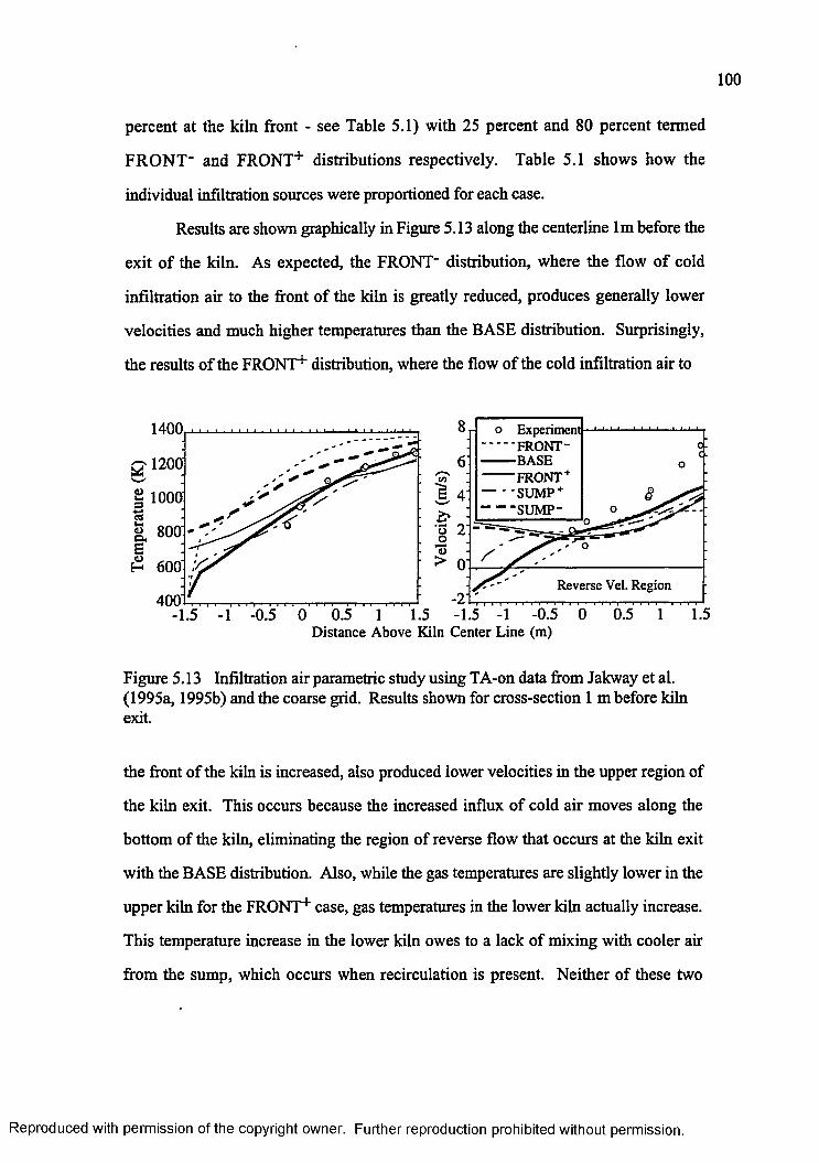
100
percent at the kiln front - see Table 5.1) with 25 percent and 80 percent termed
FRONT" and FRONT+ distributions respectively. Table 5.1 shows how the
individual infiltration sources were proportioned for each case.
Results are shown graphically in Figure 5.13 along the centerline lm before the
exit of the kiln. As expected, the FRONT" distribution, where the flow o f cold
infiltration air to the front of the kiln is greatly reduced, produces generally lower
velocities and much higher temperatures than the BASE distribution. Surprisingly,
the results o f the FRONT1' distribution, where the flow of the cold infiltration air to
1400
1200
| 1000
S. 800EH 600
o Experiment FRONT- BASE FRONT +
SUMP + SUMP-
o.c.
0 0.5 1 1.5 -1.5 -1 -0.5Distance Above Kiln Center Line (m)
Reverse Vel. Region
Figure 5.13 Infiltration air parametric study using TA-on data from Jakway et al. (1995a, 1995b) and the coarse grid. Results shown for cross-section 1 m before kiln exit.
the front of the kiln is increased, also produced lower velocities in the upper region of
the kiln exit. This occurs because the increased influx of cold air moves along the
bottom of the kiln, eliminating the region of reverse flow that occurs at the kiln exit
with the BASE distribution. Also, while the gas temperatures are slightly lower in the
upper kiln for the FRONT1" case, gas temperatures in the lower kiln actually increase.
This temperature increase in the lower kiln owes to a lack of mixing with cooler air
from the sump, which occurs when recirculation is present. Neither of these two
Reproduced with permission of the copyright owner. Further reproduction prohibited without permission.
distributions produce results that match the velocity data better than the BASE
distribution.
Several other distributions were studied, but are not shown. Of these, only
one produced even marginal improvement in the velocity prediction. In the previous
distributions (BASE, FRONT", FRONT4-), infiltration through the front and rear
seals is assumed to occur uniformly around the periphery of the seals. In one study,
50 percent of the infiltration air assigned to the front kiln seal was allowed to enter the
kiln through the bottom of the front seal, with 20 percent on the sides and the
remaining 10 percent entering in the upper region of the seal. Such a distribution
might occur if the kiln was misaligned. This distribution produced an increase in
velocities on the order of 5 percent near the top o f the kiln exit region. Still, overall
model velocities were up to 30 percent below measured values and temperature
predictions worsened. Increasing the total amount of front seal infiltration air by 10
percent, at the expense of the loading chute infiltration air, and maintaining the
unbalanced front seal distribution noted above, produced only negligible changes.
Therefore, it is concluded that changing the distribution of infiltration air at the kiln
front face has little effect on improving the match with experimental data at the exit of
the kiln.
However, varying the infiltration air allowed at the kiln front face led to an
important observation: increasing the amount of infiltration air entering the front of
the kiln by just over 20 percent of the total air infiltrating the kiln completely
eliminated the region of reverse flow at the kiln exit. Early experiments probing the
exit region of this rotary kiln incinerator showed that the lower kiln exit area contained
relatively low temperature gases very close in composition to ambient air (Cundy et
al., 1989a). This was unexpected and produced speculation that this lower area was
relatively uninvolved in the combustion and waste destruction process, at least for the
Reproduced with permission of the copyright owner. Further reproduction prohibited without permission.
experiments conducted. That this area might actually be a recirculation region was
first suggested in the numerical modeling work of Leger et al. (1993c). Recirculation
zones are important in incineration because they reduce the effective volume of the
incinerator, thereby decreasing the residence time of most gases. Low temperature
recirculation zones are especially undesirable as little to no destruction of waste takes
place in these zones.
Given these observations, a second parametric study was conducted with the
objective to examine the effect that infiltration air has on the kiln exit recirculation
region. Two new distributions were tested, SUMP" and SUMP+ shown in Table 5.1.
The SUMP" distribution has the same front distribution as the BASE case, but the
sump inlet is reduced to zero flow with its flow entering downstream of the sump.
Figure 5.13 shows that the region of reverse flow at the exit of the kiln is eliminated in
this case, similar to the result using the FRONT+ distribution, but without increased
flow from the front of the kiln. To further examine the importance of the sump inlet
flow to the exit recirculation region, the SUMP+ distribution was developed. This
has nearly the same distribution of air at the front of the kiln as the FRONT1" case,
but the flow to the sump area is increased. This re-establishes the recirculation region
originally eliminated by the FRONT1" distribution. Changes to the other infiltration
inlets o f similar magnitude had only minor effects on the flow field at the exit o f the
kiln. None of the infiltration distributions generated velocity predictions at the exit of
the kiln that were better than the original BASE distribution.
In summary, the BASE distribution of infiltration air produces results which
match the experimentally measured velocity and temperature data most accurately.
The parametric studies performed show that reverse flow at the exit of the kiln may
be affected by controlling the amounts of infiltration air leaking into the front of the
kiln and at the sump. If reverse flow is predicted for one set of inlet conditions, for
Reproduced with permission of the copyright owner. Further reproduction prohibited without permission.
example the BASE case, then reverse flow might be eliminated by either increasing the
flow of cold air to the front of the kiln, as evidenced by case FRONT-1", or by
lowering the infiltration in the transition and kiln exit areas, as in the SUMP' case.
This study also underscores the need to record velocities across a complete cross
section of the kiln in order to improve validation of numerical models. The extra data
would allow the total amount of air infiltrating at the front of the kiln to be quantified;
questions about the existence and location of reverse flow regions would also be
clarified.
Effects of Radiation. Soot, and Adiabatic Walls
As discussed previously, radiative heat transfer, including the effects of soot,
has been added to the current model, and an adiabatic wall boundary condition
replaces the isothermal wall of Leger’s model. Additional differences between the two
models, termed base differences for this discussion, include the grid, use of power law
and SIMPLIC in the solution method, a more accurate geometry, corrected heat
capacities, and slight changes in the infiltration proportioning and temperatures. The
sensitivity of the model to these changes is determined in a series of sub-studies in
which the changes are executed in succession.
Initially, the effect of the base differences is examined. Leger’s model, with its
isothermal walls, produced a maximum gas temperature of 2,350 K, which is above
the adiabatic flame temperature of 2,220 K for a stoichmetric mixture (Glassman,
1987). However, the current model, including the base differences noted above but
without radiation and using the same 800 K isothermal wall boundary condition as in
Leger’s model, predicts a more realistic maximum gas temperature of 2,190 K.
Next, the individual effect of the radiation model is characterized. This is done
without incorporation of soot in order to determine the sensitivity of the current
model to the radiation model alone. Kiln interior walls were again assumed isothermal
Reproduced with permission of the copyright owner. Further reproduction prohibited without permission.
at 800 K. When the radiation model is enabled under these conditions, along with the
base differences, the maximum gas temperature inside the rotary kiln is reduced from
2,190 K (as noted above) to 1,720 K. This overall reduction in temperature is
considered good because it is thought to represent the fuel rich, soot laden flame
temperature better, even though flame temperature measurements were not conducted.
This result is also not unexpected since, at these high temperatures, radiation should
be of first-order importance.
The effects of the isothermal kiln wall assumption are determined by changing
the kiln wall boundary condition from isothermal to adiabatic. In this sub-study the
base differences are included, and the radiation model is enabled, although soot is not
yet included. Changing to the adiabatic wall boundary condition increases the wall
temperatures throughout. The maximum wall temperature increases from 800 K
(isothermal condition) to 1,430 K at about 2 m from the front face of the kiln. Even
near the exit of the kiln, wall temperatures are predicted to be as high as 1,000 K.
This indicates not only that a single temperature cannot characterize the wall, but also
that the temperature chosen for Leger’s model, 800 K, was probably too low. The
change to adiabatic walls with the corresponding increase in wall temperatures
throughout is accompanied by an increase in the maximum gas temperature of about
120 K.
Finally, the heat transfer effects of soot are resolved. As in the previous case,
the adiabatic wall boundary condition is used and the radiation model enabled, along
with all the base differences noted previously. With the addition of soot effects in the
radiation model, the maximum gas temperature, which occurs in the combustion zone,
decreases by 130 K to 1,730 K. This is reasonable as soot tends to increase radiative
heat transfer, thereby lowering nearby gas temperatures. Correspondingly, the wall
temperature immediately adjacent to this maximum gas temperature zone increases to
Reproduced with permission of the copyright owner. Further reproduction prohibited without permission.
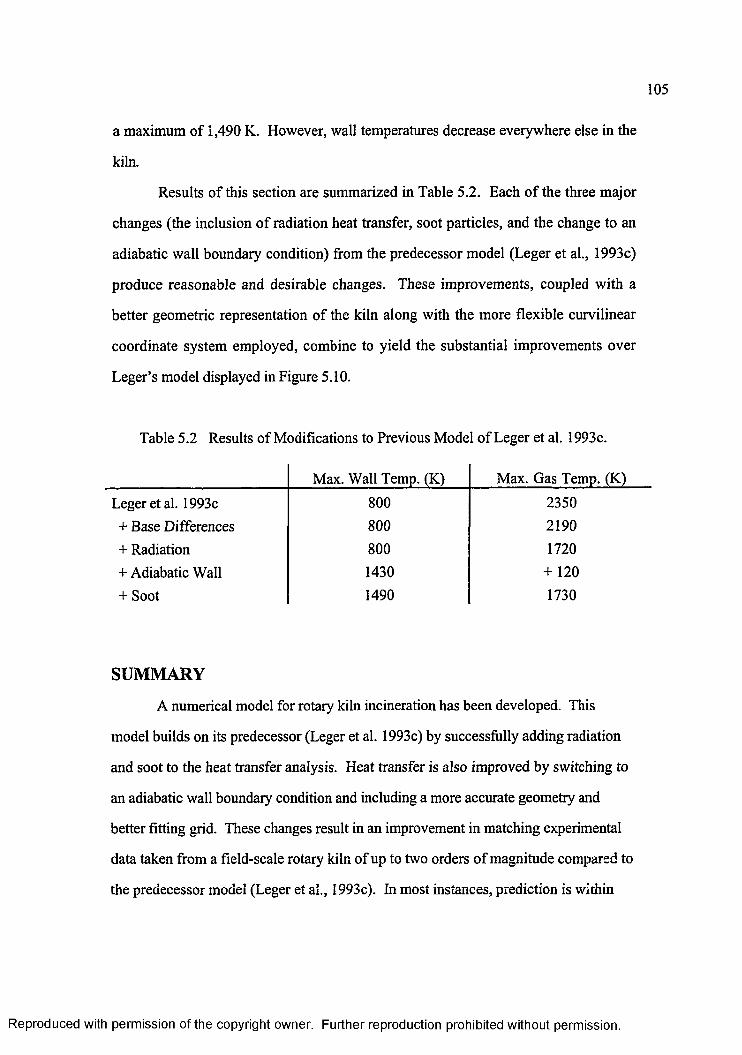
105
a maximum of 1,490 K. However, wall temperatures decrease everywhere else in the
kiln.
Results of this section are summarized in Table 5.2. Each o f the three major
changes (the inclusion of radiation heat transfer, soot particles, and the change to an
adiabatic wall boundary condition) from the predecessor model (Leger et al., 1993c)
produce reasonable and desirable changes. These improvements, coupled with a
better geometric representation of the kiln along with the more flexible curvilinear
coordinate system employed, combine to yield the substantial improvements over
Leger’s model displayed in Figure 5.10.
Table 5.2 Results of Modifications to Previous Model of Leger et al. 1993c.
Max. Wall Temp. (K) Max. Gas Temp. (K)
Leger etal. 1993c 800 2350+ Base Differences 800 2190+ Radiation 800 1720+ Adiabatic Wall 1430 + 120+ Soot 1490 1730
SUMMARY
A numerical model for rotary kiln incineration has been developed. This
model builds on its predecessor (Leger et al. 1993c) by successfully adding radiation
and soot to the heat transfer analysis. Heat transfer is also improved by switching to
an adiabatic wall boundary condition and including a more accurate geometry and
better fitting grid. These changes result in an improvement in matching experimental
data taken from a field-scale rotary kiln of up to two orders of magnitude compared to
the predecessor model (Leger et al., 1993c). In most instances, prediction is within
Reproduced with permission of the copyright owner. Further reproduction prohibited without permission.
106
repeatability limits of the experiments. The primary exception is in the prediction of
velocity; while matching experimental data at the kiln centerline, error at the top of the
kiln is as high as 40 percent. A grid dependency study showed the flow field to be
dependent on the grid, especially at the upper front of the kiln where gradients are
very steep. Still, near the exit of the kiln where the limited experimental data were
available, both grids produced very similar results. Attempts at further refinement
were not successful.
The parametric study on the effect of infiltration air distribution underscores
the need to record velocities across a complete cross section of the kiln in order to
validate numerical models of rotary kilns. This would allow the total amount of air
infiltrating at the front of the kiln to be quantified as well as answering some of the
questions about the existence and location of reverse flow regions. The sensitivity
study demonstrates the importance of the individual improvements in the heat
transfer analysis.
This complicated model of rotary kiln incineration is evolving in stages, and
while the results reported herein represent considerable improvement over the first-
generation work of Leger et al. (1993c), the model cannot yet be used to simulate
waste processing. Even so, the model in its current stage of development, can be used
for limited design and operation studies.
Reproduced with permission of the copyright owner. Further reproduction prohibited without permission.
CHAPTER 6
SUMMARY, CONCLUSIONS, AND RECOMMENDATIONS
SUMMARY
The major accomplishments of the research that has been presented in this
dissertation are summarized in this section. Conclusions and recommendations
follow.
Experimental Velocity and Temperature Measurements
A new device for measuring velocities and temperatures inside a directly-
fired, full-scale, rotary kiln incinerator has been developed, constructed, and tested.
Using this device, velocities were measured for the first time inside a field-scale
rotary kiln incinerator. Combustion gas velocities and temperatures were measured
at multiple points across a quadrant of the rotary kiln segment of a hazardous waste
incinerator near its exit. Measurements were made using a bidirectional pressure
probe and suction pyrometer. To accommodate the new bidirectional probe and gain
access to the upper portion of the kiln, a lighter and stiffer positioning boom was
designed. To ensure precise and accurate placement of the probe tip, a positioning
device was designed and attached to the incinerator. The kiln was directly fired using
natural gas in a steady state mode. Results indicate strong vertical stratification of
both velocity and temperature, with the highest values corresponding to the top of
the kiln. Access restraints prevented the lower region of the kiln from being mapped.
Horizontal variations in both temperature and velocity were insignificant. Operating
conditions were varied by adjusting the amount of ambient air added to the front of
107
Reproduced with permission of the copyright owner. Further reproduction prohibited without permission.
the kiln. Increasing the flow of ambient air into the front of the kiln reduced the
measured temperatures as expected, but did not have as significant an effect on
measured velocities possibly due to the mitigating effect of the large amount of
unmetered air infiltrating at the front of the kiln. Temperature values and data
stratification trends generated by this new device agree with previous experimental
findings on the same incinerator under similar operating conditions.
Prior to obtaining the velocity and temperature data of this paper, there were
virtually no means to quantify the mass flow inside rotary kilns. This led to
uncertainty about the distribution of unmetered infiltration air and the flow dynamics
at the locations of previous sampling efforts. Because the limited access o f this
incinerator did not allow a complete mapping of the kiln exit, the amount of
unmetered air entering the kiln is still uncertain. However, the results do help to
provide confidence that the estimated infiltration air distribution is realistic. Further,
the results indicate that, with adequate access, this probe assembly could completely
characterize the mass flow field of this rotary kiln incinerator or other similar
combustion devices. Limitations include material compatibility with kiln
environment, pressure transducer limitations, and calibration constant applicability
limits (not a theoretical limit, but so far only determined for the Reynolds Number
range o f 300 to 4000). In addition, the relatively good agreement between the
measured and calculated kiln mass flow rates suggests that the experimental
techniques used and the assumptions imposed (horizontal symmetry at the exit
region of the kiln, along with linear velocity and temperature profiles) are reasonable.
While this may seem a circular argument, it should be noted that, primarily due to the
complexity of the system, never before has the flow field of an operating rotary kiln
incinerator been quantified. With each piece of new information, the picture of what
takes place inside a rotary kiln incinerator becomes clearer, and the ability to test
Reproduced with permission of the copyright owner. Further reproduction prohibited without permission.
109
previous assumptions becomes possible. While the measurements reported in this
paper only covered a portion o f the kiln exit region, they have added considerably to
our understanding of the complicated process of rotary kiln incineration.
Numerical Model of Rotary Kiln Incinerator
A steady state numerical model for the rotary kiln segment of a direct-fired
hazardous waste incinerator has been developed. This model builds on work
previously conducted at Louisiana State University by including radiation and soot in
the heat transfer analysis, by switching to an adiabatic wall boundary condition, and
including a more accurate geometry and better fitting grid. These changes improve
agreement with data taken from a field-scale industrial rotary kiln, operating with a
natural gas support flame, but no waste processing, by up to two orders of
magnitude compared to previously developed models at Louisiana State University.
In most instances, prediction is within repeatability limits of the experiments. The
primary exception is in the prediction of velocity; while matching experimental data
at the kiln centerline, error at the top of the kiln is as high as 40 percent. Grid
dependency is demonstrated, especially at the upper front of the kiln where gradients
are very steep. However, differences between predictions by the two grids have
lessened greatly by the middle of the kiln, with both grids producing nearly identical
flow fields by the exit of the kiln where the limited experimental data are available.
Attempts at further refinement were not successful.
The parametric study on the effect of infiltration air distribution underscores
the need to record velocities across a complete cross section of the kiln in order to
validate numerical models of rotary kilns. This would allow the total amount of air
infiltrating at the front of the kiln to be quantified as well as answering some of the
questions about the existence and location of reverse flow regions. The sensitivity
Reproduced with permission of the copyright owner. Further reproduction prohibited without permission.
study demonstrates the importance of the individual improvements in the heat
transfer analysis.
This complicated model of rotary kiln incineration is evolving in stages, and
while the results reported herein represent considerable improvement over the first-
generation work, the model cannot yet be used to simulate waste processing. Even
so, the model in its current stage of development can be used for limited design and
operation studies.
CONCLUSIONS
Field-scale experimentation results presented in this dissertation expand the
general knowledge of incineration. Previous experimental work has shown that
incinerator flows can be highly stratified in both temperature and chemical species.
This latest work shows that the exit of a rotary kiln incinerator also can also be
highly stratified in velocity and presents evidence that regions of reverse flow may
exist. It is, therefore, important to consider the general velocity field when
interpreting other measurements taken from the rotary kiln section of an incinerator.
This is particularly important if single point sampling is used to characterize the
incineration process, so that stagnant areas and regions of reverse flow can be
identified. This work presents a device and methodology for measuring velocities in
high temperature, particulate laden, turbulent flows. This dissertation also provides
the research community with the proven design of a lightweight and yet stiff boom
that can be used in many high temperature applications.
Successful numerical modeling as presented in this body of work depends on
four things. First a representation of the geometry needs to include all aspects that
significantly affect areas of interest. At the same time consideration needs to be
given to possible simplifications to the geometry so that applying a grid will be
easier. The numerical grid should accurately represent the chosen geometry, produce
Reproduced with permission of the copyright owner. Further reproduction prohibited without permission.
a converged solution, and be refined enough so that the major aspects of the flow
field are not grid dependent. All physical phenomena that are important to the final
solution need to be included and correct boundary conditions applied. Finally, model
results need to be compared back to data taken from the actual facility being modeled
until confidence in the model is attained. The current model improves on its
predecessor by addressing all of these requirements. The geometry is more accurate
at the front face where the burners are located and in places in the transition section
that have a bearing on the main kiln flow field. However, simplifications are made in
the geometry of the transition and afterburner sections by eliminating regions of
recirculation that do not have direct bearing on the main flow in the kiln. A grid that
more accurately matches the combination of cylindrical and rectangular geometries
and utilizes non-uniform grid spacing is generated. Radiation, including the effects of
soot, is added and the thermal boundary condition at the walls is improved. Grid
independence is attempted but not fully attained. Finally, these improvements
combine to generate a model that does an exceptional job of quantitatively, as well as
qualitatively, matching all of the available experimental data except velocity data at
the top of the kiln. This current model is an improvement over previous models of
this facility; however, questions remain about grid dependence, and waste modeling is
not included yet.
RECOMMENDATIONS FOR FURTHER WORK
Research results presented in this dissertation represent a substantial forward
movement toward the twin goals o f obtaining a better understanding o f processes
occurring in hazardous waste rotary kiln incinerators and achieving the capability to
correctly predict incinerator performance. This work also points to the progress that
remains to be achieved. Following is a list of specific recommendations for additional
projects based on the work presented here.
Reproduced with permission of the copyright owner. Further reproduction prohibited without permission.
112
Experimental
1) The steady state velocity field of the rotary kiln discussed in this document
needs to be more completely mapped. In particular, a complete vertical
traverse is needed so that the total amount of air infiltrating at the front of the
kiln can be calculated. Sampling in the lower kiln region is needed to give
information on any recirculation regions. This may involve designing another
probe that can reach the lower region of the kiln given the existing limited
access. One possibility is to make the boom with a bend or even a dogleg in
it.
2) Data on the chemical species present should also be mapped along with the
temperature and velocity. This can be done by analyzing gases withdrawn by
the suction pyrometer.
3) A device and or methodology for quantifying soot would add a significant
piece of information to any future incineration data gathered. This would also
greatly help with attempts to include soot in numerical modeling.
4) Recording the transient response of the velocity field at several locations to
loadings of pack or drums of solid waste would be a step forward and would
allow reinterpretation of some previous data. This was attempted with packs
of clay sorbent and diesel fuel, but thermocouple problems led to inconclusive
results. Dichloromethane or toluene would be good choices for the hazardous
waste because temperature and speciation data have been recorded during
previous batch experiments using these chemicals.
Numerical Modeling
5) To design a geometry and grid combination that will have enough refinement
to not have any effect on correct prediction considering the large size of the
incinerator, the small scale at which chemical reactions and turbulence are
Reproduced with permission of the copyright owner. Further reproduction prohibited without permission.
important, and the current computing limitations, is presently impossible.
However, refinement o f the grid to the point that only very small and
localized changes occur upon further grid refinement (beyond that presented
in this document) should be attained.
6) A more accurate picture of the chemical reaction process needs to be included
to improve the current methane-only flame modeling and before waste
processing can be successfully modeled. In particular, intermediates such as
carbon monoxide and the high temperature dissociation of water vapor and
carbon dioxide need to be included. Also, while the radiation effects o f soot
were included in the current model, results could be improved by an accurate
modeling of its formation and destruction.
7) The ultimate goal is to be able to predict conversion of hazardous waste fed
to the incinerator. To do this will require the ability to model the combustion
of wastes. As relatively detailed experimental data have been recorded for the
destruction of packs containing clay sorbent and toluene, these would be good
materials to initially model.
8) Modeling the conversion of toluene absorbed onto clay sorbent and fed to the
incinerator in drums or packs is a batch process and is therefore unsteady. A
completely unsteady model could be attempted or several evolution rates
could be considered to be steady, yielding rough snap-shots of the transient
process.
9) Drum or pack processing will also require models for the initial container
destruction, mixing of the new solid material with the existing bed of solids,
heat transfer with the bed, kiln wall, and overhead gases and flames. An
initial simplifying move could be to use previously estimated evolution rates
of the waste as a boundary' condition. Reaction schemes may require the
Reproduced with permission of the copyright owner. Further reproduction prohibited without permission.
114
inclusion of a pyrolytic series. Visual observations indicate airborne soot to
be optically thick, reducing viewing to approximately 1 meter at times, and
often surviving through the rotary kiln and transition sections o f the
incinerator during batch processing of toluene and dichloromethane.
10) Improved predictive capabilities of new sub-models such as for turbulence or
chemical reactions should be examined for possible inclusion in the model.
However, these need to be weighed against any penalties in convergence,
CPU time, or computer memory requirements. The same is true for advances
in equation solution technology such as higher order differencing schemes.
11) Further data during the processing of waste, including temperature, speciation
and velocity, need to be collected to aid in the construction of this numerical
model.
Reproduced with permission of the copyright owner. Further reproduction prohibited without permission.
BIBLIOGRAPHY
Bard, S. and P. J. Pagni, "Carbon Particulate in Small Pool Fire Flames," Journal o f Heat Transfer, Vol. 103, pp. 357-362, (1981).
Bastian, R. E. and R. W. Wood, "Eastman Kodak Company Chemical Waste Incineration - Organic Compound Destruction," in Proceedings o f the Conference On Rotary Kiln Incineration of Hazardous Waste, Hazardous Waste Research Center-Department o f Mechanical Engineering-Center for Energy Studies, Louisiana State University, Baton Rouge, Louisiana, (1987).
Boris, J. P., "New Directions in Computational Fluid Dynamics," Annual Review o f Fluid Mechanics, 21: p. 345-385, (1989).
Charalampopoulos, T. T. and H. Chang, "In situ Optical Properties o f Soot Particles in the Wavelength Range from 340 nm to 600 nm," Combustion Science and Technology, Vol. 59, pp. 401-421, (1988).
Charalampopoulos, T. T. and H. Chang, “Effects of Soot Agglomeration on Radiative Transfer," Journal o f Quant. Spectrosc. Radiat. Transfer, Vol. 46, No. 3, pp. 125-134, (1991).
Chen, Y. Y. and D. J. Lee, “A Steady State Model of a Rotary Kiln Incinerator,” Hazardous Waste and Hazardous Materials, Vol. 11, No. 4, pp. 541-559, (1994).
Clark, W. D., M. P. Heap, W. Richter, and W. R. Seeker, "The Prediction of Liquid Injection Hazardous Waste Incinerator Performance," ASME/AIChE National Heat Transfer Conference, Niagara Falls, New York, (1984).
Clark, W. D, W. R. Seeker, and C. C. Lee, "Engineering Analysis of Hazardous Waste Incineration; Energy and Mass Balance," 12th Annual Hazardous Waste Research Symposium, Cincinnati, Ohio, (1986).
Code of Federal Regulations, 40: Part 261, Subpart C. July 1, (1991a).
Code of Federal Regulations, 40: Part 372. July 1, (1991b).
Code of Federal Regulations, 40: Part 268, Subpart C. July 1, (1991c).
115
Reproduced with permission of the copyright owner. Further reproduction prohibited without permission.
116
Code of Federal Regulations, 40: Part 268.42, Subpart D. July 1, (1991d).
Code of Federal Regulations, 40: Part 264.343 (c). July 1, (1991e).
Cook, C. A., V. A. Cundy, A. M. Sterling, C. Lu, A. N. Montestruc, C. B. Leger and A. L. Jakway, "Estimating Dichloromethane Evolution Rates from a Sorbent Bed in a Field-Scale Rotary Kiln Incinerator," Combustion Science and Technology, Vol. 85, pp. 217-241, (1992).
Cundy, V. A., T. W. Lester, A. M. Sterling, J. S. Morse, A. N. Montestruc, C. B. Leger, S. Acharya, and D. W. Pershing, "Rotary Kiln Injection I. An Indepth Study -- Liquid Injection," Journal o f the Air Pollution Control Association (JAPCA), Vol. 39, No. 1, pp. 63-75, (1989a).
Cundy, V. A., T. W. Lester, A. M. Sterling, J. S. Morse, A. N. Montestruc, C. B. Leger, and S. Acharya, "Rotary Kiln Injection III. An Indepth Study — Kiln Exit/Afterbumer/Stack Train and Kiln Exit Pattern Factor Measurements During Liquid CC14 Processing," Journal o f the Air Pollution Control Association, Vol. 39, No. 7, pp. 944-952, (1989b).
Cundy, V. A., T. W. Lester, A. M. Sterling, J. S. Morse, A. N. Montestruc, C. B. Leger, and S. Acharya, "Rotary Kiln Injection IV. An Indepth Study - Kiln Exit, Transition and Afterburner Sampling During Liquid CC14 Processing," Journal o f the Air Pollution Control Association, Vol. 39, No. 8, pp. 1073- 1085, (1989c).
Cundy, V. A., T. W. Lester, C. Leger, G. Miller, A. N. Montestruc, S. Acharya, and A. M. Sterling, "Rotary Kiln Incineration — Combustion Chamber Dynamics," Journal o f Hazardous Materials, Vol. 22, pp. 195-219, (1989d).
Cundy, V. A., T. W. Lester, R. Conway, A. L. Jakway, C. B. Leger, A. N. Montestruc, S. Acharya, A. M. Sterling, W. D. Owens, J. S. Lighty, W. D. Pershing, and G. D. Silcox, "An Indepth Study of Incineration - Rotary Kiln Performance Characterization," Proceedings of the Third Annual Symposium on Hazardous Waste Research, Hazardous Waste Research Center, Louisiana State University, Baton Rouge, Louisiana, (1989e).
Cundy, V. A., T. W. Lester, R. Conway, C. Cook, A. L. Jakway, C. B. Leger, C. Lu, A. N. Montestruc, S. Acharya, A. M. Sterling, D. A. Walker, F. S. Larson, R. J. Moore, D. Xian-Xue, J. S. Lighty, and W. D. Owens, "An Indepth Study of Rotary Kiln Incineration," Proceedings o f the Fourth Annual Symposium on Hazardous Waste Research, Hazardous Waste Research Center, Louisiana State University, Baton Rouge, Louisiana, (1990).
Reproduced with permission of the copyright owner. Further reproduction prohibited without permission.
117
Cundy, V. A., A. M. Sterling, T. W. Lester, A. L. Jakway, C. B. Leger, C. Lu, A. N. Montestruc, and R. B. Conway, "Incineration of Xylene/Sorbent Packs. A Study of Conditions at the Exit o f a Full-Scale Industrial Incinerator," Environmental Science and Technology, Vol. 25, No. 2, pp. 223-231, (1991a).
Cundy, V. A., C. Lu, C. A. Cook, A. M. Sterling, C. B. Leger, A. L. Jakway, A. N. Montestruc, R. Conway, and T. W. Lester, "Rotary Kiln Incineration of Dichloromethane and Xylene: A Comparison o f IncinerabilityCharacteristics Under Various Operating Conditions," Journal o f the Air & Waste Management Association, Vol. 41, No. 8, pp. 1084-1094, (1991b).
Cundy, V. A., C. Cook, A. M. Sterling, C. Lu, A. N. Montestruc, C. B. Leger, and, A. L. Jakway, "Rotary Kiln Incineration - Batch Processing of CH2 CI2 on Sorbent Contained in Plastic Packs," Proceedings of the 2nd International Congress on Toxic Combustion By-Products Formation and Control, Salt Lake City, Utah, (1991c).
Cundy, V. A., A. M. Sterling, C. Lu, C. A. Cook, C. B. Leger, A. L. Jakway, A. N. Montestruc, R. Conway, and T. W. Lester, "Rotary Kiln Incineration: A Field-Scale Study o f System Dynamics Under Various Operating Conditions," Invited paper, Fifth Annual National Symposium on Incineration o f Industrial Wastes, (unpublished paper available at conference), Simon-EEI, Inc., Houston, Texas, (1991d).
De Ris, J., "Fire Radiation - A Review," 17th Symposium International on Combustion, pp. 1003-1016, (1978).
Edwards, D. K., Radiation Heat Transfer Notes. Hemisphere Publishing Corp., Washington, (1981).
Federal Register, p. 31,114, Friday May 28, (1993).
Felske, J. D. and T. T. Charalampopoulos, "Gray Gas Weighting Coefficients for Arbitrary Gas-Soot Mixtures," International Journal o f Heat and Mass Transfer, Vol. 25, No. 12, pp. 1849-1855, (1982).
Fluent User’s Guide, Version4.2; Fluent Inc.: Lebanon, NH, June (1993).
Gardner, W. C. Jr., Combustion Chemistry. Springer-Verlay, New York, NY (1984).
Reproduced with permission of the copyright owner. Further reproduction prohibited without permission.
118
Gillis, P.A. and P. J. Smith, "Three-Dimensional Fluid Dynamics Modeling in Furnace Geometries," Western States Section of The Combustion Institute, pp. 1-12, (1988).
Glassman, I., Combustion, second edition, Academic Press, Inc., (1987).
Gorog, J. P., T. N. Adams, and J. K. Brimacombe, "Heat Transfer from Flames in a Rotaiy Kiln," Metallurgical Transactions B, Vol. 14B, pp. 411-424, (1983).
Gorog, J. P., T. N. Adams, and J. K. Brimacombe, "Radiative Heat Transfer in Rotary Kilns," Metallurgical Transactions B, Vol. 12B, pp. 55-70, (1981).
Huggins, Jonathan. Personal Communication, March 18, (1994).
Incropera, F. P. and D. P. DeWitt, Fundamentals of Heat and Mass Transfer. 2nd Ed., John Wiley and Sons, (1985).
Jakway, A. L., V. A. Cundy, and A. M. Sterling, "3-D Numerical Modeling of a Field Scale Rotary Kiln Incinerator," presentation at The ASME Winter Annual Meeting, Open Forum on Fire and Combustion, American Society of Mechanical Engineers, (unpublished paper available at conference) New Orleans, Louisiana, November 28-December 3, (1993a).
Jakway, A. L., V. A. Cundy, A. M. Sterling, and C. B. Leger, "A 3-Dimensional Detailed Numerical Model as a Design Tool for Rotary Kiln Incinerators," The 3rd International Congress on Toxic Combustion By-Products, (unpublished paper available at conference) Cambridge, Massachusetts, June 14-16, (1993b).
Jakway, A. L., V. A. Cundy, A. M. Sterling, C. A. Cook, and A. N. Montestruc, “Insitu Velocity and Temperature Measurements from an Industrial Rotary Kiln Incinerator,” Proceedings of the 14th International Incineration Conference, Seattle, Washington, May 8-12, (1995a).
Jakway, A. L., V. A. Cundy, A. M. Sterling, C. A. Cook, and A. N. Montestruc, ‘7n Situ Velocity Measurements from an Industrial Rotary Kiln Incinerator,” accepted to the Journal o f the Air and Waste Management Association, Nov., (1995b).
Jenkins, B. G. and F. D. Moles, "Modeling of Heat Transfer from a Large Enclosed Flame in a Rotary Kiln," Transactions o f the Institute o f Chemical Engineers, Vol. 59, pp. 17-25, (1981).
Reproduced with permission of the copyright owner. Further reproduction prohibited without permission.
119
Jones, W. P. and J. H. Whitelaw, "Calculation Methods for Reacting Turbulent Flows: A Review," Combustion and Flame, 48: pp. 1-26, (1982).
Kent, L. A. and M. E. Schneider, "The Design and Application of Bi-Directional Velocity Probes for Measurement in Large Pool Fires," ISA Transactions, Vol. 26, No. 4, pp. 25-32, (1987).
Khan, J. A., D. Pal, and J. S. Morse, "Numerical Modeling of a Rotary Kiln Incinerator," Hazardous Waste and Hazardous Materials, Vol. 10, No. 1, p. 81,(1993).
Leger, C. B., V. A. Cundy, A. M. Sterling, A. N. Montestruc, A. L. Jakway, and W. D. Owens, "Field-Scale Rotary Kiln Incineration: Oxygen Responses at the Kiln, Afterburner, and Stack," Remediation, Vol. 1, No. 3, pp. 275-291, (1991a).
Leger, C. B., V. A. Cundy, A. M. Sterling, C. A. Cook, A. L. Jakway, and A. N. Montestruc, "Rotary Kiln Incineration - Batch Processing of Toluene on Sorbent Contained in Plastic Packs," Proceedings of the 84th Annual Meeting of the Air and Waste Management Association, Vancouver BC, (1991b).
Leger, C. B., "A Study of Selected Phenomena Observed During Rotary Kiln Incineration," Ph.D. Dissertation, Louisiana State University, (1992).
Leger, C. B., V. A. Cundy, A. M. Sterling, A. N. Montestruc, A. L. Jakway, and W. D. Owens, "Field-Scale Rotary Kiln Incineration o f Batch Loaded Toluene/Sorbent. I. Data Analysis and Bed Motion Considerations," Journal o f Hazardous Materials, Vol. 34, pp. 1-29, (1993a).
Leger, C. B., C. A. Cook, V. A. Cundy, A. M. Sterling, A. N. Montestruc, A. L. Jakway, and W. D. Owens, "Field-Scale Rotary Kiln Incineration of Batch Loaded Toluene/Sorbent. II. Mass Balances, Evolution Rates, and Bed Motion Comparisons," Journal o f Hazardous Materials, Vol. 34, pp. 31-50, (1993b).
Leger, C. B., V. A. Cundy, and A. M. Sterling, "A Three-Dimensional Detailed Numerical Model of a Field-Scale Rotary Kiln Incinerator," Environmental Science and Technology, Vol. 27, No. 4, pp. 677-690, (1993c).
Lester, T. W., V. A. Cundy, A. N. Montestruc, C. B. Leger, S. Acharya, and A. M. Sterling, "Dynamics of Rotary Kiln Incineration of Toluene/Sorbent Packs," Combustion Science and Technology, Vol. 74, pp. 67-82, (1990).
Reproduced with permission of the copyright owner. Further reproduction prohibited without permission.
120
Lester, T. W., V. A. Cundy, A. M. Sterling, A. N. Montestruc, A. L. Jakway, C. Lu, C. B. Leger, D. W. Pershing, J. S. Lighty, G. D. Silcox, and W. D. Owens, "Rotary Kiln Incineration. Comparison and Scaling of Field-Scale and Pilot- Scale Contaminant Evolution Rates from Sorbent Beds," Environmental Science & Technology, Vol. 25, No. 6, pp. 1142-1152, (1991).
Lipp, Chuck. Personal Communication, August 3, (1992).
Magnussen, B. F.and B. H. Hjertager, "On Mathematical Modeling o f Turbulent Combustion With Special Emphasis on Soot Formation and Combustion," Sixteenth International Symposium on Combustion, pp. 719-729, the Combustion Institute, (1976).
- McCaffrey, B. J. and G. Heskestad, Brief communications: "A Robust Bidirectional Low-Velocity Probe for Flame and Fire Application," Combustion and Flame, Vol. 26, pp. 125-127, (1976).
Montestruc, A. N., “Flame Zone Sampling From an Industrial Rotary Kiln,” Masters Thesis, Louisiana State University, (1989).
Murthy, J. Y. and D. Choudhury, "Computation o f Participating Radiation in Complex Geometries," National Heat Transfer Conference, San Diego, CA, ASME TN-020, (1992).
Nasserzadeh, V., J. Swithenbank, and B. Jones, "Three-dimensional Modeling o f a Municipal Solid-Waste Incinerator," Journal o f Institute o f Energy, Vol. 64, pp. 166-175, (1991).
Nasserzadeh, V., J. Swithenbank, C. Schofield, D. W. Scott, and A. Loader, "Effects of High Speed Jets and Internal Baffles on the Gas Residence Times in Large Municipal Incinerators," Environmental Progress, Vol. 13, No. 2, pp. 124- 133, (1994).
Owens, W. D., G. D. Silcox, J. S. Lighty, X. X. Deng, D. W. Pershing, T. W. Lester, V. A. Cundy, C. B. Leger, and A. L. Jakway, "Hydrocarbon Evolution From Contaminated solids: Effects of Moisture and Operating Parameters in a Rotary Kiln Environment," Poster Session, 23rd Symposium (International) on Combustion, Orleans, France, (1990a).
Owens, W. D., G. D. Silcox, J. S. Lighty, X. X. Deng, D. W. Pershing, V. A. Cundy, C. B. Leger, and A. L. Jakway, "Thermal Analysis o f Rotary Kiln Incineration: Comparison of Theory and Experiment," Poster Session, 23rd Symposium (International) on Combustion, Orleans, France, (1990b).
Reproduced with permission of the copyright owner. Further reproduction prohibited without permission.
121
Owens, W. D., G. D. Silcox, J. S. Lighty, X. X. Deng, D. W. Pershing, V. A. Cundy, C. B. Leger, and A. L. Jakway, "Thermal Analysis o f Rotary Kiln Incineration: Comparison of Theory and Experiment," Combustion and Flame, Vol. 86, pp. 101-114, (1991).
Owens, W. D., G. D. Silcox, J. S. Lighty, X. X. Deng, D. W. Pershing, V. A. Cundy, C. B. Leger, and A. L. Jakway, "The Desorption o f Toluene from a Montmorillonite Clay Adsorbent in a Rotary Kiln Environment," Journal o f the Air and Waste Management Association, Vol. 42, No. 5: pp. 681-690, (1992).
Silcox, G. D., D. W. Pershing, B. R. Keyes, W. D. Owens, J. S. Lighty, X. X. Deng, V. A. Cundy, C. B. Leger, and A. L. Jakway, "Heat Transfer, Mass Transfer, Vaporization, and Combustion in Rotary Kilns," 1990 Summer National Meeting, AIChE, San Diego, CA., (1990).
Smith, P. J., W. A. Sowa, and P. O. Hedman, "Furnace Design Using Comprehensive Combustion Models," Combustion and Flame, Vol. 79, pp. 111-121, (1990).
Stanisic, M. M., The Mathematical Theory o f Turbulence. Springer Verlag, New York, (1985).
Sterling, A. M., V. A. Cundy, T. W. Lester, A. N. Montestruc, A. L. Jakway, C. B. Leger, C. Lu, and R. Conway, "Fundamental Kiln Processes," Fourth Annual National Symposium - Incineration of Industrial Wastes, (unpublished paper available at conference), Toxcon Engineering Company, Inc., Houston, Texas, (1990a).
Sterling, A. M., V. A. Cundy, T. W. Lester, A. N. Montestruc, A. L. Jakway, C. B. Leger, C. Lu, and R. Conway, "Rotary Kiln Incineration - The LSU In Situ Field Testing Program," Proceedings o f the 83rd Annual Meeting of the Air and Waste Management Association, Pittsburgh, PA., (1990b).
Stull, D. R. and H. Prophet, "JANAF Thermochemical Tables," NSRDS-NBS 37, National Bureau of Standards and Supplements, Washington, (1971).
Thibodeaux, L. J., "Hazardous Material Management in the Future," Environmental Science and Technology, Vol. 24, No. 4, pp. 456-459, (1990).
Wagner, H. G, "Soot Formation -- An Overview," in Particulate Carbon: Formation During Combustion, edited by D. C. Siegla and G. W. Smith, Plenum Publishing Corporation, (1981).
Reproduced with permission of the copyright owner. Further reproduction prohibited without permission.
122
Wang, T., Y. Chen, and R. Farmer, "Numerical Study o f Reactive Ramjet Dump Com bustor Flowfields with a Pressure Base CFD Method," AIAA/ASME/SAE/ASEE 25th Joint Propulsion Conference, AIAA, pp. 1- 11,(1989).
Westbrook, C. K. and F. L. Dryer, "Chemical Kinetic Modeling o f Hydrocarbon Combustion," Prog. Energy Combustion Science, Vol. 10, pp. 1-57, (1984).
Willard H. H., L. L. Merritt Jr., J. A. Dean, and F. A. Settle Jr., Instrumental Methods o f Analysis, sixth ed., Wadsworth Pub. Co., Belmont CA, pp. 854- 856, (1981).
Wood, R. W., "Eastman Kodak Company Rotary Kiln Performance Testing," in Proceedings of the Conference On Rotary Kiln Incineration of Hazardous Waste, Hazardous Waste Research Center-Department o f Mechanical Engineering-Center for Energy Studies, Louisiana State University, Baton Rouge, Louisiana, (1987).
Reproduced with permission of the copyright owner. Further reproduction prohibited without permission.
APPENDIX A
PUBLISHING INFORMATION ON CHAPTER 4
PUBLISHING PERMISSION LETTERS
123
Reproduced with permission of the copyright owner. Further reproduction prohibited without permission.
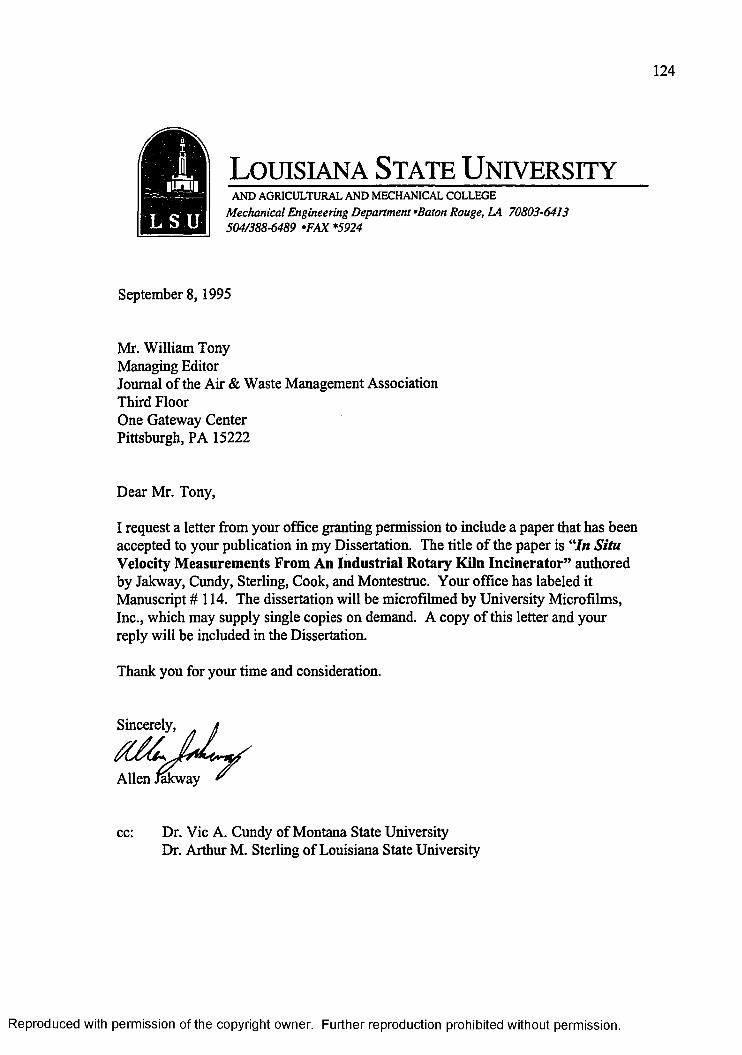
124
AND AGRICULTURAL AND MECHANICAL COLLEGE
Mechanical Engineering Department •Baton Rouge, LA 70803-6413 504/388-6489 •FAX *5924
Louisiana State University
September 8,1995
Mr. William Tony Managing EditorJournal of the Air & Waste Management AssociationThird FloorOne Gateway CenterPittsburgh, PA 15222
Dear Mr. Tony,
I request a letter from your office granting permission to include a paper that has been accepted to your publication in my Dissertation. The title of the paper is “In Situ Velocity Measurements From An Industrial Rotary Kiln Incinerator” authored by Jakway, Cundy, Sterling, Cook, and Montestruc. Your office has labeled it Manuscript # 114. The dissertation will be microfilmed by University Microfilms, Inc., which may supply single copies on demand. A copy of this letter and your reply will be included in the Dissertation.
Thank you for your time and consideration.
Sincerely,
cc: Dr. Vic A. Cundy of Montana State UniversityDr. Arthur M. Sterling of Louisiana State University
Reproduced with permission of the copyright owner. Further reproduction prohibited without permission.
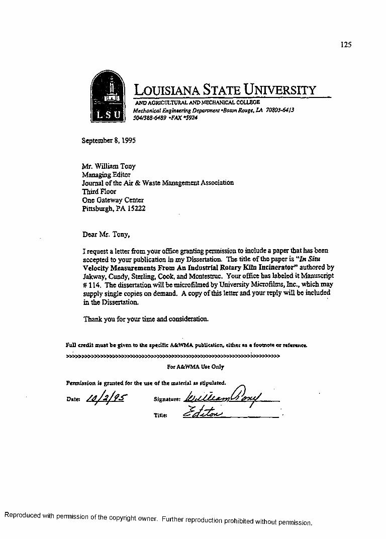
AND AGRICULTURAL AND MECHANICAL COLLEGE Mechanical Engineering Department •Baton Rouge. M 70803-6413 504/388-6489 •FAX *5924
Louisiana State University
September 8,1995
Mr. William Toay Managing EditorJournal of the Air & Waste Management AssociationThird FloorOne Gateway CenterPittsburgh, PA 15222
Dear Mr. Tony,
I request a letter from your office granting permission to include a paper that has been accepted to your publication in my Dissertation. The title of the paper is “In Situ Velocity Measurements From An Industrial Rotary Kiln Incinerator” authored by Jakway, Cundy, Sterling, Cook, and Montestruc. Your office has labeled it Manuscript # 114. The dissertation will be microfilmed by University Microfilms, Inc., which may supply single copies on demand. A copy of this letter and your reply will be included in the Dissertation.
Thank you for your time and consideration.
Full credit must be given to the specific AScWMA publication, either as a footnote or reference.
» » » » » » » » » » » » » » » » » » » » » » » » » » » » » » » > » » » » >For A&VVMA Use Only
P erm ission is eranted for the u se o f the material as stioulated.
Signature:
with permission of the copyright owner. Further reproduction prohibited withoutpermission.
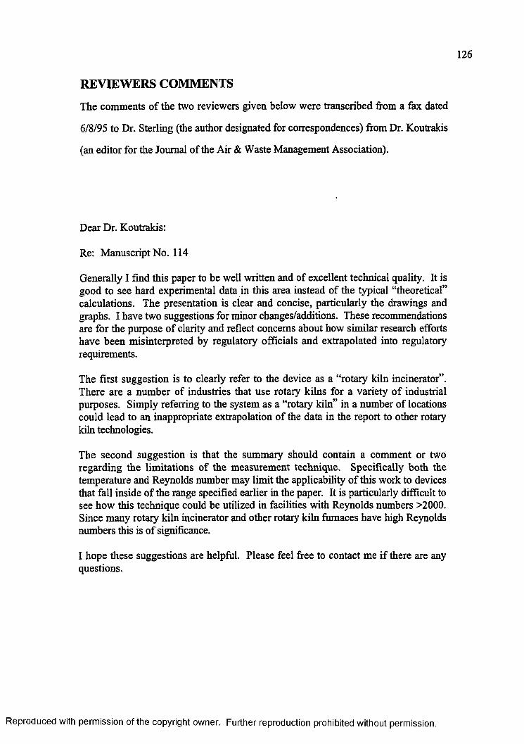
REVIEWERS COMMENTS
The comments o f the two reviewers given below were transcribed from a fax dated
6/8/95 to Dr. Sterling (the author designated for correspondences) from Dr. Koutrakis
(an editor for the Journal of the Air & Waste Management Association).
Dear Dr. Koutrakis:
Re: Manuscript No. 114
Generally I find this paper to be well written and of excellent technical quality. It is good to see hard experimental data in this area instead of the typical “theoretical” calculations. The presentation is clear and concise, particularly the drawings and graphs. I have two suggestions for minor changes/additions. These recommendations are for the purpose o f clarity and reflect concerns about how similar research efforts have been misinterpreted by regulatory officials and extrapolated into regulatory requirements.
The first suggestion is to clearly refer to the device as a “rotary kiln incinerator”. There are a number of industries that use rotary kilns for a variety of industrial purposes. Simply referring to the system as a “rotary kiln” in a number of locations could lead to an inappropriate extrapolation of the data in the report to other rotary kiln technologies.
The second suggestion is that the summary should contain a comment or two regarding the limitations of the measurement technique. Specifically both the temperature and Reynolds number may limit the applicability of this work to devices that fall inside of the range specified earlier in the paper. It is particularly difficult to see how this technique could be utilized in facilities with Reynolds numbers >2000. Since many rotary kiln incinerator and other rotary kiln furnaces have high Reynolds numbers this is of significance.
I hope these suggestions are helpful. Please feel free to contact me if there are any questions.
Reproduced with permission of the copyright owner. Further reproduction prohibited without permission.
127
Dear Dr. Koutrakis
I have read Allen Jakway’s paper and completed my review. I recommend it for publication.
The paper was clearly written and well organized. The description of the boom for the velocity probe and suction pyrometer was particularly good and needed as well. The tables and figures were clear and well organized.
The technical content of the paper was good also. As a practicing engineer I prefer English units over the metric units shown.
As a suggestion for further study, I think the industry would be interested in some analysis and the temperature profile of gas flows near the surface of the refractory.
Thank you for allowing me the opportunity to review this paper.
The comments of these two reviewers have been incorporated into the version of the
paper that appears in this dissertation as Chapter 4 with the exception of the paper
remaining in SI units.
Reproduced with permission of the copyright owner. Further reproduction prohibited without permission.
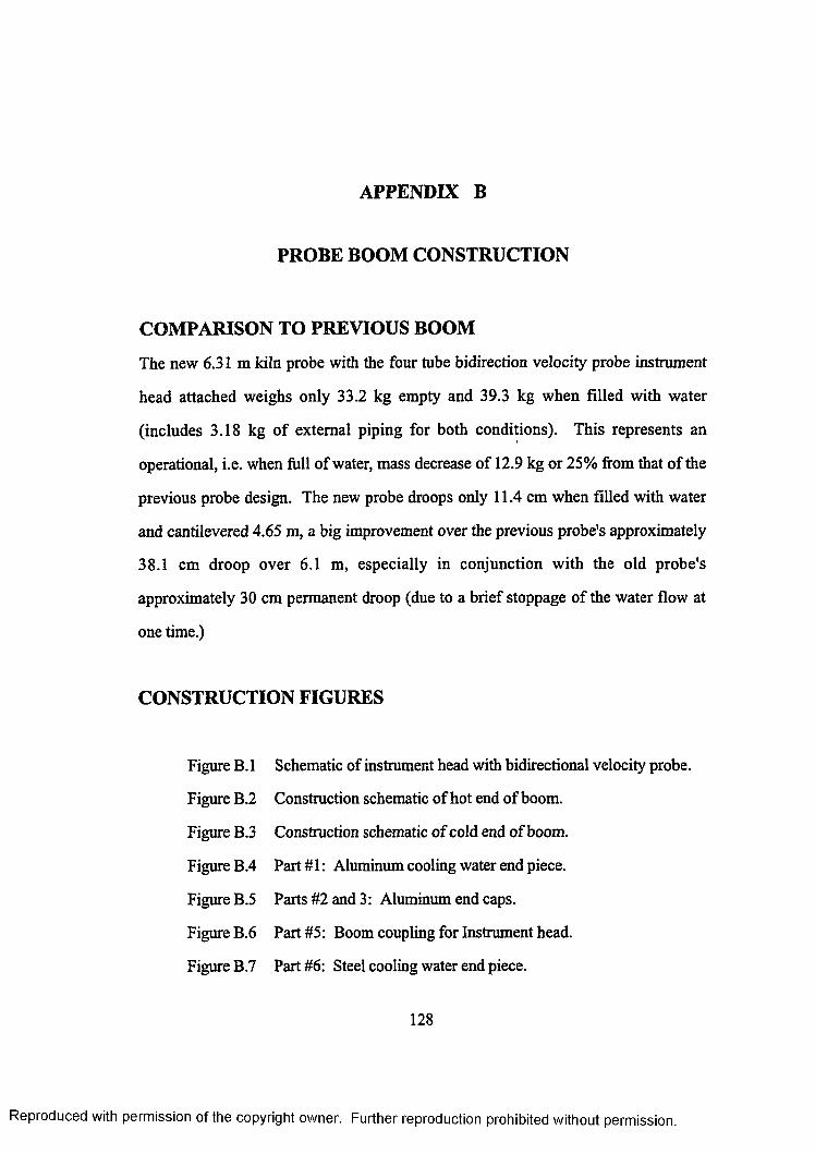
APPENDIX B
PROBE BOOM CONSTRUCTION
COMPARISON TO PREVIOUS BOOM
The new 6.31 m kiln probe with the four tube bidirection velocity probe instrument
head attached weighs only 33.2 kg empty and 39.3 kg when filled with water
(includes 3.18 kg of external piping for both conditions). This represents an
operational, i.e. when full of water, mass decrease of 12.9 kg or 25% from that of the
previous probe design. The new probe droops only 11.4 cm when filled with water
and cantilevered 4.65 m, a big improvement over the previous probe's approximately
38.1 cm droop over 6.1 m, especially in conjunction with the old probe's
approximately 30 cm permanent droop (due to a brief stoppage of the water flow at
one time.)
CONSTRUCTION FIGURES
Figure B. 1 Schematic of instrument head with bidirectional velocity probe.
Figure B.2 Construction schematic of hot end of boom.
Figure B.3 Construction schematic of cold end of boom.
Figure B.4 Part # 1: Aluminum cooling water end piece.
Figure B.5 Parts #2 and 3: Aluminum end caps.
Figure B.6 Part #5: Boom coupling for Instrument head.
Figure B.7 Part #6: Steel cooling water end piece.
128
Reproduced with permission of the copyright owner. Further reproduction prohibited without permission.
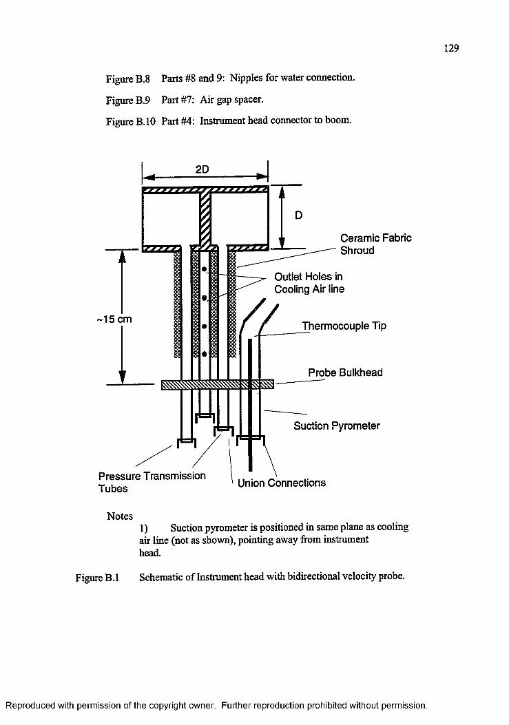
129
Figure B.8 Parts #8 and 9: Nipples for water connection.
Figure B.9 Part #7: Air gap spacer.
Figure B.10 Part #4: Instrument head connector to boom.
2D
ZSSEB
C eram ic Fabric Shroud
Outlet H oles in Cooling Air line
-1 5 cmTherm ocouple Tip
P robe Bulkhead
Suction Pyrom eter
P re ssu re Transm ission T u b es Union C onnections
Notes1) Suction pyrometer is positioned in same plane as cooling air line (not as shown), pointing away from instrument head.
Figure B. 1 Schematic of Instrument head with bidirectional velocity probe.
Reproduced with permission of the copyright owner. Further reproduction prohibited without permission.
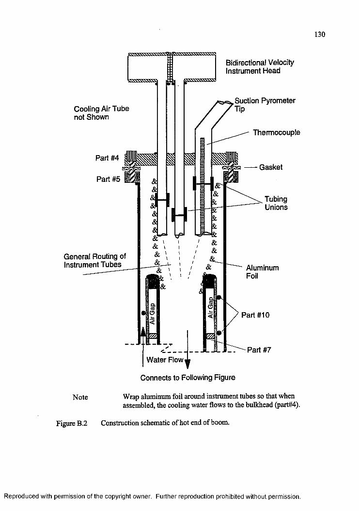
130
Cooling Air T ube not Shown
Bidirectional Velocity Instrum ent H ead
Suction Pyrom eter Tip
Part #4
Part #5
G eneral Routing of Instrum ent T ubes &
W ater Flow
Therm ocouple
G asket
TubingUnions
AluminumFoil
Part #10
P art #7
C onnects to Following Figure
Note Wrap aluminum foil around instrument tubes so that when assembled, the cooling water flows to the bulkhead (part#4).
Figure B.2 Construction schematic of hot end of boom.
Reproduced with permission of the copyright owner. Further reproduction prohibited without permission.
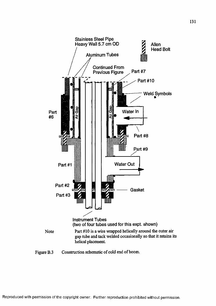
131
Part #1
Part #2
Part #3
S tain less Steel Pipe H eavy Wall 5.7 cm OD
Aluminum T ubes
Allen H ead Bolt
Continued From Previous Figure Part #7
Part #10
W ater In
Part #8
Part #9
W ater Out
W eld Sym bols
G asket
Note
Instrum ent T ubes (two of four tubes u sed for this expt. shown)Part #10 is a wire wrapped helically around the outer air gap tube and tack welded occasionally so that it retains its helical placement.
Figure B.3 Construction schematic of cold end of boom.
Reproduced with permission of the copyright owner. Further reproduction prohibited without permission.
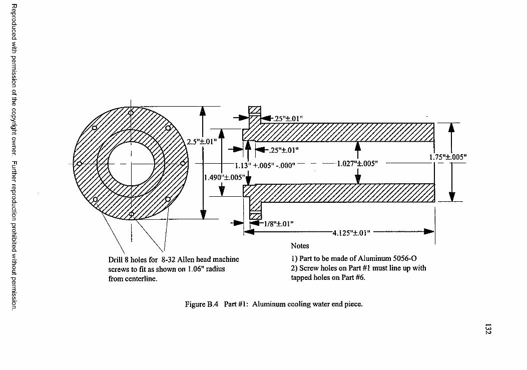
Reproduced
with perm
ission of the
copyright ow
ner. Further
reproduction prohibited
without
permission.
v977777777~
2.5 ±.01j^-.25"±.01"
1.13" +.005"-.000"1.75 ±.005
1.027 ±.005
1/8 ±.014.125 ±.01
Notes
Drill 8 holes for 8-32 Allen head machine screws to fit as shown on 1.06" radius from centerline.
1) Part to be made of Aluminum 5056-02) Screw holes on Part #1 must line up with tapped holes on Part #6.
Figure B.4 Part #1: Aluminum cooling water end piece.
U>N)
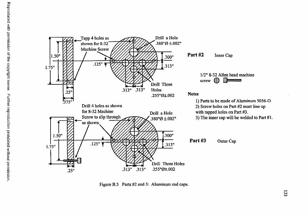
Reproduced
with perm
ission of the
copyright ow
ner. Further
reproduction prohibited
without
permission.
shown for 8-32 Machine Screw
Drill a Hole .38O"0 +.002"
.300"*1.75"
.25"i— ►375"
.313"
Drill Three 313" .313" Holes
,255"0±.OO2
Drill 4 holes as shown for 8-32 Machine Screw to slip through
Drill a Hole .38O"0 +.002"
1.75"
Part #2 Inner Cap
1/2" 8-32 Allen head machine screw © Q}zzzzzzza
Notes1) Parts to be made of Aluminum 5056-02) Screw holes on Part #2 must line up with tapped holes on Part #3.3) The inner cap will be welded to Part #1.
313"
Drill Three Holes
Part #3 Outer Cap
.313" .313" .255"0±.OO2
Figure B.5 Parts #2 and 3: Aluminum end caps.
u>U>
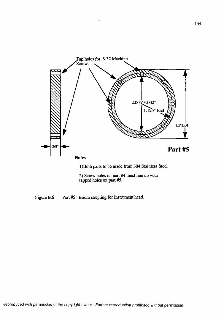
134
J a p holes for 8-32 Machine Screw. \
1.125" Rad
2.5"±.0I
3/8' Part #5Notes
1)Both parts to be made from 304 Stainless Steel
2) Screw holes on part #4 must line up with tapped holes on part #5.
Figure B.6 Part #5: Boom coupling for Instrument head.
Reproduced with permission of the copyright owner. Further reproduction prohibited without permission.
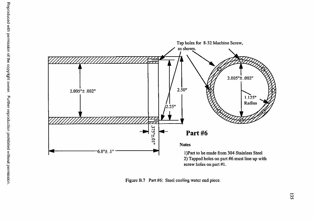
Tap holes for 8-32 Machine Screw, as shown.
2.005"± .002"
-6.0"±.l"
2.005"+ .002"
1.125"Radius
Part #6
Notes
1)Part to be made from 304 Stainless Steel2) Tapped holes on part #6 must line up with screw holes on part #1.
Figure B.7 Part #6: Steel cooling water end piece.
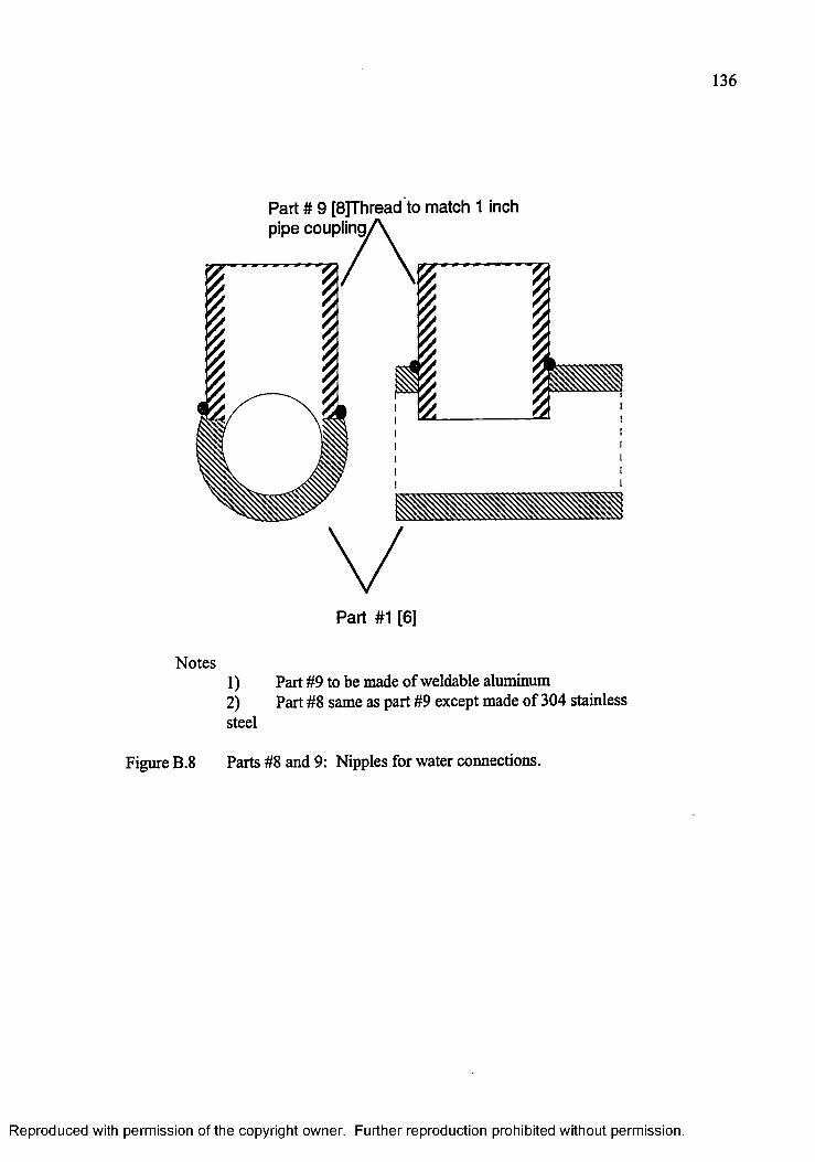
136
Part # 9 [8]Thread to m atch 1 inchpipe coupling
Part #1 [6]
Notes1) Part #9 to be made of weldable aluminum2) Part #8 same as part #9 except made of 304 stainless steel
Figure B.8 Parts #8 and 9: Nipples for water connections.
Reproduced with permission of the copyright owner. Further reproduction prohibited without permission.
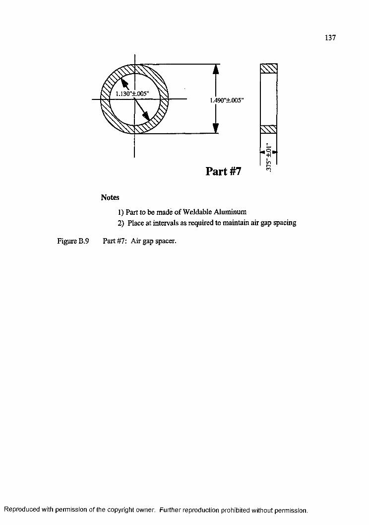
137
1.130"±.005'1.490"±.005'
Part #7
-Hin r- cn
Notes
1) Part to be made of Weldable Aluminum2) Place at intervals as required to maintain air gap spacing
Figure B.9 Part #7: Air gap spacer.
Reproduced with permission of the copyright owner. Further reproduction prohibited without permission.
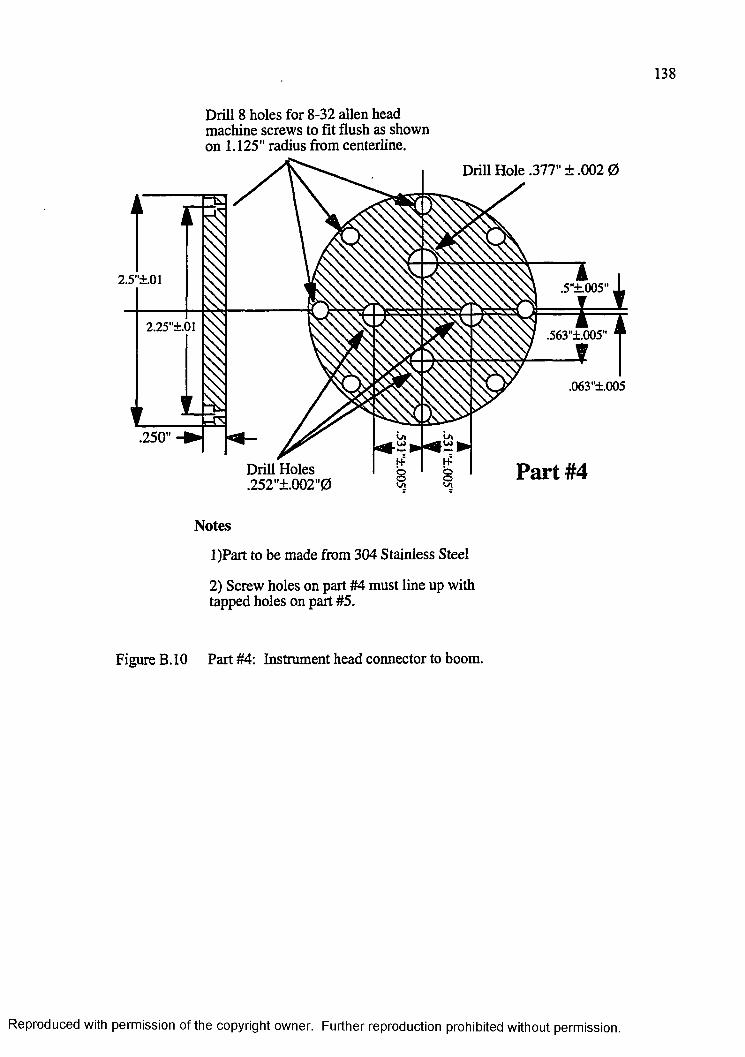
138
Drill 8 holes for 8-32 alien head machine screws to fit flush as shown on 1.125" radius from centerline.
Part #4Drill Holes .252"±.QO2"0
Notes
1)Part to be made from 304 Stainless Steel
2) Screw holes on part #4 must line up with tapped holes on part #5.
Figure B. 10 Part #4: Instrument head connector to boom.
Reproduced with permission of the copyright owner. Further reproduction prohibited without permission.
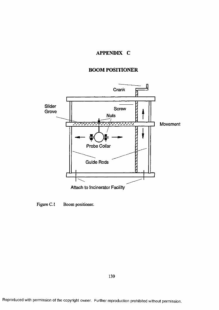
APPENDIX C
BOOM POSITIONER
Crank
SliderG rove
Screw
Nuts
Probe Collar
Guide Rods
Attach to Incinerator Facility
M ovement
Figure C. 1 Boom positioner.
139
Reproduced with permission of the copyright owner. Further reproduction prohibited without permission.
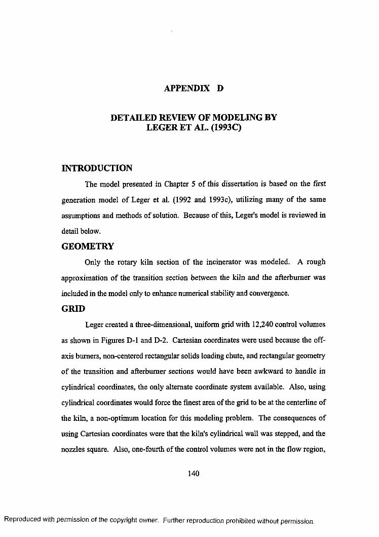
APPENDIX D
DETAILED REVIEW OF MODELING BY LEGERET AL. (1993C)
INTRODUCTION
The model presented in Chapter 5 of this dissertation is based on the first
generation model o f Leger et al. (1992 and 1993c), utilizing many of the same
assumptions and methods of solution. Because of this, Leger's model is reviewed in
detail below.
GEOMETRY
Only the rotary kiln section of the incinerator was modeled. A rough
approximation o f the transition section between the kiln and the afterburner was
included in the model only to enhance numerical stability and convergence.
GRID
Leger created a three-dimensional, uniform grid with 12,240 control volumes
as shown in Figures D-l and D-2. Cartesian coordinates were used because the off-
axis burners, non-centered rectangular solids loading chute, and rectangular geometry
o f the transition and afterburner sections would have been awkward to handle in
cylindrical coordinates, the only alternate coordinate system available. Also, using
cylindrical coordinates would force the finest area of the grid to be at the centerline of
the kiln, a non-optimum location for this modeling problem. The consequences of
using Cartesian coordinates were that the kiln's cylindrical wall was stepped, and the
nozzles square. Also, one-fourth of the control volumes were not in the flow region,
140
Reproduced with permission of the copyright owner. Further reproduction prohibited without permission.
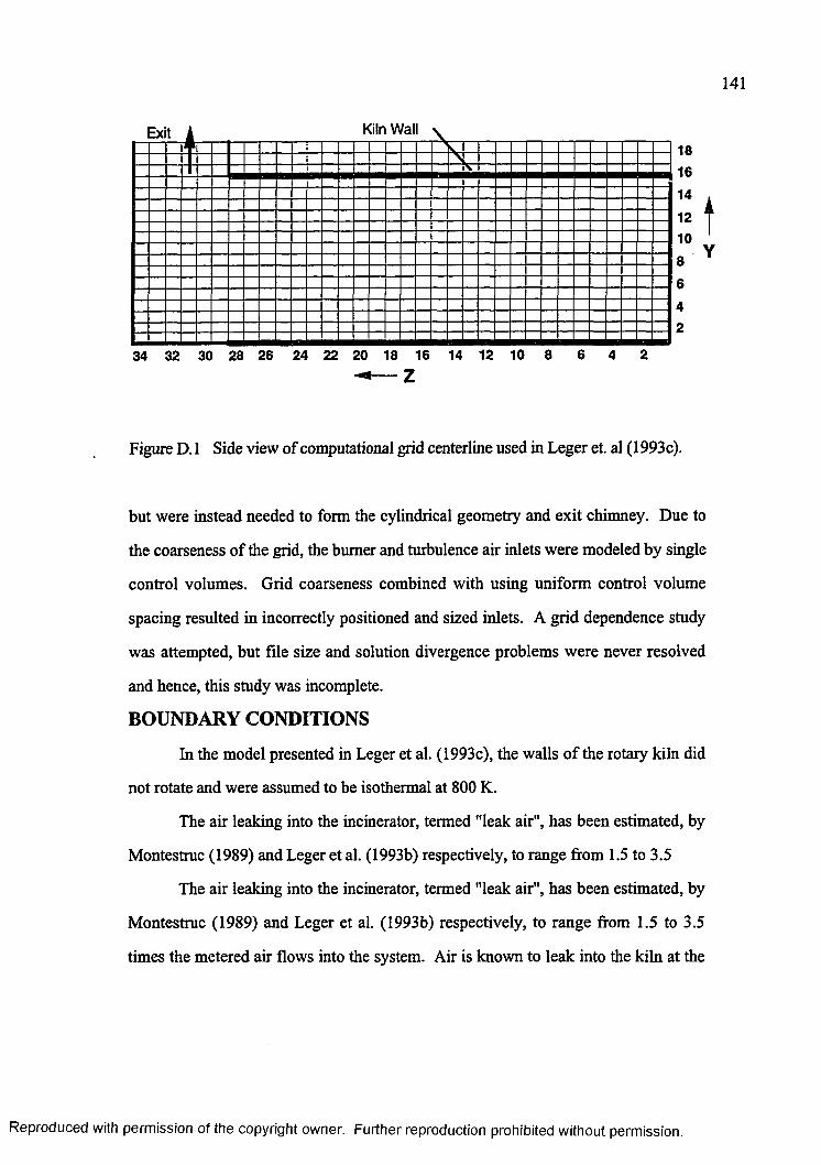
141
Kiln Wall
34 32 30 28 26 24 22 20 18 16 14 12 10 8 6 4 2
1816
14
12108642
t
Figure D. 1 Side view of computational grid centerline used in Leger et. al (1993c).
but were instead needed to form the cylindrical geometry and exit chimney. Due to
the coarseness of the grid, the burner and turbulence air inlets were modeled by single
control volumes. Grid coarseness combined with using uniform control volume
spacing resulted in incorrectly positioned and sized inlets. A grid dependence study
was attempted, but file size and solution divergence problems were never resolved
and hence, this study was incomplete.
BOUNDARY CONDITIONS
In the model presented in Leger et al. (1993c), the walls o f the rotary kiln did
not rotate and were assumed to be isothermal at 800 K.
The air leaking into the incinerator, termed "leak air", has been estimated, by
Montestruc (1989) and Leger et al. (1993b) respectively, to range from 1.5 to 3.5
The air leaking into the incinerator, termed "leak air", has been estimated, by
Montestruc (1989) and Leger et al. (1993b) respectively, to range from 1.5 to 3.5
times the metered air flows into the system. Air is known to leak into the kiln at the
Reproduced with permission of the copyright owner. Further reproduction prohibited without permission.
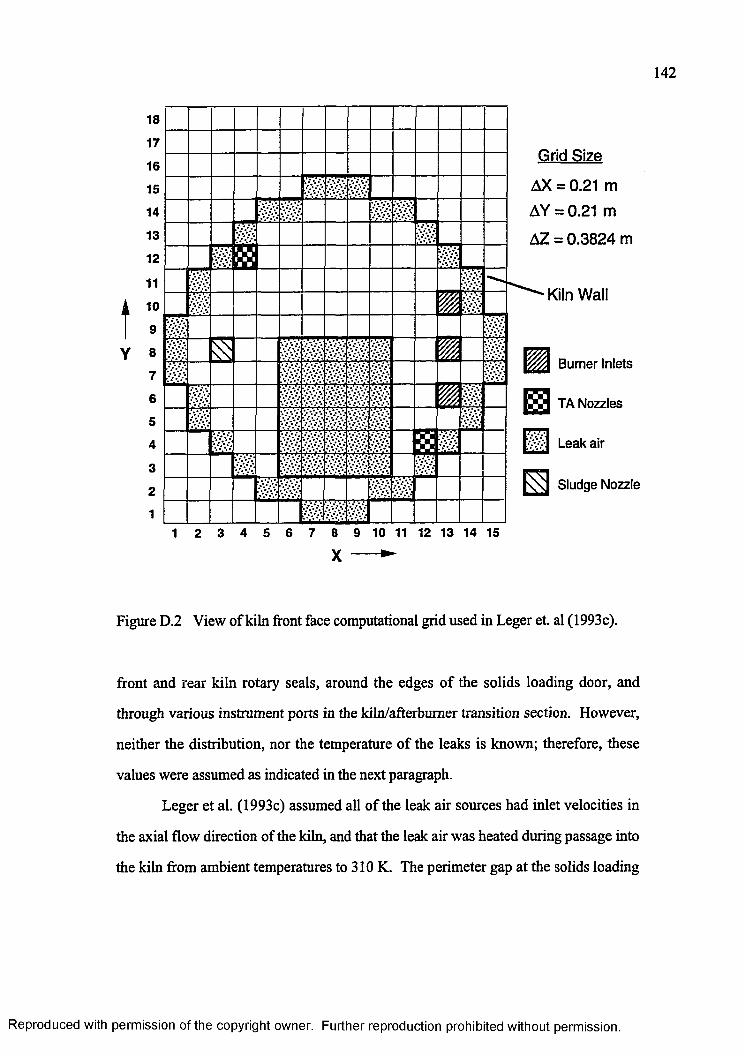
142
18
17
16
15
14
13
12
11
A 10
9
Y 87
6
5
4
3
2
11 2 3 4 5 6 7 8 9 10 11 12 13 14 15
X — ►
Figure D.2 View of kiln front face computational grid used in Leger et. al (1993c).
front and rear kiln rotary seals, around the edges of the solids loading door, and
through various instrument ports in the kiln/afterbumer transition section. However,
neither the distribution, nor the temperature of the leaks is known; therefore, these
values were assumed as indicated in the next paragraph.
Leger et al. (1993c) assumed all of the leak air sources had inlet velocities in
the axial flow direction of the kiln, and that the leak air was heated during passage into
the kiln from ambient temperatures to 310 K. The perimeter gap at the solids loading
????/Av'Ji l l :
w.v
*. .* *. .<
ess?
i
ill
yV.y' >'
y.-y;\V -.V
V;*V.
.• • .* •
■W :W y
7T7T>•••••••v’\*
■y&y* ' • ••••• *. ■
W iM“ hlil
ttr .•;.* •: -v • • • • •
__• • •
* .* •
*. «• .■* •v*J s
Grid Size
AX = 0.21 m
AY = 0.21 m
AZ = 0.3824 m
Kiln Wall
Burner Inlets
TA Nozzles
\M Leak air
Sludge Nozzle
Reproduced with permission of the copyright owner. Further reproduction prohibited without permission.
door was assumed to account for 35 percent of the leak air. The gap in the rotary
seals is small but encompasses the perimeter of the kiln; therefore, 20 percent of the
leak air was assumed to enter through each of the front and rear seals at a temperature
o f 400 K. The remaining 25 percent represents the combination of any leaks
downstream of the kiln, particularly in the kiln-to-afterbumer transition section. The
transition section leaks were modeled as a 310 K upward flow issuing from the
bottom of the transition section.
FLUID PHYSICAL PROPERTIES
The density of the gas was calculated using the ideal gas law, thereby
accounting for the effects of buoyant forces that result from the variations in gas
density caused by temperature and species concentration. The natural gas from the
burners at the field-scale contained a minimum of 95 percent methane by volume and
therefore was input as pure methane.
The reaction rate for methane combustion was determined using a combination
o f a turbulent eddy mixing model presented in Magnussen and Hjertager (1977) and
Arrhenius kinetics. However the activation energy for the reaction was decreased by
six orders of magnitude due to uncertainty about the kinetic parameters. As a result,
the reaction rate was controlled by the turbulent mixing rate.
The combustion reaction was modeled by a one step global reaction shown in
Equation D .l. Species conservation equations were solved for nitrogen, oxygen,
methane, carbon dioxide, and water vapor. Turbulent effects were modeled using the
Algebraic Stress Model (ASM).
CH4 + 2 O2 --------> C 02 + 2H20 (D.l)
Reproduced with permission of the copyright owner. Further reproduction prohibited without permission.
144
Although the effective turbulent viscosity is the overwhelming factor
controlling the fluid viscosity, the laminar viscosity was also specified. The
combustion gases, which are approximately the same composition as air, were
modeled using atmospheric air properties in the laminar viscosity and thermal
conductivity calculations. The laminar viscosity was related to temperature by fitting
a fourth order polynomial to data from Incropera and DeWitt (1985) over the 300 K
to 3,000 K range. In the same manner, the laminar thermal conductivity versus
temperature relationship was approximated by a fourth order polynomial using data
for air taken over the same temperature range and source. The energy equation was
solved in terms of enthalpy, and the temperature was then extracted from the result
using the specific heat of the fluid. The enthalpy of the gas was determined by
integrating the specific heat from a reference temperature of 298 K to the actual
temperature. The gas composition was accounted for in the enthalpy calculation by
computing the mixture specific heat as a mass fraction weighted average o f the
individual, pure component heat capacities. The pure component heat capacities
were entered as second order polynomials in temperature as presented by Theodore
and Reynolds (1987).
SOLUTION METHOD
The differential equations were solved using a commercially available software
package: FLUENT V3.03. The FLUENT code used a control volume-based finite
difference method in which the equations were discritized using a quadratic upwind
scheme called QUICK. The pressure-linked continuity and momentum equations
were solved using the Semi-Implicit Method For Pressure-Linked Equations
Consistent (SIMPLEC) algorithm. The resulting matrices were solved using a
combined Gauss-Seidel and Thomas TriDiagonal-Matrix Algorithm (TDMA) routine.
Reproduced with permission of the copyright owner. Further reproduction prohibited without permission.
145
The problem was cast as a transient problem with steady state boundary conditions
to provide better convergence.
Reproduced with permission of the copyright owner. Further reproduction prohibited without permission.
APPENDIX E
KILN WALL HEAT LOSS CALCULATIONS
Previous modeling by Leger et al. (1993c) assumed that the 33 cm thick refractory
brick walls of the rotary kiln behave isothermally. To determine the appropriate heat
transfer boundary condition, a heat balance was conducted on the rotary kiln.
Assuming an outer wall temperature of 320 K (determined by touch), a light wind of
4.5 m/s, an ambient temperature of 300 K, and an exterior wall emissivity of 0.8,
convection and radiation losses were calculated to be 24.4 and 18.5 kW, respectively.
Heat release from the natural gas support flame (assumed to be pure methane) was
calculated to be 4,637 kW. Therefore, the combined radiation and convection losses
are less than 1 percent of the total heat loading, hence the isothermal wall assumption
of the preceding model (Leger et al, 1993 c) was replaced with an adiabatic wall
assumption. This boundary condition produces a maximum wall temperature
difference between top and bottom of 100° C, which is reasonable considering the
rotation and thick, insulating construction of the wall.
146
Reproduced with permission of the copyright owner. Further reproduction prohibited without permission.
APPENDIX F
COMPUTER CODE FOR RADIATION USER SUBROUTINE
# i f NASA.FUNCTICN USERAC ( ERESSR, TEMP, MDLEFR, MASSFR, MDLWTS, LENGTH,
+ VOLUME, IVALUE, JVALUE, KVALUE, LVALUE, NUMSFC,+ ILAMDA, m S M )
# e l s eFUNCTICN USERAC ( ERESSR, TEMP, MDLEFR, MASSER, MDLWIS, LENGflH,
+ VOLUME, IVALUE, JVALUE, KVALUE, LVALUE, NUMSFC )# a x i i f
C SCCS ID @ (# )u s e r a c .F 4 .2 2 /2 7 /9 2C---------------------------------------------------------------------------------------------------CC NAME : USERAC Cc PROGRAM : FLUENTcr*
VERSION : V 3 .0 0L,c (C) COPYRIGHT BY CREARE.X, INC, 1989
cr*
ARGS DESCRIPTIONC.c INRTT : ERESSR _ ABSOLUTE PRESSUREc TEMP - TEMPERATUREc MDLEFR - MDLE FRACTIONSc MASSER - MASS FRACTIONSc MDLWTS - MOLECULAR WEIGHTSc LENGIH - LENGTH OF CELT. IN RADIATION FLUX DIRECTIONc VOLUME - VOLUME OF CRT ,Tic IVALUE - I-INDEX OF CELLc JVALUE - J-3NDEX OF CELT,c KVALUE - K-INDEX OF CELLc LVALUE - L-INDEX OF CETiTi
c NUMSPC - NUMBER OF PRIMARY PHASE SPECIES DEFINEDc ILAMDA - WAVELENGTH BAND NUMBERc INGRAY - =1 => NGN-GRAYc =0 => GRAYc OUTPUT : NONECC PURPOSE : THIS FUNCTICN EEIURNS THE ABSORPTION COEFFICIENT FOR
147
Reproduced with permission of the copyright owner. Further reproduction prohibited without permission.
148
c r a d ia t t c n frcm th e m il e a n d /o r m a ss f r a c t io n s a n dC THE LOCAL TEMPERATURE AND PRESSURECC COMMENTS : THE ORT.T. LENGTH, TEMPERATURE AND THE PRESSURE AREC IN THE USER DEFINEDUNITS SYSTEMS AND THE RETURNEDC ABSORPTION COEFFICIENT SHOULD BE IN THE USERC SPECIFIED UNITS SYSTEMCCc CALLED BY : RXCALC, RYCALC, RZCALC,CC----------------------------------------------------------------------------------------------------------------C# in c lu d e "IMPLICIT. INC"C To i i t p o r t t h e d e l c r i a t i o n s i z e o f t h e a r r a r y s [ARYSIZ]
INCLUDE 'SIZE.IN C 'C To d e te r m in e t h e c e l l t y p e [ICELL (ARYSIZ) ]c # in c lu d e ’’BOUNDS.INC"C To irrp ort t h e t e r p e r a t u r e s [T(ARYSIZ) ]C # in c lu d e "FLOPRO.INC”C F o r t h e a b s o r p t io n c o e f . [ABSR (ARYSIZ) ]# in c lu d e "REFLUX.INC"CC FUNCTION TYPE DECLARATION.. . Cc----------------------------------------------------------------------------- cC REAL USERAC Ccc--------------------------------------------------------------------------- cC ARGUMENT TYPE DECLARATIONS.. . Cc--------------------------------------------------------------------------- cc
IMPLICIT NONEINTEGER NUMSFCINTEGER IVALUEINTEGER JVALUEINTEGER KVALUEINTEGER LVALUE
REAL VOLUMEREAL LENGIHREAL ERESSRREAL TEMPREAL MOLWTS (NUMSFC)REAL MOLEFR(NUMSPC)REAL MASSFR (NUMSPC)
c# i f NASA
INTEGER ILAMCft.
Reproduced with permission of the copyright owner. Further reproduction prohibited without permission.
149
INTEGER INGRAY# e n d i fC %%%%%%%%%%%%%%%%%%%%%%%%%%%%%%%%%%%%%%%%%%%%%%%%%%%%%%%%%%%%%CC r e v 16 F eb 95 b y A l l e n Ja)<wayC THIS FUNCTICN CALCULATES THE ABSORBITVITY [AS] o fC s o o t p a r t i c l e s , o f a g a s w i t h a i r , C 02, & H20 [AG], an d t h eC com b in ed a b s o r p t i v i t y [AT] a n d a b s o r p t io n c o e f [USERAC].C %%%%%%%%%%%%%%%%%%%%%%%%%%%%%%%%%%%%%%%%%%%%%%%%%%%%%%%%%%%%C MEL = MEAN Beam L en g thC FV = V olum e F r a c t io nC DDOG = D o u b le P r e c i s io n n a t u r a l l o g , i . e . (In )C
REAL*8 MEL, A l , A 2, G l, G2, AS, AT, AG, FV, USERACDP REAL*8 E3,ABSGP, RSP, VSP, B , RDNIV REAL*8 PH20, PC02, P, PI REAL*8 TEMPDP, MDLEFRDP (NUMSFC)
C REAL ABSR (ARYSIZ)C INTEGER L, ICELLCC-------------------------------------------------------------------------------------------------------------------------CC LOCAL VARIABLE TYPE DBCLARATICNS. . . CC-------------------------------------------------------------------------------------------------------------------------CCC
REAL EMALLPARAMETER ( SMALL = 1 .0 E -1 5 )
CC P = A tm o sp h er ic P r e s s u r e i n ATM
P = 1 .D 0C C a lc u la t e t h e m ean beam l e n g t h
MEL = 0 .95D 0 * 3 .18D 0 C C hange f r o n s i n g l e t o d o u b le p r e c i s i o n
TEMPDP =TEMP MDLEFRDP =MDLEFR USERACDP =ABSR (LVALUE)
CCC S o o t o n i s s i v i t y c a l c u l a t i o n
AS =0.0D 0IF (KVALUE .LT. 7 ) THEN P I = 3 . 141593D0
C RUNIV = UNIVERSAL GAS CONSTANTRUNIV = 0 .08205D 0
C RSP = The r a d iu s o f a s o o t p a r t i c l eRSP = (5 0 .D -9 ) /2 .D 0
C VSP = The v o lu m e o f a s o o t p a r t i c l eVSP = ( 4 .DO/3.DO)*PI*RSP**3
C B = M u l t i p l i e r t o g o frcm m o le f r a c t . o f C t o v o l . f r a c t . [FV]o f s o o t
B = P *6.022045D 23*V SP*1000.D 0/(1.D 6*R U N IV )
Reproduced with permission of the copyright owner. Further reproduction prohibited without permission.
nn
no
nn
nn
no
an
on
on
no
g
oo
no
n on
o
oo
oo
oo
o
150
IF (LVALUE.EQ. 1323) THEN W R ITER ,*) 'TEMP=' ,TEMP, 1 T (LVALUE) = ' ,T (LVALUE)W RITE(*,*) 'TEMEDP=', TEMPDP, ' TEMP=',TEMP W RTIE(*,*) ,USERACDP=', USERACDP, ' ABSR (LVALUE) = ' ,ABSR (LVALUE)
END IF
C a lc u la t e t h e s o o t vo lu m e f r a c t i o n FV = MDLEFRDP(5) *B / TEMPDP
C a lc u la t e t h e a b s o r b t i v i t y o f s o o t a lo n e (n o g a s }A l = 1 .4 4 7 D 0 - ( 7 . 943D-4)*TEMPDP + (7.977I>-8)*TEMPDP**2 A2 = 1 .D 0 - A lG1 = DEXP(13.70D0 + 1.001D0*DLOG(FV))G2 = DEXP(14.83D0 + 0.9951D0*DD0G (FV))AS = A l* (1.D0-DEXP(-G1*M BL)) + A2* (l.D0-DEXP(-G 2*M BL))
END IF
Now c a l c u l a t e t h e a b s o r b t i v i t y o f t h e g a s e s a lo n e (no s o o t ) C o n v e r t f r a n m o le f r a c t i o n t o p a r t i a l p r e s s u r e PH20 = MDLEFRDP(4) * P P002 = MDLEFRDP(3) * PCALL GASRAD(1100.DOfTEMPDP,PH20,P002,MBL,EG(AG,ABSGP)
Now c a r b in e t o f i n d t o t a l a b s o r b t i v i t y o f t h e g a s a n d s o o t eAT = AS + AG -AS*AG
Now c a l c u l a t e t h e a b s o r p t io n c o e f (USERAC)IF (AT .EQ. 1 .0 D 0 ) THEN
USERACDP = 1 0 .DOPT.QF.
USERACDP = (-DDDG(l.DO-AT)) /MBL END IFUSERAC = USERACDP
O utputWRITE**,*) ' LVALUE=', LVALUE, ' USERAC=’ , USERAC IF(IVALUE.EQ. 9 .AND. JVALUE.EQ.13) THEN
IF (KVALUE. CT. 5 .AND. KVALUE.LT.18) THENW RITE(*,*) ' IVALUE=',IVALUE, 1 JVALUE=' , JVALUE, ' K=',KVALUE WRITE ( * ,* ) 1 TEMPDP=', TEMPDP, ' TEMP=',TEMP W RITE**,*) ’MDLEFR(C) = ',MDLEFR(5)
W RITE(*,*) 'MDLEFR(4) = ’ ,MDLEFRDP(4), ' MDLEFR (H20) = ‘ , MDLEFR (4) WRITE**,*) 'MDLEFR(3) = ',MDLEFRDP(3), ' MDLEFR(C02) = ' , MDLEFR(3)
W RITE**,*) ' PH20=' , PH20, ' PC02=’ ,P 002W RITE(*,*) 'E V ',F V , 1 B ’ ,B , ' VSP = ' ,VSPW RITE(*,*) ’A l ' ,A 1 , ' A 2 ' ,A 2 , ' G 1 ',G 1 , ' G 2',G 2W RITE(*,*) 'A S ',A S W RITE**,*) ' USERAC=',USERACW RITE(*,*) 'CURRENT T = ' ,TEMP, 1 NEXT TIERATICN'
Reproduced with permission of the copyright owner. Further reproduction prohibited without permission.
151
C ENDIFC ENDIF C
REIURNEND
SUBROUTINE! GASRAD(TS0,TG,PH20,PC02,L,SUMEM,SUMABS,ABSGP)CC THIS SUBROUTINE CALCULATES THE TOTAL EMISSIVTIY [SUMEM] AND ABSORBITVTIYC [SUMABS] OF A MIXIURE OF CARBCN DIOXIDE, WATER VAPOR AND A C NUN-PARTICIPATING GAS (AIR) . THE PARTIAL PRESSURES OF THE GASEOUS C CONSTITUENTS [PH20 & FQ 02], THE TEMPERATURE OF THE GAS MIXIURE [TGI, AND
C THE TEMPERATURE OF THE SOURCE OF THE RADIATION [TSO] ARE REQUIRED INPUTS.CCC
IMPLICIT REAL*8 (A-H, K, L ,N , O-Z)INTEGER V 1,V 2,V 3DIMENSION NUHH(IO) ,NUHC(10) ,DELTAH1(10) ,DELTAH2 (1 0 ) ,
$ DELTAHA3 (10) ,DELTAHB3 (1 0 ) ,$ DELTAHC3 (10) ,DELTAH4 (10) ,DELTAH5 (1 0 ) ,$ DELTAC1 (10) ,DELTAC2 (10) ,DELTAC3 (10) ,DELTAC4(10),$ DELTAC5 (10) ,DELTAC6(10) ,U (1 0 ) ,U 0 (10) ,TAUG (15),$ BLRIRNS(25) ,N U (25) ,NUL(25) ,NUU(25) ,DELNU(15) ,$ NULP(15) ,NUUP(15)
CC INPUT PARAMETERS CC WRTTE(*,*) 'TSO= ' ,T S O ,' T G = \T G ,' L = ',L C W RITE(*,*) ' PH20= ' , PH20, ' PC 02=',PC 02
P = 8 4 7 8 6 .D 0/101325.D O P0 = 1 .D 0 TO = 1 0 0 .DO
CHCEK = 1 .4388D 0
CC SPECIFY PARAMETERS FOR H20 C
NUHH(l) = 3 6 5 2 .DO NUHH(2) = 1 5 9 5 .DO NUHH(3) = 3 7 5 6 .DO
CDELTAHl(l) = 0 DELTAH1(2) = 0 DELTAH1(3) = 0 DELTAH2(1) = 0 DELTAH2(2) = 1 DELTAH2(3) = 0
Reproduced with permission of the copyright owner. Further reproduction prohibited without permission.
on
n
152
DELTAHA3(1) = 0 DELTAHA3(2) = 2 DELTAHA3(3) = 0 DELTAHB3(1) = 1 DELTAHB3(2) = 0 DELTAHB3(3) = 0 DELTAHC3 (1) = 0 DELTAHC3(2) = 0 DELTAHC3(3) = 1 DELTAH4(1) = 0 DELTAH4(2) = 1 DELTAH4(3) = 1 DELTAH5(1) = 1 DELTAH5(2) = 0 DELTAH5(3) = 1
CMH = 3 NH = 1
CEH = 8 . 6D0*(TO/TG)* * 0 .5D0 +
CA0H1 = 5 2 0 0 .DO A0H2 = 41 .2D 0 A03HA = 0 .19D 0 A03HB = 2 .3D 0 A03H2 = 2 2 .4D 0 A0H4 = 3 .0D 0 A0H5 = 2 .5D 0
CB0H1 = 0 .14311D 0 B0H2 = 0 . 09427D0 B0H3 = 0 . 13219D0 B0H4 = 0 .08169D 0 B0H5 = 0 . 11628D0
CVJ0H1 = 28 .4D 0 W0H2 = 56 .4D 0 W0H3 = 6 0 .DO W0H4 = 43 .1D 0 W0H5 = 3 2 .DO
C02 PARAMETERS
NUHC(l) = 1 3 5 1 .DO n u k : ( 2 ) = 6 6 7 .DO NUHC(3) = 2 3 9 6 .DO
CDELTACl(l) = 0 DELTAC1(2) = 1 DELTAC1(3) = 0 DELTAC2 (1) = - 1
0 .5D 0
Reproduced with permission of the copyright owner. Further reproduction prohibited without permission.
no
n
o n
n
o
on
DELTftC2(2) = 0 DELTAC2(3) = 1 DELTAC3(1) = 0 DELTAC3(2) = - 2 DELTAC3 (3) = 1 DELTAC4(1) = 0 DELTAC4(2) = 0 DELTftC4(3) = 1 EELTAC5 (1) = 1 DELTAC5(2) = 0 DELTAC5(3) = 1 DELTAC6(1) = 2 DELTAC6(2) = 0 DELTAC6(3) = 1
M2 = 3 NCI = 0 .7D 0 NC2 = 0 .8D 0 NC3 = 0 .8D 0 NC4 = 0 .8D 0 NC5 = 0 .65D 0 NC6 = 0 .65D 0
BC = 1 .3D 0
A0C1 = 1 9 .DO A0C2 = 2 .4 7 D -9 A0C3 = 2 .4 8 D -9 A0C4 = 1 1 0 .DO A0C5 = 4 .0D 0 A0C6 = 0 .066D 0
B0C1 = 0 .06157D 0 B0C2 = 0 . 04017D0 B0C3 = 0 .11888D 0 B0C4 = 0 .24723D 0 B0C5 = 0 . 13341D0 B0C6 = 0 .39305D 0
W0C1 = 12 .7D 0 W0C2 = 13 .4D 0 W0C3 = 10 .1D 0 W0C4 = 11 .2D 0 W0C5 = 2 3 .5D 0 W0C6 = 3 4 .5D 0
H20 CADCULATiaSIS
U ( l ) = HCCK*NUHH(1)/,IG U (2 ) = HCDK*NUHH (2) /TG
Reproduced with permission of the copyright owner. Further reproduction prohibited without permission.
no
oo
oo
n
on
n
on
n
on
n
on
n
on
o
no
o
nU (3 ) = HCDK*NUHH(3)/TG
CU 0 (1 ) = B2DK*NUHH(1)/T0 U 0 (2 ) = BCEK*NUHH(2)/T0 0 0 ( 3 ) = H2CK*NUHH(3)/T0
ROTATIONAL BfiND ALH1 = AOHL W RTIE(*,*) ,ALHL',ALH1
6 .3 BfiNDPSITG = 1 .D 0 / (1 .D 0 - D E X P (-U (2)))psrro = i .d o/(I.do - de x p(-u o (2)))ALEE = ALFEEA(DELTAH2,U,U0,A0H2,MH,PSITG, PSTTO)W RTIE(*,*) 'ALH2' ,AIB2
2 .7 (A) BfiND PSITG = 2 . DO/ (I.D O - D E X P (-U (2))) * * 2 .DO PSITO = 2 . D O /(I.D O - D E X P (-U 0(2)) )* * 2 .D 0 ALH3A = ALPHA. (DELTftHZG, U, UO, A03HA, MH, PSITG, PSITO)WRITE( * ,* ) 'ALH3A' ,AIH3A
2 .7 (B) BAND PSITG = I .D O /(I .D O - D E X P (-U (1)))PSITO = I .D O /(I .D O - DEXP(-UO ( 1 ) ) )ALH3B = ALPHA (DELTAHB3,U,U0,A03HB,MH, PSITG, PSITO)WRITE(*, *) 'ALH3B' ,ALH3B
2 .7 (C) BAND PSTIG = I .D O /(I .D O - D E X P (-U (3)) )PSITO = I .D O /(I .D O - DEKP(-UO ( 3 ) ) )ALH3C = ALPHA (DELTAH23,0 ,0 0 ^ 0 3 1 1 2 ,1 ® !, PSITG, PSTTO)WRITE(*, *) ,ALH3C, ,ALH3C
2 .7 BfiND AIH3 = AIH3A + AIH3B + ALH3C WRITE(*f *) 'ALH31 ,ALH3
1 .8 7 BfiNDPSTIG = I .D O /( (I .D O - D E X P (-U (2)) ) * (I.DO - D E X P (-U (3)) ) )PSITO = I .D O /( (I .D O - BEXP(-UO ( 2 ) ) ) * (I.DO - D E X P (-U 0(3)) ) )ALH4 = ALPHA(DELTAH4,U,UO,AOH4,MH, PSITG, PSITO)W RITE(*,*) 'ALH4' , AIH4
1 .3 8 BfiNDPSTIG = I .D O / ( (I.D O - D E X P (-U (1)) ) * (I.DO - D E X P (-U (3)) ) ) PSTTO = I .D O /( (I .D O - DEXP(-UO ( 1 ) ) ) * (I.DO - DEXP(-UO ( 3 ) ) ) ) ALEE = ALPHA (DELTfiH5,U,U0,A0H5,MH, PSTIG, PSTTO)W RITE(*,*) 'ALH5',ALH5
Reproduced with permission of the copyright owner. Further reproduction prohibited without permission.
<n</
><n<
n </>
</></>
-c/>
</>
</>
155
C H20 ROTATIONAL BAND C
EEIAH1 = BOHl* (TG/TO) ** (- .5 D 0 )CC 6 .3 BAND
TERMl = O.DO ERR = I.DO V2 = 0DO WHILE (ERR. G T .l.D -9 )
TERM = (V2+1) **.5D 0*D EX F(-U (2) *V 2/2 .D 0)TERMl = TEEM1 + TEEM ERR = DABS(TERM/TERM1)V2 = V2 + 1
END DOEHTIG = (I .D O / (I.D O - BEXP(-U(1) / 2 .D 0 ) }) **2.D0*TERML**2.D0*
(I .D O /(I .D O - D E X F (-U (3 )/2 .D O )) )* * 2 .D 0 * (l.D O -D E K P (-U (l)) ) * (I.DO - D E X P (-U (2 )))* * 2 .D 0 * (I.DO - D E X P (-U (3)))
W RITE(*,*) 'E H nO E ',E H T IG TERMl = O.DO ERR = I.DO V2 = 0DO WHILE (E R R .G T .l.D -9)
TERM = (V 2+ 1)** .5D 0*D E X P (-U 0(2)*V 2/2 .D 0)TERMl = TERMl + TERM ERR = DABS(TERM/TERML)V2 = V2 + 1
END DOEEHTO = (I .D O /(I .D O - D E X P (-U 0(1)/2 .D 0)))**2.D 0*T E R M L **2.D 0*
(I .D O / (I.DO - D E X P (-U 0 (3 )/2 .D 0 )))* * 2 .D 0 * (l.DO-DEXP(-UO ( 1 ) ) ) * (I.DO - D E X P (-U 0 (2 )))* * 2 .D 0 * (I.DO - DEXP(-U0 ( 3 ) ) )
W RTIEf*,*) 'EHTT0H2', EHTIG BEIAH2 = B 0H 2*(T 3/T 0)**(-.5D 0)*E H n G /E H IT 0
(A) BAND TERMl = O.DO ERR = I.DO V2 = 0DO WHILE (ERR. G T .l.D -9 )
TERM = (V 2+ 1)** .5D 0*(V 2+ 2)** .5D 0*D E X F (-U (2)*V 2/2 .D 0) TERMl = TERMl + TERM ERR = DABS(TERM/TERM1)V2 = V2 + 1
END DOEHTIG = 0 .5 D 0 * (1 .D 0 /(1 .D 0 -D E X F (-U (1 ) /2 .D 0 )) )* * 2 .D 0
*TERML**2.D0*(I .D O / ( l .D 0 -D E X E (-U (3 ) /2 .D 0 )) ) * * 2 .DO * ( l.D O -D E X E (-U (l)) ) *(l.D 0 -D E X F (-U (2 )) )* * 3 .D 0 * (1 .D 0 -D E X P (-U (3 )) )
Reproduced with permission of the copyright owner. Further reproduction prohibited without permission.
c w r it e * * ,* ) ’r a n o c A ’ , ehttgTERML = O.DO ERR = I.DO V2 = 0DO WHILE (E R R .G T .l.D -9)
TERM = (V 2+1)* * .5D 0*(V 2+2) * * . 5D0*$ D E X F (-U 0(2)*V 2/2.D 0)
TERML = TERML + TERM ERR = DABS(TERM/TERMl)V2 = V2 + 1
END DOEHITO = 0 .5D 0* (1 .D 0 /(l.D 0 -D E X P (-U 0 ( 1 ) / 2 .D 0 ) ) )* * 2 .D 0
$ *TERML**2.D0*$ (I .D O / (l.D 0-D E X P (-U 0(3) / 2 .D 0 ) ) ) * * 2 .DO$ * (1 .D 0-D E X P (-U 0(1 )) ) *$ (l.D 0-D E X P (-U 0 ( 2 ) ) ) **3 .DO* (l.D 0-D E K P (-U 0 ( 3 ) ) )
C WRITE(*, *) 1 EHTT0H3A1, EHITOEETEAH3A = B0H3* (T3/TO )** (-.5D 0)*EK nG /EH ITO
CC 2 . 7 (B) BAND
TERML = O.DO ERR = I.DO V I = 0DO W HILE(ERR.GT.l.D-9)
TERM = (V 1+ 1)** .5D 0*D E X P (-U (1)*V 1/2 .D 0)TERML = TERML + TEEM ERR = DABS(TERM/TERML)V I = V I + 1
END DOEHTIG = T E R M L * * 2 .D 0 * (1 .D 0 /(1 .D 0 -D E X P (-U (2 )/2 .D 0 ))* * 2 .D 0 )*
$ ( 1 .D 0 /(1 .D 0 -D E X P (-U (3 )/2 .D 0 ))* * 2 .D O )*$ ( l .D 0 -D E X P (-U ( l) ) )* * 2 .D 0 * ( l .D 0 -D E X P (-U (2 ) ) )*$ ( l.D 0 -D E X P (-U (3 )) )
C W RiraK*,*) 'EHTDaCB', EHTIGTERML = O.DO ERR = I.DO V I = 0DO W HILE(EER.GT.l.D-9)
TERM = (V l+1) **.5D0*DEXP(-U0 (1) *V 1 /2 .D 0)TEEMl = TERML + TERM ERR = DABS (TERM/TERML)V I = V I + 1
END DOEHTTO = TERML**2.D0* (I .D O / (l.DO-DEXE(-UO (2) / 2 .D 0 ) ) * * 2 .DO) *
$ (l.D O /(l.D O -D E X F (-U O (3 )/2 .D O ))* * 2 .D O )*$ ( l .D 0 -D E X P (-U 0 ( l) ) )* * 2 .D 0 * (l.D 0 -D E X E (-U 0 (2 ) ) )*$ (l.D 0-D E X F(-U 0 ( 3 ) ) )
C WRITE(*, *) 'EHTT0H3B', EHITOBETAH3B = B0H3* (T3/T0) ** ( - .5 D 0 ) *EHTIG/EHITO
CC 2 .7 (C) BAND
Reproduced with permission of the copyright owner. Further reproduction prohibited without permission.
</></>
<n
<n<n
157
TERMl = O.DO ERR = I.DO V3 = 0DO WHILE (E R R .G T .l.D -9)
TERM = (V 3+ 1)**.5D 0*D E X E (-U (3)*V 3/2.D 0)TERMl = TERMl + TERM ERR = DABS(TERM/TERML)V3 = V3 + 1
END DOEHTIG = ( l .D 0 /( l .D 0 - D E X F ( - U ( l ) /2 .D 0 ) ) ) * * 2 .D 0 *
(1 .DO/ (1 .D 0-D E X P (-U (2) / 2 .D 0 ) ) ) **2 .D0*TERML**2 .DO* (l.D O -D E X B (-U (l)) ) * ( l .D 0 -D E X F (-U (2 )) ) * (l.D 0 -D E X P (-U (3 )) ) * * 2 .DO
W RITE(*,*) 'EHTIGH3C1, EHTIG TERMl = O.DO ERR = I.DO V3 = 0DO WHILE (E R R .G T .l.D -9)
TERM = (V 3+ 1)** .5D 0*D E X E (-U 0(3)*V 3/2 .D 0)TERMl = TERMl + TERM ERR = DABS(TERM/TERML)V3 = V3 + 1
END DOEHTTO = ( l .D 0 /( l .D 0 - D E X F ( - U 0 ( l ) /2 .D 0 ) ) ) * * 2 .D 0 *
(l.D 0 /(l.D 0 -D E X E (-U 0 (2 )/2 .D 0 )))* * 2 .D 0 * T E R M l* * 2 .D 0 * ( 1 .DO-DEXE ( -U O ( l) ) )*(1.DO -DEXE(-UO ( 2 ) ) )*(1 .DO-DEXE(-U0 ( 3 ) ) ) **2 .DO
C W R3TE(*,*) ' EHTT0H3C1, EHTTOEEIAH3C = B 0H 3*(T G /T 0)**(-.5D 0)*E H nG /E H IT 0
CC 2 .7 BAND
EETAH3 = ( ( (ALH3A*EEIAH3A) * * . 5D0 + (ALH3B*EEIAH3B) * * . 5D0 $ + (ALH3C*BEIAH3C) * * . 5D0) * * 2 . DO) /ALH3
CC 1 .8 7 BAND
TERML = O.DO ERR = I.DO V2 = 0DO WHILE (E R R .G T .1.I>9)
TERM = (V 2+1)** .5D 0*D E X F (-U (2)*V 2/2 .D 0)TERMl = TERML + TERM ERR = DABS(TERM/TERML)V2 = V2 + 1
END DOTERM2 = O.ODO ERR = I.DO V3 = O.DODO WHILE (ERR. G T .l.D -9 )
TERM = (V 3+ 1)** .5D 0*D E X F (-U (3)*V 3/2 .D 0)TERM2 = TERM2 + TERM ERR = DABS(TERM/TERM2)
Reproduced with permission of the copyright owner. Further reproduction prohibited without permission.
158
V 3 = V3 + 1END DOEHTIG = (I .D O / ( 1 . DO-DEXE ( - U ( l ) / 2 . D O ) ) )**2.D0*TERM L**2.D0*
$ TERM2**2.D0* ( 1 .DO-DEXE ( - U ( l ) ) ) * ( l .D 0 -D E X P (-U (2 )) )$ * * 2 .DO*$ (1 . DO-DEXE ( - U ( 3 ) ) ) * * 2 .DO
C W RITE(*,*) ,H JnG H 4, > EHTIGTERMl = O.DOERR = I.DOV2 = 0DO WHILE (E R R .G T .l.D -9)
TERM = (V 2+ 1)** .5D 0*D E X E (-U 0(2)*V 2/2 .D 0)TERMl = TERMl + TERM ERR = DfiBS(TERM/TERML)V2 = V2 + 1
END DOTERM2 = 0 .0D 0ERR = I.DOV3 = O.DODO WHILE (ERR. G T .l.D -9 )
TERM = (V3+1) **.5DO*DEXE(-UO (3) *V 3/2 .DO)TERM2 = TEEM2 + TERM ERR = DfiBS(TERM/TERM2)V3 = V3 + 1
END DOEHTTO = (l.D O /(l.D O -D E X F (-U O (l)/2 .D O )))**2.D O *T E R M L **2.D O *
$ TERM2**2 .DO* (1 .DO-DEXE(-UO ( 1 ) ) ) * (1 .DO-DEXE(-UO ( 2 ) ) )$ * * 2 .DO*$ ( 1 . DO-DEXE(-U0( 3 ) ) ) * * 2 .DO
C WRITE(*, *) 1EHTT0H41, EHTIGEEIAH4 = B0H4* (TG/TO) ** {—. 5D0) *EHnG/EHITO
CC 1 . 3 8 BfiND
TERML = O.DO ERR = I.DO V I = 0DO WHILE (E R R .G T .l.D -9)
TERM = (V l+1) **.5D 0*D EX F(-U (1) *V 1 /2 .D 0) TERML = TERML + TERM ERR = DfiBS(TERM/TERML)V I = V I + 1
END DOTERM2 = 0 .0D 0 ERR = I.DO V3 = O.DODO WHILE (ERR. G T .l.D -9 )
TERM = (V 3+ 1)** .5D 0*D E X F (-U (3)*V 3/2 .D 0) TERM2 = TERM2 + TERM ERR = DfiBS(TERM/TERM2)V3 = V3 + 1
END DO
Reproduced with permission of the copyright owner. Further reproduction prohibited without permission.
159
EHTIG = T B R M L * * 2 .D 0 * (1 .D 0 /(1 .D 0 -E E X P (-U (2 )/2 .D 0 )))* * 2 .D 0 *$ T E R M 2**2.D 0*(1 .D 0-D E X P (-U (1)))**2 .D 0*$ ( l.D 0 -D E X P (-U (2 )) )*$ ( l .D 0 -E E X P (-U (3 )))* * 2 .D 0
C WRITE(*( *) 'E H T IQ B ', EHTIGTERMl = O.DO ERR = I.DO V I = 0DO WHILE (E R R .G T .l.D -9)
TERM = (V l+1) **.5D0*DEXP(-U0 (1) *V 1 /2 .D 0)TERMl = TERML + TERM ERR = DABS (TERM/TERML)V I = V I + 1
EM) DOTERM2 = 0 .0D 0 ERR = I.DO V3 = O.DODO WHILE (E R R .G T .l.D -9)
TERM = (V 3+ 1)** .5D 0*IE X P < -U 0(3)*V 3/2 .D 0)TERM2 = TERM2 + TERM ERR = DABS (TERM/TERM2)V3 = V3 + 1
EM) DOEHITO = TERML**2.DO* (I.D O / (l.D 0-D E X P (-U 0 ( 2 ) / 2 . D O ) ) ) * * 2 . DO*
$ T E R M 2**2.D 0*(1 .D 0-E E X P (-U 0(1)))**2 .D 0$ * (l.D 0-D E X P(-U 0 ( 2 ) ) ) *$ (l.D 0 -D E X P (-U 0 (3 )) )* * 2 .D 0
C ' WRTTE(*f *) 'EHIT0H5', EHTIGBEIAH5 = B0H5* (TG/TO ) * * ( - . 5D 0) *EHTIG/EHTrO
CC WRITE(*, * ) ,BETAHS\BETAH1,BEIAH2,BEEAH3/ EEEAH4,BEIAH5 C
RH = 4 . 5545D -6 RH3H = EH20/ (RH*TG)X = RHCH*LWH1 = W0H1* (TG/TO) * * . 5D0 WH2 = W0H2* (TG/TO)**.5D0 WH3 = W0H3* (TG/TO) * * . 5D0 WH4 = W0H4* (TG/TO) * * . 5D0 WH5 = W0H5* (TG/TO)**.5D0
CTMJH1 = ALHL*X/WH1 TAUH2 = ALH2*X/WH2 TAUH3 = ALH3*X/WH3 TAUH4 = ALH4*X/WH4 TAUH5 = ALH5*X/WH5
C W RTIE(*,*) 'TAUHS1 ,TAUH1,TADH2/ TAIH3/ TADH4,TADH5 C
EEH = ( (P/PO) * (I.DO + (BH - I.DO ) * (P H 20 /P ))) **NH BTAH1 = EEEAH1*EEH ETAH2 = BETAH2*PEH
Reproduced with permission of the copyright owner. Further reproduction prohibited without permission.
on
o o
160
ETAH3 = BETAH3*EEH EEAH4 = EEIAH4*FEH B M B = EEEAH5*EEHVJRITE(*, *) 'EIAHS' ,E IA H l/ EI!AH2,EIAH3/ E I M 4 / EEftH5
IF('IM H L .L E .l.D O .A N D .,E O n ..L E .E ffiH l) THEN ASIHL = TAUHl AKL = ASTHL*WHL TADG(l) = TALJKL/ASTHL
ELSE IF (TAtm.GE.ETEAHL .AND. TAUHl. LE. (1 .D 0/E IA H L )) THEN ASTHL = (4.D0*EHAH1*TAUH1)**.5D0 - E3AHL AfflL = ASIH1*WH1TADG(l) = (ETAffl^TAUHl) * * . 5D0/ASIHL
ELSE IF (TALJH1. GT. (l.DO/EIAHL) .AND.ETAKL.LE.1.D0) THEN A SIH l = DDCX3(TAUH1*EIAH1) + 2 . DO - EIAKL AHL = ASTHL *WH1 TAD3(1) = I.D O /A SIH l
ET lS h:
A SIH l = DLOG(TAUHl) + I.DO AKL = ASIHL*WH1 TADG(l) = I.DO/ASIHL
ENDIFIF(TAUG(1) .GfT.0.9D0) THEN
TADG(l) = 0 .9D 0ENDIFDELMJ(l) = AfflL/(1.D0 - T A D S(l))W RITE(*,*) 'AHT ,AKL, 'TAUG(l) ’ ,T A t)G (l), 'D E lM J(l) ' ,DELNU(1)
IF(TAUH2.LE.1.D0.AND.TAUH2.LE.EIAH2) THEN ASIH2 = TAUH2 AH2 = ASIH2*VJH2 TADS (2) = TAUH2/ASIH2
ELSE IF (TAUH2.GE.EIAH2.AND.TAUH2.LE. (I.DO/EEAH2)) THEN ASIH2 = (4.D0*ETAH2*TAUH2)**.5D0 - ETAH2 AH2 = ASIH2*WH2TADG(2) = (ETAH2*TAUH2) ** .5D0/ASIH2
ELSE IF (TADH2.GT. (1.D 0/E T A H 2).AND.ETAH2.LE.I.DO) THEN ASIH2 = DLOG(TAUH2*EIAH2) + 2 . DO - EIAH2 AH2 = ASTH2*WH2 TADS (2) = 1.D0/ASTH2
E L S EASTH2 = DL0G(TADH2) + I.DO AH2 = ASTH2*WH2 TADS (2) = 1.D 0/A SIH 2
ENDIFIF (TADS (2) .C T .0 .9D 0) THEN
TADS (2) = 0 .9D 0ENDIF
CDELNU(2) = A H 2/(I.D O - TADS(2 ))
C W R ITER ,*) 'AH2' ,AH2, 'TAD3(2) 1, TADS( 2 ) , 'DELMJ(2) 1 ,DELNLJ(2)
Reproduced with permission of the copyright owner. Further reproduction prohibited without permission.
no
n
o o
IF(TALJH3.LE.1.D0.AND.TAL]H3 .LE.EIAH3) THEN ASIH3 = TAUH3 AH3 = ASTH3*VJH3 TADG(3) = TADH3/ASTH3 •
ELSE IF (TADH3.GE.ETAH3..AND.TALJH3.LE. (1.DO/E7EAH3)) THEN ASIH3 = (4.D0*EnaH3*TAUH3)**.5D0 - EEAH3 AH3 = ASTH3*WH3TAUG(3) = (ETAH3*TAUH3) * * . 5D0/ASTH3
ELSE IF (TAUH3.CT. (1.D0/EEAH3) .AND.EIAH3 .L E .1 .D 0 ) THEN ASTH3 = DDOG(TAUH3*EI!AH3) + 2 .DO - EEAH3 AH3 = ASTH3*WH3 TALKS (3) = 1.D0/ASIH 3
~FT.gRASTH3 = DD0G(TAUH3) + 1 .D 0 AH3 = ASTH3*MC TALKS (3) = 1.D0/ASTH3
ENDIFIF (TALKS (3 ) .C T .0 .9D 0) THEN
TALKS (3) = 0 .9D 0ENDIF
CDEIMJ(3) = AH3/CL.D0 - TADG(3))WRITEL*, *) 'AH3' ,AH3, 'TALK5(3) ' ,TALKS(3), 'DEIMJ(3) ' ,DELNLJ(3)
IF(TAUH4.LE.1.D0.AND.TALJH4.LE.ETAH4) THEN ASIH4 = TALJH4 AH4 = ASIH4*WH4 TALK3(4) = TAUH4/ASIH4
ELSE IF (TADH4.GE.EEAH4.AND.TALIH4.LE. (1.D 0/E E A H 4)) THEN ASTH4 = (4.D0*ETAH4*TAUH4)**.5D0 - EIAH4 AH4 = ASTH4*WH4TALKS (4) = (EEAH4*TAUH4)**.5D0/ASIH4
ELSE IF (TADH4.GT. (1.D 0/EIA H 4) .AND.EIAH 4.LE.1.D0) THEN ASTH4 = DLOG(TAnH4*E7EAH4) + 2 . DO - BIAH4 AH4 = ASTH4*WH4 TALKS (4) = 1.D0/ASTH4
FT .OFASIH4 = rm3(TAUH4) + 1 .D 0 AH4 = ASTH4*WH4 TALK3(4) = 1.D 0/A SIH 4
ENDIFIF(TALK3(4) .G T .0 .9D 0) THEN
TALK3(4) = 0 .9D 0ENDIF
DELNU{4) = A H 4/{1 .D 0 - TALK3(4))WRITE**,*) 'AH4' ,AH4, ’TALK3(4) ’ ,TALK3(4), ’DELMJ(4) ' ,DELNU(4)
IF(TAUH5.LE.1.D0.AND.TALIH5.LE.EIAH5) THEN ASTH5 = TAUH5
Reproduced with permission of the copyright owner. Further reproduction prohibited without permission.
on
non
non
no
o n
nn
nn
162
AH5 = ASIH5*WH5 TAOS (5) = TAUH5/ASIH5
ELSE IF (TADH5.GE.ETAH5.AND.TAUH5.LE. (1 .D 0 /E IA H 5 )) THEN ASTH5 = (4.D0*EIAH5*TADH5)**.5D0 - EIAH5 AH5 = ASIH5*WH5TAOS (5) = (BTAH5*TAOH5)**.5DO/ASIH5
ELiSE IF (TAUH5.GT. (1.D 0/E IA H 5) .AND.ETAH5.LE.1.D0) THEN ASIH5 = DL0G(TALH5*EEAH5) + 2 . DO - ELCAH5 AH5 = ASTH5*WH5 TAOS (5) = 1.D0/ASTH5
PT..RRASTH5 = DD0G(TAUH5) + 1 .D 0 AH5 = ASTH5*WH5 TAOS(5) = 1.D0/ASTH5
ENDIFI F (TAOS (5) .G T .0 .9D 0) THEN
TAOS(5) = 0.9DOENDIF
CDEENU(5) = AH5/ (1 .D 0 - TAOS(5))W RITE(*,*) 'AH51 ,AH5, 'TAOS(5) ' ,T A D 3 (5 ), 'DELNU(5) M ELNIKS)
C02 CALCULATIONS
u(i) = hcdk*mm:(1)/tgU (2 ) = HSCDK*NUHS(2)/TG U (3 ) = HCDK*NUHS(3)/TG
U 0 (1 ) = HSDK*NUBS(1)/T0 U 0 (2 ) = ESD K *M BS(2)/T0 U 0 (3 ) = HKK*NOHS(3)/TO
15 BANDP SIIG = 2 . DO/ ( 1 .DO - D E X P (-U (2)) )PSITO = 2 . D O /( 1 .DO - D E X P (-U 0(2)))ALC1 = ALPHA (DELTAC1, U, UO, A0C1, MS, PSITG, PSITO)W R ITER ,*) 'ALC1' ,ALC1
1 0 .4 BANDPSITG = ( l .D 0 - D E X P ( - U ( l ) ) ) * ( l .D 0 /( l .D 0 - D E X P ( - U ( l ) ) ) * * 2 .D 0
$ - 1 .D 0) / (1 .D 0 - E E X P (-U (3 )))PSITO = ( l .D 0 - D E X P ( - U 0 ( l ) ) ) * ( l .D 0 /{ l .D 0 - D E X P ( - U 0 ( l ) ) ) * * 2 .D 0
$ - 1 .D 0) / (1 .D 0 - DEXP(-U0 ( 3 ) ) )AIC2 = ALPHA(DELTAC2/ U ,U 0,A 0C 2,M :,PSIT G ,PSIT 0)W RTIE(*,*) 'ALC2' , A I£2
9 .4 BANDADC3 = ALEHA(DELTAC3,U,U0,A0C3,MS,PSITG, PSITO)VJRITE(*,*) 'ALC3' ,AIC3
Reproduced with permission of the copyright owner. Further reproduction prohibited without permission.
163
C 4 .3 BANDPSITG = l .D O /( l .D O - D E X P (-U (3)) )p srro = i . do/ ( i .do - d e x p ( - u o ( 3 ) ) )ALC4 = ALPHA.(DELTAC4,U,U0,A0C4,M3,PSriG, PSITO)
C WRTEE(*,*) 'ALC4’ ,ALC4CC 2 .7 BAND
PSITG = l .D O / ( (l.D O - D E X P (-U (l) ) )* ( l .D O - D E X P (-U (3)) ) )PSITO = l .D O / ( (l.D O - D E X P (-U O (l)))* (l.D O - DEXP(-UO( 3 ) ) ) )ALC5 = ALPHA(DELTAC5,U,U0,A0C5,ttE,PSTIG,PSITO)
C WRTEE(*,*) 'ALC5',ALC5CC 2 .0 BAND
PSITG = 2 . DO/ ( (l.D O - D E X P (-U (1)) ) **2 .DO* (l.D O - D E X P (-U (3)) ) )PSITO = 2 . D O /( (l.D O - D E X P (-U 0 (1 )))* * 2 .D 0 *
$ (l.D O - D E X P (-U 0 (3 ))))ALC6 = ALPHA (DELTAC6,U,U0,A0C6,MC, PSITG, PSITO)
C W RITE(*,*) 'ALC6’ ,ALC6CCC 15 BAND
TERML = O.DO ERR = l.D O V I = 0DO WHILE (ERR. G T .l.D -9 )
TERM = (V 1+1)**.5D O *D EX P(-U (1)*V 1/2.D O )TERM1 = TERM1 + TERM ERR = DABS(TERM/TERML)V I = V I + 1
END DOTERM2 = O.ODO ERR = l.D O V2 = O.DODO WHILE (ERR. G T .l.D -9 )
TERM = (V2+1) * * . 5D0* (V2+2) * * . 5D0*DEXP ( -U (2) *V 2/2 .DO) TEEM2 = TEE M2 + TERM ERR = DABS(TERM/TERM2)V2 = V2 + 1
END DOPHTIG = 0.5D0*TERML**2.D0*TERM2**2.D0*
$ ( l .D 0 /( l .D 0 -D E X P ( -U (3 ) /2 .D 0 ) ) )* * 2 .D 0 *$ (l.D O -D E X P (-U (l)) ) * * 2 .DO* (l.D 0 -D E X P (-U (2 )) ) * * 3 .DO*$ (l.D 0 -D E X P (-U (3 )) )
C WRTIE(*, *) 'HECTGC1', PHTIGTERML = O.DO ERR = l.D O V I = 0DO WHILE(E R R .G T .l.D -9)
TERM = (V l+1) **.5D0*DEXP(-U0 (1) *V 1 /2 .D 0) TERM1 = TERML + TERM ERR = DABS (TERM/TERM1)
Reproduced with permission of the copyright owner. Further reproduction prohibited without permission.
n n
164
V I = V I + 1END DOTERM2 = 0 .0D 0 ERR = l.DO V2 = O.DOIX) WHILE (E R R .G T .l.D -9)
TERM = (V2+1) * * . 5D0* (V2+2) ** .5D0*$ D E X P (-U 0(2)*V 2/2 .D 0)
TERM2 = TERM2 + TERM ERR = DABS(TERM/TERM2)V2 = V2 + 1
END DOPHITO = 0.5D0*TERMl**2.D0*TERM2**2.D0*
$ ( l .D 0 /( l .D 0 -D E X P ( -U 0 (3 ) /2 .D 0 ) ) )* * 2 .D 0 *$ ( l.D 0 -D E X P (-U 0 (l) ) )* * 2 .D 0 * (l.D 0 -D E X P (-
U 0 (2 ) ) )* * 3 .D 0 *$ (l.D 0-B E X P (-U 0 ( 3 ) ) )
C W RITE(*,*) 1HH T0C1' , EHETOEEJIAC1 = B0C1* (TG/TO ) * * ( - . 5D0) *EHTIG/EHITO
1 0 .4 BfiNDTERM1 = O.DO ERR = l.DO V I = 1DO W HILE(ERR.GT.l.D-11)
TERM = (V 1+1)** .5D 0*D E X P (-U (1)*V 1/2 .D 0) TERMl = TERMl + TERM ERR = DABS(TERM/TERML)V I = V I + 1
END DOTERM2 = O.ODO ERR = l.DO V2 = O.DODO WHILE (E R R .G T .l.D -11)
TERM = (V 2+1)** .5D 0*D E X P (-U (2)*V 2/2 .D 0) TERM2 = TERM2 + TERM ERR = DRBS(TERM/TERM2)V2 = V2 + 1
END DOTERM3 = O.ODO ERR = l.D O V3 = O.DODO WHILE (E R R .G T .l.D -11)
TERM = (V 3+ 1)**.5D 0*D E X P (-U (3)*V 3/2.D 0) TERM3 = TERM3 + TERM ERR = DABS (TERM/TERM3)V3 = V3 + 1
END DOHUTG = TERM1**2.D0*TERM2**2.D0*TERM3**2.D0*
$ ( l.D 0 -D E X P (-U (2 )))* * 2 .D 0 *$ (l.D 0 -D E X P (-U (3 ))) * * 2 .DO/
Reproduced with permission of the copyright owner. Further reproduction prohibited without permission.
<f> ■</>
-c/v
165
$ ( l .D O / (l.D O -D E X P (-U (l)) )* * 2 .D 0 - l.D O )C W RITE(*,*) , m r iG C 2 , ,FH riG
TERMl = O.DO ERR = l.DO V I = 1DO WHILE (E R R .G T .l.D -11)
TERM = (V l+ l)* * .5 D 0 * D E X P (-U 0 (l)* V l/2 .D 0 ) TERMl = TERML + TERM ERR = DABS(TERM/TERM1)V I = V I + 1
END DOTERM2 = O.ODO ERR = l.D O V2 = O.DODO WHILE (E R R .G T .l.D -11)
TERM = (V2+1) **.5D0*DEXP(-U0 (2) *V 2 /2 .D 0) TERM2 = TERM2 + TERM ERR = DABS(TERM/TERM2)V2 = V2 + 1
END DOTERM3 = O.ODO ERR = l.DO V3 = O.DODO WHILE (E R R .G T .l.D -11)
TERM = (V3+1)**.5D0*DEXP(-U0 (3) *V 3 /2 .D 0)TERM3 = TERM3 + TERM ERR = DABS (TERM/TERM3)V3 = V3 + 1
END DOEHTTO = TERM1**2.D0*TERM2**2.D0*TERM3**2.D0*
(1 .D0-DEXP(-U0 ( 2 ) ) ) **2 .DO*(1 .D0-DEXP(-U0 ( 3 ) ) ) **2 .DO/(l .D O / (l.D 0-D E X P (-U 0( 1 ) ) ) * * 2 .DO - l.D O )
C W RITE(*,*) 1HHTT0C21, EHTTOEETAC2 = B0C2*(TG/T0)**(-.5D0)*EHnG/EHIT0
CC 9 .4 BAND
BETAC3 = B 0C 3*(T3/T0)**(-.5D 0)*EH TIG /EH TT0CC 4 .3 BAND
TERMl = O.DO ERR = l.D O V2 = 0DO W HILE(ERR.GT.l.D-9)
TERM = (V2+1) **.5D 0*D EX P(-U (2) *V 2/2 .D 0)TERMl = TERMl + TEEM ERR = DABS (TERM/TERM!)V2 = V2 + 2
END DOTERM2 = O.ODO ERR = l.D O
Reproduced with permission of the copyright owner. Further reproduction prohibited without permission.
o n
166
V3 = O.DODO W HILE(ERR.GT.l.D-9)
TERM = (V3+1) ** .5D 0*D E X P (-U (3)*V 3/2 .D 0) TERM2 = TERM2 + TEEM ERR = EftBS(TERM/TERM2)V3 = V3 + 1
END DOEHTIG = (l.D O -D E X P (-U (l)) ) * ( l .D 0 -D E X P (-U (2 )) ) *
$ ( l .D 0 -D E X P (-U (3 ) ) )* * 2 .D 0 /( l .D 0 -D E X P (-U ( 1 ) /2 .D 0 ) ) * * 2 .D 0
$ *TERM1**2. D0*TERM2**2. DOC WRITE!*, *) ' EHTIGC4' , EHTIG
TERMl = O.DO ERR = l.D O V2 = 0DO WHILE (ERR. G T .l .D -9 )
TERM = (V2+1) ** .5D0*DEKP(-U0 (2) *V 2 /2 .D 0 ) TERMl = TERMl + TEEM ERR = D&BS(TERM/TEEMl)V2 = V2 + 2
END DOTERM2 = O.ODO ERR = l.D O V3 = O.DODO WHILE(ERR.Gr.l.D-9)
TERM = (V3+1) **.5D0*DEXP(-U0 (3) *V 3 /2 .D 0 ) TEEM2 = TERM2 + TERM ERR = DftBS(TEEM/TERM2)V3 = V3 + 1
END DORHTTO = (1 .D 0-D E X P (-U 0(1) ) ) * ( ! . D0-DEXP(-U0 ( 2 ) ) ) *
$ ( l.D 0 -D E X P (-U 0 (3 ) ) )* * 2 .D 0 /( l .D 0 -D E X P (-U O (1)/2 .D O ))* * 2 .D O
$ *TERM1**2.D0*TERM2**2.D0C W RITE!*,*) ' EKCT0C4' , EHTTO
EEIAC4 = B0C4* (TG/TO ) * * ( - . 5D 0) *PHTIG/PfHTO
2 . 7 BANDTERML = O.DO ERR = l.D O V I = 0DO W HILE(ERR.GT.l.D-9)
TERM = (V 1+ 1)** .5D 0*D E X P (-U (1)*V 1/2 .D 0) TEEML = TERMl + TERM ERR = DABS(TERM/TERML)V I = V I + 1
END DOTERM2 = O.ODO ERR = l.D O V2 = O.DODO W HILE(ERR.GT.l.D-9)
Reproduced with permission of the copyright owner. Further reproduction prohibited without permission.
167
TERM = (V 2+ 1)** .5D 0*D E X P (-U (2)*V 2/2 .D 0) TERM2 = TERM2 + TERM ERR = DABS(TERM/TERM2)V2 = V2 + 1
END DOTERM3 = O.ODOERR = l.D OV3 = O.DODO WHILE (ERR.G fT.l.D-9)
TERM = (V 3+ 1)** .5D 0*D E X P (-U (3)*V 3/2 .D 0) TERM3 = TERM3 + TERM ERR = DABS (TERM/TERM3)V3 = V3 + 1
END DOEHTIG = TERM1**2.D0*TERM2**2.D0*TERM3**2.D0*
$ ( l .D 0 -D E X P (-U ( l) ) )* * 2 .D 0 *$ ( l .D 0 -D E X P (-U (2 )))* * 2 .D 0 *$ (l.D 0 -D E X P (-U (3 )) ) * * 2 .DO
C W RITE(*,*) 'EHTIGC51, EHTIGTERMl = O.DO ERR = l.D O V I = 0DO WHILE (E R R .G T .l.D -9)
TEEM = (V 1+ 1)** .5D 0*E E X P (-U 0(1)*V 1/2 .D 0) TERMl = TERML + TEEM ERR = DABS(TERM/TERM1)V I = V I + 1
END DOTERM2 = O.ODO ERR = l.D O V2 = O.DODO WHILE (E R R .G T .l.D -9)
TERM = (V2+1) **.5D0*DEXP(-U0 (2 )* V 2 /2 .D 0 ) TERM2 = TERM2 + TERM ERR = DABS (TERM/TERM2)V2 = V2 + 1
END DOTERM3 = O.ODO ERR = l.D O V3 = O.DODO WHILE (E R R .G T .l.D -9)
TERM = (V 3+ 1)** .5D 0*D E X P (-U 0(3)*V 3/2 .D 0) TERM3 = TERM3 + TERM ERR = DABS (TERM/TERM3)V3 = V3 + 1
END DOEHTTO = TERM1**2.D0*TERM2**2.D0*TERM3**2.D0*
$ ( l .D 0 -D E X P (-U 0 (l) ) )* * 2 .D 0 *$ (l.D 0 -D E X P (-U 0 (2 )))* * 2 .D 0 *$ (l.D O -D E X P (-U O (3)))**2.D O
C W RITE(*,*) 'EHIT0C5' ,EHIT0
Reproduced with permission of the copyright owner. Further reproduction prohibited without permission.
</>«/>
</>
168
EEJIAC5 = B0C5* (TG/TO ) * * ( - . 5D0) *EIHTIG/EHITOCC 2 .0 BAND
TERMl = O.DO ERR = l.D O V I = 0DO WHILE (E R R .G T .l.D -9)
TERM = (V 1+ 1)** .5D 0*(V 1+ 2)** .5D 0*D E X P (-U (1)*V 1/2 .D 0) TERMl = TERMl + TEEM ERR = DABS(TERM/TERM1)V I = V I + 1
END DOTERM2 = O.ODO ERR = l.D O V2 = O.DODO WHILE (ERR. G T .l.D -9 )
TERM = (V 2+1)** .5D 0*D E X P (-U (2)*V 2/2 .D 0)TERM2 = TERM2 + TERM ERR = DABS(TERM/IERM2)V2 = V2 + 1
END DOTERM3 = O.ODO ERR = l.D O V3 = O.DODO WHILE (E R R .G T .l.D -9)
TERM = (V 3+ 1)**.5D 0*D E X P (-U (3)*V 3/2 .D 0)TERM3 = TERM3 + TERM ERR = EftBS (TERM/TERM3)V3 = V3 + 1
END DOEHTIG = 0.5D0*TERM1**2.D0*TERM2**2.D0*TERM3**2.D0*
( l.D O -E E X P (-U (l)) ) **3 .DO*(l.D 0 -D E X P (-U (2 )) )**2 .D 0*( 1 .DO-EEXP (-U ( 3 ) ) ) **2 .DO
C W RITE(*,*) 1EHTTGC6' , EHTIGTERMl = O.DO ERR = l.D O V I = 0DO WHILE (ERR. G T .l.D -9 )
TERM = (V l+1) * * . 5D0* (V l+2) * * . 5D0*$ D E X P (-U 0(1)*V 1/2.D 0)
TERMl = TERMl + TERM ERR = DABS (TERM/TERM1)V I = V I + 1
END DOTERM2 = O.ODO ERR = l.D O V2 = O.DODO WHILE (E R R .G T .l.D -9)
TERM = (V2+1) ** .5D0*DEXP (-U0 (2) *V 2/2 .DO)TERM2 = TEFM2 + TERM
Reproduced with permission of the copyright owner. Further reproduction prohibited without permission.
</>«/>
-(/>
169
EE®. = DABS(TEKM/TERM2)V2 = V2 + 1
END DOTERM3 = O.ODO ERR = l.D O V3 = O.DODO WEDILE (E R R .G T .l.D -9)
TERM = (V 3+1)** .5D 0*D E X P (-U 0(3)*V 3/2 .D 0)TEEM3 = TERM3 + 'iitKM ERR = DABS (TERM/TERM3)V3 = V3 + 1
END DOFHTTO = 0.5D0*TERMl**2.D0*TEHM2**2.D0*TERM3**2.D0*
(l.D 0-D E X P(-U 0 ( 1 ) ) ) **3 .DO* ( l .D 0 -D E X P (-U 0 (2 )))* * 2 .D 0 *(l.DO-DEXP(-UO ( 3 ) ) ) * * 2 .DO
C W RITE(*,*) 1EHIT0C61, PHTTOBEEAC6 = B0C6* (TG/TO) ** ( - .5D 0) *EHTIG/EEI[TO
CC W RITE(*,*) 'BEEACS' ,EE7EAC1,EE7EAC2,EEEAC3,EEJEAC4,EEJEAC5/ EEEAC6 C
RC = 1 .8 6 4 3 D -6 RHDC = P 0 0 2 / (RC*TG)X = RHDC*LWC1 = WOC1* (T 3/T 0) * * . 5D0 WC2 = W0C2* (TG/TO) **.5D 0 WC3 = WOC3* (TG/TO) **.5D 0 WC4 = W0C4* (TG/TO) * * . 5D0 WC5 = W0C5* (TG/TO) **.5D 0 WC6 = W0C6* (TG/TO) **.5D 0
CTAUC1 = ALC1*X/WC1 TADC2 = ALC2*X/WC2 TAUC3 = ALC3*X/WC3 TAUC4 = ALC4*X/WC4 TADC5 = AL£5*X/WC5 TADC6 = ALC6*X/WC6
C WRTEE(*,*) 'TALJCS' , TADC1, TALG2, TADC3, TADC4;TADC5, TAD06 C
FECI = ( (P /P O )* (l.D O + (BC - l .D O )* (P C 02 /P )) ) **NC1 PEC2 = ((P /P O )* (l.D O + (BC - l .D O )* (P C 02 /P )) )**NC2PEC3 = ((P /P O )* (l.D O + (BC - l.D O ) * (P C 0 2 /P )) ) **MC3PEC4 = ((P /P O )* (l.D O + (BC - l .D O )* (P 0 0 2 /P )) ) **NC4 PEC5 = ((P /P O )* (l.D O + (BC - l .D O )* (P C 0 2 /P )) ) **NC5PEC6 = ((P /P O )* (l.D O + (BC - l.D O ) * (P C 0 2 /P ))) **NC6
CEEAC1 = BEEAC1*PEE1 E7EAC2 = EEI&C2*PEC2 EEAC3 = EEEAC3*FBC3 EEAC4 = EEEAC4*PEC4 EEAC5 = EEEAC5*FEE5
Reproduced with permission of the copyright owner. Further reproduction prohibited without permission.
no
n
on
o o
n
170
EEAC6 = EEEAC6*EEE6W RITE(*,*) 'ECACS' ,EEACl/ EEAC2/ BI!AC3/ BIlAC4,ET?iC5,ETAC6
IF(TADC1.LE.1.D0..AND.TADC1.LE.EJI!AC1) THEN ASIC1 = TADC1 AC1 = ASIC1*WS1 TADS(6) = TADC1/ASTC1
ELSE I F (TADS1.GE.ETAC1..AND.TADC1.LE. (1 .D 0/E T A C 1)) THEN ASTC1 = (4 .D 0*E E A C l*m JC l)** .5D 0 - ETAC1 AC1 = AS1C1*WC1TAOS(6) = (ETAC1*TAUC1)**.5D0/ASIC1
ELSE I F (TALJC1.GT. (1.D0/EEAC1)..AND. ETAC1.LE. l.D O ) IHEN ASTC1 - DIOG(TAOS1*EIAC1) + 2 . DO - EEAC1 AC1 = A S T C in C l TAOS (6 ) = 1.D0/ASTC1
PTfiRASIC1 = DLOG (TADS1) + l.D O AC1 = ASTC1*WC1 TAOS (6 ) = 1 .D 0/A SIC 1
ENDIFIF (T A 03(6) .G T .0 .9D 0) IHEN
TAOS(6) = 0 .9D 0ENDIF
DELNU(6) = AC1/ (l.D O - T A 03(6 ))T O T IE f* ,*) 'AC 1',A C 1, 'TAOS(6) ' ,TADG (6), 'DEEMJ(6) ' ,DELMJ(6)
]F(TADG2.LE. l.DO..AND. TADS2.LE.ETAC2) IHEN ASTC2 = TADC2 AC2 = ASTC2*WS2 TAOS (7) = TADS2/AS1C2
ELSE IF (TA022.GE.ETAC2.AND.TA0S2.LE. (1 .D 0/E T A C 2)) IHEN ASTC2 = (4.DO*ETAC2*TAOS2)**.5DO - EEAC2 AC2 = ASIC2*WC2TAOS (7 ) = (ETAC2*TAUC2) * * . 5D0/ASIC2
ELSE IF (TAOC2.CT. (1.D0/ETAC2) .AND.ETAC2.LE.l.DO) IHEN ASTC2 = DLOG(TAOS2*ETAC2) + 2 . DO - EIAC2 AC2 = ASTC2*WC2 TADG(7) = 1 .D 0/A SIC 2
ELSEASIC2 = DLOG(TAOS2) + l.D O AC2 = AS1C2*WC2 TAOS (7) = 1.D0/ASTC2
ENDIFIF (T A 03(7) .G T .0 .9D 0) IHEN
TADS (7) = 0 .9D 0ENDIF
DELNU(7) = AC2/ (l.D O - T A 0 3 (7 ))W RITE(*,*) ’AC2' ,AC2, 'TAOS(7) ',T A D 3 (7 ), 'DELMJ(7) ’ ,DELNU(7)
Reproduced with permission of the copyright owner. Further reproduction prohibited without permission.
o o
n on
171
IF(TAUC3. LE. l.D O . AND. TADS3.LE.EJIAC3) IHEN ASIC3 = TADC3 ACS = ASIC3*WC3 TADS(8) = TADC3/ASTC3
ELSE I F (TMOS3.GE.ETAC3.AND.TMSC3.LE. (1 .D 0/E T A C 3)) IHEN ASTC3 = (4.D0*ETAC3*TADC3)**.5D0 - ETAC3 AC3 = ASTC3*WC3TAUG(8) = (ETAC3*TADC3) * * . 5D0/ASIC3
ELSE IF (TADC3.CT. (1.D0/ETAC3) .AND.EEAC3 .L E .1 .D 0 ) THEN ASTC3 = DLOG (TALKS*ETAC3) + 2 .DO - EIAC3 AC3 = ASTC3*WC3 TAD3(8) = 1.D0/ASTC3
k I
ASTC3 = DLOG (TALKS) + l.D O AC3 = ASTC3*WC3 TAD3(8) = 1.D0/ASTC3
ENDIFIF(TADG(8) .G T .0 .9D 0) THEN
TADS(8) = 0 .9D 0ENDIF
CDEIMJ(8) = AC3/ (l.D O - TADS(8 ) )W RITE!*,*) 'ACS'.ACS, 'TADG(8) ' ,T A D 3(8 ), 'DELMJ(8) \D ELM J(8)
IF(TMJC4.LE.l.DO.MND.TAUC4.LE.EIEAC4) THEN ASIC4 = TAUC4 AC4 = ASTC4*WC4 TADS (9 ) = TADC4/ASTC4
ELSE IF (TAUC4.GE.ETIAC4.AND.TMDC4.LE. (1 .D 0/E T A C 4)) THEN ASTC4 = (4.D0*ETAC4*TADC4)**.5D0 - ETAC4 AC4 = ASTC4*WC4TADS (9 ) = (ETAC4*TADC4) * * . 5D0/ASTS4
ELSE IF (TAUC4.GT. (1.D0/ETAC4) .AND.ETAC4.LE.l.DO) THEN ASTC4 = DLOG(TAD34*ETAC4) + 2 .DO - ETAC4 AC4 = ASTC4*WC4 TADS (9) = 1.D0/ASTC4
ElfiEASIC4 = DL0G(TADC4) + l.D O AC4 = ASTC4*WC4 TAD3(9) = 1.D0/ASTC4
ENDIFIF (TADS (9) .C T .0 .9 D 0 ) THEN
TADS (9) = 0 .9D 0ENDIF
DELNU(9) = AC4/ (l.D O - TA D 3(9))W RITE!*,*) 'A C 4',A C 4, ’TAD3(9) ' ,T A D 3(9 ), 'DELNU(9) ',DELMJ(9)
IF (TALKS. LE. l.D O . AND. TMD5.LE.ETAC5) THEN ASTC5 = TADC5 ACS = ASIC5*WC5
Reproduced with permission of the copyright owner. Further reproduction prohibited without permission.
o o
o o
o o
oTADS (10) = TADC5/ASTC5
ELSE IF (TAUC5.GE.ETAC5.AND.TAUC5.LE. (1 .D 0 /E IA C 5 )) THEN ASTC5 = (4.D0*ETAC5*TAUC5)**.5D0 - EEAC5 AC5 = ASTC5*WC5TAOS(IO) = (ETAC5*TAUC5)**.5D0/ASIC5
ELSE IF (TADC5.GT. (1.D0/ETAC5) .AND.ETAC5.LE.l.DO) THEN A S K S = DLCX3{TAUC5*EEAC5) + 2 . DO - EIAC5 ACS = ASTC5*W25 TADG(IO) = 1.D0/ASTC5
FT SF1ASTC5 = DIOG(TAUC5) + l.D O ACS = ASTC5*WC5 TAUG(IO) = 1.D0/ASTC5
ENDIFIF(TA D 3(10) .G T .0 .9D 0) THEN
TAUG(IO) = 0 .9D 0ENDIF
CDEINU(IO) = AC5/ (l.D O - TAOS(IO))W RITE(*,*) 'AC5' ,AC5, ’TADG(IO) 1 ,TADG (10), ’D E m J(lO ) \DEXM J(10)
IF(TAD26.IE.1.D0.AND.TAUC6.LE.ETAC6) THEN ASTC6 = TADC6 ACS = ASTC6*WC6 TAOS (11) = TAUC6/ASIC6
ELSE IF (TADC6.GE.ETAC6.AND.TAUC6.LE. (1 .D 0 /E IA C 6 )) THEN ASTC6 = (4 .D0*ETAC6*TADC6) * * . 5D0 - EIAC6 ACS = ASTC6*WC6TAOS (11) = (ETAC6*TAUC6) * * . 5D0/ASTC6
ELSE IF (TADC6.GT. (1.D0/ETAC6) .AND.ETAC6.LE.l.DO) THEN ASTC6 = DDOG(TAOS6*ETAC6) + 2 . DO - EIAC6 AC6 = ASTC6*WC6 T A O S (ll) = 1.D0/ASTC6
KT.qRASTC6 = DLOG(TAOS6) + l.DO AC6 = ASTC6*WC6 TAOS (11) = 1.D0/ASTC6
ENDIFIF (TAOS (11) .G T .0 .9D 0) THEN
TAOS(11) = 0 .9D 0ENDIF
DELNU(ll) = AC6/ (l.D O - T A O S (ll))W RITE(*,*) 'AC6' ,AC6, ’T A O S(ll) ' ,T A 0 S (1 1 ), 'D E IN U (ll) ',D EIM J(11)
PAUSE
MJ(1) = O.DOMJ(2) = EELNU(l)NU(3) = 1 6 0 0 .DO - 0 . 5D0*DEtMJ(2)NU(4) = 1 6 0 0 .DO + 0.5D0*DE1NU(2)
Reproduced with permission of the copyright owner. Further reproduction prohibited without permission.
173
M J(5) = 3 7 6 0 .DO - 0.5D0*DELMJ(3) NU(6) = 3 7 6 0 .DO + 0.5D0*DEUSIU(3) NU(7) = 5 3 5 0 .DO - 0.5D0*DEXMJ(4) NU(8) = 5 3 5 0 .DO + 0.5D0*DEI2SU(4) NO (9) = 7 2 5 0 .DO - 0.5D0*DELNU(5) N U(10) = 7 2 5 0 .DO + 0.5D0*DELNU(5) N U ( ll) = 6 6 7 .DO - 0.5D0*DEE2flU(6) M J(12) = 6 6 7 .DO + 0.5D0*DEUSU(6) NCJ(13) = 9 6 0 .DO - 0.5D0*DELMJ(7) NU(14) = 9 6 0 .DO + 0.5D0*DELMJ(7) NU(15) = 1 0 6 0 .DO - 0.5D0*DELNU(8)NU(16) = 1 0 6 0 .DO + 0.5D0*DELMJ(8)NU(17) = 2 4 1 0 .DO - DELMJ(9)NU(18) = 2 4 1 0 .DOM J(19) = 3 6 6 0 .DO - 0.5D0*DELMJ(10)NU(20) = 3660 .DO + 0.5D0*DEEMJ(10)NU(21) = 5 2 0 0 .DO - 0.5D0*DELNU(11)NU(22) = 5 2 0 0 .DO + 0.5DO*DELMJ(11)DO 17 1 = 1 ,2 2
C WRTIE(*( *) 'M J (I ) ' ,N U (I)17 cnsm NUEC
NULP(l) = NU(1)NULP(2) = NU(3)NULP(3) = NU(5)NULP(4) = NU(7)MJLP(5) = NU(9)NULP(6) = N U (ll)N0LP(7) = NU(13)NULP(8) = NU(15)NULP(9) = NU(17)NULP(IO) = M J(19)N U L P (ll) = NU(21)
CNUUP(l) = NU(2)NUUP(2) = MJ(4)NUUP(3) = NU(6)NUUP(4) = NU{8)NUUP(5) = NU(10)NU0P(6) = NU(12)NUUP(7) = NU(14)NUUP(8) = NU(16)NUUP(9) = M J(18)MJUP(IO) = M J(20)N U U P (ll) = M J(22)
CN U L(l) = MJ(1)NUL(2) = NU(2)NUL(3) = NO (3)NUL(4) = N 0(4)N 0L(5) = MJ(5)
Reproduced with permission of the copyright owner. Further reproduction prohibited without permission.
g g
o o
o o
o
174
NUL(6) = NU(6) NUL(7) = MJ(7) NUL(8) = M J(8) NUL(9) = NU(9) NUL(IO) = NU(10) M J L (ll) = N U (ll) NUL(12) = NU(12) NUL(13) = M J(13) MIL(14) = NU(14) NUL(15) = NU(15) NUL(16) = M J(16) MIL (17) = M J(17) MIL (18) = M J(18) MJL(19) = M J(19) NUL(20) = M J(20) NUL(21) = M J(21)
CM JU(l) = MJ(2) MJU(2) = MJ(3) NUU(3) = MJ(4) NCIU(4) = MJ(5) NUU(5) = MJ(6) NUU(6) = MJ(7) NUU(7) = MJ(8) MXT(8) = MJ(9) MJU(9) = M J(10) MJU(IO) = M J ( ll) N U U (ll) = M J(12) MJU(12) = M J(13) NUU(13) = M J(14) MJU(14) = M J(15) MJU(15) = NU(16) M3U(16) = M J(17) MJU(17) = M J(18) NUU(18) = M J(19) MJU(19) = M J(20) MJU(20) = M J(21) MJU(21) = M J(22)
ORDER LBHTS
DO 60 J=l,21 DO 50 1=1,21
IF(MJ(I).LT.MJ(I+1)) GOTO 50 TEMEN = NU(I)MJ(I) = MJ(I+1)MJ(I+1) = TEMEN
QCNT3MJE QCNTIMIE
Reproduced with permission of the copyright owner. Further reproduction prohibited without permission.
o3
uu
M IL (l) = NCJ(l)MJL(2) = MI (2)NUL(3) = MJ(3)NQL(4) = MJ(4)MJL(5) = MJ(5)NUL(6) = NU(6)MIL (7) = M J(7)MJL(8) = M J(8)MJL(9) = MJ(S)MIL(10) = MJ(IO)MIL (11) = M J ( ll)M IL(12) = M J(12)M IL(13) = M J(13)MIL (14) = M J(14)NUL(15) = M J(15)M IL(16) = M J(16)NUL(17) = M J(17)M IL(18) = M J(18)MIL (19) = M I(19)M IL(20) = M J(20)M IL(21) = M J(21)
M IU (l) = M J(2)MIU(2) = MJ(3)MIU(3) = MJ(4)MJU(4) = M J(5)M U (5 ) = M I(6)MIU(6) = M J(7)MIU(7) = MJ(8)M IU(8) = M J(9)MIU(9) = M J(10)MIU(IO) = M J ( l l )M JU (ll) = M J(12)M IU(12) = M J(13)M IU(13) = M J(14)M IU(14) = M J(15)M IU(15) = M J(16)M IU(16) = M J(17)M IU(17) = M J(18)M IU(18) = M J(19)M IU(19) = M J(20)M IU(20) = M J(21)MJU(21) = M 7(22)
DO 18 1 = 1 ,2 2W RITE(*,*) M J(I)
COSmMIECALCULATE TRANaCSSIVTIY, EMISSIVITY, AND ABSORPITVriY
DO 70 1 = 1 ,2 2
Reproduced with permission of the copyright owner. Further reproduction prohibited without permission.
Su
uR
ou
u ho
a u
u
176
ELKIENS(I) = l.D O DO 80 J = l , l l
IF (N U (I) .GE.NULP(J) .AND.NU(I) .LT.N U U P(J))$ THEN
BLKTRNS(I) = ELKTRNS(I)*TAUG(J)ENDIF
CONTINUEW RITE!*,*) I , 'BLKIRNS(I) ' ,BLKIRNS(I)
CCNITNUEPAUSE
SUMABS = O.DO SUMEM = O.DO SUMABSEN = O.DO SUMABSED = O.DO
DO 100 1 = 1 ,2 1H M J = TG/NUL(I)TCNUPl = T3/NUU(I)DELF = F(TENU) - F(TDNUPl)SUMEM = SUMEM + (l.D O - ELKTRNS(I)) *DELF TTMJ = TSO/NUL(I)TCNUPl = TSO/NUU(I)DELF = F(TENU) - F(TCNUPl)SUMABS = SUMABS + (l.D O - BLKTRNS(I)) *DELF NUA = (N U U (I)+N U L (I))/2 .D 0 TCNU = TG/NUASUMABSEN = SUMABSEN + (l.DO-BLKTRNS(I) )* * 2 .D 0 *
$ B(TENU,NUA)*(NUU(I) - N U L (I))SUMABSED = SUMABSED + (l.DO-BLKTRNS(I))*
$ B(HM J,NUA)* (NUU(I) - N U L ( I ) )0 CCNITNUE
ABSGP = SUMABSEN/SUMABSEDW RITE!*,*) ’SUMEM', SUMEM,'SUMABS', SUMABS,'ABSGP',ABSGFRETURNEND
%%%%%%%%%%%%%%% FUNCITCN BECLARIATIQNS %%%%%%%%%%%%%%%%%%%%%%%%
FUNCTICN ALPHA (DEL, U, UO, ALEHO, M, PSTIG, PSITO)IMPLICIT REAL*8 (A-H, K ,L,N ,O -Z)DIMENSICN DEL(10) ,U (1 0 ) ,U 0(10 )
SUM1 = O.DO SUM2 = O.DO HCEK = 1 4 3 8 8 .DO
DO 10 1 = 1 ,MSUMl = SUM1 + U (I)*E E L (I)SUM2 = SUM2 + UO (I ) *DEL(I)
Reproduced with permission of the copyright owner. Further reproduction prohibited without permission.
</></>
«/>
IDC
CCNIIMJE
MM = (l.D O - DEXP(-SUM L))*PSnG DENCM = (l.D O - DEXP(-SUM2)) *PSIT0 IF(MM.EQ.DENCM) THEN
ALEHA = ALEHO GOTO 20
ENDIFALPHA = ALEHO*NUM/DENCM
$C20 REIURN
ENDCCC
FUNCTION F(TENU)IMPLICIT REAL*8 (A-H, M, O-Z)IF (IE N U .L T .0 .1230D 0) THEN
F = O.DO C M H T E (* ,* ) 'F 1 ' ,F
FT .RE IF(TIM J.G E.0.123D 0.A N D .TC N U .LE.0.783D 0) IHEN MO = - .4 6 5 8 2 6 D 0 Ml = 15 .7476D 0 M2 = - 2 1 1 .9D0 M3 = 1 4 5 8 .58D0 M4 = - 5 6 5 9 .26D0 M5 = 1 3 5 8 9 .9D0 M6 = - 2 0 7 9 6 .2D0 M7 = 1 9 8 2 6 .1D0 M8 = - 1 0 7 5 3 .8D0 M9 = 2 5 3 6 .15D0F = MO + Ml*IDNU + M2*1ENU**2.D0 + M3*1DNU**3.D0 +
M4*TCNU* * 4 . DO + M5*TEMJ**5.D0 + M 6*HNU**6.D0 + M 7*HNU**7.D0 + M 8*HM J**8.D0 + M9*IDMJ**9.D0
C VJRITE(*/ *) 'F 2 ' ,FC
FTflF. IF(TENU.LT.0 . 825D0.AND.TCMJ.GT.0 . 783D0) IHEN F = 0 .85D 0 + (IE N U -0.783D 0)*
$ (.85D 0 - .8 3 D O )/( .8 2 5 D 0 - .783D 0)C W RTIE(*,*) 'F 3 ' ,F
KTflF. IF (ICNU.LE.1.87D0.AND.TEM J.G E.0.825D0) IHEN MO = 0 .705509D 0 Ml = -0 .4 9 3 3 2 1 D 0 M2 = 2 . 00283DO M3 = -2 .0 3 6 4 5 D 0 M4 = 0 . 873569D0 M5 = -0 .1 3 8 6 1 7 D 0F = MO + M1*IENU + M2*TENU**2 .DO + M3*IENU**3 .DO +
$ M4*IENU**4.D0 + M5*IENU**5.D0
Reproduced with permission of the copyright owner. Further reproduction prohibited without permission.
n o
178
C WRITE( * ,* ) 'F 4' ,FKT-qK IF (T lM J .G r .l.8 7 D 0 ) THEN
F = l.D O C W RITER,*) ’F 5 ' , F
ENDIF REIURN END
FUNCTION B(TnSU,NUA)IMPLICIT REAL*8 (A-H,M, O-Z)HCTK = 1 .4 388D 0HC2 = 6 . 6 2 6 2 D -3 4 * ( 2 . 9979D 10) * * 2 .DO P I = 3 .14D 0B = 2.D0*PI*HC2*NUA**3.D0/(CEXP(KX(K/HM J) - l.D O )REIURNEND
Reproduced with permission of the copyright owner. Further reproduction prohibited without permission.
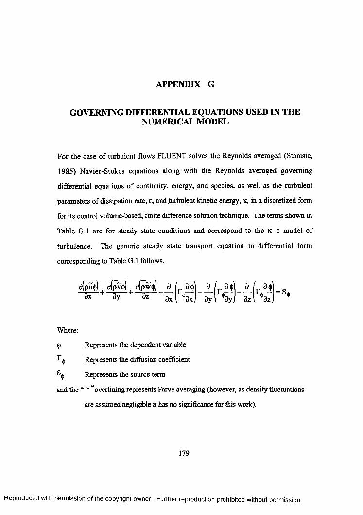
APPENDIX G
GOVERNING DIFFERENTIAL EQUATIONS USED IN THE NUMERICAL MODEL
For the case of turbulent flows FLUENT solves the Reynolds averaged (Stanisic,
1985) Navier-Stokes equations along with the Reynolds averaged governing
differential equations of continuity, energy, and species, as well as the turbulent
parameters of dissipation rate, e, and turbulent kinetic energy, k , in a discretized form
for its control volume-based, finite difference solution technique. The terms shown in
Table G.l are for steady state conditions and correspond to the K-e model of
turbulence. The generic steady state transport equation in differential form
corresponding to Table G.l follows.
Where:
<j> Represents the dependent variable
F<j) Represents the diffusion coefficient
Sjj, Represents the source term
and the “ ~ “overlining represents Farve averaging (however, as density fluctuations
are assumed negligible it has no significance for this work).
179
Reproduced with permission of the copyright owner. Further reproduction prohibited without permission.
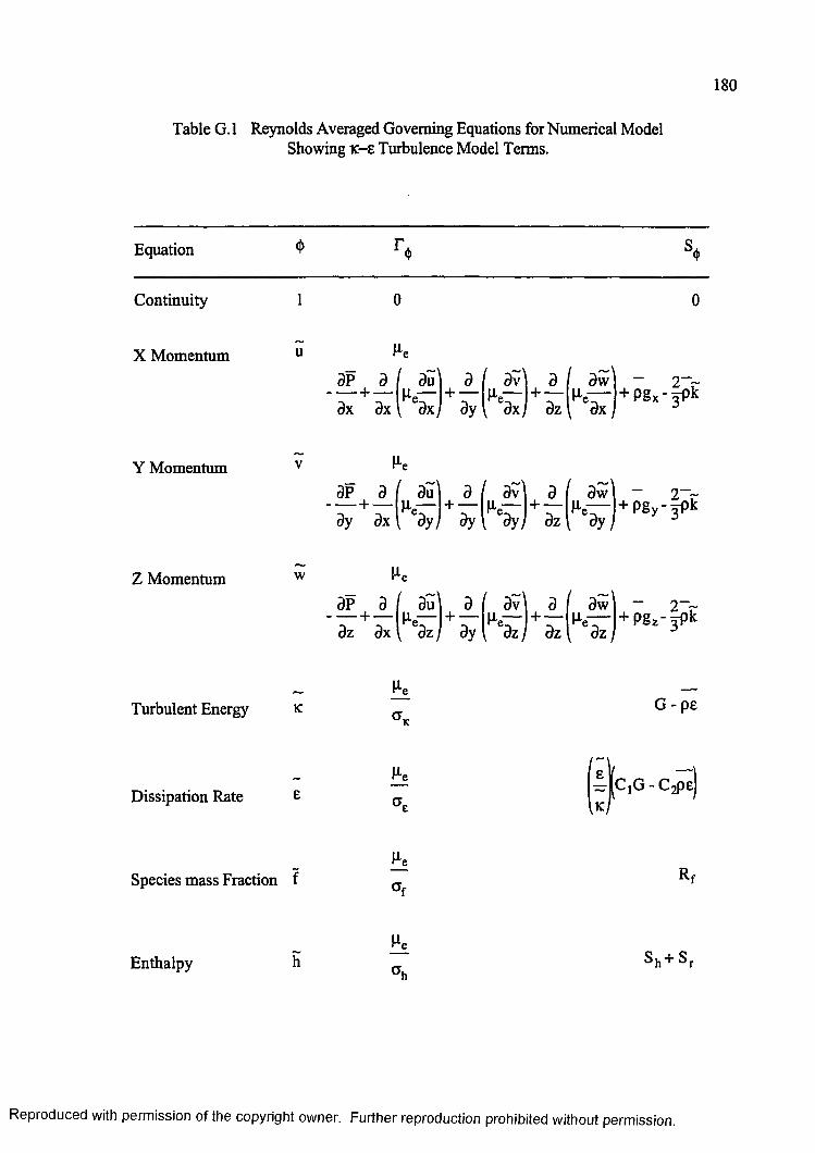
180
Table G. 1 Reynolds Averaged Governing Equations for Numerical Model Showing k - e Turbulence Model Terms.
Equation 4> ♦
Continuity
X Momentum
0
Re
3P +
3x dx
9u a [ 3v a<
3w —Re- + — R e ~ + — Re----- + P8x
dx) 3y 1 dz a x j
Y Momentum3P 3 9u
+ — |x —dy dx \ dyj
d ( dv + — R e -
ay I dy)
a aw+ — R e —
a z l 3y
~ 2 ~ ~
+ pgy-g p k
Z Momentum w Re
a p + _a_
dz dx
du
dzj
a+ —
ay
5v I aR — + —
dz j dz
3w 1 ~ 2~rRe— | + p g2-TPk
Turbulent Energy KRe
c KG - pe
Dissipation Rate eRe - J C jG - C sPE
Species mass Fraction f Rf
Enthalpy Sh+ S r
Reproduced with permission of the copyright owner. Further reproduction prohibited without permission.
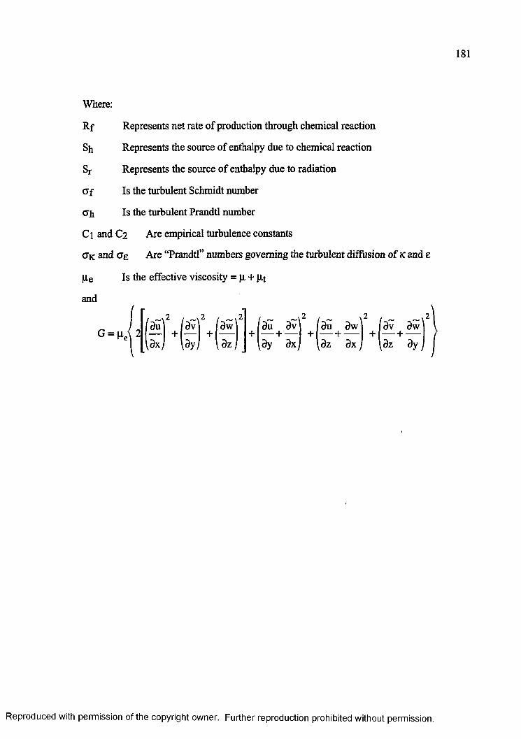
181
Where:
Rf Represents net rate of production through chemical reaction
Sh Represents the source of enthalpy due to chemical reaction
Sr Represents the source of enthalpy due to radiation
Of Is the turbulent Schmidt number
Ch Is the turbulent Prandtl number
Ci and C2 Are empirical turbulence constants
<Jk and ag Are “Prandtl” numbers governing the turbulent diffusion of k and e
|le Is the effective viscosity = |l + (Xt
and
G = \ie\ 2f9u\ (dv) fd
S + \aTj8u 3v\ i du 9w
3y dx) \9z 9 x ;
dv dw
(dz dy
Reproduced with permission of the copyright owner. Further reproduction prohibited without permission.
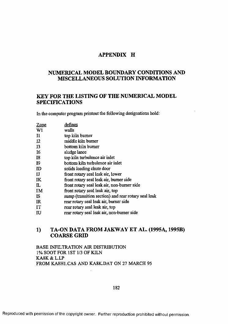
APPENDIX H
NUMERICAL MODEL BOUNDARY CONDITIONS AND MISCELLANEOUS SOLUTION INFORMATION
KEY FOR THE LISTING OF THE NUMERICAL MODEL SPECIFICATIONS
In the computer program printout the following designations hold:
1) TA-ON DATA FROM JAKWAY ET AL. (1995A, 1995B) COARSE GRID
BASE INFILTRATION AIR DISTRIBUTION 1% SOOT FOR 1ST 1/3 OF KILN KA8K & L.LPFROM KA8H1.CAS AND KA8K.DAT ON 27 MARCH 95
W11112 13 16 18 19 ID IJ IK IL IM IS IR IT IU
Zone defineswallstop kiln burner middle kiln burner bottom kiln burner sludge lancetop kiln turbulence air inletbottom kiln turbulence air inletsolids loading chute doorfront rotary seal leak air, lowerfront rotary seal leak air, burner sidefront rotary seal leak air, non-burner sidefront rotary seal leak air, topsump (transition section) and rear rotary seal leakrear rotary seal leak air, burner siderear rotary seal leak air, toprear rotary seal leak air, non-burner side
182
Reproduced with permission of the copyright owner. Further reproduction prohibited without permission.
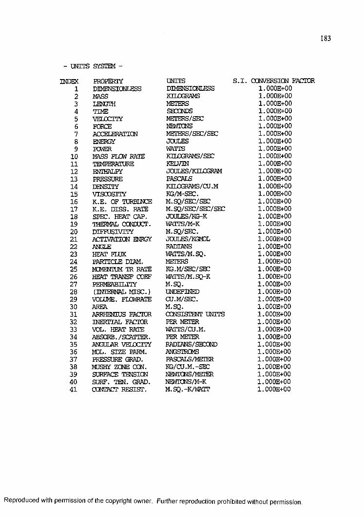
183
- UNITS SYSTEM -
INDEX PROPERTY UNITS S . I . CONVERSION FACTOR1 d im e n s ic n l e s s DIMENSICNLESS 1 . 000E+002 m a ss KILOGRAMS 1 . OOOE+OO3 LENGTH METERS 1 . 000E+004 TIME SECONDS 1 . 000E+005 VELOCITY METERS/SEC 1 . 000E+006 FORCE NEWTONS 1 . 000E+007 ACCELERATION METERS/SEC/SEC 1 . 000E+008 ENERGY JOULES 1 . OOOE+OO9 POWER WATTS 1 . OOOE+OO
10 MASS FLOW RATE KILOGRAMS/SEC 1 . OOOE+OO11 temperature KELVIN 1 . 000E+0012 ENIHALPY JOULES/KILOGRAM 1 . 000E+0013 PRESSURE PASCALS 1 . OOOE+OO14 DENSITY KELOGRAMS/CU.M 1 . OOOE+OO15 VISCOSITY KG/M-SEC. 1 . OOOE+OO16 K.E. OF TUREINCE M.SQ/SEC/SBC 1 . OOOE+OO17 K.E. D IS S . RATE M.SQ/SEC/SEC/SEC 1 . OOOE+OO18 SPEC. HEAT CAP. JOULES/KG-K 1 . OOOE+OO19 THERMAL CONDUCT. WATTS/M-K 1 . OOOE+OO20 DIEFUSIVITY M.SQ/SEC. 1 . OOOE+OO21 ACTIVATION ENRGY JOULES/KGMDL 1 . OOOE+OO22 ANGLE RADIANS 1 . OOOE+OO23 HEAT FLUX WATIS/M. SQ. 1 . OOOE+OO24 PARTICLE DIAM. METERS 1 . OOOE+OO25 MOMENIUM TR RATE KG.M/SEC/SBC 1 . OOOE+OO2 6 HEAT TRANSF COEF WATTS/M. SQ-K 1 . OOOE+OO27 PERMEABILITY M.SQ. 1 . OOOE+OO28 (INTERNAL MISC.) UNDEFINED 1 . OOOE+OO29 VOLUME. FLCWRATE CQ.M/SEC. 1 . OOOE+OO30 AREA M.SQ. 1 . OOOE+OO31 ARRHENIUS FACTOR CONSISTENT UNITS 1 . OOOE+OO32 INERTIAL FACTOR PER METER 1 . OOOE+OO33 VOL. HEAT RATE WATTS/CU.M. 1 . OOOE+OO34 ABSORB./SCATTER. PER METER 1 . OOOE+OO35 ANGULAR VELOCITY RADIANS/SECOND 1 . OOOE+OO36 MOL. SIZE PARM. ANGSTROMS 1 . OOOE+OO37 PRESSURE GRAD. PASCALS/METER 1 . OOOE+OO38 MUSHY ZONE CON. KG/CU.M.-SBC 1 . OOOE+OO39 SURFACE TENSION NEWICNS/METER 1 . OOOE+OO40 SURF. TEN. GRAD. NEWICNS/M-K 1 . OOOE+OO41 CONTACT RESIST. M.SQ.-K/WATT 1 . OOOE+OO
Reproduced with permission of the copyright owner. Further reproduction prohibited without permission.
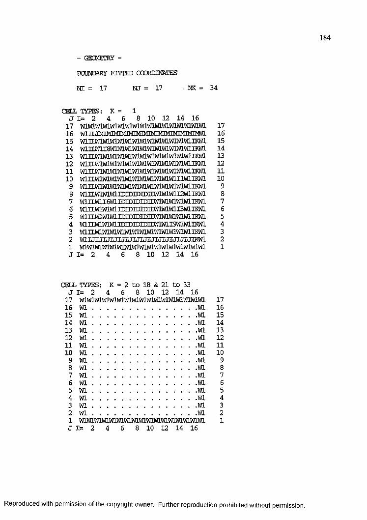
- GECMEIRY -
BOUNDARY FTITED COORDINATESNT = 17 NJ = 17 • NK = 34
CELL TYPES: K = 1J 1= 2 4 6 8 10 12 14 16
17 mwiwiwiwiwiwiwiwiwiwiwiwiwiwiwiwi16 TaTI TT,TMTMTMTMTTvrrMTMTMTMTNfTMIT»nT4TM/JI]15 vaiimmwimvawimwivawiwiwiwiiKwi 14 miimi8mwimmmmmwimwiwiiKwi 13 wiiimwimwimmmwiwiwiwiwimiKwi 12 mnmwiwiwiwiwiwiwiwiwiwiwiwiiKwi n mm/amwimmwimmwiwiwiwiwiiK&Ji 10 wiinmwiwiwiwiwiwiwiwiwiwmmiKwi 9 vaiimmmmwiwiwiwiwiwiwiwiwiiKwi 8 vaiiM m m iD iD iD iD iim m m i2m iK w i 7 miimi6miDiDiDiDmwiwiwiwiwiiKwi 6 miimwimiDiDiDroiDwiwiwii3wiiKwi 5 mnmwiwiiDiDiDiDiimmwiwiwiiKwi 4 vanmmmiDiDiDiDiEMmi9mwiiKwi 3 mnmwimwiwiwiwiwiwiwiwiwiwiiKWii mmmwimmmvammmwiwiwiwiwiwi J 1= 2 4 6 8 10 12 14 16
m.T, TYPES: K = 2 to 18 & 21 to 33J 1= 2 4 6 8 10 12 14 16
17 mmmmmmmmmmmwimwiwiwiwi16 w i ..........................................................wi15 w i ..........................................................VJl14 w i ..........................................................m13 w i ..........................................................wi12 WI............................................. WI11 WI..........................................................WI10 WI..........................................................WI
9.....WI............................................. WI8...WI............................................. WI7....WI............................................. WI6....WI............................................. WI5....WI............................................. WI4 WI............................................. WI3 WI............................................. WI2 WI............................................. WI1 W1W1W1W1W1W1W1W1W1W1W1W1W1W1W1W1W1 J 1= 2 4 6 8 10 12 14 16
1716151413121110987654321
1716151413121110987654321
Reproduced with permission of the copyright owner. Further reproduction prohibited without
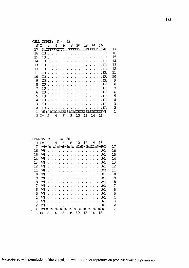
185
CRT if. TORES: K = 19J 1= 2 4 6 8 10 12 14 16
17 Wll'iTlTlTiTlTlTiTiTiTiTlTi'l'iTlTlWl16 IU . . .IR15 IU . . .IR14 IU . . .IR13 IU . . .IR12 IU . . .IR11 IU . . .IR10 IU . . .IR9 IU . . .IR8 IU . . .IR7 IU . . .IR6 IU . . .IR5 IU . . .IR4 IU . . .IR3 IU . . .IR2 IU . • • - . .IR1 W1ISISISISISISISISISISISISISISISW1J 1= 2 4 6 8 10 12 14 16
fETT. TOPES: K = 20J 1= 2 4 6 8 10 12 14 16
17 W1W1W1W1W1W1W1W1W1W1W1W1W1W1W1W1W116 WI . . . .................................... WI15 WI . . . .................................... WI14 WI . . . .................................... WI13 WI . . . .................................... WI12 WI . . . .................................... WI11 WI . . . ,................................... WI10 WI . . . .................................... WI9 m . . . .................................... WI8 m . . . ,................................... WI7 m . . . .................................... WI6 wi . . . .................................... WI5 wi . . . .................................... WI4 wi . . . .................................... WI3 wi . . . .................................... WI2 wi . . . .................................... WI1 W1ISISISISISISISISISISISISISISISW1J 1= 2 4 6 8 10 12 14 16
1716151413121110987654321
1716151413121110987654321
Reproduced with permission of the copyright owner. Further reproduction prohibited without permission.
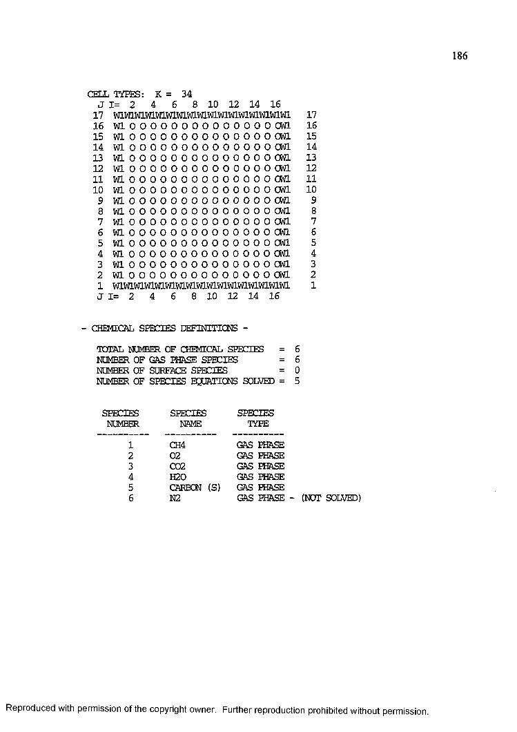
CELL TYPES: K = 34J 1= 2 4 6 8 10 12 14 16
17 m m w iv a w im m w im w iw iw iw iw iw iw iw i 1716 Wl 0 0 0 0 0 0 0 0 0 0 0 0 0 0 OWl 1615 Wl 0 0 0 0 0 0 0 0 0 0 0 0 0 0 OWl 1514 Wl 0 0 0 0 0 0 0 0 0 0 0 0 0 0 OWl 1413 Wl 0 0 0 0 0 0 0 0 0 0 0 0 0 0 OWl 1312 Wl 0 0 0 0 0 0 0 0 0 0 0 0 0 0 OWl 1211 Wl 0 0 0 0 0 0 0 0 0 0 0 0 0 0 OWl 1110 Wl 0 0 0 0 0 0 0 0 0 0 0 0 0 0 OWl 10
9 Wl 0 0 0 0 0 0 0 0 0 0 0 0 0 0 OWl 98 Wl 0 0 0 0 0 0 0 0 0 0 0 0 0 0 OWl 87 Wl 0 0 0 0 0 0 0 0 0 0 0 0 0 0 OWl 76 Wl 0 0 0 0 0 0 0 0 0 0 0 0 0 0 OWl 65 Wl 0 0 0 0 0 0 0 0 0 0 0 0 0 0 OWl 54 Wl 0 0 0 0 0 0 0 0 0 0 0 0 0 0 OWl 43 Wl 0 0 0 0 0 0 0 0 0 0 0 0 0 0 OWl 32 Wl 0 0 0 0 0 0 0 0 0 0 0 0 0 0 OWl 21 W1W1W1W1W1W1W1W1W1W1W1W1W1W1W1W1W1 1J 1= 2 4 6 8 10 12 14 16
- CHEMICAL SPECIES DEFINITIONS -TOTAL NUMBER OF CHEMICAL SPECIES = 6NUMBER OF GAS PHASE SPECIES = 6NUMBER OF SURFACE SPECIES = 0NUMBER OF SPECIES EQUATIONS SOLVED = 5
SPECIESNUMBER
123456
SPECIESNAME
CH402C02H20CARBONN2
(S)
SPECIESTYPE
GAS PHASE GAS PHASE GAS PHASE GAS PHASE GAS PHASE GAS PHASE - (NOT SOLVED)
Reproduced with permission of the copyright owner. Further reproduction prohibited without permission.
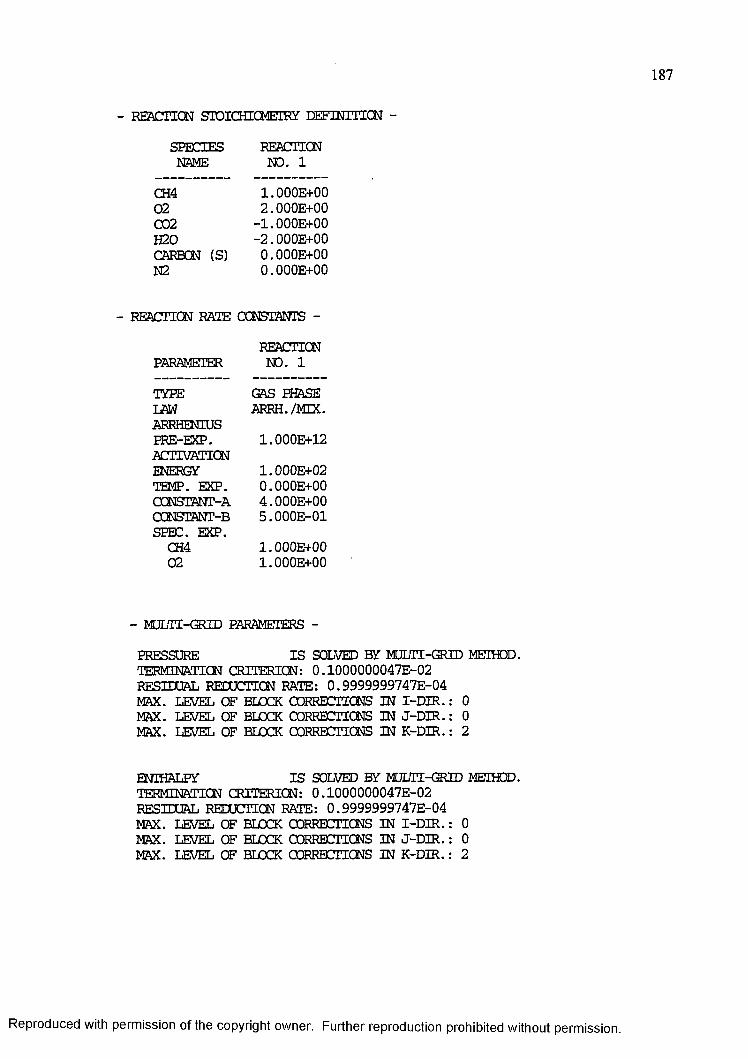
187
- REACTION STOICHIOMETRY DEFINITION -
SPECIES REACTION NAME NO. 1
CH4 1.000E+0002 2.OOOE+OOC02 -1.OOOE+OOH20 -2.OOOE+OOCARBON (S) 0.OOOE+OON2 0.OOOE+OO
- REACTICN RATE CONSTANTS -REACTION
PARAMETER NO. 1TYPE GAS PHASELAW ARRH./MIX.ARRHENIUSPRE-EXP. 1.000E+12ACTTVATICNENERGY 1.000E+02TEMP. EXP. 0.OOOE+OOQQNSTANT-A 4. OOOE+OOCCNSTANT-B 5.000E-01SPEC. EXP.
CH4 1.OOOE+OO02 1.OOOE+OO
- MULTI-GRID PARAMETERS - PRESSURE IS SOLVED BY MULTI-GRID METHOD.TERMINATION CRITERION: 0.1000000047E-02 RESIDUAL REDUCTION RATE: 0.9999999747E-04 MAX. LEVEL OF BLOCK CORRECTIONS IN I-DIR.: 0MAX. LEVEL OF BLOCK CORRECTIONS IN J-DIR.: 0MAX. LEVEL OF BLOCK CORRECTIONS IN K-DIR.: 2
ENIHALPY IS SOLVED BY MULTI-GRID METHOD.TERMINATION CRITERION: 0.1000000047E-02 RESIDUAL REDUCTION RATE: 0.9999999747E-04 MAX. LEVEL OF BLOCK CORRECTIONS IN I-DIR.: 0MAX. LEVEL OF BLOCK CORRECTIONS IN J-DIR.: 0MAX. LEVEL OF BLOCK CORRECTIONS IN K-DIR.: 2
Reproduced with permission of the copyright owner. Further reproduction prohibited without permission.
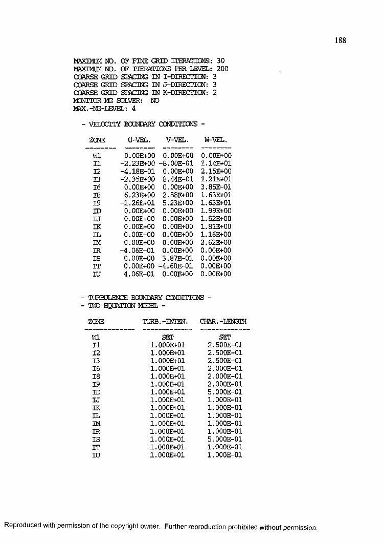
188
MAXIMUM NO. OF FINE GRID ITERATIONS: 30 MAXIMUM NO. OF ITERATIONS PER LEVEL: 200 COARSE GRID SPACING IN I-DIRECTICN: 3 COARSE GRID SPACING IN J-DIRECITGN: 3 COARSE GRID SPACING IN K-DIRECITQN: 2 MONITOR M3 SOLVER: NOMAX. -M3-LEVEL: 4
- VELOCITY BOUNDARY CCNDIITCNS -
ZONE U-VEL. V-VEL. W-VEL.
Wl 0.00E + 00 0.00E + 00 O.OOE+OO11 -2 .2 3 E + 0 0 -8 .0 0 E -0 1 1 .14E + 0112 -4 .1 8 E -0 1 0.00E + 00 2 .15E + 0013 -2 .3 5 E + 0 0 8 .4 4 E -0 1 1 .21E + 0116 O.OOE+OO O.OOE+OO 3 .8 5 E -0 118 6 .23E + 00 2 .58E + 00 1 .63E + 0119 -1 .2 6 E + 0 1 5.23E + 00 1 .63E + 01ID 0.00E + 00 O.OOE+OO 1.99E + 00U 0.00E + 00 O.OOE+OO 1.52E + 00IK 0 .00E + 00 O.OOE+OO 1.81E + 00IL 0.00E + 00 O.OOE+OO 1.16E + 00IM 0.00E + 00 O.OOE+OO 2.62E + 00IR - 4 . 06E -01 O.OOE+OO O.OOE+OOIS 0.00E + 00 3 .8 7 E -0 1 O.OOE+OOIT 0.00E + 00 - 4 . 60E -01 O.OOE+OOIU 4 .0 6 E -0 1 O.OOE+OO O.OOE+OO
- TURBULENCE BOUNDARY OGNDITTCNS -- TWO EQUATION MODEL -
ZONE TURB.-INIEN. CHAR.-LENGTH
Wl SET SET11 1 . 000E+01 2 . 500E -0112 1 . 000E+01 2 . 500E -0113 1 . 000E+01 2 . 500E -0116 1 .000E + 01 2 . 000E -0118 1 .000E + 01 2 . 000E -0119 1 . 000E+01 2 .0 0 0 E -0 1ID 1 . 000E+01 5 . 000E -01U 1.000E + 01 1 . 000E -01IK 1.000E + 01 1 .0 0 0 E -0 1IL 1 . 000E+01 1 . 000E -01IM 1.000E + 01 1 . 000E -01IR 1 .000E + 01 1 .0 0 0 E -0 1IS 1 . 000E+01 5 . 000E -01IT 1 .000E + 01 1 . 000E -01IU 1.000E + 01 1 .0 0 0 E -0 1
Reproduced with permission of the copyright owner. Further reproduction prohibited without permission.
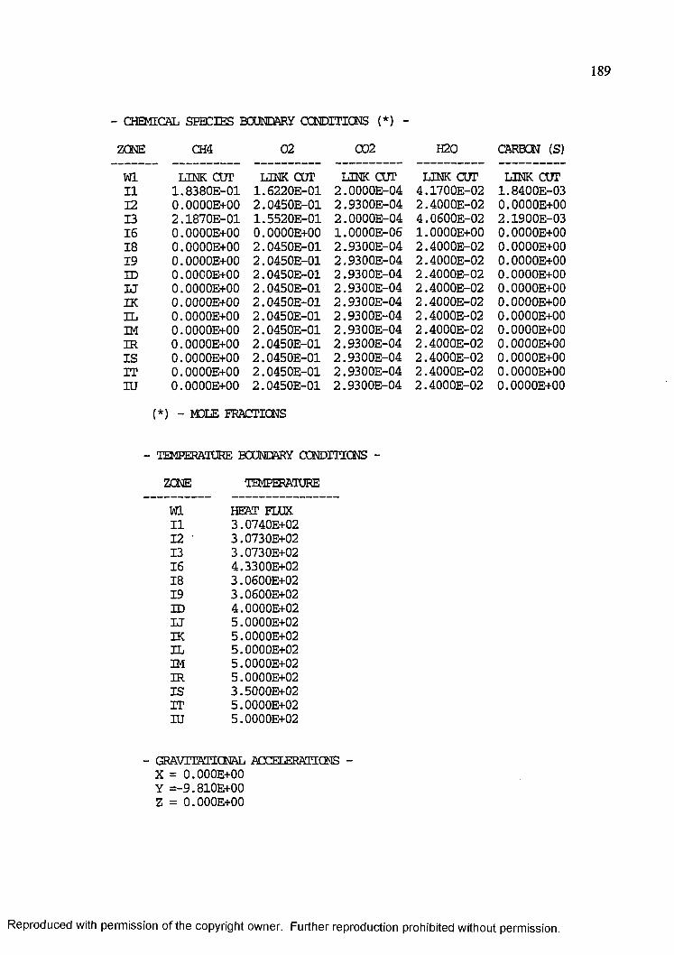
189
- CHEMICAL SPECIES BOUNDARY CCNDmCNS (*) -
ZONE CH4 02 002 H20 CARBON (S)
Wl LINK CUT LINK CUT LINK COT LINK COT LINK COT11 1 .8 3 8 0 E -0 1 1 . 6220E -01 2 . 0000E -04 4 .1 7 0 0 E -0 2 1 .8 4 0 0 E -0 312 0 . 0000E+00 2 . 0450E -01 2 .9 3 0 0 E -0 4 2 . 4000E -02 0 . OOOOE+OO13 2 .1 8 7 0 E -0 1 1 . 5520E -01 2 . 0000E -04 4 .0 6 0 0 E -0 2 2 .1 9 0 0 E -0 316 0 . 0000E+00 0 . OOOOE+OO 1 . OOOOE-06 1 . OOOOE+OO 0 . OOOOE+OO18 0 . 0000E+00 2 . 0450E -01 2 .9 3 0 0 E -0 4 2 . 4000E -02 0 . OOOOE+OO19 0 . 0000E+00 2 . 0450E -01 2 .9 3 0 0 E -0 4 2 . 4000E -02 0 . OOOOE+OOID 0 . 0000E+00 2 . 0450E -01 2 .9 3 0 0 E -0 4 2 .4 0 0 0 E -0 2 0 . OOOOE+OOU 0 . 0000E+00 2 . 0450E -01 2 .9 3 0 0 E -0 4 2 . 4000E -02 0 . OOOOE+OOIK 0 . 0000E+00 2 . 0450E -01 2 . 9300E -04 2 .4 0 0 0 E -0 2 0 . OOOOE+OOIL 0 . 0000E+00 2 . 0450E -01 2 .9 3 0 0 E -0 4 2 .4 0 0 0 E -0 2 0 . OOOOE+OOIM 0 . 0000E+00 2 . 0450E -01 2 .9 3 0 0 E -0 4 2 .4 0 0 0 E -0 2 0 . OOOOE+OOIR 0 . 0000E+00 2 . 0450E -01 2 .9 3 0 0 E -0 4 2 . 4000E -02 0 . OOOOE+OOIS 0 . 0000E+00 2 . 0450E -01 2 .9 3 0 0 E -0 4 2 . 4000E -02 0 . OOOOE+OOIT 0 . 0000E+00 2 . 0450E -01 2 .9 3 0 0 E -0 4 2 . 4000E -02 0 . OOOOE+OOIU 0 . 0000E+00 2 . 0450E -01 2 .9 3 0 0 E -0 4 2 .4 0 0 0 E -0 2 0 . OOOOE+OO
(*) - MOLE FRACTIONS
- TEMPERATURE BOUNDARY CONDITIONS -
ZONE TEMPERAT
Wl HEAT FLUX11 3 . 0740E+0212 ' 3 .0730E + 0213 3 .0730E + 0216 4 .3300E + 0218 3 . 0600E+0219 3 . 0600E+02ID 4 . 0000E+02U 5 . 0000E+02IK 5 . 0000E+02IL 5 . 0000E+02IM 5 . 0000E+02IR 5.0000E + 02IS 3 . 5000E+02IT 5 . 0000E+02IU 5 . 0000E+02
- GRAVITATIONAL ACCELERATIONS - X = 0 . OOOE+OO Y = - 9 . 810E+00 Z = 0 . OOOE+OO
Reproduced with permission of the copyright owner. Further reproduction prohibited without permission.
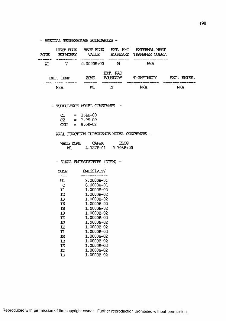
190
- SPECIAL TEMPERATURE BOUNDARIES -
HEAT FLUX HEAT FLUX EXT. H-T EXTERNAL HEAT ZONE BOUNDARY VALUE BOUNDARY TRANSFER GOEFF.
Wl Y 0 . 0000E+00 N N /A
EXT. RADEXT. TEMP. ZONE BOUNDARY T-INFINITY
N /A Wl N N /A
- TURBULENCE MODEL CONSTANTS -
C l = 1 .4E + 00C2 = 1 .9E + 00CMU = 9 .0 E -0 2
- WALL FUNCTION TURBULENCE MODEL CONSTANTS -
WALL ZONE CAPPA ELOGWl 4 . 187E -01 9 . 793E+00
- ZONAL EM ISSIV rnES (DIRM) -
ZONE EMISSIVITY
Wl 8 . 0000E -010 8 .0 0 0 0 E -0 1
11 1 .0 0 0 0 E -0 212 1 . 0000E -0213 1 . 0000E -0216 1 .0 0 0 0 E -0 218 1 . 0000E -0219 1 . 0000E -02ID 1 .0 0 0 0 E -0 2U 1 . 0000E -02IK 1 .0 0 0 0 E -0 2IL 1 . 0000E -02IM 1 . 0000E -02IR 1 . 0000E -02I S 1 . 0000E -02IT 1 .0 0 0 0 E -0 2IU 1 . 0000E -02
EXT. EMISS.
N /A
Reproduced with permission of the copyright owner. Further reproduction prohibited without permission.
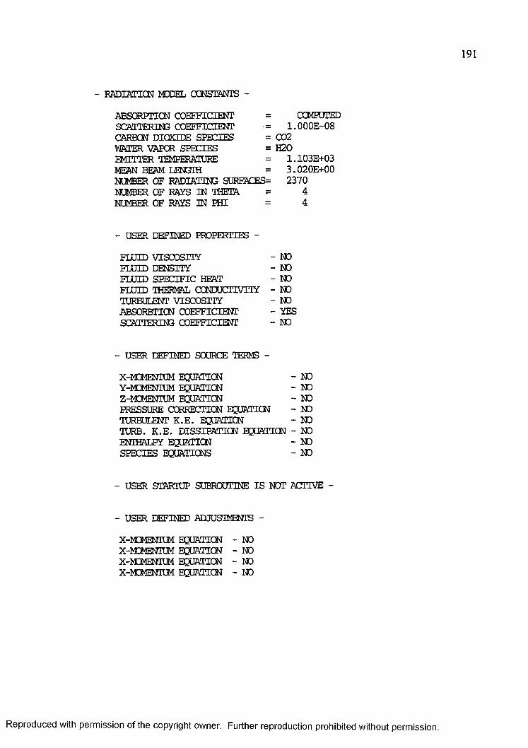
191
- RADIATION MODEL CONSTANTS -
ABSORPTION COEFFICIENT SCATTERING COEFFICIENT CARBON DIOXIDE SPECIES WATER VAPOR SPECIES EMITTER TEMPERATURE =MEAN BEAM LENGTH =NUMBER OF RADIATING SURFACES=NUMBER OF RAYS IN THEIA =NUMBER OF RAYS IN PHI
= COMPUTED = 1.000E-08= 002 = H20= 1.103E+03= 3.020E+00
2370 4 4
- USER DEFINED PROPERTIES -FLUID VISCOSITY - NOFLUID DENSITY - NOFLUID SPECIFIC HEAT - NOFLUID THERMAL CONDUCTIVITY - NOTURBULENT VISCOSITY - NOABSORBTICN COEFFICIENT - YESSCATTERING COEFFICIENT - NO
- USER DEFINED SOURCE TERMS -
X-M3MENTUM EQUATION - NOY-MCMENTUM EQUATION - NOZ-MCMENIUM EQUATION - NOPRESSURE CORRECTION EQUATION - NOTURBULENT K .E . EQUATION - NOTURB. K .E . DISSIPATION EQUATION - NOENTHALPY EQUATION - NOSPECIES EQUATIONS - NO
- USER STARTUP SUBROUTINE I S NOT ACTIVE -
- USER DEFINED ADJUSTMENTS -
X-MDMENTUM EQUATION - NO X-ICMENIUM EQUATION - NO X-MQMENIUM EQUATION - NO X-REMENIUM EQUATION - NO
Reproduced with permission of the copyright owner. Further reproduction prohibited without permission.
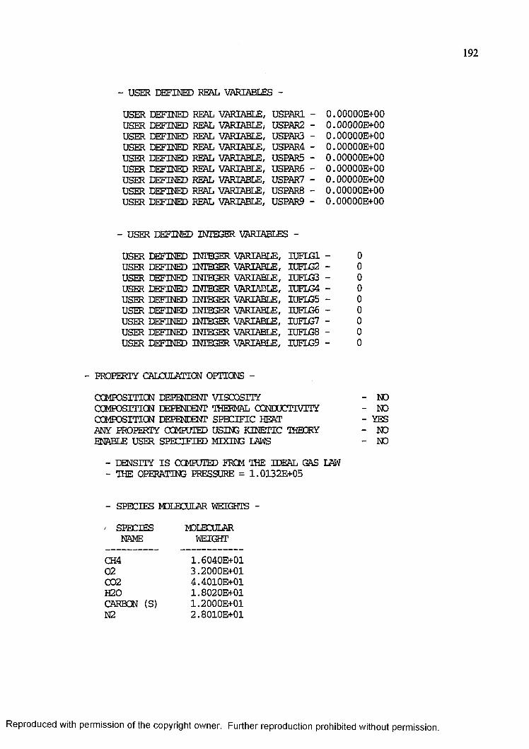
192
USER DKFTNHD REAL VARIABLES -
USERUSERUSERUSERUSERUSERUSERUSERUSER
d e f in e dd e f in e dDEFINEDDEFINEDDEFINEDDEFINEDDEFINEDDEFINEDDEFINED
REALREALREALREALREALREALREALREALREAL
VARIABLE,VARIABLE*VARIABLE,VARIABLE,VARIABLE,VARIABLE,VARIABLE,VARIABLE,VARIABLE,
USPAR1USPAR2USPAR3USPAR4USPAR5USPAR6USPAR7USPAR8USPAR9
0 . 00000E+00 0 . 00000E+00 0 . 00000E+00 O.OOOOOE+OO 0 . 00000E+00 O.OOOOOE+OO O.OOOOOE+OO O.OOOOOE+OO 0 .00000E + 00
- USER DKFTNKT) INTEGER VARIABLES -
USERUSERUSERUSERUSERUSERUSERUSERUSER
DEFINEDDEFINEDDEFINEDDEFINEDDEFINEDDEFINEDDEFINEDDEFINEDDEFINED
INTEGERINTEGERINTEGERINTEGERINTEGERINTEGERINTEGERINTEGERINTEGER
VARIABLE,VARIABLE,VARIABLE,VARIABLE,VARIABLE,VARIABLE,VARIABLE,VARIABLE,VARIABLE,
IUEIG1IUFLG2IUFLG3IUELG4IUFLG5IUFIG6UJFL37IUFLG8IUELG9
000000000
- PROPERTY CALCULATION OPTTCNS -
COMPOSITION DEPENDENT VISCOSITY - NOCOMPOSITION DEPENDENT THERMAL CCMXJCT1V3TY - NOCCMPOSITICN DEPENDENT SPECIFIC HEAT - YESANY PROPERTY COMPUTED USING KINETIC THEORY - NOENABLE USER SPECIFIED MIXING LAWS - NO
- DENSITY I S COMPUTED FROM THE IDEAL GAS LAW- THE OPERATING PRESSURE = 1 .0132E + 05
- SPECIES MOLECULAR WEIGHS -
/ SPECIES NAME
CH402C02H20CARBON (S) N2
MOLECULARWEIGH
1 .6040E + 01 3 .2000E + 01 4 .4010E + 01 1 . 8020E+01 1 .2000E + 01 2 . 8010E+01
Reproduced with permission of the copyright owner. Further reproduction prohibited without permission.
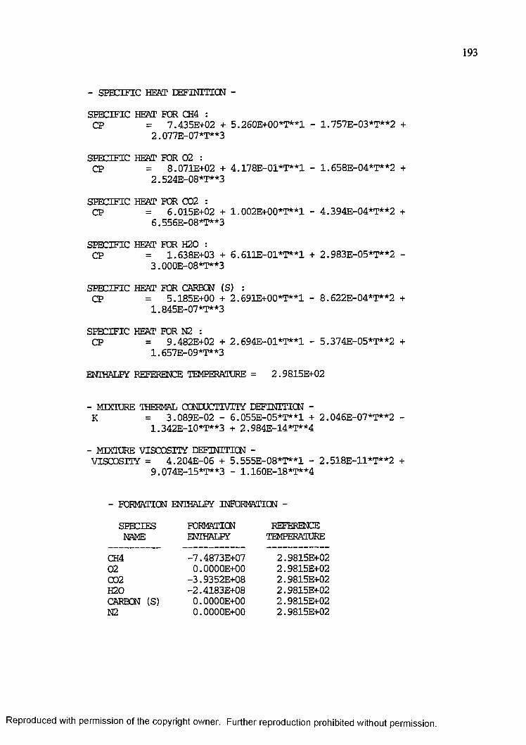
193
- SPECIFIC HEAT EEFINnTCN -
SPECIFIC HEAT FOR CH4 :CP = 7 . 435E+02 + 5 .260E + 00*T **1 - 1 .7 5 7 E -0 3 * T * * 2 +
2 . 077E -07*T **3
SPECIFIC HEAT FOR 0 2 :CP = 8 . 071E+02 + 4 .1 7 8 E -0 1 * T * * 1 - 1 . 658E -04*T **2 +
2 . 524E -08*T **3
SPECIFIC HEAT PC®. C02 :CP = 6 . 015E+02 + 1 .002E + 00*T **1 - 4 . 394E -04*T **2 +
6 .556E -08*T **3
SPECIFIC HEAT FOR H20 :CP = 1 .638E + 03 + 6 .6 1 1 E -0 1 * T * * 1 + 2 .9 8 3 E -0 5 * T * * 2 -
3 . 000E -08*T **3
SPECIFIC HEAT FOR CARBCN (S) :CP = 5 . 185E+00 + 2 . 691E+00*T**1 - 8 . 622E -04*T **2 +
1 .845E -07*T **3
SPECIFIC HEAT FOR N2 :CP = 9 . 482E+02 + 2 . 694E -01*T **1 - 5 .3 7 4 E -0 5 * T * * 2 +
1 . 657E -09*T **3
ENTHALPY REFERENCE TEMPERATURE = 2 .98 1 5 E + 0 2
- MIXIURE THERMAL CCNDXTlVTiY DEFINITICN -K = 3.089E-02 - 6.055E-05*T**1 + 2.046E-07*T**2 -
1.342E-10*T**3 + 2.984E-14*T**4
- MIXIURE VISCOSITY DEFINITICN -VISCOSITY = 4.204E-06 + 5.555E-08*T**1 - 2.518E-11*T**2 +
9.074E-15*T**3 - 1.160E-18*T**4
- FORMATION ENTHALPY INFORMATION -
SPECIES FORMATION REFERENCENAME ENTHALPY TEMPERATURE
CH4 - 7 . 4873E+07 2 .9815E + 0202 0 . OOOOE+OO 2 . 9815E+02002 - 3 . 9352E+08 2 . 9815E+02H20 - 2 . 4183E+08 2 . 9815E+02CARBCN (S) 0 . OOOOE+OO 2 .9815E + 02N2 0 . OOOOE+OO 2 . 9815E+02
Reproduced with permission of the copyright owner. Further reproduction prohibited without permission.
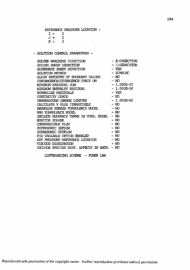
194
REFERENCE PRESSURE LOCATION : I = 2J = 2K = 2
- SOLUTION CONTROL PARAMETERS -
SOLVER MARCHING DIRECTION - K-DIREdTCNSOLVER SWEEP DIRECTION - I-DIRECTICNALTERNATE SWEEP DIRECTION - YESSOLUTION METHOD - SIMELECALLOW PATCHING OF BOUNDARY VALUES - NOOCNVEH3ENCE/DIVERGENCE CHECK ON - NOMINIMUM RESIDUAL SUM - 1 .0 0 0 E -0 3MINIMUM ENTHALPY RESIDUAL - 1 .0 0 0 E -0 6NORMALIZE RESIDUALS - YESCONTINUITY CHECK - NOTEMPERATURE CHANGE LIMITER - 1 . OOOE+OOCALCULATE Y PLUS ITERATIVELY - NOREYNOLDS STRESS TURBULENCE MODEL - NORNG TURBULENCE MODEL - NOINCLUDE BUOYANCY TERMS IN TURB. MODEL - NOMONITOR SOLVER - NOCOMPRESSIBLE FLOW - NOSUPERSONIC INFLOW - NOSUPERSONIC OUTFLOW - NOFIX VARIABLE OPTION ENABLED - NOSET PRESSURE REFERENCE LOCATION - NOVISCOUS DISSIPATION - NOINCLUDE SPECIES DIFF. EFFECTS IN ENTH. - NO
DIFFERENCING SCHEME - POWER LAW
Reproduced with permission of the copyright owner. Further reproduction prohibited without permission.
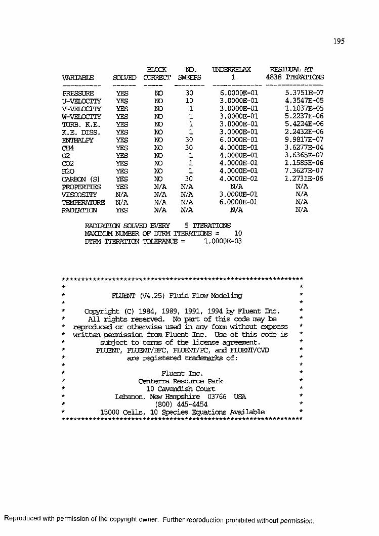
195
BLOCK NO. UNDERRELAX RESIDUAL ATVARIABLE SOLVED CORRECT SWEEPS 1 4 8 3 8 TTERATICNS
PRESSURE YES NO 30 6 . 0000E -01 5 .3 7 5 1 E -0 7U-VELOCITY YES NO 10 3 . OOOOE-Ol 4 .3 5 4 7 E -0 5V-VELOCTIY YES NO 1 3 . 0000E -01 1 .1 0 3 7 E -0 5W-VELOCTIY YES NO 1 3 . 00 0 0 E -0 1 5 .2 2 3 7 E -0 6TORB. K .E . YES NO 1 3 . 0000E -01 5 . 4 2 2 4 E -0 6K .E . D ISS . YES NO 1 3 . 0 000E -01 2 .2 4 3 2 E -0 6ENIHALPY YES NO 30 6 . 0 000E -01 9 . 98 1 7 E -0 7CH4 YES NO 30 4 . OOOOE-Ol 3 .6 2 7 7 E -0 402 YES NO 1 4 . 00 0 0 E -0 1 3 .6 3 6 5 E -0 7C02 YES NO 1 4 . 0 000E -01 1 .1 5 8 5 E -0 6H20 YES NO 1 4 . 0 000E -01 7 .3 6 2 7 E -0 7CARBON (S) YES NO 30 4 . 0 000E -01 1 .2 7 3 1 E -0 6PROPERTIES YES N /A N /A N /A N /Av i s c o s i t y N /A N /A N /A 3 . OOOOE-Ol N /ATEMPERAIURE N /A N /A N /A 6 . 0 000E -01 N /ARADIATION YES N /A N /A N /A N /A
RADIATTCN SOLVED EVERY 5 TTERATICNS MAXIMUM NUMBER OF DIEM ITERATIONS = 10DIEM ITERATION TOLERANCE = 1 .0 0 0 0 E -0 3
★ ** FLUENT (V4.25) F lu id F lo w M o d e lin g ** *
* C o p y r ig h t (C) 1984, 1989, 1991, 1994 b y F lu e n t I n c . ** A l l r i g h t s r e s e r v e d . No p a r t o f t h i s c o d e m ay b e ** r e p r o d u c e d o r o t h e r w is e u s e d i n a n y form w it h o u t e x p r e s s ** w r i t t e n p e r m is s io n fr c m F lu e n t I n c . U se o f t h i s c o d e i s ** s u b j e c t t o te r m s o f t h e l i c e n s e a g r e e m e n t. ** FLUENT, FLUENT/EPC, FLUENT/PC, and FLUENT/CVD ** a r e r e g i s t e r e d tr a d a n a r k s o f : ** ** F lu e n t I n c . ** C e n te r r a R e so u r c e P ark ** 10 C a v e n d ish C o u rt ** L ebanon , New H am pshire 03766 USA ** (800) 445-4454 ** 15000 C e l l s , 10 S p e c ie s E q u a t io n s A v a i la b le *★ ★ ★ ★ ★ ★ ★ ★ ★ ★ ★ ★ ★ ★ ★ i t * * * * * * * * * * * * * * * * * * * * * * * * * * * * * * * * * * * * * * * * * * * * * * *
Reproduced with permission of the copyright owner. Further reproduction prohibited without permission.
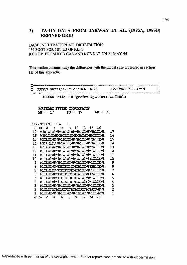
196
2) TA-ON DATA FROM JAKWAY ET AL. (1995A, 1995B) REFINED GRID
BASE INFILTRATION AIR DISTRIBUTION,1% SOOT FOR 1ST 1/3 OF KILNKCD.LP FROM KCD.CAS AND KCE.DAT ON 21 MAY 95
This section contains only the differences with the model case presented in section HI of this appendix.
x--------------------------------------------------------------------I OCJTEUT PRODUCED BY VERSION 4 .2 5 17x17x43 C .V . G r idX--------------------------------------------------------------------------------------------
10 0 0 0 0 C e l l s , 1 0 S p e c ie s E q u a tio n s A v a i la b le
BOUNDARY FITTED COORDINATESNT = 17 N J = 17 NK = 43
CRT.T. TYPES: K = 1J 1= 2 4 6 8 10 12 14 16
17 m m w iw iw iw iw iw iw iw iw iw iw iw iw iw iw i 171 6 WlWl T ^ MTMT TT1VT/ I V TMT 161 5 m m m m w m w i w i w i w i w i w i w i i M L 1514 1413 m m m m m m m m w i m m w i m i K w i 1312 m m m m m m m m m i a w i w i i K w i 1211 m m m m m m m m m w i m i m 1110 m i im m m m m m v t t M w iw iw i i iw i iK w i 10
9 m i i m m v a m m m m m v a m m m w i i K w i 98 miiM mmiDiDiDiDiDwimmi2miKwi 87 m n m i6 m m iD iD iD iD w iw iw iw iw ir K w i 76 m nm W lW lIDIDIDroiDW lW lW lI3W lIK W l 65 m i im v t t m iD iD iD iD iD m m m m m iK w i 54 m n m m m iD iD iD iD iD w im i9 w iw iiE < w i 43 m m m m w i m w i w i w i w i w i m w i w i i m 32 W 1V & IJIJIJIJIJIJIJIJIJT JIJIJIJW 1W 1 21 m m m m m m m m w im w iw iw iw iw iw iw i 1j 1= 2 4 6 8 10 12 14 16
Reproduced with permission of the copyright owner. Further reproduction prohibited without permission.
H H
H
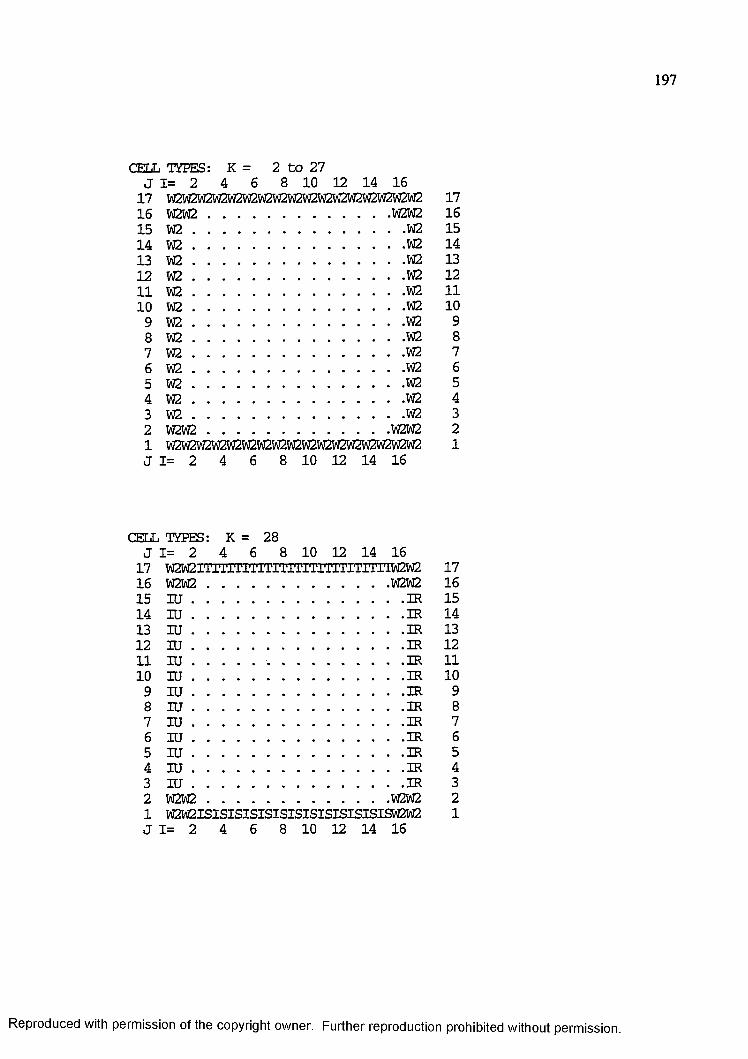
197
f'FTT.T, TYPES: K = 2 to 21J 1= 2 4 6 8 10 12 14 16
1 7 W2W2W2W2W2W2VJ2W2W2W2W2W2W2W2W2W2W21 6 W2W2 ............................................................W2W215 W 2 ......................................................................W21 4 W 2 ......................................................................W213 W 2 ......................................................................W212 W 2............................................................ W211 W2 ......................................................................W210 W2 ......................................................................W2
9 W 2 ......................................................................W28 W2 ......................................................................W27 W 2 ......................................................................W26 W 2 ............................................................ W25 W 2 ............................................................ W24 W 2 ......................................................................W23 W 2 ......................................................................W22 W2W2 ........................................................... W2W21 W2W2W2W2W2W2W2W2W2W2W2W2W2W2W2W2W2J 1= 2 4 6 8 10 12 14 16
HRT.T. TYPES: K = 28J 1= 2 4 6 8 10 12 14 16
17 W2V32ITlTTTITTTITITITTiTiTTTnTV\l2W216 W2W2 ............................................................W2W215 I U .......................................................................IR14 I U ....................................................................... IR13 I U ....................................................................... IR12 I U .......................................................................IR1 1 I U ........................ IR10 I U .......................................................................IR
9 I U ....................................................................... IR8 I U .......................................................................IR7 I U .......................................................................IR6 I U ....................................................................... IR5 I U .......................................................................IR4 I U .......................................................................IR3 I U ....................................................................... IR2 W 2W 2............................................................V32W21 W 2W 2ISISISISISISISISISISISISISW 2W 2 J 1= 2 4 6 8 10 12 14 16
1716151413121110
987654321
1716151413121110
987654321
Reproduced with permission of the copyright owner. Further reproduction prohibited without permission.
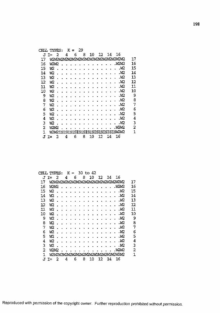
198
TJ,T4 TYPES: K = 29J 1= 2 4 6 8 10 12 14 16
17 W2W2W2W2W2W2W2W2W2W2W2VJ2W2W2W2W2W216 W2W2 . .W2W215 W2 . . . .W214 W2 . . . .W213 W2 . . . .M212 W2 . . . .M211 W2 . . . .M210 W2 . .
9 W2 . . . .W28 W2 . . . .M27 W2 . . . .M26 W2 . . . .M25 W2 . . . .M24 W2 . . . .M23 W2 . . . .W22 W2W2 . • • • . , , , .W2W21 W 2W 2ISISISISISISISISISISISISISW 2W 2J 1= 2 4 6 8 10 12 14 16
fRTT. TYPES: K = 30 t o 42J 1= 2 4 6 8 10 12 14 16
17 W2W2W2W2W2W2W2W2W2W2W2W2W2W2W2W2W216 W2W2................................................ W2W215 W 2.........................................................VJ21 4 W 2 .........................................................W213 W 2.........................................................W212 W 2.........................................................W211 W 2 .............................................................. W210 W 2.........................................................W2
9 W 2.........................................................W28 W 2.........................................................W27 W 2.........................................................W26 W 2.........................................................W25 W 2.........................................................W24 W 2.........................................................W23 W 2.........................................................W22 W2W2................................................ W2W21 VJ2W2W2W2W2W2W2W2W2W2W2W2W2W2W2W2W2 J 1= 2 4 6 8 10 12 14 16
1716151413121110
987654321
1716151413121110
987654321
Reproduced with permission of the copyright owner. Further reproduction prohibited without permission.
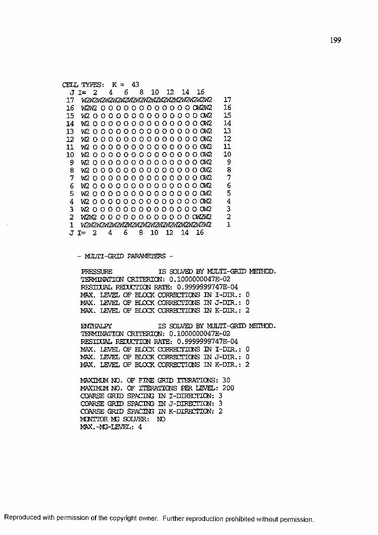
199
CFT-T. TYPES: K = 43J 1= 2 4 6 8 10 12 14 16
17 W2W2W2W2W2W2W2W2W2W2W2W2W2W2W2W2W2 1716 W2W2 0 0 0 0 0 0 0 0 0 0 0 0 OW2W2 1615 M2 0 0 0 0 0 0 0 0 0 0 0 0 0 O OW2 1514 W2 0 0 0 0 0 0 0 0 0 0 0 0 0 0 CM2 1413 W2 0 0 0 0 0 0 0 0 0 0 0 0 0 O OW2 1312 W2 0 0 0 0 0 0 0 0 0 0 0 0 0 O OW2 1211 W2 0 0 0 0 0 0 0 0 0 0 0 0 0 0 CM2 1110 W2 0 0 0 0 0 0 0 0 0 0 0 0 0 0 CM2 10
9 W2 0 0 0 0 0 0 0 0 0 0 0 0 0 O CM2 98 W2 0 0 0 0 0 0 0 0 0 0 0 0 0 O CM2 87 W2 0 0 0 0 0 0 0 0 0 0 0 0 0 O CM2 76 W2 0 0 0 0 0 0 0 0 0 0 0 0 0 O CM2 65 W2 0 0 0 0 0 0 0 0 0 0 0 0 0 0 CM2 54 W2 0 0 0 0 0 0 0 0 0 0 0 0 0 0 CM2 43 W2 0 0 0 0 0 0 0 0 0 0 0 0 0 0 CM2 32 W2W2 0 0 0 0 0 0 0 0 0 0 0 0 0W2W2 21 W2VEW2W2W2W2W2W2W2W2W2W2W2W2W2W2W2 1J 1= 2 4 6 8 10 12 14 16
- M U LTI-G RID PARAMETERS -
PRESSURE I S SOLVED BY MULTI-GRID METHOD.TERMINATION CRITERION: 0 .1 0 0 0 0 0 0 0 4 7 E -0 2 RESIDUAL REDUCTION RATE: 0 . 9 999999747E -04 MAX. LEVEL OF BLOCK CORRECTIONS IN I - D I R .: 0MAX. LEVEL OF BLOCK CORRECTIONS IN J -D I R .: 0MAX. LEVEL OF BLOCK CORRECTIONS IN K -D IR .: 2
ENIHALPY I S SOLVED BY MULTI-GRID METHOD.TERMINATION CRITERION: 0 .1 0 0 0 0 0 0 0 4 7 E -0 2 RESIDUAL REDUCTION RATE: 0 . 9 9 9 9 9 99747E -04 MAX. LEVEL OF BLOCK CORRECTIONS IN I - D I R .: 0MAX. LEVEL OF BLOCK CORRECTIONS IN J -D I R .: 0MAX. LEVEL OF BLOCK CORRECTIONS IN K -D IR .: 2
MAXIMUM NO. OF FINE GRID ITERATIONS: 30 MAXIMUM NO. OF ITERATIONS PER LEVEL: 200 COARSE GRID SPACING IN I-DIRECTTQN: 3 COARSE GRID SPACING IN J-DIRECITCN: 3 COARSE GRID SPACING IN K-DIRECIICN: 2 MONITOR M3 SOLVER: NOMAX. -M3-LEVEL: 4
Reproduced with permission of the copyright owner. Further reproduction prohibited without permission.
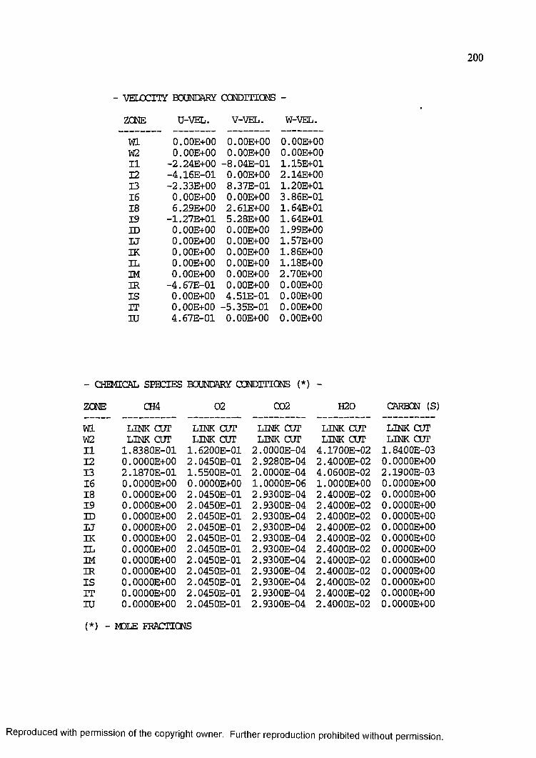
200
VELOCITY BOUNDARY CCNDITICNS -
ZCNE U-VEL. V-VEL. W-VEL.
Wl O.OOE+OOW2 O.OOE+OO11 -2 .2 4 E + 0 012 - 4 .1 6 E - 0 113 -2 .3 3 E + 0 016 O.OOE+OO18 6 .2 9 E + 0 019 -1 .2 7 E + 0 1ID O.OOE+OOU O.OOE+OOIK O.OOE+OOIL O.OOE+OOIM O.OOE+OOIR - 4 . 67E -01IS O.OOE+OOIT O.OOE+OOIU 4 . 67E -01
O.OOE+OO O.OOE+OO 0 .00E + 00 0 .00E + 00
- 8 .0 4 E - 0 1 1 . 15B+01 0 .00E + 00 2 .14E + 00 8 .3 7 E -0 1 1 .2 0 5 + 0 1 O.OOE+OO 3 .8 6 E -0 1 2 .6 1 E + 0 0 1 .6 4 5 + 0 1 5 .28E + 00 1 .6 4 5 + 0 1 O.OOE+OO 1 .99E + 00 O.OOE+OO 1 .57E + 00 O.OOE+OO 1 .86E + 00 O.OOE+OO 1 .1 8 5 + 0 0 O.OOE+OO 2 .70E + 00 O.OOE+OO O.OOE+OO 4 .5 1 E -0 1 O.OOE+OO
-5 .3 5 E - 0 1 O.OOE+OO O.OOE+OO O.OOE+OO
- CHEMICAL SPECIES BOUNDARY CCfOITICNS (*) -
ZCNE CH4 02 002 H20 CARBON (S)
Wl LINK CUT LINK COT LINK COT LINK COT LINK COTW2 LINK COT LINK COT LINK COT LINK COT LINK COT11 1 .8 3 8 0 E -0 1 1 .6 2 0 0 E -0 1 2 . 0000E -04 4 .1 7 0 0 E -0 2 1 . 8400E -0312 0 . 0000E+00 2 .0 4 5 0 E -0 1 2 . 9280E -04 2 .4 0 0 0 E -0 2 0 . OOOOE+OO13 2 .1 8 7 0 E -0 1 1 .5 5 0 0 E -0 1 2 . 000OE-04 4 . 0600E -02 2 .1 9 0 0 E -0 31 6 0 . 0000E+00 0 . OOOOE+OO 1 . 0000E -06 1 . OOOOE+OO 0 . OOOOE+OO1 8 0 . 0000E+00 2 . 0450E -01 2 .9 3 0 0 E -0 4 2 .4 0 0 0 E -0 2 0 . OOOOE+OO1 9 0 . OOOOE+OO 2 . 0450E -01 2 .9 3 0 0 E -0 4 2 .4 0 0 0 E -0 2 0 . OOOOE+OOID 0 . 0000E+00 2 . 0450E -01 2 .9 3 0 0 E -0 4 2 .4 0 0 0 E -0 2 0 . OOOOE+OOU 0 . OOOOE+OO 2 . 0450E -01 2 .9 3 0 0 E -0 4 2 . 4 000E -02 0 . OOOOE+OOIK 0 . OOOOE+OO 2 . 0450E -01 2 .9 3 0 0 E -0 4 2 . 40 0 0 E -0 2 0 . OOOOE+OOIL 0 . OOOOE+OO 2 .0 4 5 0 E -0 1 2 .9 3 0 0 E -0 4 2 . 40 0 0 E -0 2 0 . OOOOE+OOIM 0 . OOOOE+OO 2 . 0450E -01 2 . 9300E -04 2 . 4000E -02 0 . OOOOE+OOIR 0 . OOOOE+OO 2 . 0450E -01 2 .9 3 0 0 E -0 4 2 .4 0 0 0 E -0 2 0 . OOOOE+OOI S 0 . OOOOE+OO 2 . 0450E -01 2 .9 3 0 0 E -0 4 2 .4 0 0 0 E -0 2 0 . OOOOE+OOIT 0 . OOOOE+OO 2 . 0 450E -01 2 . 9300E -04 2 .4 0 0 0 E -0 2 0 . OOOOE+OOIU 0 . OOOOE+OO 2 . 0450E -01 2 .9 3 0 0 E -0 4 2 . 4000E -02 0 . OOOOE+OO
(*) - MOLE FRACTIONS
Reproduced with permission of the copyright owner. Further reproduction prohibited without permission.
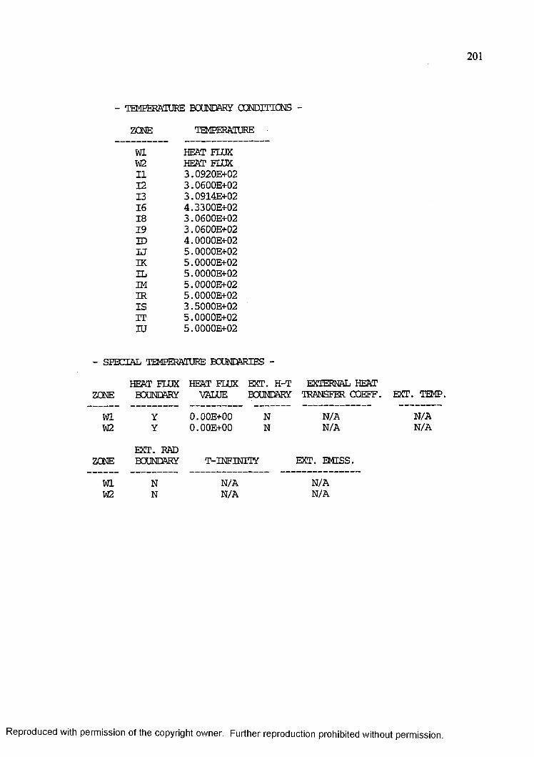
- TEMPERATURE BOUNDARY CCNDITTCNS -
ZONE TEMPERAT
Wl HEAT FLUXW2 HEAT FLUX11 3 . 0920E+0212 3 . 0600E+0213 3 . 0914E+0216 4 .3300E + 0218 3 . 0600E+0219 3 . 0600E+02ID 4 . 0000E+02U 5 . 0000E+02IK 5 . 0000E+02IL 5 . 0000E+02IM 5 . 0000E+02IR 5 . 0000E+02IS 3 . 5000E+02IT 5 . 0000E+02IU 5 . 0000E+02
- SPECIAL TEMPERATURE BOUNDARIES -
HEAT FLUX HEAT FLUX EXT. H-T EXTERNAL HEAT ZONE BOUNDARY VALUE BOUNDARY TRANSFER OOEFF.
Wl Y O.OOE+OO N N /AW2 Y O.OOE+OO N N /A
EXT. RADZONE BOUNDARY T-INFINITY EXT. EMISS.
Wl N N /A N /AW2 N N /A N /A
EXT. TEMP.
N /AN /A
Reproduced with permission of the copyright owner. Further reproduction prohibited without permission.
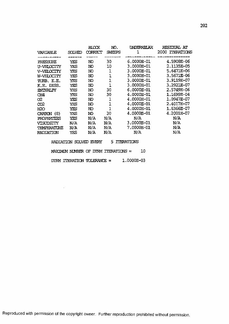
202
BLOCK NO. UNDERRELAX RESIDUAL ATVARIABLE SOLVED CORRECT SWEEPS 1 2000 ITERATIONS
PRESSURE YES NO 30 6 . 0 000E -01 4 .5 9 0 8 E -0 6U-VELOCTIY YES NO 10 3 . 00 0 0 E -0 1 2 . 1135E -05V-VELOCITY YES NO 1 3 . 0 000E -01 5 . 6471E -06W-VELOCnY YES NO 1 3 . 0 000E -01 3 . 5671E -06TURB. K .E . YES NO 1 3 . 00 0 0 E -0 1 3 . 9119E -07K .E . D ISS. YES NO 1 3 . OOOOE-Ol 3 .2 9 2 1 E -0 7ENTHALEY YES NO 30 6 . 0 000E -01 2 . 57 4 9 E -0 6CH4 YES NO 30 4 . 0 000E -01 1 . 1699E -0402 YES NO 1 4 . 0 000E -01 1 .0 9 4 7 E -0 7C02 YES NO 1 4 . 0 000E -01 2 . 4017E -07H20 YES NO 1 4 . 0 000E -01 1 .6 3 6 6 E -0 7CARBON (S) YES NO 30 4 . 00 0 0 E -0 1 4 .2 0 0 1 E -0 7PROPERTIES YES N /A N /A N /A N /AVISCOSITY N /A N /A N /A 3 . 00 0 0 E -0 1 N /ATEMPERATURE N /A N /A N /A 7 . 00 0 0 E -0 1 N /ARADIATION YES N /A N /A N /A N /A
RADIATION SOLVED EVERY 5 ITERATIONS
MAXIMUM NUMBER OF DIRM ITERATIONS = 10
DIRM ITERATICN TOLERANCE = 1 .0 0 0 0 E -0 3
Reproduced with permission of the copyright owner. Further reproduction prohibited without permission.
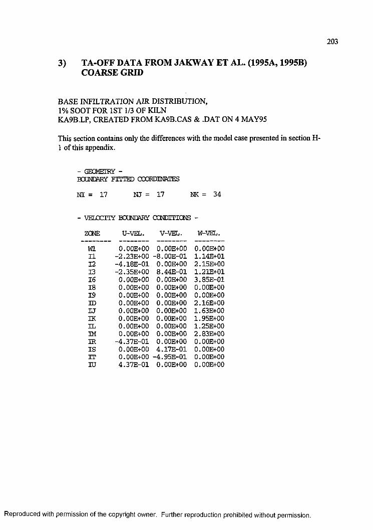
203
3) TA-OFF DATA FROM JAKWAY ET AL. (1995A, 1995B) COARSE GRID
BASE INFILTRATION AIR DISTRIBUTION,1% SOOT FOR 1ST 1/3 OF KILNKA9B.LP, CREATED FROM KA9B.CAS & .DAT ON 4 MAY95
This section contains only the differences with the model case presented in section H- 1 of this appendix.
- GEOdEIRY -BOUNDARY FITTED COORDINATES
N I = 17 NJ = 17 NK = 34
- VELOCITY BOUNDARY CONDITIONS -
ZCNE U-VEL. V-VEL. W-VEL.
Wl 0 .00E + 00 0 .00E + 00 O.OOE+OO11 -2 .2 3 E + 0 0 - 8 .0 0 E - 0 1 1 .1 4 E + 0 112 - 4 . 18 E -0 1 O.OOE+OO 2 .15E + 0013 -2 .3 5 E + 0 0 8 .4 4 E -0 1 1 .2 1 E + 0 116 0 .0 0 E + 0 0 O.OOE+OO 3 . 85E -0118 0 .0 0 E + 0 0 O.OOE+OO O.OOE+OO19 O.OOE+OO O.OOE+OO O.OOE+OOID 0.0 0 E + 0 0 O.OOE+OO 2 .16E + 00U 0 .0 0 E + 0 0 O.OOE+OO 1.63E + 00IK 0 .0 0 E + 0 0 O.OOE+OO 1.95E + 00IL 0 .00E + 00 O.OOE+OO 1.25E + 003M O.OOE+OO O.OOE+OO 2 .83E + 00IR - 4 . 3 7 E -0 1 O.OOE+OO O.OOE+OOI S 0 .0 0 E + 0 0 4 .1 7 E -0 1 O.OOE+OOIT 0 .0 0 E + 0 0 -4 .9 5 E - 0 1 O.OOE+OOIU 4 .3 7 E -0 1 O.OOE+OO O.OOE+OO
Reproduced with permission of the copyright owner. Further reproduction prohibited without permission.
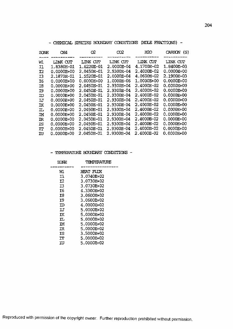
2 0 4
- CHEMICAL SPECIES BOUNDARY CCNDITICNS (MOLE FRACTIONS) -
ZCNE CH4 02 002 H20 CARBON (S)
Wl LINK CUT LINK CUT LINK CUT LINK CUT LINK CUT11 1 .8 3 8 0 E -0 1 1 . 6220E -01 2 . 0000E -04 4 .1 7 0 0 E -0 2 1 .8 4 0 0 E -0 312 0 . 0000E+00 2 . 04 5 0 E -0 1 2 .9 3 0 0 E -0 4 2 .4 0 0 0 E -0 2 0 . OOOOE+OO13 2 .1 8 7 0 E -0 1 1 . 55 2 0 E -0 1 2 . 0000E -04 4 . 0600E -02 2 .1 9 0 0 E -0 316 0 . OOOOE+OO 0 . OOOOE+OO 1 .0 0 0 0 E -0 6 1 . OOOOE+OO 0 . OOOOE+OO18 0 . OOOOE+OO 2 . 0 450E -01 2 .9 3 0 0 E -0 4 2 . 4000E -02 0 . OOOOE+OO19 0 . OOOOE+OO 2 . 04 5 0 E -0 1 2 .9 3 0 0 E -0 4 2 .4 0 0 0 E -0 2 0 . OOOOE+OOID 0 . 0000E+00 2 . 0 450E -01 2 .9 3 0 0 E -0 4 2 . 4000E -02 0 . OOOOE+OOU 0 . OOOOE+OO 2 . 0 450E -01 2 . 9300E -04 2 . 4 000E -02 0 . OOOOE+OOIK 0 . 0000E+00 2 . 0 450E -01 2 . 9300E -04 2 .4 0 0 0 E -0 2 0 . OOOOE+OOIL 0 . OOOOE+OO 2 . 0 450E -01 2 .9 3 0 0 E -0 4 2 . 4000E -02 0 . OOOOE+OOIM 0 . OOOOE+OO 2 . 0 450E -01 2 .9 3 0 0 E -0 4 2 . 4000E -02 0 . OOOOE+OOIR 0 . 0000E+00 2 . 0 450E -01 2 .9 3 0 0 E -0 4 2 . 4000E -02 0 . OOOOE+OOI S 0 . OOOOE+OO 2 . 0450E -01 2 .9 3 0 0 E -0 4 2 . 4000E -02 0 . OOOOE+OOIT 0 . OOOOE+OO 2 . 0450E -01 2 .9 3 0 0 E -0 4 2 . 4000E -02 0 . OOOOE+OOIU 0 . 0000E+00 2 . 0450E -01 2 . 9300E -04 2 . 4000E -02 0 . OOOOE+OO
- TEMPERAIURE BOUNDARY CCNDITICNS -
ZCNE TEMPERAIURE
Wl HEAT FLUX11 3 . 0740E+0212 3 . 0730E+0213 3 . 0730E+0216 4 .3300E + 0218 3 . 0600E+0219 3 . 0600E+02ID 4 .0000E + 02U 5 . 0000E+02IK 5 .0000E + 02IL 5 .0000E + 02IM 5 . 0000E+02IR 5 .0000E + 02I S 3 . 5000E+02IT 5 .0000E + 02IU 5 .0000E + 02
Reproduced with permission of the copyright owner. Further reproduction prohibited without permission.
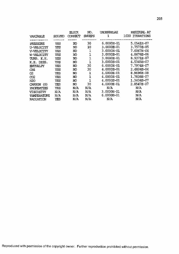
205
BLOCKVARIABLE SOLVED CORRECT
PRESSURE YES NOU-VELOCITY YES NOV-VELOCITY YES NOW-VELOCITY YES NOTURB. K .E . YES NOK .E . D ISS . YES NOENTHALPY YES NOCH4 YES NO02 YES NOC02 YES NOH20 YES NOCARBCN (S) YES NOPROPERTIES YES N /AVISCOSITY N /A N/ATEMPERATURE N /A N/ARADIATTCN YES N /A
UNDERRELAX RESIDUAL AT1 1020 TTERATICNS
6 . 0000E -01 5 . 0541E -073 . OOOOE-Ol 3 .7 5 7 3 E -0 53 . 0000E -01 7 .6 0 6 7 E -0 63 . OOOOE-Ol 4 .8 6 7 6 E -0 63 . 0 000E -01 8 .9 3 7 1 E -0 73 . 0000E -01 4 .5 3 4 5 E -0 76 . 0000E -01 7 .7 9 7 4 E -0 74 . 0000E -01 2 .4 8 2 4 E -0 44 . 0000E -01 8 .9 6 9 6 E -0 84 . 0000E -01 1 .7 8 3 8 E -0 74 . 0000E -01 1 .3 4 0 4 E -0 74 . OOOOE-Ol 2 . 8547E -07
N /A N /A3 . 0000E -01 N /A6 . 0000E -01 N /A
N /A N /A
NO.SWEEPS
3010
1111
3030
111
30N /AN /AN /AN /A
Reproduced with permission of the copyright owner. Further reproduction prohibited without permission.
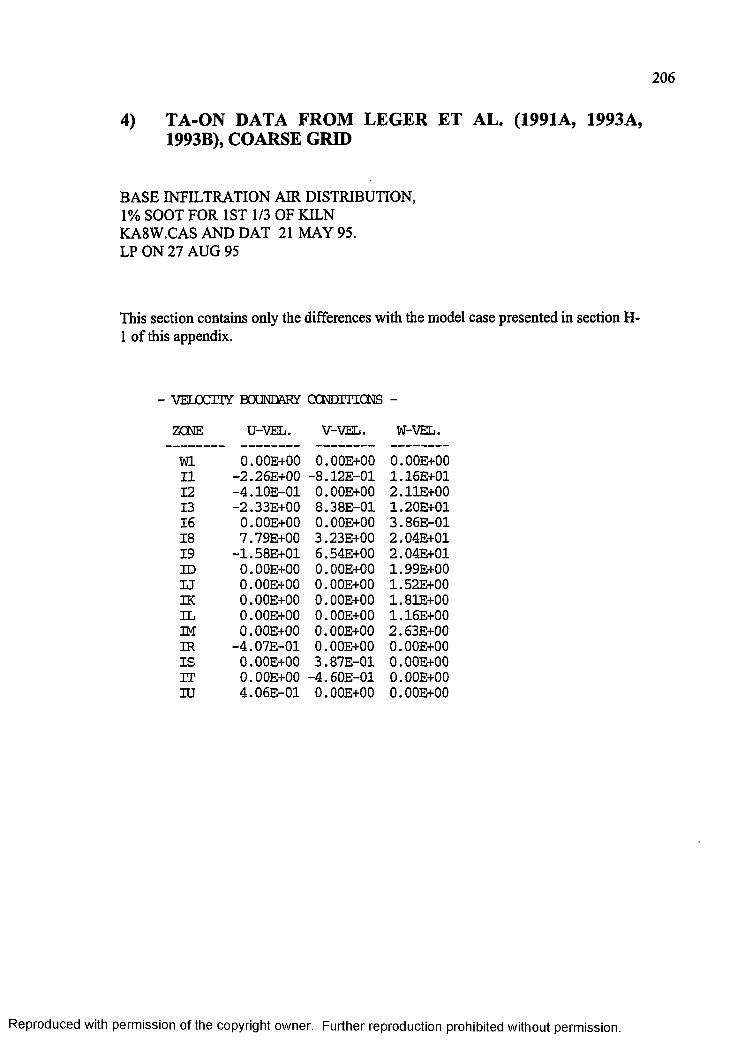
2 06
4) TA-ON DATA FROM LEGER ET AL. (1991A, 1993A, 1993B), COARSE GRID
BASE INFILTRATION AIR DISTRIBUTION, 1% SOOT FOR 1ST 1/3 OF KILN KA8W.CAS AND DAT 21 MAY 95.LP ON 27 AUG 95
This section contains only the differences with the model case presented in section H- 1 of this appendix.
- VELOCITY BOUNDARY CCNDITICNS -
ZCNE U-VEL. V-VEL. W-VEL.
Wl 0 .00E + 00 0 .00E + 00 O.OOE+OO11 -2 .2 6 E + 0 0 - 8 . 12E -01 1 .16E + 0112 - 4 .1 0 E -0 1 0.00E + 00 2 . 11E+0013 -2 .3 3 E + 0 0 8 .3 8 E -0 1 1 .20E + 0116 0 .00E + 00 0.00E + 00 3 .8 6 E -0 118 7 .79E + 00 3.23E + 00 2 .04E + 0119 -1 .5 8 E + 0 1 6 .54E + 00 2 .04E + 01ID 0 .00E + 00 0.00E + 00 1.99E + 00U 0 .00E + 00 0.00E + 00 1.52E + 00IK 0.00E + 00 O.OOE+OO 1.81E + 00IL 0 .00E + 00 0.00E + 00 1.16E + 00IM 0.00E + 00 O.OOE+OO 2.63E + 00IR - 4 .0 7 E -0 1 0 .00E + 00 0.00E + 00I S O.OOE+OO 3 .8 7 E -0 1 O.OOE+OOIT 0 .00E + 00 -4 .6 0 E -0 1 O.OOE+OOIU 4 .0 6 E -0 1 0.00E + 00 O.OOE+OO
Reproduced with permission of the copyright owner. Further reproduction prohibited without permission.
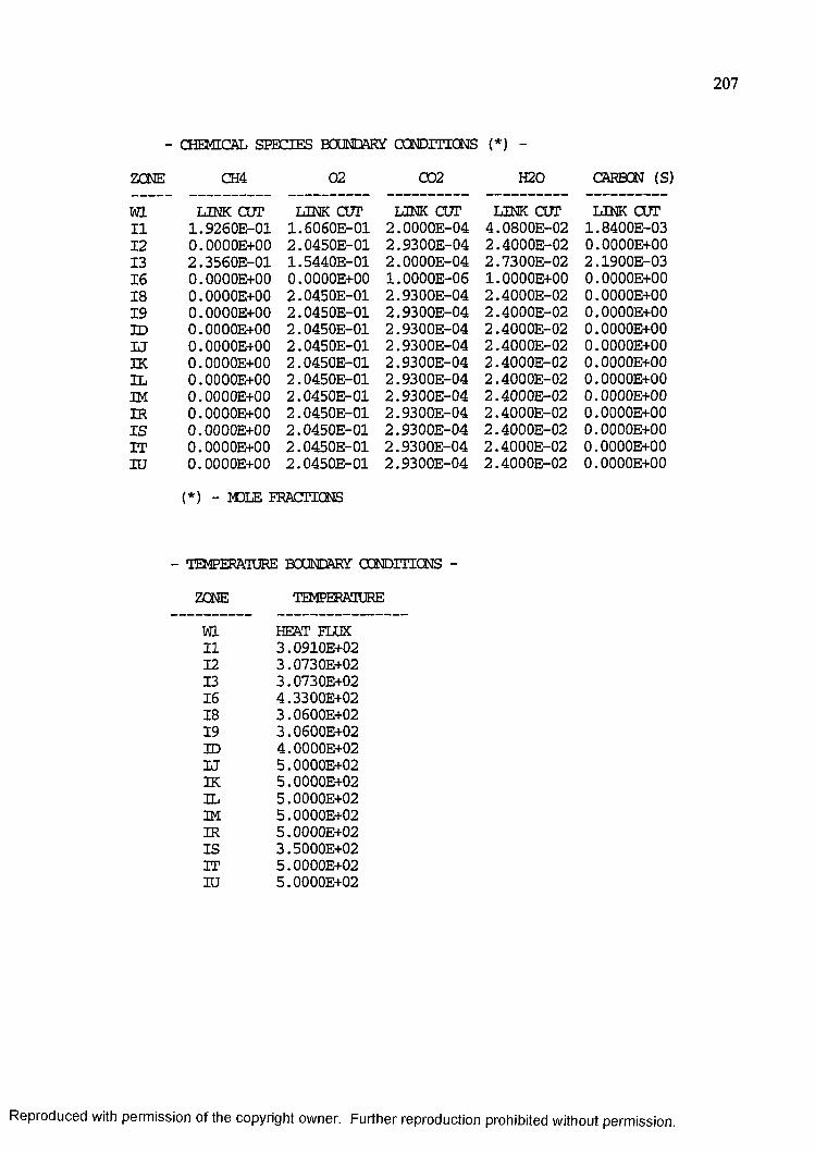
2 0 7
- CHEMICAL SPECIES BOUNDARY CCNDITICNS (*) -
ZCNE CH4 02 002 H20 CARBON (S)
Wl LINK COT LINK COT LINK COT LINK COT LINK COT11 1 .9 2 6 0 E -0 1 1 .6 0 6 0 E -0 1 2 . 00 0 0 E -0 4 4 .0 8 0 0 E -0 2 1 . 8400E -0312 0 . OOOOE+OO 2 . 0450E -01 2 .9 3 0 0 E -0 4 2 .4 0 0 0 E -0 2 0 . OOOOE+OO13 2 .3 5 6 0 E -0 1 1 .5 4 4 0 E -0 1 2 . 000O E-04 2 .7 3 0 0 E -0 2 2 . 1900E -0316 0 . OOOOE+OO 0 . OOOOE+OO 1 .0 0 0 0 E -0 6 1 . OOOOE+OO 0 . OOOOE+OO18 0 . OOOOE+OO 2 . 0450E -01 2 . 9 3 0 0 E -0 4 2 .4 0 0 0 E -0 2 0 . OOOOE+OO19 0 . OOOOE+OO 2 . 0450E -01 2 .9 3 0 0 E -0 4 2 .4 0 0 0 E -0 2 0 . OOOOE+OOID 0 . OOOOE+OO 2 . 0450E -01 2 .9 3 0 0 E -0 4 2 .4 0 0 0 E -0 2 0 . OOOOE+OOU 0 . OOOOE+OO 2 .0 4 5 0 E -0 1 2 .9 3 0 0 E -0 4 2 .4 0 0 0 E -0 2 0 . OOOOE+OOIK 0 . OOOOE+OO 2 . 0 450E -01 2 .9 3 0 0 E -0 4 2 . 4 0 0 0 E -0 2 0 . OOOOE+OOIL 0 . OOOOE+OO 2 . 0450E -01 2 .9 3 0 0 E -0 4 2 .4 0 0 0 E -0 2 0 . OOOOE+OOIM 0 . 0000E+00 2 . 0450E -01 2 .9 3 0 0 E -0 4 2 . 40 0 0 E -0 2 0 . OOOOE+OOIR 0 . OOOOE+OO 2 . 0450E -01 2 .9 3 0 0 E -0 4 2 .4 0 0 0 E -0 2 0 . OOOOE+OOI S 0 . OOOOE+OO 2 . 0450E -01 2 .9 3 0 0 E -0 4 2 . 40 0 0 E -0 2 0 . OOOOE+OOIT 0 . OOOOE+OO 2 . 0 450E -01 2 .9 3 0 0 E -0 4 2 .4 0 0 0 E -0 2 0 . OOOOE+OOIU 0 . OOOOE+OO 2 . 0450E -01 2 . 9 3 0 0 E -0 4 2 .4 0 0 0 E -0 2 0 . OOOOE+OO
{*) - MOLE FRACTIONS
- TEMPERATORE BOUNDARY CCNDITICNS -
ZCNE TEMPERATORE
Wl HEAT FLUX11 3 . 0910E+0212 3 .07 3 0 E + 0 213 3 . 0730E+0216 4 .33 0 0 E + 0 218 3 . 0600E+0219 3 . 0600E+02ID 4 . 0000E+02U 5 . OOOOE+02IK 5 . OOOOE+02IL 5 . OOOOE+02IM 5 . 0000E+02IR 5 . 0000E+02I S 3 .50 0 0 E + 0 2IT 5 . 0000E+02IU 5 . 0000E+02
Reproduced with permission of the copyright owner. Further reproduction prohibited without permission.
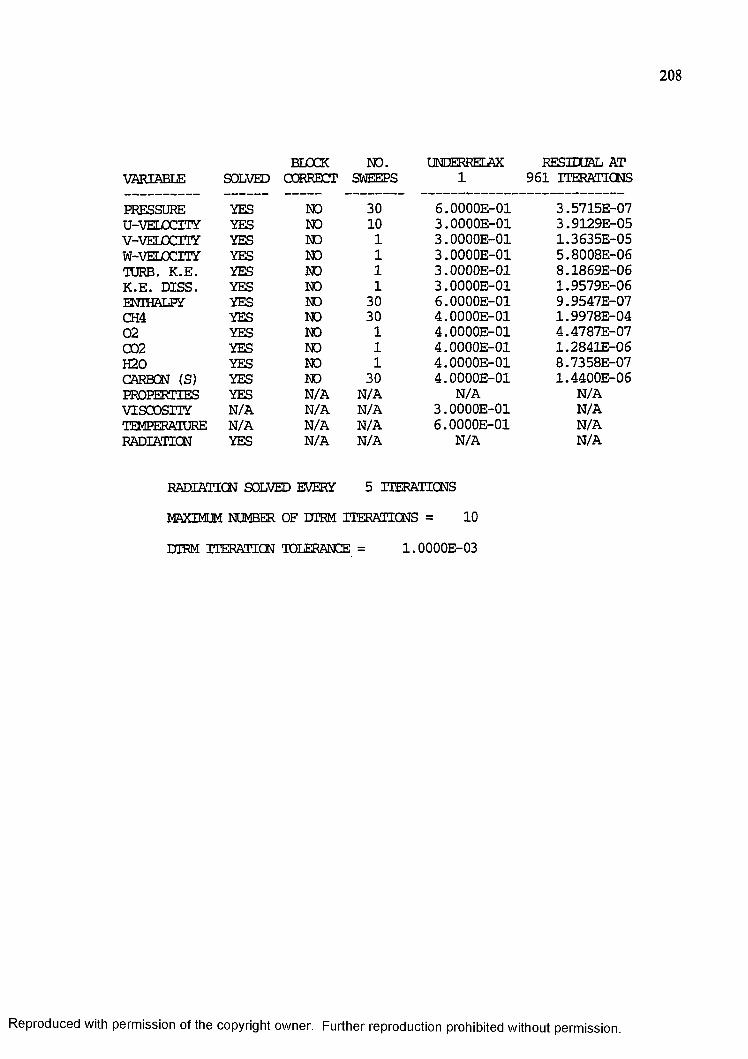
208
BLOCK NO. UNDERRELAX RESIDUAL ATVARIABLE SOLVED CORRECT SWEEPS 1 9 6 1 ITERATIONS
PRESSURE YES NO 30 6 . OOOOE-Ol 3 .5 7 1 5 E -0 7U-VELOCITY YES NO 10 3 . OOOOE-Ol 3 . 9129E -05V-VELOCTTY YES NO 1 3 . 00 0 0 E -0 1 1 .3 6 3 5 E -0 5W-VELOCITY YES NO 1 3 . 00 0 0 E -0 1 5 . 8008E -06TURB. K .E . YES NO 1 3 . 00 0 0 E -0 1 8 .1 8 6 9 E -0 6K .E . D ISS . YES NO 1 3 . 00 0 0 E -0 1 1 . 95 7 9 E -0 6ENTHALPY YES NO 30 6 . OOOOE-Ol 9 . 9 547E -07CH4 YES NO 30 4 . 00 0 0 E -0 1 1 .9 9 7 8 E -0 402 YES NO 1 4 . 0 0 0 0 E -0 1 4 .4 7 8 7 E -0 7C02 YES NO 1 4 . 00 0 0 E -0 1 1 .2 8 4 1 E -0 6H20 YES NO 1 4 . 00 0 0 E -0 1 8 .7 3 5 8 E -0 7CARBON (S) YES NO 30 4 . 0 000E -01 1 .4 4 0 0 E -0 6PROPERTIES YES N /A N /A N /A N /AVISCOSITY N /A N /A N /A 3 . 00 0 0 E -0 1 N /ATEMPERATURE N /A N /A N /A 6 . OOOOE-Ol N /ARADIATICN YES N /A N /A N /A N /A
RADIATICN SOLVED EVERY 5 ITERATIONS
MAXIMUM NUMBER OF DIRM ITERATIONS = 10
DIRM ITERATION TOLERANCE = 1 .0 0 0 0 E -0 3
Reproduced with permission of the copyright owner. Further reproduction prohibited without permission.
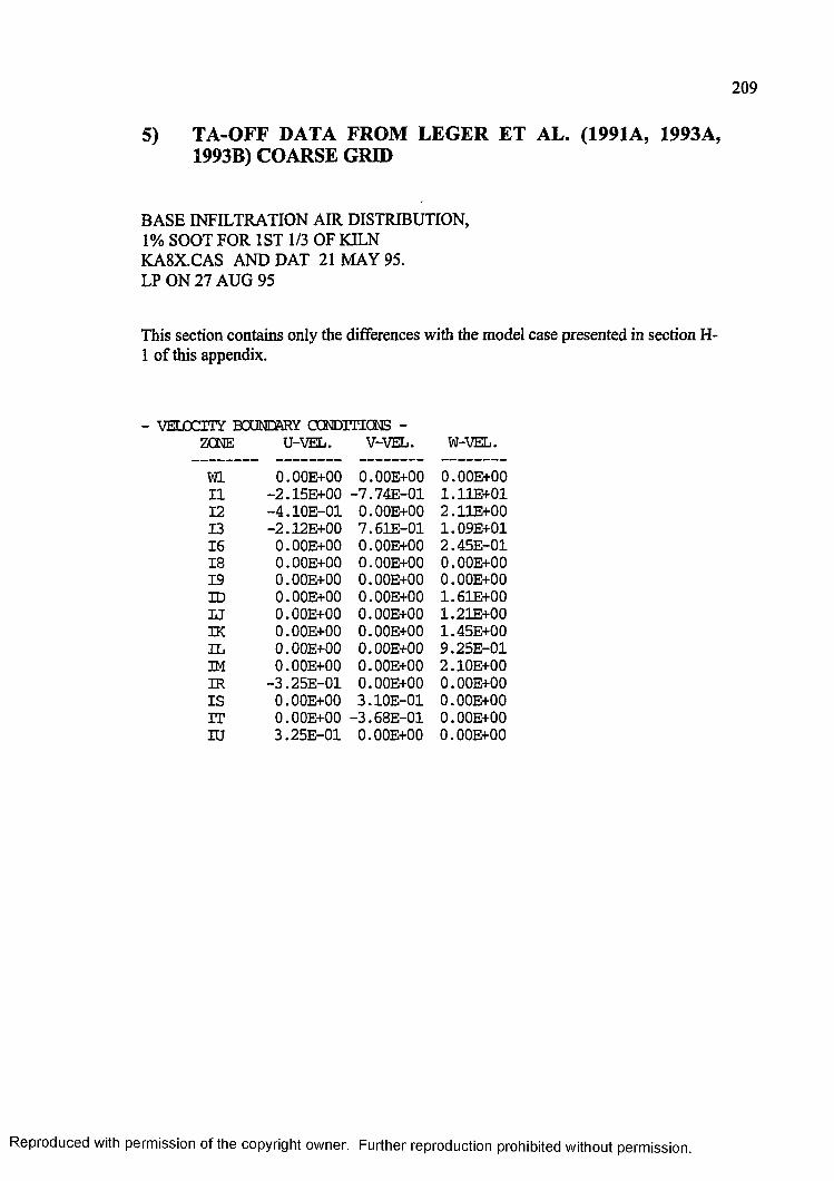
2 0 9
5) TA-OFF DATA FROM LEGER ET AL. (1991A, 1993A, 1993B) COARSE GRID
BASE INFILTRATION AIR DISTRIBUTION,1% SOOT FOR 1ST 1/3 OF KILN KA8X.CAS AND DAT 21 MAY 95.LP ON 27 AUG 95
This section contains only the differences with the model case presented in section H- 1 of this appendix.
- VELOCITY BOUNDARY CCNDITICNS -ZCNE U-VEL. V-VEL. W-VEL.
Wl 0 .00E + 00 O.OOE+OO O.OOE+OO11 - 2 . 15E+00 -7 .7 4 E -0 1 1 .11E + 0112 - 4 . 10E -01 O.OOE+OO 2 . 11E+0013 - 2 . 12E+00 7 .6 1 E -0 1 1 . 09E+0116 0.00E + 00 O.OOE+OO 2 .4 5 E -0 118 0.00E + 00 O.OOE+OO O.OOE+OO19 0.00E + 00 O.OOE+OO O.OOE+OOID 0.00E + 00 O.OOE+OO 1.61E + 00U 0.00E + 00 O.OOE+OO 1.21E + 00IK 0.00E + 00 O.OOE+OO 1.45E + 00IL 0.00E + 00 O.OOE+OO 9 .2 5 E -0 1IM O.OOE+OO O.OOE+OO 2 . 10E+00IR -3 .2 5 E -0 1 O.OOE+OO O.OOE+OOIS O.OOE+OO 3 . 10E -01 O.OOE+OOIT O.OOE+OO -3 .6 8 E -0 1 O.OOE+OOIU 3 .2 5 E -0 1 O.OOE+OO O.OOE+OO
Reproduced with permission of the copyright owner. Further reproduction prohibited without permission.
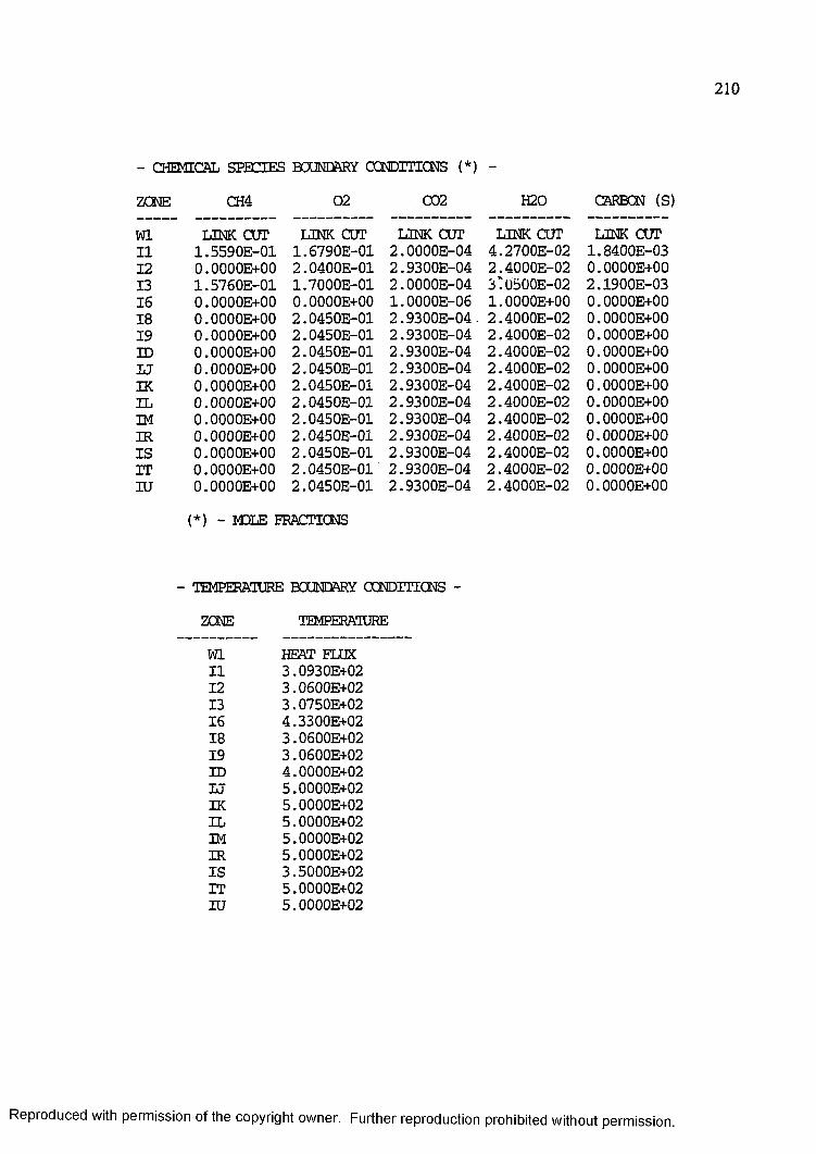
210
- CHEMICAL SPECIES BOUNDARY CXSJDITICNS (*) -
ZCNE CH4 02 C02 H20 CARBCN (S)
Wl LINK CUT LINK CUT LINK CUT LINK CUT LINK CUT11 1 .5 5 9 0 E -0 1 1 . 6790E -01 2 . 0000E -04 4 .2 7 0 0 E -0 2 1 .8 4 0 0 E -0 312 0 . 0000E+00 2 . 0400E -01 2 .9 3 0 0 E -0 4 2 . 4000E -02 0 . OOOOE+OO13 1 .5 7 6 0 E -0 1 1 .7 0 0 0 E -0 1 2 . 0000E -04 3 :0 5 0 0 E -0 2 2 . 1900E -0316 0 . 0000E+00 0 . OOOOE+OO 1 . 0000E -06 1 . 0000E+00 0 . 0000E+0018 0 . 0000E+00 2 . 0450E -01 2 .9 3 0 0 E -0 4 . 2 .4 0 0 0 E -0 2 0 . OOOOE+OO19 0 . 0000E+00 2 . 0450E -01 2 .9 3 0 0 E -0 4 2 .4 0 0 0 E -0 2 0 . OOOOE+OOID 0 . 0000E+00 2 . 0450E -01 2 .9 3 0 0 E -0 4 2 . 4000E -02 0 . OOOOE+OOU 0 . 0000E+00 2 . 0450E -01 2 .9 3 0 0 E -0 4 2 . 4000E -02 0 . OOOOE+OOIK 0 . 0000E+00 2 . 0450E -01 2 .9 3 0 0 E -0 4 2 .4 0 0 0 E -0 2 0 . 0000E+00IL 0 . 0000E+00 2 . 0450E -01 2 .9 3 0 0 E -0 4 2 . 4000E -02 0 . 0000E+00IM 0 . 0000E+00 2 . 0450E -01 2 .9 3 0 0 E -0 4 2 .4 0 0 0 E -0 2 0 . 0000E+00IR 0 . 0000E+00 2 . 0450E -01 2 .9 3 0 0 E -0 4 2 . 4000E -02 0 . 0000E+00I S 0 . 0000E+00 2 . 0450E -01 2 .9 3 0 0 E -0 4 2 .4 0 0 0 E -0 2 0 . OOOOE+OOIT 0 . 0000E+00 2 . 0450E -01 2 .9 3 0 0 E -0 4 2 . 4 000E -02 0 . OOOOE+OOIU 0 . 0000E+00 2 . 0450E -01 2 .9 3 0 0 E -0 4 2 . 4000E -02 0 . OOOOE+OO
(*) - MOLE FRACTIONS
- TEMPERATURE BOUNDARY CCNDITICNS -
ZCNE TEMPERATURE
Wl HEAT FLUX11 3 .0930E + 0212 3 . 0600E+0213 3 .0750E + 0216 4 .3300E + 0218 3 . 0600E+0219 3 . 0600E+02ID 4 . 0000E+02U 5 . 0000E+02IK 5 . 0000E+02IL 5 . 0000E+02IM 5 . 0000E+02IR 5 . 0000E+02I S 3 .5000E + 02IT 5 . 0000E+02IU 5 . 0000E+02
Reproduced with permission of the copyright owner. Further reproduction prohibited without permission.
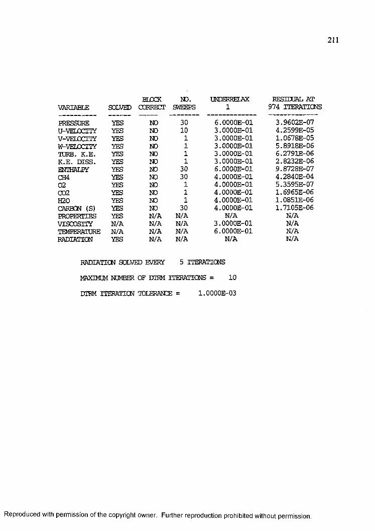
211
VARIABLE SOLVEDBLOCK
CORRECTNO.
SWEEPSUNDERRELAX
1RESIDUAL AT
974 ITERATIONS
PRESSURE YES NO 30 6 .0 0 0 0 E -0 1 3 .9 6 0 2 E -0 7U-VELOCITY YES NO 10 3 . OOOOE-Ol 4 .2 5 9 9 E -0 5V-VELOCITY YES NO 1 3 . OOOOE-Ol 1 .0 6 7 8 E -0 5W-VELOCITY YES NO 1 3 . 0 0 0 0 E -0 1 5 . 8 9 1 8 E -0 6TURB. K .E . YES NO 1 3 . OOOOE-Ol 6 .2 7 9 1 E -0 6K.E. D ISS . YES NO 1 3 . 0 0 0 0 E -0 1 2 . 8 2 3 2 E -0 6ENTHALPY YES NO 30 6 . OOOOE-Ol 9 . 8 7 2 8 E -0 7CH4 YES NO 30 4 . OOOOE-Ol 4 . 2 8 4 0 E -0 402 YES NO 1 4 . 0 0 0 0 E -0 1 5 .3 5 9 5 E -0 7C02 YES NO 1 4 . OOOOE-Ol 1 .6 9 6 5 E -0 6H20 YES NO 1 4 . OOOOE-Ol 1 .0 8 5 1 E -0 6CARBCN (S) YES NO 30 4 . OOOOE-Ol 1 .7 1 0 5 E -0 6PROPERTIES YES N /A N /A N /A N /AVISCOSITY N /A N /A N /A 3 . 00 0 0 E -0 1 N /ATEMPERATURE N /A N /A N /A 6 . 0 0 0 0 E -0 1 N /ARADIATION YES N /A N/A N /A N /A
RADIATTCN SOLVED EVERY 5 ITERATIONS
MAXIMUM NUMBER OF DIRM ITERATIONS = 10
DTRM ITERATION TOLERANCE = 1 .000Q E -03
Reproduced with permission of the copyright owner. Further reproduction prohibited without permission.
VITA
Allen Lee Jakway was bom at the venerable Baptist Hospital in New Orleans
on the 27th of February in 1962. He attended Lakeview elementary after which his
parents sacrificed to get him into St. John Lutheran for Junior High. For high school
he attended Benjamin Franklin magnet. A full scholarship convinced him to stay at
home and attend the University of New Orleans where he earned his Bachelor of
Science degree in Mechanical Engineering graduating cum laude at the top of his
engineering class. Chevron Chemical in Belle Chasse, Louisiana employed him for the
next several years where he first became interested in the environmental area of
engineering. Throughout this time, the author was active in his church particularly in
the youth group where he was introduced to singing and acting in musicals. A four
year fellowship offer then attracted the author to Baton Rouge to attend Louisiana
State University. Summers spent in Utah and New Mexico conducting research have
been particularly rewarding as have the experiences of delivering professional
conference presentations in Baton Rouge, New Orleans, Boston, and Seattle. After
graduation, the author plans to fulfill a long time dream of seeing this country at a
relaxed and more intimate pace by bicycling and camping across this continent.
212
Reproduced with permission of the copyright owner. Further reproduction prohibited without permission.
DOCTORAL EXAMINATION AND DISSERTATION REPORT
Candidate:
Major Field:
Title of Dissertation:
Date of Examination:
0 9 / 2 9 / 9 5 __________
Allen Lee Jakway
Mechanical Engineering
Experimental and Numerical-Modeling Studies of a Field-Scale Hazardous Waste Rotary Kiln Incinerator
Approved:
sor and chairman
of tseriGraduate School
INING COMMITTEE:
Reproduced with permission of the copyright owner. Further reproduction prohibited without permission.