Embed Size (px)
Citation preview
Contents lists available at ScienceDirect
Composite Structures
journal homepage: www.elsevier.com/locate/compstruct
Explicit tangent stiffness matrix for the geometrically nonlinear analysis oflaminated composite frame structures
Ardalan R. Sofia, Peter L. Bishaya,⁎, Satya N. Atlurib
a California State University, Northridge, CA, USAb Texas Tech University, Lubbock, TX, USA
A R T I C L E I N F O
Keywords:Large deformationUpdated LagrangianFinite elementsComposite beams
A B S T R A C T
In this paper, based on Von Kármán’s nonlinear theory and the classical lamination theory, a closed form ex-pression is derived for the tangent stiffness matrix of a laminated composite beam element undergoing largedeformation and rotation under mechanical and hygrothermal loads. Stretching, bending and torsion have beenconsidered. A co-rotational element reference frame is used as the Updated Lagrangian (UL) formulation. Themodel has been verified in different problems by comparison with the results of Nastran and ANSYS compositelaminate tools, and the difference in the resulting large deformations is less than 5%. The major advantage of theproposed approach is that the composite structure is modeled using 1D beam elements rather than 2D shell or 3Dsolid elements as in the case of Nastran and ANSYS where laminates are defined over surfaces or 3D solids. Theavailability of an explicit expression for the tangent stiffness matrix makes the proposed model highly efficientspecially when dealing with large composite space frame structures. The saving in computational time couldreach 93% compared to regular FE software packages. The developed model is very useful for modeling anddesigning flexible composites used in new applications such as morphing aerospace structures and flexible ro-bots.
1. Introduction
With the appearance of new technologies and inventions in thefields of automotive design, aerospace structures, smart structures, androbotics, the design and manufacturing of laminated composite mate-rials have seen a lot of development. Beside the well-known applica-tions of fiber-reinforced laminated composite materials because of theirvarious advantages, such as high specific stiffness and strength, highcorrosion resistance, good thermal insulation, fatigue resistance anddamping properties, new applications of composite materials emergedthat necessitate the development of new effective and efficient tools andapproaches in design and simulation. For example, a lot of smart ma-terial elements, such as shape memory alloy (SMA) wires or ribbons andpiezoelectric patches or fibers, are embedded in polymer compositelaminates to form smart composite structures with multi-functions suchas sensing, actuating and load bearing [1–3]. Another example is thedesign of morphing aerospace structures, such as morphing wings withflexible seamless control surfaces or flexible winglets [4]. The design ofsuch structures is challenging because of the need to have flexible, yetstrong, wing skins that can morph to different shapes and still be able tostand aerodynamic loads. Composite actuators combining shape
memory wires, glass fibers in a soft matrix that could morph intocomplex shapes utilizing coupling effects for in-plane, out-of-plane, andtwisting deformations have been proposed [5–7] and applied to inter-esting applications such as turtle-like swimming robot [8] andmorphing car spoiler [9]. Another example is robotic arms and ma-nipulators made of flexible laminated composite end-effectors [10,11].Flexible composites are manufactured as reinforcing fibers in flexiblematrix. Such flexible composites undergo large deformations, hence formodeling these structures, geometric nonlinearity should be con-sidered. In addition, composite beams and plates with high slendernessratios, normally undergo large displacements and rotations evenwithout reaching large strains and/or overcoming the material’s elasticlimit [12]. Hence, it is critical to develop computational tools to effi-ciently and accurately predict the deformation of such compositestructures subjected to any mechanical or hygrothermal loads. This willalso be very useful in the design process where large number of itera-tions are to be done sweeping the parameters in the design space toachieve the desired goals.
Introducing geometric nonlinearity to structures is an option in al-most all available commercial finite element software nowadays, suchas ANSYS, ABAQUS, and MSC Nastran. Defining a composite layup
https://doi.org/10.1016/j.compstruct.2017.11.006Received 17 August 2017; Received in revised form 21 September 2017; Accepted 6 November 2017
⁎ Corresponding author.E-mail address: [email protected] (P.L. Bishay).
Composite Structures xxx (xxxx) xxx–xxx
0263-8223/ © 2017 Elsevier Ltd. All rights reserved.
Please cite this article as: Sofi, A.R., Composite Structures (2017), https://doi.org/10.1016/j.compstruct.2017.11.006
given the material properties of all plies, their fiber orientations andthicknesses can also be done in all the aforementioned software inaddition to SOLIDWORKS Simulation, Autodesk SimulationMechanical, and Nastran-in-CAD tool integrated in any CAD softwaresuch as SOLIDWORKS or Autodesk Inventor. Composite laminates aredefined in these software on a surface or 3D solid to be meshed using 2Dplate or shell elements or 3D solid elements, respectively. Compositelaminates cannot be defined on lines to model beams or 3D frames.Hence, the computational cost of performing geometrically nonlinearstatic or dynamic analyses on large composite structures, such astrusses, frames or idealized structures, becomes very high. The devel-opment of a 3D frame element for the geometric nonlinear analysis oflaminated composite beams will then be very effective and efficient dueto the expected simplicity and low computational costs.
Several three-dimensional frame finite element formulations for thegeometric nonlinear analysis of thin-walled laminated composite beamshave been developed during the last two decades. Bhaskar and Librescu[13,14] developed nonlinear theory of thin-walled composite beamswith closed and open sections taking into account the transverse sheardeformation effect while the warping torsion component was neglected.Omidvar and Ghorbanpoor [15] and Cardoso et al. [16] proposed athree-dimensional nonlinear finite element models for thin-walledopen-section composite beams with symmetric stacking sequence, in-cluding the warping effect, and based on the Updated Lagrangian (UL)formulation. Based on Von Kármán strain tensor, Vo and Lee [17,18]developed three-dimensional thin-walled laminated beam elementswith open sections, and investigated the effects of fiber orientation,geometric nonlinearity, and shear deformation on the axial–-flexural–torsional response. Mororó et al. [12] developed three-di-mensional thin-walled laminated beam elements with closed sectionsusing Total Lagrangian (TL) formulation allowing large displacementsand moderate rotations, but without the effects of warping and trans-verse shear. Saravia [18] developed consistent large deformation-smallstrain formulation for thin-walled composite beams (TWCB) calling it a“geometrically exact TWCB formulation” suitable for modeling highaspect ratio composite beams that undergo large rigid body motions,such as wind turbine wings, satellite arms and automotive body stif-feners. Turkalj [20] presented a beam formulation for large displace-ment analysis of composite frames considering the flexibility of theconnections.
Atluri and his co-workers extensively studied large rotations inbeams, plates and shells, and attendant variational principles (see[21–24]). Explicit derivations of the tangent stiffness matrix of 3Dframes including elasto-plasticity were derived [25–27] without em-ploying either numerical or symbolic integrations. Based on a VonKármán type nonlinear theory in rotated reference frames, Cai et al.[28] developed a simple geometrically nonlinear large-rotation beamelement with arbitrary cross-section using a co-rotational referenceframe for each finitely rotated beam element as the UL reference frame
for the respective element, and accounting for stretching, bending andtorsion. An explicit expression of a symmetric tangent stiffness matrixof the beam element in the co-rotational frame was derived and vali-dated in multiple numerical examples of space frames undergoing largedeformations.
Even in the simplest formulation of the aforementioned works thatpresented geometrically nonlinear composite beams [12–20], an ex-plicit expression for the tangent stiffness matrix could not be reached.Hence in this work, a finite element formulation of laminated compo-site beams undergoing large deformation and rotation, in response tomechanical or hygrothermal loads, is developed based on Von Kármánnonlinear theory and the classical lamination theory. Stretching,bending, and torsion has been accounted for, and a closed form ex-pression of the element tangent stiffness matrix has been derived, uti-lizing the element’s co-rotational reference frame as the UL formula-tion. The model has been verified in different problems by comparisonwith Nastran and ANSYS results. In all problems, the difference in theresulting deformations is less than 5%. The relative simplicity of thederived explicit tangent stiffness matrix is one of the major advantagesof the proposed approach, which makes large deformation analyses oflaminated composite beams highly efficient specially when dealingwith large composite space frame structures.
2. Transformation between the global and the deformation-dependent co-rotational local frames of reference
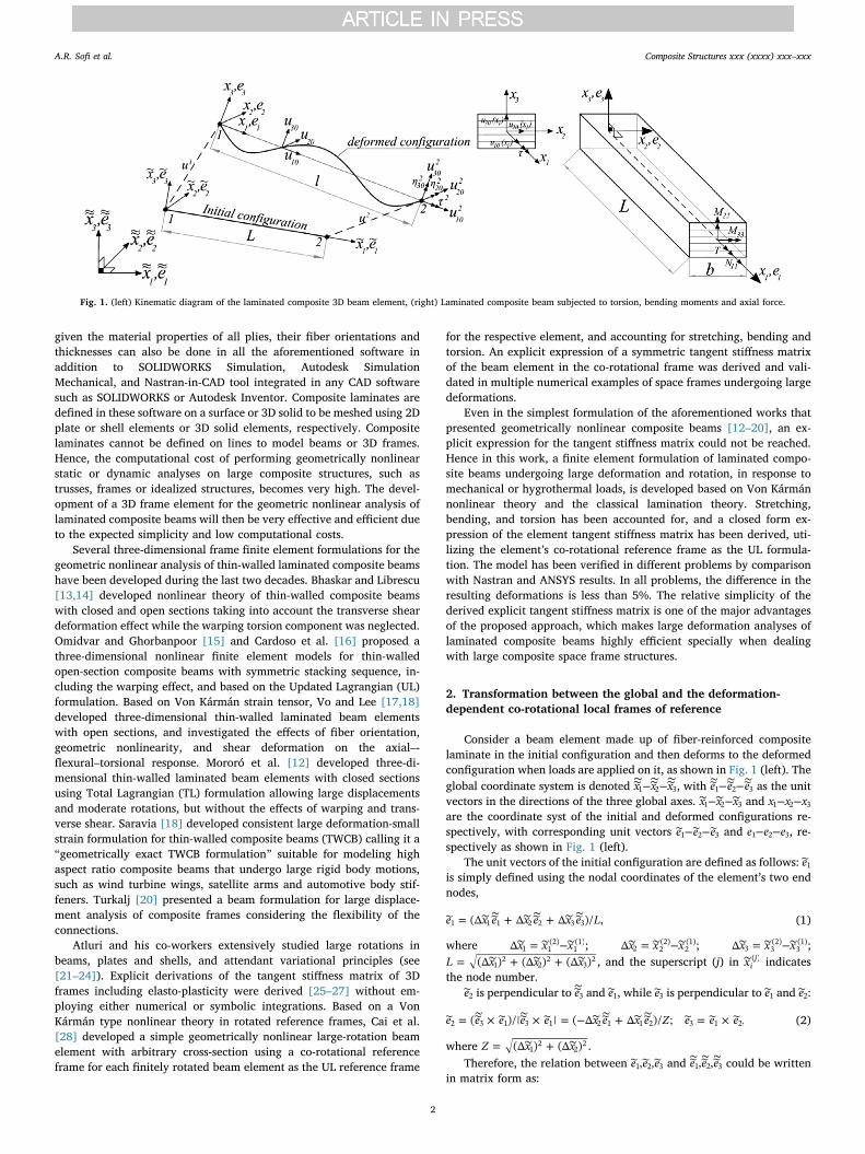
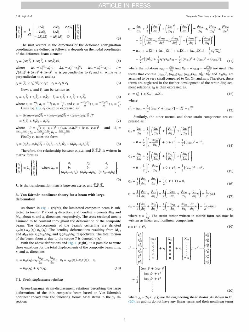
Consider a beam element made up of fiber-reinforced compositelaminate in the initial configuration and then deforms to the deformedconfiguration when loads are applied on it, as shown in Fig. 1 (left). Theglobal coordinate system is denoted − −∼ ∼ ∼∼ ∼ ∼
x x x1 2 3, with − −∼ ∼ ∼e e e1 2 3 as the unitvectors in the directions of the three global axes. − −∼ ∼ ∼x x x1 2 3 and − −x x x1 2 3
are the coordinate syst of the initial and deformed configurations re-spectively, with corresponding unit vectors − −e e e1 2 3 and − −e e e1 2 3, re-spectively as shown in Fig. 1 (left).
The unit vectors of the initial configuration are defined as follows: e1is simply defined using the nodal coordinates of the element’s two endnodes,
= + +∼ ∼ ∼∼ ∼ ∼e x e x e x e L(Δ Δ Δ )/ ,1 1 1 2 2 3 3 (1)
where = −∼ ∼ ∼x x xΔ 1 1(2)
1(1); = −∼ ∼ ∼x x xΔ 2 2
(2)2(1); = −∼ ∼ ∼x x xΔ 3 3
(2)3(1);
= + +∼ ∼ ∼L x x x(Δ ) (Δ ) (Δ )12
22
32 , and the superscript (j) in ∼xi
j( ) indicatesthe node number.
e2 is perpendicular to ∼e3 and e1, while e3 is perpendicular to e1 and e2:
= × × = − + = ×∼ ∼ ∼ ∼∼ ∼e e e e e x e x e Z e e e( )/| | ( Δ Δ )/ ; ,2 3 1 3 1 2 1 1 2 3 1 2 (2)
where = +∼ ∼Z x x(Δ ) (Δ )12
22 .
Therefore, the relation between e e e, ,1 2 3 and ∼ ∼ ∼e e e, ,1 2 3 could be writtenin matrix form as:
Fig. 1. (left) Kinematic diagram of the laminated composite 3D beam element, (right) Laminated composite beam subjected to torsion, bending moments and axial force.
A.R. Sofi et al. Composite Structures xxx (xxxx) xxx–xxx
2
⎧
⎨⎩
⎫
⎬⎭
=⎡
⎣
⎢⎢
−− −
⎤
⎦
⎥⎥
⎧
⎨⎪
⎩⎪
⎫
⎬⎪
⎭⎪
∼∼∼
∼ ∼ ∼∼ ∼
∼ ∼ ∼ ∼
eee ZL
Z x Z x Z xL x L xx x x x Z
eee
1Δ Δ ΔΔ Δ 0
Δ Δ Δ Δ
1
2
3
1 2 3
2 1
1 3 2 32
1
2
3 (3)
The unit vectors in the directions of the deformed configurationcoordinates are defined as follows: e1 depends on the nodal coordinatesof the deformed beam element,
= + +∼ ∼ ∼e x e x e x e l(Δ Δ Δ )/ ,1 1 1 2 2 3 3 (4)
where = −x x xΔ 1 1(2)
1(1); = −x x xΔ 2 2
(2)2(1); = −x x xΔ 3 3
(2)3(1); =l
+ +x x x(Δ ) (Δ ) (Δ )12
22
32 . e2 is perpendicular to e3 and e1, while e3 is
perpendicular to e1 and e2:
= × × = ×e e e e e e e e( )/| |; .2 3 1 3 1 3 1 2 (5)
Now, e1 and e3 can be written as:
= + + = + +∼ ∼ ∼ ∼ ∼ ∼e a e a e a e e c e c e c e; ,1 1 1 2 2 3 3 3 1 1 2 2 3 3 (6)
where =a xl1
Δ 1 ; =a xl2
Δ 2 ; =a xl3
Δ 3 , and = − ∼ ∼c x x
ZL1Δ Δ1 3 ; = − ∼ ∼
c x xZL2
Δ Δ2 3 ; =c ZL3 .
Using Eq. (5), e2 could be expressed as:
= − + − + −
= + +
∼ ∼ ∼
∼ ∼ ∼∗e c a c a e c a c a e c a c a e l
b e b e b e
[( ) ( ) ( ) ]/
,2 2 3 3 2 1 3 1 1 3 2 1 2 2 1 3
1 1 2 2 3 3 (7)
where = − + − + −∗l c a c a c a c a c a c a( ) ( ) ( )2 3 3 22
3 1 1 32
1 2 2 12 and =b1
−∗
c a c al
2 3 3 2 ; = −∗b c a c a
l23 1 1 3 ; = −
∗b c a c al3
1 2 2 1 .Finally e3 takes the form:
= − + − + −∼ ∼ ∼e a b a b e a b a b e a b a b e( ) ( ) ( )3 2 3 3 2 1 3 1 1 3 2 1 2 2 1 3 (8)
Therefore, the relationship between e e e, ,1 2 3 and ∼ ∼ ∼e e e, ,1 2 3 is written inmatrix form as
⎧⎨⎩
⎫⎬⎭
=⎧
⎨⎪
⎩⎪
⎫
⎬⎪
⎭⎪=
⎡
⎣⎢⎢ − − −
⎤
⎦⎥⎥
∼∼∼
eee
eee
a a ab b b
a b a b a b a b a b a bλ λ; where
( ) ( ) ( ).
123
0
1
2
3
0
1 2 3
1 2 3
2 3 3 2 3 1 1 3 1 2 2 1
(9)
λ0 is the transformation matrix between e e e, ,1 2 3 and ∼ ∼ ∼e e e, ,1 2 3.
3. Von Kármán nonlinear theory for a beam with largedeformation
As shown in Fig. 1 (right), the laminated composite beam is sub-jected to torsion T about x1 direction, and bending moments M22 andM33 about x3 and x2 directions, respectively. The cross-sectional area isassumed to be constant throughout the deformation of the compositebeam. The displacements of the beam’s centerline are denotedu x u x u x( ), ( ), ( )10 1 20 1 30 1 . The bending deformations resulting from M33
and M22 are ∂ ∂x u x( / )3 30 1 and ∂ ∂x u x( / )2 20 1 respectively. The total torsionof the beam about x1 due to the torque T is denoted τ x( )1 .
With the above definitions and Fig. 1 (right), it is possible to writethree equations for the total displacements of the composite beam in x1,x2 and x3 directions:
= − ∂∂
− ∂∂
= −
= +
u u x x ux
x ux
u u x x τ x u
u x x τ x
( ) ; ( ) ( );
( ) ( ).
1 10 1 220
13
30
12 20 1 3 1 3
30 1 2 1 (10)
3.1. Strain-displacement relations
Green-Lagrange strain-displacement relations describing the largedeformations of the thin composite beam based on Von Kármán’snonlinear theory take the following forms: Axial strain in the x1 di-rection:
⎜ ⎟
⎜ ⎟ ⎜ ⎟ ⎜ ⎟
⎜ ⎟ ⎜ ⎟
= ∂∂
+ ⎡
⎣⎢
⎛⎝
∂∂
⎞⎠
+ ⎛⎝
∂∂
⎞⎠
+ ⎛⎝
∂∂
⎞⎠
⎤
⎦⎥ = ∂
∂− ∂
∂− ∂
∂
+ ⎡
⎣⎢
⎛⎝
∂∂
− ∂∂
− ∂∂
⎞⎠
+ ⎛⎝
∂∂
⎞⎠
+ ⎛⎝
∂∂
⎞⎠
⎤
⎦⎥
= + + + + +
+ + + + +
ε ux
ux
ux
ux
ux
x ux
x ux
ux
x ux
x ux
ux
ux
u x u x u x
x x x u u u
12
12
[X ( )X ] [X ( )X ] 12
(X )
12
(X ) 12
X X 12
[( ) ( ) ( ) ],
111
1
1
1
22
1
23
1
210
12
220
12 3
230
12
10
12
220
12 3
230
12
220
1
230
1
2
10,1 2 22 10,1 22 3 33 10,1 33 22
222
32
332
2 3 22 33 10,12
20,12
30,12
(11)
where the notations = ∂∂ui jux0,ij0 and = − = − ∂
∂uXii i
ux0,11
i2 0
12 are used. The
terms that contain u( )10,12, u( )X10,1 22, u( )X10,1 33, X22
2 , X332 and X X22 33 are
assumed to be very small compared to X22, X33 and u10,1. Therefore, theseterms are neglected in the further development of the strain-displace-ment relations. ε11 is then expressed as,
= + +ε ε x xX X ,11 110
2 22 3 33 (12)
where
= + + = +ε u u u ε ε12
[( ) ( ) ] L N110
10,1 20,12
30,12
110
110
(13)
Similarly, the other normal and shear strain components are ex-pressed as:
⎜ ⎟ ⎜ ⎟ ⎜ ⎟
⎜ ⎟
= ∂∂
+ ⎡
⎣⎢
⎛⎝
∂∂
⎞⎠
+ ⎛⎝
∂∂
⎞⎠
+ ⎛⎝
∂∂
⎞⎠
⎤
⎦⎥
= + ⎡
⎣⎢
⎛⎝
− ∂∂
⎞⎠
+ + ⎤
⎦⎥ = +
ε ux
ux
ux
ux
ux
τ u τ
12
0 12
0 12
[( ) ],
222
2
1
2
22
2
23
2
2
20
1
22
20,12 2
(14)
⎜ ⎟ ⎜ ⎟ ⎜ ⎟
⎜ ⎟
= ∂∂
+ ⎡
⎣⎢
⎛⎝
∂∂
⎞⎠
+ ⎛⎝
∂∂
⎞⎠
+ ⎛⎝
∂∂
⎞⎠
⎤
⎦⎥
= + ⎡
⎣⎢
⎛⎝
− ∂∂
⎞⎠
+ + ⎤
⎦⎥ = +
ε ux
ux
ux
ux
ux
τ u τ
12
0 12
0 12
[( ) ],
333
3
1
3
22
3
23
3
2
30
1
22
30,12 2
(15)
⎜ ⎟= ⎛⎝
∂∂
+ ∂∂
⎞⎠
= − + =ε ux
ux
τ τ12
12
( ) 0,232
3
3
2 (16)
⎜ ⎟ ⎜ ⎟= ⎛⎝
∂∂
+ ∂∂
⎞⎠
= ⎛⎝
− ∂∂
+ ∂∂
+ ∂∂
⎞⎠
=ε ux
ux
ux
ux
τx
x ηx12
12
12
( )311
3
3
1
30
1
30
1 12 2
(17)
⎜ ⎟ ⎜ ⎟= ⎛⎝
∂∂
+ ∂∂
⎞⎠
= ⎛⎝
− ∂∂
+ ∂∂
− ∂∂
⎞⎠
= −ε ux
ux
ux
ux
τx
x ηx12
12
12
( )121
2
2
1
20
1
20
1 13 3
(18)
where = ∂∂η τ
x1. The strain tensor written in matrix form can now be
written as linear and nonlinear components:
= +ε ε ε ,L N (19)
=
⎧
⎨
⎪⎪⎪
⎩
⎪⎪⎪
⎫
⎬
⎪⎪⎪
⎭
⎪⎪⎪
=
⎡
⎣
⎢⎢⎢⎢⎢
⎤
⎦
⎥⎥⎥⎥⎥
+
⎡
⎣
⎢⎢⎢⎢⎢
⎤
⎦
⎥⎥⎥⎥⎥
+
⎡
⎣
⎢⎢⎢⎢⎢−
⎤
⎦
⎥⎥⎥⎥⎥
=
⎧
⎨
⎪⎪⎪
⎩
⎪⎪⎪
⎫
⎬
⎪⎪⎪
⎭
⎪⎪⎪
=
⎡
⎣
⎢⎢⎢⎢⎢⎢
+++
⎤
⎦
⎥⎥⎥⎥⎥⎥
εεεγ
γ
γ
u
xη
x
η
εεεγ
γ
γ
u uu τu τ
ε ε00000
X000
0
X0000
,
12
( ) ( )( )( )
000
L
L
L
L
L
L
L
N
N
N
N
N
N
N
11
22
33
23
31
12
10,1
2
22
3
3311
22
33
23
31
12
20,12
30,12
20,12 2
30,12 2
(20)
where = ≠γ ε i j2 ( )ij ij are the engineering shear strains. As shown in Eq.(20), ε22 and ε33 do not have any linear terms and their nonlinear terms
A.R. Sofi et al. Composite Structures xxx (xxxx) xxx–xxx
3
are relatively small. Therefore, these normal strains that are perpen-dicular to the beam's longitudinal direction could be neglected, and thelinear and nonlinear strains can be reduced to:
=⎡
⎣
⎢⎢⎢
⎤
⎦
⎥⎥⎥
= ⎡
⎣⎢
⎤
⎦⎥ +
⎡
⎣⎢⎢
⎤
⎦⎥⎥
+⎡
⎣⎢⎢−
⎤
⎦⎥⎥
=⎡
⎣
⎢⎢⎢
⎤
⎦
⎥⎥⎥
=⎡
⎣⎢⎢
+ ⎤
⎦⎥⎥
εγ
γ
ux η x
η
εγ
γ
u u
ε ε00
X
0
X0 ,
12
( ) ( )00
L
L
L
L
N
N
N
N
11
31
12
10,1
2
22
3
33 11
31
12
20,12
30,12
(21)
3.2. Stress-strain relations
Considering each composite lamina to have linear elastic materialbehavior, the additional second Piola-Kirchhoff stress tensor written inmatrix form could be written as [29]:
=σ Qε,1 (22)
where = σ σ σ σ σ σσ [ ]T1111
221
331
231
311
121 , = ε ε ε γ γ γε [ ]T11 22 33 23 31 12
and
= = =− − − − −Q Ψ T T T Ψ T( Ψ ) ,T T1 1 1 1 (23)
=
⎡
⎣
⎢⎢⎢⎢⎢⎢⎢⎢⎢⎢⎢⎢
⎤
⎦
⎥⎥⎥⎥⎥⎥⎥⎥⎥⎥⎥⎥
=
⎡
⎣
⎢⎢⎢⎢⎢
−
−
− −
⎤
⎦
⎥⎥⎥⎥⎥
− −
− −
− −
′
′ ′
′
′ ′
′′ ′
′ ′
′ ′
′
′ ′
′
′ ′
′ ′
′ ′
′ ′
′ ′
c s θs c θ
c ss c
sc sc c s
Ψ T
0 0 0
0 0 0
0 0 0
0 0 0 0 0
0 0 0 0 0
0 0 0 0 0
;
0 0 0 sin 20 0 0 sin 2
0 0 1 0 0 00 0 0 00 0 0 0
0 0 0
EvE
vE
vE E
vE
vE
vE E
G
G
G
1
1
1
1
1
1
2 2
2 2
2 2
x
x y
x
x z
xy x
y y
y z
y
z x
z
z y
z z
y z
z x
x y
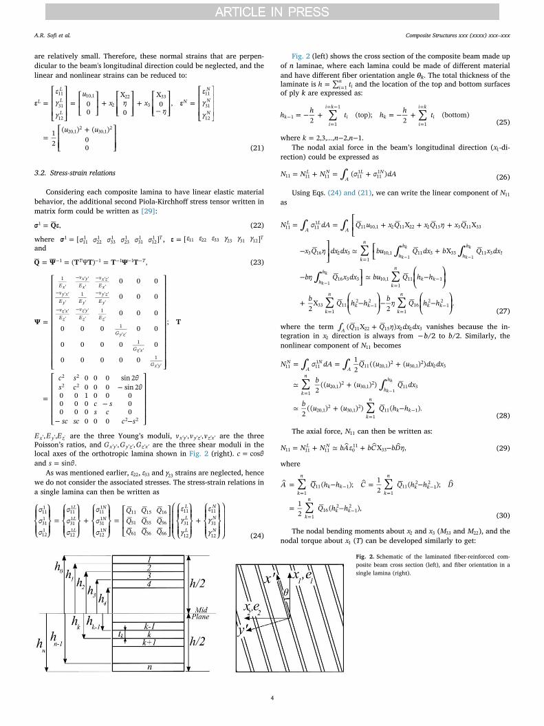
′ ′ ′E E E, ,x y z are the three Young’s moduli, ′ ′ ′ ′ ′ ′v v v, ,x y y z z x are the threePoisson’s ratios, and ′ ′ ′ ′ ′ ′G G G, ,x y y z z x are the three shear moduli in thelocal axes of the orthotropic lamina shown in Fig. 2 (right). =c θcosand =s θsin .
As was mentioned earlier, ε22, ε33 and γ23 strains are neglected, hencewe do not consider the associated stresses. The stress-strain relations ina single lamina can then be written as
⎧
⎨⎪
⎩⎪
⎫
⎬⎪
⎭⎪=
⎧
⎨⎪
⎩⎪
⎫
⎬⎪
⎭⎪+
⎧
⎨⎪
⎩⎪
⎫
⎬⎪
⎭⎪=
⎡
⎣
⎢⎢
⎤
⎦
⎥⎥
⎛
⎝
⎜⎜⎜
⎧
⎨⎪
⎩⎪
⎫
⎬⎪
⎭⎪+
⎧
⎨⎪
⎩⎪
⎫
⎬⎪
⎭⎪
⎞
⎠
⎟⎟⎟
σσσ
σσσ
σσσ
Q Q QQ Q QQ Q Q
εγ
γ
εγ
γ
L
L
L
N
N
N
L
L
L
N
N
N
111
311
121
111
311
121
111
311
121
11 15 16
51 55 56
61 56 66
11
31
12
11
31
12 (24)
Fig. 2 (left) shows the cross section of the composite beam made upof n laminae, where each lamina could be made of different materialand have different fiber orientation angle θk. The total thickness of thelaminate is = ∑ =h ti
ni1 and the location of the top and bottom surfaces
of ply k are expressed as:
∑ ∑= − + = − +−=
= −
=
=
h h t h h t2
(top);2
(bottom)ki
i k
i ki
i k
i11
1
1 (25)
where = … − −k n n2,3, , 2, 1.The nodal axial force in the beam’s longitudinal direction (x1-di-
rection) could be expressed as
∫= + = +N N N σ σ dA( )L NA
L N11 11 11 11
1111
(26)
Using Eqs. (24) and (21), we can write the linear component of N11as
∫ ∫
∫ ∫
∫
∑
∑
∑ ∑
= = ⎡
⎣⎢ + + +
− ⎤
⎦⎥ ≃ ⎡
⎣+
− ⎤⎦
≃ ⎛
⎝⎜ − ⎞
⎠⎟
+ ⎛
⎝⎜ − ⎞
⎠⎟− ⎛
⎝⎜ − ⎞
⎠⎟
=
=−
=−
=−
− −
−
N σ dA Q u x Q x Q η x Q
x Q η dx dx bu Q dx b Q x dx
bη Q x dx bu Q h h
b Q h h b η Q h h
X X
X
2X
2.
LA
LA
k
n
h
h
h
h
h
h
k
n
k k
k
n
k kk
n
k k
11 111
11 10,1 2 11 22 2 15 3 11 33
3 16 2 31
10,1 11 3 33 11 3 3
16 3 3 10,11
11 1
331
112
12
116
21
2
k
k
k
k
k
k
1 1
1
(27)
where the term ∫ +Q Q η x dx dx( X )A 11 22 15 2 2 3 vanishes because the in-tegration in x2 direction is always from −b/2 to b/2. Similarly, thenonlinear component of N11 becomes
∫ ∫
∫∑
∑
= = +
≃ +
≃ + −
=
=−
−
N σ dA Q u u dx dx
b u u Q dx
b u u Q h h
12
(( ) ( ) )
2(( ) ( ) )
2(( ) ( ) ) ( ).
NA
NA
k
n
h
h
k
n
k k
11 111
11 20,12
30,12
2 3
120,1
230,1
211 3
20,12
30,12
111 1
k
k
1
(28)
The axial force, N11 can then be written as:
= + ≃ + −N N N bA ε bC bDηX ,L N11 11 11 0
1133 (29)
where
∑ ∑
∑
= − = −
= −
=−
=−
=−
A Q h h C Q h h D
Q h h
( ); 12
( );
12
( ),
k
n
k kk
n
k k
k
n
k k
111 1
111
21
2
116
21
2
(30)
The nodal bending moments about x2 and x3 (M33 and M22), and thenodal torque about x1 (T) can be developed similarly to get:
Fig. 2. Schematic of the laminated fiber-reinforced com-posite beam cross section (left), and fiber orientation in asingle lamina (right).
A.R. Sofi et al. Composite Structures xxx (xxxx) xxx–xxx
4
∫ ⎜ ⎟= + = ⎛⎝
+ ⎞⎠
≃ + −M M M σ σ x dA bCε bF bGηX ,L NA
L N33 33 33 11
1111
3 011
33(31)
∫ ⎜ ⎟= + = ⎛⎝
+ ⎞⎠
= +M M M σ σ x dA b A b B η12
X12
,L NA
L N22 22 22 11
1111
23
223
(32)
∫ ⎜ ⎟ ⎜ ⎟= ⎛⎝
− ⎞⎠
= − + − + ⎛⎝
+ ⎞⎠
T σ x σ x dA bDε b B bG b H bM η12
X X12
,131
2 121
3 110
322 33
3
(33)
where
∑ ∑
∑
∑ ∑
= − = −
= −
= − = −
=−
=−
=−
=−
=−
B Q h h F Q h h G
Q h h
H Q h h M Q h h
( ); ( );
( )
( ); ( ).
k
n
k kk
n
k k
k
n
k k
k
n
k kk
n
k k
115 1
13
111
31
3
13
116
31
3
155 1
13
166
31
3
(34)
The generalized nodal forces can then be written in matrix form as
=S DE, (35)
=⎧
⎨⎪
⎩⎪
⎫
⎬⎪
⎭⎪
=⎧
⎨⎪
⎩⎪
⎫
⎬⎪
⎭⎪=
⎧
⎨⎪
⎩⎪
⎫
⎬⎪
⎭⎪=
⎧
⎨⎪
⎩⎪
⎫
⎬⎪
⎭⎪
=
⎡
⎣
⎢⎢⎢⎢⎢
−
−− − +
⎤
⎦
⎥⎥⎥⎥⎥
SSSS
NMMT
EEEE
ε
η
b
A C DA B
C F GD B G H M
S E D; XX
;
00 0
0
b b
b b
1
2
3
4
11
22
33
1
2
3
4
110
22
33
12 12
12 12
2 2
2 2
(36)
Now define the generalized displacement vector as
=
⎧
⎨⎪
⎩⎪
⎫
⎬⎪
⎭⎪
=⎧
⎨⎩
⎫
⎬⎭
uuuu
uuuτ
U .
1
2
3
4
102030
(37)
The generalized strain vector can be expressed as linear and non-linear components
= + = +E E E LU AHU12
( ),L N(38)
where
=
⎡
⎣
⎢⎢⎢⎢⎢⎢⎢
−
−
⎤
⎦
⎥⎥⎥⎥⎥⎥⎥
=⎡
⎣
⎢⎢
⎤
⎦
⎥⎥
∂∂
=
⎡
⎣
⎢⎢⎢⎢
⎤
⎦
⎥⎥⎥⎥
∂∂
∂∂
∂∂
∂∂
∂∂
∂∂
xL H A
0 0 0
0 0 0
0 0 0
0 0 0
;0 0 0 00 1 0 00 0 1 00 0 0 0
;
0 0
0 0 0 00 0 0 00 0 0 0
.
x
x
x
x
ux
ux
1
12
12
2
12
1
21
31
(39)
The element generalized mechanical stress vector can be written as
= + = +S DE DE S SMech L N L N (40)
3.3. Hygrothermal effects
The global coefficients of thermal expansion in a single lamina arerelated to the local ones through the transformation matrix as follows:
= −α T α ,G L1 (41)
where = ⎡⎣
⎤⎦
α α ααGα α α T
11 22 33 232
312
122 ; =αL ′ ′ ′ ′ ′ ′[ ]α α α 0 0 0x x y y z z
T .The thermal stresses in a single lamina due to a temperature change
T(Δ ) can then be written as
⎧
⎨
⎪⎪⎪
⎩
⎪⎪⎪
⎫
⎬
⎪⎪⎪
⎭
⎪⎪⎪
=
⎧
⎨
⎪⎪
⎩⎪⎪
⎫
⎬
⎪⎪
⎭⎪⎪
σσσσσσ
αααααα
TQ Δ .
Th
Th
Th
Th
Th
Th
11
22
33
23
31
12
112233233112
(42)
By neglecting σTh22 , σTh
33 and σTh23 as was done before, we get
⎧
⎨⎪
⎩⎪
⎫
⎬⎪
⎭⎪=
⎡
⎣
⎢⎢
⎤
⎦
⎥⎥
⎧⎨⎩
⎫⎬⎭
σσσ
Q Q QQ Q QQ Q Q
ααα
TΔ .
Th
Th
Th
11
31
12
11 15 16
51 55 56
61 56 66
113112
(43)
The nodal axial thermal force in x1 direction can be expressed as
∫ ∫
∫= = + +
= + + =−
N σ dA T Q α Q α Q α dA
b T Q α Q α Q α dx b TN
Δ [ ]
Δ [ ] Δ ,
ThA
ThA
h
h
11 11 11 11 15 31 16 12
11 11 15 31 16 12 3k
k
1 (44)
where
∑= + + −=
−N Q α Q α Q α h h[ ]( )k
n
k k1
11 11 15 31 16 12 1(45)
The nodal bending moments about x2 and x3 (MTh33 and MTh
22 ) and thetotal torque about x1 (TTh) due to temperature change are derived si-milarly to get
∫ ∫= = + +
=−
M σ x dA b T Q α Q α Q α x dx
b TO
Δ [ ]
Δ ,
ThA
Thh
h33 11 3 11 11 15 31 16 12 3 3
k
k
1
(46)
∫ ∫= = + + =M σ x dA T Q α Q α Q α x dAΔ [ ] 0,ThA
ThA22 11 2 11 11 15 31 16 12 2 (47)
∫ ∫= − = − + +
= −−
T σ x σ x b T Q α Q α Q α x dx
b TP
( ) Δ [ ]
Δ ,
Th Th Thh
h13 2 12 3 61 11 65 31 66 12 3 3
k
k
1
(48)
where
∑
∑
= + + −
= + + −
=−
=−
O Q α Q α Q α h h P
Q α Q α Q α h h
12
[ ]( );
12
[ ]( ).
k
n
k k
k
n
k k
111 11 15 31 16 12
21
2
161 11 65 31 66 12
21
2
(49)
The generalized nodal forces due to temperature change can then bewritten in matrix form as
=
⎧
⎨
⎪⎪
⎩⎪⎪
⎫
⎬
⎪⎪
⎭⎪⎪
=
⎧
⎨
⎪
⎩⎪
⎫
⎬
⎪
⎭⎪
=
⎧
⎨⎪
⎩⎪−
⎫
⎬⎪
⎭⎪
SSSS
NMMT
b T
N
OP
S Δ0Th
Th
Th
Th
Th
Th
Th
Th
Th
1
2
3
4
11
22
33
(50)
A.R. Sofi et al. Composite Structures xxx (xxxx) xxx–xxx
5
Following the same process, the generalized nodal forces due tomoisture absorption can be derived as
=
⎧
⎨
⎪
⎩⎪
⎫
⎬
⎪
⎭⎪
=
⎧
⎨
⎪
⎩⎪
⎫
⎬
⎪
⎭⎪
=⎧
⎨⎪
⎩⎪−
⎫
⎬⎪
⎭⎪
SSSS
NMMT
b C
R
WX
S Δ0
,Moist
Moist
Moist
Moist
Moist
Moist
Moist
Moist
Moist
1
2
3
4
11
22
33
(51)
where
∑
∑
∑
= + + −
= + + −
= + + −
=−
=−
=−
R Q β Q β Q β h h W
Q β Q β Q β h h
X Q β Q β Q β h h
[ ]( );
[ ]( )
[ ]( )
k
n
k k
k
n
k k
k
n
k k
111 11 15 31 16 12 1
12
111 11 15 31 16 12
21
2
12
161 11 65 31 66 12
21
2
(52)
βij are the moisture expansion coefficients, and CΔ is the change in theweight of moisture absorbed per unit weight of the lamina. The hy-grothermal generalized nodal forces STh and SMoist are added to themechanical generalized nodal forces SMech in Eq. (40).
4. Updated Lagrangian formulation in the co-rotational referenceframe
4.1. Interpolation functions
The generalized displacement vector in a beam element with twonodes and six degrees of freedom per node can be expressed as [30]
= = ⎧⎨⎩
⎫⎬⎭
U Na N N uu
[ ] ,1 21
2 (53)
where Ni contains the shape functions
=
⎡
⎣
⎢⎢⎢⎢
−
⎤
⎦
⎥⎥⎥⎥
=
⎡
⎣
⎢⎢⎢⎢
−
⎤
⎦
⎥⎥⎥⎥
ϕN N
N Nϕ
ϕN N
N Nϕ
N N
0 0 0 0 00 0 0 00 0 0 00 0 0 0 0
;
0 0 0 0 00 0 0 00 0 0 00 0 0 0 0
1 2
1
1 2
1 2
1
2
3 4
3 4
2
(54)
= − =
= − + = − + = −
= −
ϕ ξ ϕ ξ
N ξ ξ N ξ ξ ξ l N ξ ξ N
ξ ξ l
1 ;
1 3 2 ; ( 2 ) ; 3 2 ;
( )
1 2
12 3
22 3
32 3
4
3 2 (55)
l is the length of the beam element, and ξ is the non-dimensional co-ordinate,
=−
< <ξx x
lξ, (0 1),1 1
1
(56)
and x11 is the coordinate of first node along x1.
ui is the nodal degrees of freedom vector at node i in the UL co-rotational frame ei in Fig. 1 (left):
= = =u u u u u u u u u τ η η iu [ ] [ ] , [ 1,2]i i i i i i i T i i i i i i T1 2 3 4 5 6 10 20 30 20 30
(57)
where η i20 and η i
30 are the nodal slopes in the 1–3 and 1–2 planes re-spectively as shown in Fig. 1 (left).
The element generalized strains can be rewritten as
= + = +E E E B B a( ) ,L N L N (58)
where
=
⎡
⎣
⎢⎢⎢⎢⎢⎢⎢⎢
− −
−
− −
−
⎤
⎦
⎥⎥⎥⎥⎥⎥⎥
∂∂
∂∂
∂∂
∂∂
∂∂
∂∂
∂∂
∂∂
∂∂
∂∂
∂∂
∂∂
B
0 0 0 0 0
0 0 0 0
0 0 0 0
0 0 0 0 0
0 0 0 0 0
0 0 0 0
0 0 0 0
0 0 0 0 0
L
ϕx
Nx
Nx
Nx
Nx
ϕx
ϕx
Nx
Nx
Nx
Nx
ϕx
11
2 1
12
2 2
12
2 1
12
2 2
12
11
21
2 3
12
2 4
12
2 3
12
2 4
12
21 (59)
=
=
⎡
⎣
⎢⎢⎢⎢
−
− ⎤
⎦
⎥⎥⎥⎥
∂∂
∂∂
∂∂
∂∂
∂∂
∂∂
∂∂
∂∂
∂∂
∂∂
∂∂
∂∂
∂∂
∂∂
∂∂
∂∂
B AHN12
12
0 0
0 0 0 0 0 00 0 0 0 0 00 0 0 0 0 0
0 0
0 0 0 0 0 00 0 0 0 0 00 0 0 0 0 0
N
Nx
ux
Nx
ux
Nx
ux
Nx
ux
Nx
ux
Nx
ux
Nx
ux
Nx
ux
i i i i
i i i i
11
21
11
31
21
31
21
21
31
21
31
31
41
31
41
21
(60)
Therefore
= + = +δ δ δE B B a B B a( 2 ) ( ) ,L N L N (61)
where δ indicates the variation.
4.2. Weak formulation of the beam element in the co-rotational referenceframe
The stress tensor is equal to the initial Cauchy stress, τik0 , plus the
incremental Piola-Kirchhoff stress, σik1 , in the UL co-rotational frame
= +σ σ τ .ik ik ik1 0 (62)
The equilibrium static equation and boundary conditions in thecomposite beam can be written as
⎜ ⎟∂
∂⎡⎣⎢
+ ⎛⎝
+∂∂
⎞⎠
⎤⎦⎥
+ =x
σ τ δux
b( ) 0,i
ik ik jkj
kj
1 0
(63)
⎜ ⎟+ ⎛⎝
+∂∂
⎞⎠
− =σ τ δux
n f( ) 0,ik ik jkj
ki i
1 0
(64)
where bj are the body forces per unit volume in the current referencestate, and f j are the given boundary loads.
By taking δuj to be the test function, the weak form of Eqs. (63) and(64) can be expressed as
∫ ∫⎜ ⎟ ⎜ ⎟⎧⎨⎩
∂∂
⎡⎣⎢
⎛⎝
+∂∂
⎞⎠
⎤⎦⎥
+ ⎫⎬⎭
− ⎡⎣⎢
⎛⎝
+∂∂
⎞⎠
− ⎤⎦⎥
=
xσ δ
ux
b δu dV σ δux
n f δu dS
0,
V iik jk
j
kj j S ik jk
j
ki i j
σ
(65)
where ni is the outward unit normal to the boundary surface Sσ.By using the Divergence theorem and integration by parts, Eq. (65)
can be written as
∫ ∫ ∫⎜ ⎟− ⎛⎝
+∂∂
⎞⎠
+ + =σ δux
δu dV b δu dV f δu dS 0V ik jk
j
kj i V j j S j j,
σ (66)
Using Eq. (24), the incremental Piola-Kirchhoff stress can be writtenas
A.R. Sofi et al. Composite Structures xxx (xxxx) xxx–xxx
6
= +σ σ σik ikL
ikN1 1 1 (67)
Therefore the first term of Eq. (66) could be developed as
+ = + + + +
= + + + ⎛⎝
⎞⎠
+ ⎛⎝
⎞⎠
σ δ u δu τ τ u σ σ σ u δu
σ δu τ σ δu τ δ u u
σ δ u u
( ) ( )
( ) 12
12
,
ik jk j k j i ij ik j k ijL
ijN
ik j k j i
ijL
i j ij ijN
j i ik j k j i
ik j k j i
, ,0 0
,1 1 1
, ,
1,
0 1,
0, ,
1, , (68)
where we used = + =( )δ u u u δu u δu u δu( )j k j i j k j i j i j k j k j i12 , ,
12 , , , , , , since
=u ui j j i, , .Using Eq. (68), and the definitions =ε uij
Li j, , =ε u uij
Nk i k j
12 , , , Eq. (66)
can be written as
∫ ∫ ∫∫
+ = +
− + +
σ δε τ δε dV b δu dV f δu dS
σ τ δε σ δε dV
( )
[( ) ] .
V ijL
ijL
ij ijN
V j j S j j
V ijN
ij ijL
ij ijN
1 0
1 0 1σ
(69)
The right-hand side of Eq. (69) is the “correction” term in Newton-Rapson type iterative approach. By assuming the cross sectional area ofthe composite beam to be constant along x1-direction, and by using Eqs.(55)–(61), the integration terms in the above equation could be ex-pressed as
∫ ∫
∫ ∫
∑
∑
⎡⎣
+ ⎤⎦
= − + −
=
=
δ dl δ dl
δ δ dl δ dl
a B DB a a B τ
a F a B τ σ a B σ
( ) ( )
[ ( ) ( ) ( ) ],
e
NT
lL T L T
lN T
e
NT T
lL T N T
lN T
1
0
1
1 0 1 1
e
e
(70)
where the summation is taken over all finite elements Ne, and F1 is theexternal equivalent nodal force vector,
∫= +∗ ∗dlF N b f ,l
T1(71)
where ∗b is the external body force vector per unit volume, and ∗f is theexternal nodal boundary traction vector.
Eq. (70) can be rewritten as:
∑ ∑= −δ δa K a a F F[ ( ) ] [ ( )],e
T
e
T S1
(72)
where K the symmetric stiffness matrix of the laminated compositebeam and is expressed as
= +K K K .L N (73)
The linear and nonlinear parts of the stiffness matrix are
∫ ∫= =dl τ dlK B DB K G G( ) , ,L
lL T L N
lT
10
(74)
where we used the fact that ∫ ∫= =dl τ dlB τ G G a K a( ) ( )lN T
lT N0
10 , where
τ10 is the first term of the initial Cauchy stress. FS is the internal nodalforce,
∫ ∫= + +dl dlF B τ σ B σ( ) ( ) ( ) .S
lL T N
lN T0 1 1
(75)
By neglecting the nonlinear terms in the above equation, FS can besimplified as
∫ ∫= =dl l dξF B τ B τ( ) ( ) .S
lL T L T0
0
1 0(76)
The initial Cauchy stress in Eq. (76) can be written as
= − −τ S S SMech Th Moist0 ,0 (77)
Therefore Eq. (76) can be expanded as
∫ ∫ ∫= − −l dξ l dξ l dξF B S B S B S( ) ( ) ( )S L T Mech L T Th L T Moist0
1 ,00
1
0
1
(78)
4.3. Explicit expressions for the tangent stiffness matrix
The integration in Eq. (74) can be evaluated, and the 12×12nonlinear stiffness matrix can be simplified as
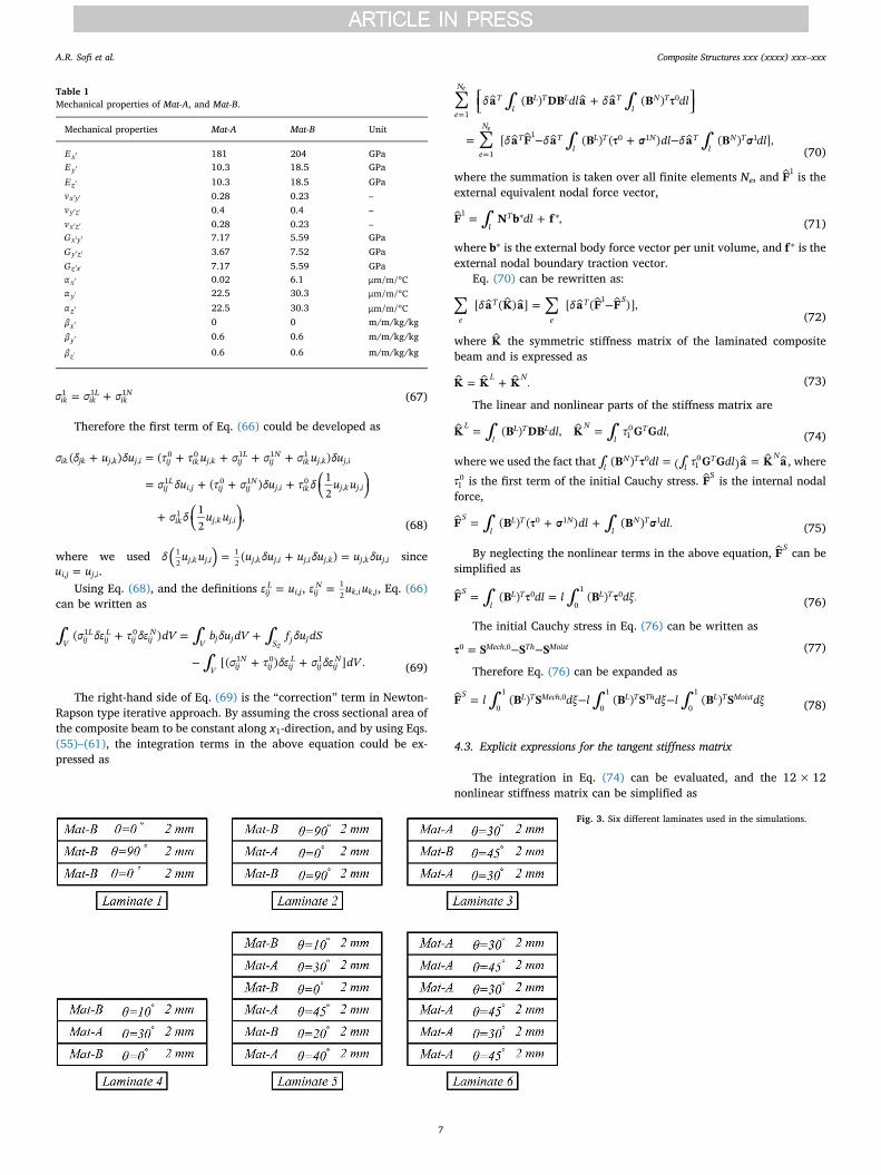
Table 1Mechanical properties of Mat-A, and Mat-B.
Mechanical properties Mat-A Mat-B Unit
′E x 181 204 GPa′E y 10.3 18.5 GPa
′E z 10.3 18.5 GPa
′ ′v x y 0.28 0.23 –
′ ′v y z 0.4 0.4 –
′ ′v x z 0.28 0.23 –′ ′Gx y 7.17 5.59 GPa
′ ′G y z 3.67 7.52 GPa
′ ′Gz x 7.17 5.59 GPa′α x 0.02 6.1 °μm/m/ C′α y 22.5 30.3 °μm/m/ C′αz 22.5 30.3 °μm/m/ C′βx 0 0 m/m/kg/kg
′βy 0.6 0.6 m/m/kg/kg
′βz 0.6 0.6 m/m/kg/kg
Fig. 3. Six different laminates used in the simulations.
A.R. Sofi et al. Composite Structures xxx (xxxx) xxx–xxx
7
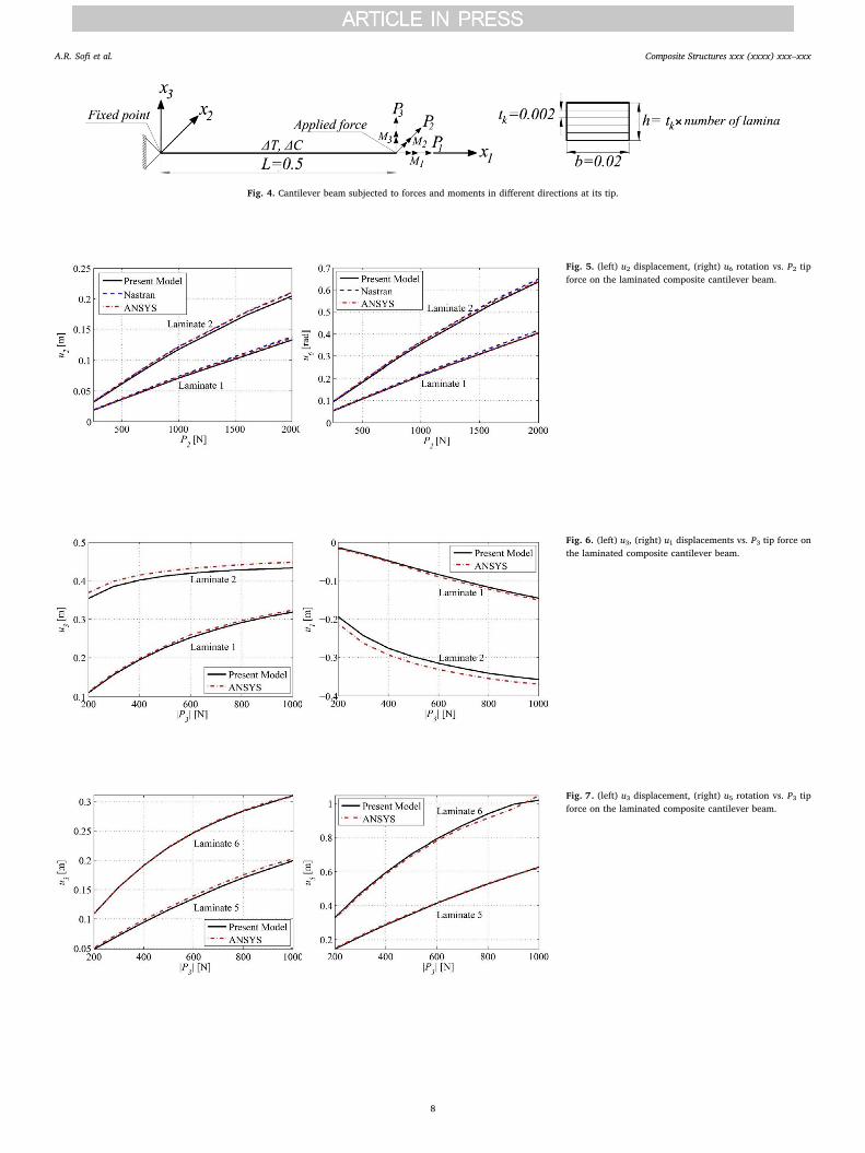
Fig. 4. Cantilever beam subjected to forces and moments in different directions at its tip.
Fig. 5. (left) u2 displacement, (right) u6 rotation vs. P2 tipforce on the laminated composite cantilever beam.
Fig. 6. (left) u3, (right) u1 displacements vs. P3 tip force onthe laminated composite cantilever beam.
Fig. 7. (left) u3 displacement, (right) u5 rotation vs. P3 tipforce on the laminated composite cantilever beam.
A.R. Sofi et al. Composite Structures xxx (xxxx) xxx–xxx
8
=
⎡
⎣
⎢⎢⎢⎢⎢⎢⎢⎢⎢⎢⎢⎢
−− − −
−− −
−
⎤
⎦
⎥⎥⎥⎥⎥⎥⎥⎥⎥⎥⎥⎥
τ
a aa a
c dc d
asym a
cc
K
0 0 0 0 0 0 0 0 0 0 0 00 0 0 0.1 0 0 0 0 0.1
0 0.1 0 0 0 0 0.1 00 0 0 0 0 0 0 0 0
0 0 0 0.1 0 00 0.1 0 0 00 0 0 0 0 0
0 0 0 0.1. 0 0.1 0
0 0 00
N10
(79)
where =a l1.2 ; =c l2
15 ; =d l30 and l is the current length of the beam in
the current local reference frame. Again, the width of the laminatedcomposite beam, b, is assumed to be constant, and the integration in Eq.(74) can be evaluated. The 12×12 linear stiffness matrix can be ex-pressed as
=
⎡
⎣⎢⎢
⎤
⎦⎥⎥
bl
KK K
K K( )
LL L
L T L1 2
2 3 (80)
where
=
⎡
⎣
⎢⎢⎢⎢⎢⎢⎢⎢⎢⎢
−
−
+ − −
⎤
⎦
⎥⎥⎥⎥⎥⎥⎥⎥⎥⎥
A D CA A
F F
H M G B
sym F
A
K
0 0 00 0 0
0 0
. 4 0
L
bl
bl
l l
b b
b
1
212 6
12 12
3
22
2
2
2 2
2
(81)
=
⎡
⎣
⎢⎢⎢⎢⎢⎢⎢⎢⎢⎢
− −−
− −
− −
−
−
⎤
⎦
⎥⎥⎥⎥⎥⎥⎥⎥⎥⎥
A D CA A
F F
D H M G B
C F G F
A B A
K
0 0 00 0 0 0
0 0 0 0
0 0
0 2 0
0 0 0
L
bl
bl
l l
b b
lb
lb b
2
212 6
12 126
2 12 6
22
2
2
2 2
2 2 2
(82)
=
⎡
⎣
⎢⎢⎢⎢⎢⎢⎢⎢⎢⎢
−−
+ − −
⎤
⎦
⎥⎥⎥⎥⎥⎥⎥⎥⎥⎥
A D CA A
F F
H M G B
sym F
A
K
0 0 00 0 0
0 0
. 4 0
L
bl
bl
l l
b b
b
3
212 6
12 12
3
22
2
2
2 2
2
(83)
The 12× 12 transformation matrix between the generalized localcoordinates of the deformed configuration of the composite beam ele-ment and the global coordinates can be written in terms of λ0 given inEq. (9) as
=⎡
⎣
⎢⎢⎢
⎤
⎦
⎥⎥⎥
= ⎡
⎣⎢
⎤
⎦⎥λ
λ 0 0 00 λ 0 00 0 λ 00 0 0 λ
0,0 0 00 0 00 0 0
.
0
0
0
0 (84)
Therefore, the generalized nodal displacement vector, the elementtangent stiffness matrix, and generalized nodal forces can be transferredfrom the local coordinates to the global coordination as
= = =∼∼∼∼a λ a K λ K λ F λ F; ; k T kk
T k kT k (85)
Now, the stiffness matrix can be assembled, and the finite elementsystem of equations can be expressed as:
= −Ka F FS1 0 (86)
At this stage, the Newton-Raphson algorithm can be used to solvethe above equation iteratively. The iterative process of the Newton-Raphson method can be written as
= −K a F Fm m S m( ) ( ) 1 ( ) (87)
where m is the iteration number and
∫= l dξF B τ( )S m L T m( )0
1 0( )(88)
The total displacements for all nodes can then be written as
= ++u u am m m( 1) ( ) ( ) (89)
A Matlab code has been developed to implement the proposed for-mulation, and solve the system of equations iteratively with appliedincrements of the mechanical loads, until the total applied load isreached and a converged solution is obtained.
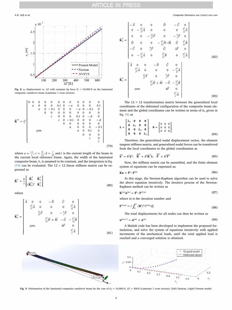
Fig. 8. u1 displacement vs. ΔT with constant tip force P1= 10,000 N on the laminatedcomposite cantilever beam (Laminate 1 cross section).
Fig. 9. Deformation of the laminated composite cantilever beam for the case of P2= 16,000 N, ΔT=300 K (Laminate 1 cross section): (left) Nastran, (right) Present model.
A.R. Sofi et al. Composite Structures xxx (xxxx) xxx–xxx
9
5. Numerical examples
Several numerical examples are presented in this section to de-monstrate the efficiency of the proposed method. The composite la-minae used in this section are made of Mat-A and Mat-B whose prop-erties are listed in Table 1. Six different composite laminates, illustratedin Fig. 3, are used to demonstrate different cases of stacking sequence,laminae materials, and symmetry.
Nastran-in-CAD finite element tool available with SolidWorks isused in the first two examples in this section for comparison with theresults of the developed Matlab code for the proposed method. This toolhas the option of using a laminated composite material given thestacking sequence and the material properties and thicknesses of alllaminae. Laminates should be defined on a shell, not a solid or struc-tural elements such as beams, and loads should be applied only in theplane of the shell. It was found that applying loads perpendicular to theplane of the laminate in Nastran (2016) always give unrealistic resultsas compared to ANSYS. This happens even if the full 3D materialproperties of the laminae are given (the nine material properties oforthotropic materials). Hence, in the following examples, we comparethe results of the developed Matlab code with Nastran results only whenthe loads are applied in the plane of the composite laminate. We also
compare with ANSYS finite element tool results when loads are appliedperpendicular to the plane of the laminate. It is important to note thatthe proposed formulation is just modeling the laminated compositestructures using 1D beam elements, while Nastran requires 2D plateelements and ANSYS requires 3D Solid elements to model compositelaminates.
5.1. Large deformation analysis of a cantilever laminated composite beam
Consider a cantilever beam subjected to forces P1, P2, P3 and mo-ments M1, M2, M3 at its tip, in addition to temperature and moisturechange on the whole beam, as shown in Fig. 4. The beam is made of afiber-reinforced composite laminate with a rectangular cross section, asshown in Fig. 3. The length of the beam is L=0.5m, its width isb=0.02m, and the thickness of each lamina is ts=0.002m. The beamis analyzed for different cases of loadings using the developed Matlabcode for the proposed method as well as using ANSYS and Nastran finiteelement packages.
To find the solution that best balances computational capacity andaccuracy, convergence study has been performed for Nastran, ANSYSand the proposed method for the cantilever beam model. The con-vergence study on Nastran and ANSYS began with 22 2D square shellelements and 40 3D solid cube elements along x1 direction respectively.The mesh density has been increased until convergence was reachedwith 225 2D shell elements along x1 direction for Nastran model, 2343D solid elements along x1 direction for ANSYS model and 30 1D beamelement along x1 direction for the developed Matlab code. Totalnumber of 2D elements in Nastran is 2030 corresponding to 2263nodes, total number of 3D solid elements in ANSYS is 2361 corre-sponding to 2576 nodes and total number of 1D elements in Matlab is30 corresponding to 31 nodes.
The results of the different applied mechanical and hygrothermalloads on beams made of a laminated fiber-reinforced composite with arectangular cross section as shown in Fig. 4 are presented in Figs. 5–10using the proposed method, Nastran and ANSYS. Specifically, Fig. 5
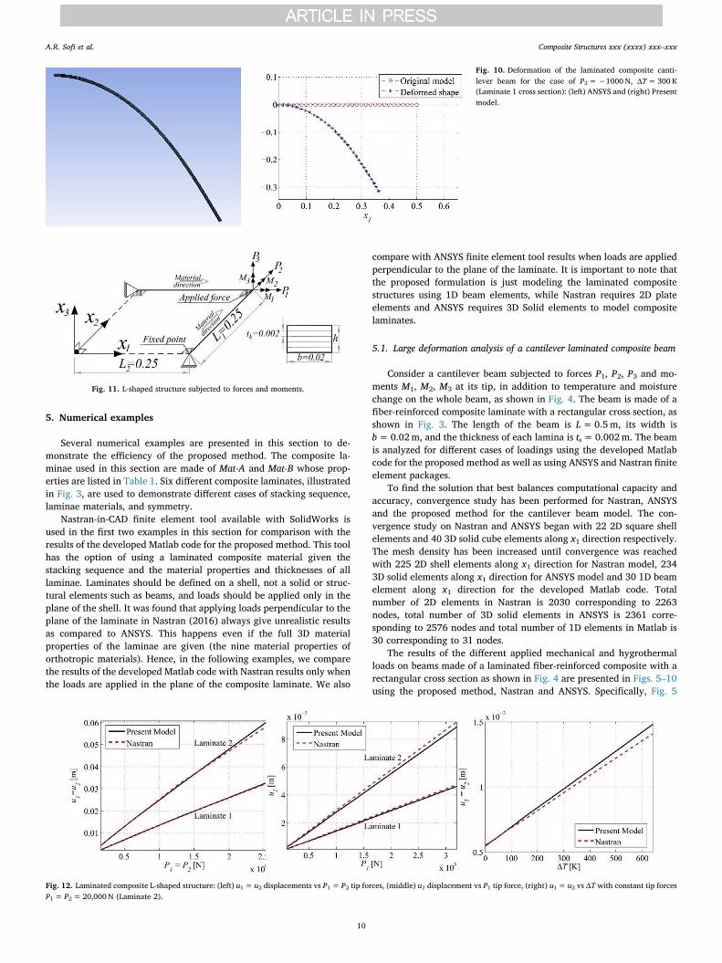
Fig. 10. Deformation of the laminated composite canti-lever beam for the case of P3=−1000 N, ΔT=300 K(Laminate 1 cross section): (left) ANSYS and (right) Presentmodel.
Fig. 11. L-shaped structure subjected to forces and moments.
Fig. 12. Laminated composite L-shaped structure: (left) u1= u2 displacements vs P1= P2 tip forces, (middle) u1 displacement vs P1 tip force, (right) u1= u2 vs ΔT with constant tip forcesP1= P2= 20,000 N (Laminate 2).
A.R. Sofi et al. Composite Structures xxx (xxxx) xxx–xxx
10
shows u2 and u6 (rotation about x3 axis) at the beam tip for increasingvalues of applied force P2. Applying force P3 at the tip of the compositebeam, Fig. 6 shows u3 and u1 at the beam tip with Laminates 1 and 2rectangular cross sections, while Fig. 7 shows u3 and u5 (rotation aboutx2 axis) with Laminates 5 and 6 for increasing values of P3. Fig. 8 showsthe effect of temperature on u1 with constant P1=10,000 N applied
force. Excellent agreement with Nastran and ANSYS can be seen in allcases. The maximum error percent is less than 5% in all cases. Fig. 9shows the deformation of Nastran model and the proposed method withLaminate 1 cross section for the case of P2= 16,000 N, ΔT=300 K. Forthis specific case, Nastran takes 26minutes and 5 seconds to find thesolution, while the developed Matlab code takes only 1minute and
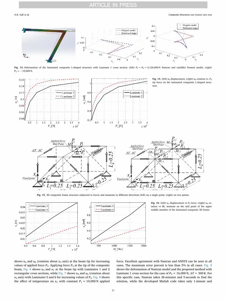
Fig. 13. Deformation of the laminated composite L-shaped structure with Laminate 1 cross section: (left) P1= P2= 5,120,000 N Nastran and (middle) Present model, (right)P3=−10,000 N.
Fig. 14. (left) u3 displacement, (right) u5 rotation vs. P3tip force on the laminated composite L-shaped struc-ture.
Fig. 15. 3D composite frame structure subjected to forces and moments in different directions (left) on a single point, (right) on two points.
Fig. 16. (left) u3 displacement vs P3 force, (right) u4 ro-tation vs M1 moment on the mid point of the uppermiddle member of the laminated composite 3D frame.
A.R. Sofi et al. Composite Structures xxx (xxxx) xxx–xxx
11
39 seconds to solve the problem. This is 6.3% the time required byNastran. Fig. 10 shows the deformation of ANSYS model and the pro-posed method with Laminate 1 rectangular cross section for the case ofP3=−1000 N, ΔT=300 K. For this specific case, ANSYS takes3minutes and 37 seconds to find the solution, while the developedMatlab code takes only 44 seconds to solve the problem. This is 20.2%the time required by ANSYS.
5.2. Large deformation analysis of simply supported L-shape structure
In this example, an L-shaped structure is subjected to forces P1, P2,P3 and moments M1, M2, M3 at the illustrated point in Fig. 11 as well aschanges in temperature and moisture content on the whole structure.This structure has two equal side lengths L1= L2=0.25m, and has twofixed points at its two ends. Each side of this structure is a laminatedcomposite beam with a rectangular cross-section of width b=0.02m.The element size of both Matlab code and Nastran models are equal tothe element size of the cantilever beam example. Accordingly, in thisexample, 30 1D beam elements (31 nodes) are used to model thestructure using the developed method, while 2029 2D elements (216 2Dshell elements along x1 direction) corresponding to 6573 nodes are usedto model the L-shaped structure in SolidWorks with Nastran-in-CADtool.
The displacement of the load-application point in the laminatedcomposite L-shaped structure made of two different composite lami-nates for the different applied mechanical and hygrothermal loads arepresented in Fig. 12 for the present method and Nastran. Excellentagreement can be seen in all cases. Fig. 13 (left and middle) show thedeformation of both Matlab code and Nastran models with Laminate 1cross section for the case of P1= P2= 5,120,000 N. Fig. 14 shows theu3 displacement of the load-application point when P3 force is applied.As was mentioned earlier, Nastran (2016) provides unrealistic largedeformations when the load is applied perpendicular to the plane of the
laminate. Fig. 13 (right) shows the deformation of the same structurewith P3=−10,000 N applied using the developed Matlab code.
5.3. Large deformation analysis of a composite 3D frame
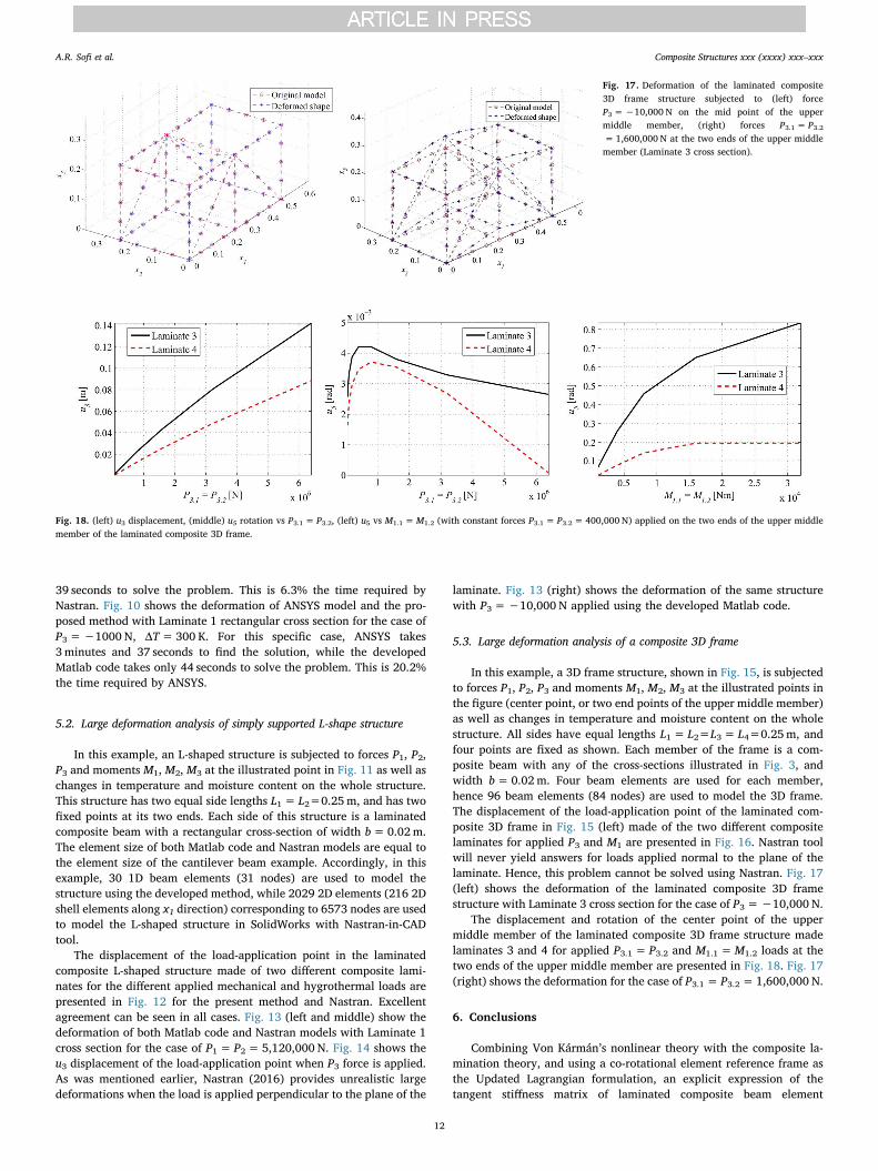
In this example, a 3D frame structure, shown in Fig. 15, is subjectedto forces P1, P2, P3 and moments M1, M2, M3 at the illustrated points inthe figure (center point, or two end points of the upper middle member)as well as changes in temperature and moisture content on the wholestructure. All sides have equal lengths L1= L2=L3= L4=0.25m, andfour points are fixed as shown. Each member of the frame is a com-posite beam with any of the cross-sections illustrated in Fig. 3, andwidth b=0.02m. Four beam elements are used for each member,hence 96 beam elements (84 nodes) are used to model the 3D frame.The displacement of the load-application point of the laminated com-posite 3D frame in Fig. 15 (left) made of the two different compositelaminates for applied P3 and M1 are presented in Fig. 16. Nastran toolwill never yield answers for loads applied normal to the plane of thelaminate. Hence, this problem cannot be solved using Nastran. Fig. 17(left) shows the deformation of the laminated composite 3D framestructure with Laminate 3 cross section for the case of P3=−10,000 N.
The displacement and rotation of the center point of the uppermiddle member of the laminated composite 3D frame structure madelaminates 3 and 4 for applied P3.1= P3.2 and M1.1=M1.2 loads at thetwo ends of the upper middle member are presented in Fig. 18. Fig. 17(right) shows the deformation for the case of P3.1= P3.2= 1,600,000 N.
6. Conclusions
Combining Von Kármán’s nonlinear theory with the composite la-mination theory, and using a co-rotational element reference frame asthe Updated Lagrangian formulation, an explicit expression of thetangent stiffness matrix of laminated composite beam element
Fig. 17. Deformation of the laminated composite3D frame structure subjected to (left) forceP3=−10,000 N on the mid point of the uppermiddle member, (right) forces P3.1= P3.2= 1,600,000 N at the two ends of the upper middlemember (Laminate 3 cross section).
Fig. 18. (left) u3 displacement, (middle) u5 rotation vs P3.1= P3.2, (left) u5 vs M1.1=M1.2 (with constant forces P3.1= P3.2= 400,000 N) applied on the two ends of the upper middlemember of the laminated composite 3D frame.
A.R. Sofi et al. Composite Structures xxx (xxxx) xxx–xxx
12
undergoing large deformation and rotation has been obtained and uti-lized in analyzing different structures subjected to multiple mechanicaland hygrothermal loads. The proposed approach has been verified bycomparison with the results of Nastran and ANSYS finite element toolsthat enable modeling laminated composites, and the differences in theresulting displacements and rotations are less than 5% in all examplesand cases. The developed beam element is much more efficient thanusing composite laminate tools in FEA software because of the ability tomodel such composites using 1D beam elements rather than 2D plate/shell or 3D solid elements. With structures undergoing large deforma-tions, the computational time is less than 7% the time needed for sol-ving the problem using Nastran shell elements and less than 21% usingANSYS 3D solid elements. The developed model will be very useful inmodeling and designing flexible composites which have a lot of newapplications, such as morphing aerospace structures and flexible robots.
Acknowledgment
The authors acknowledge the support of California State University,Northridge.
References
[1] Webber KG, Hopkinson DP, Lynch CS. Application of a classical lamination theorymodel to the design of piezoelectric composite unimorph actuators. J Intell MaterSyst Struct 2006;17(1):29–34.
[2] Khdeir AA, Aldraihem OJ. Exact analysis for static response of cross ply laminatedsmart shells. Compos Struct 2011;94(1):92–101.
[3] Khdeir AA, Aldraihem OJ. Analytical investigation of laminated arches with ex-tension and shear piezoelectric actuators. Eur J Mech A Solids 2013;37:185–92.
[4] Han M-W, Rodrigue H, Kim H-I, Song S-H, Ahn S-H. Shape memory alloy/glass fiberwoven composite for soft morphing winglets of unmanned aerial vehicles. ComposStruct 2016;140:202–12.
[5] Ahn S-H, Lee K-T, Kim H-J, Wu R, Kim J-S, Song S-H. Smart soft composite: anintegrated 3D soft morphing structure using bend-twist coupling of anisotropicmaterials. Int J Precis Eng Manuf 2012;13(4):631–4.
[6] Wu R, Han M-W, Lee G-Y, Ahn S-H. Woven type smart soft composite beam with in-plane shape retention. Smart Mater Struct 2013;22(12):125007.
[7] Rodrigue H, Wang W, Bhandari B, Han M-W, Ahn S-H. Cross-shaped twistingstructure using SMA-based smart soft composite. Int J Precis Eng Manuf-GT2014;1(2):153–6.
[8] Kim H-J, Song S-H, Ahn S-H. A turtle-like swimming robot using a smart softcomposite (SSC) structure. Smart Mater Struct 2013;22(1):014007.
[9] Han M-W, Rodrigue H, Cho S, Song S-H, Wang W, Chu W-S. Woven type smart softcomposite for soft morphing car spoiler. 2016;86:285–98.
[10] Gordaninejad FF, Azhdari AA, Chalhoub NG. Nonlinear dynamic modelling of a
revolute-prismatic flexible composite-material robot arm. ASME J Vib Acoust1991;113(4):461–8.
[11] Grossard M, Chaillet N, Regnier S, editors. Flexible robotics: applications to mul-tiscale manipulations. Wiley-ISTE; 2013. ISBN: 978-1-84821-520-7.
[12] Mororó LAT, de Melo AMC, Junior EP. Geometrically nonlinear analysis of thin-walled laminated composite beams. Latin Am J Solids Struct 2015;12:2094–117.
[13] Bhaskar K, Librescu L. A geometrically non-linear theory for laminated anisotropicthin-walled beams. Int J Eng Sci 1995;33(9):1331–44.
[14] Librescu L, Song O. Thin-walled composite beams: theory and application (solidmechanics and its applications). 1st ed. Springer; 2006.
[15] Omidvar B, Ghorbanpoor A. Nonlinear FE solution for thin-walled open-sectioncomposite beams. J Struct Eng 1996;122(11):1369–78.
[16] Cardoso JB, Benedito NM, Valido AJ. Finite element analysis of thin-walled com-posite laminated beams with geometrically nonlinear behavior including warpingdeformation. Thin-Walled Struct 2009;47(11):1363–72.
[17] Vo TP, Lee J. Geometrically nonlinear analysis of thin-walled open-section com-posite beams. Comput Struct 2010;88:347–56.
[18] Vo TP, Lee J. Geometrical nonlinear analysis of thin-walled composite beams usingfinite element method based on first order shear deformation theory. Arch ApplMech 2011;81:419–35.
[19] Saravia CM. A large deformation–small strain formulation for the mechanics ofgeometrically exact thin-walled composite beams. Thin-Walled Structures2014;84:443–51.
[20] Turkalj G, Lanc D, Brnic J, Pesic I. A beam formulation for large displacementanalysis of composite frames with semi-rigid connections. Compos Struct2015;134:237–46.
[21] Atluri SN. On some new general and complementary energy theorems for the rateproblems in finite strain, classical elastoplasticity. J Struct Mech 1980;8(1):61–92.
[22] Atluri SN. Alternate stress and conjugate strain measures, and mixed variationalformulations involving rigid rotations, for computational analyses of finitely de-formed plates and shells: part-I: theory. Comput Struct 1984;18(1):93–116.
[23] Atluri SN, Cazzani A. Rotations in computational solid mechanics, invited featurearticle. Arch Comput Methods Eng, ICNME, Barcelona, Spain 1994;2(1):49–138.
[24] Atluri SN, Iura M, Vasudevan S. A consistent theory of finite stretches and finiterotations, in space-curved beams of arbitrary cross-section. Comput Mech2001;27:271–81.
[25] Kondoh K, Tanaka K, Atluri SN. An explicit expression for the tangent-stiffness of afinitely deformed 3-D beam and its use in the analysis of space frames. ComputStruct 1986;24:253–71.
[26] Kondoh K, Atluri SN. Large-deformation, elasto-plastic analysis of frames undernonconservative loading, using explicitly derived tangent stiffnesses based on as-sumed stresses. Comput Mech 1987;2:1–25.
[27] Shi G, Atluri SN. Elasto-plastic large deformation analysis of spaceframes: a plastic-hinge and stress-based explicit derivation of tangent stiffnesses. Int J Numer MethEng 1988;26:589–615.
[28] Cai Y, Paik JK, Atluri SN. Large deformation analyses of space-frame structures,with members of arbitrary cross-section, using explicit tangent stiffness matrices,based on a Von Kármán type nonlinear theory in rotated reference frames. CMES2009;53(2):117–45.
[29] Jones RM. Mechanics of composite materials. 2nd ed. Taylor and Francis; 1999.[30] Bhati MA. Fundamental finite element analysis and applications: with mathematica
and matlab computations. Wiley; 2005.
A.R. Sofi et al. Composite Structures xxx (xxxx) xxx–xxx
13