Exploring Data and Descriptive Statistics

(using R)

Oscar Torres-ReynaData Consultantotorres@princeton.edu

http://dss.princeton.edu/training/

Data Analysis 101 Workshops

Agenda…

• What is R• Transferring data to R• Excel to R• Basic data manipulation• Frequencies• Crosstabulations• Scatterplots/Histograms• Exercise 1: Data from ICPSR using the Online Learning Center.• Exercise 2: Data from the World Development Indicators & Global Development

Finance from the World Bank

This document is created from the following:http://dss.princeton.edu/training/RStata.pdf

2OTR

What is R?• R is a programming language use for statistical analysis and graphics. It is based S‐plus. [see http://www.r‐project.org/]

• Multiple datasets open at the same time• R is offered as open source (i.e. free)• Download R at http://cran.r‐project.org/• A dataset is a collection of several pieces of information called variables (usually arranged by columns). A variable can have one or several values (information for one or several cases).

• Other statistical packages are SPSS, SAS and Stata.

3OTR

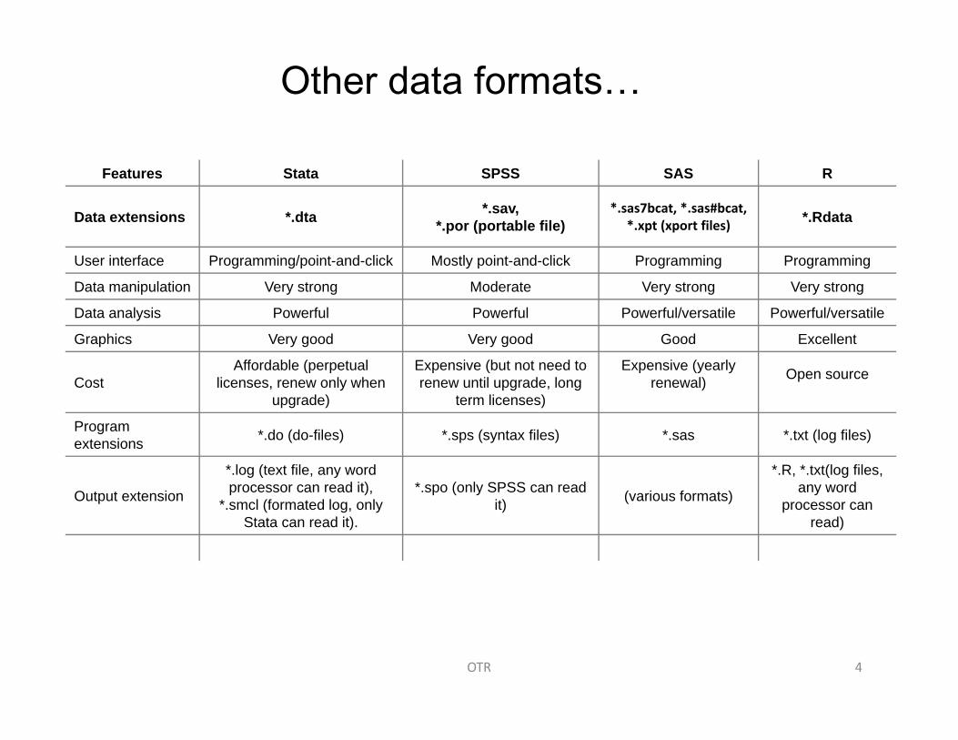
Other data formats…

Features Stata SPSS SAS R

Data extensions *.dta *.sav,*.por (portable file)

*.sas7bcat, *.sas#bcat, *.xpt (xport files) *.Rdata

User interface Programming/point-and-click Mostly point-and-click Programming Programming

Data manipulation Very strong Moderate Very strong Very strong

Data analysis Powerful Powerful Powerful/versatile Powerful/versatile

Graphics Very good Very good Good Excellent

CostAffordable (perpetual

licenses, renew only when upgrade)

Expensive (but not need to renew until upgrade, long

term licenses)

Expensive (yearly renewal) Open source

Program extensions *.do (do-files) *.sps (syntax files) *.sas *.txt (log files)

Output extension

*.log (text file, any word processor can read it),

*.smcl (formated log, only Stata can read it).

*.spo (only SPSS can read it) (various formats)

*.R, *.txt(log files, any word

processor can read)

4OTR

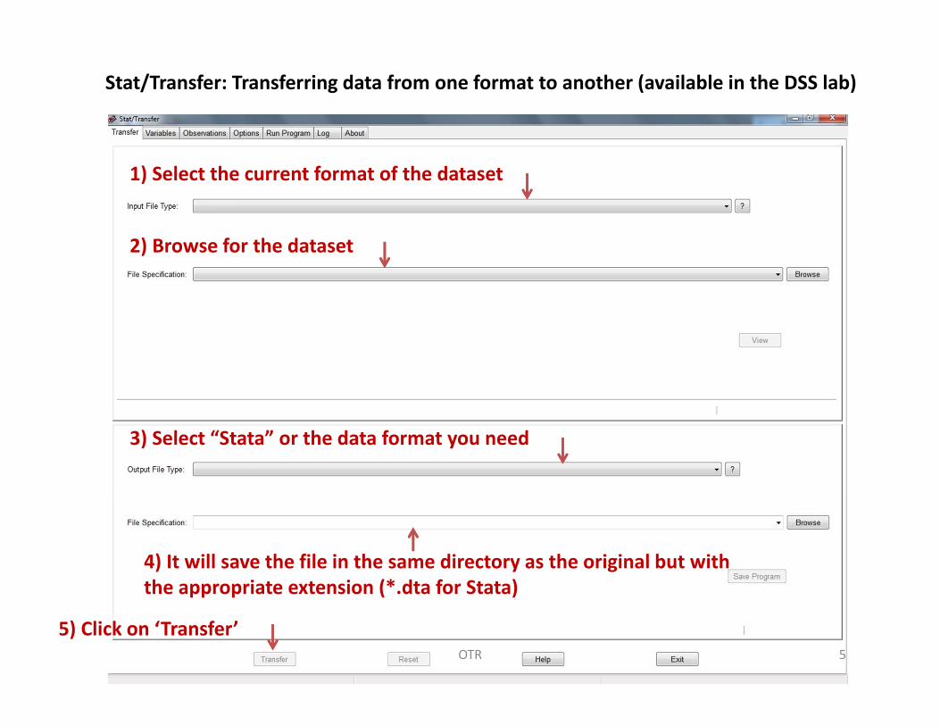
Stat/Transfer: Transferring data from one format to another (available in the DSS lab)

1) Select the current format of the dataset

2) Browse for the dataset

3) Select “Stata” or the data format you need 

4) It will save the file in the same directory as the original but with the appropriate extension (*.dta for Stata)  

5) Click on ‘Transfer’5OTR

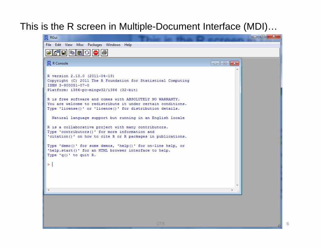
This is the R screen in Multiple-Document Interface (MDI)…

6OTR

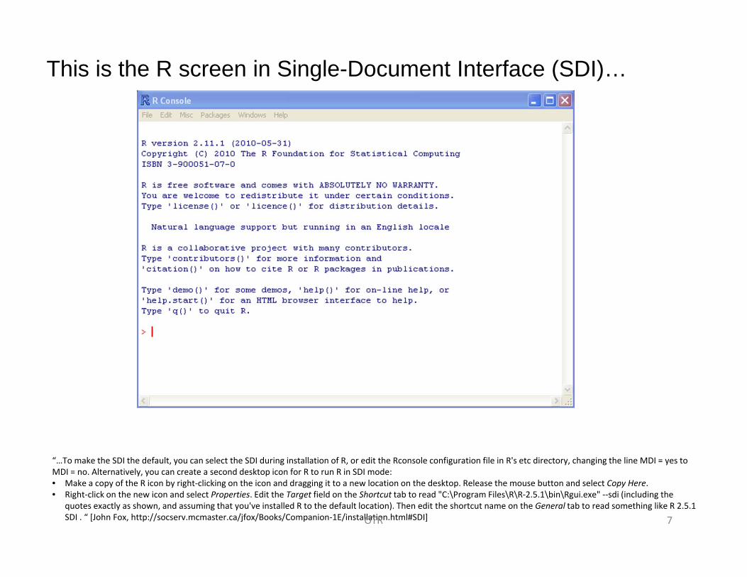
This is the R screen in Single-Document Interface (SDI)…

“…To make the SDI the default, you can select the SDI during installation of R, or edit the Rconsole configuration file in R's etc directory, changing the line MDI = yes to MDI = no. Alternatively, you can create a second desktop icon for R to run R in SDI mode: • Make a copy of the R icon by right‐clicking on the icon and dragging it to a new location on the desktop. Release the mouse button and select Copy Here. • Right‐click on the new icon and select Properties. Edit the Target field on the Shortcut tab to read "C:\Program Files\R\R‐2.5.1\bin\Rgui.exe" ‐‐sdi (including the 

quotes exactly as shown, and assuming that you've installed R to the default location). Then edit the shortcut name on the General tab to read something like R 2.5.1 SDI . “ [John Fox, http://socserv.mcmaster.ca/jfox/Books/Companion‐1E/installation.html#SDI] 7OTR

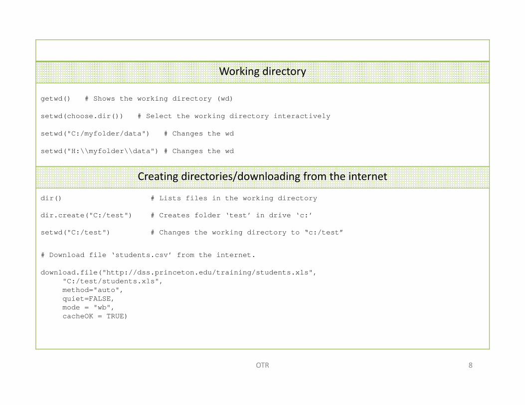
Working directory

getwd() # Shows the working directory (wd)

setwd(choose.dir()) # Select the working directory interactively

setwd("C:/myfolder/data") # Changes the wd

setwd("H:\\myfolder\\data") # Changes the wd

Creating directories/downloading from the internet

dir() # Lists files in the working directory

dir.create("C:/test") # Creates folder ‘test’ in drive ‘c:’

setwd("C:/test") # Changes the working directory to “c:/test”

# Download file ‘students.csv’ from the internet.

download.file("http://dss.princeton.edu/training/students.xls", "C:/test/students.xls", method="auto", quiet=FALSE, mode = "wb", cacheOK = TRUE)

8OTR

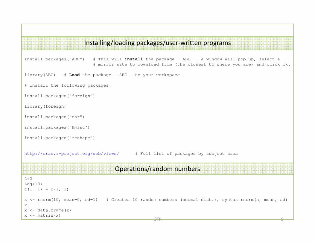
Installing/loading packages/user‐written programs

install.packages("ABC") # This will install the package –-ABC--. A window will pop-up, select a # mirror site to download from (the closest to where you are) and click ok.

library(ABC) # Load the package –-ABC-– to your workspace

# Install the following packages:

install.packages("foreign")

library(foreign)

install.packages("car")

install.packages("Hmisc")

install.packages("reshape")

http://cran.r-project.org/web/views/ # Full list of packages by subject area

Operations/random numbers2+2Log(10)c(1, 1) + c(1, 1)

x <- rnorm(10, mean=0, sd=1) # Creates 10 random numbers (normal dist.), syntax rnorm(n, mean, sd)xx <- data.frame(x)x <- matrix(x)

9OTR

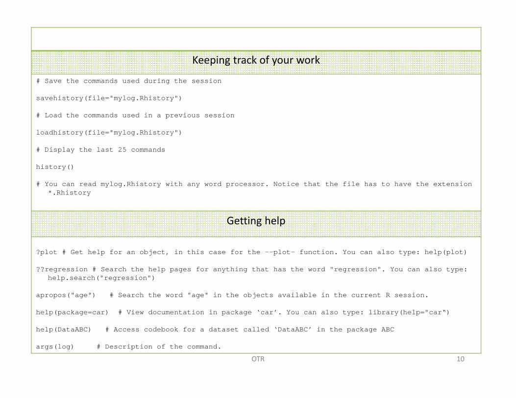
Keeping track of your work

# Save the commands used during the session

savehistory(file="mylog.Rhistory")

# Load the commands used in a previous session

loadhistory(file="mylog.Rhistory")

# Display the last 25 commands

history()

# You can read mylog.Rhistory with any word processor. Notice that the file has to have the extension *.Rhistory

Getting help

?plot # Get help for an object, in this case for the –-plot– function. You can also type: help(plot)

??regression # Search the help pages for anything that has the word "regression". You can also type: help.search("regression")

apropos("age") # Search the word "age" in the objects available in the current R session.

help(package=car) # View documentation in package ‘car’. You can also type: library(help="car“)

help(DataABC) # Access codebook for a dataset called ‘DataABC’ in the package ABC

args(log) # Description of the command.

10OTR

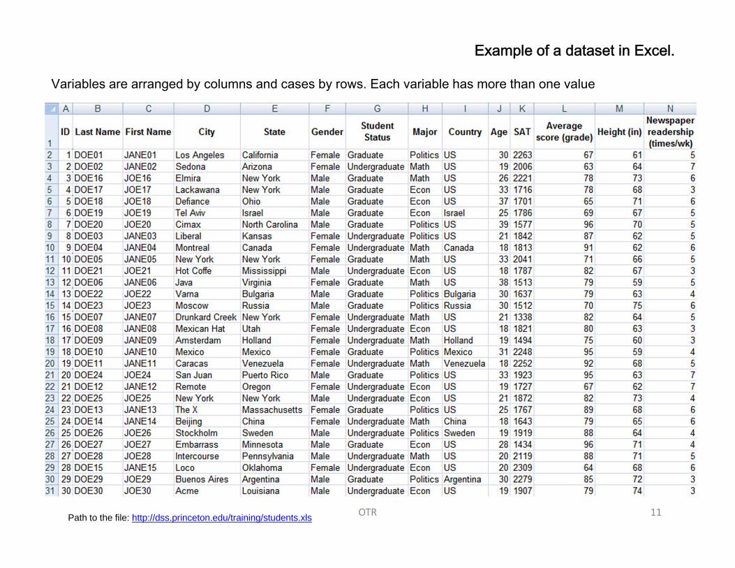
Example of a dataset in Excel.

Path to the file: http://dss.princeton.edu/training/students.xls

Variables are arranged by columns and cases by rows. Each variable has more than one value

11OTR

In Excel go to File->Save as and save the Excel file as *.csv:

From Excel to *.csv

You may get the following messages, click OK and YES…

12OTR

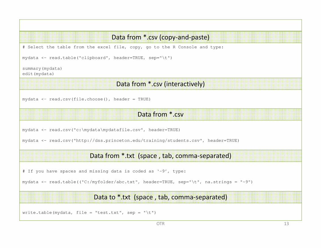
Data from *.csv (copy‐and‐paste)# Select the table from the excel file, copy, go to the R Console and type:

mydata <- read.table("clipboard", header=TRUE, sep="\t")

summary(mydata)edit(mydata)

Data from *.csv (interactively)

mydata <- read.csv(file.choose(), header = TRUE)

Data from *.csv

mydata <- read.csv("c:\mydata\mydatafile.csv", header=TRUE)

mydata <- read.csv("http://dss.princeton.edu/training/students.csv", header=TRUE)

Data from *.txt  (space , tab, comma‐separated)

# If you have spaces and missing data is coded as ‘-9’, type:

mydata <- read.table(("C:/myfolder/abc.txt", header=TRUE, sep="\t", na.strings = "-9")

Data to *.txt  (space , tab, comma‐separated)

write.table(mydata, file = "test.txt", sep = "\t")

13OTR

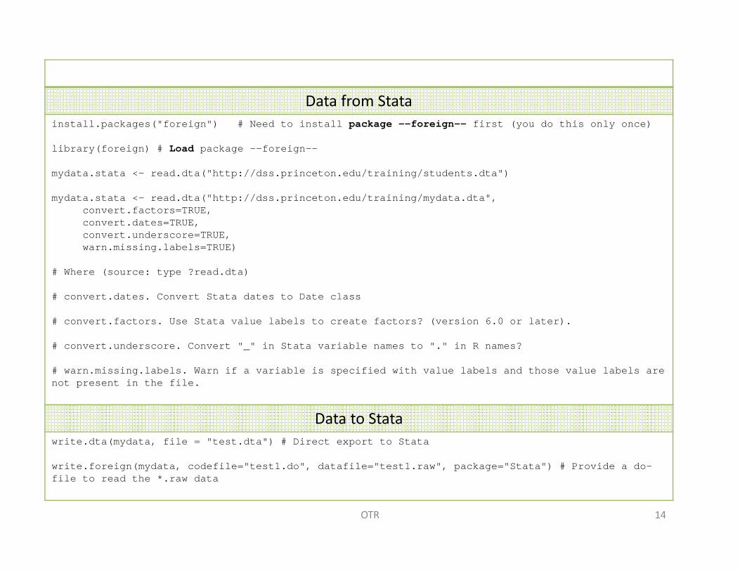
Data from Statainstall.packages("foreign") # Need to install package –-foreign–- first (you do this only once)

library(foreign) # Load package –-foreign--

mydata.stata <- read.dta("http://dss.princeton.edu/training/students.dta")

mydata.stata <- read.dta("http://dss.princeton.edu/training/mydata.dta", convert.factors=TRUE, convert.dates=TRUE, convert.underscore=TRUE, warn.missing.labels=TRUE)

# Where (source: type ?read.dta)

# convert.dates. Convert Stata dates to Date class

# convert.factors. Use Stata value labels to create factors? (version 6.0 or later).

# convert.underscore. Convert "_" in Stata variable names to "." in R names?

# warn.missing.labels. Warn if a variable is specified with value labels and those value labels are not present in the file.

Data to Statawrite.dta(mydata, file = "test.dta") # Direct export to Stata

write.foreign(mydata, codefile="test1.do", datafile="test1.raw", package="Stata") # Provide a do-file to read the *.raw data

14OTR

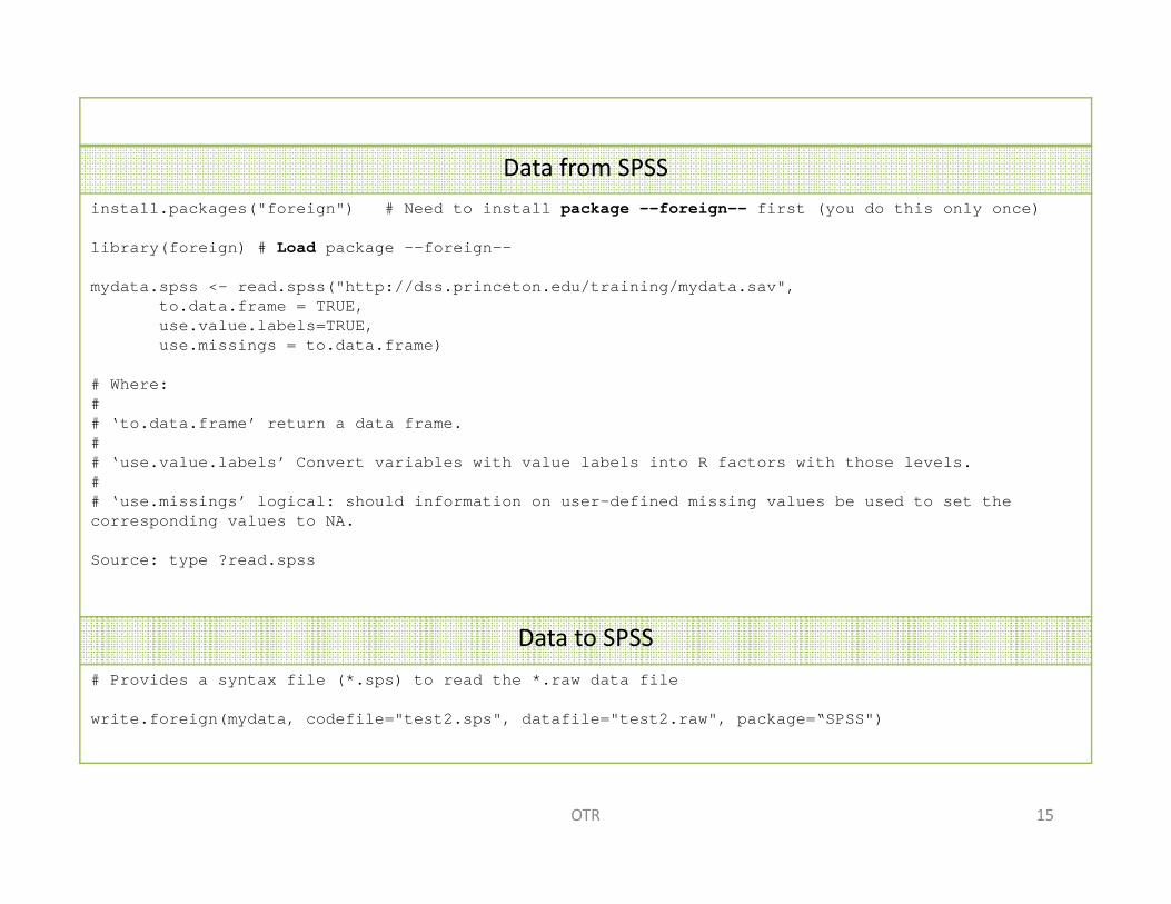
Data from SPSSinstall.packages("foreign") # Need to install package –-foreign–- first (you do this only once)

library(foreign) # Load package –-foreign--

mydata.spss <- read.spss("http://dss.princeton.edu/training/mydata.sav", to.data.frame = TRUE, use.value.labels=TRUE, use.missings = to.data.frame)

# Where:## ‘to.data.frame’ return a data frame.## ‘use.value.labels’ Convert variables with value labels into R factors with those levels.## ‘use.missings’ logical: should information on user-defined missing values be used to set the corresponding values to NA.

Source: type ?read.spss

Data to SPSS# Provides a syntax file (*.sps) to read the *.raw data file

write.foreign(mydata, codefile="test2.sps", datafile="test2.raw", package=“SPSS")

15OTR

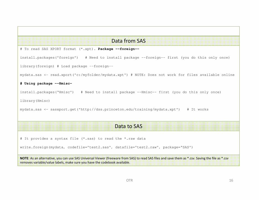
Data from SAS# To read SAS XPORT format (*.xpt). Package –-foreign--

install.packages("foreign") # Need to install package –-foreign–- first (you do this only once)

library(foreign) # Load package –-foreign--

mydata.sas <- read.xport("c:/myfolder/mydata.xpt") # NOTE: Does not work for files available online

# Using package –-Hmisc—

install.packages(“Hmisc") # Need to install package –-Hmisc–- first (you do this only once)

library(Hmisc)

mydata.sas <- sasxport.get("http://dss.princeton.edu/training/mydata.xpt") # It works

Data to SAS

# It provides a syntax file (*.sas) to read the *.raw data

write.foreign(mydata, codefile="test2.sas", datafile="test2.raw", package=“SAS")

NOTE: As an alternative, you can use SAS Universal Viewer (freeware from SAS) to read SAS files and save them as *.csv. Saving the file as *.csvremoves variable/value labels, make sure you have the codebook available.

16OTR

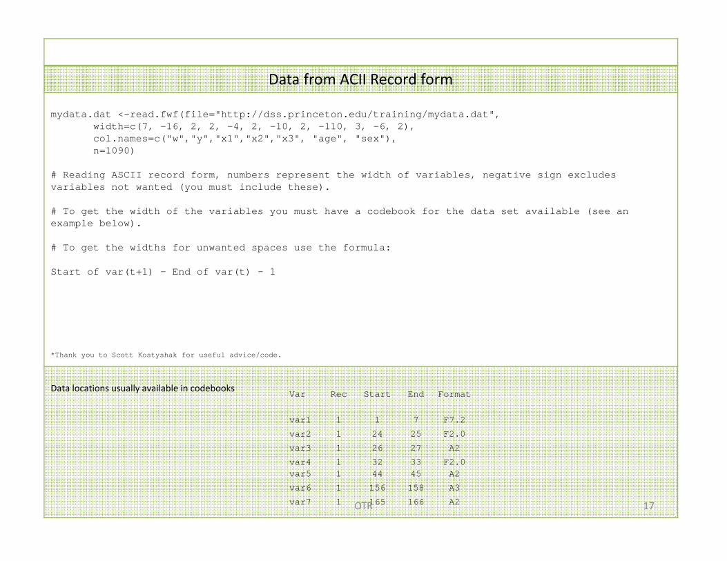
Data from ACII Record form

mydata.dat <-read.fwf(file="http://dss.princeton.edu/training/mydata.dat", width=c(7, -16, 2, 2, -4, 2, -10, 2, -110, 3, -6, 2), col.names=c("w","y","x1","x2","x3", "age", "sex"), n=1090)

# Reading ASCII record form, numbers represent the width of variables, negative sign excludes variables not wanted (you must include these).

# To get the width of the variables you must have a codebook for the data set available (see an example below).

# To get the widths for unwanted spaces use the formula:

Start of var(t+1) – End of var(t) - 1

*Thank you to Scott Kostyshak for useful advice/code.

Data locations usually available in codebooks Var Rec Start End Format

var1 1 1 7 F7.2

var2 1 24 25 F2.0

var3 1 26 27 A2

var4 1 32 33 F2.0var5 1 44 45 A2

var6 1 156 158 A3

var7 1 165 166 A2 17OTR

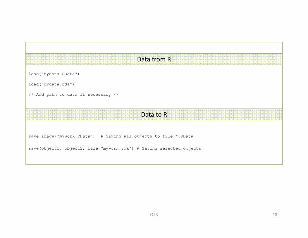
Data from R

load("mydata.RData")

load("mydata.rda")

/* Add path to data if necessary */

Data to R

save.image("mywork.RData") # Saving all objects to file *.RData

save(object1, object2, file=“mywork.rda") # Saving selected objects

18OTR

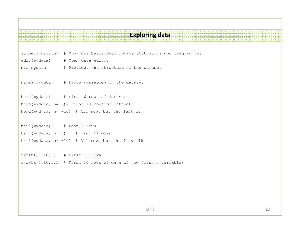
Exploring data

summary(mydata) # Provides basic descriptive statistics and frequencies.

edit(mydata) # Open data editor

str(mydata) # Provides the structure of the dataset

names(mydata) # Lists variables in the dataset

head(mydata) # First 6 rows of dataset

head(mydata, n=10)# First 10 rows of dataset

head(mydata, n= -10) # All rows but the last 10

tail(mydata) # Last 6 rows

tail(mydata, n=10) # Last 10 rows

tail(mydata, n= -10) # All rows but the first 10

mydata[1:10, ] # First 10 rows

mydata[1:10,1:3] # First 10 rows of data of the first 3 variables

19OTR

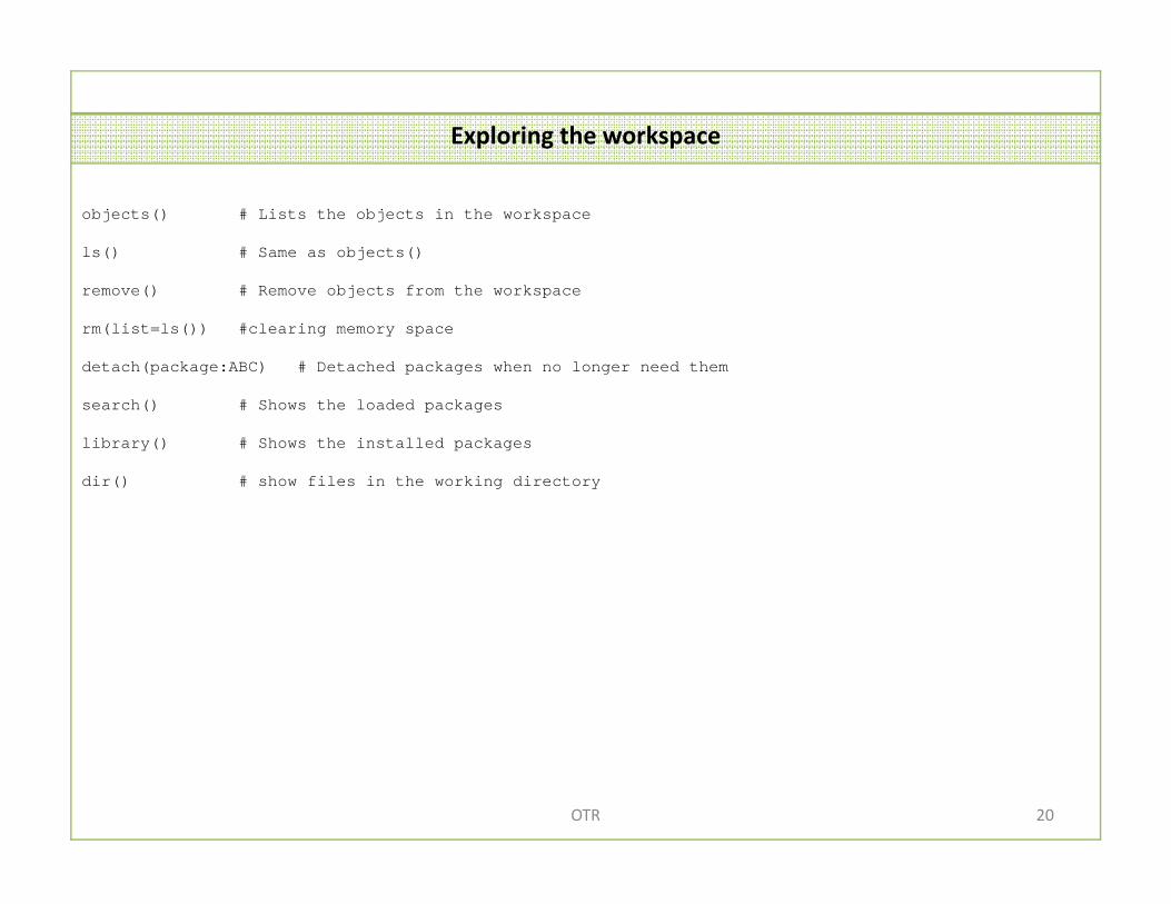
Exploring the workspace

objects() # Lists the objects in the workspace

ls() # Same as objects()

remove() # Remove objects from the workspace

rm(list=ls()) #clearing memory space

detach(package:ABC) # Detached packages when no longer need them

search() # Shows the loaded packages

library() # Shows the installed packages

dir() # show files in the working directory

20OTR

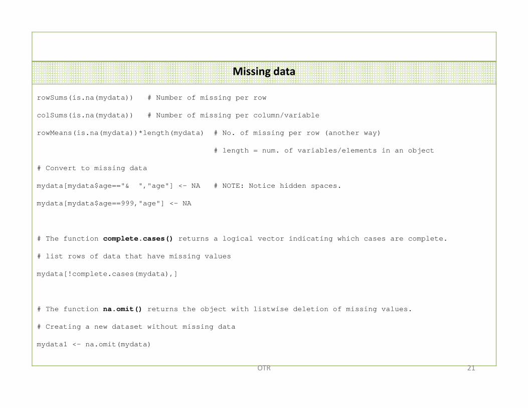
Missing data

rowSums(is.na(mydata)) # Number of missing per row

colSums(is.na(mydata)) # Number of missing per column/variable

rowMeans(is.na(mydata))*length(mydata) # No. of missing per row (another way)

# length = num. of variables/elements in an object

# Convert to missing data

mydata[mydata$age=="& ","age"] <- NA # NOTE: Notice hidden spaces.

mydata[mydata$age==999,"age"] <- NA

# The function complete.cases() returns a logical vector indicating which cases are complete.

# list rows of data that have missing values

mydata[!complete.cases(mydata),]

# The function na.omit() returns the object with listwise deletion of missing values.

# Creating a new dataset without missing data

mydata1 <- na.omit(mydata)

21OTR

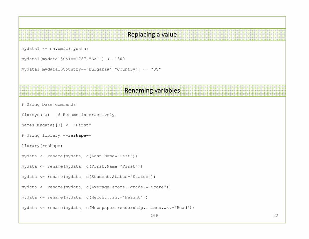
Replacing a value

mydata1 <- na.omit(mydata)

mydata1[mydata1$SAT==1787,"SAT"] <- 1800

mydata1[mydata1$Country=="Bulgaria","Country"] <- "US"

Renaming variables

# Using base commands

fix(mydata) # Rename interactively.

names(mydata)[3] <- "First"

# Using library –-reshape--

library(reshape)

mydata <- rename(mydata, c(Last.Name="Last"))

mydata <- rename(mydata, c(First.Name="First"))

mydata <- rename(mydata, c(Student.Status="Status"))

mydata <- rename(mydata, c(Average.score..grade.="Score"))

mydata <- rename(mydata, c(Height..in.="Height"))

mydata <- rename(mydata, c(Newspaper.readership..times.wk.="Read"))

22OTR

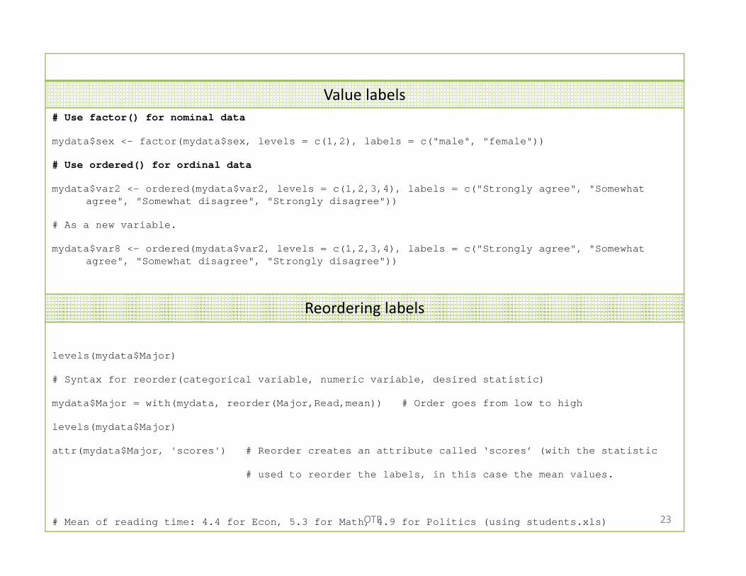
Value labels# Use factor() for nominal data

mydata$sex <- factor(mydata$sex, levels = c(1,2), labels = c("male", "female"))

# Use ordered() for ordinal data

mydata$var2 <- ordered(mydata$var2, levels = c(1,2,3,4), labels = c("Strongly agree", "Somewhat agree", "Somewhat disagree", "Strongly disagree"))

# As a new variable.

mydata$var8 <- ordered(mydata$var2, levels = c(1,2,3,4), labels = c("Strongly agree", "Somewhat agree", "Somewhat disagree", "Strongly disagree"))

Reordering labels

levels(mydata$Major)

# Syntax for reorder(categorical variable, numeric variable, desired statistic)

mydata$Major = with(mydata, reorder(Major,Read,mean)) # Order goes from low to high

levels(mydata$Major)

attr(mydata$Major, 'scores') # Reorder creates an attribute called ‘scores’ (with the statistic

# used to reorder the labels, in this case the mean values.

# Mean of reading time: 4.4 for Econ, 5.3 for Math, 4.9 for Politics (using students.xls) 23OTR

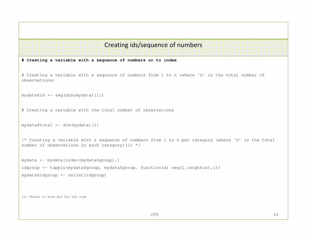
Creating ids/sequence of numbers

# Creating a variable with a sequence of numbers or to index

# Creating a variable with a sequence of numbers from 1 to n (where ‘n’ is the total number of observations)

mydata$id <- seq(dim(mydata)[1])

# Creating a variable with the total number of observations

mydata$total <- dim(mydata)[1]

/* Creating a variable with a sequence of numbers from 1 to n per category (where ‘n’ is the total number of observations in each category)(1) */

mydata <- mydata[order(mydata$group),]

idgroup <- tapply(mydata$group, mydata$group, function(x) seq(1,length(x),1))

mydata$idgroup <- unlist(idgroup)

(1) Thanks to Alex Acs for the code

24OTR

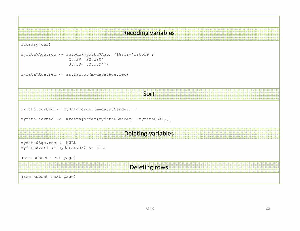
Recoding variables

library(car)

mydata$Age.rec <- recode(mydata$Age, "18:19='18to19'; 20:29='20to29';30:39='30to39'")

mydata$Age.rec <- as.factor(mydata$Age.rec)

Sort

mydata.sorted <- mydata[order(mydata$Gender),]

mydata.sorted1 <- mydata[order(mydata$Gender, -mydata$SAT),]

Deleting variablesmydata$Age.rec <- NULLmydata$var1 <- mydata$var2 <- NULL

(see subset next page)

Deleting rows(see subset next page)

25OTR

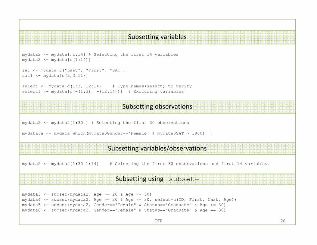
Subsetting variables

mydata2 <- mydata[,1:14] # Selecting the first 14 variablesmydata2 <- mydata[c(1:14)]

sat <- mydata[c("Last", "First", "SAT")]sat1 <- mydata[c(2,3,11)]

select <- mydata[c(1:3, 12:14)] # Type names(select) to verifyselect1 <- mydata[c(-(1:3), -(12:14))] # Excluding variables

Subsetting observations

mydata2 <- mydata2[1:30,] # Selecting the first 30 observations

mydata3a <- mydata[which(mydata$Gender=='Female' & mydata$SAT > 1800), ]

Subsetting variables/observations

mydata2 <- mydata2[1:30,1:14] # Selecting the first 30 observations and first 14 variables

Subsetting using –subset‐‐

mydata3 <- subset(mydata2, Age >= 20 & Age <= 30)mydata4 <- subset(mydata2, Age >= 20 & Age <= 30, select=c(ID, First, Last, Age))mydata5 <- subset(mydata2, Gender=="Female" & Status=="Graduate" & Age >= 30)mydata6 <- subset(mydata2, Gender=="Female" & Status=="Graduate" & Age == 30)

26OTR

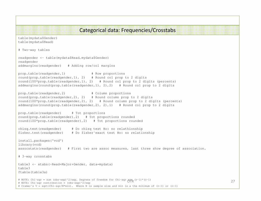
Categorical data: Frequencies/Crosstabstable(mydata$Gender)table(mydata$Read)

# Two-way tables

readgender <- table(mydata$Read,mydata$Gender)readgenderaddmargins(readgender) # Adding row/col margins

prop.table(readgender,1) # Row proportionsround(prop.table(readgender,1), 2) # Round col prop to 2 digitsround(100*prop.table(readgender,1), 2) # Round col prop to 2 digits (percents)addmargins(round(prop.table(readgender,1), 2),2) # Round col prop to 2 digits

prop.table(readgender,2) # Column proportionsround(prop.table(readgender,2), 2) # Round column prop to 2 digitsround(100*prop.table(readgender,2), 2) # Round column prop to 2 digits (percents)addmargins(round(prop.table(readgender,2), 2),1) # Round col prop to 2 digits

prop.table(readgender) # Tot proportionsround(prop.table(readgender),2) # Tot proportions roundedround(100*prop.table(readgender),2) # Tot proportions rounded

chisq.test(readgender) # Do chisq test Ho: no relathionshipfisher.test(readgender) # Do fisher'exact test Ho: no relationship

install.packages("vcd")library(vcd)assocstats(readgender) # First two are assoc measures, last three show degree of association.

# 3-way crosstabs

table3 <- xtabs(~Read+Major+Gender, data=mydata)table3ftable(table3a)

# NOTE: Chi-sqr = sum (obs-exp)^2/exp. Degrees of freedom for Chi-sqr are (r-1)*(c-1)# NOTE: Chi-sqr contribution = (obs-exp)^2/exp# Cramer's V = sqrt(Chi-sqr/N*min). Where N is sample size and min is a the minimum of (r-1) or (c-1)

27OTR

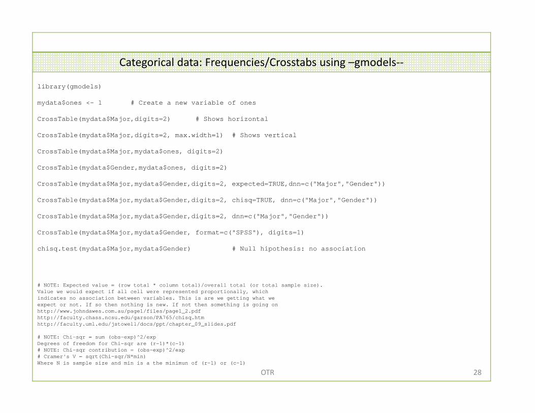
Categorical data: Frequencies/Crosstabs using –gmodels‐‐

library(gmodels)

mydata$ones <- 1 # Create a new variable of ones

CrossTable(mydata$Major,digits=2) # Shows horizontal

CrossTable(mydata$Major,digits=2, max.width=1) # Shows vertical

CrossTable(mydata$Major,mydata$ones, digits=2)

CrossTable(mydata$Gender,mydata$ones, digits=2)

CrossTable(mydata$Major,mydata$Gender,digits=2, expected=TRUE,dnn=c("Major","Gender"))

CrossTable(mydata$Major,mydata$Gender,digits=2, chisq=TRUE, dnn=c("Major","Gender"))

CrossTable(mydata$Major,mydata$Gender,digits=2, dnn=c("Major","Gender"))

CrossTable(mydata$Major,mydata$Gender, format=c("SPSS"), digits=1)

chisq.test(mydata$Major,mydata$Gender) # Null hipothesis: no association

# NOTE: Expected value = (row total * column total)/overall total (or total sample size). Value we would expect if all cell were represented proportionally, whichindicates no association between variables. This is are we getting what we expect or not. If so then nothing is new. If not then something is going onhttp://www.johndawes.com.au/page1/files/page1_2.pdfhttp://faculty.chass.ncsu.edu/garson/PA765/chisq.htmhttp://faculty.uml.edu/jstowell/docs/ppt/chapter_09_slides.pdf

# NOTE: Chi-sqr = sum (obs-exp)^2/expDegrees of freedom for Chi-sqr are (r-1)*(c-1)# NOTE: Chi-sqr contribution = (obs-exp)^2/exp# Cramer's V = sqrt(Chi-sqr/N*min)Where N is sample size and min is a the minimun of (r-1) or (c-1)

28OTR

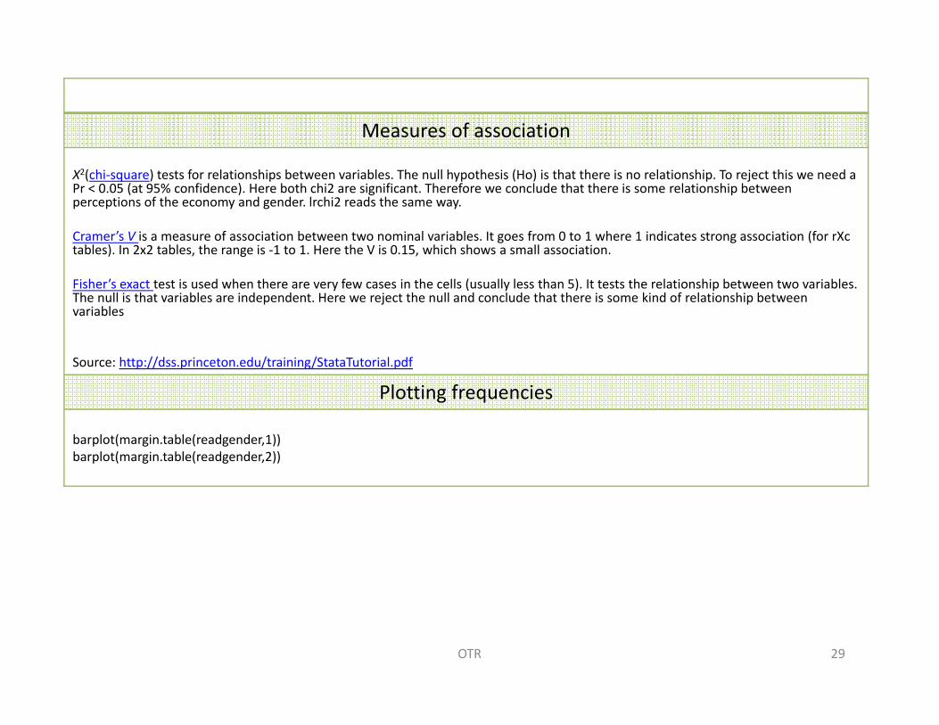
Measures of association

X2(chi‐square) tests for relationships between variables. The null hypothesis (Ho) is that there is no relationship. To reject this we need aPr < 0.05 (at 95% confidence). Here both chi2 are significant. Therefore we conclude that there is some relationship between perceptions of the economy and gender. lrchi2 reads the same way.

Cramer’s V is a measure of association between two nominal variables. It goes from 0 to 1 where 1 indicates strong association (for rXctables). In 2x2 tables, the range is ‐1 to 1. Here the V is 0.15, which shows a small association.

Fisher’s exact test is used when there are very few cases in the cells (usually less than 5). It tests the relationship between two variables. The null is that variables are independent. Here we reject the null and conclude that there is some kind of relationship betweenvariables

Source: http://dss.princeton.edu/training/StataTutorial.pdf

Plotting frequencies

barplot(margin.table(readgender,1))barplot(margin.table(readgender,2))

29OTR

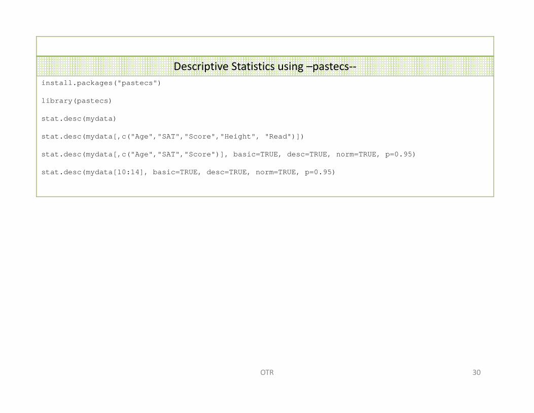
Descriptive Statistics using –pastecs‐‐install.packages("pastecs")

library(pastecs)

stat.desc(mydata)

stat.desc(mydata[,c("Age","SAT","Score","Height", "Read")])

stat.desc(mydata[,c("Age","SAT","Score")], basic=TRUE, desc=TRUE, norm=TRUE, p=0.95)

stat.desc(mydata[10:14], basic=TRUE, desc=TRUE, norm=TRUE, p=0.95)

30OTR

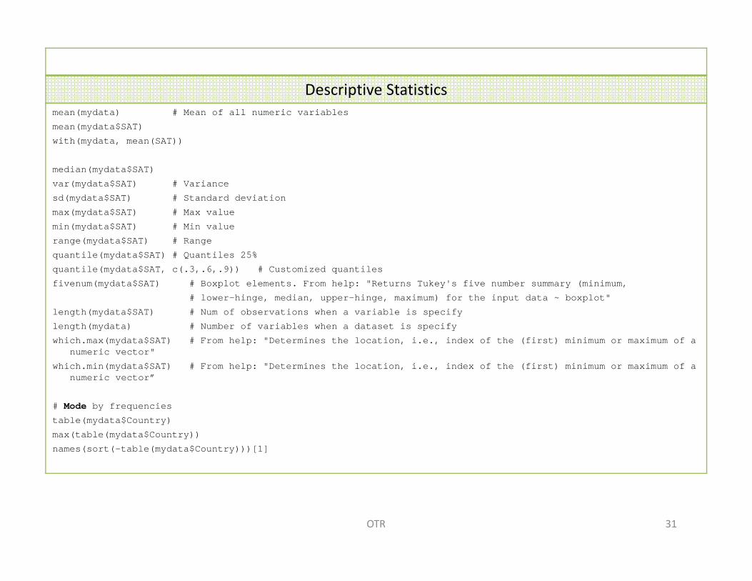
Descriptive Statisticsmean(mydata) # Mean of all numeric variables

mean(mydata$SAT)

with(mydata, mean(SAT))

median(mydata$SAT)

var(mydata$SAT) # Variance

sd(mydata$SAT) # Standard deviation

max(mydata$SAT) # Max value

min(mydata$SAT) # Min value

range(mydata$SAT) # Range

quantile(mydata$SAT) # Quantiles 25%

quantile(mydata$SAT, c(.3,.6,.9)) # Customized quantiles

fivenum(mydata$SAT) # Boxplot elements. From help: "Returns Tukey's five number summary (minimum,

# lower-hinge, median, upper-hinge, maximum) for the input data ~ boxplot"

length(mydata$SAT) # Num of observations when a variable is specify

length(mydata) # Number of variables when a dataset is specify

which.max(mydata$SAT) # From help: "Determines the location, i.e., index of the (first) minimum or maximum of a numeric vector"

which.min(mydata$SAT) # From help: "Determines the location, i.e., index of the (first) minimum or maximum of a numeric vector”

# Mode by frequencies

table(mydata$Country)

max(table(mydata$Country))

names(sort(-table(mydata$Country)))[1]

31OTR

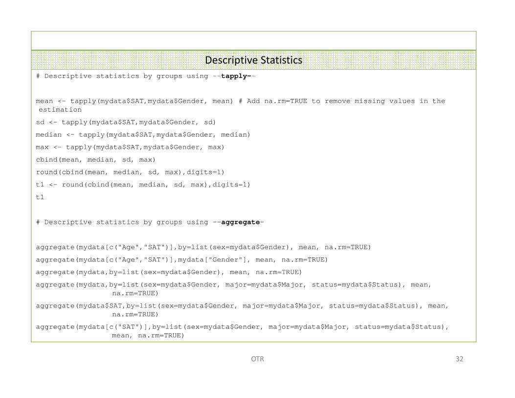
Descriptive Statistics# Descriptive statistics by groups using --tapply--

mean <- tapply(mydata$SAT,mydata$Gender, mean) # Add na.rm=TRUE to remove missing values in the estimation

sd <- tapply(mydata$SAT,mydata$Gender, sd)

median <- tapply(mydata$SAT,mydata$Gender, median)

max <- tapply(mydata$SAT,mydata$Gender, max)

cbind(mean, median, sd, max)

round(cbind(mean, median, sd, max),digits=1)

t1 <- round(cbind(mean, median, sd, max),digits=1)

t1

# Descriptive statistics by groups using --aggregate—

aggregate(mydata[c("Age","SAT")],by=list(sex=mydata$Gender), mean, na.rm=TRUE)

aggregate(mydata[c("Age","SAT")],mydata["Gender"], mean, na.rm=TRUE)

aggregate(mydata,by=list(sex=mydata$Gender), mean, na.rm=TRUE)

aggregate(mydata,by=list(sex=mydata$Gender, major=mydata$Major, status=mydata$Status), mean, na.rm=TRUE)

aggregate(mydata$SAT,by=list(sex=mydata$Gender, major=mydata$Major, status=mydata$Status), mean, na.rm=TRUE)

aggregate(mydata[c("SAT")],by=list(sex=mydata$Gender, major=mydata$Major, status=mydata$Status), mean, na.rm=TRUE)

32OTR

Histogramslibrary(car)

head(Prestige)

hist(Prestige$income)

hist(Prestige$income, col="green")

with(Prestige, hist(income)) # Histogram of income with a nicer title.

# Applying Freedman/Diaconis rule p.120 ("Algorithm that chooses bin widths and locations automatically, based on the sample size and the spread of the data" http://www.mathworks.com/help/toolbox/stats/bqucg6n.html)

with(Prestige, hist(income, breaks="FD", col="green"))

box()

hist(Prestige$income, breaks="FD")

# Conditional histograms

par(mfrow=c(1, 2))

hist(mydata$SAT[mydata$Gender=="Female"], breaks="FD", main="Female", xlab="SAT",col="green")

hist(mydata$SAT[mydata$Gender=="Male"], breaks="FD", main="Male", xlab="SAT", col="green")

# Braces indicate a compound command allowing several commands with 'with' command

par(mfrow=c(1, 1))

with(Prestige, {

hist(income, breaks="FD", freq=FALSE, col="green")

lines(density(income), lwd=2)

lines(density(income, adjust=0.5),lwd=1)

rug(income)

})33OTR

Histograms# Histograms overlaid

hist(mydata$SAT, breaks="FD", col="green")

hist(mydata$SAT[mydata$Gender=="Male"], breaks="FD", col="gray", add=TRUE)

legend("topright", c("Female","Male"), fill=c("green","gray"))

# Check

satgender <- table(mydata$SAT,mydata$Gender)satgender

Histogram with normal curve overlayx <- rnorm(100)hist(x, freq=F)curve(dnorm(x), add(T)

h <- hist(x, plot=F)ylim <- range(0. h$density, dnorm(0))hist(x, freq=F, ylim=ylim)curve(dnorm(x), add=T)

34OTR

Scatterplots# Scatterplots. Useful to 1) study the mean and variance functions in the regression of y on x p.128; 2)to identify outliers and leverage points.

# plot(x,y)

plot(mydata$SAT) # Index plotplot(mydata$Age, mydata$SAT)plot(mydata$Age, mydata$SAT, main=“Age/SAT", xlab=“Age", ylab=“SAT", col="red")abline(lm(mydata$SAT~mydata$Age), col="blue")

# regression line (y~x)lines(lowess(mydata$Age, mydata$SAT), col="green") # lowess line (x,y) identify(mydata$Age, mydata$SAT, row.names(mydata))

# On row.names to identify. "All data frames have a row names attribute, a character vector of length the number of rows with no duplicates nor missing values." (source link below).# "Use attr(x, "row.names") if you need an integer value.)" http://stat.ethz.ch/R-manual/R-devel/library/base/html/row.names.html

mydata$Names <- paste(mydata$Last, mydata$First)row.names(mydata) <- mydata$Namesplot(mydata$SAT, mydata$Age)identify(mydata$SAT, mydata$Age, row.names(mydata))

35OTR

Scatterplots# Rule on span for lowess, big sample smaller (~0.3), small sample bigger (~0.7)

library(car)

scatterplot(SAT~Age, data=mydata)

scatterplot(SAT~Age, id.method="identify", data=mydata)

scatterplot(SAT~Age, id.method="identify", boxplots= FALSE, data=mydata)

scatterplot(prestige~income, span=0.6, lwd=3, id.n=4, data=Prestige)

# By groups

scatterplot(SAT~Age|Gender, data=mydata)

scatterplot(SAT~Age|Gender, id.method="identify", data=mydata)

scatterplot(prestige~income|type, boxplots=FALSE, span=0.75, data=Prestige)

scatterplot(prestige~income|type, boxplots=FALSE, span=0.75, col=gray(c(0,0.5,0.7)), data=Prestige)

36OTR

Scatterplots (multiple)scatterplotMatrix(~ prestige + income + education + women, span=0.7, id.n=0, data=Prestige)

pairs(Prestige) # Pariwise plots. Scatterplots of all variables in the datasetpairs(Prestige, gap=0, cex.labels=0.9) # gap controls the space between subplot and cex.labels the

font size (Dalgaard:186)

3D Scatterplotslibrary(car)

scatter3d(prestige ~ income + education, id.n=3, data=Duncan)

37OTR

Scatterplots (for categorical data)plot(vocabulary ~ education, data=Vocab)

plot(jitter(vocabulary) ~ jitter(education), data=Vocab)

plot(jitter(vocabulary, factor=2) ~ jitter(education, factor=2), data=Vocab)

# cex makes the point half the size, p. 134

plot(jitter(vocabulary, factor=2) ~ jitter(education, factor=2), col="gray", cex=0.5, data=Vocab)with(Vocab, {

abline(lm(vocabulary ~ education), lwd=3, lty="dashed")lines(lowess(education, vocabulary, f=0.2), lwd=3)

})

Useful links to graphics

http://www.stat.auckland.ac.nz/~paul/RGraphics/rgraphics.html

http://addictedtor.free.fr/graphiques/

http://addictedtor.free.fr/graphiques/thumbs.php?sort=votes

http://www.statmethods.net/advgraphs/layout.html

38OTR

Exercises

Exercise 1Using the ICPSR Online Learning Center, go to guide on Civic Participation and Demographics in Rural China (1990)http://www.icpsr.umich.edu/icpsrweb/ICPSR/OLC/guides/China/sections/a01

Got to the tab ‘Dataset’ and download the data (http://www.icpsr.umich.edu/icpsrweb/ICPSR/OLC/guides/China/sections/a02)

We’ll focus on the first exercise on ‘Age and Participation’ and use the following variables:

• Respondent's year of birth (M1001)• Village meeting attendance (M3090)

Activities:

• Create the variable ‘age’ for each respondent• Create the variable ‘agegroup’ with the following categories: 16‐35, 36‐55 and 56‐79

Questions:

• What percentage of respondents reported attending a local village meeting? • Of those attending a meeting, which age group was most likely to report attending a village meeting? • Of those attending a meeting , which group was most likely to report no village meeting attendance?

Source: Inter‐university Consortium for Political and Social Research. Civic Participation and Demographics in Rural China: A Data‐Driven Learning Guide. Ann Arbor, MI: Inter‐university Consortium for Political and Social Research [distributor], July, 31 2009. Doi:10.3886/China

40OTR

Exercise 2Got to the World Development Indicators (WDI) & Global Development Finance (GDF) from the World Bank (access from the library’s Articles and Databases, http://library.princeton.edu/catalogs/articles.php) 

Direct link to WDI/GDF http://databank.worldbank.org/ddp/home.do?Step=12&id=4&CNO=2

Get data for the United States and all available years on:

• Long‐term unemployment (% of total unemployment)• Long‐term unemployment, female (% of female unemployment)• Long‐term unemployment, male (% of male unemployment)• Inflation, consumer prices (annual %)• GDP per capita (constant 2000 US$)• GDP per capita growth (annual %)

See here to arrange the data as panel data http://dss.princeton.edu/training/FindingData101.pdf#page=21For an example of how panel data looks like click here: http://dss.princeton.edu/training/DataPrep101.pdf#page=3

Activities:

• Rename the variables and explore the data (use describe, summarize)• Create a variable called crisis where it takes the value of 17 for the following years: 1960, 1961, 1969, 1970, 1973, 1974, 1975, 

1981, 1982, 1990, 1991, 2001, 2007, 2008, 2009. Replace missing with zeros (source: nber.org).• Set as time series (see http://dss.princeton.edu/training/TS101.pdf#page=6)• Create a line graph with unemployment rate (total, female and males) and crisis by year.

Questions:

• What do you see? Who tends to be more affected by the economic recessions?41OTR

References/Useful links

• DSS Online Training Section http://dss.princeton.edu/training/

• Princeton DSS Libguides http://libguides.princeton.edu/dss

• John Fox’s site http://socserv.mcmaster.ca/jfox/

• Quick‐R http://www.statmethods.net/

• UCLA Resources to learn and use R http://www.ats.ucla.edu/stat/R/

• UCLA Resources to learn and use Stata http://www.ats.ucla.edu/stat/stata/

• DSS ‐ Stata http://dss/online_help/stats_packages/stata/

• DSS ‐ R http://dss.princeton.edu/online_help/stats_packages/r

42OTR

References/Recommended books

• An R Companion to Applied Regression, Second Edition / John Fox , Sanford Weisberg, Sage Publications, 2011

• Data Manipulation with R / Phil Spector, Springer, 2008

• Applied Econometrics with R / Christian Kleiber, Achim Zeileis, Springer, 2008

• Introductory Statistics with R / Peter Dalgaard, Springer, 2008

• Complex Surveys. A guide to Analysis Using R / Thomas Lumley, Wiley, 2010

• Applied Regression Analysis and Generalized Linear Models / John Fox, Sage, 2008

• R for Stata Users / Robert A. Muenchen, Joseph Hilbe, Springer, 2010

• Introduction to econometrics / James H. Stock, Mark W. Watson. 2nd ed., Boston: Pearson Addison Wesley, 2007.

• Data analysis using regression and multilevel/hierarchical models / Andrew Gelman, Jennifer Hill. Cambridge ; New York : Cambridge University Press, 2007. 

• Econometric analysis / William H. Greene. 6th ed., Upper Saddle River, N.J. : Prentice Hall, 2008.

• Designing Social Inquiry: Scientific Inference in Qualitative Research / Gary King, Robert O. Keohane, Sidney Verba, Princeton University Press, 1994.

• Unifying Political Methodology: The Likelihood Theory of Statistical Inference / Gary King, Cambridge University Press, 1989

• Statistical Analysis: an interdisciplinary introduction to univariate & multivariate methods /  Sam    

Kachigan, New York : Radius Press, c1986 

• Statistics with Stata (updated for version 9) / Lawrence Hamilton, Thomson Books/Cole,  2006

43OTR