46 ArcUser October–December 2002 www.esri.com

Exploring Hospital Distribution Using ArcGISBy Chris Wayne, ESRI–OlympiaSpatial analysis has a wide range of applica-tions in health care, from managing beds in a facility to global health risk assessment. This exercise looks at the distribution of hospitals in the contiguous United States relative to population. You have the following specific objectives:1. Quantify hospital density within each HSA.2. Compare hospital density in California (or another region) with that of the contiguous United States.3. Compare the population characteristics of regions with high hospital density to the entire contiguous United States.4. Present your analysis as a map. This exercise assumes that you know the basics of using ArcGIS—how to start a map session and navigate in the ArcCatalog envi-ronment. You will need ArcGIS 8.1 or 8.2 with at least an ArcView license. No extensions are required. If you want a hard-copy of your map, you will need access to a printer. The data consists of points showing hospi-tal locations and polygons describing HSAs. Although HSAs are polygons that usually fol-low county lines, they sometimes cross state boundaries. Both point and polygon data are stored as feature classes in a feature dataset within a personal geodatabase.

Downloading and Exploring the DataDownload the sample data archive from the ArcUser Online Web site and copy it to your computer. Create a new folder called health_analysis and unzip the archive into it.

Exploring Data in ArcMap Start a new ArcMap session and open the map document hospitals_density.mxd located in /…/<your directory>/health_analysis/. There are two layers in this document. Zoom and pan to explore the distribution of hospitals in different regions of the U.S.

Exploring Data in ArcCatalogStart an ArcCatalog session and navigate to /…/<your directory>/health_analysis/ which contains hospitals_density.mxd and the usa_health geodatabase. Look at how the geodatabase structure is organized. The base

data is stored as feature classes in a feature dataset called health_data. An empty feature dataset named analysis will hold the results of your data analysis. There is also a stand-alone feature class, STATES, that is not in a feature dataset, and two stand-alone tables, h10k_p_stats and population_stats. Two layer files, hospital.lyr and STATES.lyr, are stored outside of the geodatabase. You may also click on the Preview tab and the Metadata tab to get more detailed informa-tion about these data. The metadata includes the URL for the National Atlas from which the HSA boundaries were derived. (Note that not all fields in the metadata are complete.)

1. Quantify Hospital DensityWithin Each HSA.The rest of the work in this tutorial will be performed in ArcMap so you can closeArcCatalog after inspecting the sample data. As you work through the exercise, remember to save your work often!

Performing a spatial join to connectthe hospitals to the HSAsPerforming a spatial join to connect the hos-pitals to the HSAs is the first step in quanti-fying hospital density within each HSA. You will join each record from the point features (hospitals) to the polygon features (HSAs) that contains those points.1. In the Table of Contents in ArcMap, right-click the HSA layer and choose Joins and Relates > Join… from the context menu. 2. In the Join Data dialog box, select Join Data from Another Layer Based on Spatial Location. For each of the steps listed in this dialog box, make the following selections:n In step 1, select hospitals as the layer to join.n In step 2, accept the default and do not check any boxes. This is because the hospitals do not have any usable attributes.n In step 3, convert the new layer to feature class in a personal geodatabase. Click the browse button and select personal geoda-tabase feature class for Save as Type: box. Open \…\<your directory>\health_analysis\usa_health.mdb\analysis and name the feature

class hospitals_in_hsa. 3. Right-click on the hospitals_in_hsa layer and choose Open Attribute Table. In the at-tribute table, note that the field called Count_ indicates how many points fall within that polygon and that some HSAs do not contain any hospitals.4. HSAs that do not contain hospitals will show a NULL value in the Count_ field. To avoid working with NULL values, replace the NULL values with zeros. Right-click on the Count_ header and choose Calculate Values. In the Field Calculator, type “is null” and click OK. Click the Show: Selected button to dis-play only the records with NULL values that were just selected. Right-click on the County_ header and choose Calculate Values. In the Field Calculator, type 0 in the text field and click OK. The Count_ field will be populated with 0s.

Add a new field and calculate number of hospitals per 10,000 peopleAlthough calculating persons-per-hospital would reflect an intuitive measurement of how many people each hospital must serve, the

Perform a spatial join to hospitals to the HSAs.

What You Will Need• ArcGIS (ArcView, ArcEditor, or ArcInfo license)• Sample data downloaded from ArcUser Online

Hands On

www.esri.com ArcUser October–December 2002 47

Add a field to the hospitals_in_hsa attribute table to store calculations of hospitals per 10,000 persons.

0 values in the Count_ field could skew your analysis. Calculating persons-per-hospital for HSAs by dividing Population by Count_, the values would yield 0 for HSAs without hos-pitals. This isn’t correct—there are not zero people per hospital, but many people in some HSAs that have no hospitals. For the purposes of statistical analysis, a count of hospitals-per-person will provide a more objective measurement. However, just doing a raw calculation of Count_/Population would produce very small numbers with lots of decimal places. Instead, you will calculate how many hospitals there are for each 10,000 people in an HSA.

1. The Attributes of hospitals_in_hsa table should still be open. Click the Options button at the bottom of the attribute table window and select Add Field from the menu. 2. In the Add Field dialog box, name the new field hosp_10k_p (short for “hospitals per 10,000 people”) and select Float as the type. Set Precision at 12 and Scale at 4. For addi-tional information on these field parameters, see the online help. Click OK.3. Right-click on the new hosp_10k_p field and choose Calculate Values. Ignore the warn-ing about calculating outside an edit session and click Yes. 4. In the Field Calculator, type in the fol-lowing equation. The parentheses are critical. [Count_]/([Population]*0.0001)5. You should get a range of values between 0 and 4.95, with most values being less than 1.0. If these values look right, close the table and return to the main ArcMap window. A recap of what you have just done—you added a new field that can store decimal values and calculated values for this field that indi-cate the number of hospitals per 1/10,000th of the population in each HSA.

Symbolizing Zero Data SeparatelyNext you will symbolize zero values in the data and choose a classification method for the remaining data. 1. In the Table of Contents, right-click on the hospitals_in_hsa layer and choose Properties. In the Layer Properties dialog box, click on the Symbology tab.2. In the left column below Show:, click Quantities then select Graduated Color. 3. In the Fields section, choose the hosp_10k_p field from the drop-down box next to Value as the field to classify on. You can accept the default color scheme or change it. Use a color scheme other than yellow or red monochromatic so the hospitals and excluded values will remain visible.4. Click the Classify button. In the Classifica-tion dialog, click the Exclusion button to bring up the Data Exclusion Properties dialog box. 5. Click on the Query tab and enter the ex-pression Hosp_10k_p = 0. This will ensure that HSAs with no hospitals will be symbol-ized separately from the rest of the HSAs.6. Still in the Data Exclusion Properties dia-log box, click on the Legend tab. Check the box next to Show Symbol for Excluded Data and use a light yellow color. Type No Hospi-

Symbolize the values just calculated for hospitals per 10,000 persons using graduated color.

tals in HSA in the Label box.7. Click OK to close the Data Exclusion Properties dialog but leave the Classification dialog box open for the next portion of the exercise. Notice that in the Classification dialog, a new class has been added with a value of 0 and the symbology you specified. This will prevent 0 from being used in the classification algorithms that you will apply in subsequent steps, and also will display which HSAs do not have any hospitals.

Continued on page 48

Use the Exclusion dialog box to apply a query that will separate out HSAs with no hospitals and symbolize them differently.

48 ArcUser October–December 2002 www.esri.com

Exploring Hospital Distribution Using ArcGISContinued from page 47

Symbolizing the remaining datausing different classification methodsIn the Classification dialog box, you can accept the default classification of Natural Breaks or change it to one of the other clas-sification methods. Notice how the class breaks on the histogram change. In particular, compare the results after applying the Natural Breaks, Quantile, and Equal Interval classifi-cation methods. To see each of these on the map, click OK in the Classification dialog, then Apply in the Symbology properties. To change the classification, open the Classification dialog box just as you did when symbolizing the null value. This time you will not need to open the exclusion dialog. Choose the classification that portrays data to your lik-ing and click OK in each of the dialog boxes. Click once on the hospitals_in_hsa layer to select it and click again and type in the text “Hospitals per 10,000 persons.”

Use the layout in the map document to display the analysis. Add the hospital density statistics as tables (shown here) or as screen captures of dialog showing histograms and statistic summary lists.

2. Comparing Hospital Density in California (or Another Region) With That of the Contiguous U.S.ArcGIS provides the ability to get statistics on the selected features or records from any numeric field in a table. You will enter these statistics in a table and display the table on your map layout. 1. On the bottom left of the Table of Contents, click on the Source tab. Now, in addition to the layers, there are also two tables—h10k_p_stats and population_stats. You will enter statistical data into these tables.2. If the Editor toolbar is not already active, make it visible by choosing View > Toolbars > Editor.3. On the Editor toolbar, click on the Editor menu and choose Start Editing. If you get an error, check the properties for the file and/or folder to be sure they are not set as read-only.4. Add the STATES layer, /…/<your directory>/health_analysis/states.lyr, to

the map document either by using the Add Data button, choosing File > Add Data from the main menu, or by dragging it in from ArcCatalog.5. Make the only STATES layer selectable by choosing Selection > Set Selectable layers from the main menu. Click the Clear All but-ton, then check the box next to STATES and close the dialog box.6. Using the select features tool, click on Cal-ifornia to select it. You can analyze density for any state that interests you but all references in this exercise will use California.7. Next select the HSAs that are in that state by choosing Selection > Select by Location from the main menu. 8. Use the fields and operators in this dialog box to create the statement “I want to: select features from the following layers: hospitals_in_hsa that: have their center in the features in this layer: states.” Keep Use Selected Features checked and click Apply, then CLOSE.

Hands On

www.esri.com ArcUser October–December 2002 49

Figure 1: Form for recording hosp_10k_p statistics

Figure 2: Form for hospitals_in _hsa statistics

9. All of the HSAs in California should be selected. Open up the attribute table for hospitals_in_hsa. In the table, right-click on the column heading for the hosp_10k_p field and choose Statistics from the context menu. A window with a histogram and numerical statistics will appear. Copy (by hand) the sta-tistics from this window into the subset_calif line on the form shown in Figure 1.10. Close the statistics window, then open the h10k_p_stats table and enter the statistics just copied into the appropriate cells by clicking in the cell and typing the value.11. Minimize the h10k_p_stats table and open the attribute table for hospitals_in_hsa. In the table window, click the Options button and choose Switch Selection to select all of the HSAs that are NOT in California. Right-click on hosp_10k_p and get statistics for this set. Restore h10k_p_stats and repeat the process of entering the statistics from hospitals_in_hsa. What do these results mean? Note that California has a lower mean and also a much lower range between the minimum and maxi-mum values than the rest of the nation. This might suggest that hospitals in California are more evenly distributed among HSAs than elsewhere in the U.S.

3. Compare Population Characteristicsof High Hospital Density Regions to the U.S. as a WholeIf you use the Natural Break classification, you will see that there is a break right around 1.0 hospitals/10,000 people. Most HSAs have fewer hospitals than this. You can run some simple statistical queries to characterize high hospital density HSAs. 1. The attribute table of hospitals_in_hsa should still be open. Click on Options and choose Select by Attributes. Create a new selection based on the query below. Click Apply after typing in this expression. [hosp_10k_p] = 02. This query will yield 41 records. Close the

Select by Attributes dialog box. 3. Move (or minimize) the table and look at the map to see where the selected HSAs are located. For the most part, they are located in rural areas of the midwestern states.4. In the table, right-click on the field heading for the Population field and choose Statistics from the context menu. Enter the statistics into the form shown in Figure 2. 5. Close the statistics window and the open the population_stats table and enter the statis-tics into the appropriate cells by clicking in the cell and typing the value.6. What you will find is that areas with the highest hospital density have a much lower population than the HSA average. Assuming that a place that is called a hospital provides a mandatory minimum standard of health care, it appears that basic health care is well distrib-uted in the USA regardless of population.7. When you have finished entering all the statistics, click Editor > Stop Editing on the Editor toolbar. Click Yes to save your edits.

4. Making a Map Showing Your AnalysisA map layout document has already been cre-ated for you. To view it, choose View > Layout View from the main menu. There are several

ways to add statistics to this layout. Before adding the statistics tables to your layout, open each table, click the Options button, choose Appearance and make any changes to font style and size and resize the table if necessary. Choose Options > Add to Layout to insert the table into the layout. Another method to add the table statistics is to open each table document and get the field statistics as described above. With the statistics window open, make a screen capture of the active window by pressing Alt + Print Screen. Close the statistics window. Right-click in the layout and choose Paste to add the screen capture image from the clipboard to the layout. You can then move the image and add text to it by choosing Insert > Text from the main menu. In addition to printing the map layout, you can export the map to Adobe portable document format (PDF) so that it can be easily printed by others who do not have GIS soft-ware or exported to Windows bit map (BMP) or tagged image format (TIF) for use in Micro-soft Office applications.

ConclusionThis tutorial provides an example of spa-tial analysis using the core functionality of ArcGIS. You can apply these techniques to other geographic problems using different data or you can continue to use statistics, classification methods, and subsets to further explore the sample data.

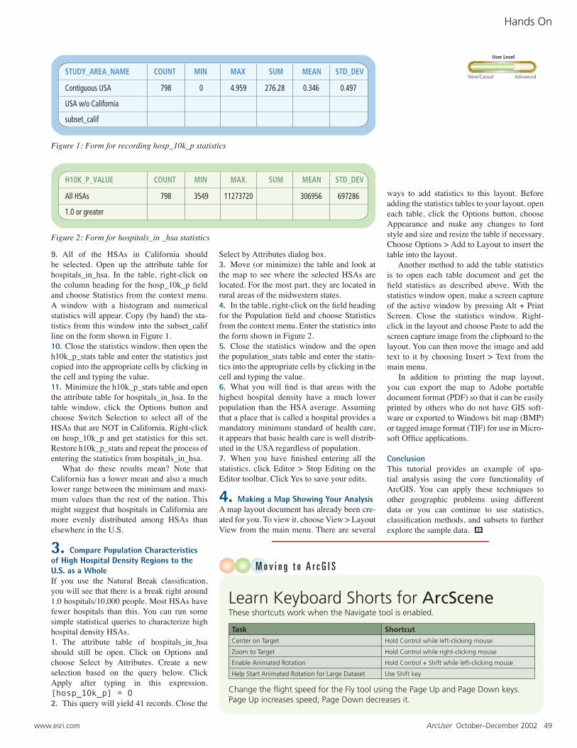
Learn Keyboard Shorts for ArcScene

Task Shortcut

Center on Target Hold Control while left-clicking mouse

Zoom to Target Hold Control while right-clicking mouse

Enable Animated Rotation Hold Control + Shift while left-clicking mouse

Help Start Animated Rotation for Large Dataset Use Shift key

Change the flight speed for the Fly tool using the Page Up and Page Down keys. Page Up increases speed; Page Down decreases it.

These shortcuts work when the Navigate tool is enabled.

New/Casual Advanced

User Level