ELSEVIER Stochastic Processes and their Applications 63 (1996) 97 116

stochastic processes and their applications

Extremes, rainflow cycles and damage functionals in continuous random processes

Igor Rychl ik I Department of Mathematical Statistics, University of Lund. Box 118, S-22100 Lund, Sweden

Received 13 July 1994; revised 19 February 1996

Abstract

We discuss some properties of damage funcfionals defined on a sequence of local extremes in continuous stochastic processes both irregular, e.g. Brownian motion, diffusions, and smooth., e.g. stationary Gaussian processes with finite intensity of local maxima. Local extremes arc represented as a point process in R 2. The main tools are rainflow cycles and oscillation measures.

Keywords." Amplitude; Brownian motion; Crossings; Diffusions; Fatigue; Local extremes: Oscil-- lation measures; Rainflow-cycle; Skorohod's equation

I. Introduction

We begin with the defini t ion of local maxima.

Def in i t ion 1. Let yt be a cont inuous funct ion y : [0, T] --~ R. A number t is called a

point o f strict local max imum, if there exists a n u m b e r 6 > 0 with ys < yt for every

s ~i [t - ,5, t + 6], s ¢ t; and a point o f local max imum, i f there exists a number 6 > 0

with Ys ~< Yt for every s C [t - 6, t + 6]. Similar definit ions apply to local minima.

It is well known that cont inuous funct ions can be very irregular and have infinite

numbers of local extremes in finite intervals; see the fol lowing theorem.

Theorem 2. For almost all samples o f a Brownian motion the set o f local max ima

is countable and dense in [0, ~ ) , and all local max ima are strict.

The proof can be found in Freedman (1983).

1Research supported in part by Office of Naval Research under Grant N00014-93-1-0841.

0304-4149/96/$15.00 @ 1996 Elsevier Science B.V. All rights reserved PIIS0304-4149(96)00062-2

98 £ Rychlik / Stochastic Processes and their Applications 63 (1996) 97-116

The last theorem shows that samples of Brownian motion are extremely irregular. By looking at a plot of the sample one can easily identify a slower "wave-like" variation. However, a typical plot uses discrete-time points and hence shows a function with finitely many extremes. The objective of this paper is to describe more stringently the "wave" properties in irregular functions and attempt to analyze what may be missed by smoothing operations.

In order to discuss these questions we need a method to identify local extremes in a continuous function and quantitatively describe their values (distributions). The method

used in this paper is to represent the local extremes of y by defining cycles (pairs of a local minimum and a local maximum) (v,u) and considering the set of cycles as a point process in d -- {(x,y): x<,y} . If the function has a continuous derivative then one can choose a cycle as a pair of a maximum and the preceding minimum. However, if y is only continuous and as highly irregular as samples of Brownian motion then a concept of "preceding minimum" cannot be defined. For that reason we use the so-called rainflow cycles, commonly employed in analysis of metal fatigue to

determine the highest and lowest points in closed hysteresis loops in the strain-stress plane, in order to pair the maxima and minima of y. The rainflow method is described in Section 2. We also introduce a damage functional, which is a sum of individual damages caused by cycles or "waves". (Damage functionals are used in oceanography and engineering, e.g. in fatigue analysis and crack growth models.)

In Section 3 we discuss some simple properties of a set of pairs of local maxima and attached (by the rainflow method) local minima. Since in an irregular function the number of extremes is often infinite, the question arises as to when a damage functional is finite and whether it is continuous for smoothing operations. These problems are addressed in Section 4, while Section 5 concerns time continuity and differentiability of a damage process.

Finally, in Section 6, we study the expectation of damage process for irregular processes such as diffusions, and regular processes with absolutely continuous sample paths. Examples are also given in which the intensity of the point process of local maxima and attached rainflow minima is computed.

2. Rainflow method

The rainflow method was introduced by Endo in the late 1960s, the first paper in English being Matsuishi and Endo (1968). His definition was a complicated recur- sive algorithm identifying the closed hysteresis loops in the strain-stress plane. Endo described the method using a model of rain flowing from a pagoda roof (which ex- plains the name). The first nonrecursive definition of the method was given in Rychlik (1987a), for smooth functions. In Rychlik (1993), this has been slightly modified to apply to continuous functions which may have infinite variation. Sheutzow (1994) has further modified the definition to apply to regular, (e.g. cadlag), functions.

Definition 3. Let Yt, 0 ~< t ~< T ~< oo, be a continuous function. Define a real function x by the following procedure:

1. Rychlik / Stochastic Processes and their Applications 63 (1996) 97 116 99

For any fixed t C [0, T] let t , t + be the following time points

s u p { s o [O, t ) ' y ,>~y t} ,

t - = 0 if ys<~yt for all s ~ [O,t),

t~ = f i n f { s c [ t , r ) " y~ > y;} ,

I T if ys < y; for all s ~ ( t ,T)

and let x T , x + be the lowest points in the intervals [ t - , t], [t, t+], respectively, i.e.

(1)

x t- = inf{ys ' t - <~s<~t}, x + = inf{y~' t<~s<~t+}, {2)

then x; is given by

~max(x t , x +) if t + < T or Y t = Y T and t < T, xt = (3)

I. x~ otherwise,

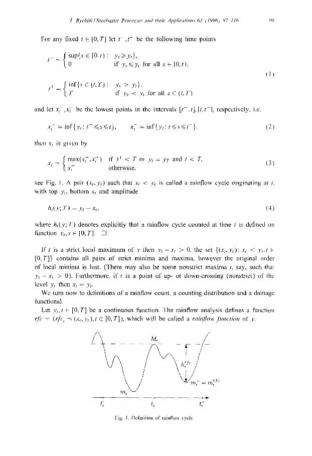
see Fig. 1. A pair (xt, Yt) such that x; < Yt is called a rainflow cycle originating at t, with top y;, bottom xt and amplitude

hi(y; T ) = Yt - x t , (4)

where hi(y; T ) denotes explicitly that a rainflow cycle counted at time t is defined on function y~,.,s c [0, T]. []

I f t is a strict local maximum of v then y; - x t > 0, the set {(xt,y~): xr < y t , t ~-

[0, T]} contains all pairs of strict minima and maxima, however the original order

of local minima is lost. (There may also be some nonstrict maxima t, say, such thai

.W - x; > 0). Furthermore, if t is a point of up- or down-crossing (nonstrict) of the

level yt then xt = Yr.

We turn now to definitions of a rainflow count, a counting distribution and a damage functional.

Let y; , t C [0, T] be a continuous function. The rainflow analysis defines a function

rfc = (; jb t = (xt, Yt), t C [0, T]), which will be called a rain[tow func t ion of y.

_ M i _ /

~/_,,_/ "ezra+ = ;<s,:

J t

Fig. 1. Definition of rainflow cycle.

100 I. Rychlik / Stochastic Processes and their Applications 63 (1996) 97-116

Lemma 4. For a continuous function Yt, t E [0, T] and T < ~ , the number of times the rainflow amplitude is at least ~ > O, i.e.

Nr(E) = #{t C [0, T]: y, -xt>~e}, (5)

is finite.

Proof. We begin with a claim: For a continuous function yt, t E [0, T] and T < cx~, the

number o f times yt >7 u and xt ~< v, v < u, is finite. This follows from the fact that for

any t~ < t2 such that xt,<~v < u<~yti,i = 1,2, inft,<~s<~t2Ys<<.v. Consequently, if there

were an infinite sequence {ti} C[0, T] such that xt, ~< v < u ~< Yt, then y is discontinuous

at the accumulation points o f the set {ti}. The lemma now follows simply from the

observation that for all t E [0, T], Yt ~< M = suP0 ~<s ~< r Ys and xt ~> m = inf0 ~s ~ Tys, and that the set

{(x ,y) : m<<.x<~y<<.M and y - x ~ > e }

can be covered by finitely many sets {(x,y) : x<~u - 6 < u + 6<~y}, for sufficiently

small & []

Denote A = {(x ,y) : x<<.y} CR 2. By Lemma 4, the se t {(xt, Yt): Yt > xt, t E [0, T]} is countable (and measurable), hence it is a point process in A. The set will be called

a rainflow count. (Measurability can be routinely checked using Definition 3.) A rainflow count can be uniquely defined using its countin9 distribution defined by

NT(V,u) = ~ l[x,,+~)(v)l(_~,y,](u)l{(x,y):x>y}(rfct), (v,u) E A. (6) tE[0,T]

It is easy to see that

I # { t E [O,T]:xt<~v < u<~yt} if v < u, (7) NT(V,U) : #{t E [0, T]: xt < u < Yt} if v = u.

In some applications one is interested in functions defined on cycles, e.g. amplitudes

in oceanography or damages in fatigue analysis. Assume that a cycle z E A, causes a

nonnegative damage d = f ( z ) . The important quantity, e.g. in fatigue analysis, is the

sum of the damages accumulated in the interval [0, T].

Definition 5. Consider a rainflow function rfct(Y), t E [0, T], and a positive function

f ( v , u) >~ O, (v, u) E A. Define a damage functional

y ~ D T ( f ) = ~ f(rfct)l{(x,y):x>y}(rfct). (8) tE[0,T]

In what follows, we shall equivalently use the notation Dr, D r ( f ) or D r ( f ;y).

In the following theorem we give an integration by parts formula, which was first given in Rychlik (1993). The formula will be used repeatedly to compute or esti-

mate Dr , given the counting distribution Nr(v, u). The theorem is proved under some assumptions on the smoothness o f the function f (v , u), specified in the following def- inition and assumed for simplicity throughout. (Although it is not necessary, we will

L Rychlik/Stochastic Processes and their Applications 63 (1996) 97 116 101

assume that f(u, u) = 0 for all u. The possible extensions of the results given in this paper to a broader class of damage functions are not discussed.)

Definition 6. Let f(v,u),(v,u) C A, be a positive real function such that, for all u, f ( u , u )= 0 (assumed for simplicity only), with the indicated derivatives:

~ f (v,u) 02 f(v,u) - f2 (v ,u ) and -- Jlz(u,u).

~?u 0vc~u

Assume that for all u E R, f2(u,u)>~O is a continuous function of u, and for all

v < u, fl2(v,u)<~O. If for all x < z

f~ fuLf12(v,u),dvdu < ~, then f will be called a damage function.

The following theorem gives an integration by parts formula to compute the total

damage Dr.

Theorem 7. For a continuous function yt, t E [0, T], let Nr(v,u) be its rainflow count- ing distribution, defined by (6). Let f (z) ,z ~ A, be a damage function, (see Definition 6). Then the total damage Dr is given by

Dr=- / ' fNT(v ,u ) f , 2 (v ,u )dvdu+~NT(U,u) f2 (u ,u )du . . . (9)

Proof. We give a simple argument for completeness. By simple calculus

f (x ,y)=-- f .~Al[X,+~)(v) l { . . . . yl(u)f,2(v,u)dvdu+~l[x,.yl(u)f2(u,u)du. (10)

Since Dr = ~ f ( r J c t ) l {(x,y)x> y}(rfc,), then using (6) and (10) and changing the inte- gration and summation operations, which is permissible since the functions j'12(t~, u), ,/'2 (u,u) have a constant sign for all v<~u, we obtain the formula (9).

The case when f~(v,u) = (u - v)~,~ > 0, is of special interest, we then refer to Dv( f ~) as ~-damage. From the last theorem it follows that

DT(JI)= ~ N r ( u ' u ) d u ' , Dr( fe):=2/ /~iNr(v 'u)dvdu"

Obviously, for ~-damage, the integration by parts formula (9) can be simplified by considering NT(h), the number of cycles with amplitude at least h, see (5), instead of NT(V, u), then

/7 D r ( f ~) = :~ U-rNr(h)dh. (I 1 )

In the following section we shall use first passage times to compute Nr(v,u) and Nr(h), for rainflow cycles. It will be seen that Nr(v,u) is easier to analyze than Nr(h)

102 I. Rychlik/Stochastic Processes and their Applications 63 (1996) 9 ~ 1 1 6

and hence the more complicated formula (9) is often more convenient to compute the c~-damage for rainflow cycles than formula (11 ).

3. R a i n f l o w count , bas i c proper t i e s

3.1. Rainflow count and oscillation measure

In the previous subsection we have defined a rainflow function (t, y) ~ rfcz(y ), then a damage functional Dr can be evaluated using formula (8). It is easy to see that for a fixed t rfct(y ) depends on ys, s E (t, T]. This is inconvenient if one wishes to study dependence of Dr on time T. In fatigue analysis this problem is resolved by splitting the set of rainflow cycle into those which are permanent, i.e. would not change if one increases T, and the rest which is called the residual or the set of half cycles.

Here we use an alternative approach using integration by parts formulas (9) or (11) to compute Dr and determine Nr(v, u) and Nr(h) dependence on T. This approach is only meaningful if one can find a way to compute Nr(v, u) and Nr(h) other than defining formulas (6), (5), respectively. The following characterization of Nr(v,u),v < u, was

given in Rychlik (1993)

Nr(v, u) = number of passages from v to u by y in [0, T], (12)

which is made precise in the following lemma. Scheutzow (1994) proves this relation- ship for regular functions.

Lemma 8. Let yt, 0 <~ t <~ T, be a continuous Junction. For a fixed level u < v define the sequence o f first passage times, see Fig. 2, To = 0 and

Sl = inf{t>j0: Yt = v}, T1 = inf{t>~Sl: Yt = u},

S 2 = i n f { t ~ T ] : y t = v } , T2 =inf{t>~S2: y t = u } , (13)

with the convention that inf{13} = +oc, then

Nr(v, u) = max{n: T, ~< T}.

The function Nr(v, u) = max{n : Tn ~ T} is" called an oscillation measure.

(14)

• . . • [

t i i i i

To = 0 $1 T1 S~ T2

Fig. 2. Illustration of the first passage times Si, ~, in Lemma 8.

I. Rvc/dik / Stochastic Processes and their Applieations 63 (1996) 97 116 103

Proof . The proof is given in Rychlik (1993).

The formulas (14) and (9) form the basis for computation of expected damage due

to rainflow cycles. In the special case of ~-damage, i.e. f ~ ( v , u ) = (u - v)~,:~ > O,

the simpler formula (11) can be used. However, we need a computationally more

convenient characteristic of NT(h), than the defining relation Nr (h ) = the number of

rainflow cycles in [0, T] with amplitude at least h. In the following subsection we give

a characterization of Nr(h) similar to (14).

3.2. Ra&flow amplitudes and Skorohod's equation

Let y~,t>~0, be a continuous function, y0 = ~'. For a fixed h > 0, a continuous

function zt, which is a solution to the Skorohod equation

zr = )'t + ~bt, (I 5)

such that zt C [v, v + h] and q~ is of bounded variation and changes values only when

zt = v or zt = v + h, is called a reflected Yt in the barriers v and v + h. From results

in Tanaka (1979) we have that for any continuous function Yt,yo = v, Eq. (15) has a

unique solution. I f yt is a path of Brownian motion starting at v then z~ is a reflected

Brownian motion in v and v + h.

Lemma 9. Let yt , t

zl be a reflected Yt

tire Jollowing sequence o f first passage times To = 0 and

>~ O, be a continuous.function, and Yo = v. For a .fixed h > O, let

in barriers v and v + h, i.e. a unique solution to Eq. (15). De[ine

S1 = 0, TI = inf{t>~S1 • zt = v + h},

s2 - - i n f { t > ~ r , ' z , = v}, T2 = inf{t >,--S2"z, = v + h}, (16)

where inf{0} +oc. Then the number o f rainflow amplitudes not smaller than h,

Nr(h) = #{t C [0, T]: ht(y; T)>~h} = max{n: Tn<~T}. (17)

Proof. The proof is given in an appendix.

3.3. Local rainflow damage and excursions

For a continuous function y and a fixed level u, define the following function

u - x ; - ifyt = u and t - < t, (18 t -+ h~(y) = 0 otherwise,

)

where t and x r are as in Definition 3. This means that, i f y.~ finishes the (downwards}

excursion from the level u at point t then u - h ~ ( y ) is the value of the global minimum

during the excursion, and otherwise h~'(y) = 0.

104 I. Rychlik / Stochastic Processes and their Applications 63 (1996) 97-116

Denote by N~(z) an excursion counting distribution, i.e.

f ~t<~vl[z,o~)(h~) if z > 0, N (z) (19) ~t~rl~0,~)(h~ ') if z = 0.

Further, let g(z)>>.O,z >~0 be an absolutely continuous nondecreasing function, then a

local damage functional is defined as follows:

u 1 u DUT(g) = ~ g(h t ) (o,~)(h t ), (20) t ~ T

and by elementary calculations, if g is differentiable, we have that

D}(g) = g'(z)Nf(z)d +

The following lemma motivates the name local damage functional.

L e n a 10. Let Yt, t E [0, T], be a continuous function and let f ( v , u) be a damage function, (see Definition 6). Then the rainflow damage D r ( f ; r f c ( y ) ) is given by

D r ( f ; r f c ( y ) ) = 2(u - ht,u)l(0,+o~)(h t )du = D~(gu) du, dR t ~ T

where gu(z) = f2(u - z, u).

Proof. Let Nr(v, u) be a rainflow counting distribution and N~(z) the excursion count- ing distribution. By Lemma 8, it is easy to see that N.~(z) = N v ( u - z , u). Consequently,

if f ( v , u) is a damage function defined as in Definition 6 and g(z) =- f2(u - z, u) then

D}du = - f 1 2 ( u - z , u ) N r ( u - z , u ) d z d u + f 2 ( u , u ) N r ( u , u ) d u = D r ,

where D r is the rainflow damage functional. []

3.4. Rainflow cycles in smoothed functions

In this subsection we shall approximate a continuous function Yt, t E [0, T], by

an absolutely continuous function fit, say, such that the oscillation measure o f y is

approximated continuously by an oscillation measure o f fit. We begin with an absolutely continuous approximation to y. The method is based

on the so called Skorohods representation (see Freedman, 1983, p. 6) used in approx-

imations o f random walks by a Brownian motion. For a fixed h > 0, let P = {yo+ih: i . . . . . - 1 , 0 , 1,2 . . . . } be a set of levels. Define

by induction a sequence o f first passage times {zj} : Let z0 = 0 and given zj, let

u = inf{z E P : z > Yrj}, V = sup{z C ~g: Z < y~},

then

Z'j+ 1 = inf{t > zj: Yt = u or Yt = v},

L RychlikIStochastic Processes and their Applications 63 (1996) 97 116 105

as before inf{(3} = +oc. Consequently, z j , j ) 1 , are the time points when Yt passes the discrete levels in ~/. Let K = sup{j: zj < T}. Then, let f~t,t E [0, T], be an approxima-

tion of y obtained by drawing straight lines between points {(%,y(%)) . . . . . (z~,y(rK),

(T, yr)}.

Lemma 11. Let Yt be a continuous function and Yt be its smooth approximation. Denote by )Vr(v,u) an oscillation measure of ~, d~fined by (14), and let Nr(v,u) be an oscillation measure of y. Then:

(a) For any u>~v,?Cr(v,u)<<.Nr(v,u) with equality when u,v E )tl. (b) The number Nr(h) of rainflow amplitudes at least h counted in y is bounded

J?om below by the number of local maxima in f:, M, say, and Nr(2h)<~M <~Nr(h). (c) For a damage function J; (see Definition 6), D r ( f ; rfe(fO) ~ Dr( f ; rib(y)) as

h~o.

Proof. Statements (a) and (b) are immediate consequences of the construction of ~,. To prove (c) we choose h = 2 -n and let n approach infinity. Then ~ converges uniformly

to y on [0, T] and for any u>~vNr(v,u) T Nr(v,u) as n ~ vc. And hence (c) follows from (9) and monotone convergence theorem.

4. Finiteness of rainflow damage

In the case of smooth functions y there are usually only finitely many local extremes in [0, T], and the rainflow damage is finite for any function f . However in many applications one uses mathematical models for elongation processes which are less regular, e.g. the second derivative may not exist, and the number of rainflow cycles is infinite, then an important question is when Dr is finite. In Lemma 4 we proved that for continuous y and any e > 0 there are only finite many rainflow cycles with amplitudes not smaller than e. Hence the finiteness of accumulated damage in y depends on negligibility of damages due to cycles with small amplitudes.

4.1. Functions with finite variation

If y has finitely many extremes then the total damage Dr is finite for any damage function. Obviously, functions of finite variation may have infinite numbers of local

+ ~ extremes in [0, T], but f '_~Nr(u ,u)du is finite by Banach's theorem, (see Freedman p. 209), and since it is assumed that f ( u ,u ) = 0, for all u, the rainflow damage is finite for all damage functions f , defined as in Definition 6.

4.2. Functions with infinite variation

For a continuous function yt, t E [0, T], let Nr(v,u) be its rainflow counting dis- tribution. Let f be a damage function (Definition 6). In order to avoid pathological cases, we assume that fz(U,U) = 0 for all u E R. (This is motivated by the proper- ties of Brownian samples, that almost all samples have the number of u-upcrossings

106 L Rychlik/Stochastic Processes and their Applications 63 (1996) 9~116

Nv(u, u) = e~, and the values of strict local minima are dense.) Under this assumption,

using the integral representation (9), the total damage is given by

M ~om-m Dr = -- fm Nr(u - h,U)fl2(U - h,u)dhdu, (21)

where M = maxtc[o,r]yt, m = mintc[o,rjyt. Hence, in order to check if the total damage

D r is finite we need to describe properties o f the damage function f ( v , u) for v close

to u more precisely, and limit the class o f functions Yt.

For simplicity consider f ( v , u) = (u - v) ~, ~ > O. Then by (11) the total damage

fo m-m D T ( f ; y ) = ~ h~-INr(h)dh,

and Nr(h) is the number o f rainflow cycles in [0, T] with amplitudes at least h, see

also Lemma 9. Obviously, the finiteness o f Dr depends on the growth rate (which will

now be estimated) o f Nr(h) as h tends to zero.

By Lemma 11, we have that Nr(2h) is bounded by a number o f local maxima in

fit, a smooth approximation of Yr. Hence, in order to bound Nr(h) we need to estimate the time it takes for y to 'travel' a distance h. This is exactly what H61der continuity

provides. More precisely, let T < cx~, and let a continuous function y be HiSlder continuous

o f order fl, i.e. there is a constant C > 0 such that

lYt - YsI <<- CI t - sl [~, for all s,t E [0, T].

Consequently, if y is H61der continuous then it takes more time than C-~/~h ~/~ to pass

between levels h apart and hence Nr(h)~< TCi/~h -1/~ proving the following lemma.

Lemma 12. Consider a damage fimction f ( v , u) = (u - v) ~. I f T < oo and y is H61der continuous o f order fl, then the a-damage D r ( f ; y ) is finite for all ct > 1~ft.

Since Brownian motion has a.s. H61der continuous samples with fl < ½, the rainflow or-damage is finite for all ~ > 2. Now we shall show that a-damage is a.s. infinite for

a ~<2. We shall prove this statement using the concept o f local time.

Recall, for a continuous function y and fixed u, a local time is defined by

L~(y) = lim~0 -el fo S l[u,u+~](yt)dt, (22)

if the limit exists. It is well-known result for Brownian samples that for a fixed

u, h N r ( u - - h , u ) --+ L~ a.s. as h .L 0, (see Revuz and Yor, 1991) and that L ° > 0, for all T and L~ is continuous in both u and T. Furthermore, the convergence hNr(u - h, u) --~ L~ is a.s. uniformly in u, as h + 0, see Theorem 2 in Chacon et al. (1981). Consequently, there exists a positive 6 such that a.s. Nr(v ,u) > C / ( u - v ) for

M M--m all v, u E [ - 3 , 3], and hence fm fm N~'(u - h, u )dh du = +cx~ proving the following theorem.

L R)'chlik / Stochastic Processes and their Applications 63 (1996) 97 116 107

Theorem 13. Let Yt, t E [0, T], be a continuous Brownian motion startin,q at zero

and f ~ ( v , u ) = ( u - v) ~, c~>~l. Then the rainflow damage Dr ( f~ ; Y) is a.s. inhnite

./or ~ <~2 and a.s. finite for o~ > 2.

5. Damage processes

Let yt, t C [0,+:xD), be a continuous function. Obviously, for any finite T > 0,

the function y restricted to [0, T/ is continuous and we can define a rainflow function

rfct(y) , t G [0, T], and the rainflow damage D v ( f ; y ) , ( D 0 = 0). In applications one

often wishes to follow the time evolution of Dr. (For example in fatigue analysis, the

failure time is defined as the first passage time of Dr to some critical level.) Hence, in

this section we shall discuss time continuity (absolute continuity) of D7-. The case when

3"~ is a continuous function was studied in Rychlik (1993). By a simple modification

of the argument we can treat a general case of continuous Yt-

Theorem 14. Let .f(v,u)~>0 be a dama qe func t ion and y a continuous Jimction. l /

Dr( , / ; y ) < vc then:

(i) Dr" is a continuous nondecreasinq./unction.

(ii) Dr is a Lipschitz continuous function, (fly is Lipschitz continuous ( f (u , u) 0 Jor all u ~ R ). Furthermore,

/o jo Dr D~dt • - l)4 dt, = = ,12(x, , Yt )(Yt (23)

u'here z- max(0,z) and x 7 is" defined as in Definition 3.

Proof. The proof is given in an appendix,

The assumption of absolute continuity of y in (ii) is necessary for validity of the:

formula (23). For example, if y is of finite variation but not absolutely continuous,

then it is well known that y can be decomposed as follows:

Yr = ZT + y~ dt,

such that = has a positive variation and z~ = 0 a.e. (Lebesgue measure). Now, if

/ '(v, u) = u - v then D r ( f ; y ) is finite, and (23) does not hold since

j, D - r ( f ; y ) = N r ( u , u ) d u > (y~)+dt.

6. Expected rainflow damage

Let Y,, t >I-0, be a random process with a.s. continuous sample paths, f a damage

function (as in Definition 6) and D T ( f ; Y) be a rainflow damage process defined in the previous section. In this section we study the expectation E/Dr/ .

108 I. Rychlik l Stochastic Processes and their Applications 63 (1996) 97-116

From (9), using Fubini's theorem, the necessary condition for finiteness of expected damage is finiteness of measure

+ o c

nr(v, u) = E[NT(v, u)] = ~ P(T,, <<. T), (24) n = l

where the oscillation measure Nr and first passage times Tn are defined in Lemma 8. Then the expected damage is given by

E [ D T ] = - / ~ v " unr(v ,u) f l2(V,u)dvdu+fRnT(u,u) f2(u ,u)du. (25)

In the following subsection we show that the expected a-damage for Brownian mo- tion is infinite. Next, we discuss the case of stationary diffusions and finally consider the important practical case of processes with absolutely continuous sample paths.

6.1. Brownian motion

Let Yt be a continuous Brownian motion starting at zero. Consider a damage function f~(v, u) = (u - v) ~, a ~> 1. As we have proved before the a-damage Dr(f~; Y) is finite only if a > 2. We turn now to the computation of expected a-damage and begin with

the function nr(v, u) defined by (24). Denote by Sa the first passage time of the level a by Y~, i.e. Sa = inf{t ~> 0: Yt = a}.

It is well known that

P(Sa<~S)=2P(Ys>~[al) and f so* f& = fso+b,a > O,b > O,

where ' , ' denotes convolution of the densities; see Revuz and Yor (1991). Using the strong Markov property of Brownian motion and Lemma 8, it follows by straightfor- ward calculations that

n T ( ~ , u ) - ~ ~ 2 k ( u - ~ )P[I~[ + 2 ( k - 1 ) ( u - ~) U - - V k = 1

TV%r(V, u) rT < fvr + 2 k ( u - v ) ] -

Z l - - I )

Now, the constant cr(v, u) can be bounded as follows:

/,7 /,7 (x - Iv[)fY~(x) dx <. r~/%r(v, u) ~< (x - Ivl + 2 (u - v))fy~(x) dx, I I -2( . -~)

and, consequently,

E[(X - T-1/2[v[) +] <~cr(u, v) <~E[(X - T-'/2(lvl - 2(u - v)))+],

where X is a standard Gaussian variable and x + = max(0,x). Finally using (25), it follows that the expected a-damage for a > 2 is infinite since

E[DT] = T1/2a(a - 1) L (u - v)~-3crT(v,u)dvdu

> T1/Zo:(a - 1) E [ ( X - T-'/zlv])+] (u - v) =-3 dudv = +oo 0<3

by Fubini's theorem for positive functions.

L Rychlik/Stochastic Processes and their Applications 63 (1996) 97-116 1 0 9

6.2. Diffusion processes

Let lit, t>~0, be a regular diffusion process on R with diffusion coefficient a(z) > 0

and drift coefficient b(z). (The sample paths of Y are a.s. continuous and have infinite

variation.) For arbitrary x0 define

S(x) = exp - a ~ d Z dy, ) 320

the so-called scale function. We assume that 2b(z) /a(z) is locally integrable and that

S(-~x~) -- - r e , S ( + o o ) = + o e and S(x) is finite, for all x E R, i.e. all points are

accessible by Yt except - o ~ and +oc . Then

1 re(x)- a(x)S'(x)'

where S' (x) = e x p { - f ~ 2b(z)dz}, is the density o f speed measure. We assume that

M = f+_~ m ( x ) d x < oe, and then the density of the stationary distribution of Y is given by

f ( x ) = M-Ira (x ) .

If the density of Y0 is f ( x ) then Y is strictly stationary, which we assume.

We now turn to the measure nr(v ,u) defined by (24). For a fixed levels v < u,

let Tg be the first passage times defined in Lemma 8, and the oscillation measure

NT(V,u) = max{n : T n ~ T }. The variables {7',. - Ti- i} , i>~2, are i.i.d, with finite expectation

E[T~ - Ti-l] = 2M(S(u ) - S(v)) ,

where M = f + ~ m ( x ) d x < oo. Note that for Brownian motion E[Ti - Ti-1 } = ~c since

2h _(2h)2/2t t > O~ f T2--T,(t) = ~ -

h = u - v. Although the diffusion process Yt is strictly stationary, T1 and T2 - Tj have different distributions. (This is a technical complication caused by the fact that

rainflow function begins at a fixed time point (zero).) Since T1, T2 - T1, T3 - T2 are

independent variables then, by the elementary renewal theorem,

lim N t ( v , u ) lim E[Nr(v ,u)] __ 1 = n ( v , u ) , (26) r-+~ T r--+~ T 2M(S (u ) - S(v) )

say. We shall call n(v,u) the oscillation intensity.

Now, it is easy to see that

(T . n(v, u) - 1)+ <~nr(V, u) (= E[NT(v, u)]) <~ T . n(v, u),

where x + = max(0,x). Consequently, we define a stationary damage intensity by

d ( f ; Y ) = - / ~ n (v ,u ) f l2 (V ,u )dvdu . (27)

110 L Rychlik l Stochastic Processes and their Applications 63 (1996) 97-116

Consider a damage function f~(v,u) = ( u - v) ~. Then the stationary intensity of a-damage is given by

d~(Y) -- -2~-1 S(u) - S(u - h) dh du. (28)

Since the derivative S~(x) is continuous and there is a closed interval where S~(x) > O, it follows that d~(Y) = cx~ for ~ 2 . Whether d~(Y) is finite for a > 2 depends on the rate of convergence of S(x) to - o e as x tends to - e c .

6.3. Example." Ornstein-Uhlenbeck process

Let Yt be a zero mean stationary Gaussian process with covariance function r(t) = E[YoYt] = a2(2v)-iexp{-v[t[}. The process Y is a stationary diffusion with diffusion coefficient a(x) = a2 and drift coefficient b(x) = -7x. The scale function is given

by S(x) = fo exp{(?/a2)z2} dz and S'(x) = exp{-(7/a2)x2}. Since S'(x) is given in an explicit form, by elementary computations, it may be checked that, the intensity of a-damage d~(Y) is finite for ~ > 2.

A stationary intensity #(v,u), say, of the point process of maxima and rainflow minima rfc(Y) is obtained from (26);

kt(v, u) _ 02n(v,u) _ S'(u)S'(v) = ax/~exp{(~/ff2)(u2 + re)} (29)

?v~3u M(S(u) - S(v)) 3 v/-x( fv u exp{(7/cr2) z 2 } dz) 3'

since M = a - l v / ~ . In Fig. 3 we present the intensity #(v,u) with simulated sample of the point process of maxima and rainflow minima rfc(Y). (In the simulation we used Yt+~ = Ytexp{-v[6]} ÷ X . cr[(1 - exp{-27161})/(27)] m, 6 = 0.002, where X is a standard Gaussian variable independent of Ys, s ~< t.)

6.4. Random processes with absolutely continuous sample paths

Let Yt be a random process with a.s. absolutely continuous sample paths. Then, by Theorem 14, the rainflow damage process is given by

T / ,

D r ( f ; Y) = / 0 (Y/)+ + f2(Xt- ' Yt)dt,

where Xt- is defined by formula (2), viz.

sup{s E [0, t): Ys > r,}, X t - = inf{Ys : t-<~s<<.t}, t - = (30)

0 if Ys<~Yt for all s E [0, t).

For simplicity we shall assume that Y is a strictly stationary and ergodic process. Simi- larly, to the previous subsection, the assumption that one starts to count rainflow cycles at time zero causes some technical complications which are manifested in the nonsta- tionarity of the process Xt-. This can be resolved by considering the process Yt, t E R, defining rainflow function rfct for t>~S and letting S go to -cx~. Then the derivative of

I. Rychlik l Stochastic Processes and their Applications 63 (1996) 97-116 111

2 ~ s°°°

-33 -2 -1 0 1 2 trough (v)

Fig. 3. Simulated rainflow count rfc(Y) (dots), where Yt, O~<t~<200, is an Ornstein-Uhlenbeck pro- cess with parameters 7 = 0.5, cr = 1; and level curves of the intensity 2 0 0 . ~t(v,u) defined by (30).

the damage process at time t goes to

D~(f; Y) = (Y~')+fz(2t, Yt),

^ _

where X t is defined by

2~--- inf{Ys: t-<~s<<.t}, t - = s u p { s E ( - o o , t)" Ys > Yt}, (3])

where sup{0} = -oo. (It is easy to see that ~-t, defined by (31) is stationary.) Now, we can define a stationary expected damage intensity by

d ( f ; Y) = E[( Y~)+ f2(2o, Yo)]. (32)

Computation of d(f ; Y) is an important problem in fatigue life prediction under

random loading. However, the distribution of ) ( t is hard to compute exactly and, hence, approximation methods are often used; see e.g. Rychlik (1988). We just briefly mention this problem here and remark that in some cases it is more convenient to work with the intensity of local damage du(f; Y), say, where obviously the damage intensity d(f ; Y) = f + ~ d u ( f ; Y)du. We begin with an alternative means for computing the expected damage using Eqs. (24) and (25).

Assume that Yt is a stationary Gaussian process with absolutely continuous paths. Then, using methods presented in Rychlik (1987b), one can prove that

nr(v,u) = E[(Y/)+I(_~,~](XZ)IYt = u] ./y,(u)dt (33)

112 1. Rychlik l Stochastic Processes and their Applications 63 (1996) 97-116

where X s- is a nonstationary nonGaussian process defined by (30). However, since Yt

is ergodic we have that

lim N r ( v , u ) _ lim n r ( v , u ) T---*~ T T----~ T

= E[(Yd) + l(-~,v]O(o )lY0 = u]fYo(U) = n(v, u), (34)

say. For a fixed u , n ( v , u ) is an intensity distribution of the global minimum of an excursion from u and for v = u,

n(u, u) = E[(Y~)+IYo = u]fro(U),

which is Rice's formula for the intensity of upcrossings of level u by Yr. Hence (34) is an extension of Rice's formula to the intensity of excursions from the level u with the global minimum smaller than v (see Leadbetter et al., 1983).

By Lemma 10, the intensity of local damage is simply given by

d u ( Y , f ) = - f l2(U - h ,u )n (u - h , u ) d h + f z ( u , u ) n ( u , u ) , (35)

which by (34) and Fubini's theorem shows that

f_ " ~ d . ( f ; Y ) d u = E[(Yd)+ f2(~?o, Yo)] = d ( f ; Y) . O G

While the formula (32) for damage intensity holds for any Yt with a.s. absolutely continuous paths the formula (35) for the local damage intensity can be proved for a smaller class of processes. The class is still large and contains Gaussian processes, functions of vector valued Gaussian processes and even some non-Gaussian (a-stable) processes. See Michna and Rychlik (1995) for more detailed discussion.

Finally, using the intensity n(v, u) we can define an intensity of maxima and rainflow minima

~2n(v, u) #(v,u) -- Ov ~u ' (36)

which has to be computed numerically.

6.5. Example : Orns te in -Uhlenbeck process (cont inued)

A stationary Ornstein-Uhlenbeck diffusion is a Gaussian process with spectral density

o-2 S(2) - (2~2)2 + ~2'

Obviously, the second spectral moment is infinite ( f (2n2)2S(2)d2 = cx~) since the derivative Y/ does not exist. However, in practice one usually cuts off the high fre- quencies and defines an approximating stationary Gaussian process Y~PP, which has mean zero and the truncated spectrum sapp(/~) = S(~.) if 121 ~<20 and 0 otherwise.

I. Rychlik / Stochastic Processes and their Applications 63 (1996) 97 116 113

, ,

2

• ~ oe • •

1 " • "

e °

0 ," ~_~ Level curves at:

-1 i0 ° - 2

_ a ~ P " -3 -2 -1 0 1 2

trough (v)

Fig. 4. Simulated rainflow count rfc(Y app) (dots), where yapp, 0 ~< t ~< 200, is a zero-mean Gaussian process

with truncated Ornstein-Uhlenbeck spectrum sapp(2), "~ = 0.5, o- - 1, 20 - rt; and level curves of the

approximation of the intensity of maxima and rainflow minima 200 . #(v, u).

The process Yt app has a.s. analytical sample paths and the intensity of local extremes is finite. I f the frequency 2o is high the p r o c e s s Yt app is a smoothed approximation of an Ornstein-Uhlenbeck process Yt and the oscillation intensity n(v,u) should be similar

for both processes. The intensity n(v,u) for the p r o c e s s Y t a p p is given by (34) but the conditional expectation in (34) cannot be computed explicitly. However, accurate numerical approximations, based on Slepian models and regression approximations (see Lindgren and Rychlik, 1991; and Rychlik and Lindgren, 1993) do exist. Here we use this method to compute n(v,u) for Yt app, see Fig. 4. The cutoff frequency is 20 = re. It is apparent that the intensities #(v,u) given in Figs. 3 and 4 are very similar when (v,u) is away from the diagonal u = v. IB

A p p e n d i x A . P r o o f o f L e m m a 9

Consider a continuous function Yt, t~O, Yo = v. For a fixed h > 0 define a sequence of functions {z],qS~}, n>~O; z ° is reflected Yt in v, i.e.,

zt ° = Y t + q 5°, qbt ° = sup ( V - y s ) ; O<~s<~t

z] is reflected z ° in v + h, i.e.,

1 = z? + ~, ~ = -( sup (z °) - (~ + h)) +, Z t O<~s<~t

114 /. Rychlik / Stochastic Processes and their Applications 63 (1996) 97-116

where x + = max(0,x); zt 2 is reflected zt ~ in v, etc. Now, consider the following sequence

o f first passage times, To = 0 and

S1 = O,

S 2 = i n f { t ~ > T l : z] = v } ,

Sk = inf{t~>Tk-l : zt 2k-3 = v},

7'1 = i n f { t ~ > S l : z ° - - - v + h } ,

/'2 = inf{t~>S2: zt 2 = v + h } ,

2k--2 T k = i n f { t > ~ S k : zt = v + h } ,

(37)

where inf{~} = +cxz. The sequence {Sk, Tk} can be written in an alternative way;

SI = 0,

$2 = inf{t/>T1 : maxr~s<<.t(ys) - yt = h},

7'1 = inf{ t />Sl :

Yt - mins~ ~s<~t(Ys ) = h},

/'2 = inf{t~>S2: Yt

-mins2 <~s<~t(Ys) = h},

(38)

Since yt is a continuous function, the sequence Tk converges to +cx~. Hence, for any

t~>0 there is a k ~>0 such that Tk ~>t and z~ = zt 2k-2, (a~ = (at 2k-2, for all n ~>2k -

2. Consequently, for any t~>0, we can define functions zt = limn~oo z~' and (at =

limn~o~ (a~'. Obviously, zt is continuous, zt = Yt + (at and zt C [v, v + h]. Furthermore, (at increases only if zt -- v and decreases only if zt = v + h. Since (a is of bounded variation, zt is an unique solution to Skorohod equation (15) and the sequence o f

stopping times {Sk, Tk} defined by (37) and (38) are identical to the sequence defined by (16). Finally, from (38) and the definition o f a rainflow amplitude it easily follows

that NT(h ) = max{n: Tn ~< T), which concludes the proof• []

Appendix B. Proof of Theorem 14

Proof of (i): For any 0~<tl < t2<~T < c~ fixed, let v = inftt<~t<~t2Yt, u =

suPt~<~t<~tzy t and to = inf{s E [ t l , t s]: y~ = u) . Assume v < u, since otherwise Dt2 = Dt~ and D is continuous at tl. We turn now to the estimation o f Dr2 - D r , .

The difficulty in analyzing the increment Dr2 - D t ~ lies in the fact that xt, (from Definition 3), depends on T, (in the c a s e Dt~ we have T = tl while for Dr2 it increases

to T = t2 and some xt can change the value). First consider 'new' cycles, i.e. T = t2

in Definition 3, {(xt , Y t ) : t C [tl,t2],Xt < Yt) . Note that only a cycle at to can be large all others are small cycles between (v, u) and by continuity o f Yt and negligibility of small cycles their damages tends to zero as t2 - tl ~ 0.

Now, we need to bound the damage of a cycle (xt0, Yto) and the changes of damages for cycles at t ~< tl which have been affected by the increase o f T = tl to T = t2. From Definition 3 it is not hard to see that only the cycles at finite many points si, defined below, have to be considered.

I. Rychlik / Stochastic Processes and their Applications 63 (1996) 97--116 115

Let Sl = tl, given Sn let

S , + l = s u p { t E [ 0 , s ~ : y~, < Yt < Y~0 andxt <Xs,}.

By the continuity of y there are only finite many say N, of such points. While com- puting Dr, the sum of damages at si is

D1 = .f(x~.~, YsN ) + " " + f(Xs~, Ys, )

and in the damage Dr: the sum of damages at si and at to is

D2 = f(X~x_~, YS.,~ ) + ' ' " + f(Xs,, y,: ) + f (v , YS, ) + f ( x , , , U).

Here the values ofx~, are the same as in the first sum. Since for a fixed v, f2(v,u)>~O,

N

D2 - Ol <~f(v,u) + Y"~(f(Xs~,U) -- f(&~,v))<~C(N + 1)(t2 - h), (39) l

by assumed continuity of f which proves (i). (That Ds is nondecreasing follows from formulas (9) and (14).)

The following lemma is needed in the proof of (ii):

Lemma 15. Let Yt, 0 < ~x~, be a continuous Jbnction with finite variation and let Ny(v, u) be its rainflow counting distribution. Consider a damage function f (x ) , (see Definition 6). Then the damage due to rainflow cycles with amplitudes smaller than

is bounded by

f(rfct(y))l(° 'd(ht(y))<~ fRR J)(U -- tE[0,T]

e,u)Nr(u,u)du<~ Ce ~ Nr(u,u)du.

(40)

Furthermore, the damage accumulated in all rainflow cycles which are inside an interval Iv, u], v < u, is bounded by

f u

f(rfct(Y))l<,~(rfct(y))<~f2(v,u ) Nv(z)dz, (41) tE[0,T]

where E~u = {(x,z): v~<x < z<~u}.

Proof. We begin with inequality (41). Let N~ u be a counting distribution of a rainflow count restricted to Evu. Obviously, N~ u is zero outside the set Evu and N~. u (x, z) ~< Nr (x, x), for all (x,z) E Evu. Now the inequality follows directly from (9).

The first inequality in (40) is proved in a similar way, and the second follows from the fact that Nr(v,u) is zero outside a compact set. []

Proof of (ii): Since y is Lipschitz (finite variation) and f (u , u) = 0, small cycles are negligible. We shall prove that there is a constant C, such that for any 0 ~< t~ < t2 ~< T fixed, Dr2 -Dt~ < C ( t 2 - tl). By (40) the damage due to small cycles in [h,t2] is bounded by C(t2 - t l ) f N r ( u , u ) d u , where C does not depend on points tl,t2. This proves Lipschitz continuity of Ds, since, in (39), N + 1 <.f~Nr(z ,z )dz . Obviously,

116 L Rychlik/Stochastic Processes and their Applications 63 (1996) 97-116

a Lipschitz continuous function is absolutely continuous and hence Ds is absolutely continuous.

Now, since Yt is Lipschitz continuous it is also absolutely continuous and hence in order to prove (23) we need only to show that D~ = f2(xT,yt)(y[) + at points where D[ and y~ exist. I f y~ < 0 then y is strictly decreasing in some neighborhood of t and

hence D~ = 0. Now, consider a point t where the derivative D[ exists and y[/> 0. Let t - < t be as in Definition 3 ( i f t - = t then D~ = y~ = 0). Introduce

u = sup{ys: s E ( t - , t ) andx~ < Ys},

to = sup{s: s E ( t - , t ) and u = y ~ } .

The following can occur; (i) D~ exists and u < Yt, then D[ is equal to its left derivative,

which is given by f2(xt,Yt)y[; (ii) O~ exists, u = Yt and x7 = inf{ys: s E (t0,t)}, then left hand derivative again equal to f2(x t , Yt)Y[; (iii) u - - Yt and xt- < inf{ys : s E (to, t)} then the left and right derivatives of Dt have different values. This proves (ii). E3

Acknowledgements

To Professors M.R. Leadbetter and P. McGill for valuable discussions at the Center for Stochastic Processes, at Chapel Hill, NC.

References

R.V. Chacon, Y. Le Jan, E. Perkins and S.J. Taylor, Generalised arc length for Brownian motion and Lfvy processes, Z. Wahrscheinlichkeitstheorie verw., Gebiete 57 (1981) 197-211.

D. Freedman, Brownian Motion and Diffusion (Springer, Berlin, 1983). M.R. Leadbetter, G. Lindgren and H. Rootzfn, Extremes and Related Properties of Random Sequences and

Processes (Springer, Berlin, 1983). G. Lindgren and I. Rychlik, Slepian models and regression approximations in crossing and extreme value

theory, Int. Statist. Rev. 59 (1991) 195-225. M. Matsuishi and T. Endo, Fatigue of metals subject to varying stress, in: Proc. Kyushu Branch of Japan

Society of Mechanical Engineers, Fukuoka (1968) 37-40. Z. Michna and I. Rychlik, The expected number of level crossings for certain symmetric ~t-stable processes,

Commun. Statist. Stochastic Models 11 (1995) 1-19. D. Revuz and M. Yor, Continuous Martingales and Brownian Motion (Springer, Berlin 1991). I. Rychlik, A new definition of the rainflow cycle counting method, Int. J. Fatigue 9 (1987a) 119-121. I. Rychlik, A note on Durbin's formula for the first passage density, Statist. Prob. Letters 5 (1987b) 425-428. I. Rychlik, Rainflow cycle distribution for ergodic load processes, SIAM J. Appl. Math. 48 (1988) 662-679. I. Rychlik, Note on cycle counts in irregular loads, Fatigue Fract. Engng Mater. Struct. 16 (1993) 377-390. I. Rychlik and G. Lindgren, CROSSREG - a technique for first passage and wave density analysis, Probab.

Eng. Inform. Sci. 7 (1993) 125-148. M. Scheutzow, A low of large numbers for upcrossing measures, Stochastic Processes Appl. 53 (1994)

285-305. H. Tanaka, Stochastic differential equations with reflecting boundary conditions in convex regions, Hiroshima

Math. J. 9 (1979) 163-177.