Embed Size (px)
Citation preview

M.Sc. thesis in Business Administration (Finance and International Business) Århus, December 2009
Family ownership and firm performance Empirical evidence from Denmark
Author: Adiba Kholmurodova Advisor: Jan Bartholdy

Abstract: Families are large shareholders in many countries. Most studies recently have found that family
firms perform better or at least as well as non-family firms. These findings raise the question of
whether the type of a blockholder matters in terms of firm performance. In our analysis we
address this question using a detailed panel dataset of 245 Danish firms using accounting based
performance measures. We find family firms to be younger, smaller and operating in slightly
different industries. Out of total family firms 80% are actively involved in the management and
an unrelated blockholders are present only in 30% of family firms. We do not find strong
evidence of significant negative or positive impact of family firms on accounting measures,
except few cases of significant impact. We conclude that family ownership might not per se be a
cause of positive or negative impact on firm performance, but rather other family firm related
characteristics (e.g. involvement in management) may explain differential performance.
Key words: family ownership, family management, agency theory, firm performance

Table of Contents Introduction………………………………………………………………………………………………...1
1.1 Research questions……………………………………………………………………………………2
1.2 Methodology………………………………………………………………………………………….3
1.3 Data………………………………………………………………………...........................................4
1.4 Limitations……………………………………………………………………………………………4
Chapter 1……………………………………………………………………………………………………5
1.1 Corporate governance………………………………………………………………………………...5
1.2 Agency theory……………………………………………………………………………...................6
1.3 Corporate ownership...........................................................................................................................10
Chapter 2…………………………………………………………………………………………………..15
2.1 Literature review…………………………………………………………………….………………15
2.2 Ownership across the world………………………………………………………………………....22
2.3 Control enhancing mechanisms…………………………………………………………..................26
Chapter 3…………………………………………………………………………………………………..28
3.1 Family ownership and performance (empirical findings)…………………………………………..28
3.2 Family ownership and CEO successions…………………………………………………................32
Chapter 4…………………………………………………………………………………………………..37
4.1 Hypothesis generation……………………………………………………………………….............37
Chapter 5………………………………………………………………………………………………..…40
5.1 Sample……………………………………………………………………………………….............40
5.2 Measuring family ownership………………………………………………………………………..41
5.3 Summary statistics………………………………………………………………………… ………47
5.4 Multivariate analysis…………………………………………………………………………….…..52
Conclusion………………………………………………………...............................................................62 Appendices

M.Sc. thesis 2009 Family ownership and firm performance ______________________________________________________________________________
1 Introduction
Families are large shareholders in many countries. Well known Danish companies such as
Mærsk, Lego, Bang and Olufsen, Danfoss, Grundfoss still have the founding families as the
largest shareholders or the founding families are either present at the board or/and at the
executive level.
Increased interest in the family ownership and its impact on performance appears to have been
motivated after studies by La Porta et al (1999) found that family ownership is as prevalent as
the diffused ownership type at the public firms both in countries with well developed and less
developed capital markets, which is in contrast to the notion of dispersed ownership of public
firms, first suggested by Berle & Means (1932). A couple of studies based on US data (Anderson
and Reeb, 2003, S&P 500; Villalonga and Amit, 2006, Fortune 500; Miller et al, 2007, Fortune
1000) found family firms with superior performance in the US, contrary to the assumptions of
negative impact of family ownership and participation in the management on value creation by
firms and their performance.
‘Whether family firms are more or less valuable than non family firms remains an open
question.’ (Villalonga & Amit, 2006).
From the theoretical perspective there are a number of propositions that discuss the potential
hazards and benefits of family ownership (Jensen & Meckling, 1976; Fama & Jensen, 1983;
Demsetz & Lehn 1985; Shleifer & Vishny, 1986). However, the empirical evidence in the field is
still lacking and often contradicting. National corporate governance characteristics differ across
countries, which might be one of the reasons for contradicting results (e.g. minority shareholders
are well protected in some countries and less in the others1). Difficulty in comparing the results
across the studies could be explained by non existence of a single definition of family firm.
Researchers take each a slightly different approach to defining the family ownership. 1 For example, family firms contribute to performance when minority shareholders are well protected, and vice versa otherwise

M.Sc. thesis 2009 Family ownership and firm performance ________________________________________________________________________
Our interest in the subject starts with the broader question of whether the identity of the the
owner matters for the firm performance. We are interested in what established theories (agency
theory, stewardship theory, signaling, entrenchment and expropriation etc) suggest and test them
in a sample of companies from Denmark. As far as we are aware, there are few studies on family
ownership using the Danish data set (Bennedson et al, 2007).
Foundations are prevalent large shareholders in public companies, as well as families in
Denmark. While CEO duality is not allowed at the boards, minority shareholders have a very
small chance of being elected to the board. Denmark as a country scores low according to
different corporate governance system efficiency indices (e.g. La Porta et al, 1999). Denmark is
also known as one of the few Scandinavian countries where dual class shares are common
practice for the majority of listed companies in the industrial production, service and trade,
which makes the market for corporate control less competitive than in other countries.
We think it would be interesting to investigate family ownership in Denmark under such
conditions.
1.1 Research questions
• Does ownership structure matter? What kinds of ownership structures are spread around
the world?
• What causes different ownership structures across firms? What internal and external
factors (e.g. institutional characteristics such as minority shareholder protection, origins
of legal system, development of equity markets) influence different ownership structures?
• What impact identity of owners has on firm performance (e.g. family firms, institutional
owners, corporate ownership, and state?)
• Families as owners: expected benefits and drawbacks
• What firm characteristics are common for family firms (based on empirical findings)?
• What is relationship link between ownership type and firm performance
- 2 -

M.Sc. thesis 2009 Family ownership and firm performance ________________________________________________________________________
Empirical study:
• What Danish evidence has to say about the family firms and their performance?
1.2 Methodology
We are going to conduct panel data set regression, based on 10 year performance observations
for a universe of Danish firms. Panel data sets are good to exploit the dynamics that are difficult
to detect with cross-sectional data. Our initial intended sample was 250 Danish joint stock
companies2 (both listed companies at the Copenhagen Stock Exchange (CSE) and unlisted
firms). However due to the small size of CSE and the length of observation period left us with
larger proportion of unlisted companies in the sample. Performance (dependent) variables are
going to be accounting based such as ROE, ROA, EBIDTA.3 Control variables are going to
include firm specific characteristics such as size, industry, firm age and so on.
Tobin’s q is often used as a proxy for firm performance in corporate governance research.
It is a good measure of how a firm employs it’s given assets to make profits. A high q value for a
firm is a sign of strong competitive advantage and the presence of growth opportunities. Rose
(2006) and Himmelberg (1999) are critical about the de-nominator in the q ratio as an
appropriate measure of firms’ replacement costs (e.g. if firms had a large share of their assets in
the form of intangible assets, then the Tobin’s q would be overstated).
Moreover, there is a critic of simple OLS regressions in similar studies that assumes that firm
performance is the only endogenous variable, i.e. ownership by a family in our case, influences
firm performance (Rose, 2006). However, as the relevant literature points out the causation can 2 In Danish ’aktieselskab’ 3Tobin’s q is defined as the sum of equity market value and liability book value divided by the sum of equity book value plus the liability book value. Hence, if q is greater than 1, then the market values the company higher than accounted 3 Financial ratios provided for the firms in both databases and print sources are according to the recommendations of Danish Association of Financial Analysts (DAF). The EBIDTA is calculated by dividing the earnings (before tax and interests, as well as amortization) (‘primært resultat’ in Danish) divided by sales.
- 3 -
M.Sc. thesis 2009 Family ownership and firm performance ________________________________________________________________________
go in the opposite direction, which is that firm performance might cause families to hold to their
ownership stakes. To avoid biased OLS parameter estimates, Rose (2006) suggests constructing
a simultaneous equation system where the equations are estimated using instrumental variables.
Himmelberg, Hubbard and Palia (1999) argue that insufficient instruments make it difficult to
establish a robust relation between ownership and performance.
1.3. Data
Our data is based on a sample of both listed (public) and unlisted joint stock Danish companies.
Our data set came from following sources:
‘Navne & Numre’ – is an electronic database of all Danish companies with ownership and
financial information for the latest five years. ‘GreensOnline’4 – is a web based database that
includes Danish companies with ownership and financial information for the last five years. To
be included in the Greens a firm should have more than 45 employees or over DKK 50 million in
sales or DKK 35 million in gross revenues. Additionally the database has background
information on leading people in the corporate world. The database also provided historical
overview over the ownership, management and board composition of the firm. ‘Greens 2004’
and ‘Greens 2006’ – encyclopedic print editions were used for the financial data in the early five
year period (1998-2004).
1.4 Limitations
The biggest limitation of this thesis is the sample size for the empirical results. Due to the limited
amount of time we have to conduct the research and limited access to the information, we
recognize that a different and more extensive sample could be desired for this kind of testing.
The thesis opts for a variety of interesting aspects to be studied, but due to the obvious limits on
the scope and extent of it, we have restricted the study to the research questions discussed in
section 1.1. 4 http://www.greens.dk/
- 4 -

M.Sc. thesis 2009 Family ownership and firm performance ________________________________________________________________________
Chapter 1 1.1 Corporate Governance This section is devoted to the theory of corporate governance in which we will provide an
overview of it and account for its central problem explained by the agency theory.
An actual definition of corporate governance lacks consensus. Thomsen (2008), points out what
corporate governance is and what it deals with and claims that it is going to differ based on
interests and views of firm stakeholders such as shareholders, employees, banks, NGOs, state
etc. From the discipline of finance, his definition seems to suit best. ‘Corporate governance
deals with control and direction of companies by ownership, boards, incentives, company law
and other mechanisms.5
As managers care about what boards do to control them, investors care about how their rights are
protected and how much value the companies they have invested in, are creating, while at the
other end, politicians, the media, and non profit organizations care about how companies are
contributing to the society or how are they harming the environment to name a few (in general
corporate social responsibility, business ethics etc).
Corporate governance differs among countries originating from differences in the legal systems,
how well the financial markets are developed, country history, cultural differences etc.
Corporate governance is an eye watch over the managers. The board as a central remote control
decides the hiring and firing of senior managers. Corporate governance is an enabling
mechanism to check on firms. Good management is important for good performance. And good
performance is beneficial for all stakeholders and for the whole economy.
5 S. Thomsen, ’Introduction to Corporate Governance’, 2008, p. 15
- 5 -

M.Sc. thesis 2009 Family ownership and firm performance ________________________________________________________________________
As discussed in the relevant literature there is not one shoe that fits all solutions to the
governance of all firms. The right solution might differ from firm to firm, industry to industry,
and country to country.
The main task of corporate governance is to ensure good management through employing the
right managers, properly motivating them through different reward systems and giving them
enough freedom to act, and combining such a system with checks that prevent the abuse of
power. Thus, we can conclude that good governance is essential for good economic performance
both at micro and macro level.
1.2 The Agency theory At the heart of the corporate governance is the agency problem (i.e. the agency theory). The
agency theory was first explained by Berly and Means (1932), in their work titled ‘separation of
ownership and control’. Thomsen (2008) argues that it would be less misleading to term it as
separation of ownership and management. The basic idea is that owners (principals) hire the
managers (agents) to manage their wealth or assets on their behalf for a certain promised
compensation (e.g. salary). This relationship gives raise to a problem since both parties have
their own self-interests involved; the agents might not always act on the best interests of the
principal.
Corporate governance thus provides mechanisms that help to eliminate the agency problem. For
example, laws6 and regulations can play a role to ensure that agents act as expected and hold
them responsible for their actions (inactions). Thus, laws are the most fundamental governance
mechanisms. However, there are informal tools such as trust and reputation.
Other mechanisms could be the presence of large owners or owners who are at the same time
managers. Such group of investors are more interested in monitoring management based on the
6 In the US there is fiduciary loyalty.
- 6 -

M.Sc. thesis 2009 Family ownership and firm performance ________________________________________________________________________
large amount of wealth that they have invested or based on emotional bonds with a firm in case
of a family firm.
Managers can be motivated to perform well due to incentives (e.g. bonuses or stock options) or
else they can feel threatened by being fired and ruing their reputations.
Agency theory, a main approach to corporate governance, is thus concerned with finding
solutions to the agency problem when both the owners and managers are rational and seek their
self interest. Economic theories of corporate governance include agency theory, transaction cost,
and incomplete contract theory. Sociologists and psychologists argue against the ‘rational
behavior’ of individuals, claiming that people do not always act rationally and on their best self-
interest.
In the real world there are often more than just two actors (principal and agent). A board elected
by shareholders is a sort of intermediary between the owners and managers; however, not all the
firms have boards. It is often a legal requirement to have a board for large firms. The
shareholders can be individuals, founders or members of founding family, institutional investors,
mutual funds or hedge funds. As the interests and stakes of the owners differ, so does their
involvement in a firm. Some of the owners are actively involved in monitoring the management,
while others might just enjoy the ‘free ride’.
Other stakeholders also play an important role to directly or indirectly influence a firm’s
corporate governance (e.g. banks, employees, suppliers, customers, governments, media, and
NGOs). Auditors, analysts, and stock exchanges play a special role by providing information to
shareholders7 and other stakeholders.
7 We use the terms shareholders and stockholders interchangeably
- 7 -

M.Sc. thesis 2009 Family ownership and firm performance ________________________________________________________________________
Types of agency problems:
1) Owner-manager problems: arises between shareholders and managers. Agents
do not always act in the best interests of the shareholders.
2) Agency problems between majority and minority investors: occurs if there
are conflicts of interest between two groups. For example a founding family in
control of the firm may have different views from those of the minority investors.
The family in charge acts on behalf of the other investors, so in this case the
family is the agent, while minority shareholders are the principals.
3) Agency problems between shareholders and stakeholders: occurs when
shareholders make decisions which influence the welfare of stakeholders. These
kinds of agency problems are mostly associated with corporate social
responsibility.
The owner-manager agency problem begins with separation of ownership and management.
Owners that also manage their companies have a natural tendency to work hard and consume
company resources for their own benefits less, since the performance of the firm have effects to
their private wealth consumption ultimately. If they consume firm resources they are more likely
to do so if the costs of consuming at the firm were less than if they had consumed at home (due
tax advantages and etc). Professional managers are more prone to consume firm resources and
extract private benefits, since they are getting extra value in addition to their assigned salaries.
Since they are not managing their own wealth, they are happy to consume firm resources.
However, they are going to put the necessary effort not to lose their job.
Separation of ownership and management makes specialization possible. From one side we get
owners that are the suppliers of finance and the management, on the other side suppliers of
human capital.
Some of the generic agency problems: criminal activities on the part of the manager; ‘self-
dealing – using firm money for the activities that benefit themselves (e.g. buying the raw
materials from a company that belongs to his or her family); excess expenditure (e.g. company
- 8 -

M.Sc. thesis 2009 Family ownership and firm performance ________________________________________________________________________
jet); empire building (e.g. especially through mergers and acquisitions, buying companies in
unrelated sectors to increase the size of the company); over-investment (same as empire
building); entrenchment (some managers create barriers which makes it difficult for them to fire
them and they then stay on for too long.
Other key elements of agency theory are:
Rationality - both principal and agent are rational and rationally further their own interests.
Asymmetric information - the agent is better informed about his own abilities, his own activities,
and what is going on in the firm than is the principal. If the asymmetric information did not exist
agency problem would disappear, since the principals would be able to perfectly evaluate the
performance of the manager.
Uncertainty (risk) - the existence of ‘other factors’ – weather, bad luck, and unforeseen changes
of any kind – means there is no one-to-one relationship between the activities of the agent and
the outcome.
Risk aversion - Performance pay will usually involve some kind of risk for the agent (either
over-or underpay), and the risk aversion will demand compensation for this. If the agent is
sufficiently risk averse, he will only want to work for a fixed pay to avoid economic uncertainty
all together. Then the principal bears the risk.
There are two problems related to the information asymmetry: moral hazard (i.e. hidden action)
and adverse selection (i.e. hidden knowledge). In adverse selection the events or activities occur
before the principal makes a decision (e.g. hiring a CEO). It happens when one party knows
more than the other party. For example when hiring a CEO, the shareholders might not fully
know how his capabilities. Shareholders can for example check his references from previous
- 9 -

M.Sc. thesis 2009 Family ownership and firm performance ________________________________________________________________________
work. The classic example of adverse selection is a used car market (also called lemons
problem). Again monitoring or screening can be a solution to the adverse selection.
Moral hazard occurs after the decision has been made (e.g. the hired CEO expropriates perks). It
is encouraged by the fact that principals can not always know what the manager is doing.
Shareholders can not keep the track of what top management is doing: they might be playing
golf, empire building. Giving incentives to the managers could be a solution, for example, a
yearly bonus for increased revenues or stock options so that managers can benefit from the good
performance of the firm in addition to their fixed salaries8. In this case some of the risk is passed
from the shareholders to the managers and managers receive an incentive to act in the interest of
the stockholders. Monitoring in the form of yearly audit checks could show how the CEO has
performed and how well the company is doing.
Thus, we can conclude that agency theory, a main approach to corporate governance, is
concerned with finding solutions to the agency problem between owners and managers who are
rational and seek their self interests in the presence of asymmetric information.
1.3 Corporate ownership Ownership is a set of rights concerning assets such as: user rights, profit rights, control rights,
transfer rights. With ownership comes the inherit responsibility. These rights can be combined
and de-combined in many different ways to create value (Thomsen, 2008).
Ownership of the firm
While shareholders of a public company cannot consume the assets of the company they do have
the rights to claim profits (e.g. dividends), rights to transfer (e.g. buy and sell their shares), and
rights to control (e.g. decide who is going to manage their firms and etc). However, they don’t
have to manage the firm on a regular basis nor be responsible for the repayment of the debt in the
case of bankruptcy. Jensen and Meckling (1976) suggested that exactly this feature of limited
8 Stock options saw their danger in forms of creative accounting and fraud in the case of Enron scandal in 2001
- 10 -

M.Sc. thesis 2009 Family ownership and firm performance ________________________________________________________________________
liability allows for the dispersed ownership. The limited liability perhaps is one of the
foundations of capitalism. The combination of the rights that an owner can have might depend on
the type of a firm. Companies can issue different classes of shares, with voting rights and non-
voting rights (which is well spread in corporate Europe). In cooperatives one can have both
control and profits rights, but might not have the transfer rights9.
Ownership structure
For widely held firms, there are two important features of the ownership structure: who are the
owners and how much do they own. The ownership stakes decide how much of a say an owner
can have over the managers, and the identity of the owners is influences the capital structure,
corporate strategy, growth rates etc based on the objectives and how the influence is executed.
We can measure the ownership concentration by finding the largest shareholder stake. For
example if a largest shareholder owns not more than 5 percent of all shares outstanding, it can be
assumed that ownership structure is dispersed, and if his or her ownership stake is more than 10
or 15 percent, it is a case of a concentrated ownership.
Agency theory suggests that the ownership stake of a single shareholder is a tradeoff between
risk and incentive efficiency. Large owners naturally are more motivated to monitor the
manager’s behavior than small shareholders as they more fortunes invested in the firm, and as a
result the risks borne by the large shareholder increases (Shleifer and Vishny, 1997). The firms
in regulated industries tend to have less concentrated ownership structures due to lower
uncertainty, while firms in more uncertain environments tend to have more concentrated
ownership. Thus the largest stake of ownership is going to differ from firm to firm due to firm
specific risk.
According to Fama and Jensen, (1983), Shleifer and Vishny, (1997) the relationship between
ownership concentration and firm performance is not necessarily uniform (monotonic), but bell 9 Similarly family owned companies can have agreements between each other not to sell their shares to people other than family members.
- 11 -

M.Sc. thesis 2009 Family ownership and firm performance ________________________________________________________________________
shaped. They suggest that up to a certain level of concentration, large shareholders are effective
to monitor the management and induce value maximization, however beyond a certain point; the
large owner becomes too powerful and starts to seek private benefits. As well as the risk profile
of the large owner becomes extremely high and undiversified. Once, a full control is reached, the
curve might head up again, as the owner realizes that he or she is going to bear the consequences
of the activities that deviate from the value maximization goal.
Owner identity
The accepted assumption in agency theory is that all individuals act to maximize their
profits/value, which is ultimately to maximize their utility. Many owners, such as banks,
companies and institutional investors act as intermediate agents to final owners. And
theoretically profit maximization is possible when markets are complete, and while they are not
in reality (when all risk in not diversifiable), even profit maximization seeking owners might
disagree about corporate strategy due to different risk preferences and the timing of expected
cash flows.
Thomsen (2008) suggest relative costs and benefits ownership for each owner as a benchmark
for assessing its dominant objectives. There are transaction costs associated with each kind of an
owner (i.e. banks, government etc). As each of them can become owners, they are relieved by the
cost of market contracting. Thus, the opportunity cost of assigning rights to another stakeholder
consists of sum of ownership plus added costs of market contracting. Thus the optimal type of –
j- minimizes transaction costs which consist of ownership costs (CO) and costs of market
contracting (CC):
Min (COj + ΣJ≠ICCi) by j,
‘ I’ is an index of the firm’s stakeholders. Furthermore, regardless of the optimality of the present
owners, the economic behavior of individual ownership types is likely to be influenced by their
ownership costs and benefits.
- 12 -

M.Sc. thesis 2009 Family ownership and firm performance ________________________________________________________________________
Following tables list the expected advantages and disadvantages associated with each kind of an
owner:
Investor ownership
Investors usually have low risk aversion and long term investment horizons. Institutional
investors are characterized by portfolio investments and easy relationships with the firms.
Their objectives can be described as shareholder value and liquidity. Institutional investor
ownership is expected to have a positive impact, despite their low ownership stakes
which makes is a bit difficult for them to influence managers. Rose (2005) finds negative
impact on performance based on the data set from Denmark.
Family ownership
Families are considered to play a double role for the firm as both owners and managers.
They are seen as risk averse, since they have invested large stakes at the firm, and are
often capital rationed. They are also prone to expropriate minority shareholder wealth.
Bank ownership
Bank ownership is different among countries. In the, US banks are not allowed to have
ownership stakes, and in U.K. banks are not that common either. However, banks play an
important role in German-based models and are crucial as providers of financial services
to industrial companies. Often due to their ownership stakes, banks might have
internalized their relationships with firms providing them with a better access to capital,
information and other services that banks provide. There seems to be a positive effect of
bank ownership on firm performance and firms are less likely to be credit rationed.
Corporate ownership
Corporations can also act as owners. In Japan (e.g. keiretsu system), France (e.g. cross-
holdings), and Sweden (e.g. business groups), in South Korea (e.g. Chaebols) companies
hold large stakes in other companies. Most of the time these companies have some
relation to the firm, for example it could be its supplier of certain inputs or distributing
company, thus a connection in the value chain. Such ownership both have advantages and
disadvantages, while these companies maybe immune during a downfall in the economy,
- 13 -
M.Sc. thesis 2009 Family ownership and firm performance ________________________________________________________________________
other times it leads to inflexibility and risk of inefficient monitoring.
Government ownership
Governments often have political goals as owners such as lower prices, employment, or
external effects relative to profitability. In welfare economics, non-profit maximizing
behavior can be a key rationale. Everything else being equal, state-owned companies are
expected to be low performers in terms of conventional performance measures.
Thus, the conclusions are that corporate ownership is important to business strategy and value
creation. The best owner of a company is the one who create most value with it, which involves
weighting costs and benefits of ownership. Some important determinants of ownership are
capital, risk aversion, information, competence, business relations etc.
- 14 -

M.Sc. thesis 2009 Family ownership and firm performance ________________________________________________________________________
Chapter 2
2.1 Literature review In this chapter we would like to present the main theories and models by different authors as a
framework for our research questions.
Defining a ‘firm’
Coase (1937) is known for his seminal contribution to defining boundaries of a firm as a range of
exchanges over which market system was suppressed and resource allocation was instead
accomplished through authority and direction. He focused on costs of using markets to effect
contracts and exchanges and argued that whenever it was expensive to use the market system,
firms emerged. However, Alchian and Demsetz (1972) questioned this argument, emphasizing
that such exchanges were of voluntary nature on contrary to being enforced by authority.
Monitoring is seen as a way to control joint input or team production. Jensen & Meckling (1976)
in critic of Alchian & Demsetz (1972) point out the narrowness of the joint production notion,
and highlight that contractual relations were not limited to employees but to suppliers,
customers, and so on, that agency and monitoring costs are present in all these contractual
relationships.
Jensen & Meckling (1976) emphasize that agency theory lies at the core of the firm or any
cooperative effort. They define the agency costs as such: the monitoring expenditures by the
principal, the bonding expenditures by the agent, and the residual loss.
They hypothesize that as a firm grows larger, agency costs incurred increase as they become
more costly to monitor. However, they argue that agency costs can decrease as the level of
managerial ownership increases, which leads to decreased monitoring costs. Similarly, lower
agency costs are associated with higher firm values other things being equal.
- 15 -

M.Sc. thesis 2009 Family ownership and firm performance ________________________________________________________________________
A simple model10 with a single investment period below explains the agency costs of outside
equity. When the manager is the sole owner he enjoys all the pecuniary benefits and bears all the
costs, as he starts to share the ownership, he continues to consume similar non-pecuniary benefits
however the fraction of the costs are now born buy outside equity providers. As outside equity
providers are aware of these interests of the manager, they evaluate the market value of the firm
accordingly. Thus, the model shows that at the end managers are negatively affected by the
agency costs (i.e. reduction in the value of the firm) and are well off trying to reduce such costs.
It also explains why managers engage in bonding costs (e.g. providing extra information on firm
accounts).
Figure.1. Determination of the optimal scale of the firm in case of where no monitoring takes place. Point C denotes optimum investment, I*, and non-pecuniary benefits, F*, when investment is 100% financed by entrepreneur. Point D denotes optimum investment, I’, and non pecuniary benefits, F, when outside equity financing is used to help finance the investment and the entrepreneur owns a fraction a’ of the firm. The distance A measures the gross agency costs.
The drawbacks of their model lie in the fact that they consider only a single investment financing
decision, instead of multiple investments and long-term horizon, and it also ignores the
relationship between owners/managers and other equity holders.
10 In this case the manager is also the owner with 100 percent stake
- 16 -

M.Sc. thesis 2009 Family ownership and firm performance ________________________________________________________________________
Demsetz & Lehn (1985) explore the forces that influence and arguably explain the variance of
corporate structure (i.e. the diffused and concentrated ownership) of firms which is consistent
with the value maximization. The main disadvantage of diffused form is shirking11 by owners,
in which case costs of such behavior are shared with other owners (while benefits not always)
and unless other offsetting advantages exist to diffused form, owners are more likely to keep
ownership in a small group of owners, which gives them more control and influence12 in the
outcome of firm success. According to authors following are factors that influence the structure
of ownership form:
Value maximizing size of the firm
A viable size of firms differ for industries and the larger the firm gets, the better for the
value of the firm to have a diffused ownership structure, since concentrated ownership
gets too costly13.
Control potential
In unstable environments14 it is beneficial to have concentrated ownership as owners
believe they can influence the firm-specific risk, and that it would be difficult to evaluate
the performance of the manager.
Systematic regulation
Regulation by government of certain industries (such as utilities) works as of subsidized
monitoring and tight control does not pay off with increased profitability since the
operating environment is more or less stable.
Amenity potential
Extra benefits such as prestige, popularity are characteristic of certain industries such as
sports and media) are argued to influence the structure of ownership form.
11 An example of which could be free riding on other owner’s efforts to monitor management 12 As they believe the outcome of the firm is neither completely random nor completely controllable 13 To keep a concentrated ownership on a large firm would require small group of owners to stake large proportion of their wealth at the firm, which at the end turns out riskier and costlier than the cost of having diffused ownership with shirking costs 14 Where for example price of the products or inputs fluctuate constantly or speed of innovation is rapid
- 17 -

M.Sc. thesis 2009 Family ownership and firm performance ________________________________________________________________________
In the empirical test based on 511 US corporations from major industries (inc. utilities and
sports/media), they find that size of a firm is negatively correlated with ownership concentration,
firms from regulated industries tend to have more diffused ownership, and media and sports
firms are positively correlated with ownership concentration possibly due to amenity potential15.
They expect and find no (positive) relationship between ownership concentration and profit
rates, as they argue that decision of owners to switch to diffused ownership is done in awareness
of the consequences of losing control over managers, that higher cost16 and reduced profitability
is offset by lower capital acquisition or other profit enhancing aspects of diffuse ownership, all
consistent with value maximization.
Fama & Jensen (1983) explore the survival of organizations in which agents that make
important decisions do not bear a substantial share of the wealth effects of their decisions.
According to the authors, the central contracts17 in any organization specify 1) the nature of
residual claims and 2) allocation of the steps of the decision process among agents. Two
hypotheses suggested by authors about the relationship between risk-bearing and decision
processes of organization are as such:
• Separation of residual risk18 bearing from management leads to decision systems that
separate decision management (DM - which involves initiation of proposals and
implementation and usually performed by the same agents) from decision control (DC -
which involves ratification of proposals and monitoring the performance usually
performed by the same agents).
• Combination of DM and DC in a few agents leads to residual claims that are largely
restricted to these agents.
15 Which is mostly attributed to family and individual holdings against institutional holdings 16 Meaning costs associated with increased monitoring, shirking etc 17 Firm is seen as a nexus of contracts, both written and unwritten according to Jensen & Meckling (1976) 18 The residual risk is risk of the difference between stochastic inflows of resources and promised payments to agents – is borne by those who contract for the rights to net cash flows. These agents are called the residual claimants or residual risk bearers (e.g. a share (shareholder) of on a public corporation is a residual claim (residual claimant).
- 18 -

M.Sc. thesis 2009 Family ownership and firm performance ________________________________________________________________________
In certain organizational forms it is efficient to combine the DM and DC functions in one or few
agents19, in such cases an efficient way to control for agency problem would be restricting
residual claims to the decision makers, supported by the examples of proprietorships, small
partnerships, and closed corporations in small-scale production activities. On the other hand,
organizations (with separation of risk-bearing from decision management) which are complex in
a way that specific information valuable for decisions is spread among many agents throughout
the organizations so it becomes beneficial to delegate decision functions at all levels to the
agents who have the relevant information, instead of allocation all decision management and
control to the residual claimants. In such cases, the agency problem is addressed by separating
the DM from DC. The efficiency of such systems then can be supported by incentive structures
that reward the agents both for initiating and implementing decisions and for ratifying and
monitoring the decision management of other agents.
Moreover in complex organizations, residual claims are diffused among many agents (e.g. large
public companies), where it is costly for all of them to take part in DC. This creates agency
problems between residual claimants and decision agents. Separation of DM and DC at all levels
of organization helps to control these agency problems by limiting the power of individual agents
to expropriate the ‘wealth’ of residual claimants.
Central hypothesis is that major mechanisms for separating decision management and decision
control are similar across organizations such as formal decision hierarchies20.
They are further supported by less formal mutual monitoring systems that are a by-product of
interaction that takes place to produce outputs and develop human capital.
19 A noncomplex organization where specific information relevant to decisions is concentrated in one or few agents 20 in which the decision initiatives of lower level agents are passed on to higher level of agents, first for the ratification and then for monitoring (found in large open corporations, large professional partnerships, large financial mutuals, and large nonprofits.
- 19 -

M.Sc. thesis 2009 Family ownership and firm performance ________________________________________________________________________
Board of directors21 is one mechanism for decision control systems of organizations both for
large and small organizations that ratifies and monitors important decisions and chooses,
dismisses, and rewards important decision agents. Boards make it difficult for the top-level
decision management and control agents to agree effortlessly, and are a mechanism that allows
separation of the management and control of organization’s most important decisions.
Shleifer and Vishny (1986) explain and model the value increasing benefits the presence of a
large shareholder in a diffused ownership company can bring. They argue that a large
shareholder can work as a partial solution to the free rider problem. Large shareholders are
interested even in small increases in the value of their stakes, and seek the improvements at the
firm that could materialize that, which sometimes might require the change of management. As a
large shareholders tries to accumulate more shares he sends a signal to minority shareholders that
the improvements he wants to implemented (via change in management brought by takeover) are
profitable, thus making them to demand higher premium price.22
The choice of how a large shareholder is going to implement changes in the management, for
example through tender offer, proxy fight, or jawboning23, signals the expected increase in the
firm value. Moreover, dividends are seen as premiums to keep large shareholders, since small
shareholders (mostly private) prefer capital gains, while large shareholders prefer dividends due
to tax preferences and this can possible explain why dividends are widely spread, as small
shareholders might see it as a way to keep large
shareholders who provide ‘monitoring and check up’ services at their own costs.
Himmelberg et al (1999) try to give a balanced view on observed differences in firm structures
across the firms24. In their analysis of the determinants of firm value they argue that unobserved
21 As well trustees, managing partners etc depending on type of organization 22 Proposition I: An increase in the proportion of shares held by large shareholder results in a decrease in the takeover premium but an increase in the market value of the firm. Proposition II: An increase in the legal and administrative costs of a takeover will result in the takeover premium but a fall in the market value of the firm. 23 Informal negotiations with the existing management 24 for example, low levels of managerial ownership could be an optimal incentive arrangement for the firms where the scope of perquisite consumption (i.e. moral hazard problem) is already low
- 20 -

M.Sc. thesis 2009 Family ownership and firm performance ________________________________________________________________________
heterogeneity generates a false correlation25 between ownership and performance. They argue
that studies, which interpret the positive relation (of firm value or performance) at low levels of
managerial ownership as evidence of incentive alignment, and the negative relation at high levels
of managerial ownership as evidence for managerial entrenchment (high moral hazard), lack to
address the endogeneity problem that opposes the use of managerial ownership as an explanatory
variable. Extending the studies of Demsetz & Lehn (1985), authors use panel data26 to
investigate the hypothesis that managerial ownership is related to observable27 and
unobservable28 firm characteristics influencing firm contracts29 30.
Their results show that proxies for the contracting environment (observable firm characteristics)
faced by the firm strongly predict the structure of managerial ownership. Moreover, they report
that the coefficient on managerial ownership is not robust to the inclusion of fixed effects31 in
the regression for Tobin’s Q, thus in support of view that managerial ownership is endogenous in
Q regressions. Thus, managerial ownership and firm performance are determined by common
characteristics some of which are observable and others are not (to the econometrician).
Instrumental variables used to control for the endogeneity of managerial ownership to
performance (as an alternative to fixed effects), show some evidence for causal link, but authors
underline that this is uncertain evidence due to the weaknesses of the instruments.
25 for example, if some of the determinants of Tobin’s Q are also determinants of managerial ownership 26 helps to address the endogeneity problem 27 e.g. firm size, industry, R&D spending etc 28 examples of unobservable characteristics could be intangible assets, firm market power etc 29 If unobserved sources of heterogeneity are relatively constant over time, they can be treated these as fixed effects and panel data techniques can be used to obtain consistent estimates of the parameter coefficients. This approach provides consistent estimates of the residuals in the Q regression, which can be used to construct a test of correlation between managerial ownership and unobserved firm heterogeneity. 30 for example, in case of two identical firms, where one operates with a higher fraction of intangible assets, it would be best to assign higher ownership levels to managers to align their interests, since intangible assets are harder to monitor, and are subject to managerial discretion. This firm will have higher Q values, because the market will value intangibles in the numerator and, and the book value of assets in the denominator. Thus, in this example unobserved level of intangibles leads to a positive correlation between managerial ownership and Tobin’s q, but this relation is spurious, not causal. 31 Unobserved heterogeneity is assumed as a ‘firm fixed effect’
- 21 -

M.Sc. thesis 2009 Family ownership and firm performance ________________________________________________________________________
2.2 Ownership across the world One of the studies of ownership structures and types around the world was conducted by La
Porta et al (1999) reports evidence contrary to the well accepted image of ‘modern corporation’
by Berle & Means (1932)32. In their study of 27 ‘richest’ countries, they examine the ultimate
ownership33 of top 20 companies.34
For a sample of large firms35 at 20 (10) percent control level36, 36 (24) percent of the firms in the
world are widely held, 30 (35) percent are family-controlled, 18 (29) percent are State-
controlled, and the remaining 15 (19) percent are divided between residual categories. Selected
for their large size and using the stiff 20% percent chain definition of control, slightly more than
one third widely held firms cast doubt to the dominance of ‘Berle and Means’s corporation.37
As authors argue, these results point out why we should care about countries with less diffused
ownership structures (despite their insignificant role at the world stock market). It is beneficial to
understand corporate governance across the countries in the world, to appreciate what is essential
in countries where widely held firms are common, and to examine how corporate governance is
changing or can be changed, as well as to recognize the extension of widely held firms to other
countries.
Prevalence of concentrated ownership with state38 and families as more frequent ultimate owners
than financial institutions (as expected by the German-bank oriented model) is surprising. For
32 Of atomistic shareholders and influential managers 33 Defined in terms of voting rights 34 We reconstruct the results of La Porta et al (1999) in a new table, Table II and III 35 For each country they select two samples: 1) top 20 companies ranked by the market capitalization of common equity at the end of 1995 (large sample) 2) smallest 10 firms with market capitalization of common equity at least $500 million at the end of 1995 (medium firms). 36 20% cutoff is usually enough for efficient control of the firm 37 While 20 firms in U.K., 18 in Japan, and 16 in the US fit the widely held description (out of 20), 0 in Argentina, 2 in Greece, 1 in Austria, 2 in Hong Kong, 2 in Portugal, 1 in Israel, or 1 in Belgium (out of 20) show the rarity of widely held firms. 38 Authors explain high percentage of companies with state control in the sample as the result of sample content of largest firms and the continuing privatization in most countries. High stakes by State in Austria 70%), in Singapore (45%), and in Israel (40%) and Italy (40%) is explained by massive post-war State ownership around the world.
- 22 -

M.Sc. thesis 2009 Family ownership and firm performance ________________________________________________________________________
medium firms, the percentage of firms controlled by families rises to a world average of 45
percent, making it the dominant ownership pattern.
A comparison of countries with good and poor shareholder protection shows that widely held
firms are more common in the former countries than in the latter (48% vs. 27%)39. Countries
with poor shareholder protection have more of other kind of principle owners such as families
(34% vs. 25%) and state (22% vs. 14%). Interestingly, firms in good shareholder protection
countries are more commonly controlled by a widely held corporation (8% vs. 2%). The results
lead to associate dispersed ownership with a good shareholder protection country, which allows
the owners to diversify.
The difference between one-share one-vote and shares with differential voting rights seems to be
small for large firms. In the sample, it takes on average 18.6 percent of capital to control 20
percent of the votes (17.7 percent on average in countries with poor shareholder protection),
which suggest that multiple classes of shares are not important mechanisms for separating
ownership and control.
On the other hand, 26 percent of firms with ultimate owners are controlled via pyramids. That
fraction is 18 and 31 percent respectively for countries with good and poor shareholder
protection. Thus, pyramidal ownership appears to be more important means of separating cash
flow rights and control rights than multiple class shares. Pyramids are used by controlling
shareholders to make existing shareholders to pay the costs, but leave them out in the benefits of
new ventures specifically in the poor shareholder protection countries.
With exception of Sweden and Germany, cross-shareholdings by sample of firms in the firms
that control them or in the controlling chain are few and interestingly appear to be common
where they are restricted (e.g. Spain, Korea, Germany, Italy and etc).
39 The difference is statistically significant (- 1.95).
- 23 -

M.Sc. thesis 2009 ________________________________________________________________________
Family ownership and firm performance
- 24 -
Significant ownership by banks seems to be rare. In the results only 5 percent of large firms are
controlled by financial institutions, and the number is higher for countries with poor protection
countries (7 % vs. 2%). Even in countries with poor protection, bank ownership of equity is
small outside Belgium and Germany. It is interesting to note that where banks are controlling
shareholders they often control several of the largest firms (in cases of Belgium, Portugal and
Sweden).
The results also show that in an average country, the ultimate family owners control on average
25 percent of the value of the top 20 firms. Moreover, a controlling family on average controls
1.33 of the top 20 firms (for Israel and Sweden 2.5). This is evidence of very significant control
of productive resources by the largest shareholding families.
In terms of participation of families in the management of the firm they control (as e.g. CEO, the
Chairman) for all the firms (at least) 69 percent of the time. It is often argued that controlling
shareholders are often monitored by other large shareholder. But authors do not have find
another large shareholders in 75 percent of the firms in total (71 percent in families), which
suggest that controlling shareholders are not monitored by other large shareholders.

M.Sc. thesis 2009 ________________________________________________________________________
Family ownership and firm performance
25
Source: Reconstructed by author from La Porta et al, 1999

M.Sc. thesis 2009 Family ownership and firm performance ________________________________________________________________________ 2.3 Control enhancing mechanisms (CEM) Large shareholders have more influence over the firm’s activities than smaller
shareholders due to larger voting rights their ownership stakes entitles to – which is a
case when there is one class shares. However, controlling shareholders around the world
are also found to have excess control over their ownership stakes through different
control enhancing mechanisms, or through active participation in the management.
Multiple class shares, pyramids, crossholdings – all give this extra influence, protection
to large shareholders.
Families as large shareholders are found to use more frequently control enhancing
mechanisms than other type of owners such as for example financial institutions. They
can exercise excess control over their ownership stakes in a number of ways. For
example they can hold top management positions, they can sit in the boards, they can
issue two class shares, and they can use pyramids and cross-holdings.
Multiple class shares
It is quite common for Continental European companies to issue two class shares, where
one class is superior than other in terms of how much voting rights it gives to the
shareholder. Divergence can be as much as 10 times voting rights for the superior share
class. Shareholders do not see dual class shares as a good thing and shares of such
companies are found to trade at discount in stock markets.
Pyramids and cross-holdings
Pyramids are found often in Europe than in North America, but also in many emerging
and East Asian countries. Pyramids can have as much as ten layers with a company
having 51% ownership at each layer (Morck et al, 2001). For example, Wallenberg
family in Sweden controls more than 40 % of total value of Swedish Stock Exchange,
though the value of their wealth would not get them into 1000 world’s richest people list.
26

M.Sc. thesis 2009 Family ownership and firm performance ________________________________________________________________________ Cross-holdings are another way of keeping control in hands of all related companies.
Disentangling cross-holdings can be problematic. The difference between two methods
could be seen as pyramids used to get control over more assets, while cross-holding are
used to keep control. Crossholdings seem to be used in Japan as an antitakeover device
(La Porta et al. 1999).
Some of the researchers argue that it is not per se the family ownership of the firm that
affects value or firm performance, but the use of CEM or the lack of them (King &
Santor, 2008).
27

M.Sc. thesis 2009 Family ownership and firm performance ________________________________________________________________________ Chapter 3
3.1 Family ownership and performance (empirical findings and discussion) In this section we discuss the empirical findings on family ownership and its impact on
firm performance. Table 3.1 gives the discussed benefits and costs of family ownership
by different researchers. Table 3.1
Source: author Despite the growing empirical evidence, the theoretical development in the area is still
lacking, which could be due to the fact that evidences are contradicting and
incomparable. A single definition of a family firms itself is not in the place.
Villalonga & Amit (2006) point out that in regard to family firm ownership and
performance the ultimate question is what agency problem is more damaging: Minority
shareholders versus large shareholders; or owner-manager conflict.
28
M.Sc. thesis 2009 Family ownership and firm performance ________________________________________________________________________ Anderson & Reeb, 2003 empirical study on S&P500 sample was one of the early studies
that increased the interest into the area (and was an inspirational paper for our research).
They find that family firms performing better than non family firms based on both
measures: accounting measures (i.e. ROA being 6.5 % higher in family firms) and market
measures (i.e. Tobin’s q being 10% higher). Both ‘young’ and ‘old’ family firms
outperformed all other firms, against the assumption that family firms are usually young
entrepreneurial firms. Active family involvement was positively associated with better
performance (e.g. family member as a CEO instead of an outsider). They also detect a
nonlinear relationship between performance and ownership levels, the former declining
roughly after 33% of ownership threshold. They suggest that in well regulated and
transparent markets family ownership of public firms might be beneficial to reduce
agency problems.
Miller et al. (2007) conduct an empirical study on a US sample, Fortune 1000 and a
random sample of 100 small companies for the period of 1996-2000. According to them
it is difficult to attribute a superior performance to a single governance variable. They
find that only family firms with a lone founder (no other relatives being present)
outperform other ownership type of firms. They argue that ‘founder effect’ which is often
found to have positive impact on firm performance in many studies, could be due to a
single member being present at the firm. It is suggested that a presence of more than one
family members leads to the inefficiency of decision making due to squabbles among the
members.
King & Santor (2008) take a sample of 613 listed Canadian firms for the period of 1998-
2005. They see Canada having a similar regulatory system as in US, but find differences
in the frequency of family firms (more frequent in Canada), and more spread use of
control enhancing mechanisms (from here and forth ‘CEM’). Their findings confirm that
family firms without CEMs have similar Tobin’s q values as non family firms, but
superior ROA and more debt. Family firms that use CEM seems to have 17% lower
Tobin’s q ratios than other firms. They argue that it is not the family firms per se but the
use of CEMs by family firms affects negatively the firm value.
29

M.Sc. thesis 2009 Family ownership and firm performance ________________________________________________________________________ Maury, (2006) takes a more of a cross country study. His sample includes 13 Western
European countries. Their results are insightful in terms of showing if the county level
differences matter for the performance of family firms. Their results are consistent with
the notion that family control reduces the classical agency problem, but gives rise to the
conflicts with the minority shareholders, especially when the control level is tight.
According to them, family control increases value for the firms in well regulated
economies, whereas it might turn harmful due to risks of expropriation when the
transparency is low. They find that active family participation (i.e. being involved in the
management) increased the profitability. However, the value creation was positive in
lower control levels.
Andres, 2008 conduct an empirical study on 275 listed German companies for the period
of 1998-2004. They find family firms being more profitable than both companies with
dispersed ownership structure and other firms with a controlling shareholder. They find
small number of family firms in capital intensive industries. They argue that family
ownership might not be the optimal structure for all companies and that family ownership
can have positive effects depending on what roles families play at the firms.
Villalonga & Amit, 2006 further contribute to studies conducted using the US sample.
Authors try to test all Fortune 500 companies for the period of 1994-2000, and at the
same time to separate the family effect on three parameters such as ownership,
management and control, which they think other authors failed to address in previous
studies. They find differential contribution of each element. According to them family
firms create value under certain forms of control and management. For example, family
control in excess of ownership reduces shareholder value. Family management creates
value when a founder is a CEO or the Chairman, but destroys value in all other
generations.
Barontini & Caprio, 2006 conduct a cross country empirical study of the effects of
family control on firm performance and value. What is notable of their research is that
they try to separate founder and descendants effect from that of general family control in
30

M.Sc. thesis 2009 Family ownership and firm performance ________________________________________________________________________ 11 countries of Continental Europe. The interesting part of their findings is that how
countries with the same legal system origin (e.g. French origin: France, Spain, Italy,
Belgium) show similar patterns and results. They find more CEO roles occupied by
families in firms from Scandinavian origin countries (e.g. Denmark, Finland, Norway,
and Sweden). However, family control in these countries seems to have negative effect
on valuation and performance.
Martinez et al (2007) conduct an empirical study based on public companies listed in
Chilean Stock Exchange. Authors argue that strengths of family firms (such as closer
monitoring, long-term view, quicker decision making, and stronger culture) help to
compensate for the weaknesses, so family firms not only do survive but also become
successful. They provide an interesting conceptual framework provided below.
Figure 3.1 ‘Conceptual framework’
Source: Martinez et al (2007)
According to them, most of weaknesses of family firms are related to lack of three things:
effectiveness and professionalization of management and governance bodies,
accountability, and ‘market pressure’ to obtain a superior performance. They conclude
that family firms when they go public are able to get rid of their weaknesses, and under
the pressure of ‘public market conditions (i.e. market scrutiny, accountability) are able to
behave as efficient performers. Private family firms according to the authors could
31

M.Sc. thesis 2009 Family ownership and firm performance ________________________________________________________________________
actually improve their performance by acting as if they were under ‘public market
conditions’.
3.2 Family ownership and CEO successions
‘One of the most contentious issues surrounding family firms relates to chief executive
officer (CEO) succession decisions’, (Bennedson et al, 2007).
‘To use Warren Buffett’s analogy, those firms that pick executives from the small pool of
family heirs would be “choosing the 2020 Olympic team by picking the eldest sons of the
gold-medal winners of the 2000 Olympics.’(Perez-Gonzalez, 2006)
There are arguments for both sides of a coin as why should family CEOs perform better
or worse. Non pecuniary benefits associated with the success of a firm, might drive
family CEOs to work harder, and they might have acquired firm specific knowledge
passed down from generations, as well as longstanding loyalty and trust from different
stakeholders. Not the last, the characteristic of families - attribute of long-term
perspective about the firm prospects. Cons range from tensions between the family
members that affect negatively firm decisions, clashes of firm interests against family
interests etc. And one of the possible important impacts of families on firm performance
is their choice of succeeding CEO. If families decide to recruit from within, then the pool
to choose from is like a drop in an ocean in comparison to what markets can supply.
Few studies give that further insight to the family characteristics (Bennedson et al, 2007;
Pérez-Gonzaléz, 2006; Lin et al, 2007; Braun & Sharma, 2007).
Bennedson et al (2007) using Danish dataset40 and employing heterogeneity41 in
departing CEOs family characteristics try to explain the variation in the CEO succession
decisions (i.e. who succeeds as a CEO a family member or unrelated professional CEO).
40 CEO successions at the limited liability companies (both private and public) for the period of 1994-2002 41 They use a gender of a first born child at the departing CEO family, as a plausible instrumental variable, since the gender of a firstborn is less likely related to the firm outcome.
32

M.Sc. thesis 2009 Family ownership and firm performance ________________________________________________________________________
Family successions occur in 1,776 out of 5,334 CEO successions (33.3 percent)42, and
out of family CEO successions 48.6 percent involve the children of the departing CEO.
Their results suggest that professional CEOs provide invaluable services to the
companies they lead.43 The interesting results of their study is that the gender of a first
born child in a departing CEO family is strongly correlated with a decision to appoint a
family CEO with a frequency of 29.4 (39) percent for a female (male) firstborn. Negative
impact of family CEO are detected as more damaging in fast-growing, innovative, and
highly skilled labour force industries44. Moreover, authors fail to find support for the
assumption that family CEOs engage in significantly larger investments45 relative to
unrelated CEOs. They also find that unrelated CEOs are going to be more likely to have
been a seasoned CEO, have attended college and so on, thus more qualified. Thus,
strengthening support for the CEOs with competitive managerial skills.
A concern Bennedson et al (2007) try to address with their study is that when testing the
impact of family or family-heir status on firm performance studies use cross-sectional
variation in the family-CEO status, or changes in family-CEO status around management
turnover, both of which they argue are unlikely to be random, which makes it difficult to
establish if a family CEO damages firm performance. And as authors explain further
family status and low performance ex-post could be the result of for example
endogenously determined board46 that is optimally weak relative to the CEO, and by
mean-reversion. Moreover, omitted variables, such as, antitakeover provisions could
explain both results.
A study of CEO successions at the U.S corporations by Pérez-Gonzaléz (2006) yields
comparable results. Out of 335 management transitions, 36.4 percent are identified as
42 Authors own explanation for seemingly small percentage of family successions is that strength of ‘rule of law’ in the country makes expropriation by outside managers less likely, and thus ‘safer’ to appoint unrelated CEO 43 OROA (operating profitability on assets) is found to be four percentage points lower in case of family CEO succession 44 Conversely, there seems to be no big gap in firm performance in industries where family CEOs are common 45 In attempt to diversify their tied up wealth in a single firm 46 Authors find that family CEOs underperform relative to unrelated managers even when the departing CEO’s family remains on the board of directors after transition
33

M.Sc. thesis 2009 Family ownership and firm performance ________________________________________________________________________
family successions, where incoming CEO is related to the departing CEO47 either by
blood or marriage. Overall they find that family CEOs are on average eight years younger
than unrelated CEOs at the time of appointment and secondly that firms that appoint a
family member significantly underperform relative to firms that promote a professional
CEO48: operating return on assets (Market to Book ratios) is 14 (16) percent lower within
three years of transition.
The interesting results of their study are that firms with a family CEO who did not attend
a selective college49, which occurred in (i.e. 45 percent of family CEO successions),
dramatically underperformed, operating return on assets and M-B ratios are around 25
percent lower within three years of the succession relative to firms that promote unrelated
CEO. These statistically significant results are not observed in firm where family CEO
attended a selective college.
Both studies (Bennedson et al, 2007; Pérez-Gonzaléz, 2006) do not show significant
differences in firm characteristics between the firms who select family CEO and those
who prefer an unrelated CEO in terms of size, industries they represent, profitability
ratios such as ROA prior to the transition. In general, it is not so much that professional
CEOs are overperforming, but family CEO is negatively impacting firm performance.
In the bigger picture, Bennedson et al (2007) points out that inferior managerial talent can
potentially extend beyond family firms, hurting aggregate total factor productivity, and
economic growth. These findings indicate nepotism costs dearly to firms and might be
borne by minority investors who do not share in private benefits of control.
47 Or the founder, largest shareholer 48 Firms with a professional CEO show positive abnormal returns both upon announcement and after the succession 49 ‘A “selective” college is an undergraduate institution classified as “very competitive” or better in Barron’s (1980) profiles. In 1980, a total of 189 colleges that primarily considered applicants who ranked in the top 50 percent of their graduating high school class were classified as “very competitive” or better.’(Perez-Gonzalez, 2006)
34

M.Sc. thesis 2009 Family ownership and firm performance ________________________________________________________________________
Another interesting study on choice of CEO at the family firms is by Lin et al (2007),
who take a sample of listed family firms from Taiwan which has similar corporate
governance environment to emerging countries.50 An argument, authors suggest, that
perhaps operational characteristics of firms51 are to influence a certain choice of CEO
(family or unrelated) and accordingly best suited for the firm performance.
They report that presence of a family member as a CEO shows a strong relationship to
low levels of R&D, small firm size, and high advertising spending52 53. Further they find
that family firms in need of high managerial skills could improve their performance with
a professional CEO54, particularly if controlling family allows them to use their expertise
freely (in case of weak control and low cash flow rights). On the other hand, when the
risk of expropriation by an outsider (CEO) is high, firms might be well of with a family
member as a CEO, and when the family has high cash flow rights55.
Thus, the main conclusions are that family firms do perform better or worse in
combination with certain family firm characteristics (and definitions) such as
management role, presence of a founder, use of control enhancing mechanisms, or in
relation to different corporate governance environments and etc.
50 Such as concentrated ownership; spread out family ownerships, pyramids and cross-holdings; and low protection for minority shareholders 51 Emerging argument that family firms are not the same, and need to be categorized (Dyer, 2007) 52 The coefficient estimates for firm size and R&D intensity are negative: it is less likely that there will be family-member CEO for large and high R&D firms 53 For Family (Professional) CEO R&D spending is 0.67% (0.92%) of book value of assets; Advertisement spending for Family (Professional) CEO 0.69% (0.35 %) to total assets 54 The coefficient of family CEO is negative both for ROA and Tobin’s Q measures for the firms in need of high skilled managerial skills 55 The coefficient for both ROA (significant at 5%) and Tobin’s q is positive
35

M.Sc. thesis 2009 Family ownership and firm performance ________________________________________________________________________
Chapter 4
4.1 Hypothesis generation Three aspects of family ownership Amit & Villalonga (2006) advise to pay attention are
the ownership, management and control. Authors argue that without identifying these
three ways families are able to impact firm performance or value creation, it would be
difficult to separate family influence on firm performance in comparison to non family
owned firms.
Ownership
Based on literature review and empirical findings that point out the positive impact of
families on firm performance, we test the following hypotheses:
• Do family firms perform better than non family owned firms (positive or
negative effect, or no effect)?
Hypotheses 1: There is a relationship between a family ownership and
firm performance.
We are not able to test the hypothesis of if the founder-present family firms perform
better in comparison to family firms without a founder and other non family owned firms,
since we do not collect such information. However, we separate our family firms into
jointly owned family firms, where multiple family owners are jointly the largest
shareholders, and into single owner family firms, where a single family member (be it a
founder or a descendant) is the largest owner and no other family members are present at
the firm. Family firms with a single owner perhaps are more efficient than other kind of
family firms (Miller et al, 2007).
36

M.Sc. thesis 2009 Family ownership and firm performance ________________________________________________________________________
Management
And similarly we further test the hypothesis if the active involvement of the family
members in the management induces superior performance or causes a negative impact
due to lack of professionalism as Bennedson and et al. (2007) suggest.
• Does family management create or destroy value/perform better (positive
or negative effect, or no effect)?
Hypotheses 2: There is a relationship between a family management and
firm performance.
Control
Similar studies capture the excess family control effect by measuring if the family firms
employ control enhancing mechanisms such as dual class shares, pyramids, and cross
shareholdings (King & Santor, 2008). As the proportion of listed firms in our sample is
small, we are not able to model for the excess control directly. However, we include a
dummy variable for listed firms and we include a dummy variable for a presence of
unrelated blockholder with the 10% ownership stake at the firm. But we are cautious to
interpret these variables since listed firms make up only 12% of the sample (31 out of
245) and only 29% of family firms have an unrelated blockholder.
• Does excess family control hinder or assist firm performance? (Positive,
negative or no effect).
Hypotheses 4. There is a relationship between family control and firm
performance.
It is possible that listed firm dummy will have a positive effect, as listed firms face
stricter monitoring by shareholders, and possibly, negative since most listed firms have
dual class shares in Denmark. Presence of an unrelated blockholder perhaps would bring
37

M.Sc. thesis 2009 Family ownership and firm performance ________________________________________________________________________ a positive effect as they are able to keep an eye on the controlling family. On the other
hand if family firms with excess control are superior performers, then a blockholder
would hamper them from bringing above average performance. On the other hand,
families involved at the management level at the firms where they are also the largest
shareholder, could also be seen as having excess control over the firm.
38

M.Sc. thesis 2009 Family ownership and firm performance ________________________________________________________________________
Chapter 5
5.1. The sample Most similar empirical studies (Anderson & Reeb, 2003; Villalonga & Amit, 2006) use
publicly held firms since these are likely to have more diffused ownership structures
unlike closely held companies where ownership is often highly concentrated. Due to the
small number of listed firms at the Copenhagen Stock Exchange (CSE) we consider
mixed sample with listed and unlisted firms. Information on firm ownership is difficult to
obtain as similar studies note. We collected sample of joint stock companies (known as
‘aktieselskab’ in Danish) operating in Denmark for the period of 1998-2007 from the
‘Navne and Numre’ online database56 as of May 12, 2009.
The sample was automatically generated by the database according to the following firm
specific requirements: a) only parent companies/concerns; b) companies with at least 190
employees57; c) companies established latest in 1998.
All the financial institutions (e.g. banks, insurance companies, pension funds) were
excluded due to the different regulatory requirements these firms face. Moreover, we
excluded both cultural and sports clubs. Further, listed companies (based on 2002) that
were not included in the database generated sample were added. The sample resulted in
245 firms and 2450 firm-year observations.
We collected our dataset in two phases. First, we collected ownership data at the
shareholder level for all the firms, and secondly we compiled (accounting) performance
variables (e.g. ROA, ROE) and firm specific variable (e.g. established year, sales, and
assets). Ownership information for around half of the firms come from 2002 and the rest
56 see part 1.3 57Database takes the recent number of employees into consideration, thus some of the firms had less than 200 employees at the beginning of the 10 year period.
39

M.Sc. thesis 2009 Family ownership and firm performance ________________________________________________________________________
half from 2007. As most studies indicate ownership stays constant for most firms, and we
can assume it is even more constant in case of large shareholders.
We collected manually the ownership data on all firms in our sample from the ‘Greens
200458’, an encyclopedia of Danish companies with the basic information (published by
Greens Erhvervsinformation A/S in 200459). In case of missing ownership information
we used two online databases: ‘Navne & Numre’ and ‘GreensOnline’, and individual
company websites and public sources.
5.2 Measuring Family Ownership
Defining ownership
Miller et al (2007) points out that there are differences in how family firms are defined
across the empirical studies, which makes comparison of studies somewhat difficult. We
decided on family firm categorization that we thought best suited our sample
characteristics and our research interests. So contrary to the similar studies, which usually
take 5% threshold for a large shareholder, we decided on 25% ownership stake in order to
be able to separate different blockholder types.
According to Danish Law, all companies have to report ownership stakes at the 5%
threshold. Companies often provide the names of the owners who own 5% or more,
without the actual ownership stake figures.60
1) Family ownership: a firm had to meet the following criteria:
58 To be included in the Greens a firm should have more than 45 employees or over 50 million kronas in sales or 35 million kronas in gross revenues 59 The editing for the publication was finished by 29th August 2003 60 ‘A small proportion of firms do not report the exact amount of blockholders (owning more than 5 percent), so the actual number of blockholders may be underestimated in the data. Furthermore, if a company holds shares of its own, this amount is excluded from the data, since a company is not entitled to vote on their own shares according to Danish Law. Thus, if an investor holds shares through a company he controls, this is included as his/her holding regardless of the company’s legal entity…’(Rose, 2006)
40

M.Sc. thesis 2009 Family ownership and firm performance ________________________________________________________________________
a) An individual is the largest shareholder with at least 25% ownership stake. In case
of dual class share systems at the listed firms voting rights have to be in excess of
50%
b) More than one family members are jointly the largest shareholders with at least
25% ownership stake. In the case of dual class share systems (for the listed firms)
family members jointly should hold more than 50% of voting rights.61
Family members were identified as such as when they shared a common last name, as
well as from the firm history provided at the firms’ website. In other cases, we identified
them as such according to two public sources. It is possible that we missed on family
members with different last names or married into a family if they did not have the same
last name, or were not stated in any public sources.
Table 5.1 ‘Variable definitions’
Variables Definition criteria a) Largest shareholder with ownership
stake of at least of 25% b) and in case of public firms
shareholder with more than 50% voting rights disregarding the actual ownership stakes
Assigned code
Ownership variables: Family firm
• More than one family members
jointly are the largest shareholders (a
& b)
Fam1
Foundations • A foundation or foundations jointly and singularly largest shareholders (a & b)
Found
Institutional owners, state and partnerships
• A financial institution or institutions jointly or singularly are the largest shareholders (a & b) (such as pension funds, insurance companies, banks
ISP
61 It is interesting to note that many closely held companies have holding companies as owners, which themselves are ultimately owned by individuals. It seems a common practice for individuals to hold ownership stakes through holding companies (e.g. ‘ApS’ in Danish) at the family firms for tax related advantages.
41

M.Sc. thesis 2009 Family ownership and firm performance ________________________________________________________________________
etc)
• A state agency or affiliated organizations jointly or singularly are the largest shareholders (a & b)
• Two individual owners with equal stakes and jointly are the largest owners (a & b)
• Firms that are not known as partnerships (consulting companies, law firms and etc)
Multiple owners • If there are a number of shareholders (unrelated) with ownership stakes less than 25%
MO
Individual owner • If a single person is the largest owner (a & b)
SO (also as Fam2)
Other • All other firms with owners types that do not match the other categories
Other
Family firm3 • More than one family members jointly are the largest shareholders (a & b)
• If a single person is the largest owner (a & b)
Fam3
Family firm4 (Family Management dummy)
• When an owner of the following two kinds of firms is the CEO or the Chairman of the board:
• 1) More than one family members jointly are the largest shareholders (a & b)
• 2) If a single person is the largest owner (a & b)
Fam4 (Mang)
Unrelated blockholder • When there is a blockholder at the 10% ownership stake at the following two kinds of firms:
• More than one family members jointly are the largest shareholders (a & b)
• If a single person is the largest owner (a & b)
Fambl
CSE dummy • If a firm is listed at the Copenhagen CSE
42
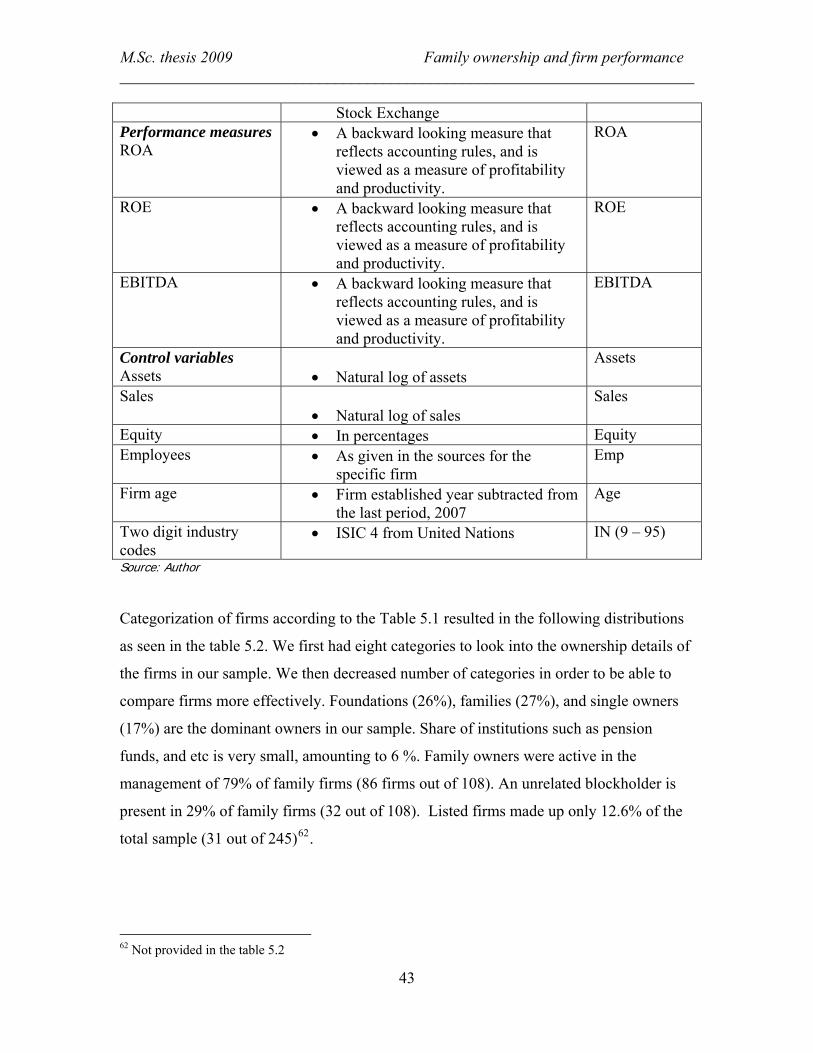
M.Sc. thesis 2009 Family ownership and firm performance ________________________________________________________________________
Stock Exchange Performance measures ROA
• A backward looking measure that reflects accounting rules, and is viewed as a measure of profitability and productivity.
ROA
ROE • A backward looking measure that reflects accounting rules, and is viewed as a measure of profitability and productivity.
ROE
EBITDA • A backward looking measure that reflects accounting rules, and is viewed as a measure of profitability and productivity.
EBITDA
Control variables Assets
• Natural log of assets
Assets
Sales • Natural log of sales
Sales
Equity • In percentages Equity Employees • As given in the sources for the
specific firm Emp
Firm age • Firm established year subtracted from the last period, 2007
Age
Two digit industry codes
• ISIC 4 from United Nations IN (9 – 95)
Source: Author
Categorization of firms according to the Table 5.1 resulted in the following distributions
as seen in the table 5.2. We first had eight categories to look into the ownership details of
the firms in our sample. We then decreased number of categories in order to be able to
compare firms more effectively. Foundations (26%), families (27%), and single owners
(17%) are the dominant owners in our sample. Share of institutions such as pension
funds, and etc is very small, amounting to 6 %. Family owners were active in the
management of 79% of family firms (86 firms out of 108). An unrelated blockholder is
present in 29% of family firms (32 out of 108). Listed firms made up only 12.6% of the
total sample (31 out of 245)62.
62 Not provided in the table 5.2
43

M.Sc. thesis 2009 Family ownership and firm performance ________________________________________________________________________ When we divide firms into only two categories, family firms make up 44% of the sample.
Similar studies include ownership by a single large shareholder into the category of
family firms. We decide here to categorize such owners as single owners. It would be
interesting to see how the performance measures of single owner type firms differ from
that of other family firms. We are cautious about high proportion of foundations owned
firms in our sample, since it is common for foundations to operate as an umbrella for
family interests. In this thesis we decided to leave them as technically foundation owned
firms.
Table 5.2 ‘Ownership frequency’63
Source: author
Firms in our sample come from wide range of different industries, 52 in total. There are a
couple of industries where firm number is more concentrated than other industries, such
as manufacture of machinery and equipment (ISIC4 code 29), wholesale trade except for
motor vehicles and motorcycles (ISIC4 code 46), manufacture of computer, electronics
and optical products (ISIC4 code 26). Family firms are represented in 33 (63%) industries
out of 52 of industries.
63 Refer to 5.1 to interpret the table
44

M.Sc. thesis 2009 Family ownership and firm performance ________________________________________________________________________
Source: author
45

M.Sc. thesis 2009 Family ownership and firm performance ________________________________________________________________________
C. Performance measures
We used accounting performance measures such as ROE, ROA, and EBITDA. These
accounting measures are considered as backward looking and can be subject to
manipulation by CEOs or the board, who are keen to present their firms positively.
D. Control Variables
We applied a number of control variables, which are standard variables in similar studies.
Danish branch codes64 were converted into two-digit ISIC 4 codes65. Firm age was
calculated subtracting firm established year from the last period, 2007, and firm size was
measured as natural log of firm’s total assets. Included were also sales (natural logarithm)
number of employees (natural logarithm), and equity level66. A dummy variable for listed
firms, a dummy variable for an unrelated blockholder presence and dummy variable for
the family management were also included as control variables.
5.3 Summary statistics Descriptive statistics on important variables are (e.g. mean, std, min, max) given in the
table 5.4. For the univariate analysis we take the time-series averages for each firm and
then across all firms similar to Andres (2008). The statistics software67 provides the
results shown in the table 5.4.
64 The firms in our sample had old (DB03) Danish industry codes, which we had to convert to the new branch codes (DB07), and then convert to ISIC 4 codes. 65 Taken from United Nations 66 We used equity proportion instead of the usual leverage ratio 67 We used Stata 9.2. The statistics results from the software are given in the appendix A.
46

M.Sc. thesis 2009 Family ownership and firm performance ________________________________________________________________________
Source: author
The average age for our sample firms is 41 years, the mean ROE is 22.4%, ROA is 9.2%,
and EBITDA is close to 7.6%, the mean equity level is 39.8%. It is important to note that
standard errors are quite high for our accounting measures. Further in Table 5.5 we
conduct difference of means tests.
47

M.Sc. thesis 2009 Family ownership and firm performance ________________________________________________________________________
Source: Author
48

M.Sc. thesis 2009 Family ownership and firm performance ________________________________________________________________________ According to our first definition of family firms (Fam1) where we exclude the firms
owned by single owners, unlike other empirical studies, we do not find significant
difference in the average ROE for the family firms and the rest of the firms. Statistically
significant means are of that of Age (at 5%) and Assets (at 1%) for the family firms. As
we can see the family firms (here Fam1), are younger, and seems to operate in slightly
different industries. There is no significant difference in the average Equity levels of
family firms and non family firms, which contradicts the assumptions that family firms
rely more on debt financing than equity financing in order to keep the control over the
firm within the family.
When we define the family firms according to the third definition (Fam3), we detect a
difference in the average ROE. For family firms (Fam3) it is around 26% while for the
non family firms it is close to 20%. Difference in the average Age and Assets still
remains significant between family firms and non family firms. Average Age for the
family firms is 37 years, while for the non family firms it is 35 years. Family firms in
both cases of Fam1 and Fam3 remain to be younger than other firms and as well as
smaller in size (in terms of Assets). This perhaps points out that family firms are smaller,
younger and operate in different industries.
When we compare the average ROE for the firms owned by single owners (SO) and the
rest of the firms, we can detect a significant difference (at 5%). The average ROE for the
single owner firms is close to 30%, while for the rest of the firms it is 21%. It could
perhaps mean that family firms, when there is only one family member as the largest
shareholder, (i.e. in the absence of other family members) tend to be more efficient and
perform better.
The average Age of single owner firms (SO), does not seem to be different than rest of
the firms. But it is interesting to see that single owner firms (SO) have lower equity levels
supporting the assumption that single owner family firms rely more on debt financing.
The average ROA for SO differ from the rest of the firms, 10.63% vs. 8.97% (significant
at 26% level) and EBITDA 9.3% vs. 7.2% (significant at 36%).
49

M.Sc. thesis 2009 Family ownership and firm performance ________________________________________________________________________
Foundations (Found) do not show significant difference in the average performance
measures (accounting) from the rest of the firms. However, there is significant difference
(at 1%) in the average Age, 51 years for the foundations and 38 years for the rest of the
firms. This supports the assumption that mature, older family firms establish foundations
to govern their firms indirectly and to sort of eliminate direct involvement of the family
members in the board, or management. Moreover, average assets are higher for the
foundations, and they have higher level of equity, which supports the picture of average
foundations owned firms as being old, large and perhaps publicly listed.
The significant difference in the average ROE at the family firms (Fam3) could be
explained by the higher average ROE for the firms with single owners (SO). Family firms
with a single owner perhaps are more efficient than number of family members involved
at the management or at the board.
Correlation data supports the findings from the means tests68.
Source: author
68 There is high positive correlation between family firms (Fam3) and foundations
50

M.Sc. thesis 2009 Family ownership and firm performance ________________________________________________________________________ 5.4 Multivariate analysis We have employed the panel data methodology for our study. It helps us to address two
issues that arise while assessing the impact of ownership on firm performance. First one
is the unobserved heterogeneity and the second one is endogeneity problem. Panel data
allows us to control for the firm specific heterogeneity, which would be difficult to do in
cross-sectional models. A family firm might have its own specific feature, which might
induce a particular behavior closely linked to the culture of the company, which in family
firms might be imposed by the controlling family (Amit & Villalonga (2006).
We are not able to conduct fixed effects tests since they by nature require the longitudinal
variation in the independent variables, and our ownership variables do not show variation
across time as we have measured ownership only for one period and assumed it constant
for the other periods.
To avoid getting biased estimates, we controlled for such heterogeneity by modeling it as
an individual effect, which is eliminated by taking the first differences of the variables.
Further on, the error term in the model, is then split into three different components. The
first one the individual effect which is captured by industry dummies, the second one
time specific effect with corresponding dummy variable, and finally the random
disturbance term.
Endogeneity of our explanatory variables, ownership concentration, may seriously affect
the ownership-performance relationship. Ownership concentration may have no
observable effect on firm performance due to the endogeneity of ownership structure
(Demsetz and Lehn, 1985). As Anderson and Reeb (2003) argue it is not clear whether
family ownership improves corporate performance, or families keep their stakes in the
superior performing firms. If the argument that families keep their stakes in superior
performing firms holds, it follows that family owners are able to predict the future
performance for an extended periods of time. Despite controlling families are better
informed about the prospects of their firms, it is a rather weak argument to accept.
51

M.Sc. thesis 2009 Family ownership and firm performance ________________________________________________________________________
We chose random-effects generalized least squares (GLS) two way model to estimate our
four models and to analyze the impact of ownership variables. The dependent variables
are ROE, ROA, and EBITDA. As independent variables, we use the family firm
dummies (fam1-fam469 ) in different models and the usual control variables such as firm
size (measured in total assets), firm age, equity level, as well as industry and year
dummies according to Anderson et al., 2003; Miller et al., 2007; Villalonga and Amit,
2006).
We also include management dummy (equal to one if the identified owner is the CEO or
the Chairman of the board), dummy for listed firms (CSE equals one if the firm is listed),
and blockholder dummy (equal one if there is another significant blockholder present at
the firm).
General form of the regression looks like this:
Firm performance = β +β (family firm, Fam1-Fam4) +β (control variables) +β (year
dummy, y1-y10) +β (ISIC 4 code dummy, sic1-sic52) +ε
Robust standard errors to counter for heteroskedasticity and serial correlation are
calculated using the Huber-White Sandwich estimator for variance. We also use natural
logarithm of our dependent variables.
To determine whether random-effects GLS model should be preferred to a pooled
ordinary least squares (OLS) model, we calculated the Breusch-Pagan Lagrangian
Multiplier Test70, which examines whether the firm-specific intercepts differ from one
another. We also provide pooled OLS results as an alternative to random effects tests.
69 Fam4 is measured as family management dummy 70 Tests are significant for all our models. The fraction of u_i is below 45% in all models similar to other studies. And the Chi² is significant in all models, meaning that our models are well specified.
52

M.Sc. thesis 2009 Family ownership and firm performance ________________________________________________________________________
We estimated four models as following71:
Model 1
Here we are trying to test if family firms where more than one family member is present
perform better than non family firms. Presence of multiple family members is argued to
bring inefficiencies and cause poor performance.
GLS, RE, ROE & ROA
Impact of Fam1 is positive (negative) β= 0.01 (β= 0.11) for ROE (ROA); however it is
not significant in column A. In column B, where we control for blockholder dummy,
CSE dummy and management dummy, coefficient improves to β = 0.16 for ROE
(decreases to β= 0.01 for ROA), however it is still insignificant. Presence of another
blockholder seems to have a negative impact, β= - 0.34 on ROE and β= - 0.33 on ROA,
and significant at 5% and 1% respectively (see column B). This is contrary to the
assumptions that presence of another influential blockholder helps to control for the
inefficiencies brought by the family. Firm size (Assets) have negative impact for both
ROE and ROA, and significant at 1% level both in column A and B.
OLS, ROE & ROA
Impact of Fam1 on ROE is positive (β= 0.10) in column B similar to GLS estimates, but
statistically significant at 10%. Fam1 has negative impact on ROA in column B (β= -
0.08) similar to GLS results, however it is unlike GLS estimates significant at 10%.
Adjusted R² is 20% similar to the over-all R² in GLS. Coefficients of control variables are
similar both quantitatively and statistically to GLS.
Model 2
71 We do not report here estimates of EBITDA, as the coefficients of ownership variables are insignificant in all models, however they are given in the appendices
53
M.Sc. thesis 2009 Family ownership and firm performance ________________________________________________________________________ Here we are considering as a family firm a firm with an individual owner as the largest
shareholder. We are trying to see whether family firms where a single owner is present
are more efficient than family firms with a number of family members.
GLS, RE, ROE & ROA
Impact of Fam2 on ROE in column A is negative (β =-0.07) and in column B it is
positive (β=0.02), however it is not statistically significant. Fam2 impact on ROA in
columns A & B resemble that of ROE in signs of coefficients and are insignificant as
well. Thus, we can conclude that single owner family firms do not necessarily perform
better in comparison to other family firms and in general to non family firms.
OLS, ROE & ROA
Fam2 impact on ROA is positive (β = 0.06) and significant at 10% in column B. Other
than this, results are quantitatively and statistically similar to GLS results.
Model 3
Here we combine family firms from the first definition (Fam1) and firms with large
single owners (Fam2), and define them as Fam3.
GLS, RE, ROE & ROA
Impact of Fam3 is negative (β= -0.03) on ROE, and (β = -0.13) on ROA, but estimates
are not statistically significant in column A. Fam3 impact on ROE is positive (β=0.32) in
column B and significant at 10%. This could be explained by increased number of family
firms (n=108) to compare with non family firms (n=137). Similarly, Fam3 has positive
impact on ROA in column B (β=0.12), but it is statistically insignificant. Family
management dummy impact on ROE in column B is negative, (β=-0.27), but it is
insignificant. Presence of unrelated blockholders has a negative impact (β= -0.42) on
ROE in column B, and it is significant at 5%. Perhaps a presence of an outside
blockholder at the family firm hampers performance.
54

M.Sc. thesis 2009 Family ownership and firm performance ________________________________________________________________________ OLS, ROE & ROA
Impact of Fam3 on ROE is similar to the corresponding GLS coefficient in column B,
(β=0.32) and significant at 1%, while in GLS it is significant at 10%. Impact of Fam3 on
ROA in column A is negative (β =-0.08) and significant at 5%, however the impact is
positive in column B (β = 0.15) and significant at 5%.
Model 4
In this model, we are trying to compare performance of family owned and managed firms
with those of non family firms and family firms with no involvement at the management
level.
GLS, RE, ROE & ROA
Impact of family managed firms on ROE in column A is positive (β=0.12) but
insignificant, and in column B it is small (β=-0.03) and negative, but again insignificant.
Impact of family managed firms on ROA in column A is negative (β=- 0.18) and
significant at 5%. In column B it is also negative, but insignificant. However, this is not
enough to conclude that family managed firms perform worse than other firms, since
ROA is more of an accounting measure and subject to manipulation.
OLS, ROA & ROE
Impact of family managed firms on ROE in column A is negative, and in column B is
positive, however both are insignificant. Impact of family managed firms on ROA in
column A is negative (β = -0.13) and significant at 1%, and in column B it is negative as
well but insignificant.
Main interesting findings are:
- Presence of another blockholder has a negative significant impact on both ROE
and ROA in most models and in both GLS and OLS estimations.
55

M.Sc. thesis 2009 Family ownership and firm performance ________________________________________________________________________
- We find positive significant impact of family firms (Fam3) on ROE in both GLS
and OLS estimations.
- Family managed firms have a negative significant impact on ROA in both GLS
and OLS estimations
Both Maury (2006) and Anderson & Reeb (2003) find family managed firms associated
with better performance, while we do not. Barontini & Caprio (2006) find family control
in Scandinavian origin countries with families occupying the CEO post associated with
negative performance.
One of the possible explanations for the weak results could be that a large proportion of
firms we have categorized as foundations are actually family firms. If this is the case, our
true non family firms make up a smaller proportion of our sample, and hence we are
unable to find any statistically significant differential performance for our family firms.
Our small sample size could be another reason our results fail to find enough support for
or against the superior or worse performance of family firms.
Despite the inclusion of industry dummies, as Andres (2008) suggests distribution of
family firms to non family firms might induce bias. As an additional robustness tests we
exclude all the industries where distribution is strongly biased either one way or the
other. However, the results do not differ from when we have included all the industries.
Perhaps, Danish privately held companies face tougher market conditions due to the fact
that Danish GDP is highly concentrated towards exports. And perhaps, there are other
laws and regulations that force these private companies to be transparent and
accountable. So these regulations could act a proxy for ‘market pressure’ faced by public
companies (Martinez et al. 2007).
56

M.Sc. thesis 2009 Family ownership and firm performance ________________________________________________________________________
Source: author
57

M.Sc. thesis 2009 Family ownership and firm performance ________________________________________________________________________
Source: Author
58

M.Sc. thesis 2009 Family ownership and firm performance ________________________________________________________________________
Source: Author
59

M.Sc. thesis 2009 Family ownership and firm performance ________________________________________________________________________
Source: Author
60

M.Sc. thesis 2009 Family ownership and firm performance ________________________________________________________________________
Conclusion
This study explores the link between family ownership and firm performance using a
panel data set of 245 Danish firms from 1998 to 2007. Following Himmelberg et al.
(1999) and Claessens et al (2002) we use panel data techniques to control for unobserved
firm heterogeneity in order to better identify family firm dynamics regarding the firm
performance.
Our main findings are firm specific characteristics of family firms in Denmark. We found
family firms to be younger (20 percentage points), with highly concentrated ownership
structures (i.e. only 29% of family firms had an unrelated blockholder at 10% ownership
stake), and 79% of families were actively involved at the management level (either as a
CEO or the chairman of the board).
The superior performance of family firms is still an open question. Our study does not
find strong evidence of significant differential performance in terms of accounting
measures such as return on equity (ROE), return on assets (ROA), and in earnings before
tax and interests (EBITDA).
We think empirical studies with a larger sample of firms, both listed and unlisted, with a
broader range of control variables, which would better capture firm specific
characteristics (e.g. use of control enhancing mechanisms, board size and independence,
presence of other blockholders etc), could possibly find a differential performance
between family blockholder and other kind of blockholder firms. Our conclusion is that
family ownership per se might not impact positively or negatively firm performance, but
other family firm specifics characteristics might be the actual contributors to the
differential performance.
61
List of appendices
1 References 2 List of firms 3 Outputs from difference of means test 4 Outputs form GLS regressions 5 Outputs from OLS regressions

References
Anderson, Ronald C., and David M. Reeb. 2004. Board composition: Balancing family influence in S&P 500 firms. Administrative Science Quarterly 49, (2) (06): 209-37.
ANDERSON, RONALD C., and DAVID M. REEB. 2003. Founding-family ownership and firm performance: Evidence from the S&P 500. Journal of Finance 58, (3) (06): 1301-28.
Anderson, Ronald C., and David M. Reeb. 2003. Founding-family ownership, corporate diversification, and firm leverage.
Andres, Christian. 2008. Large shareholders and firm performance—An empirical examination of founding-family ownership. Journal of Corporate Finance 14, (4) (09): 431-45.
Barontini, Roberto, and Lorenzo Caprio. 2006. The effect of family control on firm value and performance: Evidence from continental europe. European Financial Management 12, (5) (11): 689-723.
Ben-Amar, Walid, and Paul André. 2006. Separation of ownership from control and acquiring firm performance: The case of family ownership in Canada. Journal of Business Finance & Accounting 33, (3): 517-43.
Bennedsen, Morten, Kasper Meisner Nielsen, Francisco Perez-Gonzalez, and Daniel Wolfenzon. 2007. Inside the family firm: The role of families in succession decisions and performance. Quarterly Journal of Economics 122, (2) (05): 647-91.
Bozec, Yves, and Claude Laurin. 2008. Large shareholder entrenchment and performance: Empirical evidence from canada. Journal of Business Finance & Accounting 35, (1): 25-49.
Braun, Michael, and Anurag Sharma. 2007. Should the CEO also be chair of the board? an empirical examination of family-controlled public firms. Family Business Review 20, (2) (06): 111-26.
De Holan, Pablo M., and Luis Sanz. 2006. Protected by the family? how closely held family firms protect minority shareholders. Journal of Business Research 59, : 356.
DeAngelo, Harry, and Linda DeAngelo. 2000. Controlling stockholders and the disciplinary role of corporate payout policy: A study of the times mirror company. Journal of Financial Economics 56, : 153-207.
Demsetz, Harold. 1983. The stucture of ownership and the theory of the firm. Journal of Law and Economics 26, (2): 375-390.

Demsetz, Harold, and Kenneth Lehn. 1985. The structure of corporate ownership: Causes and consequences. Journal of Political Economy 93, (6): 1155.
Dyer, Gibb W. Jr. 2006. Examinging the 'family effect' on firm performance. Family Business Review, ABI/INFORM Global 19, (4): 253.
Faccio, Mara, and H. P. Larry Lang. 2002. The ultimate ownership of western european corporations. Journal of Financial Economics 65, : 365.
Faccio, Mara, Larry H. P. Lang, and Leslie Lang. 2001. Dividends and expropriation. The American Economic Review, ABI/INFORM Global 90, (1): 54.
Fama, Eugene F. 1980. Agency problems and theory of th firm. The Journal of Political Economy 88, (2): 288-307.
Fama, Eugene F., and Michael C. Jensen. 1983. Separation of ownership and control. Journal of Law and Economics 26, .
Gallo, M., J. Tapies, and K. Kappuyns. 2004. Comparison of family and non family business: Financial logic and personal preferences. Family Business Review, ABI/INFORM Global 17, (4).

List of firms
Company name CVR
number CompID
Own-p cat at 25% ( 8 cat)
Own with 5 cat
Own with 2 cat
Fam mang FamB
Haribo Lakrids, Aktieselskab 43423010 1 Fam Fam Fam Fam4 Fam
A/S J.Petersens Beslagfabrik, Nibe 52743419 2 Found Found Non Fam nonfam
Non Fam
A/S Jydsk Aluminium Industri 38523716 3 Fam Fam Fam Fam4 FamB
A/S Peder Nielsen Beslagfabrik 52081211 4 Found Found Non Fam nonfam
Non Fam
Aktieselskabet Østbirk Bygningsindustri 45557219 5 Found Found Non Fam nonfam
Non Fam
Alectria A/S (Ex name Birch & Krogboe A/S) 22278916 6 Found Found Non Fam nonfam
Non Fam
ALK-Abelló A/S 63717916 7 Found Found Non Fam nonfam
Non Fam
Aller Press A/S 43325612 8 Found Found Non Fam nonfam
Non Fam
Andreas Andresen A/S 81745528 9 Other Other Non Fam nonfam
Non Fam
Bang & Olufsen A/S 41257911 10 Ins ISP Non Fam nonfam
Non Fam
BB Electronics Holding A/S 80170319 11 Fam Fam Fam nonfam FamB
Bestseller A/S 88216512 12 Fam Fam Fam Fam4 Fam
Blend A/S 76180113 13 Fam Fam Fam Fam4 Fam
Brødrene A. & O. Johansen A/S 58210617 14 Other Other Non Fam nonfam
Non Fam
C.A Nielsen & Petersens Maskinfabriker A/S 63411914 15 SO SO Fam Fam4 Fam
Cabinplant International A/S 76165319 16 Par ISP Non Fam nonfam
Non Fam
Cheminova A/S 12760043 17 Other Other Non Fam nonfam
Non Fam
Chr. Hansen A/S 12516479 18 Found Found Non Fam nonfam
Non Fam
Co-Ro Food A/S 63548715 19 SO SO Fam Fam4 FamB
COWI A/S 44623528 20 Found Found Non Fam nonfam
Non Fam
Dagbladet Børsen A/S 76156328 21 Fam Fam Fam nonfam Fam
DakoCytomation Denmark A/S 33211317 22 Other Other Non Fam nonfam
Non Fam
Danbor Service A/S 49677715 23 Found Found Non Fam nonfam
Non Fam
Dan-Ejendomme A/S 20283416 24 Ins ISP Non Fam nonfam
Non Fam
Danfoss A/S 20165715 25 Found Found Non Fam nonfam
Non Fam
Danfoss Drives A/S 19883876 26 Found Found Non Fam nonfam
Non Fam
Dansk Supermarked A/S 35954716 27 Found Found Non Fam nonfam
Non Fam
Danske Spil A/S (Ex name Dansk Tipstjeneste A/S) 64011715 28 State ISP Non Fam nonfam
Non Fam
Dantherm A/S 20937106 29 Ins ISP Non Fam nonfam
Non Fam
Davidsen Partnere A/S 10498899 30 Par ISP Non Fam nonfam
Non Fam

Deloitte & Touch Statsautoriseret Revisionsaktieselskab 24213714 31 Par ISP
Non Fam nonfam
Non Fam
Dinex A/S 10504473 32 SO SO Fam Fam4 FamB
Dong (Energy Power) A/S 36213728 33 State ISP Non Fam nonfam
Non Fam
DS SM A/S 88374614 34 Fam Fam Fam nonfam Fam
Dyrup A/S 18998696 35 Found Found Non Fam nonfam
Non Fam
E. Pihl & Søn A.S 33037112 36 SO SO Fam Fam4 Fam
Einar Kornerup A/S 13703906 37 Fam Fam Fam Fam4 Fam
Ecco Sko A/S 45349918 38 SO SO Fam Fam4 Fam
El-Tec A/S 11939775 39 SO SO Fam nonfam Fam
Ernst & Young Statsautoriseret Revisionsaktieselskab 73317428 40 Par ISP
Non Fam nonfam
Non Fam
Enemærke & Petersen A/S 10503698 41 Found Found Non Fam nonfam
Non Fam
F. Junckers Industrier A/S 66920216 42 Ins ISP Non Fam nonfam
Non Fam
Ferrosan A/S 13246092 43 SO SO Fam Fam4 FamB
Fibertex A/S 40098216 44 Found Found Non Fam nonfam
Non Fam
FLSMIDT & Co. A/S (Ex name FLS Industries A/S) 58180912 45 Other Other Non Fam nonfam
Non Fam
Foss A/S 59388517 46 Fam Fam Fam Fam4 Fam
Frode Laursen A/S 29482713 47 SO SO Fam Fam4 Fam
Fyens Stiftstidende A/S 45765415 48 Found Found Non Fam nonfam
Non Fam
GN Netcom A/S 15069511 49 MO Other Non Fam nonfam
Non Fam
GN Resound A/S 55082715 50 MO Other Non Fam nonfam
Non Fam
Gåsdal Bygningindustri A/S 46911512 51 Found Found Non Fam nonfam
Non Fam
Haldor Topsøe A/S 41853816 52 SO SO Fam Fam4 FamB
H. Lundbeck A/S 56759913 53 Found Found Non Fam nonfam
Non Fam
Hansson & Knudsen A/S 37215228 54 Fam Fam Fam nonfam Fam
Harboes Bryggeri A/S 43910515 55 Fam Fam Fam Fam4 Fam
HCS A/S Transport & Spedition 71145816 56 Fam Fam Fam Fam4 Fam
Hempel A/S 59946013 57 Found Found Non Fam nonfam
Non Fam
Højbjerg Maskinfabrik A/S 43969315 58 Fam Fam Fam Fam4 Fam
Ib Andresen Industri A/S 35745114 59 SO SO Fam Fam4 Fam
Haarslev A/S 89523818 60 Fam Fam Fam Fam4 Fam
IC Companys A/S 62816414 61 Ins ISP Non Fam nonfam
Non Fam
Idealcombi A/S 25829328 62 Fam Fam Fam Fam4 Fam
ISS Facility Services A/S (Ex ISS Danmark A/S 14406042 63 MO Other Non Fam nonfam
Non Fam
J.F. - Fabriken, J. Freudendahl A/S 46099117 64 Fam Fam Fam Fam4 Fam
Jakon A/S 83955716 65 Fam Fam Fam Fam4 Fam
Kamstrup A/S 21248118 66 Other Other Non Fam nonfam
Non Fam
Kohlberg Brød A/S 11326943 67 Fam Fam Fam Fam4 FamB
Lego System A/S 47458714 68 Fam Fam Fam Fam4 Fam
Leo Pharma A/S 56759514 69 Found Found Non Fam nonfam
Non Fam
Linak A/S 66365328 70 SO SO Fam Fam4 Fam
Lind & Risør A/S 89094119 71 Par ISP Non Fam nonfam
Non Fam
Lindab A/S 33124228 72 Other Other Non Fam nonfam
Non Fam
Lindpro A/S 82675418 73 Found Found Non Fam nonfam
Non Fam
LM Glasfiber A/S 76490511 74 SO SO Fam nonfam Fam
MCH A/S 43555928 75 State ISP Non Fam nonfam
Non Fam
Mærsk Container Industry AS 13823774 76 Found Found Non Fam nonfam
Non Fam
Micro Matic A/S 17177176 77 Fam Fam Fam Fam4 Fam
Mærsk Olie og Gas A/S 22757318 78 Found Found Non Fam nonfam
Non Fam
Nilfisk-Advance A/S 62572213 79 MO Other Non Fam nonfam
Non Fam
Niras Rådgivende ingeniører og planlæggere A/S 37295728 80 Found Found Non Fam nonfam
Non Fam
Nissens KølerfabrikA/S 40212116 81 Fam Fam Fam Fam4 Fam
Novo Nordisk A/S 24256790 82 Found Found Non Fam nonfam
Non Fam
Novopan Træindustri A/S 11766110 83 Ins ISP Non Fam nonfam
Non Fam
Odense Staalskibsværft A/S 45739910 84 Found Found Non Fam nonfam
Non Fam
Oticon A/S 42334219 85 Found Found Non Fam nonfam
Non Fam
Per Aarsleff A/S 24257797 86 Found Found Non Fam nonfam
Non Fam
Persolit Entreprenørfirma A/S 55708118 87 SO SO Fam Fam4 FamB
R. Færch Plast A/S 13723540 88 Fam Fam Fam nonfam Fam
Rambøll, Hannemann & Højlund A/S 35128417 89 Found Found Non Fam nonfam
Non Fam
Rationel Vinduer A/S 40371818 90 Fam Fam Fam nonfam FamB
Riegens A/S 45478319 91 SO SO Fam Fam4 FamB
Rockwool International A/S 54879415 92 Fam Fam Fam Fam4 FamB
Sanistål A/S 42997811 93 MO Other Non Fam nonfam
Non Fam
Scandinavian Brake Systems A/S 32774210 94 Fam Fam Fam Fam4 FamB
Schur Pack Denmark A/S 83099828 95 SO SO Fam Fam4 FamB
SimCorp A/S 15505281 96 MO Other Non Fam nonfam
Non Fam
Sjørring Maskinfabrik A/S 73730317 97 SO SO Fam Fam4 Fam
Svejsemaskinefabrikken Migatronic A/S 34485216 98 Fam Fam Fam Fam4 FamB
Systematic Software Engineering A/S 78834412 99 SO SO Fam Fam4 FamB
Terma A/S 41881828 100 Found Found Non Fam nonfam
Non Fam
Thrane & Thrane A/S 65724618 101 Fam Fam Fam Fam4 Fam
Thyregod Bygningsindustri A/S 75021828 102 Found Found Non Fam nonfam
Non Fam

Tinglev Elementfabrik A/S 67192311 103 SO SO Fam Fam4 FamB
Toms Gruppen A/S 56759328 104 Found Found Non Fam nonfam
Non Fam
Unimerco A/S 21126543 105 MO Other Non Fam nonfam
Non Fam
Triax A/S 29119511 106 Fam Fam Fam Fam4 Fam
Velserv A/S 15512172 107 Found Found Non Fam nonfam
Non Fam
Vestas Wind Systems A/S 10403782 108 MO Other Non Fam nonfam
Non Fam
Viking Life - Saving Equipment A/S 15016213 109 Fam Fam Fam Fam4 Fam
Wicotec A/S 73585511 110 Found Found Non Fam nonfam
Non Fam
Øens Murefirma A/S 18814633 111 Fam Fam Fam Fam4 Fam
Aalborg Industries A/S 17830635 112 Fam Fam Fam Fam4 FamB
Andersen & Martini A/S 15313714 113 SO SO Fam Fam4 FamB
Ambu A/S 63644919 114 Other Other Non Fam nonfam
Non Fam
Arkil Holding A/S 36469528 115 Fam Fam Fam Fam4 FamB
Auriga Industries A/S 34629218 116 Found Found Non Fam nonfam
Non Fam
Coloplast A/S 69749917 117 MO Other
Non Fam nonfam
Non Fam
Dantax A/S 36591528 118 SO SO Fam Fam4 FamB
Danisco A/S 11350356 119 MO Other
Non Fam nonfam
Non Fam
DSV A/S 58233528 120 MO Other
Non Fam nonfam
Non Fam
A/S Det Østasiatiske Kompagni 26041716 121 MO Other
Non Fam nonfam
Non Fam
Egetæpper A/S 38454218 122 Found Found
Non Fam nonfam
Non Fam
Flügger A/S 32788718 123 Fam Fam Fam Fam4 FamB
Gabriel Holding A/S 58868728 124 MO Other
Non Fam nonfam
Non Fam
Glunz & Jensen A/S 10239680 125 Found Found
Non Fam nonfam
Non Fam
GPV Industri A/S 42809616 126 Ins ISP
Non Fam nonfam
Non Fam
Gyldendalske Boghandel, Nordisk Forlag; Aktieselskab
58200115 127 Found Found
Non Fam nonfam
Non Fam
Brdr.Hartmann A/S 63049611 128 Found Found
Non Fam nonfam
Non Fam
H+H International A/S 49619812 129 Fam Fam Fam nonfam Fam
Højgaard Holding A/S 16888419 130 Found Found
Non Fam nonfam
Non Fam
Brd. Klee A/S 46874412 131 Par ISP
Non Fam nonfam
Non Fam
Lastas A/S 30795016 132 Fam Fam Fam Fam4 Fam
Migatronic A/S 34485216 133 Fam Fam Fam Fam4 FamB
Monberg & Thorsen A/S 12617917 134 Found Found
Non Fam nonfam
Non Fam
NeuroSearch A/S 12546106 135 Other Other
Non Fam nonfam
Non Fam
Roblon Aktieselskab 57068515 136 SO SO Fam Fam4 FamB
RTX Telecom A/S 17002147 137 MO Other
Non Fam nonfam
Non Fam
SKAKO A/S 64427512 138 Ins ISP
Non Fam nonfam
Non Fam

Aktieselskabet Schouw & Co. 63965812 139 Found Found
Non Fam nonfam
Non Fam
SP Group A/S 15701315 140 Ins ISP
Non Fam nonfam
Non Fam
Spæncom A/S 26271010 141 Fam Fam Fam nonfam FamB
GN Store Nord 24257843 142 MO Other
Non Fam nonfam
Non Fam
Alex Andersen, Ølund A/S 66683419 143 Fam Fam Fam Fam4 Fam
Bladt Industries, A/S 14818480 144 Ins ISP Non Fam nonfam
Non Fam
Boconcept, A/S 89866618 145 SO SO Fam nonfam FamB
BTX Group, A/S 34281718 146 Fam Fam Fam nonfam Fam
Cimbria Manufacturing, A/S 15694882 147 Fam Fam Fam nonfam Fam
Deif A/S 15798416 148 SO SO Fam Fam4 Fam
Distribution Services A/S 56448810 149 SO SO Fam Fam4 Fam
Kongskilde Industries A/S 70282917 150 Ins ISP Non Fam nonfam
Non Fam
Muller Gas Equipment A/S 14126104 151 Found Found Non Fam nonfam
Non Fam
NNIT A/S 21093106 152 Found Found Non Fam nonfam
Non Fam
Petri & Haugsted A/S 58563412 153 Found Found Non Fam nonfam
Non Fam
A. Enggaard A/S, Entreprenør-og Byggefirma 18795507 154 Fam Fam Fam Fam4 Fam
A/S Harald Nyborg, Isenkram- og Sportsforretning 37783315 155 Fam Fam Fam Fam4 Fam
A/S Ikast Betonvarefabrik 37537314 156 SO SO Fam Fam4 Fam
Actona Company A/S 12143745 157 SO SO Fam Fam4 Fam
AVK International A/S 57693517 158 SO SO Fam Fam4 Fam
Bech-Hansen & Studsgaard A/S 35255516 159 Fam Fam Fam Fam4 Fam
Beierholm, Statsautoriseret Revisionsaktieselskab 24207501 160 Par ISP Non Fam nonfam
Non Fam
Blue Water Shipping A/S 40516611 161 Found Found Non Fam nonfam
Non Fam
Chr. C. Grene A/S 45803910 162 Found Found Non Fam nonfam
Non Fam
Columbus It Partner Danmark A/S 24207803 163 SO SO Fam nonfam FamB
Dalhoff Larsen & Horneman A/S 34411913 164 Found Found Non Fam nonfam
Non Fam
Dampskibsselskabet Norden A/S 67758919 165 Other Other Non Fam nonfam
Non Fam
Danapak Flexibles A/S 61725318 166 Other Other Non Fam nonfam
Non Fam
Dansk Auto Logik A/S 12625995 167 Found Found Non Fam nonfam
Non Fam
Dansk Træemballage A/S 11826687 168 MO Other Non Fam nonfam
Non Fam
Dantherm Filtration A/S 44534118 169 MO Other Non Fam nonfam
Non Fam
Davidsens Tømmerhandel A/S 87310116 170 SO SO Fam nonfam Fam
Designa A/S 17036971 171 SO SO Fam Fam4 Fam
DFI-Geisler A/S 14250794 172 Other Other Non Fam nonfam
Non Fam
Egmont Magasiner A/S 83131128 173 Found Found Non Fam nonfam
Non Fam
Eg A/S 84667811 174 Ins ISP Non Fam nonfam
Non Fam
Exhausto A/S 18683741 175 Fam Fam Fam Fam4 Fam

Genmab A/S 21023884 176 MO Other Non Fam nonfam
Non Fam
FTZ Autodele & Værktøj A/S 73648718 177 Fam Fam Fam nonfam Fam
Fritz Hansen A/S 14120211 178 Found Found Non Fam nonfam
Non Fam
Grant Thornton, Statsautoriseret Revisionsaktieselskab 12523246 179 Par ISP
Non Fam nonfam
Non Fam
H.J. Hansen Genvindingsindustri A/S 24336212 180 Fam Fam Fam Fam4 Fam
Ida Service A/S 16227501 181 Fam Fam Fam Fam4 Fam
Infocare Service A/S 20247800 182 Other Other Non Fam nonfam
Non Fam
Jysk A/S 13590400 183 SO SO Fam Fam4 Fam
Jørgen Kruuse A/S 35243216 184 Other Other Non Fam nonfam
Non Fam
Karstensens Skibsværft A/S 10859581 185 SO SO Fam Fam4 Fam
Kemp & Lauritzen A/S 57471719 186 Found Found Non Fam nonfam
Non Fam
Kirkebjerg A/S 53611214 187 Fam Fam Fam Fam4 Fam
Kommunekemi A/S 34484414 188 State ISP Non Fam nonfam
Non Fam
L&H - Rørbyg A/S 86503417 189 Found Found Non Fam nonfam
Non Fam
Martin Professional A/S 11805744 190 Found Found Non Fam nonfam
Non Fam
Matas A/S 63918113 191 Other Other Non Fam nonfam
Non Fam
Modulex A/S 66772616 192 Fam Fam Fam nonfam Fam
Nassau Door A/S 34391513 193 Fam Fam Fam nonfam Fam
Nordisk Dæk Import A/S 81203113 194 Fam Fam Fam Fam4 Fam
P. Christensen A/S 80493215 195 SO SO Fam Fam4 Fam
Palsgaard Træ A/S 15578580 196 Ins ISP Non Fam nonfam
Non Fam
Prime Cargo A/S 20601108 197 MO Other Non Fam nonfam
Non Fam
Privathospitalet Hamlet A/S 71017516 198 Ins ISP Non Fam nonfam
Non Fam
Rahbekfisk A/S 17557491 199 Fam Fam Fam Fam4 FamB
Rambøll Management Consulting A/S 60997918 200 Found Found Non Fam nonfam
Non Fam
Rynkeby Foods A/S 19982912 201 Other Other Non Fam nonfam
Non Fam
Råstof og Genanvendelse Selskabet af 1990 A/S 15084790 202 Other Other Non Fam nonfam
Non Fam
Sahva A/S 15111283 203 Other Other Non Fam nonfam
Non Fam
Scandinavian Brake Systems A/S 32774210 204 Fam Fam Fam Fam4 FamB
Scandinavian Tobacco Group Assens A/S 13405476 205 Fam Fam Fam nonfam FamB
Semler Services A/S 62951311 206 MO Other Non Fam nonfam
Non Fam
Skiold A/S 57081112 207 SO SO Fam Fam4 Fam
Skælskør Anlægsgartnere A/S 11968945 208 SO SO Fam nonfam Fam
Solar A/S 15908416 209 Found Found Non Fam nonfam
Non Fam
Sondex A/S 10035643 210 Fam Fam Fam Fam4 Fam
SP Moulding A/S 63450715 211 MO Other Non Fam nonfam
Non Fam
T. Hansen Gruppen A/S 15242485 212 SO SO Fam Fam4 Fam

Top-Toy A/S 10839238 213 Fam Fam Fam Fam4 Fam
Tresu A/S 15302798 214 Fam Fam Fam Fam4 Fam
Vestergaard Company A/S 70642212 215 Fam Fam Fam Fam4 Fam
Widex A/S 15771100 216 Par ISP Non Fam nonfam
Non Fam
Alumeco A/S (range from 190) 19851974 217 Other Other Non Fam nonfam
Non Fam
BCD Travel Denmark A/S 73624118 218 SO SO Fam Fam4 Fam
Elopak Denmark A/S 36071214 219 Other Other Non Fam nonfam
Non Fam
Epoke A/S 14125345 220 Fam Fam Fam Fam4 Fam
Primo Danmark A/S 10238935 221 Fam Fam Fam nonfam Fam
Renon Rengøring A/S 16411930 222 SO SO Fam Fam4 Fam
Ribe Jernindustri A/S 45814114 223 Found Found Non Fam nonfam
Non Fam
A/S Hydrema Produktion 13897603 224 Fam Fam Fam Fam4 Fam
Barslund A/S 10621577 225 SO SO Fam Fam4 Fam
B-Young A/S 15166436 226 Fam Fam Fam Fam4 Fam
Datagraf A/S 12907141 227 Fam Fam Fam Fam4 FamB
Fjord-Bus A/S 14428771 228 Other Other Non Fam nonfam
Non Fam
HH-Ferries A/S 19752283 229 Other Other Non Fam nonfam
Non Fam
Hotel Nyborg Strand A/S 18574985 230 Found Found Non Fam nonfam
Non Fam
Hustømrerne A/S 31309514 231 Found Found Non Fam nonfam
Non Fam
Hydra-Grene A/S, Handels- og Ingeniørfirma, Skjern 87552411 232 Other Other
Non Fam nonfam
Non Fam
Interacoustics A/S 15015446 233 Found Found Non Fam nonfam
Non Fam
J. H. Schultz Grafisk A/S 36791314 234 Found Found Non Fam nonfam
Non Fam
Kaj E.Nielsen (Ken) Maskinfabrik A/S 10676096 235 Found Found Non Fam nonfam
Non Fam
Kunde & Co. A/S 16702943 236 SO SO Fam Fam4 Fam
Lind Jensens Maskinfabrik A/S 52994918 237 Fam Fam Fam nonfam Fam
LINDBERG A/S 12940033 238 Par ISP Non Fam nonfam
Non Fam
Montana Møbler A/S 66652912 239 Fam Fam Fam Fam4 Fam
Plus Pack A/S 37754013 240 Fam Fam Fam Fam4 FamB
Rambøll Informatik A/S 41503912 241 Found Found Non Fam nonfam
Non Fam
RC Betonvarer A/S 58048917 242 Fam Fam Fam Fam4 Fam
Scanel International A/S 66630315 243 Par ISP Non Fam nonfam
Non Fam
Strøm Hansen A/S 10775345 244 Par ISP Non Fam nonfam
Non Fam
Sun-Air of Scandinavia A/S 83591528 245 SO SO Fam Fam4 Fam

Appendix A
.ttest roe by, (fam1)
------------------------------------------------------------------------------
Group | Obs Mean Std. Err. Std. Dev. [95% Conf. Interval]
---------+--------------------------------------------------------------------
0 | 178 22.03933 2.253296 30.06271 17.59254 26.48611
1 | 67 23.49254 3.26795 26.74933 16.96786 30.01721
---------+--------------------------------------------------------------------
combined | 245 22.43673 1.862154 29.14733 18.76879 26.10468
---------+--------------------------------------------------------------------
diff | -1.453211 4.185221 -9.697153 6.790731
------------------------------------------------------------------------------
diff = mean(0) - mean(1) t = -0.3472
Ho: diff = 0 degrees of freedom = 243
Ha: diff < 0 Ha: diff != 0 Ha: diff > 0
Pr(T < t) = 0.3644 Pr(|T| > |t|) = 0.7287 Pr(T > t) = 0.6356
. oneway roe fam1
Analysis of Variance
Source SS df MS F Prob > F
------------------------------------------------------------------------
Between groups 102.7984 1 102.7984 0.12 0.7287
Within groups 207191.471 243 852.639798
------------------------------------------------------------------------
Total 207294.269 244 849.566678
Bartlett's test for equal variances: chi2(1) = 1.2566 Prob>chi2 = 0.262
. ttest roa, by(fam1)
Two-sample t test with equal variances
------------------------------------------------------------------------------
Group | Obs Mean Std. Err. Std. Dev. [95% Conf. Interval]
---------+--------------------------------------------------------------------
0 | 178 9.449438 1.0819 14.43435 7.314354 11.58452
1 | 67 8.716418 .6643354 5.437819 7.39003 10.04281
---------+--------------------------------------------------------------------
combined | 245 9.24898 .8062135 12.61924 7.660954 10.83701
---------+--------------------------------------------------------------------
diff | .7330203 1.811817 -2.83585 4.301891
------------------------------------------------------------------------------
diff = mean(0) - mean(1) t = 0.4046
Ho: diff = 0 degrees of freedom = 243
Ha: diff < 0 Ha: diff != 0 Ha: diff > 0
Pr(T < t) = 0.6569 Pr(|T| > |t|) = 0.6861 Pr(T > t) = 0.3431
. oneway roa fam1
Analysis of Variance
Source SS df MS F Prob > F
------------------------------------------------------------------------

Between groups 26.1553608 1 26.1553608 0.16 0.6861
Within groups 38829.6569 243 159.792827
------------------------------------------------------------------------
Total 38855.8122 244 159.245132
Bartlett's test for equal variances: chi2(1) = 64.0281 Prob>chi2 = 0.000
The variances are not equal
. ttest roa, by(fam1) unequal welch
Two-sample t test with unequal variances
------------------------------------------------------------------------------
Group | Obs Mean Std. Err. Std. Dev. [95% Conf. Interval]
---------+--------------------------------------------------------------------
0 | 178 9.449438 1.0819 14.43435 7.314354 11.58452
1 | 67 8.716418 .6643354 5.437819 7.39003 10.04281
---------+--------------------------------------------------------------------
combined | 245 9.24898 .8062135 12.61924 7.660954 10.83701
---------+--------------------------------------------------------------------
diff | .7330203 1.269587 -1.767677 3.233717
------------------------------------------------------------------------------
diff = mean(0) - mean(1) t = 0.5774
Ho: diff = 0 Welch's degrees of freedom = 244.997
Ha: diff < 0 Ha: diff != 0 Ha: diff > 0
Pr(T < t) = 0.7179 Pr(|T| > |t|) = 0.5642 Pr(T > t) = 0.2821

. ttest ebitda, by(fam1)
Two-sample t test with equal variances
------------------------------------------------------------------------------
Group | Obs Mean Std. Err. Std. Dev. [95% Conf. Interval]
---------+--------------------------------------------------------------------
0 | 178 7.808989 1.497702 19.98184 4.853337 10.76464
1 | 67 6.970149 .9100102 7.448755 5.153255 8.787043
---------+--------------------------------------------------------------------
combined | 245 7.579592 1.115358 17.45811 5.382634 9.77655
---------+--------------------------------------------------------------------
diff | .8388395 2.506829 -4.099047 5.776726
------------------------------------------------------------------------------
diff = mean(0) - mean(1) t = 0.3346
Ho: diff = 0 degrees of freedom = 243
Ha: diff < 0 Ha: diff != 0 Ha: diff > 0
Pr(T < t) = 0.6309 Pr(|T| > |t|) = 0.7382 Pr(T > t) = 0.3691
. oneway ebitda fam1
Analysis of Variance
Source SS df MS F Prob > F
------------------------------------------------------------------------
Between groups 34.2520427 1 34.2520427 0.11 0.7382
Within groups 74333.4459 243 305.898954

------------------------------------------------------------------------
Total 74367.698 244 304.785647
Bartlett's test for equal variances: chi2(1) = 65.1586 Prob>chi2 = 0.000
Variances are not equal
. ttest ebitda, by(fam1) unequal welch
Two-sample t test with unequal variances
------------------------------------------------------------------------------
Group | Obs Mean Std. Err. Std. Dev. [95% Conf. Interval]
---------+--------------------------------------------------------------------
0 | 178 7.808989 1.497702 19.98184 4.853337 10.76464
1 | 67 6.970149 .9100102 7.448755 5.153255 8.787043
---------+--------------------------------------------------------------------
combined | 245 7.579592 1.115358 17.45811 5.382634 9.77655
---------+--------------------------------------------------------------------
diff | .8388395 1.752493 -2.613038 4.290717
------------------------------------------------------------------------------
diff = mean(0) - mean(1) t = 0.4787
Ho: diff = 0 Welch's degrees of freedom = 244.96
Ha: diff < 0 Ha: diff != 0 Ha: diff > 0
Pr(T < t) = 0.6837 Pr(|T| > |t|) = 0.6326 Pr(T > t) = 0.3163
. ttest age, by(fam1)
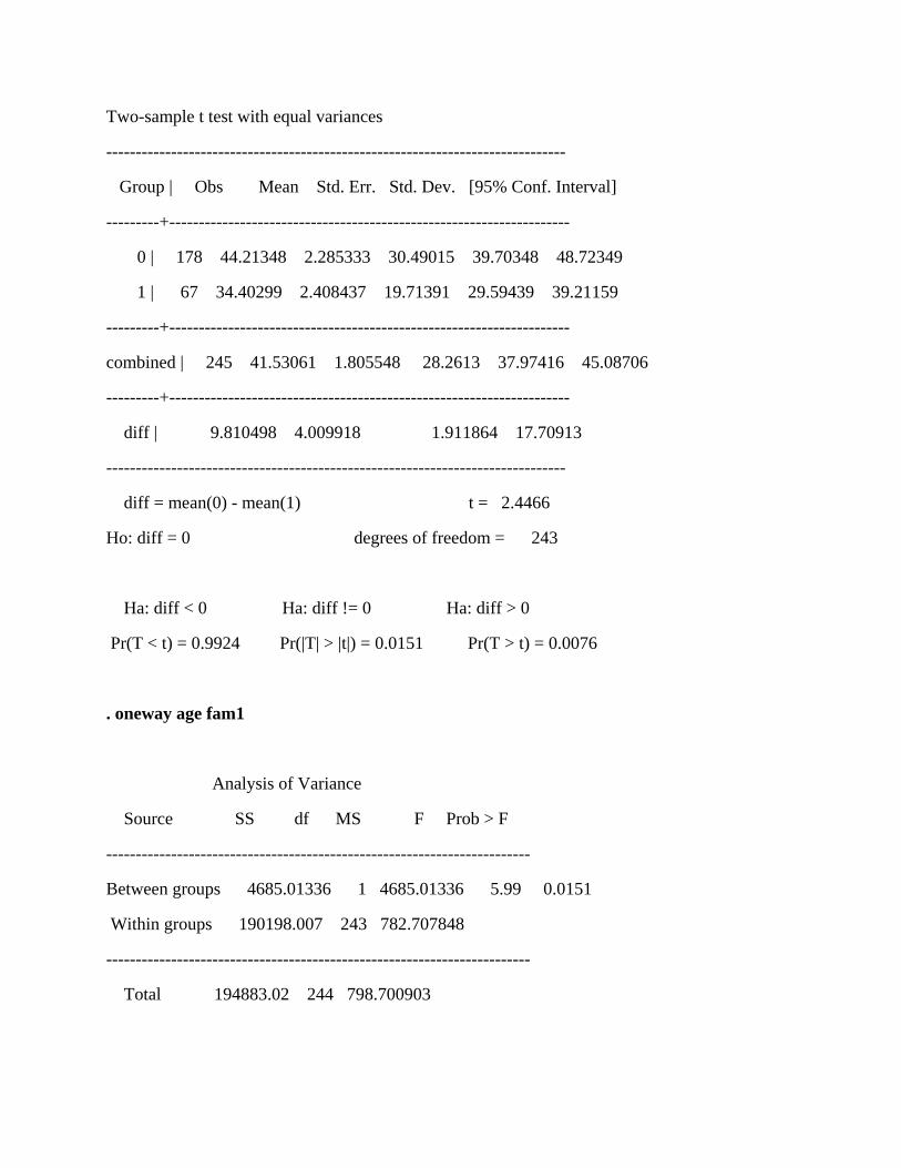
Two-sample t test with equal variances
------------------------------------------------------------------------------
Group | Obs Mean Std. Err. Std. Dev. [95% Conf. Interval]
---------+--------------------------------------------------------------------
0 | 178 44.21348 2.285333 30.49015 39.70348 48.72349
1 | 67 34.40299 2.408437 19.71391 29.59439 39.21159
---------+--------------------------------------------------------------------
combined | 245 41.53061 1.805548 28.2613 37.97416 45.08706
---------+--------------------------------------------------------------------
diff | 9.810498 4.009918 1.911864 17.70913
------------------------------------------------------------------------------
diff = mean(0) - mean(1) t = 2.4466
Ho: diff = 0 degrees of freedom = 243
Ha: diff < 0 Ha: diff != 0 Ha: diff > 0
Pr(T < t) = 0.9924 Pr(|T| > |t|) = 0.0151 Pr(T > t) = 0.0076
. oneway age fam1
Analysis of Variance
Source SS df MS F Prob > F
------------------------------------------------------------------------
Between groups 4685.01336 1 4685.01336 5.99 0.0151
Within groups 190198.007 243 782.707848
------------------------------------------------------------------------
Total 194883.02 244 798.700903

Bartlett's test for equal variances: chi2(1) = 15.6677 Prob>chi2 = 0.000
Variances are not equal
. ttest age, by(fam1) unequal welch
Two-sample t test with unequal variances
------------------------------------------------------------------------------
Group | Obs Mean Std. Err. Std. Dev. [95% Conf. Interval]
---------+--------------------------------------------------------------------
0 | 178 44.21348 2.285333 30.49015 39.70348 48.72349
1 | 67 34.40299 2.408437 19.71391 29.59439 39.21159
---------+--------------------------------------------------------------------
combined | 245 41.53061 1.805548 28.2613 37.97416 45.08706
---------+--------------------------------------------------------------------
diff | 9.810498 3.320138 3.260473 16.36052
------------------------------------------------------------------------------
diff = mean(0) - mean(1) t = 2.9548
Ho: diff = 0 Welch's degrees of freedom = 185.756
Ha: diff < 0 Ha: diff != 0 Ha: diff > 0
Pr(T < t) = 0.9982 Pr(|T| > |t|) = 0.0035 Pr(T > t) = 0.0018
. ttest assets, by(fam1)
Two-sample t test with equal variances
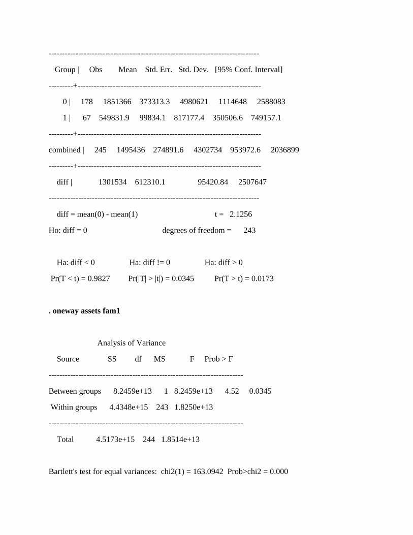
------------------------------------------------------------------------------
Group | Obs Mean Std. Err. Std. Dev. [95% Conf. Interval]
---------+--------------------------------------------------------------------
0 | 178 1851366 373313.3 4980621 1114648 2588083
1 | 67 549831.9 99834.1 817177.4 350506.6 749157.1
---------+--------------------------------------------------------------------
combined | 245 1495436 274891.6 4302734 953972.6 2036899
---------+--------------------------------------------------------------------
diff | 1301534 612310.1 95420.84 2507647
------------------------------------------------------------------------------
diff = mean(0) - mean(1) t = 2.1256
Ho: diff = 0 degrees of freedom = 243
Ha: diff < 0 Ha: diff != 0 Ha: diff > 0
Pr(T < t) = 0.9827 Pr(|T| > |t|) = 0.0345 Pr(T > t) = 0.0173
. oneway assets fam1
Analysis of Variance
Source SS df MS F Prob > F
------------------------------------------------------------------------
Between groups 8.2459e+13 1 8.2459e+13 4.52 0.0345
Within groups 4.4348e+15 243 1.8250e+13
------------------------------------------------------------------------
Total 4.5173e+15 244 1.8514e+13
Bartlett's test for equal variances: chi2(1) = 163.0942 Prob>chi2 = 0.000
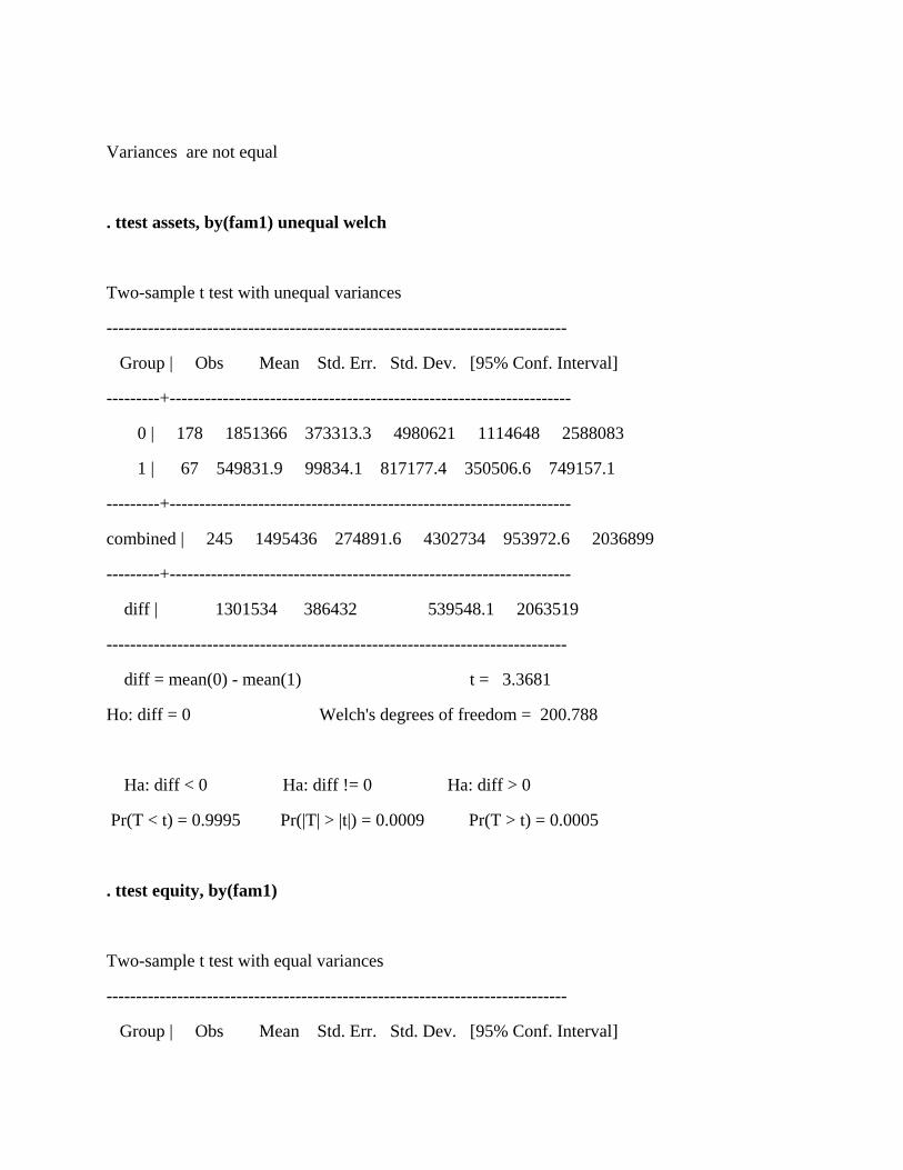
Variances are not equal
. ttest assets, by(fam1) unequal welch
Two-sample t test with unequal variances
------------------------------------------------------------------------------
Group | Obs Mean Std. Err. Std. Dev. [95% Conf. Interval]
---------+--------------------------------------------------------------------
0 | 178 1851366 373313.3 4980621 1114648 2588083
1 | 67 549831.9 99834.1 817177.4 350506.6 749157.1
---------+--------------------------------------------------------------------
combined | 245 1495436 274891.6 4302734 953972.6 2036899
---------+--------------------------------------------------------------------
diff | 1301534 386432 539548.1 2063519
------------------------------------------------------------------------------
diff = mean(0) - mean(1) t = 3.3681
Ho: diff = 0 Welch's degrees of freedom = 200.788
Ha: diff < 0 Ha: diff != 0 Ha: diff > 0
Pr(T < t) = 0.9995 Pr(|T| > |t|) = 0.0009 Pr(T > t) = 0.0005
. ttest equity, by(fam1)
Two-sample t test with equal variances
------------------------------------------------------------------------------
Group | Obs Mean Std. Err. Std. Dev. [95% Conf. Interval]

---------+--------------------------------------------------------------------
0 | 178 39.93258 1.322704 17.64707 37.32228 42.54288
1 | 67 39.52239 2.043108 16.72356 35.44319 43.60159
---------+--------------------------------------------------------------------
combined | 245 39.82041 1.109496 17.36636 37.635 42.00582
---------+--------------------------------------------------------------------
diff | .4101962 2.49409 -4.502598 5.322991
------------------------------------------------------------------------------
diff = mean(0) - mean(1) t = 0.1645
Ho: diff = 0 degrees of freedom = 243
Ha: diff < 0 Ha: diff != 0 Ha: diff > 0
Pr(T < t) = 0.5652 Pr(|T| > |t|) = 0.8695 Pr(T > t) = 0.4348
. oneway equity fam1
Analysis of Variance
Source SS df MS F Prob > F
------------------------------------------------------------------------
Between groups 8.19053004 1 8.19053004 0.03 0.8695
Within groups 73579.9074 243 302.797973
------------------------------------------------------------------------
Total 73588.098 244 301.590565
Bartlett's test for equal variances: chi2(1) = 0.2717 Prob>chi2 = 0.602

. oneway roe fam2
Analysis of Variance
Source SS df MS F Prob > F
------------------------------------------------------------------------
Between groups 2363.85448 1 2363.85448 2.80 0.0954
Within groups 204930.415 243 843.335041
------------------------------------------------------------------------
Total 207294.269 244 849.566678
Bartlett's test for equal variances: chi2(1) = 6.3535 Prob>chi2 = 0.012
. ttest roe, by(fam2) unequal welch
Two-sample t test with unequal variances
------------------------------------------------------------------------------
Group | Obs Mean Std. Err. Std. Dev. [95% Conf. Interval]
---------+--------------------------------------------------------------------
0 | 137 19.67883 2.714439 31.77169 14.31086 25.0468
1 | 108 25.93519 2.419463 25.1438 21.13888 30.73149
---------+--------------------------------------------------------------------
combined | 245 22.43673 1.862154 29.14733 18.76879 26.10468
---------+--------------------------------------------------------------------
diff | -6.256353 3.636204 -13.41856 .9058562
------------------------------------------------------------------------------
diff = mean(0) - mean(1) t = -1.7206

Ho: diff = 0 Welch's degrees of freedom = 244.998
Ha: diff < 0 Ha: diff != 0 Ha: diff > 0
Pr(T < t) = 0.0433 Pr(|T| > |t|) = 0.0866 Pr(T > t) = 0.9567
. oneway roa fam2
Analysis of Variance
Source SS df MS F Prob > F
------------------------------------------------------------------------
Between groups 7.37915487 1 7.37915487 0.05 0.8301
Within groups 38848.4331 243 159.870095
------------------------------------------------------------------------
Total 38855.8122 244 159.245132
Bartlett's test for equal variances: chi2(1) = 86.4705 Prob>chi2 = 0.000
. ttest roa, by(fam2) unequal welch
Two-sample t test with unequal variances
------------------------------------------------------------------------------
Group | Obs Mean Std. Err. Std. Dev. [95% Conf. Interval]
---------+--------------------------------------------------------------------
0 | 137 9.094891 1.363626 15.96084 6.398237 11.79154
1 | 108 9.444444 .6030575 6.267157 8.248953 10.63994
---------+--------------------------------------------------------------------
combined | 245 9.24898 .8062135 12.61924 7.660954 10.83701

---------+--------------------------------------------------------------------
diff | -.3495539 1.491025 -3.291033 2.591925
------------------------------------------------------------------------------
diff = mean(0) - mean(1) t = -0.2344
Ho: diff = 0 Welch's degrees of freedom = 186.147
Ha: diff < 0 Ha: diff != 0 Ha: diff > 0
Pr(T < t) = 0.4075 Pr(|T| > |t|) = 0.8149 Pr(T > t) = 0.5925
. oneway ebitda fam2
Analysis of Variance
Source SS df MS F Prob > F
------------------------------------------------------------------------
Between groups 15.30684 1 15.30684 0.05 0.8232
Within groups 74352.3911 243 305.976918
------------------------------------------------------------------------
Total 74367.698 244 304.785647
Bartlett's test for equal variances: chi2(1) = 68.6153 Prob>chi2 = 0.000
Within groups 74352.3911 243 305.976918
------------------------------------------------------------------------
Total 74367.698 244 304.785647
Bartlett's test for equal variances: chi2(1) = 68.6153 Prob>chi2 = 0.000

. ttest ebitda, by(fam2) unequal welch
Two-sample t test with unequal variances
------------------------------------------------------------------------------
Group | Obs Mean Std. Err. Std. Dev. [95% Conf. Interval]
---------+--------------------------------------------------------------------
0 | 137 7.357664 1.860609 21.77787 3.678197 11.03713
1 | 108 7.861111 .9232824 9.595032 6.030811 9.691411
---------+--------------------------------------------------------------------
combined | 245 7.579592 1.115358 17.45811 5.382634 9.77655
---------+--------------------------------------------------------------------
diff | -.5034469 2.077093 -4.599632 3.592738
------------------------------------------------------------------------------
diff = mean(0) - mean(1) t = -0.2424
Ho: diff = 0 Welch's degrees of freedom = 197.05
Ha: diff < 0 Ha: diff != 0 Ha: diff > 0
Pr(T < t) = 0.4044 Pr(|T| > |t|) = 0.8087 Pr(T > t) = 0.5956
. oneway age fam2
Analysis of Variance
Source SS df MS F Prob > F
------------------------------------------------------------------------
Between groups 3402.55325 1 3402.55325 4.32 0.0388
Within groups 191480.467 243 787.985462

------------------------------------------------------------------------
Total 194883.02 244 798.700903
Bartlett's test for equal variances: chi2(1) = 1.5939 Prob>chi2 = 0.207
. ttest age, by(fam2)
Two-sample t test with equal variances
------------------------------------------------------------------------------
Group | Obs Mean Std. Err. Std. Dev. [95% Conf. Interval]
---------+--------------------------------------------------------------------
0 | 137 44.83942 2.515948 29.44842 39.86398 49.81486
1 | 108 37.33333 2.522656 26.21621 32.33246 42.3342
---------+--------------------------------------------------------------------
combined | 245 41.53061 1.805548 28.2613 37.97416 45.08706
---------+--------------------------------------------------------------------
diff | 7.506083 3.612185 .3908932 14.62127
------------------------------------------------------------------------------
diff = mean(0) - mean(1) t = 2.0780
Ho: diff = 0 degrees of freedom = 243
Ha: diff < 0 Ha: diff != 0 Ha: diff > 0
Pr(T < t) = 0.9806 Pr(|T| > |t|) = 0.0388 Pr(T > t) = 0.0194
. oneway assets fam2
Analysis of Variance

Source SS df MS F Prob > F
------------------------------------------------------------------------
Between groups 1.9290e+14 1 1.9290e+14 10.84 0.0011
Within groups 4.3244e+15 243 1.7796e+13
------------------------------------------------------------------------
Total 4.5173e+15 244 1.8514e+13
Bartlett's test for equal variances: chi2(1) = 296.8718 Prob>chi2 = 0.000
. ttest assets, by(fam2) unequal welch
Two-sample t test with unequal variances
------------------------------------------------------------------------------
Group | Obs Mean Std. Err. Std. Dev. [95% Conf. Interval]
---------+--------------------------------------------------------------------
0 | 137 2283266 478571.4 5601535 1336862 3229670
1 | 108 496059.1 70294.53 730522.2 356708.4 635409.8
---------+--------------------------------------------------------------------
combined | 245 1495436 274891.6 4302734 953972.6 2036899
---------+--------------------------------------------------------------------
diff | 1787207 483706.5 831006.6 2743407
------------------------------------------------------------------------------
diff = mean(0) - mean(1) t = 3.6948
Ho: diff = 0 Welch's degrees of freedom = 141.934
Ha: diff < 0 Ha: diff != 0 Ha: diff > 0
Pr(T < t) = 0.9998 Pr(|T| > |t|) = 0.0003 Pr(T > t) = 0.0002

. oneway equity fam2
Analysis of Variance
Source SS df MS F Prob > F
------------------------------------------------------------------------
Between groups 627.083901 1 627.083901 2.09 0.1497
Within groups 72961.0141 243 300.251087
------------------------------------------------------------------------
Total 73588.098 244 301.590565
Bartlett's test for equal variances: chi2(1) = 2.3630 Prob>chi2 = 0.124
. ttest equity, by(fam2)
Two-sample t test with equal variances
------------------------------------------------------------------------------
Group | Obs Mean Std. Err. Std. Dev. [95% Conf. Interval]
---------+--------------------------------------------------------------------
0 | 137 41.24088 1.568102 18.35417 38.13986 44.34189
1 | 108 38.01852 1.532671 15.92798 34.98018 41.05686
---------+--------------------------------------------------------------------
combined | 245 39.82041 1.109496 17.36636 37.635 42.00582
---------+--------------------------------------------------------------------
diff | 3.222357 2.229735 -1.169717 7.614432
------------------------------------------------------------------------------
diff = mean(0) - mean(1) t = 1.4452
Ho: diff = 0 degrees of freedom = 243

Ha: diff < 0 Ha: diff != 0 Ha: diff > 0
Pr(T < t) = 0.9252 Pr(|T| > |t|) = 0.1497 Pr(T > t) = 0.0748
. oneway roe so
Analysis of Variance
Source SS df MS F Prob > F
------------------------------------------------------------------------
Between groups 2762.44968 1 2762.44968 3.28 0.0713
Within groups 204531.82 243 841.694731
------------------------------------------------------------------------
Total 207294.269 244 849.566678
Bartlett's test for equal variances: chi2(1) = 5.7509 Prob>chi2 = 0.016
. ttest roe, by(so) unequal welch
Two-sample t test with unequal variances
------------------------------------------------------------------------------
Group | Obs Mean Std. Err. Std. Dev. [95% Conf. Interval]
---------+--------------------------------------------------------------------
0 | 204 20.93137 2.114531 30.20154 16.76211 25.10063
1 | 41 29.92683 3.436602 22.00499 22.9812 36.87246
---------+--------------------------------------------------------------------
combined | 245 22.43673 1.862154 29.14733 18.76879 26.10468
---------+--------------------------------------------------------------------
diff | -8.995457 4.035031 -17.0327 -.9582126

------------------------------------------------------------------------------
diff = mean(0) - mean(1) t = -2.2293
Ho: diff = 0 Welch's degrees of freedom = 75.5444
Ha: diff < 0 Ha: diff != 0 Ha: diff > 0
Pr(T < t) = 0.0144 Pr(|T| > |t|) = 0.0288 Pr(T > t) = 0.9856
. oneway roa so
Analysis of Variance
Source SS df MS F Prob > F
------------------------------------------------------------------------
Between groups 94.4765204 1 94.4765204 0.59 0.4423
Within groups 38761.3357 243 159.51167
------------------------------------------------------------------------
Total 38855.8122 244 159.245132
Bartlett's test for equal variances: chi2(1) = 18.3290 Prob>chi2 = 0.000
. ttest roa, by(so) unequal welch
Two-sample t test with unequal variances
------------------------------------------------------------------------------
Group | Obs Mean Std. Err. Std. Dev. [95% Conf. Interval]
---------+--------------------------------------------------------------------
0 | 204 8.970588 .9401564 13.42812 7.116864 10.82431
1 | 41 10.63415 1.146977 7.344236 8.316019 12.95227

---------+--------------------------------------------------------------------
combined | 245 9.24898 .8062135 12.61924 7.660954 10.83701
---------+--------------------------------------------------------------------
diff | -1.663558 1.483054 -4.604032 1.276916
------------------------------------------------------------------------------
diff = mean(0) - mean(1) t = -1.1217
Ho: diff = 0 Welch's degrees of freedom = 105.459
Ha: diff < 0 Ha: diff != 0 Ha: diff > 0
Pr(T < t) = 0.1323 Pr(|T| > |t|) = 0.2645 Pr(T > t) = 0.8677
. oneway ebitda so
Analysis of Variance
Source SS df MS F Prob > F
------------------------------------------------------------------------
Between groups 148.648342 1 148.648342 0.49 0.4861
Within groups 74219.0496 243 305.428188
------------------------------------------------------------------------
Total 74367.698 244 304.785647
Bartlett's test for equal variances: chi2(1) = 8.7901 Prob>chi2 = 0.003
. ttest ebitda, by(so) unequal welch
Two-sample t test with unequal variances
------------------------------------------------------------------------------
Group | Obs Mean Std. Err. Std. Dev. [95% Conf. Interval]

---------+--------------------------------------------------------------------
0 | 204 7.230392 1.283022 18.32522 4.700634 9.760151
1 | 41 9.317073 1.920505 12.29723 5.435587 13.19856
---------+--------------------------------------------------------------------
combined | 245 7.579592 1.115358 17.45811 5.382634 9.77655
---------+--------------------------------------------------------------------
diff | -2.086681 2.309651 -6.680968 2.507606
------------------------------------------------------------------------------
diff = mean(0) - mean(1) t = -0.9035
Ho: diff = 0 Welch's degrees of freedom = 82.4113
Ha: diff < 0 Ha: diff != 0 Ha: diff > 0
Pr(T < t) = 0.1845 Pr(|T| > |t|) = 0.3689 Pr(T > t) = 0.8155
. oneway age so
Analysis of Variance
Source SS df MS F Prob > F
------------------------------------------------------------------------
Between groups 17.2183996 1 17.2183996 0.02 0.8836
Within groups 194865.802 243 801.916881
------------------------------------------------------------------------
Total 194883.02 244 798.700903
Bartlett's test for equal variances: chi2(1) = 3.8834 Prob>chi2 = 0.049
. ttest age, by(so) unequal welch

Two-sample t test with unequal variances
------------------------------------------------------------------------------
Group | Obs Mean Std. Err. Std. Dev. [95% Conf. Interval]
---------+--------------------------------------------------------------------
0 | 204 41.41176 1.893597 27.04598 37.67812 45.14541
1 | 41 42.12195 5.317619 34.04937 31.37464 52.86926
---------+--------------------------------------------------------------------
combined | 245 41.53061 1.805548 28.2613 37.97416 45.08706
---------+--------------------------------------------------------------------
diff | -.7101865 5.644712 -12.0416 10.62123
------------------------------------------------------------------------------
diff = mean(0) - mean(1) t = -0.1258
Ho: diff = 0 Welch's degrees of freedom = 51.152
Ha: diff < 0 Ha: diff != 0 Ha: diff > 0
Pr(T < t) = 0.4502 Pr(|T| > |t|) = 0.9004 Pr(T > t) = 0.5498
Analysis of Variance
Source SS df MS F Prob > F
------------------------------------------------------------------------
Between groups 5.8207e+13 1 5.8207e+13 3.17 0.0762
Within groups 4.4591e+15 243 1.8350e+13
------------------------------------------------------------------------
Total 4.5173e+15 244 1.8514e+13

Bartlett's test for equal variances: chi2(1) = 125.8309 Prob>chi2 = 0.000
. ttest assets, by(so) unequal welch
Two-sample t test with unequal variances
------------------------------------------------------------------------------
Group | Obs Mean Std. Err. Std. Dev. [95% Conf. Interval]
---------+--------------------------------------------------------------------
0 | 204 1713952 327679.8 4680203 1067859 2360044
1 | 41 408186.6 87367.29 559423.6 231610.7 584762.5
---------+--------------------------------------------------------------------
combined | 245 1495436 274891.6 4302734 953972.6 2036899
---------+--------------------------------------------------------------------
diff | 1305765 339126.9 637534.1 1973996
------------------------------------------------------------------------------
diff = mean(0) - mean(1) t = 3.8504
Ho: diff = 0 Welch's degrees of freedom = 227.521
Ha: diff < 0 Ha: diff != 0 Ha: diff > 0
Pr(T < t) = 0.9999 Pr(|T| > |t|) = 0.0002 Pr(T > t) = 0.0001
. oneway equity so
Analysis of Variance
Source SS df MS F Prob > F
------------------------------------------------------------------------
Between groups 893.353339 1 893.353339 2.99 0.0852

Within groups 72694.7446 243 299.155328
------------------------------------------------------------------------
Total 73588.098 244 301.590565
Bartlett's test for equal variances: chi2(1) = 2.7301 Prob>chi2 = 0.098
. ttest equity, by(so)
Two-sample t test with equal variances
------------------------------------------------------------------------------
Group | Obs Mean Std. Err. Std. Dev. [95% Conf. Interval]
---------+--------------------------------------------------------------------
0 | 204 40.67647 1.247103 17.81219 38.21753 43.13541
1 | 41 35.56098 2.248048 14.39453 31.0175 40.10445
---------+--------------------------------------------------------------------
combined | 245 39.82041 1.109496 17.36636 37.635 42.00582
---------+--------------------------------------------------------------------
diff | 5.115495 2.960223 -.7154761 10.94647
------------------------------------------------------------------------------
diff = mean(0) - mean(1) t = 1.7281
Ho: diff = 0 degrees of freedom = 243
Ha: diff < 0 Ha: diff != 0 Ha: diff > 0
Pr(T < t) = 0.9574 Pr(|T| > |t|) = 0.0852 Pr(T > t) = 0.0426
. oneway roe found

Analysis of Variance
Source SS df MS F Prob > F
------------------------------------------------------------------------
Between groups 363.973905 1 363.973905 0.43 0.5139
Within groups 206930.295 243 851.565002
------------------------------------------------------------------------
Total 207294.269 244 849.566678
Bartlett's test for equal variances: chi2(1) = 18.5893 Prob>chi2 = 0.000
. ttest roe, by(found) unequal welch
Two-sample t test with unequal variances
------------------------------------------------------------------------------
Group | Obs Mean Std. Err. Std. Dev. [95% Conf. Interval]
---------+--------------------------------------------------------------------
0 | 182 23.15385 2.359755 31.83484 18.49768 27.81001
1 | 63 20.36508 2.45255 19.46652 15.4625 25.26766
---------+--------------------------------------------------------------------
combined | 245 22.43673 1.862154 29.14733 18.76879 26.10468
---------+--------------------------------------------------------------------
diff | 2.788767 3.403446 -3.926864 9.504398
------------------------------------------------------------------------------
diff = mean(0) - mean(1) t = 0.8194
Ho: diff = 0 Welch's degrees of freedom = 180.613
Ha: diff < 0 Ha: diff != 0 Ha: diff > 0
Pr(T < t) = 0.7932 Pr(|T| > |t|) = 0.4136 Pr(T > t) = 0.2068

. oneway roa found
Analysis of Variance
Source SS df MS F Prob > F
------------------------------------------------------------------------
Between groups 40.7786674 1 40.7786674 0.26 0.6138
Within groups 38815.0336 243 159.732648
------------------------------------------------------------------------
Total 38855.8122 244 159.245132
Bartlett's test for equal variances: chi2(1) = 18.5495 Prob>chi2 = 0.000
Between groups 40.7786674 1 40.7786674 0.26 0.6138
Within groups 38815.0336 243 159.732648
------------------------------------------------------------------------
Total 38855.8122 244 159.245132
Bartlett's test for equal variances: chi2(1) = 18.5495 Prob>chi2 = 0.000
. ttest roa, by(found) unequal welch
Two-sample t test with unequal variances
------------------------------------------------------------------------------
Group | Obs Mean Std. Err. Std. Dev. [95% Conf. Interval]
---------+--------------------------------------------------------------------
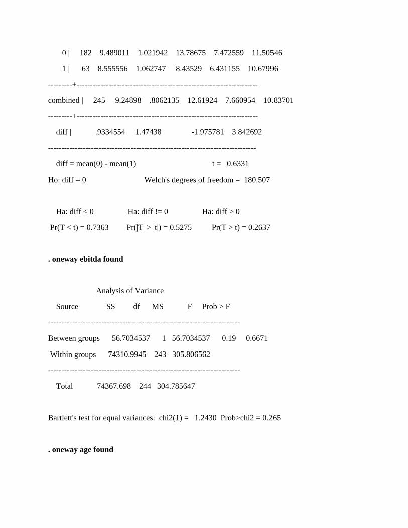
0 | 182 9.489011 1.021942 13.78675 7.472559 11.50546
1 | 63 8.555556 1.062747 8.43529 6.431155 10.67996
---------+--------------------------------------------------------------------
combined | 245 9.24898 .8062135 12.61924 7.660954 10.83701
---------+--------------------------------------------------------------------
diff | .9334554 1.47438 -1.975781 3.842692
------------------------------------------------------------------------------
diff = mean(0) - mean(1) t = 0.6331
Ho: diff = 0 Welch's degrees of freedom = 180.507
Ha: diff < 0 Ha: diff != 0 Ha: diff > 0
Pr(T < t) = 0.7363 Pr(|T| > |t|) = 0.5275 Pr(T > t) = 0.2637
. oneway ebitda found
Analysis of Variance
Source SS df MS F Prob > F
------------------------------------------------------------------------
Between groups 56.7034537 1 56.7034537 0.19 0.6671
Within groups 74310.9945 243 305.806562
------------------------------------------------------------------------
Total 74367.698 244 304.785647
Bartlett's test for equal variances: chi2(1) = 1.2430 Prob>chi2 = 0.265
. oneway age found
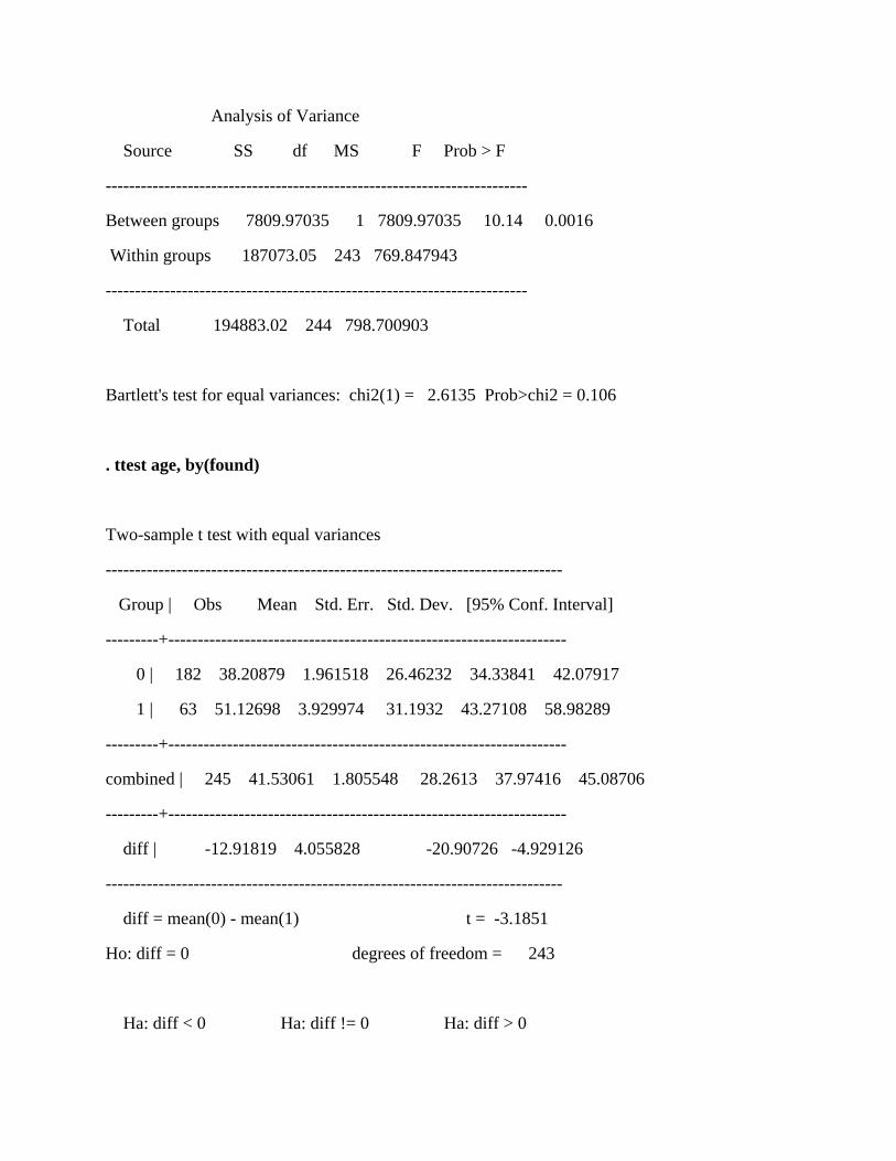
Analysis of Variance
Source SS df MS F Prob > F
------------------------------------------------------------------------
Between groups 7809.97035 1 7809.97035 10.14 0.0016
Within groups 187073.05 243 769.847943
------------------------------------------------------------------------
Total 194883.02 244 798.700903
Bartlett's test for equal variances: chi2(1) = 2.6135 Prob>chi2 = 0.106
. ttest age, by(found)
Two-sample t test with equal variances
------------------------------------------------------------------------------
Group | Obs Mean Std. Err. Std. Dev. [95% Conf. Interval]
---------+--------------------------------------------------------------------
0 | 182 38.20879 1.961518 26.46232 34.33841 42.07917
1 | 63 51.12698 3.929974 31.1932 43.27108 58.98289
---------+--------------------------------------------------------------------
combined | 245 41.53061 1.805548 28.2613 37.97416 45.08706
---------+--------------------------------------------------------------------
diff | -12.91819 4.055828 -20.90726 -4.929126
------------------------------------------------------------------------------
diff = mean(0) - mean(1) t = -3.1851
Ho: diff = 0 degrees of freedom = 243
Ha: diff < 0 Ha: diff != 0 Ha: diff > 0

Pr(T < t) = 0.0008 Pr(|T| > |t|) = 0.0016 Pr(T > t) = 0.9992
. oneway assets found
Analysis of Variance
Source SS df MS F Prob > F
------------------------------------------------------------------------
Between groups 9.6308e+13 1 9.6308e+13 5.29 0.0223
Within groups 4.4210e+15 243 1.8193e+13
------------------------------------------------------------------------
Total 4.5173e+15 244 1.8514e+13
Bartlett's test for equal variances: chi2(1) = 33.4608 Prob>chi2 = 0.000
. ttest assets, by(found) unequal welch
Two-sample t test with unequal variances
------------------------------------------------------------------------------
Group | Obs Mean Std. Err. Std. Dev. [95% Conf. Interval]
---------+--------------------------------------------------------------------
0 | 182 1126559 255601.4 3448251 622217 1630900
1 | 63 2561081 762138.9 6049290 1037587 4084575
---------+--------------------------------------------------------------------
combined | 245 1495436 274891.6 4302734 953972.6 2036899
---------+--------------------------------------------------------------------
diff | -1434523 803858.1 -3035256 166210.6
------------------------------------------------------------------------------

diff = mean(0) - mean(1) t = -1.7845
Ho: diff = 0 Welch's degrees of freedom = 76.8576
Ha: diff < 0 Ha: diff != 0 Ha: diff > 0
Pr(T < t) = 0.0391 Pr(|T| > |t|) = 0.0783 Pr(T > t) = 0.9609
diff = mean(0) - mean(1) t = -1.7845
Ho: diff = 0 Welch's degrees of freedom = 76.8576
Ha: diff < 0 Ha: diff != 0 Ha: diff > 0
Pr(T < t) = 0.0391 Pr(|T| > |t|) = 0.0783 Pr(T > t) = 0.9609
. oneway equity found
Analysis of Variance
Source SS df MS F Prob > F
------------------------------------------------------------------------
Between groups 1526.85742 1 1526.85742 5.15 0.0241
Within groups 72061.2405 243 296.548315
------------------------------------------------------------------------
Total 73588.098 244 301.590565
Bartlett's test for equal variances: chi2(1) = 0.0683 Prob>chi2 = 0.794
. ttest equity, by(found)
Two-sample t test with equal variances

------------------------------------------------------------------------------
Group | Obs Mean Std. Err. Std. Dev. [95% Conf. Interval]
---------+--------------------------------------------------------------------
0 | 182 38.35165 1.285246 17.33892 35.81566 40.88764
1 | 63 44.06349 2.125465 16.87035 39.81475 48.31224
---------+--------------------------------------------------------------------
combined | 245 39.82041 1.109496 17.36636 37.635 42.00582
---------+--------------------------------------------------------------------
diff | -5.711844 2.517241 -10.67024 -.7534468
------------------------------------------------------------------------------
diff = mean(0) - mean(1) t = -2.2691
Ho: diff = 0 degrees of freedom = 243
Ha: diff < 0 Ha: diff != 0 Ha: diff > 0
Pr(T < t) = 0.0121 Pr(|T| > |t|) = 0.0241 Pr(T > t) = 0.9879
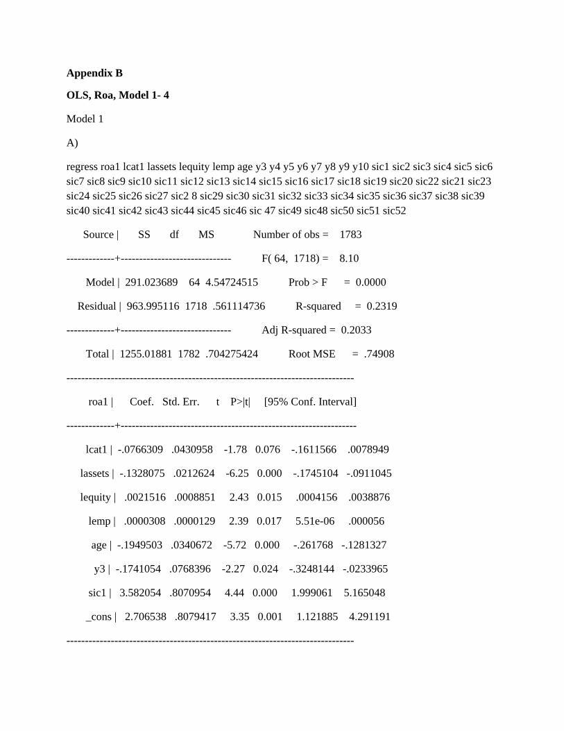
Appendix B
OLS, Roa, Model 1- 4
Model 1
A)
regress roa1 lcat1 lassets lequity lemp age y3 y4 y5 y6 y7 y8 y9 y10 sic1 sic2 sic3 sic4 sic5 sic6 sic7 sic8 sic9 sic10 sic11 sic12 sic13 sic14 sic15 sic16 sic17 sic18 sic19 sic20 sic22 sic21 sic23 sic24 sic25 sic26 sic27 sic2 8 sic29 sic30 sic31 sic32 sic33 sic34 sic35 sic36 sic37 sic38 sic39 sic40 sic41 sic42 sic43 sic44 sic45 sic46 sic 47 sic49 sic48 sic50 sic51 sic52
Source | SS df MS Number of obs = 1783
-------------+------------------------------ F( 64, 1718) = 8.10
Model | 291.023689 64 4.54724515 Prob > F = 0.0000
Residual | 963.995116 1718 .561114736 R-squared = 0.2319
-------------+------------------------------ Adj R-squared = 0.2033
Total | 1255.01881 1782 .704275424 Root MSE = .74908
------------------------------------------------------------------------------
roa1 | Coef. Std. Err. t P>|t| [95% Conf. Interval]
-------------+----------------------------------------------------------------
lcat1 | -.0766309 .0430958 -1.78 0.076 -.1611566 .0078949
lassets | -.1328075 .0212624 -6.25 0.000 -.1745104 -.0911045
lequity | .0021516 .0008851 2.43 0.015 .0004156 .0038876
lemp | .0000308 .0000129 2.39 0.017 5.51e-06 .000056
age | -.1949503 .0340672 -5.72 0.000 -.261768 -.1281327
y3 | -.1741054 .0768396 -2.27 0.024 -.3248144 -.0233965
sic1 | 3.582054 .8070954 4.44 0.000 1.999061 5.165048
_cons | 2.706538 .8079417 3.35 0.001 1.121885 4.291191
------------------------------------------------------------------------------

B)
regress roa1 lcat1 lmang1 lfambl1 lcse1 lassets lsales lequity lemp age y3 y4 y5 y6 y7 y8 y9 y10 sic1 sic2 sic3 sic4 sic5 sic6 sic7 sic8 sic9 sic10 sic11 sic12 sic13 sic14 sic15 sic16 sic17 sic18 sic19 sic20 sic22 sic21 sic23 sic24 sic25 sic26 sic27 sic28 sic29 sic30 sic31 sic32 sic33 sic34 sic35 sic36 sic37 sic38 sic39 sic40 sic41 sic42 sic43 sic44 sic45 sic46 sic47 sic49 sic48 sic50 sic51 sic52
Source | SS df MS Number of obs = 1739
-------------+------------------------------ F( 68, 1670) = 8.97
Model | 328.271222 68 4.82751798 Prob > F = 0.0000
Residual | 898.338236 1670 .537927088 R-squared = 0.2676
-------------+------------------------------ Adj R-squared = 0.2378
Total | 1226.60946 1738 .705759182 Root MSE = .73344
------------------------------------------------------------------------------
roa1 | Coef. Std. Err. t P>|t| [95% Conf. Interval]
-------------+----------------------------------------------------------------
lcat1 | .0134991 .0527968 0.26 0.798 -.0900558 .1170539
lmang1 | -.0590174 .0549789 -1.07 0.283 -.1668522 .0488174
lfambl1 | -.3356679 .0656863 -5.11 0.000 -.464504 -.2068318
lcse1 | -.1364757 .0690406 -1.98 0.048 -.2718909 -.0010605
lassets | -.2831714 .0324035 -8.74 0.000 -.3467272 -.2196156
lsales | .1930547 .0296934 6.50 0.000 .1348145 .251295
lequity | .0023984 .0008794 2.73 0.006 .0006735 .0041233
lemp | .0000108 .000013 0.83 0.406 -.0000147 .0000363
age | -.207042 .0341644 -6.06 0.000 -.2740515 -.1400324
y3 | -.1692827 .0769317 -2.20 0.028 -.3201754 -.01839
y4-y10 not given here
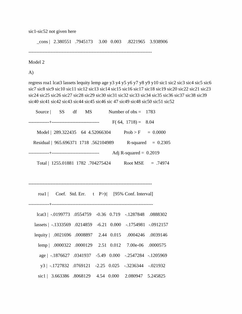
sic1-sic52 not given here
_cons | 2.380551 .7945173 3.00 0.003 .8221965 3.938906
------------------------------------------------------------------------------
Model 2
A)
regress roa1 lcat3 lassets lequity lemp age y3 y4 y5 y6 y7 y8 y9 y10 sic1 sic2 sic3 sic4 sic5 sic6 sic7 sic8 sic9 sic10 sic11 sic12 sic13 sic14 sic15 sic16 sic17 sic18 sic19 sic20 sic22 sic21 sic23 sic24 sic25 sic26 sic27 sic28 sic29 sic30 sic31 sic32 sic33 sic34 sic35 sic36 sic37 sic38 sic39 sic40 sic41 sic42 sic43 sic44 sic45 sic46 sic 47 sic49 sic48 sic50 sic51 sic52
Source | SS df MS Number of obs = 1783
-------------+------------------------------ F( 64, 1718) = 8.04
Model | 289.322435 64 4.52066304 Prob > F = 0.0000
Residual | 965.696371 1718 .562104989 R-squared = 0.2305
-------------+------------------------------ Adj R-squared = 0.2019
Total | 1255.01881 1782 .704275424 Root MSE = .74974
------------------------------------------------------------------------------
roa1 | Coef. Std. Err. t P>|t| [95% Conf. Interval]
-------------+----------------------------------------------------------------
lcat3 | -.0199773 .0554759 -0.36 0.719 -.1287848 .0888302
lassets | -.1333569 .0214859 -6.21 0.000 -.1754981 -.0912157
lequity | .0021696 .0008897 2.44 0.015 .0004246 .0039146
lemp | .0000322 .0000129 2.51 0.012 7.00e-06 .0000575
age | -.1876627 .0341937 -5.49 0.000 -.2547284 -.1205969
y3 | -.1727832 .0769121 -2.25 0.025 -.3236344 -.021932
sic1 | 3.663386 .8068129 4.54 0.000 2.080947 5.245825

_cons | 2.60337 .8065185 3.23 0.001 1.021508 4.185231
------------------------------------------------------------------------------
B)
regress roa1 lcat3 lmang1 lfambl1 lcse1 lassets lsales lequity lemp age y3 y4 y5 y6 y7 y8 y9 y10 sic1 sic2 sic3 sic4 sic5 sic6 sic7 sic8 sic9 sic10 sic11 sic12 sic13 sic14 sic15 sic16 sic17 sic18 sic19 sic20 sic22 sic21 sic23 sic24 sic25 sic26 sic27 sic28 sic29 sic30 sic31 sic32 sic33 sic34 sic35 sic36 sic37 sic38 sic39 sic40 sic41 sic42 sic43 sic44 sic45 sic46 sic47 sic49 sic48 sic50 sic51 sic52
Source | SS df MS Number of obs = 1739
-------------+------------------------------ F( 68, 1670) = 9.03
Model | 329.706242 68 4.84862121 Prob > F = 0.0000
Residual | 896.903217 1670 .537067794 R-squared = 0.2688
-------------+------------------------------ Adj R-squared = 0.2390
Total | 1226.60946 1738 .705759182 Root MSE = .73285
------------------------------------------------------------------------------
roa1 | Coef. Std. Err. t P>|t| [95% Conf. Interval]
-------------+----------------------------------------------------------------
lcat3 | .0985345 .0595548 1.65 0.098 -.0182755 .2153445
lmang1 | -.0717908 .0471968 -1.52 0.128 -.1643619 .0207804
lfambl1 | -.356901 .0668855 -5.34 0.000 -.4880892 -.2257129
lcse1 | -.1260986 .0691549 -1.82 0.068 -.2617381 .0095408
lassets | -.2773242 .032482 -8.54 0.000 -.341034 -.2136144
lsales | .1911388 .0296879 6.44 0.000 .1329093 .2493683
lequity | .0025071 .000881 2.85 0.004 .0007791 .004235
lemp | .0000111 .000013 0.85 0.394 -.0000144 .0000365
age | -.2153434 .0340581 -6.32 0.000 -.2821445 -.1485424
y3 | -.1707714 .0768629 -2.22 0.026 -.3215292 -.0200135

y4-y10 not given here
sic1 | 3.315295 .7903349 4.19 0.000 1.765144 4.865447
sic2-sic52 not given here
_cons | 2.376129 .7921215 3.00 0.003 .8224735 3.929785
------------------------------------------------------------------------------
Model 3
A
regress roa1 lown1 lassets lequity lemp age y3 y4 y5 y6 y7 y8 y9 y10 sic1 sic2 sic3 sic4 sic5 sic6 sic7 sic8 sic9sic10 sic11 sic12 sic13 sic14 sic15 sic16 sic17 sic18 sic19 sic20 sic22 sic21 sic23 sic24 sic25 sic26 sic27 sic2 8 sic29 sic30 sic31 sic32 sic33 sic34 sic35 sic36 sic37 sic38 sic39 sic40 sic41 sic42 sic43 sic44 sic45 sic46 sic 47 sic49 sic48 sic50 sic51 sic52
Source | SS df MS Number of obs = 1783
-------------+------------------------------ F( 64, 1718) = 8.12
Model | 291.543723 64 4.55537068 Prob > F = 0.0000
Residual | 963.475082 1718 .560812038 R-squared = 0.2323
-------------+------------------------------ Adj R-squared = 0.2037
Total | 1255.01881 1782 .704275424 Root MSE = .74887
------------------------------------------------------------------------------
roa1 | Coef. Std. Err. t P>|t| [95% Conf. Interval]
-------------+----------------------------------------------------------------
lown1 | -.0855693 .042307 -2.02 0.043 -.168548 -.0025905
lassets | -.1371242 .0213888 -6.41 0.000 -.1790751 -.0951733
lequity | .0019847 .0008909 2.23 0.026 .0002374 .003732
lemp | .0000291 .0000129 2.25 0.025 3.70e-06 .0000545
age | -.1891738 .0339019 -5.58 0.000 -.2556672 -.1226804
y3 | -.1726025 .0768174 -2.25 0.025 -.323268 -.0219369

y4-y10 not given here
sic1 | 3.596576 .8063191 4.46 0.000 2.015105 5.178046
sic2-sic52 not given here
_cons | 2.746943 .80878 3.40 0.001 1.160646 4.333241
------------------------------------------------------------------------------
B)
regress roa1 lown1 lmang1 lfambl1 lcse1 lassets lequity lsales lemp age y3 y4 y5 y6 y7 y8 y9 y10 sic1 sic2 sic3 sic4 sic5 sic6 sic7 sic8 sic9 sic10 sic11 sic12 sic13 sic14 sic15 sic16 sic17 sic18 sic19 sic20 sic22 sic21 sic23 sic24 sic25 sic26 sic27 sic28 sic29 sic30 sic31 sic32 sic33 sic34 sic35 sic36 sic37 sic38 sic39 sic40 sic41 sic42 sic43 sic44 sic45 sic46 sic47 sic49 sic48 sic50 sic51 sic52
Source | SS df MS Number of obs = 1739
-------------+------------------------------ F( 68, 1670) = 9.05
Model | 330.331082 68 4.85781003 Prob > F = 0.0000
Residual | 896.278377 1670 .536693639 R-squared = 0.2693
-------------+------------------------------ Adj R-squared = 0.2396
Total | 1226.60946 1738 .705759182 Root MSE = .73259
------------------------------------------------------------------------------
roa1 | Coef. Std. Err. t P>|t| [95% Conf. Interval]
-------------+----------------------------------------------------------------
lown1 | .146713 .074257 1.98 0.048 .0010665 .2923595
lmang1 | -.1659268 .0737927 -2.25 0.025 -.3106628 -.0211908
lfambl1 | -.3648483 .0672611 -5.42 0.000 -.4967732 -.2329234
lcse1 | -.1224132 .0692145 -1.77 0.077 -.2581696 .0133432
lassets | -.2803521 .0323306 -8.67 0.000 -.3437649 -.2169394
lequity | .0025669 .0008823 2.91 0.004 .0008363 .0042975

lsales | .190609 .029681 6.42 0.000 .132393 .2488249
lemp | .0000121 .000013 0.93 0.351 -.0000134 .0000376
age | -.2056694 .033804 -6.08 0.000 -.271972 -.1393668
y3 | -.1678604 .076838 -2.18 0.029 -.3185694 -.0171513
y4-y10 not given here
sic1 | 3.474929 .7932909 4.38 0.000 1.918979 5.030878
sic2-sic52 not given here
_cons | 2.229931 .796131 2.80 0.005 .6684112 3.791451
------------------------------------------------------------------------------
Model 4
A)
regress roa1 lmang1 lassets lequity lemp age y3 y4 y5 y6 y7 y8 y9 y10 sic1 sic2 sic3 sic4 sic5 sic6 sic7 sic8 sic9 sic10 sic11 sic12 sic13 sic14 sic15 sic16 sic17 sic18 sic19 sic20 sic22 sic21 sic23 sic24 sic25 sic26 sic27 sic 28 sic29 sic30 sic31 sic32 sic33 sic34 sic35 sic36 sic37 sic38 sic39 sic40 sic41 sic42 sic43 sic44 sic45 sic46 sic47 sic49 sic48 sic50 sic51 sic52
Source | SS df MS Number of obs = 1783
-------------+------------------------------ F( 64, 1718) = 8.24
Model | 294.662767 64 4.60410573 Prob > F = 0.0000
Residual | 960.356038 1718 .55899653 R-squared = 0.2348
-------------+------------------------------ Adj R-squared = 0.2063
Total | 1255.01881 1782 .704275424 Root MSE = .74766
------------------------------------------------------------------------------
roa1 | Coef. Std. Err. t P>|t| [95% Conf. Interval]
-------------+----------------------------------------------------------------
lmang1 | -.1336106 .0429356 -3.11 0.002 -.2178222 -.0493991
lassets | -.1403356 .0213773 -6.56 0.000 -.1822639 -.0984073

lequity | .0019911 .0008856 2.25 0.025 .0002542 .003728
lemp | .0000277 .0000129 2.15 0.032 2.44e-06 .000053
age | -.1855063 .0338673 -5.48 0.000 -.2519318 -.1190807
y3 | -.17079 .0766963 -2.23 0.026 -.3212179 -.0203621
y4-y10 not given here
sic1 | 3.692266 .8045167 4.59 0.000 2.11433 5.270202
sic2-sic52, not given here
_cons | 2.686888 .804553 3.34 0.001 1.108881 4.264894
------------------------------------------------------------------------------
B)
regress roa1 lmang1 lfambl1 lcse1 lassets lequity lsales lemp age y3 y4 y5 y6 y7 y8 y9 y10 sic1 sic2 sic3 sic4 sic5 sic6 sic7 sic8 sic9 sic10 sic11 sic12 sic13 sic14 sic15 sic16 sic17 sic18 sic19 sic20 sic22 sic21 sic23 sic24 sic25 sic26 sic27 sic28 sic29 sic30 sic31 sic32 sic33 sic34 sic35 sic36 sic37 sic38 sic39 sic40 sic41 sic42 sic43sic44 sic45 sic46 sic47 sic49 sic48 sic50 sic51 sic52
Source | SS df MS Number of obs = 1739
-------------+------------------------------ F( 67, 1671) = 9.11
Model | 328.236057 67 4.89904563 Prob > F = 0.0000
Residual | 898.373402 1671 .537626213 R-squared = 0.2676
-------------+------------------------------ Adj R-squared = 0.2382
Total | 1226.60946 1738 .705759182 Root MSE = .73323
------------------------------------------------------------------------------
roa1 | Coef. Std. Err. t P>|t| [95% Conf. Interval]
-------------+----------------------------------------------------------------
lmang1 | -.0511472 .0455414 -1.12 0.262 -.1404713 .038177
lfambl1 | -.3355857 .0656671 -5.11 0.000 -.4643842 -.2067872
lcse1 | -.1356657 .0689486 -1.97 0.049 -.2709004 -.000431
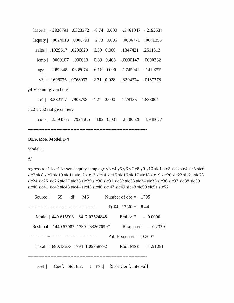
lassets | -.2826791 .0323372 -8.74 0.000 -.3461047 -.2192534
lequity | .0024013 .0008791 2.73 0.006 .0006771 .0041256
lsales | .1929617 .0296829 6.50 0.000 .1347421 .2511813
lemp | .0000107 .000013 0.83 0.408 -.0000147 .0000362
age | -.2082848 .0338074 -6.16 0.000 -.2745941 -.1419755
y3 | -.1696076 .0768997 -2.21 0.028 -.3204374 -.0187778
y4-y10 not given here
sic1 | 3.332177 .7906798 4.21 0.000 1.78135 4.883004
sic2-sic52 not given here
_cons | 2.394365 .7924565 3.02 0.003 .8400528 3.948677
------------------------------------------------------------------------------
OLS, Roe, Model 1-4
Model 1
A)
regress roe1 lcat1 lassets lequity lemp age y3 y4 y5 y6 y7 y8 y9 y10 sic1 sic2 sic3 sic4 sic5 sic6 sic7 sic8 sic9 sic10 sic11 sic12 sic13 sic14 sic15 sic16 sic17 sic18 sic19 sic20 sic22 sic21 sic23 sic24 sic25 sic26 sic27 sic28 sic29 sic30 sic31 sic32 sic33 sic34 sic35 sic36 sic37 sic38 sic39 sic40 sic41 sic42 sic43 sic44 sic45 sic46 sic 47 sic49 sic48 sic50 sic51 sic52
Source | SS df MS Number of obs = 1795
-------------+------------------------------ F( 64, 1730) = 8.44
Model | 449.615903 64 7.02524848 Prob > F = 0.0000
Residual | 1440.52082 1730 .832670997 R-squared = 0.2379
-------------+------------------------------ Adj R-squared = 0.2097
Total | 1890.13673 1794 1.05358792 Root MSE = .91251
------------------------------------------------------------------------------
roe1 | Coef. Std. Err. t P>|t| [95% Conf. Interval]
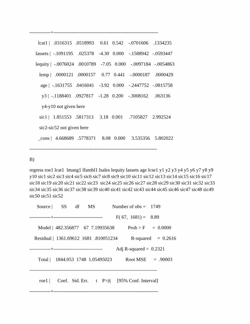
-------------+----------------------------------------------------------------
lcat1 | .0316315 .0518993 0.61 0.542 -.0701606 .1334235
lassets | -.1091195 .025378 -4.30 0.000 -.1588942 -.0593447
lequity | -.0076024 .0010789 -7.05 0.000 -.0097184 -.0054863
lemp | .0000121 .0000157 0.77 0.441 -.0000187 .0000429
age | -.1631755 .0416041 -3.92 0.000 -.2447752 -.0815758
y3 | -.1188401 .0927817 -1.28 0.200 -.3008162 .063136
y4-y10 not given here
sic1 | 1.851553 .5817313 3.18 0.001 .7105827 2.992524
sic2-sic52 not given here
_cons | 4.668689 .5778371 8.08 0.000 3.535356 5.802022
------------------------------------------------------------------------------
B)
regress roe1 lcat1 lmang1 lfambl1 lsales lequity lassets age lcse1 y1 y2 y3 y4 y5 y6 y7 y8 y9 y10 sic1 sic2 sic3 sic4 sic5 sic6 sic7 sic8 sic9 sic10 sic11 sic12 sic13 sic14 sic15 sic16 sic17 sic18 sic19 sic20 sic21 sic22 sic23 sic24 sic25 sic26 sic27 sic28 sic29 sic30 sic31 sic32 sic33 sic34 sic35 sic36 sic37 sic38 sic39 sic40 sic41 sic42 sic43 sic44 sic45 sic46 sic47 sic48 sic49 sic50 sic51 sic52
Source | SS df MS Number of obs = 1749
-------------+------------------------------ F( 67, 1681) = 8.89
Model | 482.356877 67 7.19935638 Prob > F = 0.0000
Residual | 1361.69612 1681 .810051234 R-squared = 0.2616
-------------+------------------------------ Adj R-squared = 0.2321
Total | 1844.053 1748 1.05495023 Root MSE = .90003
------------------------------------------------------------------------------
roe1 | Coef. Std. Err. t P>|t| [95% Conf. Interval]
-------------+----------------------------------------------------------------

lcat1 | .1030801 .0635939 1.62 0.105 -.0216514 .2278116
lmang1 | -.0247379 .0672259 -0.37 0.713 -.1565931 .1071174
lfambl1 | -.3175933 .0813029 -3.91 0.000 -.4770589 -.1581278
lsales | .1639054 .0340705 4.81 0.000 .0970804 .2307305
lequity | -.0067121 .0010771 -6.23 0.000 -.0088246 -.0045995
lassets | -.2237207 .0354601 -6.31 0.000 -.2932714 -.15417
age | -.1760677 .0420865 -4.18 0.000 -.2586152 -.0935202
lcse1 | -.2656095 .0854817 -3.11 0.002 -.4332713 -.0979477
y2 | .169475 .0948146 1.79 0.074 -.0164922 .3554421
y3-y10 not provided here
sic1 | 2.179983 .5322603 4.10 0.000 1.13602 3.223946
sic2-sic52 not provided here
_cons | 3.46666 .4919244 7.05 0.000 2.501811 4.431509
Model 2
A)
regress roe1 lcat3 lassets lequity lemp age y3 y4 y5 y6 y7 y8 y9 y10 sic1 sic2 sic3 sic4 sic5 sic6 sic7 sic8 sic9 sic10 sic11 sic12 sic13 sic14 sic15 sic16 sic17 sic18 sic19 sic20 sic22 sic21 sic23 sic24 sic25 sic26 sic27 sic28 sic29 sic30 sic31 sic32 sic33 sic34 sic35 sic36 sic37 sic38 sic39 sic40 sic41 sic42 sic43 sic44 sic45 sic46 sic47 sic49 sic48 sic50 sic51 sic52
Source | SS df MS Number of obs = 1795
-------------+------------------------------ F( 64, 1730) = 8.43
Model | 449.32278 64 7.02066844 Prob > F = 0.0000
Residual | 1440.81395 1730 .832840432 R-squared = 0.2377
-------------+------------------------------ Adj R-squared = 0.2095
Total | 1890.13673 1794 1.05358792 Root MSE = .9126
------------------------------------------------------------------------------

roe1 | Coef. Std. Err. t P>|t| [95% Conf. Interval]
-------------+----------------------------------------------------------------
lcat3 | .0094849 .0680409 0.14 0.889 -.1239662 .142936
lassets | -.1084683 .0256717 -4.23 0.000 -.1588191 -.0581175
lequity | -.0075886 .0010849 -6.99 0.000 -.0097165 -.0054607
lemp | .0000113 .0000157 0.72 0.470 -.0000194 .0000421
age | -.1659622 .0418306 -3.97 0.000 -.2480061 -.0839183
y3 | -.1197105 .0927892 -1.29 0.197 -.3017014 .0622804
y4-y10 not given here
sic1 | 1.815664 .5795709 3.13 0.002 .6789311 2.952398
sic2-sic52 not given here
_cons | 4.705062 .5747551 8.19 0.000 3.577774 5.83235
------------------------------------------------------------------------------
B)
regress roe1 lcat3 lmang1 lfambl1 lsales lequity lassets age lcse1 y1 y2 y3 y4 y5 y6 y7 y8 y9 y10 sic1 sic2 sic3 sic4 sic5 sic6 sic7 sic8 sic9 sic10 sic11 sic12 sic13 sic14 sic15 sic16 sic17 sic18 sic19 sic20 sic21 sic22 sic23 sic24 sic25 sic26 sic27 sic28 sic29 sic30 sic31 sic32 sic33 sic34 sic35 sic36 sic37 sic38 sic39 sic40 sic41 sic42 sic43 sic44 sic45 sic46 sic47 sic48 sic49 sic50 sic51 sic52
Source | SS df MS Number of obs = 1749
-------------+------------------------------ F( 67, 1681) = 8.87
Model | 481.637365 67 7.18861739 Prob > F = 0.0000
Residual | 1362.41564 1681 .81047926 R-squared = 0.2612
-------------+------------------------------ Adj R-squared = 0.2317
Total | 1844.053 1748 1.05495023 Root MSE = .90027
------------------------------------------------------------------------------
roe1 | Coef. Std. Err. t P>|t| [95% Conf. Interval]

-------------+----------------------------------------------------------------
lcat3 | .0967928 .0734162 1.32 0.188 -.047204 .2407897
lmang1 | .0154504 .0580452 0.27 0.790 -.0983982 .1292989
lfambl1 | -.3387099 .0828649 -4.09 0.000 -.5012391 -.1761807
lsales | .1615036 .034087 4.74 0.000 .0946461 .2283611
lequity | -.0064955 .0010802 -6.01 0.000 -.0086142 -.0043768
lassets | -.214142 .0356315 -6.01 0.000 -.2840287 -.1442552
age | -.1924089 .0420695 -4.57 0.000 -.2749231 -.1098948
lcse1 | -.2505971 .0857592 -2.92 0.004 -.4188031 -.0823911
y3 | .0329296 .0934054 0.35 0.724 -.1502736 .2161328
y2-y10 not provided here
sic1 | 2.157624 .5324915 4.05 0.000 1.113208 3.20204
sic2-sic52 not provided here
_cons | 3.423087 .4926941 6.95 0.000 2.456729 4.389446
Model 3
A)
regress roe1 lown1 lassets lequity lemp age y3 y4 y5 y6 y7 y8 y9 y10 sic1 sic2 sic3 sic4 sic5 sic6 sic7 sic8 sic9 sic10 sic11 sic12 sic13 sic14 sic15 sic16 sic17 sic18 sic19 sic20 sic22 sic21 sic23 sic24 sic25 sic26 sic27 sic28 sic29 sic30 sic31 sic32 sic33 sic34 sic35 sic36 sic37 sic38 sic39 sic40 sic41 sic42 sic43 sic44 sic45 sic46 sic47 sic49 sic48 sic50 sic51 sic52
Source | SS df MS Number of obs = 1795
-------------+------------------------------ F( 64, 1730) = 8.44
Model | 449.812686 64 7.02832322 Prob > F = 0.0000
Residual | 1440.32404 1730 .83255725 R-squared = 0.2380
-------------+------------------------------ Adj R-squared = 0.2098
Total | 1890.13673 1794 1.05358792 Root MSE = .91245

------------------------------------------------------------------------------
roe1 | Coef. Std. Err. t P>|t| [95% Conf. Interval]
-------------+----------------------------------------------------------------
lown1 | .0397372 .0509672 0.78 0.436 -.0602266 .139701
lassets | -.1070673 .0254972 -4.20 0.000 -.1570758 -.0570588
lequity | -.0075215 .001084 -6.94 0.000 -.0096476 -.0053953
lemp | .0000131 .0000158 0.83 0.409 -.000018 .0000441
age | -.1658543 .0414764 -4.00 0.000 -.2472034 -.0845051
y3 | -.119258 .0927685 -1.29 0.199 -.3012083 .0626923
y4-y10 not given here
sic1 | 1.848432 .580422 3.18 0.001 .7100296 2.986835
sic2-sic52 not given here
_cons | 4.645122 .5798193 8.01 0.000 3.507901 5.782342
------------------------------------------------------------------------------
B)
regress roe1 lown1 lmang1 lfambl1 lsales lequity lassets age lcse1 y1 y2 y3 y4 y5 y6 y7 y8 y9 y10 sic1 sic2 sic3 sic4 sic5 sic6 sic7 sic8 sic9 sic10 sic11 sic12 sic13 sic14 sic15 sic16 sic17 sic18 sic19 sic20 sic21 sic22 sic23 sic24 sic25 sic26 sic27 sic28 sic29 sic30 sic31 sic32 sic33 sic34 sic35 sic36 sic37 sic38 sic39 sic40 sic41 sic42 sic43 sic44 sic45 sic46 sic47 sic48 sic49 sic50 sic51 sic52
Source | SS df MS Number of obs = 1749
-------------+------------------------------ F( 67, 1681) = 9.10
Model | 490.661962 67 7.32331286 Prob > F = 0.0000
Residual | 1353.39104 1681 .805110672 R-squared = 0.2661
-------------+------------------------------ Adj R-squared = 0.2368
Total | 1844.053 1748 1.05495023 Root MSE = .89728

------------------------------------------------------------------------------
roe1 | Coef. Std. Err. t P>|t| [95% Conf. Interval]
-------------+----------------------------------------------------------------
lown1 | .3187403 .0885426 3.60 0.000 .145075 .4924057
lmang1 | -.2139746 .089001 -2.40 0.016 -.388539 -.0394102
lfambl1 | -.378558 .0827964 -4.57 0.000 -.5409529 -.2161631
lsales | .1609786 .0339635 4.74 0.000 .0943635 .2275938
lequity | -.006393 .0010743 -5.95 0.000 -.0085 -.004286
lassets | -.2148135 .0352908 -6.09 0.000 -.284032 -.145595
age | -.1814201 .0415911 -4.36 0.000 -.2629959 -.0998444
lcse1 | -.2251299 .0857175 -2.63 0.009 -.3932541 -.0570057
y2 | .168641 .0945159 1.78 0.075 -.0167403 .3540222
y1-y10 not provided here
sic1 | 2.152449 .5306404 4.06 0.000 1.111664 3.193235
sic2-sic52 not provided here
_cons | 3.399885 .490644 6.93 0.000 2.437548 4.362222
Model 4
A)
regress roe1 lmang1 lassets lequity lemp age y3 y4 y5 y6 y7 y8 y9 y10 sic1 sic2 sic3 sic4 sic5 sic6 sic7 sic8 sic9 sic10 sic11 sic12 sic13 sic14 sic15 sic16 sic17 sic18 sic19 sic20 sic22 sic21 sic23 sic24 sic25 sic26 sic27 sic28 sic29 sic30 sic31 sic32 sic33 sic34 sic35 sic36 sic37 sic38 sic39 sic40 sic41 sic42 sic43 sic44 sic45 sic46 sic47 sic49 sic48 sic50 sic51 sic52
Source | SS df MS Number of obs = 1795
-------------+------------------------------ F( 64, 1730) = 8.45
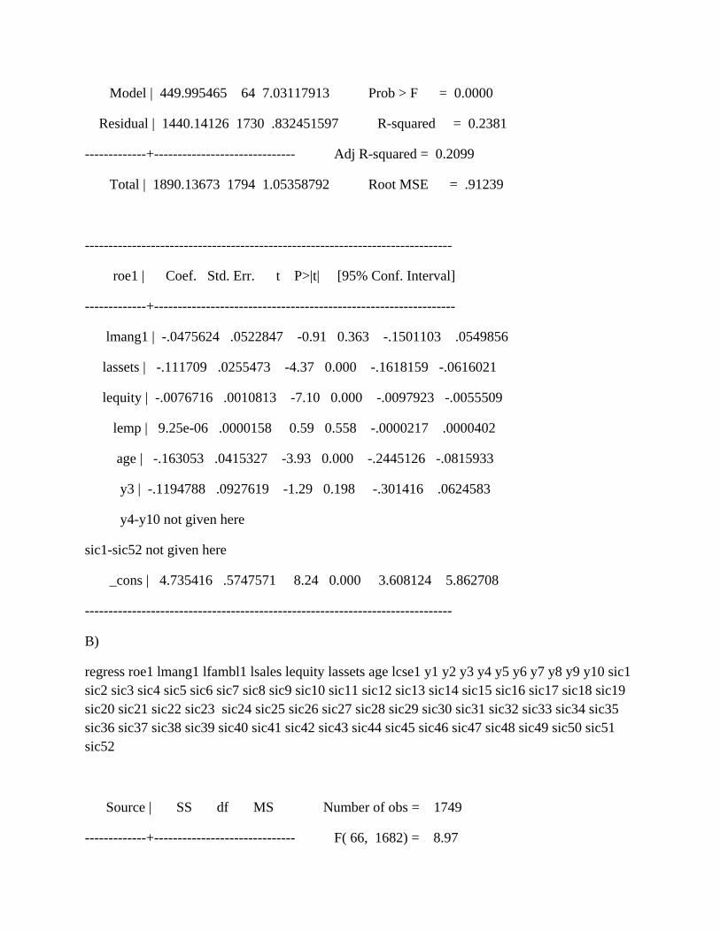
Model | 449.995465 64 7.03117913 Prob > F = 0.0000
Residual | 1440.14126 1730 .832451597 R-squared = 0.2381
-------------+------------------------------ Adj R-squared = 0.2099
Total | 1890.13673 1794 1.05358792 Root MSE = .91239
------------------------------------------------------------------------------
roe1 | Coef. Std. Err. t P>|t| [95% Conf. Interval]
-------------+----------------------------------------------------------------
lmang1 | -.0475624 .0522847 -0.91 0.363 -.1501103 .0549856
lassets | -.111709 .0255473 -4.37 0.000 -.1618159 -.0616021
lequity | -.0076716 .0010813 -7.10 0.000 -.0097923 -.0055509
lemp | 9.25e-06 .0000158 0.59 0.558 -.0000217 .0000402
age | -.163053 .0415327 -3.93 0.000 -.2445126 -.0815933
y3 | -.1194788 .0927619 -1.29 0.198 -.301416 .0624583
y4-y10 not given here
sic1-sic52 not given here
_cons | 4.735416 .5747571 8.24 0.000 3.608124 5.862708
------------------------------------------------------------------------------
B)
regress roe1 lmang1 lfambl1 lsales lequity lassets age lcse1 y1 y2 y3 y4 y5 y6 y7 y8 y9 y10 sic1 sic2 sic3 sic4 sic5 sic6 sic7 sic8 sic9 sic10 sic11 sic12 sic13 sic14 sic15 sic16 sic17 sic18 sic19 sic20 sic21 sic22 sic23 sic24 sic25 sic26 sic27 sic28 sic29 sic30 sic31 sic32 sic33 sic34 sic35 sic36 sic37 sic38 sic39 sic40 sic41 sic42 sic43 sic44 sic45 sic46 sic47 sic48 sic49 sic50 sic51 sic52
Source | SS df MS Number of obs = 1749
-------------+------------------------------ F( 66, 1682) = 8.97

Model | 480.228582 66 7.27619063 Prob > F = 0.0000
Residual | 1363.82442 1682 .81083497 R-squared = 0.2604
-------------+------------------------------ Adj R-squared = 0.2314
Total | 1844.053 1748 1.05495023 Root MSE = .90046
------------------------------------------------------------------------------
roe1 | Coef. Std. Err. t P>|t| [95% Conf. Interval]
-------------+----------------------------------------------------------------
lmang1 | .035584 .0560127 0.64 0.525 -.0742779 .1454458
lfambl1 | -.3177417 .0813422 -3.91 0.000 -.4772842 -.1581992
lsales | .1628056 .0340802 4.78 0.000 .0959615 .2296496
lequity | -.0066222 .0010762 -6.15 0.000 -.008733 -.0045114
lassets | -.2196895 .0353899 -6.21 0.000 -.2891025 -.1502766
age | -.1852331 .0417251 -4.44 0.000 -.2670717 -.1033945
lcse1 | -.2603144 .0854606 -3.05 0.002 -.4279347 -.092694
y2 | .1721287 .0948463 1.81 0.070 -.0139005 .358158
y2-y10 not provided here
sic1 | 2.17208 .5324954 4.08 0.000 1.127657 3.216503
sic2-sic52 not provided here
_cons | 3.457083 .4921268 7.02 0.000 2.491837 4.422328
------------------------------------------------------------------------------
OLS, EBITDA, Model 1-4
Model 1
A)
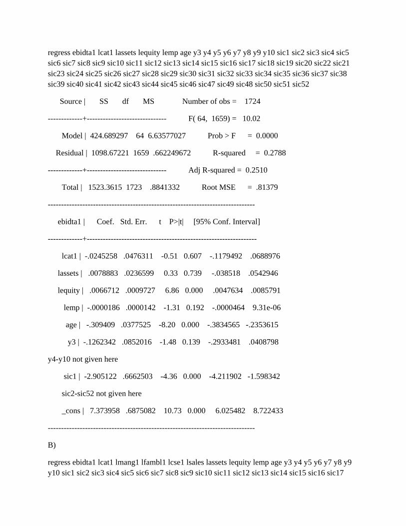
regress ebidta1 lcat1 lassets lequity lemp age y3 y4 y5 y6 y7 y8 y9 y10 sic1 sic2 sic3 sic4 sic5 sic6 sic7 sic8 sic9 sic10 sic11 sic12 sic13 sic14 sic15 sic16 sic17 sic18 sic19 sic20 sic22 sic21 sic23 sic24 sic25 sic26 sic27 sic28 sic29 sic30 sic31 sic32 sic33 sic34 sic35 sic36 sic37 sic38 sic39 sic40 sic41 sic42 sic43 sic44 sic45 sic46 sic47 sic49 sic48 sic50 sic51 sic52
Source | SS df MS Number of obs = 1724
-------------+------------------------------ F( 64, 1659) = 10.02
Model | 424.689297 64 6.63577027 Prob > F = 0.0000
Residual | 1098.67221 1659 .662249672 R-squared = 0.2788
-------------+------------------------------ Adj R-squared = 0.2510
Total | 1523.3615 1723 .8841332 Root MSE = .81379
------------------------------------------------------------------------------
ebidta1 | Coef. Std. Err. t P>|t| [95% Conf. Interval]
-------------+----------------------------------------------------------------
lcat1 | -.0245258 .0476311 -0.51 0.607 -.1179492 .0688976
lassets | .0078883 .0236599 0.33 0.739 -.038518 .0542946
lequity | .0066712 .0009727 6.86 0.000 .0047634 .0085791
lemp | -.0000186 .0000142 -1.31 0.192 -.0000464 9.31e-06
age | -.309409 .0377525 -8.20 0.000 -.3834565 -.2353615
y3 | -.1262342 .0852016 -1.48 0.139 -.2933481 .0408798
y4-y10 not given here
sic1 | -2.905122 .6662503 -4.36 0.000 -4.211902 -1.598342
sic2-sic52 not given here
_cons | 7.373958 .6875082 10.73 0.000 6.025482 8.722433
------------------------------------------------------------------------------
B)
regress ebidta1 lcat1 lmang1 lfambl1 lcse1 lsales lassets lequity lemp age y3 y4 y5 y6 y7 y8 y9 y10 sic1 sic2 sic3 sic4 sic5 sic6 sic7 sic8 sic9 sic10 sic11 sic12 sic13 sic14 sic15 sic16 sic17
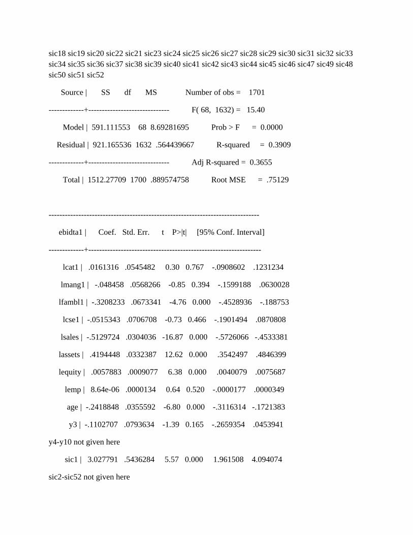
sic18 sic19 sic20 sic22 sic21 sic23 sic24 sic25 sic26 sic27 sic28 sic29 sic30 sic31 sic32 sic33 sic34 sic35 sic36 sic37 sic38 sic39 sic40 sic41 sic42 sic43 sic44 sic45 sic46 sic47 sic49 sic48 sic50 sic51 sic52
Source | SS df MS Number of obs = 1701
-------------+------------------------------ F( 68, 1632) = 15.40
Model | 591.111553 68 8.69281695 Prob > F = 0.0000
Residual | 921.165536 1632 .564439667 R-squared = 0.3909
-------------+------------------------------ Adj R-squared = 0.3655
Total | 1512.27709 1700 .889574758 Root MSE = .75129
------------------------------------------------------------------------------
ebidta1 | Coef. Std. Err. t P>|t| [95% Conf. Interval]
-------------+----------------------------------------------------------------
lcat1 | .0161316 .0545482 0.30 0.767 -.0908602 .1231234
lmang1 | -.048458 .0568266 -0.85 0.394 -.1599188 .0630028
lfambl1 | -.3208233 .0673341 -4.76 0.000 -.4528936 -.188753
lcse1 | -.0515343 .0706708 -0.73 0.466 -.1901494 .0870808
lsales | -.5129724 .0304036 -16.87 0.000 -.5726066 -.4533381
lassets | .4194448 .0332387 12.62 0.000 .3542497 .4846399
lequity | .0057883 .0009077 6.38 0.000 .0040079 .0075687
lemp | 8.64e-06 .0000134 0.64 0.520 -.0000177 .0000349
age | -.2418848 .0355592 -6.80 0.000 -.3116314 -.1721383
y3 | -.1102707 .0793634 -1.39 0.165 -.2659354 .0453941
y4-y10 not given here
sic1 | 3.027791 .5436284 5.57 0.000 1.961508 4.094074
sic2-sic52 not given here
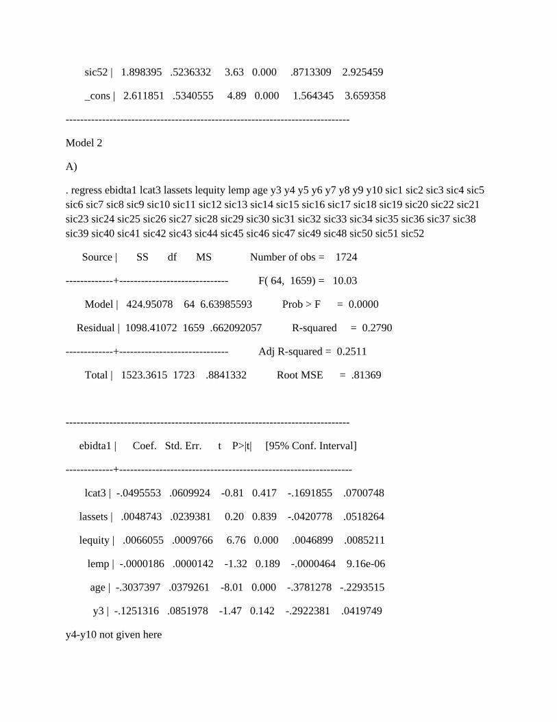
sic52 | 1.898395 .5236332 3.63 0.000 .8713309 2.925459
_cons | 2.611851 .5340555 4.89 0.000 1.564345 3.659358
------------------------------------------------------------------------------
Model 2
A)
. regress ebidta1 lcat3 lassets lequity lemp age y3 y4 y5 y6 y7 y8 y9 y10 sic1 sic2 sic3 sic4 sic5 sic6 sic7 sic8 sic9 sic10 sic11 sic12 sic13 sic14 sic15 sic16 sic17 sic18 sic19 sic20 sic22 sic21 sic23 sic24 sic25 sic26 sic27 sic28 sic29 sic30 sic31 sic32 sic33 sic34 sic35 sic36 sic37 sic38 sic39 sic40 sic41 sic42 sic43 sic44 sic45 sic46 sic47 sic49 sic48 sic50 sic51 sic52
Source | SS df MS Number of obs = 1724
-------------+------------------------------ F( 64, 1659) = 10.03
Model | 424.95078 64 6.63985593 Prob > F = 0.0000
Residual | 1098.41072 1659 .662092057 R-squared = 0.2790
-------------+------------------------------ Adj R-squared = 0.2511
Total | 1523.3615 1723 .8841332 Root MSE = .81369
------------------------------------------------------------------------------
ebidta1 | Coef. Std. Err. t P>|t| [95% Conf. Interval]
-------------+----------------------------------------------------------------
lcat3 | -.0495553 .0609924 -0.81 0.417 -.1691855 .0700748
lassets | .0048743 .0239381 0.20 0.839 -.0420778 .0518264
lequity | .0066055 .0009766 6.76 0.000 .0046899 .0085211
lemp | -.0000186 .0000142 -1.32 0.189 -.0000464 9.16e-06
age | -.3037397 .0379261 -8.01 0.000 -.3781278 -.2293515
y3 | -.1251316 .0851978 -1.47 0.142 -.2922381 .0419749
y4-y10 not given here

sic52 | -4.364491 .6437066 -6.78 0.000 -5.627054 -3.101929
sic1-sic51 not given here
_cons | 7.407422 .6890357 10.75 0.000 6.055951 8.758893
------------------------------------------------------------------------------
B)
regress ebidta1 lcat3 lmang1 lfambl1 lcse1 lsales lassets lequity lemp age y3 y4 y5 y6 y7 y8 y9 y10 sic1 sic2 sic3 sic4 sic5 sic6 sic7 sic8 sic9 sic10 sic11 sic12 sic13 sic14 sic15 sic16 sic17 sic18 sic19 sic20 sic22 sic21 sic23 sic24 sic25 sic26 sic27 sic28 sic29 sic30 sic31 sic32 sic33 sic34 sic35 sic36 sic37 sic38 sic39 sic40 sic41 sic42 sic43 sic44 sic45 sic46 sic47 sic49 sic48 sic50 sic51 sic52
Source | SS df MS Number of obs = 1701
-------------+------------------------------ F( 68, 1632) = 15.42
Model | 591.670051 68 8.70103017 Prob > F = 0.0000
Residual | 920.607037 1632 .564097449 R-squared = 0.3912
-------------+------------------------------ Adj R-squared = 0.3659
Total | 1512.27709 1700 .889574758 Root MSE = .75106
------------------------------------------------------------------------------
ebidta1 | Coef. Std. Err. t P>|t| [95% Conf. Interval]
-------------+----------------------------------------------------------------
lcat3 | .0638604 .0615185 1.04 0.299 -.0568031 .1845239
lmang1 | -.052747 .049046 -1.08 0.282 -.1489468 .0434527
lfambl1 | -.3340651 .0685491 -4.87 0.000 -.4685186 -.1996116
lcse1 | -.0451682 .0707986 -0.64 0.524 -.1840338 .0936975
lsales | -.5145372 .0304217 -16.91 0.000 -.5742069 -.4548675
lassets | .4241005 .0333753 12.71 0.000 .3586376 .4895634

lequity | .0058644 .0009099 6.45 0.000 .0040797 .0076492
lemp | 8.72e-06 .0000134 0.65 0.515 -.0000176 .000035
age | -.2481201 .0355062 -6.99 0.000 -.3177626 -.1784775
y3 | -.1113804 .0793338 -1.40 0.161 -.2669871 .0442263
y4-y10 not given here
sic1 | 2.99725 .5399328 5.55 0.000 1.938215 4.056284
sic2-sic52 not given here
_cons | 2.613083 .5313842 4.92 0.000 1.570816 3.65535
------------------------------------------------------------------------------
Model 3
A)
regress ebidta1 lown1 lassets lequity lemp age y3 y4 y5 y6 y7 y8 y9 y10 sic1 sic2 sic3 sic4 sic5 sic6 sic7 sic8 sic9 sic10 sic11 sic12 sic13 sic14 sic15 sic16 sic17 sic18 sic19 sic20 sic22 sic21 sic23 sic24 sic25 sic26 sic27 sic28 sic29 sic30 sic31 sic32 sic33 sic34 sic35 sic36 sic37 sic38 sic39 sic40 sic41 sic42 sic43 sic44 sic45 sic46 sic47 sic49 sic48 sic50 sic51 sic52
Source | SS df MS Number of obs = 1724
-------------+------------------------------ F( 64, 1659) = 10.05
Model | 425.496168 64 6.64837763 Prob > F = 0.0000
Residual | 1097.86533 1659 .661763312 R-squared = 0.2793
-------------+------------------------------ Adj R-squared = 0.2515
Total | 1523.3615 1723 .8841332 Root MSE = .81349
------------------------------------------------------------------------------
ebidta1 | Coef. Std. Err. t P>|t| [95% Conf. Interval]
-------------+----------------------------------------------------------------
lown1 | -.0567492 .0465752 -1.22 0.223 -.1481016 .0346031

lassets | .0048115 .0237818 0.20 0.840 -.0418341 .0514571
lequity | .0065575 .0009773 6.71 0.000 .0046406 .0084744
lemp | -.0000203 .0000143 -1.42 0.155 -.0000483 7.69e-06
age | -.3070121 .0376021 -8.16 0.000 -.3807647 -.2332595
y3 | -.1254206 .0851709 -1.47 0.141 -.2924743 .0416331
y4-y10 not given here
sic2 | -3.661801 .6481264 -5.65 0.000 -4.933033 -2.390569
sic1-sic51 not given here
_cons | 7.423455 .6886624 10.78 0.000 6.072716 8.774194
------------------------------------------------------------------------------
B)
regress ebidta1 lown1 lmang1 lfambl1 lcse1 lsales lassets lequity lemp age y3 y4 y5 y6 y7 y8 y9 y10 sic1 sic2 sic3 sic4 sic5 sic6 sic7 sic8 sic9 sic10 sic11 sic12 sic13 sic14 sic15 sic16 sic17 sic18 sic19 sic20 sic22 sic21 sic23 sic24 sic25 sic26 sic27 sic28 sic29 sic30 sic31 sic32 sic33 sic34 sic35 sic36 sic37 sic38 sic39 sic40 sic41 sic42 sic43 sic44 sic45 sic46 sic47 sic49 sic48 sic50 sic51 sic52
Source | SS df MS Number of obs = 1701
-------------+------------------------------ F( 68, 1632) = 15.45
Model | 592.29331 68 8.71019573 Prob > F = 0.0000
Residual | 919.983779 1632 .563715551 R-squared = 0.3917
-------------+------------------------------ Adj R-squared = 0.3663
Total | 1512.27709 1700 .889574758 Root MSE = .75081
------------------------------------------------------------------------------
ebidta1 | Coef. Std. Err. t P>|t| [95% Conf. Interval]
-------------+----------------------------------------------------------------
lown1 | .1130309 .0764851 1.48 0.140 -.0369884 .2630502

lmang1 | -.1273064 .0761046 -1.67 0.095 -.2765795 .0219666
lfambl1 | -.3431941 .0690027 -4.97 0.000 -.4785373 -.2078509
lcse1 | -.0399957 .0709445 -0.56 0.573 -.1791476 .0991561
lsales | -.5151606 .030412 -16.94 0.000 -.5748113 -.4555098
lassets | .4221993 .0331719 12.73 0.000 .3571353 .4872634
lequity | .0059191 .000911 6.50 0.000 .0041323 .007706
lemp | 9.61e-06 .0000134 0.72 0.474 -.0000167 .0000359
age | -.2419205 .0352076 -6.87 0.000 -.3109772 -.1728637
y3 | -.1095582 .0793068 -1.38 0.167 -.265112 .0459957
y4-y10 not given here
sic1 | 3.119111 .5447305 5.73 0.000 2.050666 4.187556
sic2-sic52 not given here
sic52 | 1.958908 .518204 3.78 0.000 .9424926 2.975323
_cons | 2.502071 .5377796 4.65 0.000 1.44726 3.556882
------------------------------------------------------------------------------
Model 4
A)
regress ebidta1 lmang1 lassets lequity lemp age y3 y4 y5 y6 y7 y8 y9 y10 sic1 sic2 sic3 sic4 sic5 sic6 sic7 sic8 sic9 sic10 sic11 sic12 sic13 sic14 sic15 sic16 sic17 sic18 sic19 sic20 sic22 sic21 sic23 sic24 sic25 sic26 sic27 sic28 sic29 sic30 sic31 sic32 sic33 sic34 sic35 sic36 sic37 sic38 sic39 sic40 sic41 sic42 sic43 sic44 sic45 sic46 sic47 sic49 sic48 sic50 sic51 sic52
Source | SS df MS Number of obs = 1724
-------------+------------------------------ F( 64, 1659) = 10.06
Model | 425.76919 64 6.6526436 Prob > F = 0.0000
Residual | 1097.59231 1659 .661598742 R-squared = 0.2795
-------------+------------------------------ Adj R-squared = 0.2517

Total | 1523.3615 1723 .8841332 Root MSE = .81339
------------------------------------------------------------------------------
ebidta1 | Coef. Std. Err. t P>|t| [95% Conf. Interval]
-------------+----------------------------------------------------------------
lmang1 | -.0653191 .0474169 -1.38 0.169 -.1583224 .0276841
lassets | .0042159 .0237945 0.18 0.859 -.0424545 .0508864
lequity | .0066044 .0009736 6.78 0.000 .0046947 .008514
lemp | -.0000204 .0000143 -1.43 0.152 -.0000484 7.56e-06
age | -.3054344 .0376298 -8.12 0.000 -.3792413 -.2316276
y3 | -.1247137 .0851642 -1.46 0.143 -.2917543 .042327
y4-y10 not given here
sic1 | -2.909776 .6659282 -4.37 0.000 -4.215924 -1.603627
sic2-sic52 not given here
_cons | 7.424424 .688292 10.79 0.000 6.074411 8.774436
------------------------------------------------------------------------------
B)
regress ebidta1 lmang1 lmang1 lfambl1 lcse1 lsales lassets lequity lemp age y3 y4 y5 y6 y7 y8 y9 y10 sic1 sic2 sic3 sic4 sic5 sic6 sic7 sic8 sic9 sic10 sic11 sic12 sic13 sic14 sic15 sic16 sic17 sic18 sic19 sic20 sic22 sic21 sic23 sic24 sic25 sic26 sic27 sic28 sic29 sic30 sic31 sic32 sic33 sic34 sic35 sic36 sic37 sic38 sic39 sic40 sic41 sic42 sic43 sic44 sic45 sic46 sic47 sic49 sic48 sic50 sic51 sic52
Source | SS df MS Number of obs = 1701
-------------+------------------------------ F( 67, 1633) = 15.64
Model | 591.062188 67 8.8218237 Prob > F = 0.0000
Residual | 921.2149 1633 .56412425 R-squared = 0.3908
-------------+------------------------------ Adj R-squared = 0.3658
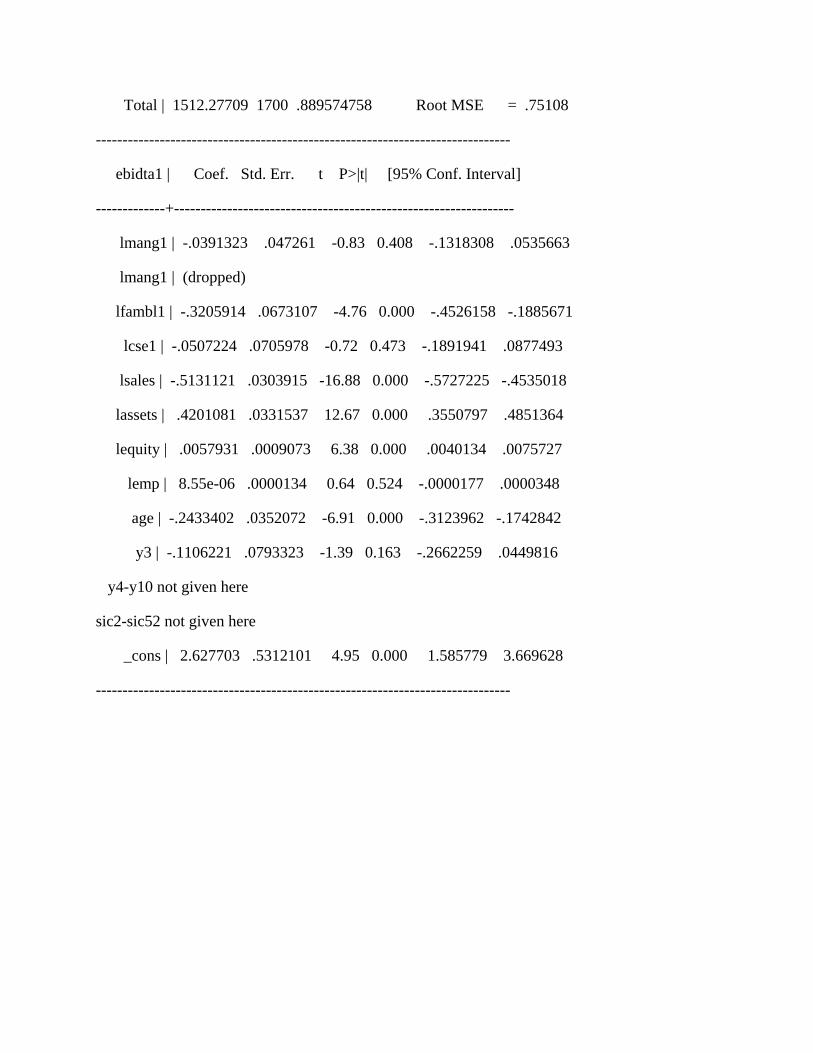
Total | 1512.27709 1700 .889574758 Root MSE = .75108
------------------------------------------------------------------------------
ebidta1 | Coef. Std. Err. t P>|t| [95% Conf. Interval]
-------------+----------------------------------------------------------------
lmang1 | -.0391323 .047261 -0.83 0.408 -.1318308 .0535663
lmang1 | (dropped)
lfambl1 | -.3205914 .0673107 -4.76 0.000 -.4526158 -.1885671
lcse1 | -.0507224 .0705978 -0.72 0.473 -.1891941 .0877493
lsales | -.5131121 .0303915 -16.88 0.000 -.5727225 -.4535018
lassets | .4201081 .0331537 12.67 0.000 .3550797 .4851364
lequity | .0057931 .0009073 6.38 0.000 .0040134 .0075727
lemp | 8.55e-06 .0000134 0.64 0.524 -.0000177 .0000348
age | -.2433402 .0352072 -6.91 0.000 -.3123962 -.1742842
y3 | -.1106221 .0793323 -1.39 0.163 -.2662259 .0449816
y4-y10 not given here
sic2-sic52 not given here
_cons | 2.627703 .5312101 4.95 0.000 1.585779 3.669628
------------------------------------------------------------------------------

Appendix C
OLS, Roa, Model 1- 4
Model 1
A)
regress roa1 lcat1 lassets lequity lemp age y3 y4 y5 y6 y7 y8 y9 y10 sic1 sic2 sic3 sic4 sic5 sic6 sic7 sic8 sic9 sic10 sic11 sic12 sic13 sic14 sic15 sic16 sic17 sic18 sic19 sic20 sic22 sic21 sic23 sic24 sic25 sic26 sic27 sic2 8 sic29 sic30 sic31 sic32 sic33 sic34 sic35 sic36 sic37 sic38 sic39 sic40 sic41 sic42 sic43 sic44 sic45 sic46 sic 47 sic49 sic48 sic50 sic51 sic52
Source | SS df MS Number of obs = 1783
-------------+------------------------------ F( 64, 1718) = 8.10
Model | 291.023689 64 4.54724515 Prob > F = 0.0000
Residual | 963.995116 1718 .561114736 R-squared = 0.2319
-------------+------------------------------ Adj R-squared = 0.2033
Total | 1255.01881 1782 .704275424 Root MSE = .74908
------------------------------------------------------------------------------
roa1 | Coef. Std. Err. t P>|t| [95% Conf. Interval]
-------------+----------------------------------------------------------------
lcat1 | -.0766309 .0430958 -1.78 0.076 -.1611566 .0078949
lassets | -.1328075 .0212624 -6.25 0.000 -.1745104 -.0911045
lequity | .0021516 .0008851 2.43 0.015 .0004156 .0038876
lemp | .0000308 .0000129 2.39 0.017 5.51e-06 .000056
age | -.1949503 .0340672 -5.72 0.000 -.261768 -.1281327
y3 | -.1741054 .0768396 -2.27 0.024 -.3248144 -.0233965
sic1 | 3.582054 .8070954 4.44 0.000 1.999061 5.165048
_cons | 2.706538 .8079417 3.35 0.001 1.121885 4.291191

------------------------------------------------------------------------------
B)
regress roa1 lcat1 lmang1 lfambl1 lcse1 lassets lsales lequity lemp age y3 y4 y5 y6 y7 y8 y9 y10 sic1 sic2 sic3 sic4 sic5 sic6 sic7 sic8 sic9 sic10 sic11 sic12 sic13 sic14 sic15 sic16 sic17 sic18 sic19 sic20 sic22 sic21 sic23 sic24 sic25 sic26 sic27 sic28 sic29 sic30 sic31 sic32 sic33 sic34 sic35 sic36 sic37 sic38 sic39 sic40 sic41 sic42 sic43 sic44 sic45 sic46 sic47 sic49 sic48 sic50 sic51 sic52
Source | SS df MS Number of obs = 1739
-------------+------------------------------ F( 68, 1670) = 8.97
Model | 328.271222 68 4.82751798 Prob > F = 0.0000
Residual | 898.338236 1670 .537927088 R-squared = 0.2676
-------------+------------------------------ Adj R-squared = 0.2378
Total | 1226.60946 1738 .705759182 Root MSE = .73344
------------------------------------------------------------------------------
roa1 | Coef. Std. Err. t P>|t| [95% Conf. Interval]
-------------+----------------------------------------------------------------
lcat1 | .0134991 .0527968 0.26 0.798 -.0900558 .1170539
lmang1 | -.0590174 .0549789 -1.07 0.283 -.1668522 .0488174
lfambl1 | -.3356679 .0656863 -5.11 0.000 -.464504 -.2068318
lcse1 | -.1364757 .0690406 -1.98 0.048 -.2718909 -.0010605
lassets | -.2831714 .0324035 -8.74 0.000 -.3467272 -.2196156
lsales | .1930547 .0296934 6.50 0.000 .1348145 .251295
lequity | .0023984 .0008794 2.73 0.006 .0006735 .0041233
lemp | .0000108 .000013 0.83 0.406 -.0000147 .0000363
age | -.207042 .0341644 -6.06 0.000 -.2740515 -.1400324
y3 | -.1692827 .0769317 -2.20 0.028 -.3201754 -.01839

y4-y10 not given here
sic1-sic52 not given here
_cons | 2.380551 .7945173 3.00 0.003 .8221965 3.938906
------------------------------------------------------------------------------
Model 2
A)
regress roa1 lcat3 lassets lequity lemp age y3 y4 y5 y6 y7 y8 y9 y10 sic1 sic2 sic3 sic4 sic5 sic6 sic7 sic8 sic9 sic10 sic11 sic12 sic13 sic14 sic15 sic16 sic17 sic18 sic19 sic20 sic22 sic21 sic23 sic24 sic25 sic26 sic27 sic28 sic29 sic30 sic31 sic32 sic33 sic34 sic35 sic36 sic37 sic38 sic39 sic40 sic41 sic42 sic43 sic44 sic45 sic46 sic 47 sic49 sic48 sic50 sic51 sic52
Source | SS df MS Number of obs = 1783
-------------+------------------------------ F( 64, 1718) = 8.04
Model | 289.322435 64 4.52066304 Prob > F = 0.0000
Residual | 965.696371 1718 .562104989 R-squared = 0.2305
-------------+------------------------------ Adj R-squared = 0.2019
Total | 1255.01881 1782 .704275424 Root MSE = .74974
------------------------------------------------------------------------------
roa1 | Coef. Std. Err. t P>|t| [95% Conf. Interval]
-------------+----------------------------------------------------------------
lcat3 | -.0199773 .0554759 -0.36 0.719 -.1287848 .0888302
lassets | -.1333569 .0214859 -6.21 0.000 -.1754981 -.0912157
lequity | .0021696 .0008897 2.44 0.015 .0004246 .0039146
lemp | .0000322 .0000129 2.51 0.012 7.00e-06 .0000575
age | -.1876627 .0341937 -5.49 0.000 -.2547284 -.1205969
y3 | -.1727832 .0769121 -2.25 0.025 -.3236344 -.021932

sic1 | 3.663386 .8068129 4.54 0.000 2.080947 5.245825
_cons | 2.60337 .8065185 3.23 0.001 1.021508 4.185231
------------------------------------------------------------------------------
B)
regress roa1 lcat3 lmang1 lfambl1 lcse1 lassets lsales lequity lemp age y3 y4 y5 y6 y7 y8 y9 y10 sic1 sic2 sic3 sic4 sic5 sic6 sic7 sic8 sic9 sic10 sic11 sic12 sic13 sic14 sic15 sic16 sic17 sic18 sic19 sic20 sic22 sic21 sic23 sic24 sic25 sic26 sic27 sic28 sic29 sic30 sic31 sic32 sic33 sic34 sic35 sic36 sic37 sic38 sic39 sic40 sic41 sic42 sic43 sic44 sic45 sic46 sic47 sic49 sic48 sic50 sic51 sic52
Source | SS df MS Number of obs = 1739
-------------+------------------------------ F( 68, 1670) = 9.03
Model | 329.706242 68 4.84862121 Prob > F = 0.0000
Residual | 896.903217 1670 .537067794 R-squared = 0.2688
-------------+------------------------------ Adj R-squared = 0.2390
Total | 1226.60946 1738 .705759182 Root MSE = .73285
------------------------------------------------------------------------------
roa1 | Coef. Std. Err. t P>|t| [95% Conf. Interval]
-------------+----------------------------------------------------------------
lcat3 | .0985345 .0595548 1.65 0.098 -.0182755 .2153445
lmang1 | -.0717908 .0471968 -1.52 0.128 -.1643619 .0207804
lfambl1 | -.356901 .0668855 -5.34 0.000 -.4880892 -.2257129
lcse1 | -.1260986 .0691549 -1.82 0.068 -.2617381 .0095408
lassets | -.2773242 .032482 -8.54 0.000 -.341034 -.2136144
lsales | .1911388 .0296879 6.44 0.000 .1329093 .2493683
lequity | .0025071 .000881 2.85 0.004 .0007791 .004235
lemp | .0000111 .000013 0.85 0.394 -.0000144 .0000365
age | -.2153434 .0340581 -6.32 0.000 -.2821445 -.1485424

y3 | -.1707714 .0768629 -2.22 0.026 -.3215292 -.0200135
y4-y10 not given here
sic1 | 3.315295 .7903349 4.19 0.000 1.765144 4.865447
sic2-sic52 not given here
_cons | 2.376129 .7921215 3.00 0.003 .8224735 3.929785
------------------------------------------------------------------------------
Model 3
A
regress roa1 lown1 lassets lequity lemp age y3 y4 y5 y6 y7 y8 y9 y10 sic1 sic2 sic3 sic4 sic5 sic6 sic7 sic8 sic9sic10 sic11 sic12 sic13 sic14 sic15 sic16 sic17 sic18 sic19 sic20 sic22 sic21 sic23 sic24 sic25 sic26 sic27 sic2 8 sic29 sic30 sic31 sic32 sic33 sic34 sic35 sic36 sic37 sic38 sic39 sic40 sic41 sic42 sic43 sic44 sic45 sic46 sic 47 sic49 sic48 sic50 sic51 sic52
Source | SS df MS Number of obs = 1783
-------------+------------------------------ F( 64, 1718) = 8.12
Model | 291.543723 64 4.55537068 Prob > F = 0.0000
Residual | 963.475082 1718 .560812038 R-squared = 0.2323
-------------+------------------------------ Adj R-squared = 0.2037
Total | 1255.01881 1782 .704275424 Root MSE = .74887
------------------------------------------------------------------------------
roa1 | Coef. Std. Err. t P>|t| [95% Conf. Interval]
-------------+----------------------------------------------------------------
lown1 | -.0855693 .042307 -2.02 0.043 -.168548 -.0025905
lassets | -.1371242 .0213888 -6.41 0.000 -.1790751 -.0951733
lequity | .0019847 .0008909 2.23 0.026 .0002374 .003732
lemp | .0000291 .0000129 2.25 0.025 3.70e-06 .0000545
age | -.1891738 .0339019 -5.58 0.000 -.2556672 -.1226804
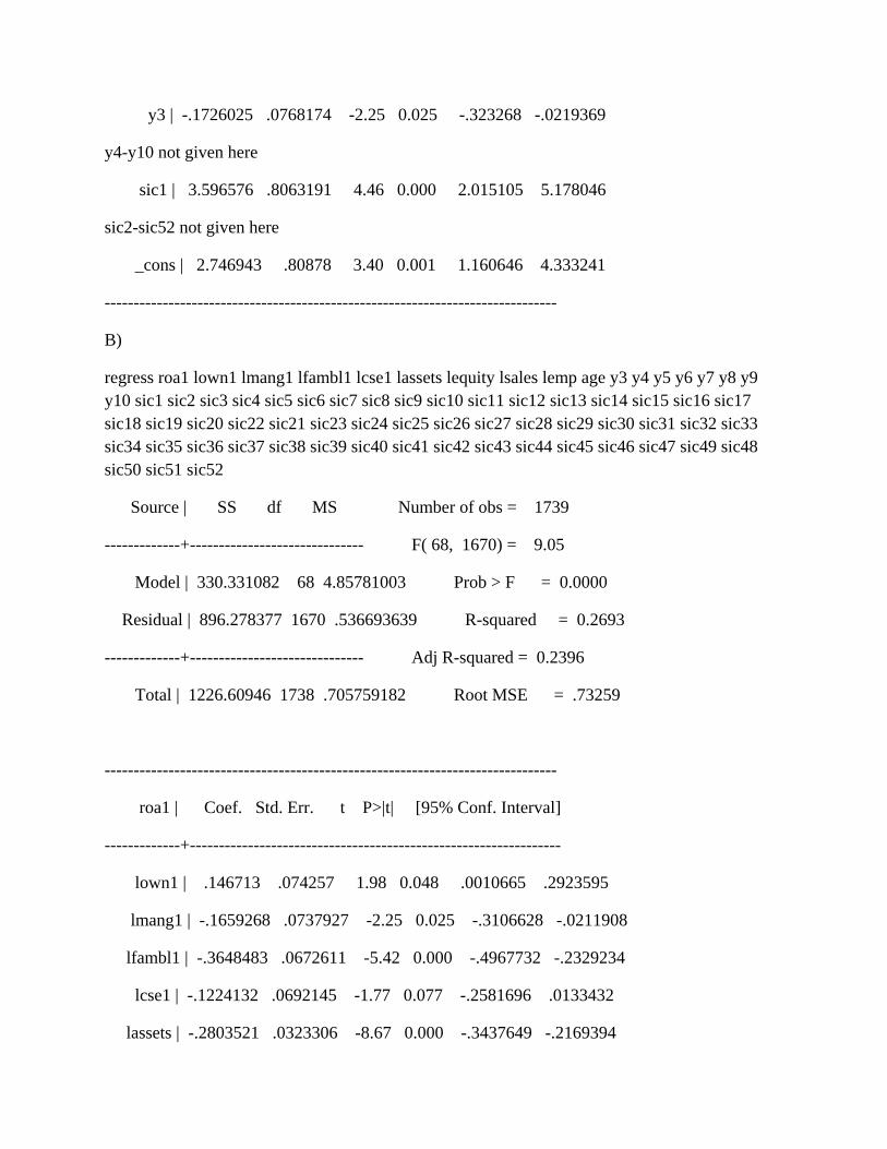
y3 | -.1726025 .0768174 -2.25 0.025 -.323268 -.0219369
y4-y10 not given here
sic1 | 3.596576 .8063191 4.46 0.000 2.015105 5.178046
sic2-sic52 not given here
_cons | 2.746943 .80878 3.40 0.001 1.160646 4.333241
------------------------------------------------------------------------------
B)
regress roa1 lown1 lmang1 lfambl1 lcse1 lassets lequity lsales lemp age y3 y4 y5 y6 y7 y8 y9 y10 sic1 sic2 sic3 sic4 sic5 sic6 sic7 sic8 sic9 sic10 sic11 sic12 sic13 sic14 sic15 sic16 sic17 sic18 sic19 sic20 sic22 sic21 sic23 sic24 sic25 sic26 sic27 sic28 sic29 sic30 sic31 sic32 sic33 sic34 sic35 sic36 sic37 sic38 sic39 sic40 sic41 sic42 sic43 sic44 sic45 sic46 sic47 sic49 sic48 sic50 sic51 sic52
Source | SS df MS Number of obs = 1739
-------------+------------------------------ F( 68, 1670) = 9.05
Model | 330.331082 68 4.85781003 Prob > F = 0.0000
Residual | 896.278377 1670 .536693639 R-squared = 0.2693
-------------+------------------------------ Adj R-squared = 0.2396
Total | 1226.60946 1738 .705759182 Root MSE = .73259
------------------------------------------------------------------------------
roa1 | Coef. Std. Err. t P>|t| [95% Conf. Interval]
-------------+----------------------------------------------------------------
lown1 | .146713 .074257 1.98 0.048 .0010665 .2923595
lmang1 | -.1659268 .0737927 -2.25 0.025 -.3106628 -.0211908
lfambl1 | -.3648483 .0672611 -5.42 0.000 -.4967732 -.2329234
lcse1 | -.1224132 .0692145 -1.77 0.077 -.2581696 .0133432
lassets | -.2803521 .0323306 -8.67 0.000 -.3437649 -.2169394

lequity | .0025669 .0008823 2.91 0.004 .0008363 .0042975
lsales | .190609 .029681 6.42 0.000 .132393 .2488249
lemp | .0000121 .000013 0.93 0.351 -.0000134 .0000376
age | -.2056694 .033804 -6.08 0.000 -.271972 -.1393668
y3 | -.1678604 .076838 -2.18 0.029 -.3185694 -.0171513
y4-y10 not given here
sic1 | 3.474929 .7932909 4.38 0.000 1.918979 5.030878
sic2-sic52 not given here
_cons | 2.229931 .796131 2.80 0.005 .6684112 3.791451
------------------------------------------------------------------------------
Model 4
A)
regress roa1 lmang1 lassets lequity lemp age y3 y4 y5 y6 y7 y8 y9 y10 sic1 sic2 sic3 sic4 sic5 sic6 sic7 sic8 sic9 sic10 sic11 sic12 sic13 sic14 sic15 sic16 sic17 sic18 sic19 sic20 sic22 sic21 sic23 sic24 sic25 sic26 sic27 sic 28 sic29 sic30 sic31 sic32 sic33 sic34 sic35 sic36 sic37 sic38 sic39 sic40 sic41 sic42 sic43 sic44 sic45 sic46 sic47 sic49 sic48 sic50 sic51 sic52
Source | SS df MS Number of obs = 1783
-------------+------------------------------ F( 64, 1718) = 8.24
Model | 294.662767 64 4.60410573 Prob > F = 0.0000
Residual | 960.356038 1718 .55899653 R-squared = 0.2348
-------------+------------------------------ Adj R-squared = 0.2063
Total | 1255.01881 1782 .704275424 Root MSE = .74766
------------------------------------------------------------------------------
roa1 | Coef. Std. Err. t P>|t| [95% Conf. Interval]
-------------+----------------------------------------------------------------
lmang1 | -.1336106 .0429356 -3.11 0.002 -.2178222 -.0493991

lassets | -.1403356 .0213773 -6.56 0.000 -.1822639 -.0984073
lequity | .0019911 .0008856 2.25 0.025 .0002542 .003728
lemp | .0000277 .0000129 2.15 0.032 2.44e-06 .000053
age | -.1855063 .0338673 -5.48 0.000 -.2519318 -.1190807
y3 | -.17079 .0766963 -2.23 0.026 -.3212179 -.0203621
y4-y10 not given here
sic1 | 3.692266 .8045167 4.59 0.000 2.11433 5.270202
sic2-sic52, not given here
_cons | 2.686888 .804553 3.34 0.001 1.108881 4.264894
------------------------------------------------------------------------------
B)
regress roa1 lmang1 lfambl1 lcse1 lassets lequity lsales lemp age y3 y4 y5 y6 y7 y8 y9 y10 sic1 sic2 sic3 sic4 sic5 sic6 sic7 sic8 sic9 sic10 sic11 sic12 sic13 sic14 sic15 sic16 sic17 sic18 sic19 sic20 sic22 sic21 sic23 sic24 sic25 sic26 sic27 sic28 sic29 sic30 sic31 sic32 sic33 sic34 sic35 sic36 sic37 sic38 sic39 sic40 sic41 sic42 sic43sic44 sic45 sic46 sic47 sic49 sic48 sic50 sic51 sic52
Source | SS df MS Number of obs = 1739
-------------+------------------------------ F( 67, 1671) = 9.11
Model | 328.236057 67 4.89904563 Prob > F = 0.0000
Residual | 898.373402 1671 .537626213 R-squared = 0.2676
-------------+------------------------------ Adj R-squared = 0.2382
Total | 1226.60946 1738 .705759182 Root MSE = .73323
------------------------------------------------------------------------------
roa1 | Coef. Std. Err. t P>|t| [95% Conf. Interval]
-------------+----------------------------------------------------------------
lmang1 | -.0511472 .0455414 -1.12 0.262 -.1404713 .038177
lfambl1 | -.3355857 .0656671 -5.11 0.000 -.4643842 -.2067872

lcse1 | -.1356657 .0689486 -1.97 0.049 -.2709004 -.000431
lassets | -.2826791 .0323372 -8.74 0.000 -.3461047 -.2192534
lequity | .0024013 .0008791 2.73 0.006 .0006771 .0041256
lsales | .1929617 .0296829 6.50 0.000 .1347421 .2511813
lemp | .0000107 .000013 0.83 0.408 -.0000147 .0000362
age | -.2082848 .0338074 -6.16 0.000 -.2745941 -.1419755
y3 | -.1696076 .0768997 -2.21 0.028 -.3204374 -.0187778
y4-y10 not given here
sic1 | 3.332177 .7906798 4.21 0.000 1.78135 4.883004
sic2-sic52 not given here
_cons | 2.394365 .7924565 3.02 0.003 .8400528 3.948677
------------------------------------------------------------------------------
OLS, Roe, Model 1-4
Model 1
A)
regress roe1 lcat1 lassets lequity lemp age y3 y4 y5 y6 y7 y8 y9 y10 sic1 sic2 sic3 sic4 sic5 sic6 sic7 sic8 sic9 sic10 sic11 sic12 sic13 sic14 sic15 sic16 sic17 sic18 sic19 sic20 sic22 sic21 sic23 sic24 sic25 sic26 sic27 sic28 sic29 sic30 sic31 sic32 sic33 sic34 sic35 sic36 sic37 sic38 sic39 sic40 sic41 sic42 sic43 sic44 sic45 sic46 sic 47 sic49 sic48 sic50 sic51 sic52
Source | SS df MS Number of obs = 1795
-------------+------------------------------ F( 64, 1730) = 8.44
Model | 449.615903 64 7.02524848 Prob > F = 0.0000
Residual | 1440.52082 1730 .832670997 R-squared = 0.2379
-------------+------------------------------ Adj R-squared = 0.2097
Total | 1890.13673 1794 1.05358792 Root MSE = .91251
------------------------------------------------------------------------------

roe1 | Coef. Std. Err. t P>|t| [95% Conf. Interval]
-------------+----------------------------------------------------------------
lcat1 | .0316315 .0518993 0.61 0.542 -.0701606 .1334235
lassets | -.1091195 .025378 -4.30 0.000 -.1588942 -.0593447
lequity | -.0076024 .0010789 -7.05 0.000 -.0097184 -.0054863
lemp | .0000121 .0000157 0.77 0.441 -.0000187 .0000429
age | -.1631755 .0416041 -3.92 0.000 -.2447752 -.0815758
y3 | -.1188401 .0927817 -1.28 0.200 -.3008162 .063136
y4-y10 not given here
sic1 | 1.851553 .5817313 3.18 0.001 .7105827 2.992524
sic2-sic52 not given here
_cons | 4.668689 .5778371 8.08 0.000 3.535356 5.802022
------------------------------------------------------------------------------
B)
regress roe1 lcat1 lmang1 lfambl1 lsales lequity lassets age lcse1 y1 y2 y3 y4 y5 y6 y7 y8 y9 y10 sic1 sic2 sic3 sic4 sic5 sic6 sic7 sic8 sic9 sic10 sic11 sic12 sic13 sic14 sic15 sic16 sic17 sic18 sic19 sic20 sic21 sic22 sic23 sic24 sic25 sic26 sic27 sic28 sic29 sic30 sic31 sic32 sic33 sic34 sic35 sic36 sic37 sic38 sic39 sic40 sic41 sic42 sic43 sic44 sic45 sic46 sic47 sic48 sic49 sic50 sic51 sic52
Source | SS df MS Number of obs = 1749
-------------+------------------------------ F( 67, 1681) = 8.89
Model | 482.356877 67 7.19935638 Prob > F = 0.0000
Residual | 1361.69612 1681 .810051234 R-squared = 0.2616
-------------+------------------------------ Adj R-squared = 0.2321
Total | 1844.053 1748 1.05495023 Root MSE = .90003
------------------------------------------------------------------------------
roe1 | Coef. Std. Err. t P>|t| [95% Conf. Interval]

-------------+----------------------------------------------------------------
lcat1 | .1030801 .0635939 1.62 0.105 -.0216514 .2278116
lmang1 | -.0247379 .0672259 -0.37 0.713 -.1565931 .1071174
lfambl1 | -.3175933 .0813029 -3.91 0.000 -.4770589 -.1581278
lsales | .1639054 .0340705 4.81 0.000 .0970804 .2307305
lequity | -.0067121 .0010771 -6.23 0.000 -.0088246 -.0045995
lassets | -.2237207 .0354601 -6.31 0.000 -.2932714 -.15417
age | -.1760677 .0420865 -4.18 0.000 -.2586152 -.0935202
lcse1 | -.2656095 .0854817 -3.11 0.002 -.4332713 -.0979477
y2 | .169475 .0948146 1.79 0.074 -.0164922 .3554421
y3-y10 not provided here
sic1 | 2.179983 .5322603 4.10 0.000 1.13602 3.223946
sic2-sic52 not provided here
_cons | 3.46666 .4919244 7.05 0.000 2.501811 4.431509
Model 2
A)
regress roe1 lcat3 lassets lequity lemp age y3 y4 y5 y6 y7 y8 y9 y10 sic1 sic2 sic3 sic4 sic5 sic6 sic7 sic8 sic9 sic10 sic11 sic12 sic13 sic14 sic15 sic16 sic17 sic18 sic19 sic20 sic22 sic21 sic23 sic24 sic25 sic26 sic27 sic28 sic29 sic30 sic31 sic32 sic33 sic34 sic35 sic36 sic37 sic38 sic39 sic40 sic41 sic42 sic43 sic44 sic45 sic46 sic47 sic49 sic48 sic50 sic51 sic52
Source | SS df MS Number of obs = 1795
-------------+------------------------------ F( 64, 1730) = 8.43
Model | 449.32278 64 7.02066844 Prob > F = 0.0000
Residual | 1440.81395 1730 .832840432 R-squared = 0.2377
-------------+------------------------------ Adj R-squared = 0.2095
Total | 1890.13673 1794 1.05358792 Root MSE = .9126

------------------------------------------------------------------------------
roe1 | Coef. Std. Err. t P>|t| [95% Conf. Interval]
-------------+----------------------------------------------------------------
lcat3 | .0094849 .0680409 0.14 0.889 -.1239662 .142936
lassets | -.1084683 .0256717 -4.23 0.000 -.1588191 -.0581175
lequity | -.0075886 .0010849 -6.99 0.000 -.0097165 -.0054607
lemp | .0000113 .0000157 0.72 0.470 -.0000194 .0000421
age | -.1659622 .0418306 -3.97 0.000 -.2480061 -.0839183
y3 | -.1197105 .0927892 -1.29 0.197 -.3017014 .0622804
y4-y10 not given here
sic1 | 1.815664 .5795709 3.13 0.002 .6789311 2.952398
sic2-sic52 not given here
_cons | 4.705062 .5747551 8.19 0.000 3.577774 5.83235
------------------------------------------------------------------------------
B)
regress roe1 lcat3 lmang1 lfambl1 lsales lequity lassets age lcse1 y1 y2 y3 y4 y5 y6 y7 y8 y9 y10 sic1 sic2 sic3 sic4 sic5 sic6 sic7 sic8 sic9 sic10 sic11 sic12 sic13 sic14 sic15 sic16 sic17 sic18 sic19 sic20 sic21 sic22 sic23 sic24 sic25 sic26 sic27 sic28 sic29 sic30 sic31 sic32 sic33 sic34 sic35 sic36 sic37 sic38 sic39 sic40 sic41 sic42 sic43 sic44 sic45 sic46 sic47 sic48 sic49 sic50 sic51 sic52
Source | SS df MS Number of obs = 1749
-------------+------------------------------ F( 67, 1681) = 8.87
Model | 481.637365 67 7.18861739 Prob > F = 0.0000
Residual | 1362.41564 1681 .81047926 R-squared = 0.2612
-------------+------------------------------ Adj R-squared = 0.2317
Total | 1844.053 1748 1.05495023 Root MSE = .90027
------------------------------------------------------------------------------

roe1 | Coef. Std. Err. t P>|t| [95% Conf. Interval]
-------------+----------------------------------------------------------------
lcat3 | .0967928 .0734162 1.32 0.188 -.047204 .2407897
lmang1 | .0154504 .0580452 0.27 0.790 -.0983982 .1292989
lfambl1 | -.3387099 .0828649 -4.09 0.000 -.5012391 -.1761807
lsales | .1615036 .034087 4.74 0.000 .0946461 .2283611
lequity | -.0064955 .0010802 -6.01 0.000 -.0086142 -.0043768
lassets | -.214142 .0356315 -6.01 0.000 -.2840287 -.1442552
age | -.1924089 .0420695 -4.57 0.000 -.2749231 -.1098948
lcse1 | -.2505971 .0857592 -2.92 0.004 -.4188031 -.0823911
y3 | .0329296 .0934054 0.35 0.724 -.1502736 .2161328
y2-y10 not provided here
sic1 | 2.157624 .5324915 4.05 0.000 1.113208 3.20204
sic2-sic52 not provided here
_cons | 3.423087 .4926941 6.95 0.000 2.456729 4.389446
Model 3
A)
regress roe1 lown1 lassets lequity lemp age y3 y4 y5 y6 y7 y8 y9 y10 sic1 sic2 sic3 sic4 sic5 sic6 sic7 sic8 sic9 sic10 sic11 sic12 sic13 sic14 sic15 sic16 sic17 sic18 sic19 sic20 sic22 sic21 sic23 sic24 sic25 sic26 sic27 sic28 sic29 sic30 sic31 sic32 sic33 sic34 sic35 sic36 sic37 sic38 sic39 sic40 sic41 sic42 sic43 sic44 sic45 sic46 sic47 sic49 sic48 sic50 sic51 sic52
Source | SS df MS Number of obs = 1795
-------------+------------------------------ F( 64, 1730) = 8.44
Model | 449.812686 64 7.02832322 Prob > F = 0.0000
Residual | 1440.32404 1730 .83255725 R-squared = 0.2380
-------------+------------------------------ Adj R-squared = 0.2098

Total | 1890.13673 1794 1.05358792 Root MSE = .91245
------------------------------------------------------------------------------
roe1 | Coef. Std. Err. t P>|t| [95% Conf. Interval]
-------------+----------------------------------------------------------------
lown1 | .0397372 .0509672 0.78 0.436 -.0602266 .139701
lassets | -.1070673 .0254972 -4.20 0.000 -.1570758 -.0570588
lequity | -.0075215 .001084 -6.94 0.000 -.0096476 -.0053953
lemp | .0000131 .0000158 0.83 0.409 -.000018 .0000441
age | -.1658543 .0414764 -4.00 0.000 -.2472034 -.0845051
y3 | -.119258 .0927685 -1.29 0.199 -.3012083 .0626923
y4-y10 not given here
sic1 | 1.848432 .580422 3.18 0.001 .7100296 2.986835
sic2-sic52 not given here
_cons | 4.645122 .5798193 8.01 0.000 3.507901 5.782342
------------------------------------------------------------------------------
B)
regress roe1 lown1 lmang1 lfambl1 lsales lequity lassets age lcse1 y1 y2 y3 y4 y5 y6 y7 y8 y9 y10 sic1 sic2 sic3 sic4 sic5 sic6 sic7 sic8 sic9 sic10 sic11 sic12 sic13 sic14 sic15 sic16 sic17 sic18 sic19 sic20 sic21 sic22 sic23 sic24 sic25 sic26 sic27 sic28 sic29 sic30 sic31 sic32 sic33 sic34 sic35 sic36 sic37 sic38 sic39 sic40 sic41 sic42 sic43 sic44 sic45 sic46 sic47 sic48 sic49 sic50 sic51 sic52
Source | SS df MS Number of obs = 1749
-------------+------------------------------ F( 67, 1681) = 9.10
Model | 490.661962 67 7.32331286 Prob > F = 0.0000
Residual | 1353.39104 1681 .805110672 R-squared = 0.2661
-------------+------------------------------ Adj R-squared = 0.2368

Total | 1844.053 1748 1.05495023 Root MSE = .89728
------------------------------------------------------------------------------
roe1 | Coef. Std. Err. t P>|t| [95% Conf. Interval]
-------------+----------------------------------------------------------------
lown1 | .3187403 .0885426 3.60 0.000 .145075 .4924057
lmang1 | -.2139746 .089001 -2.40 0.016 -.388539 -.0394102
lfambl1 | -.378558 .0827964 -4.57 0.000 -.5409529 -.2161631
lsales | .1609786 .0339635 4.74 0.000 .0943635 .2275938
lequity | -.006393 .0010743 -5.95 0.000 -.0085 -.004286
lassets | -.2148135 .0352908 -6.09 0.000 -.284032 -.145595
age | -.1814201 .0415911 -4.36 0.000 -.2629959 -.0998444
lcse1 | -.2251299 .0857175 -2.63 0.009 -.3932541 -.0570057
y2 | .168641 .0945159 1.78 0.075 -.0167403 .3540222
y1-y10 not provided here
sic1 | 2.152449 .5306404 4.06 0.000 1.111664 3.193235
sic2-sic52 not provided here
_cons | 3.399885 .490644 6.93 0.000 2.437548 4.362222
Model 4
A)
regress roe1 lmang1 lassets lequity lemp age y3 y4 y5 y6 y7 y8 y9 y10 sic1 sic2 sic3 sic4 sic5 sic6 sic7 sic8 sic9 sic10 sic11 sic12 sic13 sic14 sic15 sic16 sic17 sic18 sic19 sic20 sic22 sic21 sic23 sic24 sic25 sic26 sic27 sic28 sic29 sic30 sic31 sic32 sic33 sic34 sic35 sic36 sic37 sic38 sic39 sic40 sic41 sic42 sic43 sic44 sic45 sic46 sic47 sic49 sic48 sic50 sic51 sic52
Source | SS df MS Number of obs = 1795

-------------+------------------------------ F( 64, 1730) = 8.45
Model | 449.995465 64 7.03117913 Prob > F = 0.0000
Residual | 1440.14126 1730 .832451597 R-squared = 0.2381
-------------+------------------------------ Adj R-squared = 0.2099
Total | 1890.13673 1794 1.05358792 Root MSE = .91239
------------------------------------------------------------------------------
roe1 | Coef. Std. Err. t P>|t| [95% Conf. Interval]
-------------+----------------------------------------------------------------
lmang1 | -.0475624 .0522847 -0.91 0.363 -.1501103 .0549856
lassets | -.111709 .0255473 -4.37 0.000 -.1618159 -.0616021
lequity | -.0076716 .0010813 -7.10 0.000 -.0097923 -.0055509
lemp | 9.25e-06 .0000158 0.59 0.558 -.0000217 .0000402
age | -.163053 .0415327 -3.93 0.000 -.2445126 -.0815933
y3 | -.1194788 .0927619 -1.29 0.198 -.301416 .0624583
y4-y10 not given here
sic1-sic52 not given here
_cons | 4.735416 .5747571 8.24 0.000 3.608124 5.862708
------------------------------------------------------------------------------
B)
regress roe1 lmang1 lfambl1 lsales lequity lassets age lcse1 y1 y2 y3 y4 y5 y6 y7 y8 y9 y10 sic1 sic2 sic3 sic4 sic5 sic6 sic7 sic8 sic9 sic10 sic11 sic12 sic13 sic14 sic15 sic16 sic17 sic18 sic19 sic20 sic21 sic22 sic23 sic24 sic25 sic26 sic27 sic28 sic29 sic30 sic31 sic32 sic33 sic34 sic35 sic36 sic37 sic38 sic39 sic40 sic41 sic42 sic43 sic44 sic45 sic46 sic47 sic48 sic49 sic50 sic51 sic52
Source | SS df MS Number of obs = 1749

-------------+------------------------------ F( 66, 1682) = 8.97
Model | 480.228582 66 7.27619063 Prob > F = 0.0000
Residual | 1363.82442 1682 .81083497 R-squared = 0.2604
-------------+------------------------------ Adj R-squared = 0.2314
Total | 1844.053 1748 1.05495023 Root MSE = .90046
------------------------------------------------------------------------------
roe1 | Coef. Std. Err. t P>|t| [95% Conf. Interval]
-------------+----------------------------------------------------------------
lmang1 | .035584 .0560127 0.64 0.525 -.0742779 .1454458
lfambl1 | -.3177417 .0813422 -3.91 0.000 -.4772842 -.1581992
lsales | .1628056 .0340802 4.78 0.000 .0959615 .2296496
lequity | -.0066222 .0010762 -6.15 0.000 -.008733 -.0045114
lassets | -.2196895 .0353899 -6.21 0.000 -.2891025 -.1502766
age | -.1852331 .0417251 -4.44 0.000 -.2670717 -.1033945
lcse1 | -.2603144 .0854606 -3.05 0.002 -.4279347 -.092694
y2 | .1721287 .0948463 1.81 0.070 -.0139005 .358158
y2-y10 not provided here
sic1 | 2.17208 .5324954 4.08 0.000 1.127657 3.216503
sic2-sic52 not provided here
_cons | 3.457083 .4921268 7.02 0.000 2.491837 4.422328
------------------------------------------------------------------------------
OLS, EBITDA, Model 1-4
Model 1
A)

regress ebidta1 lcat1 lassets lequity lemp age y3 y4 y5 y6 y7 y8 y9 y10 sic1 sic2 sic3 sic4 sic5 sic6 sic7 sic8 sic9 sic10 sic11 sic12 sic13 sic14 sic15 sic16 sic17 sic18 sic19 sic20 sic22 sic21 sic23 sic24 sic25 sic26 sic27 sic28 sic29 sic30 sic31 sic32 sic33 sic34 sic35 sic36 sic37 sic38 sic39 sic40 sic41 sic42 sic43 sic44 sic45 sic46 sic47 sic49 sic48 sic50 sic51 sic52
Source | SS df MS Number of obs = 1724
-------------+------------------------------ F( 64, 1659) = 10.02
Model | 424.689297 64 6.63577027 Prob > F = 0.0000
Residual | 1098.67221 1659 .662249672 R-squared = 0.2788
-------------+------------------------------ Adj R-squared = 0.2510
Total | 1523.3615 1723 .8841332 Root MSE = .81379
------------------------------------------------------------------------------
ebidta1 | Coef. Std. Err. t P>|t| [95% Conf. Interval]
-------------+----------------------------------------------------------------
lcat1 | -.0245258 .0476311 -0.51 0.607 -.1179492 .0688976
lassets | .0078883 .0236599 0.33 0.739 -.038518 .0542946
lequity | .0066712 .0009727 6.86 0.000 .0047634 .0085791
lemp | -.0000186 .0000142 -1.31 0.192 -.0000464 9.31e-06
age | -.309409 .0377525 -8.20 0.000 -.3834565 -.2353615
y3 | -.1262342 .0852016 -1.48 0.139 -.2933481 .0408798
y4-y10 not given here
sic1 | -2.905122 .6662503 -4.36 0.000 -4.211902 -1.598342
sic2-sic52 not given here
_cons | 7.373958 .6875082 10.73 0.000 6.025482 8.722433
------------------------------------------------------------------------------
B)
regress ebidta1 lcat1 lmang1 lfambl1 lcse1 lsales lassets lequity lemp age y3 y4 y5 y6 y7 y8 y9 y10 sic1 sic2 sic3 sic4 sic5 sic6 sic7 sic8 sic9 sic10 sic11 sic12 sic13 sic14 sic15 sic16 sic17

sic18 sic19 sic20 sic22 sic21 sic23 sic24 sic25 sic26 sic27 sic28 sic29 sic30 sic31 sic32 sic33 sic34 sic35 sic36 sic37 sic38 sic39 sic40 sic41 sic42 sic43 sic44 sic45 sic46 sic47 sic49 sic48 sic50 sic51 sic52
Source | SS df MS Number of obs = 1701
-------------+------------------------------ F( 68, 1632) = 15.40
Model | 591.111553 68 8.69281695 Prob > F = 0.0000
Residual | 921.165536 1632 .564439667 R-squared = 0.3909
-------------+------------------------------ Adj R-squared = 0.3655
Total | 1512.27709 1700 .889574758 Root MSE = .75129
------------------------------------------------------------------------------
ebidta1 | Coef. Std. Err. t P>|t| [95% Conf. Interval]
-------------+----------------------------------------------------------------
lcat1 | .0161316 .0545482 0.30 0.767 -.0908602 .1231234
lmang1 | -.048458 .0568266 -0.85 0.394 -.1599188 .0630028
lfambl1 | -.3208233 .0673341 -4.76 0.000 -.4528936 -.188753
lcse1 | -.0515343 .0706708 -0.73 0.466 -.1901494 .0870808
lsales | -.5129724 .0304036 -16.87 0.000 -.5726066 -.4533381
lassets | .4194448 .0332387 12.62 0.000 .3542497 .4846399
lequity | .0057883 .0009077 6.38 0.000 .0040079 .0075687
lemp | 8.64e-06 .0000134 0.64 0.520 -.0000177 .0000349
age | -.2418848 .0355592 -6.80 0.000 -.3116314 -.1721383
y3 | -.1102707 .0793634 -1.39 0.165 -.2659354 .0453941
y4-y10 not given here
sic1 | 3.027791 .5436284 5.57 0.000 1.961508 4.094074
sic2-sic52 not given here

sic52 | 1.898395 .5236332 3.63 0.000 .8713309 2.925459
_cons | 2.611851 .5340555 4.89 0.000 1.564345 3.659358
------------------------------------------------------------------------------
Model 2
A)
. regress ebidta1 lcat3 lassets lequity lemp age y3 y4 y5 y6 y7 y8 y9 y10 sic1 sic2 sic3 sic4 sic5 sic6 sic7 sic8 sic9 sic10 sic11 sic12 sic13 sic14 sic15 sic16 sic17 sic18 sic19 sic20 sic22 sic21 sic23 sic24 sic25 sic26 sic27 sic28 sic29 sic30 sic31 sic32 sic33 sic34 sic35 sic36 sic37 sic38 sic39 sic40 sic41 sic42 sic43 sic44 sic45 sic46 sic47 sic49 sic48 sic50 sic51 sic52
Source | SS df MS Number of obs = 1724
-------------+------------------------------ F( 64, 1659) = 10.03
Model | 424.95078 64 6.63985593 Prob > F = 0.0000
Residual | 1098.41072 1659 .662092057 R-squared = 0.2790
-------------+------------------------------ Adj R-squared = 0.2511
Total | 1523.3615 1723 .8841332 Root MSE = .81369
------------------------------------------------------------------------------
ebidta1 | Coef. Std. Err. t P>|t| [95% Conf. Interval]
-------------+----------------------------------------------------------------
lcat3 | -.0495553 .0609924 -0.81 0.417 -.1691855 .0700748
lassets | .0048743 .0239381 0.20 0.839 -.0420778 .0518264
lequity | .0066055 .0009766 6.76 0.000 .0046899 .0085211
lemp | -.0000186 .0000142 -1.32 0.189 -.0000464 9.16e-06
age | -.3037397 .0379261 -8.01 0.000 -.3781278 -.2293515
y3 | -.1251316 .0851978 -1.47 0.142 -.2922381 .0419749
y4-y10 not given here

sic52 | -4.364491 .6437066 -6.78 0.000 -5.627054 -3.101929
sic1-sic51 not given here
_cons | 7.407422 .6890357 10.75 0.000 6.055951 8.758893
------------------------------------------------------------------------------
B)
regress ebidta1 lcat3 lmang1 lfambl1 lcse1 lsales lassets lequity lemp age y3 y4 y5 y6 y7 y8 y9 y10 sic1 sic2 sic3 sic4 sic5 sic6 sic7 sic8 sic9 sic10 sic11 sic12 sic13 sic14 sic15 sic16 sic17 sic18 sic19 sic20 sic22 sic21 sic23 sic24 sic25 sic26 sic27 sic28 sic29 sic30 sic31 sic32 sic33 sic34 sic35 sic36 sic37 sic38 sic39 sic40 sic41 sic42 sic43 sic44 sic45 sic46 sic47 sic49 sic48 sic50 sic51 sic52
Source | SS df MS Number of obs = 1701
-------------+------------------------------ F( 68, 1632) = 15.42
Model | 591.670051 68 8.70103017 Prob > F = 0.0000
Residual | 920.607037 1632 .564097449 R-squared = 0.3912
-------------+------------------------------ Adj R-squared = 0.3659
Total | 1512.27709 1700 .889574758 Root MSE = .75106
------------------------------------------------------------------------------
ebidta1 | Coef. Std. Err. t P>|t| [95% Conf. Interval]
-------------+----------------------------------------------------------------
lcat3 | .0638604 .0615185 1.04 0.299 -.0568031 .1845239
lmang1 | -.052747 .049046 -1.08 0.282 -.1489468 .0434527
lfambl1 | -.3340651 .0685491 -4.87 0.000 -.4685186 -.1996116
lcse1 | -.0451682 .0707986 -0.64 0.524 -.1840338 .0936975
lsales | -.5145372 .0304217 -16.91 0.000 -.5742069 -.4548675
lassets | .4241005 .0333753 12.71 0.000 .3586376 .4895634
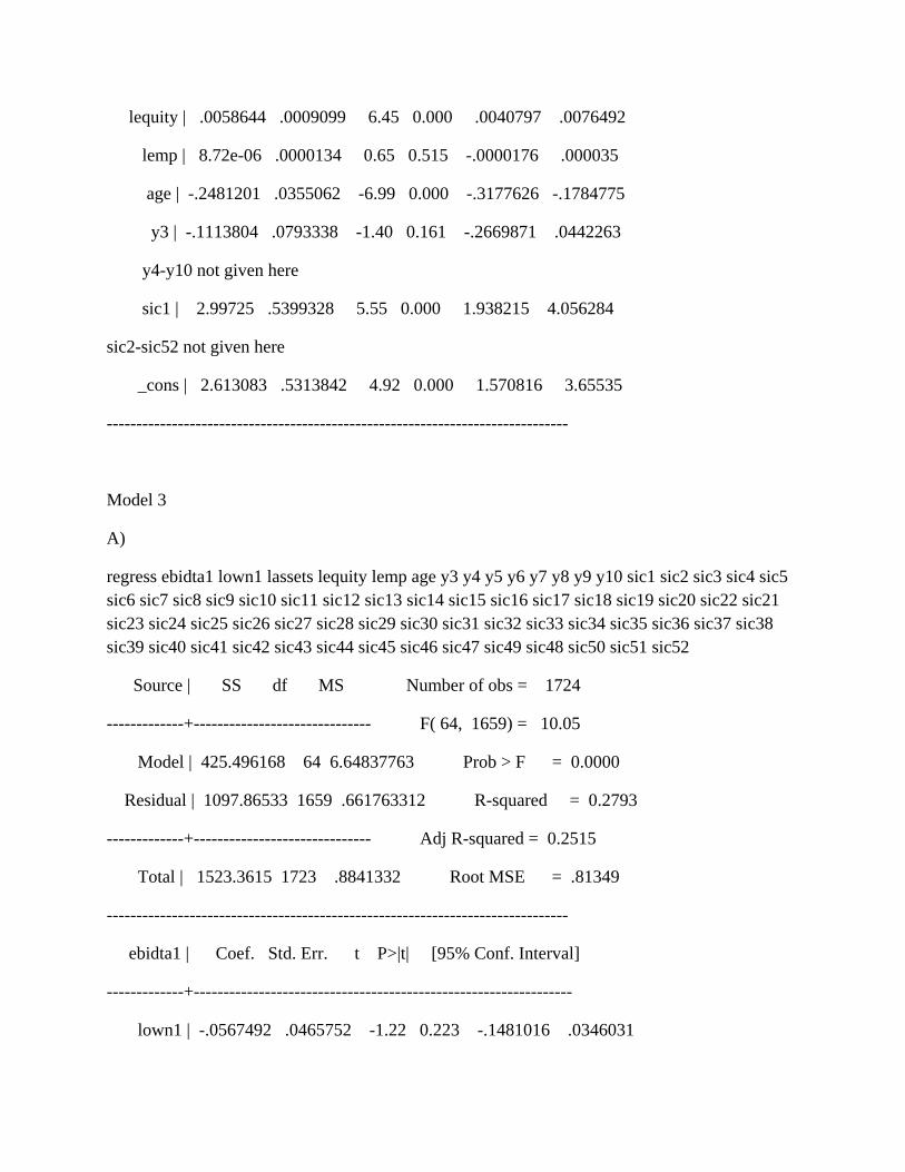
lequity | .0058644 .0009099 6.45 0.000 .0040797 .0076492
lemp | 8.72e-06 .0000134 0.65 0.515 -.0000176 .000035
age | -.2481201 .0355062 -6.99 0.000 -.3177626 -.1784775
y3 | -.1113804 .0793338 -1.40 0.161 -.2669871 .0442263
y4-y10 not given here
sic1 | 2.99725 .5399328 5.55 0.000 1.938215 4.056284
sic2-sic52 not given here
_cons | 2.613083 .5313842 4.92 0.000 1.570816 3.65535
------------------------------------------------------------------------------
Model 3
A)
regress ebidta1 lown1 lassets lequity lemp age y3 y4 y5 y6 y7 y8 y9 y10 sic1 sic2 sic3 sic4 sic5 sic6 sic7 sic8 sic9 sic10 sic11 sic12 sic13 sic14 sic15 sic16 sic17 sic18 sic19 sic20 sic22 sic21 sic23 sic24 sic25 sic26 sic27 sic28 sic29 sic30 sic31 sic32 sic33 sic34 sic35 sic36 sic37 sic38 sic39 sic40 sic41 sic42 sic43 sic44 sic45 sic46 sic47 sic49 sic48 sic50 sic51 sic52
Source | SS df MS Number of obs = 1724
-------------+------------------------------ F( 64, 1659) = 10.05
Model | 425.496168 64 6.64837763 Prob > F = 0.0000
Residual | 1097.86533 1659 .661763312 R-squared = 0.2793
-------------+------------------------------ Adj R-squared = 0.2515
Total | 1523.3615 1723 .8841332 Root MSE = .81349
------------------------------------------------------------------------------
ebidta1 | Coef. Std. Err. t P>|t| [95% Conf. Interval]
-------------+----------------------------------------------------------------
lown1 | -.0567492 .0465752 -1.22 0.223 -.1481016 .0346031

lassets | .0048115 .0237818 0.20 0.840 -.0418341 .0514571
lequity | .0065575 .0009773 6.71 0.000 .0046406 .0084744
lemp | -.0000203 .0000143 -1.42 0.155 -.0000483 7.69e-06
age | -.3070121 .0376021 -8.16 0.000 -.3807647 -.2332595
y3 | -.1254206 .0851709 -1.47 0.141 -.2924743 .0416331
y4-y10 not given here
sic2 | -3.661801 .6481264 -5.65 0.000 -4.933033 -2.390569
sic1-sic51 not given here
_cons | 7.423455 .6886624 10.78 0.000 6.072716 8.774194
------------------------------------------------------------------------------
B)
regress ebidta1 lown1 lmang1 lfambl1 lcse1 lsales lassets lequity lemp age y3 y4 y5 y6 y7 y8 y9 y10 sic1 sic2 sic3 sic4 sic5 sic6 sic7 sic8 sic9 sic10 sic11 sic12 sic13 sic14 sic15 sic16 sic17 sic18 sic19 sic20 sic22 sic21 sic23 sic24 sic25 sic26 sic27 sic28 sic29 sic30 sic31 sic32 sic33 sic34 sic35 sic36 sic37 sic38 sic39 sic40 sic41 sic42 sic43 sic44 sic45 sic46 sic47 sic49 sic48 sic50 sic51 sic52
Source | SS df MS Number of obs = 1701
-------------+------------------------------ F( 68, 1632) = 15.45
Model | 592.29331 68 8.71019573 Prob > F = 0.0000
Residual | 919.983779 1632 .563715551 R-squared = 0.3917
-------------+------------------------------ Adj R-squared = 0.3663
Total | 1512.27709 1700 .889574758 Root MSE = .75081
------------------------------------------------------------------------------
ebidta1 | Coef. Std. Err. t P>|t| [95% Conf. Interval]
-------------+----------------------------------------------------------------
lown1 | .1130309 .0764851 1.48 0.140 -.0369884 .2630502

lmang1 | -.1273064 .0761046 -1.67 0.095 -.2765795 .0219666
lfambl1 | -.3431941 .0690027 -4.97 0.000 -.4785373 -.2078509
lcse1 | -.0399957 .0709445 -0.56 0.573 -.1791476 .0991561
lsales | -.5151606 .030412 -16.94 0.000 -.5748113 -.4555098
lassets | .4221993 .0331719 12.73 0.000 .3571353 .4872634
lequity | .0059191 .000911 6.50 0.000 .0041323 .007706
lemp | 9.61e-06 .0000134 0.72 0.474 -.0000167 .0000359
age | -.2419205 .0352076 -6.87 0.000 -.3109772 -.1728637
y3 | -.1095582 .0793068 -1.38 0.167 -.265112 .0459957
y4-y10 not given here
sic1 | 3.119111 .5447305 5.73 0.000 2.050666 4.187556
sic2-sic52 not given here
sic52 | 1.958908 .518204 3.78 0.000 .9424926 2.975323
_cons | 2.502071 .5377796 4.65 0.000 1.44726 3.556882
------------------------------------------------------------------------------
Model 4
A)
regress ebidta1 lmang1 lassets lequity lemp age y3 y4 y5 y6 y7 y8 y9 y10 sic1 sic2 sic3 sic4 sic5 sic6 sic7 sic8 sic9 sic10 sic11 sic12 sic13 sic14 sic15 sic16 sic17 sic18 sic19 sic20 sic22 sic21 sic23 sic24 sic25 sic26 sic27 sic28 sic29 sic30 sic31 sic32 sic33 sic34 sic35 sic36 sic37 sic38 sic39 sic40 sic41 sic42 sic43 sic44 sic45 sic46 sic47 sic49 sic48 sic50 sic51 sic52
Source | SS df MS Number of obs = 1724
-------------+------------------------------ F( 64, 1659) = 10.06
Model | 425.76919 64 6.6526436 Prob > F = 0.0000
Residual | 1097.59231 1659 .661598742 R-squared = 0.2795
-------------+------------------------------ Adj R-squared = 0.2517

Total | 1523.3615 1723 .8841332 Root MSE = .81339
------------------------------------------------------------------------------
ebidta1 | Coef. Std. Err. t P>|t| [95% Conf. Interval]
-------------+----------------------------------------------------------------
lmang1 | -.0653191 .0474169 -1.38 0.169 -.1583224 .0276841
lassets | .0042159 .0237945 0.18 0.859 -.0424545 .0508864
lequity | .0066044 .0009736 6.78 0.000 .0046947 .008514
lemp | -.0000204 .0000143 -1.43 0.152 -.0000484 7.56e-06
age | -.3054344 .0376298 -8.12 0.000 -.3792413 -.2316276
y3 | -.1247137 .0851642 -1.46 0.143 -.2917543 .042327
y4-y10 not given here
sic1 | -2.909776 .6659282 -4.37 0.000 -4.215924 -1.603627
sic2-sic52 not given here
_cons | 7.424424 .688292 10.79 0.000 6.074411 8.774436
------------------------------------------------------------------------------
B)
regress ebidta1 lmang1 lmang1 lfambl1 lcse1 lsales lassets lequity lemp age y3 y4 y5 y6 y7 y8 y9 y10 sic1 sic2 sic3 sic4 sic5 sic6 sic7 sic8 sic9 sic10 sic11 sic12 sic13 sic14 sic15 sic16 sic17 sic18 sic19 sic20 sic22 sic21 sic23 sic24 sic25 sic26 sic27 sic28 sic29 sic30 sic31 sic32 sic33 sic34 sic35 sic36 sic37 sic38 sic39 sic40 sic41 sic42 sic43 sic44 sic45 sic46 sic47 sic49 sic48 sic50 sic51 sic52
Source | SS df MS Number of obs = 1701
-------------+------------------------------ F( 67, 1633) = 15.64
Model | 591.062188 67 8.8218237 Prob > F = 0.0000
Residual | 921.2149 1633 .56412425 R-squared = 0.3908
-------------+------------------------------ Adj R-squared = 0.3658

Total | 1512.27709 1700 .889574758 Root MSE = .75108
------------------------------------------------------------------------------
ebidta1 | Coef. Std. Err. t P>|t| [95% Conf. Interval]
-------------+----------------------------------------------------------------
lmang1 | -.0391323 .047261 -0.83 0.408 -.1318308 .0535663
lmang1 | (dropped)
lfambl1 | -.3205914 .0673107 -4.76 0.000 -.4526158 -.1885671
lcse1 | -.0507224 .0705978 -0.72 0.473 -.1891941 .0877493
lsales | -.5131121 .0303915 -16.88 0.000 -.5727225 -.4535018
lassets | .4201081 .0331537 12.67 0.000 .3550797 .4851364
lequity | .0057931 .0009073 6.38 0.000 .0040134 .0075727
lemp | 8.55e-06 .0000134 0.64 0.524 -.0000177 .0000348
age | -.2433402 .0352072 -6.91 0.000 -.3123962 -.1742842
y3 | -.1106221 .0793323 -1.39 0.163 -.2662259 .0449816
y4-y10 not given here
sic2-sic52 not given here
_cons | 2.627703 .5312101 4.95 0.000 1.585779 3.669628
------------------------------------------------------------------------------


![Alchian and Demsetz 1972 Production Information Costs and Economic Organization[1]](https://img.pdfslide.net/doc/110x75/547ac60ab4af9fda158b4c61/alchian-and-demsetz-1972-production-information-costs-and-economic-organization1.jpg)