Fast Exact Leave-One-Out Cross-Validation of Sparse Least ...theoval.cmp.uea.ac.uk/publications/pdf/nn2004a.pdf · Fast Exact Leave-One-Out Cross-Validation of Sparse Least-Squares

Fast Exact Leave-One-Out Cross-Validation of

Sparse Least-Squares Support Vector

Machines

Gavin C. Cawley a,∗ Nicola L. C. Talbot a

aSchool of Computing Sciences, University of East Anglia,

Norwich, United Kingdom, NR4 7TJ

∗ Corresponding author, tel: +44 (0)1603 593258, fax: +44 (0)1603 592245, email:

[email protected]

Abstract

Leave-one-out cross-validation has been shown to give an almost unbiased esti-

mator of the generalisation properties of statistical models, and therefore provides a

sensible criterion for model selection and comparison. In this paper we show that ex-

act leave-one-out cross-validation of sparse Least-Squares Support Vector Machines

(LS-SVMs) can be implemented with a computational complexity of only O(`n2)

floating point operations, rather than the O(`2n2) operations of a naıve implemen-

tation, where ` is the number of training patterns and n is the number of basis

vectors. As a result, leave-one-out cross-validation becomes a practical proposition

for model selection in large scale applications. For clarity the exposition concen-

trates on sparse least-squares support vector machines in the context of non-linear

regression, but is equally applicable in a pattern recognition setting.

Key words:

model selection, cross-validation, least-squares support vector machine

2

Fast Exact Leave-One-Out Cross-Validation of Sparse LS-SVMs 3

1 Introduction

The generalisation properties of statistical models are typically governed by

a small set of parameters, for instance regularisation parameters controlling

the bias-variance trade-off; finding the optimal values for these parameters

is an activity known as “model selection”. Model selection frequently seeks

to optimise a cross-validation estimate of an appropriate statistic measuring

generalisation ability on unseen data, for instance misclassification rate in the

case of pattern recognition or the sum-of-squares error in a regression set-

ting. A k-fold cross-validation procedure partitions the available data into k

disjoint subsets. k models are then trained, each model being trained on a

different combination of k− 1 of the k subsets and the test statistic evaluated

over the remaining partition. The mean of the test statistic for each of the

k models is known as the cross-validation estimate of the test statistic. The

most extreme form of cross-validation, such that k is given by the number of

training patterns, `, is known as leave-one-out cross-validation. Leave-one-out

cross-validation provides an sensible model selection criterion as it has been

shown to provide an almost unbiased estimate of the true generalisation abil-

ity of the model (Lemma 1). Empirical studies have shown that in some cases

model selection based on k-fold cross-validation out performs selection proce-

dures based on the leave-one-out estimator as the latter is known to exhibit a

comparatively high variance, e.g. [1]. However, bounds on, or approximations

to the leave-one-out estimator have proved effective criteria for model selection

for conventional support vector machines, e.g. [2–4].

Lemma 1 (Luntz and Brailovsky [5])

Given a sequence of observations Z = ziì=1, forming an independent and


identically distributed (i.i.d.) sample from an underlying distribution P (z),

and a hypothesis class H, the empirical risk can be written as

Remp(H,Z) =1

`

∑i=1

Q(zi, h | Z), h ∈ H, zi ∈ Z,

where Q(z, h | Z) measures the loss for pattern z of the optimal hypothesis

h ∈ H formed on the basis on the set of observations Z, denoted by h | Z. Let

L(H,Z) be the corresponding leave-one-out estimator,

L(H,Z) =1

`

∑i=1

Q(zi, hi | Z \ zi), hi ∈ H, zi ∈ Z,

then the leave-one-out cross-validation estimate of the risk of the hypothesis

class H on data Z, with respect to P (z),

R(H,Z) =∫

Q(z, h | Z)dP (z), h ∈ H,

is almost unbiased in the sense that

E L(H,Z) = ER(H,Z ′),

where the expectations, E·, are taken over i.i.d. samples Z,Z ′ ∼ P (z) of

size ` on the left hand side and `− 1 on the right [5, 6].

Regularisation Machines [7], Kernel Ridge-Regression [8] and the Least-Squares

Support Vector Machine (LS-SVM) [9, 10] comprise a family of closely related

techniques constructing a linear model in a kernel-induced feature space min-

imising a regularised sum-of-squares loss functional. These methods provide

an attractive approach for non-linear pattern recognition and regression prob-

lems as the optimal model parameters are given by the solution of a simple

system of linear equations. The use of formal regularisation [11] also provides

convenient control of the bias-variance trade-off [12] necessary for adequate


generalisation in non-trivial applications. In this paper, we demonstrate that

the computational complexity of leave-one-out cross-validation of a sparse for-

mulation of the least squares support vector machine is of the same order as

that of the basic training algorithm, i.e. O(`3). Exact leave-one-out cross-

validation therefore provides a feasible criterion for model selection in large

scale applications.

The remainder of this paper is structured as follows: Section 2 introduces the

sparse least-squares support vector machine and describes a computationally

efficient method for performing leave-one-out cross-validation for this class

of kernel machines. Section 3 presents results obtained using the proposed

method on two real-world non-linear regression tasks, based on well known,

public domain benchmark datasets. Section 4 discusses the origins of the pro-

posed procedure and suggests some possible extensions. Finally, the work is

summarised in Section 5.

2 Method

In this section, we first describe the least-squares support vector machine as

a kernel form of ridge regression [13], before introducing a sparse formulation

with an efficient training algorithm for large scale applications. A computa-

tionally efficient algorithm for leave-one-out cross-validation is then proposed,

based on a corollary of the familiar Sherman-Woodbury-Morrison formula.


2.1 Ridge Regression

Ridge regression [13] is a method from classical statistics that implements a

regularised form of least-squares regression. Given training data,

D = xi, tiì=1 , x ∈ X ⊂ Rd, ti ∈ T ⊂ R,

ridge regression determines the weight vector, w ∈ Rd, and bias, b, of a linear

model, f(x) = w ·x + b, via minimisation of the following objective function:

L(w, b) =1

2‖w‖2 + γ

∑i=1

(ti −w · xi − b)2. (1)

The objective function used in ridge regression (1) implements form of Tikhonov

regularisation [11] of a sum-of-squares error metric, where γ is a regularisation

parameter controlling the bias-variance trade-off [12, 13]. This corresponds to

penalised maximum likelihood estimation of w, assuming the targets have

been corrupted by an independent and identically distributed (i.i.d.) sample

drawn from a Gaussian noise process, with zero mean and fixed variance σ2,

ti = w · xi + b + εi, ε ∼ N (0, σ2).

2.2 The Least-Squares Support Vector Machine

A non-linear form of ridge regression [8], known as the Least-Squares Support

Vector Machine (LS-SVM) [9, 10], can be obtained via the so-called “kernel

trick”, whereby a linear ridge regression model is constructed in a feature

space, F (φ : X → F), induced by a Mercer kernel defining the inner prod-

uct K(x, x′) = φ(x) · φ(x′). The kernel function, K : X × X → R may be

any positive definite kernel. For an introduction to kernel methods in ma-


chine learning see Cristianini and Shawe-Taylor [14]. The objective function

minimised in constructing a least-squares support vector machine is given by

L(w, b) =1

2‖w‖2 + γ

∑i=1

(ti −w · φ(xi)− b)2.

The representer theorem [15] indicates that the solution of an optimisation

problem of this nature can be written in the form of an expansion over train-

ing patterns, i.e. w =∑`

i=1 αiφ(xi). The output of the least-squares support

vector machine is then given by the kernel expansion

f(x) =∑i=1

αiK(xi, x) + b.

It can easily be shown [8, 9] that the optimal coefficients of this expansion are

given by the solution of a set of linear equationsK + γ−1I 1

1T 0

α

b

=

t

0

,

where K = [kij = K(xi, xj)]ì,j=1, t = (t1, t2, . . . , t`)

T , α = (α1, α2, . . . , α`)T

and 1 = (1, 1, . . . , 1)T .

2.3 The Sparse Least-Squares Support Vector Machine

Unfortunately, unlike the original support vector machine [16, 17], the ker-

nel expansions defining least-squares support vector machines are typically

fully dense, i.e. αi 6= 0, ∀ i ∈ 1, 2, . . . , `. This severely limits the utility of

the LS-SVM in large scale applications as the complexity of the basic train-

ing algorithm is of order O(`3) (although more efficient methods have been

proposed, e.g. [18]). Fortunately a range of methods for obtaining sparse least-


squares support vector machines are available, see e.g. [19–21]. The sparsity

of the original support vector machine is perhaps best viewed as a convenient

consequence of the use of the hinge loss, instead of the least-squares loss, in

defining the primal optimisation problem, rather than as a deliberate design

aim of the algorithm. As a result, the kernel expansions for support vector

machine in general are not maximally sparse either and so several algorithms

have been proposed for simplifying existing support vector expansions [22–

24], or for training support vector machines using a reduced set of candidate

support vectors [25]. The latter is similar in spirit to the sparse least-squares

support vector machine used here.

In order to construct a sparse least-squares support vector machine, it is as-

sumed that the weight vector, w, can be represented as a weighted sum of a

limited number of basis vectors φ(zi)ni=1, z ∈ X ⊂ Rd, n `, such that

w =n∑

i=1

βiφ(zi).

The objective function minimised by the sparse least-squares support vector

machine then becomes

L(β, b) =1

2

n∑i=1

n∑j=1

βiβjkij + γ∑i=1

(ti −n∑

j=1

βj kij − b)2, (2)

where kij = K(zi, zj) and kij = K(xi, zj). It is straightforward to show that

this optimisation problem can again be expressed in the form of a system of

linear equations (see appendix A.3),

(R + ZT Z)p = ZT t (3)

where p = (β, b)T is the vector of model parameters, Z = [K 1], K =

[kij]i=`,j=ni=1,j=1, K = [kij]

ni,j=1, 1 = [1]ì=1 and R corresponds to the regularisation


term in (2)

R =

12γ−1K 0

0T 0

.

Note that the computational complexity of the resulting training algorithm

is of order O(`n2), being dominated by construction of the (n + 1)× (n + 1)

matrix (R+ZT Z), and therefore is far better suited to large scale application.

2.4 Selection of Reference Vectors

There are a number of viable approaches to the problem of selecting a set of

reference vectors: Baudat and Anouar [26] propose selection of a minimal set

of training vectors forming a basis for the subspace of F populated by the

data (for alternative approaches, see [19–21, 27]). Suykens et al. [9, 10] iter-

atively prune patterns having a small error from the kernel expansion (note

however that this involves starting with a fully dense least-squares support

vector machine, which is computationally demanding for large `). Alterna-

tively, one could simply select a random subsample of the training data, or

even the entire training set. For this study, we adopt the method of Baudat

and Anouar, as summarised in the following section.

2.4.1 Feature Vector Selection

The normalised Euclidean distance between the image of a datum, x, in feature

space, φ(x), and φS(x), it’s optimal reconstruction using a sub-set of the

training vectors φ(xi)i∈S , is given by

δi(S) =‖φ(xi)− φS(xi)‖2

‖φ(xi)‖2. (4)


This distance can be expressed in terms of inner products, and so via the

“kernel trick”,

δi(S) = 1− KTSiK

−1SSKSi

kii

.

where KSS is a square sub-matrix of the kernel matrix K = [kij = K(xi, xj)]ì,j=1,

such that KSS = kiji,j∈S and KSi = (kji)Tj∈S is a column vector of inner

products in F . To form a basis for the subspace in F populated by the data,

it is sufficient to minimise the mean reconstruction error δi over all patterns

in the training set [26], i.e. maximise

J(S) =1

`

∑i=1

KTSiK

−1SSKSi

kii

. (5)

Starting with S = ∅, a basis is constructed in a greedy manner, at each step

adding the training vector maximising J(S). Note that provided the feature

vectors currently selected are linearly independent KSS will be invertible. This

will always be the case; clearly one would not select a linearly dependent fea-

ture vector as this would not result in a reduction in the mean reconstruction

error. The algorithm therefore terminates when KSS is no longer invertible,

indicating that a complete basis has been identified, or when an upper bound

on the number of basis vectors is reached, or when the mean relative recon-

struction error falls below a given threshold. An efficient implementation of

the feature vector selection algorithm is given in [28]. The computational com-

plexity of the standard feature vector selection is O(`2|S|2), where |S| is the

number of feature vectors extracted. The computational complexity of the

improved algorithm is only O(|S|3), however this is achieved at the expense

of introducing a stochastic element, such that there is no guarantee that the

same set of feature vectors will be extracted each time the algorithm is exe-

cuted. However, provided the feature vectors extracted (approximately) span

the subspace in F occupied by the training data, the mapping implemented


by the sparse LS-SVM will be (approximately) the same as that of the full LS-

SVM. The storage complexity of both algorithms is O(|S|2), being dominated

by storage of KSS .

2.5 Fast Exact Leave-One-Out Cross-Validation

At each step of the leave-one-out cross-validation procedure, a sparse least-

squares support vector machine is constructed excluding a single training pat-

tern from the data. The vector of model parameters, p(i) at the ith iteration

is then given by the solution of the following system of linear equations,

p(i) =

β(i)

b(i)

=[R + ZT

(i)Z(i)

]−1ZT

(i)t

where Z(i) is the sub-matrix formed by omitting the ith row of Z. Normally

the most computationally expensive step is the inversion of the matrix C(i) =[R + ZT

(i)Z(i)

], with a complexity of O(n3) operations. Fortunately C(i) can

be written as a rank one modification of a matrix C,

C(i) =[R + ZT Z − ziz

Ti

]=[C − ziz

Ti

],

where zi is the ith row of Z and C = R+ZT Z. The following matrix inversion

lemma, a corollary of the familiar Sherman-Woodbury-Morrison formula, can

then be used to find C−1(i) in only O(n2) operations, given that C−1 is already

known.

Lemma 2 (Bartlett [29]) Given an invertible matrix A and column vector


v, then assuming 1 + vT A−1v 6= 0,

(A + vvT

)−1= A−1 − A−1vvT A−1

1 + vT A−1v.

This can be obtained straight-forwardly as a special case of the familiar Sherman-

Woodbury-Morrison formula (see appendix A.2).

The solution to the matrix inversion problem can then be written as

C−1(i) = [C − ziz

Ti ]−1 = C−1 +

C−1zizTi C−1

1− zTi C−1zi

.

The computational complexity of the leave-one-out cross-validation process is

thus reduced to only O(`n2) operations, which is the same as that of the basic

training algorithm for the sparse least-squares support vector machine.

2.6 A Further Refinement

For the purposes of model selection based on leave-one-out cross-validation,

we are not generally interested in the values of the model parameters them-

selves, but only in the predicted output of the model for the training pattern

excluded during each trial. For instance we might adopt Allen’s PRESS (pre-

dicted residual sum of squares) statistic [30],

PRESS =∑i=1

e(i)

2

i,

wheree(i)

i= ti −

y(i)

iis the residual for the ith training pattern during

the ith iteration of the leave-one-out cross-validation procedure. Fortunately it

is possible to compute these residuals without explicitly evaluating the model

parameters in each trial. It is relatively straight-forward to show that

e(i)

i=

ei

1− hii

,


(see appendix A.4) where ei = ti−yi is the residual for the ith training pattern

for a sparse least-squares support vector machine trained on the entire dataset,

H = ZC−1ZT is the hat, or smoother, matrix [31, 32] of which hii the ith

element of the leading diagonal [33]. Allen’s PRESS statistic can therefore

be evaluated in closed form without explicit inversion of C(i), again with a

computational complexity of only O(`n2).

3 Results

This section presents results obtained using conventional and fast leave-one-

out cross-validation procedures for two well-studied non-linear regression bench-

mark tasks: the Motorcycle and Boston Housing data sets. The Motorcycle

data set, being a univariate regression task is easily visualised, whereas the

Boston Housing data set is used to illustrate the scaling properties of the pro-

posed procedure. All experiments were performed using the MATLAB pro-

gramming environment on a personal computer with dual 1.7GHz Xeon pro-

cessors and 4Gb of RDRAM (400MHz bus) running under the Linux operating

system.

3.1 The Motorcycle Dataset

The Motorcycle benchmark consists of a sequence of accelerometer readings

through time following a simulated motor-cycle crash during an experiment

to determine the efficacy of crash-helmets [34]. Figure 1 shows conventional

and sparse support vector machine models of the motorcycle dataset, using a


Gaussian radial basis function (RBF) kernel,

K(x, x′) = exp−σ−2‖x− x′ |2

.

The hyper-parameters were selected to minimise a 10-fold cross-validation es-

timate of the test sum-of-squares error using a straight-forward Nelder-Mead

simplex algorithm [35] (γ = 1.2055 × 10−3 and σ−2 = 13.1). Note that the

sparse model is functionally identical to the full least-squares support vector

machine model with only 15 basis vectors comprising the sparse kernel expan-

sion. The Gram matrix for an RBF kernel is of full-rank [36], and so it is not

generally possible to form a complete sparse basis for the subspace of F in-

habited by the training data D. In this case however, only 15 basis vectors can

be extracted before the condition of KSS deteriorates to the point at which it

is no longer invertible, indicating that these vectors form an extremely close

approximation to a complete basis.

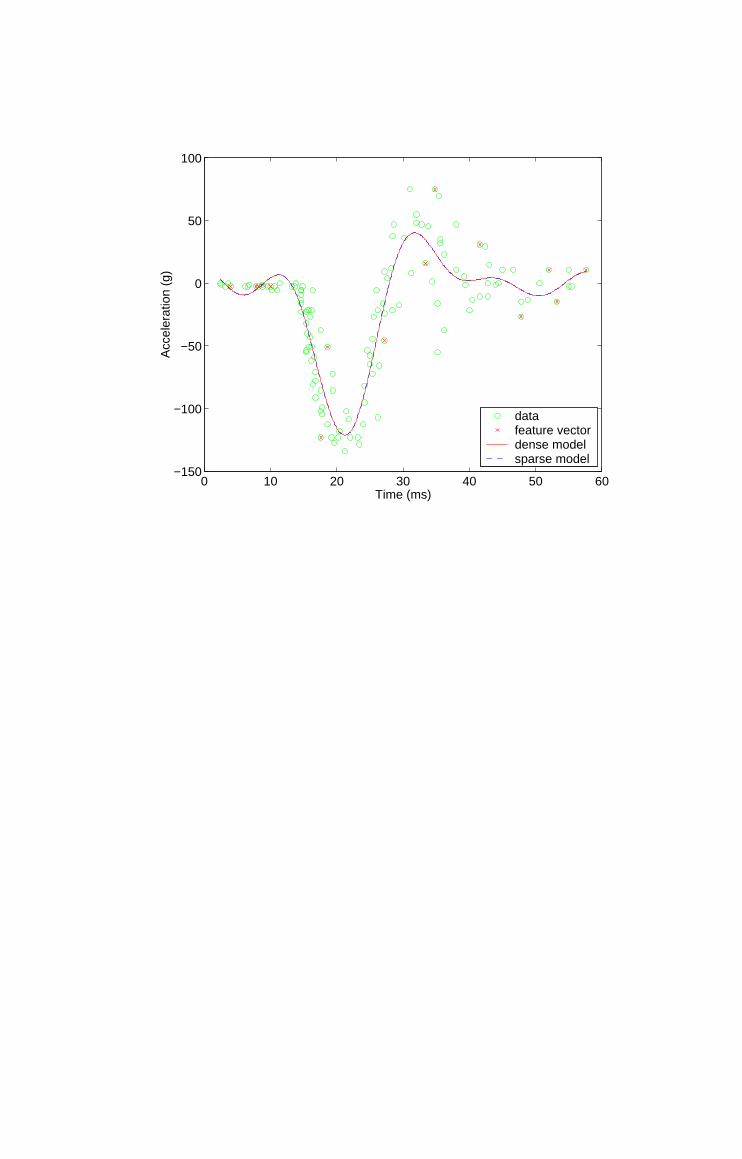
Figure 2 illustrates the leave-one-out cross-validation behaviour of the sparse

least-squares support vector machine, i.e. the predicted value for each dat-

apoint comprising the training data using a model trained only on the re-

maining datapoints. Note that the behaviour computed using the proposed

fast algorithm (depicted by the diamonds) is essentially identical to that ob-

tained by explicit leave-one-out cross-validation (depicted by crosses). The

fast leave-one-out cross-validation algorithm is however more than two orders

of magnitude faster than the conventional approach for this dataset, as shown

in table 1. Let the relative sum-of-squares error be defined as

Er =‖e− e‖‖e‖

, (6)

where e is the vector of predicted (leave-one-out) residuals computed explic-


itly and e is the vector of predicted residuals computed via the proposed

efficient method. The relative sum-of-squares error for the Motorcycle data

set is negligible (Er = 7.6× 10−6).

3.2 The Boston Housing Dataset

The Boston housing dataset describes the relationship between the median

value of owner occupied homes in the suburbs of Boston and thirteen attributes

representing environmental and social factors believed to be relevant [37]. The

input patterns, xiì=1, were first standardised, such that each element of the

input vector has a zero mean and unit variance, allowing an isotropic Gaussian

radial basis kernel (6) to be used. Again the hyper-parameters were chosen so

as to minimise a 10-fold cross-validation estimate of the test sum-of-squares

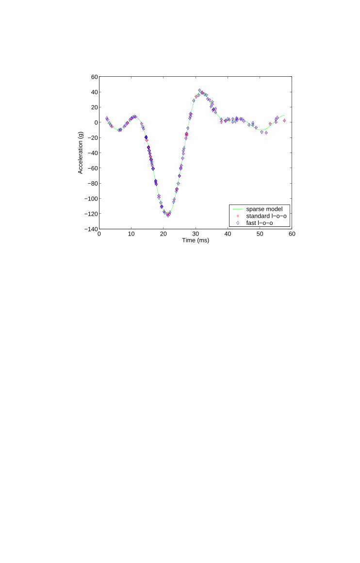
error (γ = 2.89 × 104 and σ−2 = 4.36). Figure 3 shows the mean relative

reconstruction error (4) as a function of the number of basis vectors identified

by the feature vector selection algorithm. The mean relative reconstruction

error is negligible if more than ≈ 200 basis vectors are used.

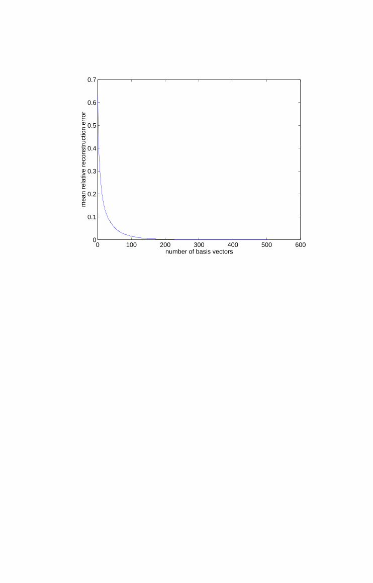
Explicit and fast leave-one-out cross-validation procedures were then evaluated

for sparse least-squares regression networks based on the first 200 basis vectors

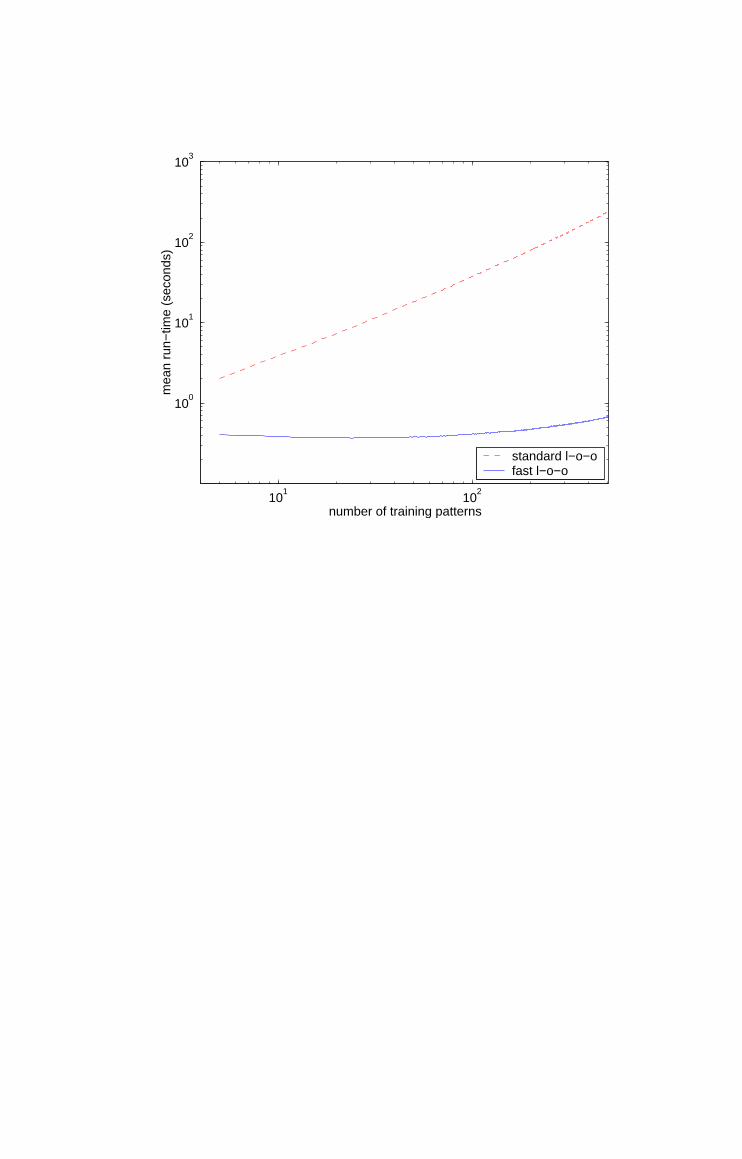
identified by the feature vector selection algorithm. Figure 4 shows the mean

run-time in seconds for both algorithms as a function of the number of training

patterns, `, over 20 trials. The fast leave-one-out cross-validation procedure is

in all cases considerably faster than explicit evaluation, and has better scaling

properties.


4 Discussion

The application of the Bartlett correction formula to the efficient evaluation

of the leave-one-out cross-validation error of linear models minimising a least-

squares criterion has been known for some time in the field of statistics [33].

The “kernel trick” allows this method to be extended to non-linear models

formed via construction of a linear model in a feature space defined by a Mer-

cer kernel. In principal it should be possible to apply a similar procedure to

related kernel models, such as least-squares support vector classification net-

works [38], Kernel Fisher Discriminant (KFD) analysis [39, 40] and 2-norm

support vector machines [6, 16, 17], where the Lagrange multipliers associated

with the support vectors are given by the solution of a system of linear equa-

tions corresponding to the Karush-Kuhn-Tucker (KKT) conditions.

5 Summary

In this paper we have shown that the Bartlett correction formula can be used to

implement exact leave-one-out cross-validation of sparse least-squares support

vector regression networks with a computational complexity of only O(`n2),

rather than the O(`2n2) of a naıve direct implementation. Since the computa-

tional complexity of the basic training algorithm is also O(`n2), leave-one-out

cross-validation becomes a practical criterion for model selection for this class

of kernel machines, as demonstrated by experiments on the Motorcycle and

Boston Housing benchmark data sets.


Acknowledgements

The authors would like to thank the anonymous reviewers, Danilo Mandic,

Tony Bagnall and Rob Foxall for their helpful comments on previous drafts.

This work was supported by Royal Society Research Grant RSRG-22270.


References

[1] R. Kohavi. A study of cross-validation and bootstrap for accuracy estimation

and model selection. In Proceedings of the Fourteenth International Conference

on Artificial Intelligence (IJCAI), pages 1137–1143, San Mateo, CA, 1995.

Morgan Kaufmann.

[2] V. Vapnik and O. Chapelle. Bounds on error expectation for support vector

machines. Neural Computation, 12(9):2013–2036, September 2000.

[3] O. Chapelle, V. Vapnik, O. Bousquet, and S. Mukherjee. Choosing multiple

parameters for support vector machines. Machine Learning, 46(1):131–159,

2002.

[4] S. S. Keerthi. Efficient tuning of SVM hyperparameters using radius/margin

bound and iterative algorithms. IEEE Transactions on Neural Networks,

13(5):1225–1229, September 2002.

[5] A. Luntz and V. Brailovsky. On estimation of characters obtained in statistical

procedure of recognition (in russian). Techicheskaya Kibernetica, 3, 1969.

[6] V. N. Vapnik. Statistical Learning Theory. Wiley Series on Adaptive and

Learning Systems for Signal Processing, Communications and Control. Wiley,

New York, 1998.

[7] T. Poggio and Girosi F. Networks for approximation and learning. Proceedings

of the IEEE, 78(9), September 1990.

[8] C. Saunders, A. Gammerman, and V. Vovk. Ridge regression learning algorithm

in dual variables. In Proceedings, 15th International Conference on Machine

Learning, pages 515–521, Madison, WI, July 24–27 1998.

[9] J. Suykens, L. Lukas, and J. Vandewalle. Sparse approximation using

least-squares support vector machines. In Proceedings, IEEE International


Symposium on Circuits and Systems, pages 11757–11760, Geneva, Switzerland,

May 2000.

[10] J. A. K. Suykens, J. De Brabanter, L. Lukas, and J. Vandewalle. Weighted

least squares support vector machines : robustness and sparse approximation.

Neurocomputing, 48(1–4):85–105, October 2002.

[11] A. N. Tikhonov and V. Y. Arsenin. Solutions of ill-posed problems. John Wiley,

New York, 1977.

[12] S. Geman, E. Bienenstock, and R. Doursat. Neural networks and the

bias/variance dilema. Neural Computation, 4(1):1–58, 1992.

[13] A. E. Hoerl and R. W. Kennard. Ridge regression: Biased estimation for

nonorthogonal problems. Technometrics, 12(1):55–67, 1970.

[14] N. Cristianini and J. Shawe-Taylor. An Introduction to Support Vector

Machines (and other kernel-based learning methods). Cambridge University

Press, Cambridge, U.K., 2000.

[15] G. S. Kimeldorf and G. Wahba. Some results on Tchebycheffian spline functions.

J. Math. Anal. Applic., 33:82–95, 1971.

[16] B. Boser, I. Guyon, and V. N. Vapnik. A training algorithm for optimal margin

classifiers. In Proceedings of the fifth annual workshop on computational learning

theory, pages 144–152, Pittsburgh, 1992. ACM.

[17] C. Cortes and V. Vapnik. Support vector networks. Machine Learning, 20:1–25,

1995.

[18] J. A. K. Suykens, L. Lukas, P. Van Dooren, B. De Moor, and J. Vandewalle.

Least squares support vector machine classifiers : a large scale algorithm.

In Proceedings of the European Conference on Circuit Theory and Design

(ECCTD-99), pages 839–842, Stresa, Italy, September 1999.


[19] C. K. I. Williams and M. Seeger. Using the Nystrom method to speed up kernel

machines. In T. K. Leen, T. G. Dietterich, and V. Tresp, editors, Advances in

Neural Information Processing Systems 13, pages 682–688. MIT Press, 2001.

[20] G. C. Cawley and N. L. C. Talbot. A greedy training algorithm for sparse least-

squares support vector machines. In Proceedings of the International Conference

on Artificial Neural Networks (ICANN-2002), volume 2415 of Lecture Notes in

Computer Science (LNCS), pages 681–686, Madrid, Spain, August 27–30 2002.

Springer.

[21] G. C. Cawley and N. L. C. Talbot. Improved sparse least-squares support vector

machines. Neurocomputing, 48:1025–1031, October 2002.

[22] C. J. C. Burges. Simplified support vector decision rules. In Proceedings of the

13th International Conference on Machine Learning, pages 71–77, Bari, Italy,

1996.

[23] C. J. C. Burges and B. Scholkopf. Improving speed and accuracy of support

vector learning machines. In Advances in Neural Information Processing

Systems, volume 9, pages 375–381. MIT Press, 1997.

[24] T. Downs, K. E. Gates, and A. Masters. Exact simplification of support vector

solutions. Journal of Machine Learning Research, 2:293–297, December 2001.

[25] Y.-J. Lee and O. L. Mangasarian. RSVM: reduced support vector machines.

In Proceedings of the First SIAM International Conference on Data Mining,

Chicago, IL, USA, April 5–7 2001.

[26] G. Baudat and F. Anouar. Kernel-based methods and function approximation.

In Proc. IJCNN, pages 1244–1249, Washington, DC, July 2001.

[27] A. J. Smola and B. Scholkopf. Sparse greedy matrix approximation for machine

learning. In Proceedings of the 17th International Conference on Machine


Learning, pages 911–918. Morgan Kaufmann, San Fransisco, CA, June 29 -

July 2 2000.

[28] G. C. Cawley and N. L. C. Talbot. Efficient formation of a basis in a kernel

induced feature space. In Proceedings of the European Symposium on Artificial

Neural Networks (ESANN-2002), pages 1–6, Bruges, Belgium, April 24–26 2002.

[29] M. S. Bartlett. An inverse matrix adjustment arising in disciminant analysis.

Annals of Mathematical Statistics, 22(1):107–111, 1951.

[30] D. M. Allen. The relationship between variable selection and prediction.

Technometrics, 16:125–127, 1974.

[31] S. Weisberg. Applied Linear Regression. Wiley, New York, 1985.

[32] T. Hastie, R. Tibshirani, and J. Friedman. The Elements of Statistical Learning:

Data Mining, Inference, and Prediction. Springer Texts in Statistics. Springer,

2001.

[33] R. D. Cook and S. Weisberg. Residuals and Influence in Regression.

Monographs on Statistics and Applied Probability. Chapman and Hall, New

York, 1982.

[34] B. W. Silverman. Some aspects of the spline smoothing approach to non-

parametric regression curve fitting. Journal of the Royal Statistical Society, B,

47(1):1–52, 1985.

[35] J. A. Nelder and R. Mead. A simplex method for function minimization.

Computer Journal, 7:308–313, 1965.

[36] C. A. Micchelli. Interpolation of scattered data: Distance matrices and

conditionally positive definite functions. Constructive Approximation, 2:11–22,

1986.


[37] D. Harrison and D. L. Rubinfeld. Hedonic prices and the demand for clean air.

Journal Environmental Economics and Management, 5:81–102, 1978.

[38] J. Suykens and J. Vandewalle. Least squares support vector machine classifiers.

Neural Processing Letters, 9(3):293–300, 1999.

[39] S. Mika, G. Ratsch, J. Weston, B. Scholkopf, and K.-R. Muller. Fisher

discriminant analysis with kernels. In Neural Networks for Signal Processing,

volume IX, pages 41–48. IEEE Press, New York, 1999.

[40] J. Xu, X. Zhang, and Y. Li. Kernel MSE algorithm: A unified framework for

KFD, LS-SVM and KRR. In Proc. IJCNN, pages 1486–1491, Washington, DC,

July 2001.

[41] J. Sherman and W. J. Morrison. Adjustment of an inverse matrix corresponding

to changes in the elements of a given column or a given row of the original

matrix. Annals of Mathematical Statistics, 20(4):621, 1949.

[42] J. Sherman and W. J. Morrison. Adjustment of an inverse matrix corresponding

to a change in one element of a given matrix. Annals of Mathematical Statistics,

21(1):124–127, 1950.

[43] M. Woodbury. Inverting modified matrices. Memorandum report 42, Princeton

University, Princeton, U.S.A., 1950.

[44] W. W. Hager. Updating the inverse of a matrix. SIAM Review, 31(2):221–239,

June 1989.

[45] G. H. Golub and C. F. Van Loan. Matrix Computations. The Johns Hopkins

University Press, Baltimore, third edition edition, 1996.


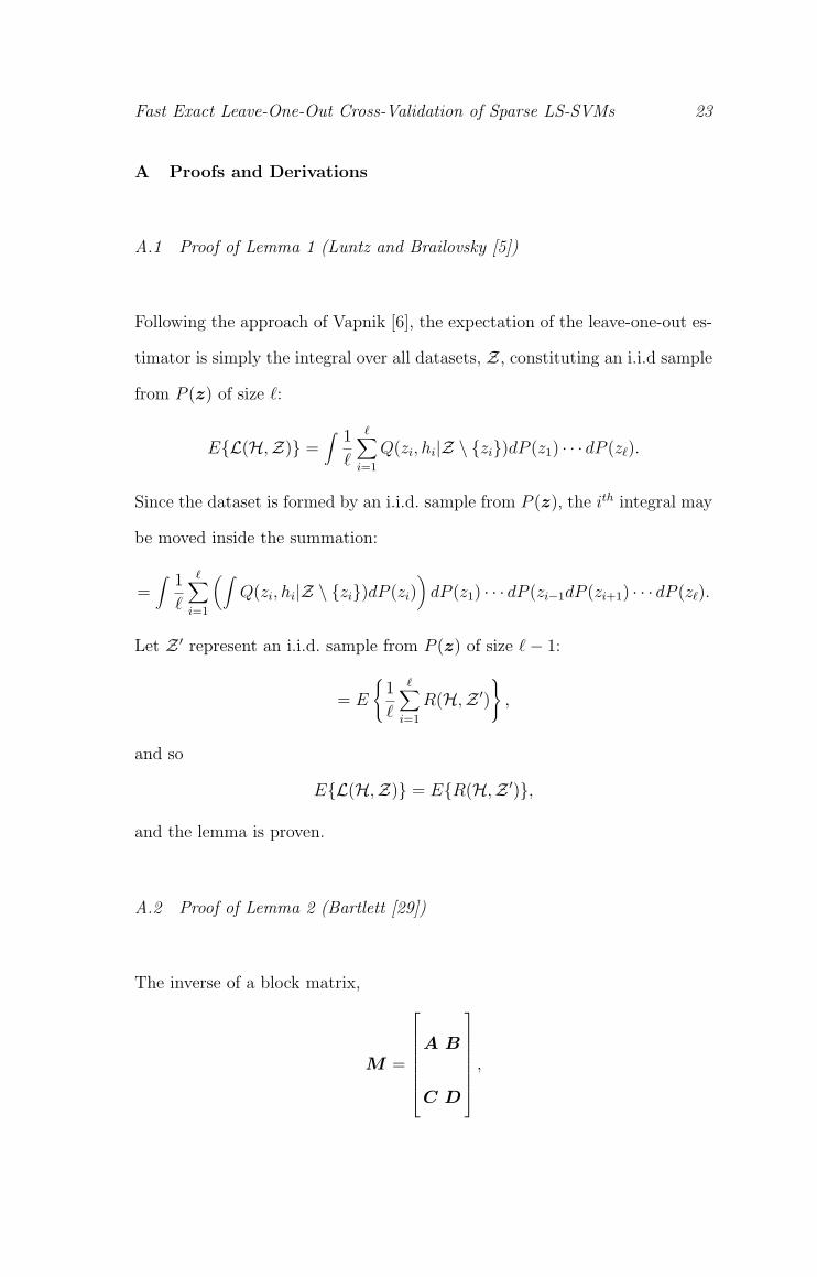
A Proofs and Derivations

A.1 Proof of Lemma 1 (Luntz and Brailovsky [5])

Following the approach of Vapnik [6], the expectation of the leave-one-out es-

timator is simply the integral over all datasets, Z, constituting an i.i.d sample

from P (z) of size `:

EL(H,Z) =∫ 1

`

∑i=1

Q(zi, hi|Z \ zi)dP (z1) · · · dP (z`).

Since the dataset is formed by an i.i.d. sample from P (z), the ith integral may

be moved inside the summation:

=∫ 1

`

∑i=1

(∫Q(zi, hi|Z \ zi)dP (zi)

)dP (z1) · · · dP (zi−1dP (zi+1) · · · dP (z`).

Let Z ′ represent an i.i.d. sample from P (z) of size `− 1:

= E

1

`

∑i=1

R(H,Z ′)

,

and so

EL(H,Z) = ER(H,Z ′),

and the lemma is proven.

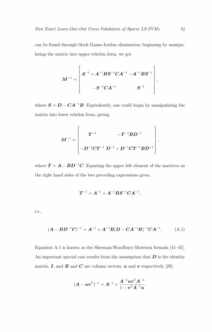
A.2 Proof of Lemma 2 (Bartlett [29])

The inverse of a block matrix,

M =

A B

C D

,


can be found through block Gauss-Jordan elimination; beginning by manipu-

lating the matrix into upper echelon form, we get

M−1 =

A−1 + A−1BS−1CA−1 −A−1BS−1

−S−1CA−1 S−1

,

where S = D −CA−1B. Equivalently, one could begin by manipulating the

matrix into lower echelon form, giving

M−1 =

T−1 −T−1BD−1

−D−1CT−1 D−1 + D−1CT−1BD−1

,

where T = A−BD−1C. Equating the upper left element of the matrices on

the right hand sides of the two preceding expressions gives,

T−1 = A−1 + A−1BS−1CA−1,

i.e.,

(A−BD−1C)−1 = A−1 + A−1B(D −CA−1B)−1CA−1. (A.1)

Equation A.1 is known as the Sherman-Woodbury-Morrison formula [41–45].

An important special case results from the assumption that D is the identity

matrix, I, and B and C are column vectors, u and v respectively [29]:

(A− uvT )−1 = A−1 +A−1uvT A−1

1− vT A−1u.


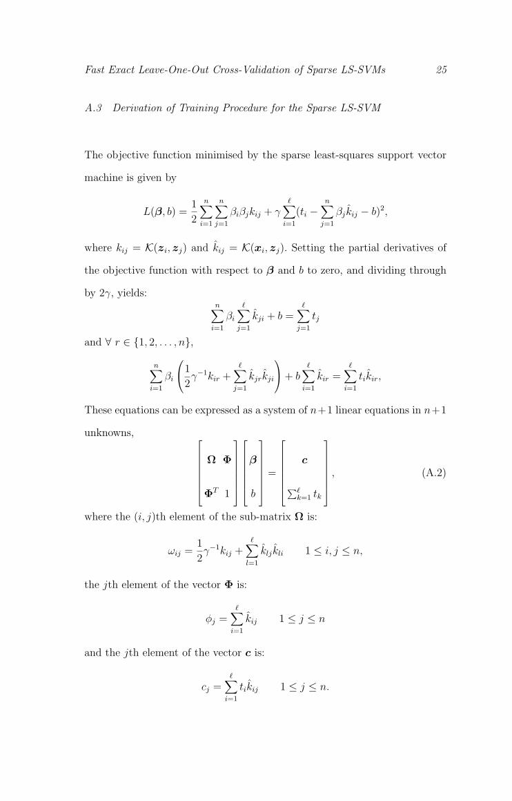
A.3 Derivation of Training Procedure for the Sparse LS-SVM

The objective function minimised by the sparse least-squares support vector

machine is given by

L(β, b) =1

2

n∑i=1

n∑j=1

βiβjkij + γ∑i=1

(ti −n∑

j=1

βj kij − b)2,

where kij = K(zi, zj) and kij = K(xi, zj). Setting the partial derivatives of

the objective function with respect to β and b to zero, and dividing through

by 2γ, yields:n∑

i=1

βi

∑j=1

kji + b =∑j=1

tj

and ∀ r ∈ 1, 2, . . . , n,

n∑i=1

βi

1

2γ−1kir +

∑j=1

kjrkji

+ b∑i=1

kir =∑i=1

tikir,

These equations can be expressed as a system of n+1 linear equations in n+1

unknowns, Ω Φ

ΦT 1

β

b

=

c

∑`k=1 tk

, (A.2)

where the (i, j)th element of the sub-matrix Ω is:

ωij =1

2γ−1kij +

∑l=1

klj kli 1 ≤ i, j ≤ n,

the jth element of the vector Φ is:

φj =∑i=1

kij 1 ≤ j ≤ n

and the jth element of the vector c is:

cj =∑i=1

tikij 1 ≤ j ≤ n.


This matrix equation can be simplified by referring to the vector consisting of

all the model parameters as p = (β, b)T , and by defining the matrices R and

Z as:

R =

12γ

K 0

0T 0

Z = [K 1]

where the (i, j)th element of K is kij, and the (i, j)th element of K is kij.

Equation (A.2) can then be written as:

(R + ZT Z)p = ZT t. (A.3)

A.4 Derivation of Closed Form Expression for Predicted Residuals

From e.g. Equation (A.3) we know that the vector of model parameters p =

(β, b) is given by

p = (R + ZT Z)−1ZT t

where Z = [K 1]. For convenience, let C = R + ZT Z and d = ZT t, such

that p = C−1d. Furthermore, let Z(i) and t(i) represent the data with the ith

observation deleted, then

C(i) = C − zizTi ,

and

d(i) = d− tizi.

The Bartlett matrix inversion formula then gives

C−1(i) = C +

C−1zizTi C−1

1− zTi C−1zi

,

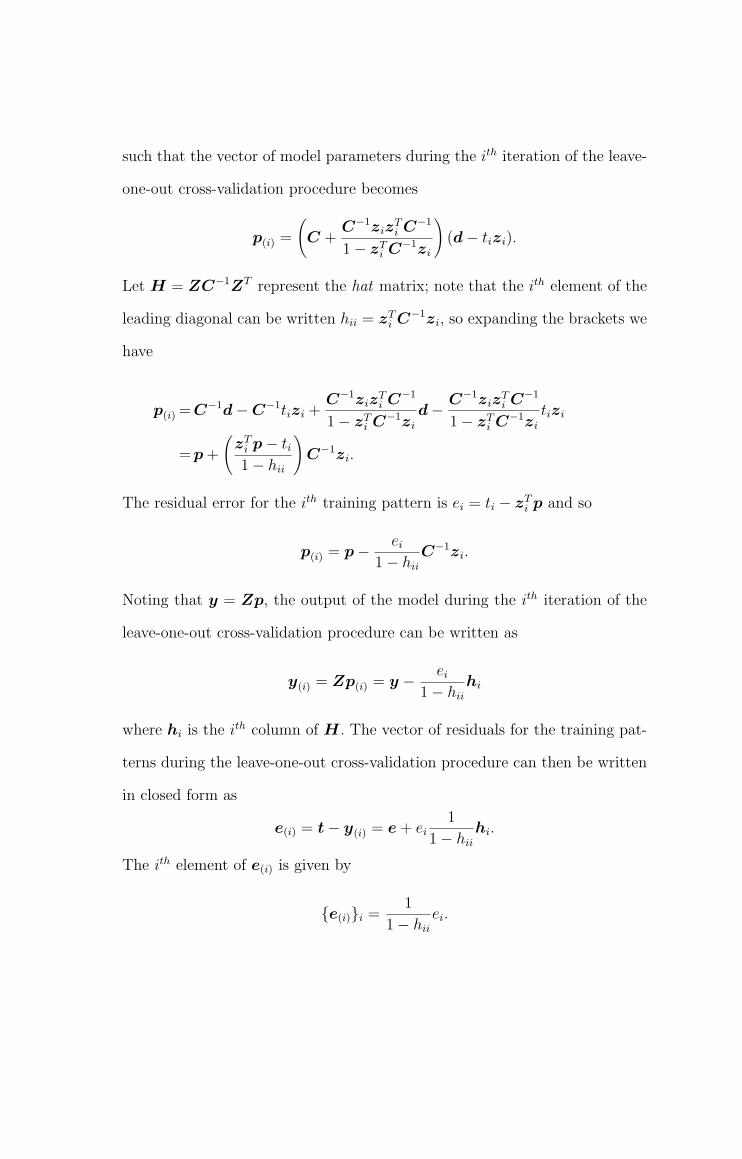
such that the vector of model parameters during the ith iteration of the leave-

one-out cross-validation procedure becomes

p(i) =

(C +

C−1zizTi C−1

1− zTi C−1zi

)(d− tizi).

Let H = ZC−1ZT represent the hat matrix; note that the ith element of the

leading diagonal can be written hii = zTi C−1zi, so expanding the brackets we

have

p(i) = C−1d−C−1tizi +C−1ziz

Ti C−1

1− zTi C−1zi

d− C−1zizTi C−1

1− zTi C−1zi

tizi

= p +

(zT

i p− ti1− hii

)C−1zi.

The residual error for the ith training pattern is ei = ti − zTi p and so

p(i) = p− ei

1− hii

C−1zi.

Noting that y = Zp, the output of the model during the ith iteration of the

leave-one-out cross-validation procedure can be written as

y(i) = Zp(i) = y − ei

1− hii

hi

where hi is the ith column of H . The vector of residuals for the training pat-

terns during the leave-one-out cross-validation procedure can then be written

in closed form as

e(i) = t− y(i) = e + ei1

1− hii

hi.

The ith element of e(i) is given by

e(i)i =1

1− hii

ei.

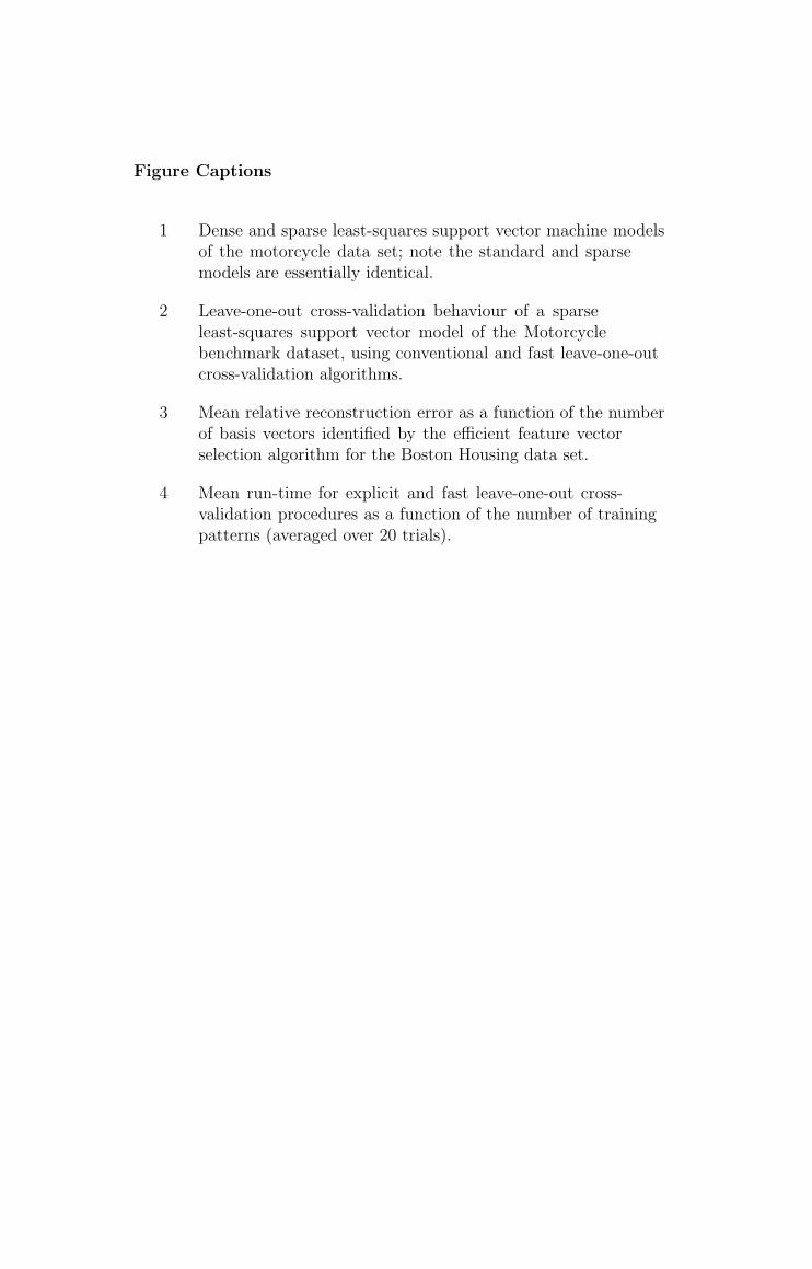
Figure Captions

1 Dense and sparse least-squares support vector machine modelsof the motorcycle data set; note the standard and sparsemodels are essentially identical.

2 Leave-one-out cross-validation behaviour of a sparseleast-squares support vector model of the Motorcyclebenchmark dataset, using conventional and fast leave-one-outcross-validation algorithms.

3 Mean relative reconstruction error as a function of the numberof basis vectors identified by the efficient feature vectorselection algorithm for the Boston Housing data set.

4 Mean run-time for explicit and fast leave-one-out cross-validation procedures as a function of the number of trainingpatterns (averaged over 20 trials).

0 10 20 30 40 50 60−150

−100

−50

0

50

100

Time (ms)

Acc

eler

atio

n (g

)

datafeature vectordense modelsparse model

0 10 20 30 40 50 60−140

−120

−100

−80

−60

−40

−20

0

20

40

60

Time (ms)

Acc

eler

atio

n (g

)

sparse modelstandard l−o−ofast l−o−o

0 100 200 300 400 500 6000

0.1

0.2

0.3

0.4

0.5

0.6

0.7m

ean

rela

tive

reco

nstr

uctio

n er

ror

number of basis vectors

101

102

100

101

102

103

mea

n ru

n−tim

e (s

econ

ds)

number of training patterns

standard l−o−ofast l−o−o

List of Tables

1 Mean run-time of standard and fast leave-one-out cross-validation algorithms for the Motorcycle benchmark dataset,over 100 trials.

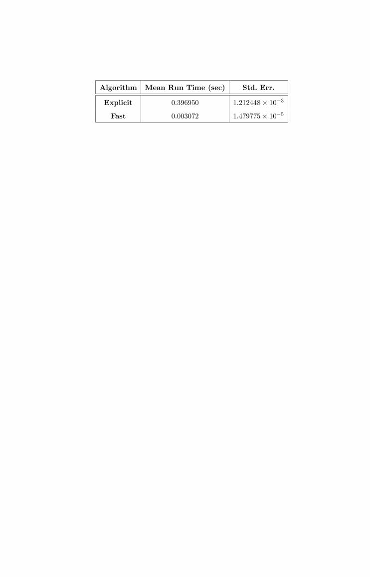
Algorithm Mean Run Time (sec) Std. Err.

Explicit 0.396950 1.212448× 10−3

Fast 0.003072 1.479775× 10−5

Documents

Fast Exact Leave-One-Out Cross-Validation of Sparse Least ...theoval.cmp.uea.ac.uk/publications/pdf/nn2004a.pdf · Fast Exact Leave-One-Out Cross-Validation of Sparse Least-Squares