Fast Penetration Depth Computation for Physically-based Animation

Young J. Kim Miguel A. Otaduy Ming C. Lin Dinesh Manocha

Department of Computer ScienceUniversity of North Carolina at Chapel Hill{youngkim,otaduy,lin,dm}@cs.unc.edu

http://gamma.cs.unc.edu/PD

Abstract

We present a novel and fast algorithm to compute penetration depth(PD) between two polyhedral models for physically-based anima-tion. Given two overlapping polyhedra, it computes the minimaltranslation distance to separate them using a combination of object-space and image-space techniques. The algorithm computes pair-wise Minkowski sums of decomposed convex pieces and performsa closest point query using rasterization hardware. It uses bound-ing volume hierarchies, object-space and image-space culling al-gorithms to further accelerate the computation and refines the esti-mated PD in a hierarchical manner. We demonstrate its applicationto contact response computation and a time-stepping method fordynamic simulation.

CR Categories: I.3.5 [Computer Graphics]: Computational Ge-ometry and Object Modeling—Geometric Algorithms, Object Hi-erarchies, Physically Based Modeling; I.3.7 [Computer Graphics]:Three-Dimensional Graphics and Realism—Visible Line/SurfaceAlgorithms

Keywords: Collision detection, Graphics hardware, Image-space computations, Dynamics simulation, Geometric modeling,Robotics

1 Introduction

The need to perform fast proximity queries, including collision de-tection, tolerance checking, distance calculation and penetrationcomputation, arises in numerous areas. Some applications includephysically-based animation, planning of autonomous characters,computer games, and virtual environments. While several of thesequeries, such as collision detection and distance computation, havebeen extensively studied in the field, there is relatively little workon penetration computation that provides a measure of intersectionor penetration between two overlapping models. Given two inter-penetrating rigid polyhedral models, the penetration measure be-tween them can be defined using different formulations. One of thewidely used measures for quantifying the amount of intersection ispenetration depth, commonly defined as the minimum translationaldistance required to separate two intersecting rigid models [Dobkinet al. 1993; Cameron and Culley 1986; Cameron 1997].

Most of existing collision detection algorithms and systems donot handle inter-penetrations and current distance computation al-gorithms do not provide a continuous distance measure when two(non-convex) objects collide. This can induce numerical problems,e.g. instability or invalid results, in dynamic simulation. Further-more, several commonly used techniques like penalty-based simu-lation methods often need to perform PD queries for imposing thenon-penetration constraint for rigid body simulation [McKenna andZeltzer 1990; Mirtich 2000; Stewart and Trinkle 1996]. Variousheuristics, such as reducing the frequency of PD computation [Mc-Neely et al. 1999] or estimating PD based on the last closest featurepairs [Mirtich 2000; Gregory et al. 2000], are sometimes used. But,the results can be inconsistent and inaccurate. Fast and reliable PDcomputation is important for robust and efficient simulation of dy-namical systems.

The PD between two overlapping objects can be formulatedbased on theirMinkowski sum. However, the worst case computa-tional complexity of computing the Minkowski sum can beO(n6),wheren is the number of features [Dobkin et al. 1993]. In addi-tion to its high computational complexity, the resulting algorithmsare also susceptible to accuracy and robustness problems. Hence,no practical algorithms are yet known for accurately computing thePD between general polyhedral models.

Main Results: We present a novel approach to approximate the PDbetween general polyhedral models using a combination of object-space and image-space techniques. Given the global nature of thePD problem, we systematically decompose the boundary of eachpolyhedron into convex pieces, compute the pairwise Minkowskisums of the resulting convex polytopes and use the polygon inter-polation based rasterization hardware to perform the closest pointquery up to image-space resolution. To further speed up this com-putation and improve the estimate, we use a hierarchical refinementtechnique that takes advantage of object-space culling and image-space acceleration. The overall approach combines image-space ac-celerated queries with object-space culling and refinement at eachlevel of the hierarchy.

This algorithm has been implemented and tested on differentbenchmarks. Depending on the combinatorial complexity of poly-hedra and their relative configuration, its performance varies froma fraction of a second to a few seconds on a 1.6GHz PC with anNVIDIA GeForce 3 graphics card. To illustrate the effectiveness ofour algorithm, we demonstrate its application to contact responsecomputation and a time-stepping method for rigid-body dynamicsimulation. To the best of our knowledge, this is the first practicalalgorithm for computing a reliable PD between general polyhedralmodels for physically-based animation and it works well for differ-ent challenging scenarios.

Organization: The rest of the paper is organized in the followingmanner. We give a brief summary of the related work in Section 2and present some background material along with an overview ofour approach in Section 3. Section 4 describes the underlying algo-rithm that uses a combination of object space and image space com-

putations. We present a number of acceleration methods in Section5 to improve the overall performance. Section 6 describes its imple-mentation and performance on different configurations. Section 7highlights its application to physically-based animation, includingpenalty-based rigid-body simulation and time-stepping methods.

2 Previous Work

In this section, we briefly review previous work related to proxim-ity queries, penetration depth computation and the use of graphicsrasterization hardware for geometric computations.

2.1 Collision and Distance Queries

The problems of collision detection and distance computations arewell studied in computational geometry, robotics, and simulated en-vironments. Most of the prior work on polyhedra can be catego-rized based on the types of models, such as convex polytopes andgeneral polygonal models.

For convex polytopes, various techniques have been developedbased on Minkowski sum [Cameron 1997; Gilbert et al. 1988] andfeature tracking using Voronoi regions [Lin and Canny 1991; Mir-tich 1998]. Some of these algorithms also utilize the spatial andtemporal coherence between successive frames and perform incre-mental computations [Baraff 1992; Cameron 1997; Lin and Canny1991; Mirtich 1998].

For general polygonal models, bounding volume hierarchies(BVHs) have been widely used for collision detection and sepa-ration (or Euclidean) distance queries. They localize the problembased on the “divide-and-conquer” paradigm. BVHs often differbased on the underlying bounding volume or traversal schemes.These include the OBB trees [Gottschalk et al. 1996], sphere trees[Hubbard 1995], k-dops [Klosowski et al. 1998], and convex hull-based trees that use surface based convex decomposition [Ehmannand Lin 2001]. Due to the global nature of the PD problem, none ofthem can be directly used for PD computation between non-convexmodels.

2.2 Penetration Depth Computation

A few efficient algorithms to compute the penetration depth (PD)between convex polytopes have been proposed. The simplest exactalgorithm is based on computing their Minkowski sum [Guibas andSeidel 1987; Kaul and Rossignac 1992] followed by computing theclosest point to its boundary from the origin. But its worst casecomplexity isO(mn), wherem andn are the number of features ineach polytope. Dobkin et al. computed the directional PD using theDobkin and Kirkpatrick polyhedral hierarchy [Dobkin et al. 1993].For any directiond, it finds the directional PD inO(lognlogm)time. A randomized algorithm to compute the PD is given in [Agar-wal et al. 2000].

Given the worst-caseO(mn) complexity of PD computation be-tween convex polytopes, a number of approximation approacheshave been proposed for interactive applications. All of them ei-ther compute a subset of the boundary or a simpler approximationof the Minkowski sum and compute an upper or lower bound to thePD [Cameron 1997; Bergen 2001; Ong and Gilbert 1996; Kim et al.2002a]. They also take advantage of frame-to-frame coherence andperform incremental computations.

Other approximation approaches for general polygonal modelsare based on discretized distance fields. These include discretizedalgorithms based on fast marching level-sets for 3D deformablemodels [Fisher and Lin 2001] and others based on graphics ras-terization hardware and multi-pass rendering for 2D objects [Hoffet al. 2001]. These techniques provide a localized estimation that

may not be correct. No good global algorithms are known for PDcomputation between general polyhedral models.

2.3 Graphics Hardware for Geometric Applications

Interpolation-based polygon rasterization hardware is increasinglybeing used for geometric applications. These include visibility andshadow computations, CSG rendering, proximity queries, morph-ing, object reconstruction etc. A recent survey on different applica-tions is given in [Theoharis et al. 2001]. All these algorithms per-form computations in a discretized space (i.e. the image-space) andtheir accuracy is governed by the underlying pixel resolution. Theset of proximity query algorithms include cross-sections and inter-ferences [Rossignac et al. 1992] and distance computations, includ-ing separation and local penetration estimation [Hoff et al. 1999;Hoff et al. 2001]. An algorithm to compute a discretized approx-imation to the convolution of general polyhedral models using therasterization hardware is presented in [Kaul and Rossignac 1992].Algorithms for direct rendering of CSG models based on graphicsrasterization hardware have been presented in [Epstein et al. 1989;Goldfeather et al. 1986; Wiegand 1996]. They render the CSG hi-erarchies using multiple passes of clipping (i.e. stencil tests) anddepth tests.

3 Background and Overview

In this section, we give a brief overview of the PD computationproblem and our approach to solve it.

3.1 Penetration Depth and Minkowski Sums

Let P and Q be two intersecting polyhedra. The PD ofP andQ, PD(P,Q), is the minimum translational distance that one ofthe polyhedra must undergo to render them disjoint. Formally,PD(P,Q) is defined as:

min{‖ d ‖ | interior(P+d) ∩ Q = /0} (1)

Here,d is a vector inR3.A general framework to compute the PD is based on Minkowski

sums. The Minkowski sum,P⊕Q, is defined as a set of pairwisesums of vectors fromP andQ. In other words,P⊕Q = {p+q| p∈P,q∈Q}. Furthermore,P⊕−Q is defined by negatingQ; i.e. P⊕−Q = {p−q| p∈ P,q∈Q}.

It is well known that one can reduce the problem of comput-ing the PD betweenP andQ to a minimum distance query on thesurface of their Minkowski sum ,P⊕−Q [Cameron 1997]. Morespecifically, if two polyhedraP andQ intersect, then the differencevector,OQ−OP, between the origins1 of P andQ is insideP⊕−Q.Let us denoteOQ−OP by OQ−P. The PD(P,Q) is defined as aminimum distance fromOQ−P to the surface ofP⊕−Q.

3.2 Local Vs. Global Computations

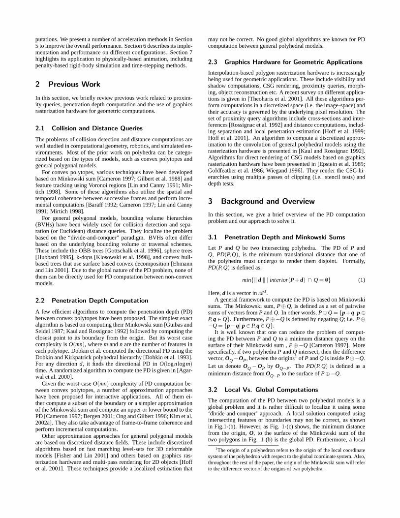
The computation of the PD between two polyhedral models is aglobal problem and it is rather difficult to localize it using some‘divide-and-conquer’ approach. A local solution computed usingintersecting features or boundaries may not be correct, as shownin Fig.1-(b). However, as Fig. 1-(c) shows, the minimum distancefrom the origin,O, to the surface of the Minkowski sum of thetwo polygons in Fig. 1-(b) is the global PD. Furthermore, a local

1The origin of a polyhedron refers to the origin of the local coordinatesystem of the polyhedron with respect to the global coordinate system. Also,throughout the rest of the paper, the origin of the Minkowski sum will referto the difference vector of the origins of two polyhedra.

solution to the PD problem may fail to compute a correct responsefor dynamic simulation, as explained in Section 7.

o

(a) (b) (c)

Figure 1: Local vs Global PD Computation.(a) shows the situation

before two polygons in 2D come into contact. (b) shows O(nm) intersections after

the polygons are intersected. However, a localized PD computation (denoted by solid

arrows) based on O(nm) intersections may not provide a global PD which is denoted

as a dotted arrow in this figure. (c) shows the Minkowski sum of the two polygons

in (b). The minimum distance from the origin to the surface of the Minkowski sum

corresponds to the global PD.

3.3 Our Approach

It is relatively easier to compute Minkowski sums of convex poly-topes as compared to general polyhedral models. However, fornon-convex polyhedra in 3D, the Minkowski sum can haveO(n6)worst-case complexity [Dobkin et al. 1993]. One possible approachfor computing Minkowski sums for general polyhedra is based ondecomposition. It uses the following property of Minkowski com-putation. IfP = P1∪P2, thenP⊕Q = (P1⊕Q) ∪ (P2⊕Q). Theresulting algorithm combines this property with convex decompo-sition for general polyhedral models:

1. Compute a convex decomposition for each polyhedron

2. Compute the pairwise convex Minkowski sums between allpossible pairs of convex pieces in each polyhedron

3. Compute the union of pairwise Minkowski sums.

In order to overcome its combinatorial and computational com-plexity, we use asurface-basedconvex decomposition of theboundary and utilize the graphics rasterization hardware to estimatethe PD. Moreover, we do not explicitly compute the boundary ofthe union or any approximation to it. Rather, we perform theclos-est point queryusing a multipass algorithm that computes the clos-est point from the origin to the boundary of the union of pairwiseMinkowski sums. The resulting maximum depth fragment at eachpixel computes an approximation to the PD, up to the image-spaceresolution used for this computation.

We improve the performance of the basic algorithm highlightedabove using a number of acceleration techniques. These includehierarchical representation based on convex bounding volumes,object-space culling approaches and image-space acceleration tech-niques applied to the multipass algorithm. These are explained indetail in Section 5.

The resulting algorithm includes a pre-computation phase aswell as a runtime query. The pre-computation phase consists ofthe following steps:

1. Decompose the boundary of each polyhedron into convexpatches using a greedy approach (Sec. 4.1).

2. Compute a bounding volume hierarchical representation ofthe model. Each node in the tree corresponds to a convexpolytope and each leaf is a convex hull of a decomposed con-vex patch (Sec. 5.2).

Given two polyhedra and their bounding volume representations,the runtime phase of the algorithm proceeds in the following man-ner:

1. Compute an upper estimate to the amount of PD. Let that es-timate bedest. Initially we compute an estimate based on theroot nodes of each tree (Sec. 5.3).

2. At each level of the two hierarchies, repeat the followingsteps:

(a) Consider all pairwise combinations of nodes at thecurrent level. Cull away all the pairs that are non-overlapping and are more thandest apart (Sec. 5.3).

(b) Compute pairwise Minkowski sums of the rest of thenode pairs that have not been culled away (Sec. 4.2).

(c) Perform the closest point query using the rasterizationhardware to compute a PD estimate (Sec. 4.3).

The entire pipeline of our PD algorithm is illustrated in Fig. 2.

Precomputation

Convex DecompositionDecompose the boundary of each polyhedron into

convex patches.

BVH ConstructionCompute a convex

hull hierarchy of the model

Run-time PD Query

Culling

Cull away the pairs of nodes that are more than dest

Pairwise Minkowski Sum

Compute Minkowski sums for the rest of

node pairs

Closest Point QueryUsing the rasterization

hardware, perform the closest point query on the union of pairwise Minkowski sums

Refine the current PD estimate, dest, and go to the next level of BVH

Figure 2: PD Computation Pipeline

3.4 Notation

We use bold-faced letters to distinguish a vector from a scalar value(e.g. the origin,O). In Table 1, we enumerate the notations that weuse throughout the paper.

Notation Meaning

∂P The boundary ofPCP

i A decomposed convex piece ofPCP,l

iA decomposed convex piece ofP at levell

Mi j Minkowski sum betweenCi andCj

dkest kth refinement of the PD estimation

Table 1: Notation Table

4 Penetration Depth Computation

In this section, we present our basic algorithm for global PD com-putation. It involves decomposing the boundary of the model intoconvex patches, computing their pairwise Minkowski sums, andthen performing a closest point query using rasterization hardware.

Given two intersecting polyhedra, the PD query reports a PDscalar value and direction, along with the associated PD features2.

2These are a pair of features that realize the reported PD. The PD valueis the same as the inter-distance between planes which locally support thePD features.

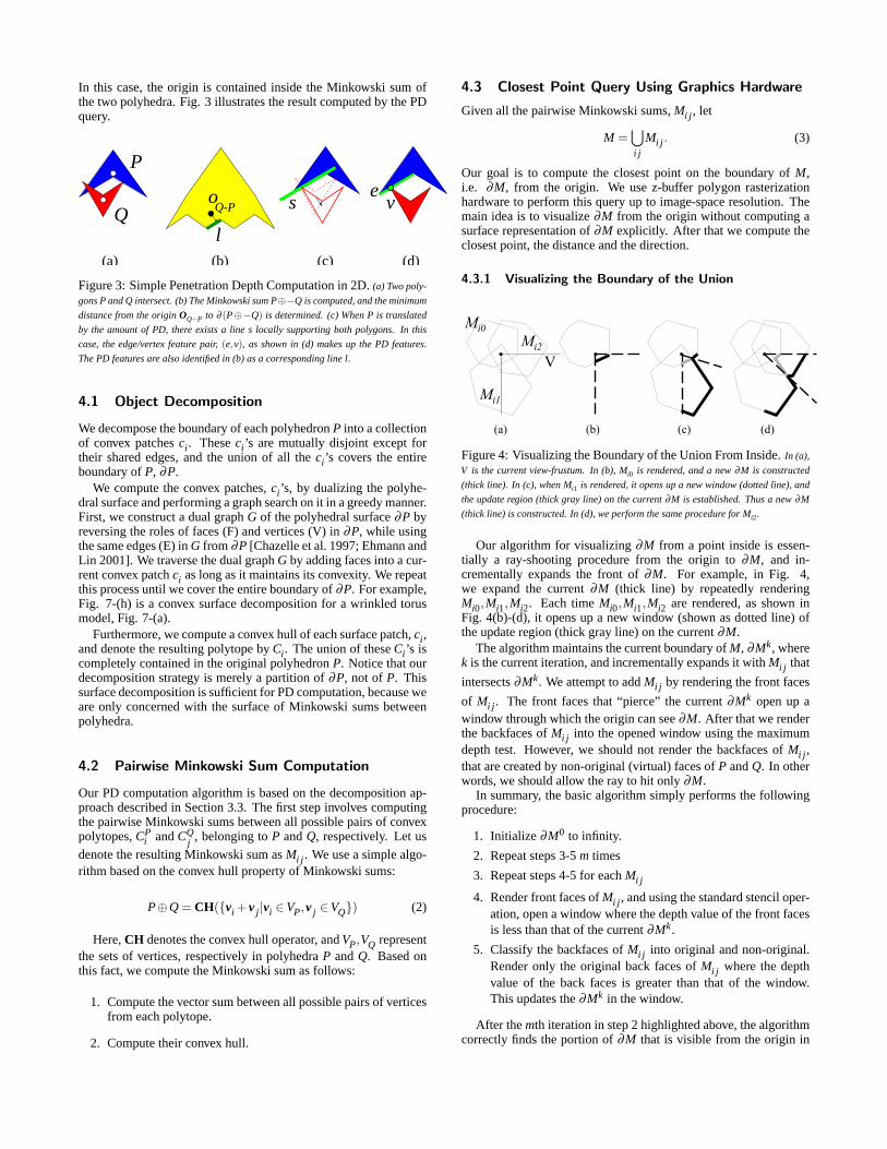
In this case, the origin is contained inside the Minkowski sum ofthe two polyhedra. Fig. 3 illustrates the result computed by the PDquery.

Q-Pe

vo

P

Ql

(a) (b) (c) (d)

s

Figure 3: Simple Penetration Depth Computation in 2D.(a) Two poly-

gons P and Q intersect. (b) The Minkowski sum P⊕−Q is computed, and the minimum

distance from the originOQ−P to ∂ (P⊕−Q) is determined. (c) When P is translated

by the amount of PD, there exists a line s locally supporting both polygons. In this

case, the edge/vertex feature pair,(e,v), as shown in (d) makes up the PD features.

The PD features are also identified in (b) as a corresponding line l.

4.1 Object Decomposition

We decompose the boundary of each polyhedronP into a collectionof convex patchesci . Theseci ’s are mutually disjoint except fortheir shared edges, and the union of all theci ’s covers the entireboundary ofP, ∂P.

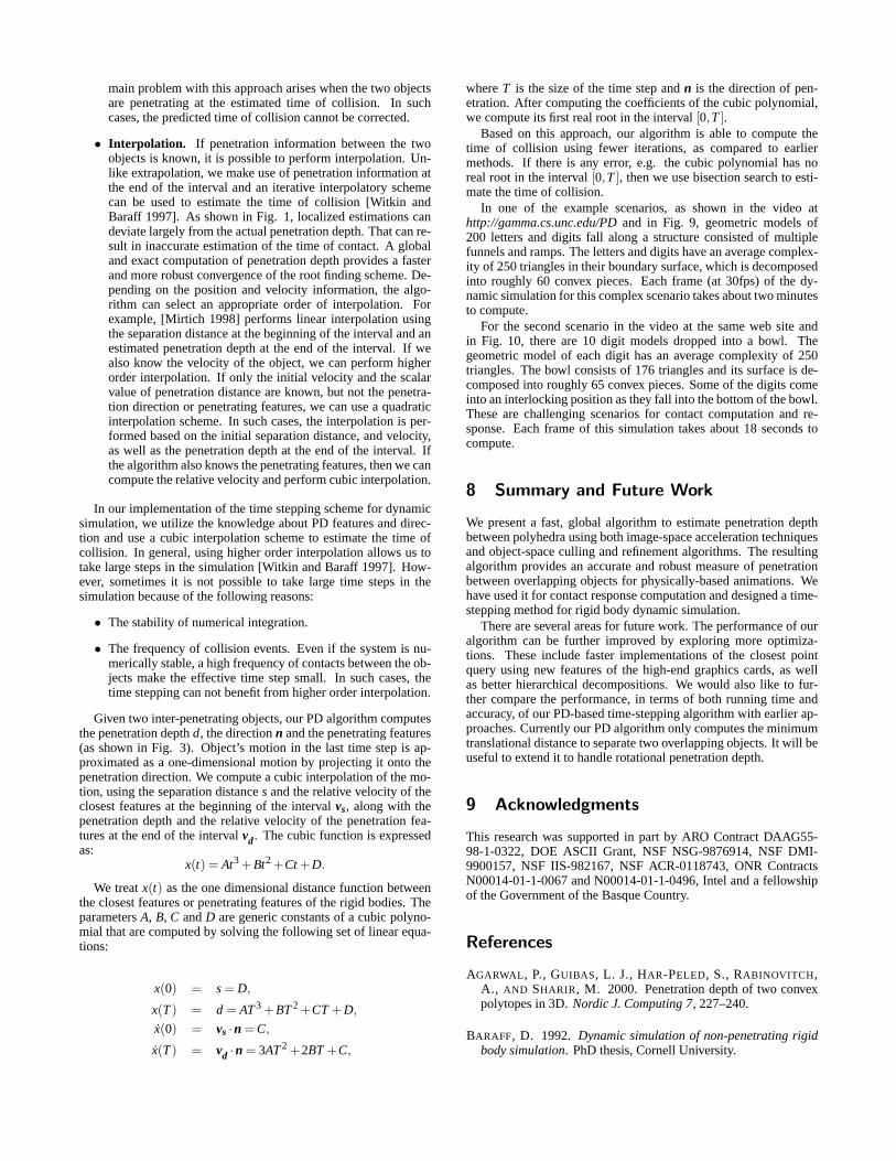
We compute the convex patches,ci ’s, by dualizing the polyhe-dral surface and performing a graph search on it in a greedy manner.First, we construct a dual graphG of the polyhedral surface∂P byreversing the roles of faces (F) and vertices (V) in∂P, while usingthe same edges (E) inG from ∂P [Chazelle et al. 1997; Ehmann andLin 2001]. We traverse the dual graphG by adding faces into a cur-rent convex patchci as long as it maintains its convexity. We repeatthis process until we cover the entire boundary of∂P. For example,Fig. 7-(h) is a convex surface decomposition for a wrinkled torusmodel, Fig. 7-(a).

Furthermore, we compute a convex hull of each surface patch,ci ,and denote the resulting polytope byCi . The union of theseCi ’s iscompletely contained in the original polyhedronP. Notice that ourdecomposition strategy is merely a partition of∂P, not of P. Thissurface decomposition is sufficient for PD computation, because weare only concerned with the surface of Minkowski sums betweenpolyhedra.

4.2 Pairwise Minkowski Sum Computation

Our PD computation algorithm is based on the decomposition ap-proach described in Section 3.3. The first step involves computingthe pairwise Minkowski sums between all possible pairs of convexpolytopes,CP

i andCQj, belonging toP andQ, respectively. Let us

denote the resulting Minkowski sum asMi j . We use a simple algo-rithm based on the convex hull property of Minkowski sums:

P⊕Q = CH({vi +v j |vi ∈VP,v j ∈VQ}) (2)

Here,CH denotes the convex hull operator, andVP,VQ representthe sets of vertices, respectively in polyhedraP andQ. Based onthis fact, we compute the Minkowski sum as follows:

1. Compute the vector sum between all possible pairs of verticesfrom each polytope.

2. Compute their convex hull.

4.3 Closest Point Query Using Graphics Hardware

Given all the pairwise Minkowski sums,Mi j , let

M =⋃i j

Mi j . (3)

Our goal is to compute the closest point on the boundary ofM,i.e. ∂M, from the origin. We use z-buffer polygon rasterizationhardware to perform this query up to image-space resolution. Themain idea is to visualize∂M from the origin without computing asurface representation of∂M explicitly. After that we compute theclosest point, the distance and the direction.

4.3.1 Visualizing the Boundary of the Union

Mi0

Mi1

Mi2V

(a) (b) (c) (d)

Figure 4: Visualizing the Boundary of the Union From Inside.In (a),

V is the current view-frustum. In (b), Mi0 is rendered, and a new∂M is constructed

(thick line). In (c), when Mi1 is rendered, it opens up a new window (dotted line), and

the update region (thick gray line) on the current∂M is established. Thus a new∂M

(thick line) is constructed. In (d), we perform the same procedure for Mi2.

Our algorithm for visualizing∂M from a point inside is essen-tially a ray-shooting procedure from the origin to∂M, and in-crementally expands the front of∂M. For example, in Fig. 4,we expand the current∂M (thick line) by repeatedly renderingMi0,Mi1,Mi2. Each timeMi0,Mi1,Mi2 are rendered, as shown inFig. 4(b)-(d), it opens up a new window (shown as dotted line) ofthe update region (thick gray line) on the current∂M.

The algorithm maintains the current boundary ofM, ∂Mk, wherek is the current iteration, and incrementally expands it withMi j that

intersects∂Mk. We attempt to addMi j by rendering the front faces

of Mi j . The front faces that “pierce” the current∂Mk open up awindow through which the origin can see∂M. After that we renderthe backfaces ofMi j into the opened window using the maximumdepth test. However, we should not render the backfaces ofMi j ,that are created by non-original (virtual) faces ofP andQ. In otherwords, we should allow the ray to hit only∂M.

In summary, the basic algorithm simply performs the followingprocedure:

1. Initialize∂M0 to infinity.

2. Repeat steps 3-5m times

3. Repeat steps 4-5 for eachMi j

4. Render front faces ofMi j , and using the standard stencil oper-ation, open a window where the depth value of the front facesis less than that of the current∂Mk.

5. Classify the backfaces ofMi j into original and non-original.Render only the original back faces ofMi j where the depthvalue of the back faces is greater than that of the window.This updates the∂Mk in the window.

After themth iteration in step 2 highlighted above, the algorithmcorrectly finds the portion of∂M that is visible from the origin in

the following sense. After thekth iteration in step 2,∂Mk includesthe subset of∂M that the ray can reach with less than or equal tok−1 hopsfrom the origin. Here, thehopon some pointp on∂M meansthe number ofMi j ’s the ray should pass through to reachp. For

example,∂M1 includes the possible contribution to the final∂M ofall Mi j ’s that contain the origin and have zero hops. Therefore, byinduction onk, we correctly find the portion of∂M that is visiblefrom the origin after themth iteration.

4.3.2 Computing the Closest Point

For a given view, we can compute the closest point on the boundaryby simply finding the pixel with the minimum distance value. Thealgorithm reads back the Z-buffer to obtain the depth values foreach pixel. However, these depth values have undergone the per-spective depth transformation and do not contain the non-linearitythat is present in the distance values.

The algorithm transforms the pixel depth values into distancevalues based on their(x,y) coordinate positions on the viewingplane. Each pixel depth value is divided by cosθ , whereθ is theangle between the vector to the(x,y) position on the viewing planeand the center viewing direction. This depth transformation is CPU-bound, and this operation typically takes a few milliseconds.

The minimum distance and direction to the closest point are de-rived from the pixel position containing the minimum transformeddepth value. In order to examine views in all directions, we con-struct six views on the faces of a cube around the origin and repeatthe operation.

5 Acceleration Techniques

The global PD computation algorithm described in Section 4 esti-mates the amount of PD between two polyhedral models. However,its running time can vary based on the underlying models as well astheir relative configuration. In the worst case, the convex decom-position algorithm can result inO(n) patches and this can lead toO(n2) pairwise Minkowski sums,Mi j . Furthermore, the cost of theclosest point query using rasterization hardware can be as high asO(m2), wherem is the number of convex polytopes. This results inO(n4) worst case complexity for the PD estimation algorithm.

In this section, we present a number of acceleration techniquesto improve its performance. These include hierarchical culling andimage-space acceleration techniques.

5.1 Object Space Culling

A significant fraction of the time of the PD estimation algorithmis spent in pairwise Minkowski sum computation. The algorithmpresented in Section 4.2 considers all pairs of convex polytopes,CP

iandCQ

j, and computes their Minkowski sum,Mi j . If we are given

an upper bound on the PD,dest, we can eliminate some pairs ofconvex polytopes without computing their Minkowski sum. This isbased on the following lemma:

LEMMA 5.1 Let di j be the separation or Euclidean distance be-

tween CPi and CQ

j. If di j >‖ dest ‖, then the closest point from the

origin to ∂M lies on∂ (M−Mi j ).

For example, in Fig. 5, there are two intersecting polygonsPandQ. We estimatedest based on the convex hull ofP andQ (Fig.5-(b)). Then, we can cull away the pairs whose separation distanceis more thandest (Fig. 5-(c)).

Based on the Lemma 5.1, we can cull away all pairs of convexpolytopes,CP

i andCQj, whose separation distances are more than

1Q

P dest1P

QC

(a) (b) (c)

C Q

C0P C

0

Figure 5: Object Space Culling.(a) There are two intersecting polygons P

(decomposed into CP0 , CP1 ) and Q (decomposed into CQ

0and CQ

1). (b) Based on the

convex hull of P and Q, we first estimate the PD as dest. (c) Using dest, we can cull

away pairs (CP0 , CQ

0), (CP

0 , CQ1

), (CP1 , CQ

1), whose separation distances are more than

dest.

dest. Computing separation distance between convex polytopes isrelatively cheap as compared to Minkowski sum computation anda number of efficient algorithms are known [Lin and Canny 1991;Cameron 1997]. The efficiency of this culling approach depends onthe quality of the estimate,dest. Furthermore, checking all possi-ble pairs for separation distance can takeO(n2) time. We improvetheir performance using a bounding volume hierarchy to performhierarchical culling.

5.2 Bounding Volume Hierarchy

We compute a bounding volume (BV) hierarchy for each polyhe-dron using a convex polytope as the underlying BV. Each convexpolytope obtained using the decomposition algorithm explained inSection 4.1 becomes a leaf node in the hierarchy. We recursivelycompute the internal nodes in a bottom-up manner, by merging thechildren nodes and computing the convex hull of the union of theirvertices. Let us define the nodes of polyhedronP at levell asCP,l

i.

The resulting hierarchy is a hierarchy of convex hulls. For exam-ple, Fig. 7-(b)∼ (h) shows a BV hierarchy for the torus model, Fig.7-(a).

This hierarchy is used in our runtime algorithm to speed up theintersection and separation distance queries for the culling algo-rithm. Furthermore, each level of the hierarchy provides an approx-imation of the model, which is used by the PD estimation algorithm.

5.3 Hierarchical Culling

We use the BV hierarchy to speed up the performance of the object-space culling algorithm. The goal is to start with an initial estimateto the PD and refine it at every level of the tree. We denote theestimate computed using levelk of each BV tree asdk

est.We initially start with the root nodes of each hierarchy,CP,0

0andCQ,0

0, which correspond to the convex hulls ofP and Q, re-

spectively. We compute the PD between those convex polytopes[Cameron 1997; Bergen 2001; Kim et al. 2002a] and use that as theestimated PD at level 0. The algorithm proceeds in a hierarchicalmanner through the levels in each tree:

1. Consider all the pairwise nodes at levelk in each tree,CP,ki

andCQ,kj

. For each(i, j) pair, compute the separation distance

between them. If the nodes overlap, the separation distance iszero.

2. Discard all the node pairs whose separation distances are morethandk

est. Compute the Minkowski sum of the rest of the pairs.

3. Perform the closest point query on the Minkowski sum pairsand compute the new PD estimate,dk+1

est using rasterizationhardware.

0P,1 C1

P,1 C0Q,1 C1

Q,1

C0Q,0

0P,0C

C

(a) Two BV hierarchies (b) BV hierarchy Traversal

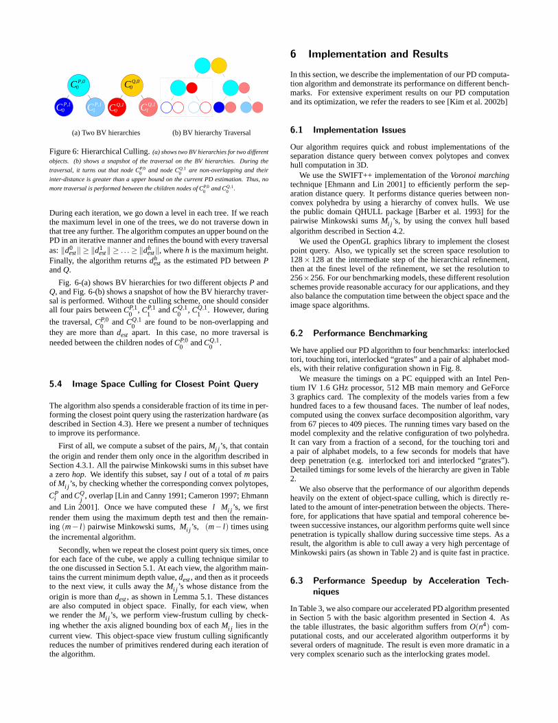
Figure 6: Hierarchical Culling.(a) shows two BV hierarchies for two different

objects. (b) shows a snapshot of the traversal on the BV hierarchies. During the

traversal, it turns out that node CP,00

and node CQ,10

are non-overlapping and their

inter-distance is greater than a upper bound on the current PD estimation. Thus, no

more traversal is performed between the children nodes of CP,00

and CQ,10

.

During each iteration, we go down a level in each tree. If we reachthe maximum level in one of the trees, we do not traverse down inthat tree any further. The algorithm computes an upper bound on thePD in an iterative manner and refines the bound with every traversalas:‖d0

est‖ ≥ ‖d1est‖ ≥ . . .≥ ‖dh

est‖, whereh is the maximum height.Finally, the algorithm returnsdh

est as the estimated PD betweenPandQ.

Fig. 6-(a) shows BV hierarchies for two different objectsP andQ, and Fig. 6-(b) shows a snapshot of how the BV hierarchy traver-sal is performed. Without the culling scheme, one should considerall four pairs betweenCP,1

0, CP,1

1andCQ,1

0, CQ,1

1. However, during

the traversal,CP,00

andCQ,10

are found to be non-overlapping andthey are more thandest apart. In this case, no more traversal isneeded between the children nodes ofCP,0

0andCQ,1

0.

5.4 Image Space Culling for Closest Point Query

The algorithm also spends a considerable fraction of its time in per-forming the closest point query using the rasterization hardware (asdescribed in Section 4.3). Here we present a number of techniquesto improve its performance.

First of all, we compute a subset of the pairs,Mi j ’s, that containthe origin and render them only once in the algorithm described inSection 4.3.1. All the pairwise Minkowski sums in this subset havea zerohop. We identify this subset, sayl out of a total ofm pairsof Mi j ’s, by checking whether the corresponding convex polytopes,

CPi andCQ

j, overlap [Lin and Canny 1991; Cameron 1997; Ehmann

and Lin 2001]. Once we have computed thesel Mi j ’s, we firstrender them using the maximum depth test and then the remain-ing (m− l) pairwise Minkowski sums,Mi j ’s, (m− l) times usingthe incremental algorithm.

Secondly, when we repeat the closest point query six times, oncefor each face of the cube, we apply a culling technique similar tothe one discussed in Section 5.1. At each view, the algorithm main-tains the current minimum depth value,dest, and then as it proceedsto the next view, it culls away theMi j ’s whose distance from theorigin is more thandest, as shown in Lemma 5.1. These distancesare also computed in object space. Finally, for each view, whenwe render theMi j ’s, we perform view-frustum culling by check-ing whether the axis aligned bounding box of eachMi j lies in thecurrent view. This object-space view frustum culling significantlyreduces the number of primitives rendered during each iteration ofthe algorithm.

6 Implementation and Results

In this section, we describe the implementation of our PD computa-tion algorithm and demonstrate its performance on different bench-marks. For extensive experiment results on our PD computationand its optimization, we refer the readers to see [Kim et al. 2002b]

6.1 Implementation Issues

Our algorithm requires quick and robust implementations of theseparation distance query between convex polytopes and convexhull computation in 3D.

We use the SWIFT++ implementation of theVoronoi marchingtechnique [Ehmann and Lin 2001] to efficiently perform the sep-aration distance query. It performs distance queries between non-convex polyhedra by using a hierarchy of convex hulls. We usethe public domain QHULL package [Barber et al. 1993] for thepairwise Minkowski sumsMi j ’s, by using the convex hull basedalgorithm described in Section 4.2.

We used the OpenGL graphics library to implement the closestpoint query. Also, we typically set the screen space resolution to128× 128 at the intermediate step of the hierarchical refinement,then at the finest level of the refinement, we set the resolution to256×256. For our benchmarking models, these different resolutionschemes provide reasonable accuracy for our applications, and theyalso balance the computation time between the object space and theimage space algorithms.

6.2 Performance Benchmarking

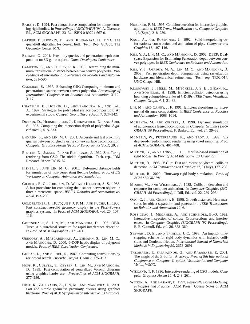
We have applied our PD algorithm to four benchmarks: interlockedtori, touching tori, interlocked “grates” and a pair of alphabet mod-els, with their relative configuration shown in Fig. 8.

We measure the timings on a PC equipped with an Intel Pen-tium IV 1.6 GHz processor, 512 MB main memory and GeForce3 graphics card. The complexity of the models varies from a fewhundred faces to a few thousand faces. The number of leaf nodes,computed using the convex surface decomposition algorithm, varyfrom 67 pieces to 409 pieces. The running times vary based on themodel complexity and the relative configuration of two polyhedra.It can vary from a fraction of a second, for the touching tori anda pair of alphabet models, to a few seconds for models that havedeep penetration (e.g. interlocked tori and interlocked “grates”).Detailed timings for some levels of the hierarchy are given in Table2.

We also observe that the performance of our algorithm dependsheavily on the extent of object-space culling, which is directly re-lated to the amount of inter-penetration between the objects. There-fore, for applications that have spatial and temporal coherence be-tween successive instances, our algorithm performs quite well sincepenetration is typically shallow during successive time steps. As aresult, the algorithm is able to cull away a very high percentage ofMinkowski pairs (as shown in Table 2) and is quite fast in practice.

6.3 Performance Speedup by Acceleration Tech-niques

In Table 3, we also compare our accelerated PD algorithm presentedin Section 5 with the basic algorithm presented in Section 4. Asthe table illustrates, the basic algorithm suffers fromO(n4) com-putational costs, and our accelerated algorithm outperforms it byseveral orders of magnitude. The result is even more dramatic in avery complex scenario such as the interlocking grates model.

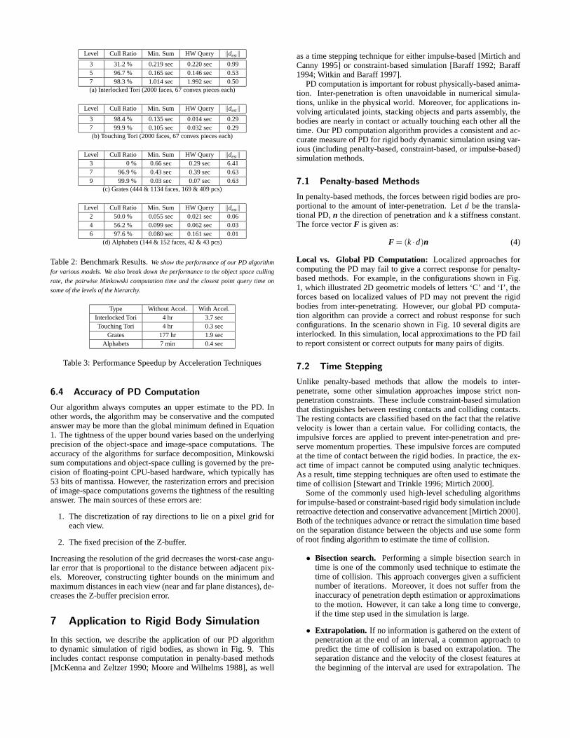
Level Cull Ratio Min. Sum HW Query ‖dest‖3 31.2 % 0.219 sec 0.220 sec 0.995 96.7 % 0.165 sec 0.146 sec 0.537 98.3 % 1.014 sec 1.992 sec 0.50(a) Interlocked Tori (2000 faces, 67 convex pieces each)

Level Cull Ratio Min. Sum HW Query ‖dest‖3 98.4 % 0.135 sec 0.014 sec 0.297 99.9 % 0.105 sec 0.032 sec 0.29(b) Touching Tori (2000 faces, 67 convex pieces each)

Level Cull Ratio Min. Sum HW Query ‖dest‖3 0 % 0.66 sec 0.29 sec 6.417 96.9 % 0.43 sec 0.39 sec 0.639 99.9 % 0.03 sec 0.07 sec 0.63

(c) Grates (444 & 1134 faces, 169 & 409 pcs)

Level Cull Ratio Min. Sum HW Query ‖dest‖2 50.0 % 0.055 sec 0.021 sec 0.064 56.2 % 0.099 sec 0.062 sec 0.036 97.6 % 0.080 sec 0.161 sec 0.01

(d) Alphabets (144 & 152 faces, 42 & 43 pcs)

Table 2: Benchmark Results.We show the performance of our PD algorithm

for various models. We also break down the performance to the object space culling

rate, the pairwise Minkowski computation time and the closest point query time on

some of the levels of the hierarchy.

Type Without Accel. With Accel.Interlocked Tori 4 hr 3.7 secTouching Tori 4 hr 0.3 sec

Grates 177 hr 1.9 secAlphabets 7 min 0.4 sec

Table 3: Performance Speedup by Acceleration Techniques

6.4 Accuracy of PD Computation

Our algorithm always computes an upper estimate to the PD. Inother words, the algorithm may be conservative and the computedanswer may be more than the global minimum defined in Equation1. The tightness of the upper bound varies based on the underlyingprecision of the object-space and image-space computations. Theaccuracy of the algorithms for surface decomposition, Minkowskisum computations and object-space culling is governed by the pre-cision of floating-point CPU-based hardware, which typically has53 bits of mantissa. However, the rasterization errors and precisionof image-space computations governs the tightness of the resultinganswer. The main sources of these errors are:

1. The discretization of ray directions to lie on a pixel grid foreach view.

2. The fixed precision of the Z-buffer.

Increasing the resolution of the grid decreases the worst-case angu-lar error that is proportional to the distance between adjacent pix-els. Moreover, constructing tighter bounds on the minimum andmaximum distances in each view (near and far plane distances), de-creases the Z-buffer precision error.

7 Application to Rigid Body Simulation

In this section, we describe the application of our PD algorithmto dynamic simulation of rigid bodies, as shown in Fig. 9. Thisincludes contact response computation in penalty-based methods[McKenna and Zeltzer 1990; Moore and Wilhelms 1988], as well

as a time stepping technique for either impulse-based [Mirtich andCanny 1995] or constraint-based simulation [Baraff 1992; Baraff1994; Witkin and Baraff 1997].

PD computation is important for robust physically-based anima-tion. Inter-penetration is often unavoidable in numerical simula-tions, unlike in the physical world. Moreover, for applications in-volving articulated joints, stacking objects and parts assembly, thebodies are nearly in contact or actually touching each other all thetime. Our PD computation algorithm provides a consistent and ac-curate measure of PD for rigid body dynamic simulation using var-ious (including penalty-based, constraint-based, or impulse-based)simulation methods.

7.1 Penalty-based Methods

In penalty-based methods, the forces between rigid bodies are pro-portional to the amount of inter-penetration. Letd be the transla-tional PD,n the direction of penetration andk a stiffness constant.The force vectorF is given as:

F = (k ·d)n (4)

Local vs. Global PD Computation: Localized approaches forcomputing the PD may fail to give a correct response for penalty-based methods. For example, in the configurations shown in Fig.1, which illustrated 2D geometric models of letters ‘C’ and ‘I’, theforces based on localized values of PD may not prevent the rigidbodies from inter-penetrating. However, our global PD computa-tion algorithm can provide a correct and robust response for suchconfigurations. In the scenario shown in Fig. 10 several digits areinterlocked. In this simulation, local approximations to the PD failto report consistent or correct outputs for many pairs of digits.

7.2 Time Stepping

Unlike penalty-based methods that allow the models to inter-penetrate, some other simulation approaches impose strict non-penetration constraints. These include constraint-based simulationthat distinguishes between resting contacts and colliding contacts.The resting contacts are classified based on the fact that the relativevelocity is lower than a certain value. For colliding contacts, theimpulsive forces are applied to prevent inter-penetration and pre-serve momentum properties. These impulsive forces are computedat the time of contact between the rigid bodies. In practice, the ex-act time of impact cannot be computed using analytic techniques.As a result, time stepping techniques are often used to estimate thetime of collision [Stewart and Trinkle 1996; Mirtich 2000].

Some of the commonly used high-level scheduling algorithmsfor impulse-based or constraint-based rigid body simulation includeretroactive detection and conservative advancement [Mirtich 2000].Both of the techniques advance or retract the simulation time basedon the separation distance between the objects and use some formof root finding algorithm to estimate the time of collision.

• Bisection search. Performing a simple bisection search intime is one of the commonly used technique to estimate thetime of collision. This approach converges given a sufficientnumber of iterations. Moreover, it does not suffer from theinaccuracy of penetration depth estimation or approximationsto the motion. However, it can take a long time to converge,if the time step used in the simulation is large.

• Extrapolation. If no information is gathered on the extent ofpenetration at the end of an interval, a common approach topredict the time of collision is based on extrapolation. Theseparation distance and the velocity of the closest features atthe beginning of the interval are used for extrapolation. The

main problem with this approach arises when the two objectsare penetrating at the estimated time of collision. In suchcases, the predicted time of collision cannot be corrected.

• Interpolation. If penetration information between the twoobjects is known, it is possible to perform interpolation. Un-like extrapolation, we make use of penetration information atthe end of the interval and an iterative interpolatory schemecan be used to estimate the time of collision [Witkin andBaraff 1997]. As shown in Fig. 1, localized estimations candeviate largely from the actual penetration depth. That can re-sult in inaccurate estimation of the time of contact. A globaland exact computation of penetration depth provides a fasterand more robust convergence of the root finding scheme. De-pending on the position and velocity information, the algo-rithm can select an appropriate order of interpolation. Forexample, [Mirtich 1998] performs linear interpolation usingthe separation distance at the beginning of the interval and anestimated penetration depth at the end of the interval. If wealso know the velocity of the object, we can perform higherorder interpolation. If only the initial velocity and the scalarvalue of penetration distance are known, but not the penetra-tion direction or penetrating features, we can use a quadraticinterpolation scheme. In such cases, the interpolation is per-formed based on the initial separation distance, and velocity,as well as the penetration depth at the end of the interval. Ifthe algorithm also knows the penetrating features, then we cancompute the relative velocity and perform cubic interpolation.

In our implementation of the time stepping scheme for dynamicsimulation, we utilize the knowledge about PD features and direc-tion and use a cubic interpolation scheme to estimate the time ofcollision. In general, using higher order interpolation allows us totake large steps in the simulation [Witkin and Baraff 1997]. How-ever, sometimes it is not possible to take large time steps in thesimulation because of the following reasons:

• The stability of numerical integration.

• The frequency of collision events. Even if the system is nu-merically stable, a high frequency of contacts between the ob-jects make the effective time step small. In such cases, thetime stepping can not benefit from higher order interpolation.

Given two inter-penetrating objects, our PD algorithm computesthe penetration depthd, the directionn and the penetrating features(as shown in Fig. 3). Object’s motion in the last time step is ap-proximated as a one-dimensional motion by projecting it onto thepenetration direction. We compute a cubic interpolation of the mo-tion, using the separation distances and the relative velocity of theclosest features at the beginning of the intervalvs, along with thepenetration depth and the relative velocity of the penetration fea-tures at the end of the intervalvd. The cubic function is expressedas:

x(t) = At3 +Bt2 +Ct +D.

We treatx(t) as the one dimensional distance function betweenthe closest features or penetrating features of the rigid bodies. TheparametersA, B, C andD are generic constants of a cubic polyno-mial that are computed by solving the following set of linear equa-tions:

x(0) = s= D,

x(T) = d = AT3 +BT2 +CT +D,

x(0) = vs ·n = C,

x(T) = vd ·n = 3AT2 +2BT +C,

whereT is the size of the time step andn is the direction of pen-etration. After computing the coefficients of the cubic polynomial,we compute its first real root in the interval[0,T].

Based on this approach, our algorithm is able to compute thetime of collision using fewer iterations, as compared to earliermethods. If there is any error, e.g. the cubic polynomial has noreal root in the interval[0,T], then we use bisection search to esti-mate the time of collision.

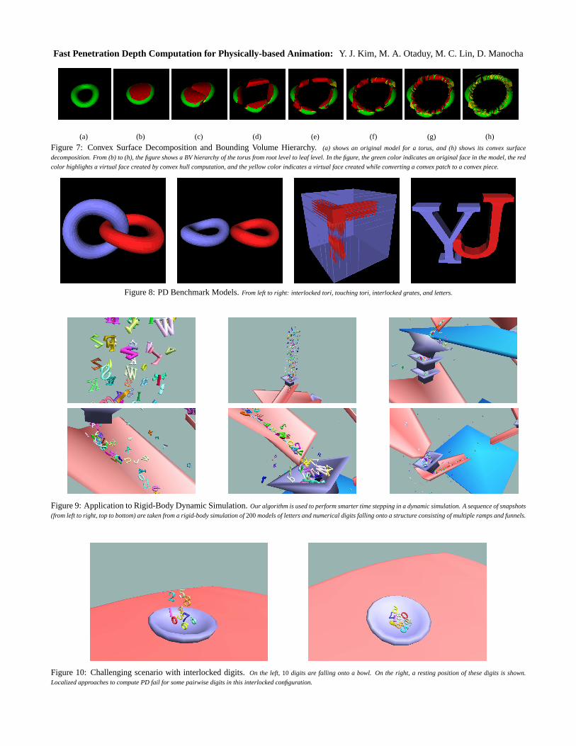
In one of the example scenarios, as shown in the video athttp://gamma.cs.unc.edu/PDand in Fig. 9, geometric models of200 letters and digits fall along a structure consisted of multiplefunnels and ramps. The letters and digits have an average complex-ity of 250 triangles in their boundary surface, which is decomposedinto roughly 60 convex pieces. Each frame (at 30fps) of the dy-namic simulation for this complex scenario takes about two minutesto compute.

For the second scenario in the video at the same web site andin Fig. 10, there are 10 digit models dropped into a bowl. Thegeometric model of each digit has an average complexity of 250triangles. The bowl consists of 176 triangles and its surface is de-composed into roughly 65 convex pieces. Some of the digits comeinto an interlocking position as they fall into the bottom of the bowl.These are challenging scenarios for contact computation and re-sponse. Each frame of this simulation takes about 18 seconds tocompute.

8 Summary and Future Work

We present a fast, global algorithm to estimate penetration depthbetween polyhedra using both image-space acceleration techniquesand object-space culling and refinement algorithms. The resultingalgorithm provides an accurate and robust measure of penetrationbetween overlapping objects for physically-based animations. Wehave used it for contact response computation and designed a time-stepping method for rigid body dynamic simulation.

There are several areas for future work. The performance of ouralgorithm can be further improved by exploring more optimiza-tions. These include faster implementations of the closest pointquery using new features of the high-end graphics cards, as wellas better hierarchical decompositions. We would also like to fur-ther compare the performance, in terms of both running time andaccuracy, of our PD-based time-stepping algorithm with earlier ap-proaches. Currently our PD algorithm only computes the minimumtranslational distance to separate two overlapping objects. It will beuseful to extend it to handle rotational penetration depth.

9 Acknowledgments

This research was supported in part by ARO Contract DAAG55-98-1-0322, DOE ASCII Grant, NSF NSG-9876914, NSF DMI-9900157, NSF IIS-982167, NSF ACR-0118743, ONR ContractsN00014-01-1-0067 and N00014-01-1-0496, Intel and a fellowshipof the Government of the Basque Country.

References

AGARWAL , P., GUIBAS, L. J., HAR-PELED, S., RABINOVITCH ,A., AND SHARIR, M. 2000. Penetration depth of two convexpolytopes in 3D.Nordic J. Computing 7, 227–240.

BARAFF, D. 1992. Dynamic simulation of non-penetrating rigidbody simulation. PhD thesis, Cornell University.

BARAFF, D. 1994. Fast contact force computation for nonpenetrat-ing rigid bodies. InProceedings of SIGGRAPH ’94, A. Glassner,Ed., ACM SIGGRAPH, 23–34. ISBN 0-89791-667-0.

BARBER, B., DOBKIN , D., AND HUHDANPAA , H. 1993. Thequickhull algorithm for convex hull. Tech. Rep. GCG53, TheGeometry Center, MN.

BERGEN, G. 2001. Proximity queries and penetration depth com-putation on 3D game objects.Game Developers Conference.

CAMERON, S.,AND CULLEY, R. K. 1986. Determining the mini-mum translational distance between two convex polyhedra.Pro-ceedings of International Conference on Robotics and Automa-tion, 591–596.

CAMERON, S. 1997. Enhancing GJK: Computing minimum andpenetration distance between convex polyhedra.Proceedings ofInternational Conference on Robotics and Automation, 3112–3117.

CHAZELLE , B., DOBKIN , D., SHOURABOURA, N., AND TAL ,A. 1997. Strategies for polyhedral surface decomposition: Anexperimental study.Comput. Geom. Theory Appl. 7, 327–342.

DOBKIN , D., HERSHBERGER, J., KIRKPATRICK, D., AND SURI,S. 1993. Computing the intersection-depth of polyhedra.Algo-rithmica 9, 518–533.

EHMANN , S.,AND L IN , M. C. 2001. Accurate and fast proximityqueries between polyhedra using convex surface decomposition.Computer Graphics Forum (Proc. of Eurographics’2001) 20, 3.

EPSTEIN, D., JANSEN, F., AND ROSSIGNAC, J. 1989. Z-bufferingrendering from CSG: The trickle algorithm. Tech. rep., IBMResearch Report RC15182.

FISHER, S., AND L IN , M. C. 2001. Deformed distance fieldsfor simulation of non-penetrating flexible bodies.Proc. of EGWorkshop on Computer Animation and Simulation.

GILBERT, E. G., JOHNSON, D. W., AND KEERTHI, S. S. 1988.A fast procedure for computing the distance between objects inthree-dimensional space.IEEE J. Robotics and Automation volRA-4, 193–203.

GOLDFEATHER, J., HULTQUIST, J. P. M.,AND FUCHS, H. 1986.Fast constructive-solid geometry display in the Pixel-Powersgraphics system. InProc. of ACM SIGGRAPH, vol. 20, 107–116.

GOTTSCHALK, S., LIN , M., AND MANOCHA, D. 1996. OBB-Tree: A hierarchical structure for rapid interference detection.In Proc. of ACM Siggraph’96, 171–180.

GREGORY, A., MASCARENHAS, A., EHMANN , S., LIN , M. C.,AND MANOCHA, D. 2000. 6-DOF haptic display of polygonalmodels.Proc. of IEEE Visualization Conference.

GUIBAS, L., AND SEIDEL, R. 1987. Computing convolutions byreciprocal search.Discrete Comput. Geom 2, 175–193.

HOFF, K., CULVER, T., KEYSER, J., LIN , M., AND MANOCHA,D. 1999. Fast computation of generalized Voronoi diagramsusing graphics hardw are.Proceedings of ACM SIGGRAPH,277–286.

HOFF, K., ZAFERAKIS, A., L IN , M., AND MANOCHA, D. 2001.Fast and simple geometric proximity queries using graphicshardware.Proc. of ACM Symposium on Interactive 3D Graphics.

HUBBARD, P. M. 1995. Collision detection for interactive graphicsapplications.IEEE Trans. Visualization and Computer Graphics1, 3 (Sept.), 218–230.

KAUL , A., AND ROSSIGNAC, J. 1992. Solid-interpolating de-formations: construction and animation of pips.Computer andGraphics 16, 107–116.

K IM , Y. J., LIN , M. C., AND MANOCHA, D. 2002. DEEP: Dual-space Expansion for Estimating Penetration depth between con-vex polytopes. InIEEE Conference on Robotics and Automation.

K IM , Y. J., OTADUY, M. A., L IN , M. C., AND MANOCHA, D.2002. Fast penetration depth computation using rasterizationhardware and hierarchical refinement. Tech. rep. TR02-014,UNC-Chapel Hill.

KLOSOWSKI, J., HELD, M., M ITCHELL , J. S. B., ZIKAN , K.,AND SOWIZRAL , H. 1998. Efficient collision detection usingbounding volume hierarchies ofk-DOPs.IEEE Trans. Visualizat.Comput. Graph. 4, 1, 21–36.

L IN , M., AND CANNY, J. F. 1991. Efficient algorithms for incre-mental distance computation. InIEEE Conference on Roboticsand Automation, 1008–1014.

MCKENNA, M., AND ZELTZER, D. 1990. Dynamic simulationof autonomous legged locomotion. InComputer Graphics (SIG-GRAPH ’90 Proceedings), F. Baskett, Ed., vol. 24, 29–38.

MCNEELY, W., PUTERBAUGH, K., AND TROY, J. 1999. Sixdegree-of-freedom haptic rendering using voxel sampling.Proc.of ACM SIGGRAPH, 401–408.

M IRTICH, B., AND CANNY, J. 1995. Impulse-based simulation ofrigid bodies. InProc. of ACM Interactive 3D Graphics.

M IRTICH, B. 1998. V-Clip: Fast and robust polyhedral collisiondetection.ACM Transactions on Graphics 17, 3 (July), 177–208.

M IRTICH, B. 2000. Timewarp rigid body simulation.Proc. ofACM SIGGRAPH.

MOORE, M., AND WILHELMS , J. 1988. Collision detection andresponse for computer animation. InComputer Graphics (SIG-GRAPH ’88 Proceedings), J. Dill, Ed., vol. 22, 289–298.

ONG, C. J.,AND GILBERT, E. 1996. Growth distances: New mea-sures for object separation and penetration.IEEE Transactionson Robotics and Automation 12, 6.

ROSSIGNAC, J., MEGAHED, A., AND SCHNEIDER, B.-O. 1992.Interactive inspection of solids: Cross-sections and interfer-ences. InComputer Graphics (SIGGRAPH ’92 Proceedings),E. E. Catmull, Ed., vol. 26, 353–360.

STEWART, D. E., AND TRINKLE , J. C. 1996. An implicit time-stepping scheme for rigid body dynamics with inelastic colli-sions and Coulomb friction.International Journal of NumericalMethods in Engineering 39, 2673–2691.

THEOHARIS, T., PAPAIANNOU , G., AND KARABASSI, E. 2001.The magic of the Z-buffer: A survey.Proc. of 9th InternationalConference on Computer Graphics, Visualization and ComputerVision, WSCG.

WIEGAND, T. F. 1996. Interactive rendering of CSG models.Com-puter Graphics Forum 15, 4, 249–261.

WITKIN , A., AND BARAFF, D. 1997.Physically Based Modeling:Principles and Practice. ACM Press. Course Notes of ACMSIGGRAPH.

Fast Penetration Depth Computation for Physically-based Animation: Y. J. Kim, M. A. Otaduy, M. C. Lin, D. Manocha

(a) (b) (c) (d) (e) (f) (g) (h)

Figure 7: Convex Surface Decomposition and Bounding Volume Hierarchy.(a) shows an original model for a torus, and (h) shows its convex surface

decomposition. From (b) to (h), the figure shows a BV hierarchy of the torus from root level to leaf level. In the figure, the green color indicates an original face in the model, the red

color highlights a virtual face created by convex hull computation, and the yellow color indicates a virtual face created while converting a convex patch to a convex piece.

Figure 8: PD Benchmark Models.From left to right: interlocked tori, touching tori, interlocked grates, and letters.

Figure 9: Application to Rigid-Body Dynamic Simulation.Our algorithm is used to perform smarter time stepping in a dynamic simulation. A sequence of snapshots

(from left to right, top to bottom) are taken from a rigid-body simulation of200models of letters and numerical digits falling onto a structure consisting of multiple ramps and funnels.

Figure 10: Challenging scenario with interlocked digits.On the left,10 digits are falling onto a bowl. On the right, a resting position of these digits is shown.

Localized approaches to compute PD fail for some pairwise digits in this interlocked configuration.