Fatigue Life Prediction using

Forces in Welded Plates of

Moderate Thickness

Pär Fransson

Gert Pettersson

Department of Mechanical Engineering

University of Karlskrona/Ronneby

Karlskrona, Sweden

2000

Thesis submitted for completion of Master of Science in Mechanical

Engineering with emphasis on Structural Mechanics at the Department of

Mechanical Engineering, University of Karlskrona/Ronneby, Karlskrona,

Sweden.

Abstract: A new finite element based method for fatigue life prediction has

been examined. The method uses nodal forces and moments along the weld

toe to define a structural stress perpendicular to the weld. The method was

found to be less mesh-sensitive than ordinarie post-processing.

Keywords:

Fatigue Life Prediction, Fillet Weld, Weld toe, Finite Element Method,

Shell elements, Nominal Stress, Structural Stress,

Keywords:

Acknowledgements

This work was carried out at the Department of Mechanical Engineering,

University of Karlskrona/Ronneby, Karlskrona, Sweden, under the

supervision of Dr. Mats Walter.

The work was initiated in 1999 as a co-operation between Volvo

Articulated Haulers AB and the Department of Mechanical Engineering at

the University of Karlskrona/Ronneby.

We wish to express our gratitude to Dr. Mats Walter and Dr. Göran

Broman, University of Karlskrona/Ronneby, and M.Sc. Bertil Jonsson,

Volvo Articulated Haulers AB, for their scientific guidance and support

throughout the work.

We also like to thank Dr. Mikael Fermér Volvo Car Corporation for

rewarding discussions, and Volvo Construction Equipment Components

AB for their help with the experimental part of this work.

Finally, we would like to thank our colleagues in the Master of Science

programme and all the other members of the Department of Mechanical

Engineering for valuable discussions and support.

Karlskrona, January 2000

Pär Fransson

Gert Pettersson

Contents

1 Notation 5

2 Introduction 7

3 Conventional Stress Determination 8

3.1 Theory 8

3.1.1 Nominal Stress Approach 8

3.1.2 Hot Spot Stress Approach 9

3.1.3 Local Notch Stress Approach 10

3.1.4 Fracture Mechanism 10

4 The Volvo Approach 11

4.1 Basic Idea 11

4.2 Calculation of Structural Stress 12

4.2.1 Global vs. Element Co-ordinate System 13

4.2.2 Start/end and Sharp Corners of Welds 13

4.2.3 Smooth Corners and Lines 15

4.3 Different Ways of Modelling Corners 15

4.4 Effect of Element Size 17

4.5 Meshing Rules 21

5 Fatigue Resistance 22

5.1 Basic Principles 22

5.2 Fatigue Resistance of Classified Structural Details 23

6 FE-models 24

6.1 FAT 511 24

6.2 FAT 521 26

6.3 FAT 523 27

6.3 Volvo Case 28

7 Experimental Results 29

7.1 Test Object 29

7.2 Weld Class 30

7.3 Experimental Set-up 31

7.4 Results 33

7.5 Hot-Spot Stress 35

8 Computer Program 37

8.1 Input 37

8.2 Program Logic 37

8.3 Output/Calculated Result 39

9 Conclusions 40

10 Further Work 42

11 References 43

5

1 Notation

A Area [m2]

E Young’s modulus [Pa]

F Force [N]

I Area moment of inertia [m4]

K Stiffness [N/m]

M Moment [Nm]

N Number of cycles [-]

R Stress ratio [-]

S Stress amplitude [Pa]

T Force [N]

W Flexural resistance [m3]

Q Force [N]

g Node [-]

k Slope [-]

m Line moment [Nm/m]

n Line force [N/m]

q Line force [N/m]

Stress [Pa]

Strain [-]

Poisson’s ratio [-]

6

Indices

a Attachment

b Bending

p Plate

s seeked

E Element

max Maximum

min Minimum

nom Nominal

hs Hot spot

x, y, z Directions

Perpendicular

[ ] Matrix

7

2 Introduction

In heavy contract vehicles, e.g. haulers and wheel loaders, the fatigue life

prediction is often the dominating design case. In order to optimise the

welds and the geometry according to quality and weight a development of

the existing calculation methods is desirable. A new method, which is going

to be examined in this thesis, starts with a FE-model, using shell elements,

including the welds and continues, collecting nodal forces and nodal

moments from which the structural stress in the interesting point, e.g. the

weld toe, is calculated. Stresses calculated from nodal forces and moments

have the advantage of not being so sensitive to element size as normal

calculated element stresses. This approach also makes it possible to

separate the contributions from bending moment and nodal force on

structural stress. This method was first proposed and presented in 1995 by

Fayard J-L., Bignonnet A. and Dang Van K. [1] In this approach, however,

the weld was modelled with beam elements. In 1997 Magnus Andréasson

and Björn Frodin performed a master thesis [2] at Volvo Car Corporation,

VCC, in which shell elements were used on thin plates. The aim with this

master thesis is to examine the possibility to apply the method on moderate

plate structures such as e.g. a hauler frame and to develop a MATLAB code

which is able to read data from a FE-program and calculate the desirable

stresses. The work has been performed for Volvo Articulated Haulers

AB, Växjö, Sweden, in co-operation with Department of Mechanical

Engineering, University of Karlskrona/Ronneby.

Figure 2.1. Articulated Hauler, Volvo A35C.

8

3 Conventional Stress Determination

3.1 Theory

The actual stress state in a weld is difficult to determine depending on,

among others, variations in the weld profile, haphazard defects in the weld,

residual stresses in the structure etc. These different factors make fatigue

resistance difficult to predict. There are today four basic approaches to

fatigue life prediction of welded components:

the nominal stress approach;

the hot spot stress approach;

the local notch stress approach;

the fracture mechanics approach.

This section aims at giving a short overview of the different approaches.

3.1.1 Nominal Stress Approach

In this approach [5,7] the fatigue resistance is determined by practical tests

which are performed on either small testpieces or in full scale. The

testpieces are equipped with different types of attachments and varying

weld-types, which causes stress-raising effects. When fatigue at the welded

attachment is considered, the nominal stress is calculated in the region

containing the weld detail but excluding any influence of other attachments

on the stress distribution. Thus, all structural discontinuity effects and local

notch effects are included in the fatigue strength so determined. Nominal

stress is calculated according to the basic formula:

b

nomW

M

A

F (3.1)

The nominal fatigue strength for several different types of attachments are

specified. The fatigue strength is presented in the form of S-N curves, also

named Wöhlerdiagram.

9

3.1.2 Hot Spot Stress Approach

In this approach [5,7-9] the fatigue strength is based on strain

measurements in association to the expected fractured zone, in this case the

weld toe. The measurement is made on specified distances from the critical

point (the hot spot), figure 3.1.

Figure 3.1. Measuring hot spot stress with strain gauges.

Usually two strain gauges with two perpendicular measuring grids are used

in order to take the stress biaxiality into account. Assuming that the shear

strain near the weld is negligible the stress perpendicular to the weld can be

calculated according to equation 3.2.

21

1

x

y

xhs E (3.2)

The hot spot stress is then extrapolated from the two points towards the

weld toe. Unlike the nominal method, the hot spot approach is not

dependent on which type of attachment being analysed. This reduces the

number of S-N curves considerably.

10

3.1.3 Local Notch Stress Approach

This approach [5,7] is based on the stress state at the notch directly. All

stress raisers must therefore be taken into account in the analyse. The

analyse will often be divided into a global FE analyse at the structural level

combined with a local analyse at the notch area. To take account of all the

variations in weld profile, an affective notch radius of 1 mm replaces the

real contour, figure 3.2.

Figure 3.2 Effective notch radius.

The method is restricted to welded joints, which are expected to fail from

the weld toe or root. Other causes of fatigue failure are not covered. The

approach is not suitable if there are considerable stress components present

parallel to the weld.

3.1.4 Fracture Mechanism

In this approach [5,7,10], stress analysis is used to determine the value of

the stress intensity factor range which, besides stresses, depends on the

crack length and the geometry around the crack. For weld toe fatigue

cracks, the effect of the local notch decreases, as the crack becomes deeper.

Fracture mechanism has a large potential for analysing most of the

phenomenon’s present at a weld. It is disadvantage is however that it is time

consuming to perform.

11

4 The Volvo Approach

This chapter aims to give a detailed account of the approach that underlies

this thesis. The proposed method was introduced in 1995 by Fayard,

Bignonnet and Dang Van [1]. The method has also been tested on welded

thin sheet structures in a master thesis from Chalmers University of

Technology [2].

The general procedure is outlined in Section 4.2 after which a number of

particular cases are discussed in the following subsections, 4.2.1–4.2.3.

Different ways of modelling corners have been tested, which is discussed in

Section 4.3. Further, in Section 4.4, a comparison is made between stresses

calculated by I-DEAS and stresses, here called structural stresses, calculated

with the proposed method. Finally, in Section 4.5 a number of meshing

rules are given.

4.1 Basic Idea

Fatigue cracks can occur in different locations in a fillet weld. In this

approach the cracks are assumed to occur parallel with the weld toe. For

that reason the structural stress is defined as the stress perpendicular to the

weld toe, . This stress is caused by the force perpendicular to the weld

and of the moment parallel with the weld according to equation 3.1. The

necessary forces and moments are calculated by the FE-solver directly from

the nodal displacements and rotations according to equation 4.1. These

forces and moments are in I-DEAS denominated “Element forces”.

EEE uKF (4.1)

When making a FE-model of a sharp corner the stress in this corner,

theoretically, raises towards infinity. In practice stresses are dependent on

both the size and the quality of the mesh. Stresses calculated using equation

3.1, with forces and moments from 4.1, are, however, not in the same way

dependent on the mesh. In this way a FE-based calculation method,

comparatively independent on the mesh size, can be created.

12

4.2 Calculation of Structural Stress

The structural stress consists of two components, the normal stress derived

from the force, Nx, perpendicular to the weld-line (g1 – g2), and a bending

stress derived from the moment, My, parallel to the weld-line, figure 4.1.

The nodal forces, e.g. N 1x1 acting on node g1 in figure 4.1, shall be

considered as external forces acting on the element. Thus, the force is a

pressure force.

Figure 4.1. Shell element with nodal force and moment.

Transferring these nodal forces and moments into a line moment, my, and a

line force, nx, the structural stress in element E1 can be calculated as [3]:

3

)(12)()(

t

zym

t

yny

yx

(4.2)

where z is the distance from the mean surface in the z-direction. Calculated

nodal forces and moments have to be transformed into line forces and line

moments. Each element generates two boundary values located at y=0 and

y=l1y. The values for these points can be written as [4]:

1

2

1

11

1 22

)0( yy

y

y MMl

m (4.3)

1

1

1

21

11 22

)( yy

y

yy MMl

lm (4.4)

1

2

1

11

1 22

)0( xx

y

x NNl

n (4.5)

13

1

1

1

21

11 22

)( xx

y

yx NNl

ln (4.6)

The structural stress at the top surface, z=t/2, can then be calculated at the

two grid-points g1 and g2 by substituting equation 4.3 – 4.6 into equation

4.2 which gives the final expressions, assuming (0)=(g1) and

(ly)=(g2), according to:

21

1

2

1

1

1

1

2

1

1

1

21222)(

tl

MM

tl

NNg

y

yy

y

xx

(4.7)

21

1

1

1

2

1

1

1

1

2

2

21222)(

tl

MM

tl

NNg

y

yy

y

xx

(4.8)

4.2.1 Global vs. Element Co-ordinate System

In the initial phase of the project there was a discussion whether it was the

global co-ordinate system or the local element co-ordinate system that

should be used. After some investigations it turned out that forces and

moments presented by I-DEAS in “Element forces” are related to the global

co-ordinate system. The choice of co-ordinate system is, in principle, of no

significance except when programming the MATLAB code for stress

calculations.

4.2.2 Start/end and Sharp Corners of Welds

Starts/stops as well as corners and other geometrical change causes stress

concentrations. The line of action when modelling these points follows the

same approach as in the master thesis from Chalmers [2]. Starts and ends

are modelled according to figure 4.2 (a) and sharp corners according to 4.2

(b). With the method proposed, no extra refinement is needed at these

points. In these cases four different stresses, 1 - 4, could be calculated

for a single node, equation 4.9 – 4.12 and figure 4.3. Note that in element

E2 the structural stress are calculated in two different directions parallel to

the element sides. The structural stress is, as before, assumed to be the

maximum magnitude, with maintained sign for the node.

14

Figure 4.2. Start/end of weld (a) and sharp corner (b).

Figure 4.3. Forces, moments and element lengths used in structural stress

calculation..

21

1

1

1

2

1

1

1

1

2

1

21222

tl

MM

tl

NN

x

xx

x

yy

(4.9)

22

2

3

2

2

2

2

3

2

2

2

21222

tl

MM

tl

NN

x

xx

x

yy

(4.10)

15

22

2

1

2

2

2

2

1

2

2

3

21222

tl

MM

tl

NN

y

yy

y

xx

(4.11)

23

3

2

3

1

3

3

2

3

1

4

21222

tl

MM

tl

NN

y

yy

y

xx

(4.12)

4.2.3 Smooth Corners and Lines

In practice, it’s not common that a weld line exactly follows a global co-

ordinate direction. In these cases FE calculated forces and moments are not

longer perpendicular respective parallel to the weld line. The resulting

forces and moments must however be transformed to directions

perpendicular and parallel to the weld line. This is done using common

trigonometry. The structural stress can then be calculated according to

equation 4.9 and 4.10. When calculating the structural stress along a weld

line, only elements with one side in common with the weld are taken into

consideration.

4.3 Different Ways of Modelling Corners

It is not obvious how to model a smooth corner. Different ways of building

the FE-model results in varying stresses. Three different ways of modelling

the corner have been tested. The appearance of the models and the

structural stress they cause are shown in figure 4.4 – 4.6. FAT 521, figure

6.3 (the different models will be described more detailed in Chapter 5), has

been used as basic data in the test. The model has been loaded with a

nominal tensile stress of 100 MPa. On the basis of the received results, the

best way of creating a smooth corner seems to be according to figure 4.6.

This method is used further on.

16

Figure 4.4. Corner and stress distribution.

Figure 4.5. Corner and stress distribution.

Figure 4.6. Corner and stress distribution.

17

4.4 Effect of Element Size

One of the main thesis in the proposed method, that the calculated stresses

should be less mesh dependent than stresses calculated by a “ordinary” FE-

solver has been tested on case FAT 521, figure 4.7 a-d. The geometry of the

part includes corners where stress concentrations and local deformation

appear. Four different grids were used in the comparison. In every case the

model were loaded with a 100 MPa tensile stress.

Figure 4.7. Different mesh. (a) 15mm (b) 10mm (c) 5mm (d) 2.5mm.

The structural stress along the weld line was calculated according to the

approached method. The received results were expected to be some type of

smooth curves but instead they showed high irregularity, figure 4.8. This

behaviour were not expected and caused quit a lot of problems. It turned out

that Dr. Mikael Fermér, Volvo Car Corporation [2] had run into the same

problem. The problem were, in his case, caused by the fact that GPFORCE

in NASTRAN included both normal and shear forces acting on the nodes.

Averaging the two nodal-values, which eliminated the influence of the

shear forces, would solve the problem. The result of averaging the results

18

achieved by the Volvo method indicated that the Element Forces in the

IDEAS Universal File probably also included the shear forces, figure 4.9.

Since the IDEAS Universal File were the only way to get results out of

IDEAS, unlike NASTRAN which had several other opportunities,

averaging were decided to be used further on despite the fact that this cause

another problem. When the weld is not closed, the results in the end-nodes

can not be averaged.

Figure 4.8. Structural stress, Volvo approach.

19

Figure 4.9. Structural stress, Volvo approach. Mean value.

The curves were now smoother than before but still, there were

irregularities. This could be explained by the fact that some elements only

have one node, out of four, located at the weld line, red marked in figure

4.10 a, and that they causes disturbance in the force field. These elements

could, according to the original approach, not be considered in the

calculations since they do not have an element length along the weld toe.

Unfortunately it showed that it was not convenient to use free mesh. To

avoid this problem, the area around the weld toe should be mapped meshed,

figure 4.10 b.

20

Figure 4.10. Free mesh,(a), around a corner, and the same corner but this

time with a mapped meshed (b).

Finally the stresses calculated by I-DEAS, figure 4.11, were compared with

the results achieved by the proposed method. As assumed, the Volvo

approach showed a less mesh dependent behaviour. When using the Volvo

approach the stress raises 6 % while decreasing the mesh-size from 10 to

2.5 mm. This should be compared with 26 % while doing the same in I-

DEAS. The 15-mm mesh is excluded from the comparisons because of too

much influence from distorted elements around the weld.

0 50 100 150 200 250 300-40

-20

0

20

40

60

80

100

Distance along weld [mm]

Str

uctu

ral str

ess [

MP

a]

2.5mm

5mm

10mm

15mm

Figure 4.11. Structural stress, I-DEAS

21

4.5 Meshing Rules

The proposed method calls for some meshing rules.

The structure should be meshed with four node shell elements. The

thickness of the elements should be constant.

The weld should also be meshed with four node shell elements except

in smooth corners where three node shell elements can be used. The

element thickness should be the same as the effective throat, figure

4.12.

The plates are described by their mean surfaces.

The nodes of the elements representing the weld are positioned t/2

below the toes, figure 4.12.

To straighten up the mesh near e.g. a smooth corner, partition or anchor

nodes can be used.

Sharp element corners are not allowed up to the weld toe. The elements

must have a surface towards the weld toe, figure 4.10 b.

Figure 4.12. Cross-section of weld connection between two thin shells.

22

5 Fatigue Resistance

Material, exposed for varying loads, can break even if the load level is far

below the yield limit. This chapter aims to refresh the most elementary parts

of the mechanics of materials concerning fatigue. In Chapter 5.1 some

common conceptions are defined, which are used in this thesis. Chapter 5.2

concerns some basic facts about the models used in this work.

5.1 Basic Principles

A fatigue fracture process can be divided into three phases. The first phase

is the so-called crack formation phase. When a crack have been initiated,

crack growth occurs. When the crack has become sufficiently big, fatigue

fracture occurs.

When determine fatigue data for a structure, test details are loaded with a

cyclically varying force. The variation can be either of constant amplitude

(CA) or more common of type spectrum. The CA-type can best be

described using the three numbers max , min and R, equation 5.1.

max

min

R (5.1)

Often used cases are pulsating loads where R=0 and alternating loads where

R=-1, see figure 5.1. The spectrum load types, which are dominating for

vehicles, have a variation, which is not easily described. One way is to use

the so-called rainflow method, which results in a diagram over cycles at

different load levels.

Figure 5.1. Alternating load (a), pulsating load (b) and varying load (c).

23

The results from fatigue tests are often compiled into a S-N diagram, also

called Wöhlerdiagram, where the logarithm of the stress amplitude is

plotted as function of the logarithm of the number of cycles to fracture (log-

log). Also log-lin diagram is used. In a certain interval there is in a log-log-

diagram a, more or less, linear relation between stress amplitude and cycles

to failure. With a known endurance, N, at a known stress-level, , and a

known slope of the endurance curve it’s possible to calculate the endurance,

Ns, at other stress levels, s, or vice versa. For welds the slope k=3 is often

used. The relationship between the terms can be described according to [6]:

s

k

s

NN

(5.2)

A Wöhlerdiagram is, unless otherwise stated, constructed so that the curve

corresponds to a 50 % fracture probability.

5.2 Fatigue Resistance of Classified Structural

Details

The fatigue assessment of classified structural details and welded joints,

used in this thesis, is based on the nominal stress range. All fatigue

resistance data [5] are assumed to have a survival probability of at least 95

% unless otherwise stated. The fatigue curves, used in Chapter 6, are based

on representative experimental investigations and includes the effect of e.g.

structural and local stress concentrations, variations in the weld profile and

welding residual stresses. Each fatigue strength curve is identified by the

characteristic fatigue strength of the detail at 2 million cycles. This value is

the fatigue class (FAT). The slope of the fatigue strength curves assessed on

the basis of normal stresses is k=3.

24

6 FE-models

One of the purposes with this master thesis was to compare stresses

calculated with the proposed method with known fatigue data. Nominal

stress can, using a FE-solver and the proposed method, be recalculated to

stresses in the weld toe. Known FAT-values can be recalculated according

to equation 5.2. All FAT values are given for 2 . 106 cycles. In Chapter 6.1-

6.3, three standardised types of attachments from the 500-serie [5] are

examined. In chapter 6.4 a special Volvo designed attachment is examined.

In this case, which also underlies the experimental part of this thesis there is

no known data.

6.1 FAT 511

The FAT511 is a transverse attachment, which should not be thicker than

the main plate. The dimensions of the plate used in this simulation is 100 x

200 mm and the height of the attachment is 50 mm. Figure 6.1 a-c shows

how loads and boundary conditions are applied. The FAT value for this

attachment is 100 MPa. Three different load cases have been tested. Apart

from the FAT-value, FE-calculations have also been made for nominal

loads of 75 and 50 MPa. The results from these calculations are shown in

figure 6.2.

Figure 6.1. FE-models.

25

106

107

101

102

103

Cycles N

Str

ess

MP

a

Figure 6.1 (a)

Figure 6.1 (b)

Figure 6.1 (c)

Figure 6.2. Results FAT 511.

26

6.2 FAT 521

The FAT521 is a longitudinal gusset with varying length. In this case there

are different FAT-values for different attachment lengths.

The height of the attachment is 50 mm. The dimensions of the plate used in

this simulation is 100 x lp mm where lp is the length of the plate according

to:

2002 ap ll (6.1)

Figure 6.3 a-b shows how loads and boundary conditions are applied for

bending respective tensile stress. The results from the calculations are

shown in figure 6.4 and 6.5. Nominal stress is 100 MPa.

Figure 6.3. FE models.

Figure 6.4. Results FAT 521. Bending stress (a) and tensile stress (b).

27

6.3 FAT 523

The FAT523 is, in the same way as FAT521, a longitudinal gusset. The

difference is that the gauss has a smooth transition, which is either sniped or

has a radius. The attachment is located on a beam with 100-mm width and

200 mm height. The FAT-value varies depending on the relationship

between the transition and the height of the beam. Figure 6.6 a shows the

beam. Since there are no data about the length of the attachment all models

has been made with an "active attachment area" of 50 x 50 mm, figure 6.6

b. The total length is then depending on the transition. FE-calculations have

been made for nominal loads of 100 MPa. The results from these

calculations are shown in figure 6.7.

Figure 6.6. FE model.

Figure 6.7. Results FAT 523.

28

6.3 Volvo Case

This attachment shows several similarities with the FAT523. The model is

made with three different lengths of the attachment in the same model,

figure 6.8, and the dimensions are shown in figure 6.9. The height of the

attachment is 50 mm. The dimensions of the beam are the same as in

Chapter 6.3. In this case there are no standardised FAT-values for the

attachment. Since no FAT-values are available for this attachment the

structural stress calculated could not be compared with any known fatigue

data. Tests were therefore performed, see Chapter 7. A more detailed

description of the beam is given in Chapter 7.

Figure 6.8. Beam with four attachments used in experiment.

Figure 6.9. Attachment, a=30.

29

7 Experimental Results

Three beams with four attachments each were specially designed and

fatigue tested within this thesis. The shape of the attachment was varied to

see if this could have any effect of the fatigue life. A total of twenty-four

weld-ends could in this way be tested. The beams were manufactured at

Volvo Articulated Haulers AB factory in Braås. The experimental

procedure took place in Eskilstuna at Volvo Construction Equipment

Component AB.

7.1 Test Object

The objects, which were tested, consist of a beam with four attachments.

The beams were manufactured in the shape of a square-profile, figure 7.1,

and the attachments according to figure 6.8. The attachment weld were,

from both sides, run “into nowhere” to achieve a smooth weld-end. A more

detailed description of the beams, with material and weld data, is given in

table 7.1.

Figure 7.1. Cross section of the beam.

30

Table 7.1. Beam specification.

Material Domex 350, E=210 000 N/mm2, =0.3

Thickness 10 mm in all parts

Weld Fillet weld, without preparations, throat a=6

Length approx. 2000 mm

Cross section 200x100 mm

7.2 Weld Class

The weld class is a way to describe the weld quality and indicates how well

the weld is manufactured, and thereby how resistant it is to fatigue. The

quality of the welds on the beam are according to Volvo Corporate

Standard STD5605,51 weld class C, which is the weld class with the

second lowest requirements. This gives a Kx (stress concentration factor for

welds) value of 3,0 [12]. The weld class is C because of surface pores and

uneven weld.

Figure 7.2. Two attachments welded on the beam used in experiment. Note

how the weld is uneven and the dark dots on the weld.

31

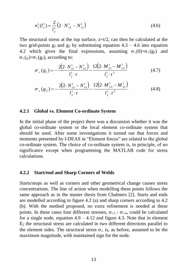
7.3 Experimental Set-up

The beams in the test have been simply supported. The moment-loss

support consists of two small pieces of a HE300 profile. The waist of the

two HE300 profiles were used to take care of the angular displacement

while the lower flange were clamped against the floor. On the upper flanges

of the HE300 profiles, supports were assembled. Into these supports the

beam, finally, were mounted, figure 7.3.

Figure 7.3. Simply supported beam.

The load was applied as close as possible to the attachments. The exact

positions varied between the beams because of different weld lengths. All

dimensions are therefore presented in table 7.2 together with the loading

force and the calculated, normal, bending stress. The stresses which are

presented are nominal bending stress (amplitude) in point A and B. When

calculating these stresses a area moment of inertia of 533.67*105 mm4 were

used. The frequency varied between 5 and 8 Hz and the stress ratio, R, were

-1.

32

A hydraulic actuator with built in LVDT transducer was used to apply the

force to the beam. Between the hydraulic actuator and the beam there were

a force transducer, Load Indicator AB Sweden Type 5-178, measuring-

range 100 kN, measuring the force and a specially designed attachment

which were able to handle possible uneven load. The tests were performed,

and load controlled, by an Alltest Industrial Computer 610 Advantech from

BIT Scandinavia AB. The experimental set-up is shown in figure 7.4.

Figure 7.4. Dimensions, measuring-points and loads.

Table 7.2. Dimensions, forces and stresses.

Beam

nr.

Upper/

Lower

F

l a b c Nom. stress

range pt. A

Nom. stress

range pt. B

kN mm mm mm mm MPa MPa

1 U 45 2090 835 110 320 154,2 126,0

1 L 2090 835 110 320 154,2 126,0

2 U 48 2120 860 80 320 168,6 134,4

2 L 2120 860 57 337 172,0 132,0

3 U 48 2192 860 85 325 172,4 139,2

3 L 2192 860 62 342 175,6 136,8

33

Figure 7.5. Experimental set-up. A hydraulic actuator with built-in LVDT

transducer (a) and a force transducer (b).

The deflection of the beam were calculated to 1 mm, but in reality it

deflected some more due to low stiffness in the flange of the HE300

profiles. This means that the moment of force was not zero in the support.

The moment loss was calculated to 115 Nm in the left HE300 profile and

119 Nm in the right [11]. Since the loss was so small, less than 0,5 %, the

influence of this moment loss were neglected.

To be able to determine the cracks, the weld and the area around it were

sprayed with white contrast colour, Byckotest 104. When a crack appeared

a magnetic powder, Byckotest 103, were used to identify the spread.

7.4 Results

As stop criteria for the fatigue test, the amplitude was used. The test

equipment was set to stop the test if the amplitude grow to large. This

means that the crack length became different for each weld-end. The results

were normalised to a specific crack-length (25 mm). This was done using

the following assumptions:

34

The material follows Paris Law according to

nKCdN

da (7.1)

with C=2.33e-12 mm/cycle and n=3.1.

The crack is supposed to start from the weld-edge and pass trough the

entire material. The stress intensity factor, K, is assumed according to

edge-crack exposed for one-axial tensile stress [13].

The whole stress-amplitude makes the crack grow.

The stress is calculated as nominal bending-stress.

The corrected numbers of cycles are presented in Table 7.3. As seen not all

weld-end resulted in a crack. Finally the achieved results are plotted in a

Wöhler-diagram, figure 7.6.

Table 7.3. Corrected number of cycles for cracks in the origin-material.

Beam

nr.

Upper/

Lower

Point Original

crack

length

Nom. stress

range

Number of

cycles

[mm] [MPa] 106

1 U A 35 154.2 1.31

1 U A 19 154.2 1.32

1 L A 39 154.2 1.31

1 L A 49 154.2 1.31

2 L A 47 168.6 0.719

3 U A 17 175.6 0.712

3 U A 15 175.6 0.716

3 U B 15 136.8 0.733

3 U B 5 136.8 0.890

3 L A 38 172.4 0.697

3 L A 20 172.4 0.707

3 L B 4 139.2 0.928

3 L B 18 139.2 0.718

35

Figure 7.6. Wöhler diagram of the received results.

7.5 Hot-Spot Stress

The Hot spot stress, or geometrical stress, has been measured at to points.

The stress was measured at point A on beam number 1, and at point B on

beam number 3. The gauges were placed according to figure 3.1 and the

stress at each point calculated according to equation 3.2. Finally the stress

were calculated trough linear interpolation towards the weld toe. In Table

7.4 the results from the three different ways of predicting the stress at the

weld toe are compared.

Table 7.4. Comparison between different approaches.

Hot Spot Nominal Volvo app.

[MPa] [MPa] [MPa]

Beam 1

Point A

98.0

77.1

82.5

Beam 3

Point B

98.3

68.4

71.2

36

(a)

(b)

Figure 7.7. Crack propagation in beam (a) front view (b) side view.

37

8 Computer Program

To calculate the structural stress in a fast way a computer program in

MATLAB was written. The program was developed for Windows NT

Workstation and MATLAB version 4.2c. But it will work on other

platforms and MATLAB versions as well.

The software was developed so that Volvo Construction Equipment could

use it for further investigation of the method.

8.1 Input

To solve equation 4.9 for an arbitrary case the following data has to be

available for the program:

nodal co-ordinates

element thickness

local XYZ nodal forces

local XYZ nodal moment of forces

All this information was exported from I-DEAS to a Universal file (UNV),

that then was imported to MATLAB. The weld information, or more

correct, the information from elements outside the weld toe, as well as the

node numbers for the nodes located at the weld toe line were semi-manually

saved in a separate file, a Node Element File (NEF).

8.2 Program Logic

The program consists of three parts. First it will import the UNV- and NEF

files to a matrix file that MATLAB can read. Second it will sort out only

the data that is needed for the stress calculation, with information from the

NEF. The third step is to calculate element lengths, nodal forces

perpendicular to the weld toe and nodal moment of forces parallel to the

weld toe. Finally the element stresses along the weld line is calculated.

38

Figure 8.1. Main parts in the program code.

Nodes, elements and the path of the weld are plotted in a figure to make

sure that the information in the NEF is correct. Figure 8.2 shows a closed

weld that goes all around the attachment. The elements plotted in this figure

are outside the weld toe, i.e. the elements that are encountered in the

calculation. Different colours1 are used in the plot to mark nodes, elements

etc. The weld toe is in the program marked with a blue (black) line,

elementedges are green (gray), nodes red (gray star) and a black dot mark

where the program starts the calculation. The direction of the calculation

can be seen in the plot. The black dot indicates the start element and a green

(gray) part of the otherwise blue (black) weldline indicates the last element

of the calculation domain.

Figure 8.2. Plot intended to simplify the control of the data in the NEF.

1 Since this report does not contain any coloured pictures explaining texts are put within brackets.

39

8.3 Output/Calculated Result

The calculated result or the output from the program is presented in a graph,

figure 8.3, and the structural stress variation along the weld line is plotted in

another graph, for example figure 4.8.

Figure 8.3. The FE-mesh around the weld.

40

9 Conclusions

A FE-based method for determining the structural stress perpendicular to

the weld toe has been established and tested. Several different types of

geometries have been used. The results show that there is no significant

difference in stresses caused by bending moment or tensile force. This is in

contrast to what Andréasson and Frodin [2] found in their thesis work. The

results have been fitted into one curve in the SN-plot, figure 9.1. The slope

of the curve was determined to -6.2.

Figure 9.1. All results in one plot.(T) in the legend stands for tensile loaded

and (B) for bending loaded.

41

A main idea was that the method should be more independent on the size of

the mesh than an ordinary FE-solver. This appeared to be true. When using

the Volvo approach the stress raises 6 % while decreasing the mesh-size

from 10 to 2.5 mm. This should be compared with 26 % while doing the

same in I-DEAS.

During the investigation of this thesis some other problems occurred as

described in chapter 4.4. The Element Force in I-DEAS as well as

GPFORCE in Nastran contained not only the load perpendicular to the

weld-line but also the shear-force acting on the element-side, figure 9.2, so

that e.g. the total force acting on node g2 is

xyg TQF 22 (9.1)

For each FEM-program that will be used further on, this is a phenomenon

that be must taken into consideration.

Figure 9.2. Forces acting on the element.

The last conclusion arises from an additional problem that appeared during

the work. It is true that the mesh-size does not affect the results, but the

appearance of the mesh does. Unlike previous works [1,2] the structures

analysed were free-meshed. This mesh-procedure often generates elements

that are distorted, although within the tolerances set in the program. Quite

often a free-mesh also results in elements with only one node located at the

weld toe. The method in its original edition is unable to handle this type of

problems. Since this means that the method demands a great deal of manual

work to be stable an expected advantage did not occur.

42

10 Further Work

During a project like this master thesis some questions are, because of

limitations and lack of time, left without any answer. In this last chapter

some of these questions are gathered and left open for further work.

The first question concerns the fact that a free mesh now and then generates

elements with only one node located at the weld-line, e.g. as in figure 4.10.

This means that equation 4.9 and 4.10 can not be solved. In this thesis

making the mesh “semi-free” has solved the problem but this is not a

practical method. Can the mesh be made in some other way or can the

elements be included in the calculation using a separate equation?

Chapter 4.3 was devoted to investigate how a smooth corner should be

modelled. It is not obvious that the chosen method is the right one. A corner

can probably be modelled in many other ways.

In practice, the creation of a FE-model sometimes starts with a solid-model.

Can the methodology be transferred onto this types of models and how?

43

11 References

1. Fayard J-L.,Bignonnet A., Dang Van K., Fatigue Design of Welded

Thin Sheet Structures, VTT symposium 156, Fatigue Design 1995,

Vol II, VTT, Espoo, Finland, pp. 239-252.

2. Andréasson M. Frodin B. Fatigue Life Prediction of MAG-welded

Thin Sheat Structures, Chalmers Tekniska Högskola, Göteborg,

Report no. 97-138, Dept. 98270, 1997.

3. Hult J. Bära Brista Fortsättningskurs i hållfasthetslära 2nd edition,

Almqvist & Wiksell, Stockholm, 1994.

4. Cook R., Malkus D., Plesha M., Concepts and Applications of Finite

Element Analysis, John Wiley & Sons, USA, 1989.

ISBN 0-471-84788-7.

5. A. Hobbacher, Fatigue Design of Welded Joints and Components,

The International Institute of Weldein, England, 1996,

ISBN 1-85573-315-3.

6. T. Dahlberg, Teknisk hållfasthetslära, Studentlitteratur, 1990, ISBN

91-44-31451-5.

7. E. Niemi, Recommendations concerning stress determination for

fatigue analysis of welded components, International Institute of

Welding, IIW, doc. XIII-1458-92/XV-797-92.

8. J. Solin, G. Marquis, A. Siljander, S. Sipilä, Fatigue Design,

European Structural Integrity Society, ESIS, Publication 16, 1993,

ISBN 0-85298-884-2.

9. M. Huther, J. Henry, Recommendations for hot spot stress definition

in welded joints, IIW doc. XIII-1416-91.

10. Y. Murakami, Stress Intensity Factors Handbook, Pergamon Press,

Oxford U.K., 1987.

11. Kleinlogel/Haselbach, Rahmenformeln, Verlag von Wilhelm Ernst &

Sohn, 1974, ISBN 3-433-00660-1.

12. Volvo Koncernstandard, Svetshandbok Dimensionering, 1989.

44

13. B. Sundström, Handbok och formelsamling i hållfasthetslära,

Institutionen för hållfasthetslära, KTH, 1998.