Feedback control of collective motion

and the design of mobile sensor networks

Derek Paley1 and Naomi Leonard2

Dept. Mechanical and Aerospace EngineeringPrinceton University, Princeton, NJ 08544

May 18, 2004

1Research supported by the National Defense Science and Engineering Graduate Fellowship, the PrincetonWu Graduate Fellowship, and the Princeton Pew Program in Biocomplexity.

2Research partially supported by by NSF grant CCR-9980058, ONR grants N00014–02–1–0826 andN00014–02–1–0861, and AFOSR grant F49620-01-1-0382.

Contents

1 Introduction 2

2 Particle Model 2

2.1 Alignment Controls . . . . . . . . . . . . . . . . . . . . . . . . . . . . . . . . . . . . . 2

2.2 Parallel Motion . . . . . . . . . . . . . . . . . . . . . . . . . . . . . . . . . . . . . . . 3

2.3 Circular Motion . . . . . . . . . . . . . . . . . . . . . . . . . . . . . . . . . . . . . . . 5

2.4 Trajectory Tracking . . . . . . . . . . . . . . . . . . . . . . . . . . . . . . . . . . . . 7

2.5 Shape Changes . . . . . . . . . . . . . . . . . . . . . . . . . . . . . . . . . . . . . . . 7

2.6 Topology Changes . . . . . . . . . . . . . . . . . . . . . . . . . . . . . . . . . . . . . 9

3 Objective Analysis 10

3.1 Gauss-Markov Theorem . . . . . . . . . . . . . . . . . . . . . . . . . . . . . . . . . . 10

3.2 Non-collocated measurements . . . . . . . . . . . . . . . . . . . . . . . . . . . . . . . 11

3.3 Autocorrelation Function . . . . . . . . . . . . . . . . . . . . . . . . . . . . . . . . . 12

3.4 Numerical Considerations . . . . . . . . . . . . . . . . . . . . . . . . . . . . . . . . . 12

3.5 Entropy Metric . . . . . . . . . . . . . . . . . . . . . . . . . . . . . . . . . . . . . . . 13

4 Sensor Network Design 15

5 Future Work 17

1

1 Introduction

This research on feedback control of collective motion is motivated by the modeling of aggrega-tions in biological systems, see e.g. [7, 10], and the design of autonomous oceanographic samplingnetworks [6]. We study a planar model of self-propelled particles subject to steering control after[12]. A natural formulation of this model permits application of results from coupled oscillatortheory [20, 4]. Our primary result is a pair of feedback controls that stabilize parallel and circularmotion of the group [18]. This result may be used to design mobile sensor arrays for oceanographicdata assimilation following a technique such as objective analysis [8, 2] or optimal experiment de-sign [19]. This paper will focus on the design and evaluation of mobile sensor arrays using objectiveanalysis. The motivation for this work is to contribute to the design of periodic trajectories foroceanographic sensor platforms including planning, real-time control and adaptation.

2 Particle Model

We consider a system of self-propelled particles with unit velocity subject to steering controllaws. In complex notation, the model is

rk = eiθk

θk = uk

where rk ∈ R2 and θk ∈ S1 are the position and heading of the kth particle, k = 1, . . . , N . Itis convenient to separate the feedback control input, uk ∈ R, into relative spacing and alignmentcomponents, i.e. uk = uspack + ualignk .

To design the feedback controls, we consider the singularly perturbed system

rk = eiθk

εθk = εuspack + ualignk

where |ε| = 1|K| � 1 is a small (signed) parameter. This introduces a time scale separation between

the alignment controls (fast) and the spacing controls (slow). The sign of the parameter determinesif the alignment coupling is attractive or repulsive. Exponential stability of the system follows fromexponential stability of the particle headings for the fast dynamics and exponential stability of theparticle spacing for the slow dynamics [13].

2.1 Alignment Controls

The complex order parameter shown in Figure 1, given by

pmθ =1N

N∑j=1

eimθj = rmeiψm ,

2

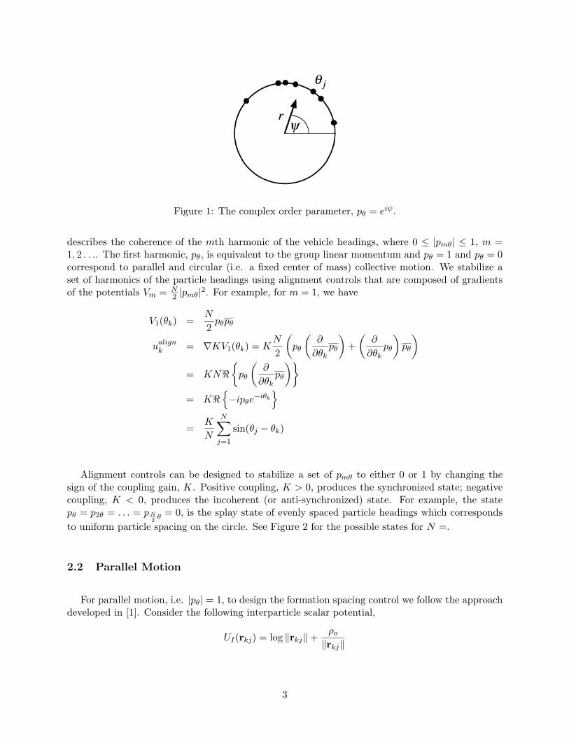
Figure 1: The complex order parameter, pθ = eiψ.

describes the coherence of the mth harmonic of the vehicle headings, where 0 ≤ |pmθ| ≤ 1, m =1, 2 . . .. The first harmonic, pθ, is equivalent to the group linear momentum and pθ = 1 and pθ = 0correspond to parallel and circular (i.e. a fixed center of mass) collective motion. We stabilize aset of harmonics of the particle headings using alignment controls that are composed of gradientsof the potentials Vm = N

2 |pmθ|2. For example, for m = 1, we have

V1(θk) =N

2pθpθ

ualignk = ∇KV1(θk) = KN

2

(pθ

(∂

∂θkpθ

)+

(∂

∂θkpθ

)pθ

)= KN<

{pθ

(∂

∂θkpθ

)}= K<

{−ipθe

−iθk

}=

K

N

N∑j=1

sin(θj − θk)

Alignment controls can be designed to stabilize a set of pmθ to either 0 or 1 by changing thesign of the coupling gain, K. Positive coupling, K > 0, produces the synchronized state; negativecoupling, K < 0, produces the incoherent (or anti-synchronized) state. For example, the statepθ = p2θ = . . . = pN

2θ = 0, is the splay state of evenly spaced particle headings which corresponds

to uniform particle spacing on the circle. See Figure 2 for the possible states for N =.

2.2 Parallel Motion

For parallel motion, i.e. |pθ| = 1, to design the formation spacing control we follow the approachdeveloped in [1]. Consider the following interparticle scalar potential,

UI(rkj) = log ‖rkj‖+ρo‖rkj‖

3

Figure 2: Illustration of the three possible states for N = 4. The black dots represent particleheadings on a unit circle.

Figure 3: Parallel motion for N = 10 and ρo = 10 without and with spacing control.

4

which is an even function of rkj = rk− rj . Using ∂rkj

∂rk= 1, the gradient of this potential is given by

∇UI(rkj) =(

1‖rkj‖

− ρo‖rkj‖2

)rkj‖rkj‖

.

We define the formation spacing control in terms of the negative of this gradient, i.e.

uspack = −N∑j 6=k

< ∇UI(rkj), ieiθk > .

where < ·, · > is a complex inner product. Thus, we are only using the component of the gradientin the direction normal to the particle velocity.

A Lyapunov function, U , that can be used to prove convergence to the set of formations thatminimize U is

U =N∑k=1

N∑j>k

UI(rkj).

This favors uniform particle spacing according to the spacing constant, ρo. An example of parallelmotion is shown in Figure 3.

2.3 Circular Motion

Consider the following variant of a single particle/beacon control law from [11],

uspack = −f(ρk) <rkρk

, ieiθk > − <rkρk

, eiθk >,

where f(ρk) is given by

f(ρk) = 1−(

ρoρk

)2

.

The particles move in a circular trajectory about the center of mass, R = 1N

∑Nj=1 rj . We define

the vector from the center of mass to particle k by rk = rk −R, and its magnitude by ρk = ‖rk‖,as shown in Figure 4. The first term is a projection in direction normal to velocity (which will beradial direction when in circular motion – so this term controls radial distance to R). The secondterm tries to enforce the motion of each vehicle onto a circle about R since it is zero when the linefrom R to rk is normal to the velocity of kth particle.

In shape coordinates, the dynamics for particle k are

ρk = sinφk

φk = −(

f(ρk)−1ρk

)cos φk − sin φk cos φk.

Convergence results for this system are presented in [11]. A Lyapunov function candidate for thesystem of N particles is the sum of individual functions, VI , given by

VI = − log(| cos φk|) + H(ρk),

5

Figure 4: Shape coordinates used for the parallel and circular feedback control, where ρk = ‖rk‖,after [11]. If the center of mass, R, is treated as fixed, one can define the angle φk relative to theradial vector rk.

Figure 5: Circular motion with N = 10 and ρo = 10 without and with splay control.

and f(ρk)− 1ρk

= dHdρk

. The time derivative of VI along the trajectories of this system is given by

VI =(

sinφkcos φk

)φk +

(f(ρk)−

1ρk

)ρk

= −sin2 φkcos φk

.

Therefore, VI ≤ 0 in the set {(ρk, φk)|ρk > 0, |φk| < π2 }. We observe that the largest invariant set

with VI = 0 is (ρk, φk) = (ρ1, 0), where

f(ρ1)−1ρ1

= 0.

For the purposes of the proof, we enforce that the spacing control preserve the fixed center ofmass, i.e. pθ = 0 using a matrix projector, Π, as follows.

pθ =1N

N∑j=1

eiθj θj = P Tθ Πuspacj = 0

6

Figure 6: Trajectory tracking with N = 20 and ρo = 25.

where P T is the matrix formed by the columns of cos θj and sin θj . By multiply the spacing controlsby Π = (I − Pθ(P T

θ Pθ)−1P Tθ ) the above constraint is satisfied.

2.4 Trajectory Tracking

The parallel and circular feedback controls are used to define five behavior primitives which canbe combined to track piecewise-linear trajectories. The behavior primitives use impulsive controlsto align the particles with the reference input and the feedback controls to stabilize this trajectory.The behaviors will be referred to as random-to-circular, circular-to-parallel, parallel-to-parallel,parallel-to-circular, and circular-to-circular. In parallel motion, the network center of mass followsa linear reference trajectory. In the circular state, the network center of mass is fixed, i.e. thegroup is stopped. An example of tracking a piecewise linear trajectory is shown in Figure 6.

2.5 Shape Changes

We provide a method to control the eccentricity of the circular motion. Consider the equationof an ellipse in Cartesian coordinates,

x2

a2+

y2

b2= 1

7

where a and b are the semi-major and -minor axes. Now consider the polar coordinates centeredat the center of the ellipse. We have (x, y) = (r cos θ′, r sin θ′), where θ′ is the angle to a point, P ,on the ellipse from the horizontal semi-major axis and r = ‖P‖. In these coordinates, we can usethe equation of the ellipse to obtain

r2 =a2b2

b2 cos2 θ′ + a2 sin2 θ′

Using the eccentricity, e2 = 1− b2

a2 , we have

r =a2(1− e2)

1− e2 cos2 θ′

To obtain the normal vector, P⊥ = (y,−x), to the ellipse at point P , we differentiate the polarcoordinates to get

x = r cos θ′ − r sin θ′θ′

y = r sin θ′ + r cos θ′θ′

Next, we differentiate the magnitude, r, using the expression in terms of a and b,

2rr = −a2b2(−2b2 cos θ′ sin θ′ + 2a2 sin θ′ cos θ′)θ′

(b2 cos2 θ′ + a2 sin2 θ′)2

or

r =a2b2(b2 − a2) sin 2θ′θ′

r(b2 cos2 θ′ + a2 sin2 θ′)2

Thus, we have

x =[a2b2(b2 − a2) sin 2θ′ cos θ′

(b2 cos2 θ′ + a2 sin2 θ′)2− r sin θ′

]θ′

y =[a2b2(b2 − a2) sin 2θ′ sin θ′

(b2 cos2 θ′ + a2 sin2 θ′)2+ r cos θ′

]θ′

We normalize the normal vector, P⊥, so obtaining an expression for θ′ is unnecessary.

We can define a circular control to follow the circumference of an ellipse. The control is a variantof our circle control law

uspack = −f ′(ρk) <rkρk

, ieiθk > − < P⊥, eiθk >,

where f ′(ρk) is given by

f ′(ρk) = 1−(‖P‖ρk

)2

.

Note that the splay state is inconsistent with this shape change. Intuitively, if the vehicles startequally spaced and move around the ellipse, they should stay equally spaced since they move atthe same constant speed. However, our splay state controller controls the relative headings to be

8

Figure 7: Ellipse tracking with N = 10, a = 30, and b = 10 without and with spacing control.

Figure 8: Topology change (two groups) with N = 4 and ρ = 10 without and with splay control.

equally spaced and this does not correspond to what we want. The latter is not possible becauseof the constant speed constraint (at least for N > 2). Therefore, we enforce spacing using theformation control (springs) with

ρo = (a + b) sin(π/N)

which is the edge length of a N-sided polygon inscribed in a circle with radius a + b.

2.6 Topology Changes

We can modify the network topologies of the spacing and alignment controls separately toachieve multiple formations. For example, by splitting the N particles into subgroups for thecenter of mass calculation we can produce distinct orbit groups that remain subject to the all-to-allheading coupling. An example of splitting into two groups is shown in Figure 8.

In this example, a block-diagonal (symmetric) adjacency matrix was used for the spacing control

9

coupling with N = 4,

Aspac =

1 1 0 01 1 0 00 0 1 10 0 1 1

While all-to-all alignment control coupling was used in this example, it is proposed to use all-to-allcoupling within each subgroup but only couple one leader from each subgroup. For example, thealignment adjacency matrix for N = 4, would be

Aalign =

1 1 1 01 1 0 01 0 1 10 0 1 1

3 Objective Analysis

The problem of determining the desired motion of a group of N sensors, for the purpose ofcollecting the best oceanographic data set, can be approached using the method of objective anal-ysis. This is a technique for optimal interpolation which uses a linear minimum variance unbiasedestimator defined by the Gauss-Markov theorem. Consider a process φ(x) where x ∈ R2 × R+ ispoint in space and time and x ∈ W ⊂, the region of interest. Let φ(x) be the estimate of theprocess, determined from a linear combination of sensor measurements of φ(x, t). The error metric,ε, for evaluating sensor arrays, is the square root of the variance of the error of this estimator,

ε2(x) =(φ(x)− φ(x)

)2

A gridded error map can be computed using the location of measurements taken, the assumedmeasurement error, and the space-time covariance of the process of interest. One model of thiscovariance which we are investigating, is Gaussian in space and time with spatial scale, σ, andtemporal scale, τ . The characteristic scales can be estimated from the autocorrelation statisticsand, in general, are not uniform functions of space and time.

3.1 Gauss-Markov Theorem

Suppose that we seek to form an estimate, φ, as a linear combination of a set of discretemeasurements, θ. The measurement weights are determined by the matrix, A, i.e.

φ = Aθ

The Gauss-Markov theorem provides a linear minimum variance unbiased estimate of φ [15]. Wederive the estimator by minimizing the error covariance, which is defined in terms of the estimate

10

error, e = φ− φ.

Ce = E(eeT )

= E[(φ− φ)(φ− φ)T

]= E

[(Aθ − φ)(θTAT − φT )

]= E(AθθTA)− E(φθTAT )− E(AθφT ) + E(φφT )

We now introduce the autocorrelation matrices, Cφ = E(φφ), Cθφ = CTφθ = E(θφT ), and

Cθ = E(θθT ) > 0, which gives

Ce = ACθAT − CφθA

T −ACTφθ + Cφ

= (A− CφθC−1θ )Cθ(A− CφθC

−1θ )T − CφθC

−1θ CT

φθ + Cφ

where we have completed the square. The error covariance is minimum then for

A = CφθC−1θ

which yieldsCe = Cφ − CφθC

−1θ CT

φθ

Furthermore, the estimate is unbiased if φ = E(φ) = CφθC−1θ E(θ).

3.2 Non-collocated measurements

Suppose that we seek to form an estimate at the P points, x ∈ (R2 × R+)P , as a linear combi-nation of a set of M discrete measurements, θ, at the points X ∈ (R2 × R+)M .

θ(X) = φ(X) + v

Then the autocorrelations matrices can be written

Cφθ = E[φ(x)(φ(X) + v)T

]= E(φ(x)φ(X)T ) + E(vvT )

and

Cθ = E[(φ(X) + v)(φ(X) + v)T

]= E(φ(X)φ(X)T ) + E(φ(X)vT ) + E(vφ(X)T ) + E(vvT )

We use the shorthand Cx = E(φ(x)φ(x)T ), CxX = E(φ(x)φ(X)T ), CX = E(φ(X)φ(X)T ), andCv = E(vvT ). We also assume the measurement noise is uncorrelated to the field so thatE(φ(X)vT ) = E(vφ(X)T ) = 0. Thus we can write the error covariance as

Ce = Cx − CxX(CX + Cv)−1CTxX

11

Note that this requires an inversion of an M×M matrix. For Cx →∞ and linear measurements,the Gauss-Markov result is identical to the discrete measurement update step of a Kalman filter.The error covariance can be put in the so-called information filter form which requires an inversionof an N × N matrix [15]. The trade-off is between the number of gridpoints and the number ofmeasurements.

Also note that we are only interested in the diagonal of Ce(x, t) which is the error variance ateach grid point. The error map values are the square root of the error variance at the points (x, t),i.e. the root-mean-square (rms) error.

3.3 Autocorrelation Function

The autocorrelation matrices are generated using a minimally parameterized model of statisticalstructure of the process. Following [8], we normalize the error covariance by the process variancewhich is the diagonal of Cx. Assuming a spatially homogeneous field, the process variance is aconstant scalar. Thus the model autocorrelation function has unit magnitude.

We use an isotropic autocorrelation function CxX = F (ξ, η) where ξ = ‖x−X‖ and η = |t− T |after [14]:

F (ξ, η) =(

1− ξ2

σ21

)exp

[−1

2

(ξ2

σ2o

+η2

τ2

)]where σo, σ1, and τ are determined by a priori statistical estimates of the process. Specifically,σo is the 1/e spatial decorrelation scale, σ1 is the zero-crossing scale, and τ is the 1/e temporaldecorrelation scale. Note that the diagonal elements of Cx = F (0, 0) = 1 as required. Furthermore,we specify a uniform instrument error Cv = EIM×M .

An snapshot of the error map calculated from the the AOSN-II experiment in Monterey, CA inAugust 2003 is shown in Figure 9.

3.4 Numerical Considerations

We elect to use the Kalman form of the Gauss-Markov theorem which requires inverting a matrixwith dimensions determined by the number of measurements, M , rather than the information filterform which requires inverting a matrix with dimensions determined by the number of grid points,P . The information filter form has potential for a recursive form of this algorithm [16]. In themeantime, several techniques were used to facilitate the numerical analysis.

First, we observe after [3] that the autocorrelation matrix, CX, is symmetric and positive definite.To avoid scaling problems caused by nearly identical measurement locations, we can use Choleskydecomposition to factor CX = UTU into an upper triangular matrix U which is readily inverted.The same is true for CX + EI. Secondly, rather than calculate the exact inverse, we use thepsuedo-inverse which is calculated by Gaussian elimination.

Lastly, in order to minimize the number of measurements need to calculate the error map at

12

Figure 9: The Scripps Institute of Oceanography (SIO) gliders error map on day (of year) 225 ofAOSN-II Monterey, CA, 2003 with σo = 20 km, σ1 = 40 km, τ = 5 days, and E = 0.1.

(x, t), we truncate the measurements in time. That is, in order to calculate the Ce at (x, ti), i =1, . . . , n, we only include measurements in the set {(X, T )|ti − kτ < T < ti + kτ}. This produces aconservative estimate of the error because removing measurements increases the error covariance.The scale factor k = 1, 2, . . . is determined by the memory constraints of the processing computer.

3.5 Entropy Metric

In order to evaluate a measurement distribution, we will utilize entropy metrics which are anatural extension of the objective map. One simple metric is to evaluate the trace of the errorcovariance, tr(Ce(x, t)) normalized by the number of grid points, P . Note that this is equal to thearithmetic mean of the eigenvalues, λ. We will describe the relationship between this metric andtwo entropy/information quantities: the Shannon and Fisher information.

The Shannon information or entropy, H(e), of the error covariance is defined to be the expectedvalue of minus the log of the error probability distribution, P (e) [17]. For a multivariate normaldistribution it can be shown, see e.g. [5], that the entropy associated with the error map is

H(e) =12

log[(2πe)P |Ce|

].

Since the determinant is a measure of volume, we see that the entropy is a scalar measure of thecompactness of the probability distribution [9].

The determinant of Ce is equal to the product of the eigenvalues. Since Ce > 0 then all the

13

Figure 10: Time series of information metric for SIO gliders during AOSN-II along with the numberof profiles used to calculate the error map on each day. The dip in the information profile aroundday 235 is due to glider 5 deviating from its assigned transect.

eigenvalues are positive and the determinant is bounded by the normalized trace. Thus, we have

H(e) ≤ 12

log[(2πe)P

]︸ ︷︷ ︸

c

+ log

[√tr(Ce)

P

],

i.e. the entropy is bounded by the log of the square-root of the normalized trace plus a constant.We also have that the entropic information in the estimate, I(e), is the negative of the entropy ofthe error [9]. Thus, we see that

I(e) ≥ −c− log

[√tr(Ce)

P

],

which is a conservative estimate of the information in the estimate. This is the metric we use inplotting a performance time series for a sequence of measurements. We ignore the additive constantbecause we are mainly interested in relative (not absolute) effects.

Another information metric is the Fisher information, F(e), which is defined to be the secondderivative of the log of the error probability distribution [9]. For a multivariate normal distribution,this is simply the inverse of the covariance matrix, i.e.

F(e) = C−1e

Therefore the Fisher information is a matrix whose eigenstructure can guide favorable changes inmeasurement locations. This is a direction that we intend to pursue in the future.

14

Also note that the Shannon and Fisher information definitions are entirely consistent; the formercan clearly be defined in terms of the later.

4 Sensor Network Design

We intend to design a sensor network that covers a large area with multiple periodic sensortrajectories. The area of interest will be split into tiles that reflect (nearly) constant statistics, i.e.σo, σ1, and τ . It is possible that there will be different scales of interest in the same area so thatthe tiles overlap. Nonetheless, we start with by posing some problems of the design of a periodictrajectory in a homogeneous, isotropic region. Later, we will consider such problems as how to tilethe original area and how many sensors to assign to each tile.

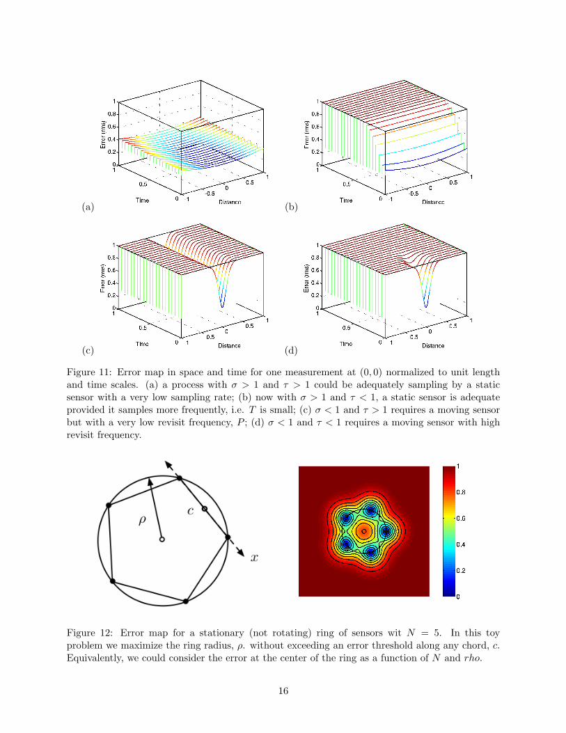
We consider the design of the radius and eccentricity of a rotating ring of mobile sensors in abounded region given N and the process statistics, σ, and τ . Including the time dimension in-troduces two additional parameters into the design problem: the sensor velocity, v, the samplingperiod, T . As a preliminary step, we consider the qualitative impact of these parameters in thedesign problem. One objective is to identify the portion of parameter space in which it is advan-tageous to have dynamic (as opposed to static) sensors. The cartoons in Figure 11 attempt toillustrate the various tradeoffs for a single space dimension.

This problem could be approached as follows: given a ring radius, ρ, how does the maximumerror on the circumference depend on N , v, T , σ, and τ? Secondly, given N , v, T , σ, and τ , findthe maximum radius ρ that satisfies ερ ≤ εmax. A static ring array is shown in Figure 12.

Clearly, even though we have reduced the spatial dimension to one by restricting the sensors to aring formation, we still have more degrees of freedom than we can easily visualize. Nonetheless, byscaling the space and time dimensions we provide a graphic that we hope provides some intuition forthe design problem. First, consider the trajectories of two adjacent sensors along the circumferenceof the ring as shown in Figure 13.a. Assuming the sensors maintain a fixed velocity, v, then thearc separation between two adjacent sensors is 2πρ/N for all time.

There are several observations to be made from this figure. First, we note that (in steady state)the maximum error will occur along the midpoint of the channel between the two trajectories. How-ever, unlike the static problem, the maximum error can not be approximated by the contributionsof the two nearest, simultaneous measurements. In fact, the error at the origin of Figure 13.a willbe determined by the nearest measurements in space and time. In particular, measurements beforeand after t = 0 will contribute to the error map.

The error at the midpoint of the chord (or arc) between two adjacent sensors is an increasingfunction of the ring radius, ρ. Simularly, the error is an increasing function of the temporalseparation, which we will call the resample period, P . In Figure 13.a, the resample period isapproximately P = 2ρπ

Nv . Clearly, increasing the velocity, v, decreases the resample period and,therefore, the error. Another way to visualize this is to observe that as v increases (decreases), thetrajectories “pivot” about the horizontal intercepts and the vertical intercepts get closer (fartherapart).

15

(a) (b)

(c) (d)

Figure 11: Error map in space and time for one measurement at (0, 0) normalized to unit lengthand time scales. (a) a process with σ > 1 and τ > 1 could be adequately sampling by a staticsensor with a very low sampling rate; (b) now with σ > 1 and τ < 1, a static sensor is adequateprovided it samples more frequently, i.e. T is small; (c) σ < 1 and τ > 1 requires a moving sensorbut with a very low revisit frequency, P ; (d) σ < 1 and τ < 1 requires a moving sensor with highrevisit frequency.

Figure 12: Error map for a stationary (not rotating) ring of sensors wit N = 5. In this toyproblem we maximize the ring radius, ρ. without exceeding an error threshold along any chord, c.Equivalently, we could consider the error at the center of the ring as a function of N and rho.

16

a) b)

Figure 13: The trajectories of two (out of N = 5) adjacent sensors moving with velocity, v, arounda circle of radius, ρ. a) The axes are arc length, ρθ and time, t. The sensor sampling period,T , determines the vertical spacing between measurements, which are plotted as black dots. Theresample period is approximately P . b) The trajectory plot with space and time axes scaled by thecharacteristic length scales, σ and τ .

Implicit in the preceding analysis is an assumption about the sample period, T . Namely, thatthe sample period is less than the resample period, i.e. T < P , so that the sensors take at leastone measurement per arc length equal to the sensor spacing. This assumption can be writtenas a specification on the the product of the sensor sample period and velocity, i.e. vT < 2ρπ

Nwhich is the arc separation between two adjacent sensors. Under this assumption, the error on thering circumference, ερ, will be inversely proportional to the sensor velocity: i.e. the error will bemaximum for v = 0.

Consider Figure 13.b, in which the space and time axes of the trajectory plot are scaled by thespace and time scales, σ and τ . Using this approach, we can study the error as a function of theseparameters. First, we observe that τ has the same impact as the sensor velocity, i.e. increasing τdecreases the slope of the trajectories and the effective resample period, P

τ . Similarly, increasingσ decreases the effective sensor separation. Both of these changes decrease the magnitude of thesteady-state error at the origin of the figure.

5 Future Work

We provide analytical and graphical tools to aid the design of a ring array for a homogeneous,isotropic, and stationary process. We plan to devise a strategy to combine multiple array primitivessuch as the ring to cover a large area, particularly for non-homogenous and non-stationary processes.Of particular concern is breaking the symmetry of the translation (and rotation) invariant controlschemes to fix the center of mass of the group (and maintain the splay separation) in the presenceof a flow field. Finally, we plan to apply the optimal experiment design procedure to select sensor

17

trajectories that follow the eigenvectors of the maximize eigenvalues of the Fisher informationmatrix, and compare to the results derived from objective analysis.

References

[1] R. Bachmayer and N. E. Leonard. Vehicle networks for gradient descent in a sampled envi-ronment. In Proc. IEEE Conf. on Decision and Control, 2002.

[2] F.P. Bretherton, R.E. Davis, and C.B. Fandry. A technique for objective analysis and designof oceanographic experiments applied to MODE-73. Deep-Sea Research, 23:559–582, 1976.

[3] F.P. Bretherton and J.C. McWilliams. Spectral estimation from irregular arrays. TechnicalReport NTIS PB299363, National Center for Atmospheric Research, 1976.

[4] E. Brown, P. Holmes, and J. Moehlis. Globally coupled oscillator networks. In Perspectives andProblems in Nonlinear Science: A Celebratory Volume in Honor of Larry Sirovich. Springer,2003.

[5] T.M Cover and J.A. Thomas. Elements of Information Theory. John Wiley & Sons, 1991.

[6] T. B. Curtin, J. G. Bellingham, J. Catipovic, and D. Webb. Autonomous oceanographicsampling networks. Oceanography, 6(3):86–94, 1993.

[7] G. Flierl, D. Grunbaum, S. Levin, and D. Olson. From individuals to aggregations: theinterplay between behavior and physics. J. theor. Biol, 196:397–454, 1999.

[8] L.S. Gandin. Objective Analysis of Meteorological Fields. Israel Program for Scientific Trans-lations, 1965.

[9] B. Grocholsky. Information-Theoretic Control of Multiple Sensor Platforms. PhD thesis, TheUniversity of Sydney, 2002. Available from http://www.acfr.usyd.edu.au.

[10] D. Grunbaum and A. Okubo. Modelling social animal aggregations. In S. A. Levin, editor,Lecture Notes in Biomathematics 100, pages 296–325. Springer-Verlag, 1994.

[11] E. W. Justh and P. S. Krishnaprasad. A simple control law for UAV formation flying. TechnicalReport 2002-38, Institute for Systems Research, University of Maryland, 2002.

[12] E. W. Justh and P. S. Krishnaprasad. Steering laws and continuum models for planar forma-tions. Technical report, Institute for Systems Research, University of Maryland, 2003.

[13] H. K. Khalil. Nonlinear Systems. Prentice Hall, third edition, 2002.

[14] P. F. J. Lermusiaux. Data assimilation via error subspace statistical estimation, part ii:Mid-atlantic bight shelfbreak front simulations, and esse validation. Montly Weather Review,127(8):1408–1432, 1999.

[15] P.B. Liebelt. An Introduction to Optimal Estimation. Addison-Wesley, 1967.

[16] J. Manyika and H. Durrant-Whyte. Data Fusion and Sensor Management: A DecentralizedInformation-Theoretic Approach. Ellis Horwood, 1994.

18

[17] A. Papoulis. Probability, Random Variables, and Stochastic Processes. McGraw-Hill, fourthedition, 2002.

[18] R. Sepulchre, D. Paley, and N. Leonard. Collective motion and oscillator synchronization. InV.J. Kumar, N.E. Leonard, and A.S. Morse, editors, (to appear) Proc. Block Island Workshopon Cooperative Control, June 2003.

[19] D. Ucinski. Optimal sensor location for parameter estimation of distributed processes. Int. J.Control, 73(13):1235–1248, 2000.

[20] S. Watanabe and S. Strogatz. Constants of motion for superconductor arrays. Physica D,74:197–253, 1994.

19