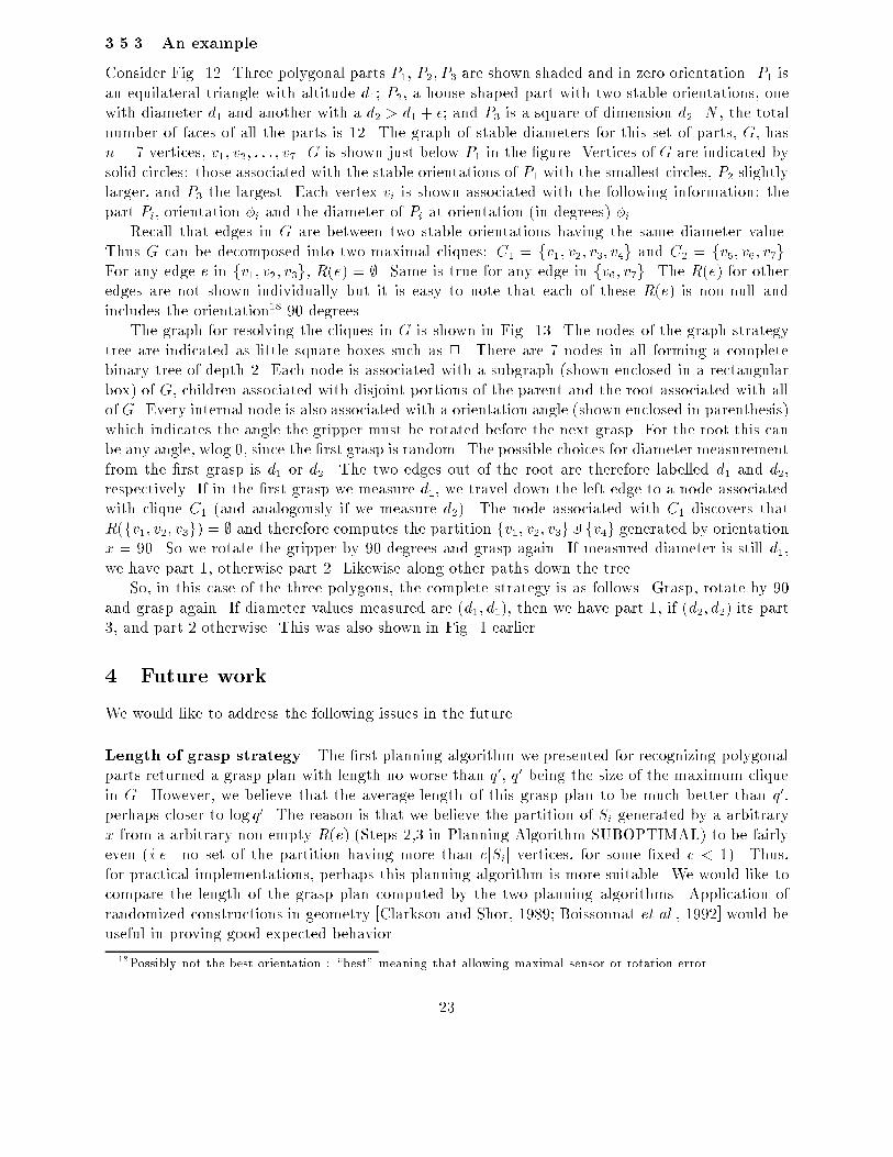
Figure 13: Grasp plan to resolve cliques in the graph of stable diameters for the parts P1; P2; P3

shown in the last �gure.

42

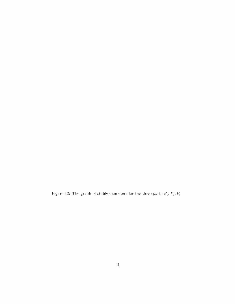
Figure 12: The graph of stable diameters for the three parts P1; P2; P3.

41

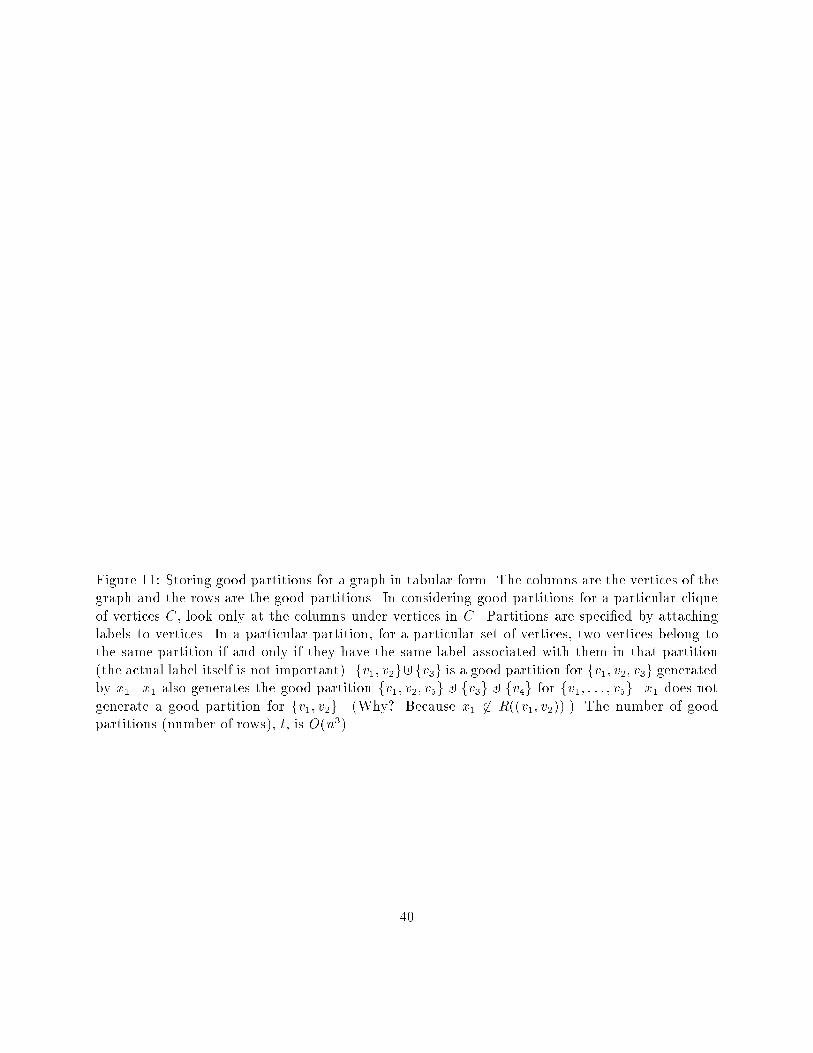
Figure 11: Storing good partitions for a graph in tabular form. The columns are the vertices of thegraph and the rows are the good partitions. In considering good partitions for a particular cliqueof vertices C, look only at the columns under vertices in C. Partitions are speci�ed by attachinglabels to vertices. In a particular partition, for a particular set of vertices, two vertices belong tothe same partition if and only if they have the same label associated with them in that partition(the actual label itself is not important). fv1; v2g]fv3g is a good partition for fv1; v2; v3g generatedby x1. x1 also generates the good partition fv1; v2; v5g ] fv3g ] fv4g for fv1; : : : ; v5g. x1 does notgenerate a good partition for fv1; v2g. (Why? Because x1 62 R((v1; v2)).) The number of goodpartitions (number of rows), t, is O(n3).

40

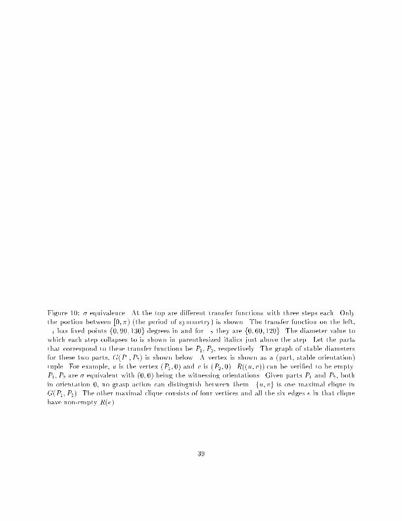
Figure 10: �-equivalence. At the top are di�erent transfer functions with three steps each. Onlythe portion between [0; �) (the period of symmetry) is shown. The transfer function on the left,�1 has �xed points f0; 90; 130g degrees in and for �2 they are f0; 60; 120g. The diameter value towhich each step collapses to is shown in parenthesized italics just above the step. Let the partsthat correspond to these transfer functions be P1; P2, respectively. The graph of stable diametersfor these two parts, G(P1; P2) is shown below. A vertex is shown as a (part, stable orientation)tuple. For example, u is the vertex (P1; 0) and v is (P2; 0). R((u; v)) can be veri�ed to be empty.P1; P2 are �-equivalent with (0; 0) being the witnessing orientations. Given parts P1 and P2, bothin orientation 0, no grasp action can distinguish between them. fu; vg is one maximal clique inG(P1; P2). The other maximal clique consists of four vertices and all the six edges e in that cliquehave non-empty R(e).

39

Figure 9: Transfer function of a rectangular part.

38

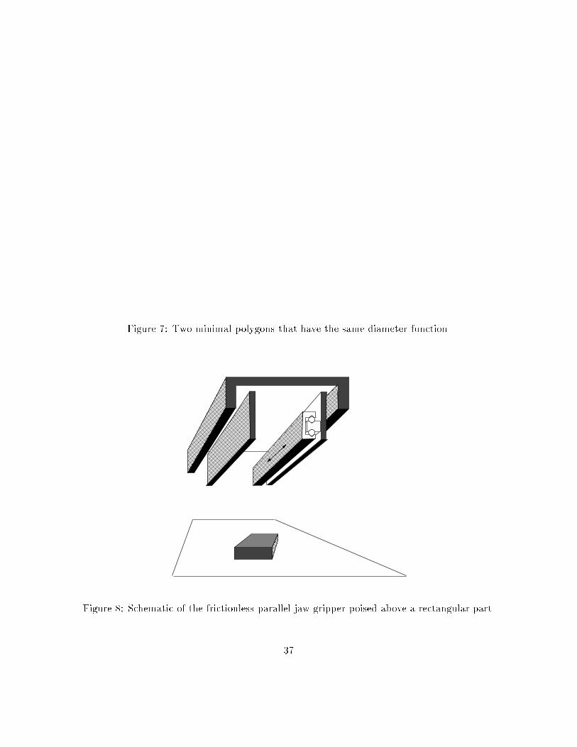
Figure 7: Two minimal polygons that have the same diameter function.

Figure 8: Schematic of the frictionless parallel jaw gripper poised above a rectangular part.

37

Figure 6: In�nitely many polygons having the same diameter function as a given polygon.

36

Polygons with Identical Diameter Function

Figure 5: Triangles and hexagons having the same diameter function.

35

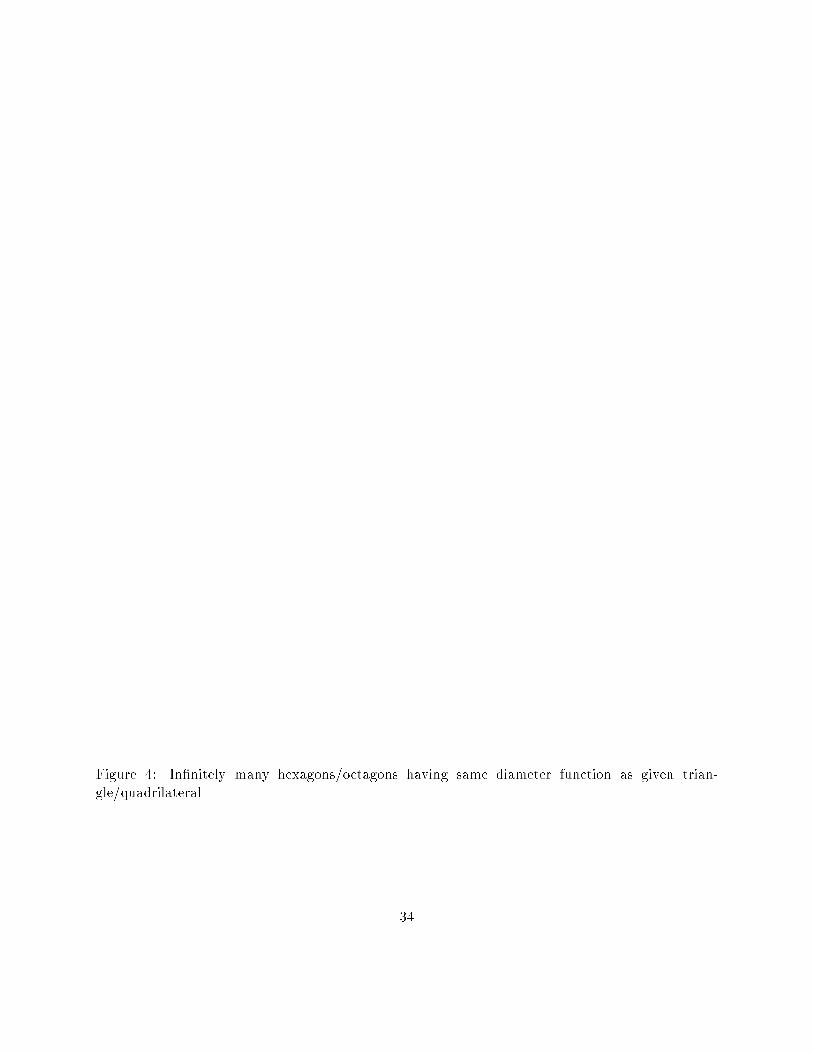
Figure 4: In�nitely many hexagons/octagons having same diameter function as given trian-gle/quadrilateral.

34

Figure 3: Orientation 0 is a kink.

33

?

Figure 1: An example grasp plan for distinguishing the three parts shown at the top.

d

θ2π3π/2ππ/20

Figure 2: The diameter function for the four-sided part shown at the right.

32

Triple-spaced copy of text

List of Figures (with captions)

30

[Rao and Goldberg, 1992c] A. S. Rao and K. Y. Goldberg. Shape from diameter: Strategies forrecognizing polygonal parts. Technical Report # 292, University of Southern California, Instituteof Robotics and Intelligent Systems (IRIS), Los Angeles, Calif. 90089-0273, April 1992.

[Rao, 1992] A. S. Rao. Algorithmic Plans for Robotic Manipulation. PhD thesis, University ofSouthern California, Department of Electrical Engineering{Systems, December 1992.

[Rappaport, 1987] D. Rappaport. Computing simple circuits from a set of line segments is NP-complete. In Annual Symposium on Computational Geometry, pages 322{330. ACM, 1987.

[Raviv, 1991] D. Raviv. A quantitative approach to camera �xation. In International Conferenceon Computer Vision and Pattern Recognition (CVPR), pages 386{392, Maui, Hawaii, June 1991.IEEE.

[Rich, 1983] E. Rich. Arti�cial Intelligence. series in AI. McGraw Hill, New York, 1983.

[Skiena, 1988] S. S. Skiena. Geometric probing. PhD thesis, University of Illinois, Dept. of Com-puter Science, Urbana, Ill., 1988.

[Skiena, 1989] S. S. Skiena. Problems in geometric probing. Algorithmica, pages 599{605, 1989.

[Spyridi and Requicha, 1990] A. J. Spyridi and A. A. G. Requicha. Accessibility analysis for theautomatic inspection of mechanical parts by coordinate measuring machines. In InternationalConference on Robotics and Automation. IEEE, May 1990.

[Taylor et al., 1987] R. H. Taylor, M. T. Mason, and K. Y. Goldberg. Sensor-based manipulationplanning as a game with nature. In Fourth International Symposium on Robotics Research,August 1987.

[Wallack and Canny, 1991] A. S. Wallack and J. F. Canny. Linear time algorithm for object local-ization using scanning. manuscript, September 1991.

[Wallack and Canny, 1992] A. S. Wallack and J. F. Canny. Object localization using �nger gapsensing. Technical Report ESRC 92-3/RAMP 92-2, Univ. of California, Berkeley, Dept. of Com-puter Science, February 1992.

[Wallack and Canny, 1993] A. S. Wallack and J. F. Canny. A geometric matching algorithm forbeam scanning. In SPIE symposium on optical tools for manufacturing and advanced automation,Boston, 1993.

[Yaglom and Boltyanskii, 1951] I. M. Yaglom and V.G. Boltyanskii. Convex Figures. Holt, Rinehartand Winston, New York, 1951.

29

[Goldberg and Furst, 1992] K. Y. Goldberg and M. Furst. Low friction gripper. U.S. Patent #5,098,145, March 1992.

[Goldberg, 1990] K. Y. Goldberg. Stochastic plans for robotic manipulation. PhD thesis, Carnegie-Mellon University, School of Computer Science, August 1990.

[Goldberg, 1993] K. Y. Goldberg. Orienting polygonal parts without sensors. Algorithmica,10(2):201{225, Aug 1993. (Special issue on Computational Robotics).

[Grimson and Lozano-Perez, 1987] W. E. L. Grimson and T. Lozano-Perez. Model-based recogni-tion and localization from sparse range or tactile data. IEEE Transactions on Pattern Analysisand Machine Intelligence, 9:469{482, July 1987.

[Jameson, 1985] J. Jameson. Analytic techniques for automated grasp. PhD thesis, Stanford Uni-versity, June 1985.

[Kang and Goldberg, 1992] D. Kang and K. Y. Goldberg. Shape recognition by random grasping.In International Conference on Intelligent Robots and Systems. IEEE/RSJ, July 1992. Submittedto the IEEE Transactions on Robotics and Automation in June 1993.

[Kolzow et al., 1989] D. Kolzow, A. Kuba, and A. Volcic. An algorithm for reconstructing convexbodies from their projections. Discrete and Computational Geometry, 4:205{237, 1989.

[Koutsou, 1988] A. Koutsou. Object exploration using a parallel-jaw gripper. GRASP Lab TechReport MS-CIS-88-48, University of Pennsylvania, 1988.

[Laumond, 1987] J. P. Laumond. Obstacle growing in a non-polygonal world. Information Pro-cessing Letters, 25(1):41{50, 1987.

[Li, 1988] S-Y. R. Li. Reconstruction of polygons from projections. Information Processing Letters,28:235{240, 12 Aug. 1988.

[Mason et al., 1988] M. T. Mason, K. Y. Goldberg, and R. H. Taylor. Planning sequencesof squeeze-grasps to orient and grasp polygonal objects. Technical Report CMU-CS-88-127,Carnegie Mellon University, Computer Science Dept., Pittsburgh, PA 15213, April 1988.

[Mason, 1986] M. T. Mason. On the scope of quasi-static pushing. In O. Faugeras and G. Giralt,editors, The Third International Symposium on Robotics Research. MIT Press, 1986.

[Peshkin, 1986] M. A. Peshkin. Planning Robotic Manipulation Strategies for Sliding Objects. PhDthesis, Carnegie-Mellon University, Department of Physics, Pittsburgh, Pennylvania, Nov 1986.Also published as a book: Robotic Manipulation Strategies, Prentice Hall, 1990, New Jersey.

[Preparata and Shamos, 1985] F. P. Preparata and M. I. Shamos. Computational Geometry, AnIntroduction. Springer-Verlag, New York, 1985.

[Rao and Goldberg, 1992a] A. S. Rao and K. Y. Goldberg. Grasping planar curved parts witha parallel-jaw gripper. Technical Report # 299, University of Southern California, Institute ofRobotics and Intelligent Systems (IRIS), Los Angeles, Calif. 90089-0273, August 1992. Submittedto the IEEE Transactions on Robotics and Automation.

[Rao and Goldberg, 1992b] A. S. Rao and K. Y. Goldberg. Orienting generalized polygonal parts.In International conference on Robotics and Automation (ICRA), Nice, France, May 1992. IEEE.

28

References

[Bajcsy, 1988] R. Bajcsy. Active perception. Proceedings of the IEEE, 76(8), 1988.

[Benson, 1966] R. V. Benson. Euclidian Geometry and Convexity. McGraw-Hill Book Company,1966.

[Boissonnat and Yvinec, 1992] J. D. Boissonnat and M. Yvinec. Probing a scene of non-convexpolyhedra. Algorithmica, 8:321{342, 1992.

[Boissonnat et al., 1992] J. D. Boissonnat, D. Devillers, R. Schott, M. Teillaud, and M. Yvinec.Application of random sampling to on-line algorithms in computational geometry. Discrete andComputational Geometry, 8:51{71, 1992.

[Brost, 1988] R. C. Brost. Automatic grasp planning in the presence of uncertainty. The Interna-tional Journal of Robotics Research, 8(1), February 1988.

[Canny and Goldberg, 1993] J. F. Canny and K. Y. Goldberg. A RISC paradigm for industrialrobotics. Technical Report ESRC 93-4/RAMP 93-2, University of California at Berkeley, Engi-neering Systems Research Center, February 1993.

[Chandru and Venkataraman, 1991] V. Chandru and R. Venkataraman. Circular hulls and Orb-iforms of simple polygons. In Symposium on Discrete Algorithms (SODA). SIAM-ACM, 1991.

[Chen and Ierardi, 1991] Y-B. Chen and D. J. Ierardi. Distinguishing polygons by sensing diam-eters. Technical Report USC-CS-92-503, University of Southern California, Dept. of ComputerScience, December 1991.

[Clarkson and Shor, 1989] K. L. Clarkson and P. W. Shor. Applications of random sampling incomputational geometry, II. Discrete and Computational Geometry, 4:387{421, 1989.

[Cole and Yap, 1987] R. Cole and C. K. Yap. Shape from probing. Journal of Algorithms, 8(1):19{38, 1987.

[Dobkin et al., 1986] D. P. Dobkin, H. Edelsbrunner, and C. K. Yap. Probing convex polytopes.In Symposium on Theory of Computing (STOC), pages 424{432. ACM, 1986.

[Edelsbrunner, 1987] H. Edelsbrunner. Algorithms in Combinatorial Geometry. EATCS Mono-graphs on Theoretical Computer Science. Springer-Verlag, Berlin, 1987.

[Ellis, 1987] R. Ellis. Acquiring tactile data for the recognition of planar objects. In IEEE Inter-national Conference on Robotics and Automation, 1987.

[Erdmann and Mason, 1986] M. A. Erdmann and M. T. Mason. An exploration of sensorless ma-nipulation. In IEEE International Conference on Robotics and Automation, 1986.

[Garey and Johnson, 1979] M. Garey and D. B. Johnson. Computers and Intractibility: A guideto the theory of NP-completeness. Freeman, New York, 1979.

[Gaston and Lozano-Perez, 1984] P. C. Gaston and T. Lozano-Perez. Tactile recognition and lo-calization using object models: The case of polyhedra on a plane. IEEE Transactions on PatternAnalysis and Machine Intelligence, 6:257{266, May 1984.

27

Ci+1 sin(�i+1 � �i) = di+2 sin(�i+1 � �i)� di+1 sin(�i+2 � �i) + di sin(�i+2 � �i+1): (6)

From the remaining 3Z � 3 equations, we can similarly get Z � 1 other linear equations in thedj. By observing the coe�cients in the linear equations, we can see that they will have at mostone solution (i.e. the case of in�nite solutions is impossible).

26

Rote, Russ Taylor, and Chee Yap for rewarding discussions on this subject. We also thank theanonymous referees for their constructive criticism and useful suggestions.

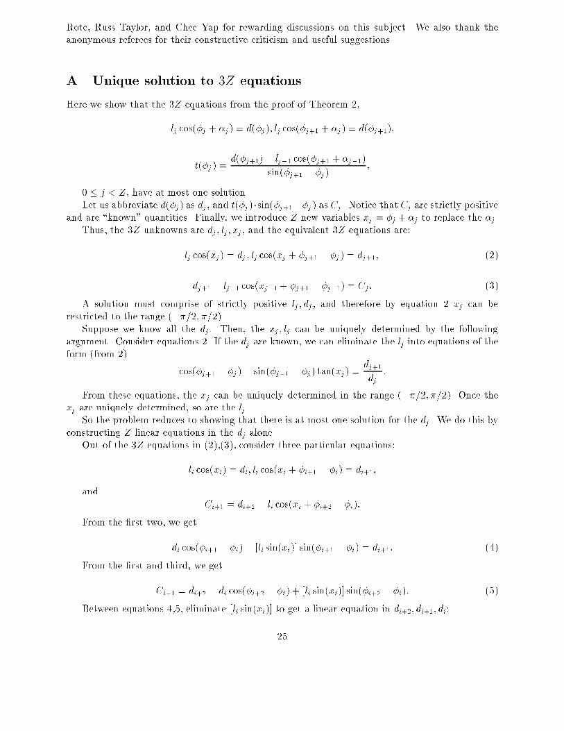
A Unique solution to 3Z equations

Here we show that the 3Z equations from the proof of Theorem 2,

lj cos(�j + �j) = d(�j); lj cos(�j+1 + �j) = d(�j+1);

t(�j) =d(�j+1)� lj�1 cos(�j+1 + �j�1)

sin(�j+1 � �j);

0 � j < Z, have at most one solution.Let us abbreviate d(�j) as dj, and t(�j) �sin(�j+1��j) as Cj. Notice that Cj are strictly positive

and are \known" quantities. Finally, we introduce Z new variables xj = �j + �j to replace the �j.Thus, the 3Z unknowns are dj; lj; xj, and the equivalent 3Z equations are:

lj cos(xj) = dj ; lj cos(xj + �j+1 � �j) = dj+1; (2)

dj+1 � lj�1 cos(xj�1+ �j+1 � �j�1) = Cj: (3)

A solution must comprise of strictly positive lj; dj, and therefore by equation 2 xj can berestricted to the range (��=2; �=2).

Suppose we know all the dj. Then, the xj ; lj can be uniquely determined by the followingargument. Consider equations 2. If the dj are known, we can eliminate the lj into equations of theform (from 2)

cos(�j+1 � �j)� sin(�j+1 � �j) tan(xj) =dj+1dj

:

From these equations, the xj can be uniquely determined in the range (��=2; �=2). Once thexj are uniquely determined, so are the lj.

So the problem reduces to showing that there is at most one solution for the dj. We do this byconstructing Z linear equations in the dj alone.

Out of the 3Z equations in (2),(3), consider three particular equations:

li cos(xi) = di; li cos(xi + �i+1 � �i) = di+1;

andCi+1 = di+2 � li cos(xi + �i+2 � �i):

From the �rst two, we get

di cos(�i+1 � �i)� [li sin(xi)] sin(�i+1 � �i) = di+1: (4)

From the �rst and third, we get

Ci+1 = di+2 � di cos(�i+2 � �i) + [li sin(xi)] sin(�i+2 � �i): (5)

Between equations 4,5, eliminate [li sin(xi)] to get a linear equation in di+2; di+1; di:

25

Identifying �-equivalent parts Our planning algorithms can identify any part (and its �nalorientation up to symmetry) from among a set of parts as long as no two are �-equivalent. Testingfor �-equivalence of parts is straightforward from the graph of stable diameters G (Section 3.4).However, can we distinguish between �-equivalent parts Pu; Pv (that are not d-equivalent)? Whilethe chance that two industrial parts are �-equivalent is very remote, this is nevertheless a theoret-ically interesting problem.19 Let �u; �v be the orientations that witness the �-equivalence For theedge e = (u; v) in G, R(e) = ;. Therefore, consider the set R2(e) � S1 � S1 de�ned by

R2(e) = f(�1; �2) j du(�u(�u(�1 + �u) + �2)) 6= dv(�v(�v(�1 + �v) + �2))g:

If R2(e) is non-empty, then a 2-tuple of orientations from R2(e) can be applied to disambiguatebetween the �-equivalent parts. In fact, we can run the planning algorithms substituting R2(e) forR(e). R2(e) can be computed in O(j�ujj�vj) time. If R2(e) is also empty, then R3(e) � (S1)3 needsto be computed. Given the R2(e) for all edges, R3(e) can be computed again in O(n2) time and soon. Surely, for d-equivalent parts, all the Ri(e) will be empty (a trivial bound on i is n2) and nograsp plan can possibly distinguish between them. However, we conjecture that for �-equivalentparts that are not d-equivalent, there exists a constant c such that Rc(e) 6= ;. If true, this wouldresult in an O(n2 log n) planning algorithm, with O(n4) preprocessing, that gives a plan of lengthat most cn to distinguish between any set of parts as long as no two of them are d-equivalent.

Non-polygonal parts To extend these results to non-polygonal shapes, we note that one ad-ditional feature of non-polygonal diameter functions is the possible existence of at regions inthe diameter function. Also, the diameter function need not be piecewise sinusoidal anymore.It will be interesting to come up with an analog to Theorem 1 characterizing diameter func-tions of even a class of non-polygonal shapes, say the class of shapes made up of piecewise lin-ear and piecewise circular segments (such parts are called generalized polygonal [Laumond, 1987;Rao and Goldberg, 1992b]). Shape recovery is another question. The existence of curves of constantwidth (or \orbiforms" [Chandru and Venkataraman, 1991]) is known since Euler. Hence completeshape recovery is impossible. However, can we have analogs to Theorem 2 stating how much infor-mation about the geometry of the shape can be recovered? If so, we may be able to come up withgrasp plans to recognize generalized polygonal parts from among a set.

5 Conclusion

We have considered the planar problem of determining the convex shape of a polygonal part froma sequence of measurements taken with a frictionless parallel-jaw gripper. We have derived bothnegative and positive results.

The negative results are related to the study of curves of constant width (Gleichdicke) in classicalgeometry, establishing a new link between computational geometry and robotics. The positiveresults are examples of sensor-based manipulation planning, but di�er from previous work in thatwe use a frictionless gripper and give a computational analysis of the planning problem. Therequired hardware is inexpensive and well-known. This is consistent with our aim to develop newsoftware for \old" hardware.

AcknowledgmentsWe thank Randy Brost, Duk Kang, Mike Erdmann, Doug Ierardi, Matt Ma-son, Babu Narayanan, Mark Overmars, Viktor Prasanna, Govindan Rajeev, Ari Requicha, G�unter

19Our algorithms in this paper can distinguish between �-equivalent parts as long as the parts do not enter intoorientations that witness their �-equivalence.

24

3.5.3 An example

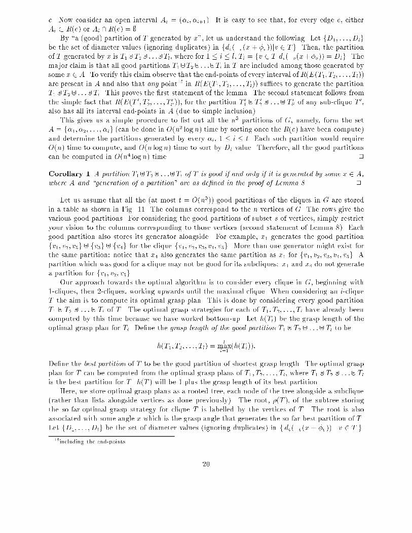
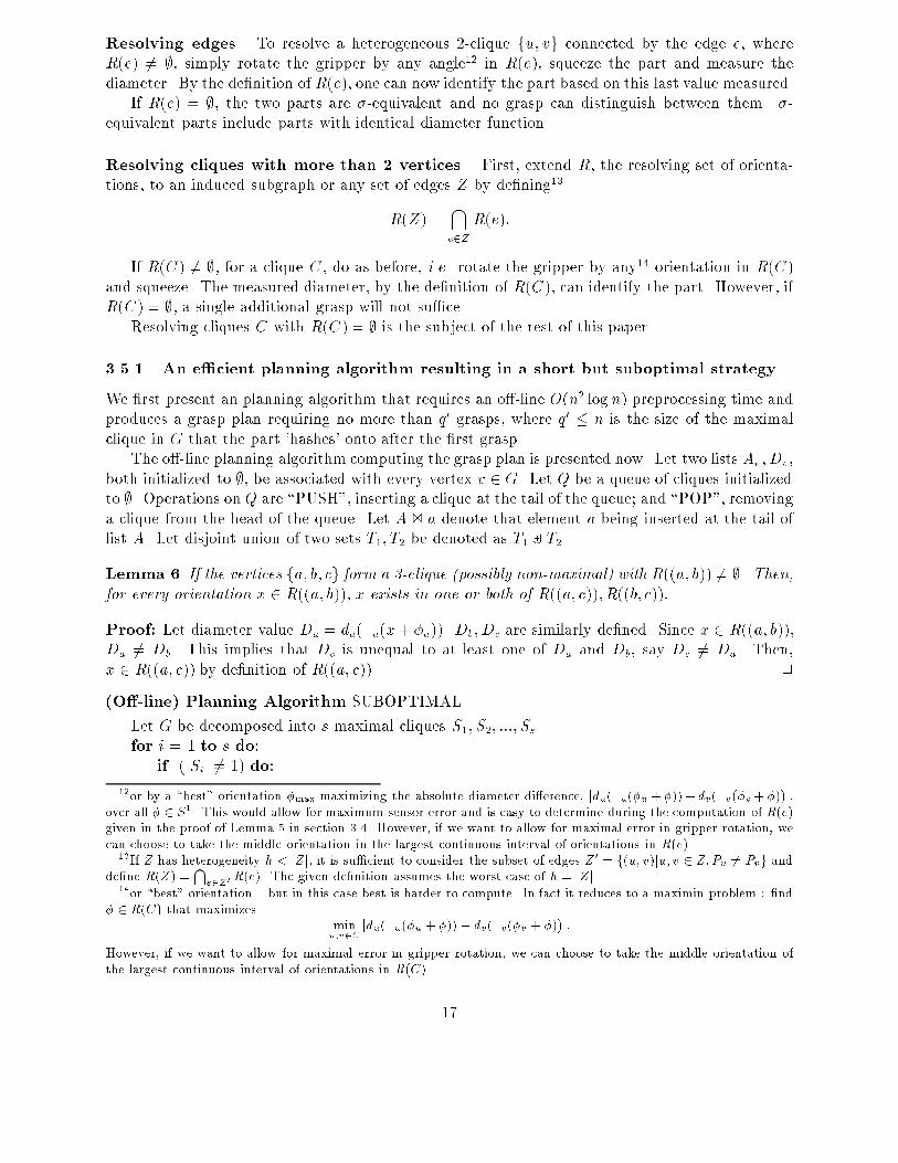
Consider Fig. 12. Three polygonal parts P1, P2; P3 are shown shaded and in zero orientation. P1 isan equilateral triangle with altitude d1; P2, a house shaped part with two stable orientations, onewith diameter d1 and another with a d2 > d1 + �; and P3 is a square of dimension d2. N , the totalnumber of faces of all the parts is 12. The graph of stable diameters for this set of parts, G, hasn = 7 vertices, v1; v2; : : : ; v7. G is shown just below P1 in the �gure. Vertices of G are indicated bysolid circles: those associated with the stable orientations of P1 with the smallest circles, P2 slightlylarger, and P3 the largest. Each vertex vi is shown associated with the following information: thepart Pi, orientation �i and the diameter of Pi at orientation (in degrees) �i.

Recall that edges in G are between two stable orientations having the same diameter value.Thus G can be decomposed into two maximal cliques: C1 = fv1; v2; v3; v4g and C2 = fv5; v6; v7g.For any edge e in fv1; v2; v3g, R(e) = ;. Same is true for any edge in fv6; v7g. The R(e) for otheredges are not shown individually but it is easy to note that each of these R(e) is non-null andincludes the orientation18 90 degrees.

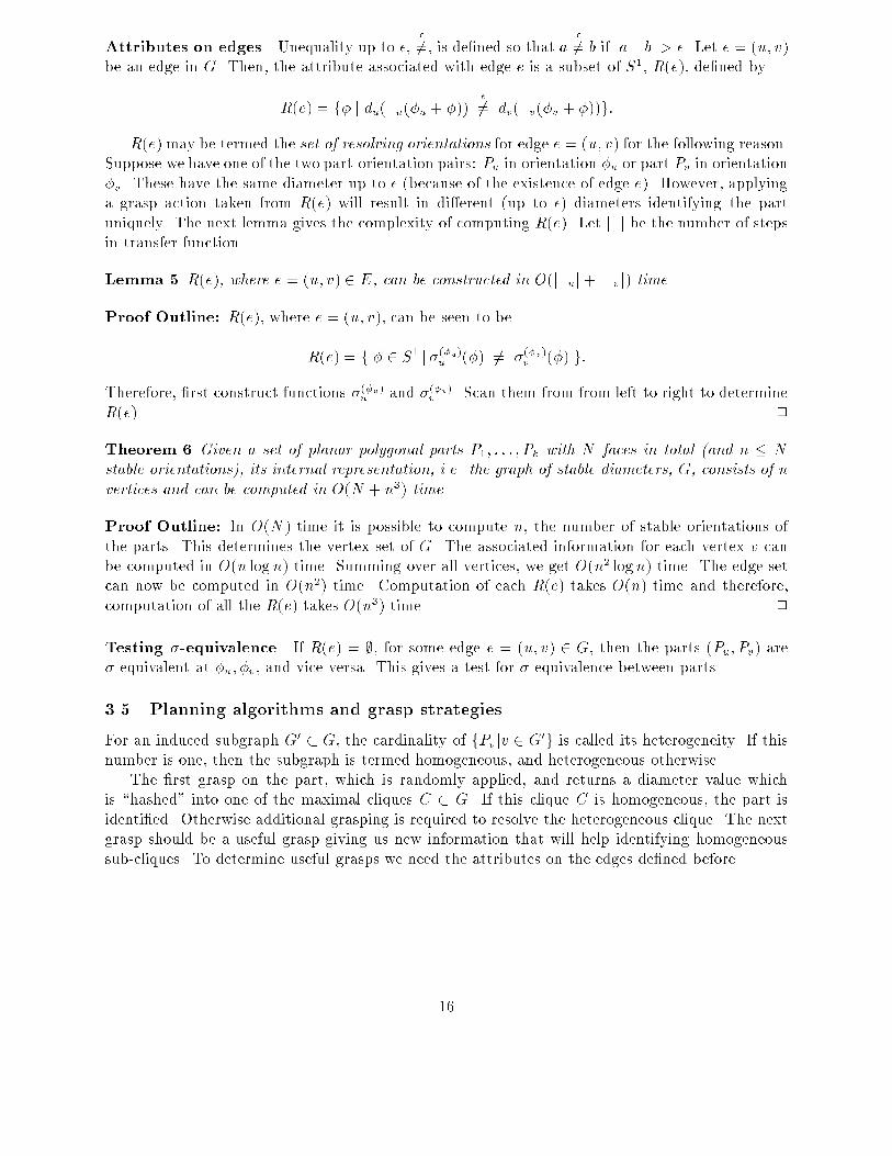
The graph for resolving the cliques in G is shown in Fig. 13. The nodes of the graph strategytree are indicated as little square boxes such as 2. There are 7 nodes in all forming a completebinary tree of depth 2. Each node is associated with a subgraph (shown enclosed in a rectangularbox) of G, children associated with disjoint portions of the parent and the root associated with allof G. Every internal node is also associated with a orientation angle (shown enclosed in parenthesis)which indicates the angle the gripper must be rotated before the next grasp. For the root this canbe any angle, wlog 0, since the �rst grasp is random. The possible choices for diameter measurementfrom the �rst grasp is d1 or d2. The two edges out of the root are therefore labelled d1 and d2,respectively. If in the �rst grasp we measure d1, we travel down the left edge to a node associatedwith clique C1 (and analogously if we measure d2). The node associated with C1 discovers thatR(fv1; v2; v3g) = ; and therefore computes the partition fv1; v2; v3g]fv4g generated by orientationx = 90. So we rotate the gripper by 90 degrees and grasp again. If measured diameter is still d1,we have part 1, otherwise part 2. Likewise along other paths down the tree.

So, in this case of the three polygons, the complete strategy is as follows. Grasp, rotate by 90and grasp again. If diameter values measured are (d1; d1), then we have part 1, if (d2; d2) its part3, and part 2 otherwise. This was also shown in Fig. 1 earlier.

4 Future work

We would like to address the following issues in the future.

Length of grasp strategy The �rst planning algorithm we presented for recognizing polygonalparts returned a grasp plan with length no worse than q0, q0 being the size of the maximum cliquein G. However, we believe that the average length of this grasp plan to be much better than q0,perhaps closer to log q0. The reason is that we believe the partition of Si generated by a arbitraryx from a arbitrary non-empty R(e) (Steps 2,3 in Planning Algorithm SUBOPTIMAL) to be fairlyeven (i.e. no set of the partition having more than cjSij vertices, for some �xed c < 1). Thus,for practical implementations, perhaps this planning algorithm is more suitable. We would like tocompare the length of the grasp plan computed by the two planning algorithms. Application ofrandomized constructions in geometry [Clarkson and Shor, 1989; Boissonnat et al., 1992] would beuseful in proving good expected behavior.

18Possibly not the best orientation : \best" meaning that allowing maximal sensor or rotation error.

23

Planning Algorithm OPT GRASP

for i = 1 to q do:for j = 1 to Ni do:

Let Cj;i be the jth i-clique in G.if i = 1 or 2

Do the needful [Trivial Cases]else do: [i > 2]

1. w jCj;ij; h(Cj;i) w.2. Consider all good partitions of Cj;i in turn.

2.1 Let T1 ] T2 ] : : :] Tl be one such good partition.2.2 Let x 2 R(E(T1; T2; : : : ; Tl)).2.3 if (1 + h(T1; T2; : : : ; Tl) < w) do:

2.3.1 w 1 + h(T1; T2; : : : ; Tl); h(Cj;i) w.2.3.2 Let fD1; : : : ; Dlg f dv(�v(x+ �v)) j v 2 Cj;i g2.3.3 For 1 � r � l, Tr = f v 2 Cj;i j dv(�v(x+ �v)) = Dr g.2.3.4 Remove all edges out the tree node X(Cj;i).2.3.5 Associate node X(Cj;i) by grasp angle x.2.3.6 Create l edges out of node X(Cj;i) with labels D1; : : : ; Dl.2.3.7 Let the rth edge, 1 � r � l, point to X(Tr).

2

Analysis: Assume that at any stage of the computation, given a clique T , the information associatedwith it, namely, h(T ) and a pointer to �(T ), can be obtained by random access in O(1) time. Alsoassume that we have precomputed the good partitions of every maximal clique and stored them intabular form (as described in the proof Lemma 8 and Fig. 11). Steps 2 and 2.1 can be implementedby loading in the next row (partition) from the table. The test for \goodness" of this partition withrespect to Cj;i consists of checking whether the partition loaded in has at least two distinct labelsfor the columns corresponding to vertices in Cj;i. This check can be done in O(i) time. Assumethat the partition also brings with it its generator which may be used as x in Step 2.2 (withoutcomputation of E(T1; : : : ; Tl) and R(E(T1; : : : ; Tl)). At this time subcliques T1; : : : ; Tl have beenprocessed and so h(T1); : : : ; h(Tl) may be accessed and their maximum, h(T1; : : : ; Tl) computedin O(l) = O(i) time for Step 2.3. A single iteration of steps 2.3.1{2.3.7 can be implemented inO(l) = O(i) time. Let T (p) represent the preprocessing time complexity to resolve a p-clique.Since there are at most O(n3) good partitions (Lemma 8), it is easy to see that

T (p) =i=p�1Xi=1

pi

!O(in3): (1)

This gives T (p) = O(n42p). Total preprocessing complexity is the sum of complexities for eachmaximal clique, which is upper bounded by n

qn42q, where q is the size of the maximum clique in

G. The on-line grasp plan still runs in O(logn) per grasp. However, because to the representationof grasps directly as trees, its implementation is straightforward and is not described.

This exponential time complexity isn't as bad as it sounds since the size of the largest clique inthe graphs we consider is likely to be small even if we have large number of parts. The correctnessfollows from the discussion before presentation of the planning algorithm and the fact that, at theend of the processing for Cj;i, the best partition for it would have been determined correctly (Step2.3).

22

Let fTjg; 1 � j � l be the partition of T induced by the diameter values. The edges out of theroot are labelled by the diameter values D1; : : : ; Dl and the children of the root are labelled by thevertices of the individual Tj and will be associated by an appropriate grasp angle.17 The leaves ofthis tree consist of vertices that all belong to the same part or a clique of vertices such that everyedge e between two vertices associated with distinct parts has R(e) = ;. Let the subtree whoseroot �(T ) is labelled by the vertices of clique T be denoted as TREE(T ). Additionally, let h(T )denote the depth of TREE(T ). It is easy to see that, at the end of the computation, this de�nitionof h(T ) and that given in the previous paragraph are the same. Initially, the tree for every clique(including the non-maximal ones) consists of a single unconnected node labelled by the vertices ofthat clique.

Let Ni be the number of i-cliques in G. q is size of maximum clique in G.

17Each internal node is just like for the root { it stores the grasp strategy for the Tj it is labelled by.

21

e. Now consider an open interval Ai = (�i; �i+1). It is easy to see that, for every edge e, eitherAi � R(e) or Ai \R(e) = ;.

By \a (good) partition of T generated by x", let us understand the following. Let fD1; : : : ; Dlgbe the set of diameter values (ignoring duplicates) in fdv(�v(x+ �v))jv 2 Tg. Then, the partitionof T generated by x is T1]T2] : : :]Tl, where for 1 � i � l, Ti = fv 2 T jdv(�v(x+�v)) = Dig. Themajor claim is that all good partitions T1]T2] : : :]Tl in T are included among those generated bysome x 2 A. To verify this claim observe that the end-points of every interval ofR(E(T1; T2; : : : ; Tl))are present in A and also that any point16 in R(E(T1; T2; : : : ; Tl)) su�ces to generate the partitionT1]T2] : : :]Tl. This proves the �rst statement of the lemma. The second statement follows fromthe simple fact that R(E(T 0

1; T02; : : : ; T

0l0)), for the partition T 0

1 ] T02 ] : : :] T

0l0 of any sub-clique T 0,

also has all its interval end-points in A (due to simple inclusion).This gives us a simple procedure to list out all the n3 partitions of G, namely, form the set

A = f�1; �2; : : : ; �tg (can be done in O(n3 logn) time by sorting once the R(e) have been compute)

and determine the partitions generated by every �i, 1 � i � t. Each such partition would requireO(n) time to compute, and O(n logn) time to sort by Di value. Therefore, all the good partitionscan be computed in O(n4 logn) time. 2

Corollary 1 A partition T1]T2] : : :]Tl of T is good if and only if it is generated by some x 2 A,where A and \generation of a partition" are as de�ned in the proof of Lemma 8. 2

Let us assume that all the (at most t = O(n3)) good partitions of the cliques in G are storedin a table as shown in Fig. 11. The columns correspond to the n vertices of G. The rows give thevarious good partitions. For considering the good partitions of subset s of vertices, simply restrictyour vision to the columns corresponding to those vertices (second statement of Lemma 8). Eachgood partition also stores its generator alongside. For example, x1 generates the good partitionfv1; v2; v5g ] fv3g ] fv4g for the clique fv1; v2; v3; v4; v5g. More than one generator might exist forthe same partition: notice that x4 also generates the same partition as x1 for fv1; v2; v3; v4; v5g. Apartition which was good for a clique may not be good for its subcliques: x1 and x4 do not generatea partition for fv1; v2; v5g.

Our approach towards the optimal algorithm is to consider every clique in G, beginning with1-cliques, then 2-cliques, working upwards until the maximal clique. When considering an i-cliqueT the aim is to compute its optimal grasp plan. This is done by considering every good partitionT1 ] T2 ] : : : ] Tl of T . The optimal grasp strategies for each of T1; T2; : : : ; Tl have already beencomputed by this time because we have worked bottom-up. Let h(Ti) be the grasp length of theoptimal grasp plan for Ti. De�ne the grasp length of the good partition T1 ] T2 ] : : :] Tl to be

h(T1; T2; : : : ; Tl) =l

maxi=1

(h(Ti)):

De�ne the best partition of T to be the good partition of shortest grasp length. The optimal graspplan for T can be computed from the optimal grasp plans of T1; T2; : : : ; Tl, where T1 ] T2 ] : : :] Tlis the best partition for T . h(T ) will be 1 plus the grasp length of its best partition.

Here, we store optimal grasp plans as a rooted tree, each node of the tree alongside a subclique(rather than lists alongside vertices as done previously). The root, �(T ), of the subtree storingthe so-far-optimal grasp strategy for clique T is labelled by the vertices of T . The root is alsoassociated with some angle x which is the grasp angle that generates the so-far-best partition of T .Let fD1; : : : ; Dlg be the set of diameter values (ignoring duplicates) in f dv(�v(x+ �v)) j v 2 T g.

16including the end-points

20

repeat:0. Let v be any vertex in Ci,1. Rotate the gripper by angle X = xi;v.2. Squeeze and measure the diameter D.3. Ci+1 = fv 2 Cijdi;v = Dg.4. i i+ 1.

until jCi+1j = jCij.

� i� 1. Let C� = fv1; : : : ; vzg be of heterogeneity w.Let fP1; P2; : : : ; Pwg be the parts associated with the vertices fv1; : : : ; vzg.Declare that the part P is one of P1; P2; : : : ; Pw.

2

Analysis: The subclique selection step, Step 3, is the dominant operation in every grasp and canbe implemented in O(logn) time per grasp. The grasp length of the plan, �, is bounded above bythe size of the Av; Dv lists, which is at most q0 = jC1j � q � n. (q is the size of the maximum cliquein G).

3.5.2 Optimal grasp strategies

The reason why the Planning Algorithm SUBOPTIMAL of section 3.5.1 does not produce theshortest grasp plan is that the partitions T1 ] T2 ] : : : ] Tl (Step 6) were chosen on basis of anarbitrary cutting edge e and arbitrary cutting orientation xe (Steps 2,3).

Let E(T1; T2; : : : ; Tl) denote the set of edges with one end point in one of the Ti and the otherend-point in one of the other Tj. That is,

E(T1; T2; : : : ; Tl) = fe = (u; v) j u 2 Ti; v 2 Tj; 1 � i; j � l; i 6= jg:

To get the optimal number of grasps, one approach is to consider every partition of everysubclique. However, even the number of 2-partitions of an i-clique is very large (�(2i)). Thereforethis naive approach would lead to an algorithm that requires at least

i=q�1Xi=1

qi

!(2i) = (3q)

operations. However, notice that we only need to consider \good" partitions T1 ] T2 ] : : :] Tl, i.e.those satisfying R(E(T1; T2; : : : ; Tl)) 6= ;. The following lemma gives a polynomial bound on thenumber of good partitions.

Lemma 8 There are only O(n3) good partitions T1 ] T2 ] : : :] Tl of any maximal clique T in G.Furthermore, the only good partitions T 0

1]T02] : : :]T

0l0 of a subclique T

0 � T are the aforementionedO(n3) partitions of T restricted to the vertices of T 0. Finally, these O(n3) partitions of maximalclique T can be computed in O(n4 logn) time.

Proof: Lemma 5 implies that every R(e) has a complexity of O(n). This implies that there existsa constant c so that each R(e) has no more than cn intervals15 over [0; �). Consider the set ofleft end points and right end points of all the R(e) as a sorted (in increasing order) set of pointsA = f�1; �2; : : : ; �tg. Note that t is at most cnn(n�1)

2= O(n3) because there are n(n�1)

2edges

15We may assume all closed intervals.

19

PUSH clique Si onto the queue Q.while (Q 6= ;) do:1. POP a clique T from Q.2. Pick arbitrary edge e = (u; w) in T satisfying R(e) 6= ;. If no such e, go to Step 1.3. Pick an arbitrary orientation xe 2 R(e).4. For every vertex v 2 T ,

4.1 (compute new orientation) �v �v(�v + xe); Let d0(v) dv(�v).4.2 (update associated lists) Av 1 xe; Dv 1 d0(v).

5. Sort the vertices v of T by their d0 value. (T is no longer a clique because of Step4.1)

6. Let the partition induced on T by dv be T1 ] T2 ] : : :] Tl.7. PUSH each sub-clique Tj; 1 � j � l, with jTjj > 1, onto Q.

2

Analysis: Because of the choice of xe and Lemma 6, there will be at least two distinct d0(v) valuesarising from the vertices of the clique T (Step 4.1). That is, l � 2 (Step 6) and jTjj � 1; 1 � j � l.Step 4 is assumed to be done in parallel for each vertex. Computing the new orientation (Step 4.1)could be understood as a vertex migration: vertex (�v; Pv; dv;�v) before Step 4.1 behaves as vertex(�(�v+xe); Pv; dv;�v) after this step. Therefore, after Step 4.1, notice that we could get duplicatedvertices, i.e. more than one vertex corresponding to the same orientation of the same part. In sucha case, we eliminate all but one of these vertices. The queue always consists of mutually disjointcliques only. In Step 2, if there is no edge e with R(e) 6= ;, then it implies that the clique T isunpartitionable, i.e. the set of parts fPuju 2 Tg are pairwise �-equivalent all at their witnessingorientations. However, Step 2 can be accomplished in linear time because:

Lemma 7 Let v be some vertex in a p-clique T . If all the p� 1 edges e from T incident on v haveR(e) = ;, then every edge f in T has R(f) = ;. 2

Proof:

Suppose there is an edge f = (u; w) with R(f) 6= ;. Let x 2 R(f). Then, by Lemma 6,x 2 R((u; v)) or x 2 R((w; v)) which contradicts R(e) = ; for every edge incident on v in T .

2

The sorting in Step 5 becomes the dominant operation in each iteration. Hence, the worst casetime complexity to empty the queue starting with the p-clique T is O(p log p+ (p� 1) log(p� 1) +: : :) = O(p2 log p) time. Repeating this process for every maximal clique Si gives us the overallcomplexity of O(n2 logn) time for this planning algorithm. Correctness essentially follows from theLemma 6 that guarantees a partition of T by grasp action xe.

The lists Av; Dv associated with a vertex v of a clique C give the grasp plan to resolve the cliqueC. This on-line grasp plan is now presented.

Let Av = fx1;v; x2;v; : : :g be the list of angles associated with vertex v. Dv = fd1;v; d2;v; : : :g isthe corresponding list of associated diameter values.

(On-line) Grasp Strategy SUBOPTIMAL

INPUT: Planar part P lying at on table.Grasp P and measure the diameter D. Hash on to the appropriate (maximal) clique C1.i.e. C1 = fv 2 Gjdv(�v) = Dg, jC1j = q0.Set i 1.

18

Resolving edges. To resolve a heterogeneous 2-clique fu; vg connected by the edge e, whereR(e) 6= ;, simply rotate the gripper by any angle12 in R(e), squeeze the part and measure thediameter. By the de�nition of R(e), one can now identify the part based on this last value measured.

If R(e) = ;, the two parts are �-equivalent and no grasp can distinguish between them. �-equivalent parts include parts with identical diameter function.

Resolving cliques with more than 2 vertices. First, extend R, the resolving set of orienta-tions, to an induced subgraph or any set of edges Z by de�ning13

R(Z) =\e2Z

R(e):

If R(C) 6= ;, for a clique C, do as before, i.e. rotate the gripper by any14 orientation in R(C)and squeeze. The measured diameter, by the de�nition of R(C), can identify the part. However, ifR(C) = ;, a single additional grasp will not su�ce.

Resolving cliques C with R(C) = ; is the subject of the rest of this paper.

3.5.1 An e�cient planning algorithm resulting in a short but suboptimal strategy

We �rst present an planning algorithm that requires an o�-line O(n2 log n) preprocessing time andproduces a grasp plan requiring no more than q0 grasps, where q0 � n is the size of the maximalclique in G that the part 'hashes' onto after the �rst grasp.

The o�-line planning algorithm computing the grasp plan is presented now. Let two lists Av; Dv,both initialized to ;, be associated with every vertex v 2 G. Let Q be a queue of cliques initializedto ;. Operations on Q are \PUSH", inserting a clique at the tail of the queue; and \POP", removinga clique from the head of the queue. Let A 1 a denote that element a being inserted at the tail oflist A. Let disjoint union of two sets T1; T2 be denoted as T1 ] T2.

Lemma 6 If the vertices fa; b; cg form a 3-clique (possibly non-maximal) with R((a; b)) 6= ;. Then,for every orientation x 2 R((a; b)); x exists in one or both of R((a; c));R((b; c)):

Proof: Let diameter value Da = da(�a(x+ �a)). Db; Dc are similarly de�ned. Since x 2 R((a; b)),Da 6= Db. This implies that Dc is unequal to at least one of Da and Db, say Dc 6= Da. Then,x 2 R((a; c)) by de�nition of R((a; c)). 2

(O�-line) Planning Algorithm SUBOPTIMAL

Let G be decomposed into s maximal cliques S1; S2; :::; Ss.for i = 1 to s do:

if (jSij 6= 1) do:

12or by a \best" orientation �max maximizing the absolute diameter di�erence, jdu(�u(�u + �))� dv(�v(�v+ �))j,over all � 2 S1. This would allow for maximum sensor error and is easy to determine during the computation of R(e)given in the proof of Lemma 5 in section 3.4. However, if we want to allow for maximal error in gripper rotation, wecan choose to take the middle orientation in the largest continuous interval of orientations in R(e).

13If Z has heterogeneity h < jZj, it is su�cient to consider the subset of edges Z 0 = f(u; v)ju; v 2 Z;Pu 6= Pvg andde�ne R(Z) =

Te2Z0

R(e). The given de�nition assumes the worst case of h = jZj.14or \best" orientation { but in this case best is harder to compute. In fact it reduces to a maximin problem : �nd

� 2 R(C) that maximizesminu;v2C

jdu(�u(�u + �))� dv(�v(�v + �))j:

However, if we want to allow for maximal error in gripper rotation, we can choose to take the middle orientation ofthe largest continuous interval of orientations in R(C).

17

Attributes on edges Unequality up to �,�

6=, is de�ned so that a�

6= b if ja� bj > �. Let e = (u; v)be an edge in G. Then, the attribute associated with edge e is a subset of S1, R(e), de�ned by

R(e) = f� j du(�u(�u + �))�

6= dv(�v(�v + �))g:

R(e) may be termed the set of resolving orientations for edge e = (u; v) for the following reason.Suppose we have one of the two part-orientation pairs: Pu in orientation �u or part Pv in orientation�v. These have the same diameter up to � (because of the existence of edge e). However, applyinga grasp action taken from R(e) will result in di�erent (up to �) diameters identifying the partuniquely. The next lemma gives the complexity of computing R(e). Let j�j be the number of stepsin transfer function �.

Lemma 5 R(e), where e = (u; v) 2 E, can be constructed in O(j�uj+ j�vj) time.

Proof Outline: R(e), where e = (u; v), can be seen to be

R(e) = f � 2 S1 j �(�u)u (�) 6= �(�v)

v (�) g:

Therefore, �rst construct functions �(�u)u and �(�v)

v . Scan them from from left to right to determineR(e). 2

Theorem 6 Given a set of planar polygonal parts P1; : : : ; Pk with N faces in total (and n � Nstable orientations), its internal representation, i.e. the graph of stable diameters, G, consists of nvertices and can be computed in O(N + n3) time.

Proof Outline: In O(N) time it is possible to compute n, the number of stable orientations ofthe parts. This determines the vertex set of G. The associated information for each vertex v canbe computed in O(n logn) time. Summing over all vertices, we get O(n2 logn) time. The edge setcan now be computed in O(n2) time. Computation of each R(e) takes O(n) time and therefore,computation of all the R(e) takes O(n3) time. 2

Testing �-equivalence If R(e) = ;, for some edge e = (u; v) 2 G, then the parts (Pu; Pv) are�-equivalent at �u; �v, and vice versa. This gives a test for �-equivalence between parts.

3.5 Planning algorithms and grasp strategies

For an induced subgraph G0 � G, the cardinality of fPvjv 2 G0g is called its heterogeneity. If this

number is one, then the subgraph is termed homogeneous, and heterogeneous otherwise.The �rst grasp on the part, which is randomly applied, and returns a diameter value which

is \hashed" into one of the maximal cliques C � G. If this clique C is homogeneous, the part isidenti�ed. Otherwise additional grasping is required to resolve the heterogeneous clique. The nextgrasp should be a useful grasp giving us new information that will help identifying homogeneoussub-cliques. To determine useful grasps we need the attributes on the edges de�ned before.

16

3.3 Problem statement

The shape identi�cation problem is de�ned below.

Given a set of k polygonal parts, fP1; P2 : : : ; Pkg, no pair of which are �-equivalent,with a total of N faces and n stable equilibrium orientations, n � N ; �nd a sensingplan consisting of parallel-jaw gripper grasp actions for identifying each part such that,if Xi is the maximum length of a sequence of grasp actions to identify part Pi, thenmaxiXi is minimized.

We call a tree of grasp actions as a grasp plan or grasp strategy. maxiXi is called the grasp lengthof the grasp plan. The problem as stated above asks for the optimal grasp plan, a grasp plan ofshortest grasp length. See Fig. 1 for an example in which each Xi = 2. Our results are twoplanning algorithms: one that constructs an optimal grasp plan (Section 3.5.2) in time O(n42n),and the other constructs a suboptimal sensing plan (Section 3.5.1) in O(n2 log n) time. Neither planrequires more than n on-line diameter measurements. Both the planning algorithms operate on aninternal representation of the stable equilibrium orientations which is computable in O(N + n3)time (Section 3.4).

The problem as stated above requires no two parts in fP1; P2 : : : ; Pkg to be �-equivalent. Theparts are identi�ed uniquely in a known �nal orientation. While it is extremely unlikely that a givenset of factory parts will contain �-equivalent parts, detecting �-equivalent pairs is straightforwardafter construction of our graph representation of the parts (Section 3.4).

3.4 Representation of stable orientations

Let the error in the linear position sensor be � > 0. All of the analysis that follows is based on arepresentation of the k parts as a graph of stable diameters, G�, which we now de�ne. G� = (V;E�) isan undirected graph with its vertex set V in a 1-1 correspondence with the set of stable equilibriumorientations (within [0; �)) of all the k polygons. Assume that every vertex v in G has the followinginformation associated with it: �v, the stable orientation it corresponds to; Pv, the associatedpart; dv, the diameter function of Pv; and �v, the transfer function of Pv. De�ne the operation,

�=

(equality up to �) as a�= b if ja � bj � �. An edge between two vertices exists if and only if the

corresponding two stable orientations have diameter values equal up to �. That is

E� = f(u; v) j u; v 2 V; du(�u)�= dv(�v)g

The graph becomes more dense as � increases. In future, we drop the subscript � on G; V and Efor convenience.

Let G have n vertices and m edges. Let jT j, where T is an induced subgraph of G, denote thenumber of vertices in T . If � is su�ciently small,11 then G partitions itself into disjoint maximalcliques (completely connected subset of vertices). Otherwise, every connected component of Gneed not be a clique. For simplicity, in future we assume that all connected components arecliques. Similar analysis applies to non-clique components.

The maximal cliques of G can be computed in O(n+m) time by �nding connected components.Each maximal clique C has an associated diameter value �C which could be chosen as the averageof the elements of the set fdv(�v)jv 2 Cg.

11more precisely, if � < X=n, where X is the smallest gap among the set of distinct stable diameters

15

3.1.1 The transfer function �

The transfer function of a part � : S1 ! S1 records the change in orientation of a part after it isgrasped (refer to Assumptions 4-6 above). That is, if � denotes an orientation of P with respect toG in the contact state, �(�) denotes the orientation in the grasped state. The connection betweenthe diameter and transfer functions is the following rule.

General principle of frictionless squeezing: The grasping process tends to (locally) minimizediameter.

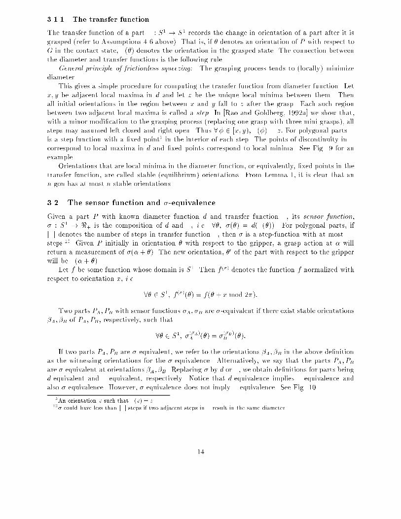
This gives a simple procedure for computing the transfer function from diameter function. Letx; y be adjacent local maxima in d and let z be the unique local minima between them. Thenall initial orientations in the region between x and y fall to z after the grasp. Each such regionbetween two adjacent local maxima is called a step. In [Rao and Goldberg, 1992a] we show that,with a minor modi�cation to the grasping process (replacing one grasp with three mini-grasps), allsteps may assumed left-closed and right-open. Thus 8� 2 [x; y); �(�) = z: For polygonal parts �is a step function with a �xed point9 in the interior of each step. The points of discontinuity in �correspond to local maxima in d and �xed points correspond to local minima. See Fig. 9 for anexample.

Orientations that are local minima in the diameter function, or equivalently, �xed points in thetransfer function, are called stable (equilibrium) orientations. From Lemma 1, it is clear that ann-gon has at most n stable orientations.

3.2 The sensor function and �-equivalence

Given a part P with known diameter function d and transfer function �, its sensor function,� : S1 ! <+ is the composition of d and �, i.e. 8�; �(�) = d(�(�)). For polygonal parts, ifj�j denotes the number of steps in transfer function �, then � is a step-function with at most j�jsteps.10 Given P initially in orientation � with respect to the gripper, a grasp action at � willreturn a measurement of �(�+ �). The new orientation, �0 of the part with respect to the gripperwill be �(�+ �).

Let f be some function whose domain is S1. Then f (x) denotes the function f normalized withrespect to orientation x, i.e.

8� 2 S1; f (x)(�) = f(� + x mod 2�):

Two parts PA; PB with sensor functions �A; �B are �-equivalent if there exist stable orientations�A; �B of PA; PB, respectively, such that

8� 2 S1; �(�A)A (�) = �

(�B)B (�):

If two parts PA; PB are �-equivalent, we refer to the orientations �A; �B in the above de�nitionas the witnessing orientations for the �-equivalence. Alternatively, we say that the parts PA; PB

are �-equivalent at orientations �A; �B. Replacing � by d or �, we obtain de�nitions for parts beingd-equivalent and �-equivalent, respectively. Notice that d-equivalence implies �-equivalence andalso �-equivalence. However, �-equivalence does not imply �-equivalence. See Fig. 10.

9An orientation z such that �(z) = z.10� could have less than j�j steps if two adjacent steps in � result in the same diameter.

14

of length at most n. The second planning algorithm (Section 3.5.2) runs in O(2nn4) time andproduces a grasp plan of optimal length. Both grasp strategies require O(logn) on-line time pergrasp. This can be improved to constant time by using e�cient hashing techniques.

3.1 Gripper and the grasping process

By a parallel jaw gripper (denoted by J) we understand a gripper consisting of two linear jawsarranged in parallel. Let L;H denote the lower jaw and upper jaw, respectively. Further assump-tions:

1. The part P is a rigid planar polygonal object resting at on a table.

2. The part's initial position is unconstrained as long as it wholly lies between the two jaws.The part remains between the jaws throughout grasping.

3. The motion of the gripper G is orthogonal to the jaws L;H .

4. All motion occurs in the plane and is slow enough that inertial forces are negligible. Thescope of this quasi-static model is discussed in [Mason, 1986; Peshkin, 1986].

5. Both jaws make contact simultaneously (pure squeezing).

6. Once contact is made between a jaw and the part, the two surfaces remain in contact through-out the grasping motion. The action continues until further motion would deform the part.The part and the gripper are now said to be in the grasped state.

7. The gripper can be rotated about an axis orthogonal to the table.

8. There is zero friction between the part and the jaws. See [Goldberg, 1990] for a designvalidating this assumption. Essentially, this can be achieved by incorporating one of the jawswith a frictionless bearing.

9. In a grasped state, the distance between L;H is measurable by a linear position sensor up toan error �.

Most of these assumptions are essentially the same as those made in [Goldberg, 1993; Raoand Goldberg, 1992b] (works dealing with orienting parts) except Assumption 9 which is new. InAssumption 7, it is not necessary that the gripper be rotatable precisely. Some margin in error ofpart orientation with respect to the gripper is allowed. This issue is studied in [Goldberg, 1993].Also, looking ahead at the planning algorithms that follow in Section 3.5, we may note that wealways choose orientations to rotate the gripper from among a set of intervals of orientations suchthat any orientation from this set is applicable. Thus, if we have an inaccurately rotating gripper,we may choose the middle most orientation in the largest interval to allow for maximal error inrotation. Assumption 5 can be relaxed to push-grasp actions [Brost, 1988] in which one of the jaws,say L, �rst makes contact with the part and pushed the part against the other jaw before squeezing.For simplicity, of presentation, we retain this assumption of pure squeezing. See Fig. 8.

13

3 Positive results : recognizing polygonal parts from a known set

The previous sections discussed some negative results for shape recovery from diameter function.However, note that we assumed nothing about the shape of the part except for it being a polygon.In this section, we consider the following problem. We have a part P whose shape is unknown butfor being one of k planar polygonal parts Q1; : : : ; Qk of known shapes. Furthermore, P is knownto lie at on a table between the jaws of a frictionless parallel jaw gripper equipped with a linearposition sensor capable of measuring, up to an error �, the distance between the jaws. The grippercan be rotated about an axis perpendicular to the table on which the part rests. The problem isto determine the shape of P using a minimum number of diameter measurements on the part.

The determination of P is up to �-equivalence between parts { a notion that will be de�nedformally in Section 3.2. For now we could understand it in light of the negative results { Theorems3,4 { presented earlier. For example, parts that have the same diameter function and are indistin-guishable by diameter measurements alone. Also, the sensor error � can play a factor in reducingdistinguishability between parts.

Section 3.4 gives a simple test to check whether two parts are �-equivalent. This test may beapplied a priori to the set of given parts and we replace each subset of �-equivalent parts by a singlerepresentative part (any single part from the subset). Thereafter we may deal with the problem ofrecognizing parts from among a set of parts, no two of which are �-equivalent.

We begin in section 3.1 with a brief description on the mechanics of the low-friction parallel jawgripper8 and by de�ning the notion of a stable grasp on the part by the gripper. The only diametermeasurements allowed are those in which the part is in a stable grasp by the gripper. There are atmost r stable grasps on an r-sided polygonal part. Section 3.4 discusses the representation of allstable grasps of the system (i.e. all stable grasps of the known parts Q1; : : : ; Qk) as a graph datastructure. If N is the total number of faces in all the polygons, and n � N the number of stableorientations, the computation of this data structure requires O(N + n3) time. We use the terms\planning algorithm" and \grasp strategy" to denote di�erent entities. \Planning algorithm" (or\planner") refers to the o�-line preprocessing done on the graph data structure. The output ofthis preprocessing is a \grasp strategy" (or \grasp plan" or just \plan") which is run on-line. Thegrasp strategy gives a sequence of angles at which grasps must be applied on the part in orderto recognize it. In general, the next grasp angle will depend on the current diameter measured.The grasp strategy is \tree-like," every node of the tree being associated with some subgraph ofG. The root is associated with the whole of G and children of a node are associated with disjointportions of the subgraph of the parent. This partition of the subgraph associated with the parent isdetermined by the current diameter value measured. We begin at the root, and travel down alonga path of the tree progressively re�ning the search by pruning the graph. At an intermediate nodeof the path, we choose the correct child to visit next depending on the diameter value measured.Search trees are popular in AI. For example see [Rich, 1983]. By the length of the grasp strategy (orplan), we understand the maximum depth (number of grasps) of any leaf in the tree representingthe strategy.

There are several measures of complexity here : the preprocessing time (complexity of the\planning algorithm"); worst case number of required grasps of the grasp plan to identify theobject (\height" of the tree representing the grasp plan); and amount of on-line work to be doneper grasp. Section 3.5 discusses tradeo�s between preprocessing time and length of the plan.Given the data structure representing the stable orientations of the parts, we present two planningalgorithms. One (Section 3.5.1) requires O(n2 logn) time and produces a non-optimal grasp plan

8Further details, including the design of such a device, may be found in [Goldberg, 1990]

12

follows. Let multiset I = I0 = fa1; : : : ; ang be an instance of EQUI PARTITION. Let it havetwo identical elements A;A. Replace the pair A;A by four elements A;M;A + 2M; 3M , whereM =

Pn

i=1 ai, to form the instance I1 containing n + 2 elements. Observe that I1 has strictly lessidentical elements as I0 and that I1 is equi-partitionable if and only if I is (this is because theelement 3M has to be in a di�erent partition as the elements M and A + 2M). Continue thisprocess creating the instances I2; I3; : : : ; containing progressively lesser identical elements until theinstance Ik containing n + 2k elements, k < n, is created containing no pair of identical elements.Ik is therefore a valid instance of EQUI SET PARTITION. Observe that each Ij; j > 0 so ob-tained satis�es the condition that Ij is equi-partitionable if and only if Ij�1 is. Therefore, Ik isequi-set-partitionable if and only if I = I0 is equi-partitionable. 2

Now we de�ne the following problem.

MINIMAL POLYGON FROM DIAMETER FUNCTION (MPFD):Given an m; k-diameter function d, is there a minimal polygon P fully consistent with d?

Theorem 5 MPFD is NP-Complete.

Proof: We use the NP-completeness of MPFS. Let algorithm MPFD(d), where d is an m; k-diameter function, return true (resp. false) according as whether there is (resp. is not) an m+ k; 0polygon P fully consistent with d.

Then we solve the MPFS problem using the following algorithm:INPUT: description (orientations, lengths) of n planar segments, no two of which are parallel.OUTPUT: true/false whether or not they form a convex polygon.

1. Let � be a circular list of the orientations of the input segments in sorted order. Let t be alist of the lengths of the segments sorted according to the order in �.

2. Use equations 6 (in Appendix A) to determine whether there is some (valid) diameter functiond that has �(d) = � and tP 0 = t, where P 0 is some polygon fully consistent7 with d.

If there does not exist such a d (Equations 6 do not have a solution), return \FALSE" andexit.

3. We assume that there exists such a valid d. It is easy to compute d after solving equations 6.Now invoke MPFD(d).

Return \TRUE" if and only if MPFD(d) returned \true".

Complexity of the �rst step is clearly polynomial in n. The second steps involves forming andsolving n linear equations in n unknowns, which basically involves inverting an n�n matrix whichhas polynomial complexity. Step 3 basically involves a call to MPFD. Therefore, if MPFD waspolynomial time decidable, so would MPFS.

Correctness follows from the following. If the set of input segments forms a polygon, then thepolygon would have to have a diameter function d which is easily computable given t;�, and d

would have its minima and kinks exactly at orientations in �. If they did not form a polygon, thenno diameter function would exist and this would be detected in Step 2. above. However, it couldhappen that a valid diameter function d exists for a polygon P 0 that has �P 0 = �; tP 0 = t, but P 0

could have parallel edges. To check for parallel edges, Step 3 calls MPFD(d). If it returned true,then it implies the original set of segments form a convex polygon. And if the original segmentsform a polygon, Step 3 would be executed and the call to MPFD(d) would return \true". 2

7Such a polygon exists since d is valid. However, P 0 could have parallel edges.

11

�xed length and orientation, does there exist an arrangement of them forming a convex polygon?

Lemma 3 PFS is NP-complete.

Proof Outline: PFS is clearly in NP. So it is su�cient to show that PFS is NP-hard. We do thisby polynomial transformation from PARTITION, the following well-known NP-complete problem.

Given a multiset of n positive numbers a1; : : : ; an, is there a set S � f1; : : : ; ng such thatXi2S

ai =X

i2f1;:::;ng�S

ai ?

Given an instance I of PARTITION having n elements, consider the following set I 0 of n + 2segments (each segment is described as (l; �), where l 2 R+ is its length and � 2 [0; �) is anglemade by it with x-axis):

I 0 = f(ai; 0)jai 2Ig [ f(1; �=2); (1; �=2)g:It can be shown easily that I has a partition if and only if the segments from I 0 form a rectangle.

2

Corollary to Lemma 3 CPFS is NP-Complete.

Lemma 4 MPFS is NP-complete.

Proof Outline:6 Again it is easy to see thatMPFS is in NP. So it is su�cient to show thatMPFSis NP-hard. We do this by polynomial transformation from the following variant of PARTITIONwhich we will show NP-hard later.EQUI SET PARTITION: Given a set of n positive numbers fa1; a2; : : : ; ang (no two of which areequal), n even,

does there exist a set S � f1; 2; : : : ; ng with exactly n=2 elements such thatP

i2S ai =P

i2f1;:::;ng�S ai?Given an instance I of EQUI SET PARTITION, a set of n positive numbers faij1 � i � ng, n even,consider the following set I 0 of segments each described as (x; y), where x (resp. y) is the length ofthe projection of the segment on the x-axis (resp. y-axis). The slope of this segment is tan�1 y=x.I 0 = f(1; a1); (1; a2); : : : ; (1; an)g. Notice that no two segments are parallel since no two of the aiare equal making I 0 a valid instance of MPFS. We now show that I is equi-set-partitionable if andonly if the segments of I 0 can be arranged to form a minimal polygon.

If I is equi-set-partitionable, let S � f1; : : : ; ng be the set of n=2 indices of one of the partitions.Arrange the n=2 segments f(1; ai) j i 2 Sg end on end as a convex chain in increasing order ofsegment slope. This chain has a net x-projection of n=2 and a net y-projection of

Pi2S ai. Similarly,

arrange the remaining segments, f(1; ai) j i 62 Sg, as another convex chain but in decreasingorder of segment slope. This second chain has the same net x; y-projections as the �rst. Identifycorresponding ends of the two chains to form a minimal polygon. Conversely, if the segments I 0 canbe formed into a minimal polygon, cut the polygon at the lowest (leftmost) and highest (rightmost)vertices (such vertices are unique because no segment in I 0 is purely vertical or horizontal) to formtwo convex chains. Each chain has the same net x; y-projections. Taking S as the set of n=2 indicescorresponding to the segments of any one chain shows that I is equi-set-partitionable.

EQUI SET PARTITION can be shownNP-hard by polynomial transformation fromEQUI PARTITION,a known NP-complete problem [Garey and Johnson, 1979]. EQUI PARTITION is PARTITIONwith the additional constraint that the cardinality of S be n=2. Brie y, this transformation is as

6This simpler proof is due to Govindan Rajeev of the University of Tennessee who pointed it out based upon apreliminary version of this paper [Rao and Goldberg, 1992c].

10

basically involved showing that a particular length t(�) could be split, in in�nitely many ways,into two segments (in the polygon), both of orientation � whose lengths sum up to t(�). Thus,most of these polygons would have parallel edges of varying lengths. This suggests that we mightde�ne a representative polygon as one without any parallel edges satisfying a given diameter func-tion. Two obvious questions arise: does there always exist a representative polygon for a givendiameter function; and if a representative polygon exists, is it always unique? We try and answerthese questions in this section. The latter question is answered in the negative in Theorem 4 byconstructing a counter-example, and the former question is shown NP-complete in Theorem 5. Amajor lemma in proving our NP-completeness result is showing that the problem of arranging a setof line segments, no two of which are parallel, into a convex polygon is NP-complete. This bearssome resemblance to the result of [Rappaport, 1987] which shows that the problem of drawing(additional) line segments to connect a collection of given �xed line segments (by their end-points)into a simple circuit is NP-complete. In our case, we allow the segments to translate and we do notallow additional line connecting segments.

A minimal polygon is a (convex) polygon without any parallel edges, i.e. an n; p-polygon withp = 0.

Theorem 4 Minimal polygons satisfying a given diameter function are not unique.

Proof: See Fig. 7. 2

The implication of this theorem is that even for minimal polygons, it is impossible to completelyrecover its shape from the diameter function.

Given an m; k-diameter function d, if there exists a minimal polygon P with n edges having das its diameter function, then by Lemma 1, n = m + k. First notice that tP ;�P are extractablefrom the diameter function d. We have seen above that there could be more than one minimal P .There can be at most a �nite number (2n�1) of possible minimal P since P is constrained to beconvex. Now we tackle the question whether there always exists such a minimal P . We show thatdeciding this question is NP-complete in Theorem 5. Before we get there, we have to show someother problems NP-complete.

By arranging a set of n planar segments S0; : : : ; Sn�1, we mean translating them in the planeso that two segments are either not intersecting, or if they intersect, they do so only at their end-points. All sets of segments in this section are multisets, i.e. they could contain more than oneidentical element. Consider the following problems.

POLYGON FROM SEGMENTS (PFS):Given a set of n planar line segments, S0; : : : ; Sn�1, each with a �xed length and orientation,can they be arranged so as to form a polygon (n-gon)?

Note that forming a polygon is equivalent to forming a simple polygon since the only intersectionswe allow between segments are at their end-points. Also note that we do not have any restriction onthe orientations of the edges (any number of them could be parallel). Thus minimality of polygonsis not addressed just as yet.

CONVEX POLYGON FROM SEGMENTS (CPFS):Given a set of n planar line segments, S0; : : : ; Sn�1, each with a �xed length and orientation,can they be arranged so as to form a convex polygon (n-gon)?

MINIMAL POLYGON FROM SEGMENTS (MPFS):Given a set of n planar line segments, S0; : : : ; Sn�1, no two of which are parallel, each with a

9

We solve these 3Z equations for the 3Z unknowns (�j; lj; d(�j)). We know that at least onesolution for the 3Z equations exists since d; d0 are valid. However, there could exist more thanone solution giving di�erent d; d0. We show in Appendix A that at most one solution for these 3Zequations exists. Thus, the diameter function is uniquely constructed. 2

In a sense, �P ; tP is the maximal non-redundant (and invertible) information of the geometryof a polygon P obtainable from its diameter function, �P giving the orientations of the faces of P ,and tP the perimeter along each orientation. However, the two lists do not completely determineP because there could be up to two faces along an orientation t(�) and the t(�) constraint is onlya constraint on the sum of the length of the two faces. In fact, as Theorem 3 shows, there arein�nitely many polygons P having the same valid diameter function (and hence the same �P ; tP ).

Diameter functions of parallelograms (4; 2-gons) are termed trivial.

Theorem 3 For every non-trivial valid diameter function d there exist in�nitely many polygonshaving diameter function d.

Proof: Fig. 4 show this is true for diameter functions of triangles and quadrilaterals. See alsoFig. 5. Towards the generalization assume that P is a polygon having diameter function d. P

exists since d is valid. Let A;C be two vertices of P touching l; h at a maxima orientation. Letthis maxima orientation be the zero orientation, WLOG. Let D;B be the vertices adjacent to C inP (i.e. DC;BC are two faces of P ). Likewise, let D�; B� be the vertices adjacent to A. D� and Dare on the same side of AC (as are B� and B). D� (resp. B�) could be coincident with D (resp.B). For example, in Fig. 4: the quadrilateral case, D = D�; B = B�. Let �1; � � �2; �3; � � �4be the orientations of faces CB;AB�; AD�; CD, respectively. Without loss of generality assume�2 < �4; �1 < �3. The other cases (including equality) are treated similarly. See Fig. 6. F 0; E0 arecan be arbitrarily chosen on CB;AB�, respectively. G0 is such that CG0 is parallel and equal toB�E0. Thus we have t(�2) = jAB�j = jAE0j + jCG0j. H 0 is determined similarly. It is de�ned sothat AH 0 is parallel and equal to BF 0. Now, t(�1) = jCBj = jCF

0j+ jAH 0j.A line is drawn parallel to AD� (resp. (DC)) through H 0 (resp. G0). Points D�0; D0 are chosen

on these two lines so that the distance between D0; D�0 is equal to that between D�; D. Now theportion of the polygon P between D�; D can be moved over to between D�0; D0:

B�0; B0 are de�ned in a similar manner. First a line is drawn parallel to AD� (resp. DC)through F 0 (resp. E0). B�0; B0 are chosen on these lines so that the distance between them equalsthat between B�; B: The portion of P between B;B� can be moved over to between B0; B�0. If thiscauses any problems of convexity, then take the faces F 0B0, E0B�0, and those originally betweenB;B�, sort them by orientation, and arrange them between F 0 and E0.

Simple geometry can be applied to show that jH 0D�0j+jB0F 0j = jAD�j= t(�3) and jG0D0j +

jE0B�0j= jDCj = t(�4). For example to show that jH 0D�0j+jB0F 0j = jAD�j, draw a line throughH 0 parallel to D�0D0 intersecting AD� at Z. Now note that triangle F 0B0B is congruent to triangleH 0ZA and so jB0F 0j = jAZj. Also note that H 0ZD�D�0 is a parallelogram, and so jH 0D�0j= jZD�j.

Thus, the two polygons Pdef= A;D�; : : : ;D; C;B; : : :; B�; A and P 0 def

= A;H 0; D�0; : : : ; D0; G0; C;F 0, B0; : : : ; B�0; E 0; A have the same diameter function by Theorem 2 since tP = tP 0 and �P = �P 0 .Finally note that there are in�nitely many P 0 since the choices of F 0; E0 (along a line segment) werearbitrary. 2

2.1 Minimal Polygons

Theorem 3 is a negative result for shape recovery from diameter: there exist in�nitely many poly-gons consistent with a given measured diameter function. However, the proof of the theorem

8

where L; � are the parameters of the sinusoid in d between (0; �1), i.e. L cos(�) = d(0); L cos(� +�1) = d(�1).

Proof Outline: (() It is enough to show that P is consistent with d at �1 as well. That is, weneed to show that d(�1) can be obtained from t(�1). Consider the equations L cos(�) = d(0) andL cos(�2 + �) = d(�2)� t(�1) � sin(�2 � �1).

L; � can be determined (uniquely) from these equations (this is also shown in Appendix A) andd(�1) can be obtained as L cos(�+ �1).

()) There are two geometric cases to consider: Orientation 0 is a kink and 0 is a local minimum.Let us consider the former case in Fig. 3. The latter case is proved similarly.

In the �gure, AA0; BB0 are faces of P at orientation 0. AC;BD are faces at orientation �1and CE;DF are faces at orientation �2. Some of these faces could be of length 0. Let BX be aline perpendicular to the x-axis. Now jABj = L and 6 ABX = �, the parameters of the sinusoidbetween 0; �1.jACj+ jBDj = t(�1). Extend BD to Q so that jDQj = jACj. Draw lines parallel to CE (i.e.

lines making angle �2 with the positive x-axis) through A;B. Draw a line perpendicular to theselines through Q intersecting them at S; T as shown. Extend BT to point R so that triangle ARBis right angled at R.

Now ASTR is a rectangle and so jST j = jARj = L cos(�+�2). Also, jTQj = jBQj sin(�2��1).Finally notice that jBQj = t(�1) and jQSj = jTQj+ jST j = d(�2). 2

Theorem 2 Two polygons P;Q have the same diameter function if and only if �P = �Q andtP = tQ.

Remark: From Cauchy's surface formula (See [Benson, 1966]), it follows that the integral of thediameter function of any planar part equals its perimeter. Thus, two parts having the same diameterfunction must have the same perimeter (but not necessarily vice versa). Our theorem above statessomething stronger for the class of polygonal parts { namely that the two parts must have the sameset of partial perimeters.

Proof: Only if: Let P;Q both have diameter function d. Then �P = �Q since each is equal to�(d) mod �. Let �1; �2; �3 be an adjacent triplet of orientations5 in �(d).

Assume WLOG that �2 2 [0; �). Then Lemma 2 gives a formula for t(�2) that must be satis�edby both polygons. A generalization of this shows that tP = tQ.

If: Let the two polygons have (valid) diameter functions d; d0. We prove d = d0 by showing thatone can reconstruct a unique diameter function d, given these two lists �P ; tP .

Let the given �P have Z = m+k orientations: �P = f�0; : : : ; �Z�1g. Let the diameter functionbetween �j ; �j+1 (assume j � 1 are modulo Z) be the sinusoid lj cos(� + �j). Thus we have theequations

lj cos(�j + �j) = d(�j); lj cos(�j+1 + �j) = d(�j+1):

The unknowns are d(�j); �j; lj. If these are recovered, it is obvious that d is. This gives us2Z equations in 3Z unknowns. The remaining Z equations are obtained from t information usingLemma 2:

t(�j) =d(�j+1)� lj�1 cos(�j+1 + �j�1)

sin(�j+1 � �j):

5Recall from the de�nition of an gpsf that �(d) must have at least four transition orientations.

7

Consider orientations � in which an face of P is ush with one of l; h. These are precisely theorientations in �(d). If the orientation is stable under jaw action (replacing l; h by a parallel jawgripper nad squeezing, see also Section 3.1.1), it is a local minimum in d, and otherwise it is a kinkorientation. Since there are n faces, we would expect n = m+k. This is true if P did not have anypairs of parallel faces. Let p be the number of pairs of parallel faces of P . Then a simple countingargument gives:

Lemma 1 n � p = m+ k: 2

Notice that the quantities on the left side n; p are the polygon's geometrical properties, while thequantities on the right m; k are properties of its diameter function. Let us refer to an n-gon havingp pairs of parallel sides as an n; p-polygon. A diameter function having m minima and k kinksis an m; k-diameter function. Thus, it is n � p, rather than n alone that decides how \complex"the diameter function of the n; p-polygon is. Parallelograms (4,2-polygons) give the \simplest"diameter functions in the sense that they are the only polygons (among convex polygons) that haven � p = 2. Triangles (3,0-polygons), trapeziums (4,1-polygons), 5,2-pentagons, and 6,3-hexagonsare the next simplest having n � p = 3. All other polygons have n� p > 3.

Corollary to Lemma 1 If an n1; p1-polygon and an n2; p2-polygon have the same diameter func-tion, then n1 � p1 = n2 � p2. 2

This is our �rst step towards shape recovery from diameter function.

2 Negative results

In this section we present our results implying that complete shape recovery of a planar part from itsdiameter function is impossible. We begin by investigating conditions for a polygon to be consistentwith a given diameter function within a range of orientations (Lemma 2). Theorem 2 presents anecessary and su�cient condition for two polygons to have the same diameter function. Theorem3 shows that there are in�nitely many polygons, all satisfying the conditions of Theorem 2, and allhaving the same diameter function. From the proofs of these negative results for the general classof polygons, it becomes natural to seek shape recovery from diameter function for a special class ofpolygons: namely those without any pair of parallel faces. We call such polygons minimal polygonsand consider the shape recovery problem restricted to these polygons in Section 2.1.

Let tP (�), 0 � � < �, be zero if � 62 �P ; otherwise it equals the sum of the lengths of allfaces4 of P that have orientation �. tP (�) is called the perimeter of P at orientation �. LettP = ftP (�)j� 2 �Pg sorted in the order of increasing �. The subscripts P are dropped if we arediscussing only one polygon.

A polygon P is said to be consistent with a valid diameter function d between orientations[�a; �b] if the diameter function of P matches d between orientations [�a; �b]. This is written asP � d[�a; �b].

Lemma 2 Let P be a polygon and d some valid diameter function, not necessarily that of P .Further, let 0 < �1 < �2 be an adjacent triplet of orientations in �(d) and also in �P . Let P beconsistent with d at orientations 0; �2. Then,

P � d[0; �2], tP (�1) =d(�2)� L cos(�2 + �)

sin(�2 � �1);

4There can be at most two such faces due to the convexity assumption on P .

6

Notice that a gpsf is continuous, single valued, and has a �nite number of local maxima andlocal minima. A gpsf is di�erentiable at all but a �nite number (at most Z) of orientations in S1.For a gpsf f , let MAX (f);MIN(f) denote the �nite set of local maxima, local minima orientations,respectively. For a gpsf f , let Z(f), the size of f , denote the �nite integer Z, and �(f), the set oftransition orientations of f , denote f�0; : : : ; �Z�1g from the de�nition of the gpsf f . If jSj refers tothe cardinality of a �nite set S, then for a gpsf f , jMAX (f)j = jMIN (f)j and j�(f)j = Z(f).

From now on all sets of orientations, such as �(f);MIN(f);MAX(f), and others to be de�nedlater, will be treated as ordered (circular) lists of orientations, i.e. their elements will be assumedsorted in a circular list. Two orientations �a; �b are said to be adjacent with respect to some propertyif they are adjacent in the (circular) list of all orientations having that property. For example, �a; �bare adjacent local maxima in a gpsf f if they are adjacent in MAX (f). From the de�nitions oflocal maxima, local minima, notice that if we merge the circular lists MAX (f);MIN (f), we get anew list MAXMIN(f) in which elements of MAX (f);MIN (f) alternate. That is, between everytwo adjacent local maxima, lies a unique local minima (and vice versa).

Theorem 1 A function f is a valid diameter function if and only if

1. f is a gpsf,

2. f has period �, and

3. MIN(f) � �(f), MAX(f) \ �(f) = ; (that is, parameters of the sinusoid change at everylocal minima and never change at any local maxima).

Proof Outline: Showing that diameter functions of polygons have these properties is not di�cult.For the other direction, assume we are given a function f satisfying these properties. We canconstruct the left half of a polygon (the right half is a re ection of the left half through thecentroid) whose diameter function is exactly f . The idea is the following.

Let 0 and �� be two adjacent local maxima in f , and let there exist y orientations �1; �2; : : : ; �yfrom �(f) between 0 and ��. The polygon we construct will have y consecutive edges ush withorientations �1; �2; : : : ; �y. The lengths of these edges can be determined from the parameters ofsinusoids in gpsf f . 2

1.3 Further notation and an initial result

Let d denote a valid diameter function and P a polygon. Unless otherwise speci�ed, d is thediameter function of P . Two circular lists of orientations are equal if they are equal after some�xed orientation (possibly zero) is added every element of one of them. From now on, maxima,minima stand for local maxima, local minima (in a diameter function), respectively.

Orientations in k(d) = �(d)�MIN (d) are called kink orientations, or more simply kinks. That is,kinks are the non-minima orientations at which the parameters of the sinusoid describing d change.Kinks and minima, i.e. orientations in �(d) = MIN (d)[ k(d), are all and the only orientations atwhich an face of the polygon P is in contact with (at least) one of l; h. For example, an obtuseangled triangle has only one minima between [0; �)) when the largest side is in contact with oneof l; h. When one of the other two sides is ush with the lines l; h, we get a kink orientation. LetMINMAXKINK(d) denote a list of all maxima, minima, kinks in the diameter function d.

Let �P denote the set of angles (module �) that the edges of polygon P make with the x-axis.�P is �(d) restricted to the range [0; �). Let m; k, respectively denote the number of minima, kinksin [0; �), in the diameter function d of an n-gon P .

5

with object but also the direction of normal there. Our negative results (Section 2) therefore implythat for shape recovery, both the length of the projection, and the o�set information (namely wherethe projection lies with respect to some �xed point on the sliding line) are necessary, and merelythe length of the projection (diameter information) is not su�cient.

Now we refer to literature related to our work on grasp strategies for recognizing polygons.Wallack and Canny consider shape and pose recognition by scanning light beam projections thatare orthogonal to the plane of the part [Wallack and Canny, 1991]. Only a few high resolution scanlines are used and the pose algorithm runs in O(n) time (on the average) for an n-sided polygonalpart. In [Wallack and Canny, 1993] they consider light beams that are in the plane of the partwhich can be used to measure diameter without a�ecting part orientation. In contrast, graspingactions with a parallel jaw gripper can be used to measure diameter after rotating the part intoa stable orientation prior to the measurement. They also consider the problem of determiningpart orientation by planning an sequence of diameter measurements [Wallack and Canny, 1992].Our's is the more general problem of recognizing a part from a known set. Also, we explore thecomputational complexity of planning an optimal sequence.

Our work on recognizing part shape also has some relation with robotic inspection [Spyridiand Requicha, 1990] and the work of Ellis [Ellis, 1987] concerned with tactile data for recognition.Chen and Ierardi [Chen and Ierardi, 1991] consider the problem of recognizing a set of polygonalparts from diameter measurements. However, they do not consider optimal plans. Kang andGoldberg [Kang and Goldberg, 1992] consider a similar problem where the diameter measurementsare corrupted by Gaussian noise. They show that data from a sequence of random grasps can beprocessed using a Bayesian estimator. However random grasping has low average-case performancewhen part shapes are similar. The relation between planning manipulation strategies and searchesthrough trees was observed in [Erdmann and Mason, 1986; Mason et al., 1988; Taylor et al., 1987].The notion of active vision, servoing sensors so as to obtain information e�ciently is popular invision recognition strategies [Raviv, 1991]. Ours is also an active sensing strategy in that we seeka best next grasp for the part based on the previous ones.

Finally, our deployment of the parallel-jaw gripper and simple diameter sensing is in tune withCanny's and Goldberg's Reduced Intricacy in Sensing and Control, or RISC, robotics [Canny andGoldberg, 1993]. They observe that for certain industrial tasks, complex (high degree of freedom)manipulators and sensors are unnecessary and that simple, robust, and inexpensive hardware iscalled for. In this paper, we demonstrate a RISC approach to shape recognition.

1.2 Valid diameter functions

We call a diameter function valid if it is the diameter function of some polygon. Since the conceptof a valid diameter function is so central to this paper, we now set about trying to characterizevalid diameter functions.

A polygon P is speci�ed by its n vertices in counter-clockwise order v0; v1; : : : ; vn�1. Let �denote addition modulo n. The orientation of an face of P , vi; vi�1 is the angle made by it mod�w.r.t the positive x-axis. Let � denotes an arbitrary orientation in S1.

A continuous function f : S1 !R+ is said to be a \good" piecewise sinusoidal function (gpsf)if there exists a �nite integer Z � 4, and a cyclic ordering of orientations

�0 < �1 < : : : < �Z�1 < �Z = �0

such that 8j 2 f0; 1; : : : ; Z � 1g; and 8� 2 [�j; �j+1] : f(�) = lj cos(�+ �j); for some lj 2 R+, and�j 2 S1.

4

except that it is a polygon. Section 3 assumes that the given part has one among a known setof polygonal cross sections. We also assume a frictionless parallel jaw gripper [Goldberg, 1990]

equipped with a linear position sensor for taking diameter measurements. We brie y discuss me-chanics of the parallel jaw gripper grasping a polygonal object [Goldberg, 1990]. We only considerstable diameter measurements (i.e. on grasping, the part settles into a stable equilibrium orienta-tion before the diameter at that orientation is measured). The aim is to compute a \grasp strategy",a sequence of stable diameter measurements, that would distinguish between the parts up to partdistinguishability. We give algorithms that consider tradeo�s between preprocessing time and thelength of the grasp strategy produced.

These results have been previously reported in technical report form [Rao and Goldberg, 1992c].In interest of space and to increase readability, we have replaced proofs of some of the lemmas andtheorems in this paper by proof outlines. The interested reader is referred to the technical reportfor complete proofs.

1.1 Related work

The concept of diameter of a set of points, the maximizing distance over all pairs of points, is wellstudied in computational geometry [Preparata and Shamos, 1985; Edelsbrunner, 1987]. Diameterfunctions, termed width functions in [Yaglom and Boltyanskii, 1951], were applied by Jameson[Jameson, 1985] to determine grasp stability for a part grasped in the jaws of a parallel-jaw gripper.Goldberg [Goldberg, 1993] used the diameter function to generate plans, in O(n2) time, to orientn-gonal parts. Rao and Goldberg [Rao and Goldberg, 1992b; Rao, 1992] extend these results tocurved parts.

Our work has some relation to geometric probing which was introduced by Cole and Yap [Coleand Yap, 1987] and inspired by work in robotics and tactile sensing [Grimson and Lozano-Perez,1987; Gaston and Lozano-Perez, 1984]. A complete description of these results appear in [Skiena,1988]. Skiena [Skiena, 1989] provides a summary of the basic results and open problems in thisarea. However, some of the basic assumptions common in geometric probing are quite unrealisticin practice. Some examples of such assumptions are that the part is not disturbed by the probes,the probes are accurate (travel in straight lines and return error-free information), and probes arepowerful (can recover information like normals from the contact face, etc.). Some of the morerelevant papers in probing are discussed brie y.

Koutsou [Koutsou, 1988] investigates tactile exploration of objects using a parallel jaw gripper.He considers how a parallel-jaw gripper equipped with a tactile array can be used to measurephysical properties of a part such as weight and sti�ness. [Kolzow et al., 1989] discusses an algorithmfor the approximative reconstruction of a planar convex body from its projections in a �nite numberof directions. However, by \projections" of a body in a particular direction �, they understand thelength of the intersection of a line (with orientation orthogonal to �) with the body as a functionof the distance of the line from the origin. Thus, their idea of \projections" is quite di�erent from\projection probes." Projection probes [Li, 1988] are a special type of hyperplane probes [Dobkinet al., 1986]. A projection probe slides a straight line in a direction normal to itself over the planeuntil it hits the polygon. When it does, it returns the projection (or image) of the polygon on theline. From 3n � 2 projection probings, [Li, 1988] shows that you can recover the complete shapeof the polygon. If the sliding straight line makes an angle � with the x-axis, then the length of theprojection is the diameter at orientation � � �=2. Boissonat and Yvinec [Boissonnat and Yvinec,1992] consider probing of non-convex objects { both polygons and polyhedra. They give algorithmsthat exactly recover shape using powerful projection probes that return not only point of contact

3

parts, for example a circle cannot be distinguished from a Reuleaux triangle (cf. the Wankel rotaryengine) merely by grasping and measuring its diameter.

First, we present the negative result that shape cannot be uniquely recovered even for polygonalparts: for a given set of diameter measurements: there is an (uncountably) in�nite set of polygonalshapes consistent with these measurements. Since most of the shapes in this set have parallel edgesof varying lengths, we consider the related problem of identifying a representative polygon with noparallel edges. We show that given a diameter function, deciding whether such a polygon exists isNP-Complete.

These results motivate us to consider the problem of recognizing a part from a known (�nite)set of parts. The challenge is to plan a sequence of grasp angles to e�ciently recognize the part,taking into account the induced rotation of the part caused by the gripper. In other words, givena set of polygonal parts with a total of N faces, �nd the shortest sensing plan for disambiguatingthe parts using a parallel-jaw gripper. See Fig. 1 for an example.

Since diameters at only stable orientations can be measured, we build a graph representation, G,of the n � N stable diameters in O(N+n3) time. Our positive results are two planning algorithms:one constructs an optimal sensing plan in time O(n42n), the other constructs a suboptimal sensingplan in time O(n2 logn). Neither plan requires more than n on-line measurements.

Our solution is an example of active sensing [Bajcsy, 1988], where the sensor is purposefullymoved to acquire appropriate data. More speci�cally, it is an example of sensor-based manipulationplanning [Taylor et al., 1987], where the part is moved in the process of acquiring sensor data. Thusthe planner requires a model of mechanics to predict part motion. In [Taylor et al., 1987], a brute-force search was used to �nd optimal plans for the related problem of determining part orientationwith a standard parallel-jaw gripper. Here, we consider a frictionless parallel-jaw gripper, modi�edwith a linear bearing to insure a �nite range of possible diameters [Goldberg and Furst, 1992]. Weanalyze the computational complexity of �nding optimal and suboptimal plans for recognizing apart from a known set.

Let S1 denote the space of planar orientations [0; 2�) and R+ the set of positive reals. Given a�xed part P in an x� y coordinate frame, the diameter function d : S1!R+ of P can be formallyde�ned as follows. Imagine two (in�nite) parallel lines l; h (supporting lines) both making angle� with the x-axis, just touching P so that P lies entirely in the region between the two lines. Insuch a case we say that the supporting lines l; h are at orientation � with respect to the (�xed)polygon P . The diameter of P at orientation �, d(�), is the distance between the two lines thatare at orientation �. The diameter function is continuous and has period �. See Fig. 2. Also, thediameter function of a part is the diameter function of its convex hull. Therefore we can only seekshape recovery of the convex hull of a part from its diameter function [Goldberg, 1990].

Call a diameter function valid if it is the diameter function of a polygon. We begin, in Section1.2 by characterizing valid diameter functions. In Section 2 we show that for every valid diameterfunction d there exist in�nitely many polygons consistent with it. Thus, complete shape recovery ofa polygon from its diameter function is impossible. However, we show that the orientation of everyedge of the polygon and partial perimeters of the polygon along any orientation are recoverable fromthe diameter function. Looking at the proofs of these results, it becomes natural to consider shaperecovery for the restricted class of polygons having no parallel edges (we call such polygons Minimalpolygons). In section 2.1 we show that although the number of minimal polygons consistent witha given diameter function is �nite, complete shape recovery still impossible. Also we show thatdeciding the question, \Given valid diameter function d, is there a minimal polygon consistent withd?" to be NP-complete.

These negative results for shape recovery assume that no a priori knowledge about the part

2

Shape from Diameter: Recognizing Polygonal Parts with a

Parallel-Jaw Gripper�

Anil S. Raoyand Kenneth Y. Goldbergz

November 5, 1993

Abstract

Our objective is to automatically recognize parts in a structured environment (such as afactory) using inexpensive and widely-available hardware. In this paper we consider the planarproblem of determining the convex shape of a polygonal part from a sequence of projections.Projecting the part onto an axis in the plane of the part produces a scalar measure, the diameter,which is a function of the angle of projection. The diameter of a part at a particular angle canbe measured using an instrumented parallel-jaw gripper.

First, we present the negative result that shape cannot be uniquely recovered: for a given setof diameter measurements, there is an (uncountably) in�nite set of polygonal shapes consistentwith these measurements. Since most of these shapes have parallel edges of varying lengths, weconsider the related problem of identifying a representative polygon with no parallel edges. Weshow that given a diameter function, deciding whether such a polygon exists is NP-Complete.

These results motivate us to consider the problem of recognizing a part from a known (�nite)set of parts. Given a set of polygonal parts with a total of N faces, can we �nd the shortestsensing plan for disambiguating the parts? Only diameters at n � N stable faces can bemeasured. We construct an internal representation of these stable diameters in O(N +n3) timeand then give two planning algorithms: one constructs an optimal sensing plan in time O(n42n),the other constructs a suboptimal sensing plan in time O(n2 logn). Neither plan requires morethan n measurements.

1 Introduction

In automated manufacturing it is often useful to sort parts according to shape. A common approachis to use machine vision, which can be sensitive to lighting conditions and requires coordinationwith a programmable manipulator. In this paper we explore an alternative approach that uses aninexpensive modi�cation to the parallel-jaw gripper. For the class of convex parts with constantpolygonal cross section (2.5 D parts), we consider the following problem: recover the shape of apart's cross section by grasping the part with a parallel-jaw gripper and measuring the distancebetween the jaws: the diameter of the part at some angle. Can a sequence of such measurementsbe used to determine part shape? Note that the answer is clearly negative if we admit curved

�This material is based upon work supported by the National Science Foundation under Award No. IRI-9123747,ESPRIT Basic Research Action No. 6546 (project PROMotion), and by an equipment grant from Adept Technology,Inc.

yDepartment of Computer Science, Utrecht University, Padualaan 14, Postbus 80.089, 3508 TB Utrecht, Nether-lands. anil@cs.ruu.nl, Tel: 31-30-533922, FAX: 31-30-513791.

zDepartment of Computer Science, Institute of Robotics and Intelligent Systems, PHE 204, University of SouthernCalifornia, Los Angeles, California 90089-0273. goldberg@iris.usc.edu, Tel: 1-213-740-9080, FAX: 1-213-740-7877.

1