Embed Size (px)
Citation preview
UKERC Review of Evidence for the Rebound Effect
Technical Report 3:
Elasticity of substitution studies
David Broadstocka Lester Hunta
Steve Sorrellb
July 2007
a Surrey Energy Economics Centre (SEEC), University of Surreyb Sussex Energy Group (SEG), University of Sussex

Draft – Not for circulation or citation
ii

Draft – Not for circulation or citation
PrefaceThis report has been produced by the UK Energy Research Centre’s Technology and Policy Assessment (TPA) function. The TPA was set up to inform decision-making processes and address key controversies in the energy field. It aims to provide authoritative and accessible reports that set high standards for rigour and transparency.
This report forms part of the TPA’s assessment of evidence for a rebound effect from improved energy efficiency. The subject of this assessment was chosen after extensive consultation with energy sector stakeholders. It addresses the following question:
What is the evidence that improvements in energy efficiency will lead to economy-wide reductions in energy consumption.
The full outputs from this assessment are as follows:
Summary Report: Evidence for a rebound effect from improved energy efficiency
Technical Report 1: Evidence from evaluation studies Technical Report 2: Evidence from econometric studies Technical Report 3: Evidence from elasticity of substitution studies Technical Report 4: Evidence from CGE modeling studies Technical Report 5: Evidence from energy, productivity and economic growth
studies
Supplementary Note 1: Graphical analysis of rebound effects Supplementary Note 2: Macro-econometric estimates of rebound effects
The assessment was led by the Sussex Energy Group (SEG) at the University of Sussex, with contributions from the Surrey Energy Economics Centre (SEEC) at the University of Surrey, the Department of Economics at the University of Strathclyde and Imperial College. The assessment was overseen by a panel of experts and is extremely wide ranging - reviewing more than 500 studies and reports from around the world.
Each Technical Report examines a different type of evidence and assesses its relevance to the rebound effect. Each seeks in particular to clarify the conceptual issues underlying this debate and to make these issues as accessible as possible to a non-technical audience. Technical Report 3 focuses upon empirical estimates of the elasticity of substitution between energy and capital. Despite its rather technical nature, this parameter has been identified as a key determinant of the likely magnitude of the rebound effect in different sectors. The aim of this review is to clarify the meaning and importance of this parameter, summarise and compare the different empirical estimates of this parameter, evaluate the reasons that have been proposed for the differing results, identify whether and what extent a consensus on this subject has been reached and draw implications for the rebound effect.
iii
Draft – Not for circulation or citation
About UKERCIt is the UK Energy Research Centre’s mission to be the UK's pre-eminent centre of research and source of authoritative information and leadership on sustainable energy systems.
The UKERC undertakes world-class research addressing the whole-systems aspects of energy supply and use while developing and maintaining the means to enable cohesive research in energy.
To achieve this we are establishing a comprehensive database of energy research, development and demonstration competence in the UK. We will also act as the portal for the energy research community to and from the UK stakeholders and the international energy research community.
AcknowledgementsThe authors would like to thank John Dimitopoulos (SPRU) and Harry Saunders (Decision Processes Inc) for their very helpful comments.
iv
Executive SummaryIntroductionStatements regarding the magnitude of the elasticity of substitution between energy and other inputs appear regularly in the rebound literature. For example, Saunders (2000b) states that:
“It appears that the ease with which fuel can substitute for other factors of production (such as capital and labour) has a strong influence on how much rebound will be experienced. Apparently, the greater this ease of substitution, the greater will be the rebound” (Saunders, 2000, p. 443).
The elasticity of substitution between energy and other inputs is also a crucial variable for Computable General Equilibrium (CGE) models of the macroeconomy. The assumptions made for this variable can have a major influence on model results in general and estimates of the rebound effect in particular.
These observations suggest that a closer examination of the nature, determinants and typical values of elasticities of substitution between energy and other inputs could provide some useful insights into the likely magnitude of rebound effects in different sectors. This was the motivation for this report, which includes an in-depth examination of empirical estimates of the elasticity of substitution between energy and capital. However, the empirical literature on this subject is extremely confusing and contradictory and more than three decades of empirical research has failed to reach a consensus on whether energy and capital can be described as either substitutes or complements. Moreover, the relationship between this literature and the rebound effect is more complex than it first appears.
Defining and measuring elasticities of substitutionThere are at least five definitions of the elasticity of substitution in common use and several others that appear less frequently. The lack of consistency in the use of these definitions and the lack of clarity in the relationship between them, combine to make the empirical literature both confusing and contradictory.
For all definitions, substitution between two inputs is ‘easier’ when the magnitude of the elasticity of substitution between them is greater, while the sign of the elasticity of substitution is commonly used to classify inputs as substitutes or complements. But the appropriate classification depends upon the particular definition being used (i.e. factors may be substitutes under one measure and complements under another).
The majority of existing empirical studies use the sign of the Allen-Uzawa elasticity of substitution (AES) to make this classification. However, this measure has a number of acknowledged drawbacks and is quantitative value lacks meaning. In many cases, the constant output Cross Price (CPE) or Morishima (MES) measures would be more appropriate, but these have yet to gain widespread use. The sign of the MES is less useful as a means of classifying substitutes and complements, since in nearly all cases the MES is positive. However, the MES (unlike the AES) is more representative of actual economic behaviour since it is asymmetric.
A large number of empirical studies estimate elasticities of substitution between different factors (or groups of factors) within different sectors and countries and over different time

Draft – Not for circulation or citation
periods. These rely upon a variety of assumptions, including in particular the specific form of the production or cost function employed (e.g. CES or translog). The estimated values may be expected to depend in part upon the assumptions made.
Standard methodological approaches rely heavily upon assumptions about the seperability of different inputs or groups of inputs. These assumptions are not always tested, and even if they are found to hold, the associated estimates of the elasticity of substitution between two inputs in the same group could still be biased. Assumptions about the nature and bias of technical change may also have a substantial impact on the empirical results, but distinguishing between price-induced technical change and price-induced factor substitution is empirically challenging. The level of aggregation of the study is also important, since a sector may still exhibit factor substitution in the aggregate due to changes in product mix, even if the mix of factors required to produce a particular product is relatively fixed. This suggests that the scope for substitution may be greater at higher levels of aggregation. However, individual factors cannot always be considered as independent, notably because energy is required for the provision of labour and capital. This suggests that the scope for substitution may appear to be smaller at higher levels of aggregation.
In general, the actual scope for substitution may be expected to vary widely between different sectors, different levels of aggregation and different periods of time, while the estimated scope for substitution may depend very much upon the particular methodology and assumptions used.
Empirical estimates of the elasticity of substitution between energy and capitalFrom an engineering perspective, energy and capital appear to be substitutes, since a decrease in use of the first may be compensated (at least to some extent, within a particular system boundary) by an increase in use of the second. Investment in improved energy efficiency can be understood as the substitution of capital for energy. But this neglects the associated adjustments of labour and material inputs within the production process as a whole. When the full pattern of adjustments is taken into account, energy and capital may well turn out to be complements under the definition given above. This is what Berndt and Wood (1975) found in their pioneering study of factor substitution in US manufacturing. The counterintuitive nature of this finding, together with its potential economic importance, has stimulated a great deal of empirical research.
A comprehensive review has been undertaken of empirical estimates of the elasticity of substitution between aggregate energy and aggregate capital. The results were analysed to see how estimates varied with factors such as the sectors covered, the functional form employed, the use of static versus dynamic estimation and the assumptions regarding seperability and technical change. The most striking result from the analysis is the lack of consensus that has been achieved to date, despite three decades of empirical work. While this may be expected if the degree of substitutability depends upon the sector, level of aggregation and time period analysed, it is notable that several studies reach different conclusions for the same sector and time period, or for the same sector in different countries.
If a general conclusion can be drawn, it is that energy and capital typically appear to be either complements (AES<0) or weak substitutes (0<AES<0.5). However, little confidence can be placed in this conclusion, given the diversity of the results and their apparent dependence upon the particular specification and assumptions used. While there appears to be some agreement on
vi
Draft – Not for circulation or citation
the possible causes of the different results, there is no real consensus on either the relative importance of different causes or the likely direction of influence of each individual cause (i.e. whether a particular specification/assumption is likely to make the estimate of the substitution elasticity bigger or smaller).
Arguably, a key weakness of many of the existing studies is that specific restrictions (such as, Hicks-neutral technical change) are assumed rather than statistically tested. This suggests that any future work should ensure that such assumptions are tested for and only accepted on empirical grounds. A full meta-analysis existing studies would also be beneficial to better ascertain the effect of the different functional forms, types of data, countries, type of separability etc. on the results.
Relevance to the rebound effectThere are considerable differences between the assumptions used by empirical studies of elasticities of substitution and those employed within CGE models. The same applies to the assumptions used in theoretical investigations of the rebound effect by Saunders and others. As a result, the empirical literature may be of relatively little value in either parameterising CGE models or in providing guidance on the likely magnitude of rebound effects.
With regard to the requirements of CGE models, most empirical studies differ with regard to the assumed functional form, the assumptions regarding seperability, the associated nesting of production factors, the definitions of elasticity of substitution, the aggregation of individual factor inputs and the aggregation of individual sectors. Combined with the fact that the process of compiling CGE parameter values is rarely transparent and sensitivity tests are uncommon, this suggests that the results of such models should be treated with great caution - quite apart from the range of other theoretical and practical difficulties associated with the CGE approach (see Technical Report 4).
The relationship between empirical estimates of elasticities of substitution and the magnitude of rebound effects is also more complex than is generally assumed. Saunders’ statement that “…the ease with which fuel can substitute for other factors of production (such as capital and labour) has a strong influence on how much rebound will be experienced” is potentially misleading. A better statement would, first, refer to ‘energy services’ (or ‘effective energy’) rather than fuel; second, clarify that the elasticity in question is the AES between energy services and a composite of other inputs; third, include the qualification that this only applies when energy services are separable from this composite; and fourth, clarify that this conclusion derives from a particular nesting structure in a CES production function. Since the majority of empirical studies use translog cost functions, measure energy rather than energy services, do not impose any seperability restrictions and estimate the AES between energy and individual inputs, they do not provide a direct test of Saunders proposition.
In more recent work with a translog cost function, Saunders (2006b) has shown that the magnitude of the elasticities of substitution between each pair of inputs may play an important role in determining the magnitude of any rebound effects. But not only does this describe a more complex situation than suggested by the above quote, it also suggests that a finding that energy is a weak AES substitute for another factor, or even a complement to that factor, is not necessarily inconsistent with the potential for large rebound effects. This is entirely consistent with Berndt and Wood’s (1979) explanation of how energy and capital may be AES complements rather than substitutes. Although not previously recognised as such, this
vii
Draft – Not for circulation or citation
explanation effectively describes how an energy efficiency improvement stimulated by an investment credit may lead to backfire.
These conclusions suggest that our survey of empirical estimates of the elasticity of substitution between energy and capital may have provided relatively insight into the likely magnitude of rebound effects. It also suggests that the discussion about elasticities of substitution in the literature may have obscured the real issue, which is the own-price elasticity of energy services in different contexts. While these are measured by elasticities of substitution, the relationship is far from straightforward. Also, the discussion regarding substitution elasticities may have obscured the important point that rebound effects are also determined by the price elasticity of output in the sector in which the energy efficiency improvement is achieved.
However, the results of this survey do arguably reinforce one of the main conclusions of Technical Report 5 - namely that energy may play a more important role in economic growth than is commonly assumed. A finding that energy and capital are at best weak substitutes and possibly may be complements is the opposite of what engineering intuition would suggest and implies that a reduction in the price of capital relative to energy (e.g. through investment subsidies) may actually increase energy consumption. This suggests the possibility of a strong link between energy consumption and economic output and potentially high costs associated with reducing energy consumption. At the same time, this is not necessarily incompatible with the potential for large rebound effects from energy efficiency improvements. It must be emphaised, however, that this conclusion lacks firm empirical foundation.
viii
Draft – Not for circulation or citation
Contents1 INTRODUCTION..............................................................................................................................................1
2 UNDERSTANDING SUBSTITUTION AND COMPLEMENTARITY.....................................................5
2.1 NEOCLASSICAL PRODUCTION THEORY......................................................................................................52.2 SUBSTITUTION AND COMPLEMENTARITY..................................................................................................8
2.2.1 Graphical exposition..........................................................................................................................102.2.2 Gross and net price elasticities..........................................................................................................18
2.3 SUMMARY...............................................................................................................................................20
3 DEFINING AND MEASURING ELASTICITIES OF SUBSTITUTION................................................21
3.1 DEFINING THE ELASITICITY OF SUBSTITUTION........................................................................................213.1.1 Marginal rate of technical substitution..............................................................................................223.1.2 The Hicks elasticity of substitution....................................................................................................243.1.3 The Shadow elasticity of substitution.................................................................................................263.1.4 The constant output cross price elasticity..........................................................................................273.1.5 Allen-Uzawa Elasticity of Substitution..............................................................................................283.1.6 Morshima Elasticity of Substitution...................................................................................................313.1.7 Summary of definitions......................................................................................................................34
3.2 ISSUES IN ESTIMATING ELASTICITIES OF SUBSTITUTION..........................................................................373.2.1 Separability........................................................................................................................................373.2.2 Aggregation........................................................................................................................................393.2.3 Cost shares.........................................................................................................................................413.2.4 Technical change...............................................................................................................................43
3.3 SUMMARY...............................................................................................................................................45
4 EMPIRICAL ESTIMATES OF THE ELASTICITY OF SUBSTITUTION BETWEEN ENERGY AND CAPITAL........................................................................................................................................................47
4.1 SUMMARY OF RESULTS FROM EXISTING STUDIES...................................................................................484.1.1 Classification according to papers....................................................................................................484.1.2 Classification according to estimated results....................................................................................494.1.3 Functional form.................................................................................................................................524.1.4 Separability assumptions...................................................................................................................534.1.5 Assumptions about technical change.................................................................................................544.1.6 Definitions of the elasticity of substitution.........................................................................................554.1.7 Static versus dynamic estimation.......................................................................................................574.1.8 Type of data........................................................................................................................................584.1.9 Analysis by sector..............................................................................................................................594.1.10 Summary........................................................................................................................................60
4.2 POSSIBLE REASONS FOR THE DIFFERENT RESULTS..................................................................................614.3 SUMMARY...............................................................................................................................................65
5 ELASTICITIES OF SUBSTITUTION AND THE REBOUND EFFECT...............................................67
5.1 ELASTICITIES OF SUBSTITUTION IN THE REBOUND LITERATURE.............................................................675.2 EMPIRICAL ESTIMATES AND MODELLING REQUIREMENTS......................................................................705.3 SEPERABILITY ASSUMPTIONS, NESTING STRUCTURES AND ENERGY SERVICES.......................................755.4 TECHNICAL CHANGE AND ‘EFFECTIVE ENERGY’.....................................................................................815.5 SUMMARY...............................................................................................................................................83
6 SUMMARY AND IMPLICATIONS............................................................................................................87
6.1 SUMMARY...............................................................................................................................................876.2 IMPLICATIONS..........................................................................................................................................89
REFERENCES.........................................................................................................................................................91
EMPIRICAL REFERENCES USED IN SECTION 4.........................................................................................95
ix
Draft – Not for circulation or citation
ANNEX 1: FUNCTIONAL FORMS......................................................................................................................99
Annex 2: Search criteria...........................................................................................................................................103
x
Draft – Not for circulation or citation
1 IntroductionMany types of energy efficiency improvement may be understood as the ‘substitution’ of
capital for energy inputs. For example, insulation materials (capital) may be substituted for fuel
(energy) to maintain the internal temperature of a building at a particular level. Simple
engineering intuition suggests that an increase in energy prices will induce the substitution of
capital for energy, since the latter has become relatively more expensive. But since changes in
relative prices can induce changes in the mix of all input types, the relationship between energy
and capital may not be a simple as engineering intuition suggests. Indeed, a large number of
empirical studies suggest that energy and capital may actually be ‘complements’, which implies
that an increase in energy prices will reduce the demand for capital as well for energy. Such a
result would suggest that energy and capital are closely linked in economic production and that
one cannot be easily substituted for another.
Within neoclassical production theory, the scope for substitution between two inputs (i,j), or
two groups of inputs, is determined by the ‘elasticity of substitution’ (EoSij) between those
inputs. High values of the elasticity of substitution between energy and other inputs mean that a
particular sector or economy is more ‘flexible’ and may therefore adapt relatively easily to
changes in energy prices. In contrast, low values of the elasticity of substitution between energy
and other inputs suggest that a particular sector or economy is ‘inflexible’ and that increases in
energy prices may have a disproportionate impact on productivity and growth.
Statements regarding the magnitude of the elasticity of substitution between energy and a
composite of other inputs (EoSE,N) also appear regularly in the rebound literature. For example,
Saunders (2000b) states that:
“It appears that the ease with which fuel can substitute for other factors of production (such as capital and labour) has a strong influence on how much rebound will be experienced. Apparently, the greater this ease of substitution, the greater will be the rebound” (Saunders, 2000, p. 443).
This suggests a possible trade off in climate policy:
“…If one believes EoSE,N is low, one worries less about rebound and should incline towards programmes aimed at creating new fuel efficient technologies. With low EoSE,N carbon taxes are less effective in achieving a given reduction in fuel use and would prove more costly to
1
Draft – Not for circulation or citation
the economy. In contrast, if one believes EoSE,N is high, one worries more about rebound and should incline towards programmes aimed at reducing fuel use via taxes. With high EoSE,N, carbon taxes have more of an effect at lower cost to the economy.” (Saunders, 2000b)
The economy-wide impact of energy efficiency improvements cannot be adequately captured
within a partial equilibrium framework, but may be usefully explored through Computable
General Equilibrium (CGE) modelling of the macroeconomy. As described in Technical Report
4, the assumptions made by these models for the elasticities of substitution between energy and
other inputs can have a profound influence on the results - both in general and for rebound
effects in particular. As an example, Grepperud and Rasmussen (2004) estimate rebound effects
to be higher in the Norwegian primary metals sector than in the fisheries sector, owing largely
to the greater opportunities for substitution in the former (Grepperud and Rasmussen, 2004).
These observations suggest that a closer examination of the nature, determinants and typical
values of elasticity of substitution between energy and other inputs could provide some useful
insights into the likely magnitude of rebound effects in different circumstances. This is the
motivation for the current report, which includes an in-depth examination of empirical
estimates of the elasticity of substitution between energy and capital (EoSKE). At first sight, this
elasticity appears particular relevant to the rebound effect since many of the energy efficiency
improvements relevant to modern economies appear to result from the substitution of capital
for energy, rather than labour or materials. Moreover, while there is some consensus on the
degree to which energy and labour may be considered substitutes, there is much less consensus
on the degree of substitutability between energy and capital. Indeed, the latter has been the
subject of controversy within energy economics for over three decades. This report therefore:
provides a straightforward summary of the relevant production theory;
clarifies the different definitions of the elasticity of substitution and the relationships
between them;
highlights the challenges associated with obtaining empirical estimates of elasticities of
substitution;
summarises the available estimates of the elasticity of substitution between energy and
capital;
summarises and evaluates the reasons that have been proposed for the widely differing
results.
2
Draft – Not for circulation or citation
identifies whether and to what extent a consensus on this subject has been reached;
identifies weaknesses and gaps in the literature; and most importantly:
examines the relevance of the above to rebound effects and identifies the lessons that
may be learned
The report includes an extensive search of the literature on EoSKE (see Annex 2), including
papers that cited the seminal study by Berndt and Wood (1975). Almost all subsequent research
on this topic stems from this paper, together with the follow up papers by Griffin and Gregory
(1976) and Berndt and Wood (1979). The key contribution of Berndt and Wood to production
economics was to argue that energy is a necessary factor of production which should be
incorporated into empirically estimated production functions along with the more traditional
inputs of capital and labour.1 Put another way, Berndt and Wood showed that the traditional
neglect of energy in empirical studies was likely to have led to biased and misleading results.
Berndt and Wood (1975) were one of the first to measure the elasticity of substitution between
capital (K), labour (L), energy (E), and materials (M) and came to the surprising conclusion that
capital and energy were complements. Arguably the insights offered by Berndt and Wood
(1975) resulted in an overhaul of production theory, leading many to question the standard
assumptions of the theory, and to raise concern over the inconsistency of empirical results.2
Even a cursory examination of the voluminous literature on elasticities of substitution reveals it
to be extremely confusing, with competing definitions of the appropriate measures to be used,
persistent measurement difficulties, conflicting results and competing explanations for these
results. This makes it difficult to provide an overview of the literature and to draw any general
conclusions. Moreover, while the statements quoted above suggest that a review of the
literature on elasticities of substitution should throw some light on the rebound effect; the
situation turns out to be far more complex than it first appears. Indeed, one of the unanticipated
conclusions from this report is that: first, the above statements by Saunders are misleading;
second, the empirical basis for CGE modelling studies appears to be weak; and third, empirical
estimates of elasticities of substitution may in practice tell us relatively little about the rebound
effect.
1 Although there is evidence of research prior to this, for instance Nerlove, (1963), who’s data was subsequently used by Christensen and Greene (1976) discussing multi-factor production functions containing energy as a factor input.
2 For example the Berndt and Wood (1975) data has produced 38 different elasticities ranging from -3.94 to 10.84, see Raj and Veall (1998).
3

Draft – Not for circulation or citation
While at first sight these appear to be rather negative conclusions, the investigation,
clarification and interpretation of this subject has nevertheless proved to be a valuable exercise.
In addition to highlighting the limitations of some key studies in the rebound literature, we also
reach a potentially important conclusion regarding the contribution of energy to economic
output and economic growth. This in turn arguably reinforces one of the main conclusions of
Technical Report 5, which is that the increased availability of energy inputs may have a
disproportionate impact on productivity and growth. The implication is that decoupling energy
consumption from economic growth could be costly.
The report is structured as follows. Section 2 introduces some key concepts from neoclassical
production theory, and provides an intuitive explanation as to why, in some circumstances,
energy and capital may appear as complements rather than substitutes. Section 3 summarises
the different definitions of the elasticity of substitution, clarifies the relationship between them
and highlights a number of issues relevant to estimating elasticities of substitution which are
often overlooked in the empirical literature. Section 4 summarises the results of a literature
review of empirical estimates of the elasticity of substitution between energy and capital,
classifies these results in a number of ways and evaluates the reasons that have been put
forward to explain the wide variation in these results. Section 5 explores the relevance of
elasticities of substitution to the rebound debate, considering in turn: the relationship between
empirical estimates and the requirements of CGE models; the importance of ‘seperability’
assumptions and ‘nesting’ structures; and the appropriate modelling of technical change. It
concludes that the relationship of this parameter to the rebound effect is rather more complex
than is commonly assumed and that a finding of complementarity between energy and capital
may in fact be compatible with large rebound effects - the opposite of what some authors have
suggested. Section 6 summarises and concludes.
4
Draft – Not for circulation or citation
2 Understanding substitution and complementarity
This section introduces the notions of substitution and complementarity and provides an
intuitive explanation as to why, in some circumstances (and under some measures) energy and
capital may appear as ‘complements’ rather than ‘substitutes’. The discussion is preceded by a
brief introduction to some relevant concepts from neoclassical production theory.
2.1 Neoclassical production theoryProduction theory is the area of economics concerned with understanding the optimal
proportions of factor inputs used in obtaining any positive level of output within an economy,
i.e. making sure that the resources available to the economy are utilised in the best possible
manner. The term ‘economy’ here may refer to a whole nation, a sector, a subsector or even an
individual firm. However, in the following description, the term ‘agent’ will be used
interchangeably for different levels of aggregation.3 This introductory discussion will largely be
confined to the three factor input case, namely capital (K), labour (L) and energy (E), although
it is also fairly common practice to include materials (M); the resulting production functions
being identified as KLE or KLEM functions respectively. In subsequent sections, it will be
argued that the omission materials may bias empirical estimates.
A standard production function can be expressed as;
(2.1)
Equation (2.1) states that agent (i)’s gross output (Y) in a given time period (t), is a function of
the factor inputs used in the same time period. Thus, the general functional form may
be expressed for any positive number of agents and/or time periods. If, for instance, the
production function were to be expressed purely for a cross section, the subscript (t) would be
dropped from equation (2.1), leaving just the subscript (i), identifying each of the individual
agents. Similarly, to represent only one agent over multiple time periods, the subscript (i)’s
would be dropped.
3 The level of aggregation used in production functions, in particular the appropriateness or otherwise of their use for the whole
economy, is the cause of much debate in the literature; recent discussions include Felipe and Fisher (2003) and Temple (2006).
5
Draft – Not for circulation or citation
The production function represents the maximum output obtainable from a specified set of
inputs given the existing technical opportunities. This abstracts from the engineering and
managerial problems associated with maximising the ‘technical efficiency’ of a production
process, so that analysis can focus on the optimal combination of factor inputs. The agent is
assumed to be making optimal choices concerning how much of each input factor to use, given
the price of the inputs and the existing technological constraints. This ‘optimising’ assumption
is central to neoclassical theory and is maintained in what follows to facilitate interpretation of
the relevant literature. However, it is the focus of much criticism (e.g. Hodgson (1988)) and is
beginning to be superseded in many areas of economics (Kahneman and Tversky, 2000).
The relationship between the level of output and the demand for any factor input is represented
by the isoquants of the production function (i.e. curves, where x=K, L, E). These are
characterised by non-negativity (i.e. there is either a positive output or no output at all), and
typically by diminishing returns to scale (i.e. as scale increases, agents use factor inputs less
efficiently). However, it is standard to assume that production functions are homogenous of
degree one, which means that the function exhibits constant returns to scale - implying that
when each input is increased by some proportion k, output increases by exactly the same
proportion.4 Homogeneous functions are a special class of homothetic function, where the slope
of an isoquant is constant for different levels of output (i.e along rays from the origin in (Y,x)
space). For non-homothetic production functions, the implication is that:
(2.2)
In other words, the curvature of the isoquants is not constant with respect to the scale of
production. Although it is standard to assume homogeneous, or at least homothetic production
functions, Spady and Friedlander (1978)have shown that this may bias the empirical estimates
of various parameters – including elasticities of substitution.
The surface between any two isoquants is termed the iso-surface curve and defines the feasible
interaction among factor inputs, i.e. how the demand for one factor will react when the demand
for another factor increases or decreases. This iso-surface curve is normally assumed to be
‘bowed outwards’ between the two isoquants, indicative of gains in efficiency to be made from
4 The production function Y= f(X1,X2) is said to be homogeneous of degree n if, given any positive constant k, f(kX1,kX2) = knf(X1,X2). When n > 1, the function exhibits increasing returns, and decreasing returns when n < 1. When it is homogeneous of degree 1, it exhibits constant returns (n=1).
6
Draft – Not for circulation or citation
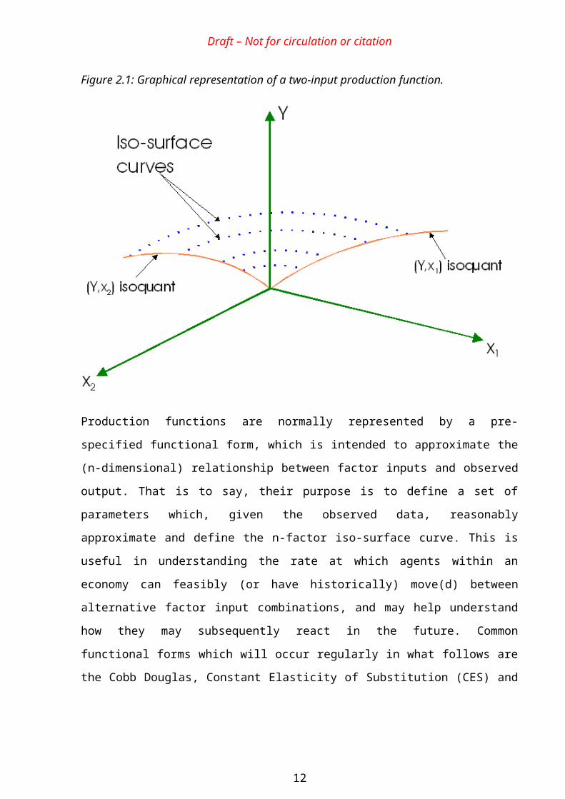
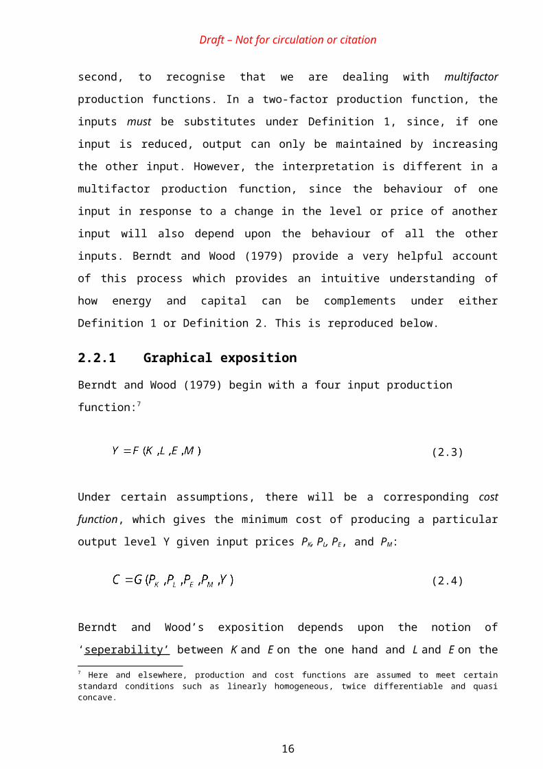
specialisation. Figure 2.1 provides a graphical representation of this relationship, although for
illustrative purposes it considers only two factor inputs.
It is generally assumed that agents are rational and that behaviour is characterised by profit
maximisation. It is further assumed that all agents are producing output at maximum efficiency
with no wastage occurring in the production process. In these circumstances, movement along
the iso-surface curves (between factor inputs) when the level of output is held constant, is
analogous to movement along the ‘production possibilities frontier’ (PPF). The iso-surface
curve will have as many dimensions as there are factor inputs to the production function.
Figure 2.1: Graphical representation of a two-input production function.
Production functions are normally represented by a pre-specified functional form, which is
intended to approximate the (n-dimensional) relationship between factor inputs and observed
output. That is to say, their purpose is to define a set of parameters which, given the observed
data, reasonably approximate and define the n-factor iso-surface curve. This is useful in
understanding the rate at which agents within an economy can feasibly (or have historically)
move(d) between alternative factor input combinations, and may help understand how they
may subsequently react in the future. Common functional forms which will occur regularly in
7
Draft – Not for circulation or citation
what follows are the Cobb Douglas, Constant Elasticity of Substitution (CES) and Translog
production functions. Each of these are briefly introduced in Annex 1.5
2.2 Substitution and complementarityFactors of production are frequently described as either substitutes or complements. These
terms typically, but not always, refer to the changes in the relative proportion of different input
factors while output is held fixed. In different contexts two factors are described as substitutes
(complements) when:6
Definition 1: the usage of one increases (decreases) when the usage of the other
decreases (increases);
Definition 2: the usage of one increases (decreases) when the price of the other
increases (decreases);
Definition 3: the usage of one relative to the other increases (decreases) when the price
of the other increases (decreases);
Definition 4: the usage of the first relative to the second increases (decreases) when the
price of the second relative to the first increases (decreases)
The existence of different definitions of substitution and complementarity can complicate the
interpretation of empirical studies. Whether two factors may be described as substitutes or
complements depends upon the definition being used. It is quite possible for two factors to be
described as substitutes under one definition and complements under another. Care must
therefore be taken in comparing one study with another.
The first two of these definitions are the most commonly used. For example, under Definition
1, energy and capital would be described as substitutes if a decrease in energy usage was
associated with an increase in capital usage, holding output constant. Alternatively, energy and
capital would be described as complements if a decrease in energy usage was associated with a
decrease in capital usage, holding output constant.
5 See also Annex 2 of Technical Report 56 This list is not exhaustive. For example, in some cases economists are interested in the effect of changes in quantities on changes in prices (e.g. the effect of immigration on relative wages). This is not simply the inverse of the effect of changes in prices on changes in quantities, and may lead to a different classification of substitutes and complements.
8
Draft – Not for circulation or citation
Definition 2 is particularly relevant for exploring the economic impact of changes in relative
prices. For example, energy and capital would be described as substitutes under this definition
if an increase in energy prices increased the demand for capital inputs, holding output constant.
Alternatively, energy and capital would be described as complements if an increase in energy
prices decreased the demand for capital inputs, holding output constant. If energy and capital
are found to be complements under this definition, the economic impact of an increase in
energy prices could be significant:
“A reduction in the use of energy by itself will have a relatively small economic impact, determined to first order by energy’s small value share. But if the reduced use of energy also produces a reduction in the use of capital, the larger value share of capital applies and the economic impact is magnified. This indirect effect through capital can be the largest component of the economic impact of reduced energy use... but this effect is often ignored in economic impact analyses of energy policy” (Hogan, 1979)
Hence, in the context of the oil price shocks of the 1970s, Berndt and Wood’s (1975) finding of
energy-capital complementarity under this definition was clearly significant. Furthermore, the
feasibility of increasing economic output with rising energy prices (e.g. due to resource
depletion) may depend in part upon the scope for substitution between capital and energy. But
despite the substantial empirical literature on this subject, there still appears to be little
consensus on whether energy and capital should be considered as substitutes or complements.
The process of improving the energy efficiency of a subsystem normally involves ‘substituting’
energy for capital inputs. Hence, energy and capital would normally be considered as
substitutes under Definition 1. For example, insulation materials can be substituted for fuel
inputs to maintain the internal temperature of a building at a particular level. Similarly, waste
heat recovery equipment can be substituted for fuel inputs to maintain a given level of steam
production. At first sight, therefore, the notion that energy and capital may be complements
appears somewhat odd from an engineering perspective. Nevertheless, beginning with Berndt
and Wood (1975) a number of econometric studies at different levels of aggregation have come
to precisely that conclusion. The key to the puzzle is, first, to recognise that there are number of
competing definitions of substitution/complementarity; and second, to recognise that we are
dealing with multifactor production functions. In a two-factor production function, the inputs
must be substitutes under Definition 1, since, if one input is reduced, output can only be
maintained by increasing the other input. However, the interpretation is different in a
multifactor production function, since the behaviour of one input in response to a change in the
9
Draft – Not for circulation or citation
level or price of another input will also depend upon the behaviour of all the other inputs.
Berndt and Wood (1979) provide a very helpful account of this process which provides an
intuitive understanding of how energy and capital can be complements under either Definition
1 or Definition 2. This is reproduced below.
2.2.1 Graphical exposition
Berndt and Wood (1979) begin with a four input production function:7
(2.3)
Under certain assumptions, there will be a corresponding cost function, which gives the
minimum cost of producing a particular output level Y given input prices PK, PL, PE, and PM:
(2.4)
Berndt and Wood’s exposition depends upon the notion of ‘seperability’ between K and E on
the one hand and L and E on the other. Seperability is a standard (although problematic)
assumption in empirical work and may be defined in two ways, which are commonly taken as
equivalent (Frondel and Schmidt, 2004):8
Primal: The optimum ratio of two factors is unaffected by the level of other inputs.
Dual: The optimum ratio of two factors is unaffected by the prices of other inputs.
If energy and capital are separable from labour and materials, a composite input of ‘utilised
capital’ (K*) can be defined which is derived from capital and energy alone. The production and
cost functions for this input are as follows:
(2.5)
(2.6)
7 Here and elsewhere, production and cost functions are assumed to meet certain standard conditions such as linearly homogeneous, twice differentiable and quasi concave.8 A distinction is commonly made between ‘weak’ and ‘strong’ seperability - for definitions, see Berndt and Christensen
(1973). In this report, all references are too ‘weak’ seperability.
10
Draft – Not for circulation or citation
Similarly, a separate composite input of labour/materials (L*) can be defined which is derived
from labour and materials alone. The production and cost functions for this input are as
follows:
(2.7)
(2.8)
Then, if seperability holds, the ‘master’ production and cost functions for output Y can be
written as a function of these composite inputs:
(2.9)
(2.10)
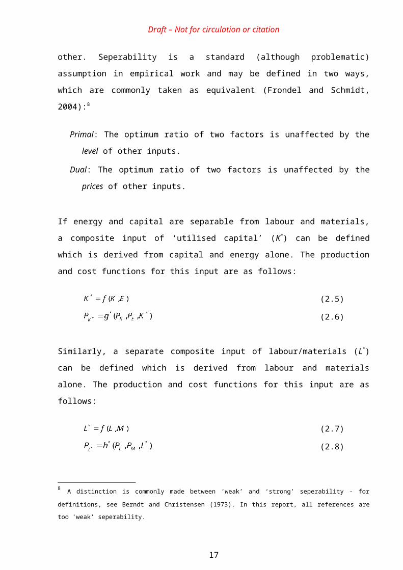
Figure 2.2 provides a graphical representation of the master production function for a
competitive, cost minimising firm producing output level Y. The original input prices for
‘utilised capital’ ( ) and the labour/materials composite ( ) are represented by the iso-cost
line AA’. The firm minimises the costs of producing Y* by using K*1 of utilised capital and L1
*
of the labour/materials composite.
11
Draft – Not for circulation or citation
Figure 2.2 Master production function – initial input prices
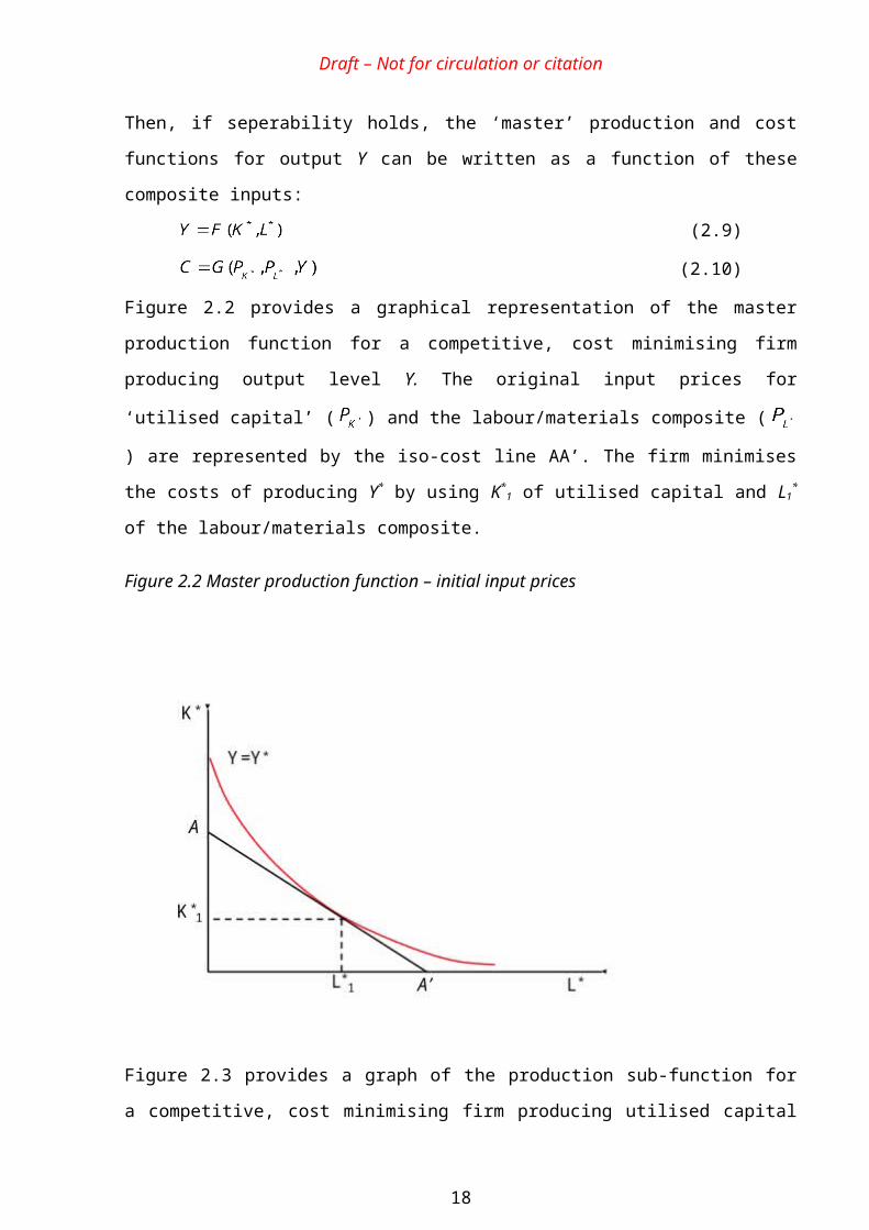
Figure 2.3 provides a graph of the production sub-function for a competitive, cost minimising
firm producing utilised capital K*1 from capital and energy inputs. Given the original prices PK
and PE reflected in the iso-cost line BB’, the firm produces K*1 using K1 units of capital and E1
units of energy.
12
Draft – Not for circulation or citation
Figure 2.3 Production sub-function for utilised capital - initial prices
K
K1
K*=K*1
B’
B
EE1
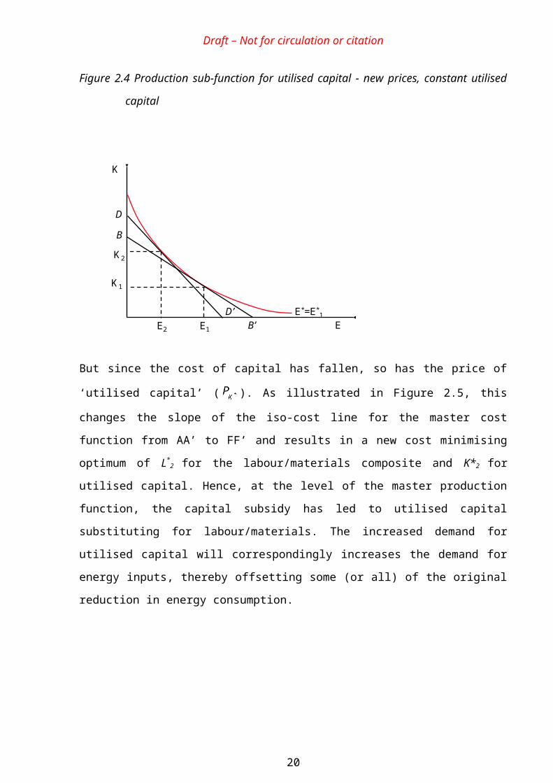
Suppose now that the cost of capital falls relative to the price of energy (say, for example, by a
government subsidy to encourage investment in capital equipment). Then firstly, holding the
production of utilised capital constant at K*1, the steeper iso-cost line DD’ in Figure 2.4
indicates that the demand for capital would increase from K1 to K2 while the demand for energy
would fall from E1 to E2. At the level of the subfunction, capital has substituted for energy
inputs to produce the same level of utilised capital (K*1). Hence, at the level of the subfunction,
capital and energy are substitutes (under this definition) as may be expected from simple
engineering intuition.
13
Draft – Not for circulation or citation
Figure 2.4 Production sub-function for utilised capital - new prices, constant utilised capital
K
K1
E*=E*1
B’
B
EE1
K2
E2
D’
D
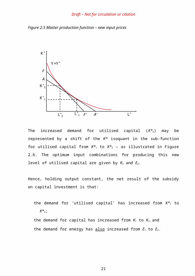
But since the cost of capital has fallen, so has the price of ‘utilised capital’ ( ). As illustrated
in Figure 2.5, this changes the slope of the iso-cost line for the master cost function from AA’
to FF’ and results in a new cost minimising optimum of L*2 for the labour/materials composite
and K*2 for utilised capital. Hence, at the level of the master production function, the capital
subsidy has led to utilised capital substituting for labour/materials. The increased demand for
utilised capital will correspondingly increases the demand for energy inputs, thereby offsetting
some (or all) of the original reduction in energy consumption.
14

Draft – Not for circulation or citation
Figure 2.5 Master production function – new input prices
K*
K*1
Y=Y*
A’
A
L*L*1
K*2
L*2 F’
F
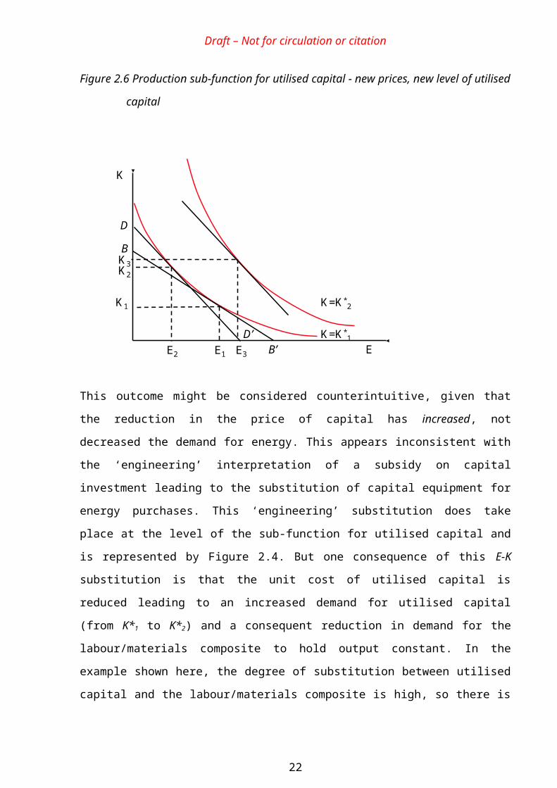
The increased demand for utilised capital (K*2) may be represented by a shift of the K*
isoquant in the sub-function for utilised capital from K*1 to K*2 – as illustrated in Figure 2.6.
The optimum input combinations for producing this new level of utilised capital are given by
K3 and E3.
Hence, holding output constant, the net result of the subsidy on capital investment is that:
the demand for ‘utilised capital’ has increased from K*1 to K*2;
the demand for capital has increased from K1 to K3; and
the demand for energy has also increased from E1 to E3.
15
Draft – Not for circulation or citation
Figure 2.6 Production sub-function for utilised capital - new prices, new level of utilised
capital
K
K1
K=K*1
B’
B
EE1
K2
E2
D’
D
K=K*2
E3
K3
This outcome might be considered counterintuitive, given that the reduction in the price of
capital has increased, not decreased the demand for energy. This appears inconsistent with the
‘engineering’ interpretation of a subsidy on capital investment leading to the substitution of
capital equipment for energy purchases. This ‘engineering’ substitution does take place at the
level of the sub-function for utilised capital and is represented by Figure 2.4. But one
consequence of this E-K substitution is that the unit cost of utilised capital is reduced leading to
an increased demand for utilised capital (from K*1 to K*2) and a consequent reduction in
demand for the labour/materials composite to hold output constant. In the example shown here,
the degree of substitution between utilised capital and the labour/materials composite is high,
so there is a substantial increase in utilised capital demand. This leads to an increase in energy
demand (from E2 to E3) which is more than sufficient to offset the original reduction in energy
demand (from E1 to E2) brought about by the investment in capital equipment. It should be clear
that the final outcome depends upon the shape of the isoquants and in practice, it is possible for
the final energy demand (E3) to be less than, equal to or greater than the original demand (E1).
Berndt and Wood (1979) termed the movement along the K-E partial isoquant (Figure 2.4) the
gross substitution effect and the movement between K-E partial isoquants (Figure 2.6) the
16
Draft – Not for circulation or citation
expansion effect; with the overall change being termed the net substitution effect.9 The gross
effect represents the change in demand for capital and energy holding the demand for utilised
capital fixed, while the expansion effect represents the change in demand for capital and energy
resulting from the increased demand for the (cheaper) utilised capital holding output fixed. This
decomposition is analogous to the decomposition of changes in consumer demand into a
substitution effect (holding utility constant) and an income effect (resulting from an increase in
the level of utility). Similarly it is also analogous to the decomposition of a change in factor
inputs into a substitution effect (holding output constant) and an output effect (resulting from
an increase in output). However, in this example, the overall output of the producer (Y) is held
constant in the definition of net substitution effects, but utilised capital inputs are allowed to
vary. Put another way, Berndt and Wood’s expansion effect may be interpreted as the output
effect for the production (sub) function for utilised capital.
The final demand for capital and energy will be the net result of the gross substitution and
expansion effects – and in principle may be greater or less than the original demand. Berndt
and Wood term capital and energy as net complements where the expansion effect is larger than
the gross effect (demand for both increases following the reduction in the cost of capital), and
capital and energy as net substitutes where the expansion effect is smaller the gross substitution
effect (demand for energy falls following an reduction in the cost of capital, while that for
capital increases). As discussed below, this is consistent with the most common interpretation
of these terms but is not the only way in which substitutes and complements may be defined.
While the independent variable for Berndt and Wood’s example is a reduction in the cost of
capital, analogous conclusions apply when the independent variable is an increase in the price
of energy. In this case, the price of utilised capital will increase, so the labour/materials
composite will substitute for utilised capital to keep output constant. This substitution will
reinforce the reduction in energy consumption caused by the substitution of capital for energy
and will offset the corresponding increase in capital use. Again, if the ‘expansion’ (contraction
in this case) effect is larger than the gross substitution effect, capital and energy will appear as
net complements and overall capital use will fall.
9 In their original paper, Berndt and Wood (1975) used the term ‘scale effect’ rather than expansion effect, but the terminology was subsequently modified to avoid confusion with ‘returns to scale’.
17
Draft – Not for circulation or citation
It is important to note that this interpretation of the origins of energy-capital complementarity is
not the only one that may be provided and also is not accepted by all commentators (Griffin,
1981). Nevertheless, it does provide a intuitively plausible account of the type of mechanisms
that may be at work.
2.2.2 Gross and net price elasticities
As indicated, Berndt and Wood (1979) defined the gross price elasticity between capital and
energy ( ) as that which is conditional upon a fixed level of utilised capital (K*):
(2.11)
The net price elasticity between capital and energy ( ) is defined as having no such
conditions, thus permitting the level of utilised capital (K*) to change in response to changes in
input prices. However, overall output (Y) is held constant.
(2.12)
A more common name for the net price elasticity is the cross price elasticity, but in this case
with the additional restriction that output held fixed. This explains the use of CPE in the above
equations. The constant output cross price elasticity is one of the measures of the elasticity of
substitution considered further in Section 3.
The net price elasticity can be expressed as follows:
(2.13)
This reduces to:10
(2.14)
Where;10 Since the production function is assumed to be linearly homogeneous Also, using Shepard’s Lemma:
18
Draft – Not for circulation or citation
= the share of capital costs in the total cost of utilised capital
= own price elasticity of utilised capital along a Y0 isoquant
Berndt and Wood denote the second term on the right hand side of this equation (
)the expansion elasticity, so that:
Net price elasticity = gross price elasticity + expansion elasticity
Since is negative and is positive, it follows that the expansion elasticity is
negative. Therefore: and the net elasticity is less than the gross elasticity.
While the gross elasticity is positive, the net elasticity may be negative if the expansion
elasticity is greater than the gross elasticity ( ). Thus, it is possible that
any two factors can be both gross substitutes and net complements under Definition 2.
Note that the greater the cost share of capital in the total cost of utilised capital, the more likely
it is that the net elasticity will be negative. The expansion elasticity is likely to be smaller
following a change in energy prices, since energy is likely to account for a smaller share of the
total cost of utilised capital ( ). Hence, the net elasticity is asymmetric.
In the example given here, the net price elasticity is really a measure of the ease of substitution
between capital and energy compared with the ease of substitution between ‘utilised capital’
(K*) and the labour/materials composite (L*). More generally, it is a measure of the relative
substitution between two inputs compared with the substitution effects of other inputs (Hogan,
1979). If the substitution between capital and energy in the sub-function is large compared to
the substitution between utilised capital and the labour/materials composite in the master
function, then capital and energy will be net substitutes under this definition. When the
substitution between capital and energy in the sub-function is relatively small compared to the
substitution between utilised capital and the labour/materials composite in the master
production function, then capital and energy will be net complements under this definition. Put
another way, capital and energy will be substitutes (complements) when the gross price
elasticity is large (small) compared to the expansion elasticity.
19
Draft – Not for circulation or citation
Hence, while capital and energy are substitutes when viewed in isolation from the rest of the
inputs to the production process, they may well be complements in the context of the overall
production function. This is precisely what Berndt and Wood (1979) found in their empirical
investigations of the (aggregate) manufacturing sectors in the US and Canada.
2.3 SummaryThis section has introduced some key concepts from neoclassical production theory and
provided a plausible account of how to inputs may appear as complements. It has shown how
the identification of two inputs as substitutes or complements depends upon the particular
definition being used. The most common definition describes two factors as substitutes
(complements) if an increase in the price of the first is associated with an increase (decrease) in
the usage of the second, holding output constant. This definition is useful when assessing the
potential impact of an increase in input prices.
From an engineering perspective, energy and capital appear to be substitutes, since a decrease
in use of the first may be compensated (at least to some extent, within a particular system
boundary) by an increase in use of the second. Investment in improved energy efficiency can be
understood as the substitution of capital for energy. But this neglects the associated adjustments
of labour and material inputs within the production process as a whole. When the full pattern of
adjustments is taken into account, energy and capital may well turn out to be complements
under the definition given above. This is what Berndt and Wood (1975) found in their
pioneering study of factor substitution in US manufacturing. This finding, together with its
potential economic importance, has stimulated a great deal of empirical research. But it appears
that a consensus has yet to be reached on whether energy and capital can be described as
substitutes or complements.
3 Defining and measuring elasticities of substitution
The elasticity of substitution is intended to measure the ease with which one factor of
production can be substituted for another. The sign of this measure is commonly used to define
whether factors may be considered substitutes or complements. However, there are a number of
definitions of this parameter, which makes interpretation of the empirical literature difficult.
This section summarises the different definitions of the elasticity of substitution and clarifies
20
Draft – Not for circulation or citation
the relationship between them. It then highlights a number of issues relevant to estimating
elasticities of substitution, which are frequently overlooked in the empirical literature.
3.1 Defining the elasiticity of substitutionThe elasticity of substitution (EoSij) is intended to measures the ease with which one varying
factor of production (i) can be substituted for another (j). Definitions of the elasticity of
substitution always refer to a situation where output is held fixed. However, there are several
competing definitions, which incorporate different assumptions about whether:
the independent variable refers to a change in the usage of a input or a change in the price
of that input;
the independent variable refers to an absolute change in the usage or price of an input or a
change relative to another input;
the dependent variable refers to an absolute change in the usage or price of an input or a
change relative to another input;
other input quantities are held fixed; and
other input prices are held fixed.
The value and sign of the estimated elasticity of substitution depends upon which definition is
used. But lack of clarity in definitions, together with inconsistency in terminology and usage
make the empirical literature in this area difficult to interpret (Stern, 2004). This also partly
explains why the substitutability between capital and energy remains a topic of controversy.
The following sections introduce six alternative measures used to define the relationship
between factor inputs in terms of substitutability/complementarity. These measures, discussed
further below, are:
Marginal rate of technical substitution (r)
Hicks elasticity of substitution (HESij)
Shadow elasticity of substitution (SESij)
Constant output cross price elasticity (CPEij)
Allen-Uzawa elasticity of substitution (AESij)
Morishima elasticity of substitution (MESij)
21
Draft – Not for circulation or citation
In the empirical literature, by far the most common measure of the elasticity of substitution is
the Allen-Uzawa. However, this has been criticised by a number of recent authors and the use
of the Morishima measure of the elasticity of substitution is becoming more widespread. Both
of these can usefully be related to the constant output cross price elasticity between two factors
of production which in many respects is a more useful measure. Both the Allen-Uzawa and
Morishima elasticities are based upon the Shadow elasticity of substitution, which in turn is
related to the Hicks definition, which was the first to be introduced (Hicks, 1932). The Hicks
definition, in turn, is based upon the marginal rate of technical substitution. The following
sections define each of these measures, clarify the relationships between them and comment on
their relative suitability for empirical work. In each case we summarise the assumptions behind
the definition; present the relevant formula(e); show whether and how the measure may be used
to classify factors as substitutes or complements; highlight some key issues in interpretation;
and identify possible extensions. The text is largely based upon the excellent surveys by
Frondel (2004) and Stern (2004).
3.1.1 Marginal rate of technical substitution
The logical starting point is the marginal rate of technical substitution (r). This measures the
rate at which one factor of production can be substituted for another factor while holding output
constant. r is a measure of the slope of an isoquant on the production surface.
3.1.1.1 Assumptions:
Two factors vary (xi and xj )
Other inputs fixed.
Output is fixed
3.1.1.2 Definitions
(3.1)
An alternative definition is:11
(3.2)
11 This can be derived by differentiating the production function (f) with respect to xj :
22
Draft – Not for circulation or citation
The marginal rate of technical substitution (r) between i and j is therefore given by the ratio of
the marginal productivity of j to the marginal productivity of i. The marginal productivity, in
turn, represents the increase in output for a unit increase in the input of a particular factor (
).
3.1.1.3 Substitutes and complements
The marginal rate of technical substitution provides a direct measure of how much of one factor
is required to substitute for another – with other inputs and output fixed. The terms substitutes
and complements are not used directly in relation to this measure, but r does provide a basis for
the Hicks elasticity of substitution, discussed next.
3.1.1.4 Issues and extensions
In the two-dimensional case, r is positive. To hold output constant, xj must increase when xi
decreases. The value of r will depend upon both the level of output and the relative proportion
of each factor (i.e. the point on the isoquant map). Typically (with convex isoquants) r is
diminishing for increasing inputs of xi.12
One drawback of r is that it depends upon the units in which factors are measured. Frondel
(2004) has proposed an alternative, non-dimensional measure of relative changes in factor
inputs, termed the ‘total elasticity of substitution’ (TES):
(3.3)
However, this elasticity measure is not in widespread use and none of the papers summarised in
the empirical review section apply this measure.
3.1.2 The Hicks elasticity of substitution
Hicks (1932) introduced this as a measure of the ease with which a decrease in one input can be
compensated by an increase in another while output is held constant. More precisely, the Hicks
elasticity of substitution measures the ratio of the relative change in factor proportions to the
relative change in the marginal rate of technical substitution. The definition refers to 12 The definition can be extended to the case where three inputs vary to give:
. In this case, r is no longer unambiguously positive. If r<0, xj
could decline when xj declines. The output is held constant by an increase in xk.
23
Draft – Not for circulation or citation
movement along a partial isoquant on the production surface and is a scale-free measure of the
curvature of this isoquant.
The original Hicks definition applies to a production function with only two inputs. The
subsequent generalisation to multi-input production functions is sometimes termed the Direct
elasticity of substitution (Chambers, 1988).
3.1.2.1 Assumptions
Two factors vary (xi and xj )
Other inputs fixed.
Output is fixed
3.1.2.2 Definition
For a multi-input production function that satisfies certain conditions,13 the HESij is defined as:14
(3.4)
3.1.2.3 Substitutes and complements
If other inputs are held fixed, output can only be held constant if a decrease in one input (i) is
compensated by an increase in a second (j) - in other words, one factor must ‘substitute’ for
another. Therefore, the HES classifies all inputs as substitutes according to Definition 1 of
Section 2.
3.1.2.4 Factor shares
The HES provides information on the effect of a change in usage of an input on the share of
that input in the value of output ( ).15 It may be shown that (Sato and Koizumi,
1973):
according to (3.5)
13 A continuous function with positive first order partial derivatives and continuous second-order partial derivatives that is quasi concave.
14 An alternative formulation is:
15 Under competitive market conditions, the latter is equal to the share of a factor in total input costs ( ).
24
Draft – Not for circulation or citation
Hence, if HESij>1 (<1,) the share of input i in total costs becomes larger (smaller) relative to j
as the usage of i becomes larger (smaller) relative to j.
3.1.2.5 Issues and extensions
The HES measures the curvature of the surface of the production function in a particular
direction. It follows from the concavity of the production function that HESij>0.
From Equation 3.4, if r does not change at all with changes in the ratio xi/xj, it indicates that
substitution is easy, because the ratio of marginal productivities of the two inputs does not
change as the input mix changes. Alternatively, if r changes rapidly for small changes in the
ratio xi/xj, it indicates that substitution is difficult because minor variations in the input mix will
have a substantial effect on the relative productivities of the two inputs.
Taking the two factor case, if HESij is large, r will not change much relative to the input ratio,
xi/xj, and the isoquant will be relatively flat. On the other hand, if HESij is small, the isoquant
will be sharply curved. The extremes are: a linear production function, where , and a
‘Leontief’ (fixed proportions) production function, where . For a ‘Cobb Douglas’
production function HESij=1, while for a ‘Constant Elasticity of Substitution’ (CES) production
function, HESij is constant (as the name suggests) between 0 and infinity. The CES may be
generalised to the multifactor case, but this places restrictive conditions on the elasticity values
(McFadden, 1963). The ‘translog’ production function allows for multiple substitution
possibilities between pairs of factors, so HESij can vary. More information on these different
types of production function is given in Annex 1.16
Since the extension of the Hicks definition to multi factor functions requires the assumption
that other factor inputs are fixed, the practical value of this definition is limited. As shown in
Section 2, it is likely that in practice any change in the ratio of two inputs will also be
accompanied by changes in the levels of other inputs. Some of these inputs may be
complementary with the ones being changed, whereas others may be substitutes, and to hold
them constant creates a rather artificial restriction.
16 See also Annex 2 of Technical Report 5.
25
Draft – Not for circulation or citation
The econometric estimation of production functions is also prone to bias, and it is more
common to estimate cost functions since the relevant independent variables (factor prices) can
usually be assumed to be exogenous. For this reason, an alternative definition of the elasticity
of substitution, based upon the cost function, is more relevant to empirical studies. This is
termed the Shadow elasticity of substitution (SESij) (McFadden, 1963).
3.1.3 The Shadow elasticity of substitution
This definition measures how the ratio of two factor inputs changes in response to changes in
the ratio of their relative prices. It is therefore a two-factor, two-price elasticity
3.1.3.1 Assumptions
Two input prices vary (pi and pj)
Other input prices (not quantities) are fixed
Total costs (C) are fixed
3.1.3.2 Definition
For a multi-input cost function (g) that satisfies certain conditions,17 the SESij is defined as:18
(3.6)
3.1.3.3 Substitutes and complements
As with the HES, the SES classifies all inputs as substitutes .
3.1.3.4 Factor shares
The SES provides information on the effect of a change in the price of an input on the share of
that input in the value of output ( ):
according to (3.7)
17 A continuous function with positive first order partial derivatives and continuous second-order partial derivatives that is strictly quasi concave.18 An alternative formulation is:
26
Draft – Not for circulation or citation
Hence, if SESij>1 (<1,) the share of input i in total costs becomes larger (smaller) relative to j
as the price of i becomes larger (smaller) relative to j.
3.1.3.5 Issues and extensions
The SES measures the curvature of the surface of the cost function in a particular direction. It
follows from the concavity of the cost function that SESij>0.
Under the assumption of perfect competition and profit maximisation, the definition of the SES
is equivalent to the Hicks elasticity. This is because, under these circumstances, the ratio of
prices of the two factors should equal the ratio of their marginal rates of technical substitution.
In these circumstances, two factors which are described as substitutes under the HES will also
be described as substitutes under the SES. However, the main advantage of this definition is
that it can be more easily generalised to the multi-factor case.
3.1.4 The constant output cross price elasticity
The constant output cross price elasticity (CPEij) forms the basis of Berndt and Wood's net and
gross elasticities, described in Section 2. It also forms the basis of the Allen Uzawa and
Morishima measures of the elasticity of substitution described below. Frondel (2004) is one of
a number of authors who have argued that the CPEij provides the best and most intuitive
measure of factor substitutability, despite the fact that most empirical studies do not state this
measure explicitly.
3.1.4.1 Assumptions
One input price varies
Other input prices (not quantities) are fixed
Output is fixed
3.1.4.2 Definition
(3.8)
3.1.4.3 Substitutes and complements
The CPE classifies a pair of inputs as substitutes (complements) if an increase in the price of
one causes the usage of the other to decrease (increase). Thus i and j are substitutes
(complements) if CPEij >0 (<0).
27
Draft – Not for circulation or citation
3.1.4.4 Issues and extensions
The CPE focuses solely on the relative change in use of factor i due to a change in the price of
factor j, with output and other factor prices held fixed. So this is a one-factor-one-price
elasticity of substitution. The CPE is asymmetric (i.e. ) and is equivalent to the
net price elasticity as defined by Berndt and Wood (i.e. the sum of the gross price and
expansion elasticities). Hence, given that the gross price elasticity is necessarily positive, the
CPE is only negative if the expansion elasticity is greater than the gross price elasticity.
3.1.5 Allen-Uzawa Elasticity of Substitution
This is by far the most common measure of the EoS in empirical work and stems from the
original definition by Allen (1938). As with the CPE, the AES is a one-factor-one-price
elasticity.
3.1.5.1 Assumptions
One input price varies (pi)
Other input prices (not quantities) are fixed
Output is fixed
3.1.5.2 Definition
Allen derived a formula for the AES based upon the production function as follows:
(3.9)
Where xk is an input factor, fk is the marginal productivity of that factor, F is the bordered
Hessian of the production function and Fij is the cofactor of fij.
Uzawa (1962) derived an alternative definition using the cost function (C), and it is this form
which is most used in the empirical literature (hence the term Allen-Uzawa elasticity of
substitution):
(3.10)
28
Draft – Not for circulation or citation
This definition is useful empirically, but is difficult to interpret. However, Blackorby and
Russell (1981; 1989) showed how this form is related to the more familiar (constant output)
cross price elasticity, as follows:19
(3.11)
Where sj represents the share of input j in total costs ( ). This formulation is much more useful for an intuitive understanding of the meaning of the AES.
3.1.5.3 Substitutes and complements
As with the CPE, the AES classifies a pair of inputs as substitutes (complements) if an increase
in the price of one causes the usage of the other to decrease (increase). Therefore i and j are
substitutes (complements) if AESij >0 (<0).
3.1.5.4 Factor shares
The AES provides information on the effect of a change in the price of input j on the share of
input i in the value of output ( ):
according to (3.12)
(3.13)
So, an increase in the price of input j causes the cost share of the input i to increase (decrease)
if the magnitude of the AES is greater than (less than) unity. While the sign of the AES provides
information on whether si increases or decreases following an increase in pj, to quantify this
change information is also required on si.
19 Their derivation uses Shephard’s Lemma – namely that the contingent demand function for any input is given by the partial
derivative of the cost function with respect to that input’s price: . Using this:
. Then multiply top and bottom by xjC:
29
Draft – Not for circulation or citation
3.1.5.5 Issues and extensions
The AES is popular in empirical studies, because it may be calculated easily from
econometrically estimated cost functions using Equation 3.11. However, Frondel (2004) argues
that it has a number of drawbacks.
First, AES always has the same sign as the CPE, hence, AES classifies inputs as complements
or substitutes in the same way as the CPE. In essence, the AES adds no more information to
that contained in the CPE, so that arguably, the CPE could be used without complicating the
issue by dividing by the cost share. Moreover, weighting of the CPE by the cost share can
result in small variations in the cost share of a particular factor leading to large variations in the
magnitude of the AES. This is particularly the case for energy, whose share of total cost
typically varies between 1% and 10%. As a result, the quantitative value of the AES may have
little meaning. As Chambers (1988) notes, Equation 3.11 is the:
“……most compelling argument for ignoring the Allen measure in applied analysis … The interesting measure is CPEij - why disguise it by dividing by a cost share? This question becomes all the more pointed when the best reason for doing so is that it yields a measure that can only be interpreted intuitively in terms of CPEij” (Chambers, 1988)
Second, the AES does not define the curvature of the isoquant in the same manner as the HES
(Blackorby and Russell, 1975). The only circumstances in which it does is when the production
function takes a non-nested Constant Elasticity of Substitution (CES) form (including Cobb-
Douglas), or when there are only two factor inputs.
Third, the AES is symmetric (AESij = AESji.), which implies that that movement in one direction
across the iso-surface is equally as easy as movement in the exact opposite direction. However,
this symmetry is only achieved by dividing the CPE by the cost share. As indicated above, the
CPE is not symmetric: in other words, the change of factor i due to a change in the price of
factor j (with output and other factor prices held fixed) is not the same as the change in factor j
due to a change in the price of factor i. This asymmetry may be important in practice, but is
disguised by the AES. For example:
“Reducing energy use due to energy-price shocks might be compensated optimally by an additional use of a third factor, say labor, while capital remains constant. Yet, conversely, a further expansion in capital use due to lower capital prices may necessitate more energy for an economically optimal way of production” (Frondel, 2004, p. 993)
30
Draft – Not for circulation or citation
3.1.6 Morshima Elasticity of Substitution
The Morishima elasticity of substitution (MESij), due originally to Morishima (1967)), has been
used instead of the AES in some more recent empirical work. In contrast to the AES and CPE,
the MES measures the change in a ratio of inputs, rather than a single input – and hence is
closer to the SES definition. However, in contrast to the SES, the measure is defined with
respect to a change in a single price rather than a ratio of prices. The MES is thus a two-factor-
one-price elasticity.
3.1.6.1 Assumptions
One input price varies (pi)
Other input prices (not quantities) are fixed
Output is fixed
3.1.6.2 Definition
Taking the general SES, but assuming that the change in pj/pi is solely due to a change in pj
gives:20
(3.14)
Blackorby and Russell (1975) use the cost function to define the MES as follows:
(3.15)
This definition is useful for empirical work with cost functions, but only applies when the
function is continuous, linearly homogeneous and concave. Use of a cost function in this way
also implies perfect competition and cost minimising behaviour. Hence, Equation 3.15 is a
more restrictive definition than Equation 3.14.21
20
21 From Shephard’s Lemma . Substituting this into the cost function definition of the MES gives:
. This is equivalent to the first definition derived
directly from the production function.
31
Draft – Not for circulation or citation
3.1.6.3 Substitutes and complements
The MES classifies a pair of inputs as substitutes (complements) if an increase in the price of
one leads to an increase (decrease) in the usage of the other relative to the usage of the input
whose price has changed. So i and j are substitutes (complements) if MESij >0 (<0). In practice,
the MES classifies the great majority of inputs as substitutes.
3.1.6.4 Factor shares
The MES provides information on the effect of a change in the price of input j on the share of
input i in the value of output relative to the share of input j:
according to (3.16)
(3.17)
So, an increase in the price of input j causes the cost share of input i relative to that of input i to
increase (decrease) if the magnitude of the MES is greater than (less than) unity.
Note that if two inputs are MES substitutes (MESij>0), it does not necessarily follow that the
cost share of input i will decrease relative to that of input j following an increase in the price of
j. This will occur only if MESij>1. In this sense, the magnitude of the MES relative to unity may
provide a more useful indication of ‘ease of substitution’ than its magnitude relative to zero –
although the latter is conventionally used to distinguish MES substitutes and complements.
Substitution is clearly easier if producers can reduce their relative expenditure on the factor
whose price have risen than if they are forced to increase their relative expenditure on this
factor: i.e. substitution is easier if MESij>1.
3.1.6.5 Issues and extensions
3.1.6.5.1 Relationship between the MES and the CPEBlackorby and Russell (1975) show that:
(3.18)
where CPEjj= the own price elasticity of input j. This shows that the effect of varying pj on the
quantity ratio xi/xj (holding output and other prices constant) is divided into two constituent
parts:
32
Draft – Not for circulation or citation
the proportional effect on xi, given by the cross price elasticity (CPEij) and
the proportional effect on xj itself, given by the own price elasticity (CPEjj)
Inversely, the effect of varying pi on the quantity ratio xj/xi - holding output and other prices
constant - is given by:
(3.19)
This shows that the MES (like the CPE but unlike the AES) is asymmetric. By implication, two
factors i and j may be MES complements with respect to changes in pi and MES substitutes with
respect to changes in pj. However, the MES is closer to the original (Hicks) notion of a
substitution elasticity in that it measures the percentage change in a factor ratio. In contrast, the
CPE measures the percentage change in factor demand.
In the simple case of only two inputs, the MES cannot be negative (this would imply that a
decline in the availability of one input could be made up through a decline in the availability of
the second input). However, with more than two inputs it is theoretically possible for the MES
to be negative. It would require the cross price elasticity between two inputs to be negative
(indicating that they are complements under the CPE/AES definition) and to be greater in
absolute value than the own price elasticity. For example, it would imply that a 1% increase in
the price of energy would reduce inputs of capital by a greater proportion than it decreased
inputs of energy. This would imply a substitution away from capital despite the fact that the
relative price of capital has decreased. Hence, the MES is likely to be positive in the majority of
cases. If substitutability is defined as MESij >0, this means that factors will be found to be MES
substitutes in practically all cases. As a result, the sign of the MES may not be useful means of
distinguishing substitutes and complements.
3.1.6.5.2 Relationship between the MES and the AESBlackorby and Russell (1981) prove that AES and MES are identical if and only if the
production technology has a non-nested CES or Cobb Douglas structure, or if there are only
two inputs. Further, in the multi-factor context it can also be shown that:
(3.20)
33
Draft – Not for circulation or citation
The AES and the CPE classify a pair of inputs as substitutes (complements) if an increase in the
price of one causes an increase (decrease) in the quantity demanded of the other. In contrast,
the MES classifies a pair of inputs as substitutes (complements) if an increase in the price of
one causes the quantity of the other to increase (decrease) relative to the quantity of the input
whose price has changed. This makes the MES lean more towards substitutability. If two inputs
are AES substitutes, then they must be MES substitutes. But if two inputs are AES
complements, either they may be MES substitutes or (less likely) complements. Because
is always negative, two inputs being AES substitutes (AESij>0) are also inevitably MES
substitutes. However, AES complements (AESij<0) are also likely to be MES substitutes. The
effective inability to distinguish between substitutes and complements is arguably a drawback
of the MES.
3.1.7 Summary of definitions
Table 3.1 summarises the key features of each of the definitions of the elasticity of substitution
discussed above. Given this range of definitions, great care must be taken when referring to
‘the’ elasticity of substitution, or to defining two factors as either substitutes or complements.
While the HES and SES have an important role theoretically, empirical studies tend to use the
CPE, AES or MES. It is only with respect to these three measures that factors can meaningfully
be classified as substitutes and complements. In all cases, substitution between two inputs is
‘easier’ when the elasticity of substitution between them is greater.
Most empirical studies use the AES and classify inputs as either substitutes or complements on
the basis of the sign of the AES. This reflects the most common understanding of these terms,
which is the effect of a change in the price of one factor on the demand for another (i.e.
Definition 2 in Section 2). However, exactly the same information is provided by the CPE – the
AES just scales that parameter by one of the cost shares, which is not necessarily very helpful
since it implies that the quantitative value of the AES lacks meaning. Hence, in many
circumstances, it would be simpler to just estimate the CPE. The sign of the MES is less useful
as a definition of substitutes or complements, since in nearly all cases the MES is positive.
However, the MES (like the CPE but unlike the AES) is asymmetric, which is more
representative of actual economic behaviour.
34
Draft – Not for circulation or citation
The magnitude of each measure relative to unity provides an indication of how the cost share of
each factor will change in either absolute or relative terms. The sign of the AES indicates
whether an increase in the price of input j will increase or decrease the share of input i in the
value of output, while the MES provides immediate quantitative information on the effect of a
change in the price of input j on the share of input i relative to the share of input j. This is
potentially valuable information.
35
Draft – Not for circulation or citation Table 3.1 Comparing different definitions of the elasticity of substitution
Measure Output Other factor inputs
Other factor prices
Definition Type Substitutes (complements
)
Factor shares
EoS 1
Symmetrical
Hicks/Direct Fixed Fixed - Primal All substitutes No
Shadow Fixed Variable Fixed DualTwo factor, two price
All substitutes No
Cross price Fixed Variable Fixed DualOne factor, one price
CPE>0 (<0) No
Allen Fixed Variable Fixed DualOne factor, one price
AES>0 (<0) Yes
Morishima Fixed Variable Fixed DualTwo factor, one price
MES>0 (<0)(most
substitutes)
No
Relationships:;
Factor shares:
;
36
Draft – Not for circulation or citation
3.2 Issues in estimating elasticities of substitutionEmpirical studies of production relationships assume a particular functional form for the
production or cost function and estimate the parameters of that form econometrically.
Elasticities of substitution may then be calculated from those estimated parameters. The most
common functional forms are the Cobb Douglas, the Constant Elasticity of Substitution (CES)
and the Translog. Each of these is briefly introduced in Annex 1. By implication, the empirical
results may depend very much on the particular form that is chosen.
Empirical studies may also be prone to bias due to omitted variables and other factors. Four
particularly important issues relevant to estimating elasticities of substitution are:
separability of input factors;
aggregation and changes in product mix;
the importance of cost shares when using static translog cost functions; and
the treatment of technical change
Each of these is discussed in turn below.
3.2.1 Separability
Assumptions regarding the separability of production factors are common in empirical work.
Separability is defined in one of two ways:
Primal: The marginal rate of technical substitution between two inputs is unaffected by
the level of other inputs:
xk: (3.23)
Dual: The marginal rate of technical substitution between two inputs (xi/xj) is unaffected
by the prices of other inputs:
pk: (3.24)
37
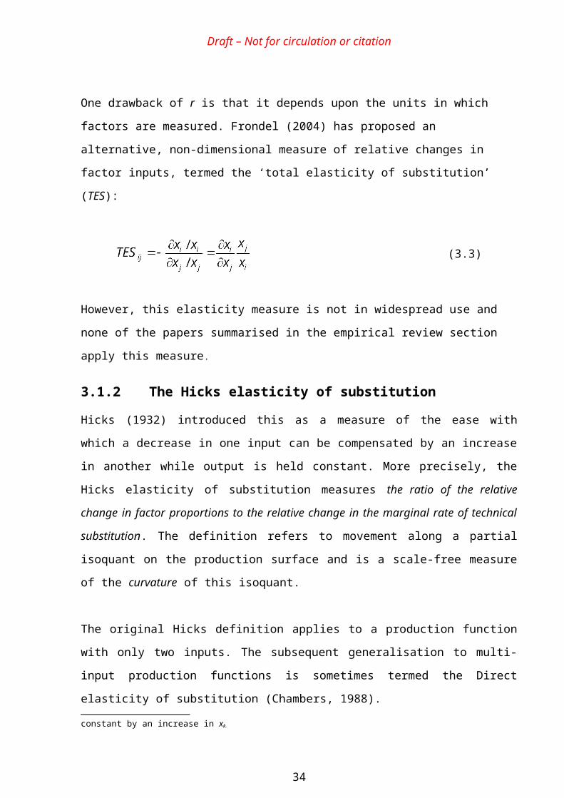
Draft – Not for circulation or citation
If two inputs (i,j) are separable from a third input (k), then the ease of substitution between i
and k (as measured by the CPE, AES or MES) is equal to that between j and k (e.g.
AESik=AESjk).
The separability of inputs in production functions is commonly used within production theory
to justify the grouping, or nesting, of different inputs. The assumption is that producers in
engage in a two-stage decision process: first optimising the combination of inputs within each
nest, and then optimising the combination of nests required to produce the final output. Two
factors may only be legitimately grouped within a nest if they are separable from factors
outside of the nest. For example, a (KL)E nesting structure requires that capital and labour are
separable from energy under the definitions given above. One of the contributions of Berndt
and Wood (1975) was to show that a nest of capital and labour inputs (often referred to as
‘value-added’) was not separable from either energy or materials within their dataset. The only
nesting structure that was supported by Berndt and Wood’s data was ,
which corresponds to the example given in Section 2.
However, defined in this way, the assumption of separability does not mean that measures of
the CPE, AES or MES between inputs within a nest (e.g. i and j) are unaffected by the level
(price) of inputs outside the nest (e.g. k) (Frondel and Schmidt, 2004). For example, even if
capital and labour inputs were separable from energy inputs according to the standard
definition, this would not necessarily imply that the ease of substitution between capital and
labour (as measured by the CPE, AES or MES) was unaffected by the level (price) of energy
inputs. Therefore, omitting measures of any input from empirical work could lead to error. This
is particularly important for empirical estimates based upon KLE production/cost functions, as
opposed to those which include materials (KLEM). The omission of materials could lead to
biased estimates, even if materials are separable from other production factors according to the
definitions above.
Frondel and Schmidt (2002) show that for AESij and CPEij to be unaffected by changes in the
price of k, both the separability condition defined above must hold and changes in the price of k
must not affect the cost shares of inputs i and j. Similar comments apply to MESij. Since this
appears unlikely in practice, it seems reasonable to assume that measures of CPEij and AESij
will generally depend upon the price of other factors, even when i and j are separable from
38
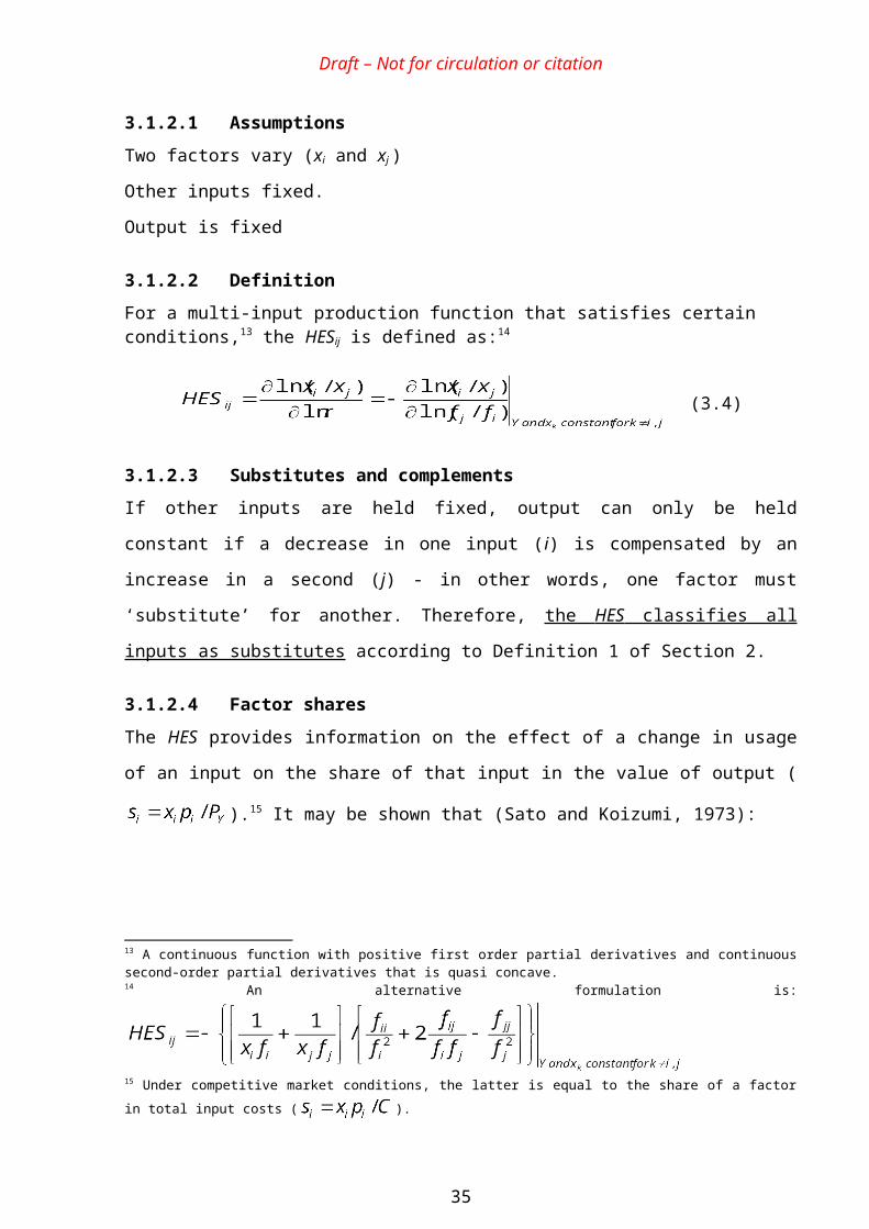
Draft – Not for circulation or citation
those factors. This suggests that empirical studies that use assumptions of separability to justify
the omission of other factors - notably materials - are likely to be biased.
Empirical work based upon translog cost functions should be less vulnerable to this problem,
since these functions do not rely upon nesting structures and do not impose separability
restrictions (although such restrictions can be tested). However, tranlog studies that omit
particular inputs due to lack of data could still be prone to bias.
3.2.2 Aggregation
Measures of the elasticity of substitution are defined with respect to constant level of output
and (implicitly) assume that this output consists of a single homogeneous product. Measures of
the elasticity of substitution are then interpreted as relating to changes in the mix of factor
inputs required to produce this single product; but in practice, this might be misleading.
Individual firms/subsectors/sectors may produce a range of different products with each
requiring a different input mix. Hence, changes in factor prices could lead to a change in the
mix of products, as well as changes in the mix of factors used to produce an individual product
(Miller, 1986; Solow, 1987). More generally, changes in factor prices could lead to a change in
the relative contribution of individual subsectors to the output of a sector, or the relative
contribution of individual sectors to the output of an economy. The scope for such influences is
likely to increase with the level of aggregation for which the elasticity of substitution is
estimated. For example, a product mix for a sector defined at the two digit level is greater than
that for a sector defined at the three digit level, which in turn is greater than that for an
individual firm.22
These considerations point to the limitations of studies that apply a partial equilibrium
approach to aggregate data. As Solow (1987) has demonstrated, production may be governed
by fixed factor ratios at a firm or sector level, but a sector or economy may still exhibit factor
substitution in the aggregate due to changes in the composition of output. Moreover, if the
scope for substitution within a particular production process is relatively limited, changes in
22 Miller (1986) argues that such effects are likely to lead the elasticity of substitution between capital and energy to be overestimated in studies using a static functional form with cross-sectional data. This is because the errors due to the excluded product mix variable are likely to be systematically correlated with factor prices (e.g. products requiring relatively large inputs of energy are likely to be produced where energy is cheaper). Similar biases are possible in time series studies, depending in part upon how capital is measured (Miller, 1986).
39
Draft – Not for circulation or citation
relative factor prices may induce changes in the composition of production at higher levels of
aggregation (Koetse, et al., 2006).
A second aggregation issue is highlighted by ecological economists such as Stern and
Cleveland (2004). Measures of the elasticity of substitution between energy and capital refer to
particular level of aggregation and implicitly assume that the relevant factors are independent
of each other. However, such estimates may overestimate the possibility for substitution
between energy and capital at a higher level of aggregation, such as the economy as a whole.
This is because they do not include the indirect energy consumption that is required to produce
and maintain the relevant capital, or the indirect capital and labour that is required to produce
and deliver energy commodities. For example, energy is required to produce and install home
insulation materials and energy efficient motors.23 This suggests that the scope for substitution
between energy and capital at the level of the macro-economy may be less than indicated by an
analysis of an individual sector:24
“From an ecological perspective, substituting capital and/or labour for energy shifts energy
use from the sector in which it is used to sectors of the economy that produce and support
capital and/or labour. In other words, substituting capital and/or labour for energy increases
energy use elsewhere in the economy” (Kaufmann and Azary-Lee, 1990)
However, the above two observations are potentially contradictory. Consideration of potential
changes in product/sector mix suggests that empirical studies at higher levels of aggregation
may indicate a greater scope for substitution between energy and capital than studies at a lower
level of aggregation, while the consideration of indirect energy consumption suggests the
opposite. The balance between the two will depend upon the particular sectors and level of
aggregation being studied. For example, the indirect energy consumption associated with the
manufacture of insulation will only be relevant to estimates of the elasticity of substitution if
the sector that manufactures installation is included in the estimates. Generally, the implications
of changes in product mix should be more relevant to estimates of the elasticity of substitution
between energy and capital within a particular sector, while the implications of indirect energy
consumption should be more relevant to economy-wide estimates. Also, empirical estimates at
lower levels of aggregation are more likely to isolate ‘pure’ substitution effects.
23 The converse is also the case: capital and labour are required for the delivery of energy commodities.24 The implications of this, and their relevance to the rebound effect, are discussed further in Technical Report 5.
40
Draft – Not for circulation or citation
A final aggregation issue relates to the potentially important distinctions between different
types of capital (e.g. machinery and structures), different types of labour (e.g. skilled and
unskilled) and different types of energy input (e.g. electricity and fuel). There will be scope for
substitution within these subcategories (e.g. between electricity and fuel), as well as between
subcategories (e.g. machinery and fuel) and studies that use more aggregate measures will not
reveal these individual patterns. As an example, there may be less scope for substitution
between capital and skilled labour than between capital and unskilled labour. Similarly,
aggregate energy and capital may be estimated to be substitutes, but capital may be a
complement for electricity inputs but a substitute for fuel oil. The estimated elasticity of
substitution involving an aggregate is not necessarily a weighted average of the elasticities of
substitution for the disaggregate inputs. However, this does not necessarily mean that estimates
of substitution possibilities between more aggregate measures of inputs will be biased.
3.2.3 Cost shares
The most common approach to measuring elasticities of substitution is to estimate a static cost
function, in which inputs are implicitly assumed to adjust their long run desired levels within
one time period. Typically, studies employ a homothetic, translog cost function (see Annex 1)
of the form:
(3.25)
With the following restrictions:
(3.26)
(3.27)
In this case (using Shephard’s lemma), the cost share (si) for each factor is given by:
(3.28)
Frondel and Schmidt (2002) show that, in this instance the cross price elasticity is given by:
(3.29)
41
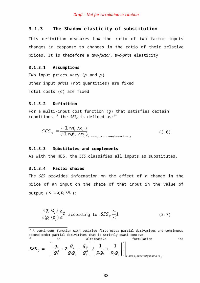
Draft – Not for circulation or citation
This shows that estimates of the cross price elasticity (and hence AES and MES) from a static
translog cost function will depend upon the cost shares of the relevant factors. In particular
CPEij will be close to the cost share of factor j if the cost share of factor i is large relative to the
second order coefficient βij (since the first term will be small). Since, in practice, βij is often
small, the cost share of factor j is likely to strongly influence the magnitude of the estimated
cross price elasticity. According to Frondel and Schmidt (2002), the economic intuition behind
this is that the larger the cost share of factor i (si), the harder it is to substitute factor i for a
factor j whose price is increasing.
In the case of capital and energy, the cost share of energy is likely to have a strong role in
determining the magnitude of CPEKE (and hence of AESKE and MESKE). Costs shares, in turn,
depend upon which factors are measured. For example, the inclusion or otherwise of materials
may be expected to have a significant influence on the estimated cost shares. Frondel and
Schmidt (2002) review the empirical literature on energy-capital substitution and find that
evidence of complementarity only occurs in cases where the cost share of energy is small.
When material inputs are included in the specification, the cost shares of capital and energy
necessarily become smaller and the finding of complementarity becomes more likely. Frondel
and Schmidt (2002) argue that this may explain the differences between time-series and cross-
sectional results noted by Apostolakis (1990) and others. The standard interpretation is that
time-series results reflect short-run substitution possibilities while cross-sectional results
represent long-run (equilibrium) substitution possibilities (Griffin and Gregory, 1976;
Apostolakis, 1990; Frondel and Schmidt, 2002). Since time-series studies appear more likely to
find energy and capital to be complements, while cross-sectional studies appear more likely to
find them to be substitutes, this suggests that there may be more scope for substitution between
capital and energy in the long-run (when capital can be replaced). However, Frondel and
Schmidt (2002) explain these results by noting that the time series studies were more likely to
include data on materials.
Prior to Frondel and Schmidt (2002), this linkage between costs shares and elasticity estimates
(with the static, translog functional form) does not appear to have been recognised. It may
explain why the estimates of CPEKE (i.e. with PE varying) are commonly small – since the cost
share of energy is typically small. Frondel and Schmidt (2004) argue that ‘… inferences
obtained from previous empirical analyses appear likely to be an artefact of cost shares and
42
Draft – Not for circulation or citation
have little to do with statistical inference about technology relationships’ (p. 72). However,
Stern argues that KLE studies are likely to be biased owing to the omission of materials and
that cost shares are not arbitrary but are instead a function of the underlying technology. For
example, energy intensive industries have a stronger incentive to substitute capital for energy
when energy prices increase, suggesting that the finding of substitution may be more common
when the cost share of energy is large. The implication is that KLEM studies are likely to reveal
the ‘true’ relationship, while KLE studies will not. In either case, these observations suggest
that dynamic functional forms may be preferable, although in practice these appear to be rarely
used.25
3.2.4 Technical change
Technical change occurs when technological improvements in an industry act as a precursor to
increased levels of output associated with any given level of factor inputs, for example through
engineering efficiency improvements. While substitution may be represented as a movement
along an isoquant of a production function, ‘technical change’ refers to the development of new
technologies and methods of organisation that shift the isoquant to the left, allowing the same level
of output to be produced from a lower level of inputs.
The inclusion of technology into production functions can be done in a number of ways so as to
reflect different assumptions about the role of technical change, the most common being the
assumption of Hicks-neutral technical change, factor augmenting (non-neutral) technical
change, or just the pure omission of technical change (Equation 2.1 is a specification of a
general production function with no technical change).
Hicks neutral technical change, is shown representatively as:
(3.30)
Where the multiplier denotes technology and is assumed to be greater than unity (
). The assumption that technical change can be separated in this way from the rest of the factors
of production ensures that it can be uniquely identified. Moreover, the parameters of the
estimated production function reflect only the decision to use a certain combination of the
available factor inputs and not the change in input use owing to technological advancements.
25 Static means that the production function is formed only of ‘current period’ variables, whereas a dynamic model includes information on all or some of the other variables in the past.
43
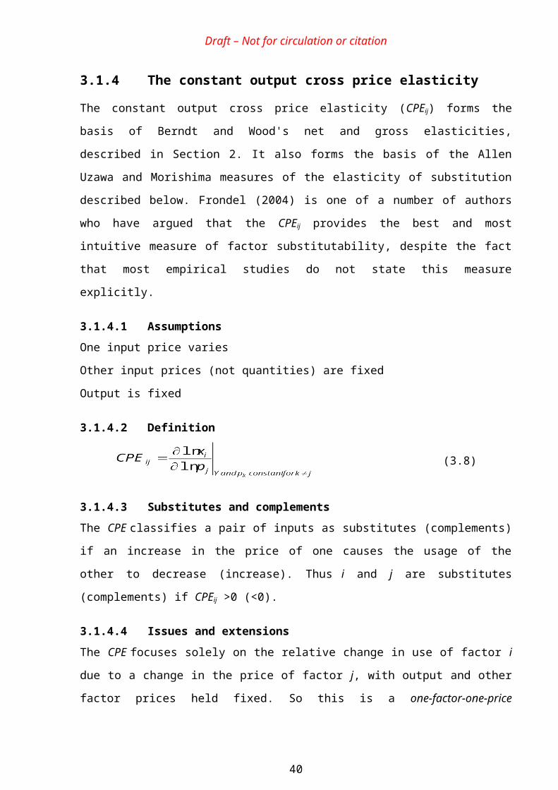
Draft – Not for circulation or citation
The effects of Hicks-Neutral technical change are indiscriminate of factor input, e.g. the
technical change benefits the use of labour equally as much as it benefits the use of capital.
More specifically,
“Hicks neutral technical change shifts the iso-surface parallel toward the origin, and hence decreases the input level of all production factors in the same proportion” (Kako, 1980)
It appears more likely, however, that the effects of technical change over time will serve to be
more beneficial to one factor input than another and should thus be disaggregated to allow for
differentiation across the factor inputs. For instance, it may be found that technical change has
improved capital productivity to a greater extent than labour productivity. Such representations
of technical change are known as ‘factor-augmenting (or non-neutral)’ and may be represented
as follows:26
(3.31)
(3.32)
(3.33)
Where Equations (3.31), (3.32) and (3.33) represent capital augmenting (Solow-Neutral),
labour augmenting (Harrod-Neutral) and energy augmenting technical change respectively.
Many empirical models allow the incorporation of multiple factor augmenting technical
change, as follows:
(3.34)
Alternatively, empirical models may omit technical change altogether. This may be justified if
technical change can be assumed to be separable from the other factors in the production
function; which means that it omission from the functional form should not lead to any bias in
the estimation of the relevant substitution parameters. However, such assumptions are not
always tested and the particular approach taken in an empirical study may have a strong
influence on the results obtained. In general, there appears to be no preferred approach, since
the role technology plays may be expected to vary widely between different agents and over
different time periods.
26 In other words, factor augmenting technical change implies that proportional savings on factor X inputs are greater than the average proportional savings on all inputs.
44
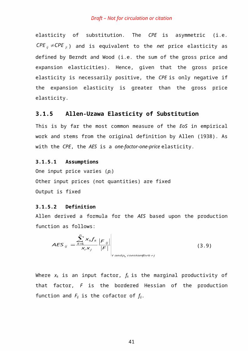
Draft – Not for circulation or citation
A standard assumption in empirical studies is that the rate and bias of technical change is fixed.
But in a long-run relationship, it seems reasonable to expect that changes in relative prices will
stimulate technical change in particular directions, as well as encouraging substitution - i.e.
movements along an existing production function. Induced technical change has become a
central feature of empirical research in this area, but distinguishing between price-induced
factor substitution and price induced technical change is empirically challenging.
3.3 Summary This section has summarised the different definitions of the elasticity of substitution, clarified
the relationship between them and highlighted a number of important issues relevant to
estimating these elasticities empirically. Taken together, the analysis suggests that considerable
caution is required when interpreting the literature in this area. In particular, the different
definitions of the elasticity of substitution, the lack of consistency in the use of these definitions
and the lack of clarity in the relationship between them, all combine to make the empirical
literature both confusing and contradictory.
For all definitions, substitution between two inputs is ‘easier’ when the magnitude of the
elasticity of substitution between them is greater. But the appropriate classification of factors as
substitute or complements depends upon the particular definition being used (i.e. factors may
be substitutes under one measure and complements under another). The majority of existing
empirical studies use the sign of the Allen-Uzawa elasticity of substitution (AES) to make this
classification. However, according to some authors, this measure has a number of drawbacks
and its quantitative value lacks meaning. Furthermore, in many cases, the constant output Cross
Price (CPE) or Morishima (MES) measures may be more appropriate, but these have yet to gain
widespread use. Furthermore, the sign of the MES is less useful as a means of classifying
substitutes and complements, since in nearly all cases the MES is positive. However, the MES
is seen by some authors as more representative of actual economic behaviour since (unlike the
AES) it is asymmetric.
For all definitions, the magnitude of the elasticity of substitution relative to unity can provide
an indication of how cost shares will change following a change in the independent variable.
While the precise interpretation depends upon the definition, the magnitude relative to unity
45
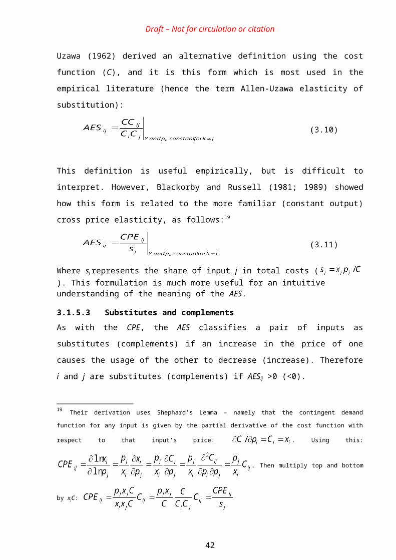
Draft – Not for circulation or citation
may provide an appropriate basis for classifying two factors as either ‘weak substitutes’
(EoS<1) or ‘strong substitutes’ (EoS>1).
A large number of empirical studies estimate elasticities of substitution between different
factors (or groups of factors) within different sectors and countries and over different time
periods. These rely upon a variety of assumptions, including in particular the specific form of
the production or cost function employed (e.g. CES or translog). The estimated values may be
expected to depend in part upon the assumptions made.
Standard methodological approaches rely heavily upon assumptions about the seperability of
different inputs or groups of inputs. These assumptions are not always tested, and even if they
are found to hold, the associated estimates of the elasticity of substitution could still be biased.
Assumptions about the nature and bias of technical change may also have a substantial impact
on the empirical results, but distinguishing between price-induced technical change and price-
induced factor substitution is empirically challenging. The level of aggregation of the study is
also important, since a sector may still exhibit factor substitution in the aggregate due to
changes in product mix, even if the mix of factors required to produce a particular product is
relatively fixed. This suggests that the scope for substitution between energy and capital may
be greater at higher levels of aggregation. However, individual factors cannot always be
considered as independent, notably because energy is required for the provision of labour and
capital. This suggests that the scope for substitution may appear to be smaller at higher levels
of aggregation.
In general, the actual scope for substitution may be expected to vary widely between different
sectors, different levels of aggregation and different periods of time, while the estimated scope
for substitution may depend very much upon the particular methodology and assumptions used.
46
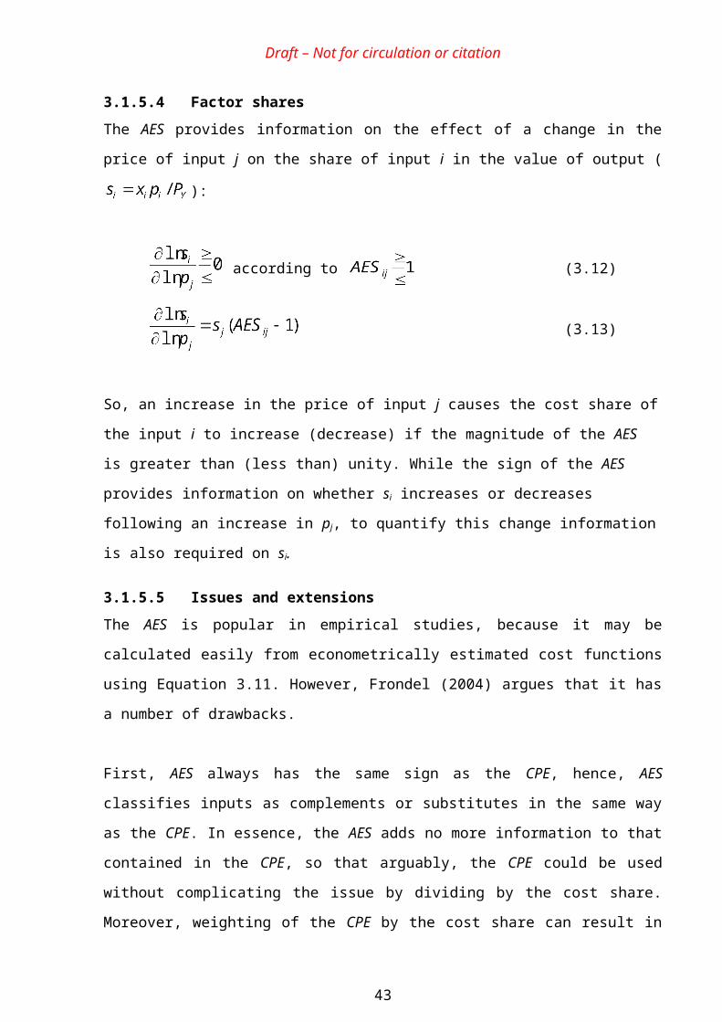
Draft – Not for circulation or citation
4 Empirical estimates of the elasticity of substitution between energy and capital
In Berndt and Wood’s (1975) study of US manufacturing, factors were classified as either
substitutes or complements on the basis of the sign of the AES. The results were:
Capital and Labour: AES substitutes
Capital and Materials: AES substitutes
Labour and Energy: AES substitutes
Labour and Materials: AES substitutes
Energy and Materials: AES substitutes
Capital and Energy: AES complements
Subsequent empirical studies have found broadly comparable results for all of the above factor
pairs except for capital and energy (Chung, 1987). In this case, no consensus appears to have
been reached.
This section summarises the results of a literature search (see Annex 2) on empirical estimates
of the elasticity of substitution between energy and capital (EoSKE). The search was confined to
estimates of the elasticity of substitution between aggregate measures of capital and energy, so
the substitution within and between different types of capital and different types of energy
carrier were not considered.27
The search identified around 100 relevant papers, that included over 200 empirical estimates of
EoSKE. Of these, 7 papers covered or included the UK, including 25 estimates of EoSKE for the
UK. Throughout what follows, energy and capital will be classified as substitutes or
complements according to the sign of the estimated AES or MES in these studies. Since the
overwhelming majority of studies estimate the AES (Section 4.1.6), these dominate the overall
results. However, since studies that used the MES are less likely to classify factors as
complements (Section 3.1.6), this creates a slight bias towards substitutability in the aggregate
results.
27 This type of substitution may nevertheless be important in determining economic behaviour in general and rebound effects
in particular. For example, see Grepperud and Rasmussen (2004)
47
Draft – Not for circulation or citation
Section 4.1 summarises and classifies these results by firstly considering ‘papers’ to identify
the different approaches taken, then by considering the ‘results’; that is classifying the
individual EoSKE estimates. Section 4.2 summarises and evaluates the different reasons that
have been put forward to explain the large variation in the empirical results. The most striking
result from the analysis is the lack of consensus that has been achieved to date, despite the
numerous studies that have been undertaken.
4.1 Summary of results from existing studies
4.1.1 Classification according to papers
In order to demonstrate the key approaches adopted, the following classifies the identified
‘papers’ according to:
Form of production (or cost) function utilised
Form of separability (KLE vs non-KLE28)
Form of technical change adopted (Hicks neutral vs non-nuetral)
Measure of EoSKE adopted
Static vs dynamic model
Type of data (time series vs cross section vs panel)
Countries covered.
Figure 4.1 shows that the overwhelming majority of studies assumed a translog cost function
and estimated the AES using a static29 approach with time series data. About half only included
capital, labour and energy as factors of production (i.e. they omitted materials); about a half
assumed Hicks neutral technical change and just under a half was for the US.
4.1.2 Classification according to estimated results
The above classification gives an indication of the predominant methodologies employed in the
studies reviewed, but in order to try and ascertain the effect of the different approaches the
28 KLE refers to studies that only include capital (K), Labour (L) and Energy (E) in the estimated production functions, whereas non-KLE primarily refers to studies that include K, L, E and Materials (M) in the production function, although there a small number of other variations.
29 Static means that the production function is formed only of ‘current period’ variables, whereas a dynamic model would include information on all or some of the other variables in the past.
48
Draft – Not for circulation or citation
‘results’ from the estimated EoSKE’s are classified. Before that, however, it is useful to consider
the overall results of estimating EoSKE. Figure 4.2 therefore summarises the estimated EoSKE’s
for the overall results (‘world’), as well as for the UK and the US individually. This shows that
the majority of estimates for EoSKE suggest that K and E are weak complements with the
average being something in the order of -0.04 to -0.12 although there is some dispersion around
this which is a little skewed. Not surprisingly, given the large number of estimates, a similar
result is obtained for the US where the average estimated EoSKE is between about -0.03 and -
0.11. However, for the UK the average estimated EoSKE is about 0.4 to 0.9 suggesting that K
and E are substitutes; but this is based on a small number of papers and the results are
dominated by those given in Harris et al (1993).
49
Draft – Not for circulation or citation
Figure 4.1 Classification according to papers
Form of function utilised. Form of separability Form of technical change Measure of σ EK
Static vs dynamic model Type of data Countries
50

Draft – Not for circulation or citation
Figure 4.2 Summary of overall EoSKE Results30
UK
n = 25 mean = 0. 384 median = 0. 911 s.d. = 2. 321
US
n = 108 mean = -0. 04 median = -0. 04 s.d. = 1. 82
World
n = 242 mean = -0. 07 median = 0. 08 s.d. = 2. 034
Another way of presenting these results is given in Figure 4.3. Overall, just over 40%
of the estimates suggest that energy and capital are complements and 60% suggest
they are substitutes. Of the latter, around 60% (representing about 35% of the total)
are less than unity. Hence, 75% of the estimates suggest that energy and capital are
either complements or weak substitutes.
Not surprisingly, there is a similar pattern for the USA. For the UK, however, only a
quarter of the results suggest that energy and capital are complements and nearly a
half suggest that energy and capital are strong substitutes (AES>1).It should be
emphasised, however that these results come from only 7 papers and that about three-
quarters of the estimates derive from Harris et al (1993).
Figure 4.3 Summary of EoSKE results
30 ‘Outliers’, where EoSKE exceeds plus or minus 10 are excluded from the results.
51
Draft – Not for circulation or citation
Behind these aggregate results, however, there are a range of different approaches,
specifications, measurements and so on. Therefore, in order to try and understand the
effect of these, the following sections classify the ‘results’ according to:
Form of production (or cost) function utilised
Form of separability (KLE vs non-KLE)
Form of technical change adopted (Hicks neutral vs non-nuetral)
Measure of EoSKE adopted
Static vs dynamic model
Type of data (time series vs cross section vs panel)
Sector analysed.
For each classification the pie charts (similar to above) are presented plus the means,
medians, and distributions of the estimated EoSKE’s for the overall results and (where
applicable) similar information for the US and the UK. This is followed by a short
discussion.
4.1.3 Functional form
Figure 4.4 Functional form (results)
This shows that, as
with the papers, the
Translog specification
dominates with just
over 80% of the
overall results derived
from this
specification. This is
also true for the US
results and for the UK
all the estimates are
derived from the
Translog
specification. The
52
Draft – Not for circulation or citation
overall mean from the Translog models is about 0.006 (with a median of 0.118)
suggesting that on average K and E are (very weak) substitutes although as can be
seen there is a wide distribution around the average. For the US, the average estimated
EoSKE from using the Translog specification is positive but quite low at about 0.18,
whereas for the small number of UK estimates the distribution is wider with the mean
of the estimates being 0.4 but a much larger median of 0.9 – but again suggesting that
on average K and E are substitutes for the UK. However, these averages here (and
below) must be treated with caution and are only indicative given that the other
factors below are not ‘controlled for’.
For the small number of CES estimates the average overall estimated EoSKE is about
0.5. This suggests that K and E are substitutes, but this is only to be expected given
the construction of the CES function (Annex 1). However, the estimates from the
‘other’ functions suggest that K and E are complements overall with the average
estimated EoSKE between -0.8 and -1.3.
4.1.4 Separability assumptions
Figure 4.5 Form of separability (results)
This shows that about half of the estimates use only KLE in the specification and
about half use KLEM (or similar). This would appear to have an effect on the results
since the average estimated EoSKE for KLE specifications is about 0.4 to 0.5
suggesting K and E are substitutes whereas the average estimated EoSKE for non-KLE
specifications gives a mean of -0.5 and a median of about -0.1 suggesting that K and E
53
Draft – Not for circulation or citation
are complements although the dispersion is a greater. These results are consistent with
the predictions of Frondel and Schmidt (2002), in that the inclusion of materials
appears to make the estimates lean more towards complementarity, possibly because
the cost share for energy is reduced. The KLE formulations may therefore be
vulnerable to omitted variable bias.
This distinction also looks to hold for the US and UK. The average estimated EoSKE
for results from specifications including KLE only are 0.1 to 0.2 and 0.8 to 1.0 for the
US and UK respectively; suggesting K and are substitutes. Whereas the average
estimated EoSKE for results from non-KLE specifications are centred around -0.1 and -
5.0 for the US and UK respectively; suggesting K and E are complements (although
the UK figure is based on only two estimates).
In summary it would appear that the separability assumption does have an impact on
the estimated elasticities. Specifically, when materials are included (i.e a particular
source of omitted variable bias is avoided) there appears to be a greater tendency for
energy and capital to be found to be complements. However, this is again a tentative
conclusion since a range of other factors are not ‘controlled for’.
4.1.5 Assumptions about technical change
Figure 4.6 Form of technical change (results)
The majority of results are based on the assumption of Hicks neutral technical change
although a fair proportion assumed non-neutral (or factor augmenting) technical
54
Draft – Not for circulation or citation
change. Moreover the distributions illustrate that, similar to the issue of separability
above, the assumption about the form of the technical change appears to have an
effect on the estimated results, although the distinction is not so clear. The overall
median of the estimated EoSKE for the Hicks-neutral specifications is 0.2 suggesting K
and E are substitutes whereas the mean is -0.2 suggesting that K and E are
complements. However, results from non-neutral specifications are more consistent
with an average estimated EoSKE of 0.2 to 0.4 suggesting that K and E are substitutes.
This general distinction also appears to be found for the US results, with the average
estimated EoSKE of -1.2 to -2.0 for the neutral specification suggesting strong E-K
complementarily, whereas the estimated EoSKE of 0.03 to 0.4 the non-neutral
specification suggesting E-K substitutability. However, for the UK (with fewer
studies), this distinction is not found with both specifications suggesting E-K
substitutability albeit of different strengths; the average estimated EoSKE for the
neutral specification being 1.3 to 1.5 and for the non-neutral specification 0.1 to 0.8.
In summary, although the different assumptions about technical change appear to
have an effect on the estimated EoSKE’s it is difficult to ascertain a clear pattern and
would appear to depend upon the underlying data generating process.
4.1.6 Definitions of the elasticity of substitution
Figure 4.7 Measure of EoSKE
(results)
This shows that the
vast majority of
results are based on
the Allen measure of
EoSKE with about 6%
based on the
Morishima definition
(and about 8%
derived from a CES
function). Given the
55
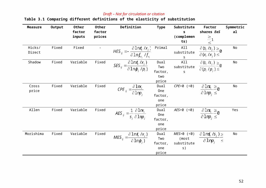
Draft – Not for circulation or citation
relative small number of results not based on the AES, it is not possible to ascertain
any particular strong pattern in the results. The mean of the estimated EoSKE’s for the
overall results is -0.3, suggesting E-K complementarity, whereas the median is 0.02
suggesting (weak) E-K substitutability; but the distribution is skewed somewhat so the
median is probably a better guide suggesting E-K substitutability. Interestingly within
this there is a clear difference between the US and the UK results; the average
estimate of the AESKE for the US is -0.1 to -0.4, suggesting that K and E are
complements, whereas the average estimate of the AESKE for the UK is 0.4 to 0.9,
suggesting K and E are substitutes.
Although based on a relatively small number of results, the average estimated MESKE
is 2.3 to 2.6, suggesting strong substitutability. But this measure is expected to give
higher numerical results than the AES for the reasons described in Section 4. Finally,
the results based on the CES function (which are constrained to be positive and hence
give E-K substitutability) give an average estimated EoSKE of 0.5.31
31 It is worth noting that Thompson and Taylor (1995) re-calculate a large number of MESKE estimates for previous studies that had used the AESKE and find that “out of 148 estimates of the MES only 4 are negative” (p. 566). These results are not included in the above given they use data from previous studies.
56
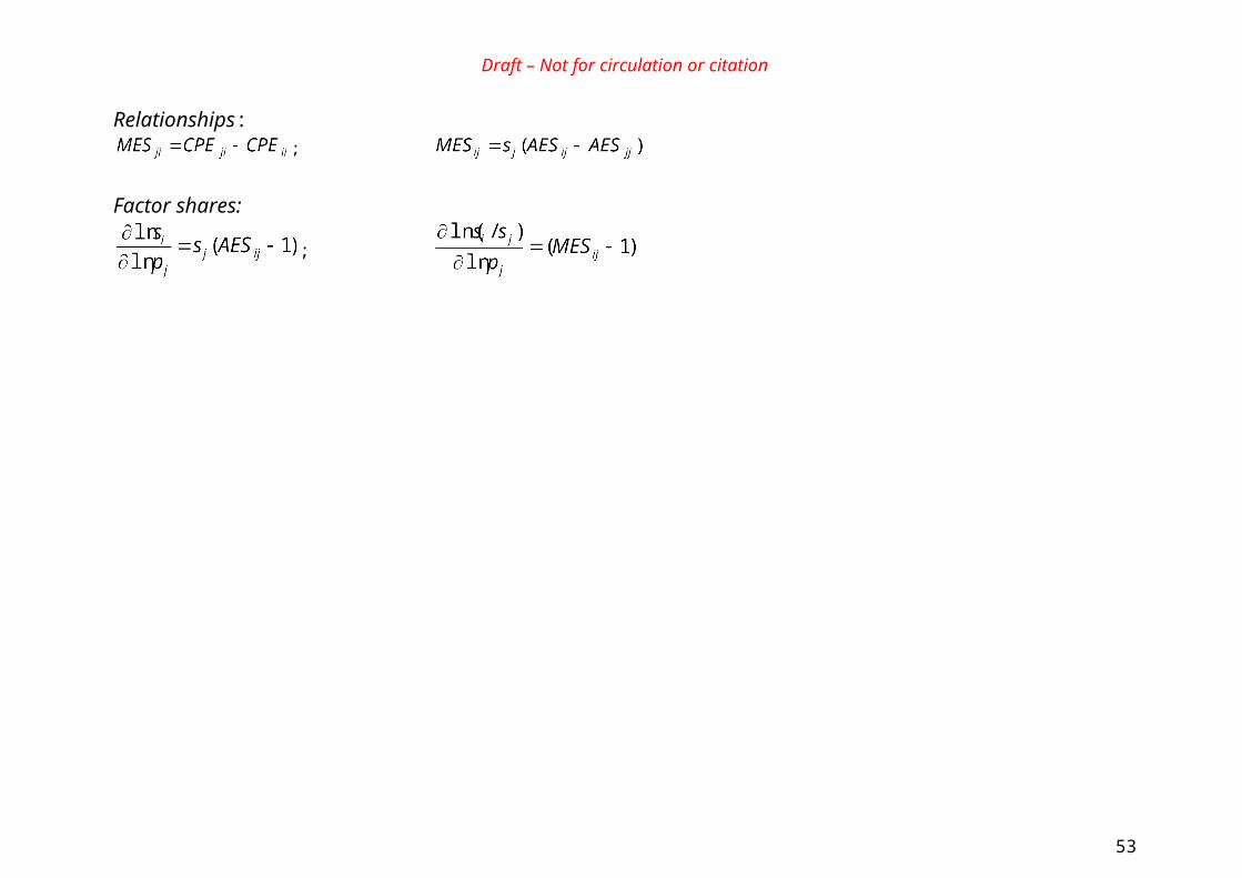
Draft – Not for circulation or citation
4.1.7 Static versus dynamic estimation
Figure 4.8 Static vs Dynamic model (results)
This shows that the results are based overwhelmingly on static models, hence it is not
possible to ascertain any particular pattern given the small number of results based
upon a dynamic specification. The dominance of static models is unfortunate, given
both the advances in time series econometrics and the potential difficulties with static
models highlighted by Frondel and Schmidt (2002).
57
Draft – Not for circulation or citation
4.1.8 Type of data
Figure 4.9 Type of data (results)
This shows that the majority of results derive from single country estimates based
upon time series data. However, about 18% are based upon cross section multi
country studies and about 24% based upon panel multi country studies. When
considering the overall results it would appear that the choice of data is important.
The average for the estimated EoSKE from time series results is -0.1 to -0.4 whereas for
the results from cross-section studies it is 0.4 to 1.0 and for the results from panel
studies it is 0.1 to 0.2. Hence, time series studies on the whole suggest E-K
complementarity whereas the multi country cross section and panel studies suggest E-
K substitutability. While this could be suggestive of greater substitutability in the
long-run (as represented by cross-section studies) compared to the short run (as
represented by time series studies), there are several difficulties with this
interpretation and the result may equally well reflect the more common inclusion of
materials in time series studies (Section 3.2.3).
58
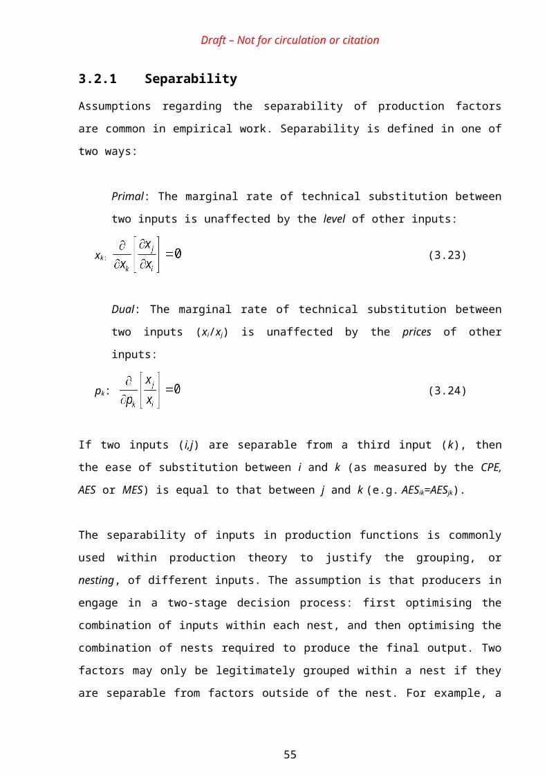
UK Whole Economy UK Manufacturing UK other
n/a n = 3 mean = -2.960 median = -3.401 s.d. = 3.799
n = n/a mean = n/a median = n/a s.d. = n/a
n = 22 mean = 0.840 median = 0.968 s.d. = 1.722
US Whole Economy US Manufacturing US other
n = 5 mean = -0.018 median = -0.140 s.d. = 0.772
n = 82 mean = -0.230 median = -0.144 s.d. = 1.994
n = 21 mean = 0.701 median = 0.475 s.d. = 0.838
World Whole Economy World Manufacturing World other
n = 32 mean = -0.071 median = 0.281 s.d. = 1.674
n = 107 mean = -0.436 median = -0.134 s.d. = 2.528
n = 102 mean = 0.345 median = 0.393 s.d. = 1.373
Draft – Not for circulation or citation
Similar results were found for the US, with an average estimated EoSKE of -0.3 to -0.9
and 0.6 to 1.2 for time series and cross section studies respectively. For the panel
study results from the US, both the mean and median are close to zero but with
opposite signs. No UK distinction is given since all bar one of the UK estimates for
EoSKE come from single country time series studies.
4.1.9 Analysis by sector
Figure 4.10 Sector (results)
Classification of results by sector needs to be viewed with caution since the
interpretation of the distributions and data are not straightforward. The definitions of
sectors are not homogenous with respect to different countries and cannot necessarily
be directly compared on such a basis. As a result, the information presented should be
seen as ‘indicative’ compared to the distributions given in previous figures where it is
clearer how to classify the different groupings. With these caveats in mind the data is
categorised into the two predominant sectors analysed, ‘whole economy’ and
‘manufacturing’, plus ’other’32.
The UK whole economy figures suggest a complementary relationship between K and
E, whereas for the US a weak complementary relationship is suggested, but for the
whole world the distribution is concentrated around zero with a negative mean
32 These other sector cover a range of industries. With too few observations to draw meaningful conclusions on their own, they are bundled together.
59
Draft – Not for circulation or citation
(suggesting complements) but with a positive median (substitutes); although the tail
of the probability goes much deeper into the negative (complements) zone.33 For
manufacturing, no evidence is available for the UK, however the distributions for the
US and the world show reasonable evidence of complementarity, with both the means
and the medians being placed firmly in the negative part of the distribution. The
‘other’ sector however, shows far more consistent evidence of substitutability
between K and E, but again it must be emphasised that, given the way this category is
formed by the bundling together of everything not specifically whole economy or
manufacturing, this should be treated with caution.
4.1.10 Summary
Estimates of the elasticity of substitution between energy and capital appear to be
highly variable between sectors, countries and time periods. The results demonstrate
no clear consensus regarding whether energy and capital may be regarded as either
substitutes or complements. Different studies have analysed different sectors using
different model specifications, data sets and methods of estimation and have often
come to quite different conclusions. While this may be expected if the degree of
substitutability depends upon the sector, level of aggregation and time period
analysed, it is notable that several studies reach different conclusions for the same
sector and time period, or for the same sector in different countries. Perhaps the most
telling example of this is that studies using the original Berndt and Wood (1975) data
have produced 38 different estimates of EoSKE, ranging from -3.94 to 10.84 (Raj and
Veall, 1998).
If a general conclusion can be drawn, it is that energy and capital appear to be either
complements (AES<0) or weak substitutes (0<AES<0.5). If capital and energy are
AES complements, then increases in energy prices are likely to lead to reductions in
capital use as well as energy use, thereby increasing the economic impact of the price
increase. If capital and energy are weak substitutes (i.e. with a small AES), then a
large amount of capital may need to be substituted to maintain a constant flow of
services from capital and energy combined.
33 However, it must be stressed that these distributions are derived from small numbers of observations.
60
Draft – Not for circulation or citation
However, it is clear that the assumptions made by the modellers can have a
considerable influence on the results obtained. Although there are some indications
that the assumptions about separability and technical change may be particularly
significant, it is not possible to come to a definitive conclusion since it is not possible
to control for all the relevant influences.
The following section therefore attempts to classify the reasons suggested in the
literature for the widely different results.
4.2 Possible reasons for the different resultsNot surprisingly, various authors have proposed different reasons for the wide
variation in empirical results for EoSKE. The first notable attempt was that by Berndt
and Wood (1979) who attempted to reconcile their 1975 results of E-K
complementarity for the USA using time series data with that of Griffin and Gregory
(1976) that suggested E-K substitutability based on a multi-country cross section
study. According to Griffin and Gregory, the time series results were estimating the
short run EoSKE whereas the cross section results were estimating the long-run EoSKE.
In contrast, Berndt and Wood (1979) argued that there was an important distinction
between ‘gross’ and ‘net’ substitutes/complements, as described in Section 2. This
debate does not appear to be satisfactorily concluded.
The divergence in results has also been suggested as deriving from: a) differences in
substitution possibilities between different sectors; b) differences in substitution
possibilities between different levels of aggregation (Section 3.2.2); c) inappropriate
seperability assumptions and omitted variable bias (Section 3.2.1); d) differences in
cost shares when static translog cost functions are estimated (Section 3.2.3) and e)
differences in the treatment of technical change. As an example of the latter, Hunt
(1986) and Harris et al (1993) argue that if non-neutral technical change is accepted
by the data then the results of E-K complementarity and substitutability can be
reversed. In a different context, Ochsen (2002) shows that the usual finding of
complementarity between capital and high-skilled labour no longer holds once non-
neutral technological progress is allowed for. However, nearly two thirds of the
61
Draft – Not for circulation or citation
studies reviewed above simply assume Hicks-neutral technical change or ignore it
altogether.
Another explanation is provided by Field and Grebenstein (1980), who suggest that
variations in the definition and aggregation of capital inputs may account for the
different results. The manner in which different types of energy input are aggregated
could also influence the empirical estimates, although this is rarely discussed.
Technical Report 5 demonstrates that the standard method of aggregating energy
inputs on a kWh basis can lead to misleading results and argues instead for ‘quality
weighting’ of energy inputs.
Also, the calculation of the AES depends upon the factor cost shares at every data
point, which may be another reason for divergence given that most studies average the
partial elasticity over time. However, Anderson and Thursby (1986) suggest that this
is the best approach, since the means of factor cost shares are likely to be distributed
normally hence allowing for standard inference. But on the other hand the distribution
of point estimates may not be normal, thereby making inference problematic.
Table 2 attempts to ‘quantify’ the reasons put forward in the reviewed literature for
explaining the different results. This distinguishes what might generally be called
‘data issues’ from ‘technical issues’. This shows that data issues are a commonly cited
reason for differences in estimated results. Furthermore, within the technical issues it
is clear that homogeneity, separability, technical change and functional form are
commonly cited.
Table 4.1 Summary of reasons offered in empirical studies for divergence in model results.
It is our conclusion that there is a
degree of agreement to the possible
causes of the different estimated
elasticities. However, there is no
real consensus on either the relative
importance of different causes, or
(at least in most cases) on the likely
Reason Times citedData Issues;
Relative Factor Shares/Prices 42 Data Type 11 Level of Aggregation 11Technical issues; Homogeneity 21 Separability 18 Technical change 17 Functional Form 10 Dynamic Specification 10 Elasticity Measure Used 4 Other 24Total 16862
Draft – Not for circulation or citation
direction of influence of each individual cause (i.e. whether a particular
specification/assumption is likely to make the estimate of the substitution elasticity
bigger or smaller). Moreover, there is no clear agreement in the literature to what is
the ‘best’ way to proceed in estimating such relationships.
To improve upon this situation, we suggest that a ‘general to specific’ approach be
utilised that ‘lets the data speak’. This means that specific restrictions (such as
homogeneity, Hicks-neutral technical change, separability, etc.) should only be
imposed if they are statistically accepted by the data. This means that issues such as
homogeneity vs heterogeneity, separability vs non- separability, neutral vs non-
neutral technical change and so on need to be tested for and only accepted on
empirical grounds. Similarly, in a time series context, a dynamic model should be
utilised unless a static model (implying that the short-run elasticities are equal to the
long run elasticities) is shown to be statistically accepted by the data. It is to be
expected that different economies and sub-sectors will have different production
structures and it is correspondingly wrong to assume that a particular theoretical
structure will be appropriate in all cases.
Unfortunately, the great majority of the existing empirical studies do not follow these
recommendations. As a consequence many of the estimates reviewed above are likely
to be biased.
Before leaving this overview, it is worth considering two other papers that review
different estimates of EoSKE and address the issue of Allen (AESKE) versus Morishima
(MESKE) elasticities of substitution.
Thompson and Taylor (1995) re-calculate a large number of MESKE estimates for
previous studies that had used the AESKE and find that out of 148 estimates of the MES
only 4 are negative. They conclude from this that capital and energy are MES
substitutes, but this is only to be expected given the definition and behaviour of the
MES, as discussed in Section 3.1.6. Since the MES means something different from
the AES (and CPE) it is arguably inappropriate to use the sign of the MES to
distinguish substitutes and complements in this way. Of perhaps greater interest is
Thompson and Taylor’s finding that for MESKE there is no dichotomy between cross-
63
Draft – Not for circulation or citation
section and time series studies and there is no excessive variability in the quantitative
estimates. The latter may result from the fact that the MES is less sensitive to the
small and variable share of energy in total costs. Thompson and Taylor also find that
the mean estimate of MES is larger when the price of energy adjusts (MESEK=1.01)
than when the price of capital adjusts ((MESKE=0.76), which suggests which suggests
the interesting policy conclusion that an increase in energy prices may induce a larger
improvement in energy efficiency than policies such as investment tax credits.
Koetse et al (2006)34 used 20 of the studies reviewed above and (re)calculated the
MESKE and CPEKE from the estimates provided in the original papers and employed
these in a meta-analysis. Echoing the (questionable) arguments of Griffin and Gregory
(1976), they argue that time series data reflects short run substitution possibilities and
cross-sectional data reflects long-run possibilities. On that basis, the CPE results
suggest that energy and capital are weak substitutes in the short run (0.17) and slightly
greater substitutes in the long-run (0.52). Their meta-analysis also demonstrates that
model assumptions regarding returns to scale, technological change, separability,
aggregation of variables, type of data used and so on, can strongly influence the
estimated results; thus reinforcing the above conclusions.
4.3 SummaryThis section has reviewed empirical estimates of the elasticity of substitution between
aggregate energy and aggregate capital and has explored how these estimates vary
with factors such as the functional form and assumptions regarding technical change.
The most striking result from the analysis is the lack of consensus that has been
achieved to date, despite three decades of empirical work. While this may be expected
if the degree of substitutability depends upon the sector, level of aggregation and time
period analysed, it is notable that several studies reach different conclusions for the
same sector and time period, or for the same sector in different countries.
If a general conclusion can be drawn, it is that energy and capital typically appear to
be either complements (AES<0) or weak substitutes (0<AES<0.5). However, little
confidence can be placed in this conclusion, given the diversity of the results and their
34 This became available after this review had begun.
64
Draft – Not for circulation or citation
apparent dependence upon the particular specification and assumptions used. While
there appears to be some agreement on the possible causes of the different results,
there is no real consensus on either the relative importance of different causes, or the
likely direction of influence of each individual cause (i.e. whether a particular
specification/assumption is likely to make the estimate of the substitution elasticity
bigger or smaller).
A key weakness of many of the existing studies is that specific restrictions (such as
homogeneity, Hicks-neutral technical change, separability) are assumed rather than
statistically tested. This suggests that any future work should ensure that such
assumptions are tested for and only accepted on empirical grounds.
65
Draft – Not for circulation or citation
66
Draft – Not for circulation or citation
5 Elasticities of substitution and the rebound effect
This section explores the relevance of empirical estimates of elasticities of
substitution to the rebound debate. It first summarises the manner in which the
elasticity of substitution has appeared within the rebound literature and then explores
its relationship to the rebound effect in more detail, considering in turn: a) the
relationship between empirical estimates and the requirements of energy-economic
models; b) the importance of seperability assumptions and nesting structures; c) and
the distinction between real and ‘effective’ energy and the appropriate modelling of
technical change.
It is argued that the relationship of this parameter to the rebound effect is more subtle
and complex than is commonly assumed. In particular a finding of limited substitution
or even complementarity between aggregate energy and capital may be entirely
compatible with backfire – the opposite to what some authors have suggested (Jaccard
and Bataille, 2000). Moreover, existing empirical estimates of elasticities of
substitution appear to be of relatively little value for either quantifying rebound
effects or calibrating energy-economic models. Nevertheless, they do suggest that
energy price increases may have a greater effect than is suggested by the small share
of energy in total costs. This arguably reinforces one of the main conclusions of
Technical Report 5 - namely that energy plays a more important role in economic
growth than has traditionally been assumed.
5.1 Elasticities of substitution in the rebound literature
Statements regarding the magnitude of the elasticity of substitution between energy
and other inputs appear regularly in the rebound literature. For example:
“It appears that the ease with which fuel can substitute for other factors of production (such as capital and labour) has a strong influence on how much rebound will be experienced. Apparently, the greater this ease of substitution, the greater will be the rebound” (Saunders, 2000, p. 443).
67

Draft – Not for circulation or citation
However, the relationship between this parameter and the magnitude of rebound
effects is more subtle than it first appears.
The primary reason for the prominence of the elasticity of substitution in the rebound
debate is the attention paid to it by Harry Saunders (1992; 2000b; 2005; 2006b). As
discussed in Technical Report 5, Saunders has made a significant contribution to the
rebound literature by using neoclassical production theory and neoclassical growth
theory to explore the consequences of ‘energy augmenting technical change’, which
improves the productivity of energy imports. For example, Saunders (1992) uses an
aggregate CES production function within a neoclassical growth model to show that
both neutral and energy augmenting technical change will lead to backfire if the HES
between energy and a composite of non-energy inputs is greater than unity (i.e. if
energy is a strong substitute for other inputs). In more recent work with a range of
functional forms, Saunders (2006b) again shows that elasticities of substitution appear
to be a key determinant of rebound effects.
Saunder’s results suggest that a high HES between energy and a composite of other
inputs could lead to large rebound effects, while a small HES could lead to small
rebound effects. Following this lead, Jaccard and and Bataille (2000) use a technology
simulation model to estimate an economy-wide value for the HES between energy and
capital for the Canadian economy (i.e. not necessarily the same thing). Finding a
fairly low value of 0.24, they conclude that rebound effects should be relatively small.
However, as argued below, this conclusion is possibly oversimplified and possibly
incorrect.
A second reason for the prominence of elasticities of substitution in the rebound
debate is the role they play in determining the results of Computable General
Equilibrium (CGE) models of the macroeconomy. The economy-wide impact of
energy efficiency improvements cannot be adequately captured within a partial
equilibrium framework, but may be usefully explored through a CGE approach.
However, the realism and policy relevance of CGE models is the subject of fierce
debate, with different models producing widely varying results for very similar policy
questions (Greenaway, et al., 1992; Barker, 2005).
68

Draft – Not for circulation or citation
The CGE literature on rebound effects is reviewed in detail in Technical Report 4. A
key conclusion from this review is that the assumptions made for the elasticities of
substitution between energy and other factors of production, as well as between
different types of energy carrier, can have a profound influence on the model results.
As an illustration, Grepperud and Rasmussen (2004) estimate rebound effects to be
higher in the Norwegian primary metals sector than in the fisheries sector, owing
largely to the greater opportunities for factor substitution in the former (Grepperud
and Rasmussen, 2004).
However, elasticities of substitution are normally specified exogenously and can vary
significantly from one CGE model to another. In principle, these parameters are
established through careful surveys of relevant empirical literature, but in practice, the
time periods, regions and sectors on which this literature is based may not be
appropriate to the model application and there may also be substantial differences
between empirical studies and model requirements in areas such as the aggregation of
different inputs and the functional form of production functions. Furthermore the
process of compiling parameter values is rarely transparent, sensitivity tests are
uncommon and the modelling usually rests on the implicit assumption that such
parameters will remain stable over time. All these features suggest that the results of
such models should be interpreted very cautiously.
The CGE literature also suggests that the scope for substitution between energy and
other inputs has a major influence on the cost of reducing carbon emissions.35 This
makes the elasticity of substitution between energy and non-energy inputs ( ) a
critical parameter in such models and suggests a potential policy trade-off:
“…If one believes is low, one worries less about rebound and should incline towards programmes aimed at creating new fuel efficient technologies. With low carbon taxes are less effective in achieving a given reduction in fuel use and would prove more costly to the economy. In contrast, if one believes is high, one worries more about rebound and should incline towards programmes aimed at reducing fuel use via taxes. With high , carbon taxes have more of an effect at lower cost to the economy.” (Saunders, 2000b)
However, Allan et al (2006) argue that this conclusion may be oversimplified:
35 For an insightful discussion of this point, see Hogan and Manne (1970).
69
Draft – Not for circulation or citation
“ ….the conclusion that there is consequently a key policy trade-off, so there if this elasticity of substitution is low one worries less about rebound…. is strictly incorrect. The problem here is that rebound... does not depend only on the elasticity of substitution of energy for other inputs. Indeed, even if this elasticity is precisely zero, as with Leontief technology, rebound and backfire remain perfectly feasible conditions, if less likely. There appears to be a widespread, but mistaken, belief in the literature that low elasticities of substitution between energy and other inputs imply that rebound must be small and backfire impossible.” (Allan, et al., 2006)
The point here is that substitution effects are isolated by holding output constant. But
in practice, output will not be fixed and the net effect of an energy efficiency
improvement on the demand for factor inputs (including energy) will depend upon the
overall reduction in production costs and the price elasticity of output (at least at the
level of individual sectors). This will tend to increase energy demand further than is
indicated by the substitution effects alone, so the rebound effect will be larger. The
overall rebound effect will therefore also depend upon the cost share of energy and
the price elasticity of the relevant product. Similar observations are made by
Grepperud and Rasmussen (2004):
“Our analysis has shown that significant rebound effects are at work in industries with limited substitution possibilities (metals) and that rebound effects can be weak in spite of a flexible technology (chemical and mineral products). The degree of substitutability among inputs (or aggregation level) is important but not essential for the results arrived at. An equally important factor is the degree to which the activity level in a sector is affected by efficiency improvements. The rebound that originates from this activity effect is not given sufficient attention in the literature.” (Grepperud and Rasmussen, 2004)
Nevertheless, both Saunders’ work and the CGE literature suggests that a better
understanding of elasticities of substitution could offer some insight into the likely
magnitude of rebound effects in different circumstances. Unfortunately, the
parameters estimated in the empirical literature and reviewed in Section 4 may not be
as useful for this purpose as may be expected.
5.2 Empirical estimates and modelling requirementsThe first problem is that empirical studies frequently differ from theoretical/modelling
studies along a number of dimensions, thereby creating problems in using empirical
estimates to infer appropriate parameter values for CGE models. In particular
modelling studies:
70
Draft – Not for circulation or citation
frequently differ from empirical studies in the manner in which individual
inputs are aggregated and in the level of sectoral aggregation.
frequently assume seperability between different groups of inputs, while
empirical studies do not.
normally use the nested CES functional form, while empirical studies
generally use less restrictive functional forms such as the translog.
frequently require estimates of the elasticity of substitution between nests of
inputs, while the parameters estimated by most empirical studies relate to
individual pairs of inputs.
define production functions by means of the HES, while empirical studies
normally estimate the AES, the CPE or the MES.
The differences in functional form and in the definitions of the elasticity of
substitution deserve further examination. Blackorby and Russell (1981) show that the
AES, MES and HES are identical if (and only if): a) there are only two inputs to the
production function; b) the production function has a Cobb Douglas structure; or c)
the production function has a non-nested CES structure. The two-input case is of no
interest for our purposes, while the Cobb-Douglas structure is excessively restrictive
since it assumes that all inputs are substitutes with an elasticity of substitution equal to
unity.36 Of potentially greater interest is the non-nested CES structure, which
combines factor inputs in the following way (McFadden, 1963):
(5.1)
With this structure, the HES (and also the AES and MES) between all inputs is
identical and greater than zero - implying that all inputs are equal substitutes for each
other. This appears unlikely in practice and also excludes the possibility of
complementarity (i.e. AES<0) between factor inputs.
In order to provide greater flexibility in substitution possibilities, most CGE models
use a nested CES functional form, in which pairs of inputs are combined together in a
36 Despite the obvious limitations of the Cobb Douglas formulation, it is still widely used.
71
Draft – Not for circulation or citation
CES function, which then combines with another factor in a second CES function
(Sato, 1967). For example, a KLEM production function could take the form:
(5.2)
Which may also be written as:
(5.3)
This is called a two-level nested CES because it contains CES production functions
for two intermediate inputs (K* and L*) embedded within a CES production function
for aggregate output (Y). The intermediate inputs in this case are a composite of
capital and energy inputs (‘utilised capital’ – K*) and a composite of labour and
materials inputs (L*), which are assumed to combine with each other to provide the
final output (Y). The assumption is that producers engage in a two-stage decision
process: first optimising the combination of factors required to produce utilised
capital and the labour/materials composite, and then optimising the combination of
these composite inputs required to produce the final output. The relevant CES
functions are:
(5.4)
(5.5)
(5.6)
The nesting structure (although not the functional form) is the same as used by Berndt
and Wood (1979) and described in the graphical example of Section 2. As discussed
in Sections 2 and 3, this type of production function rest on the assumption that
utilised capital (K*) is separable from the labour/materials composite (L*), which may
not be correct (Berndt and Christensen, 1973). Alternative nesting schemes (such as
(KL)(EM) or (EL)(KM)) are available and the choice between them in CGE models
may be made on theoretical grounds or (less commonly) tested empirically (Kemfert,
1998).37 If a distinction is made between different types of capital, labour or energy
37 For example, van der Werf (2006) tests different nesting structures for a KLE CES production functions for OECD manufacturing and finds that a (KL)E structure is preferred.
72
Draft – Not for circulation or citation
inputs (e.g. electricity and non-electricity), a multilevel CES can be formed, with more
than one function nested within the original one (Chang, 1994).
With a nested CES structure, the AES between a pair of inputs belonging to different
nests is equal to the HES between the nests. In fact, the equality of the AES between
pairs of inputs in different nests is a general result for a production function in which
one nest of inputs is separable from a second group (Berndt and Christensen, 1973).
For example, for the (KE)(LM) nesting structure implies that: AESKL = AESKM = AESEL
= AESEM.. In the case of a nested CES function, these are also equal to HESK*L*.
In contrast, with a nested CES structure the AES between a pair of inputs belonging to
the same nest is not equal to HES between those inputs. Indeed, while two inputs
within an individual nest are necessarily HES substitutes, they may at the same time
be AES complements. This is precisely what Berndt and Wood (1979) showed in their
illustrative example, where capital and energy combine in an individual nest and are
shown to be AES complements. The AES between these two inputs is only equal to the
HES if the output of the nest is held constant (K*). In Berndt and Wood’s terminology,
the gross elasticity between these two inputs (with the output of the nest held
constant) is different from the net elasticity (where the output of the nest, K*, is
allowed to vary, while still holding output, Y, constant). Again, this inequality of
gross and net elasticities is a general result for a production function in which one nest
of inputs is separable from a second group.
Sato (1967) has shown how the AES between a pair of inputs belonging to the same
nest depends upon the HES within the nest, the value share of that nest and the HES
between the nests. This is analogous to Equation 2.14, which relates Berndt and
Wood’s net price elasticity and gross price elasticity (Anderson and Moroney, 1994).
For example, in the case of capital and energy, with the production structure given by
Equation 5.2 ((KE)(LM)) it may be shown that (Sato, 1967):38
(5.7)
38 Substituting parameter values gives:
73

Draft – Not for circulation or citation
Hence, it is possible for to be negative (i.e. capital and energy to be AES
complements) even if is positive (i.e. capital and energy are HES substitutes
in the subfunction) and is positive (i.e. utilised capital and the
labour/materials composite are HES substitutes in the master function). This will
occur when - or in other words, when the scope for substitution
between utilised capital and the labour/materials composite is greater than the scope
for substitution between energy and capital in the production of utilised capital.
The main point is that empirical estimates of the AES between two inputs do not
easily translate into the HES parameters required for the nested CES production
functions used in CGE models. If the seperability assumptions were valid, a particular
nested CES could be parameterised if the function was estimated directly. But the
majority of empirical studies estimate translog rather than nested CES functions and
do not impose seperability restrictions. Moreover even if seperability restrictions are
imposed with a translog, these do not ensure that estimates of the AES between two
factors are invariant to the price of other factors. This requires Frondel and Schmidt’s
(2004) stricter condition of ‘empirical dual seperability’. Furthermore, even if
empirical dual seperability is found to hold, the implied nesting structure may not
correspond to that required within a particular energy-economic model. The links
between empirical estimates of elasticity the substitution and the values required by
CGE models therefore appears to be fairly tenuous.
The diversity of approaches to factor nesting is illustrated in Table 5.1, which
compares nesting structures and assumed values of elasticities of substitution in a
number of contemporary CGE models. Over half of these models exclude materials
inputs, so therefore implicitly assume that these are separable from other inputs.
These models vary further in terms of how they disaggregate and nest individual
inputs (e.g. fuel and electricity) and how they model technical change. The basis for
the assumed values for the HES between different inputs and nests of inputs is rarely
made clear and the values chosen appear to vary widely between different models
(although in all cases, the HES are assumed to be less than or equal to unity).
74
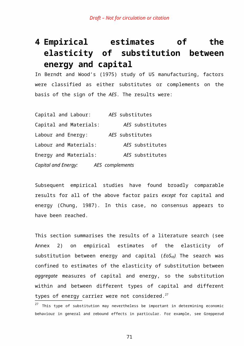
Draft – Not for circulation or citation
Table 5.1 Nesting structures and assumed elasticities of substitution in contemporary CGE models
Authors Nesting structure
Assumed values for HES
Bosetti et al (KL)E HESK,L=1.0HESKL,E=0.5
Burniaux et al (1992) (KE)L HESK,E=0 or 0.8HESKE,L=0 or 1.0
Edenhofer et al (2005) KLE HESK,L,E=0.4Gerlagh and van der Zwaan (2003) (KL)E HESK,L=1.0
HESKL,E=0.4Goulder and Schneider (1999) KLEM HESK,L,E,M=1.0Kemfert (2002) (KLM)E HESKLM,E=0.5Manne et al (1995) (KL)E HESKL=1.0
HESKL,E=0.4Popp (2004) KLE HESK,L,E=1.0Sue Wing (2003) (KL)(EM) HESK,L=0.68 to 0.94
HESE.M=0.7HESKL,EM=0.7
Source: van der Werf (2006)
5.3 Seperability assumptions, nesting structures and energy services
There is a comparable gap between the focus of empirical studies and the
requirements of Saunders’ theoretical models. Saunders (1992; 2006b) follows Hogan
and Manne (1970) in adopting a three factor CES production function in which
energy combines with a composite of capital and labour inputs (‘value added’). The
elasticity of substitution between capital and labour is assumed to be unity (i.e. a
Cobb Douglas function) and ‘energy efficiency’ improvements are represented by a
multiplier for energy augmenting technical change ( ):39
(5.8)
Saunders then examines the conditions under which energy augmenting technical
change will lead to absolute reductions in energy consumption and concludes that this
will only occur when the magnitude of the HES between energy and the capital-labour
composite ( ) is less than unity. This conclusion depends upon the
particular nesting structure assumed and Saunders (1992) argues that alternative
39 See Technical Report 5 for definitions and further discussion.
75
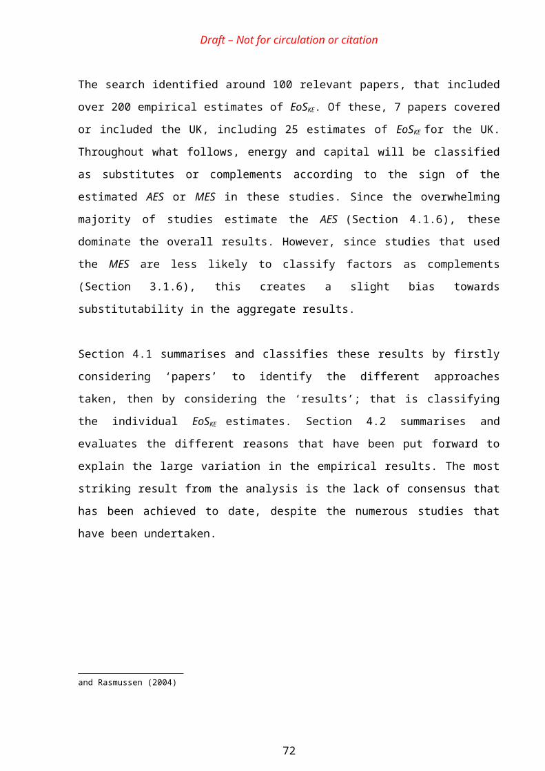
Draft – Not for circulation or citation
nesting structures of the same function (i.e. (KE)L and (LE)K) will always lead to
backfire, regardless of the HES between the nests.
Since capital and energy are in separate nests in this formulation, the AES between
them should be equal to the HES between the nests. This suggests that an estimate of
the AES between capital and energy could provide some information on the likelihood
of backfire. But this result depends (amongst other things) upon the particular nesting
structure that is assumed - and hence on the validity of the seperability assumptions.
The implication of Saunders’ nesting structure is that the AES between energy and
capital is the same as that between energy and labour (Berndt and Christensen, 1973).
But most empirical estimates with translog cost functions find these parameters to be
different, suggesting that the (KL)E nesting structure is a poor representation of actual
production relationships.
The implications of this may be made clearer by reconsidering Berndt and Wood’s
(1979) graphical illustration of energy-capital complementarity that was summarised
in Section 2. This assumed a (KE)(LM) nesting structure, since this was the only
seperability restriction that was supported by Berndt and Wood’s (1975) data.40 In
contrast to Equation 5.8, this has energy and capital in the same nest. For the purposes
of exposition, this graphical example may be taken as illustrative of the behaviour of a
(KE)(LM) nested CES function under the assumption that .
Although Berndt and Wood (1979) do not use the term, their graphical exposition also
provides a useful illustration of rebound effects. Their independent variable is a
reduction in the cost of capital, such as could be achieved through the introduction of
investment tax credits or accelerated depreciation allowances. This encourages a
substitution between capital and energy in the production of ‘utilised capital’ (Figure
2.4). If energy efficiency (or energy productivity) for this sub-function is defined as
the ratio of utilised capital output to energy inputs (K*/E), then the energy productivity
of the sub-function has increased as a result. But an improvement in some measure of
40 Various seperability assumptions may be tested by imposing restrictions upon the parameter values in the translog cost function.
76
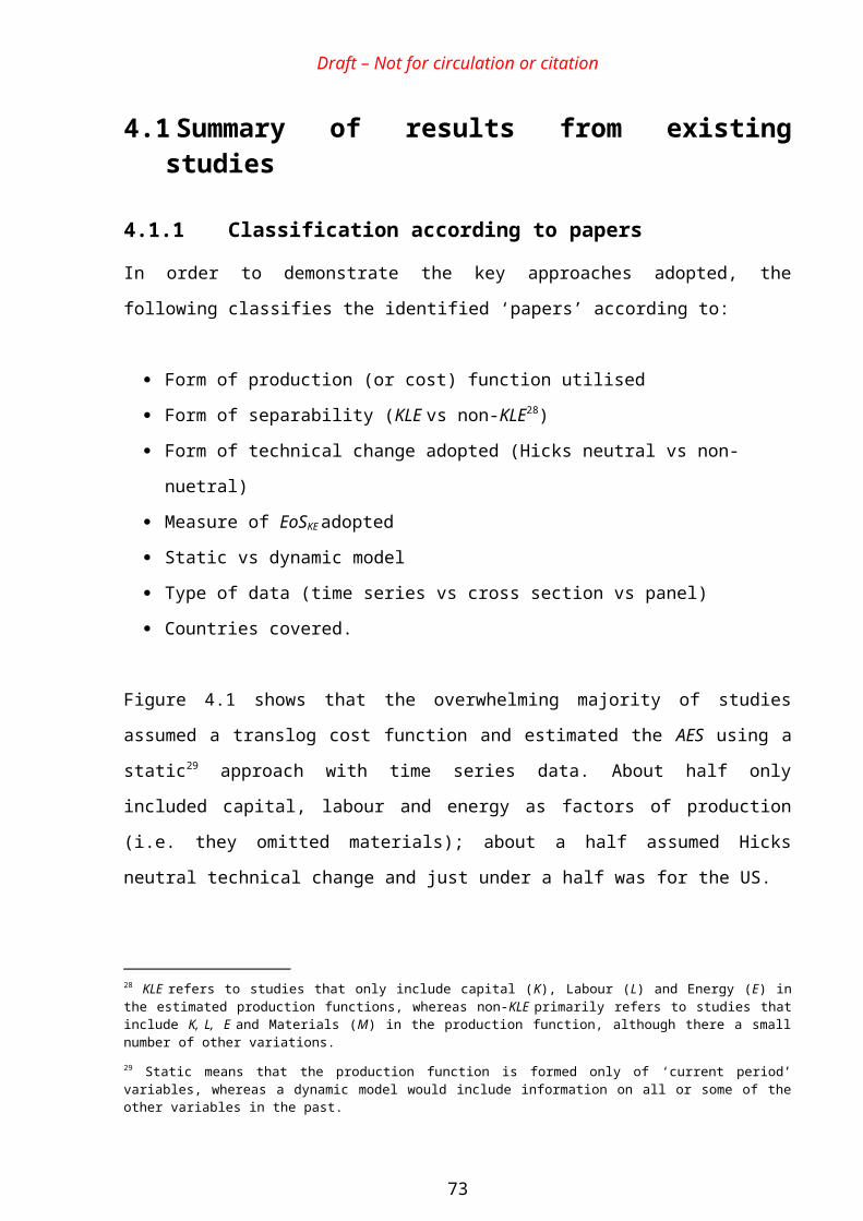
Draft – Not for circulation or citation
energy efficiency, or energy productivity, is also the relevant independent variable for
the rebound effect.41
The reduction in the cost of capital leads to a corresponding reduction in the cost of
utilised capital and hence an increase in demand for utilised capital – even while
output is held constant. The corresponding increase in energy consumption offsets the
reduction in energy consumption brought about by the energy efficiency
improvement. In Berndt and Wood’s example, overall energy demand is increased
since the expansion elasticity is greater in magnitude than the gross price elasticity.
This means that energy productivity (Y/E) for the producer as a whole has fallen, even
though energy productivity in the production of utilised capital (K*/E) has increased.42
Put another way, their results suggest that ‘energy efficiency’ improvements
stimulated by policies such as investment tax credits are likely to lead to backfire.43
In Berndt and Wood’s example, if substitution between capital and energy is large
(small) compared to the substitution between utilised capital and the labour/materials
composite, then the rebound effect (holding output constant) should be small (large).
Put another way, if the gross price elasticity is large (small) compared to the
expansion elasticity, then the rebound effect should be small (large). The expansion
elasticity, in turn, is given by the product of the own price elasticity for utilised capital
(assuming fixed output) and the cost share of the factor whose price has changed
(Equation 2.12). This relates to the more general conclusion from the rebound
literature, that rebound effects are large when the demand for ‘energy services’ is
elastic. In this case, ‘energy services’ is another name for the capital/energy
composite that Berndt and Wood term utilised capital (K*).
But while the Berndt-Wood example gives some insight into the determinants of the
rebound effect, it appears to contradict Saunders’ conclusion that rebound effects will
be small (large) when the substitution between energy and other factor inputs is also 41 In practice, this may have been achieved through the use of technologies which are more thermodynamically efficient than those used previously (e.g. energy efficient motors), or it may been achieved through other means such as a reduction in the ‘quality’ of the energy service, while maintaining the same level of ‘useful work’. For a full discussion of the different definitions of these terms, see Technical Reports 2 and 5.42 It follows that an increase in energy prices would improve energy productivity in the production of utilised capital (through the substitution of capital for energy inputs), but reduce overall energy productivity (Y/E) owing to the additional substitution of labour/materials for utilised capital.43 The results are based on data for US manufacturing over the period 1947-71 and therefore exclude the energy price rises following the oil shocks of the 1970s.
77

Draft – Not for circulation or citation
small (large). In the example given above, the AES between energy and capital is
small (i.e. they are complements), but at the same time the rebound effect is large.
The difference is due to the fact that Saunders’ bases his conclusion on a different
nesting structure which relies upon different assumptions about seperability. In
Saunders’ (KL)E case, the key variable is the HES between energy and a composite of
capital and labour inputs. Given the seperability assumptions, this is the same as the
HES between energy and capital which in turn is the same as the AES between energy
and capital. In contrast, in Berndt and Wood’s (KE)(LM) example, the key variable is
the magnitude of the HES between energy and capital relative to the HES between
utilised capital and the labour/materials composite. Taken together, these two
variables determine the AES (or net elasticity) between capital and energy and this is
different from the HES (or gross elasticity) between capital and energy in the utilised
capital nest.
In Berndt and Wood’s example, the large HES between utilised capital and the
labour/materials composite leads to a large increase in the demand for utilised capital
following the reduction in capital costs. The resulting increase in energy demand is
more than sufficient to offset the original reduction in demand brought about by the
substitution of capital for energy inputs (i.e. the improvement in energy productivity
in sub-function for utilised capital). But the high degree of substitution between
utilised capital and the labour/materials composite is also what is responsible for the
finding of energy-capital complementarity. Hence, in these circumstances empirical
findings of energy-capital complementarity for a particular sector appear consistent
with the potential for large rebound effects, or even backfire.
Saunders’ conclusion may be reconciled with Berndt and Wood’s example if the
former is reinterpreted as applying to the HES between ‘energy services’ and a
composite of other inputs. If energy services are highly substitutable for the
composite of other inputs, then reductions in the cost of energy services will lead to
substantial increases in the demand for energy services. The magnitude of the rebound
effect will be determined in part by the own price elasticity of energy services
(holding output constant), which in a nested CES function will be determined by the
HES between energy services and the composite of other inputs. However, just as
78
Draft – Not for circulation or citation
Saunders’ original conclusion only applies if energy is separable from other inputs,
this revised interpretation only applies if energy services are separable from other
inputs
In the Berndt and Wood example, ‘energy services’ are derived from a composite of
capital and energy inputs, for which they use the term ‘utilised capital’. This
framework allows energy and capital to be found to be AES complements, while the
high substitutability between energy services and a composite of other inputs leads to
high rebound effects – as Saunders predicts. But in general, the provision of ‘energy
services’ (S) is likely to require capital, labour and energy inputs, with additional
capital, labour and materials being required for the provision of final output. For
example, a combination of the boiler and fuel inputs may provide steam (energy
services) to drive separate production processes. This suggests a more general nested
production function of the form:
(5.9)
In principle, this framework allows more targeted policies to be explored. For
example, suppose we were interested in the effect on energy demand of an investment
tax credit targeted on the capital equipment used to provide energy services (KS).
Using Equation 2.14, the effect of this tax credit on energy demand, holding output
constant, will be given by:
(5.10)
: price elasticity of energy with respect to the price of energy services
capital ( , holding energy services demand (S) constant.
: own price elasticity of energy services, holding output (Y) constant
: share of capital costs in the total cost of energy services.
Then backfire will occur when
79
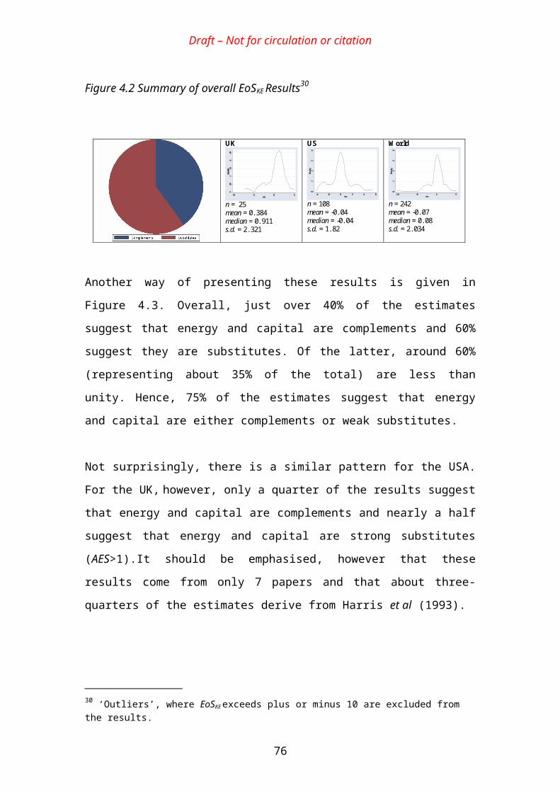
Draft – Not for circulation or citation
In principle an empirical test of Saunders prediction could be made through a
measurement of the AES between energy services and a composite of other inputs
under conditions where the (KLM)S seperability assumptions are demonstrated to hold
(i.e. AESSK = AESSL = AESSM.). But existing empirical studies measure energy rather
than energy services and estimate the AES between energy and individual inputs
without imposing any seperability restrictions. This means that the available
measures of the relevant elasticities of substitution do not provide a definitive guide to
the likely magnitude of rebound effects.
Once seperability restrictions are removed, the relationship between the measured
elasticities of substitution and the magnitude of the rebound effect becomes far more
complex. In recent (unpublished) work, Saunders has shown that the magnitude of the
rebound effect with a translog cost function is a complex function of the elasticities of
substitution between each pair of inputs, together with the cost shares of each input:
(5.11)
Hence, if production behaviour can be represented by a translog cost function, the
magnitude of the elasticities of substitution between each pair of inputs may play an
important role in determining the magnitude of any rebound effects. However, since
different combinations of these elasticities may lead to high or low rebound effects in
different circumstances, the situation is far more complex than suggested by the
Manne Richels nested CES production function. It is also more complex than is
suggested by a number of statements in the rebound literature. Notably:
The AES between each pair of inputs becomes relevant and not just that
between energy and a composite of other inputs.
A finding that energy is a weak AES substitute for another factor, or even a
complement to that factor, is not necessarily inconsistent with the potential for
large rebound effects, or even backfire.
80
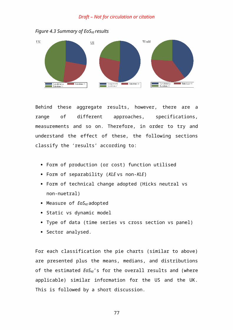
Draft – Not for circulation or citation
5.4 Technical change and ‘effective energy’The importance of distinguishing between ‘energy services’ and raw energy inputs is
further complicated by the appropriate treatment of technical change.
The Berndt and Wood example of rebound effects describes a substitution between
(all types of) capital and energy in the production of utilised capital, brought about by
a reduction in capital costs. The reframing of this example in terms of energy services
shows how it may be relevant to energy efficiency policies that target investment
subsidies at energy efficient equipment. But such policies are only desirable if they
overcome the market failures inhibiting the adoption of energy efficient technologies
cost effectively. If not, they may be may be costly to the economy overall. More
generally, the concern is with the rebound effects that may result from energy
augmenting technical change.44 These improvements are assumed to occur
independently of any changes in relative prices and are considered desirable since
they increase aggregate income. While the substitution effects brought about by the
investment subsidy may be represented by a movement along an isoquant of the
production function for utilised capital, ‘technical change’ refers to the development
of new technologies and methods of organisation that shift the isoquant to the left,
allowing the same level of utilised capital to be produced from a lower level of energy
and/or capital inputs. Energy augmenting technical change reduces the amount of
energy inputs required to produce a unit of utilised capital, but has no effect on the
amount of capital required. In Equation 5.8, it is represented by the parameter .
While Saunders (1992) refers simply to energy or fuel, Saunders (2006a) refers to the
product in Equation 5.8 as ‘energy services’. This suggests a distinction
between the energy inputs to a conversion device (e.g. the coal used by a boiler) and
the ‘energy service’, or ‘useful work’ outputs (e.g. the steam that is produced).
However, in thermodynamic terms this is potentially misleading since the ‘energy
service’ outputs ( ) are greater in magnitude than the energy inputs (
since ). An alternative terminology, frequently used with CGE
models is to refer to the product as ‘effective energy’ ( ). The improvement in
44 The terms ‘energy augmenting technical change’ and ‘energy saving technical change’ have precise definitions in the literature and are not necessarily equivalent. For a full discussion, see Technical Report 5.
81
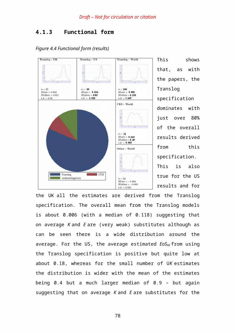
Draft – Not for circulation or citation
the productivity of energy inputs (E) that result from technical change is then
expressed increase in the quantity of effective energy inputs ( ). Hence, to examine
the implications of technical change and to be consistent with standard terminology,
the term ‘energy services’ in the preceding section should really be replaced with
‘effective energy’. This gives the following production function:
(5.12)
With this approach, the production function represented by Equation 5.9 maps the
relationship between effective factor inputs and economic output rather than real
factor inputs and economic output. The location and shape of the individual isoquants
are assumed to be fixed over time, with energy augmenting technical change reducing
the amount of real energy required to produce a unit of effective energy. Since this
reduces the cost of effective energy, technical change leads to substitution between
effective energy and other inputs. The factor augmenting perspective therefore allows
technical change to be viewed as movement along an isoquant of a production
function (i.e. substitution) as opposed to a leftwards shift of an isoquant.
The implicit assumption of this perspective is that energy augmenting technical
change is costless and is achieved without labour and capital inputs. But as suggested
above, the provision of ‘effective energy’ is likely to require dedicated capital, labour
and energy inputs and may better be represented by a sub-function. Howarth (1997)
explores the implications of this framework by simulating the provision of effective
energy inputs with a Leontief (i.e. fixed proportions) production function. The results
suggest that the size of the rebound effect depends upon the share of effective energy
in total output costs, and the share of energy costs in the total cost of effective energy.
Since both of these are likely to be small, Howarth concludes that rebound effects are
also likely to be small – even if the HES between (separable) effective energy and
other inputs equals (or exceeds) unity. However, Saunders (2000a) shows that these
results stem entirely from Howarth’s assumption of a Leontief production function for
the provision of effective energy. If the production function is assumed instead to take
a Cobb Douglas form, energy productivity improvements are found to lead to
backfire.
82
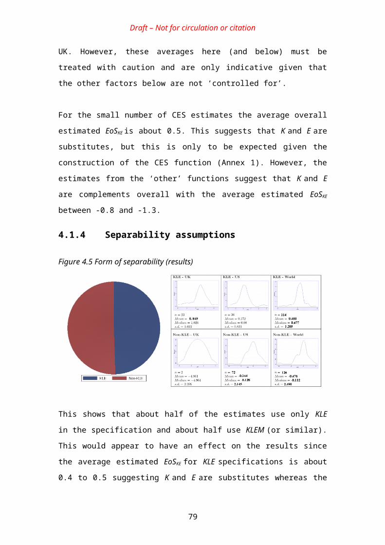
Draft – Not for circulation or citation
The implications of technical change therefore depends upon the scope for
substitution between effective energy and other inputs (assuming these are separable)
and therefore on the estimated value of AESS,KLM. However, empirical estimates of
elasticities of substitution depend upon the assumptions made for the magnitude and
bias of technical change – i.e. the relative contribution of neutral, labour augmenting,
capital augmenting and energy augmenting technical change. The estimated value of
AESS,KLM will only be accurate if the bias is estimated accurately. As an illustration,
Smithson (1979) estimates a translog cost function for the Canadian mining industry
and finds that energy and capital appear to be more complementary if neutral
technical change is imposed then if factor augmenting technical change is allowed. In
practice, however, nearly two thirds of the empirical studies reviewed in Section 4
either assume neutral technical change or ignore technical change altogether. This
suggests that the resulting estimates of the AES between different inputs could be
further biased by the failure to correctly specify the bias of technical change. This
may further limit the usefulness of empirical studies for either parameterising CGE
models or for providing insights on the likely magnitude of rebound effects in
different sectors.
5.5 Summary The implications of the preceding sections are rather disappointing, since they suggest
that the empirical literature on elasticities of substitution may be of relatively little
value in either parameterising CGE models or in providing guidance on the likely
magnitude of rebound effects.
With regard to the requirements of CGE models, most empirical studies differ with
regard to the assumed functional form, the assumptions regarding seperability, the
associated nesting of production factors, the definitions of elasticity of substitution,
the aggregation of individual factor inputs and the aggregation of individual sectors.
Combined with the fact that the process of compiling CGE parameter values is rarely
transparent and sensitivity tests are uncommon, this suggests that the results of such
models should be treated with great caution - quite apart from the range of other
83

Draft – Not for circulation or citation
theoretical and practical difficulties associated with the CGE approach (see Technical
Report 4).
The relationship between empirical estimates of elasticities of substitution and the
magnitude of rebound effects is also more complex than is generally assumed.
Saunders’ statement that “…the ease with which fuel can substitute for other factors
of production (such as capital and labour) has a strong influence on how much
rebound will be experienced” is found to be somewhat misleading. A more precise
statement would, first, refer to ‘energy services’ (or ‘effective energy’) rather than
fuel; second, clarify that the elasticity in question is the AES between energy services
and a composite of other inputs; third, include the qualification that this only applies
when energy services are separable from this composite; and fourth, clarify that this
conclusion derives from a particular nesting structure in a CES production function.
Since the majority of empirical studies use translog cost functions, measure energy
rather than energy services, do not impose any seperability restrictions and estimate
the AES between energy and individual inputs, they do not provide a direct test of this
proposition.
In more recent work with a translog cost function, Saunders (2006b) has shown that
the magnitude of the elasticities of substitution between each pair of inputs may play
an important role in determining the magnitude of any rebound effects. But not only
does this describe a considerably more complex situation than suggested by the above
quote, it also suggests that a finding that energy is a weak AES substitute for another
factor, or even a complement to that factor, is not necessarily inconsistent with the
potential for large rebound effects. This is entirely consistent with Berndt and Wood’s
(1979) explanation of how energy and capital may be AES complements rather than
substitutes. Although not previously recognised as such, this explanation (which is not
universally acknowledged) effectively describes how an energy efficiency
improvement stimulated by an investment credit may lead to backfire.
These conclusions suggest that our survey of empirical estimates of the elasticity of
substitution between energy and capital may have provided relatively little insight
into the likely magnitude of rebound effects. It also suggests that the discussion about
elasticities of substitution in the literature may have obscured the real issue, which is
84
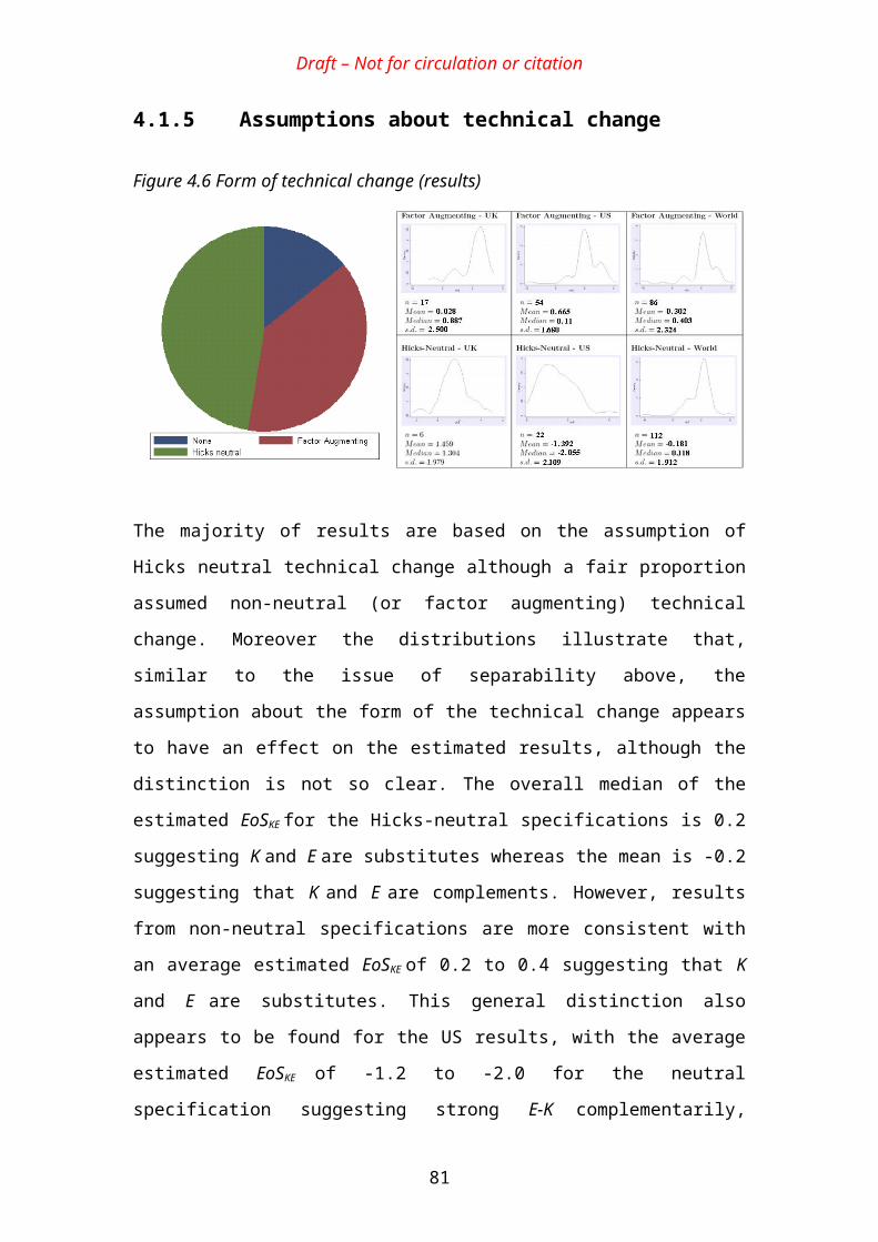
Draft – Not for circulation or citation
the own-price elasticity of energy services in different contexts. While these are
determined by elasticities of substitution, the relationship is far from straightforward
once the straitjacket of a nested CES is removed. Also, the discussion regarding
substitution elasticities may have obscured the important point that rebound effects
are also determined by the price elasticity of output in the sector in which the energy
efficiency improvement is achieved.
However, the results of this survey do potentially reinforce one of the main
conclusions of Technical Report 5 - namely that energy may play a more important
role in economic growth than has traditionally been assumed. While it is very difficult
to draw any general conclusions,45 the results of Section 4 suggest that energy and
capital are at best weak substitutes and possibly may be complements. This is the
opposite of what engineering intuition would suggest and implies that a reduction in
the price of capital relative to energy (e.g. through investment subsidies) may actually
increase energy consumption. At the same time, energy and labour are generally
found to be substitutes. This suggests that higher energy prices may reduce energy
consumption and capital formation, increase energy and capital productivity, reduce
labour productivity, and reduce economic output to a larger extent than is suggested
by the share of energy in total costs. This suggests the possibility of a strong link
between energy consumption and economic output and potentially high costs
associated with reducing energy consumption. At the same time, this is not
necessarily incompatible with the potential for large rebound effects from energy
efficiency improvements. However, such conclusions must be treated with great
caution, given the numerous limitations of the evidence base described above.
45 Since the empirical results vary greatly between sectors, levels of aggregation and methodological approach.
85
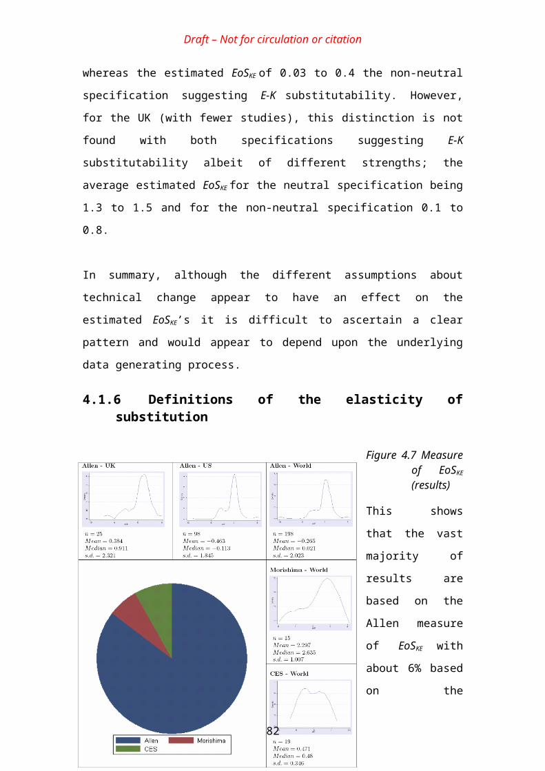
Draft – Not for circulation or citation
6 Summary and implications
6.1 Summary This report has investigated the role that elasticities of substitution may play in
determining the magnitude of rebound effects. It has also conducted a survey of
empirical estimates of the elasticity of substitution between energy and capital and
sought explanations for the widely varying results.
The results are rather mixed. On the one hand, the review has clarified a complex and
surprisingly confused area of literature and provided an overview of an important
question within energy economics: namely, whether energy and capital may be
considered as substitutes or complements. This in turn, is closely related to a key
theme of Technical Report 5, namely the relationship between energy consumption
and economic growth. On the other hand, the review has concluded that the
relationship between elasticities of substitution and the rebound effect is more subtle
and complex than is commonly assumed. As a result, it appears that empirical
estimates of elasticities of substitution may tell us relatively little about the likely
magnitude of rebound effects.
The review has shown that there are at least five definitions of the elasticity of
substitution in common use and several others that appear less frequently. The lack of
consistency in the use of these definitions and the lack of clarity in the relationship
between them, combine to make the empirical literature both confusing and
contradictory. . The majority of existing empirical studies use the sign of the Allen-
Uzawa elasticity of substitution (AES) to classify inputs as substitutes or
complements, but a number of drawbacks with this measure have been identified and
its quantitative value may lack meaning. In many cases, the constant output Cross
Price (CPE) or Morishima (MES) measures could be more appropriate, but these have
yet to gain widespread use.
While most empirical studies estimate the AES between different inputs, energy-
economic models require assumptions about the HES. The two can be difficult to
86

Draft – Not for circulation or citation
relate, owing to differences in functional form, seperability assumptions, the treatment
of technical change, nesting structures, sectoral aggregation and so on. These multiple
differences raise serious questions regarding the empirical basis of CGE models and
the usefulness of their results.
The survey of empirical literature on the elasticity of substitution between energy and
capital (EoSKE) has reached no firm conclusions. Although the majority of studies use
a static time series, single equation approach, there is a wide dispersion in their
results. This could be because the different studies genuinely reflect the different type
and degree substitutability within the various sectors, countries and/or time periods
studied. However, the results also appear to be strongly influenced by assumptions
about separability, technical change and returns to scale and demonstrate considerable
variability even when the same or similar data sets are employed. As a result, despite
more than three decades of research, no consensus has emerged on either the sign of
EoSKE (i.e. whether energy and capital are complements or substitutes) or on the
magnitude of EoSKE, (although most studies suggest that it is less than unity). If a
general conclusion can be drawn, it is that energy and capital appear at best to be
weak substitutes and possibly may be complements. But little confidence can be
placed in this statment.
We also observe that:
The issue of the distinction between short-run and long-run measures of EoSKE
has not been resolved, despite being raised in the 1970s. Furthermore, it is
surprising that static models still predominate, despite the advances in time
series econometrics over the last 25 years;
While assumptions regarding separability, technical change and other factors
appear to influence the empirical results, there is no consistent approach to
testing these assumptions in order to ‘let the data speak;
The lack of up to date and consistent UK evidence makes it impossible to
conclude on the sign and size of EoSKE for the UK.
On the basis of this review, we recommend that:
87
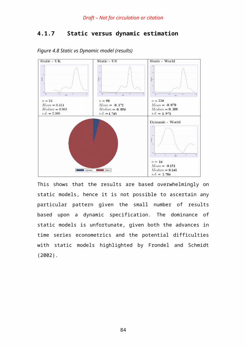
Draft – Not for circulation or citation
A full meta-analysis is undertaken to attempt to better ascertain the effect of
the different functional forms, types of data, countries, type of separability,
form of technical change, etc. on the estimated EoSKE’s;46
A new UK study is undertaken for the whole economy and various sectors of
the economy using time series analysis of a general KLEM translog
specification that explores the effect of allowing for a dynamic model and
non-neutral technical change and develops a formal statistical framework to
test the general model for restrictions such as Hicks neutral technical change,
separability of E from KLE, etc. By ‘letting the data speak’; this should
produce more robust estimates of EoSKE.for the UK that may be used to help
understand the rebound effect.
6.2 Implications The relationship between empirical estimates of elasticities of substitution and the
magnitude of rebound effects appears to be more complex than is generally assumed.
Saunders’ statement that “…the ease with which fuel can substitute for other factors
of production (such as capital and labour) has a strong influence on how much
rebound will be experienced” is potentially misleading. A more precise statement
would, first, refer to ‘energy services’ (or ‘effective energy’) rather than fuel; second,
clarify that the elasticity in question is the AES between energy services and a
composite of other inputs; third, include the qualification that this only applies when
energy services are separable from this composite; and fourth, clarify that this
conclusion derives from a particular nesting structure in a CES production function.
Since the majority of empirical studies use translog cost functions, measure energy
rather than energy services, do not impose any seperability restrictions and estimate
the AES between energy and individual inputs, they do not provide a direct test of
Saunders proposition. For similar reasons, such studies appear to be of little value in
parameterising CGE models.
On the basis of both this review and Saunders more recent work on translog cost
functions we conclude that:
46 As stated above, since staring this review Koetse et al (2006) have produced a meta-analysis of capital-energy substitution. However, this only uses just over 20 previous studies; hence the suggestion that a full meta analysis is undertaken utilising as many as possible of the previous studies covered in this review.
88
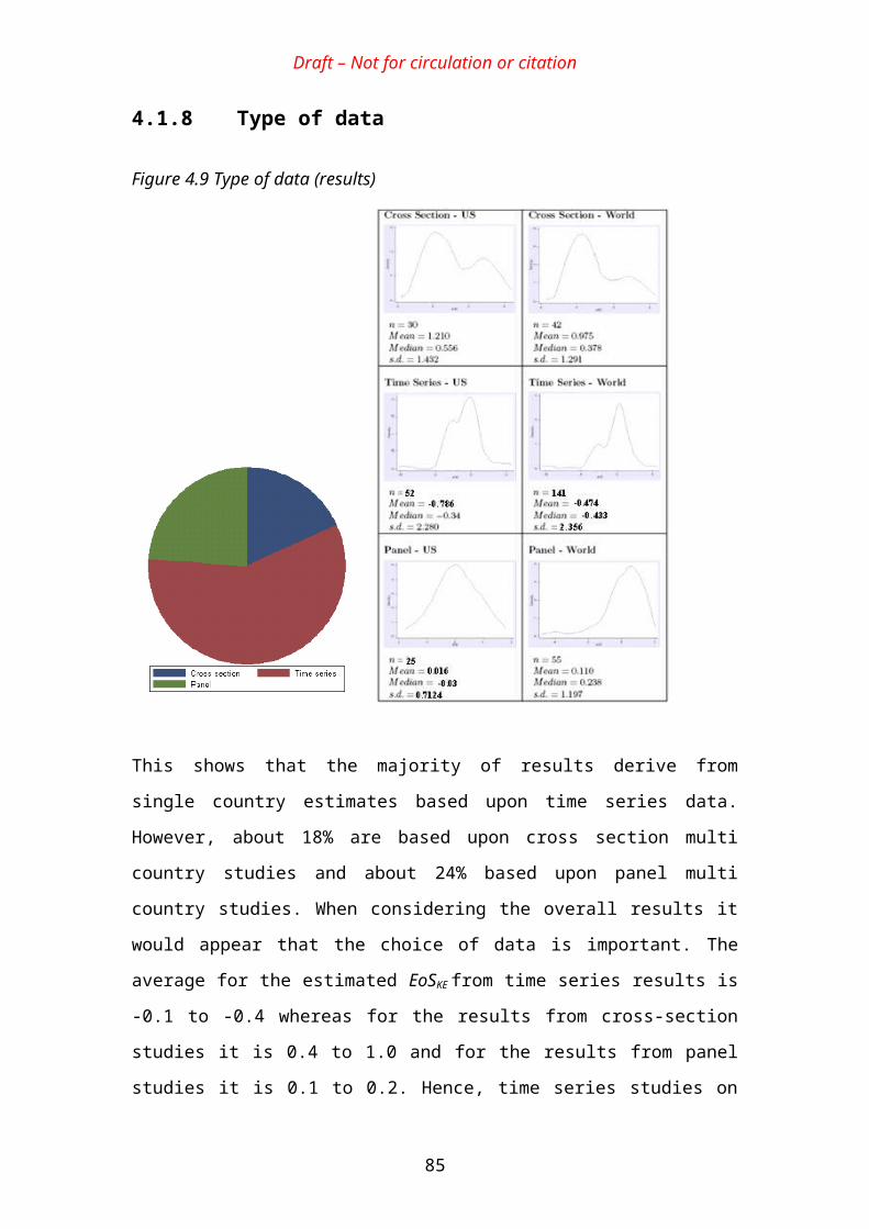
Draft – Not for circulation or citation
The AES between each pair of inputs is relevant to the magnitude of rebound
effects and not just that between energy and a composite of other inputs.
A finding that energy is a weak AES substitute for another factor, or even a
complement to that factor, is not necessarily inconsistent with the potential for
large rebound effects, or even backfire.
This suggests that our survey of empirical estimates of EoSKE has provided only
limited insight into the likely magnitude of rebound effects. It also suggests that the
discussion about elasticities of substitution in the literature may have obscured the
real issue, which is the own-price elasticity of energy services in different contexts,
together with the price elasticity of output in the sector in which the energy efficiency
improvement is achieved.
However, the results do arguably reinforce one of the main conclusions of Technical
Report 5 - namely that energy may play a more important role in economic growth
than is commonly assumed. A finding that energy and capital are at best weak
substitutes and possibly may be complements is the opposite of what engineering
intuition would suggest and implies that a reduction in the price of capital relative to
energy (e.g. through investment subsidies) may actually increase energy consumption.
This suggests the possibility of a strong link between energy consumption and
economic output and potentially high costs associated with reducing energy
consumption. At the same time, this is not necessarily incompatible with the potential
for large rebound effects from energy efficiency improvements. But once again, this
conclusion is merely suggestive only and lacks a firm empirical basis.
89
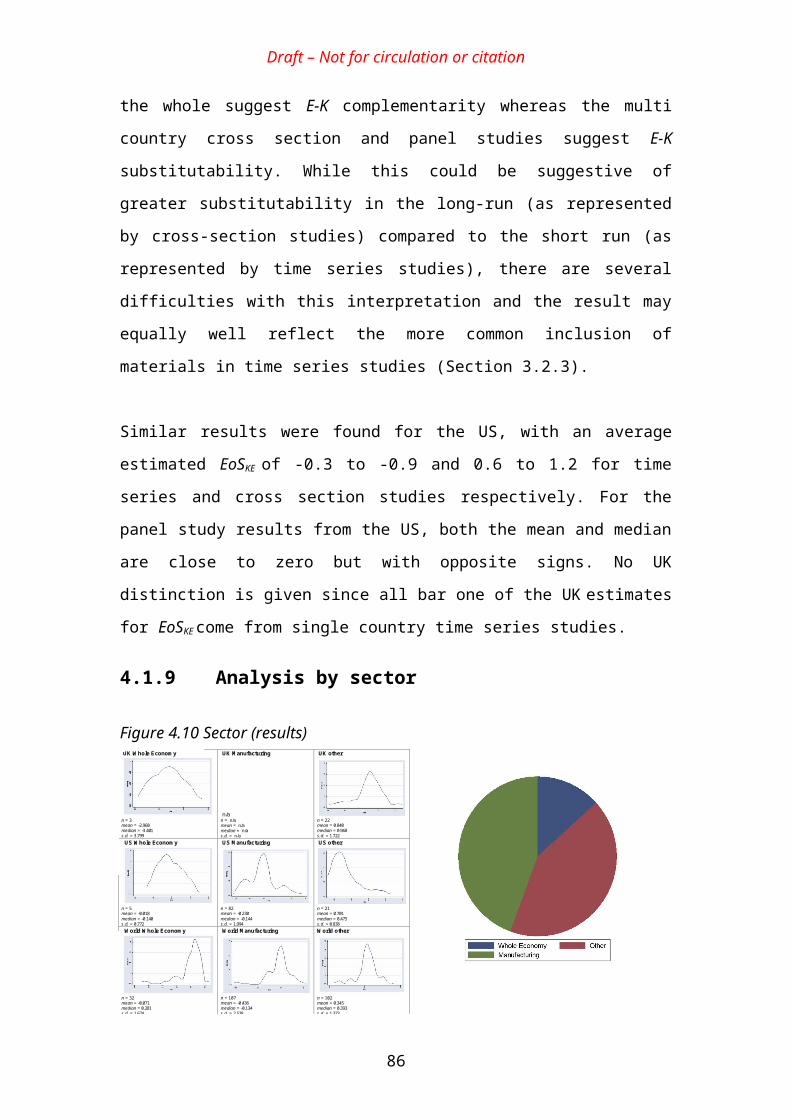
Draft – Not for circulation or citation
ReferencesAllan, G., N. Hanley, P. G. McGregor, J. Kim Swales, and K. Turner, (2006), 'The
macroeconomic rebound effect and the UK economy', Final report to the Department Of Environment Food and Rural Affairs, Department Economics, University of Strathclyde, Strathclyde.
Allen, R., (1938), Mathematical analysis for economists, MacMillan, London.Anderson, G. and J. Thursby, (1986), 'Confidence Intervals for Elasticity Estimators
in Translog Models', The Review of Economics and Statistics, 68(4), 647-56.Anderson, R. K. and J. R. Moroney, (1994), 'Substitution and complementarity in
CES models', Southern Economic Journal, 60(4), 886-95.Apostolakis, B. E., (1990), 'Energy-capital-substitutability/complementarity', Energy
Economics, 12(1), 48-58.Arrow. K, Chenery. H, M. B., and S. R., (1961), 'Capital-labour substitution and
economic efficiency', The Review of Economics and Statistics, 43(3), 225-50.Barker, T., (2005), 'The transition to sustainability: a comparison of general
equilibrium and space-time economics approaches', Working Paper Number 62, Tyndall Centre for Climate Change Research.
Berndt, E. R. and L. R. Christensen, (1973), 'The internal structure of functional relationships: seperability, substitution and aggregation', Review of Economic Studies, 40(3), 403-10.
Berndt, E. R. and D. O. Wood, (1975), 'Technology, Prices, and the Derived Demand for Energy', Review of Economics and Statistics, 57(3), 259-68.
Berndt, E. R. and D. O. Wood, (1979), 'Engineering and econometric interpretations of energy-capital complementarity', American Economic Review, June, 259-68.
Blackorby, C. and R. R. Russell, (1975), 'The partial elasticity of substitution', Discussion Paper 75-1, Department of Economics, University of California, San Diego.
Blackorby, C. and R. R. Russell, (1981), 'The Morishima elasticity of substitution: symmetry, constancy, separability and its relationship to the Hicks and Allen elasticities', Review of Economic Studies, XLVIII, 147-58.
Blackorby, C. and R. R. Russell, (1989), 'Will the real elasticity of substitution please stand up (a comparison of the Allen/Uzawa and Morishima elasticities)', American Economic Review, 79(882-888).
Chambers, R. G., (1988), Applied Production Analysis: A Dual Approach, Cambridge University Press, Cambridge.
Chang, K. P., (1994), 'Capital-Energy Substitution and Multilevel Ces Production Function', Energy Economics, 16(1), 22-26.
Chiang, A. C., (1984), Fundamental methods of Mathematical Economics, McGraw-Hill, London.
Christensen, L. R., D. W. Jorgensen, and L. L. Lau, (1973), 'Transcendental Logarithmic Production Frontiers', The Review of Economics and Statistics, 55(1), 28-45.
Chung, J. W., (1987), 'On the estimation of factor substitution in the translog model', The Review of Economics and Statistics, 69(3), 409-17.
Cobb, C. and P. Douglas, (1928), 'A theory of production', American Economic Review, 18(1), 139-65.
90

Draft – Not for circulation or citation
Felipe, J. and F. Fisher, (2003), 'Aggregation in production functions: what applied economists should know', Metroeconomica, 54(2), 208-62.
Field, B. C. and C. Grebenstein, (1980), 'Capital-energy substitution in US manufacturing', The Review of Economics and Statistics, 62(2), 207-12.
Frondel, M., (2004), 'Empirical assessment of energy price policies: the case for cross price elasticities', Energy Policy, 32, 989-1000.
Frondel, M. and C. M. Schmidt, (2002), 'The capital-energy controverst: an artifact of cost shares', The Energy Journal, 23(3), 53-75.
Frondel, M. and C. M. Schmidt, (2004), 'Facing the truth about seperability: nothing works without energy', Ecological Economics, 51, 217-23.
Greenaway, D., S. J. Leybourne, G. V. Reed, and J. Whalley, (1992), 'Applied General Equilibrium Modelling: applications, limitations and future development', UK Teasury, HMSO, London.
Grepperud, S. and I. Rasmussen, (2004), 'A general equilibrium assessment of rebound effects', Energy Economics, 26(2), 261-82.
Griffin, J. M., (1981), 'Engineering and Econometric Interpretations of Energy-Capital Complementarity: Comment', The American Economic Review, 71(5), 1100-04.
Griffin, J. M. and P. R. Gregory, (1976), 'An intercountry translog model of energy substitution responses', American Economic Review, 66(December), 845-67.
Harris, A., I. McAvinchey, and A. Yannopoulos, (1993), 'The demand for labour, capital, fuels and electricity: A sectoral model of the United Kingdom economy.' Journal of Economic Studies, 20(3), 24-35.
Hicks, J. R., (1932), The Theory of Wages, Macmillan, London.Hodgson, G. M., (1988), Economics and institutions: a manifesto for a modern
institutional economics, Polity Press, Cambridge.Hogan, W. W., (1979), 'Capital-energy complementarity in aggregate energy-
economic analysis', Resources and Energy, 2, 201-20.Hogan, W. W. and A. S. Manne, (1970), 'Energy-the economy interactions: a fable of
the elephant and the rabbit', Energy and the Economy: Report 1 of the Energy Modelling Forum, Stanford University.
Howarth, R. B., (1997), 'Energy efficiency and economic growth', Contemporary Economic Policy, 15(4), 1.
Hunt, L. C., (1986), 'Energy and capital: substitutes or complements? A note on the importance of testing for non-neutral technical change', Applied Economics, 18(729-735).
Hunt, L. C. and E. L. Lynk, (1992), 'Industrial Energy Demand in the UK: A Cointegration Approach', in Energy Demand: Evidence and Expectations, D. Hawdon ed, Academic Press, London.
Jaccard, M. and C. Bataille, (2000), 'Estimating future elasticities of substitution for the rebound debate', Energy Policy, 28(6-7), 451-55.
Kahneman, D. and A. Tversky, (2000), Choices, Values and Frames, Cambridge, Cambridge University Press.
Kako, T., (1980), 'An application of the decomposition analysis of derived demand for factor inputs in U.S. manufacturing', The Review of Economics and Statistics, 62(2), 300-01.
Kaufmann, R. K. and I. G. Azary-Lee, (1990), A biophysical analysis of substitution: does substitution save energy in the US forest products industry?, Ecological economics: its implications for forest management and research, Proceedings of a Workshop held in St Paul, Minnesota, April 2-6
91
Draft – Not for circulation or citation
Kemfert, C., (1998), 'Estimated substitution elasticities of a nested CES production function approach for Germany', Energy Economics, 20(3), 249-64.
Koetse, M. J., H. L. F. de Grooot, and R. J. G. M. Florax, (2006), 'Capital-energy substitution and shifts in factor demand: a meta-analysis', Tinbergen Institute Discussion Paper, TI2006-061/3, Tinbergen Institute, Amsterdam.
Manne, A. S. and R. G. Richels, (1990), 'CO2 emissions limits: an economic cost analysis for the USA', The Energy Journal, 11(4), 51-74.
McFadden, D., (1963), 'Constant elasticity of substitution production functions', Review of Economic Studies, 30(233-236).
Miller, E. M., (1986), 'Cross-sectional and timeseries biases in factor demand studies: explaining energy-capital complementarity', Southern Economic Journal, 52(3), 745-62.
Morishima, M., (1967), 'A few suggestions on the theory of elasticity', Kezai Hyoron (Economic Review), 16, 149-50.
Nerlove, M., (1963), 'Returns to scale in electricity supply', in Measurement in economics - studies in mathematical economics and econometrics in memory of Yehuda Grunfeld, Christ. C. ed, Stanford University Press.
Ochsen, C., (2002), 'Capital-skill complementarity, biased technical change and unemployment', Working Paper, Department of Economics, University of Oldenburg.
Raj, V. and M. R. Veall, (1998), 'The energy-capital complementarity debate: An example of a bootstrapped sensitivity analysis', Environmetrics, 9(81-92).
Sato, K., (1967), 'A two level constant elasticity of substitution production function', Review of Economics and Statistics, 34(2), 201-18.
Sato, K. and T. Koizumi, (1973), 'The production function and the theory of distributive shares', The American Economic Review, 63(3), 484-89.
Saunders, H., (2006a), 'Fuel Conserving (and Using) Production Functions', Working Paper, Decision Processes Incorporated, Danville, CA.
Saunders, H. D., (1992), 'The Khazzoom-Brookes Postulate and Neoclassical Growth', The Energy Journal, 13(4), 131.
Saunders, H. D., (2000a), 'Does predicted rebound depend on distinguishing between energy and energy services?' Energy Policy, 28(6-7), 497-500.
Saunders, H. D., (2000b), 'A view from the macro side: rebound, backfire, and Khazzoom-Brookes', Energy Policy, 28(6-7), 439-49.
Saunders, H. D., (2005), 'A calculator for energy consumption changes arising from new technologies', Topics in Economic Analysis and Policy, 5(1), 1-31.
Saunders, H. D., (2006b), 'Fuel conserving (and using) production function', Working Paper, Available from [email protected].
Smithson, C. W., (1979), 'Relative factor usage in Canadian mining: neoclassical substitution or by a technical change?' Resources and Energy, 2, 373-89.
Solow, J. L., (1987), 'The capital-energy complementarity debate revisited', The American Economic Review, 77(4), 605-14.
Solow, R., (1956), 'A contribution to the theory of economic growth', The Quarterly Journal of Economics, 70., 65-94.
Spady, R. and A. Friedlander, (1978), 'Hedonic cost functions for the regulated trucking industry', The Bell Journal of Economics, 9(1), 159-79.
Stern, D. I., (2004), 'Elasticities of substitution and complementarity', Working Paper in Economics, No. 0403, Rennsselaer Polytechnic Institute.
92
Draft – Not for circulation or citation
Stern, D. I. and C. J. Cleveland, (2004), 'Energy and economic growth', Rensselaer Working Paper in Economics, No. 0410, Rensselaer Polytechnic Institute, Troy, NY.
Temple, J., (2006), 'Aggregate production functions and growth economics', International Review of Applied Economics, 20(3), 301-17.
Urga, G. and C. Walters, (2003), 'Dynamic translog and linear logit models: a factor demand analysis of interfuel substitution in US industrial energy demand.' Energy Economics, 25, 1-21.
Uzawa, H., (1962), 'Production functions with constant elaticities of substitution', The Review of Economic Studies, 29(4), 291-99.
van der Werf, E., (2006), 'Production functions for climate policy modelling: an empirical analysis', Working Paper, Kiel Institute for the World Economy, Kiel.
Varian, H. R., (1996), Intermediate Microeconomics: a modern approach, W.W. Norton, New York.
Zellner, A., (1962), 'An efficient method of estimating seemingly unrelated regressions and tests for aggregation bias', Journal of the American Statistical Association, 57, 348-68, 57, 348-68.
93
Draft – Not for circulation or citation
Empirical references used in Section 4 Applebaum. E and Kohli. U, (1997), Import price uncertainty and the distribution of
income, The Review of Economics and Statistics, 79(4), 620-630.
Atkinson. S and Halvorsen. R, (1984), Parametric efficiency tests, economies of scale and input demand in U.S. electric power generation, International Economic Review, 25(3), 647-662.
Babin. F, Willis. C and Allen. G, (1982), Estimation of substitution possibilities between water and other production inputs, American Journal of Agricultural Economics, 64(1), 148-151.
Berndt. E and Khaled. M, (1979), Parametric productivity measurement and choice among flexible functional forms, The Journal of Political Economy, 87(6), 1220-1245.
Berndt. E and Wood. D, (1975), Technology, prices, and the derived demand for energy, The Review of Economics and Statistics, 57(3), 259-268.
Berndt. E and Wood. D, (1979), Engineering and econometric interpretations of energy-capital complementarity, The American Economic Review, 69(3), 342-354.
Bjorndal. T, Gordon. D and Singh. B, (1988), Economies of scale in the Norwegian fish-meal industry: implications for policy decisions, Applied Economics, 20, 1321-1332.
Burney. N and Al-Matrouk. F, (1996), Energy conservation in electricity generation: A case study of the electricity and water industry in Kuwaut, Energy Economics, 18, 69-79.
Casler. S, (1997), Applied production theory: explicit, flexible, and general functional forms, Applied Economics, 29, 1483-1492.
Chang. K., (1994), Capital-Energy Substitution and Multilevel CES Production Function, Energy Economics, 16(1), 22-26.
Christensen. L and Greene. W, (1976), Economies of scale in U.S. electric power generation, The Journal of Political Economy, 84(4), 655-676.
Christopoulos. D and Tsionas. E, (2002), Allocative inefficiency and the capital-energy controversy, Energy Economics, 24, 305-318.
Chung. J, (1987), On the estimation of factor substitution in the translog model, The Review of Economics and Statistics, 69(3), 409-417.
Dahl. C, Erdogan. M, (2000), Energy and Interfactor Substitution in Turkey, OPEC Review, March.
Dargay. J, (1983), The demand for energy in Swedish manufacturing industries, Scandinavian Journal of Economics, 85(1), 37-51.
Denny. M, May. J and Pinto. C, (1978), The demand for energy in Canadian manufacturing: Prologue to an energy Policy, The Canadian Journal of Economics, 11(2), 300-313.
94
Draft – Not for circulation or citation
Frondel. M, (2004), Empirical assessment of energy-price policies: the case for cross-price elasticities, Energy Policy, 32, 989-1000.
Fuss. M, (1977), The structure of technology over time: a model for testing the “putty-clay” hypothesis, Econometrica, 45(8), 1797-1821.
Garofalo. E and Malhotra. D, (1984), Input substitution in the manufacturing sector during the 1970’s: a regional analysis, Journal of Regional Science, 24(1), 51-63.
Garofalo. E and Malhotra. D, (1990), The demand for inputs in the traditional manufacturing region, Applied Economics, 22, 961-972.
Goodwin. B and Brester. G, (1995), Structural change in factor demand relationships in the U.S. food and kindred products industry, American Journal of Agricultural Economics, 77(1), 69-79.
Gopalakrishnan. C, Khaleghi. G and Shrestha. R, (1989), Energy-non-energy input substitution in US agriculture: some findings, Applied Economics, 21, 673-679.
Griffin. J and Gregory. P, (1976), An intercountry translog model of energy substitution responses, The American Economic Review, 66(5), 845-857.
Halvorsen. R and Smith. T, (1986), Substitution possibilities for unpriced natural resources: restricted cost functions for the Canadian metal mining industry, The Review of Economics and Statistics, 68(3), 398-405.
Harris. A, McAvinchey. I and Yannopoulos. A, (1993), The demand for labour, capital, fuels and electricity: A sectoral model of the United Kingdom economy, Journal of Economic Studies, 20(3), 24-35.
Huang. K, (1991), Factor demands in the U.S. food-manufacturing industry, American Journal of Agricultural Economics, 73(3), 615-620.
Hunt. L. C, (1984), Energy and capital: Substitutes or complements? Some results for the UK industrial sector, Applied Economics, 16, 783-789
Hunt. L. C, (1986), Energy and capital: substitutes or complements? A note on the importance of testing for non-neutral technical change, Applied Economics, 18, 729-735.
Iqbal. M, (1986), Substitution of labour, capital and energy in the manufacturing sector of Pakistan, Empirical Economics, 11, 81-95.
Kant. S and Nautiyal. J, (1998), Production structure, factor substitution, technical change, and total factor productivity in the Canadian logging industry, Canadian Journal of Forestry Research, 27, 701-710.
Kemfert. C, (1998), Estimated substitution elasticities of a nested CES production function approach for Germany, Energy Economics, 20, 249-264.
Kemfert. C and Welsch. H, (2000), Energy-capital-labor substitution and the economic effects of CO2 abatement: Evidence for Germany, Journal of Policy Modeling, 22(6), 641-660.
Kim. M, (1988), The structure of technology with endogenous capital utilization, International Economic Review, 29(1), 111-130.
95
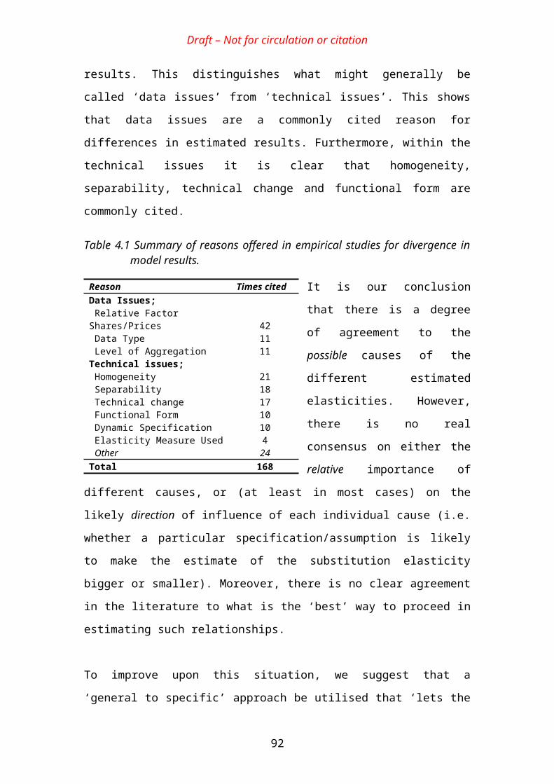
Draft – Not for circulation or citation
Klein .Y, (1988), An econometric model of the joint production and consumption of residential space heat, Southern Economic Journal, 55(2), 351-359.
Kuper. G and van Soest. D, (2003), Path dependency and input substitution: implications for energy policy modelling, Energy Economics, 25, 397-407.
Magnus. J, (1979), Substitution between energy and non-energy inputs in the Netherlands 1950-1976, International Economic Review, 20(2), 465-484.
McElroy. M, (1987), Additive general error models for production, cost, and derived demand or share systems, The Journal of Political Economy, 95(4), 737-757.
McNown. R, Pourgerami. A and von Hirschhausen. C, (1991), Input substitution in manufacturing for three LDCs: translog estimates and policy implications, Applied Economics, 23, 209-218.
Medina. J and Vega-Cervera. J, (2001), Energy and the non-energy inputs substitution: evidence for Italy, Portugal and Spain, Applied Energy, 68, 203-214.
Norsworthy. J. and Harper. M., (1981), Dynamic models of energy substitution in U.S. manufacturing, Chapter in Berndt. E. and Field. B. (eds), Modelling and Measuring Natural Resource Substitution, MIT Press, USA, 177-208.
Nguyen. S and Strietwiesser. M, (1997), Capital-energy substitution revisited: New evidence from micro data, Center for Economic Studies (CES), Research Paper 97/4.
Norsworthy. J and Malmquist. D, (1983), Input measurement and productivity growth in Japanese and US manufacturing, The American Economic Review, 73(5) 947-967.
Olson. D and Jonish. J, (1985), The robustness of translog elasticity of substitution estimates and the capital-energy controversy, Quarterly Journal of Business and Economics, 24(1), 21-35.
Ozatalay. S, Grubaugh. S and Long II. T, (1979), Energy substitution and national energy policy, The American Economic Review, 69(2), 369-371.
Pindyck. R and Rotemberg. J, (1983), Dynamic factor demands and the effects of energy price shocks, The American Economic Review, 73(5), 1066-1079.
Pollack. R and Wales. T, (1987), Specification and estimation of nonseperable two-stage technologies: the Leontief CES and the Cobb-Douglas CES, The Journal of Political Economy, 95(2), 311-333.
Raj and Veal, (1998), The energy-capital complementarity debate: An example of a bootstrapped sensitivity analysis, Environmetrics, 9, 81-92.
Serletis. A and Khumbakar. S, (1990), KLEM substitutability: a dynamic flexible demand system, Applied Economics, 22, 275-283.
Struckmeyer. C, (1987), The putty-clay perspective on the capital-energy complementarity debate, The Review of Economics and Statistics, 69(2), 320-326.
Terrell. D, (1996), Incorporating monotonicity and concavity conditions in flexible functional forms, Journal of Applied Econometrics, 11(2), 179-194.
96

Draft – Not for circulation or citation
Truett. L and Truett. D, (2001), The Spanish automotive industry: scale economies and input relationships, Applied Economics, 33, 1503-1513.
Turnovsky, M., Folie, M., and A., Ulph, (1982), Factor substitutability in Australian manufacturing with emphasis on energy inputs, Economic Record, 58(160), 61-73
Vega-Cervera. J and Medina, J, (2000), Energy as a productive input: the underlying technology for Portugal and Spain, Energy, 25, 757-775.
Welsch. H and Ochsen. C, (2005), The determinants of aggregate energy use in West Germany: factor substitution, technological change, and trade, Energy Economics, 27, 93-111.
Westoby. R and McGuire. A, (1984), Factor substitution and complementarity in energy: a case study of the UK electricity industry, Applied Economics, 16, 111-118.
Williams. E and Laumas. P, (1981), The Relation between energy and non-energy inputs in India’s manufacturing industries, The Journal of Industrial Economics, 30(2), 113-122.
Youn Kim. H, (1992), The translog production function and variable returns to scale, The Review of Economics and Statistics, 74(3), 546-522.
Youn Kim. H, (2005), Aggregation over firms and flexible functional forms, The Economic Record, 81(22), 19-29.
97
Draft – Not for circulation or citation
Annex 1: Functional formsEmpirical studies assume a particular functional form for the production function and
estimate the parameters of that form econometrically. It follows that the empirical
results may depend very much on the particular form that is chosen. Various
functional forms appear in the literature, of which the most common are:
the Cobb-Douglas, due to Cobb and Douglas (1928);
the Constant Elasticity of Substitution, defined by Solow (1956) and Arrow et al
(1961);
the Transcendental Logarithmic (Translog) form of Christensen et al (1973).
Each of these functional forms will be discussed briefly in turn using a three factor
(KLE) example.47
6.2.1.1 The Cobb-Douglas production function
A three-factor Cobb-Douglas production function (see for instance Varian (1996), p.
317) takes the form:
(A1.1)
Where α is the proportion of capital which is used in the production of Y, β is the
proportion of labour used and 1-α-β, is the proportion of energy. It is assumed that
α+β +(1-α-β) = 1, such that the proportions of all factor inputs used, sum to one.
Empirically, the assumption that factor proportions sum to unity can either be
imposed or tested for using standard statistical techniques. This functional form
satisfies the assumption of constant returns to scale (i.e. it is homogeneous of degree
1) and assumes a constant and unitary Hicks elasticity of substitution between inputs (
). Hence, a percentage reduction in one input can be fully compensated by
a percentage increase in another input.
47 This exposition is based on Saunders (2006).
98
Draft – Not for circulation or citation
6.2.1.2 The Constant Elasticity of Substitution (CES) production function.
The CES function, originally due to Solow (1956) and subsequently developed by
Arrow et al (1961) as its name indicates, assumes that there exists a constant (Hicks)
elasticity of substitution between factor inputs
This functional form can be for a two input production function:
(A1.2)
where a and b are positive constants and , with σ the Hicks
elasticity of substitution between capital and labour (HESKL).
Energy may be included in a CES function as follows:
(A1.3)
This form of a 3-input CES is called “nested” because the original CES function
contains another CES for only two factors - energy and capital. This functional form
implies at the same time: a) a constant elasticity of substitution between energy and
capital; and b) a constant elasticity of substitution between ‘energy services’ (assumed
to be derived from a combination of energy and capital) and labour. It rests on the
assumption that labour is separable from capital and energy inputs
In the same fashion, it is possible to have a multi-nested CES function that allow the
inclusion of further inputs like materials M. Following Manne & Richels (1990), the
value of the EoS in the capital-energy nest can be restricted to be unity. This
restriction gives a Cobb-Douglas within the CES function:
(A1.4)
where ,
Here, a and b are the share (or distribution) parameters, and indicates the proportions
of each factor input being used to obtain the level of output Y, thus b should be
equivalent to 1-a (see, for instance, Chiang (1984), p.426). This particular
specification assumes separability between energy and other inputs, by specifying the
99

Draft – Not for circulation or citation
relationship between capital and labour to be Cobb-Douglas, hence allowing for a
different EoS between these two factors. Thus, in this specification, the (Hicks)
elasticity of substitution between energy and capital is the same as that for energy and
labour, though alternative nested relationships could equally be expressed.
6.2.1.3 The Translog Production (and Cost) Function
The Transcendental Logarithmic function, commonly referred to as the Translog
function was first introduced by Christensen et al (1973). It was conceived in an effort
to define a less restrictive, more flexible functional form for production functions,
which offers particular advantages when there are more than two factors of production
under consideration. The term ‘transcendental’ derives from the fact that no factor can
be solved for explicitly without being a function of itself (i.e. a ‘transcendental’
equation). Importantly, and unlike the Cobb-Douglas and CES, the Translog does not
impose any restrictions on the substitutability between different factor inputs. For
three factors, it is expressed as;
(A1.5)
Although this expression appears somewhat lengthy, it amounts to assigning
parameters to all individual factors, as well as to all feasible cross products. If all the γ
coefficients are zero, then the above form is exactly equivalent to a Cobb-Douglas.
The majority of empirical studies use a Translog cost function, rather than a
production function. Assuming that agents are rational and efficient and acting in
equilibrium, the dual function of maximising production can be specified as cost
minimisation. Then the Translog cost function may be written as:
100

Draft – Not for circulation or citation
(A1.6)48
where PK, PL and PE represent the real prices of capital, labour and energy
respectively. As stated, this is the main basis for the empirical estimates reviewed in
the main text. By differentiating Equation A.1.6 with respect to each factor input (i.e.
K, L and E) and then applying Shephard’s Lemma, cost share equations for each
factor input can be derived (see Berndt and Wood, 1975). These may be estimated
econometrically to give the key parameters in Equation A.1.6 and then used to derive
the measures of the elasticity of substitution discussed above.49 In particular, the AES
is given by
(A1.7)
where and Si represents the cost share of factor i.
The MES is given by:
(A1.8)
(A1.9)
Where: , , and .
48 Note this is specification for the Translog cost function with neutral technical progress, to include non-neutral technical progress the following terms are added to equation A1.6: γtt + γttt2 + γKt t lnPK+ γLt t lnPL+ γEt t lnPE .
49 This formulation allows for convenient estimation of the Translog function via the share equations which may be estimated by the Seemingly Unrelated Regression method of Zellner (1962) or Maximum likelihood. Details of the estimation are not discussed here since it is outside the current remit but may be found in the many empirical papers reviewed below.
101
Draft – Not for circulation or citation
Annex 2: Search criteriaThe search was conducted by initially using the ISI Web of Science online database to
obtain a near comprehensive list of the academic journals to-date, which had
referenced the seminal work of Berndt and Wood (1975). Subsequently to this, the
Google/Google scholar search engine was used to search the internet for suitable
references using search terms such as;
KLE,
KLEM,
Production,
Production functions,
Capital energy,
substitutability,
Elasticity of substitution,
Multifactor production,
etc..
Combinations of these words were defined using Boolean operators to constrain
search results to be within more clearly defined parameters. Furthermore, the papers
obtained from the above approach were further consulted to identify any further
relevant studies which may have been overlooked.
It should be noted that in addition to studies of KLE or KLEM production functions
there are a number of studies that analyse, interfuel substitution instead of, or as well
as, factor substitution (see for instance Urga and Walters (2003) for a recent
example). Those that analysed interfuel substitution only and/or did not openly
present a measure of EoSKE were not included in the empirical papers reviewed.
Similarly, any paper that discussed the issue of E-K being substitutes or complements
(such as Hunt and Lynk (1992)) but did not openly present a measure of EoSKE were
also not included. No papers were rejected on the grounds of estimation method, data
type, level of aggregation, etc.
102