Progress in Nonlinear Differential Equations and Their Applications

87

Filippo Santambrogio

Optimal Transport for Applied MathematiciansCalculus of Variations, PDEs, and Modeling

Progress in Nonlinear DifferentialEquations and Their ApplicationsVolume 87

EditorHaim BrezisUniversité Pierre et Marie CurieParis, FranceandRutgers UniversityNew Brunswick, NJ, USA

Editorial BoardAntonio Ambrosetti, Scuola Internationale Superiore di Studi Avanzati

Trieste, ItalyA. Bahri, Rutgers University, New Brunswick, NJ, USAFelix Browder, Rutgers University, New Brunswick, NJ, USALuis Caffarelli, The University of Texas, Austin, TX, USALawrence C. Evans, University of California, Berkeley, CA, USAMariano Giaquinta, University of Pisa, ItalyDavid Kinderlehrer, Carnegie-Mellon University, Pittsburgh, PA, USASergiu Klainerman, Princeton University, NJ, USARobert Kohn, New York University, NY, USAP. L. Lions, University of Paris IX, Paris, FranceJean Mawhin, Université Catholique de Louvain, Louvain-la-Neuve, BelgiumLouis Nirenberg, New York University, NY, USALambertus Peletier, University of Leiden, Leiden, NetherlandsPaul Rabinowitz, University of Wisconsin, Madison, WI, USAJohn Toland, University of Bath, Bath, England

More information about this series at http://www.springer.com/series/4889

Filippo Santambrogio

Optimal Transportfor Applied MathematiciansCalculus of Variations, PDEs, and Modeling

Filippo SantambrogioLaboratoire de Mathématiques d’OrsayUniversité Paris-SudOrsay, France

ISSN 1421-1750 ISSN 2374-0280 (electronic)Progress in Nonlinear Differential Equations and Their ApplicationsISBN 978-3-319-20827-5 ISBN 978-3-319-20828-2 (eBook)DOI 10.1007/978-3-319-20828-2

Library of Congress Control Number: 2015946595

Mathematics Subject Classification (2010): 49J45, 90C05, 35J96, 35K10, 39B62, 90B06, 91A13, 90B20,26B25, 49N15, 52A41, 49M29, 76M25

Springer Cham Heidelberg New York Dordrecht London© Springer International Publishing Switzerland 2015This work is subject to copyright. All rights are reserved by the Publisher, whether the whole or part ofthe material is concerned, specifically the rights of translation, reprinting, reuse of illustrations, recitation,broadcasting, reproduction on microfilms or in any other physical way, and transmission or informationstorage and retrieval, electronic adaptation, computer software, or by similar or dissimilar methodologynow known or hereafter developed.The use of general descriptive names, registered names, trademarks, service marks, etc. in this publicationdoes not imply, even in the absence of a specific statement, that such names are exempt from the relevantprotective laws and regulations and therefore free for general use.The publisher, the authors and the editors are safe to assume that the advice and information in this bookare believed to be true and accurate at the date of publication. Neither the publisher nor the authors orthe editors give a warranty, express or implied, with respect to the material contained herein or for anyerrors or omissions that may have been made.

Printed on acid-free paper

Springer International Publishing AG Switzerland is part of Springer Science+Business Media (www.springer.com)

To my sweet wife Anna,who is furious for my book was conceivedafter hers but is ready long before. . .but she seems to love me anyway

Preface

Why this book?

Why a new book on optimal transport? Were the two books by Fields MedalistCédric Villani not enough? And what about the Bible of Gradient Flows, the bookby Luigi Ambrosio, Nicola Gigli, and Giuseppe Savaré, which also contains manyadvanced and general details about optimal transport?

The present text, very vaguely inspired by the classes that I gave in Orsay in2011 and 2012 and by two short introductory courses that I gave earlier in a summerschool in Grenoble [274, 275], would like to propose a different point of view and ispartially addressed to a different audience. There is nowadays a large and expandingcommunity working with optimal transport as a tool to do applied mathematics.We can think in particular of applications to image processing, economics, andevolution PDEs, in particular when modeling population dynamics in biology orsocial sciences, or fluid mechanics. More generally, in applied mathematics, optimaltransport is both a technical tool to perform proofs, do estimates, and suggestnumerical methods and a modeling tool to describe phenomena where distances,paths, and costs are involved.

For those who arrive at optimal transport from this side, some of the mostimportant issues are how to handle numerically the computations of optimal mapsand costs, which are the different formulations of the problem, so as to adapt themto new models and purposes; how to obtain in the most concrete ways the mainresults connecting transport and PDEs; and how the theory is used in the approach ofexisting models. We cannot say that the answers to these questions are not containedin the existing books, but it is true that probably none of them have been written withthis purpose.

The first book by C. Villani [292] is the closest to our intentions. It is a wideintroduction to the topic and its applications, suitable for every audience. Yet, someof the subjects that I decided to deal with here are unfortunately not described in[292] (e.g., the minimal flow problems discussed in Chapter 4 of this book). Also,since 2003, the theory has enormously advanced. Also the books by ST Rachev

vii

viii Preface

and L Ruschednorf (two volumes, [257, 258]) should not be forgotten, as theycover many applications in probability and statistics. But their scopes diverge quitesoon from ours, and we will not develop most of the applications nor the languagedeveloped in [257]. Indeed, we will mainly stick to a deterministic framework andto a variational taste.

If we look at what happened after [292], we should mention at least two beautifulbooks which appeared since then. The new book by C. Villani [293] has expandedthe previous presentation into an almost-thousand-page volume, where most of theextra content actually deals with geometrical issues, in particular the notion ofcurvature. Optimal transport for the quadratic cost on a manifold becomes a centraltool, and it is the starting point to study the case of metric measure spaces. Theother reference book is the one by L. Ambrosio, N. Gigli, and G. Savaré [15],devoted to the study of gradient flow evolution in metric space and in particularin the Wasserstein space of probability measures. This topic has many interestingapplications (e.g., the heat equation, Fokker-Planck equation, porous media, etc.),and the tools that are developed are very useful. Yet, the main point of view of theauthors is the study of the hidden differential structures in these abstract spaces;modeling and applied mathematics were probably not their first concerns.

Some of the above references are very technical and develop powerful abstractmachineries that can be applied in very general situations but could be difficult to usefor many readers. As a consequence, some shorter surveys and more tractable lecturenotes have appeared (e.g., [11] for a simplified version of some parts of [15] or [9] asa short introduction to the topic by L. Ambrosio and N. Gigli). Yet, a deeper analysisof the content of [9] shows that the first half deals with the general theory of optimaltransport, with some variations, while the rest is devoted to gradient flows in metricspaces in their generality and to metric measure spaces with curvature bounds. Wealso mention two very recent survey, [63] and [228]: the former accounts for themain achievements on the theory on the occasion of the centennial of the birth ofL. V. Kantorovich, and the second gives a general presentation of the topic withconnections with geometry and economics.

In the meantime, many initiatives took place underlining the increasing interestin the applied side of optimal transport: publications,1 schools, workshops, researchprojects, etc. The community is very lively since the 2010s in particular in Francebut also in Canada, Italy, Austria, the UK, etc. All these considerations suggestedthat a dedicated book could have been a good idea, and the one that you have inyour hands now is the result of the work for the last three years.

1A special issue of ESAIM M2AN on “Optimal Transport in Applied Mathematics” is inpreparation and some of the bibliographical references of the present book are taken from suchan issue.

Preface ix

What about this book?

This book contains a rigorous description of the theory of optimal transport and ofsome neglected variants and explains the most important connections that it has withmany topics in evolution PDEs, image processing, and economics.

I avoided as much as possible the most general frameworks and concentratedon the Euclidean case, except where statements in Polish spaces did not costany more and happened to help in making the picture clearer. I skipped manydifficulties by choosing to add compactness assumptions every time that thissimplified the exposition without reducing too much the interest of the statement(to my personal taste). Also, in many cases, I first started from the easiest cases(e.g., with compactness or continuity) before generalizing.

When a choice was possible, I tried to prefer more “concrete” proofs, which Ithink are easier to figure out for the readers. As an example, the existence of velocityfields for Lipschitz curves in Wasserstein spaces has been proven by approximationand not via abstract functional analysis tools, as in [15], where the main point is aclever use of the Hahn-Banach theorem.

I did not search for an exhaustive survey of all possible topics, but I structuredthe book into eight chapters, more or less corresponding to one (long) lecture each.Obviously, I added a lot of material to what one could usually deal with during onesingle lecture, but the choice of the topics and their order really follows an eight-lecture course given in Orsay in 2011 (only exceptions: Chapter 1 and Chapter 5took one lecture and a half, and the subsequent ones were shortened to half a lecturein 2011). The topics which are too far from those of the eight “lectures” have beenomitted from the main body of the chapters. On the other hand, every chapter endswith a discussion section, where extensions, connections, side topics, and differentpoints of view are presented. In some cases (congested and branched transport),these discussion sections correspond to a mini-survey on a related transport model.They are more informal; and sometimes statements are proven while at other timesthey are only sketched or evoked.

In order to enhance the readership and allow as many people as possible toaccess the content of this book, I decided to explain some notations in detail thatI could have probably considered as known (but it is always better to recall them).Throughout the chapters, some notions are recalled via special boxes called Memoor Important Notion.2 A third type of box, called Good to Know!, provides extranotions that are not usually part of the background of nonspecialized graduatestudents in mathematics. The density of the boxes, and of explanatory figures aswell, decreases as the book goes on.

For the sake of simplicity, I also decided not to insist too much on at least oneimportant issue: measurability. You can trust me that all the sets, functions, and maps

2The difference between the two is just that in the second case, I would rather consider it as aMemo, but students usually do not agree.

x Preface

that are introduced throughout the text are indeed measurable as desired, but I didnot underline this explicitly. Yet, actually, this is the only concession to sloppiness:proofs are rigorous (at least, I hope) throughout the book and could be used for sureby pure or applied mathematicians looking for a reference on the correspondingsubjects. The only chapter where the presentation is a little bit informal is Chapter 6,on numerical methods, in the sense that we do not give proofs of convergence orprecise implementation details.

Last but not least, there is a chapter on numerical methods! In particular thosethat are most linked to PDEs (continuous methods), while the most combinatorialand discrete ones are briefly described in the discussion section.

For whom is this book?

This book has been written with the point of view of an applied mathematician,and applied mathematicians are supposed to be the natural readership for it. Yet,the ambition is to speak to a much wider public. Pure mathematicians (whetherthis distinction between pure and applied makes sense is a matter of personal taste)are obviously welcome. They will find rigorous proofs, sometimes inspired by adifferent point of view. They could be interested in discovering where optimaltransport can be used and how and to bring their own contributions.

More generally, the distinction can be moved to the level of people working withoptimal transport rather than on optimal transport (instead of pure vs applied). Theformer are the natural readership, but the latter can find out they are interested in thecontent too. In the opposite direction, can we say that the text is also addressed tononmathematicians (physicists, engineers, theoretical economists, etc.)? This raisesthe question of the mathematical background that the readers need in order to readit. Obviously, if they have enough mathematical background and if they work onfields close enough to the applications that are presented, it could be interesting forthem to see what is behind those applications.

The question of how much mathematics is needed also concerns students. Thisis a graduate text in mathematics. Even if I tried to give tools to review therequired background, it is true that some previous knowledge is required to fullyprofit from the content of the book. The main prerequisites are measure theoryand functional analysis. I deliberately decided not to follow the advice of an“anonymous” referee, who suggested to include an appendix on measure theory.The idea is that mathematicians who want to approach optimal transport shouldalready know something on these subjects (what is a measurable function, what is ameasure, which are the conditions for the main convergence theorems, what aboutLp and W1;p functions, what is weak convergence, etc.). The goal of the Memo Boxesis to help readers to not get lost. For nonmathematicians reading the book, I hopethat the choice of a more concrete approach could help them in finding out whatkind of properties is important and reasonable. On the other hand, these readers are

Preface xi

also expected to know some mathematical language, and for sure, they will need toput in extra effort to fully profit from it.

Concerning readership, the numerical part (Chapter 6) deserves being discusseda little bit more. Comparing in detail the different methods, their drawbacks, andtheir strengths, the smartest tricks for their implementation, and discussing themost recent algorithms are beyond the scopes of this book. Hence, this chapter isprobably useless for people already working in this field. On the other hand, it canbe of interest for people working with optimal transport without knowing numericalmethods or for numericists who are not into optimal transport.

Also, I am certain that it will be possible to use some of the material that I presenthere for a graduate course on these topics because of the many boxes recalling themain background notions and the exercises at the end of the book.

What is in this book?

After this preface and a short introduction to optimal transport (where I mainlypresent the problem, its history, and its main connections with other part ofmathematics), this book contains eight chapters. The two most important chapters,those which constitute the general theory of optimal transport, are Chapters 1 and 5.In the structure of the book, the first half of the text is devoted to the problem of theoptimal way of transporting mass from a given measure to another (in the Monge-Kantorovich framework and then with a minimal flow approach), and Chapter 1 isthe most important. Then, in the second half, I move to the case where measuresvary, which is indeed the case in Chapter 5 and later in Chapters 7 and 8. Chapter 6comes after Chapter 5 because of the connections of the Benamou-Brenier methodwith geodesics in the Wasserstein space.

Chapter 1 presents the relaxation that Kantorovich did of the original Mongeproblem and its duality issues (Kantorovich potentials, c-cyclical monotonicity,etc.). It uses these tools to provide the first theorem of existence of an optimalmap (Brenier theorem). The discussion section as well mainly stems from theKantorovich interpretation and duality.

Chapter 2 focuses on the unidimensional case, which is easier and already hasmany consequences. Then, the Knothe map is presented; it is a transport map builtwith 1D bricks, and its degenerate optimality is discussed. The main notion hereis that of monotone transport. In the discussion section, 1D and monotone mapsare used for applications in mathematics (isoperimetric inequalities) and outsidemathematics (histogram equalization in image processing).

Chapter 3 deals with some limit cases, not covered in Chapter 1. Indeed, fromthe results of the first chapter, we know how to handle transport costs of the formjx � yjp for p 2 .1;C1/, but not p D 1, which was the original question by Monge.This requires to use some extra ideas, in particular selecting a special minimizer viaa secondary variational problem. Similar techniques are also needed for the otherlimit case, i.e., p D 1, which is also detailed in the chapter. In the discussion

xii Preface

section we present the main challenges and methods to tackle the general problemof convex costs of the form h.y � x/ (without strict convexity and with possibleinfinite values), which has been a lively research subject in the last few years, andlater we consider the case 0 < p < 1, i.e., costs which are concave in the distance.

Chapter 4 presents alternative formulations, more Eulerian in spirit: how todescribe a transportation phenomenon via a flow, i.e., a vector field w withprescribed divergence, and minimize the total cost via functionals involving w.When we minimize the L1 norm of w, this turns out to be equivalent to the originalproblem by Monge. The main body of the chapter provides the dictionary to passfrom Lagrangian to Eulerian frameworks and back and studies this minimizationproblem and its solutions. In the discussion section, two variants are proposed:traffic congestion (with strictly convex costs in w) and branched transport (withconcave costs in w).

Chapter 5 introduces another essential tool in the theory of optimal transport: thedistances (called Wasserstein distances) induced by transport costs on the space ofmeasures. After studying their properties, we study the curves in these spaces, and inparticular geodesics, and we underline the connection with the continuity equation.The discussion section makes a comparison between Wasserstein distances andother distances on probabilities and finally describes an application in terms ofbarycenters of measures.

Chapter 6 starts from the ideas presented in the previous chapter and uses themto propose numerical methods. Indeed, in the description of the Wasserstein space,one can see that finding the optimal transport is equivalent to minimizing a kineticenergy functional among solutions of the continuity equation. This provided the firstnumerical method for optimal transport called the Benamou-Brenier method. In therest of the chapter, two other “continuous” numerical methods are described, andthe discussion section deals with discrete and semidiscrete methods.

Chapter 7 contains a “bestiary” of useful functionals defined over measuresand studies their properties, not necessarily in connection with optimal transport(convexity, semicontinuity, computing the first variation, etc.). The idea is that thesefunctionals often appear in modeling issues accompanied by transport distances.Also, the notion of displacement convexity (i.e., convexity along geodesics ofthe Wasserstein space) is described in detail. The discussion section is quiteheterogeneous, with applications to geometrical inequalities but also equilibria inurban regions.

Chapter 8 gives an original presentation of one of the most striking applicationsof optimal transport: gradient flows in Wasserstein spaces, which allow us to dealwith many evolution equations, in particular of the parabolic type. The generalframework is presented, and the Fokker-Planck equation is studied in detail. Thediscussion section presents other equations which have this gradient flow structureand also other evolution equations where optimal transport plays a role, withoutbeing gradient flows.

Preface xiii

Before the detailed bibliography and the index which conclude the book, there isa list of 69 exercises from the various chapters and of different levels of difficulties.From students to senior researchers, the readers are invited to play with theseexercises and enjoy the taste of optimal transport.

Orsay, France Filippo SantambrogioMay 2015

xiv Preface

Introduction to optimal transport

The history of optimal transport began a long time ago in France, a few years beforethe revolution, when Gaspard Monge proposed the following problem in a reportthat he submitted to the Académie des Sciences [239].3 Given two densities of massf ; g � 0 on R

d, with´

f .x/ dx D ´g.y/ dy D 1, find a map T W Rd ! R

d, pushingthe first one onto the other, i.e. such that

ˆ

Ag.y/ dy D

ˆ

T�1.A/f .x/ dx for any Borel subset A � R

d; (1)

and minimizing the quantity

M.T/ WDˆ

RdjT.x/ � xj f .x/ dx

among all the maps satisfying this condition. This means that we have a collection ofparticles, distributed according to the density f on R

d, that have to be moved so thatthey form a new distribution whose density is prescribed and is g. The movementhas to be chosen so as to minimize the average displacement. In the descriptionof Monge, the starting density f represented a distribution of sand that had to bemoved to a target configuration g. These two configurations correspond to whatwas called in French déblais and remblais. Obviously, the dimension of the spacewas only supposed to be d D 2 or 3. The map T describes the movement (that wemust choose in an optimal way), and T.x/ represents the destination of the particleoriginally located at x.

In the following, we will often use the image measure of a measure � on X(measures will indeed replace the densities f and g in the most general formulationof the problem) through a measurable map T W X ! Y: it is the measure on Ydenoted by T#� and characterized, as in (1), by

.T#�/.A/ D �.T�1.A// for every measurable set A

orˆ

Y� d .T#�/ D

ˆ

X.� ı T/ d� for every measurable function �:

More generally, we can consider the problem

.MP/ minfM.T/ WDˆ

c.x;T.x// d�.x/ W T#� D �g;

for a more general transport cost c W X � Y ! R.

3This happened in 1781, but we translate his problem into modern mathematical language.

Preface xv

When we stay in the Euclidean setting, with two measures �; � induced bydensities f ; g, it is easy – just by a change-of-variables formula – to transform theequality � D T#� into the PDE

g.T.x// det.DT.x// D f .x/; (2)

if we suppose f ; g and T to be regular enough and T to be injective.Yet, this equation is highly nonlinear in T, and this is one of the difficulties

preventing an easy analysis of the Monge problem. For instance: how do we provethe existence of a minimizer? Usually, what one does is the following: take aminimizing sequence Tn, find a bound on it giving compactness in some topology(here, if the support of � is compact, the maps Tn take value in a common boundedset, spt.�/, and so one can get compactness of Tn in the weak-* L1 convergence),take a limit Tn * T, and prove that T is a minimizer. This requires semicontinuity ofthe functional M with respect to this convergence (which is true in many cases, forinstance, if c is convex in its second variable): we need Tn * T ) lim infn M.Tn/ �M.T/), but we also need that the limit T still satisfies the constraint. Yet, thenonlinearity of the PDE prevents us from proving this stability when we only haveweak convergence (the reader can find an example of a weakly converging sequencesuch that the corresponding image measures do not converge as an exercise; it isactually Ex(1) in the list of exercises).

In [239], Monge analyzed fine questions on the geometric properties of thesolution to this problem, and he underlined several important ideas that we willsee in Chapter 3: the fact that transport rays do not meet, that they are orthogonalto a particular family of surfaces, and that a natural choice along transport rays is toorder the points in a monotone way. Yet, he did not really solve the problem. Thequestion of the existence of a minimizer was not even addressed. In the next 150years, the optimal transport problem mainly remained intimately French, and theAcadémie des Sciences offered a prize on this question. The first prize was won byP. Appell [21] with a long mémoire which improved some points but was far frombeing satisfactory (and did not address the existence issue4).

The problem of Monge has stayed with no solution (does a minimizer exist?how to characterize it?) until progress was made in the 1940s. Indeed, only with thework by Kantorovich (1942, see [200]), it was inserted into a suitable frameworkwhich gave the possibility to attack it and, later, to provide solutions and study them.The problem has then been widely generalized, with very general cost functionsc.x; y/ instead of the Euclidean distance jx � yj and more general measures andspaces. The main idea by Kantorovich is that of looking at Monge’s problem asconnected to linear programming. Kantorovich indeed decided to change the pointof view, and to describe the movement of the particles via a measure � on X � Y ,satisfying .�x/#� D � and .�y/#� D �. These probability measures over X � Y

4The reader can see [181] – in French, sorry – for more details on these historical questions aboutthe work by Monge and the content of the papers presented for this prize.

xvi Preface

are an alternative way to describing the displacement of the particles of �: insteadof giving, for each x, the destination T.x/ of the particle originally located at x, wegive for each pair .x; y/ the number of particles going from x to y. It is clear thatthis description allows for more general movements, since from a single point x,particles can a priori move to different destinations y. If multiple destinations reallyoccur, then this movement cannot be described through a map T. The cost to beminimized becomes simply

´X�Yc d� . We have now a linear problem, under linear

constraints. It is possible to prove existence of a solution and to characterize it byusing techniques from convex optimization, such as duality, in order to characterizethe optimal solution (see Chapter 1).

In some cases, and in particular if c.x; y/ D jx � yj2 (another very natural cost,with many applications in physical modeling because of its connection with kineticenergy), it is even possible to prove that the optimal � does not allow this splittingof masses. Particles at x are only sent to a unique destination T.x/, thus providing asolution to the original problem by Monge. This is what is done by Brenier in [82],where he also proves a very special form for the optimal map: the optimal T is ofthe form T.x/ D ru.x/, for a convex function u. This makes, by the way, a strongconnection with the Monge-Ampère equation. Indeed, from (2), we get

det.D2u.x// D f .x/

g.ru.x//;

which is an (degenerate and nonlinear) elliptic equation exactly in the classof convex functions. Brenier also uses this result to provide an original polarfactorization theorem for vector maps (see Section 1.7.2): vector fields can bewritten as the composition of the gradient of a convex function and of a measure-preserving map. This generalizes the fact that matrices can be written as the productof a symmetric positive-definite matrix and an orthogonal one.

The results by Brenier can be easily adapted to other costs, strictly convexfunctions of the difference x�y. They have also been adapted to the squared distanceon Riemannian manifolds (see [231]). But the original cost proposed by Monge, thedistance itself, was much more difficult.

After the French school, it was time for the Russian mathematicians. From theprecise approach introduced by Kantorovich, Sudakov [290] proposed a solution forthe original Monge problem (MP). The optimal transport plan � in the Kantorovichproblem with cost jx � yj has the following property: the space R

d can bedecomposed in an essentially disjoint union of segments that are preserved by � (i.e.,� is concentrated on pairs .x; y/ belonging to the same segment). These segmentsare built from a Lipschitz function, whose level sets are the surfaces “foreseen” byMonge. Then, it is enough to reduce the problem to a family of 1D problems. If� � L d, the measures that � induces on each segment should also be absolutelycontinuous and have no atoms. And in dimension one, as soon as the source measurehas no atoms, one can define a monotone increasing transport, which is optimal forany convex cost of the difference x � y.

Preface xvii

The strategy is clear, but there is a small drawback: the absolute continuity of thedisintegrations of � along segments, which sounds like a Fubini-type theorem, failsfor arbitrary families of segments. Some regularity on their directions is needed.This has been observed by Ambrosio and fixed in [8, 10]. In the meantime, otherproofs were obtained by Evans-Gangbo [159] (via a method which is linked towhat we will see in Chapter 4 and unfortunately under stronger assumptions on thedensities) and by Caffarelli-Feldman-McCann [101] and, independently, Trudinger-Wang [291], via an approximation through strictly convex costs.

After much effort on the existence of an optimal map, its regularity propertieshave also been studied: the main reference in this framework is Caffarelli, whoproved regularity in the quadratic case, thanks to a study of the Monge-Ampèreequation above. Surprisingly, at the beginning of the present century, Ma-Trudinger-Wang [219] found out the key for the regularity under different costs. In particular,they found a condition on costs c 2 C4 on R

d (some inequalities on their fourth-order derivatives) which ensured regularity. It can be adapted to the case of squareddistances on smooth manifolds, where the assumption becomes a condition on thecurvature of the underlying manifolds. These conditions have later been proven to besharp by Loeper in [216]. Regularity is a beautiful and delicate matter, which cannothave in this book all the attention that it would deserve (refer to Section 1.7.6 formore details and references).

But the theory of optimal transport cannot be reduced to the existence and theproperties of optimal maps. The success of this theory can be associated to themany connections it has with many other branches of mathematics. Some of theseconnections pass through the use of the optimal map: think of some geometric andfunctional inequalities that can be proven (or reproven) in this way. In this book, weonly present the isoperimetric inequality (Section 2.5.3) and the Brunn-Minkowskiinequality (Section 7.4.2). We stress that one of the most refined advances inquantitative isoperimetric inequalities is a result by Figalli-Maggi-Pratelli, whichstrongly uses optimal transport tools in the proof [167].

On the other hand, many applications of optimal transport pass, instead, throughthe distances they defines (Wasserstein distances; see Chapter 5). Indeed, it ispossible to associate to every pair of measure a quantity, denoted by Wp.�; �/,based on the minimal cost to transport � onto � for the cost jx � yjp. It can beproven to be a distance and to metrize the weak convergence of probability measures(at least on compact spaces). This distance is very useful in the study of somePDEs. Some evolution equations, in particular of parabolic type, possibly withnonlocal terms, can be interpreted as gradient flows (curves of steepest descent;see Chapter 8) for this distance. This idea has first been underlined in [198, 246].It can be used to provide existence results or approximation of the solutions. Forother PDEs, the Wasserstein distance, differentiated along two solutions, may be atechnical tool to give stability and uniqueness results or rate of convergence to asteady state (see Section 5.3.5). Finally, other evolution models are connected eitherto the minimization of some actions involving the kinetic energy, as it is standard

xviii Preface

in physics (the speed of a curve of densities computed w.r.t. the W2 distance isexactly a form of kinetic energy), or to the gradient of some special convex functionsappearing in the PDE (see Section 8.4.4).

The structure of the space Wp of probability measures endowed with the distanceWp also received and still receives a lot of attention. In particular, the study of itsgeodesics and of the convexity properties of some functionals along these geodesicshas been important, both because they play a crucial role in the metric theory ofgradient flows developed in the reference book [15] and because of their geometricalconsequences. The fact that the entropy E.%/ WD ´

% log % is or not convex alongthese geodesics turned out to be equivalent, on Riemannian manifolds, to lowerbounds on the Ricci curvature of the manifold. This gave rise to a wide theory ofanalysis in metric measure spaces, where this convexity property was chosen as adefinition for the curvature bounds (see [218, 288, 289]). This theory underwentmuch progress in the last few years, thanks to the many recent results by Ambrosio,Gigli, Savaré, Kuwada, Ohta, and their collaborators (see, as an example, [18, 183]).

From the point of view of modeling, optimal transport may appear in many fieldsmore or less linked to spatial economics, traffic, networks, and collective motions,but the pertinence of the Monge-Kantorovich model can be questioned, at least forsome specific applications. This leads to the study of an alternative model, eithermore “convex” (for traffic congestion) or more “concave” (for the organization ofan efficient transport network). These models are typically built under the form ofa flow minimization under divergence constraints and are somehow a variant of theoriginal Monge cost. Indeed, the original Monge problem (optimal transport from �

to � with cost jx � yj) is also equivalent to the problem of minimizing the L1 normof a vector field w under the condition r � w D � � �. This very last problem ispresented in Chapter 4, and the traffic congestion and branched transport models arepresented as a variant in Section 4.4.

Finally, in particular due to its applications in image processing (see Sec-tions 2.5.1 and 5.5.5), it has recently become crucial to have efficient ways ofcomputing, or approximating, the optimal transport or the Wasserstein distancesbetween two measures. This is a new and very lively field of investigation: themethods that are presented in Chapter 6 are only some classical ones. This bookdoes not aim to be exhaustive on this point but sheds some light on these subjects.

It is not our intention to build a separating wall between two sides of optimaltransportation, the “pure” one and the “applied one.” Both have been progressing atan impressive rate in the last several years. This book is devoted to those topics inthe theory that could be more interesting for the reader who looks at modeling issuesin economics, image processing, social and biological evolutionary phenomena, andfluid mechanics; at the applications to PDEs; and at numerical issues. It would beimpossible to summarize the new directions that these topics are exploring in thisshort introduction, and also the book cannot do it completely.

We will only try to give a taste of these topics as well as a rigorous analysis ofthe mathematics which are behind them.

Acknowledgments

Since the beginning of this project, in which my goal is to communicate someideas on optimal transport, it was very clear in my mind whom I should thank first.Indeed, my first contact with this fascinating subject dates back to a course thatLuigi Ambrosio gave at SNS in Pisa in 2002, when I was an undergraduate student.I really want to thank him very much for what I learned from him5: the contents ofhis course have for long been the true basis of what I know about optimal transport.

I also want to thank two persons who accompanied me throughout all of mycareer and gave me the taste for optimization, modeling, and applications: myformer advisor Giuseppe Buttazzo and my close collaborator Guillaume Carlier.I thank them for their support, their advice, their ideas, and their friendship.

Another person that I bothered a lot, and who explained to me many ideas andapplications, is Yann Brenier. He devoted a lot of time to me in the last severalmonths and deserves a special thanks as well. I also acknowledge the long-standingand helpful support of Lorenzo Brasco (who has been there since the very beginningof this project and gave very useful suggestions through his “anonymous” refereereports, for a total of 28 pages) and Bertrand Maury (who observed, followed,commented, and appreciated this project from its very birth and motivated someof the applied research which is behind it).

Many other people have contributed with fruitful discussions and suggestions andby reading some parts of this book. I thank in particular my PhD students NicolasBonnotte, Jean Louet, Alpár Mészáros, Antonin Monteil, and Paul Pegon (Paul alsowrote a preliminary version of Section 4.4.2), whom I involved a lot in the creationand the evolution of this book. Let me also thank (in alphabetical order) the othercolleagues and friends who contributed by their comments on various versions ofthe manuscript: Jean-David Benamou, Aude Chupin, Maria Colombo, Guido DePhilippis, Simone Di Marino, Augusto Gerolin, Chloé Jimenez, Quentin Mérigot,Mircea Petrache, and Davide Piazzoli. Thanks also to Bruno Lévy, Gabriel Peyré,

5And I will not complain for the grade that I got in this course, I promise, even if it was the worstin my studies in Pisa.

xix

xx Acknowledgments

Julien Rabin, and Luca Nenna for their (hyper)active help with numerical figuresand to José-Antonio Carrillo, Marco Cuturi, Nicola Gigli, Robert McCann, andMike Cullen for fruitful discussions and interesting references.

I would like to acknowledge the warm hospitality of the Maths Department ofthe University of Athens (Greece, not Georgia) and of the local colleagues where Iprogressed on the manuscript while delivering a short course in May 2014, and ofthe Fields Institute at Toronto, where I drafted the final version. I also acknowledgethe support of CNRS, which allowed me to devote more time to the manuscript viaa délégation (a sort of sabbatical semester) in 2013/2014.

Contents

Preface . . . . . . . . . . . . . . . . . . . . . . . . . . . . . . . . . . . . . . . . . . . . . . . . . . . . . . . . . . . . . . . . . . . . . . . . . . . . . viiIntroduction to optimal transport . . . . . . . . . . . . . . . . . . . . . . . . . . . . . . . . . . . . . . . . . . . . . xiv

Acknowledgements . . . . . . . . . . . . . . . . . . . . . . . . . . . . . . . . . . . . . . . . . . . . . . . . . . . . . . . . . . . . . . . xix

Notation . . . . . . . . . . . . . . . . . . . . . . . . . . . . . . . . . . . . . . . . . . . . . . . . . . . . . . . . . . . . . . . . . . . . . . . . . . . xxv

1 Primal and dual problems . . . . . . . . . . . . . . . . . . . . . . . . . . . . . . . . . . . . . . . . . . . . . . . . . . 11.1 Kantorovich and Monge problems . . . . . . . . . . . . . . . . . . . . . . . . . . . . . . . . . . . . . 11.2 Duality . . . . . . . . . . . . . . . . . . . . . . . . . . . . . . . . . . . . . . . . . . . . . . . . . . . . . . . . . . . . . . . . . . . 91.3 The case c.x; y/ D h.x � y/ for h strictly convex

and the existence of an optimal T . . . . . . . . . . . . . . . . . . . . . . . . . . . . . . . . . . . . . . 131.3.1 The quadratic case in R

d . . . . . . . . . . . . . . . . . . . . . . . . . . . . . . . . . . . . . . . 161.3.2 The quadratic case on the flat torus . . . . . . . . . . . . . . . . . . . . . . . . . . . . 18

1.4 Counterexamples to existence . . . . . . . . . . . . . . . . . . . . . . . . . . . . . . . . . . . . . . . . . . 201.5 Kantorovich as a relaxation of Monge . . . . . . . . . . . . . . . . . . . . . . . . . . . . . . . . . 211.6 c-concavity, duality and optimality. . . . . . . . . . . . . . . . . . . . . . . . . . . . . . . . . . . . . 25

1.6.1 Convex and c-concave functions . . . . . . . . . . . . . . . . . . . . . . . . . . . . . . . 251.6.2 c-Cyclical monotonicity and duality . . . . . . . . . . . . . . . . . . . . . . . . . . . 281.6.3 A direct proof of duality . . . . . . . . . . . . . . . . . . . . . . . . . . . . . . . . . . . . . . . . 351.6.4 Sufficient conditions for optimality and stability. . . . . . . . . . . . . . 37

1.7 Discussion . . . . . . . . . . . . . . . . . . . . . . . . . . . . . . . . . . . . . . . . . . . . . . . . . . . . . . . . . . . . . . . 411.7.1 Probabilistic interpretation . . . . . . . . . . . . . . . . . . . . . . . . . . . . . . . . . . . . . 411.7.2 Polar factorization . . . . . . . . . . . . . . . . . . . . . . . . . . . . . . . . . . . . . . . . . . . . . . 421.7.3 Matching problems and economic interpretations . . . . . . . . . . . . 441.7.4 Multi-marginal transport problems . . . . . . . . . . . . . . . . . . . . . . . . . . . . 481.7.5 Martingale optimal transport and financial applications . . . . . . 511.7.6 Monge-Ampère equations and regularity . . . . . . . . . . . . . . . . . . . . . . 54

2 One-dimensional issues . . . . . . . . . . . . . . . . . . . . . . . . . . . . . . . . . . . . . . . . . . . . . . . . . . . . . . 592.1 Monotone transport maps and plans in 1D. . . . . . . . . . . . . . . . . . . . . . . . . . . . . 592.2 The optimality of the monotone map . . . . . . . . . . . . . . . . . . . . . . . . . . . . . . . . . . 632.3 The Knothe transport . . . . . . . . . . . . . . . . . . . . . . . . . . . . . . . . . . . . . . . . . . . . . . . . . . . 67

xxi

xxii Contents

2.4 Knothe as a limit of Brenier maps. . . . . . . . . . . . . . . . . . . . . . . . . . . . . . . . . . . . . . 722.5 Discussion . . . . . . . . . . . . . . . . . . . . . . . . . . . . . . . . . . . . . . . . . . . . . . . . . . . . . . . . . . . . . . . 79

2.5.1 Histogram equalization . . . . . . . . . . . . . . . . . . . . . . . . . . . . . . . . . . . . . . . . . 792.5.2 Monotone maps from 1D constructions . . . . . . . . . . . . . . . . . . . . . . . 812.5.3 Isoperimetric inequality via Knothe or Brenier maps . . . . . . . . . 83

3 L1 and L1 theory . . . . . . . . . . . . . . . . . . . . . . . . . . . . . . . . . . . . . . . . . . . . . . . . . . . . . . . . . . . . 873.1 The Monge case, with cost jx � yj . . . . . . . . . . . . . . . . . . . . . . . . . . . . . . . . . . . . . 87

3.1.1 Duality for distance costs. . . . . . . . . . . . . . . . . . . . . . . . . . . . . . . . . . . . . . . 883.1.2 Secondary variational problem . . . . . . . . . . . . . . . . . . . . . . . . . . . . . . . . . 893.1.3 Geometric properties of transport rays. . . . . . . . . . . . . . . . . . . . . . . . . 913.1.4 Existence and nonexistence of an optimal

transport map. . . . . . . . . . . . . . . . . . . . . . . . . . . . . . . . . . . . . . . . . . . . . . . . . . . . 993.1.5 Approximation of the monotone transport. . . . . . . . . . . . . . . . . . . . . 101

3.2 The supremal case, L1 . . . . . . . . . . . . . . . . . . . . . . . . . . . . . . . . . . . . . . . . . . . . . . . . . 1043.3 Discussion . . . . . . . . . . . . . . . . . . . . . . . . . . . . . . . . . . . . . . . . . . . . . . . . . . . . . . . . . . . . . . . 109

3.3.1 Different norms and more general convex costs . . . . . . . . . . . . . . 1093.3.2 Concave costs (Lp, with 0 < p < 1) . . . . . . . . . . . . . . . . . . . . . . . . . . . 113

4 Minimal flows. . . . . . . . . . . . . . . . . . . . . . . . . . . . . . . . . . . . . . . . . . . . . . . . . . . . . . . . . . . . . . . . . 1214.1 Eulerian and Lagrangian points of view . . . . . . . . . . . . . . . . . . . . . . . . . . . . . . . 121

4.1.1 Static and dynamical models . . . . . . . . . . . . . . . . . . . . . . . . . . . . . . . . . . . 1214.1.2 The continuity equation . . . . . . . . . . . . . . . . . . . . . . . . . . . . . . . . . . . . . . . . 123

4.2 Beckmann’s problem. . . . . . . . . . . . . . . . . . . . . . . . . . . . . . . . . . . . . . . . . . . . . . . . . . . . 1274.2.1 Introduction, formal equivalences, and variants . . . . . . . . . . . . . . . 1274.2.2 Producing a minimizer for the Beckmann Problem . . . . . . . . . . . 1294.2.3 Traffic intensity and traffic flows for measures on curves . . . . 1344.2.4 Beckman problem in one dimension . . . . . . . . . . . . . . . . . . . . . . . . . . . 1404.2.5 Characterization and uniqueness of the optimal w . . . . . . . . . . . . 142

4.3 Summability of the transport density . . . . . . . . . . . . . . . . . . . . . . . . . . . . . . . . . . 1444.4 Discussion . . . . . . . . . . . . . . . . . . . . . . . . . . . . . . . . . . . . . . . . . . . . . . . . . . . . . . . . . . . . . . . 151

4.4.1 Congested transport. . . . . . . . . . . . . . . . . . . . . . . . . . . . . . . . . . . . . . . . . . . . . 1514.4.2 Branched transport . . . . . . . . . . . . . . . . . . . . . . . . . . . . . . . . . . . . . . . . . . . . . . 162

5 Wasserstein spaces . . . . . . . . . . . . . . . . . . . . . . . . . . . . . . . . . . . . . . . . . . . . . . . . . . . . . . . . . . . 1775.1 Definition and triangle inequality . . . . . . . . . . . . . . . . . . . . . . . . . . . . . . . . . . . . . . 1795.2 Topology induced by Wp . . . . . . . . . . . . . . . . . . . . . . . . . . . . . . . . . . . . . . . . . . . . . . . . 1835.3 Curves in Wp and continuity equation . . . . . . . . . . . . . . . . . . . . . . . . . . . . . . . . . 187

5.3.1 The Benamou-Brenier functional Bp . . . . . . . . . . . . . . . . . . . . . . . . . . 1895.3.2 AC curves admit velocity fields . . . . . . . . . . . . . . . . . . . . . . . . . . . . . . . . 1925.3.3 Regularization of the continuity equation . . . . . . . . . . . . . . . . . . . . . 1945.3.4 Velocity fields give Lipschitz behavior . . . . . . . . . . . . . . . . . . . . . . . . 1975.3.5 Derivative of Wp

p along curves of measures . . . . . . . . . . . . . . . . . . . 1985.4 Constant-speed geodesics in Wp . . . . . . . . . . . . . . . . . . . . . . . . . . . . . . . . . . . . . . . 2025.5 Discussion . . . . . . . . . . . . . . . . . . . . . . . . . . . . . . . . . . . . . . . . . . . . . . . . . . . . . . . . . . . . . . . 207

Contents xxiii

5.5.1 The W1 distance . . . . . . . . . . . . . . . . . . . . . . . . . . . . . . . . . . . . . . . . . . . . . . . 2075.5.2 Wasserstein and negative Sobolev distances. . . . . . . . . . . . . . . . . . . 2095.5.3 Wasserstein and branched transport distances . . . . . . . . . . . . . . . . . 2115.5.4 The sliced Wasserstein distance . . . . . . . . . . . . . . . . . . . . . . . . . . . . . . . . 2145.5.5 Barycenters in W2 . . . . . . . . . . . . . . . . . . . . . . . . . . . . . . . . . . . . . . . . . . . . . . 215

6 Numerical methods . . . . . . . . . . . . . . . . . . . . . . . . . . . . . . . . . . . . . . . . . . . . . . . . . . . . . . . . . . 2196.1 Benamou-Brenier . . . . . . . . . . . . . . . . . . . . . . . . . . . . . . . . . . . . . . . . . . . . . . . . . . . . . . . 2206.2 Angenent-Hacker-Tannenbaum . . . . . . . . . . . . . . . . . . . . . . . . . . . . . . . . . . . . . . . . 2256.3 Numerical solution of Monge-Ampère . . . . . . . . . . . . . . . . . . . . . . . . . . . . . . . . 2326.4 Discussion . . . . . . . . . . . . . . . . . . . . . . . . . . . . . . . . . . . . . . . . . . . . . . . . . . . . . . . . . . . . . . . 235

6.4.1 Discrete numerical methods . . . . . . . . . . . . . . . . . . . . . . . . . . . . . . . . . . . . 2356.4.2 Semidiscrete numerical methods . . . . . . . . . . . . . . . . . . . . . . . . . . . . . . . 242

7 Functionals over probabilities . . . . . . . . . . . . . . . . . . . . . . . . . . . . . . . . . . . . . . . . . . . . . . 2497.1 Semi-continuity . . . . . . . . . . . . . . . . . . . . . . . . . . . . . . . . . . . . . . . . . . . . . . . . . . . . . . . . . 250

7.1.1 Potential, interaction, transport costs, dual norms. . . . . . . . . . . . . 2507.1.2 Local functionals. . . . . . . . . . . . . . . . . . . . . . . . . . . . . . . . . . . . . . . . . . . . . . . . 254

7.2 Convexity, first variations, and subdifferentials . . . . . . . . . . . . . . . . . . . . . . . 2607.2.1 Dual norms . . . . . . . . . . . . . . . . . . . . . . . . . . . . . . . . . . . . . . . . . . . . . . . . . . . . . . 2637.2.2 Transport costs . . . . . . . . . . . . . . . . . . . . . . . . . . . . . . . . . . . . . . . . . . . . . . . . . . 2647.2.3 Optimality conditions. . . . . . . . . . . . . . . . . . . . . . . . . . . . . . . . . . . . . . . . . . . 267

7.3 Displacement convexity . . . . . . . . . . . . . . . . . . . . . . . . . . . . . . . . . . . . . . . . . . . . . . . . 2697.3.1 Displacement convexity of V and W . . . . . . . . . . . . . . . . . . . . . . . . . . 2707.3.2 Displacement convexity of F . . . . . . . . . . . . . . . . . . . . . . . . . . . . . . . . . . 2717.3.3 Convexity on generalized geodesics . . . . . . . . . . . . . . . . . . . . . . . . . . . 275

7.4 Discussion . . . . . . . . . . . . . . . . . . . . . . . . . . . . . . . . . . . . . . . . . . . . . . . . . . . . . . . . . . . . . . . 2767.4.1 A case study: min F.%/C W2

2 .%; �/ . . . . . . . . . . . . . . . . . . . . . . . . . . . . 2767.4.2 Brunn-Minkowski inequality . . . . . . . . . . . . . . . . . . . . . . . . . . . . . . . . . . . 2797.4.3 Urban equilibria. . . . . . . . . . . . . . . . . . . . . . . . . . . . . . . . . . . . . . . . . . . . . . . . . 280

8 Gradient flows . . . . . . . . . . . . . . . . . . . . . . . . . . . . . . . . . . . . . . . . . . . . . . . . . . . . . . . . . . . . . . . . 2858.1 Gradient flows in R

d and in metric spaces . . . . . . . . . . . . . . . . . . . . . . . . . . . . . 2858.2 Gradient flows in W2, derivation of the PDE . . . . . . . . . . . . . . . . . . . . . . . . . . 2908.3 Analysis of the Fokker-Planck case . . . . . . . . . . . . . . . . . . . . . . . . . . . . . . . . . . . . 2938.4 Discussion . . . . . . . . . . . . . . . . . . . . . . . . . . . . . . . . . . . . . . . . . . . . . . . . . . . . . . . . . . . . . . . 301

8.4.1 EVI, uniqueness, and geodesic convexity . . . . . . . . . . . . . . . . . . . . . 3018.4.2 Other gradient flow PDEs . . . . . . . . . . . . . . . . . . . . . . . . . . . . . . . . . . . . . . 3048.4.3 Dirichlet boundary conditions. . . . . . . . . . . . . . . . . . . . . . . . . . . . . . . . . . 3118.4.4 Evolution PDEs: not only gradient flows . . . . . . . . . . . . . . . . . . . . . . 313

Exercises . . . . . . . . . . . . . . . . . . . . . . . . . . . . . . . . . . . . . . . . . . . . . . . . . . . . . . . . . . . . . . . . . . . . . . . . . . 325

References . . . . . . . . . . . . . . . . . . . . . . . . . . . . . . . . . . . . . . . . . . . . . . . . . . . . . . . . . . . . . . . . . . . . . . . . . 339

Index . . . . . . . . . . . . . . . . . . . . . . . . . . . . . . . . . . . . . . . . . . . . . . . . . . . . . . . . . . . . . . . . . . . . . . . . . . . . . . . 351

Notation

The following are standard symbols used throughout the book without alwaysrecalling their meaning.

• “domain”: a nonempty connected set in Rd, equal to the closure of its interior.

• RC: nonnegative real numbers, i.e., Œ0;C1Œ.• log: the natural neperian logarithm of a positive number.• limn, lim infn, lim supn (but n could be replaced by k; h; j : : : ): limit, inferior

limit (liminf), superior limit (limsup) as n ! 1 (or k; h; j � � � ! 1).• r and r� denote gradients and divergence, respectively.• � denotes the Laplacian: �u WD r � .ru/ (and not minus it).• �p denotes the p-Laplacian: �pu WD r � .jrujp�2ru/.• D2u: Hessian of the scalar function u.• P.X/;M .X/;MC.X/;M d.X/: the spaces of probabilities, finite measures,

positive finite measures, and vector measures (valued in Rd) on X.

• M ddiv.˝/: on˝ � R

d, the space of measures w 2 M d.˝/with r�w 2 M .˝/.• R

d;Td;Sd: the d-dimensional Euclidean space, flat torus, and sphere.• C.X/;Cb.X/;Cc.X/;C0.X/: continuous, bounded continuous, compactly

supported continuous, and continuous vanishing at infinity functions on X.• L1

c .˝/: L1 functions with compact support in ˝.• ıa: the Dirac mass concentrated at point a.• 1A: the indicator function of a set A, equal to 1 on A and 0 on Ac.• ^;_: the min and max operators, i.e., a^b WD minfa; bg and a_b WD maxfa; bg.• jAj;L d.A/: the Lebesgue measure of a set A � R

d; integration w.r.t. thismeasure is denoted by dx or dL d.

• !d: the measure of the unit ball in Rd.

• H k: the k-dimensional Hausdorff measure.• Per.A/: the perimeter of a set A in R

d (equal to H d�1.@A/ for smooth sets A).• � � �: the measure � is absolutely continuous w.r.t. �.• �n * �: the sequence of probabilities �n converges to � in duality with Cb.• f � �: the measure with density f w.r.t. �.

xxv

xxvi Notation

• � A: the measure � restricted to a set A (i.e., 1A � �).• fjA: the restriction of a function f to a set A.• T#�: the image measure of � through the map T.• Mk�h: the set of real matrices with k lines and h columns.• I: the identity matrix.• Tr: the trace operator on matrices.• Mt: the transpose of the matrix M.• cof.M/: the cofactor matrix of M, such that cof.M/ � M D det.M/I.• id: the identity map.• If T W X ! Y , the map .id;T/ goes from X to X � Y and is given by x 7!.x;T.x//.

• ˘.�; �/: the set of transport plans from � to �.• �˝ �: the product measure of � and � (s.t. �˝ �.A � B/ D �.A/�.B/).• �T: the transport plan in ˘.�; �/ associated to a map T with T#� D �.• M.T/, K.�/: the Monge cost of a map T and the Kantorovich cost of a plan � .• �x; �y; �i: the projection of a product space onto its components.• AC.˝/ (or C , if there is no ambiguity): the space of absolutely continuous

curves, parametrized on Œ0; 1� and valued in ˝.• L.!/;Lk.!/: the length or weighted length (with coefficient k) of the curve !.• et W AC.˝/ ! ˝: the evaluation map at time t, i.e., et.!/ WD !.t/.• ai

j; aijkh : : : : superscripts are components (of vectors, matrices, etc.) and sub-

scripts denote derivatives. No distinction between vectors and covectors isperformed.

• x1; : : : ; xd: coordinates of points in the Euclidean space are written as subscripts.• t; vt : : : : the subscript t denotes the value at time t, not a derivative in time,

which is rather denoted by @t or ddt .

• n: the outward normal vector to a given domain.• Wp;Wp: Wasserstein distance and Wasserstein space of order p, respectively.• Tc.�; �/: the minimal transport cost from � to � for the cost c.• Lip1.˝/: the set of 1-Lipschitz functions.• ıF

ı: first variation of F W P.˝/ ! R, defined via d

d"F.C"/j"D0 D ´ıFı

d:

—

The following, instead, are standard choices of notations.

• The dimension of the ambient space is d; we use RN when N stands for a numberof particles, of points in a discretization. . .

• T is a transport map, while T is typically a final time.• ! is usually a curve (but sometimes a modulus of continuity).• ˝ is usually a domain in R

d, and general metric spaces are usually called X.• X is typically an abstract Banach space.• � is usually a vector function (often a test function).• Q is typically a measure on C .

Notation xxvii

• � is typically a test function, while ' is a Kantorovich potential or similar.• u is typically the Kantorovich potential for the cost jx�yj or the convex potential

T D ru in the jx � yj2 case.• Velocity fields are typically denoted by v, momentum fields by w (when they

are not time dependent) or E (when they could be time dependent).

Chapter 1Primal and dual problems

In this chapter, we will start with generalities on the transport problem from ameasure � on a space X to another measure � on a space Y . In general, X andY can be complete and separable metric spaces, but soon we will focus on thecase where they are the same subset ˝ � R

d (often compact). The cost functionc W X�Y ! Œ0;C1�will be assumed to be continuous or semi-continuous, and thenwe will analyze particular cases (such as c.x; y/ D h.x � y/ for strictly convex h).

For the sake of the exposition, the structure of this chapter is somewhat involvedand deserves an explanation. In Section 1.1, we present the problems by Monge andKantorovich and prove existence for the Kantorovich problem (KP). In Section 1.2,we present the dual problem (DP), but we do not prove the duality result min .KP/ Dsup .DP/. In Section 1.3, taking this duality result as proven, we discuss cases wherethe solution of (KP) turns out to be induced by a transport map, hence solving (MP).Sections 1.4 and 1.5 are devoted to counterexamples to the existence for (MP) andto the equality min .MP/ D min .KP/. In Section 1.6, we introduce the notion ofcyclical monotonicity, which allows us to prove the duality min .KP/ D sup .DP/,as well as stability results and sufficient optimality conditions. We also give anindependent proof of duality, based on a notion of convex analysis that we actuallyintroduce in a Memo Box in the same section. The chapter is concluded by a longdiscussion in Section 1.7.

1.1 Kantorovich and Monge problems

The starting point of optimal transport is the classical problem by Monge [239]which reads in its most general version, and in modern language, as follows.

© Springer International Publishing Switzerland 2015F. Santambrogio, Optimal Transport for Applied Mathematicians,Progress in Nonlinear Differential Equations and Their Applications 87,DOI 10.1007/978-3-319-20828-2_1

1

2 1 Primal and dual problems

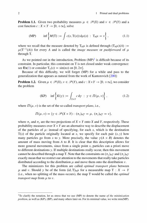
Problem 1.1. Given two probability measures � 2 P.X/ and � 2 P.Y/ and acost function c W X � Y ! Œ0;C1�, solve

.MP/ inf

�M.T/ WD

ˆc.x;T.x// d�.x/ W T#� D �

�; (1.1)

where we recall that the measure denoted by T#� is defined through .T#�/.A/ WD�.T�1.A// for every A and is called the image measure or pushforward of �through T.

As we pointed out in the introduction, Problem (MP)1 is difficult because of itsconstraint. In particular, this constraint on T is not closed under weak convergence:see Ex(1) or consider Tn.x/ D sin.nx/ on Œ0; 2��.

Because of this difficulty, we will forget (MP) for a while and pass to thegeneralization that appears as natural from the work of Kantorovich [200]:

Problem 1.2. Given � 2 P.X/, � 2 P.Y/, and c W X�Y ! Œ0;C1�, we considerthe problem

.KP/ inf

�K.�/ WD

ˆ

X�Yc d� W � 2 ˘.�; �/

�; (1.2)

where ˘.�; �/ is the set of the so-called transport plans, i.e.,

˘.�; �/ D f� 2 P.X � Y/ W .�x/#� D �; .�y/#� D �g;

where �x and �y are the two projections of X � Y onto X and Y , respectively. Theseprobability measures over X � Y are an alternative way to describe the displacementof the particles of �: instead of specifying, for each x, which is the destinationT.x/ of the particle originally located at x, we specify for each pair .x; y/ howmany particles go from x to y. More precisely, the value �.A � B/ denotes theamount of mass moving from A to B. It is clear that this description allows formore general movements, since from a single point x, particles can a priori moveto different destinations y. If multiple destinations really occur, then this movementcannot be described through a map T. Note that the constraints on .�x/#� and .�y/#�

exactly mean that we restrict our attention to the movements that really take particlesdistributed according to the distribution � and move them onto the distribution �.

The minimizers for this problem are called optimal transport plans between� and �. Should � be of the form .id;T/#� for a measurable map T W X ! Y(i.e., when no splitting of the mass occurs), the map T would be called the optimaltransport map from � to �.

1To clarify the notation, let us stress that we use (MP) to denote the name of the minimizationproblem, as well as (KP), (BP), and many others later on. For its minimal value, we write min(MP).

1.1 Kantorovich and Monge problems 3

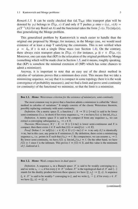
Remark 1.3. It can be easily checked that .id;T/#� (this transport plan will bedenoted by �T) belongs to ˘.�; �/ if and only if T pushes � onto � (i.e., �.A/ D�.T�1.A// for any Borel set A) and the functional takes the form

´c.x;T.x//d�.x/;

thus generalizing the Monge problem.

This generalized problem by Kantorovich is much easier to handle than theoriginal one proposed by Monge; for instance, in the Monge case, we would needexistence of at least a map T satisfying the constraints. This is not verified when� D ı0, if � is not a single Dirac mass (see Section 1.4). On the contrary,there always exist transport plans in ˘.�; �/ (for instance, � ˝ � 2 ˘.�; �/).Moreover, one can state that (KP) is the relaxation of the original problem by Monge(something which will be made clear in Section 1.5, and it means, roughly speaking,that (KP) is somehow the minimal extension of (MP) which has some chances toadmit a minimizer).

Anyway, it is important to note that an easy use of the direct method incalculus of variations proves that a minimum does exist. This means that we take aminimizing sequence, we say that it is compact in some topology (here it is the weakconvergence of probability measures), and we find a limit and prove semi-continuity(or continuity) of the functional we minimize, so that the limit is a minimizer.

Box 1.1. Memo: Weierstrass criterion for the existence of minimizers, semi-continuity

The most common way to prove that a function admits a minimizer is called the “directmethod in calculus of variations.” It simply consists of the classic Weierstrass theorem,possibly replacing continuity with semi-continuity.

Definition. On a metric space X, a function f W X ! R [ fC1g is said to be lowersemi-continuous (l.s.c. in short) if for every sequence xn ! x we have f .x/ � lim infn f .xn/.

Definition. A metric space X is said to be compact if from any sequence xn, we canextract a converging subsequence xnk ! x 2 X.

Theorem (Weierstrass). If f W X ! R [ fC1g is lower semi-continuous and X iscompact, then there exists Nx 2 X such that f .Nx/ D minff .x/ W x 2 Xg.

Proof. Define ` WD infff .x/ W x 2 Xg 2 R [ f�1g (` D C1 only if f is identicallyC1, but in this case, any point in X minimizes f ). By definition, there exists a minimizingsequence xn, i.e., points in X such that f .xn/ ! `. By compactness, we can assume xn ! Nx.By lower semi-continuity, we have f .Nx/ � lim infn f .xn/ D `. On the other hand, we havef .Nx/ � ` since ` is the infimum. This proves ` D f .Nx/ 2 R, and this value is the minimumof f , realized at Nx.

Box 1.2. Memo: Weak compactness in dual spaces

Definition. A sequence xn in a Banach space X is said to be weakly converging to x,and we write xn * x, if for every � 2 X 0 (where X 0 is the topological dual of X and h�; �istands for the duality product between these spaces) we have h�; xni ! h�; xi. A sequence

�n 2 X 0 is said to be weakly-* converging to � , and we write �n�

* � , if for every x 2 Xwe have h�n; xi ! h�; xi.

(continued)

4 1 Primal and dual problems

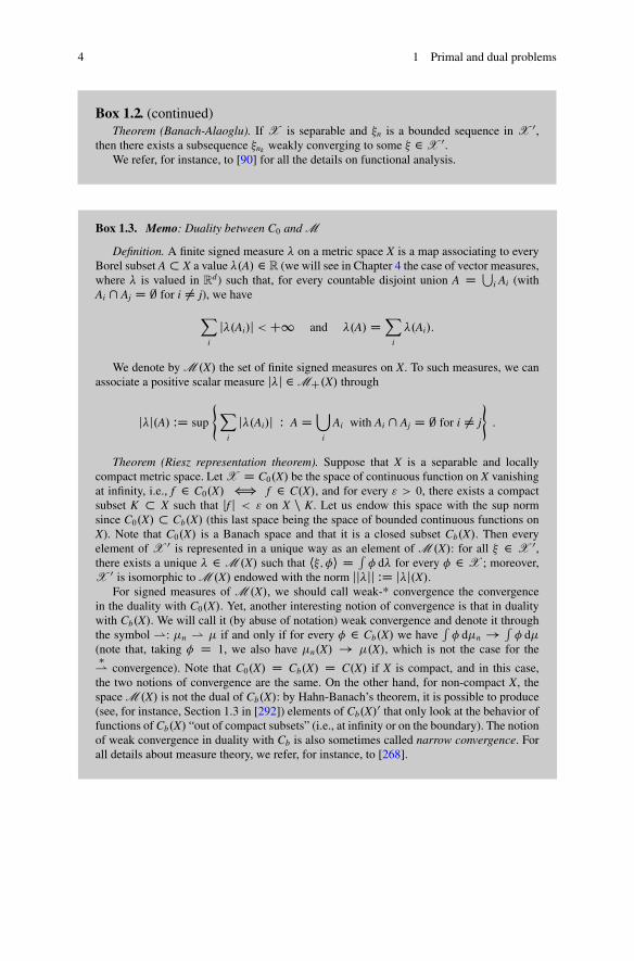
Box 1.2. (continued)Theorem (Banach-Alaoglu). If X is separable and �n is a bounded sequence in X 0,

then there exists a subsequence �nk weakly converging to some � 2 X 0.We refer, for instance, to [90] for all the details on functional analysis.

Box 1.3. Memo: Duality between C0 and M

Definition. A finite signed measure � on a metric space X is a map associating to everyBorel subset A � X a value �.A/ 2 R (we will see in Chapter 4 the case of vector measures,where � is valued in R

d) such that, for every countable disjoint union A D Si Ai (with

Ai \ Aj D ; for i ¤ j), we have

Xi

j�.Ai/j < C1 and �.A/ D Xi

�.Ai/:

We denote by M .X/ the set of finite signed measures on X. To such measures, we canassociate a positive scalar measure j�j 2 M

C

.X/ through

j�j.A/ WD sup

(Xi

j�.Ai/j W A D [i

Ai with Ai \ Aj D ; for i ¤ j

):

Theorem (Riesz representation theorem). Suppose that X is a separable and locallycompact metric space. Let X D C0.X/ be the space of continuous function on X vanishingat infinity, i.e., f 2 C0.X/ ” f 2 C.X/, and for every " > 0, there exists a compactsubset K � X such that jf j < " on X n K. Let us endow this space with the sup normsince C0.X/ � Cb.X/ (this last space being the space of bounded continuous functions onX). Note that C0.X/ is a Banach space and that it is a closed subset Cb.X/. Then everyelement of X 0 is represented in a unique way as an element of M .X/: for all � 2 X 0,there exists a unique � 2 M .X/ such that h�; �i D ´

� d� for every � 2 X ; moreover,X 0 is isomorphic to M .X/ endowed with the norm jj�jj WD j�j.X/.

For signed measures of M .X/, we should call weak-* convergence the convergencein the duality with C0.X/. Yet, another interesting notion of convergence is that in dualitywith Cb.X/. We will call it (by abuse of notation) weak convergence and denote it throughthe symbol *: �n * � if and only if for every � 2 Cb.X/ we have

´� d�n ! ´

� d�(note that, taking � D 1, we also have �n.X/ ! �.X/, which is not the case for the�

* convergence). Note that C0.X/ D Cb.X/ D C.X/ if X is compact, and in this case,the two notions of convergence are the same. On the other hand, for non-compact X, thespace M .X/ is not the dual of Cb.X/: by Hahn-Banach’s theorem, it is possible to produce(see, for instance, Section 1.3 in [292]) elements of Cb.X/0 that only look at the behavior offunctions of Cb.X/ “out of compact subsets” (i.e., at infinity or on the boundary). The notionof weak convergence in duality with Cb is also sometimes called narrow convergence. Forall details about measure theory, we refer, for instance, to [268].

1.1 Kantorovich and Monge problems 5

Box 1.4. Memo: Weak convergence of probability measures

Probability measures are particular measures in M .X/: � 2 P.X/ ” � 2 MC

.X/and �.X/ D 1 (note that for positive measures, � and j�j coincide).

Definition. A sequence �n of probability measures over X is said to be tight if for every" > 0, there exists a compact subset K � X such that �n.X n K/ < " for every n.

Theorem (Prokhorov). Suppose that �n is a tight sequence of probability measures overa complete and separable metric space X (these spaces are also called Polish spaces). Thenthere exists � 2 P.X/ and a subsequence �nk such that �nk * � (in duality with Cb.X/).Conversely, every sequence �n * � is necessarily tight.

Sketch of proof (of the direct implication). For every compact K � X, the measures.�n/ K admit a converging subsequence (in duality with C.K/). From tightness, we havean increasing sequence of compact sets Ki such that �n.K

ci / < "i D 1=i for every i and

every n. By a diagonal argument, it is possible to extract a subsequence �nh such that.�nh / Ki * �i (weak convergence as n ! 1 in duality with C.Ki/). The measures �i areincreasing in i, and define a measure � D supi �i (i.e., �.A/ D supi �i.A \ Ki/). In order toprove �nh * �, take � 2 Cb.X/ and write

´X � d.�nh ��/ � 2"i C ´

Ki� d.�nh � �i/. This

allows us to prove the convergence. Proving � 2 P.X/, we only need to check �.X/ D 1,by testing with � D 1.

We are now ready to state some existence results.

Theorem 1.4. Let X and Y be compact metric spaces, � 2 P.X/, � 2 P.Y/, andc W X � Y ! R a continuous function. Then (KP) admits a solution.

Proof. We just need to show that the set ˘.�; �/ is compact and that � 7! K.�/ D´c d� is continuous and apply Weierstrass’s theorem. We have to choose a notion

of convergence for that and we choose to use the weak convergence of probabilitymeasures (in duality with Cb.X � Y/, which is the same here as C.X � Y/ orC0.X � Y/). This gives continuity of K by definition, since c 2 C.X � Y/.

As for the compactness, take a sequence �n 2 ˘.�; �/. They are probabilitymeasures, so that their mass is 1, and hence they are bounded in the dual ofC.X �Y/. Hence, usual weak-* compactness in dual spaces guarantees the existenceof a subsequence �nk * � converging to a probability � . We just need to check� 2 ˘.�; �/. This may be done by fixing � 2 C.X/ and using

´�.x/ d�nk D´

� d� and passing to the limit, which gives´�.x/ d� D ´

� d�. This shows.�x/#� D �. The same may be done for �y. More generally, the image measurethrough continuous maps preserves weak convergence (and here we use the map.x; y/ 7! x or .x; y/ 7! y). utTheorem 1.5. Let X and Y be compact metric spaces, � 2 P.X/, � 2 P.Y/, andc W X � Y ! R [ fC1g be lower semi-continuous and bounded from below. Then(KP) admits a solution.

Proof. Only difference: K is no more continuous; it is l.s.c. for the weak conver-gence of probabilities. This is a consequence of the following lemma, applied tof D c on the space X � Y . ut

6 1 Primal and dual problems

Lemma 1.6. If f W X ! R [ fC1g is a lower semi-continuous function, boundedfrom below, on a metric space X, then the functional J W MC.X/ ! R [ fC1gdefined on positive measures on X through J.�/ WD ´

f d� is lower semi-continuousfor the weak convergence of measures.

Proof. Consider a sequence fk of continuous and bounded functions convergingincreasingly to f . Then write J.�/ D supk Jk.�/ WD ´

fk d� (actually Jk � J andJk.�/ ! J.�/ for every � by monotone convergence). Every Jk is continuousfor the weak convergence, and hence, J is l.s.c. as a supremum of continuousfunctionals. ut

Box 1.5. Memo: l.s.c. functions as suprema of Lipschitz functions

Theorem. If f˛ is an arbitrary family of lower semi-continuous functions on X, thenf D sup˛ f˛ (i.e., f .x/ WD sup˛ f˛.x/) is also l.s.c.

Proof. Take xn ! x and write f˛.x/ � lim infn f˛.xn/ � lim infn f .xn/. Then pass tothe sup in ˛ and get f .x/ � lim infn f .xn/. It is also possible to check the same fact usingepigraphs: indeed, a function is l.s.c. if and only if its epigraph f.x; t/ W t � f .x/g � X �R

is closed, and the epigraph of the sup is the intersection of the epigraphs.Theorem. Let f W X ! R [ fC1g be a function bounded from below. Then f is l.s.c.

if and only if there exists a sequence fk of k-Lipschitz functions such that for every x 2 X,fk.x/ converges increasingly to f .x/.

Proof. One implication is easy, since the functions fk are continuous, hence lower semi-continuous, and f is the sup of fk. The other is more delicate. Given f lower semi-continuousand bounded from below, let us define

fk.x/ D infy.f .y/C kd.x; y// :

These functions are k-Lipschitz continuous since x 7! f .y/ C kd.x; y/ is k-Lipschitz. Forfixed x, the sequence fk.x/ is increasing and we have inf f � fk.x/ � f .x/. We just needto prove that ` WD limk fk.x/ D supk fk.x/ D f .x/. Suppose by contradiction ` < f .x/,which implies in particular ` < C1. For every k, let us choose a point yk such that f .yk/Ckd.yk; x/ < fk.x/C 1=k. We get d.yk; x/ � `C1=k�f .yk/

k � Ck ; thanks to the lower bound on

f and to ` < 1. Hence, we know yk ! x. Yet, we have fk.x/ C 1=k � f .yk/ and we getlimk fk.x/ � lim infk f .yk/ � f .x/. This proves ` � f .x/. Finally, the functions fk may bemade bounded by taking fk ^ k.

Theorem 1.7. Let X and Y be Polish spaces, i.e., complete and separable metricspaces, � 2 P.X/, � 2 P.Y/, and c W X � Y ! Œ0;C1� lower semi-continuous.Then (KP) admits a solution.

Proof. It is now the compactness which is no more evident. We need to use theProkhorov theorem. This means showing that any sequence in ˘.�; �/ is tight. Todo that, fix " > 0 and find two compact sets KX � X and KY � Y such that�.X nKX/; �.Y nKY/ <

12" (this is possible thanks to the converse implication in the

Prokhorov theorem, since a single measure is always tight). Then the set KX � KY iscompact in X � Y and, for any �n 2 ˘.�; �/, we have

1.1 Kantorovich and Monge problems 7

�n..X � Y/ n .KX � KY// � �n..X n KX/ � Y/ C �n.X � .Y n KY//

D �.X n KX/C �.Y n KY/ < ":

This shows tightness (and hence compactness) of all sequences in ˘.�; �/. utWe add to this section an improvement of the continuity and semi-continuity

results above, which could be useful when the cost functions are not continuous.

Lemma 1.8. Let �n; � 2 ˘.�; �/ be probabilities on X � Y and a W X ! QX andb W Y ! QY be measurable maps valued in two separable metric spaces QX and QY.Let c W QX � QY ! RC be a continuous function with c.a; b/ � f .a/C g.b/ with f ; gcontinuous and

´.f ı a/ d�;

´.g ı b/ d� < C1. Then

�n * � )ˆ

X�Yc.a.x/; b.y// d�n !

ˆ

X�Yc.a.x/; b.y// d�:

Proof. We start from the case where c is bounded, say 0 � c � M. We can applythe weak version of Lusin’s theorem (see the observations in the next Memo 1.6)to maps valued in QX and QY . Let us fix ı > 0 and find two compact sets KX � X,KY � Y , with �.X n KX/ < ı and �.Y n KY/ < ı, such that a and b are continuouswhen restricted to KX and KY , respectively. Let us set K WD KX �KY � X �Y , whichis a compact set in the product.

We can writeˆ

c.a; b/ d�n �ˆ

1Kc.a; b/ d�n C 2Mı;

and the function 1Kc.a; b/ is upper semi-continuous on X �Y (since it is continuousand positive on a closed set, and vanishes outside it). This implies

lim supn

ˆc.a; b/ d�n �

ˆ1Kc.a; b/ d� C 2Mı �

ˆc.a; b/ d� C 2Mı

and, since ı is arbitrary, lim supn

´c.a; b/ d�n � ´

c.a; b/ d� . This proves uppersemi-continuity of the integral functional when c is bounded by M. An analogouscomputation with M � c instead of c proves lower semi-continuity.

If c is positive but unbounded, just approximate it from below with its truncationscM D c ^ M, and lower semi-continuity is proven for the integral functional, whichwill be a sup of lower semi-continuous functionals. By replacing c with the functionQX � QY 3 .Qx; Qy/ 7! f .Qx/C g.Qy/� c.Qx; Qy/, upper semi-continuity is proven as well. ut

8 1 Primal and dual problems

Box 1.6. Memo: Lusin’s theorem

A well-known theorem in measure theory states that every measurable function f on areasonable measure space .X; �/ is actually continuous on a set K with �.X n K/ small.This set K can be taken compact. Actually, there can be at least two statements: either wewant f to be merely continuous on K or we want f to coincide on K with a continuousfunction defined on X. This theorem is usually stated for real-valued functions, but wehappen to need it for functions valued in more general spaces. Let us be more precise: takea topological space X endowed with a finite regular measure � (i.e., any Borel set A � Xsatisfies �.A/ D supf�.K/ W K � A; K compactg D inff�.B/ W B � A; B openg). Thearrival space Y will be supposed to be second countable (i.e., it admits a countable family.Bi/i of open sets such that any other open set B � Y may be expressed as a union of Bi;for instance, separable metric spaces are second countable).

Theorem (weak Lusin). Under the above assumptions on X;Y; �, if f W X ! Y ismeasurable, then for every " > 0, there exists a compact set K � X such that �.X n K/ < "and the restriction of f to K is continuous.

Proof. For every i 2 N, set AC

i D f �1.Bi/ and A�

i D f �1.Bci /. Consider compact sets

K˙

i � A˙

i such that �.A˙

i n K˙

i / < "2�i. Set Ki D KC

i [ K�

i and K D Ti Ki. For each

i, we have �.X n Ki/ < "21�i. By construction, K is compact and �.X n K/ < 4". To prove

that f is continuous on K, it is sufficient to check that f �1.B/ \ K is relatively open in Kfor each open set B, and it is enough to check this for B D Bi. Equivalently, it is enough toprove that f �1.Bc

i /\ K is closed, and this is true since it coincides with K�

i \ K.Theorem (strong Lusin). Under the same assumptions on X, if f W X ! R is measurable,

then for every " > 0, there exists a compact set K � X and a continuous function g W X ! R

such that �.X n K/ < " and f D g on K.Proof. First apply weak Lusin’s theorem, since R is second countable. Then we just

need to extend fjK to a continuous function g on the whole X. This is possible since f

jK isuniformly continuous (as a continuous function on a compact set) and hence has a modulusof continuity !: jf .x/ � f .x0/j � !.d.x; x0// (the function ! can be taken subadditive andcontinuous). Then define g.x/ D infff .x0/C!.d.x; x0// W x0 2 Kg. It can be easily checkedthat g is continuous and coincides with f on K.

Note that this last proof strongly uses the fact that the arrival space is R. It couldbe adapted to the case of R

d just by extending componentwise. On the other hand, it isclear that the strong version of Lusin’s theorem cannot hold for any space Y: just take Xconnected and Y disconnected. A measurable function f W X ! Y taking values in twodifferent connected components on two sets of positive measure cannot be approximatedby continuous functions in the sense of the strong Lusin’s theorem.

The consequence of all these continuity, semi-continuity, and compactnessresults is the existence, under very mild assumptions on the cost and the space,of an optimal transport plan � . Then, if one is interested in the problem of Monge,the question may become, “does this minimal � come from a transport map T?”.Should the answer to this question be yes, then (MP) would have a solution, whichalso solves a wider problem, that of minimizing among transport plans. This isthe object of the next two sections, Sections 1.2 and 1.3. On the other hand, insome cases, proving that the optimal transport plan comes from a transport map (orproving that there exists at least one optimal plan coming from a map) is equivalent

1.2 Duality 9

to proving that (MP) has a solution, since very often the infimum among transportplans and among transport maps is the same. This depends on the presence of atoms(see Sections 1.4 and 1.5).

1.2 Duality

The problem (KP) is a linear optimization under convex constraints, given by linearequalities or inequalities. Hence, an important tool will be duality theory, which istypically used for convex problems. We will find a dual problem (DP) for (KP) andexploit the relations between dual and primal.

The first thing we will do is finding a formal dual problem, by means of an inf-supexchange.

Let us express the constraint � 2 ˘.�; �/ in the following way: note that, if� 2 MC.X � Y/, then we have

sup';

ˆ

X' d�C

ˆ

Y d� �

ˆ

X�Y.'.x/C .y// d� D

(0 if � 2 ˘.�; �/;C1 otherwise,

where the supremum is taken among bounded and continuous functions '; .Hence, we can remove the constraints on � if we add the previous sup, since if

they are satisfied, nothing has been added, and if they are not, we get C1 (whichwill be avoided by the minimization). Hence, we may look at the problem, we get

min�

ˆ

X�Yc d� C sup

';

ˆ

X' d�C

ˆ

Y d� �

ˆ

X�Y.'.x/C .y// d� (1.3)

and consider interchanging sup and inf:

sup';

ˆ

X' d�C

ˆ

Y d� C inf

�

ˆ

X�Y.c.x; y/ � .'.x/C .y/// d�:

We would like the two above optimization problems (“inf sup” and “sup inf”) to beequivalent and the value to be the same. This is not always possible, and the maintool to do it is a theorem by Rockafellar (see [260], Section 37) requiring concavityin one variable, convexity in the other one, and some compactness assumption. Yet,Rockafellar’s statement concerns finite-dimensional spaces, which is not the casehere. To handle infinite-dimensional situations, one needs to use a more generalmini-max theorems2.

For now, we prefer not to investigate anymore the question of obtaining theduality equality. The result is true (under suitable assumptions), and we will seelater on how to prove it. For the moment, let us accept it as true.

2We will give a proof in this spirit in Section 1.6.3.

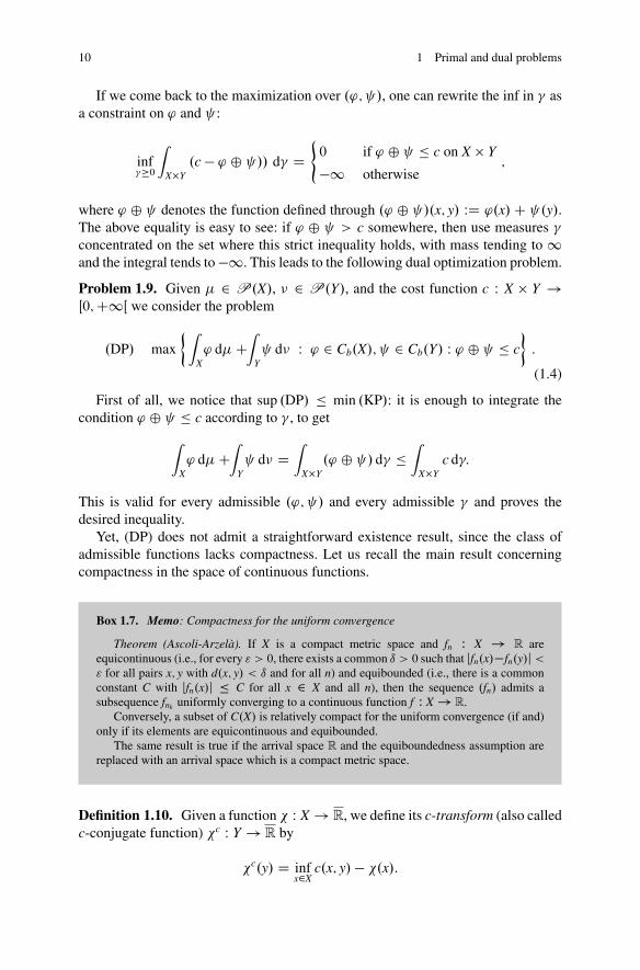
10 1 Primal and dual problems

If we come back to the maximization over .'; /, one can rewrite the inf in � asa constraint on ' and :

inf��0

ˆ

X�Y.c � ' ˚ // d� D

(0 if ' ˚ � c on X � Y

�1 otherwise;

where ' ˚ denotes the function defined through .' ˚ /.x; y/ WD '.x/C .y/.The above equality is easy to see: if ' ˚ > c somewhere, then use measures �concentrated on the set where this strict inequality holds, with mass tending to 1and the integral tends to �1. This leads to the following dual optimization problem.

Problem 1.9. Given � 2 P.X/, � 2 P.Y/, and the cost function c W X � Y !Œ0;C1Œ we consider the problem

.DP/ max

�ˆX' d�C

ˆ

Y d� W ' 2 Cb.X/; 2 Cb.Y/ W ' ˚ � c

�:

(1.4)

First of all, we notice that sup .DP/ � min .KP/: it is enough to integrate thecondition ' ˚ � c according to � , to get

ˆ

X' d�C

ˆ

Y d� D

ˆ

X�Y.' ˚ / d� �

ˆ

X�Yc d�:

This is valid for every admissible .'; / and every admissible � and proves thedesired inequality.

Yet, (DP) does not admit a straightforward existence result, since the class ofadmissible functions lacks compactness. Let us recall the main result concerningcompactness in the space of continuous functions.

Box 1.7. Memo: Compactness for the uniform convergence

Theorem (Ascoli-Arzelà). If X is a compact metric space and fn W X ! R areequicontinuous (i.e., for every " > 0, there exists a common ı > 0 such that jfn.x/�fn.y/j <" for all pairs x; y with d.x; y/ < ı and for all n) and equibounded (i.e., there is a commonconstant C with jfn.x/j � C for all x 2 X and all n), then the sequence .fn/ admits asubsequence fnk uniformly converging to a continuous function f W X ! R.

Conversely, a subset of C.X/ is relatively compact for the uniform convergence (if and)only if its elements are equicontinuous and equibounded.

The same result is true if the arrival space R and the equiboundedness assumption arereplaced with an arrival space which is a compact metric space.

Definition 1.10. Given a function W X ! R, we define its c-transform (also calledc-conjugate function) c W Y ! R by

c.y/ D infx2X

c.x; y/ � .x/:

1.2 Duality 11

We also define the Nc-transform of W Y ! R by

Nc.x/ D infy2Y

c.x; y/ � .y/:

Moreover, we say that a function defined on Y is Nc-concave if there exists such that D c (and, analogously, a function ' on X is said to be c-concave ifthere is W Y ! R such that ' D Nc), and we denote by c�conc.X/ and Nc�conc.Y/the sets of c- and Nc-concave functions, respectively (when X D Y and c is symmetric,this distinction between c and Nc will play no more any role and will be dropped assoon as possible).

It is important to note that the notion of c-concavity implies a bound on themodulus of continuity.

Box 1.8. Memo: Continuity of functions defined as an inf or sup

Proposition. Let .f˛/˛ be a family (finite, infinite, countable, uncountable, etc.) offunctions, all satisfying the same condition

jf˛.x/� f˛.x0/j � !.d.x; x0//:

Consider f defined through f .x/ WD inf˛ f˛.x/. Then f also satisfies the same estimate.This can be easily seen from f˛.x/ � f˛.x0/C!.d.x; x0//, which implies f .x/ � f˛.x0/C

!.d.x; x0// since f � f˛ . Then, taking the infimum over ˛ at the r.h.s., one gets f .x/ �f .x0/C !.d.x; x0//. Interchanging x and x0, one obtains

jf .x/� f .x0/j � !.d.x; x0//:

In particular, if the function ! W RC

! RC

satisfies limt!0 !.t/ D 0 (which meansthat the family .f˛/˛ is equicontinuous), then f has the same modulus of continuity (i.e.,the same function !) as the functions f˛ . The same idea obviously works for the supremuminstead of the infimum.

In our case, if c is continuous and finite on a compact set, and hence uniformlycontinuous, this means that there exists an increasing continuous function ! WRC ! RC with !.0/ D 0 such that

jc.x; y/ � c.x0; y0/j � !.d.x; x0/C d.y; y0//:

Hence, when we take the definition of c, we have c.y/ D infx gx.y/ with gx.y/ WDc.x; y/�.x/, and the functions gx satisfy jgx.y/�gx.y0/j � !.d.y; y0//. This provesthat c shares the same continuity modulus also.

It is quite easy to realize that, given a pair .'; / in the maximization problem(DP), one can always replace it with .'; 'c/ and then with .'cNc; 'c/, and theconstraints are preserved and the integrals increased. Actually one could go on,

12 1 Primal and dual problems

but we will see that 'cNcc D 'c for any ' (see Section 1.6). The goal of thesetransformations is to “improve” the maximizing sequence so as to get a uniformbound on its continuity.

A consequence of these considerations is the following existence result.

Proposition 1.11. Suppose that X and Y are compact and c is continuous. Thenthere exists a solution .'; / to problem (DP) and it has the form ' 2 c �conc.X/; 2 Nc�conc.Y/, and D 'c. In particular

max .DP/ D max'2c�conc.X/

ˆ

X' d�C

ˆ

Y'c d�:

Proof. From the considerations above, we can take a maximizing sequence .'n; n/

and improve it, by means of c- and Nc-transforms, so that we can assume a uniformbound on the continuity of these functions (the same modulus of continuity as c).Instead of renaming the sequence, we will still call .'n; n/ the new sequenceobtained after these transforms. We only need to check equiboundedness so as toapply Ascoli-Arzelà’s theorem. This may be done if we note that adding a constantto ' and subtracting it to is always possible: the value of the functional doesnot change, nor the constraints are affected. Hence, since 'n is continuous on acompact set and hence bounded, we can always subtract its minimum and supposewithout loss of generality that min'n D 0. We get max'n � !.diam X/ (since theoscillation of a function is always less than its modulus of continuity computed atthe highest possible distance in the set). So, if we have chosen n D 'c

n, we alsohave n.y/ D infx c.x; y/� 'n.x/ 2 Œmin c �!.diam X/;max c�. This gives uniformbounds on 'n and n and allows us to apply Ascoli-Arzelà’s theorem.

Passing to a subsequence, we can assume 'n ! ' and n ! , bothconvergences being uniform. It is easy to see that

ˆ

X'n d�C

ˆ

Y n d� !

ˆ

X' d�C

ˆ

Y d�;

as a consequence of uniform convergence. Moreover,

'n.x/C n.y/ � c.x; y/ ) '.x/C .y/ � c.x; y/

(here, pointwise convergence would have been enough). This shows that .'; / isan admissible pair for (DP) and that it is optimal. ut

If we admit the duality result min .KP/ D max .DP/ (the proof is postponed toSection 1.6), then we also have

min .KP/ D max'2c�conc.X/

ˆ

X' d�C

ˆ

Y'c d�;

1.3 Strictly convex and quadratic costs 13

which also shows that the minimum value of (KP) is a convex function of .�; �/, asit is a supremum of linear functionals.

Definition 1.12. The functions ' realizing the maximum in (3.1) are called Kan-torovich potentials for the transport from � to �. This is in fact a small abuse,because traditionally, this term was used only in the case c.x; y/ D jx � yj, butit is nowadays understood in the general case as well.

Remark 1.13. Note that the Kantorovich potential ' is not necessarily c-concave,but coincides with the c-concave function 'cNc �-a.e. However, it is always possibleto choose a c-concave Kantorovich potential, and we will do it often.

1.3 The case c.x; y/ D h.x � y/ for h strictly convexand the existence of an optimal T

This section is mainly devoted to the results that we can obtain in the case whereX D Y D ˝ � R

d and the cost c is of the form c.x; y/ D h.x � y/, for a strictlyconvex function h. We will also assume ˝ to be compact for simplicity. This caseallows for very strong results, and in particular we will find existence, as well as arepresentation formula, for the optimal T. Anyway, the first few lines of this sectionwill be concerned with a more general case: that of costs functions c satisfying atwist condition, the most remarkable case being exactly those of the form h.x � y/with h strictly convex.3

The main tool is the duality result. More precisely, we use Theorem 1.39,which applies to the case of compact domains with continuous cost functions c.It guarantees max .DP/ D min .KP/.

From the equality between the minimum of (KP) and the maximum of (DP) andthe fact that both extremal values are realized, one can consider an optimal transportplan � and a Kantorovich potential ' and write

'.x/C 'c.y/ � c.x; y/ on ˝ �˝ and '.x/C 'c.y/ D c.x; y/ on spt.�/:

The equality on spt.�/ is a consequence of the inequality which is valid everywhereand of

ˆ

˝�˝c d� D

ˆ

˝

' d�Cˆ

˝

'c d� Dˆ

˝�˝.'.x/C 'c.y// d�;

which implies equality � -a.e. These functions being continuous, the equality issatisfied on a closed set, i.e., on the support of the measure � (let us recallthe definition of support of a measure, not to be confused with sets where it isconcentrated).

3The general results of this section are essentially due to [176], as a generalization of [82, 84].

14 1 Primal and dual problems

Definition 1.14. On a separable metric space X, the support of a measure � isdefined as the smallest closed set on which � is concentrated, i.e.,

spt.�/ WD\

fA W A is closed and �.X n A/ D 0g :

This is well defined since the intersection may be taken countable, due to theseparability assumption. Moreover, there exists also this characterization:

spt.�/ D fx 2 X W �.B.x; r// > 0 for all r > 0g :

Once we have that, let us fix a point .x0; y0/ 2 spt.�/. One may deduce from theprevious computations that

x 7! '.x/ � c.x; y0/ is minimal at x D x0

and, if ' and c.�; y0/ are differentiable at x0 and x0 … @˝, one gets r'.x0/ Drxc.x0; y0/. We resume this fact in a very short statement (where we do not put thesharpest assumptions on c) since we will use it much later on.

Proposition 1.15. If c is C1, ' is a Kantorovich potential for the cost c in thetransport from � to �, and .x0; y0/ belongs to the support of an optimal transportplan � , then r'.x0/ D rxc.x0; y0/, provided ' is differentiable at x0. In particular,the gradients of two different Kantorovich potentials coincide on every pointx0 2 spt.�/ where both the potentials are differentiable.

Proof. The proof is contained in the above considerations. utThe equality r' D rxc is particularly useful when c satisfies the following

definition.

Definition 1.16. For ˝ � Rd, we say that c W ˝ � ˝ ! R satisfies the

twist condition whenever c is differentiable w.r.t. x at every point and the mapy 7! rxc.x0; y/ is injective for every x0. This condition is also known in economicsas Spence-Mirrlees condition (see, for instance, [261]). For “nice” domains and cost

functions, it corresponds to det�

@2c@yi@xj

�¤ 0.

The goal of this condition is to deduce from .x0; y0/ 2 spt.�/ that y0 is indeeduniquely defined from x0. This shows that � is concentrated on a graph, that of themap associating y0 to each x0, and this map will be the optimal transport. Since thismap has been constructed using ' and c only, and not � , it also provides uniquenessfor the optimal � .

We will see this strategy with more details in the particular case where c.x; y/ Dh.x � y/, with h strictly convex, but the reader can see how to translate it into themost general case.

For this choice of c, if ' and h are differentiable at x0 and x0 � y0, respectively,and x0 … @˝, one gets r'.x0/ D rh.x0 � y0/. This works if the function h

1.3 Strictly convex and quadratic costs 15

is differentiable; if it is not, we shall write r'.x0/ 2 @h.x0 � y0/ (using thesubdifferential of h; see Box 1.12 in Section 1.6). For a strictly convex functionh, one may inverse the relation passing to .rh/�1, thus getting

x0 � y0 D .rh/�1.r'.x0//:

Notice that the expression .rh/�1 makes sense for strictly convex functions h,independently of h 2 C1, thanks to the considerations on the invertibility of @hin Box 1.12.

This formula gives the solution to the transport problem with this cost, provided' is differentiable a.e. with respect to �. This is usually guaranteed by requiring �to be absolutely continuous with respect to the Lebesgue measure and using the factthat ' may be proven to be Lipschitz.

Box 1.9. Memo: Differentiability of Lipschitz functions

Theorem (Rademacher). Let f W Rd ! R be a Lipschitz continuous function. Then theset of points where f is not differentiable is negligible for the Lebesgue measure.

We do not provide a proof of this fact, but one can look at Chapter 3 of [12].

Then, one may use the previous computation to deduce that, for every x0, thepoint y0 (whenever it exists) such that .x0; y0/ 2 spt.�/ is unique (i.e., � is of theform �T WD .id;T/#� where T.x0/ D y0). Moreover, this also gives uniqueness ofthe optimal transport plan and of the gradient of the Kantorovich potential.

We may summarize everything in the following theorem:

Theorem 1.17. Given � and � probability measures on a compact domain ˝ �R

d, there exists an optimal transport plan � for the cost c.x; y/ D h.x � y/ withh strictly convex. It is unique and of the form .id;T/#�, provided � is absolutelycontinuous and @˝ is negligible. Moreover, there exists a Kantorovich potential ',and T and the potentials ' are linked by

T.x/ D x � .rh/�1.r'.x//:

Proof. The previous theorems give the existence of an optimal � and an optimal '.The previous considerations show that if we take a point .x0; y0/ 2 spt.�/ wherex0 … @˝ and r'.x0/ exists, then necessarily we have y0 D x0 � .rh/�1.r'.x0//.The points x0 on the boundary are negligible by assumption. The points where thedifferentiability fails are Lebesgue-negligible by Rademacher’s theorem. Indeed, 'shares the same modulus of continuity of c, which is a Lipschitz function on˝ �˝since h is locally Lipschitz continuous and˝ is bounded. Hence, ' is also Lipschitz.From the absolute continuity assumption on �, these two sets of “bad” points (theboundary and the non-differentiability points of ') are �-negligible as well. Thisshows at the same time that every optimal transport plan is induced by a transport

16 1 Primal and dual problems

map and that this transport map is x 7! x � .rh/�1.r'.x//. Hence, it is uniquelydetermined (since the potential ' does not depend on � ). As a consequence, we alsohave uniqueness of the optimal � . utRemark 1.18. All the costs of the form c.x; y/ D jx � yjp with p > 1 can be dealtwith via Theorem 1.17.

Remark 1.19. In the previous theorem, we showed the uniqueness of the optimalplan by giving an explicit expression for the optimal map. Yet, it is possible to usea more general argument: every time that we know that any optimal � must beinduced by a map T, then we have uniqueness. Indeed, suppose that two differentplans �1 D �T1 ; �2 D �T2 are optimal: consider 1

2�1 C 1

2�2, which is optimal as well

by convexity. This last transport plan cannot be induced by a map unless T1 D T2 �-a.e., which gives a contradiction.

Remark 1.20. Theorem 1.17 states that the optimal � is of the form .id;T/#�, undersome assumptions on �. If the same assumptions are also satisfied by �, then we canalso say that there is an optimal map the other way around, i.e., � D .S; id/#�. Inparticular � -a.e. we have y D T.x/ and x D S.y/, which means S.T.x// D x � -a.e.,i.e. for �-a.e. point x. Hence, T is invertible on a set of full measure and its inverseis the optimal map from � to �.

1.3.1 The quadratic case in Rd

The case where the cost is given by c.x; y/ D 12jx � yj2 in R

d deserves a specialattention. The main reason for this special attention is the connection between c-concavity and the usual notion of convexity.

Proposition 1.21. Given a function W Rd ! R [ f�1g, let us define u W Rd !R[ fC1g through u.x/ D 1

2jxj2 �.x/. Then we have uc D .u/. In particular,

a function is c-concave if and only if x 7! 12jxj2 � .x/ is convex and l.s.c.

Proof. Just compute

uc.x/ D 1

2jxj2�c.x/ D sup

y

1

2jxj2�1

2jx�yj2C.y/ D sup

yx�y�

�1

2jyj2 � .y/

�:

This proves the first part of the statement. Moreover, since c-concave functions arecharacterized by the fact that they are c-transforms and convex l.s.c. functions by thefact that they are sup of affine functions (see Box 1.11 in Section 1.6), the secondpart of the statement follows. ut

As a consequence of the above proposition, we can particularize Theorem 1.17to the quadratic case c.x; y/ D 1

2jx � yj2, thus getting the existence of an optimal

transport map

1.3 Strictly convex and quadratic costs 17

T.x/ D x � r'.x/ D r�

x2

2� '.x/

�D ru.x/

for a convex function u. Since we will also see the converse implication (sufficientoptimality conditions), this will also prove the existence and the uniqueness of agradient of a convex function transporting � onto �. This well-known fact has beeninvestigated first by Brenier (see [82]) and is usually referred to as the Breniertheorem (however, see also [227]). Section 1.7.2 will present the original approachby Brenier, called “polar factorization.”

Let us moreover note that a specific approach for the case jx � yj2, based onthe fact that we can withdraw the parts of the cost depending on x or y only andmaximize

´x�y d� , gives the same result in an easier way: we actually get '.x0/C

'.y0/ D x0 � y0 for a convex function ' and its Legendre transform ', and wededuce y0 2 @'.x0/ (see Box 1.12 in Section 1.6).

We note now that the existence of an optimal transport map is true under weakerassumptions on �: we can replace the condition of being absolutely continuous withthe condition “�.A/ D 0 for any A � R

d such that H d�1.A/ < C1” or with anycondition which ensures that the non-differentiability set of u is negligible.

In [4, 5], it is proven that the set where a convex function is not differentiable is.d �1/-rectifiable (i.e., it is contained, up to H d�1-negligible sets, in a countableunion of Lipschitz images of R

d�1); more generally, the set of points wherethe subdifferential has dimension at least k is .d �k/-rectifiable. Lipschitz .d �k/surfaces can be replaced with C1 surfaces, thanks to Lusin-type approximationresults of Lipschitz functions via C1 functions (see [160], Chapter 6).

Also, it is possible to give an even stronger result about the non-differentiabilityset: it is contained H d�1-a.e. in a countable union of .d�1/ surfaces of class C2, asit is proven in [3]. Moreover, every set which is .d�1/-rectifiable in this C2 sense iscontained in the non-differentiability set of a convex function4.

After these subtle details on the sharpest assumptions on � which guarantee theexistence of an optimal transport map T (essentially, the fact that convex functionsmust be differentiable �-a.e.), we want now to adapt our analysis to the case ofunbounded domains. This case is not covered by the general results of this sectionand has not been detailed so far. Yet, it can be handled replacing Theorem 1.39 withTheorem 1.40, which is valid for the cost c.x; y/ D 1

2jx � yj2 without compactness

assumptions on the domain (we just need´ jxj2 dx;

´ jyj2 dy < C1). It providesthe existence of solution .'; / to the following variant of (DP):

4These considerations allowed N. Gigli in [182] to prove the following characterization theorem,extending 1.17: given �; � 2 P.˝/, suppose �.A/ D 0 for every C2 surface A of co-dimension 1;then the optimal transport plan � 2 ˘.�; �/ for the quadratic cost jx � yj2 is unique and inducedby a transport map, whatever � is. Moreover, the condition “�.A/ D 0 for every C2 surface A ofco-dimension 1” characterizes the class of measures � such that the optimal transport plans (forthe quadratic cost) from � are unique and induced by maps for every target measure �.

18 1 Primal and dual problems

.DP � var/ sup

�ˆRd' d�C

ˆ

Rd d� W ' 2 L1.�/; 2 L1.�/; ' ˚ � c

�;

together with max .DP � var/ D min .KP/. The sharpest result in the unboundedcase is detailed in the following theorem.

Theorem 1.22. Let �; � be probabilities over Rd and c.x; y/ D 12jx � yj2. Suppose´ jxj2 dx;

´ jyj2 dy < C1, which implies min .KP/ < C1 and suppose that �gives no mass to .d�1/ surfaces of class C2. Then there exists, unique, an optimaltransport map T from � to �, and it is of the form T D ru for a convex function u.

Proof. We follow again the same scheme as before: an optimal � exists, andTheorem 1.40 also gives the existence of an optimal dual pair .'; / 2 L1.�/ �L1.�/ and guarantees that we have no duality gap. Then, we can see that � isconcentrated on the graph of x 7! x � r'.x/ WD ru.x/ provided u (or ', whichis equivalent) is differentiable �-a.e. Since ' 2 L1.�/, we infer that u is finite �-a.e.and, since u is convex, we get spt.�/ � fu < C1g, which is a convex set. Note that@.fu < C1g/ can be expressed locally as the graph of a concave function; hence,it is .d�1/ � C2 rectifiable set and is �-negligible by assumption. In the interior offu < C1g, u is differentiable �-a.e. (again, because of the assumption on � and ofu being convex). utRemark 1.23. As a consequence of all these considerations, the quadratic case givesa very interesting result in dimension one. Suppose that � 2 P.R/ is atomless.Then every convex function is differentiable �-a.e., since we know that the setof non-differentiability points of a convex function is at most countable (this is aconsequence of the fact that if is convex, then the intervals � 0

l .x/; 0r.x/Œ, where

0l and 0

r denote the left and right derivatives, are all nonempty and disjoint when xranges among non-differentiability points). This implies the existence of an optimaltransport map for the quadratic cost between � and any measure � 2 P.R/. Thistransport map will be the derivative of a convex function, i.e., a nondecreasing map.

Remark 1.24. Some of the properties of the quadratic case stay true if we pass to ageneral cost c.x; y/ which is C1;1 and satisfies the twist condition of Definition 1.16.Obviously, the fact that the transport is the gradient of a convex function is no moretrue; on the other hand, the differentiability properties of Kantorovich potentials arethe same as for convex functions, since one can prove that ' is semi-concave (i.e.,concave, up to subtracting a quadratic function), and this allows us to use the sameassumptions on � as in Theorem 1.22.

1.3.2 The quadratic case on the flat torus

It is useful and interesting to see what happens if we replace measures on Rd with

measures on the flat torus Td D R

d=Zd and the cost 12jx � yj2 with the squared

1.3 Strictly convex and quadratic costs 19

distance on the torus, i.e., c.x; y/ D 12jŒx � y�j2, where

jŒz�j WD minfjz C kj W k 2 Zdg: (1.5)

This is the simplest example of optimal transport on a manifold, for which a generalexistence theorem has been established by McCann in [231]. Yet, the case of thetorus, first studied in [127], is much simpler, because of the structure that Td inheritsfrom R

d. In many cases (we will see in Chapters 5 and 6, in particular), studyingwhat happens on the torus allows us to understand the main qualitative featuresof the problem, getting rid of difficulties arising from lack of compactness and/orboundary issues. In the case of compactly supported measures, it is possible to viewtheir supports as part of a large cube, to be identified with a torus, and this at noprice. Indeed, if the measures are far from the boundary of the cube, the optimaltransport maps on the torus and on the Euclidean space will coincide.

Note that an optimal Nk in (1.5) always exists. If we take z 2 Q WD Œ� 12; 12�d,

then Nk 2 f�1; 0;C1gd, and it is unique (and equal to 0) unless z 2 @Q. Moreover,the function R

d 3 z 7! 12jŒz�j2 is semi-concave, as it is the infimum of a family

of functions with Hessian equal to the identity matrix I. It is differentiable at everypoint where the optimal Nk is unique. For a given point x, we call cut locus of x the setof points y such that the squared distance function, viewed as a function of the pair.x; y/, is not differentiable at .x; y/. This is a general notion in differential geometry,and we denote it by cut.x/ (see [294] for its use in optimal transport), but in the caseof the flat torus, it simply coincides with the set of points y such that y�x 2 @QCZ

d.

Theorem 1.25. Take �; � 2 P.Td/, with � � L d and c.x; y/ D 12jŒx � y�j2.

Then there exists a unique optimal transport plan � 2 ˘.�; �/. It has the form� D �T and the optimal map T is given by T.x/ D x � r'.x/ for a.e. x, where thesum x � r'.x/ is to be intended modulo Z

d. Here, the function ' is a Kantorovichpotential, solution to the dual problem, in the transport from � to � for the cost c.Moreover, for a.e. x 2 T

d, the point T.x/ does not belong to cut.x/.

Proof. The strategy is the same as for the costs of the form h.x � y/. We take anoptimal transport plan � , together with a pair .'; /, solution of the dual problem,and we fix .x0; y0/ 2 spt.�/. We have

1

2jŒx � y0�j2 � '.x/ � .y0/;

1

2jŒx0 � y0�j2 � '.x0/ D .y0/:

Now, take k0 2 Zd such that jŒx0 � y0�j D jx0 � y0 � k0j and observe that, from the

inequality jŒx � y0�j � jx � y0 � k0j, we have

1

2jx � y0 � k0j2 � '.x/ � .y0/;

1

2jx0 � y0 � k0j2 � '.x0/ D .y0/:

20 1 Primal and dual problems

This means that the function x 7! 12jx � y0 � k0j2 � '.x/ is minimal at x D x0.

Yet, '.x/ D infy12jŒx � y�j2 � .y/ is a semi-concave function, as it is defined as

an infimum of uniformly semi-concave functions. Hence, it is differentiable a.e. and�-a.e.

If we assume that x0 is such that r'.x0/ exists, we deduce from the minimalityabove that x0 � y0 � k0 D r'.x0/. This implies that k0 is uniquely determined by x0and y0, and hence y0 … cut.x0/. Moreover, y0 is uniquely determined by x0, and weget the usual result for the existence and uniqueness of the optimal map. utRemark 1.26. In the proof of the previous theorem, we can also observe that wehave k0 D 0 if x0 � y0 2 Q; this means in particular that whenever spt.�/; spt.�/ �12Q, then the transport is completely identical to what we would have with the

classical quadratic cost in Rd instead of using the periodic framework of Td.

1.4 Counterexamples to existence

We want to give at least two examples that are not included in the statement ofTheorem 1.17 and where an optimal transport does not exist. We concentrate onexamples where the cost c.x; y/ would usually allow for existence results (take, forinstance, c.x; y/ D jx�yj2), but the reason for this lack of existence is the measure�.Other examples where this is due to the cost and not to the measures are possible;see, for instance, Ex(58) and Ex(59).

No transport may exist

The first one is very easy. Consider the case � D ıa, a 2 X, and suppose that � isnot a Dirac mass. In this case, there is no transport map at all. Indeed, it is easy tocheck that T#ıa D ıT.a/, and hence no transport map T W X ! Y can exist if � is notof the form ıb for some b 2 Y .

More generally, we can say that the image measure T#� always includes anatom of mass at least �.fag/ for every atom a of �. This implies in particular thatmeasures with atoms cannot be sent through a transport map onto measures withoutatoms. For these reasons, the absence of atoms is a typical assumption on the sourcemeasure � when one wants to solve (MP).

On the contrary, the problem (KP) by Kantorovich still makes sense even foratomic measures. In particular, the situation is very easy when � D ıa. In this case,the set ˘.�; �/ contains a unique element, which is � D �˝ � D ıa ˝ �.

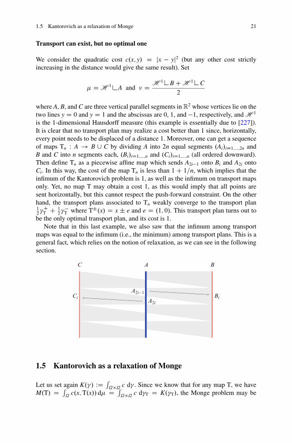
1.5 Kantorovich as a relaxation of Monge 21

Transport can exist, but no optimal one

We consider the quadratic cost c.x; y/ D jx � yj2 (but any other cost strictlyincreasing in the distance would give the same result). Set

� D H 1 A and � D H 1 B C H 1 C

2

where A, B, and C are three vertical parallel segments in R2 whose vertices lie on the

two lines y D 0 and y D 1 and the abscissas are 0, 1, and �1, respectively, and H 1

is the 1-dimensional Hausdorff measure (this example is essentially due to [227]).It is clear that no transport plan may realize a cost better than 1 since, horizontally,every point needs to be displaced of a distance 1. Moreover, one can get a sequenceof maps Tn W A ! B [ C by dividing A into 2n equal segments .Ai/iD1;:::;2n andB and C into n segments each, .Bi/iD1;:::;n and .Ci/iD1;:::;n (all ordered downward).Then define Tn as a piecewise affine map which sends A2i�1 onto Bi and A2i ontoCi. In this way, the cost of the map Tn is less than 1 C 1=n, which implies that theinfimum of the Kantorovich problem is 1, as well as the infimum on transport mapsonly. Yet, no map T may obtain a cost 1, as this would imply that all points aresent horizontally, but this cannot respect the push-forward constraint. On the otherhand, the transport plans associated to Tn weakly converge to the transport plan12�C

T C 12��

T where T˙.x/ D x ˙ e and e D .1; 0/. This transport plan turns out tobe the only optimal transport plan, and its cost is 1.

Note that in this last example, we also saw that the infimum among transportmaps was equal to the infimum (i.e., the minimum) among transport plans. This is ageneral fact, which relies on the notion of relaxation, as we can see in the followingsection.

A BC

Ci BiA2i

A2i−1

1.5 Kantorovich as a relaxation of Monge

Let us set again K.�/ WD ´˝�˝ c d� . Since we know that for any map T, we have

M.T/ D ´˝

c.x;T.x// d� D ´˝�˝ c d�T D K.�T/, the Monge problem may be

22 1 Primal and dual problems

rewritten as

min fJ.�/ W � 2 ˘.�; �/g ;

where

J.�/ D(

K.�/ D M.T/ if � D �T;

C1 otherwise.

This is simple to understand: the definition of J forces to restrict the minimizationto those plan induced by a transport map. This fact is useful in order to consider(MP) and (KP) as two problems on the same set of admissible objects, where theonly difference is the functional to be minimized, J or K.

The question is now: why did Kantorovich decide to replace J with K? Canwe easily prove that inf K D inf J? This is obviously true when, by chance, theminimizer of K is of the form � D �T, since in this case, we would have equalityof the two minima. But is it possible to justify the procedure in general? The mainmathematical justification comes from the following notion of relaxation.

Box 1.10. Memo: Relaxation

Let F W X ! R[ fC1g be a given functional on a metric space X, and suppose that itis bounded from below. We define the relaxation of F as the functional F W X ! R[fC1gwhich is the maximal functional among those G W X ! R[ fC1g which are lower semi-continuous and such that G � F. This functional exists since the supremum of an arbitraryfamily of l.s.c. functions is also l.s.c. Moreover, we also have a representation formula,which is easy to prove:

F.x/ D infflim infn

F.xn/ W xn ! xg:

A consequence of the definition is also that inf F D inf F (this latter infimum, that ofF, being often a minimum, when X is compact). This is easy to check: F � F impliesinf F � inf F; on the other hand, we have F � ` where ` WD inf F and a constant functionis l.s.c. Hence F � ` and inf F � inf F.

Here we claim that, under some assumptions, K is actually the relaxation of J. Itwill happen, in this case, by chance, that this relaxation is also continuous, insteadof only semi-continuous, and that it coincides with J on fJ < C1g.

The assumptions are the following: we take˝ � Rd to be compact, c continuous,

and � atomless (i.e., for every x 2 ˝, we have �.fxg/ D 0). Compactnessis supposed for simplicity, while the result could be true under more generalassumptions. The references on this subject are [253] and [8].

We need some preliminary results. The first concerns the one-dimensional case,we will analyze in detail in Chapter 2, but can be stated right now.

1.5 Kantorovich as a relaxation of Monge 23

Lemma 1.27. If �; � are two probability measures on the real line R and � isatomless, then there exists at least a transport map T such that T#� D �.

Proof. Just consider the monotone increasing map T provided by Remark 1.23. Thismap also optimizes the quadratic cost, but here we don’t care about it. utLemma 1.28. There exists a Borel map �d W Rd ! R which is injective, its imageis a Borel subset of R, and its inverse map is Borel measurable as well.

Proof. First, note that it is sufficient to prove this result for d D 2, since then onecan proceed by induction: if a map �d�1 is given on R

d�1, then one can produce amap �d by considering �d.x1; x2; : : : ; xd/ D �2.x1; �d�1.x2; x3; : : : ; xd//.

Then, note also that it is enough to define such a map on �0; 1Œ2, since one can gofrom R

2 to �0; 1Œ2 by considering .x; y/ 7! . 12

C 1�

arctan x; 12

C 1�

arctan y/.Then, consider the map which associates to the pair .x; y/, where x D

0; x1x2x3 : : : and y D 0; y1y2y3 : : : in decimal (or binary) notation, the point0; x1y1x2y2x3y3 : : : . In order to avoid ambiguities, we can decide that no decimalnotation is allowed to end with a periodic 9 (i.e., 0:347299999 : : : has to be writtenas 0:3473). This is why the image of this map will not be the whole interval, sincethe points like 0:39393939 : : : are not obtained through this map. But this set ofpoints is actually Borel measurable.

It is not difficult neither to check that the map is Borel measurable, as well asits inverse, since the pre-image of every interval defined by prescribing the first 2kdigits of a number in R is just a rectangle in R

2, the product of two intervals definedby prescribing the first k digits of every component. These particular intervals beinga base for the Borel tribe proves the measurability we need. utCorollary 1.29. If �; � are two probability measures on R

d and � is atomless, thenthere exists at least a transport map T such that T#� D �.

Proof. This is just obtained by considering a transport map T from .�d/#� to .�d/#�

and then composing with �d and .�d/�1. ut

Remark 1.30. We provided here, through Lemma 1.28, an explicit way of con-structing a transport map between an atomless measure � and an arbitrary measure�, when the ambient space is R

d. Actually, this fact is much more general, sinceit is well known that any measure space endowed with an atomless measure isisomorphic to Œ0; 1� with the Lebesgue measure5. Yet, we do not want to introducethis kind of arguments when an explicit construction is sufficient to deal with theEuclidean case, which already meets our scopes.

5Note that this was the argument used in [175] to obtain the existence of transport maps in generalspaces, and [253] points out that, when composing with the isomorphisms sending arbitrary spacesto Œ0; 1�, the cost function is no more continuous. Yet, this could be handled using Lemma 1.8,which allows us to use costs of this form: the composition of a continuous function with measurablemaps of x and y separately.

24 1 Primal and dual problems

A last lemma:

Lemma 1.31. Consider on a compact metric space X, endowed with a probability% 2 P.X/, a sequence of partitions Gn, each Gn being a family of disjoint subsetsCi;n such that

Si2In

Ci;n D X for every n. Suppose that size.Gn/ WD maxi diam.Ci;n/

tends to 0 as n ! 1 and consider a sequence of probability measures %n on X suchthat, for every n and i 2 In, we have %n.Ci;n/ D %.Ci;n/. Then %n * %.

Proof. Set mi;n WD %n.Ci;n/ D %.Ci;n/. It is sufficient to take a continuous function� 2 C.X/ and note that

ˇˇˆ

X� d%n �

ˆ

X� d%

ˇˇ �

Xi2In

ˇˇˆ

Ci;n

� d%n �ˆ

Ci;n

� d%

ˇˇ

� !.diam.Ci;n//Xi2In

mi;n D !.diam.Ci;n// ! 0;

where ! is the modulus of continuity of �. This is justified by the fact that, whenevertwo measures have the same mass on a set C � X, since the oscillation of � on thesame set does not exceed !.diam.C//, the difference of the two integrals is no morethan this number times the common mass.

This proves´� d%n ! ´

� d% and hence %n ! %. utWe can now prove the following.

Theorem 1.32. On a compact subset ˝ � Rd, the set of plans �T induced by a

transport is dense in the set of plans ˘.�; �/ whenever � is atomless.

Proof. Fix n and consider any partition of ˝ into sets Ki;n of diameter smaller than1=.2n/ (for instance, small cubes). The sets Ci;j;n WD Ki;n � Kj;n make a partition of˝ �˝ with size smaller than 1=n.

Let us now take any measure � 2 ˘.�; �/. Thanks to Lemma 1.31, we only needto build a transport T sending � to �, such that �T gives the same mass as � to eachone of the sets Ci;j;n. To do this, define the columns Coli;n WD Ki;n � ˝ and denoteby �i;n the restriction of � on Coli;n. Its marginal will be denoted by �i;n and �i;n.Consider now, for each i, a transport map Ti;n sending �i;n to �i;n. It exists thanks toCorollary 1.29, since for each .i; n/, we have �i;n � �, which makes these measuresatomless. Since the �i;n are concentrated on disjoint sets, by “gluing” the transportsTi;n, we get a transport T sending � to � (using

Pi �i;n D � and

Pi �i;n D �).

It is enough to check that �T gives the same mass6 as � to every Ci;j;n, but it iseasy to prove. Indeed, this mass equals that of �Ti;n and �Ti;n.Ci;j;n/ D �i;n.fx W x 2Ki;n; Ti;n.x/ 2 Kj;ng/ D �i;n.fx W Ti;n.x/ 2 Kj;ng/ D �i;n.Kj;n/ D �.Ki;n � Kj;n/. ut

6Note that [8] and [253] proved the same fact in a more complicated way: indeed, the use of aunique transport map for every column is enough. The same idea has been used in [146] for adifferent density result, concerning Lipschitz transport maps.

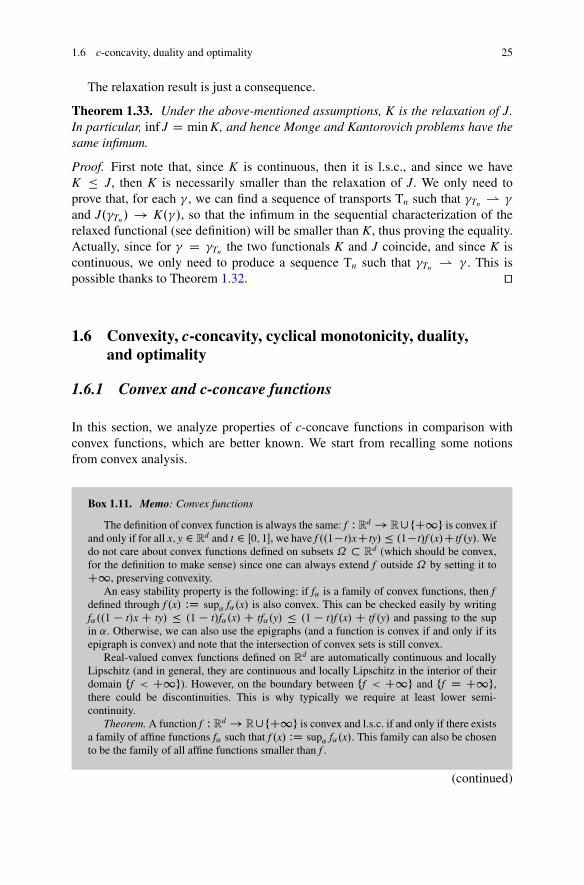
1.6 c-concavity, duality and optimality 25

The relaxation result is just a consequence.

Theorem 1.33. Under the above-mentioned assumptions, K is the relaxation of J.In particular, inf J D min K, and hence Monge and Kantorovich problems have thesame infimum.

Proof. First note that, since K is continuous, then it is l.s.c., and since we haveK � J, then K is necessarily smaller than the relaxation of J. We only need toprove that, for each � , we can find a sequence of transports Tn such that �Tn * �

and J.�Tn/ ! K.�/, so that the infimum in the sequential characterization of therelaxed functional (see definition) will be smaller than K, thus proving the equality.Actually, since for � D �Tn the two functionals K and J coincide, and since K iscontinuous, we only need to produce a sequence Tn such that �Tn * � . This ispossible thanks to Theorem 1.32. ut

1.6 Convexity, c-concavity, cyclical monotonicity, duality,and optimality

1.6.1 Convex and c-concave functions

In this section, we analyze properties of c-concave functions in comparison withconvex functions, which are better known. We start from recalling some notionsfrom convex analysis.

Box 1.11. Memo: Convex functions

The definition of convex function is always the same: f W Rd ! R[fC1g is convex ifand only if for all x; y 2 R

d and t 2 Œ0; 1�, we have f ..1� t/xC ty/ � .1� t/f .x/C tf .y/. Wedo not care about convex functions defined on subsets ˝ � R

d (which should be convex,for the definition to make sense) since one can always extend f outside ˝ by setting it toC1, preserving convexity.

An easy stability property is the following: if f˛ is a family of convex functions, then fdefined through f .x/ WD sup˛ f˛.x/ is also convex. This can be checked easily by writingf˛..1 � t/x C ty/ � .1 � t/f˛.x/ C tf˛.y/ � .1 � t/f .x/ C tf .y/ and passing to the supin ˛. Otherwise, we can also use the epigraphs (and a function is convex if and only if itsepigraph is convex) and note that the intersection of convex sets is still convex.

Real-valued convex functions defined on Rd are automatically continuous and locally

Lipschitz (and in general, they are continuous and locally Lipschitz in the interior of theirdomain ff < C1g). However, on the boundary between ff < C1g and ff D C1g,there could be discontinuities. This is why typically we require at least lower semi-continuity.

Theorem. A function f W Rd ! R[fC1g is convex and l.s.c. if and only if there existsa family of affine functions f˛ such that f .x/ WD sup˛ f˛.x/. This family can also be chosento be the family of all affine functions smaller than f .

(continued)

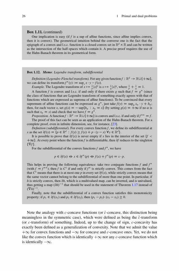
26 1 Primal and dual problems

Box 1.11. (continued)One implication is easy (if f is a sup of affine functions, since affine implies convex,

then it is convex). The geometrical intuition behind the converse one is the fact that theepigraph of a convex and l.s.c. function is a closed convex set in R

d �R and can be writtenas the intersection of the half-spaces which contain it. A precise proof requires the use ofthe Hahn-Banach theorem in its geometrical form.

Box 1.12. Memo: Legendre transform, subdifferential

Definition (Legendre-Flenchel transform). For any given function f W Rd ! R[fC1g,we can define its transform f �.y/ WD supx x � y � f .x/.

Example. The Legendre transform of x 7! 1p jxjp is x 7! 1

q jxjq, where 1p C 1

q D 1.A function f is convex and l.s.c. if and only if there exists g such that f D g� (since

the class of functions that are Legendre transform of something exactly agrees with that offunctions which are expressed as suprema of affine functions). To be convinced that everysupremum of affine functions can be expressed as g�, just take f .y/ D sup˛ x˛ � y C b˛ ;then, for each vector x, set g.x/ D � supfb˛ W x˛ D xg (by setting g.x/ D C1 if no ˛ issuch that x˛ D x) and check that we have f D g�.

Proposition. A function f W Rd ! R[fC1g is convex and l.s.c. if and only if f �� D f .The proof of this fact can be seen as an application of the Hahn-Banach theorem. For a

complete proof, even in infinite dimension, see, for instance, [23].Definition (subdifferential). For every convex function f , we define its subdifferential at

x as the set @f .x/ D fp 2 Rd W f .y/ � f .x/C p � .y � x/ 8y 2 R

dg.It is possible to prove that @f .x/ is never empty if x lies in the interior of the set ff <

C1g. At every point where the function f is differentiable, then @f reduces to the singletonfrf g.

For the subdifferential of the convex functions f and f �, we have

p 2 @f .x/ , x 2 @f �.p/ , f .x/C f �.p/ D x � p:

This helps in proving the following equivalence: take two conjugate functions f and f �

(with f D f ��); then f is C1 if and only if f � is strictly convex. This comes from the factthat C1 means that there is at most one p in every set @f .x/, while strictly convex means thatthe same vector cannot belong to the subdifferential of more than one point. In particular, ifh is strictly convex, then @h, which is a multivalued map, can be inverted, and is univalued,thus getting a map .@h/�1 that should be used in the statement of Theorem 1.17 instead of.rh/�1.

Finally, note that the subdifferential of a convex function satisfies this monotonicityproperty: if p1 2 @f .x1/ and p2 2 @f .x2/, then .p1 � p2/� .x1 � x2/ � 0.

Note the analogy with c-concave functions (or Nc-concave, this distinction beingmeaningless in the symmetric case), which were defined as being the Nc-transform(or c-transform) of something. Indeed, up to the change of sign, c-concavity hasexactly been defined as a generalization of convexity. Note that we admit the valueC1 for convex functions and �1 for concave and c-concave ones. Yet, we do notlike the convex function which is identically C1 nor any c-concave function whichis identically �1.

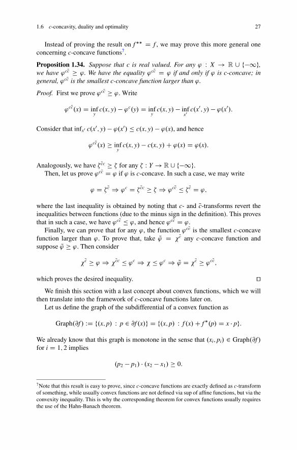
1.6 c-concavity, duality and optimality 27

Instead of proving the result on f D f , we may prove this more general oneconcerning c-concave functions7.

Proposition 1.34. Suppose that c is real valued. For any ' W X ! R [ f�1g,we have 'cNc � '. We have the equality 'cNc D ' if and only if ' is c-concave; ingeneral, 'cNc is the smallest c-concave function larger than '.

Proof. First we prove 'cNc � '. Write

'cNc.x/ D infy

c.x; y/ � 'c.y/ D infy

c.x; y/ � infx0

c.x0; y/ � '.x0/:

Consider that infx0 c.x0; y/ � '.x0/ � c.x; y/ � '.x/, and hence

'cNc.x/ � infy

c.x; y/ � c.x; y/C '.x/ D '.x/:

Analogously, we have Ncc � for any W Y ! R [ f�1g.Then, let us prove 'cNc D ' if ' is c-concave. In such a case, we may write

' D Nc ) 'c D Ncc � ) 'cNc � Nc D ';

where the last inequality is obtained by noting that c- and Nc-transforms revert theinequalities between functions (due to the minus sign in the definition). This provesthat in such a case, we have 'cNc � ', and hence 'cNc D '.

Finally, we can prove that for any ', the function 'cNc is the smallest c-concavefunction larger than '. To prove that, take Q' D Nc any c-concave function andsuppose Q' � '. Then consider

Nc � ' ) Ncc � 'c ) � 'c ) Q' D Nc � 'cNc;

which proves the desired inequality. utWe finish this section with a last concept about convex functions, which we will

then translate into the framework of c-concave functions later on.Let us define the graph of the subdifferential of a convex function as

Graph.@f / WD f.x; p/ W p 2 @f .x/g D f.x; p/ W f .x/C f .p/ D x � pg:

We already know that this graph is monotone in the sense that .xi; pi/ 2 Graph.@f /for i D 1; 2 implies

.p2 � p1/ � .x2 � x1/ � 0:

7Note that this result is easy to prove, since c-concave functions are exactly defined as c-transformof something, while usually convex functions are not defined via sup of affine functions, but via theconvexity inequality. This is why the corresponding theorem for convex functions usually requiresthe use of the Hahn-Banach theorem.

28 1 Primal and dual problems

Yet, not all monotone graphs are the graphs of the subdifferential of a convexfunction, nor they are contained in one of such graphs.8

Hence, monotonicity is not enough to characterize gradients and subdifferentialof convex functions (to be more precise, gradient vector functions that are monotoneare gradient of convex functions, but monotonicity alone does not imply gradient-ness).

A stronger notion is that of cyclical monotonicity.

Definition 1.35. A set A � Rd � R

d is said to be cyclically monotone if for everyk 2 N, every permutation � , and every finite family of points .x1; p1/; : : : ; .xk; pk/ 2A we have

kXiD1

xi � pi �kX

iD1xi � p�.i/:

The word “cyclical” refers to the fact that, since every � is the disjoint compositionof cycles, it is enough to check this property for cyclical permutations, i.e., replacingPk

iD1 xi � p�.i/ withPk

iD1 xi � piC1 in the definition (with the obvious conventionpkC1 D p1).

Note that if we take k D 2 we get the usual definition of monotonicity, since

x1 � p1 C x2 � p2 � x1 � p2 C x2 � p1 ” .p1 � p2/ � .x1 � x2/ � 0:

A famous theorem by Rockafellar ([260], Theorem 24.8) states that every cyclicallymonotone set is contained in the graph of the subdifferential of a convex function.We will not prove this theorem here as will see it as a particular case of a theoremon c-concave functions.

1.6.2 c-Cyclical monotonicity and duality

We start from the translation to the c-concave case of the definition of cyclicalmonotonicity.

Definition 1.36. Once a function c W X � Y ! R [ fC1g is given, we say that aset � � X � Y is c-cyclically monotone (briefly c-CM) if for every k 2 N, everypermutation � and every finite family of points .x1; y1/; : : : ; .xk; yk/ 2 � we have

8Take, for instance, a 90ı rotation R in R2 and consider the set A D f.x;Rx/; x 2 R

dg. This setsatisfies the monotonicity inequality since we have .Rx1 � Rx2/ � .x1 � x2/ D 0 for any x1 and x2.Yet, the map x 7! Rx is not the gradient of convex functions (it is not a gradient at all), nor can itbe contained in the graph of the subdifferential of a convex function.

1.6 c-concavity, duality and optimality 29

kXiD1

c.xi; yi/ �kX

iD1c.xi; y�.i//:

As for the convex case, the word “cyclical” refers to the fact that we can restrict ourattention to cyclical permutations. The word “monotone” is a leftover from the casec.x; y/ D �x � y.

It is useful to recall the following theorem, which is a generalization of a theoremby Rockafellar in convex analysis. The classical reference for this proof is [269], butit is interesting to see that it can actually be traced back to much older papers, suchas [261] (in the framework of rationalizability of actions in economics, Theorem 1in the paper) or [91] (for applications to liquid crystals, as a part of a proof of adiscrete Kantorovich duality for distance costs, see Lemma 2 in the paper).

Theorem 1.37. If � ¤ ; is a c-CM set in X � Y and c W X � Y ! R (notethat c is required not to take the value C1), then there exists a c-concave function' W X ! R [ f�1g (different from the constant �1 function) such that

� � f.x; y/ 2 X � Y W '.x/C 'c.y/ D c.x; y/g:

Proof. We will give an explicit formula for the function ' and prove that it is welldefined and that it satisfies the properties that we want to impose.

Let us fix a point .x0; y0/ 2 � : for x 2 X, set

'.x/ D inf fc.x; yn/ � c.xn; yn/C c.xn; yn�1/ � c.xn�1; yn�1/C � � � CCc.x1; y0/ � c.x0; y0/ W n 2 N; .xi; yi/ 2 � for all i D 1; : : : ; ng :

Since c is real valued and � is nonempty, ' never takes the value C1.If we set, for y 2 Y ,

� .y/ D inf f�c.xn; y/C c.xn; yn�1/ � c.xn�1; yn�1/C � � � C c.x1; y0/C�c.x0; y0/ W n 2 N; .xi; yi/ 2 � for all i D 1; : : : ; n; yn D yg :

Note that from the definition, we have .y/ > �1 if and only if y 2 .�y/.� /.Moreover, by construction we have ' D Nc. This proves that ' is c-concave9. Thefact that ' is not constantly �1 can be seen from '.x0/ � 0: indeed, if we takex D x0, then for any chain of points .xi; yi/ 2 � , we have

9Note that we did not spend words here on the measurability of ': from its c-concavity, this isstraightforward, as it is also continuous, but this is based on the assumption that c is uniformlycontinuous. Measurability and integrability in the general case are trickier.

30 1 Primal and dual problems

nXiD0

c.xiC1; yi/ �nX

iD0c.xi; yi/;

where we consider xnC1 D x0. This shows that the infimum in the definition of '.x0/is nonnegative.

To prove '.x/ C 'c.y/ D c.x; y/ on � , it is enough to prove the inequality'.x/ C 'c.y/ � c.x; y/ on the same set, since by definition of c-transform, theopposite inequality is always true. Moreover, since 'c D Ncc and Ncc � , it isenough to check '.x/C .y/ � c.x; y/.

Suppose .x; y/ 2 � and fix " > 0. From ' D Nc, one can find a point Ny 2 �y.� /

such that c.x; Ny/� .Ny/ < '.x/C ". In particular, .Ny/ ¤ ˙1. From the definitionof , one has the inequality � .y/ � �c.x; y/C c.x; Ny/ � .Ny/ (since every chainstarting from Ny may be completed adding the point .x; y/ 2 � /.

Putting together this information, one gets

� .y/ � �c.x; y/C c.x; Ny/ � .Ny/ < �c.x; y/C '.x/C ";

which implies the inequality c.x; y/ � '.x/C .y/ since " is arbitrary. utWe can now prove the following.

Theorem 1.38. If � is an optimal transport plan for the cost c and c is continuous,then spt.�/ is a c-CM set.

Proof. Suppose by contradiction that there exist k; � , and .x1; y1/; : : : ; .xk; yk/ 2spt.�/ such that

kXiD1

c.xi; yi/ >

kXiD1

c.xi; y�.i//:

Take now " < 12k

�PkiD1 c.xi; yi/ �Pk

iD1 c.xi; y�.i//�

. By continuity of c, there

exists r such that for all i D 1; : : : ; k and for all .x; y/ 2 B.xi; r/ � B.yi; r/, wehave c.x; y/ > c.xi; yi/ � " and for all .x; y/ 2 B.xi; r/ � B.y�.i/; r/, we havec.x; y/ < c.xi; y�.i//C ".

Now consider Vi WD B.xi; r/�B.yi; r/ and note that �.Vi/ > 0 for every i, because.xi; yi/ 2 spt.�/. Define the measures �i WD � Vi=�.Vi/ and �i WD .�x/#�i, �i WD.�y/#�i. Take "0 < 1

k mini �.Vi/.For every i, build a measure Q�i 2 ˘.�i; ��.i// at will (for instance, take Q�i D

�i ˝ ��.i/).Now define

Q� WD � � "0kX

iD1�i C "0

kXiD1

Q�i:

1.6 c-concavity, duality and optimality 31

We want to find a contradiction by proving that Q� is a better competitor than � inthe transport problem, i.e., Q� 2 ˘.�; �/ and

´c d Q� < ´

c d� .First we check that Q� is a positive measure. It is sufficient to check that � �

"0Pk

iD1 �i is positive, and, for that, the condition "0�i <1k� will be enough. This

condition is satisfied since "0�i D ."0=�.Vi//� Vi and "0=�.Vi/ � 1k .

Now, let us check the condition on the marginals of Q� . We have

.�x/# Q� D � � "0kX

iD1.�x/#�i C "0

kXiD1.�x/# Q�i D � � "0

kXiD1

�i C "0

kXiD1

�i D �;

.�y/# Q� D � � "0kX

iD1.�y/#�i C "0

kXiD1.�y/# Q�i D � � "0

kXiD1

�i C "0

kXiD1

��.i/ D �:

Finally, let us estimate´

c d� � ´c d Q� and prove that it is positive, thus

concluding the proof. We have

ˆc d� �

ˆc d Q� D "0

kXiD1

ˆc d�i � "0

kXiD1

ˆc d Q�i

� "0

kXiD1.c.xi; yi/ � "/ � "0

kXiD1.c.xi; y�.i//C "/

D "0

kX

iD1c.xi; yi/ �

kXiD1

c.xi; y�.i// � 2k"

!> 0;

where we used the fact that �i is concentrated on B.xi; r/ � B.yi; r/, Q�i on B.xi; r/ �B.y�.i/; r/ and that they have unit mass (due to the rescaling by �.Vi/). ut

From the previous theorem, together with Theorem 1.37, we get the duality resultthat we were waiting for10 from Section 1.2.

Theorem 1.39. Suppose that X and Y are Polish spaces and that c W X � Y ! R isuniformly continuous and bounded. Then the problem (DP) admits a solution .'; 'c/

and we have max .DP/ D min .KP/.

Proof. First consider the minimization problem (KP). Since c is continuous, itadmits a solution � . Moreover, the support � of � is c-cyclically monotone, thanksto Theorem 1.38. Then, since c is real valued, we can apply Theorem 1.37 and obtainthe existence of a c-concave function ' such that

� � f.x; y/ 2 ˝ �˝ W '.x/C 'c.y/ D c.x; y/g:

10We insist that this is just a possible path: we prove duality via cyclical monotonicity; instead,one could first prove duality (see Section 1.6.3) and then prove cyclical monotonicity througharguments as in Theorem 1.42.

32 1 Primal and dual problems

From their c- (and Nc-)concavity, ' and 'c are continuous. Moreover, from'c.y/ D infx c.x; y/ � '.x/, we obtain an upper bound on 'c (since c is supposedto be bounded), which turns into a lower bound on '. Symmetrically, we can alsoobtain upper bounds on ' and lower on 'c, which prove that ' and 'c are bothcontinuous and bounded.

Hence, we can use .'; 'c/ as an admissible pair in (DP). Consider now

ˆ

X' d�C

ˆ

Y'c d� D

ˆ

X�Y.'.x/C 'c.y// d� D

ˆ

X�Yc.x; y/ d�;

where the last equality is due to the fact that � is concentrated on � and there wehave '.x/ C 'c.y/ D c.x; y/. The equality just before comes from the fact that themarginals of � are � and �, respectively. This finally shows, using the optimalityof � ,

.DP/ �ˆ' d�C

ˆ'c d� D

ˆc.x; y/ d� D .KP/

and implies (DP)D(KP), since we already know (DP)� (KP). As a by-product ofthis proof, the pair .'; 'c/ turns out to be optimal for (DP). ut

We also want to deal with some cases which are not covered by the previoustheorem. First we want to give a short statement about the quadratic case in R

d,in order to comply with Section 1.3.1. The difference compared to Theorem 1.39lies in the fact that the cost c.x; y/ D 1

2jx � yj2 is neither bounded nor uniformly

continuous.

Theorem 1.40. Let �; � be probabilities over Rd and c.x; y/ D 12jx � yj2. Suppose´ jxj2 dx;

´ jyj2 dy < C1. Consider the following variant of (DP):

.DP � var/ sup

�ˆRd' d�C

ˆ

Rd d� W ' 2 L1.�/; 2 L1.�/; ' ˚ � c

�:

Then (DP-var) admits a solution .'; /, and the functions x 7! 12jxj2�'.x/ and y 7!

12jyj2 � .y/ are convex and conjugate to each other for the Legendre transform.

Moreover, we have max .DP � var/ D min .KP/.

Proof. Applying the same considerations as in Theorem 1.39, we get the existenceof a pair .'; /, with ' c-concave and D 'c such that '.x/C 'c.y/ D c.x; y/ forevery .x; y/ in the support of an optimal transport plan � . From Proposition 1.21, wededuce that x 7! 1

2jxj2�'.x/ and y 7! 1

2jyj2� .y/ are convex and conjugate to each

other. In particular, 12jxj2 � '.x/ is bounded from below by a linear function, and

hence ' is bounded from above by a second-order polynomial. This proves 'C 2L1.�/, from the assumption on �. The same can be said on , i.e., C 2 L1.�/. Wecan now integrate ' ˚ w.r.t. � , thus obtaining

1.6 c-concavity, duality and optimality 33

ˆ

Rd' d�C

ˆ

Rd d� D

ˆ

Rd�Rd' ˚ d� D

ˆ

Rd�Rdc d� � 0:

This proves´Rd ' d�;

´Rd d� > �1, and hence ' 2 L1.�/ and 2 L1.�/.

The conclusion follows as before. utThen, we also give some details about the case where c is not continuous but

only l.s.c. We recall that this assumption is sufficient for the existence of an optimaltransport plan.

The first result concerns the validity of the duality formula, i.e.,

min .KP/ D sup

�ˆX' d�C

ˆ

Y d� W ' 2 C.X/; 2 C.Y/; ' ˚ � c

�:

(1.6)

By now, we have established this equality when c is uniformly continuous andbounded, also proving that the dual problem admits a maximizing pair. We alsoknow that an inequality is always true: the minimum on the left is always larger thanthe maximum on the right. More precisely, we are able to deal with the uniformlycontinuous case (since we want to guarantee continuity of c-concave functions ofthe form '.x/ D infy c.x; y/ � .y/).

To deal with a l.s.c. cost c bounded from below, we will use the fact thatthere exists a sequence ck of continuous functions (each one being k-Lipschitz)increasingly converging to c. We need the following lemma.

Lemma 1.41. Suppose that ck and c are l.s.c. and bounded from below and that ck

converges increasingly to c. Then

limk!1 min

�ˆck d� W � 2 ˘.�; �/

�D min

�ˆc d� W � 2 ˘.�; �/

�:

Proof. Due to the increasing limit condition, we have ck � c, and hence the limiton the left (which exists by monotonicity) is obviously smaller than the quantity onthe right. Now consider a sequence �k 2 ˘.�; �/, built by picking an optimizer foreach cost ck. Up to subsequences, due to the tightness of ˘.�; �/, we can suppose�k * � . Fix now an index j. Since for k � j we have ck � cj, we have

limk

min

�ˆck d� W � 2 ˘.�; �/

�D lim

k

ˆck d�k � lim inf

k

ˆcj d�k:

By semi-continuity of the integral cost cj, we have

lim infk

ˆcj d�k �

ˆcj d�:

34 1 Primal and dual problems

Hence, we have obtained

limk

min

�ˆck d�; � 2 ˘.�; �/

��ˆ

cj d�:

Since j is arbitrary and limj´

cj d� D ´c d� by monotone convergence, we also

have

limk

min

�ˆck d�; � 2 ˘.�; �/

��ˆ

c d� � min

�ˆc d�; � 2 ˘.�; �/

�:

This concludes the proof. Note that it also gives, as a by-product, the optimality of� for the limit cost c. ut

We can now establish the validity of the duality formula for semi-continuouscosts.

Theorem 1.42. If X;Y are Polish spaces and c W X � Y ! R [ fC1g is l.s.c. andbounded from below, then the duality formula min .KP/ D sup .DP/ holds.

Proof. Consider a sequence ck of k-Lipschitz functions approaching c increasingly.Then the same duality formula holds for ck, and hence, we have

min

�ˆck d� W � 2 ˘.�; �/

�D max

�ˆ' d�C

ˆ d� W ' ˚ � ck

�

� sup

�ˆ' d�C

ˆ d� W ' ˚ � c

�;

where the max and the sup are computed among Cb functions '; . The inequalityis justified by the fact that ck � c, and hence, every pair .'; / satisfying '.x/ C .y/ � ck.x; y/ also satisfies '.x/ C .y/ � c.x; y/. The conclusion follows byletting k ! C1, using Lemma 1.41. Note that for the cost c, we cannot guaranteethe existence of a maximizing pair .'; /. ut

The duality formula also allows us to prove the following c-cyclical monotonicitytheorem.

Theorem 1.43. If c is l.s.c. and � is an optimal transport plan, then � is concen-trated on a c-CM set � (which will not be closed in general).

Proof. Thanks to the previous theorem, the duality formula holds. This means that,if we take a sequence of maximizing pairs .'h; h/ in the dual problem, we have

ˆ.'h.x/C h.y// d� D

ˆ'h d�C

ˆ h d� !

ˆc d�;

since the value of´

c d� is the minimum of the primal problem, which is also themaximum of the dual. Moreover, we have c.x; y/�'h.x/C h.y/ � 0, which implies

1.6 c-concavity, duality and optimality 35

that the functions fh WD c.x; y/ � 'h.x/ � h.y/, defined on X � Y , converge to 0 inL1.X�Y; �/ (since they are positive and their integral tends to 0). As a consequence,up to a subsequence (not relabeled), they also converge pointwisely � -a.e. to 0. Let� � X � Y be a set with �.� / D 1 where the convergence holds.

Take any k, � , and .x1; y1/; : : : ; .xk; yk/ 2 � : we have

kXiD1

c.xi; yi/ D limh

kXiD1

'h.xi/C h.yi/ D limh

kXiD1

'h.xi/C h.y�.i//

�kX

iD1c.xi; y�.i//;

which proves that this set is c-CM. utRemark 1.44. The duality formula that we proved for l.s.c. cost c differs from thatfor continuous costs in that there is no existence for the dual problem (DP). Actually,if one restates the dual problem as in (DP-var), then one can produce an optimizerby first applying Theorem 1.43 to say that the optimal � is concentrated on a c-CMset � and then build a potential ' through Theorem 1.37. This works under theassumption that c is real valued and does not depend on its continuity11.

1.6.3 A direct proof of duality

In Section 1.6.2, we paid off the debt that we contracted with duality in Section 1.2:we proved, via c-cyclical monotonicity arguments, that min .KP/ D sup .DP/, withno duality gap, under some very general assumptions.

Here we want to give an alternative proof, independent of c-cyclical monotonicityand based on a simple convex analysis trick12. We will restrict to the compact caseand only use the following fact: if H is convex and l.s.c., then H D H (seeBox 1.12 in Section 1.6.1).

Suppose that X and Y are compact metric spaces and c W X�Y ! R is continuous.For every p 2 C.X � Y/, define

11Yet, note that the construction requires to use an optimal � , which is guaranteed in the casewhere c is l.s.c., but could be the case in some special situations as well, such as when we canapply Lemma 1.8. Also, for nonuniformly continuous costs c, there are measurability issues on thefunction ' of Theorem 1.37.12Even if not strictly necessary, we prefer to give it for completeness, and because it is differentfrom what is presented in other texts, such as [292], where the main tool is a theorem from [90],Chapter 1, applied to well-chosen functions and space. The present proof, suggested by C. Jimenez,is essentially adapted from Section 4 in [70].

36 1 Primal and dual problems

H.p/ WD � max

�ˆX' d�C

ˆ

Y d� W '.x/C .y/ � c.x; y/ � p.x; y/

�;

which coincides with the opposite of the value of (DP) with cost c � p. The fact thatthis value is attained is proven in Proposition 1.11, which also provides bounds onthe modulus of continuity of the optimal ' and (the same as c � p) and on theiroscillation (if we assume '.x0/ D 0, then both ' and are bounded by a constantonly depending on sup jc � pj).Lemma 1.45. The function H W C.X � Y/ ! R is convex and l.s.c. for the uniformconvergence on the compact space X � Y.

Proof. For convexity, take p0 and p1 with their optimal potentials .'0; 0/ and.'1; 1/. For t 2 Œ0; 1�, define pt D .1 � t/p0 C tp1, 't D .1 � t/'0 C t'1, and t D .1 � t/ 0 C t 1. The pair .'t; t/ is admissible in the max defining �H.pt/.We have

H.pt/ � ��ˆ

X't d�C

ˆ

Y t d�

�D .1 � t/H.p0/C tH.p1/;

which shows convexity.For semi-continuity, take pn ! p. Extract a subsequence pnk , realizing the

liminf of H.pn/. From uniform convergence, the sequence pnk is equicontinuous andbounded (use the converse of the Ascoli-Arzelà theorem). Hence, the correspondingoptimal potential .'nk ; nk/ are also equicontinuous and bounded and we can assume'nk ! '; nk ! uniformly, up to extracting again. Obviously 'nk.x/C nk.y/ �c.x; y/ � pnk.x; y/ implies '.x/C .y/ � c.x; y/ � p.x; y/. Hence,

H.p/ � ��ˆ

X' d�C

ˆ

Y d�

�D lim

kH.pnk/ D lim inf

nH.pn/;

which proves lower semi-continuity. utLet us now compute H W M .X � Y/ ! R [ fC1g. For � 2 M .X � Y/, we have

H�.�/ WD supp

ˆ

X�Yp d�Csup

�ˆX' d�C

ˆ

Y d� W '.x/C .y/ � c.x; y/ � p.x; y/

�;

which can be written as a unique sup over p; '; . Note that, if � … MC.X�Y/, thenthere is p � 0 such that

´p0d� > 0, and one can take ' D 0, D 0, p D c C np0,

and, for n ! 1, we get H.�/ D C1. On the contrary, if � 2 MC.X � Y/, weshould choose the largest possible p, i.e., p.x; y/ D c.x; y/�'.x/� .y/. This gives

H.�/ D sup';

ˆ

X�Yc.x; y/ d� C

ˆ

X' d��

ˆ

X�Y'.x/ d� C

ˆ

Y d� �

ˆ

X�Y .x/ d�:

1.6 c-concavity, duality and optimality 37

But this is exactly the expression that we introduced in Section 1.2 (see Equa-tion (1.3)) to rewrite the constraints in (KP). Indeed we have

H.�/ D(

K.�/ if � 2 ˘.�; �/;C1 if not.

The duality theorem follows.

Theorem 1.46. If X;Y are compact spaces and c continuous, then min .KP/ Dsup .DP/ (proof by convex analysis).

Proof. We have max .DP/ D �H.0/ D �H.0/ (since H is convex and l.s.c., seeBox 1.12). Moreover, H.0/ D sup� h0; �i � H.�/ D � inf H D � min .KP/.

ut

1.6.4 Sufficient conditions for optimality and stability

The considerations of Sections 1.6.1 and 1.6.2 about c-transforms allow us to provesufficient conditions for optimality in optimal transportation, at least when the costsatisfies the twist condition of Definition 1.16. As we did in Section 1.3, we willfirst give a general statement under compactness assumptions, and we will then givea different proof in the quadratic case, with no need of compactness.

Theorem 1.47. Let ˝ � Rd be compact and c be a C1 cost function satisfying

the twist condition on ˝ � ˝. Suppose that � 2 P.˝/ and ' 2 c�conc.˝/ aregiven, that ' is differentiable �-a.e., and that �.@˝/ D 0. Suppose that the map Tsatisfies rxc.x;T.x// D r'.x/. Then T is optimal for the transport cost c betweenthe measures � and � WD T#�.

Proof. Consider the function ', which may be written as '.x/ D infy c.x; y/� .y/for a certain function W ˝ ! R. The function may be supposed to be Nc-concaveand hence continuous (actually, we can take D 'c, from the considerations ofthe previous section). Fix now x0 2 ˝ such that r'.x0/ exists and x0 … @˝. Bycompactness and continuity, one can say that infy c.x; y/ � .y/ is realized by acertain point y0. This gives

'.x/ � h.x � y0/ � .y0/ for every x '.x0/ D h.x0 � y0/ � .y0/;

and hence x 7! h.x � y0/ � '.x/ is minimal at x D x0 (note that we defined y0 bythe optimality in y, but now we use the optimality in x). As a consequence, we get

r'.x0/ D rxc.x0; y0/:

By assumption, y 7! rxc.x0; y/ is injective: this implies y0 D T.x0/. This proves'.x0/C .T.x0// D c.x0;T.x0//, and this same equality is true for �-a.e. x0. If we

38 1 Primal and dual problems

integrate with respect to �, we get

ˆ' d�C

ˆ d� D

ˆ' d�C

ˆ ı T d� D

ˆc.x;T.x//d�.x/;

which proves the optimality of T since the last integral equals the cost of T in theproblem of Monge, and we have

´' d�C ´

d� � .DP/ � .KP/, since .'; / isadmissible in (DP). ut

As we promised, here is a different proof for the case c.x; y/ D 12jx � yj2.

Theorem 1.48. Suppose that � 2 P.Rd/ is such that´ jxj2 d�.x/ < 1 and that

u W Rd ! R [ fC1g is convex and differentiable �-a.e. Set T D ru and suppose´ jT.x/j2d�.x/ < C1. Then T is optimal for the transport cost c.x; y/ WD 12jx � yj2

between the measures � and � WD T#�.

Proof. First note that, for a convex function u, we have the following properties:

u.x/C u.y/ � x � y for all x; y 2 Rd; u.x/C u.y/ D x � y if y D ru.x/:

Now, consider any transport plan � 2 ˘.�; �/ and write

ˆ

Rd�Rd.x � y/ d�.x; y/ �

ˆ

Rd�Rd

�u.x/C u.y/

d�.x; y/

Dˆ

Rdu.x/ d�.x/C

ˆ

Rdu.T.x// d�.x/ D

ˆ

Rd.x � T.x// d�.x/:

This proves´.x �y/ d� � ´

.x �y/ d�T. Subtracting these quantities from the integral,which only depends on � and �,

´12.jxj2 C jyj2/ d� D ´

12.jxj2 C jyj2/ d�T, we get

ˆ

Rd�Rd

1

2jx � yj2 d� �

ˆ

Rd�Rd

1

2jx � yj2d�T;

which proves the claim. utLet us spend some words on the two different proofs that we just gave: we needed

to prove some optimality properties of the point T.x/ among possible points y. Inthe first case, we proved that an optimal point y0 existed, and we deduced fromthe first-order optimality conditions y0 D T.x0/. In the second case, we used thecharacterization of minimizers for convex functions: whenever a gradient vanishes,we are at a minimizer. This is the idea behind the property u.x/ C u.y/ D x � y ify D ru.x/.

We now pass to a more general criterion that can be used for almost arbitrarycosts. The main idea is that we proved that optimal plans are necessarily concen-trated on c-CM sets, but the converse is also true: a plan which is concentrated ona c-CM set is optimal, at least in the most reasonable cases. We will prove this factin the easiest case, i.e., when c is uniformly continuous and bounded. Actually, we

1.6 c-concavity, duality and optimality 39

will see in the next proof that the main ingredient is Theorem (1.37), which onlyrequires finiteness of the cost, but continuity and compactness are needed to avoidintegrability issues (in this case, all the functions are measurable and bounded).Moreover, we will apply this sufficient criterion to another interesting problem,i.e., stability of the optimal plans, which will require these assumptions for otherreasons. The fact that this converse implication stays true when these assumptionsare withdrawn (and in particular for infinite costs) is a delicate matter, and we referto [10] for a counterexample when the cost takes the value C1 and to [30, 60, 254]for interesting positive proofs.

Theorem 1.49. Suppose that � 2 P.X � Y/ is given, that X and Y are Polishspaces, that c W X � Y ! R is uniformly continuous and bounded, and that spt.�/ isc-CM. Then � is an optimal transport plan between its marginals � D .�x/#� and� D .�y/#� for the cost c.

Proof. Theorem (1.37) gives the existence of a c-concave function ' such thatspt.�/ is contained in the set f.x; y/ W '.x/ C 'c.y/ D c.x; y/g. Both ' and'c are continuous thanks to the continuity of c, and hence bounded on X and Y ,respectively.

Thanks to what we know about duality, we have

.KP/ �ˆ

c.x; y/ d� Dˆ.'.x/C'c.y// d� D

ˆ' d�C

ˆ'c d� � .DP/D .KP/

which shows that � is optimal (and that .'; 'c/ solves the dual problem). utWe are now able to prove the following stability result that we only state in the

compact case.

Theorem 1.50. Suppose that X and Y are compact metric spaces and that c W X �Y ! R is continuous. Suppose that �n 2 P.X � Y/ is a sequence of transport planwhich are optimal for the cost c between their own marginals �n WD .�x/#�n and�n WD .�y/#�n, and suppose �n * � ; then �n * � WD .�x/#� , �n * � WD .�y/#�

and � is optimal in the transport between � and �.

Proof. Set �n WD spt.�n/. Up to subsequences, we can assume �n ! �

in the Hausdorff topology (see below). Each support �n is a c-CM set (Theo-rem (1.38)) and the Hausdorff limit of c-CM sets is also c-CM. Indeed, if one fixes.x1; y1/; : : : ; .xk; yk/ 2 � , there are points .xn

1; yn1/; : : : ; .x

nk ; y

nk/ 2 �n such that, for

each i D 1; : : : ; k, we have .xni ; y

ni / ! .xi; yi/. The cyclical monotonicity of �n givesPk

iD1 c.xni ; y

ni / � Pk

iD1 c.xni ; y

n�.i//; which implies, taking the limit n ! 1

kXiD1

c.xi; yi/ �kX

iD1c.xi; y�.i//:

40 1 Primal and dual problems

This proves that � is c-CM. Moreover, we know from the convergence �n * �

together with �n ! � that spt.�/ � � . This shows that spt.�/ is c-CM and impliesthe optimality of � . ut

We finish with an easy but useful consequence of Theorem 1.50. To fix thenotations, for a given cost c W X � Y ! R and � 2 P.X/; � 2 P.Y/, let usdefine

Tc.�; �/ WD min

�ˆX�Y

c d� W � 2 ˘.�; �/�:

Theorem 1.51. Suppose that X and Y are compact metric spaces and that c W X �Y ! R is continuous. Suppose that �n 2 P.X/ and �n 2 P.Y/ are two sequencesof probability measures, with �n * � and �n * �. Then we have Tc.�n; �n/ !Tc.�; �/.

Proof. Let �n be an optimal transport plan from �n to �n for the cost c. Up tosubsequences, we can assume �n * � . Theorem 1.50 provides the optimality of� . This means that we have (along this subsequence, but since it is arbitrary)

Tc.�n; �n/ Dˆ

X�Yc d�n !

ˆ

X�Yc d� D Tc.�; �/

which proves the claim. ut

Box 1.13. Memo: Hausdorff convergence

Definition. In a compact metric space X, we define the Hausdorff distance on pair ofcompact subsets of X by setting

dH.A;B/ WD max fmaxfd.x;A/ W x 2 Bg;maxfd.x;B/ W x 2 Agg :Properties. We have the following equivalent definition:

1) dH.A;B/ D maxfjd.x;A/� d.x;B/j W x 2 Xg2) dH.A;B/ D inff" > 0 W A � B"; B � A"g, where A" and B" stand for the "-

neighborhood of A and B, respectively.

Theorem (Blaschke). dH is a distance: it is positive and symmetric, it only vanishes if thetwo sets coincide, and it satisfies triangle inequality. With this distance, the set of compactsubsets of X becomes a compact metric space itself.

We refer to [12] for a detailed discussion (with proofs) of this topic. Here we only provea simple fact that we need.

Proposition. If dH.An;A/ ! 0 and �n is a sequence of positive measures such thatspt.�n/ � An with �n * �, then spt.�/ � A.

Sketch of proof. For each n, we have´

d.x;An/ d�n D 0, since �n is supported on An.Since d.x;An/ ! d.x;A/ uniformly and �n * �, thanks to the duality between uniformconvergence and weak converge of measures, we get

´d.x;An/ d�n ! ´

d.x;A/ d�. Thisimplies

´d.x;A/ d� D 0, and hence � is concentrated on A.

1.7 Discussion 41

Let us also conclude with a result on the stability of the Kantorovich potentials.

Theorem 1.52. Suppose that X and Y are compact metric spaces and that c W X �Y ! R is continuous. Suppose that �n 2 P.X/ and �n 2 P.Y/ are two sequencesof probability measures, with �n * � and �n * �. Let .'n; n/ be, for each n, apair of c-concave Kantorovich potentials for the cost c in the transport from �n to�n. Then, up to subsequences, we have 'n ! ', n ! , where the convergence isuniform and .'; / is a pair of Kantorovich potentials for � and �.

Proof. We know that c-concave functions have the same modulus of continuity as cand hence, up to translating by a constant, we can apply the Ascoli-Arzelà theorem.We have 'n ! Q' and n ! Q , the convergences being uniform. From 'n.x/ C n.y/ � c.x; y/, we deduce, as n ! 1, the inequality Q'.x/ C Q .y/ � c.x; y/.Moreover, we have

Tc.�n; �n/ Dˆ'n d�n C

ˆ n d�n !

ˆQ' d�C

ˆQ d�:

Yet, we also have (Theorem 1.50) Tc.�n; �n/ ! Tc.�; �/. We infer that the pair. Q'; Q / is admissible in the dual problem and realizes the maximal value

´ Q' d� C´ Q d� D Tc.�; �/. Hence, they are Kantorovich potentials.The convergence is obviously true on the full sequence (without passing to a

subsequence) in case of uniqueness of the Kantorovich potentials at the limit. ut

1.7 Discussion

This section presents alternative point of views (probabilistic language, polarfactorization), connections with economics and finance, generalizations and a briefpresentation of the regularity issues on the optimal transport map, and the optimalpotentials.

1.7.1 Probabilistic interpretation

We completely skipped up to now any interpretations involving probabilities, whichare actually natural in this setting. By changing for a while our language, let usdescribe the situation in the following way.

Two probability measures � and � on some spaces (often, Rd) are given and canbe interpreted as the laws of two random variables. Yet, we do not prescribe thejoint law (which corresponds to � ) of these two random variables and we considerthe optimization problem

minfEŒc.X;Y/� W X �; Y �g

42 1 Primal and dual problems

where E denotes the expected value (according to a probability P on a probabilityspace ˝, which is not relevant for the minimization, but could be considered either“large enough” or to be part of the optimization). This expected value obviouslydepends on the joint law of .X;Y/, which is the main unknown.

The particular case of real (or vector) valued r.v. with c.X;Y/ D jX � Yjp reads

minfjjX � YjjLp W X �; Y �g:

More interesting is the case p D 2, where the problem can be expressed in termsof covariance. Indeed, let us set x0 D EŒX� D ´

x d� and y0 D EŒY� D ´y d�,

these two values being the mean values of X and Y . We have

EŒjX � Yj2� D EŒj.X � x0/ � .Y � y0/C .x0 � y0/j2�D EŒjX � x0j2�C EŒjY � y0j2�C jx0 � y0j2

C2EŒX � x0� � .x0 � y0/ � 2EŒY � y0� � .x0 � y0/

�2EŒ.X � x0/ � .Y � y0/�:

In this expression, the three first terms only depend on the laws of X and Yseparately (the first being the variance of X, the second the variance of Y , andthe third the squared distance between the two mean values), and the next twoterms vanish (since the mean value of X � x0 is 0 and so for the mean value ofY � y0). The problem is hence reduced to the maximization of EŒ.X � x0/ � .Y � y0/�.This means that we need to find the joint law which guarantees maximal covariance(i.e., somehow maximal dependence) of two r.v. with given laws. In the case ofreal-valued r.v. (see next chapter), the answer will be that the optimal couplingis obtained in the case where X and Y are completely dependent and one is anincreasing function of the other. The multidimensional case obviously replaces thisincreasing behavior with other monotone behaviors.

1.7.2 Polar factorization

A classical result in linear algebra states that every matrix A 2 MN�N can bedecomposed as a product A D S �U, where S is symmetric and positive semidefinite,and U is a unitary matrix, i.e., U � Ut D I. The decomposition is unique if A isnonsingular (otherwise, U is not uniquely defined), and in such a case, S is positivedefinite. Also, one can see that the matrix U of this decomposition is also a solution(the unique one if A is nonsingular) of

maxfA W R W R � Rt D Ig;

where A W R stands for the scalar product between matrices, defined as A W R WDTr.A � Rt/.

1.7 Discussion 43

Indeed, one can write

A W R D .S � U/ W R D Tr.S � U � Rt/ DX

i;j

SiiUijRij;

where the coordinates are chosen so that S is diagonal (and hence Sii � 0). Let usobserve that U � Ut D I imposes that the vectors u.i/ with components u.i/j WD Uij

are unit vectors (let us also define the unit vectors r.i/ in the same way from thematrix R). Thus

A W R DX

i;j

SiiUijRij DX

i

Siiu.i/ � r.i/

�X

i

Sii D Tr.S/ D Tr.S � U � Ut/ D Tr.A � Ut/ D A W U:

Also note that maximizing A W R is the same as minimizing jjA � Rjj2 (where thenorm of a matrix is defined as the square root of its scalar product with itself).Indeed, we have jjA � Rjj2 D jjAjj2 � 2A W R C jjRjj2, and both jjAjj2 and jjRjj2 DTr.R � Rt/ D Tr.I/ D N are constants.

Analogously, in his first works about the quadratic optimal transport, Y. Breniernoted that Monge-Kantorovich’s theory allowed us to provide a similar decomposi-tion for vector fields instead of linear maps (see [82, 84] and also [174]).

The statement is the following:

Theorem 1.53. Given a vector map � W ˝ ! Rd with ˝ � R

d, considerthe rescaled Lebesgue measure L˝ on ˝ and suppose that �#L˝ is absolutelycontinuous; then, one can find a convex function u W ˝ ! R and a measure-preserving map s W ˝ ! ˝ (i.e., such that s#L˝ D L˝) such that � D .ru/ ı s.Moreover, both s and ru are uniquely defined a.e., and s solves

max

�ˆ�.x/ � r.x/ dx W r#L˝ D L˝

�:

Note that the statement concerning nonsingular matrices exactly corresponds tothis one when one takes ˝ D B.0; 1/, since the assumption on the image measurecorresponds to the non-degeneracy of the linear map x 7! Ax, the matrix S is thegradient of the convex function x 7! 1

2.Sx/ � x, and the unitary matrix U is measure

preserving.We give a proof of this statement; see also [84].

Proof. Consider � D �#L˝ and take the optimal transport for the quadratic costbetween � and L˝ . This transport is the gradient of a convex function that we willcall u. Set s WD .ru/ ı � , and note that s#L˝ D .ru/#.�#L˝/ D .ru/#� DL˝ ; hence s is measure preserving. Then, take the Legendre transform u of u andnote .ru/ ı s D .ru/ ı .ru/ ı � D � (indeed, the gradients of both u and u

44 1 Primal and dual problems

are defined a.e. and we always have .ru/ ı .ru/ D id). In this way, we have thedesired decomposition.

The uniqueness of ru comes from the fact that � D .ru/ ı s with s measurepreserving implies .ru/#L˝ D �, and there is only one gradient of a convexfunction transporting a given measure (here L˝) to another given measure (here,�),and it is the optimal transport between them.

Once ru is unique, the uniqueness of s is obtained by composing with ru.Concerning the optimality of s, use the optimality of ru. The maximization of

the scalar product instead of the minimization of the quadratic cost, we get

ˆ.ru.x/ � x/ dx �

ˆ

˝�Rd.y � x/ d�.x; y/

for every � 2 ˘.L˝;�/. If we consider a measure-preserving map r W ˝ ! ˝

and build � D .r; �/#L˝ , we get

ˆ.�.x/ � r.x// dx D

ˆ.y � x/ d�.x; y/

�ˆ.ru.x/ � x/ dx D

ˆ.ru.s.x// � s.x// dx D

ˆ.�.x/ � s.x// dx;

which provides the optimality of s. ut

1.7.3 Matching problems and economic interpretations

Optimal transport problems have several “abstract” economic interpretations, wherethe role of transport plan � is that of matchings between different actors of aneconomy, and the function c.x; y/ does not represent anymore a cost for movingfrom x to y but rather a compatibility of the two objects x and y, or the opposite ofthe “utility” for x and y to be coupled.13 Consider that, in economics, it is typical tomaximize utility, instead of minimizing costs.

A first easy and well-known example is that of the maximization of theproductivity. A company has a certain number of employees of different types (letus use the variable x for the types and the measure � for the distribution of thesetypes, i.e., the quantity of employees for each type) and some tasks to attribute (weuse y for the different kinds of tasks and � for the distribution of different tasks), andif the productivity p.x; y/ of the employees of type x when they work out the task yis known, then the goal of the company is to solve

13For a comprehensive introduction to some applications of otpimal transport to economics, seealso [228].

1.7 Discussion 45

max

�ˆp.x; y/ d� W � 2 ˘.�; �/

�:

This problem is easy to understand, but we want to analyze some other oneswhere also the Kantorovich potentials also play a role.

The first example is that of stable marriages. Given two populations W of womenand M of men, represented by a measure � on W and a measure � on M, we denoteby uw.x; y/ the interest of Ms x for Mr y and um.x; y/ that of Mr y for Ms x. Theproblem is that of finding a stable set of marriages, i.e., a measure � on the setW � M giving how many women of type x get married with how many men oftype y. This � must obviously belong to ˘.�; �/, and we want to select such a �so that it is stable, i.e., no new couple .x; y/ will decide to divorce (each one fromhis/her current partner) to go together. The case that we are interested in is that oftransferable utility: it means that we suppose that, once x and y get married, theydecide how to split their total utility uw.x; y/C um.x; y/. They divide into a quantity'.x/, which is the utility surplus for Ms x (now Mrs y, but let us call her with hermaiden name) and .y/ for Mr y. Note that in this case, only the sum U.x; y/ WDuw.x; y/Cum.x; y/ really plays a role. A stable marriage is a triple .�; '; / such thatU.x; y/ D '.x/C .y/ � -a.e. (this represents the fact that ' and are a splitting ofthe total utility) and U.x; y/ � '.x/C .y/ for all .x; y/ (this represents the fact thatno pair .x; y/ will be interested in quitting the status quo). It is easy to see that thiscorresponds to an optimal � with its potentials. We mention [125] for an interestingdiscussion of this problem. On the other hand, the case of nontransferable utility ismuch more involved and does not correspond to a transport problem.

If, in the previous example, the potentials represented split utilities, we can thinkof other cases where they are really prices. Indeed, consider that the variable xrepresents the goods that are available on the market and that � is the distribution(how many of each type) of these goods, which we consider as fixed. The variable yplays the role of the type of consumers and � is their distribution. Let u.x; y/ be theutility of the consumer y when he/she buys the good x. The goal is to determinethe prices of the goods and who buys what. Suppose for a while that the price'.x/ of each good is known; then, each consumer will choose what to buy bysolving maxx u.x; y/ � '.x/. Let us denote (by abuse of notation, since usually weused minimization instead of maximization) this quantity as 'u.y/. We describe thechoices of the consumers through a measure � 2 ˘.�; �/ where �.A � B/ standsfor the number of consumers of type y 2 B buying a good x 2 A. The constraint� 2 ˘.�; �/ stands for the constraints given by the supply and the demand on themarket (we say that the market is cleared). Another natural condition to impose isthe fact that each consumer only buys goods which are optimal for him, i.e., that �is concentrated over the set of pairs .x; y/ with 'u.y/ D u.x; y/�'.x/, i.e., such thatx is an optimal choice, given ', for y.

This means that we are led to the following problem:

find .�; '/ such that � 2 ˘.�; �/ and '.x/C 'u.y/ D u.x; y/ � � a:e:;

46 1 Primal and dual problems

and we can see again an optimal transport problem for the maximization ofthe cost u. Indeed, the pairs .�; '/ can be characterized as the solutions of theKantorovich problem

max

�ˆu d� W � 2 ˘.�; �/

�

and of the dual problem

min

�ˆ' d�C

ˆ'u d�

�:

By the way, this optimal transport interpretation shows that a simple equilibriumcondition (clearing the market and only using rational choices of the consumers)implies good news, i.e., the fact that the general satisfaction

´u d� is maximized.

One could remark that the values of the functions ' and 'u are only definedup to additive constants, which means that this procedure only selects the relativedifferences of prices between goods and not the complete price chart. Yet, naturalassumptions guarantee uniqueness up to additive constants of the solution of thedual problem (it is the case, for instance, when x and y belong to Euclidean spaces,u.x; y/ is differentiable and one of the two measures has strictly positive densitya.e.). In this case, as soon as the price of one special good Nx is known, theneverything is uniquely determined. A typical example can be obtained if the “empty”good is included in the market. Let us denote by x0 a special good which correspondsto “not buying anything at all.” We can normalize utilities by setting u.y; x0/ D 0 forevery y, but this is not really important. However, we can assume that no seller willcharge a price different from 0 when selling this empty good. This fixes '.x0/ D 0

and allows for computing the other prices. If the measure� is such that�.fx0g/ > 0,then this means that there are not enough goods on the market so as to satisfy allthe demands and that some of the consumers will stay “out of the market,” i.e., theywill buy the empty good.

Another interesting problem is obtained when the measure � on the sets of goodsis not fixed, and we consider a class of goods which are sold by a unique company,acting as a monopolist on this market. We suppose that the set X of feasible goods(those that the company can technically produce) is known and that it includes theempty good x0. The goal of the company is, hence, to select at the same time ameasure � (how much production for each type of goods) and a price list ' W X !R, satisfying '.x0/ D 0, so as to maximize its profit, assuming that each consumerwill buy according to the maximization of x 7! u.x � y/ � '.x/.

This problem may be expressed in two ways: indeed, the equilibrium conditionof the previous problem (when�was fixed) induces a relationship between� and ',and this allows us to consider either one or the other as the variable of the problem.

Probably the easiest way to describe the problem is to think that the companychooses the price list ', that every consumer y selects its optimal good X.y/ 2argminx u.x; y/ � '.x/, and that the total income (supposing zero production costs)

1.7 Discussion 47

of the company is´'.X.y// d�.y/ D ´

' d� for � D X#�. The measure � is alsothe measure of the real production of goods that the company will implement. Inother words, it will adapt its production to the choice of the consumers. Anyway 'has then to be chosen so as to maximize

´'.X.y// d�.y/, taking into account that

the map X depends on '. The problem can also be adapted so as to take into accountproduction costs, in the form of a function c W X ! R, and the maximizationbecomes that of

´.' � c/.X.y// d�.y/ D ´

.' � c/ d�. This formulation shouldbe revisited in case the optimal point X.y/ is not uniquely defined (since differentoptimizers for the consumer could lead to very different incomes for the company).We refer to [178], where different relaxed formulations (defined as “optimistic” and“pessimistic”) are proposed. Anyway, we will see in a while that in a very reasonablecase, there is no ambiguity.

The other approach is complementary to this one: we can give the company theright to select the production measure �; then the market is cleared thanks to theprevious considerations, thus determining a measure � 2 ˘.�; �/ and a potential '.The goal of the company is to maximize

´.' � c/ d�, where � is unknown and

' depends on �. Note that this is an optimization problem in the space of measureswhich involves the Kantorovich potential ' in the transport from a given measure �to �.

The case which is studied the most is the case where both x and y belong toconvex sets X;Y � R

d and the function u.x; y/ D x � y is a scalar product. This isnatural if one thinks that goods can be described through a set of parameters (thinkof cars: we can use number of seats, size of the luggage van, fuel consumption,maximal speed, etc.) and that consumers are described through the importance thatthey give to each one of these parameters. Customers of type y D .y1; : : : ; yn/ areready to spend yi extra unit of money for every unit increase in the ith parameter ofthe good. This means that the values of the coefficients yi give the relative value ofeach feature of the good compared to money (in the case of cars, we can expect thatthey will be higher for richer people, who care less about money, or for people wholike very much cars, or need them absolutely). The empty good can be chosen as thepoint x0 D 0 2 R

d.In this case, it is easy to check that 'u is simply the Legendre transform '

of convex analysis. Standard considerations in convex analysis imply that if 'is differentiable at y, then the optimal choice x in maxx x � y � '.x/ is exactlyx D r'.y/ and gives uniqueness a.e. in case � is absolutely continuous (due todifferentiability properties of convex functions). Then, the map r'.y/ sends �onto � and, conversely, r' sends � onto �. Hence, the optimization problem reads

max

�ˆ'� d� W � 2 P.X/

�;

where, for every �, '� is the unique convex function with .r'/#� D � and'.x0/ D 0. It can also be rephrased as an optimization problem in the classof convex functions, if one takes D ' as unknown, since in this case, oneshould maximize

´ d.r /#� D ´

. .r .y// � c.r .y/// d�, but we know

48 1 Primal and dual problems

.r .y//C .y/ D y � r .y/, which turns the problem into

max

�ˆ.y � r .y/ � .y/ � c.r .y/// d�.y/ W min D 0; convex

�;

the constraint min D 0 coming from 0 D .0/ D supy 0 � y � .y/. This isa standard calculus of variations problem but considered in the restricted class ofconvex functions. It has been deeply studied in [262], and it is usually known asprincipal-agent problem.

For more general couplings u.x; y/, [168] studied fine features on the problemand in particular which assumptions on the utility u provide a convex optimizationproblem. Interestingly, the condition to guarantee this convexity is connected to theMTW assumption that we will mention in Section 1.7.6 for regularity.

1.7.4 Multi-marginal transport problems

This recent part of the theory of optimal transport is becoming more and morepopular and finds applications in many different fields. We will only give a briefsketch of what is done or can be done on this topic.

It is not difficult to imagine that, instead of using measures � 2 P.X � Y/ withprescribed marginals on the two factors X and Y , one could consider more than twomarginals. Take some spaces X1;X2; : : : ;XN ; define X WD X1 � X2 � � � � � XN ; takea cost function c W X ! R [ fC1g, some measures �i 2 P.Xi/, and solve

min

�ˆX

c.x1; : : : ; xN/ d� W � 2 P.X /; .�i/#� D �i

�;

where �i W X ! Xi is the canonical projection map. Duality could be performed inthe same way as for the two-marginal case, getting to problems such as

max

(Xi

ˆ

Xi

'i d�i W 'i W Xi ! R;X

i

'i.xi/ � c.x1; : : : ; xN/

):

The existence of a transport map (in the sense that there exist maps Ti W X1 ! Xi,i� 2, such that the optimal � is of the form � D .id;T2; : : : ;TN/#�1) is a much moredelicate question than the usual case. In some sense, it corresponds to consideringthe above transport problem as a two-marginal Monge problem on the spaces X1and X2� � � �� XN . Yet, the difference in “dimensions” between the source and targetspaces makes the existence of an optimal map trickier. On the other hand, the imagemeasure on X2�� � ��XN is not really prescribed, but only its marginals on X2; : : : ;XN

are fixed. This means that extra optimality properties should be taken into account.

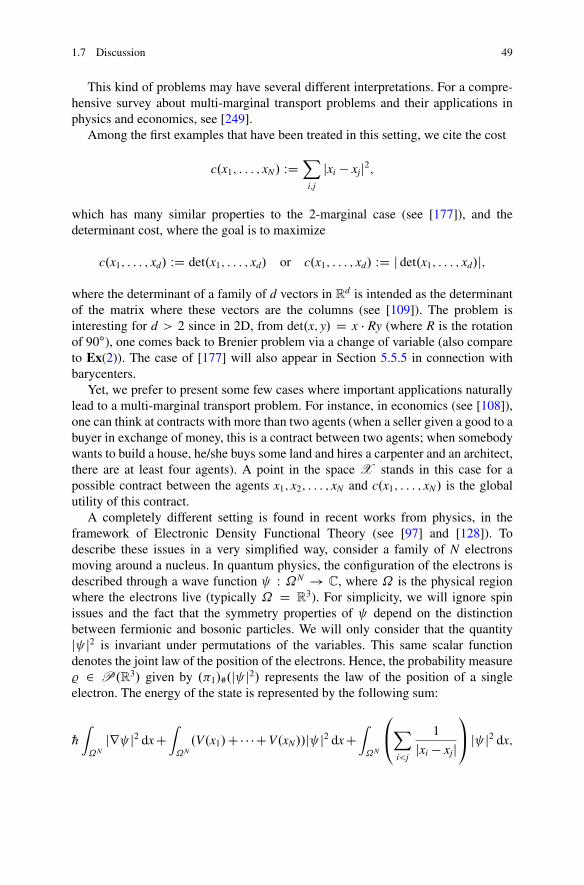
1.7 Discussion 49

This kind of problems may have several different interpretations. For a compre-hensive survey about multi-marginal transport problems and their applications inphysics and economics, see [249].

Among the first examples that have been treated in this setting, we cite the cost

c.x1; : : : ; xN/ WDX

i;j

jxi � xjj2;

which has many similar properties to the 2-marginal case (see [177]), and thedeterminant cost, where the goal is to maximize

c.x1; : : : ; xd/ WD det.x1; : : : ; xd/ or c.x1; : : : ; xd/ WD j det.x1; : : : ; xd/j;

where the determinant of a family of d vectors in Rd is intended as the determinant

of the matrix where these vectors are the columns (see [109]). The problem isinteresting for d > 2 since in 2D, from det.x; y/ D x � Ry (where R is the rotationof 90ı), one comes back to Brenier problem via a change of variable (also compareto Ex(2)). The case of [177] will also appear in Section 5.5.5 in connection withbarycenters.

Yet, we prefer to present some few cases where important applications naturallylead to a multi-marginal transport problem. For instance, in economics (see [108]),one can think at contracts with more than two agents (when a seller given a good to abuyer in exchange of money, this is a contract between two agents; when somebodywants to build a house, he/she buys some land and hires a carpenter and an architect,there are at least four agents). A point in the space X stands in this case for apossible contract between the agents x1; x2; : : : ; xN and c.x1; : : : ; xN/ is the globalutility of this contract.

A completely different setting is found in recent works from physics, in theframework of Electronic Density Functional Theory (see [97] and [128]). Todescribe these issues in a very simplified way, consider a family of N electronsmoving around a nucleus. In quantum physics, the configuration of the electrons isdescribed through a wave function W ˝N ! C, where ˝ is the physical regionwhere the electrons live (typically ˝ D R

3). For simplicity, we will ignore spinissues and the fact that the symmetry properties of depend on the distinctionbetween fermionic and bosonic particles. We will only consider that the quantityj j2 is invariant under permutations of the variables. This same scalar functiondenotes the joint law of the position of the electrons. Hence, the probability measure% 2 P.R3/ given by .�1/#.j j2/ represents the law of the position of a singleelectron. The energy of the state is represented by the following sum:

„ˆ

˝Njr j2 dxC

ˆ

˝N.V.x1/C� � �CV.xN//j j2 dxC

ˆ

˝N

0@X

i<j

1

jxi � xjj

1A j j2 dx;

50 1 Primal and dual problems

where the first term represents the kinetic energy, the second the potential energy(created, for instance, by the nucleus), and the last the electric interaction energybetween the electrons. As far as the parameter N is concerned, it is meant to bethe atomic number of an atom, which means that it ranges from two to one ortwo hundreds. The minimization of the above energy becomes a multi-marginaltransport problem as soon as one takes the semiclassical limit „ ! 0 (see [128, 129];the rigorous limit for N > 2 is an ongoing work). This allows us to get rid of the firstterm in the energy, and the second is easily seen to depend on % only. Hence, theonly unknown is the joint law of the positions of the N electrons, i.e., the probability� 2 P..˝/N/ given by � D j j2dx1 : : : dxN , with marginals all equal to %. The costc is given by

c.x1; : : : ; xN/ WDXi<j

1

jxi � xjj ;

so that � should minimize´

c d� under marginal constraints. The fact that c isneither bounded nor finite (it goes to C1 as soon as two electrons approach eachother) is a strong difficulty of this problem even in the “easy” case N D 2. It isby the way an interesting transport problem where configurations with equalitiesxi D xj cost the most, so that the problem is meaningful and intriguing even and inparticular when the marginals are all equal (which would not be the case for costsincreasingly depending on the distances).

We observe that we already faced several examples of “symmetric” cost func-tions, meaningful when the marginals are identical (which is not the case for thecosts in [177] and [109]). This raises several questions about symmetric minimizers.Indeed, that all these problems can be restricted to the set of plans � whichare invariant under permutations of the components. The theory of symmetrictransport problems, in connection with a variant of polar factorization theory andwith self-dual convex problems, has been investigated a lot by N. Ghoussoub andcollaborators, and we refer to [179, 180] without entering into extra details.

We finish this section by underlining another point: in evolution problems, andparticularly in fluid mechanics, a natural Lagrangian point of view is the descriptionof the global movement by using a measure on the set of possible trajectories. Thistypically requires the use of probabilities on the set of continuous or Lipschitz pathson Œ0; 1�, but any kind of time discretization of such a setting can be interpreted interms of measures on ˝N , where ˝ is the state space and N represents the numberof time steps, each one of length � D 1=N. In this case, the marginals are somehow“ordered” and the cost takes into account this feature: for instance, natural costscould be

c.x1; : : : ; xN/ DN�1XiD1

jxi � xiC1j or c.x1; : : : ; xN/ DN�1XiD1

jxi � xiC1j2�

;

1.7 Discussion 51

which are, respectively, the total length of a discrete path or the total kinetic energy(the term jx � yj2=� standing for the integration over a time interval of length � of aspeed jx�yj=� ). Let us mention that the continuous counterpart of this last cost, i.e.,c.!/ WD ´ 1

0j!0.t/j2dt for ! 2 C WD H1.Œ0; 1�I˝/, appears in Brenier’s variational

formulation of the incompressible Euler equation (see [83]), which gives rise to aminimization problem such as

min

�ˆH

c.!/ dQ.!/ W Q 2 P.C /; .et/#Q D L˝; .e0; e1/#Q D �0;1

�;

where et W C ! ˝ is the evaluation map et.!/ WD !.t/, L˝ is the rescaledLebesgue measure over ˝; and �0;1 is a fixed measure in P.˝ � ˝/ with bothmarginals equal to L˝ .

1.7.5 Martingale optimal transport and financial applications

We present in this section two problems from mathematical finance involving multi-marginal optimal transport. To analyze them, one should know what is an option.An option is a contract giving the owner the right to buy or sell some financialassets at some given conditions, which could bring a monetary advantage. The mosttypical case is the European Call option, saying “at time T you will have the rightto buy this asset at price K”: should the price be ST , higher than K, then you gainST � K; should it be lower, then simply do not use the option, so that finally thegain is .ST � K/C. More generally, we call option any financial contract giving theowner a gain which is a function of the value ST at time T of a given asset (a share,for instance). This value is a random variable (based on a probability P) evolving intime. More exotic options such that their payoff depends on the whole history .St/tof the asset value also exist. One of the main issues of financial mathematics is togive formulas to compute the correct price for these contracts. This is based on theno-arbitrage assumption: the only reasonable price for a contract is the one whichavoids the existence of arbitrage14 opportunities on the market, i.e., the possibilityof buying and selling this contract together with the related underlying asset and toproduce a positive amount of money out of nothing (more precisely, since all thevalues are random variables: to produce with probability 1 a nonnegative amountof money, which is strictly positive with strictly positive probability). A generaltheorem in financial mathematics (see, for instance, [139] for references) states thatall these no-arbitrage prices are actually the expected value of the contract accordingto a probability Q which is in general not P (but P � Q and Q � P, so that theyhave the same negligible sets) and which has the property that all the asset valueson the market are martingales under Q. This means, for instance, that the price of

14The absence of arbitrage is usually referred to as “no free lunch.”

52 1 Primal and dual problems

a European Call option should be EQŒ.ST � K/C�. Note that the knowledge of this

price for every K implies the knowledge of the law of ST under Q.A first problem that one could find in finance is the following: consider a

complicated option with payoff depending on the values at time T of several assetsSi

T at the same time T . One should compute EQŒf .S1T ; S2T ; : : : ; S

NT /�. Yet, this depends

on the joint law of the different assets under the unknown probability Q. If wesuppose that this option is new on the market, but that all the European Calls oneach of the assets Si are regularly sold on the market for each strike price K, thenthis means that we know the marginal laws �i under Q of each asset, and we onlylack the joint law. We can have an estimate of the correct price of the option bycomputing

min =max

�ˆf .x1; x2; : : : ; xN/ d� W .�i/#� D �i

�

which is nothing but a transport problem. We ignored here the constraints on thefact that Q should make the asset value process a martingale since they are alreadyincluded in the law of each asset and do not involve the joint law. Indeed, in thiscase, the different marginals represent different financial assets, and not differentinstants of time, and the martingale condition does not play any role15.

Another problem, much more intriguing, can be obtained when one considersa single asset but uses several marginals for several time steps. This allows us toconsider exotic options depending on the whole history of the asset value. Considera process .St/t defined for various instants of time (we will consider discrete timemodels for the sake of simplicity: t D 0; 1; : : : ;N). Suppose that an option paysf .S0; S1; : : : ; SN/. Suppose that European Calls are traded in the market for eachmaturity time t and each strike price K, which provides the law of St under theunknown martingale measure Q. Then, the price of the option may be estimated bysolving

min =max˚EQŒf .S0; S1; : : : ; SN/� W .St/#Q D �t; .St/t is a martingale under Q

:

This can also be expressed in terms of the measure � D .S0; S1; : : : ; SN/#Q as

min =max

�ˆf .x1; x2; : : : ; xN/ d� W .�i/#� D �i; � 2 MartN

�;

where the set MartT is the set of discrete time martingale measures � , satisfying foreach t � N � 1

15We could have presented this problem in Section 1.7.4, but we preferred to do it here in order tointroduce the martingale setting.

1.7 Discussion 53

ˆxtC1�.x0; x1; : : : ; xt/ d� D

ˆxt�.x0; x1; : : : ; xt// d�: (1.7)

These problems are now called martingale optimal transport problems and are outof the framework of usual transport problems that we presented before. By the way,in general, there is no reason to hope for the existence of an optimal transportmap. Indeed, even in the easiest case, i.e., two marginals, this will not be thecase. The reason is the fact that the only martingale measure which is of the form�T D .id;T/#� is that with T D id. This can be seen from Equation (1.7), since itgives

ˆT.x/�.x/ d� D

ˆy�.x/ d�T D

ˆx�.x/ d�T D

ˆx�.x/ d�;

which implies, � being an arbitrary test function, T.x/ D x �-a.e. This meansthat, unless � D �, the martingale transport problem with two marginals admits noadmissible transport plan issued by a transport map. On the contrary, it is possibleto realize � as a combination of two transport maps, and optimality results of thiskind are proven in [31, 193]. For a general presentation of the martingale optimaltransport problem, see [32] and [173].

We finish this section presenting an alternative approach, leading to the sameproblems, and based on the idea of optimal hedging. Think that f .S0; : : : ; SN/ is theloss that a company would face, depending on the prices of the asset S (i.e., it isthe amount of money that the company needs to pay, because of a debt or othercontracts). The company wants to “cover” (or “hedge”) this amount, by using thepossibilities in the market. In order to hedge this amount, the company can

• buy usual options, based on the value of the asset at time t, i.e., buy a contractwhose value will be �.St/ and whose price is known to be

´� d�t;

• buy some amounts of the asset itself: at time t � N � 1, it is possible to but fora price St and to resell at price StC1; the number of assets to buy can only bechosen according to the information that are available at time t, which meansthat one can buy (and then resell) an amount of the form .S0; S1; : : : ; St/; thisresults in covering a quantity .S0; S1; : : : ; St/.StC1 � St/, at cost 0.

The optimal hedging problem becomes

min

(NX

tD0

ˆ't d�t W

NXtD0

't.xt/CN�1XtD0

.x0; x1; : : : ; xt/.xtC1 � xt/ � f .x0; x1; : : : ; xN/

):

It is not difficult to check, thanks to the marginal constraints and to the martingalecondition (1.7), that this problem is exactly the dual of the above martingaletransport problem.

54 1 Primal and dual problems

1.7.6 Monge-Ampère equations and regularity

We saw in Section 1.3.1 that the optimal transport for the quadratic case is of theform T.x/ D ru.x/, for a convex function u. If this function is smooth and strictlyconvex, and the two measures � and � are absolutely continuous (say, with densitiesf and g), then we can write the condition T#� D � in a PDE form. Indeed, thiscondition is equivalent, if � D f .x/ dx and � D g.y/ dy and if T is C1 and injective,to the Jacobian condition

det.DT.x// D f .x/

g.T.x//

which can be obtained as a consequence of a simple change-of-variable computa-tion, as explained here below.

Box 1.14. Memo: Change-of-variable and image measures

Proposition. Suppose that % 2 L1.˝/ is a positive density on˝ � Rd and T W ˝ ! R

d

is a Lipschitz injective map, which is thus differentiable a.e. We suppose that det.DT/ ¤ 0

a.e. on f% > 0g. Then the image measure T#% is absolutely continuous and its density %T isgiven by

%T.y/ D %.T�1.y//

det.DT.T�1.y///:

If T is non-injective, the formula becomes T#% D %T � L d with %T given by

%T.y/ D XxWT.x/Dy

%.x/

det.DT.x//:

The same formulas stay true if T is not Lipschitz, but if there are measurable sets Ei suchthat j˝ nSi Eij D 0 and T is Lipschitz continuous on each set Ei (see also Definition 3.13for countably Lipschitz functions), with the differential DT which is actually the differentialof the restriction of T to each set where it is Lipschitz continuous (and coincides thus withthe approximate differential of T, see Section 3.3.2).

In the particular case where T D ru (where we suppose u to be strictlyconvex just to guarantee injectivity of T), this becomes the so-called Monge-Ampèreequation

det.D2u.x// D f .x/

g.ru.x//; (1.8)

which is a nonlinear PDE of elliptic type. Nonlinearity comes both from the right-hand side with the term g.ru/ but also from the higher-order term det.D2u/. ThisJacobian term is nonlinear but has some monotonicity property when we assume the

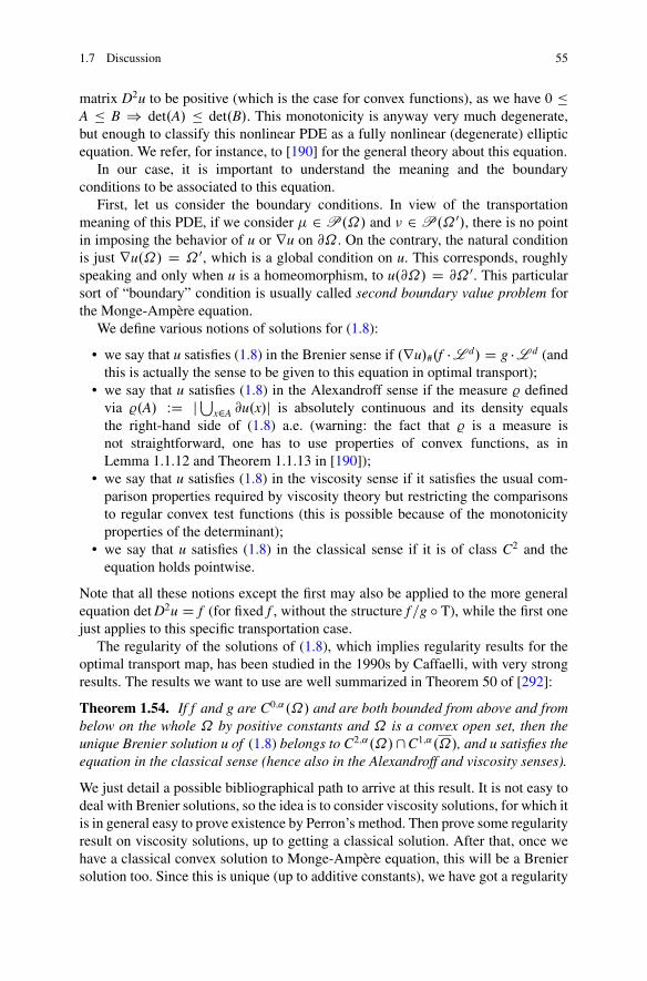
1.7 Discussion 55

matrix D2u to be positive (which is the case for convex functions), as we have 0 �A � B ) det.A/ � det.B/. This monotonicity is anyway very much degenerate,but enough to classify this nonlinear PDE as a fully nonlinear (degenerate) ellipticequation. We refer, for instance, to [190] for the general theory about this equation.

In our case, it is important to understand the meaning and the boundaryconditions to be associated to this equation.

First, let us consider the boundary conditions. In view of the transportationmeaning of this PDE, if we consider � 2 P.˝/ and � 2 P.˝ 0/, there is no pointin imposing the behavior of u or ru on @˝. On the contrary, the natural conditionis just ru.˝/ D ˝ 0, which is a global condition on u. This corresponds, roughlyspeaking and only when u is a homeomorphism, to u.@˝/ D @˝ 0. This particularsort of “boundary” condition is usually called second boundary value problem forthe Monge-Ampère equation.

We define various notions of solutions for (1.8):

• we say that u satisfies (1.8) in the Brenier sense if .ru/#.f �L d/ D g �L d (andthis is actually the sense to be given to this equation in optimal transport);

• we say that u satisfies (1.8) in the Alexandroff sense if the measure % definedvia %.A/ WD jSx2A @u.x/j is absolutely continuous and its density equalsthe right-hand side of (1.8) a.e. (warning: the fact that % is a measure isnot straightforward, one has to use properties of convex functions, as inLemma 1.1.12 and Theorem 1.1.13 in [190]);

• we say that u satisfies (1.8) in the viscosity sense if it satisfies the usual com-parison properties required by viscosity theory but restricting the comparisonsto regular convex test functions (this is possible because of the monotonicityproperties of the determinant);

• we say that u satisfies (1.8) in the classical sense if it is of class C2 and theequation holds pointwise.

Note that all these notions except the first may also be applied to the more generalequation det D2u D f (for fixed f , without the structure f=g ı T), while the first onejust applies to this specific transportation case.

The regularity of the solutions of (1.8), which implies regularity results for theoptimal transport map, has been studied in the 1990s by Caffaelli, with very strongresults. The results we want to use are well summarized in Theorem 50 of [292]:

Theorem 1.54. If f and g are C0;˛.˝/ and are both bounded from above and frombelow on the whole ˝ by positive constants and ˝ is a convex open set, then theunique Brenier solution u of (1.8) belongs to C2;˛.˝/\ C1;˛.˝/, and u satisfies theequation in the classical sense (hence also in the Alexandroff and viscosity senses).

We just detail a possible bibliographical path to arrive at this result. It is not easy todeal with Brenier solutions, so the idea is to consider viscosity solutions, for which itis in general easy to prove existence by Perron’s method. Then prove some regularityresult on viscosity solutions, up to getting a classical solution. After that, once wehave a classical convex solution to Monge-Ampère equation, this will be a Breniersolution too. Since this is unique (up to additive constants), we have got a regularity

56 1 Primal and dual problems

statement for Brenier solutions. We can find results on viscosity solutions in [98,100] and [99]. In [98], some conditions are given so as to ensure strict convexity ofthe solution of det D2u D f when f is bounded from above and below. In [100], forthe same equation it is proved C1;˛ regularity provided we have strict convexity. Inthis way, the term f=g.ru/ becomes a C0;˛ function, and in [99], it is proved C2;˛

regularity for solutions of det D2u D f with f 2 C0;˛ .Some recent improvements on this regularity theory are due to De Philippis and

Figalli, who worked on this natural question: if f and g are bounded from aboveand below, then the transport map is a BV map (since it is the gradient of a convexfunction), which happens to be continuous (since u 2 C1;˛); its derivative has nojump part (because of continuity), and the question arises whether T 2 W1;1, i.e., u 2W2;1. The answer is yes, as it is shown in [147, 148, 150], and one can even provesharper estimates (D2u is not only L1 but slightly better, including some L1C" results,also proven by Schmidt in [281]). For a comprehensive survey of the relations of theMonge-Ampére equation with optimal transport and its regularity properties, see[149].

The situation becomes much trickier when dealing with different costs than thequadratic one. If the cost c satisfies the twist condition, it is still possible to expressthe optimal map T in terms of a gradient, T.x/ D .rxc.x; �//�1.r'.x//. If we writerxc.x;T.x// D r'.x/, differentiating this equality we get

D2xxc.x;T.x//C D2

xyc.x;T.x//DT.x/ D D2'.x/;

which means that the equation on det.DT/ reads

det.D2xyc.x;T.x/// det.DT.x// D det.D2'.x/ � D2

xxc.x;T.x///;

i.e.,

det.D2'.x/ � D2xxc.x;T.x/// D det.D2

xyc.x;T.x///f .x/

g.T.x//;

which is a Monge-Ampère-type equation of the form

det.D2'.x/ � A.x;r'.x/// D F.x;r'.x//:

The regularity problem of the Kantorovich potentials for general costs has beena long-standing problem, and it was listed as open in [292]. It is now well clarifiedafter a remarkable paper by Ma, Trudinger, and Wang, who found out in [219] a keyassumption on the cost c so as to be able to develop regularity estimates, based onsome Pogorelov-type methods. The assumption on c is very technical and requiressome inequalities on its fourth-order derivatives. We do not want to write them here,but it is worth noting that these assumptions have later been proven to be sharpby Loeper in [216]. In particular, the case c.x; y/ D jx � yj2 is covered by thisassumption but is a limit case, and no other power cost jx � yjp for p 2�1;C1Œ

1.7 Discussion 57

satisfies it. The costp"2 C jx � yj2 also satisfies the MTW assumption for every

" > 0, and this allowed some approximation result for the linear cost jx � yj (see[210]). The convexity of the domain ˝ is also replaced by a suitable notion ofc-convexity that we do not detail here. The connection with convexity propertiesrelated to c-concave functions is also underlined in [168], as we saw in Section 1.7.3.The theory has been deeply studied after this discovery, and many costs have beenconsidered: the case of the squared distance on a manifold can also be investigated,and the condition translates into a curvature condition on the manifold. We refer to[164] for an interesting survey of the whole theory.

Chapter 2One-dimensional issues

This chapter is devoted to the special features of the 1D case and to a less knowntransport map in the higher-dimensional case, called the Knothe map, built from 1Dconstructions and related to some degenerate transport cost. The discussion sectiondeals with applications of 1D transport maps to image processing and geometricinequalities.

2.1 Monotone transport maps and plans in 1D

We already discussed, in Section 1.3, the quadratic cost in 1D: as soon as thesource measure � has no atoms, there exists an optimal map, which is monotonenondecreasing.

In this section we want to discuss monotone (in the following “monotone” means“monotone nondecreasing”) transport maps between two given measures in termsof their cumulative distribution functions and generalize to the case where � mayhave atoms. This discussion is independent of optimal transport considerations.

© Springer International Publishing Switzerland 2015F. Santambrogio, Optimal Transport for Applied Mathematicians,Progress in Nonlinear Differential Equations and Their Applications 87,DOI 10.1007/978-3-319-20828-2_2

59

60 2 One-dimensional issues

Box 2.1. Memo: Cumulative distribution function

Definition. Given a probability measure � 2 P.R/, we define its cumulative distribu-tion function F� through

F�.x/ D �..�1; x�/:

The cumulative distribution function F� is easily seen to be nondecreasing and rightcontinuous since if xn ! x with xn > x, then .�1; x� D \n.�1; xn� and hence�..�1; x�/ D limn �..�1; xn�/ D infn �..�1; xn�/. It is continuous at any point where� has no atom since if xn ! x with xn < x, then limn �..�1; xn�/ D �..�1; xŒ/.

The CDF F� is important because it characterizes the measure �. Indeed, the sets of theform .�1; x� are enough to generate all open sets: we have �.�a; b�/ D F�.b/ � F�.a/,�.�a; bŒ/ D supfF�.t/ � F�.a/ W t < bg and the measure of any open set is obtained viacountable disjoint unions of open intervals.

In Rd the situation is trickier, but the knowledge of �.� � 1; x1� � � � � �� � 1; xd�/

for every x D .x1; : : : ; xd/ is enough, as in 1D, to characterize � (by finite differences onecould get all the semi-open rectangles �x�

1 ; xC

1 � � � � � ��x�

d ; xC

d � and by countable disjointunions all the open sets).

Unfortunately, the CDF above cannot always be inverted, as it is not alwaysstrictly increasing, but we can define a pseudo-inverse.

Definition 2.1. Given a nondecreasing and right-continuous function F W R !Œ0; 1�, its pseudo-inverse is the function FŒ�1� W Œ0; 1� ! R given by

FŒ�1�.x/ WD infft 2 R W F.t/ � xg;

where the infimum is a minimum as soon as the set is nonempty (otherwise it isC1) and bounded from below (otherwise it is �1), thanks to right continuityof F.

Note, as a simple consequence of the definition of pseudo-inverse, that we have

FŒ�1�.x/ � a , F.a/ � x I FŒ�1�.x/ > a , F.a/ < x: (2.1)

We look now at some properties of the pseudo-inverse of cumulative distributionfunctions.

Proposition 2.2. If � 2 P.R/ and FŒ�1�� is the pseudo-inverse of its cumulative

distribution function F�, then .FŒ�1�� /#.L 1 Œ0; 1�/ D �.

Moreover, given �; � 2 P.R/, if we set � WD .FŒ�1�� ;FŒ�1�� /#.L 1 Œ0; 1�/, then� 2 ˘.�; �/ and �..�1; a� � .�1; b�/ D F�.a/ ^ F�.b/.

2.1 Monotone transport maps and plans in 1D 61

Proof. For the first part of the statement, using (2.1), we write

jfx 2 Œ0; 1� W FŒ�1�� .x/ � agj D jfx 2 Œ0; 1� W F�.a/ � xgj D F�.a/;

and this proves that the image measure is �, using the characterization of a measurethrough its CDF (see the Memo Box 2.1 above).

For the second part of the statement, � 2 ˘.�; �/ is just a consequence of thefirst. Then, let us compute

�..�1; a� � .�1; b�/ D jfx 2 Œ0; 1� W FŒ�1�� .x/ � a; FŒ�1�� .x/ � bgjD jfx 2 Œ0; 1� W F�.a/ � x; F�.b/ � xgj D F�.a/ ^ F�.b/;

which is the desired equality. utDefinition 2.3. We will call the transport plan � WD .FŒ�1�� ;FŒ�1�� /#.L 1 Œ0; 1�/ theco-monotone transport plan between � and � and denote it by �mon.

Now, consider two measures �; � 2 P.R/: we want to build a monotonetransport map (and not only a plan) sending � onto �, provided � is atomless.

We first need a simple lemma on the CDF of atomless measures.

Lemma 2.4. If � 2 P.R/ is atomless, then .F�/#� D L 1 Œ0; 1�. As aconsequence, for every ` 2 Œ0; 1�, the set fx W F�.x/ D `g is �-negligible.

Proof. First note that F� is continuous because � is atomless. Hence, for a 2�0; 1Œ,the set fx W F�.x/ � ag is a closed interval of the form �� 1; xa�, with F�.xa/ D a.Hence, �.fx W F�.x/ � ag/ D F�.xa/ D a, which proves .F�/#� D L 1 Œ0; 1�.

As a consequence, for ` 2 Œ0; 1�, the sets fx W F�.x/ D `g are �-negligible, sinceotherwise the image measure .F�/#� would have an atom at `, which contradictsthe first part of the statement. utTheorem 2.5. Given �; � 2 P.R/, suppose that � is atomless. Then, there existsa unique nondecreasing map Tmon W R ! R such that .Tmon/#� D �.

Proof. First, let us build one such a map. Let us consider the cumulative distributionfunctions F� and F� and define the map Tmon through

Tmon.x/ WD FŒ�1�� .F�.x//:

This quantity is well defined and belongs to R provided F�.x/ 2�0; 1Œ (so that theset on which we take the infimum in Definition 2.1 is neither empty nor unboundedfrom below). The sets fx W F�.x/ D 0g and fx W F�.x/ D 1g are �-negligiblethanks to Lemma 2.4. Hence, Tmon is well-defined �-a.e.

The fact that Tmon is monotone nondecreasing is obvious; we just have to prove.Tmon/#� D �. Since we already know .FŒ�1�� /#.L 1 Œ0; 1�/ D �, by compositionwe just need to use Lemma 2.4, which proves .F�/#� D L 1 Œ0; 1�.

62 2 One-dimensional issues

We now pass to the proof of uniqueness. Consider any nondecreasing functionT such that T#� D �.

From monotonicity we have T�1.� � 1;T.x/�/ � � 1; x�. We deduce

F�.x/ D �.� � 1; x�/ � �.T�1.� � 1;T.x/�// D �.� � 1;T.x/�/ D F�.T.x//;

which means T.x/ � FŒ�1�� .F�.x//. Suppose that the inequality is strict. This meansthat there exists "0 > 0 such that F�.T.x/ � "/ � F�.x/ for every " 2�0; "0Œ. On theother hand, from T�1.� � 1;T.x/ � "Œ/ �� � 1; xŒ, we get F�.T.x/ � "/ � F�.x/.

Hence, we obtain F�.T.x/� "/ D F�.x/ for every " 2�0; "0Œ. Thus, F�.T.x/� "/is the value that F� takes on an interval where it is constant. These intervals are acountable quantity; hence the values of F� on those intervals are also countable. Wecall `i these values. As a consequence, the points x where T.x/ > FŒ�1�� .F�.x// arecontained in

Sifx W F�.x/ D `ig. Lemma 2.4 proves that this set is negligible. This

allows us to conclude T.x/ D FŒ�1�� .F�.x// �-a.e. utRemark 2.6. Note that the previous proof was complicated by the possibility thatthe cumulative distribution functions could be either discontinuous or not strictlyincreasing. Should F� be continuous and strictly monotone (which means that � isatomless and supported on the whole R), then one would simply have

Tmon D .F�/�1 ı F�:

Remark 2.7. As a consequence of the explicit formula of the previous remark, onecan also study the regularity of this map Tmon depending on the regularity of � and�. Indeed, as soon as these measures are fully supported and have no atoms, the twofunctions F� and F� are homeomorphisms, and so is Tmon. Moreover, if � and � areabsolutely continuous, with continuous densities which do not vanish, then they arealso diffeomorphisms, and so is Tmon. In general, the regularity of Tmon is one degreehigher than that of the two measures, as it is the case for F�;F�;F�1

� , and F�1� .

In the next section we will see that the map Tmon that we have just builtoptimizes a whole class of transport costs. To prove it, we will need the followingcharacterization of �mon and Tmon.

Lemma 2.8. Let � 2 ˘.�; �/ be a transport plan between two measures �;� 2 P.R/. Suppose that it satisfies the property

.x; y/; .x0; y0/ 2 spt.�/; x < x0 ) y � y0: (2.2)

Then, we have � D �mon. In particular there is a unique � satisfying (2.2).Moreover, if � is atomless, then � D �Tmon .

Proof. For the first part of the statement, we just need to prove

�..�1; a� � .�1; b�/ D F�.a/ ^ F�.b/:

2.2 The optimality of the monotone map 63

Indeed, from Proposition 2.2, this condition is satisfied by �mon, and we saw thatthis is enough to characterize a measure on R

2.Consider the two sets A D�� 1; a���b;C1Œ and B D�a;C1Œ��� 1; b�. From

the assumption on � , it is not possible to have both �.A/ > 0 and �.B/ > 0

(otherwise we would have points in spt.�/ violating condition (2.2)). Hence, wecan write

�..�1; a��.�1; b�/ D �...�1; a��.�1; b�/[A/^�...�1; a��.�1; b�/[B/:

Yet, we have

�...�1; a� � .�1; b�/ [ A/ D �..�1; a� � R/ D F�.a/

and

�...�1; a� � .�1; b�/ [ B/ D �.R � .�1; b�/ D F�.b/:

This proves the first part of the claim. For the second part, we suppose � to beatomless. For any point x 2 R, one can define the interval Ix as the minimal intervalI such that spt.�/ \ .fxg � R/ � fxg � I. This interval can obviously be reducedto a singleton. The assumption on � implies that the interior of all these intervalsis disjoint (and ordered). In particular there can be at most a countable quantityof points such that Ix is not a singleton. Since these points are �-negligible (as aconsequence of � being atomless), we can define �-a.e. a map T such that � isconcentrated on the graph of T. This map will be monotone nondecreasing becauseof (2.2), and this gives T D Tmon since we already know the uniqueness of a non-decreasing map with fixed marginals (Theorem 2.5). ut

2.2 The optimality of the monotone map

Now that we know quite well the properties, definitions, and characterizations of themap Tmon and of the plan �mon, we can see that they are, in the 1D case, optimal forseveral different costs and not only for the quadratic one. This is really specific tothe 1D case; it will not be true in higher dimension. The costs that we will considerwill be convex functions of the difference x�y and, to stress the possible asymmetricbehavior of these costs, we prefer to write h.y � x/ instead of h.x � y/.

Theorem 2.9. Let h W R ! RC be a strictly convex function and �; � 2 P.R/ beprobability measures. Consider the cost c.x; y/ D h.y � x/ and suppose that (KP)has a finite value. Then, (KP) has a unique solution, which is given by �mon. In thecase where � is atomless, this optimal plan is induced by the map Tmon.

64 2 One-dimensional issues

Moreover, if the strict convexity assumption is withdrawn and h is only convex,then the same �mon is actually an optimal transport plan, but no uniqueness isguaranteed anymore.

Proof. We will use the fact that the support of any optimal � is a c-CM set � . Thismeans in particular that for .x; y/; .x0; y0/ 2 � , we have

h.y � x/C h.y0 � x0/ � h.y0 � x/C h.y � x0/: (2.3)

We only need to show that this implies (in the strictly convex case) a monotonebehavior: we will actually deduce from (2.3) that x < x0 implies y � y0, and this willallow us to conclude from Lemma 2.8.

To prove y � y0, suppose by contradiction y > y0 and denote a D y�x, b D y0�x0and ı D x0 � x > 0. Condition (2.3) reads h.a/ C h.b/ � h.b C ı/ C h.a � ı/.Moreover, the assumption y0 < y implies b C ı < a. Hence, b C ı and a � ı arelocated in the segment between b and a (and b < a). More precisely, we have

b C ı D .1 � t/b C ta; a � ı D tb C .1 � t/a; for t D ı

a � b2�0; 1Œ:

Thus, strict convexity yields

h.a/C h.b/ � h.b C ı/C h.a � ı/< .1 � t/h.b/C th.a/C th.b/C .1 � t/h.a/ D h.a/C h.b/:

This gives a contradiction and proves the statement in the strictly convex case.The statement when h is only convex is trivial if h is constant (since every � is

optimal), and, if not, it is obtained by approximation. Lemma 2.10 below provesthat there exists a sequence of strictly convex functions h" such that h � h" �.1 C "/h C ". Let us take the transport cost c".x; y/ WD h".y � x/. In this case weknow that �mon optimizes the cost

´c" d� and hence

ˆh.y�x/ d�mon �

ˆh".y�x/ d�mon �

ˆh".y�x/ d� � "C.1C"/

ˆh".y�x/ d�

for all � 2 ˘.�; �/. Passing to the limit as " ! 0, we get that �mon also optimizesthe cost c. utLemma 2.10. For every nonconstant convex and positive function h W R ! RCand every " > 0, there exists h" W R ! RC strictly convex, such that h � h" �.1C "/h C ".

Proof. We just need to prove that there is a strictly convex function f W R ! RCsuch that f � h C 1. Then, we will take h" WD h C "f . From the fact that h is convex,it is bounded from below by an affine function, and we have h.t/ � .at C b/C (wetake the positive part since we also know h � 0). It can be checked that

2.2 The optimality of the monotone map 65

f .t/ WD 1

2

p4C .at C b/2 C 1

2.at C b/

is strictly convex and satisfies f .t/ � 12.2CjatCbjC.atCb// D 1C.atCb/C. ut

Remark 2.11. Positivity of the function h is not really necessary, as soon as � and� satisfy some integrability conditions so that inf .KP/ > �1. For instance, if wehave

´ jxjd�.x/; ´ jyjd�.y/ < C1, we can add an affine function to h and make itconvex, and the cost of this affine function does not depend on � and is finite (seeExample 2.14 below).

Remark 2.12. We stress that a completely analogous proof could be used to provethat optimal maps for strictly concave costs (of the form h.y � x/ for h strictlyconcave) are monotone decreasing instead of monotone increasing. Compare withwhat is described in Section 3.3.2.

Remark 2.13. Also, the optimality of �mon is true under more general assumptions,i.e., for some costs which are not of the form h.x � y/ but satisfy the twist condition.See Ex(10).

Easy examples where c is convex but not strictly convex and Tmon is not the uniqueoptimal transport map may be built as follows.

Example 2.14 (Linear costs). Suppose that c.x; y/ D L.x�y/, the map a W Rd ! R

being linear. In this case any transport plan � is optimal and any transport map aswell. This can be easily seen if one writes

ˆL.x � y/ d� D

ˆL.x/ d� �

ˆL.y/ d� D

ˆL.x/ d� �

ˆL.y/ d�;

which shows that the result does not depend on � but only on its marginals. Thisgeneral example works for �; � compactly supported (so that we do not have anyproblem of integrability of L.x/ and L.y/) and in any dimension. Hence, also in 1D.

Example 2.15 (Distance costs on the line). Suppose that c.x; y/ D jx � yj and that�; � 2 P.R/ are such that sup spt.�/ < inf spt.�/. In this case any transport plan �is optimal and any transport map is optimal as well. This can be seen by noting thatfor every .x; y/ 2 spt.�/ � spt.�/, we have c.x; y/ D y � x; which is again a linearcost.

Example 2.16 (Book shifting). Consider c.x; y/ D jx � yj, � D 12L 1Œ0;2�, and � D

12L 1Œ1;3�. Then Tmon.x/ D xC1 is the monotone transport plan transporting � onto �.

Its cost is M.T/ D ´ jTmon.x/ � xj d� D 1. Yet, the transport map T given by

T.x/ D(

x C 2 if x � 1

x if x > 1

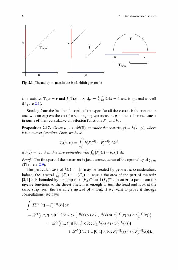
66 2 One-dimensional issues

m

Tmon

ν

m

Tν

m ν

T

Tmon

Fig. 2.1 The transport maps in the book-shifting example

also satisfies T#� D � and´ jT.x/ � xj d� D 1

2

´ 102 dx D 1 and is optimal as well

(Figure 2.1).

Starting from the fact that the optimal transport for all these costs is the monotoneone, we can express the cost for sending a given measure � onto another measure �in terms of their cumulative distribution functions F� and F� .

Proposition 2.17. Given �; � 2 P.R/, consider the cost c.x; y/ D h.x � y/, whereh is a convex function. Then, we have

Tc.�; �/ Dˆ 1

0

h.FŒ�1�� � FŒ�1�� /dL 1:

If h.z/ D jzj, then this also coincides with´R

jF�.t/ � F�.t/j dt.

Proof. The first part of the statement is just a consequence of the optimality of �mon

(Theorem 2.9).The particular case of h.z/ D jzj may be treated by geometric consideration:

indeed, the integral´ 10

ˇ.F�/�1 � .F�/�1

ˇequals the area of the part of the strip

Œ0; 1� � R bounded by the graphs of .F�/�1 and .F�/�1. In order to pass from theinverse functions to the direct ones, it is enough to turn the head and look at thesame strip from the variable t instead of x. But, if we want to prove it throughcomputations, we have

ˆjFŒ�1�� .x/ � FŒ�1�� .x/j dx

D L 2�f.x; t/ 2 Œ0; 1� � R W FŒ�1�� .x/� t<FŒ�1�� .x/ or FŒ�1�� .x/� t<FŒ�1�� .x/g

D L 2�f.x; t/ 2 Œ0; 1� � R W FŒ�1�� .x/� t<FŒ�1�� .x/g

C L 2�f.x; t/ 2 Œ0; 1� � R W FŒ�1�� .x/� t<FŒ�1�� .x/g:

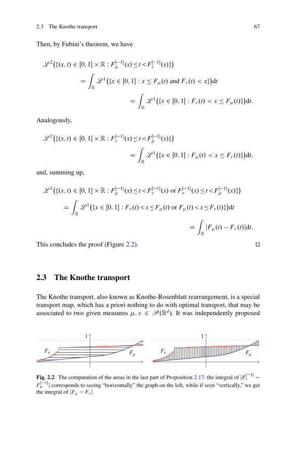
2.3 The Knothe transport 67

Then, by Fubini’s theorem, we have

L 2�f.x; t/ 2 Œ0; 1� � R W FŒ�1�� .x/� t<FŒ�1�� .x/g

Dˆ

R

L 1�fx 2 Œ0; 1� W x � F�.t/ and F�.t/ < xgdt

Dˆ

R

L 1�fx 2 Œ0; 1� W F�.t/ < x � F�.t/g

dt:

Analogously,

L 2�f.x; t/ 2 Œ0; 1� � R W FŒ�1�� .x/� t<FŒ�1�� .x/g

Dˆ

R

L 1�fx 2 Œ0; 1� W F�.t/ < x � F�.t/g

dt;

and, summing up,

L 2�f.x; t/ 2 Œ0; 1� � R W FŒ�1�� .x/� t<FŒ�1�� .x/ or FŒ�1�� .x/� t<FŒ�1�� .x/g

Dˆ

R

L 1�fx 2 Œ0; 1� W F�.t/<x�F�.t/ or F�.t/<x�F�.t/g

dt

Dˆ

R

jF�.t/ � F�.t/jdt:

This concludes the proof (Figure 2.2). ut

2.3 The Knothe transport

The Knothe transport, also known as Knothe-Rosenblatt rearrangement, is a specialtransport map, which has a priori nothing to do with optimal transport, that may beassociated to two given measures �; � 2 P.Rd/. It was independently proposed

Fν Fm

1

Fν Fm

1

Fig. 2.2 The computation of the areas in the last part of Proposition 2.17: the integral of jFŒ�1�� �FŒ�1�� j corresponds to seeing “horizontally” the graph on the left, while if seen “vertically,” we getthe integral of jF� � F� j

68 2 One-dimensional issues

by Rosenblatt [264] for statistical purposes and by Knothe [203] for applications togeometric inequalities (see also Section 2.5.3). The main interesting point of such amap is its computational simplicity. We will explain the principle of this transportmap in the simpler case where the two measures are absolutely continuous: � Df .x/ dx, � D g.y/ dy.

Let us first define the densities Of d and Ogd via

Of d.xd/ Dˆ

f .t1; t2; : : : ; td�1; xd/ dt1dt2 : : : dtd�1;

Ogd.yd/ Dˆ

g.s1; s2; : : : ; sd�1; yd/ ds1ds2 : : : dsd�1

as well as, for k < d,

Of k.xk; xkC1; : : : ; xd/ Dˆ

f .t1; : : : ; tk�1; xk; : : : ; xd/ dt1 : : : dtk�1;

Ogk.yk; ykC1; : : : ; yd/ Dˆ

f .s1; : : : ; sk�1; yk; : : : ; yd/ ds1 : : : dsk�1:

It is easy to check that Of d and Ogd are the densities of .�d/#� and .�d/#�, where�d W Rd ! R is the projection on the last variable. More generally, Of k and Ogk are thedensities of �k D .�k;d/#� and �k D .�k;d/#�, where �k;d W Rd ! R

d�kC1 is themap given by the projection onto the variables from k to d:

�k;d.x1; : : : ; xk�1; xk; xkC1; : : : ; xd/ D .xk; xkC1; : : : ; xd/:

Then, we define, for k D 1; : : : ; d�1;

f k.xk; xkC1; : : : ; xd/ DOf k.xk; xkC1; : : : ; xd/

Of kC1.xkC1; : : : ; xd/;

gk.yk; ykC1; : : : ; yd/ D Ogk.yk; ykC1; : : : ; yd/

OgkC1.ykC1; : : : ; yd/:

(Note that all these functions will only be used on the set of points where thedenominator does not vanish.)

The function f k, considered as a function of xk with parameters .xkC1; : : : ; xd/,can be actually seen as the density of the disintegration of �k according to the vari-ables .xkC1; : : : ; xd/, and gk is, in the same terms, the density of the disintegration of�k. We briefly sketch below the main notions about the disintegration of measures.With this language, the Knothe transport that we are going to define could be definedeven in the case of non-absolutely continuous measures, under some assumptionson the absence of atoms. Anyway, for the sake of simplicity, we will give most ofthe results in the case of absolutely continuous measures.

2.3 The Knothe transport 69

Box 2.2. Important notion: Disintegrations of measures

Definition. Consider a measure space X endowed with a Borel measure � and a map f WX ! Y valued in a topological space Y . We say that a family .�y/y2Y is a disintegrationof � according to f if every �y is a probability measure concentrated on f �1.fyg/, and forevery test function � 2 C.X/, the map y 7! ´

X � d�y is Borel measurable and

ˆ

X� d� D

ˆ

Yd�.y/

ˆ

X� d�y;

where � D f#�.The disintegration of � is also often written (by abuse of notation) as

� D �y ˝ �.In the particular case where X D Y �Z and f is the projection on the Y factor, we usually

identify the measures �y, which are “officially” defined as measures on Y � Z concentratedon fyg � Z, with measures on Z, so that we get

ˆ

Y�Z�.y; z/ d�.y; z/ D

ˆ

Yd�.y/

ˆ

Z�.y; z/ d�y.z/:

The disintegration of a measure � exactly corresponds to the conditional law in prob-ability. The reader is invited to consult [152] to find proofs about conditional probabilitiesand then to translate them into the disintegration language. Indeed, in probability we usuallyspeak of the conditional law of a random variable X knowing Y D y. This means that theprobability P on the probability space ˝ is disintegrated according to the map Y W ˝ ! E(where E is the image space of Y) into probabilities Py and that we take the law of X underPy. The existence and the uniqueness of the disintegration depend on some assumptions onthe spaces, but are true if X D R

d .

In order to define the Knothe rearrangement, let us start from k D d and define thetransport map Td W R ! R as the monotone nondecreasing transport map sendingf d onto gd (these functions being considered as probability densities). We know thatthis map is well defined and we know how to compute it in terms of cumulativedistribution functions. We will now define a family of maps Tk W R

d�kC1 ! R,where the variables of Tk will be .xk; xkC1; : : : ; xd/. The first one is the map Td thatwe just defined. For the sake of notations, we also define some maps OTk W Rd�kC1 !R

d�kC1 given by

OTk.xk; xkC1; : : : ; xd/ D .Tk.xk; xkC1; : : : ; xd/;TkC1.xkC1; : : : ; xd/; : : : ;T

d.xd//:

Obviously Td and OTd coincide. Now, if we write f k.xkC1;:::;xd/

and gk.ykC1;:::;yd/

for

the functions xk 7! f k.xk; xkC1; : : : ; xd/ and yk 7! gk.yk; ykC1; : : : ; yd/ and weinterpret them as densities of probability measures, we can define the map Tk, ifwe suppose that we have already defined Tj for j > k, in the following way: takeTk.xkC1;:::;xd/

to be the monotone nondecreasing transport map sending f k.xkC1;:::;xd/

onto

gkOTkC1.xkC1;:::;xd/

.

70 2 One-dimensional issues

Finally, the Knothe-Rosenblatt rearrangement T is defined by T D OT1.We want to check that this map T is a transport map from � to �.

Proposition 2.18. The Knothe-Rosenblatt rearrangement map T defined abovesatisfies T#� D �.

Proof. We will prove by induction that OTk satisfies

OTk#�

k D �k (2.4)

(let us recall that �k D .�k;d/#� and �k D .�k;d/#� are the marginals of � and �onto the last d � k C 1 variables). Equality (2.4) fact is evident by construction fork D d, and if we get it for k D 1, we have proven T#� D �.

We only need to prove that if the claim is true for a given k C 1, then it will betrue for k. To check equality (2.4), we just need to use test functions .yk; : : : ; yd/and checkˆ.Tk.xk; xkC1; : : : ; xd/;T

kC1.xkC1; : : : ; xd/; : : : ;Td.xd// d� D

ˆ.yk; : : : ; yd/ d�:

Moreover, by density (see below for Stone-Weierstrass’s theorem), it is enoughto check the equality above on functions which are separable, i.e., of the form.yk; : : : ; yd/ D �.yk/ .ykC1; : : : ; yd/. To ease the notation, for fixed k, we willdenote by Nx the vector �kC1;d.x/ and Ny D �kC1;d.y/. In this case we should check

ˆ ı OTkC1

�ˆ� ı Tk f k dxk

�Of kC1 dNx D

ˆ .Ny/

�ˆ�.yk/ gk dyk

�OgkC1 dNy:

In order to get this equality, we just need to use the definition of Tk, so that we get,for every x,

ˆ� ı Tk f k dxk D

ˆ�.yk/ gk

OTkC1.Nx/.yk/ dyk:

If we define G W Rd�k ! R the function given by G.Ny/ D ´�.yk/ gk

Ny.yk/ dyk, wehave now

ˆ ı OTkC1

�ˆ� ı Tk f k dxk

�Of kC1 dNx D

ˆ ı OTkC1 G ı OTkC1 Of kC1 dNx:

By taking the image measure of Of kC1 under OTkC1, the last expression is equal to´ .Ny/G.Ny/OgkC1.Ny/ dNy, which is in turn equal to

ˆ .Ny/

�ˆ�.yk/ gk

Ny.yk/ dyk

�OgkC1.Ny/ dNy

and proves the claim. ut

2.3 The Knothe transport 71

Box 2.3. Memo: Stone-Weierstrass’s Theorem

Theorem. Suppose that X is a compact space and that E � C.X/ is a subset of the spaceof continuous functions on X satisfying

i) constant functions belong to Eii) E is an algebra, i.e., it is stable by sum and product: f ; g 2 E ) f C g, fg 2 E

iii) E separates the points of X, i.e., for all x ¤ y 2 X, there is f 2 E such that f .x/ ¤ f .y/.

Then E is dense in C.X/ for the uniform convergence (see, for instance, [268]).This theorem is usually evoked to justify the density of polynomials when X � R

d .Trigonometric polynomials are also dense for the same reason (and, by the way, this maybe used to prove the L2 convergence of the Fourier series). In product spaces X D Y � Z,linear combinations of separable functions of the form

Pi 'i.y/ i.z/ are dense because of

this very same theorem.

We just proved that the map T is a transport map between � and �. Moreover,by construction, should it be a regular map, the Knothe transport T has a triangularJacobian matrix with nonnegative entries on its diagonal. Compare this with theBrenier optimal map for the quadratic cost: its Jacobian matrix is the Hessian matrixof a convex function, which is symmetric (instead of triangular) and has also positiveeigenvalues. Moreover, we underline that assuming absolute continuity as we did,all the monotone optimal transports that we use in defining T are invertible, since notonly the source measures are atomless but also the arrival ones are atomless (theyare all absolutely continuous). As a consequence, each map OTk is also invertible.

Remark 2.19. It is interesting to note that, due to its explicit definition, the Knothemap automatically inherits some regularity properties from the measures � and �.In general, T has the same regularity as � and � and not better. Indeed, each Tk isbuilt as a monotone transport, which gives one extra derivative than the regularity of� and � (see Remark 2.7), but only in the direction of the variable xk. With respectto the other variables, the explicit formula of monotone transports with cumulativedistribution functions allows us to prove that the dependence on .xkC1; : : : ; xd/ is asregular as the densities are.

Remark 2.20. It is also interesting to note that the Knothe map defined above isthe (unique) transport map from � to � which is monotone for the lexicographicorder, i.e., the order where x < y is defined in the following way: “there existsk 2 f1; 2; : : : ; dg such that xj D yj for j > k and xk < yk.”

Remark 2.21. How to define the Knothe transport for � and � which are not abso-lutely continuous? The construction uses the notion of disintegration of measures(Box 2.2).

First we define the transport map Td W R ! R as the monotone nondecreasingtransport map sending .�d/#� onto .�d/#�. We need to suppose that .�d/#� has noatoms. Then, for each k we consider .�k;d/#� and we disintegrate it with respect

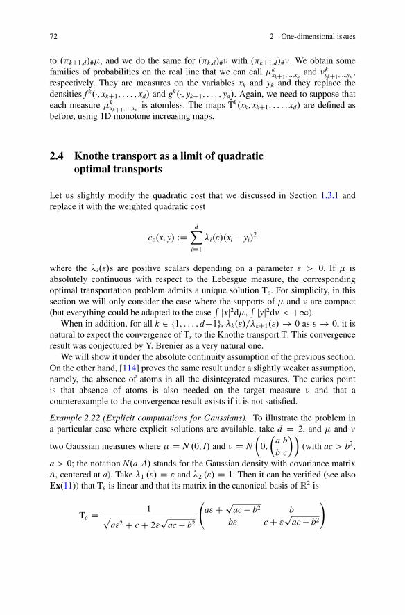
72 2 One-dimensional issues

to .�kC1;d/#�, and we do the same for .�k;d/#� with .�kC1;d/#�. We obtain somefamilies of probabilities on the real line that we can call �k

xkC1;:::;xnand �k

ykC1;:::;yn,

respectively. They are measures on the variables xk and yk and they replace thedensities f k.�; xkC1; : : : ; xd/ and gk.�; ykC1; : : : ; yd/. Again, we need to suppose thateach measure �k

xkC1;:::;xnis atomless. The maps OTk.xk; xkC1; : : : ; xd/ are defined as

before, using 1D monotone increasing maps.

2.4 Knothe transport as a limit of quadraticoptimal transports

Let us slightly modify the quadratic cost that we discussed in Section 1.3.1 andreplace it with the weighted quadratic cost

c".x; y/ WDdX

iD1�i."/.xi � yi/

2

where the �i."/s are positive scalars depending on a parameter " > 0. If � isabsolutely continuous with respect to the Lebesgue measure, the correspondingoptimal transportation problem admits a unique solution T". For simplicity, in thissection we will only consider the case where the supports of � and � are compact(but everything could be adapted to the case

´ jxj2d�; ´ jyj2d� < C1).When in addition, for all k 2 f1; : : : ; d�1g, �k."/=�kC1."/ ! 0 as " ! 0, it is

natural to expect the convergence of T" to the Knothe transport T. This convergenceresult was conjectured by Y. Brenier as a very natural one.

We will show it under the absolute continuity assumption of the previous section.On the other hand, [114] proves the same result under a slightly weaker assumption,namely, the absence of atoms in all the disintegrated measures. The curios pointis that absence of atoms is also needed on the target measure � and that acounterexample to the convergence result exists if it is not satisfied.

Example 2.22 (Explicit computations for Gaussians). To illustrate the problem ina particular case where explicit solutions are available, take d D 2, and � and �

two Gaussian measures where � D N .0; I/ and � D N

�0;

�a bb c

��(with ac > b2,

a > 0; the notation N.a;A/ stands for the Gaussian density with covariance matrixA, centered at a). Take �1 ."/ D " and �2 ."/ D 1. Then it can be verified (see alsoEx(11)) that T" is linear and that its matrix in the canonical basis of R2 is

T" D 1pa"2 C c C 2"

pac � b2

a"C p

ac � b2 bb" c C "

pac � b2

!

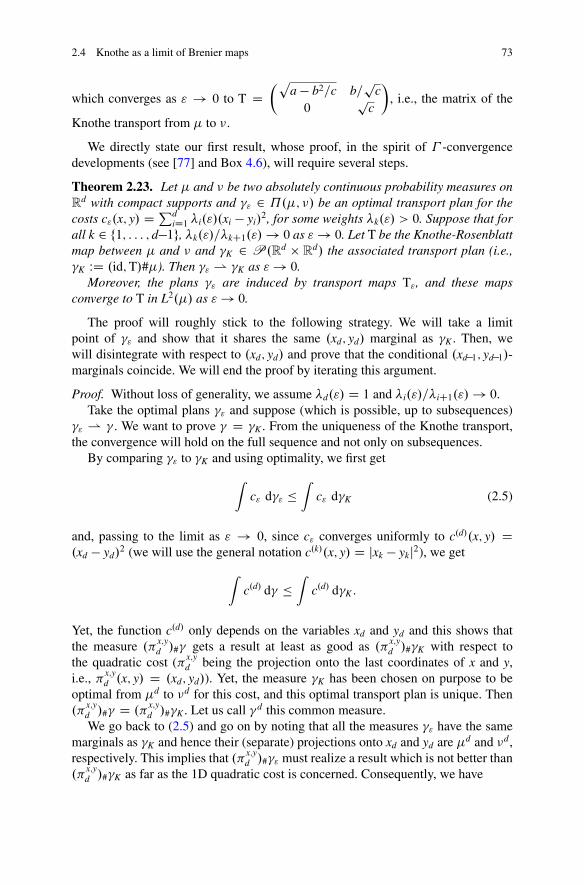
2.4 Knothe as a limit of Brenier maps 73

which converges as " ! 0 to T D�p

a � b2=c b=p

c0

pc

�, i.e., the matrix of the

Knothe transport from � to �.

We directly state our first result, whose proof, in the spirit of � -convergencedevelopments (see [77] and Box 4.6), will require several steps.

Theorem 2.23. Let � and � be two absolutely continuous probability measures onR

d with compact supports and �" 2 ˘.�; �/ be an optimal transport plan for thecosts c".x; y/ D Pd

iD1 �i."/.xi � yi/2, for some weights �k."/ > 0. Suppose that for

all k 2 f1; : : : ; d�1g, �k."/=�kC1."/ ! 0 as " ! 0. Let T be the Knothe-Rosenblattmap between � and � and �K 2 P.Rd � R

d/ the associated transport plan (i.e.,�K WD .id;T/#�). Then �" * �K as " ! 0.

Moreover, the plans �" are induced by transport maps T", and these mapsconverge to T in L2.�/ as " ! 0.

The proof will roughly stick to the following strategy. We will take a limitpoint of �" and show that it shares the same .xd; yd/ marginal as �K . Then, wewill disintegrate with respect to .xd; yd/ and prove that the conditional .xd�1; yd�1/-marginals coincide. We will end the proof by iterating this argument.

Proof. Without loss of generality, we assume �d."/ D 1 and �i."/=�iC1."/ ! 0.Take the optimal plans �" and suppose (which is possible, up to subsequences)

�" * � . We want to prove � D �K . From the uniqueness of the Knothe transport,the convergence will hold on the full sequence and not only on subsequences.

By comparing �" to �K and using optimality, we first get

ˆc" d�" �

ˆc" d�K (2.5)

and, passing to the limit as " ! 0, since c" converges uniformly to c.d/.x; y/ D.xd � yd/

2 (we will use the general notation c.k/.x; y/ D jxk � ykj2), we get

ˆc.d/ d� �

ˆc.d/ d�K :

Yet, the function c.d/ only depends on the variables xd and yd and this shows thatthe measure .�x;y

d /#� gets a result at least as good as .�x;yd /#�K with respect to

the quadratic cost (�x;yd being the projection onto the last coordinates of x and y,

i.e., �x;yd .x; y/ D .xd; yd/). Yet, the measure �K has been chosen on purpose to be

optimal from �d to �d for this cost, and this optimal transport plan is unique. Then.�

x;yd /#� D .�

x;yd /#�K . Let us call �d this common measure.

We go back to (2.5) and go on by noting that all the measures �" have the samemarginals as �K and hence their (separate) projections onto xd and yd are �d and �d,respectively. This implies that .�x;y

d /#�" must realize a result which is not better than.�

x;yd /#�K as far as the 1D quadratic cost is concerned. Consequently, we have

74 2 One-dimensional issues

ˆjxd � ydj2d.�x;y

d /#�K.xd; yd/Cd�1XiD1

�i."/

ˆ.xi � yi/

2 d�"

�ˆ

c" d�" �ˆ

c" d�K

Dˆ

jxd � ydj2d.�x;yd /#�K.xd; yd/C

d�1XiD1

�i."/

ˆ.xi � yi/

2 d�K ;

which implies, by simplifying the common term, dividing by �d�1."/, and passingto the limit,

ˆc.d�1/ d� �

ˆc.d�1/ d�K : (2.6)

We can note that both integrals depend on the variables xd�1 and yd�1 only. Anyway,we can project onto the variables .xd�1; xd/ and .yd�1; yd/ (obtaining measures.�

x;yd�1;d/#� and .�x;y

d�1;d/#�K) so that we disintegrate with respect to the measure �d.We have

ˆd�d.xd; yd/

ˆjxd�1 � yd�1j2 d�d�1

.xd ;yd/.xd�1; yd�1/

�ˆ

d�d.xd; yd/

ˆjxd�1 � yd�1j2 d�d�1

.xd ;yd/;K.xd�1; yd�1/: (2.7)

We want to prove that the measures �d�1.xd ;yd/

share the same marginals on xd�1 and yd�1of the corresponding �d�1

.xd ;yd/;K. Should this be the case, their quadratic cost would be

not better than the corresponding cost of �d�1.xd ;yd/;K

(because the Knothe measure hasbeen chosen exactly with the intention of being quadratically optimal on .xd�1; yd�1/once xd and yd are fixed). Yet, (2.7) shows that, on average, the result given by thosemeasures is not worse than the results of the optimal ones. Thus, the two resultscoincide for almost any pair .xd; yd/, and by uniqueness of the optimal transportsin the 1D case, we get �d�1

.xd ;yd/D �d�1

.xd ;yd/;K. To let this proof work, it is sufficient to

prove that the marginals of the two measures coincide for �d-a.e. pair .xd; yd/. Forfixed .xd; yd/, we would like to prove, for any �,

ˆ�.xd�1/ d�d�1

.xd ;yd/D

ˆ�.xd�1/ d�d�1

.xd ;yd/;K

(and to prove an analogous equality for functions of yd�1). Since we want to prove itfor a.e. pair .xd; yd/, it is sufficient to prove this equality:

2.4 Knothe as a limit of Brenier maps 75

ˆd�d.xd; yd/ .xd; yd/

ˆ�.xd�1/ d�d�1

.xd ;yd/

Dˆ

d�d.xd; yd/ .xd; yd/

ˆ�.xd�1/ d�d�1

.xd ;yd/;K

for any � and any . This means proving

ˆ .xd; yd/�.xd�1/ d�d�1 D

ˆ .xd; yd/�.xd�1/ d�d�1

K ;

which is not trivial. As far as now, we only know that the two measures �d�1 and�d�1

K have the same marginals with respect to the pairs .xd�1; xd/, .yd�1; yd/ (sincethey have the same projections onto x and onto y) and .xd; yd/ (since we just provedit). But here there is a function of the three variables .xd�1; xd; yd/. Yet, we knowthat the measure �d is concentrated on the set yd D Td.xd/ for a certain map Td

(here we use that the optimal plan is indeed a map), and this allows us to replacethe expression of yd, thus getting rid of one variable. This proves that the function .xd; yd/�.xd�1/ is actually a function of .xd�1; xd/ only and that equality holds whenpassing from � to �K . The same can be performed on functions .xd; yd/�.yd�1/, butwe have in this case to ensure that we can replace xd with a function of yd, i.e., thatwe can invert Td. This is possible thanks to the absolute continuity of �d, sinceTd is the optimal transport from �d to �d, but an optimal transport exists in theother direction as well and it gives the same optimal plan (thanks to uniqueness).These facts prove that the measures �d�1

.xd ;yd/and �d�1

.xd ;yd/;Khave the same marginals

and hence, since they are both optimal, they coincide for a.e. pair .xd; yd/. Thisimplies .�x;y

d�1;d/#� D .�x;yd�1;d/#�K , and we will call this common measure �d�1.

In the case d D 2, the proof would be finished. Now, it is possible to go on byinduction in the following way: we prove, by induction on N, that the statement ofthe theorem is true if d � N and that, whatever the dimension is, we have .�x;y

k;d/#� D.�

x;yk;d/#�K (i.e., that we have convergence in what concerns the components from the

kth to the dth) for every k � d � .N � 1/. Both facts are proven for N D 2.Suppose the result proven for a certain value of N. Take d > N and

k D d � .N � 1/. We want to prove .�x;yk�1;d/#� D .�

x;yk�1;d/#�K . If we can do it,

we are done, since this also proves that the result is true in dimension d D N C 1

(since in this case we have k D 2 and with our extra step we conclude the proof).Write x D .x�; xC/ and y D .y�; yC/ with x�; y� 2 R

k�1 and xC; yC 2 Rd�kC1

(decomposing into the components up to k�1 and after k). Then, define a competitor�"K in the following way: �"K is a measure on R

d � Rd with the following marginals:

.�x�;xC/#�

"K D �; .�y�;yC

/#�"K D �; .�xC;yC

/#�"K D �";k;

where �";k is the measure which optimizes the transport costPd

iDk �i."/c.i/ betweenthe marginals �k D .�xC

/#� and �k D .�yC/#�. Thanks to the recursive structure

of the proof, we know that �";k converges to .�xC;yC/#�K (since we suppose the

result to be true in dimension N).

76 2 One-dimensional issues

We need to specify how to build the measure �"K (which is likely not to beunique). One easy way to construct such a measure is the following: disintegrate �and � according to �xC

and �yC, respectively, thus getting two family of measures

�xC

and �yC

. Then, for every pair .xC; yC/ pick a transport plan � xC;yC

betweenthem. The measure � xC;yC ˝�";k satisfies the required properties. Moreover, we willchoose for � xC;yC

the Knothe transport between those two measures. Indeed, for thesake of this step of the proof, the only important point is that, in what concerns the.k � 1/th component, we choose for any .xC; yC/ the monotone map from �xC

k�1 WD.�xk�1 /#�

xC

to �yC

k�1 WD .�yk�1 /#�yC

, so that´

c.k�1/ d� xC;yC D Tc.�xC;k�1�

yC

k�1/ (inthis last expression Tc denotes the quadratic transport cost on the real line).

With this choice in mind, we write

Xi�h

�i."/

ˆjxi � yij2 d�"K C

k�1XiD1

�i."/

ˆ.xi � yi/

2 d�"

�ˆ

c" d�" �ˆ

c" d�"K

DXi�h

�i."/

ˆjxi � yij2 d�"K C

k�1XiD1

�i."/

ˆ.xi � yi/

2 d�"K ;

and consequently by erasing the common terms and dividing by �k�1."/, we get

ˆc.k�1/ d�" �

ˆc.k�1/ d�"K D

ˆTc.�

xC;k�1�

yC

k�1/d�";h:

Then we pass to the limit as " ! 0. The left-hand side of the last inequality tendsto´

c.k�1/ d� , while the right-hand side converges to

ˆTc.�

xC;k�1�

yC

k�1/d.�xC;yC/#�K D

ˆc.k�1/ d�K :

This convergence result is justified by the following Corollary 2.24 of Lemma 1.8.In the end we get

ˆc.k�1/ d� �

ˆc.k�1/ d�K

and we can go on. This last inequality was obtained thanks to a procedure whichwas similar to what we did for getting (2.6), but it required some more work since�K is not exactly optimal for all the components i � k as it was the case for k D d.

We disintegrate with respect to �x;yk;d and we act exactly as before: proving that

the marginals of the disintegrations coincide are sufficient to prove equality of themeasures. Here we will use test functions of the form

2.4 Knothe as a limit of Brenier maps 77

.xh; xkC1; : : : ; xd; yh; ykC1; : : : ; yd/'.xk�1/

and

.xh; xkC1; : : : ; xd; yh; ykC1; : : : ; yd/'.yk�1/:

The same trick as before, i.e., replacing the variables y with functions of thevariables x, is again possible. To invert the trick and replace x with y, one needsto invert part of Knothe’s transport. This is possible since, as we noted, ourassumptions implied that all the monotone transports we get are invertible. In theend we get, as before, � k�1 D � k�1

K . This proves that we can move from step N tostep .N C 1/ in the induction and allows us to conclude.

We have now proven �" * �K . Yet, if all these transport plans come fromtransport maps, then .id;T"/#� * .id;T/#� implies T" ! T in L2.�/ (seeLemma 2.25 below). ut

In the proof we used the following result, which is a corollary of Lemma 1.8.

Corollary 2.24. If� and � are two probabilities over Rd D Rk�Rd�k with compact

support which disintegrate as � D �C ˝ �xC

and � D �C ˝ �yC

and c is acontinuous cost, then the functional

� 7!ˆ

Tc.�xC

; �yC

/ d�.xC; yC/

is continuous over the transport plans between �C and �C.

Proof. It is sufficient to apply Lemma 1.8 to the following setting: X D Y D Rk,

QX D QY D P.˝/, where˝ � Rd�k is such that spt.�/; spt.�/ � R

k �˝. The spaceP.˝/ is endowed with any distance metrizing weak convergence and making thisspace a separable metric space (see, for instance, Chapter 5 for a choice of distanceswith this property, or build it with standard methods for the weak convergence in theunit ball of a Banach space). For the cost function which appears in the statement ofLemma 1.8, we take .a; b/ 7! Tc.a; b/ and a.xC/ WD �xC

, b.yC/ WD �yC

. Since thisquantity is bounded by max jcj (as we are on compact supports), there is no difficultyin choosing two bounded functions f ; g so that Tc.a; b/ � f .a/C g.b/. ut

Another easy lemma that we needed is the following.

Lemma 2.25. Given � 2 P.X/ and �n 2 P.˝/, where ˝ � Rd is a compact set,

suppose that �n WD �Tn 2 ˘.�; �n/ is such that �n ! � D �T. Then Tn ! T inL2.X; �/.

Proof. Since the functions Tn are valued in˝, they are equibounded and they admita weak limit in L2.X; �/ up to subsequences. Let us call S this limit. To prove S D T,take a continuous function � 2 C.XIRd/ and consider the limit of

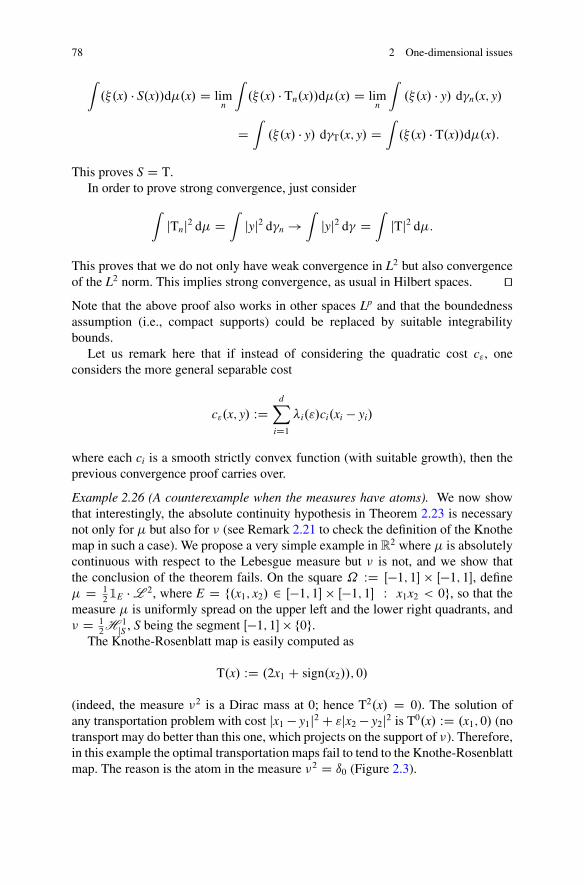
78 2 One-dimensional issues

ˆ.�.x/ � S.x//d�.x/ D lim

n

ˆ.�.x/ � Tn.x//d�.x/ D lim

n

ˆ.�.x/ � y/ d�n.x; y/

Dˆ.�.x/ � y/ d�T.x; y/ D

ˆ.�.x/ � T.x//d�.x/:

This proves S D T.In order to prove strong convergence, just consider

ˆjTnj2 d� D

ˆjyj2 d�n !

ˆjyj2 d� D

ˆjTj2 d�:

This proves that we do not only have weak convergence in L2 but also convergenceof the L2 norm. This implies strong convergence, as usual in Hilbert spaces. utNote that the above proof also works in other spaces Lp and that the boundednessassumption (i.e., compact supports) could be replaced by suitable integrabilitybounds.

Let us remark here that if instead of considering the quadratic cost c", oneconsiders the more general separable cost

c".x; y/ WDdX

iD1�i."/ci.xi � yi/

where each ci is a smooth strictly convex function (with suitable growth), then theprevious convergence proof carries over.

Example 2.26 (A counterexample when the measures have atoms). We now showthat interestingly, the absolute continuity hypothesis in Theorem 2.23 is necessarynot only for � but also for � (see Remark 2.21 to check the definition of the Knothemap in such a case). We propose a very simple example in R

2 where � is absolutelycontinuous with respect to the Lebesgue measure but � is not, and we show thatthe conclusion of the theorem fails. On the square ˝ WD Œ�1; 1� � Œ�1; 1�, define� D 1

21E � L 2, where E D f.x1; x2/ 2 Œ�1; 1� � Œ�1; 1� W x1x2 < 0g, so that the

measure � is uniformly spread on the upper left and the lower right quadrants, and� D 1

2H 1

jS , S being the segment Œ�1; 1� � f0g.The Knothe-Rosenblatt map is easily computed as

T.x/ WD .2x1 C sign.x2//; 0/

(indeed, the measure �2 is a Dirac mass at 0; hence T2.x/ D 0). The solution ofany transportation problem with cost jx1 � y1j2 C "jx2 � y2j2 is T0.x/ WD .x1; 0/ (notransport may do better than this one, which projects on the support of �). Therefore,in this example the optimal transportation maps fail to tend to the Knothe-Rosenblattmap. The reason is the atom in the measure �2 D ı0 (Figure 2.3).

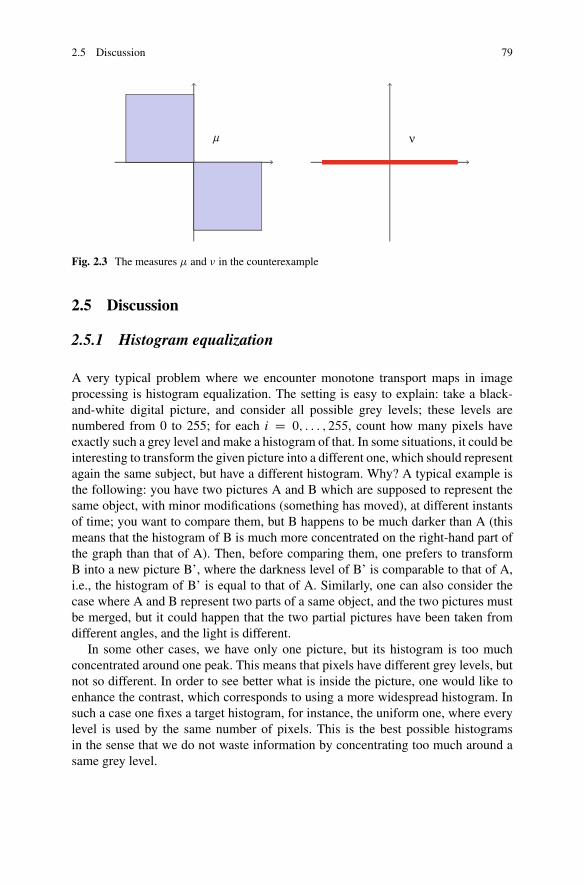
2.5 Discussion 79

m ν

Fig. 2.3 The measures � and � in the counterexample

2.5 Discussion

2.5.1 Histogram equalization

A very typical problem where we encounter monotone transport maps in imageprocessing is histogram equalization. The setting is easy to explain: take a black-and-white digital picture, and consider all possible grey levels; these levels arenumbered from 0 to 255; for each i D 0; : : : ; 255, count how many pixels haveexactly such a grey level and make a histogram of that. In some situations, it could beinteresting to transform the given picture into a different one, which should representagain the same subject, but have a different histogram. Why? A typical example isthe following: you have two pictures A and B which are supposed to represent thesame object, with minor modifications (something has moved), at different instantsof time; you want to compare them, but B happens to be much darker than A (thismeans that the histogram of B is much more concentrated on the right-hand part ofthe graph than that of A). Then, before comparing them, one prefers to transformB into a new picture B’, where the darkness level of B’ is comparable to that of A,i.e., the histogram of B’ is equal to that of A. Similarly, one can also consider thecase where A and B represent two parts of a same object, and the two pictures mustbe merged, but it could happen that the two partial pictures have been taken fromdifferent angles, and the light is different.

In some other cases, we have only one picture, but its histogram is too muchconcentrated around one peak. This means that pixels have different grey levels, butnot so different. In order to see better what is inside the picture, one would like toenhance the contrast, which corresponds to using a more widespread histogram. Insuch a case one fixes a target histogram, for instance, the uniform one, where everylevel is used by the same number of pixels. This is the best possible histogramsin the sense that we do not waste information by concentrating too much around asame grey level.

80 2 One-dimensional issues

In all these cases, we want to perform a transformation which does not act pixelby pixel, but grey level by grey level: we look for a map T from the set X of greylevels to itself (all pixels with grey level x will be turned into the grey level T.x/),and we want to prescribe the histogram of the image after the transformation. Thisis the same as saying that we have a measure � on X and we want to impose acondition of the form T#� D �. Here the important fact is that the space X is asubset of R, i.e., it is 1D and ordered. The natural condition on T is that it should bemonotone increasing. This condition translates the fact that we do not want to invertdarker and brighter pixels.

Up to the fact that, in this discrete setting (the grey level only takes value in afinite set of integers), the two measures � and � are atomic (and hence a transportmap could not exist), the situation is exactly the one described in this chapter.The problem of nonexistence of transport maps could be solved in several ways inpractice: one could introduce some rounding rules or use a transport plan whichcorresponds to use different colors on pixels which had the same colors on theoriginal picture, i.e., splitting the mass.

The situation becomes trickier when we take color images. In this case the spaceX of colors becomes 3D and the notion of monotone transport does not make senseany more. Obviously the quadratic optimal transport (Brenier’s map) could play therole of a monotone map, since it is monotone in the vector sense .T.x/� T.y// � .x �y/ � 0. On the other hand, it is expensive to compute (we will see in Chapter 6 somenumerical methods to do it and the associated difficulties) and some of its featuresare probably useless for this kind of application in image processing (the fact that itis a gradient, for instance).

Several solutions are now a matter of current research: looking for transport mapswhich are more regular but not so far from the optimal one [163], or producingmaps defined from the composition/superposition of several 1D bricks, so thatthey keep some monotonicity properties and are easier to compute (see [252] andSection 2.5.2).

Also, in some cases all the components of the color space are not equallyimportant, and one could decide to look only at one or two components or totreat them separately. In this case, colors are often described by different sets ofparameters.

See, for instance, [140], where some applications of a 1D analysis on the circleare proposed for hue component of the color space (with the HSL decompositioninto hue, saturation, and lightness).

The same space of colors can also be written as the combination of a 1Dinformation (the luma signal, corresponding to a weighted average of the threecomponents R, G, and B and standing for the brightness of the image) and of a2D information (called chrominance or chroma, standing for the color information).In Figure 2.4 we see an application of optimal transport in 1D and 2D to the colortransfer between two streets with very different colors.

For a wider discussion about 1D histogram equalization and 3D color transfer inconnection with optimal transport, we refer to [163] and [255] and the referencestherein (in particular some older papers such as [242, 259]).

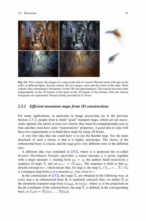
2.5 Discussion 81

Fig. 2.4 First column: the images of a souq arcade and of a narrow Western street with tags on thewalls, in different lights. Second column: the two images, each with the colors of the other. Thirdcolumn: their chrominance histograms (in the CIE-lab representation). The transfer has been doneindependently on the 1D feature of the luma on the 2D feature of the chroma. Only the chromahistograms are represented. Pictures kindly provided by G. Peyré

2.5.2 Efficient monotone maps from 1D constructions

For many applications, in particular in image processing (as in the previousSection 2.5.1), people tried to build “good” transport maps, which are not neces-sarily optimal, but satisfy at least two criteria: they must be computationally easy tofind, and they must have some “monotonicity” properties. A good idea to cope withthese two requirements is to build these maps by using 1D bricks.

A very first idea that one could have is to use the Knothe map. Yet, the maindrawback of such a choice is that it is highly anisotropic. The choice of theorthonormal basis is crucial, and the map gives very different roles to the differentaxes.

A different idea was contained in [252], where it is proposed the so-calledIterative Distribution Transfer algorithm: a source measure � is given, togetherwith a target measure �; starting from �0 D �, the authors build recursively asequence of maps Tn and set �nC1 D .Tn/#�n. The sequence is built so that �n

should converge to �, which means that, for large n, the map Tn ı Tn�1 ı : : :T1 ı T0is a transport map from � to a measure �n very close to �.

In the construction of [252], the maps Tn are obtained in the following way: atevery step n an orthonormal basis Bn is randomly selected; then, we define Tj

n asthe monotone transport map from .�j/#�n to .�j/#�, where �j is the projection onthe jth coordinate of the selected basis; the map Tn is defined, in the correspondingbasis, as Tn.x/ D .T1n.x1/; : : : ;T

dn.xd//.

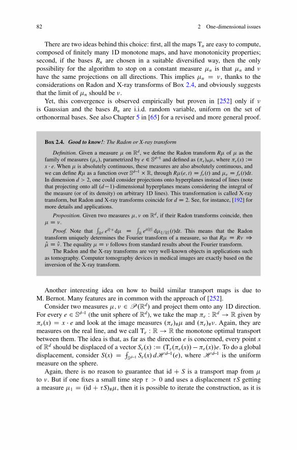
82 2 One-dimensional issues

There are two ideas behind this choice: first, all the maps Tn are easy to compute,composed of finitely many 1D monotone maps, and have monotonicity properties;second, if the bases Bn are chosen in a suitable diversified way, then the onlypossibility for the algorithm to stop on a constant measure �n is that �n and �have the same projections on all directions. This implies �n D �, thanks to theconsiderations on Radon and X-ray transforms of Box 2.4, and obviously suggeststhat the limit of �n should be �.

Yet, this convergence is observed empirically but proven in [252] only if �is Gaussian and the bases Bn are i.i.d. random variable, uniform on the set oforthonormal bases. See also Chapter 5 in [65] for a revised and more general proof.

Box 2.4. Good to know!: The Radon or X-ray transform

Definition. Given a measure � on Rd , we define the Radon transform R� of � as the

family of measures .�e/, parametrized by e 2 Sd�1 and defined as .�e/#�, where �e.x/ WD

x � e. When � is absolutely continuous, these measures are also absolutely continuous, andwe can define R� as a function over Sd�1 � R, through R�.e; t/ D fe.t/ and �e D fe.t/dt.In dimension d > 2, one could consider projections onto hyperplanes instead of lines (notethat projecting onto all .d�1/-dimensional hyperplanes means considering the integral ofthe measure (or of its density) on arbitrary 1D lines). This transformation is called X-raytransform, but Radon and X-ray transforms coincide for d D 2. See, for instance, [192] formore details and applications.

Proposition. Given two measures �; � on Rd , if their Radon transforms coincide, then

� D �.

Proof. Note that´Rd ei��x d� D ´

Reitj�j d��=j�j.t/dt. This means that the Radon

transform uniquely determines the Fourier transform of a measure, so that R� D R� )O� D O�. The equality � D � follows from standard results about the Fourier transform.

The Radon and the X-ray transforms are very well-known objects in applications suchas tomography. Computer tomography devices in medical images are exactly based on theinversion of the X-ray transform.

Another interesting idea on how to build similar transport maps is due toM. Bernot. Many features are in common with the approach of [252].

Consider two measures �; � 2 P.Rd/ and project them onto any 1D direction.For every e 2 S

d�1 (the unit sphere of Rd), we take the map �e W Rd ! R given by�e.x/ D x � e and look at the image measures .�e/#� and .�e/#�. Again, they aremeasures on the real line, and we call Te W R ! R the monotone optimal transportbetween them. The idea is that, as far as the direction e is concerned, every point xof Rd should be displaced of a vector Se.x/ WD .Te.�e.x//��e.x//e. To do a globaldisplacement, consider S.x/ D ffl

Sd�1 Se.x/ dH d�1.e/, where H d�1 is the uniformmeasure on the sphere.

Again, there is no reason to guarantee that id C S is a transport map from �

to �. But if one fixes a small time step � > 0 and uses a displacement �S gettinga measure �1 D .id C �S/#�, then it is possible to iterate the construction, as it is

2.5 Discussion 83

Fig. 2.5 Optimal transport between a finite number of points on an annulus and on a duck.Colors represent the assignment of points in the annulus to points on the duck. Middle, 1D-slicedassignment; right, optimal map for the quadratic cost. The two results are very similar (but one canfind few points with different colors, which means a slightly different assignment). Picture takenfrom [256] with permission

done in [252]. Only the definition of the transport map Tn is different. Again, oneexpects the sequence of measures �n that are built in this way to converge to �,but the problem is not really solved. From the empirical point of view, the transportmaps that are obtained in this way are quite satisfactory and have been tested inparticular in the discrete case (a finite number of Dirac masses with equal mass, i.e.,the so-called assignment problem). An example is given in Figure 2.5, where thereis a comparison between the optimal transport obtained via linear programmingmethods (see Section 6.4.1) and the assignment obtained via these 1D-sliced ideasby M. Bernot.

Moreover, we will see in Section 5.5 that one can also build an interestingdistance on the set of probabilities with this kind of idea (taking the average of adistance defined direction by direction: it will be much easier to compute than thecorresponding multidimensional distance). In Section 8.4 we will also show that theiterative algorithm above corresponds indeed to a gradient flow evolution.

2.5.3 Isoperimetric inequality via Knothe or Brenier maps

For the last discussion section of this chapter, we review one of the most spectacularapplications of optimal transport, i.e., its role in geometric inequalities. We will seehere how the isoperimetric inequality can be proven either by using the optimal(Brenier) map or even the Knothe map.

It is interesting to learn that it was indeed one of the first motivations for theuse of Knothe transport to deal with geometric inequalities (see [203]). However,the short proof of the isoperimetric inequality that we see here was first found byGromov (see the appendix in [236]), while the original goal of Knothe in [203] wasto establish other inequalities concerning convex sets.

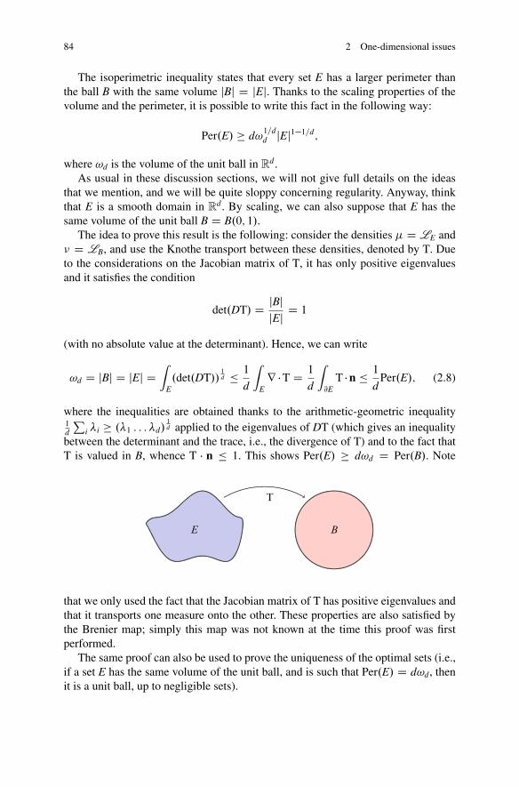
84 2 One-dimensional issues

The isoperimetric inequality states that every set E has a larger perimeter thanthe ball B with the same volume jBj D jEj. Thanks to the scaling properties of thevolume and the perimeter, it is possible to write this fact in the following way:

Per.E/ � d!1=dd jEj1�1=d;

where !d is the volume of the unit ball in Rd.

As usual in these discussion sections, we will not give full details on the ideasthat we mention, and we will be quite sloppy concerning regularity. Anyway, thinkthat E is a smooth domain in R

d. By scaling, we can also suppose that E has thesame volume of the unit ball B D B.0; 1/.

The idea to prove this result is the following: consider the densities � D LE and� D LB, and use the Knothe transport between these densities, denoted by T. Dueto the considerations on the Jacobian matrix of T, it has only positive eigenvaluesand it satisfies the condition

det.DT/ D jBjjEj D 1

(with no absolute value at the determinant). Hence, we can write

!d D jBj D jEj Dˆ

E.det.DT//

1d � 1

d

ˆ

Er � T D 1

d

ˆ

@ET � n � 1

dPer.E/; (2.8)

where the inequalities are obtained thanks to the arithmetic-geometric inequality1d

Pi �i � .�1 : : : �d/

1d applied to the eigenvalues of DT (which gives an inequality

between the determinant and the trace, i.e., the divergence of T) and to the fact thatT is valued in B, whence T � n � 1. This shows Per.E/ � d!d D Per.B/. Note

E B

T

that we only used the fact that the Jacobian matrix of T has positive eigenvalues andthat it transports one measure onto the other. These properties are also satisfied bythe Brenier map; simply this map was not known at the time this proof was firstperformed.

The same proof can also be used to prove the uniqueness of the optimal sets (i.e.,if a set E has the same volume of the unit ball, and is such that Per.E/ D d!d, thenit is a unit ball, up to negligible sets).

2.5 Discussion 85

The use of the Brenier map strongly simplifies the study of the equalitycases. Suppose indeed to have equality in the above inequalities: this implies theequality .det.DT//

1d D .r � T/=d a.e., and from the cases of equality in the

arithmetic-geometric inequality, we get that the eigenvalues of DT should all beequal. Thanks to the condition on the determinant, they are equal to 1. If the matrixis known to be symmetric (which is the case for Brenier’s map, but not for Knothe’sone), then we get DT D I and T.x/ D x C x0. Since T would be a translation, thenwe conclude E D B, up to translations.

It is slightly harder for the Knothe transport, since DT is not symmetric. Yet, ifall the eigenvalues are 1, one deduces that Td (the last component) is a translation.If we suppose from the beginning that (up to a fixed translation) E and B share thesame barycenter, then this translation is the identity. This means .�d/#� D .�d/#�.This is not yet enough to get � D �, and hence E D B, unless one uses the factthat the Knothe transport is not isotropic (i.e., its definition depends on the choiceof the axes) and that the directions of the axes are arbitrary. Hence, if E is a setgiving equality in the isoperimetric inequality, then its projections onto any directioncoincide with those of the ball. This implies E � B and, by equality of the volumes,E D B (the argument may also be done through the measures and the notion ofRadon transform, since .�d/#� D .�d/#� for arbitrary direction of the dth axisimplies � D �).

We finish the section by stressing that if the isoperimetric inequality canobviously be proven in many other ways, one recent advanced refinement of it (i.e.,the quantitative version of the anisotropic perimetric inequality, where the definitionof perimeter is modified, and the optimal set is no more the ball but another convexset, unit ball of another norm) was only proven with the optimal exponent viaoptimal transport techniques (see [167] and [276] for a short review).

Chapter 3L1 and L1 theory

Chapter 1 gave, in the framework of the general theory of optimal transportationbased on duality methods, an existence result for the optimal transport map whenthe cost is of the form c.x; y/ D h.x � y/ and h is strictly convex. In particular usingc.x; y/ D jx � yjp, this applies to the minimization problems

min˚jjT � idjjLp.�/ W T#� D �

;

(expressed in Kantorovich terms as min˚jjy � xjjLp.�/ W � 2 ˘.�; �/), for p 2

�1;C1Œ. We look in this chapter at the two limit cases p D 1 and p D 1, whichrequire additional techniques.

Then, the discussion section will go into two different directions: on the onehand, the L1 and L1 cases introduced and motivated the study of convex costswhich could be non-strictly convex or infinite valued somewhere, and the lastdevelopments on this topic will be debated in Section 3.3.1; on the other hand,one could wonder what is the situation for 0 < p < 1 and more generally for costswhich are concave increasing functions of the distance, which will be the subject ofSection 3.3.2.

3.1 The Monge case, with cost jx � yj

This section will prove that, if �; � 2 P.˝/, where ˝ � Rd is a compact domain,

and � � L d, then there exists an optimal transport map T for the cost jx � yj (theEuclidean distance in R

d). The proof that we present is essentially due to Ambrosio[8], as a modification from that of Sudakov, [290]. In the introduction, we gavereferences for the other alternative proofs of the existence in this.

© Springer International Publishing Switzerland 2015F. Santambrogio, Optimal Transport for Applied Mathematicians,Progress in Nonlinear Differential Equations and Their Applications 87,DOI 10.1007/978-3-319-20828-2_3

87

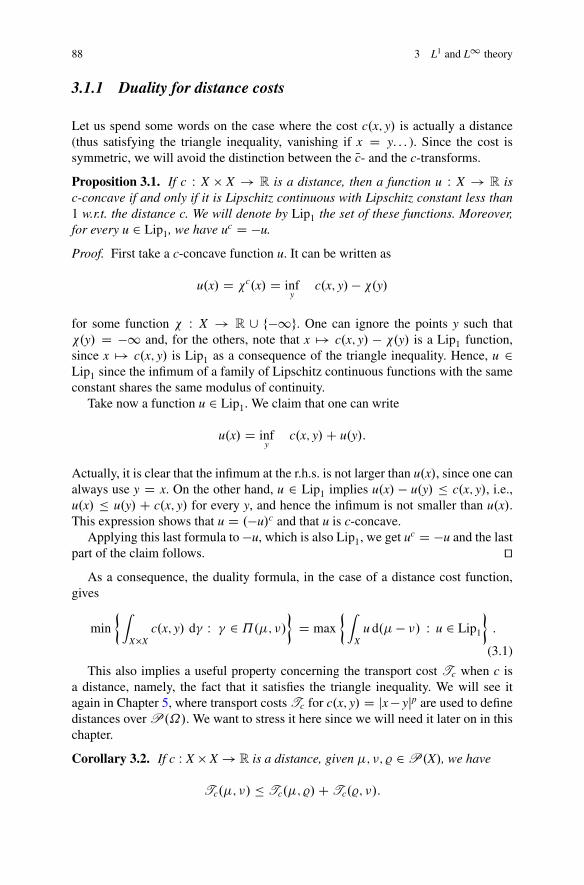
88 3 L1 and L1 theory

3.1.1 Duality for distance costs

Let us spend some words on the case where the cost c.x; y/ is actually a distance(thus satisfying the triangle inequality, vanishing if x D y. . . ). Since the cost issymmetric, we will avoid the distinction between the Nc- and the c-transforms.

Proposition 3.1. If c W X � X ! R is a distance, then a function u W X ! R isc-concave if and only if it is Lipschitz continuous with Lipschitz constant less than1 w.r.t. the distance c. We will denote by Lip1 the set of these functions. Moreover,for every u 2 Lip1, we have uc D �u.

Proof. First take a c-concave function u. It can be written as

u.x/ D c.x/ D infy

c.x; y/ � .y/

for some function W X ! R [ f�1g. One can ignore the points y such that.y/ D �1 and, for the others, note that x 7! c.x; y/ � .y/ is a Lip1 function,since x 7! c.x; y/ is Lip1 as a consequence of the triangle inequality. Hence, u 2Lip1 since the infimum of a family of Lipschitz continuous functions with the sameconstant shares the same modulus of continuity.

Take now a function u 2 Lip1. We claim that one can write

u.x/ D infy

c.x; y/C u.y/:

Actually, it is clear that the infimum at the r.h.s. is not larger than u.x/, since one canalways use y D x. On the other hand, u 2 Lip1 implies u.x/ � u.y/ � c.x; y/, i.e.,u.x/ � u.y/ C c.x; y/ for every y, and hence the infimum is not smaller than u.x/.This expression shows that u D .�u/c and that u is c-concave.

Applying this last formula to �u, which is also Lip1, we get uc D �u and the lastpart of the claim follows. ut

As a consequence, the duality formula, in the case of a distance cost function,gives

min

�ˆX�X

c.x; y/ d� W � 2 ˘.�; �/�

D max

�ˆX

u d.� � �/ W u 2 Lip1

�:

(3.1)

This also implies a useful property concerning the transport cost Tc when c isa distance, namely, the fact that it satisfies the triangle inequality. We will see itagain in Chapter 5, where transport costs Tc for c.x; y/ D jx � yjp are used to definedistances over P.˝/. We want to stress it here since we will need it later on in thischapter.

Corollary 3.2. If c W X � X ! R is a distance, given �; �; % 2 P.X/, we have

Tc.�; �/ � Tc.�; %/C Tc.%; �/:

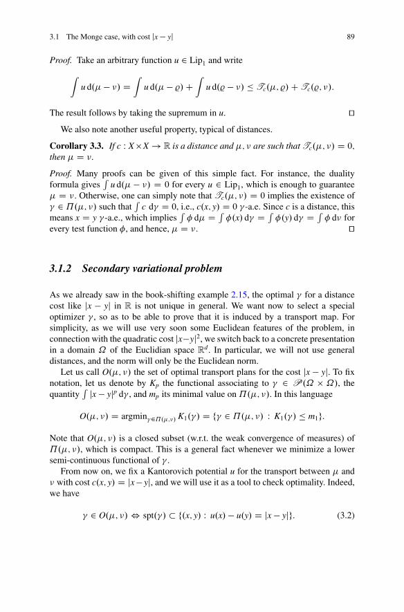
3.1 The Monge case, with cost jx � yj 89

Proof. Take an arbitrary function u 2 Lip1 and write

ˆu d.� � �/ D

ˆu d.� � %/C

ˆu d.% � �/ � Tc.�; %/C Tc.%; �/:

The result follows by taking the supremum in u. utWe also note another useful property, typical of distances.

Corollary 3.3. If c W X �X ! R is a distance and �; � are such that Tc.�; �/ D 0;

then � D �.

Proof. Many proofs can be given of this simple fact. For instance, the dualityformula gives

´u d.� � �/ D 0 for every u 2 Lip1, which is enough to guarantee

� D �. Otherwise, one can simply note that Tc.�; �/ D 0 implies the existence of� 2 ˘.�; �/ such that

´c d� D 0, i.e., c.x; y/ D 0 � -a.e. Since c is a distance, this

means x D y � -a.e., which implies´� d� D ´

�.x/ d� D ´�.y/ d� D ´

� d� forevery test function �, and hence, � D �. ut

3.1.2 Secondary variational problem

As we already saw in the book-shifting example 2.15, the optimal � for a distancecost like jx � yj in R is not unique in general. We want now to select a specialoptimizer � , so as to be able to prove that it is induced by a transport map. Forsimplicity, as we will use very soon some Euclidean features of the problem, inconnection with the quadratic cost jx�yj2, we switch back to a concrete presentationin a domain ˝ of the Euclidian space R

d. In particular, we will not use generaldistances, and the norm will only be the Euclidean norm.

Let us call O.�; �/ the set of optimal transport plans for the cost jx � yj. To fixnotation, let us denote by Kp the functional associating to � 2 P.˝ � ˝/, thequantity

´ jx � yjp d� , and mp its minimal value on ˘.�; �/. In this language

O.�; �/ D argmin�2˘.�;�/ K1.�/ D f� 2 ˘.�; �/ W K1.�/ � m1g:

Note that O.�; �/ is a closed subset (w.r.t. the weak convergence of measures) of˘.�; �/, which is compact. This is a general fact whenever we minimize a lowersemi-continuous functional of � .

From now on, we fix a Kantorovich potential u for the transport between � and� with cost c.x; y/ D jx � yj, and we will use it as a tool to check optimality. Indeed,we have

� 2 O.�; �/ , spt.�/ � f.x; y/ W u.x/ � u.y/ D jx � yjg: (3.2)

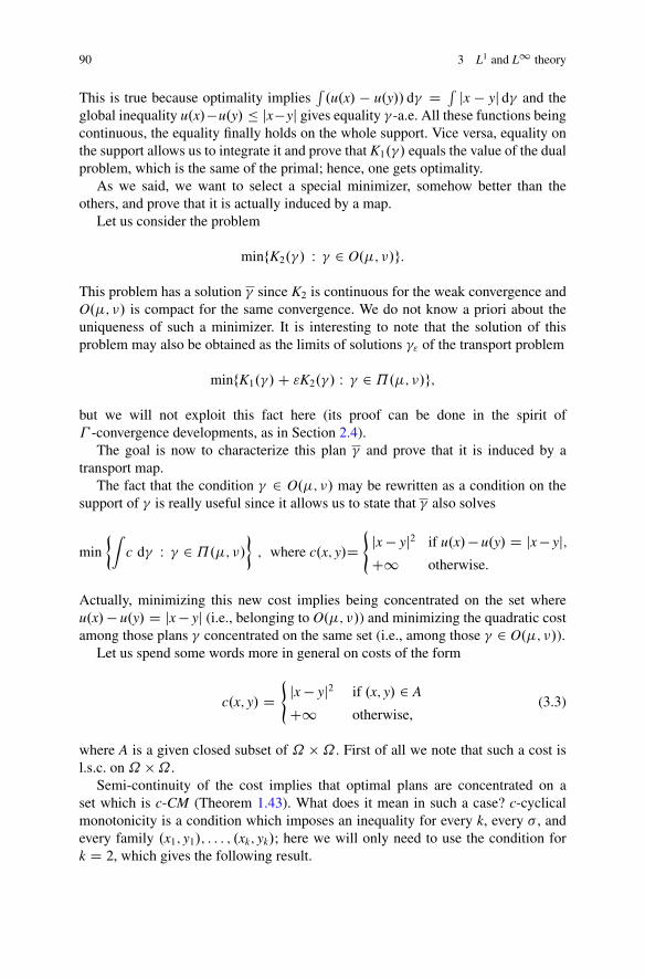
90 3 L1 and L1 theory

This is true because optimality implies´.u.x/ � u.y// d� D ´ jx � yj d� and the

global inequality u.x/�u.y/ � jx�yj gives equality � -a.e. All these functions beingcontinuous, the equality finally holds on the whole support. Vice versa, equality onthe support allows us to integrate it and prove that K1.�/ equals the value of the dualproblem, which is the same of the primal; hence, one gets optimality.

As we said, we want to select a special minimizer, somehow better than theothers, and prove that it is actually induced by a map.

Let us consider the problem

minfK2.�/ W � 2 O.�; �/g:

This problem has a solution � since K2 is continuous for the weak convergence andO.�; �/ is compact for the same convergence. We do not know a priori about theuniqueness of such a minimizer. It is interesting to note that the solution of thisproblem may also be obtained as the limits of solutions �" of the transport problem

minfK1.�/C "K2.�/ W � 2 ˘.�; �/g;

but we will not exploit this fact here (its proof can be done in the spirit of� -convergence developments, as in Section 2.4).

The goal is now to characterize this plan � and prove that it is induced by atransport map.

The fact that the condition � 2 O.�; �/ may be rewritten as a condition on thesupport of � is really useful since it allows us to state that � also solves

min

�ˆc d� W � 2 ˘.�; �/

�; where c.x; y/D

(jx � yj2 if u.x/� u.y/ D jx � yj;C1 otherwise.

Actually, minimizing this new cost implies being concentrated on the set whereu.x/� u.y/ D jx � yj (i.e., belonging to O.�; �/) and minimizing the quadratic costamong those plans � concentrated on the same set (i.e., among those � 2 O.�; �/).

Let us spend some words more in general on costs of the form

c.x; y/ D(

jx � yj2 if .x; y/ 2 A

C1 otherwise,(3.3)

where A is a given closed subset of ˝ � ˝. First of all we note that such a cost isl.s.c. on ˝ �˝.

Semi-continuity of the cost implies that optimal plans are concentrated on aset which is c-CM (Theorem 1.43). What does it mean in such a case? c-cyclicalmonotonicity is a condition which imposes an inequality for every k, every � , andevery family .x1; y1/; : : : ; .xk; yk/; here we will only need to use the condition fork D 2, which gives the following result.

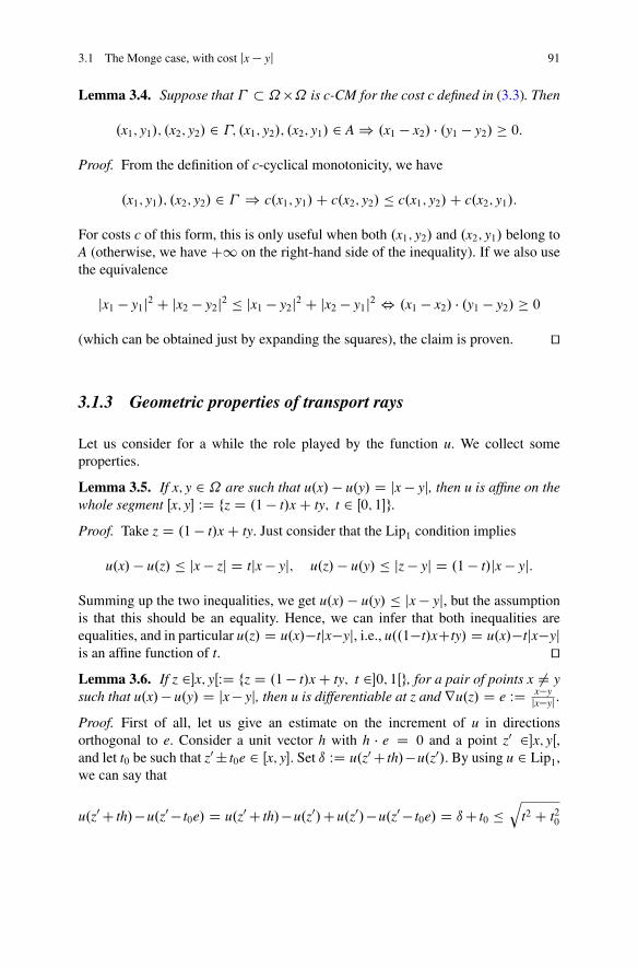
3.1 The Monge case, with cost jx � yj 91

Lemma 3.4. Suppose that � � ˝�˝ is c-CM for the cost c defined in (3.3). Then

.x1; y1/; .x2; y2/ 2 �; .x1; y2/; .x2; y1/ 2 A ) .x1 � x2/ � .y1 � y2/ � 0:

Proof. From the definition of c-cyclical monotonicity, we have

.x1; y1/; .x2; y2/ 2 � ) c.x1; y1/C c.x2; y2/ � c.x1; y2/C c.x2; y1/:

For costs c of this form, this is only useful when both .x1; y2/ and .x2; y1/ belong toA (otherwise, we have C1 on the right-hand side of the inequality). If we also usethe equivalence

jx1 � y1j2 C jx2 � y2j2 � jx1 � y2j2 C jx2 � y1j2 , .x1 � x2/ � .y1 � y2/ � 0

(which can be obtained just by expanding the squares), the claim is proven. ut

3.1.3 Geometric properties of transport rays

Let us consider for a while the role played by the function u. We collect someproperties.

Lemma 3.5. If x; y 2 ˝ are such that u.x/ � u.y/ D jx � yj, then u is affine on thewhole segment Œx; y� WD fz D .1 � t/x C ty; t 2 Œ0; 1�g.

Proof. Take z D .1 � t/x C ty. Just consider that the Lip1 condition implies

u.x/ � u.z/ � jx � zj D tjx � yj; u.z/ � u.y/ � jz � yj D .1 � t/jx � yj:

Summing up the two inequalities, we get u.x/ � u.y/ � jx � yj, but the assumptionis that this should be an equality. Hence, we can infer that both inequalities areequalities, and in particular u.z/ D u.x/�tjx�yj, i.e., u..1�t/xCty/ D u.x/�tjx�yjis an affine function of t. utLemma 3.6. If z 2�x; yŒWD fz D .1� t/x C ty; t 2�0; 1Œg, for a pair of points x ¤ ysuch that u.x/� u.y/ D jx � yj, then u is differentiable at z and ru.z/ D e WD x�y

jx�yj .

Proof. First of all, let us give an estimate on the increment of u in directionsorthogonal to e. Consider a unit vector h with h � e D 0 and a point z0 2�x; yŒ,and let t0 be such that z0 ˙ t0e 2 Œx; y�. Set ı WD u.z0 C th/�u.z0/. By using u 2 Lip1,we can say that

u.z0 C th/�u.z0 � t0e/ D u.z0 C th/�u.z0/Cu.z0/�u.z0 � t0e/ D ıC t0 �q

t2 C t20

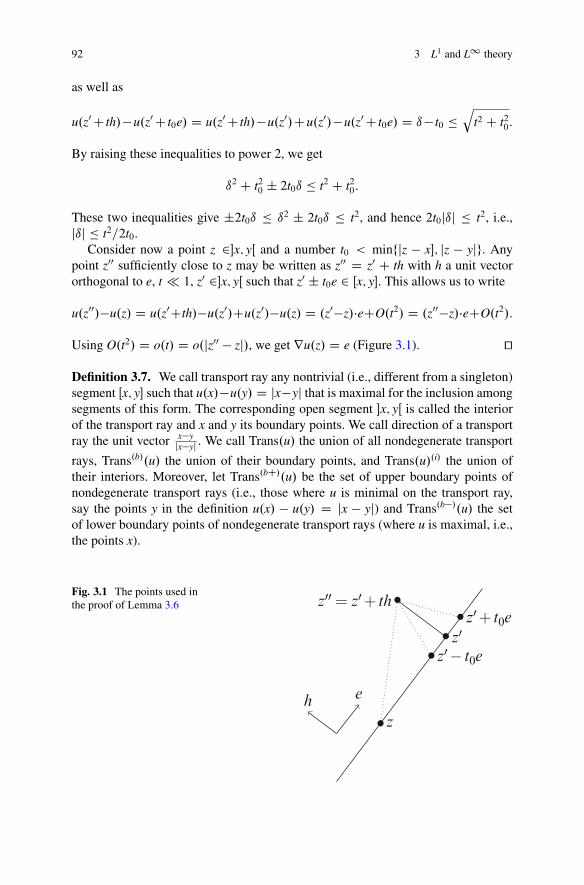
92 3 L1 and L1 theory

as well as

u.z0 C th/�u.z0 C t0e/ D u.z0 C th/�u.z0/Cu.z0/�u.z0 C t0e/ D ı� t0 �q

t2 C t20:

By raising these inequalities to power 2, we get

ı2 C t20 ˙ 2t0ı � t2 C t20:

These two inequalities give ˙2t0ı � ı2 ˙ 2t0ı � t2, and hence 2t0jıj � t2, i.e.,jıj � t2=2t0.

Consider now a point z 2�x; yŒ and a number t0 < minfjz � x�; jz � yjg. Anypoint z00 sufficiently close to z may be written as z00 D z0 C th with h a unit vectororthogonal to e, t � 1, z0 2�x; yŒ such that z0 ˙ t0e 2 Œx; y�. This allows us to write

u.z00/�u.z/ D u.z0Cth/�u.z0/Cu.z0/�u.z/ D .z0�z/�eCO.t2/ D .z00�z/�eCO.t2/:

Using O.t2/ D o.t/ D o.jz00 � zj/, we get ru.z/ D e (Figure 3.1). ut

Definition 3.7. We call transport ray any nontrivial (i.e., different from a singleton)segment Œx; y� such that u.x/�u.y/ D jx�yj that is maximal for the inclusion amongsegments of this form. The corresponding open segment �x; yŒ is called the interiorof the transport ray and x and y its boundary points. We call direction of a transportray the unit vector x�y

jx�yj . We call Trans.u/ the union of all nondegenerate transport

rays, Trans.b/.u/ the union of their boundary points, and Trans.u/.i/ the union oftheir interiors. Moreover, let Trans.bC/.u/ be the set of upper boundary points ofnondegenerate transport rays (i.e., those where u is minimal on the transport ray,say the points y in the definition u.x/ � u.y/ D jx � yj) and Trans.b�/.u/ the setof lower boundary points of nondegenerate transport rays (where u is maximal, i.e.,the points x).

Fig. 3.1 The points used inthe proof of Lemma 3.6

•z′•z′ − t0e

•z′+ t0e

•z

•z′′ = z′+ th

eh

3.1 The Monge case, with cost jx � yj 93

Corollary 3.8. Two different transport rays can only meet at a point z which is aboundary point for both of them, and in such a case, u is not differentiable at z. Inparticular, if one removes the negligible set Sing.u/ of non-differentiability points ofu, the transport rays are disjoint.

Proof. First of all, note that if a point z belongs to a transport ray with direction e,and u is differentiable at z, then necessarily we have e D ru.z/. Indeed, close toz, there are points of the form z C te which belong to the same transport ray, forarbitrarily small values of t (we do not care about the sign of t), and on these points,we can write

t D u.z C te/ � u.z/ D ru.z/ � te C o.t/:

This shows ru.z/ � e D 1. Together with jru.z/j � 1, the only possibility isru.z/D e.

Now, suppose that two transport rays meet at a point z which is internal for bothrays. In such a case, u must have two different gradients at z, following both thedirections of the rays, which is impossible (recall that the different rays meeting atone point must have different directions, since otherwise they are the same transportray, by maximality).

Suppose that they meet at z, which is in the interior of a transport ray withdirection e but is a boundary point for another ray, with direction e0 ¤ e. In sucha case, u should be differentiable at z, and again, ru.z/ should take two distinctvalues, which is impossible.

Finally, suppose that the intersection point z is a boundary point for bothsegments, one with direction e and the other one with direction e0 ¤ e. In thiscase, there is no contradiction if u is not differentiable at z. On the other hand, if onesupposes that u is differentiable at z, then we get ru.z/ D e D e0, which is, again, acontradiction. ut

We will see later on that we need to say something more on the direction of thetransport rays.

From this section on, we fix a transport plan � , optimal for the secondaryvariational problem, and we will try to prove that it is actually induced by a transportmap. We use here that � is actually concentrated on a set � which is c-CM (werecall that we are using the cost c defined as in (3.3)) and see how this interacts withtransport rays. We can suppose � � A D f.x; y/ W u.x/ � u.y/ D jx � yjg, sinceanyway � must be concentrated on such a set, so as to have a finite value for

´c d� .

We want to say that � behaves, on each transport ray, as the monotone increasingtransport. More precisely, the following is true.

Lemma 3.9. Suppose that x1; x2; y1, and y2 are all points of a transport ray Œx; y�and that .x1; y1/; .x2; y2/ 2 � . Define an order relation on such a transport raythrough x � x0 , u.x/ � u.x0/. Then if x1 < x2, we also have y1 � y2.

94 3 L1 and L1 theory

Proof. We already know that x1 � y1 and x2 � y2 (thanks to � � A). Hence,the only case to be considered is the case where we have x1 < x2 � y2 < y1.If we prove that this is not possible, then we have proven the claim. And this isnot possible due to the fact that � is c-CM, since on this transport ray, due to theorder relationship we have supposed and to the behavior of u on such a segment, thecondition .x1; y2/; .x2; y1/ 2 A is guaranteed. This implies .x1 � x2/ � .y1 � y2/ � 0.But this is the scalar product of two vectors parallel to e, and on the segment, thissimply means that y1 and y2 must be ordered exactly as x1 and x2 are. ut

From what we have seen in Chapter 2, we know that when s is a segment and� 0 � s � s is such that

.x1; y1/; .x2; y2/ 2 � 0; x1 < x2 ) y1 � y2

(for the order relation on s), then � 0 is contained in the graph of a monotoneincreasing multivalued function, which associates to every point either a point ora segment. Yet, the interiors of these segments being disjoint, there is at most acountable number of points where the image is not a singleton (see the proof ofLemma 2.8). This means that � 0 is contained in a graph over s, up to a countablenumber of points of s. We will apply this idea to � 0 D � \ .s � s/, where s is atransport ray.

If we combine what we obtained on every transport ray, we obtain:

Proposition 3.10. The optimal transport plan � is concentrated on a set � with thefollowing properties:

• if .x; y/ 2 � , then

– either x 2 Sing.u/ (but this set of points is Lebesgue-negligible),– or x … Trans.u/, i.e., it does not belong to a nondegenerate transport ray

(and in this case, we necessarily have y D x, since otherwise, Œx; y� wouldbe contained in a nondegenerate transport ray),

– or x 2 Trans.bC/.u/ n Sing.u/ (and in this case, we necessarily have y D x,since x is contained in a unique transport ray s and it cannot have otherimages y 2 s, due to the order relation x � y),

– or x 2 Trans.u/ n .Trans.bC/.u/ [ Sing.u// and y belongs to the sametransport ray s of x (which is unique);

• on each transport ray s, � \ .s � s/ is contained in the graph of a monotoneincreasing multivalued function;

• on each transport ray s, the set

Ns D fx 2 s n Trans.bC/.u/ W #.fy W .x; y/ 2 � g/ > 1g

is countable.

It is clear that � is induced by a transport map if �.S

s Ns/ D 0, i.e., if we can getrid of a countable number of points on every transport ray.

3.1 The Monge case, with cost jx � yj 95

This could also be expressed in terms of disintegration of measures (if � isabsolutely continuous, then all the measures �s given by the disintegrations of� along the rays s are atomless; see Box 2.2 in Section 2.3 for the notion ofdisintegration), but we will try to avoid such an argument for the sake of simplicity.The only point that we need is the following ( Property N, for negligibility).

Definition 3.11. We say that Property N holds for a given Kantorovich potential uif B � ˝ is such that

• B � Trans.u/ n Trans.bC/.u/,• B \ s is at most countable for every transport ray s,

then jBj D 0.

This property is not always satisfied by any disjoint family of segments in Rd, and

there is an example (by Alberti, Kirchheim, and Preiss, later improved by Ambrosio,Kirchheim and Pratelli; see [14]) where a disjoint family of segments contained in acube is such that the collection of their middle points has positive measure. We willprove that the direction of the transport rays satisfies additional properties, whichguarantee property N.

Please be aware that, as usual, we are ignoring here measurability issues ofthe transport map T that we are constructing: this map is obtained by gluing themonotone maps on every segment, but this should be done in a measurable way1.

It appears that the main tool to prove Property N is the Lipschitz regularity of thedirections of the transport rays (which is the same as the direction of ru).

Theorem 3.12. Property N holds if ru is Lipschitz continuous or if there exists acountable family of sets Eh such that ru is Lipschitz continuous when restricted toeach Eh and jTrans.u/ � nSh Ehj D 0.

Proof. First, suppose that ru is Lipschitz. Consider all the hyperplanes parallel tod�1 coordinate axes and with rational coordinates on the last coordinate. Considera set B in the definition of Property N. By definition, the points of B belong tonondegenerate transport rays, i.e., to segments with positive length. Hence, everypoint of B belongs to a transport ray that meets at least one of the above hyperplanesat exactly one point of its interior. Since these hyperplanes are a countable quantity,up to countable unions, we can suppose that B is included in a collection SY oftransport rays all meeting the same hyperplane Y . Moreover, we can also supposethat B does not contain any point which is a boundary point of two different transportrays, since we already know that those points are negligible. Now, let us fix such ahyperplane Y and let us consider a map f W Y � R ! R

d of the following form: fory 2 Y and t 2 R the point f .y; t/ is defined as y C tru.y/. This map is well definedand injective on a set A � Y � R which is the one we are interested in. This set A is

1Measurability could be proven, either by restricting to a �-compact set � or by considering thedisintegrations �s and �s and using the fact that, on each s, T is the monotone map sending �s

onto �s (and hence it inherits some measurability properties of the dependence of �s and �s w.r.t.s, which are guaranteed by abstract disintegration theorems).

96 3 L1 and L1 theory

B′ = f−1(B)⊂ A

Y

•

•

•••

•• •(y,0)

(y,t) f

Y

•

•

•••

••

B

•y

y+ t∇u(y)

Fig. 3.2 The map f in Theorem 3.12. The points of B and B0 are only a countable number on eachline and represented by bullets

defined as those pairs .y; t/ where y is in the interior of a transport ray of SY ; hence,u is differentiable at such a point, and y C tru.y/ belongs to the interior of the sametransport ray. The map f is injective, since getting the same point as the image of.y; t/ and of .y0; t0/would mean that two different transport rays cross at such a point.B is contained in the image of f by construction, so that f is a bijection between Band B0 WD f �1.B/. The map f is also Lipschitz continuous, as a consequence ofthe Lipschitz behavior of ru. Note that B0 is a subset of Y � R containing at mostcountably many points on every line fyg � R. By Fubini’s theorem, this impliesjB0j D 0. Then we have also jBj D jf .B0/j � Lip.f /djB0j, which implies jBj D 0.

It is clear that the property is also true when ru is not Lipschitz but is Lipschitzcontinuous on each set Eh of a partition covering almost all the points of Trans.u/,since one can apply the same kind of arguments to all the sets B \ Eh and then usecountable unions (Figure 3.2). ut

We now need to prove that ru is countably Lipschitz.

Definition 3.13. A function f W ˝ ! Rd is said to be countably Lipschitz if there

exists a countable family of sets Eh such that f is Lipschitz continuous on each Eh

and j˝ nSh Ehj D 0.

Note that “being Lipschitz continuous on a set E” or “being the restriction to Eof a Lipschitz continuous function defined on the whole R

d” is actually the sameproperty, due to Lipschitz extension theorems. Indeed, whenever E � X are metricspaces, every L-Lipschitz function f W E ! R can be extended to an L-Lipschitzfunction over X. This is known as Kirszbraun theorem and can be easily obtainedby using the functions fk of the Memo Box 1.5, for k � L.

We want to prove that ru is countably Lipschitz. We will first prove thatu coincides with some �-convex or �-concave functions on a sequence of setscovering almost everything. This requires a definition.

Definition 3.14. A function f W ˝ ! R is said to be �-convex if x 7! f .x/� �2jxj2 is

convex and �-concave if x 7! f .x/C �2jxj2 is concave. Note that the number � is not

required to be positive, so that �-convex functions for � > 0 are strictly convex, and,

3.1 The Monge case, with cost jx � yj 97

for � < 0, they just have second derivatives (where they exist) which are boundedfrom below. Functions which are �-convex (or �-concave) for some values of � arecalled semi-convex (or semi-concave).

Proposition 3.15. There exist some sets Eh such that

•S

h Eh D Trans.u/ n Trans.u/.bC/,• on each set Eh the function u is the restriction of a �-concave function, for a

value � depending on h.

Proof. Let us define

Eh D�

x 2 Trans.u/ W 9z 2 Trans.u/ with u.x/ � u.z/ D jx � zj > 1

h

�;

which is roughly speaking made of those points in the transport rays that are at leastat a distance 1

h apart from the upper boundary point of the ray. It is clear that Eh �Trans.u/nTrans.u/.bC/. Moreover, we easily have

Sh Eh D Trans.u/nTrans.bC/.u/.

Let us fix a function ch W Rd ! R with the following properties: ch 2 C2.Rd/,jrchj � 1, ch.z/ � jzj for all z 2 R

d, ch.z/ D jzj for all z … B.0; 1=h/. Set�h WD �jjD2chjjL1 (note that we can take this value to be of the order of � 1

h ). It iseasy to check that, if x 2 Eh, one has

u.x/ D infy2Rd

jx � yj C u.y/ � infy2Rd

ch.x � y/C u.y/ � infy…B.x;1=h/

jx � yj C u.y/ D u.x/;

where the first inequality is a consequence of jzj � ch.z/ and the second is due tothe restriction to y … B.x; 1=h/. The last equality is justified by the definition of Eh.This implies that all the inequalities are actually equalities and that u.x/ D uh.x/ forall x 2 Eh, where

uh.x/ WD infy2Rd

ch.x � y/C u.y/:

It is important to note that uh is a �h-concave function.Let us justify that uh is �h-concave. With this choice of �h, ch is obviously �h-

concave. Consider

uh.x/C �h

2jxj2 D inf

y2Rdch.x � y/C �h

22jxj2 C u.y/

D infy2Rd

ch.x � y/C �h

2jx � yj2 C �hx � y � �h

2jyj2 C u.y/:

This last expression shows that uh.x/C �h2

jxj2 is concave in x, since it is expressedas an infimum of concave functions (ch.x � y/ C �h

2jx � yj2 is concave, �hx � y is

linear, and the other terms are constant in x). Hence, uh.x/ is �h-concave. utThe previous theorem allows us to replace the function u with the functions uh,

which are more regular (since they are �-concave, they share the same regularity of

98 3 L1 and L1 theory

convex functions). Unfortunately, this is not enough yet, since convex functions ingeneral are not even differentiable. A new countable decomposition is needed andcan be obtained from the following theorem that we do not prove.

Theorem 3.16. If f is a convex function, then rf is countably Lipschitz.

The proof of this theorem may be found in [13], in Theorem 5.34. It is also truewhen we replace rf with an arbitrary BV function, and this is the framework thatone finds in [13].

Box 3.1. Memo: BV functions in Rd

On a domain ˝ � Rd , an L1 function f W ˝ ! R is said to be a BV function if its

distributional derivatives are finite measures. This means that we require

ˆ

˝

f .r � �/ dx � Cjj�jjL1 ;

for every C1c vector field � W ˝ ! R

d . The space BV is hence a wider class than theSobolev spaces W1;p, where the distributional derivatives are supposed to belong to Lp (i.e.,they are absolutely continuous measures with integrability properties).

It happens that the distributional derivative rf cannot be any measure, but must be ofthe form rf D raf .x/ dx C Dsf C Djf , where raf .x/ dx is the absolutely continuous partof rf (with respect to the Lebesgue measure), Djf is the so-called jump part and has adensity with respect to H d�1 (it is concentrated on the set Jf of those points where thereis an hyperplane such that the function f has two different limits on the two sides of thehyperplane, in a suitable measure-theoretical sense, and the density of Dju with respect toH d�1

jJfis exactly the difference of these two limit values times the direction of the normal

vector to the hyperplane: Djf D .f C � f �/nJf �H d�1jJf

), and Dc is the so-called Cantor part,which is singular to the Lebesgue measure but vanishes on any .d�1/-dimensional set.

We denote by BVloc.Rd/ the space of functions which are locally BV in the sense that

their derivatives are Radon measures, i.e., measures which are locally finite (in the definitionwith test functions � , we use � 2 C1

c .Rd/ and the constant C may depend on the support of

�). Vector-valued BV functions are just defined as functions f D .f1; : : : ; fk/ W Rd ! Rk

which are componentwise BV, i.e., fi 2 BV for each i D 1; : : : ; k. It is interesting thatgradients g D rf of convex functions are always locally BV. This depends on the factthat the Jacobian matrix of the gradient of a convex function is indeed the Hessian ofsuch a function and is positive definite. This means that the matrix-valued distributionr.rf / D D2f is a positive distribution, and we know that positive distributions arenecessarily positive measures (warning: this requires precise definitions when we work withmatrix- and vector-valued functions).

BV functions satisfy several fine regularity properties almost everywhere for theLebesgue or the H d�1-measure, and the reader may refer to [13] or [160]. In particular,we cite the following (not at all easy) result, which implies Theorem 3.16.

Theorem. If f 2 BVloc.Rd/, then f is countably Lipschitz.

As a consequence of Proposition 3.15 and Theorem 3.16 one has:

Proposition 3.17. If u is a Kantorovich potential, then ru W Trans.u/ ! Rd is

countably Lipschitz.

3.1 The Monge case, with cost jx � yj 99

Proof. It is clear that the countably Lipschitz regularity of Theorem 3.16 is also truefor the gradients of �-convex and �-concave functions. This means that this is truefor ruh and, by countable union, for ru. ut

3.1.4 Existence and nonexistence of an optimal transport map

From the analysis performed in the previous sections, we obtain the following result,essentially taken from [10, 14, 44].

Theorem 3.18. Under the usual assumption � � L d, the secondary variationalproblem admits a unique solution � , which is induced by a transport map T,monotone nondecreasing on every transport ray.

Proof. Proposition 3.17, together with Theorem 3.12, guarantees that Property Nholds. Hence, Proposition 3.10 may be applied to get � D �T. The uniquenessfollows in the usual way: if two plans � 0 D �T0 and � 00 D �T00 optimize the secondaryvariational problem, the same should be true for 1

2�T0 C 1

2�T00 . Yet, for this measure

to be induced by a map, it is necessary to have T0 D T00 a.e. (see Remark 1.19). utDefinition 3.19. The optimal transport plan � will be called ray-monotone trans-port plan and the transport map which corresponds to it ray-monotone transportmap.

Note that as a by-product of this analysis, we also obtain jTrans.u/.b/j D 0,since Trans.u/.b/ is a set meeting every transport ray in two points, and it is hencenegligible by Property N. Yet we could not have proven it before, so unfortunatelyevery strategy based on a decomposition of Trans.u/.i/ is not complete.

To complete this section, one could wonder whether the assumption � � L d isreally necessary for this existence result: would the condition “�.A/ D 0 for every.d�1/-rectifiable set A” (or other conditions as in Section 1.3.1) be enough for theexistence of an optimal map, as it happened for the quadratic case?

The answer is not, as it is shown in the following example.

Transport from a graph to a square

Consider a continuous function B W Œ0; 1� ! R with the following property: forevery Lipschitz function f W R ! R, the sets ft 2 Œ0; 1� W B.t/ D f .t/g and ft 2Œ0; 1� W f .B.t// D tg are Lebesgue negligible. Then take � D .id;B/#.L 1 Œ0; 1�/

and � D L 2 Q, where Q is the square Œ0; 1� � ŒL;L C 1� with L D jjBjjL1 .In practice, � is concentrated on the graph of B and � on a square above the

graph. With this choice, the measure� gives zero mass to any rectifiable curve of theform f.t; f .t//g or f.f .s/; s/g, for f Lipschitz. On the other hand, it is not absolutelycontinuous, as it gives positive mass to a graph, which is L 2-negligible. The goal isnow to prove that no optimal transport map exists from � to � (Figure 3.3).

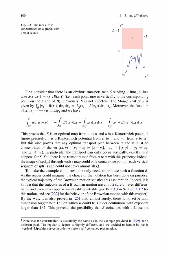
100 3 L1 and L1 theory

Fig. 3.3 The measure �concentrated on a graph, with� on a square

ν

m

B

L

L+1

x1

x2

Q

First consider that there is an obvious transport map S sending � into �. Justtake S.x1; x2/ D .x1;B.x1// (i.e., each point moves vertically to the correspondingpoint on the graph of B). Obviously, S is not injective. The Monge cost of S isgiven by

´Q jx2 � B.x1/j dx1 dx2 D ´

Q.x2 � B.x1// dx1 dx2. Moreover, the functionu.x1; x2/ D �x2 is in Lip1 and we have

ˆ

R2

u d.� � �/ D �ˆ 1

0

B.x1/ dx1 Cˆ

Qx2 dx1 dx2 D

ˆ

Qjx2 � B.x1/j dx1 dx2:

This proves that S is an optimal map from � to � and u is a Kantorovich potential(more precisely: u is a Kantorovich potential from � to � and �u from � to �).But this also proves that any optimal transport plan between � and � must beconcentrated on the set f.x; y/ W y2 � x2 D jx � yjg, i.e., on f.x; y/ W y1 D x1;and x2 � y2g. In particular the transport can only occur vertically, exactly as it

happens for S. Yet, there is no transport map from � to � with this property: indeed,the image of spt.�/ through such a map could only contain one point in each verticalsegment of spt.�/ and could not cover almost all Q.

To make the example complete2, one only needs to produce such a function B.As the reader could imagine, the choice of the notation has been done on purpose:the typical trajectory of the Brownian motion satisfies this assumption. Indeed, it isknown that the trajectories of a Brownian motion are almost surely never differen-tiable and even never approximately differentiable (see Box 3.3 in Section 3.3.2 forthis notion, and see [222] for the behavior of the Brownian motion with this respect).By the way, it is also proven in [25] that, almost surely, there is no set A withdimension bigger than 1=2 on which B could be Hölder continuous with exponentlarger than 1=2. This prevents the possibility that B coincides with a Lipschitz

2 Note that the construction is essentially the same as in the example provided in [199], for adifferent goal. The regularity degree is slightly different, and we decided to handle by hands“vertical” Lipschitz curves in order to make a self-contained presentation.

3.1 The Monge case, with cost jx � yj 101

function on a 1-dimensional set. We can even say that ft 2 Œ0; 1� W B.t/ D f .t/g hasdimension less or equal than 1=2.

For the other set (i.e., the points where t D f .B.t//), it is trickier. We can assume,by contradiction, that there exists a compact set K with jKj > 0 and f ı B D idon K. Hence, the set H D B.K/ is also compact and must have positive measure.Otherwise, if jHj D 0, K � f .H/ would be negligible too, because f is Lipschitz.We can assume that f is C1, if we restrict H. Indeed, for every Lipschitz function fand every n, there is a C1 function Qfn with jff ¤ Qfngj < 1

n (see [160] for this fact).If we set Hn D ff D Qfng, we have jH n Sn Hnj D 0 and jf .H n Sn Hn/j D 0;this proves jf .Sn Hn/j D jSn f .Hn/j > 0, and at least for some n, we must havejHnj; jf .Hn/j > 0. Hence, we can suppose f 2 C1. Now, there are two possibilities:either f 0 D 0 on H or there is a small interval where f is a diffeomorphism. In thissecond case, we find B D f �1 on a set of positive measure, which is a contradictionwith the well-known properties of Brownian motions (since f �1 is Lipschitz, andeven C1). On the contrary, if f 0 D 0 on H, then the area formula provides jKj D 0,which is also a contradiction.

3.1.5 Approximation issues for the ray-monotoneoptimal transport

The present section deals with some natural questions concerning the ray-monotoneoptimal transport plan � , and in particular approximation questions. Indeed, we haveseen (Theorem 1.50) that for any weakly converging sequence �n * � , if �n isoptimal for a continuous cost between its marginal, then so is � . Yet, we knowthat for c.x; y/ D jx � yj, the optimal transport plan is not in general unique, andfor many applications, one prefers to stick to the ray-monotone one. Hence, thequestion is how to select this special transport plan by approximation, when themeasures and/or the cost varies.

For many applications (see in particular Chapter 4), it is interesting to approxi-mate transport plans through transport maps sending a given measure to an atomicone. This is because these kinds of transport maps are actually composed of differenthomotheties defined on a partition of the domain.

Here is a useful approximation lemma in the spirit of � -convergence develop-ments (see [77], Section 2.4, and Box 4.6 in Section 4.4.2).

For fixed measures �; � 2 P.˝/, with � � L d, consider the following familyof minimization problems .P"/:

.P"/ D min˚Tc..�y/#�; �/C "K1.�/C "2K2.�/C "3dC3#..�y/#�/ W

� 2 P.˝ �˝/; .�x/#� D �g ;

102 3 L1 and L1 theory

where Tc is the minimum value of the transport problem for the cost c.x; y/ D jx�yj,Kp.�/ D ´ jx � yjp�. dx; dy/ for p D 1; 2, and the symbol # denotes the cardinalityof the support of a measure. Note that K1.�/ ¤ Tc..�x/#�; .�y/#�/ in general.

Actually, the minimization of .P"/ consists in looking for a transport plan withfirst marginal equal to � satisfying the following criteria with decreasing degree ofimportance: the second marginal must be close to �; the K1 cost of transportationshould be small; the K2 as well; and, finally, the second marginal must be atomicwith not too many atoms.

This minimization problem has obviously at least a solution (by the directmethod, since˝ is compact). We denote by �" such a solution and �" WD .�y/#�" itssecond marginal. It is straightforward that �" is an atomic measure and that �" is the(unique, since � � L d) solution of minfK1.�/C "K2.�/ W � 2 ˘.�; �"/g, whichis an optimal transport problem from � to �" for the cost jx � yj C "jx � yj2. Set

� D argmin fK2.�/ W � is a K1-optimal transport plan from � to �g : (3.4)

This transport plan � is unique, and it is the unique ray-monotone optimal transportplan from � to � (this is a consequence of Section 3.1.4); note that the functional K2could have been replaced by any functional � 7! ´

h.x � y/ d� for a strictly convexfunction h.

Lemma 3.20. As " ! 0, we have �" * � and �" * � .

Proof. It is sufficient to prove that any possible limit of subsequences coincideswith � or �; respectively. Let �0 be one such a limit and �0 D .�y/#�0 the limit ofthe corresponding subsequence of �". Consider a regular grid Gn � ˝ composedof approximately Cnd points (take Gn D 1

nZd \ ˝), and let pn be any measurable

map from ˝ to Gn, with the property jpn.x/ � xj � 1=n (for instance, pn can be theprojection map, where it is well defined). Set �n WD .pn/#� and note #�n � Cnd, aswell as �n * � and Tc.�

n; �/ � 1n .

First step: �0 D �. Take �n any transport plan from � to �n. By optimality of �"we have

Tc.�"; �/ � Tc.�n; �/C "K1.�

n/C "2K2.�n/C C"3dC3nd:

Fix n, let " go to 0, and get

Tc.�0; �/ � Tc.�n; �/ � 1

n:

Then let n ! 1 and get Tc.�0; �/ D 0, which implies �0 D � (thanks toCorollary 3.3).

Second step: �0 is optimal for K1 from � to �. Take any optimal transport plan�n (for the K1 cost) from � to �n (i.e., K1.�n/ D Tc.�; �

n/). These plans convergeto a certain optimal plan Q� from� to � (i.e., K1. Q�/ D Tc.�; �/). Then, by optimalityof �", we have

3.1 The Monge case, with cost jx � yj 103

"K1.�"/ � Tc.�n; �/C "K1.�

n/C "2K2.�n/C C"3dC3nd

� 1

nC "K1.�

n/C C"2 C C"3dC3nd:

Then take n � "�2 and divide by ":

K1.�"/ � "C K1.�n/C C"C C"dC2:

Passing to the limit, we get

K1.�0/ � K1. Q�/ D Tc.�; �/;

which implies that �0 is also optimal.Third step: �0 D � . Take any optimal transport plan � (for the cost K1) from� to

�. Set �n D .id � pn/#� , where .id � pn/.x; y/ WD .x; pn.y//. We have .�y/#�n D �n.

Then we have

Tc.�"; �/C "K1.�"/C "2K2.�"/ � Tc.�n; �/C "K1.�

n/C "2K2.�n/C C"3dC3nd:

Moreover, using the triangle inequality of Corollary 3.2, we infer

K1.�"/ � Tc.�; �"/ � Tc.�; �/ � Tc.�"; �/:

We also have

K1.�n/ � K1.�/C

ˆjpn.y/ � yj d�.x; y/ � K1.�/C 1

nD Tc.�; �/C 1

n:

Hence, we have

.1�"/Tc.�"; �/C"Tc.�; �/C"2K2.�"/ � 1

nC"Tc.�; �/C "

nC"2K2.�n/CC"3dC3nd:

Getting rid of the first term (which is positive) on the left-hand side, simplifying"Tc.�; �/ and dividing by "2, we get

K2.�"/ � 1C "

n"2C K2.�

n/C C"3dC1nd:

Here it is sufficient to take n � "�3 and pass to the limit to get

K2.�0/ � K2.�/;

which is the condition characterizing � (K2-optimality among plans which areK1-minimizers). ut

104 3 L1 and L1 theory

This approximation result will be useful in Chapter 4. It is mainly based on thefact (already mentioned in Section 3.1.2) that, when we minimize the transport costjx �yjC"jx �yj2, we converge to the solution of the secondary variational problem,i.e., to the ray-monotone transport map. As we said, any kind of strictly convexperturbation should do the same job as the quadratic one.

Yet, there are other approximations that are as natural as this one but are stillopen questions. We list two of them.

Open Problem (stability of the monotone transport): take �n to be the ray-monotone optimal transport plan for the cost jx � yj between �n and �n. Suppose�n * �; �n * �, and �n * � . Is � the ray-monotone optimal transport planbetween � and �?

Open Problem (limit ofp"2 C jx � yj2): take �" to be the optimal transport

plan for the costp"2 C jx � yj2 between two given measures � and �. If spt.�/ \

spt.�/ D ;, then �" can be easily proven to converge to the ray-monotone optimaltransport plan (because, at the first nonvanishing order in ", the perturbation of thecost is of the form jx � yjC "2=jx � yjC o."2/, and the function h.t/ D 1=t is strictlyconvex on ft > 0g). Is the same true if the measures have intersecting (or identical)supports as well?

This last approximation is very useful when proving (or trying to prove)regularity results (see [210]).

3.2 The supremal case, L1

We consider now a different problem: instead of minimizing

Kp.�/ Dˆ

jx � yjp d�;

we want to minimize the maximal displacement, i.e., its L1 norm. This problem hasbeen first addressed in [122], but the proof that we present here is essentially takenfrom [197].

Let us define

K1.�/ WD jjx � yjjL1.�/ D inffm 2 R W jx � yj � m for � � a:e:.x; y/gD maxfjx � yj W .x; y/ 2 spt.�/g

(where the last equality, between an L1 norm and a maximum on the support, isjustified by the continuity of the function jx � yj).Lemma 3.21. For every � 2 P.˝ � ˝/, the quantities Kp.�/

1p increasingly

converge to K1.�/ as p ! C1. In particular, K1.�/ D supp�1 Kp.�/1p and K1

3.2 The supremal case, L1 105

is l.s.c. for the weak convergence in P.˝ � ˝/. Thus, it admits a minimizer over˘.�; �/, which is compact.

Proof. It is well known that, on any finite measure space, the Lp norms converge tothe L1 norm as p ! 1, and we will not reprove it here. This may be applied tothe function .x; y/ 7! jx � yj on ˝ �˝, endowed with the measure � , thus getting

Kp.�/1p ! K1.�/. It is important that this convergence is monotone here, and this

is true when the measure has unit mass. In such a case, we have for p < q, usingHölder (or Jensen) inequality

ˆjf jp d� �

�ˆjf jq d�

�p=q �ˆ1 d�

�1�p=q

D�ˆ

jf jq d�

�p=q

;

for every f 2 Lq.�/. This implies, by taking the pth root, jjf jjLp � jjf jjLq . Appliedto f .x; y/ D jx � yj, this gives the desired monotonicity.

From this fact, we infer that K1 is the supremum of a family of functionals whichare continuous for the weak convergence (since Kp is the integral of a boundedcontinuous function, ˝ being compact, and taking the pth root does not breakcontinuity). As a supremum of continuous functionals, it is l.s.c. and the conclusionfollows. ut

The goal now is to analyze the solution of

minfK1.�/ W � 2 ˘.�; �/g

and to prove that there is at least a minimizer � induced by a transport map. Thismap would solve

minfjjT � idjjL1.�/ W T#� D �g:

Here as well, there will be no uniqueness (it is almost always the case when weminimize an L1 criterion); hence we define O1.�; �/ D argmin�2˘.�;�/ K1.�/,the set of optimal transport plans for this L1 cost. Note that O1.�; �/ is compact,since K1 is l.s.c. (as for O.�; �/). Set now L WD minfK1.�/ W � 2 ˘.�; �/g: wecan write

� 2 O1.�; �/ , spt.�/ � f.x; y/ W jx � yj � Lg(since any transport plan � concentrated on the pairs where jx � yj � L satisfiesK1.�/ � L and is hence optimal). We will suppose L > 0; otherwise, this meansthat it is possible to obtain � from � with no displacement, i.e., � D � and theoptimal displacement is the identity.

Consequently, exactly as for the L1 case, we can define a secondary variationalproblem:

minfK2.�/ W � 2 O1.�; �/g:

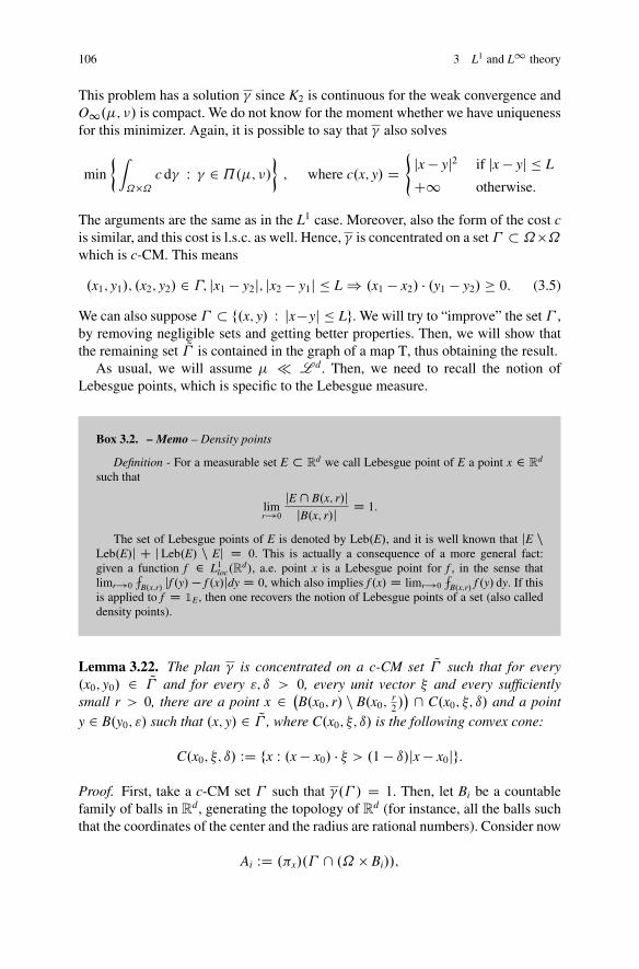
106 3 L1 and L1 theory

This problem has a solution � since K2 is continuous for the weak convergence andO1.�; �/ is compact. We do not know for the moment whether we have uniquenessfor this minimizer. Again, it is possible to say that � also solves

min

�ˆ˝�˝

c d� W � 2 ˘.�; �/�; where c.x; y/ D

(jx � yj2 if jx � yj � L

C1 otherwise.

The arguments are the same as in the L1 case. Moreover, also the form of the cost cis similar, and this cost is l.s.c. as well. Hence, � is concentrated on a set � � ˝�˝which is c-CM. This means

.x1; y1/; .x2; y2/ 2 �; jx1 � y2j; jx2 � y1j � L ) .x1 � x2/ � .y1 � y2/ � 0: (3.5)

We can also suppose � � f.x; y/ W jx�yj � Lg. We will try to “improve” the set � ,by removing negligible sets and getting better properties. Then, we will show thatthe remaining set Q� is contained in the graph of a map T, thus obtaining the result.

As usual, we will assume � � L d. Then, we need to recall the notion ofLebesgue points, which is specific to the Lebesgue measure.

Box 3.2. – Memo – Density points

Definition - For a measurable set E � Rd we call Lebesgue point of E a point x 2 R

d

such that

limr!0

jE \ B.x; r/jjB.x; r/j D 1:

The set of Lebesgue points of E is denoted by Leb.E/, and it is well known that jE nLeb.E/j C j Leb.E/ n Ej D 0. This is actually a consequence of a more general fact:given a function f 2 L1loc.R

d/, a.e. point x is a Lebesgue point for f , in the sense thatlimr!0

fflB.x;r/ jf .y/� f .x/jdy D 0, which also implies f .x/ D limr!0

fflB.x;r/ f .y/ dy. If this

is applied to f D 1E, then one recovers the notion of Lebesgue points of a set (also calleddensity points).

Lemma 3.22. The plan � is concentrated on a c-CM set Q� such that for every.x0; y0/ 2 Q� and for every "; ı > 0, every unit vector � and every sufficientlysmall r > 0, there are a point x 2 �

B.x0; r/ n B.x0;r2/ \ C.x0; �; ı/ and a point

y 2 B.y0; "/ such that .x; y/ 2 Q� , where C.x0; �; ı/ is the following convex cone:

C.x0; �; ı/ WD fx W .x � x0/ � � > .1 � ı/jx � x0jg:

Proof. First, take a c-CM set � such that �.� / D 1. Then, let Bi be a countablefamily of balls in R

d, generating the topology of Rd (for instance, all the balls suchthat the coordinates of the center and the radius are rational numbers). Consider now

Ai WD .�x/.� \ .˝ � Bi//;

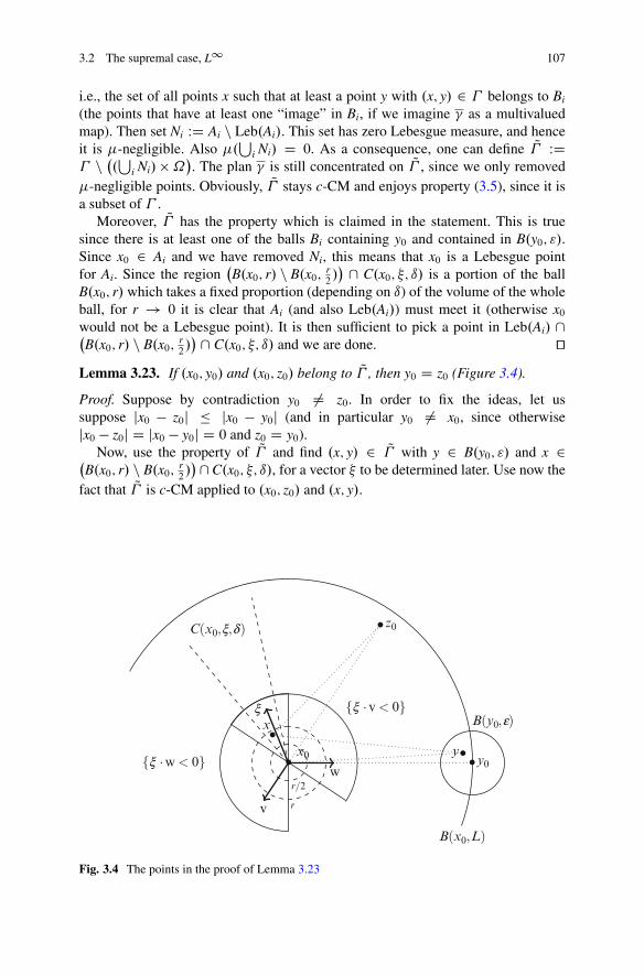
3.2 The supremal case, L1 107

i.e., the set of all points x such that at least a point y with .x; y/ 2 � belongs to Bi

(the points that have at least one “image” in Bi, if we imagine � as a multivaluedmap). Then set Ni WD Ai n Leb.Ai/. This set has zero Lebesgue measure, and henceit is �-negligible. Also �.

Si Ni/ D 0. As a consequence, one can define Q� WD

� n �.Si Ni/ �˝. The plan � is still concentrated on Q� , since we only removed�-negligible points. Obviously, Q� stays c-CM and enjoys property (3.5), since it isa subset of � .

Moreover, Q� has the property which is claimed in the statement. This is truesince there is at least one of the balls Bi containing y0 and contained in B.y0; "/.Since x0 2 Ai and we have removed Ni, this means that x0 is a Lebesgue pointfor Ai. Since the region

�B.x0; r/ n B.x0;

r2/ \ C.x0; �; ı/ is a portion of the ball

B.x0; r/ which takes a fixed proportion (depending on ı) of the volume of the wholeball, for r ! 0 it is clear that Ai (and also Leb.Ai/) must meet it (otherwise x0would not be a Lebesgue point). It is then sufficient to pick a point in Leb.Ai/ \�B.x0; r/ n B.x0;

r2/ \ C.x0; �; ı/ and we are done. ut

Lemma 3.23. If .x0; y0/ and .x0; z0/ belong to Q� , then y0 D z0 (Figure 3.4).

Proof. Suppose by contradiction y0 ¤ z0. In order to fix the ideas, let ussuppose jx0 � z0j � jx0 � y0j (and in particular y0 ¤ x0, since otherwisejx0 � z0j D jx0 � y0j D 0 and z0 D y0).

Now, use the property of Q� and find .x; y/ 2 Q� with y 2 B.y0; "/ and x 2�B.x0; r/ n B.x0;

r2/\ C.x0; �; ı/, for a vector � to be determined later. Use now the

fact that Q� is c-CM applied to .x0; z0/ and .x; y/.

B(x0,L)

•y0•y•x

• x0

•z0

B(y0,e)

w

x

C(x0,x,d)

r

r/2

v

{x ·w< 0}

{x ·v< 0}

Fig. 3.4 The points in the proof of Lemma 3.23

108 3 L1 and L1 theory

If we can prove that jx � z0j; jx0 � yj � L, then we should have

.x � x0/ � .y � z0/ � 0

and we would use this to get a contradiction, by means of a suitable choice for � .Indeed, the direction of x � x0 is almost that of � (up to an error of ı) and that ofy � z0 is almost that of y0 � z0 (up to an error of the order of "=jz0 � y0j). If wechoose � such that � � .y0 � z0/ < 0, this means that for small ı and ", we would geta contradiction.

We need to guarantee jx � z0j; jx0 � yj � L, in order to prove the claim. Let uscompute jx � z0j2: we have

jx � z0j2 D jx0 � z0j2 C jx � x0j2 C 2.x � x0/ � .x0 � z0/:

In this sum, we have

jx0�z0j2 � L2I jx�x0j2 � r2I 2.x�x0/ �.x0�z0/ D jx�x0j.� �.x0�z0/CO.ı//:

Suppose now that we are in one of the following situations: either choose � such that� �.x0�z0/ < 0 or jx0�z0j2 < L2. In both cases, we get jx�z0j � L for r and ı smallenough. In the first case, since jx � x0j � r

2, we have a negative term of the order of

r and a positive one of the order of r2; in the second, we add to jx0 � z0j2 < L2 someterms of the order of r or r2.

Analogously, for what concerns jx0 � yj, we have

jx0 � yj2 D jx0 � xj2 C jx � yj2 C 2.x0 � x/ � .x � y/:

The three terms satisfy

jx0 � xj2 � r2I jx � yj2 � L2I2.x0 � x/ � .x � y/ D jx � x0j.�� � .x0 � y0/C O.ı C "C r//:

In this case, either we have jx0 � y0j < L (which would guarantee jx0 � yj < L for"; ı small enough) or we need to impose � � .y0 � x0/ < 0.

Note that imposing � � .y0 � x0/ < 0 and � � .x0 � z0/ < 0 automatically gives� � .y0 � z0/ < 0, which is the desired condition so as to have a contradiction. Setv D y0 � x0 and w D x0 � z0. If it is possible to find � with � � v < 0 and � � w < 0,we are done. When is it the case that two vectors v and w do not admit the existenceof a vector � with both scalar products that are negative? The only case is when theygo in opposite directions. But this would mean that x0; y0, and z0 are colinear, withz0 between x0 and y0 (since we supposed jx0 � z0j � jx0 � y0j). If we want z0 and y0to be distinct points, we should have jx0 � z0j < L. Hence, in this case, we do notneed to check � � .x0 � z0/ < 0. We only need a vector � satisfying � � .y0 � x0/ < 0and � �.y0�z0/ < 0, but the directions of y0�x0 and y0�z0 are the same, so that this

3.3 Discussion 109

can be guaranteed by many choices of � , since we only need the scalar product withjust one direction to be negative. Take, for instance, � D �.y0 � x0/=jy0 � x0j. utTheorem 3.24. The secondary variational problem

minfK2.�/ W � 2 O1.�; �/g

admits a unique solution � , it is induced by a transport map T, and such a map isan optimal transport for the problem

minfjjT � idjjL1.�/ ; T#� D �g:

Proof. We have already seen that � is concentrated on a set Q� satisfying some usefulproperties. Lemma 3.23 shows that Q� is contained in a graph, since for any x0, thereis no more than one possible point y0 such that .x0; y0/ 2 Q� . Let us consider sucha point y0 as the image of x0 and call it T.x0/. Then � D �T. The optimality ofT in the “Monge” version of this L1 problem comes from the usual comparisonwith the Kantorovich version on plans � . The uniqueness comes from standardarguments (since it is true as well that convex combinations of minimizers shouldbe minimizers and this allows us to perform the proof in Remark 1.19). ut

3.3 Discussion

3.3.1 Different norms and more general convex costs

The attentive reader will have observed that the proof in Section 3.1 about the caseof the distance cost function was specific to the case of the distance induced bythe Euclidean norm. Starting from the original problem by Monge and relying onthe proof strategy by Sudakov [290] (which had a gap later solved by Ambrosio in[8, 10], but was meant to treat the case of an arbitrary norm), the case of differentnorms has been extensively studied in the last years. Note that the case of uniformlyconvex norms (i.e., those such that the Hessian of the square of the norm is boundedfrom below by a matrix which is positively definite) is the one which is most similarto the Euclidean case and can be treated in a similar way.

One of the first extensions was the case studied by Ambrosio, Kirchheim, andPratelli about crystalline norms [14], i.e., norms such that their unit balls are convexpolyhedra. One can guess that the fact that we have a finite number of facesmakes the task easier, but it already required a huge approximation work. Indeed,if one uses duality, the gradient ru.x/ of a Kantorovich potential is not enoughto determine the direction of the displacement y � x for a pair .x; y/ 2 spt.�/,because a crystalline norm has the same gradient on all the points of a same face(and not only on points on the same ray, as is the case for the Euclidean norm, or forother strictly convex norms). To handle this problem, [14] develops a strategy with a

110 3 L1 and L1 theory

double approximation, where jjzjj is replaced by something like jjzjj C "jzj C "2jzj2,jjzjj is the norm we consider, jzj is the Euclidean norm which is added so as to selecta direction, and its square is added so as to get strict convexity and monotonicityon each ray (exactly as we saw in Section 3.1). In this way, the authors provethe existence of an optimal map for crystalline norms in any dimensions and forarbitrary norms in R

2.Later, the way was open to the generalization to other norms. The main tool

is always a secondary variational problem, since for norm costs it is in generalfalse that optimal plans all come from a map, and one needs to select a specialone. The difficulty with secondary variational problems is that they correspond toa new cost c which is not finitely valued. This prevents from using duality on thesecondary problem. Indeed, Proposition 1.42 proves that we have equality betweenthe primal and the dual problem for all costs which are l.s.c., but does not guaranteethe existence of an optimizer in the dual; existence is usually guaranteed either viaAscoli-Arzelà arguments, or through Theorem 1.37, which requires finiteness of thecost. This is why some methods avoiding duality and concentrating on c-cyclicalmonotonicity have been developed. The first time they appeared is in [122], fora different problem (an L1 case): it corresponds to the idea that we presented inSection 3.2 (looking for density points of this concentration set). Later, Championand De Pascale managed to use the same tools to prove the existence of an optimalmap first for arbitrary strictly convex norms (in [119], the same result being obtaineddifferently at almost the same time by Caravenna in [103]) and then for generalnorms in [120]. This last result was more difficult to obtain and required some extraapproximation tools inspired from [273] and in particular the selection of a specialoptimal transport plan via approximation through atomic marginals, as we did inSection 3.1.5.

But the history of optimal transport did not look only at norms. Many studieshave been done for different cost functions (distances or squared distances onmanifolds, geodesic distances on R

d if obstacle are present, etc.). In this book, weprefer to stick to the Euclidean case, and in this section, we only consider costsof the form c.x; y/ D h.x � y/ for h convex. Even this case is far from beingcompletely understood. In a paper with Carlier and De Pascale (see [113]), a general(straightforward) strategy of decomposition according to the “faces” of the costfunction h is presented.

The decomposition is based on the following steps:

• Consider an optimal plan � and look at the optimality conditions as inSection 1.3. For all .x0; y0/ 2 spt.�/, if x0 is a differentiability point for thepotential ' (we write x0 2 Diff.'/), one gets r'.x0/ 2 @h.x0 � y0/; which isequivalent to

x0 � y0 2 @h.r'.x0//: (3.6)

3.3 Discussion 111

Let us define

Fh WD f@h.p/ W p 2 Rdg;

which is the set of all possible values of the subdifferential multi-map of h.These values are those convex sets where the function h is affine, and theywill be called faces of h. The fact that ' is differentiable �-a.e. is enforcedby supposing � � L d and h to be Lipschitz, so that ' is also Lipschitz.Thanks to (3.6), for every fixed x, all the points y such that .x; y/ belongs to thesupport of an optimal transport plan are such that the difference x � y belongsto a same face of h. Classically, when these faces are singletons (i.e., when his differentiable, which is the same as h being strictly convex), this is the wayto obtain a transport map, since only one y is admitted for every x.Equation (3.6) also enables one to classify the points x as follows. For everyK 2 Fh, we define the set

XK WD fx 2 Diff.'/ W @h.r'.x// D Kg:

Hence, � may be decomposed into several subplans �K according to the criterionx 2 XK . If K varies among all possible faces, this decomposition covers � -almost all pairs .x; y/. Moreover, if .x; y/ belongs to spt.�/ and x to Diff.'/,then x 2 XK implies x � y 2 K.If the set Fh is finite or countable, we define

�K WD �jXK�Rd :

In this case, the marginal measures �K and �K of �K (i.e., its images under themaps �x and �y, respectively) are sub-measures of � and �, respectively. Inparticular �K inherits the absolute continuity from �. This is often useful forproving existence of transport maps.If Fh is uncountable, in some cases, one can still rely on a countable decom-position by considering the set Fmulti

h WD fK 2 Fh W K is not a singleton g.If Fmulti

h is countable, then one can separate those x such that @h.r.'.x// isa singleton (where a transport already exists) and look at a decomposition forK 2 Fmulti

h only.• This decomposition reduces the transport problem to a superposition of trans-

port problems of the type

min

�ˆh.x � y/ d�.x; y/ W � 2 ˘.�K ; �K/; spt.�/ � fx � y 2 Kg

�:

The advantage is that the cost c restricted to K is easier to study. If K is a faceof h, then h is affine on K and in this case, the transport cost does not dependany more on the transport plan.

112 3 L1 and L1 theory

• The problem is reduced to find a transport map from �K to �K satisfying theconstraint x � T.x/ 2 K, knowing a priori that a transport plan satisfying thesame constraint exists.In some cases (e.g., if K is a convex compact set containing 0 in its interior),this problem may be reduced to an L1 transport problem. In fact if one denotesby jj � jjK the (gauge-like) “norm” such that K D fx W jjxjjK � 1g, one has

minn

maxfjjx � yjjK W .x; y/ 2 spt.�/g W � 2 ˘.�; �/o

� 1 (3.7)

and the question is whether the same inequality would be true if one restrictedthe admissible set to transport maps only (passing from Kantorovich to Monge,say). The answer would be yes if a solution of (3.7) were induced by a transportmap T. This is what we presented in Section 3.2 in the case K D B.0; 1/ andwhich was first proven in [122] via a different strategy (instead of selectinga minimizer via a secondary variational problem, selecting the limit of theminimizers for the Lp norms or p ! 1). Note also that this issue is easy in1D, where the monotone transport solves all the Lp problems and hence the L1as well (and this does not need the measure to be absolutely continuous, but justatomless).

Let us note that the assumption that the number of faces is countable is quiterestrictive and is essentially used to guarantee the absolute continuity of �K , withno need of a disintegration argument (which could lead to difficulties at least ashard as those faced by Sudakov those faced by Sudakov, see also [104]). However,an interesting example that could be approached by finite decomposition is that ofcrystalline norms. In this case, the faces of the cost h are polyhedral cones but,if the support of the two measures are bounded, we can suppose that they arecompact convex polyhedra. This means, thanks to the considerations above, thatit is possible to perform a finite decomposition and to reduce the problem to someL1 minimizations for norms whose unit balls are polyhedra (the faces of the cone).In particular, the L1 problem for crystalline norms is solved if we can solve L1optimal transport problem for other crystalline norms.

It becomes then interesting to solve the L1 problem as in Section 3.2, replacingthe unit ball constraint jx � yj � 1 with a more general constraint x � y 2 C, the setC being a generic convex set, for instance, a polyhedron. This is studied in [197] byminimizing the quadratic cost

c.x; y/ D(

jx � yj2 if x � y 2 C;

C1 otherwise,

which is also of the form c.x; y/ D h.x � y/ for h strictly convex (but not realvalued). The existence of an optimal map (better: the fact that any optimal � for thisproblem is induced by a map) is proven when � is absolutely continuous and C iseither strictly convex or has a countable number of faces. This can be achieved byadapting the arguments of Section 3.2 and proving that, if .x0; y0/ and .x0; y1/ belong

3.3 Discussion 113

to spt.�/ (and hence y0 � x0; y1 � x0 2 C), then the middle point 12.y0 C y1/ � x0

cannot lie in the interior of C. If C is strictly convex, this proves y0 D y1. If not,this proves that the points y0 � x0 and y1 � x0 are on a same face of C and one canperform a dimensional reduction argument and proceed by induction.

In particular, this argument applies to the case of polyhedra and of arbitraryconvex sets in R

2 (since no more than a countable quantity of segments may becontained in @C) and provides an alternative proof for the result of [14].

Many generalizations of this last result have been performed: Bertrand and Puel[52] studied the “relativistic” cost h.z/ WD 1�p1 � jzj2, which is naturally endowedwith the constraint jzj � 1 and is a strictly convex function (but not finite valuedsince the constraint means h.z/ D C1 outside the unit ball). They proved existenceof an optimal map by adapting the arguments of [122, 197] to the case of a strictlyconvex function h with a strictly convex constraint C (from there, adapting to thecase of a countable number of faces seems to be also possible).

Finally, Chen, Jiang, and Yang combined the arguments of [197] with those of[120], thus getting existence for the cost function

c.x; y/ D(

jx � yj if x � y 2 C;

C1 otherwise,

under the usual assumptions on C (strictly convex or countable number of faces).These results can be found in [123, 124] and are the first which combine lack ofstrict convexity and infinite values.

All these subsequent improvements paved the way to an obvious conjecture,i.e., the fact that a mixture of duality, variational approximation, and density pointstechniques could finally prove the existence of an optimal transport map in a verygeneral case:

Problem (existence for every convex cost): suppose � � L d and take a costc.x; y/ of the form h.x�y/ with h W Rd ! R[fC1g convex; prove that there existsan optimal map.

This problem was open till the final redaction phases of this book, when Bardel-loni and Bianchini’s paper [26] appeared, containing a proof of a disintegrationresult implying this very same statement, at least in the case where h is finite valuedbut not strictly convex.

3.3.2 Concave costs (Lp, with 0 < p < 1)

Another class of transport costs which is very reasonable for applications, ratherthan convex functions of the Euclidean distance, is that of concave costs3, more

3We mean here costs which are concave functions of the distance jx � yj, not of the displacementx � y, as instead we considered in Remark 2.12.

114 3 L1 and L1 theory

precisely c.x; y/ D `.jx � yj/ where ` W RC ! RC is a strictly concave andincreasing function4. From the economic and modeling point of view, this is themost natural choice: moving a mass has a cost which is proportionally less if thedistance increases, as everybody can note from travel fares of most transport means(railways, highway tolls, flights, etc.). All these costs are subadditive. In manypractical cases, moving two masses, each on a distance d, is more expensive thanmoving one at distance 2d and keeping at rest the other. The typical example ofcosts with these property is given by the power cost jx � yj˛ , ˛ < 1.

Note that all these costs satisfy the triangle inequality and are thus distances onR

d. Moreover, under strict concavity assumptions, these costs satisfy a strict triangleinequality. This last fact implies that the common mass between � and � must stayat rest, a fact first pointed out in [176].

Theorem 3.25. Let � be an optimal transport plan for the cost c.x; y/ D `.jx � yj/with ` W RC ! RC strictly concave, increasing, and such that `.0/ D 0. Let� D �D C �O, where �D is the restriction of � to the diagonal D D f.x; x/ W x 2 ˝gand �O is the part outside the diagonal, i.e., the restriction to Dc D .˝ � ˝/ n D.Then this decomposition is such that .�x/#�O and .�y/#�O are mutually singularmeasures.

Proof. It is clear that �O is concentrated on spt.�/ n D and hence .�x/#�O isconcentrated on �x.spt.�/ n D/ and .�y/#�O on �y.spt.�/ n D/. We claim thatthese two sets are disjoint. Indeed suppose that a common point z belongs to both.Then, by definition, there exists y such that .z; y/ 2 spt.�/ n D and x such that.x; z/ 2 spt.�/ n D. This means that we can apply c-cyclical monotonicity to thepoints .x; z/ and .z; y/ and get

`.jx � zj/C `.jz � yj/ � `.jx � yj/C `.jz � zj/ D `.jx � yj/ < `.jx � zj/C `.jz � yj/;

where the last strict inequality gives a contradiction. utThis gives a first constraint on how to build optimal plans � : look at � and �, take

the common part �^ �, leave it on place, subtract it from the rest, and then build anoptimal transport between the two remainders, which will have no mass in common.Note that when the cost c is linear in the Euclidean distance, then the common massmay stay at rest but is not forced to do so (think at the book-shifting example); onthe contrary, when the cost is a strictly convex function of the Euclidean distance,in general, the common mass does not stay at rest (in the previous example, onlythe translation is optimal for c.x; y/ D jx � yjp, p > 1). Note that the fact that thecommon mass stays at rest implies that in general, there is no optimal map T, sincewhenever there is a set A with �.A/ > .� ^ �/.A/ D �.A/ > 0, then almost allthe points of A must have two images: themselves and another point outside A.

4We will not explicitly state it every time, but this also implies that ` is strictly increasing.

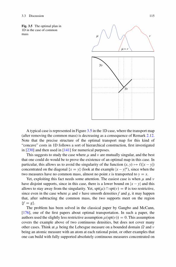
3.3 Discussion 115

Fig. 3.5 The optimal plan in1D in the case of commonmass m

m ∧ n

go

gD

n

A typical case is represented in Figure 3.5 in the 1D case, where the transport map(after removing the common mass) is decreasing as a consequence of Remark 2.12.Note that the precise structure of the optimal transport map for this kind of“concave” costs in 1D follows a sort of hierarchical construction, first investigatedin [230] and then used in [141] for numerical purposes.

This suggests to study the case where � and � are mutually singular, and the bestthat one could do would be to prove the existence of an optimal map in this case. Inparticular, this allows us to avoid the singularity of the function .x; y/ 7! `.jx � yj/concentrated on the diagonal fx D yg (look at the example jx � yj˛), since when thetwo measures have no common mass, almost no point x is transported to y D x.

Yet, exploiting this fact needs some attention. The easiest case is when � and �have disjoint supports, since in this case, there is a lower bound on jx � yj and thisallows to stay away from the singularity. Yet, spt.�/\ spt.�/ D ; is too restrictive,since even in the case where � and � have smooth densities f and g, it may happenthat, after subtracting the common mass, the two supports meet on the regionff D gg.

The problem has been solved in the classical paper by Gangbo and McCann,[176], one of the first papers about optimal transportation. In such a paper, theauthors used the slightly less restrictive assumption �.spt.�// D 0. This assumptioncovers the example above of two continuous densities, but does not cover manyother cases. Think at � being the Lebesgue measure on a bounded domain ˝ and �being an atomic measure with an atom at each rational point, or other examples thatone can build with fully supported absolutely continuous measures concentrated on

116 3 L1 and L1 theory

disjoint sets A and ˝ n A (see Ex(20)). In the present section, we show how toprove the existence of a transport map when � and � are singular to each other and� � L d.

We will prove the following result.

Theorem 3.26. Suppose that � and � are two mutually singular probabilitymeasures on R

d such that � � L d, and take the cost c.x; y/ D `.jx � yj/, for` W RC ! RC strictly concave, C1 on �0;C1Œ, and increasing. Then there exists aunique optimal transport plan � and it is induced by a transport map.

Proof. We will use the standard procedure explained in Chapter 1 for costs of theform c.x; y/ D h.x�y/. In particular, we get the existence of a Kantorovich potential' such that, if .x0; y0/ 2 spt.�/, then

x0 � y0 D .rh/�1.r'.x0//: (3.8)

This allows us to express y0 as a function of x0, thus proving that there is onlyone point .x0; y/ 2 spt.�/ and hence that � comes from a transport T.x/ Dx � .rh/�1.r'.x//. This approach also proves uniqueness in the same way. InChapter 1, we presented it under strict convexity assumptions on h, so that rh isinjective and .rh/�1 D rh. But the injectivity is also true if h.z/ D `.jzj/. Indeedwe have rh.z/ D `0.jzj/ z

jzj , and the modulus of this vector identifies the modulusjzj (since `0 is strictly increasing), and the direction identifies the direction of z.

The main difficulty is the fact that we need to guarantee that ' is differentiablea.e. with respect to �. Since � � L d, it is enough to have ' Lipschitz continuous,which is usually proven using the fact that '.x/ D infy h.jx�yj/� .y/. Yet, concavefunctions on R

C may have an infinite slope at 0 and be non-Lipschitz, and thiscould be the case for ' as well. This suggests the use of an alternate notion ofdifferentiability.

Box 3.3. Important notion: Approximate gradient

We recall here some facts about a measure-theoretical notion replacing the gradient forless regular functions. The interested reader can find many details in [160].

Let us start from the following observation: given a function f W ˝ ! R and a pointx0 2 ˝, we say that f is differentiable at x0 2 ˝ and that its gradient is v D rf .x0/ 2 R

d

if for every � > 0 the set

A.x0; v; "/ WD fx 2 ˝ W jf .x/� f .x0/� v � .x � x0/j > � jx � x0jgis at positive distance from x0, i.e., if for small ı > 0 we have B.x0; ı/ \ A.x0; v; "/ D ;.Instead of this requirement, we could ask for a weaker condition, namely, that x0 is a zero-density point for the same set A.v; "/ (i.e., a Lebesgue point of its complement). Moreprecisely, if there exists a vector v such that

(continued)

3.3 Discussion 117

Box 3.3. (continued)

limı!0

jA.x0; v; "/\ B.x0; ı/jjB.x0; ı/j D 0

then we say that f is approximately differentiable at x0 and its approximate gradient is v.The approximate gradient will be denoted by rappf .x0/. As one can expect, it enjoys severalof the properties of the usual gradient that we list here.

• The approximate gradient, provided it exists, is unique.• The approximate gradient is nothing but the usual gradient if f is differentiable.• The approximate gradient shares the usual algebraic properties of gradients, in

particular rapp.f C g/.x0/ D rappf .x0/C rappg.x0/.• If x0 is a local minimum or local maximum for f , and if rappf .x0/ exists, then

rappf .x0/ D 0.

Another very important property is a consequence of the Rademacher theorem.Proposition. Let f ; g W ˝ ! R be two functions defined on a same domain ˝ with

g Lipschitz continuous. Let E � ˝ be a Borel set such that f D g on E. Then f isapproximately differentiable almost everywhere on E and rappf .x/ D rg.x/ for a.e. x 2 E.

Proof. It is enough to consider all the Lebesgue points of E where g is differentiable.These points cover almost all E. It is easy to check that the definition of approximategradient of f at a point x0 is satisfied if we take v D rg.x0/.

As a consequence, it is also clear that every countably Lipschitz function is approxi-mately differentiable a.e.

We just need to prove that ' admits an approximate gradient Lebesgue-a.e.: thiswould imply that Equation (3.8) is satisfied if we replace the gradient with theapproximate gradient.

Recall that we may suppose

'.x/ D 'cc.x/ D infy2Rd

`.jx � yj/ � 'c.y/ :

Now consider a countable family of closed balls Bi generating the topology ofR

d, and for every i, consider the function defined as

'i.x/ WD infy2Bi

`.jx � yj/ � 'c.y/

for x 2 Rd. One cannot provide straight Lipschitz properties for 'i, since a priori

y is arbitrarily close to x and in general ` is not Lipschitz close to 0. However, 'i

is Lipschitz on every Bj such that dist.Bi;Bj/ > 0. Indeed if x 2 Bj, y 2 Bi onehas jx � yj � d > 0; therefore, the Lipschitz constant of `.j� � yj/ � 'c.y/ does notexceed `0.d/. It follows that 'i is Lipschitz on Bj, and its Lipschitz constant doesnot exceed `0.d/ and the same is true for 'i has an approximate gradient almosteverywhere on f' D 'ig\Bj. By countable union, ' admits an approximate gradienta.e. on

118 3 L1 and L1 theory

[i;j

d.Bi;Bj/>0

Œf'i D 'g \ Bj� :

In order to prove that ' has an approximate gradient �-almost everywhere, it isenough to prove that

�

[i;j

d.Bi;Bj/>0

f'i D 'g \ Bj

!D 1:

In order to do this, note that for every i and j, we have

�x.spt.�/ \ .Bj � Bi// � f' D 'ig \ Bj :

Indeed, let .x; y/ 2 spt.�/\ .Bj � Bi/. Then '.x/C 'c.y/ D l.jx � yj/. It followsthat

'i.x/ D infy02Bi

`.ˇx � y0 ˇ/ � 'c.y0/ � `.jx � yj/ � 'c.y/ D '.x/ :

On the other hand, for every x 2 Rd

'i.x/ D infy2Bi

`.jx � yj/ � 'c.y/ � infy2Rd

`.jx � yj/ � 'c.y/ D '.x/ :

As a consequence of this,

�

[i;j

d.Bi;Bj/>0

f'i D 'g \ Bj

!� �

[i;j

d.Bi;Bj/>0

�x.spt.�/ \ .Bj � Bi//

!

D �

�x

spt.�/ \

[i;j

d.Bi;Bj/>0

Bj � Bi

!!

D �.�x.spt.�/ n D//

D ��.�x/

�1.�x.spt.�/ n D//�

� �.spt.�/ n D/ D 1;

where D is the diagonal in ˝ �˝. utFrom the previous theorem, we can also easily deduce the following extension.

Define � ^ � as the maximal positive measure which is both less or equal than �and than �, and .�� �/C D �� � ^ �, so that the two measures � and � uniquelydecompose into a common part �^� and two mutually singular parts .���/C and.� � �/C.

3.3 Discussion 119

Theorem 3.27. Suppose that � and � are probability measures on˝ with .���/C� L d, and take the cost c.x; y/ D `.jx � yj/, for ` W RC ! RC strictly concave,C1 on �0;C1Œ, and increasing with `.0/ D 0. Then there exists a unique optimaltransport plan � , and it has the form .id; id/#.� ^ �/C .id;T/#.� � �/C.

As we said, the above results can be extended to more general situations:differentiability of ` is not really necessary, and the assumption � � L d can beweakened. In [250], the result is proven under the natural assumption that� does notgive mass to small sets, i.e., for every A � R

d which is .d�1/-rectifiable, we have�.A/ D 0. The key tool is the following lemma, which is an interesting result fromgeometric measure theory that can be used instead of Lebesgue points-type resultswhen we face a measure which is not absolutely continuous but “does not give massto small sets.” It states that, in such a case, for�-a.e. point x, every cone exiting fromx, even if very small, has positive � mass. In particular, it means that we can findpoints of spt.�/ in almost arbitrary directions close to x. This lemma is strangelymore known among people in optimal transport (see also [121]) than in geometricmeasure theory (even if it corresponds more or less to a part of Lemma 3.3.5 in[161]).

Lemma 3.28. Let � be a Borel measure on Rd, and suppose that � does not give

mass to small sets. Then � is concentrated on the set

fx W 8� > 0;8ı > 0;8e 2 Sd�1; �.C.x; e; ı; �// > 0g ;

where

C.x; e; ı; �/ D C.x; e; ı/ \ B.x; �/ WD fy W hy � x; ei � .1 � ı/ jy � xjg \ B.x; �/:

Chapter 4Minimal flows, divergence constraints,and transport density

4.1 Eulerian and Lagrangian points of view

We review here the main languages and the main mathematical tools to describestatic or dynamical transport phenomena.

4.1.1 Static and dynamical models

This section presents a very informal introduction to the physical interpretation ofdynamical models in optimal transport.

In fluid mechanics, and in many other topics with similar modeling issues, itis classical to consider two complementary ways of describing motions, which arecalled Lagrangian and Eulerian.

When we describe a motion via Lagrangian formalism, we give “names” toparticles (using either a specific label or their initial position, for instance) and thendescribe, for every time t and every label, what happens to that particle. “Whathappens” means providing its position and/or its velocity. Hence we could, forinstance, look at trajectories yx.t/, standing for the position at time t of particleoriginally located at x. As another possibility, instead of giving names, we couldconsider bundles of particles with the same behavior and indicate how many arethey. This amounts to giving a measure on possible behaviors.

The description may be more or less refined. For instance, if one only considerstwo different times t D 0 and t D 1, the behavior of a particle is only given by itsinitial and final positions. A measure on those pairs .x; y/ is exactly a transport plan.This explains why we can consider that the Kantorovich problem is expressed inLagrangian coordinates. The Monge problem is also Lagrangian, and particles arelabeled by their initial position.

© Springer International Publishing Switzerland 2015F. Santambrogio, Optimal Transport for Applied Mathematicians,Progress in Nonlinear Differential Equations and Their Applications 87,DOI 10.1007/978-3-319-20828-2_4

121

122 4 Minimal flows

More refined models can be easily conceived: reducing a movement to the initialand final positions is embarrassingly poor! Measures on the set of paths (curves ! WŒ0; 1� ! ˝, with possible assumptions on their regularity) have been used in manymodeling and in particular in traffic issues in branched transport (see Section 4.4 forboth these subjects), or in Brenier’s variational formulation of the incompressibleEuler equations for fluids (see Sections 1.7.4, 8.4.4, and [51, 83, 85]).

On the other hand, in the Eulerian formalism, we describe, for every time t andevery point x, what happens at such a point at such a time. “What happens” usuallymeans what are the velocity, the density, and the flow rate (both in intensity and indirection) of particles located at time t at point x.

Eulerian models may be distinguished into static and dynamical ones. In adynamical model we usually use two variables, i.e., the density %.t; x/ and thevelocity vt.x/. It is possible to write the equation satisfied by the density of a familyof particles moving according to the velocity field v. This means that we prescribethe initial density %0 and that the position of the particle originally located at x willbe given by the solution of the ODE

(y0

x.t/ D vt.yx.t//

yx.0/ D x:(4.1)

We define the map Yt through Yt.x/ D yx.t/, and we look for the measure%t WD .Yt/#%0. It is well known that %t and vt solve together the so-called continuityequation

@t%t C r � .%tvt/ D 0

that is briefly addressed in Section 4.1.2.The static framework is a bit harder to understand, since it is maybe not clear

what “static” means when we want to describe movement. One has to think to apermanent, cyclical movement, where some mass is constantly injected into themotion at some points and constantly withdrawn somewhere else. We can alsothink at a time average of some dynamical model: suppose that we observe thetraffic in a city and we wonder what happens at each point, but we do not wantan answer depending on the hour of the day. We could, for instance, consider asa traffic intensity at every point the average traffic intensity at such a point on thewhole day. In this case we usually use a unique variable w standing for the massflow rate (which equals density times velocity: hence, it is rather a momentumthan a velocity), and the divergence r � w stands for the excess of mass which isinjected into the motion at every point. More precisely, if particles are injected intothe motion according to a density � and then exit with density �, the vector fields wstanding for flows connecting these two measures must satisfy

r � w D � � �:

4.1 Eulerian and Lagrangian points of view 123

4.1.2 The continuity equation

This section is devoted to the equation

@t%t C r � .%tvt/ D 0;

its meaning, formulations, and uniqueness results. The remainder of the chapterwill mainly deal with the static divergence equation, but we will see later thatthe dynamical case can also be useful (in particular, to produce transport plansassociated with a given vector field). Hence, we need to develop some tools.

First, let us spend some words on the notion of solution for this equation. Herebelow ˝ � R

d is a bounded domain, or Rd itself.

Definition 4.1. We say that a family of pairs measures/vector fields .%t; vt/ withvt 2 L1.%tIRd/ and

´ T0

jjvtjjL1.%t/dt D ´ T0

´˝

jvtjd%t dt < C1 solves the continuityequation on �0;TŒ in the distributional sense if for any bounded and Lipschitz testfunction � 2 C1

c.�0;TŒ�˝/ (note that we require the support to be far from t D 0; 1

but not from @˝, when˝ is bounded; also˝ is usually supposed to be itself closed,but we write ˝ to stress the fact that we do include its boundary), we have

ˆ T

0

ˆ

˝

.@t�/ d%t dt Cˆ T

0

ˆ

˝

r� � vt d%t dt D 0: (4.2)

This formulation includes no-flux boundary conditions on @˝ for vt (if ˝ is notR

d itself, obviously), i.e., %tvt � n D 0. If we want to impose the initial andfinal measures, we can say that .%t; vt/ solves the same equation, in the sense ofdistribution, with initial and final data %0 and %T , respectively, if for any test function� 2 C1

c .Œ0;T� �˝/ (now we do not require the support to be far from t D 0; 1), wehave

ˆ T

0

ˆ

˝

.@t�/ d%t dt Cˆ T

0

ˆ

˝

r� � vt d%t dt Dˆ

˝

�.T; x/ d%T.x/ �ˆ

˝

�.0; x/ d%0.x/:

(4.3)

We can also define a weak solution of the continuity equation through thefollowing condition: we say that .%t; vt/ solves the continuity equation in the weaksense if for any test function 2 C1

c .˝/, the function t 7! ´ d%t is absolutely

continuous in t and, for a.e. t, we have

d

dt

ˆ

˝

d%t Dˆ

˝

r � vt d%t:

Note that in this case t 7! %t is automatically continuous for the weak convergence,and imposing the values of %0 and %1 may be done pointwisely in time.

124 4 Minimal flows

Proposition 4.2. The two notions of solutions are equivalent: every weak solutionis actually a distributional solution and every distributional solution admits arepresentative (another family Q%t D %t for a.e. t) which is weakly continuous and isa weak solution.

Proof. To prove the equivalence, take a distributional solution, and test it againstfunctions � of the form �.t; x/ D a.t/ .x/, with 2 C1

c.˝/ and a 2 C1c.�0; 1Œ/.

We get

ˆ T

0

a0.t/ˆ

˝

.x/ d%t dt Cˆ 1

0

a.t/ˆ

˝

r � vt d%t dt D 0:

The arbitrariness of a shows that the distributional derivative (in time)of

´˝ .x/ d%t is

´˝

r � vt d%t. This last function is L1 in time since´ T0

ˇ´˝

r � vt d%t

ˇdt � Lip

´ T0

jjvtjjL1.%t/dt < C1. This implies that .%; v/is a weak solution.

Conversely, the same computations show that weak solutions satisfy (4.2) forany � of the form �.t; x/ D a.t/ .x/. It is then enough to prove that finite linearcombination of these functions is dense in C1.Œ0;T� � K/ for every compact setK � R

d (this is true, but is a nontrivial exercise: Ex(23)). utIt is also classical that smooth functions satisfy the equation in the classical senseif and only if they are weak (or distributional) solutions. We can also check thefollowing.

Proposition 4.3. Suppose that % is Lipschitz continuous in .t; x/, that v is Lipschitzin x, and that the continuity equation @t% C r � .%v/ D 0 is satisfied in the weaksense. Then the equation is also satisfied in the a.e. sense.

Proof. First we note that with our assumptions both @t% and r�.%v/ are well defineda.e. Fix a countable set D � C1

c.V / which is dense for the uniform convergence

in C0c .

V / (for instance, use polynomial functions with rational coefficients timessuitable cut-off functions). Fix t0 such that .t; x/ 7! %.t; x/ is differentiable at .t0; x/for a.e. x, and also such that t 7! ´

˝� d%t is differentiable at t D t0 with derivative

given by´˝

r� � vt d%t for all � 2 D. Almost all t0 satisfy these conditions. Thenwe can also write, by differentiating under the integral sign,

d

dt jtDt0

ˆ

˝

� d%t dx Dˆ

˝

� .@t%/t0 dx;

which proves´˝.r� �vt0 /%t0 dx D ´

� .@t%/t0 dx. Yet, we can write´˝

r� �vt0%t0 dxas � ´

˝� r � .vt0%t0 / dx (by integration by parts of Lipschitz functions, with no

boundary term because of the compact support of �), and finally we getˆ

˝

� ..@t%/t0 C r � .%t0vt0 // dx D 0 for all � 2 D;

which is enough to prove .@t%/t0 C r � .%t0vt0 / D 0 a.e. in x. ut

4.1 Eulerian and Lagrangian points of view 125

After checking the relations between these different notions of solutions, fromnow on we will often say “solution” to mean, indifferently, “weak solution” or“solution in the distributional sense.”

We now try to identify the solutions of the continuity equation and we want toconnect them to the flow of the vector field vt. First, we recall some properties ofthe flow.

Box 4.1. Memo: Flow of a time-dependent vector field

We consider the ODE y0

x.t/ D vt.yx.t// with initial datum yx.0/ D x, as in (4.1).Proposition. If vt is continuous in x for every t, then for every initial datum, there is local

existence (there exists at least a solution, defined on a neighborhood of t D 0). If, moreover,v satisfies jvt.x/j � C0CC1jxj, then the solution is global in time. If vt is Lipschitz in x anduniformly in t, then the solution is unique and defines a flow Yt.x/ WD yx.t/. In this case, ifwe set L WD supt Lip.vt/, then the map Yt.�/ is Lipschitz in x, with constant eLjtj. Moreover,Yt W Rd ! R

d is invertible and its inverse is also Lipschitz with the same constant.Sketch of proof. We do not prove existence, which can be classically obtained by fixed-

point arguments in the space of curves. As for uniqueness and for the dependence on theinitial datum x, we consider two curves y.1/ and y.2/, solutions of y0.t/ D vt.y.t//, and wedefine E.t/ D jy.1/.t/� y.2/.t/j2. We have

E0.t/ D 2.y.1/.t/� y.2/.t// � .vt.y.1/.t//� vt.y

.2/.t///;

which proves jE0.t/j � 2LE.t/. By Gronwall’s lemma, this gives E.0/e�2Ljtj � E.t/ �E.0/e2Ljtj and provides at the same time uniqueness, injectivity, and the bi-Lipschitzbehavior of Yt (which is also a homeomorphism from R

d onto Rd since for every x0 2 R

d

we can solve the ODE imposing the Cauchy datum y.t/ D x0).

Then, we can prove the following that we state for simplicity in the case ofLipschitz and bounded vector fields.

Theorem 4.4. Suppose that ˝ � Rd is either a bounded domain or R

d itself.Suppose that vt W ˝ ! R

d is Lipschitz continuous in x, uniformly in t, and uniformlybounded, and consider its flow Yt. Suppose that for every x 2 ˝ and every t 2 Œ0;T�,we have Yt.x/ 2 ˝ (which is obvious for ˝ D R

d and requires suitable Neumannconditions on vt otherwise). Then, for every probability %0 2 P.˝/, the measures%t WD .Yt/#%0 solve the continuity equation @t%t C r � .%tvt/ D 0 with initial datum%0. Moreover, every solution of the same equation with %t � L d for every t isnecessarily obtained as %t D .Yt/#%0. In particular, the continuity equation admitsa unique solution.

Proof. First we check the validity of the equation when %t is obtained from such aflow through (4.1). We will prove that we have a weak solution. Fix a test function� 2 C1.Rd/ such that both � and r� are bounded, and compute

126 4 Minimal flows

d

dt

ˆ

˝

� d%t D d

dt

ˆ�.yx.t// d%0.x/ D

ˆ

˝

r�.yx.t// � y0x.t/ d%0.x/

Dˆ

˝

r�.yx.t// � vt.yx.t// d%0.x/ Dˆ

˝

r�.y/ � vt.y/ d%t.y/:

This characterizes weak solutions.In order to prove the second part of the statement, we first observe that (4.2), i.e.,

ˆ T

0

ˆ

˝

.@t� C vt � r�/ d%t dt D 0;

is also valid for all Lipschitz compactly supported test functions �, whenever%t � L d for every t. Indeed, if we fix a Lipschitz test function � and we smoothit by convolution with a compactly supported kernel, we have a sequence �" 2 C1

csuch that rt;x�" ! rt;x� a.e. and we can apply dominated convergence sincejrt;x�"j � Lip.�/ (we need %t to be absolutely continuous because we only haveLebesgue-a.e. convergence).

Then we take a test function 2 C1c.R

d/ and we define �.t; x/ WD ..Yt/�1.x//.

If we can prove that t 7! ´�.t; x/ d%t.x/ is constant, then we have proven

%t D .Yt/#%0. The function � is Lipschitz continuous, because the flow Yt isbi-Lipschitz; yet, it is not compactly supported in time (it is compactly supported inspace since spt� is compact, and if we set M WD supt;x jvt.x/j, we see that �.t; x/vanishes on all points x which are at distance larger than tM from spt ). Thus, wemultiply it with a cut-off function .t/, with 2 C1

c .�0;TŒ/. We have

@t.�/C vt � r.�/ D 0.t/�.t; x/C .t/ .@t�.t; x/C vt.x/ � r�.t; x// :

We can prove that, by definition of �, the term @t�.t; x/C vt.x/ � r�.t; x/ vanishesa.e. (this corresponds to saying that � is a solution of the transport equation; seeBox 6.3). This is true since we have �.t;Tt.x// D .x/, and differentiating it w.r.t.t (which is possible for a.e. .t; x/), we get @t.t;Yt.x//C vt.Yt.x// � r�.t;Yt.x// D 0,which means that @t� C vt � r� vanishes everywhere, as Yt is surjective.

Hence, from the definition of distributional solution, we have

ˆ T

0

0.t/dtˆ

Rd�.t; x/ d%t.x/ D

ˆ T

0

dtˆ

Rd.@t.�/C vt � r.�// d%t.x/ D 0:

The test function 2 C1c .�0;TŒ/ being arbitrary, we get that t 7! ´

Rd �.t; x/ d%t.x/is constant. ut

4.2 Beckmann’s problem 127

4.2 Beckmann’s problem

In this section we discuss a flow-minimization problem introduced by Beckmann inthe 1950s [27] as a particular case of a wider class of convex optimization problem,of the form minf´ H.w/dx W r�w D ���g, for convex H. In this section we discussthe case H.z/ D jzj, which is a limit case in the class of costs studied by Beckmann,who was indeed more interested in strictly convex costs. Strict convexity will beconsidered in “Discussion” (Section 4.4.1). The reason to stick to the linear costhere, and to spend more words on it than on the general case, lies in its equivalencewith the Monge problem. We will provide all the tools to study this equivalence andthis problem.

4.2.1 Introduction, formal equivalences, and variants

We consider here a simple version of a problem that has been proposed byBeckmann as a model for optimal transport in the 1950s. Beckmann called itcontinuous transportation model and he was not aware of Kantorovich’s works andthe possible links between the two theories.

Beckmann’s minimal flow problem

Problem 4.5. Consider the minimization problem

.BP/ min

�ˆjw.x/j dx W w W ˝ ! R

d; r � w D � � ��; (4.4)

where the divergence condition is to be read in the weak sense, with no-fluxboundary conditions, i.e., � ´ r� � dw D ´

� d.� � �/ for any � 2 C1.˝/.

We will see now that an equivalence between (BP) and (KP) (for the costc.x; y/ D jx � yj) holds true. To do that, we can look at the following considerationsand formal computations.

We take the problem (BP) and rewrite the constraint on w using

sup�

ˆ

˝

r� � w dx Cˆ

˝

� d.� � �/ D(0 if r � w D � � �;C1 otherwise.

128 4 Minimal flows

Hence one can write (BP) as

infw

ˆ˝

jwj dx C sup�

ˆ

˝

r� � w dx Cˆ

˝

� d.� � �/!

D sup�

�ˆ˝

� d.� � �/C infw

ˆ

˝

.jwj � r� � w/ dx

�; (4.5)

where inf and sup have been exchanged formally as in the computations ofChapter 1. Then, one notes that

infw

ˆ

˝

.jwj � r� � w/ dx D(0 if jr�j � 1

�1 otherwise

and this leads to the dual formulation for (BP) which gives

sup

�ˆ˝

� d.� � �/ W jr�j � 1

�:

Since this problem is exactly the same as (DP) (a consequence of the fact that Lip1functions are exactly those functions whose gradient is smaller than 1), this providesa formal equivalence between (BP) and (KP). We say that it is only formal becausewe did not prove the equality in (4.5). Note that we also need to suppose that ˝ isconvex; otherwise functions with gradient smaller than 1 are only Lip1 according tothe geodesic distance in ˝.

Most of the considerations above, especially those on the problem (BP), arespecific to the cost equal to the distance jx � yj. In general, for costs of the formh.x � y/, h needs to be 1-homogeneous, if one wants some similar result to hold.We refer to [195, 196] for a general way to transform convex costs into convex1-homogeneous ones (by adding one variable, corresponding to time)1. An inter-esting generalization which keeps the same formalism of the case of the Euclideandistance concerns a cost c which comes from a Riemannian distance k.x/.

Consider indeed

min

�ˆk.x/jw.x/j dx W r � w D � � �

�

1In this way the flow-minimization problem corresponding to costs of the form jx � yjp istransformed into the so-called Benamou-Brenier problem, which we will discuss in Chapters 5and 6, but we do not push this analogy to further conclusions.

4.2 Beckmann’s problem 129

which corresponds, by duality with the functions u such that jruj � k, to

min

�ˆdk.x; y/ d�.x; y/ W � 2 ˘.�; �/

�;

where dk.x; y/ D inf!.0/Dx; !.1/Dy Lk.!/ WD ´ 10

k.!.t//j!0.t/jdt is the distanceassociated with the Riemannian metric k.

The generalization above is suitable when we want to model a nonuniformcost for the movement (due to geographical obstacles or configurations). Sucha model is not always satisfying, for instance, in urban transport, where wewant to consider the fact that the metric k is usually not a priori known, butit depends on the traffic distribution itself. We will develop this aspect in the“Discussion” Section 4.4.1, together with a completely different problem which issomehow “opposite” (Section 4.4.2): instead of looking at transport problems whereconcentration of the mass is penalized (because of traffic congestion), we look atproblems where it is indeed encouraged, because of the so-called economy of scale(i.e., the larger the mass you transport, the cheaper the individual cost).

4.2.2 Producing a minimizer for the Beckmann Problem

The first remark on problem (BP) is that a priori it is not well-posed, in the sensethat there could not exist an L1 vector field minimizing the L1 norm under divergenceconstraints. This is easy to understand if we think at the direct method in calculusof variations to prove existence: we take a minimizing sequence wn and we wouldlike to extract a converging subsequence. Could we do this, from wn * w, it wouldbe easy to prove that w still satisfies r � w D � � �, since the relation

�ˆ

r� � wn dx Dˆ� d.� � �/

would pass to the limit as n ! 1. Yet, the information´ jw.x/j dx � C is not

enough to extract a converging sequence, even weakly. Indeed, the space L1 beingnonreflexive, bounded sequences are not guaranteed to have weakly convergingsubsequences. This is on the contrary the case for dual spaces (and for reflexivespaces, which are roughly speaking the dual of their dual).

Note that the strictly convex version that was proposed by Beckmann and that wewill review in Section 4.4.1 is much better to handle: if, for instance, we minimize´ jwj2 dx, then we can use weak compactness in L2, which is much easier to havethan compactness in L1.

To avoid this difficulty, we will choose the natural setting for (BP), i.e., theframework of vector measures.

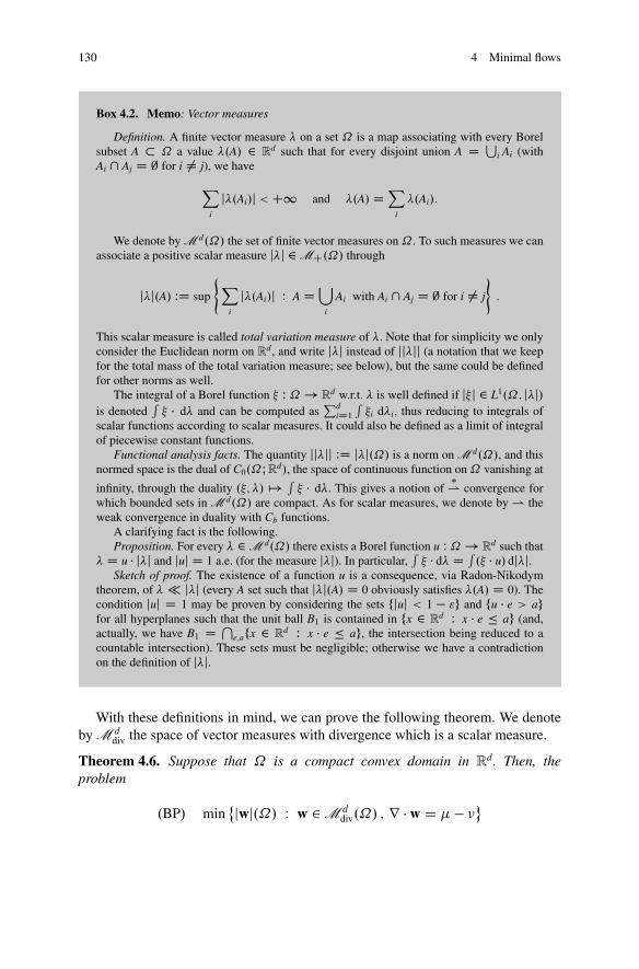
130 4 Minimal flows

Box 4.2. Memo: Vector measures

Definition. A finite vector measure � on a set ˝ is a map associating with every Borelsubset A � ˝ a value �.A/ 2 R

d such that for every disjoint union A D Si Ai (with

Ai \ Aj D ; for i ¤ j), we have

Xi

j�.Ai/j < C1 and �.A/ D Xi

�.Ai/:

We denote by M d.˝/ the set of finite vector measures on ˝. To such measures we canassociate a positive scalar measure j�j 2 M

C

.˝/ through

j�j.A/ WD sup

(Xi

j�.Ai/j W A D [i

Ai with Ai \ Aj D ; for i ¤ j

):

This scalar measure is called total variation measure of �. Note that for simplicity we onlyconsider the Euclidean norm on R

d , and write j�j instead of jj�jj (a notation that we keepfor the total mass of the total variation measure; see below), but the same could be definedfor other norms as well.

The integral of a Borel function � W ˝ ! Rd w.r.t. � is well defined if j�j 2 L1.˝; j�j/

is denoted´� � d� and can be computed as

PdiD1

´�i d�i, thus reducing to integrals of

scalar functions according to scalar measures. It could also be defined as a limit of integralof piecewise constant functions.

Functional analysis facts. The quantity jj�jj WD j�j.˝/ is a norm on M d.˝/, and thisnormed space is the dual of C0.˝IRd/, the space of continuous function on˝ vanishing at

infinity, through the duality .�; �/ 7! ´� � d�. This gives a notion of

�

* convergence forwhich bounded sets in M d.˝/ are compact. As for scalar measures, we denote by * theweak convergence in duality with Cb functions.

A clarifying fact is the following.Proposition. For every � 2 M d.˝/ there exists a Borel function u W ˝ ! R

d such that� D u � j�j and juj D 1 a.e. (for the measure j�j). In particular,

´� � d� D ´

.� � u/ dj�j.Sketch of proof. The existence of a function u is a consequence, via Radon-Nikodym

theorem, of � j�j (every A set such that j�j.A/ D 0 obviously satisfies �.A/ D 0). Thecondition juj D 1 may be proven by considering the sets fjuj < 1 � "g and fu � e > agfor all hyperplanes such that the unit ball B1 is contained in fx 2 R

d W x � e � ag (and,actually, we have B1 D T

e;afx 2 Rd W x � e � ag, the intersection being reduced to a

countable intersection). These sets must be negligible; otherwise we have a contradictionon the definition of j�j.

With these definitions in mind, we can prove the following theorem. We denoteby M d

div the space of vector measures with divergence which is a scalar measure.

Theorem 4.6. Suppose that ˝ is a compact convex domain in Rd. Then, the

problem

.BP/ min˚jwj.˝/ W w 2 M d

div.˝/ ; r � w D � � �

4.2 Beckmann’s problem 131

(with divergence imposed in the weak sense, i.e., for every � 2 C1.˝/; we impose� ´ r� � dw D ´

� d.� � �/, which also includes no-flux boundary conditions)admits a solution. Moreover, its minimal value equals the minimal value of (KP)and a solution of (BP) can be built from a solution of (KP). The two problems arehence equivalent.

Proof. The first point that we want to prove is the equality of the minimal valuesof (BP) and (KP). We start from min(BP)� min(KP). In order to do so, take anarbitrary function � 2 C1 with jr�j � 1. Consider that for any w with r�w D ���,we have

jwj.˝/ Dˆ

˝

1 djwj �ˆ

˝

.�r�/ � dw Dˆ

˝

� d.� � �/:

If one takes a sequence of Lip1 \C1 functions uniformly converging to theKantorovich potential u such that

´˝

u d.� � �/ D max .DP/ D min .KP/ (forinstance, take convolutions �k D �k � u), then we get

ˆ

˝

djwj � min .KP/

for any admissible w, i.e., min(BP)� min(KP).We will show at the same time the reverse inequality and how to construct an

optimal w from an optimal � for (KP).Actually, one way to produce a solution to this divergence-constrained problem is

the following (see [70]): take an optimal transport plan � and build a vector measurewŒ�� defined2 through

hwŒ��; �i WDˆ

˝�˝

ˆ 1

0

!0x;y.t/ � �.!x;y.t//dt d�.x; y/;

for every � 2 C0.˝IRd/, !x;y being a parametrization of the segment Œx; y� (itis clear that this is the point where convexity of ˝ is needed). Even if for thisproof it would not be important, we will fix the constant-speed parametrization, i.e.,!x;y.t/ D .1 � t/x C ty.

It is not difficult to check that this measure satisfies the divergence constraint,since if one takes � D r�, then

ˆ 1

0

!0x;y.t/ � �.!x;y.t// dt D

ˆ 1

0

d

dt

��.!x;y.t/

dt D �.y/ � �.x/

and hence hwŒ��;r�i D ´� d.� � �/ and wŒ�� 2 M d

div.˝/.

2The strange notation wŒ�� is chosen so as to distinguish from the object wQ that we will introducein Section 4.2.3.

132 4 Minimal flows

To estimate its mass, we can see that jwŒ��j � �� , where the scalar measure �� isdefined through

h�� ; �i WDˆ

˝�˝

ˆ 1

0

j!0x;y.t/j�.!x;y.t//dt d�; for all � 2 C0.˝IR/

and it is called transport density. Actually, we can even say more, since we can usethe Kantorovich potential u (see Chapter 3), and write3

!0x;y.t/ D �jx � yj x � y

jx � yj D �jx � yjru.!x;y.t//:

This is valid for every t 2�0; 1Œ and every x; y 2 spt.�/ (so that !x;y.t/ is in theinterior of the transport ray Œx; y�, if x ¤ y; anyway for x D y, both expressionsvanish).

This allows to write, for every � 2 C0.˝IRd/,

hwŒ��; �i Dˆ

˝�˝

ˆ 1

0

�jx � yjru.!x;y.t// � �.!x;y.t//dt d�.x; y/

D �ˆ 1

0

dtˆ

˝�˝ru.!x;y.t// � �.!x;y.t//jx � yj d�.x; y/:

If we introduce the function �t W ˝ �˝ ! ˝ given by �t.x; y/ D !x;y.t/ D .1 � t/x C ty, we get

hwŒ��; �i D �ˆ 1

0

dtˆ

˝

ru.z/ � �.z/ d�.�t/#.c � �/;

where c � � is the measure on ˝ �˝ with density c.x; y/ D jx � yj w.r.t. � .Since, on the other hand, the same kind of computations gives

h�� ; �i Dˆ 1

0

dtˆ

˝

�.z/ d�.�t/#.c � �/; (4.6)

we get hwŒ��; �i D h�� ;�� � rui, which shows

wŒ�� D �ru � �� :

This gives the density of wŒ�� with respect to �� and confirms jwŒ��j � �� .

3Pay attention to the use of the gradient of the Kantorovich potential u: we are using the result ofLemma 3.6 which provides differentiability of u on transport rays.

4.2 Beckmann’s problem 133

The mass of �� is obviously

ˆ

˝

d�� Dˆ

˝

ˆ 1

0

j!0x;y.t/jdt d�.x; y/ D

ˆ

˝�˝jx � yj d�.x; y/ D min .KP/;

which proves the optimality of wŒ�� since no other w may do better than this, thanksto the first part of the proof. This also proves min .BP/ D min .KP/. ut

Monge-Kantorovich system and transport density

The scalar measure �� that we have just defined is called transport density. It hasbeen introduced in [159] and [70, 71] for different goals. In [70, 71] it is connectedto some shape-optimization problems that we will not develop in this book. On theother hand, in [159] it has been used to provide one of the first solutions to theMonge problem with cost jx � yj. The important fact is that the measure � D ��solves, together with the Kantorovich potential u, the so-called Monge-Kantorovichsystem

8<ˆ:

r � .�ru/ D � � � in ˝

jruj � 1 in ˝;

jruj D 1 � � a.e.

(4.7)

This system is a priori only solved in a formal way, since the product of theL1 function ru with the measure � has no meaning if � … L1. To overcomethis difficulty there are two possibilities: either we pass through the theory of � -tangential gradient (see, for instance, [145] or [71]), or we give conditions to have�� 2 L1. This second choice is what we do in Section 4.3, where we also showbetter Lp estimates.

As we said, the solution of (4.7) has been used in [159] to find a transport map T,optimal for the cost jx�yj. This map was defined as the flow of a certain vector fielddepending on � and ru, exactly in the spirit of the Dacorogna-Moser constructionthat we will see in Section 4.2.3. However, because of the lack of regularity of �and ru, the Beckmann problem min

˚´ jwj W r � w D � � �, whose solution isw D ��ru, was approximated through min

˚´ jwjp W r � w D � � �, for p > 1.We will see in Section 4.4.1 that this problem, connected to traffic congestion issues,is solved by a vector field obtained from the solution of a �p0 equation and admitssome regularity results. In this way, the dual of the Monge problem is approximatedby p0-Laplacian equations, for p0 ! 1.

134 4 Minimal flows

4.2.3 Traffic intensity and traffic flows for measures on curves

We introduce in this section some objects that generalize both wŒ�� and �� andthat will be useful for many goals. They will be used both for proving thecharacterization of the optimal w as coming from an optimal plan � and for themodeling issues of the discussion section. As a by-product, we also present a newproof of a decomposition result by Smirnov [287] (see also [278]).

Let us introduce some notations. We define the set AC.˝/ as the set of absolutelycontinuous curves ! W Œ0; 1� 7! ˝. We suppose ˝ to be compact, with nonemptyinterior, in the whole section. Given ! 2 AC.˝/ and a continuous function �, letus set

L�.!/ WDˆ 1

0

�.!.t//j!0.t/jdt: (4.8)

This quantity is the length of the curve, weighted with the weight �. When we take� D 1, we get the usual length of ! and we denote it by L.!/ instead of L1.!/.Note that these quantities are well defined since ! 2 AC.˝/ implies that ! isdifferentiable a.e. and !0 2 L1.Œ0; 1�/ (we recall the definition of AC curves: theyare curves ! with their distributional derivative !0 2 L1 and !.t1/ � !.t0/ D ´ t1

t0!0.t/dt for every t0 < t1). For simplicity, from now on we will write C (the space of“curves”) for AC.˝/, when there is no ambiguity on the domain.

We consider probability measures Q on the space C . We restrict ourselves tomeasures Q such that

´L.!/ dQ.!/ < C1: these measures will be called traffic

plans, according to a terminology introduced in [48]. We endow the space C withthe uniform convergence. Note that the Ascoli-Arzelà Theorem guarantees that thesets f! 2 C W Lip.!/ � `g are compact (for the uniform convergence) for every `.We will associate two measures on ˝ to such a Q. The first is a scalar one, calledtraffic intensity and denoted by iQ 2 MC.˝/; it is defined by

ˆ

˝

� diQ WDˆ

C

� ˆ 1

0

�.!.t//j!0.t/jdt�

dQ.!/ Dˆ

CL�.!/dQ.!/;

for all � 2 C.˝;RC/. This definition (taken from [112]) is a generalization of thenotion of transport density. The interpretation is the following: for a subregion A,iQ.A/ represents the total cumulated traffic in A induced by Q, i.e., for every pathwe compute “how long” it stays in A, and then we average on paths.

We also associate a vector measure wQ with any traffic plan Q 2 P.C / via

8� 2 C.˝IRd/

ˆ

˝

� � dwQ WDˆ

C

�ˆ 1

0

�.!.t// � !0.t/dt

�dQ.!/:

We will call wQ traffic flow induced by Q. Taking a gradient field � D r� in theprevious definition yields

4.2 Beckmann’s problem 135

ˆ

˝

r� � dwQ Dˆ

CŒ�.!.1// � �.!.0//�dQ.!/ D

ˆ

˝

� d..e1/#Q � .e0/#Q/

(we recall that et denotes the evaluation map at time t, i.e., et.!/ WD !.t/).From now on, we will restrict our attention to admissible traffic plans Q, i.e.,

traffic plans such that .e0/#Q D � and .e1/#Q D �, where � and � are twoprescribed probability measures on ˝. This means that

r � wQ D � � �

and hence wQ is an admissible flow connecting � and �. Note that the divergence isalways considered in a weak (distributional) sense and automatically endowed withno-flux conditions, i.e., when we say r � w D f , we mean

´ r� � dw D � ´� df for

all � 2 C1.˝/, without any condition on the boundary behavior of the test function�.

Coming back to wQ, it is easy to check that jwQj � iQ; where jwQj is thetotal variation measure of the vector measure wQ. This last inequality is in generalnot an equality, since the curves of Q could produce some cancellations (imaginea non-negligible amount of curves passing through the same point with oppositedirections, so that wQ D 0 and iQ > 0).

We need some properties of the traffic intensity and traffic flow.

Proposition 4.7. Both wQ and iQ are invariant under reparametrization (i.e., if T WC ! C is a map such that for every !, the curve T.!/ is just a reparametrizationin time of !, then wT#Q D wQ and iT#Q D iQ).

For every Q, the total mass iQ.˝/ equals the average length of the curvesaccording to Q, i.e.,

´C L.!/ dQ.!/ D iQ.˝/. In particular, wQ and iQ are finite

measures thanks to the definition of traffic plan.If Qn * Q and iQn * i, then i � iQ.If Qn * Q, wQn * w and iQn * i, then jjw�wQjj � i.˝/�iQ.˝/. In particular,

if Qn * Q and iQn * iQ, then wQn * wQ.

Proof. The invariance by reparametrization comes from the invariance of bothL�.!/ and

´ 10�.!.t// � !0.t/dt.

The formula´C L.!/ dQ.!/ D iQ.˝/ is obtained from the definition of iQ by

testing against the function 1.To check the inequality i � iQ, fix a positive test function � 2 C.˝/ and suppose

� � "0 > 0. Write

ˆ

˝

� diQn Dˆ

C

�ˆ 1

0

�.!.t//j!0.t/jdt

�dQn.!/: (4.9)

Note that the function C 3 ! 7! L�.!/ D ´ 10�.!.t//j!0.t/jdt is positive and

lower semi-continuous w.r.t. !. Indeed, if we take a sequence !n ! !, from thebound � � "0 > 0, we can assume that

´ j!0n.t/jdt is bounded. Then we can

136 4 Minimal flows

infer !0n * !0 weakly (as measures, or in L1), which implies, up to subsequences,

the existence of a measure f 2 MC.Œ0; 1�/ such that f � j!0j and j!0nj * f .

Moreover, �.!n.t// ! �.!.t// uniformly, which gives´�.!n.t//j!0

n.t/jdt !´�.!.t//df .t/ � ´

�.!.t//j!0.t/jdt.This allows to pass to the limit in (4.9), thus obtaining

ˆ� di D lim

n

ˆ� diQn D lim inf

n

ˆ

CL�.!/dQn.!/ �

ˆ

CL�.!/dQ.!/ D

ˆ� diQ:

If we take an arbitrary test function � (without a lower bound), add a constant "0 andapply the previous reasoning, we get

´.�C "0/di � ´

.�C "0/diQ. Letting "0 ! 0,as i is a finite measure and � is arbitrary, we get i � iQ.

To check the last property, fix a smooth vector test function � and a number � > 1and look at

ˆ

˝

� � dwQn Dˆ

C

�ˆ 1

0

�.!.t// � !0.t/dt

�dQn.!/

Dˆ

C

�ˆ 1

0

�.!.t// � !0.t/dt C �jj�jj1L.!/

�dQn.!/ � �jj�jj1iQn.˝/;(4.10)

where we just added and subtracted the total mass of iQn , equal to the average ofL.!/ according to Qn. Now note that

C 3 ! 7!ˆ 1

0

�.!.t// � !0.t/dt C �jj�jj1L.!/ � .� � 1/jj�jj1L.!/

is l.s.c. in ! (use the same argument as above, noting that if we take !n ! !, wemay assume L.!n/ to be bounded and obtain !0

n * !0). This means that if we passto the limit in (4.10), we get

ˆ

˝

� � dw D limn

ˆ

˝

� � dwQn

�ˆ

C

�ˆ 1

0

�.!.t// � !0.t/dt C �jj�jj1L.!/

�dQ.!/ � �jj�jj1i.˝/

Dˆ

˝

� � dwQ C �jj�jj1.iQ.˝/ � i.˝//:

By replacing � with �� , we get

ˇˇˆ

˝

� � dw �ˆ

˝

� � dwQ

ˇˇ � �jj�jj1.i.˝/ � iQ.˝//:

Letting � ! 1 and taking the sup over � with jj�jj1 � 1, we get the desired estimatejjw � wQjj � i.˝/ � iQ.˝/.

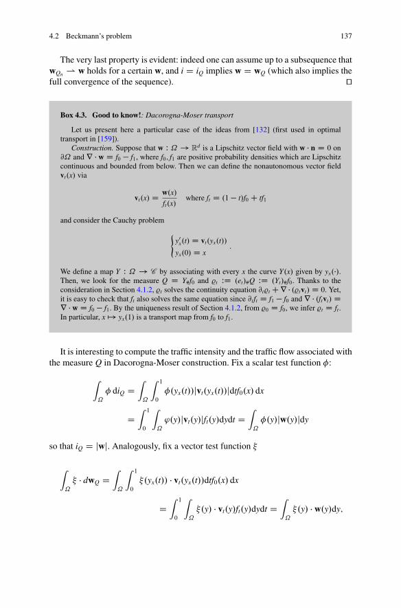
4.2 Beckmann’s problem 137

The very last property is evident: indeed one can assume up to a subsequence thatwQn * w holds for a certain w, and i D iQ implies w D wQ (which also implies thefull convergence of the sequence). ut

Box 4.3. Good to know!: Dacorogna-Moser transport

Let us present here a particular case of the ideas from [132] (first used in optimaltransport in [159]).

Construction. Suppose that w W ˝ ! Rd is a Lipschitz vector field with w � n D 0 on

@˝ and r � w D f0 � f1, where f0; f1 are positive probability densities which are Lipschitzcontinuous and bounded from below. Then we can define the nonautonomous vector fieldvt.x/ via

vt.x/ D w.x/ft.x/

where ft D .1� t/f0 C tf1

and consider the Cauchy problem

(y0

x.t/ D vt.yx.t//

yx.0/ D x:

We define a map Y W ˝ ! C by associating with every x the curve Y.x/ given by yx.�/.Then, we look for the measure Q D Y#f0 and %t WD .et/#Q WD .Yt/#f0. Thanks to theconsideration in Section 4.1.2, %t solves the continuity equation @t%t C r � .%tvt/ D 0. Yet,it is easy to check that ft also solves the same equation since @t ft D f1 � f0 and r � .ftvt/ Dr � w D f0 � f1. By the uniqueness result of Section 4.1.2, from %0 D f0, we infer %t D ft.In particular, x 7! yx.1/ is a transport map from f0 to f1.

It is interesting to compute the traffic intensity and the traffic flow associated withthe measure Q in Dacorogna-Moser construction. Fix a scalar test function �:

ˆ

˝

� diQ Dˆ

˝

ˆ 1

0

�.yx.t//jvt.yx.t//jdtf0.x/ dx

Dˆ 1

0

ˆ

˝

'.y/jvt.y/jft.y/dydt Dˆ

˝

�.y/jw.y/jdy

so that iQ D jwj. Analogously, fix a vector test function �

ˆ

˝

� � dwQ Dˆ

˝

ˆ 1

0

�.yx.t// � vt.yx.t//dtf0.x/ dx

Dˆ 1

0

ˆ

˝

�.y/ � vt.y/ft.y/dydt Dˆ

˝

�.y/ � w.y/dy;

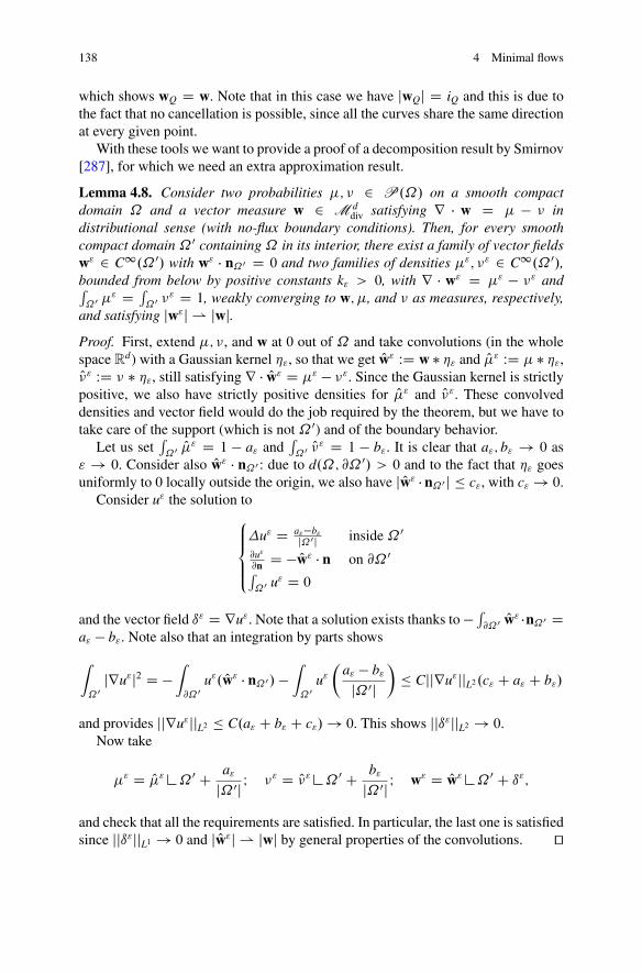
138 4 Minimal flows

which shows wQ D w. Note that in this case we have jwQj D iQ and this is due tothe fact that no cancellation is possible, since all the curves share the same directionat every given point.

With these tools we want to provide a proof of a decomposition result by Smirnov[287], for which we need an extra approximation result.

Lemma 4.8. Consider two probabilities �; � 2 P.˝/ on a smooth compactdomain ˝ and a vector measure w 2 M d

div satisfying r � w D � � � indistributional sense (with no-flux boundary conditions). Then, for every smoothcompact domain ˝ 0 containing ˝ in its interior, there exist a family of vector fieldsw" 2 C1.˝ 0/ with w" � n˝0 D 0 and two families of densities �"; �" 2 C1.˝ 0/,bounded from below by positive constants k" > 0, with r � w" D �" � �" and´˝0

�" D ´˝0

�" D 1, weakly converging to w; �, and � as measures, respectively,and satisfying jw"j * jwj.Proof. First, extend �; �, and w at 0 out of ˝ and take convolutions (in the wholespace Rd) with a Gaussian kernel �", so that we get Ow" WD w � �" and O�" WD � � �",O�" WD � � �", still satisfying r � Ow" D �" � �". Since the Gaussian kernel is strictlypositive, we also have strictly positive densities for O�" and O�". These convolveddensities and vector field would do the job required by the theorem, but we have totake care of the support (which is not ˝ 0) and of the boundary behavior.

Let us set´˝0

O�" D 1 � a" and´˝0

O�" D 1 � b". It is clear that a"; b" ! 0 as" ! 0. Consider also Ow" � n˝0 : due to d.˝; @˝ 0/ > 0 and to the fact that �" goesuniformly to 0 locally outside the origin, we also have j Ow" � n˝0 j � c", with c" ! 0.

Consider u" the solution to8<ˆ:�u" D a"�b"j˝0j inside ˝ 0@u"

@n D � Ow" � n on @˝ 0´˝0

u" D 0

and the vector field ı" D ru". Note that a solution exists thanks to � ´@˝0

Ow" �n˝0 Da" � b". Note also that an integration by parts shows

ˆ

˝0

jru"j2 D �ˆ

@˝0

u". Ow" � n˝0/ �ˆ

˝0

u"�

a" � b"j˝ 0j

�� Cjjru"jjL2 .c" C a" C b"/

and provides jjru"jjL2 � C.a" C b" C c"/ ! 0. This shows jjı"jjL2 ! 0.Now take

�" D O�" ˝ 0 C a"j˝ 0j I �" D O�" ˝ 0 C b"

j˝ 0j I w" D Ow" ˝ 0 C ı";

and check that all the requirements are satisfied. In particular, the last one is satisfiedsince jjı"jjL1 ! 0 and j Ow"j * jwj by general properties of the convolutions. ut

4.2 Beckmann’s problem 139

Remark 4.9. Note that considering explicitly the dependence on ˝ 0, it is alsopossible to obtain the same statement with a sequence of domains ˝ 0

" converging to˝ (for instance, in the Hausdorff topology). It is just necessary to choose them sothat setting t" WD d.˝; @˝ 0

"/, we have jj�"jjL1.B.0;t"/c/ ! 0. For the Gaussian kernel,this is satisfied whenever t2"=" ! 1 and can be guaranteed by taking t" D "1=3.

With these tools we can now prove

Theorem 4.10. For every finite vector measure w 2 M ddiv.˝/ and �; � 2 P.˝/

with r � w D � � �, there exists a traffic plan Q 2 P.C / with .e0/#Q D � and.e1/#Q D � such that jwQj D iQ � jwj, and jjw � wQjj C jjwQjj D jjw � wQjj CiQ.˝/ D jjwjj. In particular we have jwQj ¤ jwj unless wQ D w.

Proof. By means of Lemma 4.8 and Remark 4.9, we can produce an approximatingsequence .w"; �"; �"/ * .w; �; �/ of C1 functions supported on domains ˝"

converging to ˝. We apply Dacorogna-Moser’s construction to this sequence ofvector fields, thus obtaining a sequence of measures Q". We can consider thesemeasures as probability measures on C WD AC.˝ 0/ (where ˝ � ˝" � ˝ 0)which are, each, concentrated on curves valued in ˝". They satisfy iQ" D jw"jand wQ" D w". We can reparametrize by constant speed the curves on which Q" issupported, without changing traffic intensities and traffic flows. This means that weuse curves ! such that L.!/ D Lip.!/. The equalities

ˆ

CLip.!/ dQ".!/ D

ˆ

CL.!/ dQ".!/ D

ˆ

˝0

iQ" Dˆ

˝0

jw"j ! jwj.˝ 0/ D jwj.˝/

show that´C Lip.!/ dQ".!/ is bounded and hence Q" is tight (since the sets f! 2

C W Lip.!/ � Lg are compact). Hence, up to subsequences, we can assume Q" *

Q. The measure Q is obviously concentrated on curves valued in ˝. The measuresQ" were constructed so that .e0/#Q" D �" and .e1/#Q" D �", which implies, atthe limit, .e0/#Q D � and .e1/#Q D �. Moreover, thanks to Proposition 4.7, sinceiQ" D jw"j * jvj and wQ" * w, we get jwj � iQ � jwQj and jjw � wQjj �jwj.˝/� iQ.˝/. This gives jjw � wQjj C jjwQjj � jjw � wQjj C iQ.˝/ � jjwjj andthe opposite inequality jjwjj � jjw � wQjj C jjwQjj is always satisfied. ut

Remark 4.11. The previous statement contains a milder version of Theorem C in[287], i.e., the decomposition of any w into a cycle w � wQ (we call cycle alldivergence-free vector measures) and a flow wQ induced by a measure on paths,with jjwjj D jjw � wQjj C jjwQjj. The only difference with the theorem in [287]is the fact that it guarantees that one can choose Q concentrated on simple curves,which we did not take care of here (on the other hand, Ex(27) provides a partialsolution to this issue).

Remark 4.12. It is possible to guess what happens to a cycle through this construc-tion. Imagine the following example (as in Figure 4.1): ˝ is composed of two parts˝C and ˝�, with spt.�/ [ spt.�/ � ˝C and a cycle of w is contained in ˝�.

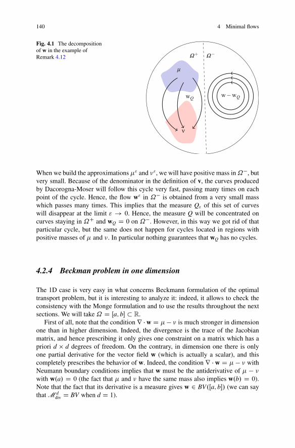
140 4 Minimal flows

Fig. 4.1 The decompositionof w in the example ofRemark 4.12

m

ν

wQw−wQ

W+ W−

When we build the approximations �" and �", we will have positive mass in˝�, butvery small. Because of the denominator in the definition of v, the curves producedby Dacorogna-Moser will follow this cycle very fast, passing many times on eachpoint of the cycle. Hence, the flow w" in ˝� is obtained from a very small masswhich passes many times. This implies that the measure Q" of this set of curveswill disappear at the limit " ! 0. Hence, the measure Q will be concentrated oncurves staying in ˝C and wQ D 0 on ˝�. However, in this way we got rid of thatparticular cycle, but the same does not happen for cycles located in regions withpositive masses of � and �. In particular nothing guarantees that wQ has no cycles.

4.2.4 Beckman problem in one dimension

The 1D case is very easy in what concerns Beckmann formulation of the optimaltransport problem, but it is interesting to analyze it: indeed, it allows to check theconsistency with the Monge formulation and to use the results throughout the nextsections. We will take ˝ D Œa; b� � R.

First of all, note that the condition r � w D �� � is much stronger in dimensionone than in higher dimension. Indeed, the divergence is the trace of the Jacobianmatrix, and hence prescribing it only gives one constraint on a matrix which has apriori d � d degrees of freedom. On the contrary, in dimension one there is onlyone partial derivative for the vector field w (which is actually a scalar), and thiscompletely prescribes the behavior of w. Indeed, the condition r � w D � � � withNeumann boundary conditions implies that w must be the antiderivative of � � �

with w.a/ D 0 (the fact that � and � have the same mass also implies w.b/ D 0).Note that the fact that its derivative is a measure gives w 2 BV.Œa; b�/ (we can saythat M d

div D BV when d D 1).

4.2 Beckmann’s problem 141

Box 4.4. Memo: Bounded variation functions in one variable

BV functions are defined as L1 functions whose distributional derivatives are measures.In dimension one this has a lot of consequences. In particular these functions coincidea.e. with functions which have bounded total variation in a pointwise sense: for each f WŒa; b� ! R, define

TV.f I Œa; b�/ WD sup

(N�1XiD0

jf .tiC1/ � f .ti/j W a D t0 < t1 < t2 < � � � < tN D b

):

Functions of bounded variation are defined as those f such that TV.f I Œa; b�/ < 1. Itis easy to check that BV functions form a vector space and that monotone functions areBV (indeed, if f is monotone, we have TV.f I Œa; b�/ D jf .b/ � f .a/j. Lipschitz functionsare also BV and TV.f I Œa; b�/ � Lip.f /.b � a/. On the other hand, continuous functionsare not necessarily BV (but absolutely continuous functions are BV), nor it is the case fordifferentiable functions (obviously, C1 functions, which are Lipschitz on bounded intervals,are BV). As an example one can consider

f .x/ D(

x2 sin�1x2

if x ¤ 0

0 for x D 0;

which is differentiable everywhere but not BV.On the other hand, BV functions have several properties.Properties of BV functions in R. If TV.f I Œa; b�/ < 1, then f is the difference of two

monotone functions (in particular we can write f .x/ D TV.f I Œa; x�/ � .TV.f I Œa; x�/ �f .x//, both terms being nondecreasing functions); it is a bounded function and sup f �inf f � TV.f I Œa; b�/; it has the same continuity and differentiability properties of monotonefunctions (it admits left and right limits at every point; it is continuous up to a countable setof points and differentiable a.e.).

In particular, in 1D, we have BV � L1 which is not the case in higher dimension (ingeneral, we have BV � Ld=.d�1/).

We finish by stressing the connections with measures: for every positive measure � onŒa; b�, we can build a monotone function by taking its cumulative distribution function,i.e., F�.x/ D �.Œa; x�/, and the distributional derivative of this function is exactly themeasure �. Conversely, every monotone increasing function on a compact interval is thecumulative distribution function of a (unique) positive measure, and every BV function isthe cumulative distribution function of a (unique) signed measure.

As a consequence, we have the following facts:

• In dimension one, there is only one competitor w which is given by w D F��F�with F�.x/ D �.Œa; x�/ and F�.x/ D �.Œa; x�/.

• This field w belongs to BV.Œa; b�/ and hence to every Lp space, including L1.• Possible higher regularity of w depends on the regularity of �� � (for instance,

we have w 2 W1;p whenever �; � 2 Lp).• The minimal cost in Beckmann’s problem is given by jjF� � F� jjL1 , which is

consistent with Proposition 2.17.

142 4 Minimal flows

• The transport density � , characterized by w D �u0 � � , is given by � D jwjand shares the same summability properties of w; it also belongs to BV as acomposition of a BV function with the absolute value function.

4.2.5 Characterization and uniqueness of the optimal w

In this section we will show two facts: first we prove that the optimal w in the(BP) always comes from an optimal transport plan � , and then we prove that all theoptimal � give the same wŒ�� and the same �� , provided one of the two measures isabsolutely continuous.

Theorem 4.13. Let w be optimal in (BP): then there is an optimal transport plan �such that w D wŒ��.

Proof. Thanks to Theorem 4.10, we can find a measure Q 2 P.C / with .e0/#Q D� and .e1/#Q D � such that jwj � jwQj. Yet, the optimality of w implies theequality jwj D jwQj and the same Theorem 4.10 gives in such a case w D wQ, aswell as jwj D iQ. We can assume Q to be concentrated on curves parametrized byconstant speed. Define S W ˝ � ˝ ! C the map associating with every pair .x; y/the segment !x;y parametrized with constant speed: !x;y.t/ D .1 � t/x C ty. Thestatement is proven if we can prove that Q D S#� with � an optimal transport plan.

Indeed, using again the optimality of w and Theorem 4.10, we get

min .BP/ D jwj.˝/ D iQ.˝/ Dˆ

CL.!/ dQ.!/ �

ˆ

Cj!.0/ � !.1/j dQ.!/

Dˆ

˝�˝jx � yj d..e0; e1/#Q/.x; y/ � min .KP/:

The equality min .BP/ D min .KP/ implies that all these inequalities are equalities.In particular Q must be concentrated on curves such that L.!/ D j!.0/�!.1/j, i.e.,segments. Also, the measure .e0; e1/#Q, which belongs to˘.�; �/, must be optimalin (KP). This concludes the proof. ut

The proof of the following result is essentially taken from [8].

Theorem 4.14. If� � L d, then the vector field wŒ�� does not depend on the choiceof the optimal plan � .

Proof. Let us fix a Kantorovich potential u for the transport between � and �.This potential does not depend on the choice of � . It determines a partition intotransport rays: Corollary 3.8 guarantees that the only points of ˝ which belong toseveral transport rays are non-differentiability points for u and are hence Lebesgue-negligible. Let us call S the set of points which belong to several transport rays: wehave �.S/ D 0, but we do not suppose �.S/ D 0 (� is not supposed to be absolutelycontinuous). However, � is concentrated on .�x/

�1.Sc/. We can then disintegrate

4.2 Beckmann’s problem 143

(see Section 2.3) � according to the transport ray containing the point x. Moreprecisely, we define a map R W ˝ � ˝ ! R, valued in the set R of all transportrays, sending each pair .x; y/ into the ray containing x. This is well-defined � -a.e.and we can write � D � r ˝ �, where � D R#� , and we denote by r the variablerelated to transport rays. Note that, for a.e. r 2 R, the plan � r is optimal betweenits own marginals (otherwise we could replace it with an optimal plan, do it in ameasurable way, and improve the cost of � ).

The measure wŒ�� may also be obtained through this disintegration, and we havewŒ�� D w� r ˝ �. This means that in order to prove that wŒ�� does not depend on� , we just need to prove that each w� r and the measure � do not depend on it. Forthe measure � this is easy: it has been obtained as an image measure through a maponly depending on x and hence only depends on �. Concerning w� r , note that it isobtained in the standard Beckmann way from an optimal plan, � r. Hence, thanksto the considerations in Section 4.2.4 about the 1D case, it uniquely depends on themarginal measures of this plan.

This means that we only need to prove that .�x/#�r and .�y/#�

r do not dependon � . Again, this is easy for .�x/#�

r, since it must coincide with the disintegrationof � according to the map R (by uniqueness of the disintegration). It is more delicatefor the second marginal.

The second marginal �r WD .�y/#�r will be decomposed into two parts:

.�y/#.�rj˝�S/ C .�y/#.�

rj˝�Sc/:

This second part coincides with the disintegration of �jSc , which obviously does notdepend on � (since it only depends on the set S, which is built upon u).

We need now to prove that �rjS D .�y/#.�

rj˝�S/ does not depend on � . Yet, this

measure can only be concentrated on the two endpoints of the transport ray r, sincethese are the only points where different transport rays can meet. This means thatthis measure is purely atomic and composed by at most two Dirac masses. Notonly the endpoint where u is maximal (i.e., the first one for the order on the ray; seeSection 3.1) cannot contain any mass of �: indeed the transport must follow a precisedirection on each transport ray (as a consequence of u.x/�u.y/ D jx�yj on spt.�/),and the only way to have some mass of the target measure at the “beginning” of thetransport ray would be to have an atom for the source measure as well. Yet, � isabsolutely continuous and Property N holds (see Section 3.1.4 and Theorem 3.12,which means that the set of rays r where �r has an atom is negligible). Hence �r

jSis a single Dirac mass. The mass equilibrium condition between �r and �r impliesthat the value of this mass must be equal to the difference 1 � �r

jSc.r/, and this lastquantity does not depend on � but only on � and �.

Finally, this proves that each w� r does not depend on the choice of � . utCorollary 4.15. If � � L d, then the solution of (BP) is unique.

Proof. We have seen in Theorem 4.13 that any optimal w is of the form wŒ�� and inTheorem 4.14 that all the fields wŒ�� coincide. ut

144 4 Minimal flows

4.3 Summability of the transport density

The analysis of the Beckmann problem performed in the previous sections wasmainly made in a measure setting, and the optimal w and the transport density �were just measures on ˝. We investigate here the question whether they have extraregularity properties supposing extra assumptions on � and/or �.

We will give summability results, proving that � is in some cases absolutelycontinuous and providing Lp estimates. The proofs are essentially taken from [273](also look at [61, 166]): previous results, through very different techniques, werefirst presented in [143–145]. In these papers, different estimates on the “dimension”of � were also presented, thus giving interesting information should � fail to beabsolutely continuous. Let us also observe that [208], while applying these tools toimage processing problems, contains a new4 proof of absolute continuity.

Note that higher-order questions (such as whether � is continuous or Lipschitzor more regular provided � and � have smooth densities) are completely open upto now. The only exception is a partial result in dimension 2 (see [171]), wherea continuity result is given if � and � have Lipschitz densities on disjoint convexdomains.

Open Problem (continuity of the transport density): Is it true that, supposingthat �; � have continuous densities, the transport density � is also continuous? Is ittrue that it is Lipschitz if they are Lipschitz, and/or Hölder if they are Hölder?

In all that follows ˝ is a compact and convex domain in Rd, and two probability

measures �; � are given on it. At least one of them will be absolutely continuous,which implies uniqueness for � (see Theorem 4.14). The first result – first proven in[162] – will concern L1 summability (i.e., absolute continuity).

Theorem 4.16. Suppose ˝ � Rd is a convex domain, and � � L d. Let � be the

transport density associated with the transport of � onto �. Then � � L d.

Proof. Let � be an optimal transport plan from � to � and take � D �� ; call �t

the standard interpolation between the two measures: �t D .�t/#� where �t.x; y/ D.1 � t/x C ty. We have �0 D � and �1 D �.

We have already seen (go back to (4.6)) that the transport density � may bewritten as

� Dˆ 1

0

.�t/#.c � �/dt;

where c W ˝ �˝ ! R is the cost function c.x; y/ D jx � yj (hence c � � is a positivemeasure on ˝ �˝).

4Their proof is somehow intermediate between that of [143] and the one we present here: indeed,approximation by atomic measures is also performed in [208], as here, but on both the source andthe target measure, which requires a geometric analysis of the transport rays as in [143].

4.3 Summability of the transport density 145

Since ˝ is bounded, it is evident that we have

� � Cˆ 1

0

�t dt: (4.11)

To prove that � is absolutely continuous, it is sufficient to prove that almost everymeasure �t is absolutely continuous, so that, whenever jAj D 0, we have �.A/ �C´ 10�t.A/dt D 0.

We will prove �t � L d for t < 1. First, we will suppose that � is finitelyatomic (the point .xi/iD1;:::;N being its atoms). In this case we will choose � to be anyoptimal transport plan induced by a transport map T (which exists, since � � L d).Note that the absolute continuity of � is an easy consequence of the behavior of theoptimal transport from � to � (which is composed by N homotheties), but we alsowant to quantify this absolute continuity, in order to go on with an approximationprocedure.

Remember that � is absolutely continuous and hence there exists a correspon-dence " 7! ı D ı."/ such that

jAj < ı."/ ) �.A/ < ": (4.12)

Take now a Borel set A and look at �t.A/. The domain ˝ is the disjoint union of afinite number of sets ˝i D T�1.fxig/. We call ˝i.t/ the images of ˝i through themap x 7! .1 � t/x C tT.x/ (Figure 4.2). These sets are essentially disjoint. Why?Because if a point z belongs to ˝i.t/ and ˝j.t/, then two transport rays cross at z,the one going from x0

i 2 ˝i to xi and the one from x0j 2 ˝j to xj. The only possibility

is that these two rays are actually the same, i.e., that the five points x0i; x0

j; z; xi; xj

are aligned. But this implies that z belongs to one of the lines connecting two atomsxi and xj. Since we have finitely many of these lines, this set is negligible. Note thatthis argument only works for d > 1 (we will not waste time on the case d D 1, sincethe transport density is always a BV , and hence bounded, function). Moreover, if westicked to the ray-monotone optimal transport map, we could have actually provedthat these sets are truly disjoint, with no negligible intersection.

Now we have

�t.A/ DX

i

�t.A \˝i.t// DX

i

�0

�A \˝i.t/ � txi

1 � t

�D �0

[i

A \˝i.t/ � txi

1 � t

!:

Since for every i we haveˇˇA \˝i.t/ � txi

1 � t

ˇˇ D 1

.1 � t/djA \˝i.t/j ;

we obtain ˇˇ[

i

A \˝i.t/ � txi

1 � t

ˇˇ � 1

.1 � t/djAj:

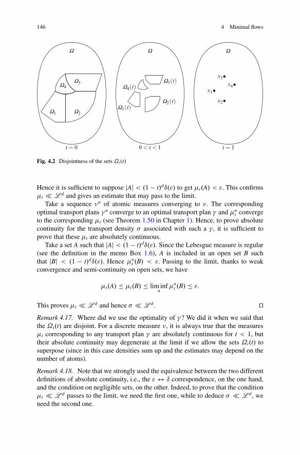
146 4 Minimal flows

x2•x1•

x4•x3•

t = 0 0< t < 1 t = 1

W1 W2

W3W4

W1(t)W2(t)

W3(t)W4(t)

W W W

Fig. 4.2 Disjointness of the sets ˝i.t/

Hence it is sufficient to suppose jAj < .1 � t/dı."/ to get �t.A/ < ". This confirms�t � L d and gives an estimate that may pass to the limit.

Take a sequence �n of atomic measures converging to �. The correspondingoptimal transport plans �n converge to an optimal transport plan � and �n

t convergeto the corresponding �t (see Theorem 1.50 in Chapter 1). Hence, to prove absolutecontinuity for the transport density � associated with such a � , it is sufficient toprove that these �t are absolutely continuous.

Take a set A such that jAj < .1 � t/dı."/. Since the Lebesgue measure is regular(see the definition in the memo Box 1.6), A is included in an open set B suchthat jBj < .1 � t/dı."/. Hence �n

t .B/ < ". Passing to the limit, thanks to weakconvergence and semi-continuity on open sets, we have

�t.A/ � �t.B/ � lim infn

�nt .B/ � ":

This proves �t � L d and hence � � L d. utRemark 4.17. Where did we use the optimality of �? We did it when we said thatthe ˝i.t/ are disjoint. For a discrete measure �, it is always true that the measures�t corresponding to any transport plan � are absolutely continuous for t < 1, buttheir absolute continuity may degenerate at the limit if we allow the sets ˝i.t/ tosuperpose (since in this case densities sum up and the estimates may depend on thenumber of atoms).

Remark 4.18. Note that we strongly used the equivalence between the two differentdefinitions of absolute continuity, i.e., the " $ ı correspondence, on the one hand,and the condition on negligible sets, on the other. Indeed, to prove that the condition�t � L d passes to the limit, we need the first one, while to deduce � � L d, weneed the second one.

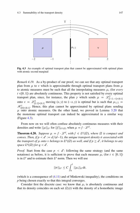
4.3 Summability of the transport density 147

−2 −1 1 2

T

m νm1/2

Fig. 4.3 An example of optimal transport plan that cannot be approximated with optimal planswith atomic second marginal

Remark 4.19. As a by-product of our proof, we can see that any optimal transportplan from � to � which is approximable through optimal transport plans from �

to atomic measures must be such that all the interpolating measures �t (for everyt 2�0; 1Œ) are absolutely continuous. This property is not satisfied by every optimaltransport plan, since, for instance, the plan � which sends � D L 2

jŒ�2;�1��Œ0;1�onto � D L 2

jŒ1;2��Œ0;1� moving .x; y/ to .�x; y/ is optimal but is such that �1=2 DH 1

jf0g�Œ0;1�. Hence, this plan cannot be approximated by optimal plans sending� onto atomic measures. On the other hand, we proved in Lemma 3.20 thatthe monotone optimal transport can indeed be approximated in a similar way(Figure 4.3).

From now on we will often confuse absolutely continuous measures with theirdensities and write jj�jjLp for jjf jjLp.˝/ when � D f � L d.

Theorem 4.20. Suppose � D f � L d, with f 2 Lp.˝/, where ˝ is compact andconvex. Then, if p < d0 WD d=.d�1/, the unique transport density � associated withthe transport of � onto � belongs to Lp.˝/ as well, and if p � d0, it belongs to anyspace Lq.˝/ for q < d0.

Proof. Start from the case p < d0: following the same strategy (and the samenotations) as before, it is sufficient to prove that each measure �t (for t 2 Œ0; 1Œ)is in Lp and to estimate their Lp norm. Then we will use

jj� jjLp � Cˆ 1

0

jj�tjjLp dt;

(which is a consequence of (4.11) and of Minkowski inequality), the conditions onp being chosen exactly so that this integral converges.

Consider first the discrete case: we know that �t is absolutely continuous andthat its density coincides on each set ˝i.t/ with the density of a homothetic image

148 4 Minimal flows

of � on ˝i, the homothetic ratio being .1 � t/. Hence, if ft is the density of �t, wehave

ˆ

˝

ft.x/p dx D

Xi

ˆ

˝i.t/ft.x/

p dx DX

i

ˆ

˝i

�f .x/

.1 � t/d

�p

.1 � t/d dx

D .1 � t/d.1�p/X

i

ˆ

˝i

f .x/p dx D .1 � t/d.1�p/ˆ

˝

f .x/p dx:

We get jj�tjjLp D .1 � t/�d=p0 jj�jjLp , where p0 D p=.p � 1/.This inequality, which is true in the discrete case, stays true at the limit as well.

If � is not atomic, approximate it through a sequence �n1 and take optimal plans

�n and interpolating measures �nt . Up to subsequences we have �n * � (for an

optimal transport plan � ) and �nt * �t (for the corresponding interpolation); by

semi-continuity, we have

jj�tjjLp � lim infn

jj�nt jjLp � .1 � t/�d=p0 jj�0jjLp

and we deduce

jj� jjLp � Cˆ 1

0

jj�tjjLp dt � Cjj�0jjLp

ˆ 1

0

.1 � t/�d=p0

dt:

The last integral is finite whenever p0 > d, i.e., p < d0 D d=.d�1/.The second part of the statement (the case p � d0) is straightforward once one

considers that any density in Lp also belongs to any Lq space for q < p. utExample 4.21. We can see an example where, even if � 2 L1, the singularityof � prevents � from being Ld0

. Consider � D f � L d with f D 1A and A DB.0;R/ n B.0;R=2/ (with R chosen so that

´f D 1), and take � D ı0. Note that

R2� � c � � � R� , which implies that the summability of � D ´ 1

0.�t/#.c � �/dt

is the same as that of´ 10.�t/#.�/dt D ´ 1

0�t dt. We have �t D ft � L d, with ft D

.1 � t/�d1.1�t/A; hence

ˆ 1

0

ft.x/ dt Dˆ 2

R jxj1R jxj

1

sdds D cjxj1�d for jxj � R

2

(where we used the change of variable s D 1 � t). This function belongs to Lp in aneighborhood of 0 in dimension d only if we have .1 � d/p C .d�1/ > �1, i.e., if.d�1/.p � 1/ < 1. This is exactly p < d0.

We saw in the previous theorems that the measures �t inherit some regularity(absolute continuity or Lp summability) from � exactly as it happens for homoth-eties of ratio 1 � t. This regularity degenerates as t ! 1, but we saw two caseswhere this degeneracy produced no problem: for proving absolute continuity, where

4.3 Summability of the transport density 149

the separate absolute continuous behavior of almost all the �t was sufficient, andfor Lp estimates, provided the degeneracy stays integrable.

It is natural to try to exploit another strategy: suppose both � and � share someregularity assumption (e.g., they belong to Lp). Then we can give estimate on �t fort � 1=2 starting from � and for t � 1=2 starting from �. In this way we have nodegeneracy!

This strategy works quite well, but it has an extra difficulty: in our previousestimates, we didn’t know a priori that �t shared the same behavior of piecewisehomotheties of �; we got it as a limit from discrete approximations. And, when wepass to the limit, we do not know which optimal transport � will be selected as alimit of the optimal plans �n. This was not important in the previous section, sinceany optimal � induces the same transport density � . But here we would like to gluetogether estimates on �t for t � 1=2which have been obtained by approximating �1and estimates on �t for t � 1=2 which come from the approximation of �0. Shouldthe two approximations converge to two different transport plans, we could not puttogether the two estimates and deduce anything on � .

Hence, the main technical issue that we need to consider is proving that oneparticular optimal transport plan, i.e., the ray-monotone one, can be approximatedin both directions. Lemma 3.20 exactly does the job (and, indeed, it was provenin [273] exactly for this purpose). Yet, the transport plans �" we build in theapproximation are not optimal for the cost jx�yj but for some costs jx�yjC"jx�yj2.We need to do this in order to force the selected limit optimal transport to be themonotone one (through a secondary variational problem, say). Anyway, this willnot be an issue: these approximating optimal transport plans will share the samegeometric properties that will imply disjointness for the sets ˝i.t/. In particular, wecan prove the following estimate.

Lemma 4.22. Let � be an optimal transport plan between � and an atomicmeasure � for a transport cost c.x; y/ D h.y � x/ where h W R

d ! R is astrictly convex function. Set as usual �t D .�t/#� . Then we have jj�tjjLp �.1 � t/�d=p0 jj�jjLp .

Proof. The result is exactly the same as in Theorem 4.20, where the key tool is thefact that �t coincides on every set ˝i.t/ with a homothety of �0. The only fact thatmust be checked again is the disjointness of the sets ˝i.t/.

To do so, take a point x 2 ˝i.t/\˝j.t/: Hence there exist xi; xj belonging to ˝i

and ˝j, respectively, so that x D .1 � t/xi C tyi D .1 � t/xj C tyj, being yi D T.xi/

and yj D T.xj/ two atoms of �. But this would mean that Tt WD .1 � t/id C tT isnot injective, which is a contradiction to the following Lemma 4.23. Hence the sets˝i.t/ are disjoint and this implies the bound on �t. utLemma 4.23. Let � be an optimal transport plan between � and � for a transportcost c.x; y/ D h.y � x/ where h W Rd ! R is a strictly convex function, and supposethat it is induced by a transport map T. Choose a representative of T such that.x;T.x// 2 spt.�/ for all x. Then the map x 7! .1 � t/x C tT.x/ is injective fort 2�0; 1Œ.

150 4 Minimal flows

Proof. Suppose that there exist x ¤ x0 such that

.1 � t/x C tT.x/ D .1 � t/x0 C tT.x0/ D x0:

Set a D T.x/� x and b D T.x0/� x0. This also means x D x0 � ta and x0 D x0 � tb.In particular, x ¤ x0 implies a ¤ b.

The c-cyclical monotonicity of the support of the optimal � implies

h.a/C h.b/ � h.T.x0/ � x/C h.T.x/ � x0/ D h.tb C .1 � t/a/C h.ta C .1 � t/b/:

Yet, a ¤ b, and strict convexity implies

h.tbC.1� t/a/Ch.taC.1� t/b/ < th.b/C.1� t/h.a/Cth.a/C.1� t/h.b/ D h.a/Ch.b/;

which is a contradiction. utTheorem 4.24. Suppose that � and � are probability measures on˝, both belong-ing to Lp.˝/, and � the unique transport density associated with the transport of �onto �. Then � belongs to Lp.˝/ as well.

Proof. Let us consider the optimal transport plan � from � to � defined by (3.4). Weknow that this transport plan may be approximated by plans �" which are optimalfor the cost jx � yj C "jx � yj2 from � to some discrete atomic measures �". Thecorresponding interpolation measures �"t satisfy the Lp estimate from Lemma 4.22and, at the limit, we have

jj�tjjLp � lim inf"!0

jj�"t jjLp � .1 � t/�d=p0 jj�jjLp :

The same estimate may be performed from the other direction, since the very sametransport plan � may be approximated by optimal plans for the cost jx�yjC"jx�yj2from atomic measures to �. Putting together the two estimates, we have

jj�tjjLp � minn.1 � t/�d=p0 jj�jjLp ; t�d=p0 jj�jjLp

o� 2d=p0

max fjj�jjLp ; jj�jjLpg :

Integrating these Lp norms, we get the bound on jj� jjLp . utRemark 4.25. The same result could have been obtained in a strongly differentway, thanks to the displacement convexity of the functional � 7! jj�jjpLp . Thisfunctional is actually convex along geodesics in the space Wq.˝/ for q > 1

(see Proposition 7.29 where, unfortunately, the notation for p and q is reversed).Then we pass to the limit as q ! 1: this gives the result on the interpolatingmeasures corresponding to the optimal plan which is obtained as a limit of the Kq-optimal plans. This plan is, by the way, � again. And the integral estimate comesstraightforward. Yet, this requires more sophisticated tools than what developedso far.

4.4 Discussion 151

Example 4.26. We can provide examples (in dimension higher than one) where thesummability of � is no more than that of � and �. Take, for instance, � D f �L d and� D g � L d with f .x1; x2; : : : ; xd/ D f0.x2; : : : xd/1Œ0;1�.x1/ and g.x1; x2; : : : ; xd/ Df0.x2; : : : xd/1Œ4;5�.x1/. It is not difficult to check that the transport rays in thisexample go in the direction of the first coordinate vector and that the optimal �is absolutely continuous with density given by �.x/ D f0.x2; : : : xd/s.x1/, wheres W R ! RC is characterized by s0 D 1Œ0;1� � 1Œ4;5�, s.0/ D s.5/ D 0 (which comesfrom the fact that s would be the transport density for the 1D transport between 1Œ0;1�and 1Œ4;5�). Hence, from s D 1 on Œ1; 4�, one sees that the summability of � is thesame of that of f0, which is also the same of those of f and g.

4.4 Discussion

4.4.1 Congested transport

As we saw in Section 4.2, Beckmann’s problem can admit an easy variant if weprescribe a positive function k W ˝ ! RC, where k.x/ stands for the local costat x per unit length of a path passing through x. This models the possibility thatthe metric is nonhomogeneous, due to geographical obstacles given a priori. Yet, ithappens in many situations, in particular in urban traffic (as many readers probablynote every day), that this metric k is indeed nonhomogeneous, but is not given apriori: it depends on the traffic itself. In Beckmann’s language, we must look for avector field w optimizing a transport cost depending on w itself!

The easiest model, chosen by Beckmann (see [27] and later [110]), is to considerthe same framework as (BP) but supposing that k.x/ D g.jw.x/j/ is a function ofthe modulus of the vector field w. This is quite formal for the moment (for instance,it is not meaningful if w is a measure, but we will see that in this case we can usebetter spaces than M d

div). In this case we would like to solve

min

�ˆH .w.x// dx W r � w D � � �

�; (4.13)

where H .z/ D H.jzj/ and H.t/ D g.t/t. Note that if H is superlinear (if g.t/ tends to1 as t ! 1, i.e., if the congestion effect becomes stronger and stronger when thetraffic increases), this problem is well-posed in the class of vector fields w 2 L1. Forinstance, if g.t/ D t, which is the easiest case one can imagine, we must minimizethe L2 norm under divergence constraints:

min

�ˆjw.x/j2 dx W w 2 L2.˝IRd/; r � w D � � �

�:

This problem is easily solvable since one can see that the optimal w must be agradient (we will develop this computation in a more general framework later), and

152 4 Minimal flows

setting w D ru one gets �u D � � �. This is complemented with Neumannboundary conditions and allows to find u and then w.

We want now to discuss the meaning and pertinence of this model, keeping intoaccount the following natural questions:

• is it correct that the coefficient k depends on jwj, or should it rather depend onother traffic quantities, such as iQ? (note that w can have cancellations);

• what is the connection with equilibrium issues? In traffic congestion, typicallyevery agent decides alone which path to choose, and the final traffic intensityis rather the output of a collection of individual choices and not the result of aglobal optimization made by a single planner;

• is the example g.t/ D t a good choice in the modeling ? This implies g.0/ D 0,i.e., no cost where there is not traffic.

To start our analysis, we would like to present first an equilibrium model developedby Wardrop, [295], on a discrete network.

Traffic equilibria on a finite network

The main data of the model are a finite-oriented connected graph G D .N;E/modeling the network, and some travel times functions ge: � 2 RC 7! ge.�/ giving,for each edge e 2 E, the travel time on e when the flow on e is � . The functions ge

are all nonnegative, continuous, and nondecreasing, and they are meant to capturethe congestion effects (which may be different on the different edges, since someroads may be longer or wider and may have different responses to congestion). Thelast ingredient of the problem is a transport plan on pairs of nodes .x; y/ 2 N2

interpreted as pairs of origins/destinations. We denote by .�x;y/.x;y/2N2 this transportplan: �x;y represents the “mass” to be sent from x to y. We denote by Cx;y the set ofsimple paths on the graph G connecting x to y, so that C WD [.x;y/2N2Cx;y is the setof all simple paths. A generic path will be denoted by ! and we will use the notatione 2 ! to indicate that the path ! uses the edge e.

The unknown of the problem is the flow configuration. The edge flows aredenoted by i D .ie/e2E and the path flows are denoted by q D .q!/!2C: this meansthat ie is the total flow on edge e and q! is the mass traveling on !. Of coursethe values ie and q! are nonnegative and constrained by the mass conservationconditions:

�x;y DX!2Cx;y

q!; 8.x; y/ 2 N2 (4.14)

and

ie DX

!2C W e2!q!; 8e 2 E; (4.15)

4.4 Discussion 153

which means that i is a function of q. Given the edge flows i D .ie/e2E, the total cost(to be interpreted as a sort of weighted length) of the path ! 2 C is

Li.!/ DXe2!

ge.ie/: (4.16)

In [295], Wardrop defined a notion of noncooperative equilibrium that has beenvery popular since then among engineers working in the field of congested transportand that may be described as follows. Roughly speaking, a Wardrop equilibrium isa flow configuration such that every actually used path should be an optimal pathfor the cost Li defined in (4.16). This leads to

Definition 4.27. A Wardrop equlibrium5 is a flow configuration q D .q!/!2C

satisfying q! � 0 and the mass conservation constraints (4.14), such that whenwe compute the values ie with (4.15), for every .x; y/ 2 N2 and every ! 2 Cx;y withq! > 0, we have

Li.!/ D min!02Cx;y

Li.!0/:

A few years after the introduction of this notion by Wardrop, Beckmann,McGuire, and Winsten [29] realized that Wardrop equilibria can be characterizedby the following variational principle:

Theorem 4.28. The flow configuration q D .q!/!2C is a Wardrop equilibrium ifand only if it solves the convex minimization problem

min

(Xe2E

He.ie/ W q � 0 satisfies (4.14)

)(4.17)

where, for each e, we define He to be an antiderivative of ge: H0e D ge.

Proof. Assume that q D .q!/!2C (with associated edge flows .ie/e2E) is optimalfor (4.17). Then, for every admissible � D .�!/!2C with associated (through (4.15))edge-flows .je/e2E, one has

0 �Xe2E

H0e.ie/.je � ie/ D

Xe2E

ge.ie/X

!2C W e2!.�! � q!/

DX!2C

.�! � q!/Xe2!

ge.ie/;

5Note that this is just an example of Nash equilibrium with a continuum of players, as we will seein Section 7.4.3 and, more particularly, in Box 7.3.

154 4 Minimal flows

so that

X!2C

q!Li.!/ �X!2C

�!Li.!/: (4.18)

Minimizing the right-hand side thus yields

X.x;y/2N2

X!2Cx;y

q!Li.!/ DX

.x;y/2N2

�x;y min!02Cx;y

Li.!0/;

which exactly says that q is a Wardrop equilibrium. To prove the converse, it isenough to see that problem (4.17) is convex so that the inequality (4.18) is indeedsufficient, and not only necessary, for a global minimum. ut

The previous characterization allows to deduce for free existence results but alsouniqueness for i (not for q) as soon as the functions ge are strictly increasing (so thatthe He are strictly convex).

Remark 4.29. It would be very tempting to deduce from Theorem 4.28 that equilib-ria are efficient since they are minimizers of (4.17). Yet, the quantity

Pe2E He.ie/

does not represent the natural total social cost measured by the total time lost incommuting which would rather be

Xe2E

iege.ie/: (4.19)

In general, �ge.�/ D He.�/ and ge D H0e are very different conditions. The efficient

transport patterns are minimizers of (4.19) and thus are different from equilibria ingeneral. Efficient and equilibria configurations coincide in the special case of powerfunctions where He.�/ D ae�

p. Yet, we must note that this case is not realistic since,for p > 1, it implies ge.0/ D 0. This means that traveling times vanish if there isno traffic, while one should expect a residual nonzero cost even without traffic.Moreover, a famous counterexample due to Braess (see [76]) shows that it may bethe case that adding an extra road with very small cost on which the traveling timeis always zero leads to an equilibrium where the total commuting time is increased!This illustrates the striking difference between efficiency and equilibrium, a topicwhich is very well documented in the finite-dimensional network setting where itis frequently associated with the literature on the so-called price of anarchy (see[266]).

Remark 4.30. In the problem presented in this paragraph, the transport plan � isfixed. This may be interpreted as a short-term problem. Instead, we could considerthe long-term problem where only the distribution of origins � and of destinations� is fixed. In this case, one also obtains as an optimality condition that � is efficient,in the sense that it minimizes among transport plans in ˘.�; �/, the total cost

4.4 Discussion 155

X�x;ydi.x; y/ with di.x; y/ WD min

!2Cx;yLi.!/:

In the long-term problem where one is allowed to change the assignment as well,equilibria still are characterized by a convex minimization problem, i.e., the sameabove, where one also optimizes over � .

Optimization and equilibrium in a continuous framework

If we want to generalize the previous analysis to a continuous framework6, wewill formulate the whole path-dependent transport pattern in terms of a probabilitymeasure Q on the set of paths (this is the continuous analogue of the path flows.q!/! of the previous paragraph). Then, we will measure the traffic intensitygenerated by Q at every point x by using the measure iQ of Section 4.2.3 (this is thecontinuous analogue of the arc flows .ie/e of the previous paragraph). The last andmain idea will be to model the congestion effects through a metric that is monotoneincreasing in the traffic intensity (the analogue of ge.ie/).

Avoiding technicalities and choosing an informal presentation (see [112] formore details), we take ˝ a domain in R

d (typically, d D 2) and

• either two probability measures � and � (distribution of sources and destina-tions) on ˝ in the case of the long-term problem,

• or a transport plan � (joint distribution of sources and destinations, i.e., a jointprobability on ˝ �˝) in the short-term case,

• or more generally a convex and closed subset � � ˘.�; �/, and we accept any� 2 � (this is just a common mathematical framework for the two previouscases, where we can take � D f�g or � D ˘.�; �/).

We will use the notations of Section 4.2.3 and use probability measures Q onC WD AC.˝/, compatible with mass conservation, i.e., such that .e0; e1/#Q 2 � .We shall denote by Q.� / the set of admissible Q.

The traffic intensity associated with Q 2 Q.� / is by definition the measure iQdefined in Section 4.2.3 and congestion effects are captured by the metric associatedwith Q: suppose iQ � L d and set

kQ.x/ WD g.x; iQ.x//

for a given increasing function g.x; :/: RC ! RC. The fact that there exists at leastone Q 2 Q.� / such that iQ � L d is not always true and depends on � . We willsee later how to guarantee it7.

In order to define the notion of Wardrop equilibrium in this continuous case, letus define

6For a survey on the continuous framework, see also [111].7Note that, even for � D f�g (which is the most restrictive case), assuming �; � 2 L1,considerations from incompressible fluid mechanics in [83] allow to build a Q such that iQ 2 L1.

156 4 Minimal flows

LkQ.!/ Dˆ 1

0

g.!.t/; iQ.!.t//j!0.t/jdt

and

dkQ.x; y/ WD inf!2C ;!.0/Dx;!.1/Dy

LkQ.!/:

Paths in C such that dkQ.!.0/; !.1// D LkQ.!/ are called geodesics (for the metricinduced by the congestion effect generated by Q).

We can define

Definition 4.31. A Wardrop equilibrium is a Q 2 Q.� / such that

Q.f! W LkQ.!/ D dkQ.!.0/; !.1//g/ D 1: (4.20)

Existence, and even well-posedness (what does it mean Lk.!/ if k is only mea-surable and ! is a Lipschitz curve?) of these equilibria are not straightforward.However, it is possible to characterize equilibria as solutions of a minimal trafficproblem.

The full proof is quite involved since it requires to take care of some regularityissues in detail. In particular, the use of the weighted length functional LNk and thusalso the geodesic distance dNk require some attention when Nk is not continuous or atleast l.s.c. In [112] a possible construction when Nk is just Lq is given.

Problem 4.32. Let us consider the (convex) variational problem

.WP/ min

�ˆ˝

H.x; iQ.x// dx W Q 2 Q.� /

�(4.21)

where H0.x; :/ D g.x; :/, H.x; 0/ D 0.

Under some technical assumptions that we do not reproduce here, the main result of[112] is

Theorem 4.33. (WP) admits at least one minimizer. Moreover, Q 2 Q.� / solves(WP) if and only if it is a Wardrop equilibrium and �Q WD .e0; e1/#Q solves theoptimization problem

min

�ˆ˝�˝

dkQ.x; y/ d�.x; y/ W � 2 ��:

In particular, if � is a singleton, this last condition does not play any role (thereis only one competitor) and we have the existence of a Wardrop equilibriumcorresponding to any given transport plan � . If, on the contrary, � D ˘.�; �/,then the second condition means that � solves a Monge-Kantorovich problem for adistance cost depending on Q itself, which is a new equilibrium condition.

4.4 Discussion 157

As in the finite-dimensional network case, Wardrop equilibria have a variationalcharacterization which is in principle easier to deal with than the definition.Unfortunately, the convex problem (WP) may be difficult to solve since it involvesmeasures on sets of curves: it means two layers of infinite dimensions!

We finish this section by proposing two recent developments, with the aim oftransforming the problem into simpler ones. The first development, easier to presentin the short-term case, gives a dual formulation and provides interesting numericalmethods. The second, only in the long-term case, gets rid of the formulation in termsof measures over curves and transforms the problem into a minimal flow problemin the spirit of Beckmann.

Duality and numerics for the short-term problem

We want here to give a tractable formulation of the variational problem for the short-term version of (WP). For every x 2 ˝ and k � 0, let us define H.x; �/ as theLegendre transform of H.x; �/. Let us now define the functional

J.k/ Dˆ

˝

H.x; k.x// dx �ˆ

˝�˝dk.x; y/ d�.x; y/ (4.22)

where, again, dk is the geodesic distance associated to the metric k. Consider

sup f�J.k/ : k � 0g : (4.23)

The above maximization problem is important because of the following dualityresult.

Proposition 4.34.

min (4.21) D max (4.23) (4.24)

and k solves (4.23) if and only if k D kQ for some Q 2 Q.�/ solving (WP).

Moreover, the optimization problem in k is “dimensionally smaller” than that onQ (in the purely continuous case, we optimize among scalar functions instead ofmeasures over curves, and if we discretize in space and compute the dimensions,we really have a huge difference between the two formulations8).

Remark 4.35. Under reasonable assumptions, the dual problem (4.23) has a uniquesolution. The equilibrium metric kQ and the equilibrium intensity of traffic iQ areunique, although Wardrop equilibria Q might not be unique.

8Note that the same duality trick is also used in the discrete problem over networks, where solvingthe dual problem is much more convenient than the original one.

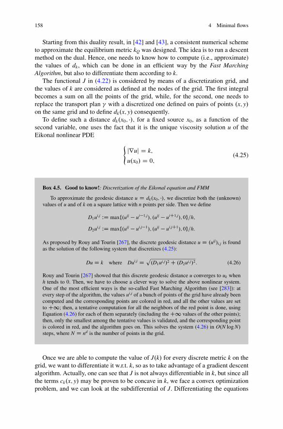
158 4 Minimal flows

Starting from this duality result, in [42] and [43], a consistent numerical schemeto approximate the equilibrium metric kQ was designed. The idea is to run a descentmethod on the dual. Hence, one needs to know how to compute (i.e., approximate)the values of dk, which can be done in an efficient way by the Fast MarchingAlgorithm, but also to differentiate them according to k.

The functional J in (4.22) is considered by means of a discretization grid, andthe values of k are considered as defined at the nodes of the grid. The first integralbecomes a sum on all the points of the grid, while, for the second, one needs toreplace the transport plan � with a discretized one defined on pairs of points .x; y/on the same grid and to define dk.x; y/ consequently.

To define such a distance dk.x0; �/; for a fixed source x0, as a function of thesecond variable, one uses the fact that it is the unique viscosity solution u of theEikonal nonlinear PDE

(jruj D k;

u.x0/ D 0;(4.25)

Box 4.5. Good to know!: Discretization of the Eikonal equation and FMM

To approximate the geodesic distance u D dk.x0; �/; we discretize both the (unknown)values of u and of k on a square lattice with n points per side. Then we define

D1ui;j WD maxf.uij � ui�1;j/; .uij � uiC1;j/; 0g=h;

D2ui;j WD maxf.uij � ui;j�1/; .uij � ui;jC1/; 0g=h:

As proposed by Rouy and Tourin [267], the discrete geodesic distance u D .uij/i;j is foundas the solution of the following system that discretizes (4.25):

Du D k where Dui;j D p.D1ui;j/2 C .D2ui;j/2: (4.26)

Rouy and Tourin [267] showed that this discrete geodesic distance u converges to uk whenh tends to 0. Then, we have to choose a clever way to solve the above nonlinear system.One of the most efficient ways is the so-called Fast Marching Algorithm (see [283]): atevery step of the algorithm, the values ui;j of a bunch of points of the grid have already beencomputed and the corresponding points are colored in red, and all the other values are setto C1; then, a tentative computation for all the neighbors of the red point is done, usingEquation (4.26) for each of them separately (including the C1 values of the other points);then, only the smallest among the tentative values is validated, and the corresponding pointis colored in red, and the algorithm goes on. This solves the system (4.26) in O.N log N/steps, where N D nd is the number of points in the grid.

Once we are able to compute the value of J.k/ for every discrete metric k on thegrid, we want to differentiate it w.r.t. k, so as to take advantage of a gradient descentalgorithm. Actually, one can see that J is not always differentiable in k, but since allthe terms ck.x; y/ may be proven to be concave in k, we face a convex optimizationproblem, and we can look at the subdifferential of J. Differentiating the equations

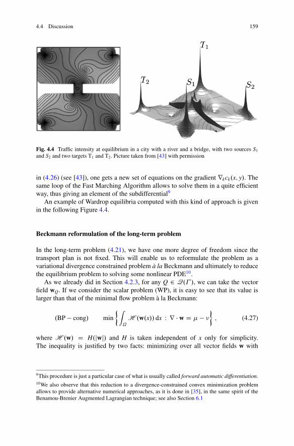
4.4 Discussion 159

Fig. 4.4 Traffic intensity at equilibrium in a city with a river and a bridge, with two sources S1and S2 and two targets T1 and T2. Picture taken from [43] with permission

in (4.26) (see [43]), one gets a new set of equations on the gradient rkck.x; y/. Thesame loop of the Fast Marching Algorithm allows to solve them in a quite efficientway, thus giving an element of the subdifferential9

An example of Wardrop equilibria computed with this kind of approach is givenin the following Figure 4.4.

Beckmann reformulation of the long-term problem

In the long-term problem (4.21), we have one more degree of freedom since thetransport plan is not fixed. This will enable us to reformulate the problem as avariational divergence constrained problem à la Beckmann and ultimately to reducethe equilibrium problem to solving some nonlinear PDE10.

As we already did in Section 4.2.3, for any Q 2 Q.� /, we can take the vectorfield wQ. If we consider the scalar problem (WP), it is easy to see that its value islarger than that of the minimal flow problem à la Beckmann:

.BP � cong/ min

�ˆ˝

H .w.x// dx W r � w D � � ��; (4.27)

where H .w/ D H.jwj/ and H is taken independent of x only for simplicity.The inequality is justified by two facts: minimizing over all vector fields w with

9This procedure is just a particular case of what is usually called forward automatic differentiation.10We also observe that this reduction to a divergence-constrained convex minimization problemallows to provide alternative numerical approaches, as it is done in [35], in the same spirit of theBenamou-Brenier Augmented Lagrangian technique; see also Section 6.1

160 4 Minimal flows

prescribed divergence gives a smaller result than minimizing over the vector fieldsof the form wQ, and then we use jwQj � iQ and the fact that H is increasing.

Actually, the two problems are equivalent. The main ingredient to prove it isTheorem 4.10. If we take a minimizer w for this minimal flow problem, then we areable to build a measure Q, and as we did in Theorem 4.13, the optimality of w givesw D wQ and jwQj D iQ, thus proving that the minimal values are the same. Also,we can build a minimizer w from a minimizer Q (just take w D wQ) and converselya minimizer Q from w (use Theorem 4.10).

Moreover, we also know from the proof of Theorem 4.10 that the main tool toconstruct the measure Q is the Dacorogna-Moser flow. If we want to use it to definea unique and canonical flow connecting the two measures � and �, then we wouldlike to have some regularity of the vector field v defined as vt.x/ D w.x/=ft.x/,where ft D .1 � t/�C t�. If v was Lipschitz continuous, then the Cauchy problem

(y0

x.t/ D vt.yx.t//

yx.0/ D x

would have a unique solution for every initial datum x and would allow to find themeasure Q (which would be unique, by the way). Obviously, we can decide to addsome assumptions on � and �, which will be supposed to be absolutely continuouswith regular densities (at least Lipschitz continuous and bounded from below).

However, one needs to prove regularity for the optimal w and for this one needsto look at the optimality conditions satisfied by w as a minimizer of (4.27). Byconsidering perturbations of the form w C " Qw with r � Qw D 0, one gets that theoptimal w must satisfy

´ rH .w/ � Qw D 0 for any divergence-free vector field Qw.This means that rH .w/ is a gradient (see Box 6.2 in Section 6.2), which has to beadapted to an Lp setting11. We can call it ru, and by inverting rH , we get that theminimizers of (4.27) satisfy w D rH .ru/ where H is the Legendre transformof H and u solves the PDE:

� r � .rH .ru// D � � �; in ˝;rH .ru/ � n D 0; on @˝:

(4.28)

This equation turns out to be a standard Laplace equation if H is quadratic, or itbecomes a p-Laplace equation for other power functions. In these cases, regularityresults are well known, under regularity assumptions on � and �.

Remark 4.36. Note that the above considerations allow to answer the question“Given �; �, does a traffic plan Q with iQ 2 Lp exist?” The answer is yes if andonly if � � � 2 .W1;q/, and the proof is left as an exercise; see Ex(26).

As we already mentioned, the case of power-like functions H is not suitable formodeling reasons. Recall that H0 D g where g is the congestion function, so it is

11Observe that the same result can also be directly obtained from duality arguments, as it is donein Theorem 2.1 in [80].

4.4 Discussion 161

natural to have g.0/ > 0: the metric should be positive even if there is no traffic!This means that the radial function H cannot be differentiable at 0 and then itssubdifferential at 0 contains a ball. By duality, this implies rH D 0 on this ballwhich makes (4.28) very degenerate, even worse than the p-Laplacian. For instance,a reasonable model of congestion is g.t/ D 1C tp�1 for t � 0, with p > 1, so that

H .w/ D 1

pjwjp C jwj; H .z/ D 1

q.jzj � 1/qC; with q D p0 D p

p � 1 (4.29)

so that the optimal w is

w D�jruj � 1

�q�1C

ru

jruj ;

where u solves the very degenerate PDE:

r ���

jruj � 1�q�1

Cru

jruj�

D � � �; (4.30)

with Neumann boundary condition

�jruj � 1

�q�1C

ru

jruj � n D 0:

Note that there is no uniqueness for u, but there is for w.For this degenerate equation, we cannot expect regularity results which go

beyond Lipschitz continuity for u (indeed, since the diffusion coefficient identicallyvanishes in the zone where jruj � 1, every u 2 Lip1 is the solution of thecorresponding homogeneous equation). On the other hand, we can expect betterregularity for w (roughly speaking, w is obtained by gluing two zones: the onewhere w D 0 and the one where the equation is elliptic). However, we will not beable to obtain w itself to be Lipschitz. On the other hand, Sobolev regularity of wand Lipschitz regularity results for u are proven in [80]. This enables one to builda flow à la DiPerna-Lions [156] and then to justify rigorously the existence of aunique and well-defined flow for a.e. initial datum x. Interestingly, recent continuityresults are also available (see [279] in dimension 2, and then [126], with a differenttechnique in arbitrary dimension), obtained as a consequence of a fine analysis ofthis degenerate elliptic PDE. Besides the interest for this regularity result in itself,we also stress that continuity for w implies continuity for the optimal iQ, and thisexactly gives the regularity which is required in the proof of Theorem 4.33 (themain difficulty being defining cNk for a noncontinuous Nk, and this is the reason whyour previous arguments are only formal).

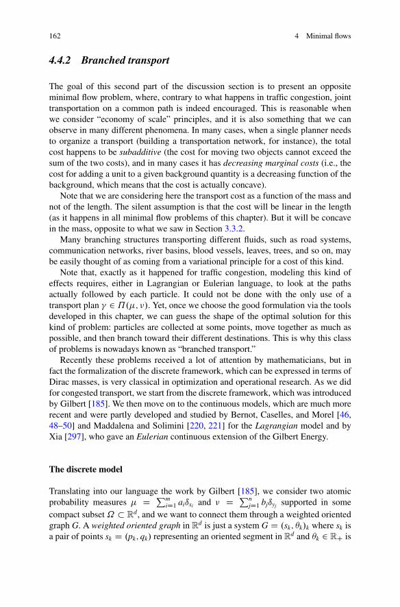
162 4 Minimal flows

4.4.2 Branched transport

The goal of this second part of the discussion section is to present an oppositeminimal flow problem, where, contrary to what happens in traffic congestion, jointtransportation on a common path is indeed encouraged. This is reasonable whenwe consider “economy of scale” principles, and it is also something that we canobserve in many different phenomena. In many cases, when a single planner needsto organize a transport (building a transportation network, for instance), the totalcost happens to be subadditive (the cost for moving two objects cannot exceed thesum of the two costs), and in many cases it has decreasing marginal costs (i.e., thecost for adding a unit to a given background quantity is a decreasing function of thebackground, which means that the cost is actually concave).

Note that we are considering here the transport cost as a function of the mass andnot of the length. The silent assumption is that the cost will be linear in the length(as it happens in all minimal flow problems of this chapter). But it will be concavein the mass, opposite to what we saw in Section 3.3.2.

Many branching structures transporting different fluids, such as road systems,communication networks, river basins, blood vessels, leaves, trees, and so on, maybe easily thought of as coming from a variational principle for a cost of this kind.

Note that, exactly as it happened for traffic congestion, modeling this kind ofeffects requires, either in Lagrangian or Eulerian language, to look at the pathsactually followed by each particle. It could not be done with the only use of atransport plan � 2 ˘.�; �/. Yet, once we choose the good formulation via the toolsdeveloped in this chapter, we can guess the shape of the optimal solution for thiskind of problem: particles are collected at some points, move together as much aspossible, and then branch toward their different destinations. This is why this classof problems is nowadays known as “branched transport.”

Recently these problems received a lot of attention by mathematicians, but infact the formalization of the discrete framework, which can be expressed in terms ofDirac masses, is very classical in optimization and operational research. As we didfor congested transport, we start from the discrete framework, which was introducedby Gilbert [185]. We then move on to the continuous models, which are much morerecent and were partly developed and studied by Bernot, Caselles, and Morel [46,48–50] and Maddalena and Solimini [220, 221] for the Lagrangian model and byXia [297], who gave an Eulerian continuous extension of the Gilbert Energy.

The discrete model

Translating into our language the work by Gilbert [185], we consider two atomicprobability measures � D Pm

iD1 aiıxi and � D PnjD1 bjıyj supported in some

compact subset˝ � Rd, and we want to connect them through a weighted oriented

graph G. A weighted oriented graph in Rd is just a system G D .sk; �k/k where sk is

a pair of points sk D .pk; qk/ representing an oriented segment in Rd and �k 2 RC is

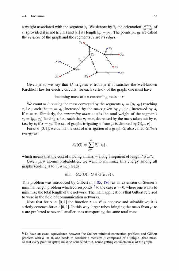
4.4 Discussion 163

a weight associated with the segment sk. We denote by Osk the orientation qk�pkjqk�pkj of

sk (provided it is not trivial) and jskj its length jqk � pkj. The points pk; qk are calledthe vertices of the graph and the segments sk are its edges.

•

>

•

>

•y1 <

•

>

•>

•y3>

•y2>

•>

•y5< •y4 <

• <

•x3• <

•x1

•x2pk

qksk

Given �; �, we say that G irrigates � from � if it satisfies the well-knownKirchhoff law for electric circuits: for each vertex x of the graph, one must have

incoming mass at x = outcoming mass at x.

We count as incoming the mass conveyed by the segments sk D .pk; qk/ reachingx, i.e., such that x D qk, increased by the mass given by �, i.e., increased by ai

if x D xi. Similarly, the outcoming mass at x is the total weight of the segmentssk D .pk; qk/ leaving x, i.e., such that pk D x, decreased by the mass taken out by �,i.e., by bj if x D yj. The set of graphs irrigating � from � is denoted by G.�; �/.

For ˛ 2 Œ0; 1�, we define the cost of ˛-irrigation of a graph G, also called Gilbertenergy as

E˛.G/ DnX

kD1�˛k jskj ;

which means that the cost of moving a mass m along a segment of length l is m˛l.Given �; � atomic probabilities, we want to minimize this energy among all

graphs sending � to �, which reads

min fE˛.G/ W G 2 G.�; �/g:This problem was introduced by Gilbert in [185, 186] as an extension of Steiner’sminimal length problem which corresponds12 to the case ˛ D 0, where one wants tominimize the total length of the network. The main applications that Gilbert referredto were in the field of communication networks.

Note that for ˛ 2 Œ0; 1� the function t 7! t˛ is concave and subadditive; it isstrictly concave for ˛ 2�0; 1Œ. In this way larger tubes bringing the mass from � to� are preferred to several smaller ones transporting the same total mass.

12To have an exact equivalence between the Steiner minimal connection problem and Gilbertproblem with ˛ D 0, one needs to consider a measure � composed of a unique Dirac mass,so that every point in spt.�/ must be connected to it, hence getting connectedness of the graph.

164 4 Minimal flows

•

•>

•>

•>

•

>

•>• <

• <

•<

••

>

•>

•

•>

•>

•>

•

>

•>• >

• >

•

>

••

>

•>

Fig. 4.5 An example of a strong cycle (left) and of a cycle which is not strong (right)

It is not evident to see why this problem admits a minimizer. Indeed, we minimizeamong finite objects, but we do not impose uniform bounds (on the number of edges,of vertices, etc.). We need to give an important definition.13

Definition 4.37. We call cycle (resp. strong cycle) of G any sequence of segments(resp. oriented segments) which are adjacent (Figure 4.5).

As the function t 7! t˛ is increasing, we can easily reduce the energy of a graphby removing strong cycles. It is not difficult to check that the concavity of the samefunction also ensures that one reduces the energy by removing any cycle. Thereforeone can take a minimizing sequence of graphs which have no cycles, i.e., which aretrees, and this implies a uniform bound on the number of edges (in terms of the totalnumber of atoms of � and �). This provides compactness and proves the existenceof a minimizer. Any minimizer will have no strong cycles and no cycles if ˛ 2�0; 1Œ.

Moreover, it is possible to prove an optimality condition on the free junctionsin the graph. This means that at every node x of the graph which is not one of thepoints xi or yj, a balance of the direction must hold: the condition is

XkWxDpk

�˛k Osk �X

kWxDqk

�˛k Osk D 0; (4.31)

which means that the sum of the unit vectors corresponding to all the segmentstouching the point x, always taken as exiting from x independently of the trueorientation Osk, each weighted with �˛k , must vanish14.

13Unfortunately, to cope with the language usually adopted in branched transport, we cannot becompletely coherent with the rest of the chapter, where we called “cycles” what we call here“strong cycles.”14For triple junctions, which are the most common ones, this gives interesting results: when ˛ D 0,we get the well-known condition about Steiner trees, with three 120ı angles, and for ˛ D 0:5, wehave a 90ı angle (see Ex(30)); yet, in general, the angles depend on the masses �k.

4.4 Discussion 165

A relaxed continuous model (Xia)

More recently Xia, in [297], has proposed a new formalization leading to generaliza-tions of this problem to arbitrary probability measures � and �. The main idea wasto translate the Kirchhoff law constraint into a divergence constraint. To be precise,and since we will need this language later on, we introduce some heavy notation.

If E � ˝ is a 1-rectifiable set15, � W E ! Sd�1 is a measurable vector field,

and � W E ! RC is H 1-integrable, we define the finite vector measure ŒE; �; �� 2M d.˝/ through

hŒE; �; ��; �i Dˆ

E�.x/�.x/ � �.x/dH 1.x/;

for all � 2 C.˝IRd/.Given a finite graph G D .sk; �k/k, we associate with G the measure

wG WDX

k

Œsk; Osk; �k� 2 M d.˝/:

We can express both the cost and the constraint in terms of wG only. First note thatG 2 G.�; �/ (i.e., it satisfies mass balance conditions for irrigating � from �) if andonly if r � wG D � � �. Then, we also write

E˛.G/ DnX

kD1�˛k jskj D

ˆ

Kj�.x/j˛ dH 1.x/;

where we called � the density of wG w.r.t. the H 1 measure.This suggests a continuous Eulerian formulation of Gilbert’s problem by gener-

alizing Gilbert’s energy, the minimization problem becoming

.XP/ min fM˛.w/ W w 2 M ddiv.˝/; r � w D � � �g: (4.32)

Obviously, one needs to define the energy M˛ (which is also called the “˛-mass” ofw). The original idea by Xia is to define it by relaxation, i.e.,

M˛.w/ WD infnlim inf

nE˛.Gn/ W Gn 2 G.�n; �n/;wGn * w in M d

div.˝/o;

where the convergence in M ddiv.˝/means wGn * w and r �wGn D �n ��n * r �w

as measures.

15We already met rectifiable sets when studying the differentiability of convex functions, inChapter 1: 1-rectifiable sets are defined as those sets which are covered, H 1-a.e., by a countableunion of Lipschitz curves. Anyway, the reader can easily pretend that “1-rectifiable” is a synonymof “1D” and it should be enough to follow the rest of the discussion.

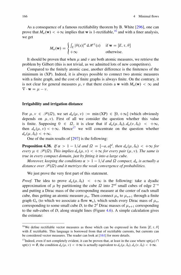
166 4 Minimal flows

As a consequence of a famous rectifiability theorem by B. White [296], one canprove that M˛.w/ < C1 implies that w is 1-rectifiable,16 and with a finer analysis,we get

M˛.w/ D( ´

E j�.x/j˛ dH 1.x/ if w D ŒE; �; ��

C1 otherwise:

It should be proven that when � and � are both atomic measures, we retrieve theproblem by Gilbert (this is not trivial, as we admitted lots of new competitors).

Compared to the finitely atomic case, another difference is the finiteness of theminimum in (XP). Indeed, it is always possible to connect two atomic measureswith a finite graph, and the cost of finite graphs is always finite. On the contrary, itis not clear for general measures �; � that there exists a w with M˛.w/ < 1 andr � w D � � �.

Irrigability and irrigation distance

For �; � 2 P.˝/, we set d˛.�; �/ WD min .XP/ 2 Œ0;C1� (which obviouslydepends on �; �). First of all we consider the question whether this valueis finite. Supposing 0 2 ˝, it is clear that if d˛.�; ı0/; d˛.�; ı0/ < C1,then d˛.�; �/ < C1. Hence17 we will concentrate on the question whetherd˛.�; ı0/ < C1.

One of the main results of [297] is the following:

Proposition 4.38. If ˛ > 1 � 1=d and ˝ D Œ�a; a�d, then d˛.�; ı0/ < C1 forevery � 2 P.˝/. This implies d˛.�; �/ < C1 for every pair .�; �/. The same istrue in every compact domain, just by fitting it into a large cube.

Moreover, keeping the conditions ˛ > 1 � 1=d and ˝ compact, d˛ is actually adistance over P.˝/ and it metrizes the weak convergence of probabilities.

We just prove the very first part of this statement.

Proof. The idea to prove d˛.�; ı0/ < C1 is the following: take a dyadicapproximation of � by partitioning the cube ˝ into 2nd small cubes of edge 2�n

and putting a Dirac mass of the corresponding measure at the center of each smallcube, thus getting an atomic measure �n. Then connect �n to �nC1 through a finitegraph Gn (to which we associate a flow wn), which sends every Dirac mass of �n,corresponding to some small cube D, to the 2d Dirac masses of �nC1 correspondingto the sub-cubes of D, along straight lines (Figure 4.6). A simple calculation givesthe estimate:

16We define rectifiable vector measures as those which can be expressed in the form ŒE; �; ��with E rectifiable. This language is borrowed from that of rectifiable currents, but currents canbe considered vector measures. The reader can look at [161] for more details.17Indeed, even if not completely evident, it can be proven that, at least in the case where spt.�/\spt.�/ D ;, the condition d˛.�; �/ < C1 is actually equivalent to d˛.�; ı0/; d˛.�; ı0/ < C1.

4.4 Discussion 167

Fig. 4.6 Different steps of the construction of Proposition 4.38

M˛.Gn/ � C2ndXkD1

am˛k 2

�n;

where the masses mk are the masses contained in each of the cubes at thenth subdivision. Then we use

PNkD1 m˛

k � N1�˛.PN

kD1 mk/˛ (which comes from

Jensen’s inequality), and get E˛.Gn/ � aC2�n.1�d.1�˛//.It is clear by construction that we only need

Pn E˛.Gn/ < C1, and this is true

as soon as 1 � d.1 � ˛/ > 0. utSome counterexamples that we do not develop here (but one can see Ex(29))

complement the previous result and show that the above statement is sharp in termsof ˛. More generally, we can think that the irrigability of a measure starting fromı0 is a matter of its dimension, but suitable notions of dimensions (which are notsimply the Hausdorff dimension of the support) have to be chosen. These mattersare discussed in [153, 154].

It is interesting to note that the above distance d˛ may also be obtained byrelaxation (see [220]) from the functional which associates with every pair of atomicprobability measures � D P

i aiıxi , � D Pj bjıyj the quantity

d˛.�; �/ WD min

8<:X

ij

jxi � yjj�.f.xi; yj/g/˛ W � 2 ˘.�; �/9=; :

This quantity, which corresponds to a sort of nonlinear version of the Kantorovichproblem, is only well defined on atomic measures. Then, we can check that we have

d˛ D sup

8<ˆ:

d W P.˝/�P.˝/ ! Œ0;C1� W

8<ˆ:

d � d˛ on atomic measures;

d is l.s.c. for *;

d satisfies the triangle inequality.

9>>=>>;:

(4.33)

168 4 Minimal flows

The Lagrangian formulation

We want now to provide an alternative formulation of the branched transportproblem, based on the use of measures on paths. This formulation18 has beenintroduced in [221] and then deeply studied in [48].

As usual, we will be given two measures �; � 2 P.˝/ and look for a trafficplan19, i.e., a measure Q 2 P.C /, where C WD AC.˝/, with

´C L.!/ dQ.!/ <

C1. As usual, we will restrict our attention to those traffic plans satisfying.e0/#Q D �; .e1/#Q D � (the case where we fix also the coupling .e0; e1/#Q D �

will not be considered, and, by the way, the connection with the previous Eulerianmodel by Xia does not work if � is fixed).

To introduce the quantity that we want to minimize, we need to define

�Q.x/ WD Q.f! 2 C W x 2 !.Œ0; 1�/g/; mQ.x/ WDˆ

C#.ft 2 Œ0; 1� W !.t/Dxg/ dQ.!/:

Proposition 4.39. The following properties are satisfied:

1. We always have 0 � �Q.x/ � mQ.x/ � 1, with equality �Q D mQ whenever Qis concentrated on loop-free curves.

2. The function .x;Q/ 7! �Q.x/ is u.s.c. w.r.t. the convergence of points x 2 ˝ andthe weak convergence of measures Q 2 P.C /.

3. The traffic intensity iQ is equal to mQ �H 1 whenever there exists a set � , � -finitefor the H 1 measure, with !.t/ 2 � for Q-a.e. curve ! and a.e. time t.

Then, we define the energy I˛ through

I˛.Q/ WDˆ

CZQ.!/ dQ.!/;

where

ZQ.!/ WD L�˛�1Q.!/ D

ˆ 1

0

�Q.!.t//˛�1j!0.t/j dt:

The problem that we consider is then

minfI˛.Q/ W Q 2 P.C /; .e0/#Q D �; .e1/#Q D �g:

18What we provide here is just a translation into the language of this chapter of the model proposedin [48, 221], which uses “parametrized traffic plans” instead of measures on paths, but it is just amatter of language.19The terminology has been introduced for this very purpose by the authors of [48].

4.4 Discussion 169

Note that the trivial estimate I˛.Q/ � ´C L.!/ dQ.!/ provides compactness on

a minimizing sequence (indeed, the energy is invariant under reparametrization ofeach curve, and hence length bounds turn into Lipschitz bounds, as we did in therest of the chapter). The existence of a minimizer is then obtained by proving semi-continuity. Indeed, combining fact 2 with a simple Fatou Lemma, we obtain that thefunction .Q; !/ 7! ZQ.!/ is l.s.c. (for the weak convergence on Q and the uniformconvergence on !). Finally we use the following:

Proposition 4.40. If f W P.C / � C ! R is l.s.c., then F W Q 7! ´C f .Q; !/ dQ.!/

is l.s.c. on P.C /.

Then, we can prove the following facts:

Proposition 4.41. 1. For every Q with I˛.Q/ < C1, the set � D fx W �Q.x/ >0g is � -finite for the measure H 1 and we have I˛.Q/ D ´

��˛�1

Q mQ dH 1.2. If Q is optimal, then it is concentrated on loop-free curves and I˛.Q/ D´

��˛Q dH 1.

3. If Q is optimal, then it is cycle-free20.

This property and the particular the expression of I˛ as the integral of the ˛-powerof the multiplicity �Q suggest the connection with the Eulerian model. A preciseequivalence can be proven, either via the tools in [48] or via Theorem 4.10.

The single-source case

It is interesting to see the special features of the problem when we fix the sourcemeasure as a single Dirac mass ı0. This particular case is already very rich. In thiscase, it is possible to study the problem with a different definition of multiplicity:indeed, we can expect that whenever two curves pass at a same point x, they hadtraveled together on all the path from 0 to x. In this case, it is better to change alittle bit the framework, because parametrizing all the curves on a fixed finite-lengthintegral Œ0; 1� could be too restrictive. Also, this gives the occasion to observe theoriginal framework presented in [221] (which can be checked to be equivalent to thegeneral one).

We consider now the space � D f! 2 Lip1.RCI˝/; !.0/ D 0g, endowed withthe topology of uniform convergence on compact sets (recall that this topology ismetrizable by some distance d and that this makes� a compact metric space thanksto the Ascoli-Arzelà theorem).

If ! 2 �, we define its stopping time by

Stop.!/ D infft � 0 W ! is constant on Œt;C1Œg:

20We can give a precise definition in the following way: for x; y 2 ˝, define Œx; y� D f! 2 C W9 s < t such that !.s/ D x and !.t/ D yg; we say that Q is cycle-free if there are not x1; : : : ; xn

with x1 D xn such that Q.Œxi; xiC1�/ > 0 or Q.ŒxiC1; xi�/ > 0 for all i D 1; : : : ; n � 1.

170 4 Minimal flows

We denote by �stop the set of curves ! such that Stop.!/ < 1. Then we define thefollowing subsets of �stop : �arc; �inj; �lf, respectively, the set of curves which areparameterized by arc length on Œ0;Stop.!/�, which are injective on Œ0;Stop.!/Œ andwhich are injective on Œ0;Stop.!/� (these curves are called loop-free).

We call traffic pattern any � 2 P.�/ (we use the notation � to distinguish fromthe case Q 2 P.C /) satisfying

ˆ

�

Stop.!/ d�.!/ < C1:

We define the multiplicity and the energy according to the following variant ofthe previous definitions: for the multiplicity, we first define

Œ!�t WD f Q! 2 �stop W !.s/ D Q!.s/ 8s 2 Œ0; t�g;

the set of curves which coincide with ! up to time t, and for notational simplicity,we set j!jt;� WD �.Œ!�t/. This last quantity will play the role of the multiplicity � .Then we define

QZ�.!/ WDˆ Stop.!/

0

j!j˛�1t;� dt

and we call �-good any curve ! with QZ�.!/ < C1. Then, we use the energy

QI˛.�/ WDˆ

�

QZ�.!/ d�.!/:

The problem becomes the minimization of QI˛ among probabilities � 2 P.�/

satisfying .e1/#� D �, where e1.!/ D !.Stop.!//. Note that e1 is well definedon�stop, but any finite energy traffic plan is necessarily concentrated on�stop; hencethe condition makes sense; moreover, � 7! .e1/#� is continuous for the weakconvergence when restricted to any set f� 2 P.�/ W ´

�Stop.!/ d�.!/ � Cg.

It is not difficult to prove the existence of a minimizer in this case, and it is alsopossible to prove that minimizers are concentrated on�arc \�inj and are even loop-free (i.e., we can prove �.�lf/ D 1, even if it is less evident). Note that we withdrewfrom the definition of the energy the term j!0j and this forces the minimizers tosaturate the constraint j!0j � 1.

Remark 4.42. Other intermediate models may be introduced, all differing in thedefinition of the multiplicity of the curve ! at time t. See, for instance, [47] or [220].

The class of �-good curves is an explicitly defined set of curves which sharesmany of the properties satisfied �-almost everywhere. For instance, if � is optimaland Q is a measure on C representing � after a suitable reparametrization in time,we have j!jt;� D �Q.!.t// D mQ.!.t//, and this is true for every ! which is �-good.

4.4 Discussion 171

An important point is the following: if !1; !2 are �-good and � is optimal, if.e1/.!1/ D .e1/.!2/, then QZ�.!1/ D QZ�.!2/ (see [272]). As a corollary, we get,for instance, that any �-good curve ! is in fact loop-free, i.e., it is injective onŒ0;Stop.�/�.

Definition 4.43 (Landscape function). We define the landscape function z� asso-ciated with the traffic pattern � through

z�.x/ D(

Z�.!/ if ! is an �-good curve and x D e1.!/;C1 if there is no �-good curve ending at x:

The introduction of the landscape function [272] is justified by several differentconsiderations. On the one hand, it plays the role of the first variation of thefunctional

X˛.�/ D d˛.ı0; �/;

as we can prove (by concavity)

X˛.�/ � X˛.�/C ˛

ˆ

˝

z� d.� � �/;

where � is any optimal traffic plan irrigating �. Considering that we also haveX˛.�/ D ´

z� d�, it seems to play the same role as the Kantorovich potential playsfor the classical Monge transport cost21.

On the other hand, and this justifies its name, z� is a natural object studied bygeophysicists when dealing with river basins (see [263] for details and [272] for abrief mathematical introduction to this theory); in their model, after a first evolutionphase, it is assumed that landscape erosion creates a stable configuration where theelevation z.x/ at each point is characterized by two properties: the river flows in thedirection of maximal slope, and the slope jrzj is proportional to the discharge (i.e.,multiplicity) coefficient � , raised to a power close to �1=2 (say ˛ � 1, with ˛ closeto the 2D critical exponent 1=2).

It is possible to prove few properties of the landscape function.

Theorem 4.44. The landscape function z is lower semi-continuous. It is Höldercontinuous22 of exponent ˇ D d.˛� .1� 1

d // whenever ˛ > 1� 1d ,˝ has Lipschitz

boundary and � � cL˝ . Moreover, z has maximal slope in the direction of theirrigation network in the following sense: if ! is an �-good curve, t0 � Stop.!/,x0 D !.t0/, and �0 D j!jt0;�, then for any x 2 ˝, we have

z.x/ � z.x0/ � �˛�10 jx � x0j � o.jx � x0j/:

21But it does not seem to come from a dual problem.22Other Holder results exist under different assumptions, if � admits different dimensional lowerbounds, i.e., it is Ahlfors regular of another exponent k < d, thus obtaining ˇ D d.˛ � .1� 1

k //;see [78].

172 4 Minimal flows

Regularity

The regularity of the optimal networks in branched transport is a delicate issue,which has been studied both in Eulerian and Lagrangian framework. One of thefirst results concerns what Xia called “interior regularity”: here interior means “farfrom the supports of � and �,” which can be considered as the boundary of thetransport network. These results, proven in [298] with a Eulerian approach andin [49] with the Lagrangian approach, state that, far from these supports, optimalnetworks are locally finite graphs. In particular, they satisfy the angle law (4.31) atevery branching point. The question now becomes whether this angle law is satisfiedat an infinitesimal level (in the sense that the directions to be considered are tangentlines and not segments) inside the support of � and �. [300] gives partial results inthis direction (characterization of the limits up to subsequences), but a full solutionis not yet available. On the other hand, in the simpler case of a single source, [241]provides the following result:

Theorem 4.45. Let ! be an �-good curve, parametrized with constant speed, of anoptimal traffic pattern irrigating a measure � with aL˝ � � � bL˝ , for 0 < a <b < 1. Suppose that ˝ is a Lipschitz bounded domain. Consider t0 < Stop.!/.Let �i, i 2 I the masses of all trees branching from ! in the interval Œ0; t0�/. ThenP

i �˛i < 1 and !0 2 BV.Œ0; t0�/. In particular, ! has two half-tangents at all

points and a tangent at all points which are not branching points. Moreover, thetangent cone at every branching point x is composed of a finite (and bounded by aconstant depending on ˛ and d) number of segments whose directions and massessatisfy (4.31). More precisely, ! satisfies in the sense of distributions on Œ0; t0� theelliptic equation

� .j!j˛t;� !0.t//0 DXi2I

�˛i ı!.ti/ Osi (4.34)

where Osi is the tangent of the branch stemming from ! at the point !.ti/ with mass�i. The fact that this tangent vector exists, and that the right-hand side is a vectormeasure with finite mass, is guaranteed by the first parts of the statement.

Counterexamples to the existence of tangent directions can be built when theassumption on � fails (see, again, [241]). For an alternative approach to the existenceof tangent directions under slightly different assumptions, one can also see the lastchapter in [271].

Numerics

From the point of view of the practical search of the solutions, branched transportproblems lie in between combinatorial optimization (they are similar to the Steinerminimal connection problem, which is, on a graph, known to be NP-hard) andcontinuous minimal flow problems. The numerical methods for finding a solutionhave to face at least two difficulties: concavity (and hence the high number of local

4.4 Discussion 173

minimizers) and singularity (i.e., working with singular structures such as networksinstead of using Lp or smoother functions, as in the congested traffic case).

Some numerical results, based on local and nonlocal improvements of a suitablychosen initial guess, are present in [297] and [299]. Yet, here we prefer to introducea completely different idea, based on a � -convergence approach.

Box 4.6. Important notion: � -convergence

� -convergence is a theory, introduced by De Giorgi (see [138] and [133]), to provideapproximations of minimization problems. It is also known as epi-convergence.

Definition. On a metric space X, let Fn W X ! R [ fC1g be a sequence of functions.We define the two lower-semi-continuous functions F� and FC (called � � lim inf and� � lim sup of this sequence, respectively) by

F�.x/ WD infflim infn!1

Fn.xn/ W xn ! xg;FC.x/ WD infflim sup

n!1

Fn.xn/ W xn ! xg:

Should F� and FC coincide, then we say that Fn actually � -converges to the commonvalue F D F� D FC. The definition of � -convergence for a continuous parameter " ! 0

obviously passes through the convergence to the same limit for any subsequence "n ! 0.Among the properties of � -convergence, we have the following:

• if there exists a compact set K � X such that infX Fn D infK Fn for any n, then Fattains its minimum and inf Fn ! min F;

• if .xn/n is a sequence of minimizers for Fn admitting a subsequence converging to x,then x minimizes F;

• if Fn is a sequence � -converging to F, then Fn C G will � -converge to F C G for anycontinuous function G W X ! R [ fC1g.

One of the first applications of � -convergence was to provide elliptic approxima-tions of free discontinuity problems, or, more generally, variational problems with“singular energies.” We will only mention the following standard example (knownas “Modica-Mortola” approximation; see [237] and [133]) because of its simplicity.Define the functional F" on L1.˝/ through

F".u/ D(1"

´W.u.x//dx C "

´ jru.x/j2dx if u 2 H1.˝/IC1 otherwise:

Then, if W.0/ D W.1/ D 0 and W.t/ > 0 for any t ¤ 0; 1, we have � -convergenceof the functionals F" toward the functional F given by

F.u/ D(

cPer.S/ if u D 1S and S is a finite-perimeter setIC1 otherwise;

where the constant c is given by c D 2´ 10

pW.t/dt.

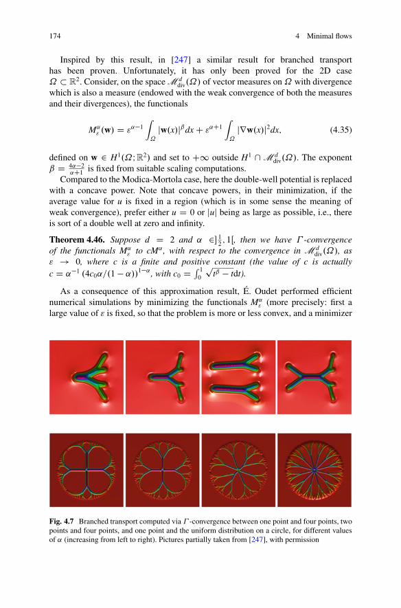
174 4 Minimal flows

Inspired by this result, in [247] a similar result for branched transporthas been proven. Unfortunately, it has only been proved for the 2D case˝ � R

2. Consider, on the space M ddiv.˝/ of vector measures on˝ with divergence

which is also a measure (endowed with the weak convergence of both the measuresand their divergences), the functionals

M˛" .w/ D "˛�1

ˆ

˝

jw.x/jˇdx C "˛C1ˆ

˝

jrw.x/j2dx; (4.35)

defined on w 2 H1.˝IR2/ and set to C1 outside H1 \ M ddiv.˝/. The exponent

ˇ D 4˛�2˛C1 is fixed from suitable scaling computations.

Compared to the Modica-Mortola case, here the double-well potential is replacedwith a concave power. Note that concave powers, in their minimization, if theaverage value for u is fixed in a region (which is in some sense the meaning ofweak convergence), prefer either u D 0 or juj being as large as possible, i.e., thereis sort of a double well at zero and infinity.

Theorem 4.46. Suppose d D 2 and ˛ 2� 12; 1Œ, then we have � -convergence

of the functionals M˛" to cM˛ , with respect to the convergence in M d

div.˝/, as" ! 0, where c is a finite and positive constant (the value of c is actuallyc D ˛�1 .4c0˛=.1 � ˛//1�˛ , with c0 D ´ 1

0

ptˇ � tdt).

As a consequence of this approximation result, É. Oudet performed efficientnumerical simulations by minimizing the functionals M˛

" (more precisely: first alarge value of " is fixed, so that the problem is more or less convex, and a minimizer

Fig. 4.7 Branched transport computed via � -convergence between one point and four points, twopoints and four points, and one point and the uniform distribution on a circle, for different valuesof ˛ (increasing from left to right). Pictures partially taken from [247], with permission

4.4 Discussion 175

is found by gradient descent, then, following a continuation method, the value of "is reduced and at every step the gradient descent starts from the previously foundminimizer). In the end we find a “well-chosen” local minimizer quite satisfactory inpractice (Figure 4.7).

Chapter 5Wasserstein distances and curvesin the Wasserstein spaces

In this chapter, we will use the minimal value of transport problems between twoprobabilities in order to define a distance on the space of probabilities. We mainlyconsider costs of the form c.x; y/ D jx � yjp in ˝ � R

d, but the analysis can beadapted to a power of the distance in a more general metric space X. The exponentp will always be taken in Œ1;C1Œ (we will briefly address the case p D C1 inthe Discussion Section 5.5.1) in order to take advantage of the properties of the Lp

norms. When ˝ is unbounded, we need to restrict our analysis to the following setof probabilities:

Pp.˝/ WD�� 2 P.˝/ W

ˆ

˝

jxjp d� < C1�:

In a metric space, we fix an arbitrary point x0 2 X, and set Pp.X/ WD f� 2 P.X/ W´d.x; x0/p d�.x/ < C1g (the finiteness of this integral does not depend on the

choice of x0).Without entering into details for the moment, let us only mention that the

distances that we use are defined in the following way: for �; � 2 Pp.X/, we setWp.�; �/ WD Tc.�; �/

1=p, where Tc is the minimal transport cost for c.x; y/ Dd.x; y/p and d is the distance on X.

The distance that we obtain in this way are called Wasserstein distances.1 Theyare very important in many fields of applications and they seem a natural way to

1The name is highly debated, in particular in Russia, since L. Vaserstein (whose name is sometimesspelled Wasserstein), a Russian scholar based in the United States, did not really play the key rolethat one could imagine in the introduction of these distances. Yet, this is nowadays the standardname in Western countries, probably due to the terminology used in [198, 246], and it seemsimpossible to change this convention, even if other names have been often suggested, such asMonge-Kantorovich distances, etc. Also note than in the most applied communities the name EarthMover Distance (EMD) is very common for this distance.

© Springer International Publishing Switzerland 2015F. Santambrogio, Optimal Transport for Applied Mathematicians,Progress in Nonlinear Differential Equations and Their Applications 87,DOI 10.1007/978-3-319-20828-2_5

177

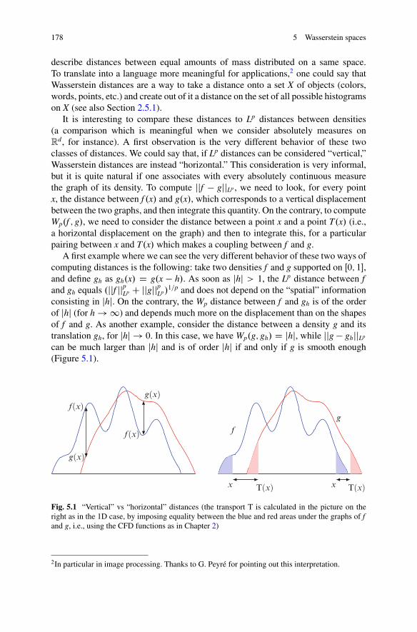
178 5 Wasserstein spaces

describe distances between equal amounts of mass distributed on a same space.To translate into a language more meaningful for applications,2 one could say thatWasserstein distances are a way to take a distance onto a set X of objects (colors,words, points, etc.) and create out of it a distance on the set of all possible histogramson X (see also Section 2.5.1).

It is interesting to compare these distances to Lp distances between densities(a comparison which is meaningful when we consider absolutely measures onR

d, for instance). A first observation is the very different behavior of these twoclasses of distances. We could say that, if Lp distances can be considered “vertical,”Wasserstein distances are instead “horizontal.” This consideration is very informal,but it is quite natural if one associates with every absolutely continuous measurethe graph of its density. To compute jjf � gjjLp , we need to look, for every pointx, the distance between f .x/ and g.x/, which corresponds to a vertical displacementbetween the two graphs, and then integrate this quantity. On the contrary, to computeWp.f ; g/, we need to consider the distance between a point x and a point T.x/ (i.e.,a horizontal displacement on the graph) and then to integrate this, for a particularpairing between x and T.x/ which makes a coupling between f and g.

A first example where we can see the very different behavior of these two ways ofcomputing distances is the following: take two densities f and g supported on Œ0; 1�,and define gh as gh.x/ D g.x � h/. As soon as jhj > 1, the Lp distance between fand gh equals .jjf jjpLp C jjgjjpLp/1=p and does not depend on the “spatial” informationconsisting in jhj. On the contrary, the Wp distance between f and gh is of the orderof jhj (for h ! 1) and depends much more on the displacement than on the shapesof f and g. As another example, consider the distance between a density g and itstranslation gh, for jhj ! 0. In this case, we have Wp.g; gh/ D jhj, while jjg � ghjjLp

can be much larger than jhj and is of order jhj if and only if g is smooth enough(Figure 5.1).

f(x)

f(x)

g(x)

g(x)

x T(x) x T(x)

f

g

Fig. 5.1 “Vertical” vs “horizontal” distances (the transport T is calculated in the picture on theright as in the 1D case, by imposing equality between the blue and red areas under the graphs of fand g, i.e., using the CFD functions as in Chapter 2)

2In particular in image processing. Thanks to G. Peyré for pointing out this interpretation.

5.1 Definition and triangle inequality 179

In several applications, this robustness of the Wasserstein distances w.r.t. pertur-bation of the densities makes them preferable to other distances, and the fact thatthey quantify spatial features of the measures is exactly what is required. Also, wewill see (in Section 5.4 and later 6.1 and 7.3) that the geodesics for these distancesprovide useful interpolations between distributions of mass.

5.1 Definition and triangle inequality

In this section, we give the basic definitions of Wasserstein distances and spaces in˝ � R

d. We will see how to adapt the analysis to the case of more general metricspaces. As we said above, we restrict our analysis to the set

Pp.˝/ WD�� 2 P.˝/ W

ˆjxjp d� < C1

�:

Note that p < q implies Pp.˝/ � Pq.˝/ and that, whenever ˝ is bounded,Pp.˝/ D P.˝/.

For �; � 2 Pp.˝/, let us define

Wp.�; �/ WD min

�ˆ˝�˝

jx � yjp d� W � 2 ˘.�; �/� 1

p

;

i.e., the pth root of the minimal transport cost Tc for the cost c.x; y/ D jx � yjp.The assumption �; � 2 Pp.˝/ guarantees finiteness of this value since jx � yjp �C.jxjp C jyjp/, whence Wp

p .�; �/ � C.´ jxjp d�C ´ jxjp d�/.

Note that, due to Jensen inequality, since all � 2 ˘.�; �/ are probabilitymeasures, for p � q we have

�ˆjx � yjp d�

� 1p

D jjx � yjjLp.�/ � jjx � yjjLq.�/ D�ˆ

jx � yjq d�

�1=q

;

which implies Wp.�; �/ � Wq.�; �/. In particular, W1.�; �/ � Wp.�; �/ for everyp � 1. We will not define here W1, but we refer to Section 5.5.1 for a definition asa limit for p ! 1.

On the other hand, for bounded ˝, an opposite inequality also holds, since

�ˆjx � yjp d�

� 1p

� diam.˝/p�1

p

�ˆjx � yj d�

� 1p

:

This implies

Wp.�; �/ � CW1.�; �/1p ; (5.1)

for C D diam.˝/.p�1/=p.

180 5 Wasserstein spaces

Proposition 5.1. The quantity Wp defined above is a distance over Pp.˝/.

Proof. First, let us note that Wp � 0. Then, we also remark that Wp.�; �/ D 0

implies that there exists � 2 ˘.�; �/ such that´ jx � yjp d� D 0. Such a � 2

˘.�; �/ is concentrated on fx D yg. This implies � D � since, for any test function� we have

ˆ� d� D

ˆ�.x/ d� D

ˆ�.y/ d� D

ˆ� d�:

We need now to prove the triangle inequality. We give two different proofs of thisfact. The first (Lemma 5.3) is easier and uses transport maps and approximation; thesecond (Lemma 5.4) is more general but requires a trickier tool, i.e., disintegrationsof measures. utLemma 5.2. Given �; � 2 Pp.R

d/ and " any even regularizing kernel in L1 with´Rd ".z/ dz D 1 and ".z/ D "�d1.z="/, then we have

1. the inequality Wp.� � "; � � "/ � Wp.�; �/

2. the limit lim"!0 Wp.� � "; � � "/ D Wp.�; �/:

Proof. Take an optimal transport plan � 2 ˘.�; �/ and define a transport plan�" 2 ˘.� � "; � � "/ through

ˆ

Rd�Rd�.x; y/ d�" WD

ˆ

Rd�Rd

ˆ

Rd�.x C z; y C z/".z/dz d�.x; y/:

We need to check that its marginals are actually � � " and � � ". Just consider

ˆ

Rd�Rd�.x/ d�" D

ˆ

Rd�Rd

ˆ

Rd�.x C z/".z/dz d�.x; y/

Dˆ

Rd�Rd.� � "/.x/ d�.x; y/ D

ˆ

Rd.� � "/.x/ d�.x/

Dˆ

Rd�.x/ d.� � "/.x/

(we use the fact that " is even to pass the convolution from � to �). Thecomputation for the second marginal is the same. It is then easy to show that´ jx � yjp d�" D ´ jx � yjp d� , since

ˆjx � yjp d�" D

ˆ

Rd�Rd

ˆ

Rdj.x C z/ � .y C z/jp".z/dz d�.x; y/ D

ˆjx � yjp d�:

This shows the first part of the statement and also

lim sup"!0

Wp.� � "; � � "/p � lim sup"!0

ˆjx � yjp d�" D

ˆjx � yjp d�:

5.1 Definition and triangle inequality 181

One can also obtain the opposite inequality by a standard semi-continuityargument. Consider �" WD � � " and �" WD � � ", and use only the weakconvergences �" * � and �" * �. Call �" the optimal plans in ˘.�"; �"/.This sequence of plans is tight, since its marginals are tight (look at the proofof Theorem 1.7). First fix a sequence "k ! 0 such that limk Wp.�"k ; �"k/ Dlim inf"!0 Wp.�"; �"/. Then extract a subsequence "kj so as to guarantee that theoptimal transport plans �"kj

have a weak limit �0. This weak limit must belong to˘.�; �/ (the fact that the marginals of �0 are � and � follows by the properties ofcomposition with continuous functions of the weak convergence). Then we have

Wpp .�; �/ �

ˆjx � yjp d�0 � lim inf

j

ˆjx � yjp d�"kj

D lim inf"!0

Wp.�"; �"/;

where the first inequality follows from the fact that �0 is not necessarily optimal butis admissible and the second follows by semi-continuity (Lemma 1.6). ut

Then, we can perform a proof of the triangle inequality based on the use ofoptimal transport maps.

Lemma 5.3. The quantity Wp satisfies the triangle inequality (proof by transportmaps and approximation).

Proof. First consider the case where � and % are absolutely continuous and � isarbitrary. Let T be the optimal transport from � to % and S the optimal one from %

to �. Then SıT is an admissible transport from � to �, since .SıT/#� D S#.T#�/ DS#% D �. We have

Wp.�; �/ ��ˆ

jS.T.x// � xjp d�.x/

� 1p

D jjS ı T � idjjLp.�/

� jjS ı T � TjjLp.�/ C jjT � idjjLp.�/:

Moreover,

jjS ı T � TjjLp.�/ D�ˆ

jS.T.x// � T.x/jp d�.x/

� 1p

D�ˆ

jS.y/ � yjpd%.y/

� 1p

and this last quantity equals Wp.%; �/. Moreover, jjT� idjjLp.�/ D Wp.�; %/, whence

Wp.�; �/ � Wp.�; %/C Wp.%; �/:

This gives the proof when �; % � L d. For the general case, first write the triangleinequality for � � ", % � ", and � � ", then pass to the limit as " ! 0 usingLemma 5.2. utThe proof above strongly uses the results about transport maps from Chapter 1 andis somehow specific to R

d (in a general metric space, the tricky part would be to

182 5 Wasserstein spaces

approximate arbitrary measures with measures such that the Wasserstein distancecan be computed with maps instead of plans3). To give a more general result, weprovide a different proof, which may happen to be more difficult for the reader whois not accustomed to disintegrations of measures (see Chapter 2).

Lemma 5.4. The quantity Wp satisfies the triangle inequality (proof by disintegra-tions).

Proof. Let us take �; % and � 2 Pp.˝/, �C 2 ˘.�; %/ and �� 2 ˘.%; �/. Wecan also choose �˙ to be optimal. Let us use Lemma 5.5 to say that there existsa measure � 2 P.˝ � ˝ � ˝/ such that .�x;y/#� D �C and .�y;z/#� D ��,where �x;y and �y;z denote the projections on the two first and two last variables,respectively. Let us take � WD .�x;z/#� . By composition of the projections, it is easyto see that .�x/#� D .�x/#� D .�x/#�

C D � and, analogously, .�z/#� D �. Thismeans � 2 ˘.�; �/ and

Wp.�; �/ ��ˆ

jx � zjp d�

� 1p

D�ˆ

jx � zjpd�

� 1p

D jjx � zjjLp.�/

� jjx � yjjLp.�/ C jjy � zjjLp.�/ D�ˆ

jx � yjpd�

� 1p

C�ˆ

jy � zjpd�

� 1p

D�ˆ

jx � yjp d�C� 1

p

C�ˆ

jy � zjp d��� 1

p

D Wp.�; %/C Wp.%; �/:

The proof is concluded. utThe following lemma is usually known as “gluing lemma” and allows to produce

a sort of “composition” of two transport plans, as if they were maps.

Lemma 5.5. Given two measures �C 2 ˘.�; %/ and �� 2 ˘.%; �/, there exists (atleast) a measure � 2 P.˝ �˝ �˝/ such that .�x;y/#� D �C and .�y;z/#� D ��,where �x;y and �y;z denote the projections on the two first and two last variables,respectively.

Proof. Start by taking �C and disintegrate it w.r.t. the projection �y (see Box 2.2 inSection 2.3). We get a family of measures �C

y 2 P.˝/ (as we pointed out in thesame box, we can think of them as measures over ˝, instead of viewing them asmeasures over ˝ � fyg � ˝ �˝). They satisfy (and are actually defined by)

ˆ

˝�˝�.x; y/ d�C.x; y/ D

ˆ

˝

d%.y/ˆ

˝

�.x; y/ d�Cy .x/;

3It is not strictly necessary to use absolutely continuous measures: we actually need atomlessmeasures, and then we can apply Theorem 1.33.

5.2 Topology induced by Wp 183

for every measurable function � of two variables. In the same way, one has a familyof measures ��

y 2 P.˝/ such that for every �, we have

ˆ

˝�˝�.y; z/ d��.y; z/ D

ˆ

˝

d%.y/ˆ

˝

�.y; z/ d��y .z/:

For every y, take now �Cy ˝ ��

y , which is a measure over ˝ �˝. Define � through

ˆ

˝�˝�˝�.x; y; z/d�.x; y; z/ WD

ˆ

˝

d%.y/ˆ

˝�˝�.x; y; z/ d

��C

y ˝ ��y

.x; z/:

It is easy to check that, for � depending only on x and y, we have

ˆ

˝3

�.x; y/d� Dˆ

˝

d%.y/ˆ

˝�˝�.x; y/ d

��C

y ˝ ��y

.x; z/

Dˆ

˝

d%.y/ˆ

˝

�.x; y/ d�Cy .x/ D

ˆ� d�C:

This proves .�x;y/#� D �C and the proof of .�y;z/#� D �� is analogous. utRemark 5.6. All the analysis of this section can be performed on a general Polishspace X instead of a subset ˝ � R

d. The only differences are the definition ofPp.X/ (we need to use Pp.X/ WD f� 2 P.X/ W ´

d.x; x0/p d�.x/ < C1g),and the fact that the first proof of the triangle inequality was specific to R

d (but thesecond works in general).

Definition 5.7. Given a Polish space X, for each p 2 Œ1;C1Œ we define itsWasserstein space of order p, Wp.X/, as the space Pp.X/, endowed with thedistance Wp.

5.2 Topology induced by Wp

In this section, we want to analyze the convergence in the space Wp and compare itto the notion of weak convergence. First of all, we recall what we mean by “weakconvergence”: as we pointed out in Box 1.3 in Chapter 1, we use this term to denotethe convergence in the duality with Cb, the space of bounded continuous functions(which is often referred to as narrow convergence), and we write �n * � to saythat �n converges in such a sense to �.

We recall that another natural notion of convergence for measures is the one induality with the space of functions vanishing at infinity

C0.X/ WD f� 2 C.X/ W for all " > 0 there is K � X compact s.t. j�j < " on X n Kg:

184 5 Wasserstein spaces

It is useful to point out some facts:

• When X is compact, the spaces C0.X/, Cc.X/, C.X/, and Cb.X/ coincide.• The condition defining � 2 C0.X/ means that � tends to 0 “out of the compact

subsets of X”: this means at infinity, for X D Rd, on @˝ when X D ˝ � R

d isopen, and it means nothing if X is itself compact.

• For every x0 2 X, the existence of functions � 2 C0.X/ with �.x0/ ¤ 0 impliesthe existence of compact neighborhoods of x0. In particular, the space C0.X/is interesting only for locally compact spaces X, and it only consists of thezero function whenever no point of X has compact neighborhoods (for instance,in infinite-dimensional Banach spaces). Indeed, the duality result stating thatM .X/ is the dual of C0.X/ is only true for locally compact spaces (see Box 1.3in Section 1.1).

The following lemma (which is true in locally compact spaces, but we only stateit for subsets of Rd) gives a helpful criterion for weak convergence.

Lemma 5.8. When all measures �n and � are probabilities over a subset˝ � Rd,

the convergence �n * � coincides with the convergence in the duality with Cc.˝/.

Proof. We only need to show that if we take 2 Cb.˝/, �n; � 2 P.˝/ and weassume

´� d�n ! ´

� d� for every � 2 Cc.˝/, then we also have´ d�n !´

d�. If all the measures are probability, then we may add “for free” a constant Cto , and, since is bounded, we can choose C so that C C � 0. Hence C Cis the sup of an increasing family of functions �n 2 Cc (take �n D . C C/n, n

being an increasing family of cutoff functions4 with n D 1 on B.0; n/). Hence bysemi-continuity, we have

´. C C/ d� � lim infn

´. C C/ d�n; which implies´

d� � lim infn´ d�n: If the same argument is performed with � , we obtain

the desired convergence of the integrals. utNote that in the above lemma one can also use C0 instead of Cc, as Cc � C0.

Once the weak convergence is understood, we can start from the following result.

Theorem 5.9. If ˝ � Rd is compact, then �n * � if and only if W1.�n; �/ ! 0.

Proof. Let us recall the duality formula, which gives for arbitrary �; � 2 P.˝/

W1.�; �/ D max

�ˆ˝

' d.� � �/ W ' 2 Lip1

�:

Let us start from a sequence �n such that W1.�n; �/ ! 0. Thanks to the dualityformula, for every ' 2 Lip1.˝/, we have

´' d.�n ��/ ! 0. By linearity, the same

will be true for any Lipschitz function. By density, it will hold for any function inC.˝/. This shows that Wasserstein convergence implies weak convergence.

4The existence of cutoff functions, i.e., a sequence of continuous compactly supported functionsconverging pointwisely to 1, is indeed peculiar to the case of locally compact spaces.

5.2 Topology induced by Wp 185

To prove the opposite implication, let us first fix a subsequence �nk such thatlimk W1.�nk ; �/ D lim supn W1.�n; �/. For every k, pick a function 'nk 2 Lip1.˝/such that

´'nk d.�nk � �/ D W1.�nk ; �/. Up to adding a constant, which does not

affect the integral, we can assume that the 'nk all vanish at a same point, and theyare hence uniformly bounded and equicontinuous. By the Ascoli-Arzelà theoremwe can extract a sub-subsequence uniformly converging to a certain ' 2 Lip1.˝/.By replacing the original subsequence with this new one, we can avoid relabeling.We have now

W1.�nk ; �/ Dˆ'nk d.�nk � �/ !

ˆ' d.� � �/ D 0;

where the convergence of the integral is justified by the weak convergence �nk *

� together with the strong convergence (in C.˝/) 'nk ! '. This shows thatlim supn W1.�n; �/ � 0 and concludes the proof. utTheorem 5.10. If ˝ � R

d is compact and p 2 Œ1;C1Œ, in the space Wp.˝/, wehave �n * � if and only if Wp.�n; �/ ! 0.

Proof. We have already proved this equivalence for p D 1. For the other values ofp, just use the inequalities

W1.�; �/ � Wp.�; �/ � CW1.�; �/1p

that give the equivalence between the convergence for Wp and for W1. utWe can now pass to the case of unbounded domains. From the fact that the

distance Wp does not really depend on the ambient domain, we can simply considerthe case ˝ D R

d.

Theorem 5.11. In the space Wp.Rd/, we have Wp.�n; �/ ! 0 if and only if �n *

� and´ jxjp d�n ! ´ jxjp d�.

Proof. Consider first a sequence �n which is converging to � in Wp.Rd/. It is still

true in this case that

sup

�ˆ� d.�n � �/ W � 2 Lip1

�! 0;

which gives the convergence when testing against arbitrary Lipschitz functions.Note that Lipschitz functions are dense (for the uniform convergence) in the spaceC0.˝/ (while it is not necessarily the case for Cb.˝/). This is enough to prove�n ! �, thanks to Lemma 5.8.

To obtain the other condition, namely,´ jxjp d�n ! ´ jxjp d� (which is not a

consequence of the weak convergence, since jxjp is not bounded), it is sufficient tonote that

186 5 Wasserstein spaces

ˆjxjp d�n D Wp

p .�n; ı0/ ! Wpp .�; ı0/ D

ˆjxjp d�:

We need now to prove the opposite implication. Consider a sequence a �n * �

satisfying also´ jxjp d�n ! ´ jxjp d�. Fix R > 0 and consider the function �.x/ WD

.jxj ^ R/p, which is continuous and bounded. We haveˆ.jxjp � .jxj ^ R/p/ d�n D

ˆjxjp d�n �

ˆ� d�n

!ˆ

jxjp d� �ˆ� d� D

ˆ.jxjp � .jxj ^ R/p/ d�:

Since´.jxjp � .jxj ^ R/p/ d� � ´

B.0;R/c jxjp d� and´Rd jxjp d� < 1, it is possible

to choose R so thatˆ.jxjp � .jxj ^ R/p/ d� < "=2

and hence one can also guarantee that´.jxjp � .jxj ^ R/p/ d�n < " for all n large

enough.We use now the inequality .jxj � R/p � jxjp � Rp D jxjp � .jxj ^ R/p which is

valid for jxj � R (see Lemma 5.12) to getˆ.jxj � R/p d�n < " for n large enough, and

ˆ.jxj � R/p d� < ":

Consider now �R W Rd ! B.0;R/ defined as the projection over B.0;R/. Thismap is well defined and continuous and is the identity on B.0;R/. Moreover, forevery x … B.0;R/, we have jx � �R.x/j D jxj � R. We can deduce

Wp.�; .�R/#�/ ��ˆ

.jxj � R/p d�

� 1p

� "1p ;

Wp.�n; .�R/#�n/ ��ˆ

.jxj � R/p d�n

� 1p

� "1p :

Note also that, due to the usual composition of the weak convergence withcontinuous functions, from �n * �, we also infer .�R/#�n * .�R/#�. Yet, thesemeasures are all concentrated on the compact set B.0;R/, and here we can use theequivalence between weak convergence and Wp convergence. Hence, we get

lim supn

Wp.�n; �/

� lim supn

�Wp.�n; .�R/#�n/C Wp..�R/#�n; .�R/#�/C Wp.�; .�R/#�/

� 2"1p C lim

nWp..�R/#�n; .�R/#�/ D 2"

1p :

5.3 Curves in Wp and continuity equation 187

As the parameter " > 0 is arbitrary, we get lim supn Wp.�n; �/ D 0, and the proofis concluded. utLemma 5.12. For a; b 2 RC and p � 1, we have ap C bp � .a C b/p.

Proof. Suppose without loss of generality that a � b. Then we can write .aCb/p Dap C p p�1b, for a point 2 Œa; a C b�. Use now p � 1 and � a � b to get.a C b/p � ap C bp. utRemark 5.13. How to handle more general metric spaces X instead of subsetsof R

d? First, we notice that Lemma 5.8 does not hold in general (for instance,it is trivially false in infinite-dimensional Banach spaces). Also, the problem ofthe density of Lipschitz functions in the space of continuous functions (even ifX is compact) appears. Indeed, in R

d the fact that smooth functions are dense iseasy to obtain by convolution, a tool which is not available in general spaces. Toovercome this difficulty, one can prove the following statement, which is enough forour scopes: “if we have convergence testing against arbitrary Lipschitz functions,than we also have convergence testing against arbitrary functions in Cb” (this isleft as an exercise, see Ex(31)). Hence, in what concerns Theorems 5.9 and 5.10,everything can be translated into the framework of Polish spaces (with no need oflocal compactness). On the other hand, the proof that we gave of Theorem 5.11 wassomehow specific to R

d: the key point was the existence of a continuous retraction�R from the whole space to a compact subset (the ball B.0;R/), with a bound on thedistance between x and �R.x/. The proof could be adapted to more general spaces,with ad hoc assumptions, but we prefer to refer the reader to [9, 15] for the generalcase.

5.3 Lipschitz curves in Wp and the continuity equation

In this section, we analyze some properties of Lipschitz and absolutely continuouscurves in the space Wp. In order to do that, we need some simple elements fromanalysis in metric spaces. The reader who wants to know more can have a look, forinstance, at [12].

Box 5.1. Good to know! Curves and speed in metric spaces

Let us recall here some properties about Lipschitz curves in metric spaces.A curve ! is a continuous function defined on a interval, say Œ0; 1� and valued in a

metric space .X; d/. As it is a map between metric spaces, it is meaningful to say whetherit is Lipschitz or not, but its velocity !0.t/ has no meaning, unless X is a vector space.

Surprisingly, it is possible to give a meaning to the modulus of the velocity, j!0j.t/.Definition: If ! W Œ0; 1� ! X is a curve valued in the metric space .X; d/, we define the

metric derivative of ! at time t, denoted by j!0j.t/ through

(continued)

188 5 Wasserstein spaces

Box 5.1. (continued)

j!0j.t/ WD limh!0

d.!.t C h/; !.t//

jhj ;

provided this limit exists.The following theorem, in the spirit of Rademacher theorem (see Box 1.9 in Sec-

tion 1.3), guarantees the existence of the metric derivative for Lipschitz curves.Theorem: Suppose that ! W Œ0; 1� ! X is Lipschitz continuous. Then the metric

derivative j!0j.t/ exists for a.e. t 2 Œ0; 1�. Moreover, we have, for t < s,

d.!.t/; !.s// �ˆ s

tj!0j.�/ d�:

The above theorem can be proved by using the fact that every compact metric space (and!.Œ0; 1�/ is the image of a compact set through a continuous map; hence it is compact) canbe isometrically embedded in `1, where one can work componentwise. For all the notionsand the proofs about metric derivatives, we refer, for instance, to [12], Chapter 4.

We also need to consider more general curves, not only Lipschitz continuous.Definition: A curve ! W Œ0; 1� ! X is defined absolutely continuous whenever there

exists g 2 L1.Œ0; 1�/ such that d.!.t0/; !.t1// � ´ t1t0

g.s/ds for every t0 < t1. The set ofabsolutely continuous curves defined on Œ0; 1� and valued in X is denoted by AC.X/.

It is well known that every absolutely continuous curve can be reparametrized in time(through a monotone-increasing reparametrization) and become Lipschitz continuous. Apossible way to achieve this goal is the following: let G.t/ WD ´ t

0 g.s/ds, and then setS.t/ D "t C G.t/ (for any " > 0), which is continuous and strictly increasing and valuedin an interval Œ0;L�; for t 2 Œ0;L�, set Q!.t/ D !.S�1.t//. It is easy to check that Q! 2 Lip1.Also, if we let " ! 0, we obtain a unit-speed reparametrization of !. If we want to haveparametrizations defined on the same interval Œ0; 1�, we just need to rescale by a factor L.

In particular, the above Rademacher theorem is also true for ! 2 AC.X/ (since thereparametrization that we defined is differentiable a.e.).

The goal of this section is to identify the absolutely continuous curves in thespace Wp.˝/ with solutions of the continuity equation @t�t C r � .vt�t/ D 0 withLp vector fields vt. Moreover, we want to connect the Lp norm of vt with the metricderivative j�0j.t/.

We recall (see Section 4.1) that the continuity equation may be interpreted asthe equation ruling the evolution of the density �t of a family of particles initiallydistributed according to �0, and each of which follows the flow

(y0

x.t/ D vt.yx.t//

yx.0/ D x:

We state below the main theorem (originally proven in [15]) relating absolutelycontinuous curves in Wp with solutions of the continuity equation. For simplicity,we will only state it in the framework of a compact domain˝ � R

d. We will explainwhere we use the compactness assumption and how to get rid of it.

5.3 Curves in Wp and continuity equation 189

Theorem 5.14. Let .�t/t2Œ0;1� be an absolutely continuous curve in Wp.˝/ (forp > 1 and ˝ � R

d compact). Then for a.e. t 2 Œ0; 1�, there exists a vector fieldvt 2 Lp.�tIRd/ such that

• the continuity equation @t�t C r � .vt�t/ D 0 is satisfied in the weak sense (seeSection 4.1.2),

• for a.e. t, we have jjvtjjLp.�t/ � j�0j.t/ (where j�0j.t/ denotes the metricderivative at time t of the curve t 7! �t, w.r.t. the distance Wp);

Conversely, if .�t/t2Œ0;1� is a family of measures in Pp.˝/ and for each t we

have a vector field vt 2 Lp.�tIRd/ with´ 10

jjvtjjLp.�t/ dt < C1 solving @t�t C r �.vt�t/ D 0, then .�t/t is absolutely continuous in Wp.˝/, and for a.e. t, we havej�0j.t/ � jjvtjjLp.�t/.

Remark 5.15. Note that, as a consequence of the second part of the statement, thevector field vt introduced in the first one must a posteriori satisfy jjvtjjLp.�t/ Dj�0j.t/.

We will split the proof of this theorem into two parts, dealing with the directand converse implications, respectively. We first introduce some tools that we need,and in particular, the following one will be needed in both parts of the statement ofTheorem 5.14.

Remark 5.16. It is important to observe that, by reparametrizing in time, it is alwayspossible to assume that the absolutely continuous curve �t of the first part of thestatement is actually Lipschitz (and we obtain in this case a uniform bound onjjvtjjLp.�t/) and that the norm jjvtjjLp.�t/ in the second part is bounded (and we obtainthat �t is Lipschitz). Hence, all the proofs will be done in this Lipschitz framework.

5.3.1 The Benamou-Brenier functional Bp

We need to start from an easy computation, which will be useful in the sequel. Weconsider a pair of exponents p and q such that 1p C 1

q D 1.

Lemma 5.17. Set Kq WD f.a; b/ 2 R�Rd W aC 1q jbjq � 0g. Then, for .t; x/ 2 R�Rd

we have

sup.a;b/2Kq

.at C b � x/ D fp.t; x/ WD

8<ˆ:

1p

jxjptp�1 if t > 0;

0 if t D 0; x D 0

C1 if t D 0; x ¤ 0; or t < 0:

(5.2)

In particular, fp is convex and l.s.c.

Proof. First of all, we establish (5.2). Suppose t > 0: then it is clear that one shouldtake the maximal possible value of a in the sup, and hence a D � 1

q jbjq. This gives

190 5 Wasserstein spaces

supb

��1

qtjbjq C b � x

�D t

�sup

b�1

qjbjq C b � �x

t

�:

If we recall that the Legendre transform of p 7! 1q jpjq is x 7! 1

p jxjp. This gives

supb

�1q

jbjq C b � y D 1

pjyjp for all y; (5.3)

and hence

sup

�at C b � x W a 2 R; b 2 R

d; a C 1

qjbjq � 0

�D t

1

p

ˇxt

ˇp D 1

p

jxjptp�1 :

The case .t; x/ D .0; 0/ is straightforward. If t D 0 and x ¤ 0, then it is clear thatany vector b may be compensated by a sufficiently negative value of a, which gives

sup

�at C b � x W a 2 R; b 2 R

d; a C 1

qjbjq � 0

�D sup

bb � x D C1:

Finally, in the case t < 0, one can take a arbitrarily negative and b D 0 so that

sup

�at C b � x W a 2 R; b 2 R

d; a C 1

qjbjq � 0

�� sup

a<0at D C1:

The fact that fp is convex and l.s.c. is a consequence of the fact that it is expressedas a supremum of linear functions. utWe can note in the above result that we computed the Legendre transform of anindicator function and that we got, as expected, a 1-homogeneous convex function.We want now to use this function fp to define a functional over measures. For % 2M .X/ and E 2 M d.X/, we set

Bp.%;E/ WD sup

�ˆX

a.x/d%Cˆ

Xb.x/ � dE W .a; b/ 2 Cb.XI Kq/

�;

where the letter B is chosen because of the role that this functional has in the so-called Benamou-Brenier formula (see Section 6.1).

We prove the following:

Proposition 5.18. The functional Bp is convex and lower semi-continuous on thespace M .X/�M d.X/ for the weak convergence. Moreover, the following propertieshold:

1. Bp.%;E/ � 0,2. Bp.%;E/ WD supf´ a.x/d%C ´

b.x/ � dE W .a; b/ 2 L1.XI Kq/g;3. if both % and E are absolutely continuous w.r.t. a same positive measure � on

X, we can write Bp.%;E/ D ´X fp.%.x/;E.x// d�.x/, where we identify % and E

with their densities w.r.t. �,

5.3 Curves in Wp and continuity equation 191

4. Bp.%;E/ < C1 only if % � 0 and E � %,5. for % � 0 and E � %, we have E D v � % and Bp.%;E/ D ´

1p jvjp d%,

6. If X D Rd, %" WD % � �" and E" WD E � �" (for standard even mollifying kernel

�"), then we have Bp.%";E"/ � Bp.%;E/.

Proof. The convexity and lower semi-continuity of Bp are a direct consequence ofits definition as a supremum of linear functionals. The first property (positivity) isstraightforward, as one can take a D 0 and b D 0 in the supremum.

In order to prove that the supremum can be taken over bounded functionsinstead of continuous ones, we just need to approximate every bounded functionwith continuous ones (beware that, by abuse of notation, the space L1.XI Kq/

denotes here the space of bounded measurable functions valued in Kq, indepen-dently of the reference measure). This can be done via Lusin’s theorem (see thecorresponding Box 1.6 in Section 1.1), and every bounded pair .a; b/ can beapproximated by continuous pairs .Qa; Qb/, such that .% C jEj/.f.a; b/ ¤ .Qa; Qb/g/ <" and sup jQaj � sup jaj and sup jQbj � sup jbj. Then, we can replace Qa withminfQa;� 1

q jQbjqg so as to guarantee to have functions valued in Kq. The differenceˇ´a.x/d%C ´

b.x/ � dE � ´ Qa.x/d%C ´ Qb.x/ � dEˇ

is bounded by C" where C onlydepends on sup jaj and sup jbj.

Once we know that we can use measurable functions a; b with no need ofcontinuity, then property 3 is a consequence of Lemma 5.2. As a consequence ofLemma 5.17, we can write

Bp.%;E/ D sup

�ˆŒa.x/%.x/C b.x/ � E.x/� d�.x/ W .a; b/ 2 L1.XI Kq/

�

Dˆ

fp.%.x/;E.x//d�.x/:

The fact that Bp is only finite if % � 0 is easy: assume it to be false forcontradiction, and take a set A such that %.A/ < 0, a D �n1A and b D 0. Wehave Bp.%;E/ � n%.A/ and, since n is arbitrary, Bp.%;E/ D C1. To prove thefact that Bp is only finite if E � %, assume that there is a set A with %.A/ D 0

and E.A/ ¤ 0. Take any unit vector e and use a D � nq

q 1A and b D ne1A. We haveBp.%;E/ � ne � E.A/. Since both e and n are arbitrary, we get Bp.%;E/ D C1.

When we restrict to the case % � 0 and E D v � %, property 5 is a consequence ofproperty 3. Indeed, just use � D %, thus getting

Bp.%; v � %/ Dˆ

fp.1; v.x//d%.x/ Dˆ1

pjvjp d%:

Let us now prove property 6. Take arbitrary bounded functions a W Rd ! R andb W Rd ! R

d satisfying a.x/C 1q jb.x/jq � 0 for all x. From standard properties of

convolutions, we have

192 5 Wasserstein spaces

ˆa d%" C

ˆb � dE" D

ˆa" d%C

ˆb" � dE;

where a" WD a � �" and b" WD b � �". Note that, by Jensen inequality

jb".y/jq Dˇˇˆ

b.x/�".x � y/ dx

ˇˇq

�ˆ

jb.x/jq�".x � y/ dx

and hence

a".y/C 1

qjb".y/jq �

ˆa.x/C

�1

qjb.x/jq

��".x � y/ dx � 0:

This proves .a"; b"/ 2 C.RdI Kq/, and hence we have

ˆa d%" C

ˆb � dE" D

ˆa" d�C

ˆb" � dE � Bp.%;E/:

Passing to the sup in a and b, one gets Bp.%";E"/ � Bp.%;E/. ut

Remark 5.19. As a convex and l.s.c. functional, Bp has admits a subdifferential,which one could usefully compute for optimization purposes: this computation isdeveloped in [235], but we will not need it in this framework.

We are now ready to prove the first part of Theorem 5.14.

5.3.2 Proof of Theorem 5.14, Part 1: � is AC ) there exists v

Proof. First of all, we note that it is not restrictive to assume that � is a Lipschitzcurve (if not, we just reparametrize in time).

We will do our proof by approximation, i.e., we build a sequence �kt of curves

which admit the existence of suitable vector fields vkt , in such a way that �k

t * �t

and that we can find a limit for the vector fields also.To define �k

t we proceed in the following way. For t D i=k, i D 0; 1; : : : ; k, wedefine �k

t D �t � �k, where �k is a smooth approximation of the identity, i.e., asmooth even positive function supported on B.0; 1=k/ and with integral equal to 1.The only goal of this smoothing is to guarantee that the measures are absolutelycontinuous. The support of the measures is now contained in a slightly biggerdomain ˝ 0 ˝ that we can choose convex. Then, for each i D 0; 1; : : : ; k � 1,we define Ti;k W ˝ 0 ! ˝ 0 to be the optimal transport (for the cost c.x; y/ Djx � yjp) from �k

i=k to �k.iC1/=k. These optimal transport maps exist since every �k

i=k

is absolutely continuous. Then, for t 2� ik ;

iC1k Œ, we define

�kt WD �

.i C 1 � kt/id C .kt � i/Ti;k

#�ki=k;

5.3 Curves in Wp and continuity equation 193

which means that the particle located at x at time i=k goes to the position Ti;k.x/at time .i C 1/=k, moving with constant speed on the segment connecting thesetwo positions in the interval � i

k ;iC1

k Œ. The velocity of this movement is given by

vi;k WD k.Ti;k.x/ � x/. Set Ti;kt WD .i C 1 � kt/id C .kt � i/Ti;k; this map is injective

(see Lemma 4.23). Thus, we can set vkt WD vi;k ı �Ti;k

t

�1. This last vector field

exactly represents the velocity that each particle has during its movement at time t:first we detect which is the original position of such a particle (at time i=k), then weassociate with this particle the velocity associated with this original position.

As a consequence of this construction and of the considerations in Section 4.1,the pair .�k

t ; vkt / solves the continuity equation @t�

kt C r � .vk

t�kt / D 0.

The important point is the computation

jjvkt jjpLp.�k

t /D

ˆjvk

t jp d�kt D

ˆjvi;kjp ı �Ti;k

t

�1d�Ti;k

t

#�

ki=k D

ˆjvi;kjp d�k

i=k

D kpWpp .�

ki=k; �

k.iC1/=k/ � kpWp

p .�i=k; �.iC1/=k/

� kp

ˆ .iC1/=k

i=kj�0j.s/ds

!p

� kˆ .iC1/=k

i=kj�0jp.s/ds:

Here we used the fact that Wp.�i=k � �"; �.iC1/=k � �"/ � Wp.�i=k; �.iC1/=k/ (seeLemma 5.2) and, at the end, Jensen’s inequality. In particular, we also get a uniformbound on jjvk

t jjLp.�kt /

since k´ .iC1/=k

i=k j�0jp.s/ds � Lip.�/.This implies that, for arbitrary time 0 � a < b � 1 (with ia=k � a � .ia C 1/=k

and ib=k � b � .ib C 1/=k), we have

ˆ b

ajjvk

t jjpLp.�kt /

dt �ibX

iDia

ˆ .iC1/=k

i=kj�0jp.s/ds

Dˆ .ibC1/=k

ia=kj�0jp.s/ds �

ˆ b

aj�0jp.s/ds C 2Lip.�/

k: (5.4)

Now, define a vector measure Ek on ˝ 0 � Œ0; 1� via

ˆ�.t; x/ � dEk WD

ˆ 1

0

�ˆ�.t; x/ � vk

t .x/ d�kt .x/

�dt:

We can easily check that

jjEkjj Dˆ 1

0

jjvkt jjL1.�k

t /dt �

ˆ 1

0

jjvkt jjLp.�k

t /dt �

�ˆ 1

0

jjvkt jjpLp.�k

t /dt

� 1p

� C:

194 5 Wasserstein spaces

Hence, up to a subsequence extraction, the sequence of vector measures Ek admitsa weak limit E. On the other hand, it is easy to check that �k converges in Wp,uniformly in time, to �. Indeed

Wp.�kt ; �t/ � Wp.�

kt ; �

ki=k/C Wp.�

ki=k; �i=k/C Wp.�i=k; �t/:

The first term may be estimated using

Wp.�kt ; �

ki=k/ � jt � i=kj jjvi;kjjLp.�k

i=k/� C

kI

the second may be estimated by the size of the support of the kernel �" (which allowsto obtain �k

i=k from �i=k), which is " D 1=k; the third is estimated by the Lipschitz

constant of � times, again, jt � ik j � 1

k . Overall, we get

Wp.�kt ; �t/ � C

k:

From @t�k C r � Ek D 0, we can easily pass to the limit and get @t�C r � E D 0.

We want now to prove that Et D vt�t, with jjvtjjLp.�t/ � j�0j.t/ a.e.This is a consequence of Proposition 5.18 on the semi-continuity of Bp. Indeed,

using (5.4) with a D 0; b D 1, we have Bp.�k;Ek/ � C (where the functional Bp

is considered on the whole space-time domain Œ0; 1� �˝). This is enough to obtainBp.�;E/ < C1 and E � �, i.e., Et D vt�t. Then, if we apply the same lemma tothe measures �k and Ek restricted to a closed interval Œa; b�, we obtain

ˆ b

ajjvtjjpLp.�t/

dt � lim infk

ˆ b

ajjvk

t jjpLp.�kt /

dt �ˆ b

aj�0jp.t/dt:

Since this is true for arbitrary values of a and b, on every Lebesgue point t0 oft 7! jjvtjjpLp.�t/

and t 7! j�0jp.t/, we get the desired inequality. utWe want now to prove the converse implication of Theorem 5.14. Again, to be

able to perform our computations rigorously, we need to regularize by convolution.The construction that we do here will be useful many times, and it deserves to bedetailed and analyzed.

5.3.3 Regularization of solutions of the continuity equation

Suppose that .�;E/ solves the continuity equation @t�tCr�Et D 0, that the supportsof all measures �t and Et are contained in a same compact set ˝ � R

d, and thatEt is bounded in the space of measure, i.e., jjEtjj WD jEtj.Rd/ � C. Take a C1strictly positive kernel �" (as a function of space only) and define �"t WD �" ��t andE"t WD �" � Et, and v"t WD E"t =�

"t . The choice is made so that @t�

"t C r � .�"t v"t / D 0.

5.3 Curves in Wp and continuity equation 195

Since we want to apply the characterization result of solutions of the continuityequation (Theorem 4.4), we want to check uniform global bounds on v". To dothis, we need to perform a particular choice of �", and in particular, we take it ofthe form �".z/ D "�d�.jzj="/, where � W RC ! R

C is a smooth function such that�.t/ D Ce�t for t � 1. In Lemma 5.20, we check that this guarantees that v" satisfiesthe required global bounds, and we also state regularity for �" (that we will need inSection 5.3.5).

Lemma 5.20. With the above choice of the convolution kernel �", the function �"

is Lipschitz in .t; x/ and v" is Lipschitz in x and bounded, uniformly in t (for fixed" > 0), provided ˝ is bounded.

Proof. We can fix " D 1 as the computations for other values of " are similar. Weset � D �". From �".t; x/ D ´

�.jy � xj/�t.dx/, we have a Lipschitz bound in xfrom standard convolution properties, but also

@t�".t; x/ D d

dt

ˆ�.y � x/d�t.x/ D

ˆr�.y � x/ � dEt.x/;

which is bounded by Lip.�/jEtj.Rd/.As far as v" is concerned, computations are trickier since it is defined as E"=�".

From � > 0, we get �" > 0 which guarantees that v" is smooth as the ratio betweentwo smooth functions, with nonvanishing denominator. Yet, we want to computeexplicit and global bounds for large jxj. If R0 D diam.˝/ and 0 2 ˝, we havefor sure, for jxj D R � 1, �".x/ � �.R C R0/. On the other hand, we have, forR � 2R0 _ 1, jE"j � C�.R � R0/, jrE"j � Cj�0.R � R0/j, and, similarly, jr�"j �Cj�0.R � R0/j. From

jv"j D jE"j�"

; jrv"j � jrE"j�"

C jE"j jr�"j.�"/2

;

using � D �0 D �00 on Œ1;C1Œ and �.R C R0/ D e�2R0�.R � R0/, we get uniformbounds. utWe will see that the application of Lemma 5.20 is the only point where we needed˝to be bounded. Without this assumption, we cannot apply the characterization resultfor the continuity equation that we presented in Theorem 4.4. On the other hand, wealready mentioned that more general uniqueness results exist (for instance, in [15]),and we simply chose not to present them for the sake of simplicity.

Thanks to our definitions, we have

@t�"t C r � .v"t�"t / D 0:

Moreover, applying Theorem 4.4, we know that the only solution of @t%t C r �.v"t %t/ D 0 is given by the flow of v". Hence, we get

196 5 Wasserstein spaces

�"t D .Yt/#�"0; where Yt.x/ D yx.t/; and

(y0

x.t/ D v"t .yx.t//;

yx.0/ D x:(5.5)

We can summarize our construction in the following proposition.

Proposition 5.21. Consider a pair .�;E/ solving @t�t C r � Et D 0, and supposethat the supports of all measures �t and Et are contained in a same compact set˝ � R

d and that Et is bounded in the space of measure, i.e., jEtj.Rd/ � C. Then,there exists a family of approximating curves .�"t /t with a velocity vector field v"tsuch that

• �" is Lipschitz in .t; x/ and v" is Lipschitz in x and bounded, uniformly in t;moreover, �" > 0 everywhere;

• �"t is obtained from �"0 by following the flow of the vector field v", in the senseof (5.5);

• For every t, we have �"t * �t and for a.e. t, we have E"t * Et.• jjv"t jjLp.�"t / � Bp.�t;Et/.

Proof. We use the construction we described above. The first property is provenin Lemma 5.20, the second has been discussed above, and the third is evident byconstruction. The fourth is a consequence of property 5 of Lemma 5.18. Note thatthis means jjv"t jjLp.�"t / � jjvtjjLp.�t/ whenever Et D vt � �t. ut

We finish this paragraph by noting that the same construction could have beenperformed on the torus.

Remark 5.22. If �t 2 P.Td/, one can consider an arbitrary approximation kernel�" 2 C1.Rd/ of the form �".z/ D "�d�.z="/ (strictly positive, but with no needof imposing exponential behavior) and define the convolution on the torus. To beprecise, let us stress that the periodic convolution ��� between a measure � on T

d

and a function � on Rd is defined as follows. Consider at first � as a measure on

Q D Œ� 12; 12� � R

d, perform standard convolution on Rd, and then define

.���/.x/ WDXk2Zd

.� � �/.x C k/:

Equivalently, this corresponds to a convolution on the torus with the convolutionkernel

Pk2Zd �.x C k/.

With this construction, the same conclusions as in Proposition 5.21 hold.Moreover, every compact domain ˝ can be seen as a subset of a cube Q identifiedwith the torus, and it can even fit an arbitrary small portion of Q. In this case, everyoptimal transport problem for the costs jx � yjp between measures on ˝ “does notsee” the fact that Q is identified with a torus (it is enough to have ˝ � 1

2Q).

We stress that the uniform bounds in the case of the torus are easier to obtain, butwe found conceptually easier to deal with measures on R

d (and in particular with

5.3 Curves in Wp and continuity equation 197

optimal transport problems in Rd). This is why we prefer the Euclidean construction

to this one. Yet, we present both of them for the use that we will do in Section 5.3.5,where compactness is crucial for our estimates.

5.3.4 Proof of Theorem 5.14, Part 2: There exists v ) � is AC

Proof. The starting point is a pair .�;E/ which solves the continuity equation,where Et D vt � �t and vt 2 Lp.�t/ for a.e. t. Again, we apply a reparametrization:with a change of variable in time, we can replace .�t;Et/ with a new pair where Et

is just multiplied by a scalar constant depending on t. By choosing our change ofvariable, we can impose a uniform bound on jjvtjjLp.�t/. This also implies a boundon jjEtjj D jEtj.Rd/ D jjvtjjL1.�t/.

Under this extra assumption (the uniform bound on jjEtjj), we can use theconstruction provided in the previous paragraph (using the construction on R

d forsimplicity of exposition). Thus, we can build an approximated curve �"t which isdriven by the flow of the smooth (in space) vector field v". This provides a usefultransport plan between �"t and �"tCh, taking � D .Tt;TtCh/#�

"0 2 ˘.�"t ; �

"tCh/.

We obtain

Wp.�"t ; �

"tCh/ �

�ˆ˝�˝

jx � yjp d�

� 1p

D�ˆ

˝

jTt.x/ � TtCh.x/jp d�"0

� 1p

� jhj1=q

�ˆ˝

ˆ tCh

t

ˇˇ d

dsTs.x/

ˇˇp

ds d�"0

� 1p

D jhj1=q

�ˆ tCh

tdsˆ

˝

ˇv"s.yx.s//

ˇpd�"0

� 1p

D jhj1=q

�ˆ tCh

tdsˆ

˝

ˇv"s.y/

ˇpd�"s.y/

� 1p

:

We proved in Lemma 5.17 that´ ˇ

v"s.y/ˇp

d�"s.y/ � jjvsjjpLp.�s/: From this, we get

Wp.�"t ; �

"tCh/ � jhj1=q

�ˆ tCh

tjjvsjjpLp.�s/

ds

� 1p

D jhj�1

jhjˆ tCh

tjjvsjjpLp.�t/

ds

� 1p

:

First we can pass to the limit " ! 0, thus obtaining

Wp.�t; �tCh/

jhj ��1

jhjˆ tCh

tjjvsjjpLp.�s/

ds

� 1p

:

198 5 Wasserstein spaces

This provides Lipschitz behavior for �t. Then, we take the limit h ! 0 at points twhere j�0j.t/ exists and which are Lebesgue points of t 7! jjvtjjpLp.�t/

, we obtain

j�0j.t/ � jjvtjjLp.�t/;

which provides the desired estimate. utWe remark that Theorem 5.14 has been proven thanks to an extensive use of the

functional Bp: we needed its convexity in the second part and its semi-continuity inthe first part.5

Remark 5.23. We also note that we only defined the functional Bp for p > 1 andthat the only natural extension for p D 1 would be given by B1.%;E/ D jjEjj. It iseasy to understand that the first part of Theorem 5.14 cannot stay true in the casep D 1. Indeed, the part of the statement which fails is the existence of a vector fieldvt, since it is no more possible to deduce E � �: it is not difficult to adapt the proofso as to get the existence of a family Et of vector measures solving @t�t Cr �Et D 0,but Et will be no more of the form vt � �t. An example where absolute continuityfails is the following: take �t WD .1 � t/ıx0 C tıx1 , which is Lipschitz in W1 (butnot in Wp, p > 1). In this case, one could take Et D x1�x0jx1�x0jH

1 Œx0; x1� (a uniformmeasure on the segment joining the two points, oriented as the same segment), butno measure concentrated on fx0; x1g can be such that its divergence is ıx1 � ıx0 .

5.3.5 Derivative of Wpp along curves of measures

We conclude this section with a useful computation which can be applied in manycases in the study of evolution PDEs. The same result is efficiently proven in [15],but we provide a different proof.

Theorem 5.24. Let .%.i/t ; v.i/t / for i D 1; 2 be two solutions of the continuity

equation @t%.i/t C r � .v.i/t %

.i/t / D 0 on a compact domain ˝ (with no-flux boundary

conditions), and suppose that %.i/t � L d for every t and that %.i/ are absolutelycontinuous curves in Wp.˝/. Then we have

d

dt

�1

pWp

p .%.1/t ; %

.2/t /

�D

ˆr't � v.1/t %

.1/t dx C

ˆr t � v.2/t %

.2/t dx

5The proof that we gave of the second part is standard and based on the interpretation of thecontinuity equation that we gave in Chapter 4. The approximations that we performed are the sameas in [15], but we tried to simplify them to make this exposition self-contained: in order to do that,we chose a very precise convolution kernel. Concerning the first part, we stress that a different, andmuch more elegant, approach can be found in [15] and does not use approximation. The approachthat we presented here is more or less inspired by a paper by Lisini, [212].

5.3 Curves in Wp and continuity equation 199

for a.e. t, where .'t; t/ is any pair of Kantorovich potentials in the transportbetween %.1/t and %.2/t for the cost 1p jx � yjp.

Proof. We first prove the result under the assumption that %.i/ is Lipschitz contin-uous in .t; x/ and v.i/ is Lipschitz in x, uniformly in t, for i D 1; 2. In this case,we write, for arbitrary t; t0, the following inequality, justified by the duality formula(Theorem 1.39):

1

pWp

p .%.1/t ; %

.2/t / �

ˆ't0%

.1/t �

ˆ t0%

.2/t � 0; (5.6)

with equality when t D t0. Choose t0 such that t 7! Wpp .%

.1/t ; %

.2/t / is differentiable

at t D t0 and %.i/.t; x/ is differentiable in t at .t0; x/ for a.e. x, and the derivative intime equals �r � .%.i/.t; x/vi.t; x//. All these conditions are satisfied for a.e. t0 (weuse Proposition 4.3). Hence, the left-hand side in (5.6) is differentiable at t D t0 andthe derivative must vanish, because of minimality at t D t0. This proves

d

dt

�1

pWp

p

�%.1/t ; %

.2/t

��jtDt0

Dˆ't0

�@t%

.1/

t0Cˆ t0

�@t%

.2/

t0;

and the desired formula is obtained by using @t%.i/ D �r � .v.i/%.i// and integrating

by parts.6

To deal with the general case, first we reduce to the case where the curves %.i/ areLipschitz in Wp.˝/, by reparametrization in time. Then, we apply the regularizationprocedure of Section 5.3.3. In order to preserve compactness, we choose to applythe construction on the torus, and we suppose ˝ � 1

2Q (which is possible up

to rescaling). Hence, we obtain two smoother families of curves %.i;"/t with theirvelocity fields v.i;"/t . For t0 < t1, the first part of the proof implies

1

pWp

p

�%.1;"/t1 ; %

.2;"/t1

�� 1

pWp

p

�%.1;"/t0 ; %

.2;"/t0

�D

ˆ t1

t0

dtˆ

Tdr'"t � E.1;"/t C r "

t � E.2;"/t ;

where E.i;"/t D %.i;"/t v.i;"/t (also set E.i/t D %

.i/t v.i/t ) and '"t and "

t are Kantorovichpotentials in the transport from %

.1;"/t to %.2;"/t .

We just need to pass to the limit in the above equality. The left-hand side triviallyconverges to the corresponding Wasserstein distances between the measures %.i/

(note that we are on a compact space, and the convolutions weakly converge to the

6One of the difficulties in this result is that the functions t 7! ´'t0%

.1/t and t 7! ´

t0%.2/t are

differentiable for a.e. t, but not necessarily at t D t0 (we know that for every integrand the integralis differentiable for a.e. T , and not that for a.e. t differentiability occurs for every integrand). Wepropose a way to overcome this difficulty via Lipschitz solutions. As an alternative approach, onecan try to find the precise set of times t such that differentiability occurs for every integrand, as in[155], based on ideas from [15].

200 5 Wasserstein spaces

original measure). Next, let us analyze the first part of the right-hand side (i.e., fori D 1, the other part being completely analogous).

For each t, we have

ˇˇˆ

Tdr'"t � E.1;"/t

ˇˇ�Lip.'"t /

v.i;"/t

L1�%.i;"/t

��C v.i;"/t

Lp�%.i;"/t

��C v.i/t

Lp�%.i/t

��C;

where we used property 5 of Proposition 5.18 and the fact that all the functions '"

are equi-Lipschitz (see Section 1.3.2).It is now enough to look at the limit for fixed t, since as a function of t, we can

apply dominated convergence. Let us set '""t WD �" � '"t : we have

ˆ

Tdr'"t � E.1;"/t D

ˆ

Tdr'"t � .�" � E.1/t / D

ˆr'""t � E.1/t ;

because of standard properties of convolutions. Thus, we only need to prove thatr'""t ! r't a.e. The functions '""t are equi-Lipschitz and equi-semi-concave (seeagain Section 1.3.2) on a compact set and, up to translating their mean, we can applythe Ascoli-Arzelà theorem. Thus they converge up to subsequence to a function Q'.Note that, because of semi-concavity, the convergence of the functions implies a.e.convergence of the gradients (see, for instance, Theorem 3.3.3 in [102]). We justneed to prove r Q' D r't (which would also imply that the convergence is true onthe whole sequence).

Note that by Theorem 1.52, the limit of '"t must be a Kantorovich potential.Moreover, we have the general estimate

j.�" � f /.x/ � f .x/j �ˆ

jf .x/ � f .x � y/j ��y

"

� dy

"d

� Lip.f /ˆ

jyj��y

"

� dy

"dD "Lip.f /

ˆjzj�.z/dz;

(where we used the change of variable y D "z). The same estimate also worksfor periodic convolution and shows jj'""t � '"t jjL1 � C Lip.'"/" � C" ! 0.This allows to conclude that the limit of '""t must be the same as that of '"t , i.e., aKantorovich potential. Even if the Kantorovich potential is not necessarily unique,its gradient is unique, and we deduce r'""t ! r't. ut

Note that in the above proof, we intensively used the compactness of the domain˝ (and of the torus: the same proof performed with regularization via measures onR

d seems delicate because of the lack of bounds on r'""t ). The assumption that themeasures are absolutely continuous is used to take advantage of the a.e. convergenceof the gradients to a unique limit (the gradient of the limit potential). Without this,one could have problems in recovering full convergence of the sequence.

As a corollary of the previous result, we obtain the following useful formula.

5.3 Curves in Wp and continuity equation 201

Corollary 5.25. Under the same assumptions of Theorem 5.24, we have

d

dt

�1

pWp

p .%.1/t ; %

.2/t /

�D

ˆ

˝

.x � Tt.x// ��

v.1/t .x/ � v.2/t .Tt.x//�%.1/t .x/ dx;

where Tt is the optimal transport map from %.1/t to %.2/t for the cost 1p jx � yjp.

Proof. We just need to rewrite the conclusion of Theorem 5.24, using r't.x/ Dx � Tt.x/ and r t.y/ D y � St.y/, where St is the optimal transport from %

.2/t to %.1/t .

We useˆ.y � St.y// � v.2/t .y/ d%.2/t .y/ D

ˆ.Tt.x/ � x/ � v.2/t .Tt.x// d%.1/t .x/;

which is a consequence of .Tt/#%.1/t D %

.2/t and St D T�1

t . Hence, the formula givenby Theorem 5.24 provides

d

dt

�1

pWp

p .%.1/t ; %

.2/t /

�

Dˆ

˝

.x � Tt.x// � v.1/t .x/ d%.1/t .x/Cˆ

˝

.Tt.x/ � x/ � v.2/t .Tt.x// d%.1/t .x/;

which gives the claim.

Some examples of application of the above computation to the uniqueness andthe properties of the solution to some evolution PDEs are presented in the Exercisesection (Ex(34), Ex(66),Ex(67),Ex(68),Ex(69)).

Here, we will only give an example of application to the uniqueness for thecontinuity equation with given vector field.

Proposition 5.26. Let vt W ˝ ! Rd be a family of vector fields on a compact

smooth domain ˝, parametrized in time, satisfying a one-sided Lipschitz condition.vt.x/� vt.y// � .x � y/ � Cjx � yj2 for a fixed constant C, not depending on x; y, nort. Suppose also that vt �n D 0 on @˝ and consider the equation @t%t Cr �.%tvt/ D 0

with given initial datum %0. Then there is at most one solution %t among AC curvesin W2.˝/ which are absolutely continuous measures for a.e. t.

Proof. Consider two solutions %.1/t ; %.2/t and compute the derivative in time of

W22 .%

.1/t ; %

.2/t /. Using Corollary 5.25, we have

d

dt

�1

2W22 .%

.1/t ; %

.2/t /

�D

ˆ

˝

.x � T.x// � .vt.x/ � vt.T.x///%.1/t dx

� Cˆ

˝

jx � T.x/j2%.1/t dx D CW22 .%

.1/t ; %

.2/t /:

202 5 Wasserstein spaces

This allows to apply Gronwall’s lemma and deduce W22 .%

.1/t ; %

.2/t / D 0 from the fact

that the same distance vanishes at t D 0. utNote that the above proof could also be used to prove uniqueness in the continuity

equation and applied to Theorem 4.4.

5.4 Constant-speed geodesics in Wp

We will see in this section how constant-speed geodesics in Wp are related to optimaltransport maps. Before doing so, we recall the main facts about geodesics in metricspaces.

Box 5.2. Good to know! Constant-speed geodesics in general metric spaces

First of all, let us define the length of a curve ! in a general metric space .X; d/.Definition: For a curve ! W Œ0; 1� ! X, let us define

Length.!/ WD sup

(n�1XkD0

d.!.tk/; !.tkC1/ W n � 1; 0 D t0 < t1 < � � � < tn D 1

):

Note that the same definition could be given for functions defined on Œ0; 1� and valuedin X, not necessarily continuous. The functions ! with Length.!/ < C1 are exactlythose which have bounded variation in the sense of the BV functions 1D (see Box 4.4 inSection 4.2.4). It is easy to see that all curves ! 2 AC.X/ satisfy Length.!/ � ´ 1

0 g.t/dt <C1.

Proposition: For any curve ! 2 AC.X/, we have

Length.!/ Dˆ 1

0

j!0j.t/dt:

We collect now some more definitions.Definition: A curve ! W Œ0; 1� ! X is said to be a geodesic between x0 and x1 2 X if it

minimizes the length among all curves such that !.0/ D x0 and !.1/ D x1.A space .X; d/ is said to be a length space if it holds

d.x; y/ D inffLength.!/ W ! 2 AC.X/; !.0/ D x; !.1/ D yg:A space .X; d/ is said to be a geodesic space if it holds

d.x; y/ D minfLength.!/ W ! 2 AC.X/; !.0/ D x; !.1/ D yg;i.e., if it is a length space and there exist geodesics between arbitrary points.

We will not enter into details here about the conditions for the existence of geodesics,but the fact that Length.!/ is defined as a sup is crucial so to establish semi-continuityresults.

(continued)

5.4 Constant-speed geodesics in Wp 203

Box 5.2. (continued)Definition: In a length space, a curve ! W Œ0; 1� ! X is said to be a constant-speed

geodesic between !.0/ and !.1/ 2 X if it satisfies

d.!.t/; !.s// D jt � sjd.!.0/; !.1// for all t; s 2 Œ0; 1�:

It is easy to check that a curve with this property is automatically a geodesic.The following characterization is useful.Proposition: Fix an exponent p > 1 and consider curves connecting x0 to x1. The three

following facts are equivalent:

1. ! is a constant-speed geodesic,2. ! 2 AC.X/ and j!0j.t/ D d.!.0/; !.1// a.e.,

3. ! solves minn´ 10 j!0j.t/pdt W !.0/ D x0; !.1/ D x1

o.

First, we prove that the space Wp.˝/ is a length space, provided ˝ is convex.

Theorem 5.27. Suppose that˝ is convex, take �; � 2 Pp.˝/ and � 2 ˘.�; �/ anoptimal transport plan for the cost c.x; y/ D jx�yjp (p � 1). Define �t W ˝�˝ ! ˝

through �t.x; y/ D .1 � t/x C ty. Then the curve �t WD .�t/#� is a constant-speedgeodesic in Wp connecting �0 D � to �1 D �.

In the particular case where � is absolutely continuous, or in general if � D �T,then this very curve is obtained as ..1 � t/id C tT/#�.

As a consequence, the space Wp.˝/ is a geodesic space.

Proof. It is sufficient to prove Wp.�t; �s/ � Wp.�; �/jt � sj. Indeed, suppose this isproven for every s > t, then we would have

Wp.�; �/ � Wp.�; �t/C Wp.�t; �s/C Wp.�s; �/ � Wp.�; �/.t C .s � t/C .1� s// D Wp.�; �/;

which implies equality everywhere. To prove the claim, take � st WD .�t; �s/#� 2

˘.�t; �s/ and compute

Wp.�t; �s/��ˆ

jx � yjp d� st

� 1p

D�ˆ

j�t.x; y/ � �s.x; y/jp d�

� 1p

D jt � sj�ˆ

jx � yjp d�

� 1p

Djt � sjWp.�; �/;

where we used that j.1 � t/x C ty � .1 � s/x � syj D j.t � s/.x � y/j. utBefore analyzing the constant-speed geodesics in Wp, we want to insist on

an important consequence of the fact that we have a geodesic space and ofTheorem 5.14. The idea behind this result, usually called Benamou-Brenier formulaand considered as a dynamical version of the Kantorovich problem, will be crucialin Section 6.1 to provide a numerical characterization.

204 5 Wasserstein spaces

Theorem 5.28. On a convex and compact domain˝, given �; � 2 P.˝/, we have

Wpp .�; �/ D minfBp.%;E/ W @t%C r � E D 0; %0 D �; %1 D �g;

where both % and E have to be considered as measures on the space-time˝� Œ0; 1�.Proof. From the fact that Wp is a length space, we have

Wpp .�; �/ D

�min

�ˆ 1

0

j%0j.t/dt W %0 D �; %1 D �

��p

:

The minimum can be restricted to constant-speed geodesics, and, thanks to thecharacterization that we gave in Box 5.2, we also have

Wpp .�; �/ D min

�ˆ 1

0

j%0j.t/pdt W %0 D �; %1 D �

�:

Then we use Theorem 5.14 which allows to replace j%0j.t/ with jjvtjjLp.%t/, thusobtaining

Wpp .�; �/ D min

�ˆ 1

0

jjvtjjpLp.%t/dt W @t%t C r � .%tvt/ D 0 %0 D �; %1 D �

�:

Setting Et D %tvt, the statement is just a rewriting of the above formula. utComing back to the structure of geodesics in Wp, keeping in mind again the

important result of Theorem 5.14, one can wonder what is the velocity fieldassociated with these geodesics. Indeed, the constant-speed geodesic curves �t areLipschitz curves, and hence they must admit the existence of a velocity field vt (atleast if p > 1) satisfying the continuity equation @t�t C r � .�tvt/ D 0.

In rough terms, this means: take y 2 spt.�t/ � ˝, for t 2�0; 1Œ, and try to findthe velocity of the particle(s) passing at y at time t. This should be the value of vt.y/.It would be easier to answer this question if we had uniqueness of “the particle”passing through y at time t. To provide this uniqueness, we use the following lemma.

Lemma 5.29. Let ˝ be compact and � be an optimal transport plan for a costc.x; y/ D h.y � x/ with h strictly convex, between two probabilities �; � 2 P.˝/

and take t 2�0; 1Œ. Define �t D .�t/#� with �t.x; y/ D .1 � t/x C ty, and takey 2 spt.�t/. Then there exists a unique pair .x; z/ 2 spt.�/ such that y D .1�t/xCtz.These values of x and z will be denoted by Xt.y/ and Zt.y/, respectively. The twomaps Xt and Zt are also continuous.

In particular, if � D �T comes from a transport map, then the map Tt WD .1 � t/id C tT is invertible and T�1

t D Xt.

Proof. The claim is essentially the same as in Lemma 4.23, and the uniqueness of.x; z/ 2 spt.�/ comes from c-cyclical monotonicity of spt.�/. The continuity of Xt

5.4 Constant-speed geodesics in Wp 205

and Zt is obtained by compactness. Take yn ! y and suppose (up to subsequences)that .Xt.yn/;Zt.yn// ! .X;Z/. Since spt.�/ is closed, then .X;Z/ 2 spt.�/.Moreover, uniqueness implies .X;Z/ D .Xt.y/;Zt.y//. Since any limit of convergingsubsequences must coincide with the value at y, and we work in a compact space,this gives continuity. ut

We can now identify the velocity field of the geodesic �t: we know that everyparticle initially located at x moves on a straight line with constant speed T.x/ � x,which implies vt.y/ D .T � id/.T�1

t .y//. More generally, if � is not induced by amap, we have vt.y/ D Zt.y/ � Xt.y/.

Proposition 5.30. Let �t D .�t/#� be the geodesic connecting � to � introducedabove. Then the velocity field vt WD Zt � Xt is well defined on spt.�t/ for eacht 2�0; 1Œ and satisfies

@t�t C r � .�tvt/ D 0; jjvtjjLp.�t/ D j�0j.t/ D Wp.�; �/:

Proof. We already saw that Xt and Zt are well defined, so we only need to checkthe continuity equation and the Lp estimate. To prove the continuity equation, take� 2 C1 and compute

d

dt

ˆ� d�t D d

dt

ˆ�..1 � t/x C tz/d�.x; z/ D

ˆr�..1 � t/x C tz/ � .z � x/d�.x; z/

Dˆ

r�.�t.x; z/�.Zt.�t.x; z//�Xt.�t.x; z///d�.x; z/

Dˆ

r�.y/ � .Zt.y/ � Xt.y//d�t.y/:

To compute the Lp norm, we have

ˆjvtjp d�t D

ˆjZt.y/ � Xt.y/jp d�t.y/ D

ˆjz � xjp d�.x; z/ D Wp

p .�; �/;

and we used in both the computations the fact that Zt.�t.x; z//�Xt.�t.x; z// D z � xfor every .x; z/ 2 spt.�/: ut

We now want to prove that, at least for p > 1, all the geodesics for the distanceWp have this form, i.e., they are given by �t D .�t/#� for an optimal � . Non-uniqueness would stay true in case � is not unique. The proof that we provide hereis different from that of [15] and is based on the following representation theorem(in the spirit of [212]). We use the set of AC.˝/ of absolutely continuous curvesdefined on Œ0; 1� and valued in ˝, and we denote by Kp W AC.˝/ ! R[ fC1g the

p-Kinetic energy, given by Kp.!/ WD ´ 10

j!0.t/jpdt (which is only finite if ! belongsto the Sobolev space W1;p.Œ0; 1�/ � AC.˝/). As usual, we write C for AC.˝/, forshort.

206 5 Wasserstein spaces

Proposition 5.31. For every Lipschitz curve .�t/t in Wp.˝/, there exists a measure

Q 2 P.C / such that �t D .et/#Q and´C Kp.!/ dQ.!/ � ´ 1

0j�0j.t/p dt.

Proof. First we note that for a.e. t, there exists, thanks to Theorem 5.14, a vectorfield vt 2 Lp.�t/ such that @t�t C r � .vt�t/ D 0, and with jjvtjjLp.�t/ � j�0j.t/.The same approximation argument (with the same convolution kernels) as inTheorem 5.14 provides a regularized curve of measures �"t and a regularized vectorfield v"t , with jjv"t jjLp.�"t / � jjvtjjLp.�t/. This vector field has a flow Y W ˝ ! AC.˝/,where Y.x/ is the curve yx.�/, and we know �"t D .Yt/#�

"0, where Yt.x/ D Y.x/.t/ D

yx.t/. Let us also define the measure Q" WD Y#�"0. We have �"t D .et/#Q".

Let us compute´C Kp dQ":

ˆ

CKp.!/ dQ".!/ D

ˆ

˝

ˆ 1

0

jv"t .yx.t//jp dt d�"0.x/ Dˆ 1

0

ˆ

˝

jv"t jp d�"t

�ˆ 1

0

ˆ

˝

jvtjp d�t Dˆ 1

0

j�0j.t/p dt:

Now (as we saw many times in Chapter 4), this implies that the measures Q" aretight, since there is a bound on

´C Kp dQ" and Kp is such that

f! 2 AC.˝/ W Kp.!/ � Lg

is compact in C0.Œ0; 1�/ (for the uniform convergence) for every L. Also, Kp is l.s.c.for the same convergence. Hence, we can obtain the existence of a subsequencesuch that Q" * Q and

´C KpdQ � lim inf"

´C KpdQ". From �"t D .et/#Q" we get

�t D .et/#Q and we conclude. utProposition 5.32. Let .�t/t be a constant-speed geodesic in Wp.˝/ between � and� and suppose p > 1. Then there exists an optimal � 2 ˘.�; �/ for the transportcost c.x; y/ D jx � yjp such that for every t 2 Œ0; 1�, we have �t D .�t/#� .

Proof. Since the curve is a constant-speed geodesic, we have j�0j.t/ D Wp.�; �/

for a.e. t (the metric derivative being computed according to Wp). Applying ourprevious Proposition 5.31, we get the existence of a measure Q 2 P.C / such that�t D .et/#Q and

´C Kp.!/ dQ.!/ � ´ 1

0j�0j.t/p dt.

From Jensen inequality, we have j!.0/ � !.1/jp � Kp.!/, with equality if andonly if ! is a segment parametrized with constant speed. Hence, we have

Wpp .�; �/ �

ˆ

Cj!.0/ � !.1/jp dQ.!/

�ˆ

CKp.!/ dQ.!/ �

ˆ 1

0

j�0j.t/p dt � Wpp .�; �/:

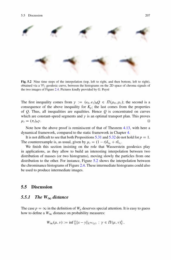
5.5 Discussion 207

Fig. 5.2 Nine time steps of the interpolation (top, left to right, and then bottom, left to right),obtained via a W2 geodesic curve, between the histograms on the 2D space of chroma signals ofthe two images of Figure 2.4. Pictures kindly provided by G. Peyré

The first inequality comes from � WD .e0; e1/#Q 2 ˘.�0; �1/; the second is aconsequence of the above inequality for Kp; the last comes from the propertiesof Q. Thus, all inequalities are equalities. Hence Q is concentrated on curveswhich are constant-speed segments and � is an optimal transport plan. This proves�t D .�t/#� . ut

Note how the above proof is reminiscent of that of Theorem 4.13, with here adynamical framework, compared to the static framework in Chapter 4.

It is not difficult to see that both Propositions 5.31 and 5.32 do not hold for p D 1.The counterexample is, as usual, given by �t D .1 � t/ıx0 C tıx1 .

We finish this section insisting on the role that Wasserstein geodesics playin applications, as they allow to build an interesting interpolation between twodistribution of masses (or two histograms), moving slowly the particles from onedistribution to the other. For instance, Figure 5.2 shows the interpolation betweenthe chrominance histograms of Figure 2.4. These intermediate histograms could alsobe used to produce intermediate images.

5.5 Discussion

5.5.1 The W1 distance

The case p D 1 in the definition of Wp deserves special attention. It is easy to guesshow to define a W1 distance on probability measures:

W1.�; �/ WD inf˚jjx � yjjL1.�/ W � 2 ˘.�; �/ ;

208 5 Wasserstein spaces

where the minimization problem in the right-hand side is exactly the one studied inSection 3.2. As we did in the rest of this chapter, the difference here is that, insteadof paying attention to the optimal map, we mainly consider the optimal cost as afunction of the two measures and use it as a distance on the space of probabilities.

In order to properly define W1.�; �/, one should restrict to P1.˝/, whichis the space of measures with bounded support. Otherwise, there could be pairsof measures such that no bounded-displacement plan � exists. From the results inSection 3.2, we know that, if � � L d, then W1.�; �/ is also equal to

inf˚jjT.x/ � xjjL1.�/ W T#� D �

:

It is not difficult to check the expected property

W1.�; �/ D limp!1 Wp.�; �/;

where the right-hand side is increasing in p (the proof is proposed as an exercise,Ex(35)). The triangle inequality can be proved by passing to the limit in p in thecorresponding triangle inequality for Wp.

Note that, in dimension one, as a consequence of the results of Chapter 2, theoptimal way to displace particles is the monotone increasing map, for every costjx � yjp with p < 1. Passing to the limit, this is also the optimal map for the L1problem.

In general, we have a new distance on probability measures on compact sets,and it measures the minimal maximal displacement that should be done to moveparticles from one distribution to the other. It is interesting to see that, though themodeling which gives rise to this distance is the same as in the case p < 1, thetopology induced by it is not at all the same.

Indeed, if one takes two different points x; y 2 ˝ and two different values s; t 2Œ0; 1�, one can easily check W1..1 � t/ıx C tıy; .1 � s/ıx C sıy/ D jx � yj. Inparticular, the probabilities .1 � t/ıx C tıy do not tend to ıx as t ! 0, even ifthere is convergence for all the distances Wp and even for the strong convergenceof measures. As a matter of fact, even if ˝ is compact, the space .P.˝/;W1/ isneither compact, nor separable, as soon as the cardinality of ˝ is larger than 1.

On the other hand, the characterization of Lipschitz curves via the existence ofa velocity field vt satisfying jjvtjjL1.�t/ � j�0jW

1

.t/ stays true and can be easilydeduced from Theorem 5.14 as a limit p ! 1. This fact, together with an extendeduse of Lipschitz curves for W1, has been used in [79] in order to analyze analternative model for branched transport. If the role of this model is very limited,some examples and considerations in the paper are useful to understand the structureof Wasserstein spaces.

However, the distance W1 appears naturally in many modeling issues andhappens to be very useful to analyze very different phenomena. One of the firstpapers using such a distance was [232], devoted to the shape of rotating stars. Insuch a paper, the choice of W1 was motivated by the following observation (that

5.5 Discussion 209

we will develop better in Section 7.4.3): a measure � is a local minimizer in W1 ofsome functional F if and only if every point x 2 spt.�/ satisfies a local minimalitycondition for a function f (equal to the first variation of F, see Section 7.2). Thisequivalence fails if we replace W1 with Wp.

Finally, it is interesting to mention a reverse inequality between W1 and Wp

(which could not be deduced from Equation (5.1)), of the form

W1.�; �/ � CWp

pCdp .�; �/;

where the constant C depends on p, on the dimension d, on the domain ˝, and ona lower bound on the density of �. This inequality is a consequence of a strongerresult proved in [74]: if � D f � L d, f � a > 0 and T is the optimal transport mapfrom � to another measure �, then we have

jjT � idjjpCdL1

� C.˝; p; d/ˆ

˝

jT.x/ � xjp dx � C.˝; p; d/

a

ˆ

˝

jT.x/ � xjp d�.x/:

This is proven by using the c-cyclical monotonicity condition on T so as to guaranteethat, whenever we fix a point x with jT.x/ � xj > 0, there exists a certain region Raround x, with volume proportional to jT.x/ � xjd, such that for every y 2 R, thedistance jT.y/ � yj is not smaller than a certain fraction of jT.x/ � xj.

5.5.2 Wasserstein and negative Sobolev distances

We already noted that the distance W1 is induced by a norm, which is the dual ofthe Lipschitz seminorm. Indeed, if we consider the space X of Lipschitz functionswith zero mean, endowed with the norm jjf jj WD Lip.f /, the distance W1 on P1.˝/

is exactly the distance associated with the norm of the topological dual X 0. Itis interesting to note that the space of probability measures with this distance iscomplete, but the space of finite measures endowed with the same norm is not.More precisely, one can consider zero-mean finite scalar measures endowed withthe norm jj%jj WD supf´ f d% W f 2 Lip1.˝/g and look at its completion. Note thatthe sequence %n WD Pn

iD1 ı1=2i � ı1=.2i�1/ is Cauchy for this norm, but its limit is aninfinite sum of Dirac masses, which is not a finite scalar measure. The completionof the set of measures for this norm has been studied in [73], where the authorsprove that it amounts to the set of distributions which are the divergence of anL1 vector field. This nice result makes an interesting link with the L1-Beckmannproblem studied in Chapter 4.

Anyway, once the role of the distance W1 in the duality with W1;1 functionsis clear, one could wonder whether other distances Wp are in duality with Sobolevspaces of the form W1;q (for instance, with q D p0 D p=.p � 1/). The answer isobviously “not,” since not all probability measures belong to the dual space W�1;p

210 5 Wasserstein spaces

(in particular, Dirac masses only belong to the dual of W1;q when functions in W1;q

are continuous, i.e., when q > d). Yet, some partial answers and some analogiesexist. For instance, the following lemma was both proven in [214] and later in [225]for different purposes.

Lemma 5.33. Assume that � and � are absolutely continuous measures on aconvex domain ˝, whose densities are bounded by the same constant C. Then, forall function � 2 H1.˝/, we have the following inequality:

ˆ

˝

� d.� � �/ � pC jjr�jjL2.˝/W2.�; �/

Proof. Let �t be the constant-speed geodesic between � and �, and let vt be thevelocity field associated with this curve by Theorem 5.14. Then .�; v/ satisfies thecontinuity equation, and jjvtjjL2.�t/ D W2.�; �/. We use the fact that �t is absolutelycontinuous for all t, and its density is bounded by the same constant C, which willbe proven in Chapter 7 (Prop 7.29). Therefore:

ˆ

˝

� d.� � �/ Dˆ 1

0

d

dt

�ˆ˝

�.x/d�t.x/

�dt D

ˆ 1

0

ˆ

˝

r� � vt d�t dt

��ˆ 1

0

ˆ

˝

jr�j2 d�t dt

�1=2 �ˆ 1

0

ˆ

˝

jvtj2 d�t dt

�1=2

� pC jjr�jjL2.˝/W2.�; �/;

and the proof is completed. utWe do not develop here the case of different exponents than p D p0 D 2, since

the quadratic case seems to be the most interesting (see Ex(38) for the general case).The exact negative Sobolev norm appearing in the quadratic case is the PH�1 norm,which deserves some remarks. First let us define

jj� � �jj PH�1.˝/ D sup

�ˆ� d.� � �/ W jjr�jjL2 � 1

�:

Note that we also have jj� � �jj PH�1.˝/ D jjrujjL2 , where u is the solution of theNeumann problem

(��u D � � �; in ˝;@u@n D 0 on @˝:

Indeed, for this choice of u, we have´� d.���/ D ´ r� � ru � jjr�jjL2 jjrujjL2 ;

with equality for � D u=jjrujjL2 . We can also see that we have

5.5 Discussion 211

jj� � �jj PH�1.˝/ D min fjjwjjL2 W r � w D � � �g ;

since the optimal w in this minimization problem is a gradient (see Section 4.4.1and the considerations on Problem (4.27)), and we have w D �ru.

The interest for the relation between the distances W2 and PH�1 (where PH�1denotes the dual of the space X of zero-mean H1 functions on a connected domain,endowed with the L2 norm of its gradient) is now very lively because these twodistances are asymptotically equivalent when the involved densities are close to thevalue % D 1, which is the relevant case when dealing with evolution problemswhere congestion imposes an L1 constraint % � 1, as in crowd motion (seeSection 8.4.2). These asymptotical equivalences can be made precise through somegeneral estimates. We cite a short note by R. Peyre [251] where some universalestimates are proven and a funny equality in dimension 1 (see Ex(64)). Moreover,we also prove the following result.

Theorem 5.34. Assume that � and � are absolutely continuous measures on aconvex domain˝, with densities bounded from below and from above by two (same)constants a; b with 0 < a < b < C1. Then, we have

b�1=2jj� � �jj PH�1.˝/ � W2.�; �/ � a�1=2jj� � �jj PH�1.˝/:

Proof. The inequality b�1=2jj� � �jj PH�1.˝/ � W2.�; �/ is a consequence of

Lemma 5.33 and of the definition of the PH�1 norm.To prove that the opposite inequality can be obtained through the Benamou-

Brenier formula of Theorem 5.28, consider any vector field E 2 M ddiv.˝/ with

r � E D � � � and %t WD .1 � t/� C t�. The pair .%t;Et/, where Et D Eis taken independent of time, is admissible in the Benamou-Brenier formula. IfE 2 L2.˝IRd/, we have

W22 .�; �/ � B2.%;E/ D

ˆ 1

0

ˆ

˝

jEj2%t

� 1

a

ˆ

˝

jEj2;

where the last inequality is justified by %t D .1 � t/� C t� � .1 � t/a C ta D a.Since E is arbitrary with the only constraint r � E D � � �, we obtain

W22 .�; �/ � 1

amin

˚jjwjj2L2 W r � w D � � � D 1

ajj� � �jj2PH�1.˝/

;

which gives the second part of the statement. ut

5.5.3 Wasserstein and branched transport distances

Another class of distances which has been compared to the Wasserstein distances isthat induced by branched transport. We recall that d˛.�; �/ is defined as the minimal

212 5 Wasserstein spaces

value of the branched transport cost (see Section 4.4.2) between two measures �; �,as soon as ˛ > 1 � 1

d . In this case, it is a distance, and it metrizes the weakconvergence of probabilities on a bounded domain.

In branched transport, the cost per unit length to move a mass m is given by m˛ ,and we can assume m � 1 (because there are no cycles in the optimal networks).Hence, one immediately remarks m˛ � m, which implies d˛ � d1, and the distanced1 is nothing but W1.

Since the two distances d˛ and W1 satisfy an inequality, and they induce thesame topology, it was a question raised by C. Villani whether the two distancesare metrically equivalent, i.e., we can bound above d˛ with W1. Inequalities of theform d˛ � CW1 are necessarily false, since they do not scale in the correct wayw.r.t. masses. Indeed, even if we stick to probability measures, we can considerthe following situation: take �; � 2 P.˝1/ and a third measure % concentratedon another domain ˝2, disjoint from ˝1. Then take �" D .1 � "/% C "� and�" D .1 � "/%C "�. Since both W1 and d˛ only depend on the difference betweenthe two measures (which is false for Wp, with p > 1), by a scaling argument it isclear that we have W1.�"; �"/ D c1" and d˛.�"; �"/ D c˛"˛ . This rules out thepossibility of a linear bound but leaves the possibility of an inequality of the formd˛ � CWˇ

1 for ˇ � ˛.This question has been analyzed in [240], where the sharp exponent has been

found, ˇ D d.˛ � .1 � 1d //. Indeed, a simple example shows that it cannot be

improved.

Example 5.35 (Optimal exponent for d˛ � Wˇ1 ). Divide the cube Œ0; 1�d into nd

small cubes of edge 1=n and set �n D Pnd

iD1 1nd ıxi and �n D Pnd

iD1 1nd ıyi , where each

xi is a vertex of one of the nd cubes (let us say the vertex with minimal sum of thed coordinates) and the corresponding yi is the center of the same cube. In this way,the point yj closest to xi is exactly yi. Thus the optimal configuration both for d˛ andW1 is obtained by linking any xi directly to the corresponding yi, and we have

d˛.�n; �n/ D nd

�1

nd

�˛ c

nD cn�d.˛�.1�1=d//

W1.�n; �n/ D nd 1

nd

c

nD cn�1

The proof of the inequality d˛ � CWd.˛�.1�1=d//1 is a bit technical. Yet, in order

to give an idea, we just sketch an alternative proof (from [81]), which providesa slightly weaker inequality, namely, d˛ � CWd.˛�.1�1=d//

p for p D 1=˛. Thisinequality is also optimal in some sense, as it is also possible to strengthen thelower bound d˛ � W1 turning it into d˛ � W1=˛ (this has been first remarked in[220] and then in [81]). The choice of the exponent p is very natural because of

scaling reasons. Indeed, Wp scales as m1p w.r.t. the mass (in the example above, if

˝1 and ˝2 are far enough so that the measure % becomes useless, then we have

Wp.�"; �"/ D c"1p ), which makes the choice p D 1=˛ the good one.

5.5 Discussion 213

Proposition 5.36. Let �; � be two probabilities on Œ0; 1�d and ˛ > 1� 1d , p D 1=˛.

Then

Wp � d˛ � CWd.˛�.1�1=d//p :

Proof. First we prove the inequality Wp � d˛ . This is a consequence of (4.33).Indeed, Wp is a distance, it is l.s.c. for *, and we have

Xij

jxi � yjj�.f.xi; yj/g/˛ �0@X

ij

jxi � yjjp�.f.xi; yj/g/1A˛

:

This inequality is due to the choice p D 1=˛ and to the subadditivity of t 7! t˛ .Passing to the minimum over � 2 ˘.�; �/, we get Nd˛.�; �/ � Wp.�; �/, whenever� and � are atomic. This implies d˛ � Wp.

In order to prove the other inequality, we divide the cube into nd small disjointcubes Qi of edge 1=n and set

�n DndX

iD1

1

nd�.Qi/ıyi and �n D

ndXiD1

�.Qi/ıyi ;

where each point yi is the center of the cube Qi. Since the branched transport from� Qi to �.Qi/ıyi costs no more than C�.Qi/

˛ 1n (see Proposition 4.38), we can

estimate

d˛.�; �/ � d˛.�; �n/C d˛.�n; �n/C d˛.�n; �/

� C

n

Xi

�.Qi/˛ C

Xi

�.Qi/˛

!C d˛.�n; �n/ � C

nnd.1�˛/ C d˛.�n; �n/;

where we used the inequalityPk

jD1 a˛j � k. 1k /˛ , which is valid whenever

PkjD1 aj D

1 and ˛ 2�0; 1Œ (it is just a version of Jensen inequality).Then, let � 2 ˘.�n; �n/ be an optimal transport plan for the cost jx � yjp. We

have � D Pi;j �ijı.xi;xj/, and we can decide to use segments connecting each point

xi to each point xj with mass �ij as a (nonoptimal) branched transport network. Itscost is

Pi;j �

˛ij jxi � xjj. We denote by K the number of pairs .i; j/ such that �ij > 0.

Since � is optimal in a linear programming problem, it may be taken extremal inthe polyhedron of matrices f.�ij/i;j W �ij � 0;

Pi �ij D �.Qj/;

Pj �ij D �.Qi/g. For

these matrices, it is well known that the number of nonzero entries does not exceedthe sum of the number of rows and columns (left as an exercise, Ex(41)), here 2nd.Hence we have

214 5 Wasserstein spaces

d˛.�n; �n/ �X

i;j

�˛ij jxi � xjj �0@X

i;j

�ijjxi � xjjp1A

1p

.2nd/1� 1

p

D CWp.�n; �n/nd.1�˛/ � C

�Wp.�; �/C 2

n

�nd.1�˛/;

where we used the triangle inequality on Wp together with Wp.�; �n/;Wp.�; �n/ �1=n. By putting together the estimates, one gets

d˛.�; �/ � Cnd.1�˛/�1 C Cnd.1�˛/Wp.�; �/

and we can conclude by taking n � Wp.�; �/�1. ut

5.5.4 The sliced Wasserstein distance

Starting from the considerations of Section 2.5.2, it is possible, and convenient inmany cases, to define a distance, which is alternative to the usual W2 distance, basedon the behavior of the measures “direction by direction.”

The idea is the following and is detailed in [256]: given two measures �; � 2P2.R

d/, we define

SW2.�; �/ WD�

Sd�1W22 ..�e/#�; .�e/#�/ dH d�1.e/

�1=2;

where �e W Rd ! R is the projection on the axis directed according to the unit

vector e, namely, �e.x/ D x � e, and H d�1 is the surface measure on Sd�1. This

quantity could have been called “projected Wasserstein distance” (as it is basedon the behavior through projections), but since in [256] it is rather called “slicedWasserstein distance,” we prefer to keep the same terminology.

The fact that SW2 is a distance comes from W2 being a distance. The triangleinequality may be proven using the triangle inequality for W2 (see Section 5.1) andfor the L2 norm. Positivity and symmetry are evident. The equality SW2.�; �/ D 0

implies W22 ..�e/#�; .�e/#�/ for all e 2 S

d�1. This means .�e/#� D .�e/#�/ for alle and it suffices (see Box 2.4 in Section 2.5.2 on Radon and X-ray transforms) toprove � D �.

It is evident from its definition and from the fact that the maps �e are 1-Lipschitz(hence W2

2 ..�e/#�; .�e/#�/ � W22 .�; �/) that we have SW2.�; �/ � W2.�; �/.

Moreover, the two distances also induce the same topology, at least on compactsets. Indeed, the identity map from W2 to .P.˝/;SW2/ is continuous (fromSW2 � W2) and bijective. Since the space where it is defined is compact, it is also ahomeomorphism.

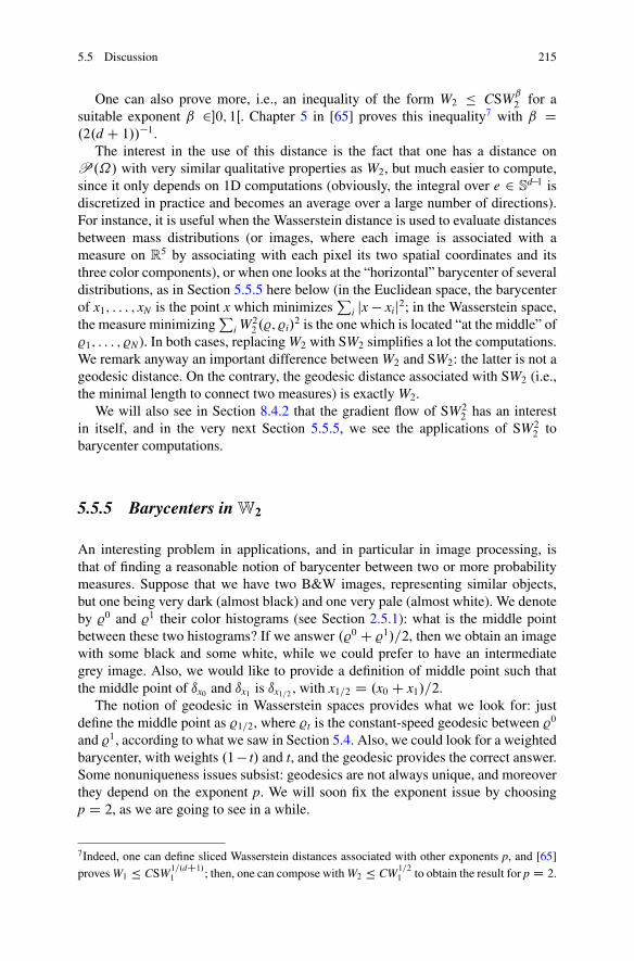
5.5 Discussion 215

One can also prove more, i.e., an inequality of the form W2 � CSWˇ2 for a

suitable exponent ˇ 2�0; 1Œ. Chapter 5 in [65] proves this inequality7 with ˇ D.2.d C 1//�1.

The interest in the use of this distance is the fact that one has a distance onP.˝/ with very similar qualitative properties as W2, but much easier to compute,since it only depends on 1D computations (obviously, the integral over e 2 S

d�1 isdiscretized in practice and becomes an average over a large number of directions).For instance, it is useful when the Wasserstein distance is used to evaluate distancesbetween mass distributions (or images, where each image is associated with ameasure on R

5 by associating with each pixel its two spatial coordinates and itsthree color components), or when one looks at the “horizontal” barycenter of severaldistributions, as in Section 5.5.5 here below (in the Euclidean space, the barycenterof x1; : : : ; xN is the point x which minimizes

Pi jx � xij2; in the Wasserstein space,

the measure minimizingP

i W22 .%; %i/

2 is the one which is located “at the middle” of%1; : : : ; %N). In both cases, replacing W2 with SW2 simplifies a lot the computations.We remark anyway an important difference between W2 and SW2: the latter is not ageodesic distance. On the contrary, the geodesic distance associated with SW2 (i.e.,the minimal length to connect two measures) is exactly W2.

We will also see in Section 8.4.2 that the gradient flow of SW22 has an interest

in itself, and in the very next Section 5.5.5, we see the applications of SW22 to

barycenter computations.

5.5.5 Barycenters in W2

An interesting problem in applications, and in particular in image processing, isthat of finding a reasonable notion of barycenter between two or more probabilitymeasures. Suppose that we have two B&W images, representing similar objects,but one being very dark (almost black) and one very pale (almost white). We denoteby %0 and %1 their color histograms (see Section 2.5.1): what is the middle pointbetween these two histograms? If we answer .%0 C %1/=2, then we obtain an imagewith some black and some white, while we could prefer to have an intermediategrey image. Also, we would like to provide a definition of middle point such thatthe middle point of ıx0 and ıx1 is ıx1=2 , with x1=2 D .x0 C x1/=2.

The notion of geodesic in Wasserstein spaces provides what we look for: justdefine the middle point as %1=2, where %t is the constant-speed geodesic between %0

and %1, according to what we saw in Section 5.4. Also, we could look for a weightedbarycenter, with weights .1� t/ and t, and the geodesic provides the correct answer.Some nonuniqueness issues subsist: geodesics are not always unique, and moreoverthey depend on the exponent p. We will soon fix the exponent issue by choosingp D 2, as we are going to see in a while.

7Indeed, one can define sliced Wasserstein distances associated with other exponents p, and [65]proves W1 � CSW1=.dC1/

1 ; then, one can compose with W2 � CW1=21 to obtain the result for p D 2.

216 5 Wasserstein spaces

What about a barycenter between three or more measures? If we want to makeuse of geodesics, we could define the barycenter of .%0; %1; %2/, with weights.1=3; 1=3; 1=3/, as the barycenter with weights .1=3; 2=3/ between %2 and themiddle point of %0 and %1. Unfortunately, in the space W2 in dimension larger than 1,there is no associativity, and this definition gives different results if we interchangethe order of the measures %i.

Hence, it is better to switch to another characterization of the barycenter inEuclidean spaces, which we will translate into the framework of Wasserstein spaces.We note that the barycenter with weights �i � 0 between points xi 2 R

d is theunique point y minimizing

Pi �ijy � xij2. Hence, we could define the barycenter

between %i with weights �i as any measure solving

min

(NX

iD1�iW

22 .%; %

i/2 W % 2 P.˝/

): (5.7)

Note that the same approach could be applied to general Riemannian manifolds, asthe barycenter is otherwise not well defined on nonlinear structures. This explainsalso the choice of the exponent p D 2: using powers p of the distances, we donot recover the usual barycenter in the Euclidean space (for p D 1, we have anotion of median), and using the square of a Wp distance is not very convenient.The uniqueness of the barycenter will be true as soon as one of the measures %i isabsolutely continuous (see Proposition 7.19).

As an interesting example, it is not difficult to analyze the 1D case. In this case,one can find the barycenter of some measures %i with weights �i in the followingway: pick one of these measures, say %1, define the optimal transport maps Ti

sending %1 onto %i (i.e., the monotone maps; note that this would work for anyexponent p), and set % WD .

Pi �iTi/#%

1, where we set T1 D id (see also Ex(63)).The minimization problem (5.7) has been first introduced in [1], where the

authors also propose an interpretation in terms of a multi-marginal optimal transportproblem. Indeed, one can choose as a variable, instead of % 2 P.˝/, a multi-marginal transport plan � 2 P.˝NC1/, with .�i/#� D %i for i D 1; : : :N and.�0/#� D % (the latter % being part of the unknown). The problem becomes

minˆ.

NXiD1

�ijxi � x0j2/ d�;

under the constraint that the marginals of � for i D 1; : : :N are the %i. The othermarginal being arbitrary, one could decide to choose x0 as a function of the points.x1; : : : ; xN/, in an optimal way, i.e., x0 D P

i �ixi (supposeP

i �i D 1). In this way,we need to solve

min

�ˆc.x1; : : : ; xN/ d� W � 2 ˘.%1; : : : ; %N/

�;

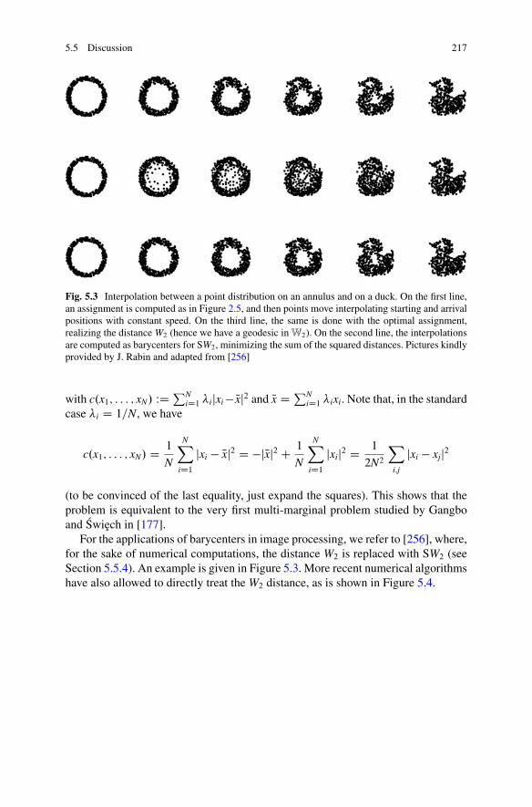
5.5 Discussion 217

Fig. 5.3 Interpolation between a point distribution on an annulus and on a duck. On the first line,an assignment is computed as in Figure 2.5, and then points move interpolating starting and arrivalpositions with constant speed. On the third line, the same is done with the optimal assignment,realizing the distance W2 (hence we have a geodesic in W2). On the second line, the interpolationsare computed as barycenters for SW2, minimizing the sum of the squared distances. Pictures kindlyprovided by J. Rabin and adapted from [256]

with c.x1; : : : ; xN/ WD PNiD1 �ijxi � Nxj2 and Nx D PN

iD1 �ixi. Note that, in the standardcase �i D 1=N, we have

c.x1; : : : ; xN/ D 1

N

NXiD1

jxi � Nxj2 D �jNxj2 C 1

N

NXiD1

jxij2 D 1

2N2

Xi;j

jxi � xjj2

(to be convinced of the last equality, just expand the squares). This shows that theproblem is equivalent to the very first multi-marginal problem studied by Gangboand Swiech in [177].

For the applications of barycenters in image processing, we refer to [256], where,for the sake of numerical computations, the distance W2 is replaced with SW2 (seeSection 5.5.4). An example is given in Figure 5.3. More recent numerical algorithmshave also allowed to directly treat the W2 distance, as is shown in Figure 5.4.

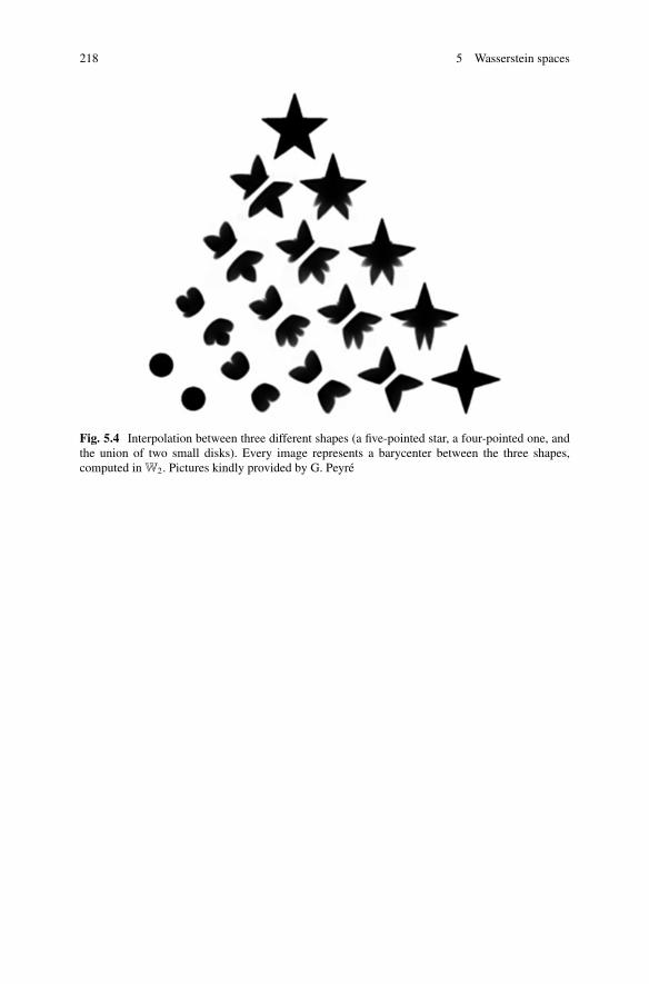
218 5 Wasserstein spaces

Fig. 5.4 Interpolation between three different shapes (a five-pointed star, a four-pointed one, andthe union of two small disks). Every image represents a barycenter between the three shapes,computed in W2. Pictures kindly provided by G. Peyré

Chapter 6Benamou-Brenier and other continuousnumerical methods

In this chapter we present some numerical methods to solve optimal transportproblems. The search for efficient numerical strategies is a very lively domainin current days, after a period where optimal transport was mainly investigatedfrom the theoretical point of view. It would be impossible to list all the recentdevelopments in the field, and because of the taste for calculus of variations andPDEs which haunts all the book, the choice has been done to prefer those methodswhich can be classified as “continuous.” This means that they are especially suitableto tackle the problem of the optimal transport between two given densities. Theyare opposite to some more discrete methods, which will be briefly presented in“Discussion” (Section 6.4), and are concerned with the case of two finitely atomicmeasures or one atomic vs one density. The most famous method is for sure theone due to J. D. Benamou and Y. Brenier, which transforms the problem into atractable convex variational problem in dimension d C1. This method gives the titleto the chapter and justifies the position of this chapter after Chapter 5. Indeed, wewill describe it strongly using the theory about Wasserstein geodesics (rather thanfinding the map, this method finds the geodesic curve �t).

Two other classical continuous methods are presented: the Angenent-Hacker-Tannenbaum method based on the fact that the optimal maps should be a gradient,and that removing non-gradient parts decreases the energy, and the Loeper-Rapettimethod based on the resolution of the Monge-Ampère equation. Both requiresmooth and non-vanishing densities, and special domains to handle boundary data(a rectangle or, better, a torus). The problem of the resolution of the Monge Ampèreequation on more general domains is much more delicate and has been addressedmore recently (see the end of Section 6.3).

In this chapter we will neither be exhaustive nor present the most recent methodsor compare the efficiency and advantages of all of them. It would be impossible,because of the huge progresses which are occurring on this topic. The goal is mainlyto provide the reader an overview of the most natural ideas which could be translatedinto numerical tools.

© Springer International Publishing Switzerland 2015F. Santambrogio, Optimal Transport for Applied Mathematicians,Progress in Nonlinear Differential Equations and Their Applications 87,DOI 10.1007/978-3-319-20828-2_6

219

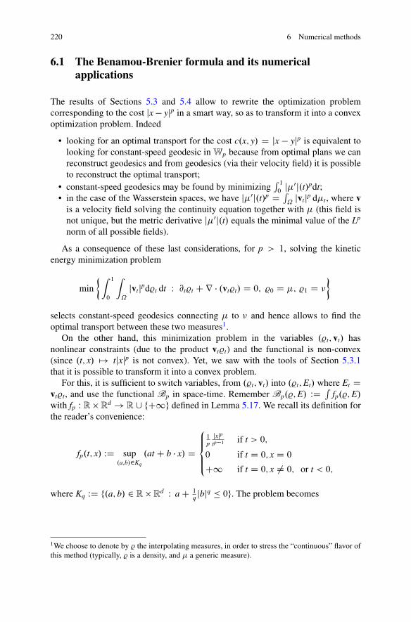
220 6 Numerical methods

6.1 The Benamou-Brenier formula and its numericalapplications

The results of Sections 5.3 and 5.4 allow to rewrite the optimization problemcorresponding to the cost jx � yjp in a smart way, so as to transform it into a convexoptimization problem. Indeed

• looking for an optimal transport for the cost c.x; y/ D jx � yjp is equivalent tolooking for constant-speed geodesic in Wp because from optimal plans we canreconstruct geodesics and from geodesics (via their velocity field) it is possibleto reconstruct the optimal transport;

• constant-speed geodesics may be found by minimizing´ 10

j�0j.t/pdt;• in the case of the Wasserstein spaces, we have j�0j.t/p D ´

˝jvtjp d�t, where v

is a velocity field solving the continuity equation together with � (this field isnot unique, but the metric derivative j�0j.t/ equals the minimal value of the Lp

norm of all possible fields).

As a consequence of these last considerations, for p > 1, solving the kineticenergy minimization problem

min

�ˆ 1

0

ˆ

˝

jvtjpd%t dt W @t%t C r � .vt%t/ D 0; %0 D �; %1 D �

�

selects constant-speed geodesics connecting � to � and hence allows to find theoptimal transport between these two measures1.

On the other hand, this minimization problem in the variables .%t; vt/ hasnonlinear constraints (due to the product vt%t) and the functional is non-convex(since .t; x/ 7! tjxjp is not convex). Yet, we saw with the tools of Section 5.3.1that it is possible to transform it into a convex problem.

For this, it is sufficient to switch variables, from .%t; vt/ into .%t;Et/ where Et Dvt%t, and use the functional Bp in space-time. Remember Bp.%;E/ WD ´

fp.%;E/with fp W R � R

d ! R [ fC1g defined in Lemma 5.17. We recall its definition forthe reader’s convenience:

fp.t; x/ WD sup.a;b/2Kq

.at C b � x/ D

8<ˆ:

1p

jxjptp�1 if t > 0;

0 if t D 0; x D 0

C1 if t D 0; x ¤ 0; or t < 0;

where Kq WD f.a; b/ 2 R � Rd W a C 1

q jbjq � 0g. The problem becomes

1We choose to denote by % the interpolating measures, in order to stress the “continuous” flavor ofthis method (typically, % is a density, and � a generic measure).

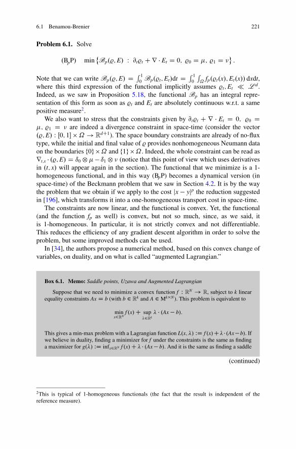
6.1 Benamou-Brenier 221

Problem 6.1. Solve

.BpP/ min˚Bp.%;E/ W @t%t C r � Et D 0; %0 D �; %1 D �

:

Note that we can write Bp.%;E/ D ´ 10Bp.%t;Et/dt D ´ 1

0

´˝

fp.%t.x/;Et.x// dxdt,where this third expression of the functional implicitly assumes %t;Et � L d.Indeed, as we saw in Proposition 5.18, the functional Bp has an integral repre-sentation of this form as soon as %t and Et are absolutely continuous w.r.t. a samepositive measure2.

We also want to stress that the constraints given by @t%t C r � Et D 0; %0 D�; %1 D � are indeed a divergence constraint in space-time (consider the vector.%;E/ W Œ0; 1� �˝ ! R

dC1). The space boundary constraints are already of no-fluxtype, while the initial and final value of % provides nonhomogeneous Neumann dataon the boundaries f0g �˝ and f1g �˝. Indeed, the whole constraint can be read asrt;x � .%;E/ D ı0 ˝�� ı1 ˝ � (notice that this point of view which uses derivativesin .t; x/ will appear again in the section). The functional that we minimize is a 1-homogeneous functional, and in this way (BpP) becomes a dynamical version (inspace-time) of the Beckmann problem that we saw in Section 4.2. It is by the waythe problem that we obtain if we apply to the cost jx � yjp the reduction suggestedin [196], which transforms it into a one-homogeneous transport cost in space-time.

The constraints are now linear, and the functional is convex. Yet, the functional(and the function fp as well) is convex, but not so much, since, as we said, itis 1-homogeneous. In particular, it is not strictly convex and not differentiable.This reduces the efficiency of any gradient descent algorithm in order to solve theproblem, but some improved methods can be used.

In [34], the authors propose a numerical method, based on this convex change ofvariables, on duality, and on what is called “augmented Lagrangian.”

Box 6.1. Memo: Saddle points, Uzawa and Augmented Lagrangian

Suppose that we need to minimize a convex function f W RN ! R, subject to k linearequality constraints Ax D b (with b 2 R

k and A 2 Mk�N ). This problem is equivalent to

minx2RN

f .x/C sup�2Rk

� � .Ax � b/:

This gives a min-max problem with a Lagrangian function L.x; �/ WD f .x/C� � .Ax�b/. Ifwe believe in duality, finding a minimizer for f under the constraints is the same as findinga maximizer for g.�/ WD infx2RN f .x/C � � .Ax � b/. And it is the same as finding a saddle

(continued)

2This is typical of 1-homogeneous functionals (the fact that the result is independent of thereference measure).

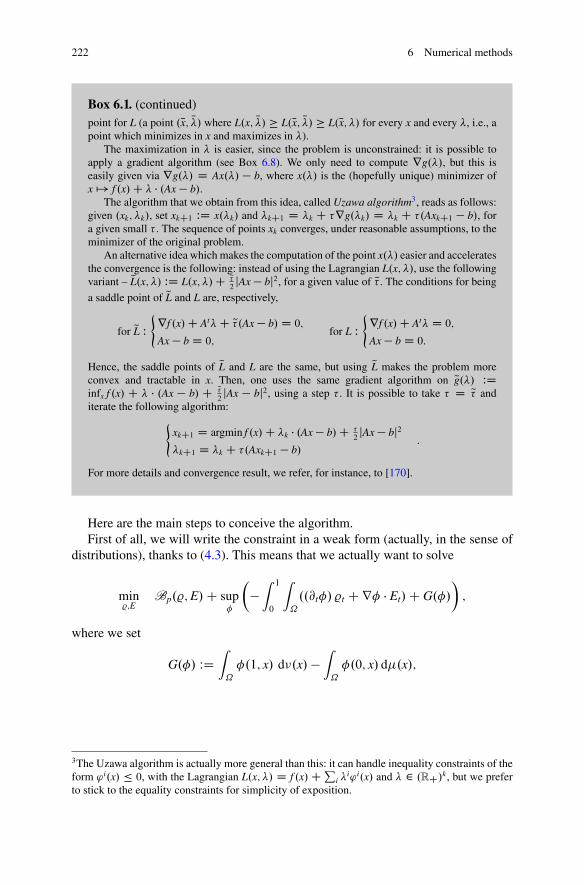
222 6 Numerical methods

Box 6.1. (continued)point for L (a point .Nx; N�/ where L.x; N�/ � L.Nx; N�/ � L.Nx; �/ for every x and every �, i.e., apoint which minimizes in x and maximizes in �).

The maximization in � is easier, since the problem is unconstrained: it is possible toapply a gradient algorithm (see Box 6.8). We only need to compute rg.�/, but this iseasily given via rg.�/ D Ax.�/ � b, where x.�/ is the (hopefully unique) minimizer ofx 7! f .x/C � � .Ax � b/.

The algorithm that we obtain from this idea, called Uzawa algorithm3, reads as follows:given .xk; �k/, set xkC1 WD x.�k/ and �kC1 D �k C �rg.�k/ D �k C �.AxkC1 � b/, fora given small � . The sequence of points xk converges, under reasonable assumptions, to theminimizer of the original problem.

An alternative idea which makes the computation of the point x.�/ easier and acceleratesthe convergence is the following: instead of using the Lagrangian L.x; �/, use the followingvariant – QL.x; �/ WD L.x; �/C Q�

2jAx � bj2, for a given value of Q� . The conditions for being

a saddle point of QL and L are, respectively,

for QL W(

rf .x/C At�C Q�.Ax � b/ D 0;

Ax � b D 0;for L W

(rf .x/C At� D 0;

Ax � b D 0:

Hence, the saddle points of QL and L are the same, but using QL makes the problem moreconvex and tractable in x. Then, one uses the same gradient algorithm on Qg.�/ WDinfx f .x/ C � � .Ax � b/ C Q�

2jAx � bj2, using a step � . It is possible to take � D Q� and

iterate the following algorithm:(

xkC1 D argmin f .x/C �k � .Ax � b/C �2jAx � bj2

�kC1 D �k C �.AxkC1 � b/:

For more details and convergence result, we refer, for instance, to [170].

Here are the main steps to conceive the algorithm.First of all, we will write the constraint in a weak form (actually, in the sense of

distributions), thanks to (4.3). This means that we actually want to solve

min%;E

Bp.%;E/C sup�

��ˆ 1

0

ˆ

˝

..@t�/ %t C r� � Et/C G.�/

�;

where we set

G.�/ WDˆ

˝

�.1; x/ d�.x/ �ˆ

˝

�.0; x/ d�.x/;

3The Uzawa algorithm is actually more general than this: it can handle inequality constraints of theform ' i.x/ � 0, with the Lagrangian L.x; �/ D f .x/CP

i �i' i.x/ and � 2 .R

C

/k, but we preferto stick to the equality constraints for simplicity of exposition.

6.1 Benamou-Brenier 223

and the sup is computed over all functions defined on Œ0; 1��˝ (we do not care hereabout their regularity, since they will be anyway represented by functions definedon the points on a grid in Œ0; 1� � R

d).

Remark 6.2. It is interesting to make a small digression to see the connectionbetween the above problem and a Hamilton-Jacobi equation. We will consider theeasiest case, p D 2. In this case we can write the problem as

min.E;%/ W %�0

ˆ 1

0

ˆ

˝

jEj22%

C sup�

�ˆ 1

0

ˆ

˝

..@t�/ %C r� � E/C G.�/;

where we expressed the functional B2 with its integral expression, valid in the caseof absolutely continuous measures, with % � 0 (where % D 0, we must have E D 0

in order to have finite energy).If we formally interchange inf and sup, we get the following problem:

sup�

G.�/C inf.E;%/ W %�0

ˆ 1

0

ˆ

˝

� jEj22%

� .@t�/ % � r� � E

�:

We can first compute the optimal E, for fixed % and �, thus getting E D %r�. Theproblem becomes

sup�

G.�/ C inf%�0

ˆ 1

0

ˆ

˝

��.@t�/% � 1

2jr�j2%

�:

The condition for the infimum to be finite (and hence to vanish) is @t�C 12jr�j2 � 0,

and at the optimum we must have equality on f% > 0g. This gives the Hamilton-Jacobi equation:

@t� C 1

2jr�j2 D 0 %-a.e.

By the way, from the optimal �, we can recover the Kantorovich potentials using .x/ WD �.1; x/ and '.x/ WD ��.0; x/.

The quantity Bp in this variational problem may be expressed as a sup and hencewe get

min%;E

sup.a;b/2Kq;�

ˆ 1

0

ˆ

˝

.a.t; x/d%C b.t; x/ � dE � @t� d% � r� � dE/C G.�/:

Denote m D .%;E/. Here m W Œ0; 1��˝ ! RdC1 is a .d C 1/-dimensional vector

field defined on a .d C 1/-dimensional space. Again, we do not care here aboutm being a measure or a true function, since anyway we will work in a discretizedsetting, and m will be a function defined on every point of a grid in Œ0; 1� � R

d.Analogously, we denote � D .a; b/. We also denote by rt;x� the space-time gradientof �, i.e., rt;x� D .@t�;r�/.

224 6 Numerical methods

The problem may be rewritten as

minm

sup�;� W �2Kq

h� � rt;x�;mi C G.�/:

Here comes the idea of using an augmented Lagrangian method. Indeed, theabove problem recalls a Lagrangian, but in a reversed way. We must think that thedual variable should be m and the primal one is the pair .�; �/. The function f .�; �/includes the term G.�/ and the constraint � 2 Kq, and there is an equality constraint� D rt;x�. We do not care actually at the original constrained problem giving rise tothis Lagrangian, bur we just decide to add in the optimization a term �

2j� � rt;x�j2

(for a small step size � ).Hence, we look for a solution of

minm

sup�;� W �2Kq

h� � rt;x�;mi C G.�/ � �

2j� � rt;x�j2:

The algorithm that one can consider to find the optimal m should do thefollowing: produce a sequence mk and find, for each k, the optimal .�k; �k/. Yet,instead of finding exactly the optimal .�k; �k/, we will optimize in two steps (firstthe optimal � for fixed � , then the optimal � for this �).

The algorithm will work in three iterate steps. Suppose we have a triplet.mk; �k; �k/.

• Given mk and �k, find the optimal �kC1, by solving

max�

�hrt;x�;mki C G.�/ � �

2jj�k � rt;x�jj2;

which amounts to minimizing a quadratic problem in rt;x�. The solution canbe found as the solution of a Laplace equation ��t;x� D r � .��k � mk/,with a space-time Laplacian and with Neumann boundary conditions. Theseconditions are homogeneous in space, and nonhomogeneous, due to the role ofG, on t D 0 and t D 1. Most Laplace solvers can find this solution in timeO.N log N/, where N is the number of points in the discretization.

• Given mk and �kC1, find the optimal �kC1, by solving

max�2Kq

h�;mki � �

2j� � rt;x�kC1j2:

By expanding the square, we see that this problem is equivalent to the projectionof rt;x�kC1C 1

�mk, and no gradient appears in the minimization. This means that

the minimization may be performed pointwisely, by selecting for each .t; x/ thepoint � D .a; b/ which is the closest to rt;x�kC1.t; x/C 1

�mk.t; x/ in the convex

set Kq. If we have a method for this projection in RnC1, requiring a constant

number of operations, then the cost for this pointwise step is O.N/.

6.2 Angenent-Hacker-Tannenbaum 225

• Finally we update m by setting mkC1 D mk � �.�kC1 � rt;x�kC1/.

This algorithm globally requires O.N log N/ operations at each iteration (warn-ing: N is given by the discretization in space-time). It can be proven to converge,even if, for convergence issues, the reader should rather refer to the works byK. Guittet and Benamou-Brenier-Guittet [36, 188, 189], as the original paper byBenamou and Brenier does not insist on this aspect. Also see the recent paper [194]which fixes some points in the proof by Guittet.

Compared to other algorithms, both those that we will present in the rest ofthe chapter and other more recent ones, the Benamou-Brenier method has someimportant advantages:

1. It is almost the only one for the moment which takes care with no difficulties ofvanishing densities and does not require special assumptions on their supports;

2. It is not specific to the quadratic cost: we presented it for power costs c.x; y/ Djx � yjp but can be adapted to other convex costs h.x � y/ and to all costs issuedfrom a Lagrangian action (see Chapter 7 in [293]); it can incorporate costsdepending on the position and time and is suitable for Riemannian manifolds;

3. It can be possibly adapted to take into account convex constraints on the density% (for instance, lower or upper bounds);

4. It can handle different “dynamical” problems, where penalizations on thedensity or on the velocity are added, as it happens in the case of mean fieldgames (see Section 8.4.4) and has been exploited, for instance, in [35];

5. It can handle multiple populations, with possibly interacting behaviors.

We refer, for instance, to [96, 248] for numerical treatments of the variants of thepoints 2 and 3 above and to [37] for an implementation of the multi-population case.Here we present a simple picture (Figure 6.1), obtained in the easiest case via theBenamou-Brenier method on a torus.

6.2 Angenent-Hacker-Tannenbaum

The algorithm that we see in this section comes from an interesting minimizingflow proposed and studied in [19] (see also [191]). The main idea is to start froman admissible transport map T between a given density f (which we will supposesmooth and strictly positive on a nice compact domain ˝) and a target measure �(we do not impose any kind of regularity on � for the moment) and then to rearrangethe values of T slowly in time, by composing it with the flow of a vector field v, i.e.,considering T ı .Yt/

�1 instead of T.x/, where Yt.x/ WD yx.t/ is, as usual, the solutionof

(y0

x.t/ D vt.yx.t//;

yx.0/ D x:

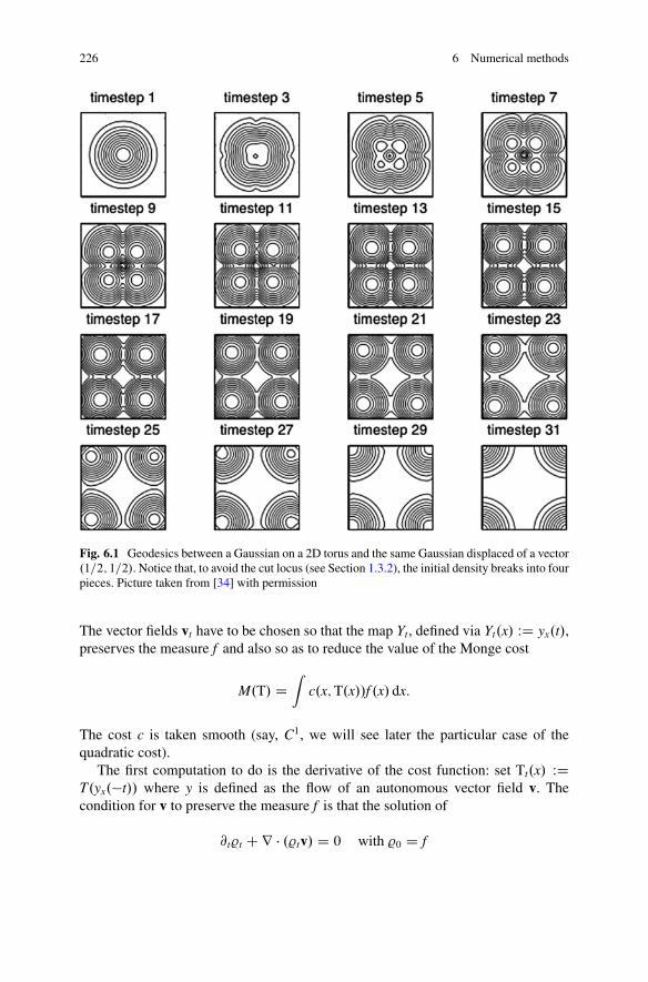
226 6 Numerical methods

Fig. 6.1 Geodesics between a Gaussian on a 2D torus and the same Gaussian displaced of a vector.1=2; 1=2/. Notice that, to avoid the cut locus (see Section 1.3.2), the initial density breaks into fourpieces. Picture taken from [34] with permission

The vector fields vt have to be chosen so that the map Yt, defined via Yt.x/ WD yx.t/,preserves the measure f and also so as to reduce the value of the Monge cost

M.T/ Dˆ

c.x;T.x//f .x/ dx:

The cost c is taken smooth (say, C1, we will see later the particular case of thequadratic cost).

The first computation to do is the derivative of the cost function: set Tt.x/ WDT.yx.�t// where y is defined as the flow of an autonomous vector field v. Thecondition for v to preserve the measure f is that the solution of

@t%t C r � .%tv/ D 0 with %0 D f

6.2 Angenent-Hacker-Tannenbaum 227

is the constant (in time) density %t D f . This requires r � .f v/ D 0. We will setw D f v for simplicity. By choosing v satisfying this condition, we can write

d

dt

�ˆ˝

c.x;T.yx.�t//f .x/ dx

�D d

dt

�ˆ˝

c.yx.t/;T.x//f .x/ dx

�

Dˆ

˝

rxc.yx.t/;T.x// � y0x.t/f .x/ dx D

ˆ

˝

rxc.yx.t/;T.x// � v.yx.t//f .x/ dx;

and, at t D 0, this gives a derivative equal to´˝

rxc.x;T.x// � v.x/f .x/ dx. In thecomputation above, we used the fact that Y�t preserves the measure f and that itsinverse is Yt (which is true for vector fields v independent of time).

We recover here an important part of the theory of optimal transport: if T isoptimal, then the vector field rxc.x;T.x// must be orthogonal to all divergence-freevector fields w, and hence it is a gradient (see Proposition 1.15). In the particularcase c.x; y/ D 1

2jx�yj2, this gives x�T.x/ D r'.x/ and hence T itself is a gradient.

The fact that T is the gradient of a convex function, and not of any function, comesfrom second-order optimality conditions, at least when one has sufficient regularity(see Ex (44)).

On the other hand, the goal here is not to study the structure of an optimal T,but to start from a nonoptimal T and to improve it. In order to do this, we mustchoose a suitable vector field v. This will be done by producing a flow Tt, and thevector field v will be chosen in some clever way at every instant t of time. Hence, itwill be no more autonomous. Several choices for v are possible, but we start fromthe simplest one: we saw that the derivative of the cost M is given by

´˝� � w,

where �.x/ D rxc.x;T.x// and w D f v. Since´˝� � w is a scalar product in L2,

this identifies the gradient of M for the L2 structure, when restricted to the set ofinfinitesimal displacements preserving the measure (i.e., we impose the constraintr � w D 0). The optimal choice of w (if we want to have a bound on jjwjjL2) is totake as w the projection of �� onto the vector space of divergence-free vector fields.Concerning the boundary conditions to associate with this divergence constraint, wechoose as usual the Neumann conditions w � n D 0, which are also those required topreserve the measure without letting any mass exit ˝.

Box 6.2. Memo: Helmholtz decomposition

Given a vector field � 2 L2.˝IRd/, it is always possible to write it as the sum of agradient and of a divergence-free vector field � D ru C w with u 2 H1.˝/ and r � w D 0

(in the distributional sense). The decomposition is unique if one imposes u 2 H10.˝/, or

w � n D 0 (in the weak sense, which, together with the zero-divergence condition, means´w � r� D 0 for all � 2 C1.˝/).

These decompositions have a variational origin: indeed one can solve

(continued)

228 6 Numerical methods

Box 6.2. (continued)

min

�ˆj� � ruj2 W u 2 H1

0.˝/

�

and get the first one, or

min

�ˆj� � ruj2 W u 2 H1.˝/;

ˆ

u D 0

�

and get the second one (if ˝ is connected). In both cases, the zero-divergence condition onw comes from the optimality conditions on u.

Note that ru is the projection of � on the set of L2 gradients (of H10 functions, in the

first case) and hence w is the projection onto the set of divergence-free vector fields (withNeumann conditions, in the second case).

The projection w D PŒ�� can be computed by writing r � � D r � w C �u, i.e.,w D � � r.��1.r � �//.

Hence, we look for a family of transport maps Tt, a flow Yt, and a vector field wt

satisfying the following conditions:

• Tt is defined as Tt D T ı .Yt/�1 at every instant t;

• the map Yt is the flow of the time-dependent vector field vt, defined throughf vt D wt;

• the vector field wt D PŒ��t�, where P is the projection onto divergence-freevector fields with w � n D 0 and �t D rxc.x;Tt.x//.

We can write the PDE satisfied by Tt, which is the transport equation @tTt C vt � rTt D 0.

Box 6.3. Memo: Linear transport equation

Given a smooth vector field vt, its flow Yt.x/ D yx.t/ (with, as usual, y0

x.t/ D vt.yx.t//and yx.0/ D x), and a smooth function g, we define gt D g ı Y�1

t . Then, we have

@tgt C vt � rgt D 0:

Indeed, we can write gt.yx.t// D g.x/ and differentiate in time, thus getting the aboveequation. As soon as vt stays Lipschitz continuous, its weak formulation is valid forarbitrary g 2 L1 since we can take a sequence of smooth approximating functions gn ! g,write

´´gn ı Y�1

t .@t' C vt � r'/, use the change of variable y D Y�1t .x/, and pass to the

limit.This equation is called transport equation. It is similar to the continuity equation, but it

is not in conservative form, and the mass of g is not conserved in time. On the contrary, L1

bounds on g are conserved, since the values of gt are the same as those of g D g0. The twoequations, transport and continuity equations, are somehow dual: if a vector field v is fixedand we take smooth solutions %t of @t%t C r � .%tvt/ D 0 and gt of @tgt C vt � rgt D 0,

(continued)

6.2 Angenent-Hacker-Tannenbaum 229

Box 6.3. (continued)then we have

d

dt

�ˆgt d%t

�D

ˆ

.@tgt/%t Cˆ

gt.@t%t/D �ˆ

%tvt � rgt �ˆ

gtr � .%tvt/D 0:

We now compute formally the derivative in time of M.Tt/ with the above choices

d

dtM.Tt/ D d

dt

�ˆc.x;Tt/f

�D

ˆryc.x;Tt/.@tTt/f D �

ˆryc.x;Tt/ � rTt � wt:

We go on using rŒc.x;Tt.x//� D rxc.x;Tt.x//Cryc.x;Tt.x//rTt.x/, together with´ rŒc.x;Tt.x//� � wt.x/ dx D 0, which comes from r � wt D 0. Hence we get

d

dtM.Tt/ D

ˆrxc.x;Tt/ � wt.x/ D

ˆ�t � wt D �

ˆ�tPŒ�t� D �jjPŒ�t�jj2 � 0:

This shows that the proposed flow makes M.Tt/ decrease in time and that thevalue of M.Tt/ is stationary if and only if PŒ�t� D 0, i.e., if �t is a gradient.

[19] proves the local existence of the above flow, i.e.,

8ˆ<ˆ:

@tTt C vt � rTt D 0;

r � .f vt/ D 0; vt � n D 0;

�rxc.x;Tt/ D f vt C rut;

T0 given;

(the second and third line can be replaced by vt D �t � r.��1.r � �t//; for �t Drxc.x;Tt/, which avoids inserting a new variable ut, but introduces nonlocal termsin the equation) is proven. Also, it is proven that the only limits of Tt for t ! 1can be those rearrangements T of T0 such that rxc.x;T/ is a gradient. The same isstudied also in the more general case of transport plans instead of transport maps,but we avoid presenting this advanced case for the sake of simplicity. However,we note that for costs c which do not satisfy the twist condition, the framework oftransport plans cannot be avoided. Indeed, in general it is not possible to convergeto an optimal transport map as t ! 1, simply because such a map could not exist.

In the very same paper [19], alternative choices of the vector field v are proposed,in particular “regularized” flows (i.e., applying regularization kernels to the abovewt, and in this case global existence is proven). There is also a possibility of a localchoice for the flow: in coordinates, we can take wj D � i

ij � �jii (superscripts are

components and subscripts are derivations). It can be checked that this choice aswell guarantees that M.Tt/ decreases in time.

230 6 Numerical methods

Even if, as we noted, the method is general for any cost, it is in the case of thequadratic cost that it has been mainly employed. The idea in this case can be roughlysummarized as “start from an admissible transport map, and then gradientize it”(i.e., transform it slowly into a gradient).

The equation becomes, for �t D x � Tt,

8<ˆ:@t�t � vt C vt � r�t D 0;

vt D 1f

��t � r.��1.r � �t//

;

�0.x/ D x � T0.x/ given:

From an implementation point of view (see [20]), the above system has beendiscretized and solved using an upwind scheme for the transport equation (roughlyspeaking, a finite difference method where the choice of the left- or right-centeredderivatives is made according to the sign of the components of the advecting vectorfield v) and standard solvers for the solution of the Laplacian (such as MatlabPoisson solver). The complexity of each time iteration is of the order of N log N,N being the number of pixels in the space discretization.

The AHT flow has been used for numerical purposes, with some advantages anddisadvantages. Even if it has been mainly used for the quadratic case, it could beused for many smooth costs, which makes it a very general approach. Yet, from thenumerical point of view, the implementation involves some difficulties, and it hasalso the disadvantage of requiring strictly positive densities. Also, its convergenceto the optimal map is not at all proven. This question can be easily understood inthe quadratic case. Beware that we do not mean here rigorous convergence results:the problem is that the flow is meant to converge to a critical point for the cost M,which means (for the quadratic case) a transport T which is a gradient map. Nothingguarantees that it is the gradient of a convex map!

A priori, even the gradient of a concave function (i.e., the worst possible map forthe quadratic cost, see Ex (2)) could be recovered. Since the flow has the propertythat M.Tt/ is strictly decreasing in time as long as one does not meet a critical point,this case can be easily excluded (the only possibility is starting from T0 being thegradient of a concave function, which is easy to avoid). But any other gradient couldbe found at the limit.

These issues have been discussed in [86]. It happens that a good idea to improvethe results and enhance the chances of converging to the good transport map,following [19, 20], is to select a good initial guess T0. Several choices (specific forthe quadratic case) are proposed (including the Dacorogna-Moser transport map;see Box 4.3 in Section 4.2.3), but, at least at a first sight, the most suitable one is theKnothe transport (see Section 2.3). Indeed, with this choice, the initial transport maphas triangular Jacobian matrix, with positive eigenvalues. Let us assume (extra thanthe previous assumptions) that � is absolutely continuous with density g.x/ boundedfrom above and below by positive constants. As we know that the map Tt satisfies.Tt/#f D g for every t, the value of j det.DTt/j can never be 0 (bounded from belowby inf f= sup g). If everything is smooth, this means that the sign of the determinant

6.2 Angenent-Hacker-Tannenbaum 231

is preserved and that no eigenvalue can ever be zero (this is also underlined in [86]).Unfortunately, the eigenvalues of DTt are real at t D 0 (if we choose the Knothemap) and are real at t D 1 (since, as a gradient, the Jacobian is symmetric), butnothing prevents the eigenvalues to become complex and to pass from �0;C1Œ to��1; 0Œ without passing through 0 during the evolution! (even if this does not seemlikely to happen, because the choice of v exactly forces Tt to become closer to theset of gradients, and gradients do not like complex eigenvalues).

A simple case, where there is no ambiguity if everything is smooth, is the 2Dcase. We can give a straightforward proposition.

Proposition 6.3. Suppose that .�t; vt/ is a smooth solution of the AHT system inthe quadratic case, with Tt.x/ D x � �t.x/ being a transport map between twogiven smooth densities f ; g 2 P.˝//, where ˝ � R

2 is a 2D smooth convex andbounded domain. Suppose that det.DT0.x// is positive for every x. Also supposethat Tt ! T1 in C1.˝/ as t ! 1 and that the evolution is nontrivial (i.e., thereexists t such that Tt ¤ T0). Then T1 is the gradient of a convex function and is thusoptimal.

Proof. From the above considerations, we have

M.T0/ � M.Tt/ Dˆ t

0

jjPŒ�t�jj2L2dt: (6.1)

This implies that´ 10

jjPŒ�tj�jj2L2dt < 1 and, at least on a sequence tn ! 1, wehave PŒ�tn � ! 0 in L2.˝/. Hence PŒ�1� D 0 since �tn ! �1 WD x � T1.x/ inC1, and hence �1 and T1 are gradients. We need to prove that T1 is the gradientof a convex function, i.e., that the eigenvalues of DT1, which is now a symmetricmatrix, are both positive (remember that we are in R

2).We know that t 7! det.DTt.x// is continuous in time, is positive at t D 0, and

cannot vanish. From C1 convergence, this implies det.DT1.x// > 0 for every x.Hence, the eigenvalues of DT1.x/ have the same sign (for each fixed x).

Let us look now at Tr.DT1.x//. This is a continuous function of x, and it cannotbe zero. Indeed, if it vanished somewhere, at such a point the two eigenvalues wouldhave different signs. Hence, the sign of this trace is constant in x. Note that this onlyworks for t D 1, as for t 2�0;1Œ one could a priori have complex eigenvalues.

If we exclude the case where Tr.DT1.x// < 0 everywhere, we have concluded.Yet, this case corresponds to T1 being the gradient of a concave function (rememberagain that in dimension two, positive determinant and negative trace imply negative2D definite). And concave functions are the worse possible transports for thequadratic case (see Ex (2)). This is impossible since M.T1/ < M.T0/ (except ifthe curve t 7! Tt were constant) from (6.1). ut

Note that the assumptions on the initial condition of the above theorem aresatisfied both by the Knothe transport and by the Dacorogna-Moser transport map.

Unfortunately, the above proof is really 2D as we characterized positive symmet-ric matrices as those which have positive trace and positive determinant. Also, in

232 6 Numerical methods

practice it is almost impossible to guarantee the assumptions of the theorem aboveand convergence can only be observed empirically.

Open Problem (convergence of AHT): justify, even assuming smoothness andvery strong convergence, that the AHT flow converges to the optimal map, ifinitialized at Knothe and/or Dacorogna-Moser, in dimension higher than two, andprove a rigorous result with minimal assumption in 2D.

6.3 Numerical solution of Monge-Ampère

As we saw in last section, we can use for numerical purposes the fact that solvingthe quadratic optimal transport problem is equivalent to finding a transport mapwhich is the gradient of a convex function. In the last section, an iterated methodwas produced where a sequence of transport maps Tn (it was a continuous flow,but in practice it is discretized), with the same image measure, was considered, andthey were forced to converge to a gradient. Here the approach is somehow opposite:a sequence of gradient maps is considered, and the corresponding measures areforced to converge to the desired target.

More precisely, the idea contained in [217] is the following: consider thesimplified case where the domain ˝ D T

d is a d-dimensional torus, the sourcemeasure % is a C0;˛ density bounded from below and from above, and the targetmeasure is the uniform measure with constant density 1; we look for a smoothfunction ' such that D2' � I (which is the condition for ' to be c-concave, withc.x; y/ D jŒx � y�j2 on the torus; see Section 1.3.2) and

det.I � D2'/ D %:

We stress the fact that, in this periodic setting, it is not possible to look for a convexfunction u satisfying det.D2u/ D %. Actually, periodic convex functions do not exist(except constant ones)! The only possibility is to stick to the framework of c-concavefunctions, without passing to the convexity of x 7! 1

2jxj2 � '.x/.

If we find such a function ', then T.x/ D x � r'.x/ (in the periodic sense) willbe the optimal map between % and L d. Note that the choice of a uniform targetmeasure gives a non-negligible simplification: the correct equation with a generictarget measure would involve a function of x � r'.x/ at the denominator in theright-hand side. This would make the following analysis much more involved.

The idea of Loeper and Rapetti in [217] is to solve the equation through aniterative scheme, based on a Newton method.

6.3 Numerical solution of Monge-Ampère 233

Box 6.4. Memo: Newton’s method to solve F.x/ D 0

Suppose we seek solutions of the equation F D 0, where F W X ! X is a smoothfunction from a vector space X into itself. Suppose a solution Nx exists, with DF.Nx/ which isan invertible linear operator. Given an initial point x0, we can define a recursive sequence inthis way: xkC1 is the only solution of the linearized equation F.xk/CDF.xk/.x�xk/ D 0. Inother words, xkC1 D xk �DF.xk/

�1 �F.xk/. This amounts at iterating the map x 7! G.x/ WDx � DF.x/�1 � F.x/. This map is well defined, and it is a contraction in a neighborhood ofNx. The iterations converge to Nx if the initial point belongs to such a suitable neighborhood.The order of convergence is quadratic, i.e., jxkC1 � Nxj � Cjxk � Nxj2. This is a consequenceof the fact that the Lipschitz constant of G in a ball B.Nx;R/ is proportional to maxfjF.x/j Wx 2 B.Nx;R/g and hence decreases as O.R/. To see this fact, just compute

DG D I � DF�1 � DF C DF�1 � D2F � DF�1 � F D DF�1 � D2F � DF�1 � F:

An alternative and less “aggressive” method can make use of a step parameter � > 0,defining xkC1 D xk � �DF.xk/

�1 � F.xk/. In this case the map G.x/ D x � �DF.x/�1 � F.x/is a contraction, but its contraction factor is of the order of 1� � , which only gives slowerconvergence (but could converge under weaker assumptions).

Here, if we have a guess ' and look for a solution 'C , the linearization of theequation reads

det.I � D2'/ � TrŒcof.I � D2'/D2 � D %;

where cof.A/ denotes the cofactor matrix of a given square matrix A, satisfyingcof.A/ � A D det.A/I.

Box 6.5. Memo: Linearization of the determinant

It is well known that det.I C "B/ D 1C "TrŒB�C O."2/ (this can be easily checked byexpanding the determinant of I C "B and looking at the terms which are first order in ").This gives the linearization of the determinant in a neighborhood of the identity matrix. Ifwe look for the linearization of the determinant around another matrix A and we suppose Ainvertible, we have

det.A C "B/ D det.A/ det.I C "A�1B/ D det.A/.1C "TrŒA�1B�C O."2//

D det.A/C "TrŒcof.A/B�C O."2/:

By continuity, the determinant and the map A 7! cof.A/ being C1 functions, this lastexpression (avoiding the use of A�1) is also valid for A non-invertible.

The iterative steps of the algorithm proposed in [217] are thus:

• Start with an arbitrary smooth function '0 such that I � D2'0 > 0 and fix asmall value of � > 0. Typically, one takes '0 D 0.

• At every step n, compute %n WD det.I � D2'n/.

234 6 Numerical methods

• Define the matrix Mn.x/ WD cof.I � D2'n/. Suppose that we can guarantee thatMn is positive definite.

• Solve TrŒMnD2 � D %n � %, which is a second-order linear elliptic equation in', on the torus (i.e., with periodic boundary conditions). The solution is uniqueup to an additive constant (choose for instance the zero-mean solution) providedMn > 0. Call n the solution.

• Define 'nC1 D 'n C � n and start again.

From the implementation point of view, the elliptic equation defining , i.e.,TrŒMnD2 � D %n � % is solved in [217] via a finite-difference discretization ofthe second-order derivatives. It is worthwhile mentioning that this kind of equation,i.e., TrŒMD2 � D f , where M is the cofactor matrix of an Hessian, can also beexpressed in divergence form. Indeed, they read

Pi;j Mij ij D f , but

Pi;j Mij ij DP

i

�Mij j

i since

Pi Mij

i D 0 for all j (see Ex (43)). This allows to give a variationalstructure to this elliptic equation and solve it via finite-element methods. On theother hand, the condition %n WD det.I � D2'n/ is more naturally interpreted interms of second-order finite differences. Let us stress that one of the main difficultiesof these equations is exactly the discretization of a nonlinear operator such as theMonge-Ampère operator (i.e., the determinant of the Hessian).

The convergence of the algorithm is guaranteed by the following theorem, underregularity assumptions:

Theorem 6.4. Suppose % 2 C0;˛.Td/ is a strictly positive density and that �is smaller than a constant c0 depending on jj log %jjL1 and jj%jjC0;˛ . Then theabove algorithm provides a sequence 'n converging in C2 to the solution ' ofdet.I � D2'/ D %.

Proof. The proof is based on a priori bounds derived from both elliptic regularitytheory (see [184], for instance) and Caffarelli’s regularity for Monge-Ampère (seeSection 1.7.6; for the periodic boundary conditions, see also [127]).

Choosing � small enough and suitable constants c1 > 0 and C1;C2;C3 largeenough, one can prove by induction the following statement: at every step n, wehave I � D2'n > c1I, jj log.%n=%/jjL1 � C1, jj%n �%jjC0;˛ � C2 and jj'njjC2;˛ � C3.To do that, note that we have jj njjC2;˛ � Cjj% � %njjC0;˛ from standard ellipticregularity theory (see Schauder Estimates in Chapter 6 in [184]). We can compute

%nC1 D det.I � D2'n � �D2 n/ D %n � �TrŒcof.I � D2'n/D2 n�C rn

D .1 � �/%n C �%C rn;

where rn is the second-order rest in the linearization of the determinant, i.e., itinvolves second derivatives of 'n and second derivatives of n, but is of order 2in �D2 n. Hence, from the algebra properties of the C0;˛ norm, we have jjrnjjC0;˛ �C�2jjD2 njj2

C0;˛� C�2jj%n � %jj2

C0;˛. Then, from %nC1 � % D .1� �/.%n � %/C rn,

we get

6.4 Discussion 235

jj%nC1�%jjC0;˛ � .1� �/jj%n�%jjC0;˛C C�2jj%n�%jj2C0;˛ � jj%n�%jjC0;˛ .1� � C C�2/:

It is enough to choose � small enough so that 1 � � C C�2 < 1, to go on with thebound on jj%nC1 � %jjC0;˛ . For the L1 bound, we use again

%nC1 D .1 � �/%n C �%C rn � ..1 � �/eC1 C � C C�2/%:

Again, for � small enough and C1 > 0, one can guarantee .1��/eC1C�CC�2 � eC1 .The lower bound works in the same way.

In order to study the bound on 'nC1, we write 'nC1 D 'n C � n. Note that, fromI � D2'n � c1I and jD2 nj � C, a suitable choice of � allows to guarantee theconvexity condition I � D2'nC1 > 0. Hence, the uniform bound jj'nC1jjC2;˛ � C3simply follows from Caffarelli’s theory and from the bounds on %nC1. And, finally,an upper bound on the Hessian of 'nC1 also implies a lower bound on I � D2'nC1because of the determinant condition.

This shows that the bounds are preserved in the iterations, and the convergencecomes from jj njjC2;˛ � Cjj% � %njjC0;˛ , where the norm jj% � %njjC0;˛ goesexponentially to 0. ut

We finish this section by mentioning that after this first work by Loper andRapetti, which indeed provided interesting numerical results, many improvementshave occurred. First, we underline that [280] extended to the case of a nonconstanttarget density (but still, Lipschitz regularity of the target density was needed).Then, we remark that another strong limitation of [217] is given by its periodicboundary conditions. When working on different domains than T

d, the situation ismuch trickier. It has been successfully studied by Benamou, Froese, and Obermanin [39, 41], by using a monotone discretization of the Monge-Ampère operator.Monotonicity allows to prove the existence of a solution of the discretized problemand to prove convergence toward the viscosity solution of the limit Monge-Ampèreequation. Finally, [39, 41] also attacked the problem of the boundary conditions andof the shape of the domain. With the approach by viscosity solutions, the authorsare able to consider non-convex and even non-connected source domains (henceallowing vanishing densities). They handle the second boundary value problemwriting the target domain as the level set of a convex function. Yet, we prefer not toenter into details of these recent results, because of their technical difficulty and ofthe notions about viscosity solutions that we did not develop here.

6.4 Discussion

6.4.1 Discrete numerical methods

We strongly used in Chapter 1 the linear and convex structure of the Kantorovichproblem, which is indeed a linear programming problem in infinite dimension. It

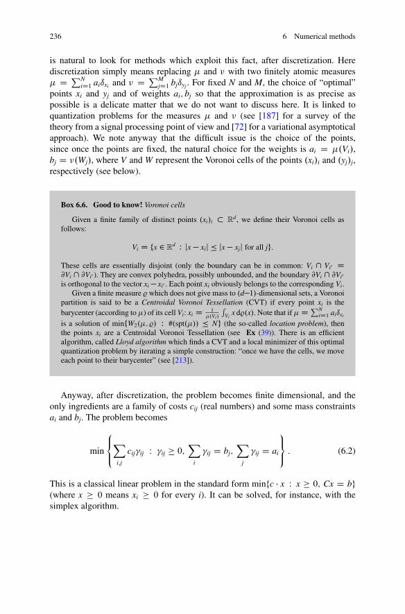
236 6 Numerical methods

is natural to look for methods which exploit this fact, after discretization. Herediscretization simply means replacing � and � with two finitely atomic measures� D PN

iD1 aiıxi and � D PMjD1 bjıyj . For fixed N and M, the choice of “optimal”

points xi and yj and of weights ai; bj so that the approximation is as precise aspossible is a delicate matter that we do not want to discuss here. It is linked toquantization problems for the measures � and � (see [187] for a survey of thetheory from a signal processing point of view and [72] for a variational asymptoticalapproach). We note anyway that the difficult issue is the choice of the points,since once the points are fixed, the natural choice for the weights is ai D �.Vi/,bj D �.Wj/, where V and W represent the Voronoi cells of the points .xi/i and .yj/j,respectively (see below).

Box 6.6. Good to know! Voronoi cells

Given a finite family of distinct points .xi/i � Rd , we define their Voronoi cells as

follows:

Vi D fx 2 Rd W jx � xij � jx � xjj for all jg:

These cells are essentially disjoint (only the boundary can be in common: Vi \ Vi0 D@Vi \ @Vi0 ). They are convex polyhedra, possibly unbounded, and the boundary @Vi \ @Vi0

is orthogonal to the vector xi � xi0 . Each point xi obviously belongs to the corresponding Vi.Given a finite measure %which does not give mass to .d�1/-dimensional sets, a Voronoi

partition is said to be a Centroidal Voronoi Tessellation (CVT) if every point xi is thebarycenter (according to�) of its cell Vi: xi D 1

�.Vi/

´Vi

x d%.x/. Note that if� D PNiD1 aiıxi

is a solution of minfW2.�; %/ W #.spt.�// � Ng (the so-called location problem), thenthe points xi are a Centroidal Voronoi Tessellation (see Ex (39)). There is an efficientalgorithm, called Lloyd algorithm which finds a CVT and a local minimizer of this optimalquantization problem by iterating a simple construction: “once we have the cells, we moveeach point to their barycenter” (see [213]).

Anyway, after discretization, the problem becomes finite dimensional, and theonly ingredients are a family of costs cij (real numbers) and some mass constraintsai and bj. The problem becomes

min

8<:X

i;j

cij�ij W �ij � 0;X

i

�ij D bj;X

j

�ij D ai

9=; : (6.2)

This is a classical linear problem in the standard form minfc � x W x � 0; Cx D bg(where x � 0 means xi � 0 for every i). It can be solved, for instance, with thesimplex algorithm.

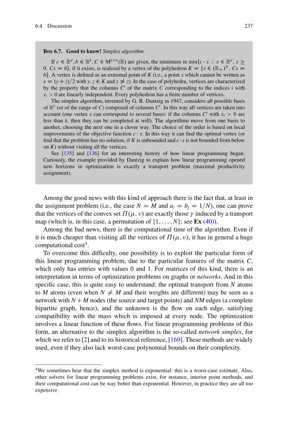
6.4 Discussion 237

Box 6.7. Good to know! Simplex algorithm

If c 2 Rd; b 2 R

k;C 2 Mk�n.R/ are given, the minimum in minfc � x W x 2 Rd; x �

0; Cx D bg, if it exists, is realized by a vertex of the polyhedron K D fx 2 .RC

/N ; Cx Dbg. A vertex is defined as an extremal point of K (i.e., a point x which cannot be written asx D .y C z/=2 with y; z 2 K and y ¤ z). In the case of polyhedra, vertices are characterizedby the property that the columns Ci of the matrix C corresponding to the indices i withxi > 0 are linearly independent. Every polyhedron has a finite number of vertices.

The simplex algorithm, invented by G. B. Dantzig in 1947, considers all possible basisof Rk (or of the range of C) composed of columns Ci. In this way all vertices are taken intoaccount (one vertex x can correspond to several bases: if the columns Ci with xi > 0 areless than k, then they can be completed at will). The algorithms move from one basis toanother, choosing the next one in a clever way. The choice of the order is based on localimprovements of the objective function c � x. In this way it can find the optimal vertex (orfind that the problem has no solution, if K is unbounded and c �x is not bounded from belowon K) without visiting all the vertices.

See [135] and [136] for an interesting history of how linear programming began.Curiously, the example provided by Dantzig to explain how linear programming openednew horizons in optimization is exactly a transport problem (maximal productivityassignment).

Among the good news with this kind of approach there is the fact that, at least inthe assignment problem (i.e., the case N D M and ai D bj D 1=N), one can provethat the vertices of the convex set˘.�; �/ are exactly those � induced by a transportmap (which is, in this case, a permutation of f1; : : : ;Ng; see Ex (40)).

Among the bad news, there is the computational time of the algorithm. Even ifit is much cheaper than visiting all the vertices of ˘.�; �/, it has in general a hugecomputational cost4.

To overcome this difficulty, one possibility is to exploit the particular form ofthis linear programming problem, due to the particular features of the matrix C,which only has entries with values 0 and 1. For matrices of this kind, there is aninterpretation in terms of optimization problems on graphs or networks. And in thisspecific case, this is quite easy to understand: the optimal transport from N atomsto M atoms (even when N ¤ M and their weights are different) may be seen as anetwork with N CM nodes (the source and target points) and NM edges (a completebipartite graph, hence), and the unknown is the flow on each edge, satisfyingcompatibility with the mass which is imposed at every node. The optimizationinvolves a linear function of these flows. For linear programming problems of thisform, an alternative to the simplex algorithm is the so-called network simplex, forwhich we refer to [2] and to its historical reference, [169]. These methods are widelyused, even if they also lack worst-case polynomial bounds on their complexity.

4We sometimes hear that the simplex method is exponential: this is a worst-case estimate. Also,other solvers for linear programming problems exist, for instance, interior point methods, andtheir computational cost can be way better than exponential. However, in practice they are all tooexpensive.

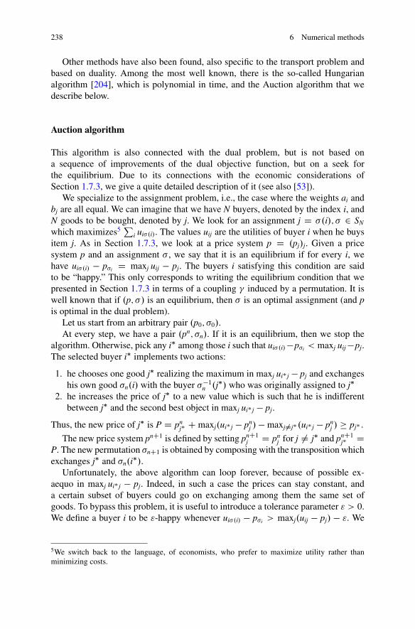
238 6 Numerical methods

Other methods have also been found, also specific to the transport problem andbased on duality. Among the most well known, there is the so-called Hungarianalgorithm [204], which is polynomial in time, and the Auction algorithm that wedescribe below.

Auction algorithm

This algorithm is also connected with the dual problem, but is not based ona sequence of improvements of the dual objective function, but on a seek forthe equilibrium. Due to its connections with the economic considerations ofSection 1.7.3, we give a quite detailed description of it (see also [53]).

We specialize to the assignment problem, i.e., the case where the weights ai andbj are all equal. We can imagine that we have N buyers, denoted by the index i, andN goods to be bought, denoted by j. We look for an assignment j D �.i/; � 2 SN

which maximizes5 Pi ui�.i/. The values uij are the utilities of buyer i when he buys

item j. As in Section 1.7.3, we look at a price system p D .pj/j. Given a pricesystem p and an assignment � , we say that it is an equilibrium if for every i, wehave ui�.i/ � p�i D maxj uij � pj. The buyers i satisfying this condition are saidto be “happy.” This only corresponds to writing the equilibrium condition that wepresented in Section 1.7.3 in terms of a coupling � induced by a permutation. It iswell known that if .p; �/ is an equilibrium, then � is an optimal assignment (and pis optimal in the dual problem).

Let us start from an arbitrary pair .p0; �0/.At every step, we have a pair .pn; �n/. If it is an equilibrium, then we stop the

algorithm. Otherwise, pick any i among those i such that ui�.i/�p�i < maxj uij �pj.The selected buyer i implements two actions:

1. he chooses one good j realizing the maximum in maxj ui�j � pj and exchangeshis own good �n.i/ with the buyer ��1

n .j/ who was originally assigned to j2. he increases the price of j to a new value which is such that he is indifferent

between j and the second best object in maxj ui�j � pj.

Thus, the new price of j is P D pnj� C maxj.ui�j � pn

j / � maxj¤j�.ui�j � pnj / � pj� .

The new price system pnC1 is defined by setting pnC1j D pn

j for j ¤ j and pnC1j� D

P. The new permutation �nC1 is obtained by composing with the transposition whichexchanges j and �n.i/.

Unfortunately, the above algorithm can loop forever, because of possible ex-aequo in maxj ui�j � pj. Indeed, in such a case the prices can stay constant, anda certain subset of buyers could go on exchanging among them the same set ofgoods. To bypass this problem, it is useful to introduce a tolerance parameter " > 0.We define a buyer i to be "-happy whenever ui�.i/ � p�i > maxj.uij � pj/ � ". We

5We switch back to the language, of economists, who prefer to maximize utility rather thanminimizing costs.

6.4 Discussion 239

look now for a pair .p; �/ where all buyers are "-happy. The algorithm evolvesas before, selecting a buyer i who is not "-happy, letting him exchange a goodwith ��1

n .j/, but the rule for price increase changes. Indeed, we can now setP D pn

j� C maxj.ui�j � pnj /� maxj¤j�.ui�j � pn

j / � pj� C ". This price is the maximalone that we can give to item j so that buyer i is "-happy if he purchases j at sucha price. The advantage is that we have now P � pn.j/ C " and there is a minimalincrement.

It is easy to see an analogy with auction systems and that this "-system imposesa minimal bid.

Now, we can see that every time that an item is chosen by a buyer and receives abid, then, from that moment on, whoever owns such an item will be "-happy. Indeed,at the very moment when a buyer gets an object by a bid, he is "-happy, and the priceof such an object cannot increase as long as he owns it, as well as the prices of theothers cannot decrease. Hence, the algorithm will stop as soon as all items will havereceived at least a bid each. Now, suppose that there is an item which has receivedno bids: his price is constant, while the prices of the other increase. It is not difficultto prove that the number of possible iterations going on in the presence of an objectwhich has never received a bid must be bounded (as soon as there is one unbiddedgood, all the others become too expensive after a certain number of received bids,and when they become too expensive, they receive no more bids). This means thatthe algorithm stops after a finite number of steps.

Once we have a pair .p; �/ which is a equilibrium in the sense that every buyeris "-happy, then we can prove that the cost

Pi ui�.i/ is almost optimal among

permutations Q� . Indeed, take any other permutation Q� . We have

ui�.i/ � p�i � maxj.uij � pj/ � " � uiQ�.i/ � pQ�.i/ � ":

Summing over i, and usingP

i p�i D Pi pQ�.i/, we get

Xi

ui�.i/ �X

i

uiQ�.i/ � N":

This proves that � is optimal, up to an error of N". By the way, if the utilities uij areinteger numbers and N" < 1, then � must actually be optimal, with no error.

A rough estimate of the number of iterations which are necessary to conclude thealgorithm is obtained in the following way: set C D max juijj and start with p0 D 0.Till there is at least an unbidded good, no other good can receive more than C="bids. This means that the number of iterations is at most of the order of NC=". Inthe case of integer utilities, an exact solution is found in O.CN2/ iterations6.

6Observe that this assumption on the values uij being integer, corresponding to integer costs oneach edge in the network interpretation, appears quite often and simplifies the complexity of otheralgorithms as well. For instance, in [245] a polynomial bound on the cost of a network simplex

240 6 Numerical methods

We remark that this cost can be indeed very high because of the presence of thefactor C. Indeed, if the costs are rational numbers between 0 and 1 with k digits, ifwe want to make them integers, we could lead to multiply up to C D 10k. A way tocircumvent this problem is to make an iterative "-scaling procedure. We first find anassignment which is N"-optimal for a certain value of ", then we divide " by two,and we go on. This procedure, introduced in [55], is also detailed in [234]. We referto these notes and to [54] for considerations about possible accelerated variants andcomputational costs of this method, very efficient in many cases. We also mentionthat in Section 8.4.4 we will briefly describe a cosmological model which has beennumerically attacked thanks to the auction algorithm.

Entropic regularization and iterated projections

We would like to discuss another, very recent, but simple to explain, approach to thediscrete linear programming version of the optimal transport problem. The startingpoint is the following variant of the linear problem (6.2): fix " > 0 and look at

min

8<:X

i;j

�cij�ij C "�ij log.�ij/

W �ij � 0;X

i

�ij D bj;X

j

�ij D ai

9=; : (6.3)

It is clear that, for " ! 0, the above minimization problem converges (in the senseof � -convergence, see Box 4.6) to the minimization in (6.2). We try to describe nowwhy this approximated problem is easier to handle.

First, we rewrite the objective function using

cij�ij C "�ij log.�ij/ D "�ij log

��ij

�ij

�;

Xi;j

�cij�ij C "�ij log.�ij/

D "KL.� j�/;

where �ij D e�cij=" and KL denotes the so-called Kullback-Leibler divergence. Thisis not at all a divergence in the sense of differential calculus, but rather a sort ofdistance based on the relative entropy:

KL.� j�/ WDX

i;j

f

��ij

�ij

��ij for f .t/ D

(t log t if t � 0;

C1 if t < 0:

Hence, the above minimization problem reads as the projection, for the Kullback-Leibler divergence, of the point � 2 R

N�N on the set of constraints C D Cx \ Cy,where Cx D f� 2 R

N�N W Pj �ij D aig and Cy D f� 2 RN�N W Pi �ij D bjg. It

is important to notice that the positivity constraint on � has disappeared, because itis included in the definition of the entropy function f , which acts as a sort of barrier

algorithm is given under this assumption, obtaining O.min.kh log.kC/; kh2 log k/ for a networkwith k nodes, h edges, and maximal cost equal to C.

6.4 Discussion 241

for this constraint (it is not a true barrier in the usual sense because it does not tendto infinity as the variable tends to 0; yet, it is set to infinity on negative numbers, andthe derivative tends to infinity at 0).

The Kullback-Leibler divergence is not a distance, but shares some of theproperties of distances. In particular it can be proven that the projection onto theintersection of two linear subspaces such as Cx and Cy can be obtained by alternateprojections, i.e., defining �2kC1 D ProjCx.�2k/ and �2kC2 D ProjCy.�2kC1/, with�0 D �, and looking at the limit as k ! 1.

The problem becomes that of the projection on one on the two subspaces, but thishappens to be doable explicitly. Given a certain � , we want to solve (for instance)the minimization problem

min

8<:X

i;j

�ij log

�ij

� ij

!WX

j

�ij D ai

9=; :

It can be seen that the problem is separable according to the variable i (i.e., thatevery i can be treated separately, and the optimality condition gives log.�ij/ Dlog.� ij/C �i, i.e., �ij D pi� ij, for some constants pi which are determined thanks tothe constraint (i.e., pi D ai=.

Pj � ij/).

Analogously, it can be proven that the projection onto Cy has the form �ij D qj� ij,for qj D bj=.

Pi � ij/).

As a consequence, one can solve the approximated problem by means of asequence of iterations of the following algorithm: start from �0 D �, define �2kC1

ij Dpi�

2kij with pi D ai=.

Pj �

2kij /, and then �2kC2

ij D qj�2kC1ij with qj D bj=.

Pi �

2kC1ij /.

The limit as k ! 1 provides the desired solution of the “regularized” problem (theregularization being given by the addition of the entropy) (Figure 6.2).

This idea, called iterative proportional fitting procedure (IPFP), can be tracedback to [142] and even [282], and it has been recently applied to many optimaltransport problems in [38]. It shows that the choice of the entropic regularizationhas several advantages:

• it allows to get rid of the positivity constraint (which would not be the case fora quadratic regularization);

• it allows to compute explicitly the projection at every step, as soon as we onlyproject on one subspace Cx or Cy only;

• it is not too costly in terms of memory storage, since at every step the current�2k is of the form �2k

ij D �ijpiqj (cumulating the product of the coefficients pi

and qj appearing at every step), which allows to stock 2N data instead of N2;• it is not too costly at every step, as it only requires O.N/ operations;• it can be easily parallelized, due to the separable structure of each step;• it can be adapted to multi-marginal problems and other linear problems.

It is also possible to deduce, from the limit value of the coefficients p and q, theKantorovich potentials ' and , but we leave it as an exercise (see Ex (42)).

242 6 Numerical methods

6.4.2 Semidiscrete numerical methods

After the study of two discrete measures, the case of one discrete measure and onecontinuous deserves a short discussion. We are speaking of the case where � Df .x/ dx has a density and � D PN

jD1 bjıyj is finitely atomic.The main ideas behind the methods that are used rely on the dual problem,7 in

the following formulation:

max

8<:F. / D

Xj

jbj Cˆ

˝

c.x/f .x/ dx

9=; ;

where the numbers j represent the values of the function at the points yj and c is the c-transform of . The considerations in Chapter 1 explain why solvingthis problem gives information on the primal problem minf´ c d� W � 2 ˘.�; �/g.In particular, once we find the optimal function , the set of points x satisfying j C c.x/ D c.x; yj/ will provide the set of points transported onto the target pointyj. We note that c.x/ D c.x; yj/� j exactly means that c.x; yj/� j � c.x; yj0/� j0

for all j0. This gives rise to the study of some sorts of Voronoi cells, whose definitionalso involves some scalar coefficients j. We will analyze these cells in the simplercase where c.x; y/ D 1

2jx � yj2. In this case we define

V .j/ D�

x W 12

jx � yjj2 � j � 1

2jx � yj0 j2 � j0 for all j0

�:

By expanding the squares, we see that each V .j/ is defined by N � 1 linearinequalities of the form x � .yj0 � yj/ � a.j; j0/ WD j � j0 C 1

2jyj0 j2 � 1

2jyjj2 and is

hence a convex polyhedron. These cells are called power cells. They coincide withthe Voronoi cells of the points yj whenever all the values j are equal.

The problem consists in finding values j such that the masses´

V .j/f .x/ dx equal

the prescribed values bj. This is indeed equivalent to maximizing the quantity F. /.The maximization of F is a finite-dimensional issue, since (thanks to � being finitelyatomic) the only values of which are relevant are those taken at the points yj.Hence, we can consider 2 R

N , and look at the derivatives of F.First, we note that F is concave in . Indeed, the first part of F is linear: 7!Pj jbj. Then, we take the values c.x/ D infj c.x; yj/� j; these values are infima

of linear functions of and thus are concave. They are weighted with a positivedensity f and then integrated; the result is a concave function of . Let us computethe derivative of F with respect to one variable j: from

7See also Example 1.6 in [176] for a first genesis of these ideas.

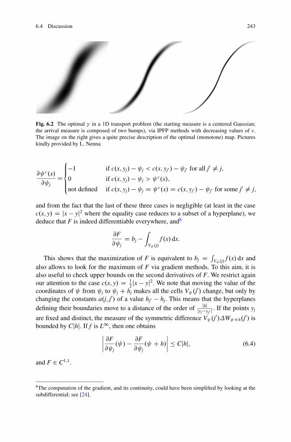
6.4 Discussion 243

Fig. 6.2 The optimal � in a 1D transport problem (the starting measure is a centered Gaussian;the arrival measure is composed of two bumps), via IPFP methods with decreasing values of ".The image on the right gives a quite precise description of the optimal (monotone) map. Pictureskindly provided by L. Nenna

@ c.x/

@ jD

8<ˆ:

�1 if c.x; yj/ � j < c.x; yj0/ � j0 for all j0 ¤ j;

0 if c.x; yj/ � j > c.x/;

not defined if c.x; yj/ � j D c.x/ D c.x; yj0/ � j0 for some j0 ¤ j;

and from the fact that the last of these three cases is negligible (at least in the casec.x; y/ D jx � yj2 where the equality case reduces to a subset of a hyperplane), wededuce that F is indeed differentiable everywhere, and8

@F

@ jD bj �

ˆ

V .j/f .x/ dx:

This shows that the maximization of F is equivalent to bj D ´V .j/

f .x/ dx andalso allows to look for the maximum of F via gradient methods. To this aim, it isalso useful to check upper bounds on the second derivatives of F. We restrict againour attention to the case c.x; y/ D 1

2jx � yj2. We note that moving the value of the

coordinates of from j to j C hj makes all the cells V .j0/ change, but only bychanging the constants a.j; j0/ of a value hj0 � hj. This means that the hyperplanesdefining their boundaries move to a distance of the order of jhj

jyj�yj0 j . If the points yj

are fixed and distinct, the measure of the symmetric difference V .j0/�W Ch.j0/ isbounded by Cjhj. If f is L1, then one obtains

ˇˇ @F

@ j. / � @F

@ j. C h/

ˇˇ � Cjhj; (6.4)

and F 2 C1;1.

8The computation of the gradient, and its continuity, could have been simplified by looking at thesubdifferential; see [24].

244 6 Numerical methods

Box 6.8. Memo: Gradient algorithm

If F W RN ! R is a differentiable convex function, an easy algorithm to look for the

minimum of F is the following: take x0 2 RN and � > 0 a fixed size, and define

xkC1 D xk � �rF.xk/:

If F is such that ˛I � D2F.x/ � LI for every x and some ˛;L > 0, then the abovealgorithm converges exponentially whenever � < 2˛=L2. More precisely, F is strictlyconvex and has a unique minimizer Nx, and we have jxk � Nxj � Cˇk, where ˇ dependson �; ˛;L, and ˇ < 1 if � 2�0; 2˛=L2Œ. The convergence F.xk/� min F is also exponential.

If D2F is bounded from above but not from below (i.e., F is smooth but not enoughconvex), but admits a minimizer Nx, then the rate of convergence is much worse: indeed, onecan only prove F.xk/� F.Nx/ � C=k, as soon as �M < 1.

Many texts present a wide introduction to gradient methods in convex optimization;see, for instance, [64] for more details. Variants where the step size � varies with k, both inprescribed and optimized manners, also exist.

As a final point, note that the above algorithm also corresponds to an explicit Eulerscheme in the discretization of the gradient flow of F (see the Memo Box 8.1).

Then, the practical implementation of a gradient algorithm of this kind dependson how one can practically compute the power cells V .j/ and the integral of thedensity f on them. This is a matter of the so-called computational geometry. Wedo not spend word on this very delicate issue, but refer, for instance, to the recentpapers [209, 233] for a detailed discussion. The original implementation of thesemethods is proposed in [233], and the implementation has been improved in [209],where spectacular numerical simulations 9 of optimal transport between geometricshapes are also presented.

Due to the very good numerical results, which we present through Figures 6.3and 6.4, we prefer to spend some extra words on the most efficient methods to beused in this semi-discrete setting.

Indeed, even if the description of the algorithm was easier in the case of a gradientalgorithm, the convergence is much quicker if one uses instead a Newton approach.Newton’s method (see Box 6.4 in Section 6.3) is suitable to find zeros of a vectorfunction from R

N to RN , which is in this case the function associating with a dual

potential D . i/i 2 RN the values bi � ´

V .i/f .x/ dx D @F=@ i. In order to be

able to use the Newton method, one needs to be able to compute their derivatives,which are indeed the entries of the Hessian matrix of F. One also needs to justifythat this Hessian matrix is nonsingular and provide lower bounds on its eigenvalues.This corresponds to uniform convexity of F.

Moreover, we know that the Newton method is only efficient when we areable to choose a suitable initialization for the algorithm, since it only converges

9The pictures in the next pages have been kindly provided by B. Lévy and are produced with thesame algorithms as in [209].

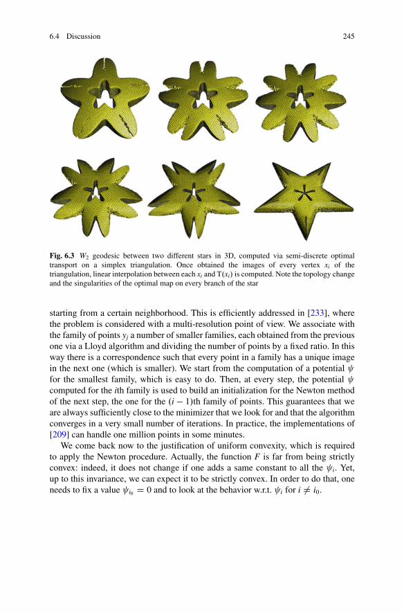
6.4 Discussion 245

Fig. 6.3 W2 geodesic between two different stars in 3D, computed via semi-discrete optimaltransport on a simplex triangulation. Once obtained the images of every vertex xi of thetriangulation, linear interpolation between each xi and T.xi/ is computed. Note the topology changeand the singularities of the optimal map on every branch of the star

starting from a certain neighborhood. This is efficiently addressed in [233], wherethe problem is considered with a multi-resolution point of view. We associate withthe family of points yj a number of smaller families, each obtained from the previousone via a Lloyd algorithm and dividing the number of points by a fixed ratio. In thisway there is a correspondence such that every point in a family has a unique imagein the next one (which is smaller). We start from the computation of a potential for the smallest family, which is easy to do. Then, at every step, the potential computed for the ith family is used to build an initialization for the Newton methodof the next step, the one for the .i � 1/th family of points. This guarantees that weare always sufficiently close to the minimizer that we look for and that the algorithmconverges in a very small number of iterations. In practice, the implementations of[209] can handle one million points in some minutes.

We come back now to the justification of uniform convexity, which is requiredto apply the Newton procedure. Actually, the function F is far from being strictlyconvex: indeed, it does not change if one adds a same constant to all the i. Yet,up to this invariance, we can expect it to be strictly convex. In order to do that, oneneeds to fix a value i0 D 0 and to look at the behavior w.r.t. i for i ¤ i0.

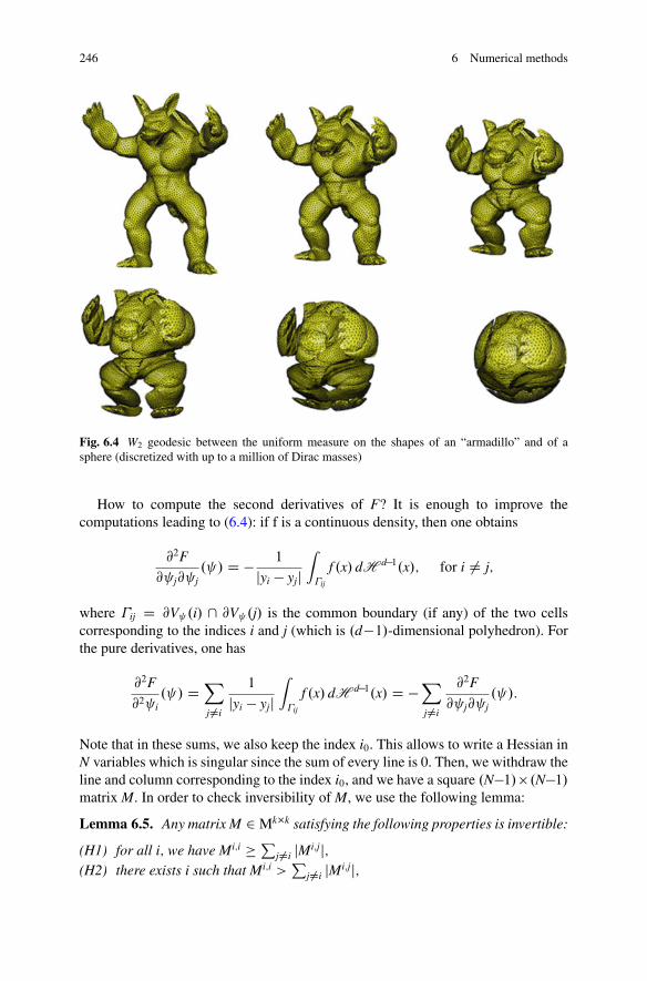
246 6 Numerical methods

Fig. 6.4 W2 geodesic between the uniform measure on the shapes of an “armadillo” and of asphere (discretized with up to a million of Dirac masses)

How to compute the second derivatives of F? It is enough to improve thecomputations leading to (6.4): if f is a continuous density, then one obtains

@2F

@ j@ j. / D � 1

jyi � yjjˆ

�ij

f .x/ dH d�1.x/; for i ¤ j;

where �ij D @V .i/ \ @V .j/ is the common boundary (if any) of the two cellscorresponding to the indices i and j (which is .d�1/-dimensional polyhedron). Forthe pure derivatives, one has

@2F

@2 i. / D

Xj¤i

1

jyi � yjjˆ

�ij

f .x/ dH d�1.x/ D �Xj¤i

@2F

@ j@ j. /:

Note that in these sums, we also keep the index i0. This allows to write a Hessian inN variables which is singular since the sum of every line is 0. Then, we withdraw theline and column corresponding to the index i0, and we have a square .N�1/� .N�1/matrix M. In order to check inversibility of M, we use the following lemma:

Lemma 6.5. Any matrix M 2 Mk�k satisfying the following properties is invertible:

(H1) for all i; we have Mi;i � Pj¤i jMi;jj;

(H2) there exists i such that Mi;i >P

j¤i jMi;jj;

6.4 Discussion 247

(H3) for any pair .i; j/, there is a sequence i1; i2; : : : ; ik with i1 D i; ik D jsatisfying Mih;ihC1 ¤ 0.

Proof. Let x 2 Ker.M/ and let i0 be an index such that jxij is maximal. We maysuppose for simplicity that xi0 is positive. Then we have

0 D Mi0;i0xi0�Xj¤i0

Mi0;jxj � Mi0;i0xi0�Xj¤i0

jMi0;jjxi0 D xi0

0@Mi0;i0�

Xj¤i0

jMi0;jj1A � 0:

This implies that all inequalities are equalities and in particular xj D xi0 wheneverMi0;j ¤ 0. Hence, the entries of x on all the indices which are “neighbors” of i0 equalto xi0 (and they are maximal as well). This allows to repeat the argument replacingi0 with another maximizing index j and so on. . . ; since any index is connected by achain of neighbors to i0, we get that all the entries are equal. But this implies that thevector that we selected in the kernel must be a multiple of the vector .1; 1; : : : ; 1/.Yet, this vector is not in the kernel since the sum of the elements on each line is notzero for all lines, by assumption .H2/. This proves that M is invertible. ut

The above lemma can be applied to the Hessian of F under some reasonableassumptions (for instance, we should require that the support of the density f isarcwise connected).

This guarantees that the Hessian of F is a strictly positive-definite matrix (on thespace R

N�1 of potentials with fixed i0 D 0) at every point. In order to applya Newton’s method, one should also bound from below its eigenvalues. This ismore delicate, and we refer to [114] both for a counterexample under the threeassumptions of the above Lemma, which are not enough for such a bound, and fora proof in the specific case where the matrix M comes from a partition into powercells.

Moreover, as we are dealing with the arguments of [114], let us underline anothersemi-discrete method, described in the same paper. The idea of the method comesfrom the considerations of our Section 2.4 about Knothe transport. Indeed, as weproved that the Knothe map is the limit of the optimal transport maps for degeneratequadratic costs corresponding to a matrix diag.1; "; "2 : : : ; "d�1/, we can start fromsuch a map (Knothe) and then let " vary. The Knothe map is easy to compute, andone can find the cells corresponding to it10. Since for the Knothe map the mostimportant coordinate is the last one, these cells are horizontal strips with prescribed

10This is the semidiscrete method coming from this idea, implemented in [114]. There is also acontinuous counterpart, i.e., a PDE on the Kantorovich potentials ". It has been studied from thetheoretical point of view in [66], where Bonnotte proved a nontrivial well-posedness result, basedon the application of the Nash-Moser implicit function theorem around " D 0 (once we are on" > 0, the equation is more regular). Later, the same author also started numerical implementationsof the time discretization of this equation in [65]. Note that his continuous method recalls in someaspects both the AHT flow described in Section 6.2 (as it starts from the Knothe map, is continuousin time but discretized for numerical purposes, and evolves by imposing prescribed image measure

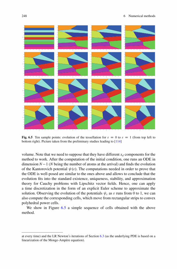
248 6 Numerical methods

0 0.1 0.2 0.3 0.4 0.5 0.6 0.7 0.8 0.9 10

0.1

0.2

0.3

0.4

0.5

0.6

0.7

0.8

0.9

1

x1

x 2

0 0.1 0.2 0.3 0.4 0.5 0.6 0.7 0.8 0.9 10

0.1

0.2

0.3

0.4

0.5

0.6

0.7

0.8

0.9

1

x1

x 2

0 0.1 0.2 0.3 0.4 0.5 0.6 0.7 0.8 0.9 10

0.1

0.2

0.3

0.4

0.5

0.6

0.7

0.8

0.9

1

x1

x 2

0 0.1 0.2 0.3 0.4 0.5 0.6 0.7 0.8 0.9 10

0.1

0.2

0.3

0.4

0.5

0.6

0.7

0.8

0.9

1

x1

x 2

0 0.1 0.2 0.3 0.4 0.5 0.6 0.7 0.8 0.9 10

0.1

0.2

0.3

0.4

0.5

0.6

0.7

0.8

0.9

1

x1

x 2

0 0.1 0.2 0.3 0.4 0.5 0.6 0.7 0.8 0.9 10

0.1

0.2

0.3

0.4

0.5

0.6

0.7

0.8

0.9

1

x1

x 2

0 0.1 0.2 0.3 0.4 0.5 0.6 0.7 0.8 0.9 10

0.1

0.2

0.3

0.4

0.5

0.6

0.7

0.8

0.9

1

x1

x 2

0 0.1 0.2 0.3 0.4 0.5 0.6 0.7 0.8 0.9 10

0.1

0.2

0.3

0.4

0.5

0.6

0.7

0.8

0.9

1

x1

x 2

0 0.1 0.2 0.3 0.4 0.5 0.6 0.7 0.8 0.9 10

0.1

0.2

0.3

0.4

0.5

0.6

0.7

0.8

0.9

1

x1

x 2

0 0.1 0.2 0.3 0.4 0.5 0.6 0.7 0.8 0.9 10

0.1

0.2

0.3

0.4

0.5

0.6

0.7

0.8

0.9

1

x1

x 2

0 0.1 0.2 0.3 0.4 0.5 0.6 0.7 0.8 0.9 10

0.1

0.2

0.3

0.4

0.5

0.6

0.7

0.8

0.9

1

x1

x 2

0 0.1 0.2 0.3 0.4 0.5 0.6 0.7 0.8 0.9 10

0.1

0.2

0.3

0.4

0.5

0.6

0.7

0.8

0.9

1

x1

x 2

0 0.1 0.2 0.3 0.4 0.5 0.6 0.7 0.8 0.9 10

0.1

0.2

0.3

0.4

0.5

0.6

0.7

0.8

0.9

1

x1

x 2

0 0.1 0.2 0.3 0.4 0.5 0.6 0.7 0.8 0.9 10

0.1

0.2

0.3

0.4

0.5

0.6

0.7

0.8

0.9

1

x1

x 2

0 0.1 0.2 0.3 0.4 0.5 0.6 0.7 0.8 0.9 10

0.1

0.2

0.3

0.4

0.5

0.6

0.7

0.8

0.9

1

x1

x 2

0 0.1 0.2 0.3 0.4 0.5 0.6 0.7 0.8 0.9 10

0.1

0.2

0.3

0.4

0.5

0.6

0.7

0.8

0.9

1

x1

x 2

Fig. 6.5 Ten sample points: evolution of the tessellation for " D 0 to " D 1 (from top left tobottom right). Picture taken from the preliminary studies leading to [114]

volume. Note that we need to suppose that they have different xd components for themethod to work. After the computation of the initial condition, one runs an ODE indimension N �1 (N being the number of atoms at the arrival) and finds the evolutionof the Kantorovich potential ."/. The computations needed in order to prove thatthe ODE is well-posed are similar to the ones above and allows to conclude that theevolution fits into the standard existence, uniqueness, stability, and approximationtheory for Cauchy problems with Lipschitz vector fields. Hence, one can applya time discretization in the form of an explicit Euler scheme to approximate thesolution. Observing the evolution of the potentials " as " runs from 0 to 1, we canalso compute the corresponding cells, which move from rectangular strips to convexpolyhedral power cells.

We show in Figure 6.5 a simple sequence of cells obtained with the abovemethod.

at every time) and the LR Newton’s iterations of Section 6.3 (as the underlying PDE is based on alinearization of the Monge-Ampère equation).

Chapter 7Functionals on the space of probabilities

We consider in this chapter various classes of functionals on the space P.˝/, whichcan be of interest in many variational problems, and are natural in many modelingissues. Indeed, in several applied models, we can face minimization problems wherethe unknown to be determined is the distribution of a certain amount of mass, andthe criteria involve one or more of the following functionals:

• The integral of a given function (potential energy)

V .�/ WDˆ

˝

V d�:

• The double integral of a function on ˝ � ˝ according to the tensor product�˝ � (interaction energy)

W .�/ WDˆ

˝�˝W.x; y/ d�.x/ d�.y/:

• The Wasserstein distance Wp (or a function of it) from a fixed measure �; forsimplicity, we consider rather the pth power of Wp:

� 7! Wpp .�; �/:

More generally, we will also consider transport cost Tc.�; �/ defined as usualas minf´ c.x; y/ d� W � 2 ˘.�; �/g; for general costs c.x; y/.

• The norm in a dual functional space: given a Banach space of functions on ˝,we take

jj�jjX 0 WD sup'2X ;jj'jj�1

ˆ' d� D sup

'2X nf0g

´' d�

jj'jj :

© Springer International Publishing Switzerland 2015F. Santambrogio, Optimal Transport for Applied Mathematicians,Progress in Nonlinear Differential Equations and Their Applications 87,DOI 10.1007/978-3-319-20828-2_7

249

250 7 Functionals over probabilities

• The integral of a function of the density

F .�/ WD( ´

˝f .%.x// dx if � D % � dx;

C1 otherwise:

• The sum of a function of the masses of the atoms

G .�/ WD(P

i g.ai/ if � D Pi aiıxi ;

C1 if � is not purely atomic:

The scope of this chapter is to study some properties of these functionals. Thefirst questions that we analyze are classical variational issues (semi-continuity,convexity, first variation, etc.). Then, we also introduce and analyze a new notion,the notion of geodesic convexity. This is a natural concept in the analysis on metricspaces: is a certain functional convex along geodesics of the metric space? In thecase of the Wasserstein spaces, and in particular of W2, this concept, introduced byMcCann in [229], is called displacement convexity. It turns out to be quite differentthan usual convexity, but very useful in many cases.

7.1 Semi-continuity

Since the main goal is to use these functionals in variational models, in order to beable to minimize them, we first give some semi-continuity criteria. We will considersemi-continuity or continuity of these functionals with respect to weak convergence(meaning as usual the duality with Cb functions). We start from the most simplefunctionals.

7.1.1 Potential and interaction energies, transport costs, dualnorms

We start this review from the easiest case: the potential energy.

Proposition 7.1. If V 2 Cb.˝/, then V is continuous for the weak convergenceof probability measures. If V is l.s.c. and bounded from below, then V is semi-continuous. Moreover, semi-continuity of V (respectively, continuity) is necessaryfor the semi-continuity (continuity) of V .

Proof. The continuity of � 7! ´V d� for V 2 Cb is straightforward by definition

of weak convergence. If V is l.s.c. and bounded from below, we know that there

7.1 Semi-continuity 251

is a sequence of Lipschitz and bounded functions Vk increasingly convergingto V (see Box 1.5). Then, by monotone convergence, we infer that V .�/ Dlimk

´Vk d� D supk

´Vk d�. This allows to see V as a supremum of continuous

functionals, and hence it is l.s.c.The necessity part is straightforward if one considers sequences of points xk ! x

and the associated Dirac masses. Since ıxk * ıx, then continuity of V impliesV.xk/ ! V.x/ and semi-continuity implies lim infk V.xk/ � V.x/. ut

We pass now to the case of the interaction functional W .

Proposition 7.2. If W 2 Cb.˝/, then W is continuous for the weak convergenceof probability measures. If W is l.s.c. and bounded from below, then W is semi-continuous.

This result is an easy consequence of the following lemma (which we prove forsubsets of Rd but could be adapted to general locally compact spaces).

Lemma 7.3. Let ˝ be a closed subset of Rd, �k; � 2 P.˝/ and �k * �, then

�k ˝ �k * �˝ �

as probabilities on ˝ �˝.

Proof. We want to prove that for any function � 2 Cb.˝ � ˝/, we have theconvergence

´� d�k ˝ �k ! ´

� d� ˝ �. First consider the case �.x; y/ D.x/ .y/. In this case

ˆ

˝�˝� d�k ˝�k D

ˆ

˝

d�k �ˆ

˝

d�k !ˆ

˝

d� �ˆ

˝

d� Dˆ

˝�˝� d�˝�:

This proves that the desired convergence is true for all functions � 2 A .˝/, wherethe class A .˝/ is given by

A .˝/ D(�.x; y/ D

NXiD1

i.x/ i.y/; N 2 N; i; i 2 Cb.˝/

):

The class A is an algebra of functions which contains the constants and separatesthe points of ˝ � ˝. Hence, by Stone-Weierstrass’s theorem (see Box 2.3 inSection 3.1), if˝�˝ is compact (i.e., if˝ is compact), it is dense in C.˝�˝/. It isa general fact that weak-* convergence in a dual space may be tested on a dense set,provided that the sequence we are considering is bounded. Here weak convergencecorresponds in the compact case to the weak-* convergence in the duality withC.˝ � ˝/, and we are considering a sequence of probability measures, which isbounded. This proves �k ˝ �k * �˝ � in the compact case.

252 7 Functionals over probabilities

If ˝ is not compact, one can use Stone-Weierstrass’s theorem to prove thatthe convergence holds against any compactly supported function. The conclusionfollows if we recall that a sequence of probability measures weakly converges (inthe duality with Cb/ if and only if it weakly-* converges in the duality with Cc. Thiswas proven in Lemma 5.8. ut

It is worthwhile to note that besides these two classes of functionals, one couldconsider higher-order interaction energies defined through

� 7!ˆ

˝

ˆ

˝

: : :

ˆ

˝

W.x1; x2; : : : ; xn/ d�.x1/ d�.x2/ : : : d�.xn/:

In particular the set of all these functional could be considered as “polynomials” onthe space P.˝/, and some analyses of the space of functions over measures arebased on this very class of functionals1.

We pass now to some different functionals.

Proposition 7.4. For any p < C1, the Wasserstein distance Wp.�; �/ to any fixedmeasure � 2 P.˝/ is continuous w.r.t. weak convergence provided ˝ is compact.If ˝ is not compact and � 2 Pp.˝/, then Wp.�; �/ is well defined and finite valuedover Pp.˝/ and it is only l.s.c.

More generally, for any continuous cost c W ˝ �˝ ! R, the functional Tc.�; �/is continuous if ˝ is compact. Without compactness on ˝, if c is l.s.c. and boundedfrom below, then Tc.�; �/ is l.s.c.

Proof. We start from the compact case. For Wasserstein distances, continuity isstraightforward since the convergence for the distance Wp exactly metrizes theweak convergence and every distance is continuous w.r.t. itself (as a consequence oftriangle inequality). For general transport costs Tc, just apply Theorem 1.51.

For the non-compact case, we give a unified proof. Consider a sequence �k * �and a sequence of optimal transport plans �k 2 ˘.�k; �/ for a cost c, l.s.c. andbounded from below (which includes the case c.x; y/ D jx � yjp). Since �k istight, �k is also tight. First extract a subsequence such that limh Tc.�kh ; �/ Dlim infk Tc.�k; �/ and then extract once more so as to guarantee �kh * � for some� . We know that image measures through continuous functions pass to the limit, sothat we obtain � 2 ˘.�; �/. Hence,

Tc.�; �/ �ˆ

c.x; y/d� � lim infh

ˆc.x; y/d�kh D lim

hTc.�kh ; �/ D lim inf

kTc.�k; �/:

Here the first inequality comes from the fact that � is admissible but maybe notoptimal. The second from semi-continuity of the integral of c (Proposition 7.1). ut

Finally, here is another class of functionals with some interesting examples.

1This is an approach used by P. L. Lions in his lectures at Collège de France; see [211].

7.1 Semi-continuity 253

Proposition 7.5. Let X be a Banach space of functions over ˝ such that X \Cb.˝/ is dense in X . Then

� 7! jj�jjX 0 WD sup'2X ;jj'jj�1

ˆ' d� D sup

'2X nf0g

´' d�

jj'jj

(a functional which is set to C1 if � … X 0) is l.s.c. for the weak convergence.

Proof. This fact is straightforward if one notes that we can write

jj�jjX 0 D sup'2Cb.˝/\X ;jj'jj�1

ˆ' d�;

which expresses jj�jjX 0 as a supremum of linear functionals, continuous for theweak convergence. ut

It is interesting to see two examples.

Proposition 7.6. Suppose X D H10.˝/ (where ˝ � R

d is a smooth compactdomain, and we endow this space with the L2 norm of the gradient) and let, forevery � 2 H�1.˝/, '� be the solution of

(��' D � in ˝;

' D 0 on @˝:

Then jj�jj2H�1 D ´

'� d� D ´ ´G.x; y/ d�.x/ d�.y/, where G.x; �/ is the Green

function of the Dirichlet Laplacian, defined as the solution of

(��' D ıx in ˝;

' D 0 on @˝:

In particular, if ˝ D .�1; 1/ � R, then

G.x; y/ D 1

2..1C x/ ^ .1C y//..1 � x/ ^ .1 � y//:

Suppose, instead, X D H1.˝/ (endowed with the full H1 norm) and let, forevery � 2 .H1.˝//0 D X 0, '� be the solution of

(��' C ' D � in ˝;@'

@n D 0 on @˝:

Then jj�jj2X 0

D ´'� d� D ´ ´

G.x; y/ d�.x/ d�.y/, where G.x; �/ is defined as thesolution of

254 7 Functionals over probabilities

(��' C ' D ıx in ˝;@'

@n D 0 on @˝:

In particular, if ˝ D .�1; 1/ � R, then

G.x; y/ D cosh..1C x/ ^ .1C y// cosh..1 � x/ ^ .1 � y//= sinh.2/:

Proof. We first prove that jj�jj2X 0

D ´'� d� in the two cases.

First case: H10 . Note that, for every function 2 H1

0 , one has

ˆ d� D

ˆr � r'� � jj jjX jj'�jjX

and equality holds for D '� (we use the homogeneous norm jj jjX WDjjr jjL2). This shows that the supremum is realized by a multiple of '� and that´'� d� D jj'�jj2X . As a consequence, we have

jj�jj2X 0

D�´

'� d�

jj'�jjX�2

Dˆ'� d�:

The case of H1 is similar, with the only exception of the first computation

ˆ d� D

ˆr � r'� C '� � jj jjX jj'�jjX

and, again, equality holds for D '�.Finally, expressing

´'� d� as a double integral

´´G.x; y/ d�.x/ d�.y/ is only a

matter of expressing '�.x/ as´

G.x; y/ d�.y/. This is possible by using the theoryof Green functions, and for the 1D case ˝ D .�1; 1/, it is enough to compute that´

G.x; y/ d�.y/ is a solution of the desired equation. utIn this way we have seen that, thanks to Green functions, we have expressed

these dual norm functionals as interaction functionals.

7.1.2 Local functionals

Local functionals over measures are defined as those functionals F W M .˝/ !R such that F.� C �/ D F.�/ C F.�/ whenever � and � are mutually singular(i.e., there exists A;B � ˝ with A [ B D ˝, �.A/ D 0 and �.B/ D 0). Thisobviously does not make much sense for probability measures, since if � and � areprobabilities, then � C � is not a probability. Yet, we will see in this section somefunctionals that can be defined over probability measures but could be also seen as

7.1 Semi-continuity 255

the restriction to probabilities of functionals defined on more general measures. Allour proofs could be easily generalized to finite positive measures; on the contrary,for simplicity we will not consider at all the case of signed or vector measures. Werefer to [67] for the general theory of these functionals.

First, let us consider functionals of the form

� D % � � 7!ˆ

f .%.x//d�.x/;

where � is a given positive measure over ˝ (for instance, the Lebesgue measure).Let us first see which are the natural conditions on f so as to ensure lower semi-

continuity. Then, we will give a precise result.As a first point, consider a sequence %n of densities, taking values a and b on

two sets An and Bn chosen in the following way: we fix a partition of ˝ into smallcubes of diameter "n ! 0 and then we select set An and Bn such that, for every cubeQ of this partition, we have �.An \ Q/ D .1 � t/�.Q/ and �.Bn \ Q/ D t�.Q/.We can check that %n weakly converges to a uniform density % D .1 � t/a C tb.Semi-continuity of the functional would imply

f ..1 � t/a C tb/ � .1 � t/f .a/C tf .b/;

i.e., convexity of f . Hence it is clear that one needs to require f to be convex.Another requirement concerns the growth of f . For simplicity it is always

possible to assume f .0/ D 0 (up to adding a constant to f ). Suppose that f satisfiesf .t/ � Ct for all t � 0. Consider the functional defined through

F .�/ W( ´

f .%.x// d�.x/ if � D % � �;C1 otherwise:

Take a sequence �n of absolutely continuous probability measures weakly converg-ing to a singular measure �: we get F .�n/ � C while F .�/ D C1, thus violatingthe semi-continuity. This suggests that one should have C D C1, i.e., f superlinear.The following theorem gives a general result which also includes compensation fornon-superlinearity:

Proposition 7.7. Let f W RC ! R be a convex l.s.c. function, and set L WDlimt!1 f .t/=t D supt>0 f .t/=t 2 R[ fC1g. Let � be a fixed finite positive measureon ˝. For every measure �, write � D % � � C �s, where % � � is the absolutelycontinuous part of � and �s be the singular one (w.r.t. �). Then, the functionaldefined through

F .�/ Dˆ

˝

f .%.x// d�.x/C L�s.˝/

(note that if L D C1, then F.�/ D C1 whenever � has a singular part) is l.s.c.

256 7 Functionals over probabilities

Proof. We will try to use the equality

f .t/ D supa2R

at � f .a/:

This equality is a consequence of f D f , which is itself due to the fact f is convexand lower semi-continuous. Moreover, it is easy to see that for a > L, we havef .a/ D C1: indeed, f .a/ D supt at � f .t/ � limt!C1 t.a � f .t/=t/. Hence, wecan write

f .t/ D supa�L

at � f .a/ D supa<L

at � f .a/

(the last equality is justified by the fact that f is continuous on the set where it isfinite).

Let us consider the following functional:

QF .�/ WD supa2Cb.˝/; sup a<L

ˆa.x/ d�.x/ �

ˆf .a.x// d�.x/:

QF is obviously l.s.c. since it is the supremum of a family of affine functionals,continuous w.r.t. the weak convergence. We want to prove QF D F .

In order to do so, first note that, thanks to Lusin’s theorem (see Box 1.6 inSection 1.1), applied here to the measure �C�, it is not difficult to replace boundedand continuous functions with measurable bounded functions. By abuse of notation,we denote measurable bounded functions by L1.˝/ (even if we do not meanfunctions which are essentially bounded w.r.t. a given measure, but really bounded)and we get

QF .�/ WD supa2L1.˝/; sup a<L

ˆa.x/ d�.x/ �

ˆf .a.x// d�.x/:

Then take a set A such that �s.˝ n A/ D �.A/ D 0: this allows to write

QF .�/ WD supa2L1.˝/; sup a<L

ˆ

˝nA

�a.x/%.x/ � f .a.x//

�d�.x/C

ˆ

Aa.x/ d�s.x/:

The values of a.x/ may be chosen independently on A and ˝ n A and we can checkthat

supa2L1.˝/; sup a<L

ˆ

˝nA

�a.x/%.x/ � f .a.x//

�d�.x/ D

ˆf .%.x// d�.x/;

supa2L1.˝/; sup a<L

ˆ

Aa.x/ d�s.x/ D L�s.A/ D L�s.˝/;

which allows to conclude QF D F . ut

7.1 Semi-continuity 257

Remark 7.8. The assumption that � is a finite measure is necessary to avoidintegrability issues for the term

´f .a.x// d�.x/. A typical case where this term

could give troubles is the entropy f .t/ D t log t, where f .s/ D es�1. Suppose that �is the Lebesgue measure on the whole Rd; it is easy to see that, for any L1 functiona, the integral

´Rd ea.x/�1 dx does not converge, and this provides QF .�/ D �1 for

every �. However, if � is � -finite (which is the case of the Lebesgue measure onR

d) and f � 0, it is possible to prove the semi-continuity by approximating � frombelow with finite measures2.

Remark 7.9. The reader could be shocked by the fact that in Proposition 7.7 wedid not require lower bounds on f . In particular, the same result is true for f .t/ Dt and f .t/ D �t, which implies continuity of the mass with respect to the weakconvergence of measures! Indeed, the weak convergence that we are using is theone in duality with Cb, and it is perfectly normal that the mass (i.e., the integralagainst the function 1) is continuous in this convergence. If we used, instead, theweak-� convergence in duality with Cc on a non-compact space, the situation wouldbe different. In order to perform the same proof, one would need at least L > 0

(otherwise, the functions a 2 Cc do not satisfy a > L), or L D 0 and f .0/ < C1).

If we come back to the interpretation of F , it is not difficult to check that F“favors” dispersed measure: first it is only finite for absolutely continuous measures;second, due to the Jensen inequality, the value of F is minimal for the constantdensity.

If we look for functionals having an opposite behavior and favoring the concen-trated part of the measure, there are at least two different choices. We can look atan interaction functional such as � 7! ´ ´ jx � yj2d�.x/d�.y/ (where the square ofthe distance could be replaced by any increasing function of it). This is a global andspatially dependent functional and has a different flavor than F . Indeed, we can findin the same class of local functionals some functionals which favor concentration,by looking in particular at the atomic part of �. It is the case of the functional

G .�/ WD(P

i g.ai/ if � D Pi aiıxi ; xi ¤ xj for i ¤ j;

C1 if � is not purely atomic:

As before, let us first understand which are the basic properties of g so as toguarantee semi-continuity.

We also assume g.0/ D 0 (which is by the way necessary if we want to avoidambiguities due to zero-mass atoms). Suppose that g satisfies g.t/ � Ct for all t > 0and take, similar to what we did before, a sequence �n * � where �n is purelyatomic but � is not (take, for instance, the sequence in Proposition 4.38). Then we

2For the case of the entropy, the lower semi-continuity on the whole Rd is false, but it is true understronger convergence assumptions; see Ex (45). This is the usual strategy to study on the wholespace the variational problems that we will present in bounded domains in Section 8.3 for theFokker-Planck equation.

258 7 Functionals over probabilities

have G .�n/ � C but G .�/ D C1. This is a contradiction with semi-continuity andsuggests that we should consider functions g such that limt!0 g.t/=t D C1.

Second consideration, take �n D aıxn Cbıyn C� (with � finitely atomic: we onlyuse � so as to come back to a total mass of 1). Suppose xn ! x and yn ! x andx … spt.�/. Then �n * � D .a C b/ıx C �. In this case semi-continuity wouldimply

g.a C b/ � g.a/C g.b/;

i.e., we need g to be subadditive.It is useful to establish the following:

Lemma 7.10. Suppose that g.0/ D 0 and that g is subadditive. Suppose that �n DPNiD1 ai;nıxi;n is a sequence of atomic probability measures with bounded number of

atoms. Then, up to a subsequence, we have �n * � where � is also atomic with atmost N atoms and G .�/ � lim infG .�n/.

Proof. Let us precise that we impose to the points xi;n to be distinct. If a measure�n has less than N atoms, then we choose points xi;n at random to complete the listof atoms and set ai;n D 0 for those extra indices.

Now extract a subsequence (not relabeled) such that for each i D 1; : : : ;N, onehas ai;n ! ai and xi;n ! xi. For this subsequence one has �n * � WD PN

iD1 aiıxi .It is possible that the points xi are not distinct. If they are distinct, we have G .�/ DPn

iD1 g.ai/; otherwise we have (thanks to subadditivity) G .�/ � PniD1 g.ai/.

Anyway we have

G .�/ �nX

iD1g.ai/ D lim

n

nXiD1

g.ai;n/ D limn

G .�n/;

which proves the desired result (one can choose the subsequence so that it realizesthe liminf of the whole sequence). ut

It is now possible to prove the following:

Lemma 7.11. Suppose that g.0/ D 0, that g.t/ � 0, that g is subadditive and l.s.c.,and that limt!0 g.t/=t D C1. Then G is l.s.c. on P.˝/.

Proof. Assume without loss of generality that all the �n are purely atomic. Fix anumber M > 0 and use limt!0 g.t/=t D C1: this implies that there exists "0such that for all t < "0 we have g.t/ > Mt. Consider a sequence �n * �, assumeG .�n/ � C < C1, and decompose it into �n D �s

n C�bn, where �b

n D PNiD1 ainıxi;n

is the sum of the atoms of �n with mass at least "0. In particular, these atoms are nomore than N WD "�1

0 . The other part �sn (the “small” part, �b

n being the “big” one) isjust defined as the remaining atoms (every�n is purely atomic since G .�n/ < C1).

7.1 Semi-continuity 259

If we write

C � G .�n/ � G .�sn/ D

Xi

g.ai;n/ � MX

i

ai;n D M�sn.˝/;

we get an estimate on the mass of the “small” part. Hence it is possible to get, up tosubsequences,

�bn * �b and �s

n * �s; �s.˝/ � C

M:

We can now apply Lemma 7.10 to prove that �b is purely atomic and thatG .�b/ � lim infn G .�b

n/ � lim infn G .�n/.This proves that � must be purely atomic, since the possible atomless part of �

must be contained in �s, but �s.˝/ � C=M. Hence the mass of the nonatomic partof � must be smaller than C=M for every M > 0, i.e., it must be zero.

We have now proven that � is purely atomic and we have an estimate of G .�b/,where �b is a part of � depending on M. If we write .ai/i for the masses of � and.aM

i /i for those of �b, we have

Xi

g.aMi / � lim inf

nG .�n/ WD `:

We want to proveP

i g.ai/ � ` and, to this aim, it is enough to let M ! 1.Actually, �s.˝/ D P

i.ai � aMi / � C=M ! 0 implies that for each i we

have ai � aMi ! 0 and thus aM

i ! ai. Using the semi-continuity of g, we haveg.ai/ � lim infM!1 g.aM

i /. If we fix an arbitrary number N, we get

NXiD1

g.ai/ � lim infM!1

NXiD1

g.aMi / � `:

By passing to the supremum over N, we finally get

1XiD1

g.ai/ � `;

which is the claim. utAs a particular example for the functionals of type F , we can consider the Lp

norms to the power p, i.e.,

F .�/ D jj�jjpLp D( ´

%.x/p dx if � D % � L d;

C1 otherwise:

260 7 Functionals over probabilities

For the functionals of type G , we can instead consider the cardinality of the support,obtained for g.t/ D 1 if t > 0 and g.0/ D 0:

G .�/ D #.spt.�//:

Box 7.1. Good to know! Characterization of local l.s.c. functionals on M d.˝/

It is also useful to note that functionals of the form F and G could be mixed, obtaininglocal functionals accepting both absolutely continuous and atomic parts. There is a generallower semi-continuity result that comes from the general theory developed in [67–69],which also characterizes the semi-continuity. It also covers the case of vector-valuedmeasures and can be expressed as follows.

Theorem: Let f W Rd ! R [ fC1g be convex and l.s.c. and g W Rd ! R [ fC1g besubadditive and l.s.c. For every vector v 2 R

d , define

f 1.v/ WD limt!C1

f .tv/t

and g0.v/ WD limt!0

g.tv/t;

and suppose f 1 D g0. Given a finite positive measure �, decompose every vector measure� 2 M d.˝/ as � D % ��C�c C�#, where �c C�# is the singular part of �w.r.t. �, whichis also decomposed into a purely atomic part �# D P

i aiıxi and the remainder, usuallyrefereed to as the Cantor part; % W ˝ ! R

d is a vector density and the ai D �.fxig/ 2 Rd

are also vectors; we also denote by w W ˝ ! Sd�1 the density of �c w.r.t. its own totalvariation measure j�cj. Then the functional

� 7!ˆ

f .%.x// d�.x/Cˆ

f 1.w.x// dj�cj.x/CXi

g.ai/

is local and lower semi-continuous for the weak convergence of measures.Conversely, every local and lower semi-continuous functional on M d.˝/ can be written

in the form above, for suitable choices of f , g, and �.

7.2 Convexity, first variations, and subdifferentials

We pass in this section to another important notion concerning these functionals. Iflower semi-continuity is crucial to establish existence results for minimization prob-lems, convexity properties (in particular, strict convexity) are crucial for uniqueness.Also, with convexity comes the notion of subdifferential; thus we come to anothervery natural question in calculus of variations: how to compute first variations ofthese functionals?

We start from the very first question: Which among these functionals are convex?

7.2 Convexity, first variations, and subdifferentials 261

Convexity and strict convexity

• V is linear and hence convex but not strictly convex.• W is quadratic, but not always convex. Take, for instance, W.x; y/ D jx � yj2

and compute

ˆ

˝

ˆ

˝

jx � yj2 d�.x/ d�.y/

Dˆ

˝

ˆ

˝

jxj2 d�.x/ d�.y/Cˆ

˝

ˆ

˝

jyj2 d�.x/ d�.y/� 2ˆ

˝

ˆ

˝

x � y d�.x/ d�.y/

D 2

ˆ

˝

jxj2 d�.x/ � 2�ˆ

˝

x d�.x/

�2:

This shows that W has (in this case) a linear part to which we subtract the squareof another linear one; it is then concave rather than convex.

• All transport costs can be expressed by duality formula as a supremum of linearfunctionals

Tc.�; �/ D sup'.x/C .y/�c.x;y/

ˆ' d�C

ˆ d�

and it is hence convex (but Wp is in general not). Strict convexity is discussedlater (it is true for c.x; y/ D jx � yjp, p > 1 and � � L d).

• The norm in a dual functional space is always convex since it is a norm, butis never strictly convex because it is 1-homogeneous. Note that also the squareof a norm could be non-strictly convex (as it is the case for the L1 or the L1

norms).• The functionals F that we considered above are actually convex due to the

assumptions on f . Strict convexity is true if f is strictly convex and L D C1(for instance, if one takes f .t/ D p

1C t2 � 1, which is strictly convex, then Fis not strictly convex because it is finite and linear on singular measures).

• On the contrary, the functionals G that we considered above are typically notconvex since the typical examples of subadditive functions are concave.

First variations

We now pass to the computation of first variations of these functionals. Since manyof them are only considered in the convex set P.˝/, which is a proper (but convex)subset of the Banach space M .˝/, we prefer to give an ad hoc, and pragmatic,definition.

262 7 Functionals over probabilities

Definition 7.12. Given a functional F W P.˝/ ! R [ fC1g, we say that % 2P.˝/ is regular for F if F..1 � "/% C " Q%/ < C1 for every " 2 Œ0; 1� and everyQ% 2 P.˝/ \ L1

c .˝/ (absolutely continuous probabilities with L1 density andcompact support), i.e., if the convex envelop of f%g and L1

c .˝/\P.˝/ is containedin fF < C1g.

If % is regular for F, we call ıFı%.%/, if it exists, any measurable function such that

d

d"F.%C "/j"D0 D

ˆıF

ı%.%/d

for every perturbation D Q% � % with Q% 2 L1c .˝/ \ P.˝/.

Remark 7.13. From the fact that we necessarily have´

d D 0, it is clear that ıFı%.%/

is defined up to additive constants. On the other hand, up to this invariance, we haveuniqueness.

• From V .�C "/ D V .�/C "´

V d, we infer ıVı%.%/ D V .

• As W is quadratic, the computation is easy:

W .�C "/ � W .�/ D

"

ˆ ˆW.x; y/ d�.x/ d.y/C "

ˆ ˆW.x; y/ d�.y/ d.x/

C "2ˆ ˆ

W.x; y/ d.x/ d.y/:

This provides

ıW

ı%.%/.y/ D

ˆW.x; y/ d�.x/C

ˆW.y; y0/ d�.y0/:

The formula becomes simpler when W is symmetric (since the two terms areequal) and even simpler when W.x; y/ D h.x � y/ for an even function h, inwhich case it takes the form of a convolution ıW

ı%.%/ D 2h � �.

• For � 7! Tc.�; �/, the first variation is given by the Kantorovich potential ',in the transport from � to �, provided it is unique; this will be discussed later.

• Analogously, the first variation of � 7! jj�jjX 0 is given by the function 'realizing the maximum in maxf´ ' d� W jj'jjX � 1g, provided it exists and isunique.

• If f 2 C1 and f 0 satisfies suitable bounds (typically we need f and f 0 to havepolynomial growth), one can see that ıF

ı%.%/ D f 0.%/. Indeed, we can take

D � � �, write F .% C "/ D ´f .%.x/ C "�.x// d�.x/, and differentiate

under the integral sign (this requires some growth conditions): we get

7.2 Convexity, first variations, and subdifferentials 263

d

d"F .%C "/j"D0 D

ˆf 0.%.x//�.x/ d� D

ˆf 0.%/ d:

The bounds on f 0 are only needed to allow derivation under the integral sign.• Note that in general the functionals G are not differentiable along this kind

of perturbations and that in general no measure is regular for G . Indeed, fromg0.0/ D C1, we can infer that G.�C "/ is usually differentiable only if isconcentrated on the same atoms as �, even if for finitely atomic one wouldhave G .�C "/ < C1.

Remark 7.14. We stress the fact that the special role given to L1c functions in the

definition of first variation is completely arbitrary. However, they represent a classof densities which is at the same time dense enough in the class of probabilities andregular enough to guarantee finiteness of most interesting functionals. In particular,we can observe that for all the functionals above except G , a probability % is regularif and only if the value of the functional is finite.

7.2.1 Dual norms

We start from the nontrivial issues above, i.e., the case of the transport costs andof the dual norms. Both are characterized by the their definition as sup of linearfunctionals. Since they are convex functionals, we start from a general fact inconvex analysis, which allows us to provide not only the first variation but alsothe subdifferential.

Lemma 7.15. Let X be a Banach space and H W X ! R[ fC1g be convex andl.s.c. Set H.y/ D sup hx; yi � H.x/ for y 2 X 0, where hx; yi denotes the dualitybetween X and X 0. Then @H.y0/ D argmaxxfhx; y0i � H.x/g.

Proof. We know x0 2 @H.y0/ ” y0 2 @H.x0/ (see Box 1.12 in Section 1.6).This is equivalent to the fact that 0 belongs to the subdifferential of x 7! H.x/ �hx; y0i at x0, but this is also equivalent to the fact that x0 minimizes the sameexpression. utProposition 7.16. Suppose that X is a reflexive separable Banach space offunctions on ˝ such that X \ Cb.˝/ is dense in X . Let F.�/ WD jj�jjX 0 Dsupf´ ' d� W jj'jjX � 1g. Suppose that, for a given �, the function '� 2 Xrealizing the maximum in the definition of F.�/ exists and is unique. Then we haveıFı%.�/ D '�. Moreover, the subdifferential @F.�/ (where we consider F to be a

functional on the Banach space M .˝/, set to C1 outside P.˝/\X 0) is alwaysequal to the set (not necessarily a singleton) of maximizers.

Proof. The second part of the statement is an easy consequence of Lemma 7.15,applied to the functional F defined as F.'/ D 0 for jj'jj � 1 and F.'/ D C1 forjj'jj > 1.For the first part, take a perturbation such that � C " belongs to X 0

264 7 Functionals over probabilities

for small ". This implies that both � and belong to X 0. From the definition of F,we can write

ˆ'� d � F.�C "/ � F.�/

"�ˆ'�C" d:

In order to pass to the limit, we just need to show that the right-hand side tends to´'� d as " ! 0. First, note that the functions '�C" belong to the unit ball of

a reflexive separable Banach space. This means that, up to subsequences, we have'�C" * ', for a function ' with jj'jj � 1. We just need to prove ' D '�. Fromthe uniqueness of the optimizer '�, we just need to show that ' is also an optimizerfor �, i.e.,

´' d� D F.�/.

To do this, note that �C " converges strongly in X 0 to �, and hence we have

lim"!0

F.�C "/ D lim"!0

ˆ'�C"d.�C "/ D

ˆ' d� � F.�/ D lim

"!0F.�C "/;

where the last equality comes from the continuity of F for strong convergence inX 0. Hence the inequality

´' d� � F.�/ is indeed an equality and ' D '�. ut

7.2.2 Transport costs

We consider here the case of Wasserstein distances to a fixed measure (in particularfunctionals of the form � 7! Wp

p .�; �/) and, more generally, transport costsTc.�; �/ WD minf´ c.x; y/ d� W � 2 ˘.�; �/g; i.e., minimal transport costsbetween measures and a fixed one. Note that for continuity issues it was useful totake advantage of the distance structure of Wp, but for convexity and first variation,this will not be the good approach.

For the sake of simplicity, the following result will only be given in the case of acompact domain ˝ � R

d.

Proposition 7.17. Let ˝ � Rd be compact and c W ˝ � ˝ ! R be continuous.

Then the functional � 7! Tc.�; �/ is convex, and its subdifferential at �0 coincideswith the set of Kantorovich potentials f' 2 C0.˝/ W ´

' d�0 C ´'c d� D

Tc.�; �/g. Moreover, if there is a unique c-concave Kantorovich potential from �0to � up to additive constants, i.e., if the c-concave functions in the above set are allgiven by the same function '� plus arbitrary additive constants, then we also haveıTc.�;�/ı%

.�/ D '�.

Proof. Let us come back to the expression

Tc.�; �/ D sup

�ˆ' d�C

ˆ'c d� W ' 2 C0.˝/

�;

7.2 Convexity, first variations, and subdifferentials 265

which allows to see Tc.�; �/ as a supremum of affine functionals of �. Here � isa fixed probability. Note that the very same supremum gives C1 if we take � 2M .˝/ n P.˝/, i.e.,

sup

�ˆ' d�C

ˆ'c d� W ' 2 C0.˝/

�D(Tc.�; �/ if � 2 P.˝/;

C1 if � 2 M .˝/ n P.˝/:

Indeed, if � is not a positive measure, then there exists a function ' 2 C0.˝/, with' � 0 and

´' d� > 0. Since 'c.y/ D infy c.x; y/�'.x/ � inf c (suppose c bounded

from below), then´' d�C ´

'c d� � ´' d�C inf c. By replacing ' with �' and

letting � ! C1, we see that the supremum is C1.On the other hand, if � � 0 but �.˝/ ¤ 1 D �.˝/, we also find C1 in the sup.

Indeed, we can always add a constant � to any ', and .' C �/c D 'c � �. Taking,for instance, ' D 0, we get

sup

�ˆ' d�C

ˆ'c d� W ' 2 C0.˝/

��ˆ0c.y/ d�.y/C �

��.˝/ � �.˝/;

which can be made as large as we want if �.˝/ � �.˝/ ¤ 0 (here 0c is a boundedfunction whose precise expression depends on c).

In order to identify the subdifferential, we apply Lemma 7.15, with X D C0.˝/

(endowed with the sup norm) and H W X ! R given by H.'/ WD � ´'c d�: We

just need to see that this functional is convex and semi-continuous (indeed, it iscontinuous). Note that if we take '0; '1 2 C0.˝/, we have

'c1.y/ D inf

xc.x; y/�'1.x/ � inf

xc.x; y/�'0.x/Cjj'1�'0jj1 D 'c

0.y/Cjj'1�'0jj1:

By interchanging the roles of '0 and '1 and using the arbitrariness of y, we getjj'c

1 � 'c0jj1 � jj'1 � '0jj1, which implies

ˇ´'c1 d� � ´

'c0 d�

ˇ � jj'1 � '0jj1and hence the continuity of the functional. As far as convexity is concerned, set't D .1 � t/'0 C t'1; we have

'ct .y/ D inf

xc.x; y/ � .1 � t/'0.x/ � t'1.x/ � .1 � t/'c

0.y/C t'c1.y/:

This implies the concavity´'c

t d� � .1 � t/´'c0 d� C t

´'c1 d� and hence H is

convex.In order to get the first variation in the situation described in the statement

(uniqueness of the c-concave Kantorovich potential), we take �" D � C " with D Q�� � and we estimate the ratio .Tc.�"; �/� Tc.�; �//=". First, by using that.'�; '

c�/ is optimal in the dual formulation for �, but not necessarily for �", we have

Tc.�"; �/ � Tc.�; �/

"�

´'� d�" C ´

'c� d� � ´

'� d� � ´'c� d�

"D

ˆ'� d;

which gives the lower bound lim inf"!0.Tc.�"; �/ � Tc.�; �//=" � ´'� d.

266 7 Functionals over probabilities

To look at the lim sup, first fix a sequence of values of "k realizing the limsup,i.e., limk.Tc.�"k ; �/ � Tc.�; �//="k D lim sup"!0.Tc.�"; �/ � Tc.�; �//=". Thenwe can estimate the same ratio using the optimality of a pair .'k; '

ck/, Kantorovich

potentials in the transport from �"k to � (we can assume them to be c-concavefunctions and such that 'k.x0/ D 0 for a fixed point x0 2 ˝). Now we may write

Tc.�"k ; �/ � Tc.�; �/

"k�

´'k d�"k C ´

'ck d� � ´

'k d� � ´'c

k d�

"kD

ˆ'k d:

(7.1)

As in Proposition 7.16, we need to pass to the limit in k. Theorem 1.52 shows thatwe have uniform convergence (up to extracting another subsequence) .'k; '

ck/ !

.'; 'c/ and that .'; 'c/ must be optimal in the duality formula for the transportbetween � and �. This implies ' D '� by uniqueness. Finally, passing to the limitin (7.1), we get also lim sup"!0.Tc.�"; �/ � Tc.�; �//=" � ´

'�d: utAs Proposition 7.17 requires uniqueness of the Kantorovich potential in order to

efficiently compute the first variation, we also give here a sufficient condition

Proposition 7.18. If˝ is the closure of a bounded connected open set, c is C1, andat least one of the measures � or � is supported on the whole˝, then the c-concaveKantorovich potential in the transport from� to � is unique up to additive constants.

Proof. Suppose that spt.�/ D ˝. First note that c 2 C1 implies that c is Lipschitzon˝ �˝, and hence all Kantorovich potentials, which are c-concave, are Lipschitzas well and are differentiable a.e. Consider two different Kantorovich potentials'0 and '1. We use Proposition 1.15, which guarantees that their gradients mustagree a.e. on ˝. Since ˝ is the closure of a connected open set, this means that thedifference '0 � '1 is constant and provides the desired result. If the measure withfull support is �, just apply the same procedure to the transport from � to � and getthe uniqueness of the potential . Then, from ' D c (here we use c-concavity),one also recovers the uniqueness of '. utNote that in order to apply the above result to Proposition 7.17, the uniqueness�-a.e. would not be enough (since one integrates it also against other measures �"),and, anyway, without connectedness assumptions on spt.�/, it would be impossibleto deduce the uniqueness of '.

We finish this section with a remark on strict convexity. We come back forsimplicity to the case c.x; y/ D jx � yjp, i.e., to the functional Wp

p .�; �/, but thereader will see that everything works the same under the twist condition (or ifc.x; y/ D h.x � y/ with h strictly convex). Also, the assumption � � L d is notsharp, at least for p D 2 (see Section 1.3.1).

Proposition 7.19. If � � L d and p > 1, the functional Wpp .�; �/ is strictly convex.

Proof. Suppose by contradiction that �0 ¤ �1 and t 2�0; 1Œ are such thatWp

p .�t; �/ D .1 � t/Wpp .�0; �/ C tWp

p .�1; �/, where �t D .1 � t/�0 C t�1. Let�0 be the optimal transport plan in the transport from � to �0 (pay attention to the

7.2 Convexity, first variations, and subdifferentials 267

direction: it is a transport map if we see it backward: from � to �0, since � � L d);we write �0 D .T0; id/#�. Analogously, take �1 D .T1; id/#� optimal from � to �1.Set �t WD .1 � t/�0 C t�1 2 ˘.�t; �/. We have

.1 � t/Wpp .�0; �/C tWp

p .�1; �/ D Wpp .�t; �/ �

ˆjx � yjp d�t

D .1 � t/Wpp .�0; �/C tWp

p .�1; �/;

which implies that �t is actually optimal in the transport from � to �t. Yet �t is notinduced from a transport map, unless T0 D T1. This is a contradiction with �0 ¤ �1and proves strict convexity. ut

7.2.3 Optimality conditions

We finish this part of the chapter devoted to first variations with an importantcomputation, which leads to optimality conditions in the space P.˝/. We do notclaim this result to be sharp, but it is enough in most situations, and the reader caneasily see how to adapt it to other cases.

Proposition 7.20. Suppose that %0 minimizes a functional F W P.˝/ ! R [fC1g, that %0 is regular for F (see Definition 7.12), and that there exists ıF

ı%.%0/.

Call this function g and set ` D ess inf g, the essential infimum of g (essential w.r.t.the Lebesgue measure).

First case: Suppose that g 2 C.˝/. Then spt.%0/ � argmin g D fg D `g, and wehave everywhere the inequality g � `, with equality g D ` on spt.%0/.

Second case: Suppose that g is only measurable, but %0 � L d. Then we have a.e.the inequality g � `, with g D ` a.e. on f%0 > 0g.

Proof. Consider a competitor Q% 2 L1c .˝/. Take %" WD .1 � "/% C " Q% D % C ",

with D Q% � %. The measure %" is an admissible competitor in the minimizationproblem as soon as " 2 Œ0; 1�. We deduce that

d

d".F.%"//j"D0 � 0:

This meansˆ

g d � 0; i.e.,ˆ

g d Q% �ˆ

g d%0:

We now use the arbitrariness of Q%. Take any `0 > `. By definition of essentialinfimum, the set fg < `0g has positive Lebesgue measure, and we can choose anL1 density Q% concentrated on it. We get `0 >

´g d%0: Letting `0 ! `, we get

` � ´g d%0.

268 7 Functionals over probabilities

In the first case, the essential infimum coincides with the infimum, and hencewe have g � ` everywhere. But integrating this inequality against %0, we have theopposite inequality, which implies g D ` %0-a.e. This equality extends to the supportof %0 since g is continuous.

In the second case, we have g � ` a.e. Since %0 is supposed to be absolutelycontinuous, the same is true %0-a.e., and hence we have g D ` %0-a.e., which meansa.e. on f%0 > 0g. ut

We will see, for instance, in Sections 7.4.1 and 8.3 some applications of thiscriterion.

We also stress that, when F is convex, alternative arguments using subdifferen-tials could be used, but the above strategy is the only possible one when we do nothave convexity. We can see how it works in some examples.

Example 7.21. Consider

min

�F.%/ WD W2

2 .%; �/Cˆ

V.x/ d%.x/ W % 2 P.˝/

�;

where ˝ � Rd is compact and V continuous. In such a case it is clear that a

minimizer %0 exists and that it is regular for F since F is finite on the whole spaceP.˝/. If the Kantorovich potential ' (for the cost c.x; y/ D jx�yj2) in the transportfrom %0 to � is unique up to additive constants, then the first variation of F at %0 isgiven by ' C V , and we can apply Proposition 7.20 to obtain the existence of aconstant C such that

' C V � C on ˝; ' C V D C on spt.%0/:

This is the case if spt.�/ D ˝, for instance.Another way to obtain the optimality conditions is the following: the second

term of F is a continuous and linear functional on M .˝/, and the first is a convexfunctional defined on M .˝/, with subdifferential given by the set of Kantorovichpotentials. Hence, we can prove

@F.%0/ D fV C ' W ' Kantorovich potential from %0 to �g :From standard optimality conditions in convex analysis, we obtain the existence ofa potential ' such that V C' D 0. In this case the result that we get is much strongerwith this convex procedure, since we get rid of the inequality case. Note, however,that the function ' that we get is not necessarily c-concave: since we know ' D 'cc

on spt.%0/, this means that it has been modified out of spt.%0/ in order to guaranteethe equality.

Example 7.22. Consider

min

�F.%/ WD W2

2 .%; �/Cˆ

˝

1

p%p.x/ dx W % 2 P.˝/; % � L d

�;

7.3 Displacement convexity 269

where ˝ � Rd is compact and p > 1. Again, a minimizer %0 2 Lp.˝/ exists and is

regular (in the sense of Definition 7.12), since F is finite on Lp.˝/ \ P.˝/ whichincludes for sure all convex combinations of %0 and L1 functions. Computing thefirst variation and using Proposition 7.20, we obtain the existence of a constant Csuch that

' C %p�1 � C on ˝; ' C %p�1 D C on spt.%0/:

This, by the way, can be rewritten as %p�1 D .C � '/C.On the other hand, even if the functional is still convex, it is not easy to compute

the subdifferential of F, viewed as a functional on M .˝/ (set to C1 outsideLp probabilities). Indeed, the subdifferential of a sum is not always the sum ofthe subdifferentials (see, for instance, [157] for convex analysis issues in infinitedimension; however, this requires continuity of at least one of the two functionals,while here both are finite on a small subset of M .˝/). Moreover, the first variationof the second term, i.e., %p�1, does not belong in general to the space C.˝/, i.e., tothe space M .˝/ is in duality with. A way of circumventing this difficulty would beto view F as a functional on Lp.˝/. Here, the second term becomes a continuousconvex functional. The first one must be rewritten as supf´ � d%C ´

�c d� W � 2Lp0

.˝/g (with a proper definition of the c-transform in terms of essential infimainstead of infima). This would provide the optimality condition: there exists an Lp0

Kantorovich potential ' such that ' C %p�1 D 0. Again, ' D 'cc %0-a.e., and' � 'cc elsewhere. This gives again

'cc C %p�1 � C on ˝; 'cc C %p�1 D C on spt.%0/:

7.3 Displacement convexity

In all the considerations of the previous section about convexity, we alwaysconsidered the standard convex interpolations Œ0; 1� 3 t 7! .1 � t/�0 C t�1. Yet,another notion of convexity, more linked to the metric structure of the space Wp.˝/,may be useful.

Let us start from this general definition.

Definition 7.23. In a geodesic metric space X, we define F W X ! R[ fC1g to begeodesically convex if for every two points x0; x1 2 X there exists a constant-speedgeodesic ! connecting !.0/ D x0 to !.1/ D x1 such that Œ0; 1� 3 t 7! F.!.t// isconvex.

This obviously reduces to usual convexity in Rd or in any other normed vector space,

where segments are the unique geodesics (note that in any normed vector spacesegments are geodesics but they may not be the unique ones, as it is the case inL1 or L1 or any non-strictly convex space). By the way, in spaces where there isnot uniqueness of the geodesics, the definition we gave could be debated, since one

270 7 Functionals over probabilities

could also choose to define as geodesically convex those functionals that satisfy thegeodesic inequality on every geodesic !. But the one we gave is the definition thatis usually chosen, as it satisfies some extra stability results that would not be truewith the more restrictive one requiring convexity for every geodesic.

The notion of geodesic convexity in the space Wp.˝/ has been introduced byMcCann in [229] and is particularly interesting since we know how to characterizegeodesics in such a space. This notion of convexity is usually referred to asdisplacement convexity. Note that it could a priori depend on the exponent p.

7.3.1 Displacement convexity of V and W

We recall that the geodesics for the Wp distance are of the form �t D .�t/#� where� is an optimal transport for c.x; y/ D jx � yjp and �t.x; y/ D .1 � t/x C ty.

Proposition 7.24. The functional V is displacement convex if and only if V isconvex. The functional W is displacement convex if W is convex.

Proof. First consider V and suppose that V is convex. Let us evaluate V .�t/:

V .�t/ Dˆ

V d.�t/#� Dˆ

V..1 � t/x C ty/ d�:

It is clear from this formula that t 7! V .�t/ is convex if V is convex.On the other hand, the convexity of V is a necessary condition for V being convex

as one can easily check by considering geodesics of the form �t D ı.1�t/xCty sinceV .�t/ D V..1 � t/x C ty/.

The proof for the convexity of W is similar: consider

W .�t/ Dˆ

W.x; x0/ d.�t/#�.x/d.�t/#�.x0/

Dˆ

W..1 � t/x C ty; .1 � t/x0 C ty0/ d�.x; y/ d�.x0; y0/;

which easily gives the condition for the convexity. utNote that we did not state that convexity of W is a necessary condition for W ,

since it is not true in general. Consider, for instance, the following 1D case.

Proposition 7.25. Let ˝ D .a; b/, �C D f.x; y/ 2 ˝ � ˝; y � xg, and �� Df.x; y/ 2 ˝ � ˝; y � xg. Then it is sufficient that W is convex when restricted to�C and ��, in order to have displacement convexity of W .

Proof. Just consider the proof of Proposition 7.24 and check that all the segmentst 7! ..1 � t/x C ty; .1 � t/x0 C ty0/ for .x; y/; .x0; y0/ 2 spt.�/ are contained eitherin �C or in ��. This is true thanks to the monotonicity properties of spt.�/ that we

7.3 Displacement convexity 271

showed in Section 2.2. Actually, we showed that, for every strictly convex cost, the(unique) optimal transport plan � satisfies

.x; y/; .x0; y0/ 2 spt.�/; x < x0 ) y � y0:

This means that if x < x0, then we have .x; x0/ 2 �C and .y; y0/ 2 �C and, byconvexity, ..1� t/x C ty; .1� t/x0 C ty0/ 2 �C. Analogously, for x > x0, we get thatthe segment is contained in ��. If x D x0, it is enough to look at the transport planfrom the point of view of y, thus getting the implication y < y0 ) x � x0 andconcluding in the same way. The only case that stays apart is x D x0 and y D y0, butin this case the segment reduces to a point.

This proves convexity of W along the geodesics in Wp for p > 1. It also worksfor W1 if we choose the same � as an optimal transport plan (in this case, it willnot be the unique one, but this will be enough to build a geodesic where there isconvexity). ut

An interesting consequence of this criterion is the fact that the squared dual norm� 7! jj�jj2X 0

for X D H1.Œ�1; 1�/ is actually displacement convex, as a corollaryof the characterization of Proposition 7.6 (but it does not work for X D H1

0). Thishas been pointed out and used in [62] and [110].

This is an example of displacement convex functional which involves, somehow,derivatives. We could say that, as an H�1 norm, it is a functional of order �1.Displacement convex functionals of order different than 0 are not so common tofind. For the first-order case, the only known example is contained in [115] and it is,again, only available in 1D. Nothing is known in the multidimensional case.

7.3.2 Displacement convexity of F

The most interesting displacement convexity result is the one for functionalsdepending on the density.

To consider these functionals, we need some technical facts.The starting point is the computation of the density of an image measure, via

standard change-of-variable techniques, as we saw in the Memo Box 1.14.Then, we underline an interesting computation.

Lemma 7.26. Let A be a d � d matrix such that its eigenvalues �i are all real andlarger than �1 (for instance, this is the case when A is symmetric and I C A � 0).Then Œ0; 1� 3 t 7! g.t/ WD det.I C tA/1=d is concave.

Proof. We can write A in a suitable basis so that it is triangular, and we get

g.t/d DdY

iD1.1C t�i/:

272 7 Functionals over probabilities

Differentiating,

dg.t/d�1g0.t/ DdX

jD1�j

dYiD1; i¤j

.1C t�i/ D g.t/ddX

jD1

�j

1C t�j;

i.e., dg0.t/ D g.t/Pd

jD1�j

1Ct�j. If we differentiate once more, we get

dg00.t/ D g0.t/dX

jD1

�j

1C t�j� g.t/

dXjD1

�2j

.1C t�j/2:

Here we use the quadratic-arithmetic mean inequality which gives

dXjD1

�2j

.1C t�j/2� 1

d

0@ dX

jD1

�j

1C t�j

1A2

D d

�g0.t/g.t/

�2

and hence

dg00.t/ � dg0.t/2

g.t/� d

g0.t/2

g.t/D 0;

which proves the concavity of g. utRemark 7.27. We observe that in dimension d D 1, the above lemma is straightfor-ward and that g is actually affine.

We can now state the main theorem, which is the main result of [229].

Theorem 7.28. Suppose that f is convex and superlinear, f .0/ D 0, and that s 7!s�df .sd/ is convex and decreasing. Suppose that ˝ is convex and take 1 < p < 1.Then F is geodesically convex in Wp.

Proof. Let us consider two measures �0, �1 with F .�0/;F .�1/ < C1. Theyare absolutely continuous and hence there is a unique constant-speed geodesic �t

between them (see Theorem 5.27 and Proposition 5.32), which has the form �t D.Tt/#�0, where Tt D idC t.T� id/. Note that Tt is injective because of Lemma 4.23.

We first look at the case p D 2, which is easier. In this case we have Tt.x/ Dx�tr'.x/;where ' is such that x2

2�' is convex. This implies, by Theorem 3.16, that

r' is countably Lipschitz, and so is Tt. Hence they are approximately differentiablea.e.3 The Hessian D2' (or, equivalently, the approximate gradient of r�) issymmetric and D2' � I. Let us define A.x/ D �D2'.x/. From the formula for

3Actually, it is also known that D2' exists a.e.: indeed, convex functions are twice differentiablea.e. (see, for instance, [160], the original result being stated in [6]).

7.3 Displacement convexity 273

the density of the image measure, we know that �t is absolutely continuous and wecan write its density %t as %t.y/ D %.T�1

t .y//= det.I C tA.T�1t .y/// and hence

F .�t/ Dˆ

f

�%.T�1

t .y///

det.I C tA.T�1t .y///

�dy D

ˆf

�%.x/

det.I C tA.x//

�det.ICtA.x// dx;

where we used the change of variable x D T�1t .y/, which gives y D Tt.x/ and

dy D det DTt.x/ dx D det.I C tA.x// dx.From Lemma 7.26 we know that det.I C tA.x// D g.t; x/d for a function g W

Œ0; 1��˝ which is concave in t. It is a general fact that the composition of a convexand decreasing function with a concave one gives a convex function. This impliesthat

t 7! f

�%.x/

g.t; x/d

�g.t; x/d

is convex (if %.x/ ¤ 0, this uses the assumption on f and the fact that t 7!g.t; x/=%.x/

1d is concave; if %.x/ D 0, then this function is simply zero). Finally,

we proved convexity of t 7! F .�t/.We now have to adapt to the case p ¤ 2. In this case, setting h.z/ D 1

p jzjp, we

have Tt.x/ D x � trh.r'.x//. Note that both h and h are C2.Rd n f0g/. First, wenote that we can decompose, up to negligible sets,˝ into two measurable parts: theset ˝ 0 where r' D 0 and the set ˝ 00 where r' ¤ 0. The analysis that we do isvery much similar to what we did in Section 3.3.2. T is the identity on ˝ 0, and alsoTt is the identity, and so is Tt. Since Tt is injective, the density is preserved on thisset, and we can apply Lemma 7.26 with A D 0. The set ˝ 00, on the contrary, canbe decomposed into a countable union of sets ˝ij where x 2 Bi, T.x/ 2 Bj, .Bi/i isa countable family of balls generating the topology of Rd, and we only take pairssuch that Bi \ Bj D ;. On this set ' D c also coincides with 'ij defined as therestriction to Bi of the function x 7! infy2Bj h.x � y/ � .y/, which is �-concavefor � D supfjjD2h.z/jj W z 2 Bj � Big. This proves that 'ij has the same regularityof concave functions and that r' and rh.r'/ are countably Lipschitz on ˝ 00. Inparticular, D2' exists a.e.

If we fix a point x0 2 ˝ 00 where r'.x0/ and D2'.x0/ exist, then we can write'.x/ � h.x�T.x0//� .T.x0//, an inequality which is true for every x, with equalityat x D x0. In particular we get D2'.x0/ � D2h.x0 � T.x0// D D2h.rh.r'.x0///.From general properties of Legendre transforms, we have

D2h.rh.z// D ŒD2h.z/��1

(just differentiate the relation rh.rh.z// D z). Hence, we can apply Lemma 7.26with A.x/ D �D2h.r'.x//D2'.x/, which is diagonalizable and has eigenvalueslarger than �1 (see Box 7.2 below). ut

274 7 Functionals over probabilities

Box 7.2. Memo: Diagonalizing products of symmetric matrices

It is well known that symmetric matrices can be diagonalized on R. A trickier result isthe following:

Theorem. If A;B are symmetric d � d matrices and A is positive definite, then AB isdiagonalizable.

We do not prove it, but we just prove the following weaker result.Proposition. If A;B are symmetric d � d matrices and A is positive definite, then AB has

real eigenvalues.Proof. Suppose that � 2 C is an eigenvalue of AB, i.e., ABv D �v for a vector v 2

Cn n f0g. Take the Hermitian product with A�1v, i.e., NvtBv D �NvtA�1v, where the symbol

t denotes transposition in the sense of matrices. Note that, by diagonalizing independentlyB and A�1, both the terms NvtBv and NvtA�1v are real, and NvtA�1v > 0. Hence, � 2 R.

Another important point that we need is the following.Proposition. If B � A�1 (in the sense of symmetric matrices, i.e., vt.A�1 � B/v � 0 for

all v), then all the eigenvalues �i of AB satisfy �i � 1.Proof. Again, write ABv D �v and deduce NvtBv D �NvtA�1v. This implies NvtA�1v �

NvtBv D �NvtA�1v, which implies � � 1.

Let us see some easy example of convex functions satisfying the assumptions ofTheorem 7.28. For instance,

• for any q > 1, the function f .t/ D tq satisfies these assumptions, sincesdf .s�d/ D s�d.q�1/ is convex and decreasing;

• the entropy function f .t/ D t log t also satisfies the assumptions sincesdf .s�d/ D �d log s is convex and decreasing;

• if 1 � 1d � m < 1, the function f .t/ D �tm is convex, and if we compute

sdf .s�d/ D �tm.1�d/, we get a convex and decreasing function since m.1 �d/ < 1; yet, these functions lack the superlinearity assumption, but this doesnot prevent us from applying the same proof of Theorem 7.28 to the case where�0 and �1 are supposed to be a priori absolutely continuous.

Let us see some consequences of Theorem 7.28 in the case f .t/ D tq; q > 1.

Proposition 7.29. Consider an exponent 1 < q � C1 and two probabilitymeasures �0; �1 2 Lq.˝/ (in the sense that they are absolutely continuous andtheir densities are Lq). Take the (unique) geodesic �t connecting them in Wp (forp > 1). Then the measures �t are also Lq and jj�tjjLq � maxfjj�0jjLq ; jj�1jjLqg:When q < C1, we also have jj�tjjqLq � .1 � t/jj�0jjqLq C tjj�1jjqLq .

Proof. The case q < C1 is an easy consequence of Theorem 7.28. Actually, if weuse f .t/ D tq, we have F .�/ D jj�jjqLq . Hence

jj�tjjqLq � .1 � t/jj�0jjqLq C tjj�1jjqLq � .maxfjj�0jjLq ; jj�1jjLqg/q :

This allows to get the desired Lq estimate.The case q D C1 is just obtained by taking the qth root and passing to the limit

q ! C1. ut

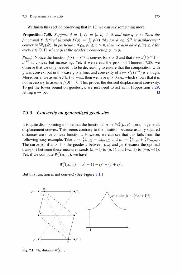
7.3 Displacement convexity 275

We finish this section observing that in 1D we can say something more.

Proposition 7.30. Suppose d D 1, ˝ D Œa; b� � R and take q > 0. Then thefunctional F defined through F.%/ D ´ b

a %.x/�qdx for � L 1 is displacement

convex in Wp.˝/. In particular, if %0; %1 � c > 0, then we also have %t.x/ � c forevery t 2 Œ0; 1�, where %t is the geodesic connecting %0 to %1.

Proof. Notice the function f .s/ D s�q is convex for s > 0 and that s 7! sdf .s�d/ DsqC1 is convex but increasing. Yet, if we reread the proof of Theorem 7.28, weobserve that we only needed it to be decreasing to ensure that the composition withg was convex, but in this case g is affine, and convexity of s 7! sdf .s�d/ is enough.Moreover, if we assume F.%/ < C1, then we have % > 0 a.e., which shows that it isnot necessary to assume f .0/ D 0. This proves the desired displacement convexity.To get the lower bound on geodesics, we just need to act as in Proposition 7.29,letting q ! 1. ut

7.3.3 Convexity on generalized geodesics

It is quite disappointing to note that the functional � 7! W22 .�; �/ is not, in general,

displacement convex. This seems contrary to the intuition because usually squareddistances are nice convex functions. However, we can see that this fails from thefollowing easy example. Take � D 1

2ı.1;0/ C 1

2ı.�1;0/ and �t D 1

2ı.t;a/ C 1

2ı.�t;�a/.

The curve �t, if a > 1 is the geodesic between ��1 and �1 (because the optimaltransport between these measures sends .a;�1/ to .a; 1/ and .�a; 1/ to .�a;�1/).Yet, if we compute W2

2 .�t; �/, we have

W22 .�t; �/ D a2 C .1 � t/2 ^ .1C t/2:

But this function is not convex! (See Figure 7.1.)

•ν•ν

•m1

•m1

•m−1

•m−1

•mt

•mt

−1 1t

a2+min{(t−1)2,(t+1)2}

Fig. 7.1 The distance W22 .�t; �/

276 7 Functionals over probabilities

The lack of geodesic convexity of this easy functional4 is a problem for manyissues (in particular for some metric approaches to gradient flows through the EVIcondition; see Section 8.4.1) and an alternate notion has been proposed, namely, thatof convexity along generalized geodesics.

Definition 7.31. If we fix an absolutely continuous probability % 2 P.˝/, forevery pair �0; �1 2 P.˝/, we call generalized geodesic between �0 and �1 withbase % in W2.˝/ the curve �t D ..1 � t/T0 C tT1/#%, where T0 is the optimaltransport map (for the cost jx � yj2) from % to �0 and T1 from % to �1.

It is clear that t 7! W22 .�t; %/ satisfies

W22 .�t; %/ �

ˆj..1 � t/T0.x/C tT1.x// � xj2d%.x/

� .1 � t/ˆ

jT0.x/ � xj2d%.x/C tˆ

jT1.x/ � xj2d%.x/

D .1 � t/W22 .�0; %/C tW2

2 .�1; %/I

and hence we have the desired convexity along this curve. Moreover, similarconsiderations to those we developed in this section show that all the functionals thatwe proved to be geodesically convex are also convex along generalized geodesics.We do not develop these proofs here, and we refer to [15] for more details: for thecase of the functional F , Lemma 7.26 has to be changed into “t 7! det..1 � t/A CtB/1=d is concave, whenever A and B are symmetric and positive-definite” (the proofis similar).

7.4 Discussion

7.4.1 A case study: min F.%/ C W22.%; �/

Among variational problems involving optimal transportation and Wassersteindistances, a very recurrent one is the following:

min%2P2.˝/

1

2W22 .%; �/C �F.%/ ; (7.2)

where F is a given functional on probability measures, � > 0 a parameter which canpossibly be small, and � is a given probability in P2.˝/ (the space of probabilitymeasures on ˝ with finite second moment

´ jxj2d%.x/ < C1). This very instance

4By the way, this functional can even be proven to be somehow geodesically concave, as it is shownin [15], Theorem 7.3.2.

7.4 Discussion 277

of the problem is exactly the one we face in the time discretization of the gradientflow of F in W2.˝/ (see Section 8.2).

But the same problem also appears, for fixed � > 0, in other frameworks as well.For instance, in image processing, if F is a smoothing functional, this is a model tofind a better (smoother) image % which is not so far from the original density � (andthe choice of the distance W2 is justified by robustness arguments); see [92, 208]. Inurban planning (see [93, 270]), � can represent the distribution of some resourcesand % that of population, who wants to be close to � but also to guarantee enoughspace to each individual. In this case the functional F favors diffuse measures (forinstance, using the functional F .%/ D ´

f .%.x// dx for a convex and superlinearfunction f with f .0/ D 0, which gives a higher cost to high densities of % and isminimized, on bounded domains, by the uniform measure). Reciprocally, � couldinstead represent the distribution of population, and % that of services, to be chosenso that they are close enough to � but more concentrated. In this case F will favorconcentrated measures. When F penalizes the number of points in the support of %,then % becomes finitely atomic and we face the so-called location problem (findingwhere to place a finite number of points so as to approximate a given continuousdistribution), useful both in logistics and in quantization issues in signal processing.See, for instance, [72, 75] for a transport-based analysis of the asymptotics of thisproblem.

Note that, when F only takes value 0 and C1, the above problem becomesa projection problem. In particular (see Section 8.4.2), the projection onto theset of densities bounded above by the constant 1 has received a lot of attentionbecause of its applications in the time discretization of evolution problems withdensity constraints, in particular for crowd motion (see [225, 265]), where a crowdis described as a population of particles which cannot overlap and cannot go beyonda certain threshold density.

In this section we would like to briefly discuss the characterization and regularityof the optimizer, at least in the case where F .%/ D ´

f .%/ for a nice convexintegrand f W RC ! R, superlinear at infinity (i.e., one of the main functionalsstudied in this chapter).

We are interested in the estimates that one can give on the minimizer O%. Theycan be roughly divided into two categories: those which are independent of � butdepend on � and those which are uniform in � but refer to similar bounds on �.

For instance, let us write down the optimality conditions for (7.2) in the caseF .%/ D ´

f .%/, using Proposition 7.20. First we suppose that f 2 C2, that we have0 < c � f 00 � C, and that spt.�/ D ˝. This allows to differentiate both terms inthe functional (the assumption on � is needed to have uniqueness of the c-concaveKantorovich potential), and we get

(' C � f 0. O%/ D C O% � a.e.,

' C � f 0. O%/ � C on f O% D 0g; (7.3)

278 7 Functionals over probabilities

where ' is a suitable Kantorovich potential in the transport from O% to �. We canwrite the above condition as

O% D .� f 0/�1�.C � '/ _ f 0.0/

: (7.4)

This provides a Lipschitz bound on %, which only depends on the Lipschitz constantof ' (which depends on diam.˝/) and of .� f 0/�1 (which is bounded by c�1). Inparticular, if we let f and � vary, keeping the condition f 00 � c > 0, we can applyAscoli-Arzelà’s theorem to % and pass to the limit (from the uniqueness of theminimizers, which is guaranteed by the strict convexity of f , the minimizers passto the limit). Hence, we can guarantee that (7.4) holds under the only assumptionf 00 � c > 0. Notice that in the case f 0.0/ D �1, we get O% D .� f 0/�1.C � '/ andthat we prefer to rewrite as � f 0. O%/ D C � '.

These considerations allow to get continuity for O%, but the bounds obviouslydegenerate as � ! 0. On the other hand, they do not really depend on �.

A different type of bound that one can prove is the following:

Proposition 7.32. If g 2 L1 is a given probability density on a compact convexand smooth domain ˝ and O% solves

min%2P.˝/

1

2W22 .%; g/C

ˆf .%.x// dx;

where f is convex and superlinear, then jj O%jjL1 � jjgjjL1 .

This bound, which, on the contrary, is independent of � , is proven in [110, 270]. Wecan provide a sketch of proof.

Proof. We start from the case where g is smooth and strictly positive, and f issmooth on �0;C1Œ, continuous on RC, with f 00 � c > 0 and f 0.0/ D �1. Fromthe above considerations (with � D 1), we know that the density of the optimal O%is a continuous function, given by O% D .f 0/�1.C � '/. Note that .f 0/�1 is Lipschitzcontinuous, as a consequence of the lower bound on f 00, and that O% > 0 since O% D 0

would imply �' D �1. From its continuity, O% admits a maximal value, O%.x0/.Note that a maximum point for O% corresponds to a minimum point for '. UsingCaffarelli’s regularity theory (see Section 1.7.6), we can provide enough regularityfor ' so as to justify all the following considerations (indeed, since g is smooth andO% is Lipschitz, and both are strictly positive, and hence bounded from below, on aconvex set, one has at least ' 2 C2;˛). First, suppose that x0 … @˝. In this case weshould have D2'.x0/ � 0. But the Monge-Ampère equation gives us

O%.x0/ D det.I � D2'.x0//g.T.x0//;

where T D id � r' is the optimal transport from O% to g. From D2'.x0/ � 0, we getdet.I � D2'.x0// � 1, and hence

7.4 Discussion 279

jj O%jjL1 D O%.x0/ � g.T.x0// � jjgjjL1 :

It remains to consider the case x0 2 @˝. Since T.x0/ D x0 � r'.x0/ 2 ˝ and ˝is convex, we have r'.x0/ � n � 0. By the optimality property of x0 (which is aminimum point for '), we also have the opposite inequality, and hence we obtainanyway r'.x0/ � n D 0. This allows to conclude that also in this case we haveD2'.x0/ � 0 (indeed, second-order minimality conditions are also satisfied on theboundary if we already know that the gradient vanishes; since the tangential partalways vanishes at extremal points, only the normal one has to be considered).

Finally, one can get rid of the assumptions on g and f by approximation (sincewe know that the minimizer of the original problem with g 2 L1 and f which isonly convex and superlinear is unique). ut

As a final remark, we stress that some limited higher-order similar estimates canalso be obtained and are the object of very recent papers. We mention a BV estimate,namely, jj O%jjBV � jjgjjBV , presented in [151], and based on some integration-by-parts techniques. We also mention a Lipschitz estimate which, together with somesemi-concavity bounds, is proved in [207] in the case where f .t/ D t log t, thanksto some Pogorelov-type methods. Both estimates can be adapted to the case wherea potential energy V is added to the functional. However, we do not develop detailshere.

7.4.2 Brunn-Minkowski inequality

Another interesting consequence of the displacement convexity in W2 is a transport-based proof of a well-known geometric inequality called Brunn-Minkowski inequal-ity. This inequality states that for every two sets E;F � R

d (we ignore heremeasurability issues), we have

jE C Fj1=d � jEj1=d C jFj1=d; where E C F D fx C y W x 2 E; y 2 Fg:

This inequality can be proven in the following way, as pointed out in [229].Consider the measures � with constant density 1

jEj on E and � with constant density1

jFj on F. Then, take the measure �1=2 obtained at time t D 1=2 on the constant-

speed geodesic between them. Since �1=2 D . 12id C 1

2T/#�0, we know that �1=2 is

concentrated on A WD 12E C 1

2F. Moreover, �1=2 is absolutely continuous and we

call % its density (we know % 2 L1 because �; � 2 L1, thanks to Proposition 7.29).Note that, for convex f , we have

1

jAjˆ

Af .%.x// dx � f

�´A %.x/ dx

jAj�

D f�jAj�1

�:

280 7 Functionals over probabilities

Geodesic convexity of F for f .t/ D �t1�1=d implies

� 1

2jEj1=d � 1

2jFj1=d D 1

2F .�/C 1

2F .�/ � F .�1=2/

Dˆ

Af .%.x// dx � jAj f

�jAj�1

�D � jAj1=d :

If we multiply this inequality by �2 on each side, using the scaling properties ofthe Lebesgue measure, we exactly obtain the Brunn-Minkowski inequality.

7.4.3 Displacement convexity, game theory, and spatialeconomics: urban equilibria

As optimal transport describes the cost of moving masses (or individuals) when theirdensity is known, it is a very natural tool to analyze problems in spatial economics,where densities of agents and of activities are involved, and one wants to take intoaccount geographical effects. Often, it is important to associate with this densitiessome “performances,”’ which let the functionals that we analyzed in this chapterappear. Among the objects studied in spatial economics, one of the most intriguing,as we can see in our everyday life, is urban structure.

Many models exist in the economic literature and most of them have nothing todo with optimal transport. An interesting treatise of some spatial problems involvingsome notions of optimal transform (more under the form of flow minimization, suchas in Chapter 4, then under the form of a Monge-Kantorovich problem) is containedin the book [28], which inspired by the way some of the works on congestedtransport contained in Section 4.4.1.

Yet, the goal of this section is not to give a comprehensive literature review onthe subject, but to point out some recent problems in urban economics where theanalysis we did in this chapter is particularly relevant. Indeed, we will see thatdisplacement convexity can play a role in proving uniqueness of equilibria and theircharacterization as the minimizers of a global energy.

In particular, we will not spend words on the models for urban planning containedin [93, 94], where the goal is to find the optimal shapes of the distribution � of thepopulation and of the distribution � of “services” in order to minimize a globalquantity F .�/ C Tc.�; �/ C G .�/. They are problems involving a social plannerwhere no equilibrium issue is addressed, and optimal transport appears directly inthe modeling and not as a tool. We will not spend word neither on the equilibriummodel contained in [106, 107], where one looks at a distribution � of residents, adistribution � of jobs, a pairing � between them, a function ' giving the price ofthe land, and a function giving wages and at other related quantities. Here anequilibrium may be found by considering ' and as Kantorovich potentials for

7.4 Discussion 281

an appropriate cost, but the model is quite long to describe (see also [275] for ashort summary of this and other models) and it uses optimal transport ideas to proveexistence and not to characterize the equilibria.

We want rather to concentrate on another, simple class of models: suppose that apopulation % is distributed in a region ˝ and that every individual wants to choosehis own position in order to minimize the sum of two costs:

• a residential cost, which is an increasing function of the density of populationat the place where he lives: the individuals living at x “pay” a function of theform h.%.x//, for h W RC ! RC increasing; this takes into account the fact thatwhere more people live, the price of land is higher (or that, for the same price,they have less space);

• an interaction cost, depending on the distances with all the other individuals:people living at x “pay” a cost of the form

´W.x�y/%.y/ dy where W is usually

an increasing function of the distance (i.e., W.z/ depends increasingly on jzj).This means that the cost that every individual pays depends on his location x andon the whole distribution % of everybody. We look for an equilibrium configuration,i.e., a density % such that, for every x0, there is no reason for people at x0 to move toanother location, since the function f%.x/ WD h.%.x//C´

W.x�y/%.y/ dy is minimalat x0, in the spirit of Nash equilibria.

Box 7.3. Important notion: Nash equilibria

Definition. Consider a game where several players i D 1; : : : ; n must choose a strategyamong a set of possibilities Si and suppose that the pay-off of each player (i.e., howmuch he gains out of the game) depends on what everybody chooses, i.e., it is given bya function pi W S1 � � � � � Sn ! R. We say that a configuration .s1; : : : ; sn/ (wheresi 2 Si) is an equilibrium (a Nash equilibrium) if, for every i, the choice si optimizesSi 3 s 7! fi.s1; : : : ; si�1; s; siC1; : : : ; sn/ (i.e., si is optimal for player i under the assumptionthat the other players freeze their choice).

Note that Nash equilibria need not exist in all situations, but the strength of Nashapproach was exactly to prove (via convex analysis arguments) that they always exist whenwe consider the so-called mixed strategies. This means that we accept that every playerinstead of choosing an element si 2 Si, only chooses a probability on Si and then randomlypicks a strategy according to the law he has chosen. This allows to convexify the gamein a way which is similar to what we do when we pass from the Monge to Kantorovichproblems.

This notion, first introduced by J. Nash in [243, 244] in the case of a finite numberof players, can be easily extended to a continuum of players where each one is negligiblecompared to the others (nonatomic games). Considering for simplicity the case of identicalplayers, we have a common space S of possible strategies and we look for a measure % 2P.S/. This measure induces a payoff function f% W S ! R and we want the followingcondition to be satisfied: there exists C 2 R such that f%.x/ D C %-a.e. and f%.x/ � Ceverywhere (if the players want to maximize the playoff, otherwise, if it is a cost to beminimized, f%.x/ � C), i.e., f% must be optimal %-a.e.

282 7 Functionals over probabilities

It is easy to see that the equilibrium condition, namely, that

h.%.x//Cˆ

W.x � y/%.y/ dy

must be minimal %-a.e. is indeed the first-order optimality condition for theminimization of

% 7! F.%/ WDˆ

H.%.x// dx C 1

2

ˆ ˆW.x � y/%.y/ dy%.x/ dx

among probabilities % 2 P.˝/, where H0 D h (just compute the first variation withrespect to perturbation of the form %" D .1 � "/% C " Q%). We can wonder whetherthis optimality condition, which is necessary for minimality, is also sufficient andif all equilibria are minimizers. This would allow to say that we face a potentialgame (i.e., a game where equilibria can be found by minimizing a global energy;see [238]). Note by the way that the energy that we minimize is not the total cost forresidents, which would be given by

´f%.x/%.x/ dx (compare to the notion of price

of anarchy in Remark 4.29). This last quantity differs from what we consider bothin the 1

2factor in the interaction part and in the fact that H.t/ ¤ th.t/ in general (as

we already saw in Section 4.4.1 concerning traffic congestion).The answer to the above question would be affirmative if the functional F was

convex. Yet, the first part is convex as H is convex (as it is the antiderivative of anincreasing function), but the interaction energy is not, as we saw in this chapter.On the other hand, if H satisfies McCann’s assumptions for displacement convexityand W is convex (which is the case for the interaction costs jx � yj or jx � yj2,for instance), then F is displacement convex. An interesting observation in [59]is exactly the fact that displacement convexity is also enough, as usual convexitywould do, in order to guarantee that equilibria are all minimizers of F. To provethis fact, it is enough to compute the derivative of F.%"/ at " D 0, when we take%" D ..1 � "/id C "T/#%, where T is the optimal transport map between % andany other admissible Q%. By the way, it is not a problem to add to the equilibriumcondition a geographical heterogeneity (i.e., a potential function), taking f%.x/ Dh.%.x// C ´

W.x � y/%.y/ dy C V.x/, and in this case we add to F.%/ a term in´V.x/%.x/ dx. The convexity of V would be the good assumption to perform the

same analysis.Since we are evoking McCann’s condition on the convex function H, it is

worthwhile to spend some words on its meaning in economic terms. To do that,we need to check how h and H depend on the density through the formation of theprice of land. This comes from an easy consideration: suppose that at every point,the agents have a certain budget to be divided into land consumption and moneyconsumption and that they have a concave and increasing utility function U forland. This means they solve a problem of the form

maxfU.L/C m W pL C m � 0g;

7.4 Discussion 283

where p represents the price for land, L is the land consumption, m is the leftover ofthe money, and the budget constraint has been set to 0 for simplicity. The optimalland consumption will saturate the constraint and be such that U0.L/ D p. Thisallows to compute the optimal utility, which is U.L/ � U0.L/L, and this gives arelation between L and utility. Yet, the land consumption is the reciprocal of thedensity, hence L D 1

%, and the residential cost h.%/, which is a cost and not a utility,

can be taken to be opposite as this utility. Hence, we take

h.%/ D 1

%U0�1

%

�� U

�1

%

�:

Since the function t 7! 1t U0. 1t /�U. 1t / is the derivative of �tU. 1t /, the correct choice

for H is indeed H.t/ D �tU. 1t /. This makes the verification of McCann’s conditionfor displacement convexity very easy, since t 7! tdH.t�d/ becomes t 7! �U.td/, andwe just need t 7! U.td/ to be concave and increasing. Monotonicity is guaranteedsince U is monotone, while the fact that it stays concave when composed with thedth power is indeed an extra assumption5.

We also stress that, in order to use displacement convexity, one needs a convexdomain ˝ and that [59] also presents examples of multiple equilibria when theconvex domain is replaced by a 1D circle (equilibria with multiple sub-cities arefound, i.e., spt.%/ can be disconnected, and the multiplicity of the equilibria is notonly due to rotational invariance, but equilibria with different shapes and differentnumber of components are found). Curiously enough, the model described in [59]strongly recalls a model by R. McCann for rotating stars, described in [232]. Insuch a paper, the author introduces a notion of W1-local minimizers which can betranslated into a notion of local equilibrium: each agent only compares his cost tothat of nearby agents; should the support of % be disconnected (which is the casein [59] and [232]), then the constant value of their utility could change from oneconnected component to the others. Note the early use of the W1 distance and thefact that this is the only distance allowing for this kind of local phenomena. Indeed,local minimality for integral distances such as Wp, if translated via optimalityconditions into the expression of an equilibrium, would not provide local minimalityfor each agent, but automatically global minimality. This can be observed in theexample of the circle in [59]: in this example many equilibria exist, and each agentis globally satisfied, not only locally, but most of them are not global minimizers ofthe global energy.

An even more interesting situation is presented in [56], in the framework of theso-called Cournot-Nash equilibria. This name is used to denote nonatomic gameswith agents which are not indistinguishable. The situation is similar to the onedescribed above, but with an extra variable, which makes the distinction between

5Thanks to an observation by R. McCann himself, this corresponds to the fact that the utility is aconcave function not only of land “volume” but also of land “linear size,” which seems reasonablesince it has to be compared to “linear” quantities such as distances in the interaction term.

284 7 Functionals over probabilities

agents: suppose that a population of agents� distributed over a space Z must choose,each, a location x 2 ˝ and that the payoff of each agent z is given by c.z; x/C f%.x/,where % is the distribution of their choices on ˝. More precisely, we look for ameasure � 2 P.Z � ˝/ such that .�Z/#� D �, and we denote .�˝/#� by %.The goal is to find � such that no agent z wants to change his choice, i.e., there is afunction ' W Z ! R with c.z; x/Cf%.x/ � '.z/ for all .z; x/ and c.z; x/Cf%.x/ D '.z/� -a.e. Note that the variable z represents the type of the agent, which cannot bemodified by the agent itself: this is why the minimality of c.z; x/ C f%.x/ is testedonly on x and gives a minimal value depending on z.

It is not difficult to prove the following facts (see [56]): a measure � is anequilibrium if and only if it is optimal for the cost c in˘.�; �/, the pair .';�f%/ is apair of Kantorovich potentials for the same transport problems, and the c-transform'c satisfies 'c.x/C f%.x/ � 0 for all x and 'c.x/C f%.x/ D 0 %-a.e. This leads to acondition on % only: find % such that C f% is minimal %-a.e., where D 'c is theKantorovich potential in the transport from % to the given measure �, for the cost c.

The same considerations of this chapter allow to view this as the optimalitycondition for the minimization of % 7! Tc.�; %/ C F.%/ and the same questionsabout displacement convexity hold. As we saw in Section 7.3.3, the functionalTc.�; �/ is not in general displacement convex, and one needs to use convexity ongeneralized geodesics. But the computations and the result are similar, as one cansee in [56].

Finally, it is interesting to see that the same kind of models would appear if,instead of defining an equilibrium on agent type z who must choose x, one directlysets an equilibrium problem on x: agents have to choose where to locate, facingboth a residential cost and an interaction cost, but also need to access a commodityz, distributed according to a distribution �, and their access cost is c.x; z/.Since the distribution of the commodity is fixed, the agents cannot simply choosethe z that they prefer (i.e., minimizing z 7! c.x; z/): a matching problem willappear and a price '.z/ for each commodity. At equilibrium, according to the theorythat we saw in Section 1.7.3, the commodity cost for the agents will be given by'.z/ C c.x; z/ D 'c.y/. This means that the agents add to their cost a new term,given by the Kantorovich potential 'c, exactly as above.

Chapter 8Gradient flows

In this chapter, we present one of the most spectacular applications of optimaltransport and Wasserstein distances to PDEs. We will see that several evolutionPDEs can be interpreted as a steepest descent movement in the space W2. As wealready developed in the previous chapters many of the technical tools that we need,a large part of this chapter will be devoted to an informal description of the generalframework.

Hence, no need to let the reader wait any more, let us immediately enter into thesubject!

8.1 Gradient flows in Rd and in metric spaces

First of all, let us present what a gradient flow is in the simplest situation. Supposeyou have a function F W R

d ! R and a point x0 2 Rd. A gradient flow is an

evolution stemming from x0 and always moving in the direction where F decreasesthe most, thus “gradually minimizing” F, starting from x0. More precisely, it is justthe solution of the Cauchy problem

(x0.t/ D �rF.x.t// for t > 0;

x.0/ D x0:

This is a standard Cauchy problem which has a unique solution if rF is Lipschitzcontinuous, i.e., if F 2 C1;1. We will see that existence and uniqueness can also holdwithout this strong assumption, thanks to the variational structure of the equation.

A first interesting property is the following, concerning uniqueness andestimates.

© Springer International Publishing Switzerland 2015F. Santambrogio, Optimal Transport for Applied Mathematicians,Progress in Nonlinear Differential Equations and Their Applications 87,DOI 10.1007/978-3-319-20828-2_8

285

286 8 Gradient flows

Proposition 8.1. Suppose that F is convex and let x1 and x2 be two solutions ofx0.t/ D �rF.x.t// (if F is not differentiable, we can consider x0.t/ 2 @F.x.t//).Then we have jx1.t/ � x2.t/j � jx1.0/ � x2.0/j for every t. In particular this givesuniqueness of the solution of the Cauchy problem.

Proof. Let us consider g.t/ D 12jx1.t/ � x2.t/j2 and differentiate it. We have

g0.t/ D .x1.t/� x2.t// � .x01.t/� x0

2.t// D �.x1.t/� x2.t// � .rF.x1.t//� rF.x2.t///:

Here we use the basic property of gradient of convex functions, i.e., that for everyx1 and x2, we have

.x1 � x2/ � .rF.x1/ � rF.x2// � 0:

More generally, it is also true that for every x1; x2 and every p1 2 @F.x1/,p2 2 @F.x2/, we have

.x1 � x2/ � .p1 � p2/ � 0:

From these considerations, we obtain g0.t/ � 0 and g.t/ � g.0/. This gives the firstpart of the claim.

Then, if we take two different solutions of the same Cauchy problem, we havex1.0/ D x2.0/, and this implies x1.t/ D x2.t/ for any t > 0. utRemark 8.2. From the same proof, one can also deduce uniqueness and stabilityestimates in the case where F is only semi-convex. We recall that semi-convexmeans that it is �-convex for some � 2 R, i.e., x 7! F.x/� �

2jxj2 is convex. Indeed,

in this case we obtain jx1.t/ � x2.t/j � jx1.0/ � x2.0/je��t; which also proves, if� > 0, exponential convergence to the unique minimizer of F. The key point isthat if F is �-convex, it is easy, by applying the monotonicity inequalities above tox 7! F.x/ � �

2jxj2, to get

.x1 � x2/ � .rF.x1/ � rF.x2// � �jx1.t/ � x2.t/j2:

This implies g0.t/ � �2�g.t/ and allows to conclude, by Gronwall’s lemma, g.t/ �g.0/e�2�t. For the exponential convergence, if � > 0, then F is coercive and admitsa minimizer, which is unique by strict convexity. Let us call it Nx. Take a solution x.t/and compare it to the constant curve Nx, which is a solution since 0 2 @F.Nx/. Thenwe get jx1.t/ � Nxj � e��tjx1.0/ � Nxj.

Another interesting feature of those particular Cauchy problems which aregradient flows is their discretization in time. Actually, one can fix a small time stepparameter � > 0 and look for a sequence of points .x�k /k defined through

x�kC1 2 argminx F.x/C jx � x�k j22�

:

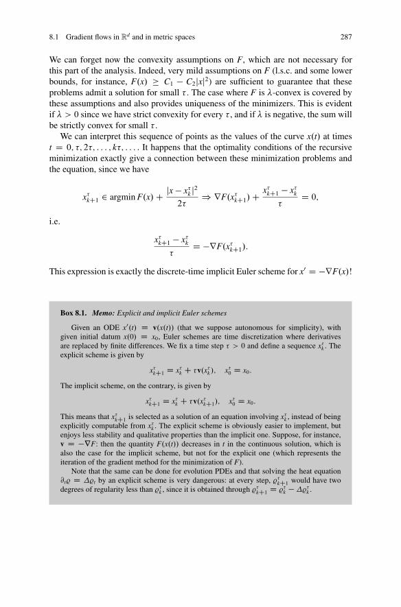
8.1 Gradient flows in Rd and in metric spaces 287

We can forget now the convexity assumptions on F, which are not necessary forthis part of the analysis. Indeed, very mild assumptions on F (l.s.c. and some lowerbounds, for instance, F.x/ � C1 � C2jxj2) are sufficient to guarantee that theseproblems admit a solution for small � . The case where F is �-convex is covered bythese assumptions and also provides uniqueness of the minimizers. This is evidentif � > 0 since we have strict convexity for every � , and if � is negative, the sum willbe strictly convex for small � .

We can interpret this sequence of points as the values of the curve x.t/ at timest D 0; �; 2�; : : : ; k�; : : : . It happens that the optimality conditions of the recursiveminimization exactly give a connection between these minimization problems andthe equation, since we have

x�kC1 2 argmin F.x/C jx � x�k j22�

) rF.x�kC1/C x�kC1 � x�k�

D 0;

i.e.

x�kC1 � x�k�

D �rF.x�kC1/:

This expression is exactly the discrete-time implicit Euler scheme for x0 D �rF.x/!

Box 8.1. Memo: Explicit and implicit Euler schemes

Given an ODE x0.t/ D v.x.t// (that we suppose autonomous for simplicity), withgiven initial datum x.0/ D x0, Euler schemes are time discretization where derivativesare replaced by finite differences. We fix a time step � > 0 and define a sequence x�k . Theexplicit scheme is given by

x�kC1 D x�k C �v.x�k /; x�0 D x0:

The implicit scheme, on the contrary, is given by

x�kC1 D x�k C �v.x�kC1/; x�0 D x0:

This means that x�kC1 is selected as a solution of an equation involving x�k , instead of beingexplicitly computable from x�k . The explicit scheme is obviously easier to implement, butenjoys less stability and qualitative properties than the implicit one. Suppose, for instance,v D �rF: then the quantity F.x.t// decreases in t in the continuous solution, which isalso the case for the implicit scheme, but not for the explicit one (which represents theiteration of the gradient method for the minimization of F).

Note that the same can be done for evolution PDEs and that solving the heat equation@t% D �%t by an explicit scheme is very dangerous: at every step, %�kC1 would have twodegrees of regularity less than %�k , since it is obtained through %�kC1 D %�k ��%�k .

288 8 Gradient flows

It is possible to prove that for � ! 0, the sequence we found, suitablyinterpolated, converges to the solution of the problem. It even suggests how to definesolutions for functions F which are only l.s.c., with no gradient at all!

But a huge advantage of this discretized formulation is also that it can easily beadapted to metric spaces. Actually, if one has a metric space .X; d/ and an l.s.c.function F W X ! R [ fC1g bounded from below, one can define

x�kC1 2 argminx F.x/C d.x; x�k /2

2�(8.1)

and study the limit as � ! 0. Obviously the assumptions on F have to be adapted,since we need existence of the minimizers and hence a little bit of compactness. Butif X is compact, then everything works for F only l.s.c.

We can consider two different interpolations of the points x�k , given, respec-tively, by

x� .t/ D x�k ; Qx� .t/ D !x�k�1;x�k

�t � .k � 1/�

�

�for t 2�.k � 1/; �; k��;

where !x;y.s/ denotes any constant-speed geodesic connecting a point x to a pointy, parametrized on the unit interval Œ0; 1�. The interpolation Qx� only makes sensein spaces where geodesics exist, obviously. It is in this case a continuous (locallyLipschitz) curve, which coincides with the piecewise constant interpolation x� attimes t D k� .

De Giorgi, in [137], defined1 the notion of minimizing movements (see also [7]).

Definition 8.3. A curve x W Œ0;T� ! X is said to be a minimizing movement ifthere exists a sequence of time steps �j ! 0 such that the piecewise constantinterpolations x�j , built from a sequence of solutions of the iterated minimizationscheme (8.1), uniformly converge to x on Œ0;T�.

Compactness results guaranteeing the existence of minimizing movements arederived from a simple property giving a Hölder behavior for the curves x� : for every� and every k, the optimality of x�kC1 provides

F.x�kC1/C d.x�kC1; x�k /2

2�� F.x�k /; (8.2)

which implies

d.x�kC1; x�k /2 � 2��F.x�k / � F.x�kC1/

:

1We avoid here the distinction between minimizing movements and generalized minimizingmovements, which is not crucial in our analysis.

8.1 Gradient flows in Rd and in metric spaces 289

If F.x0/ is finite and F is bounded from below, taking the sum over k, we have

lXkD0

d.x�kC1; x�k /2 � 2��F.x�0/ � F.x�lC1/

� C�:

Given t 2 Œ0;T�, denote by `.t/ the unique integer such that t 2�.`.t/ � 1/�; `.t/��.For t < s apply the Cauchy-Schwartz inequality to the sum between the indices `.t/and `.s/ (note that we have j`.t/ � `.s/j � jt�sj

�C 1):

d.x� .t/; x� .s// �`.s/�1XkD`.t/

d.x�kC1; x�k / �0@`.s/�1X

kD`.t/d.x�kC1; x�k /2

1A

12

j`.s/ � `.t/j 12

� Cp�.jt � sj C �/

12

p�

� C�jt � sj1=2Cp

�:

This means that the curves x� – if we forget for a while that they are actuallydiscontinuous – are morally equi-Hölder continuous of exponent 1=2. The situationis even clearer for Qx� . Indeed, we have

�

�d.x�k�1; x�k /

�

�2D

ˆ k�

.k�1/�j.Qx� /0j2.t/dt;

which implies, by summing up,

ˆ T

0

j.Qx� /0j2.t/dt � C:

This means that the curves Qx� are bounded in H1.Œ0;T�I X/ (the space of absolutelycontinuous curves with square-integrable metric derivative), which also implies aC0; 12 bound by usual Sobolev embedding.

If the space X, the distance d, and the functional F are explicitly known, in somecases it is already possible to pass to the limit in the optimality conditions of eachoptimization problem in the time-discrete setting and to characterize the limit curvex.t/. It will be possible to do so in the space of probability measures, which is thetopic of this chapter, but not in many other cases. Indeed, without a little bit of(differential) structure on X, it is almost impossible. If we want to develop a generaltheory of gradient flows in metric spaces, we need to exploit finer tools, able tocharacterize, with the only help of metric quantities, the fact that a curve x.t/ is agradient flow.

We present here an inequality which is satisfied by gradient flows in the smoothEuclidean case and which can be used as a definition of gradient flow in the metriccase, since all the quantities which are involved have their metric counterpart.Another inequality, called EVI, will be presented in the Discussion Section 8.4.1.

290 8 Gradient flows

The first observation is the following: thanks to the Cauchy-Schwartz inequality,for every curve x.t/, we have

F.x.s// � F.x.t// Dˆ t

s�rF.x.r// � x0.r/ dr �

ˆ t

sjrF.x.r//jjx0.r/j dr

�ˆ t

s

�1

2jx0.r/j2 C 1

2jrF.x.r//j2

�dr:

Here, the first inequality is an equality if and only if x0.r/ and rF.x.r// are vectorswith opposite directions for a.e. r, and the second is an equality if and only if theirnorms are equal. Hence, the condition, called EDE (Energy Dissipation Equality)

F.x.s// � F.x.t// Dˆ t

s

�1

2jx0.r/j2 C 1

2jrF.x.r//j2

�dr; for all s < t

(or even the simple inequality F.x.s//�F.x.t// � ´ ts

�12jx0.r/j2 C 1

2jrF.x.r//j2 dr)

is equivalent to x0 D �rF.x/ a.e. and could be taken as a definition of gradient flow.This is what is done in a series of works by Ambrosio, Gigli, and Savaré and inparticular in their book [15]. Developing this (huge) theory is not among the scopesof this book. The reader who is curious about this abstract approach but wants tofind a synthesis of their work from the point of view of the author can have a look at[277]. In such a paper, the role of the different parts of the theory with respect to thepossible applications is clarified as far as possible2 (we also discuss in short someof these issues in Section 8.4.1).

8.2 Gradient flows in W2, derivation of the PDE

In this section we give a short and sketchy presentation of what can be done when weconsider the gradient flow of a functional F W P.˝/ ! R[ fC1g. The functionalwill be supposed l.s.c. for the weak convergence of probabilities and ˝ compact(which implies that F admits a minimizer and is bounded from below). In particular,we will give an heuristic on how to derive a PDE from the optimality conditions ateach time step. This is obviously something that we can only do in this particularmetric space and does not work in the general case of an abstract metric space.3

Indeed, we exploit the fact that we know, from Chapter 5, that all absolutelycontinuous curves in the space W2.˝/ are solution of the continuity equation @t%t C

2Unfortunately, some knowledge of French is required (even if not forbidden, English is unusualin the Bourbaki seminar, since “Nicolas Bourbaki a une préférence pour le français”).3The original ideas which led to this theory come from [198] and [246] through what is known as“Otto’s formal calculus”, and have later been reconsidered in [15].

8.2 Gradient flows in W2, derivation of the PDE 291

r � .%tvt/ D 0, for a suitable vector field v. The goal is to identify the vector field vt,which will depend on the measure %t, in a way which is ruled by the functional F.

We consider the iterated minimization scheme

%�.kC1/ 2 argmin% F.%/C W22 .%; %

�.k//

2�: (8.3)

Each of these problems has a solution, by compactness of P.˝/ and semi-continuity of the objective function. Exactly as we did for the Euclidean case(F defined on R

d), we want to study the optimality conditions of these problemsso as to guess the limit equation.

We recall the notation ıGı%.%/ for the first variation of a functional G W P.˝/ !

R [ fC1g. We will suppose that ıFı%

is known and try to write the limit equation interms of this operator.

Now, take an optimal measure O% for the minimization problem at step k andcompute variations with respect to perturbations of the form %" WD .1 � "/ O% C " Q%,where Q% is any other probability measure. Using Proposition 7.20, we obtain

ıF

ı%.%/C '

�D constant;

where ' is a Kantorovich potential for the transport with cost 12jx � yj2 from O% to

%�.k/. Actually, the above equality holds O%-a.e. and requires uniqueness of '. Forboth these points proving %" > 0 will be enough, but we will fix this when doingthe rigorous proof.

If we combine the fact that the above sum is constant and that we have T.x/ Dx � r'.x/ for the optimal T, we get

T.x/ � x

�D �r'.x/

�D r�ıF

ı%.%/.x/: (8.4)

We will denote by �v the ratio T.x/�x�

. Why? Because, as a ratio between adisplacement and a time step, it has the meaning of a velocity, but since it is thedisplacement associated with the transport from %�.kC1/ to %�.k/, it is better to view itrather as a backward velocity (which justifies the minus sign).

Since here we have v D �r� ıFı%.%/, this suggests that at the limit � ! 0, we

will find a solution of

@t% � r � �%r�ıFı%.%/ D 0;

with no-flux boundary conditions on @˝.Before entering into the details making the above approach rigorous (next

section), we want to present some examples of this kind of equations. We willconsider two functionals that we already analyzed in Chapter 7, and more precisely

292 8 Gradient flows

F .%/ Dˆ

f .%.x// dx; and V .%/ Dˆ

V.x/d%:

In this case we already saw that we have

ıF

ı%.%/ D f 0.%/;

ıV

ı%.%/ D V:

An interesting example is the case f .t/ D t log t. In such a case, we have f 0.t/ Dlog t C 1 and r.f 0.%// D r%

%: this means that the gradient flow equation associated

with the functional F would be the heat equation

@t% ��% D 0;

and that for F C V we would have the Fokker-Planck equation

@t% ��% � r � .%rV/ D 0:

We will see a list of other gradient flow equations in Discussion section, includingthe so-called porous media equation, obtained for other choices of f .

Remark 8.4. One could wonder how the usual stochastic diffusion interpretation ofthe heat and Fokker-Planck equations is compatible with the completely determin-istic framework that we present here, where the velocity of each particle is givenby �r%=% � rV (take V D 0 to get the heat equation). Indeed, the Fokker-Planckequation is also the PDE solved by the density of a bunch of particle followinga stochastic equation dXt D �rV.Xt/dt C dBt, where B is a standard Brownianmotion (independent for each particle). The answer, as it is well pointed out in [88],is based on the idea that in this optimal transport interpretation we rearrange (i.e.,relabel) the particles. This fact is quite clear in the 1D case: if at every time stepparticles move from x to x � �rV.x/C B� (i.e., they follow the drift �rV and theydiffuse with a Gaussian law), and then we reorder them (we always call particle 1 theone which is the most at the left, particle 2 the next one : : : and particle N the onewhich is the most at the right), then we have a discrete family of trajectories whichconverge, when � goes to 0 and the number N to infinity, to a solution of Fokker-Planck where the velocity is exactly given by �r%=%� rV . Similar considerationscan be done in higher dimension with suitable notions of rearrangement.

Note that all these PDEs come accompanied by Neumann boundary conditions% @@n .

ıFı%.%// D 0 on @˝, as a consequence of the no-flux conditions for the

continuity equation of Section 5.3. We will see in Section 8.4.3 a case of extensionto Dirichlet boundary conditions.

We finish this section with some philosophical thoughts. Why should we studysome PDEs by considering them as gradient flows for the distance W2? There areat least three reasons. The first one is that it allows to give an existence result (of aweak solution of such a PDE), with the technique that we will see in the next section.This is obviously useless when the equation is already well known, as it is the case

8.3 Analysis of the Fokker-Planck case 293

for the heat equation or its Fokker-Planck variant. But the same strategy could beapplied to variants of the same equations (or to similar equations in stranger spaces,as it is nowadays done for the heat flow in metric measure spaces; see [18, 183]).It is also very useful when the equation is of new type (we will see the case ofthe crowd motion models in Section 8.4.2). The second goal could be to deriveproperties of the flow and of the solution, once we know that it is a gradient flow. Asimple one is the fact that t 7! F.%t/ must be decreasing in time. However, this canbe often deduced from the PDE in different ways and does not require in generalto have a gradient flow. The third goal concerns numerics: the discretized schemeto get a gradient flow is itself a sort of algorithm to approximate the solution. If theminimization problems at each time step are discretized and attacked in a suitableway, this can provide efficient numerical tools (see, for instance, [40]).

Finally, all the procedure we presented is related to the study and the existenceof weak solutions. What about uniqueness? We stress that in PDE applications theimportant point is to prove uniqueness for weak solutions of the continuity equationwith v D �r ıF

ı%(i.e., we do not care at the metric structure and at the definitions of

EVI and EDE). In some cases, this uniqueness could be studied independently of thegradient flow structure (this is the case for the heat equation, for instance). Anyway,should we use PDE approaches for weak solutions, or abstract approaches in metricspaces, it turns out that usually uniqueness is linked to some kind of convexity, or�-convexity, and in particular to displacement convexity. This is why a large part ofthe theory has been developed for �-geodesically convex functionals.

8.3 Analysis of the Fokker-Planck case

We consider here the case study of the Fokker-Planck equation, which is the gradientflow of the functional

J.%/ Dˆ

˝

% log %Cˆ

˝

Vd%;

where V is a Lipschitz function on the compact domain ˝. The initial measure%0 2 P.˝/ is taken such that J.%0/ < C1.

We stress that the first term of the functional is defined as

F .%/ WD( ´

˝%.x/ log %.x/ dx if % � L d;

C1 otherwise,

where we identify the measure % with its density, when it is absolutely continuous.This functional is l.s.c. thanks to Proposition 7.7 (which can be applied since we areon a domain with finite measure; otherwise the situation is trickier, and we refer toEx(45)).

294 8 Gradient flows

Semi-continuity is the key tool to establish the following result:

Proposition 8.5. The functional J has a unique minimum over P.˝/. In particularJ is bounded from below. Moreover, for each � > 0, the following sequence ofoptimization problems recursively defined is well-posed:

%�.kC1/ 2 argmin% J.%/C W22 .%; %

�.k//

2�; (8.5)

which means that there is a minimizer at every step, and this minimizer is unique.

Proof. Just apply the direct method, noting that P.˝/ is compact for the weakconvergence, which is the same as the convergence for the W2 distance (again,because ˝ is compact), and for this convergence F is l.s.c. and the other termsare continuous. This gives at the same time the existence of a minimizer for J andof a solution to each of the above minimization problems (8.5). Uniqueness comesfrom the fact that all the functionals are convex (in the usual sense) and F is strictlyconvex. ut

Optimality conditions at each time step

We will use Propositions 7.17, 7.20, and 7.18, and to do so we first need to provethe following result:

Lemma 8.6. Any minimizer O% in (8.5) must satisfy O% > 0 a.e. and log O% 2 L1.

Proof. Consider the measure Q% with constant positive density c in ˝ (i.e., c Dj˝j�1). Let us define %" as .1 � "/ O%C " Q% and compare O% to %".

By optimality of O%, we may write

F . O%/ � F .%"/ �ˆ

˝

Vd%" �ˆ

˝

Vd O%C W22 .%"; %

�.k//

2�� W2

2 . O%; %�.k//2�

: (8.6)

The Wasserstein term in the right-hand side may be estimated by convexity:

W22 .%"; %

�.k//

2�� .1 � "/W2

2 . O%; %�.k//2�

C "W22 . Q%; %�.k//2�

:

The potential term is of order " as well:

ˆ

˝

Vd%" �ˆ

˝

Vd O% D "

ˆ

˝

Vd. Q% � O%/ � C":

8.3 Analysis of the Fokker-Planck case 295

This shows that the whole right-hand side of (8.6) is estimated by C" and we get

ˆ

˝

f . O%/ � f .%"/ � C"

where f .t/ D t log t (set to 0 in t D 0). Write

A D fx 2 ˝ W O%.x/ > 0g; B D fx 2 ˝ W O%.x/ D 0g:

Since f is convex, we write, for x 2 A, f . O%.x//�f .%".x// � . O%.x/�%".x//f 0.%".x// D". O%.x/ � Q%.x//.1 C log %".x//. For x 2 B we simply write f . O%.x// � f .%".x// D�"c log."c/. This allows to write

�"c log."c/jBj C "

ˆ

A. O%.x/ � c/.1C log %".x// dx � C"

and, dividing by ",

� c log."c/jBj Cˆ

A. O%.x/ � c/.1C log %".x// dx � C: (8.7)

Note that we always have

. O%.x/ � c/.1C log %".x// � . O%.x/ � c/.1C log c/

(just distinguish between the case O%.x/ � c and O%.x/ � c/. Thus, we may write

�c log."c/jBj Cˆ

A. O%.x/ � c/.1C log c/ dx � C:

Letting " ! 0 provides a contradiction, unless jBj D 0.This proves O% > 0 a.e. We now come back to (8.7), which is an upper bound on

the integral of the functions . O%.x/ � c/.1C log %".x//. We already noted that thesefunctions are bounded from below by . O%.x/� c/.1C log c/, which is L1 because c isa constant and O% 2 L1. Hence, we can apply Fatou’s lemma and obtain, at the limitas " ! 0,

ˆ

˝

. O%.x/ � c/.1C log O%.x// dx � C

(the integral on A has been replaced by the integral on ˝, since B is negligible).Since we already know that . O% � c/.1 C log O%/ is bounded from below by anL1 function and its integral is finite, then it is L1. But we already know thatO%; O% log O% 2 L1, and we deduce log O% 2 L1. ut

296 8 Gradient flows

We can now compute the first variation and give optimality conditions on theoptimal %�.kC1/.

Proposition 8.7. The optimal measure %�.kC1/ in (8.5) satisfies

log.%�.kC1//C V C N'�

D constant a.e. (8.8)

where N' is the (unique) Kantorovich potential from %�.kC1/ to %�.k/. In particular,log %�.kC1/ is Lipschitz continuous. If T�kC1 is the optimal transport from %�.kC1/ to%�.k/, then it satisfies

v�.kC1/ WD id � T�kC1�

D �r�

log.%�.kC1//C V�

a.e. (8.9)

Proof. Take the optimal measure O% WD %�.kC1/. We can say that it is regular (seeDefinition 7.12) for the functional J, since the only term that is not finite on allprobabilities in P.˝/ is the entropy term, but it is convex and finite both onthe optimum O% and on L1 densities. We can check that J admits a first variationat O%. For the linear term it is straightforward, and for the Wasserstein term,we can apply Proposition 7.17. The uniqueness of the Kantorovich potential isguaranteed by Proposition 7.18 together with Lemma 8.6. For the entropy term,consider %" WD .1 � "/ O% C " Q%, for Q% 2 L1. Set M D jj Q%jjL1 and look at" 7! ´

%" log %": The integrand can be differentiated in " pointwisely, thus getting.1C log %"/. Q% � O%/. For " < 1=2, we can check that these functions are dominatedby . O%C M/.j log O%j C log M C 1/, which is L1 thanks to O%; log O%; O% log O% 2 L1 (fromLemma 8.6). This allows to differentiate under the integral sign and proves that thefirst variation of this term is 1C log O%.

The first variation of J is hence

ıJ

ı%D f 0.%/C V D log.%/C 1C V:

Applying Proposition 7.20 we obtain Equation (8.8), which is valid a.e. since O% > 0.In particular, this implies that %�.kC1/ is Lipschitz continuous, since we have

%�.kC1/.x/ D exp

�C � V.x/ � N'.x/

�

�:

Then, one differentiates and gets the equality

r N' D id � T�kC1�

D �r�

log.%�.kC1//C V�

a.e.

and this allows to conclude. ut

8.3 Analysis of the Fokker-Planck case 297

Interpolation between time steps and uniform estimates

Let us collect some other tools.

Proposition 8.8. For any � > 0, the sequence of minimizers satisfies

Xk

W22 .%

�.kC1/; %�.k//�

� C WD 2.J.%0/ � inf J/:

Proof. This is obtained by comparing the optimizer %�.kC1/ to the previous measure%�.k/. We get

J.%�.kC1//C W22 .%

�.kC1/; %�.k//2�

� J.%�k /; (8.10)

which implies

Xk

W22 .%

�.kC1/; %�.k//�

�X

k

2.J.%�k / � J.%�.kC1///:

This last sum is telescopic and gives the claim. utLet us define two interpolations between the measures %�.k/.With this time-discretized method, we have obtained, for each � > 0, a sequence

.%�.k//k. We can use it to build at least two interesting curves in the space of measures:

• first we can define some piecewise constant curves, i.e., %�t WD %�.kC1/ for t 2�k�; .k C 1/��; associated with this curve, we also define the velocities v�t Dv�.kC1/ for t 2�k�; .k C 1/��, where v�.kC1/ is defined as in (8.9): v�.kC1/ D .id �T�kC1/=� , taking as T�kC1 the optimal transport from %�.kC1/ to %�.k/; we also definethe momentum variable E� D %�v� ;

• then, we can also consider the densities Q%�t that interpolate the discrete values.%�.k//k along geodesics:

Q%�t D�

k� � t

�v�.k/ C id

�#%�.k/; for t 2�.k � 1/�; k�ŒI (8.11)

the velocities Qv�t are defined so that . Q%� ; Qv� / satisfy the continuity equation andjjQv�t jjL2.Q%�t / D j. Q%�/0j.t/. To do so, we take

Qv�t D v�t ı�.k� � t/v�.k/ C id

��1 I

as before, we define a momentum variable: QE� D Q%� Qv� .

298 8 Gradient flows

After these definitions we consider some a priori bounds on the curves and thevelocities that we defined. We start from some estimates which are standard in theframework of minimizing movements.

Note that the speed (i.e., metric derivative) of Q%� is constant on each interval�k�; .k C 1/�Œ and equal to

W2.%�.kC1/; %�.k//�

D 1

�

�ˆjid � T�kC1j2d%�.kC1/

�1=2D jjv�kC1jjL2.%�.kC1/

/;

which gives

jjQv�t jjL2.Q%�t / D j. Q%�/0j.t/ D W2.%�.kC1/; %�.k//�

D jjv�t jjL2.%�t /;

where we used the fact that the velocity field Qv� has been chosen so that its L2 normequals the metric derivative of the curve Q%� .

In particular, we can obtain

jE� j.Œ0;T� �˝/ Dˆ T

0

dtˆ

˝

jv�t jd%�t Dˆ T

0

jjv�t jjL1.%�t /dt �ˆ T

0

jjv�t jjL2.%�t /dt

� T1=2ˆ T

0

jjv�t jj2L2.%�t /dt D T1=2X

k

�

W2.%

�.kC1/; %�.k//�

!2� C:

The estimate on QE� is completely analogous

j QE� j.Œ0;T� �˝/ Dˆ T

0

dtˆ

˝

jQv�t jd Q%�t � T1=2ˆ T

0

jjQv�t jj2L2.Q%�t /

D T1=2X

k

�

W2.%

�.kC1/; %�.k//�

!2� C:

This gives compactness of E� and QE� in the space of vector measures on space-time,for the weak convergence. As far as Q%� is concerned, we can obtain more than that.Consider the following estimate, for s < t:

W2. Q%�t ; Q%�s / �ˆ t

sj. Q%�/0j.r/dr � .t � s/1=2

�ˆ t

sj. Q%�/0j.r/2dr

�1=2:

From the previous computations, we have again

ˆ T

0

j. Q%�/0j.r/2dr DX

k

�

W2.%

�.kC1/; %�.k//�

!2� C;

8.3 Analysis of the Fokker-Planck case 299

and this implies

W2. Q%�t ; Q%�s / � C.t � s/1=2; (8.12)

which means that the curves Q%� are uniformly Hölder continuous. Since they aredefined on Œ0;T� and valued in W2.˝/ which is compact, we can apply the Ascoli-Arzelà theorem. This implies that, up to subsequences, we have

E� * E in M d.Œ0;T� �˝/; QE� * QE in M d.Œ0;T� �˝/IQ%� ! % uniformly for the W2 distance:

The limit curve %, from the uniform bounds on Q%� , is both 12-Hölder continuous and

absolutely continuous in W2.As far as the curves %� are concerned, they also converge uniformly to the same

curve %, since W2.%�t ; Q%�t / � C

p� (a consequence of (8.12), of the fact that Q%� D %�

on the points of the form k� and of the fact that %� is constant on each interval�k�; .k C 1/��).

Let us now prove that QE D E.

Lemma 8.9. Suppose that we have two families of vector measures E� and QE� suchthat

• QE� D Q%� Qv� ; E� D %�v� ;

• Qv�t D v�t ı�.k� � t/v�.k/ C id

��1; Q%� D

�.k� � t/v�.k/ C id

�#%� ;

•´´ jv� j2d%� � C (with C independent of � );

• E� * E and QE� * QE as � ! 0.

Then QE D E.

Proof. It is sufficient to fix a Lipschitz function f W Œ0;T� �˝ ! Rd and to prove´

f � dE D ´f � d QE. To do that, we write

ˆf � d QE� D

ˆ T

0

dtˆ

˝

f � Qv�t d Q%� Dˆ T

0

dtˆ

˝

f ı ..k� � t/v� C id/ � v�t d%� ;

which implies

ˇˇˆ

f � d QE� �ˆ

f � dE�ˇˇ �

ˆ T

0

dtˆ

˝

jf ı ..k� � t/v�Cid/ � f j jv�t jd%�

� Lip.f /�ˆ T

0

ˆ

˝

jv�t j2d%� � C�:

This estimate proves that the limit of´

f � d QE� and´

f � dE� is the same, i.e.,E D QE. ut

300 8 Gradient flows

Relation between % and E

We can obtain the following:

Proposition 8.10. The pair .%;E/ satisfies, in distributional sense,

@t%C r � E D 0; E D �r% � %rV;

with no-flux boundary conditions on @˝. In particular we have found a solution to

(@t% ��%C r � .%rV/ D 0;

%.0/ D %0;

where the initial datum is to be intended in the following sense: the curve t 7! %t is(absolutely) continuous in W2, and its initial value is %0.

Proof. First, consider the weak convergence . Q%� ; QE� / * .%;E/ (which is aconsequence of QE D E). The continuity equation @t Q%� C r � QE� D 0 is satisfied(as in Section 4.1.2) in the sense of distributions by . Q%� ; QE� / (we test the equationsagainst C1

c function on �0;TŒ�˝, which means in particular that we do not requirethe test functions to vanish on @˝) and this passes to the limit.

Hence, @t%C r � E D 0.The continuity in W2 and the initial datum pass to the limit because of the

uniform C0;1=2 bound in (8.12).Then, use the convergence .%� ;E� / * .%;E/. Actually, using the optimality

conditions of Proposition 8.7 and the definition of E� D v�%� , we have, for each� > 0, E� D �r%� � %�rV (again, in the sense of distributions: the term %�rV isthe product of L1 and L1 functions). It is not difficult to pass this condition to thelimit either. Take f 2 C1

c.�0;TŒ�˝IRd/ and test:

ˆf � dE� D �

ˆf � r%� �

ˆf � rV%� D

ˆr � f d%� �

ˆf � rV%� :

These terms pass to the limit as %� * %, at least if V 2 C1, since all the testfunctions above are continuous. This would give

´f �dE D ´

.r � f /d%�´f �rV d%;

which implies E D �r% � %rV (once more, r% is to be intended in the sense ofdistributions).

To handle the case where V is only Lipschitz continuous, let us note that for every�; t we have J.%�t / � J.%0/ (this is a consequence of (8.10), which iterated over k,gives J.%�.k// � J.%0/). This gives a uniform bound on F .%�t / and the Dunford-Pettis theorem below turns the weak convergence %�t * %t as measures into a weakconvergence in L1. Look at the term

ˆf � rV%� WD

ˆ T

0

dtˆ

˝

f .t; x/ � rV.x/%�t .x/ dx:

8.4 Discussion 301

The integrand in t is uniformly bounded by jjf jjL1 jjrVjjL1 . Hence, we cancompute its limit as � ! 0 looking at the limit for each fixed t because it isdominated. And, for fixed t, we have weak convergence in L1 of %�t to %t, which,multiplied with a fixed L1 function, i.e., f �rV , gives the desired limit of the integral.

ut

Box 8.2. Memo: Equi-integrability and the Dunford-Pettis theorem

Definition. A sequence of function %n is said to be equi-integrable if for every " > 0

there exists ı > 0 such that on every set A with jAj � ı, we have´

A %n.x/ dx � " for any n.We can check that equi-integrability is equivalent to a bound

´f .%n.x// dx � C <

C1 for any superlinear function f . Let us only prove that such a bound implies equi-integrability. Indeed, fix " > 0 and take M such that for all t with t > M, we have f .t/=t >2C=" (this is possible thanks to the superlinearity of f ). Then we estimate

ˆ

A%n D

ˆ

A\f%n�Mg

%n Cˆ

A\f%n>Mg

%n

f .%n/f .%n/ dx � MjAj C "

2CC:

It is now enough to take ı D "2M and we get

´A %n.x/ dx < ".

Theorem. Suppose that %n is a sequence of probability densities weakly converging asmeasures to % 2 P.˝/. Suppose that

´f .%n/ is bounded for some superlinear function

f . Then % is also absolutely continuous and the weak convergence also holds in L1 (i.e., induality with L1 functions and not only with continuous ones).

Proof. The absolute continuity of % is a consequence of the lower semi-continuity of Fdefined as F .%/ D ´

˝ f .%.x// dx if % L d (C1 otherwise).Moreover, the bound on

´f .%n.x// dx implies equi-integrability. Fix a test function ' 2

L1 and use the fact that for every " > 0, there is a ı > 0 with jAj � ı ) ´A %n.x/ dx � "

and that, by Lusin’s theorem, for this ı > 0, there exists a continuous function Q' withjj Q'jjL1

� jj'jjL1

and f' ¤ Q'g � A, where A is open with jAj < ı. We have

ˇˇˆ

'.%n � %/

ˇˇ �

ˇˇˆ

Q'.%n � %/

ˇˇC 2jj'jjL1

ˆ

A.%n C %/:

Since A is open and %n * %, we have´

A %.x/ dx � lim inf´

A %n.x/ dx � "; hence

lim sup

ˇˇˆ

'.x/%n.x/ dx �ˆ

'.x/%.x/ dx

ˇˇ � 0C 2jj'jjL1";

which implies, " being arbitrary,´'.x/%n.x/ dx ! ´

'.x/%.x/ dx.

8.4 Discussion

8.4.1 EVI, uniqueness, and geodesic convexity

In the general theory of gradient flows [15] in metric spaces, another characteri-zation, different from the EDE, is proposed in order to cope with uniqueness and

302 8 Gradient flows

stability results. It is based on the following observation: if F W Rd ! R is convex,then the inequality

F.y/ � F.x/C p � .y � x/ for all y 2 Rd

characterizes (by definition) the vectors p 2 @F.x/, and if F 2 C1, it is only satisfiedfor p D rF.x/. Analogously, if F is �-convex, the inequality that characterizes thegradient is

F.y/ � F.x/C �

2jx � yj2 C p � .y � x/ for all y 2 R

d:

Hence, we can pick a curve x.t/ and a point y and compute

d

dt

1

2jx.t/ � yj2 D .y � x.t// � .�x0.t//:

Consequently, imposing

d

dt

1

2jx.t/ � yj2 � F.y/ � F.x.t// � �

2jx.t/ � yj2;

for all y, will be equivalent to �x0.t/ D rF.x.t//. This will provide a secondcharacterization (called EVI, evolution variational inequality) of gradient flows in ametric environment. Indeed, all the terms appearing in the above inequality have ametric counterpart (only squared distances and derivatives w.r.t. time appear). Evenif we often forget the dependence on �, it should be noted that the condition EVIshould actually be written as EVI�, since it involves a parameter �, which is a prioriarbitrary. Actually, �-convexity of F is not necessary to define the EVI� property,but it will be necessary in order to guarantee the existence of curves which satisfysuch a condition. The notion of �-convexity will hence be crucial also in metricspaces, where it will be rather “�-geodesic-convexity.”

The role of the EVI condition in the uniqueness and stability of gradient flows isquite easy to guess. Take two curves, which we call x.t/ and y.s/, and compute

d

dt

1

2d.x.t/; y.s//2 � F.y.s// � F.x.t// � �

2d.x.t/; y.s//2; (8.13)

d

ds

1

2d.x.t/; y.s//2 � F.x.t// � F.y.s// � �

2d.x.t/; y.s//2: (8.14)

If one wants to estimate E.t/ D 12d.x.t/; y.t//2, summing up the two above

inequalities, after a chain-rule argument for the composition of the function of twovariables4 .t; s/ 7! 1

2d.x.t/; y.s//2 and of the curve t 7! .t; t/, gives

4Note that a similar argument, based on doubling the variables, is also often performed for thedifferentiation of W2

2 along curves in W2, which we did differently in Section 5.3.5.

8.4 Discussion 303

d

dtE.t/ � �2�E.t/:

By Gronwall’s lemma, this provides uniqueness (when x.0/ D y.0/) and stability.The situation concerning these two different notions of gradient flows (EVI and

EDE) in abstract metric spaces has been clarified by Savaré (in an unpublished note,but the proof can also be found in [9]), who showed that

• All curves which are gradient flows in the EVI sense also satisfy the EDEcondition.

• The EDE condition is not in general enough to guarantee uniqueness of thegradient flow. As a simple example, take X D R

2 with the `1 distance

d..x1; x2/; .y1; y2// D jx1 � y1j _ jx2 � y2j;and take F.x1; x2/ D x1; we can check that any curve .x1.t/; x2.t// withx01.t/ D �1 and jx0

2.t/j � 1 satisfies EDE.• On the other hand, the existence of a gradient flow in the EDE sense is quite

easy to get and provable under very mild assumption.• The EVI condition is in general too strong in order to get existence (in the

example above of the `1 norm, no EVI gradient flow would exist), but alwaysguarantees uniqueness and stability (w.r.t. initial data).

Also, the existence of EVI gradient flows is itself very restricting on the functionF: indeed, it is proven in [134] that if F is such that from every starting point x0there is an EVI� gradient flow, then F is necessarily �-geodesically convex.

We need to stress that all these abstract considerations on EDE and EVI aremandatory when dealing with a general metric framework, but can often be skippedwhen dealing with precise applications. For the sake of the applications to PDE thatare at the core of this chapter, the point of view which seems to be more concreteis the following: there is an evolution model translated into a PDE, and we wantto study this equation (existence; uniqueness and stability; qualitative, regularity,and asymptotical properties; numerical simulations). If this PDE happens to be thegradient flow of a certain functional for the W2 distance, then much informationcan be obtained by the gradient flow approach (more specifically, the minimizingmovement approach via discretized variational problems). But the notion of solutionthat one should use is a priori the one which came with the PDE in the modeling ofthe problem (in general, the notion of weak solution of a continuity equation). Thisis why, even if (nontrivial) results exist proving equivalence between some abstract(EVI or EDE) notions in the metric space W2 and weak solutions of evolutionequations (see [15]), we preferred not to enter into these details here in this book.

On the other hand, we will see in a while (next section) that, as a last remarkin favor of the general theory developed in [15], it is not always easy to proveexistence via the minimizing movement method when we face nonlinear terms andthat exploiting the characterization of the gradient flows in W2 developed in [15]could be sometimes easier.

304 8 Gradient flows

8.4.2 Other gradient flow PDEs

We saw in Section 8.3 the example, and a detailed analysis, of the Fokker-Planckequation. The main reason to choose such example is its simplicity, because it is alinear equation. This allows easily to pass to the limit all the terms in the relationbetween E and %. Yet, many other important equations can be obtained as gradientflows in W2, choosing other functionals. We will see some of them here, withoutentering into details of the proof. We stress that handling nonlinear terms is oftendifficult and requires ad hoc estimates. We will discuss some of the ideas that oneshould apply. Note, on the other hand, that if one uses the abstract theory of [15],there is no need to produce these ad hoc estimates: after developing a general (andhard) theory for general metric spaces, the second part of [15] explains which arethe curves that one finds as gradient flows in W2, with the relation between thevelocity field v and the derivatives (with an ad hoc notion of subdifferential inthe Wasserstein space) of the functional F. This automatically gives the desiredresult as a part of a larger theory.

We will discuss six classes of PDEs in this section: the porous media equation;the Keller-Segel equation; more general aggregation models; more involvedequations with diffusion, advection, and aggregation; a model for crowd motionwith density constraints; and the flow of the squared distance SW2

2 .

Porous media equation

This equation models the diffusion of a substance into a material whose propertiesare different than the void and which slows down the diffusion. If one considersthe case of particles which are advected by a potential and subject to this kind ofdiffusion, the PDE reads

@t% ��.%m/ � r � .%rV/ D 0;

for an exponent m > 1. One can formally check that this is the equation of thegradient flow of the energy

F.%/ D 1

m � 1ˆ%m.x/ dx C

ˆV.x/%.x/ dx

(set to C1 for % … Lm). Indeed, the first variation of the first part of the functionalis m

m�1%m�1, and %r �

mm�1%

m�1 D m% � %m�2r% D r.%m/.

Note that, in the discrete step min% F.%/C W22 .%;%0/

2�, the solution % satisfies

(m

m�1%m�1 C V C '

�D C % � a.e.

mm�1%

m�1 C V C '

�� C on f% D 0g:

8.4 Discussion 305

This allows to express %m�1 D m�1m .C�V �'=�/C (see Section 7.2.3). This implies

that % is compactly supported if %0 is compactly supported, as soon as V has somegrowth conditions (see Ex(52)). This fact contradicts the usual infinite propagationspeed that one finds in linear diffusion models (Heat and Fokker-Planck equation).

The above analysis works in the case m > 1; the fact that the usual Fokker-Planck equation can be obtained for m ! 1 can be seen in the following way:nothing changes if we define F via F.%/ D 1

m�1´.%m.x/�%.x// dxC´

V.x/%.x/ dx;since the mass

´%.x/ dx D 1 is a given constant. Yet, then it is easy to guess the

limit, since

limm!1

%m � %m � 1 D % log %;

which provides the entropy that we already used in Section 8.3.It is also interesting to consider the case m < 1: the function %m � % is no longer

convex, but it is concave and the negative coefficient 1=.m � 1/ makes it a convexfunction. Unfortunately, it is not superlinear at infinity, which makes it more difficultto handle. But for m � 1 � 1=d, the functional F is still displacement convex.The PDE that we get as a gradient flow is called fast diffusion equation, and it hasdifferent (and opposite) properties in terms of diffusion rate than the porous mediaone.

From a technical point of view, proving compactness of the minimizing move-ment scheme for these equations is not very easy, since one needs to pass to the limitthe nonlinear term�.%m/, which means proving strong convergence on % instead ofweak convergence. The main ingredient is a sort of H1 bound in space, which comesfrom the fact that we have

ˆ T

0

ˆ

˝

jr.%m�1/j2 dxdt �ˆ T

0

ˆ

˝

jr'j2�2

dxdt Dˆ T

0

j%0j.t/2dt � C (8.15)

(but one has to deal with the fact that this is not a full H1 bound, and the behavior intime has to be controlled).

Keller-Segel

An interesting model in mathematical biology (see [201, 202] for the originalmodeling) is the following: a population % of bacteria evolves in time, followingdiffusion and advection by a potential. The potential is given by the concentration uof a chemoattractant nutrient substance, produced by the bacteria themselves. Thiskind of phenomenon is also known under the name of chemotaxis. More precisely,bacteria move (with diffusion) in the direction where they find more nutrient, i.e.,in the direction of ru, where the distribution of u depends on their density %. Theeasiest model uses linear diffusion and supposes that the distribution of u is relatedto % by the condition ��u D %, with Dirichlet boundary conditions u D 0 on @˝.This gives the system

306 8 Gradient flows

8<ˆ:@t%C ˛r � .%ru/ ��% D 0;

��u D %;

u D 0 on @˝; %.0; �/ D %0; @n% � ˛%@nu D 0 on @˝:

The parameter ˛ stands for the attraction intensity of bacteria toward the chemo-attractant. By scaling, instead of using probability measures % 2 P.˝/, one can set˛ D 1 and play on the mass of % (indeed, the nonlinearity is only in the term %ru,which is quadratic in %).

Alternative equations can be considered for u, such as ��u C u D % withNeumann boundary conditions. On the contrary, the boundary conditions on % mustbe of Neumann type, to guarantee conservation of the mass (see next Section 8.4.3).This system can also be set in the whole space, with suitable decay conditionsat infinity. Note also that often the PDE condition defining u as the solution of aPoisson equation is replaced, when ˝ D R

2, by the explicit formula

u.x/ D � 1

2�

ˆ

R2

log.jx � yj/%.y/ dy: (8.16)

There is some confusion in higher dimension, as the very same formula does nothold for the Poisson equation (the logarithmic kernel should indeed be replaced bythe corresponding Green function), and there are two alternatives: either keep thefact that u solves ��u D % or the fact that it derives from % through (8.16). Weprefer keeping the PDE definition, which sounds more justified.

One can see that this equation is the gradient flow of the functional

F.%/ Dˆ

˝

% log % � 1

2

ˆ

˝

jru%j2; where u% 2 H10.˝/ solves ��u% D %:

Indeed, the only nonstandard computation is that of the first variation of the Dirichletterm � 1

2

´ jru%j2. Suppose %" D %C " and set u%C" D u% C "u. Then

d

d"

��12

ˆjru%C"j2

�j"D0

D �ˆ

ru% � ru Dˆ

u%�u D �ˆ

u%:

It is interesting to note that this Dirichlet term is indeed (up to the coefficient �1=2)the square of the H�1 norm of %, since jjujjH1

0D jjrujjL2 D jj%jjH�1 . We will call it

the H�1 term.It is also possible to replace linear diffusion with nonlinear diffusion of porous

media type, replacing the entropy´% log % with a power-like energy

´%m.

Note that the variational problem min F.%/C W22 .%;%0/

2�requires some assumption

to admit the existence of minimizers, as unfortunately the Dirichlet term has thewrong sign. In particular, it would be possible that the infimum is �1 or that theenergy is not l.s.c. (the H1 part being u.s.c. because of the negative sign).

8.4 Discussion 307

When we use nonlinear diffusion with m > 2, the existence of a solution is quiteeasy (see Ex(53)). Sophisticated functional inequalities allow to handle smallerexponents, and even the linear diffusion case in dimension 2, provided ˛ � 8� . Werefer to [57] and to the references therein for details on the analysis of this equation.Some of the technical difficulties are similar to those of the porous media equation,when passing to the limit nonlinear terms. In [57], the H�1 term is treated in termsof its logarithmic kernel, and ad hoc variables symmetrization tricks are used. Notehowever that the nonlinear diffusion case is easier, as Lm bounds on % translate intoW2;m bounds on u and hence strong compactness for ru.

We also remark that the above model, coupling a parabolic equation on % and anelliptic one on u, implicitly assumes that the configuration of the chemoattractantinstantaneously follows that of %. More sophisticated models can be expressed interms of the so-called parabolic-parabolic Keller-Segel equation, in the form

8<ˆ:@t%C ˛r � .%ru/ ��% D 0;

@tu ��u D %;

u D 0 on @˝; %.0; �/ D %0; %.@n% � @nu/ D 0 on @˝;

or other variants with different boundary conditions. This equation can also bestudied as a gradient flow in two variables, using distance W2 on % and L2 on u;see [58].

Aggregation models

Consider a more general case where the movement is advected by a potentialdetermined by the superposition of many potentials, each created by one particle.For instance, given a function W W R

d ! R, the particle located at x produces apotential W.� � x/ and, globally, the potential is given by V.y/ D ´

W.y � x/d%.x/,i.e., V D W � %. The equation, if every particle follows �rV , is

@t% � r � .% ..rW/ � %// D 0;

where we used r.W � %/ D .rW/ � %. If W is even (i.e., the interaction between xand y is the same as between y and x), then this is the gradient flow of the functional

F.%/ D 1

2

ˆ ˆW.x � y/d%.x/d%.y/:

When W is convex, for instance, in the quadratic case´´ jx � yj2d%.x/d%.y/,

this gives rise to a general aggregation behavior of the particle, and as t ! 1 oneexpects %t * ıx0 (the point x0 depending on the initial datum %0: in the quadratic

308 8 Gradient flows

example above, it is the barycenter of %0; see Ex(51)). If W is not smooth enough,the aggregation into a unique point can also occur in finite time; see [118].

Obviously, more general interaction terms can be considered, of the form W.x; y/.As we saw in Chapter 7, some other energies (as the H�1 term in Keller-Segel) canalso be expressed in this way, using their Green function (but in general they loseconvexity of the kernel). Note that these equations are both nonlinear (the termin the divergence is quadratic in %) and nonlocal. It is rare to see these nonlocalaggregation terms alone in the equation, as they are often coupled with diffusion orother terms. This is why we do not provide specific references except [118]. We alsonote that from the technical point of view, this kind of nonlinearity is much morecompact than the previous ones, since the convolution operator transforms weakconvergence into strong one, provided W is regular enough (the difficulties with thekernel in Keller-Segel exactly come from its singularity).

Diffusion, advection, and aggregation: the full picture

Very often, the aggregation energy of the previous paragraph is considered togetherwith an internal energy and a confining potential energy, which brings to thefunctional

F.%/ Dˆ

f .%.x// dx Cˆ

V.x/ d%.x/C 1

2

ˆ ˆW.x � y/d%.x/d%.y/:

This gives the equation

@t% � r � �% �r.f 0.%//C rV C .rW/ � %� D 0:

Among the mathematical interest for this family of equations, we stress that they arethose where more results (in terms of stability and convergence to equilibrium) canbe proven, due to the fact that conditions to guarantee that F is displacement convexare well known (Section 7.3). See in particular [116, 117] for physical considerationsand convergence results on this equation.

Crowd motion

The theory of Wasserstein gradient flows has interestingly been applied to the studyof a continuous model of crowd movement under density constraints.

Let us explain the modeling, starting from the discrete case. Suppose that wehave a population of particles such that each of them, if alone, would follow itsown velocity u (which could a priori depend on time, position, on the particle itself,etc.). Yet, there is a constraint: these particles are modeled by rigid disks that cannotoverlap; hence, the actual velocity cannot always be u, in particular if u tends toconcentrate the masses. We will call v the actual velocity of each particle, andthe main assumption of the model is that v D Padm.q/.u/, where q is the particle

8.4 Discussion 309

configuration, adm.q/ is the set of velocities that do not induce (for an infinitesimaltime) overlapping starting from the configuration q, and Padm.q/ is the projection onthis set.

The simplest example is the one where every particle is a disk with the sameradius R and center located at qi. In this case we define the admissible set ofconfigurations K through

K WD fq D .qi/i 2 ˝N W jqi � qjj � 2R for all i ¤ jg:In this way the set of admissible velocities is easily seen to be

adm.q/ D fv D .vi/i W .vi � vj/ � .qi � qj/ � 0 for all .i; j/ with jqi � qjj D 2Rg:The evolution equation which has to be solved to follow the motion of q is then

q0.t/ D Padm.q.t//u.t/ (8.17)

(with q.0/ given). Equation (8.17), not easy from a mathematical point of view, wasstudied by Maury and Venel in [223, 224].

We are now interested in the simplest continuous counterpart of this microscopicmodel (without pretending that it is any kind of homogenized limit of the discretecase, but only an easy reformulation in a density setting). In this case the particlepopulation will be described by a probability density % 2 P.˝/, the constraintbecomes a density constraint % � 1 (we define the set K D f% 2 P.˝/ W % � 1g),the set of admissible velocities will be described by the sign of the divergence on thesaturated region f% D 1g: adm.%/ D ˚

v W ˝ ! Rd W r � v � 0 on f% D 1g, and

we will consider a projection P, which will be either the projection in L2.L d/ or inL2.%/ (this will turn out to be the same, since the only relevant zone is f% D 1g).Finally, we solve the equation

@t%t C r � �%t�Padm.%t/ut

D 0: (8.18)

The main difficulty is the fact that the vector field v D Padm.%t/ut is neither regular(since it is obtained as an L2 projection and may only be expected to be L2 a priori),nor it depends regularly on % (it is very sensitive to small changes in the values of%: for instance, passing from a density 1 to a density 1 � " completely modifies thesaturated zone and hence the admissible set of velocities and the projection onto it).

In [225] these difficulties have been overtaken in the case u D �rD (whereD W ˝ ! R is a given Lipschitz function), and the existence of a solution (withnumerical simulations) is proven via a gradient flow method. Indeed, (8.18) turnsout to be the gradient flow in W2 of the energy

F.%/ D( ´

D d% if % 2 KIC1 if % … K:

310 8 Gradient flows

We do not enter into the details of the study of this equation, but we just makea little bit more precise the definitions above. Actually, instead of considering thedivergence of vector fields which are only supposed to be L2, it is more convenientto give a better description of adm.%/ by duality :

adm.%/ D�

v 2 L2.%/ Wˆ

v � rp � 0 8p 2 H1.˝/ W p � 0; p.1 � %/ D 0

�:

In this way we characterize v D Padm.%/.u/ through

u D v C rp; v 2 adm.%/;ˆ

v � rp D 0;

p 2 press.%/ WD fp 2 H1.˝/; p � 0; p.1 � %/ D 0g;

where press.%/ is the space of functions p used as test functions in the dual definitionof adm.%/, which play the role of a pressure affecting the movement. The two conesrpress.%/ (defined as the set of gradients of elements of press.%/) and adm.%/ arein duality for the L2 scalar product (i.e., one is defined as the set of vectors whichmake a negative scalar product with all the elements of the other). This allows foran orthogonal decomposition ut D vt C rpt and gives the alternative expression ofEquation (8.18), i.e.,

(@t%t C r � �%t.ut � rpt/

D 0;

0 � % � 1; p � 0; p.1 � %/ D 0:(8.19)

More details can be found in [225, 226, 265]. In particular, in [225] it isexplained how to handle the nonlinearities when passing to the limit. Two sourcesof nonlinearity are observed: the term %rp is easy to consider, since it is actuallyequal to rp (from p D 0 on f% ¤ 1g); on the other hand, we need to deal withthe equality p.1 � %/ D 0 and pass it to the limit. This is done by obtaining strongcompactness on p, from a bound on

´ T0

´˝

jrpj2, obtained similarly to (8.15).

Sliced Wasserstein distance

We already mentioned in Section 2.5.2 the idea by M. Bernot which consisted inmoving every particle following the vector field v obtained in the following way:given two measures %; � 2 P.Rd/, we project them onto any 1D direction e 2 S

d�1via the map �e W Rd ! R given by �e.x/ D x � e; call Te W R ! R the monotoneoptimal transport between the two image measures .�e/#% and .�e/#�. Then wedefine ve.x/ WD .Te.�e.x//��e.x//e and v.x/ D ffl

Sd�1 ve.x/ dH d�1.e/, where H d�1is the uniform measure on the sphere.

For numerical approaches, Bernot proposed to iterate a construction with a timestep � > 0, but a natural continuous counterpart exists: simply define, for every

8.4 Discussion 311

absolutely continuous measure % 2 P.Rd/, the vector field v.%/ defined above(absolute continuity is just required to avoid atoms in the projections). Then, wesolve the equation

@t%t C r � .%tv.%t// D 0:

It happens that this equation has a gradient flow structure: it is indeed the gradientflow in W2 (i.e., for the distance W2) of the functional

F.%/ WD SW22 .%; �/:

Existence and estimates on the solution of this equation are proven in [65], andthe nonlinearity of v.%/ is quite easy to deal with. On the other hand, many, naturaland useful, questions are still open: Is it true that %t * � as t ! 1? Can we define(at least under regularity assumptions on the initial data) the flow of the vector fieldv.%t/, and what is the limit of this flow as t ! 1? The idea is that it should bea transport map between %0 and � and, if not the optimal transport map, at least a“good” one. This has been tested in the discrete case (where both %0 and � are afinite number of equal Dirac masses) with satisfactory numerical results, which wepresented briefly in Section 2.5.2.

8.4.3 Dirichlet boundary conditions

For sure, the attentive reader has already noted that all the equations that havebeen identified as gradient flows for the distance W2 on a bounded domain ˝are always accompanied by Neumann boundary conditions. This should not besurprising. Wasserstein distances express the movement of masses when passingfrom a configuration to another, and the equation represents the conservation ofmass. It means that we are describing the movement of a collection % of particles,bound to stay inside a given domain ˝, and selecting their individual velocity v ina way that is linked to the global value of a certain functional F.%/. It is natural inthis case to have boundary conditions which write down the fact that particles do notexit the domain. The pointwise value of the density % at the points of the boundary@˝ is not particularly relevant in this analysis. Note that “do not exit” does notmean “those on the boundary stay on the boundary,” which is what happens whensolutions are smooth and the velocity field v satisfies v � n D 0. Yet, the correctno-flux condition here is rather %v � n D 0 a.e., which means that particles could

enter from @˝ into the interiorı˝, but immediately after it happens, there will be

(locally) no mass on the boundary, and the condition is not violated, hence. On the

contrary, should some mass go fromı˝ to outside˝, then we would have a violation

of the no-flux condition, since there would be (intuitively) some mass % > 0 on theboundary with velocity directed outward.

312 8 Gradient flows

Anyway, we see that Dirichlet conditions do not find their translation into W2

gradient flows!To cope with Dirichlet boundary conditions, Figalli and Gigli defined in [165] a

sort of modified Wasserstein distance, with a special role played by the boundary@˝, in order to study the heat equation @t% D �% with Dirichlet b.c. % D 1 on @˝.

Their definition is as follows: given two finite positive measures �; � 2 MC.ı˝/

(not necessarily probabilities, not necessarily with the same mass), we define

˘b.�; �/ D f� 2 MC.˝ �˝/ W .�x/#�ı˝D �; .�y/#�

ı˝D �g:

Then, we define

Wb2.�; �/ WDs

inf

�ˆ˝�˝

jx � yj2 d�; � 2 ˘b.�; �/

�:

The index b stands for the special role played by the boundary. Informally, thismeans that the transport from � to � may be done usually (with a part of �

concentrated onı˝ � ı

˝), by moving some mass from � to @˝ (using � .ı˝

�@˝/), then moving from one point of the boundary to another point of theboundary (this should be done by using � .@˝ � @˝/, but since this part of �does not appear in the constraints, then we can forget about it, and the transport is

free on @˝), and finally moving from @˝ to � (using � .@˝� ı˝/).

In [165] the authors prove that Wb2 is a distance, and that the space MC.ı˝/ is

always a geodesic space, independently of convexity or connectedness propertiesof ˝ (differently from what happens with ˝, since here the transport is allowedto “teleport” from one part of the boundary to another, either to pass from oneconnected component to another or to follow a shorter path going out of˝), and theystudy the gradient flow, for this distance, of the functional F.%/ D ´

.% log %�%/ dx.Note that in the usual study of the entropy on P.˝/, one can decide to forget theterm � ´

%, which is anyway a constant because the total mass is fixed. Here thisterm becomes important (if the function f .t/ D t log t � t is usually preferred tot log t, it is because its derivative is simpler, f 0.t/ D log t, without changing its mainproperties).

With this choice of the functional and of the distance, the gradient flow thatFigalli and Gigli obtain is the heat equation with the particular boundary condition% D 1 on @˝. One could wonder where the constant 1 comes from and a reasonableexplanation is the following: if the transport on the boundary is free of charge, thenautomatically the solution selects the value which is the most performant for thefunctional, i.e., the constant t which minimizes f .t/ D t log t � t. In this way,changing the linear part and using F.%/ D ´

.% log % � c%/ dx could change theconstant on the boundary, but the constant 0 is forbidden for the moment. It wouldbe interesting to see how far one could go with this approach and which Dirichlet

8.4 Discussion 313

conditions and which equations could be studied in this way, but this does not seemto be done at the moment.

Moreover, the authors explain that, due to the lack of geodesic convexity ofthe entropy w.r.t. Wb2, the standard abstract theory of gradient flows is not ableto provide uniqueness results (the lack of convexity is due in some sense to thepossible concentration of mass on the boundary, in a way similar to what happenedin [225] when dealing with the door on @˝). On the other hand, standard Hilbertianresults on the heat equation can provide uniqueness for this equation, as the authorsunderlined in [165].

We observe that these kinds of distances with free transport on the boundary werealready present in [70, 71], but in the case of the Wasserstein distance W1, and theanalysis in those papers was not made for applications to gradient flows, which areless natural to study with p D 1. We can also point out a nice duality formula:

Wb1.�; �/ WD min

�ˆjx � yj d� W � 2 ˘b.�; �/

�

D sup

�ˆu d.� � �/ W u 2 Lip1.˝/; u D 0 on @˝

�:

Note that in general we also have the (easy) equality

Wbp.�; �/ D inf˚Wp.�C C; � C �/ W spt.˙/ � @˝

;

where the Wasserstein distance on the right is defined, by abuse of notation, forevery pair of positive measures with the same mass, not only for probabilities. In

the special case p D 1 and �.ı˝/ D �.

ı˝/, we also obtain

Wb1.�; �/ D Tc.�; �/; for c.x; y/ D minfjx � yj; d.x; @˝/C d.y; @˝/g:

The cost c is a pseudo-distance on ˝ where moving on the boundary is free.This kind of distance has also been used in [95] (inspired by [70]) to model freetransport costs on other lower dimensional sets and not only the boundary (with thegoal to model, for instance, transportation networks and optimize their shape). It isinteresting to see the same kind of ideas appear for so different goals.

8.4.4 Evolution PDEs: not only gradient flows

We finish this chapter (and this book) with some other applications and connectionsof optimal transport with evolution PDEs (note that we already saw connectionswith static PDEs: the Monge-Ampère equation, in Section 1.7.6, and the Monge-Kantorovich system, in Section 4.2.2).

314 8 Gradient flows

Incompressible Euler equation

Let us consider an incompressible and homogeneous fluid moving inside a smoothdomain ˝. The Euler equation for incompressible fluids describes the evolution ofits velocity field v in terms of the pressure field p:

@tvt C .vt � r/vt C rpt D 0; r � vt D 0:

To clarify the notation .v � r/v, we could write componentwise as @tvi C vjvij D �pi

(we ignore here the subscripts t for time, and use superscripts for components andsubscripts for derivatives and Einstein’s convention for summation over repeatedindices). Note that the term @tvt C .vt � r/vt is nothing but the acceleration inLagrangian coordinates. Indeed, the trajectory of a particle initially at positionx is obtained by following the vector field vt, i.e., we have, as usual, the flowy0

x.t/ D vt.yx.t// with yx.0/ D x. If we denote by Yt the map x 7! yx.t/, for eachtime t the map Yt is a measure-preserving diffeomorphism of ˝, and for each xwe have

y00x .t/ D �rpt.yx.t//:

In [22], Arnold interpreted the equation above as a geodesic equation on thespace SDiff.˝/ of measure-preserving diffeomorphism of˝, viewed as an infinite-dimensional manifold with the metric inherited from the embedding in L2.˝/ (thetangent space corresponding to the divergence-free vector fields). According to thisinterpretation, one can find solutions by minimizing

ˆ T

0

ˆ

D

1

2jPg.t; x/j2 dx dt (8.20)

among all paths g.t; �/ W Œ0;T� ! SDiff.˝/ with g.0; �/ D g0 and g.T; �/ D gT

prescribed (typically, by right invariance, g0 is taken as the identity map). In thisway, the pressure field arises as a Lagrange multiplier from the incompressibilityconstraint.

Shnirelman proved in [284, 285] that when d � 3 the infimum is not attained ingeneral and that when d D 2 there exists h 2 SDiff.D/ which cannot be connectedto the identity by a path with finite action. These “negative” results motivate thestudy of relaxed versions of Arnold’s problem.

The first relaxed version of Arnold’s minimization problem was introducedby Brenier in [83] and it is a sort of transport problem. Its relation to Arnold’sproblem is the same that Kantorovich problem has w.r.t. Monge. Brenier consideredprobability measures Q on the space AC.˝/ of absolutely continuous paths (herebelow simply denoted C ) ! W Œ0;T� ! ˝ and looked at the variational problem.

8.4 Discussion 315

Problem 8.11. Solve

.EP/ min

�ˆC

K2.!/ dQ.!/ W Q 2 P.C /; .e0; eT/#Q D �; .et/#Q D L˝ 8 t

�;

(8.21)

where K2.!/ WD ´ T012j!0.t/j2 dt is the kinetic energy of a curve ! and the transport

plan � 2 P.L˝;L˝/ is fixed, typically of the form � D .id; h/#L˝ .

The existence of a minimizer Q is standard, provided that there exists at least a Qwith finite action (see [83]), which is true when ˝ is smooth enough.

We observe that any sufficiently regular path g.t; �/ W Œ0; 1� ! SDiff.˝/ inducesa flow (a traffic plan, in our language; see Section 4.2) Q, but the converse is farfrom being true: particles starting from different points are allowed to cross at alater time, and particles starting from the same point are allowed to split, which isof course forbidden by classical flows. These solutions are called nondeterministic,and [83] proposes indeed an example in the easy case T D � , ˝ D B.0; 1/ andh.x/ D �x where they can be optimal.

On the other hand, in [83], a consistency result was proved: smooth solutions tothe Euler equation are optimal even in the larger class of admissible Q provided thepressure field p satisfies

supt2Œ0;T�

supx2˝

D2p.t; x/ � �2

T2I (8.22)

and are the unique ones if the above inequality is strict.Uniqueness of the solution of the minimal action problem is an interesting matter:

in [51] the situation is analyzed in 1D (when a general uniqueness result is provenassuming the pressure to be smooth) and 2D (where, on the contrary, [51] extendsand characterizes the nondeterministic solutions of [83] finding a very rich familyof nondeterministic optimizers).

Optimal transport appears in this framework in two aspects. First, the action-minimization problem by Brenier is indeed a multi-marginal Kantorovich problem,with marginal constraints for each time t (see Section 1.7.4). Second, when wediscretize in time this problem, natural strategies for numerics involve the followingprocedure: suppose we have determined the positions of the particles at time ti�1and tiC1 (with a uniform partition ti D T i

n ) and that they are represented bytwo functions Xi�1 and XiC1, both with image measure equal to L˝ ; without theincompressibility constraint, the intermediate value Xi D .Xi�1 C XiC1/=2 wouldbe optimal in order to minimize the kinetic energy, but its image measure is not, ingeneral, L˝ . Hence, we need to project it onto the set of maps X with prescribedimage measure, which is a classical transport problem, in the polar factorizationformulation (see Section 1.7.2).

316 8 Gradient flows

Coupling HJ and continuity equations, mean field games

We saw in Remark 6.2 in Chapter 6 that the Benamou-Brenier method provides asolution of the following PDE system

(@t%C r � .%r'/ D 0

@' C 12jr'j2 D 0; %0 D �; %1 D �;

where the second equation is satisfied %-a.e., with inequality @t' C 12jr'j2 � 0

everywhere.This kind of coupled systems with Hamilton-Jacobi and continuity equations also

arises in other situations and in particular in the newborn theory of mean field games(MFG).

Let us give a quick and informal presentation of this theory. We will only considerthe deterministic case (i.e., there will be no stochastic part in the evolution ofthe agents and we will use deterministic optimal control theory and not stochasticcontrol). The reader may refer to [205, 206] and [105] to have a wider introductionto this theory.

Suppose that a population of agents may evolve in time, each agent followingtrajectories of the controlled equation

y0.t/ D f .t; y.t/; ˛.t//; t 2 Œ0;T� (8.23)

˛ W Œ0;T� ! Rd being a control that every agent may choose. At each time t, the

goal of each agent is to maximize the payoff

�ˆ T

t

� j˛.s/j22

C g.%.s; y.s///

�ds C ˚.y.T//; (8.24)

where g is a given increasing function. This means that ˛ is the effort that everyagent makes to move in the desired direction, and he pays for it (for simplicity,we take a quadratic cost), that its position depends on ˛ through Equation (8.23),and that he tries to optimize the final payoff ˚ , but he also pays for the densitiesof the regions he passes by. In particular agents would like to avoid overcrowdedareas. At this first step, the density %.t; x/ is supposed to be a given function. Yet,the MFG problem is an equilibrium problem: given the initial density %0, find atime-dependent family of densities %t such that when every agent selects its optimaltrajectory so as to optimize (8.24), the density realized by these optimal trajectoriesat time t is exactly %t.

One can study the optimal control problem given by (8.23) and (8.24) by meansof its value function.

8.4 Discussion 317

Box 8.3. Memo: Optimal control and Hamilton-Jacobi

Consider the optimization problem

max

�ˆ T

0

L.t; y.t/; ˛.t//dt C ˚.y.T// W y0 D f .t; y; ˛/; y.0/ D x0

�;

where ˛ is the control that we can use to affect the solution of the state equation on thetrajectory x. Define the so-called value function

'.t; x/D sup

�ˆ T

tL.s; y.s/; ˛.s//ds C ˚.y.T// W y.t/ D x; y0 D f .s; y; ˛/

�:

It is well known from optimal control theory (see, for instance, Section 10.3 in [158]) that' satisfies the Hamilton-Jacobi-Bellmann equation (in the viscosity sense)

@t'.t; x/C H.t; x;r'.t; x// D 0; '.T; x/ D ˚.x/;

where the Hamiltonian H is defined through

H.t; x; �/ D sup˛

� � f .t; x; ˛/C L.t; x; ˛/: (8.25)

Moreover, it is also well known that in the control problem, for every .t; x/, the optimalchoice of ˛.t/ so as to solve the optimization problem starting from x at time t is the control˛ which maximizes in the definition of H given in (8.25) for � D r'.t; x/, i.e., whichmaximizes r'.t; x/ � f .t; x; ˛/C L.t; x; ˛/.

In the remarkable case where f .t; x; ˛/ D ˛ and L.t; x; ˛/ D � 12j˛j2 � g.t; x/, we

get H.t; x; �/ D 12j�j2 � g.t; x/, thus @t' C 1

2jr'j2 D g; and the optimal curves follow

y0 D r'.t; y/.

This gives a system of two coupled equations, since ' solves an HJB equationwhere % appears in the Hamiltonian, and % evolves according to a continuityequation @t%C r � .%v/ D 0. To be more precise, we can give an explicit example,in the case f .t; x; ˛/ D ˛. In such a case, the vector field to be put in the continuityequation is exactly r'. This gives the system

8<ˆ:@t' C jr'j2

2� g.%/ D 0;

@t%C r � .%r'/ D 0;

'.T; x/ D ˚.x/; %.0; x/ D %0.x/;

(8.26)

where the first equation is satisfied in the viscosity sense and the second in thedistributional sense.

In this case, it is also known that a solution of this system (i.e., an equilibriumin the mean field game) may be obtained by minimizing a suitable global functional(obviously, up to a change of sign, we could also express it as a maximization).Actually, one can solve

318 8 Gradient flows

minˆ T

0

ˆ

˝

�1

2j˛.t; x/j2%.t; x/C G.%.t; x//

�dxdt �

ˆ

˝

˚.x/%.T; x/ dx

among solutions .%; ˛/ of the continuity equation @t% C r � .%˛/ D 0 with initialdatum %.0; x/ D %0.x/. When the function G is chosen as the antiderivative G ofg (i.e., G0 D g, and in particular G is convex), it happens that the minimizers ofthis global functional are equilibria in the sense explained above (the trajectoriesthat the agents chose according to these densities are such that they exactly realizethese densities). These functionals are a modification of the functional proposed byBenamou and Brenier [34] and studied in Chapters 5 and 6, and the minimizationcorresponds to finding a good curve in W2, which avoids over-congested measures.This kind of problems was also studied, without equilibrium issues, by Buttazzo,Jimenez, and Oudet in [96]. Also note the analogy with the congested problemsof Section 4.4.1. The main difference here is the crucial role of time, while themovement in Section 4.4.1 was stationary.

Semi-geostrophic equation

One of the first applications of optimal transport has been its role in this equationmodeling large-scale atmospheric behavior in a certain asymptotical regime. Themain ingredients of the physical description are the Coriolis force, the gravity, andan incompressibility constraint. We suppose that the particles could have differentweights, thus leading to different impact of gravity, but their number per unit ofvolume should be constant in time and space. This consists in imposing that thedensity (mass per unit of volume) is constant in Lagrangian coordinates, but notnecessarily in time and space.

By ignoring, in a very shallow atmosphere (consider that the radius of the Earthis much larger than the width of the atmosphere), the vertical effects of the Coriolisforce and using local coordinates where the vertical axis is orthogonal to the Earthsurface, we can write an equation in Lagrangian formulation:

X00.t; a/C JX0.t; a/C rpt.X.t; a// D f .a/;

where pt is the pressure at time t, a is a Lagrangian label, and the matrix J 2 M3 � 3is given by

J D0@0 �1 01 0 0

0 0 0

1A :

The force f stands for gravity, is vertical, and only depends on the label a. Thepressure pt appears in order to take care of the incompressibility constraint, whichcorresponds to a 7! X.t; a/ being measure preserving for every t. For details on thistheory, we refer the reader to the book by M. Cullen [130].

8.4 Discussion 319

In Eulerian coordinate the above equation is written

8<ˆ:@tvt C .vt � r/vt C Jv C rpt D ft;

@tft C vt � rft D 0;

r � vt D 0;

where the second equation represents the fact that the force is transported by the flowitself (hence it “follows” the particles) and the third stands for incompressibility.

The time scale regime of the model is quasi-stationary, in the sense that wesuppose that the configuration at time t is stable. This can be interpreted in severalways. A first one, with a variational flavor, is the following: at each time t, wehave a distribution of particles, each with its velocity. Suppose that these particleswant to move, each from a position x to x0. The new distribution of positions mustbe incompressible and, among these new redistributions, we need to impose thatthe original one minimizes the energy of the system, which is given by kineticenergy and potential energy. Consider that because of Coriolis force, when movingfrom x to x0, the velocity moves from v.x/ to v.x/ C J.x0 � x/. Hence the energyto be minimized is of the form

´12jJ.x0 � x/j2 C `.x; x0 � x/, where `.x; �/ is

affine for every x (the gravity part is included in `). Consider the pressure, whichtakes care of the incompressibility constraint. This means that minimizing such anenergy under prescribed image measure (which is by the way an optimal transportproblem with a cost equivalent to the quadratic one) is the same (see also the parton incompressible Euler) as minimizing

´12jJ.x0 � x/j2 C p.x0/C `.x; x0 � x/ under

no constraints. It is clear that each position is stable if and only if it minimizesx0 7! 1

2jJ.x0 � x/j2 C p.x0/ C `.x; x0 � x/. This imposes first-order conditions, but

also the fact that x0 7! 12jJx0j2 C p.x0/ is convex.

Another way of seeing the same fact is the following. Fix a time t0 and a pointx0, where particles have a velocity v0. Suppose that some particles around x0 have asmall perturbation in their velocity v � v0. We want to see what happens to theseparticles: do they stay close to x0 or do they move far away? We freeze the pressurein time and approximate it around x0 with its Taylor expansion at x0. Consider aparticle starting from x0 with velocity v.s/: here the variable s denotes time, but at ashorter time scale than that of the global evolution in t (which justifies the fact thatwe freeze t D t0). The equation on v, if we differentiate the acceleration law, is ofthe form v00 C Jv0 C D2p.x0/v D 0 (here we take a second-order Taylor expansionfor p). By replacing v0 with �Jv C const (taking, for this lower-order condition, afirst-order Taylor expansion for p), we get

v00 C .D2p.x0/ � J2/v D const:

For stability, we want to avoid the existence of solutions of this equation whichdiverge exponentially. If only bounded solutions exist, this means that smallperturbations in the velocity produce small displacements, and hence the profileat .t0; x0/ is stable.

320 8 Gradient flows

In both interpretations (the variational one above and the one related to linearstability), the condition that we find is that D2p.x0/ � J2 (which is a symmetricmatrix) only has positive eigenvalues. This means

D2p C0@1 0 00 1 0

0 0 0

1A � 0

in the sense of positive-definite symmetric matrices. Equivalently, the function x 7!Pt.x/ WD pt.x/C 1

2.jx1j2 C jx2j2/ must be convex.

This convexity fact is known as the Cullen-Purser stability condition; see [130]or [131, 286].

We now come back to the acceleration law, we differentiate it as above, andreplacing X00 using the equation, we get

X000.t; a/C Œrtp.X.t; a//�0 � J2X0.t; a/ D Jrpt.X.t; a//:

If we decide, on this time scale, to ignore the third derivative (yep!) and we setYt.a/ D rPt.X.t; a//, we have

Y 0.t; a/ D J.Y.t; a/ � X.t; a//;

and this is an evolution equation on Y where X is defined from Y in the followingway: for each time t, X.t; �/ is measure preserving, and Y is decomposed into thecomposition of the gradient of a convex function P and X. Here is where optimaltransport, and in particular polar factorization (see Section 1.7.2) comes into play!We refer to [33] for the first applications of optimal transport in this field.

This equation is also studied in the so-called dual variables, i.e., Y and its imagemeasure % (which has nothing to do with the density of the fluid). They solve

(@t%t C r � .%tJ.y � rP

t .y/// D 0;

det.D2Pt / D %t; P

t is convex:

This equation has been mathematically studied in several papers, where recentregularity improvements on the Hessian of the Kantorovich potential (the W2;1 resultthat we briefly addressed in Section 1.7.6) have allowed for rigorous results (see, forinstance, [16, 17]).

Reconstruction of the early universe

This is another surprising domain where optimal transport for a quadratic costplayed an important role. The problem considers the evolution of the density % of the

8.4 Discussion 321

matter in the universe, subject to the gravity field created by % itself. In the so-calledco-moving coordinates the equations read as follows:

8<ˆ:@tv C .v � r/v D � 3

2

r'Cvt ;

@t%C r � .%v/ D 0;

�' D %�1t :

(8.27)

The first equation gives the acceleration of a particle in terms of the gradient of thepotential, the second is conservation of mass, and the third is the relation of thepotential with the density itself. To understand where the precise expressions ofthe first and third equations come from, the reader is invited to look at the veryfirst pages of [45]. He will easily see that the main point is given by the changeof variable imposed in the choice of the co-moving coordinates, i.e., coordinateswhich follow the expansion of the universe. In these coordinates we use x0 Da.t0/x as a space variable, where x is the physical space variable and a is theexpansion coefficient, which grows in time. We change the time scale from t tot0, via dt D a.t0/dt0. After the change of variables, we drop the superscripts inthe new variables. The expansion factor a needs to satisfy precise equations, calledFriedmann equations. Note that also the friction term in the first equation (i.e., thenegative velocity at the r.h.s.) exactly comes from this change of variable.

One sees from these equations that the density % at time 0 must be uniform. Itcorresponds to the distribution of matter in the very first instants of the universe.On the contrary, the density of the universe today is far from being uniform and iswell approximated by a number of Dirac masses corresponding each to a galaxycluster (i.e., each atom represents several galaxies, very close to each other). Thequestion arises whether we can guess the evolution of the universe in the past byonly knowing the current density %T (T being the final time, i.e., now, but we will setT D 1 for simplicity), i.e., without knowing the initial velocity. This question hasbeen analyzed by U. Frisch and collaborators, involving among others Y. Brenierbecause of the connections this problem has with optimal transport. See [89] and[172]. By the way, Appendix A in [89] explains in detail the derivation of the aboveequations in co-moving coordinates presenting the set of choices and simplificationsthat have been made compared to the general framework in [45].

The connections of these equations and of the problem of the reconstruction fromthe only knowledge of %T with optimal transport theory are twofold. First, let usstart from the so-called Zel’dovich approximation. This approximation consists inassuming that, for t > 0, all the particles move in straight lines with constant speedonly depending on the initial data. Let us be more precise: in Lagrangian coordinatesthe first equation of (8.27) reads

2t

3X00.t; x0/C X0.t; x0/ D �r't.X.t; x0//:

322 8 Gradient flows

Here the potential 't is required to satisfy 1 C t�'t D %t, where %t is the imagemeasure of X.t; �/. The approximation consists in ignoring the second derivative andfreezing the r.h.s. at its value at t D 0, i.e., X.t/ D x0 � tr'0.x0/.

It seems a rude approximation, but it gives good results in practice, and it has anoptimal transport justification, as pointed out by Y. Brenier. Indeed, choose as %t thegeodesic in W2 between %0 D 1 and %1. If �'t is the Kantorovich potential between%t and %0, we know that it solves the Monge-Ampère equation

det.I C tD2't/ D %t:

Moreover, if T is the optimal transport from %0 to %1, the Lagrangian map X.t; x0/ D.1 � t/x0 C tT.x0/ is the optimal transport from %0 to %t. This means that particlesshould arrive at time t with velocity equal to �r't.X.t; x0// and proves that�r't.X.t; x0// D T.x0/ � x0 does not depend on time. In particular, it is also equalto its initial value �r'0.x0/. In this way, we have constructed a Lagrangian mapcompatible with the Zel’dovich approximation (i.e., particles move with X00 D 0),with the only exception that it solves det.I C tD2't/ D %t instead of 1C t�'t D %t.In this way, the Zel’dovich approximation provides approximate solution for theoriginal equation but exact solutions for this new, modified equation. Note theuse of a nonlinear equation to approximate a linear one (the linear one being thelinearization of the nonlinear around t D 0), quite peculiar in this case.

From the above observations, the authors of [89] concentrated on the searchfor an optimal map T in the transport between the uniform density %0 and thecurrent density %1 and obtained satisfactory reconstruction results. Numerically,they discretized also the source measure and used an auction algorithm.

On the other hand, [89] also shows (in Section 6 and Appendix D) that System(8.27) (without approximation or replacing the Poisson equation with the Monge-Ampère equation) can be obtained as the optimality condition of a variationalproblem, namely,

min

8<ˆ:ˆ 1

0

ˆ �t3=2

2%jvj2 C 3t�1=2

4jr'j2

�W

8<ˆ:@t%C r � .%v/ D 0;

�' D % � 1;%0 D 1; %1 D given

9>>=>>;:

(8.28)

This problem is a sort of modified Benamou-Brenier problem, with a time scalefactor, and the addendum of a term F.%/ which penalizes (with a time scalecoefficient as well) the H�1 norm of % � 1. Note that this term is the same whichappears in chemotaxis gradient flows (see Section 8.4.2), but with the good sign, andalso note the same formalism as the variational formulation of mean field games.Moreover, the important fact is that this minimization problem is strictly convex,which implies uniqueness of the solution of (8.27).

We leave the proof of the fact that the optimality conditions of the aboveminimization lead to (8.27) as an exercise, Ex(54).

8.4 Discussion 323

We also stress that the existence of a minimizer is not straightforward. Indeed, thecoefficient t3=2 in front of the kinetic term does not allow to preserve the conditionat t D 0 along with minimizing sequence, and the H�1 term is multiplied with acoefficient t�1=2 which is integrable, hence not enough to compensate for it. We arein a situation analogous to the following 1D problem:

min

�ˆ 1

0

t1C˛jx0.t/j2 C t�1C˛G.x.t// W x.1/ D x1

�

where G is a convex functional, with quadratic growth, minimal at x0. We omit theconstraint x.0/ D 0 since this condition would not be stable under convergence. Inparticular, there are finite-energy curves x.t/ with x.0/ ¤ x0 (compare to Ex(56)).On the other hand, one can prove that the minimizers of this problem must satisfyan extra condition at t D 0, because of optimality (like Neumann conditions, whichare not meaningful here since they only give 0 D 0 because of the coefficient t3=2).It is possible to see, as in Ex(55), that this condition is x.0/ D x0.

The minimal action problem (8.28) has also been studied, in a simplified setting,by Loeper in [215]. We also mention a variant problem proposed by Brenier, whichis meant to give a better insight in the formation of concentration [87]. Indeed, it isquite disappointing to think that in the optimal transport problem between %0 and%1, Dirac masses only appear at the final time (coherently with the analysis of theintermediate measures �t that we did in Section 4.3). This means that they onlyappear now, i.e. today : : : what should be the conclusion if we studied again thesame question tomorrow?

Finally, it is challenging to think that both the “static” version of this cosmologi-cal problem (i.e., the optimal transport between %0 and %T ) and the “dynamical” one(8.28) still have many secrets to reveal, if treated with the new numerical methodsand approaches (see Chapter 6, in particular for semi-discrete methods which areexactly suitable for %0 D 1 and atomic %T ) which were not available at the timeof [89].

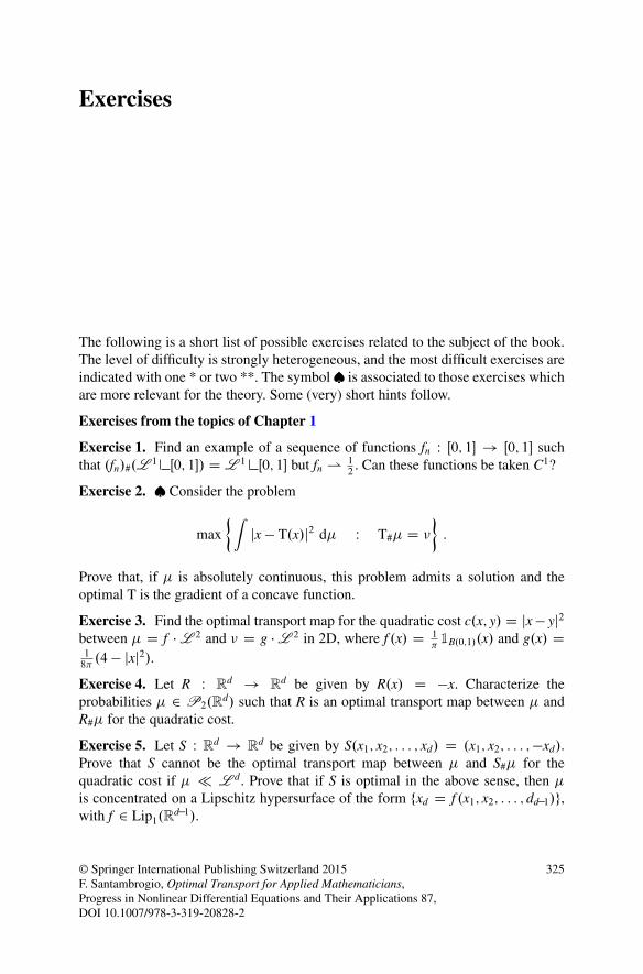
Exercises

The following is a short list of possible exercises related to the subject of the book.The level of difficulty is strongly heterogeneous, and the most difficult exercises areindicated with one * or two **. The symbol is associated to those exercises whichare more relevant for the theory. Some (very) short hints follow.

Exercises from the topics of Chapter 1

Exercise 1. Find an example of a sequence of functions fn W Œ0; 1� ! Œ0; 1� suchthat .fn/#.L 1 Œ0; 1�/ D L 1 Œ0; 1� but fn *

12. Can these functions be taken C1?

Exercise 2. Consider the problem

max

�ˆjx � T.x/j2 d� W T#� D �

�:

Prove that, if � is absolutely continuous, this problem admits a solution and theoptimal T is the gradient of a concave function.

Exercise 3. Find the optimal transport map for the quadratic cost c.x; y/ D jx � yj2between � D f � L 2 and � D g � L 2 in 2D, where f .x/ D 1

�1B.0;1/.x/ and g.x/ D

18�.4 � jxj2/.

Exercise 4. Let R W Rd ! R

d be given by R.x/ D �x. Characterize theprobabilities � 2 P2.R

d/ such that R is an optimal transport map between � andR#� for the quadratic cost.

Exercise 5. Let S W Rd ! R

d be given by S.x1; x2; : : : ; xd/ D .x1; x2; : : : ;�xd/.Prove that S cannot be the optimal transport map between � and S#� for thequadratic cost if � � L d. Prove that if S is optimal in the above sense, then �is concentrated on a Lipschitz hypersurface of the form fxd D f .x1; x2; : : : ; dd�1/g,with f 2 Lip1.R

d�1/.

© Springer International Publishing Switzerland 2015F. Santambrogio, Optimal Transport for Applied Mathematicians,Progress in Nonlinear Differential Equations and Their Applications 87,DOI 10.1007/978-3-319-20828-2

325

326 Exercises

Exercise 6. Consider the multi-marginal problem

min

�ˆc.x1; : : : ; xN/d� W � 2 P..Rd/N/ .�i/#� D �i

�;

where �i 2 P.Rd/ are given compactly supported measures. Suppose that � isconcentrated on a set f.x1; : : : ; xN/ 2 .Rd/N W x1C� � �CxN D constantg. Prove that� is optimal whenever the cost c is given by c.x1; : : : ; xN/ D h.x1 C � � � C xN/ for aconvex function h W Rd ! R and also in the case c.x1; : : : ; xN/ D �Pi¤j jxi � xjj2.Exercises from the topics of Chapter 2

Exercise 7. Consider two probability measures � and � on R that we will supposeatomless and with full support for simplicity. Let F� and F� be their cumulativedistribution functions: F�.x/ D �..�1; x�/ and F�.x/ D �..�1; x�/. Prove thatthe following facts are equivalents:

1. F� � F� ,2. there exists � 2 ˘.�; �/ concentrated on f.x; y/ W y � xg;3. there exists T W R ! R such that T#� D � and T.x/ � x for every x,4. the monotone increasing transport T from � to � satisfies T.x/ � x for every x.

Exercise 8. Prove that an optimal � 2 ˘.�;�/ for the cost c.x; y/ D 1jx�yj exists

and that it is concentrated on at most two increasing graphs, one above and onebelow the diagonal. Prove that these two graphs do not superpose and that the plancomes indeed from a transport map. Is it increasing?

Exercise 9. * In the case � D L 1 Œ0; 1�, find the optimal transport map from �

to � for the cost c.x; y/ D 1jx�yj .

Exercise 10. Prove the optimality of �mon in 1D under the assumption that thecost c W R � R ! R is C2 with @2

@x@y c.x; y/ < 0 for every .x; y/ 2 R � R. Deduce theexistence of an optimal map if � is atomless.

Exercise 11. Let A and B two symmetric positive definite matrices and LA;LB WR

d ! Rd be affine functions defined through LA.x/ D Ax C a, LB.x/ D Bx C b, for

given a; b 2 Rd. Take a reference measure % which is invariant under rotations (i.e.,

R#% D % for every matrix R s.t. R �Rt D I) and define � WD .LA/#% and � WD .LB/#%.Find the optimal transport map from � to � for the quadratic cost.

Exercises from the topics of Chapter 3

Exercise 12. Consider a domain ˝ D Œ0; 3�� Œ0; 2� and two absolutely continuousmeasures on it, �0 and �1, with density %0 and %1, respectively, given by

%0.x; y/ D 2

9if x � 1 or x 2�1; 2Œ and y � 1;

%0.x; y/ D 1

9if x � 2 or x 2�1; 2Œ and y > 1;

Exercises 327

%1.x; y/ D 2

9if x � 2 or x 2�1; 2Œ and y � 1;

%1.x; y/ D 1

9if x � 1 or x 2�1; 2Œ and y � 1:

Represent graphically these two densities and find an optimal transport, as well asa Kantorovich potential, between �0 and �1 for the cost c.x; y/ D jx � yj. Is theoptimal transport unique? And the potential?

Exercise 13. Find the optimal transport map for the cost c.x; y/ D jx � yj between� D f �L 2 and � D g �L 2 in 2D, where f .x/ D 1

�1B.0;1/.x/ and g.x/ D 1

8�.4�jxj2/.

Exercise 14. Consider the cost c.x; y/ D jx � yj˛ for a given exponent 0 < ˛ < 1.Prove that, for every pair �; � 2 P.˝/, we have

Tc.�; �/ D sup

�ˆu d.� � �/ W u 2 C0;˛.˝/; Œu�0;˛ � 1

�;

where Œu�0;˛ is the C0;˛ seminorm of u: Œu�0;˛ WD supx¤yju.x/�u.y/j

jx�yj˛ .

Exercise 15. Consider the cost c.x; y/ D arctan.jx � yj/ and two measures �; � 2P.Rd/ with compact and disjoint supports.

1. What can we say about c-concave functions for this c? Are they (uniformly)continuous, Lipschitz?

2. Do the problems min˚´

c.x; y/ d� W � 2 ˘.�; �/ admit a solution?3. Write the dual problem in terms of functions u having a given modulus of

continuity.4. What is the connection between the support of an optimal � and the optimal u

in the dual problem?5. Supposing that � is absolutely continuous, prove that the optimal � is unique

and derives from a transport. Give its expression in terms of ru.

Exercise 16. Consider h W Rd ! R defined through h.z/ D .jzj � 1/2C. Prove that,for every �; � 2 P.˝/ with � � L d and ˝ compact, there exists an optimaltransport map for the cost c.x; y/ D h.x � y/.

Exercise 17. Consider the cost c.x; y/ D bjx � yjc (the integer part of the distance:bac D maxfn 2 Z W n � ag. Prove that, for every �; � 2 P.˝/ with � � L d

and ˝ compact, there exists an optimal transport plan for such a cost of the form� D PN

iD1 �i where each �i is induced by a transport map and N � diam.˝/C 1.

Exercise 18. For " > 0, consider the cost c".x; y/ D "j jx�yj

"

kand let �" be

an optimal transport plan for such a cost between two measures �; � 2 P.˝/

(consider ˝ compact for simplicity). Prove that, up to subsequences, �" * � ,where � is an optimal transport plan between the same measures for the costc.x; y/ D jx � yj.

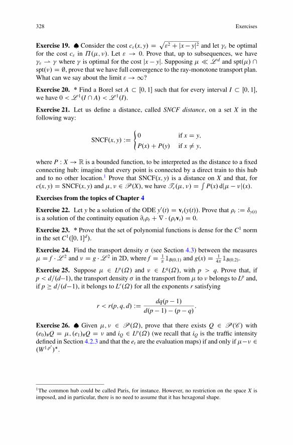
328 Exercises

Exercise 19. Consider the cost c".x; y/ D p"2 C jx � yj2 and let �" be optimal

for the cost c" in ˘.�; �/. Let " ! 0. Prove that, up to subsequences, we have�" * � where � is optimal for the cost jx � yj. Supposing � � L d and spt.�/ \spt.�/ D ;, prove that we have full convergence to the ray-monotone transport plan.What can we say about the limit " ! 1?

Exercise 20. * Find a Borel set A � Œ0; 1� such that for every interval I � Œ0; 1�,we have 0 < L 1.I \ A/ < L 1.I/.

Exercise 21. Let us define a distance, called SNCF distance, on a set X in thefollowing way:

SNCF.x; y/ WD(0 if x D y;

P.x/C P.y/ if x ¤ y;

where P W X ! R is a bounded function, to be interpreted as the distance to a fixedconnecting hub: imagine that every point is connected by a direct train to this huband to no other location.1 Prove that SNCF.x; y/ is a distance on X and that, forc.x; y/ D SNCF.x; y/ and �; � 2 P.X/, we have Tc.�; �/ D ´

P.x/ dj� � �j.x/:Exercises from the topics of Chapter 4

Exercise 22. Let y be a solution of the ODE y0.t/ D vt.y.t//. Prove that t WD ıy.t/

is a solution of the continuity equation @tt C r � .tvt/ D 0.

Exercise 23. * Prove that the set of polynomial functions is dense for the C1 normin the set C1.Œ0; 1�d/.

Exercise 24. Find the transport density � (see Section 4.3) between the measures� D f � L 2 and � D g � L 2 in 2D, where f D 1

�1B.0;1/ and g.x/ D 1

4�1B.0;2/.

Exercise 25. Suppose � 2 Lp.˝/ and � 2 Lq.˝/, with p > q. Prove that, ifp < d=.d�1/, the transport density � in the transport from � to � belongs to Lp and,if p � d=.d�1/, it belongs to Lr.˝/ for all the exponents r satisfying

r < r.p; q; d/ WD dq.p � 1/d.p � 1/ � .p � q/

:

Exercise 26. Given �; � 2 P.˝/, prove that there exists Q 2 P.C / with.e0/#Q D �; .e1/#Q D � and iQ 2 Lp.˝/ (we recall that iQ is the traffic intensitydefined in Section 4.2.3 and that the et are the evaluation maps) if and only if��� 2.W1;p0

/.

1The common hub could be called Paris, for instance. However, no restriction on the space X isimposed, and in particular, there is no need to assume that it has hexagonal shape.

Exercises 329

Exercise 27. Given Q 2 P.C / with .e0/#Q D �; .e1/#Q D �, prove thatthere exists QQ 2 P.C / concentrated on injective curves and such that .e0/# QQ D�; .e1/# QQ D � and i QQ � iQ.

Exercise 28. Consider the simplified network on the right, where the cost for acommuter to move along a segment of length ` with traffic intensity i is given by i`.Do not distinguish between different traffic directions on a samesegment (i.e., i is the sum of the number of commuters going in onedirection plus the number going in the other direction). Consider thecase where a quantity 1 of commuters must go from A to A0 andanother quantity 1 from B to B0. Find the Wardrop equilibrium.

�A

�A0

�B

�B0

Exercise 29. Prove that d˛.L˝; ı0/ D C1 for every compact domain ˝ � Rd

with nonempty interior and j˝j D 1 and every ˛ < 1 � 1=d.

Exercise 30. Consider the branched transport for ˛ D 1=2 between two atomicmeasures � D P

i aiıxi and � D Pj bjıyj . Consider a triple junction at a point z

which is not one of the points xi or yj: among the three branches at z, either two areincoming and one outcoming or two outcoming and one incoming. Prove that thetwo with the same orientation must make an angle of 90ı.

Exercises from the topics of Chapter 5

Exercise 31. Let X be a Polish metric space and �n; � 2 P1.X/ be probabilitymeasures on X such that

´� d�n ! ´

� d� for every � 2 Lip1.X/. Prove´� d�n ! ´

� d� for every � 2 Cb.X/.

Exercise 32. Prove the following equalities, for every compact set ˙ � ˝ andevery density f 2 L1.˝/ with f � 0 and

´˝

f .x/ dx D 1,ˆ

d.x; ˙/f .x/ dx D minfW1.f ; �/ W � 2 P.˙/g

D minfjwj.˝/ W w 2 M ddiv.˝/; spt.r � w � f / � ˙g:

What could we say if we considered, instead,´

d.x; ˙/pf .x/ dx, for p > 1?

Exercise 33. Let � 2 ˘.�; �/ be a transport plan between two probabilities ontwo compact spaces X and Y , respectively. Let �n * � and �n * � be twoweakly converging sequences of probabilities. Prove that there exists a sequence�n 2 ˘.�n; �n/ with �n * � . Deduce that for any sequence of costs cn converginguniformly to c, we have Tcn.�n; �n/ * Tc.�; �/.

Exercise 34. Let ˝ � Rd be smooth and compact, and V be an operator which

associates with every probability % 2 P.˝/ a vector field VŒ%� W ˝ ! Rd with

the following properties: for every %, VŒ%� is Lipschitz continuous and satisfiesLip.VŒ%�/ � C (for a constant C not depending on %) and VŒ%� � n D 0 on @˝; themap % 7! VŒ%� is Lipschitz continuous in the following sense: jjVŒ%�� VŒ��jjL1 �CW2.%; �/ for every %; �. Consider the equation @t%C r � .%VŒ%�/ D 0 with initial

330 Exercises

Cauchy datum %0 � L d. Prove that any solution %t stays absolutely continuous fort > 0 and prove uniqueness of the solution.

Exercise 35. Prove the equality W1.�; �/ D limp!1 Wp.�; �/ for �; �compactly supported. Prove also that for any sequence pn ! 1, the optimal plans�n for the cost jx � yjpn converge, up to subsequences, to an optimal plan for theproblem defining the W1 distance.

Exercise 36. Prove the inequality dH.spt.�/; spt.�// � W1.�; �/, where dH

denotes the Hausdorff distance.

Exercise 37. * Is it true that for 1 � p � q � 1, if the same map T is optimal inthe definition of Wp and Wq, then it is also optimal in the definition of Wr for everyr 2 Œp; q�?Exercise 38. Prove that if f 2 W1;p.˝/, ˝ is a convex set, �; � 2 P.˝/ \ Lr.˝/

and jj�jjLr ; jj�jjLr � C, then, for 1p C 1

q C 1r D 1C 1

qr , one has

ˆ

˝

f d.� � �/ � C1q0 jjrf jjLp.˝/Wq.�; �/:

Exercises from the topics of Chapter 6

Exercise 39. Let ˙ D fx1; : : : xNg � ˝ be a finite subset of a compact convexdomain ˝. For every i, let us set Vi WD fx 2 ˝ W jx � xij � jx � xjj for all jg.Suppose that ˙ solves the problem minf´

˝d.x; ˙/2 dx W #˙ � Ng. Prove that,

for every i, the point xi is the barycenter of Vi.

Exercise 40. For A � Rd we define the extremal points of A as those points x 2 A

such that y; z 2 A; x D yCz2

) y D z. Let K � Mn.R/ be the set of bistochasticmatrices (those matrices M D .mij/ with mij � 0,

Pj mij D P

i mij D 1 for all i; j).Prove that the extremal points of k are the permutation matrices.

Exercise 41. For a 2 .RC/n and b 2 .RC/m consider the set ˘.a; b/ definedthrough ˘ D fM 2 Mn;m.R/ W mij � 0;

Pj mij D ai;

Pi mij D bjg. Prove that

every extremal matrix M in ˘.a; b/ is such that #f.i; j/ W mij > 0g � n C m.

Exercise 42. Let �"ij WD p"i q"j �ij be a solution of the approximated problem in (6.3)(see Section 6.4.1). Suppose that " log.p"i /, " log.q"j /, and �"ij converge as " ! 0.Prove that the limit of " log.p"i / and " log.q"j / are Kantorovich potentials in the limitproblem for " D 0.

Exercise 43. Let u be a smooth function on ˝ and M.x/ WD cof.D2u.x//. Let Mij

be the .i; j/-entry of M and Mijk its derivative w.r.t. xk. Prove that for every index j,

we haveP

i Miji .x/ D 0.

Exercise 44. * Consider a smooth transport map T W ˝ ! Rd of the form

T D ru on a smooth domain ˝. Suppose T#f D �, where f is a smooth positivedensity on ˝. For every vector field v W ˝ ! R

d with r � .f v/ D 0 and v � n D 0

Exercises 331

on @˝, consider the flow of the autonomous vector field v, given by Yt.x/ D yx.t/(where y0

x.t/ D v.yx.t// and yx.0/ D x), and define Tt D T ı Yt. Let M.S/ D´ jS.x/ � xj2f .x/ dx. Prove that the function j.t/ D M.Tt/ satisfies j00.0/ � 0 forevery v if and only if u is convex.

Exercises from the topics of Chapter 7

Exercise 45. * Prove that the entropy functional

F .%/ WD( ´

Rd %.x/ log %.x/ dx if % � L d;

C1 otherwise.

is l.s.c. in W1.Rd/. Also prove that if %n 2 P2.R

d/ and %n * %,´ jxj2d%n.x/ � C,

then F .%/ � lim infn F .%n/.

Exercise 46. Prove that the problem

min

�ˆ 1

0

ˆ

˝

%jvj2dxdt W @t%C r�.%v/D0; %t 2P.˝/; %.0/ D %0; %.1/ D %1

�

is equivalent to the same problem with the additional constraint %t � 1, providedthat we have %0; %1 � 1 and ˝ is convex. Also, imagine a non-convex (butconnected) domain ˝ where this is no more the case.

Exercise 47. Given a compact and convex domain ˝ � Rd and � 2 P.˝/, prove

that the following problem admits a solution:

min

�W1.%; �/C 1

2

ˆ%2.x/ dx W % 2 L2.˝/; % � 0;

ˆ%.x/ dx D 1

�:

Is this solution unique? Write the optimality conditions satisfied by the optimal %,prove that % 2 Lip1, and find explicitly the solution when ˝ D B.0; 5/ and � D ı0.

Exercise 48. ** Given p > 1, consider g 2 P.˝/ an absolutely continuousprobability measure, and look at the problem minfWp.%; g/ W % � f g, wheref 2 L1.˝/ is a given positive function. Prove that a solution exists, that it is unique,and that it has the form % D 1Ag C 1Ac f .

Exercises from the topics of Chapter 8

Exercise 49. Consider the fourth-order PDE

@t%C r � .%r.�%//C r ��r%p

%

�D 0:

This PDE is the gradient flow in W2 of an energy: which one? Also prove thatthe variational problems to be solved at every time step (see Equation (8.3)) in thecorresponding minimizing movement scheme admit a solution.

332 Exercises

Exercise 50. Let V W Rd ! R be C1;1 and let G W P.Rd/ ! R be defined throughG.%/ D #.spt.%// and let %0 2 P.Rd/ be a purely atomic probability measure%0 D PN

iD1 aiıx0iwith finitely many atoms. Prove that for small � (depending on

what?), the solution of the following minimization problem

min

�G .%/C

ˆVd%C W2

2 .%0; %/

�W % 2 P2.R

d/

�

exists, is unique, and has the form %1 D PNiD1 aiıx1i

with G .%1/ D G .%0/. Deducethat the minimizing movement scheme for G CV gives the same limit curve as thatfor V , and find the equation of this curve.

Exercise 51. Let %0 2 P2.Rd/, x0 its barycenter, and % a solution of

@t%t � r � .%tvt/ D 0

where vt.x/ D ´.x � y/d%t.y/. Let E.t/ WD ´ jx � x0j2d%t.x/. Prove E0.t/ � �E.t/.

What can we conclude on the asymptotical behavior of %t as t ! 1?

Exercise 52. Let V W Rd ! R be a continuous function such that jV.x/j � ACBjxj2for suitable constants A;B, and let f W RC ! R a convex function with f 0.0/ > �1.Define

F.%/ Dˆ

f .%.x// dx Cˆ

V.x/%.x/ dx

and consider, for %0 2 P2.Rd/,

min

�F.%/C W2

2 .%; %0/

2�W % 2 P2.R

d/

�:

Prove that, for small � , a solution exists, is unique, and is compactly supported if %0is compactly supported.

Exercise 53. Consider m > 2 and define

F.%/ Dˆ

˝

%m � 1

2

ˆ

˝

jru%j2; where u% 2 H10.˝/ solves ��u% D %:

Prove that

min˚F.%/C W2

2 .%; %0/ W % 2 P2.Rd/

admits a solution.

Exercises 333

Exercise 54. Prove that the optimality conditions of

min

8<ˆ:ˆ T

0

ˆ �t3=2

2%jvj2 C 3t�1=2

4jr'j2

�W

8<ˆ:@t%C r � .%v/ D 0;

�' D % � 1;%0 D 1; %T D given

9>>=>>;

impose, at least formally, the system of Equation (8.27).

Exercise 55. Given ˛ 2�0; 1Œ, prove that a minimizer for

min

�ˆ 1

0

t1C˛jx0.t/j2 C ct�1C˛jx.t/ � x0j2 W x.1/ D x1

�

exists, is unique, and satisfies x.0/ D x0. Prove that a minimizer for the sameproblem adding the condition x.0/ D Qx0, with Qx0 ¤ x0, does not exist.

Exercise 56. Consider a triplet .%t; vt; 't/ on the torus Td (to avoid boundary

issues) satisfying

ˆ 1

0

ˆ �t3=2

2%jvj2 C 3t�3=2

2jr'j2

�< C1 with

(@t%t C r � .%tvt/ D 0;

�'t D %t � 1

with jj%tjjL1 � C and t 7! %t continuous for W2 on �0; 1�. Prove that we necessarilyhave W2.%t; 1/ ! 0 as t ! 0.

Miscellaneous

Exercise 57. Find the optimal transport map for the costs of the form jx�yjp, p > 0,between the two measures sketched below:

�

��

��

�

��

� D 14.ı.2;3/ C ı.3;2/ C ı.3;0/ C ı.0;�1//

� D 14.ı.0;0/ C ı.0;2/ C ı.2;1/ C ı.4;2//

Exercise 58. Find an example of a pair of compactly supported absolutely continu-ous probability measures �; � on R

d and a continuous cost c W Rd �Rd ! RC such

that no optimal transport map exists in the corresponding Monge problem.

Exercise 59. Find the optimal transport plan for the cost c.x; y/ D .x2�y2/2 in 1D,when � D L 1 Œ0; 1� and � D 1

2L 1 Œ�1; 1�.

Exercise 60. Find an example of bounded l.s.c. (but not continuous) costc W Rd ! R, together with two atomless compactly supported measures �; � 2P.Rd/ such that inf(MP)> min(KP).

334 Exercises

Exercise 61. * Prove that there exists a continuous map T W Œ0; 1� ! Œ0; 1�2 suchthat T#.L 1 Œ0; 1�/ D L 2 Œ0; 1�2.

Exercise 62. Consider a translation S W Rd ! Rd given by S.x/ D x C a.

1. Prove that S is the optimal transport for the cost c.x; y/ D jx � yj2 between anymeasure � and S#�.

2. Prove the same result for c.x; y/ D jx � yj.3. If T is the optimal transport between � and �, can we say that SıT is the optimal

transport between � and S#�? Answer this question both for c.x; y/ D jx � yj2and c.x; y/ D jx � yj.

4. More generally, is it true that the composition of two optimal transports is stilloptimal?

Exercise 63. Prove that, if J � R is a (possibly unbounded) given interval, thenWp.J/ is isometric to a closed convex subset of Lp.Œ0; 1�/.

Exercise 64. Given g 2 L1.Œ0; 1�/\ P.Œ0; 1�/, prove W2.1; g/ D jj1� gjj PH�1.Œ0;1�/:

Exercise 65. Consider �; � 2 P1.Rd/ with

´x d�.x/ D ´

y d�.y/ D 0. Let � bean optimal transport plan for the cost c.x; y/ D �x � y between these two measuresand Tc.�; �/ the optimal value of this transport cost. Prove Tc.�; �/ � 0 andspt.�/ � f.x; y/ W x � y � Tc.�; �/g. Deduce that if �n * � and

´x d�n.x/ D´

y d�.y/ D 0, then Tc.�; �/ � lim supn Tc.�n; �/:

Exercise 66. Let f ; g be two smooth probability densities on a convex domain˝ and '; the Kantorovich potentials for the transport from f to g for the costc.x; y/ D 1

2jx � yj2 . Prove

´ rf � r' C rg � r � 0. Conclude that the same istrue for f ; g 2 H1.˝/.

Exercise 67. Prove the W2 distance between two (smooth) solutions to the heatequation @t% D �% decreases in time:

1. in a bounded domain ˝ with homogeneous Neumann boundary conditions,2. in R

d, with initial data in P2.Rd/.

Exercise 68. Let v W Œ0;T� �˝ ! Rd be Lipschitz continuous in space, uniformly

in time. Prove the uniqueness of the solution to the Fokker-Planck equation @t% ��% C r � .%v/ D 0 (with no-flux boundary conditions) in the class of solutionswhich are H1.˝/\P.˝/ for every t, by differentiating W2

2 between two solutions.Why is H1 a reasonable assumption for the regularity of the solution?

Exercise 69. Let f W Rd ! R be a C2 strictly convex function with D2f � ˛I

(for ˛ > 0) on a smooth bounded domain ˝. Prove that %1 D ce�f (for c D.´

e�f /�1) is a solution of �%C r � .%rf / D 0. Consider now any smooth solutionof @t%��%� r � .%rf / D 0 with Neumann boundary conditions on ˝, and proveW2.%t; %1/ ! 0 exponentially as t ! 1.

Exercises 335

Hints

Hint to Ex. 1. Use piecewise affine oscillating functions. With C1 it is impossible,because C1 functions f with image measure with bounded density should satisfyf 0 ¤ 0 and be diffeomorphisms. Yet, only f .x/ D x and f .x/ D 1 � x preserve themeasure among diffeomorphisms.

Hint to Ex. 2. Write the Kantorovich problem and use a change of variable y 7! �yin the arrival measure.

Hint to Ex. 3. Find a monotone radial transport. The answer is

T.x/ D 4

q1 �

p1 � jxj2 x

jxj :

Hint to Ex. 4. Use c-cyclical monotonicity on two points (i.e., monotonicity).

Hint to Ex. 5. For the first question, use the characterization in terms of gradientsof convex functions. For the second, use again c-cyclical monotonicity.

Hint to Ex. 6. For the first cost, use Jensen inequality. For the second, express it as.x1 C : : : xN/

2C functions of the xi separately.

Hint to Ex. 7. You can (partially) use the transport problem with cost h.y � x/ withh.z/ D C1 for z < 0 and h.z/ D 0 for z � 0.

Hint to Ex. 8. Decompose � above and below the diagonal and use results onconvex costs in 1D. Then prove that the superposition is not optimal.

Hint to Ex. 9. Check that T defined as T.x/ D xC 12

for x < 12

and T.x/ D x� 12

forx � 1

2is optimal by using the functions �.x/ D 2�4jx� 1

2j and .y/ D 2�4jy� 1

2j

as a guess for the Kantorovich potentials.

Hint to Ex. 10. If two pairs .x0; y0/; .x1; y1/ 2 spt � exist with x0 < x1 and y0 > y1exist, integrate @2c

@x@y on Œx0; x1� � Œy1; y0� and find a contradiction.

Hint to Ex. 11. Write A�1B as the product of a symmetric positive definite matrixand a rotation.

Hint to Ex. 12. u.x/ D �x is a potential.

Hint to Ex. 13. Same idea as in Ex(3). Use the potential u.x/ D �jxj to prove thatyou have found an optimal map.

Hint to Ex. 14. The cost c.x; y/ D jx � yj˛ is a distance.

Hint to Ex. 15. Use the same analysis as in Section 3.3.2.

Hint to Ex. 16. Decomposition strategy of Section 3.3.1.

Hint to Ex. 17. Use the results about L1 optimal transport.

Hint to Ex. 18. The cost c" uniformly converges to the linear cost.

336 Exercises

Hint to Ex. 19. Consider the Taylor expansion of the cost in " to guess the lower-order term.

Hint to Ex. 20. Start from classical examples of fattened rationals.

Hint to Ex. 21. Prove that all functions u W X ! R with ju.x/j � P.x/ belong toLip1 for the distance SNCF, and apply the duality formula to have a lower boundon Tc. For the opposite bound, just leave the common mass at rest.

Hint to Ex. 22. Just test against a C1c function .x/.

Hint to Ex. 23. Two methods: induction on the dimension and use a polynomialconvolution (with something like xn.1 � x/n).

Hint to Ex. 24. By uniqueness, � is radial. The Kantorovich potential is u.x/ D�jxj. Use the Monge-Kantorovich equation.

Hint to Ex. 25. Use the same strategy as in Theorem 4.24. See also [273].

Hint to Ex. 26. It is equivalent to the existence of w 2 Lp with r � w D � � �.

Hint to Ex. 27. Solve the minimization problem

minni QQ.˝/ W .e0/# QQ D �; .e1/# QQ D �; i QQ � iQ

o:

Hint to Ex. 28. Make the ansatz that the mass from A to A0 will be split into threeparts, ˛ passing through B, ˛ through B0, and ˇ directly to A0, and the same for Bto B0. Write a 2 � 2 system for the equilibrium condition.

Hint to Ex. 29. Take a regular grid on a cube contained in˝. Count how much doesit cost to move the mass of the central half of each cube out of the cube, and sum up.

Hint to Ex. 30. Use the angle law (4.31).

Hint to Ex. 31. Suppose � � 0, and use the k-Lipschitz functions �k defined in thememo 1.5 on l.s.c. functions.

Hint to Ex. 32. Prove that the optimal � is the image of f through the projectiononto ˙ . Use Beckmann’s formulation.

Hint to Ex. 33. Use Lemma 5.5 to modify the marginals of � .

Hint to Ex. 34. Differentiate W22 .

Hint to Ex. 35. Prove � -convergence.

Hint to Ex. 36. Take a point x0 2 spt.�/ realizing max d.x; spt.�//: it must betransported somewhere.

Hint to Ex. 37. Build a counterexample with a map T which is a gradient but suchthat rh.T.x/ � x/ is not a gradient for h.z/ D jzj4.Hint to Ex. 38. Adapt the proof of Lemma 5.33.

Exercises 337

Hint to Ex. 39. Write optimality conditions when we move one point.

Hint to Ex. 40. Consider the entries of an extremal matrix which are in �0; 1Œ. Provethat if there is one such an entry, then there is a “cycle” and find a contradiction.

Hint to Ex. 41. Same strategy as above.

Hint to Ex. 42. From log �"ij D log p"i C log q"j C log �ij deduce " log p"i C " log q"j �cij, with equality if at the limit �ij > 0.

Hint to Ex. 43. Write cof.D2u/D2u D det.D2u/I and differentiate.

Hint to Ex. 44. Compute the second derivative and integrate by parts to get´uijv

ivjf .

Hint to Ex. 45. First part: add and subtract suitable functionals, continuous for W1,to make the integrand positive, and restrict it to bounded domains. Second part:prove that a bound on the second moment implies W1 convergence.

Hint to Ex. 46. Use the fact that the L1 norm is bounded by 1 on a geodesicwhenever this is the case on the starting and arrival measures.

Hint to Ex. 47. Use the direct method for existence, strict convexity for uniqueness,and let the potential appear in optimality conditions.

Hint to Ex. 48. Difficult: prove a sort of interior ball condition, i.e., if %.x0/ >g.x0/, then % D f on B.T.x0/; jx0 � T.x0/j/, and use Lebesgue points. See [151].

Hint to Ex. 49. Use´12jr%j2 C 4

p%.

Hint to Ex. 50. Consider the optimal � between %0 and %: if % has more than Natoms, then replacing each �

�fxig � Rd

with its barycenter gives a better result.

Hint to Ex. 51. Prove that the barycenter is preserved and use the equation tocompute E0.

Hint to Ex. 52. Write the optimality conditions in terms of the potential (directmethod for existence, strict convexity for uniqueness).

Hint to Ex. 53. Estimate the ru% part in terms of jj%jj2Lm , and use m > 2 to see thatthese norms must be bounded on a minimizing sequence.

Hint to Ex. 54. Write the problem as a min-max, introducing Lagrange multiplierfor the constraints, and deduce the conditions to have a saddle point.

Hint to Ex. 55. Write and solve the Euler-Lagrange equation.

Hint to Ex. 56. Prove that t 7! jj%t � 1jj2H�1 is BV, by using Young inequality and

Lemma 5.33.

Hint to Ex. 57. Check that moving every atom of � on the (a) closest atom of � ispossible.

Hint to Ex. 58. Use concave costs and measures with a common mass.

338 Exercises

Hint to Ex. 59. Try to realize the cost 0.

Hint to Ex. 60. Use � and � as in the counterexample of Section 1.4, and choosec.x; y/ as a discontinuous function of jx � yj.Hint to Ex. 61. Adapt the Peano construction for a surjective map onto the square,defining a map as a fixed point of a contracting operator.

Hint to Ex. 62. Use the characterization of optimal maps as gradients of convexfunctions (quadratic). Find a nonoptimal transport between two measures withcompact support on R and translate them far away (linear cost). Find a compositionof two gradients which is not a gradient.

Hint to Ex. 63. Use the properties of FŒ�1�� .

Hint to Ex. 64. Write the optimal transport as x � '0.x/, check jj1 � gjj PH�1 Djj'0jjL2 , and integrate by parts.

Hint to Ex. 65. For Tc � 0, use the plan � D � ˝ � to have a bound. For thesupport of � , take .x; y/ and .x0; y0/ in spt.�/, write c-cyclical monotonicity, andintegrate w.r.t. .x0; y0/. This gives an upper bound that allows to prove upper semi-continuity.

Hint to Ex. 66. Use displacement convexity of the entropy, compare the derivativeof the entropy at t D 0 and t D 1 on a geodesic.

Hint to Ex. 67. For the first question, differentiate W22 and use the Ex(66). For the

second, use the inequality in Lemma 5.2 and the semigroup properties of the heatequation.

Hint to Ex. 68. After differentiating W22 , use Gronwall. H1 is reasonable because

the H1 norm is controlled in time.

Hint to Ex. 69. Differentiate W22 between the solution of the evolution equation and

the static solution.

References

1. M. Agueh, G. Carlier, Barycenters in the Wasserstein space. SIAM J. Math. Ann. 43(2),904–924 (2011)

2. R.K. Ahuja, T. Magnanti, J. Orlin, Network Flows: Theory, Algorithms, and Applications(Prentice Hall, Upper Saddle River, 1993)

3. G. Alberti, On the structure of singular sets of convex functions. Calc.Var. Part. Differ. Equat.2, 17–27 (1994)

4. G. Alberti, L. Ambrosio, A geometrical approach to monotone functions in Rd . Math. Z. 230,

259–316 (1999)5. G. Alberti, L. Ambrosio, P. Cannarsa, On the singularities of convex functions. Manuscripta

Math. 76, 421–435 (1992)6. A.D. Aleksandrov, Almost everywhere existence of the second differential of a convex

functions and related properties of convex surfaces. Uchenye Zapisky Leningrad. Gos. Univ.Math. Ser. 37, 3–35 (1939) (in Russian)

7. L. Ambrosio, Movimenti minimizzanti. Rend. Accad. Naz. Sci. XL Mem. Mat. Sci. Fis. Natur.113, 191–246 (1995)

8. L. Ambrosio, Lecture notes on optimal transport problems, in Mathematical Aspects ofEvolving Interfaces. Lecture Notes in Mathematics (1812) (Springer, New York, 2003), pp.1–52

9. L. Ambrosio, N. Gigli, A user’s guide to optimal transport, in Modelling and Optimisation ofFlows on Networks. Lecture Notes in Mathematics (2013), Springer Berlin Heidelberg, pp.1–155

10. L. Ambrosio, A. Pratelli, Existence and stability results in the L1 theory of optimaltransportation, in Optimal Transportation and Applications, ed. by L.A. Caffarelli, S. Salsa.Lecture Notes in Mathematics (CIME Series, Martina Franca, 2001) 1813 (2003), SpringerBerlin Heidelberg, pp. 123–160

11. L. Ambrosio, G. Savaré, Gradient flows of probability measures, Handbook of DifferentialEquations, Evolutionary Equations, ed. by C.M. Dafermos, E. Feireisl, vol. 3 (Elsevier,Amsterdam, 2007)

12. L. Ambrosio, P. Tilli, Topics on Analysis in Metric Spaces. Oxford Lecture Series inMathematics and its Applications, vol. 25 (Oxford University Press, Oxford, 2004)

13. L. Ambrosio, N. Fusco, D. Pallara, Functions of Bounded Variation and Free DiscontinuityProblems (Oxford University Press, Oxford, 2000)

© Springer International Publishing Switzerland 2015F. Santambrogio, Optimal Transport for Applied Mathematicians,Progress in Nonlinear Differential Equations and Their Applications 87,DOI 10.1007/978-3-319-20828-2

339

340 References

14. L. Ambrosio, B. Kirchheim, A. Pratelli, Existence of optimal transport maps for crystallinenorms, Duke Math. J. 125, 207–241 (2004)

15. L. Ambrosio, N. Gigli, G. Savaré, Gradient Flows in Metric Spaces and in the Spaces ofProbability Measures. Lectures in Mathematics, ETH Zurich (Birkhäuser, Basel, 2005)

16. L. Ambrosio, M. Colombo, G. De Philippis, A. Figalli, Existence of Eulerian solutions to thesemigeostrophic equations in physical space: the 2-dimensional periodic case Commun. Part.Differ. Equat. 37(12), 2209–2227 (2012)

17. L. Ambrosio, M. Colombo, G. De Philippis, A. Figalli, A global existence result for thesemigeostrophic equations in three dimensional convex domains. Discr. Contin. Dyn. Syst.34(4), 1251–1268 (2013)

18. L. Ambrosio, N. Gigli, G. Savaré, Calculus and heat flow in metric measure spaces andapplications to spaces with Ricci bounds from below Inv. Math. 195(2), 289–391 (2014)

19. S. Angenent, S. Haker, A. Tannenbaum, Minimizing flows for the Monge–Kantorovichproblem. SIAM J. Math. Ann. 35(1), 61–97 (2003)

20. S. Angenent, S. Haker, A. Tannenbaum, L. Zhu, Optimal transport for registration andwarping. Int. J. Comput. Vis. 60(3), 225–240 (2004)

21. P. Appell, Mémoire sur les déblais et les remblais de systèmes continus ou discontinus,Mémoires présentés par divers savants à l’Académie royale des sciences de l’Institut deFrance. Sciences mathématiques et physiques. 1827–1914 (2e s. I-XXXV) (1887)

22. V. Arnold, Sur la géométrie différentielle des groupes de Lie de dimension infinie et sesapplications à l’hydrodynamique des fluides parfaits. (French) Ann. Inst. Fourier (Grenoble)16(1), 319–361 (1996)

23. H. Attouch, G. Buttazzo, G. Michaille, Variational Analysis in Sobolev and BV Spaces:Applications to PDEs and Optimization (SIAM, Philadelphia, 2006)

24. F. Aurenhammer, F. Hoffmann, B. Aronov, Minkowski-type theorems and least-squaresclustering. Algorithmica 20, 61–76 (1998)

25. R. Balka, Y. Peres, Restrictions of Brownian motion, preprint. C. R. Math. Acad. Sci. Paris352(12), 1057–1061 (2014)

26. M. Bardelloni, S. Bianchini, The decomposition of optimal transportation problems withconvex cost. (2014) http://arxiv.org/pdf/1409.0515

27. M. Beckmann, A continuous model of transportation. Econometrica 20, 643–660 (1952)28. M. Beckmann, T. Puu, Spatial Economics: Density, Potential and Flow (North-Holland,

Amsterdam, 1985)29. M. Beckmann, C. McGuire, C. Winsten, Studies in Economics of Transportation (Yale

University Press, New Haven, 1956)30. M. Beiglböck, Cyclical monotonicity and the ergodic theorem. Ergodic Theory Dyn. Syst.

35(3), 710–713 (2015)31. M. Beiglböck, N. Juillet, On a problem of optimal transport under marginal martingale

constraints. Ann. Probab. (2012) http://arxiv.org/abs/1208.150932. M. Beiglböck, P. Henry-Labordère, F. Penkner, Model-independent bounds for option

prices—a mass transport approach. Fin. Stoch. 17(3), 477–501 (2013)33. J.-D. Benamou, Y. Brenier, Weak existence for the semigeostrophic equations formulated as

a coupled Monge-Ampère/transport problem. SIAM J. Appl. Math. 58, 1450–1461 (1998)34. J.-D. Benamou, Y. Brenier, A computational fluid mechanics solution to the Monge-

Kantorovich mass transfer problem. Numer. Math. 84, 375–393 (2000)35. J.-D. Benamou, G. Carlier, Augmented Lagrangian methods for transport optimization, mean-

field games and degenerate PDEs. (2014) https://hal.inria.fr/hal-0107314336. J.-D. Benamou, Y. Brenier, K. Guittet, The Monge-Kantorovich mass transfer and its

computational fluid mechanics formulation. Int. J. Numer. Methods Fluids 40(1–2), 21–30(2002)

37. J.-D. Benamou, Y. Brenier, K. Guittet, Numerical analysis of a multi-phasic mass transportproblem. Contemp. Math. 353, 1–18 (2004)

References 341

38. J.-D. Benamou, G. Carlier, M. Cuturi, L. Nenna, G. Peyré, Iterative Bregman projections forregularized transportation problems. SIAM J. Sci. Comput. 37(2), A1111–A1138 (2015).

39. J.-D. Benamou, B. Froese, A. Oberman, Two numerical methods for the elliptic Monge-Ampere equation. ESAIM: Math. Model. Numer. Ann. 44(4), 737–758 (2010)

40. J.-D. Benamou, G. Carlier, Q. Mérigot, É. Oudet, Discretization of functionals involving theMonge-Ampère operator. (2014) http://arxiv.org/abs/1408.4536

41. J.-D. Benamou, B. Froese, A. Oberman, Numerical solution of the Optimal Transportationproblem using the Monge–Ampère equation. J. Comput. Phys. 260, 107–126 (2014)

42. F. Benmansour, G. Carlier, G. Peyré, F. Santambrogio, Numerical approximation of continu-ous traffic congestion equilibria. Net. Het. Media 4(3), 605–623 (2009)

43. F. Benmansour, G. Carlier, G. Peyré, F. Santambrogio, Fast marching derivatives with respectto metrics and applications. Numer. Math. 116(3), 357–381 (2010)

44. P. Bernard, B. Buffoni, The Monge problem for supercritical Mané potentials on compactmanifolds. Adv. Math. 207(2), 691–706 (2006)

45. F. Bernardeau, S. Colombi, E. Gaztanaga, R. Scoccimarro, Large-Scale Structure of theUniverse and Cosmological Perturbation Theory. Phys. Rep. 367, 1–248 (2002)

46. M. Bernot, Optimal transport and irrigation. Ph.D. Thesis, ENS Cachan (2005) http://perso.crans.org/bernot

47. M. Bernot, A. Figalli, Synchronized traffic plans and stability of optima. ESAIM ControlOptim. Calc. Var. 14, 864–878 (2008)

48. M. Bernot, V. Caselles, J.-M. Morel, Traffic plans. Publ. Math. 49(2), 417–451 (2005)49. M. Bernot, V. Caselles, J.-M. Morel, The structure of branched transportation networks. Calc.

Var. Part. Differ. Equat. 32(3), 279–317 (2008)50. M. Bernot, V. Caselles, J.-M. Morel, Optimal Transportation Networks, Models and Theory.

Lecture Notes in Mathematics, vol. 1955 (Springer, New York, 2008)51. M. Bernot, A. Figalli, F. Santambrogio, Generalized solutions for the Euler equations in one

and two dimensions. J. Math. Pures et Appl. 91(2), 137–155 (2009)52. J. Bertrand, M. Puel, The optimal mass transport problem for relativistic costs. Calc. Var. PDE

46(1–2), 353–374 (2013)53. D.P. Bertsekas, A distributed algorithm for the assignment problem, in Lab. for Information

and Decision Systems Working Paper (MIT, Cambridge, 1979)54. D.P. Bertsekas, Auction Algorithms, Encyclopedia of Optimization, Kluwer, (2001)55. D.P. Bertsekas, J. Eckstein, Dual coordinate step methods for linear network flow problems.

Math. Program. 42(1–3), 203–243 (1988)56. A. Blanchet, G. Carlier, Optimal transport and Cournot-Nash equilibria. Math. Oper. Res.

(to appear) https://www.ceremade.dauphine.fr/~carlier/publis.html57. A. Blanchet, V. Calvez, J.A. Carrillo, Convergence of the mass-transport steepest descent

scheme for the subcritical Patlak-Keller-Segel model. SIAM J. Numer. Anal. 46(2), 691–721(2008)

58. A. Blanchet, J.-A. Carrillo, D. Kinderlehrer, M. Kowalczyk, P. Laurençot, S. Lisini, A hybridvariational principle for the Keller-Segel system in R

2. ESAIM M2AN (2015). http://www.math.cmu.edu/math/faculty/kinderlehrer.php

59. A. Blanchet, P. Mossay, F. Santambrogio, Existence and uniqueness of equilibrium for aspatial model of social interactions. Int. Econ. Rev. (2014). http://cvgmt.sns.it/paper/1998/

60. S. Bianchini, L. Caravenna, On optimality of c-cyclically monotone transference plans. C. R.Math. Acad. Sci. Paris 348(11–12), 613–618 (2010)

61. S. Bianchini, M. Gloyer, On the Euler-Lagrange equation for a variational problem: thegeneral case II. Math. Zeit. 265(4), 889–923 (2009)

62. G. Blower, Displacement convexity for the generalized orthogonal ensemble. J. Statist. Phys.116(5-6), 1359–1387 (2004)

63. V.I. Bogachev, A.V. Kolesnikov, The Monge–Kantorovich problem: achievements, connec-tions, and perspectives. Russ. Math. Surv. 67(5), 785–890 (2012)

342 References

64. J.F. Bonnans, J.-C. Gilbert, C. Lemarechal, C. Sagastizábal, Numerical Optimization: Theo-retical and Practical Aspects, 2nd edn. (Springer, New York, 2006)

65. N. Bonnotte, Unidimensional and evolution methods for optimal transportation. Ph.D. Thesis,Université Paris-Sud, 2013

66. N. Bonnotte, From Knothe’s rearrangement to Brenier’s optimal transport map. SIAMJ. Math. Anal. 45(1), 64–87 (2013)

67. G. Bouchitté, G. Buttazzo, New lower semi-continuity results for nonconvex functionalsdefined on measures. Nonlinear Anal. 15, 679–692 (1990)

68. G. Bouchitté, G. Buttazzo, Integral representation of nonconvex functionals defined onmeasures. Ann. Inst. H. Poincaré Anal. Non Linéaire 9(1), 101–117 (1992)

69. G. Bouchitté, G. Buttazzo, Relaxation for a class of nonconvex functionals defined onmeasures. Ann. Inst. H. Poincaré Anal. Non Linéaire 10(3), 345–361 (1993)

70. G. Bouchitté, G. Buttazzo, Characterization of optimal shapes and masses through Monge-Kantorovich equation. J. Eur. Math. Soc. 3(2), 139–168 (2001)

71. G. Bouchitté, G. Buttazzo, P. Seppecher, Shape optimization solutions via Monge-Kantorovich equation. C. R. Acad. Sci. Paris Sér. I Math. 324(10), 1185–1191 (1997)

72. G. Bouchitté, C. Jimenez, M. Rajesh, Asymptotique d’un problème de positionnementoptimal. C. R. Acad. Sci. Paris Ser. I 335, 1–6 (2002)

73. G. Bouchitté, T. Champion, C. Jimenez, Completion of the space of measures in theKantorovich norm, proc. of “Trends in the Calculus of Variations”, Parma, 2004, E.D. Acerbiand G.R. Mingione Editors. Rivi. Mat. Univ. Parma Ser. 7(4), 127–139 (2005)

74. G. Bouchitté, C. Jimenez, M. Rajesh, A new L1 estimate in optimal mass transport. Proc.Am. Math. Soc. 135, 3525–3535 (2007)

75. G. Bouchitté, C. Jimenez, M. Rajesh, Asymptotic analysis of a class of optimal locationproblems. J. Math. Pures Appl. 95(4), 382–419 (2011)

76. D. Braess, Über ein Paradoxon aus der Verkehrsplanung. Unternehmensforschung 12,258–268 (1969)

77. A. Braides, � -Convergence for Beginners (Oxford University Press, Oxford, 2002)78. A. Brancolini, S. Solimini, On the holder regularity of the landscape function. Interfaces Free

Boundaries 13(2), 191–222 (2011)79. L. Brasco, F. Santambrogio, An equivalent path functional formulation of branched trans-

portation problems. Discr. Contin. Dyn. Syst. A 29(3), 845–871 (2011)80. L. Brasco, G. Carlier, F. Santambrogio, Congested traffic dynamics, weak flows and very

degenerate elliptic equations. J. Math. Pures et Appl. 93(6), 652–671 (2010)81. L. Brasco, G. Buttazzo, F. Santambrogio, A Benamou-Brenier approach to branched trans-

portation. SIAM J. Math. Ann. 43(2), 1023–1040 (2011)82. Y. Brenier, Décomposition polaire et réarrangement monotone des champs de vecteurs.

(French) C. R. Acad. Sci. Paris Sér. I Math. 305(19), 805–808 (1987)83. Y. Brenier, The least action principle and the related concept of generalized flows for

incompressible perfect fluids. J. Am. Mat. Soc. 2, 225–255 (1989)84. Y. Brenier, Polar factorization and monotone rearrangement of vector-valued functions.

Commun. Pure Appl. Math. 44, 375–417 (1991)85. Y. Brenier, Minimal geodesics on groups of volume-preserving maps and generalized

solutions of the Euler equations. Commun. Pure Appl. Math. 52, 411–452 (1999)86. Y. Brenier, Optimal transport, convection, magnetic relaxation and generalized Boussinesq

equations. J. Nonlinear Sci. 19(5), 547–570 (2009)87. Y. Brenier, A modified least action principle allowing mass concentrations for the early

universe reconstruction problem. Confluentes Mathematici 3(3), 361–385 (2011)88. Y. Brenier, Rearrangement, convection, convexity and entropy. Philos. Trans. R. Soc. A 371,

20120343 (2013)89. Y. Brenier, U. Frisch, M. Hénon, G. Loeper, S. Matarrese, R. Mohayaee, A. Sobolevskii,

Reconstruction of the early Universe as a convex optimization problem. Mon. Not. R. Astron.Soc. 346, 501–524 (2003)

90. H. Brezis, Analyse fonctionnelle, Théorie et applications (Masson, Paris, 1983)

References 343

91. H. Brezis, Liquid crystals and energy estimates for S2-valued maps, in Theory and Appli-

cations of Liquid Crystals. The IMA Volumes in Mathematics and its Applications, vol. 5(Springer, New York, 1987), pp. 31–52

92. M. Burger, M. Franek, C.-B. Schönlieb, Regularized regression and density estimation basedon optimal transport. Appl. Math. Res. Express 2012(2), 209–253 (2012)

93. G. Buttazzo, F. Santambrogio, A model for the optimal planning of an urban area. SIAMJ. Math. Anal. 37(2), 514–530 (2005)

94. G. Buttazzo, F. Santambrogio, A mass transportation model for the optimal planning of anUrban region. SIAM Rev. 51(3), 593–610 (2009)

95. G. Buttazzo, É. Oudet, E. Stepanov, Optimal transportation problems with free Dirichletregions, in Variational Methods for Discontinuous Structures. PNLDE, vol. 51 (Birkhäuser,Basel, 2002), pp. 41–65

96. G. Buttazzo, C. Jimenez, É. Oudet, An optimization problem for mass transportation withcongested dynamics. SIAM J. Control Optim. 48, 1961–1976 (2010)

97. G. Buttazzo, L. De Pascale, P. Gori-Giorgi, Optimal transport meets electronic densityfunctional theory. Phys. Rev. A 85(6), 062502 (2012)

98. L. Caffarelli, A localization property of viscosity solutions to the Monge-Ampère equationand their strict convexity. Ann. Math. 131(1), 129–134 (1990)

99. L. Caffarelli, Interior W2;p estimates for solutions of the Monge-Ampère equation. Ann. Math.131(1), 135–150 (1990)

100. L. Caffarelli, Some regularity properties of solutions of Monge Ampère equation. Commun.Pure Appl. Math. 44(8–9), 965–969 (1991)

101. L. Caffarelli, M. Feldman, R. McCann, Constructing optimal maps for Monge’s transportproblem as a limit of strictly convex costs. J. Am. Math. Soc. 15, 1–26 (2002)

102. P. Cannarsa, C. Sinestrari, Semiconcave Functions, Hamilton-Jacobi Equations, and OptimalControl (Birkhäuser, Basel, 2004)

103. L. Caravenna, A proof of Sudakov theorem with strictly convex norms. Math. Z. 268,371–407 (2011)

104. L. Caravenna, S. Daneri, The disintegration of the Lebesgue measure on the faces of a convexfunction. J. Funct. Anal. 258(11), 3604–3661 (2010)

105. P. Cardaliaguet, Notes on mean field games (from P.-L. Lions’ lectures at Collège de France).(2013) https://www.ceremade.dauphine.fr/~cardalia/

106. G. Carlier, I. Ekeland, The structure of cities. J. Global Optim. 29, 371–376 (2004)107. G. Carlier, I. Ekeland, Equilibrium structure of a bidimensional asymmetric city. Nonlinear

Anal. Real World Appl. 8(3), 725–748 (2007)108. G. Carlier, I. Ekeland, Matching for teams. Econ. Theory 42(2), 397–418 (2010)109. G. Carlier, B. Nazaret, Optimal transportation for the determinant. ESAIM Control Optim.

Calc. Var. 14(4), 678–698 (2008)110. G. Carlier, F. Santambrogio, A variational model for urban planning with traffic congestion.

ESAIM Control Optim. Calc. Var. 11(4), 595–613 (2005)111. G. Carlier, F. Santambrogio, A continuous theory of traffic congestion and Wardrop equilibria,

proceedings of the conference, proceedings of optimization and stochastic methods forspatially distributed information, St Petersburg, 2010, published (English version). J. Math.Sci. 181(6), 792–804 (2012)

112. G. Carlier, C. Jimenez, F. Santambrogio, Optimal transportation with traffic congestion andWardrop equilibria. SIAM J. Control Optim. 47, 1330–1350 (2008)

113. G. Carlier, L. De Pascale, F. Santambrogio, A strategy for non-strictly convex transport costsand the example of jjx � yjjp in R

2. Commun. Math. Sci. 8(4), 931–941 (2010)114. G. Carlier, A. Galichon, F. Santambrogio, From Knothe’s transport to Brenier’s map and a

continuation method for optimal transport. SIAM J. Math. Ann. 41(6), 2554–2576 (2010)115. J.-A. Carrillo, D. Slepcev, Example of a displacement convex functional of first order Calc.

Var. Part. Differ. Equat. 36(4), 547–564 (2009)

344 References

116. J.-A. Carrillo, R.J. McCann, C. Villani, Kinetic equilibration rates for granular media andrelated equations: entropy dissipation and mass transportation estimates. Rev. Math. Iberoam.19, 1–48 (2003)

117. J.-A. Carrillo, R.J. McCann, C. Villani, Contractions in the 2-Wasserstein length space andthermalization of granular media. Arch. Ration. Mech. Ann. 179, 217–263 (2006)

118. J.-A. Carrillo, M. Di Francesco, A. Figalli, T. Laurent, D. Slepcev, Global-in-time weakmeasure solutions and finite-time aggregation for nonlocal interaction equations. Duke Math.J. 156(2), 229–271 (2011)

119. T. Champion, L. De Pascale, The Monge problem for strictly convex norms in Rd . J. Eur.

Math. Soc. 12(6), 1355–1369 (2010)120. T. Champion, L. De Pascale, The Monge problem in R

d . Duke Math. J. 157(3), 551–572(2011)

121. T. Champion, L. De Pascale, On the twist condition and c-monotone transport plans. Discr.Contin. Dyn. Syst. 34(4), 1339–1353 (2014)

122. T. Champion, L. De Pascale, P. Juutinen, The 1-Wasserstein distance: local solutions andexistence of optimal transport maps. SIAM J. Math. Ann. 40(1), 1–20 (2008)

123. P. Chen, F. Jiang, X.-P. Yang, Two dimensional optimal transportation for a distance cost witha convex constraint. ESAIM: COCV 19(4), 1064–1075 (2013)

124. P. Chen, F. Jiang, X.-P. Yang, Optimal transportation in Rd for a distance cost with convex

constraint. Zeitschrift fuer Angewandte Mathematik und Physik, 66(3), 587–606 (2015)125. P.-A. Chiappori, R.J. McCann, L.P. Nesheim, Hedonic price equilibria, stable matching,

and optimal transport: equivalence, topology, and uniqueness. Econ. Theory 42(2), 317–354(2010)

126. M. Colombo, A. Figalli, Regularity results for very degenerate elliptic equations. J. Math.Pures Appl. 101(1), 94–117 (2014)

127. D. Cordero-Erausquin, Sur le transport de mesures périodiques. C. R. Acad. Sci. Paris Sér. IMath. 329(3), 199–202 (1999)

128. C. Cotar, G. Friesecke, C. Klüppelberg, Density functional theory and optimal transportationwith coulomb cost. Commun. Pure Appl. Math. 66(4), 548–599 (2013)

129. C. Cotar, G. Friesecke, C. Klüppelberg, Smoothing of transport plans with fixed marginalsand rigorous semiclassical limit of the Hohenberg-Kohn functional (in preparation)

130. M.J.P. Cullen, A Mathematical Theory of Large-Scale Atmosphere/Ocean Flow (ImperialCollege Press, London, 2006)

131. M. J. P. Cullen, W. Gangbo, A variational approach for the 2-dimensional semi-geostrophicshallow water equations. Arch. Ration. Mech. Ann. 156(3), 241–273 (2001)

132. B. Dacorogna, J. Moser, On a partial differential equation involving the Jacobian determinant.Ann. Inst. H. Poincaré Anal. Non Linéaire 7(1), 1–26 (1990)

133. G. Dal Maso, An Introduction to � -Convergence (Birkhauser, Basel, 1992)134. S. Daneri, G. Savaré, Eulerian calculus for the displacement convexity in the Wasserstein

distance. SIAM J. Math. Ann. 40, 1104–1122 (2008)135. G.B. Dantzig, Maximization of a linear function of variables subject to linear inequalities, in

Activity Analysis of Production and Allocation (Wiley, New York, 1951), pp. 339–347136. G.B. Dantzig, Linear programming, in History of Mathematical Programming: A Collection

of Personal Reminiscences, ed. by J.K. Lenstra, A.H.G. Rinnooy Kan, A. Schrijver (CWI,Amsterdam, 1991)

137. E. De Giorgi, New problems on minimizing movements, Boundary Value Problems for PDEand Applications, ed. by C. Baiocchi, J.L. Lions (Masson, Paris, 1993), pp. 81–98

138. E. De Giorgi, T. Franzoni, Su un tipo di convergenza variazionale. Atti Acc. Naz. Lincei Rend.58(8), 842–850 (1975)

139. F. Delbaen, W. Schachermayer, What is. . . a free lunch? Not. Am. Math. Soc. 51(5), 526–528(2004)

140. J. Delon, J. Salomon, A. Sobolevskii, Fast transport optimization for Monge costs on thecircle. SIAM J. Appl. Math. 70(7), 2239–2258 (2010)

References 345

141. J. Delon, J. Salomon, A. Sobolevskii, Local matching indicators for transport problems withconcave costs. SIAM J. Discr. Math. 26(2), 801–827 (2012)

142. W.E. Deming, F.F. Stephan, On a least squares adjustment of a sampled frequency table whenthe expected marginal totals are known. Ann. Math. Stat. 11(4), 427–444 (1940)

143. L. De Pascale, A. Pratelli, Regularity properties for monge transport density and for solutionsof some shape optimization problem. Calc. Var. Part. Differ. Equat. 14(3), 249–274 (2002)

144. L. De Pascale, A. Pratelli, Sharp summability for Monge transport density via interpolation.ESAIM Control Optim. Calc. Var. 10(4), 549–552 (2004)

145. L. De Pascale, L.C. Evans, A. Pratelli, Integral estimates for transport densities. Bull. Lond.Math. Soc. 36(3), 383–385 (2004)

146. L. De Pascale, J. Louet, F. Santambrogio, The Monge problem with vanishing gradientpenalization: vortices and asymptotical profile. (2015) http://cvgmt.sns.it/paper/2449/

147. G. De Philippis, A. Figalli, W2;1 regularity for solutions of the Monge-Ampère equation. Inv.Math. 192(1), 55–69 (2013)

148. G. De Philippis, A. Figalli, Sobolev regularity for Monge-Ampère type equations. SIAMJ. Math. Ann. 45(3), 1812–1824 (2013)

149. G. De Philippis, A Figalli, The Monge–Ampère equation and its link to optimal transporta-tion. Bull. Am. Math. Soc. 51(4), 527–580 (2014)

150. G. De Philippis, A. Figalli, O. Savin, A note on interior W2;1C" estimates for the Monge–Ampère equation. Math. Ann. 357(1), 11–22 (2013)

151. G. De Philippis, A. Mészáros, F. Santambrogio, B. Velichkov, BV estimates in optimaltransportation and applications. To appear in Archives of Rational Mechanics and Analysis(2015) http://cvgmt.sns.it/paper/2559/

152. C. Dellacherie, P.-A. Meyer, Probabilities and Potential. North-Holland Mathematics Studies,vol. 29 (North-Holland, Amsterdam/New York, 1978)

153. G. Devillanova, S. Solimini, On the dimension of an irrigable measure. Rend. Semin. Mat.Univ. Padova 117, 1–49 (2007)

154. G. Devillanova, S. Solimini, Elementary properties of optimal irrigation patterns. Calc. Var.Part. Differ. Equat. 28(3), 317–349 (2007)

155. S. Di Marino, A. Mészáros, Uniqueness issues for evolutive equations with density constraints(2015) http://cvgmt.sns.it/paper/2734/

156. R.J. DiPerna, P.-L. Lions, Ordinary differential equations, transport theory and Sobolevspaces. Invent. Math. 98, 511–547 (1989)

157. I. Ekeland, R. Temam, Convex Analysis and Variational Problems. Classics in AppliedMathematics, vol. 28 (SIAM, Philadelphia, 1999)

158. L.C. Evans, Partial Differential Equations. Graduate Studies in Mathematics (AmericanMathematical Society, Providence, 2010)

159. L.C. Evans, W. Gangbo, Differential equations methods for the Monge-Kantorovich masstransfer problem. Mem. Am. Math. Soc. 137(653) (1999)

160. L.C. Evans, R.F. Gariepy, Measure Theory and Fine Properties of Functions. Studies inAdvanced Mathematics (CRC, Boca Raton, 1992)

161. H. Federer, Geometric Measure Theory. Classics in Mathematics (Springer, New York, 1996(reprint of the 1st edn. Berlin, Heidelberg, New York 1969 edition)

162. M. Feldman, R. McCann, Uniqueness and transport density in Monge’s mass transportationproblem. Calc. Var. Par. Differ. Equat. 15(1), 81–113 (2002)

163. S. Ferradans, N. Papadakis, G. Peyré, J-F. Aujol, Regularized discrete optimal transport.SIAM J. Imag. Sci. 7(3), 1853–1882 (2014)

164. A. Figalli, Regularity of optimal transport maps (after Ma-Trudinger-Wang and Loeper), inProceedings of the Bourbaki Seminar (2009)

165. A. Figalli, N. Gigli, A new transportation distance between non-negative measures, withapplications to gradients flows with Dirichlet boundary conditions. J. Math. Pures et Appl.94(2), 107–130 (2010)

166. A. Figalli, N. Juillet, Absolute continuity of Wasserstein geodesics in the Heisenberg group.J. Funct. Anal. 255(1), 133–141 (2008)

346 References

167. A. Figalli, F. Maggi, A. Pratelli, A mass transportation approach to quantitative isoperimetricinequalities. Invent. Math. 182(1), 167–211 (2010)

168. A. Figalli, Y.-H. Kim, R.J. McCann, When is multidimensional screening a convex program?J. Econ. Theory 146(2), 454–478 (2011)

169. L.R. Ford Jr., D.R. Fulkerson, Flows in Networks (Princeton University Press, Princeton,1962)

170. M. Fortin, R. Glowinski, Augmented Lagrangian Methods: Applications to the NumericalSolution of Boundary-Value Problems. Studies in Mathematics and its Applications (North-Holland, Amsterdam, 1983)

171. I. Fragalà, M.S. Gelli, A. Pratelli, Continuity of an optimal transport in Monge problem.J. Math. Pures Appl. 84(9), 1261–1294 (2005)

172. U. Frisch, S. Matarrese, R. Mohayaee, A. Sobolevski, A reconstruction of the initialconditions of the Universe by optimal mass transportation. Nature 417, 260–262 (2002)

173. A. Galichon, P. Henry-Labordère, N. Touzi, A stochastic control approach to no-arbitragebounds given marginals, with an application to lookback options. Ann. Appl. Probab. 24(1),312–336 (2014)

174. W. Gangbo, An elementary proof of the polar factorization of vector-valued functions. Arch.Ration. Mech. Anal. 128, 381–399 (1994)

175. W. Gangbo, The Monge mass transfer problem and its applications. Contemp. Math. 226,79–104 (1999)

176. W. Gangbo, R. McCann, The geometry of optimal transportation. Acta Math. 177, 113–161(1996)

177. W. Gangbo, A. Swiech, Optimal maps for the multidimensional Monge-Kantorovich problem.Commun. Pure Appl. Math. 51(1), 23–45 (1998)

178. M. Ghisi, M. Gobbino, The monopolist’s problem: existence, relaxation and approximation.Calc. Var. Part. Differ. Equat. 24(1), 111–129 (2005)

179. N. Ghoussoub, B. Maurey, Remarks on multi-marginal symmetric Monge-Kantorovichproblems. Discr. Contin. Dyn. Syst. 34(4), 1465–1480 (2014)

180. N. Ghoussoub, A. Moameni, Symmetric Monge-Kantorovich problems and polar decompo-sitions of vector fields. Geom. Funct. Ann. 24(4), 1129–1166 (2014)

181. É. Ghys, Gaspard Monge, Images des Mathématiques, CNRS (2012), http://images.math.cnrs.fr/Gaspard-Monge,1094.html

182. N. Gigli, On the inverse implication of Brenier-McCann theorems and the structure of.P2.M/;W2/. Methods Appl. Anal. 18(2), 127–158 (2011)

183. N. Gigli, K. Kuwada, S. Ohta, Heat flow on Alexandrov spaces. Commun. Pure Appl. Math.66(3), 307–33 (2013)

184. D. Gilbarg, N.S. Trudinger, Elliptic Partial Differential Equations of Second Order.Grundlehren der Mathematischen Wissenschaften, vol. 224 (Springer, Berlin, 1977)

185. E.N. Gilbert, Minimum cost communication networks. Bell Syst. Tech. J. 46, 2209–2227(1967)

186. E.N. Gilbert, H.O. Pollak, Steiner minimal trees. SIAM J. Appl. Math. 16, 1–29 (1968)187. S. Graf, H. Luschgy, Foundations of Quantization for Probability Distributions (Springer,

Berlin, 2000)188. K. Guittet, Contributions à la résolution numérique de problèmes de transport optimal de

masse. Ph.D. thesis, University of Paris 6, 2003189. K. Guittet, On the time-continuous mass transport problem and its approximation by

augmented lagrangian techniques. SIAM J. Numer. Ann. 41(1), 382–399 (2004)190. C. Gutiérrez, The Monge-Ampère Equation (Birkhaüser, Basel, 2001)191. S. Haker, L. Zhu, A. Tannenbaum, S. Angenent, Optimal mass transport for registration and

warping. Int. J. Comput. Vis. 60(3), 225–240 (2004)192. S. Helgason, The Radon Transform. Progress in Mathematics (Springer, New York, 1999)193. P. Henry-Labordère, N. Touzi, An explicit martingale version of Brenier’s theorem. (2015)

http://www.cmap.polytechnique.fr/~touzi/

References 347

194. R. Hug, N. Papadakis, E. Maitre On the convergence of augmented Lagrangian method foroptimal transport between nonnegative densities (2015) https://hal.archives-ouvertes.fr/hal-01128793

195. C. Jimenez, Optimisation de Problèmes de Transport. Ph.D. thesis of Université du Sud-Toulon-Var, 2005

196. C. Jimenez, Dynamic formulation of optimal transport problems. J. Convex Anal. 15(3),593–622 (2008)

197. C. Jimenez, F. Santambrogio, Optimal transportation in the quadratic case with a convexconstraint. J. Math. Pures Appl. 98(1), 103–113 (2012)

198. R. Jordan, D. Kinderlehrer, F. Otto, The variational formulation of the Fokker-Planckequation. SIAM J. Math. Anal. 29(1), 1–17 (1998)

199. N. Juillet, On displacement interpolation of measures involved in Brenier’s Theorem. Proc.Am. Math. Soc. 139(10), 3623–3632 (2011)

200. L. Kantorovich, On the transfer of masses. Dokl. Acad. Nauk. USSR 37, 7–8 (1942)201. E.F. Keller, L.A. Segel, Initiation of slide mold aggregation viewed as an instability. J. Theor.

Biol. 26, 399–415 (1970)202. E.F. Keller, L.A. Segel, Model for chemotaxis. J. Theor. Biol. 30, 225–234 (1971)203. H. Knothe, Contributions to the theory of convex bodies. Mich. Math. J. 4, 39–52 (1957)204. H.W. Kuhn, The Hungarian method for the assignment problem. Naval Res. Log. Q. 2, 83–97

(1955)205. J.-M. Lasry, P.-L. Lions, Jeux à champ moyen. II. Horizon fini et contrôle optimal. C. R.

Math. Acad. Sci. Paris 343(10), 679–684 (2006)206. J.-M. Lasry, P.-L. Lions, Mean-field games. Jpn. J. Math. 2, 229–260 (2007)207. P.W.Y. Lee, On the Jordan-Kinderlehrer-Otto scheme. J. Math. Anal. Appl. 429(1), 131–142

(2015)208. J. Lellmann, D.A. Lorenz, C. Schönlieb, T. Valkonen, Imaging with Kantorovich-Rubinstein

discrepancy. SIAM J. Imag. Sci. 7(4), 2833–2859 (2014)209. B. Lévy, A numerical algorithm for L2 semi-discrete optimal transport in 3D. ESAIM M2AN

(2015). http://www.loria.fr/~levy/M2AN/transport.pdf210. Q.R. Li, F. Santambrogio, X.J. Wang, Regularity in Monge’s mass transfer problem. J. Math.

Pures Appl. 102(6), 1015–1040 (2014)211. P.-L. Lions, Series of lectures on mean filed games, Collège de France, Paris, 2006–2012,

video-recorderd and available at the web page http://www.college-de-france.fr/site/audio-video/

212. S. Lisini, Characterization of absolutely continuous curves in Wasserstein spaces. Calc. Var.Part. Differ. Equat. 28, 85–120 (2007)

213. S.P. Lloyd, Least squares quantization in PCM. IEEE Trans. Inf. Theory IT-28, 129–137(1982)

214. G. Loeper, Uniqueness of the solution to the Vlasov-Poisson system with bounded density.J. Math. Pures Appl. 86(1), 68–79 (2006)

215. G. Loeper, The reconstruction problem for the Euler-Poisson system in cosmology. Arch.Ration. Mech. Anal. 179(2), 153–216 (2006)

216. G. Loeper, On the regularity of solutions of optimal transportation problems. Acta Math.202(2), 241–283 (2009)

217. G. Loeper, F. Rapetti, Numerical solution of the Monge-Ampere equation by a Newton’smethod. C. R. Acad. Sci. Paris Ser. 1 340(4), 319–324 (2005)

218. J. Lott, C. Villani, Ricci curvature for metric-measure spaces via optimal transport. Ann.Math. 169, 903–991 (2009)

219. X.-N. Ma, N.S. Trudinger, X.-J. Wang, Regularity of potential functions of the optimaltransportation problem. Arch. Ration. Mech. Anal. 177(2), 151–183 (2005)

220. F. Maddalena, S. Solimini, Transport distances and irrigation models. J. Conv. Ann. 16(1),121–152 (2009)

221. F. Maddalena, S. Solimini, J.-M. Morel, A variational model of irrigation patterns. InterfacesFree Boundaries 5, 391–416 (2003)

348 References

222. J. Malý, L. Zajícek, Approximate differentiation: Jarník points. Fund. Math. 140(1), 87–97(1991)

223. B. Maury, J. Venel, Handling of contacts in crowd motion simulations. Traffic Granular Flow07, 171–180 (2007)

224. B. Maury, J. Venel, A discrete contact model for crowd motion. ESAIM: M2AN45(1), 145–168 (2011)

225. B. Maury, A. Roudneff-Chupin, F. Santambrogio, A macroscopic crowd motion model ofgradient flow type. Math. Models Methods Appl. Sci. 20(10), 1787–1821 (2010)

226. B. Maury, A. Roudneff-Chupin, F. Santambrogio, J. Venel, Handling congestion in crowdmotion modeling. Net. Het. Media 6(3), 485–519 (2011)

227. R.J. McCann, Existence and uniqueness of monotone measure preserving maps. Duke Math.J. 80, 309–323 (1995)

228. R.J. McCann, N. Guillen, Five lectures on optimal transportation: geometry, regularityand applications. In Analysis and Geometry of Metric Measure Spaces: Lecture Notes ofthe Seminaire de Mathematiques Superieure (SMS) Montreal 2011. G. Dafni et al, eds.Providence: Amer. Math. Soc. 145–180 (2013)

229. R.J. McCann, A convexity principle for interacting gases. Adv. Math. 128(1), 153–159 (1997)230. R.J. McCann, Exact solutions to the transportation problem on the line. Proc. R. Soc. Lond.

Ser. A 455, 1341–1380 (1999)231. R.J. McCann, Polar factorization of maps on Riemannian manifolds. Geom. Funct. Anal.

11(3), 589–608 (2001)232. R. J. McCann, Stable rotating binary stars and fluid in a tube. Houst. J. Math. 32(2), 603–631

(2006)233. Q. Mérigot, A multiscale approach to optimal transport. Comput. Graph. Forum 30,

1583–1592 (2011)234. Q. Mérigot, A comparison of two dual methods for discrete optimal transport, in Geometric

Science of Information. Lecture Notes in Computer Science, vol. 8085 Springer BerlinHeidelberg (2013), 389–396

235. A. Mészáros, F. Silva, A variational approach to second order Mean Field Games with densityconstraints: the stationary case. J. Math. Pures Appl. (2015) http://cvgmt.sns.it/paper/2630/

236. V.D. Milman, G. Schechtman, Asymptotic Theory of Finite-Dimensional Normed Spaces, withan appendix by M. Gromov, Lecture notes in Mathematics, vol. 1200 (Springer, Berlin, 1986)

237. L. Modica, S. Mortola, Il limite nella � -convergenza di una famiglia di funzionali ellittici.Boll. Un. Mat. Ital. A (5) 14(3), 526–529 (1977)

238. D. Monderer, L.S. Shapley, Potential games. Games Econ. Behav. 14, 124–143 (1996)239. G. Monge, Mémoire sur la théorie des déblais et des remblais. Histoire de l’Académie Royale

des Sciences de Paris, avec les Mémoires de Mathématique et de Physique pour la mêmeannée, 666–704, (1781)

240. J.-M. Morel, F. Santambrogio, Comparison of distances between measures. Appl. Math. Lett.20(4), 427–432 (2007)

241. J.-M. Morel, F. Santambrogio, The regularity of optimal irrigation patterns. Arch. Ration.Mech. Ann. 195(2), 499–531 (2010)

242. J. Morovic, P. L. Sun, Accurate 3d image colour histogram transformation. Pattern Recogn.Lett. 24, 1725–1735 (2003)

243. J. Nash, Equilibrium points in n-person games. Proc. Natl. Acad. Sci. 36(1), 48–49 (1950)244. J. Nash, Non-cooperative games. Ann. Math. 54(2), 286–295 (1951)245. J. B. Orlin, A polynomial time primal network simplex algorithm for minimum cost flows.

J. Math. Prog. 78(2), 109–129 (1997)246. F. Otto, The geometry of dissipative evolution equations: the porous medium equation.

Commun. Part. Differ. Equat. 26, 101–174 (2011)247. É. Oudet, F. Santambrogio, A Modica-Mortola approximation for branched transport and

applications. Arch. Ration. Mech. Ann. 201(1), 115–142 (2011)248. N. Papadakis, G. Peyré, É. Oudet, Optimal transport with proximal splitting. SIAM J. Imag.

Sci. 7(1), 212–238 (2014)

References 349

249. B. Pass, Multi-marginal optimal transport: theory and applications. ESAIM: M2AN (2014)http://arxiv.org/abs/1406.0026

250. P. Pegon, D. Piazzoli, F. Santambrogio, Full characterization of optimal transport plans forconcave costs. Discr. Contin. Dyn. Syst. – Series A (DCDS-A) 35(12), 6113–6132 (2015)

251. R. Peyre, Non-asymptotic equivalence between W2 distance and PH�1 norm. Available athttp://arxiv.org/pdf/1104.4631v1.pdf

252. F. Pitié, A. C. Kokaram, R. Dahyot, Automated colour grading using colour distributiontransfer. Comput. Vis. Image Underst. 107(1–2), 123–137 (2007)

253. A. Pratelli, On the equality between Monge’s infimum and Kantorovich’s minimum in optimalmass transportation. Ann. Inst. H. Poincare’ Probab. Stat. 43(1), 1–13 (2007)

254. A. Pratelli, On the sufficiency of c-cyclical monotonicity for optimality of transport plans.Math. Z. 258(3), 677–690 (2008)

255. J. Rabin, J. Delon, Y. Gousseau, Regularization of transportation maps for color and contrasttransfer, in Proceedings of IEEE ICIP’10, 1933–1936 (2010)

256. J. Rabin, G. Peyré, J. Delon, M. Bernot, Wasserstein Barycenter and its application to texturemixing, in Scale Space and Variational Methods in Computer Vision, ed. by A.M. Bruckstein,B.M. Haar Romeny, A.M. Bronstein, M.M. Bronstein. Lecture Notes in Computer Science,vol. 6667 (Springer, Berlin/Heidelberg, 2012), pp. 435–446

257. S.T. Rachev, L. Rüschendorf, Mass Transportation Problems. Vol. I: Theory (Springer,New York, 1998)

258. S.T. Rachev, L. Rüschendorf, Mass Transportation Problems. Vol. II: Applications (Springer,New York, 1998)

259. E. Reinhard, M. Adhikhmin, B. Gooch, P. Shirley, Color transfer between images. IEEETrans. Comput. Graph. Appl. 21, 34–41 (2001)

260. R.T. Rockafellar, Convex Analysis (Princeton University Press, Princeton, 1970)261. J.-C. Rochet, A necessary and sufficient condition for rationalizability in a quasilinear context.

J. Math. Econ. 16(2), 191–200 (1987)262. J.-C. Rochet, P. Choné, Ironing, sweeping, and multidimensional screening. Econometrica

66(4), 783–826 (1998)263. I. Rodríguez-Iturbe, A. Rinaldo, Fractal River Basins: Chance and Self-Organization

(Cambridge University Press, Cambridge, 2001)264. M. Rosenblatt, Remarks on a multivariate transformation. Ann. Math. Stat. 23, 470–472

(1952)265. A. Roudneff-Chupin, Modélisation macroscopique de mouvements de foule. Ph.D.

Thesis, Université Paris-Sud (2011). Available at www.math.u-psud.fr/ roudneff/Images/these_roudneff.pdf

266. T. Roughgarden, Selfish Routing and the Price of Anarchy (MIT, Cambridge, 2005)267. E. Rouy, A. Tourin, A viscosity solution approach to shape from shading. SIAM J. Numer.

Anal. 29, 867–884 (1992)268. W. Rudin, Real and Complex Analysis, 3rd edn. (McGraw-Hill, New York, 1986)269. L. Rüschendorf, On c-optimal random variables. Stat. Probab. Lett. 27, 267–270 (1996)270. F. Santambrogio, Transport and concentration problems with interaction effects. J. Global

Optim. 38(1), 129–141 (2007)271. F. Santambrogio, Variational problems in transport theory with mass concentration. Ph.D.

thesis, Edizioni della Normale, Birkhäuser, 2007272. F. Santambrogio, Optimal channel networks, landscape function and branched transport.

Interfaces and Free Boundaries 9, 149–169 (2007)273. F. Santambrogio, Absolute continuity and summability of transport densities: simpler proofs

and new estimates. Calc. Var. Par. Differ. Equat. 36(3), 343–354 (2009)274. F. Santambrogio, Introduction to optimal transport theory, in Optimal Transportation, Theory

and Applications, ed. by Y. Ollivier, H. Pajot, C. Villani. The London Mathematical Society,2014, Lecture notes for a Summer School held in Cambridge University Press, Grenoble(2009) pp. 3–21

350 References

275. F. Santambrogio, Models and applications of optimal transport theory, in Optimal Trans-portation, Theory and Applications, ed. by Y. Ollivier, H. Pajot, C. Villani. The LondonMathematical Society, 2014, Lecture notes for a Summer School held in Grenoble, CambridgeUniversity Press (2009), pp. 22–40

276. F. Santambrogio, Inégalités Isopérimétriques quantitatives via le transport optimal, (d’aprèsA. Figalli, F. Maggi et A. Pratelli), in Proceedings of the Bourbaki Seminar, 2011 (in French)

277. F. Santambrogio, Flots de gradient dans les espaces métriques et leurs applications (d’aprèsAmbrosio-Gigli-Savaré), in Proceedings of the Bourbaki Seminar, 2013 (in French)

278. F. Santambrogio, A Dacorogna-Moser approach to flow decomposition and minimal flowproblems. ESAIM: Proc. Surv. (SMAI 2013) 45, 265–174 (2014)

279. F. Santambrogio, V. Vespri, Continuity for a very degenerate elliptic equation in twodimensions. Nonlinear Anal.: Theory Methods Appl. 73, 3832–3841 (2010)

280. L.-P. Saumier, M. Agueh, B. Khouider, An efficient numerical algorithm for the L2 optimaltransport problem with periodic densities. IMA J. Appl. Math. 80(1), 135–157 (2015)

281. T. Schmidt, W2;1C" estimates for the Monge-Ampère equation. Adv. Math. 240, 672–689(2013)

282. E. Schrödinger, Uber die umkehrung der naturgesetze. Sitzungsberichte Preuss. Akad. Wiss.Berlin. Phys. Math. 144, 144–153 (1931)

283. J.A. Sethian, Level Set Methods and Fast Marching Methods (Cambridge University Press,Cambridge, 1999)

284. A.I. Shnirelman, The geometry of the group of diffeomorphisms and the dynamics of an idealincompressible fluid. (Russian) Mat. Sb. (N.S.) 128(170), 82–109 (1985)

285. A.I. Shnirelman, Generalized fluid flows, their approximation and applications. Geom. Funct.Anal. 4(5), 586–620 (1994)

286. G.J. Shutts, M.J.P. Cullen, Parcel stability and its relation to semigeostrophic theory. J. Atmos.Sci. 44, 1318–1330 (1987)

287. S.K. Smirnov, Decomposition of solenoidal vector charges into elementary solenoids, andthe structure of normal one-dimensional flows. Algebra i Analiz 5(4), 206–238 (1993). Latertranslated into English in St. Petersburg Math. J. 5(4), 841–867 (1994)

288. K.-T. Sturm, On the geometry of metric measure spaces. I. Acta Math. 196, 65–131 (2006)289. K.-T. Sturm, On the geometry of metric measure spaces. II. Acta Math. 196, 133–177 (2006)290. V.N. Sudakov, Geometric problems in the theory of infinite-dimensional probability distribu-

tions. Cover to cover translation of Trudy Mat. Inst. Steklov 141 (1976). Proc. Steklov Inst.Math. 2(i–v), 1–178 (1979)

291. N. Trudinger, X.-J. Wang, On the Monge mass transfer problem. Calc. Var. Part. Differ. Equat.13, 19–31 (2001)

292. C. Villani, Topics in Optimal Transportation. Graduate Studies in Mathematics (AmericanMathematical Society, Providence, 2003)

293. C. Villani, Optimal Transport: Old and New (Springer, New York, 2008)294. C. Villani, Regularity of optimal transport and cut locus: from nonsmooth analysis to

geometry to smooth analysis. Discr. Contin. Dyn. Syst. A 30(2), 559–571 (2011)295. J.G. Wardrop, Some theoretical aspects of road traffic research. Proc. Inst. Civ. Eng. 2,

325–378 (1952)296. B. White, Rectifiability of flat chains. Ann. Math. (2) 150(1), 165–184 (1999)297. Q. Xia, Optimal paths related to transport problems. Commun. Contemp. Math. 5(2), 251–279

(2003)298. Q. Xia, Interior regularity of optimal transport paths. Calc. Var. Part. Differ. Equat. 20(3),

283–299 (2004)299. Q. Xia, Numerical simulation of optimal transport paths, in Proceedings of the Second

International Conference on Computer Modeling and Simulation (ICCMS 2010), vol. 1(2010), pp. 521–525

300. Q. Xia, Boundary regularity of optimal transport paths. Adv. Calc. Var. 4(2), 153–174 (2011)

Index

SymbolsH�1 norm, 210, 306, 322L1 density constraints, 211, 309L1 transport cost, 104, 207� -convergence, 173, 174, 240

higher order developments, 73, 90, 101�-convexity, 96, 286, 293, 301, 302c-cyclical monotonicity, 28, 30, 64, 90, 106

Aabsolutely continuous curves, 134, 188angle laws, 164, 172approximate gradient, 116assignment problem, 83, 238atomless measures, 18, 23, 61auction algorithm, 238, 322augmented lagrangian, 159, 221

BBenamou-Brenier, 128, 189, 203, 211, 220, 318Braess paradox, 154branched transport, 162

d˛ distance, 166, 211elliptic approximation, 174

Brenier Theorem, 18, 43Brunn-Minkowski inequality, 279BV functions, 56, 98, 141, 172, 279

Cchemotaxis, 305compactness, 3

Ascoli-Arzelà, 10tightness, 5

continuity equation, 122, 291, 300, 316convex functions, 25, 98, 285convex transport costs, 15, 63, 109countably Lipschitz, 54, 96, 98, 117, 272Cournot-Nash equilibria, 283crowd motion, 211, 277, 308cumulative distribution function, 60cut locus, 19cycles, 139, 164cyclical monotonicity, 28

DDacorogna-Moser, 137, 230Density Functional Theory, 49determinant of the Jacobian, xv, 54, 84,

273Dirichlet conditions, 311disintegration of measures, 69, 182displacement convexity, 269, 275, 282, 301displacement interpolation, 202, 220, 270distance costs, 88, 114, 129, 184, 313dual norms, 209, 249, 263dual problems, 9, 31, 32, 35, 131, 157Dunford-Pettis Theorem, 301

EEarth Mover Distance, 177EDE condition, 290Eikonal equation, 158entropy, 240, 257, 274, 293, 305equi-integrability, 301equilibria, 46, 152, 238, 280, 316Euler equation (fluids), 314, 319, 321

© Springer International Publishing Switzerland 2015F. Santambrogio, Optimal Transport for Applied Mathematicians,Progress in Nonlinear Differential Equations and Their Applications 87,DOI 10.1007/978-3-319-20828-2

351

352 Index

Euler schemes, 287Euler-Poisson, 320EVI condition, 301existence of an optimal map, 15, 17–19, 63, 99,

109, 110existence of an optimal plan, 5, 6

Ffast diffusion, 304Fast Marching Method, 158first variation, 261, 291Fokker-Planck, 293

Ggeneralized geodesics, 275geodesics

in Wp, 203, 220, 270, 297in SDiff.˝/, 314in metric spaces, 202in traffic congestion, 153, 156

gluing lemma, 182gradient algorithm, 244

HHölder regularity, 55, 234Hamilton-Jacobi equations, 223, 317Hausdorff convergence, 40heat equation, 287, 292, 293, 300, 311, 312Helmholtz decomposition, 160, 227

Iimage processing, 79, 144, 215,

277incompressible fluids, 51, 314interaction energy, 249, 270, 281,

307IPFP, 241isoperimetric inequality, 83

KKantorovich duality, 9, 31–35Kantorovich potentials, 13, 17, 29, 41, 56,

133, 223, 264uniqueness, 266

kinetic energy, 205, 220, 314Knothe map, 67, 83, 230, 247Kullback-Leibler, 240

Llandscape function, 171Lebesgue points, 106Legendre-Flenchel transform, 26, 36, 256, 263local functionals, 254, 260locally compact spaces, 184location problem, 236, 277lower semi-continuity, 3, 5, 6, 104, 250Lusin theorem, 8

MMa-Trudinger-Wang, 48, 56Mean Field Games, 316measures on curves, 50, 134, 155, 168, 205,

314metric derivative, 187, 188, 298minimizing movements, 288Monge-Ampère equation, 54, 232, 278Monge-Kantorovich system, 133monotone map, 61, 63multi-marginal problems, 48, 51, 215, 241

NNash equilibria, 153, 281network simplex, 237, 239networks

congestion, 152ramified, 162

Neumann conditions, 123, 127, 224, 291Newton’s method, 233, 244non-existence of optimal maps, 20, 99, 115

Ooption pricing, 51

PPolish spaces, 5, 6, 183porous media, 304potential energy, 49, 249, 270, 293power cells, 242pressure, 310, 315, 318price of anarchy, 154, 282principal-agent problem, 48pseudo-inverse, 60

Qquadratic cost, 16

on manifolds, xvii, 18quantization, 236, 277

Index 353

RRademacher theorem, 15Radon transform, 82rectifiability

branched networks, 165, 166singular set of convex functions, 17

regularityfor branched transport, 172for congested problems, 161for potentials and maps, 54

relaxation, 22, 165Rockafellar Theorem, 29

Ssecond boundary value problem, 55, 235semi-concave functions, 18–20, 97, 200Semi-geostrophic equation, 318simplex algorithm, 237Sliced Wasserstein distance, 82, 214, 217, 310Spence-Mirrlees, 14stable marriage, 45Steiner problem, 163, 172Stone-Weierstrass theorem, 71sub-additivity, 114, 162, 258subdifferentials, 26, 159, 260super-hedging, 53

Ttorus, 18, 196, 199, 225, 232traffic congestion, 151traffic plans, 168transport density, 133, 144transport equation, 228twist condition, 14, 56, 65, 229, 266

Uurban planning, 277, 280Uzawa algorithm, 221

Vvector measures, 130very degenerate elliptic PDEs, 161Voronoi cells, 236, 242

WWasserstein distance, 179, 183

triangle inequality, 181, 182Wasserstein spaces, 183

weak convergence, 3, 4, 183weighted distances, 129, 155, 158