Embed Size (px)
Citation preview

1
Financial Computations on the GPU
A Major Qualifying Project Report
Submitted to the Faculty
Of the
WORCESTER POLYTECHNIC INSTITUTE
In partial fulfillment of the requirements for the
Degree of Bachelor of Science
By
_______________________
Andrey Yamshchikov
_______________________
Shengshi Zhao
Date: Oct 26, 2008
Approved:
_____________________________________
Professor Jon Abraham, MQP Advisor
_____________________________________
Professor Emmanuel Agu MQP Advisor

2
Contents
Abstract ............................................................................................................................... 6
Acknowledgements ............................................................................................................. 7
1. Introduction ................................................................................................................. 8
1.1 Stock Market and Algorithmic Trading ............................................................... 8
1.2 Hardware Acceleration ....................................................................................... 12
2. Technical Background .............................................................................................. 15
3. System ....................................................................................................................... 19
3.1 Components ........................................................................................................ 19
3.2 KdbAdapter ........................................................................................................ 22
3.3 HashMap ............................................................................................................ 24
3.4 Forecaster ........................................................................................................... 24
3.5 Suggested Improvements ................................................................................... 27
4. Performance .............................................................................................................. 31
4.1 Hypothesis .......................................................................................................... 31
4.2 Procedure ............................................................................................................ 31
4.3 Results ................................................................................................................ 32
4.4 Conclusion .......................................................................................................... 34
5. Algorithmic Trading Strategy ................................................................................... 35
5.1 Algorithmic Trading Strategy Overview ........................................................... 35

3
5.2 VWAP (Volume-weighted average price) Strategy ........................................... 37
5.3 TWAP Strategy (Time-weighted average price) ................................................ 40
5.4 Profit and Loss Analysis .................................................................................... 42
5.4.1 Percentage Difference between Executed Quantity and Scheduled Quantity
42
5.4.2 Price Improvement ...................................................................................... 45
5.4.3 Participation Rate Analysis ......................................................................... 51
6. Future Analysis ......................................................................................................... 57
Bibliography ..................................................................................................................... 59
Appendix A ....................................................................................................................... 61

4
List of Tables
Table 1 Compexity Test .................................................................................................... 32
Table 2 Size Test ............................................................................................................... 33
Table 3 Bid price and traded volume of AAA .................................................................. 39
Table 4 Bid price and traded volume of AAA .................................................................. 41
Table 5 Percentage Difference between Executed Quantity and Scheduled Quantity ..... 43
Table 6 Price Improvement Per Share .............................................................................. 47
Table 7 Paticipation Rate on Sample Data ....................................................................... 52
Table 8 Participation Rate on Sample Data II .................................................................. 52
Table 9 Period and Cumulative Participation Rate ........................................................... 53
5
List of Figures
Figure 1 Memory Hierarchy ............................................................................................. 17
Figure 2 Data Flow ........................................................................................................... 21
Figure 3 Forecaster Sequence Diagram ............................................................................ 22
Figure 4 Data Storage ....................................................................................................... 27
Figure 5 Improved Storage Scheme .................................................................................. 29
Figure 6 Average Calculation Time vs. Complexity ........................................................ 33
Figure 7 Average Calculation Time vs. Symbol Set Size ................................................. 34
Figure 8 VWAP Strategy on Sample Data ....................................................................... 39
Figure 9 TWAP strategy on Sample Data......................................................................... 42
Figure 10 Percentage Difference between Executed Quantity and Scheduled Quantity .. 45
Figure 11 Excel Macro for Price Improvement Analysis ................................................. 46
Figure 12 Executed Quantity and Price Improvement Per Share ..................................... 48
Figure 13 Weighed-Average Price Improvement Per Share ............................................. 49
Figure 14 Excel Macro for Weighted-average price improvement per share ................... 50
Figure 15 Excel Macro for Participation Rate .................................................................. 54
Figure 16 Participation Rate on Truncated Data............................................................... 56
Figure 17 Participation Rate on Complete Data ............................................................... 56

6
Abstract
This Major Qualifying Project investigates the performance benefits of using the
Graphics Processing Unit for algorithmic trading. The accomplished work
includes the design, development and rigorous testing of a financial application to
analyze real-time market data. Comprehensive analysis and an elaborate
discussion of the results show that the GPU outperforms the CPU by several
factors.

7
Acknowledgements
We would like to thank Jacob Lindeman and Professor Emmanuel for the
guidance throughout the project and Professor Jon Abraham for comments on
this Major Qualifying Project report. We would also like to thank Andrew
Brzezinski, Henry Eck, Samer Haj-Yehia and Venkatesh Kidambi, those who
work as the Financial Engineering, for their help in retrieving data from the stock
KDB database and constructing relevant mathematical models.

8
1. Introduction
1.1 Stock Market and Algorithmic Trading
Definition of stock market is as follows:
A stock market (or equity market), is a private or public market for the
trading of company stock and derivatives of company stock at an agreed
price; these are securities listed on a stock exchange as well as those
only traded privately. The stock market is a type of listed market, in
which security trades on exchanges, such as the New York Stock
Exchange or the International Security Exchange for the public, are
executed on an agency basis. (Hagstrom, 2001)
So brokers, who have no financial interest in the trade, execute the public order
against other brokers and charges their clients a commission for the service. This
is one way in which investment institutions make profits from the stock market. In
order to get more benefits for their customers, companies need to achieve
extremely low latency so that they could get the desired stock bid price and
enough volume. Decades ago, competed with each other by flying over the
country to conduct investment business. Upon entering 1990s, the commerce of
electronic trading changed the trading world. The globalization of electronic
trading raised the competition between companies to a next level: Simple routine
trades were automatically handled by computer algorithms so that the human

9
traders could focus on more complex trades. It was no longer a competition
between representatives, but a more intense competition between algorithms. In
a sense, algorithmic trading reduced the human labor in the stock market and
started an electronic era. Algorithmic trading is also less prone to human errors
and can achieve faster executions
Let us take a step back to have a better view of how electronic trading reached
its zenith at the beginning of the 21st century. Electronic trading was one of the
business factors that led to the globalization of capital markets. It brought a
thorough revolution to trading strategies and transaction latencies. In a sense,
electronic trading is a major reason why global markets got globalized. While
companies are less likely to want to their international business suffering from
geographical restrictions and trade barriers imposed by local governments, we
witnessed the explosive growth of international e-commerce over the Internet.
This is no surprise under the specified circumstances. Although electronic trading
was originally designed to make convenient global transactions more convenient,
companies then realized that this innovative trading system could benefit the
domestic market as well for its competitive trading speed. Realizing this business
opportunity, technology vendors started a new competition on low latency
solutions, which encouraged the enthusiasm for consumer-based electronic
trading (Norman, 2002).

10
With commerce being conducted increasingly over the Internet, we are entering a
period of dynamic pricing because the pressure on sell-side businesses to
reduce costs associated with e-commerce means that prices will inevitably fall.
Dynamic pricing will force businesses to become more agile, efficient and
technology-based. Technology-based business has been designated as a future
business type with the rise of electronic trading. Wall Street is also holding
annual conferences for technology vendors to introduce highly successful
technologies, including software and hardware, for financial development.
Technology is indispensable today for investment business operation and
technology support. The increasing adoption of algorithmic trading -- "black box
trading systems" -- is changing the way Wall Street works and is a source of new
royalties to the tune of billions of dollars
About a third of U.S. equities trading is already being done using algorithmic
trading. “With that figure expected to soar to more than 50 percent by 2010”, said
Brad Bailey, a senior analyst at the Boston-based researcher Aite Group. "I'm
even afraid I'm underestimating that number," Bailey said. The London Stock
Exchange estimates that around 40 percent of its trading is algorithmic.
"It's becoming much more mainstream," said Guy Cirillo, manager of global sales
channels for Credit Suisse's Advanced Execution Services unit, an algorithmic
trading platform that serves major hedge funds and other buy-side clients.

11
"You are seeing the traditional firms that took longer to adopt have come in
strong in the last year to two years," he said. "Realistically, if you are not using
this type of technology you are at a serious disadvantage." (Ablan, 2007 )

12
1.2 Hardware Acceleration
The two main criteria for algorithmic trading are speed – that is the speed with
which the same set of computations can be performed on multiple sets of data –
and programmability. For this principle, general-purpose hardware – such as Intel
Central Processing Unit (CPU) – is not suitable. The CPU is designed to execute
commands in a linear fashion, however, the task at hand will benefit most from
parallelization as the same calculations are required to be performed on multiple
data; this is where parallelization and hardware acceleration come into play.
Several groups have attempted using hardware acceleration to speed up
financial calculations. Hardware acceleration is achieved by utilizating specific
hardware to gain higher computational results than those provided by general
purpose CPU. Most notable devices intended for intense calculations include
Field-Programmable Gate Array (FPGA), IBM‟s Cell Broadband Engine
Architecture (Cell BE or, simply, Cell) and Graphics Processing Units (GPUs).
An FPGA is a custom integrated circuit that typically consists of a large number
of identical logic cells connected to each other by a system of programmable
switches (Stokes, 2007). Each logical cell is capable of handling a single task
from a predefined set of functions. The customization of an FPGA is achieved by
permanently burning instructions that implement functions to be accelerated onto
an FPGA according to a design specified by a client‟s program. The program can
also be loaded into an FPGA from an external source. The program is normally
implemented with an assembly-type language and then translated by software

13
(supplied by manufacturer) into a design that will eventually appear on the FPGA
(FPGA Basics, 2008). FPGAs excel at decision logic – branching and flow control
– intensive tasks. However, FPGAs are limited to integer arithmetic due to the
complexity associated with encoding floating point operations (Stokes, 2007).
The Cell processor is an architecture jointly designed by Sony, Toshiba and IBM
(the union abbreviated to STI). Among other applications it is used for vector
processing – also known as SIMD technique that is executing single instruction
on multiple data.
Until recently GPU remained on fringes of HPC (high performance computing)
mostly because of the high learning curve caused by the fact that low-level
graphics languages were the only way to program the GPUs. Now, however,
NVIDIA has come out with a new line of graphics cards – Tesla – which they
claim to be world's only C-language development environment for the GPU (High
Performance Computing (HPC), 2008). Software development for a Tesla GPU is
based on a language called CUDA (Compute Unified Device Architecture) which
is a set of libraries that extend the C programming language making it simple for
developers that are unfamiliar with graphical languages.
The Cell processor is similar in its capabilities to NVIDIA‟s Tesla GPUs since
both are used for GPGPU (General Purpose computing on Graphics Processing
Units). The two devices share the same idea – using the power of graphics
14
processors in large-scale, parallelizable computations. The Cell processor and
GPU are a good alternative to FPGA. While the computational speeds for the
Cell processor and NVIDIA GPU are lower than those of FPGA the difference is
not major. What Cell and Tesla GPU lack in speed they make up for in
programmability. The two devices are far more flexible – in terms of scalability –
and have a much steeper learning curve; both were designed for general
purpose computing.
15
2. Technical Background
NVIDIA‟s Tesla C870 GPU computing processor is at the heart of this Major
Qualifying Project. It is a massively parallel processor architecture which delivers
parallelization requirement necessary for efficiently analyzing streaming real-time
market data. It is a multithreaded, many-core processor with performance topped
off at 430 GFLOPS. Its 128 streaming processor cores operate at frequency of
1.35 Ghz each and support IEEE 754 single floating point precision (NVIDIA
CUDA Programming Guide, 2008).
One of NVIDIA GPUs‟ main features is ease of programmability made possible
with CUDA – Compute Unified Device Architecture. CUDA provides the means to
compile and run code for NVIDIA‟s GPUs. With a low learning curve, CUDA
allows developers to tap into enormous computing power of GPUs yielding high
performance benefits.
A typical structure of a CUDA program consists of host and device side code.
Host code runs on CPU and can be either C or C++ code. Device code is
restricted to C programming language and runs on GPU. Each device function is
referred to as a kernel. Kernels are launched from the host in a fashion similar to
calling a C function but with one distinction: every kernel call from host specifies
addition parameters that describe the thread configuration of the call; in other
words, the additional parameters specify how many threads will be spawned to
16
execute the same piece of device code (NVIDIA CUDA Programming Guide,
2008).
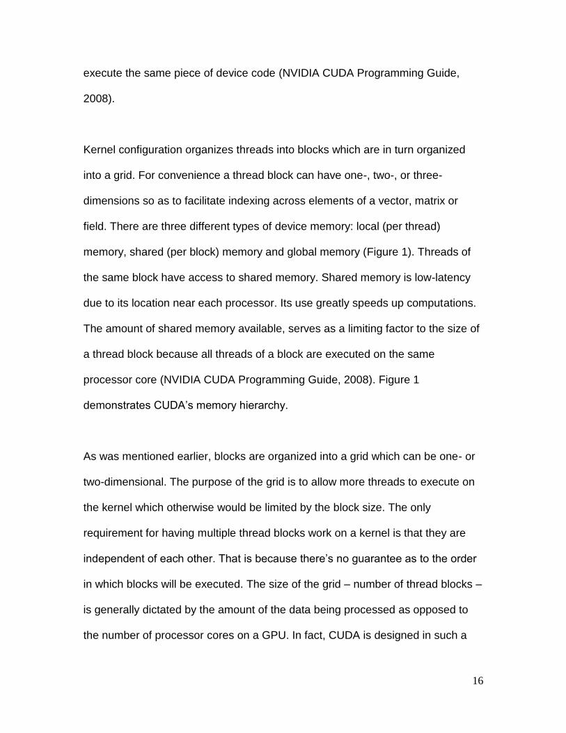
Kernel configuration organizes threads into blocks which are in turn organized
into a grid. For convenience a thread block can have one-, two-, or three-
dimensions so as to facilitate indexing across elements of a vector, matrix or
field. There are three different types of device memory: local (per thread)
memory, shared (per block) memory and global memory (Figure 1). Threads of
the same block have access to shared memory. Shared memory is low-latency
due to its location near each processor. Its use greatly speeds up computations.
The amount of shared memory available, serves as a limiting factor to the size of
a thread block because all threads of a block are executed on the same
processor core (NVIDIA CUDA Programming Guide, 2008). Figure 1
demonstrates CUDA‟s memory hierarchy.
As was mentioned earlier, blocks are organized into a grid which can be one- or
two-dimensional. The purpose of the grid is to allow more threads to execute on
the kernel which otherwise would be limited by the block size. The only
requirement for having multiple thread blocks work on a kernel is that they are
independent of each other. That is because there‟s no guarantee as to the order
in which blocks will be executed. The size of the grid – number of thread blocks –
is generally dictated by the amount of the data being processed as opposed to
the number of processor cores on a GPU. In fact, CUDA is designed in such a

17
way that the number of thread blocks can greatly exceed the number of
processors in the system (NVIDIA CUDA Programming Guide, 2008).
Figure 1 Memory Hierarchy
Another important component of this Major Qualifying Project is Kdb+. Kdb+ is an
in-memory, column-based database whose purpose in this project is to supply
the GPU with real-time market data. Kdb+ functions based on a language called
18
K which is in turn derived from a much older A Programming Language
(otherwise known as APL). Arthur Whitney, the developer of K, has put a great
deal of emphasis on brevity in his design of the language. While K may seem
somewhat obscure and obfuscated at first, it is actually extremely precise and,
more importantly, fast. The succinct quality of K, unfortunately, also reflects in the
language‟s error handling which is insufficient in Kdb+ (The Kdb+ Database,
2006).

19
3. System
3.1 Components
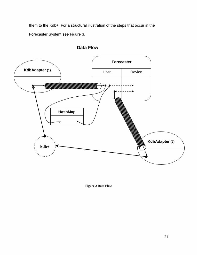
As mentioned earlier, the Forecaster application is a financial program that
analyzes the real-time market data. It includes five components: a Kdb+
database, two KdbAdapters (1 and 2), a HashMap and, the heart of the system,
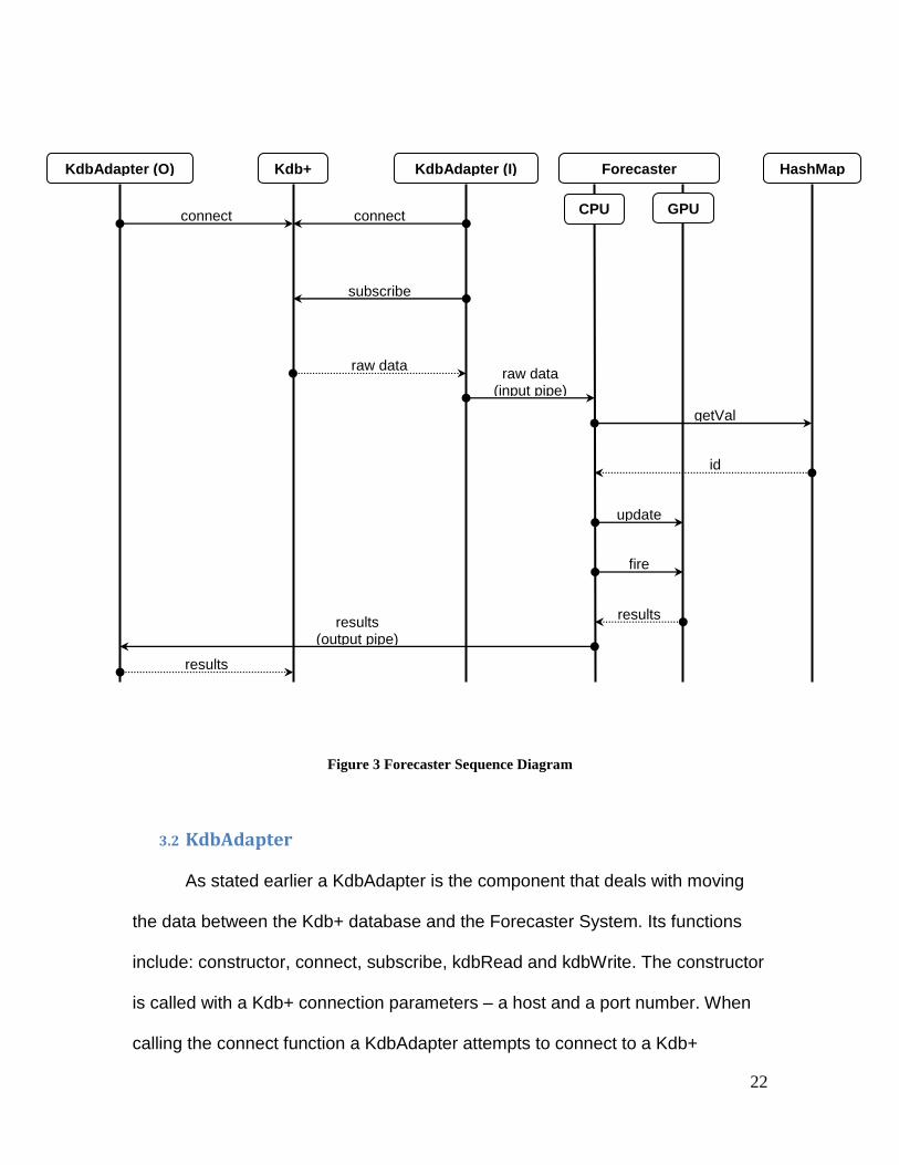
the Forecaster. Figure 2 depicts the data flow among these five components.
Upon launch, the application is split into three separate processes – the parent
and two children processes. Each child process is put in charge of one of the
KdbAdapters, while the parent is associated with the Forecaster component that
controls both the host and the device sides. The three processes communicate
with each other by a means of C-style pipes. Two pipes – input and output – are
created prior to spawning the three processes. The write end of the input pipe is
handled by the KdbAdapter (I) and the read end of the output pipe is given to the
KdbAdapter (O). The read end of the input pipe and the write end of the output
pipe is handled by the Forecaster.
The symbol data is stored on the GPU in a simple array. In order to facilitate data
storage and management on the GPU, each symbol is assigned a unique integer
id which serves as its index in the symbol data array on the GPU; this enables
access to any given symbol in a constant time. The required mapping is done in
the parent process by the HashMap component – its sole purpose is to map each
symbol string from the subscription set to a unique integer within range [0, (set

20
size) - 1]. As mapping of a symbol to a unique integer id may become a possible
bottleneck due to large volume of market data, fast hashing is imperative to the
system‟s success.
The purpose of the two KdbAdapters is to receive the real-time market data from
and send algo results to the Kdb+ database. The KdbAdapter (I) establishes a
connection with the Kdb+ and subscribes to a specified set of market symbols.
Once the Kdb+ receives a subscription request, it immediately begins to send
market data for the specified symbols to the KdbAdapter (I). The data is parsed
and sent down the input pipe to the Forecaster.
For each raw market data record received by the Forecaster from the read end of
the input pipe a symbol string is converted to a unique integer by making a
function call to the HashMap (in a fashion mentioned earlier). Then, a kernel call
is made from the host and data from the record is copied into a correct place in
the device‟s memory. As data accumulates on the device, the algos begin to
launch. The algo results are copied from the device‟s memory to the host‟s
whereupon the results are sent down through the write end of the output pipe to
the KdbAdapter (O).
Similarly to the KdbAdapter (I), the KdbAdapter (O) opens a connection to the
Kdb+ database. Once the Forecaster begins sending algo results, the
KdbAdapter (O) receives them from the read end of the output pipe and records
21
them to the Kdb+. For a structural illustration of the steps that occur in the
Forecaster System see Figure 3.
Figure 2 Data Flow
Data Flow
KdbAdapter (2)
HashMap
Host Device
Forecaster
KdbAdapter (1)
kdb+
22
Figure 3 Forecaster Sequence Diagram
3.2 KdbAdapter
As stated earlier a KdbAdapter is the component that deals with moving
the data between the Kdb+ database and the Forecaster System. Its functions
include: constructor, connect, subscribe, kdbRead and kdbWrite. The constructor
is called with a Kdb+ connection parameters – a host and a port number. When
calling the connect function a KdbAdapter attempts to connect to a Kdb+
id
HashMap
raw data
Kdb+
getVal
update
Forecaster
CPU GPU
fire
results results
(output pipe)
connect
subscribe
KdbAdapter (I)
raw data (input pipe)
connect
KdbAdapter (O)
results
23
database with parameters specified to the constructor. If the connection settings
are invalid an error code is returned. The constructor and the connect methods
must always be called in order for a KdbAdapter to function properly. Whether a
KdbAdapter is used for reading the data from or writing it to a Kdb+ database
determines what other functions will be called.
If a KdbAdapter is used for supplying the system with the market data then
the subscribe and the kdbRead functions are used. The subscribe function
accepts a symbol set and a table name as its parameters. The symbol set is the
set of symbols for which the real-time data will be obtained from a Kdb+
database. The table name is the name of the table from which to draw the data.
The KdbRead function is called after subscription is complete; its parameter is
the file descriptor, which is used for recording data from the Kdb+ database.
If the role of a KdbAdapter is to write data to a Kdb+ database then only
the kdbWrite function is used. Being a mirror image of the kdbRead, the kdbWrite
function accepts a file descriptor which is used for outputting the data to a Kdb+
database.
It should be noted that in order to minimize amount of code executed by
the kdbWrite and the kdbRead methods and to avoid unnecessary system state
checks neither function ever returns – except when the connection to a Kdb+
database is forcibly closed by an external source. In the Forecaster System, this
issue is solved by manually “killing” the child processes prior to exiting the parent
process.
24
3.3 HashMap
HashMap provides Forecaster with the ability to quickly convert a symbol string
to its appropriate unique integer id; in other words HashMap creates a minimal
perfect hash. Constructor for HashMap takes in a file that contains a set of
symbols to be analyzed by the system and creates a minimal perfect hash based
on that set.
HashMap servers as a wrapper to an application called CMPH. CMPH – C
Minimal Perfect Hashing Library – is a free API (Advanced Programming
Interface) that enables fast and efficient hashing of large sets of keys. CMPH
was developed by Davi de Castro Reis, Djamel Belazzougui, and Fabiano
Cupertino Botelho.
3.4 Forecaster
At the heart of the system is the Forecaster component. Its code is divided
between the host (CPU) and the device (GPU) memory. The host code, executed
on the CPU, handles reading of the market records from an input pipe, writing the
algo results to an output pipe and transferring the data to and from the GPU. The
device code, on the other hand, is responsible for storage and management of
the market records (inside the GPU's memory) as well as the computations.
The Forecaster's launch function accepts three parameters: two file descriptors –
one for an input and other for an output streams – and an integer value that

25
specifies the Forecaster's run time in seconds. The Forecaster‟s launch method
returns after the number of seconds specified by the run time constant. This and
all other constants are supplied in a configuration file that is passed in as a
parameter to the applications at launch time.
The data is stored in the device memory in a sliding window fashion, essentially
comprising a cyclical data structure – at any point during the execution of the
Forecaster System the amount of data on the card is limited by a time constant
specified by the user. The time window is stratified into time buckets – the
number of buckets is also defined in the configuration file. For example, if the
user chooses to keep fifteen minutes worth of data on the card divided into one-
minute buckets then, for the first fifteen minutes, data will be written to “empty”
memory locations – every minute data will be written to a new bucket: 15(min) /
1(min per bucket) = 15(buckets) – but when the fifteen minutes expire new
market records will overwrite the old ones, starting with the first bucket.
This design is implemented with a two-dimensional array (matrix), where each
row represents a time bucket and each cell in a row may potentially contain a
market record. The buckets are managed with a help of a variable that always
points to the “current bucket” – the bucket to which the data is to be written to at
that point in time. Using the previous example, in the beginning the variable
points to row zero switching to the next row every minute and after the fifteen
minutes it is again set to row zero. Refer to Figure 4 for a visual representation of
the way data is stored in the device memory.

26
The algorithmic computations used in these project are VWAP and TWAP. In
order to minimize communication between host and device, both algos are
launched with one kernel – the fire kernel. The computations are launched
according to a user-specified constant. For example, if the constant is set to ten
milliseconds, then the fire kernel will be launched every ten milliseconds. The fire
kernel is launched with the following thread configuration:
blockSize.x = the number of buckets per symbol
blockSize.y = 1
gridSize.x = the number of symbols in the set
gridSize.y = the number of algo types
In this project the number of algo types is two – TWAP and VWAP. This
configuration allows to perform both algorithmic calculations on each symbol
(possibly at the same time). Each block will execute calculations appropriate to
its algo type. First each thread in a block performs computations over a bucket
corresponding to its index and records the results. Then one thread from each
block computes overall results for a symbol based on the calculations done for
each bucket. So, if there are 100 symbols and the desired number of buckets for
each symbol is five, then the fire kernel will be launched with 200 blocks (2 algo
types by 100 symbols) where every block contains five threads. The blocks will
be split into two groups of 100 blocks each – one group for each algo. Within
each block a thread will calculate results for an appropriate bucket and then one
thread will perform final calculations using results for each bucket.

27
Figure 4 Data Storage
3.5 Suggested Improvements
The improvements discussed in this section are suggestions and are not used in
the actual implementation of the system.
Host-Device Communication Reduction
The best way to optimize system performance is to minimize the communication
between the host and the device as much as possible. One of the biggest system
bottlenecks is copying each market record to the device memory as it is passed
in to the Forecaster component. The best way to minimize the amount of copying
of data from the host to the device memory is to use the interval between the
algorithmic computations to the application's advantage; that is, storing the new
records in the host memory for the length of the “quiet” interval and only coping
the data to the device memory before the computations must be made. So, for
Bucket #0
Bucket #1
Bucket #2
Bucket #3
Bucket #4
Current
Bucket
PARAMETERS
Data amount: 30 seconds
Bucket count: 5 buckets
Records under 30 seconds old
Records over 30 seconds old
28
example, if an algo is set to fire every 100 milliseconds then the data should be
accumulated in the host memory for the length of 100 milliseconds and only
copied to the device memory just before firing the algo.
Asynchronous Device Code Execution
Another change that may optimize system performance is to combine the method
suggested above with asynchronous symbol data updates and algo firing. CUDA
supports asynchronous kernel calls by using cudaStreams, which are essentially
queues of “orders” to the device code. The cudaStream provides a form of
synchronization as the commands in a cudaStream are executed in the FIFO
(First In First Out) fashion. It would be beneficial to use the same cudaStream for
updating the symbol data and firing the algos. There are three steps in the
Forecaster component that can be queued into the same cudaStream to get the
following flow of events: the new records, that were stored in the host memory for
the interval between the algo executions, are asynchronously copied to the
device memory; then using the same cudaStream the update kernel is launched
to update the “old” symbol data with the new market records; finally, the algo
kernel is launched with the same cudaStream, using it for the third time. In this
scenario the only synchronization that will have to be done is calling the
cudaStreamSynchronize() function on the cudaStream (that was used for the
three asynchronous steps) before adding any new records to the host memory.

29
Host Memory Subdivision
For further speed up, the new records can be added to two different memory
locations. Alternating between these two locations will allow the
cudaStreamSynchronize() function to be called later, right before the call that will
copy the data from the host to the device memory thereby efficiently reducing the
delay between handling the incoming records.
Figure 5 Improved Storage Scheme
The cudaStream diagramed above contains two copy instructions. The letters “A”
and “B” represent the two host memory locations between which the storing of
data will be alternated. The “Tmp” label represents the location in the device
Sync
Cu
rren
t
Co
mm
an
d
cudaStream
Newest Command
Oldest Command
Update Fire
Copy
B A
Host Memory
Device Memory
Tmp
Copy Sync Update Fire
Copy
B A
Host Memory
Device Memory
Tmp
Copy
30
memory where the new records will be temporarily copied to before being used
to update the data for each symbol. The new records at location marked by
“Tmp” will be considered valid until the update kernel is launched. Once the
update kernel finishes – adding the records to the appropriate buckets of the
corresponding symbols – the records are considered outdated and will be
overwritten once the new set of records is copied from the host to the device
memory. The summary of the flow of events is as follows:
1. The cudaStream is synchronized – any previously unfinished instructions
are waited upon – to make sure the previous commands were executed
successfully
2. The new records are copied from the host memory location “A” to the
device memory location “Tmp”
3. The update kernel is launched
4. The algo kernel is launched
5. The new incoming records are being recorded to the host memory location
“B” until it‟s time for the algo calculations to begin
6. Steps 1 through 5 are repeated for a lifetime of the application, alternating
between the host memory locations “A” and “B”
31
4. Performance
The performance of the GPU versus the CPU was determined by two tests. The
dependent variable of each test was the average amount of time it takes to
perform a computation. The independent variables were as follows: algo
complexity and symbol set size. The results of all tests were in favor of GPU.
4.1 Hypothesis
Given the GPU‟s great potential for parallelization, it was theorized that the CPU
will be outperformed in both tests by a factor of at least five.
4.2 Procedure
In the first test the algo complexity was varied to analyze calculation time. Algo
complexity is defined by the number of calculations performed every time an algo
is fired. To increase the complexity of an algo the computations are repeated a
certain number of times by surrounding algo code with a simple loop. Therefore,
complexity is determined by the number of iterations through an algo. The first
test consisted of measuring the average time it takes – first on the GPU and then
on the CPU – for an algo to complete calculations as the complexity (number of
iterations) is increased.
The second test was used to establish performance of host and device code, in
terms of the amount of symbols used in the calculations. Let the symbol set be
defined as the collection of symbols for which data will be processed (refer back
to section 3.2 KdbAdapter). During each stage of this test the average time it
32
took to complete the algo calculations as size of the symbol set was increased
was measured.
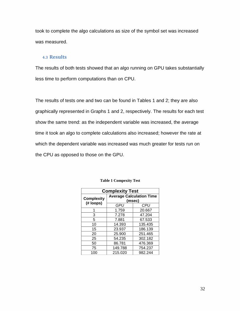
4.3 Results
The results of both tests showed that an algo running on GPU takes substantially
less time to perform computations than on CPU.
The results of tests one and two can be found in Tables 1 and 2; they are also
graphically represented in Graphs 1 and 2, respectively. The results for each test
show the same trend: as the independent variable was increased, the average
time it took an algo to complete calculations also increased; however the rate at
which the dependent variable was increased was much greater for tests run on
the CPU as opposed to those on the GPU.
Table 1 Compexity Test
Complexity Test
Complexity (# loops)
Average Calculation Time (msec)
GPU CPU
1 1.759 20.667
3 7.278 47.204
5 7.881 67.533
10 14.393 135.435
15 23.937 186.139
20 25.900 251.465
25 54.235 302.182
50 86.781 476.369
75 149.788 754.237
100 215.020 982.244

33
Table 2 Size Test
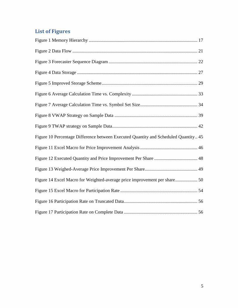
Figure 6 Average Calculation Time vs. Complexity
0
100
200
300
400
500
600
700
800
900
1000
1 3 5 10 15 20 25 50 75 100
1.759 7.278 7.881 14.393 23.937 25.90054.235
86.781
149.788
215.020
20.667 47.20467.533
135.435
186.139
251.465
302.182
476.369
754.237
982.244
Av
era
ge
Ex
ec
uti
on
Tim
e(m
sec)
Complexity(# loops)
Average CalculationTime vs Complexity
GPU CPU
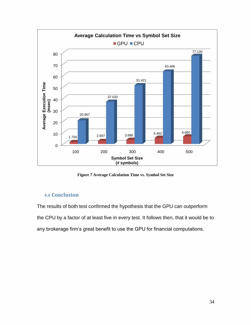
Size Test
Set Size (# symbols)
Average Calculation Time (msec)
GPU CPU
100 1.759 20.667
200 2.697 37.033
300 3.686 51.421
400 5.462 63.466
500 6.660 77.130
34
Figure 7 Average Calculation Time vs. Symbol Set Size
4.4 Conclusion
The results of both test confirmed the hypothesis that the GPU can outperform
the CPU by a factor of at least five in every test. It follows then, that it would be to
any brokerage firm‟s great benefit to use the GPU for financial computations.
0
10
20
30
40
50
60
70
80
100 200 300 400 500
1.759 2.697 3.6865.462 6.660
20.667
37.033
51.421
63.466
77.130
Av
era
ge E
xecu
tio
n T
ime
(msec)
Symbol Set Size(# symbols)
Average Calculation Time vs Symbol Set Size
GPU CPU
35
5. Algorithmic Trading Strategy
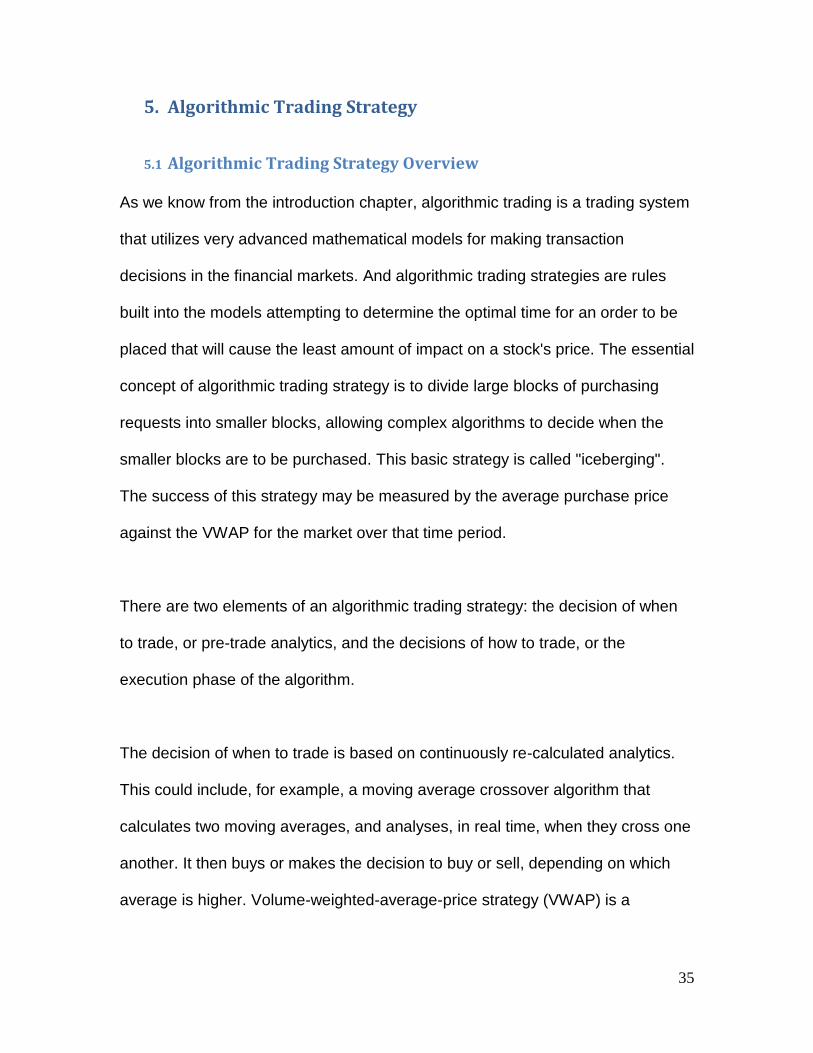
5.1 Algorithmic Trading Strategy Overview
As we know from the introduction chapter, algorithmic trading is a trading system
that utilizes very advanced mathematical models for making transaction
decisions in the financial markets. And algorithmic trading strategies are rules
built into the models attempting to determine the optimal time for an order to be
placed that will cause the least amount of impact on a stock's price. The essential
concept of algorithmic trading strategy is to divide large blocks of purchasing
requests into smaller blocks, allowing complex algorithms to decide when the
smaller blocks are to be purchased. This basic strategy is called "iceberging".
The success of this strategy may be measured by the average purchase price
against the VWAP for the market over that time period.
There are two elements of an algorithmic trading strategy: the decision of when
to trade, or pre-trade analytics, and the decisions of how to trade, or the
execution phase of the algorithm.
The decision of when to trade is based on continuously re-calculated analytics.
This could include, for example, a moving average crossover algorithm that
calculates two moving averages, and analyses, in real time, when they cross one
another. It then buys or makes the decision to buy or sell, depending on which
average is higher. Volume-weighted-average-price strategy (VWAP) is a

36
methodology to determine when to trade by continuously re-calculating price
average weighted on volume and comparing the average price to current price.
The decision of how to trade, or the order execution element of the algorithm,
can be just as complex as the decision of when to trade. For example, once an
opportunity is identified by the pre-trade analytic to buy, for example, 10,000
shares of IBM, the order execution element of an algorithmic trading strategy
may slice the order up into smaller parts (blocks of 1,000 shares). In conjunction,
it may place the order in multiple liquidity pools to take advantage of the prices
and availability of liquidity across a „virtual‟ exchange with multiple participants
(Jones, 2007). In conclusion, the decision of how to trade takes consideration of
various real-time constraints, such as current market size, stock volatility, news
feed on this company and so on. Time-weighted-average price is a strategy to
minimize the impact on market volatility and assumes that stock shares are
equally traded over the same period of time.
VWAP and TWAP are two mostly often used strategies for algorithmic trading.
There are still many more other strategies such as arbitrage strategy,
implementation shortfall and trade cost analysis.
37
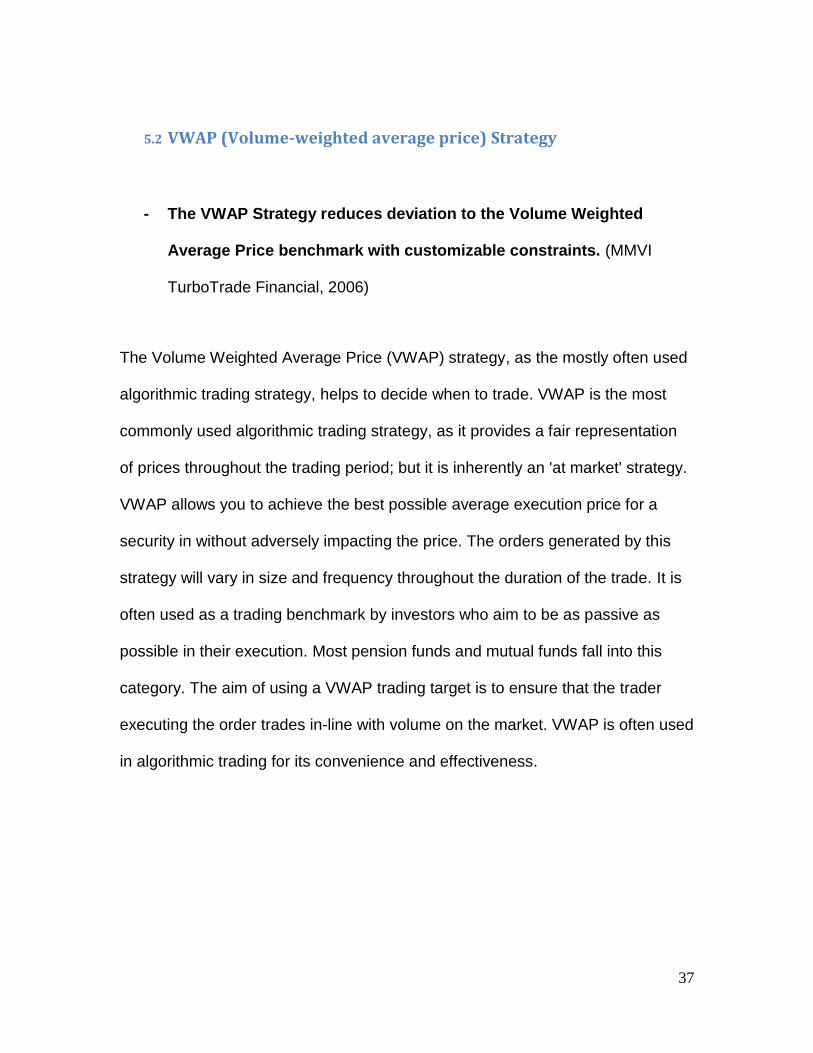
5.2 VWAP (Volume-weighted average price) Strategy
- The VWAP Strategy reduces deviation to the Volume Weighted
Average Price benchmark with customizable constraints. (MMVI
TurboTrade Financial, 2006)
The Volume Weighted Average Price (VWAP) strategy, as the mostly often used
algorithmic trading strategy, helps to decide when to trade. VWAP is the most
commonly used algorithmic trading strategy, as it provides a fair representation
of prices throughout the trading period; but it is inherently an 'at market' strategy.
VWAP allows you to achieve the best possible average execution price for a
security in without adversely impacting the price. The orders generated by this
strategy will vary in size and frequency throughout the duration of the trade. It is
often used as a trading benchmark by investors who aim to be as passive as
possible in their execution. Most pension funds and mutual funds fall into this
category. The aim of using a VWAP trading target is to ensure that the trader
executing the order trades in-line with volume on the market. VWAP is often used
in algorithmic trading for its convenience and effectiveness.

38
The VWAP is calculated using the following formula:
where: PVWAP = Volume Weighted Average Price
Pj = price of trade j
Qj = quantity of trade j
j = each individual trade that takes place over the defined period of time,
excluding cross trades and basket cross trades.
(VWAP, 2008)
To determine whether a transaction is good or not using VWAP strategy is
simple. If the current price is below the VWAP benchmark up to the end of a
chosen time horizon, the current bid price is considered good for buying in but
bad for selling out. Vice Versa, if the current price is above VWAP benchmark up
to the point, current bid price is considered good for selling out but bad for buying
in. How the rule is determined is also straightforward. As VWAP calculates
average price weighted on volume, we buy in the stock shares if current price is
lower than intra-day average so far and sell it out when the current price is higher
than volume-weighted average price. If we could keep trading this way, we could
keep ourselves above the market intra-day average, which means we will not
lose in short term, as we keep a profit range by buying under the average and
selling above the average.

39
Table 3 shows the way we apply VWAP strategy to real-world data, if we have
stock AAA has bid price and traded volume at the following times:
Table 3 Bid price and traded volume of AAA
And if we graph the sample data, Figure 8 shows that we could see that the
VWAP values are smoother than the raw market data values after weighted
average.
Figure 8 VWAP Strategy on Sample Data
Time Bid
Price Volume VWAP
9:00 35 100 =35*100/100 = 35
9:05 40 50 =(35*100+40*50)/(100+50) = 36.67
9:10 45 100 =(35*100+40*50+45*100)/(100+50+100) = 40
9:15 30 100 =(35*100+40*50+45*100+30*100)/(100+50+100+100) = 37.14
9:20 30 100 =(35*100+40*50+45*100+30*100+30*100)/(100+50+100+100+100) = 35.56

40
5.3 TWAP Strategy (Time-weighted average price)
- The TWAP Strategy distributes orders in a linear manner, balancing
adverse selection and slippage in real-time. (MMVI TurboTrade
Financial, 2006)
The TWAP strategy is also an often used intra-day benchmark. It assumes that a
stock volume follows a uniform distribution with respect to time, which means that
transaction volumes are equally distributed within a given time horizon. TWAP is
effective when we want to minimize the impact by the market volatility in a
specified time horizon. TWAP is best for those who want to adhere to a regular
trading schedule and execute in equal-size increments regardless of other trades
in the market.
TWAP (time-weighted average price) allows traders to time-slice a trade over a
certain period of time. Unlike VWAP, which typically trades less stock when
market volume dips, TWAP will trade the same number of shares at even
intervals throughout the time-period you specify. TWAP is optimal for orders that
must be completed by a specific time or for trades in illiquid stocks where you do
not want your execution schedule to depend on volumes. This strategy is best
utilized in situations where there are little or no liquidity concerns and the trade's
executions can be evenly spread throughout the given timeframe. The
cumulative volume profile for a TWAP trade is linear with a positive constant

41
slope of one, as we could see in the graph below. In addition, orders generated
by this strategy tend to be small in size and occur with relatively frequency.
Here is an example indicating how TWAP differs from VWAP. To achieve this
Time Weighted Average Price, the BXS engine divides the Order Quantity
equally over a number of equally-spaced slices. TWAP differs from the VWAP
strategy in that a VWAP trade may buy or sell 30% of a trade in the first half of
the day and then the other 70% in the second half of the day. With the TWAP
strategy, the trade would most likely execute 50% in the first half and 50% in the
second half of the day. (Stanley, 2007) From what is described above, we see
that TWAP does not take market traded volume into consideration. If trader is
selling under a TWAP strategy, the orders will be evenly time-sliced regardless of
the market impact.
A TWAP strategy example using the same data with VWAP is as follows:
Table 4 Bid price and traded volume of AAA
Time Bid Price Volume Volume Weighted
9:00 35 (100+50+100+100+100)/5 = 90 20%
9:05 40 90 40%
9:10 45 90 60%
9:15 30 90 80%
9:20 30 90 100%

42
From the graph below, we could see that TWAP strategy is not based on the
volume traded per period of time, but based on time slices. That is why TWAP is
also called time-sliced trading strategy.
Figure 9 TWAP strategy on Sample Data
5.4 Profit and Loss Analysis
5.4.1 Percentage Difference between Executed Quantity and Scheduled Quantity
The percentage difference between the executed quantity and scheduled
quantity provides us with a clearer view of how executed quantity differs from the

43
volume of shares that we planned to be. Ideally, all the brokers wish for what
they exactly need. However, with market prices and volumes fluctuating
continuously, it is impossible for brokers to get the desired volume with limited
shares of stock in the market. That is why brokers need to run the formula to
evaluate their deficiency in the actual executed quantity along the transactions,
and adjust the algorithm to face the new situation if necessary. No matter what
trading strategy we are using, we are short on purchase amount all the time due
to market limitations. That is the reason why we need to know the difference,
need to know how much we short and make up the deficiency in future trading.
Table 5 Percentage Difference between Executed Quantity and Scheduled Quantity
Sym 1 time TotExec SchdQty (Execqty-Schdqty)/SchdQty 2
LEH 9:30:00 2600 4300 -39.53%
LEH 9:30:10 1800 1800 0.00%
LEH 9:30:20 1500 1500 0.00%
LEH 9:30:30 3200 5300 -39.62%
LEH 9:30:40 2000 3300 -39.39%
LEH 9:30:50 1900 3200 -40.63%
LEH 9:31:00 1000 1700 -41.18%
LEH 9:31:10 700 1200 -41.67%
LEH 9:31:20 700 1200 -41.67%
LEH 9:31:30 1400 2300 -39.13%
LEH 9:31:40 2800 4600 -39.13%
LEH 9:31:50 2300 3900 -41.03%
LEH 9:32:00 1500 2500 -40.00%
LEH 9:32:10 1100 1800 -38.89%
LEH 9:32:20 900 1500 -40.00%
LEH 9:32:30 32100 53500 -40.00%
LEH 9:32:40 9700 9700 0.00%
LEH 9:32:50 6900 6900 0.00%
LEH 9:33:00 7000 11700 -40.17%
1 Sym = Symbol name
Time = Transaction time for every 10 seconds TotExec = Cumulated Executed Quantity within 10 seconds SchdQty = Cumulated Scheduled Quantity within 10 seconds 2 (Execqty-Schdqty)/SchdQty calculates the percentage difference between cumulated
executed quantity and cumulated scheduled quantity within 10 seconds

44
We are the seller‟s position in the table 5 above. For buyer‟s position, negative
percentage rate indicates that demand volume is greater than supplied volume.
So when the percentage difference between executed quantity and scheduled
quantity is negative for buyers, the cumulated volume of buying requests is
greater than that of selling requests. On the other hand, for seller side position,
negative percentage rate indicates that supplied volume is greater than demand
volume. At that time, cumulated volume of selling requests is greater than that of
buying requests. Usually, we have the percentage rate controlled within the
range of 10%. However, every entry of percentage rate is either negative or zero,
which points to the fact that everyone is trying to sell the stocks, resulting in the
great decline of the stock price. Below is a more straightforward diagram using
data above. Figure 10 shows that most stock holders that day were trying to sell
their shares so that there was no available stock buyer in the market. After
analyzed the difference between executed quantity and scheduled quantity, we
knew that how bad performances our orders were experiencing from the pure
negative percentage rates honestly reflected on the diagram. Knowing how hard
it was getting sold reminds us to change a trading strategy. As we could see in
Figure 10, the seller‟s executed quantity could not reach the scheduled quantity
for every single transaction. Data source from Lehman Brothers, within 3
minutes after market opens on Tue, Sept 23.
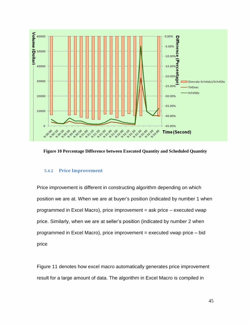
45
Figure 10 Percentage Difference between Executed Quantity and Scheduled Quantity
5.4.2 Price Improvement
Price improvement is different in constructing algorithm depending on which
position we are at. When we are at buyer‟s position (indicated by number 1 when
programmed in Excel Macro), price improvement = ask price – executed vwap
price. Similarly, when we are at seller‟s position (indicated by number 2 when
programmed in Excel Macro), price improvement = executed vwap price – bid
price
Figure 11 denotes how excel macro automatically generates price improvement
result for a large amount of data. The algorithm in Excel Macro is compiled in

46
Visual Basic. The algorithm below shows how we judge our position at first and
then calculate the price improvement per share.
Figure 11 Excel Macro for Price Improvement Analysis
What the algorithm basically produces is that it judges the trader‟s position, either
a seller or a buyer, and then applies the price improvement formula according to
the first-step judgment. The output price improvement will be located at column
46. And column 43 indicates the executed price in the market recommended by
VWAP strategy, while column 29 indicates the bid price that we desired to be.
After we run the algorithm, the truncated price improvement result table looks as
indicated in Table 5.
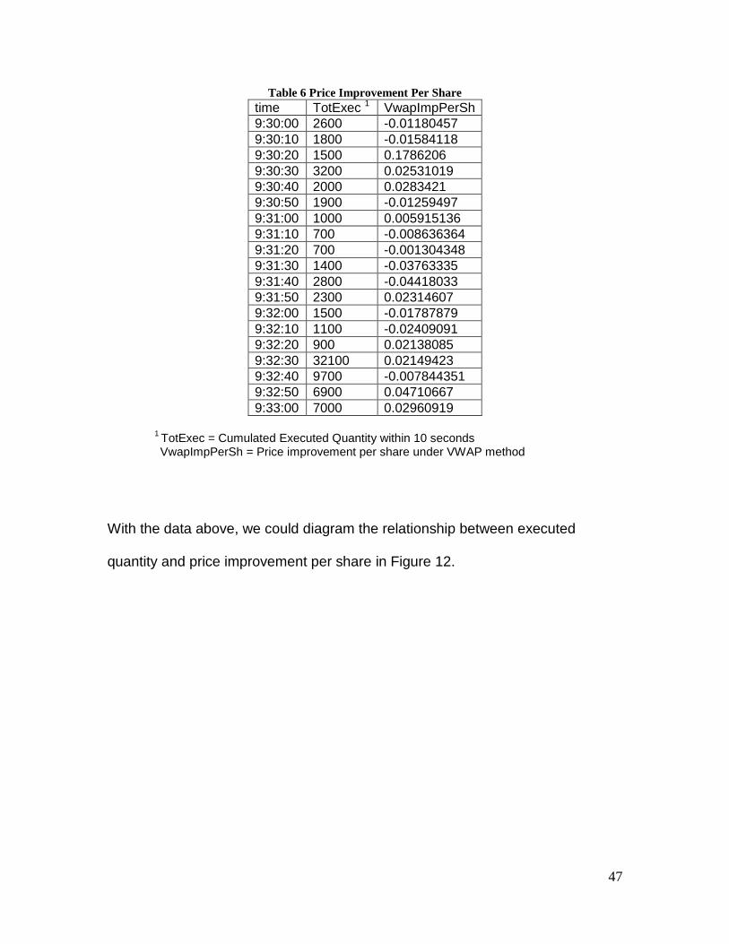
47
Table 6 Price Improvement Per Share
time TotExec 1 VwapImpPerSh
9:30:00 2600 -0.01180457
9:30:10 1800 -0.01584118
9:30:20 1500 0.1786206
9:30:30 3200 0.02531019
9:30:40 2000 0.0283421
9:30:50 1900 -0.01259497
9:31:00 1000 0.005915136
9:31:10 700 -0.008636364
9:31:20 700 -0.001304348
9:31:30 1400 -0.03763335
9:31:40 2800 -0.04418033
9:31:50 2300 0.02314607
9:32:00 1500 -0.01787879
9:32:10 1100 -0.02409091
9:32:20 900 0.02138085
9:32:30 32100 0.02149423
9:32:40 9700 -0.007844351
9:32:50 6900 0.04710667
9:33:00 7000 0.02960919
1
TotExec = Cumulated Executed Quantity within 10 seconds VwapImpPerSh = Price improvement per share under VWAP method
With the data above, we could diagram the relationship between executed
quantity and price improvement per share in Figure 12.
48
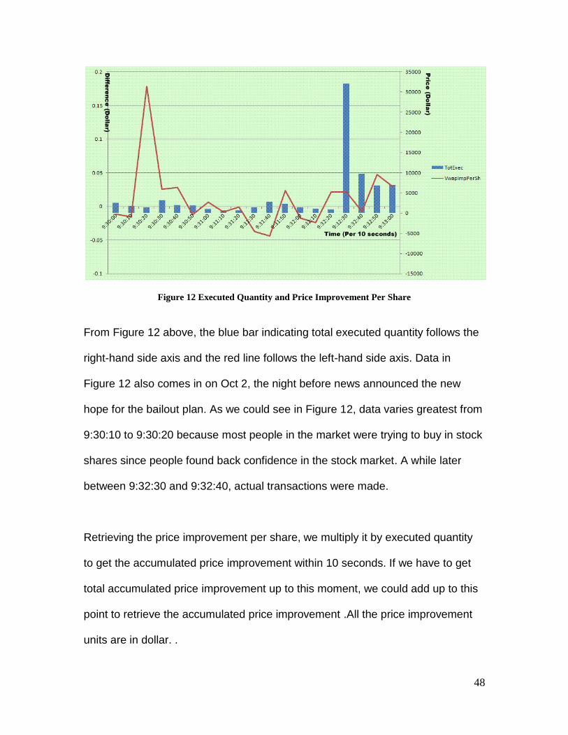
Figure 12 Executed Quantity and Price Improvement Per Share
From Figure 12 above, the blue bar indicating total executed quantity follows the
right-hand side axis and the red line follows the left-hand side axis. Data in
Figure 12 also comes in on Oct 2, the night before news announced the new
hope for the bailout plan. As we could see in Figure 12, data varies greatest from
9:30:10 to 9:30:20 because most people in the market were trying to buy in stock
shares since people found back confidence in the stock market. A while later
between 9:32:30 and 9:32:40, actual transactions were made.
Retrieving the price improvement per share, we multiply it by executed quantity
to get the accumulated price improvement within 10 seconds. If we have to get
total accumulated price improvement up to this moment, we could add up to this
point to retrieve the accumulated price improvement .All the price improvement
units are in dollar. .

49
In Figure 12, we applied price improvement method on the sample data which
was 3 minute within the market opens. When analyzing the real data in Figure
13, we weighed the price improvement rate so that the data will be less
fluctuated. The way we weigh the data is to apply the following formula:
Figure 13 Weighed-Average Price Improvement Per Share
As we could see in Figure 13, weighted-average price improvement looks much
smoother along the time comparing to Figure 12, and almost remains constant in
the end. Price improvement per share in the above diagram follows right-hand
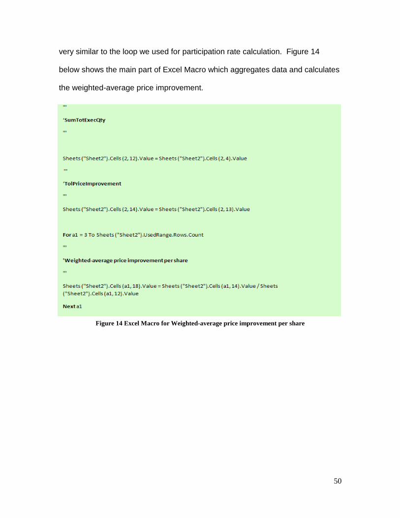
side axis. The algorithm we ran to attain weighted-average price improvement is
50
very similar to the loop we used for participation rate calculation. Figure 14
below shows the main part of Excel Macro which aggregates data and calculates
the weighted-average price improvement.
Figure 14 Excel Macro for Weighted-average price improvement per share

51
5.4.3 Participation Rate Analysis
First of all, there are two kinds of participation rates involved in our future
calculation: period participation rate and cumulative participation rate. Period
participation rate is the executed volume every 10 seconds weighted by the
actual market volume every 10 seconds. Cumulative participation rate is the
cumulative executed volume by the end of the time ticket weighted by the
cumulative market volume by the end of the time ticket. Both formulas are listed
as follows:
Here we will raise a simple example to show how the actual calculation works to
achieve both participation rates. Table 7 below shows how to calculate the
cumulated participation rate, where intvol stands for current market volume,
TotExec stands for current executed volume, SumIntVol stands for cumulative
market volume by the end of the time ticket and SumTotExecQty stands for
cumulative executed volume by the end of the time ticket. Table 8 below shows
the calculation for period participation rate using the same data in Table 7, where
10sIntVol stands for cumulative market volume for every 10 seconds and
10sTotExec stands for the cumulative executed volume for every 10 seconds.

52
Table 7 Paticipation Rate on Sample Data
time intvol TotExec SumIntVol SumTotExecQty Cumulative participation rate
9:30:00 500 200 500 200 200/500 = 0.400
9:30:08 900 300 500+900 = 1400 200+300=500 500/1400 = 0.357
9:30:09 1000 600 1400+1000=2400 500+600=1100 1100/2400 = 0.458
9:30:10 400 250 2400+400=2800 1100+250=1350 1350/2800 = 0.482
9:30:11 300 50 2800+300=3100 1350+50=1400 1400/3100 = 0.452
9:30:20 600 100 3100+600=3700 1400+100=1500 1500/3700 = 0.405
Table 8 Participation Rate on Sample Data Ⅱ
time 10sIntVol 10sTotExec Period Participation Rate
9:30:00 500+900+1000=2400 200+300+600=1100 1100/2400 = 0.458
9:30:10 400+300=1700 250+50=300 300/1700 = 0.176
9:30:20 600 100 100/600 = 0.167
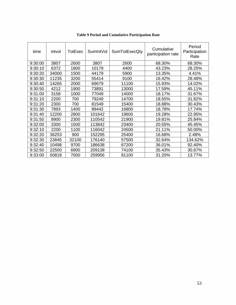
The data we actually use is already aggregated for every 10 seconds. In the
table below, intvol and TotExec are both aggregated values within 10 seconds.
So for period participation rate, we could directly use intvol and TotExec values
without any change. It is still the same way obtaining the cumulated participation
rate. Since both entries are aggregated, we only need to apply formulas below to
get both participation rates. And results are listed in Table 9.
53
Table 9 Period and Cumulative Participation Rate
time intvol TotExec SumIntVol SumTotExecQty Cumulative
participation rate
Period Participation
Rate
9:30:00 3807 2600 3807 2600 68.30% 68.30%
9:30:10 6372 1800 10179 4400 43.23% 28.25%
9:30:20 34000 1500 44179 5900 13.35% 4.41%
9:30:30 11235 3200 55414 9100 16.42% 28.48%
9:30:40 14265 2000 69679 11100 15.93% 14.02%
9:30:50 4212 1900 73891 13000 17.59% 45.11%
9:31:00 3158 1000 77049 14000 18.17% 31.67%
9:31:10 2200 700 79249 14700 18.55% 31.82%
9:31:20 2300 700 81549 15400 18.88% 30.43%
9:31:30 7893 1400 89442 16800 18.78% 17.74%
9:31:40 12200 2800 101642 19600 19.28% 22.95%
9:31:50 8900 2300 110542 21900 19.81% 25.84%
9:32:00 3300 1500 113842 23400 20.55% 45.45%
9:32:10 2200 1100 116042 24500 21.11% 50.00%
9:32:20 36253 900 152295 25400 16.68% 2.48%
9:32:30 23845 32100 176140 57500 32.64% 134.62%
9:32:40 10498 9700 186638 67200 36.01% 92.40%
9:32:50 22500 6900 209138 74100 35.43% 30.67%
9:33:00 50818 7000 259956 81100 31.20% 13.77%

54
The algorithm which we applied to calculate both participation rates is simple.
Basically, we just need to construct a loop that aggregates the cumulative sum
for market volume and executed volume. The Excel Macro for this algorithm is
shown in Figure 15.
Figure 15 Excel Macro for Participation Rate

55
What is indicated in Figure 15 above is how we aggregates executed volume and
total market traded volume. After retrieving the aggregated value, we need to
judge whether the market traded volume is zero before division, for it is possible
that no share was traded for a particular stock during a specified period of time. If
the market traded volume is non-zero, we divide the executed volume by the total
market traded volume to get cumulative participation rate. Period participation
rate calculation uses the same way except that instead of total executed volume
and total market volume, we use aggregated executed volume and market
volume for every 10 seconds. Both cumulative participation rate and period
participation rate will be compared to the configured rate, which is 10% as a
constant, in the graphs below.
The configured rate remains 10% as a constant, for it is an optimized number
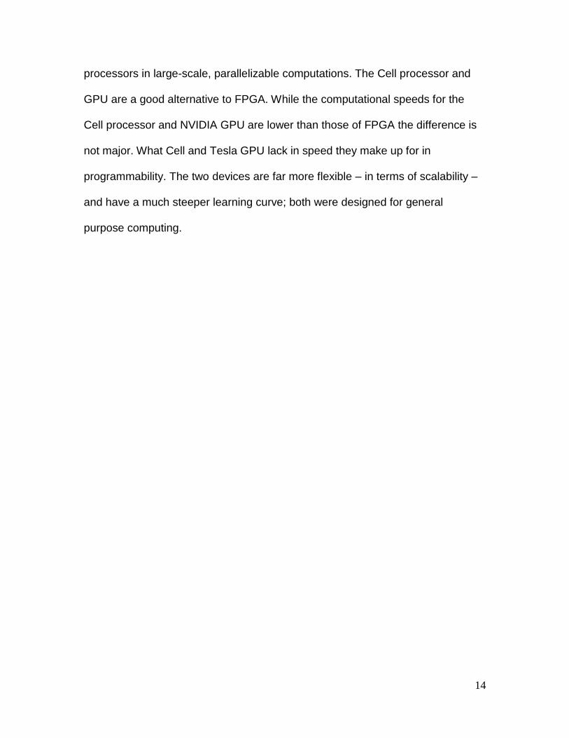
based on previous experiences. Given the above algorithm, we could graph data
listed in Table 9 as shown in Figure 16. Notice that the data we used in Table 9 is
truncated, which only contains 3-minute data after the market opens. In Figure
17, we graphed complete data received on the particular morning. In the Figure
17, it is more obvious that the cumulative participation rate looks smoother and
closer to the configured rate, which is set as 10%, even though the period rate
still maintains high volatility.

56
Figure 16 Participation Rate on Truncated Data
Figure 17 Participation Rate on Complete Data

57
6. Future Analysis
As we know, news-driven algorithms have recently become popular. News
algorithms attempt to analyze news stories and make trades based on their
predicted impact on the underlying stock. Traditional algorithmic trading system
decides what to do after analyzing the market data. In other words, algorithmic
trading system generates no result without history market data. However, market
prices nowadays could change greatly in a millisecond, and company could even
go bankrupt before people get a chance to sell the stock shares they hold.
Another issue that brought to our concern is that news today has a greater
impact on stock market than ever. Rumors about bankruptcy of United Air Lines
on Sept. 26th caused UAL stock prices dipped 15% in 30 minutes. On Oct 8th,
U.S. stocks plunged and the major indexes fell to five-year lows as traders acted
on rumors and hopes about recapitalization for some of the biggest financial
institutions in Britain and the U.S., including Morgan Stanley, Bank of America
and Royal Bank of Scotland Group. The Chicago Board Options Exchange
volatility index, which measures premiums paid for protection against stock-
market swings, closed at its highest level of the crisis, up 3.1% at 53.68 on that
day (Curran, 2008).
The Dow Jones company saw the necessity of upgrading the current algorithmic
system due to the current market environment. That is how Dow Jones decided
to cooperate with Ravenpack on the development of Dow Jones News Analytics
project. DJ Analytics reads news posted on Dow Jones News Feed with an ultra-

58
low latency. While Dow Jones News Feed covers world-wide financial news from
Dow Jones Newswires, Wall Street Journal, Barron‟s and all other trust-worthy
major news sites, DJ Analytics covers all headlines and full text of news stories
completely and generates analysis for every piece of news indicating the impact
on the oil price, bank interest rate, currency rate and other 21 major indexes and
rates. While automated, computer-based trading is widely used to capture and
leverage predictable events, the ability to correlate breaking news with streaming
financial data in real time is the next frontier for algorithmic trading. We will be
expecting a built-in news analytics as part of algorithmic trading system on GPU
in the future.

59
Bibliography 1. Ablan, J. (2007 , May 31). Algo-mania: The machines take over Wall
Street. Retrieved October 10, 2008, from Reuters:
http://www.reuters.com/article/sphereNews/idUSN2931330320070531?sp
=true&view=sphere
2. Curran, R. (2008). Morgan Stanley Sinks and BofA Loses 26%. Wall
Street Journal , 1-2.
3. Fidelity Investments Institutional Brokerage Group Enhances Investor-
Level Web Site For Brokers. (2001). Retrieved 9 29, 2008, from Inside
Fidelity:
http://content.members.fidelity.com/Inside_Fidelity/fullStory/1,,1212,00.ht
ml
4. FPGA Basics. (2008, March 16). Retrieved October 1, 2008, from Andrake
Consulting Group, Inc.: http://www.andraka.com/whatisan.htm
5. Hagstrom, R. G. (2001). The Essential Buffett: Timeless Principles for the
New Economy. New York: John Wiley & Sons.
6. Henriques, D. B. (1995). Fidelity‟s World. Scribner.
7. High Performance Computing (HPC). (2008). Retrieved October 2, 2008,
from NVIDIA: http://www.nvidia.com/object/tesla_8_series.html
8. Jones, H. (2007, November). Exchanges and Trading Venues Worldwide.
Retrieved October 10, 2008, from Trading Places:
http://64.233.169.104/search?q=cache:7oEaMsn0VXMJ:www.rsi-
ireland.com/documents/TradingPlacesNovember2007.pdf+10,000+shares

60
+of+IBM,+the+order+execution+element+of+an+algorithmic+trading+strat
egy+may+slice+the+order+up+into+smaller+parts+(blocks+of+1,000+s
9. MMVI TurboTrade Financial, L. (2006). Trading Strategies . Retrieved 10
3, 2008, from Turbo Trade:
http://www.turbotrade.com/content/view/116/94/
10. Norman, D. J. (2002). Professional Electronic Trading. Singapore: John
Wiley & Sons.
11. NVIDIA CUDA Programming Guide. (2008, June 7). Version 2.0. Santa
Clara, California, USA: NVIDIA Corporation.
12. Stanley, M. (2007). Benchmark Execution Strategies. MS BXS , 8-9.
13. Stokes, M. (2007). A Brief Look at FPGAs, GPUs and Cell Processors.
ITEA Journal , 9-11.
14. The Kdb+ Database. (2006, November). Palo Alto, California, USA: Kx
Systems, Inc. .
15. VWAP. (2008, 9 13). Retrieved 10 3, 2008, from Wikipedia:
http://en.wikipedia.org/wiki/VWAP
16. Weiss, D. M. (2006). After the trade is Made. New York: Penguin Group,
Inc.
61
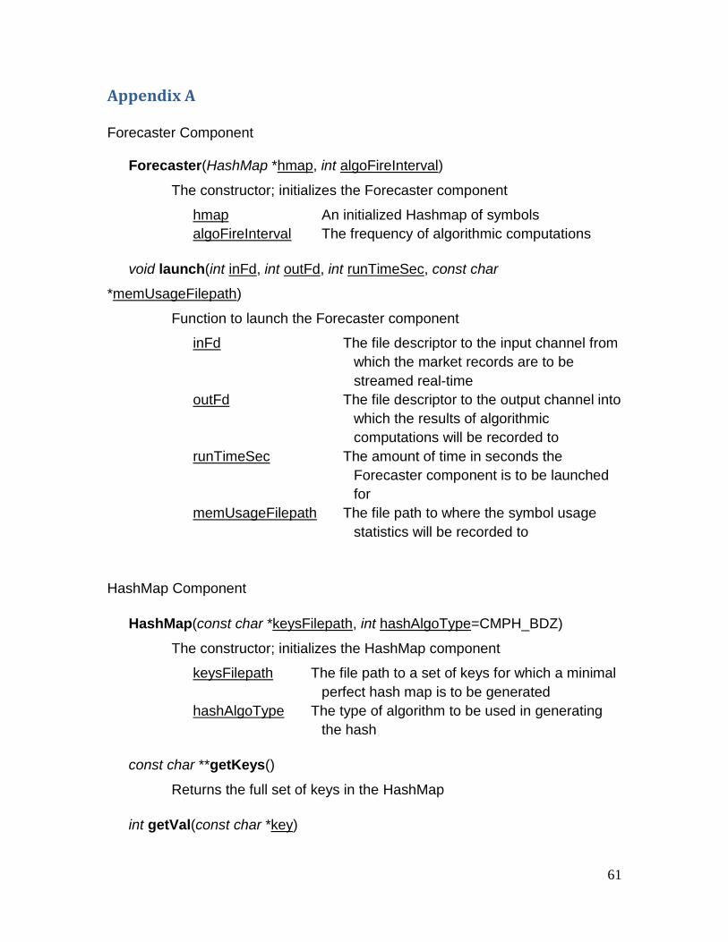
Appendix A
Forecaster Component Forecaster(HashMap *hmap, int algoFireInterval)
The constructor; initializes the Forecaster component
hmap An initialized Hashmap of symbols
algoFireInterval The frequency of algorithmic computations
void launch(int inFd, int outFd, int runTimeSec, const char
*memUsageFilepath)
Function to launch the Forecaster component
inFd The file descriptor to the input channel from
which the market records are to be
streamed real-time
outFd The file descriptor to the output channel into
which the results of algorithmic
computations will be recorded to
runTimeSec The amount of time in seconds the
Forecaster component is to be launched
for
memUsageFilepath The file path to where the symbol usage
statistics will be recorded to
HashMap Component
HashMap(const char *keysFilepath, int hashAlgoType=CMPH_BDZ)
The constructor; initializes the HashMap component
keysFilepath The file path to a set of keys for which a minimal
perfect hash map is to be generated
hashAlgoType The type of algorithm to be used in generating
the hash
const char **getKeys()
Returns the full set of keys in the HashMap
int getVal(const char *key)

62
Returns a value of the specified key
key The key for which a value is requested
const char *getKey(int val)
Returns a key to which the specified value maps to
val The value for which a key is requested
int getSize()
Returns the size of the HashMap
int getMaxKeyLen()
Returns the maximum number of characters in a key
KdbAdapter Component
KdbAdapter(const char *host, const int port)
The constructor; initializes the KdbAdapter component
host The hostname of the Kdb+ database
port The port to connect to
void connect()
Connect to a Kdb+ database using the parameters specified in the
constructor
void subscribe(const char* tableName, const char **symSet, int symSetSize)
Subscribe to a certain set of symbols from the specified table
tableName The name of the table from which to get the data
symSet The symbol set to subscribe to
symSetSize The number of symbols in the subscription set
void kdbRead(int inFd)
Continuously read the data for the subscribed symbols
inFd The file descriptor to a channel into which the subscription
data will be recorded to

63
void kdbWrite(int outFd)
Continuously write the data to the Kdb+ database
outFd The file descriptor to a channel into which the output
data will be recorded to