Embed Size (px)
Citation preview

Time Series Models for Measuring Market Risk
Technical Report
Jose Miguel Hernandez Lobato, Daniel Hernandez Lobato and Alberto Suarez
Departamento de Ingenierıa Informatica,Universidad Autonoma de Madrid,C/ Francisco Tomas y Valiente, 11,
Madrid 28049 Spain.
July 18, 2007

2
Abstract
The task of measuring market risk requires to make use of a probabilistic model thatcaptures the statistical properties of price variations in financial assets. The most impor-tant of these properties are autocorrelations, time-dependent volatility and extreme events.GARCH processes are financial models that can successfully account for the time-dependentvolatility. However, they assume Gaussian errors whereas empirical studies generally leadto residuals which exhibit more extreme events than those implied by a Gaussian distri-bution. In this document we analyze the performance of different models which try tosolve this deficiency of standard GARCH processes. The first group of models is basedon mixtures of autoregressive experts which work together following three possible strate-gies: collaboration, soft competition or hard competition. Mixtures of soft competitiveexperts produce the best estimates of risk because their hypothesis space is a mixture ofGaussian distribution which can account for extreme events. Finally, we study a modelwhich improves standard GARCH processes by means of modelling the innovations in anon-parametric way. The resulting model turns out to provide very precise measurementsof market risk and outperforms soft competitive mixtures with 2 experts.
3

4

Contents
1 Introduction 7
2 Measuring Market Risk 11
2.1 Risk, Market Risk and Risk Measures . . . . . . . . . . . . . . . . . . . . . 11
2.1.1 Market Risk . . . . . . . . . . . . . . . . . . . . . . . . . . . . . . . . 12
2.1.2 Risk Measures . . . . . . . . . . . . . . . . . . . . . . . . . . . . . . 12
2.1.3 Coherent Risk Measures . . . . . . . . . . . . . . . . . . . . . . . . . 14
2.1.4 Estimating Market Risk Measures . . . . . . . . . . . . . . . . . . . 15
2.2 Properties of Price Variations and Time Series Models . . . . . . . . . . . . 16
2.2.1 Financial Returns . . . . . . . . . . . . . . . . . . . . . . . . . . . . 16
2.2.2 Statistical Properties of Asset Returns . . . . . . . . . . . . . . . . . 17
2.2.3 Time Series Models for Asset Returns . . . . . . . . . . . . . . . . . 19
2.3 Backtesting Market Risk Models . . . . . . . . . . . . . . . . . . . . . . . . 20
2.3.1 Test of Exceedances . . . . . . . . . . . . . . . . . . . . . . . . . . . 21
2.3.2 General Tests Based on The Berkowitz Transformation . . . . . . . 22
2.3.3 Specialized Tests Based on The Functional Delta Method . . . . . . 22
3 Competitive & Collaborative Mixtures of Experts 25
3.1 Introduction . . . . . . . . . . . . . . . . . . . . . . . . . . . . . . . . . . . . 25
3.2 Financial Time Series Models . . . . . . . . . . . . . . . . . . . . . . . . . . 28
3.3 Mixtures of Autoregressive Experts . . . . . . . . . . . . . . . . . . . . . . . 29
3.3.1 Training Procedure . . . . . . . . . . . . . . . . . . . . . . . . . . . . 31
3.3.2 Validation Procedure . . . . . . . . . . . . . . . . . . . . . . . . . . . 32
3.4 Experiments and Results . . . . . . . . . . . . . . . . . . . . . . . . . . . . . 33
3.5 Summary . . . . . . . . . . . . . . . . . . . . . . . . . . . . . . . . . . . . . 34
4 GARCH Processes with Non-parametric Innovations 37
4.1 Introduction . . . . . . . . . . . . . . . . . . . . . . . . . . . . . . . . . . . . 37
4.2 Financial Time Series Models . . . . . . . . . . . . . . . . . . . . . . . . . . 39
4.3 GARCH Processes with Non-parametric Innovations . . . . . . . . . . . . . 41
4.3.1 Density Estimation for Heavy-tailed Distributions . . . . . . . . . . 42
4.4 GARCH Processes with Stable Innovations . . . . . . . . . . . . . . . . . . 44
4.5 Model Validation and Results . . . . . . . . . . . . . . . . . . . . . . . . . . 45
4.6 Summary . . . . . . . . . . . . . . . . . . . . . . . . . . . . . . . . . . . . . 49
5

6 CONTENTS
5 Conclusions and Future Work 515.1 Conclusions . . . . . . . . . . . . . . . . . . . . . . . . . . . . . . . . . . . . 515.2 Future Work . . . . . . . . . . . . . . . . . . . . . . . . . . . . . . . . . . . 52

Chapter 1
Introduction
Market risk is caused by exposure to uncertainty in the market price of an investmentportfolio [Holton, 2003]. Any financial institution which holds a portfolio of financial assetsis exposed to this kind of risk and consequently should implement risk measurement andmanagement methods in order to optimize the manner in which risk is taken. Doing sowill reduce the probability of incurring big economic losses or even bankruptcy and willmake the institution more competitive [Jorion, 1997].
The process of measuring market risk can be described as summarizing in a single num-ber the risk involved by holding a portfolio, a task which requires an accurate modeling ofthe statistical properties of future price variations in financial assets [Dowd, 2005]. The ap-proach usually followed consists in making use of machine learning techniques [Bishop, 2006]in order to infer the distribution of future price variations from historical data. The stepsinvolve suggesting a model for price changes, fitting its parameters to historical data andthen using the model to make inference about the future. Once an estimate of the dis-tribution of future price changes is available, it is necessary to employ a risk measure toquantify risk.
There are several risk measures available, some of the most commonly used are thestandard deviation, Value at Risk, and Expected Shortfall [Dowd, 2005]. The standarddeviation has the inconvenient that it is a low (second) order moment and therefore is notvery sensitive to the behavior at the tails, which is crucial for the adequate characterizationof risk. Furthermore, it is a symmetric measure which means that it would be affected byprofits as well as by losses. Value at Risk is a percentile at a high probability level (usually95% or 99%) of the distribution of losses. It can be interpreted as an estimate of thelower bound for large losses that occur with a low probability. Finally, Expected Shortfallis the expected value of the loss conditioned to the loss being larger than the Value atRisk. Expected Shortfall has the advantage that, unlike Value at Risk, it is a coherent riskmeasure [Artzner et al., 1999], and that it provides an expected value for the magnitude oflarge losses.
After choosing a particular risk measure and a model for price variations it is necessaryto validate the model for estimating risk by means of the selected risk measure. Thisprocess is called Backtesting [Dowd, 2005] and generally consists in testing the hypothesisthat the price changes observed in a certain period are consistent with the level of riskestimated immediately before that period. The process of backtesting requires to makeuse of advanced statistical tests [Kerkhof and Melenberg, 2004] and can also be used to
7

8 CHAPTER 1. INTRODUCTION
compare different models in order to determine which one leads to the best risk forecasts.
Daily price variations within various types of financial markets and a large set of dif-ferent financial assets present common empirical properties [Cont, 2001]. These propertiescan be seen as constraints that a probabilistic model should fulfill in order to accuratelycapture process of price changing. Here, we review some of the most important of theseproperties. The first characteristic is that price variations show no significant autocor-relations at lags longer than one, although sometimes a small (but significant) positiveautocorrelation appears at the first lag. The second property is that the unconditionaldistribution of price changes shows tails heavier than those of a Gaussian distribution.Finally, the last characteristic is that the standard deviation or volatility of price vari-ations is time-dependent. GARCH processes [Bollerslev, 1986] are financial models thatcan successfully account for this last property of price changes. However, in their classicalformulation they assume Gaussian innovations. Empirical studies show that after fittinga GARCH process to empirical data its residuals still exhibit tails heavier than those ofa Gaussian distribution [Bollerslev, 1987]. In order to address this problem several exten-sions of classical GARCH processes with non-Gaussian heavy-tailed innovations were pro-posed, [Bollerslev, 1987], [Forsberg and Bollerslev, 2002] and [Mittnik and Paolella, 2003]are some examples. In this document we analyze two alternative solutions, the first basedon the mixture of experts paradigm [Bishop, 2006] and the second based on non-parametrickernel density estimates [Silverman, 1986].
We first study mixtures of up to three autoregressive experts [Jacobs et al., 1991] whoseoutputs are combined using different strategies: soft competition, hard competition andcollaboration [Hernandez-Lobato and Suarez, 2006]. Soft competition implies that, for afixed input, any expert is stochastically selected for generating the output of the mixture.A hard competitive strategy requires that, for a fixed input, the output of the mixtureis always generated by a single expert which is deterministically selected. On the otherhand, collaboration implies that the output of the mixture is a weighted average of theoutput of each expert. It turns out that mixtures which employ a soft competitive strategyoutperform the other models. This is due to the fact that soft competitive mixtures predicta future distribution for price variations which is a mixture of Gaussians (one for eachexpert), a paradigm which can effectively account for the heavy tails of financial timeseries (note that a mixture of an unlimited number of Gaussians can approximate, up toany degree of precision, any density function). However, one drawback of mixture modelsis that the number of experts (Gaussians) is limited due to overfitting and training cost.
Finally, an extension of GARCH processes is given that involves modeling innova-tions in a non-parametric way [Hernandez-Lobato et al., 2007]. The distribution of in-novations is approximated in terms of kernel density estimates defined in a transformedspace [Wand et al., 1991] to better account for the heavy tails of financial time series. Thementioned kernel estimates can also be regarded as constrained mixtures of Gaussians.However, the difference with respect to soft competitive mixtures is that, in this case,it is feasible to employ thousands of Gaussians without causing overfitting. The experi-ments performed demonstrate the superiority of GARCH processes with non-parametricinnovations for performing market risk estimation.
The document is organized as follows.
• Chapter 2 is an introduction to the whole process of measuring market risk. It givesa description of risk, market risk and risk measures and indicates how a probabilistic

9
model for price changes has to be employed in order to successfully estimate marketrisk. Next, we review the most characteristic properties of price variations as wellas the the most popular financial models for price changes. Finally, the process ofvalidating market risk models (backtesting) is outlined.
• In Chapter 3 we present a study where mixtures of competitive and collaborativeautoregressive experts with Gaussian innovations are analyzed for estimating marketrisk. The output generated by a collaborative mixture is an average of the predictionsof the experts. In a competitive mixture the output is generated by a single expertwhich is selected either deterministically (hard competition) or at random with a cer-tain probability (soft competition). The different strategies are compared in a slidingwindow experiment over the series of price variations of the Spanish index IBEX 35which is preprocessed to account for its time-dependent volatility. The backtestingprocess indicates that the best performance is obtained by soft competitive mixtures.
• Chapter 4 presents a procedure to estimate the parameters of GARCH processes withnon-parametric innovations by maximum likelihood. An improved technique to esti-mate the density of heavy-tailed distributions from empirical data is also given. Theperformance of GARCH processes with non-parametric innovations is evaluated in aseries of experiments on the daily price variations of IBM stocks. These experimentsdemonstrate the capacity of the improved processes to yield a precise quantificationof market risk. Furthermore, GARCH processes with non-parametric innovationsoutperform soft competitive mixtures with 2 experts.
• Finally, Chapter 5 contains a brief summary of the conclusions reached throughoutthis document and gives some ideas for a possible extension of the research performed.

10 CHAPTER 1. INTRODUCTION
Chapter 2
Measuring Market Risk
This chapter provides the reader with a brief description of market risk, the process ofmarket risk measurement and the process of validating market risk models. Such modelsmust accurately capture the statistical properties of price variations in financial assets.Because of this, we also describe those properties and review the most popular modelswhich are currently used in the field.
2.1 Risk, Market Risk and Risk Measures
The term ’risk’ denotes an abstract concept whose meaning is rather difficult to describe.Informally, someone faces risk when they are exposed to a situation which might have adetrimental result (the word ’might’ is quite important as will be seen later). For example,if I bet 1.000� on number 7 in a roulette of a casino I am facing risk because I can loosemoney if the ball lands on a number different from 7.
A more formal definition of risk is given in [Holton, 2004], where it is argued that riskhas two components: uncertainty and exposure. Uncertainty is the state of not knowingwhether a proposition is true or false and exposure appears when we do care about theproposition actually being true or false. Both uncertainty and exposure must be present,otherwise there is no risk. Going back to the example of the roulette we notice that thereis uncertainty and exposure in that situation. There is uncertainty because I do not knowwhich of the numbers the ball is going to land on and there is exposure because I could lose1.000�. As soon as the ball stops moving uncertainty vanishes and so does risk: I haveeither won 35.000� or lost 1.000�. On the other hand, if I were the owner of the casino Iwould neither win nor lose money by betting. The result of the spin of the roulette wouldstill be uncertain. However, there would be no exposure and as a result no risk.
The level of risk is monotonically related to the levels of uncertainty and exposure. Thelower the uncertainty or the exposure, the lower the risk. This can be illustrated in theexample of the roulette. If I knew that the wheel of the roulette is biased and that theprobability of the ball landing on number 7 is 1/2 instead of 1/37, I would be less uncertainabout the possible outcomes and I would face less risk. On the other hand, if instead ofbetting 1.000� I bet 10�, I would be less exposed to the outcome of the game (I do notcare much if I lose 10�) and the level of risk would diminish.
11

12 CHAPTER 2. MEASURING MARKET RISK
2.1.1 Market Risk
Market risk is caused by exposure to uncertainty in the market value of an investmentportfolio [Holton, 2003]. If I am holding a portfolio with stocks from several companies Iknow what the market value of the portfolio is today, but I am uncertain about what itwill be at some time horizon τ in the future. If the price of the portfolio decreases I willbe exposed to economic loss: I am facing market risk. Uncertainty in price and marketrisk generally increase with τ . Because of this, we must fix a value for τ if we want toquantify the risk exposure for holding a portfolio. The appropriate value of τ depends onthe longest period needed for an orderly portfolio liquidation (in case it is necessary toreallocate investments to reduce risk for example) [Jorion, 1997]. For the trading portfolioof a bank composed of highly liquid assets a time horizon of one day may be acceptable.However, for a pension fund which is rebalanced every month a time horizon of 30 dayswould be more suitable.
The uncertainty in the future market value of a portfolio stems from the efficient mar-ket hypothesis [Fama, 1970]. This hypothesis states that current market prices reflect thecollective beliefs of all investors about future prospects. As a result, price movements cor-respond to the arrival of new unexpected information whose impact on the future expectedevolution is rapidly incorporated into the asset prices. In consequence, if the market isefficient, there should be no arbitrage opportunities. That is, it should not be possible tomake a profit without being exposed to some amount of risk. Because new information isby nature unpredictable (otherwise it would not be new) so are the variations in marketprices. Under the efficient market hypothesis investors can only outperform the marketthrough luck.
Any financial institution that holds an investment portfolio is exposed to market risk,a risk which has rapidly augmented during the last decades due to the increased trade andvolatility in financial markets [Dowd, 2005]. To cope with such markets with increasinglevels of risk, financial institutions must implement risk measurement and managementmethods. Failure to do so will only increase the list of financial disasters with billionsof dollars in losses that have taken place since the early 1990s and that could have beenavoided with adequate risk management systems [Jorion, 1997].
2.1.2 Risk Measures
The discipline of financial risk management consists in the design and implementation ofprocedures for controlling financial risk (any risk associated with the loss of money, likemarket risk) [Jorion, 1997]. By means of adequate risk management practices a financialinstitution can protect itself from situations which involve an unnecessary high level ofrisk or take action if its current level of risk is too high. However, this requires that theinstitution is able to measure the amount of risk which it is or will be facing.
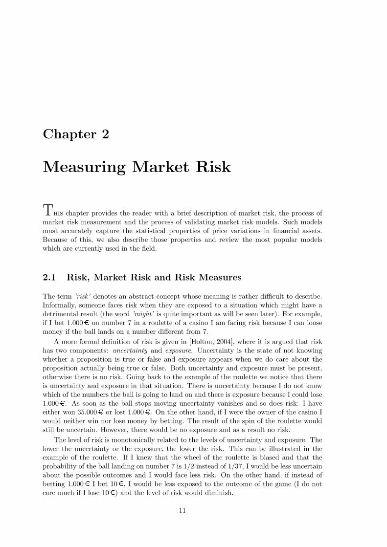
From a statistical perspective, the risk profile of a given situation can be analyzed interms of the probability distribution of its possible outcomes. This distribution containsall the information about the uncertainty and the exposure that the situation involves. Forinstance, in the case of market risk, the distribution of profits at the selected time horizonτ would be sufficient to completely characterize the risk exposure of our investment. Asan example, Figure 2.1 shows the profit distributions for holding 1.000� of two imaginaryfinancial assets for a time horizon τ = 1 year. These distributions completely characterizethe uncertainty and exposure implied by holding one asset or the other. However, at a

2.1. RISK, MARKET RISK AND RISK MEASURES 13
first glance, it is not obvious how to determine which position involves more risk and howmuch difference in risk there is between the two positions. The reason is that distributionfunctions do not provide a quantitative measurement of risk, something that risk measuresactually do.
A risk measure is a procedure that summarizes in a single number the risk which aparticular situation involves. Because risk is completely determined by the probabilitydistribution of possible outcomes a risk measure can be seen as a map from a distributionfunction to a scalar. More formally, a risk measure is a functional ρ : D → R∪±∞, whereD is the set of all distribution functions. It is not necessary for a risk measure to make useof the whole distribution function. As a matter of fact, it can use only a segment of thedistribution, for instance a fixed fraction of the worst or best outcomes.
In finance the most common general risk measures are the standard deviation, Valueat Risk and the more recently proposed Expected Shortfall [Dowd, 2005].
• Standard Deviation. This is the risk measure used in modern portfolio theory[Markowitz, 1991]. For a given distribution P its functional form is
ρsd(P) =
√
∫ ∞
−∞
x2 dP(x) −(∫ ∞
−∞
x dP(x)
)2
. (2.1)
The main disadvantage of the standard deviation as a risk measure is that it willgenerally fail to accurately quantify risk when P is not Gaussian. Interestingly, thisis precisely the case in many of the situations found in finance.
• Value at Risk (VaR). It is defined as the worst result within the α fraction of bestresults where α is usually high, 0.95 or 0.99 for example. Intuitively, the Value atRisk can be considered as the worst expected result within a probability level α. Itsfunctional form is defined as
ρV aR(P) = −P−1(1− α) . (2.2)
The minus sign is included because P−1(1 − α) is usually negative. Thus, the Valueat Risk is a positive number that corresponds to a loss. The main limitation of VaR isthat it provides no information about how bad things can get outside the α fraction ofbest results. In this way, two situations might have the same VaR, so that apparentlythey have the same risk exposure, and yet one could actually be riskier than theother.
• Expected Shortfall (ES). Also called conditional VaR, it attempts to address someof the deficiencies of Value at Risk. The Expected Shortfall for a level α (0.95 or 0.99for example) can be defined as the average result obtained when the result is worsethan the Value at Risk for the α fraction of best results. Its functional form is
ρES(P) = − 1
1− α
∫ P−1(1−α)
−∞
x dP(x) (2.3)
which, likewise Value at Risk, is a positive quantity representing a loss.
14 CHAPTER 2. MEASURING MARKET RISK
−1000 −500 0 500 1000
0.00
00.
001
0.00
20.
003
0.00
4
Profit
Den
sity
Density for profit on asset 1Density for profit on asset 2
Figure 2.1: Density functions for one-year-profits obtained after investing 1.000� in eachof two imaginary assets. The distribution for the profits is lognormal so that the highestpossible loss is 1.000�.
With the help of a risk measure it is possible to quantify the risk associated withinvestments in the assets displayed in Figure 2.1. For example, if we fix the level α = 0.95and compute the VaR for holding 1.000� of asset 1 and for holding 1.000� of asset 2 weobtain the values 151� and 208�. Informally, we can say that asset 2 is 57� riskier thanasset 1 and that if things get really bad we can expect to loose 151� if we invest in asset 1and 208� if we invest in asset 2. More formally, this means that there is a 0.05 probabilityof loosing more than 151� if we invest in asset 1 and at least 208� if we invest in asset 2.Finally, we can conclude that asset 2 is riskier than asset 1 according to the employed riskmeasure.
2.1.3 Coherent Risk Measures
In [Artzner et al., 1999] it is postulated a set of axioms which a risk measure ρ shouldfulfill in order to be considered coherent for quantifying financial risk (any risk associatedwith the loss of money, like market risk). The axioms are common-sense rules designed toavoid awkward outcomes when dealing with risk in finance. For example, if the profit forportfolio A is always bigger than the profit for portfolio B we would expect B to be riskierthan A. We would also expect diversification to decrease risk, remember the age-old saying”do not put all your eggs in only one basket”.
The set of coherent axioms is
1. Translation Invariance. If X ∼ P denotes the profit of a portfolio at some horizonin the future, and Y = X + α, Y ∼ Q where α is some fixed amount (positive ornegative) of monetary units, then ρ(Q) = ρ(P) + α.
2. Positive Homogeneity. If X ∼ P denotes the profit of a portfolio at some horizonin the future, and Y = αX, Y ∼ Q where α > 0, then ρ(Q) = αρ(P).

2.1. RISK, MARKET RISK AND RISK MEASURES 15
3. Monotonicity. If P and Q are the profit distributions for two portfolios A and Bat some horizon in the future and the profits for portfolio A are always higher thanthose for portfolio B, then ρ(P) ≤ ρ(Q).
4. Subadditivity . If P and Q are the profit distributions for two portfolios A and Bat some horizon and U is the profit distribution for the portfolio A ∪ B at the samehorizon, then ρ(U) ≤ ρ(P) + ρ(Q). It reflects the fact that due to diversificationeffects the risk for holding two portfolios is less (or at least the same) than the sumof the risks for holding each portfolio separately.
From the three risk measures previously seen only Expected Shortfall is a coherent riskmeasure. Specifically, Standard Deviation clearly fails axioms 1 and 3 and Value at Riskfails axiom 4. It is quite obvious to see why Standard Deviation is not coherent. For Valueat Risk, we can prove it is not subadditive with a counter-example where it violates thatcondition [Dowd, 2005]. Let us consider the following example:
We have two financial assets A and B. After one year, each of them can yielda loss of 100� with probability 0.04 and a loss of 0� otherwise. The 0.95 VaRfor each asset is therefore 0, so that VaR(A) = VaR(B) = VaR(A) + VaR(B)= 0�. Now suppose that losses are independent and consider the portfoliothat results from holding asset A and B. Then, we obtain a loss of 0� withprobability 0.962 = 0.9216, a loss of 200� with probability 0.042 = 0.0016, anda loss of 100� with probability 1−0.9216−0.0016 = 0.0768. Hence, VaR(A∪B)= 100� > 0 = VaR(A) + VaR(B), and the VaR violates subadditivity.
Standard Deviation and Value at Risk are therefore undesirable risk measures for quan-tifying market risk. However, these two risk measures are still being widely used becauseof their simplicity and the success of many portfolio optimization applications and riskmanagement systems (e.g. RiskMetrics
TM
[Morgan, 1996]) which employ them.
2.1.4 Estimating Market Risk Measures
We have already seen in Section 2.1.2 that the exposure to market risk of a portfolio can beeasily quantified by means of a risk measure. The only requirement is that the future profitdistribution of the portfolio for a given time horizon must be available. However, if the effi-cient market hypothesis [Fama, 1970] is taken to be true, such distribution will not generallybe known. This is so because the source of future price changes is future information whosestatistical properties might be time-dependent, having some degree of randomness. Theusual approach to tackle the problem consists in assuming that the distribution of futureprice changes will be related to that of recent past price changes. In this way, machine learn-ing and pattern recognition techniques [Bishop, 2006, MacKay, 2003, Duda et al., 2000] canbe used to make inference about the statistical properties of future prices. The general pro-cess involves choosing a probabilistic model that captures the properties of financial timeseries (series of market prices). The parameters of such model are fixed by a fit to recenthistorical data (e.g. by maximum likelihood) and then the model is used to infer the dis-tribution of future price changes. However, financial time series show complex propertiesand obtaining a good model that can accurately describe the process of price changing infinancial assets is generally a very challenging task.

16 CHAPTER 2. MEASURING MARKET RISK
2.2 Properties of Price Variations and Time Series Models
This section introduces a set of empirical properties observed in price variations within var-ious types of financial markets and a large set of different financial assets. These propertiescan be seen as constraints that a probabilistic model should fulfill in order to accuratelycapture the process of price variation. It turns out that such properties are very demandingand most of the currently existing models fail to reproduce them [Cont, 2001].
2.2.1 Financial Returns
Let Pt denote the price for a financial asset at date t. In general, financial models focuson returns instead of prices for several reasons [Campbell et al., 1997, Dowd, 2005]. First,returns are a complete and scale-free free summary of profits and losses. Second, returnshave theoretical and empirical properties which make them more attractive than prices.Third, if we have a probabilistic model for returns it is straightforward to obtain a prob-abilistic model for prices or profits. The net return, Rt, on the asset between dates t − 1and t is defined as
Rt =Pt
Pt−1− 1 . (2.4)
The net return over the most recent k periods from date t− k to date t is simply
Rt(k) = (Rt−1 + 1) · (Rt−2 + 1) · (Rt−3 + 1) · · · (Rt−k+1 + 1)− 1 , (2.5)
where this multiperiod return is called compound return. The difficulty manipulating seriesof products like 2.5 motivates another approach to calculate compound returns. This is theconcept of continuous compounding. The continuously compounded return or logarithmicreturn rt between dates t− 1 and t is defined as
rt = log(1 +Rt) = logPt
Pt−1= log(Pt)− log(Pt−1) (2.6)
and is very similar in value to the corresponding net return Rt because rt = log(1+Rt) ≃ Rt
for small values of Rt in absolute value. Continuously compounded returns implicitlyassume that the temporary profits are continuously reinvested. Furthermore, they aremore economically meaningful than net returns because they ensure that the asset pricecan never become negative no matter how negative the return could be. However, the mainadvantage of logarithmic returns becomes clear when we calculate multiperiod returns
rt(k) = log(1 +Rt(k)) = rt−1 + rt−2 + rt−3 + · · ·+ rt−k+1 , (2.7)
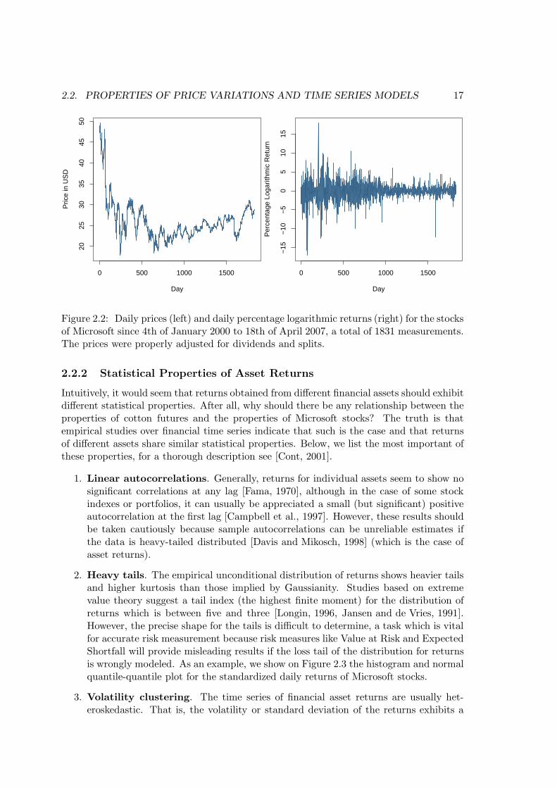
which allows to model the change in price as an additive process. As an example, we showon Figure 2.2 the time series of daily prices (properly adjusted for dividends and splits)and daily percentage logarithmic returns (100 times the logarithmic returns) for the stocksof Microsoft since 4th of January 2000 to 18th of April 2007, a total of 1831 measure-ments. Because of their multiple advantages we will focus on the statistical properties ofcontinuously compounded returns and from now on the term ’return’ will always refer tologarithmic return.
2.2. PROPERTIES OF PRICE VARIATIONS AND TIME SERIES MODELS 17
0 500 1000 1500
2025
3035
4045
50
Day
Pric
e in
US
D
0 500 1000 1500−
15−
10−
50
510
15Day
Per
cent
age
Loga
rithm
ic R
etur
n
Figure 2.2: Daily prices (left) and daily percentage logarithmic returns (right) for the stocksof Microsoft since 4th of January 2000 to 18th of April 2007, a total of 1831 measurements.The prices were properly adjusted for dividends and splits.
2.2.2 Statistical Properties of Asset Returns
Intuitively, it would seem that returns obtained from different financial assets should exhibitdifferent statistical properties. After all, why should there be any relationship between theproperties of cotton futures and the properties of Microsoft stocks? The truth is thatempirical studies over financial time series indicate that such is the case and that returnsof different assets share similar statistical properties. Below, we list the most important ofthese properties, for a thorough description see [Cont, 2001].
1. Linear autocorrelations. Generally, returns for individual assets seem to show nosignificant correlations at any lag [Fama, 1970], although in the case of some stockindexes or portfolios, it can usually be appreciated a small (but significant) positiveautocorrelation at the first lag [Campbell et al., 1997]. However, these results shouldbe taken cautiously because sample autocorrelations can be unreliable estimates ifthe data is heavy-tailed distributed [Davis and Mikosch, 1998] (which is the case ofasset returns).
2. Heavy tails. The empirical unconditional distribution of returns shows heavier tailsand higher kurtosis than those implied by Gaussianity. Studies based on extremevalue theory suggest a tail index (the highest finite moment) for the distribution ofreturns which is between five and three [Longin, 1996, Jansen and de Vries, 1991].However, the precise shape for the tails is difficult to determine, a task which is vitalfor accurate risk measurement because risk measures like Value at Risk and ExpectedShortfall will provide misleading results if the loss tail of the distribution for returnsis wrongly modeled. As an example, we show on Figure 2.3 the histogram and normalquantile-quantile plot for the standardized daily returns of Microsoft stocks.
3. Volatility clustering. The time series of financial asset returns are usually het-eroskedastic. That is, the volatility or standard deviation of the returns exhibits a

18 CHAPTER 2. MEASURING MARKET RISK
Histogram
Normalized Return
Den
sity
−5 0 5
0.0
0.1
0.2
0.3
0.4
0.5
−3 −2 −1 0 1 2 3
−5
05
Normal Q−Q Plot
Theoretical QuantilesS
ampl
e Q
uant
iles
Figure 2.3: Left, histogram for the standardized daily returns of Microsoft stocks andstandard Gaussian density. It is noticeable the higher kurtosis of the empirical densityfor the returns. Right, normal quantile-quantile plot for the standardized daily returns ofMicrosoft stocks. It can be appreciated how the tails of the empirical density are heavierthan those of a standard normal distribution.
0.5 1.0 1.5 2.0 2.5 3.0
0.00
0.05
0.10
0.15
0.20
0.25
Taylor Effect
Exponent Delta
auto
corr
elat
ion
0 20 40 60 80 100
0.0
0.2
0.4
0.6
0.8
1.0
Lag
AC
F
Series of Absolute Returns
Figure 2.4: Left, Taylor effect plot for the returns of Microsoft stocks where it is shownthe autocorrelation function between |rt|δ and |rt+h|δ for h ∈ {1, ..., 10}. Each curve corre-sponds to a different value of h = 1, 2, . . . , 10 and the maximum of each function is shownwith a cross. Right, autocorrelations between |rt| and |rt+h| where h = 1, 2, . . . , 100 forMicrosoft stocks.

2.2. PROPERTIES OF PRICE VARIATIONS AND TIME SERIES MODELS 19
time-dependent structure. Volatility clustering implies that large price variations (ei-ther positive or negative) are likely to be followed by price variations that are alsolarge. This phenomenon is evidenced by a plot of the autocorrelations in the powersof the absolute values of returns
Cδ = corr(|rt+h|δ, |rt|δ), h = 1, 2, . . . (2.8)
These correlations are positive for various delays in the range of weeks to months (seeFigure 2.4) and the highest values are usually achieved for δ around 1 [Ding et al., 1993].This behavior is known as the Taylor effect and is displayed on the left of Figure 2.4for the returns of Microsoft stocks.
2.2.3 Time Series Models for Asset Returns
Probably, the most successful models to account for the time-dependent volatility in finan-cial time series are GARCH processes [Bollerslev, 1986, Hamilton, 1994] and particularlythe GARCH(1,1) process. We say that a time series {rt}Tt=1 follows a GARCH(1,1) processwith normal innovations if
rt = σtεt (2.9)
σ2t = γ + α|rt−1|2 + βσ2
t−1 , (2.10)
where γ > 0, α ≥ 0, β ≥ 0, α + β < 1 and the innovations εt ∼ N (0, 1) are distributedaccording to a standard normal distribution. The condition α+ β < 1 guarantees that thetime series generated by the model has finite variance and the parameters α and β representrespectively the degree of surprise and the degree of correlation in the volatility process.The parameter γ allows to model the volatility as a mean-reverting process with expectedvalue γ/(1 − α − β). All the parameters are usually fixed by performing a constrainedmaximum likelihood optimization conditioning to r0 and σ0. Finally, because of theirsimplicity, there exist closed form expressions for the forecasts of GARCH(1,1) processesat any time horizon [Dowd, 2005]. However, Monte Carlo methods could be used to obtainforecasts if the complexity of the model was increased.
On the left of Figure 2.5 we show the returns for Microsoft stocks and two times thevolatility estimated by a GARCH(1,1) process. It can be appreciated how the GARCHprocess captures quite accurately the clusters of high and low volatility. On the right ofFigure 2.5 it is also displayed a plot with the autocorrelations of the absolute values of thestandardized returns. It is noticeable how the correlation present on the right of Figure 2.4has now vanished.
Even though in a GARCH(1,1) process the conditional distribution for rt given σt
is Gaussian as noticed from (2.9), the marginal distribution for rt will generally showheavy tails [Mikosch and Starica, 2000] due to the stochastic process followed by the time-dependent volatility (2.10). In this way, GARCH processes with normal innovations could,in principle, account for both the time-dependent volatility and the heavy tails of financialreturns. However, empirical studies show that after correcting the returns for volatilityclustering (standardizing the returns with the volatility estimated by a GARCH process)the residual time series still exhibits heavy tails [Bollerslev, 1987]. This fact, which canbe appreciated on Figure 2.6 for the returns of Microsoft stocks, is due to the failure ofGARCH models to describe the volatility process accurately enough [Andersen et al., 2003,

20 CHAPTER 2. MEASURING MARKET RISK
0 500 1000 1500
−15
−10
−5
05
1015
Series and 2 Coditional SD superimposed
Day
Ret
urn
0 5 10 15 20 25 30
0.0
0.2
0.4
0.6
0.8
1.0
LagA
CF
Series of Standardized Absolute Returns
Figure 2.5: Left, Time series with the returns of Microsoft stocks and two times thestandard deviation estimated by a GARCH(1,1) model. Right, autocorrelations between|rt|/σt and |rt+h|/σt+h where h = 1, 2, . . . , 20 for Microsoft stocks. A GARCH(1,1) processwas used to estimate the volatility process σt.
Forsberg, 2002] (in part because |rt−1|2 is a bad proxy for estimating past volatility). Tosolve the problem a wide variety of volatility models similar to GARCH processes butwith non-Gaussian heavy-tailed innovations were suggested. Some examples are modelswith innovations that follow Student distributions [Bollerslev, 1987], stable distributions[Panorska et al., 1995] [Mittnik and Paolella, 2003], normal inverse Gaussian distributions[Forsberg, 2002, Forsberg and Bollerslev, 2002] or the generalized hyperbolic distribution[Prause, 1999].
Other models which show more complexity than GARCH processes have also beenused to describe financial time series. They are generally based on different paradigmsof machine learning techniques [Bishop, 2006] like input output hidden Markov models[Bengio et al., 2001], mixtures of experts [Suarez, 2002, Vidal and Suarez, 2003] or neuralnetworks [Franke and Diagne, 2006, Weigend and Huberman, 1990]. Nonetheless, becauseof their higher complexity, the training process for such models is more difficult.
2.3 Backtesting Market Risk Models
Once a probabilistic model for the price of an asset is available it is necessary to validatethe model for market risk estimation before putting it into practical use. We might as wellwant to compare different models to determine which is the best for estimating marketrisk. Those two tasks can be achieved by means of backtesting, which is the applicationof quantitative methods to determine whether the risk forecasts of a model are consistentwith empirical observations [Dowd, 2005].
The general backtesting process is based on a standard hypothesis testing paradigmwhere the null hypothesis states that the model is consistent with the data. A statistic

2.3. BACKTESTING MARKET RISK MODELS 21
−10 −5 0 5
0.0
0.1
0.2
0.3
0.4
0.5
Standardized returns
Return
Den
sity
−3 −2 −1 0 1 2 3−
10−
50
5
Normal Q−Q Plot
Theoretical Quantiles
Sam
ple
Qua
ntile
s
Figure 2.6: Left, kernel density estimate for the returns of Microsoft stocks standardizedusing the volatility estimated by a GARCH(1,1) model (in black with dots) and stan-dard Gaussian density (in red). It can be appreciated the higher kurtosis of the kernelestimate. Right, normal quantile-quantile plot for the same standardized returns. Thetails are still heavier than those of a normal distribution and a Kolmogorov-Smirnov test[Papoulis and Pillai, 2002] rejects the normality hypothesis with a p-value of 2.747 · 10−05.
can be computed using the specification of the model (with its parameters fitted to sometraining data) and some empirical observations (test data different from the data usedto fit the model). Such statistic should follow a fixed distribution (standard Gaussian orBernoulli for example) under the null hypothesis and several of those statistics are usuallyobtained using different sets of training and test data. Finally, it is checked whether afunction of the obtained statistics lays within some confidence interval of its distribution(with a fixed probability like 0.95, e.g. [−1.959, 1.959] for the standard Gaussian) or not.In the latter case the model is rejected.
The backtesting process is generally performed throughout a sliding-window experi-ment. The time series of returns for a financial asset is split in overlapping windows offixed size where each window is equal to the previous one moved forward one unit in time.The model is trained with the data from each window and then tested on the first returnout of the window in order to generate one of the mentioned statistics. Below we describeseveral backtesting procedures with different ability to identify wrong models.
2.3.1 Test of Exceedances
The testing procedure suggested by [Kupiec, 1995] is probably the most widely used methodto validate risk models. This technique is also at the core of the backtesting procedure usedby the Bank for International Settlements for determining multiplication factors for capitalrequirements [Bas, 1996]. The main idea of Kupiec’s method consists in checking whetherthe observed frequency of losses that exceed the α-VaR is consistent with the theoreticalfrequency 1 − α. In this way, if our model predicts a VaR at the 0.95 level of 1.000� for

22 CHAPTER 2. MEASURING MARKET RISK
the next day, we would expect to lose more than 1.000� with a probability 0.05 on suchday.
In the sliding-window framework mentioned before, each statistic would be a variablethat takes value 1 if the first return out of the window exceeds the α-VaR and 0 otherwise.Under the null hypothesis, the sum x of n of such statistics follows the binomial distribution
B(x|n, α) =
x∑
i=0
(
ni
)
(1− α)iαn−i . (2.11)
The model is rejected if the value x lies outside a confidence interval of distribution (2.11)(e.g. [B−1(0.025|n, α),B−1(0.975|n, α)] for a significance level of 0.05). The main advantageof the test of exedancees is its simplicity. However, the test lacks power or ability to rejectwrong models [Dowd, 2005]. This is so because it throws away valuable information likethe sizes of the exceedances or their temporal pattern (exeedances should be independent).
2.3.2 General Tests Based on The Berkowitz Transformation
A more powerful test would be to verify that observed returns follow the distribution thatour model predicts. This way, in the sliding-window framework, we would like to checkthat the first return ri out of the ith window follows the distribution Pi predicted byour model (fitted to the data within the ith window), i = 1, . . . , n. The main troubleis that for each window i there is a different predictive distribution Pi and for each ofsuch distributions there is only a single observation ri, where ri ∼ Pi under the nullhypothesis. The solution to the problem is described in [Berkowitz, 2001] and consistsin performing the transformation Φ−1(Pi(ri)) of the returns, where Φ−1 is the inverse ofthe cumulative standard Gaussian distribution. As a result, under the null hypothesis wehave that ri = Φ−1(Pi(ri)) ∼ N (0, 1) and we end up with n points {ri}ni=1 that should bestandard normal distributed if the forecasts Pi of our model are right.
Applying the Berkowitz transformation we can now make use of any test for normalityover {ri}ni=1 to validate the accuracy of our model. Some of the most well-known examples ofsuch tests are the Kolmogorov-Smirnov [Papoulis and Pillai, 2002], the Anderson-Darling[Anderson and Darling, 1954], the Jarque-Bera [Jarque and Bera, 1987] or the Shapiro-Wilk [Shapiro and Wilk, 1965] tests.
2.3.3 Specialized Tests Based on The Functional Delta Method
The tests described in the previous section can be a wrong choice if we are only interestedin verifying that the risk measures estimated by our model are right. For example, I wouldnot mind if Pi is wrong as long as ρES(Pi) is accurate enough. Such a situation canhappen if the loss tail of Pi is correct but the rest of the distribution is wrongly modeled.The statistical tests described in [Kerkhof and Melenberg, 2004] allows us to determine theaccuracy of a model for specifically estimating Value at Risk or Expected Shortfall. Thosetests relay on the fact that the Berkowitz transformation is a monotonically increasingfunction and therefore it maps quantiles from one distribution to another1. This propertycreates a direct link between the deviations from normality of the empirical distribution Qn
for {ri}ni=1 and the deviations of the estimates {Pi}ni=1 from the real unknown distributions
1Note that the Value at Risk and the Expected Shortfall for a distribution P can be interpreted asfunctions of the quantiles of P [Dowd, 2005].

2.3. BACKTESTING MARKET RISK MODELS 23
for {ri}ni=1. For example, if the left tail of Qn is similar to the left tail of N (0, 1) it wouldmean that the left tails of the estimate distributions {Pi}ni=1 are right. The conclusion isthat, for a risk measure ρ, the difference between ρ(Qn) and ρ(N (0, 1)) is related to theaccuracy of the model for estimating such risk measure.
The functional delta method [Vaart, 2000] is the mathematical tool that will allow us todetermine whether the difference between ρ(Qn) and ρ(N (0, 1)) is statistically significantor not, if it is too big we will reject the null hypothesis (that our model is an accuratetool for estimating risk by means of the measure ρ). If Qn = n−1
∑ni=1 δri
is the empiricaldistribution (here δx is the step function centered at x) of a sample {ri}i=n
i=1 such thatri ∼ Q, i = 1, . . . , n and ρ is a functional which is Hadamard differentiable, then thefunctional delta method states that
√n(ρ(Qn)− ρ(Q)) ≈ ρ′Q(
√n(Qn −Q)) ≈ √n 1
n
n∑
i=1
ρ′Q(δri−Q) , (2.12)
where the function x 7→ ρ′Q(δx − Q) is the influence function of the functional ρ. Thisinfluence function can be computed as
ρ′Q(δx −Q) = limt→0
d
dtρ((1 − t)Q+ tδx) (2.13)
and measures the change in ρ(Q) if an infinitesimally small part of Q is replaced by apoint mass at x. In the last step of expression (2.12) we have made use of the linearityproperty of the influence function. The quantity ρ(Qn) − ρ(Q) behaves as an average ofindependent random variables ρ′Q(δri
−Q) which are known to have zero mean and finitesecond moments. Therefore, the central limit theorem states that
√n(ρ(Qn − Q)) has a
normal limit distribution with mean 0 and variance Ex[ρ′Q(δx −Q)2] where
Ex[ρ′Q(δx −Q)2] =
∫
ρ′Q(δx −Q)2 dQ(x) (2.14)
We can then use the statistic
Sn =
√n(ρ(Qn)− ρ(Q))√
Ex[ρ′Q(δx −Q)2]
d−→ N (0, 1) (2.15)
to determine if the difference ρ(Qn)− ρ(Q) is statistically significant or not.In [Kerkhof and Melenberg, 2004] it is proved that ρV aR and ρES are Hadamard differ-
entiable [Vaart, 2000] and if Q is standard Gaussian it is easy to show that
Ex[ρ′V aR,Q(δx −Q)2] =α(1 − α)
φ(Φ(1− α))2(2.16)
Ex[ρ′ES,Q(δx −Q)2] =
−Φ(1− α)φ(Φ(1 − α)) + 1− α(1− α)2
− φ(Φ(1 − α))
(1− α)2
2
+
Φ(1− α)2α
1− α + 2Φ(1− α)φ(Φ(1 − α))
1− αα
1− α , (2.17)
where Φ and φ are respectively the standard Gaussian distribution and density functionsand the value α represents the fraction of best results used to compute the Value at Riskand the Expected Shortfall.

24 CHAPTER 2. MEASURING MARKET RISK
We point out that it is possible to implement the test of Exceedances described by[Kupiec, 1995] utilizing the functional delta method. We just have to make use of thefunctional
ρExc(Q) =
∫ ∞
−∞
(
n∑
t=1
I(−∞,V ](y)
)
dQ(y) , (2.18)
which represents the average number of elements smaller than the constant V in a sample{xi}ni=1 from distribution Q (this is, xi ∼ Q, 1 ≤ i ≤ n). If we let V = Q−1(1 − α) thisfunctional allows us to implement the binomial test for exceedances over the Value at Riskfor the α fraction of best results. We just have to calculate the value Ex[ρ
′Exc,Q(δx −Q)2]
which turns out to be
Ex[ρ′Exc,Q(δx −Q)2] = (1− α)αn2 . (2.19)
Finally, in [Kerkhof and Melenberg, 2004] it is performed a complete study which com-pares the power of the tests for Value at Risk, Expected Shortfall and Exceedances. Theresults indicate that the most powerful test is the one for Expected Shortfall.

Chapter 3
Competitive & Collaborative
Mixtures of Experts
This chapter is mainly based on [Hernandez-Lobato and Suarez, 2006]. We comparethe performance of competitive and collaborative strategies for mixtures of autoregressiveexperts with normal innovations for conditional risk measurement in financial time series.The prediction of the mixture of collaborating experts is an average of the outputs of theexperts. In a competitive mixture the prediction is generated by a single expert. The expertthat becomes activated is selected either deterministically (hard competition) or at random,with a certain probability (soft competition). The different strategies are compared in asliding window experiment for the time series of log-returns of the Spanish stock indexIBEX 35, which is preprocessed to account for its heteroskedasticity. Experiments indicatethat the best performance for risk estimation is obtained by mixtures with soft competition.
3.1 Introduction
Machine learning and pattern recognition [Bishop, 2006] mainly deal with the problem oflearning from examples. This is, given a sample of n paired observations {xi,yi}ni=1 and anew example xn+1 whose paired component is unknown, we are requested to determine aprobability distribution for yn+1. In order to solve the problem such distribution must apriori be restricted in some way. Otherwise, the set of plausible values for yn+1 would betoo big and their distribution would be non-informative. We restrict that distribution bymeans of a probabilistic modelM (e.g. a neural network or a decision tree) that capturesthe relationship between {xi,yi} for any i. In this way, the frequentist solution to thelearning problem is P(yn+1|xn+1,M) where the parameters of M have been fixed with{xi,yi}ni=1 (by maximum likelihood for example). We previously saw in Chapter 2 that inthe context of measuring market risk we are given a time series of returns {rt}nt=1 from afinancial asset and we have to determine the distribution P(rt+1|{rt}nt=1). This is a clearproblem where we have to learn from examples and therefore machine learning techniquescan be used here.
The mixture of experts paradigm [Jacobs et al., 1991] represents an application of thedivide-and-conquer principle to the field of machine learning. The idea consists in buildinga complex model called mixture by means of several simpler models called experts. The
25

26 CHAPTER 3. COMPETITIVE & COLLABORATIVE MIXTURES OF EXPERTS
Expert 1 Expert n
Gating
Network
Output
Input
Act. 1
Act. n
Mixture Model
Figure 3.1: Architecture of a mixture of experts model. The input to the whole system isalso the input to each expert and to the gating network. The gating network determinesfor each expert the probability of being activated. The output of the system is the outputof the single expert which turns out to be activated.
input space to the mixture is divided into as many different regions as individual experts.A gating network performs this task in such a way that the boundaries between regions aresoft (data points can belong to different regions with different probabilities). Each of theindividual experts specially focuses on one of the regions and the output of the whole systemis generated by the expert whose corresponding region is stochastically selected. We displaythe whole architecture of a mixture of experts on Figure 3.1 and we show the output of agating network on Figure 3.2. The general procedure followed in order to train a mixtureof experts is maximum likelihood. The Expectation Maximization algorithm with iterativereweighted least squares being employed in the M step [Bishop, 2006] can be used for suchtask if the experts and the gating network are generalized linear [Jordan and Jacobs, 1994].Hierarchical mixtures of experts [Jordan and Jacobs, 1994] can be obtained if the individualexperts are also mixture models. Finally, a fully Bayesian treatment of the hierarchicalmixtures of experts architecture is described in [Bishop and Svensen, 2003].
Model complexity is an important factor to take into account while designing a mixtureof experts. In machine learning, the frequentist view point to model complexity is knownas the bias-variance trade-off [Bishop, 2006] which states that the error of a model can bedecomposed into the sum of its bias and its variance. It turns out that simple and rigidmodels have high bias and low variance and flexible and complex models have lower bias buthigher variance. This is the reason why very complex models have a worse generalizationerror and tend to overfit the training data. In a mixture of experts we can keep down

3.1. INTRODUCTION 27
−5 0 5
0.0
0.2
0.4
0.6
0.8
1.0
Input
Act
ivat
ion
Pro
babi
lity
Figure 3.2: Activation probabilities generated by the gating network in a mixture of threeexperts. It can be appreciated how the input to the mixture is split into three soft regions.The green expert is more likely to be activated when the input is less than −2.5, the blueexpert when the input is between −2.5 and 2.5 and the red expert when the input is greaterthan 2.5. The gating network was generalized linear, a single-layer neural network with asoftmax [Bishop, 1995] activation function in the three output units.
complexity by reducing the number of experts in the mixture and by choosing simplemodels for the experts and the gating network (e.g. generalized linear models).
Mixtures of two GARCH processes with autoregressive components were successfullyimplemented in [Suarez, 2002] to account for correlations, extreme events (heavy tails) andheteroskedasticity (time-dependent variance) in financial time series. Hierarchical mixturesof up to three autoregressive processes were also applied to the analysis of financial time se-ries in [Vidal and Suarez, 2003]. In both of the previous works the experts worked togetherfollowing a soft competitive strategy as suggested in [Jacobs et al., 1991]. Soft competitionimplies that, for a fixed input, any expert can be stochastically selected for generating theoutput of the mixture. Nevertheless, there exist other possible strategies like hard compe-tition (winner-take-all) [Jacobs et al., 1993] or collaboration. A hard competitive strategyrequires that, for a fixed input, the output of the mixture is always generated by a singleexpert which is deterministically selected. On the other hand, collaboration implies thatthe output of the mixture is a weighted average of the output of each expert.
In this chapter we perform an exhaustive study among mixtures of autoregressive ex-perts that employ collaborative, soft competitive and hard competitive strategies. Theability of the mixtures to accurately estimate market risk using different risk measures isevaluated. For this purpose we carry out a sliding-window experiment over the time seriesof returns for the Spanish stock index IBEX-35, where the series is specially preprocessedto account for its heteroskedasticity. Finally, we make use of the statistical tests describedin Section 2.3 to discriminate among the different models.

28 CHAPTER 3. COMPETITIVE & COLLABORATIVE MIXTURES OF EXPERTS
3.2 Financial Time Series Models
The future prices of a financial asset that is freely traded in an ideal market are unpre-dictable. By arguments of market efficiency any expectations on the future evolution ofthe asset value should be immediately reflected in the current price. Hence, the time seriesof asset prices follows a stochastic process, where the variations correspond to new unex-pected information being incorporated into the market price. We previously mentioned inSection 2.2.1 that, instead of modelling the time series of prices {St}Tt=0, it is common towork with the quasi-stationary series of returns {Xt}Tt=1. This latter series can be obtainedby log-differencing the series of prices, namely
Xt = logSt − logSt−1 = logSt
St−1, 1 ≤ t ≤ T. (3.1)
Before formulating a model based on mixtures of autoregressive experts for the seriesof returns, we perform a transformation to take into account its heteroskedastic structure.We previously described in Section 2.2.3 that GARCH(1,1) processes are among the mostsuccessful models for describing the time-dependent structure of volatility in financial timeseries. If the time series {Xt}Tt=1 with mean µ follows a GARCH(1,1) model, then
Xt = µ+ σtεt
σ2t = γ + α(Xt−1 − µ)2 + βσ2
t−1 , (3.2)
where {εt}Tt=1 are iidrv’s generated by a N (0, 1) distribution and the parameters γ, α andβ satisfy the constraints γ > 0, α ≥ 0, β ≥ 0 and α + β < 1. Assuming that the timeseries of returns approximately follows a GARCH(1,1) process, it is then possible to obtaina homoskedastic time series {Zt}Tt=1 by performing the normalization
Zt =Xt − µσt
, 1 ≤ t ≤ T, (3.3)
where σt follows equation (3.2). The parameters µ, γ, α and β are estimated by maximizingthe conditional likelihood of the GARCH(1,1) process to the series {Xt}Tt=1.
Note that the GARCH process is not being trained in an optimal way. In particularthe residuals {εt}Tt=1 are not independent and their distribution is leptokurtic (peaked andheavy-tailed). Nonetheless, given that the deviations from independence and normalityare small, the variance σ2
t estimated under the hypothesis of normal independent residualsshould be a good approximation to the actual variance of the process.
On the left column, Fig. 3.3 displays the graph and autocorrelations of the time seriesof returns of the Spanish stock index IBEX 35 and, on the right column, the correspondingplots for the normalized time series (3.3). The features of this series are representative oftypical time series of financial portfolio returns. The presence of medium-term correlationsfor the absolute values of the returns {Xt}Tt=1 is a clear mark of heteroskedasticity. Theseautocorrelations are not present in the normalized series {Zt}Tt=1, which appears to behomoskedastic. We now focus on the sample autocorrelations of the normalized returns{Zt}Tt=1 which appear on the bottom-right of Fig. 3.3. It is quite apparent that there is asmall but non-negligible correlation at the first lag which could be modeled by a first orderautoregressive process [Hamilton, 1994] so that
Zt = φ0 + φ1Zt−1 + σεt (3.4)

3.3. MIXTURES OF AUTOREGRESSIVE EXPERTS 29
0 1000 2000 3000 4000
−10
0
10
Daily percentage returns for IBEX−35 andfour times standard deviation
0 1000 2000 3000 4000
−10
−5
0
5
Normalized series
0 5 10 15 20−0.5
0
0.5
1
Lag
ACF absolute values log−returns IBEX−35
0 5 10 15 20−0.5
0
0.5
1
Lag
ACF absolute values normalized series
0 5 10 15 20−0.5
0
0.5
1
Lag
ACF log−returns IBEX−35
0 5 10 15 20−0.5
0
0.5
1
Lag
ACF normalized series
Figure 3.3: Daily returns (multiplied by 100) of the Spanish IBEX 35 stock index from12/29/1989 to 1/31/2006 (4034 values) provided by [Sociedad de Bolsas, 2006]. Graphs onthe left column correspond to the original series of returns (first row) and to the sampleautocorrelation functions (ACF) of the absolute values of the returns (second row) andof the returns themselves (third row). The outer lines in the top left plot correspond toµ ± 4σt, where µ and σt are obtained from a fit to a GARCH(1,1) model (3.2). On theright column it is displayed the corresponding plots for the homoskedastic series obtainedafter normalization (3.3).
where |φ1| < 1, σ > 0 and εt ∼ N (0, 1). However, this simple AR(1) process will not beable to account for the leptokurtosis in {Zt}Tt=1.
3.3 Mixtures of Autoregressive Experts
Our intention is to model the series of normalized returns {Zt}Tt=1 by a mixture of M firstorder autoregressive processes in a single level with no hierarchy [Jordan and Jacobs, 1994].
30 CHAPTER 3. COMPETITIVE & COLLABORATIVE MIXTURES OF EXPERTS
These models can be thought of as dynamical extensions of the mixture of Gaussianparadigm, which has been successfully applied to modeling the excess of kurtosis in theunconditional distribution of returns [Kon, 1984]. We intend to give an accurate and robustdescription of the conditional distribution of returns that can be used for market risk esti-mation. For this reason we evaluate the performance of the mixture models based not onlyon point predictions, but also on their capacity to model the whole distribution of returns,especially of extreme events, which are determinant for the calculation of risk measures likeValue at Risk or Expected Shortfall.
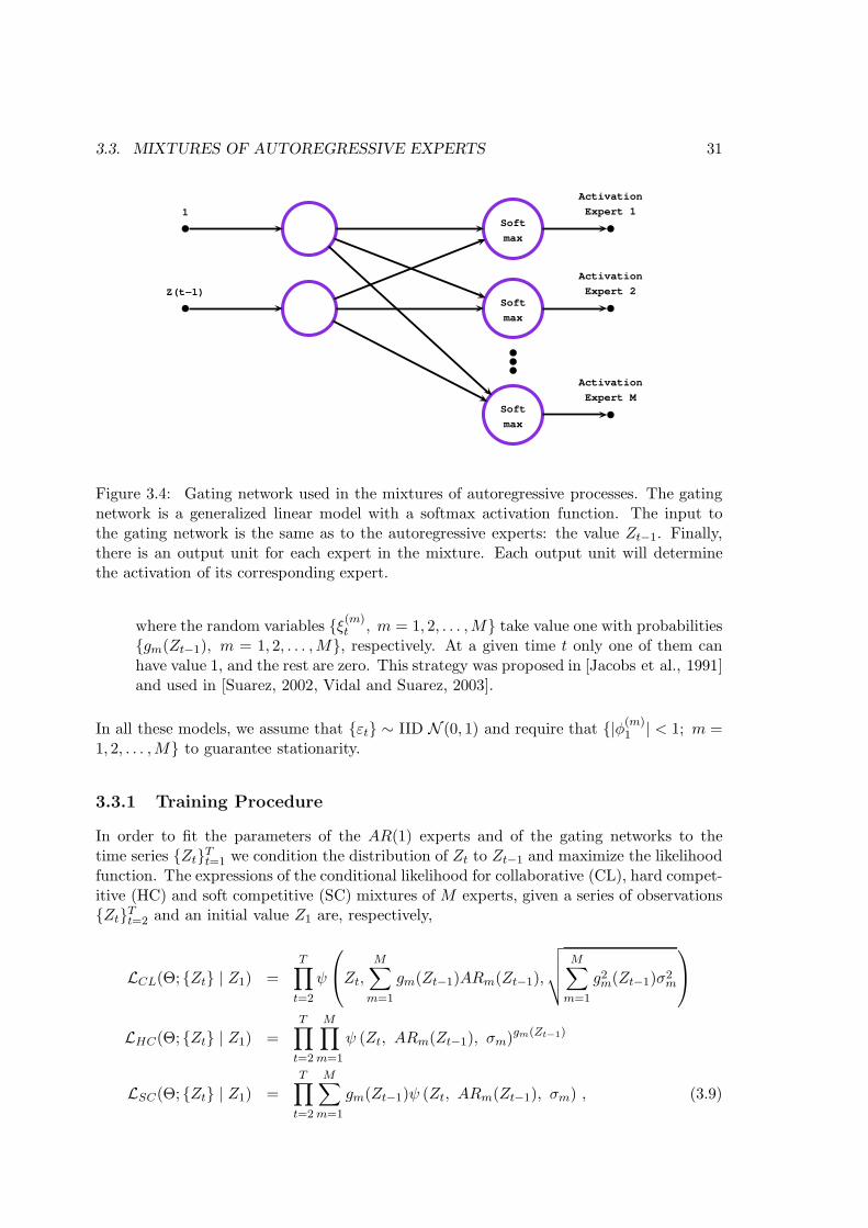
The way in which the outputs of the AR(1) experts are combined to generate a pre-diction is controlled by a gating network [Jordan and Jacobs, 1994] with a single layer, seeFig. 3.4. The input for this network is the same as the input for the experts (i.e., thedelayed value of the normalized series, Zt−1). The output layer contains as many nodesas the number of experts in the mixture. Their activation is modulated by a softmax[Bishop, 1995] function so that the outputs are within the interval [0, 1] and add up to 1.Because of these properties they can be interpreted either as activation probabilities or as
weights. In particular, if ζ(m)0 and ζ
(m)1 are the parameters of the m-th node of the gating
network, its outgoing signal is
gm(Zt−1) =exp(ζ
(m)0 + ζ
(m)1 Zt−1)
∑
j exp(ζ(j)0 + ζ
(j)1 Zt−1)
,m = 1, 2, . . . ,M. (3.5)
Let φ(m)0 , φ
(m)1 and σm be the parameters of the m-th AR(1) expert. There are different
strategies to determine how the outputs of the experts in the mixture are combined. Weconsider and compare three different paradigms: collaboration, hard competition and softcompetition.
Collaboration. The output of the mixture is a weighted average of the outputs from eachof the experts. These weights are determined by the output of the gating network.The output of the mixture is
Zt =M∑
m=1
gm(Zt−1)[
φ(m)0 + φ
(m)1 Zt−1 + σmεt
]
, (3.6)
Hard competition: Experts compete, so that only one expert is active at a given time.The output of the gating network is either 1 for m∗
t , the expert that generates theoutput, or 0 for the other experts. This strategy was proposed in [Jacobs et al., 1993]
Zt = φ(m∗
t)
0 + φ(m∗
t)
1 Zt−1 + σm∗
tεt. (3.7)
Soft competition: The output is generated by a single expert. However, in contrastto hard competition, every expert has a probability of being chosen to generate theoutput of the system. This probability is given by the output of the gating networkso that the output of the mixture is
Zt =
M∑
m=1
ξ(m)t
[
φ(m)0 + φ
(m)1 Zt−1 + σmεt
]
, (3.8)
3.3. MIXTURES OF AUTOREGRESSIVE EXPERTS 31
Soft
max
Soft
max
Soft
max
Activation
Expert 1
Activation
Expert 2
Activation
Expert M
1
Z(t−1)
Figure 3.4: Gating network used in the mixtures of autoregressive processes. The gatingnetwork is a generalized linear model with a softmax activation function. The input tothe gating network is the same as to the autoregressive experts: the value Zt−1. Finally,there is an output unit for each expert in the mixture. Each output unit will determinethe activation of its corresponding expert.
where the random variables {ξ(m)t , m = 1, 2, . . . ,M} take value one with probabilities
{gm(Zt−1), m = 1, 2, . . . ,M}, respectively. At a given time t only one of them canhave value 1, and the rest are zero. This strategy was proposed in [Jacobs et al., 1991]and used in [Suarez, 2002, Vidal and Suarez, 2003].
In all these models, we assume that {εt} ∼ IID N (0, 1) and require that {|φ(m)1 | < 1; m =
1, 2, . . . ,M} to guarantee stationarity.
3.3.1 Training Procedure
In order to fit the parameters of the AR(1) experts and of the gating networks to thetime series {Zt}Tt=1 we condition the distribution of Zt to Zt−1 and maximize the likelihoodfunction. The expressions of the conditional likelihood for collaborative (CL), hard compet-itive (HC) and soft competitive (SC) mixtures of M experts, given a series of observations{Zt}Tt=2 and an initial value Z1 are, respectively,
LCL(Θ; {Zt} | Z1) =
T∏
t=2
ψ
Zt,
M∑
m=1
gm(Zt−1)ARm(Zt−1),
√
√
√
√
M∑
m=1
g2m(Zt−1)σ2
m
LHC(Θ; {Zt} | Z1) =T∏
t=2
M∏
m=1
ψ (Zt, ARm(Zt−1), σm)gm(Zt−1)
LSC(Θ; {Zt} | Z1) =
T∏
t=2
M∑
m=1
gm(Zt−1)ψ (Zt, ARm(Zt−1), σm) , (3.9)

32 CHAPTER 3. COMPETITIVE & COLLABORATIVE MIXTURES OF EXPERTS
where ψ(x, µ, σ) is the normal probability density function with mean µ and standard
deviation σ evaluated at x, Θ = {φ(m)0 , φ
(m)1 , σm, ζ
(m)0 , ζ
(m)1 , m = 1, 2, . . . ,M} are the
parameters that determine the model and ARm(Zt−1) = φ(m)0 + φ
(m)1 Zt−1. The previous
expressions are maximized by a gradient-descent optimization algorithm applied to thelogarithm of the likelihood, taking into account the restrictions of the AR parameters. Wealso restrict the parameters of the gating network to be in the interval [-50,50] in order toavoid floating point overflows in the calculation of the softmax function. The optimizationroutine fmincon from the Matlab Optimization Toolbox [Mathworks, 2002] is used.
One well-known problem of the maximum likelihood method is that there might be noglobal maximum of the likelihood function [MacKay, 2003] and such is precisely the casein our mixture models. For example, expert m can get anchored to a single data point in
the sample if φ(m)0 + φ
(m)1 Zt−1 = Zt, σm → 0 and gm(Zt−1) > 0, which causes a divergence
in the likelihood function. This problems makes the optimization more and more difficultas the number of experts is increased or as the length of the series {Zt} is reduced. Tocircumvent this difficulty we adopt the solution proposed in [Hamilton, 1991] and modifythe a priori probabilities of the variances of each expert in order to avoid that their valuesget too close to zero. The prior information is equivalent to a direct observation of T pointsknown to have been generated by each expert and with sample variance σ2. Accordingly,the logarithmic conditional likelihood of each mixture of AR processes is modified andincludes a term of the form
M∑
m=1
−T2log(σ2
m)− T σ2
2σ2m
. (3.10)
In our experiments the values T = 0.1 and σ2 = 1.5 are used. The results are not verysensitive to reasonable choices of these parameters.
3.3.2 Validation Procedure
In order to test how accurately the different mixtures of experts fit a time series {Zt}Tt=1,we follow the approach described in Section 2.3 and apply the Berkowitz transformation.We transform each point from the series {Zt}Tt=2 to its percentile in terms of the conditionaldistribution specified by the mixture of experts (ME) and then apply the inverse of thestandard normal cumulative distribution function. In this way, we obtain the series {Yt}Tt=2
so thatYt = Ψ−1[cdfME(Zt|Zt−1)], (3.11)
where Ψ−1(u) is the inverse of the cumulative distribution function for the standard normal.The cumulative distribution functions of collaborative (CL) and competitive (CP) mixturesevaluated on Zt and conditioned to Zt−1 are
cdfCL(Zt | Zt−1) = Ψ
Zt,
M∑
m=1
gm(Zt−1)ARm(Zt−1),
√
√
√
√
M∑
m=1
g2m(Zt−1)σ2
m
cdfCP (Zt | Zt−1) =M∑
m=1
gm(Zt−1)Ψ (Zt, ARm(Zt−1), σm) , (3.12)
respectively, where Ψ(x, µ, σ) is the normal cumulative distribution function with mean µand standard deviation σ evaluated at x.

3.4. EXPERIMENTS AND RESULTS 33
Table 3.1: p-values for the different statistical tests. The values highlighted in boldfacecorrespond to the highest p-values for mixtures of 2 and 3 experts, respectively.
#experts Strategy VaR 99% VaR 95% Exc 99% Exc 95% ES 99% ES 95%
1 - 0.01 0.93 0.07 0.95 3 · 10−8 2 · 10−3
CL 0.01 0.19 0.03 0.39 2 · 10−9 10−4
2 SC 0.26 0.56 0.50 0.72 0.15 0.13HC 0.05 0.48 0.07 0.60 3 · 10−6 2 · 10−3
CL 0.02 0.08 0.02 0.17 8 · 10−7 2 · 10−4
3 SC 0.44 0.31 0.39 0.54 0.16 0.10HC 0.02 0.07 0.03 0.39 4 · 10−6 5 · 10−4
−6 −4 −2 0 2 4
0.0010.01 0.10 0.25 0.50 0.75 0.95 0.99 0.999
Data
Pro
babi
lity
Collaborative model
−4 −2 0 2 4
0.0010.01 0.10 0.25 0.50 0.75 0.95 0.99 0.999
Data
Pro
babi
lity
Soft competitive model
−6 −4 −2 0 2 4
0.0010.01 0.10 0.25 0.50 0.75 0.95 0.99 0.999
Data
Pro
babi
lity
Hard competitive model
Figure 3.5: Normal probability plots of the transformed sample points for the models with2 experts. Collaboration and Hard Competition strategies fail to correctly describe the losstail of the distribution. Plots for the models with 3 experts are very similar.
The Berkowitz transformation is monotonic and preserves the rank order of the nor-malized returns (i.e. the tails of the distribution in Zt are mapped into the tails of thedistribution in Yt). If the hypothesis that the values {Zt}Tt=2, given Z1, have been generatedby our model is correct, then the transformed values {Yt}Tt=2 should be distributed as astandard normal random variable. In consequence, it is possible to apply statistical testsfor normality to these transformed values in order to determine whether the mentionedhypothesis should be rejected. However, instead of utilizing general tests for normality wemake use of the tests for Value at Risk, Expected Shortfall and Exceedances described inSection 2.3.3 and based on the functional delta method.
3.4 Experiments and Results
We assess the accuracy of the models investigated by means of a sliding window analysisof the series of IBEX 35 returns (see Fig. 3.3). Each of the models is trained on awindow containing 1000 values and then tested on the first out-of-sample point. Theorigin of the sliding window is then displaced by one point and the training and evaluationprocesses repeated. To avoid getting trapped in local maxima of the likelihood, we restartthe optimization process several times at different initial points selected at random and

34 CHAPTER 3. COMPETITIVE & COLLABORATIVE MIXTURES OF EXPERTS
retain the best solution. Every 50 iterations in the sliding window analysis, we performan exhaustive search by restarting the optimization process 2000 times for the HC models,500 times for the CL and SC and 5 times for the GARCH(1,1) process. In the remaining49 iterations we use the solution from the previous iteration as an initial value for a singleoptimization. Once an exhaustive optimization process is completed we restart the previous50 optimizations (49 simple and 1 exhaustive) using the new solution found as the initialpoint and replace the older fits if the values of the likelihood are improved.
Table 3.1 displays the results of the statistical tests performed. All the models inves-tigated perform well in the prediction of VaR and exceedances over VaR at a probabilitylevel of 95%. At a probability level of 99% the only models that cannot be rejected aremixtures of 2 and 3 experts with soft competition and mixtures of 2 experts with hard com-petition. The tests for Expected Shortfall are more conclusive and reject all models exceptmixtures of 2 and 3 experts with soft competition. Furthermore, the p-values obtained forthe rejected models are very low, which indicates that they are clearly insufficient to cap-ture the tails of the conditional distribution. This observation is confirmed by the normalprobability plots displayed in Fig. 3.5. To summarize, soft competition between expertsoutperforms the other strategies considered. According to the experiments and statisticaltests it is not possible to tell which of the mixtures (2 or 3 experts) performs best. Morethan 3 experts would probably lead to overfitting.
A Wilcoxon rank test [Wilcoxon, 1945] has been carried out to detect differences inmean square prediction error between models with the same number of experts. Theonly significant difference appears between soft competitive and collaborative models with2 experts (i.e. it is possible to reject the hypothesis that those models have the sameerror. The p-value obtained is 0.03). A similar test indicates that there are no significantdifferences between the prediction error of a single AR(1) compared with the mixtures of2 and 3 experts with soft competition.
We analyze why collaboration and hard competition are less accurate than soft compe-tition in capturing the tails of the conditional distribution for returns. The collaborativestrategy models the conditional distribution as a single Gaussian whose mean and varianceare a weighted average of the means and variances of the Gaussians that correspond to eachof the experts. In hard competition the conditional distribution predicted is the Gaussiancorresponding to the expert that is active at that particular time. Apparently a singleGaussian distribution, even with time-dependent mean and variance, can not account forthe heavy tails of the distribution of returns (see Fig. 3.5). By contrast, the soft compe-tition strategy predicts a time-dependent mixture of Gaussians, one Gaussian per expert.The resulting hypothesis space is more expressive and can account for the excess of kurtosisin the conditional distribution of returns. Hence, we conclude that the proper dynamicalextension of the mixture of Gaussians paradigm to model the conditional probability ofreturns is a mixture of autoregressive experts with soft competition.
3.5 Summary
In this chapter we have investigated three models based on mixtures of AR(1) processes withnormal innovations for estimating conditional risk. The models differ only in the way theexperts interact to generate a prediction: one model enforces collaboration between expertsand the other two competition. In the hard competitive model only one expert (selected

3.5. SUMMARY 35
deterministically) is active at each time to generate a prediction. In the soft competitivemodel, each expert has a probability, given by the output of the gating network, to generatethe output of the system. The models are trained over a financial time series previouslynormalized by means of a GARCH(1,1) process to account for the time dependence involatility. The accuracy of the models is tested by performing a sliding window experimentover the normalized daily returns of the Spanish stock index IBEX-35 from 12/29/1989to 1/31/2006. Specialized statistical tests are carried out to measure the ability of eachmodel to give accurate estimates of conditional risk measures, such as Value at Risk andExpected Shortfall. The results obtained indicate that the model with soft competitionoutperforms the other models. The relatively poor performance of the collaborative andhard competitive models can be ascribed to the fact that they remain within the normalparadigm, which is insufficient to capture the distribution of events in the tails of thedistribution. The soft competitive strategy naturally extends the mixture of Gaussianparadigm and is able to model the distribution of extreme events.

36 CHAPTER 3. COMPETITIVE & COLLABORATIVE MIXTURES OF EXPERTS

Chapter 4
GARCH Processes with
Non-parametric Innovations
This chapter is mainly based on [Hernandez-Lobato et al., 2007]. Here, we introduce aprocedure to estimate the parameters of GARCH processes with non-parametric innova-tions by maximum likelihood. We also design an improved technique to estimate the densityof heavy-tailed distributions with real support from empirical data. The performance ofGARCH processes with non-parametric innovations is evaluated in a series of experimentson the daily logarithmic returns of IBM stocks. These experiments demonstrate the capac-ity of the improved processes to yield a precise quantification of market risk. In particular,the model provides an accurate statistical description of extreme losses in the conditionaldistribution of daily logarithmic returns.
4.1 Introduction
We previously saw in Section 2.2.3 that standard GARCH processes can account for thetime-dependent volatility in financial time series very accurately. However, after fitting aGARCH process to a series of returns, it is noticed that the empirical residuals are notGaussian. In particular, the residuals are more peaked and show heavier tails than theGaussian distribution, a fact which can be appreciated on Figure 2.6. For this reason, adhoc GARCH processes with non-Gaussian heavy-tailed innovations were proposed, we referto Section 2.2.3 for a review. All those models have one trait in common, they all constrainthe innovations to belong to a parametric family of distributions. This is, the distributionfor the innovations can be fully specified with only a few parameters, generally two orthree. The advantage is that the estimation process is simpler. However, if the empiricalinnovations deviate significantly from the selected family the model will fail to provide anaccurate measurement of risk. In this chapter we attempt to model the innovations ofGARCH processes in a non-parametric way. In this way, we make very few assumptionsabout the form of the distribution for the innovations, expecting to obtain better riskestimation results. We point out that asset returns are unidimensional and consequently,non-parametric techniques applied to returns will not suffer the curse of dimensionality[Bishop, 2006].
Kernel density estimates [Parzen, 1962, Bishop, 2006] are one of the most successful
37

38 CHAPTER 4. GARCH PROCESSES WITH NON-PARAMETRIC INNOVATIONS
tools for performing non-parametric density estimation. Given a sample of data points{xi}ni=1 where xi ∼ f, i = 1, . . . , n , a kernel density estimate fn for f would be
fn(x) =1
nh
n∑
i=1
K
(
x− xi
h
)
, (4.1)
where h > 0 is a smoothing parameter and K is a kernel function which satisfies theconstraints K(x) ≥ 0 and
∫
K(x)dx = 1 so that the resulting density estimate fn isnonnegative everywhere and integrates to one. The properties of kernel density estimateshave been thoroughly studied by several authors like [Silverman, 1986, Nadaraya, 1989,Devroye and Gyorfi, 1985, Devroye et al., 1997]. In the next paragraph we review some ofthe most important results obtained in [Silverman, 1986].
One way to measure the accuracy of a kernel estimate is through its mean integratedsquare error (MISE) which is defined as
MISE(fn) =
∫
E[(fn(x)− f(x))2] dx (4.2)
=
∫
(E[fn(x)]− f(x))2 dx +
∫
E[(fn(x)− E[fn(x)])2] dx (4.3)
= Bias(fn) + Variance(fn) , (4.4)
where the expectations are taken with respect to {xi}ni=1 , xi ∼ f, i = 1, . . . , n. If the kernelK is a symmetric function such that
∫
xK(x) dx = 0 and∫
x2K(x) dx = k2 6= 0 and thedensity f has continuous derivatives of all orders required, it can be shown that
Bias(fn) ≈ 1
4h4k2
2
∫
f ′′(x)2 dx , (4.5)
Variance(fn) ≈ 1
nh
∫
K(x)2 dx . (4.6)
The first conclusion is that MISE(fn)→ 0 if and only if h→ 0 and nh→∞. The secondconclusion is that the value for h that minimizes MISE(fn) is
hopt = n−1
5k−
2
5
2
{∫
K(x)2 dx
}1
5
{∫
f ′′(x)2 dx
}− 1
5
. (4.7)
The third conclusion is that if h = hopt then MISE(fn) converges like O(n−4
5 ). However,we note that 4.7 depends on
∫
f ′′(x) dx, a value which we do not know. If we assume thatf is Gaussian with standard deviation σ and we take K to be a standard Gaussian kernel,we have that
hopt ≈ 1.06n−1
5σ ≈ 1.06n−1
5 σ , (4.8)
where σ is an estimate of the standard deviation of the sample {xi}ni=1. Instead of using(4.8), [Silverman, 1986] suggests using his rule of thumb which should behave quite well fora wide range of densities. The rule is
hopt = 0.9min
{
σ,IRQ
1.34
}
n−1
5 , (4.9)

4.2. FINANCIAL TIME SERIES MODELS 39
where IRQ is the interquartile range of the sample {xi}ni=1. There are better ways ofchoosing a value for the smoothing parameter than Silverman’s rule, for example the plugin method described by [Sheather and Jones, 1991]. However, Silverman’s rule is simplerand accurate enough.
Because of their good properties for non-parametric density estimation, we make useof kernel density estimates for modeling the distribution of the innovations in GARCHprocesses. However, kernel estimates are no panacea and it will be seen that they havetrouble modelling heavy-tailed densities. Because of this, we suggest a new family ofGARCH processes with non-parametric innovations whose parameters will be estimated ina transformed space to account for the leptokurtosis of the return distribution. It will beseen that the new models provide an accurate statistical description of extreme losses inthe tail of the conditional distribution of daily returns. Furthermore, they can be used tocompute measures of risk which are very precise.
4.2 Financial Time Series Models
Consider the time series of daily prices of a financial asset {St}Tt=0. In general, it is commonto model the time series of logarithmic returns
rt = 100 · log(
St
St−1
)
, t = 1, 2, . . . (4.10)
which, as described in Section 2.2.1, have more desirable properties than prices themselves.Typically, the autocorrelations between returns are small and short-lived. By contrast, thetime series of financial asset returns have a time-dependent volatility: Large price variations(either positive or negative) are likely to be followed by price variations that are also large.We previously mentioned in Section 2.2.2 that such phenomenon can be observed in a plotof the autocorrelations in the powers of the absolute values of returns
Cδ = corr(|rt+h|δ, |rt|δ) , h = 1, 2, . . . (4.11)
These correlations turn out to be positive for large delays and generally obtain their highestvalue for δ = 1, a fact which can be appreciated on Figure 4.1 for the returns of IBM stocks.
As already described, GARCH processes are time-series models that can successfully ac-count for the time-dependent structure of the volatility in financial time series. In this workwe consider power GARCH(1,1,δ) processes [Ding et al., 1993], which are a generalizationof the standard GARCH(1,1) process. A time series {rt}Tt=1 follows a power GARCH(1,1,δ)process with normal innovations if
rt = σtεt
σδt = γ + α|rt−1|δ + βσδ
t−1 , (4.12)
where 0 < δ ≤ 2, γ > 0, α ≥ 0, β ≥ 0, α + β < 1 and the innovations εt ∼ N (0, 1) aredistributed according to a standard Gaussian. The condition α + β < 1 is sufficient toguarantee the existence of E[σδ
t ] and E[|rt|δ] for any value of δ [Ding et al., 1993]. PowerGARCH processes take into account the correlation between |rt+1|δ and |rt|δ. The usualchoice is δ = 2, which corresponds to the standard GARCH process. The parameters of themodel are then estimated by maximizing the model likelihood with standard optimization

40 CHAPTER 4. GARCH PROCESSES WITH NON-PARAMETRIC INNOVATIONS
0.5 1.0 1.5 2.0 2.5 3.0
0.00
0.05
0.10
0.15
Taylor Effect
Exponent Delta
auto
corr
elat
ion
Figure 4.1: Plots of the autocorrelation function between |rt|δ and |rt+h|δ for h ∈ {1, ..., 10}.Each curve corresponds to a different value of h = 1, 2, . . . , 10. The series {rt}Tt=1, withT = 9190 values, corresponds to the standardized returns of IBM stocks from 1962/07/03to 1998/12/31. The maximum of each function is shown with a cross. All maxima arelocated close to the value δ = 1.
algorithms that generally employ gradient descent. Nevertheless, an empirical analysis ofthe data (see Fig. 4.1) suggests using a value of δ closer to 1. In the experiments carriedout in the present research, the value δ = 1 is chosen and an optimization method that doesnot need to compute the gradient is used to maximize the likelihood. The value of δ = 1 ispreferred to δ = 2 to allow for the possibility of infinite-variance models for the innovations(for instance, if the innovations are assumed to follow a stable distribution [Nolan, 2002],whose second and higher moments do not exist).
If rt exhibits correlations with rt+h for a range of values of h (usually h small) it ispossible to add an autoregressive component to the GARCH process. The simplest one isan AR(1) process
rt = φ0 + φ1rt−1 + σtεt
σt = γ + α|rt−1 − φ0 − φ1rt−2|+ βσt−1 , (4.13)
where |φ1| < 1 is a necessary condition for stationarity. Assuming Gaussian innovations,the likelihood for the parameters of this GARCH process given a time series {rt}Tt=1 is
L(θ|{rt}Tt=1) =
T∏
t=1
ψ
(
ut
σt
)
1
σt, (4.14)
where θ = {φ0, φ1, γ, α, β}, ut = rt − φ0 − φ1rt−1 is the empirical autoregressive residualand ψ(x) is the standard Gaussian density function. To evaluate (4.14) we define u0 = 0,

4.3. GARCH PROCESSES WITH NON-PARAMETRIC INNOVATIONS 41
u1 = r1− µ and σ0 = σ where σ and µ are the sample standard deviation and sample meanof {rt}Tt=1.
If a GARCH process like the one described in (4.13) is fitted to the daily returns of afinancial asset, the model captures the time-dependent volatility quite accurately. However,the empirical innovations of the model ut/σt = (rt−φ0−φ1rt−1)/σt do not follow a standardGaussian distribution. In particular, the empirical distribution of the residuals has largerkurtosis (i.e., heavier tails) than the Gaussian distribution. This mismatch in the losstail of the distribution for the innovations reflects the fact that the model is unable tocorrectly describe extreme events, causing it to severely underestimate measures of marketrisk such as Value at Risk or Expected Shortfall. We propose to address this shortcomingby estimating the parameters of the GARCH process (4.13) assuming that the innovationsεt follow an unknown distribution f which is estimated in a non-parametric way.
4.3 GARCH Processes with Non-parametric Innovations
The goal is to maximize (4.14) replacing ψ by f , the (unknown) density function forthe innovations {εt = ut/σt}Tt=1. One possible solution to the problem is to use a non-parametric kernel density estimate f :
f(x ; {ci}Ni=1) =1
Nh
N∑
i=1
K
(
x− cih
)
, (4.15)
where {ci}Ni=1 are the centers of N Gaussian kernels denoted by K and h is the smoothingparameter. If c1, ..., cN ∼ f , h → 0 and Nh → ∞ as N → ∞, then f can approximatef to any degree of precision. The parameter h can be automatically fixed (under someassumptions) as a function of {ci}Ni=1 following Silverman’s rule of thumb. The function fcan be seen as a radial basis function network [Bishop, 1995] that approximates the actualdensity. The network uses Gaussian densities as basis functions with standard deviation hand centers {ci}Ni=1 (the only free parameters); there is no bias term in the network and theoutput weights are 1/N . Alternatively, f can be interpreted as a mixture of N Gaussiansmodel.
If ψ is replaced by f in (4.14) then
L(θ, {ci}Ni=1|{rt}Tt=1) =T∏
t=1
f
(
ut
σt
; {ci}Ni=1
)
1
σt
, (4.16)
where the parameters of the model are θ and {ci}Ni=1. Assuming that there are as manyGaussians with centers {ci}Ni=1 as training data {rt}Tt=1 (N = T) and that h is heldfixed, (4.16) can be maximized by iterating the following steps: First, (4.16) is maxi-mized with respect to each of the {ct}Tt=1 holding θ fixed. This is accomplished by settingct = ut/σt, t = 1, 2, . . . , T . Second, (4.16) is maximized with respect to θ (holding {ct}Tt=1
fixed) using a non-linear optimizer. This last step is the same as the one used for calibrat-ing a standard GARCH process. A maximum of (4.16) is obtained by iterating these stepsuntil the likelihood shows no significant change in two consecutive iterations. Note thatthe parameter h in the model cannot be determined by maximum likelihood. The reasonis that the value of the likelihood increases without bound as h tends to zero. A suitablevalue for h is computed on each iteration at the end of the first step using Silverman’s rule
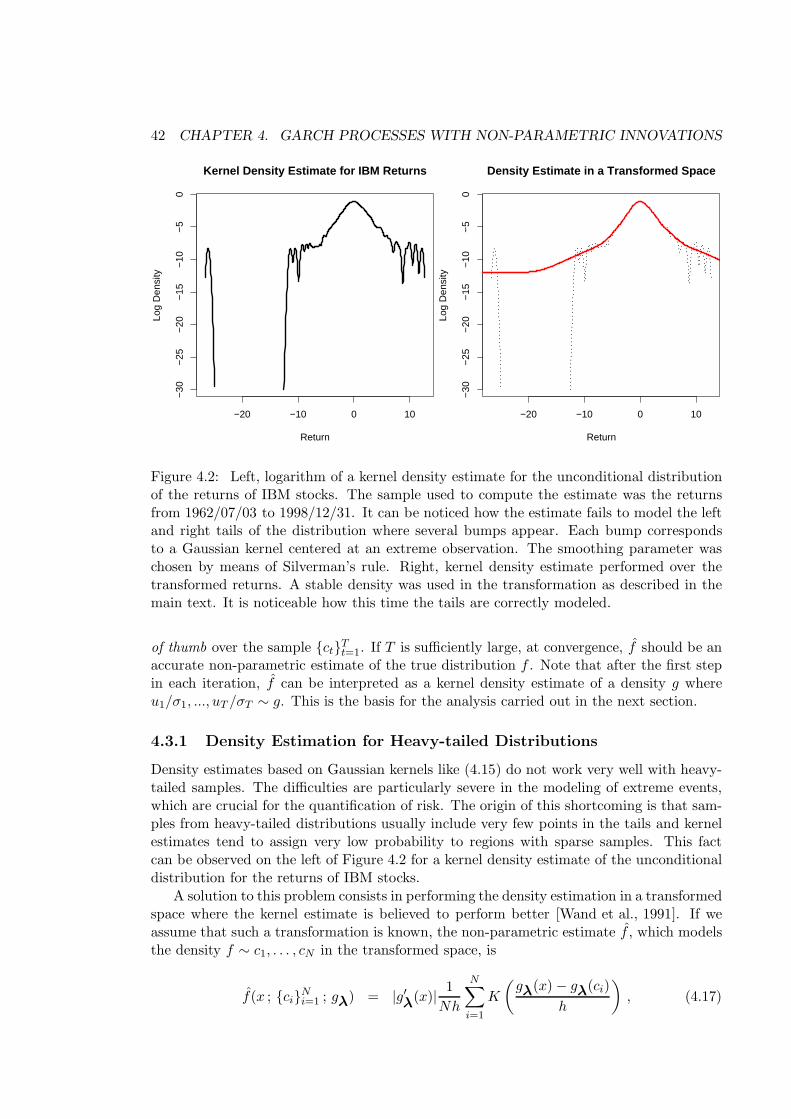
42 CHAPTER 4. GARCH PROCESSES WITH NON-PARAMETRIC INNOVATIONS
−20 −10 0 10
−30
−25
−20
−15
−10
−5
0Kernel Density Estimate for IBM Returns
Return
Log
Den
sity
−20 −10 0 10
−30
−25
−20
−15
−10
−5
0
Density Estimate in a Transformed Space
ReturnLo
g D
ensi
ty
Figure 4.2: Left, logarithm of a kernel density estimate for the unconditional distributionof the returns of IBM stocks. The sample used to compute the estimate was the returnsfrom 1962/07/03 to 1998/12/31. It can be noticed how the estimate fails to model the leftand right tails of the distribution where several bumps appear. Each bump correspondsto a Gaussian kernel centered at an extreme observation. The smoothing parameter waschosen by means of Silverman’s rule. Right, kernel density estimate performed over thetransformed returns. A stable density was used in the transformation as described in themain text. It is noticeable how this time the tails are correctly modeled.
of thumb over the sample {ct}Tt=1. If T is sufficiently large, at convergence, f should be anaccurate non-parametric estimate of the true distribution f . Note that after the first stepin each iteration, f can be interpreted as a kernel density estimate of a density g whereu1/σ1, ..., uT /σT ∼ g. This is the basis for the analysis carried out in the next section.
4.3.1 Density Estimation for Heavy-tailed Distributions
Density estimates based on Gaussian kernels like (4.15) do not work very well with heavy-tailed samples. The difficulties are particularly severe in the modeling of extreme events,which are crucial for the quantification of risk. The origin of this shortcoming is that sam-ples from heavy-tailed distributions usually include very few points in the tails and kernelestimates tend to assign very low probability to regions with sparse samples. This factcan be observed on the left of Figure 4.2 for a kernel density estimate of the unconditionaldistribution for the returns of IBM stocks.
A solution to this problem consists in performing the density estimation in a transformedspace where the kernel estimate is believed to perform better [Wand et al., 1991]. If weassume that such a transformation is known, the non-parametric estimate f , which modelsthe density f ∼ c1, . . . , cN in the transformed space, is
f(x ; {ci}Ni=1 ; gλ) = |g′λ
(x)| 1
Nh
N∑
i=1
K
(
gλ(x)− gλ(ci)
h
)
, (4.17)
4.3. GARCH PROCESSES WITH NON-PARAMETRIC INNOVATIONS 43
where gλ is a function which maps the original space to the transformed space and λ is aset of parameters that specify gλ within a family of monotonic increasing transformations.This process of estimating the density in a transformed space is similar to standard densityestimation based on kernels with varying widths [Wand et al., 1991].
By arguments similar to those in [Silverman, 1986] and already described in Section 4.1,if the smoothing parameter h is optimally chosen, then the MISE of the density estimatein the transformed space is proportional to
{∫
f ′′gλ
(x)2 dx
}1
5
, (4.18)
where fgλ
is the density followed by the data in the transformed space, this is fgλ∼
gλ(c1), . . . , gλ(cN ). It turns out that the Gaussian density provides a more than reason-able low value for (4.18) [Wand et al., 1991]. As a result, the key aspect that should beconsidered in the choice of gλ is that if ci ∼ f , then gλ(ci) should follow a distribution closeto normality. A trivial transformation that achieves this is Φ−1(F (ci)) ∼ N (0, 1), whereF is the cumulative distribution for f and Φ−1 is the inverse of the standard Gaussiandistribution. The difficulty is that if we knew F then we would also know f as f = F ′ andthe estimation process would not be necessary. Nevertheless, it is possible to approximateF by means of a parametric distribution Fλ that can account for the heavy tails in F .
The parameters λ of Fλ can be estimated by maximum likelihood to {ci}Ni=1. The final
transformation is gλ(x) = Φ−1(Fλ(x)). In this manner, a hybrid estimation is performedwhere the parametric model corrects the tails of the non-parametric estimate.
To incorporate this idea into the algorithm proposed in Section 4.3 the first step of suchalgorithm is divided into two parts. In the first one, the parameter λ of the transformationgλ is found by maximizing the likelihood of Fλ over the observed values {ut/σt}Tt=1. Inthe second part, the density of {ut/σt}Tt=1 is estimated by means of (4.17) where h isnow determined using Silverman’s rule of thumb in the transformed space as a functionof {gλ(ut/σt)}Tt=1. The second step of the algorithm remains unchanged: f(x ; {ci}Ni=1)is replaced in (4.16) by (4.17). One technical problem that remains is that the locationand scale of u1, ..., uT can be fixed in two different ways. One through the parameters θ
of the GARCH process and another one through f and the centers of the kernels {ci}Ni=1.This can lead to convergence problems and should be avoided. To address this problemf is forced to have always the same location and scale. This is achieved by standardizing{ut/σt}Tt=1 before the first step on each iteration of the algorithm. The pseudocode ofthe whole process followed to train a GARCH process with non-parametric innovations isdisplayed on Figure 4.3.
Family of Transformations
A parametric family of distributions Fλ needs to be selected to fully specify the family
of transformations gλ(x) = Φ−1(Fλ(x)). The choice used in our research is the family ofstable distributions [Nolan, 2002] which should have enough flexibility to account for theempirical properties of the marginal distribution of returns [Cont, 2001]. This family ofdistributions is parameterized in terms of a location parameter, a scale parameter, a pa-rameter describing the decay of the tails and, finally, a parameter allowing each tail to havea different behavior. Some examples of stable densities are displayed on Figure 4.4. We
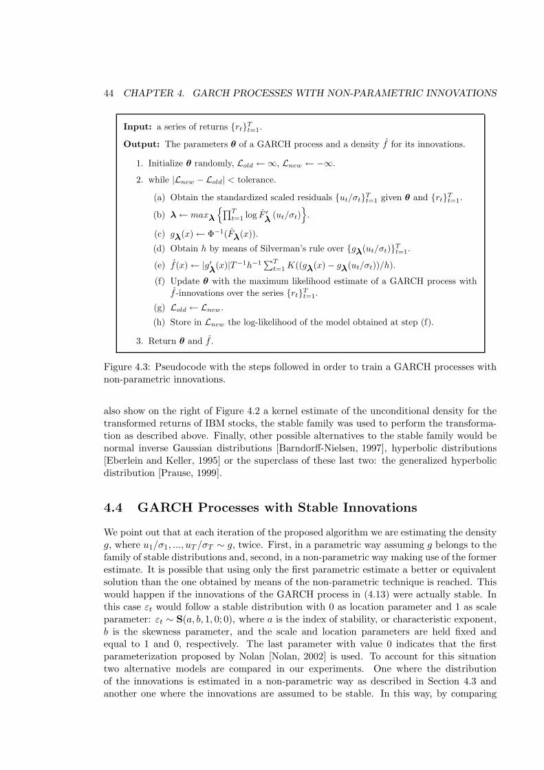
44 CHAPTER 4. GARCH PROCESSES WITH NON-PARAMETRIC INNOVATIONS
Input: a series of returns {rt}Tt=1.
Output: The parameters θ of a GARCH process and a density f for its innovations.
1. Initialize θ randomly, Lold ←∞, Lnew ← −∞.
2. while |Lnew − Lold| < tolerance.
(a) Obtain the standardized scaled residuals {ut/σt}Tt=1given θ and {rt}Tt=1
.
(b) λ← maxλ
{
∏T
t=1log F ′
λ(ut/σt)
}
.
(c) gλ(x)← Φ−1(Fλ(x)).
(d) Obtain h by means of Silverman’s rule over {gλ(ut/σt)}Tt=1.
(e) f(x)← |g′λ
(x)|T−1h−1∑T
t=1K((gλ(x)− gλ(ut/σt))/h).
(f) Update θ with the maximum likelihood estimate of a GARCH process with
f -innovations over the series {rt}Tt=1.
(g) Lold ← Lnew .
(h) Store in Lnew the log-likelihood of the model obtained at step (f).
3. Return θ and f .
Figure 4.3: Pseudocode with the steps followed in order to train a GARCH processes withnon-parametric innovations.
also show on the right of Figure 4.2 a kernel estimate of the unconditional density for thetransformed returns of IBM stocks, the stable family was used to perform the transforma-tion as described above. Finally, other possible alternatives to the stable family would benormal inverse Gaussian distributions [Barndorff-Nielsen, 1997], hyperbolic distributions[Eberlein and Keller, 1995] or the superclass of these last two: the generalized hyperbolicdistribution [Prause, 1999].
4.4 GARCH Processes with Stable Innovations
We point out that at each iteration of the proposed algorithm we are estimating the densityg, where u1/σ1, ..., uT /σT ∼ g, twice. First, in a parametric way assuming g belongs to thefamily of stable distributions and, second, in a non-parametric way making use of the formerestimate. It is possible that using only the first parametric estimate a better or equivalentsolution than the one obtained by means of the non-parametric technique is reached. Thiswould happen if the innovations of the GARCH process in (4.13) were actually stable. Inthis case εt would follow a stable distribution with 0 as location parameter and 1 as scaleparameter: εt ∼ S(a, b, 1, 0; 0), where a is the index of stability, or characteristic exponent,b is the skewness parameter, and the scale and location parameters are held fixed andequal to 1 and 0, respectively. The last parameter with value 0 indicates that the firstparameterization proposed by Nolan [Nolan, 2002] is used. To account for this situationtwo alternative models are compared in our experiments. One where the distributionof the innovations is estimated in a non-parametric way as described in Section 4.3 andanother one where the innovations are assumed to be stable. In this way, by comparing

4.5. MODEL VALIDATION AND RESULTS 45
−10 −5 0 5 10
−8
−7
−6
−5
−4
−3
−2
−1
x
Log
Den
sity
a = 1.00a = 1.25a = 1.50a = 1.75a = 2.00
−10 −5 0 5 10−
8−
6−
4−
2x
Log
Den
sity
b = −0.75b = −0.50b = 0.00b = 0.50b = 0.75
Figure 4.4: Plots of the logarithm of different stable densities with location 0 and scale 1where the first parameterization proposed by [Nolan, 2002] is used. Left, plots of densitieswith parameter a (α in [Nolan, 2002] and with range from 0 to 2) for the heaviness of thetails equal to 1, 1.25, 1.5, 1.75 and 2 and parameter b (β in [Nolan, 2002] and with rangefrom -1 to 1) for the asymmetry of the tails equal to 0 (symmetric tails). The stable densitywith parameter a = 2 has Gaussian tails. Right, plots of densities with parameter b equalto −0.75, −0.5, 0, 0.5, 0.75 and parameter a equal to 1.75. Negative values for b give moreweight to the left tail and positive values give more weight to the right tail.
the performance of both models it is possible to determine whether implementing the non-parametric estimate represents an actual improvement. The parameters of the GARCHmodel with stable innovations, θ, a and b are also estimated by maximum likelihood.
4.5 Model Validation and Results
To assess the capacity of the proposed models to accurately quantify market risk the generalbacktesting procedure described in Section 2.3 is followed. We perform a sliding windowexperiment on the daily returns of IBM stocks from 1962/07/03 to 1998/12/31, a total of9190 measurements (see Fig. 4.6). From the series of returns 8190 overlapping windowswith T = 1000 elements each are generated. Each window is equal in length to the previouswindow but is displaced forward by one time unit (one day). The parameters of the modelsare estimated by maximum likelihood using the data included in each window. Finally,the performance of the models is tested on the first point to the right of the trainingwindow. The testing process consists in calculating the cumulative probability that amodel assigns to the first point out of the window and then applying it the inverse ofthe standard Gaussian distribution (the Berkowitz transformation). This way, we obtain8190 test measurements for each model that should follow a standard Gaussian distributionunder the null hypothesis that the model is correct. The application of the statistical testsdescribed in Section 2.3.3 to those test measurements allows us to validate the models forestimating risk one day ahead in the future.
The estimation techniques are implemented in R [R Development Core Team, 2005].

46 CHAPTER 4. GARCH PROCESSES WITH NON-PARAMETRIC INNOVATIONS
−15 −10 −5 0 5 10 15
−12
−10
−8
−6
−4
−2
Return
Log
Den
sity
Gaussian DensityStable DensityNon−parametric Density
Figure 4.5: Plots in logarithmic scale of the different model density functions. The non-parametric density and the stable density have been obtained as averages of the densitiesestimated in the sliding window experiment. To compute these averages only the densitiesfor one in every fifty windows are used (a total of 163 densities). The stable densities arescaled so that their standard deviation is 1.
The non-linear optimization method used to maximize the likelihood was the downhill sim-plex method included in the function constrOptim. To avoid that the optimization processgets trapped in a local maximum, the algorithm is rerun using different initial randomvalues, and the best solution found is selected. Stable distributions have no general knownclosed form expressions for their density [Nolan, 2002]. To evaluate the stable density weemploy the technique described in [Mittnik et al., 1997]. The density is computed exactlyon a grid of 213 equally spaced points. Outside this grid the density function is calculatedby linear interpolation from the values in the grid. To evaluate the cumulative stable dis-tribution we use the R package fBasics [Wuertz et al., 2004] that implements the methoddescribed by Nolan [Nolan, 2002]. Finally, the parameter a of stable densities is restrictedto have values greater than 1.5, a bound which should be sufficiently low to account for theheavy tails in the distribution of returns.
Table 4.1 displays, for each model, the results of the statistical tests performed over thetest measurements obtained as described in Section 4.5. The level of significance consideredto reject the null hypothesis on each test is 5%. The GARCH model with stable innovationsfails all the tests but the one for Exceedances at the 95% level. The p-values obtained bythis model for the tests Exc 99% and ES 95% are rather low. In particular, the resultfor ES 95% reflects the failure of the model to accurately describe the loss tail of theconditional distribution of returns. The results of the GARCH model with non-parametricinnovations are remarkable. The model obtains very high p-values in all tests except forone. In particular, the test for Expected Shortfall at the 99% level fails. This is the mostdemanding test and it requires the model to correctly account for extreme events. In ourcase the test fails because of one single extreme event, a loss of around 5% that took place onJanuary 19, 1970 (see Fig. 4.6). Immediately prior to that observation, the value estimated

4.5. MODEL VALIDATION AND RESULTS 47
0 2000 4000 6000 8000
−20
−10
010
Day
Ret
urn
Unexpected loss
Black Monday
Figure 4.6: Returns of IBM stocks from 1962/07/03 to 1998/12/31. The loss on January19, 1970 has been singled out. The model proposed has difficulties to account for such aloss. The loss on October 19, 1987 known as Black Monday, has also been marked. Thisloss is correctly modeled.
Table 4.1: p-values obtained from the statistical tests performed. From left to right testsfor Value at Risk, Exceedances and Expected Shortfall at levels 99% and 95%. See Section2.3.3 for a description of the tests.
Model VaR 99% VaR 95% Exc 99% Exc 95% ES 99% ES 95%
stable 1.5e-3 0.01 3.7e-5 0.08 0.026 4e-4
non-parametric 0.51 0.66 0.49 0.86 0.042 0.31
mix. of 2 exp. 5.7e-3 0.30 0.025 0.19 7e-7 7.2e-4
for a in the stable distribution that characterizes the transformation gλ is fairly high 1.97,indicating that the tails are not very heavy and that the local fluctuations of the returnswere expected to be small in size (smaller than the loss observed) with a high degree ofconfidence. If this point is removed, the p-value obtained in the test ES 99% is 0.31 and allthe other tests give results above the level of significance 0.5. It is also interesting to seethat the model can properly account for the 25% loss that took place on October 19, 1987(Black Monday, see Fig. 4.6). The difference with the previous instance is that the valueestimated for the parameter a right before Black Monday is fairly low (1.88), which signalsthat the distribution tails are very heavy and that large fluctuations have a non negligiblechance of being observed. This low value of a originates in a sequence of large, but notextreme, fluctuations in the period immediately before Black Monday.
Figure 4.5 displays the average stable density and average non-parametric density ob-tained in the sliding window experiment. The tails of the stable and non-parametric den-sities are heavier than those of the standard Gaussian density. Moreover, those two distri-

48 CHAPTER 4. GARCH PROCESSES WITH NON-PARAMETRIC INNOVATIONS
0 2000 4000 6000 8000
−0.
50.
00.
51.
0
day
Diff
eren
ce in
VaR
0.9
9 es
timat
es
Difference in VaR 0.99 estimates
Den
sity
−0.5 0.0 0.5 1.0
01
23
Figure 4.7: Left, time series with the difference between the estimates of the VaR at the0.99 level from the non-parametric GARCH process and the stable GARCH process. Itcan be noticed that the series is most of the time positive, what indicates that the stableGARCH process provides estimates of risk which are generally lower than those of the non-parametric one. The units used to measure the VaR are percentage log-returns. Right,histogram of the series which appears on the left. The difference in VaR estimates aresignificantly positive.
butions are not symmetric, both densities assign a higher probability to returns close to 5than to returns close to -5. However, the right tail of the non-parametric density displaysa fast decay for returns greater than 5. This decay does not appear in the right tail ofthe stable density. This figure also shows how the tails of the non-parametric density areon average slightly less heavy than those of the stable distribution, specially in the righttail, corresponding to gains. This agrees with previous studies based on extreme valuetheory, which suggest that the tails of stable densities are probably too heavy to modelasset returns [Longin, 1996, Jansen and de Vries, 1991].
Strikingly, even though the tails of the stable densities are on average heavier thanthose of the non-parametric densities, the GARCH process with stable innovations providesestimates of one-day-ahead Value at Risk at the 0.99 level which are consistently lower thanthose of the non-parametric GARCH process. This fact can be appreciated on Figure 4.7.Because the non-parametric model obtains much better results in the test for Value at Riskat the 0.99 level, we can conclude that the stable GARCH process infraestimates risk.
We also performed the sliding-window experiment with mixtures of 2 autoregressiveexperts. The experiment was designed in the same way as the one described in Chapter 3,the only difference was that we employed the returns of IBM stocks instead of those fromthe stock index IBEX 35. The last row of Table 4.1 shows the test results obtained bymixtures of 2 autoregressive experts. It can be noticed how the mixture model fails all thetests at the 0.99 level, specially the one for Expected Shortfall. The reason why mixturesof 2 experts have now obtained much worse results than in Chapter 3 is due to the fact thatreturns from individual stocks depart from normality more than those from stock indexes.This is so because the price of stock indexes is computed as a weighted average of the price

4.6. SUMMARY 49
of individual stocks and the central limit theorem smooths extreme events away. Finally,we believe that mixtures of 3 autoregressive experts would obtain similar results.
4.6 Summary
A GARCH process with non-parametric innovations is proposed as a model for the seriesof daily stock returns. We have also described a procedure to estimate the parametersof the model and the density of the innovations by maximum likelihood in a transformedspace. The density for the innovations is modeled using a non-parametric estimate basedon kernels whose width is determined using Silverman’s rule of thumb. In the transformedspace the non-parametric estimate provides a more accurate model of heavy-tailed densities.A sliding window experiment using the returns of IBM stocks was carried out to evaluate theperformance of the proposed model. The experiments indicate that GARCH processes withnon-parametric innovations provide very accurate and sensitive estimates of risk measures,such as Value at Risk and Expected Shortfall. Furthermore, the new model outperformssoft competitive mixtures with 2 experts.

50 CHAPTER 4. GARCH PROCESSES WITH NON-PARAMETRIC INNOVATIONS

Chapter 5
Conclusions and Future Work
This chapter summarizes some of the main conclusions reached throughout the wholedocument. Furthermore, it provides some ideas that could be followed in order to extendthe current research.
5.1 Conclusions
In the second chapter we described that any financial institution which holds an investmentportfolio is exposed to market risk, a kind of risk which has recently increased becauseof globalization in financial markets. In order to be competitive and to protect fromunexpected high losses, financial institutions must implement and validate risk measuringand managing systems. The process of market risk measuring requires us to choose a riskmeasure (if possible, a coherent one) and to know the distribution of future prices for aportfolio, a distribution which is generally unknown. The usual approach to tackle thelatter problem consists in making use of a probabilistic model (e.g. GARCH process) forthe price changes. The model is fitted with historical past data and then used to infer thedistribution of future price changes. However, obtaining an accurate model is usually agreat challenge because of the complex properties displayed by financial time series (heavytails and heteroskedasticity). Once a probabilistic model is available, it must be checkedthat the risk measurements that it provides are accurate enough. This is performed bymeans of a backtesting procedure.
Throughout this document we have analyzed the performance of different models for es-timating market risk and the accuracy of each of them was measured by means of advancedstatistical tests based on the functional delta method. In the third chapter, mixtures ofup to three autoregressive experts that work together using different strategies were com-pared. It turned out that mixtures which employ a soft competitive strategy outperformedthe other models. This was due to the fact that soft competitive mixtures predict a futuredistribution for price changes which is a mixture of Gaussians (one Gaussian for each ex-pert), a paradigm which can effectively account for the heavy tails of financial time series (amixture of an unlimited number of Gaussians can approximate, up to any degree of preci-sion, any density function). However, one drawback of soft competitive mixtures is that thenumber of experts (Gaussians) is limited due to overfitting and training cost. Finally, in thefourth chapter we improved GARCH processes by means of modelling their innovations in a
51

52 CHAPTER 5. CONCLUSIONS AND FUTURE WORK
non-parametric way. The innovations were described by means of kernel density estimateswhich operate in a transformed space to better account for the leptokurtosis of financialtime series. The mentioned kernel estimates can also be regarded as constrained mixturesof Gaussians. However, the difference with respect to soft competitive mixtures is that, inthis case, it is feasible to make use of thousands of Gaussians without causing overfitting.The experiments demonstrate the superiority of GARCH processes with non-parametricinnovations for performing market risk estimation.
5.2 Future Work
The research performed in this document could be extended in several ways. First, in allthe experiments performed we have used daily returns for training and validating the mod-els. With the computerization of financial markets it is easier to obtain intra-day returnsand even tick-by-tick transaction data. The increase on available information allows tocompute better estimates of volatility and to suggest new models [Andersen et al., 2003,Engle, 2000]. Second, in this document we have dealt mainly with models for the changesin price of single financial assets. However, financial institutions hold portfolios with manydifferent assets in order to take advantage of the risk reduction caused by diversification.In such a situation it is necessary to model the dependence between individual assets if wewant to obtain accurate measurements of risk for the whole portfolio. This can be achievedby means of correlations if we work with elliptical distributions, or copulas [Nelsen, 2006]if we deal with general non-elliptical distributions. Third, we have focused on measuringrisk one day ahead on the future. Nevertheless, it is possible to study the ability of thedescribed models to estimate risk with horizons which range from weeks to months. MonteCarlo methods can be used to compute the predicting distribution determined by the mod-els when analytical solutions are not available. It would also be profitable to carry outexperiments with returns from other financial assets. Fourth, it would be interesting tocompare the performance of GARCH processes with non-parametric innovations againstGARCH processes with normal inverse Gaussian or generalized hyperbolic innovations.Also, those parametric distributions could be used to carry out the transformation neededin the non-parametric density estimation step of the training process for the models de-scribed in Chapter 4. Finally, Expected Shortfall is not the best coherent risk measure[Dowd, 2005]. This is so because it is risk-neutral between tail-region outcomes and weusually assume that investors are risk-averse. The class of spectral risk measures do nothave this problem [Acerbi, 2002].
Bibliography
[Bas, 1996] (1996). Supervisory Framework for the Use of ”Backtesting” in Conjunctionwith the Internal Models Approach to Market Risk Capital Requirements. Bank for In-ternational Settlements.
[Acerbi, 2002] Acerbi, C. (2002). Spectral measures of risk: A coherent representation ofsubjective risk aversion. Journal of Banking & Finance, 26:1505–1518.
[Andersen et al., 2003] Andersen, T. G., Bollerslev, T., Diebold, F. X., and Labys, P.(2003). Modelling and forecasting realized volatility. Econometrica, 71(2):579–625.
[Anderson and Darling, 1954] Anderson, T. W. and Darling, D. A. (1954). A test of good-ness of fit. Journal of the American Statistical Association, 49(268):765–769.
[Artzner et al., 1999] Artzner, P., Delbaen, F., Eber, J. M., and Heath, D. (1999). Coherentmeasures of risk. Mathematical Finance, 9(3):203–228.
[Barndorff-Nielsen, 1997] Barndorff-Nielsen, O. E. (1997). Normal inverse gaussian distri-butions and stochastic volatility modelling. Scandinavian Journal of Statistics, 24(1):1–13.
[Bengio et al., 2001] Bengio, Y., Lauzon, V.-P., and Ducharme, R. (2001). Experimentson the application of iohmms to model financial returns series. IEEE Transactions onNetworks Networks, 12(1):113–123.
[Berkowitz, 2001] Berkowitz, J. (2001). Testing density forecasts, with applications to riskmanagement. The Journal of Business and Economic Statistics, 19(4):465–474.
[Bishop, 1995] Bishop, C. (1995). Neural Networks for Pattern Recognition. Oxford Uni-versity Press.
[Bishop and Svensen, 2003] Bishop, C. and Svensen, M. (2003). Bayesian hierarchical mix-tures of experts. Proceedings Nineteenth Conference on Uncertainty in Artificial Intelli-gence, pages 57–64.
[Bishop, 2006] Bishop, C. M. (2006). Pattern Recognition and Machine Learning. Springer.
[Bollerslev, 1986] Bollerslev, T. (1986). Generalized autoregressive conditional het-eroskedasticity. Journal of Econometrics, 31(3):307–327.
[Bollerslev, 1987] Bollerslev, T. (1987). A conditionally heteroskedastic time series modelfor speculative prices and rates of return. The Review of Economics and Statistics,69(3):542–547.
53

54 BIBLIOGRAPHY
[Campbell et al., 1997] Campbell, J. Y., Lo, A. W., and Mackinlay, A. C. (1997). TheEconometrics of Financial Markets. Princeton University Press.
[Cont, 2001] Cont, R. (2001). Empirical properties of asset returns: stylized facts andstatistical issues. Journal of Quantitative Finance, 1:223–236.
[Davis and Mikosch, 1998] Davis, R. A. and Mikosch, T. (1998). The sample autocorre-lations of heavy-tailed processes with applications to arch. The Annals of Statistics,26(5):2049–2080.
[Devroye and Gyorfi, 1985] Devroye, L. and Gyorfi, L. (1985). Nonparametric DensityEstimation: The L1 View. John Wiley.
[Devroye et al., 1997] Devroye, L., Gyrfi, L., and Lugosi, G. (1997). A Probabilistic Theoryof Pattern Recognition (Stochastic Modelling and Applied Probability). Springer.
[Ding et al., 1993] Ding, Z., Granger, C. W. J., and Engle, R. F. (1993). A long memoryproperty of stock market returns and a new model. Journal of Empirical Finance,1(1):83–106.
[Dowd, 2005] Dowd, K. (2005). Measuring Market Risk. John Wiley & Sons.
[Duda et al., 2000] Duda, R. O., Hart, P. E., and Stork, D. G. (2000). Pattern Classifica-tion. Wiley-Interscience Publication.
[Eberlein and Keller, 1995] Eberlein, E. and Keller, U. (1995). Hyperbolic distributions infinance. Bernoulli, 1(3):281–299.
[Engle, 2000] Engle, R. F. (2000). The econometrics of ultra-high-frequency data. Econo-metrica, 68(1):1–22.
[Fama, 1970] Fama, E. F. (1970). Efficient capital markets: A review of theory and empir-ical work. Journal of Finance, 25(2).
[Forsberg, 2002] Forsberg, L. (2002). On the normal inverse gaussian distribution in mod-elling volatility in the financial markets. PhD Dissertation, Uppsala University, Sweden.
[Forsberg and Bollerslev, 2002] Forsberg, L. and Bollerslev, T. (2002). Bridging the gapbetween the distribution of realized (ecu) volatility and arch modelling (of the euro): thegarch-nig model. Journal of Applied Econometrics, 17:535–548.
[Franke and Diagne, 2006] Franke, J. and Diagne, M. (2006). Estimating market risk withneural networks. Statistics & Decisions, 24:233–253.
[Hamilton, 1991] Hamilton, J. D. (1991). A quasi-bayesian approach to estimating param-eters for mixtures of normal distributions. Journal of Business & Economic Statistics,9(1):27–39.
[Hamilton, 1994] Hamilton, J. D. (1994). Time Series Analysis. Princeton UniversityPress.
BIBLIOGRAPHY 55
[Hernandez-Lobato et al., 2007] Hernandez-Lobato, J. M., Hernandez-Lobato, D., andSuarez, A. (2007). GARCH processes with non-parametric innovations for measuringmarket risk. In de Sa, J. M., Alexandre, L., Duch, W., and Mandic, D., editors, ICANN(2), volume 4669 of Lecture Notes in Computer Science, pages 718–727. Springer.
[Hernandez-Lobato and Suarez, 2006] Hernandez-Lobato, J. M. and Suarez, A. (2006).Competitive and collaborative mixtures of experts for financial risk analysis. In Kol-lias, S. D., Stafylopatis, A., Duch, W., and Oja, E., editors, ICANN (2), volume 4132 ofLecture Notes in Computer Science, pages 691–700. Springer.
[Holton, 2003] Holton, G. A. (2003). Value-at-Risk. Elsevier.
[Holton, 2004] Holton, G. A. (2004). Defining risk. Financial Analysts Journal, 60(6).
[Jacobs et al., 1993] Jacobs, R. A., Jordan, M. I., and Barto, A. G. (1993). Task decom-postiion through competition in a modular connectionist architecture: The what andwhere vision tasks. In Machine Learning: From Theory to Applications, pages 175–202.
[Jacobs et al., 1991] Jacobs, R. A., Jordan, M. I., Nowlan, S., , and Hinton, G. E. (1991).Adaptive mixtures of local experts. Neural Computation, 3:1–12.
[Jansen and de Vries, 1991] Jansen, D. W. and de Vries, C. G. (1991). On the frequency oflarge stock returns: Putting booms and busts into perspective. The Review of Economicsand Statistics, 73(1):18–24.
[Jarque and Bera, 1987] Jarque, C. M. and Bera, A. K. (1987). A test for normality ofobservations and regression residuals. International Statistical Review / Revue Interna-tionale de Statistique, 55(2):163–172.
[Jordan and Jacobs, 1994] Jordan, M. I. and Jacobs, R. A. (1994). Hierarchical mixturesof experts and the EM algorithm. Neural Computation, 6:181–214.
[Jorion, 1997] Jorion, P. (1997). Value at Risk: The New Benchmark for Controlling Mar-ket Risk. McGraw-Hill.
[Kerkhof and Melenberg, 2004] Kerkhof, J. and Melenberg, B. (2004). Backtesting for risk-based regulatory campital. Journal of Banking and Finance, 28(8):1845–1865.
[Kon, 1984] Kon, S. J. (1984). Models of stock returns–a comparison. Journal of Finance,39(1):147–165.
[Kupiec, 1995] Kupiec, P. H. (1995). Techniques for verifying the accuracy of risk mea-surement models. The Journal of Derivatives, 3(2):73–84.
[Longin, 1996] Longin, F. M. (1996). The asymptotic distribution of extreme stock marketreturns. The Journal of Business, 69(3):383–408.
[MacKay, 2003] MacKay, D. (2003). Information Theory, Inference, and Learning Algo-rithms. Cambridge University Press.
[Markowitz, 1991] Markowitz, H. (1991). Portfolio Selection. Blackwell Publishing.

56 BIBLIOGRAPHY
[Mathworks, 2002] Mathworks (2002). Matlab Optimization toolbox 2.2. Mathworks, Inc.,Natick, MA.
[Mikosch and Starica, 2000] Mikosch, T. and Starica, C. (2000). Limit theory for the sam-ple autocorrelations and extremes of a garch(1,1) process. The Annals of Statistics,28(5):1427–1451.
[Mittnik et al., 1997] Mittnik, S., Doganoglu, T., and Chenyao, D. (1997). Computingthe probability density function of the stable paretian distribution. Mathematical andComputer Modelling, 29(10):235–240.
[Mittnik and Paolella, 2003] Mittnik, S. and Paolella, M. S. (2003). Prediction of financialdownside-risk with heavy-tailed conditional distributions. CFS Working Paper, (2003/4).
[Morgan, 1996] Morgan, J. P. (1996). RiskMetrics Technical Document. Fourth Edition,New York.
[Nadaraya, 1989] Nadaraya, E. (1989). Nonparametric Estimation of Probability Densitiesand Regression Curves. Kluwer Academic Publishers.
[Nelsen, 2006] Nelsen, R. B. (2006). An Introduction to Copulas. Springer.
[Nolan, 2002] Nolan, J. P. (2002). Stable Distributions. Birkhauser.
[Panorska et al., 1995] Panorska, A. K., Mittnik, S., and Rachev, S. T. (1995). Stablegarch models for financial time series. Applied Mathematics Letters, 8(5):33–37.
[Papoulis and Pillai, 2002] Papoulis, A. and Pillai, S. U. (2002). Probability, Random Vari-ables and Stochastic Processes. Mc Graw Hill.
[Parzen, 1962] Parzen, E. (1962). On estimation of a probability density function andmode. The Annals of Mathematical Statistics, 33(3):1065–1076.
[Prause, 1999] Prause, K. (1999). The generalized hyperbolic model: Estimation, financialderivatives and risk measures. PhD Dissertation, University of Freiburg.
[R Development Core Team, 2005] R Development Core Team (2005). R: A language andenvironment for statistical computing. R Foundation for Statistical Computing, Vienna,Austria. ISBN 3-900051-07-0.
[Shapiro and Wilk, 1965] Shapiro, S. S. and Wilk, M. B. (1965). An analysis of variancetest for normality (complete samples). Biometrika, 52(3/4):591–611.
[Sheather and Jones, 1991] Sheather, S. J. and Jones, M. C. (1991). A reliable data-basedbandwidth selection method for kernel density estimation. Journal of the Royal StatisticalSociety. Series B (Methodological), 53(3):683–690.
[Silverman, 1986] Silverman, B. W. (1986). Density Estimation for Statistics and DataAnalysis. Chapman & Hall/CRC.
[Sociedad de Bolsas, 2006] Sociedad de Bolsas (2006). Historico Cierres Indices Ibex.http://www.sbolsas.es.

BIBLIOGRAPHY 57
[Suarez, 2002] Suarez, A. (2002). volume 2415/2002 of Lecture Notes in Computer Science,chapter Mixtures of Autoregressive Models for Financial Risk Analysis. Springer Berlin/ Heidelberg.
[Vaart, 2000] Vaart, V. D. (2000). Asymptotic Statistics. Cambridge University Press.
[Vidal and Suarez, 2003] Vidal, C. and Suarez, A. (2003). volume 2714/2003 of LectureNotes in Computer Science, chapter Hierarchical Mixtures of Autoregressive Models forTime-Series Modeling. Springer Berlin / Heidelberg.
[Wand et al., 1991] Wand, M. P., Marron, J. S., and Ruppert, D. (1991). Transformationsin density estimation. with discussion and a rejoinder by the authors. Journal of theAmerican Statistical Association, 86(414):343–361.
[Weigend and Huberman, 1990] Weigend, A. S. and Huberman, B. A. (1990). Predictingsunspots and exchange rates with connectionist networks. Proc. of 1990 NATO Workshopon Nonlinear Modeling and Forecasting, Santa Fe, NM, 1990.
[Wilcoxon, 1945] Wilcoxon, F. (1945). Individual comparisons by ranking methods. Bio-metrics Bulletin, 1(6):80–83.
[Wuertz et al., 2004] Wuertz, Diethelm, and Others, M. (2004). fBasics: Financial Soft-ware Collection - fBasics.