Embed Size (px)
Citation preview

Introduction to Bayesian Risk Models
Paula Moraga
London School of Hygiene and Tropical Medicine
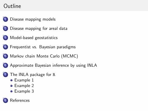
Outline
1 Disease mapping models
2 Disease mapping for areal data
3 Model-based geostatistics
4 Frequentist vs. Bayesian paradigms
5 Markov chain Monte Carlo (MCMC)
6 Approximate Bayesian inference by using INLA
7 The INLA package for RExample 1Example 2Example 3
8 References
Disease mapping models
Outline
1 Disease mapping models
2 Disease mapping for areal data
3 Model-based geostatistics
4 Frequentist vs. Bayesian paradigms
5 Markov chain Monte Carlo (MCMC)
6 Approximate Bayesian inference by using INLA
7 The INLA package for RExample 1Example 2Example 3
8 References
Paula Moraga (LSHTM) Introduction to Bayesian Risk Models 9 March 2015 3 / 101
Disease mapping models
Disease maps
Disease maps provide a rapid visual summary of spatial information andallow the identification of patterns that may be missed in tabularpresentations. Maps are crucial for
describing the spatial variation of the disease
identifying areas of unusually high risk
formulating etiological hypotheses
allowing better resource allocation
Paula Moraga (LSHTM) Introduction to Bayesian Risk Models 9 March 2015 4 / 101
Disease mapping models
Areal data
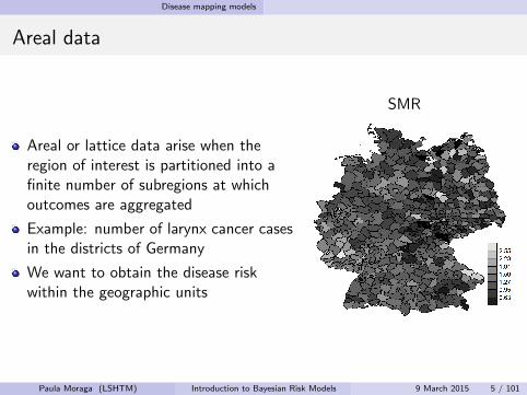
SMR
Areal or lattice data arise when theregion of interest is partitioned into afinite number of subregions at whichoutcomes are aggregated
Example: number of larynx cancer casesin the districts of Germany
We want to obtain the disease riskwithin the geographic units
Paula Moraga (LSHTM) Introduction to Bayesian Risk Models 9 March 2015 5 / 101
Disease mapping models
Geostatistical data
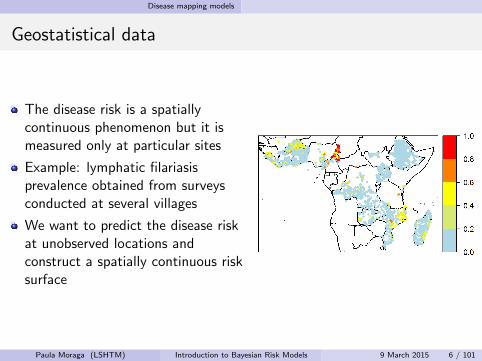
The disease risk is a spatiallycontinuous phenomenon but it ismeasured only at particular sites
Example: lymphatic filariasisprevalence obtained from surveysconducted at several villages
We want to predict the disease riskat unobserved locations andconstruct a spatially continuous risksurface
Paula Moraga (LSHTM) Introduction to Bayesian Risk Models 9 March 2015 6 / 101
Disease mapping models
Disease mapping models
Disease risk predictions are generally based on counts of the observedcases, the number of individuals at risk, and on covariate informationsuch as the age distribution, lifestyle and environmental factors
If data are spatially correlated, observations in neighboring areas willbe more similar than observations in areas that are farther away
Models describe the variability in the response variable as a functionof the explanatory variables and random effects to account for theresidual spatial autocorrelation
Paula Moraga (LSHTM) Introduction to Bayesian Risk Models 9 March 2015 7 / 101
Disease mapping models
Discrete distributions
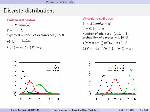
Poisson distribution
Y ∼ Poisson(µ)
y = 0, 1, 2, . . .
expected number of occurrences µ > 0
p(y |µ) = e−µµy
y !
E(Y ) = µ, Var(Y ) = µ
Binomial distribution
Y ∼ Binomial(n, π)
y = 0, 1, . . . , n
number of trials n ∈ {1, 2, . . .},probability of success π ∈ [0, 1]
p(y |n, π) =(ny
)πy (1− π)(n−y)
E(Y ) = nπ, Var(Y ) = nπ(1− π)
Paula Moraga (LSHTM) Introduction to Bayesian Risk Models 9 March 2015 8 / 101
Disease mapping models
Regression models
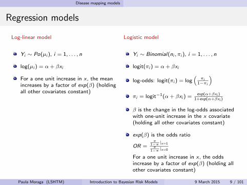
Log-linear model
Yi ∼ Po(µi ), i = 1, . . . , n
log(µi ) = α+ βxi
For a one unit increase in x , the meanincreases by a factor of exp(β) (holdingall other covariates constant)
Logistic model
Yi ∼ Binomial(ni , πi ), i = 1, . . . , n
logit(πi ) = α+ βxi
log-odds: logit(πi ) = log(
πi1−πi
)πi = logit−1(α+ βxi ) = exp(α+βxi )
1+exp(α+βxi )
β is the change in the log-odds associatedwith one-unit increase in the x covariate(holding all other covariates constant)
exp(β) is the odds ratio
OR =π
1−π|x=1
π1−π|x=0
For a one unit increase in x , the oddsincrease by a factor of exp(β) (holding allother covariates constant)
Paula Moraga (LSHTM) Introduction to Bayesian Risk Models 9 March 2015 9 / 101
Disease mapping for areal data
Outline
1 Disease mapping models
2 Disease mapping for areal data
3 Model-based geostatistics
4 Frequentist vs. Bayesian paradigms
5 Markov chain Monte Carlo (MCMC)
6 Approximate Bayesian inference by using INLA
7 The INLA package for RExample 1Example 2Example 3
8 References
Paula Moraga (LSHTM) Introduction to Bayesian Risk Models 9 March 2015 10 / 101
Disease mapping for areal data
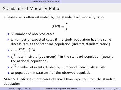
Standardized Mortality Ratio
Disease risk is often estimated by the standardized mortality ratio:
SMR =Y
E
Y number of observed cases
E number of expected cases if the study population has the samedisease rate as the standard population (indirect standardization)
E =∑m
i=1 r(s)i ni
r(s)i rate in strata (age group) i in the standard population (usually
the national population)
r(s)i number of events divided by number of individuals at risk
ni population in stratum i of the observed population
SMR > 1 indicates more cases observed than expected from the standardpopulation
Paula Moraga (LSHTM) Introduction to Bayesian Risk Models 9 March 2015 11 / 101
Disease mapping for areal data
Disease mapping
SMRs are often misleading and insufficiently reliable for reporting inareas with small populations
In contrast, model-based approaches enable to incorporate covariatesand borrow information from neighboring areas to improve localestimates, resulting in the smoothing of extreme rates based on smallsample sizes
Such approaches are often expressed as hierarchical Bayesian diseasemapping models
Paula Moraga (LSHTM) Introduction to Bayesian Risk Models 9 March 2015 12 / 101
Disease mapping for areal data
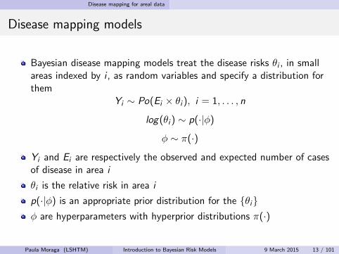
Disease mapping models
Bayesian disease mapping models treat the disease risks θi , in smallareas indexed by i , as random variables and specify a distribution forthem
Yi ∼ Po(Ei × θi ), i = 1, . . . , n
log(θi ) ∼ p(·|φ)
φ ∼ π(·)
Yi and Ei are respectively the observed and expected number of casesof disease in area i
θi is the relative risk in area i
p(·|φ) is an appropriate prior distribution for the {θi}φ are hyperparameters with hyperprior distributions π(·)
Paula Moraga (LSHTM) Introduction to Bayesian Risk Models 9 March 2015 13 / 101
Disease mapping for areal data
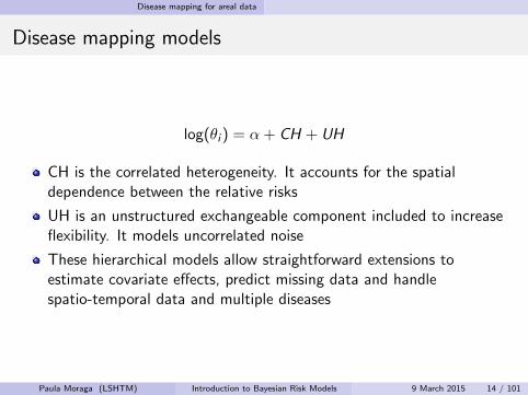
Disease mapping models
log(θi ) = α + CH + UH
CH is the correlated heterogeneity. It accounts for the spatialdependence between the relative risks
UH is an unstructured exchangeable component included to increaseflexibility. It models uncorrelated noise
These hierarchical models allow straightforward extensions toestimate covariate effects, predict missing data and handlespatio-temporal data and multiple diseases
Paula Moraga (LSHTM) Introduction to Bayesian Risk Models 9 March 2015 14 / 101
Disease mapping for areal data
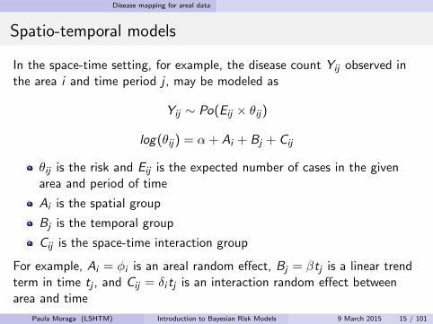
Spatio-temporal models
In the space-time setting, for example, the disease count Yij observed inthe area i and time period j , may be modeled as
Yij ∼ Po(Eij × θij)
log(θij) = α + Ai + Bj + Cij
θij is the risk and Eij is the expected number of cases in the givenarea and period of time
Ai is the spatial group
Bj is the temporal group
Cij is the space-time interaction group
For example, Ai = φi is an areal random effect, Bj = βtj is a linear trendterm in time tj , and Cij = δi tj is an interaction random effect betweenarea and time
Paula Moraga (LSHTM) Introduction to Bayesian Risk Models 9 March 2015 15 / 101
Disease mapping for areal data
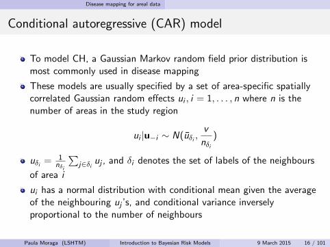
Conditional autoregressive (CAR) model
To model CH, a Gaussian Markov random field prior distribution ismost commonly used in disease mapping
These models are usually specified by a set of area-specific spatiallycorrelated Gaussian random effects ui , i = 1, . . . , n where n is thenumber of areas in the study region
ui |u−i ∼ N(uδi ,v
nδi)
uδi = 1nδi
∑j∈δi uj , and δi denotes the set of labels of the neighbours
of area i
ui has a normal distribution with conditional mean given the averageof the neighbouring uj ’s, and conditional variance inverselyproportional to the number of neighbours
Paula Moraga (LSHTM) Introduction to Bayesian Risk Models 9 March 2015 16 / 101
Disease mapping for areal data
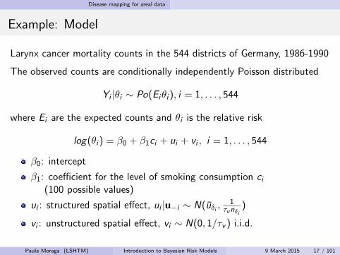
Example: Model
Larynx cancer mortality counts in the 544 districts of Germany, 1986-1990
The observed counts are conditionally independently Poisson distributed
Yi |θi ∼ Po(Eiθi ), i = 1, . . . , 544
where Ei are the expected counts and θi is the relative risk
log(θi ) = β0 + β1ci + ui + vi , i = 1, . . . , 544
β0: intercept
β1: coefficient for the level of smoking consumption ci(100 possible values)
ui : structured spatial effect, ui |u−i ∼ N(uδi ,1
τunδi)
vi : unstructured spatial effect, vi ∼ N(0, 1/τv ) i.i.d.
Paula Moraga (LSHTM) Introduction to Bayesian Risk Models 9 March 2015 17 / 101
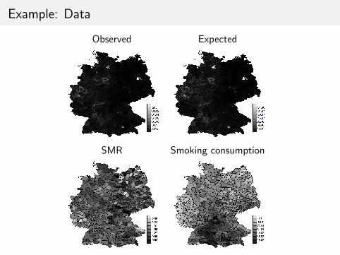
Example: Data
Observed Expected
SMR Smoking consumption
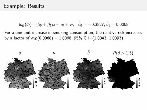
Example: Results
log(θi ) = β0 + β1ci + ui + vi , β0 = −0.3827, β1 = 0.0068
For a one unit increase in smoking consumption, the relative risk increasesby a factor of exp(0.0068) = 1.0068, 95% C.I=(1.0043, 1.0093)
u v θ P(θ > 1.5)
Model-based geostatistics
Outline
1 Disease mapping models
2 Disease mapping for areal data
3 Model-based geostatistics
4 Frequentist vs. Bayesian paradigms
5 Markov chain Monte Carlo (MCMC)
6 Approximate Bayesian inference by using INLA
7 The INLA package for RExample 1Example 2Example 3
8 References
Paula Moraga (LSHTM) Introduction to Bayesian Risk Models 9 March 2015 20 / 101
Model-based geostatistics
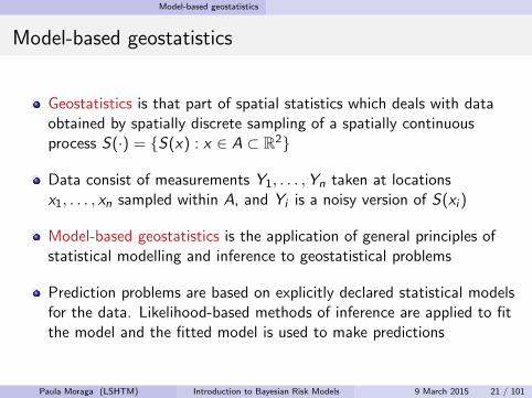
Model-based geostatistics
Geostatistics is that part of spatial statistics which deals with dataobtained by spatially discrete sampling of a spatially continuousprocess S(·) = {S(x) : x ∈ A ⊂ R2}
Data consist of measurements Y1, . . . ,Yn taken at locationsx1, . . . , xn sampled within A, and Yi is a noisy version of S(xi )
Model-based geostatistics is the application of general principles ofstatistical modelling and inference to geostatistical problems
Prediction problems are based on explicitly declared statistical modelsfor the data. Likelihood-based methods of inference are applied to fitthe model and the fitted model is used to make predictions
Paula Moraga (LSHTM) Introduction to Bayesian Risk Models 9 March 2015 21 / 101
Model-based geostatistics
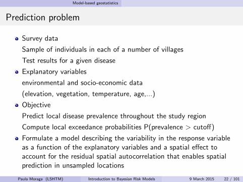
Prediction problem
Survey data
Sample of individuals in each of a number of villages
Test results for a given disease
Explanatory variables
environmental and socio-economic data
(elevation, vegetation, temperature, age,...)
Objective
Predict local disease prevalence throughout the study region
Compute local exceedance probabilities P(prevalence > cutoff)
Formulate a model describing the variability in the response variableas a function of the explanatory variables and a spatial effect toaccount for the residual spatial autocorrelation that enables spatialprediction in unsampled locations
Paula Moraga (LSHTM) Introduction to Bayesian Risk Models 9 March 2015 22 / 101
Model-based geostatistics
Model
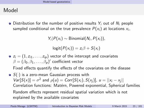
Distribution for the number of positive results Yi out of Ni peoplesampled conditional on the true prevalence P(xi ) at locations xi ,
Yi |P(xi ) ∼ Binomial(Ni ,P(xi )),
logit(P(xi )) = ziβ + S(xi )
zi = (1, zi1, . . . , zip) vector of the intercept and covariatesβ = (β0, β1, . . . , βp)′ coefficient vector
Fixed effects quantify the effects of the covariates on the disease
S(·) is a zero-mean Gaussian process withVar [S(x)] = σ2 and ρ(u) = Corr [S(xi ), S(xj)], u = ||xi − xj ||Correlation functions: Matern, Powered exponential, Spherical families
Random effects represent residual spatial variation which is notexplained by the available covariates
Paula Moraga (LSHTM) Introduction to Bayesian Risk Models 9 March 2015 23 / 101
Correlation functions
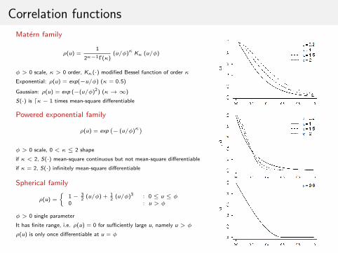
Matern family
ρ(u) =1
2κ−1Γ(κ)(u/φ)κ Kκ (u/φ)
φ > 0 scale, κ > 0 order, Kκ(·) modified Bessel function of order κ
Exponential: ρ(u) = exp(−u/φ) (κ = 0.5)
Gaussian: ρ(u) = exp (−(u/φ)2) (κ→∞)
S(·) is dκ− 1 times mean-square differentiable
Powered exponential family
ρ(u) = exp(− (u/φ)κ
)φ > 0 scale, 0 < κ ≤ 2 shape
if κ < 2, S(·) mean-square continuous but not mean-square differentiable
if κ = 2, S(·) infinitely mean-square differentiable
Spherical family
ρ(u) =
{1− 3
2(u/φ) + 1
2(u/φ)3 : 0 ≤ u ≤ φ
0 : u > φ
φ > 0 single parameter
It has finite range, i.e. ρ(u) = 0 for sufficiently large u, namely u > φ
ρ(u) is only once differentiable at u = φ
Example: Lymphatic filariasis
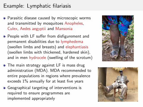
Parasitic disease caused by microscopic wormsand transmitted by mosquitoes Anopheles,Culex, Aedes aegyptii and Mansonia
People with LF suffer from disfigurement andpermanent disabilities due to lymphedema(swollen limbs and breasts) and elephantiasis(swollen limbs with thickened, hardened skin),and in men hydrocele (swelling of the scrotum)
The main strategy against LF is mass drugadministration (MDA). MDA recommended toentire populations in regions where prevalenceexceeds 1% annually for at least five years
Geographical targeting of interventions isrequired to ensure programmes areimplemented appropriately
Model-based geostatistics
Example: Data
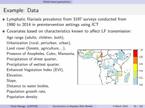
Lymphatic filariasis prevalence from 3197 surveys conducted from1990 to 2014 in preintervention settings using ICT
Covariates based on characteristics known to affect LF transmission:
Age range (adults, children, both),
Urbanization (rural, periurban, urban),
Land cover (forests, agriculture,...),
Presence of Anopheles, Culex, Mansonia,
Precipitation of driest quarter,
Precipitation of wettest quarter,
Enhanced Vegetation Index (EVI),
Elevation,
Slope,
Distance to water bodies,
Population growth rate,
Population density
Paula Moraga (LSHTM) Introduction to Bayesian Risk Models 9 March 2015 26 / 101
Model-based geostatistics
Example: Model
Conditional on the true prevalence P(xi ) at location xi , i = 1, . . . , n, thenumber of positive results Yi out of Ni people sampled at xi follows abinomial distribution,
Yi |P(xi ) ∼ Binomial(Ni ,P(xi ))
logit(P(xi )) = ziβ + S(xi )
zi = (1, zi1, . . . , zip) vector of the intercept and the p covariates
β = (β0, β1, . . . , βp)′ coefficient vector
S(xi ) spatially structured random effect
S(xi ) zero-mean Gaussian process with Matern covariance function
Paula Moraga (LSHTM) Introduction to Bayesian Risk Models 9 March 2015 27 / 101
Model-based geostatistics
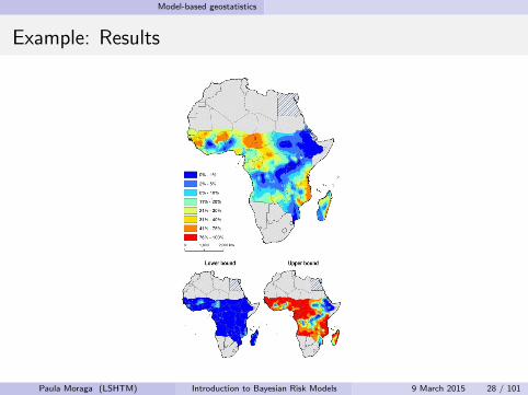
Example: Results
Paula Moraga (LSHTM) Introduction to Bayesian Risk Models 9 March 2015 28 / 101
Frequentist vs. Bayesian paradigms
Outline
1 Disease mapping models
2 Disease mapping for areal data
3 Model-based geostatistics
4 Frequentist vs. Bayesian paradigms
5 Markov chain Monte Carlo (MCMC)
6 Approximate Bayesian inference by using INLA
7 The INLA package for RExample 1Example 2Example 3
8 References
Paula Moraga (LSHTM) Introduction to Bayesian Risk Models 9 March 2015 29 / 101
Frequentist vs. Bayesian paradigms
Frequentist vs. Bayesian paradigms
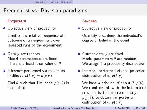
Frequentist
Objective view of probability
Limit of the relative frequency of anoutcome of an experiment overrepeated runs of the experiment
Bayesian
Subjective view of probability
Quantity describing the individual’sdegree of belief in the event
Data y are randomModel parameters θ are fixedThere is a fixed, true value of θ
Inference performed via maximumlikelihood L(θ|y) = p(y |θ)
Find θ such that likelihood p(y |θ) ismaximized
Current data y are fixedModel parameters θ are randomWe assign θ a probability distribution
Inference performed via the posteriordistribution of θ, p(θ|y)
We have a prior belief about θ, p(θ).We combine this with the informationprovided by the observed data y ,p(y |θ), to obtain the posteriordistribution of θ, p(θ|y)
Paula Moraga (LSHTM) Introduction to Bayesian Risk Models 9 March 2015 30 / 101
Frequentist vs. Bayesian paradigms
Frequentist vs. Bayesian paradigms
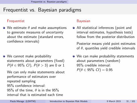
Frequentist
We estimate θ and make assumptionsto generate measures of uncertaintyabout the estimate (standard errors,confidence intervals)
Bayesian
All statistical inferences (point andinterval estimates, hypothesis tests)follow from the posterior distribution
Posterior means yield point estimatesof θ, quantiles yield credible intervals
We cannot make probabilitystatements about parameters (fixed)P(θ ∈ 95% CI ), P(θ > 3) are 0 or 1
We can only make statements aboutperformance of estimators overrepeated sampling95% confidence interval:95% of the time, θ is in the 95%interval that is estimated each time
We can make probability statementsabout parameters (random)95% credible interval:P(θ ∈ 95% CI ) = 0.95
Paula Moraga (LSHTM) Introduction to Bayesian Risk Models 9 March 2015 31 / 101
Frequentist vs. Bayesian paradigms
Bayesian inference
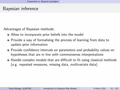
Advantages of Bayesian methods:
Allow to incorporate prior beliefs into the model
Provide a way of formalising the process of learning from data toupdate prior information
Provide confidence intervals on parameters and probability values onhypotheses that are in line with commonsense interpretations
Handle complex models that are difficult to fit using classical methods(e.g. repeated measures, missing data, multivariate data)
Paula Moraga (LSHTM) Introduction to Bayesian Risk Models 9 March 2015 32 / 101
Frequentist vs. Bayesian paradigms
Bayesian inference
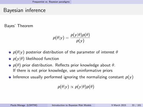
Bayes’ Theorem
p(θ|y) =p(y |θ)p(θ)
p(y)
p(θ|y) posterior distribution of the parameter of interest θ
p(y |θ) likelihood function
p(θ) prior distribution. Reflects prior knowledge about θ.If there is not prior knowledge, use uninformative priors
Inference usually performed ignoring the normalizing constant p(y)
p(θ|y) ∝ p(y |θ)p(θ)
Paula Moraga (LSHTM) Introduction to Bayesian Risk Models 9 March 2015 33 / 101
Frequentist vs. Bayesian paradigms
Continuous distributions
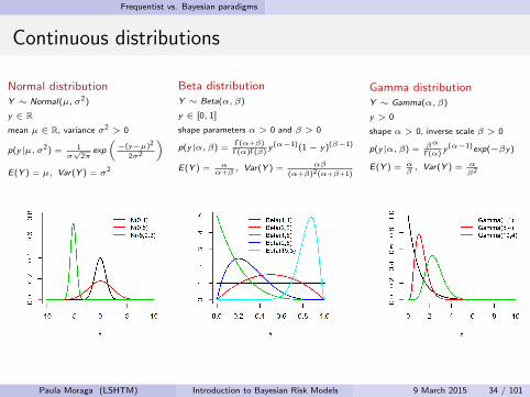
Normal distributionY ∼ Normal(µ, σ2)
y ∈ Rmean µ ∈ R, variance σ2 > 0
p(y|µ, σ2) = 1σ√
2πexp
(−(y−µ)2
2σ2
)E(Y ) = µ, Var(Y ) = σ2
Beta distributionY ∼ Beta(α, β)
y ∈ [0, 1]
shape parameters α > 0 and β > 0
p(y|α, β) =Γ(α+β)
Γ(α)Γ(β)y (α−1)(1− y)(β−1)
E(Y ) = αα+β
, Var(Y ) = αβ
(α+β)2(α+β+1)
Gamma distributionY ∼ Gamma(α, β)
y > 0
shape α > 0, inverse scale β > 0
p(y|α, β) = βα
Γ(α)y (α−1)exp(−βy)
E(Y ) = αβ, Var(Y ) = α
β2
Paula Moraga (LSHTM) Introduction to Bayesian Risk Models 9 March 2015 34 / 101
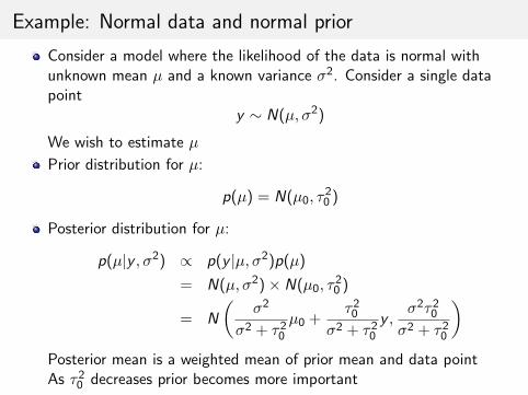
Example: Normal data and normal prior
Consider a model where the likelihood of the data is normal withunknown mean µ and a known variance σ2. Consider a single datapoint
y ∼ N(µ, σ2)
We wish to estimate µ
Prior distribution for µ:
p(µ) = N(µ0, τ20 )
Posterior distribution for µ:
p(µ|y , σ2) ∝ p(y |µ, σ2)p(µ)
= N(µ, σ2)× N(µ0, τ20 )
= N
(σ2
σ2 + τ20
µ0 +τ2
0
σ2 + τ20
y ,σ2τ2
0
σ2 + τ20
)Posterior mean is a weighted mean of prior mean and data pointAs τ2
0 decreases prior becomes more important

Frequentist vs. Bayesian paradigms
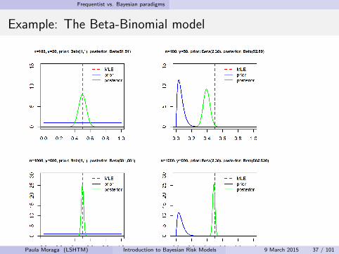
Example: The Beta-Binomial model
Let Y be the number of successes in n independent trials
Y ∼ Binomial(n, π)
We wish to estimate π
Prior distribution for π:
p(π) = Beta(α, β)
Posterior distribution for π:
p(π|y) ∝ p(y |π)p(π)
= Binomial(n, π)× Beta(α, β)
= Beta(α + y , β + n − y)
Paula Moraga (LSHTM) Introduction to Bayesian Risk Models 9 March 2015 36 / 101
Frequentist vs. Bayesian paradigms
Example: The Beta-Binomial model
Paula Moraga (LSHTM) Introduction to Bayesian Risk Models 9 March 2015 37 / 101
Frequentist vs. Bayesian paradigms
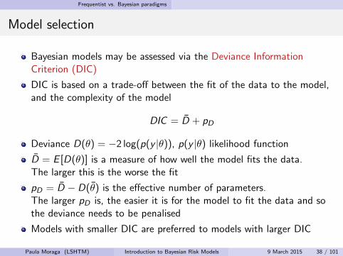
Model selection
Bayesian models may be assessed via the Deviance InformationCriterion (DIC)
DIC is based on a trade-off between the fit of the data to the model,and the complexity of the model
DIC = D + pD
Deviance D(θ) = −2 log(p(y |θ)), p(y |θ) likelihood function
D = E [D(θ)] is a measure of how well the model fits the data.The larger this is the worse the fit
pD = D − D(θ) is the effective number of parameters.The larger pD is, the easier it is for the model to fit the data and sothe deviance needs to be penalised
Models with smaller DIC are preferred to models with larger DIC
Paula Moraga (LSHTM) Introduction to Bayesian Risk Models 9 March 2015 38 / 101
Frequentist vs. Bayesian paradigms
Bayesian inference
One principal difficulty in applying Bayesian methods is the calculationof the posterior p(θ|y), which usually involves high-dimensionalintegration that is generally not tractable in closed form
Thus, even when the likelihood and the prior distribution haveclosed-form expressions, the posterior distribution may not
Methods for solving this problem:
Markov chain Monte Carlo methods (MCMC)Approximate Bayesian inference for latent Gaussian models by usingIntegrated Nested Laplace approximations (INLA)
Paula Moraga (LSHTM) Introduction to Bayesian Risk Models 9 March 2015 39 / 101
Markov chain Monte Carlo (MCMC)
Outline
1 Disease mapping models
2 Disease mapping for areal data
3 Model-based geostatistics
4 Frequentist vs. Bayesian paradigms
5 Markov chain Monte Carlo (MCMC)
6 Approximate Bayesian inference by using INLA
7 The INLA package for RExample 1Example 2Example 3
8 References
Paula Moraga (LSHTM) Introduction to Bayesian Risk Models 9 March 2015 40 / 101

Markov chain Monte Carlo (MCMC)
Markov chain Monte Carlo (MCMC)
Markov chain Monte Carlo (MCMC) techniques are methods whichsimulate draws that are approximately from a (posterior) distribution
We can take those draws and calculate quantities of interest for theposterior distribution using Monte Carlo Integration methods:
E (θ|y) =
∫p(θ|y)p(θ)dθ
can be approximated by drawing M samples from p(θ|y) andevaluating
E (θ|y) ≈ 1
M
M∑i=1
θ(i)
Paula Moraga (LSHTM) Introduction to Bayesian Risk Models 9 March 2015 41 / 101

Markov chain Monte Carlo (MCMC)
Markov chain Monte Carlo (MCMC)
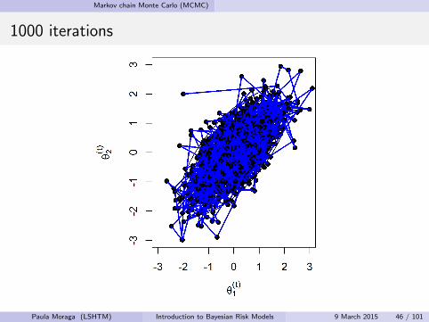
A Markov chain is a stochastic process (θ(0), θ(1), θ(2), . . .) thatsatisfies the Markov property:
p(θ(t+1)|θ(t), θ(t−1), . . . , θ(1)) = p(θ(t+1)|θ(t))
Consider a draw of θ(t) at iteration t. The next draw θ(t+1) atiteration t + 1 is dependent only on the current draw θ(t), and not onany past draws
The objective is to build a Markov chain that converges to the desiredtarget distribution p(θ|y)
Then we can run this chain to get draws that are approximately fromp(θ|y) once the chain has converged
MCMC algorithms: Gibbs sampling, Metropolis-Hastings algorithm,...
Software: WinBUGS, OpenBUGS, JAGS,...
Paula Moraga (LSHTM) Introduction to Bayesian Risk Models 9 March 2015 42 / 101
Markov chain Monte Carlo (MCMC)
Gibbs sampling
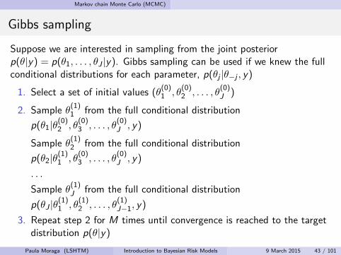
Suppose we are interested in sampling from the joint posteriorp(θ|y) = p(θ1, . . . , θJ |y). Gibbs sampling can be used if we knew the fullconditional distributions for each parameter, p(θj |θ−j , y)
1. Select a set of initial values (θ(0)1 , θ
(0)2 , . . . , θ
(0)J )
2. Sample θ(1)1 from the full conditional distribution
p(θ1|θ(0)2 , θ
(0)3 , . . . , θ
(0)J , y)
Sample θ(1)2 from the full conditional distribution
p(θ2|θ(1)1 , θ
(0)3 , . . . , θ
(0)J , y)
. . .
Sample θ(1)J from the full conditional distribution
p(θJ |θ(1)1 , θ
(1)2 , . . . , θ
(1)J−1, y)
3. Repeat step 2 for M times until convergence is reached to the targetdistribution p(θ|y)
Paula Moraga (LSHTM) Introduction to Bayesian Risk Models 9 March 2015 43 / 101
Markov chain Monte Carlo (MCMC)
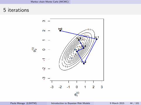
5 iterations
Paula Moraga (LSHTM) Introduction to Bayesian Risk Models 9 March 2015 44 / 101
Markov chain Monte Carlo (MCMC)
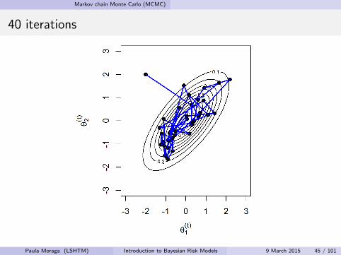
40 iterations
Paula Moraga (LSHTM) Introduction to Bayesian Risk Models 9 March 2015 45 / 101
Markov chain Monte Carlo (MCMC)
1000 iterations
Paula Moraga (LSHTM) Introduction to Bayesian Risk Models 9 March 2015 46 / 101
Markov chain Monte Carlo (MCMC)
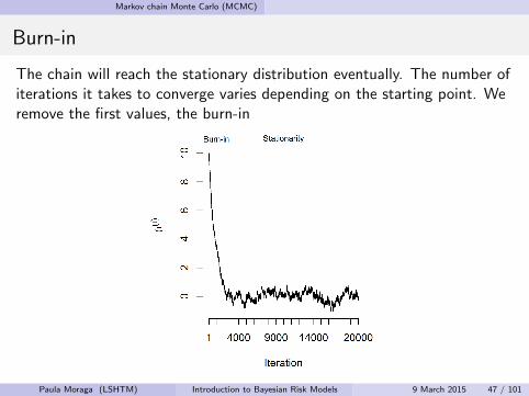
Burn-in
The chain will reach the stationary distribution eventually. The number ofiterations it takes to converge varies depending on the starting point. Weremove the first values, the burn-in
Paula Moraga (LSHTM) Introduction to Bayesian Risk Models 9 March 2015 47 / 101
Markov chain Monte Carlo (MCMC)
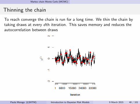
Thinning the chain
To reach converge the chain is run for a long time. We thin the chain bytaking draws at every dth iteration. This saves memory and reduces theautocorrelation between draws
Paula Moraga (LSHTM) Introduction to Bayesian Risk Models 9 March 2015 48 / 101
Convergence diagnostics
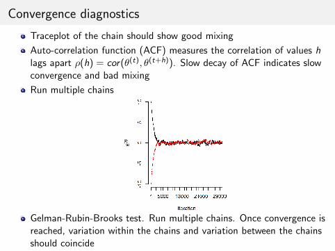
Traceplot of the chain should show good mixing
Auto-correlation function (ACF) measures the correlation of values hlags apart ρ(h) = cor(θ(t), θ(t+h)). Slow decay of ACF indicates slowconvergence and bad mixing
Run multiple chains
Gelman-Rubin-Brooks test. Run multiple chains. Once convergence isreached, variation within the chains and variation between the chainsshould coincide
Markov chain Monte Carlo (MCMC)
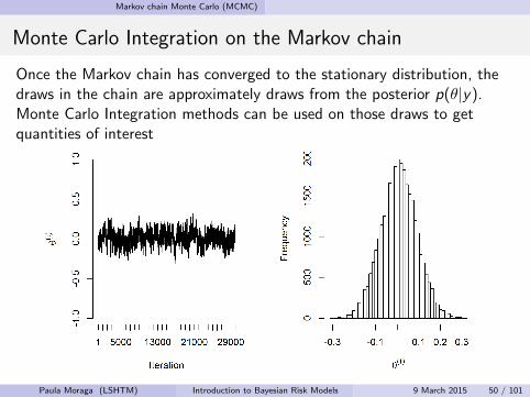
Monte Carlo Integration on the Markov chain
Once the Markov chain has converged to the stationary distribution, thedraws in the chain are approximately draws from the posterior p(θ|y).Monte Carlo Integration methods can be used on those draws to getquantities of interest
Paula Moraga (LSHTM) Introduction to Bayesian Risk Models 9 March 2015 50 / 101

Markov chain Monte Carlo (MCMC)
Monte Carlo Integration on the Markov chain
Given a sample (θ(1), . . . , θ(M)) from p(θ|y):
E (θ|y) ≈ 1M
∑Mi=1 θ
(i) = 0.006 P(θ > 0.1|y) ≈ 1M
∑Mi=1 I (θ
(i) > 0.1) = 0.13
Paula Moraga (LSHTM) Introduction to Bayesian Risk Models 9 March 2015 51 / 101
Approximate Bayesian inference by using INLA
Outline
1 Disease mapping models
2 Disease mapping for areal data
3 Model-based geostatistics
4 Frequentist vs. Bayesian paradigms
5 Markov chain Monte Carlo (MCMC)
6 Approximate Bayesian inference by using INLA
7 The INLA package for RExample 1Example 2Example 3
8 References
Paula Moraga (LSHTM) Introduction to Bayesian Risk Models 9 March 2015 52 / 101
Approximate Bayesian inference by using INLA
Approximate Bayesian inference for latent Gaussian modelsby using integrated nested Laplace approximations (INLA)
Integrated nested Laplace approximations (INLA) are an alternativeto inference via MCMC in latent Gaussian models
The main advantage of INLA is the huge improvement of speedcompared to MCMC alternatives
Laplace approximations to obtain posterior marginalsNumerical algorithms for sparse matricesParallel computing
INLA can be easily applied thanks to the R package R-INLA
Paula Moraga (LSHTM) Introduction to Bayesian Risk Models 9 March 2015 53 / 101
Approximate Bayesian inference by using INLA
Latent Gaussian models
Approximate Bayesian inference in a subclass of structured additiveregression models, named latent Gaussian models
Observed data yyi |x,θ ∼ π(yi |xi ,θ)
Latent Gaussian field
x|θ ∼ N(µ,Q(θ)−1)
Hyperparametersθ ∼ π(θ)
Paula Moraga (LSHTM) Introduction to Bayesian Risk Models 9 March 2015 54 / 101
Approximate Bayesian inference by using INLA
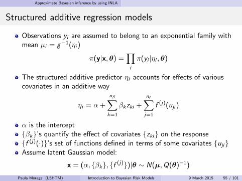
Structured additive regression models
Observations yi are assumed to belong to an exponential family withmean µi = g−1(ηi )
π(y|x,θ) =∏i
π(yi |ηi ,θ)
The structured additive predictor ηi accounts for effects of variouscovariates in an additive way
ηi = α +
nβ∑k=1
βkzki +
nf∑j=1
f (j)(uji )
α is the intercept{βk}’s quantify the effect of covariates {zki} on the response{f (j)(·)}’s set of functions defined in terms of some covariates {uji}Assume latent Gaussian model:
x = (α, {βk}, {f (j)})|θ ∼ N(µ,Q(θ)−1)
Paula Moraga (LSHTM) Introduction to Bayesian Risk Models 9 March 2015 55 / 101
Approximate Bayesian inference by using INLA
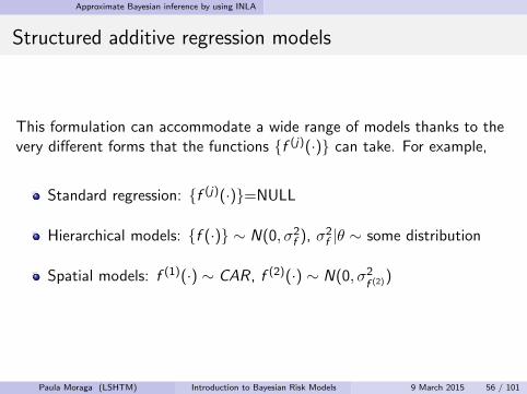
Structured additive regression models
This formulation can accommodate a wide range of models thanks to thevery different forms that the functions {f (j)(·)} can take. For example,
Standard regression: {f (j)(·)}=NULL
Hierarchical models: {f (·)} ∼ N(0, σ2f ), σ2
f |θ ∼ some distribution
Spatial models: f (1)(·) ∼ CAR, f (2)(·) ∼ N(0, σ2f (2))
Paula Moraga (LSHTM) Introduction to Bayesian Risk Models 9 March 2015 56 / 101

Approximate Bayesian inference by using INLA
Main ideas
Posteriorπ(x,θ|y) ∝ π(θ)π(x|θ)
∏π(yi |xi ,θ)
x denote the vector of all latent Gaussian variables
θ is the vector of hyperparameters which are not necessarily Gaussian
Compute the posterior marginals for the latent field
π(xi |y), i = 1, . . . , n
Compute the posterior marginals for the hyperparameters
π(θj |y), j = 1, . . . , dim(θ)
Paula Moraga (LSHTM) Introduction to Bayesian Risk Models 9 March 2015 57 / 101
Approximate Bayesian inference by using INLA
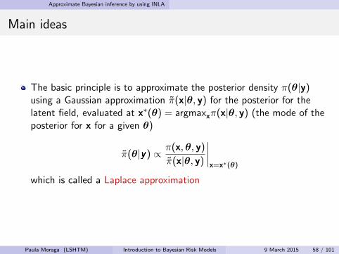
Main ideas
The basic principle is to approximate the posterior density π(θ|y)using a Gaussian approximation π(x|θ, y) for the posterior for thelatent field, evaluated at x∗(θ) = argmaxxπ(x|θ, y) (the mode of theposterior for x for a given θ)
π(θ|y) ∝ π(x,θ, y)
π(x|θ, y)
∣∣∣∣x=x∗(θ)
which is called a Laplace approximation
Paula Moraga (LSHTM) Introduction to Bayesian Risk Models 9 March 2015 58 / 101

Approximate Bayesian inference by using INLA
Main ideas
The posterior marginals for each xi and θj can be written as
π(xi |y) =
∫π(xi |θ, y)π(θ|y)dθ, π(θj |y) =
∫π(θ|y)dθ−j
Use this form to construct nested approximations
π(xi |y) =
∫π(xi |θ, y)π(θ|y)dθ, π(θj |y) =
∫π(θ|y)dθ−j
This approximation can be integrated numerically with respect to θ
π(xi |y) =∑k
π(xi |θk , y)π(θk |y)×∆k
(sum over values of θ with area-weights ∆k)
Paula Moraga (LSHTM) Introduction to Bayesian Risk Models 9 March 2015 59 / 101
Approximate Bayesian inference by using INLA
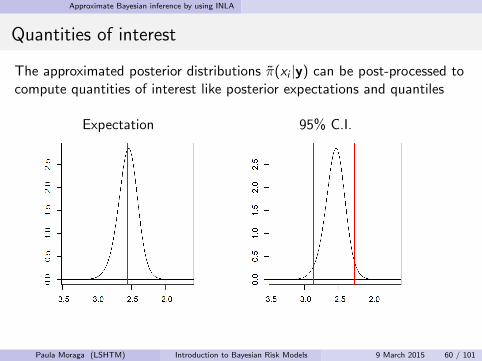
Quantities of interest
The approximated posterior distributions π(xi |y) can be post-processed tocompute quantities of interest like posterior expectations and quantiles
Expectation 95% C.I.
Paula Moraga (LSHTM) Introduction to Bayesian Risk Models 9 March 2015 60 / 101
The INLA package for R
Outline
1 Disease mapping models
2 Disease mapping for areal data
3 Model-based geostatistics
4 Frequentist vs. Bayesian paradigms
5 Markov chain Monte Carlo (MCMC)
6 Approximate Bayesian inference by using INLA
7 The INLA package for RExample 1Example 2Example 3
8 References
Paula Moraga (LSHTM) Introduction to Bayesian Risk Models 9 March 2015 61 / 101

The INLA package for R
Website http://www.r-inla.org/
Paula Moraga (LSHTM) Introduction to Bayesian Risk Models 9 March 2015 62 / 101

The INLA package for R
Installation of R-INLA
All the procedures needed to perform INLA are implemented in theR-INLA package
To install the package, type the following command line in Rsource("http://www.math.ntnu.no/inla/givemeINLA.R")
To load the package in R
library(INLA)
Paula Moraga (LSHTM) Introduction to Bayesian Risk Models 9 March 2015 63 / 101
The INLA package for R
Latent Gaussian models
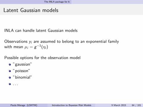
INLA can handle latent Gaussian models
Observations yi are assumed to belong to an exponential familywith mean µi = g−1(ηi )
Possible options for the observation model
”gaussian”
”poisson”
”binomial”
. . .
Paula Moraga (LSHTM) Introduction to Bayesian Risk Models 9 March 2015 64 / 101
The INLA package for R
Latent Gaussian models
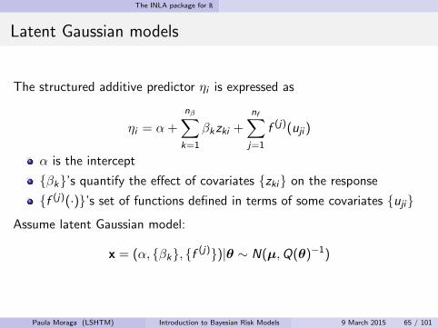
The structured additive predictor ηi is expressed as
ηi = α +
nβ∑k=1
βkzki +
nf∑j=1
f (j)(uji )
α is the intercept
{βk}’s quantify the effect of covariates {zki} on the response
{f (j)(·)}’s set of functions defined in terms of some covariates {uji}
Assume latent Gaussian model:
x = (α, {βk}, {f (j)})|θ ∼ N(µ,Q(θ)−1)
Paula Moraga (LSHTM) Introduction to Bayesian Risk Models 9 March 2015 65 / 101
The INLA package for R
Latent Gaussian models
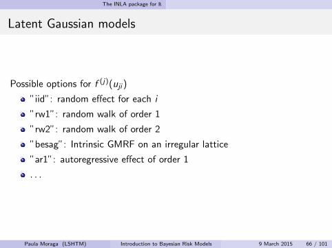
Possible options for f (j)(uji )
”iid”: random effect for each i
”rw1”: random walk of order 1
”rw2”: random walk of order 2
”besag”: Intrinsic GMRF on an irregular lattice
”ar1”: autoregressive effect of order 1
. . .
Paula Moraga (LSHTM) Introduction to Bayesian Risk Models 9 March 2015 66 / 101
The INLA package for R Example 1
Outline
1 Disease mapping models
2 Disease mapping for areal data
3 Model-based geostatistics
4 Frequentist vs. Bayesian paradigms
5 Markov chain Monte Carlo (MCMC)
6 Approximate Bayesian inference by using INLA
7 The INLA package for RExample 1Example 2Example 3
8 References
Paula Moraga (LSHTM) Introduction to Bayesian Risk Models 9 March 2015 67 / 101
The INLA package for R Example 1
Model
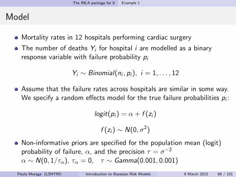
Mortality rates in 12 hospitals performing cardiac surgery
The number of deaths Yi for hospital i are modelled as a binaryresponse variable with failure probability pi
Yi ∼ Binomial(ni , pi ), i = 1, . . . , 12
Assume that the failure rates across hospitals are similar in some way.We specify a random effects model for the true failure probabilities pi :
logit(pi ) = α + f (zi )
f (zi ) ∼ N(0, σ2)
Non-informative priors are specified for the population mean (logit)probability of failure, α, and the precision τ = σ−2
α ∼ N(0, 1/τα), τα = 0, τ ∼ Gamma(0.001, 0.001)
Paula Moraga (LSHTM) Introduction to Bayesian Risk Models 9 March 2015 68 / 101
The INLA package for R Example 1
Data
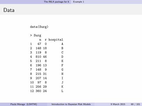
data(Surg)
> Surg
n r hospital
1 47 0 A
2 148 18 B
3 119 8 C
4 810 46 D
5 211 8 E
6 196 13 F
7 148 9 G
8 215 31 H
9 207 14 I
10 97 8 J
11 256 29 K
12 360 24 L
Paula Moraga (LSHTM) Introduction to Bayesian Risk Models 9 March 2015 69 / 101
The INLA package for R Example 1
Model fitting using R-INLA
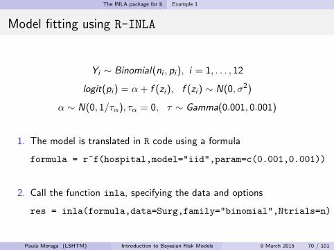
Yi ∼ Binomial(ni , pi ), i = 1, . . . , 12
logit(pi ) = α + f (zi ), f (zi ) ∼ N(0, σ2)
α ∼ N(0, 1/τα), τα = 0, τ ∼ Gamma(0.001, 0.001)
1. The model is translated in R code using a formula
formula = r~f(hospital,model="iid",param=c(0.001,0.001))
2. Call the function inla, specifying the data and options
res = inla(formula,data=Surg,family="binomial",Ntrials=n)
Paula Moraga (LSHTM) Introduction to Bayesian Risk Models 9 March 2015 70 / 101
The INLA package for R Example 1
Results
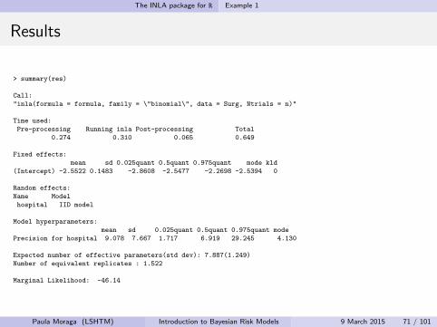
> summary(res)
Call:
"inla(formula = formula, family = \"binomial\", data = Surg, Ntrials = n)"
Time used:
Pre-processing Running inla Post-processing Total
0.274 0.310 0.065 0.649
Fixed effects:
mean sd 0.025quant 0.5quant 0.975quant mode kld
(Intercept) -2.5522 0.1483 -2.8608 -2.5477 -2.2698 -2.5394 0
Random effects:
Name Model
hospital IID model
Model hyperparameters:
mean sd 0.025quant 0.5quant 0.975quant mode
Precision for hospital 9.078 7.667 1.717 6.919 29.245 4.130
Expected number of effective parameters(std dev): 7.887(1.249)
Number of equivalent replicates : 1.522
Marginal Likelihood: -46.14
Paula Moraga (LSHTM) Introduction to Bayesian Risk Models 9 March 2015 71 / 101
The INLA package for R Example 1
Results
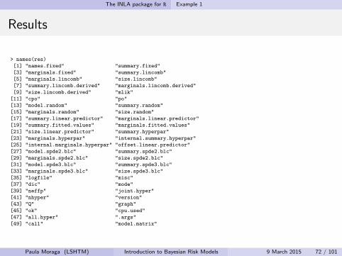
> names(res)
[1] "names.fixed" "summary.fixed"
[3] "marginals.fixed" "summary.lincomb"
[5] "marginals.lincomb" "size.lincomb"
[7] "summary.lincomb.derived" "marginals.lincomb.derived"
[9] "size.lincomb.derived" "mlik"
[11] "cpo" "po"
[13] "model.random" "summary.random"
[15] "marginals.random" "size.random"
[17] "summary.linear.predictor" "marginals.linear.predictor"
[19] "summary.fitted.values" "marginals.fitted.values"
[21] "size.linear.predictor" "summary.hyperpar"
[23] "marginals.hyperpar" "internal.summary.hyperpar"
[25] "internal.marginals.hyperpar" "offset.linear.predictor"
[27] "model.spde2.blc" "summary.spde2.blc"
[29] "marginals.spde2.blc" "size.spde2.blc"
[31] "model.spde3.blc" "summary.spde3.blc"
[33] "marginals.spde3.blc" "size.spde3.blc"
[35] "logfile" "misc"
[37] "dic" "mode"
[39] "neffp" "joint.hyper"
[41] "nhyper" "version"
[43] "Q" "graph"
[45] "ok" "cpu.used"
[47] "all.hyper" ".args"
[49] "call" "model.matrix"
Paula Moraga (LSHTM) Introduction to Bayesian Risk Models 9 March 2015 72 / 101
The INLA package for R Example 1
Results
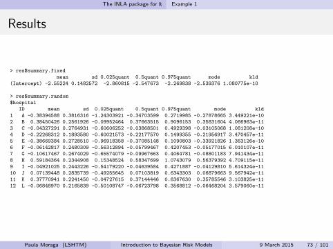
> res$summary.fixed
mean sd 0.025quant 0.5quant 0.975quant mode kld
(Intercept) -2.55224 0.1482572 -2.860815 -2.547673 -2.269838 -2.539376 1.080775e-10
> res$summary.random
$hospital
ID mean sd 0.025quant 0.5quant 0.975quant mode kld
1 A -0.38394588 0.3816316 -1.24303921 -0.34703599 0.2719985 -0.27878665 3.449221e-10
2 B 0.38450426 0.2561926 -0.09952464 0.37663515 0.9096153 0.35831604 4.066963e-11
3 C -0.04327291 0.2764931 -0.60606252 -0.03868501 0.4929398 -0.03105068 1.081208e-10
4 D -0.22268312 0.1893580 -0.60021573 -0.22177570 0.1499355 -0.21956917 3.470457e-11
5 E -0.38669384 0.2728510 -0.96918358 -0.37085148 0.1090803 -0.33921826 1.363126e-10
6 F -0.06142817 0.2480309 -0.56312894 -0.05799467 0.4207453 -0.05177015 6.010107e-11
7 G -0.10617467 0.2674029 -0.65574079 -0.09967663 0.4064781 -0.08801183 7.941434e-11
8 H 0.59184364 0.2344908 0.15348524 0.58347699 1.0743079 0.56379392 4.709115e-11
9 I -0.04921025 0.2443226 -0.54179220 -0.04639584 0.4271887 -0.04129810 5.614324e-11
10 J 0.07139448 0.2835739 -0.49255645 0.07103819 0.6343303 0.06879663 9.567942e-11
11 K 0.37770941 0.2241450 -0.04727615 0.37144446 0.8367630 0.35785546 3.103825e-11
12 L -0.06848970 0.2165839 -0.50108747 -0.06723798 0.3568812 -0.06468204 3.579060e-11
Paula Moraga (LSHTM) Introduction to Bayesian Risk Models 9 March 2015 73 / 101
The INLA package for R Example 1
Results
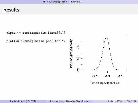
alpha <- res$marginals.fixed[[1]]
plot(inla.smarginal(alpha),t="l")
Paula Moraga (LSHTM) Introduction to Bayesian Risk Models 9 March 2015 74 / 101
The INLA package for R Example 1
Results
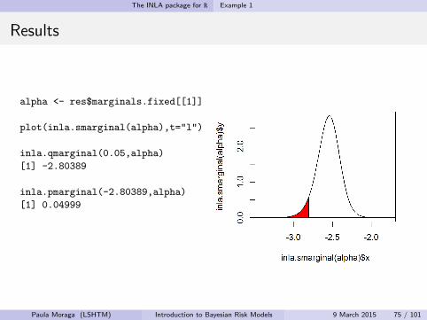
alpha <- res$marginals.fixed[[1]]
plot(inla.smarginal(alpha),t="l")
inla.qmarginal(0.05,alpha)
[1] -2.80389
inla.pmarginal(-2.80389,alpha)
[1] 0.04999
Paula Moraga (LSHTM) Introduction to Bayesian Risk Models 9 March 2015 75 / 101
The INLA package for R Example 1
Results
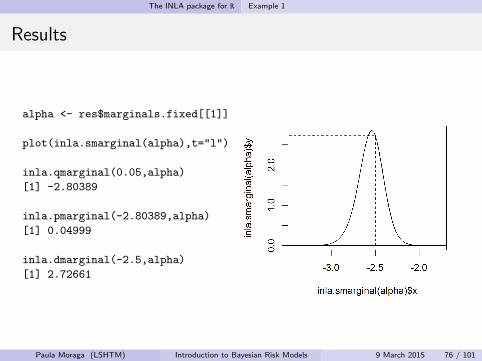
alpha <- res$marginals.fixed[[1]]
plot(inla.smarginal(alpha),t="l")
inla.qmarginal(0.05,alpha)
[1] -2.80389
inla.pmarginal(-2.80389,alpha)
[1] 0.04999
inla.dmarginal(-2.5,alpha)
[1] 2.72661
Paula Moraga (LSHTM) Introduction to Bayesian Risk Models 9 March 2015 76 / 101
The INLA package for R Example 1
Results
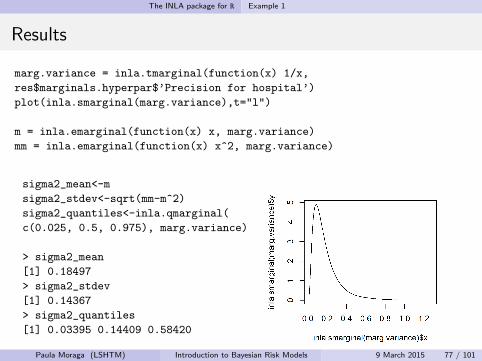
marg.variance = inla.tmarginal(function(x) 1/x,
res$marginals.hyperpar$’Precision for hospital’)
plot(inla.smarginal(marg.variance),t="l")
m = inla.emarginal(function(x) x, marg.variance)
mm = inla.emarginal(function(x) x^2, marg.variance)
sigma2_mean<-m
sigma2_stdev<-sqrt(mm-m^2)
sigma2_quantiles<-inla.qmarginal(
c(0.025, 0.5, 0.975), marg.variance)
> sigma2_mean
[1] 0.18497
> sigma2_stdev
[1] 0.14367
> sigma2_quantiles
[1] 0.03395 0.14409 0.58420
Paula Moraga (LSHTM) Introduction to Bayesian Risk Models 9 March 2015 77 / 101
The INLA package for R Example 2
Outline
1 Disease mapping models
2 Disease mapping for areal data
3 Model-based geostatistics
4 Frequentist vs. Bayesian paradigms
5 Markov chain Monte Carlo (MCMC)
6 Approximate Bayesian inference by using INLA
7 The INLA package for RExample 1Example 2Example 3
8 References
Paula Moraga (LSHTM) Introduction to Bayesian Risk Models 9 March 2015 78 / 101
The INLA package for R Example 2
Model
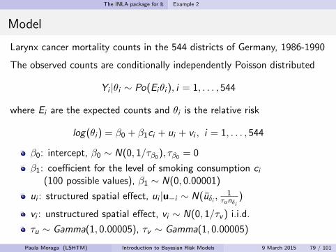
Larynx cancer mortality counts in the 544 districts of Germany, 1986-1990
The observed counts are conditionally independently Poisson distributed
Yi |θi ∼ Po(Eiθi ), i = 1, . . . , 544
where Ei are the expected counts and θi is the relative risk
log(θi ) = β0 + β1ci + ui + vi , i = 1, . . . , 544
β0: intercept, β0 ∼ N(0, 1/τβ0), τβ0 = 0
β1: coefficient for the level of smoking consumption ci(100 possible values), β1 ∼ N(0, 0.00001)
ui : structured spatial effect, ui |u−i ∼ N(uδi ,1
τunδi)
vi : unstructured spatial effect, vi ∼ N(0, 1/τv ) i.i.d.
τu ∼ Gamma(1, 0.00005), τv ∼ Gamma(1, 0.00005)
Paula Moraga (LSHTM) Introduction to Bayesian Risk Models 9 March 2015 79 / 101
The INLA package for R Example 2
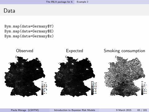
Data
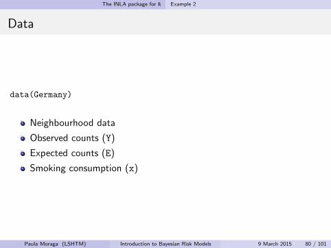
data(Germany)
Neighbourhood data
Observed counts (Y)
Expected counts (E)
Smoking consumption (x)
Paula Moraga (LSHTM) Introduction to Bayesian Risk Models 9 March 2015 80 / 101
The INLA package for R Example 2
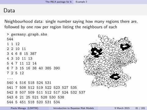
Data
Neighbourhood data: single number saying how many regions there are,followed by one row per region listing the neighbours of each
> germany.graph.nbs
544
1 1 12
2 2 10 11
3 4 6 8 15 387
4 3 10 11 13
5 4 7 11 12 14
6 7 3 15 16 38 40 385 390
7 2 5 12
...
540 4 516 518 524 531
541 7 508 512 519 522 523 527 535
542 8 507 509 511 512 517 524 532 537
543 6 21 25 521 528 530 538
544 5 451 518 520 531 534
Paula Moraga (LSHTM) Introduction to Bayesian Risk Models 9 March 2015 81 / 101
The INLA package for R Example 2
Data
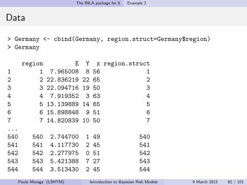
> Germany <- cbind(Germany, region.struct=Germany$region)
> Germany
region E Y x region.struct
1 1 7.965008 8 56 1
2 2 22.836219 22 65 2
3 3 22.094716 19 50 3
4 4 7.919352 3 63 4
5 5 13.139889 14 65 5
6 6 15.898848 9 51 6
7 7 14.820839 10 50 7
...
540 540 2.744700 1 49 540
541 541 4.117730 2 45 541
542 542 2.277975 0 51 542
543 543 5.421388 7 27 543
544 544 3.513430 2 45 544
Paula Moraga (LSHTM) Introduction to Bayesian Risk Models 9 March 2015 82 / 101
The INLA package for R Example 2
Data
Bym.map(data=Germany$Y)
Bym.map(data=Germany$E)
Bym.map(data=Germany$x)
Observed Expected Smoking consumption
Paula Moraga (LSHTM) Introduction to Bayesian Risk Models 9 March 2015 83 / 101
The INLA package for R Example 2
Data
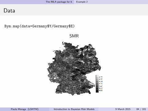
Bym.map(data=Germany$Y/Germany$E)
SMR
Paula Moraga (LSHTM) Introduction to Bayesian Risk Models 9 March 2015 84 / 101
The INLA package for R Example 2
Model fitting using R-INLA
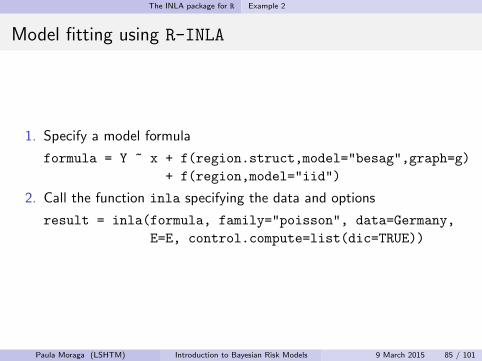
1. Specify a model formula
formula = Y ~ x + f(region.struct,model="besag",graph=g)
+ f(region,model="iid")
2. Call the function inla specifying the data and options
result = inla(formula, family="poisson", data=Germany,
E=E, control.compute=list(dic=TRUE))
Paula Moraga (LSHTM) Introduction to Bayesian Risk Models 9 March 2015 85 / 101
The INLA package for R Example 2
Results
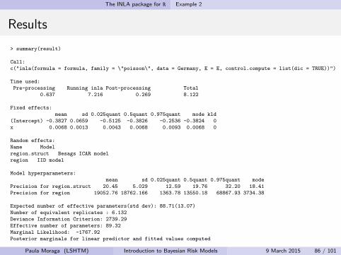
> summary(result)
Call:
c("inla(formula = formula, family = \"poisson\", data = Germany, E = E, control.compute = list(dic = TRUE))")
Time used:
Pre-processing Running inla Post-processing Total
0.637 7.216 0.269 8.122
Fixed effects:
mean sd 0.025quant 0.5quant 0.975quant mode kld
(Intercept) -0.3827 0.0659 -0.5125 -0.3826 -0.2536 -0.3824 0
x 0.0068 0.0013 0.0043 0.0068 0.0093 0.0068 0
Random effects:
Name Model
region.struct Besags ICAR model
region IID model
Model hyperparameters:
mean sd 0.025quant 0.5quant 0.975quant mode
Precision for region.struct 20.45 5.029 12.59 19.76 32.20 18.41
Precision for region 19052.76 18762.166 1363.78 13550.18 68867.93 3734.38
Expected number of effective parameters(std dev): 88.71(13.07)
Number of equivalent replicates : 6.132
Deviance Information Criterion: 2739.29
Effective number of parameters: 89.32
Marginal Likelihood: -1767.92
Posterior marginals for linear predictor and fitted values computed
Paula Moraga (LSHTM) Introduction to Bayesian Risk Models 9 March 2015 86 / 101
The INLA package for R Example 2
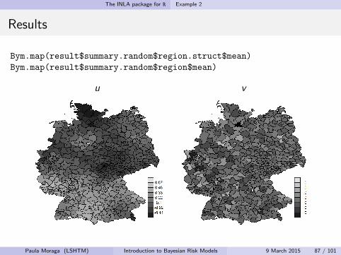
Results
Bym.map(result$summary.random$region.struct$mean)
Bym.map(result$summary.random$region$mean)
u v
Paula Moraga (LSHTM) Introduction to Bayesian Risk Models 9 March 2015 87 / 101
The INLA package for R Example 2
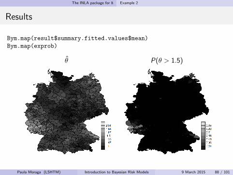
Results
Bym.map(result$summary.fitted.values$mean)
Bym.map(exprob)
θ P(θ > 1.5)
Paula Moraga (LSHTM) Introduction to Bayesian Risk Models 9 March 2015 88 / 101

The INLA package for R Example 3
Outline
1 Disease mapping models
2 Disease mapping for areal data
3 Model-based geostatistics
4 Frequentist vs. Bayesian paradigms
5 Markov chain Monte Carlo (MCMC)
6 Approximate Bayesian inference by using INLA
7 The INLA package for RExample 1Example 2Example 3
8 References
Paula Moraga (LSHTM) Introduction to Bayesian Risk Models 9 March 2015 89 / 101
The INLA package for R Example 3
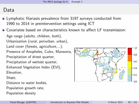
Data
Lymphatic filariasis prevalence from 3197 surveys conducted from1990 to 2014 in preintervention settings using ICT
Covariates based on characteristics known to affect LF transmission:
Age range (adults, children, both),
Urbanization (rural, periurban, urban),
Land cover (forests, agriculture,...),
Presence of Anopheles, Culex, Mansonia,
Precipitation of driest quarter,
Precipitation of wettest quarter,
Enhanced Vegetation Index (EVI),
Elevation,
Slope,
Distance to water bodies,
Population growth rate,
Population density
Paula Moraga (LSHTM) Introduction to Bayesian Risk Models 9 March 2015 90 / 101
The INLA package for R Example 3
Model
Conditional on the true prevalence P(xi ) at location xi , i = 1, . . . , n, thenumber of positive results Yi out of Ni people sampled at xi follows abinomial distribution,
Yi |P(xi ) ∼ Binomial(Ni ,P(xi ))
logit(P(xi )) = ziβ + S(xi )
zi = (1, zi1, . . . , zip) vector of the intercept and the p covariates
β = (β0, β1, . . . , βp)′ coefficient vector
S(xi ) spatially structured random effect
S(xi ) zero-mean Gaussian process with Matern covariance function
Paula Moraga (LSHTM) Introduction to Bayesian Risk Models 9 March 2015 91 / 101
The INLA package for R Example 3
Matern covariance function
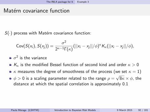
S(·) process with Matern covariance function:
Cov(S(xi ), S(xj)) =σ2
2κ−1Γ(κ)(||xi − xj ||/φ)κKκ(||xi − xj ||/φ),
σ2 is the variance
Kκ is the modified Bessel function of second kind and order κ > 0
κ measures the degree of smoothness of the process (we set κ = 1)
φ > 0 is a scaling parameter related to the range ρ =√
8κ× φ, thedistance at which the spatial correlation is approximately 0.1
Paula Moraga (LSHTM) Introduction to Bayesian Risk Models 9 March 2015 92 / 101
The INLA package for R Example 3
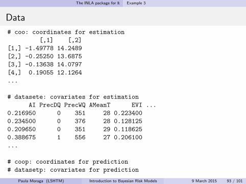
Data
# coo: coordinates for estimation
[,1] [,2]
[1,] -1.49778 14.2489
[2,] -0.25250 13.6875
[3,] -0.13638 14.0797
[4,] 0.19055 12.1264
...
# datasete: covariates for estimation
AI PrecDQ PrecWQ AMeanT EVI ...
0.216950 0 351 28 0.223400
0.234500 0 376 28 0.128125
0.209650 0 351 29 0.118625
0.388675 1 556 27 0.206100
...
# coop: coordinates for prediction
# datasetp: covariates for prediction
Paula Moraga (LSHTM) Introduction to Bayesian Risk Models 9 March 2015 93 / 101
The INLA package for R Example 3
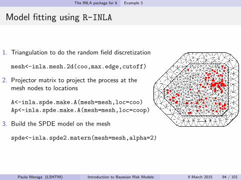
Model fitting using R-INLA
1. Triangulation to do the random field discretization
mesh<-inla.mesh.2d(coo,max.edge,cutoff)
2. Projector matrix to project the process at themesh nodes to locations
A<-inla.spde.make.A(mesh=mesh,loc=coo)
Ap<-inla.spde.make.A(mesh=mesh,loc=coop)
3. Build the SPDE model on the mesh
spde<-inla.spde2.matern(mesh=mesh,alpha=2)
Paula Moraga (LSHTM) Introduction to Bayesian Risk Models 9 March 2015 94 / 101
The INLA package for R Example 3
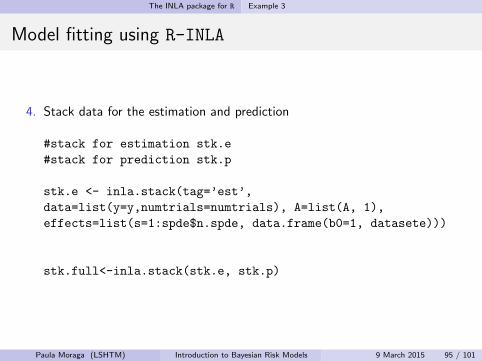
Model fitting using R-INLA
4. Stack data for the estimation and prediction
#stack for estimation stk.e
#stack for prediction stk.p
stk.e <- inla.stack(tag=’est’,
data=list(y=y,numtrials=numtrials), A=list(A, 1),
effects=list(s=1:spde$n.spde, data.frame(b0=1, datasete)))
stk.full<-inla.stack(stk.e, stk.p)
Paula Moraga (LSHTM) Introduction to Bayesian Risk Models 9 March 2015 95 / 101
The INLA package for R Example 3
Model fitting using R-INLA
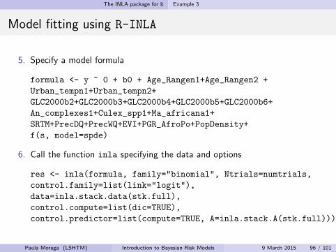
5. Specify a model formula
formula <- y ~ 0 + b0 + Age_Rangen1+Age_Rangen2 +
Urban_tempn1+Urban_tempn2+
GLC2000b2+GLC2000b3+GLC2000b4+GLC2000b5+GLC2000b6+
An_complexes1+Culex_spp1+Ma_africana1+
SRTM+PrecDQ+PrecWQ+EVI+PGR_AfroPo+PopDensity+
f(s, model=spde)
6. Call the function inla specifying the data and options
res <- inla(formula, family="binomial", Ntrials=numtrials,
control.family=list(link="logit"),
data=inla.stack.data(stk.full),
control.compute=list(dic=TRUE),
control.predictor=list(compute=TRUE, A=inla.stack.A(stk.full)))
Paula Moraga (LSHTM) Introduction to Bayesian Risk Models 9 March 2015 96 / 101
The INLA package for R Example 3
Results
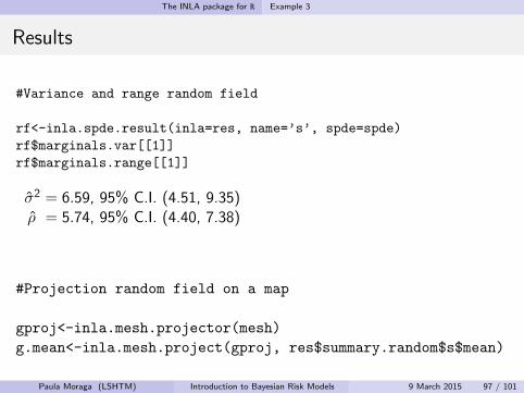
#Variance and range random field
rf<-inla.spde.result(inla=res, name=’s’, spde=spde)
rf$marginals.var[[1]]
rf$marginals.range[[1]]
σ2 = 6.59, 95% C.I. (4.51, 9.35)ρ = 5.74, 95% C.I. (4.40, 7.38)
#Projection random field on a map
gproj<-inla.mesh.projector(mesh)
g.mean<-inla.mesh.project(gproj, res$summary.random$s$mean)
Paula Moraga (LSHTM) Introduction to Bayesian Risk Models 9 March 2015 97 / 101
The INLA package for R Example 3
Results
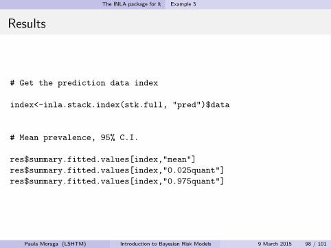
# Get the prediction data index
index<-inla.stack.index(stk.full, "pred")$data
# Mean prevalence, 95% C.I.
res$summary.fitted.values[index,"mean"]
res$summary.fitted.values[index,"0.025quant"]
res$summary.fitted.values[index,"0.975quant"]
Paula Moraga (LSHTM) Introduction to Bayesian Risk Models 9 March 2015 98 / 101
The INLA package for R Example 3
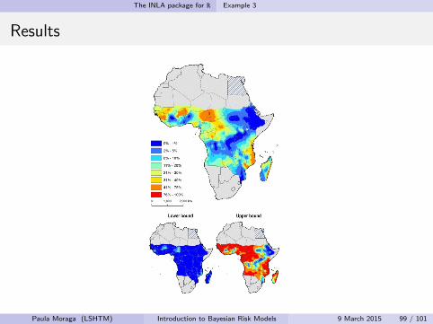
Results
Paula Moraga (LSHTM) Introduction to Bayesian Risk Models 9 March 2015 99 / 101
References
Outline
1 Disease mapping models
2 Disease mapping for areal data
3 Model-based geostatistics
4 Frequentist vs. Bayesian paradigms
5 Markov chain Monte Carlo (MCMC)
6 Approximate Bayesian inference by using INLA
7 The INLA package for RExample 1Example 2Example 3
8 References
Paula Moraga (LSHTM) Introduction to Bayesian Risk Models 9 March 2015 100 / 101
References
References
A. B. Lawson. Bayesian Disease Mapping: Hierarchical Modeling in SpatialEpidemiology, (2008), Chapman & Hall/CRC, Boca Raton, USA
P. J. Diggle and P. J. Ribeiro. Model-based Geostatistics, (2007), Springer,New York, USA
H. Rue, S. Martino and N. Chopin. Approximate Bayesian inference for latentGaussian models using integrated nested Laplace approximations (withdiscussion), (2009), Journal of the Royal Statistical Society, Series B,71(2):319-392
F. Lindgren, H. Rue and J. Lindstrom. An explicit link between Gaussianfields and Gaussian Markov random fields: the SPDE approach (withdiscussion), (2011), Journal of the Royal Statistical Society, Series B,73(4):423-498
Paula Moraga (LSHTM) Introduction to Bayesian Risk Models 9 March 2015 101 / 101