Firms and Farms: The Impact of Agricultural

Productivity on the Local Indian Economy

Gabriella Santangelo⇤

Yale University

JOB MARKET PAPERThis version: January 9, 2016

(Please click here for most recent version)

Abstract

How do agricultural productivity shocks propagate through the local economy andaffect firms? I combine firm, household and district-level data from India, andexploit weather-induced agricultural volatility, to estimate the response of manufac-turing firms to changes in agricultural productivity. I show that negative agriculturalproductivity shocks reduce firm production and employment. This holds true eventhough the local wage decreases. The effect is driven by firms that produce locally-traded goods, suggesting that the decrease in local demand induced by lower incomesplays a key role. I then examine whether the introduction of a large-scale rural work-fare program affects the response of the local economy to agricultural volatility. Ishow that the program acts as a stabilization policy and attenuates the pro-cyclicalresponse of local wage, consumption, and firms’ outcomes to agricultural productiv-ity shocks. The results highlight the importance of local rural demand for a largeshare of manufacturers and underscore how rural development policies that targethouseholds can strongly affect the industrial sector because of general equilibriumeffects.

⇤Yale University, Department of Economics, 28 Hillhouse Avenue, 06511 New Haven, CT. Email:gabriella.santangelo@yale.edu. I am extremely grateful to my advisors, Mark Rosenzweig, Chris Udryand Nancy Qian, for their guidance and support. I would also like to thank Shameel Amhad, MuneezaAlam, David Atkin, Alex Cohen, Sabysachi Das, Gabriele Foa’, Tim Guinnane, Dean Karlan, DanielKeniston, Tommaso Porzio, Camilla Roncoroni, Nick Ryan, Meredith Startz, Paul Schultz, Russell Toth,Jeff Weaver, Eric Weese and participants at the Yale Development Lunch for helpful comments anddiscussions at various stages of this project. This research was supported by grants from the SasakawaYoung Leaders Fellowship Fund (SYLFF). All errors are mine.

1

1 Introduction

Many firms in the developing world operate in economies that are primarily agricultural,where a large fraction of the population resides in rural areas and agriculture accounts fora substantial share of production and employment. In 2005, 70% of all manufacturing es-tablishments in India were located in rural areas and employment in these establishmentsaccounted for 60% of total Indian manufacturing employment1. Given these magnitudes,it is natural to ask how conditions in the rural economy affect firms and, in particular,whether rural incomes matter in determining the demand that firms face. This question isthe focus of a classical literature that examines the role of market size for industrialization(e.g. Murphy et al., 1989a, 1989b). It is also at the core of a large literature on the role ofagricultural development in the growth of the non-farm sector. Some scholars have arguedthat increases in agricultural productivity are a pre-condition for industrial development,and classical models of structural transformation have formalized this by showing howproductivity growth can generate demand for manufacturing goods2. A different strandof the literature, on the other hand, stressed the key distinction between open and closedeconomies, and noted how in open economies an increase in agricultural productivity canin fact crowd-out industrial production because manufacturing has to compete with theagricultural sector for labor 3.

This long-standing question has renewed importance for developing countries today,as the reduction in transportation costs and the consequent increased mobility of goodsand factors may have changed the influence of local conditions. In particular, do localrural incomes play an important role in determining the economic opportunities of firms,or do integrated factor and product markets make local incomes irrelevant?

In this paper, I provide direct evidence on this question by examining the dependenceof firms on the local rural economy in the context of India. The analysis entails twointertwined parts. First, I exploit weather-induced agricultural productivity fluctuationsto study how changes in agricultural incomes affect firms. Second, I take advantage ofthe introduction in rural areas of a large-scale workfare program, the National RuralEmployment Guarantee Act (NREGA), and assess the effects it had on rural incomes andwages, and how these effects translated to the rural industrial sector.

To guide the empirical analysis, I provide a simple multi-sector general equilibrium1Author’s calculations based on data from the Annual Survey of Industries and National Sample

Survey (Schedule 2.2, Manufacturing Enterprises) for the year 2005-2006.2See Rosenstein-Rodan, 1943; Lewis, 1954; Rostow, 1960; Ngai and Pissarides (2007), Baumol (1967),

Kongsamut, Rebelo and Xie (2001), Gollin, Parente and Rogerson (2002).3See Matsuyama (1992), Foster and Rosenzweig (2004, 2008).

2

model of the local economy that illustrates how agricultural productivity shocks affectthe local economy and are transmitted to firms through factor and product markets. Ithen extend the model to characterize how the introduction of a workfare program affectsthis transmission and impacts firms.

I model an economy with three distinct productive sectors: agriculture, a tradablenon-farm sector and a non-tradable non-farm sector. Agricultural goods are assumed tobe traded across space, while goods in the non-farm sector are either traded across spaceor sold locally. The distinction between firms that sell traded vs. non-traded goods iscrucial because firms will be affected differently by changes in local conditions. Considera positive shock to agricultural productivity. This has two effects on local firms: on theone hand, it induces an increase in the cost of labor because increased demand for laborin agriculture raises the equilibrium wage. On the other hand, it positively affects localincomes and thus potentially the demand that firms face. Firms that sell goods in globalmarkets are only affected by the first channel (wage channel) and their activity will becrowded-out by increases in agricultural productivity. Firms that sell their goods to localhouseholds will instead also benefit from the second channel (demand channel) and theiractivity may in fact be crowded-in by increases in agricultural productivity.

The model derives predictions for the local effects of agricultural productivity onequilibrium wage, income, and consumption, as well as sectoral employment, productionand prices. The model predictions are then examined using a unique combination of firm,household and district-level data from India. The empirical analysis requires a source ofexogenous variation in agricultural productivity. I rely on the fact that in rural India alarge fraction of agriculture is rainfed and agricultural productivity depends highly onmonsoon rainfall. Variation in rainfall realizations across Indian districts and over timeis used to estimate the response of equilibrium outcomes to agricultural productivity.

The first main result of the paper is that local rural incomes are an important determi-nant of the demand that firms face. I show that firms respond to a negative agriculturalproductivity shock by reducing production and employment. This holds true even thoughthe local wage decreases, suggesting that, while both effects are at play, the demand effectmore than compensate the wage effect. I also show that, consistently with the model,the result is driven by firms that produce locally-traded good, while firms that producetraded goods increase their activity, although the estimated elasticity is not statisticallysignificant. This set of results illustrates how an economically important share of firmsdoes not rely on national, or even state-level markets. We may have expected the mobilityof goods and factors to be sufficient to limit the influence of local conditions. The evi-

3

dence in this paper shows that this is not that case and that, instead, local rural incomescontinue to play an important role in determining the economic opportunities of firms.

Understanding how firms are affected by the conditions in the local economy hasimportant policy implications. Researchers and policymakers interested in firms in low-income countries generally focus their attention on policies that affect firms directly.The mechanisms I describe, on the other hand, underscore how policies targeted to theagricultural sector or aimed at rural households may have important consequences forfirms because of their general equilibrium implications. Ignoring these general equilibriumeffects can lead to a partial, and possibly misleading, assessment of the impact of policies.In the second part of this paper, I provide direct evidence for the policy relevance oflinkages in the local economy, and examine the impact of a large-scale workfare program,the National Rural Employment Guarantee Act (NREGA), introduced in rural India in2006.

The program entitles every household in rural India to 100 days of minimum-wagepublic employment per year. The type of work generated by the program is low-wage,unskilled manual work, often in construction. According to government administrativedata, during 2010-2011, the program generated a total of 2.3 billion person-days of em-ployment, providing employment to 53 million households in rural India4. The size ofthe program makes it one of the largest and most ambitious public-works employmentschemes ever attempted in history.

In this part, I take advantage of the timing of NREGA implementation across districtsto assess how the program affected the local economy and firms. I introduce NREGA inthe model as an additional sector that hires at a fixed wage (the program statutorywage) and obtain predictions for the impact of the program on equilibrium wage, incomeand sectoral outcomes. Intuitively, the availability of public employment guarantees tolocal workers the possibility to be remunerated at the NREGA wage. This induces awage floor, that is, it prevents the equilibrium wage from falling below the NREGA wageduring times of low agricultural productivity. Because of its stabilization effect on localwage, the program may also stabilize local income and demand. That is, it may be ableto support consumption during local downturns and behave as a counter-cyclical stimuluspolicy. This, in turn, may stabilize industrial production and employment.

In the empirical analysis, I estimate the response of equilibrium outcomes to agri-cultural productivity before and after the introduction of NREGA. The comparison ofelasticities before and after the program allows me to assess whether NREGA changes

4Figures are from the official NREGA website nrega.nic.in.

4

the way in which agricultural productivity shocks affect the local economy.The second main finding of the paper is that NREGA, through its effects on local

wage and demand, affects firms. I show that the program acts as a local stabilizationpolicy and attenuates the pro-cyclical response of local wage, consumption, and firms’outcomes to agricultural productivity shocks. The evidence supports the mechanismsoutlined in the model. First, I show that public employment under NREGA stronglyresponds to adverse agricultural shocks. That is, workers resort to NREGA to a largerextent when the local economy is hit by worse agricultural productivity shocks. Thisprovides evidence for the key channel through which the stabilization effect of NREGA isoperating. Second, I show that local rainfall has a much smaller impact on local wage andconsumption after the introduction of the program, even though it continues to have animpact on agricultural productivity. This suggests that NREGA acts on the relationshipbetween agricultural productivity and local income, and attenuates the response of thelatter to shocks. Finally, I show that, because of its effect on local income, the programattenuates the relationship between agricultural productivity and firms’ production andemployment.

This paper relates to previous work in multiple literatures. First, it relates to aclassical literature that examines the role of agricultural productivity in the developmentof the non-farm sector5. This paper is most closely linked to the more recent work in thisliterature, which empirically tests how improvements in agricultural productivity affectthe rest of the economy (Foster and Rosenzweig, 2004; Hornbeck and Keskin, 2012; Bustoset al., 2013; Marden, 2015).

Second, in the literature on NREGA, this paper is most closely related to Imbert andPapp (2015), Berg et al. (2013) and Zimmerman (2014), that study the impact of NREGAon wages, and Fetzer (2014), that shows that NREGA reduced conflict by attenuatingthe relationship between rainfall and violence. While there is a growing literature onNREGA, only few papers consider its general equilibrium implications, and those thatdo only focus on the impact on wages. My work shows that it is crucial to consider alsothe impact that the program had on demand and prices of goods sold locally. This isimportant because the effect of the program on demand can more than compensate itseffect on wage and, as I show, result in a crowd-in of local economic activity in the non-farm sector. To the best of my knowledge, no previous work has examined whether andhow workfare programs, including NREGA, affect the industrial sector. The closest paperin this regard is Magruder (2013), which used the timing of increase in minimum wages

5See Rosenstein-Rodan, 1943; Schultz, 1953; Lewis, 1954; Rostow, 1960

5

across Indonesian provinces in the 1990s to test the predictions of a big push model.Third, this paper relates to a large literature in development economics on the pro-

ductivity risk that households in low-income countries face, the extent to which they areinsured against such risk and their consumption smoothing capabilities (e.g. Binswangerand Rosenzweig, 1993; Townsend, 1994; Udry, 1994). In this literature, this paper ismost closely related to Jayachandran (2006), which shows how poverty, low mobility andcredit constraints exacerbate productivity risk. Her framework only considers the agricul-tural sector. I build on that framework adding the non-farm sector to the analysis, andshowing how the cross-sector linkages in the local economy can be additional sources ofproductivity risk exacerbation.

Fourth, the analysis and the predictions on tradable vs. non-tradable sectors arerelated to the recent literature on trade and volatility (Burgess and Donaldson, 2010;Allen and Atkin; 2015), which shows how trade integration can affect the volatility facedby local households.

More broadly, this work connects to the economics literature on local economic growth(Busso, Gregory, and Kline, 2013; Autor, Dorn, and Hanson 2013; Alcott and Keniston,2015; Moretti, 2010, 2011) and to the macro literature on the role of sector-specific shocksin macro fluctuations (Acemoglu et al., 2012; Caliendo et al., 2015).

The rest of the paper proceeds as follows. Section 2 presents a model of the localeconomy to derive the local effects of agricultural productivity shocks and to illustrate theimplications of the introduction of NREGA. Section 3 explains the various sources of dataused and how the key variables are constructed. Section 4 provides a brief background onNREGA. Section 5 develops the empirical strategy that is used to identify the impact ofagricultural productivity on the local economy and the role of NREGA. Section 5 presentsthe results. Section 6 concludes.

2 Model

In this section I present a simple multi-sector general equilibrium model of the local ruraleconomy to guide the empirical work. The purpose of the model is twofold. First, Iillustrate how shocks to the local farm-sector are transmitted to the non-farm economythrough linkages in the labor and goods market. In particular, I show how agriculturalshocks have different effects on firms that produce traded vs. non-traded goods, becauseof the key role that local agricultural income plays for the demand of non-traded goods.Second, I illustrate the implications that the introduction of a public-works program has

6

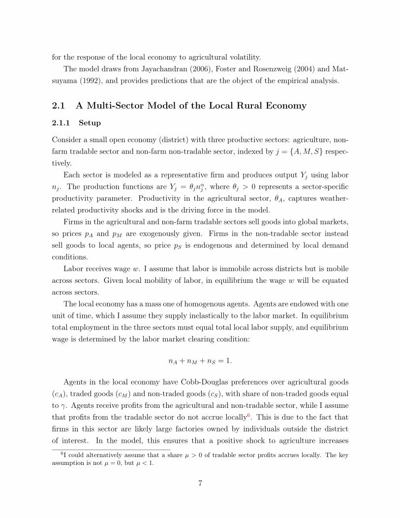
for the response of the local economy to agricultural volatility.The model draws from Jayachandran (2006), Foster and Rosenzweig (2004) and Mat-

suyama (1992), and provides predictions that are the object of the empirical analysis.

2.1 A Multi-Sector Model of the Local Rural Economy

2.1.1 Setup

Consider a small open economy (district) with three productive sectors: agriculture, non-farm tradable sector and non-farm non-tradable sector, indexed by j = {A,M, S} respec-tively.

Each sector is modeled as a representative firm and produces output Yj using labornj. The production functions are Yj = ✓jn

↵j , where ✓j > 0 represents a sector-specific

productivity parameter. Productivity in the agricultural sector, ✓A, captures weather-related productivity shocks and is the driving force in the model.

Firms in the agricultural and non-farm tradable sectors sell goods into global markets,so prices pA and pM are exogenously given. Firms in the non-tradable sector insteadsell goods to local agents, so price pS is endogenous and determined by local demandconditions.

Labor receives wage w. I assume that labor is immobile across districts but is mobileacross sectors. Given local mobility of labor, in equilibrium the wage w will be equatedacross sectors.

The local economy has a mass one of homogenous agents. Agents are endowed with oneunit of time, which I assume they supply inelastically to the labor market. In equilibriumtotal employment in the three sectors must equal total local labor supply, and equilibriumwage is determined by the labor market clearing condition:

nA + nM + nS = 1.

Agents in the local economy have Cobb-Douglas preferences over agricultural goods(cA), traded goods (cM) and non-traded goods (cS), with share of non-traded goods equalto �. Agents receive profits from the agricultural and non-tradable sector, while I assumethat profits from the tradable sector do not accrue locally6. This is due to the fact thatfirms in this sector are likely large factories owned by individuals outside the districtof interest. In the model, this ensures that a positive shock to agriculture increases

6I could alternatively assume that a share µ > 0 of tradable sector profits accrues locally. The keyassumption is not µ = 0, but µ < 1.

7

consumption of non-traded goods instead of increasing wages and price of non-tradedgoods proportionally.

The budget constraint is thus:

X

j2{A,M,S}pjcj = ⇡A + ⇡S + w.

Utility maximization with Cobb-Douglas preferences requires the expenditure share onnon-traded goods to be equal to �, so I have:

pscs = � (⇡A + ⇡S + w) .

In equilibrium, the price of non-traded goods, pS, adjusts to equilibrate non-tradable sup-ply and demand, and is determined endogenously to satisfy the market clearing condition:

YS = cS.

2.1.2 Comparative Statics: The Local Effects of a Change in Agricultural

Productivity

In this section I consider the effects of a shock to agricultural productivity on agents andfirms in the local economy. I derive the comparative statics for a change in the agriculturalproductivity parameter ✓A

7.Given that the wage and the price of the non-traded good must equilibrate their

respective markets, it is possible to solve explicitly for the equilibrium wage and the allo-cation of labor across the three sectors. Specifically, households’ utility maximization andfirms’ profit maximization, together with market clearing, imply that at the competitiveequilibrium:

w =↵

h(pA✓A)

11�↵ + C (pM✓M)

11�↵

i1�↵

(1� �)1�↵(1)

7The empirical analysis relies on variation in rainfall R, so that, for any outcome of interest y, Iestimate the reduced form impact of rainfall, that is, @y

@R . The assumption implicit to the empiricalanalysis (which will be tested below) is that agricultural productivity is a function of rainfall, so I canexploit the relation @y

@R = @y@✓A

@✓A@R . Notice how this implies that the rainfall elasticities estimated are a

function of @✓A@R , that is, the strength of the impact that rainfall has on agricultural productivity. In the

empirical analysis, I show how such strength depends on the extent of irrigation available in the district.

8

nj =(1��)(pj✓j)

11�↵

(pA✓A)1

1�↵+C(pM✓M )1

1�↵for j 2 {A,M} (2)

nS =�

h(pA✓A)

11�↵ + ↵ (pM✓M)

11�↵

i

(pA✓A)1

1�↵ + C (pM✓M)1

1�↵

(3)

where C = 1� �(1� ↵).

Prediction 1. A positive shock to agricultural productivity ✓A increases the equilibrium

wage:

@w@✓A

> 0.

The result follows immediately from Equation 1. Increases in ✓A increase the marginalreturn to labor in agriculture, increasing the demand for labor in agriculture and drivingup the equilibrium wage. Notice how, by assuming inelastic labor supply, I am excludingthe possibility that the increase in wage induces an increase in labor supply, which wouldin turn mitigate the wage increase. Inelastic labor supply simplifies the analysis but it isnot crucial for this result. What is crucial is that labor supply is not fully elastic. If laborsupply was fully elastic, changes in agricultural productivity would not affect wages, andall adjustment would occur through migration and/or movement into the labor force.

Prediction 2. A positive shock to agricultural productivity ✓A induces a reallocation of

agents towards the local farm sector:

@nA@✓A

> 0.

The result follows immediately from Equation 2. It is also immediate to show thatagricultural production and profits respond pro-cyclically, that is, @yA

@✓A> 0 and @⇡A

@✓A> 0.

Prediction 3. A positive shock to agricultural productivity ✓A has opposite effects on

the tradable and non-tradable components of the local non-farm economy. Specifically:

• The employment of local tradable firms moves counter-cyclically:

@nM@✓A

< 0.

• The employment of local non-tradable firms moves pro-cyclically:

@nS@✓A

> 0. In

addition, the price of non-tradable goods moves pro-cyclically:

@pS@✓A

> 0.

The results follows immediately from Equations 2 and 3, and from the closed-formexpression for the equilibrium price of the non-traded good:

pS =1

✓S

"�

1� �

#1�↵ h(pA✓A)

11�↵ + ↵ (pM✓M)

11�↵

i1�↵. (4)

9

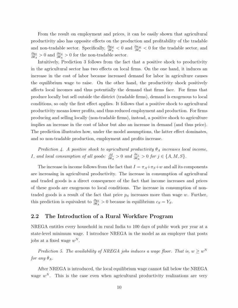
From the result on employment and prices, it can be easily shown that agriculturalproductivity also has opposite effects on the production and profitability of the tradableand non-tradable sector. Specifically, @yM

@✓A< 0 and @⇡M

@✓A< 0 for the tradable sector, and

@yS@✓A

> 0 and @⇡S@✓A

> 0 for the non-tradable sector.Intuitively, Prediction 3 follows from the fact that a positive shock to productivity

in the agricultural sector has two effects on local firms. On the one hand, it induces anincrease in the cost of labor because increased demand for labor in agriculture causesthe equilibrium wage to raise. On the other hand, the productivity shock positivelyaffects local incomes and thus potentially the demand that firms face. For firms thatproduce locally but sell outside the district (tradable firms), demand is exogenous to localconditions, so only the first effect applies. It follows that a positive shock to agriculturalproductivity means lower profits, and thus reduced employment and production. For firmsproducing and selling locally (non-tradable firms), instead, a positive shock to agricultureimplies an increase in the cost of labor but also an increase in demand (and thus price).The prediction illustrates how, under the model assumptions, the latter effect dominates,and so non-tradable production, employment and profits increase.

Prediction 4. A positive shock to agricultural productivity ✓A increases local income,

I, and local consumption of all goods:

@I@✓A

> 0 and

@cj@✓A

> 0 for j 2 {A,M, S}.

The increase in income follows from the fact that I = ⇡A+⇡S+w and all its componentsare increasing in agricultural productivity. The increase in consumption of agriculturaland traded goods is a direct consequence of the fact that income increases and pricesof these goods are exogenous to local conditions. The increase in consumption of non-traded goods is a result of the fact that price pS increases more than wage w. Further,this prediction is equivalent to @yS

@✓A> 0 because in equilibrium cS = YS.

2.2 The Introduction of a Rural Workfare Program

NREGA entitles every household in rural India to 100 days of public work per year at astate-level minimum wage. I introduce NREGA in the model as an employer that postsjobs at a fixed wage w

N .

Prediction 5. The availability of NREGA jobs induces a wage floor. That is, w � w

N

for any ✓A.

After NREGA is introduced, the local equilibrium wage cannot fall below the NREGAwage w

N . This is the case even when agricultural productivity realizations are very

10

low. The introduction of NREGA induces a threshold ✓̄

NA such that the pre-NREGA

equilibrium wage emerges for any ✓A > ✓̄

NA , while the equilibrium wage is equal to the

NREGA wage wN for any ✓A ✓̄

NA

8. This happens because for no agent it can be optimalto work for a wage lower than w

N when a NREGA job, which pays wN , is available. Thisimplies that if other employers in the local economy want to hire workers, they must payat least the NREGA wage.

I am assuming here that NREGA labor demand at wN is infinite, while we know thatthe implementation of NREGA limits employment to a maximum of 100 days. This isdone to simplify the comparative statics. The key result that NREGA induces an increasein equilibrium wage for certain agricultural productivity realizations would still remainif I assumed that NREGA offered jobs up to a maximum amount n

N . This alternativeassumption would not deliver the wage floor prediction, but would still deliver a wageincrease prediction, which is what matters for the results below.

Prediction 6. NREGA acts as a counter-cyclical stimulus policy. That is, the share of

agents working for NREGA is decreasing in ✓A:

@nN@✓A

< 0.

Before the introduction of NREGA, the labor market clears through the equilibriumwage. After the introduction of NREGA, since the wage level is fixed at w

N , the labormarket clears through the number of agents working for NREGA, nN . That is, the newmarket clearing condition is given by:

nN + nA(wN) + nM(wN) + nS(w

N) = 1.

Now notice that, after the introduction of NREGA, labor demand in the tradablesector does not depend on ✓A (this happens because ✓A does not affect the equilibriumwage anymore, and so has no impact on the cost of labor that tradable firms face).Labor demand in the agricultural and non-tradable sector, instead, still positively dependson ✓A. It follows that labor market clearing requires NREGA employment to increasewhen agricultural productivity in the local economy is low. Prediction 7 implies that,empirically, we should observe NREGA take-up to increase during “bad times”.

These considerations lead to Prediction 7, which illustrates the key implications ofNREGA for the volatility that the local economy faces. Let ✏y,✓A indicate the elasticity of

8For simplicity, I work below under the assumption that all agricultural productivity realizations arebelow the threshold ✓̄NA . The full characterization would take into consideration the fact that, for goodproductivity realizations, the post-NREGA equilibrium is equivalent to the pre-NREGA equilibrium.

11

y with respect to ✓A before the introduction of NREGA, and let ✏

Ny,✓A

indicate the sameelasticity after the introduction of NREGA.

Prediction 7. NREGA acts as a local stabilizer. Specifically, NREGA:

• Attenuates local wage elasticity: ✏

Nw,✓A

< ✏w,✓A

• Attenuates local income and consumption elasticity: ✏

NI,✓A

< ✏I,✓A and ✏

Ncj ,✓A

< ✏cj✓A

for j 2 {A,M, S}.

• Attenuates the counter-cyclical reallocation to the local non-farm tradable sector:

| ✏NnM ,✓A|<| ✏nM ,✓A |

• Attenuates the pro-cyclical reallocation to the local non-farm non-tradable sector:

✏

NnS ,✓A

< ✏nS ,✓A

Because of its stabilization effect on local wage, NREGA has an impact on local indus-trial volatility, and attenuates the short-term fluctuations in employment and productionin the non-farm sector. Consider firms selling tradable goods first. When a negativeshock hits the economy, NREGA prevents the wage to fall and thus prevents a reductionin the cost of labor that these firms face. As a consequence, these firms will increasetheir production and employment by less than they did pre-NREGA. Consider now firmsselling non-tradable goods. When a negative shock hits the economy, NREGA, by pre-venting a wage decrease, also prevents a decrease in local incomes and thus in the demandthat these firms face. Prediction 7 states that, given the model assumptions, the demandeffect prevails and so non-tradable firms will decrease their production and employmentby less than they did pre-NREGA. In sum, NREGA attenuates the volatility in local firmproduction and employment.

While I focus here on the implications of NREGA for local volatility, NREGA haseffects on the level of local economic activity as well. In particular, NREGA also causesan increase in the wage level. This translates into an increase in the cost of labor and hencea reduction in profits for firms in the tradable sector. In turn, the reduction in profitswill cause tradable firms to shrink. On the other hand, because of its positive effects onlocal demand, NREGA may induce higher production of firms in the non-tradable sector,thus fostering the development of the local non-farm non-tradable sector. The empiricalanalysis also examines these additional effects.

12

3 Data

This paper combines data from a large number of sources to provide a full picture ofthe effects of agricultural productivity on the local economy and to assess the impact ofNREGA on local economic activity. It relies on a unique combination of district-levelmeasures and micro-data for both firms and households.

3.1 Firm Data

The key dataset for firms is the Annual Survey of Industries (ASI), collected by theMinistry of Statistics and Program Implementation (MoSPI), Government of India. TheASI includes all registered manufacturing plants in India with more than fifty workers(one hundred if they operate without power) and a random one-third sample of registeredplants with more than ten workers (twenty if without power). Sampling weights areprovided so that the weighted sample reflects the population. I use sampling weightsthroughout the empirical analysis.

The ASI has extremely rich information on plant characteristics over the fiscal year(April of a given year through March of the following year) for around 50,000 plantseach year. It collects information in balance-sheet format for a large number variablesof interest (e.g. profits, output, number of employees, capital) so that it is possible toanalyze how firms respond to agricultural productivity across multiple dimensions.

This paper uses 10 waves of data, spanning the fiscal years 2000-2001 to 2009-20109.This sample includes years before the introduction of NREGA, to estimate the relevantelasticity in the absence of the policy, and years after the policy, to test whether NREGAcaused a reduction in volatility. Importantly, the availability of yearly data allows me toanalyze the exact timing of change in elasticities, and thus to verify that it tracks closelythe timing of the implementation of NREGA across districts.

The key outcome variables considered are measures of production and employment.Production is measured using the value of total output. For employment, I use the totalnumber of workers and total number of man-days employed. In some of the specifications,I distinguish blue-collar and white-collar workers, as well as permanent and contractworkers. I also consider measures of profitability (gross value added and profits) andcapital (total value of fixed capital). Finally, I construct a measure of daily wage dividing

9Additional waves are available after 2009-2010, but 2009-2010 is the last wave in which informationon firm location at district-level is disclosed. In subsequent waves, location information is only availableat the state-level. With no district information, it is not possible to match firm data to district measures.It is thus not possible to include later waves in the current analysis.

13

total compensation paid to workers by the number of man-days.The ASI data collect information on industry up to 4-digit of the Indian National

Industrial Classification (NIC). Industry classifications changed across the time span con-sidered (from NIC 1998, to NIC 2004, to NIC 2008). I develop and apply a concordanceacross industrial classifications to be able to group firms into industries in a consistentway across years.

As illustrated in the model, agricultural productivity shocks have different effectson firms depending on the the type of goods they produce (traded vs. non-traded). Itherefore require a criterion to classify firms according to the tradability of their products.I classify industries as tradable or non-tradable using three different definitions.

The first definition relies on a measure of industry tradability derived from the UnitedStates Census Commodity Flow Survey (CFS) in Holmes and Stevens (2014). Using theCFS, Holmes and Stevens (2014) calculate a measure of transportation costs for each4-digit SIC industry which is closely correlated with average product shipment distance.According to this classification, industries that produce goods such as ice-creams, newspa-pers, bricks and cardboard boxes are among the least tradable, while those that producewatches, x-ray equipment and aircraft parts are the most tradable. I match U.S. 4-digitSIC codes to India 4-digit NIC codes and define an industry as tradable if the eta pa-rameter in Holmens and Steven (2014) is less than 0.47. By this definition, 33 percentof the 4-digit manufacturing industries are tradable. Table 4 reports the list of 2-digitindustries and, for each industry, indicates the share of industry output that is classifiedas tradable.

The second and third definitions of tradability rely on Kothari (2014), which in turnbuilds on the classifications of tradable industries used in Mian and Sufi (2014). Kothari(2014) constructs two measures of tradability at the 3-digit NIC level. The first is basedon a measure of geographical concentration of industrial production across counties in theUnited States. Industries whose production is highly concentrated in a few counties inthe U.S. are considered to be tradable, while industries that have production spread overlots of counties are considered non-tradable. I apply this measure of industry tradabilitybased on U.S. levels of concentration to India. The second measure in Kothari (2014)is based on the degree of international trade carried out in any Indian industry as ashare of domestic production. Industries in which international trade is a large percentof domestic production are considered to be more tradable. These definitions distinguishindustries that are below/above median tradability, and hence classify 50 percent of the3-digit manufacturing industries are tradable.

14

I also derive a classification of industry linkages to the agricultural sector. I classify4-digit NIC industries as upstream or downstream of agriculture using the India MOSPIInput-Output tables for 2004-2005. For each industry, I calculate the agriculture outputshare, that is, the share of industry output that is purchased by the agricultural sector.I define an industry as “upstream” of agriculture if this upstream linkage share is largerthan 3 percent. I then calculate the industry agriculture input cost share, that is, theshare of industry input that is purchased from the agricultural sector. An industry is“downstream” if the agriculture input cost share is larger than 20 percent. I refer to anindustry as “non-linked” if it is neither upstream nor downstream. By this definition, 2percent of firms in the ASI data are upstream and 17 percent are downstream. The most-linked upstream industries include those that produce fertilizers, pesticides and otheragrochemical products, while the most-linked downstream industries include many thatprocess agricultural output and manufacture food.

Using ASI 2000-2001, I also define a measure of capital intensity. For each firm, Icompute the ratio between fixed assets and total compensation paid to employees. I thencompute an average of this measure at the industry level and define an industry as capitalintensive if the industry measure if above the median across industries.

Finally, I define a measure of industry dependence on external finance. I computethe ratio between outstanding loans and fixed assets. This is in the spirit of Rajan andZingales (1998). A higher ratio indicates that a higher share of capital is financed throughexternal funds. I define an industry as highly dependent on external finance if the industryaverage is above the median across industries.

Table 1 reports summary statistics for all firms in the ASI data. Tables 2 and 3 providesummary statistics distinguishing firms by industry type (tradable vs. non-tradable) andby NREGA-implementation-phase.

3.2 Consumption Data

Consumption expenditure measures come from the National Sample Survey (NSS) Con-sumer Expenditure Survey (Schedule 1). I use 7 waves spanning the years 2003-2004 to2011-2012. Specifically, the analysis includes the NSS waves 60, 61, 62, 63, 64, 66 and 68.

The survey includes extremely detailed information on consumption expenditure, col-lecting information on more than 400 consumption items. In the empirical analysis, Ifocus on monthly per capita expenditure (MPCE). This is computed as total monthlyexpenditure divided by household size. I consider both total MPCE and MPCE in differ-ent consumption categories. In particular, I group items into the three categories of food

15

consumption, manufactured goods consumption, and services consumption.I define real consumption dividing nominal consumption by the state Consumer Price

Index for Agricultural Labourers, published by the Government of India.

3.3 Wages and Employment Data

Wage and employment data are from the NSS Employment and Unemployment Survey(Schedule 10). The data include 6 waves spanning the years 2003-2004 to 2011-2012.Specifically, the analysis includes the NSS waves 60, 61, 62, 64, 66 and 68.

The NSS asks individuals who worked for a wage their total earnings in the 7 dayspreceding the survey. I construct a measure of daily wage dividing total earnings bythe number of days worked. The NSS survey provides information on the industry inwhich the individual works, so I can define an overall district wage, and, separately, anagricultural and a non-agricultural district wage. The survey also allows to distinguishworkers in regular or casual wage work. The survey covers a rich set of demographiccharacteristics, including age, gender, education and landholdings. This allows to includein the wage and employment specifications worker-level controls. This guarantees thatthe estimates capture actual impacts of agricultural shocks and not just changes in thecomposition of workers.

The NSS collects information on employment in the 7 days before the survey. Icompute the number of days that an individual spends in the labor force, unemployed orworking in different sectors.

3.4 Agricultural Data

I use data on annual district level agricultural production collected and published by theDirectorate of Economics and Statistics, Ministry of Agriculture. This data is reportedat the financial year level, which ranges from April to March in the subsequent calendaryear. For every district, I only consider crops that have been consistently planted on atleast 1,000 hectares during all the years in which the data are available. The resultingdataset is an unbalanced panel dataset covering the period from 2000-2010.

For a given crop, the yield is computed as total production divided by area cultivated. Iconstruct a yearly measure of district agricultural yield computing the weighted average ofthe yields of the different crops consistently cultivated in the district, with area cultivatedunder a given crop used as weight.

Additional agricultural data, such as district-level measures of total area cropped and

16

area irrigated, are from the Land Use Statistics Information System, Indian Ministry ofAgriculture.

3.5 Rainfall Data

This paper uses data from the Tropical Rainfall Measuring Mission (TRMM), developedby the National Aeronautics and Space Administration (NASA) and the Japan Aerospaceand Exploration Agency (JAXA). The TRMM provides gridded rainfall rates at very highspatial and temporal resolution. Daily rainfall measures are available at the 0.25 by 0.25degree grid-cell size, and are converted into overall monthly rainfall measures. Rainfallin a given district-year refers to rainfall registered on the grid point closest to the districtcentroid. For the empirical analysis, I focus on total monsoon rainfall, which I define astotal rainfall in the months of June, July, August and September. In the Indian context,monsoon rainfall accounts for at least 70% of annual rainfall.

I also define a categorical variable aimed at capturing possible non-linearities in theeffects of rainfall. The variable Rainfall Shock equals one if monsoon rainfall is greaterthan the district’s eightieth percentile of monsoon rainfall, zero if between the twentiethand eightieth percentiles, and minus one if below the twentieth percentile. This is the samemeasure used in Jayachandran (2006). I also show that results are robust to a continuosmeasure of rainfall deviation from its average, and compute the yearly fractional deviationfrom the long-run district’s mean monsoon rainfall.

3.6 NREGA Data

Data on participation to NREGA come from the NSS Employment and UnemploymentSurvey, waves 64, 66 and 68. I compute the number of days in the reference week that anindividual spends working under NREGA. Participation figures from household surveysare likely more reliable than participation figures available from administrative sources,and so are preferred to those.

The NSS Survey also asks information on the total earnings received from wage workunder NREGA. Dividing total earnings by the number of days worked, I obtain a mea-sure of the NREGA wage that a worker receives. These wages are used to compute thedistrict average wage paid under NREGA in a given year. These wages are then com-pared to the state-specific NREGA statutory wages, which vary over time. To make thecomparison possible, I complied information on NREGA statutory wages using multipleadministrative sources, including the notifications of NREGA wage revisions available in

17

the Gazette of India. Figures 6 and 7 provide an illustration of the cross-section and overtime variation in the NREGA statutory wage and its relation to the actual wage beingpaid under the program.

4 Background

The National Rural Employment Guarantee Scheme was introduced in India in 2005through the National Rural Employment Guarantee Act. The Act entitles every ruralhousehold to 100 days of public-sector work a year at a minimum wage established atthe state-level. According to government administrative data, in 2010-2011 the NREGAprovided 2.27 billion person-days of employment to 53 million households, with a budgetthat represents 0.6% of Indian GDP. The size of the program makes it one of the largestand most ambitious public-works employment schemes ever attempted worldwide.

The type of work generated by the program is low-wage, casual, unskilled manualwork, often in construction and for projects in transport infrastructure, irrigation orwater conservation. Employment creation and poverty reduction are at the core of theprogram, and this is apparent in a number of the Act provisions, including those thatgovern project costs. The Act limits material, capital and skilled wages expenditures to40% of total expenditures, thus reserving the remaining 60% to expenditure on unskilledwages. The Act also establishes that the central government bears the entire cost ofunskilled manual workers, but only 75% of the cost of material, capital and skilled workers,with the state government responsible for the remaining 25%. This creates an incentivefor states to select projects that are intensive in unskilled-labor and is meant to inducelarge employment creation per unit of budget.

Participation in NREGA does not entail formal requirements, and any individual canparticipate to the program as long as he resides in rural areas and is willing to earn atthe minimum wage and performing manual work. NREGA hence relies on self-selectionof individuals into the workfare program. Both women and men can participate to theprogram, and the Act in fact explicitly states that female workforce must be involved in atleast one third of the work created, and that men and women must receive the same wage.The importance of these provisions from a gender perspective and their implications onwomen empowerment and female labor force participation have been the object of someof the studies that have documented the introduction of NREGA (Afridi et al., 2012;Azam, 2012; Dreze and Khera, 2009).

Households can apply for work at any time of the year. The application process as

18

established in the Act entails a few steps. Households first apply for a job card which isissued by the local Gram Panchayat. Once in posses of the job card, households can submitan application to the Gram Panchayat, stating the time and duration for which they seekemployment. The Act mandates that, following such a request, employment on a public-works project is to be provided within 15 days of the application. If this statutory 15 daydeadline is exceeded, the household is entitled to a daily unemployment allowance. Theprogram was therefore designed to be demand-driven and highly responsive to the needsof rural households, though some studies and field reports have documented substantialvariation in the implementation standards across states and districts (Dreze and Khera,2009; Dutta et al., 2012; Niehaus and Sukhtankar, 2012 and 2013; Papp, 2012; Sharma,2009; World Bank, 2011).

NREGA was rolled out in rural India in three phases, between 2006 and 2008. Thefirst phase started in the first quarter of 2006, when the program was implemented in 200districts. In 2007, 130 further districts were added. In 2008, the third phase includedthe remaining districts into the scheme. NREGA currently covers all Indian districtsexcept a few entirely urban centers. Districts that received NREGA in the earlier phaseswere selected to have lower agricultural wages and lower agricultural output per worker,though this criterion was combined with the objective of starting the program in allstates. This caused a number of districts in richer states to receive the program early. Asa consequence, some early phases districts in richer states were in fact significantly betteracross a number of economic indicators than late phase districts in poorer states.

5 Empirical Strategy

The empirical analysis uses the predictions derived in Section 2 to study the effects ofagricultural productivity fluctuations on the local economy and to test whether NREGAhad an impact on how such fluctuations get transmitted through the local economy.Hence, it has two parts.

In the first part, I study the relationships between farm and non-farm sector for theyears before NREGA is introduced. In the second part, I show how the introduction ofNREGA changes the way in which the local economy responds to shocks.

The first part exploits exogenous variation in agricultural productivity due to monsoonrainfall realizations across districts and over time to estimate the elasticity of equilibriumoutcomes with respect to rainfall. The second part takes advantage of the timing inNREGA implementation to test for a change in the elasticities as predicted by the model.

19

5.1 The Effect of Agricultural Productivity on the Local Non-

Farm Sector

I estimate the relationship between rainfall and local outcomes using the time periodprior to the introduction of NREGA. This guarantees that the estimates are not affectedby any impact that NREGA may have. To establish the impact of rainfall on the localeconomy, I provide evidence for each channel of the transmission mechanism. First, I testthe key idea that rainfall affects agricultural productivity, by providing estimates of theelasticity of district crop yield to rainfall. Then, I estimate the impact of NREGA on (i)local wages, (ii) local consumption, (iii) local firm production and employment.

First, I analyze the effect of rainfall on district crop yields. I focus on monsoon rainfall(June to September) since this is the most important for India’s agricultural productivity.I estimate the following equation:

log(ydpt) = �log(Rdpt) + �d + ⌧pt + "dpt (5)

where d stands for district; p stands for NREGA implementation-phase, ranging from1 to 3; and t indicates time. The regression includes two sets of fixed effects. First,district fixed effects, which capture any time-invariant district characteristics that affectsthe level of agricultural productivity. The second are time fixed effects. The time fixedeffects are NREGA-implementation-phase specific, and thus remove yearly shocks thatare common to the districts which received NREGA in phases 1, 2 or 310.

The coefficient of interest is �. The prediction is that monsoon rainfall strongly affectsagricultural production. I expect this to be the case since in India more than 50% ofagriculture is rainfed and so highly dependent on the monsoon realization for irrigation.

In this and all regressions below, standard errors are clustered at the district level tocapture serial correlation. Results are virtually unaffected if instead I cluster standarderrors at the region-year level to allow for spatial correlation.

Second, I establish the impact of monsoon rainfall on wages through the regression:

log(widpt) = �log(Rdpt) + ⇢Xidpt + �d + ⌧pt + "idpt (6)

where i indexes an individual. Fixed effects are as above. The regression includesworker’s demographic characteristics, Xidpt, to tackle the possibility that composition

10I could alternatively introduce time fixed effects common across districts, and indeed results areunchanged in such case. NREGA-implementation-phase specific fixed effects are introduced mainly tokeep the pre-NREGA specifications consistent with the specifications that estimate the impact of NREGA.

20

changes. For robustness, I also estimate specifications that add state-specific time trends,or trends on initial district conditions (that is, time trends interacted with time-invariantdistrict characteristics such as poverty rate), to allow wages to trend differently across dif-ferent districts. I run the regression on all wages, as well as separately for high-skilled/low-skilled and agricultural/non-agricultural workers.

Third, I estimate the elasticity of local consumption. The specification is the same asthe one used for wage elasticity, except that the unit of observation is a household ratherthan a worker. I estimate the elasticity of monthly per capita expenditure using bothtotal consumption and different consumption components (specifically, food consumption,manufactured goods consumption and services consumption).

Fourth, I analyze the impact on rainfall on firm outcomes. The estimating equationis:

log(yjdpt) = �log(Rdpt) + �d + ⌧pt + #pj + ⇢jt + "jdst (7)

which studies outcome y for firms in industry j operating in district d of NREGAimplementation-phase p at time t.

District and time fixed effects are as in the specifications above. NREGA-implementation-phase specific industry fixed effects are included to capture time-invariant industry char-acteristics that are common within a NREGA implementation phase. I also includeindustry-specific time fixed effects to allow industries to grow at different rates over time.

The coefficient of interest is �. The main hypothesis is that, before the introductionof NREGA, there was a significant link between monsoon rainfall and manufacturingproduction and employment.

The model in Section 2 illustrates how we should expect the impact of rainfall to differdepending on whether a firm produces traded or non-traded goods. To capture this, Iestimate the regression separately for tradable and non-tradable sectors using a dummyTj that captures tradability of a given industry. For robustness, I use multiple tradabilitydefinitions. The data section reports information on how these dummies are constructed.

5.2 The Introduction of a Rural Workfare Program

The second part of the empirical analysis tests whether the introduction of NREGAcaused an attenuation of the relationships above. This is done using the empirical setuppresented above and adding an interaction term to those specifications. That is, I includethe interaction between rainfall and an indicator Ndpt which is equal to 1 if district d inimplementation phase p has NREGA at time t.

21

The identifying assumption in this part is that the timing of the implementationof NREGA across-districts is not correlated with any omitted variable that may alsoattenuate the rainfall-dependence of the local economy. It is important to note that thisidentifying assumption does not require the timing to be uncorrelated with trends in theoutcome variables of interest. Indeed, the inclusion in the specification of time fixedeffects that are specific to each NREGA implementation phase implies that identificationis coming off of districts within the same implementation phase. That is, the specificationflexibly allows for the possibility that different implementation phases are on differenttrends.

In this part, I first show that NREGA has the potential to attenuate local volatilitybecause NREGA jobs provision increases when the local economy is hit by a negativeagricultural productivity shock. I then proceed by studying the moderating effect ofNREGA on local outcomes following the same order of the specifications above.

First, I provide evidence that NREGA take-up responds to rainfall using the regression:

log(yidpt) = �log(Rdpt) + �log(Rdpt)⇥Ndpt + ⇢Xidpt + �d + ⌧pt + "idpt (8)

where y represents the time that individual i spends working in public works. Otherindexes are as in the specifications above. The prediction is that � = 0 and � < 0. Thatis, before the introduction of NREGA, there was no relation between public employmentand rainfall. Once NREGA is introduced, individuals respond to a negative productivityshock resorting to NREGA jobs, and do so to a larger extent the worse is the shock.

Second, I show that, at least in the time period considered, NREGA did not attenuatethe relationship between rainfall and agricultural yields. It is possible that in the long-runNREGA makes agricultural yields less sensitive to rainfall, for instance through an impacton irrigation infrastructure. However, I show that this does not seem to be happening inthe years right after its introduction. This means that any attenuation in the responseof a given variable to rainfall (the reduced form) can be interpreted as the result of anattenuation in the response of such variable to agricultural yields (the second stage), ratherthan an attenuation in the response of agricultural yields to rainfall (the first stage).

Third, I show the moderating impact of NREGA on wage elasticity. The specificationfor wage elasticity becomes as follows:

log(widpt) = �log(Rdpt) + �log(Rdpt)⇥Ndpt + ⇢Xidpt + �d + ⌧pt + "idpt (9)

Notice that the treatment dummy Ndpt is collinear to the NREGA-implementation-

22

phase-specific time fixed effects. Hence, the specification does not estimate the impactthat NREGA has on the level of the outcome variable. It instead tests whether the wayin which rainfall translates into local wages changes with the availability of NREGA jobs.The prediction is that � > 0 and � < 0, that is, NREGA reduces local wage volatility.

The same specification is used to assess the effect of the introduction of NREGA onconsumption volatility.

Finally, I test whether NREGA had a moderating impact on local industrial productionand employment. The specification for firm outcomes becomes:

log(yjdpt) = �log(Rdpt) + �log(Rdpt)⇥Ndpt + �d + ⌧pt + #pj + ⇢jt + "jdst (10)

One concern with the specifications above is that the NREGA treatment may be cap-turing a more general over-time decline in the rainfall-dependence of the local economy,or the impact of other contemporaneous policies that affect rainfall-dependence. I tacklethis possibility by estimating, for each of the outcomes above, a yearly measure of elastic-ity. This allows me to track elasticities throughout the study time period and show thatthe timing of the elasticity attenuation coincides with the introduction of NREGA acrossthe three implementation phases. Specifically, I estimate a regression that includes theterm

Ps2{�7,�6,...,2,3} �slog(Rds). The aim is to plot the estimated coefficients �s together

with their confidence intervals, and show that the pattern is such that the �s are mostlyconstant in the period before NREGA, jump in correspondence of the introduction ofNREGA and stabilize at the new level in the subsequent years.

6 Results

The results, as the empirical strategy, comprise two parts. In the first part, I estimate therelationships between rainfall and local outcomes in the period before the introductionof NREGA. In the second part, I present the results that consider the entire period andshow how the introduction of NREGA affects such relationships.

6.1 The Effect of Agricultural Productivity on the Local Non-

Farm Sector

I start by establishing that monsoon rainfall has an impact on agricultural productivityin the time period considered in this study. Table 5 shows that monsoon rainfall has a

23

large effect on district crop yields, and illustrates how the effect changes with the shareof cultivated land that is irrigated.

I then estimate the impact of monsoon rainfall on local wages. Table 6 reports theresults. Consistently with the hypothesis of local labor mobility across sectors, the esti-mates show that rainfall affects not only the wage in the agricultural sector but also thewage in the non-agricultural sector.

Table 7 presents the estimates of consumption elasticity. The consumption regressionstest the prediction that rainfall is an important driver of demand in the local economy.The results show that there is a strong relationship between rainfall and monthly percapita expenditure. Columns (2) and (3) distinguish food and non-food consumption.They show that the impact is weakest on food consumption and strongest on non-food.Column (4) reports the elasticity for consumption expenditure on manufactured goods.This is the estimate most closely related to the effect that a rainfall shock has on thedemand for the goods that manufacturing firms produce.

Estimates of the response of local firms to agricultural fluctuations are presented inTable 8. Consistently with the evidence in Table 6, Column (4) shows that a positiverainfall realization raises the cost of labor for local manufacturing firms. However, eventhough they face higher labor costs, firms respond pro-cyclically to shocks to agriculturalproductivity. The estimates of production and employment elasticities in Columns (1) to(3) are indeed positive. The results suggest that the (positive) local demand effect morethan compensate the (negative) local wage effect that results from a positive realizationof monsoon rainfall.

Evidence in support of the demand channel is presented in Table 9. The table reportsthe results from regressions that consider separately firms in tradable and non-tradableindustries. The estimates show that pro-cyclicality is driven by firms that produce non-tradable goods. For firms that produce tradable goods, instead, the estimated elasticitiesare negative, even though not significant. These estimates are consistent with the modelprediction of opposite effects on firms that sell traded vs. non-traded goods.

6.2 The Introduction of a Rural Workfare Program

In this part I test the hypothesis that the introduction of NREGA led to a moderation ofthe relationships between rainfall and local outcomes.

The stabilization potential of NREGA rests on the fact that NREGA jobs provisionincreases when the local economy is hit by a negative agricultural productivity shock. Itherefore test whether local participation to NREGA increases when there is a negative

24

rainfall realization. Results are reported in Column (2) of Table 10. The estimates confirmthat, pre-NREGA, participation in public employment was not linked to rainfall. OnceNREGA is introduced, instead, take-up of public works jobs is significantly (negatively)correlated to rainfall.

Column (1) of Table 10 shows that, in the time period considered, NREGA did notattenuate the relationship between rainfall and agricultural yields. This means that anyattenuation in the response of a given variable to rainfall (the reduced form) can beinterpreted as the result of the attenuation in the response of such variable to agriculturalyields (the second stage), rather than an attenuation in the response of agricultural yieldsto rainfall (the first stage).

Table 11 tests the prediction that the introduction of NREGA attenuated local wagevolatility. The results support the hypothesis that NREGA stabilized the wage, and infact suggest that NREGA brought the wage elasticity to zero.

That NREGA has a moderation effect on local volatility also emerges from Table 12,that reports the results for local consumption. The introduction of NREGA attenuatedthe relationship between rainfall and consumption. This means that NREGA is able tosupport local demand when agricultural productivity, and therefore incomes, are low.

Table 13 and 14 test the hypothesis that NREGA affects the way in which local firmsrespond to agricultural fluctuations. Results are reported separately for the differentNREGA implementation phases, since they differ in their pre-NREGA volatility, and, asa consequence, in the potential attenuation post-NREGA. The results are consistent withthe hypothesis that NREGA attenuated the pro-cyclical response of non-tradable firms inPhase 1 and 2 districts. Post-NREGA, production and employment fluctuate to a lesserextent in response to agricultural fluctuations.

6.3 Robustness Checks

In this section I perform a number of robustness checks to show that the estimates arerobust to deviations from the baseline framework.

First, I show the robustness of the results to alternative ways of measuring the weathershock. Table 15 reports the results of estimating firm elasticities using a measure of rainfallshock instead of total rainfall. The variable Rainfall Shock equals one if monsoon rainfallis greater than the district’s eightieth percentile of monsoon rainfall, zero if between thetwentieth and eightieth percentiles, and minus one if below the twentieth percentile. Thisis the same measure used in Jayachandran (2006). I also define the variable RainfallDeviation which is equal to the yearly fractional deviation from the long-run district’s

25

mean monsoon rainfall. The results obtained using these measures are very similar to thebaseline results and are statistically significant.

Second, I show that the heterogenous impact across tradable and non-tradable in-dustries is robust to alternative tradability classifications. Panel A in Table 16 reportsthe estimates of firm elasticities separately for tradable and non-tradable industries usingthe classification based on geographical concentration. Panel B reports the elasticitiesestimated using the classification based on international trade. The results confirm thatthe pro-cyclical response in driven by firms in non-tradable industries.

In a third set of robustness checks, I tackle the possibility that yearly fluctuations inrainfall could potentially have an impact on the non-agricultural sector through channelsother than agricultural productivity. I show results from two placebo tests. First, I ex-ploit the fact that there is large variation across districts in access to irrigation sources.I identify poorly irrigated districts (those for which less than 20% of cultivated land isirrigated) and highly irrigated districts (those for which more than 60% of cultivated landis irrigated). Each group accounts for around 30% of Indian districts. Access to irriga-tion makes agriculture less susceptible to weather variation and hence we would expectcrop yields in highly irrigated districts to be affected by monsoon rainfall very limitedly.Column 1 and 2 in Table 17 show that the first-stage effect of rainfall on agricultural pro-ductivity is strong only in districts with poor access to irrigation. Additionally, Columns3 to 10 show that the reduced-form effect of rainfall on firm outcomes only exists inthese same districts. The elasticities of firm wage, production and employment in highlyirrigated districts are much smaller and not statistically significant. This lack of bothfirst-stage and reduced-form effects in highly irrigated districts suggests that the effect ofgrowing-season rainfall on firms operates through the key channel of agricultural produc-tivity.

The second placebo check tests whether rainfall outside the main growing season hasan effect on firms. The key idea is that rainfall outside the monsoon season should not bea strong determinant of agricultural productivity and hence should not have an impacton industrial outcomes. The results are presented in Table 18. Column 1 shows thatnon-monsoon rainfall has a very limited impact on district crop yields. Consistently withagricultural productivity being the key channel through which monsoon rainfall affectsfirms, Column 2 to 5 show that the elasticities of firm outcomes to non-monsoon rainfallare small in magnitude and not statistically significant.

The fourth robustness check assesses whether the findings reflect the strength of an-other channel through which agricultural productivity can affect the manufacturing sector:

26

input-output linkages. Farming requires inputs produced by other sectors, including man-ufacturing. This means that an increase in agricultural productivity in a given districtmight increase the demand for industries that produce inputs used in agriculture, such aschemicals or fertilizers. To the extent that manufacturing firms producing chemicals andfertilizers face high transport costs, their production and employment would respond tolocal demand conditions. Therefore, the effect of rainfall that I show could potentially beexplained by an increase in the agricultural demand for manufacturing inputs. A similarargument applies to manufacturing industries that use agricultural goods as intermediateinputs – for instance, industries that process food. In order to assess the contribution ofthese direct linkages on my estimates, I use the Indian Input-Output table (2004-2005)to identify industries directly linked to agriculture through input-output linkages, eitherupstream or downstream. I then use this information to define non-linked industries andestimate elasticities for this subset. Table 19 reports the results from regressions that con-sider separately firms that are linked and non-linked to the agricultural sector, and, for thelatter, shows results separately for firms in tradable and non-tradable industries. Column(1) reports the elasticity estimates for firms that are linked to agriculture. The estimatesare indeed larger than for the overall sample. However, Columns (2) to (4) show thatrainfall has a positive impact also on firms in non-linked non-tradable industries. Takentogether, these results imply that the pro-cyclical response of the manufacturing sector isnot fully driven by the processing of agricultural output in downstream industries or bylarger agricultural sector demand for upstream industries.

Fifth, Table 20 shows that the results remain statistically significant when I correctstandard errors to account for spatial correlation by clustering at the region-year level.

Finally, I provide evidence for the robustness of the results on the stabilization impactof NREGA. One concern with the baseline specification is that the NREGA treatmentmay be capturing a more general over-time decline in the rainfall-dependence of the localeconomy, or the impact of other contemporaneous policies that affect rainfall-dependence.I tackle this possibility by estimating yearly measures of elasticity. This allows me to trackelasticities throughout the study time period and show that the timing of the change inelasticity coincides with the introduction of NREGA. Figures (1) to (3) plot the estimatedelasticities together with the confidence interval. The coefficient patterns show that elas-ticities are relatively constant in the period before NREGA, and move to a different levelin correspondence of the introduction of NREGA, thus reassuring against the hypothesisthat NREGA is capturing the attenuation effect of other omitted variables.

27

7 Conclusion

How do agricultural productivity shocks propagate through the local economy and affectmanufacturing firms? I present a simple model of a small open economy to illustrate howshocks to the farm-sector are transmitted to local firms through linkages in the labor andgoods market. Using variation in weather realizations across districts and over time, Iestimate the response of local firms’ production and employment to agricultural produc-tivity shocks, and show that firms respond pro-cyclically. The evidence best supports alocal demand story: the higher incomes resulting from agriculture translate into higherdemand for local non-tradable firms. The results highlight the importance of the mobilityof goods for local volatility, and illustrate how local rural incomes continue to play animportant role in determining the economic opportunities of manufacturing firms.

The paper additionally examines whether the introduction of a rural workfare pro-gram, the NREGA, affects the response of the local economy to agricultural volatility.It shows that the program acts as a stabilization policy and attenuates the pro-cyclicalresponse of local wage, consumption, and firms’ outcomes to agricultural productivityshocks. The evidence from NREGA exemplifies how policies not targeted to firms canstill exert sizable influence on firms’ decisions because of their impact on the economy inwhich both firms and farms operate. Attention in the past has focused only on policiesthat affect firms directly. This paper instead highlights how attention should also bepaid to policies that target rural households and the agricultural sector, as these havefar-reaching consequences.

28

References

[1] Acemoglu, A., V. Carvalho, A. Ozdalgar, and A. Tahbaz-Salehi (2012), “The NetworkOrigins of Aggregate Fluctuations,” Econometrica, 80, 1977–2016.

[2] Acemoglu, D. and V. Guerrieri (2008), “Capital Deepening and Non-Balanced Eco-nomic Growth,” Journal of Political Economy 116, 467–498.

[3] Adhvaryu, Achyuta, Amalavoyal Chari and Siddharth Sharma (2013a), “Firing Costsand Flexibility: Evidence from Firms’ Labor Adjustments to Shocks in India,” Reviewof Economics and Statistics, forthcoming.

[4] Afridi, Farzana, Abhiroop Mukhopadhyay and Soham Sahoo (2012), “Female LabourForce Participation and Child Education in India: The Effect of the National RuralEmployment Guarantee Scheme,” Working Paper.

[5] Ahluwalia, Rahul, Mudit Kapoor and Shamika Ravi (2012), “The Impact of NREGSon Urbanization in India,” Working Paper.

[6] Allcott, Hunt and Daniel Keniston, (2015) “Dutch Disease or Agglomeration? TheLocal Economic Eøects of Natural Resource Booms in Modern America,” WorkingPaper.

[7] Allen, D. and D. Atkin (2015), “Volatility, Insurance, and the Gains from Trade,”Working Paper.

[8] Asher, Sam and Paul Novosad (2012), “Factory Farming: The Impact of AgriculturalOutput on Local Economic Activity in India,” Working Paper.

[9] Autor, David H., David Dorn, and Gordon H. Hanson (2013), “The China Syndrome:Local Labor Market Effects of Import Competition in the United States,” AmericanEconomic Review 2013, 103(6): 2121–2168.

[10] Azam, Mehtabul (2012), “The Impact of Indian Job Guarantee Scheme on LaborMarket Outcomes: Evidence from a Natural Experiment,” IZA Discussion Paper6548.

[11] Binswanger, Hans (2013), “The Stunted Structural Transformation of the IndianEconomy. Agriculture, Manufacturing and the Rural Non-Farm Sector,” Economic& Political Weekly, June 29.

29

[12] Binswanger, Hans and Mark R. Rosenzweig, (1993) “Wealth, Weather Risk and theComposition and Profitability of Agricultural Investments,” The Economic Journal103: 56-78.

[13] Berg, Erlend, Sambit Bhattacharyya, Rajasekhar Durgam, and Manjula Ramachan-dra (2012), “Can Rural Public Works Affect Agricultural Wages? Evidence fromIndia,” CSAE Working Paper.

[14] Burgess, R., and D. Donaldson (2010), “Can Openness Mitigate the Effects ofWeather Shocks? Evidence from India’s Famine Era,” The American Economic Re-view, pp. 449–453.

[15] Burgess, R., and D. Donaldson (2012), “Can openness to trade reduce income volatil-ity? Evidence from colonial India’s famine era,” Working Paper.

[16] Busso, Matias, Jesse Gregory, and Patrick Kline (2013), “Assessing the Incidence andEfficiency of a Prominent Place Based Policy,” American Economic Review 2013,103(2): 897–947.

[17] Bustos, P., Caprettini, B., and Ponticelli, J. (2013) “Agricultural productivity andstructural transformation: Evidence from Brazil,” Working Paper.

[18] Caselli, F., M. Koren, M. Lisicky, and S. Tenreyro (2014): “Diversification throughtrade,” Discussion paper.

[19] Dreze, Jean and Reetika Khera (2009), “The Battle for Employment Guarantee,”Frontline 26(1).

[20] Fetzer, Thiemo (2014) “Social Insurance and Conflict: Evidence from India,” WorkingPaper.

[21] Foster, A. and M. Rosenzweig (2004), “Agricultural Productivity Growth, Rural Eco-nomic Diversity, and Economic Reforms: India, 1970 – 2000,” Economic Developmentand Cultural Change, Vol. 52, No. 3, pp. 509-542.

[22] Foster, A. and M. Rosenzweig (2008), “Economic Development and the Decline ofAgricultural Economic Develop- ment and the Decline of Agricultural Employment,”Handbook of Development Economics, 4.

[23] Ghani, E., A. Goswami, and W. Kerr (2012), “Is India’s Manufacturing Sector Mov-ing Away from Cities?” NBER Working paper 17992.

30

[24] Gollin, D., D. Lagakos, and M. Waugh (2014), “The Agricultural Productivity Gap,”Quarterly Journal of Economics, 129, 939–993.

[25] Gollin, D., S. Parente, and R. Rogerson (2002), “The Role of Agriculture in Devel-opment.” American Economic Review: Papers and Proceedings, Vol. 92, No. 2, pp.160-164.

[26] Herrendorf, B., R. Rogerson, and A. Valentinyi (2013a), “Growth and StructuralTransformation,” NBER Working Paper.

[27] Herrendorf, B., R. Rogerson, and A. Valentinyi (2013b), “Two Perspectives onPreferences and Structural Transformation,” American Economic Review 103(7),2752–2789.

[28] Hornbeck, R. and P. Keskin (2015), “Does Agriculture Generate Local EconomicSpillovers? Short-Run and Long-Run Evidence from the Ogallala Aquifer,” AmericanEconomic Journal: Economic Policy, 7, 192–213.

[29] Hornbeck, R. and E. Moretti (2015), “Who Benefits from Productivity Growth? TheLocal and Aggregate Impacts of Local TFP Shocks on Wages, Rents, and Inequality,”Mimeo.

[30] Imbert, Clement and John Papp (2015), “Labor Market Effects of Social Programs:Evidence from India’s Employment Guarantee,” forthcoming American EconomicJournal: Applied Economics.

[31] Imbert, C. and J. Papp (2015), “Short-term Migration, Rural Workfare Programsand Urban Labor Markets: Evidence from India,” Working Paper.

[32] Jayachandran, Seema (2006), “Selling Labor Low: Wage Responses to ProductivityShocks in Developing Countries,” Journal of Political Economy, vol. 114 (3), pp.538-575.

[33] Kaur, Supreet (2012), “Nominal Wage Rigidity in Village Labor Markets,” WorkingPaper.

[34] Keskin, P. (2010), “Thirsty Factories, Hungry Farmers: Intersectoral Impacts ofIndustrial Water Demand,” Working Paper.

[35] Kongsamut, P., S. Rebelo, and D. Xie (2001), “Beyond Balanced Growth,” Reviewof Economic Studies 68(4), 869–882.

31

[36] Lewis, W. (1954), “Economic Development with Unlimited Supplies of Labor,”Manchester School of Economic and Social Studies, 22, 139–191.

[37] Magruder, Jeremy R. (2013), “Can Minimum Wages Cause a Big Push? Evidencefrom Indonesia,” Journal of Development Economics, vol 100(1) pp 48-62.

[38] Marden, Sam (2015), “The agricultural roots of industrial development: ‘forwardlinkages’ in reform era China”, Working Paper.

[39] Matsuyama, K. (1992): “Agricultural Productivity, Comparative Advantage, andEco- nomic Growth,” Journal of Economic Theory, 58, 317–334.

[40] Mian, Atif and Amir Sufi (2015), “What Explains the 2007-2009 Drop in Employ-ment?,” Econometrica, Vol. 82, No. 6, 2197–2223.

[41] Moretti, E. (2010), “Local multipliers,” in “American Economic Review. Papers andProceedings”.

[42] Moretti, E. (2011), “Local Labor Markets,” in Handbook of Labor Economics, ed. byD. Card and O. Ashenfelter, Elsevier.

[43] Morten, Melanie (2013), “Temporary Migration and Endogenous Risk Sharing inVillage India,” Working Paper.

[44] Munshi, Kaivan and Mark Rosenzweig (2009), “Why is Mobility in India so Low?Social Insurances, Inequality, and Growth,” Working Paper.

[45] Murphy, Kevin M., Andrei Shleifer, and Robert W. Vishny (1989), “Industrializationand the Big Push,” The Journal of Political Economy, 97 (5), 1003–1026.

[46] Murphy, K. M., Shleifer, A., and Vishny, R. W. (1989), “Income distribution, marketsize, and industrialization,” The Quarterly Journal of Economics, 104(3):537–64.

[47] Ngai, L. R. and Pissarides, C. A. (2007), “Structural Change in a Multisector Modelof Growth” ’ The American Economic Review, 97(1):429–443.

[48] Nunn, N. and N. Qian (2011), “The Potato’s Contribution to Population and Urban-ization: Evidence from a Historical Experiment.” Quarterly Journal of Economics,Vol. 126, pp. 593- 650.

[49] Rahman, H. and D. Sengupta (2007), “Preliminary Comparison of Daily Rainfallfrom Satellites and Indian Gauge Data,” Mimeo.

32

[50] Rosenstein-Rodan, P. N. (1943), “Problems of Industrialisation of Eastern and South-Eastern Europe,” Economic Journal 53, 202–211.

[51] Rostow, W. (1960), “The Stages of Economic Growth: A Non Communist Manifesto,”Cambridge University Press, London.

[52] Schultz, T. (1953), “The Economic Organization of Agriculture,” New York:MacGraw-Hill.

[53] Topalova, Petia (2010), “Factor Immobility and Regional Impacts of Trade Liber-alization: Evidence on Poverty from India, American Economic Journal: AppliedEconomics, 4, 1-41.

[54] Townsend, Robert M. (1994), “Risk and Insurance in Village India,” Econometrica62(3): 539-91.

[55] Udry, Christopher (1994), “Risk and Insurance in a Rural Credit Market: An Em-pirical Investigation in Northern Nigeria,” Review of Economic Studies 63: 495-526.

[56] World Bank (2007), “World Development Report 2008: Agriculture for Develop-ment.”

[57] Zimmermann, Laura (2014), “Why Guarantee Employment? Evidence from a LargeIndian Public-Works Program,” Working Paper.

33

Figure 1: NREGA Phase 1 and 2 – Non-Tradable Output Elasticity Over Time

-.10

.1.2

.3.4

.5.6

Out

put E

last

icity

-6 -5 -4 -3 -2 -1 0 1 2Years to NREGA

Notes: The vertical red line indicates the date of introduction of NREGA. The blackline reports the estimated elasticity of manufacturing output with respect to monsoonrainfall for each year before and after the introduction of NREGA. The dotted blacklines indicate the 90% confidence intervals. The red dashed lines report the coefficientsobtained from the interaction of monsoon rainfall with the NREGA treatment dummy.Sample is restricted to NREGA-implementation Phases 1 and 2.

34

Figure 2: NREGA Phase 1 and 2 – Non-Tradable Employment Elasticity Over Time

-.10

.1.2

.3.4

Man

-day

s El

astic

ity

-6 -5 -4 -3 -2 -1 0 1 2Years to NREGA

Notes: The vertical red line indicates the date of introduction of NREGA. The black linereports the estimated elasticity of manufacturing employment with respect to monsoonrainfall for each year before and after the introduction of NREGA. The dotted blacklines indicate the 90% confidence intervals. The red dashed lines report the coefficientsobtained from the interaction of monsoon rainfall with the NREGA treatment dummy.Sample is restricted to NREGA-implementation Phases 1 and 2.

35

Figure 3: NREGA Phase 1 and 2 – Wage Elasticity Over Time

-.10

.1.2

Wag

e El

astic

ity

-6 -5 -4 -3 -2 -1 0 1 2Years to NREGA

Notes: The vertical red line indicates the date of introduction of NREGA. The black linereports the estimated elasticity of manufacturing wage with respect to monsoon rainfall foreach year before and after the introduction of NREGA. The dotted black lines indicate the90% confidence intervals. The red dashed lines report the coefficients obtained from theinteraction of monsoon rainfall with the NREGA treatment dummy. Sample is restrictedto NREGA-implementation Phases 1 and 2.

36

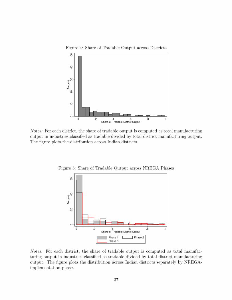
Figure 4: Share of Tradable Output across Districts

010

20

30

40

50

Perc

ent

0 .2 .4 .6 .8 1Share of Tradable District Output

Notes: For each district, the share of tradable output is computed as total manufacturingoutput in industries classified as tradable divided by total district manufacturing output.The figure plots the distribution across Indian districts.

Figure 5: Share of Tradable Output across NREGA Phases

020

40

60

Perc

ent

0 .2 .4 .6 .8 1Share of Tradable District Output

Phase 1 Phase 2

Phase 3

Notes: For each district, the share of tradable output is computed as total manufac-turing output in industries classified as tradable divided by total district manufacturingoutput. The figure plots the distribution across Indian districts separately by NREGA-implementation-phase.

37

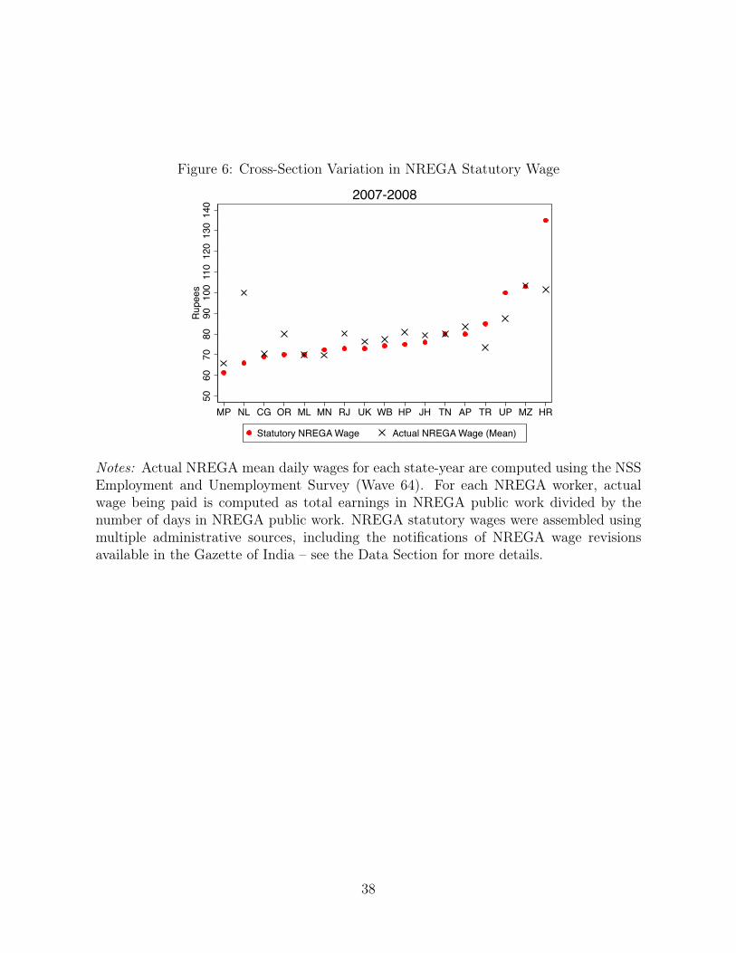
Figure 6: Cross-Section Variation in NREGA Statutory Wage

5060

7080

9010

011

012

013

014

0Ru

pees

MP NL CG OR ML MN RJ UK WB HP JH TN AP TR UP MZ HR

Statutory NREGA Wage Actual NREGA Wage (Mean)

2007-2008

Notes: Actual NREGA mean daily wages for each state-year are computed using the NSSEmployment and Unemployment Survey (Wave 64). For each NREGA worker, actualwage being paid is computed as total earnings in NREGA public work divided by thenumber of days in NREGA public work. NREGA statutory wages were assembled usingmultiple administrative sources, including the notifications of NREGA wage revisionsavailable in the Gazette of India – see the Data Section for more details.

38

Figure 7: Over-Time Variation in NREGA Statutory Wage

6090

120

150

6090

120

150

6090

120

150

2007

-08

2009

-10

2011

-12

2007

-08

2009

-10

2011

-12

2007

-08

2009

-10

2011

-12

2007

-08

2009

-10

2011

-12

Himachal Pradesh Uttaranchal Rajasthan Uttar Pradesh

Mizoram Tripura West Bengal Orissa

Chattisgarh Madhya Pradesh Andhra Pradesh Tamil Nadu

Statutory NREGA Wage Actual NREGA Wage (Mean)

Rupe

es

Notes: Actual NREGA mean daily wages for each state-year are computed using theNSS Employment and Unemployment Survey (Waves 64, 66 and 68). For each NREGAworker, actual wage being paid is computed as total earnings in NREGA public workdivided by the number of days in NREGA public work. NREGA statutory wages wereassembled using multiple administrative sources, including the notifications of NREGAwage revisions available in the Gazette of India – see the Data Section for more details.

39

Table 1: ASI Summary Statistics

Characteristics Mean Median p10 p90 S.D.

Number of Workers 68.47 23.00 7.00 144.00 155.87Value of Output (Millions Rupees) 109.71 10.47 0.70 197.09 445.21Fixed Capital (Millions Rupees) 36.24 2.03 0.15 48.22 178.01Daily Wage (Rupees) 143.26 108.30 60.14 256.27 120.34Output per Worker (Millions Rupees) 1.26 0.46 0.05 2.88 3.16Capital to Labor Ratio 8.50 3.14 0.37 16.80 44.69

TABLE - ASI SUMMARY STATISTICS

Notes: Sample refers to the years 2000-2001 to 2009-2010 and is restricted to rural areas.All estimates are obtained using sampling weights.

40

Table 2: ASI Summary Statistics by Industry Type

All IndustriesNon-tradable

IndustriesTradable Industries

Number of Workers 68.47 60.04 99.31(155.9) (138.2) (205.2)

Value of Output (Millions Rupees) 109.7 98.68 150.1(445.2) (426.0) (507.4)

Fixed Capital (Millions Rupees) 36.24 31.67 52.90(178.0) (171.3) (199.8)

Daily Wage (Rupees) 143.3 135.9 170.7(120.3) (113.5) (139.4)

Output per Worker (Millions Rupees) 1.264 1.283 1.193(3.158) (3.354) (2.301)

Capital to Labor Ratio 8.496 8.621 8.034(44.69) (49.24) (20.51)

TABLE - ASI SUMMARY STATISTICS BY INDUSTRY TYPE

Notes: Sample refers to the years 2000-2001 to 2009-2010 and is restricted to rural areas.All estimates are obtained using sampling weights.

41

Table 3: ASI Summary Statistics by NREGA Phase

All Phase 1 Phase 2 Phase 3

Number of Workers 67.00 62.76 56.01 71.86(150.8) (155.4) (141.9) (151.8)

Value of Output (Millions Rupees) 109.7 86.89 97.06 121.2(445.1) (370.0) (438.3) (468.6)

Fixed Capital (Millions Rupees) 36.43 33.93 34.61 37.81(178.9) (178.0) (194.1) (174.3)

Daily Wage (Rupees) 143.2 120.0 132.0 154.3(120.3) (91.82) (110.1) (129.7)

Output per Worker (Millions Rupees) 1.268 1.059 1.168 1.368(3.162) (2.091) (2.714) (3.555)

Capital to Labor Ratio 8.548 8.746 10.13 7.997(45.19) (22.00) (91.99) (23.74)

TABLE - ASI SUMMARY STATISTICS BY NREGA PHASE

Panel A: All Industries

Notes: Sample refers to the years 2000-2001 to 2009-2010 and is restricted to rural areas.All estimates are obtained using sampling weights.

42

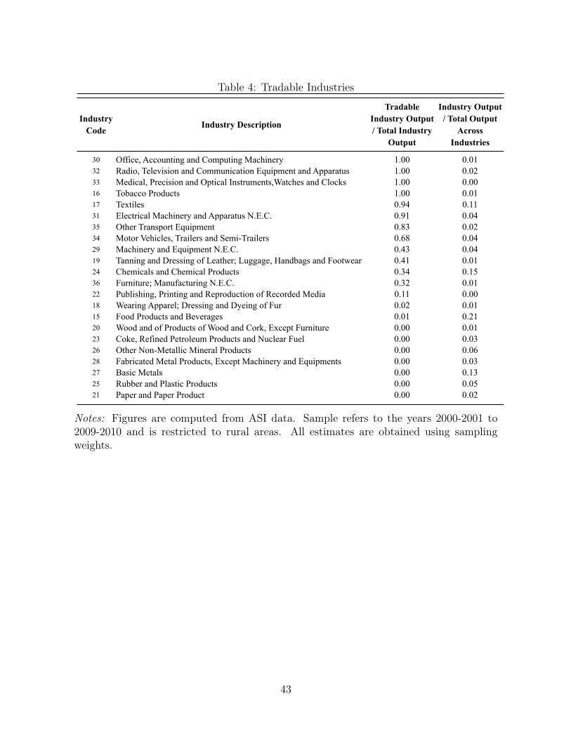
Table 4: Tradable Industries

Industry Code

Industry Description

Tradable Industry Output / Total Industry

Output

Industry Output / Total Output

Across Industries

30 Office, Accounting and Computing Machinery 1.00 0.0132 Radio, Television and Communication Equipment and Apparatus 1.00 0.0233 Medical, Precision and Optical Instruments,Watches and Clocks 1.00 0.0016 Tobacco Products 1.00 0.0117 Textiles 0.94 0.1131 Electrical Machinery and Apparatus N.E.C. 0.91 0.0435 Other Transport Equipment 0.83 0.0234 Motor Vehicles, Trailers and Semi-Trailers 0.68 0.0429 Machinery and Equipment N.E.C. 0.43 0.0419 Tanning and Dressing of Leather; Luggage, Handbags and Footwear 0.41 0.0124 Chemicals and Chemical Products 0.34 0.1536 Furniture; Manufacturing N.E.C. 0.32 0.0122 Publishing, Printing and Reproduction of Recorded Media 0.11 0.0018 Wearing Apparel; Dressing and Dyeing of Fur 0.02 0.0115 Food Products and Beverages 0.01 0.2120 Wood and of Products of Wood and Cork, Except Furniture 0.00 0.0123 Coke, Refined Petroleum Products and Nuclear Fuel 0.00 0.0326 Other Non-Metallic Mineral Products 0.00 0.0628 Fabricated Metal Products, Except Machinery and Equipments 0.00 0.0327 Basic Metals 0.00 0.1325 Rubber and Plastic Products 0.00 0.0521 Paper and Paper Product 0.00 0.02

TABLE - TRADABLE INDUSTRIES

Notes: Figures are computed from ASI data. Sample refers to the years 2000-2001 to2009-2010 and is restricted to rural areas. All estimates are obtained using samplingweights.

43

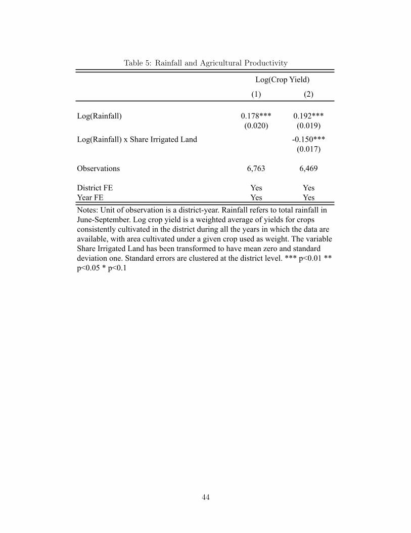
Table 5: Rainfall and Agricultural Productivity

(1) (2)

Log(Rainfall) 0.178*** 0.192***(0.020) (0.019)

Log(Rainfall) x Share Irrigated Land -0.150***(0.017)

Observations 6,763 6,469

District FE Yes YesYear FE Yes YesNotes: Unit of observation is a district-year. Rainfall refers to total rainfall in June-September. Log crop yield is a weighted average of yields for crops consistently cultivated in the district during all the years in which the data are available, with area cultivated under a given crop used as weight. The variable Share Irrigated Land has been transformed to have mean zero and standard deviation one. Standard errors are clustered at the district level. *** p<0.01 ** p<0.05 * p<0.1

Log(Crop Yield)

TABLE - RAINFALL AND AGRICULTURAL PRODUCTIVITY

44

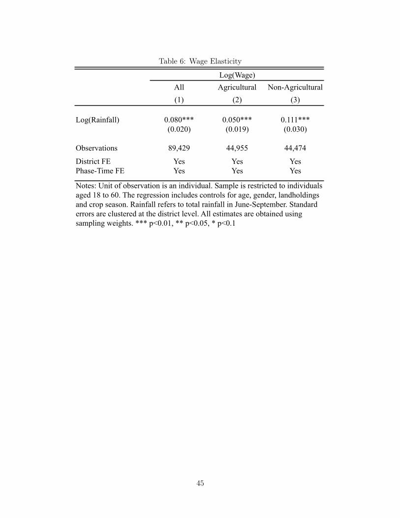
Table 6: Wage Elasticity

All Agricultural Non-Agricultural(1) (2) (3)

Log(Rainfall) 0.080*** 0.050*** 0.111***(0.020) (0.019) (0.030)

Observations 89,429 44,955 44,474

District FE Yes Yes YesPhase-Time FE Yes Yes Yes

Log(Wage)TABLE - WAGE ELASTICITY

Notes: Unit of observation is an individual. Sample is restricted to individuals aged 18 to 60. The regression includes controls for age, gender, landholdings and crop season. Rainfall refers to total rainfall in June-September. Standard errors are clustered at the district level. All estimates are obtained using sampling weights. *** p<0.01, ** p<0.05, * p<0.1

45

Table 7: Consumption Elasticity

All Goods Food Non-Food Manufactured Goods

(1) (2) (3) (3)

Log(Rainfall) 0.069*** 0.015 0.125*** 0.079***(0.021) (0.023) (0.029) (0.022)

Observations 83,212 83,176 83,206 83,205

District FE Yes Yes Yes YesPhase-Time FE Yes Yes Yes Yes

Log(Per Capita Consumption Expenditure)

TABLE - CONSUMPTION ELASTICITY

Notes: Unit of observation is a household. The regression includes controls for landholdings and crop season. Rainfall refers to total rainfall in June-September. Standard errors are clustered at the district level. All estimates are obtained using sampling weights. *** p<0.01, ** p<0.05, * p<0.1

46

Table 8: Firm Production and Employment Elasticities

Log(Value of Output) Log(Man-days) Log(Workers) Log(Wage)(1) (2) (3) (4)

Log(Rainfall) 0.122** 0.066*** 0.058*** 0.056***

(0.049) (0.025) (0.022) (0.017)

Observations 17,296 17,270 17,284 17,270

District FE Yes Yes Yes YesPhase-Year FE Yes Yes Yes YesPhase-Industry FE Yes Yes Yes YesIndustry-Year FE Yes Yes Yes Yes

TABLE - FIRM PRODUCTION AND EMPLOYMENT ELASTICITIES

Notes: Unit of observation is a district-industry-year. Industry is defined at the NIC 4-digit level. District-industry-year measures are obtained using sampling weights and are weighted in the regression by the corresponding weight. Rainfall refers to total rainfall in June-September. Value of output is in nominal terms. Number of workers and man-days include all types of firm employees. Wage refers to average real daily wage across firms -- CPI for Agricultural Labourers is used. Daily wage at the firm level is obtained as total compensation during the year divided by total number of man-days. Standard errors are clustered at the district level. *** p<0.01 ** p<0.05 * p<0.1

47

Table 9: Firm Elasticities by Industry Type

Non-tradable Tradable Non-tradable Tradable Non-tradable Tradable Non-tradable Tradable(1) (2) (3) (4) (5) (6) (7) (8)

Log(Rainfall) 0.164*** -0.060 0.118*** -0.079 0.110*** -0.090 0.063*** 0.036*(0.059) (0.065) (0.033) (0.064) (0.028) (0.066) (0.018) (0.021)

Observations 13,514 3,782 13,497 3,773 13,504 3,780 13,497 3,773

District FE Yes Yes Yes Yes Yes Yes Yes YesPhase-Year FE Yes Yes Yes Yes Yes Yes Yes YesPhase-Industry FE Yes Yes Yes Yes Yes Yes Yes YesIndustry-Year FE Yes Yes Yes Yes Yes Yes Yes Yes

TABLE - FIRM ELASTICITIES BY INDUSTRY TYPE

Log(Value of Output) Log(Man-days) Log(Workers) Log(Wage)

Notes: Unit of observation is a district-industry-year. Industry is defined at the NIC 4-digit level. District-industry-year measures are obtained using sampling weights and are weighted in the regression by the corresponding weight. Rainfall refers to total rainfall in June-September. Value of output is in nominal terms. Number of workers and man-days include all types of firm employees. Wage refers to average real daily wage across firms -- CPI for Agricultural Labourers is used. Daily wage at the firm level is obtained as total compensation during the year divided by total number of man-days. Standard errors are clustered at the district level. *** p<0.01 ** p<0.05 * p<0.1

48

Table 10: The Effect of NREGA on the Rainfall-Dependence of Agricultural Productivityand Public Employment

Log(Crop Yield) Days in Public Employment

(1) (2)

Log(Rainfall) 0.178*** -0.008(0.020) (0.013)

Log(Rainfall) x NREGA 0.000 -0.026***(0.003) (0.009)

Observations 6,763 881,601

District FE Yes YesPhase-Year FE Yes Yes

TABLE - THE EFFECT OF NREGA ON THE RAINFALL-DEPENDENCE OF AGRICULTURAL PRODUCTIVITY AND PUBLIC EMPLOYMENT

Notes: Unit of observation is a district-year in Column 1 and an individual in Column 2. In Column 2, sample is restricted to individuals aged 18 to 60. The regression in include controls for age, gender, years of schooling, landholdings and crop season. Rainfall refers to total rainfall in June-September. Standard errors are clustered at the district level. All estimates are obtained using sampling weights. *** p<0.01, ** p<0.05, * p<0.1

49

Table 11: The Effect of NREGA on Wage ElasticityTABLE - THE EFFECT OF NREGA ON WAGE ELASTICITY

Log(Wage)

All Agricultural Non-Agricultural

(1) (2) (3)

Log(Rainfall) 0.062*** 0.057*** 0.075***(0.018) (0.018) (0.021)

Log(Rainfall) x NREGA -0.053*** -0.047*** -0.049***(0.013) (0.018) (0.018)

Observations 193,602 92,106 101,496

District FE Yes Yes YesPhase-Year FE Yes Yes Yes

Notes: Unit of observation is an individual. Sample is restricted to individuals aged 18 to 60. The regression includes controls for age, gender, years of schooling, landholdings and crop season. Rainfall refers to total rainfall in June-September. Standard errors are clustered at the district level. All estimates are obtained using sampling weights. *** p<0.01, ** p<0.05, * p<0.1

50

Table 12: The Effect of NREGA on Consumption Elasticity

All Goods Food Non-Food Manufactured Goods

(1) (2) (3) (4)

log(Rainfall) 0.056*** 0.028** 0.083*** 0.063***(0.013) (0.012) (0.017) (0.014)

log(Rainfall) x NREGA -0.052*** -0.043*** -0.060*** -0.034***(0.011) (0.010) (0.015) (0.012)

Observations 223,323 223,254 223,315 223,313District FE Yes Yes Yes YesPhase-Time FE Yes Yes Yes Yes

Notes: Unit of observation is a district-year in Column 1 and an individual in Columns 2-5. In Columns 2-5, sample is restricted to individuals aged 18 to 60. The regressions in 2-5 include controls for age, gender, landholdings and crop season. Rainfall refers to total rainfall in June-September. Standard errors are clustered at the district level. All estimates are obtained using sampling weights. *** p<0.01, ** p<0.05, * p<0.1

Log(Per Capita Consumption Expenditure)

TABLE - THE EFFECT OF NREGA ON CONSUMPTION ELASTICITY

51

Table 13: The Effect of NREGA on Firm Production and Employment ElasticitiesLog(Value of Output) Log(Man-days) Log(Workers)

All Non-tradable Tradable All Non-tradable Tradable All Non-tradable Tradable(1) (2) (3) (4) (5) (6) (7) (8) (9) (10)

Log(Rainfall) 0.043*** 0.096*** 0.126*** 0.011 0.044** 0.069*** -0.020 0.040** 0.062*** -0.027(0.012) (0.035) (0.041) (0.078) (0.020) (0.025) (0.061) (0.018) (0.023) (0.057)

Log(Rainfall) x NREGA -0.032** -0.038 -0.086* 0.138 -0.016 -0.044 0.042 -0.005 -0.030 0.031(0.014) (0.037) (0.044) (0.091) (0.027) (0.028) (0.060) (0.026) (0.027) (0.057)

Observations 31,911 31,984 25,097 6,887 31,911 25,046 6,865 31,940 25,063 6,877

District FE Yes Yes Yes Yes Yes Yes Yes Yes Yes YesPhase-Year FE Yes Yes Yes Yes Yes Yes Yes Yes Yes YesPhase-Industry FE Yes Yes Yes Yes Yes Yes Yes Yes Yes YesIndustry-Year FE Yes Yes Yes Yes Yes Yes Yes Yes Yes Yes

Log(Wage)

TABLE - THE EFFECT OF NREGA ON PRODUCTION AND EMPLOYMENT ELASTICITIES

Notes: Unit of observation is a district-industry-year. Industry is defined at the NIC 4-digit level. District-industry- year measures are obtained using sampling weights and are weighted in the regression by the corresponding weight. Rainfall refers to total rainfall in June-September. Value of output is in nominal terms. Number of workers and man- days include all types of firm employees. Wage refers to average real daily wage across firms -- CPI for Agricultural Labourers is used. Daily wage at the firm level is obtained as total compensation during the year divided by total number of man-days. Standard errors are clustered at the district level. *** p<0.01 ** p<0.05 * p<0.1

52

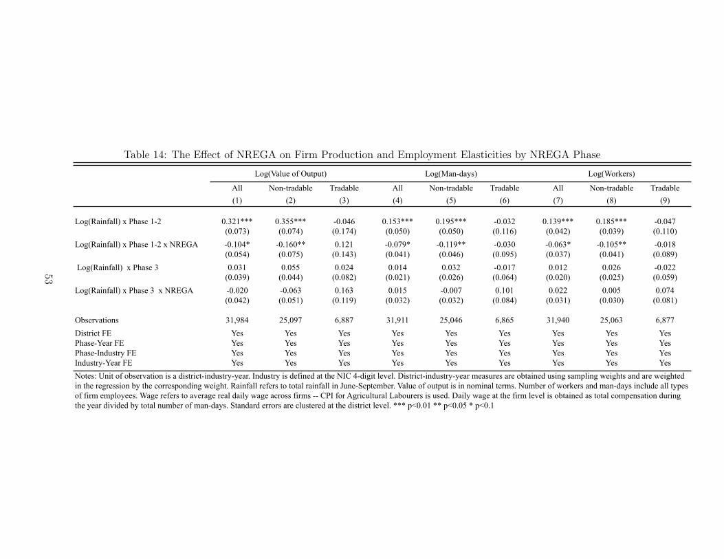
Table 14: The Effect of NREGA on Firm Production and Employment Elasticities by NREGA Phase

Log(Value of Output) Log(Man-days) Log(Workers)

All Non-tradable Tradable All Non-tradable Tradable All Non-tradable Tradable(1) (2) (3) (4) (5) (6) (7) (8) (9)

Log(Rainfall) x Phase 1-2 0.321*** 0.355*** -0.046 0.153*** 0.195*** -0.032 0.139*** 0.185*** -0.047(0.073) (0.074) (0.174) (0.050) (0.050) (0.116) (0.042) (0.039) (0.110)

Log(Rainfall) x Phase 1-2 x NREGA -0.104* -0.160** 0.121 -0.079* -0.119** -0.030 -0.063* -0.105** -0.018(0.054) (0.075) (0.143) (0.041) (0.046) (0.095) (0.037) (0.041) (0.089)

Log(Rainfall) x Phase 3 0.031 0.055 0.024 0.014 0.032 -0.017 0.012 0.026 -0.022(0.039) (0.044) (0.082) (0.021) (0.026) (0.064) (0.020) (0.025) (0.059)

Log(Rainfall) x Phase 3 x NREGA -0.020 -0.063 0.163 0.015 -0.007 0.101 0.022 0.005 0.074(0.042) (0.051) (0.119) (0.032) (0.032) (0.084) (0.031) (0.030) (0.081)

Observations 31,984 25,097 6,887 31,911 25,046 6,865 31,940 25,063 6,877District FE Yes Yes Yes Yes Yes Yes Yes Yes YesPhase-Year FE Yes Yes Yes Yes Yes Yes Yes Yes YesPhase-Industry FE Yes Yes Yes Yes Yes Yes Yes Yes YesIndustry-Year FE Yes Yes Yes Yes Yes Yes Yes Yes Yes

TABLE - THE EFFECT OF NREGA BY PHASE

Notes: Unit of observation is a district-industry-year. Industry is defined at the NIC 4-digit level. District-industry-year measures are obtained using sampling weights and are weighted in the regression by the corresponding weight. Rainfall refers to total rainfall in June-September. Value of output is in nominal terms. Number of workers and man-days include all types of firm employees. Wage refers to average real daily wage across firms -- CPI for Agricultural Labourers is used. Daily wage at the firm level is obtained as total compensation during the year divided by total number of man-days. Standard errors are clustered at the district level. *** p<0.01 ** p<0.05 * p<0.1

53

Table 15: Robustness Checks: Alternative Rainfall Measures

Log(Value of Output) Log(Man-days) Log(Workers) Log(Wage)

(1) (2) (3) (4) (5) (6) (7) (8)

Rainfall Shock 0.060* 0.030* 0.025* 0.037***(0.032) (0.016) (0.014) (0.008)

Rainfall Deviation 0.143** 0.081*** 0.072*** 0.060***(0.058) (0.027) (0.024) (0.018)

Observations 17,296 17,296 17,270 17,270 17,284 17,284 17,270 17,270District FE Yes Yes Yes Yes Yes Yes Yes YesPhase-Year FE Yes Yes Yes Yes Yes Yes Yes YesPhase-Industry FE Yes Yes Yes Yes Yes Yes Yes YesIndustry-Year FE Yes Yes Yes Yes Yes Yes Yes Yes

Notes: Unit of observation is a district-industry-year. Industry is defined at the NIC 4-digit level. District-industry-year measures are obtained using sampling weights and are weighted in the regression by the corresponding weight. The variable Rainfall Shock equals one if monsoon rainfall is greater than the district’s eightieth percentile of monsoon rainfall, zero if between the twentieth and eightieth percentiles, and minus one if below the twentieth percentile. The variable Rainfall Deviation is the fractional deviation from the the district’s mean monsoon rainfall. Value of output is in nominal terms. Number of workers and man-days include all types of firm employees. Wage refers to average real daily wage across firms -- CPI for Agricultural Labourers is used. Daily wage at the firm level is obtained as total compensation during the year divided by total number of man-days. The specification includes the standardized district share of irrigated land and district share of population in agriculture interacted with the rainfall variable. Analysis is restricted to a balanced panel of districts with at least 20 percent of population in agriculture. Standard errors are clustered at the district level. *** p<0.01 ** p<0.05 * p<0.1

54

Table 16: Robustness Checks: Alternative Classifications of Tradable vs. Non-Tradable Industries

Non-tradable Tradable Non-tradable Tradable Non-tradable Tradable Non-tradable Tradable(1) (2) (3) (4) (5) (6) (7) (8)

Log(Rainfall) 0.128** -0.022 0.067** 0.007 0.065*** -0.002 0.059*** 0.044(0.050) (0.121) (0.028) (0.083) (0.025) (0.072) (0.016) (0.031)

Observations 14,071 3,063 14,052 3,057 14,060 3,063 14,052 3,057District FE Yes Yes Yes Yes Yes Yes Yes YesPhase-Year FE Yes Yes Yes Yes Yes Yes Yes YesPhase-Industry FE Yes Yes Yes Yes Yes Yes Yes YesIndustry-Year FE Yes Yes Yes Yes Yes Yes Yes Yes

Non-tradable Tradable Non-tradable Tradable Non-tradable Tradable Non-tradable Tradable(1) (2) (3) (4) (5) (6) (7) (8)

Log(Rainfall) 0.137** 0.054 0.075*** 0.047 0.070*** 0.030 0.068*** 0.048**(0.065) (0.059) (0.028) (0.051) (0.026) (0.046) (0.017) (0.023)

Observations 10,829 6,129 10,811 6,121 10,822 6,124 10,811 6,121District FE Yes Yes Yes Yes Yes Yes Yes YesPhase-Year FE Yes Yes Yes Yes Yes Yes Yes YesPhase-Industry FE Yes Yes Yes Yes Yes Yes Yes YesIndustry-Year FE Yes Yes Yes Yes Yes Yes Yes Yes

Log(Wage)

Log(Value of Output) Log(Man-days) Log(Workers) Log(Wage)

Notes: Unit of observation is a district-industry-year. Industry is defined at the NIC 4-digit level. District-industry-year measures are obtained using sampling weights and are weighted in the regression by the corresponding weight. Rainfall refers to total rainfall in June-September. Value of output is in nominal terms. Number of workers and man-days include all types of firm employees. Wage refers to average real daily wage across firms -- CPI for Agricultural Labourers is used. Daily wage at the firm level is obtained as total compensation during the year divided by total number of man-days. The specification includes the standardized district share of irrigated land and district share of population in agriculture interacted with log-transformed rainfall. Analysis is restricted to a balanced panel of districts with at least 20 percent of population in agriculture. Standard errors are clustered at the district level. *** p<0.01 ** p<0.05 * p<0.1

Panel A: Geographical Concentration Based Classification

Panel B: International Trade Based ClassificationLog(Value of Output) Log(Man-days) Log(Workers)

55

Table 17: Placebo Test: Elasticities in Poorly and Highly Irrigated Districts

Poorly Irrigated

Highly Irrigated

Poorly Irrigated

Highly Irrigated

Poorly Irrigated

Highly Irrigated

Poorly Irrigated

Highly Irrigated

Poorly Irrigated

Highly Irrigated

(1) (2) (3) (4) (5) (6) (7) (8) (9) (10)

Log(Rainfall) 0.352*** 0.027* 0.264*** 0.032 0.151*** 0.036 0.119*** 0.042 0.052*** 0.038(0.048) (0.015) (0.053) (0.075) (0.032) (0.045) (0.030) (0.044) (0.017) (0.040)

Observations 1,972 2,265 5,481 5,034 5,471 5,028 5,474 5,029 5,471 5,028District FE Yes Yes Yes Yes Yes Yes Yes Yes Yes YesPhase-Year FE Yes Yes Yes Yes Yes Yes Yes Yes Yes YesPhase-Industry FE No No Yes Yes Yes Yes Yes Yes Yes YesIndustry-Year FE No No Yes Yes Yes Yes Yes Yes Yes Yes

Log(Value of Output) Log(Man-days) Log(Workers) Log(Wage)Log(Crop Yield)

Notes: Unit of observation is a district-year in Column 1 and district-industry-year in Columns 2-10. A district is defined as poorly (highly) irrigated if less than 20% (more than 60%) of cultivated land is irrigated. Industry is defined at the NIC 4-digit level. District-industry-year measures are obtained using sampling weights and are weighted in the regression by the corresponding weight. Rainfall refers to total rainfall in June-September. Log crop yield is a weighted average of yields for crops consistently cultivated in the district during all the years in which the data are available, with area cultivated under a given crop used as weight. Value of output is in nominal terms. Number of workers and man-days include all types of firm employees. Wage refers to average real daily wage across firms -- CPI for Agricultural Labourers is used. Daily wage at the firm level is obtained as total compensation during the year divided by total number of man-days. Standard errors are clustered at the district level. *** p<0.01 ** p<0.05 * p<0.1

56

Table 18: Placebo Test: Elasticities with Respect to Non-Monsoon Rainfall

Log(Crop Yield) Log(Value of Output) Log(Man-days) Log(Workers) Log(Wage)

(1) (2) (3) (4) (5)

Log(Non-Monsoon Rainfall) 0.015** -0.026 -0.033 -0.027 -0.016(0.007) (0.023) (0.023) (0.020) (0.010)

Observations 6,763 17,296 17,270 17,284 17,270District FE Yes Yes Yes Yes YesPhase-Year FE Yes Yes Yes Yes YesPhase-Industry FE No Yes Yes Yes YesIndustry-Year FE No Yes Yes Yes Yes

Notes: Unit of observation is a district-year in Column 1 and a district-industry-year in Columns 2-5. Industry is defined at the NIC 4-digit level. District-industry-year measures are obtained using sampling weights and are weighted in the regression by the corresponding weight. Rainfall refers to total rainfall in months other than June-September. Value of output is in nominal terms. Number of workers and man-days include all types of firm employees. Wage refers to average real daily wage across firms -- CPI for Agricultural Labourers is used. Daily wage at the firm level is obtained as total compensation during the year divided by total number of man-days.Standard errors are clustered at the district level. *** p<0.01 ** p<0.05 * p<0.1

57

Table 19: Robustness Check: Firm Elasticities by Input-Output Linkage

Linked Non-linked Non-linked Non-Tradable

Non-linked Tradable

(1) (2) (3) (4)

Log(Rainfall) 0.140 0.119** 0.150** -0.059(0.110) (0.054) (0.065) (0.063)

Log(Rainfall) 0.148* 0.055* 0.106*** -0.087(0.078) (0.028) (0.034) (0.061)

Log(Rainfall) 0.171** 0.038 0.087*** -0.098(0.071) (0.026) (0.029) (0.063)

Observations 2,980 14,304 10,632 3,672

District FE Yes Yes Yes YesPhase-Year FE Yes Yes Yes YesPhase-Industry FE Yes Yes Yes YesIndustry-Year FE Yes Yes Yes Yes

Log(Value of Output)

Log(Man-days)

Log(Workers)

TABLE - FIRM ELASTICITIES BY INPUT-OUTPUT LINKAGE

Notes: Unit of observation is a district-industry-year. Industry is defined at the NIC 4-digit level. District-industry-year measures are obtained using sampling weights and are weighted in the regression by the corresponding weight. Rainfall refers to total rainfall in June-September. Value of output is in nominal terms. Number of workers and man-days include all types of firm employees. Wage refers to average real daily wage across firms -- CPI for Agricultural Labourers is used. Daily wage at the firm level is obtained as total compensation during the year divided by total number of man-days. Standard errors are clustered at the district level. *** p<0.01 ** p<0.05 * p<0.1

58

Table 20: Robustness Check: Accounting for Spatial Correlation

Log(Value of Output) Log(Man-days) Log(Workers) Log(Wage)(1) (2) (3) (4)

Log(Rainfall) 0.122** 0.066** 0.058* 0.056***(0.049) (0.033) (0.031) (0.015)

Observations 17,296 17,270 17,284 17,270

District FE Yes Yes Yes YesPhase-Year FE Yes Yes Yes YesPhase-Industry FE Yes Yes Yes YesIndustry-Year FE Yes Yes Yes YesNotes: Unit of observation is a district-industry-year. Industry is defined at the NIC 4-digit level. District-industry-year measures are obtained using sampling weights and are weighted in the regression by the corresponding weight. Rainfall refers to total rainfall in June-September. Value of output is in nominal terms. Number of workers and man-days include all types of firm employees. Wage refers to average real daily wage across firms -- CPI for Agricultural Labourers is used. Daily wage at the firm level is obtained as total compensation during the year divided by total number of man-days. The specification includes the standardized district share of irrigated land and district share of population in agriculture interacted with log-transformed rainfall. Analysis is restricted to a balanced panel of districts with at least 20 percent of population in agriculture. Standard errors are clustered at the region-year level. *** p<0.01 ** p<0.05 * p<0.1

59