first bibliography on the general agreement on trade and services

Anthony W. LynchNew York University

Richard R. MendenhallUniversity of Notre Dame

New Evidence on Stock PriceEffects Associated with Changesin the S&P 500 Index*

I. Introduction Since October 1989,Standard and Poor’s

Papers investigating Standard and Poor’s 500 has (when possible) an-nounced changes inStock Index (S&P 500) composition changesthe composition of theover the 1976–88 period find a change-day posi-S&P 500 index 1 weektive (negative) abnormal return of approximatelyin advance. Because in-3% (1.5%) for additions (deletions).1 During this dex funds hold S&P

period it was S&P’s policy to announce and im- 500 stocks to minimizetracking error, indexplement changes in the composition of the indexcomposition changessimultaneously. Their policy since October 1989,since this date providehowever, has been (whenever possible) to an-an opportunity to exam-nounce changes 1 week prior to their imple- ine the market reactionto an anticipatedchange in the demand

* We are very grateful to Standard and Poor’s Corporation for a stock. Usingfor providing data that made this research possible. We have post–October 1989benefited from helpful discussions with Yakov Amihud, Ste- data, we document sig-phen Brown, and Robert Schwartz and from the valuable com- nificantly positive (neg-ments of John Affleck-Graves, Pierluigi Balduzzi, Larry

ative) postannounce-Brown, Ned Elton, Silverio Foresi, Antti Ilmanen, Kose John,ment abnormal returnsJohn Liew, David Musto, Cathy Niden, Eli Ofek, Ross Stevens,that are only partiallyDavid Yermack, and seminar participants at New York Univer-

sity. The comments of an anonymous referee and the editor reversed following ad-(Doug Diamond) greatly improved the paper. The able research ditions (deletions).assistance of Tania Vital-Ahuja is also acknowledged. This re- These results indicatesearch was started when Mendenhall was a visiting faculty the existence of tempo-member at New York University. rary price pressure and

1. For deletions, see Goetzmann and Garry (1986) who ex- downward-slopingamined the seven deletions on November 30, 1983 (caused bylong-run demandthe breakup of AT&T), and Harris and Gurel (1986) who exam-curves for stocks andined the 1978–83 period (13 stocks). For additions, again seerepresent a violation ofHarris and Gurel (1986) (84 stocks); Shleifer (1986), who ex-

amined the 1976–83 period (102 stocks); and Dhillon and market efficiency.Johnson (1991), who examined the 1978–88 period (187stocks).

(Journal of Business, 1997, vol. 70, no. 3) 1997 by The University of Chicago. All rights reserved.0021-9398/97/7003-0002$02.50

351

352 Journal of Business

mentation. This article analyzes price and volume data for firms addedto or deleted from the S&P 500 from March 1990 through April 1995.

For additions, we find a significant positive announcement day ab-normal return. We also find a positive cumulative abnormal return of3.807% over the period starting the day after the announcement andending the day before the effective date of the change. Further, we findsignificant negative abnormal returns following the addition itself. Thepattern of price movements for deletions is very similar but inverted.That is, returns are significantly negative between announcement anddelisting and significantly positive following delisting.

Our results are interesting for a number of reasons. First, they canbe interpreted in the context of the efficient market hypothesis (seeFama [1970, 1991] for a detailed discussion of the theory and evidencepertaining to market efficiency). The significant abnormal returns fol-lowing the announcement date are inconsistent with semi–strong formmarket efficiency. It would have been possible for investors, using onlypublicly available information, to construct trading rules that earnedeconomically significant abnormal returns. This result can be con-trasted with studies examining the pre–October 1989 period, whichfind no significant daily abnormal returns following the announcement.Thus, while the pre–October 1989 results do not violate semi–strongform efficiency, those presented here clearly do.2

Second, the price reversal on and after the effective date of the indexchange indicates a significant temporary stock-price effect prior to thechange. The price reversal that we document is consistent with heavyindex-fund trading around the time of the change that moves stockprices temporarily away from their equilibrium values (the price-pres-sure hypothesis). This behavior is plausible since the managers of indexfunds are typically evaluated on the basis of their ‘‘tracking error’’ orthe difference between their fund’s return and the return on the indexover any period. This price reversal is also strong evidence that thepostannouncement-day abnormal returns do not simply represent aslow adjustment to any value-relevant information contained in S&P’sannouncement.

In contrast, the pre–October 1989 studies find no indication of ashort-run price reversal, and their evidence regarding the existence ofa longer-term reversal is mixed.3 The lack of a temporary effect beforeOctober 1989 is also consistent with index funds’ concern with tracking

2. Goetzmann and Garry (1986) provide some evidence that investors speculated onstocks to be dropped from the S&P 500 index at the time of the AT&T breakup. Theyfind, however, that these efforts did not earn abnormal returns.

3. Harris and Gurel (1986) find that the price effect on the announcement/change dateis gradually but completely reversed in the period after addition or deletion. Shleifer (1986)and Dhillon and Johnson (1991) find that the price effect is permanent. Dhillon and Johnsonargue that Harris and Gurel’s finding may be specific to their method of risk adjustment.

Stock Price Effects 353

error. Before this date, index funds could not buy an added stock untilafter it had become part of the index. Any price premium paid by anindex fund prior to October 1989, therefore, generated a negative ex-pected tracking error. Index funds would be motivated, therefore, todelay trading (and perhaps to break up their orders) to avoid payingsuch a premium. However, a trade-off was involved since trading laterexposed them to tracking error associated with not holding the already-added stock. Since October 1989, index funds have been able to pur-chase added stocks prior to their entering the index. Any price premiumpaid by index funds just prior to the change has no impact on expectedtracking error since the stock enters the index at the inflated price.Hence, index funds, post–October 1989, are prepared to pay a premiumto be able to buy an added stock just prior to its addition. Thus, indexfunds’ concern with tracking error explains why a price reversal is onlyobserved after October 1989.

Third, the finding of a significant temporary effect for additions aswell as deletions is relevant to results reported in the block-trade litera-ture. In particular, researchers studying block trades consistently finddifferent temporary effects for buyer- versus seller-initiated blocks;seller-initiated blocks induce significant temporary price effects whilebuyer-initiated blocks do not (see Holthausen, Leftwich, and Mayers1990; Chan and Lakonishok 1993; and Keim and Madhavan 1996).Any explanation for this asymmetry must also be able to explain theobserved symmetry in temporary effects that we observe.

One hypothesis that has been advanced to explain the block-tradeasymmetry is broker reluctance to take a short position to accommodatea block purchase. According to ‘‘street wisdom,’’ this reluctance resultsin a lack of intermediary involvement and no temporary effect for mostbuyer-initiated block trades (see Holthausen, Leftwich, and Mayers1990; and Chan and Lakonishok, 1993). Unless brokers are more in-clined to short stocks being added to the S&P 500 than they are toshort other stocks, our results are inconsistent with this explanation forthe block-trade asymmetry.

Fourth, the permanent price effect (excluding the announcement-dayabnormal return) is found to be weakly positive for additions and sig-nificantly negative for deletions. This finding provides new evidencein support of downward-sloping long-run demand curves for stocks(downward-sloping demand hypothesis).

Shleifer (1986) and Harris and Gurel (1986) were the first papers torecognize that a permanent price response associated with addition to ordeletion from the index is consistent with stocks possessing downward-sloping demand curves. As firms enter the S&P 500, index-fund buyingremoves a substantial fraction of the firm’s shares from circulation.This demand by index funds reduces the stock’s supply for nonindexinginvestors, causing the market clearing price to increase. For deletions,


analogous logic predicts a price decrease. If long-term demand curvesfor stocks were horizontal, no permanent price effect would be ex-pected.

However, there are other explanations for the permanent price effectdocumented for pre–October 1989 changes. The price movement couldbe due to the information content of S&P’s addition and deletion an-nouncements (the information hypothesis). For these announcementsto have information content, S&P must have nonpublic informationabout firms and use this information to determine the composition ofthe index.4 Alternatively, if S&P 500 inclusion affects stocks’ liquidity,then this should have pricing implications (the liquidity hypothesis).Specifically, if being a member of the S&P 500 increases a stock’sliquidity, then there should be a price increase (decrease) upon the an-nouncement of addition (deletion; see Amihud and Mendelson 1986,1993).5

The post–October 1989 price patterns that we present are able todisentangle these effects. While the significant announcement-day ab-normal return (for additions and deletions) is consistent with all threehypotheses, the permanent price shift that we find after the announce-ment date is only consistent with downward-sloping long-run demandcurves for stocks. Assuming the response to any value-relevant infor-mation in S&P’s announcement or to perceived liquidity changeswould occur on the announcement day (as implied by an informa-tionally efficient market), the postannouncement price shift cannot beexplained by either of these two hypotheses.

Finally, we examine trading volume around the time of the an-nouncement and around the time of the index change. Consistent withindex-fund managers attempting to minimize tracking error by tradingimmediately prior to the index change, the largest volume occurs onthe day prior to the index modification. For example, for both additionsand deletions, the fraction of shares traded on the day prior to thechange is more than three times as great as that on the announcement

4. The information hypothesis is supported by Jain (1987), who observes significantstock-price movements when firms are added to (or deleted from) S&P auxiliary indexes(which are not mimicked by index funds), as well as by Dhillon and Johnson (1991), whoexamine the option and bond returns of firms being added to the S&P 500. Both Shleiferand Harris and Gurel discredit the information hypothesis using indirect arguments. Harrisand Gurel cite investors’ lack of interest in discovering index changes prior to September1976 (when S&P’s early notification service began) even though that information wasreadily available. Shleifer finds that firms with lower-rated debt (by S&P) do not have astronger addition-day response than those with higher-rated debt.

5. Although not a proponent of the liquidity hypothesis, Shleifer (1986) raises the possi-bility that inclusion in the index may lead to closer scrutiny of the company by analystsand investors. This, in turn, may lead to greater institutional interest, greater trading vol-ume, and lower bid-ask spreads. Harris and Gurel (1986) and Edmister et al. (1995), study-ing pre–October 1989 data, do find evidence of a permanent increase in trading volumefollowing S&P 500 inclusion.


date, which also exhibits large volume relative to the preannouncementperiod.

It is beyond the scope of this article to develop in detail the theoreti-cal underpinnings of the various hypotheses described above. However,the empirical results presented here may facilitate their rigorous devel-opment. We leave that task to future work. The next section describesthe data and the research method used in this study, while Section IIIdiscusses the empirical implications of the four hypotheses describedabove and our results. Section IV offers a summary and a conclusion.

II. Data and Methodology

A. The Sample

We asked Standard & Poor’s Corporation to supply us with data, in-cluding announcement dates and effective change dates, on the changesto the S&P 500 since October of 1989. They were able to furnish uswith the 71 additions and deletions that occurred from March 1990through April 1995. Daily stock returns are obtained from the Centerfor Research in Security Prices (CRSP) for the pre-1994 period andfrom Bloomberg after that time. For the pre-1994 period, the CRSPvalue-weighted index of New York Stock Exchange–American StockExchange (NYSE-AMEX) stocks is used as the market portfolio inabnormal return calculations. After the end of 1993, the daily return onthe S&P 500 (obtained from Bloomberg) is used as the market return.

From the original sample of additions and deletions, we construct a‘‘complete’’ sample and a ‘‘clean’’ sample. To construct the completesample, observations were eliminated from the original sample for sev-eral reasons. First, we were unable to obtain announcement dates fromS&P for three additions and three deletions. Second, we required thatuseable return data be available for at least 1 day over the event studywindows. This constraint reduced the addition (deletion) sample bythree (five). Finally, since this study relies on a separation between theannouncement and change days, 10 observations from both the additionand deletion samples were omitted because the announcement did notprecede the change date by at least 2 days.6 The complete additionssample consists of 55 firms and the complete deletions sample consistsof 53 firms.

There are two points to note regarding this complete sample. Thefirst is that it includes some observations for which the index change

6. When a firm files for bankruptcy, it is S&P’s policy to announce, after the close oftrading on that day, that it is deleted from the index effective immediately. Seven of thecases failing to qualify for lack of separation between announcement and effective changedate (both additions and deletions) were attributable to the deletion firm declaring bank-ruptcy.


does not lead to trading by index funds.7 Including these firms will tendto dampen any price effects associated with index-fund trading. Thesecond is that unrelated merger and spin-off activity around the timeof the announcement and change will add noise to the abnormal returns.In an effort to build ‘‘clean’’ samples of additions and deletions thatminimize these concerns, we eliminated any firm undergoing mergeror spin-off activity at the time of the announcement. Since market par-ticipants would be expected to know which firms were undergoing suchactivity, the implication is that our ‘‘clean’’ samples could be formedusing information available at the time of the announcement. To formthe clean sample, a firm was deleted from the complete sample if anymention of announcement date merger or spin-off activity was reportedin the Dow Jones News Retrieval Service, the Wall Street Journal orthe 1991–94 issues of the S&P 500 Directory.8 The clean additionssample contains 34 firms (9 mergers and 12 spin-offs are eliminatedfrom the complete sample) and the clean deletions sample contains 15firms (34 mergers and 4 spin-offs are eliminated).

Another concern is the impact of survivorship (see Brown et al.[1992] and Brown, Goetzmann, and Ross [1995] for discussions aboutthe effects of survivorship bias). In particular, S&P sometimes an-nounces that a change is conditional on approval of a corporate restruc-turing plan by a company’s shareholders. Such approval may not beindependent of the share price behavior of the sample firm, inducinga type of survivorship bias into the sample. This source of survivorshipbias is, however, eliminated for the clean sample since any firm under-going a merger or other restructuring activity at the time of the an-nouncement is omitted.

More generally, survivorship may still affect the abnormal returnpoint estimates if the probability of surviving is related to the criteriaused to form the sample (see Brown and Pope [1995] for a furtherdiscussion).9 However, it seems unlikely that survivorship can explainthe magnitude of the abnormal returns observed (a 0.79% abnormalreturn per day between announcement and the change day for cleanadditions) or their patterns (which include reversals).

7. For example, on May 6, 1991, USX Corp split into USX–Marathon Group and USX–U.S. Steel Group. On that day, USX Corp was deleted from the S&P 500 and the twonew firms were added. However, index funds would not trade since their shares in USXCorp would be converted into shares in the two new firms.

8. It seems unlikely that a firm in the S&P 500 or one large enough to be added to theindex could be undergoing merger or spin-off activity unreported in any of these threesources.

9. For example, the abnormal returns of the clean additions sample may be affected bysurvivorship if the probability of surviving conditional on being added to the S&P 500and not being associated with any merger activity differs from the unconditional probabilityof surviving.


B. Methodology

We use an event-study methodology with two event dates for eachsample: the announcement date of the addition/deletion (AD) and theeffective date of the addition/deletion (CD). Since S&P typically an-nounce changes after the close of trading on a particular day, the fol-lowing day is taken as the announcement day (AD). Since the changeis implemented using the closing price of a particular day, the followingday is taken as the change day (CD).

Abnormal return calculation. The abnormal return for stock i onday τ [AR i(τ)] is defined as the deviation of the stock’s raw returnfrom that of the market. The sample mean abnormal return (MAR) forevent day τ is used as a measure of the abnormal price movement onthat day. We are also interested in determining the abnormal returnover windows whose lengths sometimes vary across firms, for example,the total abnormal return from being added to or deleted from theS&P 500. A stock’s cumulative abnormal return over the window fromτ1 to τ2 is calculated by summing the stock’s abnormal returns overthat window and is denoted CAR(τ1, τ2). The stock’s average abnormalreturn over the window, AAR(τ1, τ2), is the stock’s CAR(τ1, τ2) di-vided by the number of days in the window.

Two measures of the abnormal return over a window of interest (τ1,τ2) are obtained by taking sample averages of firm CARs and firmAARs. These averages are designated as MCAR(τ1, τ2) and MAAR(τ1,τ2), respectively, and are both weighted sums of the ARs in the window.If the window’s length varies across firms, however, the relativeweights assigned by each differ. MCAR gives the same weight to everyAR in the window while MAAR places a greater weight on the ARsof firms for whom the window is short. Consequently, MAAR (MCAR)has greater power when the abnormal performance is concentrated inshort (long) window firms.10

Clearly, more sophisticated models of the return generating processcan be used to calculate abnormal returns. However, the results ob-tained using the market model are very similar to those reported hereusing market-adjusted returns.11 The market model abnormal returnsfor additions (deletions) tend to be slightly less positive (negative) onaverage than market-adjusted returns, possibly reflecting the bias in the

10. When the number of days in the window is the same for all firms, only MCAR isreported since MAAR is just a scalar multiple of MCAR and the associated t-statistics arethe same for both.

11. Since index additions (deletions) are likely to have performed well (poorly) just priorto the change, using daily returns over this period to estimate market model parameters mayproduce upwardly (downwardly) biased alpha estimates. For this reason, the market modelis estimated using returns from 872 to 673 days prior to the announcement day (requiringat least 100 nonmissing daily returns).


estimated alphas discussed in note 11. Even so, inferences are rarelyaffected. Any material differences are mentioned in the results section.

Abnormal volume calculation. Volume data are obtained fromCRSP for those firms added to or deleted from the S&P 500 up toDecember 1994. The measure of volume that we employ is defined asfollows:12

υ i(τ) 5 log[1 1 Vi(τ)]/log[1 1 Ei(τ)], (1)

where Vi(τ) is dollar volume on day τ for stock i, and Ei(τ) is the dollarvalue of the outstanding shares on stock i on day τ. This volume mea-sure approximates the dollar trading volume expressed as a fraction ofthe value of stock outstanding.13

Abnormal value (AV) is estimated using a procedure from Ajinkyaand Jain (1989).14 We begin by regressing the firm’s transformed vol-ume on that of the market:

υ i(τ) 5 φ0, i 1 φ1, iυM(τ) 1 ei(τ)

for τ 5 AD 2 258, . . . , AD 2 109,(2)

where υM(τ) is log[1 1 VM(τ)]/log[1 1 EM(τ)] and the market is repre-sented by all NYSE-AMEX stocks on the CRSP. A firm is omitted ifit has missing volume data over the 150-day estimation period. Ajinkyaand Jain find that the residual from this regression is AR(1) for U.S.equities and use an estimated generalized least squares (EGLS) proce-dure to estimate the regression coefficients.15 Since the events consid-ered here are likely to involve a sequence of days with abnormal vol-ume, abnormal volume is estimated treating the lagged residual asbeing equal to its unconditional value of zero, as discussed in Ajinkyaand Jain (1989). Thus, the abnormal volume for firm i on date τ is16

AV i(τ) 5 υ i(τ) 2 [φ0, i 1 φ1, i υM(τ)]. (3)

12. In the numerator of the volume measure, 1 is added to the dollar volume of sharestraded to accommodate zero volume. The denominator also adds one to the dollar valueof shares outstanding so that the measure equals 1 when volume equals the total numberof shares outstanding.

13. Ajinkya and Jain (1989) find that this transformed variable has a distribution thatis much closer to normal than are raw volume numbers.

14. Meulbroek (1992) and Yermack (1995) both use a market model approach to esti-mate abnormal volume, though their specification is slightly different from ours.

15. The EGLS procedure we employ involves estimating equation (2) using OLS regres-sion, then regressing the rresidual from that regression on its own lag and using the slopecoefficient from that regression as an estimate of the AR(1) coefficient used to transformthe data as in the Cochrane-Orcutt procedure. Finally, we perform an OLS regression usingthe transformed data to arrive at the estimates of φ0, i and φ1, i. See Judge et al. (1985) fora discussion of EGLS and the Cochrane-Orcutt procedure.

16. As an alternate measure of abnormal volume, we also use the deviation of υi(τ)from its sample average over the period from AD 2 258 to AD 2 109. Again a firm isomitted if it has missing volume data over this period. Inferences are not changed whenusing this alternate measure.


Mean abnormal volume for event day τ, MAV(τ) is the sample averageAV for stocks with usable volume data on that date.

Significance tests. All significance tests are performed using across-sectional variance estimator as described in Asquith (1983) anda time-series variance estimator as in Ruback (1982). The latter hasthe advantage of a sample size that depends on the time-series lengthand not the number of firms in the sample, while the former is robustto an increase in the variance of AR around the event dates.17 Detailsof the variance calculations are provided in the appendix.

III. Hypotheses and Results

A. Empirical Implications of the Competing Hypotheses

Four possible explanations for price movements around the time of anindex change are discussed above: temporary price pressure associatedwith index-fund trading (the price-pressure hypothesis); downward-sloping long-run demand curves for stocks (the downward-sloping de-mand hypothesis); S&P’s change announcements contain value-rele-vant information (the information hypothesis); and addition or deletionaffects the stock’s liquidity (the liquidity hypothesis). To help untanglethese explanations, we focus attention on five windows over the eventperiod:

1. run-up window runs from the day after the announcement (AD1 1) through the day before the change day (CD 2 1);18

2. release window runs from the change day (CD) until the release-ending day;19

3. postrelease window runs from the day following the release-end-ing day until the end of the event window 10 days after the changeday (CD 1 10);

4. post-AD permanent effect window runs from the day after theannouncement (AD 1 1) until the release-ending day; and

17. The cross-sectional variance estimator is also robust to the variance effects of survi-vorship; i.e., the variance of a firm’s AR over the last 3 years conditioning on survivingthose 3 years may differ from its postannouncement AR variance conditional on beingincluded in the sample. For further details see Kothari and Warner (1996).

18. Keim and Madhavan (1996) present a model that predicts a positive relation betweenthe temporary price impact of a block trade and order size. In the context of the price-pressure hypothesis, their model suggests that the temporary price impact on each day isincreasing in the level of index-fund trading. Consistent with the notion that index fundscare about tracking error, it is assumed that most funds rebalance their portfolios on theday before the change (CD 2 1). It follows that the largest temporary effect occurs onthe day before the change. Consequently, the price-pressure hypothesis implies a pricereversal that commences on the change day (CD).

19. Under the price-pressure hypothesis, any price release ends when all index fundshave completed their trades. The criterion used to determine the release-ending day isdescribed in Sec. IIIB, ‘‘Price Results.’’


5. total permanent effect window runs from the announcement day(AD) until the release-ending day.

Figure 1 depicts the time sequencing of the announcement and the changeand indicates exactly when the different windows begin and end.

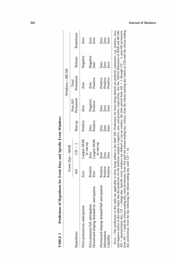
Table 1 summarizes the implications of each hypothesis for the MARon AD and CD 2 1 and for the MCAR over the five windows. Whiletable 1 presents predictions only for additions, predictions are symmet-ric for deletions; that is, table entries of positive, zero, and negativeimply negative, zero, and positive abnormal returns, respectively, fordeletions. The posited effects for the price-pressure and downward-sloping demand hypotheses assume that most funds rebalance theirportfolios on the day before the change (CD 2 1). Predictions for twoextreme cases associated with each of these two hypotheses are pre-sented in table 1.

For the downward-sloping demand hypothesis, the associated per-manent price effect may not occur until index funds make the purchases(in the case of an addition) that reduce the stock’s supply for activeinvestors (no-anticipation case). At the other extreme, the price effectcould occur on the announcement day if the actions of risk arbitragers,anticipating the upcoming price change, move the price to its new equi-librium level on this day (full-anticipation case). In reality, arbitragersmay cause partial price movement on the announcement day. In addi-tion, trading by some arbitragers and index funds between AD andCD 2 1 may cause positive (negative) abnormal returns for additions(deletions) over this interval. Finally, testing for a nonzero MCAR overthe post-AD permanent effect window is a conservative test of thedownward-sloping demand hypothesis. It is conservative because some(or all) of the AD price movement may be caused by downward-slopingdemand curves, but this test attributes the entire AD abnormal returnto other causes (i.e., to price pressure, information, or liquidity).

We specify two similar extreme cases for the price-pressure hypothe-sis. Again, the timing of price movements depends on the extent towhich market participants attempt to profit from index-fund behaviorand the extent to which index funds concentrate their trading on dayCD 2 1. Either way, however, the price release starts on the changeday as index-fund trading starts to decline. Consequently, since thedownward-sloping demand hypothesis implies a zero MCAR over therelease window, the best test of the price-pressure hypothesis examinesthe release window for a price reversal.

The final rows in table 1 indicate abnormal return predictions forthe information and liquidity hypotheses. Under the information hy-pothesis, an addition announcement by S&P is assumed to be goodnews, while a deletion announcement is assumed to be bad news. Thepredictions for the liquidity hypothesis assume that inclusion in the


Fig.

1.—

Tim

elin

eof

the

anno

unce

men

tan

dim

plem

enta

tion

ofan

S&P

500

chan

ge.

AD

isth

ean

noun

cem

ent

day;

CD

isth

ech

ange

day;

RE

isth

ere

leas

e-en

ding

day.


TA

BL

E1

Pre

dict

ions

ofH

ypot

hese

sfo

rE

vent

Day

san

dSp

ecifi

cE

vent

Win

dow

s

Win

dow

s—M

CA

RE

vent

Day

—M

AR

Post

-AD

Tot

alH

ypot

hese

sA

DC

D2

1R

un-u

pPe

rman

ent

Perm

anen

tR

elea

sePo

stre

leas

e

Pric

e-pr

essu

re/n

oan

ticip

atio

nZ

ero

Lar

gest

MA

RPo

sitiv

eZ

ero

Zer

oN

egat

ive

Zer

oin

run-

upPr

ice-

pres

sure

/ful

lan

ticip

atio

nPo

sitiv

eZ

ero

Zer

oN

egat

ive

Zer

oN

egat

ive

Zer

oD

ownw

ard-

slop

ing

dem

and/

noan

ticip

atio

nZ

ero

Lar

gest

MA

RPo

sitiv

ePo

sitiv

ePo

sitiv

eZ

ero

Zer

oin

run-

upD

ownw

ard-

slop

ing

dem

and/

full

antic

ipat

ion

Posi

tive

Zer

oZ

ero

Zer

oPo

sitiv

eZ

ero

Zer

oIn

form

atio

nPo

sitiv

eZ

ero

Zer

oZ

ero

Posi

tive

Zer

oZ

ero

Liq

uidi

tyPo

sitiv

eZ

ero

Zer

oZ

ero

Posi

tive

Zer

oZ

ero

Not

e.—

The

pred

ictio

nsin

this

tabl

ear

eap

plic

able

tofir

ms

bein

gad

ded

toth

eS&

P50

0.Pr

edic

tions

for

firm

sbe

ing

dele

ted

are

perf

ectly

sym

met

ric,

e.g.

,po

sitiv

e,ze

ro,

and

nega

tive

entr

ies

inth

ista

ble

impl

yth

atth

epr

edic

tion

for

the

dele

tions

sam

ple

isne

gativ

e,ze

ro,a

ndpo

sitiv

e,re

spec

tivel

y.Se

eSe

c.II

Bfo

rde

finiti

ons

ofM

AR

and

MC

AR

;A

D5

anno

unce

men

tda

y;C

D5

chan

geda

y.Sp

ecifi

cev

ent

win

dow

sar

ede

fined

asru

n-up

win

dow

,th

etim

epe

riod

from

AD

11

thro

ugh

CD

21;

post

-AD

perm

anen

t,fr

omA

D1

1un

tilth

ere

leas

e-en

ding

day;

tota

lpe

rman

ent,

from

AD

until

the

rele

ase-

endi

ngda

y;re

leas

e,fr

omth

ere

leas

e-st

artin

gda

y(t

aken

asC

D)

until

the

rele

ase-

endi

ngda

y;po

stre

leas

e,fr

omth

eda

yfo

llow

ing

the

rele

ase-

endi

ngda

yun

tilC

D1

10.


S&P 500 increases liquidity, while being deleted decreases liquidity.The predictions for both the information and liquidity hypothesesassume that the market is informationally efficient.

Since trading-volume predictions are less extensive, they are notspecified in table 1. If index-fund trading is concentrated on the daybefore the change, then, for both additions and deletions, we shouldobserve the largest MAV over the run-up window occurring on the daybefore the change (CD 2 1). The liquidity hypothesis implies thatMAV is positive (negative) after the change day for additions (dele-tions).

B. Price Results

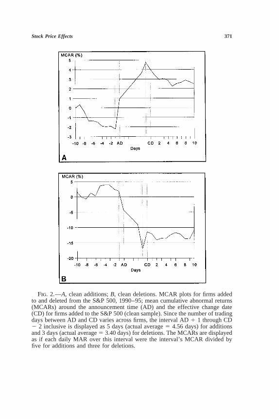
Tables 2 and 3 present mean abnormal returns around the two eventdays for additions, while tables 4 and 5 display the same results fordeletions. Figure 2 plots mean cumulative abnormal returns for theclean additions (part A) and clean deletions (part B). A natural concernis the small number of clean observations—especially deletions. Eachof the four hypotheses for price movements around index compositionchanges (price-pressure, downward-sloping demand, information, andliquidity) predicts a roughly symmetric price effect for additions anddeletions. Thus, we alleviate the small sample problems by combiningthe additions and deletions after multiplying the deletion firms’ abnor-mal returns by minus one. While the point estimates contain little newinformation, hypothesis testing is more powerful because of the largersample sizes. These results (unreported) are discussed whenever infer-ences are affected.

Part A of tables 2 and 4 presents daily mean abnormal returns relativeto the announcement date, while part B of tables 2 and 4 reports dailymean abnormal returns relative to the change date. Tables 3 and 5 dis-play multiple-day window results. Each table contains results for theclean sample and the complete sample. The subsequent discussion fo-cuses on the results for the clean samples since these show the effectsof addition to and deletion from the S&P 500 in those cases for whichwe are sure that index funds have an incentive to trade.

For each of the 10 event days after the announcement date shownin part A, only those firms for which the change date has not yet oc-curred are used. Thus, the sample size declines with the passage ofevent time past the announcement date. This presentation allows themagnitude of the abnormal returns between the announcement date andthe change date to be assessed using part A without contamination fromany reversal that may occur on or after the change date. Similarly, foreach of the 10 event days prior to the change date shown in part B,only those firms for which the announcement date has occurred on aprior day are used.

Results for AD appear as event day 0 in part A of tables 2 and 4.


TA

BL

E2

Dai

lyM

arke

t-A

djus

ted

Abn

orm

alR

etur

ns(A

R)

for

Fir

ms

Add

edto

S&P

500,

Mar

ch19

90–A

pril

1995

Cle

anSa

mpl

eC

ompl

ete

Sam

ple

Eve

ntD

ayN

MA

Rt C

(MA

R)

t T(M

AR

)%

AR

.0

NM

AR

t C(M

AR

)t T

(MA

R)

%A

R.

0

A.

AD

50:

210

342

.018

2.0

62

.04

.53

482

.204

2.6

92

.63

.50

29

34.3

831.

52.9

8.7

1*49

.239

.98

.75

.61

28

342

.728

22.

882

1.86

.29*

492

.549

22.

352

1.73

.35*

27

342

1.00

42

2.46

22.

57.3

2*49

2.8

092

2.61

22.

54.3

92

634

.038

.11

.10

.41

49.4

191.

431.

32.5

32

534

2.1

622

.58

2.4

1.4

149

2.2

762

1.22

2.8

7.4

32

434

2.4

192

1.38

21.

07.3

549

2.1

072

.43

2.3

4.4

32

334

2.0

562

.20

2.1

4.4

749

.172

.65

.54

.51

22

34.0

52.1

3.1

3.5

650

.147

.45

.47

.54

21

342

.295

21.

022

.75

.41

502

.245

21.

002

.78

.44

034

3.15

86.

668.

08.9

1*50

2.85

97.

409.

07.8

8*

134

.825

2.20

2.11

.65

50.9

252.

742.

94.6

8*2

321.

129

3.58

2.80

.72*

44.6

182.

101.

84.6

8*3

28.9

762.

582.

27.6

139

1.04

93.

382.

94.6

24

24.7

881.

521.

69.7

9*33

.891

1.92

2.30

.76*

56

2.6

242

.38

2.6

7.3

311

2.2

492

.26

2.3

7.3

66

:10

#4

#9

Stock Price Effects 365B

.C

D5

0:2

6:2

10#

4#

92

56

1.78

11.

971.

91.8

311

1.25

12.

211.

86.7

32

424

.728

1.64

1.56

.63

33.6

882.

031.

77.6

42

328

.891

2.33

2.07

.57

39.4

891.

381.

37.5

62

232

1.32

74.

003.

29.7

5*44

1.17

64.

163.

50.7

0*2

134

1.12

72.

032.

88.7

4*50

1.51

43.

374.

81.7

6*

034

2.7

262

2.35

21.

86.2

9*50

22.

018

21.

872

6.41

.24*

134

2.6

062

1.95

21.

55.1

8*55

2.6

152

1.87

22.

05.2

4*2

342

.469

21.

012

1.20

.50

552

.380

21.

062

1.26

.47

334

.127

.37

.33

.50

55.0

54.1

8.1

8.5

14

342

.216

2.6

82

.55

.47

55.1

28.5

1.4

3.5

65

342

.616

21.

532

1.57

.47

552

.372

21.

132

1.24

.45

634

.292

.76

.75

.56

552

.119

2.4

12

.40

.49

734

.107

.36

.27

.50

55.1

56.5

6.5

2.5

18

33.2

39.6

9.6

0.4

854

.320

1.13

1.06

.50

933

2.1

762

.43

2.4

4.4

254

2.1

832

.58

2.6

0.4

410

332

.228

2.5

42

.57

.48

542

.350

21.

172

1.15

.41

Not

e.—

The

sam

ples

are

desc

ribe

din

Sec.

IIA

and

the

calc

ulat

ion

ofA

Ri(τ

)is

disc

usse

din

the

first

part

ofSe

c.II

B,

whi

chal

sode

fines

MA

R(τ

).N

isth

enu

mbe

rof

firm

sus

ed,a

ndt C

(MA

R)

uses

the

cros

s-se

ctio

nal

vari

ance

estim

ator

ineq

.(A

1);

t T(M

AR

)us

esth

etim

e-se

ries

vari

ance

estim

ator

ineq

.(A

2).A

lleq

uatio

nsar

ein

the

appe

ndix

.The

cros

s-se

ctio

nal

t-st

atis

tics

are

dist

ribu

ted

Stud

ent’

st

with

(N2

1)de

gree

sof

free

dom

,whi

leth

etim

e-se

ries

t-st

atis

tics

are

appr

oxim

atel

yno

rmal

lydi

stri

bute

d.A

Ris

expr

esse

das

ape

rcen

tage

.*

%.

0is

sign

ifica

ntly

diff

eren

tfr

om.5

usin

ga

bino

mia

lte

stw

itha

5%cu

toff

.


TA

BL

E3

Lon

gW

indo

wSt

atis

tics

for

Dai

lyM

arke

t-A

djus

ted

Abn

orm

alR

etur

ns(A

R)

for

Fir

ms

Add

edto

S&P

500,

Mar

ch19

90–A

pril

1995

Cle

anSa

mpl

eC

ompl

ete

Sam

ple

Spec

ific

Eve

ntW

indo

wE

vent

Day

sN

MC

AR

t Ct T

%C

AR

.0

NM

CA

Rt C

t T%

CA

R.

0

Run

-up

AD

11,

CD

21

343.

807

4.15

4.25

.79*

503.

490

5.22

4.79

.80*

Post

-AD

perm

anen

tA

D1

1,C

D1

734

1.70

11.

231.

22.7

1*50

.084

.05

.07

.66*

AD

11,

CD

110

331.

760

1.52

1.12

.73*

49.1

20.0

7.1

0.6

5*

Tot

alpe

rman

ent

AD

,C

D1

734

4.85

93.

443.

36.7

4*50

2.94

31.

732.

52.7

0*A

D,

CD

110

334.

864

3.86

3.02

.73*

492.

936

1.75

2.27

.69*

Rel

ease

CD

,C

D1

734

22.

106

21.

832

1.96

.32*

502

3.40

62

2.28

23.

94.3

6*

Post

rele

ase

CD

18,

CD

110

332

.165

2.2

02

.19

.58

542

.213

2.3

82

.32

.52

NM

AA

Rt C

t TM

NM

AA

Rt C

t TM

Run

-up

AD

11,

CD

21

34.7

944.

754.

3918

950

.811

5.70

5.43

282

Post

-AD

perm

anen

tA

D1

1,C

D1

734

.112

1.05

1.06

461

502

.016

2.1

22

.19

682

AD

11,

CD

110

33.1

101.

471.

1454

749

.001

.01

.01

816

Tot

alpe

rman

ent

AD

,C

D1

734

.339

3.42

3.35

495

50.1

951.

542.

3973

2A

D,

CD

110

33.2

913.

873.

1358

049

.169

1.64

2.26

865

Not

e.—

The

sam

ples

are

desc

ribe

din

Sec.

IIA

;de

finiti

ons

ofM

CA

R(τ

1,τ 2

)an

dM

AA

R(τ

1,τ 2

)ar

efo

und

inSe

c.II

B.

Mis

the

num

ber

ofda

ysin

the

win

dow

sum

min

gac

ross

firm

s;t C

(MC

AR

)an

dt C

(MA

AR

)us

eth

ecr

oss-

sect

iona

lva

rian

cees

timat

orin

eq.

(A1)

;t 1

(MC

AR

)an

dt T

(MA

AR

)us

eth

etim

e-se

ries

vari

ance

estim

ator

ineq

.(A

2).

Bot

heq

uatio

nsar

ein

the

appe

ndix

.The

cros

s-se

ctio

nalt

-sta

tistic

sar

edi

stri

bute

dSt

uden

t’s

twith

(N2

1)de

gree

sof

free

dom

,whi

leth

etim

e-se

ries

t-st

atis

tics

are

appr

oxim

atel

yno

rmal

lydi

stri

bute

d.A

Ris

expr

esse

das

ape

rcen

tage

.*

%.

0is

sign

ifica

ntly

diff

eren

tfr

om.5

usin

ga

bino

mia

lte

stw

itha

5%cu

toff

.


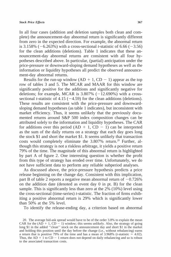
In all four cases (addition and deletion samples both clean and com-plete) the announcement-day abnormal return is significantly differentfrom zero in the expected direction. For example, the abnormal returnis 3.158% (26.263%) with a cross-sectional t-statistic of 6.66 (23.56)for the clean additions (deletions). Table 1 indicates that these an-nouncement-day abnormal returns are consistent with all four hy-potheses described above. In particular, (partial) anticipation under theprice-pressure or downward-sloping demand hypotheses as well as theinformation or liquidity hypotheses all predict the observed announce-ment-day abnormal returns.

Results for the run-up window (AD 1 1, CD 2 1) appear as the toprow of tables 3 and 5. The MCAR and MAAR for this window aresignificantly positive for the additions and significantly negative fordeletions; for example, MCAR is 3.807% (212.690%) with a cross-sectional t-statistic of 4.15 (24.59) for the clean additions (deletions).These results are consistent with the price-pressure and downward-sloping demand hypotheses (as table 1 indicates), but inconsistent withmarket efficiency. Thus, it seems unlikely that the previously docu-mented returns around S&P 500 index composition changes can beattributed solely to the information and liquidity hypotheses. The CARfor additions over this period (AD 1 1, CD 2 1) can be interpretedas the sum of the daily returns on a strategy that each day goes longthe stock $1 and short the market $1. It seems unlikely that transactioncosts would completely eliminate the 3.807% return.20 Further, al-though this strategy is not a riskless arbitrage, it yields a positive return79% of the time. The magnitude of this abnormal return is highlightedby part A of figure 2. One interesting question is whether the profitfrom this type of strategy has eroded over time. Unfortunately, we donot have sufficient data to perform any reliable subperiod analyses.

As discussed above, the price-pressure hypothesis predicts a pricerelease beginning on the change day. Consistent with this implication,part B of table 2 reports a negative mean abnormal return of 20.726%on the addition date (denoted as event day 0 in pt. B) for the cleansample. This is significantly less than zero at the 2% (10%) level usingthe cross-sectional (time-series) t-statistic. The fraction of firms exhib-iting a positive abnormal return is 29% which is significantly lowerthan 50% at the 5% level.

To identify the release-ending day, a criterion based on abnormal

20. The average bid-ask spread would have to be of the order 3.8% to explain the meanCAR for the (AD 1 1, CD 2 1) window; this seems unlikely. Also, the strategy of goinglong $1 in the added ‘‘clean’’ stock on the announcement day and short $1 in the marketand holding this position until the day before the change (i.e., without rebalancing) earnsa return that is positive 79% of the time and has a mean of 3.968% (t-statistic 5 4.02).Thus, the AD 1 1 to CD 2 1 return does not depend on daily rebalancing and so is robustto the associated transaction costs.


TA

BL

E4

Dai

lyM

arke

t-A

djus

ted

Abn

orm

alR

etur

ns(A

R)

for

Fir

ms

Del

eted

from

S&P

500,

Mar

ch19

90–A

pril

1995

Cle

anSa

mpl

eC

ompl

ete

Sam

ple

Eve

ntD

ayN

MA

Rt C

(MA

R)

t T(M

AR

)%

AR

.0

NM

AR

t C(M

AR

)t T

(MA

R)

%A

R.

0

A.

AD

50:

210

151.

674

1.47

2.64

.53

52.2

57.5

7.9

1.4

82

915

21.

778

21.

982

2.81

.33

52.6

63.6

02.

34.4

82

815

2.5

432

.57

2.8

6.3

352

2.3

682

1.10

21.

30.4

02

715

1.92

1.9

53.

03.7

352

.247

.37

.87

.58

26

152

.933

2.8

12

1.47

.47

52.1

31.3

3.4

6.5

82

515

3.27

91.

455.

17.8

7*52

1.08

51.

523.

83.6

5*2

415

.345

.29

.54

.47

52.3

16.7

91.

11.4

82

315

2.0

302

.03

2.0

5.4

052

2.4

732

.98

21.

67.4

82

215

21.

435

21.

532

2.26

.47

522

.188

2.5

22

.66

.46

21

152

.544

2.3

72

.86

.27

522

.063

2.1

42

.22

.44

015

26.

263

23.

562

9.88

.13*

522

1.46

32

2.15

25.

16.4

4

115

23.

609

23.

712

5.69

.13*

512

.787

21.

582

2.75

.45

212

2.3

212

.29

2.4

5.4

246

.638

.59

2.11

.48

312

23.

224

22.

802

4.55

.25

412

.882

22.

012

2.76

.37

48

26.

447

22.

052

7.43

.13

332

1.75

42

1.98

24.

93.3

65

42

10.5

282

2.65

28.

58.0

010

24.

901

22.

252

7.58

.30

6:1

00

#6


.C

D5

0:2

10:2

60

#6

25

42

1.71

32

1.47

21.

40.2

510

2.6

182

1.13

2.9

5.3

02

48

23.

514

23.

552

4.05

.00*

332

.888

22.

172

2.49

.39

23

122

1.72

72

1.38

22.

44.3

340

2.3

082

.61

2.9

5.4

52

212

21.

203

21.

302

1.70

.33

452

.746

21.

862

2.45

.40

21

152

8.01

62

3.97

212

.65

.13*

502

2.57

02

3.17

28.

89.4

0

014

5.59

02.

988.

52.8

6*40

1.97

62.

366.

11.6

0

114

2.6

532

.45

2.9

9.4

337

.322

.46

.96

.51

214

22.

019

2.8

42

3.08

.64

372

.299

2.3

22

.89

.62

314

.572

.61

.87

.50

36.2

02.4

7.5

9.5

64

142

.094

2.1

52

.14

.64

35.2

02.6

6.5

8.5

75

141.

243

.88

1.89

.57

35.7

951.

292.

30.5

16

14.7

06.4

11.

08.4

334

.425

.59

1.21

.53

714

2.4

522

.34

2.6

9.5

733

2.1

792

.30

2.5

0.5

58

142

1.48

42

2.30

22.

26.4

333

2.7

612

2.19

22.

14.3

99

142

.190

2.1

92

.29

.43

332

.118

2.2

52

.33

.45

1014

2.98

71.

974.

55.7

133

.779

1.05

2.19

.45

Not

e.—

See

note

tota

ble

2.*

%.

0is

sign

ifica

ntly

diff

eren

tfr

om.5

usin

ga

bino

mia

lte

stw

itha

5%cu

toff

.


TA

BL

E5

Lon

gW

indo

wSt

atis

tics

for

Dai

lyM

arke

t-A

djus

ted

Abn

orm

alR

etur

ns(A

R)

for

Fir

ms

Del

eted

from

S&P

500,

Mar

ch19

90–A

pril

1995

Cle

anSa

mpl

eC

ompl

ete

Sam

ple

Spec

ific

Eve

ntW

indo

wE

vent

Day

sN

MC

AR

t Ct T

%C

AR

.0

NM

CA

Rt C

t T%

CA

R.

0

Run

-up

AD

11,

CD

21

152

12.6

902

4.59

210

.28

.07*

502

2.98

62

1.86

24.

62.3

8

Post

-AD

perm

anen

tA

D1

1,C

D1

514

28.

875

22.

902

4.54

.21

342

1.62

92

.73

21.

40.4

1A

D1

1,C

D1

1014

27.

308

22.

742

3.09

.14*

322

1.71

92

.78

21.

20.3

4

Tot

alpe

rman

ent

AD

,C

D1

514

215

.711

23.

692

7.69

.07*

342

4.55

22

1.61

23.

76.3

2*A

D,

CD

110

142

14.1

442

3.84

25.

80.1

4*32

24.

781

21.

742

3.24

.31*

Rel

ease

CD

,C

D1

514

4.63

91.

363.

13.7

134

2.99

01.

973.

58.6

5

Post

rele

ase

CD

16,

CD

110

141.

567

.78

1.15

.57

33.1

14.1

2.1

5.4

5

NM

AA

Rt C

t TM

NM

AA

Rt C

t TM

Run

-up

AD

11,

CD

21

152

2.86

92

5.04

29.

3866

502

.857

23.

182

6.22

264

Post

-AD

perm

anen

tA

D1

1,C

D1

514

2.8

842

2.59

24.

7414

834

2.2

642

1.43

22.

5539

6A

D1

1,C

D1

1014

2.4

752

2.64

23.

1221

832

2.1

722

1.50

21.

9753

5

Tot

alpe

rman

ent

AD

,C

D1

514

21.

444

23.

152

8.12

162

342

.513

22.

112

5.19

430

AD

,C

D1

1014

2.8

812

3.57

25.

9723

232

2.3

562

2.36

24.

2056

7

Not

e.—

See

note

tota

ble

3.*

%.

0is

sign

ifica

ntly

diff

eren

tfr

om.5

usin

ga

bino

mia

lte

stw

itha

5%cu

toff

.


Fig. 2.—A, clean additions; B, clean deletions. MCAR plots for firms addedto and deleted from the S&P 500, 1990–95; mean cumulative abnormal returns(MCARs) around the announcement time (AD) and the effective change date(CD) for firms added to the S&P 500 (clean sample). Since the number of tradingdays between AD and CD varies across firms, the interval AD 1 1 through CD2 2 inclusive is displayed as 5 days (actual average 5 4.56 days) for additionsand 3 days (actual average 5 3.40 days) for deletions. The MCARs are displayedas if each daily MAR over this interval were the interval’s MCAR divided byfive for additions and three for deletions.


volume is applied to the clean samples.21 This criterion relies on recenttheoretical work concerning block trades (see, e.g., Keim and Madha-van 1996) that explains the documented temporary price pressure asbeing compensation for the liquidity being provided by the counterpart-ies. These models predict a positive relation between order size andprice. Any temporary price pressure for index changes that is due toindex-fund trading would be driven by the same factors as those drivingthe temporary price pressure observed for block trades. Thus, it is thelarge index-fund trades associated with adding or deleting the relevantstock that drives any temporary price pressure. For this reason, theprice pressure ends once trading volume has returned to its normalpostchange level. The volume is estimated to have returned to its nor-mal postchange level on the earliest day after the change day with anMAV that is lower than the average MAV for all later days throughCD 1 10. The implied release-end day is CD 1 7 for additions andCD 1 5 for deletions.22

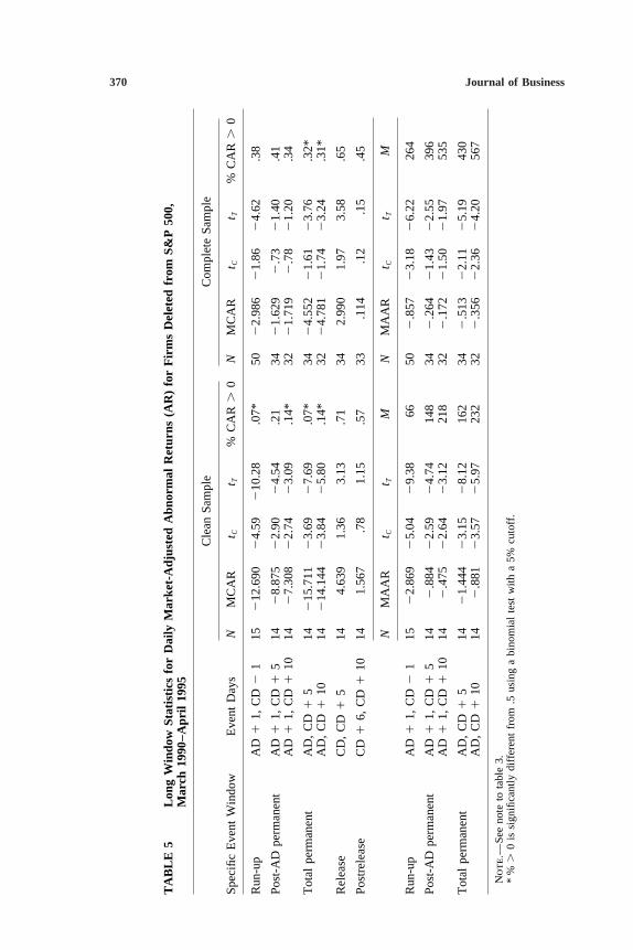
The mean CAR for the release window is reported in table 3 as22.106% for clean additions and significantly different from zero atthe 5% (10%) level using the time-series (cross-sectional) t-statistic.The fraction of CARs that are positive is significantly less than 50%at the 5% level. Deletions also exhibit a price reversal. The price releaseon the change day (CD) for the clean deletions sample is 5.59% andis significant at 5% using the cross-sectional or time-series t-statistic.The mean CAR over the release window is 4.639% but is only signifi-cant using the time-series t-statistic.

Taken together, the addition and deletion results provide strong evi-dence of a significant price reversal following S&P 500 compositionchanges. The combined sample (results not reported) further confirmsthis conclusion by exhibiting an MCAR over the release window thatis significantly negative at the 5% level using either t-statistic. We con-clude that price-pressure effects contribute to the abnormal return pat-terns that occur around index changes. It is possible, however, thatdownward-sloping demand curves also play a role, and we now addressthis issue.

Tables 3 and 5 report results for the post-AD permanent windowusing the volume-based release-end day and the end of the event win-dow (CD 1 10). As discussed above, the abnormal return over thispost-AD permanent window provides a lower bound on the permanent

21. Since longer-horizon CARs have greater sampling variability, extending the release,post-AD, and total permanent effect windows beyond the actual release-ending day reducesthe power of the tests. This reduced power motivates our attempts to determine the actualrelease-ending day instead of using the last day observed (CD 1 10).

22. For the combined sample, MAV for an event day is taken as a weighted averageof the MAVs for the additions and deletions on that day; the implied release-ending dayis CD 1 9.


price effect associated with the downward-sloping demand curve hy-pothesis. Given the price reversal documented above, choosing a pre-mature release-ending day would overstate the abnormal return for thispost-AD permanent window. However, note that the MCAR for thepost-release window in tables 3 and 5 is insignificant for all four sam-ples. This suggests that the criterion for determining the release-endday probably does not end the release period prematurely. Despite this,the MCAR and MAAR for the post-AD permanent window are sig-nificant (using either t-statistic) for the clean deletions (table 5) andclean combined samples (unreported) regardless of the release-endingday employed. For the clean additions, the MCAR is of the predictedsign but not significant. Thus, the additions evidence is less supportiveof the downward-sloping demand hypothesis than the deletions or com-bined-sample evidence. Even so, the fraction of positive CARs is al-ways on the predicted side of 50% for all three clean samples (includingcombined, which is not reported) and is significant in five of six tests(three clean samples times two release-ending days). Taken together,this evidence provides additional support, relative to the pre–October1989 studies, that stocks possess downward-sloping demand curves.

A final question is the total magnitude of the CAR associated withbeing added to or deleted from the S&P 500 index. In table 3, the meanCAR for clean additions over the total permanent window is greaterthan 4.8% and is significant at the 5% level for each assumed release-ending day. For the complete additions sample, the mean CAR overthis window is about 2.94%, which is comparable to theannouncement/change-day effect found in earlier studies that usedanalogous samples (e.g., Harris and Gurel 1986; Shleifer 1986; andDhillon and Johnson 1991). For the clean deletion sample, the meanCAR over the total permanent window in table 5 is 215.7% using therelease-ending day (CD 1 5) and is 214.1% using CD 1 10; it isalways significant at the 1% level. The magnitude of this decline isillustrated in figure 2. It seems that a significant negative permanentprice effect is associated with deletion from the S&P 500.

To summarize, the abnormal price movements for the addition anddeletion samples provide consistent evidence concerning the fourhypotheses presented above and market efficiency. The significantlypositive (negative) abnormal return from AD 1 1 to CD 2 1 for addi-tions (deletion) is inconsistent with semi–strong form market effi-ciency. The price reversal on and following the effective change datesupports the price-pressure hypothesis. The weakly positive (signifi-cantly negative) abnormal return from AD 1 1 through the release-ending day for additions (deletions) supports the downward-slopingdemand hypothesis. Finally, while we can rule out the information andliquidity hypotheses as complete explanations for the price patterns ob-served around S&P 500 composition changes, we cannot rule out the


possibility that they contribute to the announcement-day returns and,therefore, to the total permanent price effect.

C. Volume Results

Table 6 reports mean abnormal volume by day, relative to the event,for the two additions samples (complete and clean), while table 7 doesthe same for the two deletions samples. For both tables, part A’s eventtime is relative to the announcement date, while part B’s is relative tothe addition/deletion date. As with tables 2 and 4, only firms whosechange dates have not yet occurred are used to calculate any givenday’s mean AV in part A, and only firms whose announcement dateshave already past are used for any given day in part B. Since the logtransformation used to calculate AV understates high volumes, figure3 contains plots of the daily means for dollar volumes expressed as afraction of the dollar value of shares outstanding (mean fractional vol-umes, MFVs) for the clean additions (part A) and clean deletions(part B).

For additions, part A of table 6 shows that abnormal volume is unre-markable up until one day before the announcement. Each of six con-secutive days starting with the announcement day exhibits significantlypositive abnormal volume at the 5% level for each additions sample.Part B reveals that the largest abnormal volume occurs on the day priorto addition with a t-statistic greater than 13 for each sample. In particu-lar, the clean sample’s point estimate of AV is 11.612%, which com-pares to 5.784% for the announcement day and 1.334% for the dayprior to the announcement.23 This result is consistent with index fundsdoing most of their purchasing on this date to minimize tracking error.

It is interesting that this relatively large abnormal volume on theday preceding addition is not associated with relatively large abnormalreturn. Instead, the MAR for the clean sample on the day prior to addi-tion is 1.127%, which compares to 3.158% on the announcement day.Comparing the parts labeled ‘‘A’’ for figures 3 and 2 clearly illustratesthis pattern of volume and returns. Explaining the patterns in these twofigures is a challenge for future theoretical work.

As can be seen by comparing the two parts of figure 3, the volumeresults for deletions reported in table 7 are generally very similar tothose for additions. The largest abnormal volume is on the day beforedeletion (CD 2 1), followed by the announcement day (AD). Abnormalvolume is unremarkable until AD but the next 6 days (including AD)are all significantly positive. It is interesting that MAV remains sig-

23. The log transformation understates the difference in raw dollar volume across thesethree days. For the day before addition, the announcement day and the day before theannouncement, the MFVs are 4.39%, 1.39%, and 0.57%, respectively (see fig. 3).


nificantly positive from CD through until CD 1 8 for the clean dele-tions sample.

IV. Conclusion

This article analyzes price and volume data for firms added to and de-leted from the S&P 500 since October 1989. Because of the temporalseparation of the announcements from the index changes during thisperiod, this new data set has the potential to contribute to our under-standing of several issues associated with the determination of market-clearing prices for individual stocks.

For both additions and deletions, the data reveal a distinct patternof stock-price movements. Specifically, for additions, while we finda significantly positive announcement effect, we also find a positiveabnormal return of about 3.8% over the period starting the day afterthe announcement and ending the day before the effective date of thechange. Further, we find a significant negative abnormal return follow-ing the addition. Firms being deleted from the index also exhibit asignificant postannouncement drift and a significant price reversal, butin directions opposite to those for additions.

Our results can be interpreted in the context of the efficient markethypothesis. The significant abnormal returns following the announce-ment date are inconsistent with semi–strong form market efficiency.It would have been possible to construct trading rules that use publiclyavailable information to earn positive abnormal returns, particularlybetween the announcement day and the change day. This violation ofmarket efficiency is anomalous. While the rationale for the trading pat-terns of index funds is clear, the reason why risk arbitragers do nottrade the profits away on the announcement day is less obvious. How-ever, with more data, it becomes possible to test whether the run-upeffect has declined over time. Evidence of such a decline would indi-cate that the inefficiency existed because the market was not fully awareof the implications of index-fund behavior around index changes. Weare currently gathering such evidence.

The price reversal after addition and deletion strongly suggests theexistence of temporary price effects, caused by index-fund trading as-sociated with S&P 500 composition changes. It also has implicationsfor a well-documented asymmetry in the block-trade literature: seller-initiated block trades exhibit a similar price reversal, but buyer-initiatedtrades do not. The symmetry of our price reversal results for additionsand deletions is a new empirical fact that any potential explanation ofthe block-trade asymmetry must also address. Fully reconciling ourfindings with the temporary effects documented for block trades andpre–October 1989 index composition changes is an issue requiring ad-ditional research.


TA

BL

E6

Dai

lyM

arke

tM

odel

Abn

orm

alV

olum

e(A

V)

for

Fir

ms

Add

edto

S&P

500,

Mar

ch19

90–D

ecem

ber

1994

Cle

anSa

mpl

eC

ompl

ete

Sam

ple

Eve

ntD

ayN

MA

Vt C

(MA

V)

t T(M

AV

)%

AV

.0

NM

AV

t C(M

AV

)t T

(MA

V)

%A

V.

0

A.

AD

50:

210

28.1

76.2

8.2

7.5

035

.301

.58

.54

.51

29

282

.224

2.4

92

.34

.43

352

.216

2.5

32

.38

.46

28

282

.532

2.8

72

.83

.32

352

.120

2.2

12

.21

.37

27

28.8

901.

091.

38.5

435

.715

1.02

1.28

.54

26

28.4

70.7

1.7

3.5

735

.507

.92

.90

.57

25

28.3

15.5

4.4

9.4

635

.357

.70

.64

.49

24

282

.046

2.0

72

.07

.50

352

.019

2.0

32

.03

.51

23

28.4

54.8

3.7

1.4

335

.377

.78

.67

.43

22

28.1

78.3

2.2

8.5

035

.153

.31

.27

.54

21

281.

334

2.47

2.07

.68

351.

606

2.77

2.86

.66

028

5.78

411

.45

8.99

.96*

355.

247

10.0

99.

35.9

4*

128

4.27

66.

096.

64.8

6*35

4.01

06.

677.

14.8

6*2

264.

031

4.34

6.26

.81*

313.

598

4.17

6.41

.77*

322

4.77

44.

687.

42.8

6*27

4.52

55.

108.

06.8

5*4

199.

782

8.45

15.2

01.

0023

8.78

97.

1015

.66

.91*

55

4.07

82.

186.

34.8

08

3.05

92.

175.

45.7

56

:10

#3

#6


.C

D5

0:2

10:2

6#

3#

62

55

1.75

41.

432.

73.8

08

1.80

31.

873.

21.7

52

419

3.16

64.

444.

92.7

923

3.21

65.

395.

73.8

3*2

322

2.58

24.

854.

01.8

6*27

2.47

64.

294.

41.7

8*2

226

4.32

06.

936.

71.8

8*31

4.17

46.

397.

44.8

7*2

128

11.6

1219

.28

18.0

41.

00*

3510

.481

13.5

618

.67

1.00

*

028

5.27

011

.31

8.19

1.00

*35

4.70

310

.18

8.38

1.00

*

128

3.53

86.

615.

50.8

6*35

3.25

36.

875.

80.8

9*2

283.

221

5.67

5.00

.86*

353.

043

6.06

5.42

.86*

328

2.10

84.

933.

27.8

2*35

2.04

45.

113.

64.8

0*4

282.

118

3.90

3.29

.75*

351.

893

3.76

3.37

.71*

528

2.24

34.

263.

48.7

5*35

2.50

54.

154.

46.7

7*6

281.

859

4.55

2.89

.75*

352.

087

5.44

3.72

.80*

727

1.63

43.

452.

54.7

4*34

1.59

33.

752.

84.7

4*8

271.

745

2.79

2.71

.70*

341.

561

2.85

2.78

.65*

927

1.70

13.

922.

64.7

8*34

1.55

13.

982.

76.7

4*10

272.

070

4.24

3.22

.81*

342.

259

4.45

4.02

.82*

Not

e.—

The

sam

ples

are

desc

ribe

din

Sec.

IIA

.T

heca

lcul

atio

nof

AV

i(τ)

and

MA

V(τ

)is

disc

usse

din

the

mid

dle

ofSe

c.II

B.

Nis

the

num

ber

offir

ms

used

;t C

(MA

V)

isca

lcul

ated

usin

gth

ecr

oss-

sect

iona

lva

rian

cees

timat

orde

fined

ineq

.(A

1);

t T(M

AV

)is

calc

ulat

edus

ing

the

time-

seri

esva

rian

cees

timat

orde

fined

ineq

.(A

2).

Bot

heq

uatio

nsar

ein

the

appe

ndix

.T

hecr

oss-

sect

iona

lt-

stat

istic

sar

edi

stri

bute

dSt

uden

t’s

tw

ith(N

21)

degr

ees

offr

eedo

m,

whi

leth

etim

e-se

ries

t-st

atis

tics

are

appr

oxim

atel

yno

rmal

lydi

stri

bute

d.A

Vis

expr

esse

das

ape

rcen

tage

.*

%.

0is

sign

ifica

ntly

diff

eren

tfr

om.5

usin

ga

bino

mia

lte

stw

itha

5%cu

toff

.


TA

BL

E7

Dai

lyM

arke

tM

odel

Abn

orm

alV

olum

e(A

V)

for

Fir

ms

Del

eted

from

S&P

500,

Mar

ch19

90–D

ecem

ber

1994

Cle

anSa

mpl

eC

ompl

ete

Sam

ple

Eve

ntD

ayN

MA

Vt C

(MA

V)

t T(M

AV

)%

AV

.0

NM

AV

t C(M

AV

)t T

(MA

V)

%A

V.

0

A.

AD

50:

210

131.

372

1.08

1.12

.69

421.

983

2.54

4.28

.71*

29

13.3

42.2

8.2

8.6

242

1.88

62.

264.

07.6

22

813

2.4

112

.32

2.3

4.4

642

.818

.97

1.77

.55

27

132.

054

2.21

1.68

.62

422.

074

3.22

4.48

.62

26

131.

069

.99

.88

.46

421.

942

2.76

4.19

.62

25

131.

178

.91

.96

.62

422.

884

4.31

6.23

.74*

24

13.2

62.1

7.2

1.5

442

1.82

12.

353.

93.6

9*2

313

2.1

712

.14

2.1

4.4

642

1.36

21.

912.

94.6

22

213

22.

084

21.

252

1.71

.38

421.

238

1.51

2.68

.64

21

13.0

63.0

4.0

5.5

442

1.26

61.

752.

73.6

9*

013

8.13

97.

646.

661.

00*

424.

911

6.92

10.6

1.8

6*

113

7.73

98.

676.

341.

00*

414.

804

7.73

10.3

7.8

5*2

116.

697

5.55

5.48

1.00

*37

4.97

26.

5110

.74

.86*

311

9.58

84.

727.

851.

00*

326.

163

5.88

13.3

1.9

4*4

710

.976

3.11

8.99

.86

257.

962

5.80

17.2

0.9

2*5

314

.964

9.50

12.2

51.

007

6.96

02.

3115

.03

.86

6:1

00

#4


.C

D5

0:2

10:2

60

#4

25

36.

354

11.6

65.

201.

007

3.59

92.

757.

77.8

62

47

7.02

56.

025.

751.

00*

253.

642

4.36

7.87

.80*

23

117.

376

6.02

6.04

1.00

*32

4.65

15.

8410

.05

.88*

22

115.

222

3.58

4.28

.91*

374.

363

6.26

9.45

.89*

21

1314

.974

10.1

912

.26

1.00

*41

9.63

79.

3320

.81

.93*

012

10.6

135.

468.

691.

00*

325.

808

4.70

12.5

5.8

1*

112

5.95

44.

164.

88.8

3*28

3.60

53.

497.

79.7

5*2

124.

291

4.52

3.51

.83*

282.

380

2.85

5.14

.71*

312

5.25

82.

794.

31.6

727

2.55

01.

965.

51.6

74

125.

037

4.15

4.12

.92*

261.

986

1.58

4.29

.77*

512

3.07

12.

482.

51.8

3*26

.432

.39

.93

.65

612

4.44

72.

063.

64.8

3*26

.151

.09

.33

.62

712

3.28

74.

502.

69.8

3*24

.435

.34

.94

.67

812

3.87

63.

693.

17.9

2*24

1.65

11.

123.

57.7

1*9

121.

418

1.29

1.16

.67

242

.058

2.0

52

.13

.54

1012

3.14

21.

682.

57.7

524

1.03

5.7

22.

24.6

7

Not

e.—

See

note

tota

ble

6.*

%.

0is

sign

ifica

ntly

diff

eren

tfr

om.5

usin

ga

bino

mia

lte

stw

itha

5%cu

toff

.


Fig. 3.—A, clean additions; B, clean deletions. MFV plots for firms added toand deleted from the S&P 500, 1990–94; mean volume as a fraction of sharesoutstanding (MFV) around the announcement date (AD) and the effective changedate (CD) for firms added to and deleted from the S&P 500 (clean sample). Sincethe number of trading days between AD and CD varies across firms, the intervalAD 1 1 through CD 2 2 inclusive is displayed as 4 days (actual average 5 4.00days) for additions and as 4 days (actual average 5 3.57 days) for deletions. TheMFVs are displayed as if each daily MFV over this interval was the interval’smean cumulative FV divided by 4.00 for additions and 3.57 for deletions. Dottedlines are two standard errors from the point estimates.


We also find that, for additions, the cumulative abnormal return fromthe day following the announcement through the price reversal isweakly positive. We interpret this abnormal return as a lower boundon the price effect caused by index-fund trading in the presence ofdownward-sloping long-term demand curves. Results for firms beingdeleted from the S&P 500 are stronger than those for additions. Takentogether, the two results provide new evidence in support of downward-sloping long-run demand curves for stocks.

It is interesting that our postannouncement abnormal return resultsseem qualitatively similar to the significantly positive (negative) abnor-mal returns found by Eades, Hess, and Kim (1984) in the week priorto (following) stocks’ ex-dividend dates. In both cases, there is an eventknown in advance by the market (the change day in our sample, theex-dividend date in theirs) and abnormal returns prior to and after thisevent. A closer comparison of the market’s behavior around each eventmay lead to a greater understanding of the driving forces behind theseabnormal returns.

The article also presents volume results indicating that the day beforeaddition or deletion is associated with particularly high volume. Ex-plaining how the behavior of index funds and investors can generatethe observed patterns of returns and trading volume for the added anddeleted firms is an interesting task for future work.

Appendix

Significance Tests

Two types of standard error calculations are employed to assess the significanceof abnormal returns and abnormal volumes. The first uses the cross-sectionaldispersion of each metric to estimate its variance.24 For the MAR(τ) abnormalreturn measure, the cross-sectional variance is given by

s2C[MAR(τ)] 5

1N(τ) ^

N(τ)

i51

[AR i(τ) 2 MAR(τ)]2/[N(τ) 2 1]. (A1)

Under the assumption that the ARi(τ)’s are cross-sectionally independently andidentically distributed normal, the resulting t-statistic for MAR(τ) is Student-tdistributed with N(τ) 2 1 degrees of freedom. A directly analogous calculationgives a variance estimate for the MCAR(τ1, τ2) and MAAR(τ1, τ2) abnormalreturn measures and for the MAV(τ) abnormal volume measure.

The second method of calculating standard errors uses a times series of obser-

24. Asquith (1983) has used this cross-sectional error estimator for mean cumulativeabnormal return in a context where the number of days in the window varies across firms.The advantage of the cross-sectional estimator relative to the time-series estimator pre-sented below is its robustness to any increase in the variance of firm abnormal returnaround the two event dates. See Brown and Warner (1985) for a further discussion of thisissue.


vations from a prior period as in Ruback (1982). The method assumes that eachfirm’s AR follows an MA(1) process and that these processes are identical andindependent across firms. Letting ni(τ1, τ2) be the number of days between τ1

and τ2 for firm i, this variance estimate for MCAR(τ1, τ2) is given by

s2T[MCAR(τ1, τ2)] 5

1N(τ1, τ2) ^

N(τ1, τ2)

i51

s2T[CAR i(τ1, τ2)], (A2)

where

s2T[CAR i(τ1, τ2)] 5 ni(τ1, τ2)s2

T[AR(τ0)]

1 2[ni(τ1, τ2) 2 1]sT[AR(τ0), AR(τ0 1 1)];

avT[AR i(τ0)] 51

48 ^τb147

τ5τb

ARi(τ);

s2T[AR(τ0)] 5

148 N(τb, τb 1 47) ^

N(τb, τb147)

i51^τb147

τ5τb

{AR i(τ) 2 avT[AR i(τ0)]}2;

and

sT[AR(τ0), AR(τ0 11)] 51

47N(τb, τb 147)

3 ^N(τb, τb147)

i51^τb146

τ5τb

{AR i(τ) 2avT [AR i(τ0)]}

3{AR i(τ11) 2avT[AR i(τ0)]}.

A directly analogous variance estimate can be derived for MAAR(τ1, τ2). Theassociated t-statistic is normally distributed asymptotically. Since MAR(τ0) isjust MCAR(τ0, τ0), setting ni(τ0, τ0) equal to one in (A2) provides a varianceestimate for MAR(τ). An analogous variance estimate can be obtained forMAV(τ).25 For MCAR, τb is equal to (AD 2 672) and for MAV(τ), τb is equalto (AD 2 108) which in each case is the day after the relevant market modelestimation period.

Finally, for each event day τ, the fraction of firms in the sample for whichAR(τ) is positive is reported. A test of the hypothesis that the sign of each AR(τ)has probability 0.5 of being positive is performed under the assumption that thesigns of the firms’ ARs are independent (see Hollander and Wolfe [1973] fordetails of this binomial test). Analogous tests are performed for the fraction offirms with positive CARs over various windows and for the fraction of firms withpositive AVs on each event-time day.

25. This time-series estimator is not identical to Ruback’s for two reasons. First, thewindow length here often varies across stocks, a condition that cannot be easily accommo-dated by Ruback’s estimator. Second, although the window length is the same across stocksfor MAR(τ) and MAV(τ), the number of firms used to calculate these measures is oftenmuch smaller than the number of firms with data over the variance estimation period.Ruback notes that if the number of firms used in the variance estimation period is morethan the number used to calculate MCAR(τ1, τ2), his t-statistic will be upward biased; ourt-statistic explicitly allows for sample size differences in the two periods.


References

Ajinkya, B., and Jain, P. 1989. The behavior of daily stock market volume. Journal ofAccounting and Economics 11:331–59.

Amihud, Y., and Mendelson, H. 1986. Asset pricing and the bid-asked spread. Journal ofFinancial Economics 17:223–49.

Amihud, Y., and Mendelson, H. 1993. Does market microstructure matter? Evidence fromthe Tel Aviv Securities Exchange. Working paper. New York: New York University,Stern School of Business.

Asquith, P. 1983. Merger bids, uncertainty and stockholder returns. Journal of FinancialEconomics 11:51–83.

Brown, S.; Goetzmann, W.; Ibbotson, R.; and Ross, R. 1992. Survivorship bias in perfor-mance studies. Review of Financial Studies 5:553–80.

Brown, S.; Goetzmann, W.; and Ross, R. 1995. Survival. Journal of Finance 50:853–73.Brown, S., and Pope, P. 1995. Post-earnings announcement drift: Market inefficiency or

research design biases? Working paper. New York: New York University, Stern Schoolof Business.

Brown, S., and Warner, J. 1985. Using daily stock returns: The case of event studies.Journal of Financial Economics 14:3–31.

Chan, L., and Lakonishok, J. 1993. Institutional trades and intra-day stock price behavior.Journal of Financial Economics 33:173–200.

Dhillon, U., and Johnson, H. 1991. Changes in the Standard and Poor’s 500 list. Journalof Business 64:75–85.

Eades, K.; Hess, P.; and Kim, H. 1984. On interpreting security returns during the ex-dividend period. Journal of Financial Economics 13:3–34.

Edmister, R.; Graham, S.; and Pirie, W. 1995. Trading cost expectations: Evidence fromS&P 500 index replacement stock announcements. Working paper. Oxford: Universityof Mississippi, Department of Economics and Finance.

Fama, E. 1970. Efficient capital markets: A review of theory and empirical work. Journalof Finance 25:383–417.

Fama, E. 1991. Efficient capital markets: II. Journal of Finance 46:1575–1618.Goetzmann, W., and Garry, M. 1986. Does delisting from the S&P 500 affect stock price?

Financial Analysts Journal 42:64–69.Harris, L., and Gurel, E. 1986. Price and volume effects associated with changes in the

S&P 500 list: New evidence for the existence of price pressures. Journal of Finance41:815–29.

Hollander, M., and Wolfe, D. 1973. Nonparametric Statistical Methods. New York: Wiley.Holthausen, R.; Leftwich, R.; and Mayers, D. 1990. Large-block transactions, the speed

of response, and temporary and permanent stock-price effects. Journal of Financial Eco-nomics 26:71–95.

Jain, P. 1987. The effect on stock price from inclusion in or exclusion from the S&P 500.Financial Analysts Journal 43:58–65.

Judge, G.; Griffiths, W.; Hill, C.; Lutkepohl, H.; and Lee, T. 1985. The Theory and Practiceof Econometrics. New York: Wiley.

Keim, D., and Madhavan, A. 1996. The upstairs market for large block transactions: Analy-sis and measurement of price effects. Review of Financial Studies 9:1–36.

Kothari, S., and Warner, J. 1996. Measuring long-horizon security performance. Workingpaper. Rochester, N.Y.: University of Rochester, Graduate School of Business Adminis-tration.

Meulbroek, L. 1992. An empirical analysis of illegal insider trading. Journal of Finance47:1661–99.

Ruback, R. 1982. The effect of discretionary price control decisions on equity values.Journal of Financial Economics 10:83–105.

Shleifer, A. 1986. Do demand curves for stocks slope down? Journal of Finance 41:579–90.

Yermack, D. 1995. Good timing: CEO stock option awards and company news announce-ments. Working paper. New York: New York University, Stern School of Business.

Documents

first bibliography on the general agreement on trade and services