Fixed versus Flexible: Lessons from EMS Order Flow

William P. Killeen∗ BNP Paribas Asset Management, London

Richard K. Lyons

University of California, Berkeley, and NBER

Michael J. Moore The Queens University of Belfast, Northern Ireland

20 January 2004

Abstract

This paper addresses the puzzle of regime-dependent volatility in foreign exchange. We extend the literature in two ways. First, our microstructural model provides a qualitatively new explanation for the puzzle. Second, we test implications of our model using Europes recent shift to rigidly fixed rates (EMS to EMU). In the model, shocks to order flow induce volatility under flexible rates because they have portfolio-balance effects on price, whereas under fixed rates the same shocks do not have portfolio-balance effects. These effects arise in one regime and not the other because the elasticity of speculative demand for foreign exchange is (endogenously) regime-dependent: low elasticity under flexible rates magnifies portfolio-balance effects; under perfectly credible fixed rates, elasticity of speculative demand is infinite, eliminating portfolio-balance effects. New data on FF/DM transactions show that order flow had persistent effects on the exchange rate before EMU parities were announced. After announcement, the FF/DM rate was decoupled from order flow, as the model predicts. JEL Classification: F31; G11; G15; D8 Keywords: Exchange rate regime; Order flow; Euro

∗ Killeen now works for Setanta Asset Management in Dublin. The address for correspondence is: Michael J. Moore, School of Management and Economics, Queens University, Belfast, Northern Ireland BT7 1NN, United Kingdom, Tel +44 28 90273208, Fax +44 28 90335156, email m.moore@qub.ac.uk. We thank the following for valuable comments: two anonymous referees, Kathryn Dominguez, Ken Froot, Carol Osler, Hélène Rey, Dagfinn Rime, Andrew Rose, participants at the Fall 2000 NBER IFM meeting, and the lunch-groups at Berkeley and Queens. Killeen also wishes to thank Mr. Loic Meinnel, Global Head of Foreign Exchange at BNP Paribas for very useful discussions on FX markets during this project. Thanks too to Tina Kane. Lyons thanks the National Science Foundation for financial assistance, which includes funding for a clearinghouse for micro-based research on exchange rates (at faculty.haas.berkeley.edu/lyons). The views expressed in this paper are entirely the responsibility of the authors, and not BNP Paribas nor Setanta Asset Management.

1

Fixed versus Flexible: Lessons from EMS Order Flow

1. Introduction

If there is a topic at the center of international macroeconomics, it is fixed versus

flexible exchange rates. Whether teaching the Mundell-Fleming model, speaking about

the impossible trinity,1 or writing about excess volatility, the fixed-versus-flexible

debate is deeply relevant. At the same time, many of the issues in this debate remain

unresolved. Important among them is the regime-volatility puzzle: similar

macroeconomic environments produce much more exchange-rate volatility under

flexible-rate regimes (e.g., Baxter and Stockman 1989; Flood and Rose 1995).2 From this

some have concluded that the critical determinants of flexible-rate volatility are not

macroeconomic. Empirically, however, it remains unclear what these non-macro

determinants might be.

This paper addresses the regime-volatility puzzle from a microeconomic

perspective. Our approach augments the traditional macro-asset approach with a high-

resolution look at how prices are actually determined. In particular, we focus our analysis

on the role of order flow. (Order flow is a measure of signed transaction flow: seller-

initiated trades are negative order flow and buyer-initiated trades are positive order flow.)

Order flow plays an important causal role in micro models of price determination that

arises because order flow conveys information.3 The type of information that order flow

conveys includes any information that is relevant to the realization of uncertain demands,

so long as that information is not common knowledge. (If common knowledgeas is

generally assumed in macro exchange-rate modelsthen price adjusts without any need 1 The impossible trinity being that countries cannot simultaneously achieve (1) fixed exchange rates, (2) perfect capital mobility, and (3) monetary policy autonomy. 2 To some, lower volatility under fixed rates may seem obvious. But empirically, fixed rates have a distribution over time (due to parity changes). In most models, keeping the variance of this distribution below that under flexible rates requires keeping the variance of fundamentals below that under flexible rates. As an empirical matter, this has not been the case, per Flood and Rose (1995). Our explanation provides a source of fundamental volatility that is magnified under flexible rates, but is not in the set of macro fundamentals previously considered for resolving this puzzle.

2

for an order-flow role.) For example, order flow may convey information about dispersed

shifts in portfolio balance (e.g., shifts in hedging demands or risk tolerances, which are

not normally considered in macro analysis), or about more traditional macro variables

(e.g., transactions tied to exports/imports, which when aggregated correspond to pre-

announcement information on the trade balance). In a non-common-knowledge setting,

order flow becomes the intermediate link between evolving information and pricea

proximate cause of price movements (Evans and Lyons 1999).

Importantly, the impact of order flow on exchange rates is persistent (i.e., flow

affects volatility at the longer horizons associated with the regime-dependent volatility

puzzle). Though our model makes this persistence explicit, let us provide some

perspective. Note that if order flow conveys information, then its price impact should

persist, at least under the identifying assumption used regularly in empirical work that

information effects on price are permanent (e.g., French and Roll 1986, Hasbrouck 1991).

That is not to suggest that order flow cannot also have transitory effects on price, e.g.,

from temporary indigestion effects (sometimes called inventory effects). But insofar as

order flow communicates informationalong the lines noted in the previous paragraph

then some portion of order flows effects on price will persist.

This information role for order flow may be key to resolving the regime-volatility

puzzle. One reason it has not been considered is because empirical work on the puzzle

examines macro determinants, whereas order flow is generally viewed as non-macro. If

order flow is indeed a determinant, then it might explain why flexible regimes produce

more volatility than macroeconomics predicts. There is now considerable evidence that

the if part of that last sentence is met: order flow is a determinant (Lyons 1995, Rime

2000, Cai et al. 2001, Evans 2002, Evans and Lyons 2002, Hau, Killeen and Moore

2002b, Payne 2003). Whether the relation found by these authors for flexible rates is

affected by differences in exchange-rate regime is an open question, however, one that

we address in this paper (both theoretically and empirically).

3 The focus of order-flow analysis is on first moments: signed transaction flows and signed returns. There is a parallel literature that focuses on second moments, i.e., information flows that simultaneously affect (unsigned) transaction volume and return volatility (the mixture of distributions approach). For useful perspective, see Jorion (1996).

3

The main lesson from the theoretical portion of the paper is the following: exchange

rates are more volatile under flexible rates because of order flow.4 Importantly, this is not

because order flow is more volatile under flexible rates (indeed, its volatility is

unchanged in our model across regimes). The intuition for order flows role is tied to the

elasticity of speculative demand. Under flexible rates, the elasticity of speculative

demand is (endogenously) low: volatility causes rational speculators to trade less

aggressively. Their reduced willingness to take the other side of shocks to order flow

adds room for portfolio-balance effects on price. The size of those portfolio-balance

effects is determined by the size of the observed order-flow shocks. This is the price-

relevant information that order-flow conveys. Under perfectly credible fixed rates, the

elasticity of speculative demand is infinite (return volatility shrinks to zero), which

precludes portfolio-balance effects, thereby eliminating order flows information role.

Consequently, as a return factor order flow is shut down.

To test our explanation for regime-dependent volatility empirically, we exploit a

natural experiment for why order flow can induce volatility under flexible rates, but not

under fixed rates. The natural experiment is the switch from flexible (wide band) to

rigidly fixed rates in the transition from the European Monetary System (EMS) to the

European Monetary Union (EMU).5 Starting in January 1999, the euro-country currencies

have been rigidly fixed to one anotheras close to a perfectly credible fixed-rate regime

as one might hope to observe. Before May 1998, there was still uncertainty about which

internal parities would be chosen and about the timing of interest-rate harmonization in

the May-to-December period.

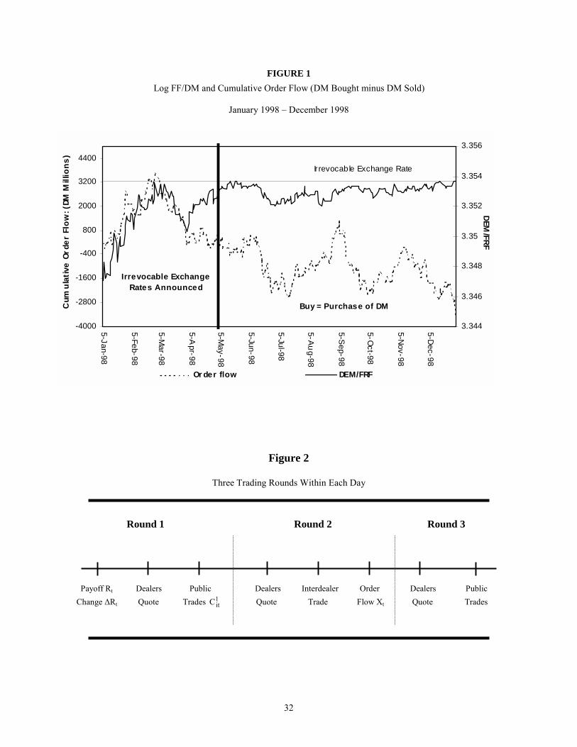
Figure 1 provides an initial, suggestive illustration of our results. It shows the

relationship between the FF/DM exchange rate in 1998 and cumulative order flow.

(These are interdealer orders; see section 3 for details.) The vertical line is 4 May 1998.

This was the first trading day after the announcement of the irrevocable conversion rates 4 For perspective on how surprising this statement is, note that in textbook exchange rate models (all of which are based wholly on public information), signed transaction flows plays no role in moving prices. So long as shifts in demand are driven by the arrival of public information, then there shouldnt be any relation between signed transaction flows and the direction of price movements (on average, there is no incentive for buying or selling at new, unbiased prices). 5 Though the EMS allowed some flexibility, it was not a free float. That said, the transition to EMU was indisputably a transition toward exchange-rate fixity. Low variability of the FF/DM rate in the EMS portion of our sample (relative to major flexible rates such as Yen/$) does not undermine the validity of our tests. (Variability in that portion of our sample was certainly high enough to be significant economically for market participants, given the low transaction

4

for the euro. Before that date, the basis on which the irrevocable lock-in rates were to be

determined was unknown. For example, on the Monday before the summit (April 27th

1998), there was a speculative flurry in the forex markets that rates would be realigned

from their existing EMS central rates. (See Financial Times, April 28th 1998). The most

obvious indicator that a regime change took place over that critical weekend is that grey-

market trading in euros kicked off on the very next day (Monday, May 4th, 1998; see

Euro Trading to start on Monday, Financial Times, May 2/3 1998).

The positive relationship between the two series up to Friday May 1st 1998 is clear:

the correlation is about 0.7. (This accords with the strong positive relationship under

flexible rates found for other currencies and samples, e.g., by Rime 2000 and Evans and

Lyons 2002). After 4th May, however, there is a sharp unwinding of long DM positions

with no corresponding movement in the exchange rate. In fact, there is a negative

correlation during the second period. Though total variation in the exchange rate is small

(roughly 20 times the median bid-offer spread), the effect of order flow appears to have

changed from one of clear impactas has been found in other studies for flexible rates

to one of no impact.6 (Visually it appears the relationship is loosening in April, but

according to the statistical evidence provided below the break does not emerge until early

May.) The model we develop in the following section provides a framework for

addressing why these order-flow effects might disappear, and how their disappearance

helps to resolve the regime-volatility puzzle.

To our knowledge, this paper is the first in the literature to address fixed-versus-

flexible rates using the concept of order flow (despite the long history of order flow as an

object of analysis in the field of finance). The two most closely related bodies of work on

fixed-versus-flexible rates include (1) the balance-of-payments flow approach and (2) a

more recent literature that introduces non-rational traders to account for high flexible-

regime volatility. Work on the balance-of-payments flow approach dates back to

Robinson (1949) and Machlup (1949). (See also the survey in Rosenberg 1996.) In those

models, exchange rates are determined from balance-of-payments flows, e.g., imports

and exports. Balance-of-payments flows depend, in turn, on the exchange-rate regime.

costs.) Extending the model of the next section to environments of imperfectly credible fixed rates is a natural direction for further research. 6 A test of whether the variance is equal across the two sub-periods is rejected at the 5 percent level.

5

Empirically, however, this approach has not borne fruit: balance-of-payments flows are

unsuccessful in accounting for exchange-rate movements (see, e.g., Frankel and Rose

1996).7 The second related body of work introduces non-rational traders to account for

high flexible-regime volatility, for example, Hau (1998) and Jeanne and Rose (2002). In

both of these papers, what causes volatility under flexible rates is that flexibility induces

new FX traders to enter, and their entry increases the level of noise. The mechanism in

our (rational) model is different. In our case it is the (endogenous) unwillingness of

speculators to take the other side of order-flow shocks that produces higher volatility.

The remainder of this paper is organized as follows. Section 2 presents our model

and the analytical results that can explain regime-dependent volatility. Section 3

describes our data. Section 4 presents empirical tests of our models implications. Section

5 concludes.

2. Model

The trading model developed in this section serves three important purposes. First,

it expresses market dynamics in terms of measurable variables, most notably order flow.8

The type of order flow shown in Figure 1 is interdealer order flow, which necessitates a

specification of interdealer trading and how that type of trading relates to underlying

demands in the economy. Second, the model provides a clear demonstration of the type

of dispersed information that order flow can convey, and how that information is

subsequently impounded in price. Third, the model shows why under flexible rates

cumulative order flow and price share a long run relationship. The properties of this

relationship and how it is affected by the shift to fixed rates provide a set of testable

implications that we examine empirically in section 4.

The model includes two trading regimes: a flexible-rate regime followed by a fixed-

rate regime. The shift from flexible to fixed rates is a random event that arrives with

7 These negative empirical results are less applicable to the noise-trade models of Osler (1998) and Carlson and Osler (2000) because the current account flows in those models can be interpreted more broadly (e.g., as flows from hedging demand), which need not manifest as identifiable balance-of-payments flows. Importantly for our approach here, order flows and balance-of-payment flows are not one to one; see, e.g., the discussion in Lyons (2001), chapter 9. 8 This is not a property of more abstract approaches to trading, for example, rational expectations models (such as Grossman and Stiglitz 1980 and Diamond and Verrecchia 1981), which are not directly estimable. (In rational expectations models, trades cannot be translated into order flow; i.e., buys versus sells, because counterparties are symmetricneither side is the initiator.)

6

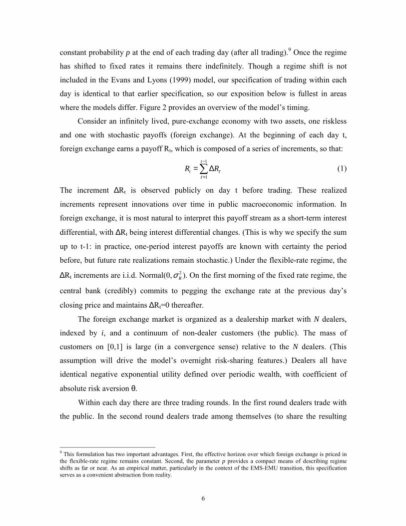
constant probability p at the end of each trading day (after all trading).9 Once the regime

has shifted to fixed rates it remains there indefinitely. Though a regime shift is not

included in the Evans and Lyons (1999) model, our specification of trading within each

day is identical to that earlier specification, so our exposition below is fullest in areas

where the models differ. Figure 2 provides an overview of the models timing.

Consider an infinitely lived, pure-exchange economy with two assets, one riskless

and one with stochastic payoffs (foreign exchange). At the beginning of each day t,

foreign exchange earns a payoff Rt, which is composed of a series of increments, so that:

1

1

t

tR Rττ

−

=

= ∆∑ (1)

The increment ∆Rt is observed publicly on day t before trading. These realized

increments represent innovations over time in public macroeconomic information. In

foreign exchange, it is most natural to interpret this payoff stream as a short-term interest

differential, with ∆Rt being interest differential changes. (This is why we specify the sum

up to t-1: in practice, one-period interest payoffs are known with certainty the period

before, but future rate realizations remain stochastic.) Under the flexible-rate regime, the

∆Rt increments are i.i.d. Normal(0, 2σ R ). On the first morning of the fixed rate regime, the

central bank (credibly) commits to pegging the exchange rate at the previous days

closing price and maintains ∆Rt=0 thereafter.

The foreign exchange market is organized as a dealership market with N dealers,

indexed by i, and a continuum of non-dealer customers (the public). The mass of

customers on [0,1] is large (in a convergence sense) relative to the N dealers. (This

assumption will drive the models overnight risk-sharing features.) Dealers all have

identical negative exponential utility defined over periodic wealth, with coefficient of

absolute risk aversion θ.

Within each day there are three trading rounds. In the first round dealers trade with

the public. In the second round dealers trade among themselves (to share the resulting

9 This formulation has two important advantages. First, the effective horizon over which foreign exchange is priced in the flexible-rate regime remains constant. Second, the parameter p provides a compact means of describing regime shifts as far or near. As an empirical matter, particularly in the context of the EMS-EMU transition, this specification serves as a convenient abstraction from reality.

7

inventory risk). In the third round dealers trade again with the public (to share inventory

risk throughout the economy).

Each day begins with payment and public observation of the payoff Rt. Then each

dealer quotes a scalar price to his customers at which he agrees to buy and sell any

amount (quoting is simultaneous). We denote this round 1 price of dealer i on day t as 1

itP . Each dealer then receives a customer-order realization 1itC that is executed at his

quoted price 1itP . Let 1

itC <0 denote net customer selling (dealer i buying). The individual

1itC s are distributed normally with mean zero and variance 2

Cσ . They are uncorrelated

across dealers and uncorrelated with the payoff Rt at all leads and lags. (For the analysis

below, it is useful to define the aggregate public demand in round 1 as the sum of

customer demands over the N dealers, or ∑=

=N

iitt CC

1

11 .) These orders represent

exogenous portfolio shifts of the non-dealer public. Their realizations are not publicly

observable, and they arrive every day, regardless of regime (with an unchanged

distribution). In this aspect we part company with Hau (1998) and Jeanne and Rose

(2002): in those papers, the change in regime induces non-rational traders to exit the

market, resulting in reduced trading. In our model one might think of this exiting as an

abrupt fall in 2Cσ (with the added assumption that the customer orders represent non-

rational trades, which they do not in our specification).10

In round 2, dealers quote a scalar price to other dealers at which they agree to buy

and sell any amount. These quotes are effected simultaneously so that they cannot be

conditioned on one another. Moreover, they are observable and available to all dealers.

Each dealer then trades on other dealers quotes. Trades too are effected simultaneously

so that they cannot be conditioned on one another. Orders at a given price are split evenly

across dealers quoting that price. Let Tit denote the (net) interdealer trade initiated by

dealer i in round 2 (we denote Tit as negative for dealer-i net selling). At the close of

round 2, all dealers observe the interdealer order flow Xt from that day:

∑=

=N

iitt TX

1

. (2)

10 Our model remains partial equilibrium, in so far as we treat the initial customer demands as exogenous. The partial equilibrium framework is a characteristic that we share with Hau (1998) and Jeanne and Rose (2002).

8

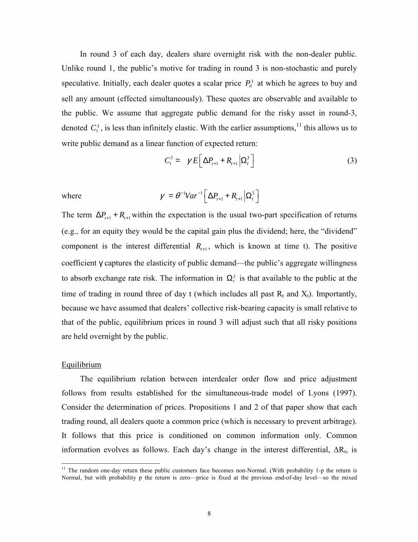
In round 3 of each day, dealers share overnight risk with the non-dealer public.

Unlike round 1, the publics motive for trading in round 3 is non-stochastic and purely

speculative. Initially, each dealer quotes a scalar price 3itP at which he agrees to buy and

sell any amount (effected simultaneously). These quotes are observable and available to

the public. We assume that aggregate public demand for the risky asset in round-3,

denoted 3tC , is less than infinitely elastic. With the earlier assumptions,11 this allows us to

write public demand as a linear function of expected return:

3 31 1t t t tC E P Rγ + +

= ∆ + Ω (3)

where 1 1 31 1t t tVar P Rγ θ− −

+ + = ∆ + Ω

The term 1 1t tP R+ +∆ + within the expectation is the usual two-part specification of returns

(e.g., for an equity they would be the capital gain plus the dividend; here, the dividend

component is the interest differential 1tR + , which is known at time t). The positive

coefficient γ captures the elasticity of public demandthe publics aggregate willingness

to absorb exchange rate risk. The information in 3tΩ is that available to the public at the

time of trading in round three of day t (which includes all past Rt and Xt). Importantly,

because we have assumed that dealers collective risk-bearing capacity is small relative to

that of the public, equilibrium prices in round 3 will adjust such that all risky positions

are held overnight by the public.

Equilibrium

The equilibrium relation between interdealer order flow and price adjustment

follows from results established for the simultaneous-trade model of Lyons (1997).

Consider the determination of prices. Propositions 1 and 2 of that paper show that each

trading round, all dealers quote a common price (which is necessary to prevent arbitrage).

It follows that this price is conditioned on common information only. Common

information evolves as follows. Each days change in the interest differential, ∆Rt, is 11 The random one-day return these public customers face becomes non-Normal. (With probability 1-p the return is Normal, but with probability p the return is zeroprice is fixed at the previous end-of-day levelso the mixed

9

common information on day t at the beginning of round 1, so it is fully impounded in

round-1 price 1tP . (The information in ∆Rt is straightforward: Each increment ∆Rt is

permanently embedded in the stream of future payoffs Rt+τ, τ=1,,∞, per equation 1, so

each increment affects current price as a perpetuity). Interdealer order flow Xt, however,

is not observed until the end of round 2. Consequently, it is not until round-3 trading that

the price 3tP impounds information about the realizations of Xt.

The information in interdealer order flow Xt is as follows. In equilibrium, each

dealers interdealer trade, Tit, will be proportional to the customer order flow 1itC he

receives in round one. This implies that when dealers observe Xt at the end of round 2

(equation 2), they can infer the aggregate portfolio shift on the part of the public in round

1, 1tC . Dealers also know that, for a risk-averse public to re-absorb this portfolio shift in

round 3, price must adjusta portfolio-balance effect. In particular, price must adjust in

round 3 to induce full absorption of 1tC , so that 1 3 0t tC C+ ∆ = , where the publics total

demand 3tC is given by equation (3).

The resulting price level at the end of day t can be written as:

1 21 1

1 2 31 1 1

τ ττ τ

τ τ ττ τ τ

λ λ

λ λ λ

= =

= = = +

∆ += ∆ + +

∑ ∑

∑ ∑ ∑

t t

tT T t

T

R X

P

R X X

(4)

where we use T to denote the day on which the regime shifts from flexible to fixed rates.

The message of this equation is important: it describes a cointegrating relationship

between the level of the exchange rate, cumulative macro fundamentals, and cumulative

order flow. (This long-run relationship between cumulative order flow and the level of

the exchange rate is not predicted by any traditional exchange-rate model.) The

cointegrating vector is regime dependent, however.

probability mass is relatively concentrated at the center.) Accordingly, we need to assume that utility of these agents is quadratic to enable us to write their demands as in equation (3).

under flexible rates (t≤≤≤≤T)

under fixed rates (t>T)

10

Under flexible rates, the change in the exchange rate from the end of day t-1 to the

end of day t can be written as:

∆Pt = λ1∆Rt + λ2Xt (5)

where λ1 and λ2 are positive constants.12 The portfolio-balance effects from order flow

enter through λ2, which depends inversely on γ the elasticity of public demand in

equation (3) and also on α, the parameter that relates interdealer order flow to

customer dealer trade (see Evans and Lyons 1999 for details). The parameter λ2 is

commonly referred to as a price impact parameter since it governs the price impact of

order flow.

In every time period there is a known fixed probability, p, that floating exchange

rate regime will come to an end. In the event a fixed-rate regime is introduced, it is

known that it will be imposed by the central bank at the end of trading round 3 and before

a payoff 1TR +∆ is realized. In fact, as stated, the central bank sets the latter to zero in

perpetuity as part of the announcement of the new regime. Note that the expected return

in equation (3) contains an element of a peso-problem: the expectation is less than the

observed moment in the data. Using 1tP+∆ to symbolize the sample mean of 1tP+∆ , we

have 31 1 1 1(1 )t t t t tE P R p P R+ + + +

∆ + Ω = − ∆ + . In addition, defining the observed variance

of 1tP+∆ as 2σ , we have:

( )23 21 1 1t t tVar P R p σ+ +

∆ + Ω = − (6)

a relation that we shall return to below.

To understand why interdealer order flow Xt has price impact under flexible rates,

consider the price at the close of trading on the final flexible-rate day, day T (before the

fixing is announced). The second term in equation (4) is the portfolio balance term.

(Forward-looking variables do not enter equation 4 due to our simple specification of ∆Rt

and 1tC as independently distributed across time with mean zero.) To understand this

12 Note that we have not yet added an error term to either equation (4) or equation (5). The cointegration model we estimate in section 4 adds a stationary (but not necessarily white noise) error term to equation (4). When differenced, this adds a non-invertible moving average term to equation (5), which represents the error-correction mechanism we estimate.

11

term, note that in the Evans-Lyons flexible-rate model the interdealer trading rule for

each dealer is:

1itit CT α=

where α is the optimal trading parameter. This implies that:

1

1 1

1t

N

i

N

iititt CCTX αα ==≡∑ ∑

= =

(7)

Therefore, we can write:

1 1

1 1

T T

t tt t

X Cα −

= =

=∑ ∑ (8)

The sum over time of the random portfolio shifts 1

1

T

tt

C=∑ represents changes in effective

asset supply: exogenous shifts out of foreign exchange (e.g., by some subset of agents for

non-speculative purposes) are an increase in the net supply that the rest of the speculating

public must re-absorb. (We couch this in terms of supply to connect with traditional

portfolio-balance intuition.)13 To get the sign right, note that the total increase in net

supply is the sum of past portfolio shifts out of foreign exchange, 1

1

T

tt

C=

−∑ , where the

minus sign arises because a round-1 shift out of foreign exchangean increase in foreign

exchange held by the rest of the publiccorresponds to 1tC being negative. Equilibrium

at the end of day T must be such that:

3 1

10

T

T tt

C C=

− =∑ (9)

We can substitute equations (3) and (8) into equation (9) to solve for TP :

13 Here is a simple one-period example that illustrates the basic economics of the model. An uncertain payoff R is realized at time 1 and the market-clearing gap E[R]P0 will be a function of the risky assets net supply. In traditional portfolio balance models, demand D is a function of relative returns, and supply S is time varying. That is: ( [ ] )0− = !D E R P S where the tilde denotes random variation. Our model looks different. In our model (gross) supply is fixed. But what we are calling net supply is moving over time, due to demand shifts that are unrelated to E[R]P0. These demand shifts are the realizations of 1Cit (which one could model explicitly as arising from hedging demands, liquidity demands, or changing risk tolerances). Conceptually, our model looks more like: ( [ ] , )0− =!D E R P C S where S denotes fixed gross supply and !C denotes shifts in net supply, that is, shifts in demand unrelated to E[R]P0. In this one-period example, the higher the t=0 realization of !C , the lower the net supply to be absorbed by the rest of the public, and the higher the market-clearing price P0 (to achieve stock equilibrium). In a sense, our multi-period model is akin to a single-period model in which net supply is shocked multiple times before the single trading period takes place, each shock having its own incremental impact on price.

12

[ ]1 1 31

1|T

T T T tt

P E P R Xαγ+ +

=

= + ∆ Ω + ∑

This yields the upper panel of equation (4) with ( ) 12λ αγ −= .14

The connection between equation (4) and traditional measures of macro

fundamentals deserves some attention. For traditional measures, it is useful to distinguish

between narrow fundamentals and broad fundamentals. Under the monetary macro

approach, the set of variables considered fundamental (e.g., money supplies, interest

rates, and output levels) does not include variables that affect equilibrium risk premia

(because monetary models do not admit risk premia). Fundamental variables under this

approach constitute the set of narrow fundamentals. In contrast, the portfolio-balance

macro approach does admit risk premia, so variables affecting these premia become

fundamental drivers of exchange rates under this approach (e.g., changes in hedging

demands, risk tolerances, or asset supplies). When added to the set of narrow

fundamentals, these variables affecting risk-premia define the set of broad fundamentals.

In terms of equation (4), the set of narrow fundamentals includes the payoff terms, ∆Rt,

but does not include the portfolio-balance terms, Xt. The set of broad fundamentals

includes all the terms (in keeping with the idea that equilibrium determination of risk

premia is fundamental to asset pricing). As we show next, a change in regime does not

change which variables are included within broad fundamentals, but it does alter the price

response to variables in that set (specifically, the price response to a given amount of

order flowthe coefficient on Xt in equation 4).

Differences Across Trading Regimes

The effects of the different trading regimesand the changing role of order flow

can be understood from the effect of the exchange-rate regime on the price impact

parameter 2λ . We begin by stating our first proposition:

14 The parameter λ1 pins down the perpetuity value of the payoff level Rt (i.e., according to the perpetuity formula Pt=Rt/r, where r is the appropriate intertemporal discount rate). Its structural composition is not relevant for our analysis of regime-dependent portfolio balance effects.

13

Proposition 1

(i) The variance of the spot exchange rate, 2σ , depends on the number of dealers, N, the

variances of customer order flow and the payoff innovation, 2 2and c Rσ σ , the coefficient of

absolute risk aversion, θ , the probability of a regime change, p , and the payoff discount

parameter, 1λ .

(ii) Given 22 4 2

1

14 (1 )R

cN pσ

λ θ σ≤

−, there are two positive real solutions for 2σ .

(iii) For the stable solution, 2

2

00

R

Limσ

σ→

→ .

Proof:

(i) Take the variance of equation (5); use equation (7) to obtain the variance of inter-

dealer order flow as 2 2cNα σ ; substitute out for ( ) 1

2 2using λ λ α γ −= ; use equations (3)

and (6) to express γ as ( )12 21 pθ σ

− − . This yields:

4 2 0σ µσ µε− + =

where1

2 2Rε λ σ= and ( ) 12 2 4(1 )cN pµ σ θ

−= − .

(ii) The expression for 2σ derived in the proof of Proposition 1 (i) is a quadratic. The solutions are:

( ) 12 2 21 4

2σ µ µ µε = ± −

The solutions are real if and only if 4µ ε≥ , which is equivalent to the condition

1

22 2 4 2

14 (1 )R

cN pσ

λ θ σ≤

−. Then the result that the solutions are both positive follows

from 0ε > and 0µ > .

(iii) Consider the smaller solution ( )12 2 21 4

2σ µ µ µε = − −

.15 Its limit as 0ε → is

zero.

15 Only the lower variance solution is stable. See Stability of Equilibrium in Appendix.

14

The restriction 22 4 2

1

14 (1 )R

cN pσ

λ θ σ<

− (or equivalently 4µ ε> ), places an upper bound

on the variance of payoffs. It is unlikely to be binding unless the variance of customer

dealer trades is relatively large. The higher the probability of a regime change, the less

restrictive is the condition.

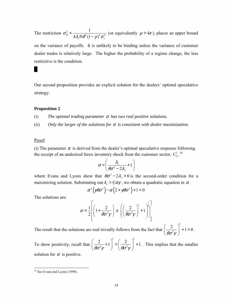
Our second proposition provides an explicit solution for the dealers optimal speculative

strategy:

Proposition 2

(i) The optimal trading parameter α has two real positive solutions.

(ii) Only the larger of the solutions for α is consistent with dealer maximization.

Proof:

(i) The parameter α is derived from the dealers optimal speculative response following the receipt of an undesired forex inventory shock from the customer sector, 1

itC .16

22

2

12

λαθσ λ

= + −

where Evans and Lyons show that 222 0θσ λ− > is the second-order condition for a

maximizing solution. Substituting out 2 1λ αγ= , we obtain a quadratic equation in α .

( ) ( )2 2 22 1 0α γθσ α γθσ− + + = The solutions are:

12 2

2 2

1 2 21 12

αθσ γ θσ γ

= + ± +

The result that the solutions are real trivially follows from the fact that 2

2

2 1 0θσ γ

+ >

.

To show positivity, recall that 2 2

2 2

2 21 1θσ γ θσ γ

+ > +

. This implies that the smaller

solution for α is positive.

16 See Evans and Lyons (1999).

15

The second-order condition restated in the proof of Proposition 1(i) above can be re-expressed as ( ) 122α γθσ

−> using ( ) 1

2λ αγ −= . The condition is trivially met by the larger solution for α . The proof that the smaller solution does not satisfy the condition is by contradiction. Suppose that ( ) 122α γθσ

−> holds. This implies that

2 2

2 21 1θσ γ θσ γ

+ < −

. Squaring, we conclude that 24 /( ) 0γθσ < , which provides the

contradiction.

Following the above result, we limit our consideration to the larger of the two

solutions for α . The probability of a regime change does not enter the solution for α

because unlike the customer segment, the dealer never has to worry about the risk of an

exchange rate regime change.17 This is because she never carries forex inventory

overnight. We are now in a position to state the main result of the paper in the following

proposition:

Proposition 3

The price impact parameter 2λ goes to zero when the payoff is fixed:

2 2

00

R

Limσ

λ→

=

Proof: Using the results of Proposition 2, the expression for the inverse of the price impact

parameter 2λ becomes:

( )

( )( )

2 22

2

22 2 2

1 21

12 2 1

1

p

p

θσθ σαγ

θσ θ σ

+ −

= + + −

It is clear that ( ) 1αγ − is increasing in 2σ . The result then follows immediately from part

(iii) of Proposition 1.

17 However, the value of α is endogenous to the policy stance. It is straightforward to show that the limit of α as

2 0Rσ → equals 1. In other words, there is no hot potato interdealer trade under a fixed rate regime: the dealers simply mediate the customer-dealer business.

16

The point of Proposition 3 is that the parameter γ, which represents the elasticity of

public demand, is regime-dependent. This comes from the regime-dependence of 3

1 1t t tVar P R+ + ∆ + ∆ Ω (γ being proportional to the inverse of this variance, per equation

3). The elimination of portfolio-balance effects under fixed rates shown below reduces

this variance, implying that flexible fixedγ γ< . Public demand is therefore more elastic in the

(credible) fixed-rate regime than the flexible-rate regime. The implication for the price

impact parameters λ2 and λ3 in equation (4)henceforth λflexible and λfixed respectively

is that flexible fixedλ λ> . Thus, the exchange rate reacts more to order flow under flexible

rates than under fixed rates. For perfectly credible fixed rates (i.e., for which 3

1 1 0t t tVar P R+ + ∆ + ∆ Ω = ), we have fixed 0λ = . The exchange rate does not respond to

order flow in this case. The intuition is clear: under perfect credibility, the variance of

exchange-rate returns goes to zero because public demand is perfectly elastic, and vice

versa.

Intuition for Cointegration in Equation (4)

Consider PT+1, the price at the close of the first day of the fixed-rate regime. Foreign

exchange is a riskless asset at this point, with return variance equal to zero. A return

variance of zero implies that the elasticity of the publics speculative demand is infinite,

and the price impact parameter λ3 in equation (4) equals zero. This yields a price at the

close of trading (round 3) on day T+1 of:

PT+1 = 1 21 1

λ λ= =

∆ +∑ ∑T T

t tt t

R X

The summation over the payoff increment ∆Rt does not include an increment for day T+1

because the central bank maintains ∆Rt at zero in the fixed regime. Though interdealer

17

order flow XT+1 is not equal to zero, this has no effect on price because λ3=0, as noted.

This logic holds throughout the fixed-rate regime.

As is standard in portfolio balance models, increases in supply lower price, and

decreases in supply raise price. This is why a positive cumulative Xt in equation (4) raises

price: if cumulative interdealer flow Xt is positive, this implies that exogenous customer

flow 1tC is also positive, which is a decrease in net supply in the hands of the rest of the

public, requiring an increase in price to clear the market. Xt is the variable that conveys

this information about the decrease in net supply ( 1tC is unobservable). The round-three

price on day T, PT, depends on the sum of the Xt because each additional decrease in

supply 1tC requires an incremental increase in price. As payoff uncertainty shrinks to zero

(as in the fixed-rate regime), the arrival of new Xt no longer induces portfolio balance

effects.

In our model, a credible fixed-rate regime is one in which the private sector, not

the central bank, absorbs innovations in order flow. This theoretical point contrasts with

extant models where innovations in order flow are absorbed by central banks, but at a

cost (e.g., selling reserves at domestic-currency prices that are too low; see, e.g.,

Guembel and Sussman 2001). Empirically, as we turn attention to testing implications of

our model below, our understanding is that there was little intervention by the national

central banks or the ECB during our sample period from May to December, 1998 (per

conversations with ECB and national central bank officialshard data are not available).

The Bretton Woods era, too, provides many periods in which exchange-rate volatility was

quite low, at the time that central banks were intervening very little (relative to the size of

the market).

3. Data

Our data set includes the daily value of purchases and sales in the FF/DM market

for twelve months, January to December 1998. Electronic Broking Services (EBS), the

leading foreign-exchange broker, provided the data. Each trading day (weekday) covers

the twenty four-hour period starting from midnight GMT.

18

A brief overview of the market structure may be useful for understanding the data

and evidence.18 There are three types of trades in the forex market: customer-dealer

trades, direct interdealer trades, and brokered interdealer trades. Customers are non-

financial firms and non-dealers in financial firms (e.g., corporate treasurers, hedge funds,

mutual funds, pension funds, proprietary trading desks, etc.). Dealers are marketmakers

employed in banks worldwide (the largest 10 dealing banks account for more than half of

the volume in major currencies). At the time of our sample, these three trade types

accounted for roughly equal shares of total volume in major marketsone-third each.

Our data come from the third trade type: brokered interdealer trading. There are two

main interdealer broking systems, EBS and Reuters Dealing 2000-2. We estimate that

our EBS sample of spot trading in FF/DM amounts to about 21% of all trading in that

market. This estimate is based on comparing our EBS volume data with data provided by

the BIS (1999) for April 1998one of the months in our sample. Specifically, for the

FF/DM rate the BIS-reported total daily average spot volume for April 1998 was $7.17

billion. In our EBS sample, average daily spot volume in FF/DM for April 1998 was

$1.5 billion, or 21 percent of the $7.17 billion total. The BIS (1999) also provides data on

the share of total FF/DM trading accounted for by interdealer trading: 72 percent ($5.14

billion per day on average versus total volume of $7.17).19 This implies that EBSs share

of interdealer trading in FF/DM was about 29 percent.

Three features of our data set are noteworthy. First, it spans a considerably longer

period than previous data on interdealer order flow. For example, Evans and Lyons

(2002) use four months of data. Second, the brokered interdealer trading it covers is the

most rapidly growing category of trade (see BIS, 2001), and anecdotal evidence suggests

that EBS is also increasing its market share. Third, our data include daily order flow

measured in terms of DM value. The Evans (2002) data, also used by Evans and Lyons

(2002), include only order flow measured as the number of buys minus the number of

sells (e.g., a sale of any DM amount is measured as 1).20 This allows us to use a measure

of cumulative order flow that tightly matches our model, namely:

18 For more detail see Lyons (2001), Hau Killeen and Moore (2002a) and the EBS website at www.ebsp.com. Trading in other European cross rates on EBS was not thick enough to estimate our model on a panel of currencies. 19 This includes both the brokered and direct interdealer markets. It is also includes both voice and electronic trading. 20 Our data set enable us to construct both of these two measures. They behave quite similarly. For example, the correlation between the two order-flow measures in the flexible-rate portion of our sample (January to April) is 0.98.

19

( )1 1

τ τ ττ τ= =

= −∑ ∑t t

X B S

where Bτ and Sτ are the DM values of buyer-initiated and seller-initiated orders on day τ,

respectively.

The rest of the data is measured as follows. The spot exchange rate is measured as

the French franc price of a DM and is sampled daily at the close of business in London.21

The interest differential is calculated from the overnight Euro-Franc and Euro-Mark

interest rates. These rates are also sampled at the London close. Both exchange rate and

interest rate data are from Datastream.

Institutional Details on EBS

EBS is an electronic broking system for trading spot foreign exchange among

dealers. It is limit-order driven, screen-based, and ex-ante anonymous (ex-post, counter-

parties settle directly with one another). The EBS screen displays the best bid and ask

prices submitted to it together with information on the cash amounts available for trading

at these prices. Amounts available for trading at prices other than the best bid and offer

are not displayed. Activity fields on this screen track a dealers own recent trades,

including price and amount, as well as tracking recent trades executed on EBS system-

wide.

There are two ways that dealers can trade currency on EBS. Dealers can either post

prices (i.e., submit limit orders), which does not insure execution, or dealers can hit

prices (i.e., submit market orders), which does insure execution. To construct a

measure of order flow, trades are measured as positive or negative depending on the

direction of the initiating market order. For example, a market order to sell DM 10

million that is executed against a posted limit order would generate order flow of 10

million Deutschemarks.

21 We know of no source for transaction prices sampled at midnight GMT. Even if a source were available, it would be relatively noisy because the market is quite thin around that time, with wide bid-offer spreads (which generate measurement error due to transaction prices bouncing from bid to ask). Most all trading in FF/DM is carried out before the London close (there is relatively little trading in this currency pair in New York). Finally, it is not feasible for us to re-measure our daily order flow as of the London close because we do not have the flow data on an intraday basis.

20

When a dealer submits a limit order, she is displaying to other dealers an intention

to buy or sell a given cash amount at a specified price.22 Bid prices (limit order buys) and

offer prices (limit order sells) are submitted with the hope of being executed against the

market order of another dealerthe initiator of the trade. To be a bit more precise, not

all initiating orders arrive in the form of market orders. Sometimes, a dealer will submit a

limit-order buy that is equal to or higher than the current best offer (or will submit a

limit-order sell that is equal to or lower than the current best bid). When this happens, the

incoming limit order is treated as if it were a market order, and is executed against the

best opposing limit order immediately. In these cases, the incoming limit order is the

initiating side of the trade.

4. Results

The analytical results in section 2 offer five testable hypotheses that we collect here

as a guide for our empirical analysis:

Hypothesis 1: Under flexible rates, the level of the exchange rate, cumulative

interdealer order flow are individually nonstationary and jointly cointegrated.

Hypothesis 2: Cumulative interdealer order flow remains nonstationary after the

shift from flexible to fixed rates, but the level of the exchange rate becomes stationary.

Hypothesis 3: A structural break in the cointegrating relationship occurs when the

regime shifts from flexible to fixed rates. Hypothesis 4: Under flexible rates, error correction in the cointegrating

relationship occurs through exchange rate adjustment, not order flow adjustment.

Hypothesis 5: Under flexible rates, there is no Granger causality from the

exchange rate to order flow (strong exogeneity of order flow).

22 EBS has a pre-screened credit facility whereby dealers can only see prices for trades that would not violate their bilateral credit limits, thereby eliminating the potential for failed deals because of credit issues.

21

Hypotheses 1-3 summarize the section-two discussion of equation (4). Hypotheses 4 and

5 follow from the models specification of public order flow in round one as exogenous.

This particular assumption of the model is a strong one; our cointegration framework

provides a natural way to test its implications.23

The empirical analysis proceeds in two stages. First, we address hypotheses 1-3 by

testing for unit roots, cointegration, and structural breaks. This first stage also examines

the related issue of coefficient size within the cointegrating relationship. The second

stage addresses hypotheses 4 and 5 by estimating the appropriate error-correction model

and (separately) testing for Granger causality.

4.1 Stage 1: Testing Hypotheses 1 to 3

Let us begin by repeating equation (4) from the model, which establishes the

relationship between the level of the exchange rate Pt, a variable summarizing public

information about payoffs (Σ∆Rt), and accumulated order flow (ΣXt).

1 21 1

1 2 31 1 1

τ ττ τ

τ τ ττ τ τ

λ λ

λ λ λ

= =

= = = +

∆ += ∆ + +

∑ ∑

∑ ∑ ∑

t t

tT T t

T

R X

P

R X X

(4)

Like Evans and Lyons (2002), we use the interest differential as our measure of

cumulative public information about foreign-exchange payoffs.24

Stationarity

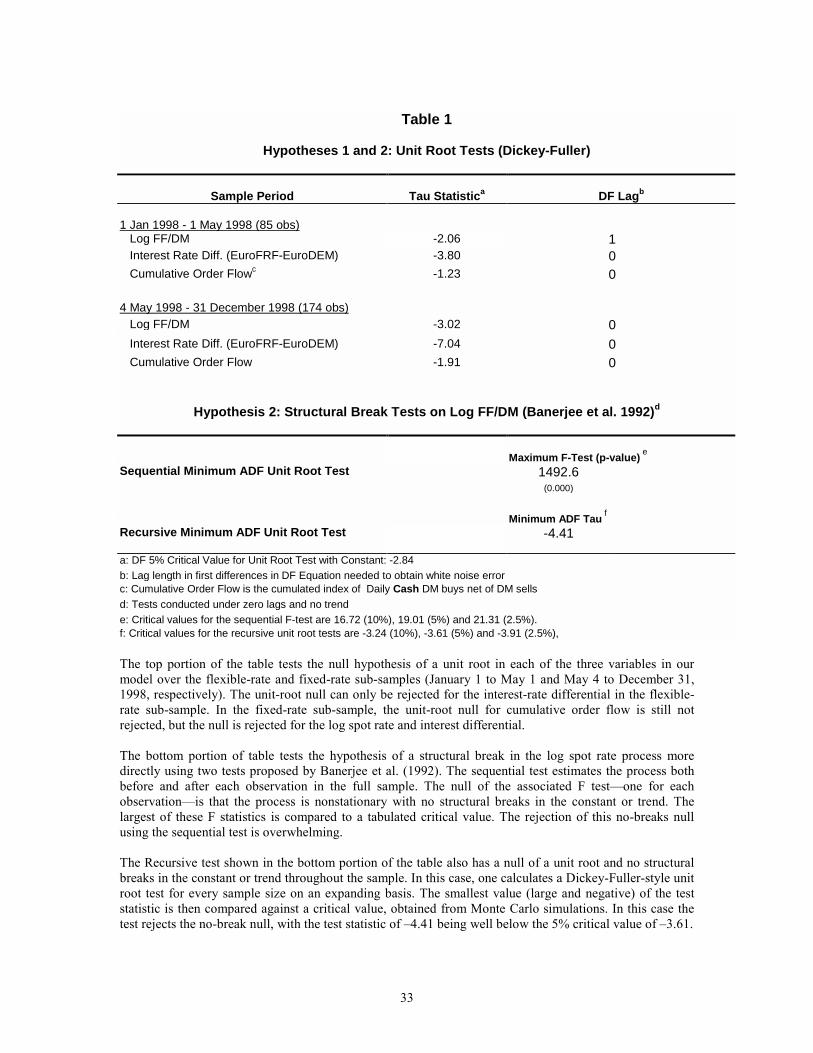
The first step is to test for the stationarity of all variables in the two sub-periods of

1998, January 1 to May 1 and May 4 to December 31. Table 1 shows the results of six

Dickey-Fuller tests, one for each of the three variables in each of the two sub-periods. 23 Cheung and Chinn (1998) also use cointegration as a means of evaluating exchange rate models, though in their case the modeling includes only macro variables.

under fixed rates (t>T)

under flexible rates (t≤≤≤≤T)

22

Consistent with hypothesis 1, in the first four months of 1998 the exchange rate level and

cumulative order flow appear non-stationary: the unit-root null cannot be rejected.25

Though predicted by our model, cumulative order flow being non-stationary is not

obvious; indeed, a common intuition is that market clearing would produce cumulative

order flow that rapidly reverts to zero.

Consistent with hypothesis 2, for the remaining eight months the exchange rate

appears stationary (unit-root null is rejected), whereas cumulative order flow remains

non-stationary. The combination in the latter period of a stationary exchange rate and

non-stationary cumulative order flow is consistent with a price impact parameter λ3 of

zero, as predicted by the model. It remains to be determined whether equation (4) actually

holds for the January1 to May 1 period, i.e., whether the variables are cointegrated

(which we return to below).

The bottom panel of Table 1 speaks to hypothesis 2 by implementing a univariate

test for a structural break in the spot rate process. The two tests shown, due to Banerjee,

Lumsdaine, and Stock (1992), are described in more detail in the table legend. The null

for both of these tests is that spot-rate process is nonstationary over the whole sample

period with no structural breaks in the constant or trend. In both cases, the null is

rejected. We return to a direct test of stability in the cointegrating relationship below,

following the cointegration results. (See also the appendix for results from implementing

the Rigobon 1999 test for parameter stability in settings with heteroskedasticity,

endogeneity, and omitted variables.)

Cointegration

Because the log exchange rate and cumulative order flow are non-stationary in the

flexible-rate period from January to May 1, equation (4) only holds if they are

cointegrated. We use two different procedures to test for cointegration: the Granger-

Engle ADF test and the Johansen test. Both begin with a baseline model that includes the

three variables of our model of section two, a constant, and a trend. We determine the lag 24 At the daily frequency, the interest differential is arguably the best public-information measure of changing macroeconomic conditions. That said, it does not constitute a well-specified macro model of expected payoffs. We return to the measurement error this entails below.

23

length for the Johansen vector autogression using Sims likelihood ratio tests; a lag length

of four allows for all significant dynamic effects (results available from authors on

request).

Hypothesis 1 is borne out: evidence for cointegration (rejecting the null of no-

cointegration) over the flexible-rate period is strong. Table 2 presents results for the

Granger-Engle ADF test. In this test, the log spot rate is regressed against cumulative

order flow, the interest differential, a constant, and a trend. (We use Phillips-Hansen fully

modified estimation. This is a semi-parametric technique that gives more accurate point

estimates in small samples by diminishing second-order asymptotic bias. It also yields

consistent standard errors. The residuals from the regression are then tested for

stationarity using conventional Augmented Dickey-Fuller tests.) The null of non-

cointegration is rejected at the 5 percent level, per the Dickey-Fuller tau statistics at the

bottom. The top of the table shows the estimated coefficients (constant not reported).

Note that the interest differential is insignificant26. We do not take this insignificance to

mean that macro does not matter (though it is in keeping with the results of Meese and

Rogoff 1983 and the long empirical literature that followed that paper). It may be due to

the measurement error (or mis-specification) inherent in our use of the interest

differential for the variable Rt from the model. The cointegration we find between the

exchange rate and cumulative order flow demonstrates that the model is indeed able to

account for a steady-state relationship. Having found significance, henceforth we focus

on the bivariate cointegrating relationship between the exchange rate and cumulative

order flow.27

Next we estimate the magnitude of the coefficients in the bivariate cointegrating

relationship (flexible-rate period). These are reported in Table 3. Of particular importance

25 The interest rate differential is stationary in both periods: however its variance declines marginally from 0.76% in the first period to 0.70% in the May to December period. The stationarity of interest differentials is a common result: for a discussion, see Moore and Roche (2001). 26 This is not surprising since the interest differential is stationary. 27 The second of our cointegration testsusing the Johansen proceduretests the null hypothesis of no-cointegration in the bivariate model against the alternative of a single cointegrating vector. That test is rejected at the 5 percent level (not reported). The Johansen procedure also suggests that there is only one cointegrating vector: A Johansen test of the null of one cointegrating vector against the alternative of two is not rejected at the 5 percent level. In independent work, Bjonnes and Rime (2001) also find evidence of cointegration between cumulative interdealer order flow and the level of the spot exchange rate (they examine the DM/$ and Norwegian Krona/DM markets). The relationship is not the focus of their paper, however; it is addressed in a closing subsection.

24

is the coefficient on cumulative order flow.28 Our use of the log spot rate makes this

coefficient easy to interpret: an increase in cumulative order flow of DM 1 billion (i.e.,

net DM purchases) increases the French franc price of a DM by 3 basis points. This is

much smaller than the contemporaneous impact of order flow estimated by Evans and

Lyons (2002) for the DM/$ market (roughly 50 basis points per $1 billion).29 Three

factors contribute to this. First, our estimate is per billion marks whereas their estimate is

per billion dollars. With the DM price of a dollar at the time at about 1.5, on an

equivalent per-DM basis the Evans-Lyons coefficient is one-third lower. Second, Evans

and Lyons are measuring the impact effect, whereas we are measuring the long-run

impact (i.e., the persistent impact).30 To the extent any of the impact effect is transitory,

this will account for part of the difference. Finally, and perhaps most important in the

context of our model, one would expect the sensitivity of price to order flow to be lower

in the FF/DM market precisely because the EMS target zones were not a free float (and

therefore the elasticity of absorptive private demand is higher).

We turn now to evaluating hypothesis 3: a structural break should occur in the

cointegrating relationship when the regime shifts from flexible to fixed rates. Results

from two different tests appear in Table 4. The first, the F-test (see Hanson 1992), is akin

to a non-stationary analog of the familiar Chow test in stationary settings. Importantly, it

is valid for settings in which the date of the structural break is known in advance. Using

May 4, 1998, as a known break date, the F-test rejects the null of no structural break over

the year at the 5 percent level (column two), consistent with hypothesis 3. For robustness,

we also tested for a structural break in the cointegrating relationship over the full year

using a test that does not rely on knowing the break date in advance. That test, the Mean-

F, also rejects the null of no structural break at the 5 percent level (column two). The

Mean-F test can also be applied to specifically to the flexible-rate portion of our sample.

There is no evidence of structural instability in the bivariate relationship over the flexible

28 A reassuring feature is the similarity between the modified least squares estimates in the trivariate model of Table 2 and the maximum likelihood bivariate estimates of Table 3. 29 Our use of the logged spot rate in estimation (rather than unlogged) makes our work directly comparable to earlier work. It also squares with the empirical distribution of exchange rates, which is (approximately) Lognormal. 30 One might be tempted to check robustness of our result that order flow effects persist by regressing the level of the spot rate on lags of unaccumulated order flow (i.e., past daily flows). The notion being that more distant order flow lags might be negative. Econometrically, however, this is an unbalanced regression, mixing non-stationary and stationary variables, thereby undermining inference. Cointegration tests are the proper way to resolve this issue.

25

period from January through May 1 (p-value >20%). (For visual evidence that order

flows price impact had dropped off by May 4, see the appendix.)

4.2 Stage 2: Testing Hypotheses 4 and 5

From the Granger representation theorem (Engle and Granger 1987), we know that

a cointegrated system has a vector error-correction representation. Tables 5 and 6 explore

this and its implications for whether order flow can be considered exogenous, as

predicted by hypotheses 4 and 5.

Table 5 presents evidence that order flow over the flexible-rate period is indeed

weakly exogenous for the parameters in the cointegrating vector and the error correction

parameter, as predicted by hypothesis 4. Recall that weak exogeneity of order flow

means that error correction in the cointegrating relationship occurs through exchange rate

adjustment, not order flow adjustment. Or, econometrically, it means that the error-

correction term is significant in the exchange rate equation but not in the order flow

equation. Table 5 shows that the null of weak exogeneity of order flow cannot be rejected

at conventional levels (p-value 10 percent). In contrast, the null of weak exogeneity of the

exchange rate is strongly rejected (p-value 1 percent).31 It appears that the burden of

adjustment to long-run equilibrium falls exclusively on the exchange rate.

Table 6 presents evidence that order flow is, in fact, strongly exogenous, as

predicted by hypothesis 5. The key result is that for the test labeled F(8,67), noted in the

table legend with h. This is a test for any feedback to order flow from lagged values of

either the exchange rate or the interest differential. Because exclusion of these variables

from the general (unconstrained) model cannot be rejected, there is no evidence of

Granger causality running from these variables to order flow (thus, there is no evidence

of feedback trading). This combination of weak exogeneity and absence of Granger

causality implies that cumulative order is strongly exogenous.32

31 This test is based on the full-information maximum likelihood approach of the Johansen (1992) procedure, which takes account of possible cross-equation dependencies (as opposed to testing the significance of the error-correction term equation by equation). 32 It is unlikely, but possible, that this lack of Granger causality is due to the six-hour mismatch in the timing of our order flow and exchange rate data. Remember, however, that little of the order flow in FF/DM occurs between 6pm and midnight GMT. For a test of an even stronger form of statistical exogeneitystrict exogeneitysee the appendix.

26

The final model specification is displayed in Table 7. The error-correction

representation allows us to answer an important question: How rapidly does this system

return to its long-run equilibrium? (Though important, this question is purely empirical in

that our model makes no prediction.) The answer to this question comes directly from the

estimate of the systems error-correction term. That estimate is 0.237, implying that

about one-quarter of departures from long-run equilibrium is dissipated each day.33 We

interpret the additional lags in order flow as inventory effects. In fact, we test that the

sum of the coefficients on the additional lags is zero and are unable to reject this

hypothesis. This is reported in the notes to table 7 and the restriction is imposed in the

final specification. Note that, though significant, the inventory adjustment parameters are

economically small compared to the error correction parameter.

This result is also helpful for judging whether four months of data is sufficient to

produce reliable analysis of cointegration. If one-quarter of any departure is dissipated

each day, the half-life of departures is less than three days. Four months of data is enough

to cover about 40 of these half-lives, quite a lot in the context of estimating cointegrating

relationships. For comparison, adjustment back to the cointegrating relationship of

Purchasing Power Parity (PPP) has a half-life around 5 years. One would need 200 years

of data on a single exchange rate to estimate PPP error correction with as many half-lives

in the sample. At the same time, we recognize that cointegration may not be literally true;

if not, one is left with the result that order flow effects on price are very persistent, but

not truly permanent.

5. Conclusions

Previous theoretical work offers three approaches to resolving the regime-

dependent volatility puzzle: flexible-rate regimes induce either additional policy shocks

(e.g., from greater policy autonomy), additional noise (e.g., entry of noise traders), or

additional equilibria. Our explanation of the puzzle does not rely on any of these. Instead,

flexible rates produce additional price volatility because the markets willingness to

absorb unchanged shocks to order flow is reduced. Under flexible rates, these shocks

33 For those less familiar with cointegration models, note that this result does not imply that order flows effect on price is transitory: this error-correction estimate applies to departures from the long-run relationship, not to the long-run relationship itself.

27

produce portfolio-balance effects on price because elasticity of speculative demand is

(endogenously) low under flexible rates. Under perfectly credible fixed rates, the

elasticity of speculative demand is infinite, eliminating portfolio-balance effects.

Testable implications of our explanation for the puzzle are borne out in the data. We

use a unique data set on FF/DM order flow in 1998 to show that before the rigid parity-

rates where announced, cumulative order flow and the spot rate were cointegrated, as our

model predicts. (This result emerges despite the FF/DM rate varying considerably less

than major flexible rates such as DM/$.) Thus, at least some of the effects of order flow

on the exchange rate appear to be permanent. This is contrary to received wisdom: many

people believe that order flow has only transitory indigestion effects on price, but this

is not the case.34 After the conversion rates for the euro-participating currencies were

announced, the FF/DM rate was decoupled from order flow. The model we develop

predicts this as well.

We also address the degree to which order flow can be considered exogenous, as

our model assumes. Our findings are supportive in this regard. We find that order flow is

(at least) strongly exogenous. This has two key implications. First, the burden of

adjustment to long-run equilibrium falls on the exchange rate, not on order flow. Second,

there is no Granger causality running from the exchange rate back to order flow (i.e.,

feedback trading does not appear to be present).

It is common to characterize fixed-rate regimes in terms of the central banks

willingness to trade domestic currency at a predetermined price; i.e., it is the central bank

that absorbs the order flow. In our model, a credible fixed-rate regime is one in which the

private sector, not the central bank, absorbs innovations in order flow. As a practical

matter, if the central bank needs to intervene, the fixed exchange rate regime is already in

difficulty because the private sectors demand is no longer perfectly elastic, and the

portfolio-balance channel is operative.

Though we model a regime shift from flexible to fixed rates, it may be useful to

revisit models of currency crises (i.e., shifts from fixed to flexible) with order flows role

in mind. For example, our model directs attention to the variance of order flow shocks

34 Though received wisdom, it should also be noted that transitory price effects of significant size are difficult to reconcile with market efficiency anyway: the implied profit opportunities would be too large.

28

( 1tC in the model) and to the evolving elasticity of order-flow absorption by the private

sector (the γ coefficient in the model). Interest differentials and other empirical proxies

for credibility and expected devaluation can be recast in terms of these other, now

increasingly measurable variables. In this setting, policymakers take their cues on

necessary adjustment of interest rates and reserves from the private order flows they

observe in the market (not from a macro model). That is, order flows become the vehicle

for conveying dispersed market information about credibility and fundamentals. At the

same time, order flow is by no means a noiseless signal, leading (potentially) to learning

dynamics quite different from those in macro collapse models (for work in this direction,

see, e.g., Carrera 1999, Calvo 1999, and Corsetti, Pesanti, and Roubini 2001).

29

References

Banerjee, A., R. Lumsdaine, and J. Stock, 1992, Recursive and sequential tests of the

unit-root and trend-break hypotheses: Theory and international evidence, Journal of Business and Economic Statistics, 10: 271-287.

Baxter, M., and A. Stockman, 1989, Business cycles and the exchange rate regime: Some international evidence, Journal of Monetary Economics, 23, 377-400.

BIS (Bank for International Settlements), 1999, Central bank survey of foreign exchange market activity in April 1998, publication of the Monetary and Economics Department, BIS, May (available at www.bis.org).

BIS (Bank for International Settlements), 2001, BIS 71st Annual Report, June (available at www.bis.org).

Bjonnes, G., and D. Rime, 2001, FX trading live! Dealer behavior and trading systems in foreign exchange markets, typescript, Norwegian School of Management, University of Oslo, March (www.uio.no/~dagfinri).

Cai, J., Y. Cheung, R. Lee, and M. Melvin (2001), Once-in-a-generation yen volatility in 1998: Fundamentals, intervention, or order flow? Journal of International Money and Finance, 20: 327-347.

Calvo, G., 1999, Contagion in Emerging Markets: When Wall Street Is a Carrier, University of Maryland working paper.

Carlson, J., and C. Osler, 2000, Rational speculators and exchange rate volatility, European Economic Review, 44: 231-253.

Carrera, J., 1999, Speculative attacks to currency target zones: A market microstructure approach, Journal of Empirical Finance, 6, 555-582.

Cheung, Y.-W., and M. Chinn, 1998, Integration, cointegration, and the forecast consistency of structural exchange rate models, Journal of International Money and Finance, 17: 813-830.

Corsetti, G., P. Pesenti, and N. Roubini, 2001, The role of large players in currency crises, NBER Working Paper 8303, May.

Devereux, M., and C. Engel, 1999, The optimal choice of exchange-rate regime: Price-setting rules and internationalized production, NBER Working Paper 6992.

Diamond, D. and R. Verrecchia 1981. Information Aggregation in a Noisy Rational Expectations Economy, Journal of Financial Economics, 9: 221-235.

Engle, R., and C. Granger, 1987, Cointegration and error correction: Representation, estimation and testing, Econometrica, 55: 251-276.

Evans, Martin, 2002, FX trading and exchange rate dynamics, Journal of Finance, 57: 2405-2448.

Evans, M., and R. Lyons, 1999, Order flow and exchange rate dynamics, typescript, U.C. Berkeley (available at faculty.haas.berkeley.edu/lyons/wp.html)

Evans, M., and R. Lyons, 2002, Order flow and exchange rate dynamics, Journal of Political Economy, 110, 170-180.

Evans, M., and R. Lyons, 2001, Portfolio balance, price impact, and secret intervention, NBER Working Paper 8356, July.

Financial Times, April 28 1998, CURRENCIES & MONEY: Realignment rumours stir ERM

30

Financial Times, May 2/3 1998, Euro Trading to start on Monday Flood, R., and A. Rose, 1995, Fixing exchange rates: A virtual quest for fundamentals,

Journal of Monetary Economics, 36: 3-37. French, K., and R. Roll, 1986, Stock return variance: The arrival of information and the

reaction of traders, Journal of Financial Economics 17, 99-117. Froot, K., and M. Obstfeld, 1991, Exchange Rate Dynamics Under Stochastic Regime

Shifts: A Unified Approach, Journal of International Economics, 31: 203-229. Grossman. S., and J. Stiglitz, 1980, On the impossibility of informationally efficient

markets, American Economic Review, 70: 393-408. Guembel, A., and O. Sussman, 2001, Optimal exchange rates: A market-microstructure

approach, typescript, Said Business School, Oxford University. Hansen, B., 1992, Tests for parameter instability in regressions with I(1) processes,

Journal of Business and Economic Statistics, 10: 321-335. Hasbrouck, J., 1991, Measuring the information content of stock trades, Journal of

Finance, 46: 179-207. Hau, H., 1998, Competitive entry and endogenous risk in the foreign exchange market,

Review of Financial Studies, 11: 757-788. Hau, H., W. Killeen, and M. Moore, 2002a, The euro as an international currency:

Explaining puzzling first evidence from the foreign exchange market, Journal of International Money and Finance, 21: 351-383.

Hau, H., W. Killeen, and M. Moore, 2002b, Euros forex role: How has the euro changed the foreign exchange market? Economic Policy, April, 151-191.

Jeanne, O. and A. Rose, 2002, Noise trading and exchange rate regimes, Quarterly Journal of Economics.

Johansen, S., 1992, Cointegration in partial systems and the efficiency of single equation analysis, Journal of Econometrics, 52: 389-402.

Jorion, P., 1996, Risk and Turnover in the Foreign Exchange Market. In Jeffrey A. Frankel, Giampaolo Galli and Alberto Giovannini (eds.), The Microstructure of Foreign Exchange Markets. University of Chicago Press, Chicago, pp. 1937.

Krugman, P., and M. Miller, 1993, Why have a target zone? Carnegie-Rochester Conference Series on Public Policy, 38: 279-314.

Lyons, R. 1995. Tests of Microstructural Hypotheses in the Foreign Exchange Market, Journal of Financial Economics, 39: 321-351.

Lyons, R., 1997, A simultaneous trade model of the foreign exchange hot potato, Journal of International Economics, 42: 275-298.

Lyons, R., 2001, The Microstructure Approach to Exchange Rates, MIT Press: Cambridge (chapters at faculty.haas.berkeley.edu/lyons).

Moore, M and M. Roche, 2001, Liquidity in the Forward Exchange Market, Journal of Empirical Finance, May 2001, 8: 157-170.

Moore, M and M. Roche, 2002, Less of a puzzle: A new look at the forward forex market, Journal of International Economics, 58: 387411.

Machlup, F., 1949, The theory of foreign exchanges. Reprinted in Readings in the Theory of International Trade, edited by H. Ellis and L. Metzler, Philadelphia: Blakiston.

McKinnon, R., 1976, Floating exchange rates, 1973-74: The emperors new clothes, Carnegie-Rochester Conference Series on Public Policy, 3: 79-114.

31

Meese, R., and K. Rogoff, 1983, Empirical exchange rate models of the seventies, Journal of International Economics, 14: 3-24.

Osler, C., 1998, Short-term speculators and the puzzling behavior of exchange rates, Journal of International Economics, 45: 37-57.

Payne, R. 2003, Informed trade in spot foreign exchange markets: An empirical analysis, Journal of International Economics, 61: 307-329.

Rime, D., 2000, Private or public information in foreign exchange markets? An empirical analysis, typescript, Norwegian School of Management, University of Oslo, March (www.sifr.org/dagfinn.html).

Rigobon, R., 1999, On the measurement of the international propagation of shocks, NBER Working Paper 7354, September 1999.

Robinson, J., 1949, The foreign exchanges. Reprinted in Readings in the Theory of International Trade, edited by H. Ellis and L. Metzler, Philadelphia: Blakiston.

Rosenberg, M., 1996, Currency Forecasting: A Guide to Fundamental and Technical Models of Exchange Rate Determination. Chicago: Irwin Professional Publishing.

32

FIGURE 1 Log FF/DM and Cumulative Order Flow (DM Bought minus DM Sold)

January 1998 December 1998

Figure 2

Three Trading Rounds Within Each Day

Round 1 Round 2 Round 3

Payoff Rt Dealers Public Dealers Interdealer Order Dealers Public

Change ∆Rt Quote Trades 1itC Quote Trade Flow Xt Quote Trades

-4000

-2800

-1600

-400

800

2000

3200

4400

5-Jan-98

5-Feb-98

5-Mar-98

5-Apr-98

5-May-98

5-Jun-98

5-Jul-98

5-Au

g-98

5-Sep-98

5-Oct-98

5-Nov-98

5-Dec-98

3.344

3.346

3.348

3.35

3.352

3.354

3.356

Or der flow DEM/FRF

Cum

ulat

ive

Orde

r Fl

ow: (

DM M

illio

ns)

DEM/FRF

Buy = Purchase of DM

Irrevocable Exchange Rates Announced

Ir revocable Exchange Rate

33

Table 1

Hypotheses 1 and 2: Unit Root Tests (Dickey-Fuller)

Sample Period

Tau Statistica

DF Lagb

1 Jan 1998 - 1 May 1998 (85 obs)

Log FF/DM -2.06 1 Interest Rate Diff. (EuroFRF-EuroDEM) -3.80 0 Cumulative Order Flowc -1.23 0

4 May 1998 - 31 December 1998 (174 obs) Log FF/DM -3.02 0 Interest Rate Diff. (EuroFRF-EuroDEM) -7.04 0 Cumulative Order Flow -1.91 0

Hypothesis 2: Structural Break Tests on Log FF/DM (Banerjee et al. 1992)d

Maximum F-Test (p-value) e

Sequential Minimum ADF Unit Root Test 1492.6 (0.000)

Minimum ADF Tau f

Recursive Minimum ADF Unit Root Test

-4.41

a: DF 5% Critical Value for Unit Root Test with Constant: -2.84 b: Lag length in first differences in DF Equation needed to obtain white noise error c: Cumulative Order Flow is the cumulated index of Daily Cash DM buys net of DM sells d: Tests conducted under zero lags and no trend e: Critical values for the sequential F-test are 16.72 (10%), 19.01 (5%) and 21.31 (2.5%). f: Critical values for the recursive unit root tests are -3.24 (10%), -3.61 (5%) and -3.91 (2.5%), The top portion of the table tests the null hypothesis of a unit root in each of the three variables in our model over the flexible-rate and fixed-rate sub-samples (January 1 to May 1 and May 4 to December 31, 1998, respectively). The unit-root null can only be rejected for the interest-rate differential in the flexible-rate sub-sample. In the fixed-rate sub-sample, the unit-root null for cumulative order flow is still not rejected, but the null is rejected for the log spot rate and interest differential. The bottom portion of table tests the hypothesis of a structural break in the log spot rate process more directly using two tests proposed by Banerjee et al. (1992). The sequential test estimates the process both before and after each observation in the full sample. The null of the associated F testone for each observationis that the process is nonstationary with no structural breaks in the constant or trend. The largest of these F statistics is compared to a tabulated critical value. The rejection of this no-breaks null using the sequential test is overwhelming. The Recursive test shown in the bottom portion of the table also has a null of a unit root and no structural breaks in the constant or trend throughout the sample. In this case, one calculates a Dickey-Fuller-style unit root test for every sample size on an expanding basis. The smallest value (large and negative) of the test statistic is then compared against a critical value, obtained from Monte Carlo simulations. In this case the test rejects the no-break null, with the test statistic of 4.41 being well below the 5% critical value of 3.61.

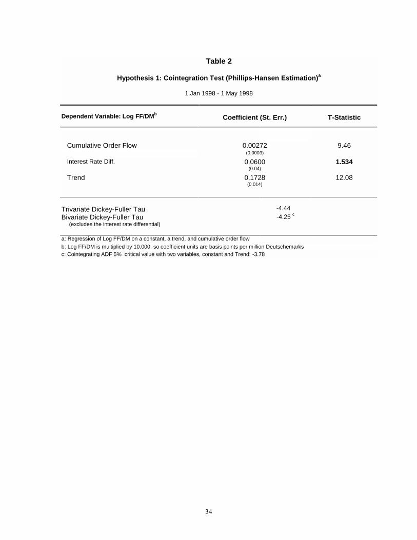
34

Table 2

Hypothesis 1: Cointegration Test (Phillips-Hansen Estimation)a

1 Jan 1998 - 1 May 1998

Dependent Variable: Log FF/DMb

Coefficient (St. Err.)

T-Statistic

Cumulative Order Flow 0.00272 9.46 (0.0003)

Interest Rate Diff. 0.0600 1.534 (0.04)

Trend 0.1728 12.08 (0.014)

Trivariate Dickey-Fuller Tau

-4.44

-4.25 c Bivariate Dickey-Fuller Tau (excludes the interest rate differential) a: Regression of Log FF/DM on a constant, a trend, and cumulative order flow b: Log FF/DM is multiplied by 10,000, so coefficient units are basis points per million Deutschemarks c: Cointegrating ADF 5% critical value with two variables, constant and Trend: -3.78

35

Table 3

Cointegrating Vector from Johansen Procedure

1 January 1998 - 1 May 1998

Coefficient

T-Statistic a

Cumulative Net Order Flow

0.003

2.81

Trend

0.145 b

2.69

a: Tests for exclusion of each variable b: The constant is unrestricted and is not reported. The trend is restricted to be within the cointegration vector.

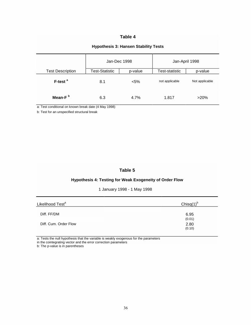
36

Table 4

Hypothesis 3: Hansen Stability Tests

Jan-Dec 1998

Jan-April 1998

Test Description Test-Statistic p-value Test-statistic p-value

F-test a 8.1 <5% not applicable Not applicable

Mean-F b 6.3 4.7% 1.817 >20%

a: Test conditional on known break date (4 May 1998) b: Test for an unspecified structural break

Table 5

Hypothesis 4: Testing for Weak Exogeneity of Order Flow 1 January 1998 - 1 May 1998 Likelihood Testa

Chisq(1)b

Diff. FF/DM 6.95 (0.01) Diff. Cum. Order Flow 2.80 (0.10)

a: Tests the null hypothesis that the variable is weakly exogenous for the parameters in the cointegrating vector and the error correction parameters

b: The p-value is in parentheses

37

Table 6

Hypothesis 5: Testing for Strong Exogeneity of Order Flow

1 Jan 1998 - 1 May 1998

Equation 1: Diff. Cum. Order Flow

Coeff. (Excl. Lags)

T-statistic (Excl. Lags)

Dependent Variable: Diff. Cum. Order Flow Constant 6.240 0.233 Diff. Cum. Order Flow(-1) 0.258 2.41

Diagnostics

General Order Flow Returns Model Specificationa Final Model Specificationb

R2 (adjusted) 4.0% R2 (adjusted) 5.5% Q (36) p-valuec 0.79 Q (36) p-value 0.36

F-Testd p-value F-Test p-value

F(4,67)e 0.16 0.957 F(11,67)i 0.428 0.953 F(4,67)f 0.473 0.754 F(4,67)g 1.83 0.13 F(8,67)h 0.282 0.969

a : General model includes constant, Diff.Cum Order Flow(-1 to -4), Interest Rate Diff.(-1 to -4) and Diff. FF/DM(-1 to -4) b: Final model includes constant and Diff. Cum. Order Flow(-1) c: This tests for residual autocorrelation up to 36th order d: All F tests relate to exclusions from the general model e: Test for the exclusion of Interest Rate Diff. (-1 to -4) f: Test for the exclusion of Diff. Log FF/DM (-1 to 4) g: Test for the exclusion of Diff. Cum. Order Flow (-1 to -4) h: Test for exclusion of Diff. FF/DM(-1 to -4) and Interest Rate Diff. (-1 to -4) i: Test for exclusion of all variables except Diff. Cum. Order Flow(-1)

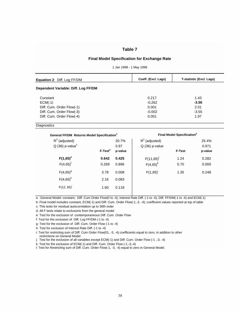
38

Table 7

Final Model Specification for Exchange Rate

1 Jan 1998 - 1 May 1998

Equation 2: Diff. Log FF/DM

Coeff. (Excl. Lags)

T-statistic (Excl. Lags)

Dependent Variable: Diff. Log FF/DM Constant 0.217 1.43 ECM(-1) -0.262 -3.56 Diff. Cum. Order Flow(-1) 0.001 2.01 Diff. Cum. Order Flow(-3) -0.002 -3.55 Diff. Cum. Order Flow(-4) 0.001 1.97

Diagnostics

General FF/DM Returns Model Specificationa Final Model Specificationb

R2 (adjusted) 20.7% R2 (adjusted) 25.4% Q (36) p-valuec 0.97 Q (36) p-value 0.971

F-Testd p-value F-Test p-value

F(1,65)e 0.642 0.425 F(11,65)j 1.24 0.282 F(4,65)f 0.269 0.896 F(4,65)k 5.70 0.000

F(4,65)g 3.78 0.008 F(1,65)l 1.35 0.248

F(4,65)h

F(12, 65)i

2.16

1.60

0.083 0.118

a :General Model: constant, Diff. Cum Order Flow(0 to -4), Interest Rate Diff. (-1 to -4), Diff. FF/DM(-1 to -4) and ECM(-1) b: Final model includes constant, ECM(-1) and Diff. Cum. Order Flow(-1,-3, -4); coefficient values reported at top of table c: This tests for residual autocorrelation up to 36th order d: All F tests relate to exclusions from the general model e: Test for the exclusion of contemporaneous Diff. Cum. Order Flow f: Test for the exclusion of Diff. Log FF/DM (-1 to -4) g: Test for the exclusion of Diff. Cum. Order Flow (-1 to -4) h: Test for exclusion of Interest Rate Diff. (-1 to -4) i: Test for restricting sum of Diff. Cum Order Flow(01, -3, -4) coefficients equal to zero, in addition to other restrictions on General Model j: Test for the exclusion of all variables except ECM(-1) and Diff. Cum. Order Flow (-1 ,-3, -4) k: Test for the exclusion of ECM(-1) and Diff. Cum. Order Flow (-1,-3,-4) l: Test for Restricting sum of Diff. Cum. Order Flow(-1, -3, -4) equal to zero in General Model.

39

Appendix Testing Structural Shifts versus Changing Shock Variance (Rigobon 1999)

Rigobon (1999) proposes a powerful and flexible test for parameter stability in

settings with possible heteroskedasticity, endogeneity, and omitted variables. (Previous

tests are unable to handle all three simultaneously.) His DCC35 test is based on the

assumption that the data can be divided into two sub-samples: a tranquil and a turbulent

period, with a known break. The null hypothesis is that heteroskedasticity is caused by a

shift in the variance of just one of the shocks affecting the system, which can include

structural shocks or innovations in unobservable omitted variables. The alternative

hypothesis is that the heteroskedasticity is caused by parameter change. The test is simple

to implement: the variance-covariance matrix is calculated for each sub-sample, the two

estimated matrices are subtracted, and the determinant of their difference is calculated.

Under the null, the determinant is zero. Large absolute values provide evidence of

parameter instability.

Though Rigobons test is designed for systems that exhibit change from tranquility

to turbulence (e.g., contagious transmission of a financial crisis from one country to

another), there is no reason why the test cannot be applied to systems that move in the

opposite direction, such as ours. The null, in our case, is that the volatility of the FF/DM

rate simply declined without any structural change at the beginning May 1998. The

alternative is that fundamental parameter change occurred, which is what we contend

(that the cointegrating relationship between the nominal exchange rate and cumulative

order flow disintegrated).

Table A1 presents results for the DCC test in our sample.36 One of the maintained

hypotheses for the test is that the decline in volatility is due to a decline in a single

structural variance. The longer the second sub-sample, the more implausible that

assumption is (lowering the power of the test). On the other hand, the shorter the second

35 Acronym for determinant of the change in covariance matrix. 36 The distribution of the DCC test is non-standard and dependent on nuisance parameters. The standard deviations and p-values in the table are obtained by bootstrapping. A Gauss program to implement this is available from rigobon@mit.edu. For the three sub-samples studied in this paper, the distribution for the DCC statistic is available from the authors on request.

40

sub-sample, the less precise are the estimates of the covariance matrix, making the size of

the test unreliable. To balance these considerations, we look at three different lengths for

the second sub-sample. For the longest periodMay to December 1998parameter

stability is rejected. For the shortest periodMay 1998 onlyparameter stability cannot

be rejected. Both of these results are suspicious for the reasons given above. Most

convincing is the result for the intermediate period, May and June 1998. This test rejects

parameter stability at the 5% level, providing further support for treating the period

before May 2/3 as parametrically different from the remainder of 1998.37

Table A1

Second Sub-sample

DCC Test Value

p-value %

May 1998

-6327

22.7

May and June 1998

-12166 3.5

May to December 1998

-139816 0.0

Visual Evidence that Order Flows Impact on Price Drops Off

Though not appropriate statistically (given the cointegrating relationship), it is

nevertheless instructive to consider the time pattern of coefficients in a regression of

exchange rate changes on order flows. The following Figure A1 provides some visual

evidence from a rolling regression of FF/DM changes (50 observation window) on

current and past (up to lag 5) order flows. The solid line plots the sum of those order-flow

coefficients that are statistically significant in the January to May 1 sample (the

coefficients are summed at each window-sample snap shot). The plot begins in mid-

37 The DCC result does not permit us to conclude that the relationship between FF/DM and order flow changed from a cointegrating relationship to a non-cointegrating one, nor that May 2/3 is the date of change. A version of this test has not yet been developed for the case of an unknown break (nor can it be specific about the precise nature of the parameter instability).

41

March to accommodate the 50 (trading day) rolling period. The plot indicates a clear drop

off of order flow impact. The timing of the drop off is also suggestive of market

anticipation of the May2/3 announcement (subject to the statistical caveat noted above).

Figure A1

-0.03

-0.02

-0.01

0

0.01

0.02

0.03

0.04

13-M

ar-9

8

27-M

ar-9

8

10-A

pr-9

8

24-A

pr-9

8

08-M

ay-9

8

22-M

ay-9

8

05-J

un-9

8

19-J

un-9

8

03-J

ul-9

8

17-J

ul-9

8

31-J

ul-9

8

14-A

ug-9

8

28-A

ug-9

8

11-S

ep-9

8

25-S

ep-9

8

09-O

ct-9

8

23-O

ct-9

8

06-N

ov-9

8

20-N

ov-9

8

04-D

ec-9

8

18-D

ec-9

8

01-J

an-9

9

Sum of Coefficients from Rolling Regresson of FF/DM Returns on Lag 1, 3 and 4 of Differences in Net Orderflow50 Observation window rolled from 13th March to 31 December 1998

Sum

of O

rder

flow

-pric

e im

pact

coe

ffici

ents

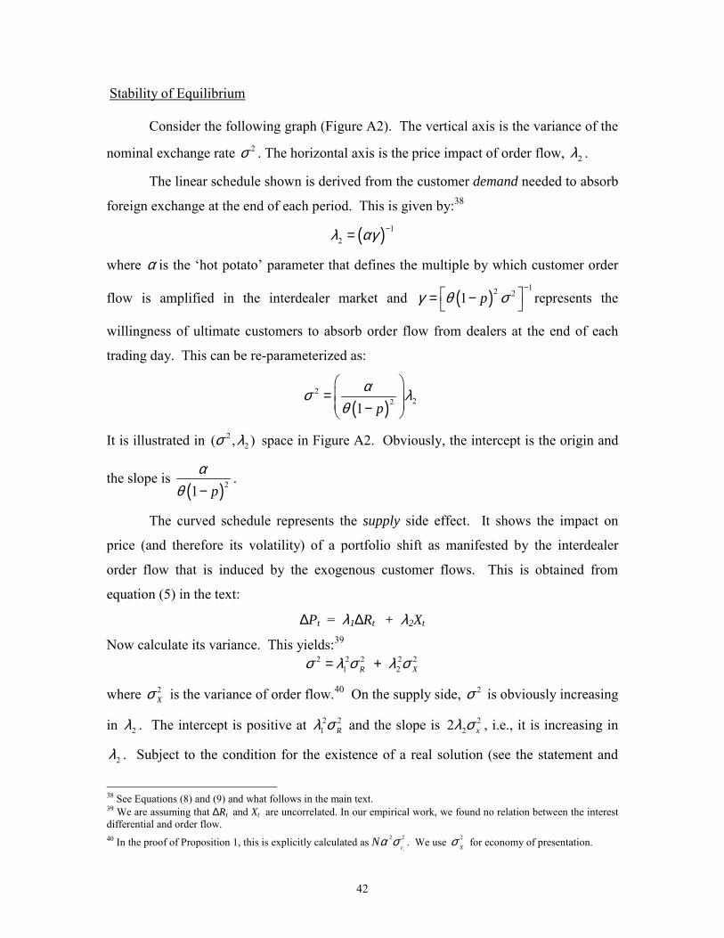
42

Stability of Equilibrium

Consider the following graph (Figure A2). The vertical axis is the variance of the

nominal exchange rate 2σ . The horizontal axis is the price impact of order flow, 2λ .

The linear schedule shown is derived from the customer demand needed to absorb

foreign exchange at the end of each period. This is given by:38

( ) 12λ αγ −=

where α is the hot potato parameter that defines the multiple by which customer order

flow is amplified in the interdealer market and ( )12 21 pγ θ σ

− = − represents the

willingness of ultimate customers to absorb order flow from dealers at the end of each

trading day. This can be re-parameterized as:

( )2

221 pασ λ

θ

= −

It is illustrated in 22( , )σ λ space in Figure A2. Obviously, the intercept is the origin and

the slope is ( )21 p

αθ −

.

The curved schedule represents the supply side effect. It shows the impact on

price (and therefore its volatility) of a portfolio shift as manifested by the interdealer

order flow that is induced by the exogenous customer flows. This is obtained from

equation (5) in the text:

∆Pt = λ1∆Rt + λ2Xt

Now calculate its variance. This yields:39 2 2 2 2 2

1 2R Xσ λ σ λ σ= +

where 2Xσ is the variance of order flow.40 On the supply side, 2σ is obviously increasing

in 2λ . The intercept is positive at 2 21 Rλ σ and the slope is 2

22 xλ σ , i.e., it is increasing in

2λ . Subject to the condition for the existence of a real solution (see the statement and

38 See Equations (8) and (9) and what follows in the main text. 39 We are assuming that ∆Rt and Xt are uncorrelated. In our empirical work, we found no relation between the interest differential and order flow. 40 In the proof of Proposition 1, this is explicitly calculated as 2 2

cNα σ . We use 2

Xσ for economy of presentation.

43

proof of Proposition 1), there will, in general, be two solutions as demonstrated in the

proof of Proposition 1(ii). Note that when 2 0Rσ = , both the demand and supply

schedules go through zero: this is the focus of Propositions 1 and 3. However, even when 2 0Rσ = , there is a second high-variance solution.

We now appeal to the following argument to demonstrate that the low variance

solution is stable but that the high variance solution is not.

In Figure A2, consider the point A. This is a 22( , )λ σ pair that is not on the linear

demand schedule, though it is on the supply schedule. Point A lies to the left of the

schedule: 2σ is high relative to 2λ . This means that ultimate customers will be relatively

reluctant to absorb interdealer flow: the price impact of order flow will increase driving

2λ upwards, to a point such as point B. Next consider point B: this is a 22( , )λ σ pair that

lies below the supply schedule. The variance is low relative to the price impact of order

flow. However the higher price impact of order flow from exogenous portfolio shifts

drives up the variance of price to a point such as point C. A sequence of such arguments

brings us to the low variance equilibrium.

Now consider points such as D or D'. These are located on the demand and

supply schedules respectively between the two equilibria. Analogous arguments to the

above indicate that, from such initial positions, the 22( , )λ σ pair tends towards the lower

variance equilibrium. Consequently, the low variance solution is stable and the high

variance solution is unstable.

However, we can go further. Consider points such as A', B' and C'. These all lie

above the high variance solution. Here the curved supply schedule lies above the linear

demand schedule as in the initial argument with respect to points A, B and C that lie

below both solutions. Using an identical argument, starting from A', B' or C', both 2

2 and λ σ tend towards infinity. We interpret this as describing the microstructure of

exchange rate dynamics during a hyperinflationary episode. We leave this to later

research.

44

2σ

C'

B' A'

D'D

C

B A

222(1 )p

ασ λθ

= −

2 2 2 2 21 2R Xσ λ σ λ σ= +

Figure A2

Stability of Equilibrium

2λ

2 21 Rλ σ