Embed Size (px)
Citation preview

Flow preferences of benthic macroinvertebrates in three
Scottish Rivers
by
Matthew Thomas OHare
This thesis is submitted for the degree of Doctor of Philosophy, Division of Environmental & Evolutionary Biology, Insitute of Biomedical & Life
Sciences and the Department of Civil Engineering, University of Glasgow,September 1999.
© Matthew T. OHare, September 1999.

ProQuest Number: 13818646
All rights reserved
INFORMATION TO ALL USERS The quality of this reproduction is dependent upon the quality of the copy submitted.
In the unlikely event that the author did not send a com p le te manuscript and there are missing pages, these will be noted. Also, if material had to be removed,
a note will indicate the deletion.
uestProQuest 13818646
Published by ProQuest LLC(2018). Copyright of the Dissertation is held by the Author.
All rights reserved.This work is protected against unauthorized copying under Title 17, United States C ode
Microform Edition © ProQuest LLC.
ProQuest LLC.789 East Eisenhower Parkway
P.O. Box 1346 Ann Arbor, Ml 48106- 1346

G IASG OWUNIVERSITYLIBRARY

This thesis is dedicated to my parents.

Abstract
Scottish freshwaters have been described as a national resource of international significance. The high quality of Scotland’s lotic systems is integral to the formation of this view. The research presented here aims to provide an insight into the interaction between benthic invertebrates and their hydraulic habitat within some of Scotland’s lotic systems. A further aim of this project is that this information presented here will aid the design of river rehabilitation and management schemes thereby helping maintain the integrity of the opening statement.
There is a large amount o f literature existing which addresses the interactions between benthic invertebrates and flow parameters; substrate type, vegetation, velocity, depth and near bed stresses. However significant gaps remain in our understanding, particularly at the level of individual taxa preferences. Furthermore, little work has been done in Scotland. To address these gap in the data the distribution of macro- invertebrates in relation to flow parameters were assessed for three rivers representative of highland (River Etive), central belt (Blane Water) and borders rivers (Duneaton Water).
The importance of deep and shallow reaches as habitat units for benthic invertebrates was analysed and the methods for categorising reaches into riffles, runs and pools assessed. The analysis showed that at the sites examined differences between invertebrate community in deep and shallow reaches were minimal and limited to the preferences of a number of key species. Categorising reaches into riffles, runs and pools on purely visual grounds was insufficient and some measures of velocity and depth are required if the work is to be used for between site comparisons.
Benthic invertebrates did show preferences for flow parameters. At the physical scale examined (Surber sample) community structure was influenced in a limited manner by flow parameters; velocity and depth wre the most important. A gradient from erosional to depositional conditions was observed at two of the sites.
Limitations of Instream Flow Incremental Methodology (IFIM) as applied to benthic invertebrate habitat identification were identified. Estimates of near bed flow parameters based on point measurements of velocity profiles to samples collected at the scale of Surber samples do not explain any additional variation in the distribution of benthic invertebrates. Analysis of individual flow preferences o f macroinvertebrates suggest that to identify flow preference curves, an aim of IFIM, finer scale habitat measurements are needed.
Laboratory experiments were carried out to identify the upper velocity tolerances of some benthic invertebrates; Tipulidae and Gammarus pulex. The results show that individuals were flexible in their responses to high velocities. What constituted ‘high’ velocity was taxa specific.
Benthic invertebrate community structure was investigated in areas of the Blane Water vegetated with Callitriche instagnalis. Submerged vegetated patches supported a

greater abundance of invertebrates than bare substrate. The hydraulic habitat of the macrophyte stands was more diverse than that of bare substrate with higher velocities occurring on the outside of the macrophyte stands than on the bare substrate. Simuliidae dominated the outside of the stands, the area exposed to the highest velocities. The invertebrate community on the outside o f the plant stands was less equitable than that found at the root-substrate interface. It is suggested that macrophytes can be used as a tool in the rehabilitation of hydraulic habitat for benthic invertebrates in Scottish rivers.
The importance of these results are discussed in the context of river rehabilitation and our ecological understanding of benthic invertebrate community structure.
CONTENTS
ABSTRACT..................................................................................................................................................................... i
CONTENTS................................................................................................................................................................... iii
DECLARATION...........................................................................................................................................................vi
ACKNOWLEDGEMENTS.......................................................................................................................................vii
CHAPTER 1 GENERAL INTRODUCTION........................................................................................................... 1
1.1 T h e b io l o g y o f fl o w in g -w a t e r b e n t h ic m a c r o -in v e r t e b r a t e s ................................................................1
1.2 L o t ic s y s t e m s : P h y sic a l s t r u c t u r e ........................................................................................................................ 71.2.1 Life, light, temperature & water chemistry............................................................................................ 81.2.2 Drainage networks and Channel Structure.......................................................................................... 101.2.3 Scale o f physical processes, implications fo r ecology........................................................................12
1.3 L o t ic s y s t e m s : e c o l o g ic a l in t e r p r e t a t io n .......................................................................................................13
1.4 Spec ific s o f St u d y ........................................................................................................................................................... 17
1.5 T h e sis o u t l in e ....................................................................................................................................................................23
CHAPTER 2: HYDRAULIC AND INVERTEBRATE SURVEYS OF REACHES IN THE BLANE WATER, RIVER ETIVE AND DUNEATON WATER ................................................................................................. 25
2.1 In t r o d u c t io n ..................................................................................................................................................................... 25
2.2 M e t h o d s ................................................................................................................................................................................ 302.2.1 Site choice ..................................................................................................................................................302.2.2 Description o f s ite s ...................................................................................................................................312.2.3 Field measurements..................................................................................................................................332.2.4 Estimation o f hydraulic parameters from velocity profiles............................................................... 342.2.5 Statistical analysis.................................................................................................................................... 36
2.3 R e s u l t s ...................................................................................................................................................................................382.3.1 General Conditions...................................................................................................................................382.3.2 Comparison o f flow conditions at different sites ................................................................................ 402.3.3 Substrate available in the reaches......................................................................................................... 442.3.4 Distribution o f Turbulent and Laminar flow within reaches.............................................................482.3.5 Species lists.................................................................................................................................................502.3.6 Reach preferences o f taxa ....................................................................................................................... 53
2 .4 D is c u s s io n ............................................................................................................................................................................ 542.4.1 Physical character o f the Sections......................................................................................................... 552.4.2 Biological character o f the Sections......................................................................................................56
2.5 C o n c l u s io n s ........................................................................................................................................................................ 602.5.1 Physical study ............................................................................................................................................ 602.5.2 Biological study .........................................................................................................................................61
CHAPTER 3: BENTHIC INVERTEBRATE COMMUNITY ORDINATION......................................................63
3.1 In t r o d u c t io n .................................................................................................................................................................. 633.1.1 Outline...................................................................................................................................................... 63

3.1.2 Physical patchiness.................................................................................................................................. 633.1.3 Spatial aggregations................................................................................................................................ 643.1.4 Assessment o f the ecohydrological health o f rivers............................................................................64
3.2 Methods............................................................................................................................................................ 673.2.1 Data Collection and Dataset Structures.............................................................................................. 673.2.2 Analysis procedure....................................................................................................................................68
3.3 Results...............................................................................................................................................................723.3.1 Suitability o f data sets .............................................................................................................................. 723.3.2 River E tive .................................................................................................................................................. 733.3.3 Duneaton Water.........................................................................................................................................763.3.4 Blane Water................................................................................................................................................81
3.4 Discussion......................................................................................................................................................... 843.5 Conclusions..................................................................................................................................................... 88
CHAPTER 4: INDIVIDUAL RESPONSES TO HYDRAULIC PARAMETERS........................................... 90
4.1 Introduction................................................................................................................................................... 90
4.2 Methods............................................................................................................................................................ 934.2.1 Data source.................................................................................................................................................934.2.2 Statistical analysis....................................................................................................................................93
4.3 Results...............................................................................................................................................................984.3.1 Curve fitting ................................................................................................................................................984.3.2 Relationships o f totalled maximum abundance to the frequency o f variable intervals................984.3.3 Relationships o f maximum sample abundance to the frequency o f variable intervals............. 1034.3.4 Velocity.................................................................................................................................................... I l l4.3.5 Depth ........................................................................................................................................................ 1204.3.6 Substrate....................................................................................................................................................129
4.4 D iscussion....................................................................................................................................................... 130
4.5 Conclusions....................................................................................................................................................132
CHAPTER 5: FLUME EXPERIMENTS: ENTRAINMENT VELOCITIES OF BENTHIC INVERTEBRATES....................................................................................................................................................133
5.1 Introduction................................................................................................................................................. 133
5.2 Materials....................................................................................................................................................... 1385.2.1 Flumes...................................................................................................................................................... 1385.2.2 Flow Structure in the flum e ................................................................................................................. 1415.2.3 Experimental animals........................................................................................................................... 143
5.3 Methods...........................................................................................................................................................1445.3.1 Weighing and morphometric measurements..................................................................................... 1445.3.2 Experimental design and statistical analysis................................................................................... 146
5.4 Results............................................................................................................................................................. 1505.4.1 Head width to frontal area ra tios ...................................................................................................... 1505.4.2 Phototaxis................................................................................................................................................ 1505.4.3 Rheotaxis and swimming...................................................................................................................... 1515.4.4 Entrainment logistic curves................................................................................................................. 154
iv

5.4.5 Effect o f weight on entrainment ofTipulidae ................................................................................ 157
5.5 D is c u s s io n ....................................................................................................................................................... 158
5.6 C o n c lu s i o n s ....................................................................................................................................................162
CHAPTER 6: INVERTEBRATE HYDRAULIC MICROHABITAT AND COMMUNITY STRUCTURE IN CALLITRICHE STAGNALIS SCOP. PATCHES.................................................................163
6.1 I n t r o d u c t i o n ..................................................................................................................................................1636.2 M e t h o d s ........................................................................................................................................................... 164
6.2.1 Source o f p lan ts ..................................................................................................................................... 1646.2.2 Measurements...........................................................................................................................................1656.2.3 Data manipulation................................................................................................................................. 1666.2.4 Statistical analysis...................................................................................................................................166
6.3 R e s u l t s ............................................................................................................................................................. 1686.3.1 Comparisons between plant and Surber sam ples............................................................................ 1686.3.2 Comparisons between plant sections................................................................................................. 1686.3.3 Community structure............................................................................................................................. 1736.3.4 Prevalent flow conditions.......................................................................................................................176
6.4 D is c u s s io n ........................................................................................................................................................1776.5 C o n c lu s i o n s .................................................................................................................................................... 179
CHAPTER 7: GENERAL DISCUSSION.............................................................................................................. 181
7.1 R e v ie w o f r e s u l t s ...........................................................................................................................................................181
7.2 F u t u r e W o r k .................................................................................................................................................................... 182
7.3 M a n a g e m e n t r e c o m m e n d a t io n s ............................................................................................................................ 184
REFERENCES............................................................................................................................................................ 189
APPENDIX I: DEFINITIONS OF FLOW UNITS AND PARAMETERS......................................................205
APPENDIX II: EXAMPLE OF LOG PLOTTING OF VELOCITY PROFILES WITH NOTES ON DISTRIBUTION PATTERNS OF SIGNIFICANT PROFILES........................................................................ 206
APPENDIX III: VELOCITY PROFILES. RAW DATA AND REGRESSION ANALYSIS .................... 212
APPENDIX IV: TWINSPAN ORDERED SPECIES BY SAMPLES TABLES........................................... 228
APPENDIX V: INDIVIDUAL RESPONSES OF BENTHIC INVERTEBRATES TO VELOCITY.DEPTH AND SUBSTRATE.................................................................................................................................... 233

Declaration
I declare that the work described in this thesis has been carried out by myself unless otherwise acknowledged. It is entirely of my own composition and has not, in whole or part, been submitted for any other degree.
Matthew OHare September 1999

Acknowledgements
First of all I would like to gratefully thank my supervisors, Dr Kevin
Murphy, Dr. Alan Taylor and Prof. D. Alan Ervine, for having the
patience to let the study go its own way whilst offering excellent
supervision and encouragement throughout.
I lived at the University Field Station, Rowardennan for the majority of the
project, so I would like to gratefully thank the Field Station folk for their
kindness, encouragement, help and good humour; Dr. Colin Adams, Dr.
Roger Tippett, Dr. Ian McCarthy, Rona Brennan, Vivien Cameron, Ishbel
McColl, Caroline Askew, Peter Willmott, Chris Cutts, Nicola Bissett,
Alistair Duguid, Alan Campbell, Alan Grant, Deborah Hamilton, Dave
Stevens, Melaine Fletcher, Mat Cottam and post-grads and under-grads in
Glasgow to numerous to mention The help of technical staff at the main
campus was often sought and received and I am particularly grateful to,
Davy Watson, June Freel, Willlie Orr and Pat McLauglin. Alan McGregor
and his staff in the IBLS work shop deserve special thanks for
constructing my various flume designs and altering them to the point
where they would work!
I have contacted many academics during this study for advise and I am
grateful to them all. Dr. Jill Lancaster was especially generous not only
with her time but ideas too. Her help extended to the practical by getting

me access to the Edinburgh University library while I worked in
Edinburgh during the winter of 1998-99. Other assorted folk at the
Freshwater Biological Association have been intermittently pestered for
help with identification of invertebrates and they also gave of their time
generously. Dr. Marian Scott, Geoff Hancock and Dr. Nigel Willby of
Glasgow University gave free and helpful advice on statistics and
dipteran biology and freshwater ecology respectively.
Last but not least I would like to thank Judith Milne and her kin and my
own family: Mum, Dara and Paula for all their support both emotional and
financial, go raibh maith agaibh.
This study was carried out whilst in receipt of a University of Glasgow
scholarship funded by a Scottish Office Initiative on improved river
management.

General Introduction
Chapter 1:General Introduction
The main aim of this project was to improve the scientific knowledge base of benthic
invertebrate - environment interactions in streams, to assist the better design of river
rehabilitation and management schemes. The basic question to answer is whether or not
instream flow preferences o f benthic invertebrates can be identified. There is a large body
o f work addressing various aspects o f this question but it remains to a large extent
unanswered especially in a quantified manner. The thesis chapters outlined at the end of
the introduction, show a progression from field surveys to laboratory experiments, where
initial measurements made in the field are tested in the laboratory. Finally macrophytes,
which provide a velocity gradient are examined as macroinvertebrate habitat. Part of the
aim of this work is to follow the ecohydrological approach, that is the combining of
ecology and hydrology to better improve our understanding and management of
freshwaters. In its infancy, this discipline still suffers from a lack o f basic definitions
hampering work. The first sections of this general introduction cover the basic biology and
physical structure of rivers, partly for general information but also to clarify some of these
basic definitions, and paradigms as I perceive them. A more specific introduction to the
work follows the general sections.
General background
1.1 The biology of flowing water benthic macroinvertebrates
Macroinvertebrates are a practical grouping of freshwater organisms, simply defined as
invertebrates occurring in or on (or associated with) the substrate, and visible to the naked
eye. Meiofauna which are invisible to the naked eye are often the more species rich and

General Introduction
abundant o f the two categories o f benthic fauna but remain relatively neglected (Poff et al.
1993; Ward et al. 1998). Being wholly dependent on size, membership of the two groups
is not exclusive, a situation well illustrated by the Chironomidae which can occupy both
groupings during their larval stage. Constituting a number o f phyla the macro
invertebrates exhibit a range o f life histories. The majority of the phyla spend their entire
life cycles in the lotic system; Crustacea, Mollusca, Annelida and Platyhelminthes1}
The remaining major grouping, the Insecta spend only their juvenile stages in the system,
although among some groups there are exceptions; the Coleoptera and the Hemiptera. The
insects are the most extensively studied o f the benthic invertebrates and several texts are
exclusively devoted to them (Merrit & Cummins 1979; Williams & Feltmate 1994).
Most o f the insects are univoltine or bivoltine but some species can take two years to
mature. It is very rare for animals to take longer than two years to mature in lotic systems
(Williams & Feltmate 1994). Adult emergence for the Ephemeroptera and some members
of the other groups is famously synchronised but time spent on the wing can be highly
variable. In the Trichoptera some taxa can spend the entire summer on the wing waiting to
reproduce. From a number o f studies it clear is that growth rates are plastic, and may
reflect ambient temperature and food availability or other environmental variables (Petts &
Bickerton 1994; Webb & Walling 1993). As the fecundity of these animals is almost
1 Other phyla do occur in running freshwater but were not encountered during this study. A checklist of the north European taxa is given in (Fitter & Manuel 1994). For simplicity the taxonomic hierarchy used in that publication is used throughout the thesis and is not a reflection of the author's views on the taxonomic structure of the Arthropoda which remains unresolved and controversial (Brusca & Brusca 1990).
2 There are a number of exceptions among the Gastropoda: it has been stated that it is difficult to distinguish between aquatic and terrestrial forms. (Macan 1977). The sub-class Euthyneura are exclusively represented by the order Pulmonata in this study are air breathers and can exist in quite dry conditions. Of their members the species most frequently encountered in the study is Artcylus fluviadlis which does not need to breath air and is wholly aquatic (Clegg 1952)!
2

General Introduction
exclusively dependent on juvenile feeding - see below - environmental conditions during
the juvenile stage are of the utmost importance.
Few adult aquatic insects have been observed feeding but some Trichoptera and
Chironomidae adults have been observed sipping nectar, Homopteran honeydew and sugar
water in the wild and captivity (Armitage et al. 1995; Malicky 1981). The contribution to
the animals’ overall fecundity is likely to be slight as these food sources contain little more
than carbohydrates (Svensson 1972). Dragonflies feed throughout their adult lives, but
were not encountered in the work presented here (Hammond & Merrit 1983; Miller
1987). Some Plecoptera (Nemouridae) need to feed before they can lay eggs, but even in
these cases the majority o f the adult biomass must come from larval feeding (Hynes 1976).
Diptera are the major exception, with fecundity closely related to blood feeding across
some of the families. In general though, investment by invertebrate adults in individual
young is limited.
Oviposition strategy can have a strong influence on the distribution of the juvenile forms
on the substrate and may, in the case o f insects and depending on species, be a product of
parental habitat use rather than larval preference (Harrison & Hildrew 1998). This is more
likely in lentic systems than lotic where there are fewer modes of larval dispersal. The
Gastropoda encountered in this study produce their eggs in jellied masses on rocks and
other submerged substrata (Clegg 1952) and in the case of Potamopyrgus jenkinsi by
asexual means (Maitland 1990). Among the Annelida, egg laying also occurs; the eggs
being laid in capsules (Brinkhurst 1963). In the insects, parental care appears limited to
3

General Introduction
oviposition. Eggs are laid in the water under stones (Baetis) on the water surface
(Ephemerella ignita) or on bankside vegetation (some Trichoptera).
The numbers o f eggs produced by all members o f the aquatic taxa shows high degrees of
intra and interspecies variation (Macan 1963), hinting at a range o f reproductive
strategies. Sexual reproduction appears to be the norm among aquatic insects but asexual
reproduction in the Chironomidae and Ephemeroptera has been recorded (Armitage et al.
1995).
The only aquatic groups which do show some maternal care are the amphipod and isopod
crustaceans which brood their young (Clegg 1952). It has recently been shown that the
amphipod Crangonyx pseudogracilis also actively cares for their broods by flexing their
bodies which alters the microhabitat o f their brood pouches (Dick et al. 1998).
Although fundamental to our understanding o f lotic ecosystems, little detailed work has
been done on the dispersal o f aquatic insects during the adult phase. Work on the genetic
variability between populations o f the Trichoptera in Australia indicate that there can be a
much greater transfer o f genetic material over large geographic areas than had previously
been believed (Hughes et aL 1998)3. Aquatic insects occurring in a river stretch can be
viewed as members o f metapopulations, where the entire population may range in spatial
occupation from a single island to the entire globe. Aquatic insects are thereby, potentially
resilient to localised disturbance o f lotic systems as long as their particular habitat patch
continues to exist after the disturbance event and can be colonised by animals from
1 Research on Plecoptera showed distinct differences between streams suggesting that they do not disperse to the same extent as the Trichoptera of the other study (Hughes et al. 1999).
4

General Introduction
unaffected sites, e.g., if aquatic insects are subject to metapopoulation dynamics (Hanski
1994 & Levins 1969).
Dispersal between non-contiguous river systems is particularly difficult to assess for non
insect taxa which have no aerial phase. The rate o f dispersal o f invasive Crustacea
{Crangonyx pseudogracilis) and Mollusca (Potamopyrgus jenkinsi) in the UK has been
impressive, with both invaders now found throughout the country, less than one hundred
and twenty years after being first recorded (Maitland 19904, Dick et al. 1997). Whether
this was purely mediated by humans or reflects a natural ability to disperse between
systems is difficult to determine at present. In the case o f Crangonyx there is good
evidence that the animal has moved between different catchments via the canal network
although this is not always the case. It is likely that humans have influenced the dispersal,
in the case o f many fish species (Adams & Maitland 1998) and zebra mussels (Buchan &
Padilla 1999). Future genetic work species and systems not heavily influenced by humans
would help determine the degree o f isolation o f populations o f these groups.
Once hatched benthic invertebrates find themselves near the base o f the food chain, usually
as primary consumers or detritivores, although some taxa are predatory right from
hatching, e.g. the Tanypodinae. Depending on food particle size and feeding mechanisms
of benthic invertebrates, the taxa have been assigned to functional feeding groups
(Cummins 1973). .Initially derived for insects only, it is now applied to the entire benthos
(Moss 1988). The primary distinction is between herbivory, detritivory and camivory.
Ephemeroptera are viewed as mainly collector gatherers feeding on Fine Particulate
5

General Introduction
Organic Matter (FPOM) and scrapers, Plecoptera as predators or feeding on Coarse
Particulate Organic Matter (CPOM) shredders. Tipulidae and Chironomidae can be
shredders, collector gatherers (filterers) or predators. The Simuliidae, the other dipteran
family are filter-collectors (Hart & Latta 1986). The Trichoptera and Coleoptera occur in
almost all o f the categories (Williams & Feltmate 1994: after Cummins 1973). The
gastropods are viewed as scrapers, the Annelida as predators or deposit feeders and the
Amphipoda and Isopoda as scrapers or collectors. The degree to which these groupings
are exclusive is less certain. Gammarus pulex have scraping mouth parts but can use these
to predate other amphipods which in turn may reduce interspecific competition (Dick
1992; Dick et al. 1990).
The link between feeding groups, animal mobility and morphology is strong. It is clear that
to be a filterer being located in areas of high velocity and on stable substrate is useful and
requires special adaptations e.g. suckers or retreats from energy consuming flow
conditions. For collector gatherers, mobility is important and the animal must be able to
swim through the water or crawl through / across the substrate matrix. It suggests there is
a link between species (identified using morphological characteristics) and how they
exploit their physical habitat. The river bed is heterogeneous and it is postulated that these
animals occupy different physical niches (areas of stream bed) depending on their
functional feeding groups.
Some of the major benthic taxa o f interest in this study have the ability to be either
parasitic or commensal on other invertebrates, feeding groups not addressed in Cummin’s
1 As a human food source invasive crayfish species are excluded from the example as the influence of man in their dispersal is well recorded and affords little room to speculate about natural mechanisms.( \ pseudogracilis is still largely absent from the Scottish highlands.
6

General Introduction
classification, (Cummins, 1973). Chironomidae appear best suited to this role and are
usually commensal, but can be parasitic (Tokeshi 1993). There has been at least one
record o f a Trichopteran (Orthotrichia) larva parasitic on other Trichopteran pupae (Wells
1992). The Hirudinea are o f course the most famously parasitic freshwater group but in
the systems studied here some leech species are predators, feeding directly on
invertebrates (Elliot & Mann 1979). Although it is felt that flowing water somewhat
negates the impact of ecto and endo parasites they do occur on the freshwater benthos.
Hickin (1967) reviews the epizoites and epiphytes found on Trichopteran larvae and
includes a mite, Atturus scaber infesting Goer a pilosa and protozoa on a range of other
species. Disease in general, is an area that has received little attention but could have a
profound effect on aquatic benthos distribution.
So potentially, predation, food availability, disturbance and physical habitat structure
alteration can affect the instream distribution of invertebrates and are well researched
(Boulton et al. 1992; Crowl & Schnell 1990; Crowl et al. 1997; Dahl & Greenberg 1996;
Death 1996; Dudgeon 1991; Dudgeon 1993; Dudgeon & Chan 1992; Hansen et al. 1991).
Before proceeding further it is necessary to describe the physical habitat of lotic systems
indicating the limits and opportunities which they present to aquatic benthic invertebrates.
1.2 Lotic systems: Physical structure
This section gives a short review o f the physicochem ical nature and geom orphological
structu re o f lotic systems. The section on the geom orphological structure o f rivers and
their substrates focuses on the subject o f the thesis, instream flow conditions; the physical
factors examined as possible environm ental gradients for invertebrates.
7

General Introduction
1.2.1 Life, light, temperature & water chemistry
The basic requirements o f almost all life: water, light, oxygen, carbon dioxide and
nutrients are available in lotic systems (Hutchinson 1957; Hynes 1972). Light penetration
in rivers is normally limited by the turbidity o f the water and it is only in the lower reaches
of rivers, or in very large systems that depth becomes a limiting factor (Hynes 1972).
Turbidity is usually dependent on discharge mobilising small particulate matter, and high
turbidity is therefore more frequent in winter when the temperature (in temperate rivers)
is too cool for much plant growth and the number o f hours o f sunlight are few and less
intense. Dissolved atmospheric gases are rarely limiting in running waters which are
frequently completely saturated or super saturated with oxygen, nitrogen and carbon
dioxide. Freshwater insects appear to be dependent on this high level o f available oxygen.
Lowering the percentage o f dissolved oxygen even slightly can have significant effects on
the health of rheophilic amphipods, Trichoptera, Simuliidae, Ephemeroptera and
Plecoptera (Golubkov et al. 1992; Kiel & Frutiger 1997; Macan 1963; Nagell &
Larshammar 1981). For some Trichoptera their cases facilitate oxygen uptake (Williams et
al. 1987) possibly allowing them to live in areas with lower oxygen levels. The capacity to
tolerate lower oxygen levels is observed across most o f the groups and tends to be found
mainly among burrowers.
Rain water contains varying amounts o f dissolved elements. The nutrient content o f the
river water is primarily dependent on the underlying bedrock geology, modified (often
substantially) by catchment land use and other anthropogenic factors. Land use,
particularly intensive agriculture and urban centres, have a detrimental impact on the
8

General Introduction
chemical quality o f water which may have a direct effect on the resident invertebrates. In
Scotland, surface drift which, when glacially derived, can be of different chemical
composition to the underlying bed rock, also contributes to the water chemistry (Survey
1971; Survey 1977).
The osmotic potential o f freshwater can obviously be variable for the same reason nutrient
concentration is variable. Aquatic insects are know to be hypertonic relative to freshwater
and are capable o f withstanding the normal fluctuations in its osmotic potential. They are
not capable of withstanding the essential potential o f salt water concentrations and this is
one of the reasons cited as limiting the lotic benthos to rivers and making it non
contiguous with the marine system5. Also it is one of the many reasons cited why aquatic
invertebrates do not drift too far downstream.
Temperature in running freshwaters varies more rapidly than in standing waters.
Superimposed on seasonal changes are diurnal cycles. Surface water streams reflect mean
air temperature over their entire length although this may alter as one proceeds down a
valley. Spring melt o f snows (which would be likely to affect all the rivers studied in this
work) may have temperatures below that of the mean air temperature for significant
periods subsequent to melting. On average, the upper sources of a catchment system tend
to be cooler than further down. Temperature can have a profound effect on larval growth
and emergence in the aquatic insects, best studied o f these is probably Baetis and
temperature is likely to effect the development of non-insect taxa in a similar manner, see
5 It has been pointed out that of the freshwater insects some groups have members occurring in marine environments. Tire trichopteran Philanisus plebeius lives in intertidal rock pools but has an additional organ not present in freshwater species which helps retain water within its hypotonic body (Leader 1976). As such the argument that limited osmoregulatory systems prevented insect colonisation of salt water begin to weaken.
9

General Introduction
Williams & Feltmate (1994) for a review of the effects of temperature on aquatic insects.
Feeding is rarely limited by temperature according to (Cummins 1973), but it can effect
instream distribution (Guinand et al. 1994).
Lotic systems have all the ingredients for primary productivity to succeed. They also have
another factor which to a greater or lesser extent excludes the growth of instream
macrophytes. That is the constant movement of water which makes the rooting of plants
not only difficult but, if they do succeed in rooting, subject to removal by flooding. The
constant erosion of fine sediment also leaves little suitable rooting material, most usually
found in the lower reaches o f river systems with mosses on rocks as the only rooted plants
in the upper reaches The macrophytes which do occur in rivers are adapted to this
disturbed habitat and often grow in shapes suitable for minimising drag (Sand-Jensen &
Mebus 1996). Phytoplankton are also often only found in the lower reaches of rivers:
frequently a major source of primary productivity is algae encrusting on rocks.
Filamentous algae also grow attached to the substrate and under suitable conditions, a
mixture o f Chironomidae, diatoms and other Protista grow among their strands to form
mats termed 'Aufwuchs' (Flynes 1972). Allochthonous material accounts for a large
proportion of the energy entering the system and the amount is closely linked to the
structure of the drainage system.
1.2.2 Drainage networks and Channel Structure
The sim plest hierarchy is that o f stream size; those tributaries furthest upstream are
sm allest in width and, as they progress to the sea, they join forming increasingly larger
10

General Introduction
channels o f higher stream order. The idea o f ordering streams is that o f R.A. Horton
(Hynes 1972). The instream structure o f channels also changes with distance from their
source. Higher up in the catchments slopes tend to be steep, quickly shedding water,
creating an erosional environment dominated by large substrate elements which can form
‘step and pool’ sequences (Carling 1995). Further down the system, the rivers still contain
a lot o f energy but are now wider and begin to deposit and erode material in a sequential
manner (Carling 1995). This leads to the riffle-pool structure where when discharge is
high pools are scoured out and the material deposited further downstream forming an
extended lip called a riffle (Clifford 1993). During low discharge, fine substrates deposit in
the pool sections, but not to the same extent in the riffle areas. Although relatively stable,
the riffle-pool system is a constantly shifting dynamic habitat (Carling 1995). In gravel bed
rivers some stability is created by the formation o f an armoured layer where, through
successive minor increases in discharge, the bed becomes compacted and in some cases
the substrate elements align their long axis with the direction o f flow. The armoured layer
allows the persistence o f finer substrate below this top compacted layer which, if it was
not present, would be eroded. These middle reaches are the subject of the work done in
this study this thesis. There can also be a zone o f low permeability below the river bed
were the water is no longer saturated with oxygen (van't Woudt & Nicolle 1978).
The deposition of material sorts it into mixed aggregates o f different sized substrate
elements; cobble bars, riffles, pools etc. These are often viewed as microhabitats for
macrobenthos (Brown & Brussock 1991) and this is one o f the questions addressed in this

General Introduction
thesis. As the landscape flattens, energy in the river dissipates and its ability to carry
sediment becomes reduced, here fine sediments become deposited as the river meanders.
The discharge down a river is seasonal, reflecting precipitation within its catchment. Such
fluctuations that do occur are classed by their return period, once in one hundred, twenty,
ten years etc. Related to their intensity is their capacity to move substrate and alter the
channel; some rivers in Scotland frequently migrate across their flood plains as a result of
large, intermittent floods (Smith & Lyle 1994), e.g. the River Feshie.
1.2.3 Scale ofphysical processes, implications for ecology
Climate and topography are obviously not the only factors important in fashioning a river
system and to aid biologists understanding o f these processes and their biological context
they have been categorised in a hierarchy with a number o f spatial and temporally scales.
A biological hierarchy o f processes has also been identified and linked to this physical
hierarchy o f factors. The simplest method o f linking the two is where the temporal scale of
a physical process is similar to that o f a biological one e.g. at a scale of 107 years,
megaform processes such as plate tectonics, climate change and eustatic change create
drainage networks which are on the same temporal scale as regional species pulses and
evolutionary differentiation. Each level in the hierarchy influences that below it. There are
a number of external physical and geomorphological processes working over a range of
time intervals which, with the physical size o f the area effected, are designated as mega,
macro, meso, and microform processes. Macroform processes include flood plain change
and channel evolution affecting river segments and are on the same time scale as possibly
short term localised extinctions and variations in the available habitat. Meso form processes
12

General Introduction
are listed as the influence o f shear stress, sediment deposition and channel processes which
effect reach pool/riffle systems - microhabitats and work over similar time periods as
metapopulation and patch dynamics and probability refugia. Microform processes include
annual flow fluctuations, scour and deposition working on fine scale patches and the same
time / and physical scale as the continuous distribution o f invertebrates.
1.3 Lotic system s:ecological interpretation
Ecology is the study o f the abundance, diversity and distribution o f living organisms in the
environment (Begon et al. 1996). Factors intrinsic to the macrobenthos and the extrinsic
or environmental factors affecting their ecology were reviewed earlier in the introduction.
General theories which attempt to explain the mechanisms underlying the ecology of
organisms are numerous and some have been applied to lotic systems. Others have been
developed specifically for lotic systems and what follows is a review o f some o f these
theories.
The River Continuum Concept which integrates the changing structure o f the temperate
riverine environment along its length postulates that the middle reaches o f rivers support
the greatest range o f animals (Statzner & Higler 1985). Reaches near the river’s source
lack light and therefore depend on allochthonous material supporting mainly shredders and
their predators. The main food sources in the lower reaches are resident plankton and
large amounts of FPOM derived from upstream sources which favours collector species.
13
General Introduction
The middle reaches are intermediate in type between the other two and therefore support
the most diverse community.6
The assumption o f the previous paragraph was that animals have different habitat
preferences and when the habitat is diverse, the community is too; it assumes the animals
are occupying different niches. The Competitive Exclusion Principle states that ‘complete
competitors cannot co-exist’. So how do so many species live together without driving
one another to the point o f extinction? This question is addressed indirectly in this thesis
by attempting to show that the animals present are using different ranges o f the flow
gradients present; that there is niche differentiation along these physical hydraulic axes.
There are numerous models to choose from which attempt to explain species richness:
Crawley (1986) lists eight. Freshwater ecologists argue as to whether the community
structure is in a state o f dynamic equilibrium, and hence structured mainly by species
interactions (Minshall et al. 1985), or whether the system is constantly being disturbed by
physical forces and is in non-equilibrium flux thus allowing species richness to be
maintained at high levels (Tokeshi 1994). Giller & Malmquist (1998) point out that a more
pluralist approach is now being adopted by ecologists and although this is the case it is
informative to briefly reviews the merits o f the different approaches (see Williams &
Feltmate (1994) for a full review).
Some o f the biological models (e.g. Spatial heterogeneity and The Musical Chairs Models)
are dependent on the habitat being patchy while the non-equilibrium models depend on the
6 The River Continuum Concept is based on a number of studies looking at the diversity of the benthos along river systems; these works include a study on the River Endrick, of which the Blane Water is one of the study sites used here. The River Endrick another of the sites would be viewed as rithron dominated and although a middle order stream is more upland in nature.
14

General Introduction
natural disturbance (flooding) o f river systems. Both are particularly applicable to lotic
systems which are believed to be both patchy and disturbed.
It is known that benthic invertebrates frequently have aggregated and patchy distributions.
The link between physical patchiness and invertebrate distribution has been made for
individual species and communities distributions (Elliot 1977). Patchy distributions o f
invertebrates in lotic systems are reported at a number o f scales; between-stream, and at a
finer scale in stream patches (Badcock 1976; Evans & Norris 1997). Instream conditions
can cause patchy distributions o f invertebrates at a between-stream scale (Rutt et al.
1989), but o f interest in this study are in stream distributions o f invertebrates caused by
instream habitat patchiness. Riffles and pools have already been mentioned as patches but
patches can also occur on a finer physical scale. (Minshall 1984) gives a comprehensive
review o f insect - substratum relationships in which he cites references to show that
animals have preferences for particle size, particle mixture and particle density (Malmquist
& Otto 1987). It has also been recorded that animals prefer different aspects o f stones
(Whetmore et al. 1990). Velocity and depth are important variables with patchy spatial
distributions and can cause the distribution o f macrobenthos to mirror this patchiness;
some caddis avoid areas o f the stream bed where they would have to expend energy to
withstand shear stresses (Bacher & Waringer 1996).
In lotic systems, disturbance is thought to be a major factor, although what constitutes a
natural disturbance for lotic invertebrates is hard to say. They can be redistributed by flood
events but normally they recover quickly unless the flood is very severe (Koetsier & Bryan
1995; Matthaei et al. 1996). As invertebrates drift as a normal means of redistributing,
15

General Introduction
mortality seems likely to be rarely caused by it and sub-lethal impacts the more likely
result o f most disturbance events.
The theories mentioned above tend to concentrate on one aspect o f the environment
(either biotic or abiotic) as the major determinant o f community structure. In reality there
are interactions between major habitat characteristics e.g. disturbance events are
ameliorated by habitat patchiness (Lancaster & Hildrew 1993) and more patchy habitats
are possibly most resilient (Death 1996). Patch type can also differentially increase or
decrease the impact o f a disturbance event, e.g. taxa associated with sandy sections were
significantly reduced after logging disturbance, but those on rock covered substrate
increased (Gurtz & Wallace 1984)
Competition for patches can be influenced by disturbance which complicates models such
as the ‘Musical Chairs Model’ which does not take into account disturbance at all, e.g.
some sessile benthic invertebrate species have been shown not to prefer the most stable
patches (stones) as predicted but those o f intermediate stability, hence manipulating the
relative importance o f competition for space (Malmquist & Otto 1987). When predation is
factored in along with competition and physical factors the situation can get very complex
(Hart 1992).
As the natural situation is so complex there has been a general consensus in lotic ecology
that it is most important to describe the scale, both physical and temporal, at which
processes (and models) are most likely to operate rather than concentrating on testing
models alone (Hildrew & Giller 1994). The categorisation o f processes at different scales
was described in detail in section 1.2 and it has been shown that hydrological factors can
16

General Introduction
act in a scale dependent manner (Statzner & Higler 1986; LeRoy Poff 1996). Processes
not only include the maintenance o f species richness, but also the mechanisms that the
animals use under these different circumstances, e.g., life history strategy. Rivers and
streams can be considered as a habitat templates on which the animal’s ‘bauplane’ adapts
(Brusca & Brusca 1990; Southwood 1977). Associations between the disturbance
frequency and habitat heterogeneity o f a system and its fauna have been devised
(Townsend 1989). In the general discussion (Chapter 7) the position o f the three rivers
examined are discussed in relation to this classification system.
1.4 Specifics of study
In an ecological context, the aims o f this thesis were simple; to identify habitat patch
preferences for benthic invertebrates and identify the relative importance o f two scales, the
larger being reach scale and the smaller at the scale o f Surber (lamboum form) samples,
thereby covering habitat produced by both meso and microform processes. The project
concentrates on small rivers typical o f those occurring in Scotland, from highland to
lowland conditions: River Etive (Highlands), Blane Water (Central Belt) and the Duneaton
Water (Borders): see Chapter 2 Section 2.2 for full site descriptions. All three river sites
would be o f middle order, 3-5. The river reaches studied here are all middle reaches and
were expected to have a wide range o f functional groups represented, in keeping with the
River Continuum Concept. This study focuses on flow variables at what can be viewed as
ambient, rather than disturbing, spatey discharges, and does not examine the impact of
predators, disease or disturbance on the distribution o f the macrobenthos.
17

General Introduction
There are a number o f key mechanisms in ecology which could influence the identification
o f invertebrate habitat preferences and are addressed here before proceeding to the details
o f the study.
Firstly, a suitable model describing the state o f the community has yet to be derived,
making it difficult to decide whether the benthic invertebrate community was at
equilibrium or in the process o f recovering from disturbance in the rivers examined.
Existing models such as the intermediate disturbance hypothesis do not successfully
describe community structure (Malmquist & Otto 1987) although other workers (Death &
Winterboum 1995) support the theory o f dynamic equilibrium at least at the patch level.
So where possible, data on the long term flow variability o f each site are provided. It was
assumed that despite the constant redistribution o f benthic invertebrates by flood events
and invertebrate drift, optimal habitat patches will have higher numbers of animals due to
‘bottlenecks’ occurring in the more suitable habitats (Townsend 1980). It was therefore
expected that the detection o f habitat preferences of even very mobile benthic
invertebrates was feasible.
The structure o f this study and the choice of environmental variables focused on direct
effects and therefore covers only a small subset o f the potential interactions which can
occur, e.g. those between the animals and their physical habitat, in the form of flow
preferences it is unable to detect some o f these interactions. The results presented should
therefore be considered cautiously, especially as such key mechanisms as competitive
exclusion may function causing some taxa not to be encountered in their preferred flow
conditions if a more successful competitor has already monopolised them.
General Introduction
As mentioned earlier environmental conditions during the juvenile stage are highly
important for the fecundity of these animals. Taxa which feed as adults were infrequently
encountered in samples in this study, although some simulids and fully aquatic
ceratopogonids were collected, both of which require blood feasts to reproduce in a
maximal fashion (Williams & Feltmate 1994)7. In this study I have assumed that any
correlations between physical variables and the distribution o f benthic invertebrates
reflects preferences of the juvenile stages and are not a function o f adult habitat selection.
This is valid given the lack o f overhanging vegetation, which adults use as shelter, at all
sites. Vegetation such as this has been reported to be influence juvenile distribution on the
river bed indirectly as the vegetation attracts egg laying adults (Harrison, in press). Having
now outlined the assumptions upon which the work is based I can proceed to the details of
the study.
Crustacea, Insecta, Mollusca, Annelida and Platyhelminthes were all encountered in this
study with both exopterygota and endopterygota insects represented. The hemimetabolic
developers in this study are the Ephemeroptera and Plecoptera. The holometabolic taxa
represented were the Trichoptera, Coleoptera and Diptera.
As mentioned earlier the rivers were chosen to represent the range of available conditions
in the middle reaches of Scottish rivers. Excluding the similarities mentioned above the
rivers differ not only in hydrology but a number of other factors. Like the majority of
running waters found north of the Highland Boundary Fault, the River Etive is on resistant
rocks, and consequently nutrient poor. The geology in the Borders and Central Valley (the

General Introduction
location o f the other sites used in this study) is mixed and the majority o f streams would
be naturally o f intermediate nutrient level (McKirdy 1999; Werritty et al. 1994).
The steep gradients of many Scottish valleys can cause shading of the river bed reducing
its productivity. The River Etive would be the most strongly effected o f the three sites
examined. Filamentous and encrusting algae are believed to be the main primary producers
within the rivers examined in this study. The moss Fontinalis does occur in these rivers as
does the macrophyte Callitriche stagnalis, but neither are known to be major sources of
food for macrobenthos and were not found in the sections o f river used in this thesis for
the identification o f general flow preferences (There is evidence that on occasion several
common invertebrates will graze most soft macrophytes).
In Scotland, staining o f water by humic acids from peat is common, giving the water a
brown colour which reduces light penetration (Hutchinson 1957). Again the R. Etive is the
site most likely to be affected by this phenomena, although the other two rivers have some
peat in their upper catchments too. Underwater ice does occur in Scottish rivers and is
likely to be common in the River Etive and Duneaton Water, both o f which are at high
altitude.
When choosing potential sites, frazil ice or possibly the first soft deposits o f anchor ice
were observed on the bed o f the Upper Clyde at Abington, less than 20 miles from, and at
the same altitude as, the Duneaton Water, one o f the other sites examined in this study
(see Hynes (1972) for ice definitions)8. The role of this natural form of disturbance is not
known. It is clear however that there is a large amount o f between site variation in
8 Trichoptera, Plecoptera and Ephemeroptera collected from the river bed ice remained immobile until they defrosted in the laboratory. Upon defrosting they became active and appeared healthy.
20

General Introduction
physical processes. At the very start o f this chapter, I mention that studies often suffer
from unclear definitions o f the physical habitat. The first results chapter o f this thesis tests
the hypothesis that riffles and pools can be described visually in a consistent manner or
with Jowett’s rule (Jowett, 1993) which is based on ambient flow measurements, e.g., that
these habitat units have constant physical characteristics at the three rivers examined and
that the benthos exhibit preferences for these habitat units irrespective of all the other
physical variables which may influence their distribution.
Recent work suggests that hydraulic habitat may be extremely important. Studies on a
regulated river in Norway have shown that growth rates o f Baetis rhodani increased post
regulation by ten to twenty times, (Raddum & Fjellheim, 1993). It was suggested by the
authors that, the reduced flow, subsequent increase in summer temperature and retention
of organic matter contributed to the increased carrying capacity for this animal. The
animal’s life cycle was also one month faster. Increased discharge, on another regulated
Norwegian river, appeared to cause an overall reduction in biomass o f invertebrates
(Fjellheim et al. 1993). At this site, rheophilic species increased in biomass, but lentic
species’ biomass decreased. These result suggests that indirect effects of altered flow
parameters are important and can have both positive and negative, sub-lethal effects on
benthic invertebrates. By identifying hydraulic habitat preferences o f benthic invertebrates
it was hoped that this work would improve approaches to habitat creation in river
restoration and rehabilitation schemes. A potential mechanism underlying these
observations is that the physical flow habitat is patchy and that invertebrates find some
patches more suitable than others. Chapter three, the second results chapter, tests the
21
General Introduction
hypothesis that benthic invertebrate distribution is patchy at the surber sample scale and
dependent on flow variables. By using multivariate analysis I was able to test the amount
o f variation in the benthic invertebrate community structure explained by flow variables.
As mentioned earlier, Townsend (1980) has postulated that it is possible to detect benthic
invertebrate patch preferences. By inference, if the animals are choosing patches on the
basis o f flow conditions we should be able to detect this by increased abundances in their
preferred patches. Chapter 4 examines the responses o f individual species to flow
variables. There is a presumption that taxa will congregate in areas with suitable habitat
conditions, frequently leading to the animaPs abundance showing a unimodal response to
environmental variables, Jongman et al (1988). I test the responses o f individual taxa to
see if they exhibit a unimodal response. This also allows us to visualise the degree o f niche
overlap along these environmental variables at the different sites. As sampling effort was
not equal at all points along the environmental variables gradients -samples were taken
randomly - it is possible that any positive responses are an artefact o f the sampling regime.
This aspect is also investigated.
Chapter five presents the results o f flume experiments designed to detect the upper flow
preferences o f benthic invertebrates. The main aim here was to try and replicate the results
of the field data.
The final results chapter addresses the use o f an instream macrophyte species, C.
instagnalis by invertebrates. In particular the diversity o f flow conditions within the plant
is examined and related to the distribution o f invertebrates. The hypothesis tested is that
different sections of the plants support different benthic invertebrate assemblages and that
22

General Introduction
these are consistent between different plants at the same site. That the outside o f the
plants, where velocity is highest, supports a more limited fauna is explored.
1.5 Thesis outline
• Chapter 2 is the first o f three concentrating on the ecohydrology of three Scottish
rivers. It focuses on large scale habitat units; riffles, runs and pools. General
descriptions o f the hydrological habitat of reaches examined are given. Jowett’s rule
for objectively identifying riffles, runs and pools is assessed and the biological
implications discussed. The following two chapters focus on finer physical scales.
• Chapter 3 discusses the distribution o f benthic macro invertebrates in relation to
hydraulic environmental variables at a finer physical scale than the previous chapter.
Ordination analysis is used to find patterns in the macro-invertebrate distributions;
aggregations or associated clumps o f taxa. The structure o f the community is then
related to the environmental variables measured, the relative importance o f the
variables is discussed.
• Chapter 4 reports individual taxon response curves to the flow variables measured.
The applicability o f Gaussian response curves to such data is investigated as is the
importance o f availability o f the environmental variable on the response o f the taxa.
Plasticity of species responses is discussed as are the implications o f deriving habitat
simulation models from such data.
23

General Introduction
• Chapter 5 investigates the responses o f individual benthic invertebrates to high
velocities. Behavioural observations are presented and some data on morphometries of
Ecdyonurus.
• Chapter 6 compares the abundance and diversity o f benthic invertebrates within stands
o f Callitriche stagnalis to substrate without vegetation. The hypothesis that the
outside o f stands represents an extreme environment are examined by comparing the
fauna o f the outer part o f stands to that found in the middle and underneath. Data on
the evenness and abundance o f taxa is presented. It is suggested that plant architecture
and velocity combine to create a range o f stability and thus microhabitats.
• Chapter 7 contains a general synthesis o f all the results and their implications for
benthic macroinvertebrate ecology and discusses how each set o f results complements
one another.
24

Reach scale comparisons
Chapter 2: Hydraulic and invertebrate surveys of reaches in the Blane
Water, River Etive and Duneaton Water
2.1 Introduction
Fundamental to river rehabilitation is the ability of researchers to describe a river reach
in language understood by both engineers and ecologists. Engineers and
geomorphologists are increasingly required to understand ecological requirements
when designing flood alleviation schemes and other works. Although frequently
working on a smaller physical scale, ecologists have increasingly recognised the
potential o f hydrological studies and techniques to describe the world of benthic
invertebrates. In the next three chapters I follow this trend by examining the hydraulic
world of invertebrates using a combination of ecological and engineering techniques.
Hydrological techniques have been applied to ecological studies in a rather piecemeal
manner, which has tended to make comparison of the applicability of such techniques
difficult. Hence in the recent ecological literature there have been calls for a consistent
systematic approach to hydraulic surveys of invertebrate microhabitats (Davis &
Barmuta 1989; Carling 1992). Davis lists a standard hierarchy of hydraulic parameters
to use when surveying invertebrate habitat, which is used here in a modified form. The
upper echelon of this hierarchy, involves measures of entire reaches, and it proceeds
down the physical scale to measurements of flow around individual stones,
transcending the scales used by engineers and ecologists. Results collected by using the
entire hierarchy facilitate an interdisciplinary understanding and allow comparisons
between work by different ecologists using the same methods.
25

Reach scale comparisons
The data presented in the next three chapters were collected over a survey period of
two months using the hierarchical approach mentioned above. The chapters are
structured on two themes. The first theme is physical and the second biological. This
chapter compares the three rivers investigated at the reach scale. The next chapter uses
data gathered on a smaller physical scale to compare community structure in relation
to flow parameters at the three sites. The final chapter concentrates on the responses
of individual taxa to flow, and possibilities for modelling these preferences. This layout
of results has the benefit o f making the transition from a larger physical scale familiar
to engineers, to the finer scale important to invertebrates.
In this chapter I attempt to differentiate between riffles, runs and pools (20m reaches)
using objective hydraulic data and individual taxon preferences. I also looked at the
same question subjectively by seeing if invertebrates identified elsewhere as having
preferences for either riffles or pools did so at our sites.
Riffles and pools are bed forms viewed by geomorphologists as possible primary
determinants of meanders and as discrete habitat units by ecologists, with runs
somewhat intermediate between the other two structures. In both disciplines an abiding
problem is the reliable identification o f these units. Investigators rarely give specific
criteria. Where criteria are given they tend to be relative visual estimates. Riffles are
frequently defined as steep, shallow reaches of fast, shallow flow with the water
surface broken by emergent substrate. Pools are deep slow reaches with an unbroken
surface, and runs are intermediate in form.
A number of techniques have been described which identify pools and riffles in a more
objective manner. Jowett (1993) has categorised these into those based on: substrate
size, water surface slope, the ranges of water depths and velocities, bed topography,
Froude number and water surface characteristics. Which criteria one uses depend on
26

Reach scale comparisons
the purpose o f the survey: geomorphologists tend to use changes in bed topography
and ecologists water depth to velocity ratios.
As objective measures, water surface slope and measures of longitudinal bed profiles
are the best. The main advantage of using changes in longitudinal bed slope, from a
geomorphologist’s point o f view is that it is independent o f discharge (unless discharge
is high enough to mobilise the bed). However this is the main disadvantage for
ecologists who are interested in studying aquatic invertebrates, as a riffle chosen using
this criterion may be dry when one goes to sample it, or its size may have altered
significantly from when it is first identified. A combination of water surface slope and
longitudinal changes in bed topography which can be assessed at the same time of
sampling, is most practical.
In this chapter I describe the survey reaches I studied using some of these criteria.
Following Jowett (1993) I also attempt to determine which physical parameters best
differentiate between riffles and pools.
As mentioned earlier, riffles and pools are viewed as distinguishable habitat units by
ecologists. This is most clearly evident in their use by fish, particularly by salmonids.
Invertebrate communities have been shown to differ between riffles and pools, with
riffles exhibiting greater species richness (Briggs 1948; Brown & Brussock 1991;
Egglishaw & Mackay 1966; Surber 1937; Wohl et al. 1995). Species composition
differs between riffles and pools reflecting the functional groups of the species present.
Higher numbers of collector gatherers, shredders and predators tend to be found in
pools (depositional areas). In riffles (erosional) these groups and filterers tend to be
represented too (Wohl et al. 1995) (NB Wohl does not include scrapers in his
assessment). The ability of heterogeneous habitats (riffle) to support greater species
richness is dealt with elsewhere but the capacity of riffles to support a more diverse
27

Reach scale comparisons
range o f functional groups than pools may be part of the explanation for this
phenomena. Care must be taken in interpreting these examples as contrary findings do
exist.
Armitage (1976) reported that on the River Tees, species richness is not highest in
riffles but is highest in the pools. This river was organically enriched which may have
lead to the high numbers o f Mollusca, Hydra and Nias sp. which the author attributes
to the high diversity in Tees pools. The velocities encountered in Tees riffles were
notably high, 0.5-0.75 ms'1 which may explain why they did not have the highest
diversity of invertebrates.
Biomass of invertebrates, (Wohl et al. 1993) a factor not addressed in this thesis, can
be greatest in either riffles (Briggs 1948; Brown & Brussock 1991; Surber 1937) or
other less heterogeneous areas including pools (Armitage 1976; Egglishaw & Mackay
1966; Hynes et al. 1976).
A suite o f other factors interact with the depth velocities typical of riffles and pools to
make these habitats selectively attractive to certain groups. As pointed out by Brown
(1987) adult riffle beetles (Elmidae) probably require water highly saturated with
oxygen for their breathing apparatus to function; they use an air bubble as a plastron
which absorbs oxygen from the water as it is used up the animal in respiration by
diffusion. The need for highly saturated oxygen conditions is also thought to be
important in the distribution of Plecoptera and Ephemeroptera and has been suggested
as a possible reason for their perceived preference for riffles (Nagell & Larshammar
1981).In the study described here I examine the distribution of laminar flow between
riffles and pools. Laminar flow conditions, which have the potential to limit oxygen
diffusion in rivers can occur in two different flow structures. Firstly the entire
boundary layer can be laminar or alternatively laminar sublayers to a turbulent
28

Reach scale comparisons
boundary layer are formed near the river bed. Whether laminar flow occurs is
dependent on the velocity of the river and bed roughness. If water flow is laminar,
diffusion o f dissolved gases and excreta is limited to a molecular rate, potentially
leading to toxic build up or (hypo) anoxia in the vicinity of an animal. In turbulent
water the random motion of molecules increases the diffusion rates preventing such
adverse conditions (Moog & Jirka 1999). Some caddis can use their cases to increase
flow rates over their gills and this could potentially provide a mechanism for dealing
with laminar flows (Williams et al. 1987). Under a fully developed turbulent boundary
layer a laminar sublayer may be present. Previously it has been suggested that this may
provide a refuge from turbulent flow for benthic invertebrates (Ambuhl 1959). This
theory was based on flume studies which over - estimated the depth of the sublayer
and was refuted by work using more accurate flow measurement devices; laser doppler
anometry (Statzner & Holm 1982) However this study was also based on flume work
and to date no field results on the existence or otherwise of the laminar sublayer at
invertebrate sampling points have been published.
This chapter has a number of aims which if condensed into one, would be the clear
description of hydraulic habitat at the three rivers examined at a riffle-pool scale and
the determination of any evidence that invertebrates distinguish between these habitat
units. Specifically the first aim is to test Jowett’s rule for differentiating between pools,
riffles and runs and comparing the results of it to visual categorisation, (Jowett 1993).
This rule uses cut of values of dimensionless combinations of flow variables, e.g.
Froudes number and a velocity-depth ratio. I attempt to see if the same cut of points
work at my sites.
The second aim is to test the hypothesis that invertebrate community composition is
not statistically different in the deep and shallow examined.
29

Reach scale comparisons
The final aim is to report estimates of near bed flow conditions and by so doing show
that, in the field laminar sublayers to the boundary layer are rare. The chapter also
contains a general description of the river sites examined.
2.2 Methods
2.2.1 Site choice
In an effort to cover the range of stream types found in Scotland a lowland river, an
upland river (rithron in nature) and a river in agricultural land with a flow regime
intermediate in character between the other two rivers, were sought for the study. A
number of potential rivers were screened using the following criteria:
• Non-channelled reaches o f river were available with sample reaches devoid of
macrophytes. (The effect o f macrophytes on flow and therefore indirectly on
invertebrate distribution is covered in a later chapter.)
• High Water Quality - Scottish Environment Protection Agency (SEPA) biological
and chemical water quality monitoring showed the rivers selected had high water
quality and a diverse invertebrate community. Where possible SEPA could also
provide long-term flow data.
• Accessibility - Each site was within 2-3 hours drive of Glasgow. All sites were
accessible by road and riparian owners were willing to allow sampling.
• Presence of pools and riffles - Suitable reaches were present which could be visually
categorised as riffles or pools.
Prior to the commencement sampling a number of rivers in each category were
assessed in this manner. Candidate sites were chosen and searched for suitable reaches.
Where reaches did suit qualitative samples o f invertebrates were taken and identified to
30

Reach scale comparisons
genus. Candidate intermediate rivers included the Mouse Water, North Medwin, the
Upper Clyde, Douglas Water and Duneaton Water; candidate lowland rivers included
the River Endrick, Douglas Water (flowing into Loch Lomond), River Kelvin (upper
reaches), Bannock Burn and the Blane Water; candidate highland rivers included River
Etive and rivers flowing of Rannoch Moor and those flowing into Loch Rannoch. The
three rivers selected best met the criteria outlined above: these were the Blane Water,
River Etive and the Duneaton Water, see Fig 2-1.
River Etive
Blane Water
Duneaton Water
Figure 2-1 Map of Scotland showing the locations of the 3 rivers sampled.
2.2.2 Description of sites
The chosen rivers fall into three of the four categories defined by the UK River Habitat
Survey (RHS): Steep streams (River Etive), Mountain valley rivers (Duneaton Water)
and Small lowland rivers (Blane Water). The fourth category (chalk streams) is non
existent in Scotland and hence the survey was representative of major Scottish river
types, although limited to three sites.
31

Reach scale comparisons
The River Etive (NN 224 521 UK National Grid Reference) is an upland stream
located north of the Highland Boundary Fault. Its upper catchment is largely occupied
by Rannoch Moor, a blanket peat bog overlying igneous resistant rock. Many feeder
streams are acidic but the main channel is circumneutral (pH 6.96, spot measure). The
catchment is generally unproductive with a low specific conductivity (mean
conductivity 62 pS cm'1). The site was sampled between the 9 and 30 August 1996.
The river forms the southern border of the Glencoe Regional Park. SEPA figures
available for the river downstream of the sampling point at site NN 136462 show
average annual rainfall at 2.5 1 per annum, and average daily flow as 9.671 mV1. The
river's invertebrates have previously been studied as part of the extensive and excellent
survey of highland streams (n = 52) by the Freshwater Fisheries Laboratory at
Pitlochry in the 1960s (Morgan & Egglishaw 1966), at a site upstream of the study
area used here.
The Duneaton Water (NS 869 221) is located at the head of the R. Clyde catchment
and is a major tributary of that system. Geology in the catchment is mixed and includes
coal seams and a range of other marine sedimentary rock types . Land use is mainly
mixed farming with heathland in the upper catchment. A SEPA gauging station
downstream from the site recorded minimum flow as 0.356 mV1 and maximum flow
as 85.390 mV1 between 1993 and 1996. Standard annual rainfall was 1.33 1. The site
was sampled between the 17-19 July 1996.
The Blane Water (NS 507 852) is a tributary of the R. Endrick and lies some 25 km
north of Glasgow. The site is situated in an agricultural area, downstream from a trout
fishery, and the river is quite nutrient rich. Lower Red Sandstone dominates the
geology at the site and within the catchment with a small pocket of Upper Red
Sandstone north of the site at Killearn and calciferous sandstone and basaltic lavas
32

Reach scale comparisons
present in the top o f the catchment. Glacial clay covers the bedrock throughout. A full
discussion of the biology and geology of the Blane Water is given in Doughty &
Maitland (1994). The site was sampled between the 3 and 9 July 1996.
2.2.3 Field measurements
Two reaches were chosen at each site, one deep and one shallow, estimated visually to
be riffles and pools. Riffle reaches had steeper bed gradients than the adjacent pool
reach and the water surface was broken. At the Etive site a clear riffle-pool sequence
did not exist. The ‘riffle’ reach did however have a steeper bed gradient and was
shallower than the pool with a lower mean velocity; see Table 2-1.
Table 2-1, Channel characteristics at the station reaches.
Reach Mean(cm)
depth Width (m) Mean velocity (ms’1)
Mean slope
Etive A deep 37.0 23.9 0.096 0B shallow 15.7 24.6 0.291 0.01232
Duneaton A deep 22.1 9.0 0.072 0.00022B shallow 13.7 3.7 0.271 0.00567
Blane A deep 22.1 15.3 0.182 0.00455B shallow 7.6 8.1 0.350 0.01695
A hydrological survey o f each reach (station) was undertaken to quantify available
habitat. The method used was a version of Instream Flow Incremental Methodology
(IFIM) previously adapted successfully for estimating available invertebrate hydraulic
habitat (Jowett et al. 1991). At each reach flow measurements were taken across a
total of 10 transects, at lm intervals, 0.5 m from the banks, and at the banks (only
eight transects were sampled in each reach at the Blane Water; this was due to the flow
meter breaking down). Transects were marked out in a sequential manner, at 1 m
intervals, moving upstream. The flow measurements included mean water column
33

Reach scale comparisons
velocity (mwc) and depth, which were measured using a SENS A electromagnetic
velocity meter on a calibrated rod.
At three random sampling points, across each transect, invertebrate density and
additional flow variables were sampled. Flow variables included, substrate composition
and a velocity profile. Substrate type was visually estimated (% scale) using the
following particle size scale: sand (0.06-2 mm nominal diameter), fine gravel (2-10
mm), gravel (10-64 mm), cobble (64-256 mm), boulder (>256 mm) and bedrock (solid
rock surface) (Jowett et al. 1991). A velocity profile o f 10 points was also recorded. It
was not always possible to record velocity profiles as the water was too shallow or no
flow could be detected and water depth sampled was limited to 1.5 m.
Quantitative benthic invertebrate samples were taken using a Lambourn sampler (frame
size 1375 cm2) at 3 random points across each transect. The Lambourn sampler had a
heavy skirt attached around its base to prevent loss of animals. Invertebrate samples
were preserved immediately in 70% alcohol. An equal amount of effort was expended
on collecting each invertebrate sample. Large substrate particles were scrubbed using a
nailbrush, after which remaining substrate was disturbed for 2 minutes to a depth of
10cm. All samples were sorted on white trays and animals identified to the following
taxonomic levels: Annelida to subclass; Diptera to family, genus and species; all other
taxa to genus or species. As identification to species was not possible in all cases
animals were assigned to operational taxonomic units (OTU).
2.2.4 Estimation of hydraulic parameters from velocity profiles
Hydraulic parameters were calculated to give a hydrological description of the two
reaches. Froude and Reynolds number were calculated from depth and mean water
column velocity at each sampling point. Shear stress, shear velocity and Reynolds
34

Reach scale comparisons
roughness number were derived from lognormal plots o f velocity profiles, see
Appendix II for an example and below for definitions of parameters. These parameters
are thought to be useful descriptors of near bed flow for ecologists (Davis & Barmuta
1989; Young 1993). Davis & Barmuta (1989) was used as the source for the correct
equations and choice of parameters. More recent clarifications of definitions and
applications o f some of these equations exist and were applied when necessary
(Carling 1992; Young 1992) (Carling 1993; Lamouroux 1993). Appendix II assesses
the limitations o f the technique.
Only parameter estimates generated from profiles which were statistically significant
(P< 0.05) were used, see Appendix III. This was based on the premise that being
dependent on the log normal relationship the parameter estimates are only valid when
vthe relationship is shown to exist, e.g., where it is statistically significant (Dingman
1984, Carling 1992, Smith 1975). Where data taken close to the substrate produced a
lognormal profile, disturbed only by gross turbulence higher up in the water column, a
truncated version of the profile was used; that is the lognormal readings were used on
their own. Recent evidence suggests this may give better estimates o f shear stress in
the field (Biron et al. 1998). The data from non-significant profiles was not completely
discarded. In chapter 3 (Section 3.2.1) mean water column velocity was generated
from the profiles and used in the multivariate ordinations, e.g. these points were
included in the ‘larger dataset’.
Classification of Flow
Reynolds numbers were calculated for each point of each reach. Re is given by:
Re = (UxD)/v
35

Reach scale comparisons
Where U = mean velocity, D = depth and v= kinematic viscosity. Reynolds number
describes whether mean flow is laminar or turbulent. Froude number further
differentiates flow. Froude number is given by:
Fr = U / J g D
Where g = acceleration due to gravity 9.8mV1. When Fr < 1 flow is designated sub-
critical (tranquil).
Flow in rivers usually forms a fully developed boundary layer. When this is the case a
velocity profile measured up through the water column can be used to measure
hydraulic parameters (see Appendix II). When the velocity profile is plotted on a
lognormal graph, shear velocity (u*) and equivalent bed hydraulic roughness (k s ) can
be calculated. Shear velocity is inversely proportional to the gradient of the velocity
profile and z 0 (characteristic roughness length) can be calculated by extrapolating the
regression line to zero velocity. The variable z 0 can be taken as an estimate of k s .
These variables are useful in classifying near bed flow. Reynolds roughness number
(Re*) can be calculated from these two variables.
Re, = n*ks / v
Critical values of Re, delineate flow as to the presence of the laminar sublayer o f the
boundary layer. Where the laminar sublayer is present its thickness (8 ) can be
estimated as follows:
8 = 11.6v / w,
2.2.5 Statistical AnalysisMann Whitney U tests were used to examine differences in Reynolds number, mean
water column velocity and, depth measurements between deep and shallow reaches
36

Reach scale comparisons
(Sidney, 1956). Spearman rank correlations were performed on the variables to
identify relationships between them. Discriminant Analysis was used to select the
variable which best distinguished between the deep and slow reaches. Discriminant
analysis is a parametric test which requires the data to be normally distributed.
Square-root transformations were used to normalise data.
TWINSPAN was used to objectively separate deep and shallow reach invertebrate
assemblages in each river. Twinspan (Two Way Indicator Species Analysis, (Jongman
et al 1988) is a hierarchical divisive clustering technique which classifies sites and
species by constructing an ordered two-way table from the site by species matrix. A
CA axis is generated and then divided at its centre of gravity (centroid) (Jongman et al
1988). The two groups are then divided further. This dichotomous branching continues
until a pre-set number of cuts have been under taken. Eigenvalues are quoted for each
division and can be interpreted as P values.
TWINSPAN was chosen over the rival clustering techniques, because it not only
provides a cluster analysis but also presents results in a table arrangement, which was
particularly useful in this analysis. It is viewed as the best method for table
arrangement and is recommended for hierarchical classification too (Gauch 1982).
Gauch (1982) does not address the use of fuzzy-clustering which is useful with
datasets where variation is continuous and TWINSPAN would force hard partitions on
what is effectively non-discrete data (Equihua 1990). It works by allowing samples to
belong to more than one group. This technique has been successfully applied to
terrestrial invertebrate data (McCracken 1994). However the whole premise of this
chapter is that there is a clear difference between the invertebrate populations in the
37
Reach scale comparisons
deep and shallow sections of the rivers, a sample can only be in one or the other, not in
both. Therefore TWINSPAN remained as the preferred ordination method.
2.3 Results
2.3.1 General Conditions
As expected, the deep reaches were slow-flowing and the shallow reaches faster-
flowing, see Table 2-1. In the Blane water velocity (0.182 ms’1) was quite high in the
deep reach, being greater than half the velocity in the shallow reach (0.35 ms’1). At the
other two sites mean velocity in the deep reaches was a third of that in the shallow.
This is in agreement with SEPA data which shows the Endrick/Blane catchment at the
time of sampling (1.3 m3s’1) was below mean discharge (2.3 mV1 averaged over 1993-
98) for the sampling month, but that it had experienced an increase in discharge during
the first sampling days, see Figure 2-2. That is it was experiencing a small summer
spate. The Duneaton Water was below mean discharge (mean =1. 1 m3s'1 averaged
over 1993-98) for the sampling month (July) at the time of sampling, 0.5 m3s'1, see
Figure 2-3. No long-term flow data on the Etive were available.
38

Reach scale comparisons
4 8
4.4
4.0
3.6
3.25° 2 8
f 2-4C
1 2 3 4 5 6 7 8 9 10 11 12 13 14 15 16 17 18 19 20 21 22 23 24 25 26 27 28 29 30 31
Date
Figure 2-2 Mean daily flow in inJs 1 (9am-9am) for the R. Endrick, of which the Blane is a tributary, July 1996. Data from the gauging station at Gaidrew (NS 485 866) courtesy of the Scottish Environment Protection Agency (SEPA). Sampling dates are in bold italic type.
T - ( N ( 9 ^ i n ( O N c o o ) O T - f \ j { o t i n ( D K Q D a > O T - ( \ j ( o t i n ( O N c o a ) o ^T - T - T - r - ^ T - ^ ^ ^ t - f N f N ( N ( N ( N ( N ( N ( N ( N ( N ( 0 ( ^
D ate
Figure 2-3 Mean daily flow in m3s 1 (9am-9am) for Duneaton Water July 1996. Data from the gauging station at Maidencots (NS 929 259) courtesy of the Scottish Environment Protection Agency (SEPA). Sampling dates are in bold italic type.
A s it w as suggested that rivers like the R E tive do not break dow n into a p ro p er riffle
and pool sequence (Fozzard , et a! 1994) it is im portant to dem onstra te w hether the
tw o reaches exam ined w ere in fact different M edian channel depth w as significantly
39

Reach scale comparisons
deeper in the pool than in the riffle area of the river (Mann Whitney U test W=
80152.0, P>0.0001 adjusted for ties, Pool N=261 Median = 31 cm Riffle N=233
Median = 15 cm).
2.3.2 Comparison of flow conditions at different sites
I wished to see if the magnitude of Reynolds number could be used objectively to show
a difference between the riffles and pools chosen. In the case of the Blane and
Duneaton Water, Reynolds number was significantly lower in the pools; Mann Whitney
U test (Blane P<0.005 W=7938, Riffle N= 86 Median =37900, Pool N= 79
Median=20680), (Duneaton Water W=9224.5 P<0.0001, Riffle N=65 Median =
37620, Pool N=117 Median = 4200). There was no significant difference in Reynolds
number between reaches examined in the Etive.
Previous studies have shown strong intercorrelations between the environmental
variables which I used in this work. Some in fact are combinations of each other
(Reynolds number and Froude number are both derived from velocity and depth
measurements). A sub-set of measurements (those where substrate was also measured)
were examined using Spearman Rank correlation; see Table 2-2. The same general
trends show across all sites although there are site-specific differences. At all sites
velocity was significantly and positively correlated with Froude and Reynolds numbers.
Table 2-1, Spearman rank correlation matrix of hydraulic variables. Values are combined from the deep and shallow reaches at each river. *P<0.05.
velocity depth substrate Fr (mwc)
River EtivedepthsubstrateFrRe
-0.070.31* -0.11 0.95* -0.36 0.76* 0.56'
0.330.18* 0.53
40

Reach scale comparisons
Duneaton Waterdepth 0.11substrate 0.6* -0.02Fr 0.95* -0.2 0.59*Re 0.88*
*0.54 0.51*
Blane Waterdepth 0.23substrate 0.07 -0.003Fr 0.76* -0.22 0.10Re 0.78* 0.75* 0.08
*
0.68
*0.34
41

Reach scale comparisons
Table 2-2 Classification success of discriminant models using velocity, depth, substrate, and Froude number. Analysis was performed on square-root transformed data from each river separately and then combined. All figures are percentage of correctly classified samples. N = 60 (Duneaton w ater, R. Etive), N = 48 Blane Water.
deep A shallow Total PB
River EtiveVelocity 85 76 80 <0.00001Depth 59 80 70 <0.001Substrate 51 66 59 <0.05Fr 88 80 84 <0.00001
DuneatonWaterVelocity 68 75 71 <0.001Depth 64 67 66 <0.01Substrate 84 67 75 <0.00001Fr 80 85 83 <0.00001Blane WaterDepth 73 68 71 <0.01Fr 78 78 78 <0.01CombinedVelocity 69 72 70 <0.00001Depth 54 72 64 <0.00001Substrate 72 62 67 <0.0001Fr 71 70 70 <0.00001
Depth also showed the same relationship with Reynolds number across all sites. Depth
only showed a significant and negative relationship with Froude number in the Etive.
Velocity showed a significantly positive relationship with average substrate size in the
Duneaton and Blane. Depth was negatively correlated with substrate at all sites but
only significantly so for the River Etive. Froude and Reynolds numbers were
significantly correlated with all other variables. Froude number and depth at the
Duneaton Water and depth and substrate at the Blane were exceptions, not being
42

Reach scale comparisons
significantly correlated with either Reynolds number or Froude number. Discriminant
analysis showed that all variables, with the exception of Reynolds number (it was not
significant), could correctly classify riffle and pool reaches. In this subset of the data
velocity and substrate showed no difference between riffle and pool reaches. This was
not the case with the larger data set, where Reynolds number and velocity were
different at these sites. Froude number consistently showed the highest percentages
when it came to differentiating between the riffles and pools (always >70%: see Table
2-2). A combined model using all variables other than Reynolds number could identify
higher percentages than any individual variable for the combined data set (77%).
However it was believed that this result could be misleading (due to the high inter
correlations between variables) and the model was discarded.
0.6
0.4
0.2
0.00.8 1.60.0 0.4 1.2
Velocity m/s
Figure 2-4. Classification of pool, run and riffle by velocity/depth (V/D) ratios of 1.24 and Froude number (Fr) of 0.18; using Jowett’s rule any point with Fr less than 0.18 or V/D less than 1.24 is classified as a pool. Plot showing the combined deep (open) and shallow (solid) points for the three rivers from the smaller dataset (in which substrate variables were also measured); R.Etive (squares), Duneaton Water (diamonds), and the Blane Water (circles). For points with Fr > 0.18 and V/D > 1.24 (those not from pools) those from reaches with a surface slope of less than or equal to 0.0099 are classified as runs and as riffles if the slope was > 0.0099.
43

Reach scale comparisons
I applied Jowett's rule for differentiating between riffles, pools and runs, see Figure 2-4
and Table 2-3. Based on the outcome the deep and the shallow reaches have been
assigned to the distinct categories, see Table 2-3. As can be seen from Figure 2-4 not
all sampling points from one reach were in the same category, so I allocated one of the
categories to each reach on the basis of which category predominated for the reach
e.g. which category had the greatest number of points.
Table 2-3 Categories reaches sampled were allocated to using Jowett’s rule
River deep shallow
River Etive Pool RiffleDuneaton Water Pool RunBlane Water Run Riffle
2.3.3 Substrate available in the reaches
Substrate type at the three sites reflected their ambient flow conditions. The R. Etive
was dominated by boulder, cobble and gravel (Figures 2-5, 2-8). The Duneaton Water
was intermediate between the other two rivers having a high proportion of cobble in
the faster reaches, but generally being dominated by gravel and sand (Figures 2-6, 2-9).
The Blane water had hardly any large substrate elements and was almost exclusively
dominated by gravel (Figures 2-7, 2-10). With the exception of the Blane, in the
shallow reaches, larger substrate elements were more dominant than in the deep
reaches. To a small extent, the mixture of available substrates was greatest in the deep
reaches.
44

Reach scale comparisons
Figure 2-5, River Etive: substrate composition of the deep reach (a). Fingrav
Fine gravel
90 -
80 -
70 -
5 60 --i=>
& 50 -
40 -o 30 -
20 -
10 -
0 - □ 1 = 1 _— I----------- 1------------1----------- 1----------- 1------------1----G rav e l S a n d C o b b le F in g ra v B o u ld e rB e d ro c k
Sdostrate type
Figure 2-6, Duneaton Water: substrate composition of the deep reach (a).
45
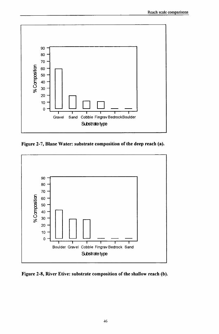
Reach scale comparisons
90 -
80 -
60 “
40 -
30 “
1----------1---------- 1----------1---------- 1----------TG rav e l S a n d C o b b le F in g ra v B e d ro c k B o u ld e r
Sitostratetype
Figure 2-7, Blane Water: substrate composition of the deep reach (a).
90 “
80 -
70 -
s 60 -
a 50 “
40 ~o 30 -
20 -
10 -
o -— I---------- 1------------ 1----------- 1----------- 1----------- 1—B o u ld e r G ra v e l C o b b le F in g ra v B e d ro c k S a n d
Substrate type
Figure 2-8, River Etive: substrate composition of the shallow reach (b).
46

Reach scale comparisons
90 -
80 -
70 -
j* 6 0 -
I 50 "£ 4 0 “O
30 “
20 -
10 -
0 - 1 1 1 1 1 1-----G ravel C o b b le S a n d B o u ld e r F in g ra v B e d ro c k
Sitostratetype
Figure 2-9, Duneaton Water: substrate composition of the shallow reach (b).
90
80
70
60
50
40
30
20
100
G ravel C o b b le S a n d F in g rav B e d ro c k B o u ld e r
Sitostratetype
Figure 2-10, Blane Water: substrate composition of the shallow reach (b).
Only two thirds of the 136 velocity profiles recorded at the three rivers could be
measured with sufficient accuracy to estimate the presence and depth of the laminar
47

Reach scale comparisons
sub-layer. In cases where it was impossible to measure velocity profiles accurately this
was due to the gross turbulence of the water and it is reasonable to assume that a
laminar sub-layer would be prevented from forming in such conditions. Laminar sub
layers were rarely present elsewhere and when present were <lmm thick (Table 2-4).
Table 2-4, Characteristics of the laminar sub-layer of the boundary layer.
SITE N Depth of Laminar sublayer
SmoothPresent
TransitionalDisrupted
RoughAbsent
Etive 27 0.4 mm 8 12 15Duneaton 34 0.9 mm 8 20 9Blane 36 1 mm 3 11 17
2.3.4 Distribution of Turbulent and Laminar flow within reaches
Water flow at all sites was predominately turbulent or transitional, see Figures 2-11 to
2-13. Where flow was laminar it was in shallow water, near the channel margins. Flow
was also predominately sub-critical (tranquil) as determined from critical values of
Froude number.
48

Reach scale comparisons
10
10
10 '
Turbulent
10 '
10 '
Lam inar
1 0 ' 10 ' 10 10 '
Velocity M/s
10 10 10 '
Figure 2-11. Variation in turbulent flow in the River Etive. O denote the shallow reach and + denote the deep reacl^ The parallel lines demarcate the area of transitional flow Re = 500-2000 (Smith 1975).
Turbulent
ooQ .O)O + +
1 0 '1
+ +oocol + +
o oLaminar oo oo
10"1Velocity M/s
Figure 2-12. Variation in turbulent flow in the Duneaton Water. O denote the shallow reach and + denote the deep reach. The parallel lines demarcate the area of transitional flow Re = 500-2000 (Smith 1975).
49

Reach scale comparisons
Turbulent
o o
Q .(0o
10 '1
+ t+
+ oLam inar
10"1Velocity M/s
Figure 2-13. Variation in turbulent flow in the Blane Water. O denote the shallow reach and + denote the deep reach. The parallel lines demarcate the area of transitional flow Re = 500-2000 (Smith 1975).
2.3.5 Species lists
A comparison between the species composition of the reaches was performed on a
river by river basis. Table 2-6 gives the taxa list for all sites. A comparison of the
invertebrate assemblages in the deep and shallow reach of each river was performed
using TWINSPAN analysis, but it did not separate them clearly; data shown in
Appendix IV. At both the Blane and the Duneaton Water either the Chironomidae or
Ephemeroptera were numerically dominant. In the R. Etive, Trichoptera (mainly
Hydroptila sp.) were the most dominant with Ephmeroptera and Chironomidae the
next most dominant groups.
50

Reach scale comparisons
Table 2-5. List of taxa present in the deep (A) and shallow (B) reaches of the three rivers. Some taxa were identified to different levels depending on the quality of specimens. Chironomidae from the R. Etive were identified to genus and are presented in a second table. Names standardised to those in (Maitland 1977).
Operational Taxonomic Units OTU Etive Blane Duneaton
code
A B A B A BOligochaeta Olig 48 10 26 22Lumbricidae Lum 2 1Hirudinea Hir 8 4
Succinea Sue 3 1Ancvlus fluviatilis Muller Anfl 14 40 12 5Potamopvrgns ienkinsi (Smith) Poie 1 1
Hvdracarina Hvdra 7 1
Gammarus pulex (L.) Ganu 19 72 3 4Asellus aquaticus (L.) Asaq 6 18
Limnius volckmari (Panzer) Livo 23 29 41 71 8 45Oulimnius Ouli 0 2 35 48Oulimnius tuberculatus Outu 27 8Oulimnius troglodytes Outr 0 1Esolus parallelepipedus Espa 5 3Elmis aenea (Muller) Elan 19 44Dvtiscidae Dvti 2 0Dvtiscidae Oreodvtes? Dvor 5 1
Chironomidae Chir >1000 >1000 527 129Tanvnodinae Tanv 10 9Orthocladiinae Ortho 13 31Diamesinae Dia 0 2Simuliidae Simu 0 3 0 75Tipulidae Tinu 13 6 53 100
Baetis rhodani (Pictet) Barh 12 24 4 43 8 64Baetis scambus Eaton group Base 3 9Caenis rivulorum Eaton Cari 1 14C. luctuosa (Burmeister) Calu 0 1Ephemerella ignita (Poda) Enig 23 16 526 597 107 185Ecdvonurus Eaton Ecdv 0 2 67 75 86 265Rhithrogena semicolorata Rise 1 4Heptagenia Walsh Hept 2 7Ephemera danica Muller Enda 0 1Siphlonurus armatus Eaton ? Siar 0 1
Leuctridae Genus? Lege 77 99 3 5Leuctra moselvi Morton Lemo 3 2 28 92Leuctra fusca (L J Lefu 2 49Perlodes microcephala (Pictet) Pemi 0 2 0 1Perla bipunctata Pictet Pebi 0 1
51

Reach scale comparisons
Operational Taxonomic Units OTU
code
Etive Blane Duneaton
A B A B A B
Hvdrovtila so. Dalman Hvdr 86 21Oxvethira sp. Oxvt 16 1Polvcentropus kingi McLachlan Poki 3 4Polvcentropus flavomaculatus Pofl 8 5 1 0Plectrocnemia conspersa Pico 1 3Rhvacophila septentrionis Rhse 1 2Rhvacophila dorsalis (Curtis) Rhdo 1 3 0 3Agravlea multipunctata Curtis Agmu 0 1Hvdropsvche so. Hvdro 0 10Hvdropsyche siltalai Hvsi 3 6Rhvacophilidae Agapetus Rhag 0 4Glossosoma boltoni Curtis Glbo 2 66Lepidostoma hirtum (Fabricius) Lehi 3 0Anabolia nervosa Curtis Anne 9 0Agapetus fuscipes Curtis Agfu 1 11Psvchomvia pusilla (Tabricius) Psou 7 0Number of taxa 18 25 18 17 21 26Number of individuals 266 202 829 1196 930 1087
Table 2-7. List of Chironomidae present in the slow (A) and fast (B) reaches of the River Etive.
Taxa OTU code A B
TanypodinaeAblabesmyia annulata group 2 0Paramerina 5 2Trissopelopia 2 6Nilotanypus 0 1Macropelopia 1 0OrthocladiinaeCricotopus 7 21Heterotany tarsus 1 0Thienemanniella 2 0Tventenia 2 10Orthocladiinae Genus II 1 0ChironominaeVirgatany tarsus 0 1Tanytarsus 6 4Rheotany tarsus 5 1Total 11 6
52

Reach scale comparisons
Reach preferences of taxa
Correlation between deep and shallow section community structure was tested by the
non-parametric (G)amma Test on a contingency table based on table 2-6 . For the R.
Etive communities correlation was moderate G = 0.59, P < 0.0001, at the Duneaton
Water the correlation was weaker G = 0.45, P < 0.005 but at the Blane Water the
correlation was particularly strong, G = 0.67, P <0.001. Note however that for the
Blane Water the Chironomidae were excluded from the analysis as their numbers were
only estimates.
River Etive
Invertebrates from both the deep and shallow reaches were more typical of riffle fauna
than pool. Occurrence of animals was low, (468 specimens collected) reflecting the
poor nutrient status of the river. A total of 38 taxa was recorded from the two reaches,
29 taxa from the deep (pool) reach and 32 from the shallow (riffle) (note
Chironomidae were identified to genus level where possible for Etive samples but not
for the other sites, increasing the number of taxa). A biodiversity index of similarity
was calculated for the two reaches PSc = 52% (Cowan & Peckarsky 1990). This
indicates only a medium degree of similarity between the two reaches. OTU were
tested for differences in distribution between the two reaches using the Mann-Whitney
U test. Only two OTU showed a statistically significant preference for either reach.
Median abundance of Hydroptila spp was greatest in the pool reach, (W = 860.0,
P<0.001 adjusted for ties) while Caenis rivulorum median abundance was greatest in
the riffle reach (W = 610, P<0.05 adjusted for ties).
53

Reach scale comparisons
Duneaton Water
In total 2017 animals were collected. A total of 47 taxa was recorded from the two
reaches, 21 taxa from the deep reach and 26 from the shallow. OTUs were tested for
differences in frequency distribution between the two reaches using the Mann-Whitney
U test. The abundance o f benthic invertebrates was compared between the shallow
(run) and deep (pool) using the Mann Whitney U test. The test was applicable to 19
OTU (other OTUs had extremely low abundances and were excluded). Ecdyonurus
had a median preference for riffles (P<0.001). Other Ephemeroptera, Baetis rhodani
and Ephemerella ignita also showed a strong preference for the run reach (P<0.05).
Both species of Leuctridae showed a preference for the run reach as did the riffle
beetle larvae Limnius volkmari (P<0.05). The Tipulidae also showed a strong
preference for the run reach (P<0.05). The only OTU with a significant preference for
the pool was Oulimnius tuberculatus (P<0.05).
Blane Water
Excluding chironomids, a total o f 2025 animals was collected. In both reaches
chironomids were estimated at greater than 1000 individuals and not identified further.
A total o f 35 taxa was recorded fr om the two reaches, 18 taxa from the deep (run)
reach and 17 from the shallow (riffle). OTUs were tested for differences in distribution
between the two reaches using the Mann-Whitney U test. The abundance o f benthic
invertebrates was compared betweem the riffle and run using the Mann Whitney U test.
Other OTUs had extremely low abundances and were excluded. Baetis rhodani and
Glossoma boltoni showed a strong preference for the run reach (P<0.05).
2.4 Discussion
54
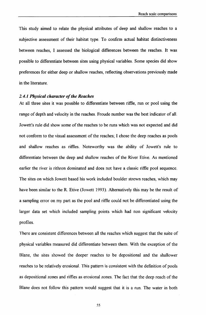
Reach scale comparisons
This study aimed to relate the physical attributes of deep and shallow reaches to a
subjective assessment of their habitat type. To confirm actual habitat distinctiveness
between reaches, I assessed the biological differences between the reaches. It was
possible to differentiate between sites using physical variables. Some species did show
preferences for either deep or shallow reaches, reflecting observations previously made
in the literature.
2.4.1 Physical character of the ReachesAt all three sites it was possible to differentiate between riffle, run or pool using the
range of depth and velocity in the reaches. Froude number was the best indicator of all.
Jowett's rule did show some of the reaches to be runs which was not expected and did
not conform to the visual assessment of the reaches; I chose the deep reaches as pools
and shallow reaches as riffles. Noteworthy was the ability of Jowett's rule to
differentiate between the deep and shallow reaches of the River Etive. As mentioned
earlier the river is rithron dominated and does not have a classic riffle pool sequence.
The sites on which Jowett based his work included boulder strewn reaches, which may
have been similar to the R. Etive (Jowett 1993). Alternatively this may be the result o f
a sampling error on my part as the pool and riffle could not be differentiated using the
larger data set which included sampling points which had non significant velocity
profiles.
There are consistent differences between all the reaches which suggest that the suite of
physical variables measured did differentiate between them. With the exception of the
Blane, the sites showed the deeper reaches to be depositional and the shallower
reaches to be relatively erosional. This pattern is consistent with the definition of pools
as depositional zones and riffles as erosional zones. The fact that the deep reach of the
Blane does not follow this pattern would suggest that it is a run. The water in both

Reach scale comparisons
reaches o f each river was predominately turbulent with laminar flow being rare. This is
also consistent with the findings of other studies and the predictions of
geomorphologists.
Others using a more descriptive classification of near bed flows have suggested that
the habitat classifications o f pool, riffle and run do not necessarily apply to near bed
habitats as all their near bed flow categories were recorded in each class (Young
1993). It is perhaps better to view these habitat classes as aggregates of smaller habitat
units especially as they do have some biological significance, see below.
2.4.2 Biological character of the Reaches Diversity
The riffle reaches supported greater numbers o f taxa than the deep reaches conforming
with the norm in other studies, see introduction for references (reach 1.1. paragraph
9); however again the Blane was an exception.
Species composition
Ephemeroptera and Chironomidae dominated the fauna at all sites a situation noted in
previous comprehensive surveys o f the summer fauna of highland rivers, (Morgan &
Egglishaw 1966). The methods employed by Morgan and Egglishaw were similar to
the one I used, being a combination of disturbing sediment and stone scrubbing adding
a degree of certainty to the comparison. This result reflects the seasonality in relative
abundance of taxa as the same survey found the spring fauna to be dominated by
Plecoptera and Ephemeroptera and suggests applying data gathered on benthic
commmunity structure and composition in one season to other seasons is potentially
misleading.
Hydroptilidae were detected in the River Etive in high numbers but not at the other
sites. This may again reflect a seasonal effect as the R. Etive was sampled later in the
56

Reach scale comparisons
summer, in August, than the other two sites. This hypothesis is supported by a
seasonal study on invertebrate fauna in another Scottish river, Shelligan Bum a
tributary of the River Almond, where Hydroptilidae were detected in low numbers
until August when their numbers increased (Egglishaw & Mackay 1966). As the taxon
is known to occur in both the Blane Water and the Duneaton Water (SEPA pers
comm.) it would seem likely that the effect is seasonal rather than the R. Etive being a
site o f particular suitability for the taxon. Further evidence is that during their sampling
of the R. Etive Morgan & Egglishaw (1966) found the taxon in low numbers; their
sampling was in July, the same period the my sites were sampled.
Caseless caddis were represented by more species in all rivers than cased; the Blane did
have the highest number of cased species. Again this mirrors the findings of other
workers (Armitage & Gunn 1996; Morgan & Egglishaw 1966) who also found as I did
that the Orthocladiinae dominated the chironomid fauna. The Etive was the most
extreme in this respect with the largest number of caseless caddis species represented
of all the rivers and probably reflects the instability of depositional habitat within the
site; the larger boulders and lack of small substrate elements at the site attest to this.
Cased caddis do tend to require more stable conditions on the whole. Both the Blane
and the Duneaton had greater amounts of finer substrate, no or few boulders and
greater numbers of cased caddis species than the Etive. Using riffles, pools and rock
outcrops as mesoscale habitat units others have identified functionally distinct caddisfly
communities (Huryn & Wallace 1988). There is some evidence from this study that this
might be occurring here too. The Hydropsyche larvae preferred the fast reaches,
Anabolia nervosa and Glossoma boltoni favoured the slower reaches and there is the
possible link between Hydroptila spp. and boulders. Some of these relationships are
57

Reach scale comparisons
not statistically significant and the functional feeding strategies of some of the species
need to be clarified.
Other unique aspects of the R. Etive species assemblage is the absence of both
Mollusca and crustacean macroinvertebrates which is likely to be a product of the
underlying geology as is the case with the high numbers of Mollusca in the Blane
Water (Egglishaw & Morgan 1965). Macan (1977) divides the British freshwater
molluscs into two major groups based on their preference for hard or soft waters.
Calcium which is needed to form shells is the underlying determinant for separating the
two groups and is an element which is likely to be in short supply at the R. Etive.
Individual species responses in relation to site specific factors
A number of species showed preferences for either deep or shallow reaches,
suggesting that for some invertebrates at least, the different types of reaches represent
habitat units. How Hydroptila species avoid getting washed out of the Etive system is
interesting to ponder; it may be that their small size allows them to seek refuge in the
filamentous algae on which they are known to feed. I observed in the field that the
greatest amounts of filamentous algae were on boulder tops, submerged in the deep
reach, a most stable substrate. Alternatively the preference of Hydroptila species for
the deep reach for the R.Etive may be explained by the need of this taxon for very fine
sand grains to form cases during it's last instar (Wallace 1981). Sand did occur with
greater frequency in the deep reach of the river. Hydroptilidae also had a significant
preference for pools in the Almond Water (Egglishaw & Mackay 1966). Caenis
rivulorum the only other animal found to have a preference in the R.Etive was found
by Armitage (1976) to prefer the 'intermediate' (0.2-0.6 ms'1) reaches of the R. Tees,
which has comparable velocities to the Etive riffle reach.
58

Reach scale comparisons
The preferences exhibited by both mayfly and stonefly in the Duneaton water (run) for
faster reaches have been observed elsewhere in British rivers, in the Tees (riffle), the
Afon Hirnant (riffle) (Hynes et al. 1976) and the Almond (riffle), although the reflected
patterns were not perfect. In the Tees, Leuctra fusca and Ecdyonurus dispar were
among some of the few taxa to show no preferences, whereas in the Almond
Ecdyonurus spp. were in greatest abundances in the pools in April and the riffles in
September. Morgan & Egglishaw (1966) believed this seasonal variation was due to
different preferences being exhibited either by Ecdyonurus spp. instars or species.
Alternatively they believed that pre-emergence behaviour altered the animals habitat
choice. Again it is interesting to note that Limnius volckmari had a preference for the
pools in the Tees which were o f similar velocity range as the run in the Duneaton
water to which it was also partial (Rosillon 1988).
Contrary to its previously reported preferences I found Tipulidae to occur most
frequently in the riffle of the Blane which is difficult to explain. Easier to explain, yet
equally at odds with previous studies, is the preference exhibited by Baetis rhodani for
the run reach. An extensive study covering a greater number of rivers found Baetis
species indicative of riffles (Harper et al. 1998). This trend can be seen in the
Duneaton Water where Baetis rhodani also showed a preference for the run. The fact
that the animal occurred with greater frequency in the run of the Blane Water suggests
that it was avoiding the riffle reach o f the stream (the run reach was immediately
downstream of the riffle). Drift rates of baetid mayfly have been experimentally shown
to be greater during spates (Lancaster 1992). Harper's study (1998) also showed
Caenis species as being indicative of silted riffles and runs whereas my data suggests
they occur preferentially in the shallow reaches of the R. Etive.
59

Reach scale comparisons
Some OTUs showed differential preferences for the reach types present at different
sites. Based on substrate type the R. Etive experiences the highest shear forces of the
three rivers with the Duneaton Water having the next highest. As the substrate was
only sampled to a depth of 10cm, composition of the armoured layer only was
measured. Hence the substrate types reflect the rivers’ recent past only. Any larger
substrate elements will have been buried by more minor spates. In this context the R.
Etive is likely to have more intense spates than the other two rivers, as one would
expect from the steep gradients in the catchment. I suggest that the intensity of recent
disturbance at the three sites, as experienced by invertebrates is most intense in the R.
Etive, least intense in the Blane Water and intermediate at the Duneaton Water. This
measure does not differentiate between disturbance events with high frequency, low
force and low frequency, high intensity. There is also the possibility that the armoured
layer, if compacted by low intensity spates becomes more resistant to entrainment and
this index based solely on substrate type could underestimate the resistance of the
substrate. This is most likely at the Blane where the substrate appeared quite compact.
2.5. Conclusions
2.5.1 Physical study• Jowett's rule accurately differentiated between riffles and pools; it also identified the
deep reach of the Blane as a run highlighting the danger of choosing a site during
one set of flow conditions and sampling under another. It also classified the R. Etive
reaches into pool and riffle although geomorphologists would disagree on the
grounds of the highly erosional nature of the stream and ecologists on the basis of
the predominantly riffle type fauna of the ‘pool’. In rivers of high slope the rule
should probably be applied with caution if at all.
60

Reach scale comparisons
• Separating pools, runs and riffles on a subjective observational basis is insufficient
on the evidence of this study. Some measurements of velocity and depth need to be
performed.
• A large proportion of the physical variability between the riffles and pools was
consistent between sites. Further the mixture of substrate in the deep and shallow
reaches suggested that they were depositional and erosional zones respectively.
• Flow was turbulent in all reaches with a measurable laminar sub-layer being rare. I
conclude that at the substrate surface oxygen is unlikely to be a limiting factor.
2.5.2 Biological study• Each river had a unique assemblage of invertebrates, although there was a large
degree of overlap in composition between sites. Differences could be explained by
comparing my results with previous studies on the distribution o f invertebrates in
relation to geology and water chemistry.
• Riffles supported a greater diversity of species than the pools although the
assemblage of species in both pools and riffles were not sufficiently different to
separate them using TWINSPAN.
• Some species showed preferences for either deep or shallow reaches, these
preferences were usually site specific and reflected a large number o f local factors,
but velocity and substrate type are probably the most important.
• Based on the physical and biological data it seems clear that riffles and pools
represent local combinations o f physical habitat conditions which alter temporally
and are fundamental to maintaining the diversity of macroinvertebrates in Scottish
rivers.
61

Reach scale comparisons
• Most taxa can survive outwith their preferred habitat unit (either riffle or pool)
suggesting that their own physical habitat preferences are acting on a smaller
physical scale.
• The species that make up the assemblages are likely to exhibit preferences for the
environmental variables associated with pools and riffles e.g. depth, velocity,
substrate type etc. The evidence also suggests that these variables are fundamental
to niche separation among the species present. This is explored in the next two
chapters.
62

Community ordination
Chapter 3: Benthic invertebrate community ordination
3.1 Introduction
3.1.1 Outline
The purpose of this chapter is to examine the distribution of benthic invertebrates in
relation to hydraulic environmental variables at a finer physical scale than the previous
chapter. The data presented here reflect the habitat complexity on an intra-reach scale
and gives some indication of inter-river variation. The analysis consists of two stages:
the first attempts to find structures in the invertebrate community e.g. associations or
clumps o f species from samples within the same river. The second stage tries to relate
community organisation to environmental factors. By using ordination and cluster
analysis it was hoped to identify groups of invertebrate species with indicator species
which have similar flow requirements.
3.1.2 Physical patchiness
The design of a program monitoring the ecohydrological health of rivers could
successfully incorporate the results of such analysis. By exploring species distribution
independently of environmental variables in the first instance the two stage process has
the advantage, of following (Pringle et al. 1988) advice - 'that variability among
patches in lotic systems be viewed as valuable information rather than statistical
noise to be overcome by manipulating sampling protocols'.
Hildrew & Giller (1994) explored the link between habitat patchiness, scale,
disturbance and the stream benthos. They made the link between the concept of habitat
template (the river: Southwood 1988) and benthos, pointing out that although the river
63

Community ordination
habitat is heterogeneous, clumping or aggregation o f similar types of habitat is
common:
"Undoubtedly the major architects o f physical patchiness in streams are the forces o f
flow. Flow is scale-dependent, being heterogeneous and 1aggregated' (i.e. different
habitat "patches' have different average flow characteristics) at different spatial
scales ranging from the sub-millimetre to whole river reaches or entire drainage
networks. "
3.1.3 Spatial aggregations
The more obvious aggregations include riffles and pools (which were the subject o f the
previous chapter), but within these there occur smaller habitat units. In a diagram
illustrating scale effects (Hildrew & Giller 1994) showed fine gravel patches, moss on
boulders, transverse bar o f cobbles and sand and silt over cobbles as aggregate units at
the 'microhabit scale (1 0 1 m ). By using cluster and ordination methods it might be
possible to reflect this pattern, by clumping species together that occur in the same
habitat aggregates. Although the quadrat size used to sample invertebrates is on a
comparable scale (sample area = 0.0625 m2) to the microhabit scale, in my study there
was the possibility of sampling across two or more discrete habitat units, due to the
random choice of sampling points. All physical variables were measured on continuous
or integer scales so that taxa responses to variables could be observed even when more
than one microhabit was sampled.
3.1.4 Assessment of the ecohydrological health of rivers
Research in this area is driven by two forces, firstly the pure scientific interest in niche
separation and habitat patchiness in rivers and secondly the development of
conservation and monitoring strategies for river health using responses of benthic
64

Community ordination
invertebrates to flow in regulated rivers. The 1999 draft of the EC Water Frameworks
Directive (19 February 1999) underlines the potential importance of this type of study.
The draft requires member countries to identify high quality reference sites for surface
waters, including rivers (Annex II section 1.3, paragraph iv). Ecological status is to be
defined using biological and hydromorphological elements. The hydromorphological
elements are defined as those which support the biological element and include
hydrological regime, river continuity and morphological conditions; depth, width,
structure of bed and substrate type (Annex V section 1.1.1). Under the directive these
pristine rivers would form a standard all other rivers would have to reach. In
preparation for this legislation SEPA are currently trialing Instream Flow Incremental
Methodology (IFIM, (Bovee 1982)) and its associated computer programme Physical
Habitat Simulation (PHABSIM). PHABSIM is one of a number o f models which
evaluate riverine physical habitat, specifically it models the available habitat for aquatic
species at different discharges (Johnson & Law 1995). Its successful application
elsewhere as a means of estimating instream habitat make it a suitable candidate ( e.g.
(Armour & Taylor 1991) reports 616 applications o f IFIM up to the early 1990s in the
United States alone). Both the methodology and the program have mainly been applied
to salmonid fisheries management (Armour & Taylor 1991; Johnson et al. 1995;
Jowett 1998; Strevens 1999). This list o f references is not by any means exhaustive:
rather it is intended to give the reader a representation of the work being carried out on
different continents.
IFIM has been used to estimate habitat suitability curves for benthic invertebrates
(Jowett et al. 1991) and PHABSIM predictions o f increased habitat availability for
benthic invertebrates in artificial riffles have shown positive and significant correlations
65

Community ordination
with actual measures of increased biodiversity (Gore et al. 1998). By using a variant of
IFIM developed for collecting data on benthic invertebrates (Jowett et al. 1991) in the
work reported here, it is hoped to make the work comparable to other similar studies.
When using PHABSIM there can be a conflict between the flow requirements of
different species. One aspect o f this study is to attempt to find clusters or guilds of
species associated with combinations of flow variables which simplifies this
management problem. This technique has been successfully applied to the management
of fish stocks (Jowett & Richardson 1995).
Criticism can be levelled at PHABSIM on a number of fronts, probably the most
fundamental being that annual flows for a river are determined from one or few 'snap
shot' IFIM studies which only reflect the fauna's preferences at the time of sampling.
Another serious problem is that PHABSIM assumes 'that target organisms have
specific microhabitat preferences and the ability to move to areas o f suitable
hydraulic conditions in response to changes in stream discharge' (Layzer & Madison
1995). Although this is obviously the case for invertebrates which end up in flow
refugia during spates (Lancaster & Hildrew 1993b), as Layzer and Madison point out
these assumptions do not apply to sessile or slow moving invertebrates e.g. Mollusca.
(they also point out that their study organism, freshwater mussels, appears to have
different flow preferences at different discharges). Neither does PHABSIM address the
importance of disturbance flood events which redistribute and alter the species
composition of riverine invertebrate communities (Boulton et al. 1992; Brooks &
Boulton 1991; Cobb et al. 1992; Dudgeon 1993; Hildrew & Giller 1994).
The aims of this chapter are to test the structure of the benthic invertebrate community
at the surber sample scale, identify any aggregations in the distribution of taxa and
66

Community ordination
estimate the influence of flow variables on the variation in community structure using
multivariate analysis. The hypothesis is that the distribution of benthic invertebrates
should be clumped and that flow variables should describe a large amount of the
variation. The interrelations between the environmental variables are described in this
context.
By addressing these questions PHABSIM is also tested indirectly, as it assumes that
benthic invertebrates are responding to flow variables at this scale, in a predictable
manner.
3.2 Methods
3.2.1 Data Collection and Dataset Structures
Collection methods for data examined here are described in the previous chapter. For
each river data from both reaches were amalgamated into a matrix of taxa by sites, and
a second matrix containing environmental variable by site data. For each river the
ordination was attempted using an environmental variable data set which contained
variables derived from velocity profiles.
The profiles were measured at all points where invertebrates were sampled. For each
profile, velocity should show a linear relationship with log depth if a full developed
boundary layer exists and the layer is not disturbed by gross alterations in water
movement, e.g. a velocity profile taken downstream of a semi submerged boulder may
show a log linear relationship at the depths above the boulder but back edding may
distort the profile lower down. Not all profiles had significant R2 values and these were
discarded as near bed flow variables could not be calculated from them being
dependent on the log linear relationship between depth and velocity being intact, see
67

Community ordination
chapter 2.2.4 and Annexes II and III. It has been suggested that some data could be
salvaged from these profiles. The mean water column velocity was calculated for these
points from the profiles allowing their inclusion in the ‘larger dataset’, see below.
An alternative method of salvaging data from the profile was to use them to estimate
turbulence above the bed, using their deviation from the predicted log-normal
relationship as a turbulence surrogate. Given that turbulence at the bed is the factor of
most interest, as that is where the animals are and, not turbulence further up the water
column, the use of the profiles in this way was not suitable.
Two data sets for each river were now analysed. The dataset containing sampling
points for which velocity profiles were intact and a second larger dataset which
included all sampling points where invertebrates were sampled. The larger datasets
contained a more limited array of environmental variables; mean water column
velocity, depth, % sand, % fine gravel, % gravel, % cobble, % boulder and % bed
rock. The smaller datasets with significant velocity profiles also contained these
measures.
Where the smaller data sets proved unsuitable the larger parent data set was used
instead, see section 3.3.1. For the R. Etive where many taxa occurred in few samples
the data set excluded taxa occurring in less than 5 samples.
3.2.2 Analysis procedure
The production of an ordination analysis requires refinements to the input data which
influences the final result as does the structure of the data sets involved. Initially a
TWINSPAN analysis was carried out on the data from each site and the groups
overlaid in a Detrended Correspondence Analysis (DCA) taxa scatter plot. As
TWINSPAN and DC A both use the same algorithm to order a species by site matrix
this process is acceptable. This allows TWINSPAN groups to be visualised in an
68

Community ordination
ordination diagram as opposed to a dendogram aiding interpretation and allowing
comparison with constrained ordinations (see last paragraph for an expanded
explanation). No TWINSPAN analysis was performed on the Blane Water data
because DCA showed the length of the environmental gradient to be short suggesting
taxa were exhibiting linear responses to the environment. As TWINSPAN is based on
a unimodal model it was not applicable.
Outlined below are the methods used to derive the final ordinations, highlighting the
peculiarities o f each river's data set and the refinements made. For each site a DCA
was carried out initially to measure the length of the environmental gradient as
suggested by the CANOCO computer program help (ter Braak 1997, 1998).
Depending on the length o f the gradient, either a unimodal (gradient >3-4 s.d.) or
linear (gradient <3 s.d.) based ordination technique was used. The results o f each
ordination were interpreted with the aid of the explanations given in the CANOCO
manual, chapter 6 (ter Braak & Smilauer 1998) and adjusted where necessary.
Constrained ordination techniques (Canonical Correspondence Analysis (CCA),
Redundancy Analysis (RDA)) have been criticised for being potentially misleading
(McCune 1997), so some clarification of their purpose is useful. Other ordination
techniques which are not constrained describe community structure e.g. DCA scatter
plots will clump species together which co-occur. Constrained ordination techniques
do not: primarily they relate species distribution to environmental variables. If one
wishes to relate community structure to environmental variables one should apply an
indirect gradient analysis and subsequently relate this ordination to environmental
variables, e.g. DCA and superimpose the environmental variables on top of a scatter
diagram. Jongman et al. (1988) suggests a number of methods for relating
69
Community ordination
unconstrained ordinations to environmental variables. Another useful alternative is to
first carry out an unconstrained analysis and compare it to a constrained one as is the
case herev\Here I compared DCA to CCA, though there has been the criticism that
DCA should only be compared to DCCA, presumably on the basis that both are
detrended. Detrending is a remedial tool for fixing the ‘arch effect’ in ordinations
(Jongman et al, 1988). It was not necessary to apply it to the C C ^ here. A dataset
which produces an arch effect when processed by unconstrained ordination does not
necessarily do so when the ordination is constrained (Jongman et al 1988). That was
the case here. The arch effect occurs for two fundamentally different reasons in CA
and CCA. In CCA diagrams it is usually caused by the inclusion of too many
environmental variables whereas in CA it a mathematical artifact caused by the
structure of the species by samples data set. Although detrending alters the position of
points in an ordination, their relative positions to one another should remain relatively
constant making it feasible to compare between ordinations.
River Etive
The length of the environmental gradient as determined by DCA was long (Axis 1 =
4.135 s.d ), so a unimodal based analysis was used i.e. CCA. The best four explanatory
variables were chosen using forward selection. The variables % bed rock (1 sample) ,
% fine gravel (6 samples) and % sand (1 sample) were not used in the analysis as all
occurred in very few samples. They were included as passive variables only. The taxon
Oxythira was used passively after demonstrating a much stronger relationship with axis
1 & 2 than all the other species.
70

Community ordination
Duneaton Water
The length of the environmental gradient as determined by DCA for the larger data set
was between 3 and 4 s.d. (Axis 1 =3.05 s.d.), the cut off point for selecting either a
linear or a unimodal based analysis. In this instance either a unimodal or linear method
is applicable, CCA was chosen. Log transformation of the species data reduced the
variance in the species data explained by the first two ordination axes to 11.4% and the
explained variance in the fitted species data from 78.7% and was not applied in the
final analysis. Extreme values were detected for 7 samples, but all ‘really belong to the
population’ (ter Braak & Smilauer 1998, pi 18) so these outliers remained in the
analysis. Of the possible variables used in the analysis, both % composition of boulder
and % composition o f fine gravel were excluded as both substrate types were found
very infrequently (n = 2 and n = 6 samples respectively) causing them to appear to be
collinear with the variable % composition of sand. None of the remaining variables had
a variance inflation factor >20 indicating that they all had a unique contribution to the
canonical ordination.
Blane
A DCA of the Blane Water species data set (40 useable samples) showed the gradient
length to be less than 3 s.d. (2.505) suggesting a linear as opposed to a unimodal
model was most applicable e.g. redundancy analysis (RDA). RDA analysis was not
significant for all canonical axes taken together (Monto Carlo test full model p =
0.085) although the first axis was significant (Monto Carlo test p = 0.015).
Constraining the ordination with environmental variables was not significant, so the
species data are presented in an indirect gradient analysis ordination, Principal
Components Analysis (PCA). Four samples had extreme values for some of the
71

Community ordination
environmental variables but did not reflect any detectable mistakes in data collection so
they were not removed from the analysis.
3.3 Results
3.3.1 Suitability o f data sets
For all sites, the data subsets containing variables derived from velocity profiles
produced ordinations with no significant canonical axes (Monto Carlo Permutation test
p > 0.05), see table 3.1.
Table 3-1, Eigenvalues and their significance from ordinations performed using parameters derived from velocity profiles as environmental variables. For the Duneaton Water and River Etive the ordinations were CCA, for the Blane Water the ordination was an RDA. Permutation tests were Monto Carlo tests carriedout using 199 randomly seeded runs.______________________________________River Axis 1 All
canonical
Axis
Eigenvalue F-ratio P-value Sum of all F-ratio P-value
eigenvalues
Blane 0.134 3.875 0.91 0.185 0.566 0.88
Water
Duneaton 0.141 1.951 0.665 0.539 0.997 0.435
Water
River Etive 0.133 2.003 0.33 0.45 1.056 0.345
72

Community ordination
3.3.2 River Etive
The DCA scatter plot (figure 3-1) shows two major groups as split by TWINSPAN on
its first iteration (TWINSPAN eigenvalue = 0.705). Further iterations produced splits
which had low eigenvalues and were not used (0.350 or less).
Monto Carlo tests of the first canonical axis o f the CCA and all the canonical axes
together were significant (p = 0.005, F-ratio 3.516 and 2.361 respectively). The biplot
(Figure 3-2) based on the first two canonical axes explains 11.3% of the variance in the
species data and 67 .4% of the variance in the fitted species data.
Sim
OulR ise
Pem i
Livo
Dia
Barh
Hep PebiOrth CanEcdyOlig
Lemo
DytTany
+0 . 0 Chir
0 . 5 + 5 . 5
Figure 3-1 Etive DCA. TWINSPAN group A is enclosed by the polygon, all other taxa are in Group B. See chapter 2 tables 2-6, 2-7 for a key to the species codes.
73
Community ordination
Axis 1 (eigenvalue 0.38) can be interpreted as a microhabitat gradient from erosional
to depositional conditions. Velocity and % cover of cobble are most strongly
correlated with Axis 1 ( weighted correlation 0.69 and 0.41 respectively). Depth and %
cover of boulders are both negatively correlated with Axis 1. Axis 2 (eigenvalue 0.24)
is most strongly correlated with % cover of boulder and cobble. The coarser material,
boulder, is unusually associated with slow flows, in reality boulders were found
throughout both sections but only in the deeper, slower areas, where they remained
submerged, and available to invertebrates. Only submerged boulders were sampled.
The smaller TWINSPAN group members are scattered throughout the right hand side
of the CCA diagram. Mayfly and stonefly species occur almost exclusively on the right
hand side of the CCA diagram as does the riffle beetle larvae Limnius volckmari. To
the right of the centre o f the diagram are Trichoptera larvae which require stable
substrates on which they can construct their filter nets. The left hand side of the CCA
plot is dominated by detritivorous Chironominae, Tanypodinae, Tipulidae and
Oligochaeta and the tiny Trichopteran genera Hydroptila and Oxyethira. These taxa
have known preferences for depositional areas, either for feeding or case building
material (Hynes 1972; Wallace et al. 1990). The presence of Orthocladiinae larvae in
samples with higher percentages o f cobble reflects a general trend within the
Chironomidae. Orthocladiinae prefer large substrate elements to the Chironominae and
Tanypodinae (Williams & Feltmate 1994). The Simuliidae were present at extremely
high velocities. Representatives o f both TWINSPAN groups occurred in each stretch,
with only two OTUs showed a strong preference for either deep or shallow stretches.
Scattered throughout the diagram are predators. The only cased caddis present were
members of the Hydroplilidae which are extremely small. Larger sized cased caddis
74

Community ordination
species were notable by their absence. Hence, the CCA ordination showed that the
observed differences in invertebrate occurrence could potentially be functionally
related to differences in habitat conditions which were paralleled in the literature.
o
B oulderCalu
PemiOuli
Rise • Cobble * .
/ SimuVelocity
Depth
Hydr I Epig- - - T
* • •Oxyt# Chir % |
Tipu Tany;
• BarhI-----Livo Can
• • Lemo Poki
Pebi
Hept
RhseOlig
Siar
1 . 0 + 1 . 0
Figure 3-2, CCA species-environment biplot for the R. Etive data. Variance added (A,k) for environmental variables: Velocity 0.32 (P = 0.005), Boulder 0.25(P = 0.005), Cobble 0.19(P = 0.015), Depth 0.15(P = 0.045), Gravel was not significant and was eliminated from the ordination. Only OTUs with an occurrence greater than 5 were used in the analysis. OTU codes are give in table 1-6 with the exception of the Chironomidae which were amalgamated in to subfamilies: Chironominae (Chir), Orthocladiinae (Orth), Tanypodinae (Tany) and Diamesinae (Diam).
75

Community ordination
3.3.3 Duneaton Water
The DCA scatter plot below (Figure 3-3) shows two major groups as split by
TWINSPAN (TWINSPAN eigenvalue = 0.784). Further splits by TWINSPAN had
low eigenvalues and were not used (0.345 or less).
For the final CCA, Monto Carlo tests of the first canonical axis and all the canonical
axis together were significant (p = 0.005, F-ratio = 7.373, 3.080 respectively). The
analysis used 5 environmental variables and orientated 28 species which occurred 353
times in the data set. The variance in the species data explained by the first two
ordination axes was 19.4% and the explained variance in the fitted species data from
was 67.7%.
76

Community ordination
Sim
RhdoLegeHyps
AgmuTip
BaseOliLemoChi
OutrBaerhoHyd
LehiHir Anne
LivoEpig
Gapu
Espa AnflOutu
Ecdy
Pemi
Sue
Glag
0 . 5 + 4 . 0
Figure 3-3, Duneaton Water DCA with TWINSPAN groups overlaid. Group A is enclosed in the polygon, group B includes all other taxa. See table 1-6 for OTU codes.
77

% Cobble
24.00 31.00
-.4995 .4109
.6931 .0223
1.0000%
Gravel
53.00 28.00
-.1308 -.5434
-.1309 .2465
-.5496 1.0000
% Sand
18.00 26.00
.7923 .0926
-.6234 -.2763
-.4968 -.2753
1.000
ocpT3 CP
PP<Ooo
~o £
o otOI—‘ to
a* oofl> rt < P— • 3& O-O3 Cl*
toov
toc/v-aVO
VOOvto
U)U )VO
oooo
to
CPpp<ooo
oCD
o x
noCT cr
ox00P3CL
& I 2 ©i *3 wP -*5T <!ceS* 2.' QTQ 3*<-K
CDa.n©*nCD
O3
3&2 .K‘T2.ire'sr
p3•ocTop
p2 .p 'O '
P9a.►
N»O
3“©nP3O3 'o’
o*nQ.S’pV*o’3C%O.
©c3C6P©3
acpT3
toVOVOcyi
-0Ov4L
OO
VOto
LO<01
OOOO
OvOOVOOV
to-PU)
toOv-oVO
oooo
o x
noCTcrCP
o
oVOVO
oU)VO00u>
oooo
oxwocatcp
o o I—* U)to to 4L U)00 u> o oo o
o o to 4Lto ■_ 4L -tLo vo o
o Oo
ou>toU)00
o O o o1—> to cyito Ov o U)OO - a to ■oVO to VO o
oooo
apP
CP ►—* •00O'r icpCL
00poCLp
CLCD<I ’oo
to
oxWocata
ox
OocrcrcT
CPpo<ooo
OCP
Table 3-2, W
eighted correlation
matrix
(weight
= sam
ple total)
for environm
ental variables and
Axis 1
and 2
of the
canonical ordination
used in
the R.
Etive
analysis.

Community ordination
As can be seen from Table 3-4, velocity is strongly positively correlated with cobble,
the larger more stable substrate element at the site, and is negatively correlated with
sand. Depth is not strongly negatively correlated with velocity as it often is at other
sites. Axis 1 (eigenvalue 0.404) is strongly positively correlated with the % sand in
samples and strongly negatively correlated with both mean velocity and % cobble.
Axis 2 (eigenvalue 0.175) is most strongly correlated with % gravel (negative) and
positively correlated with % cobble and mean velocity. The use of biplot scaling with
the focus on inter-species distances as used in the analysis of the Etive data resulted in
the species points clustering in the diagram centre making interpretation difficult and
the scaling was altered to inter-species scaling using Hill’s scaling (ter Braak &
Smilauer 1998). The species are grouped along axis 1 and to the left of axis 2 . The
Ephemeroptera and Plecoptera occur exclusively on the left hand side of the origin, the
other orders are scattered across the diagram depending on the preferences of their
composite genera.
TWINSPAN group A members, plotted in the Duneaton Water DCA remain
associated with one another in the CCA plot (Figure 3-4). Some group A members are
strongly associated with high percentages of sand and independent o f other variables
and can be found to the right of the diagram; Succinea, Hydrocarina, Chironomidae
and Ouliminius tuberculatus. Closer to the origin, and occurring in samples where
velocity and the percentage of cobble would be low, is Leptistoma hiratum and
Hirundinae. Closer to the origin where the mean of all variables occur are the
Oligochaeta and Gammarus pulex (which is a group B member). This suggests these
two taxa have a either a preference for the mean of all condition measured or are

Community ordination
Sim
VMo COBBLE
Outr*
LOCITY
Hydop
Suc SANDGlagLefJ Outu
BarhChi H?dLemo * japu
Oli *,LeGe G roup C y Lehi
Ecdy
LumAgmu Espa1
DEP™ Pemi.Ann<
GRAVEL
+4 . 01 . 5
Figure 3-4, Duneaton Water CCA. Group C enclosed by the box includes E. ignita, B. Scambus, L. volkmari and A. fluviatilis. Variance added by the environmental variables listed in order of their inclusion in the model; variance (A.A) values in brackets are the amount of additional variance explained by the inclusion of each variable sand (0.39 p = 0.005), cobble (0.14 p = 0.005), depth (0.09 p = 0.045), gravel (0.06 p = 0.205) and mean water column (mwc) velocity (0.06 p = 0.315).
ubiquitous in their presence. Anabolia nervosa, one of only two group A members not
closely associated with other group A members in the CCA shows a preference for
high % gravel and deep water. The other vagrant is Oulimnius troglodytes which has a
preference for high % cobble and fast water.
The taxa of group B show a more varied series of interactions with flow variables. At
the top left of axis 2 are two taxa, the Simuliidae and Rhyacophila dorsalis with a
strong affinity for high % of cobble and fast water. The Hydropsyche also have a
80

Community ordination
strong preference for fast water but their preference for high % of cobble is less. These
3 taxa can be found close together in the DCA plot. To the left of the origin there is a
group with no strong affinity for either velocity or depth. This grouping does prefer
samples with less sand and more of the other substrate types, it includes;
Glossomatidae (possibly Agapelus), Leuctra sp., Baetis rhodani, Baetis scam bus,
Ephemerella ignita, Ancylus fluviatilis and the Tipulidae. It is the largest of all the
groups. Strongly associated with deep water are the Lumbricidae, Agraylea
multipunctata and Esolus parallelepipedus.
3.3.4 Blane Water
The data used in the PCA covers 19 taxa which occurred, cumulatively 254 times in 40
samples. The variance inflation factors for all environmental variables were low (all <
2) suggesting that the variables are not highly correlated with one another which
agrees with their product moment correlations in Table 3-4, all o f which were less
than 0.5. Depth is positively correlated with both velocity and high percentages of
cobble. Velocity is not strongly positively correlated with % cobble as was expected
although it is relatively strongly and negatively correlated with % sand.
81

oha
SO so vOO ' O ' O ' O 'cdp3
<2*Oo
C/3 T lg 5 g. «OQ•~i
P<CD
nocrSicT
o o 1—1 On On •o1—1 4L to 4L LA ONJL to LA to 00 oto 00 -0 00 NO U>►—1 00 U)
toJL JL
LA 002 .
o q "5 “CDCL
3cdp3
HP2«r<*>
2srBftfta
oBsCDB
«!P3.695T
o o t—1 b—I to NOb U) O n o -o ON00 to 4L h—‘ JL i—»NO o NO to 4L oON o o to NO o-o to - J
Ot ot oLAU)
o O Ob b toU) NO 1— 1LA 4L Lk)00 00 -tL
o o o oto ’o b toto to u>t—1 00 NO LAo u> LA O
: O8\ OJ
o o •-*b P* oU> no o4L O O—] On O
o o o oH-* O~o o
oooo
c/3r +p3CL
a*CD<Bo3
ox
noc rct;cT
ef'
xoxrrj5’CD
OQ>-t%CD
32.il*<■*■ft
c .
BfttoB
PBa.pQ.a.CD■<
OBPBa.
T9*noa.B
oo 3 8"-J o Oi o
o xC/3P3C L
\ P3 tO8 NO oooo
i CD i P! 3I <f 2 * I o S 2.( r-KI'C
5 O ; O 8 O 8 O
! O! CD T3er
Com
munity
ordination

Community ordination
Glbo
AgfuBarh
MnVelRhdo
Anfl Hysi
Gapu
Li vo Elae Asaq
PoflDepth
Fine graOulPspu
Poje Epda
DyOr
Sand
- 1 . 01 . 0 +1.0
Figure 3-5, Blane PCA correlation biplot with environmental variables imposed over the ordination. Solid arrows = environmental variables, dashed lines = taxa. Scaling focuses on intcrspccies distances and the ordination diagram displays standardised species data (by dividing by their standard deviation) post transformation, and correlations. The values that can be inferred by the biplot rules are thus correlation coefficients(ter Braak 1997,1998)
The biplot in Figure 3-5 can be interpreted using the rules given by Jongman et al
(1987: p i27). The arrow for each taxon indicates a vector increasing in the direction of
increasing abundance for each species, arrows pointing in the same direction are
positively correlated, perpendicular arrows reflect a lack of correlation between the
variables represented by the vectors.
The species are scattered throughout the diagram with little grouping apparent. The
distribution of Limnius volckmari and Elmis aenea are closely correlated as are
Ancylus fluviatilis and Agapetus fuscipes. Glossoma boltoni increases in the same
83

Community ordination
direction as gravel, as does Rhyacophila dorsalis with mean velocity. A group of 3
species with similar distributions are Baetis rhodani, Hydropsyche siltalai and
Gammarus pulex. Potamopyrgus jenkinsi and Ephemerella danica are also similar in
distribution.
3.4 DiscussionThe constrained ordinations shows that clustering of the invertebrate data was limited
to two major groups at the Duneaton water and the R. Etive sites. The flow variables
in these constrained ordinations showed strong relationships between some taxa and
flow variables. The often observed selective occurrence of macroinvertebrates at either
erosional or depositional conditions were also observed here although, as found by
Barmuta (1989) community structure appeared more continuous in nature and
confirms the view of earlier researchers that the use o f substrate as a basis for
delimitation bottom fauna may be limited (Thorup 1966). These selective occurrences
reflected the preferences of most taxa for slow or fast reaches as observed in the
previous chapter.
The implications for IFIM based studies are profound. Although some taxa showed
similar responses to flow variables in the different rivers e.g. Rhyacophila dorsalis
others were inconsistent. This reinforces the argument that data collected at one site
should not be used to build a model for other locations. It also highlights that there
can be considerable variation in the response of a taxon to flow variables.
Improvements to sampling strategy for future work in this area are suggested and the
implications for how we should view the patchy nature of the stream bed are discussed.
Clustering of the taxa data from the Duneaton Water and R. Etive with TWINSPAN
split both site communities into two main groups. For each site the composition of the
two groups produced was very different, probably reflecting site specific factors. The
84

Community ordination
smaller Duneaton Water group preferred deposition conditions whereas for the R.
Etive the smaller group was erosional in nature. One possible criticism of these results
is that as both groups contained a mixture of functional feeding groups (Group A from
the R. Etive contains Simulliidae and Baetis rhodani, respectively a sedentary filter
feeder and a swimming deposit feeder (Williams & Feltmate 1994)), it would be
expected that such groups would be separated by a cluster analysis on data with
sufficient habit resolution.
The limited success of TWINSPAN at splitting the communities into a greater number
of intelligible groups could be for one of two main reasons, either the communities are
relatively homogenous in composition and spatial distribution or alternatively
individual quadrats covered a sufficient range of underlying microhabits that
heterogeneity was disguised. Either way this is good news for those using quadrat
sampling as a representative measure of invertebrate community structure at a
particular site. In future work a sampling program based on smaller quadrat sizes
would be expected to yield clearer results as it has been frequently shown that the
distributions of benthic invertebrates are aggregated (Elliot 1977).
The data from the Blane Water proved more difficult to analyse and interpret probably
because of the more homogenous nature of the sampling points in this site. The range
of depths was less than at the other sites and the substrate was always mainly gravel,
see Chapter 2, Figures 2-7, 2-10. As the DCA examination showed the taxa appeared
to follow a linear rather than a unimodal response to the environmental variables
measured supporting the reasoning above.
Constraining ordinations with flow variables illuminated the individual taxon’s
preferences. Although the amount o f variance explained by the direct gradient
ordinations (CCAs) was low, suggested that the variables used are important
85

Community ordination
influences on the spatial distribution of benthic invertebrates in Scottish rivers and
elsewhere. A gradient between erosional and depositional conditions was displayed in
both constrained ordinations along which some of the taxa exhibited preferences
consistent with previously published data.
The small amount of variance in the species data explained by the ordination diagrams
suggests that the variables selected are only one of many factors influencing the
distribution of benthic invertebrates in the data set. That the multivariate environment
of stream benthos is complex has frequently been recognised and its potential for
limiting the success of such studies noted e.g. Williams & Smith (1996) endorses the
sentiments of (Hart 1992):
“that meaningful models o f lotic community structure will only arise if researchers
acknowledge the multifactorial organisation and dynamic nature o f these
communities ”.
It has been pointed out previously that species abundance data are frequently very
noisy leading to a small percentage of the variance in the data being explained (ter
Braak & Smilauer 1998: p i21). But it has also been stated that an ordination diagram
that explains a low percentage of the data can be quite informative (Gauch 1982) e.g.
the use of CA on benthic invertebrates data with comparable eigenvalues to the data
presented here showed clear patterns in distribution in Italian river systems (Rossaro &
Pietrangelo 1993).
There is another possible reason for the low amount of variance explained by the
environmental variables, that is they were not measured on a physical or temporal scale
suitable to easily detect invertebrate preferences. Downes has repeatedly shown that
finer scale measurements o f environmental variables yields illuminating results
(Downes & Jordan 1993; Downes et al. 1995) as have others (Whetmore et al. 1990).

Community ordination
Unfortunately these papers have concentrated their fine scale measurements on larger
substrate elements to the exclusion of other substrate types (sand, fine gravel) and
therefore were not applicable here. Others have suggested that invertebrate distribution
is a function of flow events that have preceded the current conditions (Clausen &
Biggs 1997) or that conditions directly upstream can affect spatial distribution (Quinn
et al. 1996). Although this is a persuasive argument, when one thinks o f the
disturbance caused by flooding it is not wholly convincing particularly in light of the
rapid ability of invertebrates to recolonise the stream bed post disturbance (Brooks &
Boulton 1991). This rapid response is somewhat dependent on the slope and bed
structure o f the river (Armitage & Gunn 1996). A final possibility is that different
instars or species within a taxon had different habitat preferences but when
amalgamated together under their taxon name these habitat preferences were hidden. It
has been shown that small nymphs and large nymphs o f Ecdyonurus species, a taxa
occurring in this study exhibit preferences for different bed roughness (Buffagni et al.
1995).
There are many other possible reasons for the small amount of variation explained but
they are not related to flow variables, e.g. predation or periphyton availability
(Dudgeon & Chan 1992; Lancaster et al. 1990). It is not possible to discuss these
factors in detail because no measurements of such interactions are recorded. Finally the
possibility exists that the animals are not strongly influenced by the environmental
variables measured.
That no additional variation in the data was explained by variables derived from
velocity profiles was disappointing. Although others have successfully incorporated
such measures into multivariate analysis of similar data (Quinn & Hickey 1994) I
conclude that estimates of near-bed flow conditions derived from one velocity profile,
87

Community ordination
measured over one spot on a river bed in a standard 25 x 25 cm quadrat are not
applicable to the whole of that quadrat. The complex range of near-bed flow patterns
that can occur in one quadrat would be the cause. The more traditional use of mean
water column velocity and depth are more likely to be indicative of the incident flow
arriving over a qaudrat and is applicable to the whole quadrat because it is not hugely
effected by the bed form directly below. Measures of substrate type are important to
complete the picture. The advent o f new technology (acoustic doppler velocimeter) has
allowed the rapid measurement of turbulence in 3 dimensions above the stream bed and
has been shown as an important variable in the distribution of invertebrates (Bouckaert
& Davis 1998). Although heeding the advice of Pringle et al. (1988): advise cited in
the introduction (chapter 1) one imagines the incorporation of measures o f turbulence
into future sampling plans would be highly illuminating. Interestingly, test ordinations
of the velocity profile variables showed the R2 values for the profiles explained
additional variation in the distribution of invertebrates (data not shown). As the R2
value can be interpreted as a measure o f the deviation o f the flow structure above the
bed from the a standard log-normal relationship it can be seen as a measure of gross
turbulence (which would not be reflected in Re) and may provide a useful additional
measure of habitat complexity.
3.5 Conclusions• Unconstrained ordinations did not produce clear aggregations of taxa, mirroring
some other studies.
• Constrained ordinations did show a gradient of erosional to depositional conditions
with some taxa showing preferences for these conditions.
• Responses of some taxa varied between rivers as did the relationships between
physical parameters measured, implying that models produced for one river are
88

Community ordination
likely to be site specific, limiting the use of IFIM based PHABSIM studies in river
management o f invertebrate habitat
• A re-evaluation of the importance of flow parameters is necessary with the
inclusion of turbulence measurements, spatial scales tailored to individual species
and more emphasis on alternative effects o f flow parameters, e.g. spatial
redistribution of invertebrates, conditions for periphyton growth etc.
89

Individual responses
Chapter 4: Individual responses to hydraulic parameters
4.1 Introduction
This chapter concentrates on the responses of individual taxa to the environmental
variables measured in Chapter 2. The multivariate techniques used in Chapter 3 are
based on the assumption that species respond to environmental gradients either in a
linear or a unimodal manner. As the methods used are robust enough to deal with
noisy data (Jongman et al. 1988) few users actually publish the underlying response
curves of the species o f interest. This pragmatic approach has left significant gaps in
our knowledge. As mentioned in the previous chapter, management tools such as
PHABSIM make a number of assumptions about the responses o f animals, including a
constant or fixed response curve to flow (Milhous et al. 1984).
Finding information to support these assumptions is very difficult simply because there
is such a small amount of published data on species responses to individual flow
variables. Only three references were found (Jowett et al 1991; Lancaster1999;
Fjellheim 1996) which give response plots of invertebrates to flow variables in the field
using measures of abundance. Based on presence absence data others have provided
logistic (or logit) regression analysis curves, plotting the probability of gammarid
species occurring along various environmental gradients (Peeters & Gardeniers 1998)
including water velocity. The technique has also been successfully applied to the
distribution of water beetles, although the interest here, was mainly in lentic species
(Eyre et al. 1992; Eyre et al. 1993).
There have been a large number of papers examining the flow preferences of
freshwater benthic invertebrates in the field. Some older studies do look at individual
variables but the results tend to be descriptive only (Jones et al. 1977). Of the more
recent works few look at variables singly instead, analysis tends to be multivariate
90

Individual responses
(Downes et al. 1995; Hawkins et al. 1997; Puckridge et al. 1998). This makes sense
when one is dealing with a large number of variables and species, especially as many of
the variables may have synergistic effects. However examination of responses of
individual species or taxa allow us to ask some important questions.
The first question is whether or not the animals actually respond to the variables at all
and if they do, do they conform to our views of niche occupation. In attempts to show
taxon preferences, abundance can be plotted against an environmental variable and a
curve fitted.
If the environmental variable data was collected using a randomised sampling regime
any curve fitted to the data is highly dependent on the distribution of the
environmental variable. For example a taxon may prefer a velocity of 0.5 ms"1 but 0.2
ms"1 is the most common velocity sampled and lies within the taxon’s velocity
tolerance range. Then the taxon’s maximum abundance could occur at 0.2 ms'1. A
fitted curve describing this type of response represents the taxon's compromise
distribution.
Data collected in this manner has been used to produce in-stream flow-habitat
suitability curves for benthic invertebrates (Jowett et al. 1991). So the possibility exists
that the invertebrate’s actual preferences are not being identified and the models are
based on incorrect assumptions. This is more likely to happen if the species have a
broad tolerance for the environmental variables in question and also covers the
available range of the environmental variable. Unfortunately these studies do not
report the distribution of the environmental variables of interest so it is impossible to
judge the quality of their results.
Here abundance of individual taxa is plotted against depth, velocity and substrate type
with frequency histograms of these environmental variables also present. The
91

Individual responses
relationship between the environmental variables and taxon abundance was tested in
two ways for each taxon.
Where possible the following hypotheses were tested:
H'0: That the animals were responding to individual flow variables in a gaussian
manner, this response includes both linear and unimiodal response types.
H20:That the observed responses were not artifacts of the sampling program and did
indicate an actual response by the invertebrates.
It was not possible to test the second hypothesis conclusively. But it was believed that
if the maximum abundance of a taxon in individual samples (dependent variable) was
correlated to the uneven sampling of the environmental (independent) variable that this
might indicate any relationship was a sampling artifact.
By this I mean that variables such as velocity, if recorded at random sampling points in
a stream will show a strongly schewed distribution, e.g. some velocities are being
recorded more frequently, their ‘abundance’ is higher. If velocity does not have a large
influence on the distribution of a particular species it may still show a positive
correlation with the more common velocities simply because these represent more
frequently sampled points on the river bed and with each sample ones chances of
recording the animals at high densities increases. Therefore I predict that a given taxon
will reach its maximum abundance in samples in which the environmental variable also
reaches its maximum abundance e.g. if the most frequent velocity was 0.25 ms'1 then
the species of interest would reach its maximum abundance in areas of the river where
that velocity occurred.
To ecologists there is an obvious alternative reason why a species would occur at the
most frequently available point along an environmental gradient and that is because it
is highly adapted to it! However some of the variables measured, such as depth and
92

Individual responses
velocity alter on a daily or even hourly basis in rivers so it would be odd that the
animals were exactly adapted to the conditions on the day, but not on the previous day
for example. It was not possible to exclude this possibility from the analysis but it is
hoped that by presenting the responses o f the animals at each site separately,
comparisons of responses at the different rivers would aid the evaluation o f this
possibility.
4.2 Methods
4.2.1 Data
The data collection methods are given in Section 2.2 of Chapter 2. Not all taxa
sampled were used in model fitting. Those excluded had low occurrences. The samples
taken were quantitative and are represented as numbers of individuals per sample in all
cases. Actual number of animals recorded is used in the response plots, so the reader
can clearly see the number o f individuals each plot is based upon.
4.2.2 Statistical Analysis
To test the two hypotheses each environmental variable was divided into a number of
intervals and the frequency of each interval calculated (frequency = no. of samples in
which that interval occurred). The intervals for each variable, at the three rivers are
given in tables 4-1, 4-2 and 4-3. Intervals were chosen using a pragmatic approach
which attempted to assign the same number of intervals to the same variable at all
sites, which was not always possible due to the distribution o f the variables. It is
possible that by increasing the number of intervals I increased n and the possibility of
getting a significant correlation but if I had given the same number of intervals to all
variables their occurrence would have been too low in all categories to show any
responses. The maximum sample abundance of each taxon for each interval was
identified using an excel pivot table. By maximum sample abundance for a particular

Individual responses
interval I mean the density of individuals occurring within a sample which has the
highest density o f individuals for all samples whose environmental variable measures
fall within that interval. Least squares regression was performed with the frequency of
a given variable's intervals as the independent variable and the maximum density of
individuals per interval as the response variable. This analysis was repeated for each
taxon at each river. The results of this analysis are presented in a general review of
taxon responses to environmental variables which also includes non - significant
responses. The totalled abundances were also examined to test the second
hypothesis and represent the summed abundance for a particular interval.
94

Individual responses
Table 4-1, Velocity (mean water column velocity) intervals used in regression
analysis.
R. Etive
Intervals
ms' 1Frequency
DuneatonWater
Intervalsms' 1
Frequency
Blane Water
Intervalsms
Frequency
0-0.05 7 0-0.05 14 0-0.1 60.05-0.1 8 0.05-0.1 4 0.1 - 0.2 40.1-0.15 7 0.1-0.15 6 0 .2-0 .3 40.15-0.2 6 0.15-0.2 5 0.3 -0.4 100.2 - 0.25 2 0.2 - 0.25 6 0.4-0.5 20.25-0.3 5 0.25 - 0.3 1
oo'io
40 .3-0.35 2 0.3-0.35 6 0.6 -0.7 40.35-0 .4 2 0.35-0.4 1
0©o'1r-o' 10.4 - 0.45 3 0.4 - 0.45 2 0.8-0 .9 10.55-0.6 2 0.5-0.55 1 0.9-1.0 20.6-0.65 2 0.55-0.6 1 > 1.0 20.65-0.7 3 0.6-0.65 2 X
>0.7 2 0.65-0.7 2 X

Individual responses
Table 4-2, Depth intervals used in regression analysis.
R. Etive Duneaton Water Blane WaterInterval Frequency Interval Frequency Interval Frequency
m m m0-0.05 3 0-0.05 6 0-0.05 60.05-0.1 3 0.05-0.1 9 0.05-0.1 110.1-0.15 6 0.1-0.15 8 0.1-0.15 60.15-0.2 10 0.15-0.2 7 0.15-0.2 70.2 - 0.25 7 0.2 - 0.25 9 0.2-0.25 60.25-0.3 3 0.25 - 0.3 4 0.25-0.3 10.3-0.35 4 0.3-0.35 3 0.3-0.35 20.35-0.4 4 0.35-0.4 3 >0.5 10.4 - 0.45 1 0.4 - 0.45 30.5-0.55 4 0.45-0.5 10.55-0.6 10.6-0.65 10.65-0.7 1>0.7 3
96

Individual responses
Table 4-3, Substrate intervals used in regression analysis. Percentage composition of standard substrate units, cobble, gravel etc., were transformed to average length measures in mm by taking the mean length of each substrate category and using it to get the weighted average for each sample._______________
R. Etive DuneatonWater
BlaneWater
Interval Frequency Interval Frequency Interval Frequencymm mm mm
0-50 11 0-20 12 0-10 150-100 11 20-40 13 10-20 2100-150 4 40-60 6 20-30 7100-200 5 60-80 5 30-40 12200-250 7 80-100 9 40-50 10250-300 12 100-120 1 50-60 1
>120 7 >60 5
I attempted to fit Gaussian curves to the abundance data directly using a version of the
method suggested by (Jongman et al. 1987): c.f. Section 3.4 ‘Regression for
abundance data with many zero values'. They advocate the use of log-linear regression
where the Gaussian curve takes the form:
log(y) = b0 + bjx -+ b2 x2
where b2 <0. As the term b0 + bix + b2 x2 is a linear predictor it allows the use of
multiple regression applications in statistical packages where x and x2 can be entered
as separate variables (Lancaster, J. Edinburgh University pers comm ). This was the
method used here. There is an alternative form of the equation which has some
attraction for biologists this is:
log(y) = a -0.5(x - u)2 / t 2
such that ii is the optimum position of the species along the environmental gradient
(value of x where the maximum abundance occurs), t is its tolerance (a measure of
ecological amplitude) and a is the log of the species maximum abundance (c) (ter
Braak & Prentice 1988).
97

Individual responses
It is possible to estimate these parameters using the following conversions:
the optimum, u = - b,/(2b2)
the tolerance, t = 1 / ^(~2b2)
the maximum, c = exp(b0 + bjx + b2 x2)
4.3 Results
The results are divided into three main sections; one for each environmental variable.
These sections are subdivided by river and at the end of each section, comments on
taxa which occur in more than a single river are made. Presentation o f information as
basic scatter plots of individual taxa against environmental variables aids interpretation
of the statistical analyses. An introductory review of these analyses is followed by the
presentation of the results by variable and by taxon.
4.3.1 Curve Fitting
Attempts to fit Gaussian curves to the data produced mainly non-significant results, in
spite o f the apparent unimodal responses suggested by many of the scatter plots o f
abundance against environmental gradients, see Appendix V. Of the cases where
curves fitted were significant see Figure 4-1.
4.3.2 Relationships o f totalled maximum abundance to the frequency o f variable
intervals
For the majority of taxa which did show a significant response, the correlations were
moderate; for 26 out of the 31 significant correlation’s, the R 2a<ij value was less than
0.75, figs 4-2a, 4-2b, and 4-3. Of the 3 variables examined, substrate had the fewest
significant correlations (6), all o f which were for the Blane Water. Depth intervals
were most frequently correlated (14) and velocity intervals were the second most
98

Log
abun
danc
e Lo
g ab
unda
nce
Log
abun
danc
e
Individual responses
River Etive y = -0 .53 + 5.08*x - 6.53*x*x
0.5
0.0
D epth m T anypodinae
D uneaton W ate r y = 1.42 - 8.55*x + 13.79*x*x
-0.1 0.1 0.3 0.5 0.70 .0 0.2 0 .4 0.6 0.8
Velocity m s"1 Oulimnius tuberculatus
River Etive y =0.83- 3.75*x + 3.69*x*x
0.8
0.4
0.0
■0.1 0.1 0.3 0.5 0.7 0 .9 1.1D epth m
Polycentropus flavomaculatus
D uneaton W ate r y = 2 .6 2 -8 .9 4 * x + 12.16*x*x
4.5• _ •
3.5
2 .51.5 #0.5
-0 5
• • • • « • • • •
-0.1 0.1 0 .3 0.5 0.70 .0 0.2 0 .4 0 .6 0.8
Velocity m s"1 C hironom idae
Blane W ate r y = -0 .33 + 3.37*x + 0.0004*x*x
3
2
1
01 ..........................................0.05 0.05 0.15 0 .25 0 .35
0.00 0.10 0 .20 0 .30 0.40D epth m
Ancylus fluviatilis
D uneaton W ate r y = 1.03 + 8.87*x - 13.23*x*x
5 4
0) oo 3 c(0 n
T3 Z C
j> 1 (0D) 0 O- 1 -1
-0.1 0.1 0.3 0 .5 0.70.0 0.2 0.4 0.6 0.8
Velocity m s '1 Ecdyonurus spp
Figure 4-1. Plots of log abundance against depth or velocity for animals exhibiting statistically significant gaussian relationships.
99

Figure 4-2a,
Regression
scatter plots
of m
aximum
sam
ple abundance
against frequency
of velocity
intervals. Ephemerella
ignita, p
0.01, R2adj =
0.47 F
= 11.73, n
= 13; H
ydroptila spp., p
< 0.01, R
2adj = 0.58, F
= 18.10, n
= 13;
Chironom
idae, p <
0.001, R2adj =
0.69, F 28.9, n
= 14
and O
ligochaeta spp., p
< 0.01, R
2adj = 0.54, F
= 15.41, n
= 14.
Maximum ab u n d a n ce values
3X)cd>3O< is> 5 r* a> oi a1 1 3 o a 2.oi ^
Maximum ab u n d an ce values io u A 01
Maximum ab u n d a n ce values ) —» oj a 01 o
Maximum ab u n d a n ce values
N o w t u a i o M t O )
« ° « co 3
a> s- * ® X ->
: <l> Oi
3C l
D.303
R. Etive
R. E
tive -.37+
0.58*x y
= -2.25
+ 1
,75*x

Figure 4-2b, R
egression scatter
plots of m
aximum
sam
ple abundance
against frequency
of depth
intervals. Orthocladiinae
spp. p <
0.01, R
2«dj = 0.44
F =11.38, n
= 14; Baetis
rhodani p <
0.05, R2adj =
0.286 F
= 4.8, n
= 14; Baetis
spp. p
< 0.05, R
2adj = 0.45, F
= 8.46, n
= 10;
Limnius
volckmari p
< 0.001, R
2„dj = 0.81, F
= 40.31, n
= 10;
Oulimnius troglodytes
p <
0.05, R2adj =
0.39, F =
6.85, n =
10; Tipulidae. p
< 0.05, R
2adj = 0.34, F
=5.67, n =
10 and
Oulimnius
spp. p <
0.05, R2adj =
0.54, F =
9.31, n =
8.
Mawtum abundance values Maximum abundance values Maximum abundance values
Maamum abundance values
abundance value?
Individual responses

Figure 4-3, R
egression scatter
plots of
maxim
um
sample
abundance against
frequency of
substrate intervals. H
ydroptila spp.
p <
0.05, R
2adj = 0.68, F
=12.04, n =
6; Chironom
idae spp.
p <
0.05, R2adj =
0.63, F =11.55, n
=7;OH
gochaeta spp. p
< 0.05, R
2adj = 0.70, F
=15.40, n =7;
Tipulidae spp. p
< 0.0001, R
2adj = 0.97, F
=201.0, n =
7; Leuctra
spp. p <
0.01, R2adj =
0.85 F
= 35.77, n
= 7; Lim
nius volckm
ari p
< 0.05, R
2adj = 0.57
F =
8.82, n =
7; Oulimnius spp.
p <
0.05, R2adJ =
0.54, F =
8.18, n =
7.
Maximum abundance values Maximum abundance values
Individual responses

Individual responses
frequently correlated (11). The R. Etive had the fewest significant conditions,
reflecting the limited number o f taxa which occurred in sufficient abundance to be
assessed. The Duneaton Water had fewer significant relationships than the Blane
Water.
4.3.3 Relationships between maximum sample abundance to the frequency of
variable intervals
Significant relationships were limited to a small number of the taxa. With the exception
of substrate, which had 7 significant correlations, the number of correlations was fewer
than for the relationships between totalled abundance and the environmental variables
depth (7) and velocity (4): Table 4-4.
There were no significant correlations for velocity at the Blane Water which was
represented among the sites with significant relationships for the other two variables. It
had the fewest significant relationships o f all sites with 4 in total while the R. Etive had
5 and the Duneaton Water had 9.
103

Duneaton W
ater Chironom
idae <0.05
(1,5) 11.14
0.62 7
-23.46 11.47
Ephemerella
ignita <0.01
(1,9) 15.22 0.58
11 24.75
0.78O
ligochaeta <0.05
(1,5) 9.15 0.57
7 -0.37
2.93Oulim
nius tuberculatus
<0.05 (1,9) 8.38
0.42 11
30.86 .
72
ocdXS
m<'cd
Wp *s
Pn>
T3Cpa>
O3croop*Bt3 ’pcd
toft 204&3-0
1
a*•>4.ataa<>3
a*
Ci>!SS&
s
^ sCl* 3 PCD aCn
C§
(S'Oj
OQOocrpcdpfp
acdCD&o3
Bcd
O3t►-toaogalpa>
• C>c nS £*5: ^ pCD
<SLoo
Wp-+-
CD
>Ta S'S’ cTa
a*C&
3C>
&f5"
A A A A A A A A A A A A A A AO O O 0 O 0 O O O 0 O O O O OO O O 0 ’0 0 O O 0 ’0 O O O O OO N O 1—>* t— * 1—> O n o n O n O O O O ►—* O 1—1
1—* 0 1 -^ O1—1 >— >
1— 1 1— > t— >
1— * 1— * VO VO VO VO f—i i—* _ ito to to 1—1 I—* 1—* •—> 1— * i_ i ►—* *—*
'— ■/ '— ' 1—1 O n 00 ^ ^ s— ■' '— - '— ' '— - '■—' ' w 'o n l—l VO O to b> rr\ O n to VO VO VO 1—* O n 1—1l—l O VO 41* '4 •—* 44* •—» 0 VO to 1 4^ O n ►-*1—* ON VO U ) 1— * 0 1 O OO b v 0 4^ VO 4 .
t—» VO OO O n to 00 to
0to 0 0 0 0
Lo 0 0O n O 0 0 0 0 0
to&
to00 On00044* 400 OnVO 4-0 4CO
0u> 1—14 00
VO<1co ■01—1 Onto OOto 4
O n
31—14 l—l 4 1—1 »—i1—1 1—1 l—lOJ CO 1—1co l—lOJ CO CO l—lCO 1—1VO bo
0.36-2.84-0.93-2.93-1.213.27
18.095.5
10000
-1.05-52.25
-1.22-0.706
-6.76-0.8
to to0 l— l 0 t o V O l— l ,— i H-1 O N O O n
1— 1
o> 0
to - 0 NO O n t o O n 0 to 1— 1 NO O n 0 0 VO- 0 - 0 O n to 4 s* 4^ VO ON ON 45* 00 1— 1 to ■ o
<P
a*
•nonr+Pr—t-OO ’o’
xto3
Table 4-4, The
results of the regression
analysis of totalled taxa
abundances (dependent variable) against frequency
of environmental gradient intervals
(independent).

C/0ccr
Sp*S
SCD
sp*g
R<D
oSi33S'Oj
; Ja : 3
S- S 3 § s S s- 3 g* D PT«ri?►£s3
a-ns
.*■*. aSi*N4
"5s
0)'•s.*»l.<A2-o
Sic>I
sa*»•*.tn<O
a-§si"HSiOj
xscalpa
A A A A A A A A A A A Ao o o o o o o O O o o O'o o ‘o o o o o o o o OoLA
L n oLA
oLA 1—1 o
LALA LA LA o
LAoLA LA
J —* I—* •—* >—1 i—i l—l l—l l—l l—l i—i i—i l—l"l a LA "l a "l a "l a ON ON "o n "o n ON ^ON "l as —^ s N—S s—^ '■ws s—^ sLk) i—i Lk) to to i-^ i 0 0 -o O n i—i i—i <3-o i—i Lk) LA o NO to ON 4 ^
OO |—1 i—i'4^ LA ON o 0 0 LA - O - J to LAto 'O LA •—1 - P to Lk) OO
O00LA £
90
0.8
4
0.8
0.7
6
0.7
2
0.5
1
0.4
8
0.4
3 i—iON
LANOP
0.5
7
- o ~ o ~ o ~ o OO OO OO 00 00 00 - o
1l-^l
1Lk)
■00
■ ■t o
1t o t o
1l—l P -2
.6
io
t oi—i
OOPOO
O nPO n
~ ot o ~ o
t oLk)
<1 i Lk)
t o Lk) O n Lk) t o t o u > Lk)t oLA t o Lk) t o
- Pt o
Oi—i
O
t oo00
O ni—i
NOON
op
i—i►—i
oNO
- OLA
NOLk)
cro
cr 3
Variable River
Taxon p
value F
statistic

Individual responses
1413
</)coOJEa> </>
-Q OO
I Ioz
oII >-'tN<*)'finiDPaico
7
65
4
3
210■1-0 1 0 1 0 3 0 5 0 7 0 9
7
65
4
3
2
1
0•1-01 0.1 0.3 0.5 0.7 0.9
V eloc ity m s r1Velocity m s-1 B ae tis rhodan i
Velocity m s 1 C hironom inae
5 5
4.5
oiu
X IEDZ
-0 1 0 1 0 3 0.5 0 7 0 9
12
108
6
4
2
02•0.1 0 1 0.3 0.5 0 7 0 9
22
w(0u"O>TJCotf)oz
-01 0.1 0 3 0 5 0 7 0 9
Velocity m s 1 E phem ere lla ign ita
Velocity m s 1 HydroptHa
Velocity m s~1 O ligochaeta
12
10
8
6
4
2
0-2-0 1 0 1 0 3 0 5 0 7 0 9
3 5
O
0.0
-0 1 0 1 0 3 0 5 0 7 0 9
3 5
3 0
2 5
2 01.5
1 00 5
0 0-0 5
-0 1 0 1 0 3 0 5 0 7 0 9
Velocity m s- 1 O rthoclad iinae
Velocity m s 1 Tanypodinae
Velocity ms~ T ipu lidae
Figure 4-4, Etive velocity scatter plots with a histogram showing the frequency distribution ofvelocity at sampling points. Abundance values are number of individuals per sample.
106

Individual responses
20
18
m 14CB 12 <0I 10 </>o 8oi/>oz
o cn n ■« m (o P s
j/t TO 3■g>"Oc'oui
76
5
01-0 1 0 1 0.3 0 5 0 7
Velocity ms
0 0 0 2 0 4 0 6 O.i
Velocity m s*1 Ancylus fluviatilis
14
10nI 8 >T3 6coinOz
-0 1 0 1 0 3 0 5 0 70 0 0 2 0 4 0 6 Ol
Velocity m s-1 Baetis sp.
65
55
45_C/>
3 35 >Y 25
omoz
■0.1 0.1 0 3 0 5 0 70 0 0 2 0 4 0 6 0 8
Velocity m s-1 Chironom idae spp.
70
60
50
| 40
■§ 30TOc— 20o
-10-0 1 0 1 0 3 0 5 0 7
0 0 0.2 0 4 0 6 0.I
Velocity m s-1 E cdyonurus spp
35
jn™ 25■g>TOE 15o
-0 1 01 0 3 0 5 0 70 0 0 2 0 4 0 6 0 i
Velocity m s-1 Ephemerella ignita
2 5
o
8 05 z 0 0-0 5
-0 1 0 1 0.3 0 5 0 70 0 0 2 0 4 0 6 01
Velocity m s’1 H ydropsyche sp.
28
22
COoj 16 ■g1 10ooz
-0 1 0 1 0 3 0 5 0 70 0 0 2 0 4 0 6 0 1
Velocity m s"1 Leuctra spp.
8
7
6
5
4
3
2
1
01-0 1 0.1 0 3 0 5 0 7
0 0 0 2 0 4 0 6 O.i
Velocity m s- 1 Limnius volckmari
F ig u re 4-5a , D un ea to n W a t e r ve loci ty s c a t t e r p lo ts w ith a h is to g ra m sh ow in g th e f r e q u e n c yd is t r ib u t io n o f velocity a t s a m p l in g poin ts . A b u n d a n c e values a r e n u m b e r o f in d iv id ua ls p e rsam ple .
107

Individual responses
20
oii
U)cuD■g>TDC
if)o
4.5
3.5
2.5
1.5
0.5
-0.5
OO o
o o
O O o
(OOOOOOO O O o o o
V elocity m s-1
-0.1 0.1 0.3 0.5 0.70.0 0.2 0.4 0.6 0.8
V eloc ity ms1 O ligochaeta sp.
8
7
6
5
4
3
2
1
0
10.1 0.1 0.3 0.5 0.7
0.0 0.2 0.4 0.6 0.8
V eloc ity ms1 Oulimnius tubercu la tus
<j)cuD■g>TDC
if)o
18
14
10o o
6
o o CD
2 OO
•o
20.1 0.1 0.3 0.5 0.7
0.0 0.2 0.4 0.6 0.8
V eloc ity ms Tipulidae spp .
F ig u re 4 -5b , D u n ea to n W a t e r ve loci ty s c a t t e r p lo ts w ith a h is to g ra m sho w ing th e f r e q u e n c yd is t r ib u t io n o f velocity a t s a m p l in g points . A b u n d a n c e v a lues a r e n u m b e r o f in d iv id ua ls p e rsam p le .
108
3773

Individual responses
Velocity m s 1Ecdyonurus sppVelocity ms
10j/>CO
■O>T3C
H—ocooz
1.8- 0.2 0 2 0.6 10 14
22
£OJcoXIo
10
oCOO
Z
14 1.8- 0.2 0.2 0 6 10Velocity m s "1 Velocity m s ~1
Ancylus fluviatilis Elmis aenea
oz
18
14
10
6
2
2 L_-0.2 1.00.2 0.6 1.4 1.8Velocity m s -1 Baetis rhodani
90V)(0=3 70"O>T3 50 c>*—o 30COoZ
-10-0.2 02 0.6 1.0 1.81.4
Velocity m s 1Ephemerella ignita
F ig u re 4 -6a , B lane W a t e r ve loci ty s c a t t e r p lo ts w ith a h is to g ra m sh o w in g th e f r e q u e n c yd is t r ib u t io n of velocity a t s a m p l in g points . A b u n d a n c e values a r e n u m b e r o f in d iv id ua ls p e rsam p le .
109

Individual responses
151413121110
9876543210
CDCM CD CO CN CD
Velocity msr 1
22
18
14
x i 10
6
2
2 —-0 2 0.2 0.6 1.0 14 1.8Velcoity m s ~1
Limnius volckmari
4.5
3.5JLOCO13^ 2.5>X)c
o</)J? 0.5
-0.5-0 2 0.6 1.0 14 180.2Velocity m s 1
Agapetus fuscipes
30
26
w 22 (0I 18I 14 c
10H—ooz:
-0.2 0.2 0.6 10 14 18-1Velocity ms
Leuctra spp
16
14
1210864
202 —-0.2 0.2 1.00.6 1.4 1.8
Velocity m s 1Glossoma boltom
11
9
7
5
3
1
1 —-0.2 0.2 1.00.6 1.4 1.8
Velocity m s 1Oulimnius spp
F ig u re 4-6b , B lan e W a t e r veloci ty s c a t t e r p lo ts w ith a h is to g ra m sh o w in g th e f r e q u e n c yd is t r ib u t io n o f velocity a t s a m p l in g po in ts . A b u n d a n c e va lues a r e n u m b e r o f in d iv id u a ls p e rsam p le .
110

Individual responses
4.3.4 Velocity
River Etive
The majority of the taxa (6 out o f 8) assessed were most abundant in samples where
velocity was 0 - 0.2ms'1, the most frequent velocity class, Fig 4-4. Of these
Oligochaeta, Tanypodinae and Tipulidae showed a decreasing maximum sample
abundance which is coincident with a decrease in occurrence o f velocity, Fig 4-1. The
totalled abundance of Hydroptila spp., Tanypodinae, Tipulidae and E. ignita were also
significantly correlated with the frequency intervals, Table 4-2. Baetis rhodani,
Hydroptila spp. and Ephemerella ignita appear to have a broader tolerance than the
other three taxa, occurring in relatively high numbers up to 0.5ms'1 or 0.7ms'1 in the
case of B. rhodani, Fig 4-4. The Orthocladiinae show maximum abundance in samples
of higher velocity 0.3-0.4 ms'1. Of all the taxa, Ephemerella ignita and the Hydroptila
spp. were the only taxa which have their maximal abundance correlated to frequency
of velocity intervals.
Duneaton Water
The frequency distribution of velocity at the Duneaton Water was log-normal and
similar to that at the R. Etive, Fig 4-5a, b. Few taxa exhibit the same pattern of
maximum sample abundance coincident with the commonest velocity observed at the
R. Etive. Only the maximum sample abundance of the Oligochaeta and Chironomidae
showed a significant correlation with the frequency of velocity intervals, Fig 4-1. The
totalled abundance of both these taxa were also significantly correlated with velocity
intervals, as are those of the Tipulidae and Oulimnius troglodytes, Table 4-4.
The maximum for E. ignita was near 0.25 ms'1 (excluding the outlier at 0.7 ms'1)
somewhat higher than at the R. Etive although it again exhibited a wide tolerance.
Baetis sp. Ancylus fluviatilis, Hydropsyche sp. and Limnius volckmari all have a
111

Individual responses
maximum abundance between 0.3 - 0.4 ms’1 which was higher than that at the most
abundant velocities. L. volckmari also appeared to have a wide tolerance. The
remaining taxon, Ecdyonurus spp. had its highest abundance at 0.2 ms’1.
Blane Water
The distribution of velocity is unimodal, skewed to the right and different from the
other two rivers, Fig 4-6 a,b. The most abundant velocity here was higher than at the
other two sites being between 0.2 and 0.4 ms'1. Here only Ecdyonurus spp. appeared
to follow the distribution o f velocities but, like all other taxa at the site, its maximum
sample abundance did not show a statistically significant correlation with frequency of
velocity. Its totalled abundance was significantly correlated with depth intervals as was
that of E. ignita, Oulimnius and Leuctra spp, Table 4-4.
The most frequent velocity interval was around 0.6 - 0.7 ms’1. The majority of the taxa
appeared to have their maximum sample abundance at slightly higher velocities than
this interval; included in this list are Elmis aenea, Glossoma boltoni, Leuctra spp.,
Oulimnius spp. Agapetus fuscipes, Ancylus fluviatilis and Baetis rhodani, Fig 4-6 a,b.
L. volckmari had an even higher maximum sample abundance at 1.0 ms’1.
Cross site comparisons
Taxa occurring at all sites
E. ignita
At the Blane Water and the Duneaton Water, E. ignita occurred in high numbers in
samples at all available velocities. At the R. Etive there was a sharp decrease in
occurrence around 0.5 ms’1. . At the other two sites where it was more abundant, it
occurs at higher velocities, 0.7 ms'1 in the Duneaton Water and 1 ms’1 in the Blane
Water. The low abundance at these velocities in the R. Etive would appear to be a
112
Individual responses
function of the very low abundance of E. igttita in the upland river as opposed to
reflecting any particular velocity preference.
So although significant correlations between maximum sample abundance of E. ignita
and velocity were recorded for the R. Etive data, the response to velocity should be
viewed cautiously. The Blane Water had the widest range of velocities and high
abundances of the animal and should give a truer reflection of the animals preferences.
Here the totalled abundance of animals was only correlated with velocity intervals.
Baetis spp.
At both the Duneaton and Blane the taxon showed maximum abundance in samples
with velocities just higher (0.4 and 0.5 ms'1 respectively) than the most available
velocities; 0.1-0.2 ms'1 and 0.2-0.4 ms'1 respectively. It was not correlated with
velocity in any of the rivers.
Taxa occurring in the R. Etive and Duneaton Water
At both sites the Chironomidae showed a preference for low velocities although there
is one outlier at 0.7 ms'1 at the Duneaton Water. At both sites, totalled abundance was
significantly correlated with depth intervals as was sample maximum at the Duneaton
Water. Abundance of Oligochaeta at both sites was low and decreased with increasing
velocity in a linear manner. At the Duneaton Water it showed significant relationships
with available velocity intervals. The Tipulidae exhibited a wide tolerance for all
velocities encountered.
Taxa occurring in the Duneaton Water and Blane Water
Leuctra spp. occurred at high abundances across all velocities with the animal
exhibiting a wider range in the Blane.
113

Individual responses
18
16
(/)coTO £ d) </I XJoooz
< = 0 (.1, 2] (.3, 4] (.5, 6] (.7, 8] > .9(0 ,1 ] (.2,.3] ( 4. 5] (.6,.7] (.8, 9]
Depth m
5.5
4.5J/)? 3.5"D>xi 2 5 c
o(/)oZ
-0.5-0 1 0.1 0.3 0 .5 0.7 0 9 1.1
Depth mEphemerella ignita
7
65
4
xi 3
2101 ■ ■ ■ ------0.1 0.1 0.3 0.5 0.7 0 .9 1.1
Depth mBaetis rhodam
1210864
202 . ------0.1 0.1 0.3 0.5 0.7 0 .9 1.1
Depth mHydroptila
7
65
4
3
2101 -------------------------0.1 0.1 0 3 0 .5 0.7 0 .9 1.1
22
18
14
10
6
2
2 -------------------------------------0.1 0.1 0.3 0 .5 0.7 0.9 1.1
Depth m Depth mChironominae Limnlus volckmari
F ig u re 4-7a , R iv e r E tivc d e p th s c a t t e r p lo ts w ith a h is to g ra m sh o w in g th e f r e q u e n c yd is t r ib u t io n of d e p th at s a m p l in g po in ts . A b u n d a n c e va lues a r e n u m b e r o f in d iv id u a ls p e rsam ple .
114

Individual responses
X)o
18
16
14
1210864
20
< = 0 (.1 ,.2] (.3, 4] (.5, 6] (.7, 8] > .9(0 ,1 ] (.2,.3] (.4,.5] (.6, 7] (.8,.9]
Depth m
TO=3T?
0.1 0.3 0.5 0.7 0.9 1.1
Depth m Tanypodinae
3 5
3 0
w 2.5TO2.0
>T3 1 5 cOg 0.5 Z 0 0
-0.5-0.1 0.1 0.3 0.5 0.7 0.9 1.1
22
w3 14 ~o-o 10c:H—o
-0 1 0.1 0.3 0 5 0.7 0 .9 1.1
Depth m Depth mOligochaeta Tipulidae
1210864
202 . ------0.1 0.1 0.3 0.5 0.7 0 .9 1.1
Depth m Orthocladiinae
F ig u re 4-7b , R iv e r E tivc d e p th s c a t t e r p lo ts w ith a h is to g ra m sh o w in g th e f r e q u e n c yd is t r ib u t io n of d ep th a t s a m p l in g po in ts . A b u n d a n c e va lues a r c n u m b e r o f in d iv idu a ls p e rsam ple .

Individual responses
(/>.2 10 (0« 8 inja° R'omo2
<=0 (1 3, > 5
7
65
4
3
210
_1 . . .-0.05 0 15 0 35 0.55
(0, 1] (.2, 3] (4 . 5]
Depth m
0 05 0 25 0 45
Depth m Ancylus fluviatilis
3 5
3 0
2.5
o
00-0.5
-005 0 15 0 3 5 C0 05 0 25 0 45
55
Depth m Anabolia nervosa
16
14
v> 10 (0-D 8>-O 6oino2
-0 05 0 15 0 35 0 550 05 0 25
Depth m Baetis sp.
65
55
45inco<0£o$ 25
X )oomo2
V-0 05 0 15 0 35 0 55
0 05 0 25 0 45
Depth m Chironomidae spp
70
60
50
ro 40
20
-101 ................-0 05 0 15 0 35 0 55
0 05 0 25 0 45
Depth m Ecdyonums sp.
45
35
25
15
5
5 L , . .-0 05 0 15 0 35 0 55
0 05 0 25 0 45
Depth m Ephemerella ignita
F ig u re 4-Sa, D un ca to n W a t e r d e p th s c a t t e r p lo ts w ith a h is to g ra m sh o w in g th e f r e q u e n c yd is t r ib u t io n o f d e p th a t s a m p l in g points. A b u n d a n c e values a r e n u m b e r o f in d iv idu a ls p e rsam ple .
I 16

Individual responses
0 (0, 1] (1 . 2] ( 2, 3] ( 3, 4] ( 4, 5] > 5
D epth m
4 5
3 5
2 5
1.5
0 5
-0 5-0 05 0 05 0 15 0 25 0 35 0 45 0 55
Depth m Otigochaeta sp
05 0 05 0 15 0 25 0 35 0 45 0 55
Depth mHydropsyche sp.
0 05 0 15 0 25 0 35 0 45 0 55
Depth m Ouhmnius tuberculatus
28
'oino
-0 05 0 05 0 15 0 25 0 35 0 45 0 55
Depth m Leuctra spp
18
14
1062-2-0 05 0 05 0 15 0 25 0 35 0 45 0 55
Depth m Tipulidae spp
876543210-1-0 05 0 05 0 15 0 25 0 35 0 45 0 55
Depth m Limnius volckmah
Figure 4-8b, Duneaton W ater depth scatter plots with a histogram showing the frequencydistribution of depth at sam pling points. Abundance values arc number of individuals persample.
117
999999999999999458

Individual responses
121110
9876543210
< = 0 (.05,.1] (.15,.2] (.25,.3] > 35(0, 05] ( 1 .15 ] (.2,.25] (.3,.35]
Depth m
ro3"O>
18
14
10
6
2
-2 ■ . —-0 .05 0 05 0 .15 0.25 0.35
0 00 0 .10 0 20 0 .30 0 40
Depth m Baetis rhodani
T3>
-0 05 0.05 0 15 0 25 0.350 .00 0.10 0.20 0 .30 0 4 0
Depth mAgaptus fuscipes
26
22inro3~o>-OcoCDo
0 .15 0.25-0.05 0.05 0.350.00 0.10 0.20 0.30
Depth m Ecdyonurus spp
0.40
22
H—o(/)oz
-0.05 0.05 0.15 0.25 0.350 .00 0.10 0 .20 0 3 0
Depth m Ancylus fluviatilis
0.40
>T3
864
20-2 —-0.05 0.05 0.25 0.350.15
0 .00 0.10 0.20 0 .30 0.40
Depth m Elmis aenea
F ig u re 4 -9a , B lan e W a t e r d e p th s c a t t e r p lo ts w ith a h is to g ra m sh o w in g th e f r e q u e n c yd is t r ib u t io n of d e p th a t s a m p l in g points . A b u n d a n c e v a lu es a r e n u m b e r o f in d iv id ua ls p e rsam ple .
1 18

Individual responses
10C/>aoIS£ <1) CO X2o'oo
> .35.05, .1 15, .25,<= 0(0,.05) ( 1 ,15] (.2,.25] (.3,.35]
Depth m
22
3~o>T3C
oCOo
-0.05 0 05 0 .15 0 .25 0 350.00 0.10 0 .20 0.30
Depth mLimnius volckmari
0.40
110
•90 •
•CO • •ro3X>
70 •
> 50 •T5C .* * • •*—o 30 • ; • • •(O 10
• • • so - - • •
-10; • • •• • •
-0.05 0.05 0 .15 0 .25 0 350 00 0 10 0 .20 0 30 0.40
Depth mEphemerella ignita
30
26
in 22 ro=> 18 T3> 14 ~o- 10
0 35-0.05 0.05 0.15 0.250 .00 0 10 0.20 0 .30 0.40
Depth mLeuctra spp.
864
2o
-2 ■—0 05 0 .05 0.15 0 25 0.35
0 0 0 0.10 0 .20 0 .30 0.40
Depth m Glossoma boltoni
~o>x>
119
7
5
3
1-1 ■-0.05 0.05 0.350.15 0.25
0 .00 0 .10 0 .20 0.30
Depth m Oulimnius spp
0.40
Figure 4-9b, Blane W ater depth scatter plots. Abundance values are number of individuals persample.
4.3.5 Depth
1 19

Individual responses
River Etive
Of the three sites the R. Etive had the deepest sampling points extending down to 0.9
m, Fig 4-7a,b. Unfortunately because species occurred at very low abundances at the
site, with some exceptions (Hydroptila spp. and Chironomidae), caution must be
exercised in interpreting taxon responses. The majority of taxa (7 o f 9) occurred in the
highest numbers in samples which had the most frequently occurring depths, Fig 4-7
a,b. These taxa also tend to decrease in number mirroring the decrease in the
availability of depths. Taxa exhibiting this type of response include, Hydroptila, Baetis
rhodani, the Oligochaeta, Orthocladiinae and the Tipulidae. The maximum sample
abundance of Hydroptila and Orthocladiinae were significantly correlated with
available depths (Fig 4-2) while the totalled abundance of B. rhodani, Orthocladiinae
and Tipulidae were also significantly correlated, Table 4-4. Both the Tanypodinae and
the Chironomidae appeared to exhibit a preference for depths (0.4 m) just slightly
greater than the most abundant ones. Both taxa were present in low numbers and
caution should be exercised in interpreting these results.
Duneaton Water
The range of depths in the Duneaton Water was more limited than in the R. Etive
extending to 0.5 m, only Fig 4-8 a,b. All taxa followed the distribution of available
depths occurring at maximum densities at samples which had the most frequent depths,
of these Baetis spp., Limnius volckmari, Oulimnius troglodytes and the Tipulidae was
the only taxon whose maximum sample abundance was significantly correlated with
the frequency of depth classes Fig 4-2. However the totalled abundance of
Chironomidae, E.ignita, the Oligochaeta, Oulimnius tuberculatus and the Tipulidae
were correlated with available depths Table 4-4. Ancylus fluviatilis, Anabolia nervosa
and Hydropsyche sp. were not statistically assessed as they were deemed to have too
120
Individual responses
few occurrences. A. nervosa was the only taxon not to show a preference for deeper
water, but, again this species occurred in low numbers so the result should be
interpreted with caution.
Blane Water
Depth range at this site was even more limited than at the other two sites getting no
deeper than 0.35 m, Fig 4-9a,b. The totalled abundance o f Ecdyonurus, E. Ignita, L.
volckmari, Leuctra and Oulimnius were all significantly correlated with available
depths, Table 4-4. The maximum abundance of few taxa follow the available depths
directly in the manner of those at the Duneaton Water. The only taxa exhibiting this
kind of response are Ecdyonurus spp., Elmis aenea and Oulimnius spp. Of these the
maximum sample abundance of Oidimnius was the only one significantly correlated
with depths, Fig 4-2.
The majority (7 of 10) of the other taxa did exhibit a similar response occurring in the
greatest numbers in samples of depths between 0.15 - 0.20 m which are very common
depths in this data set, but just higher than the most abundant depths of 0.05-0.1 m.
Taxa exhibiting this kind of response include E. ignita, G. boltoni, L. volckmari, A.
fuscipes, A. fluviatilis and B. rhodani. Of these, E. ignita showed a preference for the
deeper sections. Leuctra is the only taxon to show a definite preference for the deeper
sections reaching maximum numbers at 0.35 m.
Cross-site comparisons
Taxa occurring at all sites
E. ignita sample abundance showed no significant relation to the frequency of depth
intervals at any site, but its totalled abundance did at the Duneaton Water. In both the
Duneaton Water and the R. Blane the animal appeared to follow the available depths
121

Individual responses
although at the R. Etive it showed a preference for deeper water. Once again numbers
in the R. Etive are low and were therefore not subject to statistical analysis.
Limnius spp. at the Duneaton Water its maximum sample abundance was correlated
with depth intervals, but its totalled abundance was not. This situation was reversed at
the Blane Water.
Baetis spp. sample maximum was correlated with depth intervals at the R. Etive and
the Blane Water and totalled abundance was correlated with depth intervals at the R.
Etive too.
Duneaton Water and the R. Etive
Only at the Duneaton Water did Oligochaeta totalled abundance correlate with depth.
A similar response pattern occurs at the R.Etive but was not significant.
At both the R. Etive and the Duneaton Water the totalled abundance of Tipulidae was
significantly correlated with depth. Maximum sample abundance was also correlated
with depth at the Duneaton Water.
122

Individual responses
-20 40 100 160 220 280
S ubstra te A verage length mmChironominae
< = 0 (50,100] (150,200] > 2 5 0(0,50] (100,150] (200,250]
Substrate Average length mm
TD>
-20 40 100 160 220 280
S ubstrate A verage length mmBaetis rhodani
5.5
4.5
"O>~o 2.5
1.5
0.5
-0.5• • •• •
-20 40 100 160 220 280
S ubstra te A verage length mmEphemerella ignita
-20 40 100 160 220 280
S ubstrate A verage length mmCaenis rivulorum
10inCO
oino
-20 40 160 220 280100S ubstrate A verage length mm
Hydroptila
F ig u re 4 -10a , R iv e r E tive s u b s t r a t e s c a t t e r plots w ith a h is to g ra m sh o w in g th e f r e q u e n c yd is t r ib u t io n of s u b s t r a t e a v e ra g e leng th a t s a m p l in g points. A b u n d a n c e va lues a r e n u m b e r o fin d iv id u a ls p e r sam ple .
123

Individual responses
131211109876543210
< = 0 (50,100] (150,200] > 2 5 0(0,50] (100,150] (200,250]
Substrate Average length mm
-20 40 100 160 220 280
S u b stra te A vera g e length mm
Orthocladiinae
22
18
ro 14
T3 1 0
3.5
3.0 ••
</) 2.5ro-§ 2 .0 • • t o>TJ 1.5c- 1.0 • • • • • • •
g 0 .5•• • • • • 2
• • • • • • 0.0 • • • • • • • • mm m • •
• • • 1 • t • t • • • •
-0.520 40 100 160 220 280
S u b strate A verage length mm
Limnius volckmah
-20 40 100 160 220 280
S u b strate A verage length mm
Tanypodinae
•
3.5
3.0 •
to 2.505-g 2.0 •>
^ 1-5c
• •- 1.0 • • • • • • • m • • •
8 0.5• •• • z :• • • • • 0.0 • • • • • • • • • • m • •
• • • • • • • • «fc» • m m •-0.5
-20 40 100 160 220 280
S u b strate A verage length mm
Oligochaeta
-20 40 100 160 220 280
S u b strate A verage length mm
Tipulidae
Figure 4-10b, River Etive substrate scatter plots with a histogram showing the frequency distribution of substrate average length at sampling points. Abundance values are number of individuals per sample.
124

Individual responses
14
oON
Substrate Average length mm
70 60
§ 50 ^ 40 ^ 30w 20° 10 <no o
-10-20 20 60 100 140 180 220 260
Substrate Average length mm Ecdyonurus spp.
7654321
0-1
-20 20 60 100 140 180 220 260
Substrate Average length mm Ancylus fluviatilis
:> 25
-20 20 60 100 140 180 220 260
Susbtrate Average length mm Ephemerella ignita
1614
121086420
-2-20 20 60 100 140 180 220 260
Substrate Average length mm Baetis sp.
-20 20 60 100 140 180 220 260
Substrate Average depth mm Hydropsyche sp
655545
352515
5
-5-20 20 60 100 140 180 220 260
Substrate Average length mm Chironomidae spp
F ig u re 4-1 l a ,D u n e a to n W a t e r s u b s t r a t e s c a t t e r p lo ts w ith a h is to g ra m sh ow in g th e f r e q u e n c yd is t r ib u t io n of s u b s t r a t e a v e ra g e len g th a t s a m p l in g poin ts . A b u n d a n c e v a lues a r e n u m b e r o fin d iv id u a ls p e r sam ple .

Individual responses
1413121110
9876543210
Substrate Average length mm
4.5
<5 35roa^ 2.5-5c>♦—oto2 0.5
-0.520 20 60 100 140 180 220 260
S ubstrate A verage length mmOligochaeta spp.
>X >
28
22
16
10
4
220 20 60 100 140 180 220 260
S ubstrate A verage length mmLeuctra sp
>Xj
O
8
7
6
5
4
3
2
1
01•20 20 60 100 140 180 220 260
S ubstra te A verage length mmOulimnius tuberculatus
8
7
6
5
4
3
2
1
01
20 20 60 100 140 180 220 260
S ubstrate A verage length mmLimnius volckmari
18
14
10
6
2
•2-20 20 60 100 140 180 220 260
S ubstra te A verage length mmTipulidae spp
F ig u re 4-1 lb ,D u n e a to n W a t e r s u b s t r a t e s c a t t e r p lo ts w ith a h is to g ra m sh o w in g th e f r e q u e n c yd is t r ib u t io n o f s u b s t r a t e a v e ra g e len g th at s a m p l in g poin ts . A b u n d a n c e va lu es a r e n u m b e r ofin d iv id u a ls p e r sam ple .
o o o o o o o o o o o o o S- r ( M ' t ( D ( O O M ^ ( O O O O N ^ r j° o o o o As ^ ^ f N - ^ r t D o o o o o o o o
O N ' f IO ffl O NW ^ - T - T - T - T - t N ( N
126

Individual responses
<=0 (10,20] (30,40] (50,60] (70,80] >90(0,10] (20,30] (40,50] (60,70] (80,90]
Substrate Average length m
m 22
> 14
70 11030 50 90-10 10
Substrate Average length mm Ecdyonurus spp
— 35<U 031 , 5 T3C , ,
oin 0 5oZ!
-0 530 50 70 90 110-10 10
Substrate Average length mm Agaptus fuscipes
• •• • • •
• • m m •
-10 10 30 50 70 90
Substrate Average length mm Elmis aenea
110
22
18
14
10
6
2
-25010 10 30 70 90 110
Substrate Average length mmAncylus fluviatilis
110joTO3■g>*DcoinoZ
-1010 30 50 70 90 110-10
Substrate Average length mm Ephemerella ignita
18
14
10
6
2
230 50 70 90 110-10 10
Substrate Average length mm Baetis rhodani
Figure 4-12a,B lane W ater substrate scatter plots with a histogram showing the frequencydistribution of substrate average length at sam pling points. Abundance values are number ofindividuals per sample.
127

Individual responses
131211109876543210
oii
Substrate Average length m
30
26
w 22 ro~o 18>o 14c
i/>oZ
-10 10 30 50 70 90 110
S ubstra te A verage length mmLeuctra spp
-o>
16
14
12
10
8
6
4
2
0■2
-10 10 30 50 70 90 110
S ubstrate A verage length mmGlossoma boltonl
22
U)5 14T3>■D 10cotf)oz:
-10 10 30 50 70 90 110
S ubstra te A verage length mmLimnius volckmari
2.2
° 0.6</)O2 0.2
-0 2-10 10 30 50 70 90 110
S ubstrate A verage length mmHydropsyche si It a! at
-O>X)
11
9
7
5
3
1
1-10 10 30 50 70 90 110
S ubstra te A verage length mmOulimnius spp
F ig u re 4 -1 2 b ,B la n e W a t e r s u b s t r a t e s c a t t e r p lo ts w ith a h is to g ra m sh o w in g th e f r e q u e n c yd is t r ib u t io n o f s u b s t r a t e a v e ra g e leng th a t sam p l in g poin ts . A b u n d a n c e v a lu es a r e n u m b e r ofin d iv id u a ls p e r sam ple .
128

Individual responses
4.3.6 Substrate
River Etive
The distribution of substrate in the R. Etive was bimodal reflecting the high proportion
of both fine substrates and, at the other end of the scale, boulders and bed rock, Fig 4-
10a,b. Only the maximum sample abundance of Hydroptila spp. was significantly
correlated with substrate intervals at this site, Fig 4-3. The highest abundances of other
taxa are predominantly at the lower end of the substrate size scale. The Orthocladiinae
were the only exception having two samples with relatively high abundances in
samples dominated by larger substrate elements. The totalled abundance of none of the
taxa present showed a significant correlation to substrate intervals.
Duneaton Water
Availability of substrate lengths decreased with increasing length of substrate elements,
Fig 4-11 a,b. The maximum sample abundance of three taxa was correlated with the
distribution of substrate intervals; Chironomidae, Oligochaeta and Tipulidae. For the
last taxon the relationship was very strong, Fig 4-3. The other taxa show a range of
responses; the maximum abundance of Leuctra spp. for example appeared to be
inversely related to average substrate length, but this relationship was not significant.
Oulimnius tuberculatus occurred predominantly in finer substrates while Baetis spp.,
Ancylus fluviatilis, Limnius volckmari, Ephemerella ignita and Hydropsyche larvae all
appeared most abundant at around an average substrate length o f 100 to 120 mm. The
totalled abundance of none of the taxa present showed a significant correlation to
substrate intervals.
Blane Water
The distribution of substrate was unimodal and therefore different from that at the
other two sites, Fig 4-12 a,b. The range of average substrate lengths was much less
129

Individual responses
here reaching only 90 mm. A high proportion of the taxa exhibited unimodal type
responses but only the maximum sample abundance of Leuctra spp., Limnius
volckmari and Oulimnius spp. were significantly correlated with the availability of
substrate intervals, Fig 4-3. These 3 taxa plus B. rhodani and E. ignita had their
totalled abundance related to the distribution of substrate intervals, Fig 4-4.
4.4 Discussion
Despite the limited success of fitting Gaussian response curves to the data it is clear
that many of the taxa exhibit unimodal or linear responses to the data. Where curve
fitting was possible some of the taxa exhibited what appears to be bimodal
distributions. This is likely to be a sampling artifact as the lower velocities and depths
were sampled more frequently than the higher velocities / deeper depths, increasing the
chances of animals being sampled there. Given that the higher velocities and deeper
depths are less frequent and these taxa occur in relatively large numbers at these points
suggests that these areas are actively sought out, e.g. it is likely that Oulmnius
tuberculatus has a preference for faster waters.
When the taxa exhibit a maximum density in relation to a flow variable they frequently
occur at lower densities at the same measure of that variable, i.e. in the Blane Water
Limnius volckmari has a maximum density of 18 at a depth of 15 cm but it also occurs
at a density of 1 at that depth. This factor would have reduced the correlation
coefficients of the regressions.
As others have used alternative measures of abundance, including biomass (Makipaa
1999) or even using presence/absence in combination with logit regression (Saetersdal
& Birks 1997) for other groups suggest a certain flexibility in approach. I would
therefore advocate the use of maximal or summed abundance values, depending on the
question being asked, as possible alternative values.
130

Individual responses
The responses o f individual species indicate a close correlation with the distribution of
the environmental variables measured. What is clear from the results is that often when
an animal is dependent on the distribution of the environmental variable its maximum
sample abundance is too. This suggests that the taxon is either adapted to the ambient
conditions at the time of sampling or there is a statistical relationship between the
chance of getting a sample with a high number of individuals in it and the number of
samples at a particular point along the environmental gradient. Given the dynamic
nature of the variables measured, particularly velocity and depth it would seem
unlikely that the animals are that specifically adapted to the ambient conditions at the
time of sampling. That most of the taxa have a broad tolerance for depth and mean
water column velocity would seem most likely. Given that some of the same taxa
exhibit this kind of response at different sites to different variables over different
sections of the gradient supports the case for a statistical artefact. This is particularly
obvious at the R. Etive where abundance was low compared to the other sites. The
maximum sample abundance of some taxa showed strong correlations to the
distribution of velocity intervals. When compared to the other river where the species
occurred (the Blane) it was clear that the animals were within their natural tolerance
range and could reach much higher abundance.
It would seem advisable in future work to have a non-random sampling strategy and
take equal numbers of samples along the environmental gradient in question. Where a
stratified sampling regime has been used it was more successful at identifying
microdistributions of Hydrobiosidae larvae than the results shown here (Collier et al.
1995). The stratified sampling regime had been based on obtaining combinations o f
velocity and depths in the range of 0.1 - 1.5 ms'1 and 0.1 - 1.5 m respectively, using
five increments. Unfortunately some combinations o f velocity and depth were difficult

Individual responses
to obtain leading to ‘over sampling’ of some combinations. This is a situation likely to
occur in Scotland too. However, retaining the use of maximum sample values and
relating them to intervals of the environmental gradient would help to control for any
bias in the sampling.
This chapter is not meant to suggest that general survey work should not be carried or
that it cannot be used to identify species-habitat relationships, rather that care should
be taken in interpreting the results of such survey work in a quantitative manner, e.g.
CCA analysis has the capacity to identify relationships between organisms and
environmental variables even with this type of data. This is particularly the case for
PHABSIM studies were the results can be used to control discharge from reservoirs.
There is not only the chance that the incorrect ecological flows will be released but
that by releasing too much water the reservoir managers will lose money; water is
money.
One alternative option for survey work is to concentrate on a single or few species.
This type of study can be very successful at identifying the spatial distribution of
benthic invertebrates and related flow preferences (Cudney & Wallace 1980; Waringer
1987).
4.5 Conclusions
• Data collected using Instream Flow Incremental Methodology on benthic
invertebrates should not be used to model available hydraulic habitat.
• Structured sampling regimes need to be used if species flow preference curves are
to be recorded correctly.
132

Flume experiments
Chapter 5; Flume experiments; entrainment velocities of benthic
invertebrates
5.1 Introduction
The expression of an animal's tolerance of an environmental variable as being bounded
by a minimum, optimum and maximum is not only intrinsically satisfying but also
useful in the field o f water quality management and restoration projects (Peeters &
Gardeniers 1998). Water movement is a fundamental environmental variable in lotic
systems and can be viewed as the main engineer of the system habitats (Petts et al.
1995). Of the various aspects o f water movement velocity is the most temporally
variable. The aim of the work reported in this chapter was to accurately measure the
capacity of different invertebrates to resist entrainment. The point at which this occurs
can be viewed as the animal’s upper tolerance limit for velocity.
Of the three measures, the upper tolerance was chosen as the most useful. Managers
controlling regulated rivers frequently need to release water from dams for
maintenance and water level control behind the dam wall. These releases presumably
exceed the upper flow tolerances o f macrobenthos because they are known to cause
considerable disturbance of community structure in the receiving channel (Dejalon &
Sanchez 1994). The lower tolerances o f the animals are likely to be provided by the
release of Q90 or Q95 flows, a SEPA requirement requested during the planning
process for the discharge below dams in Scotland (Town and Countryside Act 1997).
Determining the optimum velocity for stream benthos, although attractive, is difficult
to measure in the field and artificial channels, particularly for the more mobile taxa.
The capacity of benthic invertebrates to withstand high velocities has repeatedly
intrigued researchers. Some very early work had excellent observations on the
importance of shape and behaviour of aquatic insects in withstanding entrainment
Flume experiments
(Dodds & Hisaw 1924; Dodds & Hisaw 1925). When the upper velocity tolerances of
individuals were actually measured, variations in results between workers were
considerable (Dittmar 1955; Dorier & Vaillant 1955) leading Hynes (1972) to observe
that laboratory experiments were not particularly informative, probably due to the
unnatural conditions to which the animals were exposed. There are probably many
reasons for the inconsistencies observed, the most obvious being that the velocities
measured were not recorded in front of the animals, but further up in the water column
(Dittmar 1955; Dorier & Vaillant 1955). Other complicating factors include the fact
that the animals were on different substrates. Neither of Dittmar’s studies reported the
depth at which velocity measurements were made so it was impossible to calculate
Reynolds number (which would have allowed more direct comparisons). Although
some studies did calculate the force of water incident to the animals, the measurements
were not taken from in front of the animals. To compound the difficulty with
interpreting these results, some o f the experiments were carried out in circular flumes
where vortex forces apply (Bournaud 1963). The accuracy of the results is therefore
questionable.
An increased awareness of invertebrate drift stimulated large numbers of flume and
field experiments which began to accumulate the lengthy list of factors which can
influence drifting. Velocity and substrate are included among these factors
(Ciborowski 1983; Holomuzki 1996). The majority of flume experiments avoided
studying the responses of individuals looking at groups on animals instead, but did
report on the importance o f density; drift does increase with density. (Borchardt &
Statzner 1990; Ciborowski 1983; Ciborowski 1987)
Some experiments looked at drift under extreme flow conditions in flumes, but again
the interest was not in individual capabilities (Lancaster 1992). Rather, the interest was
134

Flume experiments
in the importance of disturbance events. Whilst it was clear that both natural and
human simulated spates had the capacity to cause animals to drift (Matthaei et al.
1997; Matthaei et al. 1996), it was not until later that it could be shown that animals
could avoid being washed out of the system by accumulating in refugia (Lancaster &
Hildrew 1993 a). Both active movement and passive drifting were observed (Lancaster
1999) which contributed to no net loss in animals from spate channels and control
channels if refugia were present. This capacity helps to explain the exceptionally fast
rates o f recolonisation that are observed post spates (Death 1996). The circumstantial
evidence was mounting that animals were not only being entrained passively, but
would actively enter the drift. Supporting evidence already existed since it had been
shown that baetids drifted in response to the distribution of food resources within
experimental areas in artificial channels (Kohler 1985).
An animal can choose where it is going but, by drifting, the animal would appear to
forfeit control of its choice. This view is repeatedly seen in the work that does
concentrate on individual animal responses to extreme flow conditions.
Laser Doppler Anemometry (Statzner & Holm 1982) proved that a laminar sub-layer
would be too thin to afford protection to invertebrates from turbulent flow, which was
contrary to the long held understanding that they could (Ambuhl 1959). It was
necessary, in light of this discovery, to explain how animals resisted entrainment.
Reviews prior to Statzner’s discovery concentrated on the anchoring equipment and
streamlining of animals (Hynes 1972). Now the concept of drag was introduced
(Statzner 1988). As Vogel (1994) states 'it is easy to define drag as the removal o f
momentum from a moving body by an immersed body' but 'where in it does shape
enter?'. Some animals are streamlined, others flattened, in attempts to reduce drag but
it has been pointed out that such adaptations can have counter-intuitive implications
135

Flume experiments
i.e. flattening can cause positive rather than negative lift which has the potential to lift
the animal off the substrate (Vogel 1994). As drag and lift are not the only factors
affecting the animals it became clear that any animal shape is a compromise (Statzner
& Holm 1989) and the need to acquire food also can conflict with the demand to
reduce drag (Hart 1991). Even the different instars have different ideal drag-reducing
shapes because they live at different Reynolds numbers (Statzner 1988). The need to
compromise means that either structural anchors (claws or suckers) and muscle power
must be used to avoid entrainment. Ecdyonurus can achieve negative lift as its legs act
to produce a downward force, but it is likely that it must remain static to achieve this
because any movement would mean altering the angle o f the legs presented to the on
coming water (Weissenberger et al. 1991). Any movement from that location would
require energy to be expended, unless the animal was to actively drift out of this
position. The attachment mechanism of water pennies does allow movement across
rocks exposed to high velocities with potentially limited effort, but this is likely to be a
rather exceptional case as this taxon spends most o f its time on the underside of stones
(McShaffrey & McCafferty 1987, Smith & Dartnall 1980).
A simple measure of the energy required to resist entrainment was calculated by
subtracting the animals' passive resistance to drift (when dead) from its active (live)
resistance (Waringer 1989b; Waringer 1993). This approach was not new: Walton
(1978) had also compared dead and live animals. This was achieved by accurately
measuring the animals’ frontal area exposed to oncoming flow and calculating the
velocity to which it was exposed across this area at entrainment. The relative
importance of the animals’ shape and muscle power were not assessed. However the
results of the analysis did predict the distribution of some of the animals in the field
(Bacher & Waringer 1996; Waringer 1989a). Waringer’s field data suggested
136

Flume experiments
Allogamus auricollis Pictet should never occur outwith areas where it could resist
flow passively, although this was not the case for other Trichoptera. This suggested
that the situation was complex and that apparently similar species could behave rather
differently in real systems.
I decided to attempt this experimental approach. It not only gathers data on the upper
velocity tolerance of the individual animal, but gives some idea of the energy it must
expend to avoid entrainment. This is done by calculating the force exerted on the
frontal area of the animal by the moving water. I wished to extend the observations to
groups other than the Trichoptera. In reality, my success was limited for a number of
reasons. The principal difficulty was in obtaining accurate measures of velocity
incident to the frontal area of the experimental animals. However some potentially
useful data were obtained, and are presented here.
The experiments presented here tried to repeat Waringer’s work, but use
Ephemeroptera, Crustacea and Diptera, the aim being the same to determine the
amount of effort the animals put into maintaining position and to find the highest
velocity to which they are tolerant. The morphometric measurements were made on
the animals, but are reported here for only one of the animals; Ecdyonurus because
problems with the methodology prevented the study being extended to other species,
(see section 5.2.1).
Due to difficulties measuring accurately the upper velocity tolerance limit, and the
animals’ apparent ability to drift over a range of velocities, a different approach using
logistic regression, was adopted to show the range of drifting velocities for the
animals. This formed the second aim of the chapter. Logisitic regression shows, in
graphical form, the probability of the animals drifting over a range of velocities, and

Flume experiments
was the method adopted here. The hypothesis being that with increased water velocity
the chances of the animals becoming entrained increases.
So to conclude the real aim of this chapter is to present some results salvaged from
attempts to replicate Waringer’s experiments. Morphometric relationships between
head width and head frontal area are presented for Ecdyonurus. Observations on the
behaviour of benthic invertebrates exposed to high water velocity made during the
experiments are presented. Some data is presented on the phototrophic responses of
the study animals (light was to be used as a non-invasive stimulus during the
experiments). Finally logistic response curves of Gammarus pulex and Tipulidae to
water velocity and the influence o f body weight on this response, for the Tipulidae.
5.2 Materials
5.2.1 Flumes
52.1.1 Waringer's Flume
A bench top flume designed and described by Waringer (1989b) was built but a
number of difficulties were encountered in accurately calculating velocity. Firstly, it
proved impossible to use conventional flow measuring techniques because water
depth was limited to < 0.05 m in most areas. The flow measurement technique used by
Waringer corrected surface velocity, measured with a piece o f floating polystyrene, to
velocity deeper in the water column i.e. in front of the animals.
To use this method at higher velocities a video camera was mounted above the flume
which recorded the movement of the polystyrene ball over a fixed distance marked on
the flume floor. On play back, the number of frames could be counted and since the
time length of each frame was already known, velocity could be calculated.
138

Flume experiments
To correct surface velocity to that occurring directly in front o f experimental animals
Waringer used diagrams relating water depth to velocity in Dingman (1984), not the
equations quoted in the paper (Waringer pers comm). These equations can only be
applied if the Reynolds number (Re) for a point in the flume can be calculated and this
is not possible from the data. Waringer calculated Re using the diagrams given by
Dingman (1984). However one cannot apply these diagrams unless the Re is known:
the argument seems uncomfortably circular. Secondly the diagrams can only be applied
to areas of steady flow. Steady flow describes flow where velocity at a point is
constant or varies in a predictable manner, all fluctuation in flow is at a molecular level
(Walker 1995). Flow in the flume constructed at Glasgow proved to be unsteady, due
to the creation of a hydraulic jump near the start of the channel. This led me to
reappraise the flow-measuring techniques used above. Flow was also unsteady because
the flume widens toward its end, so depth and velocity vary constantly. Alternative
methods of measuring flow including the use of dyes did not prove successful. An
alternative flume was required which had the capacity to produce velocities o f >1.5
ms'1, and permit the use o f standard electromagnetic velocity meters Such a flume is
described below.
139
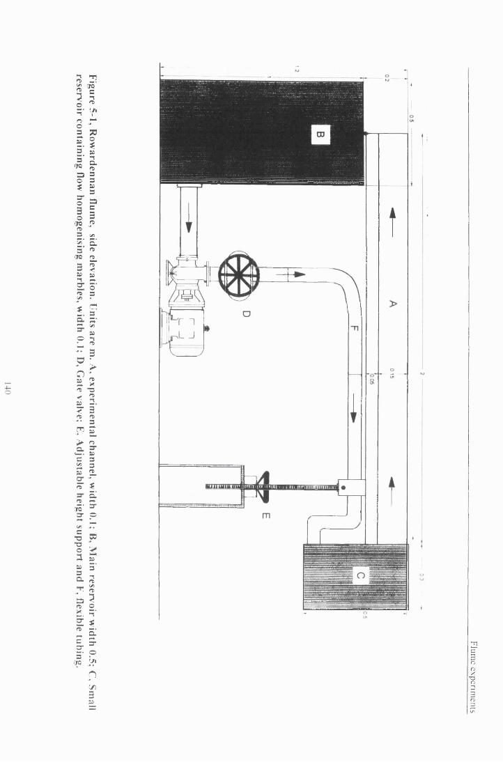
Figure 5-1, R
owardennan
flume,
side elevation. Units
are m
. A, experimental channel, width
0.1; B, M
ain reservoir
width 0.5; C,
Sm
all reservoir
containing flow
homogenising
marbles, width
0.1; D, Gate
valve; E, Adjustable
height support and
F, flexible tubing.
Flume
experiments

Flume experiments
5.2.1.2 Rowardennan Flume
Most of the experiments were carried out in a narrow flume 0.1 m wide, (Figure 5-1).
The water circulatory system is closed. Water was aerated by falling from the
experimental channel into the main reservoir. This process was sufficient to keep the
water saturated with oxygen during all operations; dissolved oxygen was measured
using a field probe (Hanna Dissolved Oxygen meter 1997 model). The flume was
housed in an unheated shed at the University field Station loch lomondside, under low
light intensities, and at ambient temperature. Water was supplied from Loch Lomond
(pumped from c. 10 m below the surface and 200 m from the shore). The water was
untreated, but was filtered through a phytoplankton net before use. The operation of
the pump could increase temperature by 1-2°C per hour and, when this occurred, the
water was replaced.
Discharge to the experimental channel was produced by a pump working at 12 Is'1 and
controlled by a gate valve. This allowed a very fast increase in discharge if required.
The slope of the channel could be altered by adjusting its height. Flow was
homogenised through a bed of marbles placed in the small reservoir. Depth in the
channel was controlled by means o f 0.02 m high perspex blocks which could be slotted
into the end. A zooplankton net was placed over the mouth of the main reservoir to
collect any animals swept out of the channel during experiments.
5.2.2 Flow Structure in the Flume
Flow in the channel varied gradually along its length, which was too short for steady
uniform flow to develop (i.e. flow was not full developed: the boundary layer did not
extend to the surface, but only partially through the water column, e.g. to a depth of 3
cm above the floor near the end of the flume). Estimation of velocity at different
heights above the bed using velocity profiles required the identification of the height of
141

Flume experiments
the boundary layer. In the boundary layer, the log-normal relationship between
velocity and depth applies and can be used to estimate velocity at different depths, i.e.
in front of an animal. Above the boundary layer velocity, does not vary with depth so
no estimation process is necessary.
To calculate the force o f water acting on the surface of the animals we can apply
equation 6.32 from (Dingman 1984).
Where u is the velocity at depth y (See Appendix I for definitions of terms)
This equation applies to hydraulically smooth flow, as is the situation when contact is
made with the substrate. It was developed for wide channels rather than the narrow
flow and channel used in the present experiments. As a result, their assumptions for
This replaces Sf for S0, where S0 = Channel slope tangent.
Manning’s n was estimated as 0.01 for flume with Perspex sides.
Equation 6-33 in Dingman (1984) can be applied for rough flow but ks would have to
be calculated.
v
calculating U* are not valid. Instead, U* in gradually varying flow is
n = Mannings n for the channel
Sf = Slope of the energy line
U' = -JgRSf

Flume experiments
Both equations 6-32, and 6-33 in Dingman (1984) are for fully-developed flow but can
be applied to the case in question here since we are only interested in the region of
developed flow at the bottom of the water column (D.A. Ervine, Glasgow University
pers comm).
5.2.3 Animals
All o f the species used are common in Scotland and are sufficiently abundant in rivers
to provide numbers for experimental analysis. The mayfly taxa Baetis rhodani and,
Ecdyonurus, the dipteran Tipulidae, and two crustacean species Gammarus pulex,
and Asellus aquaticus were all used. It was not possible to identify the Ecdyonurus
larvae to species but they were either E. torrentis or E. dispar, both of which were
present at the site. During some of the later work adults emerged: all were E.
torrentis. The Tipulidae were all of one species as yet not identified as no keys are
available to identify this larvae to species. Specimens have been retained and it is
hoped to rear some larvae of the same species to adulthood this year. Keys do exist for
identifying adults. All animals were collected from the Blane Water (site description,
Chapter 2 Section 2). Animals were collected by a number of means, usually stones
were turned over by hand and the animals allowed to float downstream into a pond
net. Where animals remained on rocks they were gently removed either with the finger
or an artist's paint brush to prevent damage to their cerci and other appendages.
Animals were transported to the field station in containers of river water which were
aerated using a portable air pump. On arrival, they were immediately transferred to
communal tanks (0.3 x 0.2 x 0.15 m), one tank per taxon in the shed housing the
experimental flume, which were also constantly aerated. Water was changed in the
tanks every 2 -3 days. Animals were not fed during their captivity but none were kept
longer than a week. Mortalities were infrequent.
143

Flume experiments
5.3 Methods
5.3.1 Weighing and Morphometric Measurements
Animals were removed from their holding tanks, carefully dried on absorbent paper
then weighed. Subsequently they were observed under a binocular dissecting
microscope and the head width measured using an eye piece micrometer. Animals
were then transferred to individually numbered plastic cups and remained in the flume
shed until they were used in the experiments. Tipulidae lasted in this type of
confinement without any reduction in observable health for up to a week, Gammarus
pulex and Baetis rhodani remained in good condition for approximately 4-5 days.
For Ecdyonurus, head width was related to the frontal area that would be exposed to
the current. After measurements of head width had been made, the animals were then
killed and mounted on to pieces o f card which were covered in nail varnish. Animals
were posed on the card in a position assumed by Ecdynonurus when resisting
entrainment, as observed by Weissenberger et al. (1991). Animals were placed facing a
binocular microscope lens to which a video camera was attached which was, in turn,
linked to a computer, Figure (5-2).
144

Flume experiments
Tocomputer
Figure 5-2, Measurement of Ecdyonurus frontal area. Binocular dissecting microscope. A, Cast iron right angle mount for specimens with built in spirit level; B Video camera linked to computer.
An image of the animal was recorded using a frame grabbing video card and then
analysed using Sigma Plot software. The image of the animal was outlined by hand and
then filled: the irregular filled area could then be measured using the computer
145

Flume experiments
program. Pixels. Counts were transformed into SI units using a calibration based on
measurements taken with a slide micrometer.
5.3.2 Experimental design and Statistical Analysis
In all the experiments carried out, randomisation of treatment order and allocation of
individuals to treatment was used to avoid any experimental bias. Hurlbert (1984) has
suggested that randomisation procedures can inadvertently create patterns in the
designation of experimental subjects to particular exposures thereby creating a bias
that they were trying to avoid. After each randomisation procedure I checked to make
sure no aggregations occurred. The main factor of concern was particular exposures
aggregating at particular times of the day. All experiments were carried out in daylight
hours and stopped before the onset o f dusk.
Phototaxis:
All experimental taxa were first screened to determine their response to light. During
some of the experiments which follow, a quantifiable stimulus was given to the animals
to move upstream. Light was the only stimulus which would not interfere with water
velocity around the animal and could be applied to specific areas of the flume. To
determine the animals’ responses under non-flowing conditions, the experimental
channel was dammed at both ends and flooded to capacity. This exposure acted as a
control for later experiments. A board was placed over the top of the flume, 0.3 m
from its end and extended 0.5 m along the flume. Underneath this area the walls were
blocked with card. A bench lamp with a 60 W bulb was then placed on top of the
plank and shone toward the downstream end of the tank. This created a sharp border
between the light and dark zones of the flume. As mentioned earlier, the flume hut had
low background light levels. From groups of about twenty animals (depending on
availability) individuals were placed singularly in the flume, on the border line and

Flume experiments
exposed for 3 minutes to moving water, or, in the case of the control, still water.
Exposures were randomised as described above. Animals were placed parallel to the
border line facing neither into the light nor the shade. Head width and weight of all
animals was recorded. A non-parametric Mann Whitney U test was performed on the
data for the B. rhodani groups responding preferentially to either light or shade.
Statistical comparison between light and shade preferences under flowing water
conditions were not performed. When exposed to running water the vast majority of
the animals sought in the illuminated zone. Only a limited number of animals remained
in the dark zone. It was clear that light was of secondary importance to remaining in
the channel.
Rheotaxis and suimming
The initial aim of this work was not solely to observe the animals’ behavioural
responses to high water flow rates, rather it was to measure the upper velocity
tolerance of the various taxa. Animals were placed in the flume individually on the
border between the light and dark areas with the channel flooded and the water still.
They were allowed to settle for five minutes and then some of the barrier at the end of
the experimental channel was carefully removed in sections to prevent any surging
motion in the water upstream which would inadvertently entrain the animal. The
pump was then started and the gate valve, which had been kept completely shut, was
slowly opened which allowed water to begin flowing gently. Velocity was increased
slowly over 3 to 4 minutes by opening the gate valve further. When required, the
experimental channel was also angled upward to increase velocity. This was necessary
only in exceptional cases to achieve velocities over 1.2 ms'1 for ecdyonurids. When the
animal became entrained it was recovered from the end of the flume and, at the point
where entrainment occurred a velocity profile was measured at 10 positions through
147

Flume experiments
the water column, by taking 15s averages at each point. It soon became clear that the
animals had an impressive capacity to find areas o f the flume where velocity was low
(near the walls) as refuges and that these locations were also inaccessible to the
velocity meter. They also showed a willingness to drift over a range of velocities and
appeared unwilling to expend energy withstanding entrainment. For this reason it was
felt that measuring an upper velocity tolerance limit in this manner was not informative
and only the animals’ behavioural responses are reported.
Logistic response curves
The previous experiment determined the range of velocities at which the different taxa
normally drifted and this allowed a new experiment to be designed which
concentrated on determining the probability of animals drifting at different velocities.
The velocity range of animals had been determined in the previous experiment. From
the range a number of velocity ‘exposures’ were chosen (see Table 5-1). Animals were
collected, weighed and measured as described above. They were then assigned to each
exposure in a random manner, 5 animals to each exposure. Each animal was treated to
its velocity exposure individually for a period of 3 minutes and then its behaviour was
scored using the list of behavioural categories presented in Table 5-2. The order in
which each exposure was made was completely randomised.
Frontal area to head width
To predict the frontal area of Ecdyonurus exposed to flow from its head width a
simple linear model was used. Animals were chosen to cover the maximum range of
head widths available.
148

Flume experiments
Table 5-1 The velocity to which the three taxa were exposed.
Taxa Number of exposures Exposures ms'1
Tipulidae 7 0, 0.04, 0.06, 0.08, 0.1,0.12
Gammarus pulex 5 0, 0.10, 0.15, 0.20, 0.30
Baetis rhodani 4 0, 0.3, 0.5, 1.10
Table 5-2, Definitions of behaviour scored during exposures to velocity. Given in Table 5-1.
Behaviour Definition
Entrained Any movement downstreamResisting flow Struggling to remain in situ or moving to flume edgeActive Moving upstream or lateral movement without any downstream
movementInactive Remaining still
Effect o f weight on entrainment o f Tipulidae
Animals were collected in the field as previously described. Animals were ranked in
order of their weight. Of these, 30 animals were chosen covering the range of weights
available. This equated to 1 individual representing every 0.01 g increment in weight.
Each individual was exposed in a similar manner to a series of velocities: 0.04, 0.06,
0.07, 0.08, 0.10, and 0.12 ms'1. The order in which the animals were selected for the
experiments was randomised and the order an individual was exposed to the velocity
intervals was also randomised. Animals would frequently become entrained at
velocities below their upper velocity tolerance. The lowest and highest velocity at
which an animal was entrained were recorded to take account of this behaviour.
149

Flume experiments
5.4 Results
5.4.1 Head width to frontal area ratios
There was a positive significant relationship between head width squared and frontal
area of Ecdyonurus (p < 0.0001, F (1, 73) = 144.5, R2adj =0.65). Although the
relationship was significant, there was fairly substantial degree o f individual variation.
Frontal area = - 0.40 + 0.409(Head width)2.
CN
EoCO<D(0oj■*-*co
LL
0 2 4 6 8 10 12 14 16
Head width squared cn?
Figure 5-3, The relationship between head width and frontal area of Ecdyonurus.
5.4.2 Phototaxis
All the taxa tested except Baetis rhodani showed a strong preference for the shaded
area, Table 5-3. The almost 50-50 response to either light or shade would indicate that
Baetis rhodani has no preference. There was no significant difference in the weights of
B. rhodani individuals which preferred shade to those that preferred light.
When the animals were exposed to the same conditions with moving water they all
initially moved upstream into the shaded zone, including B. rhodani. However as
velocity increased, they moved into the lit zone where they would still resist
entrainment.
76543210
O QCP
150

Flume experiments
Table 5-3, Percentage of animals preferring the shaded area over the lit area.
TaxaEcdyonurus Baetis
rhodaniGammarus
pulexAsellus
aquaticusTipulidae
Mean Weight g
0.015 0.005 0.045 0.011 0.191
Standarddeviation
0.009 0.003 0.062 0.006 0.088
n 20 19 20 20 20Shade
% of animals90 52 95 85 80
5.4.3 Rheotaxis and swimming
Ecdyonurus
This species, like B. rhodani, swam in short bursts . The length o f the bursts decreased
with increasing velocity (personal observation only). It remained close to the substrate
for the majority of the time but on occasion would swim further up into the water
column. When velocity increased B. rhodani would either enter the drift or, if the
water velocity was not sufficient to wash the animal out of the experimental channel, it
would frequently alight on the floor and then enter the drift again. There was a marked
decrease in an individual’s upper velocity tolerance with repeated exposure making it
impossible to use the same animal for two consecutive runs. This was only attempted
if there had been a problem during the first run. On a number of occasions individuals
would resist entrainment until the velocity was very high >1.5 m s1. When this
occurred they assumed a flattened position with their body pressed closely to the floor.
This posture was taken up as velocity increased although only infrequently did the
animals persevere until velocities were very high (>1.5 ms'1). On other occasions the
animals would move to the flume edge as velocity increased, presumably gaining
advantage from the reduced water velocity at these locations.
151

Flume experiments
Baetis rhodani
When moving upstream or downstream, the animal swam in bursts coming back down
onto the floor periodically. Above a certain velocity the animal would not swim
downstream: instead it appeared to drift. After leaving the substrate it would move up
through the water column rather than drift near the floor. It was not clear whether this
action was voluntary or passive. Once in the water column the animal assumed a
posture where its abdomen was arched upward and its cerci aimed forward over its
head. After travelling in this manner the animal would float down through the water
column and grasp the floor with its claws. If the animal had not travelled far enough
(assuming the animal is making the decision about what distance to travel), while still
suspended it would flick its abdomen when descending which stopped the descent and
allowed further travel downstream. Some individuals would also move to the side of
the flume where they could resist entrainment more easily. It was clear that an
individual would choose whether or not to enter the drift, although there was always a
point at which velocity was sufficiently high that they could no longer remain in
contact with the substratum.
Gammarus pitlex
Like the previous two taxa, this species showed a range of responses to high
velocities. Unlike the other taxa, G. pulex would quickly move upstream once
introduced into the flume. It also differed in its use of the whole water column while
swimming, something only B. rhodani did as frequently. As velocity increased G.
pidex would either get washed out of the experimental channel or alternatively would
move down onto the flume floor. There it would hold on with its frontal appendages,
from either thoracic or head sections, while facing upstream. This animal would
frequently tilt its body upwards to the rear, from its point of anchorage, at an angle of
152

Flume experiments
as much as 45° or more. Depending on the individual and the exposure velocity, three
related responses were observed. Firstly individuals would release their hold and drift
downstream (after moving up into the water column), alternatively they would release
and move downstream pushed by the flow, but would remain close to the floor and
periodically re-attach and then get swept down again, sometimes simultaneously
moving to the flume wall. Their capacity to perform this action was extraordinary; they
could on occasion move at right angles to the direction o f flow, although more
normally there was some downstream drift involved also. This movement at right
angles could occur even at quite high velocities.
Asellus aquaticus
Animal availability in the wild decreased shortly after the initial phototaxtic test and no
behavioural observations could be made in running water.
Tipulidae
When moving upstream or against the current, the animals appeared to bite the
substrate with their mandibles and while so anchored would draw their abdomen
further forward. This activity was accompanied by moving the head from side to side.
If the current proved too strong the animal would release its grip and roll downstream
angling its body so it ended up at the flume wall. This process was completed in stages
with the animal holding on, reorienting, and then releasing until it reached its
destination. Once it reached the flume wall it expanded its body into the comer
between floor and wall. Here velocity was not measurable, but was noticeably less
than in the centre of the channel.
The increase in discharge necessary to dislodge a tipulid from this refuge was
substantial. If the water velocity was too fast and the animal could not reach the flume
edge it would release its grip and drift downstream, usually rolling over the flume
153
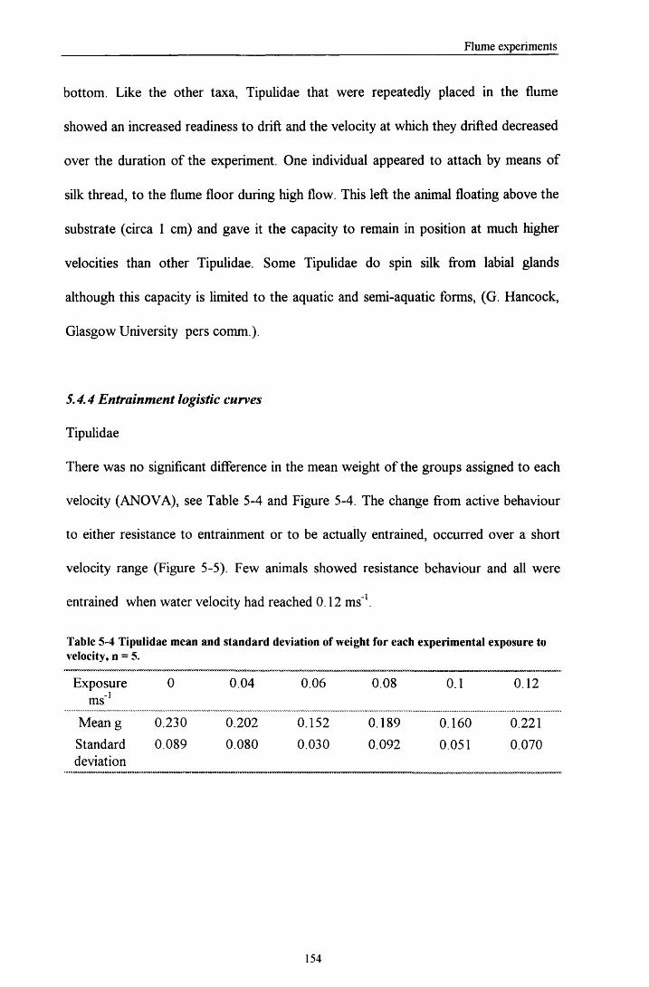
Flume experiments
bottom. Like the other taxa, Tipulidae that were repeatedly placed in the flume
showed an increased readiness to drift and the velocity at which they drifted decreased
over the duration of the experiment. One individual appeared to attach by means of
silk thread, to the flume floor during high flow. This left the animal floating above the
substrate (circa 1 cm) and gave it the capacity to remain in position at much higher
velocities than other Tipulidae. Some Tipulidae do spin silk from labial glands
although this capacity is limited to the aquatic and semi-aquatic forms, (G. Hancock,
Glasgow University pers comm.).
5.4.4 Entrainment logistic curves
Tipulidae
There was no significant difference in the mean weight of the groups assigned to each
velocity (ANOVA), see Table 5-4 and Figure 5-4. The change from active behaviour
to either resistance to entrainment or to be actually entrained, occurred over a short
velocity range (Figure 5-5). Few animals showed resistance behaviour and all were
entrained when water velocity had reached 0.12 ms'1.
Table 5-4 Tipulidae mean and standard deviation of weight for each experimental exposure tovelocity, n = 5.
Exposurems’1
0 0.04 0.06 0.08 0.1 0.12
Mean g 0.230 0.202 0.152 0.189 0.160 0.221Standarddeviation
0.089 0.080 0.030 0.092 0.051 0.070
154

Flume experiments
COc:o03£CDCO
_QO
«4—Oo
13121110
9876543210
<=.1 (.1,15] (.15,.2] (.2,.25] (.25,.3] (.3,.35] > .35
Weight g
Figure 5-4, Weight distribution of Tipulidae used in logistic regression experiments.
1.2
1.0
> , 0 8
0.6
0.4
0.2
0.0
_Q03
XIO
- 0.20.00 0.02 0.04 0.06
Velocity ms
0.08
- 10.10 0.12
Figure 5-5, Logistic regression analysis of Tipulidae behaviour showing the probability of the animal exhibiting either resistance to entrainment or the animal actually being entrained. Equation of the line is y = exp(-7.35+(89.69)*x)/(l+exp(-7.35+(89.69)*x)), Chi square = 22.7, pcO.0001.
89999999999

Flume experiments
(/)CoCD
£Q)(/)
_QO
M—Oo
109876543210
<=.01 (.01,.02] (.02,.03] (.03,.04] (.04,.05] > .0 5
Weight g
Figure 5-6, Weight distribution of Gammaruspulex used in logistic regression experiments.
Velocity mFigure 5-7, Logistic regression analysis of Gammarus pulex behaviour showing the probability of the animal exhibiting either resistance to entrainment or the animal actually being entrained. Equation of the line is y = exp(-5.12 +(45.6)*x)/(l+exp(-5.12 +(45.6 )*x)), Chi - square = 20.58,p<0.0001.
Gammants pulex
T here w as no significant difference in the w eights o f anim als assigned to each
exposu re (A N O V A ), see Table 5-5 and Figure 5-6. The range o f responses to velocity
w as g rea te r for G. pulex than for the T ipulidae, F igure 5-7
156

Flume experiments
Table 5-5, Gammarus pulex mean and standard deviation of weight for each experimental exposure to velocity.
Exposure ms'1 0 0.1 0.15. 0.2 0.3
n 5 4 5 5 4Mean g 0.027 0.029 0.023 0.027 0.027
Standard deviation 0.013 0.018 0.007 0.012 0.012
5.4.5 Effect o f weight on entrainment o f Tipulidae
All animals were entrained in a short band of velocities. There were significant positive
correlations between weight and the lowest and highest velocity at which animals
became entrained. One o f the individuals used was very large (0.763 g) and considered
an outlier. Removal of the outlier did not affect the significance of the relationship
between velocity and the lower velocity o f entrainment. The relationship between the
highest velocity of entrainment and velocity did become non-significant on its removal.
0.085
0.075
i^ 0.065
O 0.055 <D >
0.045
0.0350.0 0.1 0.2 0.3 0.4 0.5 0.6 0.7 0.8 0.9
W eight gFigure 5-8, The lowest velocity of entrainment exhibited by the Tipulidae against body weight. Spearman rank correlation, R = 0.56, p<0.005, n= 29. Equation of the line; y = 0.052+0.044*x.
O O
O O CO O O CD O
o oo cm o o o
o oo o
157

Flume experiments
0.11
0.10
0 .0 9
'(/) 0 .0 8 E>> 0 .07 Oo 0 .0 6d)
^ 0 .0 5
0 .0 4
0 .0 30 .0 0.1 0 .2 0 .3 0 .4 0 .5 0 .6 0 .7 0 .8 0 .9
Weight gFigure 5-9, The highest velocity of entrainment exhibited by the Tipulidae against body weight.
Spearman rank correlation, R = 0.40, p<0.05, n= 29. Equation of the line; y = 0.06+0.053*x.
5.5 Discussion
The observed responses of the benthic invertebrates are consistent with the hypothesis
that animals frequently choose to enter the drift. Similar behaviour to that observed
here has been interpreted as a reluctance to drift (Lancaster 1999) and this is not
contradicted, rather it is suggested that a choice is being made and that the animals can
become more willing to enter the drift if stressed. In none of the exposures made
during the present study were the animals given any refugia. Their capacity to find the
edge of the flume where velocity was low, highlights a highly developed rheosensory
capability, across all taxa examined. This capacity together with the ability to alter the
length of drift - by either rolling (tipulids) or flicking the body (Baetis rhodani) up
into the water column - may help explain the capacity of invertebrates to choose
substrate type directly from drifting (Walton Jr 1978).
The negative phototactic response of all subject animals, excluding B. rhodani
supports the use of substrate as shelter. Where the river is not shaded by vegetation
the substratum is the only place which is dark. By seeking such a location
158

Flume experiments
macroinvertebrates are choosing an area in which is presumably difficult for visual
predators to operate. Areas which are dark are likely to be deep in the substrate matrix
and should have lower shear stresses than substrate elements close to the bed surface,
however the hyporheic refuge theory has only been supported in part by field
experiments (Palmer et al. 1993b) but the question here is more concerned with
animals sheltering not from serious floods but from ‘normal’ flow conditions. Animals
in the substratum would require less energy to maintain position.
However both G. pulex and E. ignita have been shown to use woody debris as shelter
when velocity is increased, although G. pulex made more efficient use of the refuge
(Borchardt 1993). Although no light measurements were reported from amongst the
woody debris it is clear from their size that they would have had some shaded areas.
From the evidence presented here it is possible that the two stimuli, both light and
current could work in concert or independently. Further work which identifies which
stimulus is dominant would give a possible insight into the relative importance of
predator avoidance versus entrainment.
That no response to light was observed in B. rhodani also fits with our knowledge of
the animal as a good swimmer and suggests that it is more flexible in its response to
negative stimuli than the other taxa, e.g. predators. The situation is not simple though
as both B. rhodani and heptageniids nymphs are known to seek shelter among the
substrata; in this case it was suggested that they are avoiding predators (Huhta et al.
1995). Baetis species are known to show strong diel periodicity in drifting (Poff &
Ward 1991; Tikkanen et al. 1994), but it is not clear if this is regulated by light levels
or circadian rhythms. In this instance, if B. rhodani was shown to drift at night, the
lack of preference for light or dark conditions would be indirect evidence for an
internal clock. As drifting in Baetis can be very seasonal and local drift records are few
159

Flume experiments
so no direct conclusions on this subject can be made (Rincon & LobonCervia 1997),
but the possibility for future work exists. 1
The Tipulidae occur at higher velocities in the field than those at which they were
entrained in the flume (see Chapter 4 Section 4.3). This could be for two reasons.
Firstly the flume substrate afforded less grip than the substratum in the field, or,
second, the animal remains below the surface of the river bed for the majority o f the
time. As the tipulids could withstand only very low velocities, lower than those
expected near the river bed, they must avoid the substratum surface. This highlights
the fact that these organisms are exploiting the habitat in very different ways and
suggests that niche differentiation is occurring along these physical gradients.
The increased ability of larger Tipulidae to withstand entrainment is a situation
observed in other taxa. For some Trichoptera it has been suggested, that because of
this relationship the chances o f accidental dislodgement decrease with size (Otto
1976). That the surface area to volume ratio of a small object is much greater than
that of a similarly shaped large object is often quoted in texts on thermo-regulation. It
is well established that the surface area to volume ratio of a small object is much
greater than that o f a similar shaped large object (Schmidt-Nielson 1990). If we
assume that weight will increase in a linear manner with increasing volume, ignoring
for the moment the stepped size increases exhibited by insect instars, then the ratio of
frontal area to weight o f a small tipulid will be relatively greater than that of a larger
specimen. Therefore, there would be relatively less force exerted on a larger animal
per unit weight. In theory, therefore, a larger animal would need to expend less energy
to withstand entrainment. This should be applicable to other taxa also: the only limit
1 Some 24 hr drift samples were taken from the Blane Water but the sample size was small and the results inconclusive. Directly upstream of the drift nets was a very large population of Hydropsyche
160

Flume experiments
would be the individual's height increase. As the animal’s height increases it could
project too high into the boundary layer subjecting the animal to relatively higher
velocities. This would be dependent on the increase in velocity with depth which, in
shallow riffles, can be steep. This would provide one explanation for the ability of
large tipulids to withstand higher velocities since the relative increase in volume
equates to increased muscle. Whether resistance is a physical act or passive inertia
needs to be clarified. From the observations of the animals’ behaviour it seems likely
to be a combination of both.
The velocities at which the Tipulidae and G. pulex drifted will have been influenced by
the substrate in the flume bottom. It seems likely that this type of work will increase
where it is necessary to get exact measurements of the flow preferences of
invertebrates. It would appear likely, therefore, that further studies of this type are
required during which exact measurements of the flow preferences of different species
of invertebrates could be made. Standard substrates would be used to allow
comparisons with both field conditions and other experimental studies.
Giller & Malmquist (1998) have suggested that a pluralist approach to understanding
community structure is necessary; it is no longer sufficient to only argue about the
relative importance of biotic versus abiotic factors. Drift by benthic invertebrates
appears to be a general response to both types of factors (Brittain & Eikeland 1988;
Collier & Wakelin 1992; Kratz 1996). The data presented in this chapter add weight to
the argument that individuals actively choose to drift and that this response is plastic at
the level of the individual. Individual plasticity is therefore a useful measure of the
relative importance of the various factors affecting community structure.
---------------------larvae which could also have significantly altered the composition of the drift (Georgian & Thorp 1992).
161

Flume experiments
The process of drifting is likely to reduce the fitness of the animal. By this I mean the
actual drift itself not the process which is actually beneficial e.g. drifting from one food
patch to another is consuming time which could be spent feeding, but the process may
be necessary if food is to be found at all (Kohler 1985). So if the drifting behaviour of
an animal is altered its fitness, as measured by fecundity, is likely to be altered too.
5.6 Conclusions
• Negative phototactic responses o f benthic invertebrates agree with their known use
of substrate as a shelter.
• Benthic invertebrates have strong rheosensory responses.
• Entrance into the drift is a matter o f choice below certain upper velocity limits.
These limits are species-specific.
• There is a positive relationship between body size and the capacity of a tipulid
larvae to withstand entrainment.
162
Invertebrate community structure in Callitriche stagnalis patches
Chapter 6: Invertebrate hydraulic microhabitat and community structure in Callitriche stagnalis Scop, patches
6.1 Introduction
When macrophytes are included in rehabilitation schemes for channelled rivers they
can potentially provide a diverse habitat for invertebrates by interacting with local flow
conditions (Marshall & Westlake 1990; Newbury & Gaboury 1993). For practical
management purposes it is useful to know how much additional invertebrate diversity
and biomass may be supported by utilising macrophytes as part of an individual river
rehabilitation scheme, under specific flow conditions. I use the term diversity of
invertebrates to encompass taxon richness, abundance and evenness (the relative
number o f individuals o f each taxa). Previous work e.g. (Gregg & Rose 1982) has
demonstrated the extent to which macrophytes can alter the stream flow
microenvironment. Large-scale studies (e.g. Jenkins et al. 1984; Ormerod 1988) have
demonstrated how this increased habitat diversity in turn influences the occurrence of
invertebrate assemblages in vegetated and unvegetated parts of the river environment.
Sand-Jensen & Mebus (1996) showed that a range of flow conditions were present in
patches of the submerged macrophyte Callitriche cophocarpa. Other studies (Wright
1992); Jeppesen et al. (1984) found that invertebrate communities present in
macrophyte patches (including Callitriche) could differ substantially from those
occurring in unvegetated patches of river bed, having higher taxon richness, numerical
abundance and specifically high numbers of Chironomidae and Simuliidae. Woody
debris has been show to have increased species richness if its complexity is increased in
streams, suggesting increased habitat complexity as the mechanism behind high species
richness and abundance in plant patches too (O'Connor 1991).
163

Invertebrate community structure in Callitriche stagnalis patches
The Blane Water is a small unregulated stream which supports a Callitriche-
dominated macrophyte flora typical of many small British rivers in which rehabilitation
schemes are being considered or implemented. The relationship between flow
conditions and invertebrate community structure within different parts of submerged
beds of Callitriche stagnalis Scop., and in adjacent unvegetated patches of river
substrate in the Blane Water was investigated. The results are considered in relation to
the value added to river rehabilitation schemes by the inclusion of macrophytes, in
terms o f increased invertebrate diversity support capacity.
The aims of the chapter are to show that different sections of Callitriche instagnalis
support different assemblages o f benthic invertebrates and that this may in part be
related to the flow conditions in and around the plants. Specifically that the outside of
the plants is an extreme environment for benthic invertebrate suitable for a limited
number of specialist taxa only.
6.2 Methods
6.2.1 Source o f Plants
Plants and substrate were collected from riffle sections o f the Blane Water, a gravel
bed river, at Blane Bridge (UK National Grid reference NS507852) in Scotland during
June 1998. The site is down stream from a trout fishery and is classified as organically
enriched by the Scottish Environmental Protection Agency, although water quality is
classified as high (Doughty & Maitland 1994). The only noticeable effects of
enrichment are higher numbers o f chironomids and annelids than would otherwise be
expected. Channel width in the sampling area ranged from 8-13 m, depth from 7-22
cm and velocity from 0 to 0.35 ms'1.
164

Invertebrate community structure in Callitriche stagnalis patches
6.2.2 Measurements
Ten Callitriche stagnalis stands were chosen at random within a c.100 m stretch of
river. Water velocity and depth were measured in front, above, in the middle and at the
bottom of each stand using an electromagnetic velocity meter (SENSA). At the mid
channel side of each plant, velocity and depth were measured and substrate type was
visually estimated (% scale) using the following particle size scale: sand (0.06 mm-2
mm nominal diameter), fine gravel (2-10 mm), gravel (10-64 mm) and cobble (64-256
mm). A reference scale was carried in the field to confirm particle size when necessary.
Mean water column velocity measurements taken outwith the stands were measured at
0.4 depth from the river bed (Smith 1975) as 50 second averages.
The total area of bed occupied by each stand was estimated using a quadrat with 25
cm2 squares. Invertebrate samples were taken separately from the outer, middle and
root sections of the plants by placing a net downstream and trimming the desired
section of the stand with scissors and letting it float into the net. Sections were defined
using stand length and depth as follows; outer = outer 20%, mid = all other material
above substrate, root = material within the bed. When removing the roots all the
substrate which had been underneath the stand was disturbed and the invertebrates
collected into the net placed downstream. A Surber sample was then taken from the
mid channel point where substrate type had been assessed, 10 surber samples in total. I
estimated the near bed velocities at the Surber samples by using values which were
10% of those at 0.4 depth from bed, as suggested by Carling (1992).These samples,
and the sections of stands, were immediately placed in 70% alcohol to preserve the
invertebrates. All samples were sorted on white trays and animals identified to the
following taxonomic levels: Annelida to subclass; Diptera to family or genus and all
165

Invertebrate community structure in Callitriche stagnalis patches
other taxa to genus or species. Other studies show larvae and adults of Coleoptera
have differing hydraulic habitat preferences (Degani et al. 1993) and so are treated
separately here.
6.2.3 Data manipulation
To compare densities of invertebrates between stand sections, abundance values were
standardised to estimated wet weight of stands. Because of the necessity of
immediately preserving invertebrate samples in alcohol, in the field, the plant material
in the samples could only be weighed after a storage period in 70% alcohol. It was
necessary to see if samples o f different weights were affected equally. The relationship
between dry weight post storage with wet weight prior to storage was linear for log-
log data as determined by regressing the wet weight of 24 control stand samples
against their dry weight.
LnWet weight = 2.59+0.92(Ln Dry weight), (R2 = 0.978)
This equation was used to transform dry weight values to wet weight for the
experimental plants.
6.2.4 Statistical analysis
Where direct comparisons between samples were made the Wilcoxon Matched-Pairs
Signed-Ranks Test was used, which allows comparison between related samples
(Sidney 1956). As either different sections of stands are compared or stands and
adjacent sections of substrate (Surber samples) it was considered that they represented
related, non-independent samples and that this test was the most applicable. Benthic
invertebrates can have clumped distributions and it is possible that this could occur
around some of the Callitriche stands; see Elliot (1977) for a comprehensive
assessment of the possible spatial dispersions of benthic invertebrates. It was believed
166

___________________________________Invertebrate community structure in Callitriche stagnalis patches
this could further influence the relatedness of spatially close samples and enhanced the
applicability of the Wilcoxon Matched-Pairs Signed-Ranks Test
167
Invertebrate community structure in Callitriche stagnalis patches
6.3 Results
6.3.1 Taxa abundance and richness compared between plant and surber samples
Although composed of many individual plant fronds, all stands had a similar growth
form, being wider at the upstream end and tapering downstream, similar to a classic
streamlined strut as described by Vogel (1994) but wider at the upstream end and
generally more ragged. The area of stream bed occupied by stands was on average
467cm2 (s.d.+/- 290cm2). Substrate in the Surber samples was dominated by gravel (%
composition of gravel always >90%). The substrate underneath the Callitriche
stagnalis stands was mainly sand (% composition of sand always > 80%). Callitriche
stands had higher, and significantly different total taxa abundance (no. o f individuals of
all taxa) and taxa richness than neighbouring substrate samples (Wilcoxon Matched-
Pairs test p<0.01, N=10. Values standardised for sample area: the area of bed
occupied by each stand. P value is for both cases, see Table 6-1 for abundance and
richness data per sample). A list of taxa occurring in the Surber samples and plant
stands is given in Table 6-2 with abundance (no. o f individuals per sample) and
frequency of occurrence (no. of samples a taxon occurs in).
6.3.2 Taxa abundance and richness compared between plant sections
Taxa richness was significantly different between outer and root sections of the stands.
From the box plot in Figure 6-1 it is clear that the outer section supports the lowest
taxa richness. Total taxon abundance was significantly different between outer and
mid sections and outer and root sections. The box plot shows that the outer section of
the stand supported the greatest abundance, see Figure 6-2, Table 6-1 for abundance
and richness data per sample.
168

1.29 1.81
1.99 546
90 0.14
0.24 0.49
ON
® * - »3 < a 35*S ' <W o- sr32 O c« "B•a *t32 S'
< $ P SOs 2
S» 1O I—b •
" E? £ ® a 2
NO 00 - J On On 4 u> t o C/3P3
* 2aT
ONtoC7NO3kl
MM-3p<-K2 #
ffc 3*a sS' 3 3 p<» 3
i—iNO
U) OnU)
OnO
t oNO O
U)On
l—ll—l OnOC
O>1
2Sm' 2 «> 3 «n » B CB 3
ON t o 1—* - j 4NO
O ON U) r-f-a>*-»
33a
Ml*< <2
01 t o to i—i t o to _l H 1—1%
p30n>
a*»c*«W9
3 a*S' »P* "*
O on to On o On On 4 U) a *■*» M Oto ON to ►—i 4 4 4 4 o l
3*1 O ^
° 5* ^ a
to o O to 1—1 On F 23* p
B 5.o 1—1 00 NO ON o> ■O -O NO 0 f j fD Q.o NO -o o U) NO OO O n O n 0 p Vi W> 3
ts> Vi rt- r? p»Vi
P3
P M3 «®
NO Jin t o u> -U O n 4 O n cn 3 aVi
Q . O p “*j~o t o 1—1 OO 00 —1 00 O n NO II
O
B «aNO to U) 00 On 00 00 O nO
t o P3a
p■1
J P0. sSS’ m -
pa.»9
a £ a- 89Ol NO ON NO i—i NO 00 i—i -0 00
-U - o U) -U u>4 'O U)O n
ca*fD*-i
sMfMna
^ *3< B 2 vi
to’ 2 2 3 0 S '
o o o o o o 0 O . 0 O r+P 'Z
0m -
U) o 1—1 t o l—l l—l l—l O) l—l c X 0 crt o <1 u» O n - o 4 00 NO 00 r+
a>"ip »
pM) A
*3 P
o o o o o O 0 O 0
0i-h 30e ^ H-o O) o l—l l—l ’—1 t o l—l K 3 3 g2 8 » S 2. B
On U> -o O n to o> t o 4 Cl*02
O o o O o O 0 to O & < ’ 2 S '4 t o i—I t o 4 O) '4 0 ON 0 n — s rNO 4 U) NO 00 ■0 U) OJ 0 3 sC+
Vi O'na.
f6 Mas c« 0 *
i— i 1— 1 1— 1 l—l i— i l—l l—l l—l 1—1 C/3 n 3 “ g ,00 O) U> NO ON O n NO 4 t o !“►
p3a.
0n■»a
fp2 3 S ’. 30 33 31—1 1— 1 l—l l—l I— i 1— 1 l—l l—l 1— 1 C/3 3* cr
U> O l ON to 4 ON 4 co '0l—t
PC/33n
0 « ? 2 s . 3- S®55*® »w2 o-5**® «« 2. f»
£ &■ "*3 c S*0 2 3S* ** j§1 13 ^^ « rt3 ^O QTQ
3<T>3CDO'>-lBSCDno33e»C/)
§oS’3
p
o ’:5~o1>5
c§
VlT 3BJOtr

Odontocerum
0 0
0.2+/-0.5 0.2+/-0.5
albicorne(Scopoli)
ST £a Cl
O V;^ 55 a 2Co ^
U)+io
OO
oON+
vo
a -■7
Orso&Cl05
0 U) +1o
OO
toOl+IOl
OO
O)I
O n
4^
O to
to
to to
~4. 1 3
O: OE ^cd ^
"O ^ ^ c 3 ^3 , ‘CO
ci'O
0 *u» +1o
to+I4^
4^
o oO) -o l—l+ +_
o l—l-o Ol
to
to
5 r"7 .© O Oq"7 rts
&S1
CD3&
S?$•©33V«Co
o o 1—1 l—lu> ■o o>
+ + o1 1o 14L. 1to 00 41* •o
f ft §O <D a* 3:
toto+Ito
OO
to
O Ol
o -o
O VO
to VO
Oll-l 4~o ,+
I
toOOtoI
U)U)
Ol vo•o to
o1UJ
1to4L.vo
o 4^to 00 o>+_ +_
1o
1Ol OO
Ol U) l—l
VO
a g 1Oa ss- w S*0
1
VOo>+
O n.+i00u>
toOll—l+ItoOl
O n
OO
+
O n
00
ON
PCl3
fflRo3
too ON VO i— i
U) ■o 00 U)+ + + +1o 1
l— l100 1to
O n 4^O n
O n VO
U)■to
VO
UJIOl
Ol
Io4^
to
to
ocCD
&oo
OO<“+&3a .
cocO*CD
Oc
oo
cor-f33a*
ooc■-tc rCD
H
p
£3a§oCD
2oo’-V
a 2 ^ < < 2 . 5* » <g. ft » S0 G.3 p«< °S o - « . * ~ nH f f (9 © CD 3w v, «■*■3 2 33 5 s®1 a 9o- 2 3.« ™ £ . ■7 CZ> O° s? 3- ►2 CD O ' o -1 gfi «j 3=5 g a .2 3 *®CD ~ mS - «G rt »cP **" 2 s ^M H £■^ O csr • cd cd 0 »s 3>^ M* W5 3 "*3 a ^b * 5* ! •CD 5 . s*** a ©o e cd; s , « » “ £ S'S 5 73 S$ a .X. ^ M3 <« a 9989 « g r o aS 7 )2 s c| « ’ l 2c a*3 a. S g*^ 3 ‘ ► ‘S .
-3 0 “ ^ - d CD O MM 2 M G “ o CD D £" S c= g s J L a lo TO’ 5 31CD *
3 3-*7 CD CD 3
i s i3 3t« < -+ O > -»
2.
a ^3 cr•7 CD B . O.
► ^ O' »s S3 ?T°* rK fig ON 3 i2 tOCD •CD«< ^3 ^ci X3 3CD _<» 3!5 s ^ ■» oM “**g 53 < o . »% 3-5 CD2- o'ff. *7 O 35 CD
M3
&* A 2 CD 2 O2 B3 2 3 -•CL 3to TO•7a 5*CMQ- »S ’ ^^ §; CD S'*
TO* ^b * a^ aO Qtq"*» a1- fe3 M,
^ 2 3 § R a .CD 2 . » SL s
a -B oCD 3 3r> c 3 “ 3M3 ^CDCD ®9CD*-• P4-OB if
9 ao• 30 3“
2S* “* 3 36
a ee 52- 3*M3 rD
■a **“7 3TO 31 S’CD (TJ
3<n>3o '
oo2333
V)2nr"+3►-to
?
era
733ndrn>
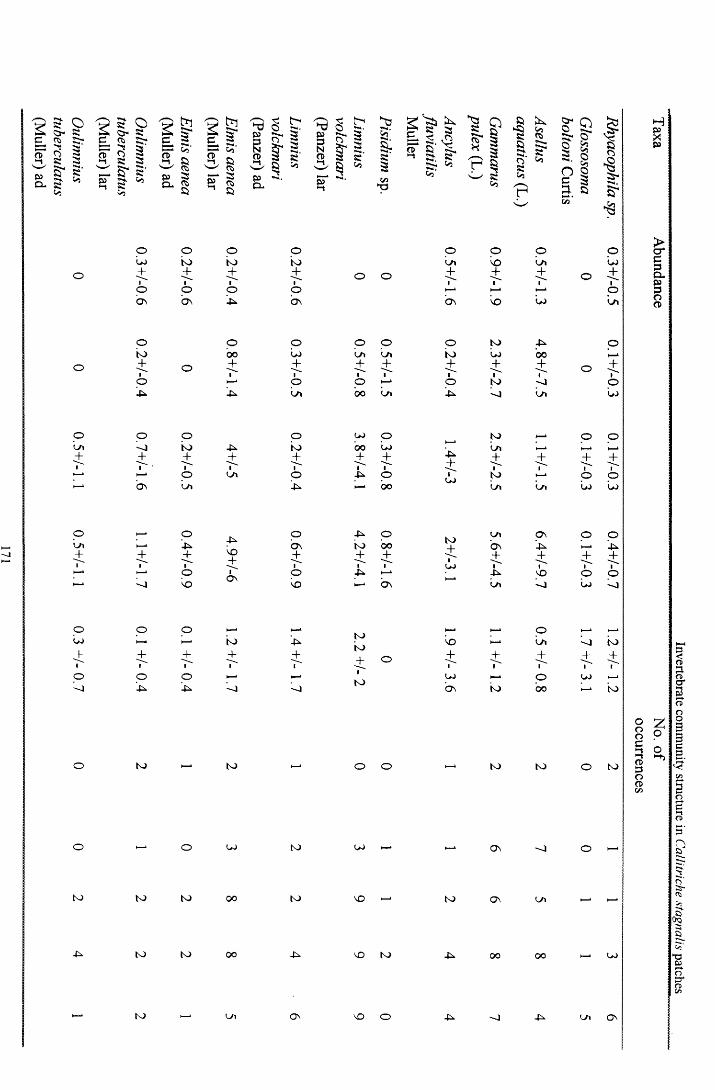
^ 3“ O^ O Si c ftr
« I I-i 55 *5^ s .
p a §CL S ’0n
O l+
to
155ft->!
Oatft?s
£c£ 3
1*Cn’
15r0 3
pS3N
Of t 4 3
aPS3N
<Oft* 3
3On’
&|? r
<*•■4 .ft3
ftj55ft-ftXoT-n ft
55 53 CD*l-l SiftcT*—1 Sift
CDft 55
OnCD►1 ft
55On
SS3
1 **4 .ftr
ssOn 1?
p “ SiS 'Vi
siCn p
CL3<55a
p * ftftSiPCL P *•-»
*•*4. 0 0*p
Zn w
O O O OU ) to to to+ + + +1
O1
O1
01
0O n O n 4 L ON
to4io-JL
+
'O
to
4l+io
NO
oOO+
O O OO l - O t o 4 L+ 4 ^ + + _1
t—»■
I—*1
01
O lt—* ON O l
4lNO4IO n
O 0 0 l—lLk) ’l—l I— to+ 4^ +0 O 0
• 0 4L 4L - 0
to
to
O OJ
to to OO
to to 0 0
0 u> +1001
0 to +1o-fL
O n
Iovo
4L4-
to
to
Ol+Io00
004 -
001+
0U )+1obo
OO4 -
O n
to to + ° I
to
JLto4 “
U )
NO
ON
NO t o
NO O
4L4 -
to+
NO
.+I
U )
ON
ft ft- Cl r f t►ft On O55 ft ft- 0ft O & ftft. ft ftOsiOn
1?
On *•4.OC3
SJ
03ft
ft-*•*4.s -C/3"
0 O O 0O l NO O l u >+ + + 0 4 :1
I— *1 1
l— l1
0
O n N O U ) O l
0 to 4L 0
to U) 00 l— l
+ +0 4 l1
01to 1<1 1
0
4L • 0 0 1 u>
to 0 0
Ol 1—1 »—> I_1+ + + +1to 1 ■
01
0
Ol Ol U) U)
O l ON O OO n 4L 4L+ 4 ; + +14L 1
NO■O 1
0
O l 'O U ) Ci
1— * 0 l— l l— l
I— * O l ~ o to+ 4- 4 - 4 -
to
to
o00
to
to
to
O n - O O
to ON O i t—>
-(L 00 OO
-JL - o 4l O l ON
Invertebrate com
munity
structure in
Callitriche stagnalis
patches
Taxa Abundance
No. of
occurrences

OQOOc rpa><-+■P
ffi2CL5 'pa>
O
►3’ooBCLPn>
C/33c
CLPOf
£2
i
oa
S'a
yVSa ?aaro
£3a
"Ph ^ w a_ C5^ S 'O Sie*o a 5LjCNS3
Q. 9 o g 5. a?& « 5* 38 B * ^ |p s* a
x— OjpCL
a 2n> a
&!oS 'Co
w g .P Kft- CL ^ 3
£bSTCo
o l—l t o ou> t o 4L OJ vo l- l+ 1—* 4L O l 1 +
11 l—l 00 l—l 'Oo0 0
VO +i
JL +1
oo j
to4L+UJt o
+_io
Os)
U)+
00
-P t oO l JL U) 4L00 Ol Ol U)vo + Ol +
0 t o +1o4L
0 t o
1oJL
+Io
OJ
Ol+I
o \o
Ol00
VO
VO 0 0
Os) Os) i—i
+
1
+
1
0 0
+1—1 1-^
o I—* 4LOs) O n
00 + I
01 4L
-0+Io
vo
Ov+
oU)
t o+Io4L
Ol+
vo+
00
obo+
l—l Os)to vo Os) l—l'O 'O oO ON o 004L + -o +
t o+Io4L
Ol+I
O l4L
o p1—IOl
- o l—l -pL+ +
1o
1o
1l—l
vo Os) 4LOl
t o+Io
4L
Ol+
Ol t ol—lON 00
t o ON OJ +1+ + +1 1 1 l—lt o o t o Os)- o - o l—l vo
Ol
l—l o o Ol ovo I—I to OO l—l
+ + +
to o o Ol o'l—l 4L - o Os) 4L
0 t o+_1001
O l 4L o v •—1 •—1■ O 00 o
00 VO 4L O) O vo 4L O ' O O
OO VO 4L V O -JL
o o -pL - o O O n t o
Invertebrate
comm
unity structure
in Callitriche
stagnalis patches
Taxa Abundance
No. of
occurrences
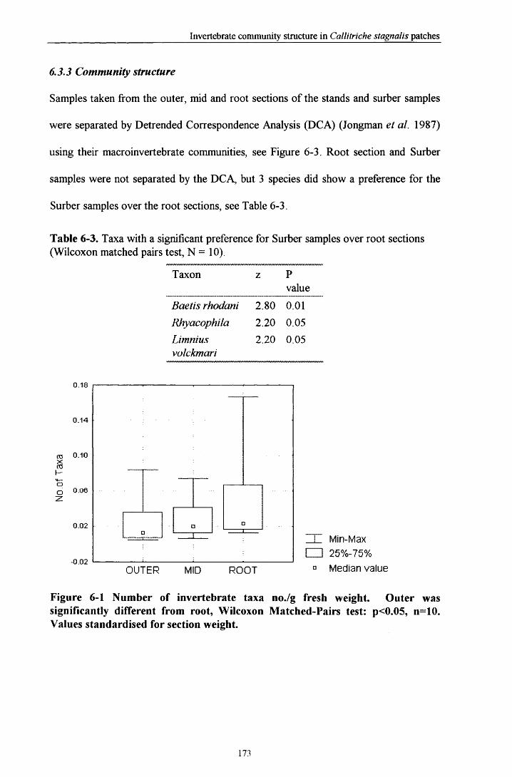
Invertebrate community structure in Callitriche stagnalis patches
6.3.3 Community structure
Samples taken from the outer, mid and root sections of the stands and surber samples
were separated by Detrended Correspondence Analysis (DCA) (Jongman et al. 1987)
using their macroinvertebrate communities, see Figure 6-3. Root section and Surber
samples were not separated by the DCA, but 3 species did show a preference for the
Surber samples over the root sections, see Table 6-3.
Table 6-3. Taxa with a significant preference for Surber samples over root sections (Wilcoxon matched pairs test, N = 10).
Taxon z Pvalue
Baetis rhodani 2.80 0.01Rhyacophila 2.20 0.05Limniusvolckmari
2.20 0.05
_ i_ Min-Max 1 I 25%-75%
OUTER MID ROOT D Median value
Figure 6-1 Number of invertebrate taxa no./g fresh weight. Outer was significantly different from root, Wilcoxon Matched-Pairs test: p<0.05, n=10. Values standardised for section weight.
0.14
CO 0.10XCOh-
N—oQ 0 . 0 0
0.02
173

Invertebrate community structure in Callitriche stagnalis patches
H I Min-Max d j 25%-75%
OUTER MID ROOT D Median value
Figure 6-2 Relative abundance of invertebrates no./g fresh weight. Outer was significantly different from mid and root, Wilcoxon Matched-Pairs test: p<0.05, n=10. Values standardised for section weight.
To standardise between Surber and stand samples, sample area was used, but section
weight was not taken into account. Other analyse showed that the same separation
occurred if section weight was also used but separation of sites was not so clear.
Samples from the outer section were most dissimilar to the Surber sample, the root
section was most similar. The outer section was dominated by the filter feeding
Simuliidae while in all other plant sections Ephemerella ignita dominates. In the
Surber samples Baetis rhodani was the most abundant invertebrate. Community
structure also differed between sections, see Figure 6-4. All three stand sections
supported invertebrate communities which followed the broken stick model (Gray
1987). The outer section, which is exposed to the highest velocities, was the least
equitable with the steepest gradient at the start and is the closest to a geometric series.
Such a series is found in communities poor in species at the earliest successional stage
after colonisation or when exposed to extreme conditions (Gray 1987). The middle
section is more equitable and the root section is the most equitable having the largest
174

Invertebrate community structure in Callitriche stagnalis patches
lDCO+
elmad
+
ephign
f ■ •_ O
gampul
sim + + + + +leutus
♦o
aseaqu
chi
limvad
oultul i
°0bra°^ o
lim / tip
ecd
baerho
hydsil
• . \ | oHhir nmvla
♦ ♦ath esopar
caenv ancflurhy
psi
lOO J globol
- 0 . 5 + 4 . 0
Figure 6-3 Detrended Correspondence Analysis Site by species biplot, (eigenvalues: axis 1 = 0.6, axis 2 = 0.136) Plant section and Surber symbols: Outer +, Mid ■ , Root 0 and Surber O. The location of each taxa is marked with ♦ and a taxa code. Taxa codes: Caenis rivulorum (caeriv), Baetis rhodani (baerho), Ephemerella ignita (ephign), Ecdyonurus (ecd), Hydropsyche siltalai (hydsil), Athripsodes (ath), Brachycentrus subnubilus (brasub), Rhyacophila sp. (rhy), Glossosoma boltoni (globol), Asellus aquatic us (aseaqu), Gammarus pulex (gampul), Ancylus fluviatilis (ancflu), Pisidium sp. (psi), Limnius volckmari larva (limvla), Limnius volckmari adult (limvad), Elmis aenea larva (elmaen), Elmis aenea adult (elmad), Oulimnius tuberculatus adult (oultuad), Oulimnius tuberculatus larva (oultula), Esolus parat/e/pipedus (esopar), Leuctra fusca group (leufus), Tipulinae (tip), Limoniinae (lim), Simulidae (sim), Chironomidae (chi), Hirudidae (hir), Oligochaeta (oli).
175

Invertebrate community structure in Callitriche stagnalis patches
number of species which share the resource more evenly, in terms of producing
individuals.
6.3.4 Prevalent flow conditions
It is suggested that stand structure and velocity combine to create a range of stability
conditions, forming a series o f microhabitats, in, on and outwith the plant beds.
Velocity was significantly different and noted to be lower over the top of the stands
than directly in front o f the stands or in the adjacent Surber samples (Wilcoxon
Matched Pairs p<0.05, n = 10). It is suggested that the shape of the stand is deflecting
water to either side and creating flow conditions which are similar to sheet flow over
the top of the stand; that is turbulent but uniform in direction o f flow. The velocity at
the top of the stand (0.25 ms'1) was higher and significantly different (Wilcoxon
Matched Pairs p<0.05, n= 6) than that in the middle (0.046 ms'1) but velocity at the
bottom (0.040m/s) of the stand was not significantly different from that in the middle.
The near bed velocities at the Surber sample points (0.042 ms'1), (estimated by
adjusting velocity measured at 0 .4 of depth from the bed) are not significantly different
to those found in the mid and root sections of the stand. Estimates o f near bed velocity
over substrate were an order of magnitude lower than those measured on the outside
of the plant stands. An estimate of the required velocity at 0.4 of depth above
substrate flowing over unvegetated substrate that would produce a near bed velocity
similar to the velocity experienced by the outer section of the stands would equate to
2.5ms'1, or near spate condition, see Figure 6-5. This figure was derived from using
Carling's (1992) estimate procedure in reverse starting with the flow over the outer
section of the stands (0.25 m/s).
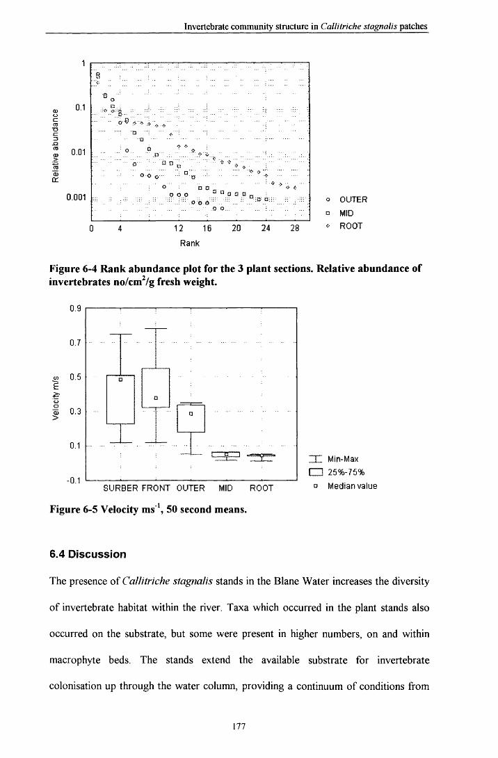
Invertebrate community structure in Callitriche stagnalis patches
0.1t=OJ73
CDa:
0.01
0.001
ono o c,
n o , .) o o lJ a a I
:: o o 6 ... :Q O
12 16 20
Rank
24 28
O OUTER
= MID
ROOT
Figure 6-4 Rank abundance plot for the 3 plant sections. Relative abundance of invertebrates no/cm2/g fresh weight.
0.9
co U.uEuo3 0.3 >
~T~ Min-Max
! i 25%-75%
a Median valueSURBER FRONT OUTER MID ROOT
Figure 6-5 Velocity m s1, 50 second means.
6.4 Discussion
The presence of Callitriche stagnalis stands in the Blane Water increases the diversity
of invertebrate habitat within the river. Taxa which occurred in the plant stands also
occurred on the substrate, but some were present in higher numbers, on and within
macrophyte beds. The stands extend the available substrate for invertebrate
colonisation up through the water column, providing a continuum of conditions from
177

Invertebrate community structure in Callitriche stagnalis patches
high to low velocity. Adjacent benthic substrate does not provide the high velocities
present on the outside of the plant stand in a sustained manner, that is only under near
spate conditions would these high velocities be achieved. In addition the external
surface of the stands greatly increases the area of high-flow substrate available for
colonisation by invertebrates adapted to high flow conditions, especially Simuliidae
(Hart & Latta 1986). Their habitat requirements include the need for fast flowing
water through their labral fans but they avoid areas o f maximum shear stress (Craig &
Chance 1981; Lacoursiere 1991) and it is likely that the correct complex of hydraulic
conditions are available on the surface of the plants.
Although taxon richness and abundance were not significantly different between the
mid and root sections o f the plants they were separable using DCA. The rank
abundance plots demonstrated that the root section was more equitable than the mid
section in resource distribution, hence the separation in the DCA biplot. This would
suggest that conditions were more extreme in the mid section than the root section,
which could be a product o f longer term conditions than those measured in this study.
The conditions present in these two sections allowed E.ignita to dominate where B.
rhodani dominated in the Surber samples.
It has been suggested by (Sand-Jensen & Madsen 1992) that Callitriche cophocarpa
"patches form a mutually protecting structure against high flows“ and “may,
therefore... increase nutrient supply from sedimentation fine-grained particles". He
later found that the sediment under stands often has high levels of organic matter
(Sand-Jensen 1998) which could provide food for detritivores. In this study, despite
finding that the substrate under our stands was more fine grained than that in
unvegetated areas we found that no detrivore showed a preference for the root

Invertebrate community structure in Callitriche stagnalis patches
section, compared to the adjacent unvegetated sediment. I did not measure the amount
of organic matter in the sediment.
The net result o f the presence o f the plants is to increase the invertebrate abundance
and diversity present in the Blane Water. The assemblages present can be related to
the structure o f the stands, and how this influences the flow conditions experienced by
the animals. The complexity of invertebrate community supported appears to be
functionally related to position within the stand, with extreme conditions (on the
external surface) supporting fewer species than within the bed. The total diversity
supported is however a function of the total available set o f conditions present in the
river: on, in and between the stands.
From a management point o f view it is clear that the presence of the stands
substantially increases the invertebrate diversity and abundance supported by the river,
particularly by increasing the habitat available for organisms (e.g. Simuliidae) which
would otherwise find only a limited space for colonisation in their preferred high-flow
conditions.
Callitriche stagnalis is a common species in British rivers, and elsewhere in Europe,
with a high tolerance of disturbance (Sabbatini & Murphy 1996). Inclusion o f
transplanted material as part of rehabilitation schemes in the small gravel-bed rivers
which are well-suited to this species would be likely to make a useful contribution to
improving invertebrate support function of the river.
6.5 Conclusions
• The macrophyte stands supported a greater abundance of benthic macroinvertebrates than bare substrate.
• Higher velocities were recorded on the surface of the macrophyte stands than on the bare substrate.
179

Invertebrate community structure in Callitriche stagnalis patches
• The invertebrate community occurring on the outside of the stands was dominated by Simuliidae and was less equitable than the community living on the interface between the plant stands and the substrate.
• By diversifying the habitat for benthic invertebrates, macrophyte stands are a potentially useful tool in river rehabilitation.
180

General Discussion
Chapter 7: General Discussion
7.1 Review of results
The original aim of this study was to provide data on flow preferences of benthic
invertebrates which could contribute both to our ecological understanding of these
organisms, and assist in construction of river management tools. In Chapter 2 ,1 attempted
to define deep and shallow river sections as riffles, pools and runs, using a range of
criteria, and came to the conclusion that visual observation, coupled with depth and
velocity measurements was necessary. Despite the minimal differences in benthic
invertebrate community between the deep and shallow reaches of rivers used in this study
it is likely that, indirectly at least, deep and shallow reaches do form important habitat
units for the benthos. Predatory fish, salmonids, have a direct effect on the benthic
community by catching animals drifting out of riffles into pools (Ade 1989); they also use
riffle areas as spawning grounds. It has also been suggested that riffles provide more
refugia and are less disturbed than pools (Scarsbrook & Townsend 1993).
In Chapter 3, I demonstrated both the relative homogeneity of the invertebrate community
within each river, and also the existence of gradients between erosional and depositional
conditions, with taxa occurring along these gradients: a situation found in similar studies in
Australia (Barmuta 1989). The results of the analysis presented in Chapter 4 suggest that
data collected using a randomised sampling strategy on instream habitat is not suitable for
precise quantification of invertebrate flow preferences. The methods are sufficient to
identify habitat preferences in a general manner - whether the animal prefers fast or slow
conditions - but not quantitatively. This type of study does inform us of the relative
importance of the environmental variables and how they interact with one another.

General Discussion
Laboratory flume experiments as carried out in Chapter 5 were also necessary to confirm
findings made in the field. The approach taken in Chapter 5 allows for some measure of
the plasticity in species responses to adverse flow conditions but does not offer a velocity
gradient to the animals (which would be the most useful approach). The results also
showed that the taxa had very different tolerance ranges for velocity and that behavioural
control of drift may be possible. The final results chapter (Chapter 6) looked at a natural
gradient of flow conditions in an aquatic macrophyte stand. The results presented in this
chapter suggested that the higher velocities found on the outside of plant stands are not
preferred by some species but were by others, e.g. Simulium. Whether this was due to
velocity or some other another factor such as the presence of predators is difficult to
elucidate from the present study and requires more work. Exposing the animals in a flume
to a velocity gradient which covers the range found in the macrophyte patch under
controlled conditions would go some way to testing the theory that water velocity
preference is one of the main factors influencing benthic invertebrate occurrence.
7.2 Future Work
Identifying flow preferences of benthic invertebrates remains as a major aim necessary for
the ecology and management of lotic freshwater systems. A refined version of the
approach taken in this thesis could supply the information required.
A potential approach to elucidating the instream distribution of invertebrates involves both
increasing and decreasing the spatial scale examined. To demonstrate clearer differences in
invertebrate community structure one would need to examine a wider range of conditions
e.g. in the rivers used in my study the deepest pool section was 1.5 m but a deeper range
would be more informative, see Chapter 2, section 2.3. Large scale studies as suggested
182

General Discussion
here have previously identified habitat units at the start of the study and based their
sampling round these; edge, riffle, pool etc. A greater emphasis on covering wide ranges
of parameters of interest, such as velocity, depth, substrate type and periphyton cover is an
alternative approach advocated here. Reducing the scale of sample area and thereby
making velocity measurements more accurate is also necessary and would seem sensible.
Which spatial scale is correct for this type of procedure could be determined by a nested
sampling design where the spatial scale is reduced at a number of levels. This type of study
has been done at large physical scale, between rivers and reaches but not for instream
habitat. Elliot (1977) gives a number of methods for determining whether benthic
invertebrate distribution is aggregated or not and these could be applied to such data. It is
likely that different taxa will exhibit clumping at different spatial scales and that a single
taxon can also clump at different scales, e.g. in Chapter 2.3.6, p47, B. rhodani showed a
preference for run sections in the Duneaton Water and Blane Water which is possibly
caused by the presence of suitable, smaller habitat units: rocks with periphyton, which if
examined at this scale the animals would also show a preference. This type o f study could
potentially use some of the new sampling methodology available such as stereo
photography which allow fine scale measures of invertebrate distribution (Evans & Norris
1997). Direct measures of turbulence were not included in this study and it is proposed
that any future work would include small scale localised measures of turbulence, which
given the potential of turbulent water to surprise invertebrates and entrain them must mean
areas of high turbulence are avoided. By turbulence here I do not simply mean non-laminar
flow but gross, random motion of water at scales larger than the molecular.
183

General Discussion
By concentrating on individual species and recording their velocity and depth tolerances
under controlled laboratory conditions we could begin to determine the importance of
biotic and abiotic factors in their distribution. The lack o f this type of basic knowledge
hampers our interpretation of large survey work as carried out in this study. Based in the
laboratory the work could proceed faster than trying to make accurate measurements of
single species distributions in relation to velocity in the field, as suggested in the previous
paragraph, which requires painstaking and time consuming methods, e.g. Hart et al.
(1996). Field based measurements can only be applied to animals while they are on the
surface o f the substrate and, as many species spend large portions o f time among the
substrate matrix, a second series of experiments would be necessary to identify the
proportion of time spent in both locations.
The spatial complexity o f instream habitat has been linked to invertebrates’ ability to
withstand disturbance events (Lancaster & Hildrew 1993b). It is possible that streams of
different retention capacity support invertebrates with different life history strategies. The
homogeneity of instream habitat in channelled rivers could therefore cause the strategies
of these organisms to be altered and could exert a selective pressure on the animals. The
implications this has for the genetic variability or life history strategies of these animals has
yet to be addressed. New work is required to look at this question which must incorporate
studies o f both juveniles and adults.
7.3 Management recommendations
This study aimed at a very specific question of river management: how to improve
instream habitat for benthic macroinvertebrates. There are three major impacts on this
184
General Discussion
habitat type in small Scottish streams; river channelisation and alteration of channel
discharge either by damming, changes in catchment land use or water abstraction, often
for fish farms. Management solutions applied in Scotland include the maintenance of
minimum discharges (Q90 and Q95) from reservoirs and in streams from which water is
abstracted, as imposed by SEP A (Marsden, M., SEP A pers comm) and the physical
rehabilitation of channelised systems (Gilvear & Bradley 1997).
To date management guidelines suggested by public bodies (SNH and SEP A) and Non
Governmental Bodies (e.g. RSPB) have mainly concentrated on physical habitat
improvement for taxa other than macroinvertebrates, usually fish, birds and vegetation
(Hoey et al. 1998). With the forthcoming EU Water Framework Directive which
emphasises the ecological and physical naturalness of surface waters there will be a
growing need to improve instream rehabilitation for invertebrates.
The importance of aquatic macrophytes as a useful tool in the conservation of
macroinvertebrates has been previously highlighted (Wright et al. 1995). The results of
Chapter 6 emphases this fact and illustrate the need for more basic research in this area if
we are to manage aquatic vegetation for the benefit o f macroinvertebrates without
compromising the capacity of channels to deal with high flows; a problem which has a
number of potential solutions (Fox & Murphy 1990a; Fox & Murphy 1990b). The density
of macrophytes can even be incorporated into PHABSIM models if one wished (Hearne et
al. 1994)! If used correctly macrophytes could potential mitigate the impacts of
disturbance caused by rising discharge in a similar manner to woody debris (Borchardt
1993) and potentially increase the number of macrophyte species too (Hey et al. 1994).
185

General Discussion
Structural rehabilitation schemes are usually very successful in improving the diversity and
productivity o f the altered reaches (Swales & O'Hara 1980). The process of community
alteration resulting from structural alterations to channels as part of habitat enhancement
schemes can be difficult to judge in detail (Lynch & Murray 1994). If we wish to advance
the science of this process and its usefulness as a management tool studies such a those
advocated in section 7.2 will be necessary to improve their design.
PHABSIM is one of the few models which is now used to predict the amount of useable
habitat for invertebrates at different discharges. In Chapters 3 and 4 I identified a number
of problems with the data on which this model is based which need to be addressed if the
model is to more accurately predict useable habitat for invertebrates. The previous section
on further research suggests the type of projects necessary to collect this data.
There is a more fundamental problem associated with using this type of model and that is
that its aim is only to make sure there is suitable habitat available for the animals. It does
not take into account the dynamic nature of lotic systems which fuel the natural evolution
of the invertebrate community e.g. it is quite possible for the same Q90 to be realised daily
without variation. As ecologists our advice to managers should be to keep the physical
system as natural as possible and the invertebrates will adapt to it. For the present it may
be more suitable to use models based on historical flows or the flows implied by the rivers
geomorphology, (see Jowett (1997) for a review of approaches). Geomorphologists have
a more developed understanding of how any particular river should look and act than
ecologists have of how animals interact with the habitat provided by the river (Werritty et
al. 1994). Given the present state of knowledge in both disciplines ecologists should
186

General Discussion
support the work o f managers where they try and recreate the natural geomorphology of
rivers.
Frequently this approach is too simplistic as it can be impossible to recreate a river’s
‘natural’ geomorphology given the small sections of rivers that can be worked on and the
numerous impacts presently outwith the control of managers, e.g. climate change and
catchment land use (Langan et al. 1997). There is also the possibility that by increasing
flow variability one could decrease available benthic invertebrate habitat (Englund &
Malmquist 1996). This emphasises the need for an improved understanding of the
interaction between benthic invertebrates and the physical habitat of rivers is necessary.
The approach taken in this thesis utilised a direct assessment of the habitat usage by
invertebrate organisms: to develop suitable management models indirect interactions also
need to be understood. The key to this understanding is the role of natural disturbance
(flood events), interactions with riparian ecotones and instream habitat patchiness. Recent
research which has started to describe the mechanisms underpinning these interactions was
discussed at the start o f this thesis (Chapter 1, section 1.1): it appears that much more
work is required in this field.
Recent papers on the state of freshwater ecology and the management of freshwaters
emphasises the need for ecologists to champion the relevance of their work and to review
the paradigms of aquatic ecology (Reynolds 1998). This work also emphasises the need
for 'quantitative bench marks and empiricised strategies to be set'. Reynolds (1998), similar
to the approach take in the restoration of the Danube fish populations, (Keckeis &
Schiemer 1992; Schiemer & Wieser 1992; Tockner & Schiemer 1997). This promotion of
systems ecology has been heeded by UNESCO which now has a work program which is
187

General Discussion
developing the tools and the paradigm of 'Ecohydrology'. Among the many UNESCO
projects are those that look at the interactions of river flow instream and in the wider
context of the catchment.
In summary the advice given to managers of aquatic ecosystems is not new and is that
more basic scientific research is needed (Welcomme 1992). That UNESCO considers an
ecologically balanced and soft engineering approaches to river management o f importance
emphasises the need for both more research and sensitive management.
188

References
References
Adams, C. E. & Maitland, P. S. 1998 The ruffe population of Loch Lomond, Scotland: Its introduction, population expansion, and interaction with native species. Journal o f Great Lakes Research 24, 249-262.
Ade, R. 1989 The Trout and Salmon Handbook. A Guide to the Wild Fish. Bromley: Christopher Helm Ltd.
Ambuhl, H. 1959 Die Bedeutung der Stromung als okologischer Faktor. Schweiz Z. Hydrol 21, 133-264.
Armitage, P. D. 1976 A quantitative study of the invertebrates of the River Tees below Cow Green Reservoir. Freshwater Biology 6, 229-240.
Armitage, P. D. 1995 Faunal community change in response to flow manipulation. In The EcologicalBasis o f River Management (ed. D. M. Harper & A. J. D. Ferguson), pp. 59-78. Chichester: John Wiley & Sons.
Armitage, P. D., Cranston, P. S. & Pinder, L. V. C. 1995 The Chironomidae : Biology and Ecology o f Non-biting Midges. London: Chapman and Hall.
Armitage, P. D. & Gunn, R. J. M. 1996 Differential response of benthos to natural and anthropogenicdisturbances in 3 lowland streams. Internationale Revue Der Gesamten Hydrobiologie 81, 161- 181.
Armour, C. L. & Taylor, J. G. 1991 Evaluation of the instream flow incremental methodology by United- States fish and wildlife service field users. Fisheries 16, 36-43.
Bacher, I. & Waringer, J. A. 1996 Hydraulic microdistribution of cased caddis larvae in an Austrian mountain brook. Internationale Revue Der Gesamten Hydrobiologie 81, 541-554.
Badcock, R. M. 1976 The distribution of the Hydropsychidae in Great Britain. In Proceedings o f the First International symposium on Trichoptera (ed. H. Malicky). The Hague.
Barmuta, L. A. 1989 Habitat patchiness and macrobenthic community structure in an upland stream in temperate Victoria, Australia. Freshwater Biology 21, 223-236.
Begon, M., Harper, J. L. & Townsend, C. R. 1996 Ecology: Individuals, Populations and Communities. Oxford: Blackwell Science.
Biron, P. M., Lane, S. N., Roy, A. G., Bradbrook, K. F. & Richards, K. S. 1998 Sensitivity of bed shear stress estimated from vertical velocity profiles: The problem of sampling resolution. Earth Surface Processes and Landforms 23, 133-139.
Borchardt, D. 1993 Effects of flow and refugia on drift loss of benthic macroinvertebrates - Implications for habitat restoration in lowland streams. Freshwater Biology 29, 221-227.
Borchardt, D. & Statzner, B. 1990 Ecological impact of urban stormwater runoff studied in experimental flumes - population loss by drift and availability of refugial space. Aquatic Sciences 52. 299-314.
Bouckaert, F. W. & Davis, J. 1998 Microflow regimes and the distribution of macroinvertebrates around stream boulders. Freshwater Biology 40, 77-86.
189

References
Boulton, A. J., Peterson, C. G., Grimm, N. B. & Fisher, S. G. 1992 Stability of an aquaticmacroinvertebrate community in a multiyear hydrologic disturbance regime. Ecology 73, 2192- 2207.
Boumaud, M. 1963 Le courant, facteur ecologique et ethologique de la vie aquatique. Hydrobiologia 21, 125-65.
Bovee, K. D. 1982 A guide to stream habitat analysis using instream flow incremental methodology.United States Fish and Wildlife Service, Cooperative Instream Flow Group, Instream Flow information paper 12, 248.
Briggs, J. C. 1948 The quantitative effects of a dam upon bottom fauna of a small Californian stream.Transactions o f the American Fisheries Society 78, 70-81.
Brinkhurst, R. O. 1963 A Guide fo r the Identification o f British Aquatic Oligochaeta. Scientific Publication No. 22: Freshwater Biological Association.
Brittain, J. E. & Eikeland, T. J. 1988 Invertebrate Drift - A Review. Hydrobiologia 166, 77-93.
Brooks, S. S. & Boulton, A. J. 1991 Recolonization dynamics of benthic macroinvertebrates after artificial and natural disturbances in an Australian temporary stream. Australian Journal o f Marine and Freshwater Research 42, 295-308.
Brown, A. V. & Brussock, P. P. 1991 Comparisons of Benthic Invertebrates Between Riffles and Pools.Hydrobiologia 220, 99-108.
Brown, H. P. 1987 Biology of riffle beetles. Annual Review o f Entomology 32, 253-273.
Brusca, R. C. & Brusca, G. J. 1990 Invertebrates. Sunderland, Massachusetts: Sinauer Associates, Inc.
Buchan, L. A. J. & Padilla, D. K. 1999 Estimating the probability of long-distance overland dispersal of invading aquatic species. Ecological Applications 9, 254-265.
Buffagni, A., Crosa, G. & Marchetti, R. 1995 Size-related shifts in the physical habitat of 2 mayfly species (Ephemeroptera). Freshwater Biology 34, 297-302.
Carling. 1992 The nature of the fluid-boundary layer and the selection of parameters for benthic ecology. Freshwater Biology 28, 273-284.
Carling, P. 1995 Implications of sediment transport for instream flow modelling of aquatic habitat. In The ecological basis fo r river management (ed. D. Harper & A. J. D. Ferguson). Chichester: John Wiley & Sons.
Carling, P. A. 1993 The nature of the fluid boundary layer and the selection of parameters for benthic ecology: Reply to Lamouroux. Freshwater Biology 30, 333-335.
Ciborowski, J. J. H. 1983 Influence of current velocity, density, and detritus on drift of 2 mayfly species (Ephemeroptera). Canadian Journal o f Zoology 61, 119-125.
Ciborowski, J. J. H. 1987 Dynamics of drift and microdistribution of 2 mayfly populations - a predictive model. Canadian Journal o f Fisheries and Aquatic Sciences 44, 832-845.
190

References
Clausen, B. & Biggs, B. J. F. 1997 Relationships between benthic biota and hydrological indices in New Zealand streams. Freshwater Biology 38, 327-342.
Clegg, J. 1952 The Freshwater Life o f the British Isles. London and New York: Fredrick Wame &Co.,Ltd.
Clifford, N. J. 1993 Formation of riffle pool sequences - field evidence for an autogenetic process. Sedimentary Geology 85, 39-51.
Cobb, D. G., Galloway, T. D. & Flannagan, J. F. 1992 Effects of discharge and substrate stability ondensity and species composition of stream insects. Canadian Journal o f Fisheries and Aquatic Sciences 49, 1788-1795.
Collier, K. J., Croker, G. F., Hickey, C. W., Quinn, J. M. & Smith, B. S. 1995 Effects of hydraulicconditions and larval size on the microdistribution of Hydrobiosidae (Trichoptera) in two New Zealand rivers. New Zealand Journal o f Marine and Freshwater Research 29, 439-451.
Collier, K. J. & Wakelin, M. D. 1992 Drift of aquatic macroinvertebrate larvae in Manganuiateao River, Central North Island, New Zealand. New Zealand Natural Sciences 19, 15-26.
Cowan, C. A. & Peckarsky, B. L. 1990 Feeding by a lotic mayfly grazer as quantified by gut fluorescence. Journal o f the North American Benthological Society 9, 368-378.
Craig, D. A. & Chance, M. M. 1981 Filter feeding in larvae of Simuliidae (Diptera: Culicomorpha):aspects of functional morphology and hydrodynamics. Canadian Journal o f Zoology 60, 712-724.
Crawley, M. J. 1986 Plant Ecology. Oxford: Blackwell Scientific Publications.
Crowl, T. A. & Schnell, G. D. 1990 Factors determining population-density and size distribution of a fresh-water snail in streams - effects of spatial scale. Oikos 59, 359-367.
Crowl, T. A., Townsend, C. R.. Bouwes, N. & Thomas, H. 1997 Scales and causes of patchiness in stream invertebrate assemblages: Top-down predator effects? Journal o f the North American Benthological Society 16, 277-285.
Cudney, M. D. & Wallace, J. B. 1980 Life cycles, microdistribution and production dynamics of sixspecies of net-spinning caddisflies in a large southeastern stream. Holartic Ecology 3, 169-182.
Cummins, K. W. 1973 Trophic relations of aquatic insects. Annual review o f entomology 18, 183-206.
Dahl, J. & Greenberg, L. 1996 Effects of habitat structure on habitat use by Gammarus pulex in artificial streams. Freshwater Biology 36, 487-495.
Davis, J. A. & Barmuta, L. A. 1989 An ecologically useful classification of mean and near -bed flows in streams and rivers. Freshwater Biology 21, 271-278.
Death, R. G. 1996 The effect of patch disturbance on stream invertebrate community structure - the influence of disturbance history. Oecologia 108, 567-576.
Death, R. G. & Winterboum, M. J. 1995 Diversity patterns in stream benthic invertebrate communities - the influence of habitat stability. Ecology 76, 1446-1460.
191

References
Degani, G., Herbst, G. N., Ortal, R., Bromley, H. J., Levanon, D., Netzer, Y., Harari, N. & Glazman, H. 1993 Relationship between current velocity, depth and the invertebrate community in a stable river system. Hydrobiologia 263, 163-172.
Dejalon, D. G. & Sanchez, P. 1994 Downstream effects of a new hydropower impoundment on macrophyte, macroinvertebrate and fish communities. Regulated Rivers: Research & Management 9, 253-261.
Dick, J. T. A. 1992 The nature and implications of differential predation between Gammarus-pulex and G duebeni-celticus (Crustacea, Amphipoda). Journal o f Zoology 227, 171-183.
Dick, J. T. A., Faloon, S. E. & Elwood, R. W. 1998 Active brood care in an amphipod: influences of embryonic development, temperature and oxygen. Animal Behaviour 56, 663-672.
Dick, J. T. A., Irvine, D. E. & Elwood, R. W. 1990 Differential predation by males on molted females may explain the competitive displacement of Gammarus-duebeni by G-pulex (Amphipoda). Behavioral Ecology and Sociobiology 26, 41-45.
Dick, J. T. A., Nelson, N. & Bishop, J. D. D. 1997 Introduction experiments with Gammarus spp.(Crustacea: Amphipoda) in the Isle of Man (British Isles), 1949-1995. Journal o f Zoology 242, 209-216.
Dingman, S. L. 1984 Fluvial Hydrology. New York: Freeman and Company.
Dittmar, H. 1955 Ein Sauerlandbach. Untersuchungen an einem Wiesen-Mittel-gebirgsbach. Arch. Hydrobiol. 50, 305-552.
Dodds, G. S. & Hisaw, F. L. 1924 Ecological studies of aquatic insects. I. Adaptation of mayfly nymphs to swift streams. Ecology 5, 137-148.
Dodds, G. S. & Hisaw, F. L. 1925 Ecological studies of aquatic insects. III. Adaptation of caddisfly larvae to swift streams. Ecology 6, 123-137.
Dorier, A. & Vaillant, F. 1955 Sur le facteur vitesse du courant. Verh. int. Verein. theor. angew. Limnol. 12, 593-597.
Doughty, C. R. & Maitland, P. S. 1994 The ecology of the River Endrick: present status and changes since 1960. Hydrobiologia 290, 131-151.
Downes, B. J. & Jordan, J. 1993 Effects of stone topography on abundance of net-building caddisfly larvae and arthropod diversity in an upland stream. Hydrobiologia 252, 163-174.
Downes, B. J., Lake, P. S. & Schreiber, E. S. G. 1995 Habitat structure and invertebrate assemblages on stream stones: A multivariate view from the riffle. Australian Journal o f Ecology 20, 502-514.
Dudgeon, D. 1991 An experimental-study of abiotic disturbance effects on community structure and function in a tropical stream. Archiv Fur Hydrobiologie 122, 403-420.
Dudgeon, D. 1993 The effects of spate-induced disturbance, predation and environmental complexity on macroinvertebrates in a tropical stream. Freshwater Biology 30, 189-197.
Dudgeon, D. & Chan, I. K. K. 1992 An experimental-study of the influence of periphytic algae on invertebrate abundance in a Hong-Kong stream. Freshwater Biology 27, 53-63.
192

References
Ebrahimnezhad, M. & Harper, D. M. 1997 The biological effectiveness of artificial riffles in river rehabilitation. Aquatic Conservation-Marine and Freshwater Ecosystems 7, 187-197.
Egglishaw, H. J. & Mackay, D. W. 1966 A survey of the bottom fauna of streams in the Scottishhighlands. Pt. III. Seasonal changes in the fauna of three streams. Hydrobiologia 30, 305-334.
Egglishaw, H. J. & Morgan, N. C. 1965 A survey of the bottom fauna of streams in the Scottishhighlands. Pt. II. The relationships of the fauna to the chemical and geological conditions.Hydrobiologia 26, 173-183.
Elliot, J. M. 1977 Some Methods fo r the Statistical Analysis o f Samples o f Benthic Invertebrates. Windemere: Freshwater Biological Association.
Elliot, J. M. & Mann, K. H. 1919 A Key to the British Freshwater Leeches with Notes on their Life Cycles and Ecology. Freshwater Biological Association.
Englund, G. & Malmquist, B. 1996 Effects of flow regulation, habitat area, and isolation on themacroinvertebrate fauna of rapids in North Swedish Rivers. Regulated Rivers: Research and Managment 12, 433-445.
Equihua, M. 1990 Fuzzy clustering of ecological data. Journal o f Ecology. 78 519-534.
Evans, L. J. & Norris, R. H. 1997 Prediction of benthic macroinvertebrate composition using microhabitat characteristics derived from stereo photography. Freshwater Biology 37, 621-633.
Eyre, M. D., Carr, R., McBlane, R. P. & Foster, G. N. 1992 The effects of varying site-water duration on the distribution of water beetle assemblages, adults and larvae (Coleoptera, Haliplidae,Dytiscidae, Hydrophilidae). Archiv Fur Hydrobiologie 124, 281-291.
Eyre, M. D., Foster, G. N. & Young, A. G. 1993 Relationships between water-beetle distributions and climatic variables - a possible index for monitoring global climatic-change. Archiv Fur Hydrobiologie 127, 437-450.
Fitter, R. & Manuel, R. 1994 Lakes, Rivers and Streams o f Britain and North-West Europe. Collins Photo Guide. Hong Kong: Harper Collins Publishers.
Fjellheim, A. 1996 Distribution o f benthic invertebrates in relation to stream flow characteristics in a Norwegian river. Regulated Rivers-Research & Management 12, 263-271.
Fjellheim, A., Havardstun, J., Raddum, G. G. & Schnell, O. A. 1993 Effects of increased discharge onbenthic invertebrates in a regulated river. Regulated Rivers-Research & Management 8, 179-187.
Fox, A. M. & Murphy, K. J. 1990a The efficacy and ecological impacts of herbicide and cutting regimes on the submerged plant-communities of 4 british rivers . 1. A comparison of management efficacies. Journal o f Applied Ecology 27, 520-540.
Fox, A. M. & Murphy, K. J. 1990b The efficacy and ecological impacts of herbicide and cutting regimes on the submerged plant-communities of 4 british rivers .2. A multivariate-analysis of the effects of management regimes On macrophyte communities. Journal o f Applied Ecology 27, 541-548.
Fozzard, I.R., Doughty, C.R. & Clelland, B.E. 1994 Invertebrates. The Freshwaters o f Scotland-ANational Resource o f International Significance. (Ed. Maitland, P. S., Boon, P. J. & McLusky, D.S.) John Wiley & Sons. Chichester.
193

References
Gauch, H. G. 1982 Multivariate Analysis in Community Ecology. Cambridge: Cambridge University Press.
Georgian, T. & Thorp, J. H. 1992 Effects of microhabitat selection on feeding rates of net-spinning caddisfly Larvae. Ecology 73, 229-240.
Giller, P. S. & Malmquist, B. 1998 The Biology o f Streams and Rivers. Biology of habitats. Oxford: Oxford University Press.
Gilvear, D. & Bradley, S. 1997 Geomorphological adjustment of a newly engineered upland sinuousgravel-bed river diversion: Evan Water, Scotland. Regulated Rivers: Research and Management 13, 377-389.
Golubkov, S. M., Tiunova, T. M. & Kocharina, S. L. 1992 Dependence of the respiration rate of aquatic insects upon the oxygen concentration in running and still water. Aquatic Insects 14, 137-144.
Gore, J. A., Crawford, D. J. & Addison, D. S. 1998 An analysis of artificial riffles and enhancement of benthic community diversity by physical habitat simulation (PHABSIM) and direct observation.Regulated Rivers-Research & Management 14, 69-77.
Gray, J. S. 1987 Species-abundance patterns. In Organisation o f Communities; Past and Present (ed. J. H.R. Gee & P. S. Giller), pp. 53-68. Oxford: Blackwell Scientific Publications.
Gregg, W. W. & Rose , F. L. 1982 The effects of aquatic macrophytes on the stream microenvironment.Aquatic Botany 14, 309-324.
Guinand, B., Tachet, H. & Roux, C. 1994 Longitudinal distribution and ecophysiological charcteristics of Hydropsyche exocellata (Trichoptera: Hydropsychidae) in large rivers. Ecography 17, 189-197.
Gurtz, M. E. & Wallace, J. B. 1984 Substrate-mediated response of stream invertebrates to disturbance.Ecology 65, 1556-1569.
Hammond, C. & Merrit, R. 1983 The Dragonflies o f Great Britain and Ireland. Colchester: Harley Books, Martins, Great Horkesley, Essex C06 4AH.
Hansen, R. A., Hart, D. D. & Merz, R. A. 1991 Flow mediates predator-prey interactions between tricladflatworms and larval black flies. Oikos 60, 187-196.
Hanski, I. 1994 Metapopulation Ecology. In Spatial and Temporal Aspects o f Population Processes (ed.O. E. Rhodes Jr). Georgia: University of Georgia.
Harper, D., Ebrahimnezhad, M. & Cot, F. C. I. 1998 Artificial riffles in river rehabilitation: setting the goals and measuring the successes. Aquatic Conservation-Marine and Freshwater Ecosystems 8, 5-16.
Harrison, S. S. C. & Hildrew, A. G. 1998 Distribution dynamics of epilithic insects in a lake littoral.Archiv Fur Hydrobiologie 143, 275-293.
Hart, D. D. 1991 Feeding postures of suspension-feeding larval black flies - The conflicting demands of drag and food acquisition. Oecologia 85, 457-463.
Hart, D. D. 1992 Community organization in streams - the importance of species interactions, physical factors, and chance. Oecologia 91, 220-228.
194

References
Hart, D. D., Clark, B. D. & Jasentuliyana, A. 1996 Fine-scale field measurement o f benthic flowenvironments inhabited by stream invertebrates. Limnology and Oceanography 41, 297-308.
Hart, D. D. & Latta, S. C. 1986 Determinants of ingestion rates in filter-feeding larval blackflies (Diptera, Simuliidae). Freshwater Biology 16, 1-14.
Hawkins, C. P., Hogue, J. N., Decker, L. M. & Feminella, J. W. 1997 Channel morphology, water temperature, and assemblage structure of stream insects. Journal o f the North American Benthological Society 16, 728-749.
Heame, J., Johnson, I. & Armitage, P. 1994 Determination of ecologically acceptable flows in rivers with seasonal-changes in the density of macrophyte. Regulated Rivers-Research & Management 9, 177-184.
Hey, R. D., Heritage, G. L. & Patterson, M. 1994 Impact of flood alleviation schemes on aquatic macrophytes. Regulated Rivers: Research and Managment 9, 103-119.
Hickin, N. E. 1967 Caddis Larvae o f the British Trichoptera. London: Hutchinson & Co. Ltd.
Hildrew, A. G. & Giller, P. S. 1994 Patchiness, species interactions and disturbance in the streambenthos. In Aquatic Ecology, Scale, Pattern and Process (ed. P. S. Giller, A. G. Hildrew & D. G. Raffaelli), pp. 649. Oxford: Blackwell Scientific Ltd.
Hoey, T. B., Smart, D. W. J., Pender, G. & Metcalfe, N. 1998 Engineering Methods fo r Scottish Gravel Bed Rivers. SNH Review No. 47. Battleby: Scottish Natural Heritage.
Holomuzki, J. R. 1996 Effects of substrate and predator type on microdistributions and drift of a lotic mayfly. Journal o f the North American Benthological Society 15, 520-528.
Hughes, J. M., Bunn, S. E., Hurwood, D. A. & Cleary, C. 1998 Dispersal and recruitment of Tasiagma ciliata (Trichoptera: Tasimiidae) in rainforest streams, south-eastern Australia. Freshwater Biology 39, 117-127.
Hughes, J. M., Mather, P. B., Sheldon, A. L. & Allendorf, F. W. 1999 Genetic structure of the stonefly, Yoraperla brevis, populations: the extent of gene flow among adjacent montane streams. Freshwater Biology 41. 63-72.
Huhta, A., Muotka, T. & Tikkanen, P. 1995 Diel foraging periodicity of lotic mayfly (Ephemeroptera) nymphs during the sub-arctic summer. Archiv Fur Hydrobiologie 134, 281-294.
Hurlbert, S. H. 1984 Pseudoreplication and the design of ecological field experiments. Ecological Monographs 54, 187-211.
Huryn, A. D. & Wallace, J. B. 1988 Community structure of Trichoptera in a mountain stream - spatial patterns of production and functional-organization. Freshwater Biology 20, 141-155.
Hutchinson, G. E. 1957 Geography, physics and chemistry. A Treatise on Limnology. New York: John Wiley & Sons, inc.
Hynes, H. B. N. 1972 The Ecology o f Running Waters. Liverpool: Liverpool University Press.
Hynes, H. B. N. 1976 Biology of Plecoptera. Annual Rview o f Entomology 21, 135-153.
195

References
Hynes, H. B. N., Williams, D. D. & Williams, N. E. 1976 Distribution of the benthos within the substratum of a Welsh mountain stream. Oikos 27, 307-310.
Jenkins, R. A., Wade, K. R. & Pugh, E. 1984 Macroinvertebrate habitat relationships in the Tefi catchment and significance to conservation. Freshwater Biology 14, 23-42.
Jeppesen, E., Iversen, T. M., Sand-Jensen, K. & Jorgensen, C. P. 1984 0kologiske konsekvenser af reduceret vandforing i Sus&n. In Biologiske processor og vandvalitets-forhold., vol. 2. Copenhagen: Miljostryrelsen.
Johnson, I. W., Elliott, C. R. N. & Gustard, A. 1995 Using the IFIM to model salmonid fish habitat in the River Allen, England. Bulletin Francais De La Peche Et De La Pisciculture , 355-363.
Johnson, I. W. & Law, F. M. 1995 Computer-models for quantifying the hydro-ecology of British rivers. Journal o f the Chartered Institution o f Water and Environmental Management 9, 290-297.
Jones, N. V., Litterick, M. R. & Pearson, R. G. 1977 Stream flow and the behaviour of caddis larvae. In Proceedings o f the Second International Conference on Trichoptera. Junk, The Hague.
Jongman, R. H. G., Ter Braak, C. J. F. & Van Tongeren, O. F. R. 1988 Data Analysis in Community and Landscape Ecology. Cambridge: Cambridge University Press.
Jowett, I. G. 1993 A method for objectively identifying pool, run, and riffle habitats from physical measurements. New Zealand Journal o f Marine and Freshwater Research 27, 241-248.
Jowett, I. G. 1998 Hydraulic geometry o f New Zealand rivers and its use as a preliminary method of habitat assessment. Regulated Rivers-Research & Management 14, 451-466.
Jowett, I. G. & Richardson, J. 1995 Habitat preferences of common riverine New Zealand native fishesand implications for flow managment. New Zealand Journal o f Marine and Freshwater Research 29, 13-23.
Jowett, I. G., Richardson, J., Biggs, B. J. F., Hickey, C. W. & Quinn, J. M. 1991 Microhabitat preferences of benthic invertebrates and the development of generalized Deleatidium spp habitat suitability curves, applied to 4 New-Zealand rivers. New Zealand Journal o f Marine and Freshwater Research 25, 187-199.
Jowett, I. G. 1997 Instream flow methods: A comparison of approaches. Regulated Rivers-Research & Management 13, 115-127.
Keckeis, H. & Schiemer, F. 1992 Food-consumption and growth of larvae and juveniles of 3 cyprinid species at different food levels. Environmental Biology o f Fishes 33, 33-45.
Kiel, E. & Frutiger, A. 1997 Behavioural responses of different blackfly species to short -term oxygen depletion. International Revue der gesampten Hydrobiologie 82, 107-120.
Koetsier, P. & Bryan, C. F. 1995 Effects of abiotic factors on macroinvertebrate drift in the lower Mississippi river, Louisiana. American Midland Naturalist 134, 63-74.
Kohler, S. L. 1985 Identification of stream drift mechanisms: An experimental and observational approach. Ecology 66, 1749-1761.
196

References
Kratz, K. W. 1996 Effects of stoneflies on local prey populations - mechanisms of impact across prey density. Ecology 77, 1573-1585.
Lacoursiere, J. O. 1991 A laboratory study of fluid flow and microhabitat selection by larvae of Simulium vittatum (Diptera: Simuliidae). Canadian Journal o f Zoology 70, 582-596.
Lamouroux, N. 1993 Comment on 'The nature of the fluid boundary layer and the selection of parameters for benthic ecology' (Carling, 1992). Freshwater Biology 30, 331-332.
Lancaster, J. 1992 Diel variations in the effect of spates on mayflies (Ephemeroptera, Baetis). Canadian Journal o f Zoology 70, 1696-1700.
Lancaster, J. 1999 Small-scale movements of lotic macroinvertebrates with variations in flow. Freshwater Biology 41, 605-619.
Lancaster, J. & Hildrew, A. G. 1993a Characterising in-stream flow refugia. Canadian Journal o f Fisheries and Aquatic Sciences 50, 1663-1675.
Lancaster, J. & Hildrew, A. G. 1993b Flow refugia and the microdistribution of lotic macroinvertebrates. Journal o f the North American Benthological Society 12, 385-393.
Lancaster, J., Hildrew, A. G. & Townsend, C. R. 1990 Stream-flow and predation effects on the spatial dynamics of benthic invertebrates. Hydrobiologia 203, 177-190.
Langan, S. J., Wade, A. J., Smart, R., Edwards, A. C., Soulsby, C., Billett, M. F., Jarvie, H. P., Cresser,M. S., Owen, R. & Ferrier, R. C. 1997 The prediction and management of water quality in a relatively unpolluted major Scottish catchment: Current issues and experimental approaches. Science o f the Total Environment 194, 419-435.
Layzer, J. B. & Madison, L. M. 1995 Microhabitat use by ffesh-water mussels and recommendations for determining their instream flow needs. Regulated Rivers-Research & Management 10, 329-345.
Leader, J. P. 1976 Marine caddis flies (Trichoptera: Philanisidae). In Marine Insects (ed. L. Cheng), pp. 581. Amsterdam: North-holland publishing company.
LeRoy Poff, N. 1996 A hydrogeography of unregulated streams in the United States and an examination of scale-dependence in some hydrological descriptors. Freshwater Biology 36, 71-91.
Levins, R. 1969 Some demographic and genetic consequences of environmental heterogeneity for biological control. Bulletin o f the Entomological Society o f America 15, 237-240.
Lynch, J. M. & Murray, D. A. 1994 Fishery rehabilitation enhancment following arterial drainage in Ireland. Verh. Internat. Verein. Limnol. 25, 1502-1508.
Macan, T. T. 1963 Freshwater Ecology: Longmans, Green & Co. Ltd.
Macan, T. T. 1977 A Key to the British Fresh- and Brackish-water Gastropods with Notes on theirEcology. Scientific Publication No. 13. Far Sawrey, Ambleside, Cumbria: Freshwater Biological Association.
Maitland, P. S. 1977 A Coded Checklist o f Animals Occurring in Fresh Water in the British Isles:Institute of Terrestrial Ecology.
197

References
Maitland, P. S. 1990 Biology o f Freshwater s. Tertiary Level Biology. Glasgow & London: Blackie.
Makipaa, R. 1999 Response patterns of Vaccinium myrtillus and N-vitis-idaea along nutrient gradients in boreal forest. Journal o f Vegetation Science 10, 17-26.
Malicky, H. 1981 The phenology o f dispersal of several caddisfly (Trichoptera) species in the island of Crete. In Third International Symposium on Trichoptera. (ed. G.P. Moretti). Junk The Hague, 157-163.
Malmquist, B. & Otto, C. 1987 The influence of substrate stability on the compositon of stream benthos: an experimental study. Oikos 48, 33-38.
Marshall, E. J. P. & Westlake, D. F. 1990 Water velocities around water plants in chalk streams. Folia geobotanic et phytotaxonomica 25, 279-289.
Matthaei, C. D., Uehlinger, U. & Frutiger, A. 1997 Response of benthic invertebrates to natural versus experimental disturbance in a Swiss prealpine river. Freshwater Biology 37, 61-77.
Matthaei, C. D., Uehlinger, U., Meyer, E. I. & Frutiger, A. 1996 Recolonization by benthic invertebrates after experimental disturbance in a swiss prealpine river. Freshwater Biology 35, 233-248.
McCracken, D.I. 1994 A fuzzy classification o f moorland ground beetle (Coleoptera: Carabidae) and plant communities. Pedobiologia 38 12-27.
McCune, B. 1997 Influence of noisy environmental data on canonical analysis. Ecology 78, 2617-2623.
McKirdy, A. 1999^4 Landscape Fashioned by Geology: Scotland - Creation o f its Natural landscape'. Scottish Natural Heritage.
McShaffrey, D. & McCafferty, W. P. 1987 The behaviour and form of Psephenus herrichi(DeKay) (Coleoptera: Psephenidae) in realtion to water flow. Freshwater Biology 18, 319-324.
Merrit, R. W. & Cummins, K. W. 1979 An Introduction to Aquatic Insects. Dubuque, Iowa: Kendall/Hunt Publishing.
Milhous, R. T., Wegner, D. L. & Waddle, T. 1984 User's guide to the physical habitat simulation system. US Fish and Wildlife Service Biological Services Program FWS/OBS-81/43.
Miller, P. 1987 Dragonflies. Naturalists' handbooks 7. Cambridge: Cambridge University Press.
Minshall, G. W. 1984 Aquatic insect -substratum relationships. In Ecology o f Aquatic Insects.
Minshall, G. W., Cummins, K. W., Petersen, R. C., Cushing, C. E., Bruns, D. A., Sedell, J. R. &Vannote, R. L. 1985 Developments in stream ecosystem theory. Canadian Journal o f Fisheries and Aquatic Sciences 42. 1045-1055.
Moog, D.B. & Jirka, G.H. 1999 Stream reaeration in nonuniform flow: Macroroughness enhancement. Journal of Hydraulic Engineering-ASCE, Vol. 125, N o.l , pp. 11-16
Morgan, N. C. & Egglishaw, H. J. 1966 A survey of the bottom fauna of streams in the Scottish Highlands. Pt. I. Composition of the fauna. Hydrobiologia 25, 181-211.
Moss, B. 1988 Ecology o f Freshwaters Man and Medium. Oxford: Blackwell Scientific Publications.
198

References
Nagell, B. & Larshammar, P. 1981 Critical oxygen-demand in Plecoptera and Ephemeroptera nymphs as determined by 2 methods. Oikos 36, 75-82.
Newbury, R. & Gaboury, M. 1993 Exploration and rehabilitation of hydraulic habitats in streams using principles of fluvial behaviour. Freshwater Biology 29, 195-210.
Nowell, A. R. M. & Church, M. 1979 Turbulent flow in a depth-limited boundary layer. Journal o f Geophysical Research 84, 4816-4823.
O'Connor, N. A. 1991 The effects of habitat complexity on the macroinvertebrates colonising wood substrates in a lowland stream. Oecologia , 504-512.
Ormerod, S. J. 1988 The micro-distribution of aquatic macroinvertebrates in the Wye river system: the result of biotic or abiotic factors? Freshwater Biology 20, 241-247.
Otto, C. 1976 Factors affecting the drift o f Potamophylax cingulatus (Trichoptera) larvae. Oikos 27, 93- 100.
Palmer, C., O Keeffe, J. & Palmer, A. 1993a Macroinvertebrate functional feeding groups in the middle and lower reaches of the Buffalo River, Eastern Cape, South-Africa .2. Functional-morphology and behaviour. Freshwater Biology 29, 455-462.
Palmer, C., O Keeffe, J., Palmer, A., Dunne, T. & Radloff, S. 1993b Macroinvertebrate functional feeding groups in the middle and lower reaches of the buffalo river, Eastern Cape, South-Africa .1. dietary variability. Freshwater Biology 29, 441-453.
Peeters, E. & Gardeniers, J. J. P. 1998 Logistic regression as a tool for defining habitat requirements of two common gammarids. Freshwater Biology 39, 605-615.
Petts, G., Maddock, I., Bickerton, M. & Ferguson, A. J. D. 1995 Linking Hydrology and Ecology: The scientific basis of river managment. In The Ecological Basis o f River Management (ed. D. M. Harper & A. J. D. Ferguson), pp. 1-16. Chichester: John Wiley & Sons.
Petts, G. E. & Bickerton, M. A. 1994 Influence of water abstraction on the macroinvertebrate community gradient within a glacial stream system: La Borgne d'Arolla, Valais, Switzerland. Freshwater Biology 32, 375-386.
Poff, N. L., Palmer, M. A., Angermeier, P. L., Vadas, R. L., Hakenkamp, C. C., Bely, A., Arensburger, P. & Martin, A. P. 1993 Size structure of the metazoan community in a piedmont stream.Oecologia 95, 202-209.
Poff, N. L. & Ward, J. V. 1991 Drift responses of benthic invertebrates to experimental streamflowvariation in a hydrologically stable stream. Canadian Journal o f Fisheries and Aquatic Sciences 48, 1926-1936.
Pringle, C. M., Naiman, R. J., Bretschko, G., Karr, J. R., Oswood, M. W., Webster, J. R., Welcomme, R. L. & Winterboum, M. J. 1988 Patch dynamics in lotic systems: the stream as a mosaic. Journal o f the North American Benthological Society 7, 503-524.
Puckridge, J. T., Sheldon, F., Walker, K. F. & Boulton, A. J. 1998 Flow variability and the ecology of large rivers. Marine and Freshwater Research 49, 55-72.
199

References
Quinn, J. M. & Hickey, C. W. 1994 Hydraulic parameters and benthic invertebrate distributions in 2 gravel-bed New-Zealand rivers. Freshwater Biology 32, 489-500.
Quinn, J. M., Hickey, C. W. & Linklater, W. 1996 Hydraulic influences on periphyton and benthicmacroinvertebrates - simulating the effects of upstream bed roughness. Freshwater Biology 35, 301-309.
Raddum, G. G. & Fjellheim, A. 1993 Life-cycle and production of Baetis rhodani in a regulated river in western Norway - comparison - o f pre-regulation and post-regulation conditions. Regulated Rivers-Research & Management 8, 49-61.
Reynolds, C. S. 1998 The state of freshwater ecology. Freshwater Biology 39, 741-753.
Rincon, P. A. & LobonCervia, J. 1997 Temporal patterns in macroinvertebrate drift in a northern Spanish stream. Marine and Freshwater Research 48, 455-464.
Rosillon, D. 1988 Food preference and relative influence of temperature and food quality on life-history characteristics of a grazing mayfly, Ephemerella-ignita (poda). Canadian Journal o f Zoology 66, 1474-1481.
Rossaro, B. & Pietrangelo, A. 1993 Macroinvertebrate distribution in streams: a comparision of CA ordination with biotic indices. Hydrobiologia 263, 109-118.
Rutt, G. P., Weatherley, N. S. & Ormerod, S. J. 1989 Microhabitat availibility in Welsh moorland and forest streams as a determinant of macroinvertebrate distribution. Freshwater Biology 22, 247- 261.
Sabbatini, M. R. & Murphy, K. J. 1996 Response of Callitriche and Potamogeton to cutting, dredging and shade in English drainage channels. Journal o f Aquatic Plant Management 34, 8-12.
Saetersdal, M. & Birks, H. J. B. 1997 A comparative ecological study of Norwegian mountain plants in relation to possible future climatic change. Journal o f Biogeography 24, 127-152.
Sand-Jensen, K. 1998 Influence of submerged macrophytes on sediment composition and near- bed flow in lowland streams. Freshwater Biology 39, 663-679.
Sand-Jensen, K. & Madsen, T. V. 1992 Patch dynamics of the stream macrophyte, Callitriche- cophocarpa. Freshwater Biology 27, 277-282.
Sand-Jensen, K. & Mebus, J. R. 1996 Fine-scale patterns of water velocity within macrophyte patches in streams. Oikos 76, 169-180.
Scarsbrook, M. R. & Townsend, C. R. 1993 Stream community structure in relation to spatial andtemporal variation: a habitat template study of two contrasting New Zealand streams. Freshwater Biology 29, 395-410.
Schiemer, F. & Wieser, W. 1992 Food and feeding, ecomorphology, energy assimilation and conversion in cyprinids - epilogue. Environmental Biology o f Fishes 33, 221-221.
Schmidt - Nielson, K. 1990 Animal Physiology. Adaptation and Environment. Cambridge: Cambridge University Press.
200

References
Sidney, S. 1956 Nonparametric Statistics for the Behavioural Sciences. Tokyo: McGraw-Hill Book Company, Inc.
Smith, I. R. 1975 Turbulence in Lakes and Rivers. Scientific publication no. 29. Ambleside: Freshwater Biological Association.
Smith, I. R. & Lyle, A. A. 1994 Running Waters. In The Freshwaters o f Scotland, A National Resource o f International Significance (ed. P. S. Maitland, P. J. Boon & D. S. Mclusky), pp. 17-34: John Wiley & Sons.
Smith, J. A. & Dartnall, A. J. 1980 Boundary layer control by water pennies (Coleoptera: Psephenidae).Aquatic Insects 2, 65-72.
Southwood, T. R. E. 1977 Habitat: the template for ecological strategies? Journal o f Animal Ecology 46, 337-365.
Southwood, T. R. E. 1988 Tactics, strategies and templates. Oikos 52, 3-18.
Statzner, B. 1988 Growth and Reynolds-number o f lotic macroinvertebrates - a problem for adaptation of shape to drag. Oikos 51, 84-87.
Statzner, B. & Higler, B. 1985 Questions and comments on the river continuum concept. Canadian Journal o f Fisheries and Aquatic Sciences 42, 1038-1044.
Statzner, B. & Higler, B. 1986 Stream hydraulics as a major determinant of benthic invertebrate zonation patterns. Freshwater Biology 16, 127-139.
Statzner, B. & Holm, T. F. 1982 Morphological adaptations of benthic invertebrates to stream-flow - an old question studied by means of a new technique (laser doppler anemometry). Oecologia 53, 290-292.
Statzner, B. & Holm, T. F. 1989 Morphological adaptation of shape to flow: Microcurrents around lotic macroinvertebrates with known Reynolds numbers at quasi-natural flow conditions. Oecologia 78, 145-157.
Strevens, A. P. 1999 Impacts of groundwater abstraction on the trout fishery of the River Piddle, Dorset; and an approach to their alleviation. Hydrological Processes 13, 487-496.
Surber, E. W. 1937 Rainbow trout and bottom fauna in one mile of stream. Transactions o f American Fisheries Society 66, 193-202.
Survey, G. 1971 Geological map of Great Britain. Sheet 1. Chessington. Ordance Survey.
Survey, G. 1977 Geological Survey, North Sheet: Institute of Geological Sciences.
Svensson, B. W. 1972 Flight periods, ovarian maturation and mating in Trichoptera at a South Swedish stream. Oikos 23, 370-383.
Swales, S. & O'Hara, K. 1980 Instream habitat improvement devices and their use in freshwater fisheries management. Journal o f Environmental Management 10, 167-179.
ter Braak, C. J. F. & Prentice, I. C. 1988 A theory of gradient analysis. Advances in Ecological Research 18. 271-317.
201

References
ter Braak 1997, 1998 Canoco for Windows. Wageningen.
ter Braak, C. J. F. & Smilauer, P, 1998 CANOCO Reference Manual and User's Guide to Canoco for Windows. Ithaca: Microcomputer Power.
Thorup, J. 1966 Substrate type and its value as a basis for the delimitation of bottom fauna communities in running waters. Special publication number4 Pymatuning Labortory o f Ecology University o f Pittsburg , 59-74.
Tikkanen, P., Muotka, T. & Huhta, A. 1994 Predator detection and avoidance by lotic mayfly nymphs of different size. Oecologia 99, 252-259.
Tockner, K. & Schiemer, F. 1997 Ecological aspects of the restoration strategy for a river-floodplainsystem on the Danube River in Austria. Global Ecology and Biogeography Letters 6, 321-329.
Tokeshi, M. 1993 On the evolution of commensalism in the Chironomidae. Freshwater Biology 29, 481- 489.
Tokeshi, M. 1994 Community ecology and patchy freshwater habitats. In Aquatic Ecology: Scale, Pattern and Process (ed. P. S. Giller, A. G. Hildrew & D. G. Raffaelli), pp. 63-92. Oxford: Blackwell Science.
Townsend, C. R. 1980 The Ecology o f Streams and Rivers. Studies in Biology no. 122. Southhampton: Camelot Press Ltd.
Townsend, C. R. 1989 The patch dynamics concept of stream community ecology. Journal o f the North American Benthological Society 8, 36-50.
van't Woudt, B. D. & Nicolle, K. 1978 Flow processes below a gravelly riverbed. Journal o f Hydrology (N.Z.) 17, 103-120.
Vogel, S. 1994 Life in Moving Fluids The Physical Biology o f Flow. Princeton, New Jersey: Princeton University Press.
Walker, P. M. B. 1995 Dictionary o f Science and Technology. Edinburgh & New York: Larousse.
Wallace, I. D. 1981 A key to larvae of the family Leptoceridae (Trichoptera) in Great- Britain and Ireland.Freshwater Biology 11, 273-297.
Wallace, I. D., Wallace, B. & Philipson, G. N. 1990 4 Key to the Case Bearing Caddis Larvae o f Britain and Ireland. Scientific Publication No. 53. Far Sawrey: Freshwater Biological Association.
Walton Jr, O. E. 1978 Substrate attachment by drifting aquatic insect larvae. Ecology 59, 1023-1030.
Ward, J. V., Bretschko, G., Brunke, M., Danielopol, D., Gibert, J., Gonser, T. & Hildrew, A. G. 1998 The boundaries of river systems: the metazoan perspective. Freshwater Biology 40, 531-569.
Waringer, J. A. 1987 Spatial-distribution of Trichoptera larvae in the sediments of an Austrian mountain brook. Freshwater Biology 18, 469-482.
Waringer, J. A. 1989a Life cycle, horizontel microdistribution and current resistance of Allogamusauricollis (Trichoptera: Limnophilidae) in an Austrian mountain brook. Freshwater Biology 22, 177-188.
202

References
Waringer, J. A. 1989b Resistance of a cased caddis larva to accidental entry into the drift - the contribution of active and passive elements. Freshwater Biology 21, 411-420.
Waringer, J. A. 1993 The drag coefficient of cased caddis larvae from running waters - experimental- determination and ecological applications. Freshwater Biology 29, 419-427.
Webb, B. W. & Walling, D. E. 1993 Temporal variability in the impact of river regulation on thermal regime and some biological implications. Freshwater Biology 29, 167-182.
Weissenberger, J., Spatz, H., Emanns, A. & Schwoerbel, J. 1991 Measurement of lift and drag forces in the mN range experienced by benthic arthropods at flow velocities below 1.2 m/s. Freshwater Biology 25, 21-31.
Welcomme, R. L. 1992 River conservation - Future perspectives. In River Conservation and Management (ed. P. J. Boon, P. Calow & G. E. Petts), pp. 453-462. Chichester: John Wiley & Sons.
Wells, A. 1992 The 1st parasitic Trichoptera. Ecological Entomology 17, 299-302.
Werritty, A., Brazier, V., Gordon, J. E. & McManus, J. 1994 Geomorphology. In The Freshwaters o fScotland, A National Resource o f International Significance (ed. P. S. Maitland, P. J. Boon & D. S. Mclusky), pp. 65-88: John Wiley & Sons.
Whetmore, S. H., Mackay, R. J. & Newbury, R. W. 1990 Characterization of the hydraulic habitat of Brachycentrus - occidentalis, a filter-feeding caddisfly. Journal o f the North American Benthological Society 9, 157-169.
Williams, D. D. & Feltmate, B. W. 1994 Aquatic Insects. Wallingford: CAB International.
Williams, D. D. & Smith, M. R. 1996 Colonisation dynamics of river benthos in response to local changes in bed charcterstics. Freshwater Biology 36, 237-248.
Williams, D. D., Tavares, A. F. & Bryant, E. 1987 Respiratory device or camouflage - a case for the caddisfly. Oikos 50, 42-52.
Wohl, D. L., Wallace, J. B. & Meyer, J. L. 1995 Benthic macroinvertebrate community structure, function and production with respect to habitat type, reach and drainage-basin in the southern Appalachians (USA). Freshwater Biology 34, 447-464.
Wohl, E. E., Vincent, K. R. & Merritts, D. J. 1993 Pool and Riffle Characteristics in Relation to Channel Gradient. Geomorphology 6, 99-110.
Wright, J. F. 1992 Spatial and temporal occurrence of invertebrates in a chalk stream,. Hydrobiologia 248, 11-30.
Wright, J. F., Blackburn, J. H., Westlake, D. F., Furse, M. T. & Armitage, P. D. 1995 Anticipating theconsequences of river management for the conservation of macroinvertebrates. In The Ecological Basis o f River Management (ed. D. M. Harper & A. J. D. Ferguson), pp. 137-150. Chichester: John Wiley & Sons.
Young, W. J. 1992 Clarification of the criteria used to identify near-bed flow regimes. Freshwater Biology 28, 383-391.
203

References
Young, W. J. 1993 Field techniques for the classification of near-bed flow regimes. Freshwater Biology 29, 377-383.
204

Appendix I
Appendix I: Definitions of flow units and parameters
Symbol Definition
D Water depth (m)Fr Froude number
g Acceleration due to gravity 9.8m2s'1
ks Nikuradse’s roughnessRe Reynolds numberRe* Reynolds roughness numberU Water velocity measured at 0.4D from the substrate. It equates to depth
averaged velocity in a full developed boundary layer.u* Shear velocity (ms'1)
Zo Characteristic Roughness length (m)
6 Thickness of the laminar sublayer (mm)
V kinematic viscosity (= 1 X 10'6 m V 1 at 20 °C)
To Boundary shear stress (Nm'2)
205

Appendix II
Appendix II: Log plotting of velocity profiles
Introduction
Plots of velocity against natural log of depth, show a linear relationship from which a
number of hydraulic variables can be estimated. Variables generated from this
relationship and presented in this thesis were produced using a Microsoft Excel
template file designed by Dr. Trevor Hoey of Glasgow University Department of
Geography and Topographic Sciences. A large number o f these files were generated
during analysis, River Etive (49), Duneaton Water (52) and Blane Water (42), see
appendix III. An example from one river is given showing the generation of derived
variables from raw data. For all other regressions summaries of the variables generated
are presented. Velocity profiles were chosen to be used in further analysis if their
regression lines were statistically significant. I checked for patterns in the data that
may bias further analysis.
Methods
When the velocity profile is plotted on a lognormal co-ordinate shear velocity (u*) and
equivalent bed hydraulic roughness (k s ) can be calculated.
Shear velocity is inversely proportional to the gradient o f the velocity profile and
z 0 (characteristic roughness length) can be calculated by extrapolating the regression
line to zero velocity. The variable z 0 can be taken as an estimate of k s . These
variables are useful in classifying near bed flow. Reynolds roughness number (Re*)
can be calculated from these two variables.
Re* = u+ks / v
206
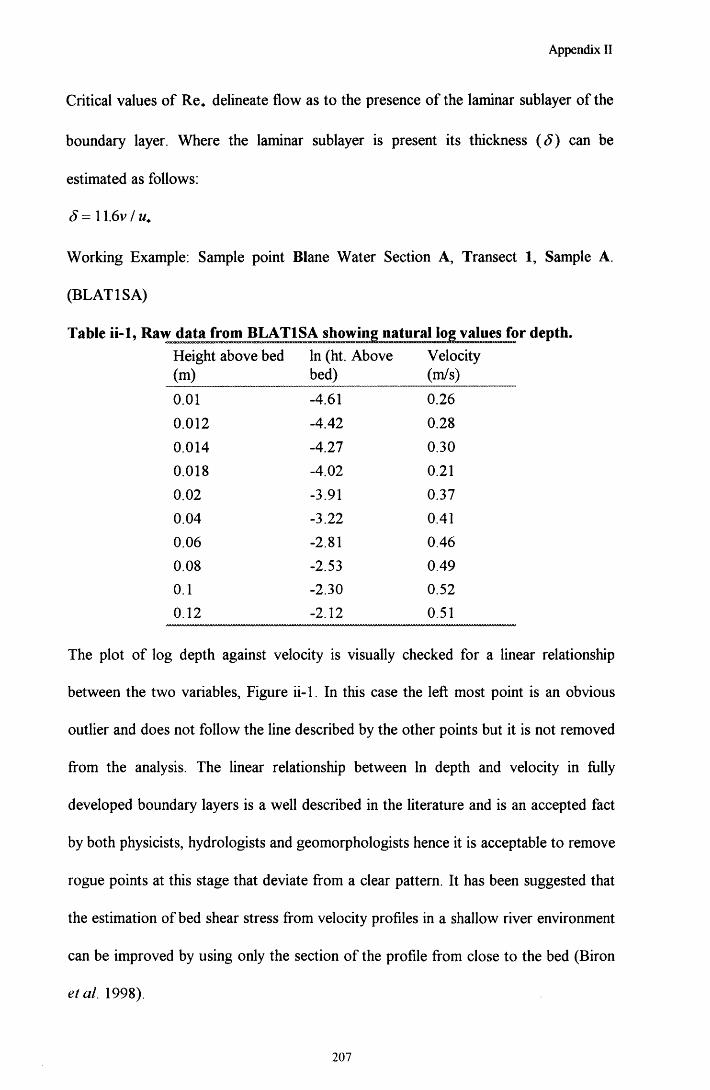
Appendix II
Critical values of Re* delineate flow as to the presence of the laminar sublayer of the
boundary layer. Where the laminar sublayer is present its thickness ( J ) can be
estimated as follows:
S = 11.6v / m*
Working Example: Sample point Blane Water Section A, Transect 1, Sample A.
(BLAT1SA)
Height above bed (m)
In (ht. Above bed)
Velocity(m/s)
0.01 -4.61 0.260.012 -4.42 0.280.014 -4.27 0.300.018 -4.02 0.210.02 -3.91 0.370.04 -3.22 0.410.06 -2.81 0.460.08 -2.53 0.490.1 -2.30 0.520.12 -2.12 0.51
The plot of log depth against velocity is visually checked for a linear relationship
between the two variables, Figure ii-1. In this case the left most point is an obvious
outlier and does not follow the line described by the other points but it is not removed
from the analysis. The linear relationship between In depth and velocity in fully
developed boundary layers is a well described in the literature and is an accepted fact
by both physicists, hydrologists and geomorphologists hence it is acceptable to remove
rogue points at this stage that deviate from a clear pattern. It has been suggested that
the estimation of bed shear stress from velocity profiles in a shallow river environment
can be improved by using only the section of the profile from close to the bed (Biron
etal. 1998).
207

Appendix II
In a number of cases (R.Etive 14, Duneaton Water 2, Blane Water 0) I did remove
points which did not follow the log-linear relationship. This was exclusively where
points high up in a profile failed to follow the log-linear relationship, Figure ii-2. In the
example plotted in Figure ii-2 the removal of the top 4 points of the plot improved the
fit from R2 = 0.31 to R2 = 0.87.
There are a number of situations were velocity profiles of this type are likely to
happen, ' ...non-logarithmic layers may occur in strongly accelerating or de-
accelerating flow such as occurs in river reaches which narrow or widen rapidly. The
logarithmic profile may be distorted by spatial variation in the mixture o f roughness
types on the bed, or by extreme bed roughness such as occurs over dunes and over
large rocks. ..... However even in these circumstances it is possible to obtain near
log-normal distributions o f velocity, from close to the bed, which can be used to
estimate the local bed shear stress ' from (Carling 1992). The second instance where
bed roughness is the important factor would occur at the 3 rivers examined in this
study.
0.00 -|
T3<]> -1.00 -<u& -2.00 -cd
43OX) -3.00 -(D
43e -4.00 -
-5.00 -
0.00 0.10 0.20 0.30 0.40 0.50 0.60
Velocity (m /s)
Figure ii-1 Velocity (u) measured at a number of depths above a single point on the stream bed plotted against In depth (D).
208

Appendix II
•§> -3.00
0.00 0.05 0.10 0.15 0.20
Velocity (m /s)
0.25 0.30
Figure ii-2 Plot from River Etive data, section A, Transect 4, sample c showing the breakdown of log linear relationship between depth and velocity higher up the water column.
Results
Estimates of the variables generated for our working example are given in table ii-2:
Table ii-2, Estimates of flow parameters from log normal plot of velocity against depth for River Etive sample A4C.
Variable Estimate
rA2 0.87Gradient 0.11Intercept 0.77
zo 0.001136u* 0.0454
tau 2.06
s.e. grad 1.67E-02
s.e. tau 6.07E-01Umax 0.53
U profile 0.42U real 0.42U at 0.37 depth 0.42Fr 0.38
The R-squared value for each line was checked for its significance by looking up
standard statistical tables. There was a clear relationship between the significance of
profiles and mean water column velocity. The ranked plots showing the distribution of
209

Appendix II
significant velocity profiles to mean water column velocity show the majority of non
significant profiles occurred in slow water in the Blane water and the Duneaton water
Figures ii-3-5. This pattern was also evident in the River Etive but here there was also
a strong scatter o f non-significant profiles over the entire range of velocities sampled.
Blane
1.6 T
1.4 -
+ P 0.01 QN/s0.8
♦ ♦ ♦0.6 -
0.4 -
0.2
20 25 30 35
Samples
Figure ii-3 Rank order of Blane Water samples (velocity profiles) by increasing velocity mean water column velocity. Diamonds = statistically significant velocity profiles, squares = non significant velocity profiles.
Duneaton
0.7 T
0.6e>i 0.5
o 0.4om> 0.3cra® 0.2 -
0 10 20 30 40 50 60
Samples
Figure ii-4 Rank order of Duneaton Water samples (velocity profiles) by increasing velocity mean water column velocity. Diamonds = statistically significant velocity profiles, squares = non significant velocity profiles.
210

Appendix II
E tive
0.8 T
0.7 -
2* 0.5 u•2 0.4
30
Samples
Figure ii-5 Rank order of River Etive samples (velocity profiles) by increasing velocity mean water column velocity. Diamonds = statistically significant velocity profiles, squares = non significant velocity profiles.
Discussion
The method worked well. The observed bias o f non significant velocity profiles
occurring in low velocity areas agrees with field observations. The most difficult
velocity profiles to measure were in the slow shallows but also in the deeper water
when slow. This often occurred behind large substrate elements where one would
expect low flows. In the R. Etive large boulders frequently acted as weirs causing
areas o f both decelerating and accelerating water. The data presented here in
combination with substrate measures can be used to identify the qualitative flow
categories of skimming, wake interference and isolated roughness flows, but this
aspect was not carried out (Davis & Barmuta 1989; Nowell & Church 1979).
211
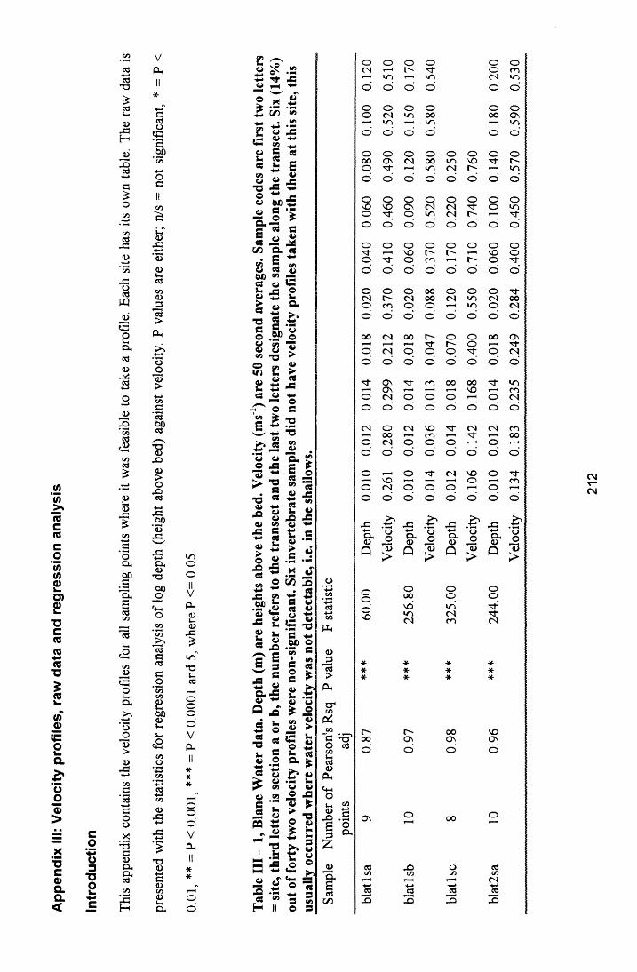
<n'inroc(0coin<no>k.U)0)k.
■Oc(0<Q*-«C0
T3S(0k.
<n0)
o*_a>
o0 a>>
== c— ox *;1 =I ?a.< -E
cc3hj03
T3
03(_CD
GH
jdgo3
G£o
03G45
Go03
w
tHou,Oh03<L>
G03
J 53
<dUh45
G£
C'oCLh00G
3 ,So3(Z)
3
<2CAJJ23ot_O h
oo45>45
G
co3H->ooo
33a<L>O hO hc3ca
3H
VP h
occ3o
t oO.00
"55+-»OC
CA
3
bG-t-j'5<dV-Hcc3caa>
3>Ph
H—>ao
3>
C"3oo03
45G45>o
Go3+-•00
"5
O h45
T300O
t+Ho
3g03co
45Uh0045Uht-H
3175o
03H-<CA
45GH-JG-*->' ?T3(Oh->C<0ca(OUhO h
GOo'IIVP hCOknCO
G£
T3s
OOOOVP h
ooo'VP h
oo
«Ak.45kHk*
0 s■ t
CA• pkG
45 kk
O 45kkH-* CD ’vi
■MCAkt
H-Su
Vi
Ge45
45CAG
kHkk66
kn 66« t<u 45
■o £O *■* 45 00
■5 .1S *cd a“ i4/ «00 <*> A »kn jjj
5 s■QC CO WD o *£V 4)CA
.9 ««ID k.45 £k. Sce a>
4)G
cV
G66
5oua
45J3
>45>66
JCk*OG
“g I sw k - - O. ca
• P4u_ 450 G
13 ~> -a c
-o C6 4/ H-»G u4/a/ vs G c k- e6
> * 5 “G -S 66 **W5 2 H-» ^G ««.op ^aj
k.£ *-m aj66 £
1 ij= ®a >e4/ +*
Q
£ oa _,
73k- g v o
CJ^ «505 cnc *-« b pa c
- «
.a S
i =
« G G «« k. V G G 45 ^t : b45 *"
&
x 45CD 2
. ? 66
45
G 45
I IG Hk 00 O
' GCACA
- S 4fH **■G
i uHH *2M "5hH k -45 J 'G -G66 “H II
G O G
£ .^ 145 45* 3CA 4545 >ts b o 7 : J- Ga
£45 45O G45 •£
k. G 45 45 Ot :
£ ^ o 13 tS 3G (A O G
03"&APh
(OD
1 3>PP
crCA
P h_CAG 'O’ O 03CAWho3<o
P h
PhO
CO
1G
JO'O h6oJ
CD
o<N
o*Y~)
or- oto
oo(N
o ’ o ’ o o' o
OO o<Ncr>
o*rs o00CO
o 00 r—HO o ’ O o ’ o ’
O00O
oOS■rO<Nr-H
o00to
oto<N
oGr-o
O o ’ o ’ o ’ o ’ o o'
OVOo
oNO oOsO
o<Nto
o<NCN
or-
oo
o' o o' o' o ’ o o'
oo
o oNOo
oro
o o oGO
o' o o' o ’ o' o o'
o<No
or-m
o<No
00ooo
o<NT—4oGG
o(No
o' O o' o’ o' o' o’
00o
<N<N
00o ro
or"o
ooooo
o' o’ o' o’ o’ o o’
■ro
OsOS<N
ro
CO
oOO
O00G
ro
o o' o' o' o' o' o’
<NO
Ooo<N(Nr* 4o
NOCOo o
(N <NO
o' o o' o' o' o' o'
oo
t-hG<N
oO
^ro
<No
GO o
oo' o’ o' o’ o’ o' o’
Dep
thV
eloc
ityD
epth
Vel
ocity
Dep
thV
eloc
ityD
epth
o o oo 00 o o(—s G G
G <N Tj-H/ <N (N
* * * ** * * ** * * *
r-~ 00 G00 Os Os Oso' o' o’ o'
ON
oJ
rttG
03G
00
o
o3G
03CA
(Nc3
G
Velo
city
0.134
0.1
83
0.235
0.2
49
0.284
0.4
00
0.450
0.5
70
0.590
0.
530

oONr -H
oO nd -
o04m
o00vo
oO n04
o04O '
oro
omCO
oO 'o
oVOc o
oONo
ON00O
oc n0 4
ooCO
ovo
oood -
om
oVOCO
or -H
0 4o o o ’ o ’ o ’ d o ’ d o ’ o ’ o ’ d d o ’ o ’ o ’ d d o ’
ooo
o04in
OOc o
ooO '
oOO0 4
VOVOO '
oo
r -H
ON04
ovoo
COCO04
oooo
OOO nO
oOO
o0 4d -
O0 4
oVOd*
o04
ovod-
o00
o ' o ’ d o ’ o ’ o ’ o ’ o ’ o ’ d o ’ d o ’ d d o ’ d o ’ o ’
od -r -H
oo-d -
om04
oO nVO
om04
ovoO '
omo
ONd"04
oino
04d-
ovoo
ON0 0o
o0 41—H
oVOCO
oooo
o0 4d "
oor -H
ovoCO
od -1—H
o ' o ’ o ’ d o ’ o ’ d d o ’ d o ’ d d d d d o ’ d d
OoT—H
oONc o
OO 'f—H
O
VO
oVO^ H
ovoVO
o0 4o
d -oo o
d -o
ONj—i od -o
0 4ooo
ovoo
00O '0 4
od -o
O nO n0 4
oOOo
od -CO
oo
o o ’ d o ’ d d d o ’ o ’ d o ’ d d o ’ o ’ d d o ’ d
oVOO
O04co
oo
oO 'd -
oO nO
oO 'm
m
ovoO '
0404o
mo
o0 4o
voO 'o
o0 4o
c nONT—H
o0 4o
voc n0 4
od -o
ON0 004
ovoo
o ’ O o ’ d O o ’ o ’ d o ’ d d o ’ o ’ d d d o ’ d d
o0 4o
r H
c o(N
o04O
0404ON
O0 4O
oCO
d -
omO '1—H
o0 4o
04m
0 0
od -O 'o
00
o00O n
0 0
of—H
0 4
o0 4O
O 'oo04
o0 4O
o o ’ o ’ o ’ o ' o ’ d o ’ o ’ o ' o ’ d o o ’ d o ’ o ’ o ' o ’
OOT—<o
ini n04
00
oc oO '04
0 0
O
omCO
CO
o00CO^ H
00
oom04
voo
mVOO
VO
oO nvo
voo
O '
0 4
00
o000004
00
oo ' o ’ d o ’ o ' o ’ d o ’ o ’ d o ’ o ’ o ’ d o ’ d o ’ o ’ o ’
d -1—H
oo-04
d -T“ H
oc nm04
d -^ -H
o0 0ON0 4
0 4
oooCO
d -
oONCO
"sf
o0 0O 'o
d-o
0 0VO
d -r -H
oON0 40 4
d "
or - '04
d"r -H
Oo ' o ’ d o ’ o ’ o ’ d o ’ o ’ d o ’ d o ’ o ’ o ’ o ’ o ’ d d
04
ocoON
04
oi nON04
0 4
oO noCO o
I— <
CO04
oON
0 4
or —1*
VOo
04
o04CO1 -H
0 4
od " 00 r H
04
o04O -0 4
04
Oo ’ d o ’ d o ' d o ’ o ’ o ’ o ‘ d o ’ o ’ d o ’ d d o ’ d
or H
o00o
oo
00d -» 4
oo
0 4OO
oo
ood-
or -H
oCOo
oo
ovoo
or—1o
ooo
04O nr —H
ot—H
oo0004
oo
o ’ d d d d o ’ d d d d d d d o ’ d d d o ’ d
Dep
th
Vel
ocity
Dep
th
Vel
ocity
Dep
th
Vel
ocity
Dep
th
Vel
ocity
Dep
th
Vel
ocity
Dep
th
Vel
ocity
Dep
th
Vel
ocity
Dep
th
Vel
ocity
Dep
th
Vel
ocity
Dep
th
oVi-t-*ed -*—>ViH-I
<u
>P h
crC/3
P4J /3
"S ^O edViWhCd<U
«4Hou,<U
E3
£
<D3Eedc/o
ooino>
inON
edVimcd
-O
OOON
■d-
ooON
ooTTvoen
O'ON
ooooo04
VOON
VOVOrvj
VO
o'
d -vooid -
0400
oooONo0 4
VOOn
OO0 4VOm
o«On
ONinoo
VOVO
J=>Vic n~cdIS
oVicoed
J=>
edVid"edIS
-OVid --4->cd
3
cdViined
3
-OC/3intd3
ot/3ined3
cdViVOcd
X>
OOO(N0 4
VOON
X)ViVO•4—>cd3
Velo
city
0.132
0.1
44
0.162
0.1
65
0.149
0.2
86
0.350
0.4
00
0.430
0.
380
blat
6sc
9 0.9
6 **
* 18
2.00
Dept
h 0.0
10
0.012
0.0
14
0.018
0.0
20
0.050
0.1
00
0.150
0.
200

Sam
ple
Num
ber
of Pe
arso
n's
Rsq
P va
lue
F st
atist
ic
poin
ts ad
j
Velo
city
0.095
0.1
04
0.130
0.1
37
0.17
1 0.1
95
0.246
0.2
68
0.26
1 bl
at7s
a 9
0.89
***
62.57
De
pth
0.010
0.0
12
0.014
0.0
16
0.018
0.0
20
0.030
0.0
40
0.05
0
o o o o o X o o o X o o o o on - T—1 1—1 CO X X CO 0 0 CO F " CO CN 00 ■sj- Obr - H CO CN "St r -H CN CN CO CO CN o CO r -H X r H
o ’ o ' o ' o o ’ o ’ o ' o o ’ o ’ o ’ o ’ o o ’ o
CN o o o o o oo o o o CO oo O o o oX 1— I ^ H X CN CN CO r - X X X CN "St r - CO X’—1 I— I ^ t 1 CN r H CO CN CN o CO ^ H X I— I
O o o o o o ’ o ' o ' o ' o o o ’ o ’ o ’ o ’ o ’
o o CO o o o X O o o o X p ^ o o oX oo r~- CN Ob 00 I—I CN CO c - r - CN 00 CN CO oI— I o CN 1—1 CO o CN i— i CO ■—i ■—i o CN i—| X I— I
o ’ o ’ o ’ o ’ o ’ o ' o ’ O o ’ o ’ o ' o ’ o ’ o ’ o ’ o ’
r - o o 's t o Ob o o o ■'sf 'S t Ob o o o■st x o r - o X O r - C" Ob CO CN oo X -St Xy—* o cn o CO o CN o CN o I— I O CN o X oo ' o ' o ' o ' o ’ o ’ o ’ o ’ o ' o ' o ’ o ’ o ’ o ’ o ’ o ’
c o o X o r - o 00 o X o CO o X o o oc o <N 00 CN X CN o CN ■St CN r - H CN 1— 1 CN X CNr - H o I—I o (N o CN o y—> o i—' o CO o X oo ' o o ’ o o ’ o ’ o ' o o ' o ' o ’ o ’ o o o ’ o ’
00 Ob 00 X 00 00 00 oo o 00 o 00 o oo1—1 i— i r - ^ h X r* H 1-H 1—1 Ob 1- o r - H ■St r -H CN 1—1I— I1 o ^ h o I— I1 o CN o I— I o ^ H o CN o X oo ’ o ' o ' o ’ o ’ o ' o ' o ' o ’ o ’ o o ’ o ’ o ’ o ’ o ’
o X -St X X X CN X r - X X X X o XI—1 r - H r - f—H CN I—1 00 1—1 X I— I CO i—i o 1— 1 r - 1— 1
i— ' o y—> o (N o r - H o y—> o i—| o CN o 'S t oo ’ o ’ o ’ o ’ o ’ o ’ o ’ o ’ o ’ o ’ o ’ o ’ o ’ o ' o ’ o ’
x CO 'vt CN ^ r X ■st Ob ^ r Ob 'S t t-" ■St o ■StO r “H X 1—H O i—i 00 I—1 X i—i CO i—i 'St I—I 1— 1 I—It “H o i— ' o CN o i—' o I—I1 o I—I o CN o 'S t oo ’ o ' o ' o ' O o ' o ' o o ’ o o o ’ o ’ o ’ o ’ o ’
X CN X CN CN CN CO CN o CN X CN oo CN o CNOb 1— 1 ^ r r— i—t i— i X r - H CN i—i 00 i-^ CO 1— 1 oo 1 - ^
o o •—1■ o CN o I—I o o o o CN o CO oo ’ o ' o ’ o ' o ’ o ’ o ’ o ’ o ’ o ’ o ’ o ’ o o ’ o ’ o
■St o X o ■st o o 00 o o r-- o o oo 1— 1 X 1—1 o l—l X r - H 1—1 1—1 o I— I CN 1—1 Ob 1—1I— I o ■—11 o CN o I— I o •—I o ^ H o CN o CO oo ’ o ’ o ’ o ' o ’ o ' o ' o ’ o ’ o ' o ’ o ’ o ’ o ’ o ’ o ’
.ts 43 .ts -C .t i 43 .tJ ^3 .t i ^5 .t i -C .t iOJD(L>>
^ O<DQ £
o. g<Da go. o<D J ZQ ^ >
O- oo JxQ g >
a. g<DQ >
O h<DQ
CNCOx>Ob
Oboor-Ob
o oObCOoCO
oObr -CN
ox
o-stbd
oo
Obo'
Obo '
t-"f"- r-Ob
tor- obD COVO Ob
xtr>r-tg15
ocot"-+->egX
edco00tg3
XcoOO-*->eg
3
oCO00eg
3xx
x3
Velo
city
0.350
0.4
30
0.510
0.4
90
0.440
0.4
90
0.700
0.7
90
0.910
0.
950
blbt
2sa
10 -0
.11
n/s
0.08
Dept
h 0.0
10
0.012
0.0
14
0.016
0.0
18
0.020
0.0
40
0.060
0.0
80
0.10
0Ve
locit
y 0.0
27
0.027
0.0
36
0.087
0.0
68
0.132
0.0
68
0.115
0.
061
0.01
8

CNc oo
inc o
oCN
o oVOO
ovo
oc n
oo
oVOr — I
oo
^ rmo
VOmo
omo
CM
1—H
o" s f
oo00
oi no
or-~c n
oVOo
oCM
oVO
o ’ o o ’ o ’ o ’ o ’ o ’ o ’ o ’ o ’ o ’ o ’ o ’ o ’ o ’ o ' o ’ o
oCOO
oCN
oo
oo
omo
oi nm
oor c
oo
ocnT“H
ovoo
CMc nO
CM o-3-o
r -o
oCM
ovooo
oo
oO
omo
oCN• r
o
o ’ o ’ o ’ o ’ o ’ o ’ o o ’ o ’ o ' o ’ o ' o ’ o ’ o ’ o ’ o ' o ’
0 0CNo
O s0 0
o0 0o
oo
o■'vl'o
o ot " -o
oo s
oo
o,!d -o
0 0CMo
oom
oc no
voi no
oO sO
o00r"-
mc nO
o0 0c n
o"xf-o
or -H
c n
oo
o ’ o ’ o ’ o ’ o o ’ o ’ o ’ o ’ o ’ o ’ o ’ o ’ o o ’ o ' o ’ o ’ o ’
CNo
T— 4 00
or ro
or foo
oc no
or -^ r
o^ ro
oc noo
ovoo
oc no
VOCMO
CM00
mCNo
O sVOO
oVOO
ocnt " -
Oc nO
ovoc n
oc no
O sCN
ovoo
o ’ o ’ o ’ o ’ o ’ o o ’ o ’ o ’ o ’ o ’ o ’ o ’ o ’ o o ’ o ’ o ’ o ’ o ’
o<No
oCNCN
oCNo
oVO00
oCNo
or -c n
oCMO
ooVO
oCNo
oCNOO
oCNo
c noor -H
oCNo
"d-o
OCMO
oVOm
OCNo
voCNc n
oCNo
r fO sCN
oCNo
C5 o ’ o ’ o o ’ o ' o ’ o o ’ o c> O o ' o o o ' o ’ o ’ o o ’ o ’
00 T H
oCOO s
00o
oo
00o
ooc n
00o
o00m
00o
o00
00o
voCM
ooo
omo
00o
o00
00o
oOc n
00o
T—H
O sCN
00o
o ’ o ’ o ’ o ' o ’ o ’ o ’ o ’ o ’ o o ’ o ’ o ’ o ’ o ’ o ’ o ’ o ’ o ’ O o ’
VOI 1 4O
OS O
voo
ovo
vor —*o
CMooCN
voo
oId"VO
voo
o00r-
voo
OOT-Hvoo
c nc no
VO
oooo’d -
voo
C-O sCN
voo
oc n
voo
o ’ O o ’ o ’ o ’ o ’ o ’ o ’ o ’ o o ’ o ’ o ' o ’ o ’ o ’ o ’ o ’ o ’ o ’ o ’
ro
m 'If»—Ho
oi nC- o
c nvoCM o
o00m
ro
ovor - o
VO- ro
c no
ooO si n
ro
orc n
r—<o
O sooCM
^ r
oo ’ o ’ o ’ o o ’ o ’ o ’ o ’ o ’ o ' o ' o o ’ o ’ o ’ o ' o ’ o ’ o ’ o ’ o ’
CN
oO sr**H
CN
ooOOvo
CN
ooc n
CMf 1O
omin
CM
oooVO
CNr -H
oO s^ r
CM
oc n■d-o
CN
O
oc nCM
CM
ovoc -CM
CM
oc n00CM
CM
Oo ’ o ’ o ’ o ’ o ’ o ’ o ’ o ' o ’ o ’ o ’ o ’ o ' o ’ o ’ o ' o ’ o ’ o ’ o ’ o '
oo
m oo
ovo
oT“Ho
CNmCN
oo
oi n
oo
oc n
or -H
omo
oo
c -VOo
O
O
o oo
r -i nCN
o1—HO
O sVO
oo
o ’ o ’ o ’ o ’ o o ’ o ’ o ’ o ’ o ’ o ' o ’ o ’ o ’ o ’ o ’ o ’ o ’ o ’ o ’ o ’
Dep
thV
eloc
ityD
epth
Vel
ocity
Dep
thV
eloc
ityD
epth
Vel
ocity
Dep
thV
eloc
ityD
epth
Vel
ocity
Dep
thV
eloc
ityD
epth
Vel
ocity
Dep
thV
eloc
ityD
epth
Vel
ocity
Dep
th
ot/3o3on
Hh
CTC/3
P^J /3
"g -o*O «JC/5
c5<DPm
Cmov-i <«<u £
. S6 g.3 CM
£
JJCM6
CO
oc nrr
r -CMo
• gCM-«->£x>
ooTTo
CMO s
O^ rvo’m
VOOO
oo00VOCM
r -ON
o■ rCMCM
Or "
ovoCM
C/5
'tS
ITSo '
oc n
r -
oC"rt-c o
O s
oCMOCN
ooVO
oC/3
CN-t-i£3
cciC/3
CO-t—' £ 3
X>C/3
CO■«->-O3
oC/3
CO£IB
ctfC/3
jO3
-Oc/3-+-*
3
oC/3
^ r-»—>jg3
ctiC/3
■*->jO3
C/3vn+->3
vo
VO
r'-~oo
oc/3m■<->3

Sam
ple
Num
ber
of Pe
arso
n's
Rsq
P va
lue
F st
atist
ic
poin
ts ad
jVe
locit
y 0.1
89
0.202
0.2
54
0.233
0.2
39
0.25
1 0.4
10
0.400
0.4
10
0.37
0bl
bt6s
a 10
0.82
** 42
.70
Dept
h 0.0
10
0.012
0.0
14
0.016
0.0
18
0.020
0.0
30
0.050
0.0
70
0.09
0Ve
locit
y 0.2
69
0.360
0.2
64
0.278
0.
251
0.340
0.4
60
0.460
0.5
30
0.58
0 o o o o o c n o o o oX oo O n CN X ON o c n CNo X O oo o CN t- h X o O n
o o ' o ' o ' o o ' o ’ o o ' o ’
o o O o o CN o o oo oX O n r - ON ON oo CN Xo X o 00 o CN o X o 00o o ' o ' o ’ o o o ’ o ' o ' o
o O o o o X o o X o<N X CN c n CN X c n CN O n
o X o I"- o CN o X o r ^ -
o ' o ’ o ’ o ' o ’ o ' o ’ o ’ o o
o o X o X T“ H o o oc n 00 c n X CN o r - CNo i n o X o CN o ^ r o Xo ' o ' o ' o ' o ’ o ’ o ’ o o ' o '
o o o o o " c r o o o oCN X CN X CN c n CN 00 CNO i n o r r o CN o CN o C "o o o ' o ’ o o ’ o ’ o ' o o ’
00 o 00 o 00 CN 00 o 00 or -H c n r —H X r -H oo r -H I— I Xo i n o X o CN o c n o C "o ' o ' o ' o ’ o o ' o ' o ’ o ’ o '
X o X o X c n X o X oi— i c n I— 1 c n I— I 1— 1 ^ r I— I r -H
o i n o X o CN o CN o r -o ' o ' o ' o ’ o o ’ o ’ o ' o ’ o
r3- o ^ r o TT I"- c n oI— 1 CN 1— 1 o I— I c n X r -H ooo i n o X o CN o CN o Xo o ' o ' o ’ o ' o ' o ' o ' o ' o ’
CN o CN o CN o CN CN CN oI—H 00 I— I CN I— I CN I— I X 1— 1 r— 1
o X o 'v f o CN o r -H o Xo ' o ' o ’ o o ’ o ' o ' o ' o ’ o '
o o o o o r - o CN o oI— I 1— 1 X I— I ON 1— 1 ’'nT I— I O no o o o CN o 1— 1 o T fo ' o ' o o ’ o ' o ’ o ' o ' o ’ o
js .t i x .t i j : .t ; . s a : .t iex<Da
oo1 3>
cx<DQ
oo13>
c x<L>Q
oo1 3>
cx(L)O
oo1 3>
c x<uQ
oo<d>
oXKc n
oooOnCN
CNc no '
o
ooo
ONC "
O nCN
cn'a
o00o ’
NOr -
00o CN
ONNOr-
x>cnNO+->jO3
ocnNO-t-*X3
aScnr-x3
xcnr"x3
or-+-»x3
216

o£ 4-S J S4-* u 4>4
+->VI©cn ?
U 3G ed 3
u 054J 4-1 1CfiS o> 3cn JC 4^
4^ cn4J"3 (3DO 3 tEej O4> 3 u
c .3 <u
E 3 , 4-4ed E ’E
C/5tm03
• cn "Ecn© >(31) -C ©A 4^u 4) a9 i j *> 3«
■ o3(3D
4^O33 s® —© © s«-> ^ -a
£ » -on f c ,45© £ IT) C45 £
a
* 1
Cd I —W B«W5 fc« I ^^ *S? ® *-£ *•» « ej
* s*5 " © ■©© 5^ CB■M_: u "O «45 cn
•© 3a j CdJs i
> *© nsa
u _ «£ •SP s
<u us« I_ 3
s sw 45JB 5
USo *-M 0 CQ
* g■o .2L ■*•*45 ©^ Oicd 89
e a>0 s* J8c T?s .is Q -cCN (U
1 --
45 £
a ©£ "3a jccn cn © 45« -O 2 *- «® s45 •"t£ 45
> p ~4- -®js *DD oW I a 73W oa cC•— cn 3 «.2° ^
osai u45£cnJDCOL.
J£ U3 ©4-»ed 4-»H ii
u3 > i.45cd£© u
0 -5£> * *5 "o© £ v u > 3
© «4 °£>=* £ edIS ©el- «« —* 3© ©+- .2 2 -fi© 4->
C©* ©NT -M O •■cnS . 2^ - 3c *■* © t!lV AA 2CUD 45
W €
O NO o m o CN o d - o d - o CN o m o00 O 00 CN CN r - NO On CN CN ON 00 in NOo o CN O CN o c n i—i o o o c n r - H CNo ' o ' o ' o ' o ' o ' o ’ O o ' o ' o ’ o ' o ’ o ’ o '
o o o NO o ON O 00 o NO o ON o r-~ oNO CN t - oo NO 00 o ON CN 00 o o d " oo o CN o I—1 o CN CN o o o o c n 1—1 CNo ' o ' o ’ o ’ o ’ o ' o ’ o ' o ’ o ' o ’ o ' o o o '
o NO o 'd - o "d- o in o c n o NO o CN oin CN in r- •"d- r - o o o r - CN NO I— I o in oo o •-11 o i— 11 o CN r H o o o o CN I— I 1—H
o ' o o ' o o ' o ' o ' o ' o ’ o ' o ' o ' o ' o ' o '
o m o CN o o o CN o CN o NO o in oN- c n o 00 00 m o CN d - CN d - o o CN i no o I— 1 o o o >—1 I ( o o o o I— I I— I oo ' o ' o c > o ’ o ’ o ’ o ’ o o ’ o ' o ’ o ' o o
o r- o NO o NO o m o 00 o NO o d - oCN y—( CN m CN c n CN CN 1-H CN CN CN CN CNo o o o o O o o o o o o o I— I oo ' o ' o ’ o ’ o ' o ’ o ' o ' o ' o ’ o ’ o ’ o ' o ' o '
00 r- 00 NO o o n - 00 d - 00 o 00 o 00 oo 00y—l o I—1 c - 1 - ^ ■'d- 1— t 1— 1 CN 1 - ^ 1— 1 t*h o 1— 1
o o o o o o o o o o o o I— I oo o ' o ’ o ’ o ’ o o ’ o ' o ’ o ’ o ’ o ’ o ' o ’ o '
NO ^ r NO c n NO r - NO CN NO r - NO NO NO r~" NOT— ( o T“ H in 1— 1 c n 1— t i— i 1— 1 1— 1 o T-h 00 T-H
o o o o o o o r— • o o o o o o oo ' o ’ o ' o ' o o ' o ’ o ' o ' o ’ o ' o ’ o ' o ’ o '
TJ- r- ■'d- ON "d- CN 'd - CN d " c n d " On d " ON d -1—H o in CN 1— t O i— i CN 1— 1 o 1 ( ON 1— 1
O o o O o O o o o o o o o oo o ' o o ’ o ' o ' o ' o ' o ’ o ’ o ’ o ' o ' o ' o '
CN , — 1 CN o CN ON CN NO CN 1— 1 CN CN CN CN CN-H 1—H 1—H CN T— On c n r -H ^ H 00 r H
O o O c n o o o O o o o o o o oc > o ' O o ' o ’ o ’ o ’ o ' o ’ o ' o ' o ' o ’ o ’ o '
o o O in o m o CN o CN o c n o NO of— I o 1— 1 CN 1— 1 CN 1— 1 On i— i o 1— 1 H 1— 1 r- r -H
o o o O o o o O o o o o o o oo ' o ' o ' o ' o ' o ' o ’ o ' o ' o ' c > o ' o ’ o ' o '
Pn Pn Pn-C 4 -> yG, 4-> J p 4 -* -3 4 -> -3 4-> JS 4-> -3 _4—> -34-> "o 4 -» o 4—* o 4-> o 4-» ’o 4-> " o 4 -* 'o 4->c x o c x c x CX JD CX o c x c x c x0) <L> CD <D CD CD © CD
Q ©> Q > Q ’flD
> Q CD
> Q > Q > Q 1 3
> Q
cd-t->cn(-X
CD
3>
3 T3 O cd1/5 — H
ed cn ©
CfHou.©
*1
©3 ,£ed
C/D
OnO n
«3
cd
cd3'O
ONm
cn
3
OOCNTT00
CNON»ri-d-
C/NNO
o m o c n C "c n o ON oo oo ' o ’1 o ’ o ’ o '
oo
c3
mCN
ocn
■'d"oo
o
ed3d3<d3T3
cdcnCNtd3TD
J=>cnCN"S3T3
<N3T3
edcnmtd3d3
r-in
moo'
cnrotd3TO
Velo
city
0.019
0.0
05
0.010
0.0
20
0.014
0.0
31
0.014
0.0
13
0.019
0.
024
duat
3sc
10 -0
.03
n/s
0.75
Dept
h 0.0
10
0.012
0.0
14
0.016
0.0
18
0.020
0.0
40
0.060
0.0
80
0.09
0

Sam
ple
Num
ber
of Pe
arso
n's
P va
lue
F st
atist
ic
poin
ts Rs
q ad
j
Velo
city
0.005
0.0
08
0.014
0.0
28
0.028
0.0
19
0.015
0.0
14
0.006
0.
006
duat
4sa
10 0.8
0 **
36.97
De
pth
0.010
0.0
12
0.014
0.0
16
0.018
0.0
20
0.100
0.2
00
0.300
0.
420
Velo
city
0.086
0.0
77
0.060
0.0
68
0.082
0.0
88
0.087
0.
131
0.162
0.
177 o c n o oo o CN o c n O CN o n r o n r o Ov
I— I T-H nT CN t—i nT I -H nT n r c n 0 0 o v/n o vo OVnT CN CN o c n o CN O n r I— I n r c n i—i o CN CNo ' o ’ o ’ o ' o ' o ' o ’ o ' o ' o ' o ’ o o ’ o ' o ' o ’o c n o vo o I— 1 o CN o v/n o c n o n r o Ovo o 0 0 c n CN c n v/n vn o ov o ^H CN o o r~-c n <N 1—1 O CN O i— i o c n o nT m i—| o CN CNo ' o ' o ' o ' o ’ o ' o ’ o ' o ' o ’ o ' o ' o ’ o ’ o ' o ’o VO o o o o 0 0 vo Ov o VO o n r o r_H o OVo o CN c n v/n v/n o n r CN c n o o o r - oo r ^ n r c nCN C N r c O T— 1 o I— I o o o CN I— I c n CN o o I— I CNo ' o ' o ’ o ' o ’ o ’ o ’ o ' o ' o ’ o ' o ' o ' o o ’ o ' o ’ o ’o 0 0 o OV o r -H o o c n c n o CN O v/n o c n o c no r - VO CN oo CN v/n cn CN T“H o v/n v/n r -H n r 1 -H nT voI—1 i— 1 o o o O o O O o I— I r -H ^H CN o o o r H
o ’ o o ’ o ' o ' o ' o ' o ' o ’ o ’ o ’ o ' o ’ o ’ o ' o ' o ' o ’o Ov o o o o nT o c n o c - o vo o c - o CN o o o<N i— i CN c n CN o CN r H CN o CN n r CN T— 1 CN I— I CN CNo i— 1 o O o o o O o o o o o I— I O o o ^Ho ' o o ' o o ' o ' o ' o ' o ' o ' o ' o ' o o ' o ' o ' o ' o ’oo r - 0 0 c n 0 0 r - 0 0 v/n o o n r 0 0 Ov 0 0 VO 0 0 c n 0 0 nTr*H nT r -H CN I -H I -H r -H CN I - H vo r -H r - I -H c n I - H 1-H T—H v/no O o O O o o o o o o o o t—h o o o I— I
o ' o ' o ' o ' o ’ o ’ o ’ o ' o ' o ' o ' o ' o ’ o ' o ' o ’ o ' o 'VO CN VO n r VO un vo 0 0 vo o vo CN vo o VO o vo or -H i— i i— i CN t- h o I—1 I -H 1— 1 T-H I— I r - 1 -H 0 0 I -H I - H T“ H CNo i—1 o o o o o o o o o o o o o o o r -H
o ’ o ' o ' o ' o ' o o o ' o ’ o ’ o c l o ’ o o ’ o ’ o ' o 'n r VO n r nT n r n r nT cn n r r - n r n r nT nT Ov n r oI-H Ov I— 1 CN f—H i—i I-H I^H t- h o I -H 0 0 I -H o I -H o 1 -H nTo O o o o o o O o o o o o r -H o o oo ' o ’ o ' o ' o ' o ' o ' o ' o ' o ' o ' o ’ o ’ o ’ o ' o ' o ' o 'CN Ov CN r*H CN Ov CN c n CN vo CN n r CN VO CN vo CN t - Hr -H VO I -H m ^ H t- h I -H ^ H ^ H o I -H r ~ - I -H OO I -H o r*H CNo O o o O o o O o o o o o o o o oo ' o ’ o ’ o ' o ' o ' o ' o ’ o ’ o ' o ' o ' o ' o ' o ’ o ’ o ' o ’o c n o oo o n r o oo o CN o n r o c n o r ^ o 0 0t- h vo I -H n r I -H o I -H o I -H o r*H nT r -H O r -H o p H r -H
o o o ^ H o o o o o o o o o o o o t- h
o ' o ' o ' o ’ o ' o ’ o ' o ' o ' o ' o ’ o ’ o ’ o ’ o ' o ’ o ' o '>% >>
-C p p -C Jp •*-» rP ,P H—> , p H—< rP •/-> rP •£2o -4-» o •*-» "o H-* o 'o H—* o H—» o H—* o + -» o
c x j d c x o c x c x c x j o c x o c x o c x o c x J OCD CD a> CD CD CD CD CD 0)Q > Q
*o3> Q
'aS> Q
’a3> Q
CD
> Q > Q’a3> Q
*a3> Q >
VOOOr-VO
OO00
cnOv
VOOOo ’(N
oo ’
OvVO
VOO n
OOVO
0000
00 ocn
cdP
TD
cdp
TD
cd
cdP
TD
cdP
TD
OO
00
O cn VOtdP
TD
OVO
00Ocn<N
voOV
OOo
oo'
CNcncnoo
voOV
cdcdVOcdPTD
ed
edP
TD
cdP
TD
edc/500cdP
TD
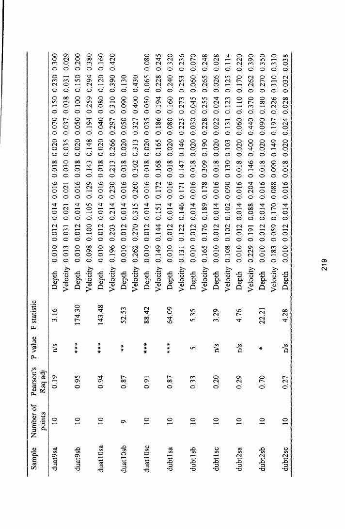
Sam
ple
Num
ber
of Pe
arso
n's
P va
lue
F st
atist
ic
poin
ts Rs
q ad
jdu
at9s
a 10
0.19
n/s
3.16
Dept
h 0.0
10
0.012
0.0
14
0.016
0.0
18
0.020
0.0
70
0.150
0.2
30
0.30
0Ve
locit
y 0.0
13
0.031
0.0
21
0.02
1 0.0
30
0.035
0.0
37
0.038
0.
031
0.02
9 du
at9s
b 10
0.95
***
174.3
0 De
pth
0.010
0.0
12
0.014
0.0
16
0.018
0.0
20
0.050
0.1
00
0.150
0.
200 o o O o in
oo SO CN 00 nrcn 1—*1 nT o CNo ' o ’ o ’ o ’ o ’"sf o o o o m oooc CN Os cn cn CO CNCN 1 cn >—i1 nr O CNo ’ o ’ o ’ o ’ o ’ o ’ o 'Oc o O o o O nrin oo T—l OC o m OsCM o cn o nr o I—Io ' o ’ o ’ o ’ o o ’ onr o r - o r - m COOc nr Os in CN cn 001—!1 o CN o cn Oo ' o ’ o ’ o ’ o ’ o ’ o ’00 o CO o cn O mnr <N CO CN i—i CN CO1—11 o CN o cn oo ‘ o ’ o ’ o o ’ o ’ c>cn 00 cn 00 CN 00 00nr t-h i—i 1—1 O H CO
o CN o cn o T—1o ' o ’ o ’ o ’ o ’ o ’ o ’O n CD o CO o CD CN<N cn r-H CO 1-H r -T-H o CN o CN O *—•
o ’ o ’ o o ’ o ’ o ’ o ’in nr nf nr in nro 1—H T— 1 r ■■ H r-H ^H mT—' o CN o cn O 1-H
o ’ o ’ o ’ o ’ o ’ o ’ o ’o CN cn CN o CN nro i—H o i—i r - 1—H nrI—I1 o CN o CN O I—Io ’ o ’ o ’ o ’ o ’ o ’ o ’00 o CO o CN o OSOs i—1 Os H CO I— I nro o i—■ o CN o I—*o ’ o ’ o ’ o ’ o ’ o ’ o ’Sn >>
-C X X -+—*7 3 7 3 H-* * 5 H-> oo cx o cx j d CX j d
<D 0> <D7 3
> Q7 3
>Q
7 3
>Q
<D
>
00 cn CN\ ] m nTcn CN 00XI in 00
***
**
***
nT r -Os oo Oco ’ c> o ’
O Os o
cd x > ou s u s u sO O oi- 1— 4 r-H
cd cd cdP 3 3
T3
o CO o oo oo nT o oCN cn t-~ nT CN r - H CN occn CN o CN o I— 1 CN cno ’ o ’ o o ’ o ’ o ’ o ’ o ’o cn o m co m o CNn r m CO CO CN CN r - COCN CN o CN o I— I 1— I CNo ’ o ’ o ' o ’ o ' o ’ o ’ o ’o cn m m nT cn o oCO r - n r i n CN CN r — 1 e ' r - H CN o CN o I— I I— I eno ’ o ’ o ’ o ’ o ’ o ’ o ’ o ’o cn o oo CN I— 1 o o00 CN cn CN CN cn CO n ro CN o CN o I— I o n ro ’ o ’ o o ’ o ’ o ’ o ' o ’o co o o o cn o oCN n r CN Oc CN o CN oo I— 1 o T -h o l—H o n ro ’ o ’ o ’ o o ' o ’ o ' o ’00 f - oo OC 00 o 00 CO1 -H n r I— I o I— I cn I— I n ro I— I o cn o I— I o I— I
o ’ o ’ o ' o ’ o ’ o ’ o ’ o ’CO CO 00 CD o CO nT1 -H r - ^ H r - I— I Oc r - H oo r - H o I— I o o o CNo ’ o ’ o ' o ' o ’ o ' o ’ o ’n r CO nT Oc n r CN n r 00I— I nT I— I 00 1 -H o 1— 1 ooo o I— I1 o 1 -H o oo ’ o ’ o ' o ' o ’ o ' o ’ o ’CN CN CN CO CN CN CN1— 1 CN I— I r - I— I o r - H Oco I— I o I— I o I— I o I— I
o ’ o ’ o ’ o ’ o ’ o ’ o ’ o ’o ,— I o m o oo o Ocr - H cn 1— 1 CO 1 - ^ o I— H CNo I— 1 o r " H o I— I o CNo ’ o ’ o ’ o ’ o ’ o ’ o ’ o ’
> 1 > 1 > >-C H—> X +-» -C X H -*
H—1 73 o o 73c x o c x j d c x JD c x JD<L> (L> <1>
Q73> Q
7 3> Q
73> Q
7 3>
Oc<25 m Oc CO
cn CN r -nTCO m cn n r
* u s u s**
m
r - cn o Oc00 cn CN CNo ’ o ’ o ' o ’
o o o or - H I—H
cd X o edu s u s u s u s
1 i I— I I— I CNN—> H-* H-H H-*x > pO X x3 3 3 3
n3 T 3 T 3 T 3 dubt
2sb
10 0.7
0 *
22.2
1 De
pth
0.010
0.0
12
0.014
0.0
16
0.018
0.0
20
0.090
0.1
80
0.270
0.
350
Velo
city
0.183
0.0
59
0.170
0.0
88
0.090
0.1
49
0.197
0.2
26
0.310
0.
310
dubt
2sc
10 0.2
7 n/s
4.2
8 De
pth
0.010
0.0
12
0.014
0.0
16
0.018
0.0
20
0.024
0.0
28
0.032
0.
038

Sam
ple
Num
ber
of Pe
arso
n's
P va
lue
F st
atist
ic
poin
ts Rs
q ad
j
Velo
city
0.109
0.1
39
0.157
0.1
63
0.162
0.1
62
0.166
0.1
46
0.176
0.
152
dubt
3sa
10 0.4
4 n/s
1.4
1 De
pth
0.010
0.0
12
0.014
0.0
16
0.018
0.0
20
0.050
0.0
90
0.130
0.
180
Velo
city
0.180
0.2
22
0.215
0.2
08
0.214
0.2
18
0.172
0.1
85
0.219
0.
289 o o oo o o
CN c n CN i f VO<N 1 f o o CNO o ' o ' o ’ o ’O o VO i f oVO 0 0 (N i f Ov'—1 c n O o i— i
o ' o ' o ’ o ' o ’o CN " s f Ov o! H r - CN m c nI H (N O o >—•O o ’ o o ’ o ’o ON CN CN oVO I f CN i f t " -O CN o o oo ' o ' o ’ o ’ o ’o _ o o o<N <N CN o CNo CN o m oo o ' o ' o ' o '0 0 OV 00 r - 00t- h I— I r -H i f T-h
o CN o o oo ' o ' o ' o ' o 'VO CN VO VO VOt—h <N i— i i f I -H
o CN o O oo ' o ' o ' o ' o 'i f Ov i f O i f! H r - i— i I -H
O t—h o o oO o ' o ’ o ' o 'CN c n CN 0 0 CNt—h in i— i i f I - H
o o O oo ' o ' o ' o ' o 'o CN o VO oT—H i f I— I CN I— I
o i— 1 o O oo ' o ' o ' o ' o ’
> >
x z xz - CH~» o o -!-*c x o c x j o c x<D CD CD
Q1 3
> Qo
> Q
o O o m i ■ i
oo OO OV c n Ovi f I— 1 i f o Oo ’ o ’ o ' o ’ Oo o O CN _
r - i f 0 0 c n c ni f t- h I f o i— i
o o ' o ’ o ’ o ’vo o o oo 0 0Ov OV vo CN 0 0CN o i f O oO o ' o ' o ’ o ’i f o o i f ooe n <n in CN ooCN o c n o oO o ’ o ' o ’ o ’r - o o o I— ,r H CN f " CN Ov
o c n o oo o ' o ' o oCN 0 0 o 0 0 T-h
r - I -H ' i j - I -H oor H o c n o oo ' o ' o ' o ' o 'r - vo o vo T—H
m ^ H c n I -H oo*—• o c n o oo o ' o ’ o ’ o 'CN i f o i f r -OO I -H r - i— i OvI— 1 o e n o Oo ’ o ’ o ’ o ’ o ’r -H CN Ov CN r -c n r -H ' l i r -H OvT i o e n o Oo ’ o o ’ o ’ o 'CN o i f o ' i i -r -H T-H Ov t- h voi— l1 o CN o oo ’ o ' o ’ o ’ o ’
-*->X Z
H-> xz H-*
o H-> o H-> Bo c x JD CX o<L) 0 )CD
> Q’B> Q
CD
>
o o o o VOo CN o Ov c nCN c n CN in oo ’ o ’ o ' o ' o 'o o o o CNm 0 0 in i f c n
CN 1—' VO oo o ’ o ’ o ' oo r - o o 00o e n o o CNI—1 1 >—1 m o(O o ’ o ' o ’ o 'o 00 o o I fm CN m c n CNo o o i f oo ’ o ' o ’ o ’ o ’o vo o o oCN i—i CN m CNO o o c n oo o O o ' o0 0 VO 0 0 c n ooT-h T-h t- h CN ^HO o o c n oo ' o ’ o ' o ' o 'VO VO VO Ov vot- h T -H t—h o t- h
o o o c n oo ’ o ’ c i o ’ o 'I f o O I frH ^ H t—H i f 1—H
o o o c n oo ' o ' o ' o ' o 'CN r - CN O CNI - H o r - H r - Ho o o CN Oo ' o ' o ’ o ' o 'o vo o o oI—1 o I— I m I - H
o o o CN oo ’ o ’ o ' o ' o '
xz H-* rC xzH-> o H-> o ■Hcx JO cx o cxa> CD CD
Q > Q(D
> Q Velo
city
0.009
0.0
17
0.018
0.0
18
0.020
0.0
16
0.02
1 0.0
24
0.018
0.
035
dubt
6sa
10 0.9
7 **
* 29
3.93
De
pth
0.010
0.0
12
0.014
0.0
16
0.018
0.0
20
0.050
0.1
00
0.150
0.
190
Velo
city
0.049
0.0
71
0.082
0.0
95
0.120
0.1
87
0.260
0.5
10
0.600
0.
590

Sam
ple
Num
ber
of Pe
arso
n's
P va
lue
F st
atist
ic
poin
ts Rs
q ad
jdu
bt6s
b 10
0.73
* 25
.23
Dept
h 0.0
10
0.012
0.0
14
0.016
0.0
18
0.020
0.0
50
0.080
0.1
10
0.14
0Ve
locit
y 0.6
00
0.620
0.6
10
0.650
0.6
40
0.650
0.6
70
0.730
0.6
80
0.69
0 du
bt6s
c 10
0.73
* 25
.23
Dept
h 0.0
10
0.012
0.0
14
0.016
0.0
18
0.020
0.0
35
0.050
0.0
65
0.08
0 o o C" o oo o o o o o o o o o o o o oO s O s CO n r s o n r c - r H O s CO r~~ O s 00 o c n 1-H c n O sc n o CM CM o CM nT n r '—I oo o in 1 H 00 I -H voO o ’ o ’ o ’ o ’ o ’ o o ’ o ’ o ’ o ’ o ’ o ’ o ’ o ’ o ' o ’ o ’O m 00 o 00 o o o o o o o o o o o o oe' r - r - 00 O s 00 00 00 s o r-^ m c - O s 00 O s 00 r - ine n o o 1—< o s o o nr 1—* 00 o m o c - o s o I -H
O o ’ o ’ o ’ o ’ o ' o ’ o ’ o ’ o ’ o ’ o ’ o ’ o ' o ’ o ’ o ' o ’O o 00 o CM o o o o o o o o o o o o o>—i s o O s CM O s CM 00 s o CM oo O s m o vo CM vo 00 oc n o o 1 o I—11 VO o CO o C " o vo o r - o voo ’ o ’ o ’ o ’ o ’ o ’ o ’ o ’ o ’ o ’ o ’ o ’ o ’ o ’ o o ’ o ’ o ’o I/O in O O s o o o O s o o m o m o o o oCM c o S O S O 00 s o CM n r 00 m oo CO S O c n O S n r c n mCO O O o o m o CO o s o o m o ■n- o VO oO o ' o ’ o ’ o ’ o ’ o ’ o ’ o ’ o ’ o ’ o ’ o ’ o ' o o ’ o ’ o ’CM o CM O o o o o o o o o o o o o o oO CM r - CM 00 CM CO CM C " CM r - CM nT CM c n CM O s CMCO o •—11 O o o n r o CM o m o m o n r o m Oo ’ o o ' c> o ’ o ' o o ’ o ’ o ’ o o ’ o o ' o ’ o ’ o ’ o 'm 00 cm 00 o 00 o oo CM 00 o 00 o 00 o o o o ooO s I— I CM T < XT I -H o r*H I -H 1 1 O s I -H in I -H nT r-H o I - H<N o »—• o o o n r o CM o n r o m o nr o vo oo ’ o ' o ’ o ' o ’ o ' o ’ o ’ o ’ o ’ o ’ o ’ o ’ o ' o o ’ o ’ o ’CM s o m S O O s s o o S O m vo o vo o VO o VO o vot" - I -H m T—< n r I -H n r I -H CM l - H I-H I -H 00 I -H CM 1- I -H I -H
CM o i—1 O o o CO o o nr o m o n r o s o oo ’ o ' o ’ o ’ o ’ o ’ o ’ o ’ o ’ o ’ o ’ o ’ o ’ o ' o ’ o ’ o ’ o ’o n r O S n r O s n r o n r in n r o n r o n r o n r o n ro i—i CM I— 1 00 I -H n r CM I - H O s I -H vo T-H nT I -H o I -H
CO o o o o CO o o o CO o m o n r o i n oo ’ o ’ o ’ o ’ o ’ o ’ o ’ o ’ o ’ o ’ o ’ o ’ o ’ o ' o ’ o ’ o ' o ’o CM O s CM CO CM o CM r - CM nT CM o CM o CM o CMO s O I -H O s i n I -H o r—* r—4 n r I -H r » r—H 00 C“HCM o i—1 o o o CO o o o CM o m o c n o m oo ’ o ’ o ' o ’ o ’ o ’ o ’ o ’ o ’ o ’ o ’ o ’ o ’ o ’ o o ’ o ’ o ’O S o O s o so o o o r - o o o o o n r o o oOO I -H so I -H CO I -H o I - H O s 1 -H 00 I -H m I -H n r I - HCM o o o o o CO o o o CM o n r o CM o m oo ’ o ’ o ’ o ’ o ’ o ’ o ’ o ’ o ’ o ’ o ’ o ’ o ’ o o ’ o ’ o ’ o ’
Sn So So Sn Sn_-t—> -C JC _-t—> .■£3 -C ."£3 ,£3o o -»-* o o ■*-> o o +-* o +-• "c3 QJ O CX JD cx jd cx o cx o cx o cx jd cx jd cx o cx<u <D <L> <D <D <L> <D £> &>d>> Q 13
> Q 13> Q 13
> Q 1 3> Q 13
> Q 13> Q 13
> Q 13> Q

Ii
o’■fj cr>•cdc/2
Mh
<DCl>
P<
C/2“e 'O ’O cd«-i crcd C/2<U
P . p4
<4-1Ot_ i C/2
<DX> "SS o
O h
£
<u
C/3
o■d*d~
oCN
o or-"CN
o ' o ’ o 'o•d"d "
oONo o
CNo ' o ’ o ’o■d"
ovooVOVOr“
o ’ o ’ o ’o00CN
or~>O
>noo ' o ’ o 'oom
OCNO
VOr -o
o o ’ o<nr ^CN
oor -H
ovoi no
o o ’ o ’mc nCN
voo 0 0o
o ’ o ' o 'T *
mCN
■d"
ovoi no
o ' o ’ o ’ooCN
CN
oONi no
o ' o ’ oVOCNCN
oo
r -■d-o
o ' o ’ o '-4-*
GJO
Dep
th
>2■*-»
'oo13>
(L>>
'd-vqinVO
***
VO00o ’
o
x>C/2ox>3T 3

ooCNONr~"t i
oNO CNr-"oo»N<N
00CNCNo00CN
ONCN^ H
oCNr-H
ood" o00CNCNCNCN
oNOr"o 00 1—H
o ' o ’ o ’ o ’ o ' o ' o ’ o ’ o ’ o o ’ o ’ o ’ o ’oNO OnIN oCN
r -H
r~-o ocnCN
CNCNoooCN
cnr -H
oCN d-CN ooCNd-CNCN
ooNOCNoo or"00
o o ’ o ’ o ’ o ’ o ' o ’ o ’ o ’ o ’ o ' o ’ o ’ o ’ o ’o00o
ONCNr*H
o00o NOoo•N o00o
ooCNCNCN oooo
od- ooCNCNCNr -H
ood"00oCN
oor-o ’ o ’ o ’ o ’ o ’ o ' o ’ o ’ o ’ o ’ o ’ o ’ o ’ o ’ o ’od"o
oCN od"oCNo
ocno
CNi—1r—1oo CNooo
od"oCNCN oo CNd" ooCN
NOCN ooNOo o o ’ o ’ o ' o ' o ’ o ’ o o ’ o ' o ' o ' o ’ o ’o(No
00CNhhoCNo CNo
oCNo00CN oCNo
t- h
r"ooCNo
OnT-H
oCNocno oCNo
NOCNoooCN
o o ’ o ’ o ' o ’ o ’ o ’ o ’ o ’ o ' o ' o ’ o ’ o ’ o ’00o
00CNI i00r -H
or-CNo
00o
NOCN1—-t00o
ooNOo00o
r--o 00o
CNONoNOCNo
CNo
CNd"oo ’ o ’ o ’ o ’ o ’ o ' o ’ o ’ o ’ o ' o ’ o ’ o ’ o ’ o ’NOrHo
00d"r -H
NOo
CNCNoNOo
NOf “H
NOr -H
o NOoNOT“ H
o00 NO
oo00o
CNCNor-00o
od-oo ’ o ’ o ’ o ’ o ' o ’ o ' o ’ o ’ o ’ o ' o ' o ’ o ’ o ’d-o
r-CN! 4d"r -H
oOnCNo
d"r -H
od"d" d-
oCNNOo
TfHo
1 Hd"fHo
CNd"oooo
r-cno
oCNoo ’ o ’ o ’ o ’ o o ’ o ’ o ’ o ’ o ' o o ’ o ’ o ’ o ’CNo
INd" CNo
OnCNoCNo
Ono CNo
od“oCNo Ono
CNr -H
oCNNOo
d"o
r-CNooCNo
o ’ o ’ o ’ o ’ o ’ o ’ o ' o ’ o ’ o ’ o ’ o ’ o ’ o ’ o ’ohHo
o oo
r"d"ooo ooo
oT—Ho
oCNooo
Onr-ooo
d"CNooo d*o
oo
o ’ o ’ o ’ o ’ o ’ o ’ o ' o ' o ’ o ' o ’ o ' o ' o ’ o ’
Dep
th ’oo<D> D
epth
>>H-»‘6oI d> D
epth ‘oo
<D> D
epth H-H
oo1 3>
Dep
th
>3'ooCD> D
epth +-*
o1 3> D
epth o13> D
epth
I— I ON NOoo I— 1 I— 1
CN 0 0 o '
On o r-- ooCN CN CN NOCN r-i CN NOr-~ d- d- ON
ON
CNC/3
s ^ = H
cn d" ON CN CN I—1 I—1CN d" oo oo oo ON r—lo ’ o ’ 1 o ' o ’ o ’ o ’ o1
NO cn
© £
K ■£►—( -*-* o cdC/3<NH-»cd-t-«<d
.©C/3CNtdI d
oC/3<NcdI d
cdC/3
c n-*->cd-*-»cd
C/3c n
tdId
oC/3
c n-+->cd-♦-»CD
cnd-tdtd
Velo
city
0.071
0.0
91
0.145
0.0
62
0.147
0.0
25
0.053
0.0
19
0.34
3 et
at4s
c 4
0.31
5 5.1
1 De
pth
0.010
0.0
15
0.020
0.0
25
0.030
0.0
35
0.200
0.4
00
0.600
0.
650

Sam
ple
Num
ber
of Pe
arso
n's
P va
lue
F st
atist
ic
poin
ts Rs
q ad
j
Velo
city
0.138
0.1
96
0.206
0.2
95
0.276
0.2
80
0.274
0.2
77
0.266
0.
297
etat
5sa
10 0.8
**
37.33
De
pth
0.010
0.0
12
0.014
0.0
16
0.018
0.0
20
0.050
0.2
50
0.450
0.
550
Velo
city
0.012
0.0
57
0.044
0.0
65
0.049
0.0
90
0.202
0.1
60
0.213
0.
223 omm
oNO 000<NNO00 00CN
cnNO00CNin
CNNO 00cn
0cn 0n -r-~
NOO OOcn mOOCNin
OnOr—sO00N"
CN0
o ’ o ’ o ’ o ’ o ’ o ’ o ’ o ’ o ’ o ’ o ’ O O o ’ o ’ o ’ 0 o ’omTf-
oom OCNCN ON Om 0N-00in'sf
NOmOOinCN
r-CN 00NOONr-0
OOCNNOr0
0mn-CNO 00cn
NOOOo' o' o' 0 o ’ o ’ o ’ o ’ o ’ o ’ O o ’ o ’ o ’ o ’ o ’ o ’ o ’omCN
oOnOONO1“ H cn 00 NO■rr0
OOcn
r~~000inr“H
ininOOO mNO0
0in ON0
00cn 0r--l
OOCNCNCNO
o' o ’ o' o ’ o ’ o ’ o ’ o ’ o ’ o ’ o ’ o ’ o ’ o ’ o ’ o ’ o ’ o ’omo
inr-oOO 000 0mO
NOr0Oint i
mCNO0mO
cnO
00CNcn000
OOr" i r0
0mr H
OnNOOOO 0cnO
o' o ’ o' o ’ O o ’ o ’ 0 o ’ o ’ O o ’ o ’ o ’ 0 ’ o ’ O o ’oCNo
OnO
O<NO00
OCNOt"-mO
OCNONOOO
0CNOinCNO
ONOO■'sf-ONO
0CNOCNNOO
mCN0r"-m0
mCNONOCNO
o ’ o ’ o ’ o ’ o ’ o ’ o ’ o ’ O’ O o ’ o ’ o ’ o ’ 0 o ’ o ’ o ’00o
cncno000 ■"sf0
OOO
cncnO
000
00OO000
cnr—HO
0inONOr"0
00HO
r-n-0CNCNO
r—•cn0CNCNO
mCNOo' o' o ’ o ’ o ’ o ’ o ’ o ’ o ’ o ’ o ’ o ’ o ’ o ’ o ’ o ’ o ’ o ’NOo
NOinoNO0
00
NO0
CNtTO
NOO
cnO
NO^H0
NO0000
CN000NOr IO
cnr-0OnO
ONm0ON0
r-CN0o ’ o ’ o ’ o ’ o ’ o ’ o ’ o ’ o ’ o ’ o ’ o ’ o ’ o ’ o ’ o ’ o ’ o ’
o mo 000
Tl-1—HO CN0
N-0
OCNO 0NO00
0cnOmNOO rHO
On
ONOO
00CNONO0 CNO
o ’ o ’ 0 o ’ o ’ o ’ o ’ O o ’ 0 o ’ o ’ O o ’ o ’ o ’ 0 o ’CNo
oinOCNO
incnOCNO
0000CN0
NOcnOCNp* HO
00000CNO
CNinOCNO
ONCNOcn0
’'t0
cn0
H
Oo ’ o' o ’ o ’ O o ’ o ’ o ’ o ’ o ’ o ’ O o ’ o ’ o ’ o ’ o ’ o ’oo
CNTTO00
Orf-OOO
000
00 O
0r-H0
cncnO00
NONOOOr-H0
OnNOO00
0r -0
00
OO
o ’ o ’ o ’ o ’ o ’ o ’ o ’ o ’ o ’ o ’ o ’ o ’ o ’ O o ’ o ’ o ’ o ’
Dep
th -t—*‘5O
> Dep
th -t—•’ 0JO<u
> Dep
thV
eloc
ityD
epth
Vel
ocity
Dep
thV
eloc
ityD
epth H->’O
JO<D
> Dep
th
>>’ 0O'to> D
epth ’O
O<D
> Dep
th +->OO
>
mNOr~"
cnooON
OnNOCN
CNr r-CN
ONcn
ooNO cncn
CN
t/3 C/5
’sT00 cnON
r-(N inr <No'
ino ON
NO«>o
NO
c / 3 o n c / 3 c « c « c n t / 5 i / i t / 5m m v o N O N o r ^ r ^ - o o o oa j < u a ) ( L ) < i > ( D ( U < D a )

Sam
ple
Num
ber
of Pe
arso
n's
P va
lue
F st
atist
ic
poin
ts Rs
q ad
j
etat
8sc
5 0.2
7 n/s
4.3
7 De
pth
0.010
0.0
15
0.020
0.0
25
0.030
0.0
35
0.150
0.3
00
0.450
0.
580
Velo
city
0.034
0.0
49
0.038
0.0
67
0.069
0.0
60
0.058
0.0
59
0.082
0.
060
etat
9sc
6 -0
.1 n/s
0.1
5 De
pth
0.010
0.0
12
0.014
0.0
16
0.180
0.0
20
0.040
0.0
80
0.012
0.
016 o
00o
o00cn
oC"VO
oocn
VOCN
on rCN
r-"m
ooo
cnom
oCNCN
oot"-
OVOcn
voi nCN
00CN
o ' o ' o ' o ' o ’ o ’ o ' o ’ o ’ o ’ o ’ o ’ o '
nTC"o
oOcn
ooor -
ooCN
oOscn
o00
oovo
oi n1—H
CNr -n r
ooo
oVOm
onTCN
omcn
0i n^H
o ' o ' o ' o ' o ' o ’ o ' o ' o ' o ' o ' o ' o ’ o ’
I-"mo
OOCN
or "nT
oi n
ovocn
oo
oH
oo
r- oo
cnCN
ovor -H
00cncn
00
o ' o ' o ' o ' o ' o ' o ’ o ' o o ’ o ’ o ' o ' o ’
n rSOO
oo
on rcn
oo
cnvocn
omo
oOsVO
oi no
cnoo1—H
omo
VOO
oooo
CN
CN
0m0
o ' o ' o ' o ' o ' o ’ o ' o ' o ' o ' o ’ o ' o ' o '
cnr "o
oCNo
VOmcn
ocno
oOscn
oCNo
VOmcn
oCNo
oOscn
oCNo
Oscn
oCNo
OnTo
oCNo
cnn r
0CN0
o ' o ' o ’ o ' o ' o ' o ' o ’ o ' o ' o ’ o ’ o ’ o o ’ o '
CNr ^o
00
omnTcn
VOCNO
nT00cn
00
oi nn rcn
00
oom
00
or-m
00
oCN 00
ovocnr -H
001-H0
o ' o ' o ' o ' o ' o ' o ' o ' o ' o ' o ' o ' o ' o ' o ' o ’
nTVOO
vo
ocncncn
CNCNO
OsCNCN
voT—1o
cncncn
vo
oor^-
vo
oCNn r
VOr -H
oVOr- vo
oOscnr H
vo
0
o ' o ' o ' o ' o ’ o ' o ' o ' o o ’ o ' o ' o ’ o ’ o ’ o '
nTnTO
nT
on rJ—1cn
00 1—H
oO S
n rr -H
onT
cn
n r1-Ho
ooovo
nT
ocn
n r
o00OSo
nTr -H
oOS
CN
n r
0
C> o o ' o ' o o ' o ' o ' o ' o ’ o ’ o ' o o o ' c>
00n ro
CN
or -H
cn
n r
on f
cn
CNr —H
O cn
CN
oon rvo
CN
or- CN
ovoo
CN
omn r
CN
0
o ' o ' o ' o ' o ' o ' o ’ o ' o ' o ' o o ' o ' o ' o ' o ’
i nVOO
o?“H
onTvo
oo
nTCN
O
O
nTvor*H
oo
t"-00CN
oo
VOOsO
oo
cncnr -H
oo
Os^ H
o0
0
o ' o ' o ' o ' o ' o ’ o ' o ' o ' o ' o ' o ' o ' o ' o ' 0
4 -*
'5J O
> De
pth
Ve
loc
ity
De
pth
> >
' 3o<u
>
De
pth
-t—■* 3
o1 3
> De
pth ' 3
o1 3
>
De
pth
> >
* 3o
1 3
> De
pth ' 3
JO<D
>
De
pth
S n-t—*
■ 30
1 3
>
De
pth
inin CN
nTC N
cncn
invo VO
nToO s
COOsC"
oO S
lb in
vo
o1/3
o
<u <D
CdC/3
CN
-t—><u
c/3CN-4->X>O
oc/3
CN-4->
<L>
cdC/3
CO-4-Jx>-t-*<L>
x>C/3
CO+-*x>-4-*<L>
Velo
city
0.490
0.6
30
0.420
0.6
20
0.199
0.5
50
0.550
0.5
90
0.760
0.
860
etbt
3sc
10 0.6
7 *
19.70
De
pth
0.010
0.0
12
0.014
0.0
16
0.018
0.0
20
0.070
0.1
20
0.170
0.
220

Sam
ple
Num
ber
of Pe
arso
n's
P va
lue
F st
atist
ic
poin
ts Rs
q ad
jVe
locit
y 0.0
71
0.266
0.2
03
0.094
0.2
86
0.287
0.5
70
0.660
1.3
60
0.63
0etb
t4sb
10
0.51
5 10
.47
Dept
h 0.0
10
0.012
0.0
14
0.016
0.0
18
0.020
0.0
40
0.080
0.1
60
0.24
0Ve
locit
y 0.1
91
0.264
0.2
25
0.266
0.2
30
0.273
0.2
75
0.29
1 0.2
77
0.30
7 ooc n
or rm
o00
c n oVO1—
oVO
oCN
oTj-vo
or -o
ON^ rCN
ovoCN
oc -c n
or -o
C"oom
oo
m
c n
oCN
or~~in
o ’ o ’ o ’ o o ’ o ’ o ’ o ’ o ’ o ’ o ' o ’ o ’ o ’ o ’ o ’ o ’ o ’
ooCN
Ooovo
oin
CNOin
oCN
oO nVO
oo
oooVO
omo
oVOin
ooCN
oCNin
omo
c n
i n
inc nO
c nO nCN
oONo
omin
o ’ o o ’ o ' o o o ' c> c> o ’ o ' o ’ cd o ’ c d o ’ c d o ’
oo
oovo
oo
oo
T“^
o00o
oTl-vo
o00o
oc -vo
on -o
-ri-o o
oot t
o-'Cj-o
voc n
oc no
OOc nCN
ovoo
oc nm
o ' o ' o ’ o ' o ’ o ’ o ’ o ’ o ' o o ' o o ’ o ’ o ’ o ’ o ’ o ’
omo
oinin
oino
00 oo
oCN00
oTl-o
oC"vo
oc nO
oooCN
oooo
omTt-
oc no
oc nc n
mCNo
m
CN
oc no
o-tTin
o ’ o ' o ' o ' o ’ o ' o ’ o ' o ' o ’ o ' o ' o ’ o ’ o ’ o ’ o ’ o ’
oCNo
o00m
oCNo
c nCN
oCNo
om00
oCNo
oONm
oCNo
omc -
oCNo
t TmCN
oCNo
c nOc n
oCNo
CNCNCN
oCNO
oVOm
o ’ o ’ o ’ o ’ o ’ o ’ o ’ o ’ c d o c d o ’ o ’ o ’ o ’ o ’ c d c d
00
oovoi n
00 r"H
ooooo
00
oomr "
00 r —<
oof— i
VO
00
oo^ rCN
00
oo-Tie n
oo
ovoc nc n
00
ooCN
00
ooc nm
o ’ o ' o ’ o ’ o ’ o ’ o ’ o ’ <d o ’ o ’ o ’ o ’ o ’ o ’ o ’ o ’ o '
voo
oom
VO
Oc n
VO
ooCOr -
voo
ovovo
voo
r -oc n
VO
oor -c n
VO
oc nCN
voo
T fmCN
voo
om
o ’ o ’ o ’ o ’ o ’ o ’ o ' o ’ o ’ o ’ o ’ o ’ o ’ o ’ o ' o ’ o ’ o ’
T f
ooc nc n
T f
oo oVOo
T f
ooOOr -
Tj-
oooc -
-n-
or
CNT f
ovoCNc n
T f
oo00o
Tj-
o-TfT tCN
-Tf
oomin
o ’ o ’ o ’ o o o ’ o ’ o o ’ c> o ' o ’ o ’ o ’ o o ’ o ’ o ’
CN
ooON^ r
CN
oCNOOo
CN
or -VOVO
CN
oovovo
CN
ooooCN
CN
omc nc n
CN
oc nCN
CN
ooCNCN
CN1 <
oom
o ’ o ' o ’ o ' o ' o ’ o ’ o ’ o ' o ’ o ' o ’ o ’ o ’ o ’ o ' o ’ o ’
oo
ot "" 3 -
oo
i nc no
oo
OCNVO
oo
ocnr -
oo
COooCN
oo
Oi nCN
oo
oi nt t
oo
CNc nr—l
oo
oc nm
o ’ o ’ o ’ o ’ o ' o ’ o ’ o ’ o ’ o ’ o ' o ' o ’ o o ’ o ’ o ’ o ’
Dep
thV
eloc
ityD
epth
Vel
ocity
Dep
thV
eloc
ityD
epth
Vel
ocity
Dep
th -t-J‘ 5o<u
> Dep
th
>>
oo'<5> D
epth
Vel
ocity
Dep
th ’o
> Dep
th>> -*—*oo13>
'aCO
'a 'a a
00c n
voCN
CNO O nO i nON c n
m CNO
VO VO VO VO
0 c d j D 0 « j , 0 > 0 « j 0^ j - u ^ i r N v n v o v o v o r ^ r ^
N—» -f-> +->( u < u < D < u a > a > < i > ( U ( D
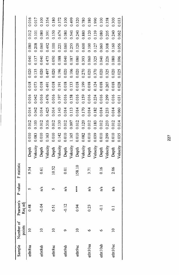
Sam
ple
Num
ber
of Pe
arso
n's
P va
lue
F st
atist
ic
poin
ts Rs
q ad
jet
bt8s
a 10
0.48
5 9.5
4 De
pth
0.010
0.0
12
0.014
0.0
16
0.018
0.0
20
0.040
0.0
80
0.012
0.
016
Velo
city
0.083
0.1
03
0.042
0.0
42
0.073
0.1
35
0.137
0.2
08
0.10
1 0.
017
etbt8
sb
10 -0
.04
n/s
0.61
Dept
h 0.0
10
0.012
0.0
14
0.016
0.0
18
0.020
0.0
40
0.060
0.0
80
0.10
0 ^r o (N o Ov o o o o o 00 o c ncn o o t-" o Ov CN 00 oo Ov o cn o c ncn 1—1 cn I—1 cn r ^ r-H ov I—1 cn c n oo ’ o ’ o o ' o ’ o ' o ' o ' o ' o ' o ' o '
o o o o o o Ov o cn o CNOv VT) r - oo r r 00 CN cn 00 o voc n '—1 VO o cn CN 00 1-H 1-H o CN CN oo ' o ’ o ’ o ' o ’ o ' o ' o ' o ' o ' o ’ o ’ o '
<N o _ o o o o r - o oo o voOv o CN vo cn CN o o CN VO o vo cn^r I—* CN o CN i—1 VO 1—' T—H o c n 1-H oo o ’ o ' o ' o ' o ' o ' o ' o ' o ’ o ' o ' o '
w o OO o o cn o cn o vo o vor - irv oo 00 00 OV vo CN CN 00 Ov
o I—11 o I—1! o cn o cn o CN o oo o ' o ' o ’ o ' o ’ o ' o ' o ' o ' o ’ o ' o ’
r - o vo o vo o o o o o w o cnOv (N Ov CN o CN r - CN o CN CN CN CN^r o I— 1 o o CN o cn o c n o oo o ' o ' o ’ o o ’ o ' o ' o ' o ’ o ' o ’ o ’
00 00 cn 00 Ov 00 00 cn 00 00Ov 1—1 Ov 1—1 cn 1-H Ov CN 1-H vo 1-H CN^r o I—11 o 4—11 o i—' o o CN o oo o ’ o ' o ' o ' o ’ o ’ o ' o ’ o ' o ' o ' o '
VO vo r" vo oo vo Ov vo "3- VO ov vor - 1—1 Ov 1-H un 1-H cn r-H CN 1-H Ov 1-H cn’s f o 1 o i—' o I—1 o CN o CN o oo ' o ’ o ' o ' o ’ o ' o ' o ’ o ' o ’ o ' o ' o ’
cn c n c n N" o 'nT CN c n Tj- o<N 1—1 1-H 1-H 1-H t" ' 1-H 00 1—1 c n 1-H vo
o »—11 o 1-H o 1—' o 1 -H o CN o oo ' o ’ o ’ o ’ o ' o ' o ' o ’ o ' o ' o ’ o ' o ’
VO <N o CN r - CN o CN c n CN c n CNi— CO 1-H Ov r— l CN 1-H 00 1 -H c n 1 -H r H
cn o i—' o o o o 1 -H o CN o oo ' o ' o ’ o ’ o ’ o ’ o ' o ’ o ' o ’ o ' o ' o ’
m o CN o cn o CN o Ov o Ov o cnvo 1— 1 ■*fr 1-H vo 1-H oo 1 -H cn 1— 1 ov 1-H c nr -H o o o o o o o CN o oo ' o ' o ’ o ' H o ’ o ' o ’ o ' o ' o ' o ' o '
.ti x:oo13>
CX<L>Q
ojo13>
x: .tz x .tz x .ts x .ti x .t:cxa>Q
oo1 3>
cx<L>Q
o13>
cx<DQ
oo
1 3>
cx<L>Q
ooa>>
cx&>Q
Qo1 3>
<Ni/"> Oo' ooIT) c n
vo voOCN
t/3
cnO
<N
Or
Ovc nCN
Ov VO vo
ocn00-t-*X(U
xcnOvXa>
ocnON+->X-4-*a>
cnO
-4-»a>
xicnO
X>+-»<L>
OC/2o
Xa>
227

Appendix IV
Appendix IV: TWINSPAN ordered species by samples tables
Introduction
The results of the TWINSPAN analyses used in chapters 2 and 3, is presented here as order
species by samples tables. Taxon (OTU) codes are used throughout. The full taxon names are
given in table 2-5,chapter 2. In each matrix a and b refer to the deep and shallow sections
respectively. The last column and last row give the cuts produced by TWINSPAN. These are
represented as ones and zeros, the line o f binary digits closest to the rest of the matrix represents
the first cut. The numbers in the matrix are pseudospecies counts. Pseudospecies are a
representation of the species abundance in simplified form, (Jongman 1988) .
For all sites TWINSPAN failed to make a clear destination between samples from deep and
shallow sections.
228
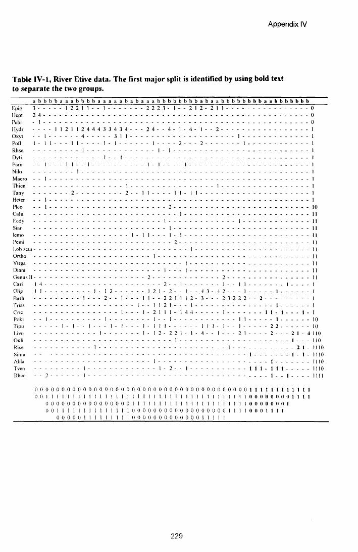
Appendix IV
Table IV-1, River Etive data. The first major split is identified by using bold text to separate the two groups.
a b b b b a a a b b b b a a a a a b a b a a a b b b b b b b b a b a a b b b b b b b b a a b b b b b b bI-'P'g 3 --------------1 2 2 1 1 - - 1 - 2 2 2 3 - 1 - - 2 1 2 - 2 1 1 ---------- _ -------0Hept 2 4 - - ................................... - -------0Pebi . 1 ------------------------------------- -------0Hydr ---------- 1 1 2 1 1 2 4 4 4 3 3 4 3 4 - - - 2 4 - - 4 - 1 - 4 - 1 - - 2 ...................... - - - - . . . - -------1Oxyt - - 1 -----------------4 ------------- - 3 1 1 -------1 . . -------1Pofl 1 - 1 1 - - - 1 1 - - - - 1 - 1 - - l . . . . 2 - - - 2 . . . . l . -------1Rhse ................................... 1 ------------- . . . ] . l . . -------1Dyti - - ...................... ..................... I 1 - -------1Para . - 1 -------1 1 - - 1 ---------- . I . ] ---------- 1 ------- -------1Nilo ----------------------- 1 ---------------- -------1Macro . . i --------------------------------- -------1Thicn - 1 1 -------1Tany -------------------- 2 -------------------- - - - 2 - - 1 1 ---------- 11 - 1 1 - -------1Heter - - 1 - ........................................ -------1Pico - - 1 ............................................ ..................2 - - -------10Calu ...........................1 -------11Fxdy ---------- 1 ---------- -------1 - . -------11Siar .................. I ' -------11lemo 1 - l l ------- 1 - 1 -------11Pemi - ..................2 - -------11I.ob scui - 1 - - -------11Ortho - - 1 .................. -------11Virga 1 ------- -------11Diam ------- --- | ------- 1 ------- -------11Genus Ii - 2 ...................... 2 .................. -------11Cari 1 4 ................................................ ---------- 2 - - 1 1 - - 1 1 - - - 1 -------1Olig 1 1 ................................... 1 - 1 2 - - - - - - 1 2 1 - 2 - - I - - . 4 3 - 4 2 - - - 1 - - - - - 1 - - - - - - 1Barh ................................... 1 ----------2 - - 1 - - - 1 1 - - 2 2 11 1 2 - 3 - - - 2 3 2 2 2 - - 2 - - . . . - - - - 1Triss - 1 - - 11 2 1 - - - 1 - - 1 - - -------1Cric 1 - 1 - 2 1 1 1 - 1 4 4 - - 1 .................. 1 1 - 1 - - - 1 - 1Poki - - 1 ........................................1 . . i . . l . . -------1 1 - 1 - - -------10Tipu ------------- 1 . i . . | ---------- 1 - 1 - 1 - 1 1 1 ------- -------1 1 1 - 1 - - 1 - - - - - 2 2 - - - -------10Livo ................................................ 1 - - - - - - - 1 - 1 2 - 2 2 1 - 1 - 4 1 -------2 1 - 2 2 1 - 4 110Ouli ...................... 1 - 1 -------110Rise --------------------------------- 1 . . - 1 ---------- 2 1 - 1110Sinni ------------- 1 1 - 1 - 1110Abla . . | ------------- I -------1110Tven ---------------------------] ------------- -------1 - 2 - - 1 ------- 1 1 1 - 1 1 1 -------1110Rhco _ _ 2 -----------------1 ------------- 1 - - 1 -------1111
0 0 0 0 0 0 0 0 0 0 0 0 0 0 0 0 0 0 0 0 0 0 0 0 0 0 0 0 0 0 0 0 0 0 0 0 0 0 0 0 1 1 1 1 1 1 1 1 1 1 1 10 0 1 1 1 1 1 1 1 1 1 1 1 1
0 0 0 0 0 0 0 0 0 0 0 0 0 0 1 1 1 1 1 1 1 1 1 1
0 0 0 0 0 1 1 1 1 1
1 1 0 0 1 1 1 1
1 1 0 0 1 1 1 1
1 1 1 10 0 0 0
1 1 1 1 1 1 1 1 1 11 1 1 I 1 10 0 0 0 0 0 0 0 0 0 0 0 0 0 0 0
1 1 1 1 11 110 0 0 0 0 0 0 1
1 1 1 10 0 1 1
1101
11 1 11 0 1 1 1 11 0 0 1 1 1 1 01
0 0 0 0 0 0 0 0 1
001
0 0 0 0 0 1 1 1
1 1 1 1
229

Tabl
e IV
- 2,
Blan
e W
ater
da
ta.
The
first
maj
or
split
is
iden
tified
by
using
bo
ld tex
t to
sepa
rate
the
tw
o gr
oups
.oo o o o o o o
£ i£ ixcd i« icd i
X iX •
A iCd icd ied i
X ied i
X T“™*Xed 1ed 1
X CNX CO
X iX iX iX iX icd r -H
cd 1
ed —X 1
X 1
X 1
X 1
X CNX CNX coX i
X <NX COX cocd i
X i
X ■
X coX i
X i
cd iXX icd (Ncd CN
X CNX icd i
(N
<N
1 1 1 i i i 1 1 1 1 1 1 1 1
1
1
1
1
1
1
i
i
i i
i i
1 1 -H
1 1
1 1
1 1
1
1
1 1
1 1
1
1
1
1
1
1
1
1
1
1
i
i
i i
i i
1 1
1 1
1 1
1 1
1
1
1 1
1 1
1 1
1
1 1 1 i i i 1 1 1 1 1 1 1 1 ^ H
1 1 1 i i i 1 1 1 1 1 1 1 C N 1
1 1 1 i i i 1 1 1 1 1 1 1 1 -H 1
1 1 1 i i i 1 1 i - H 1 1 1 1 1
— ■ 1 1 i i i 1 ^ H CO 1 1 1 1 CO 1
1 1 1 i i i 1 ^ H CO 1 1 . ^ H CN 1
1 1 1 i i i 1 1 1 1 1 1 1 CO 1
1 1 1 i i i 1 CO CN 1 1 1 1 1
1 1 1 i i i 1 1 CN 1 1 1 ^ H CN 1
1 1 1 i i i 1 1 1 1 1 1 1 1
1 1 1 i i i 1 1 CN 1 1 1 1 1
1 ! 1 i i i 1 1 CO 1 E 1 1 t- h 1
1 1 1 i i i 1 CN CO 1 1 1 1 CN 1
- H 1 1 i i i i i 1 1 1 1 CN 1
1 1 i CN ■ ■ CN CO 1 1 - H . f—H 1
1 I 1 i i i i CN ^ 1 1 a t- h ^ r 1
— 1 1 i i i 1 CO n - 1 1 1 1 <N 1
CN 1 1 i rH i 1 1 i 1 . ^ H ^ 1 - 1
CN 1 1 i 1 1 1 CN CO 1 1 1 ^H 1
i 1 1 i 1 1 1 CN ^H I 1 1 1 CO 1
CN 1 1 i 1 1 i i CO ■ 1 . ^H CO 1
CO 1 1 i 1 1 i i ^ ■ r*H 1 1 CO 1
CN 1 i 1 1 i i ^ 1 1 1 1 CN 1
CN ^ r 1 1 i 1 1 I CO CN 1 1 1 1 CN 1
CN ^ r 1 CN ^H , 1 CO CO I 1 1 1 1
— 1 1 ^ r 1 1 1 CN CO 1 1 1 1 CN 1
i 1 CN t- h CN i ■ ^ ^ 1 1 1 1 x f 1
CO CN t—H i ^ H , i ^ r tT 1 1 1 1 1
CO r - i CO ^ H , i CN CO <—1 1 1 1 1
1 i 1 1 1 1 CO ■ 1 1 1 CN 1
CO 1 i 1 1 I CO ■ 1 1 1 CN
— 1 t- h 1 1 ^ H 1 1 ^ 1 1 1 1 1
CO 1 1 1 1 1 1 1 1 1 1 !—H
1 CN 1 1 1 1 ^ H CO 1 1 1 1 x f 1
1 1 i 1 1 1 1 CN i 1 1 1 1
1 1 i 1 1 1 1 1 1 1 1 1 CNT-H 1 t—h 1 1 1 1 1 i 1 . 1
CO 1 1 1 1 1 1 1 i r -H 1 1 CN 1
CN 1 1 1 1 1 1 "sT » 1 1 1 1-H
CO 1 1 1 1 1 CO i t 1 1 1 t—H
1 1 1 1 1 1 1 1 1 1 1 1 1 1
CO 1 CN 1 1 1 1 1 1 1 1 1 1 1 T—h
— 1 i 1 1 1 1 ^ H 1 1 1 1 1 1 1-H
CN " s f i r -H | 1 1 1 1 1 1 1 1 1
1 1 i i 1 1 1 1 1 1 1 1 t 1 1
> 'S<U -3<D <D
oS<D
hJ
OT3
cd .33
S o x >>c xi b ^PQ C/3 f f i P h O PQ W
T3
ocoCN
Esp
a

T“ H
p fi 1
X i 1
■ a 1
A 1
ed 1
ed 1
£ 1
JQ
CM
ed CM
cd -H
X )
cd — *
X> CM
X>
cd 1
Cd CM
X> 1
X> CM
X> (N
X ) CM
X ) 1
X r —H
X ) r - H
cd f - H
cd 1
cd —
X>
X> d -
X ) d -
X> CM
X ) c o
X> c o
X ) CM
X c o
X d "
X
X> d -
cd d "
X c o
X 1
X c o
x c o
X ) CM
cd 1
X> —
X 1
cd d -
cd CO
X d -
X ) Cdcd
Tipu
2
CM
CM
<DCC<
0 O O rH T—H T-H r—i*—i T—H 11 ^ 1 1 t—H
1 1 1 1 fO 1 ^H ^H■ 1 1 CM 1 CM 1 l-H ^H
■d 1 1 1 1 1 1 l“H O
■d 1 1 1 1 1 1 ^H Od rH 1 fO 1 t—H Od 1 1 1 'pH CM 1 O
d 1 1 fO 1 ^H Od CM l 1 1 1 1 ^H O
d CM CM 1 1 1 1 1 O
d 1 1 1 1 CM CM O
d 1 1 1 CM CM ^4 O
d CO 1 I 1 1 O
CM CM ^H 1 I 1 1 O
d~ CM 1 1 1 1 1 O
cn t—h 1 1 I 1 1 O
CM 1 1 1 1 1 1 O r-H
1 1 1 1 1 1 1 O
d 1 1 1 I 1 O■ — 1 I CM 1 O
CM — 1 1 1 1 O1 — 1 1 I 1 1 O t—h
1 CM — 1 I ! 1 O
— CO 1 r—i I 1 1 O * -1 1 1 1 I 1 1 O rH
CM 1 1 I 1 — O
— 1 1 1 I 1 1 O
— 1 1 I 1 1 O1 1 1 1 1 1 1 O
—■ — 1 I t- h ■ O r—h
CM * - 1 1 1 1 1 O r-H
CM 1 1 1 I 1 1 O rH
CO 1 1 1 I 1 ■ O
— 1 1 1 I 1 1 O T“H
CO 1 1 1 1 ■ O
d 1 * 1 1 I 1 1 O
d — - h 1 I sT ■ O-H 1 1 1 I 1 1 O
CM CM 1 1 I 1 1 O t—H
d 1 1 I 1 1 O
d CM I 1 I 1 ■ O
d 1 1 I 1 1 O1 1 1 1 1 O1 1 I 1 I 1 1 O■ 1 1 1 I 1 1 O1 1 1 1 I 1 1 O ^H
1 1 1 1 I 1 ■ O t-h
CO 1 1 1 1 1 ■ O —1 1 1 1 I 1 1 O 0
CM 1 1 1 1 1 1 O 0
1 T—H 1 1 I 1 1 O 0
d CM I 1 1 1 1 O 0
co 1 1 1 I 1 1 O 01 CM 1 1 — 1 ■ O 0
cdu,
X lig I— O
3 <D3M—>D
Whd3> ,
O O s cn O X
COCM

Tabl
e IV
-3,
Dun
eato
n W
ater
da
ta.
The
first
m
ajor
sp
lit
is id
entif
ied
by us
ing
bold
te
xt
to se
para
te
the
two
gro
up
s.
©X ■X iX hH
3 i
OS ■3 i
X i
X ■
3 ■
3 ■
s i ■os ■
x ■03 ■
X r -
X
3 13 1
X CN
-O c o
x iX i
X iX »
X i3 p—H
3 1
3 r H
X 1X I
X 1X 1X CN
X CN
X CO
X 1X CN
X c o
X CO
3 iX i
X iX co
X i
X i03 i
X
X i03 CN
3 CN
X CN
X i3 i
o o o o o © © o © © ©
<N
CN
r*
hJ"
(N - h
m
CN 3 -
cnnj-
_ <D -3 © W) X d <u03 J _ l
CN
c o
O Os ■§ <U XX «
—< CN
1 H
H CO ,
CO ,
1CO
1 1CN ,
1 CN ,
1
1
I iCN ,
1 c o ,
CN CO (
• ^ 1CN CO ,
CN r t (
c o
iCN CO tCN 1
CO %^ ,
^ •CO CN ,
CO CO tCN CO (
,
^ ,
CN CO
CO ^ ,
CO ^ 1,
^ 1
— CO (
CN (
,
f
,
,
,
CN
CN
1
i
1
1
1
1
1
I
I
1
1
1
1 ^
I
. «
1 1 1 1 1 1 1 I l
1 1 1 1 1 1 1 I l
1 i 1 rH T* H rH CO
rH 1 I I r r 1 1 1 rH CN
rH 1 I T f rH H i W
1 I rH I T f CN 1 1 i iN I rH CN <N , i arH I CN I i I i a ^T f 1 <N I T f CO I i a ^CO i — i CO i a aCN i — a CN CN i a aCO I I CN i i i a
i (N a CO -H i i a aCN i i CN 1 a a a t-H i 1 i i 1 i a i i
i <N i , a a a a
— i i rH i — a a ^CN i <N I CN i i aCN i <N I , rH a » a ar“—t i <N I i CN i a a'Tt i i 1 m i a iCN i rH I 1 ■ i a a a
i rH I CN rH a a a i
a n 1 — 1 i a i aCO i 1 CN rH a a a aCO a — a t 1 a a a aCO i — i — rH i 1CN a a CN a a a iCN i r CN 1 a i a a
i CN a CO 1 a a a aCN a CO i 1 i i i a
a CO a CO a a a i
a CN i rH i a a a
i CO i iCN l i 1 a a t aCN rH — i CN <N a i a a
1 i i *—H a i irH i fN i a a i
1 CO a a a a a
1 1 i i 1 a a »—H1CN rH CO i i 1 I i i a
1 CO a i 1 i i a aCN 1 CN i i 1 i i i i
1 CN a 1 a i i a
- < i CO 1 a a a i
»-l © ©
H ©
H ©
ll © H © 1-1 © 11 © H ©© r H
© -1 © r H
© >1 © r H
© r H
© r H
© — <
© rH © r H
© rH © rH © -1 © —• © rH © ^
© r H
© r H
© r H
© r H
© r H
© r H
© -1 © rH © ~ H
© rH © r H
© 1 © r H
© r H
© r H
© r H
© r H
© rl© r H
© 1 © © © © © © © © © ©
n © n © n © ©©
i-H i-H
HH ^ O
r-H ^ H O
i—H i—H c ;
H © rH © ©
r H © ©
rH © © r H O O
^H © ©
H © © r H O O
r-H © ©
rH O ©r H © ©
© rH . © r H
© r H -
© - H -
© - H ,
© rH
O r H ,
© r H ,
© rH © r-H
© r H O
© r H O
© © '
© © r H
© © ' © © r H
© © ©
©©
O X > r . 1hco g ~0 S ^ " 0 ‘ 5 - r ^ u r s o 3 P3c/dDCDhO0QPQO
g ^ 3b 3* ■
CUD 3 S <L> fH euoOha XH <CU O•Pi 2 ^
VH o £ *5:-H 3 (U H P»i
232

Appendix V
Appendix V: Individual responses of benthic invertebrates to velocity, depth and substrate.
Introduction
The raw data for the analyses presented in chapter 4 are given below. For each site there is a table giving
each taxon’s log abundance and the corresponding values o f flow variables. Each row represents a
sample. There is a second table for each site giving the results of the gaussian curve fitting.
233

Tabl
e V
-l, R
iver
Et
ive
data
. As
th
e ab
unda
nce
data
is
log
tran
sfor
med
ze
ros
are
pres
ente
d.a
■sc.Q
180 0
OCd
tr o
191 0 ONc-o o
OnO
tnIT,o
oc•c,O o
VC•CNo
•'TCNO
r lO 0
76 cncnO
VC|NClO
Cl«c,O
119 0____
dO O
To
T7o
1C,clO
OOCNo
ClClo
cnCl <NO
clo O
ocOo
rlo 0 0
51 -rro 0 1
2| ClO
ONOO
111 0 ocCNo 0 1
91
£ <NO
,90 0 d 0 1
40 1
6!0.0
00.
29: 810
clO 0.
13 0 06
0.08
100 o
0 05
0.09
' r-o 0 13
0 04 0.12
0 39 r-r-
60 0 0
27
99 0 0.
07 OnClO
NOClO
Clo
890
C I cnClo 0.
59:
0 43
0.34 Clo
dvnCN ■**NO
d O
J;
Subs
trate
Ve
37 voci
9 19 23
125
6
256 (N
VOr-CN
90.7
5'212
.2 r»CO 3723
4.1 On
cic> 123.1
' ■Li •*T£
NO
256,
oe C,Cl 256
98.5 COOCl 73 9
234
1 CN NONCNCl 256 r»
r-TT
.091 NONT)Cl
9 19 25
6 OnCNC- 25
673
973
9'
| Li
mm
us
1 vo
lckm
ari
CN00ci
ood
000 [ f
0 0
0
0 69 o 69
0
OnNOO
690
ood
VOCl
69 0
000 ood
Olig
ocha
eta
1
• rNOci
ooo 1.
79
000 i
ooo
; 0.
69 OOd
OnCl
oo
ooo
’69 0 l.
lOj j
oo
o
[00 0
ooo
T3
00 0
00 0
000000
000 00 0
ood
000 1.10, 000
[o
oo
ood
169 0
ood
000
3a.
Chi
rono
min
ae
1 0
00|
1.79
000 |
000 1
00 0
|
oOd o
oo
j OnVOo 0.00
J
ooo
[o
oo
[00 0
00 0
Ort
hocl
adiin
ae
Ood
I 1 3
9 OnVOd
oo
j 01' l
ood 1.10
1 O ooo
100 0
On Oci 2.
401 1690
Tany
podm
ae
Oil
00 0
| 0.
69
00 0
I
0.69
00 0
00 0
OOO 0 6
91 OnNOd
ood 0.0
01 [o
oo 0 0
0|
1 c
690 i
000 Ooo
O
| 1.6
11
0 00 o OO
d
on oo
dOnVOO
OnVOO 1.6
11
l.lO
j loo 0
OOd
O
Cae
nis
rivu
loru
m
Ood
OnNOO
100 0
ooo
ooo
On Ooo
Bae
tisrh
odan
i!
1 79
I 0
00 OnVOO
00 0
ooo
Oncn 0 691 OnNO
o
169 0
OnNOO
loo 0
oOO
OnNOO
00 0
[69 0
[69 0
[01 l
j P
olyc
entr
opus
690
690 !
ood
69 0
!
ooo
690
ooo
! oo
o
I
OOo
ood 0.
69] [
oo
o 0.69
j
Poly
cent
ropu
sfla
vom
acul
atus
69 0
00 0
ooo
000 8o
ooo
00 0
ood
69 0
_____
0 00
Hyd
roph
la
00 0
|01
I
| 1
95|
2 40
| 1
95
| 1
79 On 69 0
1 \ 1
10 c;Cl
| 2
20f
0 00
| 0
69
00 0
I
On 00 0
| | 2
30
00 0
1
oClcl
234
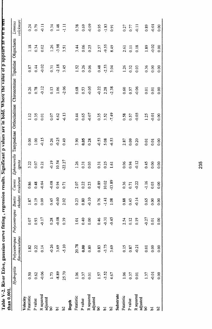
u€341Q.a.csao<u3e5>41c41UV
G2©-Qs©I*03c/i4>J3>a■<—> c03©£3.2P
©imW)©J.
WDC
ca>£3uCA
30304)
#S41>
wh.©>►
<V © > °. © ° z s * 5
i * 0 o
- f a s ^H Tf- 00 o o OS a s i n cn r~ 1— -H a sCN r- cn ■*t cn s o o OS 00 Os CN r-~ 1—1 00O o o 1 O ^H1 o ' o ' o '■ o ' H1 o ' o ' o ' o 1 o '
so oo CN cn SO SO OO Cn cn CN OO 0 0 o r~-CN r~- i-H H O o so in o CN CN cn SO ino’ o o'• o CN■ o' o' o'1 O■ CN CN■ O o
voo
oo'
0 0 -d" CN SO 00a s -rt- SO m r - in Os _ 00 o s CN o
I—1 cn O CN in T f O CN in in r f s o i-H P—H oo o o'-I o' o' ^H cn’t c n Cn o' o' CN a s■ 0 0 CN c> o' ^H o'1 o'
Id" CN 1—H 00 i n CN SO SO 00 cn N" SO cn cn SO o o0 0 O ■p i n CN O rj- SO O CN cn O cn o oo' o' o'1 o' CN■ cn o' o' o' CNi cn o' o’ o' o' o'
^Ho o o
CN <nc n o
r~o
CNs o
cn••d-
>nSO
r ~o <n
cnCNi n
a s 0 0i n m
mo m
CN o oo^H o o’ o ■'d- SO1 o' o’ o’1 o’ cn K■ o' o’ o'1 o’1 o'
oo
oo
m^H s o
CN<nCN Os
*d-oOs
mo
00CN
cnm 0 0
ocni n r-
0 0OSo
oCN O o
oo
o' f—H o'i o' o'1 o' c n © o’ o’■ in ’ VOi CN o' o' o' o’ o'
CNCN
r-o CN
Osi n
-22.2
7 s oCN cn
c no cn
mcn SO
SOO
Ida s
CNH i nrt"
oo
oo
cn o' o' o'i o’ 1 d o’ o’ o’ o o' o’ o'■ o' c> o’
s o00
00-d-
00o ■Mf
a s r~ r -©
CNCN
cnCN
Os00
CNO
OsOO SO
cn r -CNCN
SO cno
oo
o' o' o'1 o'1 o' o' CN o’ o’ o’■ o’ cn■ o' o' o'■ ^H
1 o’ o
t"00
a si-H
a so
i n oSO CN
©cncn
ooo
oH SO
r ~^H 0 0
p000 0
cn -d- i nSO
oo
oo
o' o' o' o’i CN O o' o’1 o’ i 1-H o' o' O■ o’ o' o
("o
cna s
r~ 00CN
00o Os
cn po■d- o
oso’d"
i-Hcn
i n"d- "d-
i nCN^H
Os1-H
r~-cN
^Ho
oo
o' o o■ o’ o’■ o' ^H © o’ o’ o1 O■ CN o' o' O■ o’ o'
CN00
CNCN
Ht1-H
SOCN
OSs q
oF“H
00r - o
oooo
cn00
i nr- Os
pi n^H 00
^HCN o
oo
oo
^H o' o' o’■ cn i n■ o’CN © o’ o’ cni c n o' o' o'■ o’ o’ o'
omCNso
SOO
cnC"
Os00
op SOo
rcn
^Ho >n
(N\D
soO cn o
r -cn o o
oo’ o' o'1 001 i n
CN o’ o’ ^H cni ^H o' o' o’1 o’
cd <U cd 4>
*o OCm d O -—i CN X> X>
235

Tabl
e V
-3,
Dun
eato
n W
ater
da
ta.
As
the
abun
danc
e da
ta
is log
tr
ansf
orm
ed
zero
s ar
e pr
esen
ted.
309
>
(Ua35ooe>o
«oT3
3CX
<o3T3
eO3O«-i2u
•I |I so ■§
ss:o
Q
<*>-30&1£'o ir*a qq"S' |c c
oo
oo
i n in i n. CD CO 00 r- .
CO CD CDN" N" m N -
CD N" CD COCN CN CO x—O O o o o
CXD CD h - CO CNCD lO CD CN X—
O O X“ o oO o o o o
CD o CD oCO o CD oO o o o
s cn co inL Ji O 0> 0> 2CN CN N" CD
CDN-COCNLOCNCNLOCOCNN;N-CNCOCNN-d o d d d d d d
CD S O) N O) O) CO T - CO T - T -
CD lO N" x-o o
O O O ^ C O T -C N O M in cO( Ot- cOCDCOCOCOt-CNM-v; O t- t- O O O t-O C Nd d d d d d d d d o
h-oo
h-CNd
cocoCNo
in t- t- o co CN o d d
o CNo d
00 CD in 0 0 ino CO 00 d 00CO h - CD CO CD
CD r - CD CD COo X— X— o COo d o o d
CO T_ o CO CDCD CO 00 CD CNX— CO CO T — CNd o o o o
o CDO CDd o
ooo
O O CD CD O O x - c o CO o
§ °> LO CO
O CN COo o o
O CD x- (O C\l t CN CO CNO O O
oo
o o o o O o o 00 CD O x— O O O X— O O Oo o o x- ; O o x - N" CD O CD x— X— O N- N" O Oo o o x - d o x~ CN O O X— X - X— o CN CN O o
X— N" o CD o CD N - O O h - CN O in O CD CD oCD N - o CD CO CO CD NT O CO CN O CO CD O CD oCO co d o CO X - CN CN o c o CO CO CO CO o o Csi X - 1
o o X— X - CD CD CD OX— o CD CD CD CO CO ■x—X— o X— x - d d X— x—
CDCDo
oo
CD O CD O CD X—CD O CD O CD CDd d o o o X—
CDCOCN
o CD X— X— o o CO O o CDo CO CD CD X— o 00 o o COCO x— X— X— XT" o CN CO d X—-
CD N" h - o ON - x— ■x— N" CN
T“ CO CN CN
CD CD o o CD CD i n o o ^ r CO 00 CD o CO 00 00 o oc o Is*- CD o o CO CD a> o q o CD CO o CO o 0 0 o o N"
T_ x - o o d T“ O T“ o T_ o CN CO CN T~ o csi CN CN cvi T_
OO OO CD COo o
oo
o o o oo d
CD CD o oCD CD ■X— o < Dd d X— o
oo
CDCO CDCDCO o
oo
CD CD CDCD CO r-*d T_ T_
o o CDCN o COCN o d CN CN O O

ca(U3
>
03OobO
<D0323ex
5:I ij►o O
I ^ 05 CO CO Is- 05 ini f x - CM r CM in 05 __ CO in CM M" (O _ x_ CM CO CMSi ° x— CM o CM X— No CM CM o x— o . X~ CM o x— X~ o
i ° d o o o o O o o d d o o ° o o o o o ° o d o o
CO CM in M- 05 05 00 05 05 CO 0 5 CO Is- 00 M" CM Is- T_ o Is- CM 05 COCM X— CO CO CM 00 CO CO X— X- Is- CM M" o M" CO 00 X— Is- x — CO m COx- CM 00 O CO o X— o o CO CO X— o i n CO CO X— i n CO CO X— o
d O d o o o d o o d o o o o o o o o o o o o o o
O 05 05 05 o o o o o 05 o o oX- CO CO CO o o o o o CO o o oT_ o T— o d d d d o d o o o
o o o in 05 X— 05 05 o o 05 o 05 o 05 05 o o 05 COo x- o 5 05 CO CO CO CO o o CO X— CO CM Is - CO X— CM CO ino o o o d o o 'r ~ CM T— o T_ CM T_ CM
CX) in 05 o o 05 05 o 05 o o 05 0 5 05 o 0505 CO o o Is- CO CO s CM CO CM o CO CO CO CO CO
CM o d o' CO X- d CM CM d d d CM d
*- s5 s: bo
-s: ~
■3-
«ss
I
s* >
CM 00 M;K. CO CO fv CO in CO in in m
c dCM
CMIs-
inCO
1 ^CO
CO05
1 —CO X—
CO0005 CO
0005
0005
0005
05 O LO CO 0 0 00 * - 05 CM
Is-h-J-
00 o un° o Zo ^ ^oo CO 0 0
T_ 0 5
0500CM
LO05
o 05 o x— in o o 05 o 05 05 X—o CO X— CD 05 o o Is- X— CO CD CDd X— X— X— X— d o X— X— d d X—
m in o CO CO x— o o X— 05 05 m in 05 x— X — 05 05 o05 05 M" 00 in CD CO CM CO o CO CO 05 05 Is- CO CO CO Is- COX— X— CM CM CM X— csi c \i X— cd o d X— X— X— X - X— d X " CM
05 05 co o 00 o o o X— o 05 o 00 o 05 o 05 X— oCOCOo x— o o x— x— Is- ■sf CO ■M" CM COCOX— COIs- X—o o CM X— CM o x-^ X— cd CM o CM csi CM d CM X— o CM x -’
05 o 05 O 05 05 05 o 05 05 05 05 05 oCO o CO T - CO CO CO CM CO CO Is- CO Is- CO oX— o X— x—" o o X— CM CM d X— o X— X— d
OO
05COo
o o o od o
oo o o o O T- o oo
oo oo
X— 05 o o CO o o o 0 5 05 o 1 ^ o o CO CM 05CO Is- o o o o o o CO CO CD CM Is - o CO M" CM COX— X - o d CM o o d d X— CM CM CM d CM CM cd o
237

cC3
3Mc7i
aftW)aftCUDc
cCit3uC<3
3«COC
«■oft-fta
*c0-ta-ceas3
Q
h ?1>Ci
3«
H
cd-*-*<Dcdoo0 0
CDcd
TD
3CX
(Dcd
TD
SoGOft
2u
ao
cna
•SftoX.ca
< 5ft
s sJc?s -S•*** *"1*O o
X
«nftv.ftft0
1 -ft:
I .u"§h£ r
ca«Qq<a
- f t0£>
§ •
1cn ft5ft ftq>-«4 -Ki
ft
Io f t <a
<1
*§J
cn m £7 'O M ^ NO m ° .O O 9
- s(NO
''D-on
CN so00 o o^r o cn00 o o ’
CN3 -i n ©
©
m ON t—h
3- CN ONCN <—< oCN o ’ o ’
ON ^r cnCN o f"NO m i—11—i o ’ o ’
csi a S!^ 3 ^ ° d o
oo r - Os so IT)
j ^ oo o
^ 2 ° l A l V r — 1
o’ Q o’
m 00H*T <cn 00NJ
CNo ’
CNoo ’
r -o
CNo ’
cn! i
cnSOCN
t—h COA CN,T ocn o o ’
V i W im tN oo’ cn
r - CN ON 00 CN3" o m On r-Ho ’ o ’ o ’ o ’ o ’
inO in om 00 m
o 'To ’
003 ’ cn 3 d (N 7
sot"-
O m00 cn r->o ’ f—I o ’
u . z i 2 td0J ■•-> £ “
■Si £ -a s 5 « 2.. _ 3 g_ _ <*> - ft,c , H O ’—1 CNX pH K cd JD X) X)
in m .ON T-l ^Tf- so o o’ o’ '
3 - NO cno ON r -m o oCN o ’ o ’
3" NO in NO OnON H On cn00 CN l"- r —H o
1 T“ H t—h o ’ o ’
CN so r -
cn o
h m 2so cn p: O On ° .o ’ o ’ 9
r -H C N
ON NOm m o' o'
o o OO r -NO On r - CNo ’ o ' o On
i i o ’ o ’
3 -
3 -
cnin r -
NOr -o CN
NO00
CNm* m NO CN i-Hoi 00 ■ o ’ o ’
___ On inCN [-- NOo ’ CN NO1
vo ^ 00 t t ^ ^, ’ CN r~ l
r--o
3-cn
mCN
ON NO r^I"1 c i—io ’ 1—1 CN
cn r - cnCN C"
i—iT|-NO00
cnin 00 r -
o oo cn o NO 3"r -H 00 r -H• o o ' o ’■ CN
^ r- 9 m cn 00
cn m NOo m 1—1o ’ o ’ CN i
^ a “ •f" cn
r-~CNo ’
cn rr-mON
NO NO m O n r o
m ON ONcn o ONTT i i oCN o ’ o ’
r - cn1-H in inm ON oo o ’ o ’o ’ 1
oo 00o OO oor - o oCN O O
no m cn r— 9 ooo ’ o ’ 9
NO ON 1— 1 ONo
NO r - cn m cn00 NO in cn "d" ON o cnm m CD CN cn Oo ’ o ’ o ’i
t- hi
oi H o ’ o ’
m oo nom r~- ^v > c ”cn r - o ' o '
3-o
cn r - r -O cn o
3- i—icn o o
CN o cnCN NO TfO t—H CNin o ’ o ’
cn°N £ 2 NO .O ’ ° 9
r- __
g gcn 1 . O’ °
inCNo ’
NO m 00 cnr -
00 mON
t|- cnTf3"
tTNO
cnO ON o NO
oCNH
o ’ o ’ o ’■cni m cn o ’ o ’
aCiO
o"ScdooPh
uy£ . 2 3■*“ 4—> 4—ICDJ33>cu
T3<D _ ,ft 3cd o—t -t-<3. c r pon -G,TO O i—i CN
K cd X> Xi X>
Ci-*■*esftcn,£3(/)
O333PU|
CD_3cd>CU
TD<D __, ft TD 3 <D
. TD O «—■ CN « cd JO JO X>
0.92
-2.02
-8
.44
-0.05
0.8
3 1.9
2 -0
.03
1.33
2.77
1.00
0.78
0.00
0.08
0.14
0.02
0.01
0.00
0.03
-0.02
-0
.03
0.00
-0.0
10.0
0 0.0
0 0.0
0 0.0
0 0.0
0 0.0
0 0.0
0 0.0
0 0.0
0 0.0
0 0.
00

Tabl
e V
-5,
Blan
e W
ater
da
ta.
As
the
abun
danc
e da
ta
is log
tr
anst
orm
ed
zero
s ar
e pr
esen
ted.
l-l -t—< ON c n o c n un 00 i n NO N" cn o N" o oo ^ r c n t" - CN NOJO c n ^ r c n 'vf cn c n c n m c n CN r~~ 1—I CN CN 1—1 NO NO in 00Don
JS <N ^ r ON o ON CN O n ON ON c n NO CN c n r-~- ^ r r -H NO ^ r o cn 00e xD B CN o 1— cn CN o o O CN '1 CN CN o 1 CN i—1 CN o oQ o' o' o’ o' o' o' o' o' o' o' o' o' o’ o’ o' o’ o' o’ o’ o’ o' o'
■4—*r - IT) c n ON o o 00 ON c n cn c n o 00 m c n OO i n 00 m c n o o O n o io ,c i—i c n NO o o C-" N" o ON c n oo T < ■*d- CN CN c n CN CN o o T—H i no C ^ r i n o o o c n m NO 1-H i—1 o c n c n c n CN l—1 m c n CN c n o CN m"a>
>G o 1 o' o’ o' o’ o' o’ o' o’ o' o’ o’ o' o’ o' o’ o’ o’ o’ o’ o'
•S Q o o ON o o O o o ON ON ON ma r* o o NO o o o r — I o NO NO c n O n
3 5J o' o' o' o’ o' o’ o’ o’ o’ i—H
a fc .a ©S J i
©
aOtoa'W.Ci,bo
©S 's a ^<5 o Cn .aS O3 03
a*^ afr-g a &
§oa<1
■a s a I© o "Q-S
toa!kaa©
-aa.
o oO T-H
ooo'
oo
onr -
VO O Oo o ONNO ooo o o
oTfCN
NOONNO
oo O nr-~
o o o oo o ’
oo
oo
oo oo
oo ON O n c n c n
ONc n
cncn
O n m NO ON
oo
o o
ONc n
ONc n
oo ooCN
00o<N
O o o o O n O n ON ON o o O n 00O >— _ CN o NO c n NO NO c n i— • o c n oo ’ CN o ' o ' r ~ l o ’ < I o ' r* ^ CN
O nNO
oo
cn
oo
oo
ON o o in r -NO o o O n r-o’ o’ o' T 'H CN
O n 00 ON O n O n o in ON o m O n O O n ■*d- i—ir - ^ r c n r-_ c n <—; ON NO o ON r-~ «“ ; r - * NO
i—I CN i—’ r —H -—I i—i o' o’ r —H l—H c n i—i
0 0 O n r - 00 t- - O ^ r c n ON ON 00 o o 00 mN" c n c n m oo On o 1—1 c n OO OO o r - m CN ON
"cT c n c n CN c n c n c n CN CN CN CN CN c n ^d" c n
CDCOCN

-O3tn
o- c <u c
’5 rT o £' a j C<D>
r i ^
S ?5
•« ^ ^ O >
0t-n ■>*
&C
Q1 *I ■§8 s
■2 R1 1 0, .g
>)aaco
f3
-5:
m CN cn NO OO CN in ,—1 ON r-" r - t"- r - oo in On r -n r 3" N" 3" CN NO CN Xj- cn cn cn cn CN CN n - cn
on o cn NO r - N" in 3" NO NO O NO tJ-,—1 !■■ 4 f-H o 1—4 >—• cn o i—1 o O o o 1— O i—i oo ' o ’ o ’ o ’ o ’ o ’ o ’ o ’ o ’ o ’ o ’ o ’ o ’ o ’ o ’ o ’ o ’
,_, in o cn CN ON in ^r cn cn cn 3- ON CN cn r fm> NO cn On 00 3- CN NO oo cn i—i 00 oo NO m m inr - o ON cn oo ON 1—4 o NO cn cn cn m NO CN NOo ’ o ’ o ’ o ’ o ’ o ’ o ’ o ’ o ’ o ’ o ’ o ’ o ’ o ’ o ’ o ’ o ’
On o On ON o o m ON ocn I—1 NO NO o o NO On NO cn
1— o ’ o ’ o ’ o ’ T— o ’ CN
O 3" O o ON O o oo o ON o o ON<N ON O o NO o o ''3- o NO CN o cnr s CN o ’ o ’ o ’ o ’ o ’ CN o ’ o ’ CN o ’
o o On ON o ON ON O o o’—_ o NO cn o NO NO NO CN o o NO
o ’ o ’ '—, o ’ o ’ 1—1 o ’ CN o ' o ’ 1—1
o ON o o'—« cn o o
1—1 o ’ o ’
1" On 00 m ON o On ON ONno cn o ON r - CN NO NO NO<Ni
"CN
”CN o ’ o ’ o ’
On On o o O O oVO NO o o cn »—1 oO o ' o ’ o ’ CN 1—1 o ’
ON ON ON f 4 NO N" On ON ON ON ONNO NO cn t"- m NO NO cn NO 00 r - cno ’ o ’ 1—4 CN CN CN T**H 1—1 CN ' '
o m o oNO NO o ON o o
o ’ o ' o ’
o NO o o oo o o ON1—' m NO r-H CN o o o cn
CN 1—I CN CN o ’ o ’
O cn ON 3- ON NO o cn ■ r ON On 3 -m cn 00 m r - CN m oo NO NO r - r -^r 1—H cn I—i cn «—<’ cn cn cn cn o ’ 1—4 cn
240

cOJD
i Z
aLa01)au
0£c
1=<D
t3uCa
3C8Oi
«S■oLa4>+HCS
£a>3CO
5VOI>
2etH
cn QI =fcq §
•N*o O
aO
cnSS>•*»
t>C
P Ocn8 O5 05
U5 •*«-I ^ ^ ■ S* sJ S
INjacu
< l
cn R
* -S, 5 <p OQ -5
a*.
cnab.as :o
• &
$
<i>- 5Cl
O N CN NO i n m r— c r ~ ' — • O m O N oo 3"3" N O o 3 " o CO O N 3 " 9 O N 3 " o r- 3- o oO o ’ o ’
1 o' o' o’ o' o' 9 o' CN■ o' o' o o 9
r -m
C OC N
3 ^OO N3 "
OO C OC N
9 o’ o’ o' o' 9
oo ON NO IT) o O nCO NO o oo o To' o o’1 c> o’ o’
oo cn r? no r r\o ^ a °O O 9 9 9
£ •* 3 .2£ ta> pH
onNO
<l>3
1 3>
PH
T d<U
3 33
T da>«-H33crcn
P h
NOO
r -vo^ ^ 00ov 9 o\
o ' 9 o ' <9oo
no 3* 9 o o oO On ° . Os r. OO O 9 o' 9 o'
NO CN ON NO CO o r- Onin r"H r—> o r“ H CO © 3"CN o' o' o'■ o' o’ 9 © o'
C Oc o c o
oo
CNON 3"
oo ° 9 ooo
00 o in CN NO 00 NO o o O 00 NO c n CO00 3- 3 " CO o CN CN r " o o CO o CN 1 NOo’ o’ o'■ o’ o' o’ o’ o' r—H 3 -' o’ o' o' o'1
o3 "
NO NO 3 " o NO m 3 " OO 3 " oo o C O oo3 ; C N O o o o NO CN o c o r - o oo’—l o ' o ’ 1—11 o ' o ’ o ’ o
1 T—' o ' o ’ o ' o ’
3 - N O C O ■'T 0 0 i n 3 - 3 " m o C N ON3 ; C N ■3" O C N r - C N o oo o T- ON
C N o ' o r—41 o ’ 9 9 o ’ o o ’ 9 o ' o ’ o ’
r-o
ox 1—1 CN X X
CN3"
3
'O<D
333
33a>Wh33cr
P h P h P4
r-o
oino o
l > r - £ r O n c nCN Is" 9 0 0 3 "o o’ 9 o' o'
in o in in CN m t - OO CN ON o ON in CO NO o00 CO CN in o in CO 3" "“I NO o r- m *“! 3"9 o ' o ’ o '1 o ' 9 CO o ' o o1 9 o' co o' o' o■ 9
CNCOo'
OO O ) Ono 9 3 " m
o' o 9 o o'
NO
oo’
ooo
N OC O o 3 "
0 0
3 -O N
Oo O N
C N3 - O m o
3"T—H o ’ o 9 C N■ o ' o' O o’
■ 9 o'
C NO
ooC O
ooin3;
C No OC N
On (NC O
r —1o NO
C Noo
r-NO
C Nm
mo
0 0C N
0 0C O
9 o' o' < N o' o’ 9 o' o' C O C N1 o' o’ o’ o' C O o’
oX CN
X
-7.30
-8
.66
-2.19
2.0
6 7.5
3 -2
.36
16.83
-2
.09
-5.30
-1
0.50