Force Estimation and Prediction from Time-Varying Density Images

Force Estimation and Prediction fromTime-Varying Density Images

Srinivasan Jagannathan, Berthold Klaus Paul Horn, Purnima Ratilal, and

Nicholas Constantine Makris

Abstract—We present methods for estimating forces which drive motion observed in density image sequences. Using these forces,

we also present methods for predicting velocity and density evolution. To do this, we formulate and apply a Minimum Energy Flow

(MEF) method which is capable of estimating both incompressible and compressible flows from time-varying density images. Both the

MEF and force-estimation techniques are applied to experimentally obtained density images, spanning spatial scales from

micrometers to several kilometers. Using density image sequences describing cell splitting, for example, we show that cell division is

driven by gradients in apparent pressure within a cell. Using density image sequences of fish shoals, we also quantify 1) intershoal

dynamics such as coalescence of fish groups over tens of kilometers, 2) fish mass flow between different parts of a large shoal, and

3) the stresses acting on large fish shoals.

Index Terms—Force estimation, density prediction, compressible flow estimation, minimum energy flow.

Ç

1 INTRODUCTION

ESTIMATING velocity and force fields from image se-quences is an essential and often first step of analysis

in a wide variety of applications such as object detectionand tracking, robot navigation, visual odometry, medicalimaging, remote sensing, and satellite imagery. Imagesequences used in these applications describe both com-pressible and incompressible flows. A variety of methodsexist for estimating velocity fields, such as Optical Flow [23]and pressure gradients [38], [54] from time-varying imagesdescribing incompressible motion.

In this paper, we develop and apply methods forestimating the forces driving motion observed in densityimage sequences, where pixel values can be modeled asproportional to the density of a compressible fluid. Using theseforces, we also present methods for predicting futurevelocity and density values. To do this, we formulate andapply a Minimum Energy Flow (MEF) method to estimatevelocity fields from image sequences, describing bothcompressible and incompressible flows.

The MEF and force-estimation techniques can be gener-ally applied to any density image sequence, where pixelvalues can be modeled as proportional to the density of acompressible fluid. Here, for example, we demonstrate these

techniques at the microscale by quantifying the dynamics ofcell division, and at the macroscale by quantifying fish shoaldynamics over tens of kilometers. Using density images of acell undergoing mitosis [19], we quantify the velocity, netforce, and apparent pressure fields inside the cell. We findthat the cell division is driven by the formation of two regionsof low apparent pressure at opposite sides of the cell and aregion of high apparent pressure at the center. Using fishpopulation density images obtained with an Ocean AcousticWaveguide Remote Sensing (OAWRS) [32], [27] system, wequantify 1) intershoal dynamics such as coalescence of fishgroups over tens of kilometers, 2) fish mass flow betweendifferent parts of a large shoal, and 3) the stresses acting onlarge fish shoals. To study collective behavior, large animalgroups, including fish shoals, are often modeled as com-pressible fluids [51], [52]. Such theoretical group behaviormodels predict average velocities and forces inside animalgroups, which can be verified using our MEF and forceestimation techniques.

2 BACKGROUND

Classical motion estimation from image sequences describ-ing incompressible motion is based on Horn and Schunk’s[23] work on determining Optical Flow. Barron et al. [4]review and compare the different optical flow techniques,including [23], [31], [53], [37], [2], [47], [22], [55], and [18],where the 2D velocity field (u) is computed from spatialand temporal variations in the image intensity (E) patternsby minimizing a global cost function of the formZZ

�

f@E

@tþrE � u

� �þ �g ruj jð Þ dx dy;

where fð�Þ and gð�Þ are monotonically increasing functions(usually the magnitude squared of the argument), � is anempirically determined weight, and � is the image plane.

The above choice of cost function is especially suited forincompressible motion estimation since 1) the argument of

1132 IEEE TRANSACTIONS ON PATTERN ANALYSIS AND MACHINE INTELLIGENCE, VOL. 33, NO. 6, JUNE 2011

. S. Jagannathan and N.C. Makris are with the Department of MechanicalEngineering, Massachusetts Institute of Technology, 77 MassachusettsAvenue, Cambridge, MA 02139. E-mail: {jsrini, makris}@mit.edu.

. B.K.P. Horn is with the Computer Science and Artificial IntelligenceLaboratory, Department of Electrical Engineering and Computer Science,Massachusetts Institute of Technology, Room 32-D434, 32 Vasar Street,Cambridge, MA 02139. E-mail: [email protected].

. P. Ratilal is with the Department of Electrical and Computer Engineering,Northeastern University, Room 311, 302 Stearns Center, 360 HuntingtonAvenue, Boston, MA 02115. E-mail: [email protected].

Manuscript received 8 Apr. 2010; revised 26 July 2010; accepted 28 July 2010;published online 30 Sept. 2010.Recommended for acceptance by S. Belongie.For information on obtaining reprints of this article, please send e-mail to:[email protected], and reference IEEECS Log NumberTPAMI-2010-04-0251.Digital Object Identifier no. 10.1109/TPAMI.2010.185.

0162-8828/11/$26.00 � 2011 IEEE Published by the IEEE Computer Society

fð�Þ should be zero in an incompressible fluid [5] when E isproportional to the density � of the fluid, and 2) minimizinggð�Þ, also known as the “unsmoothness of flow” criterion,suppresses large gradients in velocity which are usuallyassociated with compressible flows.

In compressible flow estimation, a modification of theOptical Flow technique is to replace the first term in the costfunction with the corresponding term from the compres-sible equation of continuity [5] for fluids. Methods based onthis modification [1], [7], [56], however, retain the “un-smoothness of flow” criterion, which may not be suitablefor estimating flows with large spatial gradients in thevelocity field, as we show in comparisons with the MEFapproach (Appendix A). In the case of compressible flows,it is the spatial gradients in velocity which containinformation about the compressible nature of the motion,and using the “unsmoothness of flow” criterion may distortthe velocity field [13]. Higher order penalty functions suchas “second order div-curl” minimization [49] have beensuggested for fluid flow estimation. These methods pena-lize sharp changes in vorticity and divergence of flow,which may not be appropriate in estimating generalturbulent flow either.

Penalty functions other than the “unsmoothness of flow”of Optical Flow have also been proposed for nonrigiddeformation estimation. Devalminck and Dubus [13], andothers [35], [41], [50] propose formulations based onminimizing the strain energy of deformation, which isapplicable only for objects that undergo elastic deforma-tions with a known stress-strain relationship but not forfluids undergoing compressible motion.

The MEF technique uses a physically motivated penaltyfunction that does not directly depend on the spatialgradients of velocity. The total kinetic energy is used insteadof the “unsmoothness of flow” criterion. The choice of kineticenergy is motivated by the Least Action Principle [34],according to which the evolution of a physical system fromone state to another corresponds to the minimum of theaction [29]. Since we are interested in estimating compres-sible fluid flow, this principle reduces to minimizing thekinetic energy of fluid particles corresponding to the densityat an image pixel.

Our force-estimation technique uses the flow fieldscomputed by MEF as inputs and is applicable to bothsteady and unsteady flows. That is, the forces are estimatedby taking into account temporal fluctuations in the velocityfield. The nonlinear Navier-Stokes equation [5] is used andboth conservative and nonconservative forcing terms areassumed to be present. The force-estimation technique itselfis a separate “module” that can, in general, have inputsfrom any motion estimation model. We have developed andapplied a MEF technique for motion esimation because ourmethod performs better than existing techniques of com-pressible flow estimation (Appendix A).

3 FORMULATION

3.1 Velocity Field

Let �ðx; y; tÞ be the density corresponding to a point ðx; yÞ inthe image plane � at time t. If we assume that � is thedensity of a compressible fluid, then in the absence of anysources and sinks, the velocities are constrained by theequation of continuity [5]

@�

@tþ @

@xð�uÞ þ @

@yð�vÞ ¼ 0; ð1Þ

where u and v are the components of the flow velocity in the

x and y directions, respectively.This is a single equation relating the measured spatial

and temporal variations of density and the two unknownvelocity components u and v. To determine a particularvelocity field, we set up an optimization problem where wetake the square of the error in the constraint (the left side of(1)) and add a multiple of the kinetic energy of the system

T ¼ �ðu2 þ v2Þ ð2Þ

as a penalty term or objective function, and minimize the

following integral over �:

Z Z�

@�

@tþ @ð�uÞ

@xþ @ð�vÞ

@y

� �2

þ��ðu2 þ v2Þ" #

dx dy: ð3Þ

The velocity field we determine through this minimiza-tion is the one that results in the least kinetic energy whilemaking the deviation from satisfying the continuity equa-tion as small as possible.

The term � is a constant that defines the “penalty for”high kinetic energy in the solution. We expect that largevalues of � will tend to suppress high kinetic energyexcursions in the solution (at the cost of not matching theconstraint equation as well), while small values of � willtend to make the solution match the constraint equationmore closely (at the cost of being more sensitive tomeasurement noise).

For convenience, we now define

�u ¼ �u and �v ¼ �v ð4Þ

representing the mass flow rates in the x and y directions,

respectively. We can rewrite (3) in terms of these flow rates asZ Z�

ð�t þ �ux þ �vyÞ2 þ�

�ð�u2 þ �v2Þ dx dy

¼Z Z

�

F��u; �ux; �uy; �v; �vx; �vyÞ dx dy;

ð5Þ

where the subscripts indicate the variable with respect towhich partial derivatives are to be taken. Minimization of(5) can be treated as a problem of the calculus of variations,where we solve the following set of Euler-Lagrangeequations:

F�u �@

@xF�ux �

@

@yF�uy ¼ 0; ð6Þ

F�v �@

@xF�vx �

@

@yF�vy ¼ 0: ð7Þ

Substituting the expression for F into (6) and (7) leads to

�u ¼ �

�ð�tx þ �uxx þ �vxyÞ; ð8Þ

�v ¼ �

�ð�ty þ �uxy þ �vyyÞ: ð9Þ

JAGANNATHAN ET AL.: FORCE ESTIMATION AND PREDICTION FROM TIME-VARYING DENSITY IMAGES 1133

In Appendix B, we present a numerical technique tosolve (8) and (9).

Earlier work by Fitzpatrick [17] involves a strict enforce-ment of the continuity constraint, which may not hold in thepresence of measurement noise. A Lagrangian multiplier,denoted by �ðx; yÞ, is used as a spatially varying unknown,and closed form analytic solutions are pursued. In theformulation here, departures from satisfying the continuitycondition are allowed, but penalized. Additionally, we haveused a fixed multiplier � to weigh the energy term. We haveassumed that the changes in pixel intensity in the imagesequences are purely due to the motion of objects imagedand not due to the motion of the observer. It is possible tocorrect for observer motion prior to applying MEF. Thecomputational techniques presented in the paper work wellfor imaging applications with high frame rates. For lowframe-rate applications, a coarse-to-fine approach as de-scribed in [6], [15] may be employed.

3.2 Force Field

A velocity field can be the result of an underlying force fielddriving the motion. We can determine these forces using theNavier-Stokes equation [5] for compressible flow in twodimensions:

�@U

@tþ ðU � rÞU

� �¼ �rpþ F; ð10Þ

where U ¼ ðu; vÞ is the vector velocity field, p is thepressure field, and F ¼ ðf1; f2Þ is any external “forcedensity” (body force per unit volume) acting on the fluid.The right-hand side of (10) is the sum of a conservativeforce per unit volume (rp) and a nonconservative force perunit volume (F). The x and y components, respectively, ofthis vector equation are

�ðut þ uux þ vuyÞ ¼ �px þ f1; ð11Þ

�ðvt þ uvx þ vvyÞ ¼ �py þ f2; ð12Þ

where subscripts again indicate the variable with respect towhich partial derivatives are to be taken. For special casesof fluid flow when either the conservative force or thenonconservative force is zero, the system of (11) and (12)directly provide us the solution for either ðf1; f2Þ or p. In themore general case that we consider here, we assume thatneither rp nor ðf1; f2Þ terms can be neglected and arecomparable to each other.

Determining the unknowns p, f1, and f2 from (11) and(12) is an ill-posed problem, which we will reframe as twodecoupled variational problems in order to determineapproximate least-squares solutions.

Subtraction of the y derivative of (11) and thex derivative of (12) eliminates p and yields

@

@y½�ðut þ uux þ vuyÞ� �

@

@x½�ðvt þ uvx þ vvyÞ

¼ @f1

@y� @f2

@x:

ð13Þ

We then find ðf1; f2Þ that minimizesZ Z�

@

@y½�ðut þ uux þ vuyÞ� �

@

@x½�ðvt þ uvx þ vvyÞ�

�� @f1

@y� @f2

@x

� ��2

dx dy:

The solutions f1; f2 are then given by the following Euler-

Lagrange equations:

@2f1

@y2¼ @2

@y2½�ðut þ uux þ vuyÞ�

� @2

@x@y½�ðvt þ uvx þ vvyÞ� þ

@2f2

@x@y

ð14Þ

@2f2

@x2¼ @2

@x@y½�ðut þ uux þ vuyÞ�

� @2

@x2½�ðvt þ uvx þ vvyÞ� �

@2f1

@x@y:

ð15Þ

The coupled equations (14) and (15) are solved using afixed-point iteration technique, which is described inAppendix C.

After determining ðf1; f2Þ, we again use (11) and (12) to

solve for p

px ¼ ��ðut þ uux þ vuyÞ þ f1; ð16Þ

py ¼ ��ðvt þ uvx þ vvyÞ þ f2: ð17Þ

This is a Dirichlet Boundary Value Problem and, in general,is overconstrained. For example, in the computationdomain ðx 2 ½0; L�; y 2 ½0; L�Þ, the explicit integration of(16) yields

pðx; yÞ ¼Z x

0

½��ðut þ uux þ vuyÞ þ f1�dxþ pð0; yÞ; ð18Þ

which may not satisfy the boundary condition at x ¼ L.In order to obtain a best fit solution for the system of (16)

and (17), we reframe it as a variational problem. One way todo this is to find the solutionp that minimizes the square of theeuclidean norm of the residues of (16) and (17), much like theprocedure adopted to find ðf1; f2Þ. We thus minimizeZ Z

�

½px þ �ðut þ uux þ vuyÞ � f1�2

þ ½py þ �ðvt þ uvx þ vvyÞ � f2�2 dx dy:

The Euler-Lagrange equation for this variational problem is

r2p ¼ @

@x½��ðut þ uux þ vuyÞ� þ

@f1

@x

þ @

@y½��ðvt þ uvx þ vvyÞ� þ

@f2

@y;

ð19Þ

where r2 is the Laplacian. We solve this inhomogeneousLaplace equation using a fixed-point iteration, in Appendix C.

3.3 Predicting Densities Using Forces

The ability to quantify forces also provides us with amethod to predict future density distributions once we havean initial estimate of the velocity field and the force field.


In order to do this, we assume that the initial force

computed stays constant for some time before there is a

substantial change in its magnitude and spatial distribution.

This means that over some time scale, the accelerations (or

the driving forces) remain constant. Under these assump-

tions, we suggest the following prediction scheme:

. Step 1Obtain density data �ðnÞ; �ðnþ1Þ; �ðnþ2Þ

(superscripts indicate time steps).. Step 2

Compute ðuðnÞ; vðnÞÞ and ðuðnþ1Þ; vðnþ1ÞÞ using �ðnÞ,

�ðnþ1Þ, �ðnþ2Þ, and (8) and (9).. Step 3

Calculate rpðnÞ and FðnÞ using (14), (15), and (19).. Step 4

Set

rpðnþ1Þ rpðnÞ;Fðnþ1Þ FðnÞ:

. Step 5Use ðuðnþ1Þ; vðnþ1ÞÞ, �ðnþ1Þ in (11) and (12) and

compute ðuðnþ2Þ; vðnþ2ÞÞ.. Step 6

Use ðuðnþ2Þ; vðnþ2ÞÞ and �ðnþ1Þ in (1) to predict �ðnþ3Þ.. Step 7

Repeat steps 1-6 by setting

�ðnÞ �ðnþ1Þ;

�ðnþ1Þ �ðnþ2Þ;

�ðnþ2Þ �ðnþ3Þ:

4 APPLICATIONS

4.1 Synthetic Image Sequences

To evaluate the performance of the MEF method, we usesynthetic image sequences describing 1) contraction of adensity feature, 2) coalescence of two density groups, and3) splitting of one density group into two. In all of theseexamples, the MEF-estimated flows and pressure fieldsmatch well with the “ground-truth” values, as can be seen


Fig. 1. (a) Initial, (b) intermediate, and (c) final density distributions of a contracting density feature. (d) The ground-truth pressure distribution thatresults in contraction. (e) Comparison between ground-truth and MEF-computed horizontal mass flow rates at t ¼ 0 s along the y ¼ 0 cut in (a).(f) Comparison between ground-truth and MEF-computed pressures at t ¼ 0 s along the y ¼ 0 cut in (a). The maximum error in flow estimates is lessthan 5 percent, while the maximum error in the pressure estimate is �10 percent.

from Figs. 1, 2, and 3. The places where the MEF-estimatedmass flow vectors differ the most from the “ground-truth”flows are areas of low density and low-density gradient.This is because MEF, similarly to the traditional OpticalFlow method [23], relies on spatial gradients and temporalchanges of density to provide information about theunderlying motion. In a special case, if the observed imagesdescribe a constant flow along iso-density lines, the velocityfields are indeterminate.

In this paper, we use two-dimensional density imagesand two-dimensional flow fields to illustrate the utility ofthe force-estimation and MEF techniques. The sametechniques can be applied to three-dimensional densityimages in biomedical imaging systems such as MagneticResonance Imaging (MRI) [43] and CT.

4.1.1 Illustrative Example 1: Contraction of a Density

Feature

Here we consider a circular density feature with a radius, r,of 20 m at t ¼ 0 s (Fig. 1a), which contracts uniformly so thatits radius at t ¼ 1 s is 19 m (Fig. 1b) and at t ¼ 2 s is 18 m

(Fig. 1c). The “ground truth” flow fields that result in the

changes in density distribution observed in Figs. 1a, 1b, and

1c can be readily computed using pairs of density images,

the continuity constraint (1), and the geometrical constraints

for this problem

u ¼ �kx;v ¼ �ky;

where k ¼ 1=r. The ground-truth flow at each time step is

then computed as the product of the known constant

velocity field and the known density distribution. Using

the ground truth flows at t ¼ 0 s and t ¼ 1 s, we then

compute the driving pressure field at t ¼ 0 s (Fig. 1d) using

(11) and (12).We now apply the MEF and force estimation techniques

developed in Sections 3.1 and 3.2, to the density image

sequence in Figs. 1a, 1b, and 1c. Our MEF-computed flows

and pressures are compared to the “ground truth” values in

Figs. 1e and 1f, respectively. The maximum error in flow


Fig. 2. Example of two density groups coalescing into one. The density distributions during the (a) initial, (b) intermediate, and (c) final stages ofcoalescence, respectively. (d), (e), (f) Comparison between ground-truth and MEF-computed mass flow rates along a 45 degree cut in (a), (b), and(c), respectively. The maximum error in the MEF-estimated flow is �10 percent.

estimates is less than 5 percent, while the maximum error inthe pressure estimate is � 10 percent.

The type of compressible motion we have chosen inFig. 1 is commonly encountered in medical imaging, where,for example, CT image sequences describe contraction andexpansion of the heart [48] and lungs [21], both of which areelastic deformable objects.

4.1.2 Illustrative Example 2: Coalescence of Two

Density Groups

Here we consider a sequence of density images thatdescribes a coalescence episode, where two density groups(Fig. 2a) translate toward each other at a constant speeduntil they merge. The total density at each step and pixel isthe algebraic sum of the densities of the two density groups.As seen from Fig. 2a, the two groups are initially (t ¼ 0 s)separated such that their centers of mass are, respectively,at (15 m, 15 m) and (�15 m;�15 m). At t ¼ 6 s, their centershave moved to (7.5 m, 7.5 m) and ð�7:5 m;�7:5 mÞ (Fig. 2b),

and finally, at t ¼ 13 s, they have merged (Fig. 2c). Theentire sequence consists of 15 frames, each separated by� t ¼ 1 s. Since the two density groups translate towardeach other at a constant speed, there is no external force orpressure that acts on the groups.

The ground truth flow at each time step is computed as theproduct of the known constant velocity field and the knowndensity distribution. The MEF flow field is computed byusing (8) and (9), and corresponding pairs of densitydistributions ð�ðt ¼ 0Þ; �ðt ¼ 1ÞÞ, ð�ðt ¼ 6Þ; �ðt ¼ 7ÞÞ, andð�ðt ¼ 13Þ; �ðt ¼ 14ÞÞ. In Fig. 2, we compare MEF andground-truth flows during the initial (Figs. 2a and 2d),intermediate (Figs. 2b and 2e), and final (Figs. 2c and 2f)stages of the coalescence episode. The maximum error in theMEF-estimated flow is � 10 percent.

The example in Fig. 2 illustrates the application of MEF toestimate both incompressible translation (Figs. 2a and 2d) andcompressible coalescence (Figs. 2c and 2f). These motiontypes are commonly encountered in quantifying cloud field


Fig. 3. The density distributions during the (a) initial, (b) intermediate, and (c) final stages of splitting, respectively. (d), (e), (f) Comparison betweenground-truth and MEF-computed mass flow rates along a horizontal cut, y ¼ 0, in (a), (b), and (c), respectively. (g), (h), (i) Comparison betweenground truth and MEF-computed pressure along a horizontal cut, y ¼ 0, in (a), (b), and (c), respectively. The MEF-estimated pressure lies almostexactly on top of the ground-truth pressures. The maximum error in the MEF-estimated flow is less than 5 percent, while the maximum error in ourestimated pressure is less than 1 percent.

kinematics using satellite images [8] and, as we shall see inSection 4.3, in imaging large fish shoals [32] using OAWRS.

4.1.3 Illustrative Example 3: Splitting of Density Groups

The final example we consider for evaluating the MEF andforce-estimation techniques is a density image sequencedescribing the splitting of one density group into two. Inthis example, a single dense group (Fig. 3a) splits into two(Figs. 3b and 3c) over a time frame of 6 s. The “ground-truth” flows and pressures (black solid lines in Figs. 3d, 3e,3f, 3g, 3h, and 3i) are computed at each time step using theprocedure described in Appendix D. We also apply theMEF and force-estimation techniques to the density imagesequence and estimate the flows and pressures (gray linesin Figs. 3d, 3e, 3f, 3g, 3h, and 3i).

The maximum error in the MEF-estimated flow is lessthan 5 percent (Figs. 3d, 3e, and 3f), while the maximumerror in our estimated pressure is less than 1 percent.

Image sequences describing splitting of density groups,such as the example we have chosen in Fig. 3, are encounteredin imaging systems that capture cell division, such asFlourescent Speckle Microscopy [11]. We will show anapplication of the MEF and force-estimation techniques inSection 4.2, where we quantify the mass flows and pressuredistribution inside a cell undergoing mitotic cell division.

4.2 Quantifying Velocity and Force Fields DrivingCell Division

Here, we quantify the dynamics of cell division using theMEF and force-estimation techniques developed in Sec-tions 3.1 and 3.2. Currently, it is hypothesized [25], [26] thatintracellular forces driving cell division are generated bylong, fiber-like structures called microtubules. It is alsopostulated that the microtubules pull apart newly formedchromosome pairs by generating a combination of repulsiveforces at the center and attractive forces at the poles of thecell [26], [30]. While several molecular mechanisms havebeen proposed for force generation [30], it has been difficultto quantify these forces and their distribution within thecell, prompting the need for “a combination of bio-physicalforce measuring methods and molecular biological muta-genesis methods” [30].

By applying the MEF and force-estimation techniques toan image sequence describing mitosis (the process by whicha cell replicates itself by splitting in two), we quantifyintracellular forces driving cell division. We use an imagesequence describing mitosis in a Xenopus laevis [40] cell(Fig. 4a). The cell has been injected with a fixed amount of aflourescent marker called GFP alpha-tubulin [11]. Thecolorscale in Fig. 4a is proportional to the areal numberdensity of GFP alpha-tubulin [11]. Before the cell splits, thevelocity field inside the cell is random and has a smallmagnitude (on the order of 0:1�m=s) compared to thevelocity field during mitosis (Fig. 5).

Figs. 5a, 5b, and 5c describe “Anaphase” [19], one of thefour stages in mitosis, where newly formed chromosomepairs [19] within the cell are pulled apart, resulting in celldivision. Using the density image sequence (Figs. 5a, 5b, and5c), we compute the velocity field that describes the effectivedynamics of the fluorescent tubulin within the cell (Fig. 5d).The velocity vectors indicate a tubulin flux toward oppositeends of the cell at rates of 2�m=s, which is consistent withprevious velocity estimates [30]. Using the velocity field, wethen compute the net force density (i.e., the right-hand sideof (11) and (12)) driving cell division (Fig. 5e). Themaximum areal density of tubulin in our density images is1:5� 10�14kg=�m2, and is computed using an intertubulinspacing of 4 nm [30] within a microtubule, a molecular massof 55 kDa (55� 1:66� 10�24 kg) for tubulin and a typical cellthickness of 10 �m [39]. We find that the magnitudes of ournet force density vectors are comparable with experimentallymeasured values of force exerted by microtubules on glassmicrobeads (0:2 pico N) [14].

In order to compute our intracellular forces, we have madea continuum assumption that is suitable for fluid motion. Inthe case of cell division, such a fluid assumption may still beapplicable, given the semiflexible nature [28] of microtubulesthat are suspended and moving in a cytoplasmic fluid. Itshould also be noted that the net force density may includecomponents arising from the elasticity of microtubules,which can be estimated only by including additionalconstraints in our force model. We find the difference in totaltubulin density between Figs. 5a and 5c to be less than10 percent, suggesting that the approximation we made in


Fig. 4. (a) Xenopus laevis cell before undergoing mitosis. The colorscale corresponds to the relative areal density of a flourescent marker, GFPalpha-tubulin, which attaches itself to structures called microtubules. The density is normalized so that the maximum number of tubulin per square�m is 1 in Fig. 5c. The red contour represents the cell boundary (cytoplasm). (b) Pressure distribution inside a Xenopus laevis cell prior to mitosis.The pressures are one order of magnitude smaller compared to those in Fig. 5f.

neglecting source and sink terms in our fomulation is a goodone for this problem. Such source or sink terms may arise dueto polymerization or depolymerization of tubulin molecules,and can be easily included in (1).

Under our assumptions of fluid flow in a cell, the netforce is the result of the effective pressure field shown inFig. 5f. We find that cell division is driven by the formationof two regions of low apparent pressure at opposite sides ofthe cell, and a region of high apparent pressure at thecenter. This is in contrast to the random pressure fieldinside the cell before mitosis (Fig. 4b), which has a muchsmaller magnitude. These effective pressures are differentfrom the hydrodynamic pressures related to the flow of thecytoplasmic fluid. The visualization of pressure shown inFig. 5f quantifies the repulsive force field at the center aswell as the attractive force fields at opposite poles of thecell. Such force fields have been previously postulated todrive cell division [26], [30].

4.3 Application to Fish Population Density Images

We now apply the MEF and force-estimation techniquesdeveloped in Sections 3.1 and 3.2 on fish population densityimages obtained using an Ocean Acoustic WaveguideRemote Sensing system, to quantify flow rates and pressurefields driving the dynamics of large fish shoals. Using theMEF-computed flow fields, we quantify the behavior oflarge fish shoals including 1) translation and coalescence offish groups, and 2) mass exchange between different partsof a large shoal via hourglass patterns.

The OAWRS system has been recently developed [32] todetect, image, and continuously monitor large fish shoalsover continental shelf-scale areas. It consists of a source thattransmits low-frequency sound in the audible frequencyrange, which is trapped between the ocean-air and ocean-seabed boundaries as it propagates over long distances andscatters off fish shoals and other submerged targets. Thesescattered returns are collected by a towed receiver andcharted in range and bearing, resulting in an instantaneoussnapshot of the ocean over hundreds of square kilometers.The intensity of the scattered returns from fish shoals isproportional to the fish population density [3], [27], so that,by repeating transmissions at regular intervals, a popula-tion density image sequence is generated. A detailedtechnical description of the OAWRS system can be foundin [20], [27], [32], [33].

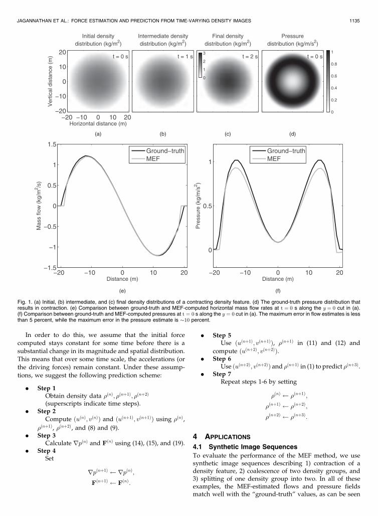
An example of the type of population density imageobtained using OAWRS is shown in Fig. 6, which shows alarge shoal of fish centered roughly 12 km south and 5 km eastof the source. This image was obtained on 14 May 2003, off thecoast of New Jersey during the OAWRS 2003 experiment [32].The shoal was observed for an entire day using OAWRS,which provided snapshots of population density every 50 s.We will apply MEF to the sequence of fish population densityimages in an area defined by the box in Fig. 6.

To compute force fields using (11) and (12), we assumethat individual fish behave like fluid particles so that theentire fish shoal (Fig. 6) behaves like an anisotropic,compressible fluid. This assumption is consistent withOAWRS observations of spatial and temporal variation of


Fig. 5. (a), (b), (c) Sequence of frames showing mitosis in a Xenopus laevis cell. Same colorscale as that in Fig. 4a. Cell boundary is marked by redcontours. The black box in (c) is the area zoomed in (d), (e). Note long fiber-like structures called microtubules. (d) Velocity field derived from densityimage pairs (a), (b). The vectors are shown every 10 pixels. (e) Net force density computed using velocity and density fields in (11) and (12).(f) Pressure field that gives rise to the force field in (e). Same colorscale as in Fig. 4b. Formation of two low apparent pressure regions at the oppositeends of the cell and a high apparent pressure region at the center of the cell is shown. Two regions of high microtubule density and the cell boundaryare shown as black contours.

population density, which showed that fish could convergeor diverge, making their motion highly compressible.Similar observations of fish schools behaving like an“animate fluid” [10] have been reported for small schoolsof a few meters in extent.

Under our continuum assumptions, the net force can bethought of as the result of a pressure field, with regions of lowpressure acting as centers of attraction and regions of highpressure acting as centers of repulsion. These pressures aredifferent from the hydrodynamic pressures related to theflow of water in the ocean. They are effective biologicalstresses that drive fish shoaling behavior.

4.4 Translation and Coalescence of Fish Groups

Here, we use the MEF and force-estimation techniques toquantify the rates at which fish groups within a large shoaltranslate and coalesce. We find that the rate of translation isconsistent with the swimming speeds of individual fish. Wealso find that coalescence of fish groups can occur due toformation of “attraction zones” or regions of low pressure.These phenomena are quantified by tracking the motion oftwo high population density regions, A and B, shown in Fig. 7.The MEF-estimated velocity vectors, shown in Fig. 8, describethe translation and coalescence of A and B, occurring at ratesof roughly 0.5-1 m/s. The merger of A and B can also be


Fig. 6. Large shoal of fish imaged off the New Jersey coast on 14 May2003 using OAWRS. The colorscale represents the areal density of thefish. The image resolution is 30 m/pixel. The bathymetric contours areshown using white dashed lines. The black dashed box is the area overwhich MEF and force-estimation techniques are applied to study thedynamics of the large shoal and is the area shown in Figs. 7 and 10.

Fig. 7. Fish population density image showing schools A and B beforemerger. Same colorscale as in Fig. 6. The original OAWRS densityimage has been smoothed such that the areal density at any point in theimage shown above, is the unweighted mean of the areal densities overa 120 m� 120 m square area centered at that point. The dashed boxrepresents the zoom area over which velocity vectors are shown inFig. 8. Black lines are 1:5 fish=m2 population density contours.

Fig. 8. (a) Flow vectors describing the merger of groups A (marked inred) and B (marked in blue). Blue and red lines represent the 1:5 fish=m2

population density contours. The gray line represents the 0:2 fish=m2

population density contour. (b) Flow field after the merger of A and B.The red line represents the 1:5 fish=m2 population density contour. Thegroups merge within a span of 3 minutes. The mass flow vectors areshown every 10 pixels or 300 m.

thought of as the result of a low pressure, “attraction zone”formed between the schools, as shown in Fig. 9.

The mean velocity of groups A and B can also be estimatedby tracking their centers of mass (COM) defined by

�XA ¼P

i2A �ixiPi2A �i

; �YA ¼P

i2A �iyiPi2A �i

; ð20Þ

�XB ¼P

i2B �ixiPi2B �i

; �YB ¼P

i2B �iyiPi2B �i

; ð21Þ

where i represents the pixel number. We find that group Amoves toward group B at roughly 1 m/s, which is

consistent with the velocities obtained using MEF (Fig. 8).These values are also consistent with the typical speeds atwhich individual fish swim [16], [24], [36].

4.5 Mass Exchange between Different Parts of aShoal

We now quantify fish flow rates between different parts ofthe large shoal shown in Fig. 6. In particular, we quantifythe rate of mass transfer between two wings of an hourglasspattern formed by the fish shoal, as shown in Fig. 10. Wefind that there is a steady depopulation of the southernwing and the fish “flow” into the northern wing, as can beseen from the sequence of images in Fig. 11. There is asteady flow of �300-450 fish/s across the neck of thehourglass connecting the two wings of the shoal. Thedepopulation episode can also be explained by the forma-tion of a high-pressure region near the neck of the hourglass(Fig. 12).

Hourglass patterns have been observed in smaller fishgroups spanning spatial scales on the order of a square km[42]. Mass transfers of the kind described above have beenknown to occur and have been shown in these smallgroupings. Flow from one part of the shoal to the other via


Fig. 9. Pressure (N=m2 per unit fish mass) distribution within large fishshoal showing formation of a low-pressure region that attracts schools Aand B. Black lines represent the 1:5 fish=m2 population density contours.The gray line represents the 0:2 fish=m2 population density contour.Same zoom area as Fig. 8.

Fig. 10. Fish density distribution showing hourglass type formation.Same colorscale as in Fig. 6. The southern shoal gets depopulated andthere is mass flow across the neck of the hourglass shown. The blackbox is the area zoomed in Figs. 11 and 12. The areal density has beensmoothed using the same algorithm as that employed in Fig. 7.

Fig. 11. Mass flow distribution frames showing depopulation of thesouthern wing over a span of 3 minutes. The area shown is zoomedaround the neck of the hourglass shown in Fig. 10. The flow rate offish normal (red arrow) to the neck (red solid line) is found to be� 300-450 fish/s. The flow vectors are shown every 5 pixels. The graylines are 0:2 fish=m2 density contours.

the “neck” usually signifies predatory pressure on one ofthe wings [42]. The depopulation described by the MEFcalculation could very well be in response to such apressure acting on the southern wing of the large shoaldescribed by the OAWRS density images.

5 PREDICTION USING FORCES: APPLICATION TO

SYNTHETIC IMAGES

Here we apply the prediction procedure shown in Section 3.3to density images in Fig. 1, where a circular feature undergoesuniform contraction.

In Fig. 1, we considered density images for t = 0, 1, and2 s, and computed the flow field and pressure field drivingcontraction. We now continue this contraction, and predictthe density distribution at times t = 3-7 s (Fig. 13).Comparison of our predicted densities with actual values(Fig. 13) shows a good match (errors < 10 percent) untilt = 7 s, after which the cumulative effect of errors becomeslarge and causes significant (errors > 10 percent) differencebetween predicted and actual densities.

In general, we expect our prediction scheme to work wellwithin some time interval for cases where the pressures andforces driving the flow remain more or less constant for thetime interval. This is indeed the case in many natural flowswhich follow environmental pressure gradients, such as themovement of clouds in the atmosphere driven by theformation of low and high-pressure regions.

6 CONCLUSIONS

We have presented methods for 1) estimating forces thatdrive motion observed in density image sequences and2) predicting flow and density evolution. To do this, wedeveloped a Minimum Energy Flow method for estimatingvelocity fields in both compressible and incompressibleflows. The MEF and force-estimation techniques have beendemonstrated with synthetic and experimentally obtainedimages. Using a density image sequence describing cellmitosis, we showed that cell division is driven by gradientsin apparent pressure in the cell. Using density image

sequences of fish shoals, we also quantified 1) coalescenceof fish groups over tens of kilometers, 2) fish mass flowbetween different parts of a large shoal, and 3) the stressesacting on large fish shoals.

The MEF and force estimation techniques can begenerally applied to any density image sequence wherepixel values can be modeled as proportional to the densityof a compressible fluid. In addition to the examplespresented here, such density image sequences are fre-quently encountered in biomedical imaging and satelliteimaging for meteorology and oceanography. MRI, forexample, provides tomography image sequences of bloodflow in arteries, which could be monitored using our MEFand force-estimation techniques. Satellite images of densitydistribution of water vapor (clouds), for example, can be


Fig. 13. Comparison of actual and predicted densities for different times.The same example as that in Fig. 1 is used. The curves are cuts throughy ¼ 0 in the actual and predicted density images. The prediction schemeworks well within some time interval when the forces remain more orless constant. After some time, the cumulative effect of errors becomeslarge and causes a significant (errors > 10 percent) difference betweenpredicted and actual densities.

Fig. 12. Pressure (N=m2 per unit fish mass) distribution within a largefish shoal showing formation of a high-pressure region near the “neck” ofan hourglass pattern, forcing fish mass flow from one wing to the other.The black lines are 0:2 fish=m2 density contours.

used to compute flow and force fields in the atmosphere

that drive meteorological processes. Other applications are

in studies of collective behavior, where the MEF and force-

estimation tools can be used to verify theoretical models

that predict average velocities and forces acting in large

animal groups.

APPENDIX A

COMPARISON OF MEF WITH THE METHOD PROPOSED

BY WILDES ET AL.

Here, we compare the performance of MEF and the method

proposed by Wildes et al. [56], in recovering motion

involving large changes in velocity over space. As mentioned

in Section 2, we expect the latter to “smooth out” large

variations and the former to preserve these variations. For

flows that involve small variations in velocity over space,

both of these methods are expected to perform equally well.In this section, we quantify the ability of both methods to

recover an idealization of a Karman vortex street [5], which

is a good example of a flow with large spatial gradients in

velocity, as illustrated in Fig. 14. Such a repeating pattern of

swirling vortices is caused by the unsteady separation of

flow of a fluid over bluff bodies [5]. Accurately quantifying

vortices is important in many fields such as medical

imaging of blood flow using MRI, where the presence of

vortices, for example, indicates blockages of arteries [44].

Here, we have idealized each vortex in Fig. 14 as a “Lamb-

Oseen vortex” [45], which models a line vortex that decays

due to viscosity. The tangential velocity of the vortex is

given as a function of radius r

V�ðrÞ ¼ V�;max

� �1þ 0:5

�

� �rcr

1� exp ��r2

r2c

� �� ; ðA-22Þ

where V�;max is the peak tangential velocity, � is a viscosity-

dependent constant, and rc is the core radius of the vortex.

In this example, we have chosen V�;max ¼ 1, � ¼ 1:26 [12],

and rc ¼ 10 for each vortex shown in Fig. 14.In the example we have chosen, the MEF technique

recovers the motion to within 10 percent accuracy except in

regions of very low velocity, as can be seen from Fig. 14.

This contrasts with the method proposed by Wildes et al.,

where errors are high (30-40 percent) even in regions of

high velocity (Fig. 14) and shows that the “unsmoothness of

flow” criterion chosen in [56] distorts the flow field in order

to make it vary more smoothly than in the actual flow.Corpetti et al. have employed a more complicated “div-

curl minimization” technique [9] to preserve vortices in the

flow field, rather than the Principle of Least Action used

here. They report errors on the order of 10 percent [9] when

recovering vortices in fluid flow, as we find here for the

simpler MEF approach.

APPENDIX B

DISCRETIZATION AND NUMERICAL IMPLEMENTATION

OF MEF

In order to solve (8) and (9) numerically on a discrete grid,

we employ a finite difference method to approximate the

partial derivatives.For this purpose, we use the following “computational

stencils”:

ð�uxxÞi;j ¼�ui;jþ1 � 2�ui;j þ �ui;j�1

�2; ðB-23Þ

ð�uxyÞi;j ¼�uiþ1;jþ1 � �ui�1;jþ1 � �uiþ1;j�1 þ �ui�1;j�1

4�2; ðB-24Þ

ð�vyyÞi;j ¼�viþ1;j � 2�vi;j þ �vi�1;j

�2; ðB-25Þ

ð�vxyÞi;j ¼�viþ1;jþ1 � �vi�1;jþ1 � �viþ1;j�1 þ �vi�1;j�1

4�2; ðB-26Þ

where the subscripts i and j are row and column indices,

respectively, and � is the grid interval.Replacing the spatial partial derivatives in (8) and (9)

with finite differences and grouping the terms in �ui;j and

�vi;j, we obtain

�

�i;jþ 2

�2

� ��ui;j ¼ ð�txÞi;j þ

�ui;j�1 þ �ui;jþ1

�2þ ð�vxyÞi;j; ðB-27Þ

�

�i;jþ 2

�2

� ��vi;j ¼ ð�tyÞi;j þ

�vi�1;j þ �viþ1;j

�2þ ð�uxyÞi;j: ðB-28Þ

Based on (B-27) and (B-28), we suggest an iterative

algorithm:


Fig. 14. Comparison of MEF and the method proposed in [56]. (Top)Ground-truth flow field—an idealization of a von-Karman vortex street.(Bottom left) Comparison between MEF-estimated (blue) and ground-truth mass flows in the zoom region shown in (Top). The vectors liealmost on top of each other and the maximum error is � 10 percent.(Bottom right) Comparison between flow vectors estimated using themethod proposed by Wildes et al. (blue arrows) and the ground-truthvectors (red arrows). There is significant error (� 30-40 percent) in theestimated vectors.

�

�i;jþ 2

�2

� ��uðnþ1Þi;j ¼ ð�txÞi;j þ

�uðnÞi;j�1 þ �u

ðnÞi;jþ1

�2þ ð�vxyÞðnÞi;j ;

ðB-29Þ

�

�i;jþ 2

�2

� ��vðnþ1Þi;j ¼ ð�tyÞi;j þ

�vðnÞi�1;j þ �v

ðnÞiþ1;j

�2þ ð�uxyÞðnÞi;j ; ðB-30Þ

where the superscripts ðnþ 1Þ and ðnÞ represent the

iteration numbers.

APPENDIX C

SOLVING FOR PRESSURE AND FORCE FIELD

In order to solve (14) and (15), we rewrite them as

ðf1Þyy ¼ gðx; y; tÞ þ ðf2Þxy; ðC-31Þðf2Þxx ¼ hðx; y; tÞ þ ðf1Þxy: ðC-32Þ

We now write the spatial derivatives of f1 and f2 at each

pixel ði; jÞ using finite differences as

ðf1Þyy

i;j¼ðf1Þiþ1;j þ ðf1Þi�1;j � ð2f1Þi;j

�2; ðC-33Þ

ðf1Þxy

i;j¼ðf1Þiþ1;jþ1 þ ðf1Þi�1;j�1 � ðf1Þiþ1;j�1 � ðf1Þi�1;jþ1

4�2;

ðC-34Þ

ðf2Þxx� �

i;j¼ðf2Þi;jþ1 þ ðf2Þi;j�1 � ð2f2Þi;j

�2; ðC-35Þ

ðf2Þxy

i;j¼ðf2Þiþ1;jþ1 þ ðf2Þi�1;j�1 � ðf2Þiþ1;j�1 � ðf2Þi�1;jþ1

4�2:

ðC-36Þ

Based on the above finite difference scheme, we suggest

the following iterative procedure:

ðf1Þðnþ1Þi;j ¼ y

�fðnÞ1 �

�2�gi;j þ ððf2ÞxyÞ

ðnÞi;j

�2

; ðC-37Þ

ðf2Þðnþ1Þi;j ¼ x

�fðnÞ2 �

�2�hi;j þ ððf1ÞxyÞ

ðnÞi;j

�2

; ðC-38Þ

where

y�f1 ¼

ðf1Þiþ1;j þ ðf1Þi�1;j

2; ðC-39Þ

x�f2 ¼

ðf2Þi;jþ1 þ ðf2Þi;j�1

2; ðC-40Þ

and n is the iteration number.Similarly, we rewrite (19) as

r2p ¼ lðx; y; tÞ ðC-41Þ

and

r2pi;j ¼ 4�pi;j � pi;j

�2; ðC-42Þ

where

�pi;j ¼piþ1;j þ pi�1;j þ pi;jþ1 þ pi;j�1

4: ðC-43Þ

We then suggest the following iterative procedure:

pðnþ1Þi;j ¼ �p

ðnÞi;j �

�2li;j4

; ðC-44Þ

where n is the iteration number.

APPENDIX D

COMPUTING GROUND TRUTH AND MEF VELOCITIES

AND PRESSURES FOR SYNTHETIC IMAGE SEQUENCES

The following algorithm is followed for computing the

ground truth flow field in Fig. 3:

. Step 1

Use �ð1Þ and �ð2Þ along with (8) and (9) to find

ð�uð1Þ; �vð1ÞÞ. We will assume this to be our ground-truth

flow, ð�uð1Þgt ; �vð1Þgt Þ. Superscripts indicate time steps.

. Step 2

Use �ð2Þ and �ð3Þ along with (8) and (9) to find

ð�uð2Þgt ; �vð2Þgt Þ.

. Step 3

Use (1), ð�uð1Þgt ; �vð1Þgt Þ, and �ð1Þ to compute ��ð2Þ.

Similarly, use ð�uð2Þgt ; �vð2Þgt Þ and ��ð2Þ to compute ��ð3Þ.

. Step 4

Compute MEF flow rates, ð�uð1ÞMEF; �vð1ÞMEFÞ and

ð�uð2ÞMEF; �vð2ÞMEFÞ, using density pairs ð�ð1Þ; ��ð2ÞÞ and

ð��ð2Þ; ��ð3ÞÞ, respectively, and (8) and (9).. Step 5

Use ð�uð1Þgt ; �vð1Þgt Þ and ð�uð2Þgt ; �v

ð2Þgt Þ in (11) and (12) to

compute the ground-truth pressure. Assume that

there is no external forcing.. Step 6

Use ð�uð1ÞMEF; �vð1ÞMEFÞ and ð�uð2ÞMEF; �v

ð2ÞMEFÞ in (11) and (12)

to compute the MEF pressure. Assume that there is

no external forcing.

ACKNOWLEDGMENTS

This research was supported by the US Office of Naval

Research, the Alfred P. Sloan Foundation, the US National

Oceanographic Partnership Program, and is a contribution

to the Census of Marine Life. The authors thank Margrit

Betke for her useful discussions and her suggestion to apply

MEF to the problem of cell division.

REFERENCES

[1] A. Amini, “A Scalar Function Formulation for Optical Flow,” Proc.European Conf. Computer Vision, pp. 125-131, 1994.

[2] P. Anandan, “A Computational Framework and an Algorithm forthe Measurement of Visual Motion,” Int’l J. Computer Vision, vol. 2,pp. 283-310, 1989.


[3] M. Andrews, Z. Gong, and P. Ratilal, “High Resolution Popula-tion Density Imaging of Random Scatterers with the MatchedFiltered Scattered Field Variance,” The J. Acoustical Soc. of Am.,vol. 126, no. 3, pp. 1057-1068, 2009.

[4] J. Barron, D. Fleet, and S. Beauchemin, “Performance of OpticalFlow Techniques,” Int’l J. Computer Vision, vol. 12, no. 1, pp. 43-77,1994.

[5] G.K. Batchelor, An Introduction to Fluid Dynamics. CambridgeUniv. Press, 1967.

[6] R. Battiti, E. Amaldi, and C. Koch, “Computing Optical Flowacross Multiple Scales: An Adaptive Coarse-to-Fine Strategy,” Int’lJ. Computer Vision, vol. 6, no. 2, pp. 133-145, June 1991.

[7] D. Bereziat, I. Herlin, and L. Younes, “A Generalized Optical FlowConstraint and Its Physical Interpretation,” Proc. IEEE Conf.Computer Vision and Pattern Recognition, vol. 2, pp. 487-492, 2000.

[8] D. Bereziat and J.-P. Berroir, “Motion Estimation on MeteorologicalInfrared Data Using a Total Brightness Invariance Hypothesis,”Environmental Modeling and Software, vol. 15, pp. 513-519, 2000.

[9] T. Corpetti, D. Heitz, G. Arroyo, E. Memin, and A. Santa-Cruz,“Fluid Experimental Flow Estimation Based on an Optical-FlowScheme,” Experiments in Fluids, vol. 40, pp. 80-97, 2006.

[10] I.D. Couzin and J. Krause, “Self-Organization and CollectiveBehavior in Vertebrates,” Advances in the Study of Behavior, vol. 32,pp. 1-75, 2003.

[11] G. Danuser and C.M. Waterman-Storer, “Quantitative FluorescentSpeckle Microscopy: Where It Came from and Where It Is Going,”J. Microscopy, vol. 211, pp. 191-207, Sept. 2003.

[12] W.J. Devenport, M.C. Rife, S.I. Liapis, and G.J. Follin, “TheStructure and Development of a Wing-Tip Vortex,” J. FluidMechanics, vol. 312, pp. 67-106, 1996.

[13] V. Devlaminck and J.-P. Dubus, “Estimation of Compressible orIncompressible Deformable Motions for Density Images,” Proc.Int’l Conf. Image Processing, vol. 1, pp. 125-128, Sept. 1996.

[14] L.G. Ekatarina, M.I. Maxim, I.A. Fazly, and J.R. McIntosh, “ForceProduction by Disassembling Microtubules,” Nature, vol. 438,pp. 384-388, 2005.

[15] W. Enkelmann, “Investigation of Multigrid Algorithms for theEstimation of Optical Flow Fields in Image Sequences,” ComputerVision, Graphics, and Image Processing, vol. 43, no. 2, pp. 150-177,Aug. 1988.

[16] D.M. Farmer, M.V. Trevorrow, and Q.B. Pederson, “IntermediateRange Fish Detection with a 12-kHz Sidescan Sonar,” TheJ. Acoustical Soc. of Am., vol. 106, pp. 2481-2490, 1999.

[17] J. Fitzpatrick, “A Method for Calculating Fluid Flow in TimeDependent Images Based on the Continuity Equation,” Proc. IEEEConf. Computer Vision and Pattern Recognition, pp. 78-81, 1985.

[18] D.J. Fleet and A.D. Jepson, “Computation of Component ImageVelocity from Local Phase Information,” Int’l J. Computer Vision,vol. 5, pp. 77-104, 1990.

[19] S. Freeman, “Cell Division,” Biological Science, Prentice Hall, 2002.[20] Z. Gong, M. Andrews, S. Jagannathan, R. Patel, J.M. Jech, N.C.

Makris, and P. Ratilal, “Low-Frequency Target Strength andAbundance of Shoaling Atlantic Herring (Clupea Harengus) in theGulf of Maine during the Ocean Acoustic Waveguide RemoteSensing 2006 Experiment,” The J. Acoustical Soc. of Am., vol. 127,pp. 104-123, 2010.

[21] T. Guerrero et al., “Dynamic Ventilation Imaging from Four-Dimensional Computed Tomography,” Physics in Medicine andBiology, vol. 51, no. 4, pp. 777-791, 2006.

[22] D.J. Heeger, “Optical Flow Using Spatiotemporal Filters,” Int’lJ. Computer Vision, vol. 1, pp. 279-302, 1988.

[23] B. Horn and B. Schunck, “Determining Optical Flow,” ArtificialIntelligence, vol. 17, pp. 185-203, 1981.

[24] I. Huse and E. Ona, “Tilt Angle Distribution and Swimming Speedof Overwintering Norwegian Spring Spawning Herring,” Int’lCouncil for the Exploration of the Sea J. Marine Science, vol. 53,pp. 863-873, 1996.

[25] S. Inoue and H. Sato, “Cell Motility by Labile Association ofMolecules: The Nature of Mitotic Spindle Fibers and Their Role inChromosome Movement,” The J. General Physiology, vol. 50,pp. 259-292, 1967.

[26] S. Inoue and E.D. Salmon, “Force Generation by MicrotubuleAssembly/Disassembly in Mitosis and Related Movements,”Molecular Biology of the Cell, vol. 6, no. 12, pp. 1619-1640, 1995.

[27] S. Jagannathan, I. Bertsatos, D. Symonds, H.T. Nia, A. Jain, M.Andrews, Z. Gong, R. Nero, L. Ngor, M. Jech, O.R. Godø, S. Lee, P.Ratilal, and N. Makris, “Ocean Acoustic Waveguide RemoteSensing (OAWRS) of Marine Ecosystems,” Marine Ecology ProgressSeries, vol. 395, 2009.

[28] K.E. Kasza, A.C. Rowat, J. Liu, T.E. Angelini, C.P. Brangwynne,G.H. Koenderink, and D.E. Weitz, “The Cell as a Material,”Current Opinion in Cell Biology, vol. 19, pp. 101-107, 2007.

[29] L.D. Landau and E.M. Lifshitz, Mechanics. Pergammon Press, 1976.[30] H. Lodish, A. Berk, P. Matsudaira, C.A. Kaiser, M. Krieger, M.P.

Scott, S.L. Zipursky, and J. Darnell, Molecular Cell Biology. Freemanand Company, 2004.

[31] B. Lucas and T. Kanade, “An Iterative Image RegistrationTechnique with an Application to Stereo Vision,” Proc. DefenseAdvanced Research Projects Agency Image Understanding Workshop,pp. 121-130, 1981.

[32] N.C. Makris, P. Ratilal, D. Symonds, S. Jagannathan, S. Lee, and R.Nero, “Fish Population and Behavior Revealed by InstantaneousContinental Shelf Scale Imaging,” Science, vol. 311, pp. 660-663,2006.

[33] N.C. Makris, P. Ratilal, S. Jagannathan, Z. Gong, M. Andrews, I.Bertsatos, O.R. Godø, R. Nero, and M. Jech, “Critical PopulationDensity Triggers Rapid Formation of Vast Oceanic Fish Shoals,”Science, vol. 323, no. 5922, pp. 1734-1737, 2009.

[34] P.L.M. de Maupertuis, “Accord de Diffrentes Lois de la NatureQui Avaient Jusqu’ici paru Incompatibles” Mm. As. Sc. Paris,p. 417, 1744.

[35] D. Metaxas and D. Terzopoulos, “Shape and Nonrigid Motion andStructure,” IEEE Trans. Pattern Analysis and Machine Intelligence,vol. 15, no. 6, pp. 580-591, June 1993.

[36] O.A. Misund, A. Ferno, T. Pitcher, and B. Totland, “TrackingHerring Schools with a High Resolution Sonar. Variations inHorizontal Area and Relative Echo Intensity,” Int’l Council for theExploration of the Sea J. Marine Science, vol. 55, pp. 58-66, 1998.

[37] H.-H. Nagel, “On the Estimation of Optical Flow: Relationsbetween Different Approaches and Some New Results,” ArtificalIntelligence, vol. 33, pp. 299-324, 1987.

[38] Y. Nakajima, H. Inomatad, H. Nogawab, Y. Satoa, S. Tamuraa, K.Okazakic, and S. Torii, “Physics-Based Flow Estimation of Fluids,”Pattern Recognition, vol. 36, no. 5, pp. 1203-1212, 2003.

[39] R. Ortega, G. Deves, and A. Carmona, “Bio-Metals Imaging andSpeciation in Cells Using Proton and Synchrotron RadiationX-Ray Microspectroscopy,” J. Royal Soc. Interface, vol. 6, pp. S649-S658, 2009.

[40] T. Potapova and G. Gorbsky, “Classic Mitosis in a VertebrateCell,” ASCB Image and Video Library, VID-31, http://cellimages.ascb.org/u?/p4041coll12,233, Aug. 2007.

[41] A. Pentland and B. Horowitz, “Recovery of Nonrigid Motion andStructure,” IEEE Trans. Pattern Analysis and Machine Intelligence,vol. 13, no. 7, pp. 730-742, July 1991.

[42] T.J. Pitcher and J. Parrish, The Behavior of Teleost Fishes, T. J. Pitcher,ed., pp. 363-439. Chapman and Hall, 1993.

[43] J.L. Prince, “Motion Estimation from Tagged MR Image Se-quences,” IEEE Trans. Medical Imaging, vol. 11, no. 2, pp. 238-249,June 1992.

[44] K. Rhode et al., “Validation of an Optical Flow Algorithm toMeasure Blood Flow Waveforms in Arteries Using DynamicDigital X-Ray Images,” Proc. SPIE Conf., p. 1414, 2000.

[45] P.G. Saffman, M.J. Ablowitz, E. Hinch, J.R. Ockendon, and P.J.Olver, Vortex Dynamics. Cambridge Univ. Press, 1992.

[46] J. Simpson and J. Gobat, “Robust Velocity Estimates, StreamFunctions and Simulated Lagrangian Drifters from SequentialSpacecraft Data,” IEEE Trans. Geosciences and Remote Sensing,vol. 32, no. 3, pp. 479-493, May 1994.

[47] A. Singh, “An Estimation-Theoretic Framework for Image FlowComputation,” Proc. Third IEEE Int’l Conf. Computer Vision,pp. 168-177, 1990.

[48] S.M. Song and R.M. Leahy, “Computation of 3D Velocity Fieldsfrom 3D Cine CT Images of a Human Heart,” IEEE Trans. MedicalImaging, vol. 10, no. 3, pp. 295-306, Sept. 1991.

[49] D. Suter, “Motion Estimation and Vector Splines,” Proc. IEEE CSConf. Computer Vision and Pattern Recognition, pp. 939-942, June1994.

[50] D. Terzopoulos and K. Waters, “Analysis and Synthesis of FacialImage Sequences Using Physical and Anatomical Processes,” IEEETrans. Pattern Analysis and Machine Intelligence, vol. 15, no. 6,pp. 569-579, June 1993.


[51] J. Toner and Y. Tu, “Long-Range Order in a Two-DimensionalDynamical XY Model: How Birds Fly Together,” Physical Rev.Letters, vol. 75, no. 23, pp. 4326-4329, 1995.

[52] J. Toner and Y. Tu, “Flocks, Herds, and Schools: A QuantitativeTheory of Flocking,” Physical Rev. E, vol. 58, pp. 4828-4858, 1998.

[53] S. Uras, F. Girosi, A. Verri, and V. Torre, “A ComputationalApproach to Motion Perception,” Biological Cybernetics, vol. 60,pp. 79-87, 1988.

[54] A. Vlasenko and C. Schnorr, “Variational Approaches to ImageFluid Flow Estimation with Physical Priors” Imaging MeasurementMethods for Flow Analysis, pp. 247-256, Springer, 2009.

[55] A.M. Waxman, J. Wu, and F. Bergholm, “Convected ActivationProfiles and Receptive Fields for Real Time Measurement of ShortRange Visual Motion,” Proc. IEEE Conf. Computer Vision andPattern Recognition, pp. 723-771, 1988.

[56] R.P. Wildes et al. “Recovering Estimates of Fluid Flow from ImageSequence Data,” Computer Vision and Image Understanding, vol. 80,pp. 246-266, 2000.

Srinivasan Jagannathan received the BTechdegree in ocean engineering from the IndianInstitute of Technology (IIT) Madras, India, in2004. Currently, he is working toward the PhDdegree in mechanical engineering at the Mas-sachusetts Institute of Technology (MIT). He is aresearch assistant at the Laboratory for Under-sea Remote Sensing at MIT. He is the recipientof the US Office of Naval Research GraduateFellowship in Underwater Acoustics.

Berthold Klaus Paul Horn received theBScEng degree from the University of theWitwatersrand in 1965, and the SM and PhDdegrees from the Massachusetts Institute ofTechnology (MIT) in 1968 and 1970, respec-tively. He is a professor of electrical engineeringand computer science at MIT. He is the author orcoauthor of three books on machine vision andprogramming. He was awarded the Rank Prizefor pioneering work leading to practical vision

systems in 1989 and was elected a fellow of the American Association ofArtificial Intelligence in 1990. He was elected to the National Academy ofEngineering in 2002.

Purnima Ratilal received the PhD degree inacoustics from the Massachusetts Institute ofTechnology (MIT) in 2002. She is an associateprofessor of electrical and computer engineeringat Northeastern University, Boston. She waspreviously a postdoctoral associate in theDepartment of Ocean Engineering at MIT(2002-2004) and a research scientist atSingapore’s DSO National Laboratories (1994-1998). She has extensive experimental and

theoretical experience in remote sensing with acoustics and ultrasonics.She was awarded the US Office of Naval Research (ONR) PostdoctoralAward in Ocean Acoustics in 2002, the Bruce Lindsay Award by theAcoustical Society of America in 2006, the ONR Young InvestigatorAward in 2007, and the Presidential Early Career Award for Scientistsand Engineers in 2008.

Nicholas Constantine Makris is a professor atthe Massachusetts Institute of Technology. Formore information, see http:// acoustics.mit.edu/faculty/makris/makris.html.

. For more information on this or any other computing topic,please visit our Digital Library at www.computer.org/publications/dlib.


Documents

Force Estimation and Prediction from Time-Varying Density Images