FREE MOTION OF INITIALLY BOX-LIKE WAVEPACKETS

FREE MOTION OF INITIALLY BOX-LIKEWAVEPACKETS

with special reference to the rate at which they disperse

Nicholas Wheeler, Reed College Physics Department

September 2003

Introduction. That the initially Gaussian wavefunction

ψ(x, 0) =[

1σ√

2π

] 12

exp{− 1

4

[xσ

]2} (1)

when allowed to evolve by action of the free particle Hamiltonian

H = 12mp2

becomes progressively less compact is a fact of which students of quantummechanics are very soon made aware.1 Students are encouraged to think

1 See, for example, Problems 2.22 & 2.40 which appear on pages 50 & 69 ofDavid Griffiths’ Introduction to Quantum Mechanics (). While Schrodingerhimself was certainly well aware of this “characteristic feature of the quantumtheory,” the evidence is circumstantial, for examination of his early papers(English translations of which can be found in his Collected Papers on WaveMechanics, the augmented 3rd edition of which was published by Chelsea in) reveals that in those papers Schrodinger treated the hydrogen atom,the oscillator, the rotor, the perturbed atom . . .but avoided the free particle—perhaps because it is in some respects pathological (the energy/momentumeigenstates are not normalizable), but more probably because he was anxious todemonstrate that his new theory had things to say about experimental realities,and people tend not to experiment with free particles. However, near the end ofhis 3rd quantum mechanical paper (“The continuous transition from micro- tomacro-mechanics,” ) he points out how remarkable it is that the Gaussianstate (1), when allowed to evolve by action of the oscillator Hamiltonian

H = 12mp2 + 1

2mω2 x2

is periodically recurrent . . .which is to say: does not disperse.

2 Free motion of initially box-like wavepackets

that this analytically-neat property of Gaussian wavepackets is typical ofwavepackets-in-general . . . and in many respects it is. My objective here willbe to discuss an instance and a sense in which it isn’t.

More specifically, I will discuss properties of the initially box-likewavepacket

ψ(x, 0) =

0 : x < −b1√2b

: −b < x < +b

0 : x > +b

(2)

My interest in such packets derives from the coincidental confluence of twocircumstances:

• a conversation with David Griffiths (late August, ), whose effort toprepare a 2nd edition of his text1 had exposed a certain computationaldifficulty, and

• the realization, while pondering potential thesis topics, that I had yet toestablish the sense in which—by my intuition (and Einstein’s)—Griffiths’initial state (2) describes the universal end-state of all particle-in-a-boxsystems, whatever might have been the initial state.

The latter issue will be reserved for a companion essay.

1. Gaussian preliminaries. The dynamical evolution of any initial wavepacketcan, in principle, be described

ψ(x, t) =∫

K(x, t; y, 0)ψ(y, 0) dy (3)

where in the case H = 12mp2 the propagator becomes

K(x, t; y, 0) =√

mi 2π� t

exp{i�

(x− y)2

t

}

which can be looked upon as the solution of{(�2/2m)∂2

x+i�∂t

}K(x, t; •, •) = 0

that evolves in time t from the idealized wavepacket δ(x− y):

limt↓0

K(x, t; y, 0) = δ(x− y)

Introducing (1) into (3) we compute

ψ(x, t) =[

1σ[1 + (t/τ)]

√2π

]12

exp{− 1

4x2

σ2[1 + i(t/τ)]

}(4)

whereτ ≡ 2mσ2/� (5)

The (complex-valued) function (4) goes smoothly over to the (real-valued)

Gaussian preliminaries 3

function (1) as t ↓ 0, and it supplies

P (x, t) ≡ |ψ(x, t)|2 = 1σ(t)

√2π

exp{− 1

2

[x

σ(t)

]2}

(6)

σ(t) ≡ σ√

1 + (t/τ)2 (7)

Looking to the moving moments to which the normal distribution (6) givesrise, we note that because P (x, t) is, for all t, and even function of x it isimmediate that

〈xodd〉t =∫ +∞

−∞xoddP (x, t) dx = 0

while by calculation〈x0〉t = 1

〈x2〉t = 1 · [σ(t)]2

〈x4〉t = 1 · 3 · [σ(t)]4

〈x6〉t = 1 · 3 · 5 · [σ(t)]6

〈x8〉t = 1 · 3 · 5 · 7 · [σ(t)]8

...

A standard measure of the instantaneous “width” or “degree of localization”of the moving distribution is provided by the “uncertainty” or “variance” or“rms ≡

√centered second moment ”

[∆x]t ≡√

〈(x − 〈x〉t)2〉t =√〈x2〉t − 〈x〉2t

=√

[σ(t)]2 − 02 = σ(t) (8)

In (8) we see the analytical source of the familiar claim that if ψ(x, 0) isGaussian, and refers to the initial state of a free particle, then

[∆x]t grows hyperbolically : [∆x]t = σ√

1 + (t/τ)2 (9)

An identical statement is readily shown to pertain to “launched” Gaussiansthat are initially centered at points arbitrarily distant from the origin.2 Lessfamiliar is the claim that (9) pertains also to many/most non-Gaussian initialstates. Our main concern here will be with a simple initial state that provides,however, a vivid exception to the rule.

2 Mathematica stands ready to verify all the computational details that Ihave omitted in the preceding discussion. Those and many related details aredeveloped in “Gaussian wavepackets” ().


1. Quantum mechanics as a theory of interactive moments. I have describedelsewhere3 the sense in which quantum mechanics can be looked upon as a“theory of interactive moments.” Within that formalism it becomes the businessof the Hamiltonian operator to set the system-specific design of the (generallyinfinite) set of coupled “moment equations” that lie at the analytic heart of thetheory. I have shown in particular that in the case H = 1

2mp2 one has

ddt 〈p〉 = 0ddt 〈x〉 = 1

m 〈p〉

ddt 〈p

2〉 = 0ddt 〈xp + px〉 = 2

m 〈p2〉ddt 〈x

2〉 = 1m 〈xp + px〉

...

(10)

These equations are readily integrated, and give

〈p〉t = 〈p〉0〈x〉t = 〈x〉0 + 1

m 〈p〉0t

〈p2〉t = 〈p2〉0〈xp + px〉t = 〈xp + px〉0 + 2

m 〈p2〉0t〈x2〉t = 〈x2〉0 + 1

m 〈xp + px〉0t + 1m2 〈p2〉0t2

...

(11)

from which it follows in particular that

[∆x]2t =[〈x2〉0 + 1

m 〈xp + px〉0t + 1m2 〈p2〉0t2

]−

[〈x〉0 + 1

m 〈p〉0t]2

is always a quadratic function of t, can always be written

= σ20

[1 +

(t−t0

τ

)2]

(12.1)

with

σ20 =

[〈x2〉0 − 〈x〉20

]−

[〈xp + px〉0 − 2〈x〉0〈p〉0

]24[〈p2〉0 − 〈p〉20

]σ2

0/τ2 =

〈p2〉0 − 〈p〉20m2

t0 =2〈x〉0〈p〉0 − 〈xp + px〉0

2[〈p2〉0 − 〈p〉20

]

(12.2)

3 See Advanced Quantum Topics (), Chapter 2 (“Weyl Transform & thePhase Space Formalism”), pages 51–60.

Theory of interactive moments 5

To make use of this information we must possess evaluations of the initialmoments 〈x〉0, 〈x2〉0, 〈p〉0, 〈xp + px〉0 and 〈p2〉0 .4 We have already remarkedthat if ψ(x, 0) is even (symmetric about the point x = 0) then transparently

〈xodd〉0 = 0

Equally transparent is the fact that if ψ(x, 0) is real-valued—as are both theinitial Gaussian (1) and the initial box packet (2)—then5

〈podd〉0 = 0

Real-valuedness, by that same argument, entails

〈xp + px〉0 = 0

The implication is that if ψ(x, 0) is simultaneously even and real-valued then(11) simplifies radically: under such circumstances we have

σ20 = 〈x2〉0

σ20/τ

2 =〈p2〉0m2

=⇒ τ =√

m2〈x2〉0/〈p2〉0t0 = 0

giving

[∆x]2t = 〈x2〉0{

1 + t2

m2〈x2〉0/〈p2〉0

}(13)

4 The full -blown “theory of interactive moments” identifies the higher-ordercompanions of the mixed construction 1

2 (xp + px), but in those we have noimmediate interest.

5 To establish the point it is sufficient to write

〈podd〉0 =∫

ψ(x, 0)(

�

i∂∂x

)oddψ(x, 0) dx

and to observe that the expression on the left is, by self-adjointness, necessarilyreal, while the expression on the right is manifestly imaginary. If follows, bythe way, that if we would “launch” ψ(x, 0) with velocity v ≡ p/m then we mustcomplexify the wavefunction: specifically, we must send

ψ(x, 0) �−→ ψlaunched(x, 0) ≡ ei�

px· ψ(x, 0)

That done, we by quick argument obtain

〈podd〉0 = (mv)odd

See again Griffiths’ Problem 2.40. An elaborate discussion can be found in §5of “Gaussian wavepackets” ().


Look back again, in the light of this result, to the Gaussian case (1). Wehave already established that 〈x2〉0 = σ2, and by calculation have

〈p2〉0 = (�/2σ)2

so in instance of (13) obtain

[∆x]2t = σ2{

1 + (t/τ)2}

τ =√

m2σ2/(�/2σ)2 = 2mσ2/�

This is precisely the statement encountered already at (9), but obtained nowas the Gaussian instance of a much more general “law of hyperbolic dispersal.”

2. Theory of interactive moments applied to the box-packet. Working from (2)we find

〈xn〉0 =bn + (−b)n

2(n + 1)=

0 : n = 1, 3, 5, . . .

1n+1b

n : n = 0, 2, 4, . . .

so by (13)

[∆x]2t = 13b

2

{1 + t2

13m

2b2〈p2〉0

}(14)

and we confront the problem of evaluating 〈p2〉0. This might be attempted bythe following line of argument:

Let (2) be notated

ψ(x, 0) = 1√2b

{θ(x + b) − θ(x− b)

}(15)

where θ(x) refers to the Heaviside step function:

θ(x) ≡∫ x

−∞δ(y) dy =

{ 0 : x < 012 : x = 01 : x > 0

We note in passing that ψ(x, 0), thus described, is manifestly real (withconsequences spelled out on the preceding page) and that its evenness followsfrom the identity θ(−x) = 1 − θ(x). From (15) we are led to write

〈p2〉0 = 12b

(�

i

)2∫ {

θ(x + b) − θ(x− b)}{

θ′′(x + b) − θ

′′(x− b)

}dx

= − 12b�

2

∫ {θ(x + b) − θ(x− b)

}{δ

′(x + b) − δ

′(x− b)

}dx

which after an integration-by-parts becomes

= + 12b�

2

∫ {δ(x + b) − δ(x− b)

}{δ(x + b) − δ(x− b)

}dx

= + 12b�

2{δ(0) − δ(−2b) − δ(2b) + δ(0)

}= + 1

2b�2{∞− 0 − 0 + ∞

}= ∞ (16)

Formal application of the theory to box-packets 7

But is this result for real? Can we have confidence in conclusions drawn form anargument that culminates in naked δ -functions (δ -functions unprotected by theshade of an

∫-sign), that asks us to regard the Dirac distribution as function?

Perhaps not . . .but evidence that (16) is nevertheless correct as it stands isprovided by the fact that several alternative lines of argument lead to the sameconclusion. Most simply:

By Fourier transformation

ψ(x, 0) �−→ ϕ(p, 0) = 1√2π�

∫ +∞

−∞ψ(x, 0) e−

i�

px dx

= 1√2π�

∫ +b

−b

e−i�

px dx

=

√�/πb sin bp

�

p(17)

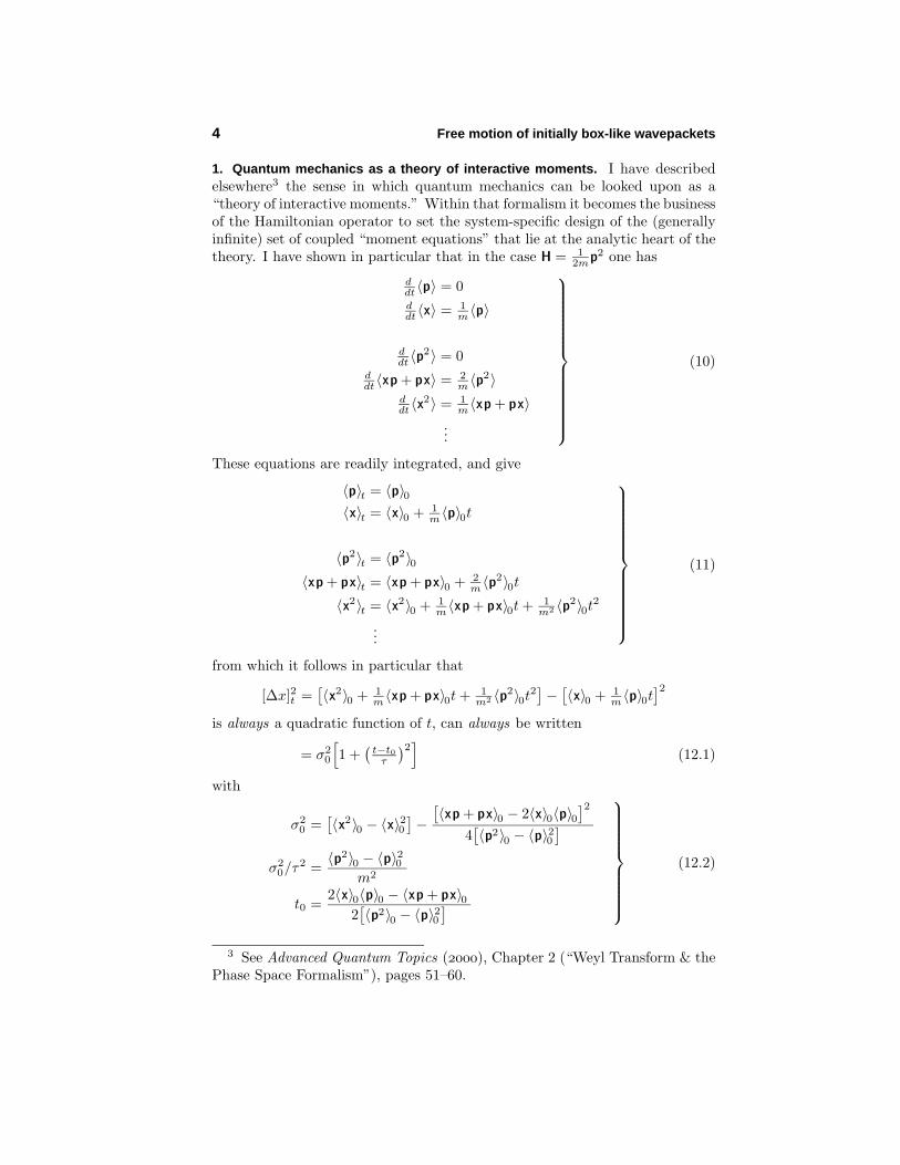
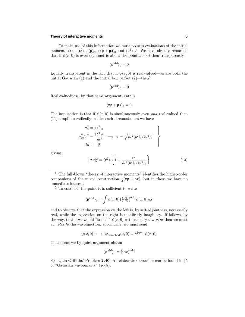
obtain the momentum representation of the box packet (2), which is the caseb = � = 1 is displayed in Figure 1b. From the obvious facts that ϕ(p, 0) isreal-valued and even (symmetric about p = 0) we recover

〈podd〉0 = limq↑∞

∫ +q

−q

ϕ(p, 0) podd ϕ(p, 0) dp = 0

while by calculation6

〈p2〉0 = limq↑∞

∫ +q

−q

ϕ(p, 0) p2 ϕ(p, 0) dp = limq↑∞

�

πb

{q − �

2b sin 2bq�

}= ∞

. . .which is (16) again.

Equation (14) has now become

[∆x]2t ={

13b

2 : t = 0∞ : t > 0

(18)

6 More generally one finds

〈pn〉0 = limq↑∞

∫ +q

−q

ϕ(p, 0) pn ϕ(p, 0) dp = ∞ : n = 2, 4, 6, . . .

but Mathematica seems to find it difficult to establish that

limq↑∞

∫ +q

−q

ϕ(p, 0) p0 ϕ(p, 0) dp = 1


-1 1

0.7

Figure 1a: Graph, based upon (15), of the initial boxpacket ψ(x, 0),in the case b = 1.

-15 -10 -5 5 10 15

0.5

Figure 1b: Fourier transform ϕ(p, 0) of the wavepacket shownabove, taken from (17) with b = � = 1

which is, I now argue, . . .

3. Strange . . . but by no means impossible. For the phenomenon encounteredat (18) is precisely reproduced by the following simple model. Let G(x ;σ)be Gaussian (or “normal”) and let L(x ; a) describe what physicists call a“Lorentzian” (and mathematicians call a “Cauchy”) distribution:7

G(x ;σ) = 1σ√

2πe−

12 (x/σ)2

L(x ; a) = 1aπ

11+(x/a)2

7 For review of the basic properties of Lorentzian distribution functions seepages 415–417 in Chapter 7 of principles of classical electrodynamics(/).

Strange . . . but by no means impossible 9

-3 -2 -1 1 2 3

1

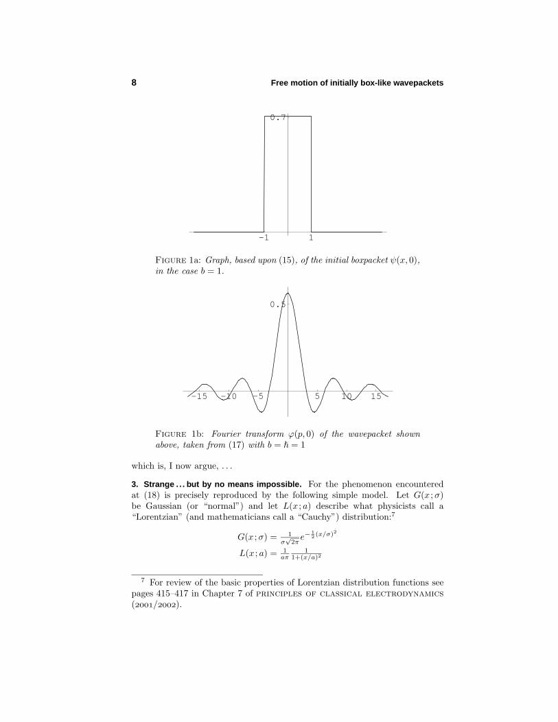
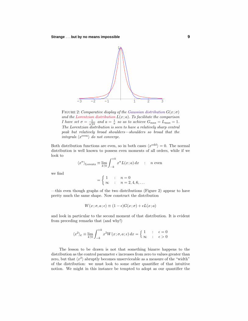
Figure 2: Comparative display of the Gaussian distribution G(x ;σ)and the Lorentzian distribution L(x ; a). To facilitate the comparisonI have set σ = 1√

2πand a = 1

π so as to achieve Gmax = Lmax = 1.The Lorentzian distribution is seen to have a relatively sharp centralpeak but relatively broad shoulders—shoulders so broad that theintegrals 〈xeven〉 do not converge.

Both distribution functions are even, so in both cases 〈xodd〉 = 0. The normaldistribution is well known to possess even moments of all orders, while if welook to

〈xn〉Lorentz ≡ limk↑0

∫ +k

−k

xnL(x ; a) dx : n even

we find

={

1 : n = 0∞ : n = 2, 4, 6, . . .

—this even though graphs of the two distributions (Figure 2) appear to havepretty much the same shape. Now construct the distribution

W (x ;σ, a ; ε) ≡ (1 − ε)G(x ;σ) + εL(x ; a)

and look in particular to the second moment of that distribution. It is evidentfrom preceding remarks that (and why!)

〈x2〉ε ≡ limk↑0

∫ +k

−k

x2W (x ;σ, a ; ε) dx ={ 1 : ε = 0∞ : ε > 0

The lesson to be drawn is not that something bizarre happens to thedistribution as the control parameter ε increases from zero to values greater thanzero, but that 〈x2〉 abruptly becomes unserviceable as a measure of the “width”of the distribution: we must look to some other quantifier of that intuitivenotion. We might in this instance be tempted to adopt as our quantifier the


distance between the points at which the distribution falls to half of its maximalvalue; i.e., where

W (x ;σ, a ; ε) = 12W (0;σ, a ; ε)

The problem is that, while those points would be easy to locate on a graph,they are not easy to describe analytically. The short of it: there appears to beno universally available natural descriptor of “distribution width.”

A physical problem has led us—at (18)—to a situation in which the mostcommon “width descriptor” happens to fail. Such a development is, in the lightof the preceding discussion, hardly an occasion for surprise, and certainly notan occasion for distress.

4. Motion of the probability density: first approach. The “theory of interactivemoments” to which I have alluded,3 and of which we have in fact been makinguse, proceeds from and lends weight to the proposition that if one were inposition to describe the motion of a certain infinite set of moments then onewould in effect possess all the physical information latent in the moving wavefunction ψ(x, t). We, however, are in position to describe the motion of only asmall handfull of low-order moments, which collectively are but a pale shadowof—and cast only a dim light upon—the motion of the wave function thatevolves from the ψbox(x, 0) described at (2), and again at (15). It was to discusscomputational problems latent in the construction of ψbox(x, t) that Griffithssought me out, and it is to consideration of those that I now turn.

In design H = 12mp2 of the free particle Hamiltonian is so exceptionally

simple that in the momentum representation the time-dependent Schrodingerequation becomes

12mp2ϕ(p, t) = i�∂tϕ(p, t)

which is an ordinary differential equation, of only first order. Its solution isimmediate8

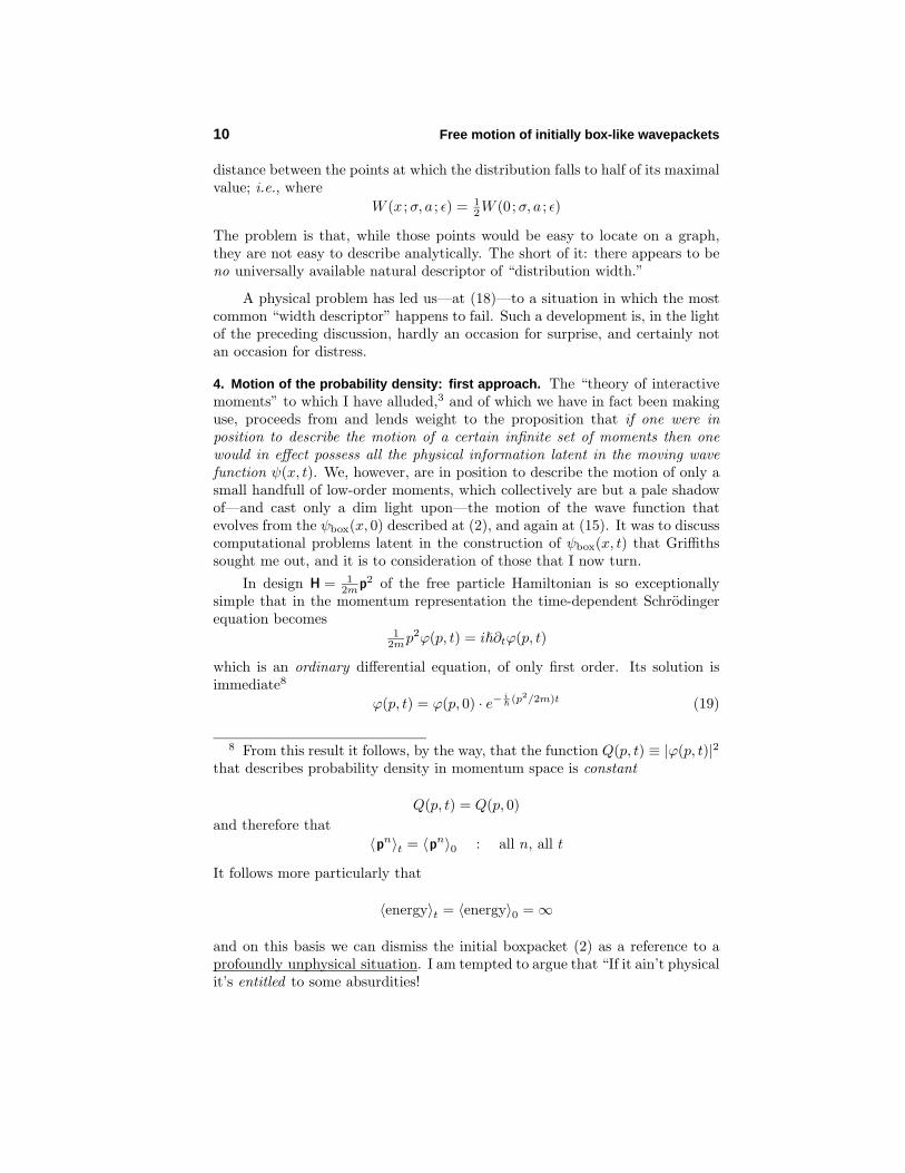
ϕ(p, t) = ϕ(p, 0) · e− i�(p2/2m)t (19)

8 From this result it follows, by the way, that the function Q(p, t) ≡ |ϕ(p, t)|2that describes probability density in momentum space is constant

Q(p, t) = Q(p, 0)and therefore that

〈pn〉t = 〈pn〉0 : all n, all t

It follows more particularly that

〈energy〉t = 〈energy〉0 = ∞

and on this basis we can dismiss the initial boxpacket (2) as a reference to aprofoundly unphysical situation. I am tempted to argue that “If it ain’t physicalit’s entitled to some absurdities!

Motion of the probability density: first approach. 11

and gives

ψ(x, t) = 1√2π�

∫ϕ(p, t) e

i�

px dp

= 1√2π�

∫ϕ(p, 0) e

i�[px−(p2/2m)t] dp (19)

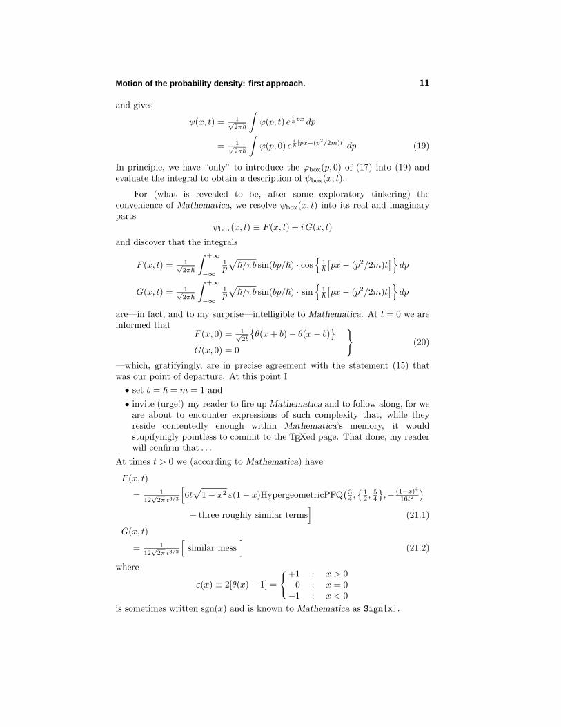
In principle, we have “only” to introduce the ϕbox(p, 0) of (17) into (19) andevaluate the integral to obtain a description of ψbox(x, t).

For (what is revealed to be, after some exploratory tinkering) theconvenience of Mathematica, we resolve ψbox(x, t) into its real and imaginaryparts

ψbox(x, t) ≡ F (x, t) + iG(x, t)

and discover that the integrals

F (x, t) = 1√2π�

∫ +∞

−∞1p√

�/πb sin(bp/�) · cos{

1�

[px− (p2/2m)t

]}dp

G(x, t) = 1√2π�

∫ +∞

−∞1p√

�/πb sin(bp/�) · sin{

1�

[px− (p2/2m)t

]}dp

are—in fact, and to my surprise—intelligible to Mathematica. At t = 0 we areinformed that

F (x, 0) = 1√2b

{θ(x + b) − θ(x− b)

}G(x, 0) = 0

}(20)

—which, gratifyingly, are in precise agreement with the statement (15) thatwas our point of departure. At this point I• set b = � = m = 1 and• invite (urge!) my reader to fire up Mathematica and to follow along, for we

are about to encounter expressions of such complexity that, while theyreside contentedly enough within Mathematica’s memory, it wouldstupifyingly pointless to commit to the TEXed page. That done, my readerwill confirm that . . .

At times t > 0 we (according to Mathematica) have

F (x, t)

= 112

√2π t3/2

[6t

√1 − x2 ε(1 − x)HypergeometricPFQ

(34 ,

{12 ,

54

},− (1−x)4

16t2

)+ three roughly similar terms

](21.1)

G(x, t)

= 112

√2π t3/2

[similar mess

](21.2)

where

ε(x) ≡ 2[θ(x) − 1] =

{+1 : x > 00 : x = 0

−1 : x < 0is sometimes written sgn(x) and is known to Mathematica as Sign[x].


One might expect F (x, t) + iG(x, t) to give back (20) at t = 0, butMathematica refuses to do so, claiming that it has encountered “indeterminateexpressions and complex singularities.” Look again to where t appears on theright side of (21) and such complaints will not seem implausible.

Our primary interest attaches not to F (x, t) and G(x, t) themselves, butto the probability density

P (x, t) ≡ |ψ(x, t)|2 = F 2(x, t) + G2(x, t)

constructed from them, with the aid of which we propose to study

〈 x2〉t =∫

x2P (x, t) dx

Mathematica appears not to mind that P (x, t) is a horrible (!) mess whenwritten out in detail, but again declines to speak of P (x, 0). . . for reasons upon

0.2 0.4 0.6 0.8 1

0.5

1

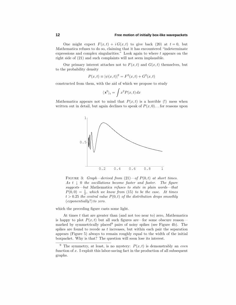
Figure 3: Graph—derived from (21)—of P (0, t) at short times.As t ↓ 0 the oscillations become faster and faster. The figuresuggests—but Mathematica refuses to state in plain words—thatP (0, 0) = 1

2 , which we know from (15) to be the case. At timest > 0.25 the central value P (0, t) of the distribution drops smoothly(exponentially?) to zero.

which the preceding figure casts some light.

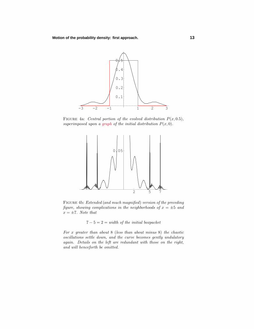
At times t that are greater than (and not too near to) zero, Mathematicais happy to plot P (x, t) but all such figures are—for some obscure reason—marked by symmetrically placed9 pairs of noisy spikes (see Figure 4b). Thespikes are found to recede as t increases, but within each pair the separationappears (Figure 5) always to remain roughly equal to the width of the initialboxpacket. Why is that? The question will soon lose its interest.

9 The symmetry, at least, is no mystery: P (x, t) is demonstrably an evenfunction of x. I exploit this labor-saving fact in the production of all subsequentgraphs.

Motion of the probability density: first approach. 13

-3 -2 -1 1 2 3

0.1

0.2

0.3

0.4

0.5

Figure 4a: Central portion of the evolved distribution P (x, 0.5),superimposed upon a graph of the initial distribution P (x, 0).

2 5 7

0.05

Figure 4b: Extended (and much magnified) version of the precedingfigure, showing complications in the neighborhoods of x = ±5 andx = ±7. Note that

7 − 5 = 2 = width of the initial boxpacket

For x greater than about 8 (less than about minus 8) the chaoticoscillations settle down, and the curve becomes gently undulatoryagain. Details on the left are redundant with those on the right,and will henceforth be omitted.


2 4 6 8 10 12

0.01

0.02

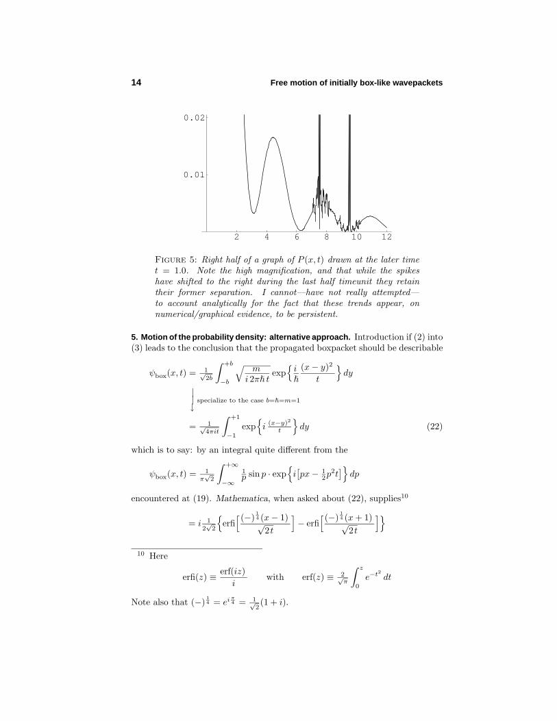
Figure 5: Right half of a graph of P (x, t) drawn at the later timet = 1.0. Note the high magnification, and that while the spikeshave shifted to the right during the last half timeunit they retaintheir former separation. I cannot—have not really attempted—to account analytically for the fact that these trends appear, onnumerical/graphical evidence, to be persistent.

5. Motion of the probability density: alternative approach. Introduction if (2) into(3) leads to the conclusion that the propagated boxpacket should be describable

ψbox(x, t) = 1√2b

∫ +b

−b

√m

i 2π� texp

{i�

(x− y)2

t

}dy

|| specialize to the case b=�=m=1↓

= 1√4πit

∫ +1

−1

exp{i (x−y)2

t

}dy (22)

which is to say: by an integral quite different from the

ψbox(x, t) = 1π√

2

∫ +∞

−∞1p sin p · exp

{i[px− 1

2p2t

]}dp

encountered at (19). Mathematica, when asked about (22), supplies10

= i 12√

2

{erfi

[ (−)14 (x− 1)√

2t

]− erfi

[ (−)14 (x + 1)√

2t

]}

10 Here

erfi(z) ≡ erf(iz)i

with erf(z) ≡ 2√π

∫ z

0

e−t2 dt

Note also that (−)14 = ei π

4 = 1√2(1 + i).

Motion of the probability density: alternative approach. 15

We now use the command ComplexExpand[%] to resolve this result into its realand imaginary parts. After assuring Mathematica that we understand t to bea positive real number we obtain

ψbox(x, t) = F (x, t) + iG(x, t)

where

F (x, t) = − 12√

2

{Im

(Erfi

[(−)

14 (x− 1)√

2t

])− Im

(Erfi

[(−)

14 (x + 1)√

2t

])}

G(x, t) = 12√

2

{Re

(Erfi

[(−)

14 (x− 1)√

2t

])− Re

(Erfi

[(−)

14 (x + 1)√

2t

])}

may look to us like paraphrases of the question, but are evidently understoodby Mathematica to be answers. The functions F and G should be identicalto the F and G encountered at (21) on page 11, but wear tildes to emphasizethat they have been assembled now not from HypergeometricPFQ functions butfrom the real and imaginary parts of the so-called “imaginary error function.”

Finally we ask Mathematica to construct (and to retain in its memory)

P (x, t) = F 2(x, t) + G2(x, t)

Possibly Euler himself, if presented with TEX’d renditions of P (x, t) and P (x, t),would recognize that they provide alternative descriptions of the same function,but I do not know off hand how to establish the point . . . except to remark thatif one uses P (x, t) to reconstruct the information displayed in (say) Figure 4aone finds—see Figure 6—that the agreement is precise. The important point isthat . . .

Mathematica appears to find it easier to work with P (x, t): see Figure 7,which Mathematica refused to draw when asked to work with P (x, t).

Experimental calculations such as the one that produced Figure 8 leadme to think that P (x, t) is “easier” to work with because computationallymore stable, and that the “regions of wild fluctuation” that have been seento bedevil work based upon P (x, t) are computational artifacts—not real. Itmust be possible to account for such artifacts, to explain why graphs of P (x, t)display spurious details, but as the explanation is unlikely to involve any pointof physical principle I will not pursue the matter.


2 4 6 8 10 12

0.01

0.02

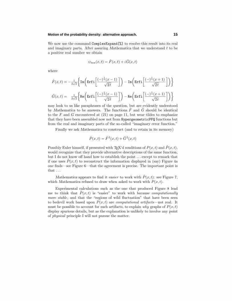
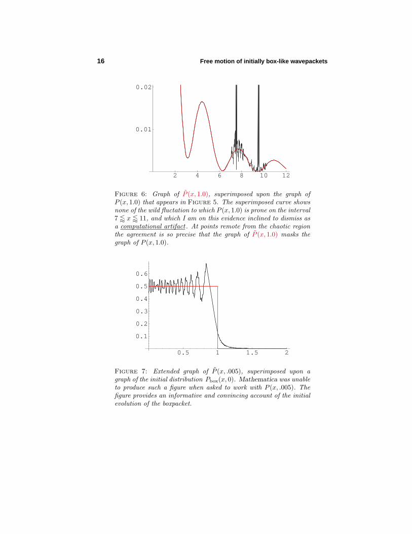
Figure 6: Graph of P (x, 1.0), superimposed upon the graph ofP (x, 1.0) that appears in Figure 5. The superimposed curve showsnone of the wild fluctation to which P (x, 1.0) is prone on the interval7 � x � 11, and which I am on this evidence inclined to dismiss asa computational artifact. At points remote from the chaotic regionthe agreement is so precise that the graph of P (x, 1.0) masks thegraph of P (x, 1.0).

0.5 1 1.5 2

0.1

0.2

0.3

0.4

0.5

0.6

Figure 7: Extended graph of P (x, .005), superimposed upon agraph of the initial distribution Pbox(x, 0). Mathematica was unableto produce such a figure when asked to work with P (x, .005). Thefigure provides an informative and convincing account of the initialevolution of the boxpacket.

New light on why the positional uncertainty explodes 17

6. Direct approach to the description of 〈x2〉t . It was by application of the“theory of interactive moments” that we were led—at (18)—to the conclusionthat ∆x grows “explosively.” We stand now in position to reproduce thatsomewhat surprising property of boxpackets by direct analysis, by an argumentthat proceeds without reference to the unfamiliar formalism just mentioned.

We work in a context where (because the packet was assumed to have beeninitially centered at the origin) 〈x〉t = 0, so we have [∆x ]t =

√〈x2〉t and it is

to the moving second moment

〈x2〉t = 2 ·

∫ ∞

0

x2P (x, t) dx, alternatively∫ ∞

0

x2P (x, t) dx

that we direct our computational attention.The distributions P (x, t) and P (x, t)are so complicated that the integration must be done numerically . . .whichrequires that we temper the ∞ upper limit: we study

limξ↑∞

∫ ξ

0

x2P (x, t) dx, alternatively

∫ ξ

0

x2P (x, t) dx

but discover that if ξ lies on the far side of the spikes then numerical evaluationof the first of those integrals is not feasible. Subsequent work will proceed,therefore, from the statement

〈x2〉t = 2 · limξ↑∞

NIntegrate[x2P (x, t),{x, 0, ξ

}] : t given & fixed

where P (x, t) is the tempered (spike-free) variant of P (x, t).

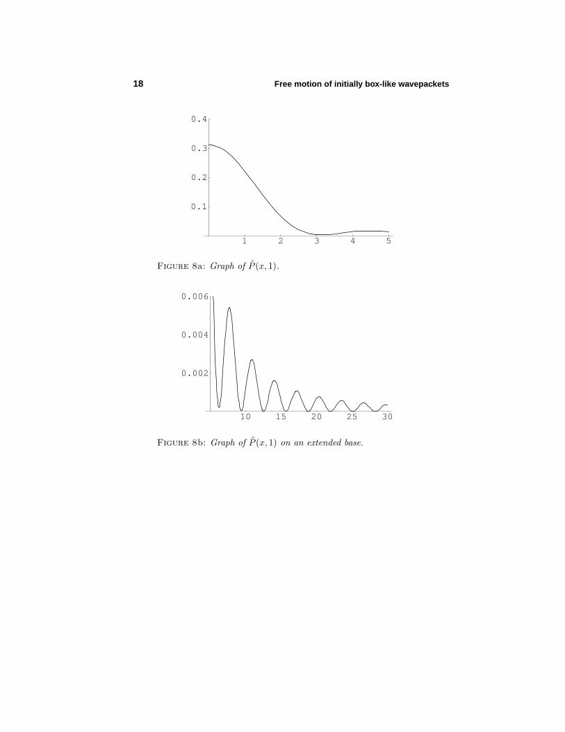
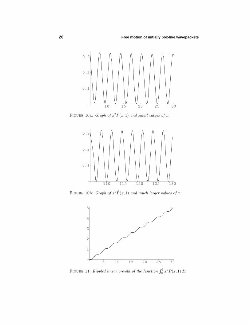
We remind ourselves that, on graphical evidence (Figures 8 & 9), P (x, t)is (for every t > 0) a function that oscillates to a rapid death. How rapid? Theevidence of Figures 10 strongly suggests that P (x, t) dies like x−2, that

x2P (x, t) oscillates with asymptotically constant amplitude and period

The structure of

w(ξ) ≡∫ ξ

0

x2P (x, t) dx

becomes in this light qualitatively obvious (see Figure 11), and we acquire freshinsight into why it is that

〈x2〉t = 2 · limξ↑∞

w(ξ) = ∞ (23)


1 2 3 4 5

0.1

0.2

0.3

0.4

Figure 8a: Graph of P (x, 1).

10 15 20 25 30

0.002

0.004

0.006

Figure 8b: Graph of P (x, 1) on an extended base.

New light on why the positional uncertainty explodes 19

101 102 103 104 105 106

0.00001

0.00002

0.00003

Figure 8c: Highly magnified graph of P (x, 1) at large x-values.

101 102 103 104 105 106

-0.004

-0.002

0.002

0.004

Figure 9a: Graph of F (x, 1), the real part of ψbox(x, 1), for thatsame set of x-values.

101 102 103 104 105 106

-0.004

-0.002

0.002

0.004

Figure 9b: Graph of G(x, 1), the imaginary part of ψbox(x, 1).It may seem remarkable that P (x, 1) = F 2(x, 1) + G2(x, 1) has thesimple form shown in Figure 8c.


10 15 20 25 30

0.1

0.2

0.3

Figure 10a: Graph of x2P (x, 1) and small values of x.

110 115 120 125 130

0.1

0.2

0.3

Figure 10b: Graph of x2P (x, 1) and much larger values of x.

5 10 15 20 25 30

1

2

3

4

5

Figure 11: Rippled linear growth of the function∫ ξ

0x2P (x, 1) dx.

Asymptotics 21

7. Asymptotic properties of the tempered probability density. Let the resultsreported on page 15 be abbreviated

F (x, t) = − 12√

2

{Im

(H(x− 1)

)− Im

(H(x+ 1)

)}

G(x, t) = 12√

2

{Re

(H(x− 1)

)− Re

(H(x+ 1)

)}

where11

H(x) ≡ erfi[(1 + i)x

2√t

]with erfi(z) ≡ 2√

π

∫ z

0

ey2dy

The command Series[Erfi[x],{x,∞,2}] supplies erfi(z) ∼ 1√πz e

z2, and if

we assume that result can be extended onto relevant sectors of the complexplane we find (with the assistance of ComplexExpand) that

H(x) ∼√t/π

{sin x2

2t + cos x2

2t

x+ i

sin x2

2t − cos x2

2t

x

}: x2/t� 1

giving

F (x, t) ∼ −√

18π t

{sin (x−1)2

2t − cos (x−1)2

2t

x− 1− sin (x+1)2

2t − cos (x+1)2

2t

x+ 1

}

G(x, t) ∼√

18π t

{sin (x−1)2

2t + cos (x−1)2

2t

x− 1− sin (x+1)2

2t + cos (x+1)2

2t

x+ 1

}

Looking with the assistance of Mathematica to the evaluation of

P (x, t) = F 2(x, t) + G2(x, t)

we Simplify, then use 1 + cos 2z = 2 cos2 z and 1 − cos 2z = 2 sin2 z to obtain

∼ 1π t

cos2(x/t) + x2 sin2(x/t)(x2 − 1)2

∼ 1π t

sin2(x/t)x2

(24)

Upon relaxation of the assumptions b = � = m = 1 we therefore expect (ondimensional grounds) to have

P (x, t) ∼ 1π

�

mb tsin2(mbx/�t)

x2: x2/t� �/m (25)

11 See again the preceding footnote. I have, by the way, found it naturalto adopt Mathematica’s conventions, which agree with those of Abramowitz &Stegun, Handbook of Mathematical Functions (), page 297 but differ by afactor by those encountered in Erdelyi, Higher Transcendental Functions (),§9.9, Volume 2, page 147.


10 15 20 25 30

0.002

0.004

0.006

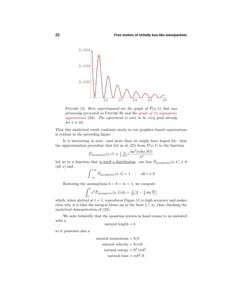
Figure 12: Here superimposed are the graph of P (x, 1) that waspreviously presented as Figure 8b and the graph of its asymptoticapproximant (24). The agreement is seen to be very good alreadyfor x ≈ 10.

That this analytical result conforms nicely to our graphics-based expectationsis evident in the preceding figure.

It is interesting to note—and more than we might have hoped for—thatthe approximation procedure that led us at (25) from P (x, t) to the function

Pasymptotic(x, t) ≡ 1π

�

mb tsin2(mbx/�t)

x2

led us to a function that is itself a distribution: one has Pasymptotic(x, t) � 0(all x) and ∫ +∞

−∞Pasymptotic(x, t) = 1 : all t � 0

Restoring the assumptions b = � = m = 1, we compute∫ ξ

0

x2Pasymptotic(x, t) dx = t2π

[ξ − 1

2 sin 2ξt

]which, when plotted at t = 1, reproduces Figure 11 to high accuracy and makesclear why it is that the integral blows up in the limit ξ ↑ ∞, thus clinching theanalytical demonstration of (23).

We note belatedly that the quantum system in hand comes to us endowedwith a

natural length = b

so it possesses also a

natural momentum = �/b

natural velocity = �/mb

natural energy = �2/mb2

natural time = mb2/�

Observations concerning Mathematica itself, in relation to this work 23

The statements

(natural length) · (natural momentum)= (natural energy) · (natural time)= �

are pretty but convey no real information: they are corollaries of the precedingdefinitions. It is, however, curious that a “natural energy” should attach to asystem that in point of idealized physical fact8 has infinite energy.

7. Things learned from and about Mathematica. The work summarizedhere could not have been accomplished without the major assistance ofMathematica, which in the instance meant Mathematica 4 running on my400 MHz PowerBook (Mac OS 9.1). But the work also taught me some thingsabout Mathematica . . . and, more particularly, about some of the differencesbetween Mathematica 4 and Mathematica 5. For as the work neared completionI was fortunate enough to acquire a PowerMac G5 (running OS 10.2 at1.6 GHz), on which I undertook to repeat some of my calculations, with curious—and ultimately quite informative—results.

It was a Mathematical quirk—still unexplained—that had originally sentGriffiths into my office: when he had attempted to evaluate the integral (19)he had been informed by Mathematica 5 (Mathematica 4 concurs) that

1√2π

∫ +∞

−∞

sin pp

ei[px−(p2/2)t] dp

=i{− log[−i(x− 1)] + log[i(x− 1)] + log[−i(x+ 1)] − log[i(x+ 1)]

}2√

2π

which—absurdly—is t-independent, and which upon simplification is found tobe also x-independent, to vanish identically! But when I resolved the complexexponential into its real and imaginary parts I was promptly led, at (21), tothe complicated functions F (x, t) and G(x, t) upon which the early part of thiswork is based.

Reconstruction of those functions was the very first calculation attemptedon my fancy new computer, with its improved software. I was distressedto discover that Mathematica 5 refused to do the integrals. I brought thisdisappointing development to the attention of Richard Crandall, Stan Wagonand (at Wagon’s suggestion) Michael Trott.12 Crandall made inquiries ofWolfram Research, and learned that “they do indeed have software problems not

12 Crandall (www.perfsci.com/) is the author of Mathematica for the Sciences() and of a great many other Mathematica -based publications. Wagon(www.stanwagon.com/) is the author of Mathematica in Action (2nd edition) and regularly conductsMathematica workshops. Michael Trott, a physicistturned computer graphics specialist at Wolfram Research, is well-established asa leading expert in the field.


yet ironed out,” and speculated that I had run afoul of one of those. Wagon wasable to replicate both my success and my failure, and to satisfy himself that theresults (21) reported by Mathematica 4 are indeed correct.13 He attributed myproblem to “subtle changes in some of the algorithms [necessitated by the factthat] some integrals and sums [as done] in version 4 were based on algorithmsthat were not entirely correct in the generality they were used.” Wagon reportedon the basis of his own direct experience that the adjustments made in version 5have had “an impact on some sums” and speculated that they may have hadan impact also on some symbolic integrals.

Wagon’s take on the situation conformed to my discovery (of which he wasunaware) that the results (21) supplied by version 4 appear to be susceptible tonumerical instabilities (see again the spikes and underbrush in Figures 4b & 5).

Trott, while granting that the situation I had encountered was “not nice,”considered that “such situations are basically unavoidable in developingcomplex software with millions of lines of code.” He reports that the peopleat Wolfram Research “run thousands of tests every night to make sure thatno capabilities or features are lost” but emphasizes that “the process is notfoolproof.” He interprets my experience to mean that I “found an examplethat did indeed get lost,” and reports that he has “sent your example to theIntegrate Developer, [who will] try to restore it for the next version.” I am leftto wonder (in view of the above-mentioned instability problem) whether theIntegrate Developer will report back to Trott that “We dropped that integralintentionally, because it was faulty.”

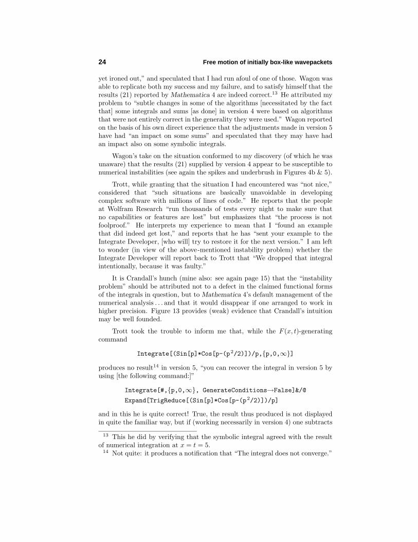
It is Crandall’s hunch (mine also: see again page 15) that the “instabilityproblem” should be attributed not to a defect in the claimed functional formsof the integrals in question, but to Mathematica 4’s default management of thenumerical analysis . . . and that it would disappear if one arranged to work inhigher precision. Figure 13 provides (weak) evidence that Crandall’s intuitionmay be well founded.

Trott took the trouble to inform me that, while the F (x, t)-generatingcommand

Integrate[(Sin[p]*Cos[p-(p2/2)])/p,{p,0,∞}]

produces no result14 in version 5, “you can recover the integral in version 5 byusing [the following command:]”

Integrate[#,{p,0,∞}, GenerateConditions→False]&/@

Expand[TrigReduce[(Sin[p]*Cos[p-(p2/2)])/p]

and in this he is quite correct! True, the result thus produced is not displayedin quite the familiar way, but if (working necessarily in version 4) one subtracts

13 This he did by verifying that the symbolic integral agreed with the resultof numerical integration at x = t = 5.

14 Not quite: it produces a notification that “The integral does not converge.”

Observations concerning Mathematica itself, in relation to this work 25

2 4 6 8 10 12

0.01

0.02

Figure 13: The function P (x, 1) was a creation of Mathematica 4,but has been plotted here by Mathematica 5. Comparison withFigure 5 (which was drawn by Mathematica 4) shows a greatreduction of “underbrush,” which—on the presumption that thenewer version has improved numerical analysis capabilities—mightbe interpreted as evidence that, as Richard Crandall has suggested,Mathematica 4 manages the integral correctly, but stumbles on thenumerical interpretation of its own symbolic result. Note, however,that the spikes persist.

the result of Trott’s command from the result of the original command andSimplifys one does get 0. The integral G(x, t) can be recovered similarly.At present I do not understand how Trott’s command manages to persuadeMathematica 5 to do what it had declared to be impossible.

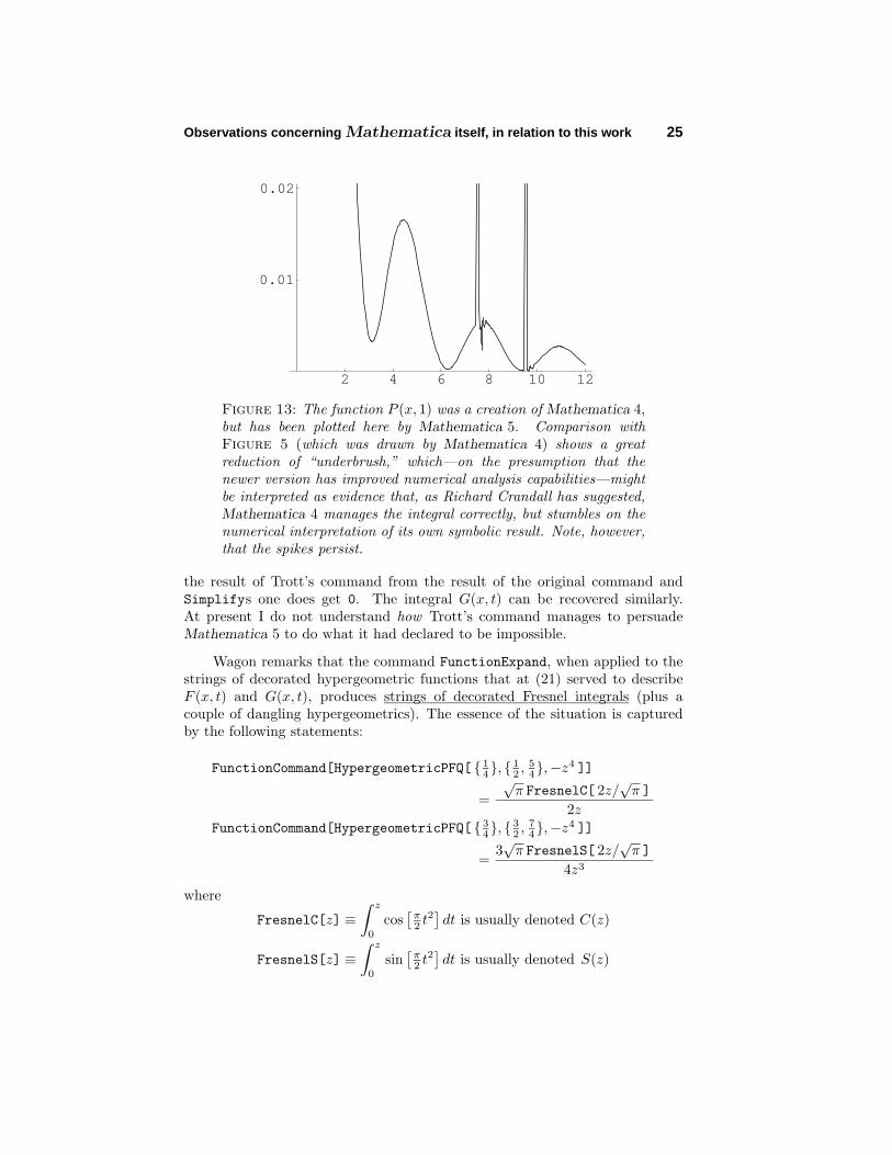
Wagon remarks that the command FunctionExpand, when applied to thestrings of decorated hypergeometric functions that at (21) served to describeF (x, t) and G(x, t), produces strings of decorated Fresnel integrals (plus acouple of dangling hypergeometrics). The essence of the situation is capturedby the following statements:

FunctionCommand[HypergeometricPFQ[ { 14}, { 1

2 ,54},−z4 ]]

=√π FresnelC[ 2z/

√π ]

2zFunctionCommand[HypergeometricPFQ[ { 3

4}, { 32 ,

74},−z4 ]]

=3√π FresnelS[ 2z/

√π ]

4z3

where

FresnelC[z] ≡∫ z

0

cos[

π2 t

2]dt is usually denoted C(z)

FresnelS[z] ≡∫ z

0

sin[

π2 t

2]dt is usually denoted S(z)


The Fresnel integrals are well known15 to be closely related to confluenthypergeometric functions on the one hand, and to the error function on theother, so—fine details aside!—we should perhaps not be surprised to find thatfunctions which by one line of argument came on page 11 to be described interms of hypergeometric functions have on page 15 come, by a different line ofargument, to be described in terms of error functions. But the devil lives in thedetails . . . for which at the moment I have no stomach.

One final remark: Marianne Colgrove, who serves at the office of Computing& Information Services as the college’s Mathematica contact person, hasapproached Wolfram Research on my behalf, and has been informed—this inresponse to my observation that version 5, even though running on a fastermachine, sometimes takes longer than version 4 to compute symbolic integrals16

—that Mathematica 5 presently exploits only a fraction of the G5’s resources.A 64-bit version is under development, but it is not yet possible to estimatewhen it will be ready for distribution.

15 See Abramowitz & Stegun’s Chapter 7, especially §7.3.16 Trott writes that, while my observation is accurate, it is easily explained:

version 5 routinely “tries many more transformations than version 4 did, andreturns much more exhaustive convergence conditions.”

Documents

FREE MOTION OF INITIALLY BOX-LIKE WAVEPACKETS