Fundamentals of Aircraft Aerodynamicsengineeringolympics.gatech.edu/sites/default/files/images/... · Dr. Dimitri N. Mavris, Director ASDL School of Aerospace Engineering Georgia

Dr. Dimitri N. Mavris, Director ASDL School of Aerospace Engineering Georgia Institute of Technology Atlanta, GA 30332-0150 [email protected]

Fundamentals of Aircraft Aerodynamics

Presented by:

Dr. Dimitri Mavris Director of Aerospace Systems Design Laboratory

Boeing Professor for Advanced Aerospace Systems Analysis

http://www.asdl.gatech.edu/



The Standard Atmosphere

Why do we need to know about the atmosphere?

The performance of aircraft, spacecraft, and their engines depend on the atmosphere in which they operate, primarily density and viscosity. Density and viscosity, in turn, are functions of altitude.

Density, ρ, varies with pressure, p, and temperature, T Viscosity, µ, varies only with temperature, T

The “standard atmosphere” is defined from the equation of state of a perfect gas:

p = ρ RT Perfect Gas Law




The Standard Atmosphere

Remember:

R = F + 459.7 K = C + 273.15

For our purposes, the atmosphere can be regarded as a homogenous gas of uniform composition that satisfies the perfect gas law.

p = pressure in lb/ft2 or N/m2 ρ = density in slugs/ft3 or kg/m3 T = absolute temperature in Rankine (R) or Kelvin (K) R = gas constant = 1718 ft-lb/slugsR or 287.05 N-m/kgK




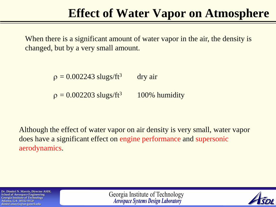
Effect of Water Vapor on Atmosphere

When there is a significant amount of water vapor in the air, the density is changed, but by a very small amount.

ρ = 0.002243 slugs/ft3 dry air ρ = 0.002203 slugs/ft3 100% humidity

Although the effect of water vapor on air density is very small, water vapor does have a significant effect on engine performance and supersonic aerodynamics.




International Standard Atmosphere

To allow for comparison of the performance of airplanes, as well as calibration of altimeters, “standard” properties of the atmosphere have been established by the International Civil Aviation Organization (ICAO). The ICAO and the U.S. Standard Atmosphere are identical below 65,617 feet. This standard atmosphere is representative of mid latitudes of the northern hemisphere.

“Standard” sea level properties are:

g0 = 32.17 ft/s2 = 9.806 m/s2 P0 = 29.92 in Hg = 2116.2 lb/ft2 = 1.013 x 105 N/m2 T0 = 59 F = 518.7 R = 15 C = 288.2 K ρ0 = 0.002377 slugs/ft3 = 1.225 Kg/m3




Regions of the Atmosphere Exosphere-rarefied

Ionosphere Positive Temperature Gradient

Stratosphere Zero Temperature Gradient

Troposphere Negative Temperature Gradient

Tropopause ( 36,089 ft)

300 ~ 600 mi

50 ~ 70 mi

5 ~ 10 mi

In airplane aerodynamics, only the troposphere and stratosphere are important.




Temperature Variation with Altitude

Below 36,089 ft, we assume there is a constant drop of temperature from sea level to altitude

T = T1 + a ( h - h1)

a = “lapse rate” = -0.00356616 F/ft in the standard atmosphere T1 and h1 are reference temperatures. For sea level, T1 = T0 and h1 = 0

Above 36,089 ft in the stratosphere, the standard temperature is assumed constant and equal to -69.7 F.




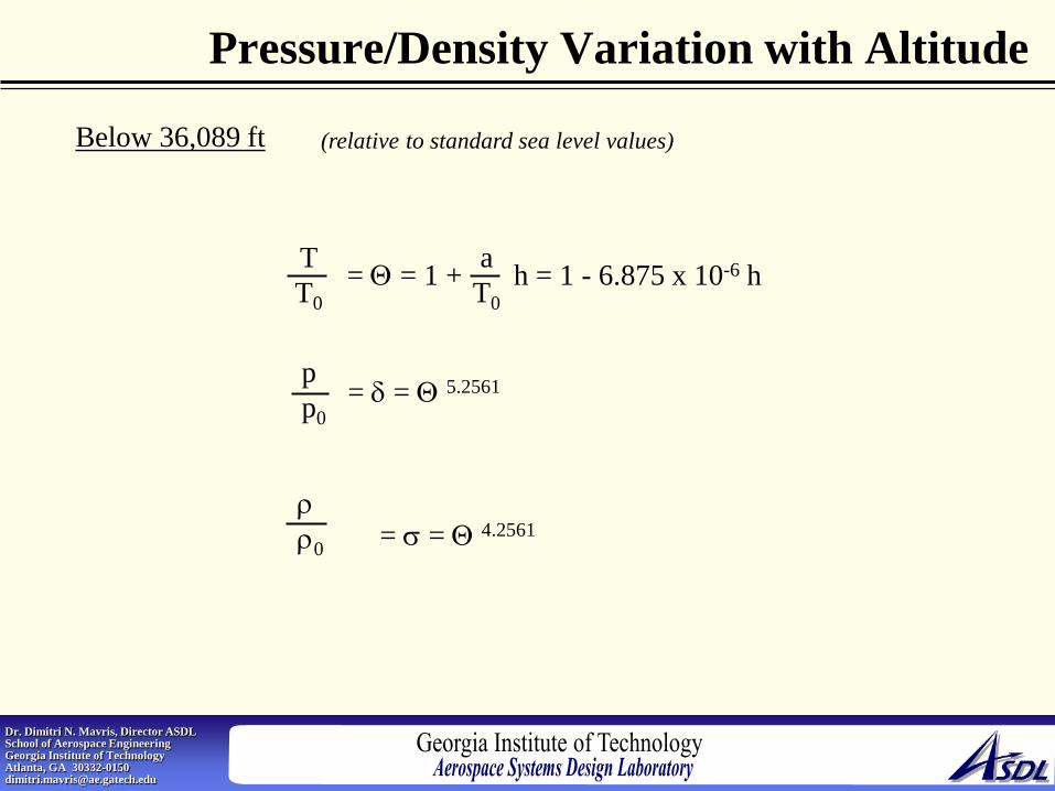
Pressure/Density Variation with Altitude

Below 36,089 ft (relative to standard sea level values)

T T0

= Θ = 1 + h = 1 - 6.875 x 10-6 h a T0

p p0

= δ = Θ 5.2561

ρ ρ0 = σ = Θ 4.2561




Pressure/Density Variation with Altitude

p p0

ρ ρ0

= 0.2234 exp

h-36,089 20806.7

= 0.2971 exp

Above 36,089 ft (relative to standard sea level values)

h-36,089 20806.7

T = constant = -69.7 F




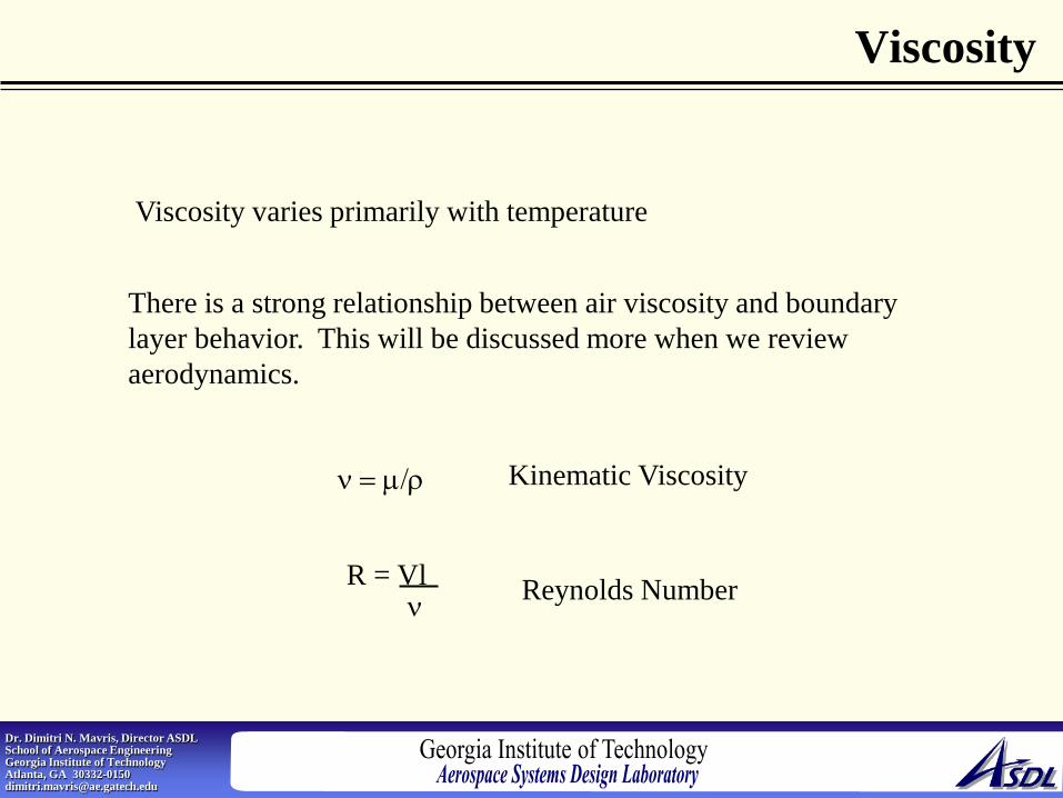
Viscosity

Viscosity varies primarily with temperature

There is a strong relationship between air viscosity and boundary layer behavior. This will be discussed more when we review aerodynamics.

Kinematic Viscosity ν = µ/ρ

R = Vl ν Reynolds Number




Types of Airspeeds

Indicated Airspeed (IAS) - is the direct reading from the airspeed indicator. This represents the airplane’s speed through the air, NOT necessarily its speed across the ground. Calibrated Airspeed (CAS) - is the indicated airspeed corrected for instrument position and instrument error. This is a function of each unique aircraft and the position of its pitot tube. There is no direct reading of CAS in the cockpit! The pilot must refer to the Pilot’s Operating Handbook for a table corresponding to that particular aircraft. True Airspeed (TAS) - because an airspeed indicator is calibrated for standard sea level conditions, when the airplane is flying at altitude, the airspeed is not correctly reflected. The amount of error is a function of temperature and altitude. TAS can be approximated by increasing the indicated airspeed by 2% per thousand feet of altitude.




Fundamentals of Aircraft Aerodynamics




The Anatomy of the Airplane




Introduction to Performance

Flight Mechanics is the study of the motions of bodies (aircraft and rockets), through a fluid.

Stability and Control Aerodynamic Performance

the science of designing for steady and controllable flight characteristics

speed rate of climb range fuel consumption maneuverability runway length requirements




Aircraft Performance

Aircraft performance is defined as how the aircraft responds (its motion) to the four forces of flight. It is considered to be a branch of the Flight Mechanics discipline. Performance is obtained once the aircraft weight and its aerodynamic and propulsion characteristics are defined. We use the following information in performance:

aerodynamics propulsion

drag polar, lift coefficient thrust or power, SFC




The Four Forces of Flight

V

always in the direction of the local flight of the aircraft. Shows flow velocity relative to the airplane

L

W

perpendicular to by definition

V

always acts towards the center of the earth

T

D parallel to by definition

V

ε

not necessarily in the flight direction

Lift, Drag, Weight, Thrust Lift and Drag are for complete airplane

Steady, Level Flight




Four Forces in Climbing Flight

V

W

L

flight path

θ

θ

Earth

local climb angle




Turning, Banking the Aircraft

φ

φ

Wcosθ

T sin ε

L

φ Bank (roll) angle




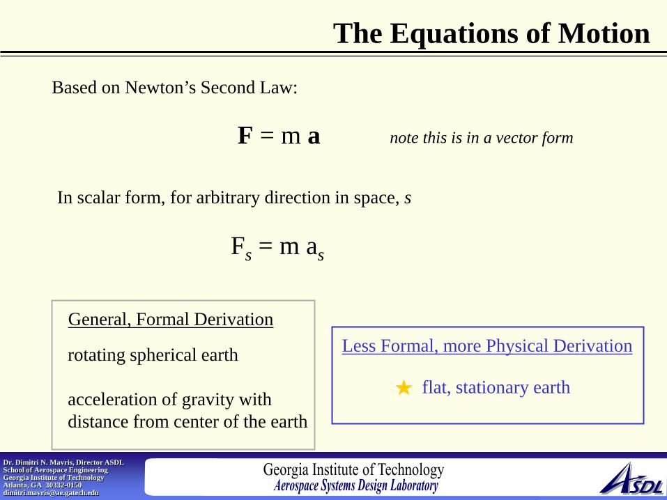
The Equations of Motion

Based on Newton’s Second Law:

F = m a note this is in a vector form

In scalar form, for arbitrary direction in space, s

Fs = m as

General, Formal Derivation Less Formal, more Physical Derivation rotating spherical earth

acceleration of gravity with distance from center of the earth

flat, stationary earth




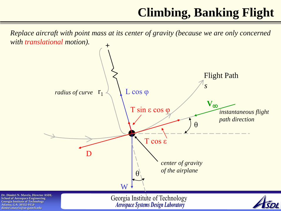
Climbing, Banking Flight Replace aircraft with point mass at its center of gravity (because we are only concerned with translational motion).

Flight Path

W

+

r1 radius of curve L cos φ

T sin ε cos φ

s

T cos ε D

center of gravity of the airplane θ

θ

V instantaneous flight path direction




First Equation of Motion

Take components parallel to the flight path

F = T cos ε - D - W sin θ

The acceleration is

The force is

Therefore, Newton’s Second Law parallel to the flight path is

a dV dt =

m dV dt = T cos ε - D - W sin θ

First Equation of Motion

ma = F




Second Equation of Motion Take components perpendicular to the flight path

F = L cos φ + T sin ε cos φ - W cos θ

The radial acceleration is

The force is

Therefore, Newton’s Second Law perpendicular to the flight path is

a V r1

=

m =

Second Equation of Motion

2

V r1

2

L cos φ + T sin ε cos φ - W cos θ

ma = F




Forces on Horizontal Plane Now look at flight path from a “top” view

+

r2

projection of flight path

L sin φ

T cos ε cos θ

T sin ε sin φ

D cos θ V cos θ




Third Equation of Motion Take components perpendicular to the flight path in the horizontal plane (2)

F2 = L sin φ + T sin ε sin φ

The radial acceleration is

The force is

Therefore, Newton’s Second Law perpendicular to the horizontal flight path is

a2 (V cos θ)

r2 =

m =

Third Equation of Motion

2

L sin φ + T sin ε sin φ

ma = F

(V cos θ) r2

2




Summary

The three Equations of Motion are simply statements of Newton’s Second Law. The three Equations of Motion describe the translational motion of an airplane through three-dimensional space over a flat earth. There are three additional equations of motion that describe the rotational motion of the aircraft about its three axes. Final note: the three equations of motion here do not assume a yaw component. The free stream velocity vector is assumed always parallel to the symmetry plane of the aircraft.




Sources of Aerodynamic Force

A body immersed in an airflow will experience an Aerodynamic Force due to:

Pressure

S

p=p(s)

τ=τ(s) S

Shear Stress

acts perpendicular to the surface

acts parallel to the surface

Integrate around the surface of the body to get the total force:

R = ∫∫ ∫∫+S S

Sdk Sdn p τ

n k

dS




2-D Sources of Aerodynamic Forces

Only 2 sources of resultant aerodynamic force (R):

Integral of Pressure Integral of Shear Stress Newton’s 2nd Law:

Conservation of Momentum gives the relationship between

pressure and velocity

p0 = p1 + ( ) ρ V12 = p2 + ( ) ρ V2

2 1 2

1 2

Friction (Viscous Forces) No slip condition at the surface

creates shear stress

Affected by: Affected by:

airfoil shape angle of attack shocks vortices

smoothness wetted area




References: Anderson; Fundamentals of Aerodynamics, 3rd Edition.

Let’s derive Bernoulli’s equation from the x component of the momentum equation:

xp

zu

yu

xuu

tu

∂∂

−=∂∂

+∂∂

+∂∂

+∂∂ ρωρυρρ

viscousxx Ffxp

DtDu )(++

∂∂

−= ρρ

xp

zu

yu

xuu

∂∂

−=∂∂

+∂∂

+∂∂

ρωυ 1

For an inviscid flow with no body forces this equation becomes:

For steady flow, du/dt = 0 and the equation above is written as below:

dxxpdx

zudx

yudx

xuu

∂∂

−=∂∂

+∂∂

+∂∂

ρωυ 1

Multiply by dx:

Derivation of Bernoulli’s Equation





dxxpdz

zudy

yudx

xuu

∂∂

−=

∂∂

+∂∂

+∂∂

ρ1

00

=−=−

udydxdxudz

υω

dyzudy

yudx

xudu

∂∂

+∂∂

+∂∂

=

Then substitute the Cartesian equations of a streamline shown below:

And now the equation looks like this:

Recall that given a function u = u(x,y,z), the differential is:

Substituting this you get:

dxxpudu

∂∂

−=ρ1

dxxpud

∂∂

−=ρ1)(

21 2or:






dzzpd

dyypd

dxxpud

∂∂

−=

∂∂

−=

∂∂

−=

ρω

ρυ

ρ

1)(21

1)(21

1)(21

2

2

2

Similarly by applying these assumptions, inviscid, steady flow, to flow along a streamline, you can get the equations for the y and z components of the momentum equation:

Add these equations to get:

ρ

ρωυ

dpVd

dzzpdy

ypdx

xpud

−=

∂∂

+∂∂

+∂∂

−=++

)(21

1)(21

2

222

Euler’s Equation:

Or:

VdVdp ρ−=






Euler’s Equation works for Incompressible and Compressible Flow under the previous assumptions:

VdVdp ρ−=However, with the incompressible flow assumption, where ρ = constant, the flow can easily be integrated between two points along a streamline to get Bernoulli’s Equation:

222

211

21

22

12

2

1

2

1

21

21

22

VpVp

VVpp

VdVdp

ρρ

ρ

ρ

+=+

−−=−

−= ∫∫





Is Bernoulli’s Equation valid for Compressible Flow?

Reference: Anderson; Fundamentals of Aerodynamics, 3rd Edition.

Answer: No Because it was derived with incompressible flow assumptions.

Bernoulli’s Equation




Source of Aerodynamic Force

A body immersed in an airflow will experience an Aerodynamic Force due to:

Pressure

S

p=p(s)

τ=τ(s) S

Shear Stress

acts perpendicular to the surface

acts parallel to the surface

Integrate around the surface of the body to get the total force:

R = ∫∫ ∫∫+S S

Sdk Sdn p τ

n k

dS

2




Aerodynamic Lift, Drag, and Moments

α

V ∞

R L

D

“free stream velocity” or “relative wind”

(defined as parallel to V ) ∞

(defined as perpendicular to V ) ∞

(not perpendicular to V ) ∞

AERODYNAMIC FORCES MOMENTS

c

M M LE

c 4

By convention, a moment which rotates a body causing an increase in angle of attack is positive.

3




Aerodynamic Coefficients

From intuition and basic knowledge, we know:

aerodynamic force = f (velocity, density, size of body, angle of attack, viscosity, compressibility)

L = L(ρ∞, V ∞, S, α, µ ∞, a ∞) D = D(ρ∞, V ∞, S, α, µ ∞, a ∞) M = M(ρ∞, V ∞, S, α, µ ∞, a ∞)

To find out how the lift on a given body varies with the parameters, we could run a series of wind tunnel tests in which the velocity, say, is varied and everything else stays the same. From this we could extract the change in lift due to change in velocity. If we did this for each parameter, and each force (moment), we would have to conduct experiments that resulted in 19 stacks of data (one for each variation plus a baseline). This is bad: wind tunnel time is very expensive and the whole process is time consuming.

5




Aerodynamic Coefficients Let’s define lift, drag, and moment coefficients for a given body:

CL = L q∞ S CD = D

q∞ S CM = M q∞ Sc

and q is defined as the dynamic pressure:

q = ρ V∞ 2 1 2

c is defined as a characteristic length of a body, usually the chord length

Now define the following similarity parameters:

Re = ρ ∞ V ∞ c µ ∞

Reynolds Number (based on chord length)

M ∞ = V ∞ a ∞

Mach Number




Aerodynamic Coefficients Using dimensional analysis, we get the following results. For a given body shape:

CL = f1( α, Re, M ∞)

CD = f2( α, Re, M ∞)

CM = f3( α, Re, M ∞)

If we conduct the same experiments, we can now get the equivalent data with 10 stacks of data.

But more fundamentally, dimensional analysis tells us that, if the Reynolds Number and the Mach Number are the same for two different flows (different density, velocity, viscosity, speed of sound), the lift coefficient will be the same, given two geometrically similar bodies at the same angle of attack. This is the driving principle behind wind tunnels. But…be careful. In real life, it is very difficult to match both Re and M.




Reference Area, S

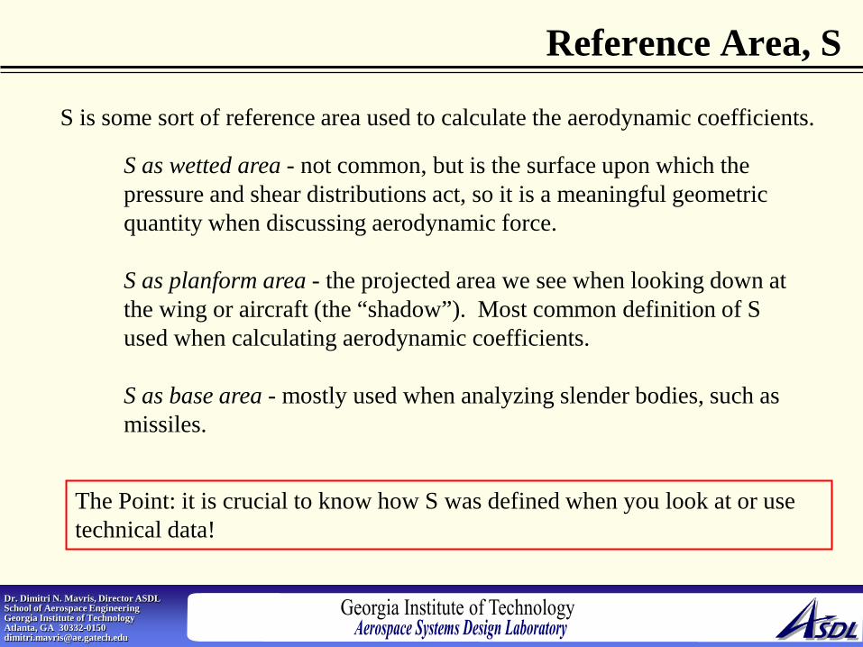
S is some sort of reference area used to calculate the aerodynamic coefficients.

S as wetted area - not common, but is the surface upon which the pressure and shear distributions act, so it is a meaningful geometric quantity when discussing aerodynamic force. S as planform area - the projected area we see when looking down at the wing or aircraft (the “shadow”). Most common definition of S used when calculating aerodynamic coefficients. S as base area - mostly used when analyzing slender bodies, such as missiles.

The Point: it is crucial to know how S was defined when you look at or use technical data!




Variation of Coefficients with Parameters How do the coefficients vary with α, Re, and M?

Answer: it depends on the flow regime and the shape of the body. Primarily, the effect of the three parameters is that they change the pressure distribution, and thus R.

Generic Lift Curve Slope

Note linear shape of slope




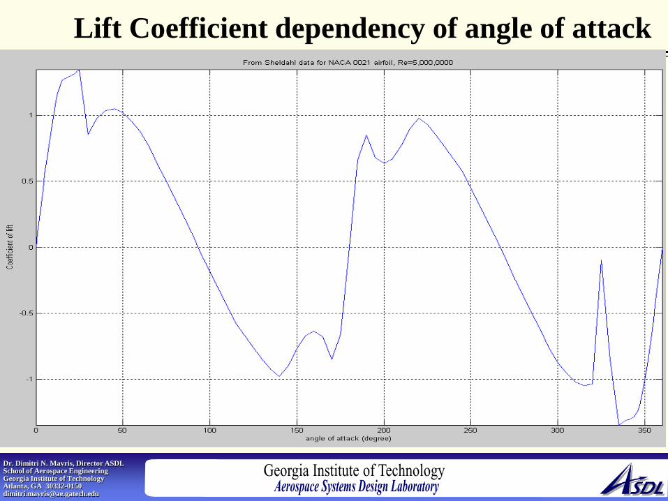
Lift Coefficient dependency of angle of attack




Variation of cl vs. α First question: What is difference between CL and cl?

CL is for the whole (3-D) aircraft. cl is for a 2-D shape, usually just airfoil.

Features of Typical Airfoils and Lift Curve Slope:

• Slope is mostly linear over practical range of alpha • For thin airfoils, theoretical maximum of lift curve slope is 2π per radian • For most conventional airfoils, experimentally measured lift slopes are very close to theoretical values. • All positively cambered airfoils have negative zero-lift angles of attack. A symmetric airfoil has a zero-lift angle of attack equal to zero (α L=0=0 deg) • At high angles of attack, slope becomes non-linear and airfoil exhibits stall due to separated flow.




Drag Polar: cd vs. cl

Remembering that the lift coefficient is a linear function of the angle of attack, cl could be effectively replaced by α for trend. For a cambered airfoil, the minimum drag value does not necessarily occur at zero angle of attack, but rather at some finite but small α.

Generic Drag Curve

primarily due to friction drag and pressure drag

primarily due to large pressure drag (separated flow)




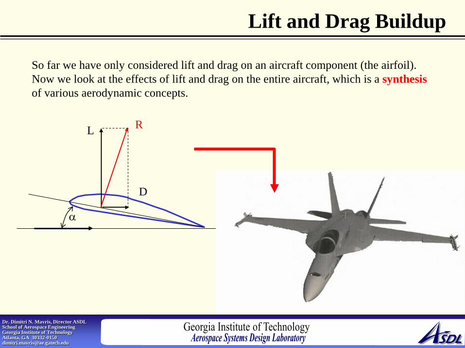
Lift and Drag Buildup

So far we have only considered lift and drag on an aircraft component (the airfoil). Now we look at the effects of lift and drag on the entire aircraft, which is a synthesis of various aerodynamic concepts.

α

R L

D




Creating Even More Lift

In general, there are four ways to create more lift

A larger wing will lift more weight (up to a point)

Increasing the camber of the airfoil will increase the lift

Increasing the speed of the wing will increase the lift




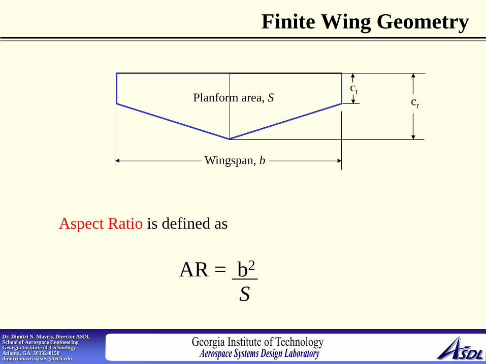
Finite Wing Geometry

Wingspan, b

Planform area, S ct

cr

Aspect Ratio is defined as

AR = b2 S




High Aspect Ratio Straight Wing

Used primarily for relatively low speed subsonic airplanes.

Classic theory for such wings, most straightforward engineering approach to estimate aerodynamic coefficients is Prandtl’s Lifting Line Theory

To estimate the lift curve slope of a finite wing:

a a0

1 + a0/(πeAR) =

a0 is section lift curve slope (per radian)

e is wing efficiency factor (usually about 0.95)

Equation good for high aspect ratio, straight wings in incompressible flow. Good for wings with aspect ratio 4 or higher.




Effect of Aspect Ratio on Lift Curve

Lift curve slope decreases as aspect ratio decreases. As aspect ratio decreases, induced effects from wing tip vortices become stronger and lift is decreased for a given angle of attack.

Note that zero lift angle of attack is same for all wings, but lift curve slope varies with aspect ratio




Compressibility Correction

Prandtl’s Lifting Line Theory may be corrected for compressibility effects at higher speeds.

a0, comp a0

1 - M 2 ∞

=

Prandtl-Glauert Rule Now replace a0 in Prandtl’s Lifting Line Theory with a0,comp to get corrected lift curve slope.

acomp a0

1 - M 2 ∞ + a0/(πeAR) =

good for Mach numbers up to about 0.7

For Supersonic High Aspect Ratio Wings, use this equation derived from supersonic linear theory:

acomp M 2- 1

= 4

∞




Effect of Mach Number on Lift Slope

Supersonic correction equation

Subsonic correction equation

For transonic region, use CFD




Low Aspect Ratio Straight Wings

Cannot use Prandtl’s Lifting Line Theory for low aspect ratio wings (AR < 4). It is based on lifting line theory, which models high aspect ratio wings well, but models low aspect ratio wings poorly. It is more appropriate to use lifting surface.

Lifting Line

Trailing Vortices

High Aspect Ratio Wing

Lifting Line Low Aspect Ratio Wing Low Aspect Ratio Wing

Lifting Surface

Lifting line produces bad model for low AR wings

Lifting surface provides better model for low AR wings




Low AR Wing Lift Approximations

a0

1 + [a0 / (πAR)]2 + a0/πAR) a =

For incompressible flow based on lifting surface solution for elliptical wings, but used for straight wings

a0

1 - M 2 + [a0 / (πAR)]2 + a0/πAR) a =

∞

For subsonic, compressible flow modified from above equation

acomp 4

∞

= 2AR M 2 - 1 ∞

1 1 - For supersonic flow,

low AR, straight wing

Valid as long as Mach cones from the two wing tips do not overlap

Helmbold’s Equation

M 2- 1




Panel methods for calculating cL for finite wings

• What is wrong with lifting line theory? – Prandtl’s lifting-line theory doesn’t yield good

results for wings that are not straight and/or have low aspect ratios

• How can we get lift and drag calculations for other wings? – Use a series of chordwise-distributed lifting lines




Wing Body Combinations Liftwing + Liftbody = Liftwing/body combination

No accurate analytical way to predict lift of wing-body interaction Wind tunnel tests CFD analysis Can’t even say if it will be more or less However, work by Hoerner and Borst shows that the lift of the wing-body combination can be treated as simply the lift on the complete wing by itself, including that portion which is covered by the fuselage.

reasonable approximation for preliminary design and performance at subsonic speeds




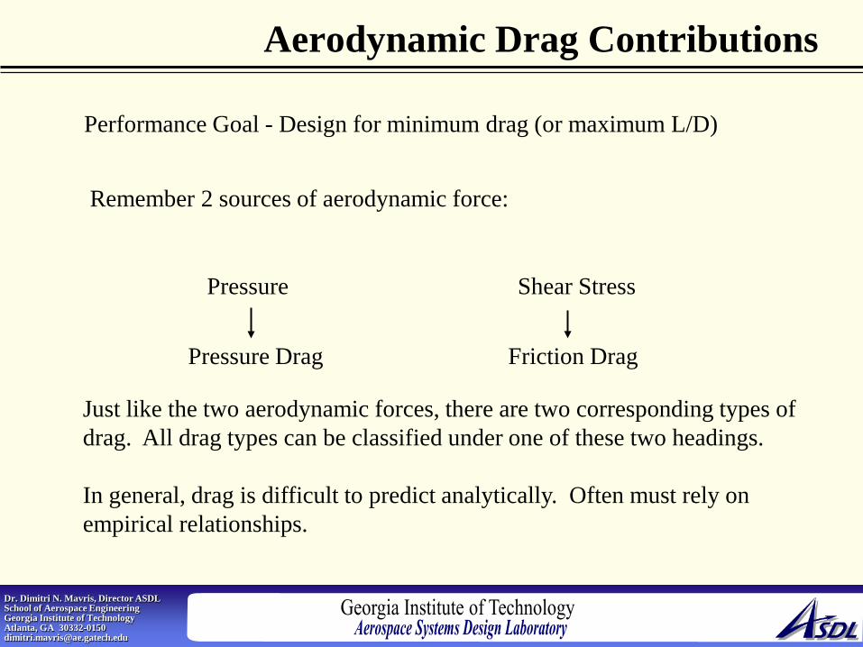
Aerodynamic Drag Contributions

Performance Goal - Design for minimum drag (or maximum L/D)

Remember 2 sources of aerodynamic force:

Pressure Shear Stress

Pressure Drag Friction Drag

Just like the two aerodynamic forces, there are two corresponding types of drag. All drag types can be classified under one of these two headings. In general, drag is difficult to predict analytically. Often must rely on empirical relationships.




Subsonic Drag-Airfoils Section drag, also called profile drag, is what you see in typical airfoil cl vs cd data, like the NACA airfoil data.

cd = cf + cd,p

profile drag = skin-friction + pressure drag drag due to separation

Skin friction drag due to frictional shear stress acting on the surface of the airfoil

For thin airfoils and wings, cf can be estimated by using formulas for a flat plate

cf = 1.328

Re laminar

Exact theoretical for laminar incompressible flow over a flat plate, but we use it as an approximation of an airfoil




Skin Friction Drag

cf = Df q∞S Re = ρ ∞ V ∞ c

µ ∞

Df friction on one side of plate c length of plate in flow direction S planform area of plate

For turbulent flow, must use approximations

cf -1/2

= 4.13 log (Re cf) turbulent Karman-Schoenherr (solve implicitly)

or

cf 0.42 ln2(0.056 Re)

= accurate within +/- 4% for 105 < Re < 109

Now, when do you apply these equations? Assumption: for high Re normally encountered in flight, laminar flow region is very small, so assume entire surface is turbulent.




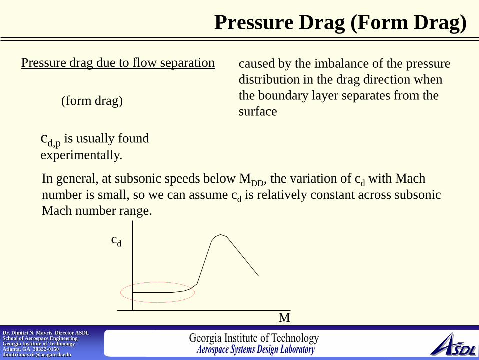
Pressure Drag (Form Drag)

Pressure drag due to flow separation caused by the imbalance of the pressure distribution in the drag direction when the boundary layer separates from the surface

(form drag)

cd,p is usually found experimentally.

In general, at subsonic speeds below MDD, the variation of cd with Mach number is small, so we can assume cd is relatively constant across subsonic Mach number range.

cd

M




Subsonic Drag-Finite Wings Now we need to add in induced drag, which is a form of pressure drag.

For a high aspect ratio straight wing, use Prandtl’s Lifting Line Theory to get:

CDi = CL

2

π e AR

CDi = Di q∞S

e is efficiency factor

0 < e < 1 function of aspect ratio and taper

Realize that induced drag and lift are caused by the same mechanism: change in pressure distribution between top and bottom surfaces. So, it makes sense that CDi and CL are strongly coupled. Induced drag is the “cost” of lift.




Subsonic Drag-Finite Wings

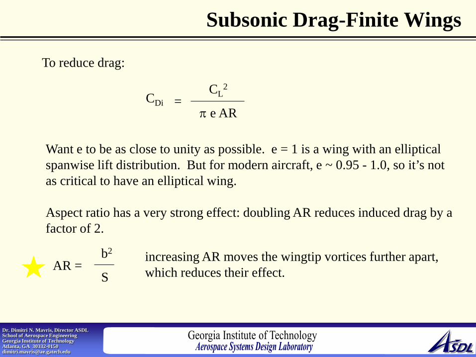
To reduce drag:

CDi = CL

2

π e AR

Want e to be as close to unity as possible. e = 1 is a wing with an elliptical spanwise lift distribution. But for modern aircraft, e ~ 0.95 - 1.0, so it’s not as critical to have an elliptical wing. Aspect ratio has a very strong effect: doubling AR reduces induced drag by a factor of 2.

AR = b2 S

increasing AR moves the wingtip vortices further apart, which reduces their effect.




Subsonic Drag-Finite Wings Although high aspect ratios are aerodynamically best, they are structurally expensive. Most subsonic aircraft today: 6 < AR < 9 Modern sailplanes: 10 < AR < 30




Subsonic Drag- Fuselages

Fuselages experience substantial drag:

skin-friction - function of wetted area pressure drag due to flow separation Interference drag - interaction that occurs at the junction of the wing and fuselage

region of interference drag

No analytical way to predict interference drag. Use experimental data.




Summary of Subsonic Drag skin friction drag - due to frictional shear stress over the surface pressure drag due to flow separation (form drag) - due to pressure imbalance caused by flow separation profile drag (section drag) - sum of skin friction drag and form drag interference drag - additional pressure drag that is caused when two surfaces (components) meet. parasite drag - term used for the profile drag of the complete aircraft, including interference drag. induced drag - pressure drag caused by the creation of wing tip vortices (induced lift) of finite wings zero-lift drag - parasite drag of complete aircraft that exists at its zero-lift angle of attack drag due to lift - total aircraft drag minus zero lift drag. It measures the change in parasite drag as α changes from α L=0




Other Contributions to Drag The previous drags were the main categories of drag. Sometimes they are broken into more detailed categories.

Ex: External Store Drag Landing Gear Drag Protuberance Drag Leakage Drag Engine Cooling Drag (reciprocating engines) Flap Drag Trim Drag

Wing

Tail




Drag Breakdown For subsonic: Most drag at cruise is parasite drag Most drag at takeoff is lift-dependent drag For supersonic: Most drag at cruise is wave drag (both kinds) Most drag at takeoff is lift-dependent drag

About 2/3 of total parasite drag in cruise is due to skin friction, the rest is interference and form drag. Recall friction drag is a function of total wetted surface area, so to estimate friction drag, we should get an estimate of wetted area. Wetted surface area, Swet, is usually 2 to 8 times the reference planform area of the wing, S.




Wetted Area Estimation The zero-lift parasite drag, D0, can be written

D0 = q∞ Swet Cfe

The zero-lift drag coefficient, CD,0, is defined as

CD,0 = D0

q∞ S

Substituting, we get

CD,0

q∞ Swet Cfe

q∞ S = =

Swet

S

Cfe




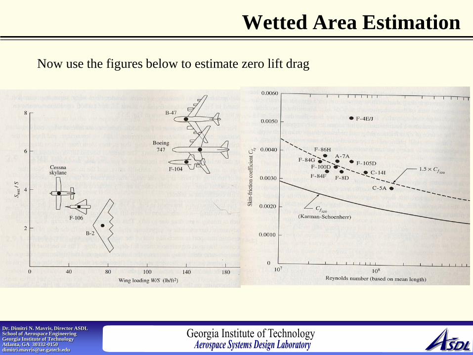
Wetted Area Estimation

Now use the figures below to estimate zero lift drag




The Drag Polar For every aerodynamic body, there exists a relationship between CL and CD. This relationship can be expressed as either an equation or a graph. Both are called “drag polar”.

Virtually all information necessary for a performance analysis is contained in the drag polar.

Recall

Total Drag = parasite drag + wave drag + induced drag

CD = CD,e + CD,w + CL2

π e AR




Parasite Drag

First, look at CD,e

CD,e = CD,e,0 + ∆ CD,e

parasite drag at zero lift

increment in parasite drag

due to lift Now realize

∆ CD,e is a function of α and

cd varies as cl2

This implies that ∆ CD,e varies w/ CL2

So, CD,e = CD,e,0 + ∆ CD,e = CD,e,0 + k1 CL2




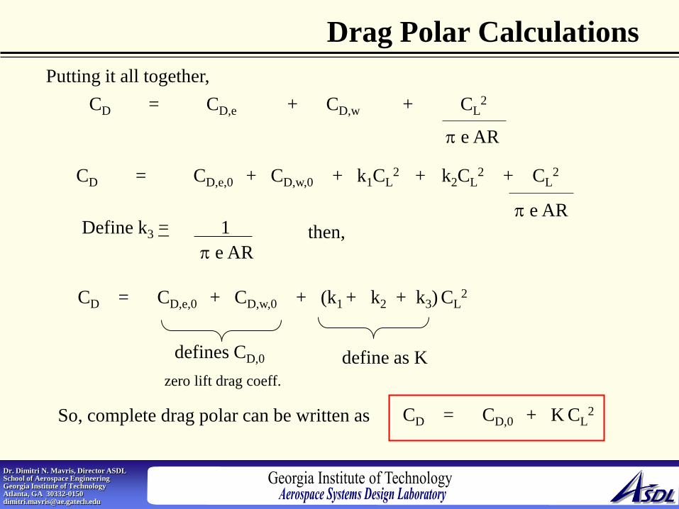
Drag Polar Calculations Putting it all together,

CD = CD,e + CD,w + CL2

π e AR

CD = CD,e,0 + CD,w,0 + k1CL2 + k2CL

2 + CL2

π e AR

Define k3 = 1 π e AR

then,

CD = CD,e,0 + CD,w,0 + (k1 + k2 + k3) CL2

defines CD,0 zero lift drag coeff.

define as K

So, complete drag polar can be written as CD = CD,0 + K CL2




Drag Polar Calculations CD = CD,0 + K CL

2

CD

CD,0

K CL2

total drag coefficient zero lift parasite drag coefficient or “zero lift drag coefficient”

drag due to lift

Equation is valid for both subsonic and supersonic At supersonic, CD,0 contains wave drag at zero lift, friction drag, form drag. The value for wave drag due to lift is part of K

CL

CD

K CL2 CD,0

zero lift drag coefficient

drag polar




Graphic Drag Polar CL

CD

0

The slope of the line from the origin to any point on the drag polar is the L/D at that point. It will have a corresponding α. A line drawn from the origin tangent to the drag polar identifies the (L/D)max of the aircraft. Sometimes called the “design point” Corresponding CL is called “design lift coefficient” Note (L/D)max does NOT occur at point of minimum drag




Graphic Drag Polar

CL

CD 0

CL

CD 0

Note: for most real aircraft, minimum drag point is NOT the same as zero lift point, although we have been drawing it that way.

But for airplanes with wings of moderate camber, the difference between CD,0 and Cdmin are small and can be ignored.




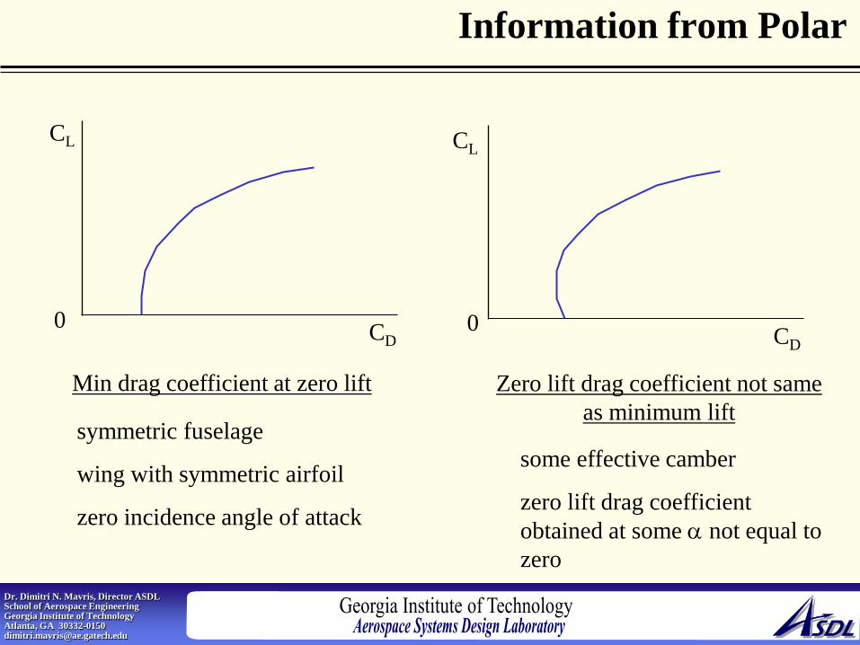
Information from Polar

CL

CD 0

CL

CD 0

Min drag coefficient at zero lift Zero lift drag coefficient not same as minimum lift

symmetric fuselage wing with symmetric airfoil zero incidence angle of attack

some effective camber zero lift drag coefficient obtained at some α not equal to zero




General Drag Polar Notes

The same aircraft will have different drag polars for different Mach numbers. At low M, this can be effectively ignored At high M, differences are significant

As M increases, curve shifts to the right minimum drag coefficient increases due to drag divergence effects

Subsonic

Supersonic

As M increases, curve shifts to the left and “squashes” minimum drag coefficient decreases CL decreases

cd

M

cl

M




General Drag Polar Notes




Some Key References S.F. Hoerner, Fluid Dynamic Drag, Hoerner Fluid Dynamics, Brick Town, NJ 1965 S.F. Hoerner and H.V. Borst, Fluid Dynamic Lift, Hoerner Fluid Dynamics, Brick Town, NJ 1975 Ira H. Abbott and Albert E. Von Doenhoff, Theory of Wing Sections, McGraw-Hill, New York, 1991. John D. Anderson, Jr. Introduction to Flight, 3rd Edition, McGraw-Hill, New York, 1989 John D. Anderson, Jr. Fundamentals of Aerodynamics, 2nd Edition, McGraw-Hill, New York, 1991 Joseph Katz and Allen Plotkin, Low-Speed Aerodynamics, McGraw-Hill, New York, 1991 Deitrich Kuchemann, The Aerodynamic Design of Aircraft, Pergamon Press, Oxford, 1978 Daniel P. Raymer, Aircraft Design: A Conceptual Approach, 2nd Edition, AIAA Education Series, American Institute of Aeronautics and Astronautics, Washinton, 1992.



Documents

Fundamentals of Aircraft Aerodynamicsengineeringolympics.gatech.edu/sites/default/files/images/... · Dr. Dimitri N. Mavris, Director ASDL School of Aerospace Engineering Georgia