GALERKIN AND RUNGE{KUTTA METHODS: UNIFIED …rhn/papers/pdf/rk-superconvergence.pdf · galerkin and runge{kutta methods: unified formulation, a posteriori error estimates and nodal

GALERKIN AND RUNGE–KUTTA METHODS: UNIFIEDFORMULATION, A POSTERIORI ERROR ESTIMATES

AND NODAL SUPERCONVERGENCE

GEORGIOS AKRIVIS, CHARALAMBOS MAKRIDAKIS, AND RICARDO H. NOCHETTO

Abstract. We unify the formulation and analysis of Galerkin and Runge–Kuttamethods for the time discretization of parabolic equations. This, together withthe concept of reconstruction of the approximate solutions, allows us to establish aposteriori superconvergence estimates for the error at the nodes for all methods.

1. Introduction

In this paper we consider a unified formulation of the most popular implicit single-

step time–stepping methods. Based on this formulation we derive a posteriori esti-

mates and in particular superconvergence estimates at the nodes of the time partition.

We consider Runge–Kutta (RK for short) schemes, in particular interpolatory implicit

RK (collocation or perturbed collocation schemes), as well as the Continuous and the

Discontinuous Galerkin methods (cG and dG for short). We formulate the methods,

cast them into a unified abstract method, and carry out the a posteriori error analysis

for linear equations in a Hilbert space setting: Seek u : [0, T ]→ D(A) satisfying

(1.1)

{u′(t) + Au(t) = f(t), 0 < t < T,

u(0) = u0,

with A a positive definite, self-adjoint, linear operator on a Hilbert space (H, 〈·, ·〉)with domain D(A) dense in H, and a given forcing term f : [0, T ]→ H.

This paper is a continuation of our previous work on a posteriori error estimation

via appropriate reconstructions of the approximate solutions with focus on different

Date: August 14, 2010.2000 Mathematics Subject Classification. 65M15, 65M50.Key words and phrases. Continuous and discontinuous Galerkin methods, Runge–Kutta methods,

collocation methods, perturbed collocation methods, reconstruction, a posteriori error analysis,superconvergence, parabolic equations.

The first author was partially supported by the Institute of Applied and Computational Mathemat-ics, FORTH, Greece.The second author was partially supported by the RTN-network HYKE, HPRN-CT-2002-00282, theEU Marie Curie Dev. Host Site, HPMD-CT-2001-00121 and the program Pythagoras of EPEAEKII.The third author was partially supported by NSF grants DMS-0505454 and DMS-0807811.

1

2 G. AKRIVIS, CH. MAKRIDAKIS, AND R. H. NOCHETTO

methods: dG and Runge-Kutta-Radau methods [19]; Crank–Nicolson [3]; and cG

schemes and RK collocation methods [4]. Here we provide a unified treatment of

essentially all single-step time-stepping schemes. Notably, with the aid of reconstruc-

tions, we even cast cG and dG schemes into a unified formulation, a connection we

explore here.

For previous a posteriori results using various discretization methods which are

covered by the formulation presented in this paper we refer, e.g., to [3, 4, 9, 10, 12,

13, 16, 19, 22]. Regarding a posteriori superconvergence results at the time nodes

we refer to [9] where fully discrete schemes combined with dG piecewise linear time

discretization methods were considered.

1.1. Notation. For convenience, we use the notation F (t, v) = Av−f(t) to describe

the time-stepping methods for (1.1).

To discretize (1.1) we consider piecewise polynomial functions in arbitrary parti-

tions 0 = t0 < t1 < · · · < tN = T of [0, T ], and let Jn := (tn−1, tn] and kn := tn− tn−1.

We denote by Vdq , q ∈ N0, the space of possibly discontinuous functions at the nodes

tn that are piecewise polynomials of degree at most q in time in each subinterval Jn,

i.e., Vdq consists of functions g : [0, T ]→ D(A) of the form

g|Jn(t) =

q∑j=0

tjwj, wj ∈ D(A),

without continuity requirements at the nodes tn; the elements of Vdq are taken con-

tinuous to the left at the nodes tn. Let Vq(Jn) consist of the restrictions to Jn of

the elements of Vdq . The spaces Hd

q and Hq(Jn) are defined analogously by requiring

wj ∈ H. Furthermore, let the spaces Vcq and Hc

q consist of the continuous elements of

Vdq and Hd

q , respectively. For v ∈ Vdq we let vn := v(tn), vn+ := limt↓tn v(t).

1.2. The general discretization method. To describe the discretization method

we consider two operators: Πq−1 will be a projection operator to piecewise polynomials

of degree q − 1,

(1.2) Πq−1 : C([0, T ];H)→ ⊕Nn=1Hq−1(Jn)

that does not enforce continuity at {tn}Nn=1. In addition, Πq : Hq(Jn)→ H`(Jn) is an

operator mapping polynomials of degree q to polynomials of degree `, with ` = q or

` = q− 1, depending on the example. Note that to avoid confusion, Πq−1 and Πq are

defined in a reference time interval and then transformed into Jn.

With the aid of these operators we define the time discrete approximation U to

the solution u of (1.1) as follows: We seek U ∈ Vcq satisfying the initial condition

U(0) = u0 as well as the pointwise equation

(1.3) U ′(t) +Πq−1F (t, ΠqU(t)) = 0 ∀t ∈ Jn.

SINGLE–STEP METHODS: RECONSTRUCTION AND A POSTERIORI ANALYSIS 3

An equivalent Galerkin formulation is

(1.4)

∫Jn

[〈U ′, v〉+ 〈Πq−1F (t, ΠqU(t)), v〉

]dt = 0 ∀v ∈ Vq−1(Jn),

for n = 1, . . . , N. We already considered methods of this form in [4].

Recall, in particular, that the continuous Galerkin (cG) method is just

(1.5)

∫Jn

[〈U ′, v〉+ 〈F (t, U(t)), v〉

]dt = 0 ∀v ∈ Vq−1(Jn),

i.e., Πq−1 := Pq−1, with P` denoting the (local) L2 orthogonal projection operator

onto H`(Jn), for each n,∫Jn

〈P`w, v〉 ds =

∫Jn

〈w, v〉 ds ∀v ∈ H`(Jn).

It follows from (1.5) that U ∈ Vcq satisfies also the following pointwise equation

(1.6) U ′(t) + Pq−1F (t, U(t)) = 0 ∀t ∈ Jn.

This method is indeed the simplest one described in (1.3), with Πq−1 = Pq−1, Πq = I.

One thus may view the class of methods (1.4) as a sort of numerical integration

applied to the continuous Galerkin method. In Section 2 we will see that (1.4) covers

all important implicit single-step time stepping methods. In particular

• the cG method with Πq−1 := Pq−1, and Πq = I (the identity);

• the RK collocation methods (RK-C) with Πq−1 := Iq−1 and Πq = I, with Iq−1

denoting the interpolation operator at the collocation points;

• all other interpolatory RK methods with Πq−1 := Iq−1, and appropriate Πq (with

` = q) described below in (2.23);

• the dG method with Πq−1 := Pq−1 and Πq = Iq−1, where Iq−1 is the interpolation

operator at the Radau points 0 < τ1 < · · · < τq = 1 (so ` = q − 1).

1.3. Superconvergence condition. The single-step time–stepping schemes we con-

sider in this paper are associated to q pairwise distinct points τ1, . . . , τq ∈ [0, 1]. These

points are transformed to the interval Jn as

(1.7) tn,i := tn−1 + τikn, i = 1, . . . , q.

Since we are interested in Galerkin and RK methods attaining higher order accuracy

at the nodes {tn}Nn=1 than globally, a phenomenon known as superconvergence, we

assume that the points τ1, . . . , τq satisfy the orthogonality condition

(1.8)

∫ 1

0

q∏i=1

(τ − τi)v(τ) dτ = 0 ∀v ∈ Pr

for some 1 ≤ r ≤ q− 1, whence q ≥ 2. Condition (1.8) is satisfied if and only if every

element of Pq+r and its Lagrange interpolant at τ1, . . . , τq have the same integral, i.e.,

if the interpolatory quadrature formula with nodes τ1, . . . , τq integrates the elements


of Pq+r exactly. For cG and collocation methods the maximal superconvergence order

is then O(kq+1+r). From now on, for these methods, we let

(1.9) p := q + 1 + r

be the superconvergence order at the nodes, and call it the superorder.

Since q ≥ 2, we exclude the Crank-Nicolson-Galerkin scheme (q = 1) from our

discussion of cG methods. This is natural, since it is well known that the Crank-

Nicolson-Galerkin scheme yields second order approximations, both globally and at

the nodes. We also exclude the backward Euler and Crank-Nicolson methods from

the present analysis of RK methods for the same reason; they yield first and second

order approximations, respectively, both globally and at the nodes.

The superconvergence order p might be reduced compared to (1.9) for the Per-

turbed Collocation methods considered in Section 2.4. In that case, although (1.8)

still holds, we make use only of part of it as in [21], namely orthogonality with respect

to Pr′ , 1 ≤ r′ ≤ r. Then our assumption on the superorder p will be

(1.10) p ≥ q + 1 + r′ .

1.4. Reconstruction. Let projection operators Πq onto Hq(Jn), n = 1, . . . , N, sat-

isfy the fundamental property that Πqw agrees with Πq−1w at tn,i:

(1.11) (Πq −Πq−1)w(tn,i) = 0, i = 1, . . . , q, ∀w ∈ C([0, T ];H).

For each n = 1, . . . , N, the reconstruction U ∈ Hq+1(Jn) of U is given by

(1.12) U(t) := U(tn−1)−∫ t

tn−1

Πq

[AΠqU(s)− f(s)

]ds ∀t ∈ Jn.

In view of (1.8) for v(τ) = 1 and (1.11), we obtain U(tn) = Un and conclude that U

is continuous. Differentiation of U yields

(1.13) U ′(t) = −Πq[AΠqU(t)− f(t)] = −ΠqF (t, ΠqU(t)) ∀t ∈ Jn,

which has a similar structure to (1.3). The idea behind (1.12) is not new: this

reconstruction was introduced in [4] for cG and collocation methods, with Πq = I

and so ΠqΠqU = ΠqU . The operator Πq is here chosen as follows, depending on

discrete compatibility conditions such as (1.22) (further discussed in Section 6):

• for the cG methods, Πq is either Pq or an interpolation operator at q + 1 Gauss

points, q from Jn and one from an adjacent interval, applied to Pq−1; see (6.4);

• for the dG methods, Πq = Pq, whence ΠqIq−1U = Iq−1U ;

• for the RK-C methods, Πq is an interpolation operator at the q collocation points

of Jn plus another point either in Jn or a collocation point in an adjacent interval;

• for the perturbed RK-C methods, Πq is the first option for RK-C methods.


If v ∈ Hr(Jn), then 〈(Πq − Πq−1)w, v〉 ∈ Pq+r and vanishes at tn,i, i = 1, . . . , q.

Thus, (1.8) leads to the orthogonality property

(1.14)

∫Jn

〈(Πq −Πq−1)w(s), v(s)〉 ds = 0 ∀w ∈ C([0, T ];H), v ∈ Hr(Jn),

for n = 1, . . . , N, which will play a central role in the superconvergence analysis. To

see why, subtract (1.13) from (1.3) to get

(1.15) U ′ − U ′ = (Πq −Πq−1)(f − AΠqU),

whence, in view of (1.11),

(1.16) (U − U)′(tn,i) = 0, i = 1, . . . , q.

Moreover, we observe that (1.14) and (1.15) yield the orthogonality relation∫Jn

〈(U − U)′, v〉dt = 0 ∀v ∈ Hr(Jn).

Integrating by parts and using the fact that U −U vanishes at tn−1 and tn, we arrive

at the first abstract orthogonality condition with r ≥ 1

(1.17)

∫Jn

〈U − U, v〉 dt = 0 ∀v ∈ Hr−1(Jn).

The second one is a further assumption on Πq−1, namely for all V ∈ Hq(Jn),

(1.18)

∫Jn

〈V −Πq−1V, v〉dt = 0 ∀v ∈ Hr−1(Jn),

which, in view of (1.14), yields

(1.19)

∫Jn

〈ΠqV − V, v〉dt = 0 ∀v ∈ Hr−1(Jn).

Condition 1.18 is verified by both cG and dG methods, for which Πq−1 = Pq−1, as

well as by RK methods, for which Πq−1 = Iq−1; see Subsection 1.2.

Remark 1.1 (Roots of ΠqV − V ). We notice for later use that for cG, dG and RK

methods there holds

(1.20) Πq−1V (tn,i) = V (tn,i), i = 1, . . . , q,

for all V ∈ Hq(Jn). This is obvious for RK methods, since Πq−1 = Iq−1. It also holds

for cG and dG methods since V − Πq−1V is a multiple of the Legendre polynomial

of degree q. Combining (1.20) with (1.11), we obtain

(1.21) (ΠqV − V )(tn,i) = 0, i = 1, . . . , q,

for all V ∈ Hq(Jn).


1.5. Superconvergence estimates. For cG it is known that the error decays a

priori with optimal rate O(k2q) at the nodes (thus p = 2q) [5], provided restrictive

compatibility conditions of the form [8, 1, 7, 22, 6]

(1.22) f ∈ D(Aρ), U0 ∈ D(Aρ+1)

hold for 1 ≤ ρ ≤ q − 1. In Subsection 4.1 we establish the following a posteriori

analogue of these results for the error e := u−U by using duality (see Theorem 4.1)

(1.23) |e(tn)| ≤ CILn max1≤m≤n

(kρm|Aρ−1R|L∞(Jm)

),

in terms of the residual R := U ′ +AU − f with Πq = Pq; we denote by | · | the norm

of H. Note that a compatibility condition of the form (1.22) is implicitly assumed

in (1.23) provided |Aρ−1R|L∞(Jn) is bounded. We examine this discrete regularity in

Section 6 and show that the alternative choice of Πq requires, instead of (1.22),

(1.24) f ∈ D(Aρ), U0 ∈ D(Aρ).

Compared with the bound in L∞([0, T ];H) in Theorem 2.1 in [4], this additional

regularity of R yields the asserted extra power ρ of km in (1.23) at the nodes tn. Such

estimate is valid for dG as well, but the order of the residual R is in general at most

q instead of q + 1 for cG; see Theorem 4.2 and Remarks 4.2 and 4.4.

In contrast, superconvergence order at the nodes for RK methods is the classical

order of the method in the standard terminology of RK methods [14, 15]. Since

the seminal work of Crouzeix [8], it is known that this order is limited by requiring

nontrivial conditions of the form (1.22) which may fail to be fulfilled in applications [7,

17, 18, 22]. This lack of superconvergence at the nodes is usually called order reduction

in the literature [7, 22]. A result similar to (1.23) is established in Theorem 5.1 for

collocation methods. The proof follows along the same lines as (1.23) but additional

difficulties arise due to the quadrature effect inherent to collocation methods. Note

that we avoid time derivatives of f in the final estimate. In fact, quadrature errors

are quantified by higher interpolation errors of the form

(1.25) kjm|Aj−1(f − Ip−j−1f)|L∞(Jm), j = 1, . . . , p− q − 2,

in the final estimate. A similar multiorder splitting has been proposed in [20] to avoid

the explicit use of the Bramble-Hilbert lemma. Similar results hold in the perturbed

collocation case assuming that the final superconvergence order is given.

The paper is organized as follows: in Section 2 we cast the classes of single-step

schemes into the unified formulation. In Sections 3 we develop an error representation

formula, which exploits the nature of the unified formulation and simplifies the forth-

coming analysis. Sections 5 and 6 are devoted to proving a posteriori error bounds

that account for nodal superconvergence for Galerkin and RK methods, respectively.

They hinge on compatibility properties of the discrete solution U , which are further

explored in Section 6 for all the methods.


2. Casting single-step schemes into the unified formulation

In this section we cast various single-step time-stepping schemes, in particular

interpolatory RK methods and the cG and dG methods, into the unified formulation.

It is instructive to start with the cG method, since all other methods are obtained as

perturbations using appropriate operators and quadrature.

2.1. The cG method. We already described the cG method in Subsection 1.2; see

(1.5) and (1.6). Here we recall some of its properties.

A natural norm for error estimates for parabolic type equations is the L∞([0, T ];H)

norm. Since U is piecewise polynomial of degree q, the highest possible order of

convergence in L∞([0, T ];H) is q + 1. This is indeed the order of the cG method:

(2.1) max0≤t≤T

|u(t)− U(t)| = O(kq+1)

with k := maxn kn provided u is sufficiently smooth; see [5] and [22, p. 206–207].

Higher accuracy can be obtained at the nodes {tn}Nn=1 for ODEs. In particular the

maximal order of the cG method at the nodes is p = 2q, i.e.,

(2.2) maxn|u(tn)− U(tn)| = O(k2q) .

This superconvergence phenomenon for cG is well understood, [5], [2]: it is due to the

relation between cG methods, the q Gauss points τ1, . . . , τq, and their orthogonality

property (1.8) with r = q − 1. This property is the basis of our a posteriori analysis

at the nodes in Section 5. We stress, however, that superconvergence is not just a

consequence of extra regularity but of compatibility conditions; see Section 6.1.

2.2. The dG method. The time discrete dG(q−1) approximation V to the solution

u of (1.1) is defined as follows: we seek V ∈ Vdq−1 such that V (0) = u(0), and

(2.3)

∫Jn

[〈V ′, v〉+ 〈F (t, V ), v〉

]dt+ 〈V n−1+ − V n−1, vn−1+〉 = 0 ∀v ∈ Vq−1(Jn),

n = 1, . . . , N. The dG(q− 1) method gives a convergence rate O(kq) in L∞([0, T ];H)

and the superorder

(2.4) maxn|u(tn)− V (tn)| = O(k2q−1)

provided certain compatibility conditions hold for u [22, Chapter 12]; see Section 6.2.

The approximations in the unified formulation (1.3), as well as in its variational

counterpart (1.4), are continuous piecewise polynomials; in contrast, the dG approx-

imations may be discontinuous. Therefore, in order to cast the dG method into the

unified formulation we first need to associate discontinuous piecewise polynomials to

continuous ones. To this end, we let 0 < τ1 < · · · < τq = 1 be the abscissae of the

Radau quadrature formula in the interval [0, 1]; this formula integrates exactly poly-

nomials of degree at most 2q − 2. The Radau nodes tn,i ∈ Jn satisfy (1.7). Now, we

introduce an invertible linear operator Iq : Vdq−1 → Vc

q as follows: To every v ∈ Vdq−1


we associate an element v := Iqv ∈ Vcq defined by locally interpolating at the Radau

nodes and at tn−1 in each subinterval Jn, i.e., v|Jn ∈ Vq(Jn) is such that

(2.5)

{v(tn−1) = v(tn−1),

v(tn,i) = v(tn,i), i = 1, . . . , q.

We call v a reconstruction of v [19], and use this notation throughout this subsection.

Exploiting the exactness of the Radau integration rule and the fact that v and v

coincide at the q Radau points in Jn, we deduce (for q ≥ 2)

(2.6)

∫Jn

〈v − v, w′〉 dt = 0 ∀v, w ∈ Vq−1(Jn),

i.e.,

(2.7)

∫Jn

〈v′, w〉 dt =

∫Jn

〈v′, w〉 dt+ 〈vn−1+ − vn−1, wn−1+〉 ∀v, w ∈ Vq−1(Jn);

this relation will prove useful in the sequel. This reconstruction was introduced in

[19] as the main tool in the a posteriori error analysis of dG methods. Conversely, if

v ∈ Vcq is given and Iq−1 is the interpolation operator at the Radau nodes tn,i, i.e.,

(Iq−1ϕ)(tn,i) = ϕ(tn,i), i = 1, . . . , q, we can recover v locally via interpolation, i.e.,

v = Iq−1v in Jn; furthermore, v(0) = v(0). Thus, Iq−1 = I−1q .

Using the dG reconstruction V ∈ Vcq of V ∈ Vd

q−1, from (2.3) and (2.7) we obtain

(2.8)

∫Jn

[〈V ′, v〉+ 〈F (t, V ), v〉

]dt = 0 ∀v ∈ Vq−1(Jn),

n = 1, . . . , N. Obviously, (2.8) can be written in the form

(2.9)

∫Jn

[〈V ′, v〉+ 〈F (t, Iq−1V ), v〉

]dt = 0 ∀v ∈ Vq−1(Jn),

n = 1, . . . , N. It is easily seen that the variational formulation (2.9) for the recon-

struction V can in turn be equivalently written as a pointwise equation, namely

(2.10) V ′(t) + Pq−1F(t, (Iq−1V )(t)

)= 0 ∀t ∈ Jn.

Obviously (2.10) is of the form of (1.3) with Πq−1 = Pq−1 and Πq = Iq−1, with

Iq−1 being the interpolation operator at the Radau points. To avoid confusion in the

forthcoming analysis we denote by U = V ∈ Vcq the continuous in time approximation

associated to the dG method and rewrite (2.10) in the form of (1.3):

(2.11) U ′(t) + Pq−1F(t, (Iq−1U)(t)

)= 0 ∀t ∈ Jn,

with Pq−1 and Iq−1 as above. We emphasize that U = V is continuous whereas

the standard dG approximation V for dG is not. We may thus wonder how the


reconstruction U of (1.12) with Πq = Pq relates to U . A simple calculation, employing

(1.12) and (2.11), reveals the following interesting property for all t ∈ Jn:

(2.12) U(t) = U(tn−1)−∫ t

tn−1

[AV − Pqf ]ds = U(t) +

∫ t

tn−1

(Pq − Pq−1)fds.

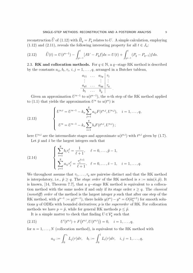
2.3. RK and collocation methods. For q ∈ N, a q−stage RK method is described

by the constants aij, bi, τi, i, j = 1, . . . , q, arranged in a Butcher tableau,

a11 . . . a1q τ1...

......

aq1 . . . aqq τqb1 . . . bq

.

Given an approximation Un−1 to u(tn−1), the n-th step of the RK method applied

to (1.1) that yields the approximation Un to u(tn) is

(2.13)

Un,i = Un−1 − kn

q∑j=1

aijF (tn,j, Un,j), i = 1, . . . , q,

Un = Un−1 − knq∑i=1

biF (tn,i, Un,i) ;

here Un,i are the intermediate stages and approximate u(tn,i) with tn,i given by (1.7).

Let p and s be the largest integers such that

(2.14)

q∑i=1

biτ`i =

1

`+ 1, ` = 0, . . . , p− 1,

q∑j=1

aijτ`j =

τ `+1i

`+ 1, ` = 0, . . . , s− 1, i = 1, . . . , q.

We throughout assume that τ1, . . . , τq are pairwise distinct and that the RK method

is interpolatory, i.e., p ≥ q. The stage order of the RK method is s := min(s, p). It

is known, [14, Theorem 7.7], that a q−stage RK method is equivalent to a colloca-

tion method with the same nodes if and only if its stage order s ≥ q. The classical

(nonstiff) order of the method is the largest integer p such that after one step of the

RK method, with yn−1 := y(tn−1), there holds y(tn)− yn = O(kp+1n ) for smooth solu-

tions y of ODEs with bounded derivatives; p is the superorder of RK. For collocation

methods we have p = p, while for general RK methods p ≤ p.

It is a simple matter to check that finding U ∈Vcq such that

(2.15) U ′(tn,i) + F(tn,i, U(tn,i)

)= 0, i = 1, . . . , q,

for n = 1, . . . , N (collocation method), is equivalent to the RK method with

aij :=

∫ τi

0

Lj(τ)dτ, bi :=

∫ 1

0

Li(τ)dτ, i, j = 1, . . . , q,


with L1, . . . , Lq the Lagrange polynomials of degree q − 1 associated with the nodes

τ1, . . . , τq, in the sense that U(tn,i) = Un,i, i = 1, . . . , q, and U(tn) = Un; see [14,

Theorem 7.6]. If Iq−1 denotes the (local) interpolation operator

(2.16) Iq−1v ∈ Hq−1(Jn) : (Iq−1v)(tn,i) = v(tn,i), i = 1, . . . , q,

then (2.15) can be written equivalently as follows because U ′ and Iq−1F are polyno-

mials of degree q − 1 in each interval Jn:

(2.17) U ′(t) + Iq−1F (t, U(t)) = 0 ∀t ∈ Jn.

Thus the RK Collocation (RK-C) class (2.17) is a subclass of (1.3) with Πq−1 = Iq−1

and Πq = I.

As in the case of cG we are interested in estimating the L∞([0, T ];H)−norm of

the error. If U is piecewise polynomial of degree q, then the highest possible order of

convergence in L∞([0, T ];H) is q + 1, namely

(2.18) max0≤t≤T

|u(t)− U(t)| = O(kq+1)

with k := maxn kn. This is indeed the order of the RK-C class provided that the

classical order p of the method satisfies p ≥ q + 1. Estimators of optimal order in

L∞([0, T ];H) in this case were derived in our recent paper [4]. The classical order

for ODEs is the convergence order observed at the nodes {tn}Nn=1:

(2.19) maxn|u(tn)− U(tn)| = O(kp) .

Recall that the classical order of the RK-C method is p > q, if and only if the nodes

τ1, . . . , τq satisfy the orthogonality condition (1.8) for r ≥ 0, where r = p− q− 1, [14,

Theorem 7.8]. If p > q + 1, then classical order p of the RK-C method corresponds

to the maximal superconvergence order at the nodes {tn}Nn=1 (superorder for short)

[14, 15]. The superorder is reduced unless nontrivial compatibility conditions of the

form (1.22) are valid for 1 ≤ ρ ≤ r. We explore their discrete counterpart in Section

6.3 and apply them to derive a posteriori error estimates in Section 5.1; compare with

the a priori results in [17, 18]. We refer to, e.g., [4], for three well-known important

classes of collocation methods, namely the RK Gauss–Legendre, the RK Radau IIA,

and the RK Lobatto IIIA methods.

We now discuss the collocation reconstruction. According to Section 1.4 there are

two variants depending on the choice of Πq. The first one, called Iq, is the extended

interpolation operator defined on continuous functions v over Jn by

(2.20) Iqv ∈ Hq(Jn) : (Iqv)(tn,i) = v(tn,i), i = 0, . . . , q,

where tn,0 6= tn,i, i = 1, . . . , q, and tn,0 ∈ Jn; compare with (2.16). An immediate

by-product of (2.14) is (1.14) with Πq = Iq and Πq−1 = Iq−1. We now define a RK-C

reconstruction U ∈ Hq+1(Jn) of the approximation U by

(2.21) U(t) = U(tn−1)−∫ t

tn−1

[AU(s)− Iqf(s)

]ds ∀t ∈ Jn;


comparing with (1.12) we see that Πq = Iq and Πq = I. If τq = 1 and τ1 > 0, then

the natural choice would be tn,0 = tn−1. This is what happens with the RK Radau

IIA methods (with τq = 1) for q > 1; see also Subsection 6.3.

The second alternative for Πq exploits the fact that the discrete compatibility at

collocation points is better than at the nodes and picks tn,0 /∈ Jn; see Section 6.3:

• Case τq < 1 (tn is not a collocation point): If n = 1, let t1,0 = t2,1 be the first

collocation node in J2. If n > 1, let tn,0 = tn−1,q be the last collocation node in

Jn−1.

• Case τq = 1 (tn is a collocation point): If n > 1, let tn,0 = tn−1 ∈ Jn. If n = 1 let

t1,0 = 0, provided that AU0 − f(0) ∈ D(Aρ), or as in the case τq < 1, let t1,0 = t2,1.

The RK-C reconstruction U is defined according to (1.12) with Πq = I:

(2.22) U(t) = U(tn−1)−∫ t

tn−1

Πq

[AU(s)− f(s)

]ds ∀t ∈ Jn.

2.4. Interpolatory RK and perturbed collocation methods. We consider here

q-stage RK methods with stage order s < q, because s ≥ q corresponds to collocation

RK methods (see Subsection 2.3), and follow Nørsett and Wanner [21] to cast them

into the unified form (1.3). To this end, we introduce the operator Πq : Hq(Jn) →Hq(Jn) given by

(2.23) Πqv(t) = v(t) +

q∑j=1

Nj

(t− tn−1

kn

)v(j)(tn−1) kjn , t ∈ Jn .

Here Nj ∈ Pq−1 are given polynomials. For τ1, . . . , τq ∈ [0, 1] pairwise distinct, the

corresponding perturbed collocation method is: Seek U ∈ Vcq such that

(2.24) U ′(tn,i) + F(tn,i,

(ΠqU

)(tn,i)

)= 0, i = 1, . . . , q,

for n = 1, . . . , N. Since U ′ and Iq−1F are polynomials of degree q− 1 in each interval

Jn, it follows that (2.24) is equivalently written as

(2.25) U ′(t) + Iq−1F (t, ΠqU(t)) = 0 ∀t ∈ Jn,

with Iq−1 the interpolation operator of (2.16).

It is proved in [21] that each interpolatory RK method with pairwise different

τ1, . . . , τq is equivalent to a perturbed collocation method. Note that, for a given RK

method, the polynomials Nj needed in the definition (2.23) of Πq can be explicitly

constructed. Thus all interpolatory RK schemes can be written in the form (1.3) with

Πq−1 = Iq−1 and Πq as in (2.23). Since we consider collocation methods separately

in Subsection 2.3, we assume that Πq 6= I for perturbed collocation methods.

Assessing both the convergence order in the L∞([0, T ];H)−norm and the super-

order is not obvious due to the presence of Πq. The stage order is s < q if and only

if Nj = 0, j = 1, . . . , s, [21]; thus ‖v − Πqv‖L∞([0,T );H) = O(ks+1n ) and the order in

L∞([0, T );H) is s+ 1. In the perturbed collocation case we assume throughout, that


the superorder p satisfies p ≥ q + r′ + 1, for some r′, 1 ≤ r′ ≤ r, [21], where r is

the full orthogonality polynomial order in (1.8). Since the order of the residual of

(2.24) is just s + 1, we resort to the perturbed collocation reconstruction to derive

superconvergence estimates at the nodes, namely U ∈ Hq+1(Jn) defined by

(2.26) U(t) := U(tn−1)−∫ t

tn−1

[AΠqU(s)− Iqf(s)] ds ∀t ∈ Jn,

with

(2.27) Πqv(t) = v(t) +

q∑j=s+1

Nj

(t− tn−1

kn

)v(j)(tn−1) kjn , t ∈ Jn .

In Subsection 5.2 we develop such an analysis upon using only part of (1.8), i.e.,

orthogonality with respect to Pr′ , 1 ≤ r′ ≤ min{r, 2s − q + 1}, and the following

orthogonality properties for Nj [21, Theorem 10]

(2.28)

∫ 1

0

Nj(τ)v(τ) dτ = 0 ∀v ∈ Pq+r′−j, j = s+ 1, . . . , q.

3. Nodal error representation formula

To avoid repetitions, in this section we derive a nodal error representation formula

for the unified method (1.3). It will be used in Section 4 for Galerkin methods and

in Section 5 for RK schemes.

Let R be the residual of U ,

(3.1) R(t) := U ′(t) + AU(t)− f(t).

Subtracting (3.1) from the differential equation in (1.1), we obtain the equation

(3.2) e′(t) + Ae(t) = −R(t),

for the error e := u− U , which we rewrite in the form

(3.3) e′(t) + Ae(t) = RbU(t) +R eΠq(t) +R bΠq

(t) +Rf (t)

with

(3.4) RbU := A(U − U), R bΠq:= A(Πq − I)ΠqU, Rf := f − Πqf,

and

(3.5) R eΠq(t) := A(ΠqU − U).

We set RI := RbU +R bΠq+Rf , and observe that R bΠq

vanishes when Πq is a projector

over Hq(Jn) whereas R eΠqvanishes when Πq = I.

We resort to a duality argument. For n ∈ {1, . . . , N}, we let ζ be the solution of

(3.6)

{− ζ ′ + Aζ = 0 in (0, tn),

ζ(tn) = e(tn).


Then, the following strong stability estimate holds true [22, Lemma 12.5]

(3.7) maxt∈Jn

|ζ(t)|+∫ tn−1

0

|ζ ′(t)| dt ≤ Ln|e(tn)|

with

(3.8) Ln :=(

logtn

kn

)1/2

+ 1.

We use (3.3) and (3.6), as well as e(0) = 0, to get the error representation formula

|e(tn)|2 = |e(tn)|2 =

∫ tn

0

〈e, ζ〉′ dt =

∫ tn

0

[〈e′, ζ〉+ 〈e, ζ ′〉

]dt

=

∫ tn

0

[〈e′, ζ〉+ 〈e, Aζ〉

]dt =

∫ tn

0

〈e′ + Ae, ζ〉 dt = −∫ tn

0

〈R, ζ〉 dt.

We now wonder about possible orthogonality properties of the right-hand side. In

view of (1.17) and (1.19), we easily infer that

(3.9)

∫Jn

〈A(U − U), v〉 dt =

∫Jn

〈A(Πq − I)ΠqU, v〉dt = 0 ∀v ∈ Hr−1(Jn).

We recall the range of r for cG and RK-C. For cG we have r = q−1, so our assumption

excludes the case q = 1, namely the Crank–Nicolson–Galerkin method. In this case,

however, the superorder 2q coincides with the order q + 1; therefore, in the sequel

we assume q ≥ 2 for cG. On the other hand, the superorder p of RK-C satisfies

q + 2 ≤ p ≤ 2q. Since the interpolatory quadrature formula with nodes τ1, . . . , τqintegrates polynomials of degree at most p − 1 exactly (see (1.8) and (1.9)), and

RbU ∈ Hq+1 vanishes at tn,1, . . . , tn,q, we get (1.17) with r = p− q − 1 ≥ 1.

We now make use of (3.9) to rewrite |e(tn)|2 as follows

|e(tn)|2 =n∑

m=1

∫Jm

〈RI(t), ζ − Pρ−1ζ〉 dt

+n∑

m=1

∫Jm

〈Rf , Pρ−1ζ〉 dt+n∑

m=1

∫Jm

〈R eΠq(t), ζ〉 dt =: V +Q+ V ,

(3.10)

where Pρ−1ζ is the orthogonal projection of ζ on Hρ−1(Jm), for 1 ≤ ρ ≤ r and

m = 1, . . . , n. The first term V is the variational component of the error whereas

the second term Q is the quadrature part of it. To estimate term V we assume in

Sections 4 and 5 the following compatibility condition for all t ∈ [0, T ]

(3.11) U(t) ∈ D(Aρ), RI(t) ∈ D(Aρ−1), 1 ≤ ρ ≤ r,

and further explore its validity in Section 6. The last term V accounts for the per-

turbation due to Πq and vanishes when Πq = I, in which case RI = −R.


Both terms Q and V may vanish. For the Galerkin methods, both cG and dG, we

have Πq−1 = Pq−1 whence, utilizing (1.14), we deduce for 1 ≤ ρ ≤ r

(3.12)

∫Jm

〈Rf , Pρ−1ζ〉dt =

∫Jm

〈f − Πqf, Pρ−1ζ〉dt =

∫Jm

〈f − Pq−1f, Pρ−1ζ〉dt = 0.

The second variational term V vanishes for cG and collocation methods because

Πq = I. In contrast, we account for Q in Section 5 for RK methods and for V in

Subsections 4.2 for dG and 5.2 for perturbed collocation schemes.

4. Nodal superconvergence for Galerkin schemes

In this section we establish a posteriori estimates for the errors at the nodes for

Galerkin methods. Our point of departure is the nodal error representation formula

(3.10) along with the fact that Q = 0 for both cG and dG, as shown in (3.12).

The first variational term V in (3.10) can be handled in a unified manner for both

Galerkin and RK methods; we examine it next. We split V as V = V1 + V2 with

(4.1) V1 :=n−1∑m=1

∫Jm

〈RI , ζ − Pρ−1ζ〉 dt, V2 :=

∫Jn

〈RI , ζ − Pρ−1ζ〉 dt.

To estimate V1, we observe that ζ = A−1ζ ′ and∣∣∣ ∫Jm

〈RI , ζ − Pρ−1ζ〉 dt∣∣∣ ≤ ∫

Jm

|Aρ−1RI | |A−(ρ−1)(ζ − Pρ−1ζ

)| dt.

Consequently,∣∣∣ ∫Jm

〈RI , ζ − Pρ−1ζ〉 dt∣∣∣ ≤ |Aρ−1RI |L∞(Jm)

∫Jm

|A−(ρ−1)(ζ − Pρ−1ζ

)| dt

≤ CIkρm|Aρ−1RI |L∞(Jm)

∫Jm

|A−(ρ−1)ζ(ρ)| dt

= CIkρm|Aρ−1RI |L∞(Jm)

∫Jm

|ζ ′| dt,

where CI is a suitable interpolation constant depending on ρ. This implies

(4.2) |V1| ≤ CI max1≤m≤n−1

(kρm|Aρ−1RI |L∞(Jm)

) ∫ tn−1

0

|ζ ′| dt.

Similarly,

|V2| ≤∫Jn

|Aρ−1RI | |A−(ρ−1)(ζ − Pρ−1ζ

)| dt

≤ kn|A−(ρ−1)(ζ − Pρ−1ζ

)|L∞(Jn) |Aρ−1RI |L∞(Jn)

≤ CIkρn|A−(ρ−1)ζ(ρ−1)|L∞(Jn) |Aρ−1RI |L∞(Jn),

whence

(4.3) |V2| ≤ CIkρn maxt∈Jn

|ζ(t)| |Aρ−1RI |L∞(Jn).


4.1. Nodal superconvergence for cG. We now focus on cG, which means ρ ≤r = q − 1. The derivation above thus becomes the following result.

Theorem 4.1 (Nodal superconvergence for cG). Let q ≥ 2 and R ∈ D(Aρ−1) hold

for some 1 ≤ ρ ≤ q − 1 and all t ∈ [0, T ]. Then, the following a posteriori error

estimate is valid for the cG method of order q


kρm|Aρ−1R|L∞(Jm),

where CI is an interpolation constant depending on ρ and Ln is given in (3.8).

Proof. It suffices to insert (3.7) into (4.2) and (4.3) and observe that RI = −R. �

Corollary 4.1 (Explicit error estimate). If χq, ϕq+1 are the polynomials

χq(τ) :=

q∏i=1

(τ − τi), ϕq+1(τ) := (q + 1)

∫ τ

0

χq(s) ds,

then the following representation formulas are valid

U(t)− U(t) =1

(q + 1)!kq+1n U (q+1)ϕq+1

(t− tn−1

kn

),

ΠqU(t)− U(t) = kq+1n Wqχq

(t− tn−1

kn

)for a suitable function Wq ∈ D(Aρ) which vanishes if Πq = Pq. Moreover, if (3.11)

holds, so does the following a posteriori estimate

(4.5)|e(tn)| ≤ CILn max

1≤m≤n

(kq+ρ+1m αq|AρU (q+1)|L∞(Jm)

+ kq+ρ+1m βq|AρWq|L∞(Jm) + kρm|Aρ−1(f − Pqf)|L∞(Jn)

)with CI , Ln as in Theorem 4.1 and constants αq, βq given by

αq :=1

(q + 1)!max0≤τ≤1

|ϕq+1(τ)|, βq := max0≤τ≤1

|χq(τ)|.

Proof. We argue as in [4, Theorem 2.2]. It suffices to observe that (1.16) and (1.21)

translate into

(U ′ − U ′)(t) =1

q!U (q+1)kqnχq

(t− tn−1

kn

), (ΠqU − U)(t) = Wqk

qnχq

(t− tn−1

kn

).

Integration in time of the first term gives

(4.6) U(t)− U(t) =1

(q + 1)!kq+1n U (q+1)ϕq+1

(t− tn−1

kn

),

and splitting the residual R according to (3.4) completes the proof. �


Remark 4.1 (Roots of U − U). Relation (4.6) applies to all methods considered

in this paper. In particular cases, χq, ϕq+1, αq, βq, and the roots of U − U can be

given explicitly. For instance, for the Galerkin schemes and the RK Gauss–Legendre

method, τ1, . . . , τq are the Gauss points in (0, 1) and the roots of U −U are the q+ 1

Lobatto points in Jn; see Subsection 3.1 in [4].

Remark 4.2 (Rate of convergence). If f admits q+1 time derivatives, then all three

terms in (4.5) are of the same order. Therefore, we realize that 1 ≤ ρ ≤ q − 1 is the

additional convergence rate at the nodes, so that the superorder becomes q+ρ+1 ≤ 2q

depending on the degree of data compatibility (3.11). �

4.2. Nodal superconvergence for dG. We recall that Πq = Pq and Πq = Iq−1

for dG, whence R bΠq= 0 and R eΠq

6= 0. On the other hand, (2.12) implies the

orthogonality property (3.9) with r = q − 1. So it remains to estimate R eΠq.

Theorem 4.2 (Nodal superconvergence for dG). Let q ≥ 2 and R ∈ D(Aρ−1) hold

for some 1 ≤ ρ ≤ q − 1 and all t ∈ [0, T ]. Then, the following a posteriori error

estimate is valid for the dG(q − 1) method


kρm|Aρ−1R|L∞(Jm).

Proof. First, we observe that according to (2.6)

(4.8)

∫Jn

〈R eΠq, v〉 dt =

∫Jn

〈A(Iq−1U − U), v〉 dt = 0 ∀v ∈ Vq−2(Jn).

This orthogonality property is similar to (3.9) with r = q − 1. Consequently, we can

combine terms V with V in (3.10), split V + V as in (4.1), and proceed thereafter as

we did with term V . This completes the proof. �

Remark 4.3 (Explicit error estimate). An explicit error estimate for dG can be

easily established. It suffices to combine Corollary 5.1 with the representation of the

interpolation error U − Iq−1U in terms of U (q).

Remark 4.4 (Rate of convergence). Notice that the highest possible order of the

residual R for dG is q in (4.7), whereas it is q + 1 in (4.4) for cG. The difference is

due to the fact that in the dG case the residual R contains R eΠq= A(U − Iq−1U).

5. Nodal superconvergence for Runge–Kutta methods

In this section we establish a posteriori estimates for the nodal error for RK meth-

ods under the restrictive compatibility condition (3.11). Since estimating the varia-

tional term V is similar to (4.4) and (4.5), it remains to deal with the quadrature

term Q in (3.10) and, in addition for perturbed RK, with the variational term V .


5.1. Nodal superconvergence for RK-C methods. We recall that the super-

order p of the RK-C method satisfies q + 2 ≤ p ≤ 2q, whence 1 ≤ ρ ≤ r = p− q − 1.

If P−1ζ = 0, then the telescopic decomposition Pρ−1ζ =∑ρ−1

j=0(Pj − Pj−1)ζ gives

(5.1)

∫Jm

〈Rf , Pρ−1ζ〉 dt =

ρ−1∑j=0

∫Jm

〈f − Iqf, (Pj − Pj−1)ζ〉 dt.

Let tm,j ∈ Jm, with j = 1, . . . , ρ, be pairwise distinct and different from tn,i, with

i = 0, . . . , q. Let I` be the following interpolation operators of order ` with ` =

q + 1, . . . , q + ρ, defined on continuous functions v on [0, T ] and values on H`(Jm):

(I`v)(σ) = v(σ), σ = tm,i, tm,j, i = 0, . . . , q, j = 1, . . . , `− q.

A simple but crucial consequence of the orthogonality condition (1.8) reads∫Jm

〈(Iq+ρ−j − Iq)f, (Pj − Pj−1)ζ〉 dt = 0,

because the total polynomial degree is q + ρ ≤ q + r = p− 1 and (Iq+ρ−jf − Iqf)(t)

vanishes at the nodes t = tm,i, i = 1, . . . , q, whence it contains the factor∏q

i=1(t−tn,i).Consequently, (5.1) becomes

(5.2)

∫Jm

〈Rf , Pρ−1ζ〉 dt =

ρ−1∑j=0

∫Jm

〈f − Iq+ρ−jf, (Pj − Pj−1)ζ〉 dt.

Now, for m = 1, . . . , n− 1,∣∣∣ ∫Jm

〈f − Iq+ρ−jf,(Pj − Pj−1)ζ〉 dt∣∣∣ ≤

≤∫Jm

|Aj−1(f − Iq+ρ−jf)| |A−(j−1)(Pj − Pj−1)ζ| dt

≤ |Aj−1(f − Iq+ρ−jf)|L∞(Jm)

∫Jm

|A−(j−1)(Pj − Pj−1)ζ| dt

≤ CIkjm|Aj−1(f − Iq+ρ−jf)|L∞(Jm)

∫Jm

|A−(j−1)ζ(j)| dt

and thus

(5.3)

∣∣∣ ∫Jm

〈f − Iq+ρ−jf,(Pj − Pj−1)ζ〉 dt∣∣∣

≤ CIkjm|Aj−1(f − Iq+ρ−jf)|L∞(Jm)

∫Jm

|ζ ′| dt.

Similarly,

(5.4)

∣∣∣ ∫Jn

〈f − Iq+ρ−jf,(Pj − Pj−1)ζ〉 dt∣∣∣

≤ CIkjn|Aj−1(f − Iq+ρ−jf)|L∞(Jn) |ζ|L∞(Jn).


Invoking (5.2), (5.3) and (5.4), in conjunction with (3.7), we obtain

(5.5) |Q| ≤ CILn|e(tn)|ρ−1∑j=0

max1≤m≤n

(kjm|Aj−1

(f − Iq+ρ−jf

)|L∞(Jm)

).

Theorem 5.1 (Superorder). Let the superorder p of a q−stage RK-C method satisfy

p ∈ {q+2, . . . , 2q} and let R ∈ D(Aρ−1) for 1 ≤ ρ ≤ r = p−q−1. Then the following

a posteriori error estimate is valid at the nodes {tn}Nn=1

|e(tn)| ≤ CILn(E1 + E2

),

with

E1 = max1≤m≤n

(kρm|Aρ−1R|L∞(Jm)

), E2 =

ρ−1∑j=0

max1≤m≤n

(kjm|Aj−1

(f − Iq+ρ−jf

)|L∞(Jm)

).

In addition, as in Corollary 4.1, the estimator E1 has the explicit expression

E1 = max1≤m≤n

(kq+ρ+1m αq|AρU (q+1)|L∞(Jm)

+ kq+ρ+1m βq|AρWq|L∞(Jm) + kρm|Aρ−1(f − Iqf)|L∞(Jm)

).

Remark 5.1 (Rate of convergence). The order of these estimators is q+ρ+ 1 ≤ p ≤2q, provided the solution u and forcing function f are sufficiently smooth.

5.2. Nodal superconvergence for perturbed collocation methods. The only

difference with the RK-C case is the presence of the residual R eΠqand corresponding

term V in (3.10). To estimate V , we use (2.27) to obtain

V =n∑

m=1

∫Jm

〈R eΠq, ζ〉 dt =

n∑m=1

∫Jm

q∑j=s+1

kjmNj

(t− tm−1

km

)〈AU (j)(tm−1), ζ〉 dt,

i.e., in view of the orthogonality assumption (2.28), V =∑q

j=s+1 Vj with

Vj :=n∑

m=1

kjm

∫Jm

Nj

(t− tm−1

km

)〈AU (j)(tm−1), ζ − Pρj

ζ〉 dt, j = s+ 1, . . . , q,

and ρj := q + ρ− j ≤ q + r − j. In analogy to (4.1), we write Vj = V 1j + V 2

j with

(5.6)

V 1j :=

n−1∑m=1

kjm

∫Jm

Nj

(t− tm−1

km

)〈AU (j)(tm−1), ζ − Pρj

ζ〉 dt

V 2j := kjn

∫Jn

Nj

(t− tn−1

kn

)〈AU (j)(tn−1), ζ − Pρj

ζ〉 dt.


To estimate V 1j , we proceed as in the proof of (4.2) to obtain∣∣∣ ∫

Jm

〈AU (j)(tm−1), ζ − Pρjζ〉 dt

∣∣∣ ≤ ∫Jm

|Aρj+1 U (j)(tm−1)| |A−ρj(ζ − Pρj

ζ)| dt

≤ Ckρj+1m |Aρj+1 U (j)|L∞(Jm)

∫Jm

|A−ρjζ(ρj+1)| dt

= Ckρj+1m |Aρj+1 U (j)|L∞(Jm)

∫Jm

|ζ ′| dt;

therefore

(5.7) |V 1j | ≤ C max

1≤m≤n−1

(kq+ρ+1m |Aq+ρ+1−j U (j)|L∞(Jm)

) ∫ tn−1

0

|ζ ′| dt,

with a constant C proportional to ‖Nj‖L∞(0,1). Furthermore, as in (4.3), we get

(5.8)|V 2j | ≤ CIk

j+ρjn |A−ρjζρj |L∞(Jn)

∫Jn

|Aρj+1 U (j)| dt

≤ CIkq+ρ+1n max

t∈Jn

|ζ(t)| |Aq+ρ+1−j U (j)|L∞(Jn),

with C as in (5.7). Consequently, combining the above arguments with the analysis of

Subsections 4.1 and 5.1 we conclude the final a posteriori bound for Perturbed-RK-C

methods.

Theorem 5.2 (Superorder for Perturbed-RK-C). Let p > q be the superorder and

s < q be the stage order of a q−stage Perturbed-RK-C method. Let r′, 1 ≤ r′ ≤ r,

with r defined in (1.8), satisfy

r′ = min{2s− q + 1, p− q − 1}.

Let (2.28), and the compatibility condition (3.11) hold for 1 ≤ ρ ≤ r′. Then the

following a posteriori error estimate is valid at the nodes {tn}Nn=1

|e(tn)| ≤ CILn(E1 + E2 + E3

),

where CI is an interpolation constant, Ln is given by (3.8), E1 and E2 are defined in

Theorem 5.1 with r′ in the place of r, and E3 is given by

E3 = C max1≤m≤n

(kq+ρ+1m max

s+1≤j≤q|Aq+ρ+1−jU (j)|L∞(Jm)

),

with a constant C3 that depends on maxs+1≤j≤q ‖Nj‖L∞(0,1).

Remark 5.2 (Order of perturbed collocation methods). Our assumptions in Theo-

rem 5.2 mimic those of the a priori theory [21, Theorem 10]: let Nj = 0, j = 1, . . . , s,

Nj ∈ Pj, j = s + 1, . . . , q, let (1.8) and (2.28) be valid for r′ ∈ {1, . . . , r} and

2(s + 1) ≥ q + r′. Then the (classical) order p of the perturbed collocation method

is at least q + r′ + 1 [21, Theorem 10]. Therefore, our Theorem 5.2 gives an a poste-

riori counterpart of [21, Theorem 10] with the same formal order.


6. Discrete compatibility

The nodal superconvergence estimates of the previous two sections require rather

stringent discrete compatibility conditions of U and its reconstruction U that mimic

the a priori error analysis [8], [22, Chapter 12], [5]:

(6.1) U(t), U(t) ∈ D(Aρ), RI(t) ∈ D(Aρ−1), 1 ≤ ρ ≤ r.

Note that for periodic boundary conditions the compatibility conditions are natural;

indeed, compatibility and smoothness requirements coincide in this case. In this sec-

tion we discuss (6.1) in detail for the Galerkin and collocation methods. We leave

out of our discussion Perturbed Collocation methods since, as the simpler Collocation

case suggests, the derivation of compatibility conditions is heavily case dependent.

Notice though that these conditions might be derived following the reasoning of Sec-

tion 6.3 once a given method is at hand.

6.1. Compatibility for cG. The solution U of (1.6) satisfies

(6.2) U ′(tn,i) + AU(tn,i) = Pq−1f(tn,i), i = 1, . . . , q,

because Pq−1U(tn,i) = U(tn,i) at the Gauss points tn,i. The regularity of the nodal

values Un for cG is not better than that of U0 whereas the smoothness of U(tn,i) is

better. We quantify this statement now and exploit it below.

Lemma 6.1 (Discrete compatibility for cG). If ρ ≥ 1, f(t) ∈ D(Aρ−1) for all t ∈[0, T ] and U0 ∈ D(Aρ), then U(t) ∈ D(Aρ) for all t ∈ [0, T ]. If in addition f(t) ∈D(Aρ) for all t ∈ [0, T ], then U(tn,i) ∈ D(Aρ+1) for all 1 ≤ i ≤ q and 1 ≤ n ≤ N .

Proof. We use a nested induction argument in ρ and n. Suppose that the first asser-

tion is true for ρ ≥ 1. This implies that U ′(t) ∈ D(Aρ) for all t ∈ [0, T ] because U(t)

is a polynomial in time with coefficients in D(Aρ). On the other hand, f(t) ∈ D(Aρ)

yields Pq−1f(t) ∈ D(Aρ) for all t ∈ [0, T ]. This, in conjunction with (6.2), translates

into U(tn,i) ∈ D(Aρ+1) and yields the first assertion.

Since we only have q Gauss points, this is not enough to conclude regularity of U(t),

which is a polynomial of degree ≤ q. To do so, we employ an induction argument

in n, and assume Un−1 ∈ D(Aρ+1). This is true for n = 1 by assumption. If this is

true for n ≥ 1, then U(t) belongs to D(Aρ+1) at q + 1 distinct points of Jn, whence

U(t) ∈ D(Aρ+1) for all t ∈ Jn and so Un ∈ D(Aρ+1). This concludes the induction

argument in n and leads to the first assertion for ρ+ 1. �

We now recall the definition of U ∈ Hcq+1

(6.3) U(t) := U(tn−1)−∫ t

tn−1

[AΠqU(s)− Πqf(s)

]ds ∀t ∈ Jn,

where the interpolation operator Πq must satisfy the fundamental property (1.11).

The first choice Πq = Pq gives PpU = U , which is as smooth as U0 but not better.


Corollary 6.1 (L2-projection). Let Πq = Pq in (6.3). If f(t) ∈ D(Aρ) for all

t ∈ [0, T ] and U0 ∈ D(Aρ+1), then condition (6.1) holds.

Proof. Applying Lemma 6.1, we deduce U(t) ∈ D(Aρ+1) for all t ∈ [0, T ]. We next

combine (6.3), namely U(t) ∈ D(Aρ) for all t ∈ [0, T ], with (3.4) to obtain (6.1). �

In contrast, we construct as in [4] an alternative operator Πq. Given a piecewise

smooth function v, let Iqv ∈ Vq(Jn) be the restriction to Jn of the polynomial of

degree ≤ q that interpolates v at the q Gauss points tn,i of Jn, plus tn,0,

Iqv(tn,i) = v(tn,i), i = 0, . . . , q,

the latter being the last Gauss point tn−1,q of Jn−1 if n > 1 or the first Gauss point

t2,1 of J2 if n = 1. To define Πqv, we first project v onto Vq−1 and next interpolate

the resulting piecewise polynomial of degree ≤ q − 1

(6.4) Πqv := Iq(Pq−1v).

Since Πq−1 = Pq−1, the fundamental property (1.11) holds. Moreover, since Pq−1|Pq =

Iq−1, ΠqU interpolates U at the q+1 Gauss points tn,i, i = 0, . . . , q, and thus improves

the discrete compatibility relative to Corollary 6.1.

Corollary 6.2 (Interpolation at Gauss points). Let Πq in (6.3) be defined by (6.4).

If f(t) ∈ D(Aρ) for all t ∈ [0, T ] and U0 ∈ D(Aρ), then condition (6.1) holds.

Proof. Since f(t) ∈ D(Aρ), we have Pq−1f ∈ D(Aρ) and thus Πqf ∈ D(Aρ). Apply

Lemma 6.1 to infer that U(tn,i) ∈ D(Aρ+1) at all Gauss points tn,i. Hence, (6.3)

implies U(t) ∈ D(Aρ) for all t ∈ [0, T ] and (3.4) completes the proof. �

6.2. Compatibility for dG. Since dG is a dissipative scheme, the nodal values Un

are smoother than U0 (smoothing effect); see Lemma 6.2. We start with the pointwise

counterpart of (6.2), namely (2.10), which we write in the form

(6.5) V ′(tn,i) + AV (tn,i) = Pq−1f(tn,i), i = 1, . . . , q.

Note the presence of both V = U and V = Iq−1V in (6.5), which however coincide at

the q Radau points tn,i; moreover V (tn−1) = V (tn−1) according to (2.5). Recall that

Iq−1 is the interpolation operator at the q Radau points in Jn.

Lemma 6.2 (Discrete compatibility for dG). If ρ ≥ 1, f(t) ∈ D(Aρ−1) for all

t ∈ [0, T ] and U0 ∈ D(Aρ), then V (t), V (t) ∈ D(Aρ) for all t ∈ [0, T ]. Moreover,

if also f(t) ∈ D(Aρ) for all t ∈ [0, T ], then V (tn,i) ∈ D(Aρ+1) at all Radau points

{tn,i}qi=1, V (t) ∈ D(Aρ+1) for all t ∈ [0, T ], and Un = V (tn) ∈ D(Aρ+1) for all

n = 1, . . . , N .

Proof. Proceed as in Lemma 6.1 and use the fact that the last Radau point in Jncoincides with the rightmost node tn,q = tn. �


Recall that the dG reconstruction U ∈ Vcq+1 reads

(6.6) U(t) = U(tn−1)−∫ t

tn−1

[AIq−1U(s)− Pqf(s)

]ds, ∀t ∈ Jn,

Corollary 6.3 (Interpolation at Radau points). If f(t) ∈ D(Aρ) for all t ∈ [0, T ]

and U0 ∈ D(Aρ), then condition (6.1) holds for dG.

Proof. Apply Lemma 6.2 to deduce Iq−1U(t) = V (t) ∈ D(Aρ+1) and U(t) = V (t) ∈D(Aρ) for all t ∈ [0, T ]. Since U(tn−1) ∈ D(Aρ) for n ≥ 1, (6.6) yields (6.1). �

6.3. Compatibility for RK-C. The collocation method reads

(6.7) U ′(tn,i) + AU(tn,i) = f(tn,i), i = 1, . . . , q,

according to (2.17). The RK-C reconstruction U ∈ Hq+1(Jn) is given by

(6.8) U(t) = U(tn−1)−∫ t

tn−1

Iq(AU − f)(s) ds ∀t ∈ Jn ,

with Iq the operator defined on (6.4) that interpolates at the collocation points

{tn,i}qi=1 of Jn plus an extra point which may or may not belong to Jn.

The compatibility conditions for RK-C depend partly on the particular choice of

the collocation points and the resulting smoothing properties of the methods. In all

cases the following simple observation will be important.

Lemma 6.3 (Discrete compatibility for RK-C). Let ρ ≥ 1. If U0, f(t) ∈ D(Aρ) for

all t ∈ [0, T ], then U(t) ∈ D(Aρ) for all t ∈ [0, T ] and for all 1 ≤ n ≤ N

(6.9) Un,i ∈ D(Aρ+1), i = 1, . . . , q.

If, in addition,

(6.10) Un,0 ∈ D(Aρ+1), n = 1, . . . , N,

then

(6.11) Iq(AU − f)(t), U(t) ∈ D(Aρ) ∀t ∈ [0, T ].

Proof. Let t ∈ Jn. Since U(t) ∈ D(Aρ) and is a polynomial, so is U ′(t). This, in

conjunction with the regularity of f and (6.8), implies (6.9). If, in addition, (6.10)

is valid, then Iq interpolates functions of D(Aρ+1) at q + 1 distinct points, whence

IqU(t) ∈ D(Aρ+1) for all t ∈ [0, T ]. Therefore, (6.11) follows immediately. �

Next we find conditions on the data U0, f and the reconstruction U which guarantee

U ∈ D(Aρ) depending on the method and nodes {tn,i}qi=0. To this end, we proceed as

in [4, Subsection 5.1], namely we examine two cases in accordance with the location

of node τ1 i.e., whether τ1 > 0 or τ1 = 0.


Corollary 6.4 (Case τ1 > 0). Let ρ ≥ 1, and U0, f(t) ∈ D(Aρ) for all t ∈ [0, T ]. If

τq < 1, then let t1,0 = t2,1 be the first collocation node in J2, and tn,0 = tn−1,q be the

last collocation node in Jn−1 if n > 1. If τq = 1, then let t1,0 = t2,1 and tn,0 = tn−1,

for n ≥ 2. In both cases, (6.1) holds.

Proof. We apply Lemma 6.3 to obtain Un,i ∈ D(Aρ+1), i = 1, . . . , q. So, it remains to

check the validity of (6.10). The two choices of tn,0, depending on whether τq < 1 or

not, guarantee that (6.10) holds, and Lemma 6.3 along with (6.8) lead to (6.1). �

Corollary 6.5 (Case τ1 = 0, τq = 1). Let ρ ≥ 1, U0 ∈ D(Aρ+1) and f(t) ∈ D(Aρ)

for all t ∈ [0, T ]. If t1,0 = t2,1 is the first collocation node in J2, and tn,0 = tn−1,q is

the last collocation node in Jn−1 if n > 1, then (6.1) holds.

Proof. Since τ1 = 0, τq = 1, the solution U(t) is continuous at the nodes tn, and so is

U ′(t) in view of (6.7). Arguing as in Lemma 6.1, we infer that U(t) ∈ D(Aρ) for all

t ∈ [0, T ] and Un,i ∈ D(Aρ+1). Applying Lemma 6.3 together with (6.8), we obtain

(6.1) as desired. �

It is worth observing that, for τ1 = 0 the compatibility of U(tn,i) is not better than

that of U0. In particular, the extra regularity U0 ∈ D(Aρ+1) guarantees U ′(0) =

−AU0 + f(0) ∈ D(Aρ), a necessary condition to infer that U(t) ∈ D(Aρ) for t ∈ J1.

If in addition τq < 1, then the compatibility of Un is worse than that of Un−1.

Indeed, arguing as in Lemma 6.1 we see that the regularity of U(t) is one degree less

than that at the collocation points U(tn,i), and in particular at t = tn 6= tn,i. The

explicit Euler scheme is an instructive example.

References

1. G. Akrivis and M. Crouzeix, Linearly implicit methods for nonlinear parabolic equations, Math.Comp. 73 (2004) 613–635. pages 6

2. G. Akrivis and Ch. Makridakis, Galerkin time–stepping methods for nonlinear parabolic equa-tions, M2AN Math. Model. Numer. Anal. 38 (2004) 261–289. pages 7

3. G. Akrivis, Ch. Makridakis and R. H. Nochetto, A posteriori error estimates for the Crank–Nicolson method for parabolic equations, Math. Comp. 75 (2006) 511–531. pages 2

4. G. Akrivis, Ch. Makridakis and R. H. Nochetto, Optimal order a posteriori error estimates fora class of Runge–Kutta and Galerkin methods, Numer. Math. 114 (2009) 133–160. pages 2, 3,4, 6, 10, 15, 16, 21, 22

5. A. K. Aziz and P. Monk, Continuous finite elements in space and time for the heat equation,Math. Comp. 52 (1989) 255–274. pages 6, 7, 20

6. N. Yu. Bakaev, Linear Discrete Parabolic Problems. North–Holland Mathematical Studies v.203, Elsevier, Amsterdam, 2006. pages 6

7. P. Brenner, M. Crouzeix and V. Thomee, Single step methods for inhomogeneous linear differ-ential equations in Banach space, RAIRO Anal. Numer. 16 (1982) 5–26. pages 6

8. M. Crouzeix, Sur l’approximation des equations differentielles operationelles lineaires par desmethodes de Runge–Kutta, These, Universite de Paris VI, 1975. pages 6, 20

9. K. Eriksson and C. Johnson, Adaptive finite element methods for parabolic problems. I. A linearmodel problem, SIAM J. Numer. Anal. 28 (1991) 43–77. pages 2


10. K. Eriksson, C. Johnson and S. Larsson, Adaptive finite element methods for parabolic problems.VI. Analytic semigroups, SIAM J. Numer. Anal. 35 (1998) 1315–1325. pages 2

11. K. Eriksson, C. Johnson and A. Logg, Adaptive computational methods for parabolic problems,In: E. Stein, R. de Borst and T.J.R. Houghes (eds). Encyclopedia of Computational Mechanics,pp. 1–44. J. Wiley & Sons, Ltd., New York, 2004. pages

12. D. Estep and D. French, Global error control for the Continuous Galerkin finite element methodfor ordinary differential equations, RAIRO Model. Math. Anal. Numer. 28 (1994) 815–852.pages 2

13. D. Estep, M. Larson and R. Williams, Estimating the error of numerical solutions of systemsof reaction-diffusion equations, Mem. Amer. Math. Soc., 146 (2000), no. 696, 109 pp. pages 2

14. E. Hairer, S. P. Nørsett and G. Wanner, Solving Ordinary Differential Equations I: NonstiffProblems. Springer Series in Computational Mathematics v. 8, Springer–Verlag, Berlin, 2nd

revised ed., 1993, corr. 2nd printing, 2000. pages 6, 9, 1015. E. Hairer and G. Wanner, Solving Ordinary Differential Equations II: Stiff and Differential–

Algebraic Problems. Springer Series in Computational Mathematics v. 14, Springer–Verlag,Berlin, 2nd revised ed., 2002. pages 6, 10

16. A. Lozinski, M. Picasso, and V. Prachittham, An anisotropic error estimator for the Crank-Nicolson method : Application to a parabolic problem, SIAM J. Sci. Comp. 31 (2009) 2757–2783.pages 2

17. Ch. Lubich and A. Ostermann, Runge–Kutta methods for parabolic equations and convolutionquadrature, Math. Comp. 60 (1993) 105–131. pages 6, 10

18. Ch. Lubich and A. Ostermann, Runge–Kutta approximation of quasi-linear parabolic equations,Math. Comp. 64 (1995) 601–627. pages 6, 10

19. Ch. Makridakis and R. H. Nochetto, A posteriori error analysis for higher order dissipativemethods for evolution problems. Numer. Math. 104 (2006) 489–514. pages 2, 8

20. R. H. Nochetto, A. Schmidt, K. G. Siebert and A. Veeser, Pointwise a posteriori error estimatesfor monotone semi-linear equations, Numer. Math. 104 (2006) 515–538. pages 6

21. S. P. Nørsett, and G. Wanner, Perturbed collocation and Runge-Kutta methods, Numer. Math.38 (1981) 193–208. pages 4, 11, 12, 19

22. V. Thomee, Galerkin Finite Element Methods for Parabolic Problems. 2nd ed., Springer–Verlag,Berlin, 2006. pages 2, 6, 7, 13, 20

Computer Science Department, University of Ioannina, 451 10 Ioannina, Greece

E-mail address: akrivis@ cs.uoi.gr

Department of Applied Mathematics, University of Crete, 71409 Heraklion-Crete,

Greece and Institute of Applied and Computational Mathematics, FORTH, 71110

Heraklion-Crete, Greece.

URL: http://www.tem.uoc.gr/~makrE-mail address: makr@ tem.uoc.gr

Department of Mathematics and Institute for Physical Science and Technology,

University of Maryland, College Park, MD 20742, USA.

URL: http://www.math.umd.edu/~rhnE-mail address: rhn@ math.umd.edu

Documents

GALERKIN AND RUNGE{KUTTA METHODS: UNIFIED …rhn/papers/pdf/rk-superconvergence.pdf · galerkin and runge{kutta methods: unified formulation, a posteriori error estimates and nodal