Embed Size (px)
Citation preview
Gamma-ray Signals fromGravitino Dark Matter Decaying
to Massive Vector Bosons
Paul Christoph Batzing
Department of Physics
University of Oslo
A thesis submitted for the degree of
Master of Physics
June 2012
Abstract
In this thesis the width of the gravitino under radiative loop decays G →Z0ν and G → W+l− in R-parity violating SUSY with trilinear R-parity
violating couplings is calculated. It is compared to other decay channels [1,
2] and used to set limits on the R-parity violating couplings. It is found
that in scenarios with third generation fermions in the loop radiative decays
dominate over tree level decays for high sfermion masses and that decays
to massive vector bosons can dominate for high sfermion masses and left-
right mass splitting. However, the thesis concludes with that including
massive vector boson decays changes the limits set on the R-parity violating
couplings from the extra-galactic photon spectrum only to a limited degree,
even in scenarios where these decay channels dominate.

To my wonderful wife Marit Victoria Rosenvinge.
Du er gleden i mitt liv.
Acknowledgements
I would like to acknowledge the extraordinary help of my advisor Are Rak-
lev, without whom I could never have finished the project. I would also like
to thank my fellow master students Ola Liabøtrø, Havard Sannes, Veronica
Øverbye and Kristin Ebbesen for listening to my questions until we could
come up with an answer. A great many thanks also to the fellow PhD
students in the group, Anders Kvellestad, Lars Andreas Dal and Theresa
Palmer. Also many thanks to all the teachers I have had in my life and all
the professors that have inspired me on my way.
Contents
List of Figures vii
List of Tables ix
1 Introduction 1
2 Supersymmetry 3
2.1 The Superpoincare algebra and the general SUSY Lagrangian . . . . . . 3
2.1.1 Superpoincare algebra and its representations . . . . . . . . . . . 3
2.1.2 Superspace and superfields . . . . . . . . . . . . . . . . . . . . . 7
2.1.3 The supergauge transformations . . . . . . . . . . . . . . . . . . 8
2.1.4 A general supersymmetric Lagrangian . . . . . . . . . . . . . . . 10
2.1.5 Lagrangians of component fields. . . . . . . . . . . . . . . . . . . 12
2.2 Building the MSSM . . . . . . . . . . . . . . . . . . . . . . . . . . . . . 13
2.2.1 The superfields of the MSSM . . . . . . . . . . . . . . . . . . . . 14
2.2.2 The MSSM Lagrangian . . . . . . . . . . . . . . . . . . . . . . . 15
2.2.3 R-parity and alternatives . . . . . . . . . . . . . . . . . . . . . . 17
2.2.4 Reasons for a supersymmetric model . . . . . . . . . . . . . . . . 18
2.2.5 MSSM with R-parity violation at particle colliders . . . . . . . . 19
3 The Gravitino 21
3.1 The gravitino Lagrangian . . . . . . . . . . . . . . . . . . . . . . . . . . 21
3.2 Spin-3/2 particles . . . . . . . . . . . . . . . . . . . . . . . . . . . . . . . 22
3.2.1 The spin sum for spin-3/2 particles . . . . . . . . . . . . . . . . . 23
3.3 Gravitino dark matter . . . . . . . . . . . . . . . . . . . . . . . . . . . . 26
3.4 Gravitino decays . . . . . . . . . . . . . . . . . . . . . . . . . . . . . . . 27
iii
CONTENTS
3.5 Detecting gravitino dark matter . . . . . . . . . . . . . . . . . . . . . . . 28
4 Calculation of the Width of the Gravitino 31
4.1 Two body decay of a gravitino . . . . . . . . . . . . . . . . . . . . . . . 31
4.2 The Passarino-Veltman integral decomposition . . . . . . . . . . . . . . 33
4.3 Calculation of |M|2 . . . . . . . . . . . . . . . . . . . . . . . . . . . . . . 35
4.4 G→ Z0ν . . . . . . . . . . . . . . . . . . . . . . . . . . . . . . . . . . . 38
4.4.1 Diagrams and amplitudes . . . . . . . . . . . . . . . . . . . . . . 39
4.4.1.1 Type 1 diagrams . . . . . . . . . . . . . . . . . . . . . . 40
4.4.1.2 Type 2 diagrams . . . . . . . . . . . . . . . . . . . . . . 42
4.4.1.3 Type 3 diagrams . . . . . . . . . . . . . . . . . . . . . . 44
4.4.2 The total amplitude . . . . . . . . . . . . . . . . . . . . . . . . . 46
4.4.3 The width in the channel Z0ν . . . . . . . . . . . . . . . . . . . . 50
4.5 G→W+l− . . . . . . . . . . . . . . . . . . . . . . . . . . . . . . . . . . 50
4.5.1 Diagrams and amplitudes . . . . . . . . . . . . . . . . . . . . . . 51
4.5.1.1 Type 1 diagrams . . . . . . . . . . . . . . . . . . . . . . 51
4.5.1.2 Type 2 diagram . . . . . . . . . . . . . . . . . . . . . . 53
4.5.1.3 Type 3 diagram . . . . . . . . . . . . . . . . . . . . . . 54
4.5.2 The total amplitude . . . . . . . . . . . . . . . . . . . . . . . . . 55
4.5.3 The width in the channel W+l− . . . . . . . . . . . . . . . . . . 60
4.6 Numerical evaluation of the width in FORTRAN . . . . . . . . . . . . . 60
5 The Extragalactic Photon Spectrum 63
5.1 Red-shifting and smearing the spectrum . . . . . . . . . . . . . . . . . . 63
5.2 Setting limits . . . . . . . . . . . . . . . . . . . . . . . . . . . . . . . . . 65
6 Results and Discussion 67
6.1 Flavor and mass dependence of the width . . . . . . . . . . . . . . . . . 68
6.2 Stability of the gravitino . . . . . . . . . . . . . . . . . . . . . . . . . . . 77
6.3 The decay spectrum and limits . . . . . . . . . . . . . . . . . . . . . . . 78
7 Conclusion and Outlook 83
iv
CONTENTS
A Conventions and Feynman Rules 85
A.1 Conventions . . . . . . . . . . . . . . . . . . . . . . . . . . . . . . . . . . 85
A.2 Initial states, final states and propagators . . . . . . . . . . . . . . . . . 87
A.3 Vertices . . . . . . . . . . . . . . . . . . . . . . . . . . . . . . . . . . . . 89
A.3.1 The RPV couplings . . . . . . . . . . . . . . . . . . . . . . . . . 89
A.3.2 Gravitino couplings to a scalar and a fermion . . . . . . . . . . . 92
A.3.3 Z0 couplings . . . . . . . . . . . . . . . . . . . . . . . . . . . . . 92
A.3.4 W couplings . . . . . . . . . . . . . . . . . . . . . . . . . . . . . 95
B Passarino-Veltman Integrals 99
B.1 Cµ . . . . . . . . . . . . . . . . . . . . . . . . . . . . . . . . . . . . . . . 99
B.2 Cµν . . . . . . . . . . . . . . . . . . . . . . . . . . . . . . . . . . . . . . 101
C Calculation of the Trace 105
D Programs 115
References 125
v

CONTENTS
vi
List of Figures
4.1 Diagram 1L for the radiative gravitino decay G→ Z0ν . . . . . . . . . . 40
4.2 Diagram 1R for the radiative gravitino decay G→ Z0ν . . . . . . . . . . 40
4.3 Diagram 2L for the radiative gravitino decay G→ Z0ν . . . . . . . . . . 42
4.4 Diagram 2R for the radiative gravitino decay G→ Z0ν . . . . . . . . . . 43
4.5 Diagram 3L for the radiative gravitino decay G→ Z0ν . . . . . . . . . . 44
4.6 Diagram 3R for the radiative gravitino decay G→ Z0ν . . . . . . . . . . 45
4.7 Diagram 1L for the radiative gravitino decay G→W+l− . . . . . . . . 51
4.8 Diagram 1R for the radiative gravitino decay G→W+l− . . . . . . . . 52
4.9 Diagram 2 for the radiative gravitino decay G→ W+l− . . . . . . . . . 53
4.10 Diagram 3 for the radiative gravitino decay G→ W+l− . . . . . . . . . 54
6.1 Width of the gravitino in different decay channels for λ′333 for mfL =
mfR = ms . . . . . . . . . . . . . . . . . . . . . . . . . . . . . . . . . . . 68
6.2 Width of decay channels for the gravitino for λ′333 plotted against ms . . 69
6.3 Width of decay channels for the gravitino for λ233 . . . . . . . . . . . . 71
6.4 Width of decay channels for the gravitino for λ′333 . . . . . . . . . . . . 72
6.5 Width of decay channels for the gravitino, comparing λ133 to λ122 . . . 73
6.6 Width of decay channels for the gravitino, comparing λ′333 to λ′322 . . . 74
6.7 Width of decay channels for the gravitino for λ′333 and formbR/L = 1TeV
compared to mbR/L = 100TeV . . . . . . . . . . . . . . . . . . . . . . . 75
6.8 Width of decay channel G→W+τ− for the gravitino for λ′333 and for a
range of values for mbR/L . . . . . . . . . . . . . . . . . . . . . . . . . . 75
6.9 Width of decay channels for the gravitino for λ233 with mτR = 1 TeV
compared to mτR = 100 TeV . . . . . . . . . . . . . . . . . . . . . . . . 76
6.10 Total lifetime of the gravitino plotted against the gravitino mass . . . . 77
vii
LIST OF FIGURES
6.11 Extra galactic gamma-ray spectrum for mG = 120 GeV . . . . . . . . . 78
6.12 ∆χ2(λ′333) distribution for mG = 120 GeV . . . . . . . . . . . . . . . . . 79
6.13 Plot of the limits on λ′333 as a function of mG at 95% confidence level . 80
A.1 Feynman rule for initial and final vector bosons . . . . . . . . . . . . . . 87
A.2 Feynman rule for initial and final spin-1/2 fermions . . . . . . . . . . . . 88
A.3 Feynman rule for initial and final gravitinos . . . . . . . . . . . . . . . . 88
A.4 Feynman propagator for scalar particles . . . . . . . . . . . . . . . . . . 88
A.5 Feynman propagator for spin-1/2 fermions . . . . . . . . . . . . . . . . . 88
A.6 The two vertices with an outgoing neutrino from LLE . . . . . . . . . . 90
A.7 The two vertices with an outgoing lepton from LLE . . . . . . . . . . . 91
A.8 The two vertices with an outgoing neutrino from LQD . . . . . . . . . . 92
A.9 The two vertices with an outgoing lepton from LQD . . . . . . . . . . . 92
A.10 The vertices for the coupling between a gravitino, a sfermion and a fermion 92
A.11 The vertices of two down type fermions coupling to a Z0 boson with
both reading directions . . . . . . . . . . . . . . . . . . . . . . . . . . . . 94
A.12 The vertices for the coupling of two down type sfermions to a Z boson . 95
A.13 4-particle vertices with one gravitino, one Z, one fermion and one sfermion 96
A.14 The vertices for the coupling of two fermions to a W boson . . . . . . . 97
A.15 The vertex of the coupling of two sfermions to a W boson . . . . . . . . 97
A.16 4-particle vertex with one gravitino, one W, one fermion and one sfermion 98
viii
List of Tables
2.1 Chiral fields in the MSSM with all quantum numbers . . . . . . . . . . . 15
2.2 Gauge fields in the MSSM with all quantum numbers . . . . . . . . . . 16
4.1 Masses to replace for different indices on the PaVe integrals for the Z0ν
diagrams . . . . . . . . . . . . . . . . . . . . . . . . . . . . . . . . . . . . 47
4.2 Masses to replace for different indices on the PaVe integrals for theW+l−
diagrams . . . . . . . . . . . . . . . . . . . . . . . . . . . . . . . . . . . . 56
5.1 The extra galactic background flux as measured by Fermi-LAT . . . . . 66
ix

LIST OF TABLES
x
1
Introduction
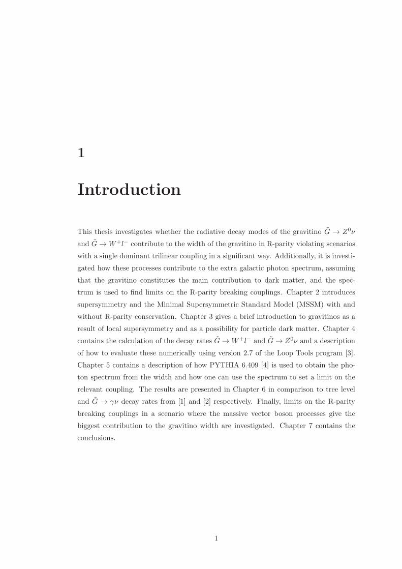
This thesis investigates whether the radiative decay modes of the gravitino G → Z0ν
and G→W+l− contribute to the width of the gravitino in R-parity violating scenarios
with a single dominant trilinear coupling in a significant way. Additionally, it is investi-
gated how these processes contribute to the extra galactic photon spectrum, assuming
that the gravitino constitutes the main contribution to dark matter, and the spec-
trum is used to find limits on the R-parity breaking couplings. Chapter 2 introduces
supersymmetry and the Minimal Supersymmetric Standard Model (MSSM) with and
without R-parity conservation. Chapter 3 gives a brief introduction to gravitinos as a
result of local supersymmetry and as a possibility for particle dark matter. Chapter 4
contains the calculation of the decay rates G→W+l− and G→ Z0ν and a description
of how to evaluate these numerically using version 2.7 of the Loop Tools program [3].
Chapter 5 contains a description of how PYTHIA 6.409 [4] is used to obtain the pho-
ton spectrum from the width and how one can use the spectrum to set a limit on the
relevant coupling. The results are presented in Chapter 6 in comparison to tree level
and G → γν decay rates from [1] and [2] respectively. Finally, limits on the R-parity
breaking couplings in a scenario where the massive vector boson processes give the
biggest contribution to the gravitino width are investigated. Chapter 7 contains the
conclusions.
1

1. INTRODUCTION
2
2
Supersymmetry
This chapter contains a brief introduction to supersymmetry, the general supersym-
metric Lagrangian and the Minimal Supersymmetric Standard Model (MSSM). It is
inspired by Martin [5], Wiedemann and Muller-Kirsten [6] and the lectures in FYS5190
at the University of Oslo. The notation used in this thesis follows closely the one used
by Wiedemann and Muller-Kirsten. The conventions and definitions used in this thesis
can be found in Appendix A.1.
Supersymmetric (SUSY) field theories are quantum field theories that can be con-
structed from extending the space-time symmetries to include gauge symmetries. In
the following a general supersymmetric Lagrangian is derived, and then the most pop-
ular supersymmetric theory, the MSSM, is summarized with the extension of including
R-parity breaking terms.
2.1 The Superpoincare algebra and the general SUSY La-
grangian
2.1.1 Superpoincare algebra and its representations
The internal symmetries of space-time are contained in the restricted Poincare group,
whose generators are the generators of Lorentz transformationsMµν and the generators
for translation Pµ, where a general Lorentz transformation Λµν = [exp(− i
2ωρσMρσ)]
µν
is restricted to detΛ = 1 and Λ00 ≥ 1. This removes space reflections and makes sure
time moves in the forward direction. The generators of the group fulfill the following
3
2. SUPERSYMMETRY
Lie algebra
[Mµν ,Mρσ] = −i (gµρMνσ − gµσMνρ − gνρMµσ + gνσMµρ) , (2.1)
[Pµ, Pν ] = 0, (2.2)
[Mµν , Pρ] = −i (gµρPν − gνρPµ) . (2.3)
It was shown by Haag, Lopuszanski and Sohnius [7] that the most general non-
trivial way of extending this symmetry is by constructing a graded Lie algebra, or
superalgebra. This is done by introducing N new sets of operators, the Majorana
spinor charges Qαa with a = 1, 2, 3, 4 and α = 1, ..., N . One can introduce up to N = 8
such sets of operators before the theory is not renormalizable as fields with spin larger
than two emerge. This thesis looks at N = 1 supersymmetry, where only one such set
is introduced. These new operators can be constructed with the Weyl spinors QA and
QA where A, A = 1, 2,
Qa =
(
QA
QA
)
. (2.4)
These spinors fulfill the following algebra:
QA, QB =
QA, QB
= 0, (2.5)
QA, QB = 2σµABPµ, (2.6)
[QA, Pµ] =[
QA, Pµ
]
= 0 and (2.7)
[QA,Mµν ] = iσµνA
BQB . (2.8)
To find what kind of particles these operators act on, meaning what the properties of
the elements in the vector spaces that a given irreducible representation of the algebra
act on are, one finds the Casimir operators of the algebra. The Casimir operators are
operators that commute with all elements in the algebra. They are
P 2 ≡ PµPµ, (2.9)
and
C2 ≡ CµνCµν , (2.10)
where
Cµν ≡ BµPν −BνPµ, (2.11)
4
2.1 The Superpoincare algebra and the general SUSY Lagrangian
and where Bµ is given by
Bµ ≡Wµ +1
4Xµ, (2.12)
and
Xµ ≡ QBσBAµ QA. (2.13)
Schur’s lemma states that in any irreducible representation of a Lie algebra, the Casimir
operators are proportional to the identity. The states on which the operators in a given
representation act can therefore be classified with respect to the eigenvalues under
operations of the Casimir operators. Any state in a given representation can be labeled
with an eigenvalue under P 2, labeled m2, and under C2, labeled −m4j(j + 1). The
first eigenvalue is interpreted as the mass squared, such that a state in a representation
with mass m and quantum number j fulfills
P 2|m, j〉 = m2|m, j〉 and (2.14)
C2|m, j〉 = −m4j(j + 1)|m, j〉. (2.15)
The following calculations are done for a massive state in its rest frame. This can be
done in a similar way for massless particles, by transforming to a frame that is boosted
in one direction. However, since the Casimir operators commute with all elements in
the algebra the result below is valid for any state. In the rest frame of the particle Pµ
reduces to
Pµ = (m,~0). (2.16)
This leads to
C2 = 2m2B2 − 2m2B20 = 2m2BkB
k, (2.17)
where
Bk =Wk −1
4QBσ
BAk QA, (2.18)
where Ji =1mBi is a generalization of the spin operator Si that fulfills the spin algebra
[Jk, Jl] = iǫklmJm. (2.19)
One can show in the rest frame of the particle that Wi = mSi such that
mJk = mSk −1
4QBσ
BAk QA. (2.20)
5
2. SUPERSYMMETRY
Because Jk fulfills Eq. (2.19), a general state in a representation with the quantum
numbers m and j can now be quantized by the quantum number j3, where j can take
half integer values, while j3 = −j,−j+1, ..., j−1, j. It can be shown that Jk commutes
with the operators QA and QA.
For a given state with quantum numbers |m, j, j3〉 there exists a state |Ω〉, calledthe Clifford vacuum, which fulfills
Q1|Ω〉 = Q2|Ω〉 = 0. (2.21)
The definition in Eq. (2.21) in combination with Eq. (2.20) gives that a Clifford vacuum
state has
Jk|Ω〉 = Sk|Ω〉 = jk|Ω〉. (2.22)
This means that the state |Ω〉 has total spin s = j and spin in a chosen direction
s3 = j3. There exist four different states with the same quantum numbers j, j3 and
m but different quantum numbers s and s3, from combinations of this state and the
operators QA. These are
|Ω〉m,j,j3, Q1|Ω〉m,j,j3 , Q
2|Ω〉m,j,j3 and Q1Q
2|Ω〉m,j,j3. (2.23)
As J3 commutes with the spinors, the spin in one direction for the state QC |Ω〉m,j,j3 can
now be found using the anti-commutation relations for the spinor charges in Eq. (2.6)
S3QC |Ω〉m,j,j3 = J3Q
C |Ω〉m,j,j3 −1
4mQBσ
BA3 QAQ
C |Ω〉m,j,j3
= QCJ3|Ω〉m,j,j3 −
1
4m(Q1Q1 −Q2Q2)Q
C |Ω〉m,j,j3
= QCj3|Ω〉m,j,j3 −
1
4mQ1(Q
CQ1 − 2mσ01
DǫDC)|Ω〉m,j,j3
+1
4mQ2(Q
CQ2 − 2mσ02
DǫDC)|Ω〉m,j,j3
= j3QC |Ω〉m,j,j3 +
1
2(Q1σ
01DǫDC −Q2σ
02DǫDC)|Ω〉m,j,j3 .(2.24)
This gives for the states Q1|Ω〉m,j,j3 and Q
2|Ω〉m,j,j3 :
S3Q1|Ω〉m,j,j3 =
(
j3 +1
2
)
Q1|Ω〉m,j,j3 (2.25)
S3Q2|Ω〉m,j,j3 =
(
j3 −1
2
)
Q2|Ω〉m,j,j3 . (2.26)
6
2.1 The Superpoincare algebra and the general SUSY Lagrangian
Similarely one can show that
S3Q1Q
2|Ω〉m,j,j3 = j3Q1Q
2|Ω〉m,j,j3 . (2.27)
This means that if the states |Ω〉m,j,j3 and Q1Q
2|Ω〉m,j,j3 are bosonic, then the states
Q1|Ω〉m,j,j3 and Q
2|Ω〉m,j,j3 are fermionic, and vice versa. This means two things.
Firstly, the Majorana spinor charges transform between fermionic and bosonic degrees
of freedom, and secondly there exist exactly as many fermionic degrees of freedom as
bosonic degrees of freedom in any supersymmetric theory.
2.1.2 Superspace and superfields
Salam and Strathdee [8] show that a general element in the coset space of the Super-
poincare group and the Lorentz group SP/L can be expressed by a set of coordinates
called superspace coordinates Zπ = (xµ, θA, θA) as follows:
L(x, θ) = exp[−ixµPµ + iθAQA + iθAQA]. (2.28)
Here θA and θA are Grassmann numbers that anti-commute. The elements of the
algebra that are on the form L(x0, θ) where xµ0 = (0,~0), are called SUSY transforma-
tions. As this are transformations containing only the Majorana spinor charges, they
transform between fermionic and bosonic degrees of freedom, as shown in the previous
section.
Grassmann calculus, as defined in Appendix A.1, allows any function of superspace
coordinates to be expanded in orders of θ as shown in Eq. (A.11). A general function
of superspace coordinates is called a superfield. After second quantization it is an
operator valued function, that creates and annihilates particles. The component fields
in the superfield can be constructed from the states described in the previous section.
A general superfield can be written as
Φ(x, θ, θ) = f(x) + θAϕA(x) + θAχA(x) + θθm(x) + θθn(x)
+θσµθVµ(x) + θθθAλA(x) + θθθAψA(x) + θθθθd(x). (2.29)
As shown in the literature, e.g. in Chapter 6.5 of [6], one can find covariant derivatives
that commute with all SUSY transformations. These are
DA = ∂A + i(σµθ)A∂µ and (2.30)
DA = −∂A − i(θσµ)A∂µ. (2.31)
7
2. SUPERSYMMETRY
One can define two types of superfields that are more restricted than the general su-
perfield. The left handed scalar superfield fulfills
DAΦ(x, θ, θ) = 0. (2.32)
This leads to the general form of a left handed scalar superfield (also called a chiral
superfield)
Φ(x, θ, θ) = A(x) + i(θσµθ)∂µA(x)−1
4θθθθA(x)
+√2θψ(x)− i√
2θθ∂µψ(x)σ
µθ + θθF (x), (2.33)
where A(x) and F (x) are complex scalar fields and ψ(x) is a left handed Weyl spinor
field. Taking the Hermitian conjugate of this field one gets a so-called right handed
scalar superfield, which contains two scalar fields and one right handed Weyl spinor
field.
The vector superfield fulfills
Φ†(x, θ, θ) = Φ(x, θ, θ). (2.34)
Its general form is
Φ(x, θ, θ) = C(x) + θϕ(x) + θϕ(x) + θθM(x) + θθM∗(x)
+θσµθVµ(x) + θθθλ(x) + θθθλ(x) + θθθθD(x). (2.35)
Here C(x) andD(x) are real scalar fields, V µ(x) is a real vector field,M(x) is a complex
scalar field and ϕ(x) and λ(x) are left handed Weyl spinor fields.
2.1.3 The supergauge transformations
The vector superfield contains a high number of component fields. In order for it to
describe a vector boson and its super partner, it should contain no more then one left-
handed spinor field and one complex vector field. The highest order auxiliary field D(x)
can be removed through the equations of motion, as will be discussed in Section 2.1.5.
One can, however, define the abelian supergauge transformation of a vector superfield
V (x, θ, θ) as
V (x, θ, θ) → V ′(x, θ, θ) ≡ V (x, θ, θ) + Φ(x, θ, θ) + Φ†(x, θ, θ), (2.36)
8
2.1 The Superpoincare algebra and the general SUSY Lagrangian
where Φ(x, θ, θ) is a left handed chiral superfield. This leads to the following transfor-
mations of the component fields of the vector superfield:
C(x) → C ′(x) = C(x) +A(x) +A∗(x) (2.37)
ϕ(x) → ϕ′(x) = ϕ(x) +√2Ψ(x) (2.38)
M(x) → M ′(x) =M(x) + F (x) (2.39)
Vµ(x) → V ′µ(x) = Vµ(x) + i∂µ(A(x)−A∗(x)) (2.40)
λ(x) → λ′(x) = λ(x) (2.41)
D(x) → D′(x) = D(x) (2.42)
These transformations can be used to remove degrees of freedom using the Wess-Zumino
gauge, where one chooses the scalar field to have the component fields ψ(x) = − 1√2ϕ(x),
F (x) = −M(x), A(x) + A∗(x) = −C(x), removing these fields and leaving standard
Abelian gauge freedom in terms of Im[A(x)]. This leads to the vector field in the
Wess-Zumino gauge.
VWZ(x, θ, θ) = (θσµθ)[Vµ(x) + i∂µ(A(x)−A∗(x))] + θθθλ(x) + θθθλ(x) + θθθθD(x).
(2.43)
The abelian supergauge transformation on a chiral field is defined as
Φi → Φ′i ≡ e−iΛ(x)qiΦi, (2.44)
where qi is the charge of the field under the U(1) transformation. From requiring that
Φ′i is a left handed chiral field, one gets that Λ(x) must be a left handed chiral field.
In the more general non-Abelian case, where the gauge group has the generators ta,
the transformation is
Φ → Φ′ ≡ e−iqΛ(x)ataΦ, (2.45)
where again Λ(x)a is a set of left handed chiral fields. The non-Abelian definition of a
supergauge transformation for a vector superfield is the following
eqV′ata ≡ eqΦ
†ataeqVataeqΦ
ata , (2.46)
and renaming Φa = iΛa one gets
eqV′ata = e−iqΛ†ataeqV
ataeiqΛata . (2.47)
9
2. SUPERSYMMETRY
This can again be used to remove the superfluous degrees of freedom from the vector
superfield, leaving it in the Wess-Zumino gauge as is shown by Ferrara and Zumino in
[9].
2.1.4 A general supersymmetric Lagrangian
Connecting the pieces above, one can write down a general Lagrangian for a supersym-
metric theory constructed of superfields. The action S ≡∫
R d4xL is to be invariant
under SUSY transformations and under generalized gauge transformations. This is
the case, if the Lagrangian density satisfies L′ = L + ∂µf(x) where f(x) → 0 on the
boundaries of R. It can be shown, see e.g. Chapter 6.8 of [6], that the highest order of
theta component of any superfield d(x) transforms under global SUSY transformations
as
d′(x)− d(x) =i
2(∂µψ(x)σ
µα− ∂µλ(x)σµα), (2.48)
which is a total derivative. If all components of the Lagrangian are of highest order in
θ, one guarantees that the resulting action is invariant under SUSY transformations.
Equation (A.13) shows that integrating over a volume element in Grassmann calculus
projects out terms that go with highest order in θ, such that one can write a manifestly
SUSY invariant Lagrangian as
L =
∫
d4θL. (2.49)
Here L is the supersymmetric Lagrangian density. It was shown byWess and Bagger [10]
that this density can not contain more than third order in chiral fields for it to be
renormalizable. This leaves the following possibilities, using only chiral fields Φi,
L = Φ†iΦi + θθW [Φ] + θθW [Φ†]. (2.50)
Here the first term is called the kinetic term, while W is the superpotential. It is
defined as
W [Φ] = giΦi +mijΦiΦj + λijkΦiΦjΦk, (2.51)
where the first term is called the tadpole term, the second is the mass term and the third
the Yukawa term. This is to be invariant under the generalized gauge transformations
as well. This sets a number of restrictions on the superpotential. They are (for a
10
2.1 The Superpoincare algebra and the general SUSY Lagrangian
general non-Abelian transformation with the matrix representation Uij):
gi = 0 if giUir 6= gr, (2.52)
mij = 0 if mijUirUjs 6= mrs, (2.53)
λijk = 0 if λijkUirUjsUkt 6= λrst, (2.54)
where U = (e−iqΛata). For the kinetic term this is a bit more tricky. It transforms as:
Φ′†iΦ
′i = Φ†
ieiqΛa†tae−iqΛataΦi. (2.55)
To compensate for the change in the term, one introduces a set of vector superfields
that transform like in Eq. (2.47). This leads to introducing a kinetic term:
Φ†eqVataΦ → Φ′†eqV
′ataΦ′ = Φ†eiqΛa†tae−iqΛ†ataeqV
ataeiqΛatae−iqΛataΦ = Φ†eqV
ataΦ.
(2.56)
The field strength terms of the fields V a can, as shown in the literature, e.g. Chap-
ter 7.3 of [6], be written1
2T (R)TrWAWAθθ, (2.57)
where
WA ≡ −1
4DDe−V ataDAe
V ata , (2.58)
and where the Dynkin index is given by
T (R)δab = Tr[tatb]. (2.59)
The complete Lagrangian density of a supersymmetric theory is then in terms of su-
perfields given as
L =
∫
d4θΦ†ie
qV ataΦi + θθW [Φ] + θθW [Φ†] +1
2T (R)TrWAWAθθ. (2.60)
The theory described by this Lagrangian density is by construction invariant under
global SUSY transformations.
It was shown by Ferrara et al. [11] that the supertrace, which is a weighted sum of
eigenvalues of the mass matrix in a SUSY theory, vanishes at tree level. This means
that the masses of Standard Model particles and their supersymmetric partners can not
be split arbitrarily, which has as a consequence that this theory contains light scalar
partners to Standard Model fermions, and light fermionic partners to Standard Model
11
2. SUPERSYMMETRY
gauge bosons. This is not observed in experiments. To explain this, supersymmetry
must be broken such that the new scalar and fermionic particles gain mass. There have
been different schemes proposed to break supersymmetry. All of them introduce so
called soft terms, which are called soft because these terms contribute with a factor no
worse then logarithmically in divergent loop corrections for scalar masses, as discussed
in Section 2.2.4. These soft terms parametrize SUSY-breaking and give additional
masses to supersymmetric particles. Their general form is
Lsoft = − 1
4T (R)MθθθθTrWAWA −
1
6aijkθθθθΦiΦjΦk
−1
2bijθθθθΦiΦj − tiθθθθΦi + h.c.
−m2ijθθθθΦ
†iΦj. (2.61)
Additionally, there are so-called maybe-soft terms
Lmaybe−soft = −1
2cijkθθθθΦ
†iΦjΦk + h.c., (2.62)
which are soft as long as none of the scalar superfields is a singlet under all gauge
symmetries. In this thesis the details of SUSY breaking are ignored, and the scalar
masses are taken to be free parameters. However, the soft-breaking terms are generally
thought to be the result of spontaneous SUSY-breaking in a hidden sector that enters
at some high scale. It is also important to note that theories with Lagrangians on the
same form as shown in Eq. (2.60) are invariant under global SUSY transformations only.
If one constructs a theory with local SUSY invariance, one must introduce new fields
which lead to supergravity and contain the massive spin-3/2 gravitino, as discussed by
Freedman, van Nieuwenhuizen and Ferrara [12]. Chapter 3 contains a more detailed
discussion of gravitinos.
2.1.5 Lagrangians of component fields.
It was mentioned above that the auxiliary fields F (x) and D(x) vanish by virtue of the
equations of motion for the Lagrangian. In addition, one needs to find the Lagrangian
density in terms of component fields to be able to calculate in terms of said component
fields. Chapter 8 in Wiedemann and Muller-Kirsten [6] contains explicit derivations of
all terms in a general Lagrangian build of vector and chiral fields. To do the derivation
12
2.2 Building the MSSM
one needs to remember that the only components of the super-Lagrangian that survive
the integral are the ones that have highest order in theta.
As an example we can take a general chiral field Φi with component fields as in
Eq. (2.33) and without any gauge fields to get the Lagrangian density
L = −A∗iAi + |Fi|2 + i(∂µψ
†i )σ
µψi
+[giFi +mij(AiFj + FiAj + 2ψiψj)
+λijk(AiAjFk +AiFjAk + FiAjAk
+ψiψjAk + ψiAjψk +Aiψjψk) + h.c.]. (2.63)
Here some total derivatives were removed. Looking on the Euler-Lagrange functions
for the auxiliary field F (x) one can see that
∂µL
∂(∂µFi)− ∂L
∂Fi= 0 gives (2.64)
2Fi + [gi +mijAj + λijkAjAk + h.c.] = 0. (2.65)
This can be solved for Fi to replace all Fi in the Lagrangian, as promised above. This
leads to
L = i(∂µψ†i )σ
µψi −A∗iAi
−1
2Wijψiψj −
1
2W ijψ
†iψ
†j − |Wi|2 (2.66)
where
Wi =W [A1, A2..., An]
∂Ai(2.67)
Wij =W [A1, A2..., An]
∂Ai∂Aj. (2.68)
For the auxiliary field D(x) a similar derivation can be done, such that the auxiliary
field D(x) can be replaced in the Lagrangian.
2.2 Building the MSSM
The Lagrangian (2.60) describes a general theory. One would like to construct a theory
that contains the fields/particles measured that make up the Standard Model. The
Minimal Supersymmetric Standard Model (MSSM) is a minimal version of this theory.
It is minimal in the sense that it contains the least amount of superfields with which
one can construct a theory containing all fields and couplings of the Standard Model.
13
2. SUPERSYMMETRY
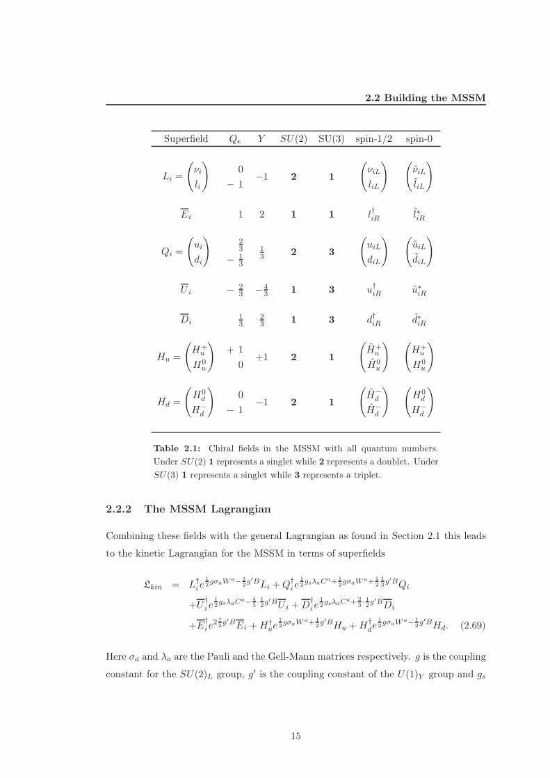
2.2.1 The superfields of the MSSM
The superfields needed to construct all Standard Model particles and give them their
Standard Model masses are given in Table 2.1 on the facing page and Table 2.2 on
page 16. The Standard Model fermion fields emerge as the spin-1/2 components of the
left handed scalar superfields Li, Ei, Qi, U i and Di. The remaining spin-0 components
form the superpartners of these fields, called sleptons, sneutrinos and squarks. The
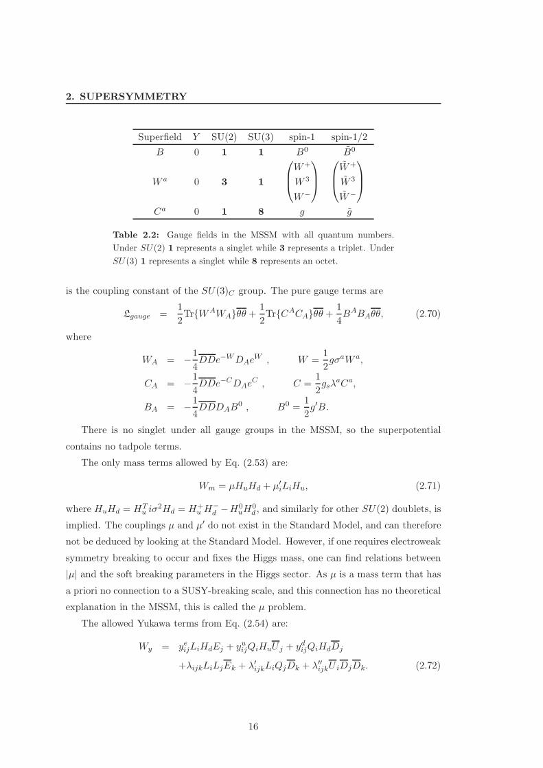
Standard Model gauge fields emerge as the spin-1 parts of the vector superfields B,
W a and Ca. The remaining spin-1/2 components form the superpartners of the gauge
fields, called bino, wino and gluino. Note that the bars over the names of the fields do
not designate conjugation, but are part of the name of the field. The fields responsible
for the Higgs boson are a bit more complicated. Because one can only include chiral
left-handed fields in the superpotential, one needs to introduce two Higgs-doublet su-
perfields to be able to give mass to both up-type and down-type quarks. Radiative
electroweak symmetry breaking, see e.g. Section 7.1 of Martin [5], leads to the mixing
of the scalar component fields of the Higgs superfields as presented in Table 2.1, to
mass eigenstates h0, H0, H± and A0. The scalar field h0 (called the light Higgs field)
is the Standard Model equivalent of the Higgs particle. Additionally there exist four
fermionic Higgs fields, called Higgsino fields. The bino, wino and Higgsino states that
have equal charge mix to mass eigenstates and form four neutralinos and two charginos.
As the Standard Model equivalents have the measured properties of the Standard
Model particles, their masses and couplings are given by the Standard Model couplings
and masses. Note that as the Higgs fields are constructed in a different way, the
couplings of the Higgs fields are not the same as in the Standard Model, but have
a direct relation. However, as none of the superpartners are measured to this date,
superpartners and the extra Higgs fields need to have considerably higher masses than
the Standard Model fields except in certain limited corners of parameter space.
14
2.2 Building the MSSM
Superfield Qe Y SU(2) SU(3) spin-1/2 spin-0
Li =
(
νi
li
)
−1 2 1
(
νiL
liL
) (
νiL
liL
)
0
− 1
Ei 1 2 1 1 l†iR l∗iR
Qi =
(
ui
di
)
13 2 3
(
uiL
diL
) (
uiL
diL
)
23
− 13
U i − 23 −4
3 1 3 u†iR u∗iR
Di13
23 1 3 d†iR d∗iR
Hu =
(
H+u
H0u
)
+1 2 1
(
H+u
H0u
) (
H+u
H0u
)
+ 1
0
Hd =
(
H0d
H−d
)
−1 2 1
(
H−d
H−d
) (
H0d
H−d
)
0
− 1
Table 2.1: Chiral fields in the MSSM with all quantum numbers.
Under SU(2) 1 represents a singlet while 2 represents a doublet. Under
SU(3) 1 represents a singlet while 3 represents a triplet.
2.2.2 The MSSM Lagrangian
Combining these fields with the general Lagrangian as found in Section 2.1 this leads
to the kinetic Lagrangian for the MSSM in terms of superfields
Lkin = L†ie
12gσaW a− 1
2g′BLi +Q†
ie12gsλaCa+ 1
2gσaW a+ 1
213g′BQi
+U†ie
12gsλaCa− 4
3· 12g′BU i +D
†ie
12gsλaCa+ 2
3· 12g′BDi
+E†ie
2 12g′BEi +H†
ue12gσaW a+ 1
2g′BHu +H†
de12gσaW a− 1
2g′BHd. (2.69)
Here σa and λa are the Pauli and the Gell-Mann matrices respectively. g is the coupling
constant for the SU(2)L group, g′ is the coupling constant of the U(1)Y group and gs
15
2. SUPERSYMMETRY
Superfield Y SU(2) SU(3) spin-1 spin-1/2
B 0 1 1 B0 B0
W+
W 3
W−
W+
W 3
W−
W a 0 3 1
Ca 0 1 8 g g
Table 2.2: Gauge fields in the MSSM with all quantum numbers.
Under SU(2) 1 represents a singlet while 3 represents a triplet. Under
SU(3) 1 represents a singlet while 8 represents an octet.
is the coupling constant of the SU(3)C group. The pure gauge terms are
Lgauge =1
2TrWAWAθθ +
1
2TrCACAθθ +
1
4BABAθθ, (2.70)
where
WA = −1
4DDe−WDAe
W , W =1
2gσaW a,
CA = −1
4DDe−CDAe
C , C =1
2gsλ
aCa,
BA = −1
4DDDAB
0 , B0 =1
2g′B.
There is no singlet under all gauge groups in the MSSM, so the superpotential
contains no tadpole terms.
The only mass terms allowed by Eq. (2.53) are:
Wm = µHuHd + µ′iLiHu, (2.71)
where HuHd = HTu iσ
2Hd = H+u H
−d −H0
uH0d , and similarly for other SU(2) doublets, is
implied. The couplings µ and µ′ do not exist in the Standard Model, and can therefore
not be deduced by looking at the Standard Model. However, if one requires electroweak
symmetry breaking to occur and fixes the Higgs mass, one can find relations between
|µ| and the soft breaking parameters in the Higgs sector. As µ is a mass term that has
a priori no connection to a SUSY-breaking scale, and this connection has no theoretical
explanation in the MSSM, this is called the µ problem.
The allowed Yukawa terms from Eq. (2.54) are:
Wy = yeijLiHdEj + yuijQiHuU j + ydijQiHdDj
+λijkLiLjEk + λ′ijkLiQjDk + λ′′ijkU iDjDk. (2.72)
16
2.2 Building the MSSM
Since the Standard Model particles have their (measured) masses, one can identify the
Yukawa couplings yeij , yuij and ydij with the ones between the corresponding Standard
Model fields and the Higgs field. However, the couplings λijk, λ′ijk and λ′′ijk do not exist
in the Standard Model, and can therefore not be deduced by looking at the Standard
Model. Additionally, there are soft breaking terms on the form shown in Eq. (2.61).
These are not listed here. Instead the masses of the supersymmetric particles are used
as free parameters in the calculation in this thesis.
2.2.3 R-parity and alternatives
In the superpotential (2.72), terms in the second line break lepton or baryon number.
These allow the proton to decay, and if both a lepton number violating and a baryon
number violating coupling exists it can even decay at tree level. As measurements
tell us that the proton lifetime is τp > 2.1 × 1029 years [13], the concept of R-parity,
a multiplicative conserved quantum number, was introduced by Fayet [14]. This is
defined by
PR = (−1)2s+3B+L (2.73)
where B is baryon number, L is lepton number and s is the spin of the particle. This
forbids the Yukawa terms that have the couplings λijk, λ′ijk and λ′′ijk and the mass
term with the coupling µ′ from the superpotential, and has the consequence that the
supersymmetric partners in the theory can only be produced and destroyed in pairs.
There are, however, few good theoretical arguments within grand unified theories or
string theories for R-parity conservation in the MSSM [15]. Additionally, the proton
can be made stable by virtue of other symmetries. One can observe that at tree level
both baryon and lepton number have to be broken to allow the proton to decay into
a lepton and a pion. This means that at least two of the couplings are needed in
the decay. As an alternative one can propose lepton or baryon triality [16, 17], where
either leptons or baryons get a new parity that is conserved. The consequence of barion
triality is that the trilinear couplings λ′′ijk are forbidden, while lepton triality forbids µ′,
λijk and λ′ijk. As the decays in this thesis break lepton number, baryon triality allows
the couplings used. There are direct limits on individual fermion number violation as
well, which limit the extent to which any given lepton number and baryon number can
be broken. These can be found in the latest review of particle physics data [13].
17
2. SUPERSYMMETRY
2.2.4 Reasons for a supersymmetric model
This far the only reason why one would construct a supersymmetric model quoted is
that such a model is the largest possible extension of special relativity. In the following,
further indications for SUSY are given.
Already in the 1930s Zwicky [18] observed that the dispersion of the velocities of
galaxies can not be explained by visible matter. Since then an overwhelming amount
of evidence for this has been found, for which Zwicky coined the term dark matter.
Dark matter has no electromagnetic couplings, meaning that any cosmologically stable,
neutral and massive particle can in principle be dark matter. The measured dark matter
density is ΩDMh2 ≡ (ρDM/ρc)h
2 = 0.1123 ± 0.0035 [19] where the critical density is
ρc = 1.05 ·10−5h2GeV/cm3 and h is the unitless Hubble constant. Many particles have
been proposed as candidates for dark matter, see e.g. reviews by Bertone, Hooper and
Silk [20], but the only Standard Model candidate are neutrinos. One can set an upper
limit on the abundance of Standard Model neutrinos in the universe of Ωνh2 < 0.0067
at 95% confidence level [20]. This means that the total dark matter content of the
universe is not completely explained by the Standard Model.
The MSSM with R-parity conservation intact, however, yields natural candidates if
the lightest supersymmetric particle (LSP) has neutral electric charge. In fact, if any
weakly interacting massive particle (WIMP) χ exists and is stable, it is automatically
a prime dark matter candidate. A particle is weakly interacting if its couplings are
on the order of the weak interactions αweak ≈ 10−2. The reason for this is that the
calculated dark matter density from WIMPs, see e.g. [21], is approximately Ωχh2 ≈
0.1 × (αweak/α)2 for a particle with a mass in the order of 100 GeV. This means
that the MSSM with a neutralino LSP with a mass of about 100 GeV would lead to
about the right dark matter density. This is a strong argument for SUSY. Axinos, the
superpartners of axions, sneutrinos and gravitinos are other possible SUSY dark matter
candidates. In this thesis gravitino dark matter is discussed in Section 3.3.
From measurements of the properties of the weak interactions one can find that
m2H ∼ O(100 GeV), and the LHC has seen some evidence of Higgs particles with mass
at that scale [22, 23, 24]. If one calculates the loop calculations to the Higgs mass ∆m2H
for a Higgs particle coupling to two fermions f with the coupling λf , see e.g. [5], one
18
2.2 Building the MSSM
gets that the contribution is proportional to the cut-off squared as
∆m2H = −|λf |2Λ2
UV /(8π2) +O(|λf |4), (2.74)
where ΛUV is the cut off scale, often taken to be the Planck scale mP = 2.4×10¹⁸ GeV.
In the Standard Model the most important coupling is the top-quark coupling, which
is of order of magnitude 1. This leads to corrections that are 1016 times bigger than
O(100 GeV). This is the so called hierarchy problem. In unbroken SUSY, however, the
Higgs mass is protected by scalar particle loops which couple with λs. They contribute
as
∆m2H = λsΛ
2UV /(16π
2) +O(λ2s), (2.75)
and one has λs = |λf |2 and twice as many scalar particles as fermions, such that all
contributions cancel exactly.
In theories where SUSY is broken the the Higgs mass gets extra contributions.
These are chosen in such a way that a scalar particle with mass ms contributes with
at most
∆m2H = −(λs/16π
2)m2s ln
Λ2UV
m2s
, (2.76)
Couplings like this are called soft, and the couplings used in softly broken supersym-
metric theories are written down in Eq. (2.61) and Eq. (2.62). As long as there is
SUSY below the TEV scale, the loop corrections to the Higgs mass are of the order
∼ O(10 GeV). This is another strong indication for SUSY at relatively low energies.
2.2.5 MSSM with R-parity violation at particle colliders
As mentioned above, not a single supersymmetric particle has been found in any collider
experiment up until now. One can use the non-detection to set limits on the crossection
of a given process, and given that one can calculate crossections in the MSSM, one can
set limits on the parameters of the MSSM. This turns out to be an extremely hard
exercise. The main reason for this is that the parameter space is complex and hard to
understand. More constrained models, like the CMSSM, give better limits, but even
in these the parameter space can be hard to handle. In R-parity conserving (RPC)
supersymmetric theories the experimental signatures are expected to be decay chains
which give multiple leptons or quarks and missing energy. This is because any produced
SUSY particle cascades to the LSP which is stable.
19
2. SUPERSYMMETRY
In R-parity violating (RPV) theories SUSY particles decay in the detector unless
the RPV coupling λ is very small. A simple dimensional analysis gives for a massive
particle with mass ms and a dimensionless coupling λ with which it can decay, an
approximate decay rate of Γ ∼ λ2ms, such that the decay time for ms = 100 GeV can
be written as τ ∼ (10−28/λ2) s. The decay length is then given by
l = γτ ∼ 10−20/λ2(E/ms) m (2.77)
where E is the energy of the particle in the lab frame. As an example, the ATLAS
detector at the LHC has a distance of 5 cm between the beam and the innermost pixel
detectors. Assuming that the particle has an energy on the TeV scale, one gets that
for λ2 & 10−8 the particle decays before it hits the pixel detector. A conservative
estimate is therefore that with a coupling strength of λ ≥ 10−6, a sparticle with a mass
of O(100 GeV) decays promptly, i.e. before it can be seen to have moved away from the
interaction point. The collider signature is then multi-lepton/multi-jet events from the
LSP decay through the RPV couplings. In particular for models with a gravitino LSP
and R-parity violation one expects all heavier particles to decay inside the detector
to Standard Model particles as the gravitino inherits its couplings from gravitational
theory as presented in Section 3.1 with the consequence that decays to a gravitino LSP
are extremely suppressed.
20
3
The Gravitino
The action of the theory in the previous chapter can be made invariant under local
SUSY transformations. This is called supergravity. An important consequence of
making the transformations local is the emergence of a massless spin-3/2 Majorana
fermion field which is the super partner of the spin-2 graviton, called the gravitino
field. That the field is a Majorana field means that its particle is identical to its anti-
particle. This field can obtain a mass mG via the so-called super-Higgs mechanism, see
e.g. Freedman et al. [12], when local SUSY is spontaneously broken.
In this thesis the low-energy phenomenological consequences of the gravitino, irre-
spective of the supergravity theory and the SUSY-breaking scheme, are investigated.
This means that the gravitino mass mG is kept as a free parameter.
3.1 The gravitino Lagrangian
Following Cremmer et al. [25] the dimension-5 terms of the effective supergravity La-
grangian are
L = − i√2M
[(D∗µφ
∗)ψνγµγνPLχ−(Dµφ)χPRγ
νγµψµ]−i
8Mψµ[γ
ν , γρ]γµλaF aνρ. (3.1)
Here χ designate chiral fermion fields, φ their superpartners, Dµ is the covariant deriva-
tive given by Dµφi = (∂µδ
ij + igT aijA
aµ)φ
j , F aµν is the field strength tensor of the gauge
fields Aaµ:
F aµν = ∂µA
aν − ∂νA
aµ − gfabcAb
µAcν , (3.2)
21
3. THE GRAVITINO
where g is the gauge coupling, λa are the superpartner gaugino fields, ψµ is the grav-
itino field, and M = mpl/√8π where mpl =
√
~c/G ≈ 1.2209× 10¹⁹ GeV is the Planck
mass. Higher order terms are suppressed by additional factors of msc/M in low energy
phenomenology, where msc is a mass scale of particles involved. Standard Model parti-
cles and their supersymmetric partners considered in this thesis are much lighter then
the Planck scale and the higher order terms are therefore ignored. This is an effective
theory and is only valid in the limit where the momentum of the gravitino is small
compared to the Planck mass. As this thesis considers gravitinos as cold dark matter
that have little kinetic energy, this is not an issue here.
3.2 Spin-3/2 particles
This section is a short introduction to spinor algebra for Majorana spin-3/2 fields. As
mentioned above, a spin-3/2 field emerges when supersymmetry is made local. In the
notation developed by Rarita and Schwinger [26] one can write the equations of motion
for a spin-3/2 field with momentum p and mass m =√
p2 as
γµψµ(p) = 0 (3.3)
(/p −m)ψµ(p) = 0 (3.4)
which also yield
pµψµ(p) = 0. (3.5)
These are known as the Rarita-Schwinger equations. Here ψµ is a vector-spinor, where
the Dirac index is suppressed such that the components of the four vector are Dirac
spinors. These vector-spinors can be constructed by combining Dirac spinors for spin-
1/2 particles with polarization vectors of massive spin-1 particles as follows (see e.g.
Bolz [27] page 6):
ψl+µ (P ) =
∑
s,k
C(l, s, k)us(p)ǫkµ (3.6)
ψl−µ (P ) =
∑
s,k
C(l, s, k)vs(p)ǫkµ. (3.7)
Here C(l, s,m) are Clebsch-Gordon coefficients, l = +3/2,+1/2,−1/2,−3/2 is the
helicity index of the spin-3/2 particle, s = ±1/2 is the spinor index of the spinor
22
3.2 Spin-3/2 particles
and k = +1, 0,−1 is the helicity index of the polarization vector. As the field is a
Majorana field, the charge conjugated wave function equals the wave function itself. In
the following the positive solution will be used, leaving out the + in the equations. A
similar derivation can be constructed for the negative solution. The Dirac spinors are
normalized as
usus′
= 2mδss′
, (3.8)
where m is the mass of the spin-3/2 particle and the polarization vectors fulfill
ǫkµǫk′∗µ = −δkk′ . (3.9)
This gives
ψlµψ
l′µ =∑
s,k,s′,k′
C(l, s, k)C(l′, s′, k′)us(p)ǫ∗kµ us′(p)ǫk
′µ, (3.10)
which can be written as
ψlµψ
l′µ = −2m∑
s,k
C(l, s, k)C(l′, s, k) = −2mδll′
, (3.11)
because of the unitarity of Clebsch-Gordon coefficients.
3.2.1 The spin sum for spin-3/2 particles
The calculation performed in Chapter 4 of this thesis will contain squared matrix
elements which are summed over all four gravitino polarizations. In the following the
polarization tensor for a spin-3/2 field with momentum p and mass m is calculated.
The spin sum
Πµν(p) =∑
l
ψlµ(p)ψ
lν(p), (3.12)
can in general contain any combination of gµν γµ and pµ, and has units of m since there
are no other masses involved. All terms have mass dimension one, as can be seen from
Eq. (3.11). This gives that the general structure of the spin-sum is
Πµν(p) = x1mgµν + x2mγµγν + x3γµpν + x4pµγν + x5pµpνm
+x7/pγµγν + x8/pγµpνm
+ x9/ppµmγν + x10/p
pµpνm2
, (3.13)
23
3. THE GRAVITINO
where all coefficients are unitless scalars. Πµν must satisfy the equations of motion
Eqs. (3.3), (3.4) and (3.5) as ψlµ is a solution of the Rarita-Schwinger equations. Con-
tracting two spin sums and using Eq. (3.11) one gets
Πλµ(p)Πλν(p) =
∑
ll′
ψlµ(p)ψ
lλ(p)ψl′
λ (p)ψl′
ν (p)
= −2m∑
ll′
ψlµ(p)δ
ll′ψl′
ν (p) = −2mΠµν(p). (3.14)
Using Eq. (3.4) one can write
0 =(
/p−m)
[
x1mgµν + x2mγµγν + x3γµpν + x4pµγν + x5pµpνm
+x6/pgµν + x7/pγµγν + x8/pγµpνm
+ x9/ppµmγν + x10/p
pµpνm2
]
. (3.15)
Splitting the sum gives
0 =(
m/p−m2)
[x1gµν + x2γµγν ]
+(
/p2 −m/p
)
[
x6gµν + x7γµγν + x8γµpνm
+ x9pµmγν + x10
pµpνm2
]
+(
m/p−m2)
[
x3γµpνm
+ x4pµmγν + x5
pµpνm2
]
. (3.16)
One can now use that /p2 = p2 = m2 and collect terms to get
0 = m(
/p−m)
[
(x1 − x6)gµν + (x2 − x7)γµγν − (x8 − x3)γµpνm
−(x9 − x4)pµmγν − (x10 − x5)
pµpνm2
]
. (3.17)
This requires that x1 = x6, x2 = x7, x3 = x8, x4 = x9 and x5 = x10, which reduces the
expression for the spin sum to
Πµν(p) =(
/p+m)
[
x1gµν + x2γµγν + x3γµpνm
+ x4pµγνm
+ x5pµpνm2
]
. (3.18)
Using Eq. (3.3) one can write
0 = γµ(
/p+m)
[
x1gµν + x2γµγν + x3γµpνm
+ x4pµγνm
+ x5pµpνm2
]
. (3.19)
Commuting γµ with(
/p+m)
gives
0 =(
2pµ − /pγµ +mγµ
)
[
x1gµν + x2γµγν + x3γµpνm
+ x4pµγνm
+ x5pµpνm2
]
. (3.20)
24
3.2 Spin-3/2 particles
Contracting µ in this and simplifying one can write this as
0 = (2x1 + x5 + 4x3) pν + (x4 + x1 + 4x2)mγν
+(−2x2 + x4 − x1) /pγν + (−2x3 + x5) /ppνm. (3.21)
This gives the four equations
0 = 2x1 + x5 + 4x3, (3.22)
0 = x4 + x1 + 4x2, (3.23)
0 = −2x2 + x4 − x1 and (3.24)
0 = −2x3 + x5. (3.25)
Solving the set of Eqs. (3.22)–(3.25) yields
x2 = −1
3x1, (3.26)
x3 = −1
3x1, (3.27)
x4 =1
3x1 and (3.28)
x5 = −2
3x1. (3.29)
This can be used to write the spin sum as a function of x1:
Πµν(p) = x1(
/p+m)
[
gµν −pµpνm2
− 1
3
(
γµγν +mγµpνm2
−mpµγνm2
− pµpνm2
)
]
. (3.30)
This can be rewritten using the commutation relations of gamma matrices and a lot of
algebra as
Πµν(p) = x1(
/p+m)
[
gµν −pµpνm2
− 1
3
(
gµρ −pµpρm2
)(
gνσ − pνpσm2
)
γργσ]
. (3.31)
It remains to find the absolute normalization in x1. Equation (3.14) can be written as
− 2mΠµν(p) = x21(
/p+m)2[
gµλ − pµp
λ
m2− 1
3
(
gµρ −pµpρm2
)
(
gλσ − pλpσm2
)
γργσ]
[
gλν −pλpνm2
− 1
3
(
gλρ′ −pλpρ′
m2
)(
gνσ′ − pνpσ′
m2
)
γρ′
γσ′
]
, (3.32)
where it was used that γργσ/p = −γρ/pγσ + 2γρpσ = /pγργσ + 2γρpσ − 2pργσ and that(
gλσ − pλpσ/m2)
pσ = 0 such that
(
gµρ −pµpρm2
)
(
gλσ − pλpσm2
)
γργσ/p = /p(
gµρ −pµpρm2
)
(
gλσ − pλpσm2
)
γργσ.
25
3. THE GRAVITINO
Contracting λ yields
− 2mΠµν(p) = 2mx21(
/p+m)
[
gµν −pµpνm2
− 1
3
(
gµρ −pµpρm2
)(
gνσ − pνpσm2
)
γργσ
−1
3
(
gµρ′ −pµpρ′
m2
)(
gνσ′ − pνpσ′
m2
)
γρ′
γσ′
+1
9
(
gµρ −pµpρm2
)
γργσ(
gσρ′ −pσpρ′
m2
)(
γρ′
γν − γρ′ pνm2 /p
)
]
. (3.33)
Here the last term can be multiplied out to give
− 2mΠµν(p) = 2mx21(
/p+m)
[
gµν −pµpνm2
− 1
3
(
gµρ −pµpρm2
)(
gνσ − pνpσm2
)
γργσ
−1
3
(
gµρ′ −pµpρ′
m2
)(
gνσ′ − pνpσ′
m2
)
γρ′
γσ′
+1
3
(
gµρ −pµpρm2
)(
gνσ − pνpσm2
)
γργσ]
. (3.34)
The right hand side now gives
−2mΠµν(p) = 2mx1Πµν(p). (3.35)
This means that x1 = −1. The final result is:
Πµν(p) = −(
/p+m)
[
gµν −pµpνm2
− 1
3
(
gµρ −pµpρm2
)(
gνσ − pνpσm2
)
γργσ]
. (3.36)
3.3 Gravitino dark matter
In Section 2.2.4 dark matter and WIMPs were discussed. In this section gravitino dark
matter will be discussed. Gravitino LSPs are very ”dark” dark matter candidates,
because all their effective couplings are much smaller then the weak scale, as they are
suppressed by the Planck scale. Gravitino LSPs can be realized in various supersym-
metric models. Bolz, Brandenburg and Buchmuller [28] treat thermal production of
a gravitino LSP. They find that the density of gravitino dark matter from thermal
production can be expressed by
ΩGh2 = 0.27
(
TR1010 GeV
)(
100 GeV
mG
)2(mg(µ)
1 TeV
)2
. (3.37)
Here TR is the reheating temperature of the universe and mg is the mass of the gluino.
For high reheating temperatures TR ∼ 1010 GeV, a gluino mass on the TeV scale
and a gravitino mass on the 100 GeV scale, this gives a prediction that is on the right
26
3.4 Gravitino decays
order of magnitude compared to the experimental value ΩDMh2 = 0.1123 ± 0.0035.
The reheating temperature is dependent on which model is used for inflation and is
unknown, so one can in principle adjust it to get the right amount of gravitinos to
constitute cold dark matter. Reheating temperatures on such a scale are required by
theories that realize baryogenesis by thermal leptogenesis [29].
In R-parity conserving theories a gravitino LSP is absolutely stable. There is how-
ever a problem with this. As the next to LSP (NLSP) can only decay into gravitinos
with a strongly suppressed decay rate, the NLSP can be relatively long lived. This cre-
ates problems for nucleosynthesis models [30]. In scenarios where R-parity is violated
the NLSP would decay mainly through direct R-parity violating processes, as the decay
to the LSP is suppressed, saving nucleosynthesis. One would still need to require the
lifetime of the gravitino to be on the scale of the age of the universe or higher such that
the dark matter density does not decay to a too low value or causes problems with the
history of the Universe. Such decays are discussed in the section below, and how one
can use these decays to detect gravitino dark matter is discussed in Section 3.5.
3.4 Gravitino decays
In R-parity violating scenarios gravitino LSPs can decay. As the supergravity La-
grangian does not include any direct R-parity violating terms, the decay has to go
through a virtual sparticle. For the trilinear R-parity breaking couplings, one can con-
struct such decays either at tree level or over a radiative loop. Tree level decays for
the gravitino in R-parity violating scenarios with trilinear couplings with three leptons,
three quarks and two quarks and a lepton in the final state were studied by Moreau and
Chemtob [1], while Lola, Osland and Raklev [2] studied radiative decays with a photon-
neutrino final state. In both cases one-coupling dominance was assumed, meaning that
only one R-parity violating coupling is significant. Lola et al. showed that radiative
decays can dominate for low gravitino masses and that one can get a big enough life-
time for the gravitino for it to be a viable dark matter candidate even with R-parity
violating couplings of order O(10−3) for a wide range of gravitino masses. This thesis
extends this work for the case of Z0ν and W+l− final states.
The other possibility to make a gravitino decay is to mix charginos with leptons
and neutrinos with neutralinos with bilinear R-parity breaking terms. Tran and Ibarra
27
3. THE GRAVITINO
[31] studied gravitino decays in the channels G → γν, G → Z0ν and G → W+l−
in scenarios with bilinear RPV couplings and found that the last two processes are
especially important as sources of cosmic anti-matter for gravitino masses bigger then
the Z0 mass.
3.5 Detecting gravitino dark matter
Any type of dark matter has at most three ways of being detected. These are direct
detection, where one tries do detect interactions of a detector with dark matter particles,
indirect detection, where one tries to detect the end products of decaying or annihilating
dark matter and production/evidence at particle colliders. For gravitinos the coupling
to matter is very small, and the hope of directly detecting gravitino dark matter is
slim. Stable gravitinos allow massive metastable charged particles (MMCPs) in some
scenarios which would in principle be observable at collider experiments, but this would
not be conclusive evidence for a gravitino as there are several other scenarios allowing
MMCPs, for a review see e.g. [32]. Directly produced gravitinos would only be seen as
missing energy at colliders and determining what kind of particle is responsible for the
missing energy is nontrivial.
Indirect detection has the advantage that one can use the whole universe as the
production area for the detected particles. For dark matter particle models that as-
sume the particles to only be produced and destroyed in pairs, the detection rate is
proportional to the density of dark matter squared. Models where the dark matter
particles decay, however, have a detection rate proportional to the density of dark mat-
ter. This is especially good for detecting dark matter in parts of the universe that have
a lower density of dark matter, which usually are the parts where the background is
lowest as well. Decay modes that contain photons are especially good for this kind of
detection, as photons are not affected by the magnetic fields of the galaxy and point
to their origin. This means that one can focus searches on areas of the universe that
have a high dark matter density, or on areas that have little or no known background
photons.
As the background inside our galaxy is very big, this thesis will look at the extra-
galactic photon flux measured by Fermi-LAT as presented in [33]. No clear signals have
been seen in indirect detection experiments. One can, however, use measured spectra to
28
3.5 Detecting gravitino dark matter
set limits on the decay rates of the dark matter candidates. In this thesis the gravitinos
are unstable, such that one can use the extragalactic photons to set limits on the RPV
couplings. The details on how to do this are discussed in Chapter 5. In addition to
that one could use the anti-matter created in gravitino decays to set limits, however, as
detectable anti-matter usually is charged its propagation through the galactic magnetic
field must be included, which makes the calculation of the flux at the Earth is much
more complicated.
29

3. THE GRAVITINO
30
4
Calculation of the Width of the
Gravitino
In this chapter the partial widths of the gravitino in the decay channels G→ Z0ν and
G → W+l− for trilinear R-parity violating couplings are calculated. Note that the
Hermitian conjugated processes G → Z0ν and G → W−l+ give the same contribution
because the gravitino is a Majorana particle.
In Section 4.1 the kinematics of the two-body decay of the gravitino are discussed
and the width of the gravitino for a given Feynman amplitude is calculated. Section 4.2
introduces the Passarino-Veltman integral decomposition used in the following sections.
Section 4.3 contains the calculation of the spin averaged Feynman amplitude in a generic
2-body gravitino decay process. Section 4.4 contains the calculation of the width in the
Z0ν channel, first Subsection 4.4.1 shows the construction of the Feynman amplitudes
for each diagram, Subsection 4.4.2 calculates the total amplitude for all diagrams and
finally Subsection 4.4.3 contains the combination of all parts to the total width in the
channel. Similarely Section 4.5 contains the calculation of the width in the W+l−
channel. Finally Section 4.6 contains a description of how computational tools are used
to evaluate the width numerically.
4.1 Two body decay of a gravitino
Before we can start calculating the width, the kinematics of the decay must be discussed.
We are discussing a two body decay of a gravitino with mass mG and four momentum
31
4. CALCULATION OF THE WIDTH OF THE GRAVITINO
p decaying into two particles with mass and four-momentum mB , k and ml, q. The
four-momentums satisfy
p2 = m2G, k2 = m2
B and q2 = m2l . (4.1)
As the four-momentums have to be conserved in the collision one can find
q = p− k. (4.2)
Eqs. (4.1) and (4.2) give in combination that
p · k =1
2
(
m2G+m2
B −m2l
)
. (4.3)
As the three-momentums are conserved as well, one can find in the rest frame of the
decaying particle that
|k| = |q| = m+m−2mG
. (4.4)
where
m2+ = m2
G− (mB +ml)
2 and m2− = m2
G− (mB −ml)
2. (4.5)
A two body decay for a given spin configuration in the rest frame of the decaying
particle has the differential decay width
dΓ =1
32π2|M|2 |k|
m2G
dΩ. (4.6)
Here M is the Feynman amplitude for the process and k is the three-momentum of the
first final state particle.
To get the total decay width for any spin state, the initial spins are averaged over
while the final spins are summed over. The gravitino has four spin states, so to average
these we sum over all spin states sG of the gravitino and multiply by 1/4. In the final
state we sum over the final fermion spin states s and the polarization states of the final
boson l. The spin averaged amplitude of the process is then
|M|2 =1
4
∑
sG,s,l
|M|2. (4.7)
In the rest frame of the decaying particle there can not be any preferred direction
after spin averaging and the solid angle can be integrated out to give 4π. This gives
together with Eq. (4.4)
Γ =1
16π
m+m−m3
G
|M|2. (4.8)
32
4.2 The Passarino-Veltman integral decomposition
4.2 The Passarino-Veltman integral decomposition
In this thesis the techniques of Passarino-Veltman (PaVe) integral decomposition [34]
are used to remove divergences and the package LoopTools 2.7 [3] is used for numeri-
cal calculation. This section will introduce the integrals used in this work and which
divergences they have. Then they are decomposed into their tensor components. Ap-
pendix B contains explicit decompositions of the tensor integrals used in this work.
The notation used is consistent with the definitions of the LoopTools package. The
definitions below are meant as integral definitions, interpretations of these as diagrams
can be found in Section 4.4 and Section 4.5.
In this thesis two and three point integrals, meaning diagrams with two or three
propagators, are used. In the standard definitions for Passerino-Veltman integrals the
general scalar two point integral is written as
B0(p102,m2
1,m22) =
(2πµ)(4−d)
iπ2
∫
ddq(
q2 −m21
) (
(q + p1)2 −m22
) , (4.9)
where pij = (pi − pj) and p0 = (0,~0). Here pi are external momenta, while q is the
loop momentum to be integrated over. Note that the integral is done in d = 4 − ǫ
dimensions, and that an anomalous mass dimension µ is introduced to keep the mass
dimension of the integral independent of ǫ. The physical limit ǫ → 0 is taken in the
end. Similarly the general scalar three point function is written as
C0(p102, p122, p202,m2
1,m22,m
23) =
(2πµ)(4−d)
iπ2
∫
ddq(
q2 −m21
) (
(q + p1)2 −m22
) (
(q + p2)2 −m23
) . (4.10)
The general scalar n-point function is designated by the nth letter in the alphabet with
index 0.
In the same notation tensor three point integrals can be written as
Cµ =(2πµ)(4−d)
iπ2
∫
qµddq(
q2 −m21
) (
(q + p1)2 −m22
) (
(q + p2)2 −m23
) , (4.11)
and
Cµν =(2πµ)(4−d)
iπ2
∫
qµqνddq(
q2 −m21
) (
(q + p1)2 −m22
) (
(q + p2)2 −m23
) , (4.12)
33
4. CALCULATION OF THE WIDTH OF THE GRAVITINO
where we have omitted the parameters (p102, p122, p202,m21,m
22,m
23) on the left hand
side for simplicity. Because of Lorentz invariance these can be decomposed in their
tensor-structure as
Cµ = pµ1Cp1 + pµ2Cp2, (4.13)
and
Cµν = gµνC00 + pµ1pν1Cp1p1 + pµ2p
ν2Cp2p2 + (pµ1p
ν2 + pµ2p
ν1)Cp1p2 . (4.14)
The constants Ci and Cij can again be decomposed into the scalar two and three point
functions above.
While the scalar three point function C0 in Eq. (4.10) has no divergences, the scalar
two-point function in Eq. (4.9) diverges as
Div[B0(p102,m2
1,m22)] =
2
ǫ(4.15)
where ǫ is the anomalous dimension. As the divergence is independent of the masses
in the loop and the masses of the external particles, any difference between two scalar
two-point functions is finite.
For the diagrams in the discussed processes the external momenta will be defined
as follows: p1 = −p, p2 = −k with p2 = m2G, k2 = m2
B and (p − k)2 = m2l . Here mG
is the gravitino mass and p its four-momentum, mB is the gauge boson mass and k its
four-momentum and ml is the mass of the final lepton (either a charged lepton or a
neutrino) which has a four momentum of p − k. The loop masses vary from diagram
to diagram.
In Appendix B the constants Ci and Cij are written down explicitly in terms of scalar
PaVe integrals and the external momenta with generic loop massesm1, m2 andm3. For
m2G6= 0 and m2
B 6= 0 Eqs. (B.11) and (B.12) contain the finite expressions for the scalar
constants for the tensor three point integral with one free tensor index in Eq. (4.13),
which are rewritten in a dimensionless form in Eqs. (B.13) and (B.14) respectively. The
constants for the tensor three point integral with two free tensor indices in Eq. (4.14)
have a finite part and a divergent part. They are given in Eqs. (B.17), (B.19),(B.21)
and (B.23). They can be rewritten as finite dimensionless constants C ′00, C
′pp, C
′kk and
C ′pk plus a second divergent part as shown in Eqs. (B.18), (B.20), (B.22) and (B.24)
respectively. From these we see that C00 diverges as 2/ǫ, while Cpp, Ckk and Cpk
contain a term that goes as 1/m2l . In cases where ml → 0 the latter terms manifest
34
4.3 Calculation of |M|2
as a superficial divergence, and one has to cancel them explicitly before evaluating the
constants numerically.
4.3 Calculation of |M|2
In this section, the averaged amplitude is calculated. Below, e.g. Eq. (4.92), the form
of the amplitude M for all radiative processes involved will be found to be
M = −i λe
2 sin θW
mfdmG
16π2√2M
F. (4.16)
Here λ is the R-parity violating coupling involved, θW is the weak mixing angle, mG
is the mass of the gravitino, mfd is the mass of the down type fermion in the loop and
M is the reduced Planck mass. The reduced amplitude F is on the form
F = ǫ∗(k)ρu(p− k)PR (CPpkpρ +CPγkγρ + CPkkkρ)kµ + CPggρµψµ(p), (4.17)
where kρ is the 4-momentum of the final state boson, pρ is the 4-momentum of the
gravitino, ǫ(k) is the polarization vector of the gauge boson, u(p − k) is the spinor of
the final state lepton and ψµ(p) is the vector-spinor of the gravitino. The constants
CPij contain combinations of the constants Ci and Cij introduced in Section 4.2. The
reason for this structure is that the equations of motion of the gravitino, Eqs. (3.3)–
(3.5), eliminate occurrences of pµψµ(p) and γµψ
µ(p).
Writing down |M|2, the absolute square of the Feynman amplitude averaged over
spin states of the gravitino, in terms of the reduced amplitude, one gets
|M|2 =αλ2m2
G
512π3 sin2 θW
m2fd
M2|F|2, (4.18)
where
|F|2 =1
4
∑
sG,s,l
FF†, (4.19)
is the spin averaged reduced amplitude. This can be written
|F|2 =1
4
∑
sG,s,l
ǫ∗l (k)ρǫl(k)
η
×us(p− k)PR (CPpkpρ + CPγkγρ + CPkkkρ)kµ + CPggµρψµsG(p)
×ψπsG(p)
(C∗Ppkpη + C∗
Pγkγη + C∗Pkkkη)kπ + C∗
Pggηπ
PLus(p − k). (4.20)
35
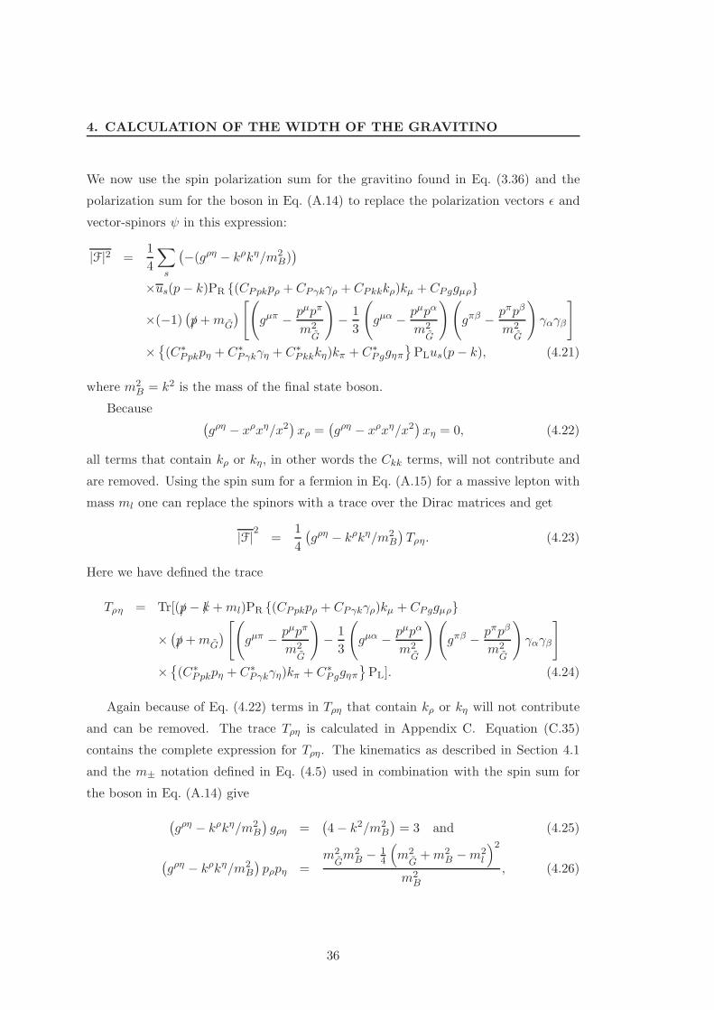
4. CALCULATION OF THE WIDTH OF THE GRAVITINO
We now use the spin polarization sum for the gravitino found in Eq. (3.36) and the
polarization sum for the boson in Eq. (A.14) to replace the polarization vectors ǫ and
vector-spinors ψ in this expression:
|F|2 =1
4
∑
s
(
−(gρη − kρkη/m2B))
×us(p − k)PR (CPpkpρ + CPγkγρ + CPkkkρ)kµ +CPggµρ
×(−1)(
/p+mG
)
[(
gµπ − pµpπ
m2G
)
− 1
3
(
gµα − pµpα
m2G
)(
gπβ − pπpβ
m2G
)
γαγβ
]
×
(C∗Ppkpη + C∗
Pγkγη + C∗Pkkkη)kπ + C∗
Pggηπ
PLus(p− k), (4.21)
where m2B = k2 is the mass of the final state boson.
Because(
gρη − xρxη/x2)
xρ =(
gρη − xρxη/x2)
xη = 0, (4.22)
all terms that contain kρ or kη, in other words the Ckk terms, will not contribute and
are removed. Using the spin sum for a fermion in Eq. (A.15) for a massive lepton with
mass ml one can replace the spinors with a trace over the Dirac matrices and get
|F|2 =1
4
(
gρη − kρkη/m2B
)
Tρη. (4.23)
Here we have defined the trace
Tρη = Tr[(/p − /k +ml)PR (CPpkpρ + CPγkγρ)kµ + CPggµρ
×(
/p+mG
)
[(
gµπ − pµpπ
m2G
)
− 1
3
(
gµα − pµpα
m2G
)(
gπβ − pπpβ
m2G
)
γαγβ
]
×
(C∗Ppkpη + C∗
Pγkγη)kπ + C∗Pggηπ
PL]. (4.24)
Again because of Eq. (4.22) terms in Tρη that contain kρ or kη will not contribute
and can be removed. The trace Tρη is calculated in Appendix C. Equation (C.35)
contains the complete expression for Tρη. The kinematics as described in Section 4.1
and the m± notation defined in Eq. (4.5) used in combination with the spin sum for
the boson in Eq. (A.14) give
(
gρη − kρkη/m2B
)
gρη =(
4− k2/m2B
)
= 3 and (4.25)
(
gρη − kρkη/m2B
)
pρpη =m2
Gm2
B − 14
(
m2G+m2
B −m2l
)2
m2B
, (4.26)
36
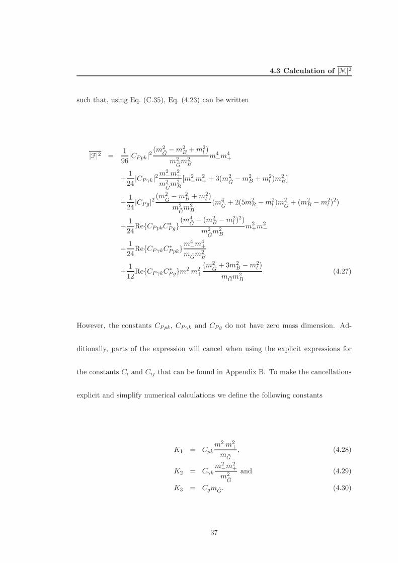
4.3 Calculation of |M|2
such that, using Eq. (C.35), Eq. (4.23) can be written
|F|2 =1
96|CPpk|2
(m2G−m2
B +m2l )
m2Gm2
B
m4−m
4+
+1
24|CPγk|2
m2−m
2+
m2Gm2
B
[m2−m
2+ + 3(m2
G−m2
B +m2l )m
2B]
+1
24|CPg|2
(m2G−m2
B +m2l )
m2Gm2
B
(m4G+ 2(5m2
B −m2l )m
2G+ (m2
B −m2l )
2)
+1
24ReCPpkC
∗Pg
(m4G− (m2
B −m2l )
2)
m2Gm2
B
m2+m
2−
+1
24ReCPγkC
∗Ppk
m4−m
4+
mGm2B
+1
12ReCPγkC
∗Pgm2
−m2+
(m2G+ 3m2
B −m2l )
mGm2B
. (4.27)
However, the constants CPpk, CPγk and CPg do not have zero mass dimension. Ad-
ditionally, parts of the expression will cancel when using the explicit expressions for
the constants Ci and Cij that can be found in Appendix B. To make the cancellations
explicit and simplify numerical calculations we define the following constants
K1 = Cpkm2
−m2+
mG
, (4.28)
K2 = Cγkm2
−m2+
m2G
and (4.29)
K3 = CgmG. (4.30)
37
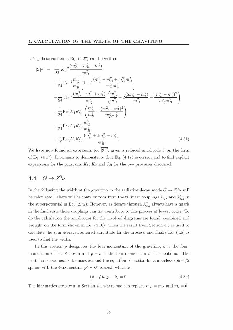
4. CALCULATION OF THE WIDTH OF THE GRAVITINO
Using these constants Eq. (4.27) can be written
|F|2 =1
96|K1|2
(m2G−m2
B +m2l )
m2B
+1
24|K2|2
m2G
m2B
[
1 + 3(m2
G−m2
B +m2l )m
2B
m2−m
2+
]
+1
24|K3|2
(m2G−m2
B +m2l )
m2G
(
m2G
m2B
+ 2(5m2
B −m2l )
m2B
+(m2
B −m2l )
2
m2Gm2
B
)
+1
24ReK1K
∗3(
m2G
m2B
− (m2B −m2
l )2
m2Gm2
B
)
+1
24ReK1K
∗2m2
G
m2B
+1
12ReK2K
∗3
(m2G+ 3m2
B −m2l )
m2B
. (4.31)
We have now found an expression for |F|2, given a reduced amplitude F on the form
of Eq. (4.17). It remains to demonstrate that Eq. (4.17) is correct and to find explicit
expressions for the constants K1, K2 and K3 for the two processes discussed.
4.4 G → Z0ν
In the following the width of the gravitino in the radiative decay mode G → Z0ν will
be calculated. There will be contributions from the trilinear couplings λijk and λ′ijk in
the superpotential in Eq. (2.72). However, as decays through λ′′ijk always have a quark
in the final state these couplings can not contribute to this process at lowest order. To
do the calculation the amplitudes for the involved diagrams are found, combined and
brought on the form shown in Eq. (4.16). Then the result from Section 4.3 is used to
calculate the spin averaged squared amplitude for the process, and finally Eq. (4.8) is
used to find the width.
In this section p designates the four-momentum of the gravitino, k is the four-
momentum of the Z boson and p − k is the four-momentum of the neutrino. The
neutrino is assumed to be massless and the equation of motion for a massless spin-1/2
spinor with the 4-momentum pµ − kµ is used, which is
(/p− /k)u(p − k) = 0. (4.32)
The kinematics are given in Section 4.1 where one can replace mB = mZ and ml = 0.
38
4.4 G→ Z0ν
4.4.1 Diagrams and amplitudes
The contributing diagrams are shown in Figs. 4.1–4.6 and are divided into three types
of diagrams. Type 1 diagrams, shown in Figs. 4.1 and 4.2 on the following page, are the
diagrams where the boson radiates of the fermion in the loop. Type 2 diagrams, shown
in Figs. 4.3 on page 42 and 4.4 on page 43, are the diagrams where the boson radiates
off the sfermion in the loop. Type 3 diagrams, shown in Figs 4.5 on page 44 and 4.6
on page 45, are the diagrams that contain the four-particle couplings. All diagrams
come in two versions, one where the scalar particles in the loop are the superpartners
of the left handed fermions, which we call the left handed diagrams, and one where the
scalar particles in the loop are the superpartners of the right handed fermions, which
we call the right handed diagrams. The right handed diagrams have reversed fermion
number flow in the loop, compared to the left handed diagrams. In all diagrams the
loop particles with an index L are understood to be contained in a SU(2) doublet of
superfields with weak hypercharge YL. The additional index u(d) designates that the
particle is contained in the upper (lower) component of the doublet. Similarly, all loop
particles with an index R are understood to be contained in an SU(2) singlet superfield
with weak hypercharge YR. Here the additional index u(d) indicates which SU(2)
singlet superfield the particle is contained in.
As the Z-couplings as well as the gravitino-couplings do not violate fermion flavor,
while the R-parity violating interaction does, all the (s)fermions in the loops in the
diagrams must have the same flavor. As λiik = 0 because of SU(2) symmetry, the
neutrino must have a different flavor than the ones in the leptonic loop. This is not
the case for quark-squark loops. For simplicity λ will designate both λijk and λ′ijk and
flavor indices will be omitted in the following.
The Feynman rules and conventions used in this part are given in Appendix A. All
momenta are defined to flow left to right. Note that diagrams with colored particles
have to be multiplied by a color factor 3 because quarks exist in three colors, such
that three copies of the diagram exist. The loop masses are labeled by the name of
the particle, e.g. mfdL is the mass of the down type sfermion belonging to the SU(2)
doublet. The dimensionless constants
a =[1− (1− YL) sin
2 θW ]
cos θWand b =
[YR sin2 θW ]
cos θW, (4.33)
are used to separate the different structures of the amplitudes for this process.
39
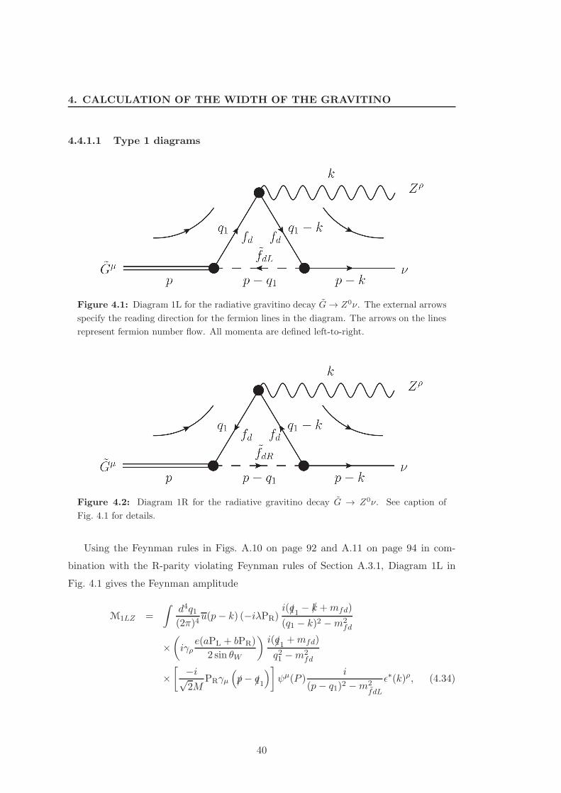
4. CALCULATION OF THE WIDTH OF THE GRAVITINO
4.4.1.1 Type 1 diagrams
Figure 4.1: Diagram 1L for the radiative gravitino decay G→ Z0ν. The external arrows
specify the reading direction for the fermion lines in the diagram. The arrows on the lines
represent fermion number flow. All momenta are defined left-to-right.
Figure 4.2: Diagram 1R for the radiative gravitino decay G → Z0ν. See caption of
Fig. 4.1 for details.
Using the Feynman rules in Figs. A.10 on page 92 and A.11 on page 94 in com-
bination with the R-parity violating Feynman rules of Section A.3.1, Diagram 1L in
Fig. 4.1 gives the Feynman amplitude
M1LZ =
∫
d4q1(2π)4
u(p− k) (−iλPR)i(/q1 − /k +mfd)
(q1 − k)2 −m2fd
×(
iγρe(aPL + bPR)
2 sin θW
)
i(/q1 +mfd)
q21 −m2fd
×[ −i√
2MPRγµ
(
/p− /q1
)
]
ψµ(P )i
(p − q1)2 −m2fdL
ǫ∗(k)ρ, (4.34)
40
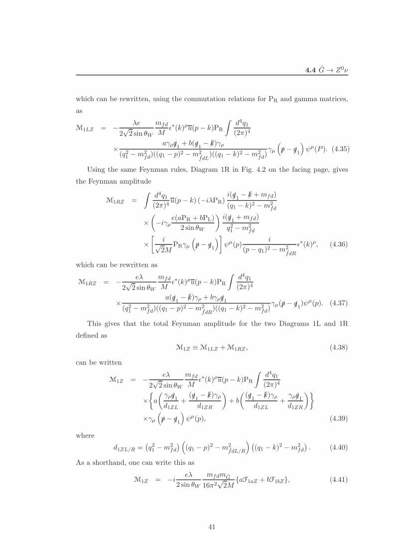
4.4 G→ Z0ν
which can be rewritten, using the commutation relations for PR and gamma matrices,
as
M1LZ = − λe
2√2 sin θW
mfd
Mǫ∗(k)ρu(p− k)PR
∫
d4q1(2π)4
×aγρ/q1 + b(/q1 − /k)γρ
(q21 −m2fd)((q1 − p)2 −m2
fdL)((q1 − k)2 −m2
fd)γµ
(
/p− /q1
)
ψµ(P ). (4.35)
Using the same Feynman rules, Diagram 1R in Fig. 4.2 on the facing page, gives
the Feynman amplitude
M1RZ =
∫
d4q1(2π)4
u(p− k) (−iλPR)i(/q1 − /k +mfd)
(q1 − k)2 −m2fd
×(
−iγρe(aPR + bPL)
2 sin θW
)
i(/q1 +mfd)
q21 −m2fd
×[
i√2M
PRγµ
(
/p− /q1
)
]
ψµ(p)i
(p− q1)2 −m2fdR
ǫ∗(k)ρ, (4.36)
which can be rewritten as
M1RZ = − eλ
2√2 sin θW
mfd
Mǫ∗(k)ρu(p− k)PR
∫
d4q1(2π)4
×a(/q1 − /k)γρ + bγρ/q1
(q21 −m2fd)((q1 − p)2 −m2
fdR)((q1 − k)2 −m2
fd)γµ(/p− /q1)ψ
µ(p). (4.37)
This gives that the total Feynman amplitude for the two Diagrams 1L and 1R
defined as
M1Z ≡ M1LZ +M1RZ , (4.38)
can be written
M1Z = − eλ
2√2 sin θW
mfd
Mǫ∗(k)ρu(p− k)PR
∫
d4q1(2π)4
×
a
(
γρ/q1d1ZL
+(/q1 − /k)γρ
d1ZR
)
+ b
(
(/q1 − /k)γρ
d1ZL+γρ/q1d1ZR
)
×γµ(
/p− /q1
)
ψµ(p), (4.39)
where
d1ZL/R =(
q21 −m2fd
)
(
(q1 − p)2 −m2fdL/R
)
(
(q1 − k)2 −m2fd
)
. (4.40)
As a shorthand, one can write this as
M1Z = −i eλ
2 sin θW
mfdmG
16π2√2M
aF1aZ + bF1bZ, (4.41)
41
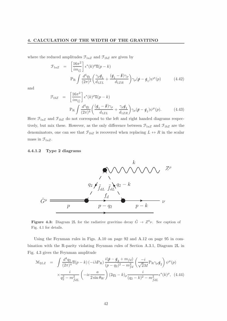
4. CALCULATION OF THE WIDTH OF THE GRAVITINO
where the reduced amplitudes F1aZ and F1bZ are given by
F1aZ =
[
16π2
imG
]
ǫ∗(k)ρu(p − k)
PR
∫
d4q1(2π)4
(
γρ/q1d1ZL
+(/q1 − /k)γρ
d1ZR
)
γµ(/p− /q1)ψµ(p) (4.42)
and
F1bZ =
[
16π2
imG
]
ǫ∗(k)ρu(p − k)
PR
∫
d4q1(2π)4
(
(/q1 − /k)γρ
d1ZL+γρ/q1d1ZR
)
γµ(/p− /q1)ψµ(p). (4.43)
Here F1aZ and F1bZ do not correspond to the left and right handed diagrams respec-
tively, but mix these. However, as the only difference between F1aZ and F1bZ are the
denominators, one can see that F1bZ is recovered when replacing L ↔ R in the scalar
mass in F1aZ .
4.4.1.2 Type 2 diagrams
Figure 4.3: Diagram 2L for the radiative gravitino decay G → Z0ν. See caption of
Fig. 4.1 for details.
Using the Feynman rules in Figs. A.10 on page 92 and A.12 on page 95 in com-
bination with the R-parity violating Feynman rules of Section A.3.1, Diagram 2L in
Fig. 4.3 gives the Feynman amplitude
M2LZ =
∫
d4q2(2π)4
u(p− k) (−iλPR)i(/p − /q2 +mfd)
(p − q2)2 −m2fd
( −i√2M
PRγµ/q2
)
ψµ(p)
× i
q22 −m2fdL
(
−ie a
2 sin θW
)
(2q2 − k)ρi
(q2 − k)2 −m2fdL
ǫ∗(k)ρ, (4.44)
42
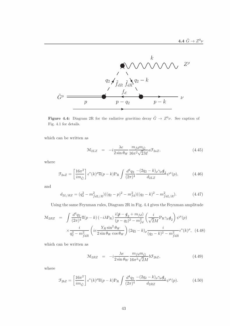
4.4 G→ Z0ν
Figure 4.4: Diagram 2R for the radiative gravitino decay G → Z0ν. See caption of
Fig. 4.1 for details.
which can be written as
M2LZ = −i λe
2 sin θW
mfdmG
16π2√2M
aF2aZ , (4.45)
where
F2aZ =
[
16π2
imG
]
ǫ∗(k)ρu(p− k)PR
∫
d4q2(2π)4
−(2q2 − k)ργµ/q2d2LZ
ψµ(p), (4.46)
and
d2L/RZ = (q22 −m2fdL/R
)((q2 − p)2 −m2fd)((q2 − k)2 −m2
fdL/R). (4.47)
Using the same Feynman rules, Diagram 2R in Fig. 4.4 gives the Feynman amplitude
M2RZ =
∫
d4q2(2π)4
u(p− k) (−iλPR)i(/p − /q2 +mfd)
(p − q2)2 −m2fd
(
i√2M
PRγµ/q2
)
ψµ(p)
× i
q22 −m2fdR
(
ieYR sin2 θW
2 sin θW cos θW
)
(2q2 − k)ρi
(q2 − k)2 −m2fdR
ǫ∗(k)ρ, (4.48)
which can be written as
M2RZ = −i λe
2 sin θW
mfdmG
16π2√2M
bF2bZ , (4.49)
where
F2bZ =
[
16π2
imG
]
ǫ∗(k)ρu(p − k)PR
∫
d4q2(2π)4
−(2q2 − k)ργµ/q2d2RZ
ψµ(p). (4.50)
43
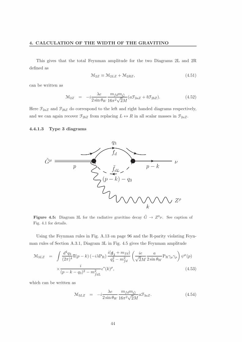
4. CALCULATION OF THE WIDTH OF THE GRAVITINO
This gives that the total Feynman amplitude for the two Diagrams 2L and 2R
defined as
M2Z ≡ M2LZ +M2RZ , (4.51)
can be written as
M2Z = −i λe
2 sin θW
mfdmG
16π2√2M
(aF2aZ + bF2bZ). (4.52)
Here F2aZ and F2bZ do correspond to the left and right handed diagrams respectively,
and we can again recover F2bZ from replacing L↔ R in all scalar masses in F2aZ .
4.4.1.3 Type 3 diagrams
Figure 4.5: Diagram 3L for the radiative gravitino decay G → Z0ν. See caption of
Fig. 4.1 for details.
Using the Feynman rules in Fig. A.13 on page 96 and the R-parity violating Feyn-
man rules of Section A.3.1, Diagram 3L in Fig. 4.5 gives the Feynman amplitude
M3LZ =
∫
d4q3(2π)4
u(p− k) (−iλPR)i(/q3 +mfd)
q23 −m2fd
(
ie√2M
a
2 sin θWPRγµγρ
)
ψµ(p)
× i
(p− k − q3)2 −m2fdL
ǫ∗(k)ρ, (4.53)
which can be written as
M3LZ = −i λe
2 sin θW
mfdmG
16π2√2M
aF3aZ . (4.54)
44
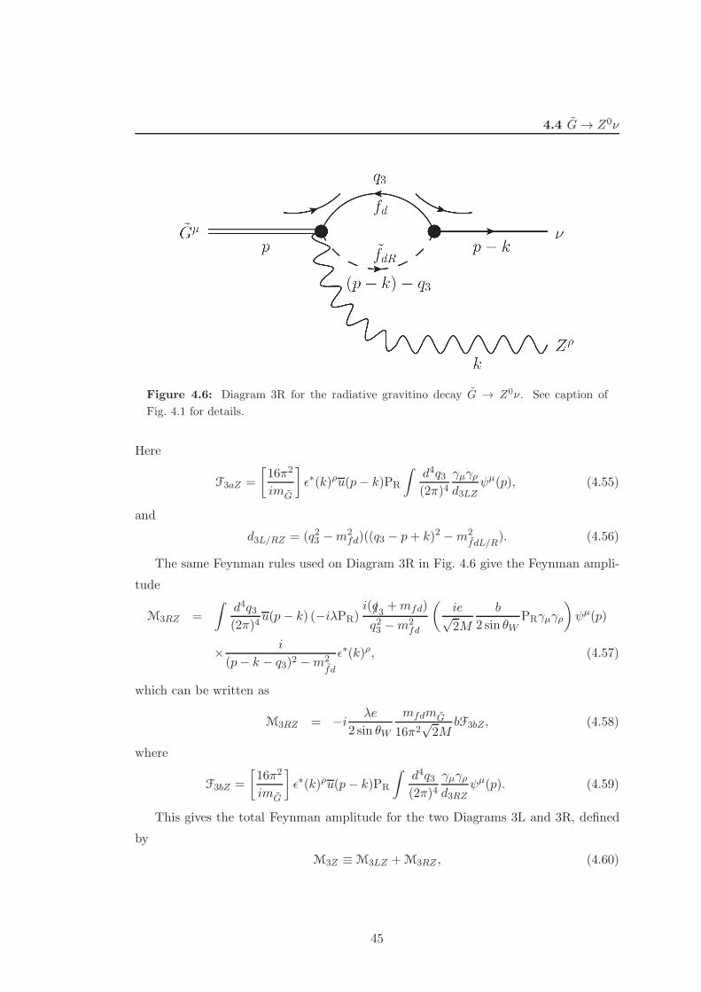
4.4 G→ Z0ν
Figure 4.6: Diagram 3R for the radiative gravitino decay G → Z0ν. See caption of
Fig. 4.1 for details.
Here
F3aZ =
[
16π2
imG
]
ǫ∗(k)ρu(p− k)PR
∫
d4q3(2π)4
γµγρd3LZ
ψµ(p), (4.55)
and
d3L/RZ = (q23 −m2fd)((q3 − p+ k)2 −m2
fdL/R). (4.56)
The same Feynman rules used on Diagram 3R in Fig. 4.6 give the Feynman ampli-
tude
M3RZ =
∫
d4q3(2π)4
u(p − k) (−iλPR)i(/q3 +mfd)
q23 −m2fd
(
ie√2M
b
2 sin θWPRγµγρ
)
ψµ(p)
× i
(p− k − q3)2 −m2fd
ǫ∗(k)ρ, (4.57)
which can be written as
M3RZ = −i λe
2 sin θW
mfdmG
16π2√2M
bF3bZ , (4.58)
where
F3bZ =
[
16π2
imG
]
ǫ∗(k)ρu(p− k)PR
∫
d4q3(2π)4
γµγρd3RZ
ψµ(p). (4.59)
This gives the total Feynman amplitude for the two Diagrams 3L and 3R, defined
by
M3Z ≡ M3LZ +M3RZ , (4.60)
45
4. CALCULATION OF THE WIDTH OF THE GRAVITINO
as
M3Z = −i λe
2 sin θW
mfdmG
16π2√2M
(aF3aZ + bF3bZ). (4.61)
Again, F3aZ and F3bZ correspond to the left and right handed diagram respectively,
and are interchanged when switching L and R for the scalar mass in the propagator.
4.4.2 The total amplitude
Now the amplitudes for each type of diagram are combined below to the total amplitude
in the radiative process G→ Z0ν. To do this, all the amplitudes above are added. Then
the equations of motion for the gravitino, the neutrino and the Z-boson are used to
bring the expression on the form of Eq. (4.17), such that the results of Section 4.3 can
be used.
Combining the results from the three sections above, one can write the total am-
plitude for the radiative decay G→ Z0ν at one loop level as
MZ = M1Z +M2Z +M3Z , (4.62)
which can be written in terms of the reduced amplitudes FaZ and FbZ as
MZ = −i λe
2 sin θW
mfdmG
16π2√2M
(aFaZ + bFbZ), (4.63)
where
Fa/bZ = F1a/bZ + F2a/bZ + F3a/bZ . (4.64)
As mentioned in the previous three subsections, one recovers FibZ by replacing L↔ R
in all scalar masses in FiaZ . Since Fa/bZ is just the sum of these the calculation will
be done only for FaZ . FbZ can then be recovered by replacing the scalar masses in the
result.
We use the notation in Eqs. (4.9)–(4.14) with indices on the PaVe integrals to specify
which set off masses m1, m2 and m3 to use, as shown in Table 4.1 on the facing page.
Replacing these in FaZ the expression can be written as
FaZ =
[
1
mG
]
ǫ∗(k)ρu(p − k)PR−C1RZ/kγργµ/p+ (Cη1LZγργη + Cη
1RZγηγρ)γµ/p
+Cη1RZ/kγργµγη −Cηπ
1LZγργηγµγπ − Cηπ1RZγηγργµγπ
+Cη2LZγµγηkρ − 2C2LZ
ηργµγη +B0(0,m
2fd,m
2f dL
)γµγρψµ(p). (4.65)
46
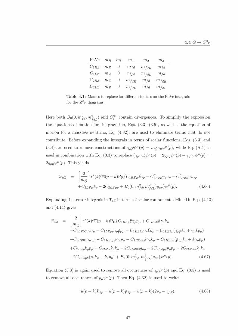
4.4 G→ Z0ν
PaVe mB ml m1 m2 m3
C1RZ mZ 0 mfd mfdR mfd
C1LZ mZ 0 mfd mfdL mfd
C2RZ mZ 0 mfdR mfd mfdR
C2LZ mZ 0 mfdL mfd mfdL
Table 4.1: Masses to replace for different indices on the PaVe integrals
for the Z0ν diagrams.
Here both B0(0,m2fd,m
2fdL
) and Cηπi contain divergences. To simplify the expression
the equations of motion for the gravitino, Eqs. (3.3)–(3.5), as well as the equation of
motion for a massless neutrino, Eq. (4.32), are used to eliminate terms that do not
contribute. Before expanding the integrals in terms of scalar functions, Eqs. (3.3) and
(3.4) are used to remove constructions of γµ/pψµ(p) = mGγµψ
µ(p), while Eq. (A.1) is
used in combination with Eq. (3.3) to replace (γµγη)ψµ(p) = 2gµηψ
µ(p)− γηγµψµ(p) =
2gµηψµ(p). This yields
FaZ =
[
2
mG
]
ǫ∗(k)ρu(p− k)PRC1RZµ/kγρ − Cη1LZµγργη − Cη
1RZµγηγρ
+C2LZµkρ − 2C2LZµρ +B0(0,m2fd,m
2fdL
)gµρψµ(p). (4.66)
Expanding the tensor integrals in FaZ in terms of scalar components defined in Eqs. (4.13)
and (4.14) gives
FaZ =
[
2
mG
]
ǫ∗(k)ρu(p − k)PRC1RZp/kγρpµ +C1RZk/kγρkµ
−C1LZ00γργµ − C1LZppγρ/ppµ − C1LZkkγρ/kkµ − C1LZkp(γρ/pkµ + γρ/kpµ)
−C1RZ00γµγρ − C1RZpp/pγρpµ − C1RZkk/kγρkµ − C1RZpk(/pγρkµ + /kγρpµ)
+C2LZpkρpµ + C2LZkkρkµ − 2C2LZ00gµρ − 2C2LZpppρpµ − 2C2LZkkkρkµ
−2C2LZpk(pρkµ + kρpµ) +B0(0,m2fd,m
2fdL
)gµρψµ(p). (4.67)
Equation (3.3) is again used to remove all occurences of γµψµ(p) and Eq. (3.5) is used
to remove all occurences of pµψµ(p). Then Eq. (4.32) is used to write
u(p− k)/kγρ = u(p − k)/pγρ = u(p− k)(2pρ − γρ/p). (4.68)
47
4. CALCULATION OF THE WIDTH OF THE GRAVITINO
Finally Eq. (3.4) is used to replace /pψµ(p) = mGψµ(p). This gives
FaZ =
[
2
mG
]
ǫ∗(k)ρu(p− k)PRC1RZk(2pρ − γρmG)kµ
−C1LZkk(2kρ − 2pρ + γρmG)kµ − C1LZkpγρmGkµ
−2C1RZ00gρµ − C1RZkk(2pρ − γρmG)kµ − C1RZpk(2pρ − γρmG)kµ
+C2LZkkρkµ − 2C2LZ00gµρ − 2C2LZkkkρkµ
−2C2LZpkpρkµ +B0(0,m2fd,m
2fdL
)gµρψµ(p). (4.69)
However, the kµkρ part here will not contribute to the final result, as shown in Sec-
tion 4.3. Using this one can sort the expression in terms of tensor structure as
FaZ =
[
2
mG
]
ǫ∗(k)ρu(p− k)PR
×2pρkµ(C1LZkk − C1RZkk − C1RZpk − C2LZpk + C1RZk)
+mGγρkµ(C1RZkk −C1LZkk + C1RZpk − C1LZpk − C1RZk)
+gρµ(B0(0,m2fd,m
2fdL
)− 2C2LZ00 − 2C1RZ00)ψµ(p). (4.70)
One can now write down the set of constants on the form of the ones in Eq. (4.17) as
CaZpk =4
mG
(C1LZkk − C1RZkk − C1RZpk −C2LZpk + C1RZk) (4.71)
CaZg =2
mG
(B0(0,m2fd,m
2f dL
)− 2C2LZ00 − 2C1RZ00) (4.72)
CaZγk = 2(C1RZkk − C1LZkk +C1RZpk − C1LZpk − C1RZk). (4.73)
To retrieve the constants for the b case, replace all L ↔ R. Using Eqs. (B.18)–(B.24)
one can write Eq. (4.71) in terms of the dimensionless constants defined in Appendix B.
Doing this all 1/m2ν divergent terms cancel and leave an expression without superficial
divergences:
CaZpk = −4mG(C
′1LZkk − C ′
1RZkk − C ′1RZpk − C ′
2LZpk + C ′1RZk)
(m2G−m2
Z)2
. (4.74)
For Eq. (4.72) this leaves
CaZg =1
mG
(2B0(0,m2fd,m
2fdL
)−B0(m2G,mfdL,m
2fd)−B0(m
2G,m2
fd,m2f dR
)
−4C ′2LZ00 − 4C ′
1RZ00). (4.75)
48
4.4 G→ Z0ν
Here B0(0,m2fd,m
2f dL
), B0(m2G,mf dL,m
2fd) and B0(m
2G,m2
fd,m2f dR
) each diverge with
1/ǫ, but the dimensionless constant is finite as the divergences cancel exactly. As
B0(0,m2fd,m
2f dL
) comes from diagrams of type three, while the two canceling terms
come from diagrams of type two and type one respectively, this shows that the diver-
gences cancel between all three types of diagrams.
For Eq. (4.73) all terms containing 1/m2ν divergences cancel as well and leave
CaZγk = −2m2
G(C ′
1RZkk − C ′1LZkk + C ′
1RZpk − C ′1LZpk − C ′
1RZk)
(m2G−m2
Z)2
. (4.76)
Taken together the results in this section give that the total amplitude of the process
G→ Z0ν at lowest order can be written on the form of Eq. (4.16) and Eq. (4.17) where
one can identify
CZpk = aCaZpk + bCbZpk, (4.77)
CZg = aCaZg + bCbZg and (4.78)
CZγk = aCaZγk + bCbZγk. (4.79)
Instead of this choice of constants, one can use the dimensionless constants defined in
Eqs. (4.28)–(4.30) which are
K1Z = 4[a(C ′1LZkk − C ′
1RZkk − C ′1RZpk −C ′
2LZpk +C ′1RZk)
+b(C ′1RZkk − C ′
1LZkk − C ′1LZpk − C ′
2RZpk +C ′1LZk)], (4.80)
and
K2Z = 2[a(C ′1RZkk − C ′
1LZkk + C ′1RZpk −C ′
1LZpk −C ′1RZk)
+b(C ′1LZkk − C ′
1RZkk + C ′1LZpk − C ′
1RZpk −C ′1LZk)], (4.81)
and
K3Z = [a(2B0(0,m2fd,m
2f dL
)−B0(m2G,mf dL,m
2fd)−B0(m
2G,m2
fd,m2f dR
)
−4C ′2LZ00 − 4C ′
1RZ00)
+b(2B0(0,m2fd,m
2fdR
)−B0(m2G,mf dR,m
2fd)−B0(m
2G,m2
fd,m2fdL
)
−4C ′2RZ00 − 4C ′
1LZ00)], (4.82)
where the dimensionless constants can be found from Appendix B by replacing the
masses as in Table 4.1.
49
4. CALCULATION OF THE WIDTH OF THE GRAVITINO
4.4.3 The width in the channel Z0ν
In this section the results from the previous two sections are combined. As shown in
Eq. (4.8) together with Eq. (4.17), one can write the width of the gravitino in the
radiative decay G→ Zν as
ΓG→Z0ν =1
16
αλ2mG
512π4 sin2 θW
m2fd
M2
(m2G−m2
Z)
m2G
|F|2. (4.83)
The general form of |F|2 is shown in Eq. (4.31), which can be written for the special
case of mB = mZ and ml = 0 as
|F|2 =1
96|K1Z |2
(
m2G
m2Z
− 1
)
+1
24|K2Z |2
[
m2G
m2Z
+ 3m2
G
(m2G−m2
Z)
]
+1
24|K3Z |2
(
1− m2Z
m2G
)(
10 +m2
G
m2Z
+m2
Z
m2G
)
+1
24ReK1ZK
∗3Z
(
m2G
m2Z
− m2Z
m2G
)
+1
24ReK1ZK
∗2Z
m2G
m2Z
+1
12ReK2ZK
∗3Z
(
3 +m2
G
m2Z
)
. (4.84)
K1Z , K2Z and K3Z have been written down in Eqs. (4.80)–(4.82).
4.5 G → W+l−
In the following the width of the gravitino in the radiative decay mode G→W+l− will
be calculated. There will again be contributions from the trilinear couplings λijk and
λ′ijk in the superpotential in Eq. (2.72). Again, contributions of the involved diagrams
are found, combined and brought on the form shown in Eq. (4.16). Then the result of
Section 4.3 is used to calculate the spin averaged squared amplitude for the process, and
Eq. (4.8) is used to find the width. The particles are designated by indices as presented
in Section 4.4. The main difference to the Z-case is that the final state lepton has
mass. For the lepton we will in the following use the equation of motion for a massive
spin-1/2 spinor with the four momentum pµ − kµ and mass ml, which is
(/p− /k)u(p − k) = mlu(p − k). (4.85)
The kinematics in Section 4.1 are used, where one can replace mB = mW .
50
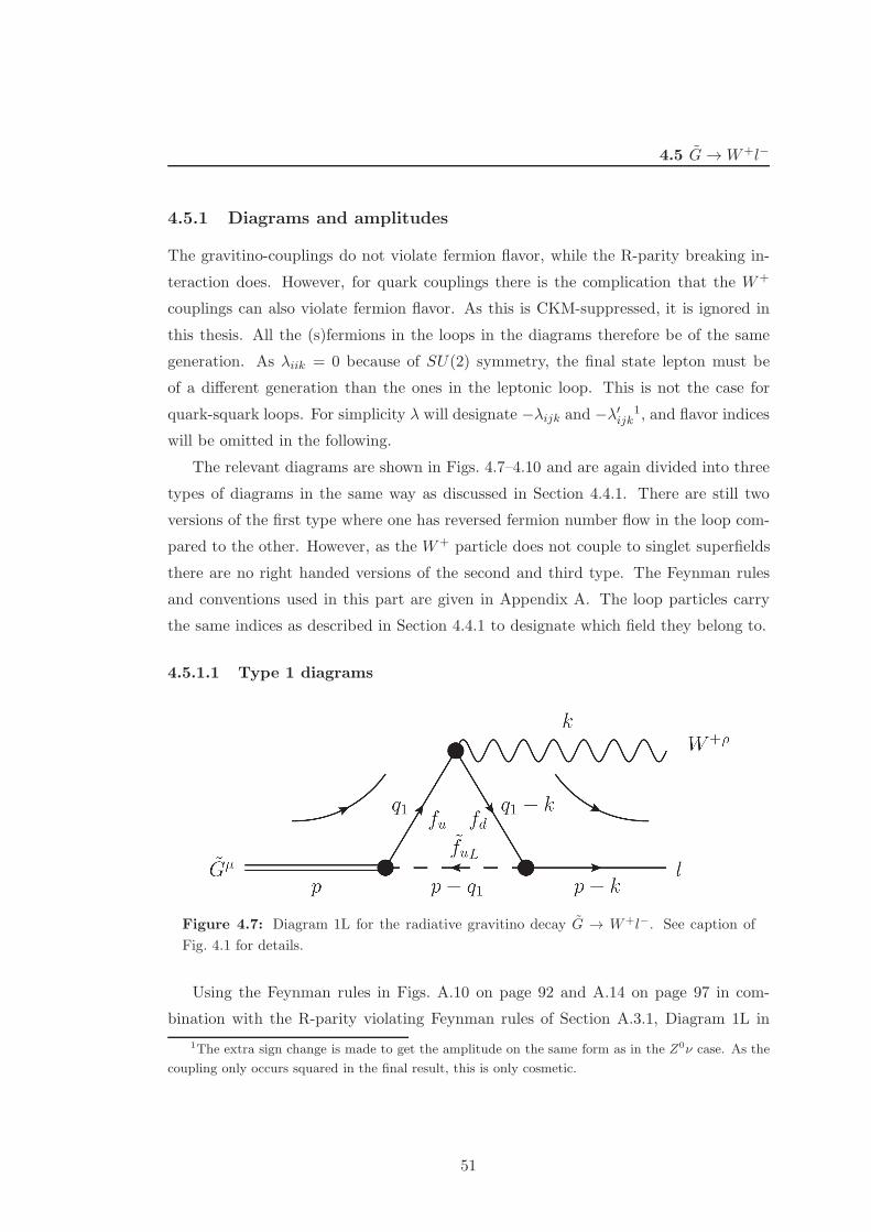
4.5 G→W+l−
4.5.1 Diagrams and amplitudes
The gravitino-couplings do not violate fermion flavor, while the R-parity breaking in-
teraction does. However, for quark couplings there is the complication that the W+
couplings can also violate fermion flavor. As this is CKM-suppressed, it is ignored in
this thesis. All the (s)fermions in the loops in the diagrams therefore be of the same
generation. As λiik = 0 because of SU(2) symmetry, the final state lepton must be
of a different generation than the ones in the leptonic loop. This is not the case for
quark-squark loops. For simplicity λ will designate −λijk and −λ′ijk1, and flavor indices
will be omitted in the following.
The relevant diagrams are shown in Figs. 4.7–4.10 and are again divided into three
types of diagrams in the same way as discussed in Section 4.4.1. There are still two
versions of the first type where one has reversed fermion number flow in the loop com-
pared to the other. However, as the W+ particle does not couple to singlet superfields
there are no right handed versions of the second and third type. The Feynman rules
and conventions used in this part are given in Appendix A. The loop particles carry
the same indices as described in Section 4.4.1 to designate which field they belong to.
4.5.1.1 Type 1 diagrams
Figure 4.7: Diagram 1L for the radiative gravitino decay G → W+l−. See caption of
Fig. 4.1 for details.
Using the Feynman rules in Figs. A.10 on page 92 and A.14 on page 97 in com-
bination with the R-parity violating Feynman rules of Section A.3.1, Diagram 1L in
1The extra sign change is made to get the amplitude on the same form as in the Z0ν case. As the
coupling only occurs squared in the final result, this is only cosmetic.
51
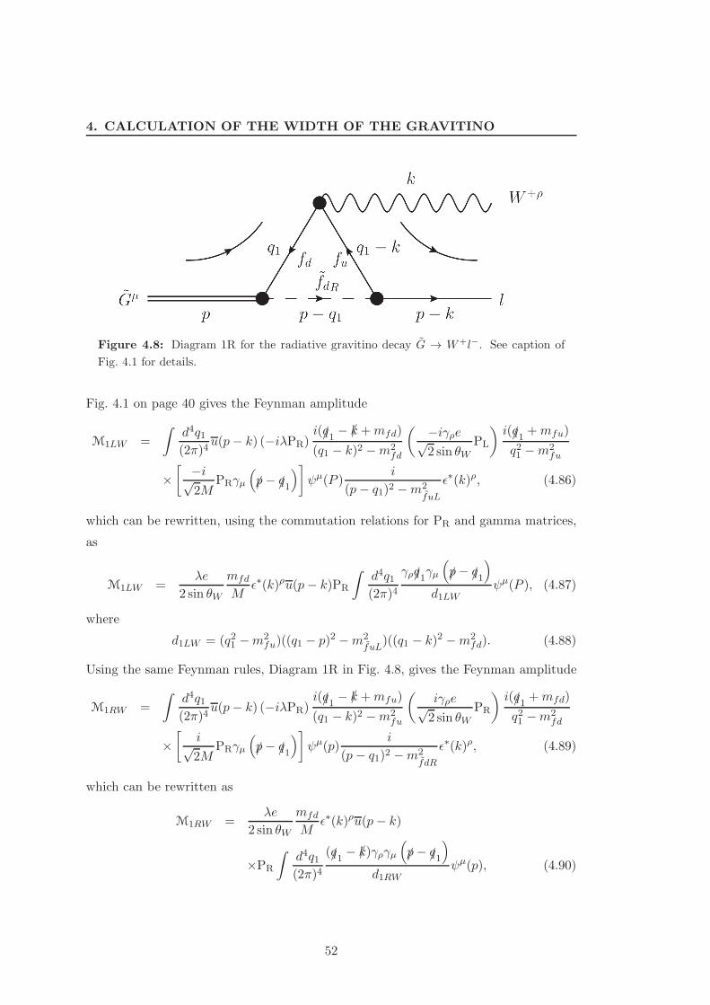
4. CALCULATION OF THE WIDTH OF THE GRAVITINO
Figure 4.8: Diagram 1R for the radiative gravitino decay G → W+l−. See caption of
Fig. 4.1 for details.
Fig. 4.1 on page 40 gives the Feynman amplitude
M1LW =
∫
d4q1(2π)4
u(p− k) (−iλPR)i(/q1 − /k +mfd)
(q1 − k)2 −m2fd
( −iγρe√2 sin θW
PL
)
i(/q1 +mfu)
q21 −m2fu
×[ −i√
2MPRγµ
(
/p− /q1
)
]
ψµ(P )i
(p − q1)2 −m2fuL
ǫ∗(k)ρ, (4.86)
which can be rewritten, using the commutation relations for PR and gamma matrices,
as
M1LW =λe
2 sin θW
mfd
Mǫ∗(k)ρu(p− k)PR
∫
d4q1(2π)4
γρ/q1γµ
(
/p− /q1
)
d1LWψµ(P ), (4.87)
where
d1LW = (q21 −m2fu)((q1 − p)2 −m2
fuL)((q1 − k)2 −m2
fd). (4.88)
Using the same Feynman rules, Diagram 1R in Fig. 4.8, gives the Feynman amplitude
M1RW =
∫
d4q1(2π)4
u(p− k) (−iλPR)i(/q1 − /k +mfu)
(q1 − k)2 −m2fu
(
iγρe√2 sin θW
PR
)
i(/q1 +mfd)
q21 −m2fd
×[
i√2M
PRγµ
(
/p− /q1
)
]
ψµ(p)i
(p − q1)2 −m2fdR
ǫ∗(k)ρ, (4.89)
which can be rewritten as
M1RW =λe
2 sin θW
mfd
Mǫ∗(k)ρu(p− k)
×PR
∫
d4q1(2π)4
(/q1 − /k)γργµ
(
/p− /q1
)
d1RWψµ(p), (4.90)
52
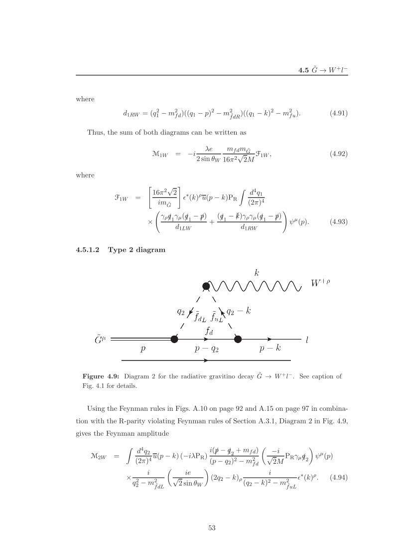
4.5 G→W+l−
where
d1RW = (q21 −m2fd)((q1 − p)2 −m2
fdR)((q1 − k)2 −m2
fu). (4.91)
Thus, the sum of both diagrams can be written as
M1W = −i λe
2 sin θW
mfdmG
16π2√2M
F1W , (4.92)
where
F1W =
[
16π2√2
imG
]
ǫ∗(k)ρu(p − k)PR
∫
d4q1(2π)4
×(
γρ/q1γµ(/q1 − /p)
d1LW+
(/q1 − /k)γργµ(/q1 − /p)
d1RW
)
ψµ(p). (4.93)
4.5.1.2 Type 2 diagram
Figure 4.9: Diagram 2 for the radiative gravitino decay G → W+l−. See caption of
Fig. 4.1 for details.
Using the Feynman rules in Figs. A.10 on page 92 and A.15 on page 97 in combina-
tion with the R-parity violating Feynman rules of Section A.3.1, Diagram 2 in Fig. 4.9,
gives the Feynman amplitude
M2W =
∫
d4q2(2π)4
u(p− k) (−iλPR)i(/p − /q2 +mfd)
(p− q2)2 −m2fd
( −i√2M
PRγµ/q2
)
ψµ(p)
× i
q22 −m2fdL
(
ie√2 sin θW
)
(2q2 − k)ρi
(q2 − k)2 −m2fuL
ǫ∗(k)ρ. (4.94)
53
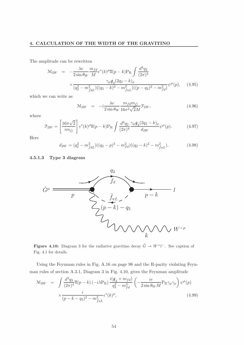
4. CALCULATION OF THE WIDTH OF THE GRAVITINO
The amplitude can be rewritten
M2W = − λe
2 sin θW
mfd
Mǫ∗(k)ρu(p− k)PR
∫
d4q2(2π)4
×γµ/q2(2q2 − k)ρ
(q22 −m2fdL
)((q2 − k)2 −m2fuL
)((p − q2)2 −m2fd)
ψµ(p), (4.95)
which we can write as
M2W = −i λe
2 sin θW
mfdmG
16π2√2M
F2W , (4.96)
where
F2W =
[
16π√2
imG
]
ǫ∗(k)ρu(p− k)PR
∫
d4q2(2π)4
γµ/q2(2q2 − k)ρ
d2Wψµ(p). (4.97)
Here
d2W = (q22 −m2fdL
)((q2 − p)2 −m2fd)((q2 − k)2 −m2
fuL). (4.98)
4.5.1.3 Type 3 diagram
Figure 4.10: Diagram 3 for the radiative gravitino decay G → W+l−. See caption of
Fig. 4.1 for details.
Using the Feynman rules in Fig. A.16 on page 98 and the R-parity violating Feyn-
man rules of section A.3.1, Diagram 3 in Fig. 4.10, gives the Feynman amplitude
M3W =
∫
d4q3(2π)4
u(p − k) (−iλPR)i(/q3 +mfd)
q23 −m2fd
(
− ie
2 sin θWMPRγµγρ
)
ψµ(p)
× i
(p− k − q3)2 −m2fuL
ǫ∗(k)ρ, (4.99)
54
4.5 G→W+l−
which can again be rewritten using the commutation relations for projection operators
and gamma matrices as
M3W =λe
2 sin θW
1
Mǫ∗(k)ρu(p− k)PR
∫
d4q3(2π)4
(/q3 +mfd)
q23 −m2fd
PRγµγρ
× 1
(p− k − q3)2 −m2fuL
ψµ(p). (4.100)
This amplitude can also be written in terms of a reduced amplitude F3W
M3W = −i λe
2 sin θW
mfdmG
16π2√2M
F3W , (4.101)
where
F3W =
[
16π2√2
imG
]
ǫ∗(k)ρu(p− k)PR
∫
d4q3(2π)4
−γµγρd3W
ψµ(p). (4.102)
Here
d3W = (q23 −m2fd)((q3 − p+ k)2 −m2
fuL). (4.103)
4.5.2 The total amplitude
In this section the amplitudes of the three types of diagrams are combined to give the
total amplitude of the radiative process G→W+l− to lowest perturbation order. The
equations of motion for the gravitino, the lepton and the gauge boson are then used to
bring the expression on the form of Eq. (4.16), such that the results of Section 4.3 can
be used.
Combining the results from the three subsections above, one can write the total
amplitude for the radiative decay G→W+l− at one loop level as
MW = M1W +M2W +M3W , (4.104)
which can be written in terms of the reduced amplitude FW as
MW = −i λe
2 sin θW
mfdmG
16π2√2M
FW , (4.105)
where
FW = F1W + F2W + F3W . (4.106)
55
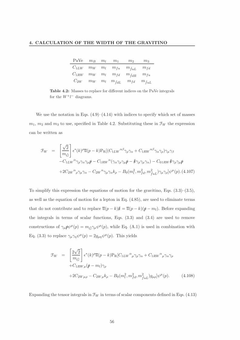
4. CALCULATION OF THE WIDTH OF THE GRAVITINO
PaVe mB ml m1 m2 m3
C1LW mW ml mfu mfuL mfd
C1RW mW ml mfd mf dR mfu
C2W mW ml mfdL mfd mfuL
Table 4.2: Masses to replace for different indices on the PaVe integrals
for the W+l− diagrams.
We use the notation in Eqs. (4.9)–(4.14) with indices to specify which set of masses
m1, m2 and m3 to use, specified in Table 4.2. Substituting these in FW the expression
can be written as
FW =
[√2
mG
]
ǫ∗(k)ρu(p − k)PR[(C1LWαβγργα + C1RW
αβγαγρ)γµγβ
−C1LWαγργαγµ/p− C1RW
α(γαγργµ/p− /kγργµγα)− C01RW /kγργµ/p
+2C2Wαργµγα − C2W
αγµγαkρ −B0(m2l ,m
2fd,m
2fuL
)γµγρ]ψµ(p).(4.107)
To simplify this expression the equations of motion for the gravitino, Eqs. (3.3)–(3.5),
as well as the equation of motion for a lepton in Eq. (4.85), are used to eliminate terms
that do not contribute and to replace u(p− k)/k = u(p− k)(/p−ml). Before expanding
the integrals in terms of scalar functions, Eqs. (3.3) and (3.4) are used to remove
constructions of γµ/pψµ(p) = mGγµψ
µ(p), while Eq. (A.1) is used in combination with
Eq. (3.3) to replace γµγηψµ(p) = 2gµηψ
µ(p). This yields
FW =
[
2√2
mG
]
ǫ∗(k)ρu(p− k)PR[C1LWαµγργα + C1RW
αµγαγρ
+C1RWµ(/p−ml)γρ
+2C2Wµρ −C2Wµkρ −B0(m2l ,m
2fd,m
2fuL
)gµρ]ψµ(p). (4.108)
Expanding the tensor integrals in FW in terms of scalar components defined in Eqs. (4.13)
56
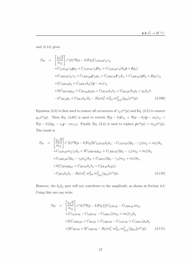
4.5 G→W+l−
and (4.14) gives
FW =
[
2√2
mG
]
ǫ∗(k)ρu(p− k)PR[C1LW00γργµ
+C1LWppγρ/ppµ +C1LWkkγρ/kkµ + C1LWpkγρ(kµ/p+ /kpµ)
+C1RW00γµγρ + C1RWpp/pγρpµ + C1RWkk/kγρkµ + C1RWpk(/pkµ + /kpµ)γρ
+(C1RWppµ + C1RWkkµ)(/p−ml)γρ
+2(C2W00gµρ +C2Wpppµpρ + C2Wkkkµkρ + C2Wpk(kµpρ + pµkρ))
−(C2Wppµ + C2Wkkµ)kρ −B0(m2l ,m
2fd,m
2fuL
)gµρ]ψµ(p). (4.109)
Equation (3.3) is then used to remove all occurences of γµψµ(p) and Eq. (3.5) to remove
pµψµ(p). Then Eq. (4.85) is used to rewrite u(p − k)/kγρ = u(p − k)(/p − ml)γρ =
u(p − k)(2pρ − γρ/p −mlγρ). Finally Eq. (3.4) is used to replace /pψµ(p) = mGψµ(p).
The result is
FW =
[
2√2
mG
]
ǫ∗(k)ρu(p− k)PR[2C1LWkkkρkµ − C1LWkk(2pρ − γρ(mG +ml))kµ
+C1LWpkmGγρkµ + 2C1RW00gµρ + C1RWkk(2pρ − γρ(mG +ml))kµ
+C1RWpk(2pρ − γρmG)kµ + C1bWk(2pρ − γρ(mG +ml))kµ
+2(C2W00gµρ + C2Wkkkµkρ + C2Wpkkµpρ)
−C2Wkkµkρ −B0(m2l ,m
2fd,m
2fuL
)gµρ]ψµ(p). (4.110)
However, the kµkρ part will not contribute to the amplitude, as shown in Section 4.3.
Using this one can write
FW =
[
2√2
mG
]
ǫ∗(k)ρu(p− k)PR[(C1LWpk − C1RWpk)mG
+(C1LWkk − C1RWkk − C1RWk)(mG +ml)]γρkµ
+2(C1RWpk + C2Wpk + C1RWkk − C1LWkk + C1RWk)pρkµ
+[2C2W00 + 2C1RW00 −B0(m2l ,m
2fd,m
2fuL
)]gµρψµ(p). (4.111)
57
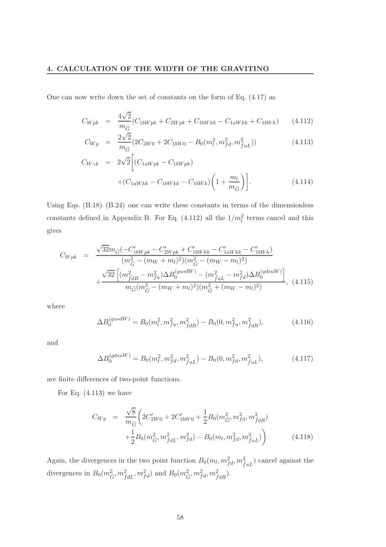
4. CALCULATION OF THE WIDTH OF THE GRAVITINO
One can now write down the set of constants on the form of Eq. (4.17) as
CWpk =4√2
mG
(C1bWpk + C2Wpk + C1bWkk − C1aWkk +C1bWk) (4.112)
CWg =2√2
mG
(2C2W0 + 2C1bW0 −B0(m2l ,m
2fd,m
2fuL
)) (4.113)
CWγk = 2√2
[
(C1aWpk − C1bWpk)
+(C1aWkk − C1bWkk − C1bWk)
(
1 +ml
mG
)]
. (4.114)
Using Eqs. (B.18)–(B.24) one can write these constants in terms of the dimensionless
constants defined in Appendix B. For Eq. (4.112) all the 1/m2l terms cancel and this
gives
CWpk =
√32mG(−C ′
1bWpk −C ′2Wpk + C ′
1bWkk −C ′1aWkk − C ′
1bWk)
(m2G− (mW +ml)2)(m
2G− (mW −ml)2)
+
√32[
(m2fdR
−m2fu)∆B
(gusdW )0 − (m2
fuL−m2
fd)∆B(gdsuW )0
]
mG(m2G− (mW +ml)2)(m
2G+ (mW −ml)2)
, (4.115)
where
∆B(gusdW )0 = B0(m
2l ,m
2fu,m
2f dR
)−B0(0,m2fu,m
2fdR
), (4.116)
and
∆B(gdsuW )0 = B0(m
2l ,m
2fd,m
2fuL
)−B0(0,m2fd,m
2fuL
), (4.117)
are finite differences of two-point functions.
For Eq. (4.113) we have
CWg =
√8
mG
(
2C ′2W0 + 2C ′
1bW0 +1
2B0(m
2G,m2
fd,m2fdR
)
+1
2B0(m
2G,m2
f dL,m2
fd)−B0(ml,m2fd,m
2fuL
)
)
(4.118)
Again, the divergences in the two point function B0(ml,m2fd,m
2fuL
) cancel against the
divergences in B0(m2G,m2
f dL,m2
fd) and B0(m2G,m2
fd,m2f dR
).
58
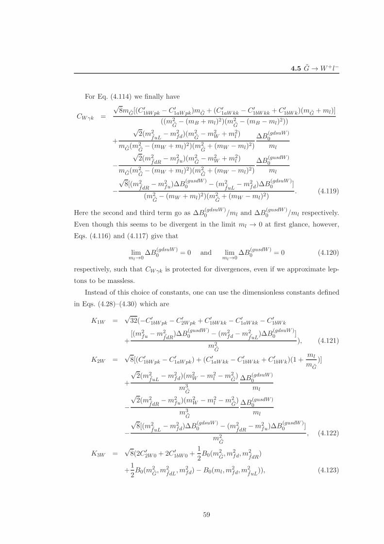
4.5 G→W+l−
For Eq. (4.114) we finally have
CWγk =
√8mG[(C
′1bWpk − C ′
1aWpk)mG + (C ′1aWkk − C ′
1bWkk + C ′1bWk)(mG +ml)]
((m2G− (mB +ml)2)(m
2G− (mB −ml)2))
+
√2(m2
fuL−m2
fd)(m2G−m2
W +m2l )
mG(m2G− (mW +ml)2)(m
2G+ (mW −ml)2)
∆B(gdsuW )0
ml
−√2(m2
f dR−m2
fu)(m2G−m2
W +m2l )
mG(m2G− (mW +ml)2)(m
2G+ (mW −ml)2)
∆B(gusdW )0
ml
−√8[(m2
f dR−m2
fu)∆B(gusdW )0 − (m2
fuL−m2
fd)∆B(gdsuW )0 ]
(m2G− (mW +ml)2)(m
2G+ (mW −ml)2)
. (4.119)
Here the second and third term go as ∆B(gdsuW )0 /ml and ∆B
(gusdW )0 /ml respectively.
Even though this seems to be divergent in the limit ml → 0 at first glance, however,
Eqs. (4.116) and (4.117) give that
limml→0
∆B(gdsuW )0 = 0 and lim
ml→0∆B
(gusdW )0 = 0 (4.120)
respectively, such that CWγk is protected for divergences, even if we approximate lep-
tons to be massless.
Instead of this choice of constants, one can use the dimensionless constants defined
in Eqs. (4.28)–(4.30) which are
K1W =√32(−C ′
1bWpk − C ′2Wpk + C ′
1bWkk − C ′1aWkk − C ′
1bWk
+[(m2
fu −m2fdR
)∆B(gusdW )0 − (m2
fd −m2fuL
)∆B(gdsuW )0 ]
m2G
), (4.121)
K2W =√8[(C ′
1bWpk − C ′1aWpk) + (C ′
1aWkk − C ′1bWkk +C ′
1bWk)(1 +ml
mG
)]
+
√2(m2
fuL−m2
fd)(m2W −m2
l −m2G)
m3G
∆B(gdsuW )0
ml
−√2(m2
fdR−m2
fu)(m2W −m2
l −m2G)
m3G
∆B(gusdW )0
ml
−√8[(m2
fuL−m2
fd)∆B(gdsuW )0 − (m2
fdR−m2
fu)∆B(gusdW )0 ]
m2G
, (4.122)
K3W =√8(2C ′
2W0 + 2C ′1bW0 +
1
2B0(m
2G,m2
fd,m2fdR
)
+1
2B0(m
2G,m2
fdL,m2
fd)−B0(ml,m2fd,m
2fuL
)), (4.123)
59
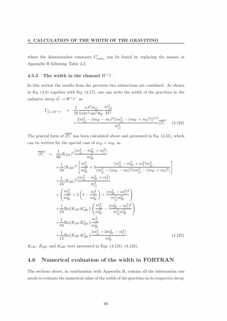
4. CALCULATION OF THE WIDTH OF THE GRAVITINO
where the dimensionless constants C ′index can be found by replacing the masses in
Appendix B following Table 4.2.
4.5.3 The width in the channel W+l−
In this section the results from the previous two subsections are combined. As shown
in Eq. (4.8) together with Eq. (4.17), one can write the width of the gravitino in the
radiative decay G→W+l− as
ΓG→W+l− =1
16
αλ2mG
512π4 sin2 θW
m2fd
M2
×[(m2
G− (mW −ml)
2)(m2G− (mW +ml)
2)]1/2
m2G
|F|2. (4.124)
The general form of |F|2 has been calculated above and presented in Eq. (4.31), which
can be written for the special case of mB = mW as
|F|2 =1
96|K1W |2
(m2G−m2
W +m2l )
m2W
+1
24|K2W |2
[
m2G
m2W
+ 3(m2
G−m2
W +m2l )m
2G
(m2G− (mW −ml)2)(m
2G− (mW +ml)2)
]
+1
24|K3W |2
(m2G−m2
W +m2l )
m2G
×(
m2G
m2W
+ 2
(
5− m2l
m2W
)
+(m2
W −m2l )
2
m2Gm2
W
)
+1
24ReK1WK
∗3W
(
m2G
m2W
− (m2W −m2
l )2
m2Gm2
W
)
+1
24ReK1WK
∗2W
m2G
m2W
+1
12ReK2WK
∗3W
(m2G+ 3m2
W −m2l )
m2W
. (4.125)
K1W , K2W and K3W were presented in Eqs. (4.121)–(4.123).
4.6 Numerical evaluation of the width in FORTRAN
The sections above, in combination with Appendix B, contain all the information one
needs to evaluate the numerical value of the width of the gravitino in its respective decay
60
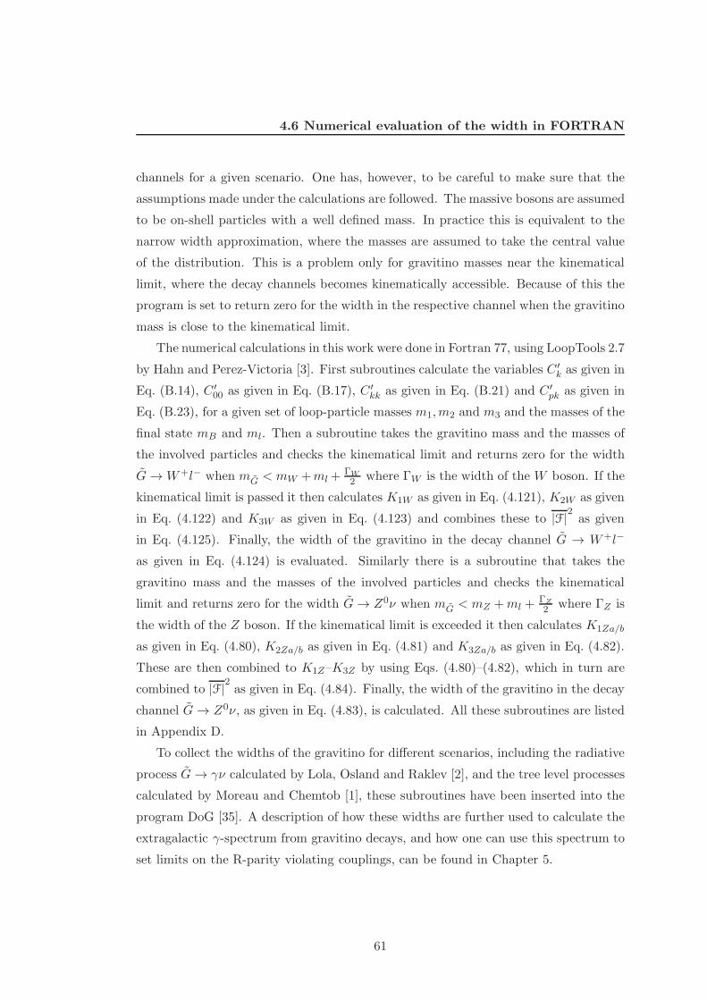
4.6 Numerical evaluation of the width in FORTRAN
channels for a given scenario. One has, however, to be careful to make sure that the
assumptions made under the calculations are followed. The massive bosons are assumed
to be on-shell particles with a well defined mass. In practice this is equivalent to the
narrow width approximation, where the masses are assumed to take the central value
of the distribution. This is a problem only for gravitino masses near the kinematical
limit, where the decay channels becomes kinematically accessible. Because of this the
program is set to return zero for the width in the respective channel when the gravitino
mass is close to the kinematical limit.
The numerical calculations in this work were done in Fortran 77, using LoopTools 2.7
by Hahn and Perez-Victoria [3]. First subroutines calculate the variables C ′k as given in
Eq. (B.14), C ′00 as given in Eq. (B.17), C ′
kk as given in Eq. (B.21) and C ′pk as given in
Eq. (B.23), for a given set of loop-particle masses m1,m2 and m3 and the masses of the
final state mB and ml. Then a subroutine takes the gravitino mass and the masses of
the involved particles and checks the kinematical limit and returns zero for the width
G→W+l− when mG < mW +ml +ΓW
2 where ΓW is the width of the W boson. If the
kinematical limit is passed it then calculates K1W as given in Eq. (4.121), K2W as given
in Eq. (4.122) and K3W as given in Eq. (4.123) and combines these to |F|2 as given
in Eq. (4.125). Finally, the width of the gravitino in the decay channel G → W+l−
as given in Eq. (4.124) is evaluated. Similarly there is a subroutine that takes the
gravitino mass and the masses of the involved particles and checks the kinematical
limit and returns zero for the width G→ Z0ν when mG < mZ +ml +ΓZ
2 where ΓZ is
the width of the Z boson. If the kinematical limit is exceeded it then calculates K1Za/b
as given in Eq. (4.80), K2Za/b as given in Eq. (4.81) and K3Za/b as given in Eq. (4.82).
These are then combined to K1Z–K3Z by using Eqs. (4.80)–(4.82), which in turn are
combined to |F|2 as given in Eq. (4.84). Finally, the width of the gravitino in the decay
channel G→ Z0ν, as given in Eq. (4.83), is calculated. All these subroutines are listed
in Appendix D.
To collect the widths of the gravitino for different scenarios, including the radiative
process G→ γν calculated by Lola, Osland and Raklev [2], and the tree level processes
calculated by Moreau and Chemtob [1], these subroutines have been inserted into the
program DoG [35]. A description of how these widths are further used to calculate the
extragalactic γ-spectrum from gravitino decays, and how one can use this spectrum to
set limits on the R-parity violating couplings, can be found in Chapter 5.
61

4. CALCULATION OF THE WIDTH OF THE GRAVITINO
62
5
The Extragalactic Photon
Spectrum
In this chapter it is first shown how one can calculate the photon spectrum from a
decaying gravitino at rest using PYTHIA 6.409 [4]. Then it is discussed how one
can use this spectrum to extract the extragalactic photon spectrum from gravitino
dark matter decays, how to smear the result according to the resolution of the Fermi-
LAT experiment [33] and finally how to use the resulting spectrum to set limits on
R-parity breaking couplings by performing a least square fit.
The extra galactic photon spectrum is the spectrum of photons that come from
outside our galaxy. It is found by measuring the photon spectrum at earth coming
from high latitude as compared to the galactic plane and then subtracting known
galactic backgrounds. A detailed description of the backgrounds used by the Fermi-
LAT experiment can be found in [33].
5.1 Red-shifting and smearing the spectrum
In Chapter 4 the decay width of the gravitino in the decay modes Z0ν and W+l− was
calculated and a program to calculate the total width of the gravitino and the branching
ratios in all decay channels is described. One of the outputs of the program is a
SLHA [36] file, which is a file that can be used to simulate decays in the PYTHIA Monte
Carlo event generator, containing the total width of the gravitino and the branching
ratios in the respective channels. The event generator is then used to generate Nev =
63
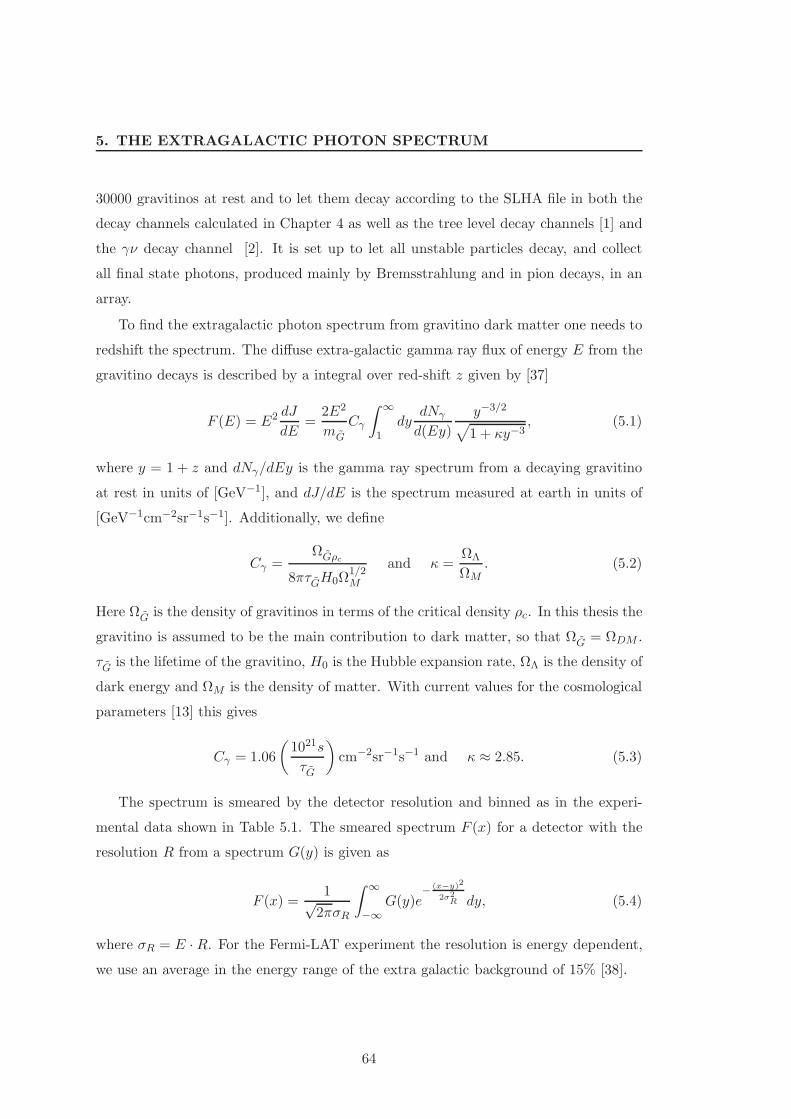
5. THE EXTRAGALACTIC PHOTON SPECTRUM
30000 gravitinos at rest and to let them decay according to the SLHA file in both the
decay channels calculated in Chapter 4 as well as the tree level decay channels [1] and
the γν decay channel [2]. It is set up to let all unstable particles decay, and collect
all final state photons, produced mainly by Bremsstrahlung and in pion decays, in an
array.
To find the extragalactic photon spectrum from gravitino dark matter one needs to
redshift the spectrum. The diffuse extra-galactic gamma ray flux of energy E from the
gravitino decays is described by a integral over red-shift z given by [37]
F (E) = E2 dJ
dE=
2E2
mG
Cγ
∫ ∞
1dy
dNγ
d(Ey)
y−3/2
√
1 + κy−3, (5.1)
where y = 1 + z and dNγ/dEy is the gamma ray spectrum from a decaying gravitino
at rest in units of [GeV−1], and dJ/dE is the spectrum measured at earth in units of
[GeV−1cm−2sr−1s−1]. Additionally, we define
Cγ =ΩGρc
8πτGH0Ω1/2M
and κ =ΩΛ
ΩM. (5.2)
Here ΩG is the density of gravitinos in terms of the critical density ρc. In this thesis the
gravitino is assumed to be the main contribution to dark matter, so that ΩG = ΩDM .
τG is the lifetime of the gravitino, H0 is the Hubble expansion rate, ΩΛ is the density of
dark energy and ΩM is the density of matter. With current values for the cosmological
parameters [13] this gives
Cγ = 1.06
(
1021s
τG
)
cm−2sr−1s−1 and κ ≈ 2.85. (5.3)
The spectrum is smeared by the detector resolution and binned as in the experi-
mental data shown in Table 5.1. The smeared spectrum F (x) for a detector with the
resolution R from a spectrum G(y) is given as
F (x) =1√2πσR
∫ ∞
−∞G(y)e
− (x−y)2
2σ2R dy, (5.4)
where σR = E · R. For the Fermi-LAT experiment the resolution is energy dependent,
we use an average in the energy range of the extra galactic background of 15% [38].
64
5.2 Setting limits
5.2 Setting limits
This spectrum can now be compared to the data for the extra galactic background
(EGB) flux taken from [33]. This is done as a least square analysis, as described e.g. by
Cowan [39]. As the width of the process goes as λ2 the normalization of the spectrum
has to be proportional to λ2 as well. The background is assumed to follow a power law
distribution
F (E) = IBG(E
1GeV)−γBG . (5.5)
To analyze how well the theoretical calculation fits the data one calculates the least
squares function χ2(λ, IBG, γBG) which can be expressed as
χ2(λ, IBG, γBG) =∑
i
(
yobsi − ythi (λ, IBG, γBG)
σi
)2
, (5.6)
where yobsi is the measured value in the ith bin with an experimental error of σi and
can be found in Table 5.1, while ythi = yGi · λ2 + yBGi (IBG, γBG) is the theoretical
prediction, where yBGi (IBG, γBG) is the background for given parameters and yGi is the
signal prediction in the ith bin from the gravitino decay for λ = 1. The theoretical
error is assumed to be smaller than the experimental error and is ignored.
To set a limit on the coupling λ one calculates
∆χ2(λ) = χ2(λ, IBGλ, γBGλ)− χ2(0, IBG, γBG), (5.7)
where IBG and γBG are chosen such that the function is minimized for the case with only
background, while IBGλ and γBGλ are chosen such that the distribution is minimized
for a given coupling λ. Using the one sided chi-squared distribution the upper limit
for the coupling is then given by the coupling where ∆χ2(λmax) = 3.84 at a confidence
level of 95%. The results of this analysis are shown in Section 6.3.
65
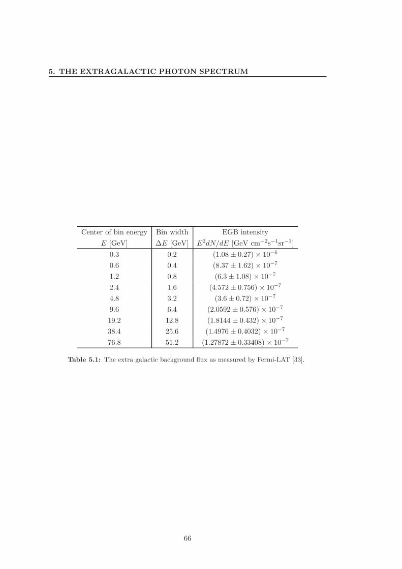
5. THE EXTRAGALACTIC PHOTON SPECTRUM
Center of bin energy Bin width EGB intensity
E [GeV] ∆E [GeV] E2dN/dE [GeV cm−2s−1sr−1]
0.3 0.2 (1.08 ± 0.27) × 10−6
0.6 0.4 (8.37 ± 1.62) × 10−7
1.2 0.8 (6.3± 1.08) × 10−7
2.4 1.6 (4.572 ± 0.756) × 10−7
4.8 3.2 (3.6± 0.72) × 10−7
9.6 6.4 (2.0592 ± 0.576) × 10−7
19.2 12.8 (1.8144 ± 0.432) × 10−7
38.4 25.6 (1.4976 ± 0.4032) × 10−7
76.8 51.2 (1.27872 ± 0.33408) × 10−7
Table 5.1: The extra galactic background flux as measured by Fermi-LAT [33].
66
6
Results and Discussion
In the following the results found in Chapters 4 and 5 are presented together with the
decay modes G → γν calculated by Lola, Osland and Raklev [2] and the tree level
decay modes found by Moreau and Chemtob [1] for comparison. First the results are
investigated for mass and flavor dependence, then the stability of the gravitino in one
scenario is discussed and finally limits are set on the R-parity violating coupling for
interesting scenarios.
Note that the widths below are only plotted for one final state. As the gravitino is
a Majorana particle there exists charge conjugated processes, Z0ν for Z0ν and W−l+
for W+l−, which give the same result. To get the total width one has to multiply the
sum of all channels by two. Note also that the width in all channels is proportional to
the R-parity breaking coupling squared, so that one can rescale the result for a given
coupling λ by multiplying by λ2/λ2u where λu is the coupling used in the plots. The
width plots are all plotted in units of GeV/λ2, so that one can easily rescale the result
by multiplying by λ2.
As the calculations done in this thesis are only valid for gravitino masses larger than
the sum of the final state particle masses and because it is found in this thesis that tree
level processes dominate for gravitino masses much bigger than the gauge boson mass,
the mass range considered in the following discussion is 50 GeV ≤ mG ≤ 250 GeV. In
the following one-coupling dominance is also assumed, meaning that only one of the
trilinear R-parity violating couplings is significant at a time.
67
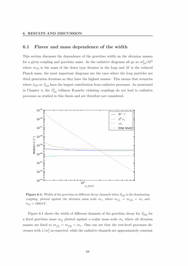
6. RESULTS AND DISCUSSION
6.1 Flavor and mass dependence of the width
This section discusses the dependence of the gravitino width on the sfermion masses
for a given coupling and gravitino mass. As the radiative diagrams all go as m2fd/M
2
where mfd is the mass of the down type fermion in the loop and M is the reduced
Planck mass, the most important diagrams are the ones where the loop particles are
third generation fermions as they have the highest masses. This means that scenarios
where λi33 or λ′i33 have the largest contribution from radiative processes. As mentioned
in Chapter 4, the λ′′ijk trilinear R-parity violating couplings do not lead to radiative
processes as studied in this thesis and are therefore not considered.
103
ms [GeV]
10-43
10-42
10-41
10-40
10-39
10-38
10-37
10-36
10-35
Width[GeV/λ
2]
W+ τ−
Z0 ντγντ
tree level
Figure 6.1: Width of the gravitino in different decay channels when λ′333 is the dominating
coupling, plotted against the sfermion mass scale ms, where mfL = mfR = ms and
mG = 190GeV .
Figure 6.1 shows the width of different channels of the gravitino decay for λ′333 for
a fixed gravitino mass mG plotted against a scalar mass scale ms where all sfermion
masses are fixed to mfL = mfR = ms. One can see that the tree-level processes de-
creases with 1/m4s as expected, while the radiative channels are approximately constant
68
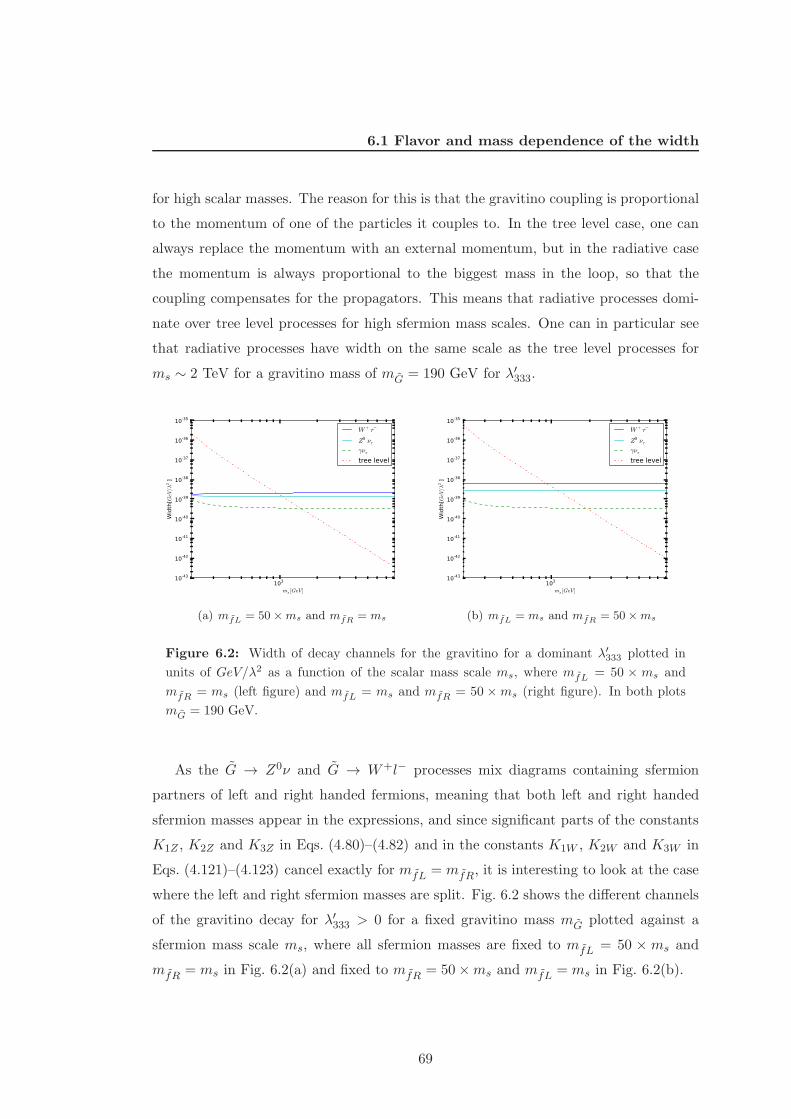
6.1 Flavor and mass dependence of the width
for high scalar masses. The reason for this is that the gravitino coupling is proportional
to the momentum of one of the particles it couples to. In the tree level case, one can
always replace the momentum with an external momentum, but in the radiative case
the momentum is always proportional to the biggest mass in the loop, so that the
coupling compensates for the propagators. This means that radiative processes domi-
nate over tree level processes for high sfermion mass scales. One can in particular see
that radiative processes have width on the same scale as the tree level processes for
ms ∼ 2 TeV for a gravitino mass of mG = 190 GeV for λ′333.
103
ms [GeV]
10-43
10-42
10-41
10-40
10-39
10-38
10-37
10-36
10-35
Width[GeV/λ
2]
W+ τ−
Z0 ντγντ
tree level
(a) mfL = 50×ms and mfR = ms
103
ms [GeV]
10-43
10-42
10-41
10-40
10-39
10-38
10-37
10-36
10-35
Width[GeV/λ
2]
W+ τ−
Z0 ντγντ
tree level
(b) mfL = ms and mfR = 50×ms
Figure 6.2: Width of decay channels for the gravitino for a dominant λ′333 plotted in
units of GeV/λ2 as a function of the scalar mass scale ms, where mfL = 50 × ms and
mfR = ms (left figure) and mfL = ms and mfR = 50 ×ms (right figure). In both plots
mG = 190 GeV.
As the G → Z0ν and G → W+l− processes mix diagrams containing sfermion
partners of left and right handed fermions, meaning that both left and right handed
sfermion masses appear in the expressions, and since significant parts of the constants
K1Z , K2Z and K3Z in Eqs. (4.80)–(4.82) and in the constants K1W , K2W and K3W in
Eqs. (4.121)–(4.123) cancel exactly for mfL = mfR, it is interesting to look at the case
where the left and right sfermion masses are split. Fig. 6.2 shows the different channels
of the gravitino decay for λ′333 > 0 for a fixed gravitino mass mG plotted against a
sfermion mass scale ms, where all sfermion masses are fixed to mfL = 50 × ms and
mfR = ms in Fig. 6.2(a) and fixed to mfR = 50×ms and mfL = ms in Fig. 6.2(b).
69
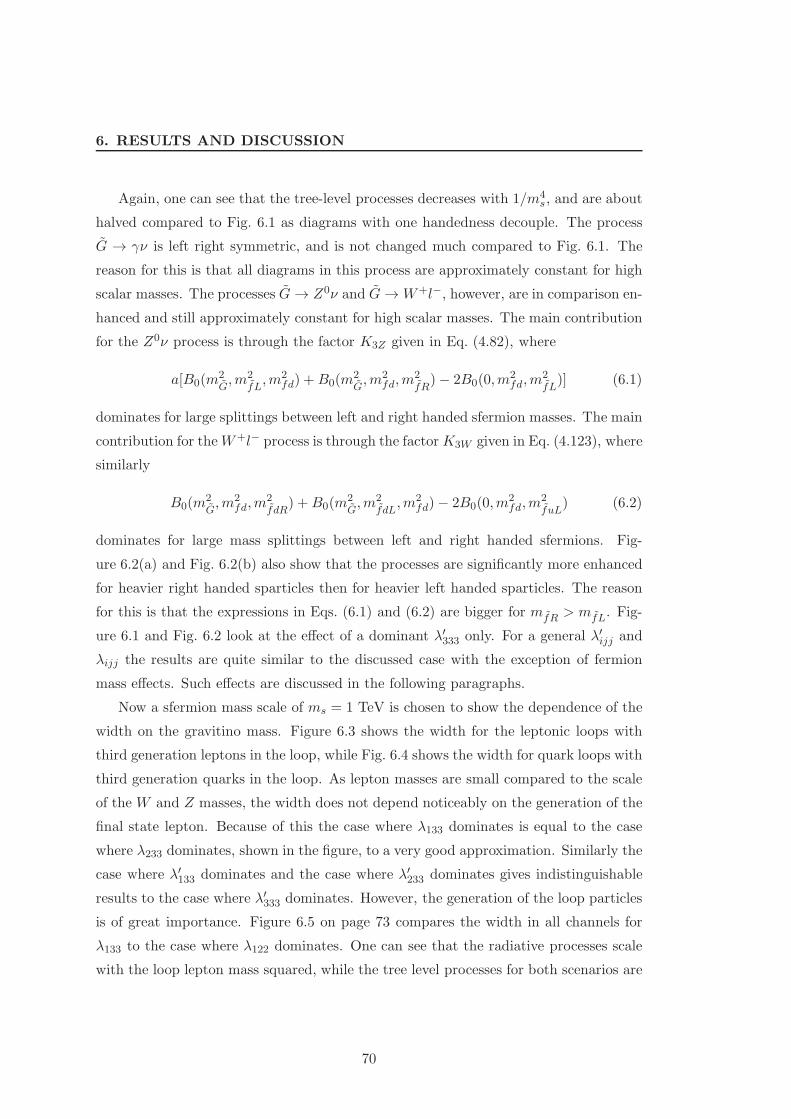
6. RESULTS AND DISCUSSION
Again, one can see that the tree-level processes decreases with 1/m4s, and are about
halved compared to Fig. 6.1 as diagrams with one handedness decouple. The process
G → γν is left right symmetric, and is not changed much compared to Fig. 6.1. The
reason for this is that all diagrams in this process are approximately constant for high
scalar masses. The processes G→ Z0ν and G→W+l−, however, are in comparison en-
hanced and still approximately constant for high scalar masses. The main contribution
for the Z0ν process is through the factor K3Z given in Eq. (4.82), where
a[B0(m2G,m2
fL,m2
fd) +B0(m2G,m2
fd,m2fR
)− 2B0(0,m2fd,m
2fL
)] (6.1)
dominates for large splittings between left and right handed sfermion masses. The main
contribution for theW+l− process is through the factorK3W given in Eq. (4.123), where
similarly
B0(m2G,m2
fd,m2f dR
) +B0(m2G,m2
fdL,m2
fd)− 2B0(0,m2fd,m
2fuL
) (6.2)
dominates for large mass splittings between left and right handed sfermions. Fig-
ure 6.2(a) and Fig. 6.2(b) also show that the processes are significantly more enhanced
for heavier right handed sparticles then for heavier left handed sparticles. The reason
for this is that the expressions in Eqs. (6.1) and (6.2) are bigger for mfR > mfL. Fig-
ure 6.1 and Fig. 6.2 look at the effect of a dominant λ′333 only. For a general λ′ijj and
λijj the results are quite similar to the discussed case with the exception of fermion
mass effects. Such effects are discussed in the following paragraphs.
Now a sfermion mass scale of ms = 1 TeV is chosen to show the dependence of the
width on the gravitino mass. Figure 6.3 shows the width for the leptonic loops with
third generation leptons in the loop, while Fig. 6.4 shows the width for quark loops with
third generation quarks in the loop. As lepton masses are small compared to the scale
of the W and Z masses, the width does not depend noticeably on the generation of the
final state lepton. Because of this the case where λ133 dominates is equal to the case
where λ233 dominates, shown in the figure, to a very good approximation. Similarly the
case where λ′133 dominates and the case where λ′233 dominates gives indistinguishable
results to the case where λ′333 dominates. However, the generation of the loop particles
is of great importance. Figure 6.5 on page 73 compares the width in all channels for
λ133 to the case where λ122 dominates. One can see that the radiative processes scale
with the loop lepton mass squared, while the tree level processes for both scenarios are
70
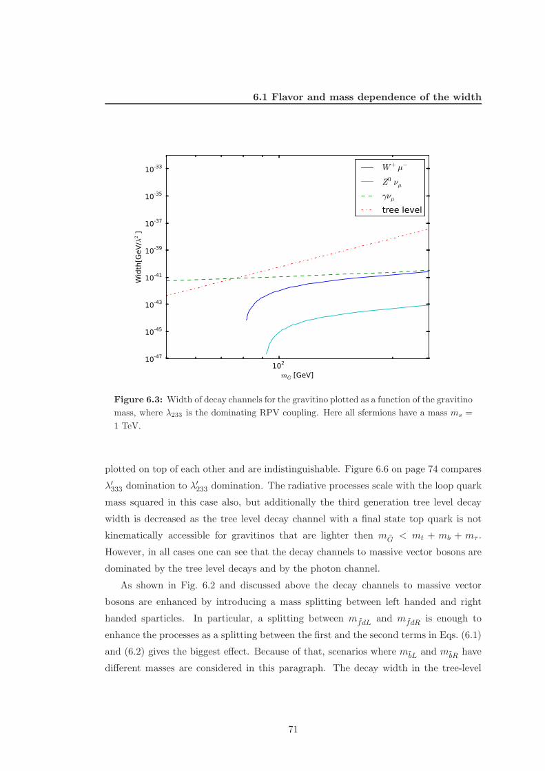
6.1 Flavor and mass dependence of the width
102
mG [GeV]
10-47
10-45
10-43
10-41
10-39
10-37
10-35
10-33
Width[G
eV/λ
2]
W+ µ−
Z0 νµ
γνµ
tree level
Figure 6.3: Width of decay channels for the gravitino plotted as a function of the gravitino
mass, where λ233 is the dominating RPV coupling. Here all sfermions have a mass ms =
1 TeV.
plotted on top of each other and are indistinguishable. Figure 6.6 on page 74 compares
λ′333 domination to λ′233 domination. The radiative processes scale with the loop quark
mass squared in this case also, but additionally the third generation tree level decay
width is decreased as the tree level decay channel with a final state top quark is not
kinematically accessible for gravitinos that are lighter then mG < mt + mb + mτ .
However, in all cases one can see that the decay channels to massive vector bosons are
dominated by the tree level decays and by the photon channel.
As shown in Fig. 6.2 and discussed above the decay channels to massive vector
bosons are enhanced by introducing a mass splitting between left handed and right
handed sparticles. In particular, a splitting between mfdL and mfdR is enough to
enhance the processes as a splitting between the first and the second terms in Eqs. (6.1)
and (6.2) gives the biggest effect. Because of that, scenarios where mbL and mbR have
different masses are considered in this paragraph. The decay width in the tree-level
71
6. RESULTS AND DISCUSSION
102
mG [GeV]
10-44
10-43
10-42
10-41
10-40
10-39
10-38
10-37
10-36
10-35
10-34
10-33
10-32
10-31
Width[G
eV/λ
2]
W+ au−
Z0 νauγνau
tree level
Figure 6.4: Width of decay channels for the gravitino plotted as a function of the gravitino
mass, where λ′333 is the dominating RPV coupling. Here all sfermions have a mass ms =
1 TeV.
channels and the γν channel are plotted for mbL = mbR = ms = 1TeV for comparison.
As discussed above, the γν process does not change for mass splitting, while the tree-
level processes are halved in the decoupled limit. Figure 6.7(a) on page 75 shows
the decay channels for mbR = 1 TeV compared to mbR = 100 TeV for λ′333 and with
mbL = 1 TeV. Figure 6.7(b) shows the decay channels for mbL = 1 TeV compared to
mbL = 100 TeV for λ′333 with mbR = 1 TeV. In both cases one can see that in the case
where the left and right sbottom masses are split, the W+τ− process gives the biggest
contribution to the gravitino width in a mass range between mG ≈ 90 GeV–210 GeV,
while the Z0ντ width is bigger than the tree level width and the γντ width for a mass
in the range mG ≈ 110 GeV–190 GeV. Figure 6.8 on page 75 shows how the width of
the decay channel G → W+τ− varies with different mbR and mbL. One can see that
there are gravitino masses where the W+τ− decay mode gives the biggest contribution
already formbR/L = 3×mbL/R, and that formbR/L = 10×mbL/R there is a considerable
72
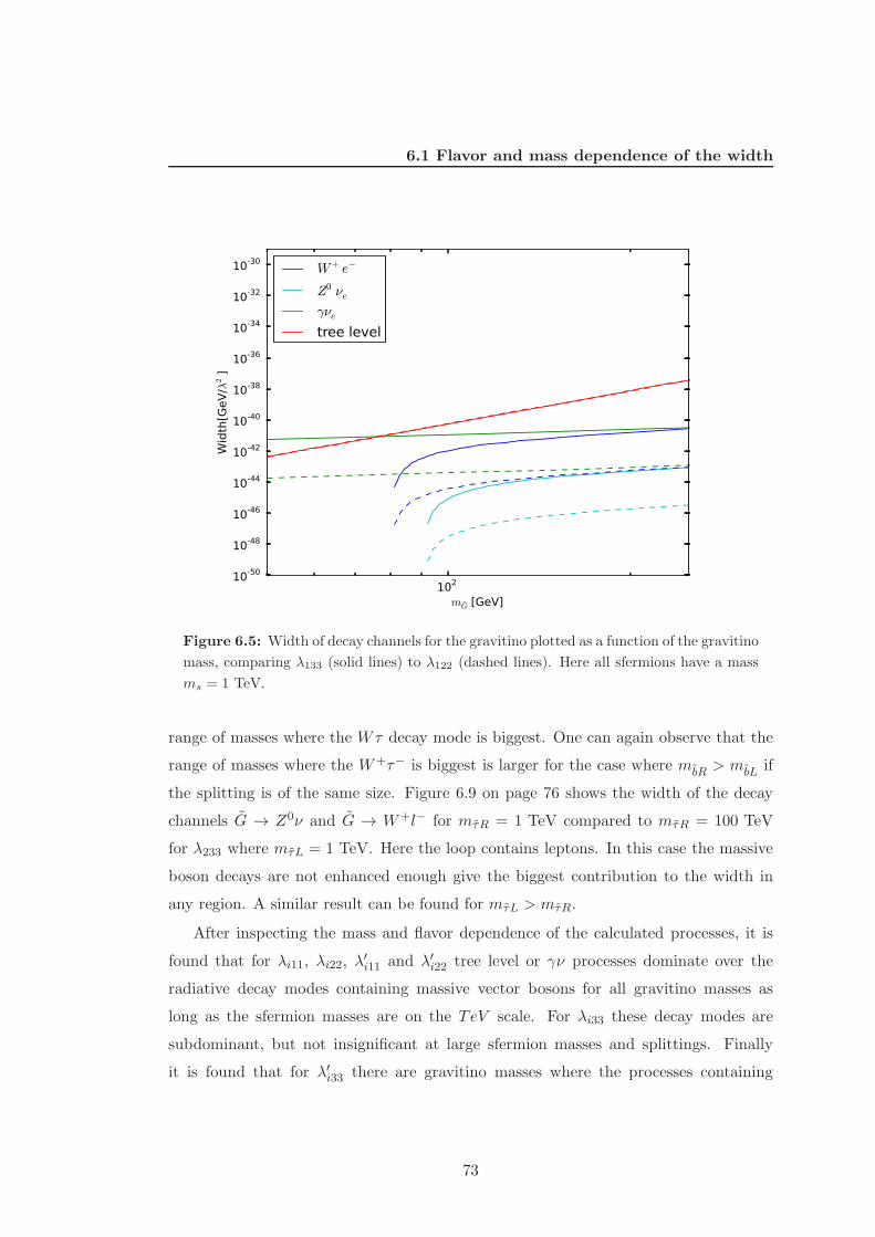
6.1 Flavor and mass dependence of the width
102
mG [GeV]
10-50
10-48
10-46
10-44
10-42
10-40
10-38
10-36
10-34
10-32
10-30
Width[G
eV/λ
2]
W+ e−
Z0 νeγνe
tree level
Figure 6.5: Width of decay channels for the gravitino plotted as a function of the gravitino
mass, comparing λ133 (solid lines) to λ122 (dashed lines). Here all sfermions have a mass
ms = 1 TeV.
range of masses where the Wτ decay mode is biggest. One can again observe that the
range of masses where the W+τ− is biggest is larger for the case where mbR > mbL if
the splitting is of the same size. Figure 6.9 on page 76 shows the width of the decay
channels G → Z0ν and G → W+l− for mτR = 1 TeV compared to mτR = 100 TeV
for λ233 where mτL = 1 TeV. Here the loop contains leptons. In this case the massive
boson decays are not enhanced enough give the biggest contribution to the width in
any region. A similar result can be found for mτL > mτR.
After inspecting the mass and flavor dependence of the calculated processes, it is
found that for λi11, λi22, λ′i11 and λ′i22 tree level or γν processes dominate over the
radiative decay modes containing massive vector bosons for all gravitino masses as
long as the sfermion masses are on the TeV scale. For λi33 these decay modes are
subdominant, but not insignificant at large sfermion masses and splittings. Finally
it is found that for λ′i33 there are gravitino masses where the processes containing
73
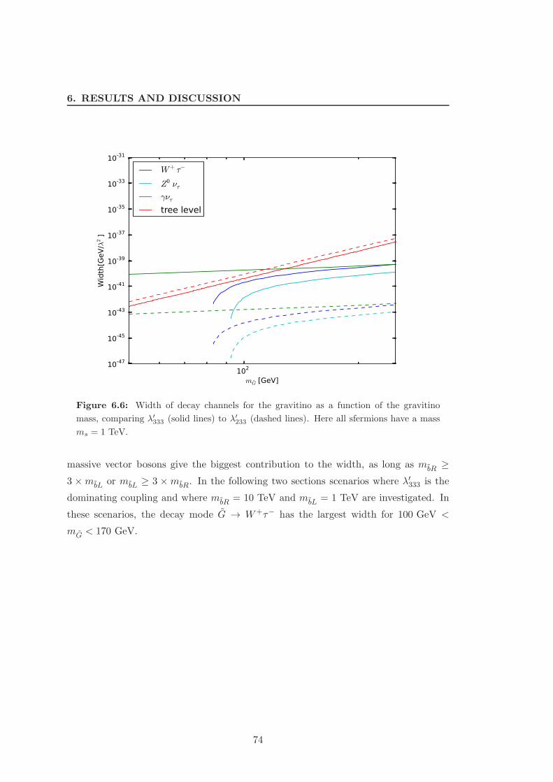
6. RESULTS AND DISCUSSION
102
mG [GeV]
10-47
10-45
10-43
10-41
10-39
10-37
10-35
10-33
10-31
Width[G
eV/λ
2]
W+ τ−
Z0 ντγντ
tree level
Figure 6.6: Width of decay channels for the gravitino as a function of the gravitino
mass, comparing λ′333 (solid lines) to λ′233 (dashed lines). Here all sfermions have a mass
ms = 1 TeV.
massive vector bosons give the biggest contribution to the width, as long as mbR ≥3 ×mbL or mbL ≥ 3 ×mbR. In the following two sections scenarios where λ′333 is the
dominating coupling and where mbR = 10 TeV and mbL = 1 TeV are investigated. In
these scenarios, the decay mode G → W+τ− has the largest width for 100 GeV <
mG < 170 GeV.
74
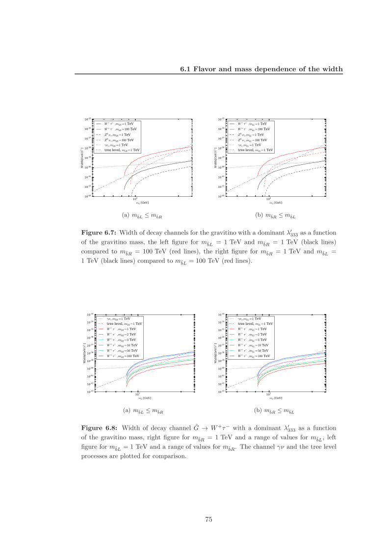
6.1 Flavor and mass dependence of the width
102
mG [GeV]
10-43
10-42
10-41
10-40
10-39
10-38
10-37
10-36
10-35
Width[G
eV/λ
2]
W+ τ− ,mbR=1 TeV
W+ τ− ,mbR=100 TeV
Z0 ντ ,mbR=1 TeV
Z0 ντ ,mbR=100 TeV
γντ ,mbR=1 TeV
tree level, mbR=1 TeV
(a) mbL ≤ mbR
102
mG [GeV]
10-43
10-42
10-41
10-40
10-39
10-38
10-37
10-36
10-35
Width[G
eV/λ
2]
W+ τ− ,mbL=1 TeV
W+ τ− ,mbL=100 TeV
Z0 ντ ,mbL=1 TeV
Z0 ντ ,mbL=100 TeV
γντ ,mbL=1 TeV
tree level, mbL=1 TeV
(b) mbR ≤ mbL
Figure 6.7: Width of decay channels for the gravitino with a dominant λ′333 as a function
of the gravitino mass, the left figure for mbL = 1 TeV and mbR = 1 TeV (black lines)
compared to mbR = 100 TeV (red lines), the right figure for mbR = 1 TeV and mbL =
1 TeV (black lines) compared to mbL = 100 TeV (red lines).
102
mG [GeV]
10-43
10-42
10-41
10-40
10-39
10-38
10-37
10-36
10-35
10-34
10-33
Width[G
eV/λ
2]
γντ ,mbR=1 TeV
tree level, mbR=1 TeV
W+ τ− ,mbR=1 TeV
W+ τ− ,mbR=2 TeV
W+ τ− ,mbR=3 TeV
W+ τ− ,mbR=10 TeV
W+ τ− ,mbR=50 TeV
W+ τ− ,mbR=100 TeV
(a) mbL ≤ mbR
102
mG [GeV]
10-43
10-42
10-41
10-40
10-39
10-38
10-37
10-36
10-35
10-34
10-33
Width[G
eV/λ
2]
γντ ,mbL=1 TeV
tree level, mbL=1 TeV
W+ τ− ,mbL=1 TeV
W+ τ− ,mbL=2 TeV
W+ τ− ,mbL=3 TeV
W+ τ− ,mbL=10 TeV
W+ τ− ,mbL=50 TeV
W+ τ− ,mbL=100 TeV
(b) mbR ≤ mbL
Figure 6.8: Width of decay channel G → W+τ− with a dominant λ′333 as a function
of the gravitino mass, right figure for mbR = 1 TeV and a range of values for mbL, left
figure for mbL = 1 TeV and a range of values for mbR. The channel γν and the tree level
processes are plotted for comparison.
75
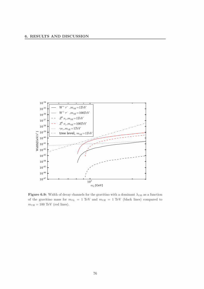
6. RESULTS AND DISCUSSION
102
mG [GeV]
10-47
10-46
10-45
10-44
10-43
10-42
10-41
10-40
10-39
10-38
10-37
10-36
10-35
10-34
Width[G
eV/λ
2]
W+ τ− ,mτR=1TeV
W+ τ− ,mτR=100TeV
Z0 ντ ,mτR=1TeV
Z0 ντ ,mτR=100TeV
γντ ,mτR=1TeV
tree level, mτR=1TeV
Figure 6.9: Width of decay channels for the gravitino with a dominant λ133 as a function
of the gravitino mass for mτL = 1 TeV and mτR = 1 TeV (black lines) compared to
mτR = 100 TeV (red lines).
76
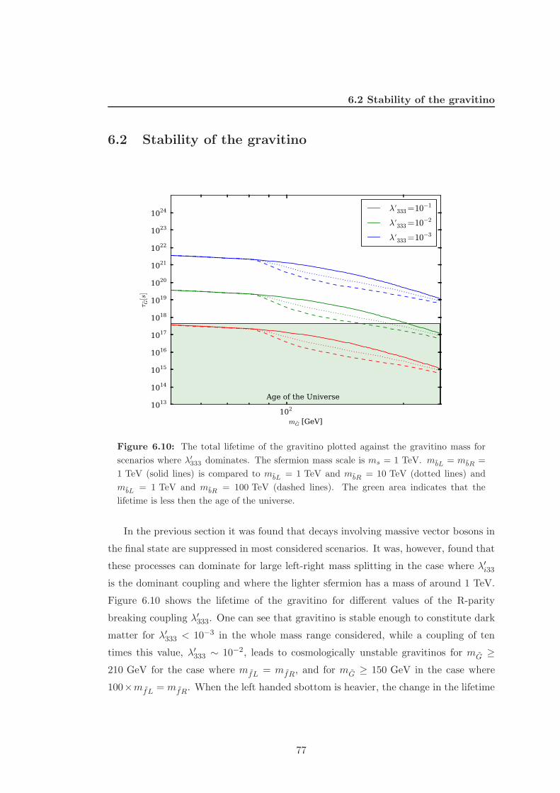
6.2 Stability of the gravitino
6.2 Stability of the gravitino
102
mG [GeV]
1013
1014
1015
1016
1017
1018
1019
1020
1021
1022
1023
1024
τ G[s]
λ′333=10−1
λ′333=10−2
λ′333=10−3
Age of the Universe
Figure 6.10: The total lifetime of the gravitino plotted against the gravitino mass for
scenarios where λ′333 dominates. The sfermion mass scale is ms = 1 TeV. mbL = mbR =
1 TeV (solid lines) is compared to mbL = 1 TeV and mbR = 10 TeV (dotted lines) and
mbL = 1 TeV and mbR = 100 TeV (dashed lines). The green area indicates that the
lifetime is less then the age of the universe.
In the previous section it was found that decays involving massive vector bosons in
the final state are suppressed in most considered scenarios. It was, however, found that
these processes can dominate for large left-right mass splitting in the case where λ′i33
is the dominant coupling and where the lighter sfermion has a mass of around 1 TeV.
Figure 6.10 shows the lifetime of the gravitino for different values of the R-parity
breaking coupling λ′333. One can see that gravitino is stable enough to constitute dark
matter for λ′333 < 10−3 in the whole mass range considered, while a coupling of ten
times this value, λ′333 ∼ 10−2, leads to cosmologically unstable gravitinos for mG ≥210 GeV for the case where mfL = mfR, and for mG ≥ 150 GeV in the case where
100×mfL = mfR. When the left handed sbottom is heavier, the change in the lifetime
77
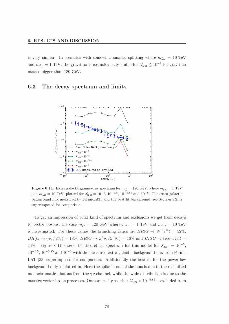
6. RESULTS AND DISCUSSION
is very similar. In scenarios with somewhat smaller splitting where mbR = 10 TeV
and mbL = 1 TeV, the gravitino is cosmologically stable for λ′333 ≤ 10−2 for gravitino
masses bigger than 180 GeV.
6.3 The decay spectrum and limits
10-1 100 101 102 103
Energy [GeV]
10-9
10-8
10-7
10-6
10-5
E2dNdE[GeV
cm−2
s−1
sr−
1]
Best fit for Background only
λ′333=10−5
λ′333=10−5.5
λ′333=10−5.85
λ′333=10−6
EGB measured at FermiLAT
Figure 6.11: Extra galactic gamma-ray spectrum formG = 120 GeV, wherembL = 1 TeV
and mbR = 10 TeV, plotted for λ′333 = 10−5, 10−5.5, 10−5.85 and 10−6. The extra galactic
background flux measured by Fermi-LAT, and the best fit background, see Section 5.2, is
superimposed for comparison.
To get an impression of what kind of spectrum and exclusions we get from decays
to vector bosons, the case mG = 120 GeV where mbL = 1 TeV and mbR = 10 TeV
is investigated. For these values the branching ratios are BR(G → W±τ∓) = 52%,
BR(G → γντ/γντ ) = 18%, BR(G → Z0ντ/Z0ντ ) = 16% and BR(G → tree-level) =
14%. Figure 6.11 shows the theoretical spectrum for this model for λ′333 = 10−5,
10−5.5, 10−5.85 and 10−6 with the measured extra galactic background flux from Fermi-
LAT [33] superimposed for comparison. Additionally the best fit for the power-law
background only is plotted in. Here the spike in one of the bins is due to the redshifted
monochromatic photons from the γν channel, while the wide distribution is due to the
massive vector boson processes. One can easily see that λ′333 > 10−5.85 is excluded from
78
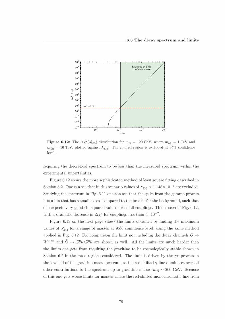
6.3 The decay spectrum and limits
10-7 10-6 10-5 10-4
λ′333
10-3
10-2
10-1
100
101
102
103
104
105
106
107
108
109
∆χ2(λ
′ 333)
Excluded at 95% confidence level
∆χ2 =3.84
Figure 6.12: The ∆χ2(λ′333) distribution for mG = 120 GeV, where mbL = 1 TeV and
mbR = 10 TeV, plotted against λ′333. The colored region is excluded at 95% confidence
level.
requiring the theoretical spectrum to be less than the measured spectrum within the
experimental uncertainties.
Figure 6.12 shows the more sophisticated method of least square fitting described in
Section 5.2. One can see that in this scenario values of λ′333 > 1.148×10⁻⁶ are excluded.
Studying the spectrum in Fig. 6.11 one can see that the spike from the gamma process
hits a bin that has a small excess compared to the best fit for the background, such that
one expects very good chi-squared values for small couplings. This is seen in Fig. 6.12,
with a dramatic decrease in ∆χ2 for couplings less than 4 · 10−7.
Figure 6.13 on the next page shows the limits obtained by finding the maximum
values of λ′333 for a range of masses at 95% confidence level, using the same method
applied in Fig. 6.12. For comparison the limit not including the decay channels G →W±l∓ and G → Z0ν/Z0ν are shown as well. All the limits are much harder then
the limits one gets from requiring the gravitino to be cosmologically stable shown in
Section 6.2 in the mass regions considered. The limit is driven by the γν process in
the low end of the gravitino mass spectrum, as the red-shifted γ line dominates over all
other contributions to the spectrum up to gravitino masses mG ∼ 200 GeV. Because
of this one gets worse limits for masses where the red-shifted monochromatic line from
79
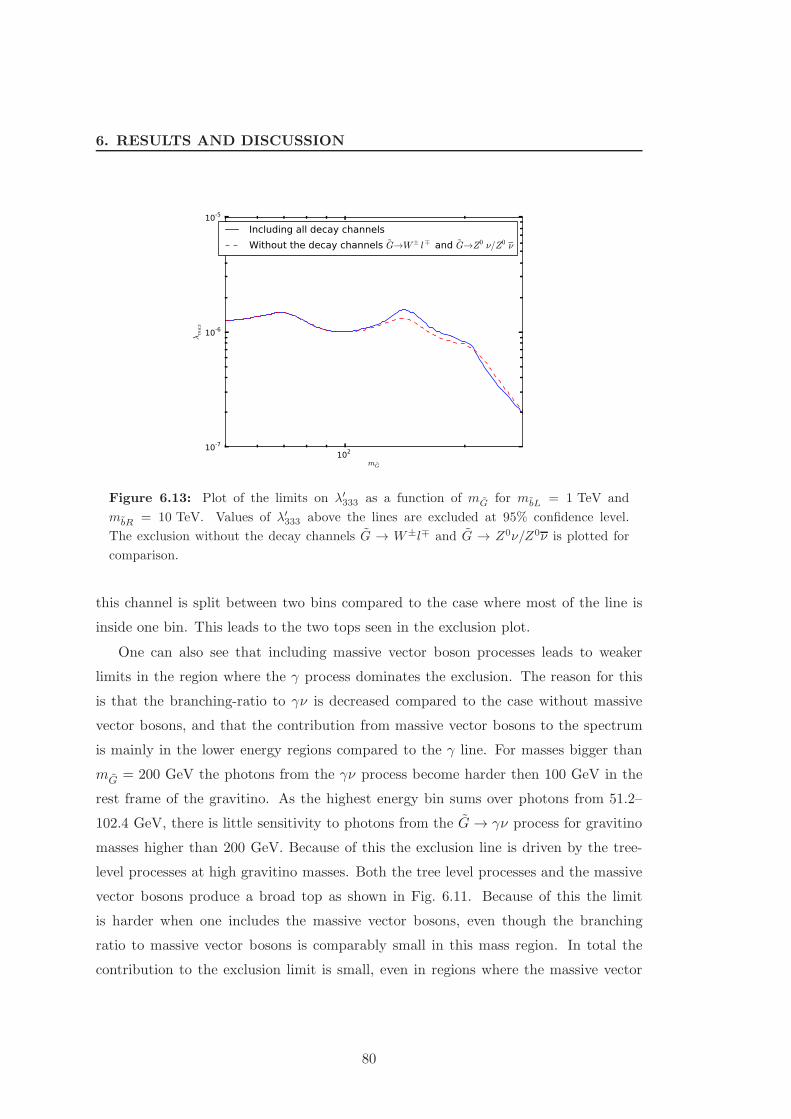
6. RESULTS AND DISCUSSION
102
mG
10-7
10-6
10-5
λmax
Including all decay channels
Without the decay channels G→W± l∓ and G→Z0 ν/Z0 ν
Figure 6.13: Plot of the limits on λ′333 as a function of mG for mbL = 1 TeV and
mbR = 10 TeV. Values of λ′333 above the lines are excluded at 95% confidence level.
The exclusion without the decay channels G → W±l∓ and G → Z0ν/Z0ν is plotted for
comparison.
this channel is split between two bins compared to the case where most of the line is
inside one bin. This leads to the two tops seen in the exclusion plot.
One can also see that including massive vector boson processes leads to weaker
limits in the region where the γ process dominates the exclusion. The reason for this
is that the branching-ratio to γν is decreased compared to the case without massive
vector bosons, and that the contribution from massive vector bosons to the spectrum
is mainly in the lower energy regions compared to the γ line. For masses bigger than
mG = 200 GeV the photons from the γν process become harder then 100 GeV in the
rest frame of the gravitino. As the highest energy bin sums over photons from 51.2–
102.4 GeV, there is little sensitivity to photons from the G→ γν process for gravitino
masses higher than 200 GeV. Because of this the exclusion line is driven by the tree-
level processes at high gravitino masses. Both the tree level processes and the massive
vector bosons produce a broad top as shown in Fig. 6.11. Because of this the limit
is harder when one includes the massive vector bosons, even though the branching
ratio to massive vector bosons is comparably small in this mass region. In total the
contribution to the exclusion limit is small, even in regions where the massive vector
80
6.3 The decay spectrum and limits
boson decays are the dominant channel.
The exclusions for λ′133 and λ′233 have been checked as well, and it was found that the
same limits as shown in Fig. 6.13 apply in these channels in the mass range considered.
Additionally exclusion limits for ms = 10 TeV without splitting were checked and it
was found that the inclusion of massive vector boson decay channels does not improve
the limits.
81

6. RESULTS AND DISCUSSION
82
7
Conclusion and Outlook
In this thesis the importance of the gravitino decay channels G→ Z0ν and G→W+l−
in scenarios with significant trilinear R-parity violating couplings was considered. The
spin-polarization tensor Πµν for spin-3/2 particles was found and used to calculate the
width of the gravitino in the decay channels G → Z0ν and G → W+l− expressed in
the Passarino-Veltman formalism. It was found that, in scenarios with third genera-
tion fermions in the loops, radiative decay channels can dominate over tree-level decay
channels for the gravitino for high sfermion masses, and that because the channels
G→ Z0ν and G→W+l− mix left and right handed diagrams, they are very sensitive
to the mass splitting between the left and right handed sparticles involved. Further-
more it was found that the decay channels to massive vector bosons can be the biggest
contribution to the gravitino width in scenarios where λ′i33 is the dominant RPV cou-
pling, for a large splitting between left and right handed sbottom squarks, for a range
of gravitino masses between 100 GeV < mG < 170 GeV. However, the contribution
to the gamma-ray spectrum leads only to minor changes in exclusion limits on the R-
parity violating couplings, even scenarios where decays to massive vector bosons give
the largest contribution to the gravitino decay width.
There are further possibilities how to use and extend this result, that could not be
part of this thesis because of time constraints. Here some of them will be mentioned.
• One could calculate these decays including virtualW and Z bosons. This leads to
a small enhancement for gravitino masses around the boson masses, and it allows
the processes to be calculated in all mass regions. However, this approach leads
83
7. CONCLUSION AND OUTLOOK
to much more complicated final states with at least three final state particles, and
the calculations are very complicated.
• One could extend the analysis to galactic gamma-rays. This is a difficult exercise,
as the galactic backgrounds are complicated and large compared to the flux from
gravitino decays.
• The results found can also be used to calculate the amount of antimatter or
neutrinos produced. The cosmological background for anti-matter is much more
limited than the photon backgrounds, and this approach might lead to better
exclusion limits. One can compare the results to measured anti-matter spectra
from astro-physical experiments and set limits in much the same way as done
in this work. This would also mean that processes with massive vector bosons
could be important for scenarios where the G → γν process dominates over the
massive vector boson processes for high scalar mass scales ms, as they would be
the dominant source of anti-matter in gravitino decays. However, this is much
harder to do, as doing this would need a detailed study of anti-matter propagation
through the galaxy and a much more complicated detection efficiency evaluation
in the detector used.
84
Appendix A
Conventions and Feynman Rules
Here the necessary Feynman rules for this thesis and conventions for traces and calcu-
lations are found. The Feynman rules are closely modeled on Appendix A in Bolz [27].
In this thesis reading direction rules for Feynman diagrams as defined by Denner et
al. [40] are used. The indices i, j and k are used as the generational indices of the
(s)fermions, while s and t are used for gauge group matrix representation indices.
A.1 Conventions
Throughout this thesis the metric is assumed to be (+ − −−). Natural units are
used where ~ = c = 1. Additionally the value of the gravitational constant used
is G = 6.70881 × 10−39~c/ GeV2. The gamma matrices are defined by the Clifford
algebra
γµ, γν = 2gµν . (A.1)
One can construct an additional gamma matrix γ5
γ5 ≡ iγ0γ1γ2γ3 (A.2)
which leads to
γµ, γ5 = 0. (A.3)
From γ5 one can construct projection operators PR and PL
PR/L =1
2(1± γ5). (A.4)
85
A. CONVENTIONS AND FEYNMAN RULES
Using the commutation relation defined in Eq. (A.3) one finds that these operators
satisfy the projection relations
P2R/L = PR/L, PL + PR = 1 and PLPR = 0. (A.5)
The anti-commuting Grassmann numbers θA and θA, where A ∈ 1, 2 and A ∈ 1, 2,
are defined by the commutation relations
[xµ, θA] = [xµ, θA] = θA, θB = θA, θB = θA, θB = θA, θB = 0. (A.6)
Indices can be lowered and raised with
ǫAB = ǫAB =
(
0 −11 0
)
, (A.7)
ǫAB = ǫAB =
(
0 1−1 0
)
. (A.8)
These two properties lead to
θAθA = 0, θθ ≡ θAθA = −2θ1θ2 and θθ ≡ θAθ
A= 2θ
1θ2. (A.9)
One defines differentiation and integration for Grassmann numbers as
∂AθB ≡ δA
B ,
∫
dθA ≡ 0 and
∫
dθAθA ≡ 1. (A.10)
Because of the anti-commutation, one can write a general function of θA as
f(θA) = f0 + f1θA, (A.11)
as all higher order terms are zero. One can then define volume elements
d2θ = −1
4dθAdθA, d2θ = −1
4dθAdθ
Aand d4θ = d2θd2θ, (A.12)
such that∫
d4θ(θθ)(θθ) = 1. (A.13)
The boson polarization vector ǫν(k) in the Feynman-’t-Hooft gauge for a massive
spin-1 boson with mass M and momentum k satisfies
∑
pol.
ǫν(k)ǫ∗ρ(k) = −(gνρ − kνkρ/M2). (A.14)
The spin–1/2 fermion spinor for a massive fermion with mass m and momentum p
satisfies∑
spin
u(p)u(p) = /p+m. (A.15)
86
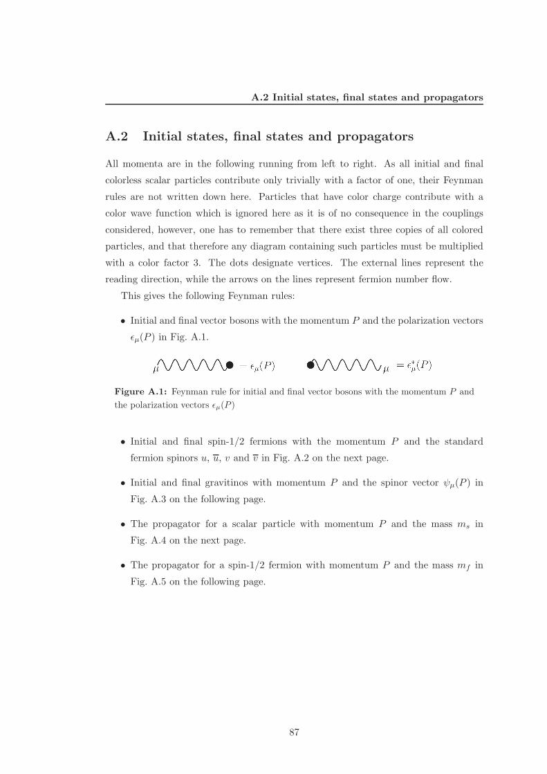
A.2 Initial states, final states and propagators
A.2 Initial states, final states and propagators
All momenta are in the following running from left to right. As all initial and final
colorless scalar particles contribute only trivially with a factor of one, their Feynman
rules are not written down here. Particles that have color charge contribute with a
color wave function which is ignored here as it is of no consequence in the couplings
considered, however, one has to remember that there exist three copies of all colored
particles, and that therefore any diagram containing such particles must be multiplied
with a color factor 3. The dots designate vertices. The external lines represent the
reading direction, while the arrows on the lines represent fermion number flow.
This gives the following Feynman rules:
• Initial and final vector bosons with the momentum P and the polarization vectors
ǫµ(P ) in Fig. A.1.
Figure A.1: Feynman rule for initial and final vector bosons with the momentum P and
the polarization vectors ǫµ(P )
• Initial and final spin-1/2 fermions with the momentum P and the standard
fermion spinors u, u, v and v in Fig. A.2 on the next page.
• Initial and final gravitinos with momentum P and the spinor vector ψµ(P ) in
Fig. A.3 on the following page.
• The propagator for a scalar particle with momentum P and the mass ms in
Fig. A.4 on the next page.
• The propagator for a spin-1/2 fermion with momentum P and the mass mf in
Fig. A.5 on the following page.
87
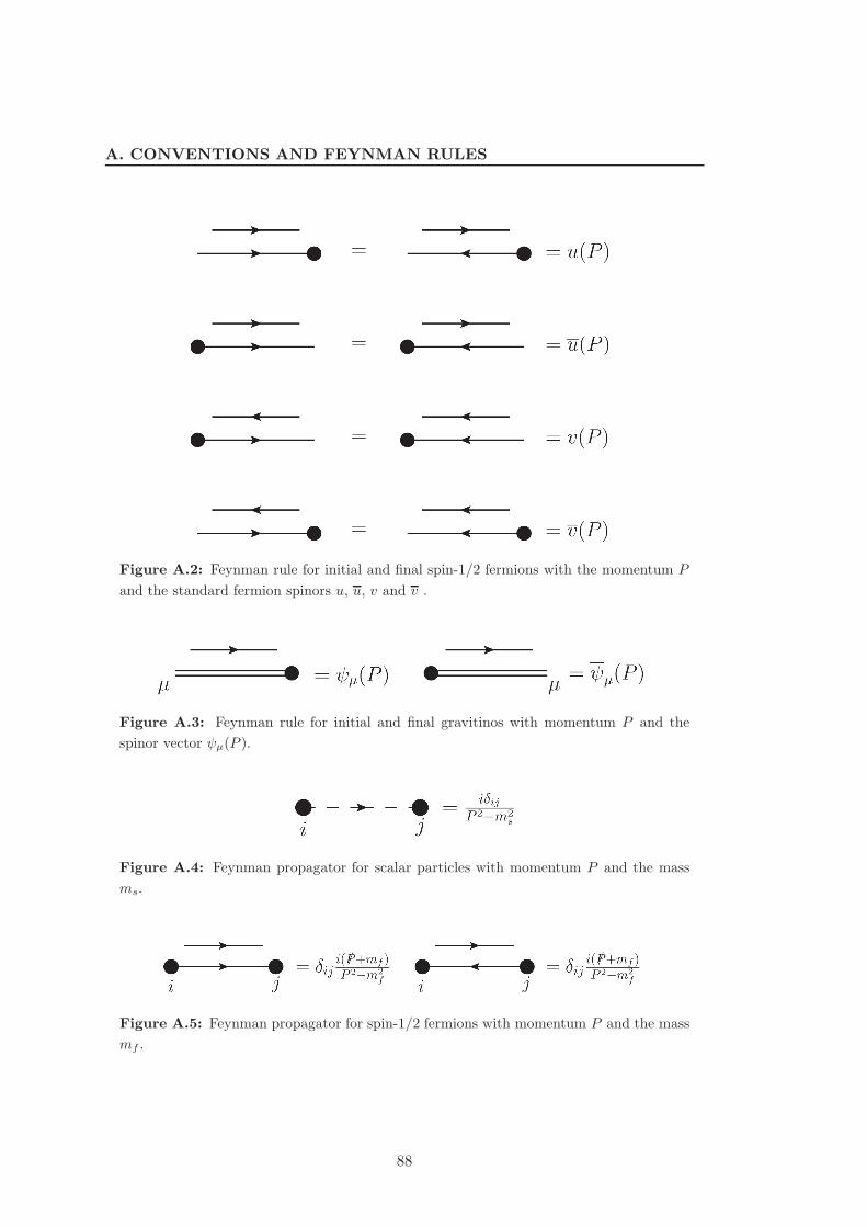
A. CONVENTIONS AND FEYNMAN RULES
Figure A.2: Feynman rule for initial and final spin-1/2 fermions with the momentum P
and the standard fermion spinors u, u, v and v .
Figure A.3: Feynman rule for initial and final gravitinos with momentum P and the
spinor vector ψµ(P ).
Figure A.4: Feynman propagator for scalar particles with momentum P and the mass
ms.
Figure A.5: Feynman propagator for spin-1/2 fermions with momentum P and the mass
mf .
88
A.3 Vertices
A.3 Vertices
The following section contains all the vertices used in this work. All the momenta are
defined running left to right.
A.3.1 The RPV couplings
The LLE part of the superpotential is given by
WLLE =1
2λijkLiiσ2LjEk, (A.16)
or written as the SU(2) components νi and li
WLLE =1
2λijk(νilj − liνj)Ek, (A.17)
where λijk = −λjik.The superfield li contains the left handed fermion field liL and the scalar field liL,
while Ek contains the left handed fermion field lkR and the scalar field l∗kR and νi
contains the left handed fermion field νiL and the scalar field νiL. Here the R-s and L-s
are part of the name of the field, and do not designate handedness. In the same way
the bar does not contain any conjugation, but is part of the name of the field.
To find the Lagrangian terms from this superpotential term that give us a coupling
between two leptons and one slepton, we use the part of the Lagrangian that reads
−12Wabψaψb − 1
2W∗abψ
†aψ
†b and the results of Section 2.1.5 where
Wab =∂W [A1, ..., An]
∂Aa∂Ab, (A.18)
so using only the LLE part of the superpotential one gets
1
2Wabψaψb =
λijk2
[
(ljLνiL + νiLljL − νjLliL − liLνjL)lkR
+l∗kR(ljLνiL − νjLliL)]
(A.19)
and using that λijk = −λjik and writing it only for i < j simplifies to
1
2Wijψiψj = λijk
[
ljLνiLlkR + νiLljLlkR + l∗kRνiLljL]
. (A.20)
Similarly
1
2W ∗
ijψ†iψ
†j = λ∗ijk
[
l∗jLν†iLl
†kR + ν∗iLl
†jLl
†kR + lkRν
†iLl
†jL
]
. (A.21)
89
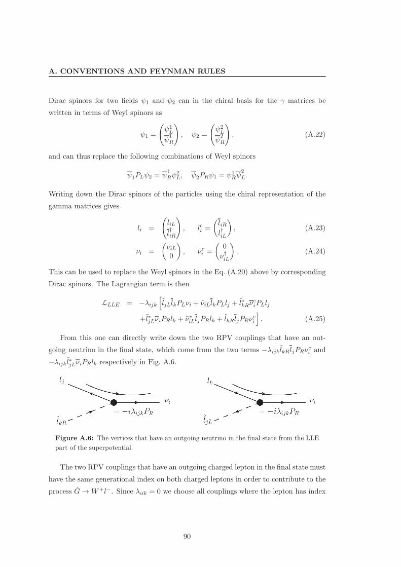
A. CONVENTIONS AND FEYNMAN RULES
Dirac spinors for two fields ψ1 and ψ2 can in the chiral basis for the γ matrices be
written in terms of Weyl spinors as
ψ1 =
(
ψ1L
ψ1R
)
, ψ2 =
(
ψ2L
ψ2R
)
, (A.22)
and can thus replace the following combinations of Weyl spinors
ψ1PLψ2 = ψ1Rψ
2L, ψ2PRψ1 = ψ1
Rψ2L.
Writing down the Dirac spinors of the particles using the chiral representation of the
gamma matrices gives
li =
(
liL
l†iR
)
, lci =
(
liRl†iL
)
, (A.23)
νi =
(
νiL0
)
, νci =
(
0
ν†iL
)
. (A.24)
This can be used to replace the Weyl spinors in the Eq. (A.20) above by corresponding
Dirac spinors. The Lagrangian term is then
LLLE = −λijk[
ljLlkPLνi + νiLlkPLlj + l∗kRνciPLlj
+l∗jLνiPRlk + ν∗iLljPRlk + lkRljPRνci
]
. (A.25)
From this one can directly write down the two RPV couplings that have an out-
going neutrino in the final state, which come from the two terms −λijk lkRljPRνci and
−λijk l∗jLνiPRlk respectively in Fig. A.6.
Figure A.6: The vertices that have an outgoing neutrino in the final state from the LLE
part of the superpotential.
The two RPV couplings that have an outgoing charged lepton in the final state must
have the same generational index on both charged leptons in order to contribute to the
process G→W+l−. Since λiik = 0 we choose all couplings where the lepton has index
90
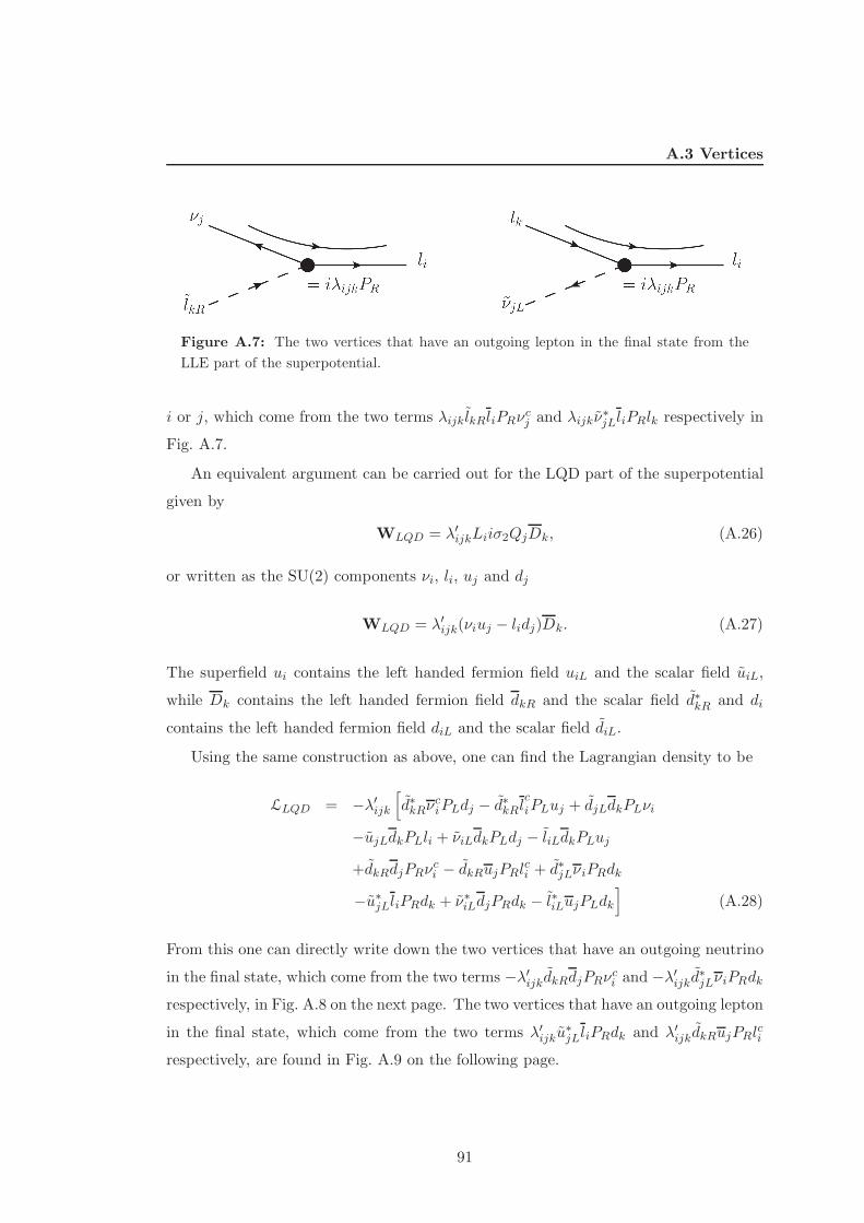
A.3 Vertices
Figure A.7: The two vertices that have an outgoing lepton in the final state from the
LLE part of the superpotential.
i or j, which come from the two terms λijk lkRliPRνcj and λijkν
∗jLliPRlk respectively in
Fig. A.7.
An equivalent argument can be carried out for the LQD part of the superpotential
given by
WLQD = λ′ijkLiiσ2QjDk, (A.26)
or written as the SU(2) components νi, li, uj and dj
WLQD = λ′ijk(νiuj − lidj)Dk. (A.27)
The superfield ui contains the left handed fermion field uiL and the scalar field uiL,
while Dk contains the left handed fermion field dkR and the scalar field d∗kR and di
contains the left handed fermion field diL and the scalar field diL.
Using the same construction as above, one can find the Lagrangian density to be
LLQD = −λ′ijk[
d∗kRνciPLdj − d∗kRl
ciPLuj + djLdkPLνi
−ujLdkPLli + νiLdkPLdj − liLdkPLuj
+dkRdjPRνci − dkRujPRl
ci + d∗jLνiPRdk
−u∗jLliPRdk + ν∗iLdjPRdk − l∗iLujPLdk
]
(A.28)
From this one can directly write down the two vertices that have an outgoing neutrino
in the final state, which come from the two terms −λ′ijkdkRdjPRνci and −λ′ijkd∗jLνiPRdk
respectively, in Fig. A.8 on the next page. The two vertices that have an outgoing lepton
in the final state, which come from the two terms λ′ijku∗jLliPRdk and λ′ijkdkRujPRl
ci
respectively, are found in Fig. A.9 on the following page.
91
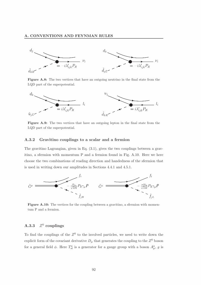
A. CONVENTIONS AND FEYNMAN RULES
Figure A.8: The two vertices that have an outgoing neutrino in the final state from the
LQD part of the superpotential.
Figure A.9: The two vertices that have an outgoing lepton in the final state from the
LQD part of the superpotential.
A.3.2 Gravitino couplings to a scalar and a fermion
The gravitino Lagrangian, given in Eq. (3.1), gives the two couplings between a grav-
itino, a sfermion with momentum P and a fermion found in Fig. A.10. Here we here
choose the two combinations of reading direction and handedness of the sfermion that
is used in writing down our amplitudes in Sections 4.4.1 and 4.5.1.
Figure A.10: The vertices for the coupling between a gravitino, a sfermion with momen-
tum P and a fermion.
A.3.3 Z0 couplings
To find the couplings of the Z0 to the involved particles, we need to write down the
explicit form of the covariant derivative Dµ that generates the coupling to the Z0 boson
for a general field φ. Here T ast is a generator for a gauge group with a boson Aa
µ, g is
92
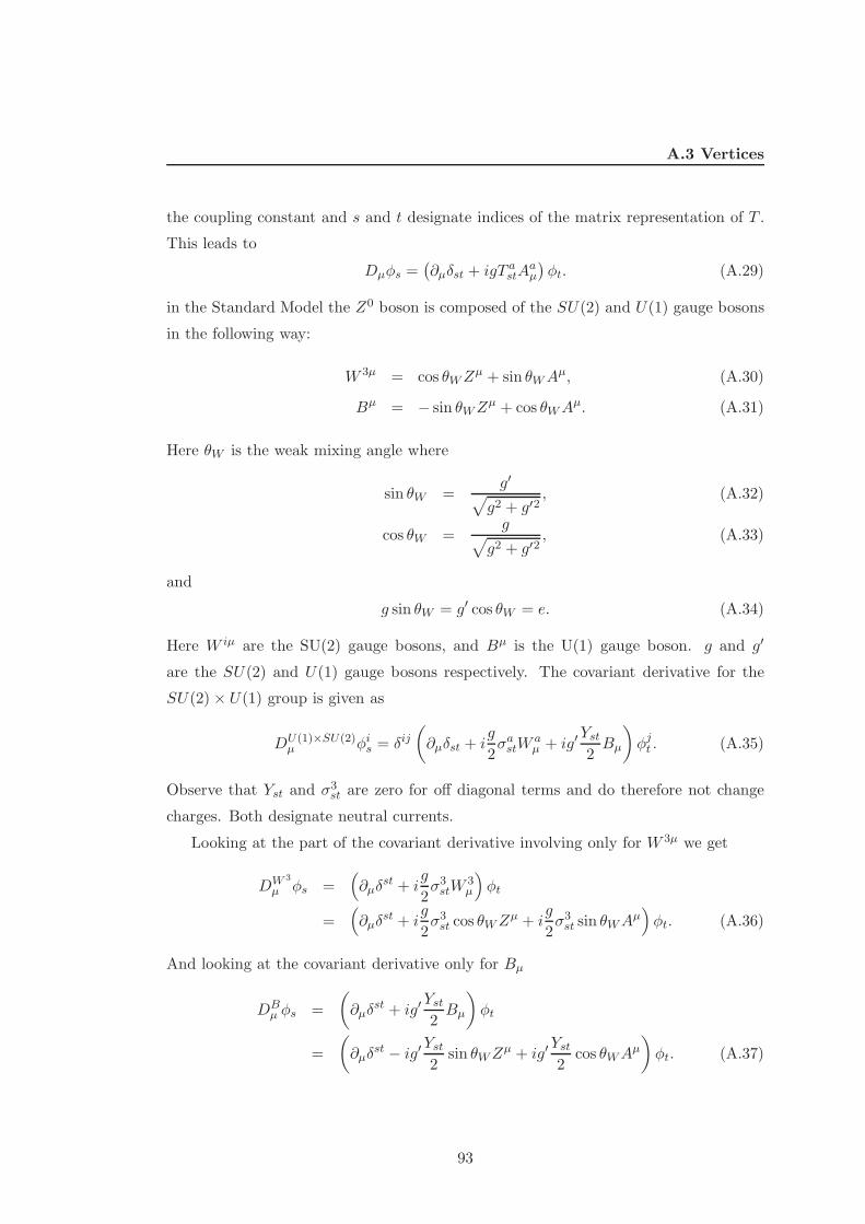
A.3 Vertices
the coupling constant and s and t designate indices of the matrix representation of T .
This leads to
Dµφs =(
∂µδst + igT astA
aµ
)
φt. (A.29)
in the Standard Model the Z0 boson is composed of the SU(2) and U(1) gauge bosons
in the following way:
W 3µ = cos θWZµ + sin θWA
µ, (A.30)
Bµ = − sin θWZµ + cos θWA
µ. (A.31)
Here θW is the weak mixing angle where
sin θW =g′
√
g2 + g′2, (A.32)
cos θW =g
√
g2 + g′2, (A.33)
and
g sin θW = g′ cos θW = e. (A.34)
Here W iµ are the SU(2) gauge bosons, and Bµ is the U(1) gauge boson. g and g′
are the SU(2) and U(1) gauge bosons respectively. The covariant derivative for the
SU(2) × U(1) group is given as
DU(1)×SU(2)µ φis = δij
(
∂µδst + ig
2σastW
aµ + ig′
Yst2Bµ
)
φjt . (A.35)
Observe that Yst and σ3st are zero for off diagonal terms and do therefore not change
charges. Both designate neutral currents.
Looking at the part of the covariant derivative involving only for W 3µ we get
DW 3
µ φs =(
∂µδst + i
g
2σ3stW
3µ
)
φt
=(
∂µδst + i
g
2σ3st cos θWZ
µ + ig
2σ3st sin θWA
µ)
φt. (A.36)
And looking at the covariant derivative only for Bµ
DBµ φs =
(
∂µδst + ig′
Yst2Bµ
)
φt
=
(
∂µδst − ig′
Yst2
sin θWZµ + ig′
Yst2
cos θWAµ
)
φt. (A.37)
93
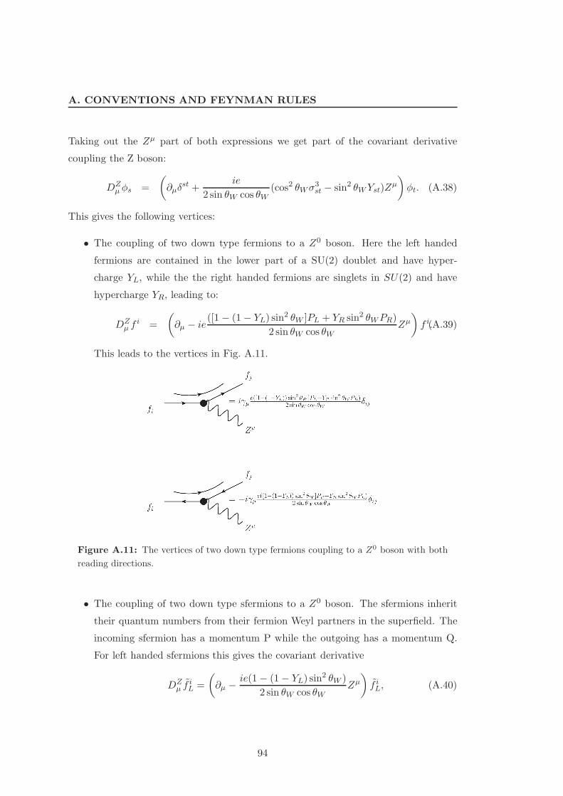
A. CONVENTIONS AND FEYNMAN RULES
Taking out the Zµ part of both expressions we get part of the covariant derivative
coupling the Z boson:
DZµ φs =
(
∂µδst +
ie
2 sin θW cos θW(cos2 θWσ
3st − sin2 θWYst)Z
µ
)
φt. (A.38)
This gives the following vertices:
• The coupling of two down type fermions to a Z0 boson. Here the left handed
fermions are contained in the lower part of a SU(2) doublet and have hyper-
charge YL, while the the right handed fermions are singlets in SU(2) and have
hypercharge YR, leading to:
DZµ f
i =
(
∂µ − ie([1 − (1− YL) sin
2 θW ]PL + YR sin2 θWPR)
2 sin θW cos θWZµ
)
f i.(A.39)
This leads to the vertices in Fig. A.11.
Figure A.11: The vertices of two down type fermions coupling to a Z0 boson with both
reading directions.
• The coupling of two down type sfermions to a Z0 boson. The sfermions inherit
their quantum numbers from their fermion Weyl partners in the superfield. The
incoming sfermion has a momentum P while the outgoing has a momentum Q.
For left handed sfermions this gives the covariant derivative
DZµ f
iL =
(
∂µ − ie(1 − (1− YL) sin2 θW )
2 sin θW cos θWZµ
)
f iL, (A.40)
94
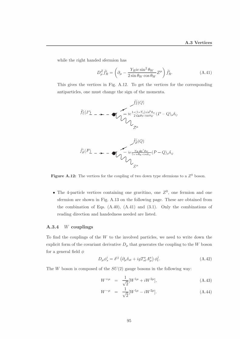
A.3 Vertices
while the right handed sfermion has
DZµ f
iR =
(
∂µ − YRie sin2 θW
2 sin θW cos θWZµ
)
f iR. (A.41)
This gives the vertices in Fig. A.12. To get the vertices for the corresponding
antiparticles, one must change the sign of the momenta.
Figure A.12: The vertices for the coupling of two down type sfermions to a Z0 boson.
• The 4-particle vertices containing one gravitino, one Z0, one fermion and one
sfermion are shown in Fig. A.13 on the following page. These are obtained from
the combination of Eqs. (A.40), (A.41) and (3.1). Only the combinations of
reading direction and handedness needed are listed.
A.3.4 W couplings
To find the couplings of the W to the involved particles, we need to write down the
explicit form of the covariant derivative Dµ that generates the coupling to theW boson
for a general field φ
Dµφis = δij
(
∂µδst + igT astA
aµ
)
φjt . (A.42)
The W boson is composed of the SU(2) gauge bosons in the following way:
W+µ =1√2[W 1µ + iW 2µ], (A.43)
W−µ =1√2[W 1µ − iW 2µ]. (A.44)
95
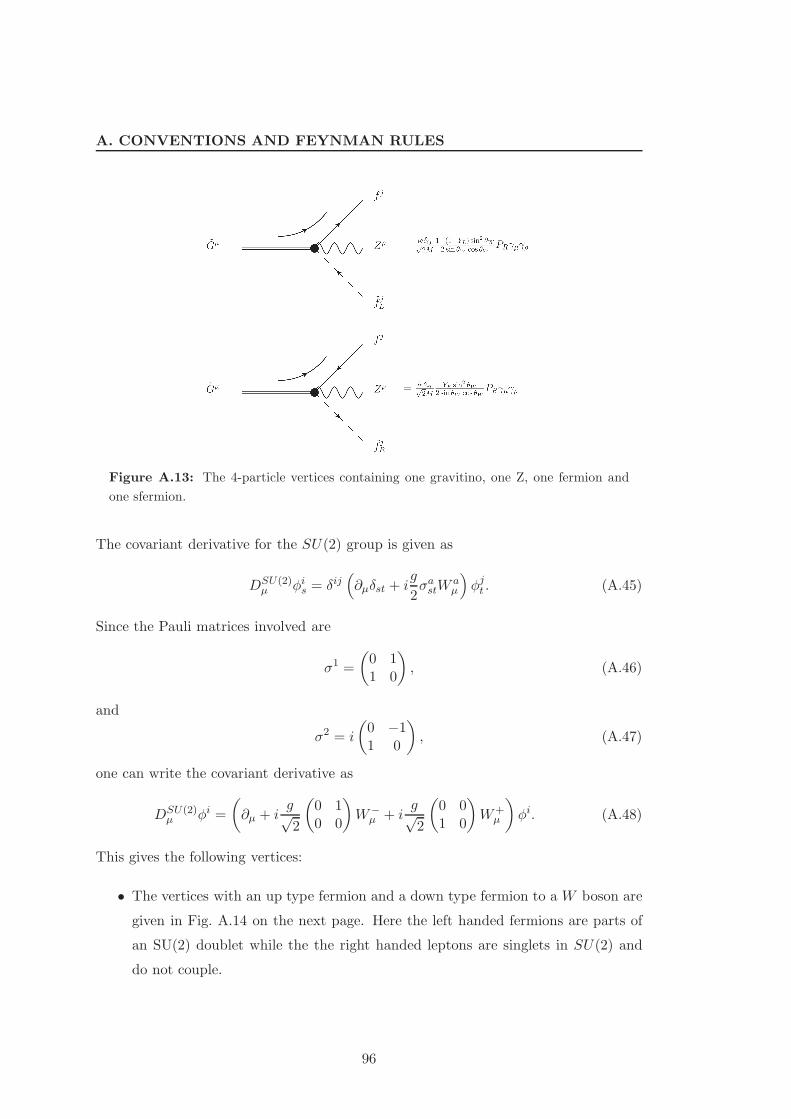
A. CONVENTIONS AND FEYNMAN RULES
Figure A.13: The 4-particle vertices containing one gravitino, one Z, one fermion and
one sfermion.
The covariant derivative for the SU(2) group is given as
DSU(2)µ φis = δij
(
∂µδst + ig
2σastW
aµ
)
φjt . (A.45)
Since the Pauli matrices involved are
σ1 =
(
0 11 0
)
, (A.46)
and
σ2 = i
(
0 −11 0
)
, (A.47)
one can write the covariant derivative as
DSU(2)µ φi =
(
∂µ + ig√2
(
0 10 0
)
W−µ + i
g√2
(
0 01 0
)
W+µ
)
φi. (A.48)
This gives the following vertices:
• The vertices with an up type fermion and a down type fermion to a W boson are
given in Fig. A.14 on the next page. Here the left handed fermions are parts of
an SU(2) doublet while the the right handed leptons are singlets in SU(2) and
do not couple.
96
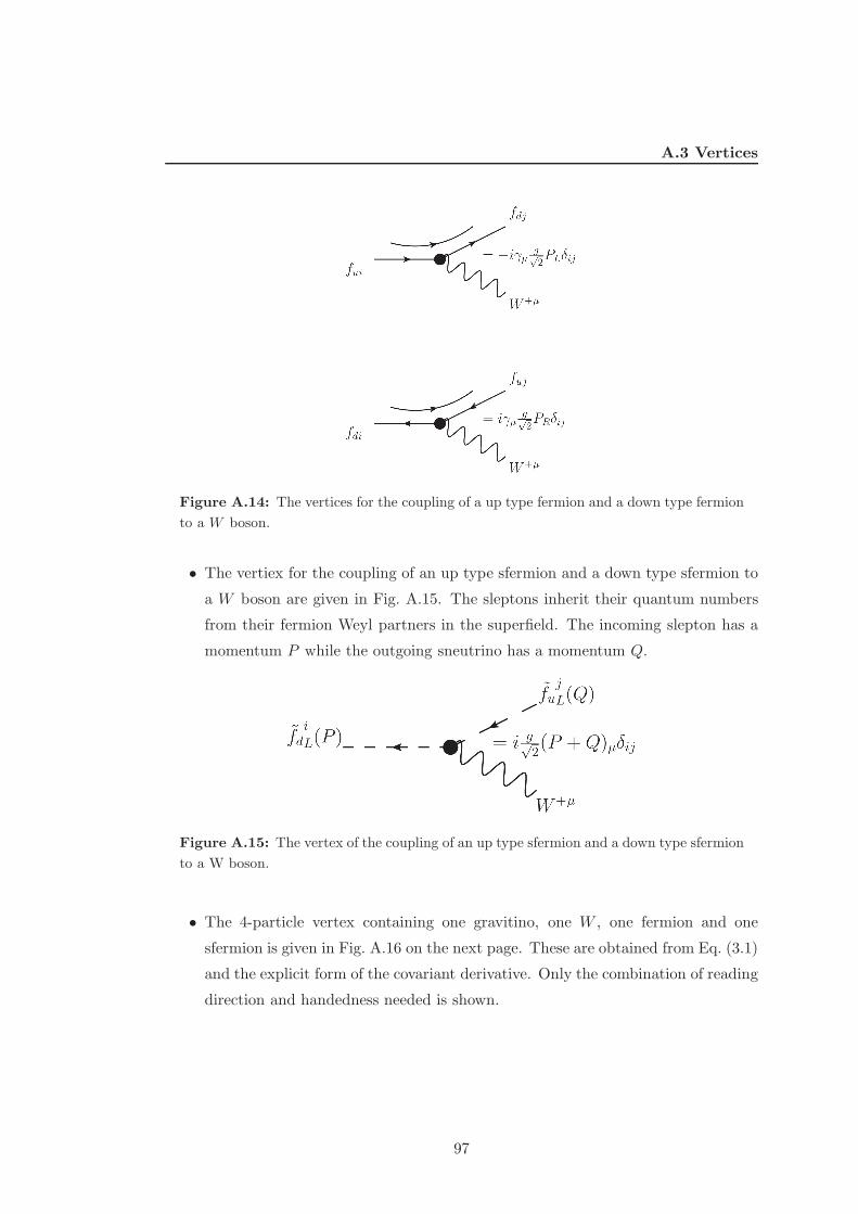
A.3 Vertices
Figure A.14: The vertices for the coupling of a up type fermion and a down type fermion
to a W boson.
• The vertiex for the coupling of an up type sfermion and a down type sfermion to
a W boson are given in Fig. A.15. The sleptons inherit their quantum numbers
from their fermion Weyl partners in the superfield. The incoming slepton has a
momentum P while the outgoing sneutrino has a momentum Q.
Figure A.15: The vertex of the coupling of an up type sfermion and a down type sfermion
to a W boson.
• The 4-particle vertex containing one gravitino, one W , one fermion and one
sfermion is given in Fig. A.16 on the next page. These are obtained from Eq. (3.1)
and the explicit form of the covariant derivative. Only the combination of reading
direction and handedness needed is shown.
97
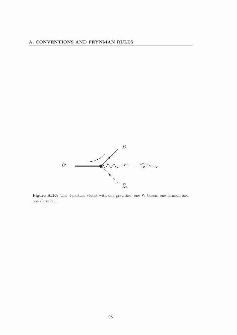
A. CONVENTIONS AND FEYNMAN RULES
Figure A.16: The 4-particle vertex with one gravitino, one W boson, one fermion and
one sfermion.
98
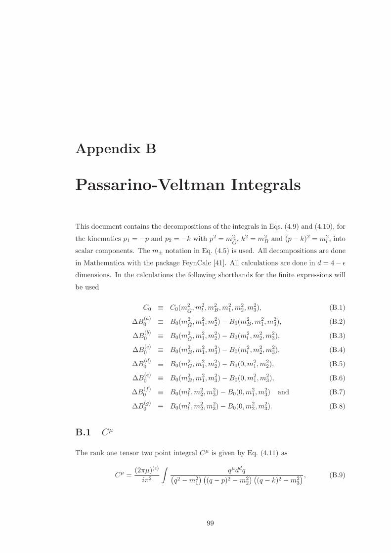
Appendix B
Passarino-Veltman Integrals
This document contains the decompositions of the integrals in Eqs. (4.9) and (4.10), for
the kinematics p1 = −p and p2 = −k with p2 = m2G, k2 = m2
B and (p− k)2 = m2l , into
scalar components. The m± notation in Eq. (4.5) is used. All decompositions are done
in Mathematica with the package FeynCalc [41]. All calculations are done in d = 4− ǫ
dimensions. In the calculations the following shorthands for the finite expressions will
be used
C0 ≡ C0(m2G,m2
l ,m2B ,m
21,m
22,m
23), (B.1)
∆B(a)0 ≡ B0(m
2G,m2
1,m22)−B0(m
2B ,m
21,m
23), (B.2)
∆B(b)0 ≡ B0(m
2G,m2
1,m22)−B0(m
2l ,m
22,m
23), (B.3)
∆B(c)0 ≡ B0(m
2B ,m
21,m
23)−B0(m
2l ,m
22,m
23), (B.4)
∆B(d)0 ≡ B0(m
2G,m
21,m
22)−B0(0,m
21,m
22), (B.5)
∆B(e)0 ≡ B0(m
2B ,m
21,m
23)−B0(0,m
21,m
23), (B.6)
∆B(f)0 ≡ B0(m
2l ,m
22,m
23)−B0(0,m
21,m
23) and (B.7)
∆B(g)0 ≡ B0(m
2l ,m
22,m
23)−B0(0,m
22,m
23). (B.8)
B.1 Cµ
The rank one tensor two point integral Cµ is given by Eq. (4.11) as
Cµ =(2πµ)(ǫ)
iπ2
∫
qµddq(
q2 −m21
) (
(q − p)2 −m22
) (
(q − k)2 −m23
) , (B.9)
99
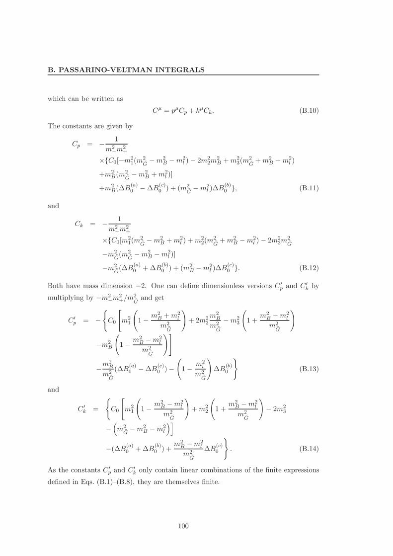
B. PASSARINO-VELTMAN INTEGRALS
which can be written as
Cµ = pµCp + kµCk. (B.10)
The constants are given by
Cp = − 1
m2−m
2+
×C0[−m21(m
2G−m2
B −m2l )− 2m2
2m2B +m2
3(m2G+m2
B −m2l )
+m2B(m
2G−m2
B +m2l )]
+m2B(∆B
(a)0 −∆B
(c)0 ) + (m2
G−m2
l )∆B(b)0 , (B.11)
and
Ck = − 1
m2−m
2+
×C0[m21(m
2G−m2
B +m2l ) +m2
2(m2G+m2
B −m2l )− 2m2
3m2G
−m2G(m2
G−m2
B −m2l )]
−m2G(∆B
(a)0 +∆B
(b)0 ) + (m2
B −m2l )∆B
(c)0 . (B.12)
Both have mass dimension −2. One can define dimensionless versions C ′p and C ′
k by
multiplying by −m2−m
2+/m
2Gand get
C ′p = −
C0
[
m21
(
1− m2B +m2
l
m2G
)
+ 2m22
m2B
m2G
−m23
(
1 +m2
B −m2l
m2G
)
−m2B
(
1− m2B −m2
l
m2G
)]
−m2B
m2G
(∆B(a)0 −∆B
(c)0 )−
(
1− m2l
m2G
)
∆B(b)0
(B.13)
and
C ′k =
C0
[
m21
(
1− m2B −m2
l
m2G
)
+m22
(
1 +m2
B −m2l
m2G
)
− 2m23
−(
m2G−m2
B −m2l
)]
−(∆B(a)0 +∆B
(b)0 ) +
m2B −m2
l
m2G
∆B(c)0
. (B.14)
As the constants C ′p and C ′
k only contain linear combinations of the finite expressions
defined in Eqs. (B.1)–(B.8), they are themselves finite.
100
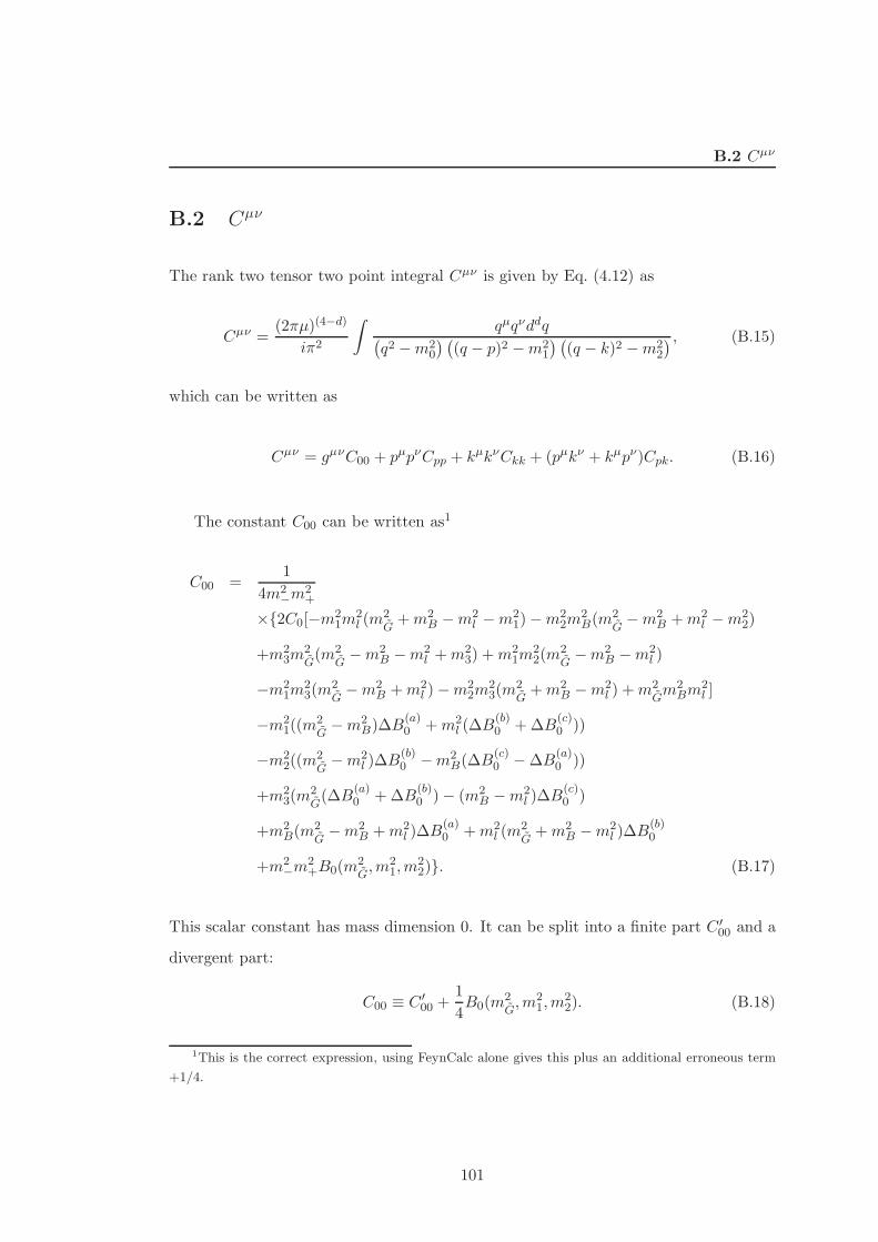
B.2 Cµν
B.2 Cµν
The rank two tensor two point integral Cµν is given by Eq. (4.12) as
Cµν =(2πµ)(4−d)
iπ2
∫
qµqνddq(
q2 −m20
) (
(q − p)2 −m21
) (
(q − k)2 −m22
) , (B.15)
which can be written as
Cµν = gµνC00 + pµpνCpp + kµkνCkk + (pµkν + kµpν)Cpk. (B.16)
The constant C00 can be written as1
C00 =1
4m2−m
2+
×2C0[−m21m
2l (m
2G+m2
B −m2l −m2
1)−m22m
2B(m
2G−m2
B +m2l −m2
2)
+m23m
2G(m2
G−m2
B −m2l +m2
3) +m21m
22(m
2G−m2
B −m2l )
−m21m
23(m
2G−m2
B +m2l )−m2
2m23(m
2G+m2
B −m2l ) +m2
Gm2
Bm2l ]
−m21((m
2G−m2
B)∆B(a)0 +m2
l (∆B(b)0 +∆B
(c)0 ))
−m22((m
2G−m2
l )∆B(b)0 −m2
B(∆B(c)0 −∆B
(a)0 ))
+m23(m
2G(∆B
(a)0 +∆B
(b)0 )− (m2
B −m2l )∆B
(c)0 )
+m2B(m
2G−m2
B +m2l )∆B
(a)0 +m2
l (m2G+m2
B −m2l )∆B
(b)0
+m2−m
2+B0(m
2G,m2
1,m22). (B.17)
This scalar constant has mass dimension 0. It can be split into a finite part C ′00 and a
divergent part:
C00 ≡ C ′00 +
1
4B0(m
2G,m2
1,m22). (B.18)
1This is the correct expression, using FeynCalc alone gives this plus an additional erroneous term
+1/4.
101
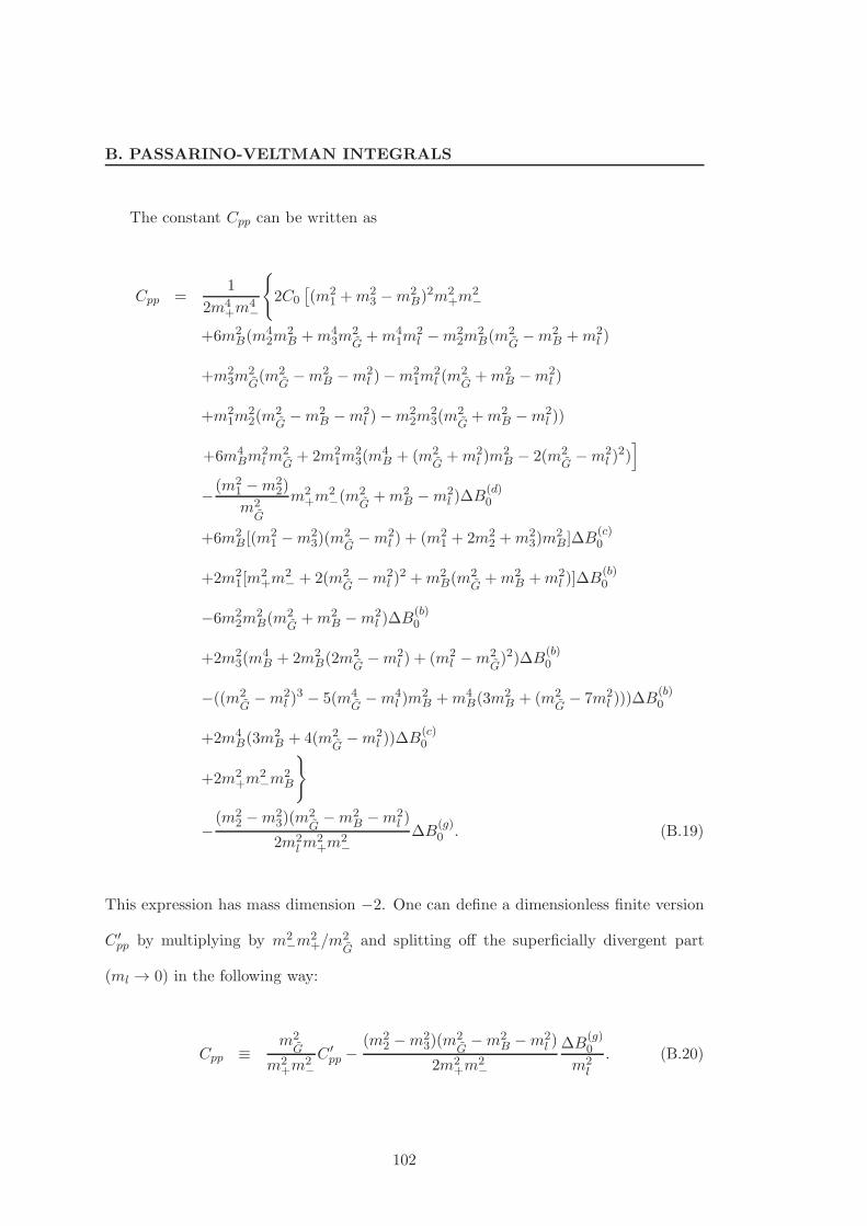
B. PASSARINO-VELTMAN INTEGRALS
The constant Cpp can be written as
Cpp =1
2m4+m
4−
2C0
[
(m21 +m2
3 −m2B)
2m2+m
2−
+6m2B(m
42m
2B +m4
3m2G+m4
1m2l −m2
2m2B(m
2G−m2
B +m2l )
+m23m
2G(m2
G−m2
B −m2l )−m2
1m2l (m
2G+m2
B −m2l )
+m21m
22(m
2G−m2
B −m2l )−m2
2m23(m
2G+m2
B −m2l ))
+6m4Bm
2lm
2G+ 2m2
1m23(m
4B + (m2
G+m2
l )m2B − 2(m2
G−m2
l )2)]
−(m21 −m2
2)
m2G
m2+m
2−(m
2G+m2
B −m2l )∆B
(d)0
+6m2B [(m
21 −m2
3)(m2G−m2
l ) + (m21 + 2m2
2 +m23)m
2B]∆B
(c)0
+2m21[m
2+m
2− + 2(m2
G−m2
l )2 +m2
B(m2G+m2
B +m2l )]∆B
(b)0
−6m22m
2B(m
2G+m2
B −m2l )∆B
(b)0
+2m23(m
4B + 2m2
B(2m2G−m2
l ) + (m2l −m2
G)2)∆B
(b)0
−((m2G−m2
l )3 − 5(m4
G−m4
l )m2B +m4
B(3m2B + (m2
G− 7m2
l )))∆B(b)0
+2m4B(3m
2B + 4(m2
G−m2
l ))∆B(c)0
+2m2+m
2−m
2B
−(m2
2 −m23)(m
2G−m2
B −m2l )
2m2lm
2+m
2−
∆B(g)0 . (B.19)
This expression has mass dimension −2. One can define a dimensionless finite version
C ′pp by multiplying by m2
−m2+/m
2G
and splitting off the superficially divergent part
(ml → 0) in the following way:
Cpp ≡m2
G
m2+m
2−C ′pp −
(m22 −m2
3)(m2G−m2
B −m2l )
2m2+m
2−
∆B(g)0
m2l
. (B.20)
102
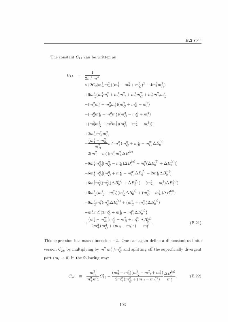
B.2 Cµν
The constant Ckk can be written as
Ckk =1
2m4+m
4−
×2C0[m2+m
2−((m
21 −m2
2 +m2G)2 − 4m2
1m2G)
+6m2G(m4
1m2l +m4
2m2B +m4
3m2G+m2
lm2Bm
2G
−(m21m
2l +m2
2m23)(m
2G+m2
B −m2l )
−(m22m
2B +m2
1m23)(m
2G−m2
B +m2l )
+(m23m
2G+m2
1m22)(m
2G−m2
B −m2l ))]
+2m2−m
2+m
2G
−(m21 −m2
3)
m2B
m2−m
2+(m
2G+m2
B −m2l )∆B
(e)0
−2(m21 −m2
2)m2−m
2+∆B
(c)0
−6m21m
2G[(m2
G−m2
B)∆B(a)0 +m2
l (∆B(b)0 +∆B
(c)0 )]
−6m22m
2G[(m2
G+m2
B −m2l )∆B
(b)0 − 2m2
B∆B(c)0 ]
+6m23m
2G(m2
G(∆B
(a)0 +∆B
(b)0 )− (m2
B −m2l )∆B
(c)0 )
+6m2G(m2
G−m2
B)(m2G∆B
(a)0 + (m2
G−m2
B)∆B(c)0 )
−6m2Gm2
l (m2G∆B
(a)0 + (m2
G+m2
B)∆B(c)0 )
−m2−m
2+(3m
2G+m2
B −m2l )∆B
(c)0
+(m2
2 −m23)(m
2G−m2
B +m2l )
2m2+(m
2G+ (mB −ml)2)
∆B(g)0
m2l
. (B.21)
This expression has mass dimension −2. One can again define a dimensionless finite
version C ′kk by multiplying by m2
−m2+/m
2G
and splitting off the superficially divergent
part (ml → 0) in the following way:
Ckk ≡m2
G
m2+m
2−C ′kk +
(m22 −m2
3)(m2G−m2
B +m2l )
2m2+(m
2G+ (mB −ml)2)
∆B(g)0
m2l
. (B.22)
103
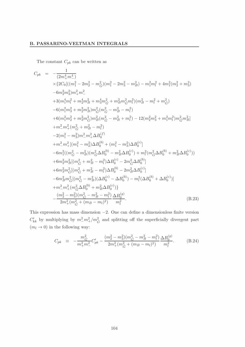
B. PASSARINO-VELTMAN INTEGRALS
The constant Cpk can be written as
Cpk = − 1
(2m4+m
4−)
×2C0[((m21 − 2m2
2 −m2G)(m2
1 − 2m23 −m2
B)−m21m
2l + 4m2
1(m22 +m2
3)
−6m22m
23)m
2+m
2−
+3(m41m
2l +m4
2m2B +m4
3m2G+m2
Bm2Gm2
l )(m2B −m2
l +m2G)
−6(m21m
23 +m2
2m2B)m
2G(m2
G−m2
B −m2l )
+6(m21m
22 +m2
3m2G)m2
B(m2G−m2
B +m2l )− 12(m2
2m23 +m2
1m2l )m
2Gm2
B]
+m2−m
2+(m
2G+m2
B −m2l )
−2(m21 −m2
3)m2−m
2+∆B
(f)0
+m2−m
2+[(m
21 −m2
2)∆B(b)0 + (m2
1 −m23)∆B
(c)0 ]
−6m21((m
2G−m2
B)(m2G∆B
(b)0 −m2
B∆B(c)0 ) +m2
l (m2G∆B
(b)0 +m2
B∆B(c)0 ))
+6m22m
2B [(m
2G+m2
B −m2l )∆B
(c)0 − 2m2
G∆B
(b)0 ]
+6m23m
2G[(m2
G+m2
B −m2l )∆B
(b)0 − 2m2
B∆B(c)0 ]
−6m2Bm
2G[(m2
G−m2
B)(∆B(c)0 −∆B
(b)0 )−m2
l (∆B(b)0 +∆B
(c)0 )]
+m2−m
2+(m
2G∆B
(b)0 +m2
B∆B(c)0 )
−(m2
2 −m23)(m
2G−m2
B −m2l )
2m2+(m
2G+ (mB −ml)2)
∆B(g)0
m2l
. (B.23)
This expression has mass dimension −2. One can define a dimensionless finite version
C ′kk by multiplying by m2
−m2+/m
2G
and splitting off the superficially divergent part
(ml → 0) in the following way:
Cpk ≡ −m2
G
m2+m
2−C ′pk −
(m22 −m2
3)(m2G−m2
B −m2l )
2m2+(m
2G+ (mB −ml)2)
∆B(g)0
m2l
. (B.24)
104
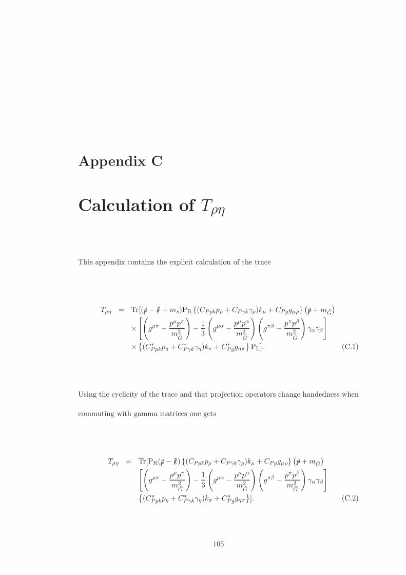
Appendix C
Calculation of Tρη
This appendix contains the explicit calculation of the trace
Tρη = Tr[(/p− /k +ms)PR (CPpkpρ + CPγkγρ)kµ + CPggµρ(
/p+mG
)
×[(
gµπ − pµpπ
m2G
)
− 1
3
(
gµα − pµpα
m2G
)(
gπβ − pπpβ
m2G
)
γαγβ
]
×
(C∗Ppkpη + C∗
Pγkγη)kπ + C∗Pggηπ
PL]. (C.1)
Using the cyclicity of the trace and that projection operators change handedness when
commuting with gamma matrices one gets
Tρη = Tr[PR(/p− /k) (CPpkpρ + CPγkγρ)kµ + CPggµρ(
/p+mG
)
[(
gµπ − pµpπ
m2G
)
− 1
3
(
gµα − pµpα
m2G
)(
gπβ − pπpβ
m2G
)
γαγβ
]
(C∗Ppkpη + C∗
Pγkγη)kπ + C∗Pggηπ
]. (C.2)
105
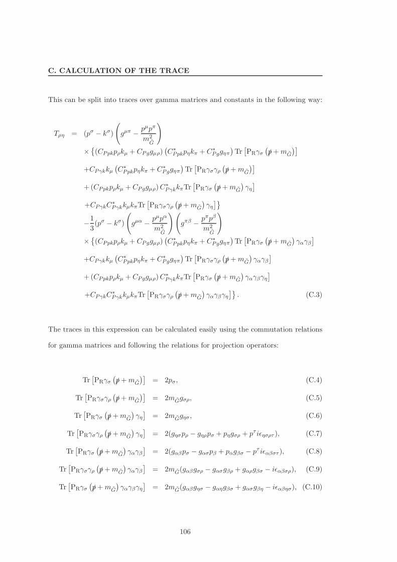
C. CALCULATION OF THE TRACE
This can be split into traces over gamma matrices and constants in the following way:
Tρη = (pσ − kσ)
(
gµπ − pµpπ
m2G
)
×
(CPpkpρkµ + CPggµρ)(
C∗Ppkpηkπ + C∗
Pggηπ)
Tr[
PRγσ(
/p+mG
)]
+CPγkkµ(
C∗Ppkpηkπ + C∗
Pggηπ)
Tr[
PRγσγρ(
/p+mG
)]
+(CPpkpρkµ + CPggµρ)C∗PγkkπTr
[
PRγσ(
/p+mG
)
γη]
+CPγkC∗PγkkµkπTr
[
PRγσγρ(
/p+mG
)
γη]
−1
3(pσ − kσ)
(
gµα − pµpα
m2G
)(
gπβ − pπpβ
m2G
)
×
(CPpkpρkµ + CPggµρ)(
C∗Ppkpηkπ + C∗
Pggηπ)
Tr[
PRγσ(
/p+mG
)
γαγβ]
+CPγkkµ(
C∗Ppkpηkπ + C∗
Pggηπ)
Tr[
PRγσγρ(
/p+mG
)
γαγβ]
+(CPpkpρkµ + CPggµρ)C∗PγkkπTr
[
PRγσ(
/p+mG
)
γαγβγη]
+CPγkC∗PγkkµkπTr
[
PRγσγρ(
/p+mG
)
γαγβγη]
. (C.3)
The traces in this expression can be calculated easily using the commutation relations
for gamma matrices and following the relations for projection operators:
Tr[
PRγσ(
/p+mG
)]
= 2pσ, (C.4)
Tr[
PRγσγρ(
/p+mG
)]
= 2mGgσρ, (C.5)
Tr[
PRγσ(
/p+mG
)
γη]
= 2mGgησ , (C.6)
Tr[
PRγσγρ(
/p+mG
)
γη]
= 2(gησpρ − gηρpσ + pηgσρ + pτ iǫησρτ ), (C.7)
Tr[
PRγσ(
/p+mG
)
γαγβ]
= 2(gαβpσ − gασpβ + pαgβσ − pτ iǫαβστ ), (C.8)
Tr[
PRγσγρ(
/p+mG
)
γαγβ]
= 2mG(gαβgσρ − gασgβρ + gαρgβσ − iǫαβσρ), (C.9)
Tr[
PRγσ(
/p+mG
)
γαγβγη]
= 2mG(gαβgησ − gαηgβσ + gασgβη − iǫαβησ), (C.10)
106
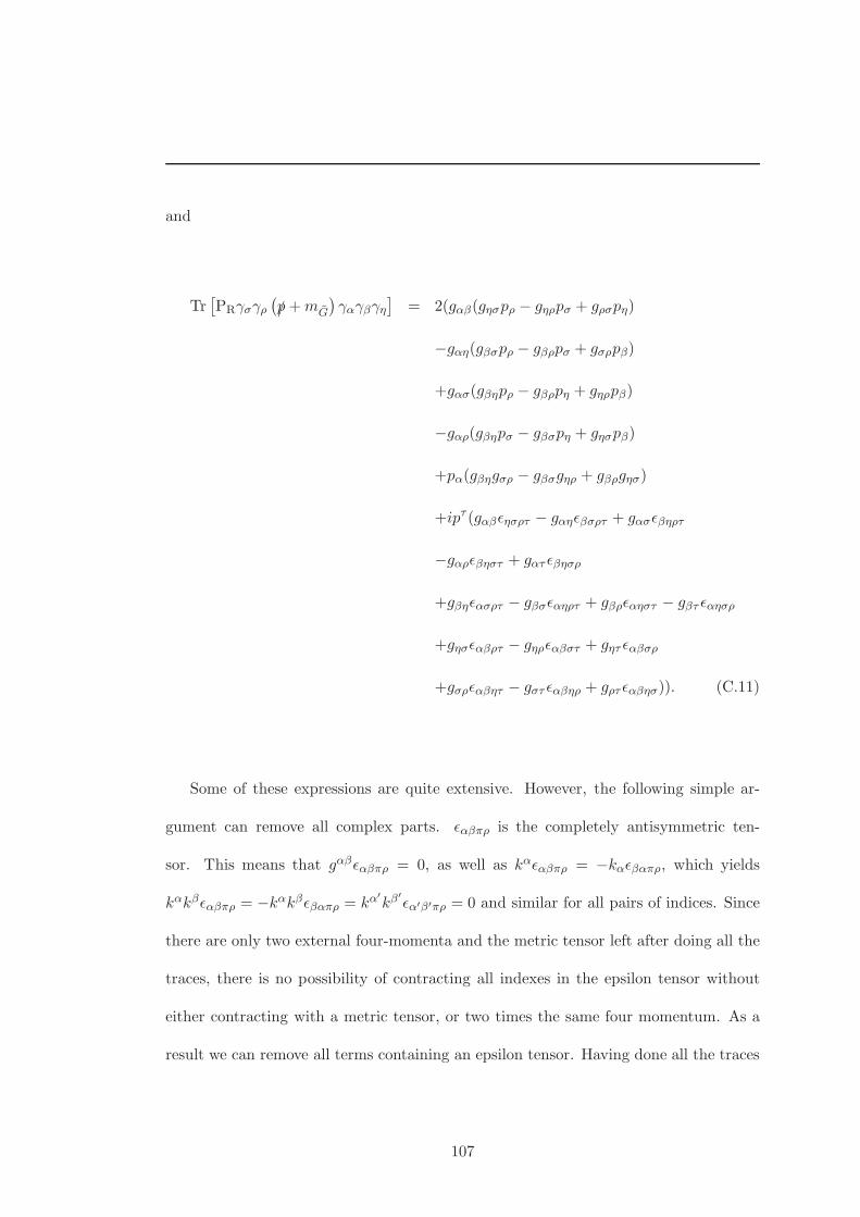
and
Tr[
PRγσγρ(
/p+mG
)
γαγβγη]
= 2(gαβ(gησpρ − gηρpσ + gρσpη)
−gαη(gβσpρ − gβρpσ + gσρpβ)
+gασ(gβηpρ − gβρpη + gηρpβ)
−gαρ(gβηpσ − gβσpη + gησpβ)
+pα(gβηgσρ − gβσgηρ + gβρgησ)
+ipτ (gαβǫησρτ − gαηǫβσρτ + gασǫβηρτ
−gαρǫβηστ + gατ ǫβησρ
+gβηǫασρτ − gβσǫαηρτ + gβρǫαηστ − gβτ ǫαησρ
+gησǫαβρτ − gηρǫαβστ + gητ ǫαβσρ
+gσρǫαβητ − gστ ǫαβηρ + gρτ ǫαβησ)). (C.11)
Some of these expressions are quite extensive. However, the following simple ar-
gument can remove all complex parts. ǫαβπρ is the completely antisymmetric ten-
sor. This means that gαβǫαβπρ = 0, as well as kαǫαβπρ = −kαǫβαπρ, which yields
kαkβǫαβπρ = −kαkβǫβαπρ = kα′kβ
′ǫα′β′πρ = 0 and similar for all pairs of indices. Since
there are only two external four-momenta and the metric tensor left after doing all the
traces, there is no possibility of contracting all indexes in the epsilon tensor without
either contracting with a metric tensor, or two times the same four momentum. As a
result we can remove all terms containing an epsilon tensor. Having done all the traces
107
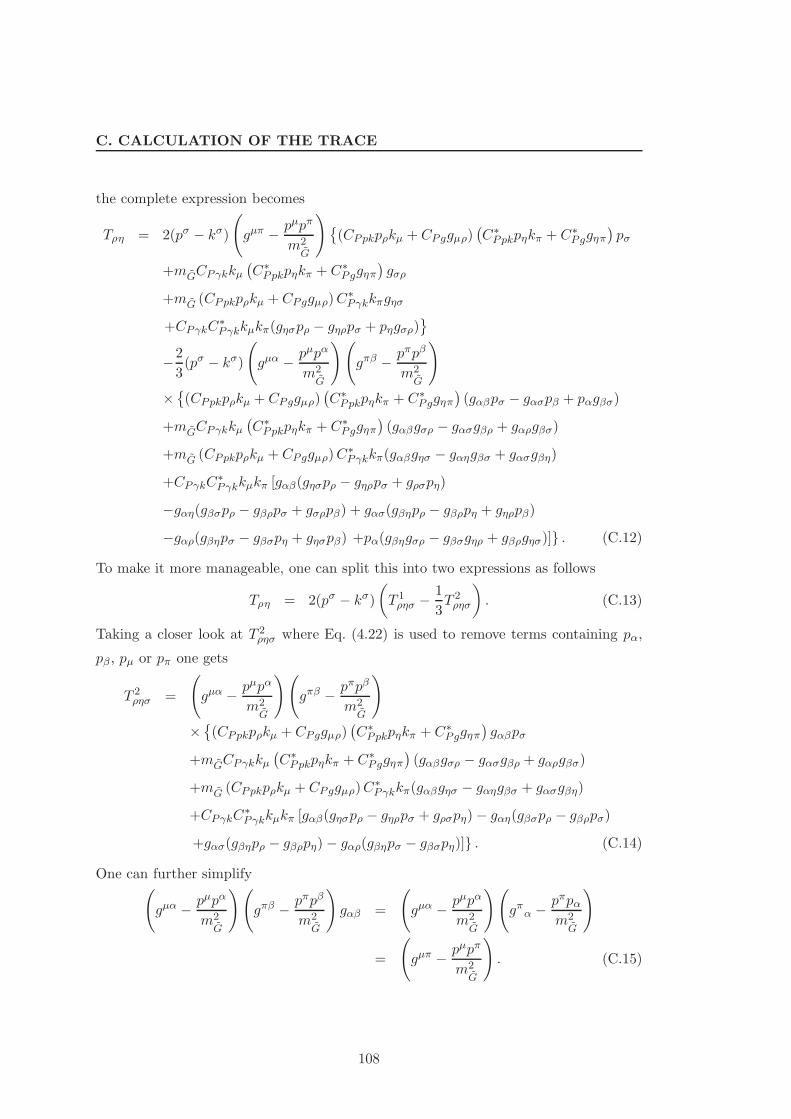
C. CALCULATION OF THE TRACE
the complete expression becomes
Tρη = 2(pσ − kσ)
(
gµπ − pµpπ
m2G
)
(CPpkpρkµ + CPggµρ)(
C∗Ppkpηkπ + C∗
Pggηπ)
pσ
+mGCPγkkµ(
C∗Ppkpηkπ + C∗
Pggηπ)
gσρ
+mG (CPpkpρkµ + CPggµρ)C∗Pγkkπgησ
+CPγkC∗Pγkkµkπ(gησpρ − gηρpσ + pηgσρ)
−2
3(pσ − kσ)
(
gµα − pµpα
m2G
)(
gπβ − pπpβ
m2G
)
×
(CPpkpρkµ + CPggµρ)(
C∗Ppkpηkπ + C∗
Pggηπ)
(gαβpσ − gασpβ + pαgβσ)
+mGCPγkkµ(
C∗Ppkpηkπ + C∗
Pggηπ)
(gαβgσρ − gασgβρ + gαρgβσ)
+mG (CPpkpρkµ + CPggµρ)C∗Pγkkπ(gαβgησ − gαηgβσ + gασgβη)
+CPγkC∗Pγkkµkπ [gαβ(gησpρ − gηρpσ + gρσpη)
−gαη(gβσpρ − gβρpσ + gσρpβ) + gασ(gβηpρ − gβρpη + gηρpβ)
−gαρ(gβηpσ − gβσpη + gησpβ) +pα(gβηgσρ − gβσgηρ + gβρgησ)] . (C.12)
To make it more manageable, one can split this into two expressions as follows
Tρη = 2(pσ − kσ)
(
T 1ρησ − 1
3T 2ρησ
)
. (C.13)
Taking a closer look at T 2ρησ where Eq. (4.22) is used to remove terms containing pα,
pβ, pµ or pπ one gets
T 2ρησ =
(
gµα − pµpα
m2G
)(
gπβ − pπpβ
m2G
)
×
(CPpkpρkµ + CPggµρ)(
C∗Ppkpηkπ + C∗
Pggηπ)
gαβpσ
+mGCPγkkµ(
C∗Ppkpηkπ +C∗
Pggηπ)
(gαβgσρ − gασgβρ + gαρgβσ)
+mG (CPpkpρkµ + CPggµρ)C∗Pγkkπ(gαβgησ − gαηgβσ + gασgβη)
+CPγkC∗Pγkkµkπ [gαβ(gησpρ − gηρpσ + gρσpη)− gαη(gβσpρ − gβρpσ)
+gασ(gβηpρ − gβρpη)− gαρ(gβηpσ − gβσpη)] . (C.14)
One can further simplify(
gµα − pµpα
m2G
)(
gπβ − pπpβ
m2G
)
gαβ =
(
gµα − pµpα
m2G
)(
gπα − pπpαm2
G
)
=
(
gµπ − pµpπ
m2G
)
. (C.15)
108
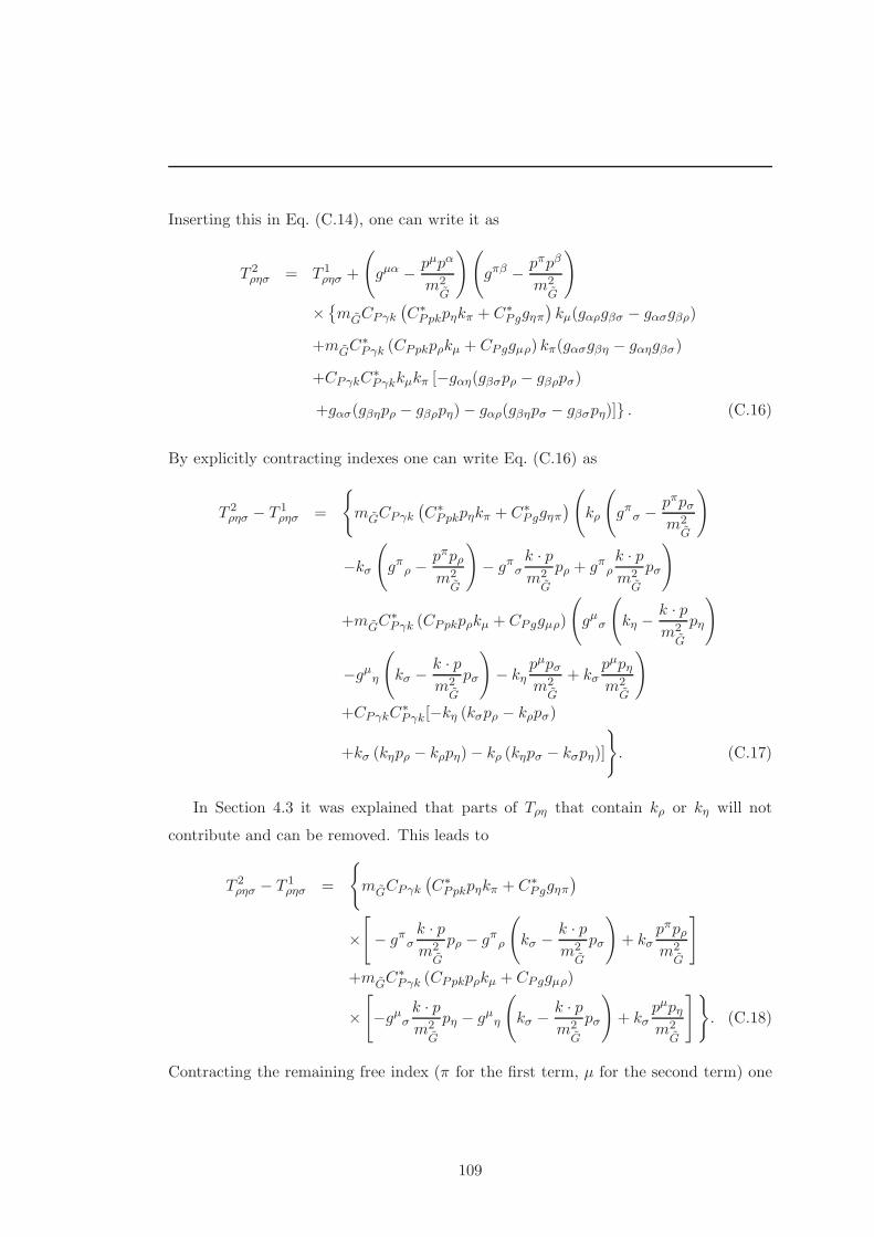
Inserting this in Eq. (C.14), one can write it as
T 2ρησ = T 1
ρησ +
(
gµα − pµpα
m2G
)(
gπβ − pπpβ
m2G
)
×
mGCPγk
(
C∗Ppkpηkπ + C∗
Pggηπ)
kµ(gαρgβσ − gασgβρ)
+mGC∗Pγk (CPpkpρkµ + CPggµρ) kπ(gασgβη − gαηgβσ)
+CPγkC∗Pγkkµkπ [−gαη(gβσpρ − gβρpσ)
+gασ(gβηpρ − gβρpη)− gαρ(gβηpσ − gβσpη)] . (C.16)
By explicitly contracting indexes one can write Eq. (C.16) as
T 2ρησ − T 1
ρησ =
mGCPγk
(
C∗Ppkpηkπ + C∗
Pggηπ)
(
kρ
(
gπσ − pπpσm2
G
)
−kσ(
gπρ −pπpρm2
G
)
− gπσk · pm2
G
pρ + gπρk · pm2
G
pσ
)
+mGC∗Pγk (CPpkpρkµ + CPggµρ)
(
gµσ
(
kη −k · pm2
G
pη
)
−gµη(
kσ − k · pm2
G
pσ
)
− kηpµpσm2
G
+ kσpµpηm2
G
)
+CPγkC∗Pγk[−kη (kσpρ − kρpσ)
+kσ (kηpρ − kρpη)− kρ (kηpσ − kσpη)]
. (C.17)
In Section 4.3 it was explained that parts of Tρη that contain kρ or kη will not
contribute and can be removed. This leads to
T 2ρησ − T 1
ρησ =
mGCPγk
(
C∗Ppkpηkπ + C∗
Pggηπ)
×[
− gπσk · pm2
G
pρ − gπρ
(
kσ − k · pm2
G
pσ
)
+ kσpπpρm2
G
]
+mGC∗Pγk (CPpkpρkµ + CPggµρ)
×[
−gµσk · pm2
G
pη − gµη
(
kσ − k · pm2
G
pσ
)
+ kσpµpηm2
G
]
. (C.18)
Contracting the remaining free index (π for the first term, µ for the second term) one
109
C. CALCULATION OF THE TRACE
can write this as
T 2ρησ − T 1
ρησ =
mGCPγk
[
− C∗Ppk(kσ − k · p
m2G
pσ)pηkρ
−C∗Pg
(
(gησpρ − gηρpσ)k · pm2
G
+
(
gηρ −pηpρm2
G
)
kσ
)]
+mGC∗Pγk
[
− CPpk
(
kσ − k · pm2
G
pσ
)
pρkη
−CPg
((
gσρpη − gηρpσ
)
k · pm2
G
+
(
gηρ −pρpηm2
G
)
kσ
)]
. (C.19)
Here one can again remove occurrences of kρ and kη and get
T 2ρησ − T 1
ρησ = −mGCPγkC∗Pg
[
(gησpρ − gηρpσ)k · pm2
G
+
(
gηρ −pηpρm2
G
)
kσ
]
−mGC∗PγkCPg
[
(gσρpη − gηρpσ)k · pm2
G
+
(
gηρ −pρpηm2
G
)
kσ
]
. (C.20)
This is put into Eq. (C.13) and gives
Tρη =4
3(pσ − kσ)T 1
ρησ +2mG
3(pσ − kσ)
×[
CPγkC∗Pg
(
kσ
(
gηρ −pηpρm2
G
)
+k · pm2
G
(gησpρ − gηρpσ)
)
+C∗PγkCPg
(
kσ
(
gρη −pρpηm2
G
)
+k · pm2
G
(gρσpη − gρηpσ)
)]
. (C.21)
Now one can contract the last index σ in the second term of this expression and get
Tρη =4
3(pσ − kσ)T 1
ρησ +2
3mG
[(CPγkC∗Pg + C∗
PγkCPg)
×(gηρ((k · p)2 − k2p2) + pηpρk2)
−k · p(CPγkC∗Pgkηpρ − C∗
PγkCPgkρpη)], (C.22)
where one can again remove kρ and kη which yields
Tρη =4
3(pσ − kσ)T 1
ρησ +4
3mG
ReCPγkC∗Pg[gηρ((k · p)2 − k2p2) + pηpρk
2].(C.23)
110
To calculate the whole trace Tρη we now only need to calculate T 1ρησ . It is given by
T 1ρησ =
(
gµπ − pµpπ
m2G
)
(CPpkpρkµ + CPggµρ)(
C∗Ppkpηkπ + C∗
Pggηπ)
pσ
+mGCPγkkµ(
C∗Ppkpηkπ + C∗
Pggηπ)
gσρ
+mG (CPpkpρkµ + CPggµρ)C∗Pγkkπgησ
+|CPγk|2kµkπ(gησpρ − gηρpσ + pηgσρ)
. (C.24)
Contracting over the index µ one gets
T 1ρησ =
1
m2G
(
CPpkpρ(
p2kπ − (k · p)pπ)
+ CPg(p2gπρ − pρp
π))
×(
C∗Ppkpηkπ + C∗
Pggηπ)
pσ
+1
mG
CPγk
(
p2kπ − (k · p)pπ) (
C∗Ppkpηkπ + C∗
Pggηπ)
gσρ
+1
mG
(
p2kµ − (k · p)pµ)
(CPpkpρkµ + CPggµρ)C∗Pγkgησ
+1
m2G
|CPγk|2(k2p2 − (p · k)2)(gησpρ − gηρpσ + pηgσρ). (C.25)
The first term (in the following called t1ρηpσ) can be written
m2Gt1ρη = |CPpk|2pρpη
(
p2kπ − (k · p)pπ)
kπ
+CPpkC∗Pgpρ
(
p2kπ − (k · p)pπ)
gηπ
+CPgC∗Ppkpη
(
p2gπρ − pρpπ)
kπ
+|CPg|2(
p2gπρ − pρpπ)
gηπ. (C.26)
Contracting over π one gets
m2Gt1ρη = |CPpk|2pρpη
(
p2k2 − (k · p)2)
+CPpkC∗Pgpρ
(
p2kη − (k · p)pη)
+CPgC∗Ppkpη
(
p2kρ − (k · p)pρ)
+|CPg|2(
p2gρη − pρpη)
. (C.27)
One can again remove kρ and kη, and get
m2Gt1ρη = |CPpk|2
(
p2k2 − (k · p)2)
pρpη
−2ReCPpkC∗Pg(k · p)pρpη
+|CPg|2(
p2gρη − pρpη)
. (C.28)
111
C. CALCULATION OF THE TRACE
The second and third term in Eq. (C.25), in the following collectively called t23ρησ, is
t23ρησ =1
mG
CPγkC∗Ppk
(
p2kπ − (k · p)pπ)
kπgσρpη
+1
mG
CPγkC∗Pg
(
p2kπ − (k · p)pπ)
gηπgσρ
+1
mG
C∗PγkCPpk
(
p2kµ − (k · p)pµ)
kµgσηpρ
+1
mG
C∗PγkCPg
(
p2kµ − (k · p)pµ)
gµρgση . (C.29)
Contracting over π one gets
t23ρησ =1
mG
[(
p2k2 − (k · p)2)
[CPγkC∗Ppkgσρpη + C∗
PγkCPpkgσηpρ]
+CPγkC∗Pg
(
p2kη − (k · p)pη)
gσρ + C∗PγkCPg
(
p2kρ − (k · p)pρ)
gση ], (C.30)
where one can remove kη and kρ
t23ρησ =1
mG
[(
p2k2 − (k · p)2)
[CPγkC∗Ppkgσρpη +C∗
PγkCPpkgσηpρ]
−CPγkC∗Pg(k · p)pηgσρ − C∗
PγkCPg(k · p)pρgση ]. (C.31)
Inserting Eqs. (C.28) and (C.31) in Eq. (C.25) and multiplying both sides by (pσ − kσ)
one gets
(pσ − kσ)T 1ρησ =
(pσ − kσ)pσm2
G
[
|CPpk|2(
p2k2 − (k · p)2)
pρpη
−2ReCPpkC∗Pg(k · p)pρpη + |CPg|2
(
p2gρη − pρpη)
]
+1
mG
(pσ − kσ)[(
p2k2 − (k · p)2)
×[CPγkC∗Ppkgσρpη + C∗
PγkCPpkgσηpρ]
−CPγkC∗Pg(k · p)pηgσρ − C∗
PγkCPg(k · p)pρgση ]
+1
m2G
|CPγk|2(k2p2 − (p · k)2)
×(pσ − kσ)(gησpρ − gηρpσ + pηgσρ). (C.32)
112
Contracting σ this expression can be written as
(pσ − kσ)T 1ρησ =
(p2 − k · p)m2
G
[
|CPpk|2(
p2k2 − (k · p)2)
pρpη
−2ReCPpkC∗Pg(k · p)pρpη + |CPg|2
(
p2gρη − pρpη)
]
+1
mG
(
p2k2 − (k · p)2)
[CPγkC∗Ppk(pρ − kρ)pη
+C∗PγkCPpk(pη − kη)pρ]
− 1
mG
CPγkC∗Pg(k · p)pη(pρ − kρ)
− 1
mG
C∗PγkCPg(k · p)pρ(pη − kη)
+1
m2G
|CPγk|2(k2p2 − (p · k)2)
×((pη − kη)pρ − gηρ(p2 − k · p) + pη(pρ − kρ)). (C.33)
Removing again kη and kρ this becomes
(pσ − kσ)T 1ρησ =
(p2 − k · p)m2
G
(|CPpk|2(
p2k2 − (k · p)2)
pρpη
−2ReCPpkC∗Pg(k · p)pρpη + |CPg|2
(
p2gρη − pρpη)
)
+2
mG
ReCPγkC∗Ppk
(
p2k2 − (k · p)2)
pηpρ
− 2
mG
ReCPγkC∗Pg(k · p)pρpη
+1
m2G
|CPγk|2(k2p2 − (p · k)2)(2pηpρ − gηρ(p2 − k · p)).(C.34)
This can be inserted in Eq. (C.23). To remove a common factor the expression is
113
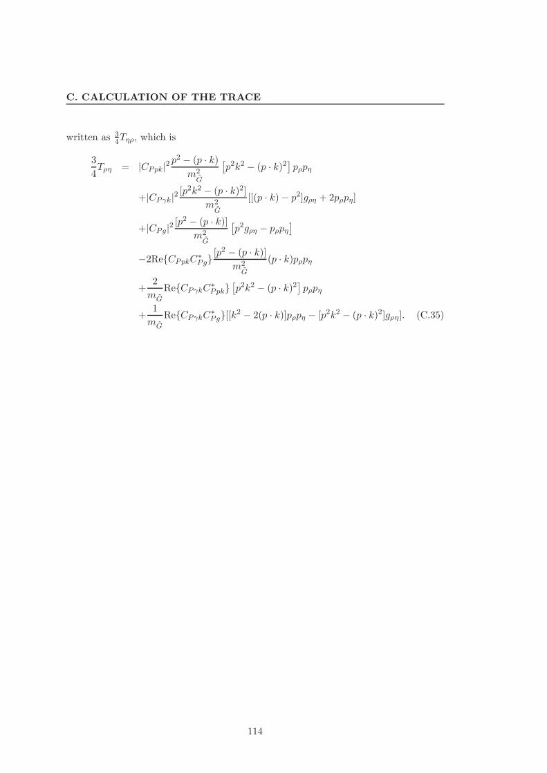
C. CALCULATION OF THE TRACE
written as 34Tηρ, which is
3
4Tρη = |CPpk|2
p2 − (p · k)m2
G
[
p2k2 − (p · k)2]
pρpη
+|CPγk|2[p2k2 − (p · k)2]
m2G
[[(p · k)− p2]gρη + 2pρpη]
+|CPg|2[p2 − (p · k)]
m2G
[
p2gρη − pρpη]
−2ReCPpkC∗Pg
[p2 − (p · k)]m2
G
(p · k)pρpη
+2
mG
ReCPγkC∗Ppk
[
p2k2 − (p · k)2]
pρpη
+1
mG
ReCPγkC∗Pg[[k2 − 2(p · k)]pρpη − [p2k2 − (p · k)2]gρη]. (C.35)
114
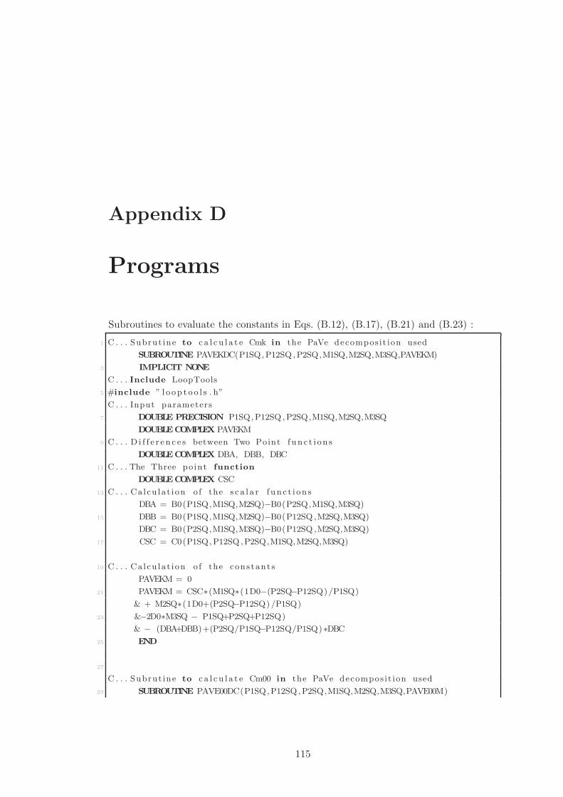
Appendix D
Programs
Subroutines to evaluate the constants in Eqs. (B.12), (B.17), (B.21) and (B.23) :
1 C . . . Subrut ine to c a l c u l a t e Cmk in the PaVe decompos it ion used
SUBROUTINE PAVEKDC(P1SQ,P12SQ ,P2SQ,M1SQ,M2SQ,M3SQ,PAVEKM)
3 IMPLICIT NONE
C . . . Include LoopTools
5 #include ” l o op t o o l s . h”
C . . . Input parameters
7 DOUBLE PRECISION P1SQ,P12SQ ,P2SQ,M1SQ,M2SQ,M3SQ
DOUBLECOMPLEX PAVEKM
9 C . . . D i f f e r e n c e s between Two Point fun c t i on s
DOUBLECOMPLEX DBA, DBB, DBC
11 C . . . The Three point function
DOUBLECOMPLEX CSC
13 C . . . Ca l cu la t ion o f the s c a l a r f un c t i on s
DBA = B0(P1SQ,M1SQ,M2SQ)−B0(P2SQ,M1SQ,M3SQ)
15 DBB = B0(P1SQ,M1SQ,M2SQ)−B0(P12SQ ,M2SQ,M3SQ)
DBC = B0(P2SQ,M1SQ,M3SQ)−B0(P12SQ ,M2SQ,M3SQ)
17 CSC = C0(P1SQ,P12SQ ,P2SQ,M1SQ,M2SQ,M3SQ)
19 C . . . Ca l cu la t ion o f the cons tan t s
PAVEKM = 0
21 PAVEKM = CSC∗(M1SQ∗(1D0−(P2SQ−P12SQ)/P1SQ)
& + M2SQ∗(1D0+(P2SQ−P12SQ) /P1SQ)
23 &−2D0∗M3SQ − P1SQ+P2SQ+P12SQ)
& − (DBA+DBB)+(P2SQ/P1SQ−P12SQ/P1SQ)∗DBC
25 END
27
C . . . Subrut ine to c a l c u l a t e Cm00 in the PaVe decompos it ion used
29 SUBROUTINE PAVE00DC(P1SQ,P12SQ ,P2SQ,M1SQ,M2SQ,M3SQ,PAVE00M)
115
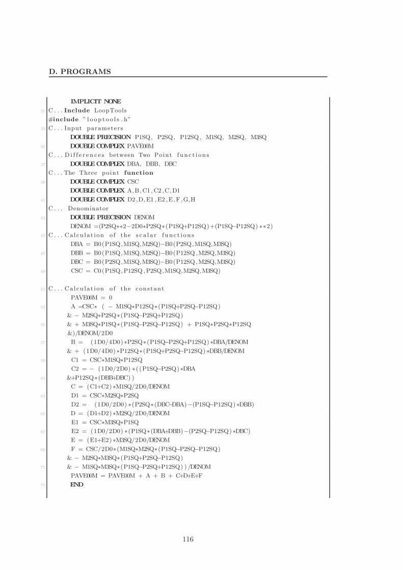
D. PROGRAMS
IMPLICIT NONE
31 C . . . Include LoopTools
#include ” l o op t o o l s . h”
33 C . . . Input parameters
DOUBLE PRECISION P1SQ, P2SQ, P12SQ , M1SQ, M2SQ, M3SQ
35 DOUBLECOMPLEX PAVE00M
C . . . D i f f e r e n c e s between Two Point fun c t i on s
37 DOUBLECOMPLEX DBA, DBB, DBC
C . . . The Three point function
39 DOUBLECOMPLEX CSC
DOUBLECOMPLEX A,B,C1 ,C2 ,C,D1
41 DOUBLECOMPLEX D2,D,E1 , E2 ,E,F ,G,H
C . . . Denominator
43 DOUBLE PRECISION DENOM
DENOM =(P2SQ∗∗2−2D0∗P2SQ∗(P1SQ+P12SQ)+(P1SQ−P12SQ) ∗∗2)
45 C . . . Ca l cu la t ion o f the s c a l a r f un c t i on s
DBA = B0(P1SQ,M1SQ,M2SQ)−B0(P2SQ,M1SQ,M3SQ)
47 DBB = B0(P1SQ,M1SQ,M2SQ)−B0(P12SQ ,M2SQ,M3SQ)
DBC = B0(P2SQ,M1SQ,M3SQ)−B0(P12SQ ,M2SQ,M3SQ)
49 CSC = C0(P1SQ,P12SQ ,P2SQ,M1SQ,M2SQ,M3SQ)
51 C . . . Ca l cu la t ion o f the constant
PAVE00M = 0
53 A =CSC∗ ( − M1SQ∗P12SQ∗(P1SQ+P2SQ−P12SQ)
& − M2SQ∗P2SQ∗(P1SQ−P2SQ+P12SQ)
55 & + M3SQ∗P1SQ∗(P1SQ−P2SQ−P12SQ) + P1SQ∗P2SQ∗P12SQ
&)/DENOM/2D0
57 B = (1D0/4D0)∗P2SQ∗(P1SQ−P2SQ+P12SQ) ∗DBA/DENOM
& + (1D0/4D0) ∗P12SQ∗(P1SQ+P2SQ−P12SQ) ∗DBB/DENOM
59 C1 = CSC∗M1SQ∗P12SQ
C2 = − (1D0/2D0) ∗ ( (P1SQ−P2SQ) ∗DBA
61 &+P12SQ∗(DBB+DBC) )
C = (C1+C2) ∗M1SQ/2D0/DENOM
63 D1 = CSC∗M2SQ∗P2SQ
D2 = (1D0/2D0) ∗(P2SQ∗(DBC−DBA)−(P1SQ−P12SQ) ∗DBB)
65 D = (D1+D2) ∗M2SQ/2D0/DENOM
E1 = CSC∗M3SQ∗P1SQ
67 E2 = (1D0/2D0) ∗(P1SQ∗(DBA+DBB)−(P2SQ−P12SQ) ∗DBC)
E = (E1+E2) ∗M3SQ/2D0/DENOM
69 F = CSC/2D0∗(M1SQ∗M2SQ∗(P1SQ−P2SQ−P12SQ)
& − M2SQ∗M3SQ∗(P1SQ+P2SQ−P12SQ)
71 & − M1SQ∗M3SQ∗(P1SQ−P2SQ+P12SQ) ) /DENOM
PAVE00M = PAVE00M + A + B + C+D+E+F
73 END
116
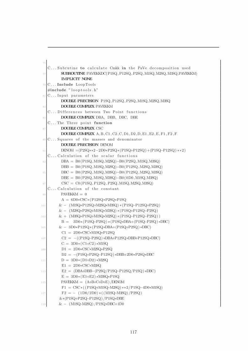
75
C . . . Subrut ine to c a l c u l a t e Cmkk in the PaVe decompos it ion used
77 SUBROUTINE PAVEKKDC(P1SQ,P12SQ ,P2SQ,M1SQ,M2SQ,M3SQ,PAVEKKM)
IMPLICIT NONE
79 C . . . Include LoopTools
#include ” l o op t o o l s . h”
81 C . . . Input parameters
DOUBLE PRECISION P1SQ,P12SQ ,P2SQ,M1SQ,M2SQ,M3SQ
83 DOUBLECOMPLEX PAVEKKM
C . . . D i f f e r e n c e s between Two Point fun c t i on s
85 DOUBLECOMPLEX DBA, DBB, DBC, DBE
C . . . The Three point function
87 DOUBLECOMPLEX CSC
DOUBLECOMPLEX A,B,C1 ,C2 ,C,D1,D2 ,D,E1 , E2 ,E, F1 , F2 ,F
89 C . . . Squares o f the masses and denominator
DOUBLE PRECISION DENOM
91 DENOM =(P2SQ∗∗2−2D0∗P2SQ∗(P1SQ+P12SQ)+(P1SQ−P12SQ) ∗∗2)
C . . . Ca l cu la t ion o f the s c a l a r f un c t i on s
93 DBA = B0(P1SQ,M1SQ,M2SQ)−B0(P2SQ,M1SQ,M3SQ)
DBB = B0(P1SQ,M1SQ,M2SQ)−B0(P12SQ ,M2SQ,M3SQ)
95 DBC = B0(P2SQ,M1SQ,M3SQ)−B0(P12SQ ,M2SQ,M3SQ)
DBE = B0(P2SQ,M1SQ,M3SQ)−B0(0D0,M1SQ,M3SQ)
97 CSC = C0(P1SQ,P12SQ ,P2SQ,M1SQ,M2SQ,M3SQ)
C . . . Ca l cu la t ion o f the constant
99 PAVEKKM = 0
A = 6D0∗CSC∗(P12SQ∗P2SQ∗P1SQ
101 & − (M1SQ∗P12SQ+M2SQ∗M3SQ) ∗(P1SQ−P12SQ+P2SQ)
& − (M2SQ∗P2SQ+M1SQ∗M3SQ) ∗(P1SQ+P12SQ−P2SQ)
103 & + (M3SQ∗P1SQ+M1SQ∗M2SQ) ∗(P1SQ−P12SQ−P2SQ) )
B = 3D0∗(P1SQ−P2SQ) ∗(P1SQ∗DBA+(P1SQ−P2SQ) ∗DBC)
105 & − 3D0∗P12SQ∗(P1SQ∗DBA+(P1SQ+P2SQ) ∗DBC)
C1 = 2D0∗CSC∗M1SQ∗P12SQ
107 C2 = −((P1SQ−P2SQ) ∗DBA+P12SQ∗DBB+P12SQ∗DBC)
C = 3D0∗(C1+C2) ∗M1SQ
109 D1 = 2D0∗CSC∗M2SQ∗P2SQ
D2 = −(P1SQ+P2SQ−P12SQ)∗DBB+2D0∗P2SQ∗DBC
111 D = 3D0∗(D1+D2) ∗M2SQ
E1 = 2D0∗CSC∗M3SQ
113 E2 = (DBA+DBB−(P2SQ/P1SQ−P12SQ/P1SQ)∗DBC)
E = 3D0∗(E1+E2) ∗M3SQ∗P1SQ
115 PAVEKKM = (A+B+C+D+E) /DENOM
F1 = CSC∗ ( (P1SQ+M1SQ−M2SQ) ∗∗2/P1SQ−4D0∗M1SQ)
117 F2 = − (1D0/2D0) ∗ ( (M1SQ−M3SQ) /P2SQ)
&∗(P1SQ+P2SQ−P12SQ) /P1SQ∗DBE
119 & − (M1SQ−M2SQ) /P1SQ∗DBC+1D0
117
D. PROGRAMS
& − (3D0/2D0∗P1SQ+P2SQ/2D0−P12SQ/2D0) /P1SQ∗DBC
121 F = (F1+F2)
PAVEKKM = PAVEKKM + F
123 END
125
127 C . . . Subrut ine to c a l c u l a t e Cmpk in the PaVe decompos it ion used
SUBROUTINE PAVEPKDC(P1SQ,P12SQ ,P2SQ,M1SQ,M2SQ,M3SQ,PAVEPKM)
129 IMPLICIT NONE
C . . . Include LoopTools
131 #include ” l o op t o o l s . h”
C . . . Input parameters
133 DOUBLE PRECISION P1SQ, P12SQ , P2SQ, M1SQ, M2SQ, M3SQ
DOUBLECOMPLEX PAVEPKM
135 C . . . D i f f e r e n c e s between Two Point fun c t i on s
DOUBLECOMPLEX DBB, DBC, DBF
137 C . . . The Three point function
DOUBLECOMPLEX CSC
139 DOUBLECOMPLEX A,B,C1 ,C2 ,C,D1 ,D2,D, E1 , E2 ,E, F1 , F2 ,F
C . . . Squares o f the masses and the denominator
141 DOUBLE PRECISION DENOM
DENOM =(P2SQ∗∗2−2D0∗P2SQ∗(P1SQ+P12SQ)+(P1SQ−P12SQ) ∗∗2)
143 C . . . Ca l cu la t ion o f the s c a l a r f un c t i on s
DBB = B0(P1SQ,M1SQ,M2SQ)−B0(P12SQ ,M2SQ,M3SQ)
145 DBC = B0(P2SQ,M1SQ,M3SQ)−B0(P12SQ ,M2SQ,M3SQ)
DBF = B0(P12SQ ,M2SQ,M3SQ)−B0(0D0,M1SQ,M3SQ)
147 CSC = C0(P1SQ,P12SQ ,P2SQ,M1SQ,M2SQ,M3SQ)
C . . . Ca l cu la t ion o f the constant
149 PAVEPKM = 0
A = CSC∗( 3D0∗P12SQ∗P2SQ∗(P1SQ+P2SQ−P12SQ)
151 & − 6D0∗(M1SQ∗M3SQ+M2SQ∗P2SQ) ∗(P1SQ−P2SQ−P12SQ)
& + 6D0∗(M1SQ∗M2SQ+M3SQ∗P1SQ)∗P2SQ/P1SQ∗(P1SQ−P2SQ+P12SQ)
153 & − 12D0∗(M2SQ∗M3SQ+M1SQ∗P12SQ) ∗P2SQ)
B = 3D0∗P2SQ∗ ( (P2SQ−P1SQ) ∗(DBC−DBB)
155 &+P12SQ∗(DBB+DBC) )
C1 = M1SQ∗P12SQ∗CSC∗(P1SQ+P2SQ−P12SQ)
157 C2 = (P2SQ−P1SQ) ∗(P1SQ∗DBB−P2SQ∗DBC)
&+P12SQ∗(P1SQ∗DBB+P2SQ∗DBC)
159 C = 3D0∗(C1+C2)∗M1SQ/P1SQ
D1 = CSC∗M2SQ∗(P1SQ+P2SQ−P12SQ)
161 D2 = (P2SQ−P12SQ+P1SQ) ∗DBC−2D0∗P1SQ∗DBB
D = (D1+D2) ∗3D0∗M2SQ∗P2SQ/P1SQ
163 E1 = M3SQ∗CSC∗(P1SQ+P2SQ−P12SQ)
E2 = (P2SQ−P12SQ+P1SQ) ∗DBB−2D0∗P2SQ∗DBC
118
165 E = 3D0∗(E1+E2) ∗M3SQ
PAVEPKM = (A+B+C+D+E) /DENOM
167 F1 = CSC∗ ( (M1SQ−2D0∗M2SQ−P1SQ) ∗(M1SQ−2D0∗M3SQ−P2SQ)
&−M1SQ∗P12SQ+4D0∗M1SQ∗(M2SQ+M3SQ)−6D0∗M2SQ∗M3SQ) /P1SQ
169 F2 = (1D0/2D0+P2SQ/(2D0∗P1SQ)−P12SQ/(P1SQ∗2D0) )
& − (M1SQ−M3SQ) /P1SQ∗DBF+(1D0/2D0) ∗ ( (M1SQ−M2SQ) /P1SQ∗DBB
171 & + (M1SQ−M3SQ) /P1SQ∗DBC)+(DBB/2D0 + (P2SQ/P1SQ) ∗DBC/2D0)
F = F1+F2
173 PAVEPKM = PAVEPKM+F
END
Evaluation of the widths in the required channels as given in Eqs. (4.83) and (4.124):
1 C . . . Subroutine to c a l c u l a t e the width o f the g r av i t i n o in the decay
channel Z nu
SUBROUTINE GRAVITINO2BZ(LAMBDA,YFERL,YFERR,MSFERL,MSFERR,MFER
3 +, MLFIN,GAMMA)
IMPLICIT NONE
5 C . . . Commonblocks dec la r ed in s ep e r a t e include f i l e
#include ”DoG. h”
7 C . . . Include LoopTools
#include ” l o op t o o l s . h”
9 C . . . Input parameters
DOUBLE PRECISION LAMBDA, YFERL, YFERR
11 DOUBLE PRECISION MSFERL,MSFERR,MFER
DOUBLE PRECISION GAMMA, MLFIN
13 C . . . For c a l c u l a t i n g matrix element
DOUBLE PRECISION ASQ,MFERSQ,MSFLSQ,MSFRSQ,MGRAVSQ
15 DOUBLE PRECISION COSTHETAW, MZSQ, MLFINSQ,GA,GB
DOUBLECOMPLEX K1,K2,K3,K1A,K2A,K3A,K1B,K2B,K3B
17 DOUBLECOMPLEX C1RZPK,C1LZPK,C2RZPK,C2LZPK,C1RZKK,C1LZKK
DOUBLECOMPLEX C1RZK,C1LZK,C1RZ0 ,C1LZ0 ,C2RZ0 ,C2LZ0
19 DOUBLECOMPLEX DBEXTRA,DBEXTRB, AAA
C . . . I n i t i a l i z e con s tan t s
21 MFERSQ = MFER∗MFER
MSFLSQ = MSFERL∗MSFERL
23 MSFRSQ = MSFERR∗MSFERR
MGRAVSQ = MGRAV∗MGRAV
25 MZSQ = MZ∗MZ
MLFINSQ = MLFIN∗MLFIN
27 GA = 0
GB = 0
29 K1 = 0
K1A = 0
31 K1B = 0
119
D. PROGRAMS
K2 = 0
33 K2A = 0
K2B = 0
35 K3 = 0
K3A = 0
37 K3B = 0
C1LZKK = 0
39 C1RZKK = 0
C1LZPK = 0
41 C1RZPK = 0
C2LZPK = 0
43 C2RZPK= 0
C1RZK = 0
45 C1LZK = 0
C1LZ0 = 0
47 C1RZ0 = 0
C2LZ0 = 0
49 C2RZ0 = 0
GAMMA = 0
51 C . . . Return 0 f o r f o r low Grav it ino masses
IF (MGRAV.LT. (MZ+MLFIN+GAMMAZ/2D0) ) THEN
53 RETURN
END IF
55 C . . . I n i t i a l i z i n g coup l ings and 2−point fun c t i on s
C . . . At the Z mass in the MSbar scheme
57 COSTHETAW = SQRT(1D0−SINSQTHETAW)
GA = (1D0−(1D0−YFERL) ∗SINSQTHETAW)/COSTHETAW
59 GB = YFERR∗SINSQTHETAW/COSTHETAW
DBEXTRA = 2D0∗B0(0D0,MFERSQ,MSFLSQ)−B0(MGRAVSQ,MFERSQ,MSFRSQ)
61 &−B0(MGRAVSQ,MSFLSQ,MFERSQ)
DBEXTRB = 2D0∗B0(0D0,MFERSQ,MSFRSQ)−B0(MGRAVSQ,MFERSQ,MSFRSQ)
63 &−B0(MGRAVSQ,MFERSQ,MSFLSQ)
C . . . Find the cons tan t s needed f o r the c a l c u l a t i o n s
65 CALL PAVEKKDC(MGRAVSQ,MLFINSQ,MZSQ,MFERSQ,MSFLSQ,MFERSQ,C1LZKK)
CALL PAVEKKDC(MGRAVSQ,MLFINSQ,MZSQ,MFERSQ,MSFRSQ,MFERSQ,C1RZKK)
67 CALL PAVEPKDC(MGRAVSQ,MLFINSQ,MZSQ,MFERSQ,MSFLSQ,MFERSQ,C1LZPK)
CALL PAVEPKDC(MGRAVSQ,MLFINSQ,MZSQ,MFERSQ,MSFRSQ,MFERSQ,C1RZPK)
69 CALL PAVEPKDC(MGRAVSQ,MLFINSQ,MZSQ,MSFLSQ,MFERSQ,MSFLSQ,C2LZPK)
CALL PAVEPKDC(MGRAVSQ,MLFINSQ,MZSQ,MSFRSQ,MFERSQ,MSFRSQ,C2RZPK)
71 CALL PAVEKDC(MGRAVSQ,MLFINSQ,MZSQ,MFERSQ,MSFLSQ,MFERSQ,C1LZK)
CALL PAVEKDC(MGRAVSQ,MLFINSQ,MZSQ,MFERSQ,MSFRSQ,MFERSQ,C1RZK)
73 CALL PAVE00DC(MGRAVSQ,MLFINSQ,MZSQ,MFERSQ,MSFLSQ,MFERSQ,C1LZ0)
CALL PAVE00DC(MGRAVSQ,MLFINSQ,MZSQ,MFERSQ,MSFRSQ,MFERSQ,C1RZ0)
75 CALL PAVE00DC(MGRAVSQ,MLFINSQ,MZSQ,MSFLSQ,MFERSQ,MSFLSQ,C2LZ0)
CALL PAVE00DC(MGRAVSQ,MLFINSQ,MZSQ,MSFRSQ,MFERSQ,MSFRSQ,C2RZ0)
120
77 C . . . Ca l cu la t e d imens ion l e s s the cons tan t s K 1 , K 2 and K 3
K1A = 4D0∗(C1LZKK−C1RZKK+C1RZPK+C2LZPK−C1RZK)
79 K1B = 4D0∗(C1RZKK−C1LZKK+C1LZPK+C2RZPK−C1LZK)
K2A = 2D0∗(C1RZKK−C1LZKK−C1RZPK+C1LZPK+C1RZK)
81 K2B = 2D0∗(C1LZKK−C1RZKK−C1LZPK+C1RZPK+C1LZK)
K3A = DBEXTRA−4D0∗C1RZ0−4D0∗C2LZ0
83 K3B = DBEXTRB−4D0∗C1LZ0−4D0∗C2RZ0
85 K1 = GA∗K1A + GB∗K1B
K2 = GA∗K2A + GB∗K2B
87 K3 = GA∗K3A + GB∗K3B
89 C . . . Ca l cu la t ion o f the squared matrix element
ASQ = 1/96D0∗DBLE(K1∗CONJG(K1) ) ∗(MGRAVSQ/MZSQ−1D0)
91 & + 1/24D0∗DBLE(K2∗CONJG(K2) )
&∗(MGRAVSQ/(MZSQ)+3D0∗MGRAVSQ/(MGRAVSQ−MZSQ) )
93 & + 1/24D0∗DBLE(K3∗CONJG(K3) ) ∗(1D0−MZSQ/MGRAVSQ)
&∗(MZSQ/MGRAVSQ + MGRAVSQ/MZSQ+10D0)
95 & + 1/24D0∗DBLE(K1∗CONJG(K3) ) ∗(MGRAVSQ/MZSQ−MZSQ/MGRAVSQ)
& + 1/24D0∗DBLE(K1∗CONJG(K2) ) ∗MGRAVSQ/MZSQ
97 & + 1/12D0∗DBLE(K2∗CONJG(K3) ) ∗(3D0+MGRAVSQ/MZSQ)
99 C . . . Ca l cu la t ion o f the p r e f a c t o r s
GAMMA = ALPHA∗LAMBDA∗∗2∗MFERSQ
101 &∗(MGRAVSQ−MZSQ)
&/(8192D0∗PI∗∗4∗SINSQTHETAW∗MGRAV∗MP∗∗2)
103
C . . . Ca l cu la t ion o f the Width
105 GAMMA = ASQ∗GAMMA
END
107
109 C . . . Subroutine to c a l c u l a t e the width o f the g r av i t i n o in the decay
channel Wl
SUBROUTINE GRAVITINO2BW(LAMBDA,MSFERDL,MSFERDR,MSFERUL,MFERD
111 +,MFERU,MLFIN,GAMMA)
IMPLICIT NONE
113 C . . . Commonblocks dec la r ed in s ep e r a t e include f i l e
#include ”DoG. h”
115 C . . . Include LoopTools
#include ” l o op t o o l s . h”
117 C . . . Input parameters
DOUBLE PRECISION LAMBDA
119 DOUBLE PRECISION MSFERDL,MSFERDR,MSFERUL,MSFERD,MFERU,MLFIN
DOUBLE PRECISION GAMMA,MFERD
121
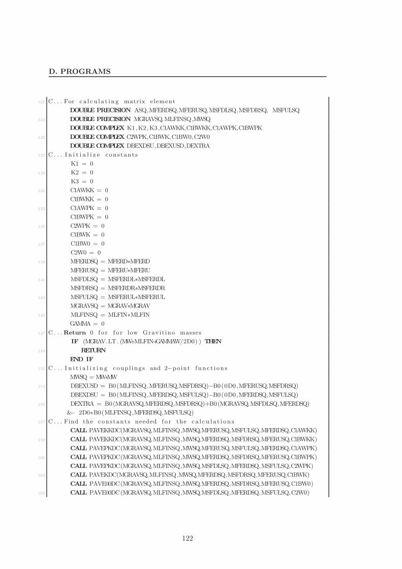
D. PROGRAMS
121 C . . . For c a l c u l a t i n g matrix element
DOUBLE PRECISION ASQ,MFERDSQ,MFERUSQ,MSFDLSQ,MSFDRSQ, MSFULSQ
123 DOUBLE PRECISION MGRAVSQ,MLFINSQ,MWSQ
DOUBLECOMPLEX K1,K2,K3,C1AWKK,C1BWKK,C1AWPK,C1BWPK
125 DOUBLECOMPLEX C2WPK,C1BWK,C1BW0,C2W0
DOUBLECOMPLEX DBEXDSU,DBEXUSD,DEXTRA
127 C . . . I n i t i a l i z e con s tan t s
K1 = 0
129 K2 = 0
K3 = 0
131 C1AWKK = 0
C1BWKK = 0
133 C1AWPK = 0
C1BWPK = 0
135 C2WPK = 0
C1BWK = 0
137 C1BW0 = 0
C2W0 = 0
139 MFERDSQ = MFERD∗MFERD
MFERUSQ = MFERU∗MFERU
141 MSFDLSQ = MSFERDL∗MSFERDL
MSFDRSQ = MSFERDR∗MSFERDR
143 MSFULSQ = MSFERUL∗MSFERUL
MGRAVSQ = MGRAV∗MGRAV
145 MLFINSQ = MLFIN∗MLFIN
GAMMA = 0
147 C . . . Return 0 f o r f o r low Grav it ino masses
IF (MGRAV.LT. (MW+MLFIN+GAMMAW/2D0) ) THEN
149 RETURN
END IF
151 C . . . I n i t i a l i z i n g coup l ings and 2−point fun c t i on s
MWSQ = MW∗MW
153 DBEXUSD = B0(MLFINSQ,MFERUSQ,MSFDRSQ)−B0(0D0,MFERUSQ,MSFDRSQ)
DBEXDSU = B0(MLFINSQ,MFERDSQ,MSFULSQ)−B0(0D0,MFERDSQ,MSFULSQ)
155 DEXTRA = B0(MGRAVSQ,MFERDSQ,MSFDRSQ)+B0(MGRAVSQ,MSFDLSQ,MFERDSQ)
&− 2D0∗B0(MLFINSQ,MFERDSQ,MSFULSQ)
157 C . . . Find the cons tan t s needed f o r the c a l c u l a t i o n s
CALL PAVEKKDC(MGRAVSQ,MLFINSQ,MWSQ,MFERUSQ,MSFULSQ,MFERDSQ,C1AWKK)
159 CALL PAVEKKDC(MGRAVSQ,MLFINSQ,MWSQ,MFERDSQ,MSFDRSQ,MFERUSQ,C1BWKK)
CALL PAVEPKDC(MGRAVSQ,MLFINSQ,MWSQ,MFERUSQ,MSFULSQ,MFERDSQ,C1AWPK)
161 CALL PAVEPKDC(MGRAVSQ,MLFINSQ,MWSQ,MFERDSQ,MSFDRSQ,MFERUSQ,C1BWPK)
CALL PAVEPKDC(MGRAVSQ,MLFINSQ,MWSQ,MSFDLSQ,MFERDSQ,MSFULSQ,C2WPK)
163 CALL PAVEKDC(MGRAVSQ,MLFINSQ,MWSQ,MFERDSQ,MSFDRSQ,MFERUSQ,C1BWK)
CALL PAVE00DC(MGRAVSQ,MLFINSQ,MWSQ,MFERDSQ,MSFDRSQ,MFERUSQ,C1BW0)
165 CALL PAVE00DC(MGRAVSQ,MLFINSQ,MWSQ,MSFDLSQ,MFERDSQ,MSFULSQ,C2W0)
122
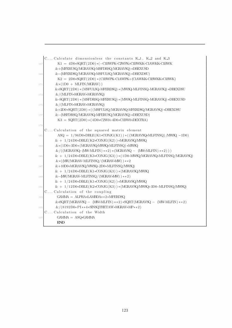
C . . . Ca l cu la t e d imens ion l e s s the cons tan t s K 1 , K 2 and K 3
167 K1 = 4D0∗SQRT(2D0)∗(−C1BWPK−C2WPK+C1BWKK−C1AWKK−C1BWK
&+(MFERUSQ/MGRAVSQ−MSFDRSQ/MGRAVSQ) ∗DBEXUSD
169 &−(MFERDSQ/MGRAVSQ−MSFULSQ/MGRAVSQ) ∗DBEXDSU)
K2 = 2D0∗SQRT(2D0) ∗(C1BWPK−C1AWPK+(C1AWKK−C1BWKK+C1BWK)
171 &∗(1D0 + MLFIN/MGRAV) )
&+SQRT(2D0) ∗(MSFULSQ−MFERDSQ) ∗(MWSQ−MLFINSQ−MGRAVSQ) ∗DBEXDSU
173 &/(MLFIN∗MGRAV∗MGRAVSQ)
&−SQRT(2D0) ∗(MSFDRSQ−MFERUSQ) ∗(MWSQ−MLFINSQ−MGRAVSQ) ∗DBEXUSD
175 &/(MLFIN∗MGRAV∗MGRAVSQ)
&+2D0∗SQRT(2D0) ∗ ( (MSFULSQ/MGRAVSQ−MFERDSQ/MGRAVSQ)∗DBEXDSU
177 &−(MSFDRSQ/MGRAVSQ−MFERUSQ/MGRAVSQ) ∗DBEXUSD)
K3 = SQRT(2D0) ∗(4D0∗C2W0+4D0∗C1BW0+DEXTRA)
179
C . . . Ca l cu la t ion o f the squared matrix element
181 ASQ = 1/96D0∗DBLE(K1∗CONJG(K1) ) ∗ ( (MGRAVSQ+MLFINSQ) /MWSQ −1D0)
& + 1/24D0∗DBLE(K2∗CONJG(K2) ) ∗MGRAVSQ/MWSQ
183 &∗(1D0+3D0∗(MGRAVSQ−MWSQ+MLFINSQ) ∗MWSQ
&/((MGRAVSQ−(MW−MLFIN) ∗∗2) ∗(MGRAVSQ − (MW+MLFIN) ∗∗2) ) )
185 & + 1/24D0∗DBLE(K3∗CONJG(K3) ) ∗(1D0−MWSQ/MGRAVSQ+MLFINSQ/MGRAVSQ)
&∗((MW/MGRAV−MLFINSQ/(MGRAV∗MW) ) ∗∗2
187 &+10D0+MGRAVSQ/MWSQ−2D0∗MLFINSQ/MWSQ)
& + 1/24D0∗DBLE(K1∗CONJG(K3) ) ∗(MGRAVSQ/MWSQ
189 &−(MW/MGRAV−MLFINSQ/(MGRAV∗MW) ) ∗∗2)
& + 1/24D0∗DBLE(K1∗CONJG(K2) ) ∗MGRAVSQ/MWSQ
191 & + 1/12D0∗DBLE(K2∗CONJG(K3) ) ∗(MGRAVSQ/MWSQ+3D0−MLFINSQ/MWSQ)
C . . . Ca l cu la t ion o f the coup l ing
193 GAMMA = ALPHA∗LAMBDA∗∗2∗MFERDSQ
&∗SQRT(MGRAVSQ − (MW+MLFIN) ∗∗2) ∗SQRT(MGRAVSQ − (MW−MLFIN) ∗∗2)
195 &/(8192D0∗PI∗∗4∗SINSQTHETAW∗MGRAV∗MP∗∗2)
C . . . Ca l cu la t ion o f the Width
197 GAMMA = ASQ∗GAMMA
END
123

D. PROGRAMS
124
References
[1] G. Moreau and M. Chemtob, “R-parity Violation and the Cosmological Gravitino
Problem,” Phys.Rev. D65 (2002) 024033, arXiv:hep-ph/0107286 [hep-ph]. ii, 1, 27,
61, 64, 67
[2] S. Lola, P. Osland, and A. Raklev, “Radiative gravitino decays from R-parity violation,”
Phys.Lett. B656 (2007) 83–90, arXiv:0707.2510 [hep-ph]. ii, 1, 27, 61, 64, 67
[3] T. Hahn and M. Perez-Victoria, “Automatized One Loop Calculations in
Four-Dimensions and D-Dimensions,” Comput.Phys.Commun. 118 (1999) 153–165,
arXiv:hep-ph/9807565 [hep-ph]. http://www.feynarts.de/looptools/. 1, 33, 61
[4] T. Sjostrand, S. Mrenna, and P. Skands, “Pythia 6.4 physics and manual,” JHEP 0605
(2006) 026. doi:10.1088/1126-6708/2006/05/026. 1, 63
[5] S. P. Martin, “A Supersymmetry primer,” arXiv:hep-ph/9709356 [hep-ph]. 3, 14, 18
[6] H. J. W. Muller-Kirsten and A. Wiedemann, Introduction to Supersymmetry. World
Scientific Publishing Co. Pte. Ldt., second ed., 2010. 3, 7, 10, 11, 12
[7] R. Haag, J. T. Lopuszanski, and M. Sohnius, “All Possible Generators of
Supersymmetries of the S Matrix,” Nucl.Phys. B88 (1975) 257. 4
[8] A. Salam and J. Strathdee, “On Superfields and Fermi-Bose Symmetry,” Phys.Rev. D11
(1975) 1521–1535. 7
[9] S. Ferrara and B. Zumino, “Supergauge Invariant Yang-Mills Theories,” Nucl.Phys. B79
(1974) 413. 10
[10] J. Bagger and J. Wess, “Partial Breaking of Extended Supersymmetry,” Phys.Lett. B138
(1984) 105. 10
[11] S. Ferrara, L. Girardello, and F. Palumbo, “A General Mass Formula in Broken
Supersymmetry,” Phys.Rev. D20 (1979) 403. 11
[12] D. Z. Freedman, P. van Nieuwenhuizen, and S. Ferrara, “Progress Toward a Theory of
Supergravity,” Phys.Rev. D13 (1976) 3214–3218. 12, 21
125
REFERENCES
[13] Particle Data Group Collaboration, K. Nakamura et al., “Review of Particle Physics,”
J.Phys.G G37 (2010) 075021. 17, 64
[14] P. Fayet, “Spontaneous Supersymmetry Breaking Without Gauge Invariance,” Phys.Lett.
B58 (1975) 67. 17
[15] H. K. Dreiner, “An Introduction to Explicit R-Parity Violation,” arXiv:hep-ph/9707435
[hep-ph]. Published in ’Perspectives on Supersymmetry’, Ed. by G.L. Kane, World
Scientific. 17
[16] L. E. Ibanez and G. G. Ross, “Discrete Gauge Symmetries and the Origin of Baryon and
Lepton Number Conservation in Supersymmetric Versions of the Standard Model,”
Nucl.Phys. B368 (1992) 3–37. 17
[17] S. Lola and G. G. Ross, “Baryon and lepton number (non)conservation in
supersymmetric theories,” Phys.Lett. B314 (1993) 336–344. 17
[18] F. Zwicky, “Spectral Displacement of Extra Galactic Nebulae,” Helv.Phys.Acta 6 (1933)
110–127. 18
[19] WMAP Collaboration, D. N. Spergel et al., “First Year Wilkinson Microwave
Anisotropy Probe (WMAP) Observations: Determination of Cosmological Parameters,”
Astrophys. J. Suppl. 148 (2003) 175–194, arXiv:astro-ph/0302209. 18
[20] G. Bertone, D. Hooper, and J. Silk, “Particle Dark Matter: Evidence, Candidates and
Constraints,” Phys.Rept. 405 (2005) 279–390, arXiv:hep-ph/0404175 [hep-ph]. 18
[21] G. Jungman, M. Kamionkowski, and K. Griest, “Supersymmetric Dark Matter,”
Phys.Rept. 267 (1996) 195–373, arXiv:hep-ph/9506380 [hep-ph]. 18
[22] ATLAS Collaboration, G. Aad et al., “Search for the Standard Model Higgs Boson in
the Decay Channel H→ZZ(*)→4l with 4.8 fb−1 of pp Collision Data at sqrt(s) = 7 TeV
with ATLAS,” Phys. Lett. B710 (2012) 383–402, arXiv:1202.1415 [hep-ex]. 18
[23] ATLAS Collaboration, G. Aad et al., “Search for the Standard Model Higgs boson in
the Diphoton Decay Channel with 4.9 fb−1 of pp Collisions at sqrt(s)=7 TeV with
ATLAS,” Phys.Rev.Lett. 108 (2012) 111803, arXiv:1202.1414 [hep-ex]. 18
[24] ATLAS Collaboration, G. Aad et al., “Combined Search for the Standard Model Higgs
Boson using up to 4.9 fb−1 of pp Collision Data at sqrt(s) = 7 TeV with the ATLAS
Detector at the LHC,” Phys.Lett. B710 (2012) 49–66, arXiv:1202.1408 [hep-ex]. 18
[25] E. Cremmer, S. Ferrara, L. Girardello, and A. Van Proeyen, “Yang-Mills Theories with
Local Supersymmetry: Lagrangian, Transformation Laws and SuperHiggs Effect,” Nucl.
Phys. B212 (1983) 413. 21
126
REFERENCES
[26] W. Rarita and J. Schwinger, “On a Theory of Particles with Half Integral Spin,”
Phys.Rev. 60 (1941) 61. 22
[27] M. Bolz, “Thermal production of gravitinos,”. Ph.D. Thesis (Advisor: W. Buchmuller).
22, 85
[28] M. Bolz, A. Brandenburg, and W. Buchmuller, “Thermal Production of Gravitinos,”
Nucl.Phys. B606 (2001) 518–544, arXiv:hep-ph/0012052 [hep-ph]. 26
[29] M. Fukugita and T. Yanagida, “Baryogenesis Without Grand Unification,” Phys.Lett.
B174 (1986) 45. 27
[30] F. D. Steffen, “Gravitino Dark Matter and Cosmological Constraints,” JCAP 0609
(2006) 001, arXiv:hep-ph/0605306 [hep-ph]. 27
[31] A. Ibarra and D. Tran, “Gamma Ray Spectrum from Gravitino Dark Matter Decay,”
Phys. Rev. Lett. 100 (2008) 061301, arXiv:0709.4593 [astro-ph]. 28
[32] A. R. Raklev, “Massive Metastable Charged (S)Particles at the LHC,” Mod. Phys. Lett.
A24 (2009) 1955–1969, arXiv:0908.0315 [hep-ph]. 28
[33] Fermi-LAT Collaboration, A. Abdo et al., “The Spectrum of the Isotropic Diffuse
Gamma-Ray Emission Derived From First-Year Fermi Large Area Telescope Data,”
Phys.Rev.Lett. 104 (2010) 101101, arXiv:1002.3603 [astro-ph.HE]. 28, 63, 65, 66, 78
[34] G. Passarino and M. Veltman, “One Loop Corrections for e+ e- Annihilation Into mu+
mu- in the Weinberg Model,” Nucl.Phys. B160 (1979) 151. 33
[35] A. Raklev, “Dog - a program for the decay of gravitinos..” private code, 2012. 61
[36] P. Z. Skands, B. Allanach, H. Baer, C. Balazs, G. Belanger, et al., “SUSY Les Houches
Accord: Interfacing SUSY Spectrum Calculators, Decay Packages, and Event
Generators,” JHEP 0407 (2004) 036, arXiv:hep-ph/0311123 [hep-ph]. 63
[37] A. Ibarra and D. Tran, “Antimatter Signatures of Gravitino Dark Matter Decay,” JCAP
0807 (2008) 002, arXiv:0804.4596 [astro-ph]. 64
[38] LAT Collaboration, W. Atwood et al., “The Large Area Telescope on the Fermi
Gamma-Ray Space Telescope Mission,” Astrophys.J. 697 (2009) 1071–1102,
arXiv:0902.1089 [astro-ph.IM]. 64
[39] G. Cowan, Statistical Data Analysis. Oxford Science Publications. Clarendon Press,
1998. 65
[40] A. Denner, H. Eck, O. Hahn, and J. Kublbeck, “Feynman Rules for Fermion Number
Violating Interactions,” Nucl.Phys. B387 (1992) 467–484. 85
127

REFERENCES
[41] R. Mertig, M. Bohm, and A. Denner, “FEYN CALC: Computer Algebraic Calculation of
Feynman Amplitudes,” Comput.Phys.Commun. 64 (1991) 345–359. www.feyncalc.org.
99
128