Embed Size (px)
Citation preview
University of South FloridaScholar Commons
Graduate Theses and Dissertations Graduate School
June 2017
Cybersecurity: Stochastic Analysis and Modellingof Vulnerabilities to Determine the NetworkSecurity and Attackers BehaviorPubudu Kalpani KaluarachchiUniversity of South Florida, [email protected]
Follow this and additional works at: http://scholarcommons.usf.edu/etd
Part of the Arts and Humanities Commons, and the Statistics and Probability Commons
This Dissertation is brought to you for free and open access by the Graduate School at Scholar Commons. It has been accepted for inclusion inGraduate Theses and Dissertations by an authorized administrator of Scholar Commons. For more information, please [email protected].
Scholar Commons CitationKaluarachchi, Pubudu Kalpani, "Cybersecurity: Stochastic Analysis and Modelling of Vulnerabilities to Determine the NetworkSecurity and Attackers Behavior" (2017). Graduate Theses and Dissertations.http://scholarcommons.usf.edu/etd/6862
Cybersecurity: Stochastic Analysis and Modelling of Vulnerabilities to Determinethe Network Security and Attackers Behavior
by
Pubudu Kalpani Kaluarachchi
A dissertation submitted in partial fulfillmentof the requirements for the degree of
Doctor of PhilosophyDepartment of Mathematics and Statistics
College of Arts and SciencesUniversity of South Florida
Major Professor: Chris P. Tsokos, Ph.D.Kandethody Ramachandran, Ph.D.
Dan Shen, Ph.D.Lu Lu, Ph.D.
Date of Approval:June 20, 2017
Keywords: Cyber Security, Markov Model, Vulnerability, Risk Rank
Copyright c© 2017, Pubudu Kalpani Kaluarachchi

Dedication
This doctoral dissertation is dedicated to my father, my mother and my husband.

Acknowledgments
It was a wonderful opportunity that I was able to study at USF. I would like
to pay my gratitude to everyone for helping me in numerous ways during my time of
study at USF.
It is with my utmost respect and gratitude that I mention here, proper guid-
ance, selfless gifts of knowledge, encouragement and motivation for independent re-
search interests given by my advisor, the Distinguished University Professor Chris
P. Tsokos. His considerate attention for students was exceptional. Through out my
doctoral program, directions and advice inspired me in my research efforts.
I am thankful to Prof. Kandethody Ramachandran, Prof. Dan Shen, Prof. Lu
Lu for their kind assistance and time in my dissertation research.
It is with great pleasure and gratitude that I remind all the faculty members
in the Department of Mathematics and Statistics for their effort full teaching in the
courses I have taken. I express my gratitude to the administration of the the Depart-
ment of Mathematics and Statistics for all the helps and resources made available to
me as a student.
I would also like to express my gratitude to the Florida Center of Cyber Secu-
rity at USF (FC2), for the Summer internship granted me in 2016.
It is with great pleasure and love that I mention the helpfulness of my husband,

Sasith Rjajasooriya.
Many thanks to my fellow friends, Xing Wang, Jason, Muditha, Bashar and
all other graduate students for their support and friendship in last four years.
4
Table of Contents
List of Tables iv
List of Figures v
Abstract vi
1 Introduction 1
1.1 Research Problems and Their Background . . . . . . . . . . . . . . . 1
1.2 Vulnerability Data Base and Analysis of Vulnerability Types . . . . . 4
1.3 A Statistical Predictive Model for the Expected Path Length . . . . . 5
1.4 NonHomogeneous Stochastic Model for Cyber Security Predictions . . 6
1.5 Nonhomogeneous Risk Rank Analysis Method for Security NetworkSystem . . . . . . . . . . . . . . . . . . . . . . . . . . . . . . . . . . . 6
2 Vulnerability Data Base and Analysis of Vulnerability Types 7
2.1 Introduction . . . . . . . . . . . . . . . . . . . . . . . . . . . . . . . . 7
2.2 Vulnerability . . . . . . . . . . . . . . . . . . . . . . . . . . . . . . . 8
2.3 Common Vulnerability Scoring System (CVSS) . . . . . . . . . . . . 9
2.3.1 Base Metric . . . . . . . . . . . . . . . . . . . . . . . . . . . . 10
2.3.2 Temporal Metric . . . . . . . . . . . . . . . . . . . . . . . . . 13
2.3.3 Environmental Metric . . . . . . . . . . . . . . . . . . . . . . 13
2.4 Vulnerabilities Life Cycle . . . . . . . . . . . . . . . . . . . . . . . . . 14
2.4.1 Birth (Pre-Discovery) . . . . . . . . . . . . . . . . . . . . . . . 15
2.4.2 Discovery . . . . . . . . . . . . . . . . . . . . . . . . . . . . . 15
2.4.3 Disclosure . . . . . . . . . . . . . . . . . . . . . . . . . . . . . 16
2.4.4 Scripting (Exploiting) and Exploit Availability . . . . . . . . . 17
2.4.5 Patch Availability and Death: (Patched) . . . . . . . . . . . . 17
2.5 Categorizing and Ranking Different Types of Vulnerabilities . . . . . 18
i
2.5.1 Rank and Distribution of Vulnerability Types in Low level (CVSSscore 0-3.9) . . . . . . . . . . . . . . . . . . . . . . . . . . . . 20
2.5.2 Rank and Distribution of Vulnerability Types in Medium Level(CVSS score 4-6.9) . . . . . . . . . . . . . . . . . . . . . . . . 20
2.5.3 Rank and Distribution of Vulnerability Types in High Level(CVSS score 7-10) . . . . . . . . . . . . . . . . . . . . . . . . 22
2.5.4 Behavior of DOS Vulnerability Type with Respect to Time . . 24
2.5.5 Behavior of Memory Corruption Vulnerability Type with Re-spect to Time . . . . . . . . . . . . . . . . . . . . . . . . . . . 25
2.6 Contribution . . . . . . . . . . . . . . . . . . . . . . . . . . . . . . . . 26
3 A Statistical Predictive Model for the Expected Path Length 28
3.1 Introduction . . . . . . . . . . . . . . . . . . . . . . . . . . . . . . . . 28
3.2 Background and Related Methodologies . . . . . . . . . . . . . . . . . 29
3.2.1 Markov Chain and Transition Probability . . . . . . . . . . . 29
3.2.2 Transient States . . . . . . . . . . . . . . . . . . . . . . . . . . 31
3.3 Cybersecurity Analysis Method . . . . . . . . . . . . . . . . . . . . . 32
3.3.1 Attack Prediction . . . . . . . . . . . . . . . . . . . . . . . . . 33
3.3.2 Illustration: The Attacker . . . . . . . . . . . . . . . . . . . . 35
3.3.3 Adjacency Matrix for the Attack Graph . . . . . . . . . . . . 38
3.4 Finding Stationary Distribution and Minimum Number of Steps . . . 39
3.5 Expected Path Length (EPL) Analysis . . . . . . . . . . . . . . . . . 40
3.6 Development of the Statistical Models . . . . . . . . . . . . . . . . . 40
3.6.1 Developing a Statistical Model to Predict the Minimum Numberof Steps . . . . . . . . . . . . . . . . . . . . . . . . . . . . . . 41
3.6.2 Developing a Statistical Model to Predict the Minimum Numberof Steps . . . . . . . . . . . . . . . . . . . . . . . . . . . . . . 42
3.7 Contribution . . . . . . . . . . . . . . . . . . . . . . . . . . . . . . . . 44
4 NonHomogeneous Stochastic Model for Cyber Security Predictions 47
4.1 Introduction . . . . . . . . . . . . . . . . . . . . . . . . . . . . . . . . 47
4.2 Background and Related Methodologies . . . . . . . . . . . . . . . . . 49
4.2.1 Cybersecurity Analysis Method . . . . . . . . . . . . . . . . . 49
4.2.2 Risk Factor Model . . . . . . . . . . . . . . . . . . . . . . . . 50
4.3 Attack Prediction . . . . . . . . . . . . . . . . . . . . . . . . . . . . . 52
4.3.1 Multi Step Attack Prediction . . . . . . . . . . . . . . . . . . 52
4.3.2 Prediction of Expected Path Length (EPL) . . . . . . . . . . . 53
ii
4.4 Attack Graph and Attack Risk Evaluation . . . . . . . . . . . . . . . 54
4.4.1 Application: The Attacker . . . . . . . . . . . . . . . . . . . . 54
4.4.2 Host Centric Attack graph . . . . . . . . . . . . . . . . . . . . 57
4.5 Adjacency Matrix for the Attack Graph . . . . . . . . . . . . . . . . 57
4.5.1 Expected Path length . . . . . . . . . . . . . . . . . . . . . . . 60
4.6 Contributions . . . . . . . . . . . . . . . . . . . . . . . . . . . . . . . 63
5 Nonhomogeneous Risk Rank Analysis Method for Security Network System 65
5.1 Introduction . . . . . . . . . . . . . . . . . . . . . . . . . . . . . . . . 65
5.2 Google Page Rank Algorithm . . . . . . . . . . . . . . . . . . . . . . 66
5.3 Risk Rank Algorithm . . . . . . . . . . . . . . . . . . . . . . . . . . . 68
5.4 Illustration of Applying of the Risk Rank Algorithm . . . . . . . . . . 71
5.4.1 Behavior of Risk Ranks Over Time . . . . . . . . . . . . . . . 75
5.5 Contributions . . . . . . . . . . . . . . . . . . . . . . . . . . . . . . . 77
6 Future Research 78
References 81
Appendices 88
iii
List of Tables
2.1 Rank of Vulnerability Types in Low Category . . . . . . . . . . . . . 21
2.2 Rank of Vulnerability Types in Medium Category . . . . . . . . . . . 21
2.3 Rank of Vulnerability Types in High Category . . . . . . . . . . . . . 23
3.1 Vulnerability Scores . . . . . . . . . . . . . . . . . . . . . . . . . . . . 36
3.2 Parametric Model: R2 and adjusted R2 values . . . . . . . . . . . . . 41
3.3 Parametric model (EPL): R2 and R2adj values . . . . . . . . . . . . . . 43
3.4 Number of Steps for Absorbing Matrix . . . . . . . . . . . . . . . . . 45
3.5 Expected Path Length for several Vulnerabilities. . . . . . . . . . . . 46
4.1 Model Equations of Risk Factors for three different categories of vul-nerabilities. . . . . . . . . . . . . . . . . . . . . . . . . . . . . . . . . 51
4.2 Vulnerability Scores. . . . . . . . . . . . . . . . . . . . . . . . . . . . 56
4.3 Expected Path Length relative to number of days after first attack . . 61
5.1 Vulnerability Scores. . . . . . . . . . . . . . . . . . . . . . . . . . . . 73
5.2 Ranking results in attack states . . . . . . . . . . . . . . . . . . . . . 75
5.3 Ranking results for each state with time . . . . . . . . . . . . . . . . 76
iv
List of Figures
2.1 Common Vulnerability Scoring System . . . . . . . . . . . . . . . . . 10
2.2 Common Vulnerability Scoring System- Base Metric Calculation Model 11
2.3 Common Vulnerability Scoring System- Temporal Metric CalculationModel . . . . . . . . . . . . . . . . . . . . . . . . . . . . . . . . . . . 13
2.4 Key Steps of the Rank Vulnerability Types. . . . . . . . . . . . . . . 19
2.5 Distribution of vulnerability Types in Low Category . . . . . . . . . . 20
2.6 Distribution of vulnerability Types in Medium Category . . . . . . . 22
2.7 Distribution of vulnerability Types in High Category . . . . . . . . . 22
2.8 Distribution of DOS vulnerability types with time . . . . . . . . . . . 24
2.9 Distribution of Memory Corruption vulnerability types with time . . 25
3.1 Network Topology . . . . . . . . . . . . . . . . . . . . . . . . . . . . 36
3.2 Host Centric Attack Graph . . . . . . . . . . . . . . . . . . . . . . . . 37
4.1 Network Topology . . . . . . . . . . . . . . . . . . . . . . . . . . . . 55
4.2 Host Centric Attack Graph . . . . . . . . . . . . . . . . . . . . . . . . 57
4.3 Behavior of Expected Path Length over the time . . . . . . . . . . . . 62
5.1 Key Steps of the Risk Rank Algorithm. . . . . . . . . . . . . . . . . . 71
5.2 Network Topology . . . . . . . . . . . . . . . . . . . . . . . . . . . . 72
5.3 Host Centric Attack Graph . . . . . . . . . . . . . . . . . . . . . . . . 74
v
Abstract
Development of Cybersecurity processes and strategies should take two main
approaches. One is to develop an efficient and effective set of methodologies to identify
software vulnerabilities and patch them before being exploited. Second is to develop
a set of methodologies to predict the behavior of attackers and execute defending
techniques based on attacking behavior. Managing of Vulnerabilities and analyzing
them is directly related to the first approach. Developing of methodologies and mod-
els to predict the behavior of attackers is related to the second approach. Both these
approaches are inseparably interconnected. Our effort in this study mainly focuses
on developing useful statistical models that can give us signals about the behavior of
cyber attackers.
Analytically understanding of vulnerabilities in statistical point of view helps
to develop a set of statistical models that works as a bridge between Cybersecurity
and Abstract Statistical and Mathematical knowledge. Any such effort should begin
with properly understanding the nature of Vulnerabilities in a computer network sys-
tem. We start this study with analyzing ”Vulnerability” based on inferences that can
be taken from National Vulnerability Database (NVD).
In Cybersecurity context, we apply Markov approach to develop suitable pre-
vi
dictive models to successfully estimate the minimum number of steps to compromise a
security goal that an attacker would take using the concept of Expected Path Length
(EPL).
We have further developed Non-Homogeneous Stochastic model by improving
EPL estimates in to a time dependent variable. This approach analytically applied
in a simple model of computer network with discovered vulnerabilities resulted in
several useful observations exemplifying the applicability in real world computer sys-
tems. The methodology indicated a measure of the ”Risk” associated with the model
network as a function of time indicating defending professionals on the threats they
are facing and should anticipate to face.
Further more, using a similar approach taken in well known Google page rank
algorithm, a new ranking algorithm of vulnerability ranks with respect to time for
computer network system is also presented in this study.
With better IT resources analytical models and methodologies presented in
this study can be developed into more generalized versions and apply in real world
computer network environments.
vii
1 Introduction
Present study is a series of Statistical and Mathematical applications that is proposed
as set of decision making tools in the filed of Cybersecurity. This dissertation consists
of five chapters where the first two chapters present the background of the research of
interest and other chapters present with the methodologies, applications and research
outcomes.
In this chapter, we discuss our research problems and their background, im-
portance of Statistical Approaches in the area of Cybersecurity, current trends in the
filed of Cybersecurity and basis of our strategies from Statistical perspective.
1.1 Research Problems and Their Background
Cyber-attacks are one of the most formidable security challenge faced by many gov-
ernments and large scale companies. Cyber criminals are increasingly using sophisti-
cated network and social engineering techniques to steal the crucial information which
directly affects the operational effects of the Government or Companys objectives.
According to the Secunia [1] report 2015 we can see how crucial the volume and mag-
nitude of increasing Cybersecurity threats. Thus, in understanding the performance,
1
availability and reliability of computer networks, security measuring techniques plays
an important role in the subject area.
Quantitative measures are now commonly used to evaluate the security of
computer network systems. These measures help administrators to make important
decisions regarding their network security [3].
However, security of any computer system at last is about the weaknesses it
has and capability of defending the system from attackers who would try to use those
weaknesses to exploit the system. It is logical to compare, this situation to a war
fare, where an army of enemies would tries to break in to a security station using its
weaker points while defending forces are trying to track attackers, understand their
own weaknesses and deploy solutions to those weaknesses so that the ability of the
enemy forces to exploit those weaknesses are eliminated or minimized. This means
that Cybersecurity require a great deal of analysis in two main aspects. The first one
is the analysis of the weaknesses in computer systems. The second is the analysis of
the behavior of attackers and defenders. Indeed the analysis of the behavior of the
attacker is critical.
While we paid our attention to both the behavioral aspect analysis and system
susceptibility analysis this dissertation focus more into the behavioral aspect of the
analysis. In other words, we pay our specific attention to develop analytical models
to analyze ”attackers behavior”.
There are indeed a lots of efforts taken by Information Technology special-
ists and related professionals in this respect, developing models to track attackers.
2
However, our mission here is to develop set of Statistical Models that can be used in
analyzing or predicting the attackers behavior.
Subil Abrahim and Suku Nair [3] in 2014 introduced a stochastic model for
cybersecurity quantification using absorbing Markov chain. In [3] they introduced
a non homogeneous Markov model for security quantification. Kijsanayothin Phong-
phun [4] in her/his thesis ”Network Security Modeling with Intelligent and Complexity
Analysis” discussed the need for generating automated preventive network security
systems and an approach to do it using ”host centric attack graphs”. This study
used both quantitative and qualitative approaches in security model analysis named
”exploit based analysis” and ”preference based analysis” respectively. All three of
these studies mentioned have used Markov Chain methods in their methodologies in
Cybersecurity analysis.
In 2006 Stefan Frei [10] and others, in their study titled ”Large-Scale Vulnera-
bility Analysis” presented with several important analytical outcomes. In this study,
an overall statistical analysis on the vulnerability data [2] uptodate was conducted
using over 80,000 vulnerabilities recorded from 1995.
Yashwant K. Malaiya and Alhazmi [5] also have conducted a series of very use-
ful and important studies analyzing the vulnerability data in several aspects. Malaiya
talks about vulnerability life cycle and CVSS Metrics in an analytical view point of
security risk and proposed a method for risk evaluation [8]. Malaiya discuss and
analyze different states of vulnerabilities and proposed some models to evaluate risk
associated with those states [6] & [7].
3
Hiroyuki Okamura [36] in 2013 proposed a quantitative security evaluation
method using stochastic process for software systems using vulnerability data that
the discovery dates, patch dates and exploit publish dates are available. Leyla Bilge
and Tudor Dumitras in 2012 described a method to automatically identify ”zero-day”
vulnerabilities [9].
Considering these efforts in the subject area of Cybersecurity it is our un-
derstanding that the need for better and improved analytical tools for vulnerability
analysis and the likelihood to be exploited is at the highest importance. Therefore, we
raise our research problems from the defenders point of view to seek answers. First,
how to develop a set of successful statistical models to analyze the vulnerability status
of a computer network system. Second, could an analysis on vulnerability and their
likelihood to be exploited be observed and relate those observations in predicting the
attackers success. To answer those problems, we first need to take better statistical
and probabilistic approaches in analyzing the attacking process. Next few chapters
as summarized below discuss these problems in details with the methodologies used
and results obtained.
1.2 Vulnerability Data Base and Analysis of Vulnerability Types
In Chapter two, an overview about the nature of vulnerabilities and Common Vulner-
ability Scoring System (CVSS) [2],[14] is given. The methodology used in CVSS and
metric system used to arrive the CVSS are discussed. The concept of Vulnerability
Life Cycle and its stages are also introduced. Following this introduction and back-
4
ground is an analysis on various type of vulnerabilities. In this chapter, we take the
entire vulnerability data base [2],[19] into consideration and rank number of vulnera-
bilities of 13 different types as given in the National Vulnerability Database. Resulting
ranks of vulnerabilities important in terms of the frequency are presented graphically.
Further, a suitable forecasting models are arrived based on the shape of the scatter
plots where the number of different types of vulnerabilities are plotted with respect
to time.
Main objective of chapter two is to have the basic analysis and gain the overall
understanding about vulnerabilities and National Vulnerability Database which will
make the platform for our deeper analysis in chapters to follow.
1.3 A Statistical Predictive Model for the Expected Path Length
In Chapter three, the concept of Expected Path Length (EPL)[3],[4] as an applica-
tion in Cybersecurity filed is introduced. The main objective of the chapter is to
develop a successful Statistical Model to estimate the Expected Path Length. Using
a model computer network example, a methodology and an analysis on Attack Pre-
diction Method is discussed. Steps that were taken using the Markov Chain Process
[16] and the development of the Transition Probability Matrix are presented under
Methodology. Concept of Attack graph and developing of Attack Graphs are also
introduced. Finally, successful Statistical Models to predict the minimum number of
steps (Expected Path Length) that an Attacker would take to compromise a security
state presented. Developed Statistical Models are tested for the quality and accuracy.
5
1.4 NonHomogeneous Stochastic Model for Cyber Security Predictions
Objective of Chapter four is to develop and present a Non-Homogeneous Stochastic
Model for better Cybersecurity predictions. In this chapter Cyber Security Analysis
Method of Vulnerability Life Cycle is used as an index of Risk Factor[20],[21] asso-
ciated with a particular vulnerability. But, the chapter further develop this analysis
method and Risk Analysis to develop a time dependent analytical methodology. The
new methodology proposed is applied in a model network system which allows to
analyze the behavior of EPL as a function of time. This improvement is significant
because the Risk is now calculated for a set of vulnerabilities in a network system and
also observable with respect to time.
1.5 Nonhomogeneous Risk Rank Analysis Method for Security Network
System
Chapter five in this dissertation presents a new Risk Rank Algorithm [13],[27] were
the risk ranks of vulnerabilities exist in a computer network system can be obtained.
Development of this new algorithm is based on well-known Google Page Rank Al-
gorithm. New algorithm we propose in this chapter is significant since the Ranks of
vulnerabilities of a computer network system can be observed with respect to time as
well. Therefore, the results from this method can be used by network administrators
and defending professionals to understand the priorities and allocate resources based
on these priorities at the time of consideration.
6
2 Vulnerability Data Base and Analysis of Vulnerability Types
2.1 Introduction
In this chapter, an overview about the nature of vulnerabilities and Common Vul-
nerability Scoring System (CVSS)[14] is given. The methodology used in CVSS and
metric system used to arrive the CVSS are discussed. The concept of Vulnerability
Life Cycle and its stages are also introduced. Following this introduction and back-
ground is an analysis on various type of vulnerabilities. In this chapter, we take the
entire vulnerability data base into consideration and rank number of vulnerabilities
of 13 different types as given in the National Vulnerability Database [2]. Resulting
ranks of vulnerabilities important in terms of the frequency are presented graphically.
Further, a suitable forecasting models are arrived based on the shape of the scatter
plots where the number of different types of vulnerabilities [19] are plotted with re-
spect to time. .
However, it should be noticed that our study results in some new definitions
also. Applying of Mathematical and Statistical approaches into the field of Cyberse-
curity is relatively new compared to many such other fields that use Mathematical
and Statistical approaches. Therefore, in some cases we needed to define concepts our
7
own. In all such cases, we tried our best to maintain the integrity of Mathematical,
Statistical and Computer science practices.
2.2 Vulnerability
Properly understanding what is called ”vulnerability” [2] in the field of Cybersecurity
is of the core in our study. Therefore, in this chapter we discuss all the basic aspects
of vulnerability including vulnerability information, vulnerability data base and vul-
nerability life cycle [8].
In computer security, a vulnerability is a weakness which allows an attacker
to reduce a system’s information assurance. Vulnerability is the intersection of three
elements, which are, systems susceptibility to the flaw, attacker access to the flaw,
and attacker capability to exploit the flaw.
To exploit a vulnerability, an attacker must have at least one applicable tool
or technique that can connect to a system weakness. In this frame, vulnerability is
also known as the attack surface.
The attack surface of a software environment is the sum of the different points
(the ”attack vectors”) where an unauthorized user (the ”attacker”) can try to enter
data to or extract data from an environment.
8
2.3 Common Vulnerability Scoring System (CVSS)
Common Vulnerability Scoring System (CVSS)[14] is a free and open industry stan-
dard for assessing the severity of computer system security vulnerabilities. It is under
the custodianship of the Forum of Incident Response and Security Teams (FIRST).
CVSS is composed of three metric groups, Base, Temporal, and Environmental, each
consisting of a set of metrics. It attempts to establish a measure of how much concern
a vulnerability warrants, compared to other vulnerabilities, so efforts can be prior-
itized. The scores are based on a series of measurements (called metrics) based on
expert assessment. The scores range from 0 to 10 [2]. Vulnerabilities with a base
score in the range 7.0-10.0 are High, those in the range 4.0-6.9 as Medium, and 0-3.9
as Low. Figure 2.1, 2.2 and 2.3 below give a schematic presentation of the Com-
mon Vulnerability Scoring System (CVSS) which is the basis of the metric calculation
model and the temporal and environmental matrices calculation model, respectively.
Calculation methodology for the CVSS is given in Appendix A.
9
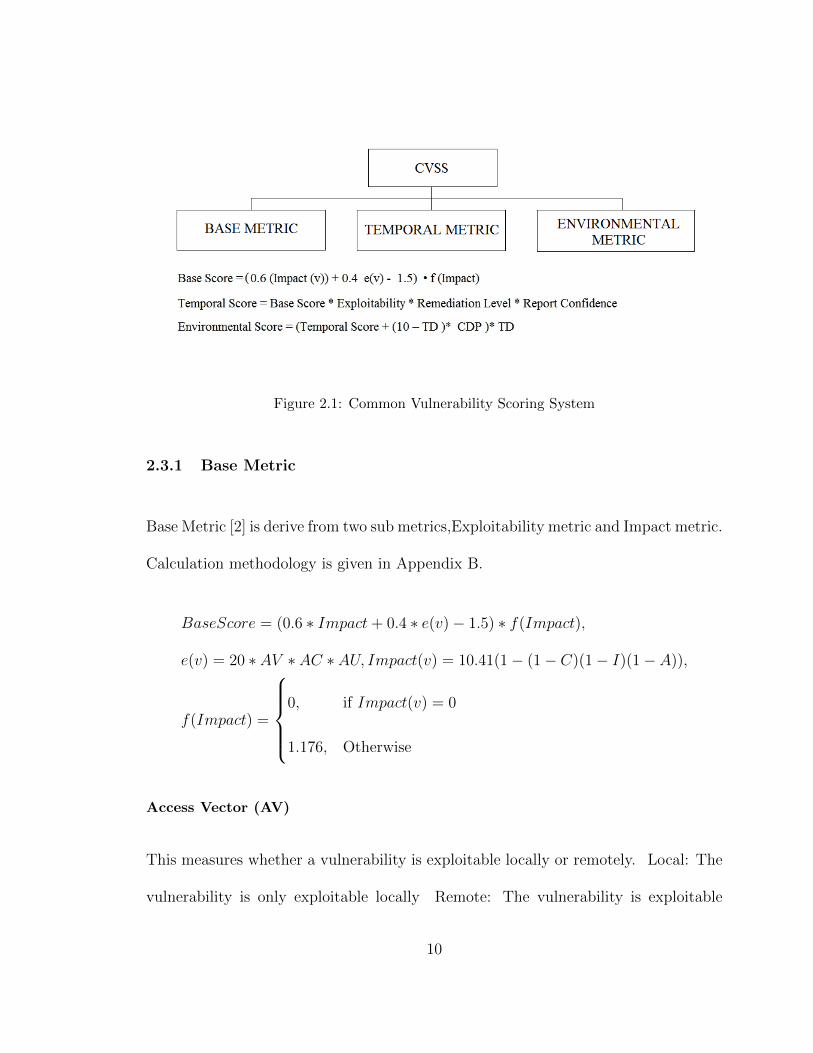
Figure 2.1: Common Vulnerability Scoring System
2.3.1 Base Metric
Base Metric [2] is derive from two sub metrics,Exploitability metric and Impact metric.
Calculation methodology is given in Appendix B.
BaseScore = (0.6 ∗ Impact+ 0.4 ∗ e(v)− 1.5) ∗ f(Impact),
e(v) = 20 ∗ AV ∗ AC ∗ AU, Impact(v) = 10.41(1− (1− C)(1− I)(1− A)),
f(Impact) =
0, if Impact(v) = 0
1.176, Otherwise
Access Vector (AV)
This measures whether a vulnerability is exploitable locally or remotely. Local: The
vulnerability is only exploitable locally Remote: The vulnerability is exploitable
10
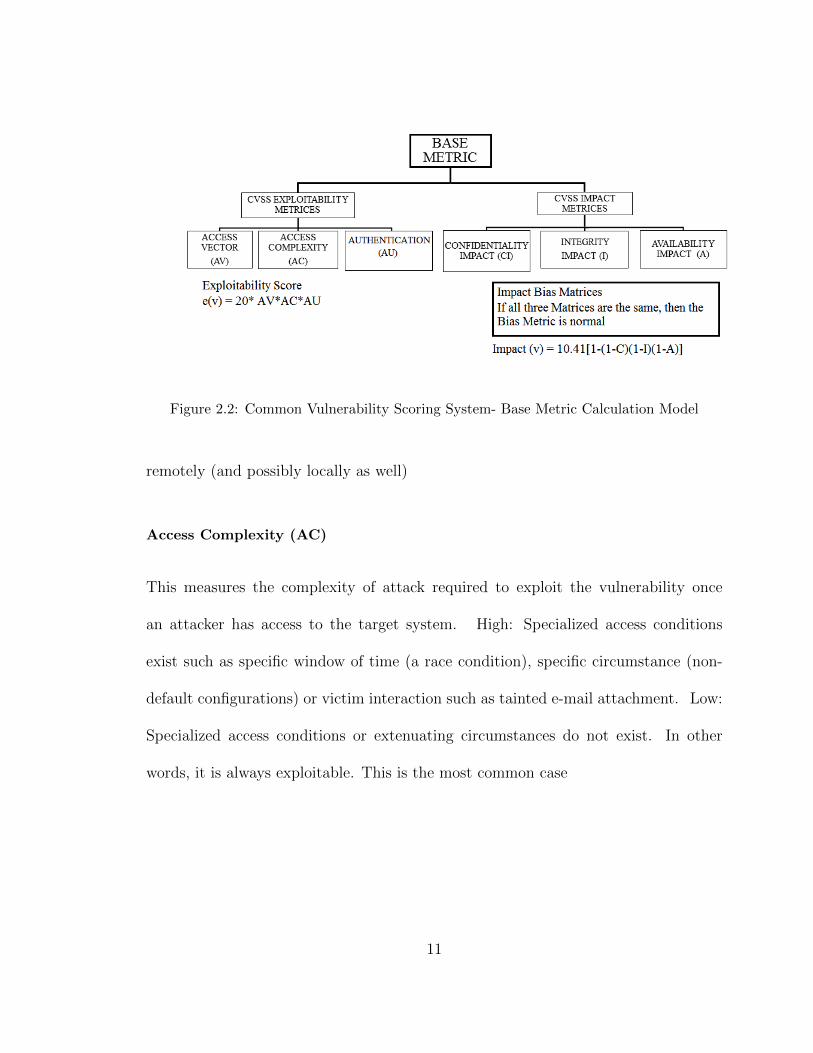
Figure 2.2: Common Vulnerability Scoring System- Base Metric Calculation Model
remotely (and possibly locally as well)
Access Complexity (AC)
This measures the complexity of attack required to exploit the vulnerability once
an attacker has access to the target system. High: Specialized access conditions
exist such as specific window of time (a race condition), specific circumstance (non-
default configurations) or victim interaction such as tainted e-mail attachment. Low:
Specialized access conditions or extenuating circumstances do not exist. In other
words, it is always exploitable. This is the most common case
11
Authentication (AW)
This measures whether or not an attacker needs to be authenticated to the target
system in order to exploit the vulnerability. Required: Authentication is required to
access and exploit the vulnerability. Not Required: Authentication is not required
to access or exploit the vulnerability.
Confidentiality Impact (C)
Confidentiality Impact measures the impact on Confidentiality of a successful exploit
of the vulnerability on the target system. None: No impact on confidentiality. Par-
tial: There is consider able informational disclosure. Complete: A total compromise
of critical system information.
Integrity Impact (I)
Integrity Impact measures the impact on Integrity of a successful exploit of the vul-
nerability on the target system. None: No impact on integrity. Partial: Considerable
breach in integrity. Complete: A total compromise of system integrity.
Availability Impact (A)
Availability Impact measures the impact on Availability of a successful exploit of
the vulnerability on the target system. None: No impact on availability Partial:
Considerable lag in or in eruptions in resource availability Complete: Total shutdown
of the affected resource
12
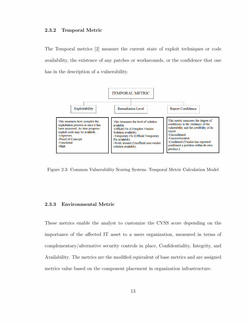
2.3.2 Temporal Metric
The Temporal metrics [2] measure the current state of exploit techniques or code
availability, the existence of any patches or workarounds, or the confidence that one
has in the description of a vulnerability.
Figure 2.3: Common Vulnerability Scoring System- Temporal Metric Calculation Model
2.3.3 Environmental Metric
These metrics enable the analyst to customize the CVSS score depending on the
importance of the affected IT asset to a users organization, measured in terms of
complementary/alternative security controls in place, Confidentiality, Integrity, and
Availability. The metrics are the modified equivalent of base metrics and are assigned
metrics value based on the component placement in organization infrastructure.
13
Collateral Damage Potential (CDP)
This metric measures the potential for loss of life or physical assets through damage
or theft of property or equipment. The metric may also measure economic loss of
productivity or revenue. The possible values for this metric are listed in Appendix A.
Naturally, the greater the damage potential, the higher the vulnerability score.
Target Distribution (TD)
This metric measures the proportion of vulnerable systems. It is meant as an environment-
specific indicator in order to approximate the percentage of systems that could be af-
fected by the vulnerability. The possible values for this metric are listed in Appendix
A. The greater the proportion of vulnerable systems, the higher the score.
2.4 Vulnerabilities Life Cycle
The Life Cycle of a Vulnerability [10] can be introduced with different stages that
a vulnerability passes through. We shall discuss specific stages that are commonly
identified in a given situation. Commonly identified stages are involved with the
events such as the Birth (Pre-discovery Stage), Discovery, Disclosure, Availability for
Patching and Availability for Exploiting.
14
2.4.1 Birth (Pre-Discovery)
The birth of a vulnerability occurs at the development of a software, mostly due to a
weakness or a mistake in coding of the software. At this stage the vulnerability is not
yet discovered or exploited. In a well-developed software package where its reliability
has been identified, one can identify the probability of the birth of the problem.
2.4.2 Discovery
Vulnerability is said to be discovered once someone identifies the flaw in the software.
It is possible that the vulnerability is discovered by the system developers themselves,
skilled legitimate users or by the attackers also. If the vulnerability is discovered
internally or by white hackers, (who are making breaking attempts on a system to
identify the flaws and vulnerabilities with good intentions of helping them to be
patched so that the system security is strengthened) it will be notified to be fixed as
soon as possible. But, if a black hacker [40] discovers a vulnerability it is possible
that he or she will try to exploit it, or sell in the black market or distribute it among
hackers to be exploited.
It should be noted here that while vulnerabilities could actually exist prior to
the discovery, until it is discovered, it is not a potential security risk. ”Time of the
discovery” is the earliest time that a vulnerability is identified. In a vulnerability life
cycle the ”time of discovery” is an important and critical event. Exact discovery time
might not be published or disclosed to the public due to the other risks that could
15
be associated with a vulnerability. However, in general after the ”disclosure” of a
vulnerability, public may know the time of discovery subject to security risk review.
We would like to mention here that in developing our statistical model, we
consider only pre-exploit discovery. There are rare chances that a discovery of a
vulnerability could occur after it is actually exploited. As an example, an attacker
could run an exploit attempt aiming to exploit a particular vulnerability. But, the
exploit actually breaks into the system through another unidentified or undiscovered
vulnerability instead of expected vulnerability at that time. Such rare occurrences
are not taken into account in our our present study.
2.4.3 Disclosure
Once a vulnerability is discovered, it is subject to be disclosed. Disclosure could take
place in different ways based on the system design, authentication and who discovered
it. However, ”disclosure” in widely accepted form in the information security means
the event that a particular vulnerability is made known to public through relevant
and appropriate channels. Definition for the disclosure of vulnerability is however
presented differently by different individuals.
In general, public disclosure of a vulnerability is based on several principles.
The availability of access to the vulnerability information for the public is one such
important principle. Another such important principle is validity of information.
Validity of information principle is to ensure the users ability to use those information,
assess the risk and take security measures. Also, the independence of information
16
channels is also considered to be important to avoid any bias and interferences from
organizational bodies including the vendor.
2.4.4 Scripting (Exploiting) and Exploit Availability
A Vulnerability enters to the stage of exploit availability [22],[23] from the earliest
time that an exploit program of code is available. Once the exploits are available
even low skilled crackers (or in other words a black hat hacker) could be capable
of exploiting the vulnerability. As we mentioned earlier, there are some occurrences
that the exploit could happen even before the vulnerability is discovered. However in
the present study we consider the modeling of Vulnerability Life Cycles with exploit
availability occurs only after the discovery.
2.4.5 Patch Availability and Death: (Patched)
Patch is a software solution that the vendor or developer release to provide necessary
protection from possible exploits of the vulnerability. Patch will act against possible
exploit codes or attacking attempts for a vulnerability and protect the system and
ensure the integrity. The vulnerability dies when one applies a security patch to all
the vulnerable systems.
When a White Hat Researcher discovers a vulnerability, the next transition is
likely to be the internal disclosure leading to patch development. On the other hand,
if a Black Hat Hacker discovers a vulnerability, the next transition could be an exploit
17
or internal disclosure to his underground community. Some active black hats might
develop scripts that exploit the vulnerability.
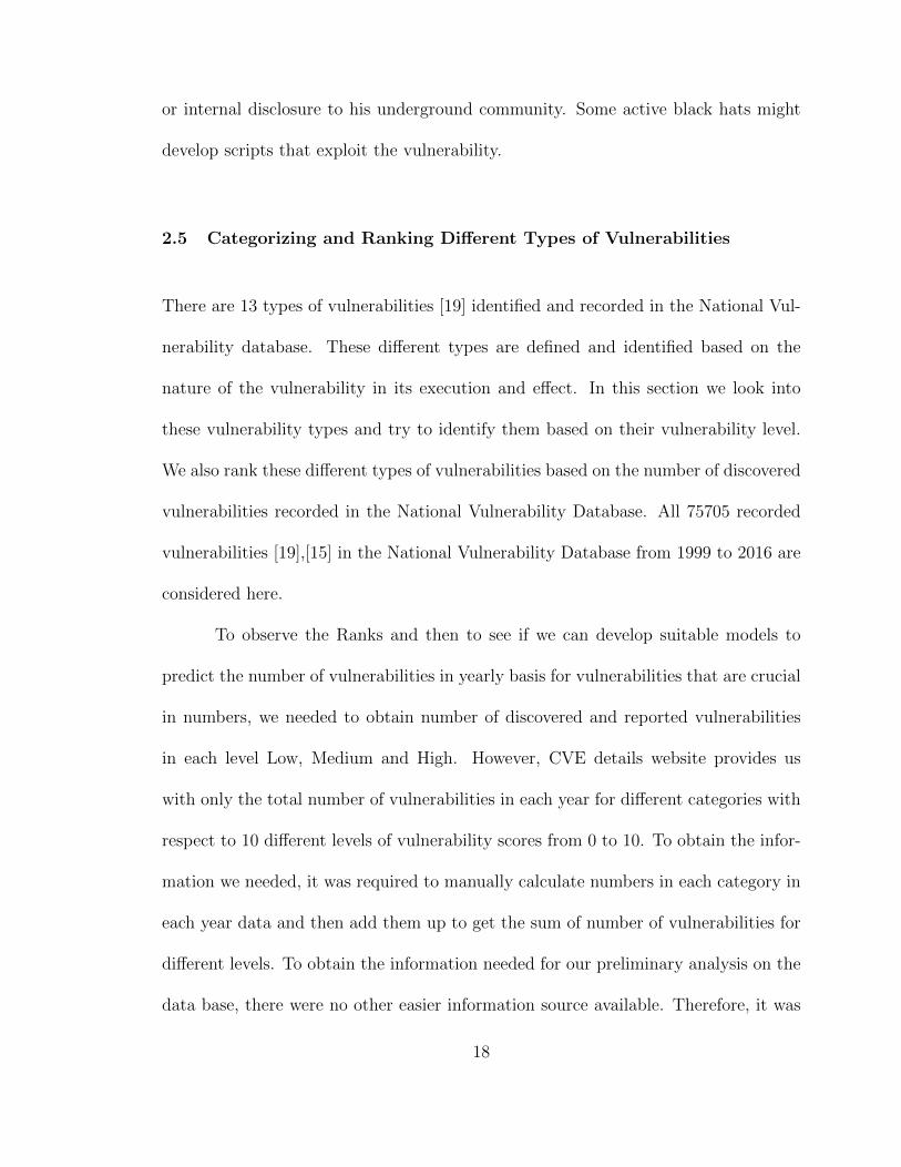
2.5 Categorizing and Ranking Different Types of Vulnerabilities
There are 13 types of vulnerabilities [19] identified and recorded in the National Vul-
nerability database. These different types are defined and identified based on the
nature of the vulnerability in its execution and effect. In this section we look into
these vulnerability types and try to identify them based on their vulnerability level.
We also rank these different types of vulnerabilities based on the number of discovered
vulnerabilities recorded in the National Vulnerability Database. All 75705 recorded
vulnerabilities [19],[15] in the National Vulnerability Database from 1999 to 2016 are
considered here.
To observe the Ranks and then to see if we can develop suitable models to
predict the number of vulnerabilities in yearly basis for vulnerabilities that are crucial
in numbers, we needed to obtain number of discovered and reported vulnerabilities
in each level Low, Medium and High. However, CVE details website provides us
with only the total number of vulnerabilities in each year for different categories with
respect to 10 different levels of vulnerability scores from 0 to 10. To obtain the infor-
mation we needed, it was required to manually calculate numbers in each category in
each year data and then add them up to get the sum of number of vulnerabilities for
different levels. To obtain the information needed for our preliminary analysis on the
data base, there were no other easier information source available. Therefore, it was
18
necessary to go through this manual process. Following schematic network presents
the steps we used in the calculation process.
Total Number of Vulnerabilities from 1999-2015 (75705)
Calculate the yearly basis,
number of vulnerabilities in
each type in 10 different levels
Calculate the yearly basis number
of Vulnerabilities in 10 different lev-
els for 13 different vulnerability types.
Calculate the total number of vul-
nerabilities for 17 years for 10 dif-
ferent levels (for 13 categories)
Categorize number of vulnerabilities into Low risk (0-3.9), Medium risk (4-6.9) and High risk (7.10)
Order (descending) the number of vul-
nerabilities in each type for three differ-
ent levels to observe the Ranks based
on most frequent type of vulnerabilities.
Figure 2.4: Key Steps of the Rank Vulnerability Types.
19
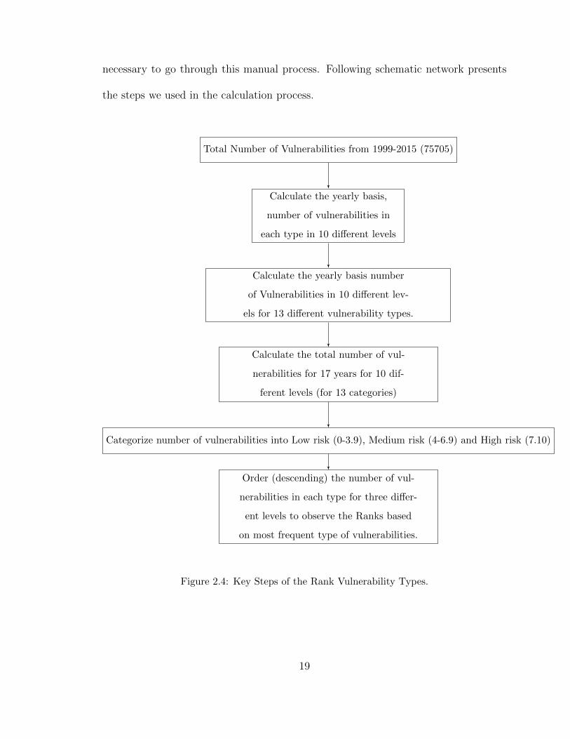
2.5.1 Rank and Distribution of Vulnerability Types in Low level (CVSS
score 0-3.9)
Figure 2.5: Distribution of vulnerability Types in Low Category
The most common type of vulnerability that is in lower level category is XSS
(Cross-site scripting Vulnerabilities). According to the number of vulnerabilities in
each type, the second and third in the lower level are DOS (Denial of service) and
Gain Information respectively. Table below illustrates the rank of vulnerability types,
based on number of discovered vulnerabilities in the lower level category.
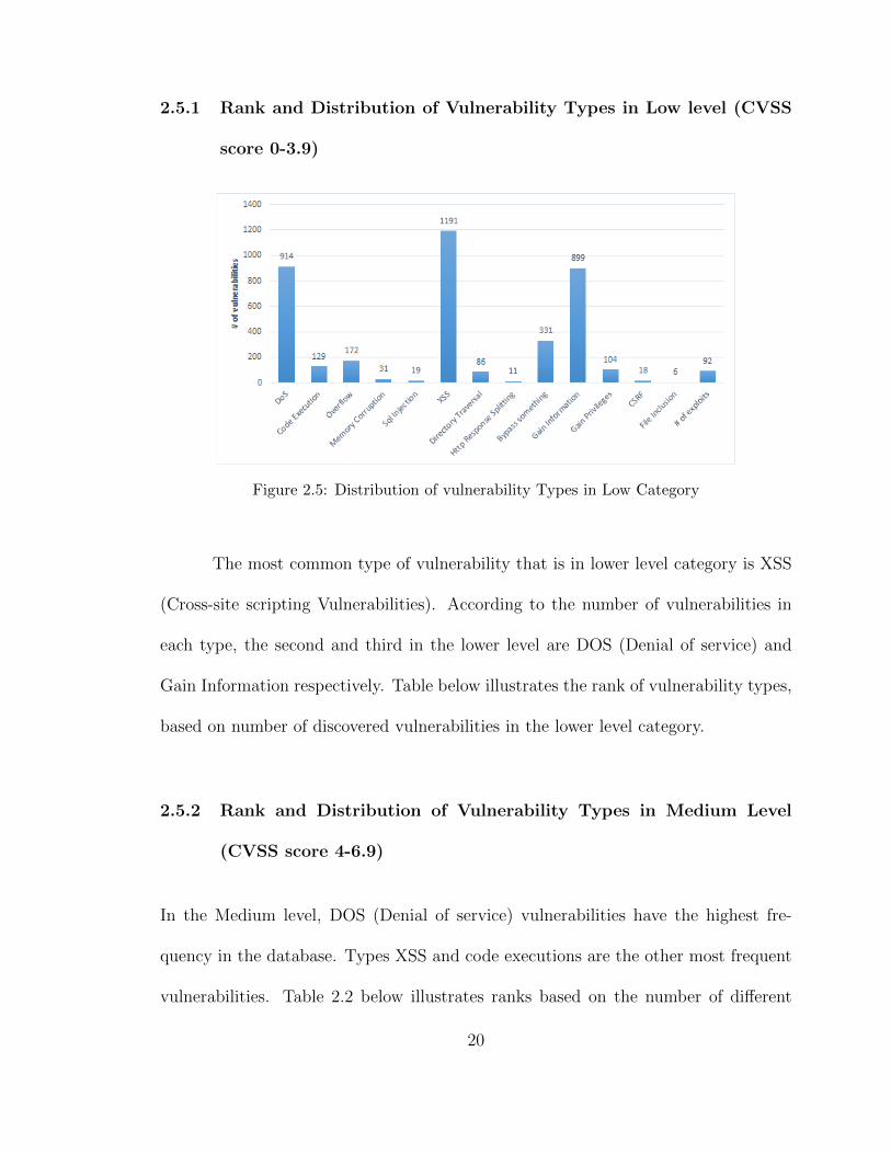
2.5.2 Rank and Distribution of Vulnerability Types in Medium Level
(CVSS score 4-6.9)
In the Medium level, DOS (Denial of service) vulnerabilities have the highest fre-
quency in the database. Types XSS and code executions are the other most frequent
vulnerabilities. Table 2.2 below illustrates ranks based on the number of different
20
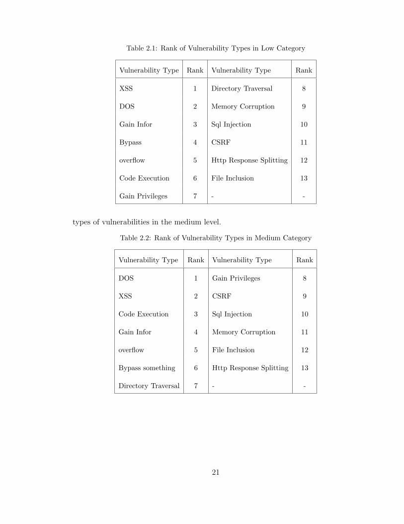
Table 2.1: Rank of Vulnerability Types in Low Category
Vulnerability Type Rank Vulnerability Type Rank
XSS 1 Directory Traversal 8
DOS 2 Memory Corruption 9
Gain Infor 3 Sql Injection 10
Bypass 4 CSRF 11
overflow 5 Http Response Splitting 12
Code Execution 6 File Inclusion 13
Gain Privileges 7 - -
types of vulnerabilities in the medium level.
Table 2.2: Rank of Vulnerability Types in Medium Category
Vulnerability Type Rank Vulnerability Type Rank
DOS 1 Gain Privileges 8
XSS 2 CSRF 9
Code Execution 3 Sql Injection 10
Gain Infor 4 Memory Corruption 11
overflow 5 File Inclusion 12
Bypass something 6 Http Response Splitting 13
Directory Traversal 7 - -
21
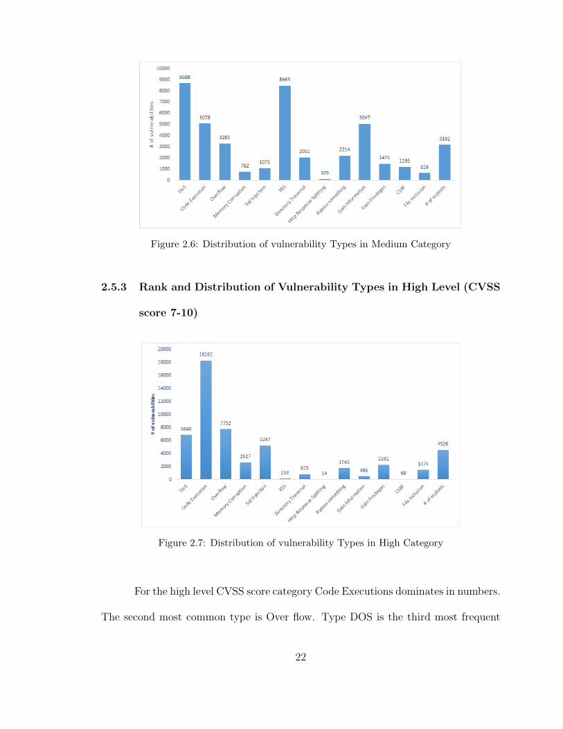
Figure 2.6: Distribution of vulnerability Types in Medium Category
2.5.3 Rank and Distribution of Vulnerability Types in High Level (CVSS
score 7-10)
Figure 2.7: Distribution of vulnerability Types in High Category
For the high level CVSS score category Code Executions dominates in numbers.
The second most common type is Over flow. Type DOS is the third most frequent
22
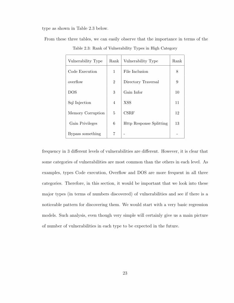
type as shown in Table 2.3 below.
From these three tables, we can easily observe that the importance in terms of the
Table 2.3: Rank of Vulnerability Types in High Category
Vulnerability Type Rank Vulnerability Type Rank
Code Execution 1 File Inclusion 8
overflow 2 Directory Traversal 9
DOS 3 Gain Infor 10
Sql Injection 4 XSS 11
Memory Corruption 5 CSRF 12
Gain Privileges 6 Http Response Splitting 13
Bypass something 7 - -
frequency in 3 different levels of vulnerabilities are different. However, it is clear that
some categories of vulnerabilities are most common than the others in each level. As
examples, types Code execution, Overflow and DOS are more frequent in all three
categories. Therefore, in this section, it would be important that we look into these
major types (in terms of numbers discovered) of vulnerabilities and see if there is a
noticeable pattern for discovering them. We would start with a very basic regression
models. Such analysis, even though very simple will certainly give us a main picture
of number of vulnerabilities in each type to be expected in the future.
23
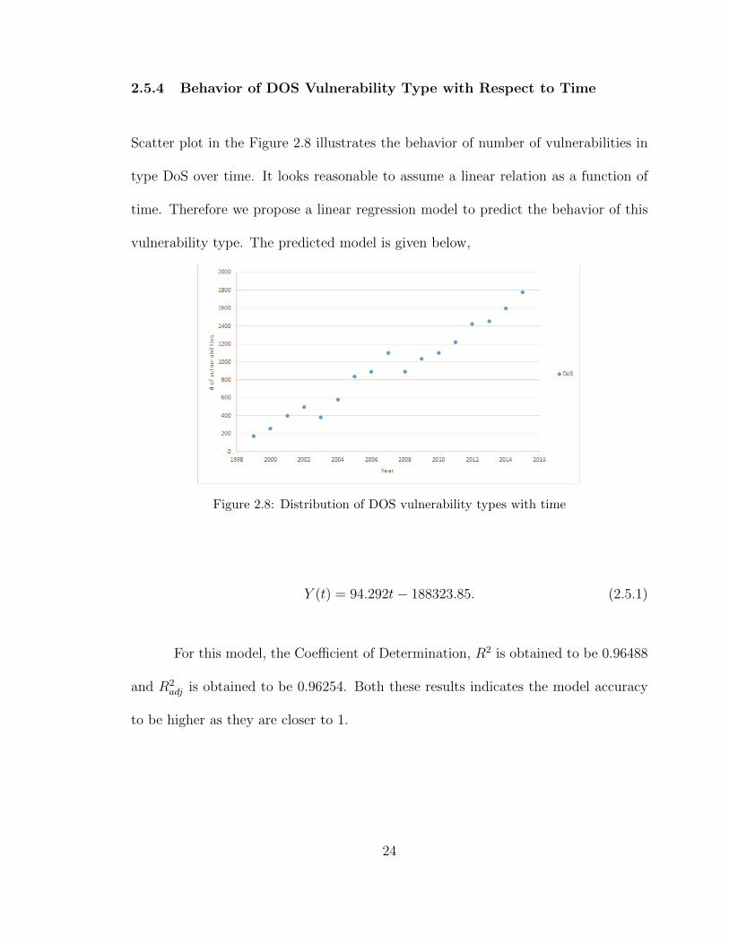
2.5.4 Behavior of DOS Vulnerability Type with Respect to Time
Scatter plot in the Figure 2.8 illustrates the behavior of number of vulnerabilities in
type DoS over time. It looks reasonable to assume a linear relation as a function of
time. Therefore we propose a linear regression model to predict the behavior of this
vulnerability type. The predicted model is given below,
Figure 2.8: Distribution of DOS vulnerability types with time
Y (t) = 94.292t− 188323.85. (2.5.1)
For this model, the Coefficient of Determination, R2 is obtained to be 0.96488
and R2adj is obtained to be 0.96254. Both these results indicates the model accuracy
to be higher as they are closer to 1.
24
2.5.5 Behavior of Memory Corruption Vulnerability Type with Respect
to Time
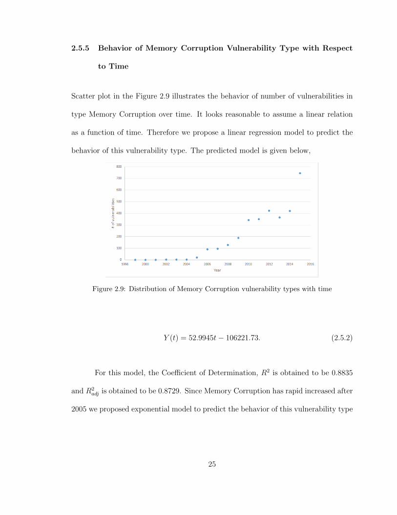
Scatter plot in the Figure 2.9 illustrates the behavior of number of vulnerabilities in
type Memory Corruption over time. It looks reasonable to assume a linear relation
as a function of time. Therefore we propose a linear regression model to predict the
behavior of this vulnerability type. The predicted model is given below,
Figure 2.9: Distribution of Memory Corruption vulnerability types with time
Y (t) = 52.9945t− 106221.73. (2.5.2)
For this model, the Coefficient of Determination, R2 is obtained to be 0.8835
and R2adj is obtained to be 0.8729. Since Memory Corruption has rapid increased after
2005 we proposed exponential model to predict the behavior of this vulnerability type
25

and the predicted model is given below,
Y (t) = 1.381E−05 ∗ e(t) + 29.586t− 110.4284. (2.5.3)
For exponential model, the Coefficient of Determination, R2 is obtained to
be 0.9221 and R2adj is obtained to be 0.9109. Both these results indicates the model
accuracy to be higher as they are closer to 1. Since R2adj for second model is much
higher than linear regression model, we proposed exponential model to predict the
behavior of Memory Corruption.
2.6 Contribution
In this chapter, we discussed the vulnerability data base in several aspects including
the computational methodology used in the calculation of ”Common Vulnerability
Scoring System (CVSS)[39]. We observed thirteen different vulnerability types in
the vulnerability database for over 75000 different software vulnerabilities. In this
chapter, we conducted the basic analysis of number of vulnerabilities for the use of
following chapters.
To further understand different types of vulnerabilities and their role in the
cyber world we observed the data available in the vulnerability data base with respect
to different types of vulnerabilities and rank them based on the number of vulnera-
bilities. Once the number of different types of vulnerabilities are calculated for three
different levels of vulnerabilities recorded in each year from 1996 to 2015, we ranked
26

the vulnerability types based on number of vulnerabilities discovered or recorded in
each of the three levels. This analysis is important since different types of vulnera-
bilities have different effects on the security and solutions to be implemented are also
different based on these different types.
Finally, taking the ranks based on number of vulnerabilities into consideration,
we observed the vulnerability type DOS constitute a major role in all three different
levels based on the number of vulnerabilities. Therefore, to have a general predictive
model for DOS we have developed a Linear Regression Model with higher degree of
the Coefficient of Determination (R2).
We also developed a non linear predictive model where we observed an expo-
nential type of behavior for the vulnerability type ”Memory Corruption” with very
good prediction accuracy.
27
3 A Statistical Predictive Model for the Expected Path Length
3.1 Introduction
Cyber-attacks are the most formidable security challenge faced by most governments
and large scale companies. Cyber criminals are increasingly using sophisticated net-
work and social engineering techniques to steal the crucial information which directly
affects the operational effects of the Government or Companys objectives. According
to the Secunia report 2015 [1] one can see how crucial the volume and magnitude of
increasing cybersecurity threaten. Thus, in understanding the performance, availabil-
ity and reliability of computer networks, measuring techniques plays an important
role in the subject area.
Quantitative measures are now commonly used to evaluate the security of
computer network systems [35],[36]. These measures help administrators to make im-
portant decisions regarding their network security.
In the present study we have first proposed a stochastic model for security
evaluation [17] based on vulnerability exploitability scores and attack path behav-
ior. Here, we consider small case scenarios which include three vulnerabilities (high,
medium and small) as a base model to understand the behavior of network topology.
28
We structure the attack graph which includes all possibilities that the attacker reach
the goal state and used probabilistic analysis to measure the security of the network
[30]. In addition we propose a statistical model that is driven by the mentioned
vulnerabilities along with the significant interactions that is highly accurate. This
statistical model will allow us to estimate the Expected Path Length and Minimum
number of steps to reach the target with probability one. Having these important
estimates we can take counter steps and acquire relevant resources to protect the se-
curity system from the attacker. In addition, utilizing this model we have identified
the significant interaction of the key attributable variables. Also we can rank the at-
tributable variables (vulnerabilities) to identify the percentage of contribution to the
response (Expected path length and Minimum number of steps to reach the target)
and furthermore one can perform surface response analysis to identify the acceptable
values that will minimize the Expected Path Length among others.
3.2 Background and Related Methodologies
The background of the inherent problems with the Markov property [16],[44] that we
are going to use in our new model are discussed in the following subsections.
3.2.1 Markov Chain and Transition Probability
A discrete type stochastic process X = {XN , N ≥ 0} is called a Markov chain if for
any sequence {X0, X1, ..., XN} of states, the next state depends only on the current
29

state and not on the sequence of events that preceded it, which is called the Markov
property. Mathematically we can write this as follows.
P (XN = j|X0 = i0, X1 = i1, ..., XN−2 = iN−2, XN−1 = i) = P (XN = j|XN−1 = i).
(3.2.1)
We will also make the assumption that the transition probabilities P (XN = j|X0 =
i0, X1 = i1, ..., XN−2 = iN−2, XN−1 = i) do not depend on time. This is called time
homogeneity. The transition probabilities (Pi,j) for Markov chain can be defined as
follows.
(Pi,j) = P (XN = j|XN−1 = i). (3.2.2)
The transition matrix P of the Markov chain is the NxN matrix whose (i, j) entry
Pi,j satisfied the following properties.
0 ≤ Pi,j ≤ 1, 1 ≤ i, j ≤ N, (3.2.3)
N∑j=1
Pi,j = 1, 1 ≤ i, j ≤ N. (3.2.4)
Any matrix satisfying the above two equations is the transition matrix for a Markov
chain. To simulate a Markov chain, we need its stochastic matrix P and an initial
probability distribution π0.
30

3.2.2 Transient States
Let P be the transition matrix [16],[4] for Markov chain Xn. A state i is called
transient state if with probability 1 the chain visits i only a finite number of times.
Let Q be the sub matrix of P which includes only the rows and columns for the
transient states. The transition matrix for an absorbing Markov chain [16] has the
following canonical form.
P =
Q R
0 I
. (3.2.5)
Here P is the transition matrix, Q is the matrix of transient states, R is the
matrix of absorbing states and I is the identity matrix.
The matrix P represents the transition probability matrix of the absorbing
Markov chain. In an absorbing Markov chain the probability that the chain will be
absorbed is always 1. Hence, we have,
Qn →∞, n→∞.
Thus, is it implies that all the eigenvalues of Q have absolute values strictly
less than 1. Hence, I-Q is an invertible matrix and there is no problem in defining the
matrix
M = (I −Q)−1 = I +Q+Q2 +Q3 + ....
31
This matrix is called the fundamental matrix of P. Let i be a transient state
and consider Yi, the total number of visits to i. Then we can show that the expected
number of visits to i starting at j is given by Mij, the (i, j) entry of the matrix M.
Therefore, if we want to compute the expected number of steps until the chain enters
a recurrent class, assuming starting at state j, we need only sum Mij over all transient
states i.
3.3 Cybersecurity Analysis Method
The core component of this method is the attack graph [11],[12],[13]. When we draw
an attack graph for a cybersecurity system it has several nodes which represent the
vulnerabilities that the system has and the attackers state [11]. We consider that it
is possible to go to a goal state starting from any other state in the attack graph.
Also an attack graph has at least one absorbing state or goal state. Therefore we will
model the attack graph as an absorbing Markov chain.
Absorbing state or goal state is the security node which is exploited by the
attacker. When the attacker has reached this goal state, attack path [18] is completed.
Thus, the entire attack graph consists of these type of attack paths.
Given the CVSS score for each of the vulnerabilities in the attack Graph [43],
we can estimate the transition probabilities of the absorbing Markov chain by normal-
izing the CVSS scores over all the edges starting from the attackers source state.We
define,
pij = probability that an attacker is currently in state j and exploits a
32
vulnerability in state i.
n = number of outgoing edges from state i in the attack model.
vj = CVSS score for the vulnerability in state j.
Then formally we can define the transition probability below,
Pij =vj∑nk=1 vk
. (3.3.6)
By using these transition probabilities we can derive the absorbing transition
probability matrix P, which follows the properties defined under Markov chain prob-
ability method.
3.3.1 Attack Prediction
Under the Attack prediction, we consider two methods to predict the attackers be-
havior.
Multi Step Attack Prediction
The absorbing transition probability matrix shows the presence of each edge in a
network attack graph [29]. This matrix shows every possible single-step attack. In
other words, the absorbing transition probability matrix shows attacker reachability
within one attack step. We can navigate the absorbing transition probability matrix
by iteratively matching rows and columns to follow multiple attack steps, and also
33

raise the absorbing transition probability matrix to higher powers, which shows multi-
step attacker reachability at a glance.
For a square (n × n) adjacency matrix P and a positive integer k, then Pk is
P raised to the power k: Since P is an absorbing transition probability matrix with
time, this matrix goes to some stationary matrix Π, where the rows of this matrix are
identical. That is,
limk→∞
PK = Π. (3.3.7)
At the goal state column of this matrix Π has ones, so we can find the minimum
number of steps that the attacker should try to reach to the goal state with probability
1.
Prediction of Expected Path Length (EPL)
The Expected Path Length (EPL)[3],[26] measures the expected number of steps the
attacker will take starting from the initial state to reach the goal state (the attackers
objective). As we discussed earlier P has the following canonical form.
P =
Q R
0 I
. (3.3.8)
Here, P is the transition matrix, Q is the matrix of transient states, R is the matrix of
absorbing states and I is the identity matrix. The matrix P represents the transition
probability matrix of the absorbing Markov chain. In an absorbing Markov chain the
34
probability that the chain will be absorbed is always 1. Thus, we have
Qn →∞, n→∞.
Thus, is it implies that all the eigenvalues of Q have absolute values strictly
less than 1. Hence, I-Q is an invertible matrix and there is no problem in defining the
matrix
M = (I −Q)−1 = I +Q+Q2 +Q3 + ....
Using this fundamental matrix M of the absorbing Markov chain we can compute the
expected total number of steps to reach the goal state until absorption.
Taking the summation of first row elements of matrix M gives the expected
total number of steps to reach the goal state until absorption and the probability
value relates to the goal state gives the expected number of visits to that state before
absorption.
3.3.2 Illustration: The Attacker
To illustrate the proposed approach model that we discussed in section 3.3.1, we con-
sidered a Network Topology given in Figure 3.1, below. The network consists of two
service hosts IP 1, IP 2 and an attackers workstation, Attacker connecting to each of
the servers via a central router.
35
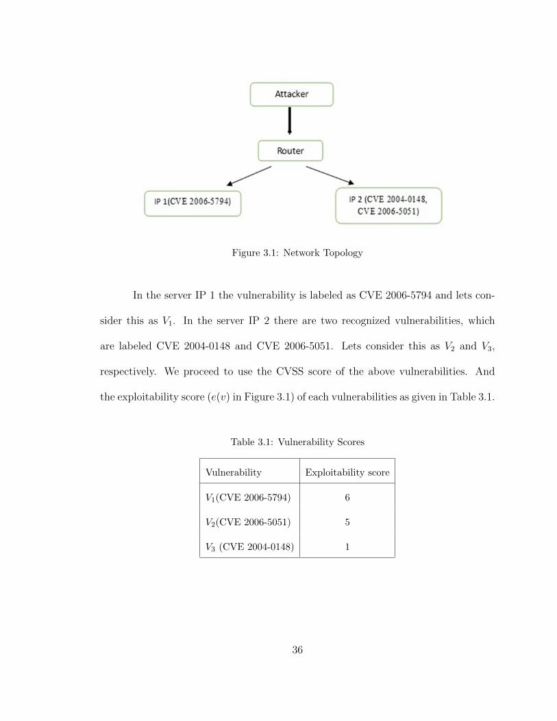
Figure 3.1: Network Topology
In the server IP 1 the vulnerability is labeled as CVE 2006-5794 and lets con-
sider this as V1. In the server IP 2 there are two recognized vulnerabilities, which
are labeled CVE 2004-0148 and CVE 2006-5051. Lets consider this as V2 and V3,
respectively. We proceed to use the CVSS score of the above vulnerabilities. And
the exploitability score (e(v) in Figure 3.1) of each vulnerabilities as given in Table 3.1.
Table 3.1: Vulnerability Scores
Vulnerability Exploitability score
V1(CVE 2006-5794) 6
V2(CVE 2006-5051) 5
V3 (CVE 2004-0148) 1
36
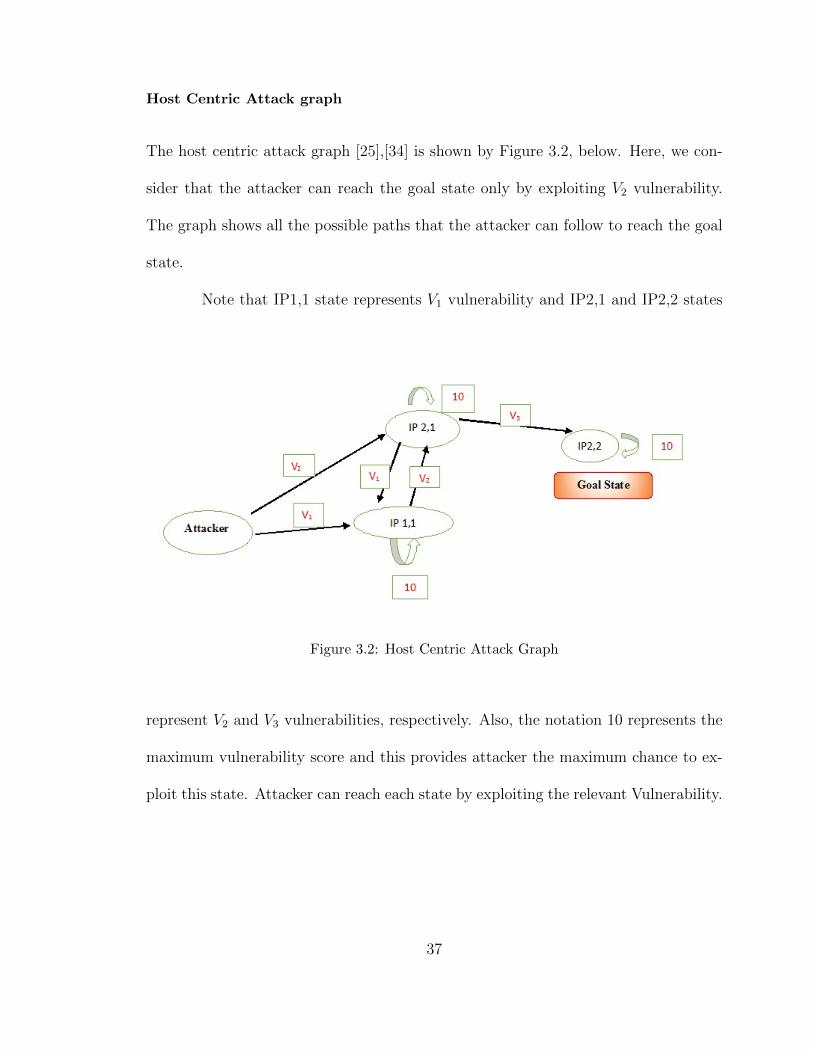
Host Centric Attack graph
The host centric attack graph [25],[34] is shown by Figure 3.2, below. Here, we con-
sider that the attacker can reach the goal state only by exploiting V2 vulnerability.
The graph shows all the possible paths that the attacker can follow to reach the goal
state.
Note that IP1,1 state represents V1 vulnerability and IP2,1 and IP2,2 states
Figure 3.2: Host Centric Attack Graph
represent V2 and V3 vulnerabilities, respectively. Also, the notation 10 represents the
maximum vulnerability score and this provides attacker the maximum chance to ex-
ploit this state. Attacker can reach each state by exploiting the relevant Vulnerability.
37
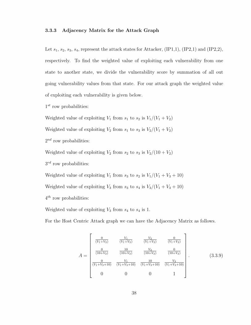
3.3.3 Adjacency Matrix for the Attack Graph
Let s1, s2, s3, s4, represent the attack states for Attacker, (IP1,1), (IP2,1) and (IP2,2),
respectively. To find the weighted value of exploiting each vulnerability from one
state to another state, we divide the vulnerability score by summation of all out
going vulnerability values from that state. For our attack graph the weighted value
of exploiting each vulnerability is given below.
1st row probabilities:
Weighted value of exploiting V1 from s1 to s2 is V1/(V1 + V2)
Weighted value of exploiting V2 from s1 to s3 is V2/(V1 + V2)
2nd row probabilities:
Weighted value of exploiting V2 from s2 to s3 is V2/(10 + V2)
3rd row probabilities:
Weighted value of exploiting V1 from s3 to s2 is V1/(V1 + V3 + 10)
Weighted value of exploiting V3 from s3 to s4 is V3/(V1 + V3 + 10)
4th row probabilities:
Weighted value of exploiting V3 from s4 to s4 is 1.
For the Host Centric Attack graph we can have the Adjacency Matrix as follows.
A =
0(V1+V2)
V1
(V1+V2)V2
(V1+V2)0
(V1+V2)
0(10+V2)
10(10+V2)
V2
(10+V2)0
(10+V2)
0(V1+V3+10)
V1
(V1+V3+10)10
(V1+V3+10)V3
(V1+V3+10)
0 0 0 1
. (3.3.9)
38
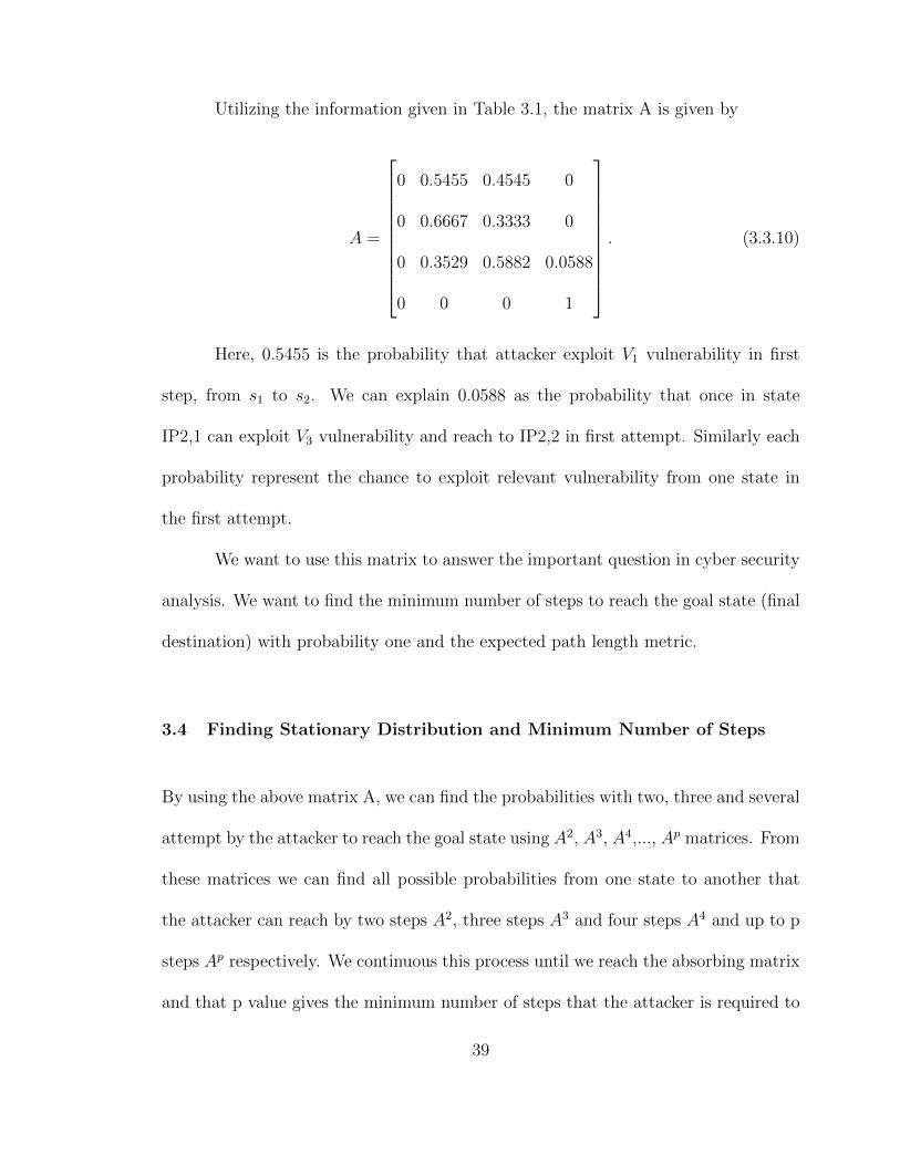
Utilizing the information given in Table 3.1, the matrix A is given by
A =
0 0.5455 0.4545 0
0 0.6667 0.3333 0
0 0.3529 0.5882 0.0588
0 0 0 1
. (3.3.10)
Here, 0.5455 is the probability that attacker exploit V1 vulnerability in first
step, from s1 to s2. We can explain 0.0588 as the probability that once in state
IP2,1 can exploit V3 vulnerability and reach to IP2,2 in first attempt. Similarly each
probability represent the chance to exploit relevant vulnerability from one state in
the first attempt.
We want to use this matrix to answer the important question in cyber security
analysis. We want to find the minimum number of steps to reach the goal state (final
destination) with probability one and the expected path length metric.
3.4 Finding Stationary Distribution and Minimum Number of Steps
By using the above matrix A, we can find the probabilities with two, three and several
attempt by the attacker to reach the goal state using A2, A3, A4,..., Ap matrices. From
these matrices we can find all possible probabilities from one state to another that
the attacker can reach by two steps A2, three steps A3 and four steps A4 and up to p
steps Ap respectively. We continuous this process until we reach the absorbing matrix
and that p value gives the minimum number of steps that the attacker is required to
39
reach the goal state with probability one.
We proceed by changing the CVSS score and calculate for each combination
of V1, V2 and V3 the minimum number of steps that the attacker will reach the goal
state with probability one. These calculations are given in Table 3.4.
For example, it will take minimum 68 steps with vulnerability configuration of
V1 = 10, V2 = 9, V3 = 8 for the attacker to reach the final goal with probability one.
The largest number of steps for the attacker to achieve his goal is 844 steps by using
the vulnerabilities, V1 = 10, V2 = 2 and V3 = 1, with probability one.
3.5 Expected Path Length (EPL) Analysis
As described under Section 3.3.1 we measure the expected number of steps the attacker
will take starting from the initial state to compromise the security goal. In Table 3.5,
we present the calculations of the Expected Path Length of the attacker for various
combinations of the vulnerabilities V1, V2 and V3.
For example, it will take 8.25 EPL with vulnerability configuration of V1 = 10,
V2 = 9, V3 = 8 for the attacker to compromise the security goal. The largest Expected
Path Length of the attacker is 72.8 using V1 = 8, V2 = 2 and V3 = 1.
3.6 Development of the Statistical Models
The primary objective here is to utilize the information that we have calculated to
develop a statistical model [32],[33], [46] to predict the minimum number of steps
40
to reach the stationary matrix and EPL of the attacker. We used the application
software package R [41] for required calculations in developing these models.
3.6.1 Developing a Statistical Model to Predict the Minimum Number of
Steps
By using the information in Table 3.4, we developed a statistical model that esti-
mates the minimum number of steps the attacker takes to reach the goal state with
probability one.
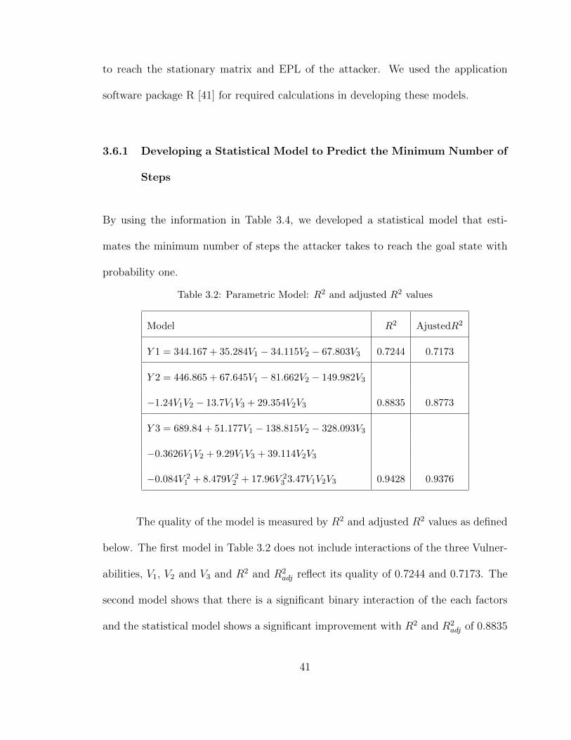
Table 3.2: Parametric Model: R2 and adjusted R2 values
Model R2 AjustedR2
Y 1 = 344.167 + 35.284V1 − 34.115V2 − 67.803V3 0.7244 0.7173
Y 2 = 446.865 + 67.645V1 − 81.662V2 − 149.982V3
−1.24V1V2 − 13.7V1V3 + 29.354V2V3 0.8835 0.8773
Y 3 = 689.84 + 51.177V1 − 138.815V2 − 328.093V3
−0.3626V1V2 + 9.29V1V3 + 39.114V2V3
−0.084V 21 + 8.479V 2
2 + 17.96V 23 3.47V1V2V3 0.9428 0.9376
The quality of the model is measured by R2 and adjusted R2 values as defined
below. The first model in Table 3.2 does not include interactions of the three Vulner-
abilities, V1, V2 and V3 and R2 and R2adj reflect its quality of 0.7244 and 0.7173. The
second model shows that there is a significant binary interaction of the each factors
and the statistical model shows a significant improvement with R2 and R2adj of 0.8835
41

and 0.8773 respectively. However, the best statistical model is obtained when we
consider in addition to individual contributions of V1, V2 and V3, two way and three
way significant interactions. Thus, from the above table the third model with R2 and
R2adj of 0.9428 and 0.9376 respectively attest to the fact that this statistical model is
excellent in estimating the minimum number of steps that an attacker will need to
achieve his goal.
Not only an individual could do the predictions but also he could perform
surface response analysis. For example using the third model Y 3 one could maximize
the number of steps for an attacker to reach his goal state by taking defending steps
to ensure to maintain their systems with the minimum vulnerability scores. Similarly
one could estimates confidence intervals for vulnerability scores so that the necessary
steps can be taken to maintain the expected security level.
3.6.2 Developing a Statistical Model to Predict the Minimum Number of
Steps
By using Table 3.5 results we developed a model to find the Expected Path Length
[46] that the attacker will take starting from the initial state to reach the security
goal. To utilize the quality of the model we use R2 concept and by comparing the
values in Table 3.3, the third model gives the highest R2 = 0.943 and R2adj = 0.9378
value. Therefore we can conclude that the third model gives the best prediction of
EPL. Not only an individual could predict the EPL but also he could perform
surface response analysis. For example using the third model ”Y 3” one could max-
42
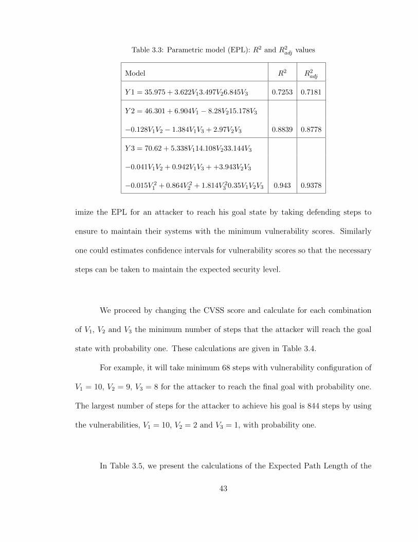
Table 3.3: Parametric model (EPL): R2 and R2adj values
Model R2 R2adj
Y 1 = 35.975 + 3.622V13.497V26.845V3 0.7253 0.7181
Y 2 = 46.301 + 6.904V1 − 8.28V215.178V3
−0.128V1V2 − 1.384V1V3 + 2.97V2V3 0.8839 0.8778
Y 3 = 70.62 + 5.338V114.108V233.144V3
−0.041V1V2 + 0.942V1V3 + +3.943V2V3
−0.015V 21 + 0.864V 2
2 + 1.814V 23 0.35V1V2V3 0.943 0.9378
imize the EPL for an attacker to reach his goal state by taking defending steps to
ensure to maintain their systems with the minimum vulnerability scores. Similarly
one could estimates confidence intervals for vulnerability scores so that the necessary
steps can be taken to maintain the expected security level.
We proceed by changing the CVSS score and calculate for each combination
of V1, V2 and V3 the minimum number of steps that the attacker will reach the goal
state with probability one. These calculations are given in Table 3.4.
For example, it will take minimum 68 steps with vulnerability configuration of
V1 = 10, V2 = 9, V3 = 8 for the attacker to reach the final goal with probability one.
The largest number of steps for the attacker to achieve his goal is 844 steps by using
the vulnerabilities, V1 = 10, V2 = 2 and V3 = 1, with probability one.
In Table 3.5, we present the calculations of the Expected Path Length of the
43

attacker for various combinations of the vulnerabilities V1, V2 and V3.
For example, it will take 8.25 EPL with vulnerability configuration of V1 = 10,
V2 = 9, V3 = 8 for the attacker to compromise the security goal. The largest Expected
Path Length of the attacker is 72.8 using V1 = 8, V2 = 2 and V3 = 1.
3.7 Contribution
We have developed a very accurate statistical model that can be utilized to predict
the minimum steps to reach the goal state and predict the expected path length. This
developed model can be used to identify the interaction among the vulnerabilities and
individual variables that drive the EPL.
We ranked the attributable variables and their contribution in estimating the subject
length. By using these rankings security administrators can have a better knowledge
about priorities. This will help them to take the necessary actions regarding their
security system.
Here we develop a model for three vulnerabilities and we can expand this model to any
Large Network System. Thus, the proposed methods will assist in making appropriate
security decisions in advance.
44
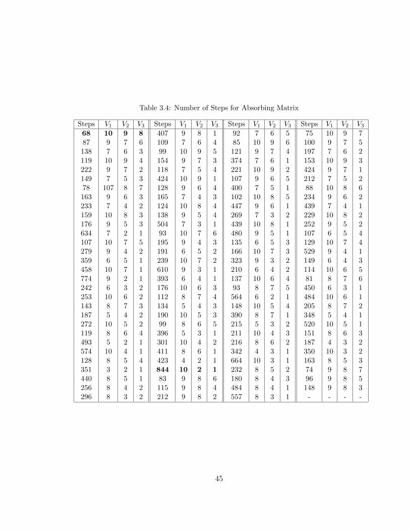
Table 3.4: Number of Steps for Absorbing Matrix
Steps V1 V2 V3 Steps V1 V2 V3 Steps V1 V2 V3 Steps V1 V2 V368 10 9 8 407 9 8 1 92 7 6 5 75 10 9 787 9 7 6 109 7 6 4 85 10 9 6 100 9 7 5138 7 6 3 99 10 9 5 121 9 7 4 197 7 6 2119 10 9 4 154 9 7 3 374 7 6 1 153 10 9 3222 9 7 2 118 7 5 4 221 10 9 2 424 9 7 1149 7 5 3 424 10 9 1 107 9 6 5 212 7 5 278 107 8 7 128 9 6 4 400 7 5 1 88 10 8 6163 9 6 3 165 7 4 3 102 10 8 5 234 9 6 2233 7 4 2 124 10 8 4 447 9 6 1 439 7 4 1159 10 8 3 138 9 5 4 269 7 3 2 229 10 8 2176 9 5 3 504 7 3 1 439 10 8 1 252 9 5 2634 7 2 1 93 10 7 6 480 9 5 1 107 6 5 4107 10 7 5 195 9 4 3 135 6 5 3 129 10 7 4279 9 4 2 191 6 5 2 166 10 7 3 529 9 4 1359 6 5 1 239 10 7 2 323 9 3 2 149 6 4 3458 10 7 1 610 9 3 1 210 6 4 2 114 10 6 5774 9 2 1 393 6 4 1 137 10 6 4 81 8 7 6242 6 3 2 176 10 6 3 93 8 7 5 450 6 3 1253 10 6 2 112 8 7 4 564 6 2 1 484 10 6 1143 8 7 3 134 5 4 3 148 10 5 4 205 8 7 2187 5 4 2 190 10 5 3 390 8 7 1 348 5 4 1272 10 5 2 99 8 6 5 215 5 3 2 520 10 5 1119 8 6 4 396 5 3 1 211 10 4 3 151 8 6 3493 5 2 1 301 10 4 2 216 8 6 2 187 4 3 2574 10 4 1 411 8 6 1 342 4 3 1 350 10 3 2128 8 5 4 423 4 2 1 664 10 3 1 163 8 5 3351 3 2 1 844 10 2 1 232 8 5 2 74 9 8 7440 8 5 1 83 9 8 6 180 8 4 3 96 9 8 5256 8 4 2 115 9 8 4 484 8 4 1 148 9 8 3296 8 3 2 212 9 8 2 557 8 3 1 - - - -
45
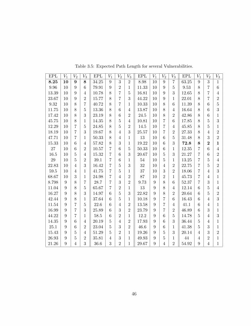
Table 3.5: Expected Path Length for several Vulnerabilities.
EPL V1 V2 V3 EPL V1 V2 V3 EPL V1 V2 V3 EPL V1 V2 V38.25 10 9 8 34.25 9 3 2 8.98 10 9 7 63.25 9 3 19.96 10 9 6 79.91 9 2 1 11.33 10 9 5 9.53 8 7 613.39 10 9 4 10.78 8 7 5 16.81 10 9 3 12.65 8 7 423.67 10 9 2 15.77 8 7 3 44.22 10 9 1 22.01 8 7 29.32 10 8 7 40.72 8 7 1 10.33 10 8 6 11.39 8 6 511.75 10 8 5 13.36 8 6 4 13.87 10 8 4 16.64 8 6 317.42 10 8 3 23.19 8 6 2 24.5 10 8 2 42.86 8 6 145.75 10 8 1 14.35 8 5 4 10.81 10 7 6 17.85 8 5 312.29 10 7 5 24.85 8 5 2 14.5 10 7 4 45.85 8 5 118.19 10 7 3 19.67 8 4 3 25.57 10 7 2 27.33 8 4 247.71 10 7 1 50.33 8 4 1 13 10 6 5 31.48 8 3 215.33 10 6 4 57.82 8 3 1 19.22 10 6 3 72.8 8 2 1
27 10 6 2 10.57 7 6 5 50.33 10 6 1 12.35 7 6 416.5 10 5 4 15.32 7 6 3 20.67 10 5 3 21.27 7 6 229 10 5 2 39.1 7 6 1 54 10 5 1 13.25 7 5 4
22.83 10 4 3 16.42 7 5 3 32 10 4 2 22.75 7 5 259.5 10 4 1 41.75 7 5 1 37 10 3 2 18.06 7 4 368.67 10 3 1 24.98 7 4 2 87 10 2 1 45.73 7 4 18.798 9 8 7 28.7 7 3 2 9.73 9 8 6 52.37 7 3 111.04 9 8 5 65.67 7 2 1 13 9 8 4 12.14 6 5 416.27 9 8 3 14.97 6 5 3 22.82 9 8 2 20.64 6 5 242.44 9 8 1 37.64 6 5 1 10.18 9 7 6 16.43 6 4 311.54 9 7 5 22.6 6 4 2 13.58 9 7 4 41.1 6 4 116.99 9 7 3 25.89 6 3 2 23.79 9 7 2 46.89 6 3 144.22 9 7 1 58.5 6 2 1 12.2 9 6 5 14.78 5 4 314.35 9 6 4 20.19 5 4 2 17.93 9 6 3 36.44 5 4 125.1 9 6 2 23.04 5 3 2 46.6 9 6 1 41.38 5 3 115.43 9 5 4 51.29 5 2 1 19.26 9 5 3 20.14 4 3 226.93 9 5 2 35.81 4 3 1 49.93 9 5 1 44 4 2 121.26 9 4 3 36.6 3 2 1 29.67 9 4 2 54.92 9 4 1
46
4 NonHomogeneous Stochastic Model for Cyber Security Predictions
4.1 Introduction
In this study, we continue our research efforts in integrating Mathematical and Sta-
tistical theories into better understanding the complex behavior of computer network
systems in the perspective of Cybersecurity. Thus, we propose a new method to esti-
mate the EPL as a function of time t. The EPL is a major factor in determining the
risk level of a given computer system and lesser the EPL, the network system is more
vulnerable and probable to be exploited.
In our recent studies [20],[21] and [46] we introduced several stochastic models
to better understand the behavior of vulnerabilities, network systems with respect
to cybersecurity. Initially, we introduced a stochastic model that can estimate the
Expected Path Length of a system with any three vulnerabilities and two machines.
Then, we introduced a new approach of estimating the probability of a given vul-
nerability being exploited at a time t, using Markovian approach with respect to the
Vulnerability life cycle. We have further introduced a set of three stochastic time
dependent models for each categories of vulnerabilities with Low, Medium and High
exploitability scores that can estimate the probability of a given vulnerability getting
47
exploited without going through the Markovian process each time. Additionally, the
concept of Risk Factor that we introduced and its analytical formulation allowed us
to present a more sophisticated way of estimating the risk associated with a specific
vulnerability of a computer network system. In the present study, we introduce a
Non Homogeneous Stochastic Model that allows the computer system administrators
to predict the time, that the system is most vulnerable for an attack in terms of the
EPL. This estimate is based on the assumption that a system is more susceptible to
be exploited when the EPL is at a minimum at a particular time t. In developing this
model we have used a network system of two IPs with three vulnerabilities as a base
model.
With the introduction of this new approach we will be re-defending the ca-
pability to estimate the probability of getting exploited as a function of time for a
computer network system with given set of vulnerabilities. Even though we have al-
ready developed a successful statistical model to find the EPL of a possible attack,
it is more important to estimate the EPL as a function of time. Thus, for a system
with a given set of vulnerabilities, estimating of most probable exploit times can be
modelled on the logical assumption that a system is more susceptible to be exploited
at a time where the Expected Path Length (number of steps that an attacker needs
to pass before achieving the goal state) is at its minimum.
48
4.2 Background and Related Methodologies
4.2.1 Cybersecurity Analysis Method
The core component of this method is the attack graph [11]. When we draw an
attack graph for a cybersecurity system it has several nodes which represent the
vulnerabilities that the system has and the attackers state [12]. We consider that it
is possible to go to a goal state starting from any other state in the attack graph.
Also an attack graph has at least one absorbing state or goal state. Therefore we will
model the attack graph as an absorbing Markov chain [12].
Absorbing state or goal state is the security node which is exploited by the
attacker. When the attacker has reached this goal state, attack path is completed.
Thus, the entire attack graph consists of these type of attack paths.
Given the CVSS score for each of the vulnerabilities in the attack Graph, we
can estimate the transition probabilities of the absorbing Markov chain by normalizing
the CVSS scores over all the edges starting from the attackers source state.We define,
pij = probability that an attacker is currently in state j and exploits a
vulnerability in state i.
n = number of outgoing edges from state i in the attack model.
vj = CVSS score for the vulnerability in state j.
Then formally we can define the transition probability below,
49
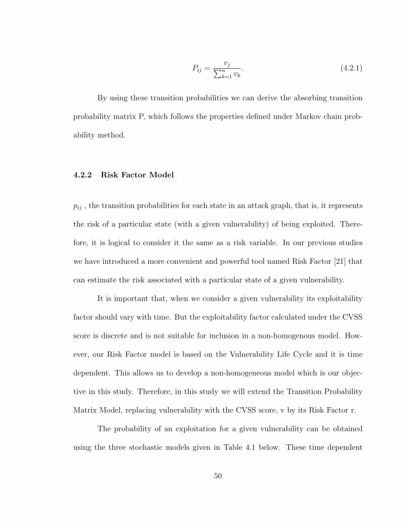
Pij =vj∑nk=1 vk
. (4.2.1)
By using these transition probabilities we can derive the absorbing transition
probability matrix P, which follows the properties defined under Markov chain prob-
ability method.
4.2.2 Risk Factor Model
pij , the transition probabilities for each state in an attack graph, that is, it represents
the risk of a particular state (with a given vulnerability) of being exploited. There-
fore, it is logical to consider it the same as a risk variable. In our previous studies
we have introduced a more convenient and powerful tool named Risk Factor [21] that
can estimate the risk associated with a particular state of a given vulnerability.
It is important that, when we consider a given vulnerability its exploitability
factor should vary with time. But the exploitability factor calculated under the CVSS
score is discrete and is not suitable for inclusion in a non-homogenous model. How-
ever, our Risk Factor model is based on the Vulnerability Life Cycle and it is time
dependent. This allows us to develop a non-homogeneous model which is our objec-
tive in this study. Therefore, in this study we will extend the Transition Probability
Matrix Model, replacing vulnerability with the CVSS score, v by its Risk Factor r.
The probability of an exploitation for a given vulnerability can be obtained
using the three stochastic models given in Table 4.1 below. These time dependent
50
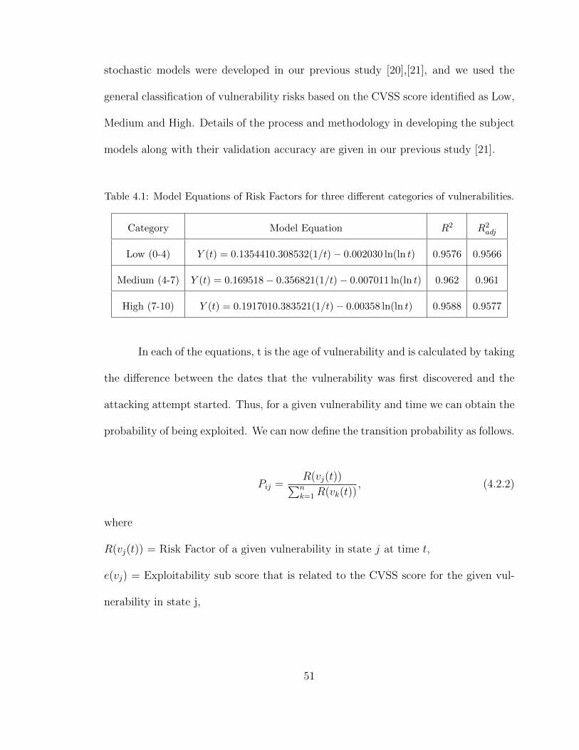
stochastic models were developed in our previous study [20],[21], and we used the
general classification of vulnerability risks based on the CVSS score identified as Low,
Medium and High. Details of the process and methodology in developing the subject
models along with their validation accuracy are given in our previous study [21].
Table 4.1: Model Equations of Risk Factors for three different categories of vulnerabilities.
Category Model Equation R2 R2adj
Low (0-4) Y (t) = 0.1354410.308532(1/t)− 0.002030 ln(ln t) 0.9576 0.9566
Medium (4-7) Y (t) = 0.169518− 0.356821(1/t)− 0.007011 ln(ln t) 0.962 0.961
High (7-10) Y (t) = 0.1917010.383521(1/t)− 0.00358 ln(ln t) 0.9588 0.9577
In each of the equations, t is the age of vulnerability and is calculated by taking
the difference between the dates that the vulnerability was first discovered and the
attacking attempt started. Thus, for a given vulnerability and time we can obtain the
probability of being exploited. We can now define the transition probability as follows.
Pij =R(vj(t))∑nk=1R(vk(t))
, (4.2.2)
where
R(vj(t)) = Risk Factor of a given vulnerability in state j at time t,
e(vj) = Exploitability sub score that is related to the CVSS score for the given vul-
nerability in state j,
51
R(vj(t)) = Y (t) ∗ e(vj). (4.2.3)
Above equation gives the analytic form of the risk factor as a function of Y (t)
and e(vj) where Y(t) is the exploitability probability factor as a function of time and
e(vj) is the exploitability score taken from the CVSS.
4.3 Attack Prediction
Under the Attack Prediction, we consider two methods to predict the attackers be-
havior.
4.3.1 Multi Step Attack Prediction
The absorbing transition probability matrix shows the presence of each edge in a
network attack graph. This matrix shows every possible single-step attack. In other
words, the absorbing transition probability matrix shows attacker reachability within
one attack step. We can navigate the absorbing transition probability matrix by
iteratively matching rows and columns to follow multiple attack steps, and also raise
the absorbing transition probability matrix to higher powers, which shows multi-step
attacker reachability at a glance.
For a square (n × n) adjacency matrix P and a positive integer k, then Pk is
P raised to the power k: Since P is an absorbing transition probability matrix with
52
time, this matrix goes to some stationary matrix Π, where the rows of this matrix are
identical. That is,
limk→∞
PK = Π. (4.3.4)
At the goal state column of this matrix Π has ones, so we can find the minimum
number of steps that the attacker should try to reach to the goal state with probability
1.
4.3.2 Prediction of Expected Path Length (EPL)
The Expected Path Length (EPL) measures the expected number of steps the attacker
will take starting from the initial state to reach the goal state (the attackers objective).
As we discussed earlier P has the following canonical form.
P =
Q R
0 I
. (4.3.5)
Here, P is the transition matrix, Q is the matrix of transient states, R is the matrix of
absorbing states and I is the identity matrix. The matrix P represents the transition
probability matrix of the absorbing Markov chain. In an absorbing Markov chain the
probability that the chain will be absorbed is always 1. Thus, we have
Qn →∞, n→∞.
53
Thus, is it implies that all the eigenvalues of Q have absolute values strictly
less than 1. Hence, I-Q is an invertible matrix and there is no problem in defining the
matrix
M = (I −Q)−1 = I +Q+Q2 +Q3 + ....
Using this fundamental matrix M of the absorbing Markov chain we can compute the
expected total number of steps to reach the goal state until absorption.
Taking the summation of the first row elements of matrix M gives us the
expected total number of steps to reach the goal state which is defined as the Expected
Path Length. Given below is an application that illustrate a computer network system
of our proposed analytic process to estimate the EPL of a hacker.
4.4 Attack Graph and Attack Risk Evaluation
In this section we present an example illustrating the application of the usefulness
of our method. We combine the application of methodology with an attack graph
relevant to a typical network exemplified with three different recorded vulnerabilities.
4.4.1 Application: The Attacker
To illustrate the proposed analytical approach model that we have developed as dis-
cussed above, we considered a Network Topology [4],[37], given by Figure 4.1, below.
54
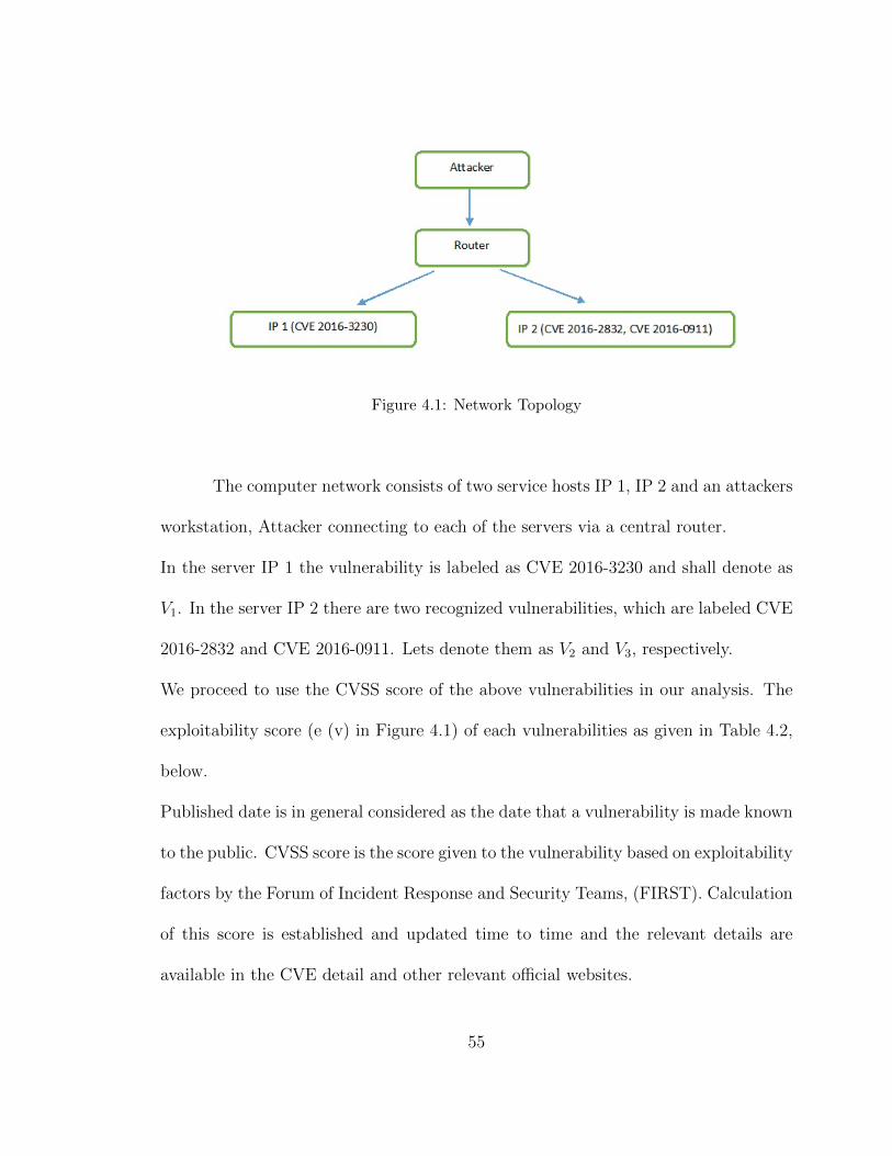
Figure 4.1: Network Topology
The computer network consists of two service hosts IP 1, IP 2 and an attackers
workstation, Attacker connecting to each of the servers via a central router.
In the server IP 1 the vulnerability is labeled as CVE 2016-3230 and shall denote as
V1. In the server IP 2 there are two recognized vulnerabilities, which are labeled CVE
2016-2832 and CVE 2016-0911. Lets denote them as V2 and V3, respectively.
We proceed to use the CVSS score of the above vulnerabilities in our analysis. The
exploitability score (e (v) in Figure 4.1) of each vulnerabilities as given in Table 4.2,
below.
Published date is in general considered as the date that a vulnerability is made known
to the public. CVSS score is the score given to the vulnerability based on exploitability
factors by the Forum of Incident Response and Security Teams, (FIRST). Calculation
of this score is established and updated time to time and the relevant details are
available in the CVE detail and other relevant official websites.
55
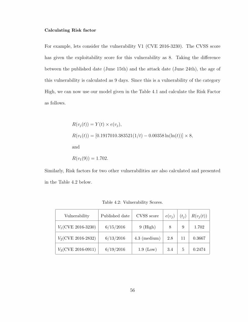
Calculating Risk factor
For example, lets consider the vulnerability V1 (CVE 2016-3230). The CVSS score
has given the exploitability score for this vulnerability as 8. Taking the difference
between the published date (June 15th) and the attack date (June 24th), the age of
this vulnerability is calculated as 9 days. Since this is a vulnerability of the category
High, we can now use our model given in the Table 4.1 and calculate the Risk Factor
as follows.
R(vj(t)) = Y (t)× e(vj),
R(v1(t)) = [0.1917010.383521(1/t)− 0.00358 ln(ln(t))]× 8,
and
R(v1(9)) = 1.702.
Similarly, Risk factors for two other vulnerabilities are also calculated and presented
in the Table 4.2 below.
Table 4.2: Vulnerability Scores.
Vulnerability Published date CVSS score e(vj) (tj) R(vj(t))
V1(CVE 2016-3230) 6/15/2016 9 (High) 8 9 1.702
V2(CVE 2016-2832) 6/13/2016 4.3 (medium) 2.8 11 0.3667
V3(CVE 2016-0911) 6/19/2016 1.9 (Low) 3.4 5 0.2474
56
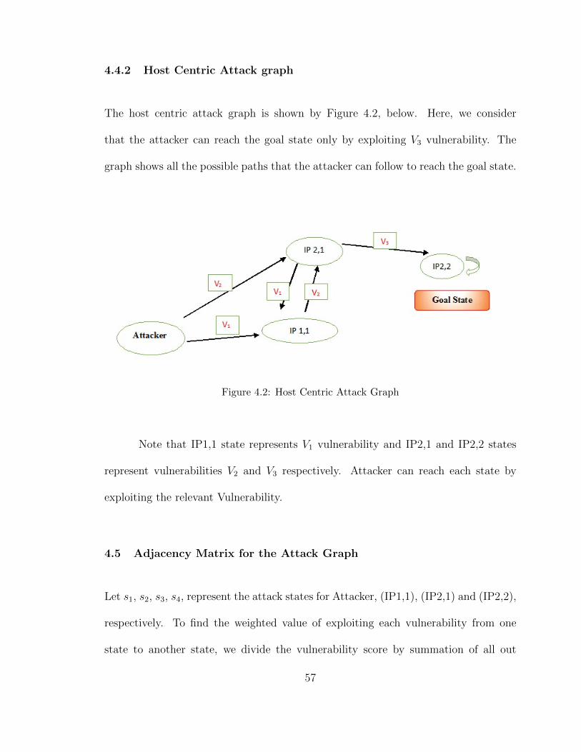
4.4.2 Host Centric Attack graph
The host centric attack graph is shown by Figure 4.2, below. Here, we consider
that the attacker can reach the goal state only by exploiting V3 vulnerability. The
graph shows all the possible paths that the attacker can follow to reach the goal state.
Figure 4.2: Host Centric Attack Graph
Note that IP1,1 state represents V1 vulnerability and IP2,1 and IP2,2 states
represent vulnerabilities V2 and V3 respectively. Attacker can reach each state by
exploiting the relevant Vulnerability.
4.5 Adjacency Matrix for the Attack Graph
Let s1, s2, s3, s4, represent the attack states for Attacker, (IP1,1), (IP2,1) and (IP2,2),
respectively. To find the weighted value of exploiting each vulnerability from one
state to another state, we divide the vulnerability score by summation of all out
57
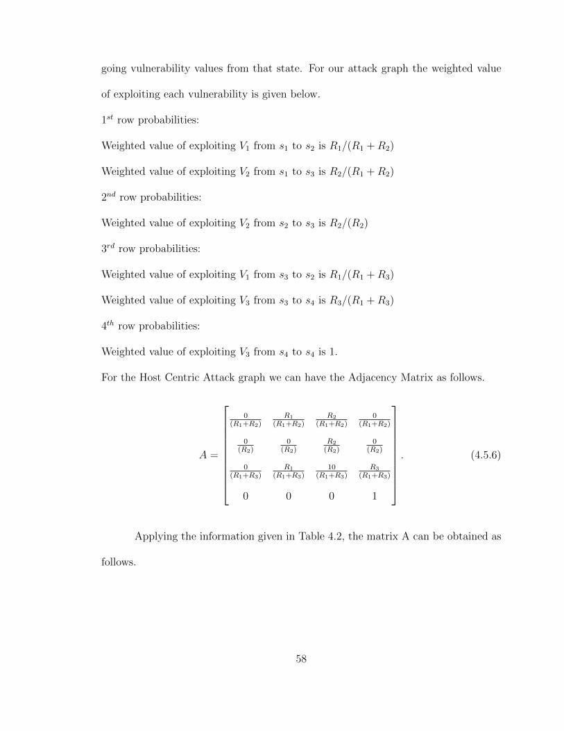
going vulnerability values from that state. For our attack graph the weighted value
of exploiting each vulnerability is given below.
1st row probabilities:
Weighted value of exploiting V1 from s1 to s2 is R1/(R1 +R2)
Weighted value of exploiting V2 from s1 to s3 is R2/(R1 +R2)
2nd row probabilities:
Weighted value of exploiting V2 from s2 to s3 is R2/(R2)
3rd row probabilities:
Weighted value of exploiting V1 from s3 to s2 is R1/(R1 +R3)
Weighted value of exploiting V3 from s3 to s4 is R3/(R1 +R3)
4th row probabilities:
Weighted value of exploiting V3 from s4 to s4 is 1.
For the Host Centric Attack graph we can have the Adjacency Matrix as follows.
A =
0(R1+R2)
R1
(R1+R2)R2
(R1+R2)0
(R1+R2)
0(R2)
0(R2)
R2
(R2)0
(R2)
0(R1+R3)
R1
(R1+R3)10
(R1+R3)R3
(R1+R3)
0 0 0 1
. (4.5.6)
Applying the information given in Table 4.2, the matrix A can be obtained as
follows.
58
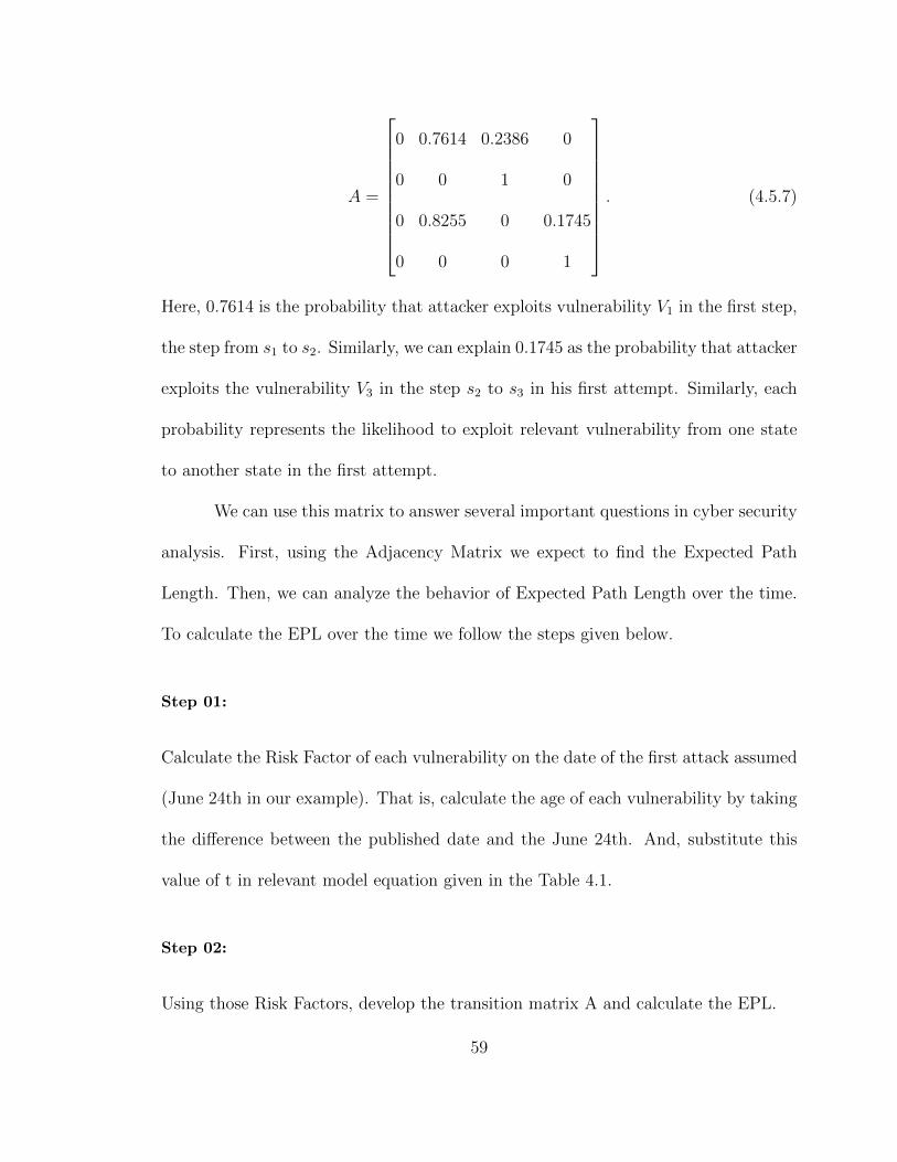
A =
0 0.7614 0.2386 0
0 0 1 0
0 0.8255 0 0.1745
0 0 0 1
. (4.5.7)
Here, 0.7614 is the probability that attacker exploits vulnerability V1 in the first step,
the step from s1 to s2. Similarly, we can explain 0.1745 as the probability that attacker
exploits the vulnerability V3 in the step s2 to s3 in his first attempt. Similarly, each
probability represents the likelihood to exploit relevant vulnerability from one state
to another state in the first attempt.
We can use this matrix to answer several important questions in cyber security
analysis. First, using the Adjacency Matrix we expect to find the Expected Path
Length. Then, we can analyze the behavior of Expected Path Length over the time.
To calculate the EPL over the time we follow the steps given below.
Step 01:
Calculate the Risk Factor of each vulnerability on the date of the first attack assumed
(June 24th in our example). That is, calculate the age of each vulnerability by taking
the difference between the published date and the June 24th. And, substitute this
value of t in relevant model equation given in the Table 4.1.
Step 02:
Using those Risk Factors, develop the transition matrix A and calculate the EPL.
59
Step 03:
Repeat the same process for all the following dates that we need to calculate the
Expected Path Length.
4.5.1 Expected Path length
The Table 4.3 below show us the EPL for this computer system for 100 days starting
from 24th of June.
From the Table 4.3 above, we can identify that the number of days a hacker will
take to reach his goal of exploitability for the given computer network system we have
structured.
For example, lets consider 20th day. Under step 1, we calculate Risk factors for
V1, V2 and V3. For 20th day age of three vulnerabilities V1, V2 and V3 are, t1 = 9 + 20,
t2 = 11 + 20 and t3 = 5 + 20 respectively. Then, by substituting these ages in the
respective model equation from the Table 4.1 and multiplying the answers by respec-
tive exploitability score, we calculate three risk factors.
V1 is a vulnerability of category High. Therefore we use the 3rd model equation
from Table 4.3 and obtain the Risk factor.
Substituting t1 = 29 to the Risk factor model we obtain, R1 = 1.393. Simi-
larly for V2 and V3 we obtain following Risk factors calculated using relevant model
equations. For V2 substitute t2 = 31 and obtained R2 = 0.4182 and similarly for V3,
t3 = 25 and R3 = 0.4105.
60
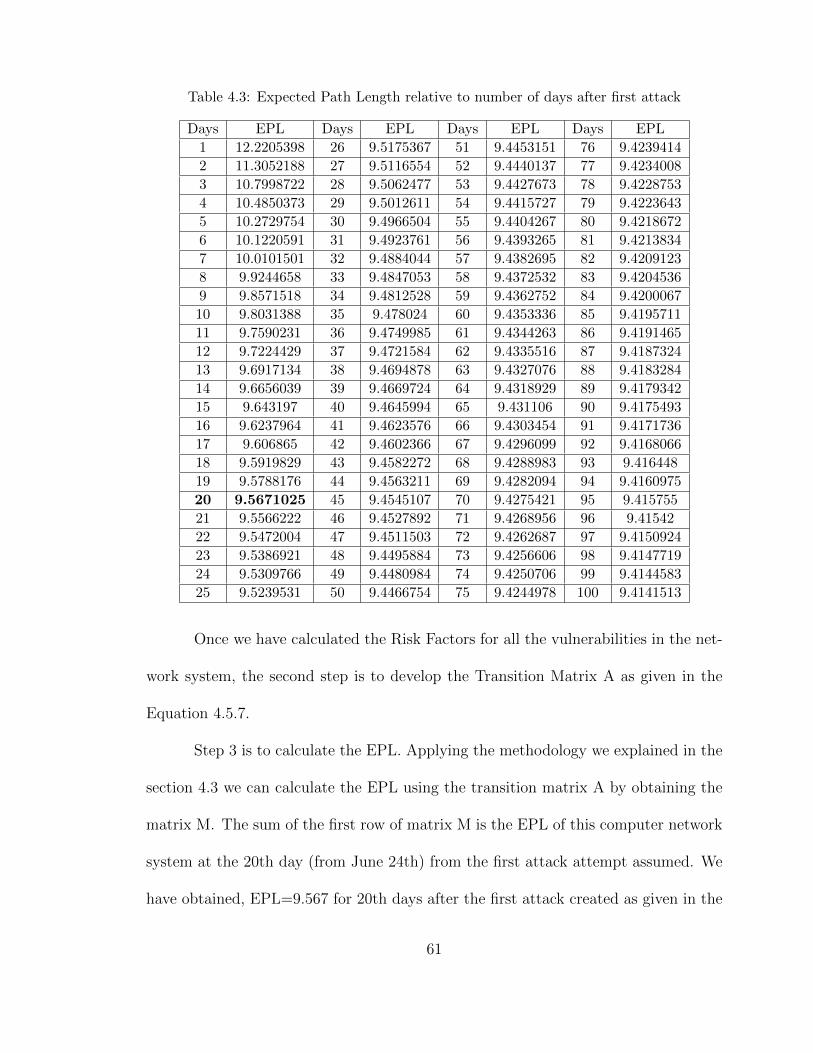
Table 4.3: Expected Path Length relative to number of days after first attack
Days EPL Days EPL Days EPL Days EPL
1 12.2205398 26 9.5175367 51 9.4453151 76 9.4239414
2 11.3052188 27 9.5116554 52 9.4440137 77 9.4234008
3 10.7998722 28 9.5062477 53 9.4427673 78 9.4228753
4 10.4850373 29 9.5012611 54 9.4415727 79 9.4223643
5 10.2729754 30 9.4966504 55 9.4404267 80 9.4218672
6 10.1220591 31 9.4923761 56 9.4393265 81 9.4213834
7 10.0101501 32 9.4884044 57 9.4382695 82 9.4209123
8 9.9244658 33 9.4847053 58 9.4372532 83 9.4204536
9 9.8571518 34 9.4812528 59 9.4362752 84 9.4200067
10 9.8031388 35 9.478024 60 9.4353336 85 9.4195711
11 9.7590231 36 9.4749985 61 9.4344263 86 9.4191465
12 9.7224429 37 9.4721584 62 9.4335516 87 9.4187324
13 9.6917134 38 9.4694878 63 9.4327076 88 9.4183284
14 9.6656039 39 9.4669724 64 9.4318929 89 9.4179342
15 9.643197 40 9.4645994 65 9.431106 90 9.4175493
16 9.6237964 41 9.4623576 66 9.4303454 91 9.4171736
17 9.606865 42 9.4602366 67 9.4296099 92 9.4168066
18 9.5919829 43 9.4582272 68 9.4288983 93 9.416448
19 9.5788176 44 9.4563211 69 9.4282094 94 9.4160975
20 9.5671025 45 9.4545107 70 9.4275421 95 9.415755
21 9.5566222 46 9.4527892 71 9.4268956 96 9.41542
22 9.5472004 47 9.4511503 72 9.4262687 97 9.4150924
23 9.5386921 48 9.4495884 73 9.4256606 98 9.4147719
24 9.5309766 49 9.4480984 74 9.4250706 99 9.4144583
25 9.5239531 50 9.4466754 75 9.4244978 100 9.4141513
Once we have calculated the Risk Factors for all the vulnerabilities in the net-
work system, the second step is to develop the Transition Matrix A as given in the
Equation 4.5.7.
Step 3 is to calculate the EPL. Applying the methodology we explained in the
section 4.3 we can calculate the EPL using the transition matrix A by obtaining the
matrix M. The sum of the first row of matrix M is the EPL of this computer network
system at the 20th day (from June 24th) from the first attack attempt assumed. We
have obtained, EPL=9.567 for 20th days after the first attack created as given in the
61
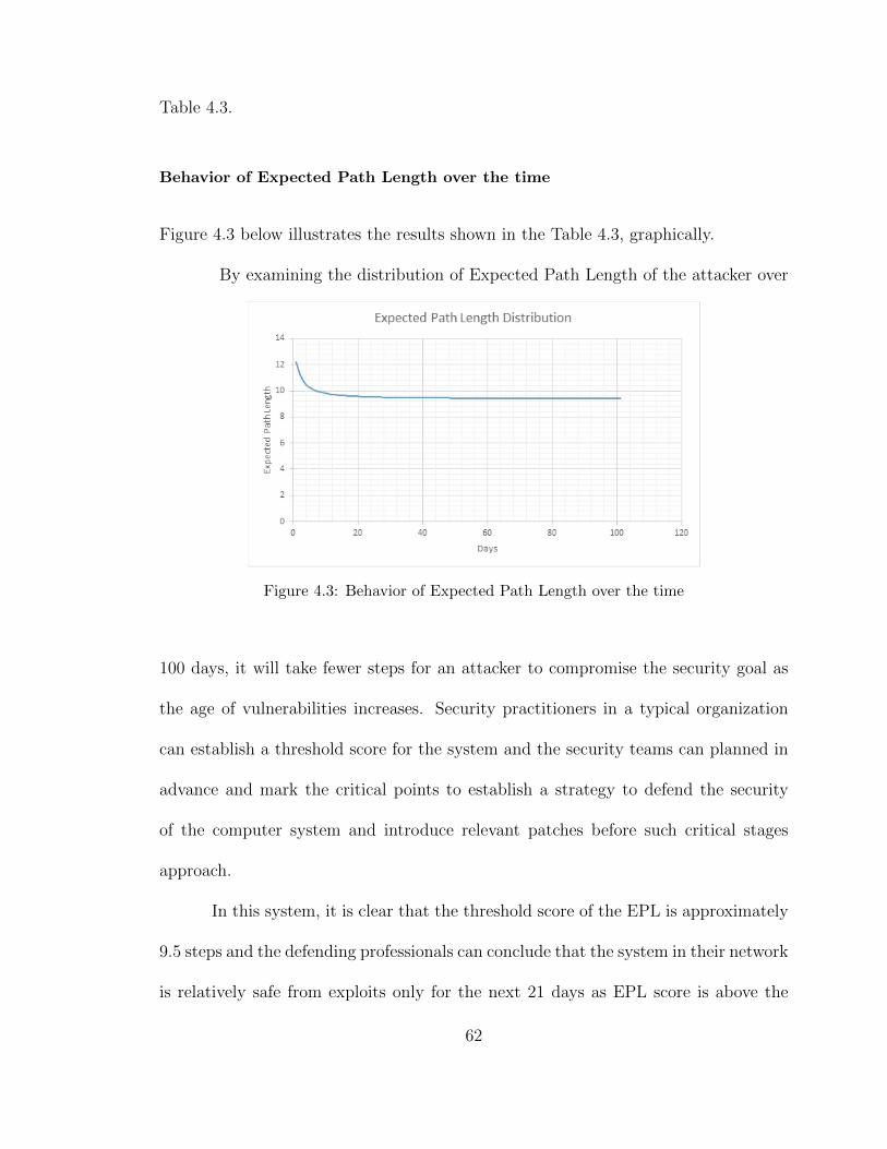
Table 4.3.
Behavior of Expected Path Length over the time
Figure 4.3 below illustrates the results shown in the Table 4.3, graphically.
By examining the distribution of Expected Path Length of the attacker over
Figure 4.3: Behavior of Expected Path Length over the time
100 days, it will take fewer steps for an attacker to compromise the security goal as
the age of vulnerabilities increases. Security practitioners in a typical organization
can establish a threshold score for the system and the security teams can planned in
advance and mark the critical points to establish a strategy to defend the security
of the computer system and introduce relevant patches before such critical stages
approach.
In this system, it is clear that the threshold score of the EPL is approximately
9.5 steps and the defending professionals can conclude that the system in their network
is relatively safe from exploits only for the next 21 days as EPL score is above the
62
threshold value.
It is clear that, any vulnerability that exists creates a threat to the computer
system and the risk of probable exploitation will increase over the time of its existence
without being patched. In other words, for a particular network system a higher
Expected Path Length for an attacker to reach a goal state represents more difficulty
for the hacker and would be reasonable to assume that the attacker has to face many
defending measure with a higher expected path length compared a lower Expected
Path Length. Now using the probabilistic models that we have developed in our
previous studies, using the Vulnerability Life Cycle approach enables us to develop a
time dependent stochastic models so that we could extend their application to develop
a relevant and well defined process of monitoring the behavior of threats. Thus, our
proposed analytic process illustrates its capability of estimating a Risk Index as a
function of attacking time for a given computer system with known vulnerabilities.
4.6 Contributions
In the present study, we have developed a nonhomogeneous stochastic model for pre-
dicting the Expected Path Length (EPL) of a computer network system with a given
set of vulnerabilities at time t.
Knowing EPL as a function of time is extremely important in developing defending
strategies. Such strategy will reduce the likelihood of the computer network system
being hacked. As we observe the behavior of the EPL over the time, it is possible
to identify the time ranges where EPL reached a minimum. Low EPL implies higher
63
chance for hacker to be successful. In other words, a computer network system is
more vulnerable to be exploited on the days where the EPL is at lowest. On such
time t, vulnerabilities and the system hence are more susceptible to be hacked. The
same scenario from an attackers point of view can be explained. That is, on the
days where EPL is at its lowest, likelihood of making a successful attack attempt is
higher. Therefore, an attacker (hacker), who identifies the set of vulnerabilities in a
given computer system would put more attempt on exploiting the system on such date
where the EPL is at its lowest. This means, we can use this method as a prediction
method of attacking (hacking) time.
By knowing this time for any computer network system, security engineers or IT archi-
tectures can take the necessary actions in advance to protect their computer system.
Finally, we have developed over methodology based on a typical computer network
system that exists in a real world situation with given vulnerabilities that identifies
the EPL and actual time that the subject computer system could be exploited. Thus,
industry can apply developed methodology in their own computer network system
with given (known) vulnerabilities to predict the EPL and most probable time of
being exploited.
64
5 Nonhomogeneous Risk Rank Analysis Method for Security Network
System
5.1 Introduction
This chapter describes our approach to rank a set of vulnerabilities based on the
risk, called ”nonhomogeneous risk rank analysis” that identifies the rank of vulner-
abilities for each attack state in a network security model. We study and use the
approach taken in wellknown Google Page Rank Algorithm. Here section 5.2 presents
the method of Google page rank algorithm [24],[27],[28]. Section 5.3 presents our pro-
posed Risk Rank algorithm, which provides the core of the ranking analysis approach
along with an illustration in Section 5.4. Section 5.5 discusses the generality and
theoretical implications of the approach.
A Network systems could have numerous vulnerabilities. We understand the
process of generating vulnerabilities is highly stochastic and outcomes are hard to
predict. Similarly the behavior of attacks and attackers also have higher level unpre-
dictability. When considering a particular system based on the discovered vulnerabil-
ities the analysis must consider the dynamic nature of the effect of vulnerabilities over
time. As we observed in the previous chapters, effect of the vulnerabilities vary with
65
the time over their life cycle. Therefore, for a particular system, the most threatening
vulnerability at time t1 might not be the same at time t2. Hence, it would be very
useful to have analytical models to observe the behavior of the rank of vulnerabilities
based on the magnitude of the threat with respect to time for a given network system.
Such ranking distribution over time would empower the defenders by giving
the priority directions to attend on fixing vulnerabilities. In this chapter we attempt
to address this need.
5.2 Google Page Rank Algorithm
This section provides a background for our quantitative analysis of risk rank algorithm
method. Ranking web pages is an important function of an internet search engine
[27],[4]. Google Page Rank Algorithm is one of the most accurate and efficient page
ranking methods in use. Methodology behind this algorithm will be briefly discussed
below.
Output of this algorithm gives a probability distribution which is used to repre-
sent the likelihood that a person randomly clicking on links will arrive at any particular
page. Using this method we can rank the likelihood of clicking on any web link. This
can be calculated for any number of web links. In this algorithm, the sum of the page
rank values of all the considered web links is equal to be one and it is assumed that
the probability of selecting a web page initially is equal for any available option.
Google page rank algorithm simulates the clicking behavior of a web link in
two ways. First is to visit a web link via an incoming link to the current web page and
66

second way is to pick a web page randomly. Google page rank theory holds that an
any surfer who is randomly clicking on web links will eventually stop clicking. At any
of these stages, a damping factor d is the probability that the web surfer will continue
surfing. Many researches have tested various damping factors but in generally it is
assumed that the damping factor will be set around 0.85.
Let pt(v) be the probability of visiting web page v at time t and V be a set of
all web pages under consideration. Here out(v) represents the set of web pages in V
with an outgoing link from v, and in(v) represents the set of incoming link to v. The
page rank computation can be viewed as a Markov process whose states are pages
and the links between pages represent state transitions. This computation is given in
the Equation (5.2.1) below.
Pt+1(v) = (1− d) ∗∑∀u∈V
Pt(u)
|V |+ d ∗
∑∀u∈in(v)
Pt(u)
|out(u)|. (5.2.1)
Let, |V | be the number of pages considered. Surfer will stop clicking on any link with
probability 1 − d. Since there are |V | number of pages and probability of visiting v
from any page is equally likely, the probability for each case is equal to 1|V | .
Here d ∗∑∀u∈in(v)
Pt(u)|out(u)| represents the case when the surfer continues clicking
links with probability d and goes to page v at time t + 1 from page u that has an
incoming link to v.
Initially at t = 0, each page has the same ranking value probability which is
equal to 1|V | . Then iterations are executed over time until the stability is achieved.
Once the probability distribution for each page becomes stable, considering high to
67

low probabilities ranks are assigned.
5.3 Risk Rank Algorithm
By developing the concept applied in Google Page Rank Algorithm here we introduce
a ranking method for risk [31] of vulnerabilities in a network system.
To estimate the probabilities in Risk Rank Algorithm Markov model tech-
niques can be applied similarly as in Google Page Rank Algorithm. However there
is a difference between web surfing behavior and Cyber security attacking behavior.
A web surfing user can randomly select a web page but in cyberattacks an attacker
doesn’t have the same freedom. In web surfing user can arrive at any web page in one
single step by using it’s URL. But attacker has many restrictions. In computer net-
work system an attacker doesn’t have the access to all vulnerabilities in the network
system. To achieve attacker’s target state he must exploits several vulnerabilities in
a particular order and enters in to the target system.
In the attacking process an attacker has two options. He can either continue
or quit from his current path. If it is too difficult for him to achieve his goal state he
can quit on the current path and try an alternative path by starting over from one
of the set of initial states. Base on these assumptions here we propose our model to
calculate the probability distribution of a given security attack model.
To obtain the risk rank we used the risk factor R(v(t)) of each vulnerability
at each state and calculated normalized risk factor matrix A(V,R) for the attack net-
work system by using ψ(u, v) transition probabilities from state u to v. Thus, we can
68
calculate transition probabilities using the equation ψ(u, v) = R(v(t))∑∀w∈out(u) R(w(t))
Let Pk(v) be the probability of exploiting state v at time k and V be a set of
all states under consideration. Here out(v) represents the set of states in V with an
outgoing link from v, and in(v) represents the set of incoming link to v. The Risk
rank computation can be viewed as a Markov process whose state are vulnerabilities
and the links between vulnerabilities represent state transitions. This computation is
given in the Equation (5.3.2) below.
Pk+1(v) =
(1−d)|I| + d ∗
∑∀u∈in(v) Pk(u).ψ(u, v), if v is an initial state
d ∗∑∀u∈in(v) Pk(u).ψ(u, v), if v is not an initial state
(5.3.2)
Let |I| be the number of initial states and attacker will stop his current path
with probability 1 − d. Since there are |V | number of states and probability of ex-
ploiting v from any other state is equally likely, the probability for each case is 1|V | .
Here in equation 5.3.2,
d ∗∑
∀u∈in(v)
Pk(u).ψ(u, v)
represents the case when the attacker continues his current path with probability d
and attack to state v at time t+ 1 from state u that has an incoming link to vulner-
ability v.
Initially at t = 0 each state has the same ranking value which is equal to 1|V | .
Then computing iterations over time once the stability achieved. Once the probability
distribution for each state become stable, assigning rank to each vulnerability.
69

Algorithm 1 Risk Rank Algorithm
1: procedure Risk Rank Algorithm(Input)
2: Determine the input values.
3: A(V,R)= Probability transition matrix, V - Set of states in the attack graph,
R(v(t))-Risk factor of vulnerability v at time t, ψ(u, v)- transition probability from
state u to v, I - Set of initial states. out(v) - Set of all states out going from state v,
|V |- Number of states.
4: begin each v ∈ V
5: set P0(v) = 1|V |
6: for ∀u ∈ out(v) do
7: ψ(u, v) = R(v(t))∑∀w∈out(u) R(w(t))
8: end
9: for k = k + 1
10: Pk+1(v) = d∑∀u∈in(v) Pk(u).ψ(u, v)
11: if v ∈ I then
12: Pk+1(v) = Pk+1(v) + (1−d)|I|
13: end if
14: end for
15: break if Pk+1(v) = Pk(v), ∀v ∈ V
16: end procedure
This procedure is illustrated by the following schematic network.
70
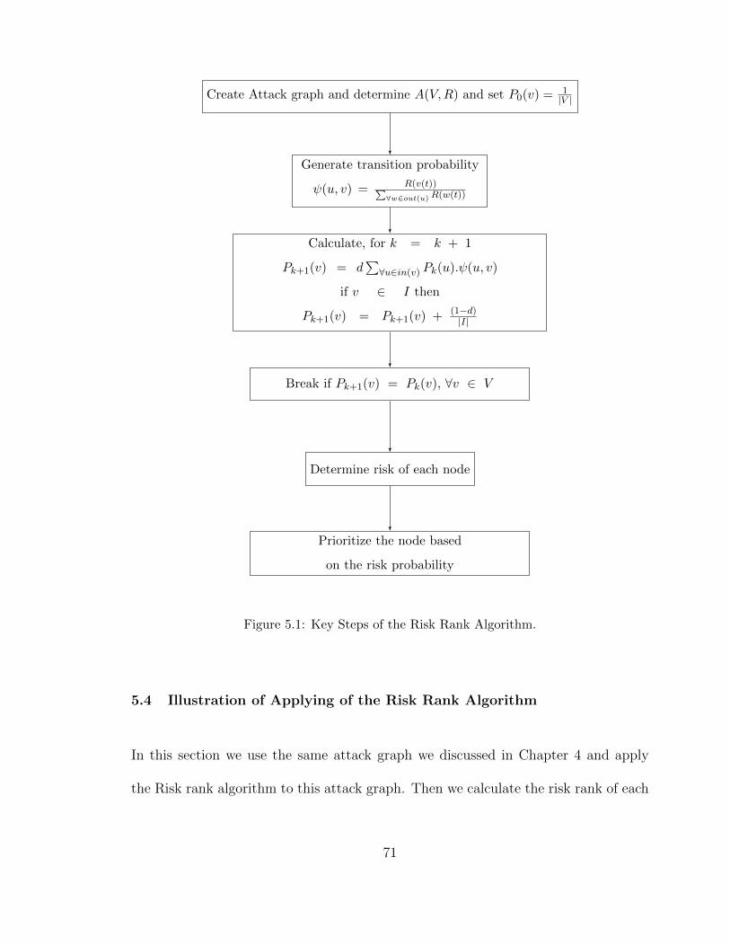
Create Attack graph and determine A(V,R) and set P0(v) = 1|V |
Generate transition probability
ψ(u, v) = R(v(t))∑∀w∈out(u) R(w(t))
Calculate, for k = k + 1
Pk+1(v) = d∑∀u∈in(v) Pk(u).ψ(u, v)
if v ∈ I then
Pk+1(v) = Pk+1(v) + (1−d)|I|
Break if Pk+1(v) = Pk(v), ∀v ∈ V
Determine risk of each node
Prioritize the node based
on the risk probability
Figure 5.1: Key Steps of the Risk Rank Algorithm.
5.4 Illustration of Applying of the Risk Rank Algorithm
In this section we use the same attack graph we discussed in Chapter 4 and apply
the Risk rank algorithm to this attack graph. Then we calculate the risk rank of each
71
vulnerability in the network system [21].
To illustrate the proposed analytical approach model that we have developed
as discussed above, we considered a Network Topology, given by Figure 5.2, below.
Figure 5.2: Network Topology
The computer network consists of two service hosts IP 1, IP 2 and an attackers
workstation. Attacker is connecting to each of the servers via a central router. In
the server IP 1 the vulnerability is labeled as CVE 2016-3230 and shall denote as V1.
In the server IP 2 there are two recognized vulnerabilities, which are labeled as CVE
2016-2832 and CVE 2016-0911. Lets denote them as V2 and V3, respectively.
We proceed to use the CVSS score of the above vulnerabilities in our analysis.
The exploitability score (e(v) in Figure 5.2) and Risk Factor R(vj(t)) of each vulner-
abilities as given in Table 5.1, below.
72
Table 5.1: Vulnerability Scores.
Vulnerability Published date CVSS score e(vj) (tj) R(vj(t))
V1(CVE 2016-3230) 6/15/2016 9 (High) 8 9 1.702
V2(CVE 2016-2832) 6/13/2016 4.3 (medium) 2.8 11 0.3667
V3(CVE 2016-0911) 6/19/2016 1.9 (Low) 3.4 5 0.2474
For example we can calculate the Risk Factor of V1 as follows.
R(vj(t)) = Y (t)× e(vj),
R(v1(t)) = [0.1917010.383521(1/t)− 0.00358 ln(ln(t))]× 8,
and
R(v1(9)) = 1.702.
Although our proposed algorithm can be applied to any form of network sys-
tem, for simplicity we will use our host centric attack graph model introduced in
chapter 4 to illustrate the process.
The host centric attack graph is shown by Figure 5.3, below. Here, we consider
that the attacker can reach the goal state only by exploiting V3 vulnerability. The
graph shows all the possible paths that is available for the attacker to reach the goal
state.
Note that IP1,1 state represents vulnerability V1 and states IP2,1 and IP2,2
represent vulnerabilities V2 and V3 respectively. Attacker can reach each state by
exploiting the relevant Vulnerability.
In this methodology for the Host Centric Attack graph we can have the Ad-
73
Figure 5.3: Host Centric Attack Graph
jacency Matrix as follows. Applying the information given in Table 5.1, the matrix
A(V,R) can be obtained as follows. Where we can find the transition probabilities
from one state to another state.
A =
0 0.7614 0.2386 0
0 0 1 0
0 0.8255 0 0.1745
0 0 0 1
. (5.4.3)
Applying this normalized risk matrix into Algorithm 1, we can obtain steady
state probabilities for each state in the network which represent risk of being exploited.
Results we obtained for each state are shown in the Table 5.2.
Table 5.2 results are in the order of being exploited by attacker at time t.
Order of vulnerabilities based on the rank we obtained is s1, s2, s3, s0. This result
74
Table 5.2: Ranking results in attack states
States Rank probability Rank
s0 0.15 4
s1 0.293669 1
s2 0.279731 2
s3 0.2766 3
suggest that s1 has the highest likelihood of being attacked. This means at time t,
s1 is the most vulnerable state. However according to Table 5.1 risk factor values for
vulnerability v1 is 1.702 which is higher than the risk factor values of vulnerabilities
v2 and v3. Therefore it is reasonable to assume that reaching state s1 from initial
state s0 (attacker’s state) by exploiting v1 vulnerability is easier than reaching states
s2 and s3. Therefore, the risk rank of the state s1 is higher than other states.
5.4.1 Behavior of Risk Ranks Over Time
In this section we extend our methodology to obtain the risk ranks of each attack state
over time. Since our risk factor is a function of time, with the age of vulnerabilities
the transition probability matrix with respect to the attack graph also varies. In our
attack graph we consider dates according to the Table 5.1 and therefore after each
day, transition probabilities in the matrix vary.
Table 5.3 illustrates risk ranks obtained for the next 10 days using the new
algorithm we proposed. As these results indicate ”risk ranks” for vulnerabilities varies
75
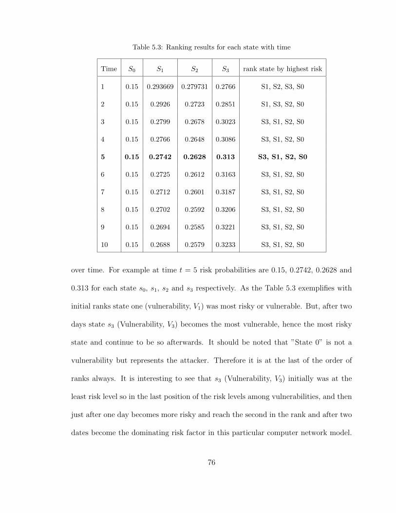
Table 5.3: Ranking results for each state with time
Time S0 S1 S2 S3 rank state by highest risk
1 0.15 0.293669 0.279731 0.2766 S1, S2, S3, S0
2 0.15 0.2926 0.2723 0.2851 S1, S3, S2, S0
3 0.15 0.2799 0.2678 0.3023 S3, S1, S2, S0
4 0.15 0.2766 0.2648 0.3086 S3, S1, S2, S0
5 0.15 0.2742 0.2628 0.313 S3, S1, S2, S0
6 0.15 0.2725 0.2612 0.3163 S3, S1, S2, S0
7 0.15 0.2712 0.2601 0.3187 S3, S1, S2, S0
8 0.15 0.2702 0.2592 0.3206 S3, S1, S2, S0
9 0.15 0.2694 0.2585 0.3221 S3, S1, S2, S0
10 0.15 0.2688 0.2579 0.3233 S3, S1, S2, S0
over time. For example at time t = 5 risk probabilities are 0.15, 0.2742, 0.2628 and
0.313 for each state s0, s1, s2 and s3 respectively. As the Table 5.3 exemplifies with
initial ranks state one (vulnerability, V1) was most risky or vulnerable. But, after two
days state s3 (Vulnerability, V3) becomes the most vulnerable, hence the most risky
state and continue to be so afterwards. It should be noted that ”State 0” is not a
vulnerability but represents the attacker. Therefore it is at the last of the order of
ranks always. It is interesting to see that s3 (Vulnerability, V3) initially was at the
least risk level so in the last position of the risk levels among vulnerabilities, and then
just after one day becomes more risky and reach the second in the rank and after two
dates become the dominating risk factor in this particular computer network model.
76
So, application of this algorithm in more a generalized real life network model would
give us with the similar observations with respect to time. According to this model
example, network administrators and defending resources must be allocated to resolve
s3 (Vulnerability, V3) at priority.
5.5 Contributions
In this chapter a new Ranking Algorithm was introduced to rank the vulnerabilities
in a particular computer network system. The methodology of well-known Google
Page Rank Algorithm was used and we further developed it to fit a computer network
environment. General assumptions used in Google Page Rank Algorithm with respect
to the probability of selecting a particular web link were changed according to the
probability distributions we obtained by normalized vulnerability scores in subject
computer network system. Ranks were obtained for each vulnerability based on the
likelihood of those vulnerabilities getting exploited.
We have further developed the algorithm so that the Distribution of Ranks
of Vulnerabilities in the subject computer network system is given as a function of
time. That is, using our new algorithm, a user (a network system administrator or a
researcher) would be able to observe the behavior of the ranks of vulnerabilities with
respect to time. This new methodology will greatly help relevant parties to make
better decisions to protect network systems because at a particular time t, the algo-
rithm will indicate which vulnerabilities are most vulnerable and needed immediate
attention or priority.
77
6 Future Research
Our main objective in subject research area is to develop successful Statistical Mod-
els and Analytical tools to be effectively applied in the area of Cybersecurity. With
respect to our analytical approaches on vulnerability data we have, two main re-
search focuses are to apply Power Law process [38] and Non-Homogeneous Poison
Process. Having identified the intensity function of the power-law process on exist-
ing vulnerabilities of a particular computer network system or a software, we will be
able to analytically obtain a measure of successfulness of a network modification or a
defending attempt such as network re-design, patching vulnerabilities, disclosing vul-
nerabilities, replacing or updating software etc. If we can acquire relevant data, such
an analytical model with a highest degree of accuracy will be able to indicate whether
the modification on the computer network system of a software resulted in decreasing,
increasing or made no significant change of the likelihood of being exploited, increased
or remained the same.
It is also possible to analytically model the hacking times using Non-Homogeneous
Poison Process. If we can obtain relevant data with respect to times and time inter-
vals for hacking attempts related to vulnerabilities, we would be able to make new
78
approaches in developing models to further predict the behavior of attackers.
Further, from a subjective and analytical point of view, a vulnerability is a
resource or an opportunity for the attacker. But, for defenders the software is the
resource and the vulnerability is a threat that question the survival of the software. If
we track the vulnerabilities and the exploitation data and simulate hacking approaches
it is possible to execute a survival analysis on the relevant software. We would be able
to define and estimate parameters indicating the behavior of the survival functions
for different categories of vulnerabilities, software and computer network systems,
In this dissertation, we presented several important analytical tools and statis-
tical models with respect to vulnerability analysis [42],[45]. In the future, we would
develop these models further and apply software resources to improve the models to
fit and apply in Large-Scale real world computer network systems with any number
of computers and network nodes with variety of discovered vulnerabilities.
Another important research objective we have for the near future is to ana-
lyze the CVSS model. As it was discussed in the previous chapters, we have CVS
scores given for each vulnerability in the CVE detail website [19] and presented in the
National Vulnerability Database [2]. Calculation of these scores are based on several
factors represented by several metrics and equations. However, at this point we do
not know any methodology to measure the accuracy or the degree of confidence in
these methodologies and calculations. We also do not know the relevant assumptions
which these calculations are based on. Therefore, we expect to coordinate with the
administration of the National Vulnerability Data base and other relevant government
79

organizations to test and improve these scoring system further.
80
References
[1] Secunia Vulnerability Review 2015: Key figures and facts from a global informa-
tion security perspective, March 2015.
[2] NVD, National vulnerability database, http://nvd.nist.gov/.
[3] S.Abraham and S.Nair, ”Cyber Security Analytics: A stochastic model for Secu-
rity Quantification using Absorbing Markov Chains” Journal of Communications
Vol. 9, No. 12, December 2014, pp. 899-907.
[4] Phongphun Kijsanayothin, (2010) Network Security Modeling with Intelligent
and Complexity Analysis. Ph.D. Dissertation, Texas Tech University.
[5] Alhazmi, O. H. and Malaiya, Y. K. (2005) Modeling the Vulnerability Discovery
Process. Proceedings of 16th International Symposium on Software Reliability
Engineering, Chicago, 8-11 November 2005, 129-138.
[6] O. H. Alhazmi, Y. K. Malaiya, and I. Ray, Measuring, analyzing and predicting
security vulnerabilities in software systems, Computers and Security Journal, vol.
26, no. 3, pp. 219228, May 2007.
81
[7] Alhazmi, O. H. and Malaiya, Y. K. (2008) Application of Vulnerability Discovery
Models to Major Operating Systems, IEEE Transactions on Reliability, Vol. 57,
No. 1, 2008, pp. 14-22.
[8] Joh, H. and Malaiya, Y.K. (2010) A framework for Software Security Risk Eval-
uation using the Vulnerability Lifecycle and CVSS Metrics, Proc. International
Workshop on Risk and Trust in Extended Enterprises, November 2010,pp.430-
434.
[9] Leyla Bilge, Tudor Dumitras, An Empirical Study of Zero-Day Attacks in the
real world. ACM’s Conference on Computer and Communications Security, Oct.
16-18, 2012.
[10] S. Frei, Security Econometrics: The Dynamics of (IN) Security, Ph.D. dissertation
at ETH Zurich, 2009.
[11] S. Noel, M. Jacobs, P. Kalapa, and S. Jajodia. Multiple Coordinated Views
for Network Attack Graphs. In VIZSEC’05: Proc. of the IEEE Workshops on
Visualization for Computer Security, Minneapolis, MN, October, 2005, pages
99106.
[12] Jajodia, S. and Noel, S. (2005) Advanced Cyber Attack Modeling, Analysis,
and Visualization, 14th USENIX Security Symposium, Technical Report 2010,
George Mason University, Fairfax, VA.
[13] Mehta, V., C. Bartzis, H. Zhu, E. M. Clarke, and J. M. Wing (2006). Ranking
attack graphs. In D. Zamboni and C. Kr ugel (Eds.), Recent Advances in Intru-
82
sion Detection, Volume 4219 of Lecture Notes in Computer Science, pp. 127144.
Springer.
[14] M. Schiffman, Common Vulnerability Scoring System (CVSS).
http://www.first.org/cvss/.
[15] T. Bass, Intrusion detection system and multi-sensor data fusion, Communica-
tions of the ACM, vol. 43, no. 4 pp. 99-105, 2000.
[16] Gregory F. Lawler. (2006) Introduction to Stochastic processes. 2nd Edition,
Chapman and Hall/CRC Taylor and Francis Group, London, New York.
[17] L. Wang, A. Singhal, and S. Jajodia, ”Measuring overall security of network
configurations using attack graphs,” Data and Applications Security XXI, vol.
4602, pp. 98-112, August 2007.
[18] L. Wang, T. Islam, T. Long, A. Singhal, and S. Jajodia, ”An attack graph-based
probabilistic security metric,” DAS 2008, LNCS 5094, pp. 283-296, 2008.
[19] CVE details. http://www.cvedetails.com/
[20] Rajasooriya, S.M., Tsokos, C.P. and Kaluarachchi, P.K. (2016) Stochastic Mod-
elling of Vulnerability Life Cycle and Security Risk Evaluation. Journal of infor-
mation Security, 7, 269-279. http://dx.doi.org/10.4236/jis.2016.74022
[21] Rajasooriya, S. , Tsokos, C. and Kaluarachchi, P. (2017) Cyber Security: Non-
linear Stochastic Models for Predicting the Exploitability. Journal of Information
Security, 8, 125-140. doi: 10.4236/jis.2017.82009.
83
[22] 2016 U.S Government Cybersecurity report.
https://cdn2.hubspot.net/hubfs/533449/
[23] Symantec, Internet security threat report 2016-Volume 21,
https://resource.elq.symantec.com
[24] Gleich, David F. (January 2015). ”PageRank Beyond the Web”. SIAM Review.
57 (3): 321363.
[25] Hewett, R. and P. Kijsanayothin (2008). Host-centric model checking for net-
work vulnerability analysis. In ACSAC 08: Proceedings of the 2008 Annual
Computer Security Applications Conference, Washington, DC, USA, pp. 225234.
IEEE Computer Society.
[26] S.Abraham and S.Nair, ”A Stochastic Model for Cyber Security Analytics” Tech
Report 13-CSE-02, CSE Dept, Southern Methodist University, Dallas, Texas,
2013.
[27] R. Sawilla and X. Ou. Googling Attack Graphs. Techni-cal Report TM-2007-205,
Defense Research and Devel-opment Canada, September 2007.
[28] D. Geer and J. Harthorne. Penetration Testing: A Duet. In ACSAC’02: Proc. of
the 18th Annual Computer Security Applications Conference, page 185, Wash-
ington, DC, USA, 2002. IEEE Computer Society.
[29] S. Noel and S. Jajodia. Understanding Complex Network Attack Graphs through
Clustered Adjacency Matrices. In ACSAC ’05: Proceedings of the 21st Annual
84
Computer Security Applications Conference, pages 160-169, Washington, DC,
USA, 2005. IEEE Computer Society.
[30] M. Stamp (2011). Information Security: Principles and Practice, second edition,
Hoboken, NJ: Wiley-Interscience.
[31] I. Mkpong-Ruffin, D. Umphress, J. Hamilton, and J. Gilbert, Quantitative soft-
ware security risk assessment model, ACM workshop on Quality of protection,
2007, pp. 3133.
[32] Izenman, A. (2008). Modern multivariate statistical techniques (Vol. 1). New
York: Springer.
[33] Hansen, B. E. (2009). Lecture notes on nonparametrics. Lecture notes.
[34] Ou, X., Boyer, W., McQueen, M.: A Scalable Approach to Attack Graph Gen-
eration. ACM (2006)
[35] J. Jones, Estimating software vulnerabilities, Security & Privacy,IEEE, vol. 5,
no. 4, pp. 2832, July-Aug. 2007.
[36] H. Okamura, M. Tokuzane and T. Dohi, ”Quantitative Security Evaluation for
Software System from Vulnerability Database,” Journal of Software Engineering
and Applications, Vol. 6 No. 4A, 2013, pp. 15-23. doi: 10.4236/jsea.2013.64A003.
[37] Ingols, K., Lippmann, R., Piwowarsi, K.: Practical attack graph generation for
network defense. In: 22nd Annual Conference on Computer Security Application,
pp. 121130 (2006)
85
[38] Hongzhu Qiao, Chris P.Tsokos, Best efficient estimates of the intensity function
of the power law process. Journal of Applied Statistics, vol. 25, No. 1, pp 111-120,
1998
[39] Mell, P., Scarfone, K. and Romanosky, S. (2007) A Complete Guide to the Com-
mon Vulnerability Scoring System Version 2.0. FIRST-Forum of Incident Re-
sponse and Security Teams, 1-23.
[40] Bilge, L.and Dumitras, T. (2012) Before We Knew It: An Empirical Study of
Zero- Day Attacks in the Real World. Proceedings of the 2012 ACM Conference
on Computer and Communications Security, Raleigh, 16-18 October 2012, 833-
844.
[41] R statistics tool. http://www.r-project.org
[42] Krsul, I.V. (1998) Software Vulnerability Analysis. Doctoral Dissertation, Purude
University, Indiana.
[43] Jha, S., Sheyner, O. and Wing, J. (2002) Two Formal Analyses of Attack Graphs.
Proceedings of 15th IEEE Computer Security Foundations Workshop, Cape Bre-
ton, 24-26 June 2002, 49-63.
[44] Bolch, G., Greiner, S., de Meer, H. and Trivedi, K.S. (2006) Queueing Networks
and Markov Chains: Modeling and Performance Evaluation with Computer Sci-
ence Applications. John Wiley & Sons, Somerset.
[45] Trivedi, K.S. (2002) Probability & Statistics with Reliability, Queuing and Com-
puter Science Applications. John Wiley & Sons, New Work.
86

[46] Kaluarachchi, P.K., Tsokos, C.P. and Rajasooriya, S.M. (2016) Cybersecurity:
A Statistical Predictive Model for the Expected Path Length. Journal of infor-
mation Security, 7, 112-128. http://dx.doi.org/10.4236/jis.2016.73008
87

Appendices
88
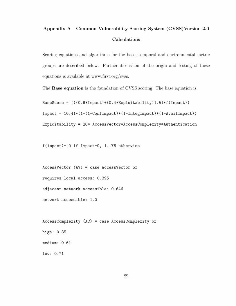
Appendix A - Common Vulnerability Scoring System (CVSS)Version 2.0
Calculations
Scoring equations and algorithms for the base, temporal and environmental metric
groups are described below. Further discussion of the origin and testing of these
equations is available at www.first.org/cvss.
The Base equation is the foundation of CVSS scoring. The base equation is:
BaseScore = (((0.6*Impact)+(0.4*Exploitability)1.5)*f(Impact))
Impact = 10.41*(1-(1-ConfImpact)*(1-IntegImpact)*(1-AvailImpact))
Exploitability = 20* AccessVector*AccessComplexity*Authentication
f(impact)= 0 if Impact=0, 1.176 otherwise
AccessVector (AV) = case AccessVector of
requires local access: 0.395
adjacent network accessible: 0.646
network accessible: 1.0
AccessComplexity (AC) = case AccessComplexity of
high: 0.35
medium: 0.61
low: 0.71
89
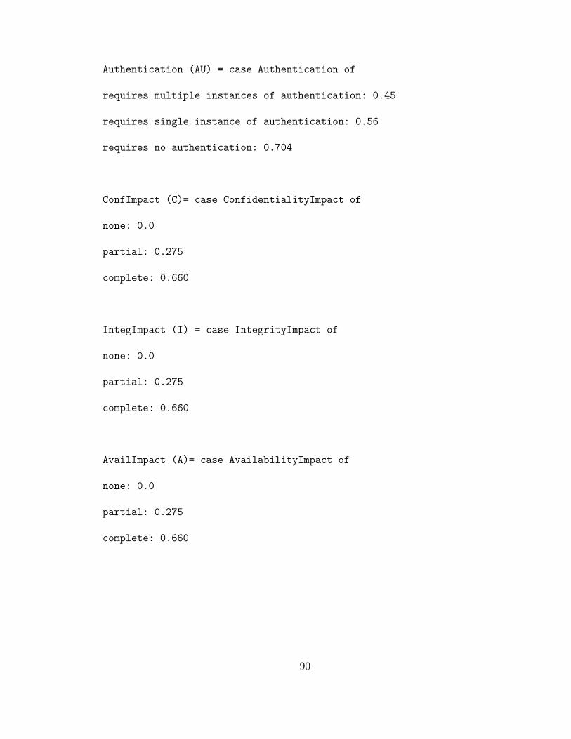
Authentication (AU) = case Authentication of
requires multiple instances of authentication: 0.45
requires single instance of authentication: 0.56
requires no authentication: 0.704
ConfImpact (C)= case ConfidentialityImpact of
none: 0.0
partial: 0.275
complete: 0.660
IntegImpact (I) = case IntegrityImpact of
none: 0.0
partial: 0.275
complete: 0.660
AvailImpact (A)= case AvailabilityImpact of
none: 0.0
partial: 0.275
complete: 0.660
90
Appendix A (Continued)
Temporal Equation
If employed, the temporal equation will combine the temporal metrics with the
base score to produce a temporal score ranging from 0 to 10. Further, the temporal
score will produce a temporal score no higher than the base score, and no less than
0.33 lower than the base score. The temporal equation is:.
TemporalScore = (BaseScore*Exploitability*RemediationLevel*ReportConfidence)
Exploitability = case Exploitability of
unproven: 0.85
proof-of-concept: 0.9
functional: 0.95
high: 1.00
not defined: 1.00
RemediationLevel = case RemediationLevel of
official-fix: 0.87
temporary-fix: 0.90
workaround: 0.95
unavailable: 1.00
not defined: 1.00
91
ReportConfidence = case ReportConfidence of
unconfirmed: 0.90
uncorroborated: 0.95
confirmed: 1.00
not defined: 1.00
92

Appendix A (Continued)
Environmental Equation If employed, the environmental equation will combine
the environmental metrics with the temporal score to produce an environmental score
ranging from 0 to 10. Further, this equation will produce a score no higher than the
temporal score. The environmental equation is:
EnvironmentalScore =(AdjustedTemporal+(10-AdjustedTemporal) *CDP) *TD)
AdjustedTemporal = TemporalScore recomputed with the
BaseScores Impact sub- equation replaced with the AdjustedImpact equation
AdjustedImpact = min(10,10.41*(1-(1-ConfImpact*ConfReq)*(1-IntegImpact*IntegReq)
*(1-AvailImpact*AvailReq)))
CollateralDamagePotential (CDP) = case CollateralDamagePotential of
none: 0
low: 0.1
low-medium: 0.3
medium-high: 0.4
high: 0.5
not defined: 0
TargetDistribution (TD)= case TargetDistribution of
93
none: 0
low: 0.25
medium: 0.75
high: 1.00
not defined: 1.00
ConfReq = case ConfReq of
low: 0.5
medium: 1.0
high: 1.51
not defined: 1.0
IntegReq = case IntegReq of
low:0.5
medium: 1.0
high: 1.51
not defined: 1.0
AvailReq = case AvailReq of
low:0.5
medium: 1.0
high: 1.51
94

not defined: 1.0
95
Appendix B
Example-CVE-2002-0392
Below, we provide steps of how CVSS is used for three different metric.
----------------------------------------------------
BASE METRIC EVALUATION SCORE
----------------------------------------------------
Access Vector [Network] (1.00)
Access Complexity [Low] (0.71)
Authentication [None] (0.704)
Confidentiality Impact [None] (0.00)
Integrity Impact [None] (0.00)
Availability Impact [Complete] (0.66)
Impact = 10.41*(1-(1)*(1)*(0.34)) == 6.9
Exploitability = 20*0.71*0.704*1 == 10.0 f(Impact) = 1.176
BaseScore = (0.6*6.9 + 0.4*10.0 1.5)*1.176 =7.8
----------------------------------------------------
TEMPORAL METRIC EVALUATION SCORE
----------------------------------------------------
Exploitability [Functional] (0.95)
96
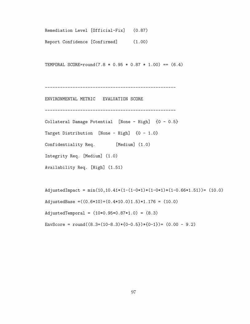
Remediation Level [Official-Fix] (0.87)
Report Confidence [Confirmed] (1.00)
TEMPORAL SCORE=round(7.8 * 0.95 * 0.87 * 1.00) == (6.4)
----------------------------------------------------
ENVIRONMENTAL METRIC EVALUATION SCORE
----------------------------------------------------
Collateral Damage Potential [None - High] {0 - 0.5}
Target Distribution [None - High] {0 - 1.0}
Confidentiality Req. [Medium] (1.0)
Integrity Req. [Medium] (1.0)
Availability Req. [High] (1.51)
AdjustedImpact = min(10,10.41*(1-(1-0*1)*(1-0*1)*(1-0.66*1.51))= (10.0)
AdjustedBase =((0.6*10)+(0.4*10.0)1.5)*1.176 = (10.0)
AdjustedTemporal = (10*0.95*0.87*1.0) = (8.3)
EnvScore = round((8.3+(10-8.3)*{0-0.5})*{0-1})= (0.00 - 9.2)
97
Appendix C
Scientific Research Publishing, Inc.
SCIRP, http://www.scirp.org
JIS COPYRIGHT FORM
This form is intended for original material submitted to the Journal Journal of Infor-
mation Security (JIS) sponsored by Scientific Research Publishing Inc. (SCIRP). The
following agreement must be signed and returned to the JIS Editorial Office before
the manuscript can be published. Please read it carefully and keep a copy for your
files
Journal: Journal of Information Security (JIS)
Paper ID: 7800364
Paper Title:Cybersecurity: A Statistical Predictive Model for the Expected Path
Length(7800364)
Author(s): Pubudu Kaluarachchilage, Chris Tsokos, Sasith Rajasooriya
COPYRIGHT CONCESSION AGREEMENT
The undersigned hereby grants SCIRP a nonexclusive copyright that may exist in
and to the above Work, and any revised or expanded derivative works submitted to
the Journal JIS by the undersigned based on the Work on the understanding that on
completion of the layout SCIRP will make the final paper available online without
delay, SCIRP guarantees that no university library or individual reader will ever have
to buy a subscription or buy access through pay-per-view fees to access the papers
published in the Journal JIS.
98

The undersigned hereby warrants that the Work is original and that he/she is the
author of the Work; to the extent the Work incorporates text passages, figures, data
or other material from the works of others, the undersigned has obtained any necessary
permission including permission from any and all co-authors.
RETAINED RIGHTS, TERMS, AND CONDITIONS
Since the undersigned grants SCIRP a nonexclusive copyright, the undersigned retains
the original copyright while SCIRP is granted the same set of rights including the right
to sublicense the Work.
SCIRP will publish the Work under a Creative Commons license.By default This is
the Creative Commons Attribution 4.0 International License,
CC BY: http://creativecommons.org/licenses/by/4.0/.
Alternatively upon request it is also possible for SCIRP to publish under:Creative
Commons Attribution-NonCommercial 4.0 International License,
CC BY- NC:http://creativecommons.org/licenses/by-nc/4.0/.
Authors choice (specify CC BY-NC only if you do not want the default CC BY)
Authors and their employers retain all proprietary rights in any process, procedure,
or article of manufacture described in the Work.
Authors who are US Government employees may reproduce or authorize others to re-
produce the Work, material extracted verbatim from the Work, or derivative works to
the extent permissible under USs law for works authored by US Government employ-
ees, and for the authors personal use or for company or organizational use, provided
that the source and any SCIRP copyright notice are indicated, the copies are not used
99

in any way that implies SCIRP endorsement of a product or service of any employer,
and the copies themselves are not offered for sale.
In the case of a Work performed under a China Government contract or grant, the
SCIRP recognizes that the China Government has royalty-free permission to repro-
duce all or portions of the Work, and to authorize others to do so, for official China
Government purposes only, if the contract/grant so requires.
SCIRP Copyright
It is the formal policy of SCIRP to be granted the nonexclusive copyrights to all
copyrightable material in its technical publications and to the individual contributions
contained therein, in order to protect the interests of SCIRP, its authors and their
employers, and, at the same time, to facilitate the appropriate re-use of this material
by others. SCIRP distributes its technical publications throughout the world and
does so by various means such as hard copy, microfiche, microfilm, and electronic
media. It also abstracts and may translate its publications, and articles contained
therein, for inclusion in various compendiums, collective works, databases and similar
publications.
No royalties are paid to authors if SCIRP produces revenues by these activities.
Author/Employer Rights
If you are employed and prepared the Work on a subject within the scope of your
employment, the copyright in the Work belongs to your employer as a work-for-hire.
In that case, SCIRP assumes that when you sign this Form, you are authorized to do so
by your employer and that your employer has consented to granting the nonexclusive
100

copyright, to the representation and warranty of publication rights, and to all other
terms and conditions of this Form. If such authorization and consent has not been
given to you, an authorized representative of your employer should sign this Form as
the Author.
In the event the above work ts not accepted and published by SCIRP or is withdrawn
by the author(s) before acceptance by SCIRP, the foregoing granting the nonexclusive
copyright shall become null and void and all materials embodying the Work submitted
to JIS will be destroyed.
The author signs for and accepts responsibility for releasing this material on behalf
of any and all co-authors.
Creative Commons License Type:
O CC BY
O CC BY-NC
Attention: Please choose either one of these two above.
Signature:
Date ( 03/15/2016)
101

![New Approach for Stochastic Modelling of Microgrid ... · involves various stochastic modelling and simulation methods [4, 6, 7]. The survey of stochastic modelling of microgrid is](https://img.pdfslide.net/doc/110x75/5f4190048356da16412b2f00/new-approach-for-stochastic-modelling-of-microgrid-involves-various-stochastic.jpg)