Embed Size (px)
Citation preview
1
The Laplace Transform
M. J. Roberts - All Rights Reserved. Edited by Dr. Robert Akl
1
Generalizing the Fourier Transform
The CTFT expresses a time-domain signal as a linearcombination of complex sinusoids of the form e jωt . In thegeneralization of the CTFT to the Laplace transform, thecomplex sinusoids become complex exponentials of theform est where s can have any complex value. Replacingthe complex sinusoids with complex exponentials leads tothis definition of the Laplace transform.
L x t( )( ) = X s( ) = x t( )e− st dt−∞
∞
∫ x t( ) L← →⎯ X s( )
M. J. Roberts - All Rights Reserved. Edited by Dr. Robert Akl 2
Generalizing the Fourier Transform
The variable s is viewed as a generalization of the variable ω ofthe form s = σ + jω . Then, when σ , the real part of s, is zero, theLaplace transform reduces to the CTFT. Using s = σ + jω the Laplace transform is
X s( ) = x t( )e− σ + jω( )t dt−∞
∞
∫= F x t( )e−σ t⎡⎣ ⎤⎦
which is the Fouriertransform of x t( )e−σ t
M. J. Roberts - All Rights Reserved. Edited by Dr. Robert Akl 3
Generalizing the Fourier Transform The extra factor e−σ t is sometimes called a convergence factorbecause, when chosen properly, it makes the integral convergefor some signals for which it would not otherwise converge.For example, strictly speaking, the signal Au t( ) does not havea CTFT because the integral does not converge. But if it ismultiplied by the convergence factor, and the real part of sis chosen appropriately, the CTFT integral will converge.
Au t( )e− jωt dt−∞
∞
∫ = A e− jωt dt0
∞
∫ ← Does not converge
Ae−σ t u t( )e− jωt dt−∞
∞
∫ = A e− σ + jω( )t dt0
∞
∫ ←Converges (if σ > 0)
M. J. Roberts - All Rights Reserved. Edited by Dr. Robert Akl 4
Complex Exponential Excitation
M. J. Roberts - All Rights Reserved. Edited by Dr. Robert Akl 5
Complex Exponential Excitation
M. J. Roberts - All Rights Reserved. Edited by Dr. Robert Akl 6
2
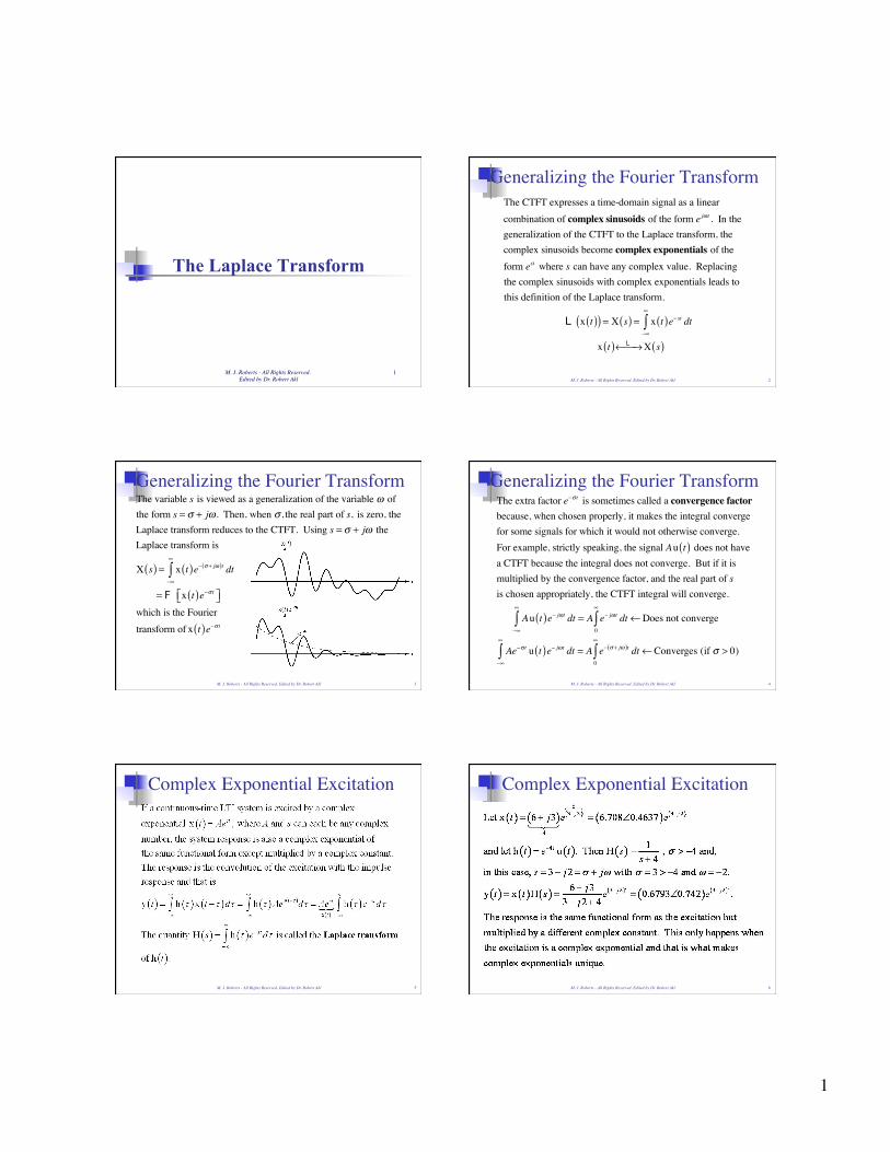
Pierre-Simon Laplace
3/23/1749 - 3/2/1827
M. J. Roberts - All Rights Reserved. Edited by Dr. Robert Akl 7
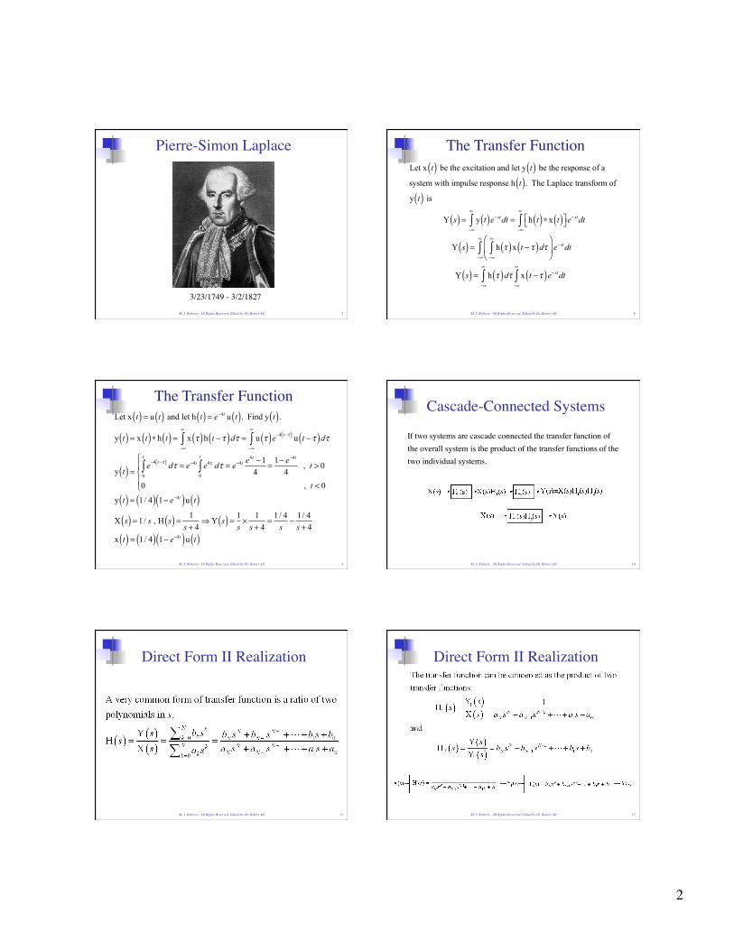
The Transfer Function
Let x t( ) be the excitation and let y t( ) be the response of a
system with impulse response h t( ). The Laplace transform of
y t( ) is Y s( ) = y t( )e−stdt
−∞
∞
∫ = h t( )∗x t( )⎡⎣ ⎤⎦e−stdt−∞
∞
∫
Y s( ) = h τ( )x t −τ( )dτ−∞
∞
∫⎛
⎝⎜⎞
⎠⎟e−stdt
−∞
∞
∫
Y s( ) = h τ( )dτ−∞
∞
∫ x t −τ( )e−stdt−∞
∞
∫
M. J. Roberts - All Rights Reserved. Edited by Dr. Robert Akl 8
The Transfer Function
Let x t( ) = u t( ) and let h t( ) = e−4t u t( ). Find y t( ).y t( ) = x t( )∗h t( ) = x τ( )h t −τ( )dτ
−∞
∞
∫ = u τ( )e−4 t−τ( ) u t −τ( )dτ−∞
∞
∫
y t( ) = e−4 t−τ( ) dτ0
t
∫ = e−4t e4τ dτ0
t
∫ = e−4t e4t −14
= 1− e−4t
4 , t > 0
0 , t < 0
⎧
⎨⎪
⎩⎪
y t( ) = 1/ 4( ) 1− e−4t( )u t( )X s( ) = 1/ s , H s( ) = 1
s + 4⇒ Y s( ) = 1
s× 1
s + 4= 1/ 4
s− 1/ 4
s + 4x t( ) = 1/ 4( ) 1− e−4t( )u t( )
M. J. Roberts - All Rights Reserved. Edited by Dr. Robert Akl 9
Cascade-Connected Systems
If two systems are cascade connected the transfer function ofthe overall system is the product of the transfer functions of thetwo individual systems.
M. J. Roberts - All Rights Reserved. Edited by Dr. Robert Akl 10
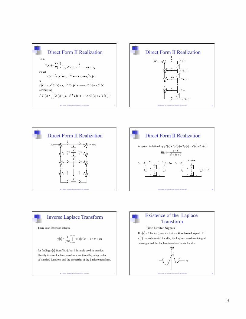
Direct Form II Realization
M. J. Roberts - All Rights Reserved. Edited by Dr. Robert Akl 11
Direct Form II Realization
M. J. Roberts - All Rights Reserved. Edited by Dr. Robert Akl 12
3
Direct Form II Realization
M. J. Roberts - All Rights Reserved. Edited by Dr. Robert Akl 13
Direct Form II Realization
M. J. Roberts - All Rights Reserved. Edited by Dr. Robert Akl 14
Direct Form II Realization
M. J. Roberts - All Rights Reserved. Edited by Dr. Robert Akl 15
Direct Form II Realization
A system is defined by ′′y t( ) + 3 ′y t( ) + 7y t( ) = ′x t( )− 5x t( ).
H s( ) = s − 5s2 + 3s + 7
M. J. Roberts - All Rights Reserved. Edited by Dr. Robert Akl 16
Inverse Laplace Transform
There is an inversion integral
y t( ) = 1j2π
Y s( )estdsσ − j∞
σ + j∞
∫ , s = σ + jω
for finding y t( ) from Y s( ), but it is rarely used in practice.
Usually inverse Laplace transforms are found by using tablesof standard functions and the properties of the Laplace transform.
M. J. Roberts - All Rights Reserved. Edited by Dr. Robert Akl 17
Existence of the Laplace Transform
Time Limited Signals
If x t( ) = 0 for t < t0 and t > t1 it is a time limited signal. If
x t( ) is also bounded for all t, the Laplace transform integral
converges and the Laplace transform exists for all s.
M. J. Roberts - All Rights Reserved. Edited by Dr. Robert Akl 18
4
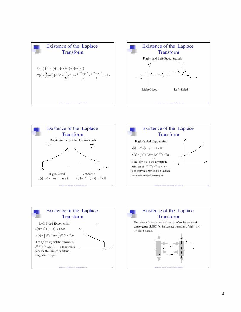
Existence of the Laplace Transform
Let x t( ) = rect t( ) = u t +1/ 2( )− u t −1/ 2( ).X s( ) = rect t( )e−st dt
−∞
∞
∫ = e−st dt−1/2
1/2
∫ = e−s/2 − es/2
−s= es/2 − e−s/2
s , All s
M. J. Roberts - All Rights Reserved. Edited by Dr. Robert Akl 19
Existence of the Laplace Transform
Right- and Left-Sided Signals
Right-Sided Left-Sided
M. J. Roberts - All Rights Reserved. Edited by Dr. Robert Akl 20
Existence of the Laplace Transform
Right- and Left-Sided Exponentials
Right-Sided Left-Sided x t( ) = eαt u t − t0( ) , α ∈ x t( ) = eβt u t0 − t( ) , β ∈
M. J. Roberts - All Rights Reserved. Edited by Dr. Robert Akl 21
Existence of the Laplace Transform
Right-Sided Exponential
x t( ) = eα t u t − t0( ) , α ∈
X s( ) = eα te− stdtt0
∞
∫ = e α −σ( )te− jω tdtt0
∞
∫If Re s( ) = σ >α the asymptotic
behavior of e α −σ( )te− jω t as t→∞ is to approach zero and the Laplace transform integral converges.
M. J. Roberts - All Rights Reserved. Edited by Dr. Robert Akl 22
Existence of the Laplace Transform
Left-Sided Exponential
x t( ) = eβt u t0 − t( ) , β ∈
X s( ) = eβte− stdt−∞
t0
∫ = e β−σ( )te− jωtdt−∞
t0
∫If σ < β the asymptotic behavior of
e β−σ( )te− jωt as t→−∞ is to approach zero and the Laplace transformintegral converges.
M. J. Roberts - All Rights Reserved. Edited by Dr. Robert Akl 23
Existence of the Laplace Transform
The two conditions σ >α and σ < β define the region ofconvergence (ROC) for the Laplace transform of right- and left-sided signals.
M. J. Roberts - All Rights Reserved. Edited by Dr. Robert Akl 24
5
Existence of the Laplace Transform
Any right-sided signal that grows no faster than an exponential in positive time and any left-sided signal that grows no faster than an exponential in negative time has a Laplace transform.If x t( ) = xr t( ) + xl t( ) where xr t( ) is the right-sided part andxl t( ) is the left-sided part and if xr t( ) < Kre
α t and xl t( ) < Kleβt
and α and β are as small as possible, then the Laplace-transform integral converges and the Laplace transform exists for α < σ < β. Therefore if α < β the ROC is the region α < β. If α > β, there is no ROC and the Laplace transform does not exist.
M. J. Roberts - All Rights Reserved. Edited by Dr. Robert Akl 25
Laplace Transform Pairs
The Laplace transform of g1 t( ) = Aeαt u t( ) is
G1 s( ) = Aeαt u t( )e− stdt−∞
∞
∫ = A e− s−α( )tdt0
∞
∫ = A e α−σ( )te− jωtdt0
∞
∫ = As −α
This function has a pole at s = α and the ROC is the region to the right of that point. The Laplace transform of g2 t( ) = Aeβt u −t( ) is
G2 s( ) = Aeβt u −t( )e− stdt−∞
∞
∫ = A e β−s( )tdt−∞
0
∫ = A e β−σ( )te− jωtdt−∞
0
∫ = − As − β
This function has a pole at s = β and the ROC is the region to the left of that point.
M. J. Roberts - All Rights Reserved. Edited by Dr. Robert Akl 26
Region of Convergence
The following two Laplace transform pairs illustrate the importance of the region of convergence.
e−αt u t( ) L← →⎯ 1s +α
, σ > −α
− e−αt u −t( ) L← →⎯ 1s +α
, σ < −α
The two time-domain functions are different but the algebraic expressions for their Laplace transforms are the same. Only the ROC’s are different.
M. J. Roberts - All Rights Reserved. Edited by Dr. Robert Akl 27
Region of Convergence
δ t( ) L← →⎯ 1 , All σ
u t( ) L← →⎯ 1/ s , σ > 0 − u −t( ) L← →⎯ 1/ s , σ < 0
ramp t( ) = t u t( ) L← →⎯ 1/ s2 , σ > 0 ramp −t( ) = −t u −t( ) L← →⎯ 1/ s2 , σ < 0
e−αt u t( ) L← →⎯ 1/ s +α( ) , σ > −α − e−αt u −t( ) L← →⎯ 1/ s +α( ) , σ < −α
e−αt sin ω0t( )u t( ) L← →⎯ω0
s +α( )2+ω0
2, σ > −α − e−αt sin ω0t( )u −t( ) L← →⎯
ω0
s +α( )2+ω0
2, σ < −α
e−αt cos ω0t( )u t( ) L← →⎯ s +α
s +α( )2+ω0
2, σ > −α − e−αt cos ω0t( )u −t( ) L← →⎯ s +α
s +α( )2+ω0
2, σ < −α
Some of the most common Laplace transform pairs (There is more extensive table in the book.)
M. J. Roberts - All Rights Reserved. Edited by Dr. Robert Akl 28
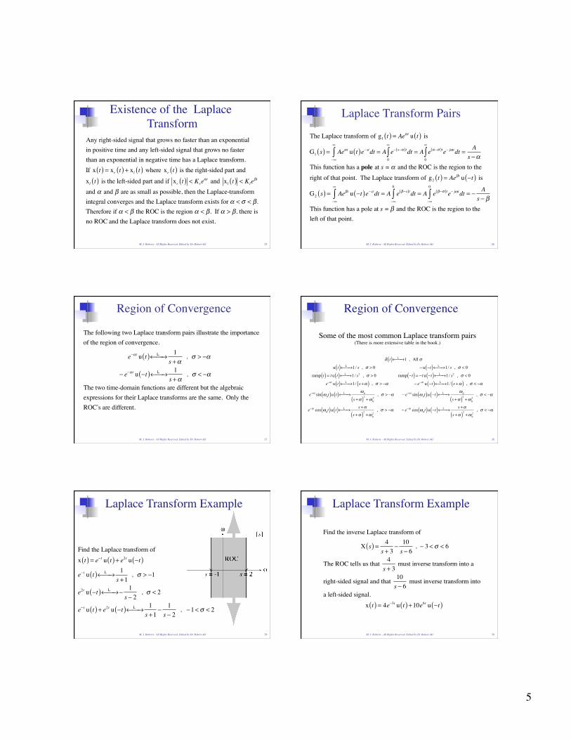
Laplace Transform Example
Find the Laplace transform of x t( ) = e− t u t( ) + e2t u −t( )
e− t u t( ) L← →⎯ 1s +1
, σ > −1
e2t u −t( ) L← →⎯ − 1s − 2
, σ < 2
e− t u t( ) + e2t u −t( ) L← →⎯ 1s +1
− 1s − 2
, −1<σ < 2
M. J. Roberts - All Rights Reserved. Edited by Dr. Robert Akl 29
Laplace Transform Example
Find the inverse Laplace transform of
X s( ) = 4s + 3
− 10s − 6
, − 3 <σ < 6
The ROC tells us that 4s + 3
must inverse transform into a
right-sided signal and that 10s − 6
must inverse transform into
a left-sided signal. x t( ) = 4e−3t u t( ) +10e6t u −t( )
M. J. Roberts - All Rights Reserved. Edited by Dr. Robert Akl 30
6
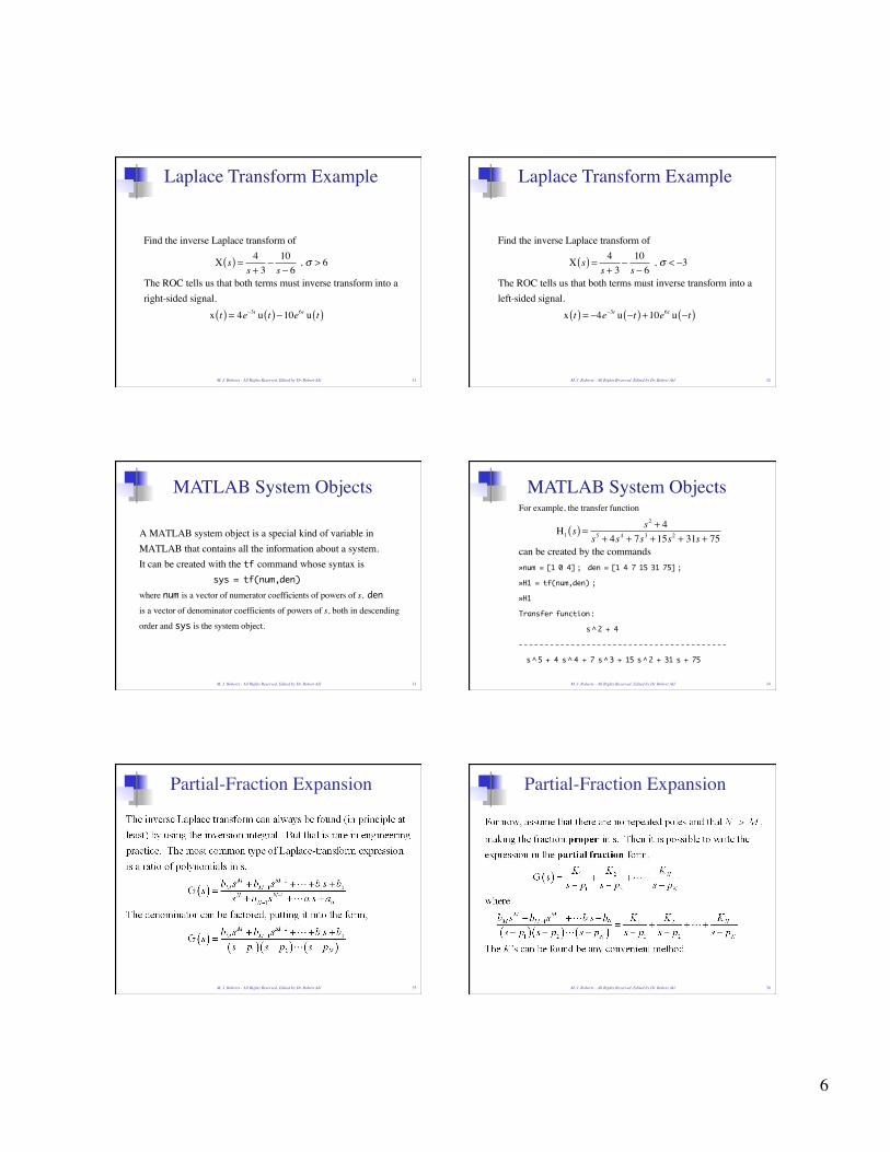
Laplace Transform Example
Find the inverse Laplace transform of
X s( ) = 4s + 3
− 10s − 6
, σ > 6
The ROC tells us that both terms must inverse transform into a right-sided signal. x t( ) = 4e−3t u t( )−10e6t u t( )
M. J. Roberts - All Rights Reserved. Edited by Dr. Robert Akl 31
Laplace Transform Example
Find the inverse Laplace transform of
X s( ) = 4s + 3
− 10s − 6
, σ < −3
The ROC tells us that both terms must inverse transform into a left-sided signal. x t( ) = −4e−3t u −t( ) +10e6t u −t( )
M. J. Roberts - All Rights Reserved. Edited by Dr. Robert Akl 32
MATLAB System Objects
A MATLAB system object is a special kind of variable inMATLAB that contains all the information about a system.It can be created with the tf command whose syntax is sys = tf(num,den)where num is a vector of numerator coefficients of powers of s, denis a vector of denominator coefficients of powers of s, both in descending
order and sys is the system object.
M. J. Roberts - All Rights Reserved. Edited by Dr. Robert Akl 33
MATLAB System Objects
For example, the transfer function
H1 s( ) = s2 + 4s5 + 4s4 + 7s3 +15s2 + 31s + 75
can be created by the commands»num = [1 0 4] ; den = [1 4 7 15 31 75] ;
»H1 = tf(num,den) ;
»H1
Transfer function:
s ^ 2 + 4
----------------------------------------
s ^ 5 + 4 s ^ 4 + 7 s ^ 3 + 15 s ^ 2 + 31 s + 75
M. J. Roberts - All Rights Reserved. Edited by Dr. Robert Akl 34
Partial-Fraction Expansion
M. J. Roberts - All Rights Reserved. Edited by Dr. Robert Akl 35
Partial-Fraction Expansion
M. J. Roberts - All Rights Reserved. Edited by Dr. Robert Akl 36
7
Partial-Fraction Expansion
M. J. Roberts - All Rights Reserved. Edited by Dr. Robert Akl 37
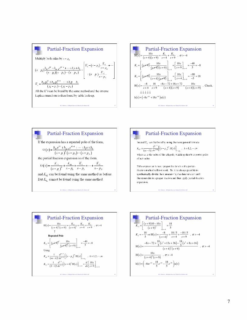
Partial-Fraction Expansion H s( ) = 10s
s + 4( ) s + 9( ) =K1
s + 4+ K2
s + 9 , σ > −4
K1 = s + 4( ) 10ss + 4( ) s + 9( )
⎡
⎣⎢⎢
⎤
⎦⎥⎥s=−4
= 10ss + 9
⎡⎣⎢
⎤⎦⎥s=−4
= −405
= −8
K2 = s + 9( ) 10ss + 4( ) s + 9( )
⎡
⎣⎢⎢
⎤
⎦⎥⎥s=−9
= 10ss + 4
⎡⎣⎢
⎤⎦⎥s=−9
= −90−5
= 18
H s( ) = −8s + 4
+ 18s + 9
= −8s − 72 +18s + 72s + 4( ) s + 9( ) = 10s
s + 4( ) s + 9( ) . Check.
↓ ↓ ↓ ↓ ↓
h t( ) = −8e−4 t +18e−9t( )u t( )
M. J. Roberts - All Rights Reserved. Edited by Dr. Robert Akl 38
Partial-Fraction Expansion
M. J. Roberts - All Rights Reserved. Edited by Dr. Robert Akl 39
Partial-Fraction Expansion
M. J. Roberts - All Rights Reserved. Edited by Dr. Robert Akl 40
Partial-Fraction Expansion
H s( ) = 10ss + 4( )2 s + 9( )
= K12
s + 4( )2 +K11
s + 4+ K2
s + 9 , σ > 4
↑ Repeated Pole
K12 = s + 4( )2 10ss + 4( )2 s + 9( )
⎡
⎣
⎢⎢
⎤
⎦
⎥⎥s=−4
= −405
= −8
Using
Kqk =1
m − k( )!dm−k
dsm−k s − pq( )m H s( )⎡⎣
⎤⎦s→ pq
, k = 1,2,,m
K11 =1
2 −1( )!d 2−1
ds2−1 s + 4( )2 H s( )⎡⎣ ⎤⎦s→−4= dds
10ss + 9
⎡⎣⎢
⎤⎦⎥s→−4
M. J. Roberts - All Rights Reserved. Edited by Dr. Robert Akl 41
Partial-Fraction Expansion K11 =
s + 9( )10 −10ss + 9( )2
⎡
⎣⎢
⎤
⎦⎥s=−4
= 185
K2 = −185⇒ H s( ) = −8
s + 4( )2 +18 / 5s + 4
+ −18 / 5s + 9
, σ > −4
H s( ) =−8s − 72 + 18
5s2 +13s + 36( )− 18
5s2 + 8s +16( )
s + 4( )2 s + 9( ) , σ > −4
H s( ) = 10ss + 4( )2 s + 9( )
, σ > −4
h t( ) = −8te−4 t + 185e−4 t − 18
5e−9t⎛
⎝⎜⎞⎠⎟ u t( )
M. J. Roberts - All Rights Reserved. Edited by Dr. Robert Akl 42
8
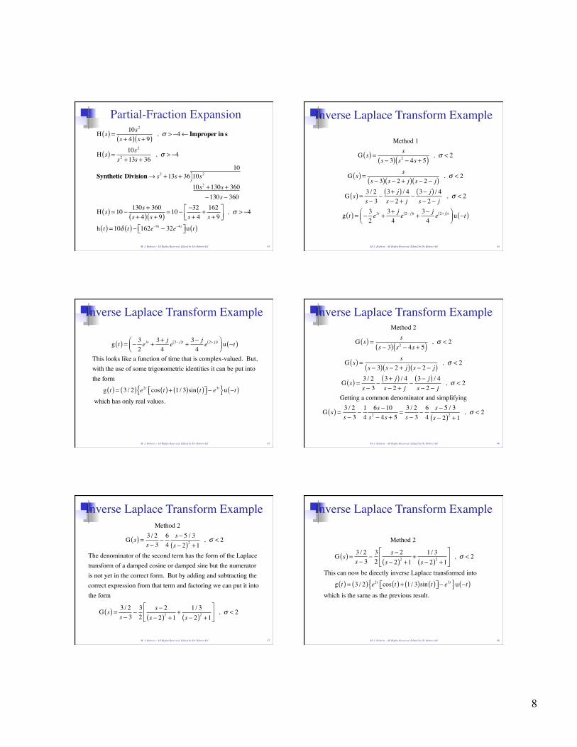
Partial-Fraction Expansion H s( ) = 10s2
s + 4( ) s + 9( ) , σ > −4 ← Improper in s
H s( ) = 10s2
s2 +13s + 36 , σ > −4
Synthetic Division→ s2 +13s + 36 10s2
10s2 +130s + 360−130s − 360
10
H s( ) = 10 − 130s + 360s + 4( ) s + 9( ) = 10 − −32
s + 4+ 162s + 9
⎡⎣⎢
⎤⎦⎥
, σ > −4
h t( ) = 10δ t( )− 162e−9t − 32e−4 t⎡⎣ ⎤⎦u t( )
M. J. Roberts - All Rights Reserved. Edited by Dr. Robert Akl 43
Method 1
G s( ) = ss − 3( ) s2 − 4s + 5( ) , σ < 2
G s( ) = ss − 3( ) s − 2 + j( ) s − 2 − j( ) , σ < 2
G s( ) = 3 / 2s − 3
−3+ j( ) / 4s − 2 + j
−3− j( ) / 4s − 2 − j
, σ < 2
g t( ) = − 32e3t + 3+ j
4e 2− j( )t + 3− j
4e 2+ j( )t⎛
⎝⎜⎞⎠⎟ u −t( )
Inverse Laplace Transform Example
M. J. Roberts - All Rights Reserved. Edited by Dr. Robert Akl 44
g t( ) = − 32e3t + 3+ j
4e 2− j( )t + 3− j
4e 2+ j( )t⎛
⎝⎜⎞⎠⎟ u −t( )
This looks like a function of time that is complex-valued. But,with the use of some trigonometric identities it can be put intothe form
g t( ) = 3 / 2( ) e2t cos t( ) + 1 / 3( )sin t( )⎡⎣ ⎤⎦ − e3t{ }u −t( )
which has only real values.
Inverse Laplace Transform Example
M. J. Roberts - All Rights Reserved. Edited by Dr. Robert Akl 45
Method 2
G s( ) = ss − 3( ) s2 − 4s + 5( ) , σ < 2
G s( ) = ss − 3( ) s − 2 + j( ) s − 2 − j( ) , σ < 2
G s( ) = 3 / 2s − 3
−3+ j( ) / 4s − 2 + j
−3− j( ) / 4s − 2 − j
, σ < 2
Getting a common denominator and simplifying
G s( ) = 3 / 2s − 3
−14
6s −10s2 − 4s + 5
=3 / 2s − 3
−64
s − 5 / 3s − 2( )2 +1
, σ < 2
Inverse Laplace Transform Example
M. J. Roberts - All Rights Reserved. Edited by Dr. Robert Akl 46
Method 2
G s( ) = 3 / 2s − 3
− 64
s − 5 / 3s − 2( )2 +1
, σ < 2
The denominator of the second term has the form of the Laplacetransform of a damped cosine or damped sine but the numeratoris not yet in the correct form. But by adding and subtracting thecorrect expression from that term and factoring we can put it intothe form
G s( ) = 3 / 2s − 3
− 32
s − 2s − 2( )2 +1
+ 1 / 3s − 2( )2 +1
⎡
⎣⎢
⎤
⎦⎥ , σ < 2
Inverse Laplace Transform Example
M. J. Roberts - All Rights Reserved. Edited by Dr. Robert Akl 47
Method 2
G s( ) = 3 / 2s − 3
− 32
s − 2s − 2( )2 +1
+ 1 / 3s − 2( )2 +1
⎡
⎣⎢
⎤
⎦⎥ , σ < 2
This can now be directly inverse Laplace transformed into
g t( ) = 3 / 2( ) e2t cos t( ) + 1 / 3( )sin t( )⎡⎣ ⎤⎦ − e3t{ }u −t( )
which is the same as the previous result.
Inverse Laplace Transform Example
M. J. Roberts - All Rights Reserved. Edited by Dr. Robert Akl 48
9
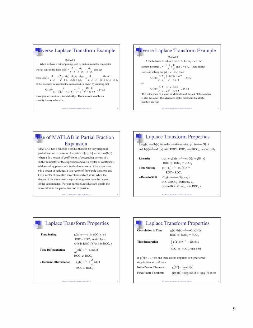
Method 3 When we have a pair of poles p2 and p3 that are complex conjugates
we can convert the form G s( ) = As − 3
+ K2
s − p2
+ K3
s − p3
into the
form G s( ) = As − 3
+s K2 + K3( )− K3p2 − K2 p3
s2 − p1 + p2( )s + p1p2
= As − 3
+ Bs +Cs2 − p1 + p2( )s + p1p2
In this example we can find the constants A, B and C by realizing that
G s( ) = ss − 3( ) s2 − 4s + 5( ) ≡
As − 3
+ Bs +Cs2 − 4s + 5
, σ < 2
is not just an equation, it is an identity. That means it must be anequality for any value of s.
Inverse Laplace Transform Example
M. J. Roberts - All Rights Reserved. Edited by Dr. Robert Akl 49
Inverse Laplace Transform Example Method 3 A can be found as before to be 3 / 2. Letting s = 0, the
identity becomes 0 ≡ − 3 / 23
+ C5
and C = 5 / 2. Then, letting
s = 1, and solving we get B = −3 / 2. Now
G s( ) = 3 / 2s − 3
+−3 / 2( )s + 5 / 2s2 − 4s + 5
, σ < 2
or
G s( ) = 3 / 2s − 3
− 32
s − 5 / 3s2 − 4s + 5
, σ < 2
This is the same as a result in Method 2 and the rest of the solutionis also the same. The advantage of this method is that all the numbers are real.
M. J. Roberts - All Rights Reserved. Edited by Dr. Robert Akl 50
Use of MATLAB in Partial Fraction Expansion
MATLAB has a function residue that can be very helpful inpartial fraction expansion. Its syntax is [r,p,k] = residue(b,a)where b is a vector of coefficients of descending powers of s in the numerator of the expression and a is a vector of coefficients of descending powers of s in the denominator of the expression, r is a vector of residues, p is a vector of finite pole locations and k is a vector of so-called direct terms which result when the degree of the numerator is equal to or greater than the degree of the denominator. For our purposes, residues are simply the numerators in the partial-fraction expansion.
M. J. Roberts - All Rights Reserved. Edited by Dr. Robert Akl 51
Laplace Transform Properties
Let g t( ) and h t( ) form the transform pairs, g t( ) L← →⎯ G s( ) and h t( ) L← →⎯ H s( ) with ROC's, ROCG and ROCH respectively.
Linearity α g t( ) + β h t( ) L← →⎯ αG s( ) + βH s( ) ROC ⊇ ROCG ∩ROCH
Time Shifting g t − t0( ) L← →⎯ G s( )e− st0 ROC = ROCG
s-Domain Shift es0t g t( ) L← →⎯ G s − s0( ) ROC = ROCG shifted by s0 , (s is in ROC if s − s0 is in ROCG )
M. J. Roberts - All Rights Reserved. Edited by Dr. Robert Akl 52
Time Scaling g at( ) L← →⎯ 1 / a( )G s / a( ) ROC = ROCG scaled by a (s is in ROC if s / a is in ROCG )
Time Differentiation ddt
g t( ) L← →⎯ sG s( ) ROC ⊇ ROCG
s-Domain Differentiation − t g t( ) L← →⎯ dds
G s( ) ROC = ROCG
Laplace Transform Properties
M. J. Roberts - All Rights Reserved. Edited by Dr. Robert Akl 53
Convolution in Time g t( )∗h t( ) L← →⎯ G s( )H s( ) ROC ⊇ ROCG ∩ROCH
Time Integration g τ( )dτ−∞
t
∫ L← →⎯ G s( ) / s
ROC ⊇ ROCG ∩ σ > 0( )
If g t( ) = 0 , t < 0 and there are no impulses or higher-order singularities at t = 0 then
Initial Value Theorem: g 0+( ) = lims→∞
sG s( )Final Value Theorem: lim
t→∞g t( ) = lim
s→0sG s( ) if lim
t→∞g t( ) exists
Laplace Transform Properties
M. J. Roberts - All Rights Reserved. Edited by Dr. Robert Akl 54
10
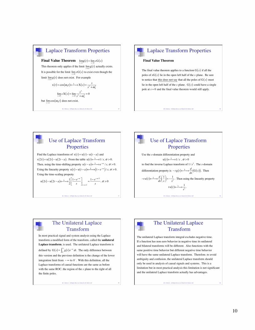
Final Value Theorem limt→∞
g t( ) = lims→0
sG s( )This theorem only applies if the limit lim
t→∞g t( ) actually exists.
It is possible for the limit lims→0
sG s( ) to exist even though the
limit limt→∞
g t( ) does not exist. For example
x t( ) = cos ω0t( ) L← →⎯ X s( ) = ss2 +ω0
2
lims→0
sX s( ) = lims→0
s2
s2 +ω02 = 0
but limt→∞
cos ω0t( ) does not exist.
Laplace Transform Properties
M. J. Roberts - All Rights Reserved. Edited by Dr. Robert Akl 55
Final Value Theorem
Laplace Transform Properties
The final value theorem applies to a function G s( ) if all thepoles of sG s( ) lie in the open left half of the s plane. Be sureto notice that this does not say that all the poles of G s( ) must
lie in the open left half of the s plane. G s( ) could have a singlepole at s = 0 and the final value theorem would still apply.
M. J. Roberts - All Rights Reserved. Edited by Dr. Robert Akl 56
Use of Laplace Transform Properties
Find the Laplace transforms of x t( ) = u t( )− u t − a( ) and
x 2t( ) = u 2t( )− u 2t − a( ). From the table u t( ) L← →⎯ 1 / s, σ > 0.
Then, using the time-shifting property u t − a( ) L← →⎯ e−as / s, σ > 0.
Using the linearity property u t( )− u t − a( ) L← →⎯ 1− e−as( ) / s, σ > 0.
Using the time-scaling property
u 2t( )− u 2t − a( ) L← →⎯ 12
1− e−as
s⎡
⎣⎢
⎤
⎦⎥s→s /2
= 1− e−as /2
s, σ > 0
M. J. Roberts - All Rights Reserved. Edited by Dr. Robert Akl 57
Use of Laplace Transform Properties
Use the s-domain differentiation property and
u t( ) L← →⎯ 1 / s , σ > 0
to find the inverse Laplace transform of 1 / s2 . The s-domain
differentiation property is − t g t( ) L← →⎯ dds
G s( )( ). Then
−t u t( ) L← →⎯ dds
1s
⎛⎝⎜
⎞⎠⎟ = − 1
s2 . Then using the linearity property
t u t( ) L← →⎯ 1s2 .
M. J. Roberts - All Rights Reserved. Edited by Dr. Robert Akl 58
The Unilateral Laplace Transform
In most practical signal and system analysis using the Laplacetransform a modified form of the transform, called the unilateralLaplace transform, is used. The unilateral Laplace transform is
defined by G s( ) = g t( )e− st dt0−
∞
∫ . The only difference between
this version and the previous definition is the change of the lowerintegration limit from − ∞ to 0−. With this definition, all the Laplace transforms of causal functions are the same as beforewith the same ROC, the region of the s plane to the right of allthe finite poles.
M. J. Roberts - All Rights Reserved. Edited by Dr. Robert Akl 59
The Unilateral Laplace Transform
The unilateral Laplace transform integral excludes negative time.If a function has non-zero behavior in negative time its unilateral and bilateral transforms will be different. Also functions with the same positive time behavior but different negative time behavior will have the same unilateral Laplace transform. Therefore, to avoid ambiguity and confusion, the unilateral Laplace transform should only be used in analysis of causal signals and systems. This is a limitation but in most practical analysis this limitation is not significant and the unilateral Laplace transform actually has advantages.
M. J. Roberts - All Rights Reserved. Edited by Dr. Robert Akl 60
11
The Unilateral Laplace Transform
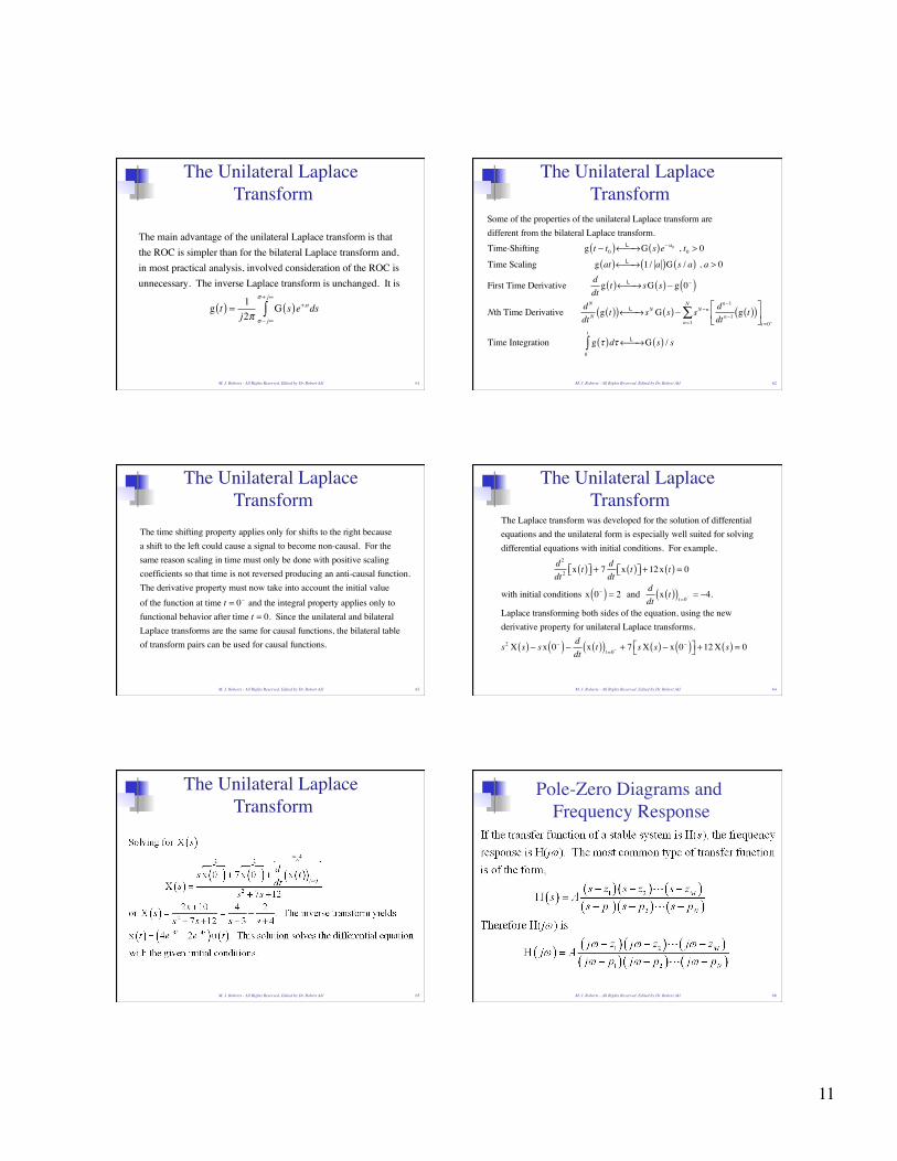
The main advantage of the unilateral Laplace transform is that the ROC is simpler than for the bilateral Laplace transform and,in most practical analysis, involved consideration of the ROC isunnecessary. The inverse Laplace transform is unchanged. It is
g t( ) = 1j2π
G s( )e+ stdsσ − j∞
σ + j∞
∫
M. J. Roberts - All Rights Reserved. Edited by Dr. Robert Akl 61
The Unilateral Laplace Transform
Some of the properties of the unilateral Laplace transform aredifferent from the bilateral Laplace transform.
Time-Shifting g t − t0( ) L← →⎯ G s( )e− st0 , t0 > 0
Time Scaling g at( ) L← →⎯ 1 / a( )G s / a( ) , a > 0
First Time Derivative ddt
g t( ) L← →⎯ sG s( ) − g 0−( )
Nth Time Derivative dN
dt Ng t( )( ) L← →⎯ sN G s( ) − sN −n dn−1
dt n−1 g t( )( )⎡
⎣⎢
⎤
⎦⎥t=0−n=1
N
∑
Time Integration g τ( )dτ0−
t
∫ L← →⎯ G s( ) / s
M. J. Roberts - All Rights Reserved. Edited by Dr. Robert Akl 62
The Unilateral Laplace Transform
The time shifting property applies only for shifts to the right because a shift to the left could cause a signal to become non-causal. For thesame reason scaling in time must only be done with positive scalingcoefficients so that time is not reversed producing an anti-causal function.The derivative property must now take into account the initial valueof the function at time t = 0− and the integral property applies only tofunctional behavior after time t = 0. Since the unilateral and bilateralLaplace transforms are the same for causal functions, the bilateral tableof transform pairs can be used for causal functions.
M. J. Roberts - All Rights Reserved. Edited by Dr. Robert Akl 63
The Unilateral Laplace Transform
The Laplace transform was developed for the solution of differentialequations and the unilateral form is especially well suited for solvingdifferential equations with initial conditions. For example,
d2
dt 2 x t( )⎡⎣ ⎤⎦ + 7 ddt
x t( )⎡⎣ ⎤⎦ +12x t( ) = 0
with initial conditions x 0−( ) = 2 and ddt
x t( )( )t=0− = −4.
Laplace transforming both sides of the equation, using the new derivative property for unilateral Laplace transforms,
s2 X s( ) − sx 0−( ) − ddt
x t( )( )t=0− + 7 sX s( ) − x 0−( )⎡⎣ ⎤⎦ +12 X s( ) = 0
M. J. Roberts - All Rights Reserved. Edited by Dr. Robert Akl 64
The Unilateral Laplace Transform
M. J. Roberts - All Rights Reserved. Edited by Dr. Robert Akl 65
Pole-Zero Diagrams and Frequency Response
M. J. Roberts - All Rights Reserved. Edited by Dr. Robert Akl 66
12
Pole-Zero Diagrams and Frequency Response
M. J. Roberts - All Rights Reserved. Edited by Dr. Robert Akl 67
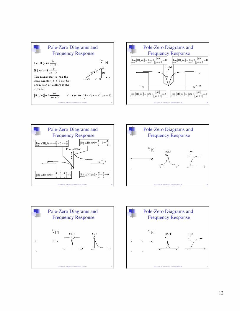
Pole-Zero Diagrams and Frequency Response
limω→0+
H jω( ) = limω→0+
3jω
jω + 3= 0lim
ω→0−H jω( ) = lim
ω→0−3
jωjω + 3
= 0
limω→+∞
H jω( ) = limω→+∞
3jω
jω + 3= 3lim
ω→−∞H jω( ) = lim
ω→−∞3
jωjω + 3
= 3
M. J. Roberts - All Rights Reserved. Edited by Dr. Robert Akl 68
Pole-Zero Diagrams and Frequency Response
limω→0+H jω( ) = π
2− 0 = π
2 limω→0−H jω( ) = − π
2− 0 = − π
2
limω→−∞H jω( ) = − π
2− − π
2⎛⎝⎜
⎞⎠⎟ = 0
limω→+∞H jω( ) = π
2− π2= 0
M. J. Roberts - All Rights Reserved. Edited by Dr. Robert Akl 69
Pole-Zero Diagrams and Frequency Response
M. J. Roberts - All Rights Reserved. Edited by Dr. Robert Akl 70
Pole-Zero Diagrams and Frequency Response
M. J. Roberts - All Rights Reserved. Edited by Dr. Robert Akl 71
Pole-Zero Diagrams and Frequency Response
M. J. Roberts - All Rights Reserved. Edited by Dr. Robert Akl 72
13
Pole-Zero Diagrams and Frequency Response
M. J. Roberts - All Rights Reserved. Edited by Dr. Robert Akl 73
Pole-Zero Diagrams and Frequency Response
M. J. Roberts - All Rights Reserved. Edited by Dr. Robert Akl 74
Pole-Zero Diagrams and Frequency Response
M. J. Roberts - All Rights Reserved. Edited by Dr. Robert Akl 75
Pole-Zero Diagrams and Frequency Response
M. J. Roberts - All Rights Reserved. Edited by Dr. Robert Akl 76
Pole-Zero Diagrams and Frequency Response
M. J. Roberts - All Rights Reserved. Edited by Dr. Robert Akl 77