Generative Moment Matching Networks

Yujia Li1 YUJIALI@CS.TORONTO.EDUKevin Swersky1 KSWERSKY@CS.TORONTO.EDURichard Zemel1,2 ZEMEL@CS.TORONTO.EDU1Department of Computer Science, University of Toronto, Toronto, ON, CANADA2Canadian Institute for Advanced Research, Toronto, ON, CANADA

AbstractWe consider the problem of learning deep gener-ative models from data. We formulate a methodthat generates an independent sample via a sin-gle feedforward pass through a multilayer per-ceptron, as in the recently proposed generativeadversarial networks (Goodfellow et al., 2014).Training a generative adversarial network, how-ever, requires careful optimization of a difficultminimax program. Instead, we utilize a tech-nique from statistical hypothesis testing knownas maximum mean discrepancy (MMD), whichleads to a simple objective that can be interpretedas matching all orders of statistics between adataset and samples from the model, and can betrained by backpropagation. We further boostthe performance of this approach by combiningour generative network with an auto-encoder net-work, using MMD to learn to generate codes thatcan then be decoded to produce samples. Weshow that the combination of these techniquesyields excellent generative models compared tobaseline approaches as measured on MNIST andthe Toronto Face Database.

1. IntroductionThe most visible successes in the area of deep learning havecome from the application of deep models to supervisedlearning tasks. Models such as convolutional neural net-works (CNNs), and long short term memory (LSTM) net-works are now achieving impressive results on a number oftasks such as object recognition (Krizhevsky et al., 2012;Sermanet et al., 2014; Szegedy et al., 2014), speech recog-nition (Graves & Jaitly, 2014; Hinton et al., 2012a), imagecaption generation (Vinyals et al., 2014; Fang et al., 2014;

Proceedings of the 32nd International Conference on MachineLearning, Lille, France, 2015. JMLR: W&CP volume 37. Copy-right 2015 by the author(s).

Kiros et al., 2014), machine translation (Cho et al., 2014;Sutskever et al., 2014), and more. Despite their successes,one of the main bottlenecks of the supervised approach isthe difficulty in obtaining enough data to learn abstract fea-tures that capture the rich structure of the data. It is wellrecognized that a promising avenue is to use unsupervisedlearning on unlabelled data, which is far more plentiful andcheaper to obtain.

A long-standing and inherent problem in unsupervisedlearning is defining a good method for evaluation. Gen-erative models offer the ability to evaluate generalizationin the data space, which can also be qualitatively assessed.In this work we propose a generative model for unsuper-vised learning that we call generative moment matchingnetworks (GMMNs). GMMNs are generative neural net-works that begin with a simple prior from which it is easyto draw samples. These are propagated deterministicallythrough the hidden layers of the network and the output isa sample from the model. Thus, with GMMNs it is easyto quickly draw independent random samples, as opposedto expensive MCMC procedures that are necessary in othermodels such as Boltzmann machines (Ackley et al., 1985;Hinton, 2002; Salakhutdinov & Hinton, 2009). The struc-ture of a GMMN is most analogous to the recently pro-posed generative adversarial networks (GANs) (Goodfel-low et al., 2014), however unlike GANs, whose training in-volves a difficult minimax optimization problem, GMMNsare comparatively simple; they are trained to minimize astraightforward loss function using backpropagation.

The key idea behind GMMNs is the use of a statistical hy-pothesis testing framework called maximum mean discrep-ancy (Gretton et al., 2007). Training a GMMN to mini-mize this discrepancy can be interpreted as matching allmoments of the model distribution to the empirical data dis-tribution. Using the kernel trick, MMD can be representedas a simple loss function that we use as the core trainingobjective for GMMNs. Using minibatch stochastic gradi-ent descent, training can be kept efficient, even with largedatasets.

Generative Moment Matching Networks

As a second contribution, we show how GMMNs can beused to bootstrap auto-encoder networks in order to fur-ther improve the generative process. The idea behind thisapproach is to train an auto-encoder network and then ap-ply a GMMN to the code space of the auto-encoder. Thisallows us to leverage the rich representations learned byauto-encoder models as the basis for comparing data andmodel distributions. To generate samples in the originaldata space, we simply sample a code from the GMMN andthen use the decoder of the auto-encoder network.

Our experiments show that this relatively simple, yet veryflexible framework is effective at producing good gener-ative models in an efficient manner. On MNIST and theToronto Face Dataset (TFD) we demonstrate improved re-sults over comparable baselines, including GANs. Sourcecode for training GMMNs is available at https://github.com/yujiali/gmmn.

2. Maximum Mean DiscrepancySuppose we are given two sets of samples X = {xi}Ni=1

and Y = {yj}Mj=1 and are asked whether the generatingdistributions PX = PY . Maximum mean discrepancy isa frequentist estimator for answering this question, alsoknown as the two sample test (Gretton et al., 2007; 2012a).The idea is simple: compare statistics between the twodatasets and if they are similar then the samples are likelyto come from the same distribution.

Formally, the following MMD measure computes the meansquared difference of the statistics of the two sets of sam-ples.

LMMD2 =

∥∥∥∥∥∥ 1

N

N∑i=1

φ(xi)−1

M

M∑j=1

φ(yj)

∥∥∥∥∥∥2

(1)

=1

N2

N∑i=1

N∑i′=1

φ(xi)>φ(xi′)−

2

NM

N∑i=1

M∑j=1

φ(xi)>φ(yj)

+1

M2

M∑j=1

M∑j′=1

φ(yj)>φ(yj′) (2)

Taking φ to be the identity function leads to matching thesample mean, and other choices of φ can be used to matchhigher order moments.

Written in this form, each term in Equation (2) only in-volves inner products between the φ vectors, and thereforethe kernel trick can be applied.

LMMD2 =1

N2

N∑i=1

N∑i′=1

k(xi, xi′)−2

NM

N∑i=1

M∑j=1

k(xi, yj)

+1

M2

M∑j=1

M∑j′=1

k(yj , yj′) (3)

The kernel trick implicitly lifts the sample vectors intoan infinite dimensional feature space. When this featurespace corresponds to a universal reproducing kernel Hilbertspace, it is shown that asymptotically, MMD is 0 if and onlyif PX = PY (Gretton et al., 2007; 2012a).

For universal kernels like the Gaussian kernel, defined ask(x, x′) = exp(− 1

2σ |x − x′|2), where σ is the bandwidth

parameter, we can use a Taylor expansion to get an explicitfeature map φ that contains an infinite number of terms andcovers all orders of statistics. Minimizing MMD under thisfeature expansion is then equivalent to minimizing a dis-tance between all moments of the two distributions.

3. Related WorkIn this work we focus on generative models due to theirability to capture the salient properties and structure ofdata. Deep generative models are particularly appealingbecause they are capable of learning a latent manifold onwhich the data has high density. Learning this manifoldallows smooth variations in the latent space to result innon-trivial transformations in the original space, effectivelytraversing between high density modes through low densityareas (Bengio et al., 2013a). They are also capable of disen-tangling factors of variation, which means that each latentvariable can become responsible for modelling a single,complex transformation in the original space that wouldotherwise involve many variables (Bengio et al., 2013a).Even if we restrict ourselves to the field of deep learning,there are a vast array of approaches to generative mod-elling. Below, we outline some of these methods.

One popular class of generative models used in deeplearning are undirected graphical models, such as Boltz-mann machines (Ackley et al., 1985), restricted Boltzmannmachines (Hinton, 2002), and deep Boltzmann machines(Salakhutdinov & Hinton, 2009). These models are nor-malized by a typically intractable partition function, mak-ing training, evaluation, and sampling extremely difficult,usually requiring expensive Markov-chain Monte Carlo(MCMC) procedures.

Next there is the class of fully visible directed models suchas fully visible sigmoid belief networks (Neal, 1992) andthe neural autoregressive distribution estimator (Larochelle& Murray, 2011). These admit efficient log-likelihood cal-culation, gradient-based learning and efficient sampling,but require that an ordering be imposed on the observ-able variables, which can be unnatural for domains suchas images and cannot take advantage of parallel computingmethods due to their sequential nature.

More related to our own work, there is a line of research de-voted to recovering density models from auto-encoder net-works using MCMC procedures (Rifai et al., 2012; Bengio

Generative Moment Matching Networks

et al., 2013b; 2014). These attempt to use contraction op-erators, or denoising criteria in order to generate a Markovchain by repeated perturbations during the encoding phase,followed by decoding.

Also related to our own work is the class of deep, varia-tional networks (Rezende et al., 2014; Kingma & Welling,2014; Mnih & Gregor, 2014). These are also deep, directedgenerative models, however they make use of an additionalneural network that is designed to approximate the poste-rior over the latent variables. Training is carried out via avariational lower bound on the log-likelihood of the modeldistribution. These models are trained using stochastic gra-dient descent, however they either require that the latentrepresentation is continuous (Kingma & Welling, 2014), orrequire many secondary networks to sufficiently reduce thevariance of gradient estimates in order to produce a suffi-ciently good learning signal (Mnih & Gregor, 2014).

Finally there is some early work that proposed the ideaof using feed-forward neural networks to learn generativemodels. MacKay (1995) proposed a model that is closelyrelated to ours, which also used a feed-forward networkto map the prior samples to the data space. However, in-stead of directly outputing samples, an extra distributionis associated with the output. Sampling was used exten-sively for learning and inference in this model. Magdon-Ismail & Atiya (1998) proposed to use a neural networkto learn a transformation from the data space to anotherspace where the transformed data points are uniformly dis-tributed. This transformation network then learns the cu-mulative density function. In recent independent work,Dziugaite et al. (2015) proposed an idea very similar toour’s, which trains a feed-forward neural network gener-ative model by optimizing MMD. A more thorough com-parison with their approach is left to future work.

4. Generative Moment Matching Networks4.1. Data Space Networks

The high-level idea of the GMMN is to use a neural net-work to learn a deterministic mapping from samples of asimple, easy to sample distribution, to samples from thedata distribution. The architecture of the generative net-work is exactly the same as a generative adversarial net-work (Goodfellow et al., 2014). However, we propose totrain the network by simply minimizing the MMD crite-rion, avoiding the hard minimax objective function used ingenerative adversarial network training.

More specifically, in the generative network we have astochastic hidden layer h ∈ RH with H hidden units atthe top with a prior uniform distribution on each unit inde-

Uniform Prior

ReLU

ReLU

ReLU

Sigmoid

GMMN

Sample G

eneration

ReLU

Uniform Prior

Sigmoid Sigmoid

Sigmoid

Input Data Reconstruction

Auto-Encoder

GMMN

Dropout

Dropout

Sample G

eneration

ReLU

ReLU

ReLU

Sigmoid

ReLU

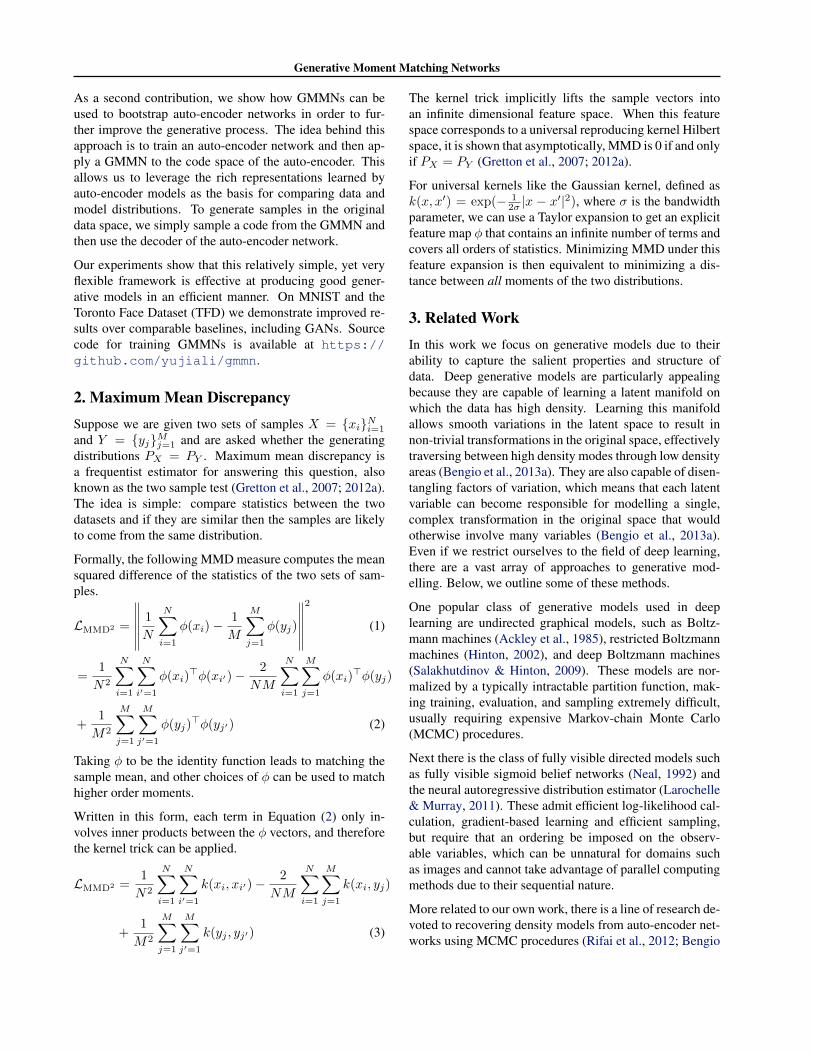
(a) GMMN (b) GMMN+AE

Figure 1. Example architectures of our generative moment match-ing networks. (a) GMMN used in the input data space. (b)GMMN used in the code space of an auto-encoder.

pendently,

p(h) =

H∏j=1

U(hj) (4)

Here U(h) = 12I[−1 ≤ h ≤ 1] is a uniform distribu-

tion in [−1, 1], where I[.] is an indicator function. Otherchoices for the prior are also possible, as long as it is asimple enough distribution from which we can easily drawsamples.

The h vector is then passed through the neural network anddeterministically mapped to a vector x ∈ RD in the D di-mensional data space.

x = f(h;w) (5)

f is the neural network mapping function, which can con-tain multiple layers of nonlinearities, and w represents theparameters of the neural network. One example architec-ture for f is illustrated in Figure 1(a), which has 4 inter-mediate ReLU (Nair & Hinton, 2010) nonlinear layers andone logistic sigmoid output layer.

The prior p(h) and the mapping f(h;w) jointly defines adistribution p(x) in the data space. To generate a samplex ∼ p(x) we only need to sample from the uniform priorp(h) and then pass the sample h through the neural net toget x = f(h;w).

Goodfellow et al. (2014) proposed to train this network byusing an extra discriminative network, which tries to distin-guish between model samples and data samples. The gen-erative network is then trained to counteract this in orderto make the samples indistinguishable to the discriminativenetwork. The gradient of this objective can be backprop-agated through the generative network. However, becauseof the minimax nature of the formulation, it is easy to get

Generative Moment Matching Networks

stuck at a local optimum. So the training of generative net-work and the discriminative network must be interleavedand carefully scheduled. By contrast, our learning algo-rithm simply involves minimizing the MMD objective.

Assume we have a dataset of training examples xd1, ...,xdN

(d for data), and a set of samples generated from our modelxs1, ...,x

sM (s for samples). The MMD objective LMMD2 is

differentiable when the kernel is differentiable. For exam-ple for Gaussian kernels k(x,y) = exp

(− 1

2σ ||x− y||2),

the gradient of xsip has a simple form

∂LMMD2

∂xsip=

2

M2

M∑j=1

1

σk(xsi ,x

sj)(x

sjp − xsip)

− 2

MN

N∑j=1

1

σk(xsi ,x

dj )(x

djp − xsip) (6)

This gradient can then be backpropagated through the gen-erative network to update the parameters w.

4.2. Auto-Encoder Code Space Networks

Real-world data can be complicated and high-dimensional,which is one reason why generative modelling is such adifficult task. Auto-encoders, on the other hand, are de-signed to solve an arguably simpler task of reconstruction.If trained properly, auto-encoder models can be very goodat representing data in a code space that captures enoughstatistical information that the data can be reliably recon-structed.

The code space of an auto-encoder has several advantagesfor creating a generative model. The first is that the dimen-sionality can be explicitly controlled. Visual data, for ex-ample, while represented in a high dimensional space, of-ten exists on a low-dimensional manifold. This is beneficialfor a statistical estimator like MMD because the amount ofdata required to produce a reliable estimate grows with thedimensionality of the data (Ramdas et al., 2015). The sec-ond advantage is that each dimension of the code space canend up representing complex variations in the original dataspace. This concept is referred to in the literature as disen-tangling factors of variation (Bengio et al., 2013a).

For these reasons, we propose to bootstrap auto-encodermodels with a GMMN to create what we refer to as theGMMN+AE model. These operate by first learning anauto-encoder and producing code representations of thedata, then freezing the auto-encoder weights and learninga GMMN to minimize MMD between generated codes anddata codes. A visualization of this model is given in Figure1(b).

Our method for training a GMMN+AE proceeds as fol-lows:

1. Greedy layer-wise pretraining of the auto-encoder(Bengio et al., 2007).

2. Fine-tune the auto-encoder.

3. Train a GMMN to model the code layer distributionusing an MMD objective on the final encoding layer.

We found that adding dropout to the encoding layers can bebeneficial in terms of creating a smooth manifold in codespace. This is analogous to the motivation behind contrac-tive and denoising auto-encoders (Rifai et al., 2011; Vin-cent et al., 2008).

4.3. Practical Considerations

Here we outline some design choices that we have found toimprove the peformance of GMMNs.

Bandwidth Parameter. The bandwidth parameter in thekernel plays a crucial role in determining the statistical ef-ficiency of MMD, and optimally setting it is an open prob-lem. A good heuristic is to perform a line search to obtainthe bandwidth that produces the maximal distance (Sripe-rumbudur et al., 2009), other more advanced heuristics arealso available (Gretton et al., 2012b). As a simpler approx-imation, for most of our experiments we use a mixture ofK kernels spanning multiple ranges. That is, we choose thekernel to be:

k(x, x′) =

K∑q=1

kσq (x, x′) (7)

where kσq is a Gaussian kernel with bandwidth parameterσq . We found that choosing simple values for these such as1, 5, 10, etc. and using a mixture of 5 or more was sufficientto obtain good results. The weighting of different kernelscan be further tuned to achieve better results, but we keptthem equally weighted for simplicity.

Square Root Loss. In practice, we have found that betterresults can be obtained by optimizing LMMD =

√LMMD2 .

This loss can be important for driving the difference be-tween the two distributions as close to 0 as possible. Com-pared to LMMD2 which flattens out when its value getsclose to 0, LMMD behaves much better for small LMMD

values. Alternatively, this can be understood by writingdown the gradient of LMMD with respect to w

∂LMMD

∂w=

1

2√LMMD2

∂LMMD2

∂w(8)

The 1/(2√LMMD2) term automatically adapts the effec-

tive learning rate. This is especially beneficial when bothLMMD2 and ∂LMMD2

∂w become small, where this extra factorcan help by maintaining larger gradients.

Generative Moment Matching Networks

Algorithm 1: GMMN minibatch training

Input : Dataset {xd1, ...,xdN}, prior p(h), networkf(h;w) with initial parameter w(0)

Output: Learned parameter w∗

1 while Stopping criterion not met do2 Get a minibatch of data Xd ← {xdi1 , ...,x

dib}

3 Get a new set of samples Xs ← {xs1, ...,xsb}4 Compute gradient ∂LMMD

∂w on Xd and Xs

5 Take a gradient step to update w

6 end

Minibatch Training. One of the issues with MMD is thatthe usage of kernels means that the computation of the ob-jective scales quadratically with the amount of data. Inthe literature there have been several alternative estimatorsdesigned to overcome this (Gretton et al., 2012a). In ourcase, we found that it was sufficient to optimize MMD us-ing minibatch optimization. In each weight update, a smallsubset of data is chosen, and an equal number of samplesare drawn from the GMMN. Within a minibatch, MMDis applied as usual. As we are using exact samples fromthe model and the data distribution, the minibatch MMD isstill a good estimator of the population MMD. We foundthis approach to be both fast and effective. The minibatchtraining algorithm for GMMN is shown in Algorithm 1.

5. ExperimentsWe trained GMMNs on two benchmark datasets: MNIST(LeCun et al., 1998) and the Toronto Face Dataset (TFD)(Susskind et al., 2010). For MNIST, we used the standardtest set of 10,000 images, and split out 5000 from the stan-dard 60,000 training images for validation. The remaining55,000 were used for training. For TFD, we used the sametraining and test sets and fold splits as used by (Goodfellowet al., 2014), but split out a small set of the training data andused it as the validation set. For both datasets, rescaling theimages to have pixel intensities between 0 and 1 is the onlypreprocessing step we did.

On both datasets, we trained the GMMN network in boththe input data space and the code space of an auto-encoder.For all the networks we used in this section, a uniformdistribution in [−1, 1]H was used as the prior for theH-dimensional stochastic hidden layer at the top of theGMMN, which was followed by 4 ReLU layers, and theoutput was a layer of logistic sigmoid units. The auto-encoder we used for MNIST had 4 layers, 2 for the encoderand 2 for the decoder. For TFD the auto-encoder had 6 lay-ers in total, 3 for the encoder and 3 for the decoder. For bothauto-encoders the encoder and the decoder had mirroredarchitectures. All layers in the auto-encoder network used

sigmoid nonlinearities, which also guaranteed that the codespace dimensions lay in [0, 1], so that they could match theGMMN outputs. The network architectures for MNIST areshown in Figure 1.

The auto-encoders were trained separately from theGMMN. Cross entropy was used as the reconstruction loss.We first did standard layer-wise pretraining, then fine-tunedall layers jointly. Dropout (Hinton et al., 2012b) was usedon the encoder layers. After training the auto-encoder, wefixed it and passed the input data through the encoder to getthe corresponding codes. The GMMN network was thentrained in this code space to match the statistics of gen-erated codes to the statistics of codes from data examples.When generating samples, the generated codes were passedthrough the decoder to get samples in the input data space.

For all experiments in this section the GMMN networkswere trained with minibatches of size 1000, for each mini-batch we generated a set of 1000 samples from the net-work. The loss and gradient were computed from these2000 points. We used the square root loss function LMMD

throughout.

Evaluation of our model is not straight-forward, as we donot have an explicit form for the probability density func-tion, it is not easy to compute the log-likelihood of data.However, sampling from our model is easy. We thereforefollowed the same evaluation protocol used in related mod-els (Bengio et al., 2013a), (Bengio et al., 2014), and (Good-fellow et al., 2014). A Gaussian Parzen window (kerneldensity estimator) was fit to 10,000 samples generated fromthe model. The likelihood of the test data was then com-puted under this distribution. The scale parameter of theGaussians was selected using a grid search in a fixed rangeusing the validation set.

The hyperparameters of the networks, including the learn-ing rate and momentum for both auto-encoder and GMMNtraining, dropout rate for the auto-encoder, and numberof hidden units on each layer of both auto-encoder andGMMN, were tuned using Bayesian optimization (Snoeket al., 2012; 2014)1 to optimize the validation set likelihoodunder the Gaussian Parzen window density estimation.

The log-likelihood of the test set for both datasets areshown in Table 1. The GMMN is competitive with otherapproaches, while the GMMN+AE significantly outper-forms the other models. This shows that despite being rel-atively simple, MMD, especially when combined with aneffective decoder, is a powerful objective for training goodgenerative models.

Some samples generated from the GMMN models are

1We used the service provided by https://www.whetlab.com

Generative Moment Matching Networks

(e) GMMN nearest neighbors for MNIST samples

(a) GMMN MNIST samples (b) GMMN TFD samples (f) GMMN+AE nearest neighbors for MNIST samples

(g) GMMN nearest neighbors for TFD samples

(c) GMMN+AE MNIST samples (d) GMMN+AE TFD samples (h) GMMN+AE nearest neighbors for TFD samples

Figure 2. Independent samples and their nearest neighbors in the training set for the GMMN+AE model trained on MNIST and TFDdatasets. For (e)(f)(g) and (h) the top row are the samples from the model and the bottom row are the corresponding nearest neighborsfrom the training set measured by Euclidean distance.

Model MNIST TFDDBN 138 ± 2 1909 ± 66

Stacked CAE 121 ± 1.6 2110 ± 50Deep GSN 214 ± 1.1 1890 ± 29

Adversarial nets 225 ± 2 2057 ± 26GMMN 147 ± 2 2085 ± 25

GMMN+AE 282 ± 2 2204 ± 20

Table 1. Log-likelihood of the test sets under different models.The baselines are Deep Belief Net (DBN) and Stacked Contrac-tive Auto-Encoder (Stacked CAE) from (Bengio et al., 2013a),Deep Generative Stochastic Network (Deep GSN) from (Bengioet al., 2014) and Adversarial nets (GANs) from (Goodfellow et al.,2014).

shown in Figure 2(a-d). The GMMN+AE produces themost visually appealing samples, which are reflected in itsParzen window log-likelihood estimates. The likely expla-nation is that any perturbations in the code space corre-spond to smooth transformations along the manifold of thedata space. In that sense, the decoder is able to “correct”noise in the code space.

To determine whether the models learned to merely copythe data, we follow the example of (Goodfellow et al.,2014) and visualize the nearest neighbour of several sam-ples in terms of Euclidean pixel-wise distance in Figure2(e-h). By this metric, it appears as though the samples

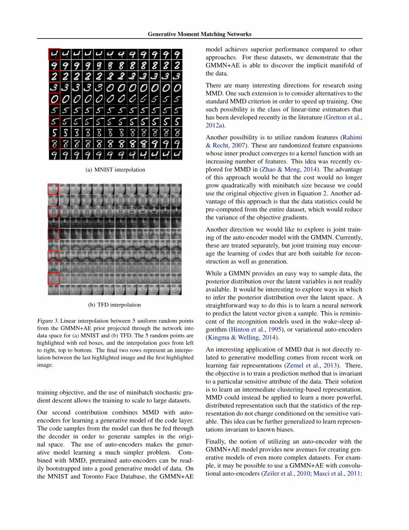
are not merely data examples.One of the interesting aspects of a deep generative modelsuch as the GMMN is that it is possible to directly ex-plore the data manifold. Using the GMMN+AE model,we randomly sampled 5 points in the uniform space andshow their corresponding data space projections in Fig-ure 3. These points are highlighted by red boxes. Fromleft to right, top to bottom we linearly interpolate betweenthese points in the uniform space and show their corre-sponding projections in data space. The manifold is smoothfor the most part, and almost all of the projections cor-respond to realistic looking data. For TFD in particular,these transformations involve complex attributes, such asthe changing of pose, expression, lighting, gender, and fa-cial hair. More results can be found at http://www.cs.toronto.edu/˜yujiali/proj/gmmn.html.

6. Conclusion and Future WorkIn this paper we provide a simple and effective frameworkfor training deep generative models called generative mo-ment matching networks. Our approach is based off of opti-mizing maximum mean discrepancy so that samples gener-ated from the model are indistinguishable from data exam-ples in terms of their moment statistics. As is standard withMMD, the use of the kernel trick allows a GMMN to avoidexplicitly computing these moments, resulting in a simple

Generative Moment Matching Networks

(a) MNIST interpolation

(b) TFD interpolation

Figure 3. Linear interpolation between 5 uniform random pointsfrom the GMMN+AE prior projected through the network intodata space for (a) MNIST and (b) TFD. The 5 random points arehighlighted with red boxes, and the interpolation goes from leftto right, top to bottom. The final two rows represent an interpo-lation between the last highlighted image and the first highlightedimage.

training objective, and the use of minibatch stochastic gra-dient descent allows the training to scale to large datasets.

Our second contribution combines MMD with auto-encoders for learning a generative model of the code layer.The code samples from the model can then be fed throughthe decoder in order to generate samples in the origi-nal space. The use of auto-encoders makes the gener-ative model learning a much simpler problem. Com-bined with MMD, pretrained auto-encoders can be read-ily bootstrapped into a good generative model of data. Onthe MNIST and Toronto Face Database, the GMMN+AE

model achieves superior performance compared to otherapproaches. For these datasets, we demonstrate that theGMMN+AE is able to discover the implicit manifold ofthe data.

There are many interesting directions for research usingMMD. One such extension is to consider alternatives to thestandard MMD criterion in order to speed up training. Onesuch possibility is the class of linear-time estimators thathas been developed recently in the literature (Gretton et al.,2012a).

Another possibility is to utilize random features (Rahimi& Recht, 2007). These are randomized feature expansionswhose inner product converges to a kernel function with anincreasing number of features. This idea was recently ex-plored for MMD in (Zhao & Meng, 2014). The advantageof this approach would be that the cost would no longergrow quadratically with minibatch size because we coulduse the original objective given in Equation 2. Another ad-vantage of this approach is that the data statistics could bepre-computed from the entire dataset, which would reducethe variance of the objective gradients.

Another direction we would like to explore is joint train-ing of the auto-encoder model with the GMMN. Currently,these are treated separately, but joint training may encour-age the learning of codes that are both suitable for recon-struction as well as generation.

While a GMMN provides an easy way to sample data, theposterior distribution over the latent variables is not readilyavailable. It would be interesting to explore ways in whichto infer the posterior distribution over the latent space. Astraightforward way to do this is to learn a neural networkto predict the latent vector given a sample. This is reminis-cent of the recognition models used in the wake-sleep al-gorithm (Hinton et al., 1995), or variational auto-encoders(Kingma & Welling, 2014).

An interesting application of MMD that is not directly re-lated to generative modelling comes from recent work onlearning fair representations (Zemel et al., 2013). There,the objective is to train a prediction method that is invariantto a particular sensitive attribute of the data. Their solutionis to learn an intermediate clustering-based representation.MMD could instead be applied to learn a more powerful,distributed representation such that the statistics of the rep-resentation do not change conditioned on the sensitive vari-able. This idea can be further generalized to learn represen-tations invariant to known biases.

Finally, the notion of utilizing an auto-encoder with theGMMN+AE model provides new avenues for creating gen-erative models of even more complex datasets. For exam-ple, it may be possible to use a GMMN+AE with convolu-tional auto-encoders (Zeiler et al., 2010; Masci et al., 2011;

Generative Moment Matching Networks

Makhzani & Frey, 2014) in order to create generative mod-els of high resolution color images.

AcknowledgementsWe thank David Warde-Farley for helpful clarifications re-garding (Goodfellow et al., 2014), and Charlie Tang forproviding relevant references. We thank CIFAR, NSERC,and Google for research funding.

ReferencesAckley, David H, Hinton, Geoffrey E, and Sejnowski, Ter-

rence J. A learning algorithm for boltzmann machines.Cognitive science, 9(1):147–169, 1985.

Bengio, Yoshua, Lamblin, Pascal, Popovici, Dan,Larochelle, Hugo, et al. Greedy layer-wise training ofdeep networks. In Advances in Neural Information Pro-cessing Systems (NIPS), 2007.

Bengio, Yoshua, Mesnil, Gregoire, Dauphin, Yann, andRifai, Salah. Better mixing via deep representations.In Proceedings of the 28th International Conference onMachine Learning (ICML), 2013a.

Bengio, Yoshua, Yao, Li, Alain, Guillaume, and Vincent,Pascal. Generalized denoising auto-encoders as gener-ative models. In Advances in Neural Information Pro-cessing Systems, pp. 899–907, 2013b.

Bengio, Yoshua, Thibodeau-Laufer, Eric, Alain, Guil-laume, and Yosinski, Jason. Deep generative stochas-tic networks trainable by backprop. In Proceedings ofthe 29th International Conference on Machine Learning(ICML), 2014.

Cho, Kyunghyun, van Merrienboer, Bart, Gulcehre, Caglar,Bougares, Fethi, Schwenk, Holger, and Bengio, Yoshua.Learning phrase representations using rnn encoder-decoder for statistical machine translation. In Confer-ence on Empirical Methods in Natural Language Pro-cessing (EMNLP), 2014.

Dziugaite, Gintare Karolina, Roy, Daniel M., and Ghahra-mani, Zoubin. Training generative neural networks viamaximum mean discrepancy optimization. In Uncer-tainty in Artificial Intelligence (UAI), 2015.

Fang, Hao, Gupta, Saurabh, Iandola, Forrest, Srivas-tava, Rupesh, Deng, Li, Dollar, Piotr, Gao, Jianfeng,He, Xiaodong, Mitchell, Margaret, Platt, John, Zitnick,C. Lawrence, and Zweig, Geoffrey. From captions to vi-sual concepts and back. arXiv preprint arXiv:1411.4952,2014.

Goodfellow, Ian, Pouget-Abadie, Jean, Mirza, Mehdi, Xu,Bing, Warde-Farley, David, Ozair, Sherjil, Courville,Aaron, and Bengio, Yoshua. Generative adversarial nets.In Advances in Neural Information Processing Systems,pp. 2672–2680, 2014.

Graves, Alex and Jaitly, Navdeep. Towards end-to-endspeech recognition with recurrent neural networks. InProceedings of the 31st International Conference on Ma-chine Learning (ICML-14), pp. 1764–1772, 2014.

Gretton, Arthur, Borgwardt, Karsten M, Rasch, Malte,Scholkopf, Bernhard, and Smola, Alex J. A kernelmethod for the two-sample-problem. In Advances inNeural Information Processing Systems (NIPS), 2007.

Gretton, Arthur, Borgwardt, Karsten M, Rasch, Malte J,Scholkopf, Bernhard, and Smola, Alexander. A kerneltwo-sample test. The Journal of Machine Learning Re-search, 13(1):723–773, 2012a.

Gretton, Arthur, Sejdinovic, Dino, Strathmann, Heiko, Bal-akrishnan, Sivaraman, Pontil, Massimiliano, Fukumizu,Kenji, and Sriperumbudur, Bharath K. Optimal kernelchoice for large-scale two-sample tests. In Advances inNeural Information Processing Systems, pp. 1205–1213,2012b.

Hinton, Geoffrey E. Training products of experts by mini-mizing contrastive divergence. Neural Computation, 14(8):1771–1800, 2002.

Hinton, Geoffrey E, Dayan, Peter, Frey, Brendan J, andNeal, Radford M. The “wake-sleep” algorithm for un-supervised neural networks. Science, 268(5214):1158–1161, 1995.

Hinton, Geoffrey E., Deng, Li, Yu, Dong, Dahl, George E.,Mohamed, Abdel-rahman, Jaitly, Navdeep, Senior, An-drew, Vanhoucke, Vincent, Nguyen, Patrick, Sainath,Tara N., and Kingsbury, Brian. Deep neural networksfor acoustic modeling in speech recognition: The sharedviews of four research groups. IEEE Signal Process.Mag., 29(6):82–97, 2012a.

Hinton, Geoffrey E, Srivastava, Nitish, Krizhevsky, Alex,Sutskever, Ilya, and Salakhutdinov, Ruslan R. Improvingneural networks by preventing co-adaptation of featuredetectors. arXiv preprint arXiv:1207.0580, 2012b.

Kingma, Diederik P. and Welling, Max. Auto-encodingvariational Bayes. In International Conference onLearning Representations, 2014.

Kiros, Ryan, Salakhutdinov, Ruslan, and Zemel, Richard S.Unifying visual-semantic embeddings with multi-modal neural language models. arXiv preprintarXiv:1411.2539, 2014.

Generative Moment Matching Networks

Krizhevsky, Alex, Sutskever, Ilya, and Hinton, Geoffrey E.Imagenet classification with deep convolutional neuralnetworks. In Advances in Neural Information ProcessingSystems (NIPS), 2012.

Larochelle, Hugo and Murray, Iain. The neural autoregres-sive distribution estimator. In roceedings of the 14thInternational Conference on Artificial Intelligence andStatistics (AISTATS), 2011.

LeCun, Yann, Bottou, Leon, Bengio, Yoshua, and Haffner,Patrick. Gradient-based learning applied to documentrecognition. Proceedings of the IEEE, 86(11):2278–2324, 1998.

MacKay, David JC. Bayesian neural networks and densitynetworks. Nuclear Instruments and Methods in PhysicsResearch Section A: Accelerators, Spectrometers, Detec-tors and Associated Equipment, 354(1):73–80, 1995.

Magdon-Ismail, Malik and Atiya, Amir. Neural networksfor density estimation. In NIPS, pp. 522–528, 1998.

Makhzani, Alireza and Frey, Brendan. A winner-take-allmethod for training sparse convolutional autoencoders.In NIPS Deep Learning Workshop, 2014.

Masci, Jonathan, Meier, Ueli, Ciresan, Dan, and Schmid-huber, Jurgen. Stacked convolutional auto-encoders forhierarchical feature extraction. In Artificial Neural Net-works and Machine Learning–ICANN 2011, pp. 52–59.Springer, 2011.

Mnih, Andriy and Gregor, Karol. Neural variational infer-ence and learning in belief networks. In InternationalConference on Machine Learning, 2014.

Nair, Vinod and Hinton, Geoffrey E. Rectified linear unitsimprove restricted boltzmann machines. In InternationalConference on Machine Learning, pp. 807–814, 2010.

Neal, Radford M. Connectionist learning of belief net-works. Artificial intelligence, 56(1):71–113, 1992.

Rahimi, Ali and Recht, Benjamin. Random features forlarge-scale kernel machines. In Advances in Neural In-formation Processing Systems (NIPS), 2007.

Ramdas, Aaditya, Reddi, Sashank J, Poczos, Barnabas,Singh, Aarti, and Wasserman, Larry. On the decreasingpower of kernel and distance based nonparametric hy-pothesis tests in high dimensions. In The Twenty-NinthAAAI Conference on Artificial Intelligence (AAAI-15),2015.

Rezende, Danilo Jimenez, Mohamed, Shakir, and Wierstra,Daan. Stochastic backpropagation and approximate in-ference in deep generative models. In International Con-ference on Machine Learning, pp. 1278–1286, 2014.

Rifai, Salah, Vincent, Pascal, Muller, Xavier, Glorot,Xavier, and Bengio, Yoshua. Contractive auto-encoders:Explicit invariance during feature extraction. In Pro-ceedings of the 28th International Conference on Ma-chine Learning (ICML-11), pp. 833–840, 2011.

Rifai, Salah, Bengio, Yoshua, Dauphin, Yann, and Vincent,Pascal. A generative process for sampling contractiveauto-encoders. In International Conference on MachineLearning (ICML), 2012.

Salakhutdinov, Ruslan and Hinton, Geoffrey E. Deep boltz-mann machines. In International Conference on Artifi-cial Intelligence and Statistics, 2009.

Sermanet, Pierre, Eigen, David, Zhang, Xiang, Mathieu,Michael, Fergus, Rob, and LeCun, Yann. Overfeat:Integrated recognition, localization and detection usingconvolutional networks. In International Conference onLearning Representations, 2014.

Snoek, Jasper, Larochelle, Hugo, and Adams, Ryan P.Practical Bayesian optimization of machine learning al-gorithms. In Advances in Neural Information ProcessingSystems, 2012.

Snoek, Jasper, Swersky, Kevin, Zemel, Richard S., andAdams, Ryan P. Input warping for bayesian optimizationof non-stationary functions. In International Conferenceon Machine Learning, 2014.

Sriperumbudur, Bharath K, Fukumizu, Kenji, Gretton,Arthur, Lanckriet, Gert RG, and Scholkopf, Bernhard.Kernel choice and classifiability for rkhs embeddings ofprobability distributions. In Advances in Neural Infor-mation Processing Systems, pp. 1750–1758, 2009.

Susskind, Joshua, Anderson, Adam, and Hinton, Geof-frey E. The toronto face dataset. Technical report, De-partment of Computer Science, University of Toronto,2010.

Sutskever, Ilya, Vinyals, Oriol, and Le, Quoc VV. Se-quence to sequence learning with neural networks. InAdvances in Neural Information Processing Systems, pp.3104–3112, 2014.

Szegedy, Christian, Liu, Wei, Jia, Yangqing, Sermanet,Pierre, Reed, Scott, Anguelov, Dragomir, Erhan, Du-mitru, Vanhoucke, Vincent, and Rabinovich, Andrew.Going deeper with convolutions. arXiv preprintarXiv:1409.4842, 2014.

Vincent, Pascal, Larochelle, Hugo, Bengio, Yoshua, andManzagol, Pierre-Antoine. Extracting and composingrobust features with denoising autoencoders. In Proceed-ings of the 25th international conference on Machinelearning, pp. 1096–1103. ACM, 2008.

Generative Moment Matching Networks

Vinyals, Oriol, Toshev, Alexander, Bengio, Samy, and Er-han, Dumitru. Show and tell: A neural image captiongenerator. arXiv preprint arXiv:1411.4555, 2014.

Zeiler, Matthew D, Krishnan, Dilip, Taylor, Graham W, andFergus, Robert. Deconvolutional networks. In ComputerVision and Pattern Recognition, pp. 2528–2535. IEEE,2010.

Zemel, Richard, Wu, Yu, Swersky, Kevin, Pitassi, Toni, andDwork, Cynthia. Learning fair representations. In Inter-national Conference on Machine Learning, pp. 325–333,2013.

Zhao, Ji and Meng, Deyu. Fastmmd: Ensemble of circulardiscrepancy for efficient two-sample test. arXiv preprintarXiv:1405.2664, 2014.