GEOGRAPHICALLY WEIGHTED REGRESSION WORKBOOK …csiss.org/.../2008/PSU/docs/GWR_Workbook_PSU_2008.pdf · GEOGRAPHICALLY WEIGHTED REGRESSION WORKBOOK ... 3.1 Importing a Coverage from

Population Research Institute

GWR WORKSHOP

University Park, PA – 1st - 6th June 2008

GEOGRAPHICALLY WEIGHTED

REGRESSION

WORKBOOK

Martin Charlton

A Stewart Fotheringham

Chris Brunsdon

National Centre for Geocomputation National University of Ireland Maynooth

Maynooth Co. Kildare IRELAND

The first two authors acknowledge generous funding from Science Foundation Ireland which helped

create the National Centre for Geocomputation

i

© The contents of this book are the copyright of the authors and may not be reproduced or used without their permission. This extends to both the software and the data files distributed with the

workbook.

ii

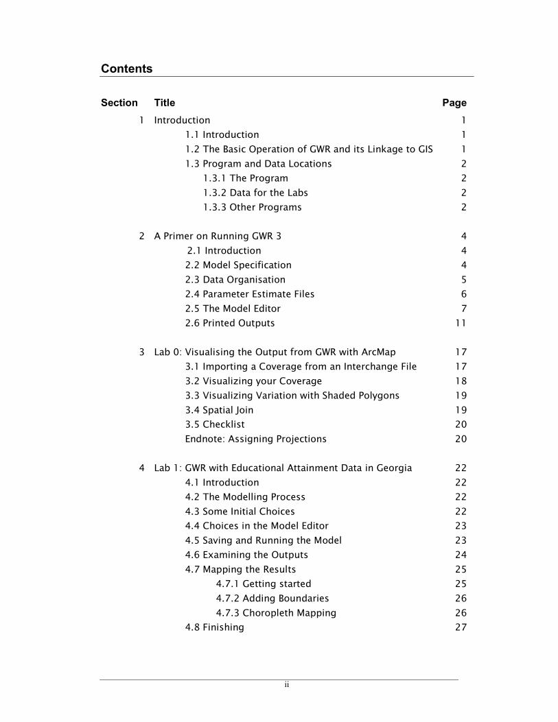
Contents

Section Title Page

1 Introduction 1

1.1 Introduction 1

1.2 The Basic Operation of GWR and its Linkage to GIS 1

1.3 Program and Data Locations 2

1.3.1 The Program 2

1.3.2 Data for the Labs 2

1.3.3 Other Programs 2

2 A Primer on Running GWR 3 4

2.1 Introduction 4

2.2 Model Specification 4

2.3 Data Organisation 5

2.4 Parameter Estimate Files 6

2.5 The Model Editor 7

2.6 Printed Outputs 11

3 Lab 0: Visualising the Output from GWR with ArcMap 17

3.1 Importing a Coverage from an Interchange File 17

3.2 Visualizing your Coverage 18

3.3 Visualizing Variation with Shaded Polygons 19

3.4 Spatial Join 19

3.5 Checklist 20

Endnote: Assigning Projections 20

4 Lab 1: GWR with Educational Attainment Data in Georgia 22

4.1 Introduction 22

4.2 The Modelling Process 22

4.3 Some Initial Choices 22

4.4 Choices in the Model Editor 23

4.5 Saving and Running the Model 23

4.6 Examining the Outputs 24

4.7 Mapping the Results 25

4.7.1 Getting started 25

4.7.2 Adding Boundaries 26

4.7.3 Choropleth Mapping 26

4.8 Finishing 27

iii

5 Lab 2: GWR and House Price Determinants 28

5.1 Introduction 28

5.2 The Data 28

5.3 The Exercise 29

5.4 Modelling House Price Variation 29

5.5 Exploration, then Modelling 29

5.6 Model 1 – Price~Floorspace 31

5.7 Model 2 – Price~Floorspace+Type 33

5.8 Model 3 – Price~Floorspace+Age 35

5.9 Model 4 _ Price ~Floorspace+Type+Age 36

5.10 Points or Surfaces 37

6 Lab 3: GW Poisson Regression with Tokyo Mortality Data 39

6.1 Introduction 39

6.2 Mortality in Tokyo 40

6.3 Setting Up the Model 41

6.4 Examine the Output 41


6.6 Tasks 45

7 Lab 4: Logistic GWR with Landslides in Clearwater, Idaho 46

7.1 Introduction 46

7.2 Landslide Hazard: Clearwater National Forest 47

7.3 Examining the Data 48

7.4 Setting up the Model 49

7.5 Examine the Output 49


7.7 Further Tasks 52

8 Finally 53

Appendix Geographically Weighted Descriptive Statistics 54

8.1 Introduction 54

8.2 Local Statistics 54

8.3 Educational Attainment 55

8.4 GIS Manipulation 56

8.5 Tasks 57

1

1

Introduction

1.1 Introduction

This series of linked labs is designed to introduce you to applying

Geographically Weighted Regression to problems with your spatial data. They

assume a little familiarity with ArcGIS and none with the GWR software.

There are 5 labs as follows:

Lab 0: The Use of ArcGIS

Lab 1: GWR and Educational Attainment Levels in Georgia

Lab 2: GWR and House Price Determinants in Tyne & Wear

Lab 3: Poisson GWR and Mortality Data in Tokyo

Lab 4: Logistic GWR and Educational Attainment Levels in Georgia

The workshops will be lead by Stewart Fotheringham and Martin Charlton

Before explaining each lab in detail (see subsequent chapters of this workbook),

we first describe some basic operational issues with the software package used

in each lab – GWR 3.0. Some of this material is covered in the lectures.

1.2 The Basic Operation of GWR 3.0 and its Linkage to GIS

The following diagram summarises the basic operation of GWR 3.0 and

how its outputs are linked to a GIS.

The user supplies a data file plus ideas on what form of model to calibrate into

the user-friendly GWR Model Editor which is completed in a series of ‘Windows-

2

Gwr30.exe

style’ menus and tick boxes. Unseen to the user, this creates a control file for a

large FORTRAN program which produces two types of output. A Listing File is

written to the screen and an Output File is saved in the user’s workspace. This

latter file contains location-specific parameter estimates and other diagnostics

which can be read into a GIS (along with other spatially referenced data) for

mapping.

1.3 Program and Data Locations

1.3.1 The Program

To run the GWR software you will need to click on the GWR icon which

you will usually find on the Start/Programs menu or on the desktop.

1.3.2 Data for the Labs

There are three sets of data that will be used in the labs. These are contained in

three subfolders named:

Georgia Housing Tokyo

within the SampleData folder. Each subfolder has a number of files containing

data on variables used in the GWR software and data used for mapping the

results. The various files to be used are listed in each of the lab descriptions in

subsequent sections.

1.3.3 Other Programs

You may need some other software as well; you will need to make a note of how

to start these here:

1. ArcGIS: this will probably be Start/Programs/ArcGis/ArcMap;

however, check this and write down the correct path below:

________________________________________________________________________

2. ArcToolBox: this will probably be Start/Programs/ArcGis/ArcToolBox;

however check this and write down the correct path below:

3

________________________________________________________________________

3. My Computer////Explorer we will need this in order to change some

filenames. There’s usually an icon at the top left of the desktop or it might

be on the Start menu. Write down the correct path below:

________________________________________________________________________

4. The software and SampleData folder you will need will usually be in the

C:\GWR3 folder, but may be somewhere else. Note here where this folder is:

________________________________________________________________________

5. The Work folder, which you will need, is usually c:\GWR3\Work but it may

be somewhere else – if it is, note its location here.

________________________________________________________________________

6. Note how to access ExcelExcelExcelExcel in case you want to manipulate some data files

_______________________________________________________________________

7. Note how to access SPSSSPSSSPSSSPSS, R, R, R, R or some other statistical software with which

you are familiar

_____________________________________________________________________

8. We may make some announcements prior to the workshop so note these

below:

4

5

2

A Primer on Running GWR3

What you will learnWhat you will learnWhat you will learnWhat you will learn:

1 How to set up, run and interpret a GWR model

2 How to specify a GWR model and understand the workflow

3 How your data file should be organised

4 The content of the parameter estimate (output) file

5 Using the Model Editor to specify the model and associated options

6 Interpreting the Listing File

2.1 Introduction2.1 Introduction2.1 Introduction2.1 Introduction

This section shows how to set up and run a GWR model using the Visual Basic

GWR Model Editor. Much of this has already been covered in the lecture material

so feel free to skip it if you want. There are several different varieties of

regression model that can be run – here we will assume that you wish to run a

geographically weighted regression with a Gaussian error term. This is the

geographically weighted equivalent of an ordinary least squares regression, such

as you might find in SPSS and is probably the most frequently encountered

application of GWR.

The GWR software is located in a folder on your machine or on a network. The

folder is usually named GWR3. There are two binaries in this folder. The name of

the GWR Model Editor is GWR30.exe. A link can be created to the file GWR30.exe

from the desktop or in a toolbar which will create a GWR icon. There is also a

subfolder named SampleData which contains some test data for the software.

Then the appropriate icon is selected to run the program. We assume that you

will place your own data and the results from any analyses on those data in a

different folder.

6

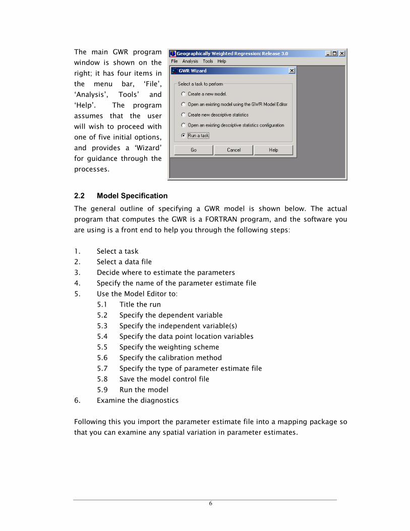
The main GWR program

window is shown on the

right; it has four items in

the menu bar, ‘File’,

‘Analysis’, Tools’ and

‘Help’. The program

assumes that the user

will wish to proceed with

one of five initial options,

and provides a ‘Wizard’

for guidance through the

processes.

2.2 Model Specification

The general outline of specifying a GWR model is shown below. The actual

program that computes the GWR is a FORTRAN program, and the software you

are using is a front end to help you through the following steps:

1. Select a task

2. Select a data file

3. Decide where to estimate the parameters

4. Specify the name of the parameter estimate file

5. Use the Model Editor to:

5.1 Title the run

5.2 Specify the dependent variable

5.3 Specify the independent variable(s)

5.4 Specify the data point location variables

5.5 Specify the weighting scheme

5.6 Specify the calibration method

5.7 Specify the type of parameter estimate file

5.8 Save the model control file

5.9 Run the model

6. Examine the diagnostics

Following this you import the parameter estimate file into a mapping package so

that you can examine any spatial variation in parameter estimates.

7

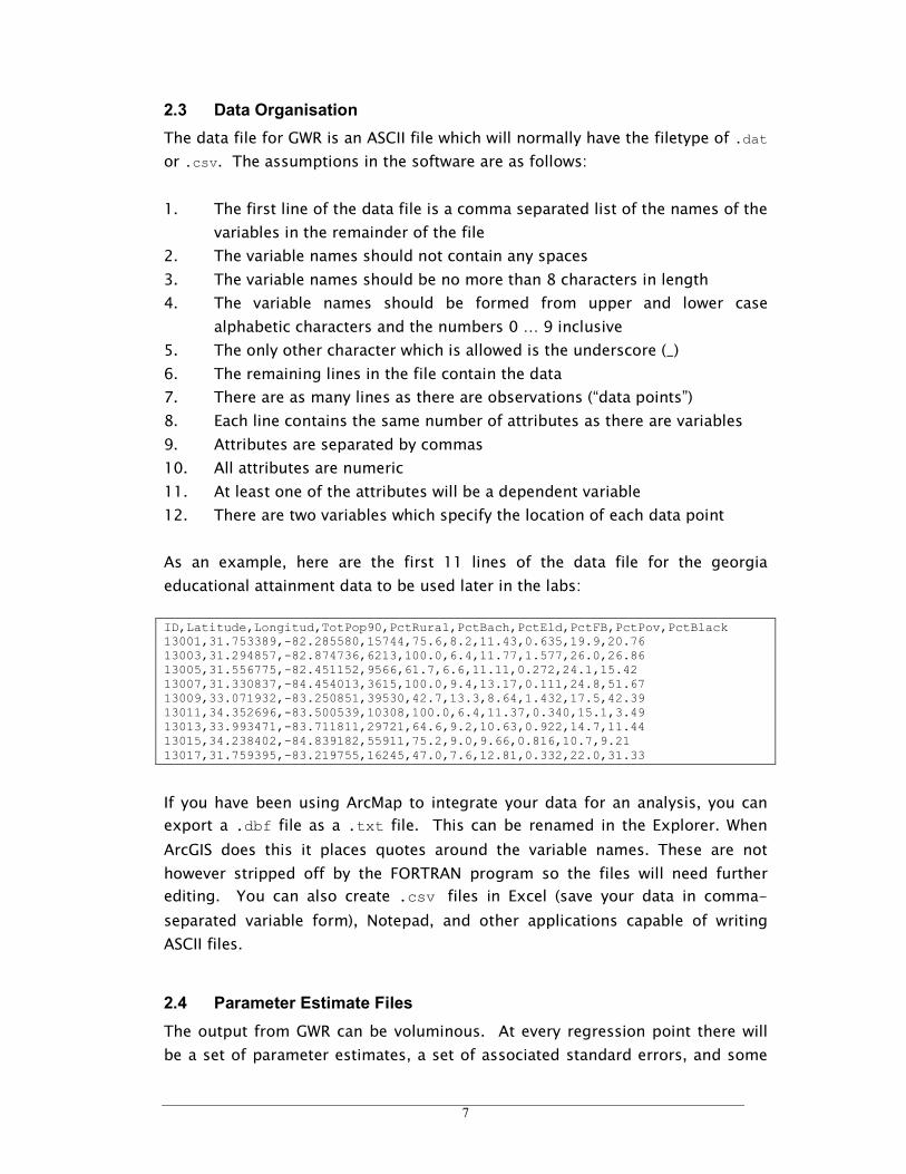
2.3 Data Organisation

The data file for GWR is an ASCII file which will normally have the filetype of .dat

or .csv. The assumptions in the software are as follows:

1. The first line of the data file is a comma separated list of the names of the

variables in the remainder of the file

2. The variable names should not contain any spaces

3. The variable names should be no more than 8 characters in length

4. The variable names should be formed from upper and lower case

alphabetic characters and the numbers 0 … 9 inclusive

5. The only other character which is allowed is the underscore (_)

6. The remaining lines in the file contain the data

7. There are as many lines as there are observations (“data points”)

8. Each line contains the same number of attributes as there are variables

9. Attributes are separated by commas

10. All attributes are numeric

11. At least one of the attributes will be a dependent variable

12. There are two variables which specify the location of each data point

As an example, here are the first 11 lines of the data file for the georgia

educational attainment data to be used later in the labs:

ID,Latitude,Longitud,TotPop90,PctRural,PctBach,PctEld,PctFB,PctPov,PctBlack 13001,31.753389,-82.285580,15744,75.6,8.2,11.43,0.635,19.9,20.76 13003,31.294857,-82.874736,6213,100.0,6.4,11.77,1.577,26.0,26.86 13005,31.556775,-82.451152,9566,61.7,6.6,11.11,0.272,24.1,15.42 13007,31.330837,-84.454013,3615,100.0,9.4,13.17,0.111,24.8,51.67 13009,33.071932,-83.250851,39530,42.7,13.3,8.64,1.432,17.5,42.39 13011,34.352696,-83.500539,10308,100.0,6.4,11.37,0.340,15.1,3.49 13013,33.993471,-83.711811,29721,64.6,9.2,10.63,0.922,14.7,11.44 13015,34.238402,-84.839182,55911,75.2,9.0,9.66,0.816,10.7,9.21 13017,31.759395,-83.219755,16245,47.0,7.6,12.81,0.332,22.0,31.33

If you have been using ArcMap to integrate your data for an analysis, you can

export a .dbf file as a .txt file. This can be renamed in the Explorer. When

ArcGIS does this it places quotes around the variable names. These are not

however stripped off by the FORTRAN program so the files will need further

editing. You can also create .csv files in Excel (save your data in comma-

separated variable form), Notepad, and other applications capable of writing

ASCII files.

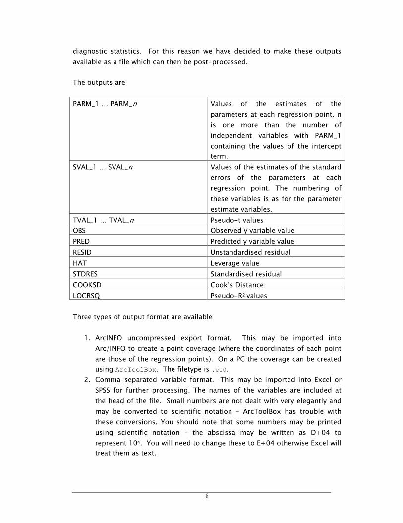
2.4 Parameter Estimate Files

The output from GWR can be voluminous. At every regression point there will

be a set of parameter estimates, a set of associated standard errors, and some

8

diagnostic statistics. For this reason we have decided to make these outputs

available as a file which can then be post-processed.

The outputs are

PARM_1 … PARM_n Values of the estimates of the

parameters at each regression point. n

is one more than the number of

independent variables with PARM_1

containing the values of the intercept

term.

SVAL_1 … SVAL_n Values of the estimates of the standard

errors of the parameters at each

regression point. The numbering of

these variables is as for the parameter

estimate variables.

TVAL_1 … TVAL_n Pseudo-t values

OBS Observed y variable value

PRED Predicted y variable value

RESID Unstandardised residual

HAT Leverage value

STDRES Standardised residual

COOKSD Cook’s Distance

LOCRSQ Pseudo-R2 values

Three types of output format are available

1. ArcINFO uncompressed export format. This may be imported into

Arc/INFO to create a point coverage (where the coordinates of each point

are those of the regression points). On a PC the coverage can be created

using ArcToolBox. The filetype is .e00.

2. Comma-separated-variable format. This may be imported into Excel or

SPSS for further processing. The names of the variables are included at

the head of the file. Small numbers are not dealt with very elegantly and

may be converted to scientific notation – ArcToolBox has trouble with

these conversions. You should note that some numbers may be printed

using scientific notation – the abscissa may be written as D+04 to

represent 104. You will need to change these to E+04 otherwise Excel will

treat them as text.

9

3. MapInfo Interchange Format. A .mif/.mid pair of files is created. These

can be imported into MapINFO. The files are ASCII files and can be hand

edited to remove any anomalies. This is somewhat experimental at the

moment.

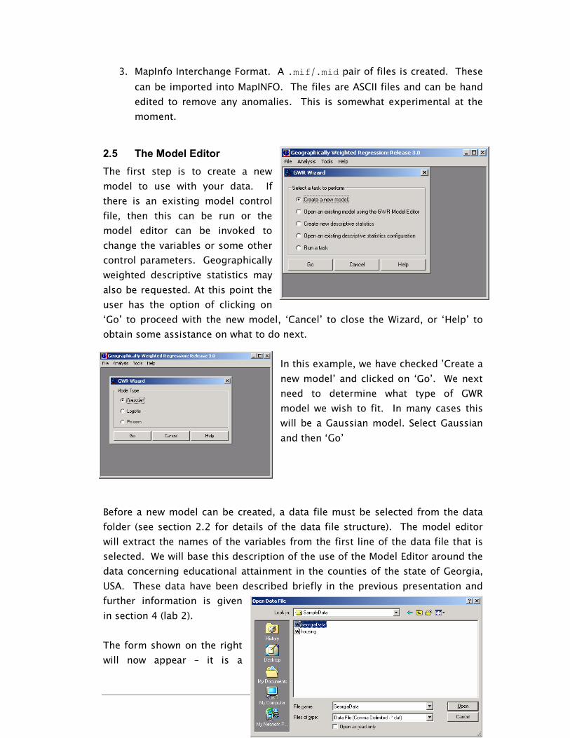
2.5 The Model Editor

The first step is to create a new

model to use with your data. If

there is an existing model control

file, then this can be run or the

model editor can be invoked to

change the variables or some other

control parameters. Geographically

weighted descriptive statistics may

also be requested. At this point the

user has the option of clicking on

‘Go’ to proceed with the new model, ‘Cancel’ to close the Wizard, or ‘Help’ to

obtain some assistance on what to do next.

In this example, we have checked ’Create a

new model’ and clicked on ‘Go’. We next

need to determine what type of GWR

model we wish to fit. In many cases this

will be a Gaussian model. Select Gaussian

and then ‘Go’

Before a new model can be created, a data file must be selected from the data

folder (see section 2.2 for details of the data file structure). The model editor

will extract the names of the variables from the first line of the data file that is

selected. We will base this description of the use of the Model Editor around the

data concerning educational attainment in the counties of the state of Georgia,

USA. These data have been described briefly in the previous presentation and

further information is given

in section 4 (lab 2).

The form shown on the right

will now appear – it is a

10

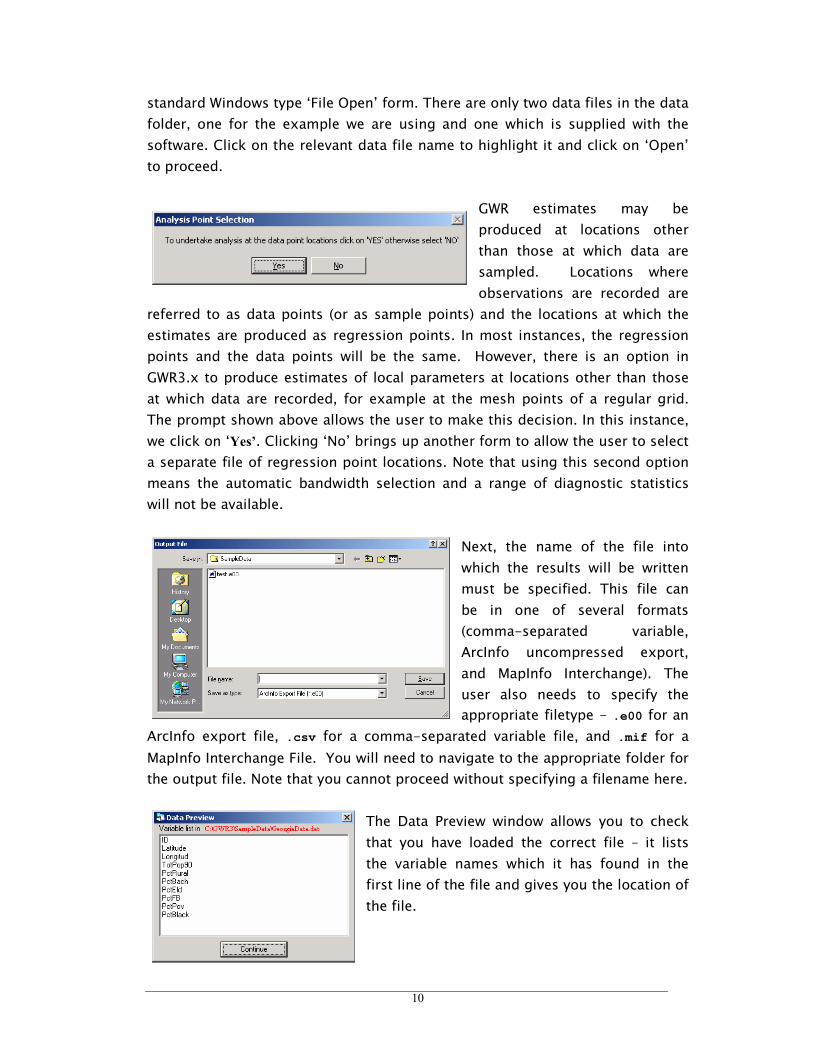
standard Windows type ‘File Open’ form. There are only two data files in the data

folder, one for the example we are using and one which is supplied with the

software. Click on the relevant data file name to highlight it and click on ‘Open’

to proceed.

GWR estimates may be

produced at locations other

than those at which data are

sampled. Locations where

observations are recorded are

referred to as data points (or as sample points) and the locations at which the

estimates are produced as regression points. In most instances, the regression

points and the data points will be the same. However, there is an option in

GWR3.x to produce estimates of local parameters at locations other than those

at which data are recorded, for example at the mesh points of a regular grid.

The prompt shown above allows the user to make this decision. In this instance,

we click on ‘Yes’. Clicking ‘No’ brings up another form to allow the user to select

a separate file of regression point locations. Note that using this second option

means the automatic bandwidth selection and a range of diagnostic statistics

will not be available.

Next, the name of the file into

which the results will be written

must be specified. This file can

be in one of several formats

(comma-separated variable,

ArcInfo uncompressed export,

and MapInfo Interchange). The

user also needs to specify the

appropriate filetype - .e00 for an

ArcInfo export file, .csv for a comma-separated variable file, and .mif for a

MapInfo Interchange File. You will need to navigate to the appropriate folder for

the output file. Note that you cannot proceed without specifying a filename here.

The Data Preview window allows you to check

that you have loaded the correct file – it lists

the variable names which it has found in the

first line of the file and gives you the location of

the file.

11

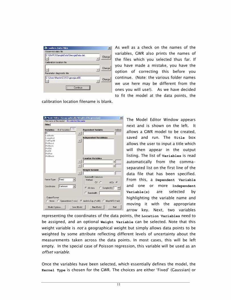
As well as a check on the names of the

variables, GWR also prints the names of

the files which you selected thus far. If

you have made a mistake, you have the

option of correcting this before you

continue. (Note: the various folder names

we use here may be different from the

ones you will use!). As we have decided

to fit the model at the data points, the

calibration location filename is blank.

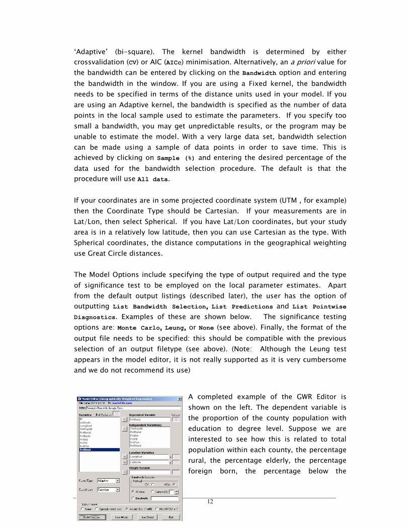
The Model Editor Window appears

next and is shown on the left. It

allows a GWR model to be created,

saved and run. The Title box

allows the user to input a title which

will then appear in the output

listing. The list of Variables is read

automatically from the comma-

separated list on the first line of the

data file that has been specified.

From this, a Dependent Variable

and one or more Independent

Variable(s) are selected by

highlighting the variable name and

moving it with the appropriate

arrow key. Next, two variables

representing the coordinates of the data points, the Location Variables need to

be assigned, and an optional Weight Variable can be selected. Note that this

weight variable is not a geographical weight but simply allows data points to be

weighted by some attribute reflecting different levels of uncertainty about the

measurements taken across the data points. In most cases, this will be left

empty. In the special case of Poisson regression, this variable will be used as an

offset variable.

Once the variables have been selected, which essentially defines the model, the

Kernel Type is chosen for the GWR. The choices are either ‘Fixed’ (Gaussian) or

12

‘Adaptive’ (bi-square). The kernel bandwidth is determined by either

crossvalidation (CV) or AIC (AICc) minimisation. Alternatively, an a priori value for

the bandwidth can be entered by clicking on the Bandwidth option and entering

the bandwidth in the window. If you are using a Fixed kernel, the bandwidth

needs to be specified in terms of the distance units used in your model. If you

are using an Adaptive kernel, the bandwidth is specified as the number of data

points in the local sample used to estimate the parameters. If you specify too

small a bandwidth, you may get unpredictable results, or the program may be

unable to estimate the model. With a very large data set, bandwidth selection

can be made using a sample of data points in order to save time. This is

achieved by clicking on Sample (%) and entering the desired percentage of the

data used for the bandwidth selection procedure. The default is that the

procedure will use All data.

If your coordinates are in some projected coordinate system (UTM , for example)

then the Coordinate Type should be Cartesian. If your measurements are in

Lat/Lon, then select Spherical. If you have Lat/Lon coordinates, but your study

area is in a relatively low latitude, then you can use Cartesian as the type. With

Spherical coordinates, the distance computations in the geographical weighting

use Great Circle distances.

The Model Options include specifying the type of output required and the type

of significance test to be employed on the local parameter estimates. Apart

from the default output listings (described later), the user has the option of

outputting List Bandwidth Selection, , , , List Predictions and List Pointwise

Diagnostics. Examples of these are shown below. The significance testing

options are: Monte Carlo, , , , Leung, , , , or None (see above). Finally, the format of the

output file needs to be specified: this should be compatible with the previous

selection of an output filetype (see above). (Note: Although the Leung test

appears in the model editor, it is not really supported as it is very cumbersome

and we do not recommend its use)

A completed example of the GWR Editor is

shown on the left. The dependent variable is

the proportion of the county population with

education to degree level. Suppose we are

interested to see how this is related to total

population within each county, the percentage

rural, the percentage elderly, the percentage

foreign born, the percentage below the

13

poverty line and the percentage black. We would also like to see if there are any

geographical variations in the relationships between educational attainment and

these variables.

The sample point location variables are Longitud (x) and Latitude (y). There is

no aspatial weight variable. We have chosen an adaptive kernel and the

bandwidth will be chosen by AICc minimisation using all the data. A Monte Carlo

significance testing procedure has also been selected for the local parameter

estimates. Printing of a range of diagnostics has been requested and the output

will be written to an ArcInfo export file. Some of the output will, by default, also

be written to the screen in a listing file.

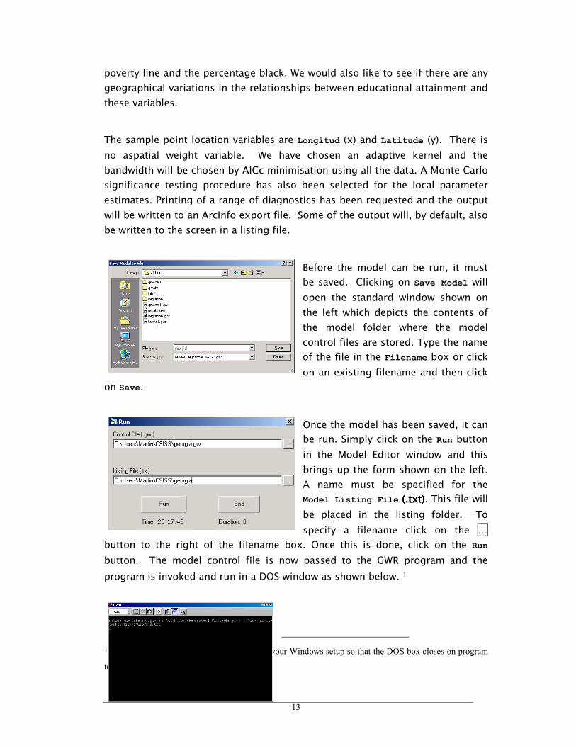
Before the model can be run, it must

be saved. Clicking on Save Model will

open the standard window shown on

the left which depicts the contents of

the model folder where the model

control files are stored. Type the name

of the file in the Filename box or click

on an existing filename and then click

on Save.

Once the model has been saved, it can

be run. Simply click on the Run button

in the Model Editor window and this

brings up the form shown on the left.

A name must be specified for the

Model Listing File (.txt) (.txt) (.txt) (.txt). This file will

be placed in the listing folder. To

specify a filename click on the …

button to the right of the filename box. Once this is done, click on the Run

button. The model control file is now passed to the GWR program and the

program is invoked and run in a DOS window as shown below. 1

1 You may need to make a small alteration in your Windows setup so that the DOS box closes on program

termination.

14

With small data sets and simple models, the program runs very quickly. For

instance, calibrating a bivariate GWR model using the 159 counties of Georgia

on a Pentium III PC took less time than it has taken to type this sentence.

However, the time requirements increase rapidly as both model complexity and

the number of data points increases. One solution to very slow run times is to

use the option in the Model Editor which allows the user to supply a percentage

of the data points on which to base the bandwidth selection procedure.

When the run has completed, the DOS window

closes, and you are asked whether you wish to

examine the listing file:

2.6 Printed Outputs

Once the program has run, the user

is asked if the output listing is to be

viewed. This listing appears in a

separate window; an example of this

for the Georgia educational

attainment model is shown on the

left. The user can scroll down the

file to view other sections. The

listing file is a text file with the

filetype of .txt so that it can also be opened in MS Word or Notepad for viewing

or printing.

Following a description of the model that has been calibrated, the first section of

the output from GWR3 contains the parameter estimates and their standard

errors from a global model fitted to the data. This is shown below.

********************************************************** * GLOBAL REGRESSION PARAMETERS * ********************************************************** Diagnostic information... Residual sum of squares......... 1816.210715 Effective number of parameters.. 7.000000 Sigma........................... 3.456697 Akaike Information Criterion.... 855.443391 Coefficient of Determination.... 0.645830

15

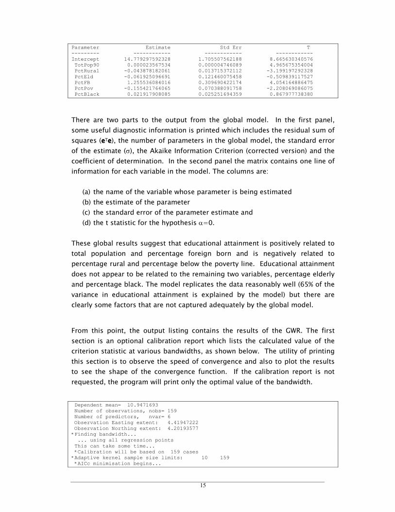
Parameter Estimate Std Err T --------- ------------ ------------ ------------ Intercept 14.779297592328 1.705507562188 8.665630340576 TotPop90 0.000023567534 0.000004746089 4.965675354004 PctRural -0.043878182061 0.013715372112 -3.199197292328 PctEld -0.061925096691 0.121460075458 -0.509839117527 PctFB 1.255536084016 0.309690422174 4.054164886475 PctPov -0.155421764065 0.070388091758 -2.208069086075 PctBlack 0.021917908085 0.025251694359 0.867977738380

There are two parts to the output from the global model. In the first panel,

some useful diagnostic information is printed which includes the residual sum of

squares (eeeeTeeee), the number of parameters in the global model, the standard error

of the estimate (σ), the Akaike Information Criterion (corrected version) and the

coefficient of determination. In the second panel the matrix contains one line of

information for each variable in the model. The columns are:

(a) the name of the variable whose parameter is being estimated

(b) the estimate of the parameter

(c) the standard error of the parameter estimate and

(d) the t statistic for the hypothesis α=0.

These global results suggest that educational attainment is positively related to

total population and percentage foreign born and is negatively related to

percentage rural and percentage below the poverty line. Educational attainment

does not appear to be related to the remaining two variables, percentage elderly

and percentage black. The model replicates the data reasonably well (65% of the

variance in educational attainment is explained by the model) but there are

clearly some factors that are not captured adequately by the global model.

From this point, the output listing contains the results of the GWR. The first

section is an optional calibration report which lists the calculated value of the

criterion statistic at various bandwidths, as shown below. The utility of printing

this section is to observe the speed of convergence and also to plot the results

to see the shape of the convergence function. If the calibration report is not

requested, the program will print only the optimal value of the bandwidth.

Dependent mean= 10.9471693 Number of observations, nobs= 159 Number of predictors, nvar= 6 Observation Easting extent: 4.41947222 Observation Northing extent: 4.20193577 *Finding bandwidth... ... using all regression points This can take some time... *Calibration will be based on 159 cases *Adaptive kernel sample size limits: 10 159 *AICc minimisation begins...

16

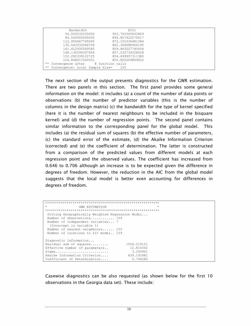
Bandwidth AICc 56.043532255000 952.763365832809 84.500000000000 894.827422579517 112.956467745000 872.102336481384 130.543532046749 862.364688964195 141.412935569545 859.863227740004 148.130596397659 857.532739228028 152.282339122725 856.699997311380 154.848257244551 855.820209809022 ** Convergence after 8 function calls ** Convergence: Local Sample Size= 155

The next section of the output presents diagnostics for the GWR estimation.

There are two panels in this section. The first panel provides some general

information on the model: it includes (a) a count of the number of data points or

observations (b) the number of predictor variables (this is the number of

columns in the design matrix) (c) the bandwidth for the type of kernel specified

(here it is the number of nearest neighbours to be included in the bisquare

kernel) and (d) the number of regression points. The second panel contains

similar information to the corresponding panel for the global model. This

includes (a) the residual sum of squares (b) the effective number of parameters,

(c) the standard error of the estimate, (d) the Akaike Information Criterion

(corrected) and (e) the coefficient of determination. The latter is constructed

from a comparison of the predicted values from different models at each

regression point and the observed values. The coefficient has increased from

0.646 to 0.706 although an increase is to be expected given the difference in

degrees of freedom. However, the reduction in the AIC from the global model

suggests that the local model is better even accounting for differences in

degrees of freedom.

********************************************************** * GWR ESTIMATION * ********************************************************** Fitting Geographically Weighted Regression Model... Number of observations............ 159 Number of independent variables... 7 (Intercept is variable 1) Number of nearest neighbours...... 155 Number of locations to fit model.. 159 Diagnostic information... Residual sum of squares......... 1506.219121 Effective number of parameters.. 12.814342 Sigma........................... 3.209901 Akaike Information Criterion.... 839.193981 Coefficient of Determination.... 0.706280

Casewise diagnostics can be also requested (as shown below for the first 10

observations in the Georgia data set). These include:

17

1. the observation sequence number

2. the observed data

3. the predicted data

4. the residual

5. the standardised residual

6. the local pseudo r-square

7. the influence and

8. Cook’s D.

Whilst in general it might be helpful to look at a printout of these statistics, it is

probably a little more useful to be able to map them: with a large data set you

run the risk of being swamped in output. All of these statistics are saved

automatically in the output results file so that requesting them in the listing file

should be done judiciously. This panel is not available when the regression

points are different from the data points.

********************************************************** * CASEWISE DIAGNOSTICS * ********************************************************** Obs Observed Predicted Residual Std Resid R-Square Influence Cook's D ----- -------------- -------------- -------------- ----------- ----------- ----------- ----------- 1 8.20000 9.26692 -1.06692 -0.258875 0.819218 0.021879 0.000117 2 6.40000 7.33714 -0.93714 -0.232802 0.820589 0.066868 0.000303 3 6.60000 8.70596 -2.10596 -0.525272 0.819776 0.074367 0.001730 4 9.40000 8.11559 1.28441 0.319607 0.840207 0.069997 0.000600 5 13.30000 13.58140 -0.28140 -0.070091 0.839357 0.071855 0.000030 6 6.40000 8.79625 -2.39625 -0.591102 0.844322 0.053656 0.001546 7 9.20000 11.61571 -2.41571 -0.587443 0.846859 0.026203 0.000725 8 9.00000 11.61646 -2.61646 -0.636924 0.852840 0.028236 0.000920 9 7.60000 10.26846 -2.66846 -0.654270 0.826147 0.042107 0.001468 10 7.50000 9.48755 -1.98755 -0.489605 0.822446 0.051028 0.001006

Another optional set of information that can be printed to the screen concerns

the predicted values (as shown below for the first 10 observations in the Georgia

data set). If this option is selected, the following data are printed to the screen:

1. Obs the sequence number of the observation

2. Y(i) the observed value

3. Yhat(i) the predicted value

4. Res(i) the residual

5. X(i) the x-coordinate of the regression point

6. Y(i) the y-coordinate of the regression point and

7. an indicator of whether the matrix inverse was computed using either

the Gauss-Jordan method (F) or a generalised inverse (T). The latter is

only used if there is severe multicollinearity in the design matrix

18

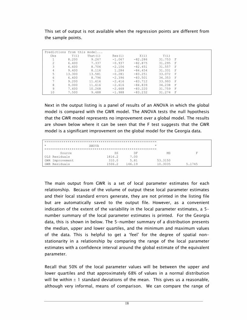
This set of output is not available when the regression points are different from

the sample points.

Predictions from this model... Obs Y(i) Yhat(i) Res(i) X(i) Y(i) 1 8.200 9.267 -1.067 -82.286 31.753 F 2 6.400 7.337 -0.937 -82.875 31.295 F 3 6.600 8.706 -2.106 -82.451 31.557 F 4 9.400 8.116 1.284 -84.454 31.331 F 5 13.300 13.581 -0.281 -83.251 33.072 F 6 6.400 8.796 -2.396 -83.501 34.353 F 7 9.200 11.616 -2.416 -83.712 33.993 F 8 9.000 11.616 -2.616 -84.839 34.238 F 9 7.600 10.268 -2.668 -83.220 31.759 F 10 7.500 9.488 -1.988 -83.232 31.274 F

Next in the output listing is a panel of results of an ANOVA in which the global

model is compared with the GWR model. The ANOVA tests the null hypothesis

that the GWR model represents no improvement over a global model. The results

are shown below where it can be seen that the F test suggests that the GWR

model is a significant improvement on the global model for the Georgia data.

********************************************************** * ANOVA * ********************************************************** Source SS DF MS F OLS Residuals 1816.2 7.00 GWR Improvement 310.0 5.81 53.3150 GWR Residuals 1506.2 146.19 10.3035 5.1745

The main output from GWR is a set of local parameter estimates for each

relationship. Because of the volume of output these local parameter estimates

and their local standard errors generate, they are not printed in the listing file

but are automatically saved to the output file. However, as a convenient

indication of the extent of the variability in the local parameter estimates, a 5-

number summary of the local parameter estimates is printed. For the Georgia

data, this is shown in below. The 5-number summary of a distribution presents

the median, upper and lower quartiles, and the minimum and maximum values

of the data. This is helpful to get a ‘feel’ for the degree of spatial non-

stationarity in a relationship by comparing the range of the local parameter

estimates with a confidence interval around the global estimate of the equivalent

parameter.

Recall that 50% of the local parameter values will be between the upper and

lower quartiles and that approximately 68% of values in a normal distribution

will be within ± 1 standard deviations of the mean. This gives us a reasonable,

although very informal, means of comparison. We can compare the range of

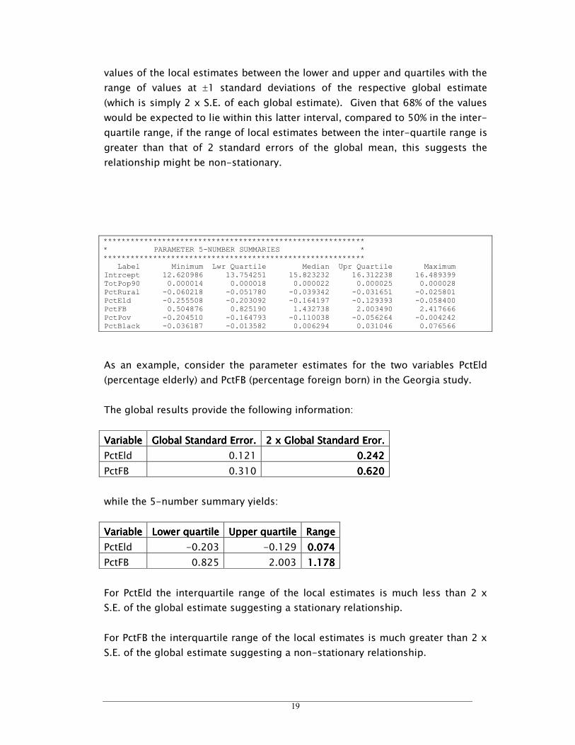
19

values of the local estimates between the lower and upper and quartiles with the

range of values at ±1 standard deviations of the respective global estimate

(which is simply 2 x S.E. of each global estimate). Given that 68% of the values

would be expected to lie within this latter interval, compared to 50% in the inter-

quartile range, if the range of local estimates between the inter-quartile range is

greater than that of 2 standard errors of the global mean, this suggests the

relationship might be non-stationary.

********************************************************** * PARAMETER 5-NUMBER SUMMARIES * ********************************************************** Label Minimum Lwr Quartile Median Upr Quartile Maximum Intrcept 12.620986 13.754251 15.823232 16.312238 16.489399 TotPop90 0.000014 0.000018 0.000022 0.000025 0.000028 PctRural -0.060218 -0.051780 -0.039342 -0.031651 -0.025801 PctEld -0.255508 -0.203092 -0.164197 -0.129393 -0.058400 PctFB 0.504876 0.825190 1.432738 2.003490 2.417666 PctPov -0.204510 -0.164793 -0.110038 -0.056264 -0.004242 PctBlack -0.036187 -0.013582 0.006294 0.031046 0.076566

As an example, consider the parameter estimates for the two variables PctEld

(percentage elderly) and PctFB (percentage foreign born) in the Georgia study.

The global results provide the following information:

VariableVariableVariableVariable Global Standard Error.Global Standard Error.Global Standard Error.Global Standard Error. 2 x Global Standard Eror.2 x Global Standard Eror.2 x Global Standard Eror.2 x Global Standard Eror.

PctEld 0.121 0.2420.2420.2420.242

PctFB 0.310 0.6200.6200.6200.620

while the 5-number summary yields:

VariableVariableVariableVariable Lower quartileLower quartileLower quartileLower quartile Upper quartile Upper quartile Upper quartile Upper quartile RangeRangeRangeRange

PctEld -0.203 -0.129 0.0740.0740.0740.074

PctFB 0.825 2.003 1.1781.1781.1781.178

For PctEld the interquartile range of the local estimates is much less than 2 x

S.E. of the global estimate suggesting a stationary relationship.

For PctFB the interquartile range of the local estimates is much greater than 2 x

S.E. of the global estimate suggesting a non-stationary relationship.

20

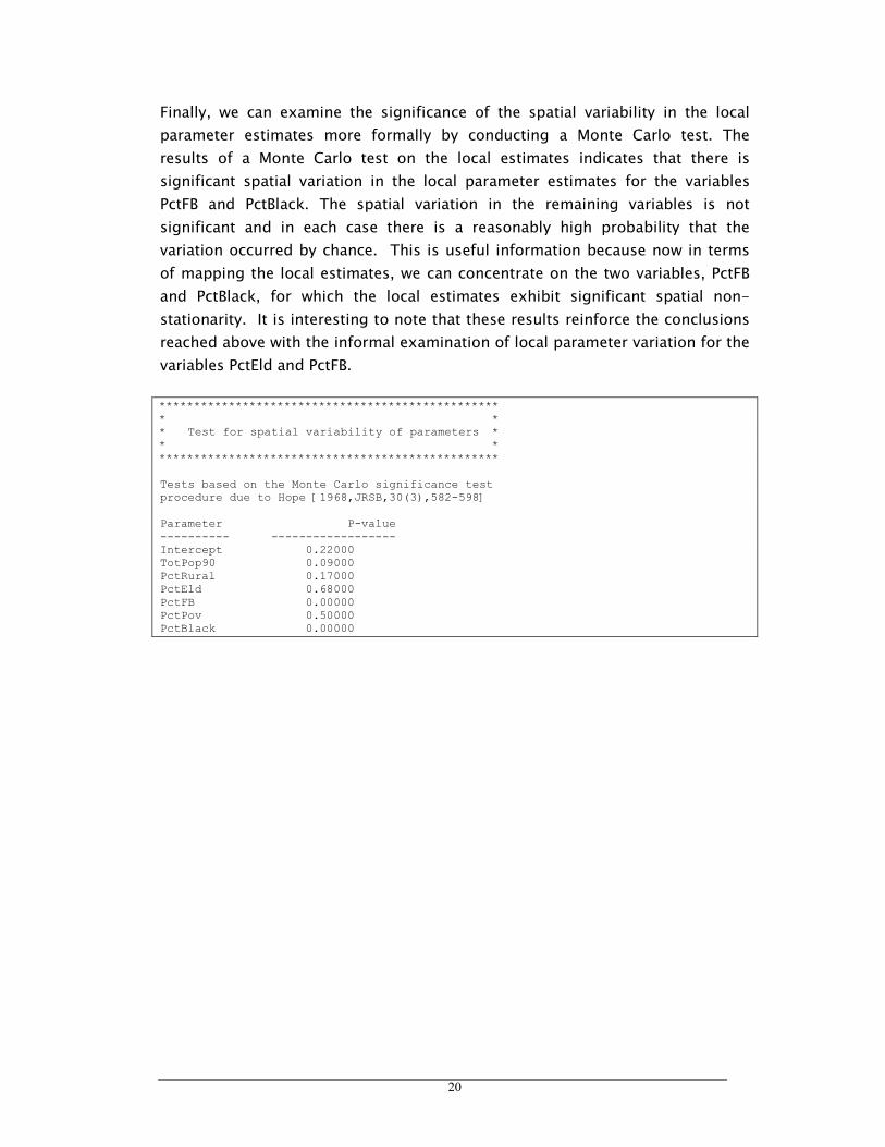
Finally, we can examine the significance of the spatial variability in the local

parameter estimates more formally by conducting a Monte Carlo test. The

results of a Monte Carlo test on the local estimates indicates that there is

significant spatial variation in the local parameter estimates for the variables

PctFB and PctBlack. The spatial variation in the remaining variables is not

significant and in each case there is a reasonably high probability that the

variation occurred by chance. This is useful information because now in terms

of mapping the local estimates, we can concentrate on the two variables, PctFB

and PctBlack, for which the local estimates exhibit significant spatial non-

stationarity. It is interesting to note that these results reinforce the conclusions

reached above with the informal examination of local parameter variation for the

variables PctEld and PctFB.

************************************************* * * * Test for spatial variability of parameters * * * ************************************************* Tests based on the Monte Carlo significance test procedure due to Hope [1968,JRSB,30(3),582-598] Parameter P-value ---------- ------------------ Intercept 0.22000 TotPop90 0.09000 PctRural 0.17000 PctEld 0.68000 PctFB 0.00000 PctPov 0.50000 PctBlack 0.00000

21

3

Lab 0: Visualising the Output from GWR with ArcMap

What you will learnWhat you will learnWhat you will learnWhat you will learn

1 Importing an interchange file into ArcGIS

2 Options for visualising a point coverage

3 Adding a shapefile into an ArcGIS project

4 How to carry out a spatial join

5 Symbolising a polygon shapefile

6 [Optional: Assigning map projection information]

The main output from GWR is a set of localised parameter estimates and

associated diagnostics. Unlike the single global values traditionally obtained in

modelling, these local values lend themselves to being mapped. Indeed, in large

data sets, mapping, or some other form of visualisation, is the only way to make

sense of the large volume of output that will be generated. We now describe

ways of visualising the output from GWR. Although we concentrate only on

displays of the local parameter estimates, in many instances it might be

instructive to plot other local statistics such as the influence and Cook’s D

statistics. Similarly, it might be useful to plot the local r-square statistic or the

local standard deviation. No matter which local statistic is mapped, however,

there is a choice of map types that can be employed. We now describe some of

these briefly after first discussing mapping the results in a commonly used, PC-

based, Geographic Information System (GIS), ArcMap.

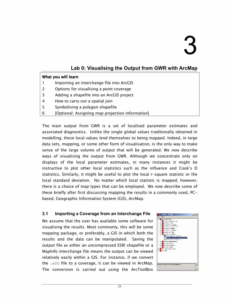
3.1 Importing a Coverage from an Interchange File

We assume that the user has available some software for

visualising the results. Most commonly, this will be some

mapping package, or preferably, a GIS in which both the

results and the data can be manipulated. Saving the

output file as either an uncompressed ESRI shapefile or a

MapInfo interchange file means the output can be viewed

relatively easily within a GIS. For instance, if we convert

the .e00 file to a coverage, it can be viewed in ArcMap.

The conversion is carried out using the ArcToolBox

22

program.

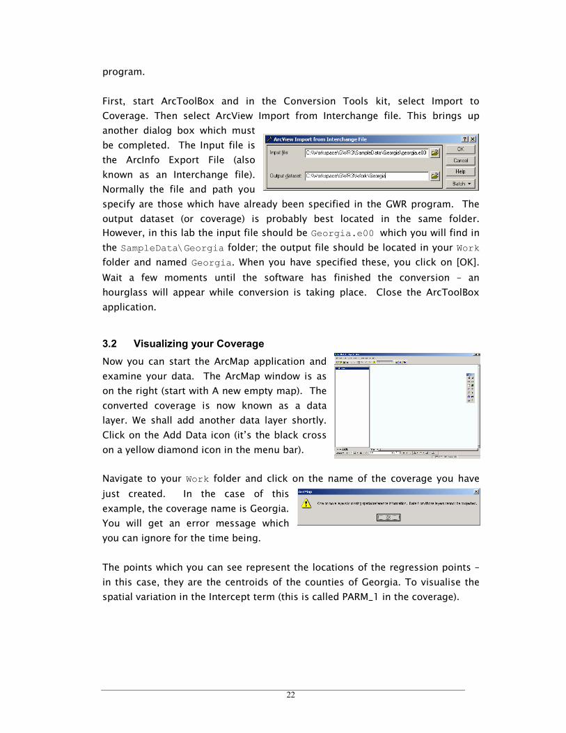
First, start ArcToolBox and in the Conversion Tools kit, select Import to

Coverage. Then select ArcView Import from Interchange file. This brings up

another dialog box which must

be completed. The Input file is

the ArcInfo Export File (also

known as an Interchange file).

Normally the file and path you

specify are those which have already been specified in the GWR program. The

output dataset (or coverage) is probably best located in the same folder.

However, in this lab the input file should be Georgia.e00 which you will find in

the SampleData\Georgia folder; the output file should be located in your Work

folder and named Georgia. When you have specified these, you click on [OK].

Wait a few moments until the software has finished the conversion – an

hourglass will appear while conversion is taking place. Close the ArcToolBox

application.

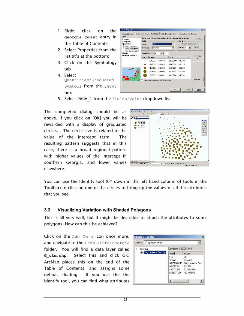
3.2 Visualizing your Coverage

Now you can start the ArcMap application and

examine your data. The ArcMap window is as

on the right (start with A new empty map). The

converted coverage is now known as a data

layer. We shall add another data layer shortly.

Click on the Add Data icon (it’s the black cross

on a yellow diamond icon in the menu bar).

Navigate to your Work folder and click on the name of the coverage you have

just created. In the case of this

example, the coverage name is Georgia.

You will get an error message which

you can ignore for the time being.

The points which you can see represent the locations of the regression points –

in this case, they are the centroids of the counties of Georgia. To visualise the

spatial variation in the Intercept term (this is called PARM_1 in the coverage).

23

1. Right click on the

georgia point entry in

the Table of Contents

2. Select Properties from the

list (it’s at the bottom)

3. Click on the Symbology

tab

4. Select Quantities/Graduated

Symbols from the Show:

box

5. Select PARM_1 from the Fields/Value dropdown list

The completed dialog should be as

above. If you click on [OK] you will be

rewarded with a display of graduated

circles. The circle size is related to the

value of the intercept term. The

resulting pattern suggests that in this

case, there is a broad regional pattern

with higher values of the intercept in

southern Georgia, and lower values

elsewhere.

You can use the Identify tool (6th down in the left hand column of tools in the

Toolbar) to click on one of the circles to bring up the values of all the attributes

that you see.

3.3 Visualizing Variation with Shaded Polygons

This is all very well, but it might be desirable to attach the attributes to some

polygons. How can this be achieved?

Click on the Add Data icon once more,

and navigate to the SampleData\Georgia

folder. You will find a data layer called

G_utm.shp. Select this and click OK.

ArcMap places this on the end of the

Table of Contents, and assigns some

default shading. If you use the the

Identify tool, you can find what attributes

24

the data has. Here’s a typical entry on the right. Unfortunately, the AREAKEY

item is not present in the Georgia point coverage. We need to use a “spatial join”

to match the attributes of the points with the attributes of the polygons.

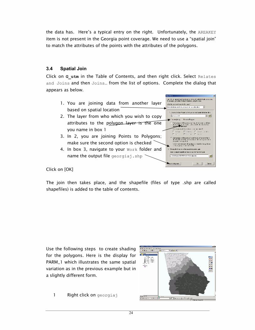
3.4 Spatial Join

Click on G_utm in the Table of Contents, and then right click. Select Relates

and Joins and then Joins… from the list of options. Complete the dialog that

appears as below.

1. You are joining data from another layer

based on spatial location

2. The layer from who which you wish to copy

attributes to the polygon layer is the one

you name in box 1

3. In 2, you are joining Points to Polygons;

make sure the second option is checked

4. In box 3, navigate to your Work folder and

name the output file georgiaj.shp

Click on [OK]

The join then takes place, and the shapefile (files of type .shp are called

shapefiles) is added to the table of contents.

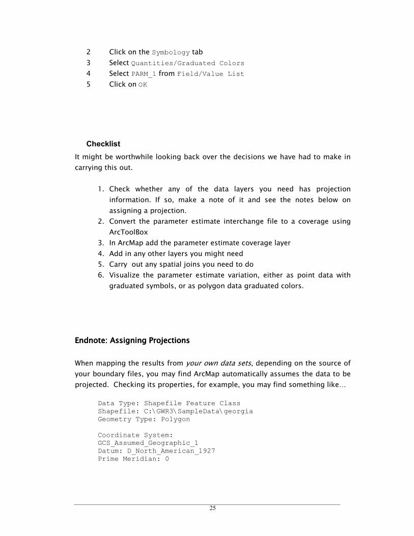
Use the following steps to create shading

for the polygons. Here is the display for

PARM_1 which illustrates the same spatial

variation as in the previous example but in

a slightly different form.

1 Right click on georgiaj

25

2 Click on the Symbology tab

3 Select Quantities/Graduated Colors

4 Select PARM_1 from Field/Value List

5 Click on OK

Checklist

It might be worthwhile looking back over the decisions we have had to make in

carrying this out.

1. Check whether any of the data layers you need has projection

information. If so, make a note of it and see the notes below on

assigning a projection.

2. Convert the parameter estimate interchange file to a coverage using

ArcToolBox

3. In ArcMap add the parameter estimate coverage layer

4. Add in any other layers you might need

5. Carry out any spatial joins you need to do

6. Visualize the parameter estimate variation, either as point data with

graduated symbols, or as polygon data graduated colors.

Endnote: Endnote: Endnote: Endnote: Assigning ProjectionsAssigning ProjectionsAssigning ProjectionsAssigning Projections

When mapping the results from your own data sets, depending on the source of

your boundary files, you may find ArcMap automatically assumes the data to be

projected. Checking its properties, for example, you may find something like…

Data Type: Shapefile Feature Class Shapefile: C:\GWR3\SampleData\georgia Geometry Type: Polygon Coordinate System: GCS_Assumed_Geographic_1 Datum: D_North_American_1927 Prime Meridian: 0

26

This may cause a problem in that the output from the GWR program will not

have such a projection assigned and the two data sets will therefore not be

compatible. If such a problem occurs, you will need to assign the same

projection to your GWR output coverage as ArcMap has assigned to your

boundary data. This can be done as follows:

You will need to close the ArcMap application and assign a projection to the

parameter estimate coverage. Suppose the projection you wish to assign is that

of geographic NAD 1927. The projection conversion is carried out in

ArcToolBox. You may need to do this every time you Import an interchange file.

1. Close the ArcMap application

2. Start the ArcToolBox application

3. Select Data Management Tools/Projections

4. Select Define Projection Wizard (coverages, grids, TINs)

5. Check define the coordinate system interactively: click [Next]

6. Navigate to your work folder and select Georgia: click [Next]

7. Select Geographic as the dataset projection: click [Next]

8. Select DD as the Units parameter: click [Next]

9. Select NAD 1927 (US-NADCON) as the Datum: click [Next]

10. Check the settings and click [Finish]

11. Exit the ArcToolBox application

You will have noticed that the Wizard also allows you to copy the information

about the projection from another coverage, so if you create a ‘master’ coverage

and assign the projection information, then you can use this as the source for a

copy.

27

4

Lab 1: GWR with Educational Attainment Data in Georgia

4.1 Introduction

The context of this particular modelling exercise has been outlined earlier. You

now have a chance to use GWR and some associated software to explore the

data and to model the relationships yourself.

We’ll use the Georgia data on educational attainment by county for our first

foray into GWR. The idea is to predict the level of education attainment from

some social attributes of the counties in the State of Georgia and then to map

the variation in the local parameter estimates and some diagnostics.

4.2 The Modelling Process

We envisage that GWR will be used in some larger data exploration and

modelling exercise. Typically the steps either side of GWR may include the

following

1. Prepare the data – may involve Excel, SPSS, SAS, or a GIS program.

2. Model relationships in GWR: examine printed diagnostics

3. Save the parameter estimates in a suitable format

4. Import the parameter estimates into a GIS program

5. Display the parameter variation – further analysis

6. Display the diagnostic variation – further analysis

It should be stressed that these are not the only routes. However these

workshops are based loosely around this approach.

4.3 Some Initial Choices

You need to make some initial choices

1. Run GWR by clicking on the GWR icon

2. Check the Create a new model option and click on Go

3. Check Gaussian as the model type and click Go

28

4. Change the file type to .csv then in the SampleData\Georgia folder find

gdata_utm.csv, select it and click on Open

5. In the Analysis Point Selection form click on Yes

6. Change the file type to ArcInfo Export File then navigate to your Work

folder and enter GeorgiaOut.e00 in the Output File form.

7. After the Data Preview and file confirmation, the model editor will appear.

4.4 Choices in the Model Editor

The model editor is central to your analysis. It will have read the first line of the

data file and extracted the names of the variables. These appear in the

Variables box. Completing the rest of the options appears somewhat complex

but will become familiar with practice.

1. Enter something like Georgia Educational Attainment in the title area.

You can put anything you like here: it’s printed on the output.

2. From the list of variables click on PctBach followed by the [->] symbol

beside the Dependent Variable box

3. From the list of variables click on TotPop90 then the [->] symbol to

the left of the Independent Variables box.

4. Do this for the variables PctRural, PctEld, PctFB, PctPov, PctBlack. If

you enter a variable in error, highlight it in the Independent

Variables list and click on the [<-} symbol.

5. Next we specify the Location Variables. Enter X as the x variable

and Y as the y variable.

6. Change the Kernel Type to Adaptive

7. In Model Options Check the List Bandwidth Selection option…

8. …and the List Predictions option

9. …and the List Pointwise Diagnostics option

10. Check Monte Carlo in the Significance test option: click Continue

11. Check AIC in the Bandwidth Selection Method option (there should

be nothing in the bandwidth box

12. Check All Data in the method box

13. Check the Arc/INFO Exp (*.e00) option in the Output Format list

You have now completely specified a GWR model.

29

4.5 Saving and Running the Model

The control file which is created by the Model Editor has to be saved to the Work

folder before you can run it.

1. Click on the Save Model option at the bottom of the Model Editor

2. Enter Georgia.gwr as the name of the control file in your Work folder

and click on Save

3. Click on Run Model

4. In the Run the Model form enter Georgia.txt as the Model Listing

File name (again in your Work folder)

5. Click on the Run button

A DOS window will appear – it should take less than a minute for the program to

run with this dataset. The window title bar will tell you when the program has

finished and the command Exit appears in this window. The DOS window will

then disappear. WAIT until this has happened and then:

1. Click on Yes on the Run Completed form to view the Listing file

2. Click on End on the Run the Model form

4.6 Examining the Outputs

Although you might think it would be illuminating to start plotting the

parameter estimates, it’s worth taking some time to examine the output.

1. Are you using the correct files in the correct folders?

2. Is the list of variables correct?

3. Are the dependent, location, and independent variables correctly

specified?

4. Have you checked the correct options?

Some initial values are reported: (you will need to scroll down to see these)

Dependent mean= 10.9471693 Number of observations, nobs= 159 Number of predictors, nvar= 6 Observation Easting extent: 423741.688 Observation Northing extent: 471492

5. Next check the bandwidth selection. The current values of the bandwidth

and the associated AIC are printed on the output (you can cut these out

30

and put them in Excel if you wish to create a plot of the minimisation

function). These functions can be quite messy at times.

The program has converged at 155 nearest neighbours. As there are only 159

counties, the GWR results may be fairly close to the global results – but

remember that in the GWR model the data are weighted by geographic location.

6. Have a look at the global model parameters and diagnostic statistics. The

AIC for the global model is 855.44 and the global coefficient of

determination is 0.65. It looks as if the global model is a reasonable one,

although 35% of the variation in our dependent variable is from sources

other than the ones in our model.

7. Check the global parameter values: there is a positive association with

Population, Foreign Born and Black and a negative association with Rural,

Elderly and Poverty. However the coefficients for Elderly and PctBlack are

small enough for us to regard them as having no effect on the model (t <

~1.96).

8. Check the GWR parameter estimates and diagnostics. The AIC for this

model is 840.07. This is less than that for the global model and this

suggests that the GWR model is “better” at modelling the data. The

coefficient of determination is a little higher at 0.72.

9. You have requested the complete listing of the pointwise diagnostics and

predictions. We’ll skip these and move down to the ANOVA. The

computed value of 5.01 is in excess of the critical value for F with 7.0 and

146.2 degrees of freedom so we reject the null hypothesis that the GWR

represents no improvement over the global model. This conclusion is in

line with the AIC results above.

10. Finally check the five number summaries.

(a) Are the medians different from the global values?

(b) Are the signs similar?

(c) Do the signs of the coefficients change?

(d) How large is the interquartile range?

(e) Compare the interquartile ranges with the 2 x S.E. of

the global estimates (you’ll have to do this by hand)

11 If you have requested a significance test, which parameters exhibit

significant spatial variation?

31

12 If you want to close GWR at this point you can, but you need not do

so.

4.7 Mapping the Results

At this point we turn to ArcMap.

4.7.1 Getting started

The Arc/INFO .e00 file which you saved earlier has to be converted into an

Arc/INFO coverage2. Find the ArcToolBox utility3 which is part of the ArcMap

system and run it following the procedures we described in Lab 1. The input file

is georgiaout.e00 in your Work folder and the output file is gparms also in

your Work folder.

We’ll store the imported coverages in your

work folder for convenience. Alternatively,

however, you may place them in any

convenient folder

When you’re ready click on OK.

The above will create an Arc/INFO point coverage (called gparms in this case)

Start the ArcMap program and click on the Add Data icon.

Navigate to whatever folder you have saved your parameter coverage and

highlight the name of the file and click on Add.

The name of the theme (gparms point in this case) appears in the Table of

Contents. Right-click its name and select Open Attribute Table from the list of

options. The theme table contains the values of:

the pointwise parameter estimates (PARM_1…)

the pointwise standard errors (SVAL_1…)

the pointwise pseudo-t values (TVAL_1…)

the observed y value OBS

the predicted y value PRED

2 We will eventually support shapefiles but this will be later rather than sooner.

3 We’ll put the location on an overhead

32

the residual RESID

the standardised residual STDRES

the trace of the hat matrix HAT

Cook’s D COOKSD

There are 7 sets of data for the PARM, SVAL and TVAL items numbered thus

1. Intercept

2. Totpop90

3. PctRural

4. PctEld

5. PctFB

6. PctPov

7. PctBlack

PARM_1 contains the values of the Intercept term and SVAL_1 contains the

values of the corresponding standard errors.

To show the variation in the intercept term with proportional symbols located at

the centroids of the regression points:

1. Right click on gparms point again and select Properties, then

2. Select Symbology/Quantities/Graduated symbols

3. Select Value/Field: Parm_1

4. Click Apply to apply this symbolism to your data.

Experiment with different types of symbolism:

Graduated Color symbols may be easier to interpret

You can change the number of classes and the classification method in Classify

You can also change symbol colours.

4.7.2 Adding Boundaries

Whilst it is clear from the map that the value of the intercept term increases

gently from North West to South East Georgia, it will enhance your map to have

some county boundaries.

1. Click on the Add Data icon

33

2. Highlight g_utm.shp in the SampleData\Georgia folder and click on Add:

3. Right click on G_utm to bring up Properties/Symbology, click in the

middle of the Symbol (which will be colored as the polygons on the map)

4. In the Symbol selector change Options/Fill Color to No Color

5. Click on the various OKs to return you to your map

4.7.3 Choropleth Mapping

The data refer to the counties of Georgia rather than point locations within

them. It would be desirable to attach the parameter values to the attribute table

for the county boundaries. One way of doing this is to use a spatial join

between the gparms point coverage and the g_utm shapefile.

1. Right click on g_utm in the Table of Contents and select Joins and Relates/Joins…

2. In the first box under the question “What do you want to do to this

layer?” Select “Join data from another layer based on spatial

location”

3. Choice 1: the layer you wish to join will be gparms point

4. Choice 2: you are joining Points to Polygon. Check the second

option here “Each polygon will be given all the attributes of the points…”

5. Choice 3: name the output layer gparmsj.shp in your Work folder

6. Click OK

7. gparmsj is then added as a layer to the Table of Contents. Use

Properties/Symbology to assign suitable shading to display the

parameter estimates.

An interesting diagnostic is the STDRES – this is the standardised residual. Try

setting Manual class breaks, with 5 classes at –1.96, 0, 1.96, 2.58 and 3.53. The

counties of Clarke and Oconee have unusually high positive residuals; Hall and

Clayton have rather large negative residuals – why might this be? Why have we

chosen 1.96 and 2.58 as class breaks?

4.8 Finishing

We’ve now completed our lighting tour of GWR. The next labs explore in some

greater detail the operation of GWR and its relationship with GIS as well as

reinforcing what has already been learned.

34

5

Lab 2: GWR and House Price Determinants

5.1 Introduction

This workshop introduces you to geographically weighted model selection by

exploring price variation in the UK housing market using a set of explanatory

variables.

5.2 The Data

The data have been extracted from the anonymised records of a UK Building

Society4. They form a sample of all mortgages approved on properties sold in

the UK in 1991. There are 519 properties in the sample from a population of

about 78000. The variables of interest are as follows:

VariableVariableVariableVariable DescriptionDescriptionDescriptionDescription Easting

x-coordinate of the property Northing

y-coordinate of the property Purprice

Purchase price in £ sterling BldIntWr

Built between 1914 and 1939 BldPostW

Built between 1939 and 1959 Bld60s



Built between 1980 and 1990 TypDetch

Detached building TypSemiD

SemiDetached Building TypFlat

Flat/Apartment FlrArea

Floor area in m2

There are 5 binary variables indicating the age of the property. If a property is

recorded with 0 in all 5 fields, it is by default one that was built pre-1914.

4 We are grateful to the Nationwide Anglia Building Society for making their data available for academic

use.

35

TypDetch is a binary variable indicating a detached property (i.e. a stand-alone

property with no shared walls with neighboring properties)

TypSemiD is a binary variable indicating a semi-detached property (i.e. a

property that shares one common wall with an adjoining property – a ‘duplex’ in

US terminology)

TypFlat is a binary variable indicating a flat (apartment in US terminology). Flats

include both purpose built flats as well as those converted from older single

occupancy buildings.

If a property has 0 values recorded for all three of the above property types, it is

by default a terraced property (‘row house’ in US parlance) – i.e. a property

joined to its neighbours on both sides.

5.3 The Exercise

In this exercise we will first explore the housing data using ArcMap, and then

attempt to predict the price using GWR. The results will be loaded back into

ArcMap so that we can examine the spatial variation in the parameter estimates

and some diagnostic variables. We shall look at the use of the AIC statistic to

determine whether to include different groups of variables in the model.

5.4 Modelling House Price Variation

There are many ways of exploring the linkage between the price of property and

its attributes; although the most commonly employed technique is known as

hedonic modelling. It might not be unreasonable to assume that the price of a

house is related in some fashion to the size of the property – bigger houses tend

to be more expensive than smaller ones. The coefficient for floorspace in a

hedonic model represents the price per unit area for property.

However the type of property may also influence its price – in a small island such

as Britain the ubiquity of semi-detached and terraced housing means that

homeowners may be prepared to pay extra for the isolation from the neighbours

that a detached property offers. The relationship between price and floor area

may well be different therefore across different types of property. We can

examine this through the use of dummy variables to represent property type.

We can also explore the relationship between house price and age. People may

well be interested in paying more for a new property – there are fewer

immediate maintenance and decoration costs. However older properties may

also be seen to be more desirable by some who might for example rather live in

a medieval cottage than a more recent building. The coefficients on the age

36

dummies represent the added value of owning a property built during the age

range to which the dummy refers.

People often refer to some areas as being “more expensive” than others. Some

suburbs are seen as more desirable and properties in the more sought after

suburbs may have higher prices than ones with the same attributes in less

desirable areas. To explore this with a global model all we have are the

residuals. With GWR, rather than confine the geography of the phenomenon to

the error term, we can model it directly. Also rather than impose some pre-

determined geography on the model (sometimes dummies for regions are

included) we let the model tell us where the desirable areas are.

5.5 Exploration, then modelling

We’ll begin by loading the data into ArcMap and looking at some of the variation

within England and Wales. You might find it helpful to have the Regional

Development Agency map as an additional layer to help you get your bearings.

The following steps explain how to do this.

1. Start ArcMap

2. Click the Add Data icon, and add regions.shp, HousData.txt and

Places.txt from the SampleData/Housing folder

3. For a brief overview of Britain’s regions, right click on the layer name

(regions) and select Label features. You might wish to use to Zoom

tool from the Toolbar (it’s a magnifying glass with a + sign on it) to zoom

a little to exclude Scotland since we will not be concerned with the

housing market in Scotland.

4. The region names probably won’t mean too much, so we’ll add the names

of some well known towns and cities. Right click on Places.txt in the

Table of Contents and select Display X-Y Data…; the X Field and Y Field

choices should have been chosen as X and Y. Click OK.

5. Remove the region names (right click on regions in the Table of

Contents and uncheck Label Features

6. Right click on Places.txt Events in the Table of Contents, and select

Label Features; right click on this layer again and select Zoom to

Layer. Spend a few seconds examining the names. You can use the

Identify tool from the ToolBar to check the grid references – they are in

metres (which city is further north, Carlisle or Newcastle?).

7. Uncheck the Places.txt Events layer in the Table of Contents

8. Right click on HousData.txt in the Table of Contents and select Display

X-Y Data. The X Field should be Easting and the Y Field should be

37

Northing, so change these from those that ArcMap has selected. Click on

OK.

9. You can examine the variation in housing cost by right clicking on

HousData.txt Events in the Table of Contents, selecting Properties

and then clicking on the Symbology tab.

10. Click on Quantities/Graduated Symbols

11. The Value Field should be PurPrice

12. Click on Classify, and change the classification method from Natural

Breaks (Jenks) to Quantile. Click on OK, and OK.

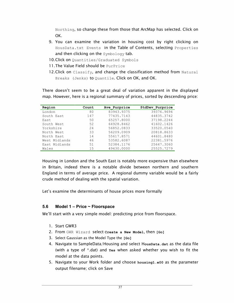
There doesn’t seem to be a great deal of variation apparent in the displayed

map. However, here is a regional summary of prices, sorted by descending price:

Region Count Ave_Purprice StdDev_Purprice London 80 83943.9375 39376.9694 South East 147 77435.7143 44835.3742 East 50 65257.8000 37198.2244 South West 52 64928.8462 41602.1426 Yorkshire 24 56852.0833 33520.0540 North West 33 56209.0909 20818.8633 North East 14 55617.8571 44601.8480 West Midlands 46 53582.6087 22381.5976 East Midlands 51 52384.1176 25647.3060 Wales 15 49430.0000 25525.7279

Housing in London and the South East is notably more expensive than elsewhere

in Britain, indeed there is a notable divide between northern and southern

England in terms of average price. A regional dummy variable would be a fairly

crude method of dealing with the spatial variation.

Let’s examine the determinants of house prices more formally

5.6 Model 1 – Price ~ Floorspace

We’ll start with a very simple model: predicting price from floorspace.

1. Start GWR3

2. From GWR Wizard select Create a New Model, then [Go]

3. Select Gaussian as the Model Type the [Go]

4. Navigate to SampleData/Housing and select HousData.dat as the data file

(with a type of *.dat) and Yes when asked whether you wish to fit the

model at the data points.

5. Navigate to your Work folder and choose housing1.e00 as the parameter

output filename; click on Save

38

11955

11960

11965

11970

11975

11980

25 35 45 55 65 75 85 95

6. Check the Data Preview and File Confirmation choices to make sure that

you have the correct input and output data.

7. Choose the following options in the model editor:

(1) Title Price ~ Area model

(2) dependent variable: PurPrice

(3) independent variable: FlrArea

(4) X-variable: Easting

(5) Y-variable: Northing

(6) Kernel type: Adaptive

(7) All three listing options from Model Options

(8) Bandwidth selection: AICc

(9) Output format: Arc/INFO Export

(10) Save your model as housing1.gwr (in Work)

(11) Click Run Model

(12) Save the listing file as housing1.txt

(13) Click Run

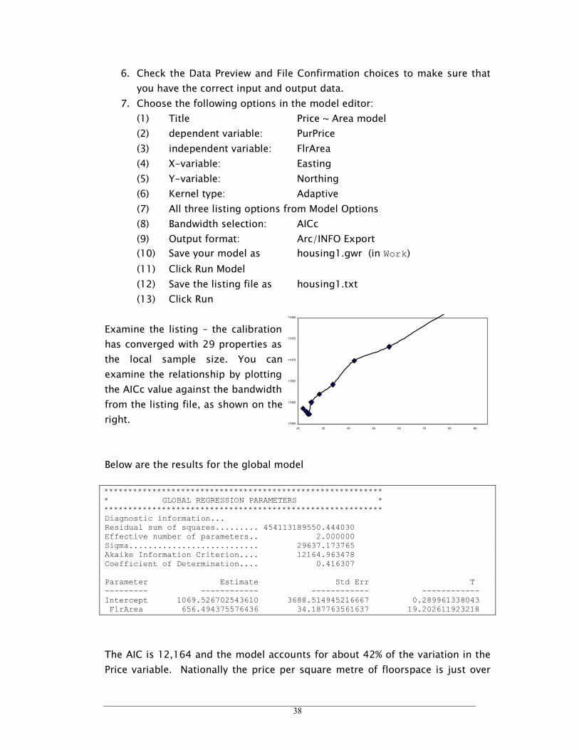
Examine the listing – the calibration

has converged with 29 properties as

the local sample size. You can

examine the relationship by plotting

the AICc value against the bandwidth

from the listing file, as shown on the

right.

Below are the results for the global model

********************************************************** * GLOBAL REGRESSION PARAMETERS * ********************************************************** Diagnostic information... Residual sum of squares......... 454113189550.444030 Effective number of parameters.. 2.000000 Sigma........................... 29637.173765 Akaike Information Criterion.... 12164.963478 Coefficient of Determination.... 0.416307 Parameter Estimate Std Err T --------- ------------ ------------ ------------ Intercept 1069.526702543610 3688.514945216667 0.289961338043 FlrArea 656.494375576436 34.187763561637 19.202611923218

The AIC is 12,164 and the model accounts for about 42% of the variation in the

Price variable. Nationally the price per square metre of floorspace is just over

39

£650. The parameter estimate for the floorspace variable is significantly

different from zero but the intercept term is not. It would seem that non-

existent houses are free for the taking!

The equivalent results for the local model are:


Notice that the local AIC is much lower and the local coefficient of determination

is much higher. We can be more confident that we have a ‘better’ model with

GWR. Note that because the effective number of parameters is different for the

global and local models that we can’t compare the r2 values directly.

The parameter 5 number summary is also interesting:

********************************************************** * PARAMETER 5-NUMBER SUMMARIES * ********************************************************** Label Minimum Lwr Quartile Median Upr Quartile Maximum Intrcept -64327.508064 -6189.706002 4492.787561 15304.148108 99446.460090 FlrArea -19.135883 447.434134 583.102579 730.316064 1540.075262

For 50% of the properties in the analysis the floorspace parameter varies from

£447.43 to £730.31. The average size of property is 101m2. This implies a

price variation from £45,190 to £73,761 depending on where the property was

located.

Notice that for the FlrArea parameter, the inter-quartile range of the local

estimates is 283.9 whereas 2 x SE of the global estimate is only 68.4 so there

appears to be a great deal of spatial variation in the local estimates. We can

explore this, and other features of the results, by mapping the output data as

follows:

40

1. Use ArcToolBox to convert the housing1.e00 file in your Work folder into

an Arc/INFO coverage. Call the resulting coverage housing1 and leave it

in the Work folder.

2. Add the coverage as a layer in the Table of Contents.

3. Change the fill on the regions layer to ‘No Fill’ and uncheck the other

layers except housing1.

4. Examine the standardised residuals (STDRES) – there appears to be very

little geographical pattern within them. The model has captured much of

the geographical variation through its weighting scheme although there

are a handful of outliers all west of London.

5. Now plot the PARM_2 coefficients. These are for the floorspace variable.

Under Classify change the Classification method to Standard Deviation.

6. You can choose a Color Ramp that looks pleasing to the eye – green to

red, or red to blue are good choices. If you right click on one of the

symbols in the Symbology dialog, you can Flip the color ramp round if

necessary (try it and see).

Some patterns immediately stand out. Some of the strongest relationships are

in the areas to the west of London as far as the Bristol Channel and,

interestingly, in Northern England. Some of this, of course, may be an artefact

of the particular sample chosen.

5.7 Model 2 – Price ~ Floorspace + Property Type

We will now examine the effect of adding a group of dummy variables

representing the type of property. The dummy variable for detached properties

takes the value 1 for a detached property and 0 otherwise. In a global

regression its effect is to create a separate intercept for detached houses

compared to other properties.

If you look back to the above table describing the data for this lab you will

observe that we have included dummy variables in the dataset for detached

properties, semi-detached properties and flats/apartments. Most of the other

types of property in the dataset are terraced (row houses). One of the more

famous terraces in Britain is the Royal Crescent in Bath, an elegant Georgian

terrace of very desirable property. At the other end of the market are the large

areas of low-cost terraced housing built by factory owners adjacent to their

factories in the mid to late 19th century. Such housing is usually cramped and

poorly constructed. We might therefore expect to see some spatial variation in

the GWR parameter for this type of property. This would appear in the intercept

term.

41

Royal Crescent, Bath 19thC Workers' Housing, Newcastle (Mary Ann Sullivan) (BBC)

The steps for this analysis are as follows:

1. Close all the windows in the GWR main window and select Tools/Analysis

Wizard/Open an existing model in the GWR Model Editor.

2. Navigate to your Work folder and select housing1.gwr and click OK

3. Add the variables TypDetch, TypSemiD and TypFlat into the list of

independent variables

4. Select Save the Model and overwrite the existing control file. The

existing interchange file will be reused.

5. Select Run Model, name the Listing File housing2.txt and proceed as

before

Here are some of the diagnostics for the global model

********************************************************** * GLOBAL REGRESSION PARAMETERS * ********************************************************** Diagnostic information... Residual sum of squares......... 391372117830.287660 Effective number of parameters.. 5.000000 Sigma........................... 27593.918782 Akaike Information Criterion.... 12093.912039 Coefficient of Determination.... 0.496951 Parameter Estimate Std Err T --------- ------------ ------------ ------------ Intercept 14739.342677934595 4038.893840041817 3.649351358414 TypDetch 15135.424430767123 4692.434978262239 3.225494861603 TypSemiD -10496.662116166888 4030.874273729064 -2.604065895081 TypFlat -14828.893957866609 3894.269647828749 -3.807875394821 FlrArea 569.641342931521 36.800583930017 15.479138374329

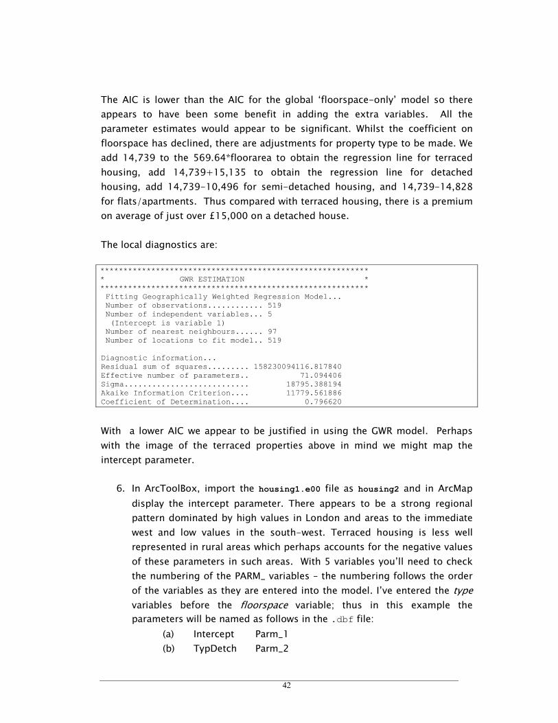
42

The AIC is lower than the AIC for the global ‘floorspace-only’ model so there

appears to have been some benefit in adding the extra variables. All the

parameter estimates would appear to be significant. Whilst the coefficient on

floorspace has declined, there are adjustments for property type to be made. We

add 14,739 to the 569.64*floorarea to obtain the regression line for terraced

housing, add 14,739+15,135 to obtain the regression line for detached

housing, add 14,739-10,496 for semi-detached housing, and 14,739-14,828

for flats/apartments. Thus compared with terraced housing, there is a premium

on average of just over £15,000 on a detached house.

The local diagnostics are:


With a lower AIC we appear to be justified in using the GWR model. Perhaps

with the image of the terraced properties above in mind we might map the

intercept parameter.

6. In ArcToolBox, import the housing1.e00 file as housing2 and in ArcMap

display the intercept parameter. There appears to be a strong regional

pattern dominated by high values in London and areas to the immediate

west and low values in the south-west. Terraced housing is less well

represented in rural areas which perhaps accounts for the negative values

of these parameters in such areas. With 5 variables you’ll need to check

the numbering of the PARM_ variables – the numbering follows the order

of the variables as they are entered into the model. I’ve entered the type

variables before the floorspace variable; thus in this example the

parameters will be named as follows in the .dbf file:

(a) Intercept Parm_1

(b) TypDetch Parm_2

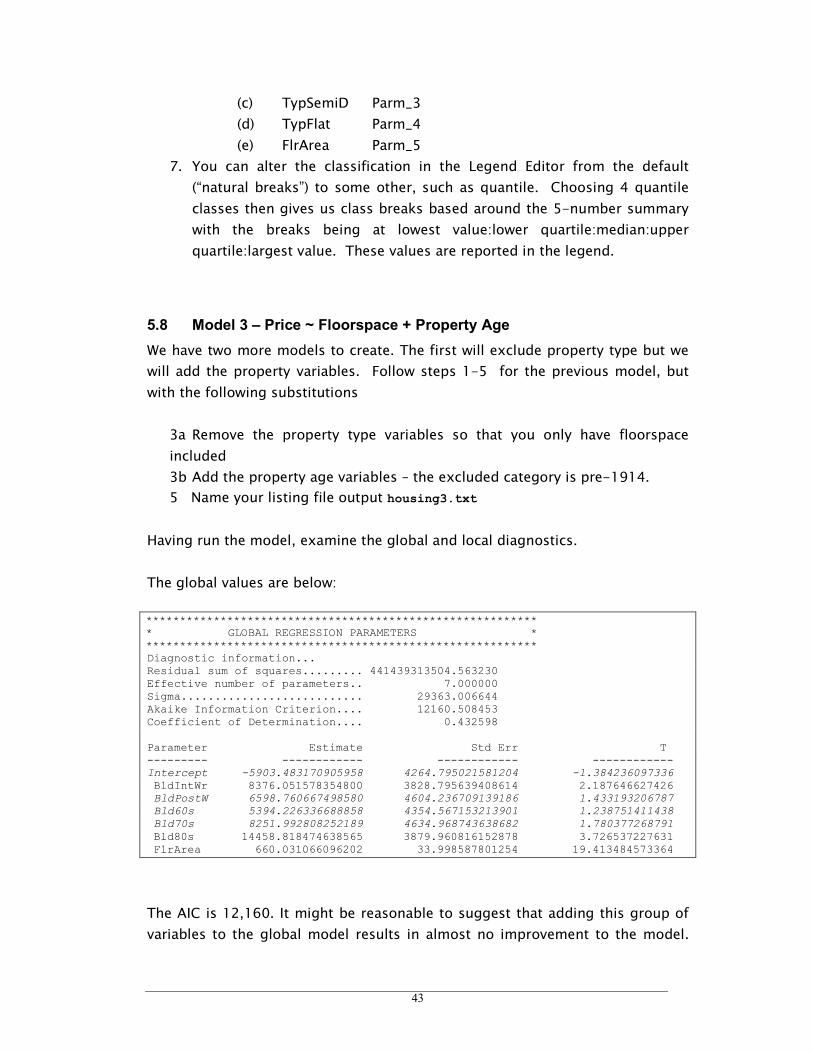
43

(c) TypSemiD Parm_3

(d) TypFlat Parm_4

(e) FlrArea Parm_5

7. You can alter the classification in the Legend Editor from the default

(“natural breaks”) to some other, such as quantile. Choosing 4 quantile

classes then gives us class breaks based around the 5-number summary

with the breaks being at lowest value:lower quartile:median:upper

quartile:largest value. These values are reported in the legend.

5.8 Model 3 – Price ~ Floorspace + Property Age

We have two more models to create. The first will exclude property type but we

will add the property variables. Follow steps 1-5 for the previous model, but

with the following substitutions

3a Remove the property type variables so that you only have floorspace

included

3b Add the property age variables – the excluded category is pre-1914.

5 Name your listing file output housing3.txt

Having run the model, examine the global and local diagnostics.

The global values are below:

********************************************************** * GLOBAL REGRESSION PARAMETERS * ********************************************************** Diagnostic information... Residual sum of squares......... 441439313504.563230 Effective number of parameters.. 7.000000 Sigma........................... 29363.006644 Akaike Information Criterion.... 12160.508453 Coefficient of Determination.... 0.432598 Parameter Estimate Std Err T --------- ------------ ------------ ------------ Intercept -5903.483170905958 4264.795021581204 -1.384236097336

BldIntWr 8376.051578354800 3828.795639408614 2.187646627426 BldPostW 6598.760667498580 4604.236709139186 1.433193206787

Bld60s 5394.226336688858 4354.567153213901 1.238751411438

Bld70s 8251.992808252189 4634.968743638682 1.780377268791

Bld80s 14458.818474638565 3879.960816152878 3.726537227631 FlrArea 660.031066096202 33.998587801254 19.413484573364

The AIC is 12,160. It might be reasonable to suggest that adding this group of

variables to the global model results in almost no improvement to the model.

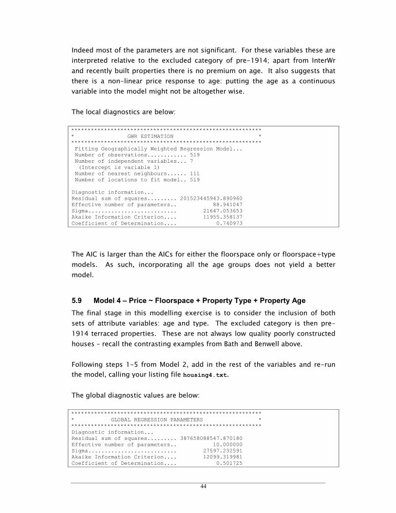
44

Indeed most of the parameters are not significant. For these variables these are

interpreted relative to the excluded category of pre-1914; apart from InterWr

and recently built properties there is no premium on age. It also suggests that

there is a non-linear price response to age: putting the age as a continuous

variable into the model might not be altogether wise.

The local diagnostics are below:


The AIC is larger than the AICs for either the floorspace only or floorspace+type

models. As such, incorporating all the age groups does not yield a better

model.

5.9 Model 4 – Price ~ Floorspace + Property Type + Property Age

The final stage in this modelling exercise is to consider the inclusion of both

sets of attribute variables: age and type. The excluded category is then pre-

1914 terraced properties. These are not always low quality poorly constructed

houses – recall the contrasting examples from Bath and Benwell above.

Following steps 1-5 from Model 2, add in the rest of the variables and re-run

the model, calling your listing file housing4.txt.

The global diagnostic values are below:

********************************************************** * GLOBAL REGRESSION PARAMETERS * ********************************************************** Diagnostic information... Residual sum of squares......... 387658088547.870180 Effective number of parameters.. 10.000000 Sigma........................... 27597.232591 Akaike Information Criterion.... 12099.319981 Coefficient of Determination.... 0.501725

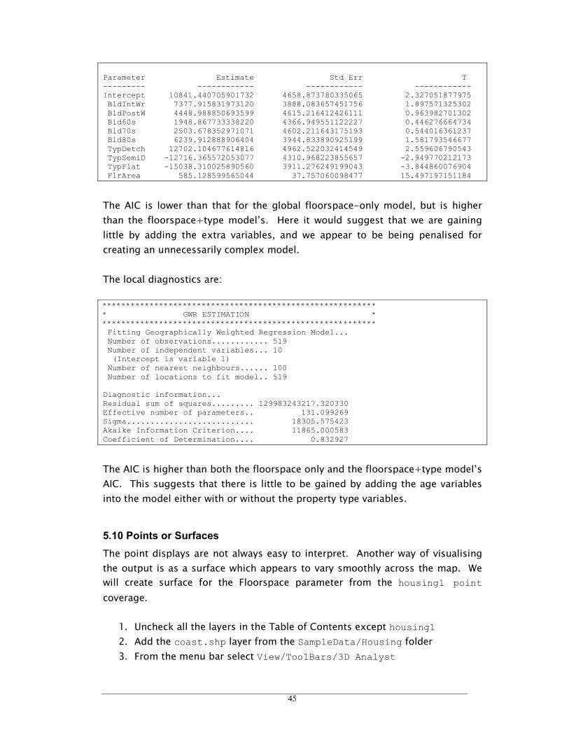
45

Parameter Estimate Std Err T --------- ------------ ------------ ------------ Intercept 10841.440705901732 4658.873780335065 2.327051877975 BldIntWr 7377.915831973120 3888.083657451756 1.897571325302 BldPostW 4448.988850693599 4615.216412426111 0.963982701302 Bld60s 1948.867733338220 4366.949551122227 0.446276664734 Bld70s 2503.678352971071 4602.211643175193 0.544016361237 Bld80s 6239.912888906404 3944.833890925199 1.581793546677 TypDetch 12702.104677614816 4962.522032414549 2.559606790543 TypSemiD -12716.365572053077 4310.968223855657 -2.949770212173 TypFlat -15038.310025890560 3911.276249199043 -3.844860076904 FlrArea 585.128599565044 37.757060098477 15.497197151184

The AIC is lower than that for the global floorspace-only model, but is higher

than the floorspace+type model’s. Here it would suggest that we are gaining

little by adding the extra variables, and we appear to be being penalised for

creating an unnecessarily complex model.

The local diagnostics are:


The AIC is higher than both the floorspace only and the floorspace+type model’s

AIC. This suggests that there is little to be gained by adding the age variables

into the model either with or without the property type variables.

5.10 Points or Surfaces

The point displays are not always easy to interpret. Another way of visualising

the output is as a surface which appears to vary smoothly across the map. We

will create surface for the Floorspace parameter from the housing1 point

coverage.

1. Uncheck all the layers in the Table of Contents except housing1

2. Add the coast.shp layer from the SampleData/Housing folder

3. From the menu bar select View/ToolBars/3D Analyst

46

4. From 3D Analyst, select Options

5. In General change the Working Directory to C:\Temp; set the Analysis

Mask to coast.shp

6. In Extent, set Analysis Extent to “Same as layer coast”

7. In Cell Size, choose “As specified below” and enter 5000 in the Cell

Size box; click OK

8. From 3D Analyst, select Interpolate to Raster/Inverse Distance Weighted

9. Input points should be housing1 point

10. Z value field should be PARM_2

11. Search type radius should be Variable

12. Number of points should be 12

13. Output raster should be <temporary>

14. Click on OK – the surface appears on the map with suitable shading to

show variation in the intensity of the relationship

15. Check the Places.txt Events layer to bring up the place names

The surface does reveal the patterns in a slightly different way. West of London,

there is a corridor of highly priced floorspace with peaks in Reading and Bristol –

this follows the route of the M4 motorway and the high speed rail link to Bristol

and Cardiff. Reading is both a commuter dormitory in its own right as well as

home to number of companies in the computing sector. There is a small peak

between London and Brighton, again reflecting the importance of the rail link

which connects Brighton, Crawley, Gatwick Airport and London. The apparent

rise in floorspace prices in northern England is probably a reflection of basing

the analysis on a .7% sample.

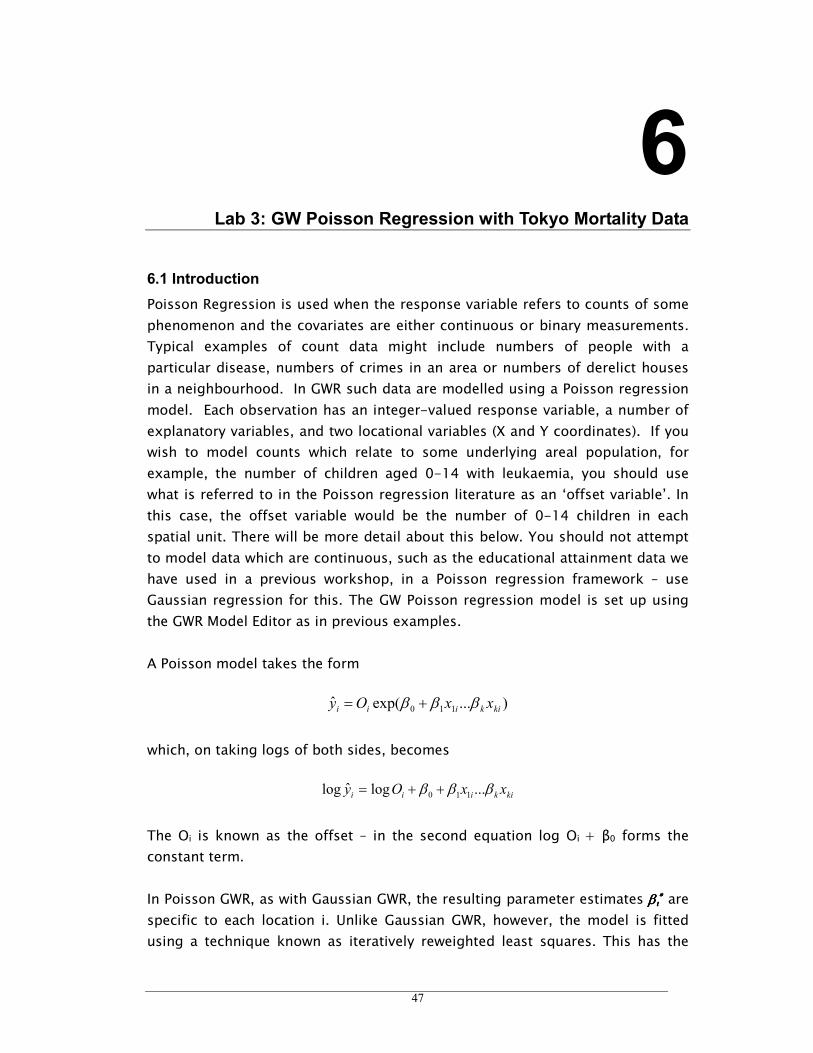
47

6

Lab 3: GW Poisson Regression with Tokyo Mortality Data

6.1 Introduction

Poisson Regression is used when the response variable refers to counts of some

phenomenon and the covariates are either continuous or binary measurements.

Typical examples of count data might include numbers of people with a

particular disease, numbers of crimes in an area or numbers of derelict houses

in a neighbourhood. In GWR such data are modelled using a Poisson regression

model. Each observation has an integer-valued response variable, a number of

explanatory variables, and two locational variables (X and Y coordinates). If you

wish to model counts which relate to some underlying areal population, for

example, the number of children aged 0-14 with leukaemia, you should use

what is referred to in the Poisson regression literature as an ‘offset variable’. In

this case, the offset variable would be the number of 0-14 children in each

spatial unit. There will be more detail about this below. You should not attempt

to model data which are continuous, such as the educational attainment data we

have used in a previous workshop, in a Poisson regression framework – use

Gaussian regression for this. The GW Poisson regression model is set up using

the GWR Model Editor as in previous examples.

A Poisson model takes the form

)...exp(ˆ110 kikiii xxOy βββ +=

which, on taking logs of both sides, becomes

kikiii xxOy βββ ...logˆlog 110 ++=

The Oi is known as the offset – in the second equation log Oi + β0 forms the

constant term.

In Poisson GWR, as with Gaussian GWR, the resulting parameter estimates ββββιιιι∗∗∗∗ are

specific to each location i. Unlike Gaussian GWR, however, the model is fitted

using a technique known as iteratively reweighted least squares. This has the

48

following implications. First, the fitting technique is iterative and so a typical

GW Poisson regression will take approximately 5 times as long to run as an

equivalent Gaussian regression. Second, to compute the standard errors, the

observed counts are required, so parameter estimates may only be obtained at

the data points.

The output file contains the parameter estimates from the Poisson model and

their standard errors as well as the exponentials of the parameter estimates and

the standard errors of these exponentiated values. Positive parameter values

when exponentiated are greater than unity, a parameter of zero when

exponentiated yields a value of unity, and negative parameter values when

exponentiated are less than unity. In all cases, the exponentiated values are

positive.

6.2 Mortality in Tokyo

For this workshop, we will be using a dataset concerned with premature

mortality levels in 262 municipalities in Tokyo5. These data refer to areas of

different underlying populations. In order to account for this we shall use the

expected number of deaths (based on population age composition and national

death rates) in each area as an offset. There is, as in the previous lab, a set of

continuous explanatory variables – these are the proportion of the population

aged over 65, the proportion of the population who are unemployed, the

proportion of the population who own their dwelling, and the proportion of the

population in professional occupations. One might expect higher mortality

counts in areas associated with economic problems and lower mortality counts

in more prosperous areas.

Mapping

Before beginning the analysis, you should examine the spatial distribution of the

variable.

1. Start ArcMap

2. From the SampleData/Tokyo folder add the layer TMABSU.shp – these are

the boundaries of the polygons which form municipalities in the Tokyo

Metropolitan Area.

5 Premature mortality counts are defined here as the number of deaths occurring to people aged 25-65 in

each area. We are grateful to Dr Tomoki Nakaya of the Department of Geography, Ritsumeikan University,

Kita-Ku, Kyoto for this dataset.

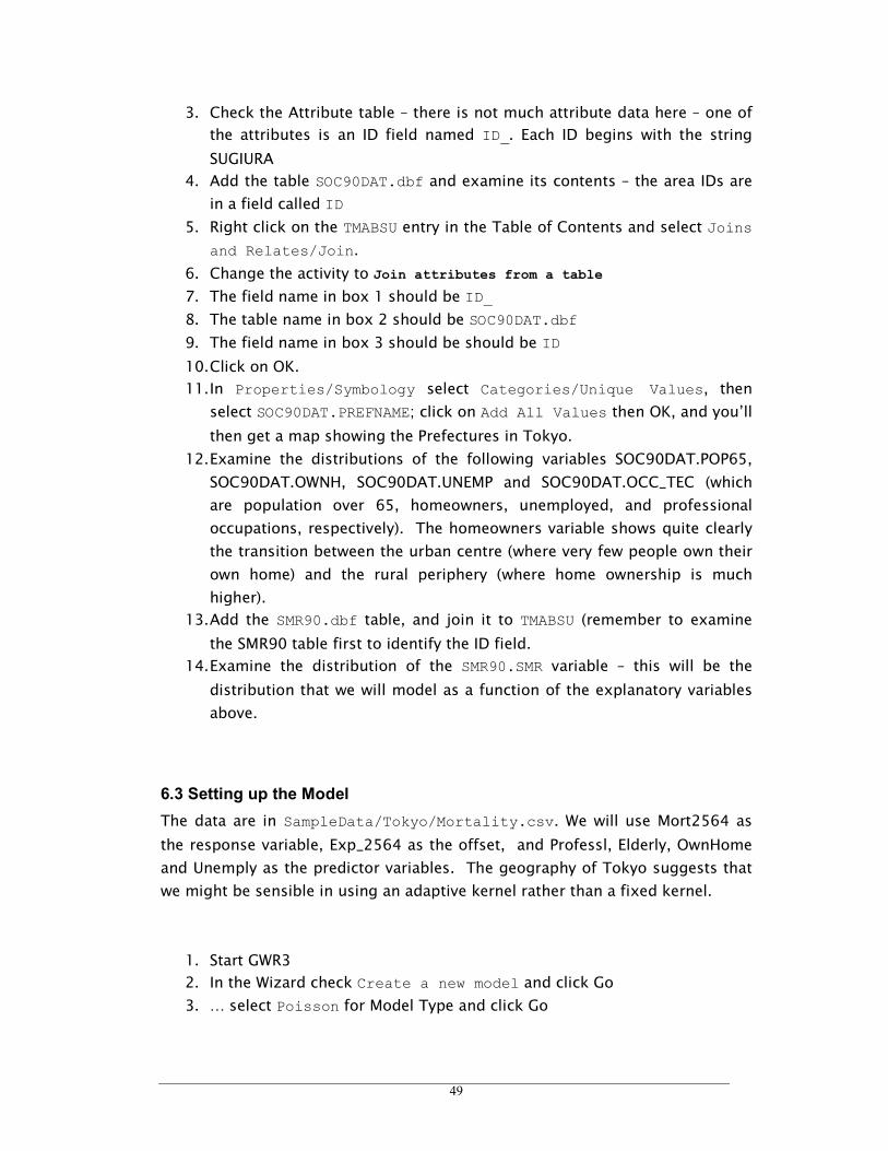
49

3. Check the Attribute table – there is not much attribute data here – one of

the attributes is an ID field named ID_. Each ID begins with the string

SUGIURA

4. Add the table SOC90DAT.dbf and examine its contents – the area IDs are

in a field called ID

5. Right click on the TMABSU entry in the Table of Contents and select Joins

and Relates/Join.

6. Change the activity to Join attributes from a table

7. The field name in box 1 should be ID_

8. The table name in box 2 should be SOC90DAT.dbf

9. The field name in box 3 should be should be ID

10. Click on OK.

11. In Properties/Symbology select Categories/Unique Values, then

select SOC90DAT.PREFNAME; click on Add All Values then OK, and you’ll

then get a map showing the Prefectures in Tokyo.

12. Examine the distributions of the following variables SOC90DAT.POP65,

SOC90DAT.OWNH, SOC90DAT.UNEMP and SOC90DAT.OCC_TEC (which

are population over 65, homeowners, unemployed, and professional

occupations, respectively). The homeowners variable shows quite clearly

the transition between the urban centre (where very few people own their

own home) and the rural periphery (where home ownership is much

higher).

13. Add the SMR90.dbf table, and join it to TMABSU (remember to examine

the SMR90 table first to identify the ID field.

14. Examine the distribution of the SMR90.SMR variable – this will be the

distribution that we will model as a function of the explanatory variables

above.

6.3 Setting up the Model

The data are in SampleData/Tokyo/Mortality.csv. We will use Mort2564 as

the response variable, Exp_2564 as the offset, and Professl, Elderly, OwnHome

and Unemply as the predictor variables. The geography of Tokyo suggests that

we might be sensible in using an adaptive kernel rather than a fixed kernel.

1. Start GWR3

2. In the Wizard check Create a new model and click Go

3. … select Poisson for Model Type and click Go

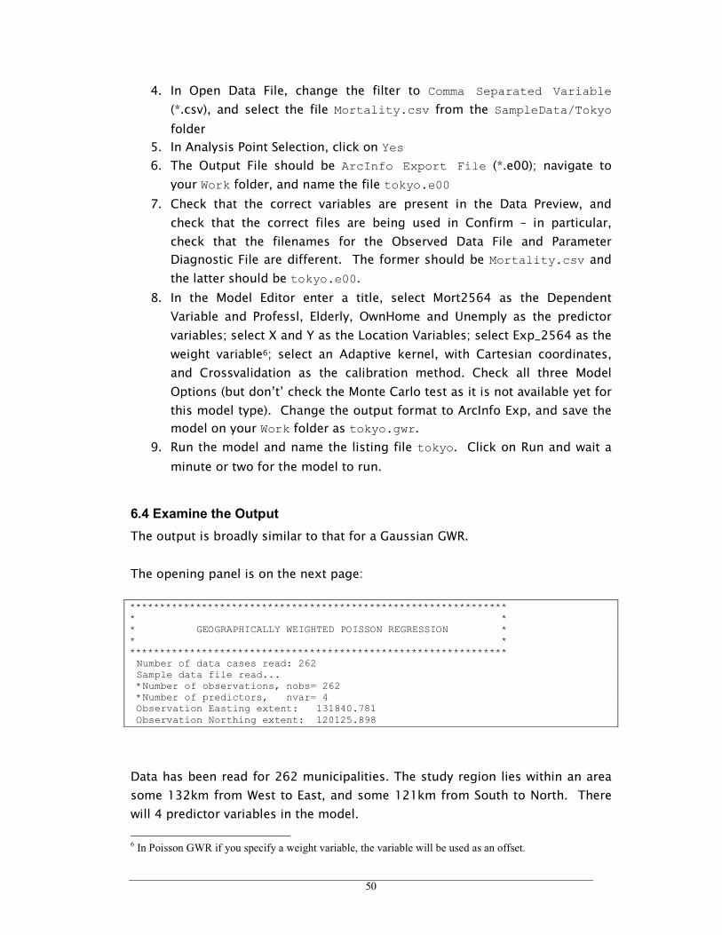
50

4. In Open Data File, change the filter to Comma Separated Variable

(*.csv), and select the file Mortality.csv from the SampleData/Tokyo

folder

5. In Analysis Point Selection, click on Yes

6. The Output File should be ArcInfo Export File (*.e00); navigate to

your Work folder, and name the file tokyo.e00

7. Check that the correct variables are present in the Data Preview, and

check that the correct files are being used in Confirm – in particular,

check that the filenames for the Observed Data File and Parameter

Diagnostic File are different. The former should be Mortality.csv and

the latter should be tokyo.e00.

8. In the Model Editor enter a title, select Mort2564 as the Dependent

Variable and Professl, Elderly, OwnHome and Unemply as the predictor

variables; select X and Y as the Location Variables; select Exp_2564 as the

weight variable6; select an Adaptive kernel, with Cartesian coordinates,

and Crossvalidation as the calibration method. Check all three Model

Options (but don’t’ check the Monte Carlo test as it is not available yet for

this model type). Change the output format to ArcInfo Exp, and save the

model on your Work folder as tokyo.gwr.

9. Run the model and name the listing file tokyo. Click on Run and wait a

minute or two for the model to run.

6.4 Examine the Output

The output is broadly similar to that for a Gaussian GWR.

The opening panel is on the next page:

*************************************************************** * * * GEOGRAPHICALLY WEIGHTED POISSON REGRESSION * * * *************************************************************** Number of data cases read: 262 Sample data file read... *Number of observations, nobs= 262 *Number of predictors, nvar= 4 Observation Easting extent: 131840.781 Observation Northing extent: 120125.898

Data has been read for 262 municipalities. The study region lies within an area

some 132km from West to East, and some 121km from South to North. There

will 4 predictor variables in the model.

6 In Poisson GWR if you specify a weight variable, the variable will be used as an offset.

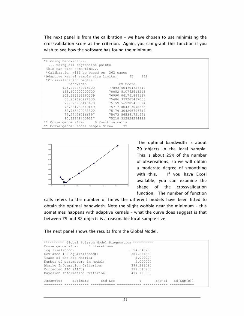
51

The next panel is from the calibration – we have chosen to use minimising the

crossvalidation score as the criterion. Again, you can graph this function if you

wish to see how the software has found the minimum.

*Finding bandwidth... ... using all regression points This can take some time... *Calibration will be based on 262 cases *Adaptive kernel sample size limits: 65 262 *Crossvalidation begins... Bandwidth CV Score 125.876348015000 77093.504704727718 163.500000000000 78852.510762618243 102.623652260339 76090.041761883127 88.252695924830 75486.337205487056 79.370956440679 75159.569289465624 73.881739549149 75717.804317078335 82.763479033300 75179.304206706714 77.274262166597 75473.565361751971 80.666784759217 75218.352828294883 ** Convergence after 9 function calls ** Convergence: Local Sample Size= 79

The optimal bandwidth is about

79 objects in the local sample.

This is about 25% of the number

of observations, so we will obtain

a moderate degree of smoothing

with this. If you have Excel

available, you can examine the

shape of the crossvalidation

function. The number of function

calls refers to the number of times the different models have been fitted to

obtain the optimal bandwidth. Note the slight wobble near the minimum – this

sometimes happens with adaptive kernels – what the curve does suggest is that

between 79 and 82 objects is a reasonable local sample size.

The next panel shows the results from the Global Model.

********** Global Poisson Model Diagnostics ********** Convergence after 3 iterations Log-likelihood: -194.640790 Deviance (-2LogLikelihood): 389.281580 Trace of the Hat Matrix: 5.000000 Number of parameters in model: 5.000000 Akaike Information Criterion: 399.281580 Corrected AIC (AICc) 399.515955 Bayesian Information Criterion: 417.123303 Parameter Estimate Std Err T Exp(B) Sd(Exp(B)) --------- ------------ ------------ ------------ ------------ ------------

75000

75500

76000

76500

77000

77500

78000

78500

79000

60 80 100 120 140 160 180

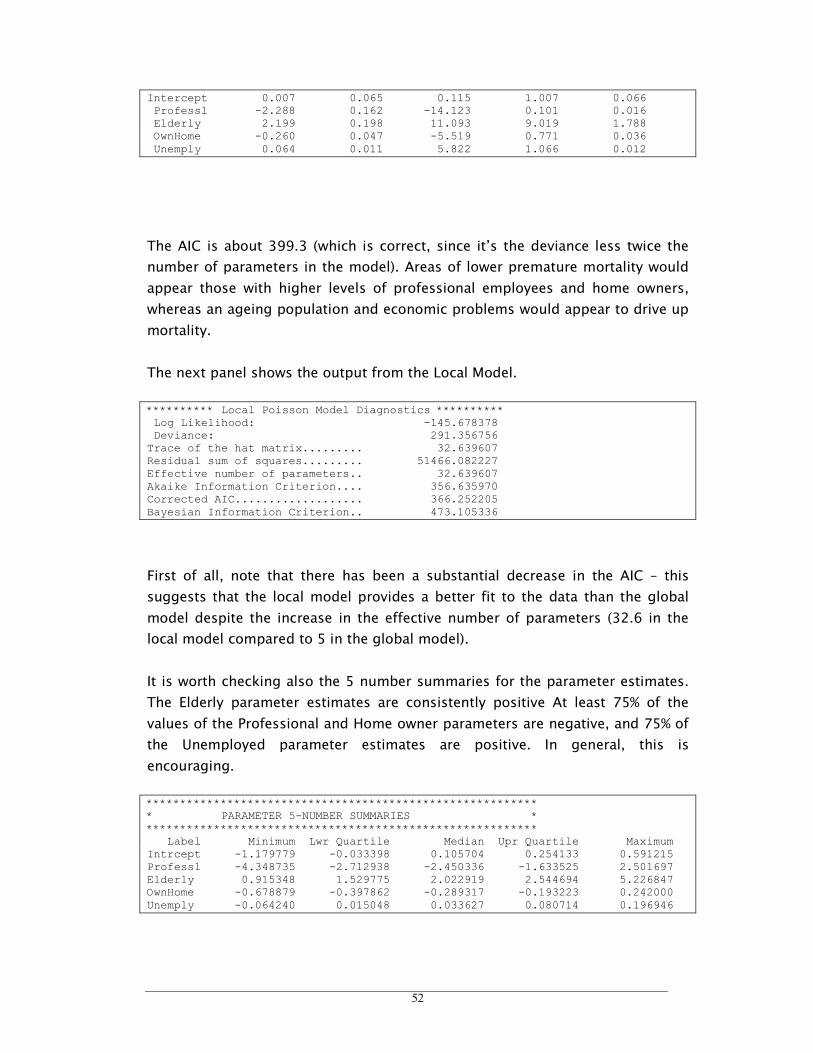
52

Intercept 0.007 0.065 0.115 1.007 0.066 Professl -2.288 0.162 -14.123 0.101 0.016 Elderly 2.199 0.198 11.093 9.019 1.788 OwnHome -0.260 0.047 -5.519 0.771 0.036 Unemply 0.064 0.011 5.822 1.066 0.012

The AIC is about 399.3 (which is correct, since it’s the deviance less twice the

number of parameters in the model). Areas of lower premature mortality would

appear those with higher levels of professional employees and home owners,

whereas an ageing population and economic problems would appear to drive up

mortality.

The next panel shows the output from the Local Model.

********** Local Poisson Model Diagnostics ********** Log Likelihood: -145.678378 Deviance: 291.356756 Trace of the hat matrix......... 32.639607 Residual sum of squares......... 51466.082227 Effective number of parameters.. 32.639607 Akaike Information Criterion.... 356.635970 Corrected AIC................... 366.252205 Bayesian Information Criterion.. 473.105336

First of all, note that there has been a substantial decrease in the AIC – this

suggests that the local model provides a better fit to the data than the global

model despite the increase in the effective number of parameters (32.6 in the

local model compared to 5 in the global model).

It is worth checking also the 5 number summaries for the parameter estimates.

The Elderly parameter estimates are consistently positive At least 75% of the

values of the Professional and Home owner parameters are negative, and 75% of

the Unemployed parameter estimates are positive. In general, this is

encouraging.

********************************************************** * PARAMETER 5-NUMBER SUMMARIES * ********************************************************** Label Minimum Lwr Quartile Median Upr Quartile Maximum Intrcept -1.179779 -0.033398 0.105704 0.254133 0.591215 Professl -4.348735 -2.712938 -2.450336 -1.633525 2.501697 Elderly 0.915348 1.529775 2.022919 2.544694 5.226847 OwnHome -0.678879 -0.397862 -0.289317 -0.193223 0.242000 Unemply -0.064240 0.015048 0.033627 0.080714 0.196946

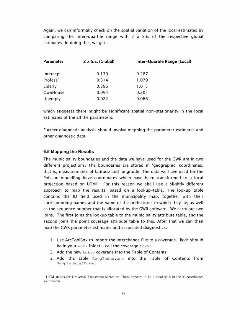
53

Again, we can informally check on the spatial variation of the local estimates by

comparing the inter-quartile range with 2 x S.E. of the respective global

estimates. In doing this, we get…

ParameterParameterParameterParameter 2 x S.E. (Global)2 x S.E. (Global)2 x S.E. (Global)2 x S.E. (Global) InterInterInterInter----Quartile Range (Local)Quartile Range (Local)Quartile Range (Local)Quartile Range (Local)

Intercept 0.130 0.287

Profess1 0.314 1.079

Elderly 0.396 1.015

OwnHouse 0.094 0.205

Unemply 0.022 0.066

which suggests there might be significant spatial non-stationarity in the local

estimates of the all the parameters.

Further diagnostic analysis should involve mapping the parameter estimates and

other diagnostic data.


The municipality boundaries and the data we have used for the GWR are in two

different projections. The boundaries are stored in ‘geographic’ coordinates,

that is, measurements of latitude and longitude. The data we have used for the

Poisson modelling have coordinates which have been transformed to a local

projection based on UTM7. For this reason we shall use a slightly different

approach to map the results, based on a lookup-table. The lookup table

contains the ID field used in the municipality map, together with their

corresponding names and the name of the prefectures in which they lie, as well

as the sequence number that is allocated by the GWR software. We carry out two

joins. The first joins the lookup table to the municipality attribute table, and the

second joins the point coverage attribute table to this. After that we can then

map the GWR parameter estimates and associated diagnostics.

1. Use ArcToolBox to Import the Interchange File to a coverage. Both should

be in your Work folder – call the coverage tokyo

2. Add the new tokyo coverage into the Table of Contents

3. Add the table GeogIndex.csv into the Table of Contents from SampleData/Tokyo

7 UTM stands for Universal Transverse Mercator. There appears to be a local shift in the Y coordinates

southwards.

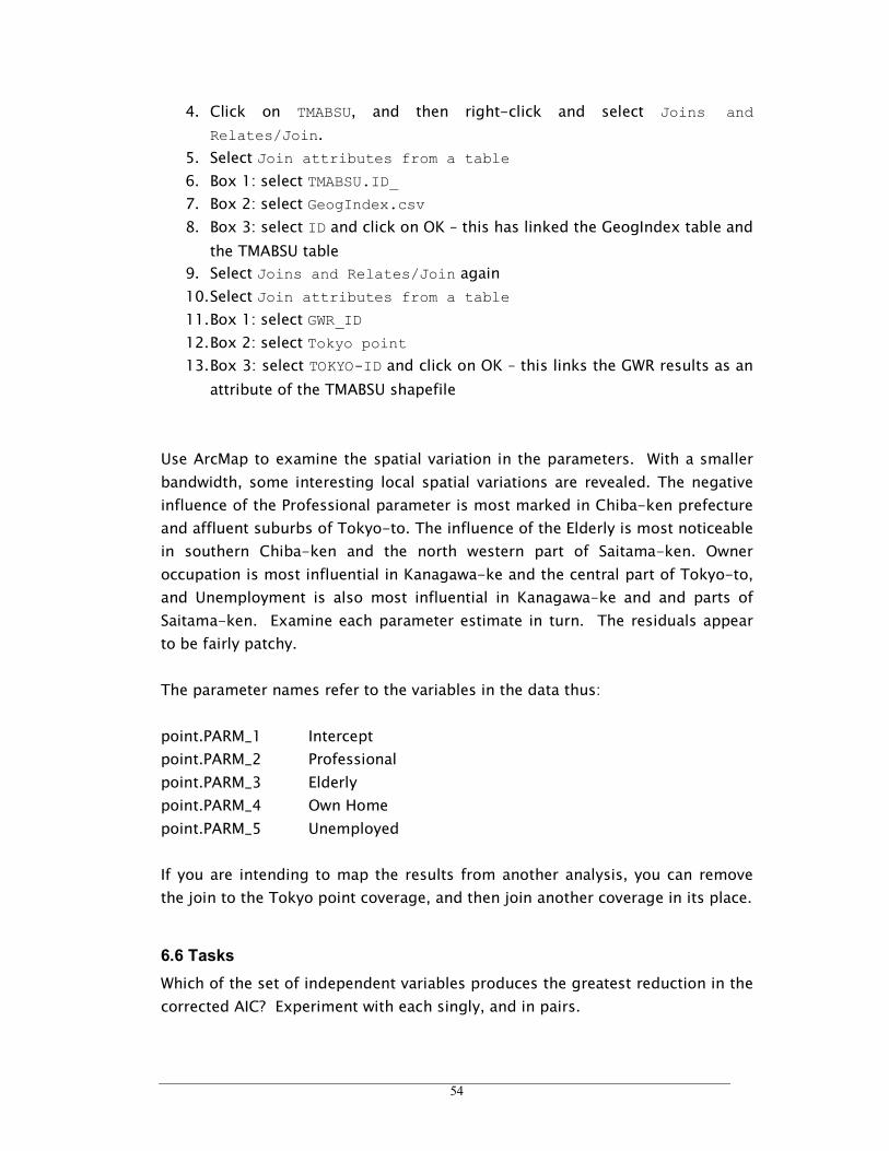
54

4. Click on TMABSU, and then right-click and select Joins and

Relates/Join.

5. Select Join attributes from a table

6. Box 1: select TMABSU.ID_

7. Box 2: select GeogIndex.csv

8. Box 3: select ID and click on OK – this has linked the GeogIndex table and

the TMABSU table

9. Select Joins and Relates/Join again

10. Select Join attributes from a table

11. Box 1: select GWR_ID

12. Box 2: select Tokyo point

13. Box 3: select TOKYO-ID and click on OK – this links the GWR results as an

attribute of the TMABSU shapefile

Use ArcMap to examine the spatial variation in the parameters. With a smaller

bandwidth, some interesting local spatial variations are revealed. The negative

influence of the Professional parameter is most marked in Chiba-ken prefecture

and affluent suburbs of Tokyo-to. The influence of the Elderly is most noticeable

in southern Chiba-ken and the north western part of Saitama-ken. Owner

occupation is most influential in Kanagawa-ke and the central part of Tokyo-to,

and Unemployment is also most influential in Kanagawa-ke and and parts of

Saitama-ken. Examine each parameter estimate in turn. The residuals appear

to be fairly patchy.

The parameter names refer to the variables in the data thus:

point.PARM_1 Intercept

point.PARM_2 Professional

point.PARM_3 Elderly

point.PARM_4 Own Home

point.PARM_5 Unemployed

If you are intending to map the results from another analysis, you can remove

the join to the Tokyo point coverage, and then join another coverage in its place.

6.6 Tasks

Which of the set of independent variables produces the greatest reduction in the

corrected AIC? Experiment with each singly, and in pairs.

55

For a given model (perhaps take a simple one with only Unemployed as the

explanatory variable) what is the effect of choosing different calibration

methods?

Experiment with different bandwidths. What is the effect on the AICc and the

effective number of parameters of reducing the bandwidth? Try 17000 as the

bandwidth for a Fixed kernel, and 40 as the Local Sample Size for an Adaptive

kernel.

56

7

Lab 4: Logistic GWR with Landslides in Clearwater, Idaho

7.1 Introduction

Logistic Regression (also known as Binary Logit Regression) is used when your

response variable is binary and the covariates are either continuous or binary

measurements. Typical examples of binary data might include yes/no,

alive/dead or above/below. In GWR such data are modelled using a logistic

regression model. You will find the term binary or dichotomous used as names

for the 0/1 data – note, however, that these data are not binomial, and the

model is not binomial. In GWR each observation has a 1/0 valued response

variable, a number of explanatory variables, and some locational variables. The

problem is set up using the GWR Model Editor as before.

Mathematically, the situation is that we need a model form that predicts yi ,

where i = 1…n, as a value in the interval 0-1 based on a set of explanatory

variables, 1…k. Such a model is,

)...exp(1

)...exp(ˆ

110

110

kiki

kikii

xx

xxy

ββββββ++++

+++=

where yi* is the predicted value of yi,

because, as exp(β0 + β1x1i …+ βkxki) → 0, yi* → 0 and as exp(β0 + β1x1i …+ βkxki)

→ ∞, yi* → 1

Note that

)...exp(1

1ˆ1

110 kiki

ixx

yβββ ++++

=−

so that

)...exp(ˆ1

ˆ110 kiki

i

i xxy

yβββ +++=

−

57

and

kiki

i

i xxy

yβββ +++=

−...

ˆ1

ˆlog 110

The term on the left hand side of the equation is known as the logit

transformation and this produces a linear function in terms of the right hand

side of the equation.

In logistic GWR, as with Gaussian GWR, the local parameter estimates ββββιιιι∗∗∗∗ are

specific to each location i. The model calibration, however, is more complicated

than in OLS regression and the model is fitted using a technique known as

iteratively reweighted least squares. This has two implications for our analysis.

First, the fitting technique is iterative, and a typical problem will take

approximately 5 times as long to run as a Gaussian GWR. Second, to compute

the standard errors, the observed 0/1 values are required, so parameter

estimates may only be obtained at the data points – that is, we no longer have

the option of producing local parameter estimates at points other than the data

points.

The output file from logistic GWR contains the parameter estimates and their

standard errors from (7.4). Positive parameter values when exponentiated are

greater than unity, a parameter of zero yields an exponentiated value of unity,

and negative parameter values when exponentiated are less than unity. In all

cases, the exponentiated values are positive. Exponentiating the parameter

values is an add-on task (see section 7.7)

7.2 Landslide Hazard: Clearwater National Forest

For this workshop, we will revisit some research into the probabilities of

landslide occurrence. In November 1995 and in February 1996 there were some

900 landslides in Clearwater National Forest in northern Idaho. Following the

landslides there were a number of attempts at predicting landslide hazard. Some

interesting work was carried out by Peter Gorsevski and Paul Gessler of the

Department of Forest Resources at the University of Idaho in conjunction with

Randy Folz of the USDA Forest Service Rocky Mountain Research Station. Using

logistic regression they attempted to create a hazard map for landslides in the

Forest. They found they could predict the probability of landslide occurrence

reliably using information on the landscape morphology and proximity to water.

We’ll use GWR to look at a subset of the landslide data with a similar set of data.

58

The data for this workshop is in the SampleData/Clearwater folder in the file

landslides.csv. They are the landslides in a small part of the Forest, about

33 x 29km in size, extracted from the Clearwater National Forest GIS Library. A

digital elevation model was downloaded from the Shuttle Radar Topography

Mission data archive at the Jet Propulsion Laboratory and re-projected into UTM

Zone 11 with a 25m grid interval – this gives us an estimate of the elevation of

every 25 grid square in the forest. The DEM was then used to create slope and

aspect grids the slope is given in percent, and the aspect in degrees. Two more

grids were created with the sin and cosine of the aspect. Digitised streams data

was downloaded from the CWNF website. A basemap extracted from TerraServer

is included to help in interpreting the results.

For the 138 landslides sites in the study area we extracted the following data

(a) elevation in metres

(b) slope (%)

(c) sin of the aspect

(d) cosine of the aspect

(e) absolute deviation of the aspect from due south

(f) distance in metres to the nearest watercourse

We also need observations from sites where there were no landslides. 101

random locations were sampled in the area for the same 5 variables. We’ll refer

to the first sample as the landslide sites and the second sample as the control

sites.

The two samples were merged. A 7th variable was added with the value of 1 for

the landslide sites and 0 for the control sites. This will be used as the y variable

in the logistic regression. The topographic variables will be used as predictors

and the output will include the probability of a landslide occurring given the

characteristics of the site, whether landslide or not. A satisfactory outcome will

be high probabilities at the landslide sites and low probabilities at the control

sites.

We have taken a small area of the Forest to keep the GWR run times short. The

models take about 2 minutes to fit on a 1.70GHz laptop. On the same system

fitting the dataset of 875 sample sites and the same number of controls takes

an hour.

59

7.3 Examining the data

Before beginning the analysis, you should map the spatial distribution of the

landslides on the basemap.

1. Start ArcMap

2. From the SampleData/Clearwater folder add basemap.jpg and

landslides.csv.

3. Right-click on landslides.csv in the Table of Contents, and select

Display XY Data from the options that are presented. A form

will be presented – there’s not much to do except note that

ArcMap has selected X as the X variable and Y as Y variable. Click

on OK at the bottom of the screen

4. Right click on landslides.csv Events in the Table of Contents and

select Properties/Symbology.

5. Select Categories/Unique Values in the Show: list

6. Select Landslid as the Value Field

7. Click on the Add Values button and add the values 0 and 1.

8. Uncheck the symbol for ‘All Other Values’

9. Change the fill colours to red for 1 and blue for 0 and click OK.

Remember that landslide sites are coded 1 and control sites are

coded 0. You might want to change the colours to red for 1 and

blue or green for 0.

10. You can also examine the spatial variation in some of the explanatory

variables. As these are point data, you should use Graduated Graduated Graduated Graduated

ColorsColorsColorsColors as the symbolism.

7.4 Setting up the Model

We will use Landslid as the response variable and initially Elev and Slope as

the predictor variables.

1. Start GWR3

2. In the Wizard check Create a new model and click Go

3. … select Logistic for Model Type and click Go

4. In Open Data File, change the filter to Comma Separated Variable

(*.csv), and select the file landslides.csv from the

SampleData/Clearwater folder

5. In Analysis Point Selection, click on Yes

6. The Output File should be an ArcInfo Export File (*.e00); navigate to

your Work folder, and name the file logmodela.e00

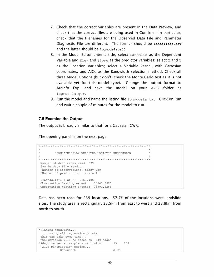
60

7. Check that the correct variables are present in the Data Preview, and

check that the correct files are being used in Confirm – in particular,

check that the filenames for the Observed Data File and Parameter

Diagnostic File are different. The former should be landslides.csv

and the latter should be logmodela.e00.

8. In the Model Editor enter a title, select Landslid as the Dependent

Variable and Elev and Slope as the predictor variables; select X and Y

as the Location Variables; select a Variable kernel, with Cartesian

coordinates, and AICc as the Bandwidth selection method. Check all

three Model Options (but don’t’ check the Monte Carlo test as it is not

available yet for this model type). Change the output format to

ArcInfo Exp, and save the model on your Work folder as

logmodela.gwr.

9. Run the model and name the listing file logmodela.txt. Click on Run

and wait a couple of minutes for the model to run.

7.5 Examine the Output

The output is broadly similar to that for a Gaussian GWR.

The opening panel is on the next page:

*************************************************************** * * * GEOGRAPHICALLY WEIGHTED LOGISTIC REGRESSION * * * *************************************************************** Number of data cases read: 239 Sample data file read... *Number of observations, nobs= 239 *Number of predictors, nvar= 4 P(Landslid=1 | X) = 0.577406 Observation Easting extent: 33543.0625 Observation Northing extent: 28802.6289

Data has been read for 239 locations. 57.7% of the locations were landslide

sites. The study area is rectangular, 33.5km from east to west and 28.8km from

north to south.

*Finding bandwidth... ... using all regression points This can take some time... *Calibration will be based on 239 cases *Adaptive kernel sample size limits: 59 239 *AICc minimisation begins... Bandwidth AICc

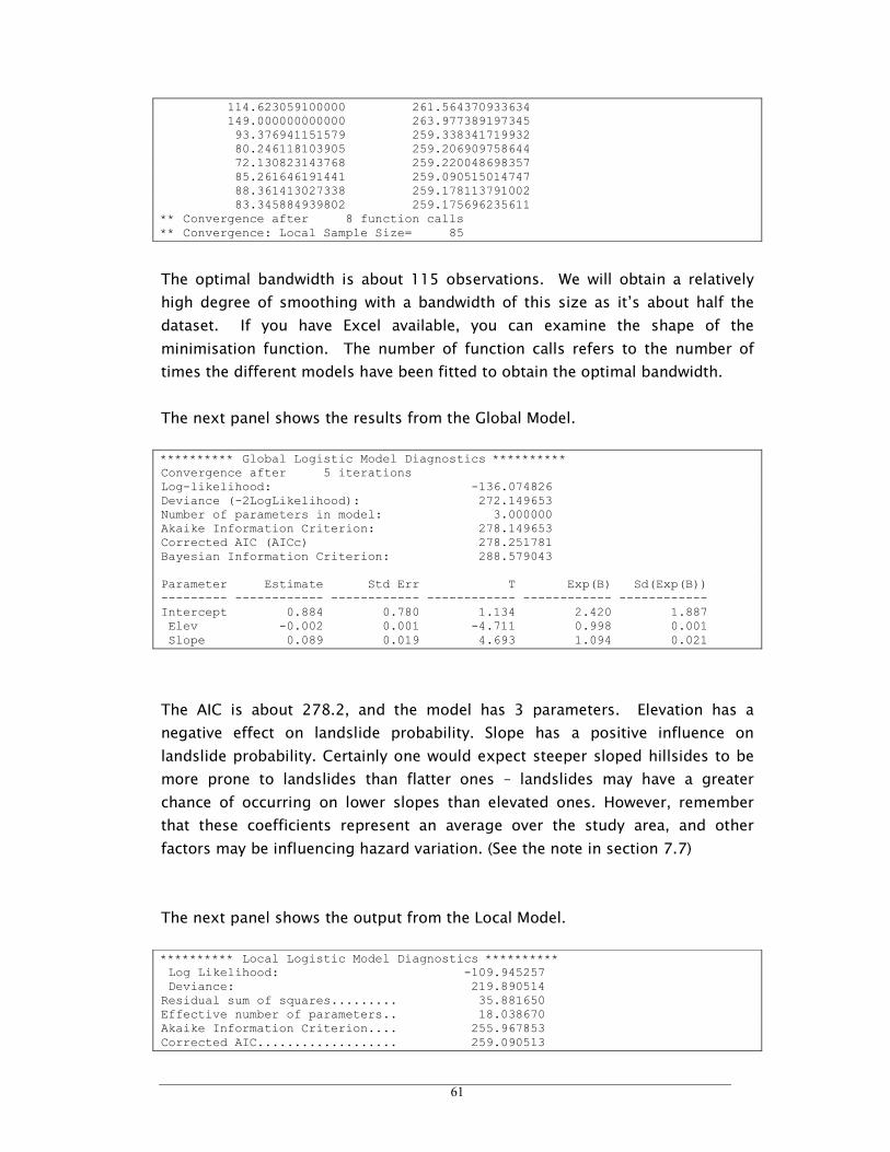
61

114.623059100000 261.564370933634 149.000000000000 263.977389197345 93.376941151579 259.338341719932 80.246118103905 259.206909758644 72.130823143768 259.220048698357 85.261646191441 259.090515014747 88.361413027338 259.178113791002 83.345884939802 259.175696235611 ** Convergence after 8 function calls ** Convergence: Local Sample Size= 85

The optimal bandwidth is about 115 observations. We will obtain a relatively

high degree of smoothing with a bandwidth of this size as it’s about half the

dataset. If you have Excel available, you can examine the shape of the

minimisation function. The number of function calls refers to the number of

times the different models have been fitted to obtain the optimal bandwidth.

The next panel shows the results from the Global Model.

********** Global Logistic Model Diagnostics ********** Convergence after 5 iterations Log-likelihood: -136.074826 Deviance (-2LogLikelihood): 272.149653 Number of parameters in model: 3.000000 Akaike Information Criterion: 278.149653 Corrected AIC (AICc) 278.251781 Bayesian Information Criterion: 288.579043 Parameter Estimate Std Err T Exp(B) Sd(Exp(B)) --------- ------------ ------------ ------------ ------------ ------------ Intercept 0.884 0.780 1.134 2.420 1.887 Elev -0.002 0.001 -4.711 0.998 0.001 Slope 0.089 0.019 4.693 1.094 0.021

The AIC is about 278.2, and the model has 3 parameters. Elevation has a

negative effect on landslide probability. Slope has a positive influence on

landslide probability. Certainly one would expect steeper sloped hillsides to be

more prone to landslides than flatter ones – landslides may have a greater

chance of occurring on lower slopes than elevated ones. However, remember

that these coefficients represent an average over the study area, and other

factors may be influencing hazard variation. (See the note in section 7.7)

The next panel shows the output from the Local Model.

********** Local Logistic Model Diagnostics ********** Log Likelihood: -109.945257 Deviance: 219.890514 Residual sum of squares......... 35.881650 Effective number of parameters.. 18.038670 Akaike Information Criterion.... 255.967853 Corrected AIC................... 259.090513

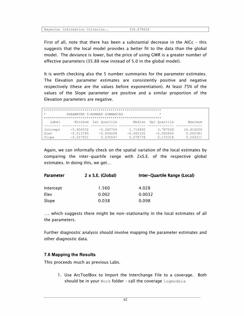
62

Bayesian Information Criterion.. 318.678626

First of all, note that there has been a substantial decrease in the AICc – this

suggests that the local model provides a better fit to the data than the global

model. The deviance is lower, but the price of using GWR is a greater number of

effective parameters (35.88 now instead of 5.0 in the global model).

It is worth checking also the 5 number summaries for the parameter estimates.

The Elevation parameter estimates are consistently positive and negative

respectively (these are the values before exponentiation). At least 75% of the

values of the Slope parameter are positive and a similar proportion of the

Elevation parameters are negative.

********************************************************** * PARAMETER 5-NUMBER SUMMARIES * ********************************************************** Label Minimum Lwr Quartile Median Upr Quartile Maximum -------- ------------- ------------- ------------- ------------- ------------- Intrcept -5.856532 -0.240704 1.719492 3.787028 16.416200 Elev -0.013785 -0.004208 -0.002330 -0.000893 0.000381 Slope -0.027931 0.035047 0.078778 0.133318 0.243211

Again, we can informally check on the spatial variation of the local estimates by

comparing the inter-quartile range with 2xS.E. of the respective global

estimates. In doing this, we get…

ParameterParameterParameterParameter 2 x S.E. (Global)2 x S.E. (Global)2 x S.E. (Global)2 x S.E. (Global) InterInterInterInter----Quartile Range (Local)Quartile Range (Local)Quartile Range (Local)Quartile Range (Local)

Intercept 1.560 4.028

Elev 0.002 0.0032

Slope 0.038 0.098

…. which suggests there might be non-stationarity in the local estimates of all

the parameters.

Further diagnostic analysis should involve mapping the parameter estimates and

other diagnostic data.


This proceeds much as previous Labs.

1. Use ArcToolBox to Import the Interchange File to a coverage. Both

should be in your Work folder – call the coverage logmodela

63

2. Add the new logmodela coverage into the Table of Contents

The new layer is added to the Table of Contents. Use ArcMap to examine the

spatial variation in the parameters. As you might expect given the relatively

large bandwidth, there are some broad regional variations present in the

parameter estimates. Remember that we have taken a small sample of landslides

in the Forest, so it might be unwise to draw general conclusions about

landslides in Clearwater. The influence of elevation on landslide hazard is most

negative towards the east and western parts of the study area – higher

elevations imply lower hazard. There is a north south pattern to the variation in

the slope parameter, with slopes in the south part of the study area having the

greatest influence on hazard.

Examine the spatial variation in the predicted probabilities:

1. In Symbology choose Quantities/Graduated Colors

2. Select PRED as the Field/Value

3. Under Classify, select Equal Interval as the Method, with 5

classes. This should give class breaks about 0.2, 0.4, 0.6, and 0.8.

4. Click OK

An interesting task is to examine the relationship between the observed and

predicted values. The easiest way of doing this is by examining the residuals.

Remember that these are the difference between the observed y and the

predicted y. The observed ys have the values 0 and 0, whereas the predicted ys

are probabilities in the range 0…1. A residual of -1 would occur when the

model has predicted a landslide at a location where one did not occur (false

positive). A residual of -1 would occur when the model predicts no landslide at a

landslide site. This second case is the more worrying, and we might wish to plot

their locations.

1. In Symbology choose Quantities/Graduated Color

2. Select RESID as the Value Field

3. Click on OK

There is a small cluster of high negative residuals about 3km west of Sheep

Mountain Work Center in the south west of the map. These are landslides which

the model has failed to predict (use the Properties/Symbology/Classify option to

change the class breaks to 3, and set the lower two breaks at -0.5 and 0.5). You

can use a red/blue color ramp but you map need to flip the symbol order (right

click in the symbol/key area).

64

7.7 Further Tasks

We have included both the sin and cosine of the site aspect as well as the

distance to the nearest watercourse in the data file. Create two further models,

including (a) the distance to the nearest watercourse and (b) the aspect. Is there

evidence for the hypothesis that either of these variables contribute to

improvements in either the local or global model.

Note:Note:Note:Note: The coefficient on a variable in logistic regression represents the change

in the log odds of the response given a unit change in the predictor variable. If

we take the anti-log then we obtain the odds ratio corresponding to a unit

change in the variable. In the global model the coefficient for slope was 0.089

whose anti-log is 1.094. The odds that a steeper sloped site will be a landslide

site increase 9.5% over those of a gentler slope with each percentage point

increase in slope. For a 5% point difference the increase is 1.0945 = 1.567 or

about 57%.

You can experiment with taking the anti-logs of the coefficients. You will need

to add another field to the attribute table (use a type of double, a precision of

12, and a scale of 7). The Exp() function will compute the anti-logs for you.

65

8

Finally

We hope that these labs have given you some of the flavour of GWR in action

and the relationship it has with GIS.

Further information about GWR can be found at the GWR website:

http://ncg.nuim.ie/GWR

Not only is there a brief description of the methodology but there is information

on how to obtain your own copy of the software. The GWR manual, including

information on installing the software is available from this website.

The contact address for GWR is:

[email protected]

66

Appendix

Geographically Weighted Descriptive Statistics

8.1 Introduction

This appendix introduces you to geographically weighted descriptive statistics.

We shall explore a simple set of these which are incorporated within the GWR

software. Some of this exploration will involve the GWR program, and some will

involve the GIS program.

8.2 Local Statistics

The geographically weighted mean is the starting point for thinking about

geographically weighted statistics. Let us consider the arithmetic mean – its

formula is:

n

x

x

n

i

i∑== 1

This is simply the sum of the values making up a batch of numbers divided by

the size of the batch. More generally, we can consider a weighted mean:

∑

∑

=

==n

i

i

n

i

ii

w

xw

x

1

1

where the wis are the weights. Here we multiply each value by its weight, and

divide by the sum of the weights. In the case that each observation has a weight

of unity, then this formula and the one above are equivalent.

In many cases the weights are integers, but they may also be non-integer

numbers. In this case, we can use weights generated from the same

geographical weighting scheme that we have used for geographically weighted

regression. Rather than being a whole-map statistic, a geographically weighted

mean is available at a particular location, say, u. Thus the formula for a

geographically weighted mean at location u is:

67

∑

∑

=

==n

i

i

n

i

ii

uw

xuw

ux

1

1

)(

)(

)(

W(u)i is the geographical weight of the ith observation relative to the location u.

The weights may be generated using a fixed radius or an adaptive kernel.

By analogy the local geographically weighted variance is

∑

∑

=

=

−=

n

i

i

n

i

ii

uw

uxxuw

u

1

1

2

2

)(

))(()(

)(σ

and the locally weighted standard deviation is the square root of this. Notice

that the mean here is the geographical mean around point u and NOT the global

mean of the data.

The GWR software currently supplied (GWR3.0) allows the user to compute

geographically weighted means, variances, and standard deviations for a set if

input data, and for either a fixed or an adaptive kernel. However, as there is no

concept here of an optimal bandwidth, the bandwidth must be supplied by the

user. If a fixed kernel is used, the bandwidth must be in the same units as the

coordinates on the input data; if an adaptive kernel is used, the bandwidth is the

number of objects to include in the local sample. If the bandwidth is very small,

the degree of smoothing from the weighting scheme will be very small: the local

means will approach the original data values and the variances will be very

small. A zero bandwidth may cause premature and possibly inelegant

termination of the program. The larger the bandwidth, the greater will be the

degree of smoothing in the resulting geographically weighted statistic. With a

fixed kernel the bandwidth can be as large as you wish, although anything

greater than the study area width will result in an almost similar set of means.

With the adaptive kernel, the bandwidth should not be greater than the number

of observations in your dataset.

8.3 Educational Attainment

We will start by considering the educational attainment data set we have already

used. The objective will be to examine the variation in the proportion of

residents holding a bachelor’s degree across the counties of Georgia.

68

1. Start GWR

2. Select “Create new descriptive statistics” and click Go

3. Select the data file gdata_utm.csv from SampleData\Georgia and click Open

4. Click Yes to undertake analysis at the data point locations

5. For the output file, navigate to your Work folder, change the file type to

ArcInfo Export File, and enter gstats.e00 as the file name, and click Save

6. Check that the variable names and file locations are correct in the data

preview and file confirmation windows

7. In the Model Editor, enter a title…

8. Enter PctBach, PctEld, PctFB and PctPov into the Variable(s) list

9. The location variables should be X and Y

10. The kernel shape should be adaptive with Cartesian coordinates

11. Enter 30 as the bandwidth

12. Select ArcInfo Exp as the output file type

13. Save the control file as gstats.gwr in your Work folder

14. Run the model with gstats.txt as the listing file

The output from the program is fairly brief:

*************************************************************** * * * GEOGRAPHICALLY WEIGHTED SUMMARY STATISTICS * * * *************************************************************** Number of data cases read: 159 ** Data file read... Number of observations, nobs= 159 Number of predictors, nvar= 4 ** Adaptive kernel: local sample size is 30 ** Results written to .e00 file

To examine these data, we need first to convert the Export file to a point

coverage, and then assign the values from the attribute table to the county

boundary polygons.

1. Using ArcToolbox, Convert the gstats.e00 file to a point coverage call

gstats in your Work folder

2. Add gstats point and g_utm.shp as layer into a data frame in ArcMap

3. Using a spatial join, create a new layer gstats30.shp in your Work folder.

4. Plot a choropleth map of MEAN_1 (the locally weighted mean of the

educational attainment variable).

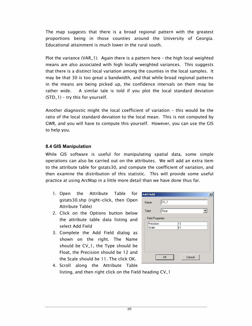
69

The map suggests that there is a broad regional pattern with the greatest

proportions being in those counties around the University of Georgia.

Educational attainment is much lower in the rural south.

Plot the variance (VAR_1). Again there is a pattern here – the high local weighted

means are also associated with high locally weighted variances. This suggests

that there is a distinct local variation among the counties in the local samples. It

may be that 30 is too great a bandwidth, and that while broad regional patterns

in the means are being picked up, the confidence intervals on them may be

rather wide. A similar tale is told if you plot the local standard deviation

(STD_1) – try this for yourself.

Another diagnostic might the local coefficient of variation – this would be the

ratio of the local standard deviation to the local mean. This is not computed by

GWR, and you will have to compute this yourself. However, you can use the GIS

to help you.

8.4 GIS Manipulation

While GIS software is useful for manipulating spatial data, some simple

operations can also be carried out on the attributes. We will add an extra item

to the attribute table for gstats30, and compute the coefficient of variation, and

then examine the distribution of this statistic. This will provide some useful

practice at using ArcMap in a little more detail than we have done thus far.

1. Open the Attribute Table for

gstats30.shp (right-click, then Open

Attribute Table)

2. Click on the Options button below

the attribute table data listing and

select Add Field

3. Complete the Add Field dialog as

shown on the right. The Name

should be CV_1, the Type should be

Float, the Precision should be 12 and

the Scale should be 11. The click OK.

4. Scroll along the Attribute Table

listing, and then right click on the Field heading CV_1

70

5. Select Calculate Values and then click yes to the warning which follows.

6. Complete the Field Calculator as

shown on the right. The calculation

should be [STD_1]/[MEAN_1] – select

these from the Fields list with a

single mouseclick. Click on OK

What you now see is the spatial variation in

the locally weighed coefficient of variation.

Whilst this ratio is higher in the northern

than in the southern parts of the state, in

the area around the University of Georgia

the coefficient is lower implying that given the local mean values, the local

standard deviations are smaller than elsewhere in the north.

8.5 Tasks

1. Examine the spatial distributions of the other variables in the coverage,

compute local coefficients of variation, and examine the regional

patterns.

2. ArcMap uses a local sample size of 12 in its computation of the surface

we used in the housing workshop. Rerun the GWR stats with an adaptive

kernel as before, but with a bandwidth of 12. You can use the same

model control file (gstats.gwr), the same output file (gstats.e00) and the

same listing file (gstats.txt). Remove gstats point from the Table of

Contents, and then use ArcToolBox to convert the output file to a

coverage called gstats12. In the spatial join to the boundary data, the

joined shapefile should be named gstats12. Examine the spatial patterns

for at least PctBach (MEAN_1) and notice what effects changing the

bandwidth has.

3. In the first GWR exercise, we used a fixed kernel and allow the calibration

routine to find the optimal bandwidth. This was 94km. Rerun the local

statistics with a fixed kernel, with a bandwidth of 94000 (the map units

are in metres!). Convert the output file to a coverage called gstats94, and

the joined shapefile should be called gstats94. Again, examine the effect

of changing the bandwidth. (The kernel smoothing literature suggests

that the bandwidth changes have a much greater impact on the

smoothing than kernel shape changes).

71

By this time, you should be adept in using both GWR and ArcGIS in tandem. You

should also have an appreciation of local statistics and the ways in which you

can use the GIS software to assist you with your tasks.

Documents

GEOGRAPHICALLY WEIGHTED REGRESSION WORKBOOK …csiss.org/.../2008/PSU/docs/GWR_Workbook_PSU_2008.pdf · GEOGRAPHICALLY WEIGHTED REGRESSION WORKBOOK ... 3.1 Importing a Coverage from