Geographically Weighted Poisson Regression (GWPR)

for Analyzing The Malnutrition Data in Java-Indonesia

Asep Saefuddin · Didin Saepudin · Dian Kusumaningrum

Abstract Many regression models are used to provide some recommendations in private

sectors or government public policy. Data are usually obtained from several districts which

may varies from one to the others. Assuming there is no significant variation among local

data, a single global model may provide appropriate recommendations for all districts.

Unfortunately this is not common in Indonesia where regional disparities are very large.

Geographically weighted regression (GWR) is an alternative approach to provide local

specific recommendations. The paper compares between global model and local specific

models of Poisson regression. The secondary data set used in this study is obtained from

Podes (Village Potential Data) of 2008 in Java. Malnutrition as the outcome variable is the

number of malnourished patients in a district. The parameter estimation in the local models

used a weighting matrix accommodating the proximity among locations. Iterative Fisher

scoring is used to solve the parameter estimation process. The corrected AIC shows that

geographically weighted Poisson model produces better performance than the global model.

Variables indicating poverty are the most influencing factors to the number of malnourished

patients in a region followed by variables related to health, education, and food. The local

parameter estimates based on the geographically weighted Poisson models can be used for

specific recommendations.

Keywords Geographically weighted Poisson regression · Weighting matrix · Local specific

parameters

JEL Codes C12 · C21 · C31

Asep Saefuddin

Professor/Head of Statistical Modeling Division

Department of Statistics, Bogor Agricultural University, Bogor, Indonesia

email: a.saefuddin@gmail.com

Didin Saepudin

Department of Statistics, Bogor Agricultural University, Bogor, Indonesia

email: efu_din@yahoo.com

Dian Kusumaningrum

Department of Statistics, Bogor Agricultural University, Bogor, Indonesia

email: dian99163@yahoo.com

2

Introduction

Poisson regression is a statistical method used to analyze the relationship between the

dependent variable and the explanatory variables, where the dependent variable is in the form

of counted data that has a Poisson distribution. For example, the case of relation between

cervical cancer disease incidence rates in England and socio-economic deprivation (Cheng et

al. 2011). In the parameter estimation, it is assumed that the fitted value for all of the

observations or regression points are the same. This assumption is referred to as homogeneity

(Charlton & Fotheringham 2009).

However, there is a problem if the observations are recorded in a regional or territorial

data, which is known as spatial data. If the spatial data was analyzed by Poisson regression,

itwill ignore the variation across the study region. The decision to ignore potential local

spatial variation in parameters can lead to biased results (Cheng et al. 2011). Whereas, the

local spatial variation can be important and such information may have important

implications for policy makers.

Malnutrition data in Java island was choosen in this research because the number of

malnourished patients was counted data which was assumed to have a Poisson distribution.

Based on the data taken from National Institute of Health Research and Development (2008),

there are differences of malnutrition prevalence in every province in Java island. The

malnutrition prevalence was based on indicators of Weight/Age (BB/U),East Java (4.8%) had

the highest malnutrition prevalence, followed by Banten (4.4%), Central Java (4.0%), West

Java (3.7%), DKI Jakarta (2.9%), and Jogjakarta (2.4%). These difference can be related to

the phenomenon of spatial variability. The variability of malnutrition prevalence in each

province might vary in each city or regency. Directorate of Public Health Nutrition (2008)

described that the indirect factors that influence malnutrition are food supply, sanitation,

health services, family purchasing power and the level of education. Nevertheless

geographical aspect could also influence malnutrition. Handling the malnutrition case is very

important because malnutrition will directly or indirectly reduce the level of children

intelligence, impaired growth and children development and decreased the productivity.

This research has three objectives. There are To compare the better model between global

Poisson model and GWPR model for the malnutrition data in Java, to create the spatial

variability map, and to analyze the factors influencing the number of malnourished patients

for each regency and city in Java. Generally, Similar with the other research related with

GWPR model, this research also creates the parameter estimates map of GWPR. However,

3

one of the difference is creating a significant explanatory variables map developed from t-

map.

Theoritical Framework

Definition of Malnutrition

Based Statistics Indonesia (2008), definition of malnutrition is a condition of less severe level

of nutrients caused by low consumption of energy and protein in a long time characterized by

the incompatibility of body weight with age.

Poisson Regression Model

The standard model for counted data is the Poisson regression model, which is a nonlinear

regression model. This regression model is derived from the Poisson distribution by allowing

the intensity parameter μto depend on explanatory variables (Cameron & Trivedi 1998).

Probability to count the numbers of events yi (dependent variable for ith

observation) given

variable x can be defined as:

Pr(yi|xi)= 𝑒−𝜇 𝑖𝜇 𝑖

𝑦 𝑖

𝑦𝑖 !

where,

yi= 0,1,2,...

i = 1,2,...,n

μi =E(yi|xi)=exp(𝒙i′𝜷)

xi′= [1,xi1,...,xik]

k = the number of explanatory variables (Long 1997).

Poisson regression model defined by Fleiss et al. (2003) as,

ln μi = β0 + β1xi1 + β2xi2 + ... + β(p-1)xi(p-1) = 𝒙i′𝜷,

where p is the number of parameters regression. μi is the expected value of Poisson

distribution for observation ith and

β′ =[β0,β1,..., βp-1].

Breusch-Pagan Test (BP-test)

Breusch and Pagan (1979) in Arbia (2006) proposed a generic form of homoscedasticity

expressed by the following equation:

E ui2 𝐱 = α1𝑥1i + α2𝑥2i + ⋯ + αk𝑥ki

4

where, 𝛂′ = α1, α2 , … , αk ′isa set of constants. 𝑥1isthe constant term of the regression and

𝑥2, … , 𝑥kare the constant terms for the regressors. The null and alternative hypothesis of BP-

test are:

H0 : α2 = α3 =…= αk = 0

H1 :∃i, where αi ≠ 0 ; (i=2,3,...,k)

Under H0, we assume that 𝜎𝑖2=α1 = constant.

Anselin (1988) in Arbia (2006) has described that Breusch-Pagan test statistics can be

derived using the general expression of the Lagrange multiplier test, which could be

expressed as:

1 1 1

1( ) '( ')( )

2

n n n

i i i i i i

i i i

BP x f x x x f (1)

where,

fi =u i

σ − 1

u i = (yi − 𝛃 ′𝒙i)

σ 2 = ui 2n

i=1

The test-statistic in equation (1) has a χ² distribution with k-1 degrees of freedom (kis the

number of explanatory variables).

Geographically Weighted Regression

Geographically Weighted Regression (GWR) is an alternative method for the local analysis of

relationships in multivariate data sets.The underlying model for GWR is,

0

1

( , ) ( , )p

i i i k i i ik i

k

y u v u v x

where {β0(ui,vi),...,βk(ui,vi)} are k+1 continuous functions of the location (ui,vi) in the

geographical study area. The εis are random error terms (Fotheringham et al. 2002).

Geographically Weighted Poisson Regression

Geographically Weighted Poisson Regression (GWPR) model is a developed model of GWR

where it brings the framework of a simple regression model into a weighted regression.

Coefficients of GWPR can be estimated by calibrating a Poisson regression model where the

likelihood is geographically weighted, with the weights being a Kernel function centred on ui

(ui is a vector of location coordinates(ui,vi)) (Nakaya et al. 2005).

The steps used to estimate the coefficients of GWPR are:

5

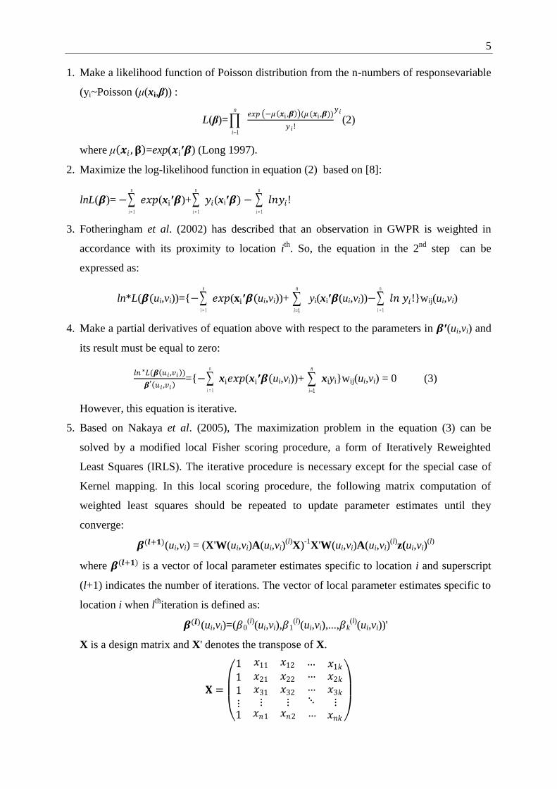
1. Make a likelihood function of Poisson distribution from the n-numbers of responsevariable

(yi~Poisson (μ(xi,β)) :

L(β)=1

n

i

𝑒𝑥𝑝 −𝜇 𝒙i ,𝜷 (𝜇 (𝒙i ,𝜷))

𝑦𝑖 !

𝑦𝑖

(2)

where μ 𝒙𝑖 , 𝛃 =exp(𝒙i′𝜷) (Long 1997).

2. Maximize the log-likelihood function in equation (2) based on [8]:

lnL(𝜷)= −n

i = 1

𝑒𝑥𝑝(xi′𝜷)+n

i = 1

𝑦𝑖(xi′𝜷) −n

i = 1

𝑙𝑛𝑦𝑖!

3. Fotheringham et al. (2002) has described that an observation in GWPR is weighted in

accordance with its proximity to location ith

. So, the equation in the 2nd

step can be

expressed as:

ln*L(𝜷(ui,vi))={−n

i = 1

𝑒𝑥𝑝(xi′𝜷(ui,vi))+ 1

n

i yi(xi′𝜷(ui,vi))−

n

i = 1

𝑙𝑛 𝑦𝑖!}wij(ui,vi)

4. Make a partial derivatives of equation above with respect to the parameters in 𝜷′(ui,vi) and

its result must be equal to zero:

𝑙𝑛 ∗𝐿(𝜷 𝑢𝑖 ,𝑣𝑖 )

𝜷′ 𝑢𝑖 ,𝑣𝑖 ={−

n

i = 1

xi𝑒𝑥𝑝(xi′𝜷(ui,vi))+ 1

n

i xiyi}wij(ui,vi) = 0 (3)

However, this equation is iterative.

5. Based on Nakaya et al. (2005), The maximization problem in the equation (3) can be

solved by a modified local Fisher scoring procedure, a form of Iteratively Reweighted

Least Squares (IRLS). The iterative procedure is necessary except for the special case of

Kernel mapping. In this local scoring procedure, the following matrix computation of

weighted least squares should be repeated to update parameter estimates until they

converge:

𝜷(𝒍+𝟏)(ui,vi) = (X'W(ui,vi)A(ui,vi)(l)

X)-1

X'W(ui,vi)A(ui,vi)(l)

z(ui,vi)(l)

where 𝜷(𝒍+𝟏) is a vector of local parameter estimates specific to location i and superscript

(l+1) indicates the number of iterations. The vector of local parameter estimates specific to

location i when lth

iteration is defined as:

𝜷(𝒍)(ui,vi)=(𝛽0(l)

(ui,vi),𝛽1(l)

(ui,vi),...,𝛽k(l)

(ui,vi))'

X is a design matrix and X' denotes the transpose of X.

𝐗 =

1 𝑥11 𝑥12 … 𝑥1𝑘

11⋮

𝑥21

𝑥31

⋮

𝑥22

𝑥32

⋮

……⋱

𝑥2𝑘

𝑥3𝑘

⋮1 𝑥𝑛1 𝑥𝑛2 … 𝑥𝑛𝑘

6

W(ui,vi) denotes the diagonal spatial weights matrix for ith

location:

W(ui,vi) = diag[wi1, wi2,..., win]

and A(ui,vi)(l)

denotes the variance weights matrix associated with the Fisher scoring for

each ith

location:

A(ui,vi)(l)

=diag[𝑦 1(𝜷(𝒍)(ui,vi)),

𝑦 2(𝜷(𝒍)(ui,vi)),...,𝑦 𝑛 (𝜷(𝒍)(ui,vi))]

Finally, z(ui)(l)

is a vector of adjusted dependent variables defined as:

z(l)

(ui,vi)=[z1(l)

(ui,vi),z2(l)

(ui,vi),..., zn(l)

(ui,vi)]'

By repeating the iterative procedure for every regression point i, sets of local parameter

estimates are obtained.

6. At convergence, we can omit the subscripts (l) or (l+1) and then rewrite the estimation of

𝜷(ui,vi) as:

𝜷 (ui,vi)=(X'W(ui,vi)A(ui,vi)X)-1

X'W(ui,vi) A(ui,vi)z(ui,vi)

Standard Error of Parameters in GWPR

The standard error of the kth

parameter estimate is given by

Se(𝛽k(ui,vi))= cov(𝜷 (𝑢𝑖 , 𝑣𝑖))𝑘

where,

cov(𝜷 (ui,vi))=C(ui,vi)A(ui,vi)-1

[C(ui,vi)]'

C(ui,vi)=(X'W(ui,vi)A(ui,vi)X)-1

X'W(ui,vi)A(ui,vi).

cov(𝜷 (ui,vi)) is the variance–covariance matrix of regression parameters estimate and

cov(𝜷 (𝑢𝑖 , 𝑣𝑖))𝑘 is the kth

diagonal element of cov(𝜷 (ui,vi)) (Nakaya et al. 2005).

Parameters Significance Test in GWPR

Hypothesis for testing the Significance for the local version of the kth

parameter estimate is

described as:

H0 : 𝛽k(ui,vi) = 0

H1 : ∃k, where 𝛽k(ui,vi) ≠ 0 ; (k=0,1,2...,(p-1)).

The local pseudo t-statistic for the local version of the kth

parameter estimate is then computed

by:

𝑡k(ui,vi) = 𝛽𝑘(𝑢𝑖 ,𝑣𝑖)

𝑆𝑒(𝛽𝑘(𝑢𝑖 ,𝑣𝑖))

7

This can be used for local inspection of parameter significance. The usual threshold of p-

values for a significance test is effectively |t|>1.96 for tests at the five percent level with large

samples (Nakaya et al. 2005).

Kernel Weighting Function

The parameter estimates at any regression point are dependent not only on the data but also on

the Kernel chosen and the bandwidth for that Kernel. Two types of Kernel that can be selected

are a fixed Kernel and an adaptive Kernel. The adaptive Kernel permits using a variable

bandwidth. Where the regression points are widely spaced. The bandwidth is greater when the

regression points are more closely spaced (Fotheringham et al. 2002).

The particular function in adaptive Kernel’s method is a bi-square function. A bi-square

function where the weight of the jth

data point at regression point i is given by:

2 2

( ) ( )

( )

[1 ( / ) ] ; when

0 ; when

ij i k ij i k

ij

ij i k

d b d bw

d b

where wijis weight value of observation at the location j for estimating coefficient at the

location i. dijis the Euclidean distance between the regression point i and the data point j and

bi(k)is an adaptive bandwidth size defined as kth

nearest neighbour distance (Fotheringham et

al. 2002).

Materials And Methods

Data Sources

The data used in this study are secondary data from Podes (Village Potential Data) of 2008 in

Java. The objects of this research are 112 regrencies and cities in Java island.

The dependent variable used in this research is total number of malnourished patients

during last three years in each regency or city in each regency and city in Java island. It is

initialized by name of MalPat. The explanatory variables is selected from four aspects, which

include poverty, health, education, and food aspect. There were 14 explanatory variables used

which is described in detail in Table 1.

Methodology

In the case of spatial processes which is referred to spatial non-stationarity (Fotheringham et

al. 2002). Geographically Weighted Poisson Regression (GWPR) will be the most appropriate

analysis if the data has a non-stationary condition and the dependent variable was assumed

8

Poissonly distributed. GWPR model uses weighting matrix which depends on the proximity

between the location of the observation. In this research, a modified local Fisher scoring

procedure is used to estimate the local parameters of GWPR iteratively and using the bi-

square adaptive Kernel function to find the weighting matrix is expected. The Kernel function

determines weighting matrix based on window width (bandwidth) where the value is

accordance with the conditions of the data and adaptive because it has a wide window

(bandwidth) that varies according to conditions of observation points.

After estimating the GWPR parameters, the map of spatial variability for each parameters

of GWPR and a significant explanatory variables map is created. The softwares used for this

research are GWR4 and ArcView 3.2.

Table 1 Description of explanatory variable

Aspect Explanatory

variable Description Unit

Poverty

FamLabour Total number of families whose members are farm

labour in each regency or city Families

FamRiver Total number of families residing along the river in

each regency or city Families

FamSlums Total number of families residing in the slums in

each regency or city Families

FamPovIns

Total number of families which received poor

family health insurance (Asuransi kesehatan

keluarga miskin/Askeskin) in each regency or city

Families

Health

Midwife Total number of midwifes in each regency or city Persons

Doctor Total number of general doctors in each regency or

city Persons

ISP Total number of integrated services post

(Posyandu) in each regency or city Units

ActISP

Total number of villages that all of integrated

services post (Posyandu) in a village is actively

operated in each regency or city

Villages

HlthWrk Total number ofmantri kesehatan and dukun bayiin

each regency or city Persons

Education

ElmSch Total number of elementary schools or equivalent

in each regency or city Units

JHSch Total number of junior high schools or equivalent in

each regency or city Units

Illiteracy Total number of villages that there are eradication

programme of illiteracy during one last year Villages

Education DiffPlace

Total number ofvillages having insufficient or poor

access towards the village office and the capital of

sub-district in each regency or city

Villages

9

Result and Discussion

Data Exploration

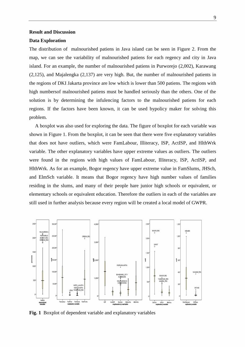
The distribution of malnourished patiens in Java island can be seen in Figure 2. From the

map, we can see the variability of malnourished patiens for each regency and city in Java

island. For an example, the number of malnourished patiens in Purworejo (2,002), Karawang

(2,125), and Majalengka (2,137) are very high. But, the number of malnourished patients in

the regions of DKI Jakarta province are low which is lower than 500 patiens. The regions with

high numbersof malnourished patiens must be handled seriously than the others. One of the

solution is by determining the infulencing factors to the malnourished patiens for each

regions. If the factors have been known, it can be used bypolicy maker for solving this

problem.

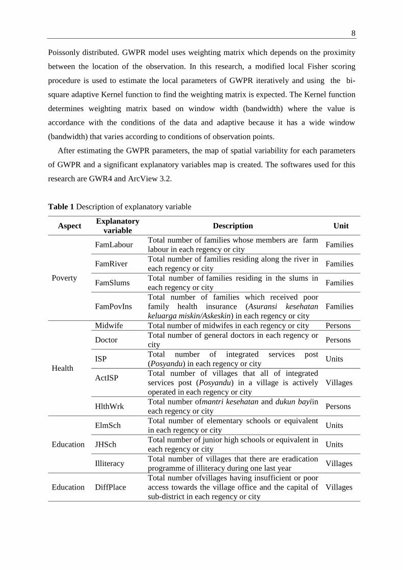
A boxplot was also used for exploring the data. The figure of boxplot for each variable was

shown in Figure 1. From the boxplot, it can be seen that there were five explanatory variables

that does not have outliers, which were FamLabour, Illiteracy, ISP, ActISP, and HlthWrk

variable. The other explanatory variables have upper extreme values as outliers. The outliers

were found in the regions with high values of FamLabour, Illiteracy, ISP, ActISP, and

HlthWrk. As for an example, Bogor regency have upper extreme value in FamSlums, JHSch,

and ElmSch variable. It means that Bogor regency have high number values of families

residing in the slums, and many of their people hare junior high schools or equivalent, or

elementary schools or equivalent education. Therefore the outliers in each of the variables are

still used in further analysis because every region will be created a local model of GWPR.

Fig. 1 Boxplot of dependent variable and explanatory variables

10

Fig. 2 Map of malnourished patiens distribution for each regency and city in Java island

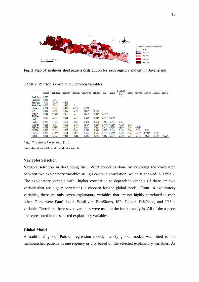
Table 2 Pearson’s correlation between variables

*|r|≥0.7 is strong Correlation [14].

Underlined variable is dependent variable.

Variables Selection

Variable selection in developing the GWPR model is done by exploring the correlation

between two explanatory variables using Pearson’s correlation, which is showed in Table 2.

The explanatory variable with higher correlation to dependent variable (if there are two

variablesthat are highly correlated) is choosen for the global model. From 14 explanatory

variables, there are only seven explanatory variables that are not highly correlated to each

other. They were FamLabour, FamRiver, FamSlums, ISP, Doctor, DiffPlace, and JHSch

variable. Therefore, these seven variables were used in the further analysis. All of the aspects

are represented in the selected explanatory variables.

Global Model

A traditional global Poisson regression model, namely global model, was fitted to the

malnourished patients in one regency or city based on the selected explanatory variables. As

11

explained above, seven explanatory variables were selected and used to create global model.

Their parameter estimates and p-values are displayed in Table 3.

A Global model from seven explanatory variables, namely global model 1,showed that

only one variable was not significant at five percent level of significance which was Doctor

variable. This global model will be selected as model to create GWPR model. In this research,

non-significant variable still used for modeling GWPR because this model accomodated all

factors. Therefore, it will explain the influencing factors of the number of malnourished

patients better.

Spatial Variability Test

The test used for detecting spatial variability was Breusch-Pagan test (BP test). The null

hypothesis for this test is error variance for all of the observations is constant. While, the

alternative hypothesis is heteroscedasticity in error variance (there are variability among

observations).

From Table 3, the p-value of BP test was significant at afive percent significance level. It

meansthat there are variability among observations. Therefore, there are special

characteristics for each region. Hence, the data must be analyzed by local modeling in order

to capture the variation of data and explain the characteristic of each region better.

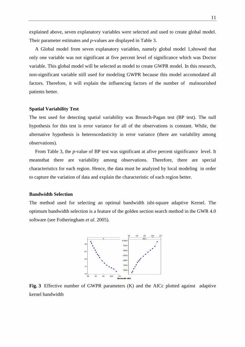
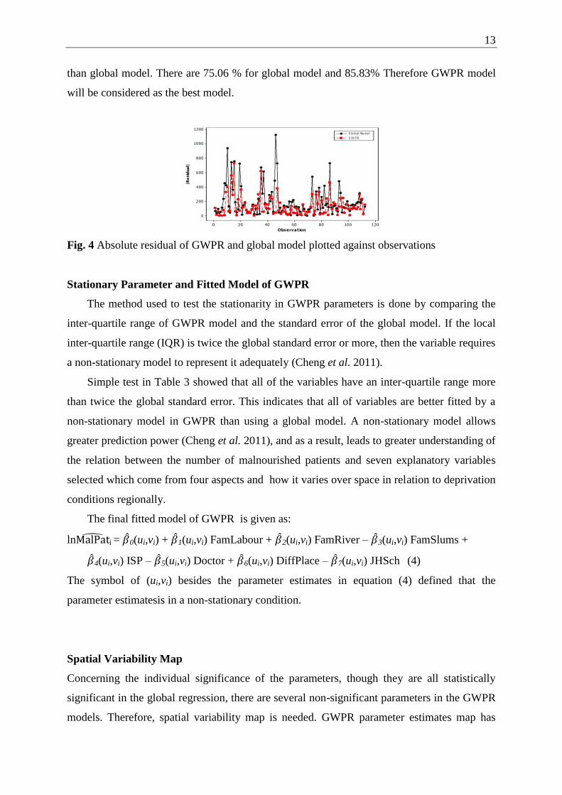
Bandwidth Selection

The method used for selecting an optimal bandwidth isbi-square adaptive Kernel. The

optimum bandwidth selection is a feature of the golden section search method in the GWR 4.0

software (see Fotheringham et al. 2005).

Fig. 3 Effective number of GWPR parameters (K) and the AICc plotted against adaptive

kernel bandwidth

12

From Figure 3, it can be seen that the selected optimum bandwidth from this method is 46

neighboring regencies or cities nearest to the ith

regency or city. In selecting the optimum

bandwidth, GWPR model with bi-square adaptive Kernel has an AICc value of 6705.39. The

effective number of GWPR parameters is 32.23. Afterwards the selected optimum bandwith

will be used to calculate the weighting matrix in a regency or city.

Table 3 Statistics Comparison of Global Model and GWPR Model

Covariate Global Model GWPR Model

Estimate Pr(>|t|) Std. Error Mean Std. Dev. IQR

Intercept 5.039338 < 2x10-16

* 0.010759 4.817929 0.164236 0.237853

FamLabour 0.000002 < 2x10-16

* 0.000000** 0.000005 0.000002 0.000003

FamRiver 0.000053 < 2x10-16

* 0.000002 0.000052 0.000024 0.000031

FamSlums -0.000008 < 1.46x10-12

* 0.000001 0.000033 0.000055 0.000094

ISP 0.00074 < 2x10-16

* 0.000008 0.000858 0.000212 0.000377

Doctor -0.000029 0.124 0.000019 -0.000710 0.000924 0.001992

DiffPlace 0.001539 < 7.74x10-9

* 0.000266 -0.001510 0.005036 0.010788

JHSch -0.001113 < 2x10-16

* 0.000059 -0.002040 0.001421 0.002455

BP test*** 37.5913 3.623x10-6

AICc 11657.58

6705.39

AICc

Difference 4952.14

0

Deviance

R-Square 75.06 %

85.8 3%

Notes: *Significant at α = 5%

** Value in 10 digit decimals is 0.0000000089

*** Degree of freedom fo BP test is 7.

GWPR Model

The next analysis is modeling with GWPR. From this model with an optimum bandwidth,

GWPR model also has a minimum AICc value. Before further interpretation of GWPR

model, GWPR model must be compared with global model to select the best model between

them.

Table 4 showed that the AICc difference with the global model is 4952.14. It indicates that

GWPR model is better than the global model. This difference of AICc of global model is very

high. Based on the AICc difference criterion from Nakaya et al. (2005), GWPR model was

better than global model.

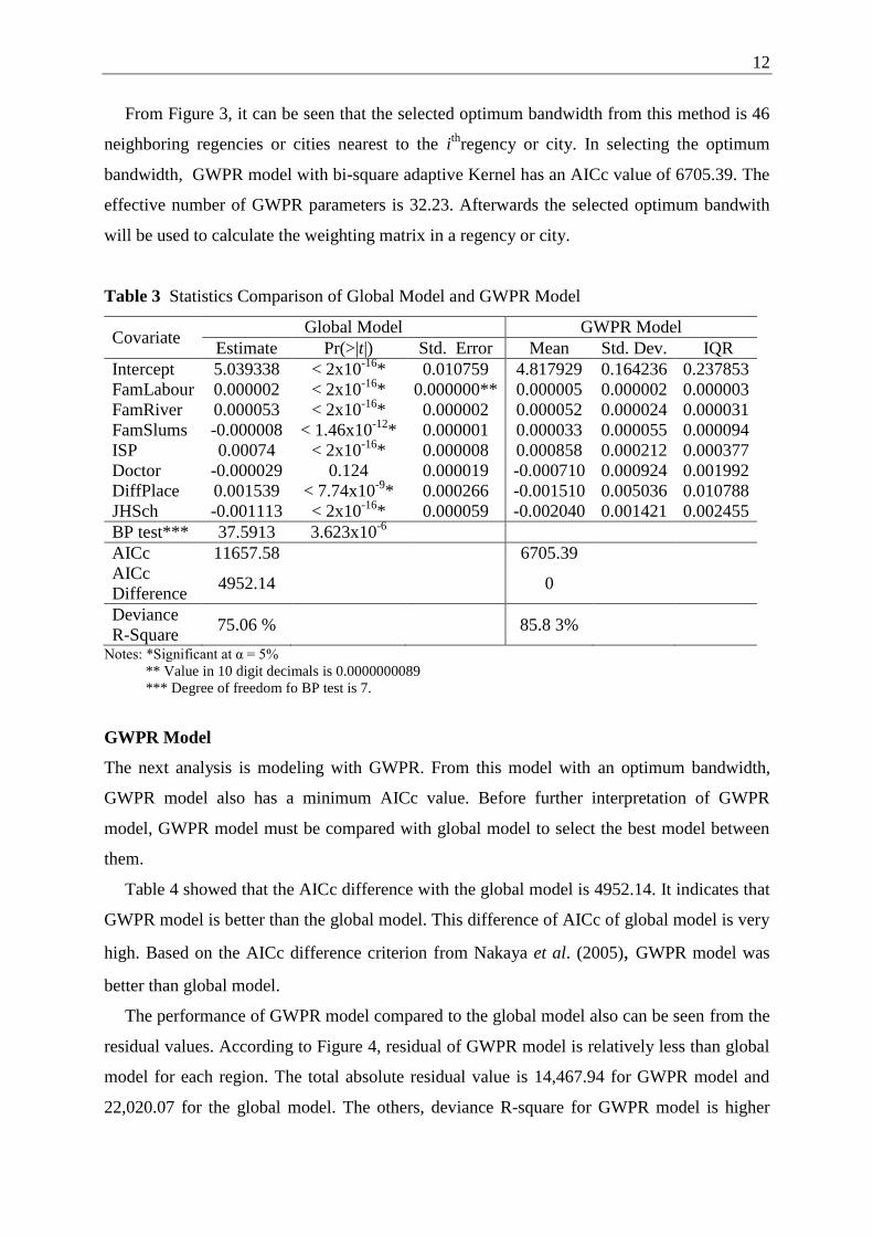
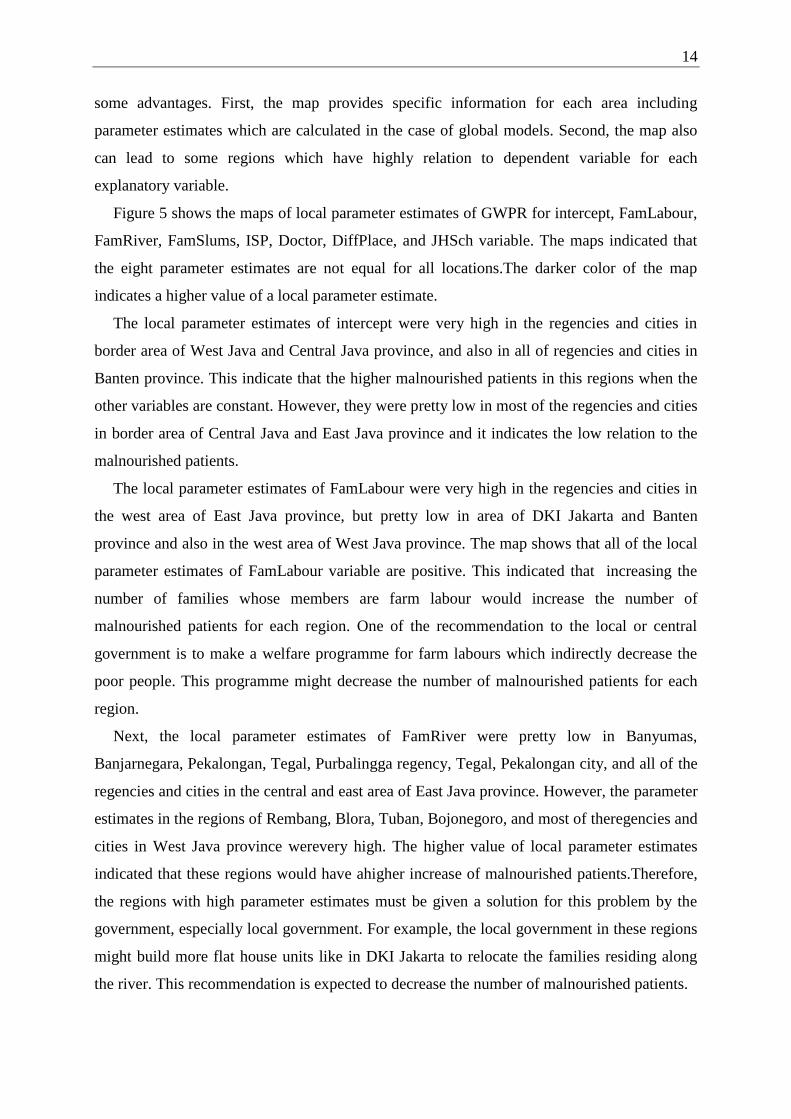
The performance of GWPR model compared to the global model also can be seen from the

residual values. According to Figure 4, residual of GWPR model is relatively less than global

model for each region. The total absolute residual value is 14,467.94 for GWPR model and

22,020.07 for the global model. The others, deviance R-square for GWPR model is higher

13

than global model. There are 75.06 % for global model and 85.83% Therefore GWPR model

will be considered as the best model.

Fig. 4 Absolute residual of GWPR and global model plotted against observations

Stationary Parameter and Fitted Model of GWPR

The method used to test the stationarity in GWPR parameters is done by comparing the

inter-quartile range of GWPR model and the standard error of the global model. If the local

inter-quartile range (IQR) is twice the global standard error or more, then the variable requires

a non-stationary model to represent it adequately (Cheng et al. 2011).

Simple test in Table 3 showed that all of the variables have an inter-quartile range more

than twice the global standard error. This indicates that all of variables are better fitted by a

non-stationary model in GWPR than using a global model. A non-stationary model allows

greater prediction power (Cheng et al. 2011), and as a result, leads to greater understanding of

the relation between the number of malnourished patients and seven explanatory variables

selected which come from four aspects and how it varies over space in relation to deprivation

conditions regionally.

The final fitted model of GWPR is given as:

lnMalPat i = 𝛽 0(ui,vi) + 𝛽 1(ui,vi) FamLabour + 𝛽 2(ui,vi) FamRiver – 𝛽 3(ui,vi) FamSlums +

𝛽 4(ui,vi) ISP – 𝛽 5(ui,vi) Doctor + 𝛽 6(ui,vi) DiffPlace – 𝛽 7(ui,vi) JHSch (4)

The symbol of (ui,vi) besides the parameter estimates in equation (4) defined that the

parameter estimatesis in a non-stationary condition.

Spatial Variability Map

Concerning the individual significance of the parameters, though they are all statistically

significant in the global regression, there are several non-significant parameters in the GWPR

models. Therefore, spatial variability map is needed. GWPR parameter estimates map has

14

some advantages. First, the map provides specific information for each area including

parameter estimates which are calculated in the case of global models. Second, the map also

can lead to some regions which have highly relation to dependent variable for each

explanatory variable.

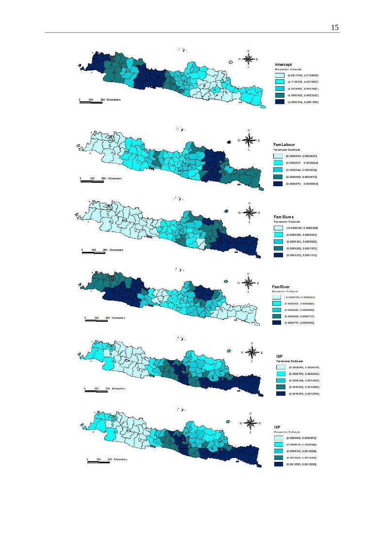
Figure 5 shows the maps of local parameter estimates of GWPR for intercept, FamLabour,

FamRiver, FamSlums, ISP, Doctor, DiffPlace, and JHSch variable. The maps indicated that

the eight parameter estimates are not equal for all locations.The darker color of the map

indicates a higher value of a local parameter estimate.

The local parameter estimates of intercept were very high in the regencies and cities in

border area of West Java and Central Java province, and also in all of regencies and cities in

Banten province. This indicate that the higher malnourished patients in this regions when the

other variables are constant. However, they were pretty low in most of the regencies and cities

in border area of Central Java and East Java province and it indicates the low relation to the

malnourished patients.

The local parameter estimates of FamLabour were very high in the regencies and cities in

the west area of East Java province, but pretty low in area of DKI Jakarta and Banten

province and also in the west area of West Java province. The map shows that all of the local

parameter estimates of FamLabour variable are positive. This indicated that increasing the

number of families whose members are farm labour would increase the number of

malnourished patients for each region. One of the recommendation to the local or central

government is to make a welfare programme for farm labours which indirectly decrease the

poor people. This programme might decrease the number of malnourished patients for each

region.

Next, the local parameter estimates of FamRiver were pretty low in Banyumas,

Banjarnegara, Pekalongan, Tegal, Purbalingga regency, Tegal, Pekalongan city, and all of the

regencies and cities in the central and east area of East Java province. However, the parameter

estimates in the regions of Rembang, Blora, Tuban, Bojonegoro, and most of theregencies and

cities in West Java province werevery high. The higher value of local parameter estimates

indicated that these regions would have ahigher increase of malnourished patients.Therefore,

the regions with high parameter estimates must be given a solution for this problem by the

government, especially local government. For example, the local government in these regions

might build more flat house units like in DKI Jakarta to relocate the families residing along

the river. This recommendation is expected to decrease the number of malnourished patients.

15

16

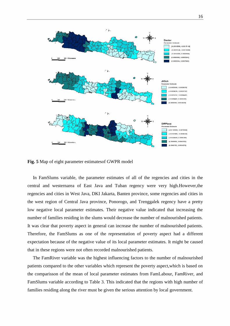
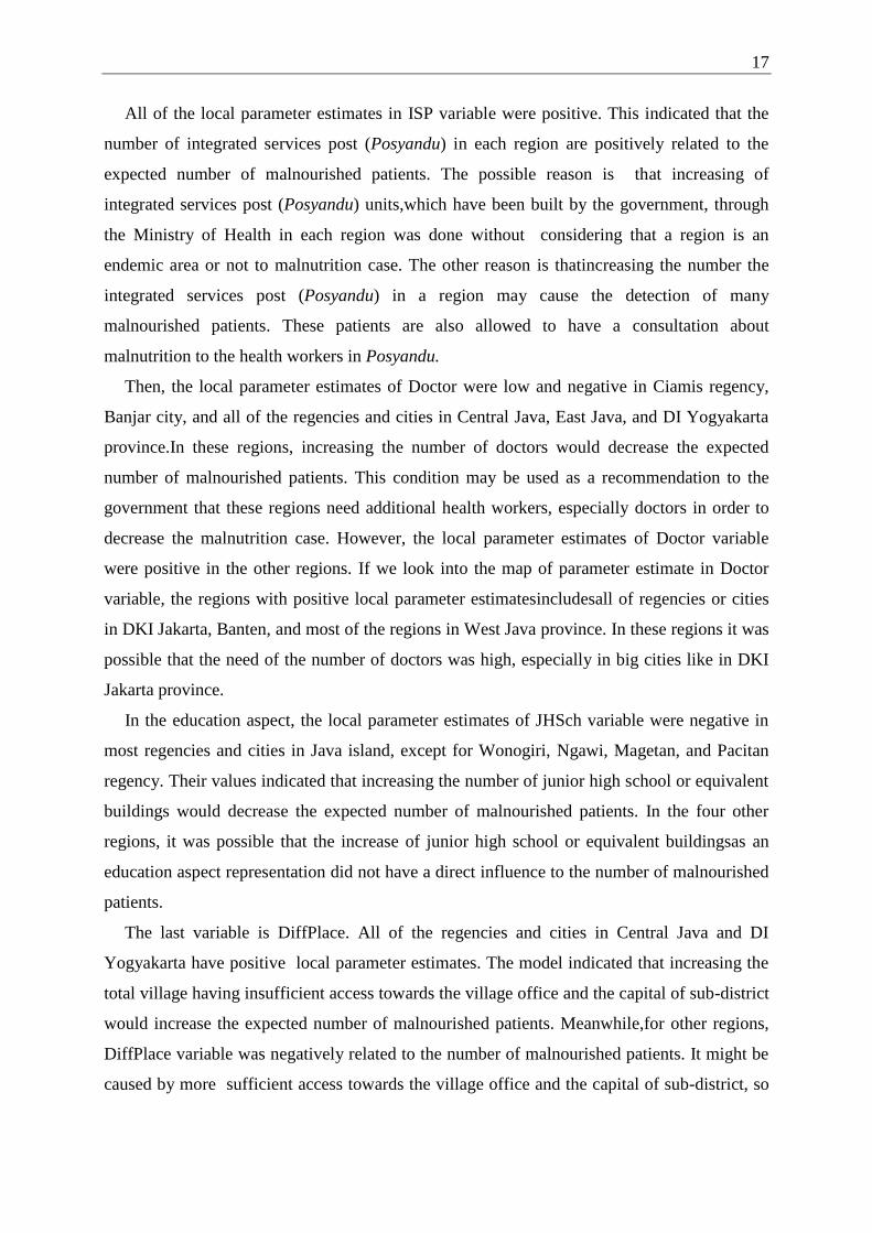
Fig. 5 Map of eight parameter estimatesof GWPR model

In FamSlums variable, the parameter estimates of all of the regencies and cities in the

central and westernarea of East Java and Tuban regency were very high.However,the

regencies and cities in West Java, DKI Jakarta, Banten province, some regencies and cities in

the west region of Central Java province, Ponorogo, and Trenggalek regency have a pretty

low negative local parameter estimates. Their negative value indicated that increasing the

number of families residing in the slums would decrease the number of malnourished patients.

It was clear that poverty aspect in general can increase the number of malnourished patients.

Therefore, the FamSlums as one of the representation of poverty aspect had a different

expectation because of the negative value of its local parameter estimates. It might be caused

that in these regions were not often recorded malnourished patients.

The FamRiver variable was the highest influencing factors to the number of malnourished

patients compared to the other variables which represent the poverty aspect,which is based on

the comparisson of the mean of local parameter estimates from FamLabour, FamRiver, and

FamSlums variable according to Table 3. This indicated that the regions with high number of

families residing along the river must be given the serious attention by local government.

17

All of the local parameter estimates in ISP variable were positive. This indicated that the

number of integrated services post (Posyandu) in each region are positively related to the

expected number of malnourished patients. The possible reason is that increasing of

integrated services post (Posyandu) units,which have been built by the government, through

the Ministry of Health in each region was done without considering that a region is an

endemic area or not to malnutrition case. The other reason is thatincreasing the number the

integrated services post (Posyandu) in a region may cause the detection of many

malnourished patients. These patients are also allowed to have a consultation about

malnutrition to the health workers in Posyandu.

Then, the local parameter estimates of Doctor were low and negative in Ciamis regency,

Banjar city, and all of the regencies and cities in Central Java, East Java, and DI Yogyakarta

province.In these regions, increasing the number of doctors would decrease the expected

number of malnourished patients. This condition may be used as a recommendation to the

government that these regions need additional health workers, especially doctors in order to

decrease the malnutrition case. However, the local parameter estimates of Doctor variable

were positive in the other regions. If we look into the map of parameter estimate in Doctor

variable, the regions with positive local parameter estimatesincludesall of regencies or cities

in DKI Jakarta, Banten, and most of the regions in West Java province. In these regions it was

possible that the need of the number of doctors was high, especially in big cities like in DKI

Jakarta province.

In the education aspect, the local parameter estimates of JHSch variable were negative in

most regencies and cities in Java island, except for Wonogiri, Ngawi, Magetan, and Pacitan

regency. Their values indicated that increasing the number of junior high school or equivalent

buildings would decrease the expected number of malnourished patients. In the four other

regions, it was possible that the increase of junior high school or equivalent buildingsas an

education aspect representation did not have a direct influence to the number of malnourished

patients.

The last variable is DiffPlace. All of the regencies and cities in Central Java and DI

Yogyakarta have positive local parameter estimates. The model indicated that increasing the

total village having insufficient access towards the village office and the capital of sub-district

would increase the expected number of malnourished patients. Meanwhile,for other regions,

DiffPlace variable was negatively related to the number of malnourished patients. It might be

caused by more sufficient access towards the village office and the capital of sub-district, so

18

there are many malnourished patients being recorded by the local government official

workers, especially by the health workers.

The local parameter estimates that were inversely related with some variables might

produce bad interpretation. For better results of GWPR model, the study of regions for the

next research should be done at a lower, such as be sub-district or village level. Using lower

levels might enhance the precision of parameter estimates in spatial analysis.

Significant Explanatory Variables Map

GWPR model usually displays the map of non-stationary parameter estimates. However, in

every point of the regression, in this case each regency or city, it also has a pseudo t-value

which is formulated as by the parameter estimate divided with the standard error in each point

of the regression. As a result, the GWPR local parameters of explanatory variables (we

exclude the intercept) have t-maps (Mennis 2006). Each t-map has an advantage that is it can

detect the significancy of an explanatory variables for each region. The other advantage is it

can detect the combination of significant explanatory variables for each region. But, the

disadvantage of this mapping approach is that potentially interesting patterns may not be

observed regarding the magnitude of the relationship between the explanatory and dependent

variable as contained in the actual parameter estimate values, as well as in the magnitude of

the significance (Mennis 2006).

In this research, every t-map of GWPR local parameter of explanatory variable would be

joined as a map which is named as map of significant explanatory variable. Figure 6 shows

the significant explanatory variable map. The explanatory variables used in the map are the

explanatory variables used in the selected global model.

Fig. 6 Significant explanatory variables map

The map in Figure 7 displays six groups of color. The colors indicate that there were

different groups without implaying a rank like the map in Figure 4. The dominant color was

19

dark brown, it indicates that in these regions, all of the explanatory variables were significant.

A region where FamSlums and DiffPlace variable were not significant is Ponorogo regency.

Tulungagung, Pacitan, and Majalengka regency only had DiffPlace variable as a significant

variable. Then, FamRiver variable was significant in eastern area of East Java. FamSlums

variable was not significant in Pemalang, Trenggalek, and Purbalingga regency. The last

group is the regions which JHSch was not a significant variable. The regions include Blora,

Wonogiri, and Ngawi regency. The other advantage for creating this map is it can give

recommendations for policy maker or the local government and central government especially

Ministry of Health about the factors influencing the number of malnourished patients in each

regency or city in Java island.

Conclusion And Recommendation

Conclusion

GWPR model was proven to be a better model than global model.GWPR model had highly

difference of AICc compared to the global model. A condition of non-stationarity in

parameters was fulfilled, and its residual relatively less than global model for eachregion.

Map of parameter estimates showed more meaningful results.The FamRiver variable was the

highest influencing factors to the number of malnourished patients compared to the other

variables which represent the poverty aspect. There were six groups of the factors influencing

the number of malnourished patients for each regency and city in Java based on the map of

significant explanatory variable.

Recommendation

For better results of GWPR model, the study of regions for the next research should be lower

level than regency or city level, such as thesub-district or village level. Conducting GWPR at

this level might give a better local parameter estimates.

References

Arbia G. 2006. Spatial econometrics: Statistical Foundations and Applications to Regional

Convergence. Berlin: Springer Publishing.

Burnham and Anderson (1998). Model selection and multimodel inference: a practical

information-theoretic approach. New York: Springer Publishing.

Cameron AC and Trivedi PK. 1998. Regression Analysis of Count Data. Cambridge:

Cambridge University Press.

20

Charlton M and Fotheringham AS. 2009. Geographically Weighted Regression White

Paper[Paper]. Maynooth: Science Foundation Ireland.

Cheng EMY, Atkinson PM, and Shahani AK. 2011. Elucidating the spatially varying relation

between cervical cancer and socio-economic conditions in England, International Journal

of Health Geographics, 10:51.

C:\data\StatPrimer\correlation.wpd.http://www.sjsu.edu/faculty/gerstman/StatPrimer/correlati

on.pdf.[September 12th

, 2012]

Fleiss JL, Levin B, and Paik MC. 2003. Statistical Methods for Rates and Proportions 3rd

Ed.

New York: Columbia University.

Fotheringham AS, Brunsdon C, and Charlton M. 2002. Geographically Weighted Regression:

The Analysis of Spatially Varying Relationship. Chichester: John Wiley and Sons, ltd.

Hardin JW and Hilbe JM. 2007. Generalized Linear Models and Extensions. Texas: A Stata

Press Publication.

Long JS. 1997. Regression Models for Categoricals and Limited Dependent Variables.

California: SAGE Publications.

Mennis J. 2006. Mapping the Results of Geographically Weighted Regression, The

Cartographic Journal, 43(2):171–179.

Nakaya T, Fotheringham AS, Brunsdon C, and Charlton M. 2005. Geographically Weighted

Poisson Regression for Disease Association Mapping, Statistics in Medicine, 24:2695-

2717.

National Institute of Health Research and Development. 2008. Laporan Hasil Riset

Kesehatan Dasar (Riskesdas) Nasional. Jakarta: Ministry of Health Republic of Indonesia.

Directorate of Public Health Nutrition. 2008. Pedoman Respon Cepat Penanggulangan

Gizi Buruk. Jakarta: Ministry of Health Republic of Indonesia.

Statistics Indonesia. 2008. Pedoman Pencacah. Jakarta: Statistics Indonesia.