Embed Size (px)
Citation preview
Found Comput Math (2012) 12:263–293DOI 10.1007/s10208-012-9119-7
Geometric Variational Crimes: Hilbert Complexes,Finite Element Exterior Calculus, and Problemson Hypersurfaces
Michael Holst · Ari Stern
Received: 28 May 2010 / Revised: 25 February 2012 / Accepted: 29 February 2012 /Published online: 5 April 2012© SFoCM 2012
Abstract A recent paper of Arnold, Falk, and Winther (Bull. Am. Math. Soc.47:281–354, 2010) showed that a large class of mixed finite element methods canbe formulated naturally on Hilbert complexes, where using a Galerkin-like approach,one solves a variational problem on a finite-dimensional subcomplex. In a seeminglyunrelated research direction, Dziuk (Lecture Notes in Math., vol. 1357, pp. 142–155,1988) analyzed a class of nodal finite elements for the Laplace–Beltrami equation onsmooth 2-surfaces approximated by a piecewise-linear triangulation; Demlow laterextended this analysis (SIAM J. Numer. Anal. 47:805–827, 2009) to 3-surfaces, aswell as to higher-order surface approximation. In this article, we bring these lines ofresearch together, first developing a framework for the analysis of variational crimesin abstract Hilbert complexes, and then applying this abstract framework to the set-ting of finite element exterior calculus on hypersurfaces. Our framework extendsthe work of Arnold, Falk, and Winther to problems that violate their subcomplexassumption, allowing for the extension of finite element exterior calculus to approx-imate domains, most notably the Hodge–de Rham complex on approximate mani-folds. As an application of the latter, we recover Dziuk’s and Demlow’s a priori es-timates for 2- and 3-surfaces, demonstrating that surface finite element methods canbe analyzed completely within this abstract framework. Moreover, our results gener-
Communicated by Douglas Arnold.
M. Holst · A. Stern (�)Department of Mathematics, University of California, San Diego, 9500 Gilman Dr #0112, La Jolla,CA 92093-0112, USAe-mail: [email protected]
M. Holste-mail: [email protected]
264 Found Comput Math (2012) 12:263–293
alize these earlier estimates dramatically, extending them from nodal finite elementsfor Laplace–Beltrami to mixed finite elements for the Hodge Laplacian, and from 2-and 3-dimensional hypersurfaces to those of arbitrary dimension. By developing thisanalytical framework using a combination of general tools from differential geome-try and functional analysis, we are led to a more geometric analysis of surface finiteelement methods, whereby the main results become more transparent.
Keywords Finite element exterior calculus · Variational crimes · Mixed finiteelements · Surface finite elements · Isoparametric finite elements
Mathematics Subject Classification Primary 65N30 · 58A12
1 Introduction
The aim of this paper is to bring together three distinct ideas that have influenced, inseparate ways, the development and analysis of geometric finite element methods forelliptic partial differential equations.
The first idea is that of a variational crime. Suppose we have a variational problemof the form: Find u ∈ V such that
B(u, v) = F(v), ∀v ∈ V, (1)
where V is a Hilbert space, B : V × V → R is a bounded, coercive bilinear form,and F ∈ V ∗ is a bounded linear functional. If Vh ⊂ V is a subspace (usually finitedimensional), then one can obtain an approximate solution by solving the Galerkinvariational problem: Find uh ∈ Vh such that
B(uh, v) = F(v), ∀v ∈ Vh.
This is the typical abstract setting for finite element methods. However, for manyproblems of interest, especially finite element methods on surfaces or on domainswith curved boundaries, one cannot efficiently compute the bilinear form B(·, ·) or thefunctional F(·) on a subspace of V . Instead, one must take an approximating spaceVh �⊂ V , along with an approximate bilinear form Bh : Vh × Vh → R and functionalFh ∈ V ∗
h , and formulate the generalized Galerkin variational problem: Find uh ∈ Vh
such that
Bh(uh, v) = Fh(v), ∀v ∈ Vh. (2)
Such modifications to the original variational problem are called “variational crimes.”There is a well-understood framework for the analysis of a large class of variationalcrimes, represented by the Strang lemmas [7]: for instance, the first and second Stranglemmas allow for the complete analysis of numerical quadrature, the use of geometricmodeling technology such as isoparametric elements, and many other examples ofvariational crimes.
The emergence of surface finite elements represents a second distinct idea thathas influenced the development of geometric finite element methods. The analysis of
Found Comput Math (2012) 12:263–293 265
surface finite element methods, which by construction are “criminal” methods, hasrequired a more sophisticated approach that exploits the specific nature of the crimein order to obtain a satisfactory error analysis; this custom-tailored analysis contrastswith the more general approach given by the Strang lemmas. The surface finite el-ement research area was effectively initiated with the 1988 article of Dziuk [17],although there is related work appearing about ten years earlier by Nédélec [27].While there was some activity in the area during the 1990s (cf. [12, 18]), beginningin 2001 there was a tremendous expansion of research in the general area of surfacefinite element methods, with many applications arising in material science, biology,and astrophysics; examples include [10, 13–16, 19, 20, 22].
The third distinct idea that has had a major influence on the development of ge-ometric methods is that of mixed finite elements, whose early success in areas suchas computational electromagnetics was later found to have surprising connectionswith the calculus of exterior differential forms, including de Rham cohomology andHodge theory [6, 21, 28, 29]. This has culminated, very recently, in the powerful the-ory of finite element exterior calculus developed by Arnold, Falk, and Winther [2,3]. A key insight of the latter work, from a functional-analytic point of view, is thata mixed variational problem can be posed on a Hilbert complex: a differential com-plex of Hilbert spaces, in the sense of Brüning and Lesch [8]. Galerkin-type mixedmethods are then obtained by solving the variational problem on a finite-dimensionalsubcomplex.
In this article, we bring these lines of research together, first developing a frame-work for the analysis of variational crimes in abstract Hilbert complexes, and thenapplying this abstract framework to the setting of finite element exterior calculus onhypersurfaces. Our framework extends the work of Arnold et al. [3] to problems thatviolate their subcomplex assumption, allowing for the extension of finite element ex-terior calculus to approximate domains, most notably the Hodge–de Rham complexon approximate manifolds. As an application of the latter, we recover Dziuk’s [17]and Demlow’s [15] a priori estimates for 2- and 3-surfaces, demonstrating that sur-face finite element methods can be analyzed completely within this abstract frame-work. Moreover, our results generalize these earlier estimates dramatically, extendingthem from nodal finite elements for Laplace–Beltrami to mixed finite elements for theHodge Laplacian, and from 2- and 3-dimensional hypersurfaces to those of arbitrarydimension. By developing this analytical framework using a combination of generaltools from differential geometry and functional analysis, we are led to a more geo-metric analysis of surface finite element methods, whereby the main results becomemore transparent.
The remainder of the article is organized as follows. In Sect. 2, we review theabstract framework of Hilbert complexes, which plays a central role in the work ofArnold et al. [3] on finite element exterior calculus. This includes a brief introductionto Hilbert complexes and their morphisms, domain complexes, Hodge decomposi-tion, the Poincaré inequality, the Hodge Laplacian, mixed variational problems, andapproximation using Hilbert subcomplexes. In Sect. 3, we consider the approxima-tion of a Hilbert complex by a second complex, related to the first complex through aninjective morphism rather than through subcomplex inclusion. Since this morphism isnot necessarily unitary (i.e., inner-product preserving), this allows the approximating
266 Found Comput Math (2012) 12:263–293
complex to have a different inner product, which only approximates that of the orig-inal complex. We develop some basic results for the pair of complexes and the mapsbetween them, and then prove error estimates for generalized Galerkin-type approxi-mations of solutions to variational problems using the approximating complex; theseestimates generalize the results of Arnold et al. [3] to “external” approximations. Ourresults may be viewed as establishing Strang-type lemmas for approximating varia-tional problems in Hilbert complexes.
In Sect. 4, we apply the framework developed in Sect. 3 to the Hodge–de Rhamcomplex of differential forms on a compact, oriented Riemannian manifold. We firstreview Hodge–de Rham theory, and then consider a pair of Riemannian manifoldsrelated by diffeomorphisms, establishing estimates for the maps needed to apply thegeneralized Hilbert complex approximation framework. After reviewing the conceptof a tubular neighborhood, we then consider the specific case of Euclidean hyper-surfaces. We subsequently show how the results of the previous sections recover theanalysis framework and a priori estimates of Dziuk [17], Demlow and Dziuk [16],Demlow [15], and moreover extend their results from scalar functions on 2- and 3-surfaces to general k-forms on arbitrary dimensional hypersurfaces. We also indicatehow our results generalize the a priori estimates of Dziuk [17], Demlow [15] fromnodal finite element methods for the Laplace–Beltrami operator to mixed finite ele-ment methods for the Hodge Laplacian.
2 Review of Hilbert Complexes
In this section, we quickly review the abstract framework of Hilbert complexes, whichforms the heart of the analysis in Arnold et al. [3] for mixed finite element methods.Just as the space of L2 functions is a prototypical example of a Hilbert space, the pro-totypical example of a Hilbert complex to keep in mind is the L2-de Rham complexof differential forms. (This example will be discussed at greater length in Sect. 4.)After stating the basic definitions, we will summarize some of the key results fromArnold et al. [3] on mixed variational problems and their numerical approximationusing Hilbert subcomplexes. The interested reader may also refer to Brüning andLesch [8] for a comprehensive treatment of Hilbert complexes from the viewpoint offunctional analysis.
2.1 Basic Definitions
Let us introduce the basic objects of study, Hilbert complexes, and their morphisms.
Definition 2.1 A Hilbert complex (W,d) consists of a sequence of Hilbert spacesWk , along with closed, densely defined linear maps dk : V k ⊂ Wk → V k+1 ⊂ Wk+1,possibly unbounded, such that dk ◦ dk−1 = 0 for each k.
· · · V k−1dk−1
V kdk
V k+1 · · ·
Found Comput Math (2012) 12:263–293 267
This Hilbert complex is said to be bounded if dk is a bounded linear map from Wk toWk+1 for each k, i.e., (W,d) is a cochain complex in the category of Hilbert spaces.It is said to be closed if the image dkV k is closed in Wk+1 for each k.
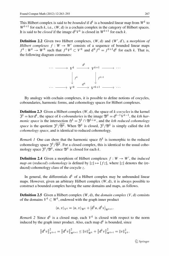
Definition 2.2 Given two Hilbert complexes, (W,d) and (W ′,d′), a morphism ofHilbert complexes f : W → W ′ consists of a sequence of bounded linear mapsf k : Wk → W ′k such that f kV k ⊂ V ′k and d′kf k = f k+1dk for each k. That is,the following diagram commutes:
· · · V k
f k
dk
V k+1
f k+1
· · ·
· · · V ′k d′kV ′k+1 · · ·
By analogy with cochain complexes, it is possible to define notions of cocycles,coboundaries, harmonic forms, and cohomology spaces for Hilbert complexes.
Definition 2.3 Given a Hilbert complex (W,d), the space of k-cocycles is the kernelZk = ker dk , the space of k-coboundaries is the image Bk = dk−1V k−1, the kth har-monic space is the intersection Hk = Zk ∩ Bk⊥W , and the kth reduced cohomologyspace is the quotient Zk/Bk . When Bk is closed, Zk/Bk is simply called the kthcohomology space, and is identical to reduced cohomology.
Remark 1 One can show that the harmonic space Hk is isomorphic to the reducedcohomology space Zk/Bk . For a closed complex, this is identical to the usual coho-mology space Zk/Bk , since Bk is closed for each k.
Definition 2.4 Given a morphism of Hilbert complexes f : W → W ′, the inducedmap on (reduced) cohomology is defined by [z] �→ [f z], where [z] denotes the (re-duced) cohomology class of the cocycle z.
In general, the differentials dk of a Hilbert complex may be unbounded linearmaps. However, given an arbitrary Hilbert complex (W,d), it is always possible toconstruct a bounded complex having the same domains and maps, as follows.
Definition 2.5 Given a Hilbert complex (W,d), the domain complex (V ,d) consistsof the domains V k ⊂ Wk , endowed with the graph inner product
〈u,v〉V k = 〈u,v〉Wk + ⟨dku,dkv
⟩Wk+1 .
Remark 2 Since dk is a closed map, each V k is closed with respect to the norminduced by the graph inner product. Also, each map dk is bounded, since
∥∥dkv∥∥2
V k+1 = ∥∥dkv∥∥2
Wk+1 ≤ ‖v‖2Wk + ∥∥dkv
∥∥2Wk+1 = ‖v‖2
V k .
268 Found Comput Math (2012) 12:263–293
Thus, the domain complex is a bounded Hilbert complex; moreover, it is a closedcomplex if and only if (W,d) is closed.
For the remainder of the paper, we will follow the simplified notation used byArnold et al. [3]: the W -inner product and norm will be written simply as 〈·, ·〉 and‖·‖, without subscripts, while the V -inner product and norm will be written explicitlyas 〈·, ·〉V and ‖ · ‖V .
2.2 Hodge Decomposition and Poincaré Inequality
The Helmholtz decomposition states that a rapidly decaying vector field on R3 can
be decomposed into curl-free and divergence-free components; i.e., the vector fieldcan be written as the sum of the gradient of a scalar potential and the curl of a vec-tor potential. For differential forms, this is generalized by the Hodge decomposition,which states that any differential form can be written as a sum of exact, coexact, andharmonic components. Here, we recall an even further generalization of the Hodgedecomposition to arbitrary Hilbert complexes; this immediately gives rise to an ab-stract version of the Poincaré inequality, which will be crucial to much of the lateranalysis.
Following Brüning and Lesch [8], we can decompose each space Wk in terms oforthogonal subspaces,
Wk = Zk ⊕ Z
k⊥W = Zk ∩ (
Bk ⊕ Bk⊥W
) ⊕ Zk⊥W = Bk ⊕ H
k ⊕ Zk⊥W ,
where the final expression is known as the weak Hodge decomposition. For the do-main complex (V ,d), the spaces Zk , Bk , and Hk are the same as for (W,d); conse-quently, we get the decomposition
V k = Bk ⊕ Hk ⊕ Z
k⊥V ,
where Zk⊥V = Zk⊥W ∩ V k . In particular, if (W,d) is a closed Hilbert complex, thenthe image Bk is a closed subspace, so we have the strong Hodge decomposition
Wk = Bk ⊕ H
k ⊕ Zk⊥W ,
and likewise for the domain complex,
V k = Bk ⊕ H
k ⊕ Zk⊥V .
From here on, following the notation of Arnold et al. [3], we will simply write Zk⊥in place of Zk⊥V when there can be no confusion.
Lemma 2.6 (Abstract Poincaré Inequality) If (V ,d) is a bounded, closed Hilbertcomplex, then there exists a constant cP such that
‖v‖V ≤ cP
∥∥dkv∥∥
V, ∀v ∈ Z
k⊥.
Found Comput Math (2012) 12:263–293 269
Proof The map dk is a bounded bijection from Zk⊥ to Bk+1, which are both closedsubspaces, so the result follows immediately by applying the bounded inverse theo-rem. �
Corollary 2.7 If (V ,d) is the domain complex of a closed Hilbert complex (W,d),then
‖v‖V ≤ cP
∥∥dkv∥∥, ∀v ∈ Z
k⊥.
We close this subsection by defining the dual complex of a Hilbert complex, andrecalling how the Hodge decomposition can be interpreted in terms of this complex.
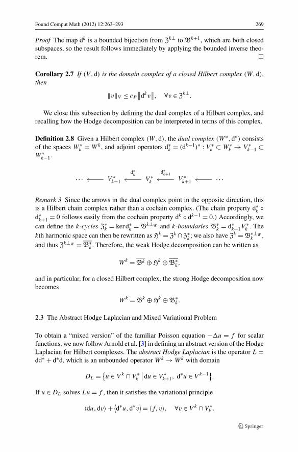
Definition 2.8 Given a Hilbert complex (W,d), the dual complex (W ∗,d∗) consistsof the spaces W ∗
k = Wk , and adjoint operators d∗k = (dk−1)∗ : V ∗
k ⊂ W ∗k → V ∗
k−1 ⊂W ∗
k−1.
· · · V ∗k−1 V ∗
k
d∗k
V ∗k+1
d∗k+1 · · ·
Remark 3 Since the arrows in the dual complex point in the opposite direction, thisis a Hilbert chain complex rather than a cochain complex. (The chain property d∗
k ◦d∗k+1 = 0 follows easily from the cochain property dk ◦ dk−1 = 0.) Accordingly, we
can define the k-cycles Z∗k = ker d∗
k = Bk⊥W and k-boundaries B∗k = d∗
k+1V∗k . The
kth harmonic space can then be rewritten as Hk = Zk ∩Z∗k ; we also have Zk = B∗⊥W
k ,and thus Zk⊥W = B∗
k . Therefore, the weak Hodge decomposition can be written as
Wk = Bk ⊕ Hk ⊕ B∗
k,
and in particular, for a closed Hilbert complex, the strong Hodge decomposition nowbecomes
Wk = Bk ⊕ H
k ⊕ B∗k.
2.3 The Abstract Hodge Laplacian and Mixed Variational Problem
To obtain a “mixed version” of the familiar Poisson equation −�u = f for scalarfunctions, we now follow Arnold et al. [3] in defining an abstract version of the HodgeLaplacian for Hilbert complexes. The abstract Hodge Laplacian is the operator L =dd∗ + d∗d, which is an unbounded operator Wk → Wk with domain
DL = {u ∈ V k ∩ V ∗
k
∣∣du ∈ V ∗k+1, d∗u ∈ V k−1}.
If u ∈ DL solves Lu = f , then it satisfies the variational principle
〈du,dv〉 + ⟨d∗u,d∗v
⟩ = 〈f, v〉, ∀v ∈ V k ∩ V ∗k .
270 Found Comput Math (2012) 12:263–293
However, as noted by Arnold et al. [3], there are some difficulties in using this vari-ational principle for a finite element approximation. First, it may be difficult to con-struct finite elements for the space V k ∩ V ∗
k . A second concern is the well-posednessof the problem. If we take any harmonic test function v ∈ Hk , then the left-hand sidevanishes, so 〈f, v〉 = 0; hence, a solution only exists if f ⊥ Hk . Furthermore, for anyq ∈ Hk = Zk ∩ Z∗
k , we have dq = 0 and d∗q = 0; therefore, if u is a solution, then sois u + q .
To avoid these existence and uniqueness issues, one can define instead the follow-ing mixed variational problem: Find (σ,u,p) ∈ V k−1 × V k × Hk satisfying
〈σ, τ 〉 − 〈u,dτ 〉 = 0, ∀τ ∈ V k−1,
〈dσ, v〉 + 〈du,dv〉 + 〈p,v〉 = 〈f, v〉, ∀v ∈ V k,
〈u,q〉 = 0, ∀q ∈ Hk.
(3)
Here, the first equation implies that σ = d∗u, which weakly enforces the conditionu ∈ V k ∩V ∗
k . Next, the second equation incorporates the additional term 〈p,v〉, whichallows for solutions to exist even when f �⊥ Hk . Finally, the third equation fixes theissue of non-uniqueness by requiring u ⊥ Hk . The following result establishes thewell-posedness of the problem (3).
Theorem 2.9 (Arnold et al. [3], Theorem 3.1) Let (W,d) be a closed Hilbert complexwith domain complex (V ,d). The mixed formulation of the abstract Hodge Laplacianis well posed. That is, for any f ∈ Wk , there exists a unique (σ,u,p) ∈ V k−1 ×V k ×Hk satisfying (3). Moreover,
‖σ‖V + ‖u‖V + ‖p‖ ≤ c‖f ‖,where c is a constant depending only on the Poincaré constant cP in Lemma 2.6.
To prove this, one observes that (3) can be rewritten as a standard variationalproblem (1) on the space V k−1 × V k × Hk , with the bilinear form
B(σ,u,p; τ, v, q) = 〈σ, τ 〉 − 〈u,dτ 〉 + 〈dσ, v〉 + 〈du,dv〉 + 〈p,v〉 − 〈u,q〉and functional F(τ, v, q) = 〈f, v〉. The well-posedness then follows immediatelyfrom the following theorem, which establishes the inf-sup condition for the bilinearform B .
Theorem 2.10 (Arnold et al. [3], Theorem 3.2) Let (W,d) be a closed Hilbertcomplex with domain complex (V ,d). There exists a constant γ > 0, dependingonly on the constant cP in the Poincaré inequality (Lemma 2.6), such that for any(σ,u,p) ∈ V k−1 × V k × Hk , there exists (τ, v, q) ∈ V k−1 × V k × Hk with
B(σ,u,p; τ, v, q) ≥ γ(‖σ‖V + ‖u‖V + ‖p‖)(‖τ‖V + ‖v‖V + ‖q‖).
From the well-posedness result, it follows that there exists a bounded solutionoperator K : Wk → Wk defined by Kf = u.
Found Comput Math (2012) 12:263–293 271
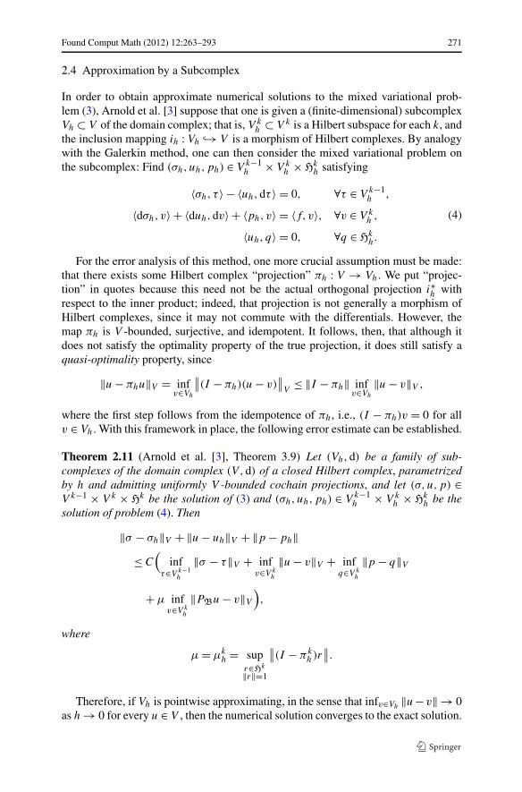
2.4 Approximation by a Subcomplex
In order to obtain approximate numerical solutions to the mixed variational prob-lem (3), Arnold et al. [3] suppose that one is given a (finite-dimensional) subcomplexVh ⊂ V of the domain complex; that is, V k
h ⊂ V k is a Hilbert subspace for each k, andthe inclusion mapping ih : Vh ↪→ V is a morphism of Hilbert complexes. By analogywith the Galerkin method, one can then consider the mixed variational problem onthe subcomplex: Find (σh,uh,ph) ∈ V k−1
h × V kh × Hk
h satisfying
〈σh, τ 〉 − 〈uh,dτ 〉 = 0, ∀τ ∈ V k−1h ,
〈dσh, v〉 + 〈duh,dv〉 + 〈ph, v〉 = 〈f, v〉, ∀v ∈ V kh ,
〈uh, q〉 = 0, ∀q ∈ Hkh.
(4)
For the error analysis of this method, one more crucial assumption must be made:that there exists some Hilbert complex “projection” πh : V → Vh. We put “projec-tion” in quotes because this need not be the actual orthogonal projection i∗h withrespect to the inner product; indeed, that projection is not generally a morphism ofHilbert complexes, since it may not commute with the differentials. However, themap πh is V -bounded, surjective, and idempotent. It follows, then, that although itdoes not satisfy the optimality property of the true projection, it does still satisfy aquasi-optimality property, since
‖u − πhu‖V = infv∈Vh
∥∥(I − πh)(u − v)∥∥
V≤ ‖I − πh‖ inf
v∈Vh
‖u − v‖V ,
where the first step follows from the idempotence of πh, i.e., (I − πh)v = 0 for allv ∈ Vh. With this framework in place, the following error estimate can be established.
Theorem 2.11 (Arnold et al. [3], Theorem 3.9) Let (Vh,d) be a family of sub-complexes of the domain complex (V ,d) of a closed Hilbert complex, parametrizedby h and admitting uniformly V -bounded cochain projections, and let (σ,u,p) ∈V k−1 × V k × Hk be the solution of (3) and (σh,uh,ph) ∈ V k−1
h × V kh × Hk
h be thesolution of problem (4). Then
‖σ − σh‖V + ‖u − uh‖V + ‖p − ph‖≤ C
(inf
τ∈V k−1h
‖σ − τ‖V + infv∈V k
h
‖u − v‖V + infq∈V k
h
‖p − q‖V
+ μ infv∈V k
h
‖PBu − v‖V
),
where
μ = μkh = sup
r∈Hk
‖r‖=1
∥∥(I − πkh)r
∥∥.
Therefore, if Vh is pointwise approximating, in the sense that infv∈Vh‖u−v‖ → 0
as h → 0 for every u ∈ V , then the numerical solution converges to the exact solution.

272 Found Comput Math (2012) 12:263–293
3 Analysis of Variational Crimes
In this section, we extend the results of Arnold et al. [3], summarized in the previ-ous section, by removing the requirement for Vh to be a subcomplex of V . The keypoint of departure is in the map ih : Vh ↪→ V ; rather than being an inclusion, we re-quire only that it is an injective morphism of Hilbert complexes, with the propertythat πh ◦ ih is the identity. (The latter requirement simply corresponds to the earliercondition that πh be idempotent in the case of subcomplexes.) After stating somebasic results about complexes equipped with such maps, we develop error estimatesfor the mixed variational problem and eigenvalue problem on Vh. These estimatescontain two additional error terms, in addition to those in the analysis of Arnold etal. [3]. These extra terms, analogous to those in the Strang lemmas for generalizedGalerkin methods, measure the “severity” of two variational crimes: first, how wellthe right-hand side ihfh approximates f ; and second, the extent to which ih fails tobe unitary.
3.1 Approximation by an Arbitrary Complex
In order to approximate a Hilbert complex (W,d), suppose we have another Hilbertcomplex (Wh,dh), along with a pair of morphisms: an injection ih : Wh ↪→ W and aprojection πh : W → Wh, such that πk
h ◦ ikh is the identity on Wkh for each k. Recall
that, by Definition 2.2 of a Hilbert complex morphism, the maps ikh and πkh must be
bounded for each k. The relationships among the domains and maps are illustrated inthe following diagram:
· · · V k
πkh
dk
V k+1
πk+1h
· · ·
· · · V kh
ikh
dkh
V k+1h
ik+1h
· · · .
Arnold et al. [3] consider the case where Wh ⊂ W is a subcomplex, and ih is theinclusion of Wh into W . In this special case, ih is unitary (i.e., an isometry), since forall u,v ∈ Wk
h , we have 〈ihu, ihv〉 = 〈u,v〉 = 〈u,v〉h. Indeed, if ih is unitary, then wecan simply identify Wh with the subcomplex ihWh ⊂ W . However, more generally,we will consider cases where Wh �⊂ W , and where ih is not necessarily unitary.
We begin by demonstrating some basic facts about these approximations.
Theorem 3.1 If (W,d) is a bounded Hilbert complex, then so is (Wh,dh).
Proof∥∥dk
h
∥∥ = ∥∥πk+1h ik+1
h dkh
∥∥ = ∥∥πk+1h dkikh
∥∥ ≤ ∥∥πk+1h
∥∥∥∥dk∥∥∥∥ikh
∥∥ < ∞. �
Theorem 3.2 If (W,d) is a closed Hilbert complex, then so is (Wh,dh).
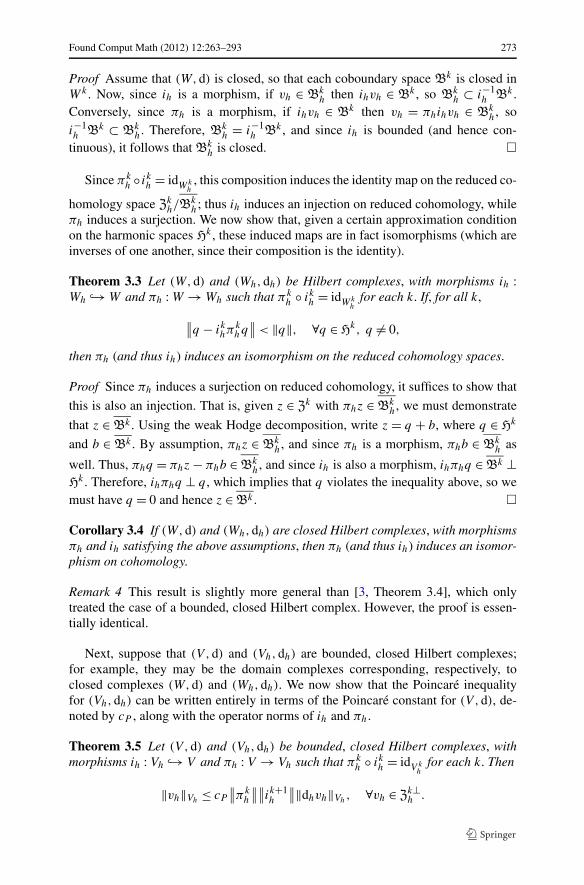
Found Comput Math (2012) 12:263–293 273
Proof Assume that (W,d) is closed, so that each coboundary space Bk is closed inWk . Now, since ih is a morphism, if vh ∈ Bk
h then ihvh ∈ Bk , so Bkh ⊂ i−1
h Bk .Conversely, since πh is a morphism, if ihvh ∈ Bk then vh = πhihvh ∈ Bk
h, soi−1h Bk ⊂ Bk
h. Therefore, Bkh = i−1
h Bk , and since ih is bounded (and hence con-tinuous), it follows that Bk
h is closed. �
Since πkh ◦ ikh = idWk
h, this composition induces the identity map on the reduced co-
homology space Zkh/B
kh; thus ih induces an injection on reduced cohomology, while
πh induces a surjection. We now show that, given a certain approximation conditionon the harmonic spaces Hk , these induced maps are in fact isomorphisms (which areinverses of one another, since their composition is the identity).
Theorem 3.3 Let (W,d) and (Wh,dh) be Hilbert complexes, with morphisms ih :Wh ↪→ W and πh : W → Wh such that πk
h ◦ ikh = idWkh
for each k. If, for all k,
∥∥q − ikhπkhq
∥∥ < ‖q‖, ∀q ∈ Hk, q �= 0,
then πh (and thus ih) induces an isomorphism on the reduced cohomology spaces.
Proof Since πh induces a surjection on reduced cohomology, it suffices to show that
this is also an injection. That is, given z ∈ Zk with πhz ∈ Bkh, we must demonstrate
that z ∈ Bk . Using the weak Hodge decomposition, write z = q + b, where q ∈ Hk
and b ∈ Bk . By assumption, πhz ∈ Bkh, and since πh is a morphism, πhb ∈ Bk
h as
well. Thus, πhq = πhz − πhb ∈ Bkh, and since ih is also a morphism, ihπhq ∈ Bk ⊥
Hk . Therefore, ihπhq ⊥ q , which implies that q violates the inequality above, so wemust have q = 0 and hence z ∈ Bk . �
Corollary 3.4 If (W,d) and (Wh,dh) are closed Hilbert complexes, with morphismsπh and ih satisfying the above assumptions, then πh (and thus ih) induces an isomor-phism on cohomology.
Remark 4 This result is slightly more general than [3, Theorem 3.4], which onlytreated the case of a bounded, closed Hilbert complex. However, the proof is essen-tially identical.
Next, suppose that (V ,d) and (Vh,dh) are bounded, closed Hilbert complexes;for example, they may be the domain complexes corresponding, respectively, toclosed complexes (W,d) and (Wh,dh). We now show that the Poincaré inequalityfor (Vh,dh) can be written entirely in terms of the Poincaré constant for (V ,d), de-noted by cP , along with the operator norms of ih and πh.
Theorem 3.5 Let (V ,d) and (Vh,dh) be bounded, closed Hilbert complexes, withmorphisms ih : Vh ↪→ V and πh : V → Vh such that πk
h ◦ ikh = idV kh
for each k. Then
‖vh‖Vh≤ cP
∥∥πkh
∥∥∥∥ik+1h
∥∥‖dhvh‖Vh, ∀vh ∈ Z
k⊥h .
274 Found Comput Math (2012) 12:263–293
Proof Given vh ∈ Zk⊥h , let z ∈ Zk⊥ be the unique element such that dz = dihvh =
ihdhvh. Then, applying the abstract Poincaré inequality on V ,
‖z‖V ≤ cP ‖dz‖V = cP ‖ihdhvh‖V ≤ cP
∥∥ik+1h
∥∥‖dhvh‖Vh.
It now suffices to show ‖vh‖Vh≤ ‖πk
h‖‖z‖V . Observe that vh − πhz ∈ V kh , and fur-
thermore,
dhπhz = πhdz = πhihdhvh = dhvh,
so vh − πhz ∈ Zkh ⊥ vh. Therefore,
‖vh‖2Vh
= 〈vh,πhz〉Vh+ 〈vh, vh − πhz〉Vh
= 〈vh,πhz〉Vh≤ ‖vh‖Vh
∥∥πkh
∥∥‖z‖V ,
and the result follows. �
Corollary 3.6 If (V ,d) and (Vh,dh) are the domain complexes corresponding, re-spectively, to closed Hilbert complexes (W,d) and (Wh,dh), then
‖vh‖Vh≤ cP
∥∥πkh
∥∥∥∥ik+1h
∥∥‖dhvh‖h, ∀vh ∈ Zk⊥h .
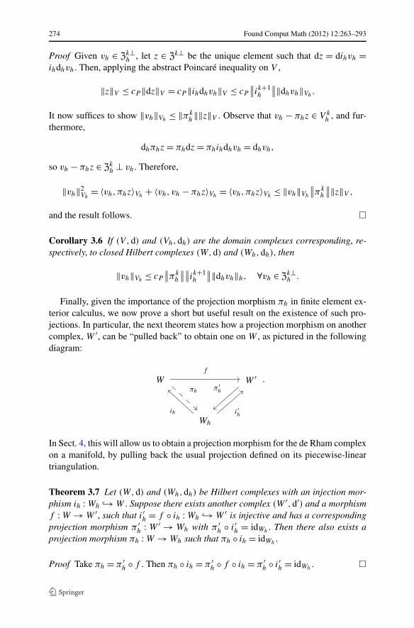
Finally, given the importance of the projection morphism πh in finite element ex-terior calculus, we now prove a short but useful result on the existence of such pro-jections. In particular, the next theorem states how a projection morphism on anothercomplex, W ′, can be “pulled back” to obtain one on W , as pictured in the followingdiagram:
Wf
πh
W ′π ′
h
Wh
ih i′h
.
In Sect. 4, this will allow us to obtain a projection morphism for the de Rham complexon a manifold, by pulling back the usual projection defined on its piecewise-lineartriangulation.
Theorem 3.7 Let (W,d) and (Wh,dh) be Hilbert complexes with an injection mor-phism ih : Wh ↪→ W . Suppose there exists another complex (W ′,d′) and a morphismf : W → W ′, such that i′h = f ◦ ih : Wh ↪→ W ′ is injective and has a correspondingprojection morphism π ′
h : W ′ → Wh with π ′h ◦ i′h = idWh
. Then there also exists aprojection morphism πh : W → Wh such that πh ◦ ih = idWh
.
Proof Take πh = π ′h ◦ f . Then πh ◦ ih = π ′
h ◦ f ◦ ih = π ′h ◦ i′h = idWh
. �
Found Comput Math (2012) 12:263–293 275
3.2 Modified Inner Product and Hodge Decomposition
As noted in the previous section, this generalized framework introduces some newcomplications, due to the possible non-unitarity of ih. The following result showsthat the subspace ihWh ⊂ W can be identified with Wh, endowed with a modifiedinner product 〈Jh·, ·〉h instead of 〈·, ·〉h. This defines a modified Hilbert complex,which will be denoted by (i∗hW,dh).
Theorem 3.8 Let ih : Wh ↪→ W be a morphism of Hilbert complexes, and defineJ k
h = ik∗h ikh : Wk
h → Wkh for each k. Then
〈Jhuh, vh〉h = 〈ihuh, ihvh〉, ∀uh, vh ∈ Wkh ,
is an inner product, which defines a Hilbert space structure on Wkh .
Proof 〈ihuh, ihvh〉 = 〈i∗hihuh, vh〉h = 〈Jhuh, vh〉h. This is an inner product, since ih
is linear and injective. Moreover, Wkh is closed with respect to the induced norm,
since ‖ihvh‖ ≤ ‖ih‖‖vh‖ and ih is bounded, so this is indeed a Hilbert space. �
Remark 5 We use the notation Jh due to the similarity with the Jacobian determinantused in the “change of variables” formula for integration. Note that, although eachJ k
h : Wkh → Wk
h is a bounded linear map, Jh is not necessarily a Hilbert complexautomorphism. This happens because, in general, d commutes with ih but not withits adjoint i∗h . Also, clearly ikh is unitary if and only if J k
h = idWkh
.
Now, if ih does not preserve the inner product, in particular it does not preserveorthogonality: that is, uh ⊥ vh does not imply ihuh ⊥ ihvh. This has significant im-
plications for the Hodge decomposition, since although Wkh = Bk
h ⊕ Hkh ⊕ Zk⊥Wh
h isWh-orthogonal, it is generally not i∗hW -orthogonal. Therefore, we define the new,modified subspaces
H′kh = {
z ∈ Zkh | ihz ⊥ ihB
kh
}, Z
k⊥′Wh = {
v ∈ Wkh | ihv ⊥ ihZ
kh
}.
This gives a modified Hodge decomposition Wkh = Bk
h ⊕ H′kh ⊕ Zk⊥′W
h , which is nolonger necessarily Wh-orthogonal, but is now i∗hW -orthogonal. As before, this also
gives a modified Hodge decomposition for the domain complex V kh = Bk
h ⊕ H′kh ⊕
Zk⊥′h .
3.3 Stability and Convergence of the Mixed Method
Let (W,d) be a closed Hilbert complex with domain complex (V ,d). To approximatea solution to the mixed variational problem (3), suppose that (Wh,dh) is anotherHilbert complex with domain complex (Vh,dh), and that we have morphisms ih :Vh ↪→ V and πh : V → Vh such that πk
h ◦ ikh = idV kh
for each k. We assume that ih isW -bounded, so that it also can be extended to Wh ↪→ W , but that πh might only be
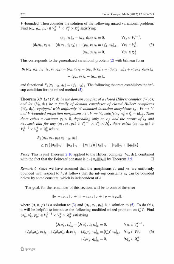
276 Found Comput Math (2012) 12:263–293
V -bounded. Then consider the solution of the following mixed variational problem:Find (σh,uh,ph) ∈ V k−1
h × V kh × Hk
h satisfying
〈σh, τh〉h − 〈uh,dhτh〉h = 0, ∀τh ∈ V k−1h ,
〈dhσh, vh〉h + 〈dhuh,dhvh〉h + 〈ph, vh〉h = 〈fh, vh〉h, ∀vh ∈ V kh ,
〈uh, qh〉h = 0, ∀qh ∈ Hkh.
(5)
This corresponds to the generalized variational problem (2) with bilinear form
Bh(σh,uh,ph; τh, vh, qh) = 〈σh, τh〉h − 〈uh,dhτh〉h + 〈dhσh, vh〉h + 〈dhuh,dhvh〉h+ 〈ph, vh〉h − 〈uh, qh〉h
and functional Fh(τh, vh, qh) = 〈fh, vh〉h. The following theorem establishes the inf-sup condition for the mixed method (5).
Theorem 3.9 Let (V ,d) be the domain complex of a closed Hilbert complex (W,d),and let (Vh,dh) be a family of domain complexes of closed Hilbert complexes(Wh,dh), equipped with uniformly W -bounded inclusion morphisms ih : Vh ↪→ V
and V -bounded projection morphisms πh : V → Vh satisfying πkh ◦ ikh = idV k
h. Then
there exists a constant γh > 0, depending only on cP and the norms of ih andπh, such that for any (σh,uh,ph) ∈ V k−1
h × V kh × Hk
h, there exists (τh, vh, qh) ∈V k−1
h × V kh × Hk
h where
Bh(σh,uh,ph; τh, vh, qh)
≥ γh
(‖σh‖Vh+ ‖uh‖Vh
+ ‖ph‖h
)(‖τh‖Vh+ ‖vh‖Vh
+ ‖qh‖h
).
Proof This is just Theorem 2.10 applied to the Hilbert complex (Vh,dh), combinedwith the fact that the Poincaré constant is cP ‖πh‖‖ih‖ by Theorem 3.5. �
Remark 6 Since we have assumed that the morphisms ih and πh are uniformlybounded with respect to h, it follows that the inf-sup constants γh can be boundedbelow by some constant, which is independent of h.
The goal, for the remainder of this section, will be to control the error
‖σ − ihσh‖V + ‖u − ihuh‖V + ‖p − ihph‖,where (σ,u,p) is a solution to (3) and (σh,uh,ph) is a solution to (5). To do this,it will be helpful to introduce the following modified mixed problem on i∗hV : Find(σ ′
h,u′h,p
′h) ∈ V k−1
h × V kh × H′k
h satisfying
⟨Jhσ
′h, τh
⟩h
− ⟨Jhu
′h,dhτh
⟩h
= 0, ∀τh ∈ V k−1h ,
⟨Jhdhσ
′h, vh
⟩h
+ ⟨Jhdhu
′h,dhvh
⟩h
+ ⟨Jhp
′h, vh
⟩h
= ⟨i∗hf, vh
⟩h, ∀vh ∈ V k
h ,⟨Jhu
′h, q
′h
⟩h
= 0, ∀q ′h ∈ H′k
h .
(6)
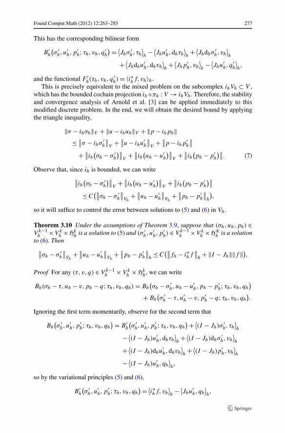
Found Comput Math (2012) 12:263–293 277
This has the corresponding bilinear form
B ′h
(σ ′
h,u′h,p
′h; τh, vh, q
′h
) = ⟨Jhσ
′h, τh
⟩h
− ⟨Jhu
′h,dhτh
⟩h
+ ⟨Jhdhσ
′h, vh
⟩h
+ ⟨Jhdhu
′h,dhvh
⟩h
+ ⟨Jhp
′h, vh
⟩h
− ⟨Jhu
′h, q
′h
⟩h,
and the functional F ′h(τh, vh, q
′h) = 〈i∗hf, vh〉h.
This is precisely equivalent to the mixed problem on the subcomplex ihVh ⊂ V ,which has the bounded cochain projection ih ◦πh : V → ihVh. Therefore, the stabilityand convergence analysis of Arnold et al. [3] can be applied immediately to thismodified discrete problem. In the end, we will obtain the desired bound by applyingthe triangle inequality,
‖σ − ihσh‖V + ‖u − ihuh‖V + ‖p − ihph‖≤ ∥∥σ − ihσ
′h
∥∥V
+ ∥∥u − ihu′h
∥∥V
+ ∥∥p − ihp′h
∥∥
+ ∥∥ih(σh − σ ′
h
)∥∥V
+ ∥∥ih(uh − u′
h
)∥∥V
+ ∥∥ih(ph − p′
h
)∥∥. (7)
Observe that, since ih is bounded, we can write∥∥ih
(σh − σ ′
h
)∥∥V
+ ∥∥ih(uh − u′
h
)∥∥V
+ ∥∥ih(ph − p′
h
)∥∥
≤ C(∥∥σh − σ ′
h
∥∥Vh
+ ∥∥uh − u′h
∥∥Vh
+ ∥∥ph − p′h
∥∥h
),
so it will suffice to control the error between solutions to (5) and (6) in Vh.
Theorem 3.10 Under the assumptions of Theorem 3.9, suppose that (σh,uh,ph) ∈V k−1
h ×V kh ×Hk
h is a solution to (5) and (σ ′h,u
′h,p
′h) ∈ V k−1
h ×V kh ×H′k
h is a solutionto (6). Then
∥∥σh − σ ′h
∥∥Vh
+ ∥∥uh − u′h
∥∥Vh
+ ∥∥ph − p′h
∥∥h
≤ C(∥∥fh − i∗hf
∥∥h
+ ‖I − Jh‖‖f ‖).
Proof For any (τ, v, q) ∈ V k−1h × V k
h × Hkh, we can write
Bh(σh − τ,uh − v,ph − q; τh, vh, qh) = Bh
(σh − σ ′
h,uh − u′h,ph − p′
h; τh, vh, qh
)
+ Bh
(σ ′
h − τ,u′h − v,p′
h − q; τh, vh, qh
).
Ignoring the first term momentarily, observe for the second term that
Bh
(σ ′
h,u′h,p
′h; τh, vh, qh
) = B ′h
(σ ′
h,u′h,p
′h; τh, vh, qh
) + ⟨(I − Jh)σ
′h, τh
⟩h
− ⟨(I − Jh)u
′h,dhτh
⟩h
+ ⟨(I − Jh)dhσ
′h, vh
⟩h
+ ⟨(I − Jh)dhu
′h,dhvh
⟩h
+ ⟨(I − Jh)p
′h, vh
⟩h
− ⟨(I − Jh)u
′h, qh
⟩h,
so by the variational principles (5) and (6),
B ′h
(σ ′
h,u′h,p
′h; τh, vh, qh
) = ⟨i∗hf, vh
⟩h
− ⟨Jhu
′h, qh
⟩h,
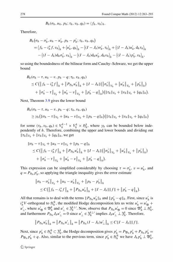
278 Found Comput Math (2012) 12:263–293
Bh(σh,uh,ph; τh, vh, qh) = 〈fh, vh〉h.Therefore,
Bh
(σh − σ ′
h,uh − u′h,ph − p′
h; τh, vh, qh
)
= ⟨fh − i∗hf, vh
⟩h
+ ⟨u′
h, qh
⟩h
− ⟨(I − Jh)σ
′h, τh
⟩h
+ ⟨(I − Jh)u
′h,dhτh
⟩h
− ⟨(I − Jh)dhσ
′h, vh
⟩h
− ⟨(I − Jh)dhu
′h,dhvh
⟩h
− ⟨(I − Jh)p
′h, vh
⟩h,
so using the boundedness of the bilinear form and Cauchy–Schwarz, we get the upperbound
Bh(σh − τ,uh − v,ph − q; τh, vh, qh)
≤ C(∥∥fh − i∗hf
∥∥h
+ ∥∥PHhu′
h
∥∥h
+ ‖I − Jh‖(∥∥σ ′
h
∥∥Vh
+ ∥∥u′h
∥∥Vh
+ ∥∥p′h
∥∥h
)
+ ∥∥σ ′h − τ
∥∥Vh
+ ∥∥u′h − v
∥∥Vh
+ ∥∥p′h − q
∥∥h
)(‖τh‖Vh+ ‖vh‖Vh
+ ‖qh‖h
).
Next, Theorem 3.9 gives the lower bound
Bh(σh − τ,uh − v,ph − q; τh, vh, qh)
≥ γh
(‖σh − τ‖Vh+ ‖uh − v‖Vh
+ ‖ph − q‖h
)(‖τh‖Vh+ ‖vh‖Vh
+ ‖qh‖h
)
for some (τh, vh, qh) ∈ V k−1h × V k
h × Hkh, where γh can be bounded below inde-
pendently of h. Therefore, combining the upper and lower bounds and dividing out‖τh‖Vh
+ ‖vh‖Vh+ ‖qh‖h, we get
‖σh − τ‖Vh+ ‖uh − v‖Vh
+ ‖ph − q‖h
≤ C(∥∥fh − i∗hf
∥∥h
+ ∥∥PHhu′
h
∥∥h
+ ‖I − Jh‖(∥∥σ ′
h
∥∥Vh
+ ∥∥u′h
∥∥Vh
+ ∥∥p′h
∥∥h
)
+ ∥∥σ ′h − τ
∥∥Vh
+ ∥∥u′h − v
∥∥Vh
+ ∥∥p′h − q
∥∥h
).
This expression can be simplified considerably by choosing τ = σ ′h, v = u′
h, andq = PHh
p′h, so applying the triangle inequality gives the error estimate∥∥σh − σ ′
h
∥∥Vh
+ ∥∥uh − u′h
∥∥Vh
+ ∥∥ph − p′h
∥∥h
≤ C(∥∥fh − i∗hf
∥∥h
+ ∥∥PHhu′
h
∥∥h
+ ‖I − Jh‖‖f ‖ + ∥∥p′h − q
∥∥h
).
All that remains is to deal with the terms ‖PHhu′
h‖h and ‖p′h − q‖h. First, since u′
h isi∗hV -orthogonal to H′k
h , the modified Hodge decomposition lets us write u′h = u′
B+
u′⊥, where u′B
∈ Bkh and u′⊥ ∈ Zk⊥′
h . Now, observe that PHhu′
B= 0 since Bk
h ⊥ Hkh,
and furthermore PHhJhu
′⊥ = 0 since u′⊥ ∈ Zk⊥′h implies Jhu
′⊥ ⊥ Zkh. Therefore,
∥∥PHhu′
h
∥∥h
= ∥∥PHhu′⊥
∥∥h
= ∥∥PHh(I − Jh)u
′⊥∥∥
h≤ C‖I − Jh‖‖f ‖.
Next, since p′h ∈ H′k
h ⊂ Zkh, the Hodge decomposition gives p′
h = PBhp′
h +PHhp′
h =PBh
p′h + q . Also, similar to the previous term, since p′
h ∈ H′kh we have Jhp
′h ⊥ Bk
h,
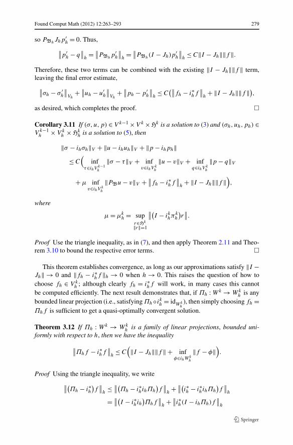
Found Comput Math (2012) 12:263–293 279
so PBhJhp
′h = 0. Thus,
∥∥p′h − q
∥∥h
= ∥∥PBhp′
h
∥∥h
= ∥∥PBh(I − Jh)p
′h
∥∥h
≤ C‖I − Jh‖‖f ‖.Therefore, these two terms can be combined with the existing ‖I − Jh‖‖f ‖ term,leaving the final error estimate,
∥∥σh − σ ′h
∥∥Vh
+ ∥∥uh − u′h
∥∥Vh
+ ∥∥ph − p′h
∥∥h
≤ C(∥∥fh − i∗hf
∥∥h
+ ‖I − Jh‖‖f ‖),as desired, which completes the proof. �
Corollary 3.11 If (σ,u,p) ∈ V k−1 ×V k ×Hk is a solution to (3) and (σh,uh,ph) ∈V k−1
h × V kh × Hk
h is a solution to (5), then
‖σ − ihσh‖V + ‖u − ihuh‖V + ‖p − ihph‖≤ C
(inf
τ∈ihV k−1h
‖σ − τ‖V + infv∈ihV k
h
‖u − v‖V + infq∈ihV k
h
‖p − q‖V
+ μ infv∈ihV k
h
‖PBu − v‖V + ∥∥fh − i∗hf∥∥
h+ ‖I − Jh‖‖f ‖
),
where
μ = μkh = sup
r∈Hk
‖r‖=1
∥∥(I − ikhπk
h
)r∥∥.
Proof Use the triangle inequality, as in (7), and then apply Theorem 2.11 and Theo-rem 3.10 to bound the respective error terms. �
This theorem establishes convergence, as long as our approximations satisfy ‖I −Jh‖ → 0 and ‖fh − i∗hf ‖h → 0 when h → 0. This raises the question of how tochoose fh ∈ V k
h ; although clearly fh = i∗hf will work, in many cases this cannotbe computed efficiently. The next result demonstrates that, if Πh : Wk → Wk
h is anybounded linear projection (i.e., satisfying Πh◦ ikh = idWk
h), then simply choosing fh =
Πhf is sufficient to get a quasi-optimally convergent solution.
Theorem 3.12 If Πh : Wk → Wkh is a family of linear projections, bounded uni-
formly with respect to h, then we have the inequality
∥∥Πhf − i∗hf∥∥
h≤ C
(‖I − Jh‖‖f ‖ + inf
φ∈ihWkh
‖f − φ‖).
Proof Using the triangle inequality, we write
∥∥(Πh − i∗h
)f
∥∥h
≤ ∥∥(Πh − i∗hihΠh
)f
∥∥h
+ ∥∥(i∗h − i∗hihΠh
)f
∥∥h
= ∥∥(I − i∗hih
)Πhf
∥∥h
+ ∥∥i∗h(I − ihΠh)f∥∥
h
280 Found Comput Math (2012) 12:263–293
≤ ‖I − Jh‖‖Πhf ‖h + ∥∥i∗h∥∥∥∥(I − ihΠh)f
∥∥
≤ C(‖I − Jh‖‖f ‖ + inf
φ∈ihWkh
‖f − φ‖),
where the final step follows from the W -boundedness of Πh and the quasi-optimalityproperty of I − ihΠh, i.e., (I − ihΠh)f = (I − ihΠh)(f − φ) for any φ ∈ ihW
kh . �
3.4 Remarks on Obtaining Improved Error Estimates
Arnold et al. [3] were also able to obtain improved error estimates by makingsome additional assumptions: namely, that πh is W -bounded rather than merelyV -bounded, and that the Hilbert complex V satisfies a certain compactness property.With these assumptions, the continuous solution operator K : Wk → Wk becomesa compact operator, and hence converts the pointwise convergence of I − πh → 0(which follows from the quasi-optimality property) to norm convergence. This normconvergence is essential for applying the “Aubin–Nitsche trick” (also known as “L2
lifting”), where one obtains improved estimates by applying the solution operatorto the error term itself. Roughly speaking, one needs norm convergence, rather thanpointwise convergence, since the solution operator is being applied to quantities thatdepend on the parameter h.
However, there are no such improved estimates for the additional error terms ob-tained in the previous subsection; essentially, because norm convergence is alreadyrequired for ‖I − Jh‖ → 0 as h → 0, and there is no analogous quasi-optimalityresult for Jh as there is for πh. Therefore, these terms remain the same, and the im-proved estimates only apply to the terms already analyzed by Arnold et al. [3] for thesubcomplex case.
3.5 Convergence of the Eigenvalue Problem
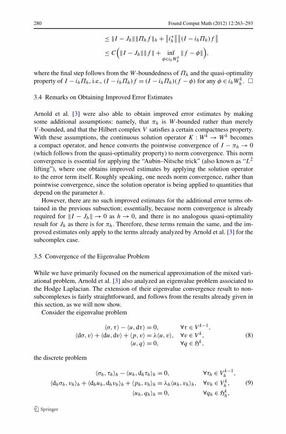
While we have primarily focused on the numerical approximation of the mixed vari-ational problem, Arnold et al. [3] also analyzed an eigenvalue problem associated tothe Hodge Laplacian. The extension of their eigenvalue convergence result to non-subcomplexes is fairly straightforward, and follows from the results already given inthis section, as we will now show.
Consider the eigenvalue problem
〈σ, τ 〉 − 〈u,dτ 〉 = 0, ∀τ ∈ V k−1,
〈dσ, v〉 + 〈du,dv〉 + 〈p,v〉 = λ〈u,v〉, ∀v ∈ V k,
〈u,q〉 = 0, ∀q ∈ Hk,
(8)
the discrete problem
〈σh, τh〉h − 〈uh,dhτh〉h = 0, ∀τh ∈ V k−1h ,
〈dhσh, vh〉h + 〈dhuh,dhvh〉h + 〈ph, vh〉h = λh〈uh, vh〉h, ∀vh ∈ V kh ,
〈uh, qh〉h = 0, ∀qh ∈ Hkh,
(9)
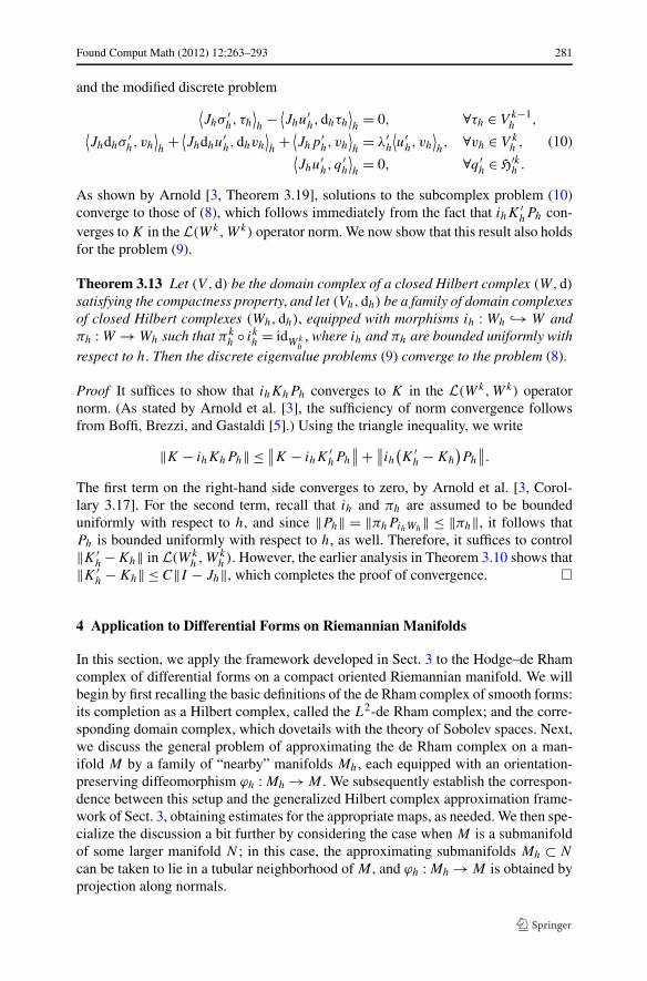
Found Comput Math (2012) 12:263–293 281
and the modified discrete problem⟨Jhσ
′h, τh
⟩h
− ⟨Jhu
′h,dhτh
⟩h
= 0, ∀τh ∈ V k−1h ,
⟨Jhdhσ
′h, vh
⟩h
+ ⟨Jhdhu
′h,dhvh
⟩h
+ ⟨Jhp
′h, vh
⟩h
= λ′h
⟨u′
h, vh
⟩h, ∀vh ∈ V k
h ,⟨Jhu
′h, q
′h
⟩h
= 0, ∀q ′h ∈ H′k
h .
(10)
As shown by Arnold [3, Theorem 3.19], solutions to the subcomplex problem (10)converge to those of (8), which follows immediately from the fact that ihK
′hPh con-
verges to K in the L(Wk,Wk) operator norm. We now show that this result also holdsfor the problem (9).
Theorem 3.13 Let (V ,d) be the domain complex of a closed Hilbert complex (W,d)
satisfying the compactness property, and let (Vh,dh) be a family of domain complexesof closed Hilbert complexes (Wh,dh), equipped with morphisms ih : Wh ↪→ W andπh : W → Wh such that πk
h ◦ ikh = idWkh
, where ih and πh are bounded uniformly withrespect to h. Then the discrete eigenvalue problems (9) converge to the problem (8).
Proof It suffices to show that ihKhPh converges to K in the L(Wk,Wk) operatornorm. (As stated by Arnold et al. [3], the sufficiency of norm convergence followsfrom Boffi, Brezzi, and Gastaldi [5].) Using the triangle inequality, we write
‖K − ihKhPh‖ ≤ ∥∥K − ihK′hPh
∥∥ + ∥∥ih(K ′
h − Kh
)Ph
∥∥.
The first term on the right-hand side converges to zero, by Arnold et al. [3, Corol-lary 3.17]. For the second term, recall that ih and πh are assumed to be boundeduniformly with respect to h, and since ‖Ph‖ = ‖πhPihWh
‖ ≤ ‖πh‖, it follows thatPh is bounded uniformly with respect to h, as well. Therefore, it suffices to control‖K ′
h −Kh‖ in L(Wkh ,Wk
h ). However, the earlier analysis in Theorem 3.10 shows that‖K ′
h − Kh‖ ≤ C‖I − Jh‖, which completes the proof of convergence. �
4 Application to Differential Forms on Riemannian Manifolds
In this section, we apply the framework developed in Sect. 3 to the Hodge–de Rhamcomplex of differential forms on a compact oriented Riemannian manifold. We willbegin by first recalling the basic definitions of the de Rham complex of smooth forms:its completion as a Hilbert complex, called the L2-de Rham complex; and the corre-sponding domain complex, which dovetails with the theory of Sobolev spaces. Next,we discuss the general problem of approximating the de Rham complex on a man-ifold M by a family of “nearby” manifolds Mh, each equipped with an orientation-preserving diffeomorphism ϕh : Mh → M . We subsequently establish the correspon-dence between this setup and the generalized Hilbert complex approximation frame-work of Sect. 3, obtaining estimates for the appropriate maps, as needed. We then spe-cialize the discussion a bit further by considering the case when M is a submanifoldof some larger manifold N ; in this case, the approximating submanifolds Mh ⊂ N
can be taken to lie in a tubular neighborhood of M , and ϕh : Mh → M is obtained byprojection along normals.
282 Found Comput Math (2012) 12:263–293
Finally, we then look at the specific case where N = Rn, and where we wish to
approximate a solution on some m-dimensional Euclidean hypersurface M ⊂ Rn,
n = m + 1, by finite elements defined on a piecewise-linear mesh Mh ⊂ Rn. This is
now the realm of surface finite element methods, as analyzed in Dziuk [17], Demlowand Dziuk [16], Demlow [15]. We subsequently show how our results of the previoussections recover the analysis framework and a priori estimates of Dziuk [17], Demlowand Dziuk [16], Demlow [15], extending their results from scalar functions on 2-and 3-surfaces to general k-forms on arbitrary dimensional hypersurfaces. We alsoindicate how our results generalize the a priori estimates of Dziuk [17], Demlow [15]from nodal finite element methods for the Laplace–Beltrami operator to mixed finiteelement methods for the Hodge Laplacian.
4.1 A Brief Review of Hodge–de Rham Theory
Given a smooth, m-dimensional manifold M , let Ωk(M) denote the space of smoothk-forms on M for k = 0,1, . . . ,m, and let dk : Ωk(M) → Ωk+1(M) be the exteriorderivative for k = 0,1, . . . ,m − 1. Then (Ω(M),d) is a cochain complex,
0 Ω0(M)d
Ω1(M)d · · · d
Ωm(M) 0.
called the de Rham complex on M .Suppose that, in addition, M is oriented and compact, and has a Riemannian met-
ric g. Then, we can define the L2-inner product of any u,v ∈ Ωk(M) to be
〈u,v〉L2Ω(M) =∫
M
u ∧ gv =∫
M
〈〈u,v〉〉gμg.
Here, g : Ωk(M) → Ωm−k(M) is the Hodge star operator associated to the metric,〈〈·, ·〉〉g : Ωk(M) × Ωk(M) → C∞(M) is the pointwise inner product induced by themetric, and μg is the Riemannian volume form. (The Hodge star is defined preciselyso that u∧ gv = 〈〈u,v〉〉gμg , and it follows that g is an isometry.) The Hilbert spaceL2Ωk(M) is then defined, for each k, to be the completion of Ωk(M) with respect tothe L2-inner product.
To show that this forms a Hilbert complex (L2Ω(M),d), we must now de-fine the weak exterior derivative dk on some dense domain of L2Ωk(M). Givenu ∈ L2Ωk(M), we say that w ∈ L2Ωk+1(M) is the weak exterior derivative of u,and write du = w, if
⟨u,d∗v
⟩L2Ω(M)
= 〈w,v〉L2Ω(M), ∀v ∈ Ωk+1(M).
Therefore, one defines the dense domains HΩk(M) ⊂ L2Ωk(M), consisting of el-ements in L2Ωk(M) that have a weak exterior derivative in L2Ωk+1(M). Thus, wehave
0 HΩ0(M)d
HΩ1(M)d · · · d
HΩm(M) 0,
Found Comput Math (2012) 12:263–293 283
where each HΩk(M) can be given the graph inner product
〈u,v〉HΩ(M) = 〈u,v〉L2Ω(M) + 〈du,dv〉L2Ω(M).
(Note the similarity with the definition of the Sobolev spaces H 1, H(curl), andH(div).) Since each HΩk(M) is complete, it follows that dk is a closed operator;therefore, (L2Ω(M),d) is indeed a Hilbert complex, and (HΩ(M),d) is the corre-sponding domain complex. Furthermore, it can be shown that (L2Ω(M),d) satisfiesthe compactness condition, so these Hilbert complexes are in fact closed and satisfythe conditions necessary for the improved error estimates. (For more details on theconstruction of these complexes, see Arnold et al. [3].)
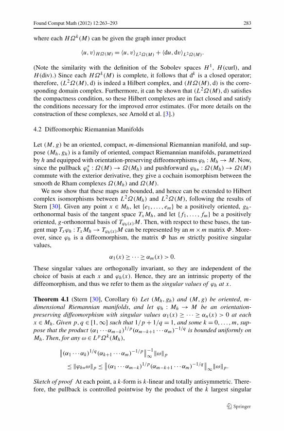
4.2 Diffeomorphic Riemannian Manifolds
Let (M,g) be an oriented, compact, m-dimensional Riemannian manifold, and sup-pose (Mh,gh) is a family of oriented, compact Riemannian manifolds, parametrizedby h and equipped with orientation-preserving diffeomorphisms ϕh : Mh → M . Now,since the pullback ϕ∗
h : Ω(M) → Ω(Mh) and pushforward ϕh∗ : Ω(Mh) → Ω(M)
commute with the exterior derivative, they give a cochain isomorphism between thesmooth de Rham complexes Ω(Mh) and Ω(M).
We now show that these maps are bounded, and hence can be extended to Hilbertcomplex isomorphisms between L2Ω(Mh) and L2Ω(M), following the results ofStern [30]. Given any point x ∈ Mh, let {e1, . . . , em} be a positively oriented, gh-orthonormal basis of the tangent space TxMh, and let {f1, . . . , fm} be a positivelyoriented, g-orthonormal basis of Tϕh(x)M . Then, with respect to these bases, the tan-gent map Txϕh : TxMh → Tϕh(x)M can be represented by an m×m matrix Φ . More-over, since ϕh is a diffeomorphism, the matrix Φ has m strictly positive singularvalues,
α1(x) ≥ · · · ≥ αm(x) > 0.
These singular values are orthogonally invariant, so they are independent of thechoice of basis at each x and ϕh(x). Hence, they are an intrinsic property of thediffeomorphism, and thus we refer to them as the singular values of ϕh at x.
Theorem 4.1 (Stern [30], Corollary 6) Let (Mh,gh) and (M,g) be oriented, m-dimensional Riemannian manifolds, and let ϕh : Mh → M be an orientation-preserving diffeomorphism with singular values α1(x) ≥ · · · ≥ αn(x) > 0 at eachx ∈ Mh. Given p,q ∈ [1,∞] such that 1/p + 1/q = 1, and some k = 0, . . . ,m, sup-pose that the product (α1 · · ·αm−k)
1/p(αm−k+1 · · ·αm)−1/q is bounded uniformly onMh. Then, for any ω ∈ LpΩk(Mh),
∥∥(α1 · · ·αk)1/q(αk+1 · · ·αm)−1/p
∥∥−1∞ ‖ω‖p
≤ ‖ϕh∗ω‖p ≤ ∥∥(α1 · · ·αm−k)1/p(αm−k+1 · · ·αm)−1/q
∥∥∞‖ω‖p.
Sketch of proof At each point, a k-form is k-linear and totally antisymmetric. There-fore, the pullback is controlled pointwise by the product of the k largest singular
284 Found Comput Math (2012) 12:263–293
values of ϕh, while the pushforward is controlled by the product of the k largest sin-gular values of ϕ−1
h (i.e., the reciprocals of the k smallest singular values of ϕh).Thus, we obtain pointwise inequalities
∣∣ϕ∗hη
∣∣ ≤ α1 · · ·αk
(|η| ◦ ϕh
), |ϕh∗ω| ≤ [
(αm−k+1 · · ·αm)−1|ω|] ◦ ϕ−1h .
For the Lp upper bound, we can apply the pushforward inequality to get a factorof (αm−k+1 · · ·αm)−p in the integrand. Using the change of variables theorem in-troduces the Jacobian determinant α1 · · ·αm, so multiplying by this gives a factor ofα1 · · ·αm−k(αm−k+1 · · ·αm)−p+1. We can then use Hölder’s inequality to pull out theL∞-norm of this expression, and raising to the exponent 1/p gives
∥∥(α1 · · ·αm−k)1/p(αm−k+1 · · ·αm)−1+1/p
∥∥∞= ∥∥(α1 · · ·αm−k)
1/p(αm−k+1 · · ·αm)−1/q∥∥∞,
as desired. The lower bound follows in a similar fashion, starting with the identityω = ϕ∗
hϕh∗ω and applying the pointwise pullback inequality. �
Since M and Mh are compact, the uniform boundedness hypothesis of this theo-rem is clearly satisfied. Therefore, taking p = q = 2, it follows that the diffeomor-phism ϕh induces Hilbert complex isomorphisms ϕh∗ : L2Ω(Mh) → L2Ω(M) andϕ∗
h : L2Ω(M) → L2Ω(Mh). An important consequence of this is stated in the fol-lowing corollary, which follows directly from Theorem 3.7 and Theorem 4.1.
Corollary 4.2 Suppose that there exists a family of subcomplexes Wh ⊂ L2Ω(Mh)
admitting uniformly bounded projection morphisms π ′h : L2Ω(Mh) → Wh, and let
ϕh : Mh → M be a family of orientation-preserving diffeomorphisms with singularvalues bounded uniformly in h. Then the maps
ih = ϕh∗|Wh: Wh ↪→ L2Ω(M), πh = π ′
h ◦ ϕ∗h : L2Ω(M) → Wh,
are uniformly bounded Hilbert complex morphisms, satisfying πh ◦ ih = idWh.
Remark 7 In brief, Corollary 4.2 states that orientation-preserving diffeomorphismsinduce an equivalence of families of finite element subcomplexes of the L2-de Rhamcomplex with bounded cochain projections. In particular, any sufficiently regular tri-angulation Th → M gives corresponding P −
r and Pr families (cf. Arnold et al. [2, 3])of piecewise-polynomial differential forms on M .
Note that we are not claiming that every subcomplex of L2Ω(Mh) necessarilyadmits a bounded cochain projection—only that if such a projection exists, then thisinduces an equivalent projection for L2Ω(M). In the case of a triangulation Th, reg-ularity conditions for a “smoothed projection” to exist were obtained in Christiansenand Winther [11].
Finally, let us see how this definition of ih can be used to control the error term‖I − Jh‖. Theorem 4.1 implies that, for any vh ∈ V k
h , we have the estimate
Found Comput Math (2012) 12:263–293 285
∥∥(α1 · · ·αk)1/2(αk+1 · · ·αm)−1/2
∥∥−1∞ ‖vh‖h
≤ ‖ihvh‖ ≤ ∥∥(α1 · · ·αm−k)1/2(αm−k+1 · · ·αm)−1/2
∥∥∞‖vh‖h,
and since Jh = i∗hih, this implies
∥∥α1 · · ·αk(αk+1 · · ·αm)−1∥∥−1
∞ ‖vh‖h
≤ ‖Jhvh‖h ≤ ∥∥α1 · · ·αm−k(αm−k+1 · · ·αm)−1∥∥∞‖vh‖h.
This bounds the spectrum of the self-adjoint operator Jh, so finally we obtain a boundon the error term ‖I − Jh‖ in terms of the singular values,
‖I − Jh‖ ≤ max{∣∣1 − ∥∥α1 · · ·αk(αk+1 · · ·αm)−1
∥∥−1∞
∣∣,∣∣1 − ∥∥α1 · · ·αm−k(αm−k+1 · · ·αm)−1
∥∥∞∣∣}.
(11)
It follows that, if each singular value satisfies |1 − αi | ≤ Chs+1, then ‖I − Jh‖ ≤Chs+1 as well; moreover, this will hold for every k = 0, . . . ,m. Obtaining suchbounds on the singular values, for particular choices of ϕh, will be the topic of thenext subsection.
4.3 Tubular Neighborhoods and Euclidean Hypersurfaces
Suppose that (N,γ ) is an oriented, n-dimensional Riemannian manifold, and letj : M ↪→ N be the inclusion of a submanifold M , endowed with the metric g = j∗γinherited from N . If M is compact, then it is possible to construct a tubular neighbor-hood U around M ; this is diffeomorphic to an open neighborhood of the zero sectionof the normal bundle of M , so there is a normal projection map a : U → M . In partic-ular, there exists some δ0 > 0 such that the set Mδ0 , consisting of points in N whoseRiemannian distance to M is less than δ0, is contained in U . (For details, see, e.g.,Abraham and Marsden [1], Lang [24], Lee [25].) Now, let jh : Mh ↪→ N be a familyof inclusions of m-dimensional submanifolds Mh, parametrized by h, each endowedwith the Riemannian metric gh = j∗
hγ . If Mh lies inside the tubular neighborhood U
and is transverse to a (i.e., Mh corresponds to a section of a), then it is possible todefine the diffeomorphism ϕh = a|Mh
: Mh → M .An important case is when N = R
n, where n = m + 1 and γ is the standard Eu-clidean metric, so that M ⊂ R
n is an oriented Euclidean hypersurface. It is possibleto define a signed distance function δ : U → R on the tubular neighborhood, so that|δ(x)| = dist(x,M) and ∇δ(x) = ν(x) is the outward-facing unit normal to M ata(x). Every point x ∈ U in the tubular neighborhood has a unique decomposition
x = a(x) + δ(x)ν(x),
so the normal projection map a : U → M can be written as
a(x) = x − δ(x)ν(x).
286 Found Comput Math (2012) 12:263–293
Therefore,
∇a = I − ∇δ ⊗ ν − δ∇ν = I − ν ⊗ ν − δ∇ν = P + δS,
where P = I − ν ⊗ ν is the projection map onto T M and S = −∇ν = −∇2δ is theshape operator, or Weingarten map. (Note that Dziuk [17], Demlow and Dziuk [16],Demlow [15] define a Weingarten map H = −S using the opposite sign convention,but this is less common in the differential geometry literature.)
Instead of directly computing the tangent map T a : U → M , we can look atits adjoint, which “lifts” vectors on M to those on U . Given the pullback mapa∗ : Ω1(M) → Ω1(U), the metric can then be used to identify covectors with vec-tors, thereby obtaining a pullback map of vector fields X(M) → X(U). Specifically,let Y ∈ TyM and x ∈ a−1(y) ⊂ U . Then define the lifted vector a∗Y ∈ TxU satisfying
X · a∗Y = T a(X) · Y, ∀X ∈ TxU.
In terms of the Riemannian sharp and flat maps, this can be written as
[a∗(Y )
]� = a∗(Y �) ⇐⇒ a∗Y = [
a∗(Y �)]�
.
The following theorem allows us to compute this lifted vector explicitly, in terms ofthe signed distance function and shape operator.
Theorem 4.3 Let M be an oriented, compact, m-dimensional hypersurface of Rm+1
with a tubular neighborhood U . If Y ∈ TyM and x ∈ a−1(y) ⊂ U , then the liftedvector a∗Y ∈ TxU satisfies
a∗Y = (I + δS)Y.
Proof Extend Y to a constant vector field on Rm+1, so that Y = ∇ψ(y) for the scalar
function ψ(x) = x · Y . Using the definition of the gradient ∇ψ = (dψ)�, and the factthat the exterior derivative d commutes with pullback, we have the following chainof equalities:
a∗Y = a∗(∇ψ) = [a∗(dψ)
]� = [d(a∗ψ
)]� = ∇(ψ ◦ a).
Therefore, applying the chain rule, we get
a∗Y = ∇a(x) · ∇ψ(a(x)
) = (P + δS)Y = (I + δS)Y,
where the last equality follows from PY = Y . �
Finally, when x ∈ Mh, we can restrict to TxMh by composing with the adjoint ofjh, i.e., the projection Ph = I − νh ⊗ νh, which gives
Yh = j∗ha∗Y = Ph(I + δS)Y.
This map j∗ha∗ = Ph(I + δS) is immediately seen to be the adjoint of the restricted
tangent map T ϕh = T (a|Mh) = T (a ◦ jh) = T a ◦Tjh. In the next theorem, we bound
Found Comput Math (2012) 12:263–293 287
the singular values of this map, thereby obtaining an estimate for the error term‖I − Jh‖ in the case of Euclidean hypersurfaces.
Theorem 4.4 Let M be an oriented, compact, m-dimensional hypersurface of Rm+1
with a tubular neighborhood U . If Mh is a hypersurface lying in U and transverse toits fibers, then
‖I − Jh‖ ≤ C(‖δ‖∞ + ‖ν − νh‖2∞
).
Proof To obtain bounds on Yh = Pha∗Y , and hence on the singular values, suppose
without loss of generality that |Y | = 1. By the triangle inequality,
∣∣1 − |Yh|2∣∣ ≤ ∣∣1 − ∣∣a∗Y
∣∣2∣∣ + ∣∣∣∣a∗Y∣∣2 − |Yh|2
∣∣.
For the first term, the eigenvalues of the shape operator are the principal curvaturesκ1(x), . . . , κm(x) for a surface parallel to M at x; as noted in Demlow and Dziuk [16],Demlow [15], these are related to the principal curvatures at a(x) ∈ M by
κi(x) = κi(a(x))
1 + δ(x)κi(a(x)).
It follows that the eigenvalues of δS at x can be estimated by∣∣∣∣
δ(x)κi(a(x))
1 + δ(x)κi(a(x))
∣∣∣∣ =∣∣∣∣1 − 1
1 + δ(x)κi(a(x))
∣∣∣∣ ≤ C∣∣δ(x)
∣∣.
Since a∗Y = (I + δS)Y and |Y | = 1, this immediately implies
∣∣1 − ∣∣a∗Y∣∣2∣∣ ≤ C|δ|.
For the remaining term, observe that since Yh = Pha∗Y ,
|Yh|2 = ∣∣a∗Y − νh
(νh · a∗Y
)∣∣2 = ∣∣a∗Y∣∣2 − (
νh · a∗Y)2
,
and therefore∣∣∣∣a∗Y
∣∣2 − |Yh|2∣∣ = (
νh · a∗Y)2 = (
Pνh · a∗Y)2 ≤ |Pνh|2
∣∣a∗Y∣∣2
.
Now,
|Pνh|2 = ∣∣νh − ν(ν · νh)∣∣2 = 1 − (ν · νh)
2 = (1 + ν · νh)(1 − ν · νh) ≤ 2(1 − ν · νh),
and since 2(1 − ν · νh) = |ν − νh|2, it follows that
∣∣∣∣a∗Y∣∣2 − |Yh|2
∣∣ ≤ |ν − νh|2∣∣a∗Y
∣∣2 ≤ |ν − νh|2(1 + ∣∣1 − ∣∣a∗Y
∣∣2∣∣) ≤ C|ν − νh|2.Putting these together, we have
∣∣1 − |Yh|2∣∣ ≤ C
(|δ| + |ν − νh|2),
288 Found Comput Math (2012) 12:263–293
from which it follows that at each x ∈ Mh, the singular values satisfy
|1 − αi | ≤ C(|δ| + |ν − νh|2
), i = 1, . . . ,m.
Finally, applying (11), we obtain the uniform bound
‖I − Jh‖ ≤ C(‖δ‖∞ + ‖ν − νh‖2∞
),
which completes the proof. �
We now apply this theory to an important class of examples, where Mh corre-sponds to a family of piecewise-linear triangulations (as in Dziuk [17], Demlow andDziuk [16]), or more generally, to the family of approximate surfaces obtained bydegree-s Lagrange interpolation over each element of the triangulation (as in Dem-low [15]), where the piecewise-linear case corresponds to s = 1. Here, the elementsof this triangulation are assumed to be “shape-regular and quasi-uniform of diame-ter h” [15]. Note that Mh is always constructed from an underlying piecewise-lineartriangulation, even in the case of higher-order polynomial interpolation. Thus, byCorollary 4.2, we can define the P −
r and Pr families of finite element differentialforms on Mh, and obtain bounded cochain projections, even when s > 1.
By Demlow [15, Proposition 2.3], for sufficiently small h, the surfaces Mh ob-tained by degree-s Lagrange interpolation satisfy
‖δ‖∞ ≤ Chs+1, ‖ν − νh‖∞ ≤ Chs. (12)
Therefore, we obtain the following corollary to Theorem 4.4.
Corollary 4.5 If Mh is a family of surfaces approximating M , obtained by degree-sLagrange interpolation, then ‖I − Jh‖ ≤ Chs+1 for sufficiently small h.
Proof Applying (12), we have
‖I − Jh‖ ≤ C(‖δ‖∞ + ‖ν − νh‖2∞
) ≤ Chs+1 + Ch2s ≤ Chs+1,
which completes the proof. �
This result generalizes Demlow [15, Proposition 4.1]—which applies only toscalar functions (k = 0) on hypersurfaces of dimension m = 2,3—to hold for ar-bitrary k-forms, k = 0, . . . ,m, on hypersurfaces of any dimension. In particular, thespecial case k = 0, m = 2, s = 1 gives ‖I − Jh‖ ≤ Ch2, which recovers the originalestimate of Dziuk [17] for piecewise-linear triangulation of surfaces in R
3. The cor-respondence between this framework and that of Dziuk and Demlow will be madeexplicit in the following worked example.
Example 4.6 (The Hodge–Laplace operator on a 2-D surface) Let M be a closed,2-dimensional surface, embedded in R
3, and suppose the approximate surface Mh
is obtained from degree-s Lagrange interpolation over a piecewise-linear triangula-tion Th. Assume that Th is contained in a tubular neighborhood of M , that its verticeslie on M , and that its triangles are shape-regular and quasi-uniform of diameter h.
Found Comput Math (2012) 12:263–293 289
Take the continuous Hilbert complex to be the L2-de Rham complex on M , i.e.,W = L2Ω(M) and V = HΩ(M). Since Th is piecewise-linear and simplicial, wecan take the discrete complex to be any of those considered in Arnold [2, 3]. For thisexample, let us take V k
h to be the space of Pr k-forms, and V k−1h to be the space
of Pr+1 (k − 1)-forms. We emphasize that the fact that Th is a surface embeddedin R
3, rather than a flat region in R2, does not introduce any additional complications
as far as the discrete complex is concerned. Indeed, the shape functions are definedwith respect to a 2-dimensional reference triangle, and this reference triangle canbe mapped onto a triangle embedded in R
3 just as easily as one in R2. These shape
functions can, likewise, be lifted up from Th to the curved triangles on the interpolatedsurface Mh. For nodal Lagrange finite elements (k = 0), this observation was made byDziuk [17] in the piecewise-linear case, leading to the development of surface finiteelements, while Demlow [15] later extended this argument to higher-order Lagrangepolynomials. (Similar ideas had also been used in the development of isoparametricfinite elements for Euclidean domains with curved boundaries.)
Now, given some f ∈ L2Ωk(M), we obtain a solution (σ,u,p) to the variationalproblem (3) on M . For the discrete variational problem (5), we can use the tubu-lar neighborhood projection to take fh = a|∗Mh
f , thus obtaining a discrete solution(σh,uh,ph) on Mh. The modified discrete solution (σ ′
h,u′h,p
′h)—which is used only
for the analysis, but is not necessary for computation—also lives on Mh, while itsimage (ihσ
′h, ihu
′h, ihp
′h) lives on M itself.
Therefore, assuming sufficient elliptic regularity, the “improved estimates” ofArnold et al. [2, 3] yield the L2 estimates for the modified problem,
∥∥u − ihu′h
∥∥ + ∥∥p − ihp′h
∥∥ ≤ Chr+1‖f ‖Hr−1,∥∥d
(u − ihu
′h
)∥∥ + ∥∥σ − ihσ′h
∥∥ ≤ Chr‖f ‖Hr−1,
∥∥d(σ − ihσ
′h
)∥∥ ≤ Chr−1‖f ‖Hr−1,
which can be combined into the single estimate∥∥u − ihu
′h
∥∥ + ∥∥p − ihp′h
∥∥ + h(∥∥d
(u − ihu
′h
)∥∥ + ∥∥σ − ihσ′h
∥∥) + h2∥∥d
(σ − ihσ
′h
)∥∥
≤ Chr+1‖f ‖Hr−1 .
Applying Corollary 4.5 to account for the surface approximation error, we obtain thefinal error estimate for the discrete problem,
‖u − ihuh‖ + ‖p − ihph‖ + h(∥∥d(u − ihuh)
∥∥ + ‖σ − ihσh‖) + h2
∥∥d(σ − ihσh)∥∥
≤ C(hr+1‖f ‖Hr−1 + hs+1‖f ‖).
In particular, this implies that choosing isoparametric elements, with r = s, yieldsthe optimal rate of convergence.
The case k = 0 and r = s = 1 corresponds to the lowest-order approximation ofthe Laplace–Beltrami equation, where Mh is piecewise-linear and V 0
h consists ofpiecewise-linear “hat functions” on Mh. In this case, the estimate above becomes
‖u − ihuh‖ + ‖p − ihph‖ + h∥∥∇(u − ihuh)
∥∥ ≤ Ch2‖f ‖,
290 Found Comput Math (2012) 12:263–293
which precisely recovers the estimate of Dziuk [17], Demlow and Dziuk [16]. Moregenerally, taking k = 0 with arbitrary r and s, we have
‖u − ihuh‖ + ‖p − ihph‖ + h∥∥∇(u − ihuh)
∥∥ ≤ C(hr+1‖f ‖Hr−1 + hs+1‖f ‖),
which agrees with Demlow [15].On the other hand, we can also extend these estimates to the cases k = 1, which
corresponds to the mixed formulation of the vector Laplacian, and k = 2, which cor-responds to the mixed formulation of the scalar Laplacian. For k = 1, the estimate forgeneral r and s becomes
‖u − ihuh‖ + ‖p − ihph‖ + h(∥∥∇ × (u − ihuh)
∥∥ + ‖σ − ihσh‖)
+ h2∥∥∇(σ − ihσh)
∥∥
≤ C(hr+1‖f ‖Hr−1 + hs+1‖f ‖),
while for k = 2, we obtain
‖u − ihuh‖ + ‖p − ihph‖ + h‖σ − ihσh‖ + h2∥∥∇ · (σ − ihσh)
∥∥
≤ C(hr+1‖f ‖Hr−1 + hs+1‖f ‖).
4.4 Other Variational Crimes
The variational crimes framework developed in Sect. 3 is quite general, represent-ing a natural extension of the Strang lemmas from Hilbert spaces to Hilbert com-plexes. As such, the standard “crimes” that are typically analyzed in Hilbert spaceswith the Strang lemmas may now be analyzed in the setting of Hilbert complexes.These crimes—including numerical quadrature, approximate coefficients, approxi-mate boundary data, approximate domains, as well as isoparametric and other geo-metric approximations to more complex domain shapes—can all be represented as anapproximate bilinear form Bh, an approximate linear functional Fh, and an approx-imation subspace Vh �⊂ V , as in (2). In addition, techniques such as mass-lumping,which yield a number of benefits, such as discrete maximum principles and more ef-ficient evolution algorithms for parabolic equations, are often analyzed in a similarway, and as such may now be analyzed in Hilbert complexes through the frameworkdeveloped in Sect. 3.
5 Conclusion
We began the article in Sect. 2 with a review of the mathematical concepts that play afundamental role in finite element exterior calculus, as developed in Arnold et al. [3];these included abstract Hilbert complexes and their morphisms, domain complexes,Hodge decomposition, the Poincaré inequality, the Hodge Laplacian, mixed varia-tional problems, and approximation using Hilbert subcomplexes. In Sect. 3, we thenconsidered approximation of a Hilbert complex by a second complex, related to the
Found Comput Math (2012) 12:263–293 291
first complex through an injective morphism rather than through subcomplex inclu-sion. We developed several key results for this pair of complexes and the maps be-tween them, and then derived error estimates for generalized Galerkin-type approxi-mations of solutions to variational problems using the approximating complex; theseestimates can be viewed as generalizing the results of Arnold et al. [3] to “external”approximations. Our main abstract results are thus essentially Strang-type lemmas forapproximating variational problems in Hilbert complexes.
As an application of the new framework developed in Sect. 3, we developed asecond distinct set of results in Sect. 4 for the case of the Hodge–de Rham complexof differential forms on a compact, oriented Riemannian manifold. We first reviewedHodge–de Rham theory, and then considered a pair of Riemannian manifolds relatedby diffeomorphisms. We then established estimates for the maps needed to apply thegeneralized Hilbert complex approximation framework from Sect. 3, subsequentlyspecializing this analysis to the case of a Euclidean hypersurface, with approximat-ing hypersurfaces living in a tubular neighborhood. The surface finite element meth-ods, as analyzed in Dziuk [17], Demlow and Dziuk [16], Demlow [15], fit preciselyinto this class of approximation problems; as such, we illustrated how our resultsrecover the analysis framework and a priori estimates of Dziuk [17], Demlow andDziuk [16], Demlow [15], and also extend their results from scalar functions on 2-and 3-surfaces to general k-forms on arbitrary dimensional hypersurfaces. Our re-sults also generalize those earlier estimates from nodal finite element methods forthe Laplace–Beltrami operator to mixed finite element methods for the Hodge Lapla-cian. By analyzing surface finite element methods using a combination of generaltools from differential geometry and functional analysis, we are led to a more geo-metric analysis of surface finite element methods, whereby the main results becomemore transparent.
Several interesting and challenging problems were not addressed in the currentarticle. One such problem is the extension of the pointwise error estimates of Dem-low [15] for 0-forms to general k-forms; this analysis relies on known results for theGreen’s function of the Laplace–Beltrami operator on the continuous surface (cf. [4]),and analogous results would be needed for general k-forms. A second problem of in-terest is an extension of the Hilbert complex framework to more general Banach com-plexes, as would be needed to handle some nonlinear problems. This leads to a thirdinteresting problem, which would involve the extension of the weak-∗ convergenceand contraction frameworks, used for adaptive finite element methods for linear [9,26] and nonlinear [23] problems, to the setting of finite element exterior calculus, aswell as to the surface finite element setting.
Acknowledgements We are grateful to the editor and anonymous referees for their valuable commentsand suggestions. Their diligence and attention to detail during the review process was truly extraordinary,and the final paper has benefited greatly from their efforts. We also thank Paul Leopardi for catchinga typographical error in one of the equations shortly before this article went to press. Finally, we wish toexpress our appreciation to Douglas Arnold, Snorre Christiansen, Alan Demlow, Richard Falk, and RagnarWinther for reading earlier versions of the manuscript so carefully, and for providing helpful feedback.
M.H. was supported in part by NSF DMS/CM Awards 0715146 and 0915220, NSF MRI Award0821816, NSF PHY/PFC Award 0822283, and by DOD/DTRA Award HDTRA-09-1-0036.
A.S. was supported in part by NSF DMS/CM Award 0715146 and by NSF PHY/PFC Award 0822283,as well as by NIH, HHMI, CTBP, and NBCR.
292 Found Comput Math (2012) 12:263–293
References
1. R. Abraham, J.E. Marsden, Foundations of Mechanics (Benjamin/Cummings, Reading, 1978).2. D.N. Arnold, R.S. Falk, R. Winther, Finite element exterior calculus, homological techniques, and
applications, Acta Numer. 15, 1–155 (2006). doi:10.1017/S0962492906210018.3. D.N. Arnold, R.S. Falk, R. Winther, Finite element exterior calculus: from Hodge theory to nu-
merical stability, Bull., New Ser., Am. Math. Soc. 47(2), 281–354 (2010). doi:10.1090/S0273-0979-10-01278-4.
4. T. Aubin, Nonlinear Analysis on Manifolds. Monge–Ampère Equations, Grundlehren der Mathema-tischen Wissenschaften, vol. 252 (Springer, New York, 1982).
5. D. Boffi, F. Brezzi, L. Gastaldi, On the problem of spurious eigenvalues in the approximationof linear elliptic problems in mixed form, Math. Comput. 69(229), 121–140 (2000). doi:10.1090/S0025-5718-99-01072-8.
6. A. Bossavit, Whitney forms: a class of finite elements for three-dimensional computations in electro-magnetism, IEE Proc. A, Sci. Meas. Technol. 135(8), 493–500 (1988).
7. D. Braess, Finite elements. Theory, Fast Solvers, and Applications in Elasticity Theory, 3rd edn. (Cam-bridge University Press, Cambridge, 2007). Translated from the German by L.L. Schumaker.
8. J. Brüning, M. Lesch, Hilbert complexes, J. Funct. Anal. 108(1), 88–132 (1992). doi:10.1016/0022-1236(92)90147-B.
9. J.M. Cascon, C. Kreuzer, R.H. Nochetto, K.G. Siebert, Quasi-optimal convergence rate for an adaptivefinite element method, SIAM J. Numer. Anal. 46(5), 2524–2550 (2008). doi:10.1137/07069047X.
10. S.H. Christiansen, Résolution des équations intégrales pour la diffraction d’ondes acoustiques et élec-tromagnétiques: Stabilisation d’algorithmes itératifs et aspects de l’analyse numérique. Ph.D. thesis,École Polytechnique, 2002. http://tel.archives-ouvertes.fr/tel-00004520/.
11. S.H. Christiansen, R. Winther, Smoothed projections in finite element exterior calculus, Math. Com-put. 77(262), 813–829 (2008). doi:10.1090/S0025-5718-07-02081-9.
12. K. Deckelnick, G. Dziuk, Convergence of a finite element method for non-parametric mean curvatureflow, Numer. Math. 72(2), 197–222 (1995). doi:10.1007/s002110050166.
13. K. Deckelnick, G. Dziuk, Numerical approximation of mean curvature flow of graphs and level sets,in Mathematical Aspects of Evolving Interfaces, Funchal, 2000, Lecture Notes in Math., vol. 1812,pp. 53–87 (Springer, Berlin, 2003).
14. K. Deckelnick, G. Dziuk, C.M. Elliott, Computation of geometric partial differential equations andmean curvature flow, Acta Numer. 14, 139–232 (2005). doi:10.1017/S0962492904000224.
15. A. Demlow, Higher-order finite element methods and pointwise error estimates for elliptic problemson surfaces, SIAM J. Numer. Anal. 47(2), 805–827 (2009). doi:10.1137/070708135.
16. A. Demlow, G. Dziuk, An adaptive finite element method for the Laplace-Beltrami opera-tor on implicitly defined surfaces, SIAM J. Numer. Anal. 45(1), 421–442 (2007) (electronic).doi:10.1137/050642873.
17. G. Dziuk, Finite elements for the Beltrami operator on arbitrary surfaces, in Partial Differential Equa-tions and Calculus of Variations, Lecture Notes in Math., vol. 1357, pp. 142–155 (Springer, Berlin,1988). doi:10.1007/BFb0082865.
18. G. Dziuk, An algorithm for evolutionary surfaces, Numer. Math. 58(6), 603–611 (1991).doi:10.1007/BF01385643.
19. G. Dziuk, C.M. Elliott, Finite elements on evolving surfaces, IMA J. Numer. Anal. 27(2), 262–292(2007). doi:10.1093/imanum/drl023.
20. G. Dziuk, J.E. Hutchinson, Finite element approximations to surfaces of prescribed variable meancurvature, Numer. Math. 102(4), 611–648 (2006). doi:10.1007/s00211-005-0649-7.
21. P.W. Gross, P.R. Kotiuga, Electromagnetic Theory and Computation: A Topological Approach. Math-ematical Sciences Research Institute Publications, vol. 48 (Cambridge University Press, Cambridge,2004).
22. M. Holst, Adaptive numerical treatment of elliptic systems on manifolds, Adv. Comput. Math. 15(1–4), 139–191 (2001). doi:10.1023/A:1014246117321.
23. M. Holst, G. Tsogtgerel, Y. Zhu, Local convergence of adaptive methods for nonlinear partial differ-ential equations. arXiv:1001.1382 [math.NA] (2010)
24. S. Lang, Introduction to Differentiable Manifolds, 2nd edn. Universitext (Springer, New York, 2002).25. J.M. Lee, Riemannian Manifolds. Graduate Texts in Mathematics, vol. 176 (Springer, New York,
1997).26. P. Morin, K.G. Siebert, A. Veeser, A basic convergence result for conforming adaptive finite elements,
Math. Models Methods Appl. Sci. 18(5), 707–737 (2008). doi:10.1142/S0218202508002838.
Found Comput Math (2012) 12:263–293 293
27. J.C. Nédélec, Curved finite element methods for the solution of singular integral equations on surfacesin R
3, Comput. Methods Appl. Mech. Eng. 8(1), 61–80 (1976).28. J.C. Nédélec, Mixed finite elements in R
3, Numer. Math. 35(3), 315–341 (1980). doi:10.1007/BF01396415.
29. J.C. Nédélec, A new family of mixed finite elements in R3, Numer. Math. 50(1), 57–81 (1986).
doi:10.1007/BF01389668.30. A. Stern, Lp change of variables inequalities on manifolds. Math. Inequal. Appl. (2012, in press).
arXiv:1004.0401 [math.DG].


![Projected Dynamical Systems, Evolutionary Variational ... · solutions to projected dynamical equations in Hilbert spaces (see [6] and [7]). For completeness and deflniteness, we](https://img.pdfslide.net/doc/110x75/60294d1aac77a707331df60d/projected-dynamical-systems-evolutionary-variational-solutions-to-projected.jpg)