Embed Size (px)
Citation preview
Geometry and Billiards
Serge Tabachnikov
Department of Mathematics, Penn State, University
Park, PA 16802

1991 Mathematics Subject Classification. Primary 37-02, 51-02;
Secondary 49-02, 70-02, 78-02
Contents
Foreword: MASS and REU at Penn State University vii
Preface ix
Chapter 1. Motivation: Mechanics and Optics 1
Chapter 2. Billiard in the Circle and the Square 21
Chapter 3. Billiard Ball Map and Integral Geometry 33
Chapter 4. Billiards inside Conics and Quadrics 51
Chapter 5. Existence and Non-existence of Caustics 73
Chapter 6. Periodic Trajectories 99
Chapter 7. Billiards in Polygons 113
Chapter 8. Chaotic Billiards 135
Chapter 9. Dual Billiards 147
Bibliography 167
v

Foreword: MASS andREU at Penn StateUniversity
This book starts the new collection published jointly by the American
Mathematical Society and the MASS (Mathematics Advanced Study
Semesters) program as a part of the Student Mathematical Library
series. The books in the collection will be based on lecture notes for
advanced undergraduate topics courses taught at the MASS and/or
Penn State summer REU (Research Experience for Undergraduates).
Each book will present a self-contained exposition of a non-standard
mathematical topic, often related to current research areas, accessible
to undergraduate students familiar with an equivalent of two years
of standard college mathematics and suitable as a text for an upper
division undergraduate course.
Started in 1996, MASS is a semester-long program for advanced
undergraduate students from across the USA. The program’s curricu-
lum amounts to 16 credit hours. It includes three core courses from
the general areas of algebra/number theory, geometry/topology and
analysis/dynamical systems, custom designed every year; an interdis-
ciplinary seminar; and a special colloquium. In addition, every par-
ticipant completes three research projects, one for each core course.
The participants are fully immersed in mathematics, and this, as well
vii
viii Foreword: MASS and REU at Penn State University
as intensive interaction among the students, usually leads to a dra-
matic increase in their mathematical enthusiasm and achievement.
The program is unique for its kind in the United States.
The summer mathematical REU program is formally independent
of MASS, but there is a significant interaction between the two: about
half of the REU participants stay for the MASS semester in the fall.
This makes it possible to offer research projects that require more
than 7 weeks (the length of an REU program) for completion. The
summer program includes the MASS Fest, a 2–3 day conference at
the end of the REU at which the participants present their research
and that also serves as a MASS alumni reunion. A non-standard
feature of the Penn State REU is that, along with research projects,
the participants are taught one or two intense topics courses.
Detailed information about the MASS and REU programs at
Penn State can be found on the website www.math.psu.edu/mass.
Preface
Mathematical billiards describe the motion of a mass point in a do-
main with elastic reflections from the boundary. Billiards is not a
single mathematical theory; to quote from [57], it is rather a math-
ematician’s playground where various methods and approaches are
tested and honed. Billiards is indeed a very popular subject: in Jan-
uary of 2005, MathSciNet gave more than 1,400 entries for “billiards”
anywhere in the database. The number of physical papers devoted to
billiards could easily be equally substantial.
Usually billiards are studied in the framework of the theory of
dynamical systems. This book emphasizes connections to geometry
and to physics, and billiards are treated here in their relation with
geometrical optics. In particular, the book contains about 100 figures.
There are a number of surveys devoted to mathematical billiards,
from popular to technically involved: [41, 43, 46, 57, 62, 65, 107].
My interest in mathematical billiards started when, as a fresh-
man, I was reading [102], whose first Russian edition (1973) contained
eight pages devoted to billiards. I hope the present book will attract
undergraduate and graduate students to this beautiful and rich sub-
ject; at least, I tried to write a book that I would enjoy reading as an
undergraduate.
This book can serve as a basis for an advanced undergraduate or
a graduate topics course. There is more material here than can be
ix
x Preface
realistically covered in one semester, so the instructor who wishes to
use the book will have enough flexibility. The book stemmed from
an intense1 summer REU (Research Experience for Undergraduates)
course I taught at Penn State in 2004. Some material was also used
in the MASS (Mathematics Advanced Study Semesters) Seminar at
Penn State in 2000–2004 and at the Canada/USA Binational Math-
ematical Camp Program in 2001. In the fall semester of 2005, this
material will be used again for a MASS course in geometry.
A few words about the pedagogical philosophy of this book. Even
the reader without a solid mathematical basis of real analysis, differ-
ential geometry, topology, etc., will benefit from the book (it goes
without saying, such knowledge would be helpful). Concepts from
these fields are freely used when needed, and the reader should ex-
tensively rely on his mathematical common sense.
For example, the reader who does not feel comfortable with the
notion of a smooth manifold should substitute a smooth surface in
space, the one who is not familiar with the general definition of a
differential form should use the one from the first course of calcu-
lus (“an expression of the form...”), and the reader who does not
yet know Fourier series should consider trigonometric polynomials
instead. Thus what I have in mind is the learning pattern of a begin-
ner attending an advanced research seminar: one takes a rapid route
to the frontier of current research, deferring a more systematic and
“linear” study of the foundations until later.
A specific feature of this book is a substantial number of digres-
sions; they have their own titles and their ends are marked by ♣.
Many of the digressions concern topics that even an advanced un-
dergraduate student is not likely to encounter but, I believe, a well
educated mathematician should be familiar with. Some of these top-
ics used to be part of the standard curriculum (for example, evolutes
and involutes, or configuration theorems of projective geometry), oth-
ers are scattered in textbooks (such as distribution of first digits in
various sequences, or a mathematical theory of rainbows, or the 4-
vertex theorem), still others belong to advanced topics courses (Morse
theory, or Poincare recurrence theorem, or symplectic reduction) or
1Six weeks, six hours a week.
Preface xi
simply do not fit into any standard course and “fall between cracks
in the floor” (for example, Hilbert’s 4-th problem).
In some cases, more than one proof to get the same result is
offered; I believe in the maxim that it is more instructive to give dif-
ferent proofs to the same result than the same proof to get different
results. Much attention is paid to examples: the best way to un-
derstand a general concept is to study, in detail, the first non-trivial
example.
I am grateful to the colleagues and to the students whom I dis-
cussed billiards with and learned from; they are too numerous to be
mentioned here by name. It is a pleasure to acknowledge the support
of the National Science Foundation.
Serge Tabachnikov

Chapter 1
Motivation: Mechanicsand Optics
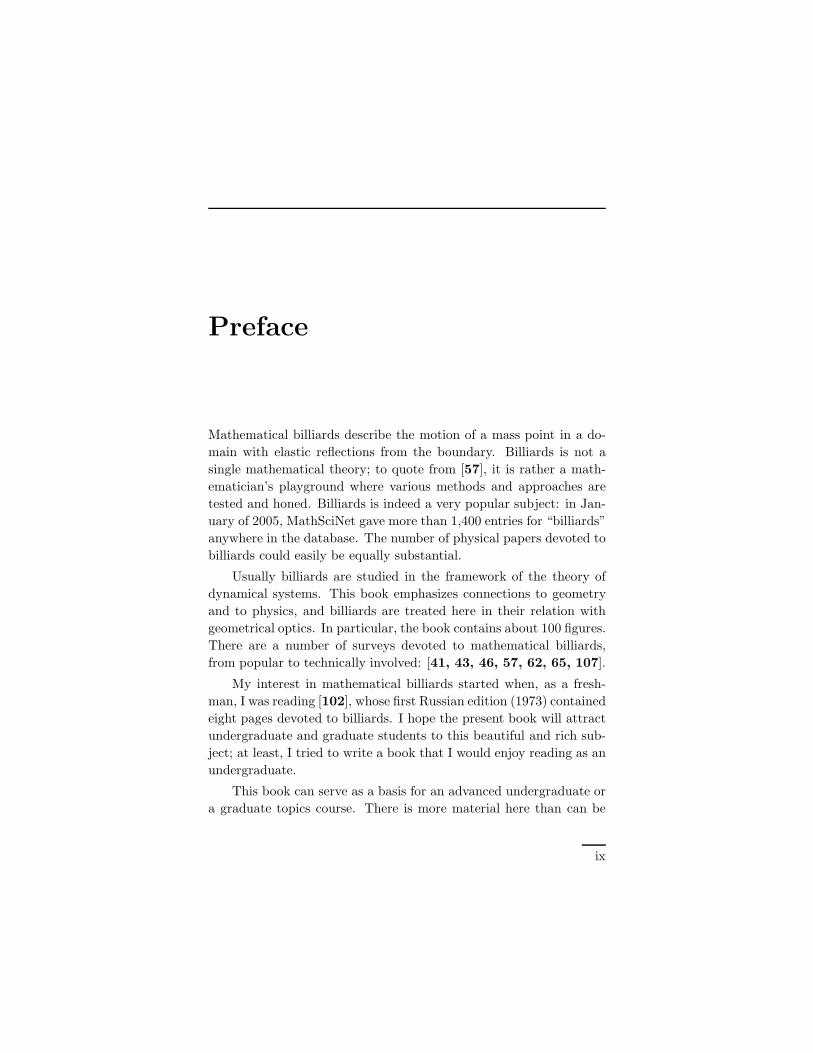
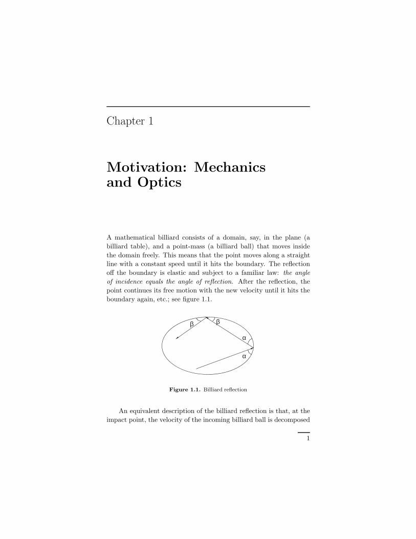
A mathematical billiard consists of a domain, say, in the plane (a
billiard table), and a point-mass (a billiard ball) that moves inside
the domain freely. This means that the point moves along a straight
line with a constant speed until it hits the boundary. The reflection
off the boundary is elastic and subject to a familiar law: the angle
of incidence equals the angle of reflection. After the reflection, the
point continues its free motion with the new velocity until it hits the
boundary again, etc.; see figure 1.1.
α
α
β β
Figure 1.1. Billiard reflection
An equivalent description of the billiard reflection is that, at the
impact point, the velocity of the incoming billiard ball is decomposed
1
2 1. Motivation: Mechanics and Optics
into the normal and tangential components. Upon reflection, the
normal component instantaneously changes sign, while the tangential
one remains the same. In particular, the speed of the point does not
change, and one may assume that the point always moves with the
unit speed.
This description of the billiard reflection applies to domains in
multi-dimensional space and, more generally, to other geometries, not
only to the Euclidean one. Of course, we assume that the reflection
occurs at a smooth point of the boundary. For example, if the billiard
ball hits a corner of the billiard table, the reflection is not defined and
the motion of the ball terminates right there.
There are many questions one asks about the billiard system;
many of them will be discussed in detail in these notes. As a sample,
let D be a plane billiard table with a smooth boundary. We are
interested in 2-periodic, back and forth, billiard trajectories inside D.
In other words, a 2-periodic billiard orbit is a segment inscribed in
D which is perpendicular to the boundary at both end points. The
following exercise is rather hard; the reader will have to wait until
Chapter 6 for a relevant discussion.
Exercise 1.1. a) Does there exist a domain D without a 2-periodic
billiard trajectory?
b) Assume that D is also convex. Show that there exist at least two
distinct 2-periodic billiard orbits in D.
c) LetD be a convex domain with smooth boundary in three-dimensional
space. Find the least number of 2-periodic billiard orbits in D.
d) A disc D in the plane contains a one parameter family of 2-periodic
billiard trajectories making a complete turn inside D (these trajec-
tories are the diameters of D). Are there other plane convex billiard
tables with this property?
In this chapter, we discuss two motivations for the study of math-
ematical billiards: from classical mechanics of elastic particles and
from geometrical optics.
Example 1.2. Consider the mechanical system consisting of two
point-masses m1 and m2 on the positive half-line x ≥ 0. The collision
1. Motivation: Mechanics and Optics 3
between the points is elastic; that is, the energy and momentum are
conserved. The reflection off the left end point of the half-line is also
elastic: if a point hits the “wall” x = 0, its velocity changes sign.
Let x1 and x2 be the coordinates of the points. Then the state of
the system is described by a point in the plane (x1, x2) satisfying the
inequalities 0 ≤ x1 ≤ x2. Thus the configuration space of the system
is a plane wedge with the angle π/4.
Let v1 and v2 be the speeds of the points. As long as the points
do not collide, the phase point (x1, x2) moves with constant speed
(v1, v2). Consider the instance of collision, and let u1, u2 be the speeds
after the collision. The conservation of momentum and energy reads
as follows:
(1.1) m1u1 +m2u2 = m1v1 +m2v2,m1u
21
2+m2u
22
2=m1v
21
2+m2v
22
2.
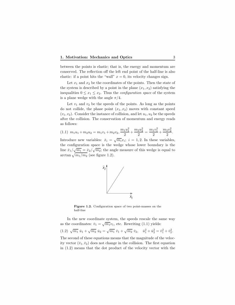
Introduce new variables: xi =√mixi; i = 1, 2. In these variables,
the configuration space is the wedge whose lower boundary is the
line x1/√m1 = x2/
√m2; the angle measure of this wedge is equal to
arctan√m1/m2 (see figure 1.2).
x_
1
x_
2
Figure 1.2. Configuration space of two point-masses on the
half-line
In the new coordinate system, the speeds rescale the same way
as the coordinates: v1 =√m1v1, etc. Rewriting (1.1) yields:
(1.2)√m1 u1 +
√m2 u2 =
√m1 v1 +
√m2 v2, u2
1 + u22 = v2
1 + v22 .
The second of these equations means that the magnitude of the veloc-
ity vector (v1, v2) does not change in the collision. The first equation
in (1.2) means that the dot product of the velocity vector with the
4 1. Motivation: Mechanics and Optics
vector (√m1,
√m2) is preserved as well. The latter vector is tan-
gent to the boundary line of the configuration space: x1/√m1 =
x2/√m2. Hence the tangential component of the velocity vector does
not change, and the configuration trajectory reflects in this line ac-
cording to the billiard law.
Likewise one considers a collision of the left point with the wall
x = 0; such a collision corresponds to the billiard reflection in the
vertical boundary component of the configuration space. We conclude
that the system of two elastic point-massesm1 andm2 on the half-line
is isomorphic to the billiard in the angle arctan√m1/m2.
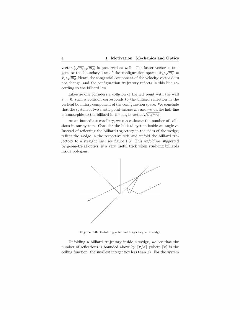
As an immediate corollary, we can estimate the number of colli-
sions in our system. Consider the billiard system inside an angle α.
Instead of reflecting the billiard trajectory in the sides of the wedge,
reflect the wedge in the respective side and unfold the billiard tra-
jectory to a straight line; see figure 1.3. This unfolding, suggested
by geometrical optics, is a very useful trick when studying billiards
inside polygons.
Figure 1.3. Unfolding a billiard trajectory in a wedge
Unfolding a billiard trajectory inside a wedge, we see that the
number of reflections is bounded above by ⌈π/α⌉ (where ⌈x⌉ is the
ceiling function, the smallest integer not less than x). For the system
1. Motivation: Mechanics and Optics 5
of two point-masses on the half-line, the upper bound for the number
of collisions is
(1.3)
⌈π
arctan√m1/m2
⌉.
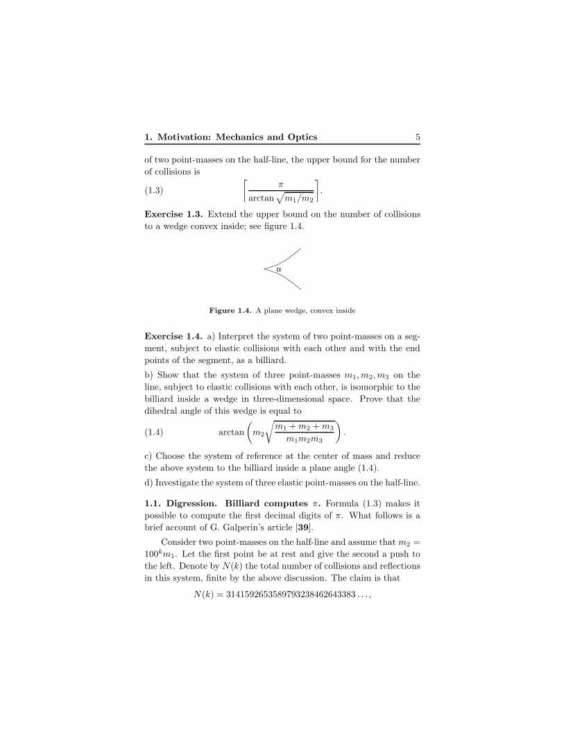
Exercise 1.3. Extend the upper bound on the number of collisions
to a wedge convex inside; see figure 1.4.
α
Figure 1.4. A plane wedge, convex inside
Exercise 1.4. a) Interpret the system of two point-masses on a seg-
ment, subject to elastic collisions with each other and with the end
points of the segment, as a billiard.
b) Show that the system of three point-masses m1,m2,m3 on the
line, subject to elastic collisions with each other, is isomorphic to the
billiard inside a wedge in three-dimensional space. Prove that the
dihedral angle of this wedge is equal to
(1.4) arctan
(m2
√m1 +m2 +m3
m1m2m3
).
c) Choose the system of reference at the center of mass and reduce
the above system to the billiard inside a plane angle (1.4).
d) Investigate the system of three elastic point-masses on the half-line.
1.1. Digression. Billiard computes π. Formula (1.3) makes it
possible to compute the first decimal digits of π. What follows is a
brief account of G. Galperin’s article [39].
Consider two point-masses on the half-line and assume that m2 =
100km1. Let the first point be at rest and give the second a push to
the left. Denote by N(k) the total number of collisions and reflections
in this system, finite by the above discussion. The claim is that
N(k) = 3141592653589793238462643383 . . . ,
6 1. Motivation: Mechanics and Optics
the number made of the first k + 1 digits of π. Let us explain why
this claim almost certainly holds.
With the chosen initial data (the first point at rest), the config-
uration trajectory enters the wedge in the direction, parallel to the
vertical side. In this case, the number of reflections is given by a
modification of formula (1.3), namely
N(k) =
⌈π
arctan (10−k)
⌉− 1.
This fact is established by the same unfolding method.
For now, denote 10−k by x. This x is a very small number, and
one expects arctanx to be very close to x. More precisely,
(1.5) 0 <
(1
arctanx− 1
x
)< x for x > 0.
Exercise 1.5. Prove (1.5) using the Taylor expansion for arctanx.
The first k digits of the number⌈π
x
⌉− 1 = ⌈10kπ⌉ − 1 = ⌊10kπ⌋
coincide with the first k+ 1 decimal digits of π. The second equality
follows from the fact that 10kπ is not an integer; ⌊y⌋ is the floor
function, the greatest integer not greater than y.
We will be done if we show that
(1.6)
⌈π
x
⌉=
⌈π
arctanx
⌉.
By (1.5),
(1.7)
⌈π
x
⌉≤⌈
π
arctanx
⌉≤⌈π
x+ πx
⌉.
The number πx = 0.0 . . . 031415 . . . has k − 1 zeros after the decimal
dot. Therefore the left- and the right-hand sides in (1.7) can differ
only if there is a string of k−1 nines following the first k+1 digits in
the decimal expansion of π. We do not know whether such a string
ever occurs, but this is extremely unlikely for large values of k. If
one does not have such a string, then both inequalities in (1.7) are
equalities, (1.6) holds, and the claim follows. ♣
1. Motivation: Mechanics and Optics 7
Let us proceed with examples of mechanical systems leading to
billiards. Example 1.2 is quite old, and I do not know where it was
considered for the first time. The next example, although similar to
the previous one, is surprisingly recent; see [45, 29].
Example 1.6. Consider three elastic point-massesm1,m2,m3 on the
circle. We expect this mechanical system also to be isomorphic to a
billiard.
Let x1, x2, x3 be the angular coordinates of the points. Consider-
ing S1 as R/2πZ, lift the coordinates to real numbers and denote the
lifted coordinates by the same letters with bar (this lift is not unique:
one may change each coordinate by a multiple of 2π). Rescale the
coordinates as in Example 1.2. Collisions between pairs of points
correspond to three families of parallel planes in three-dimensional
space:
x1√m1
=x2√m2
+ 2πk,x2√m2
=x3√m3
+ 2πm,x3√m3
=x1√m1
+ 2πn
where k,m, n ∈ Z.
All the planes involved are orthogonal to the plane
(1.8)√m1x1 +
√m2x2 +
√m3x3 = const,
and they partition this plane into congruent triangles. The planes
partition space into congruent infinite triangular prisms, and the sys-
tem of three point-masses on the circle is isomorphic to the billiard
inside such a prism. The dihedral angles of the prisms were already
computed in Exercise 1.4 b).
Arguing as in Exercise 1.4 c), one may reduce one degree of free-
dom. Namely, the center of mass of the system has the angular speed
m1v1 +m2v2 +m3v3m1 +m2 +m3
.
One may choose the system of reference at this center of mass which,
in the new coordinates, means that
√m1v1 +
√m2v2 +
√m3v3 = 0,
8 1. Motivation: Mechanics and Optics
and therefore equation (1.8) holds. In other words, our system reduces
to the billiard inside an acute triangle with the angles
arctan
(mi
√m1 +m2 +m3
m1m2m3
), i = 1, 2, 3.
Remark 1.7. Exercise 1.4 and Example 1.6 provide mechanical sys-
tems, isomorphic to the billiards inside a right or an acute triangle.
It would be interesting to find a similar interpretation for an obtuse
triangle.
Exercise 1.8. This problem was communicated by S. Wagon. Sup-
pose 100 identical elastic point-masses are located somewhere on a
one-meter interval and each has a certain speed, not less than 1 m/s,
either to the left or the right. When a point reaches either end of
the interval, it falls off and disappears. What is the longest possible
waiting time until all points are gone?
In dimensions higher than 1, it does not make sense to consider
point-masses: with probability 1, they will never collide. Instead one
considers the system of hard balls in a vessel; the balls collide with
the walls and with each other elastically. Such a system is of great
interest in statistical mechanics: it serves a model of ideal gas.
In the next example, we will consider one particular system of
this type. Let us first describe collision between two elastic balls.
Let two balls have masses m1,m2 and velocities v1, v2 (we do not
specify the dimension of the ambient space). Consider the instance
of collision. The velocities are decomposed into the radial and the
tangential components:
vi = vri + vt
i , i = 1, 2,
the former having the direction of the axis connecting the centers of
the balls, and the latter perpendicular to this axis. In collision, the
tangential components remain the same, and the radial components
change as if the balls were colliding point-masses in the line, that is,
as in (1.1).
Exercise 1.9. Consider a non-central collision of two identical elastic
balls. Prove that if one ball was at rest, then after the collision the
balls will move in orthogonal directions.
1. Motivation: Mechanics and Optics 9
Example 1.10. Consider the system of two identical elastic discs
of radius r on the “unit” torus R2/Z2. The position of a disc is
characterized by its center, a point on the torus. If x1 and x2 are the
positions of the two centers, then the distance between x1 and x2 is
not less than 2r. The set of such pairs (x1, x2) is the configuration
space of our system. Each xi can be lifted to R2; such a lift is defined
up to addition of an integer vector. However, the velocity vi is a well
defined vector in R2.
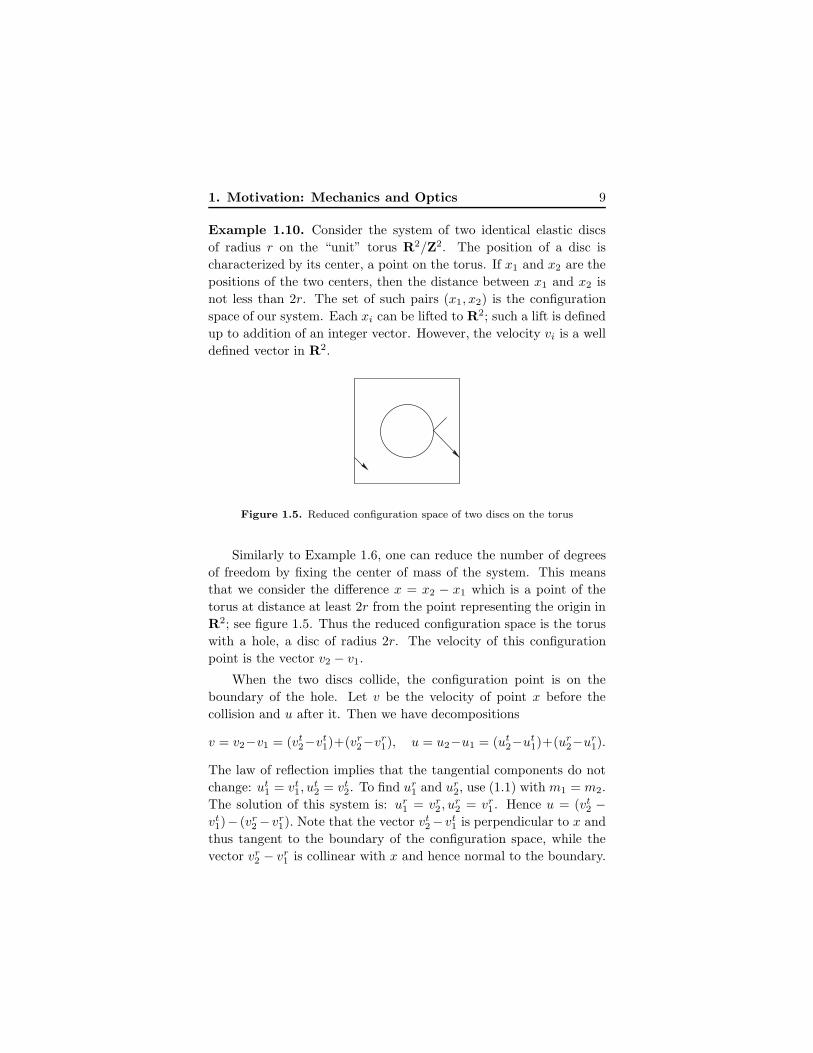
Figure 1.5. Reduced configuration space of two discs on the torus
Similarly to Example 1.6, one can reduce the number of degrees
of freedom by fixing the center of mass of the system. This means
that we consider the difference x = x2 − x1 which is a point of the
torus at distance at least 2r from the point representing the origin in
R2; see figure 1.5. Thus the reduced configuration space is the torus
with a hole, a disc of radius 2r. The velocity of this configuration
point is the vector v2 − v1.
When the two discs collide, the configuration point is on the
boundary of the hole. Let v be the velocity of point x before the
collision and u after it. Then we have decompositions
v = v2−v1 = (vt2−vt
1)+(vr2−vr
1), u = u2−u1 = (ut2−ut
1)+(ur2−ur
1).
The law of reflection implies that the tangential components do not
change: ut1 = vt
1, ut2 = vt
2. To find ur1 and ur
2, use (1.1) with m1 = m2.
The solution of this system is: ur1 = vr
2 , ur2 = vr
1 . Hence u = (vt2 −
vt1)− (vr
2 − vr1). Note that the vector vt
2− vt1 is perpendicular to x and
thus tangent to the boundary of the configuration space, while the
vector vr2 − vr
1 is collinear with x and hence normal to the boundary.
10 1. Motivation: Mechanics and Optics
Therefore the vector u is obtained from v by the billiard reflection off
the boundary.
We conclude that the (reduced) system of two identical elastic
discs on the torus is isomorphic to the billiard on the torus with a
disc removed. This billiard system is known as the Sinai billiard, [100,
101]. This was the first example of a billiard system that exhibits a
chaotic behavior; we will talk about such billiards in Chapter 8.
Examples 1.2, 1.6 and 1.10 confirm a general principle: a con-
servative mechanical system with elastic collisions is isomorphic to a
certain billiard.
1.2. Digression. Configuration spaces. Introduction of configu-
ration space is a conceptually important and non-trivial step in the
study of complex systems. The following instructive example is com-
mon in the Russian mathematical folklore; it is due to N. Konstanti-
nov (cf. [4]).
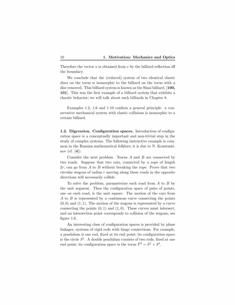
Consider the next problem. Towns A and B are connected by
two roads. Suppose that two cars, connected by a rope of length
2r, can go from A to B without breaking the rope. Prove that two
circular wagons of radius r moving along these roads in the opposite
directions will necessarily collide.
To solve the problem, parameterize each road from A to B by
the unit segment. Then the configuration space of pairs of points,
one on each road, is the unit square. The motion of the cars from
A to B is represented by a continuous curve connecting the points
(0, 0) and (1, 1). The motion of the wagons is represented by a curve
connecting the points (0, 1) and (1, 0). These curves must intersect,
and an intersection point corresponds to collision of the wagons; see
figure 1.6.
An interesting class of configuration spaces is provided by plane
linkages, systems of rigid rods with hinge connections. For example,
a pendulum is one rod, fixed at its end point; its configuration space
is the circle S1. A double pendulum consists of two rods, fixed at one
end point; its configuration space is the torus T 2 = S1 × S1.
1. Motivation: Mechanics and Optics 11
cars
wagons
AB
Figure 1.6. The two roads problem
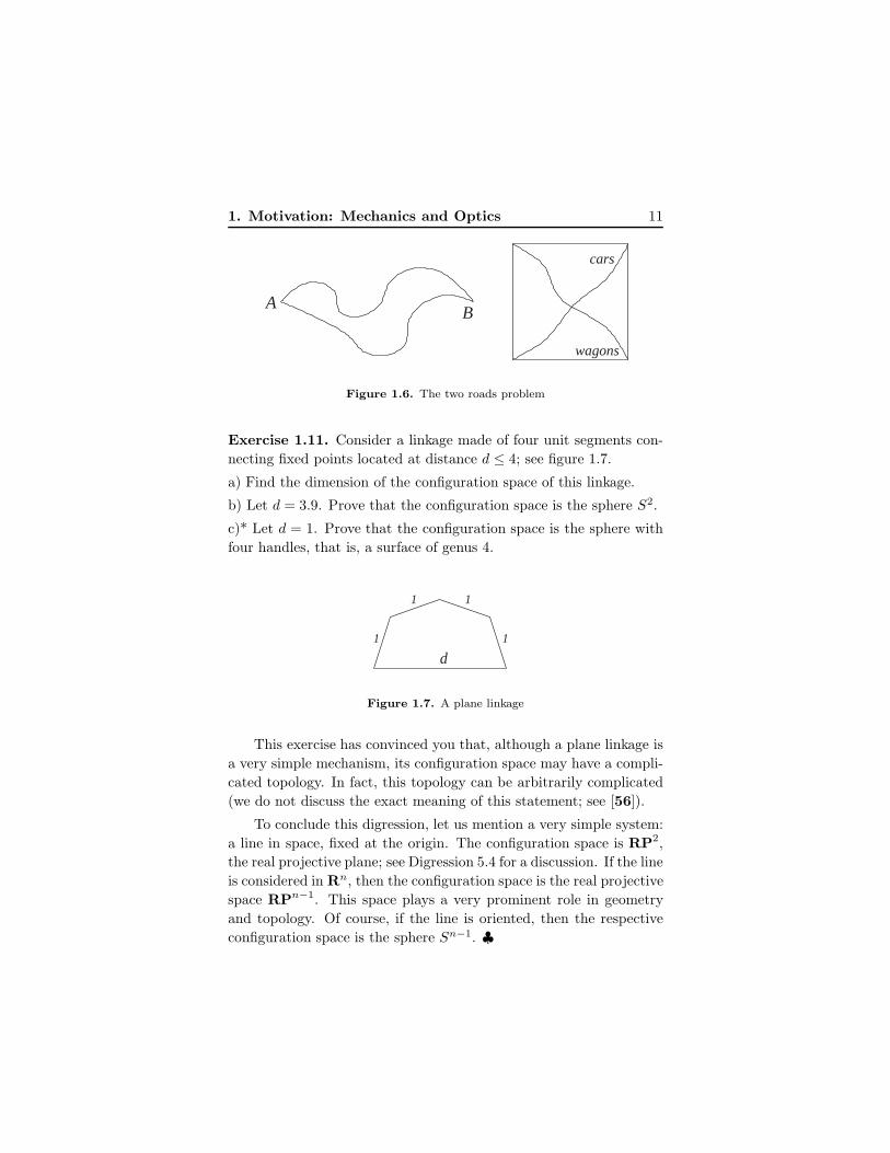
Exercise 1.11. Consider a linkage made of four unit segments con-
necting fixed points located at distance d ≤ 4; see figure 1.7.
a) Find the dimension of the configuration space of this linkage.
b) Let d = 3.9. Prove that the configuration space is the sphere S2.
c)* Let d = 1. Prove that the configuration space is the sphere with
four handles, that is, a surface of genus 4.
1
1 1
1
d
Figure 1.7. A plane linkage
This exercise has convinced you that, although a plane linkage is
a very simple mechanism, its configuration space may have a compli-
cated topology. In fact, this topology can be arbitrarily complicated
(we do not discuss the exact meaning of this statement; see [56]).
To conclude this digression, let us mention a very simple system:
a line in space, fixed at the origin. The configuration space is RP2,
the real projective plane; see Digression 5.4 for a discussion. If the line
is considered in Rn, then the configuration space is the real projective
space RPn−1. This space plays a very prominent role in geometry
and topology. Of course, if the line is oriented, then the respective
configuration space is the sphere Sn−1. ♣
12 1. Motivation: Mechanics and Optics
Now let us briefly discuss another source of motivation for the
study of billiards, geometrical optics. According to the Fermat prin-
ciple, light propagates from point A to point B in the least possible
time. In a homogeneous and isotropic medium, that is, in Euclidean
geometry, this means that light “chooses” the straight line AB.
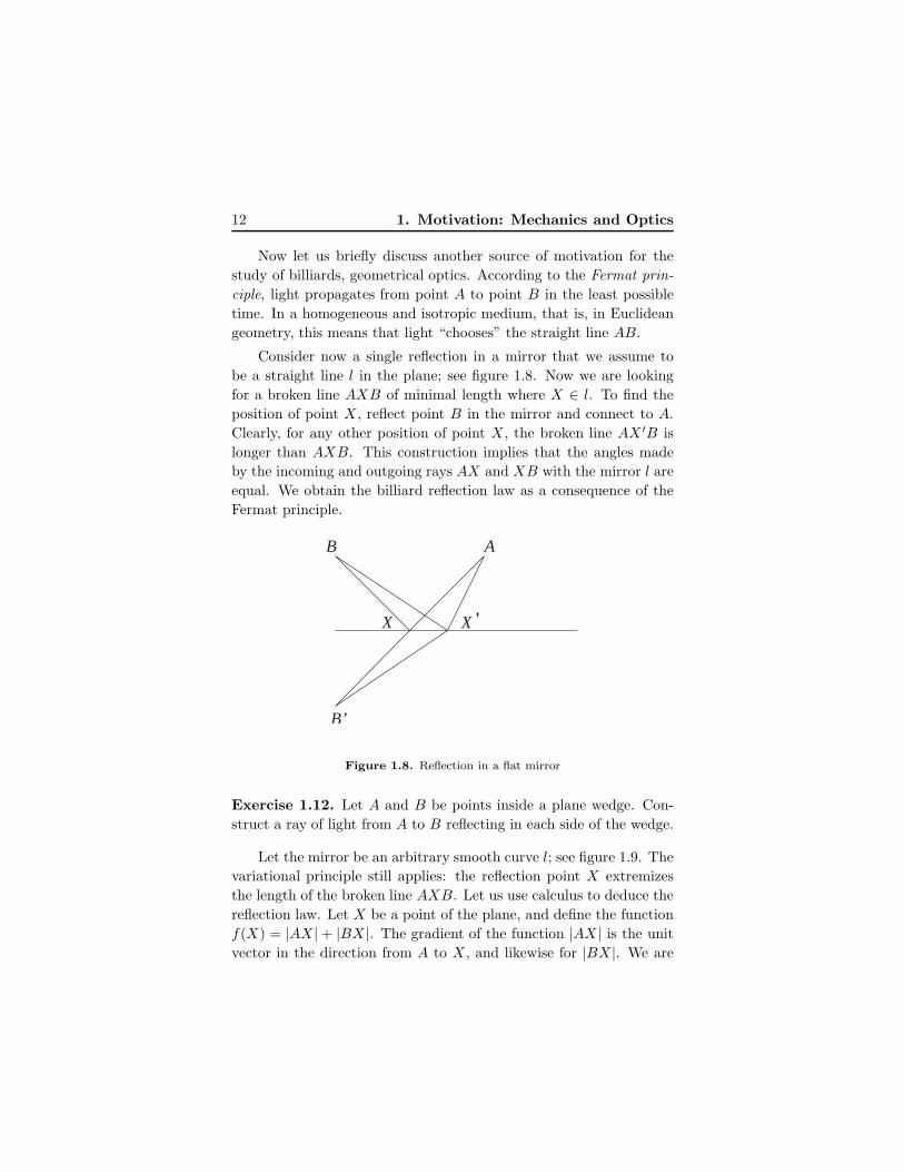
Consider now a single reflection in a mirror that we assume to
be a straight line l in the plane; see figure 1.8. Now we are looking
for a broken line AXB of minimal length where X ∈ l. To find the
position of point X , reflect point B in the mirror and connect to A.
Clearly, for any other position of point X , the broken line AX ′B is
longer than AXB. This construction implies that the angles made
by the incoming and outgoing rays AX and XB with the mirror l are
equal. We obtain the billiard reflection law as a consequence of the
Fermat principle.
AB
B’
X X '
Figure 1.8. Reflection in a flat mirror
Exercise 1.12. Let A and B be points inside a plane wedge. Con-
struct a ray of light from A to B reflecting in each side of the wedge.
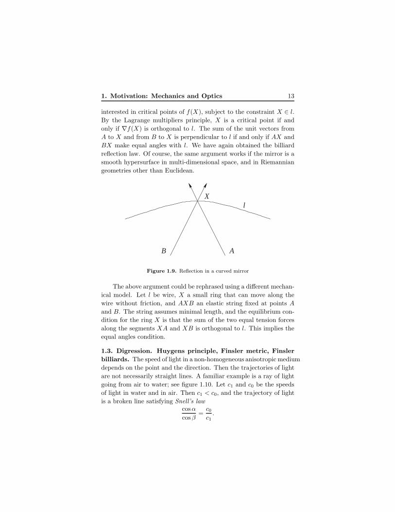
Let the mirror be an arbitrary smooth curve l; see figure 1.9. The
variational principle still applies: the reflection point X extremizes
the length of the broken line AXB. Let us use calculus to deduce the
reflection law. Let X be a point of the plane, and define the function
f(X) = |AX | + |BX |. The gradient of the function |AX | is the unit
vector in the direction from A to X , and likewise for |BX |. We are
1. Motivation: Mechanics and Optics 13
interested in critical points of f(X), subject to the constraint X ∈ l.
By the Lagrange multipliers principle, X is a critical point if and
only if ∇f(X) is orthogonal to l. The sum of the unit vectors from
A to X and from B to X is perpendicular to l if and only if AX and
BX make equal angles with l. We have again obtained the billiard
reflection law. Of course, the same argument works if the mirror is a
smooth hypersurface in multi-dimensional space, and in Riemannian
geometries other than Euclidean.
l
AB
X
Figure 1.9. Reflection in a curved mirror
The above argument could be rephrased using a different mechan-
ical model. Let l be wire, X a small ring that can move along the
wire without friction, and AXB an elastic string fixed at points A
and B. The string assumes minimal length, and the equilibrium con-
dition for the ring X is that the sum of the two equal tension forces
along the segments XA and XB is orthogonal to l. This implies the
equal angles condition.
1.3. Digression. Huygens principle, Finsler metric, Finsler
billiards. The speed of light in a non-homogeneous anisotropic medium
depends on the point and the direction. Then the trajectories of light
are not necessarily straight lines. A familiar example is a ray of light
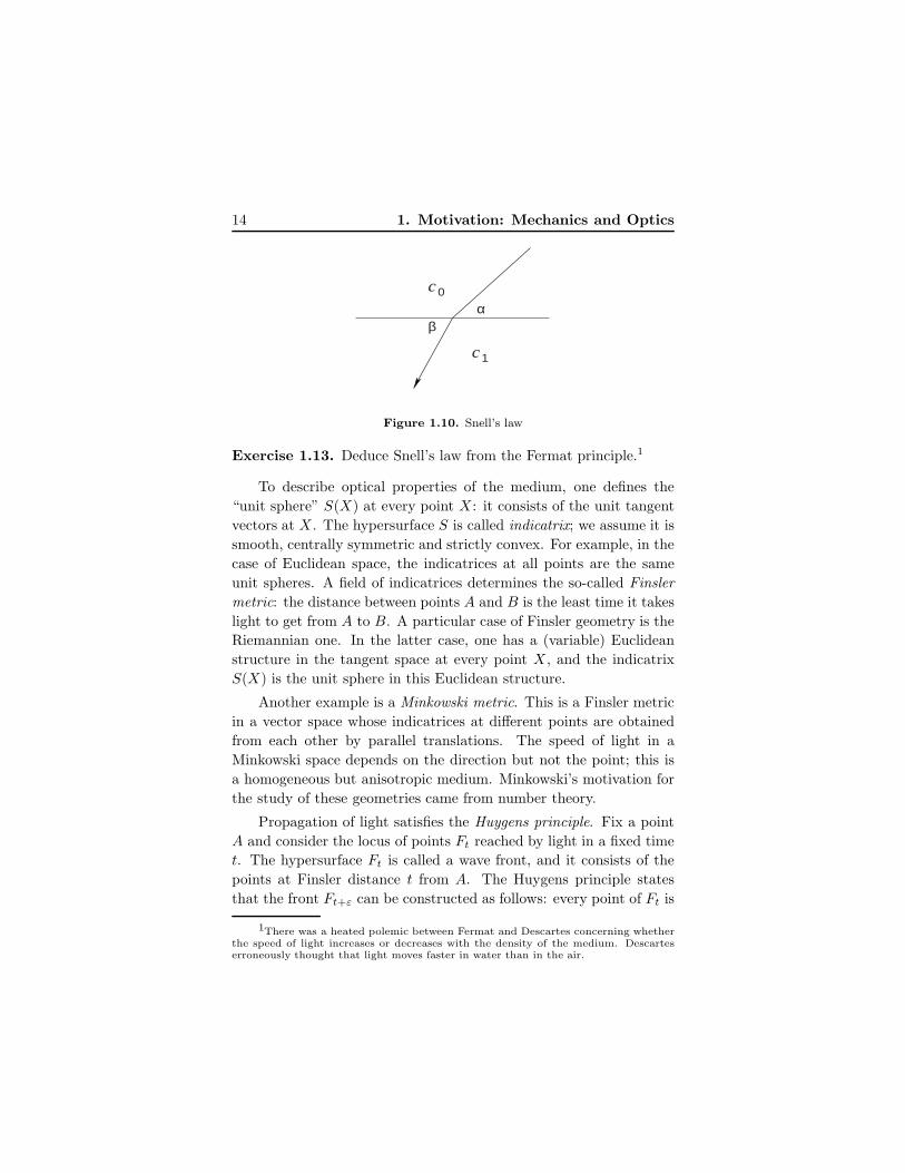
going from air to water; see figure 1.10. Let c1 and c0 be the speeds
of light in water and in air. Then c1 < c0, and the trajectory of light
is a broken line satisfying Snell’s lawcosα
cosβ=c0c1.
14 1. Motivation: Mechanics and Optics
c
c
α β
0
1
Figure 1.10. Snell’s law
Exercise 1.13. Deduce Snell’s law from the Fermat principle.1
To describe optical properties of the medium, one defines the
“unit sphere” S(X) at every point X : it consists of the unit tangent
vectors at X . The hypersurface S is called indicatrix; we assume it is
smooth, centrally symmetric and strictly convex. For example, in the
case of Euclidean space, the indicatrices at all points are the same
unit spheres. A field of indicatrices determines the so-called Finsler
metric: the distance between points A and B is the least time it takes
light to get from A to B. A particular case of Finsler geometry is the
Riemannian one. In the latter case, one has a (variable) Euclidean
structure in the tangent space at every point X , and the indicatrix
S(X) is the unit sphere in this Euclidean structure.
Another example is a Minkowski metric. This is a Finsler metric
in a vector space whose indicatrices at different points are obtained
from each other by parallel translations. The speed of light in a
Minkowski space depends on the direction but not the point; this is
a homogeneous but anisotropic medium. Minkowski’s motivation for
the study of these geometries came from number theory.
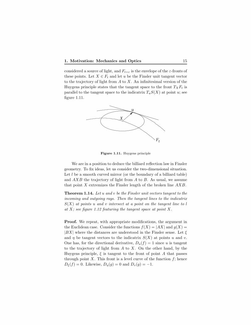
Propagation of light satisfies the Huygens principle. Fix a point
A and consider the locus of points Ft reached by light in a fixed time
t. The hypersurface Ft is called a wave front, and it consists of the
points at Finsler distance t from A. The Huygens principle states
that the front Ft+ε can be constructed as follows: every point of Ft is
1There was a heated polemic between Fermat and Descartes concerning whetherthe speed of light increases or decreases with the density of the medium. Descarteserroneously thought that light moves faster in water than in the air.
1. Motivation: Mechanics and Optics 15
considered a source of light, and Ft+ε is the envelope of the ε-fronts of
these points. Let X ∈ Ft and let u be the Finsler unit tangent vector
to the trajectory of light from A to X . An infinitesimal version of the
Huygens principle states that the tangent space to the front TXFt is
parallel to the tangent space to the indicatrix TuS(X) at point u; see
figure 1.11.
F
X
u
t
Figure 1.11. Huygens principle
We are in a position to deduce the billiard reflection law in Finsler
geometry. To fix ideas, let us consider the two-dimensional situation.
Let l be a smooth curved mirror (or the boundary of a billiard table)
and AXB the trajectory of light from A to B. As usual, we assume
that point X extremizes the Finsler length of the broken line AXB.
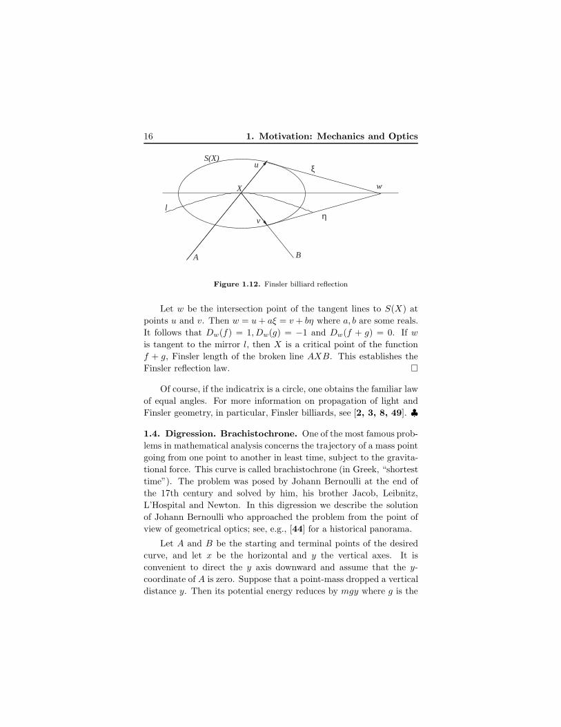
Theorem 1.14. Let u and v be the Finsler unit vectors tangent to the
incoming and outgoing rays. Then the tangent lines to the indicatrix
S(X) at points u and v intersect at a point on the tangent line to l
at X; see figure 1.12 featuring the tangent space at point X.
Proof. We repeat, with appropriate modifications, the argument in
the Euclidean case. Consider the functions f(X) = |AX | and g(X) =
|BX | where the distances are understood in the Finsler sense. Let ξ
and η be tangent vectors to the indicatrix S(X) at points u and v.
One has, for the directional derivative, Du(f) = 1 since u is tangent
to the trajectory of light from A to X . On the other hand, by the
Huygens principle, ξ is tangent to the front of point A that passes
through point X . This front is a level curve of the function f ; hence
Dξ(f) = 0. Likewise, Dη(g) = 0 and Dv(g) = −1.
16 1. Motivation: Mechanics and Optics
η
ξ S(X)
w
BA
l
v
u
X
Figure 1.12. Finsler billiard reflection
Let w be the intersection point of the tangent lines to S(X) at
points u and v. Then w = u+ aξ = v + bη where a, b are some reals.
It follows that Dw(f) = 1, Dw(g) = −1 and Dw(f + g) = 0. If w
is tangent to the mirror l, then X is a critical point of the function
f + g, Finsler length of the broken line AXB. This establishes the
Finsler reflection law.
Of course, if the indicatrix is a circle, one obtains the familiar law
of equal angles. For more information on propagation of light and
Finsler geometry, in particular, Finsler billiards, see [2, 3, 8, 49]. ♣
1.4. Digression. Brachistochrone. One of the most famous prob-
lems in mathematical analysis concerns the trajectory of a mass point
going from one point to another in least time, subject to the gravita-
tional force. This curve is called brachistochrone (in Greek, “shortest
time”). The problem was posed by Johann Bernoulli at the end of
the 17th century and solved by him, his brother Jacob, Leibnitz,
L’Hospital and Newton. In this digression we describe the solution
of Johann Bernoulli who approached the problem from the point of
view of geometrical optics; see, e.g., [44] for a historical panorama.
Let A and B be the starting and terminal points of the desired
curve, and let x be the horizontal and y the vertical axes. It is
convenient to direct the y axis downward and assume that the y-
coordinate of A is zero. Suppose that a point-mass dropped a vertical
distance y. Then its potential energy reduces by mgy where g is the
1. Motivation: Mechanics and Optics 17
gravitational constant and m is the mass. Let v(y) be the speed of
the point-mass. Its kinetic energy equals mv(y)2/2, and it follows
from conservation of energy that
(1.9) v(y) =√
2gy.
Thus the speed of the point-mass depends only on its vertical coor-
dinate.
Consider the medium described by equation (1.9). According to
the Fermat principle, the desired curve is the trajectory of light from
A to B. One can approximate the continuous medium by a discrete
one consisting of thin horizontal strips in which the speed of light is
constant. Let v1, v2, . . . be the speeds of light in the first, second,
etc., strips, and let α1, α2, . . . be the angles made by the trajectory
of light (a polygonal line) with the horizontal border lines between
consecutive strips. By Snell’s law, cosαi/vi = cosαi+1/vi+1; see
figure 1.10. Thus, for all i,
(1.10)cosαi
vi= const.
Now return to the continuous case. Taking (1.9) into account, equa-
tion (1.10) yields, in the continuous limit:
(1.11)cosα(y)√
y= const.
Taking into account that tanα = dy/dx, equation (1.11) gives a
differential equation for the brachistochrone y′ =√
(C − y)/y; this
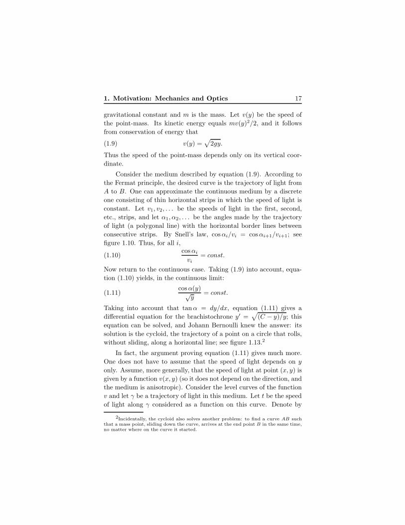
equation can be solved, and Johann Bernoulli knew the answer: its
solution is the cycloid, the trajectory of a point on a circle that rolls,
without sliding, along a horizontal line; see figure 1.13.2
In fact, the argument proving equation (1.11) gives much more.
One does not have to assume that the speed of light depends on y
only. Assume, more generally, that the speed of light at point (x, y) is
given by a function v(x, y) (so it does not depend on the direction, and
the medium is anisotropic). Consider the level curves of the function
v and let γ be a trajectory of light in this medium. Let t be the speed
of light along γ considered as a function on this curve. Denote by
2Incidentally, the cycloid also solves another problem: to find a curve AB suchthat a mass point, sliding down the curve, arrives at the end point B in the same time,no matter where on the curve it started.
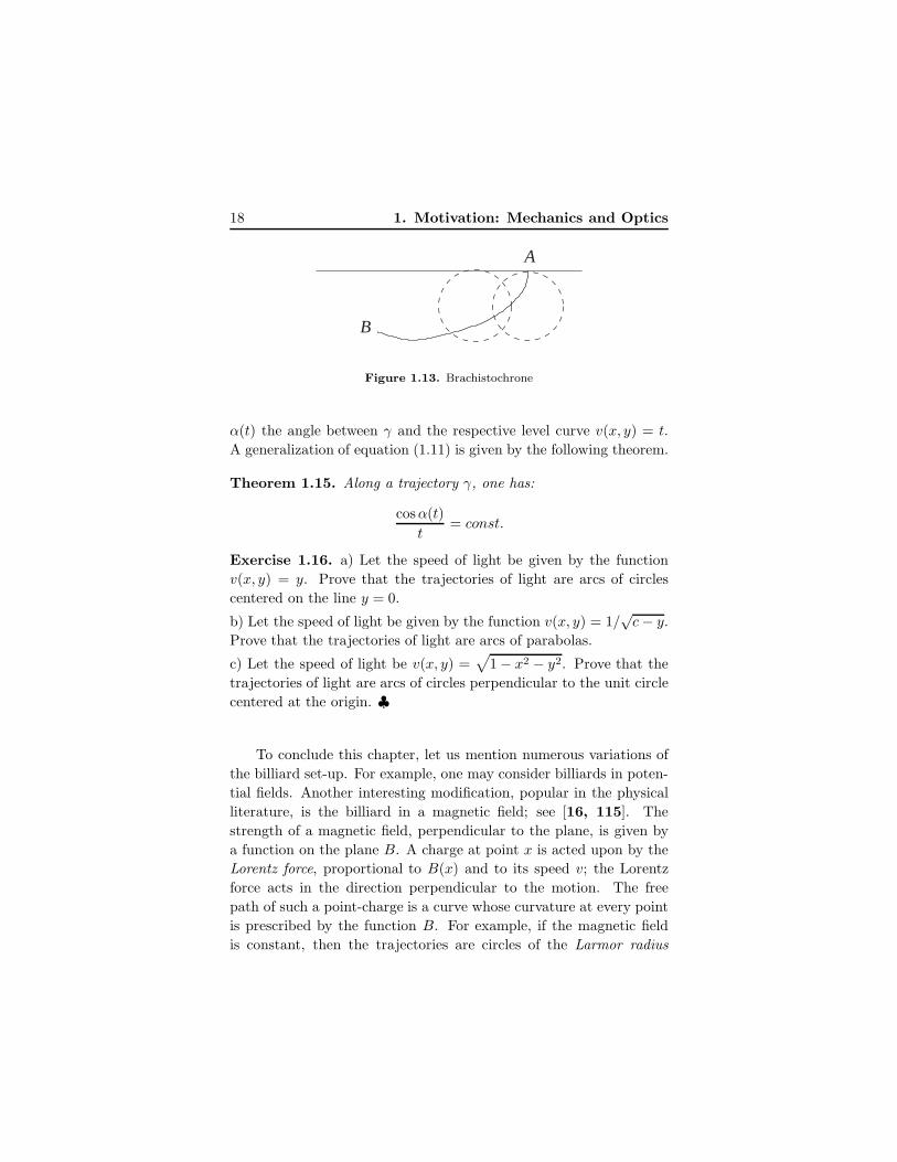
18 1. Motivation: Mechanics and Optics
A
B
Figure 1.13. Brachistochrone
α(t) the angle between γ and the respective level curve v(x, y) = t.
A generalization of equation (1.11) is given by the following theorem.
Theorem 1.15. Along a trajectory γ, one has:
cosα(t)
t= const.
Exercise 1.16. a) Let the speed of light be given by the function
v(x, y) = y. Prove that the trajectories of light are arcs of circles
centered on the line y = 0.
b) Let the speed of light be given by the function v(x, y) = 1/√c− y.
Prove that the trajectories of light are arcs of parabolas.
c) Let the speed of light be v(x, y) =√
1 − x2 − y2. Prove that the
trajectories of light are arcs of circles perpendicular to the unit circle
centered at the origin. ♣
To conclude this chapter, let us mention numerous variations of
the billiard set-up. For example, one may consider billiards in poten-
tial fields. Another interesting modification, popular in the physical
literature, is the billiard in a magnetic field; see [16, 115]. The
strength of a magnetic field, perpendicular to the plane, is given by
a function on the plane B. A charge at point x is acted upon by the
Lorentz force, proportional to B(x) and to its speed v; the Lorentz
force acts in the direction perpendicular to the motion. The free
path of such a point-charge is a curve whose curvature at every point
is prescribed by the function B. For example, if the magnetic field
is constant, then the trajectories are circles of the Larmor radius
1. Motivation: Mechanics and Optics 19
v/B.3 When the point-charge hits the boundary of the billiard ta-
ble, it reflects elastically, so the magnetic field does not affect the
reflection law. A peculiar feature of magnetic billiards is their time-
irreversibility: if one changes the velocity to the opposite, the point-
charge will not traverse its trajectory backward (unless the magnetic
field vanishes).
Remark 1.17. Classical mechanics and geometrical optics, discussed
in this chapter, are intimately related. The configuration trajectories
of mechanical systems are extremals of a variational principle, similar
to the trajectories of light. In fact, mechanics can be described as a
kind of geometrical optics; this was Hamilton’s approach to mechanics
(see [3] for details). The brachistochrone problem is a good example
of this optics-mechanics analogy.
3Equivalently, one may consider billiards subject to the action of Coriolis forcerelated to rotation of the Earth.

Chapter 2
Billiard in the Circleand the Square
Although a unit circle is a very simple figure, there are a few interest-
ing things one can say about the billiard inside it. The circle enjoys
rotational symmetry, and a billiard trajectory is completely deter-
mined by the angle α made with the circle. This angle remains the
same after each reflection. Each consecutive impact point is obtained
from the previous one by a circle rotation through angle θ = 2α.
If θ = 2πp/q, then every billiard orbit is q-periodic and makes p
turns about the circle; one says that the rotation number of such an
orbit is p/q. If θ is not a rational multiple of π, then every orbit is
infinite. The first result on π-irrational rotations of the circle is due
to Jacobi. Denote the circle rotation through angle θ by Tθ.
Theorem 2.1. If θ is π-irrational, then the Tθ-orbit of every point
is dense. In other words, every interval contains points of this orbit.
Proof. Let x be the initial point. Starting at x, we traverse the
circle making steps of length θ. After some number of steps, say, n,
we return back to x and step over it. Note that one does not return
exactly to x; otherwise θ = 2π/n. Let y = x + nθ mod 2π be the
point immediately before x and z = y + θ mod 2π the next point.
21
22 2. Billiard in the Circle and the Square
One of the segments yx or xz has length at most θ/2. To fix
ideas, assume it is the segment yx, and let θ1 be its length. Note
that θ1 is again π-irrational. Consider the n-th iteration T nθ . This
map is the rotation of the circle, in the negative sense, through angle
θ1 ≤ θ/2. We can take this Tθ1as a new circle rotation and apply the
previous argument to it.
Thus we obtain a sequence of rotations through π-irrational an-
gles θk → 0; each of these rotations is an iteration of Tθ. Given an
interval I on the circle, one can choose k so large that θk < |I|. Then
the Tθk-orbit of x cannot avoid I, and we are done.
Exercise 2.2. The segments making the angle α with the unit circle
are tangent to the concentric circle of radius cosα. Prove that if α
is π-irrational, then the consecutive segments of a billiard trajectory
fill the annulus between the circles densely.
Let us continue the study of the sequence xn = x + nθ mod 2π
with π-irrational θ. If θ = 2πp/q, this sequence consists of q elements
which are distributed in the circle very regularly. Should one expect
a similar regular distribution for π-irrational θ?
The adequate notion is that of equidistribution (or uniform dis-
tribution). Given an arc I, let k(n) be the number of terms in the
sequence x0, . . . xn−1 that lie in I. The sequence is called equidis-
tributed on the circle R/2πZ if
(2.1) limn→∞
k(n)
n=
|I|2π
for every I. The next theorem is due to Kronecker and Weyl; it
implies Theorem 2.1.
Theorem 2.3. If θ is π-irrational, then the sequence xn = x + nθ
mod 2π is equidistributed on the circle.
Proof. (Sketch). We will establish a more general statement: if f(x)
is an integrable function on the circle, then
(2.2) limn→∞
1
n
n−1∑
j=0
f(xj) =1
2π
∫ 2π
0
f(x)dx;
2. Billiard in the Circle and the Square 23
the time average equals the space average. To deduce equidistribution
one takes f to be the characteristic function of the arc I, equal to 1
inside and 0 outside. Then (2.2) becomes (2.1).
One may approximate the function f(x) by a trigonometric poly-
nomial, a linear combination of cos kx and sin kx with k = 0, 1, . . . , N .
We establish (2.2) for pure harmonics or, better still, for f(x) =
exp(ikx) (which is a complex-valued function whose real and imagi-
nary parts are k-th harmonics). If k = 0, that is, f = 1, then both
sides of (2.2) are equal to 1. If k ≥ 1, then the left-hand side of (2.2)
becomes a geometric progression:
1
n
n−1∑
j=0
eikjθ =1
n
eiknθ − 1
eikθ − 1→ 0
as n → ∞. On the other hand,∫ 2π
0 exp(ikx)dx = 0, and (2.2) holds.
Theorems 2.1 and 2.3 have multi-dimensional versions. Consider
the torus T n = Rn/Zn. Let a = (a1, . . . , an) be a vector and
Ta : (x1, . . . , xn) 7→ (x1 + a1, . . . , xn + an)
the respective torus rotation. The numbers a1, . . . , an are called in-
dependent over integers if an equality
k0 + k1a1 + · · · + knan = 0, ki ∈ Z
implies k0 = k1 = · · · = kn = 0. The multi-dimensional theorem on
torus rotations asserts that if a1, . . . , an are independent over integers,
then every orbit of Ta is dense and equidistributed on the torus.
2.1. Digression. Distribution of first digits and Benford’s
Law. Consider the sequence
1, 2, 4, 8, 16, 32, 64, 128, 256, 512, 1024, . . .
consisting of consecutive powers of 2. Can a power of 2 start with
2005? Is a term in this sequence more likely to start with 3 or 4?
This kind of question is answered by Theorems 2.1 and 2.3.
Let us consider the second question: 2n has the first digit k if,
for some non-negative integer q, one has 10q ≤ 2n < (k+ 1)10q. Take
24 2. Billiard in the Circle and the Square
logarithm base 10:
(2.3) log k + q ≤ n log 2 < log(k + 1) + q.
Since q is of no concern to us, let us consider fractional parts of the
numbers involved. Denote by x the fractional part of the real num-
ber x. Inequalities (2.3) mean that n log 2 belongs to the interval
I = [log k, log(k + 1)) ⊂ S1 = R/Z.
Note that log 2 is an irrational number (why?) Thus we are in the
situation of Theorem 2.3, which implies the following result.
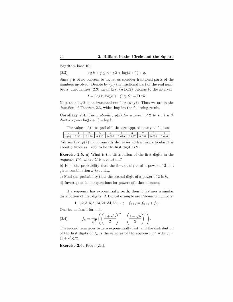
Corollary 2.4. The probability p(k) for a power of 2 to start with
digit k equals log(k + 1) − log k.
The values of these probabilities are approximately as follows:
k 1 2 3 4 5 6 7 8 9p(k) 0.301 0.176 0.125 0.097 0.079 0.067 0.058 0.051 0.046
We see that p(k) monotonically decreases with k; in particular, 1 is
about 6 times as likely to be the first digit as 9.
Exercise 2.5. a) What is the distribution of the first digits in the
sequence 2nC where C is a constant?
b) Find the probability that the first m digits of a power of 2 is a
given combination k1k2 . . . km.
c) Find the probability that the second digit of a power of 2 is k.
d) Investigate similar questions for powers of other numbers.
If a sequence has exponential growth, then it features a similar
distribution of first digits. A typical example are Fibonacci numbers
1, 1, 2, 3, 5, 8, 13, 21, 34, 55, . . . ; fn+2 = fn+1 + fn.
One has a closed formula:
(2.4) fn =1√5
((1 +
√5
2
)n
−(
1 −√
5
2
)n).
The second term goes to zero exponentially fast, and the distribution
of the first digits of fn is the same as of the sequence ϕn with ϕ =
(1 +√
5)/2.
Exercise 2.6. Prove (2.4).
2. Billiard in the Circle and the Square 25
Surprisingly, many “real life” sequences enjoy a similar distribu-
tion of first digits! This was first noted in 1881 in a 2-page article by
American astronomer S. Newcomb [78]. This article opens as follows:
“That the ten digits do not occur with equal frequency must be evi-
dent to any one making much use of logarithmic tables, and noticing
how much faster the first pages wear out than the last ones. The first
significant figure is oftener 1 than any other digit, and the frequency
diminishes up to 9.”
This peculiar distribution of first digits in “real life” sequences
is known as Benford’s Law, for F. Benford, a physicist at General
Electric, who, 57 years after Newcomb, published a long article [11]
entitled “The law of anomalous numbers”.1 Benford provides am-
ple experimental data confirming this pattern, ranging from areas of
rivers to populations of cities and from street addresses in the current
issue of American Men of Science to atomic weights. The reader may
want to collect his own data; I suggest the areas and populations of
the countries of the world (measured in any units: by Exercise 2.5 a),
the result does not change under rescaling).
There is substantial literature devoted to Benford’s Law. Various
explanations were offered; see [85] for a survey. One of the most con-
vincing ones, [52], deduces Benford’s Law as the only frequency dis-
tribution, satisfying certain natural axioms, which is scale-invariant.
The subject continues to attract attention of mathematicians, statis-
ticians, physicists and engineers. As an application, it was suggested
that the IRS use Benford’s Law to check whether the numbers ap-
pearing on a tax return are truly random or have been doctored. ♣
Exercise 2.7. Let α be an irrational number. Consider the numbers
0, α, 2α, . . . , nα, 1.Show that the n+1 intervals into which these numbers partition [0, 1]
have at most three distinct lengths.
Let us now consider the billiard inside a unit square. Although
the square has a very different shape from a circle, the two figures do
1It is rather common in the history of science to name results for persons otherthan their first discoverers.
26 2. Billiard in the Circle and the Square
not differ as far as billiards inside them are concerned. We use the
unfolding method described in Chapter 1.
Unfolding yields the plane with a square grid, and billiard trajec-
tories become straight lines in the plane. Two lines in the plane cor-
respond to the same billiard trajectory if they differ by a translation
through a vector from the lattice 2Z+2Z. Note that two neighboring
squares have opposite orientations: they are symmetric with respect
to their common side. Consider a larger square that consists of four
unit squares with a common vertex, and identify its opposite sides to
obtain a torus. A billiard trajectory becomes a geodesic line on this
flat torus.
Consider the trajectories in a fixed direction α. Start a trajec-
tory at point x of the lower side of the 2 × 2 square. This trajectory
intersects the upper side at point x+2 cotα mod 2. Rescaling every-
thing by a factor of 1/2, we arrive at the circle S1 = R1/Z rotation
x 7→ x + cotα mod 1. Thus the billiard flow in a fixed direction
reduces to a circle rotation.
In particular, if the slope of a trajectory is rational, then this tra-
jectory is periodic; and if the slope is irrational, then it is everywhere
dense and uniformly distributed in the square.
The same approach applies to the billiard inside a unit cube in
Rn. Fixing a direction of the billiard trajectories, one reduces the
billiard to a rotation of the torus T n−1.
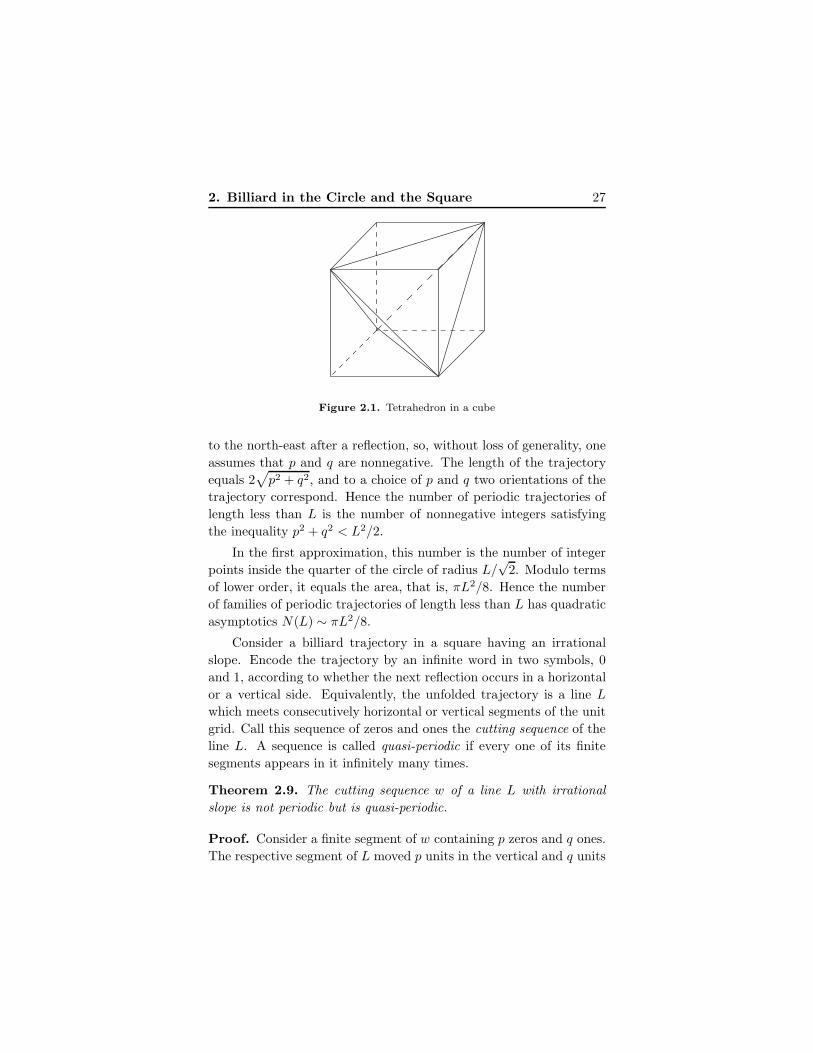
Exercise 2.8. Inscribe a tetrahedron into a cube; see figure 2.1. Con-
sider the billiard ball at a generic point on the surface of the tetra-
hedron going in a generic direction tangent to this surface. Describe
the closure of this billiard trajectory; cf. [90].
A natural question to ask about the billiard in a square is how
many periodic trajectories of length less than L it has. This ques-
tion should be understood properly: periodic trajectories appear in
parallel families; the number of such families is what one counts.
The unfolding of a periodic trajectory is a segment in the plane
whose end-points differ by a translation through a vector from the
lattice 2Z + 2Z. Assume that an unfolded trajectory goes from the
origin to point (2p, 2q). A trajectory in the south-east direction will go
2. Billiard in the Circle and the Square 27
Figure 2.1. Tetrahedron in a cube
to the north-east after a reflection, so, without loss of generality, one
assumes that p and q are nonnegative. The length of the trajectory
equals 2√p2 + q2, and to a choice of p and q two orientations of the
trajectory correspond. Hence the number of periodic trajectories of
length less than L is the number of nonnegative integers satisfying
the inequality p2 + q2 < L2/2.
In the first approximation, this number is the number of integer
points inside the quarter of the circle of radius L/√
2. Modulo terms
of lower order, it equals the area, that is, πL2/8. Hence the number
of families of periodic trajectories of length less than L has quadratic
asymptotics N(L) ∼ πL2/8.
Consider a billiard trajectory in a square having an irrational
slope. Encode the trajectory by an infinite word in two symbols, 0
and 1, according to whether the next reflection occurs in a horizontal
or a vertical side. Equivalently, the unfolded trajectory is a line L
which meets consecutively horizontal or vertical segments of the unit
grid. Call this sequence of zeros and ones the cutting sequence of the
line L. A sequence is called quasi-periodic if every one of its finite
segments appears in it infinitely many times.
Theorem 2.9. The cutting sequence w of a line L with irrational
slope is not periodic but is quasi-periodic.
Proof. Consider a finite segment of w containing p zeros and q ones.
The respective segment of L moved p units in the vertical and q units
28 2. Billiard in the Circle and the Square
in the horizontal direction. Assume that w is periodic, and let the
period contain p0 zeroes and q0 ones. The slope of L is the limit,
as n → ∞, of the slopes of its segments Ln, corresponding to the
segments of w made of n periods. The slope of Ln is (np0)/(nq0),
and the limit is p0/q0 ∈ Q. This contradicts our assumption that the
slope of L is irrational.
If two points of the square are sufficiently close to each other, then
sufficiently long segments of the cutting sequences of parallel billiard
trajectories through these points coincide. Theorem 2.3 implies that
since the slope of L is irrational, it will return to any neighborhood of
its points infinitely many times. Quasi-periodicity of w follows.
Example 2.10. In a sense, the most interesting irrational number
is the golden ratio, ϕ = (1 +√
5)/2. Let L be the line through the
origin with slope ϕ. The respective cutting sequence
w = . . . 0100101001001 . . .
is called the Fibonacci sequence (see Exercise 2.11 for the reason why).
This sequence enjoys a remarkable property: w is invariant under the
substitution
σ : 0 7→ 01, 1 7→ 0.
To prove this property, consider the linear transformation
A =
( −1 1
1 0
).
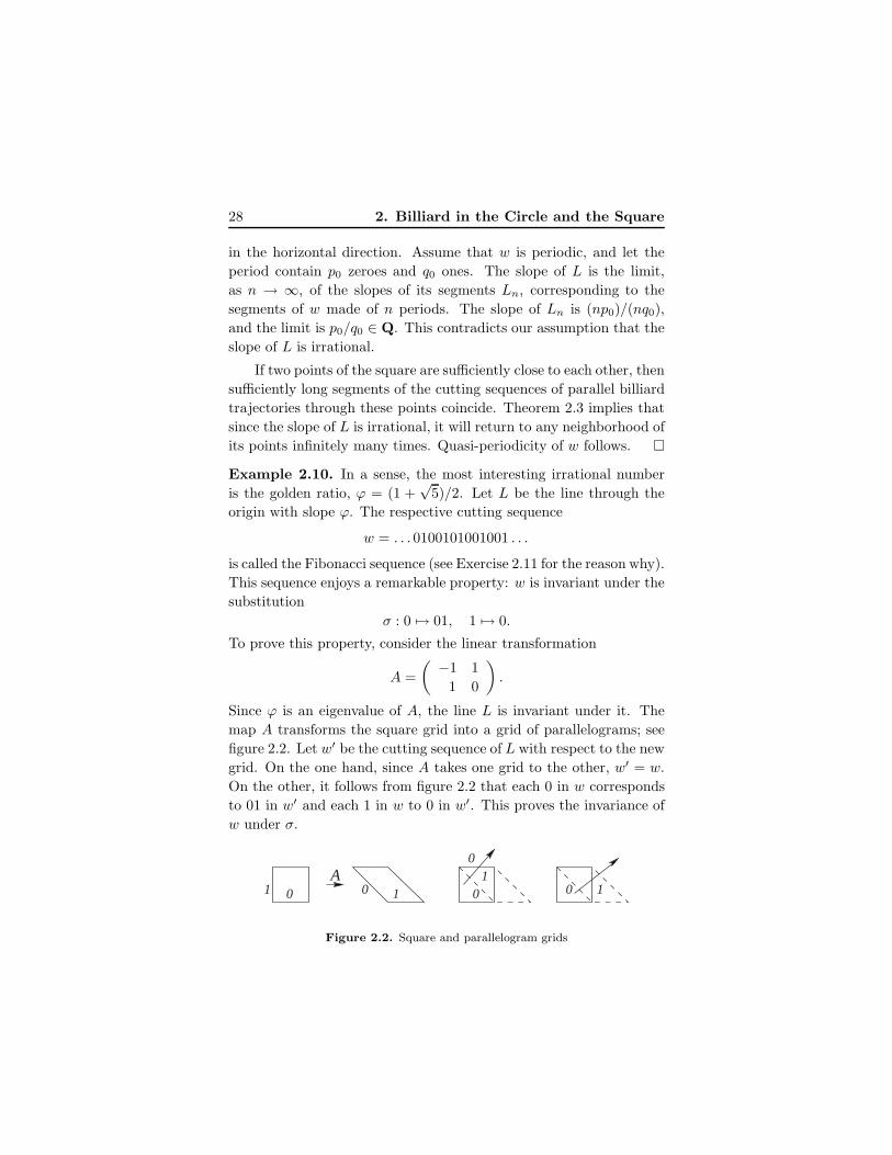
Since ϕ is an eigenvalue of A, the line L is invariant under it. The
map A transforms the square grid into a grid of parallelograms; see
figure 2.2. Let w′ be the cutting sequence of L with respect to the new
grid. On the one hand, since A takes one grid to the other, w′ = w.
On the other, it follows from figure 2.2 that each 0 in w corresponds
to 01 in w′ and each 1 in w to 0 in w′. This proves the invariance of
w under σ.
01
0A
1 0 0 110
Figure 2.2. Square and parallelogram grids
2. Billiard in the Circle and the Square 29
We leave it to the reader to muse on similar substitution rules
for the lines whose slopes are other quadratic irrationalities and their
relation to continued fractions.
Exercise 2.11. Let wn = σn(0). Prove that the lengths of wn are
the Fibonacci numbers.
One would like to have a quantitative measure of the complexity
of the cutting sequence of a billiard trajectory. Let w be an infinite
sequence of some symbols (zeros and ones, in our case). The com-
plexity function p(n) is the number of distinct segments of length n in
w. The faster p(n) grows, the more complex the sequence w is. For
two symbols, the fastest possible growth is p(n) = 2n.
For complexity of the cutting sequence of a line L with an irra-
tional slope, we have the following result.
Theorem 2.12. p(n) = n+ 1.
Proof. Since a billiard trajectory with an irrational slope comes arbi-
trarily close to any point of the square, the sets of length n segments of
the cutting sequences of any two parallel trajectories coincide. Thus
one can find the complexity by computing the number of different
initial segments of length n in the cutting sequences of all parallel
lines with a given slope. In fact, it suffices to consider the lines that
start on the diagonal of the unit square.
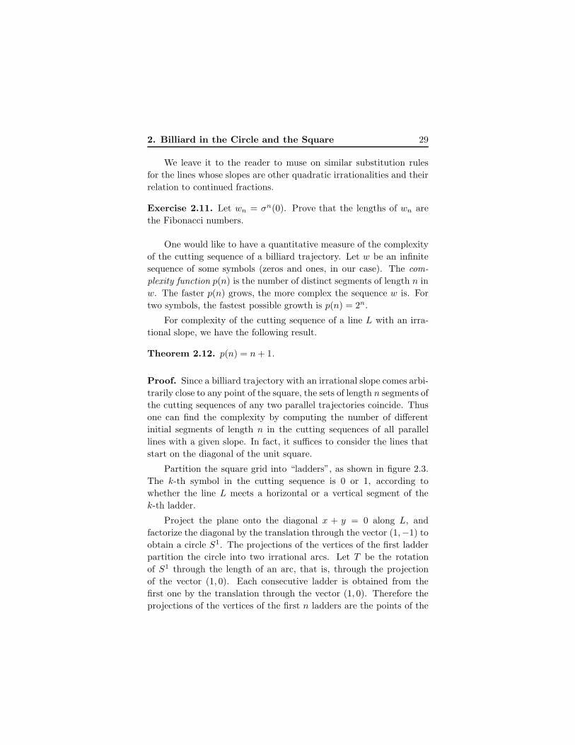
Partition the square grid into “ladders”, as shown in figure 2.3.
The k-th symbol in the cutting sequence is 0 or 1, according to
whether the line L meets a horizontal or a vertical segment of the
k-th ladder.
Project the plane onto the diagonal x + y = 0 along L, and
factorize the diagonal by the translation through the vector (1,−1) to
obtain a circle S1. The projections of the vertices of the first ladder
partition the circle into two irrational arcs. Let T be the rotation
of S1 through the length of an arc, that is, through the projection
of the vector (1, 0). Each consecutive ladder is obtained from the
first one by the translation through the vector (1, 0). Therefore the
projections of the vertices of the first n ladders are the points of the
30 2. Billiard in the Circle and the Square
(0,0)
Figure 2.3. Square grid partitioned into ladders
orbit T i(0), i = 0, . . . , n. Since T is an irrational rotation, all these
points are distinct and there are n+ 1 of them.
To describe the initial n-segments of the cutting sequences, start
with the line through the origin (0, 0) and parallel translate it along
the diagonal of the unit square toward point (−1, 1). The n-segments
of the cutting sequence change when the line passes through a vertex
of one of the first n ladders. As we have seen, there are n + 1 such
events, and hence p(n) = n+ 1.
Remark 2.13. One can similarly encode billiard trajectories in a
k-dimensional cube: the cutting sequence consists of k symbols cor-
responding to the directions of the faces. The complexity p(n) of such
a cutting sequence is polynomial in n of degree k − 1; see [9] for an
explicit formula. There is substantial literature on the complexity of
polygonal billiards; see [50, 54, 117] for a sampler.
2.2. Digression. Sturmian sequences. The sequences with com-
plexity p(n) = n + 1 are called Sturmian sequences. This is the
smallest possible complexity of non-periodic sequences, as the next
proposition states.
Lemma 2.14. Let w be an infinite word in a finite number of symbols
and p(n) its complexity. Then w is ultimately periodic if and only if
p(n) ≤ n for some n.
2. Billiard in the Circle and the Square 31
Proof. Assume that w is ultimately periodic; let p be the pre-period
length and q the length of the period. Then p(n) ≤ p + q and hence
p(n) ≤ n for n ≥ p+ q.
We claim that if w is not ultimately periodic, then p(n+1) > p(n)
for all n. Assuming this claim, note that p(1) > 1 (otherwise w
consists of one symbol only). Then p(2) > p(1) ≥ 2, etc., and finally,
p(n) ≥ n+ 1.
It remains to prove the above claim. If p(n+1) = p(n), then each
segment of length n in w has a unique right extension to a segment of
length n+1. There are only finitely many distinct segments of length
n. Let aiai+1 . . . ai+n−1 and ajaj+1 . . . aj+n−1 be two identical n-
segments. By the uniqueness of the right extension, ai+n = aj+n,
etc., so that ai+k = aj+k for all k ≥ 1. In particular, the segment
aiai+1 . . . aj−1 is a period of w.
Thus, Sturmian sequences are the non-periodic sequences with
the smallest possible complexity. ♣
The result of the next exercise was discovered by Lord Rayleigh
in a study of the vibrating string and rediscovered by S. Beatty in
1926; see [90].
Exercise 2.15. a) Let a and b be positive irrational numbers sat-
isfying 1/a + 1/b = 1. Consider the lines y = ax and y = bx and
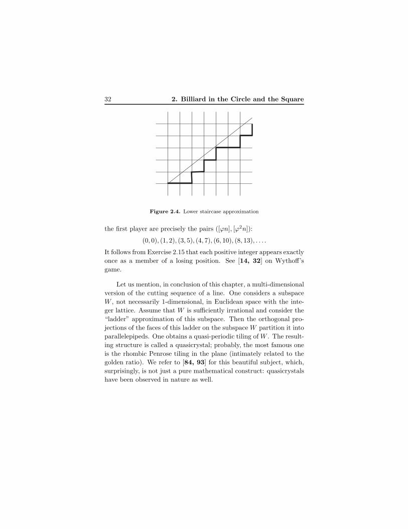
approximate them by the “lower staircases”, see figure 2.4. Prove
that every positive integer appears exactly once as the height of a
step of either of these two staircases. In other words, every natural
number can be represented either as [ak] or as [bn] with k, n ∈ Z, but
not both.
b) Let ϕ be the golden ratio. Prove that
[ϕ2n] = [ϕ[ϕn]] + 1 for n = 1, 2, . . . .
Remark 2.16. Exercise 2.15 is closely related to Wythoff’s game.
There are two players; the moves alternate. One has two piles of
objects (say, pebbles), and in a move a player can take any number
of objects from one of the piles or an equal number of objects from
both piles. The first unable to move loses. The losing positions for
32 2. Billiard in the Circle and the Square
Figure 2.4. Lower staircase approximation
the first player are precisely the pairs ([ϕn], [ϕ2n]):
(0, 0), (1, 2), (3, 5), (4, 7), (6, 10), (8, 13), . . . .
It follows from Exercise 2.15 that each positive integer appears exactly
once as a member of a losing position. See [14, 32] on Wythoff’s
game.
Let us mention, in conclusion of this chapter, a multi-dimensional
version of the cutting sequence of a line. One considers a subspace
W , not necessarily 1-dimensional, in Euclidean space with the inte-
ger lattice. Assume that W is sufficiently irrational and consider the
“ladder” approximation of this subspace. Then the orthogonal pro-
jections of the faces of this ladder on the subspace W partition it into
parallelepipeds. One obtains a quasi-periodic tiling of W . The result-
ing structure is called a quasicrystal; probably, the most famous one
is the rhombic Penrose tiling in the plane (intimately related to the
golden ratio). We refer to [84, 93] for this beautiful subject, which,
surprisingly, is not just a pure mathematical construct: quasicrystals
have been observed in nature as well.
Chapter 3
Billiard Ball Map andIntegral Geometry
So far we have talked mostly about the billiard flow, a continuous time
system. One replaces continuous time by discrete time and considers
the billiard ball map.
To fix ideas, consider a plane billiard table D whose boundary is
a smooth closed curve γ. Let M be the space of unit tangent vectors
(x, v) whose foot points x are on γ and which have inward directions.
A vector (x, v) is an initial position of the billiard ball. The ball moves
freely and hits γ at point x1; let v1 be the velocity vector reflected
off the boundary. The billiard ball map T : M → M takes (x, v) to
(x1, v1). Note that if D is not convex, then T is not continuous: this
is due to the existence of billiard trajectories touching the boundary
from inside.
Parameterize γ by arc length t and let α be the angle between
v and the positive tangent line of γ. Then (t, α) are coordinates on
M ; in particular, M is the cylinder. A fundamental property of the
billiard ball map is the existence of an invariant area form.
Theorem 3.1. The area form ω = sinα dα ∧ dt is T -invariant.
Proof. Note first that sinα > 0 on M ; therefore ω is an area form.
To prove its invariance, let f(t, t1) be the distance between points
33
34 3. Billiard Ball Map and Integral Geometry
γ(t) and γ(t1). The partial derivative ∂f/∂t1 is the projection of the
gradient of the distance |γ(t)γ(t1)| on the curve at point γ(t1). This
gradient is the unit vector from γ(t) to γ(t1) (cf. Chapter 1) and
it makes angle α1 with the curve; hence ∂f/∂t1 = cosα1. Likewise,
∂f/∂t = − cosα. Therefore
df =∂f
∂tdt+
∂f
∂t1dt1 = − cosα dt+ cosα1 dt1,
and hence
0 = d2f = sinα dα ∧ dt− sinα1 dα1 ∧ dt1.This means that ω is a T -invariant area form.
Whenever we need to integrate some function over the billiard
phase space, we do this with respect to the area form ω. In particular,
one has the following corollary. Let L be the length of γ and A the
area of D.
Corollary 3.2. The area of the phase space M equals 2L.
Proof. The area of M equals∫ L
0
∫ π
0
sinα dα dt,
and the result easily follows.
In the spirit of geometrical optics, let us consider the space N
of oriented lines in the plane. An oriented line can be characterized
by its direction, an angle ϕ, and its signed distance p from the origin
O (the sign of p is that of the frame that consists of the orthogonal
vector from the origin to the line and the direction vector of the line).
Thus N is a cylinder with coordinates (ϕ, p).
Exercise 3.3. Describe the space of non-oriented lines in the plane.
Exercise 3.4. Let O′ = O+ (a, b) be a different choice of the origin.
Show that the new coordinates depend on the old ones as follows:
(3.1) ϕ′ = ϕ, p′ = p− a sinϕ+ b cosϕ.
The space of lines N has an area form Ω = dϕ ∧ dp.
3. Billiard Ball Map and Integral Geometry 35
Lemma 3.5. The area form Ω is invariant under the orientation
preserving motions of the plane.
Proof. Every orientation preserving motion is a composition of a
rotation about the origin and a parallel translation. Under a rotation,
ϕ′ = ϕ+ c, p′ = p,
and clearly Ω′ = Ω. The result of a parallel translation is described
in (3.1). It follows that
dϕ′ = dϕ, dp′ = dp− (a cosϕ+ b sinϕ)dϕ
and hence dϕ′ ∧ dp′ = dϕ ∧ dp.
Exercise 3.6. a) Prove that Ω is the unique, up to a constant factor,
area form on the space of oriented lines invariant under the orientation
preserving motions of the plane.
b) Is there a Riemannian metric on the space of oriented lines invari-
ant under the orientation preserving motions of the plane?
The two spaces, M and N , are related by the map Φ : M → N
that associates the oriented line with a unit vector. If the billiard
table is convex, then Φ is one-to-one. The relation between the area
forms is as follows.
Lemma 3.7. Φ∗(Ω) = ω.
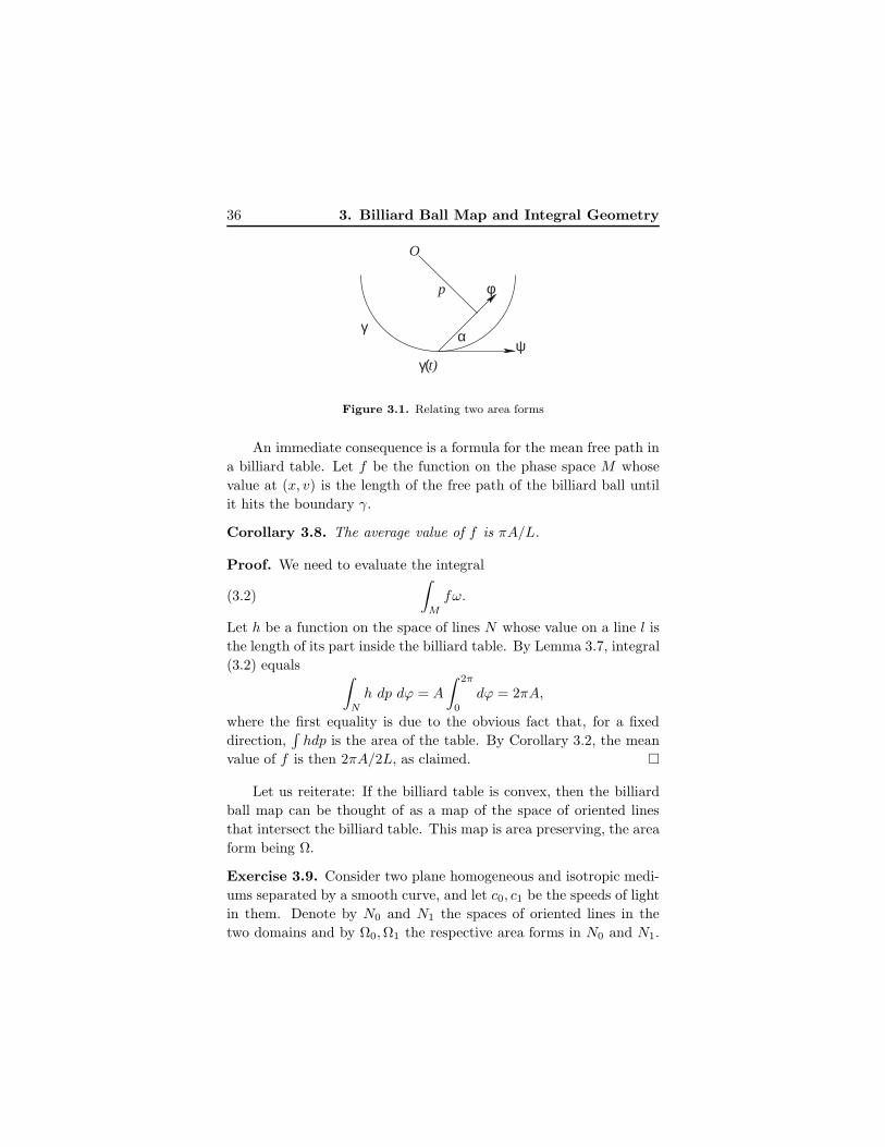
Proof. Let (t, α) be the coordinates in M and (ϕ, p) the respective
coordinates in N . Denote by ψ(t) the direction of the positive tan-
gent line to the curve γ at point γ(t), and let γ1 and γ2 be the two
components of the position vector γ. Then one has:
ϕ = α+ ψ(t), p = γ × (cosϕ, sinϕ);
see figure 3.1. It follows that
dϕ = dα+ψ′dt, dp = (γ′1 sinϕ−γ′2 cosϕ)dt+(γ1 cosϕ+γ2 sinϕ)dϕ,
and hence
dϕ ∧ dp = (γ′1 sinϕ− γ′2 cosϕ)dα ∧ dt.Since (γ′1, γ
′2) = (cosψ, sinψ), one has: γ′1 sinϕ−γ′2 cosϕ = sinα, and
therefore dϕ ∧ dp = sinα dα ∧ dt, as claimed.
36 3. Billiard Ball Map and Integral Geometry
O
p φ
γ ψ
α
γ( t)
Figure 3.1. Relating two area forms
An immediate consequence is a formula for the mean free path in
a billiard table. Let f be the function on the phase space M whose
value at (x, v) is the length of the free path of the billiard ball until
it hits the boundary γ.
Corollary 3.8. The average value of f is πA/L.
Proof. We need to evaluate the integral
(3.2)
∫
M
fω.
Let h be a function on the space of lines N whose value on a line l is
the length of its part inside the billiard table. By Lemma 3.7, integral
(3.2) equals ∫
N
h dp dϕ = A
∫ 2π
0
dϕ = 2πA,
where the first equality is due to the obvious fact that, for a fixed
direction,∫hdp is the area of the table. By Corollary 3.2, the mean
value of f is then 2πA/2L, as claimed.
Let us reiterate: If the billiard table is convex, then the billiard
ball map can be thought of as a map of the space of oriented lines
that intersect the billiard table. This map is area preserving, the area
form being Ω.
Exercise 3.9. Consider two plane homogeneous and isotropic medi-
ums separated by a smooth curve, and let c0, c1 be the speeds of light
in them. Denote by N0 and N1 the spaces of oriented lines in the
two domains and by Ω0,Ω1 the respective area forms in N0 and N1.
3. Billiard Ball Map and Integral Geometry 37
Let T : N0 → N1 be the (partially defined) map corresponding to
refraction of light described by Snell’s law; see figure 1.10. Prove that
T ∗(Ω1) = (c1/c0)Ω0.
The area form Ω on the space of lines can be used to evaluate
the length of a curve. The following result, whose particular case we
already encountered in Corollary 3.2, is called the Crofton formula.
Given a smooth plane curve γ (not necessarily closed or simple),
let nγ(l) be the function on the space of oriented lines equal to the
number of intersection points of l with γ. The function nγ is well
defined for almost every line and is locally constant; namely, the value
of nγ changes when the lines become tangent to the curve γ. If (ϕ, p)
are the coordinates of the line l, we write the function as nγ(ϕ, p).
Theorem 3.10. One has:
(3.3) length (γ) =1
4
∫ ∫nγ(ϕ, p) dϕ dp.
Proof. The curve γ can be approximated by a polygonal line, and it
suffices to prove (3.3) for such a line. Suppose that a polygonal line is
the concatenation of two, γ1 and γ2. Both sides of (3.3) are additive,
and the formula for γ would follow from those for γ1 and γ2. Hence it
suffices to establish (3.3) for a segment. This can be done by a direct
computation or, in a more “lazy” way, as follows.
Let γ0 be the unit segment and let∫
N
nγ0(l) Ω = C
(the constant does not depend on the position of the segment because
the area form on the space of lines is isometry invariant). Then, again
by additivity, ∫
N
nγ(l) Ω = C|γ|
for every segment γ. By the above arguments,∫
N
nγ(l) Ω = C length (γ)
for every smooth curve γ. It remains to see that C = 4. This is easiest
seen when γ is the unit circle centered at the origin: nγ(ϕ, p) = 2 for
all ϕ and −1 ≤ p ≤ 1 and zero otherwise.
38 3. Billiard Ball Map and Integral Geometry
Exercise 3.11. Make a direct computation of the right-hand side of
(3.3) when γ is a segment.
Exercise 3.12. The distance between the lines on a ruled paper is 1.
Find the probability that a unit segment randomly dropped on the
paper intersects a line.1
Hint: Assume, more generally, that one randomly drops a curve on
the ruled paper. The average number of intersections with a line
depends only on the length of the curve and equals 2 for a circle of
diameter 1 whose perimeter length is π.
The Crofton formula has numerous applications; see [89]. We
will discuss four.
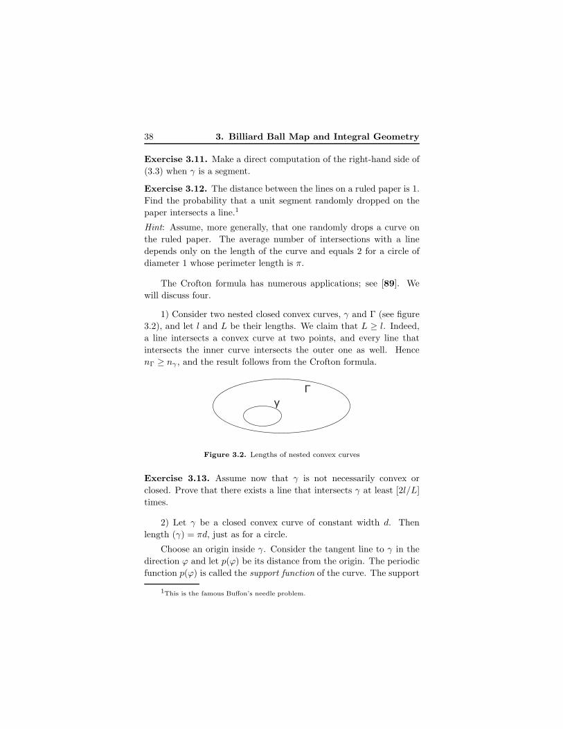
1) Consider two nested closed convex curves, γ and Γ (see figure
3.2), and let l and L be their lengths. We claim that L ≥ l. Indeed,
a line intersects a convex curve at two points, and every line that
intersects the inner curve intersects the outer one as well. Hence
nΓ ≥ nγ , and the result follows from the Crofton formula.
Γ γ
Figure 3.2. Lengths of nested convex curves
Exercise 3.13. Assume now that γ is not necessarily convex or
closed. Prove that there exists a line that intersects γ at least [2l/L]
times.
2) Let γ be a closed convex curve of constant width d. Then
length (γ) = πd, just as for a circle.
Choose an origin inside γ. Consider the tangent line to γ in the
direction ϕ and let p(ϕ) be its distance from the origin. The periodic
function p(ϕ) is called the support function of the curve. The support
1This is the famous Buffon’s needle problem.
3. Billiard Ball Map and Integral Geometry 39
function determines a one-parameter family of lines p = p(ϕ), and
the curve γ is their envelope.
The constant width condition reads: p(ϕ) + p(ϕ+ π) = d. Now,
by the Crofton formula,
length (γ) =1
4
∫ 2π
0
∫ p(ϕ)
−p(ϕ+π)
2 dp dϕ =1
2d
∫ 2π
0
dϕ = πd,
as claimed.
Exercise 3.14. a) How does the support function depend on the
choice of the origin?
b) Express the area bounded by γ in terms of its support function.
c) Parameterize γ by the angle ϕ made by its tangent with a fixed
direction, and let p(ϕ) be the support function. Prove that
(3.4) γ(ϕ) = (p(ϕ) sinϕ+ p′(ϕ) cosϕ,−p(ϕ) cosϕ+ p′(ϕ) sinϕ).
d) Show that the radius of curvature of γ(ϕ) equals p′′(ϕ) + p(ϕ).
3) The celebrated isoperimetric inequality asserts that the length
L of a simple closed plane curve γ and the area A bounded by it
satisfy
(3.5) L2 ≥ 4πA
with equality only for a circle. There are many proofs of this inequal-
ity; see [26] for a comprehensive reference. The following proof was
found by W. Blaschke; see [89].
Assume that γ is convex and smooth, and let t, α be the coor-
dinates in the phase space M of the billiard inside γ. As before, let
f(t, α) be the length of the free path of the billiard ball. Consider two
independent phase points, (t, α) and (t1, α1). The following integral
is obviously non-negative:
(3.6)
∫
M×M
(f(t, α) sinα1 − f(t1, α1) sinα)2dt dα dt1 dα1.
Integral (3.6) is not hard to evaluate. First, by the formula for area
in polar coordinates,∫ π
0
f2(t, α)dα = 2A,
40 3. Billiard Ball Map and Integral Geometry
and hence ∫
M
f2(t, α) dα dt = 2AL.
Next, ∫ π
0
sin2 α dα =π
2,
and therefore ∫
M
sin2 α dα dt =πL
2.
Finally, ∫
M
f(t, α) sinα dα dt = 2πA,
as proved in Corollary 3.8. Combining all this yields the following
value for integral (3.6):
2πAL2 − 2(2πA)2 = 2πA(L2 − 4πA) ≥ 0,
and the isoperimetric inequality follows.
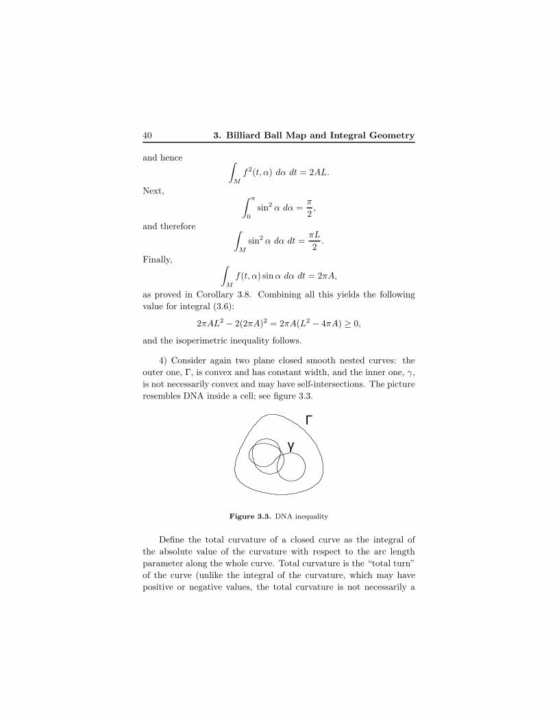
4) Consider again two plane closed smooth nested curves: the
outer one, Γ, is convex and has constant width, and the inner one, γ,
is not necessarily convex and may have self-intersections. The picture
resembles DNA inside a cell; see figure 3.3.
Γ
γ
Figure 3.3. DNA inequality
Define the total curvature of a closed curve as the integral of
the absolute value of the curvature with respect to the arc length
parameter along the whole curve. Total curvature is the “total turn”
of the curve (unlike the integral of the curvature, which may have
positive or negative values, the total curvature is not necessarily a
3. Billiard Ball Map and Integral Geometry 41
multiple of 2π). The average absolute curvature of a curve is the total
curvature divided by the length.
One has the following DNA geometric inequality.
Theorem 3.15. The average absolute curvature of Γ is not greater
than the average absolute curvature of γ.
Proof. We already know that the length of Γ is πd, and its total
curvature is 2π. Denote the total curvature of γ by C, and let L be
its length. We want to prove that
(3.7)C
L≥ 2
d.
As before, let N be the space of oriented lines intersecting Γ with its
coordinates (ϕ, p). Give γ an orientation and define a locally constant
function q(ϕ) on the circle as the number of oriented tangent lines to
γ having direction ϕ. One has the following integral formula for the
total curvature:
(3.8) C =
∫ 2π
0
q(ϕ) dϕ.
Indeed, if t is the arc length parameter on γ and ϕ the direction of its
tangent line, then the curvature is k = dϕ/dt. The total curvature
∫ L
0
|k|dt =
∫ L
0
∣∣∣∣dϕ
dt
∣∣∣∣ dt
is the total variation of ϕ. This implies (3.8).
We use the Crofton formula to evaluate L. The crucial observa-
tion is that
(3.9) nγ(ϕ, p) ≤ q(ϕ) + q(ϕ+ π)
for all p, ϕ. Indeed, between two consecutive intersections of γ with a
line whose coordinates are (ϕ, p), the tangent line to γ at least once
has the direction of ϕ or ϕ + π; this is, essentially, Rolle’s theorem
(see figure 3.4).
As before, denote the support function of Γ by p(ϕ). It remains to
integrate the inequality (3.9) taking into account the Crofton formula
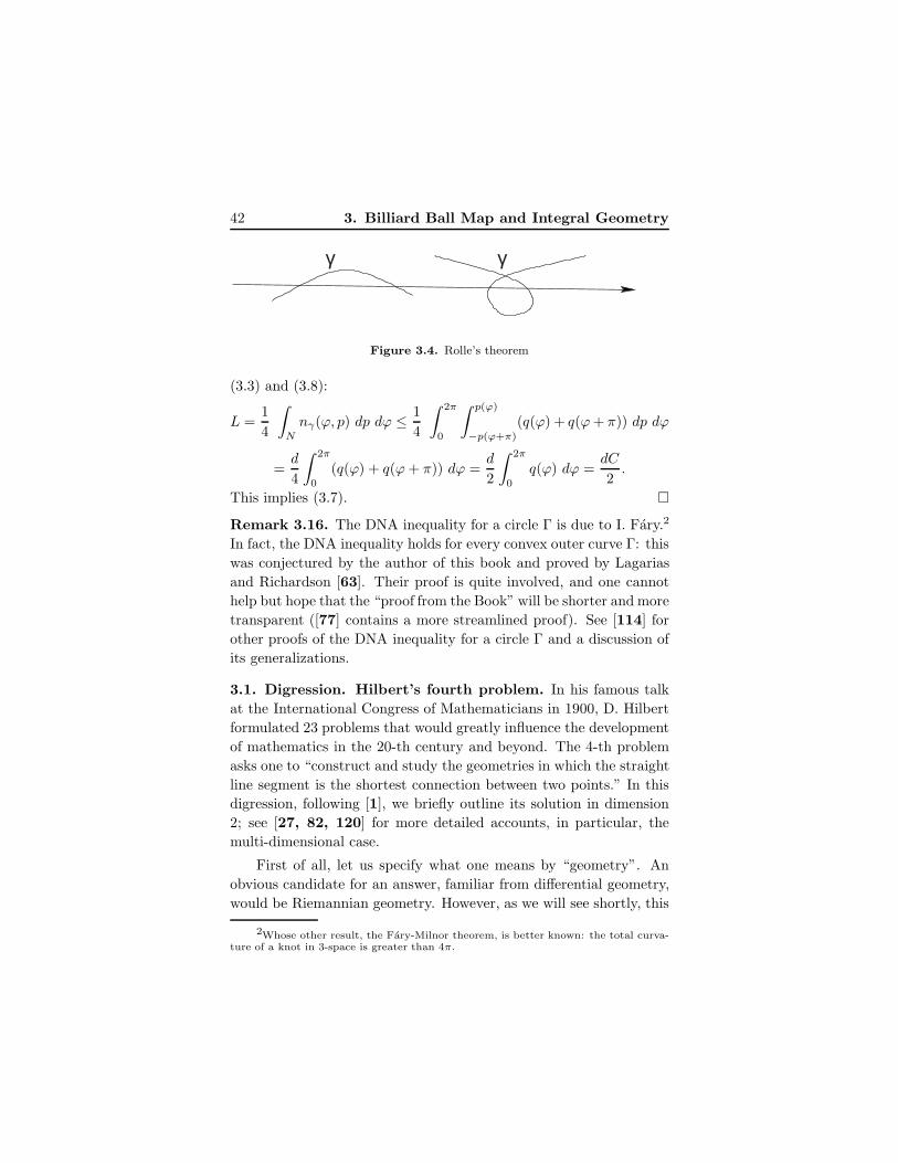
42 3. Billiard Ball Map and Integral Geometry
γ γ
Figure 3.4. Rolle’s theorem
(3.3) and (3.8):
L =1
4
∫
N
nγ(ϕ, p) dp dϕ ≤ 1
4
∫ 2π
0
∫ p(ϕ)
−p(ϕ+π)
(q(ϕ) + q(ϕ+ π)) dp dϕ
=d
4
∫ 2π
0
(q(ϕ) + q(ϕ+ π)) dϕ =d
2
∫ 2π
0
q(ϕ) dϕ =dC
2.
This implies (3.7).
Remark 3.16. The DNA inequality for a circle Γ is due to I. Fary.2
In fact, the DNA inequality holds for every convex outer curve Γ: this
was conjectured by the author of this book and proved by Lagarias
and Richardson [63]. Their proof is quite involved, and one cannot
help but hope that the “proof from the Book” will be shorter and more
transparent ([77] contains a more streamlined proof). See [114] for
other proofs of the DNA inequality for a circle Γ and a discussion of
its generalizations.
3.1. Digression. Hilbert’s fourth problem. In his famous talk
at the International Congress of Mathematicians in 1900, D. Hilbert
formulated 23 problems that would greatly influence the development
of mathematics in the 20-th century and beyond. The 4-th problem
asks one to “construct and study the geometries in which the straight
line segment is the shortest connection between two points.” In this
digression, following [1], we briefly outline its solution in dimension
2; see [27, 82, 120] for more detailed accounts, in particular, the
multi-dimensional case.
First of all, let us specify what one means by “geometry”. An
obvious candidate for an answer, familiar from differential geometry,
would be Riemannian geometry. However, as we will see shortly, this
2Whose other result, the Fary-Milnor theorem, is better known: the total curva-ture of a knot in 3-space is greater than 4π.
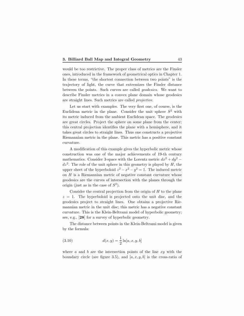
3. Billiard Ball Map and Integral Geometry 43
would be too restrictive. The proper class of metrics are the Finsler
ones, introduced in the framework of geometrical optics in Chapter 1.
In these terms, “the shortest connection between two points” is the
trajectory of light, the curve that extremizes the Finsler distance
between the points. Such curves are called geodesics. We want to
describe Finsler metrics in a convex plane domain whose geodesics
are straight lines. Such metrics are called projective.
Let us start with examples. The very first one, of course, is the
Euclidean metric in the plane. Consider the unit sphere S2 with
its metric induced from the ambient Euclidean space. The geodesics
are great circles. Project the sphere on some plane from the center;
this central projection identifies the plane with a hemisphere, and it
takes great circles to straight lines. Thus one constructs a projective
Riemannian metric in the plane. This metric has a positive constant
curvature.
A modification of this example gives the hyperbolic metric whose
construction was one of the major achievements of 19-th century
mathematics. Consider 3-space with the Lorentz metric dx2 + dy2 −dz2. The role of the unit sphere in this geometry is played by H , the
upper sheet of the hyperboloid z2 − x2 − y2 = 1. The induced metric
on H is a Riemannian metric of negative constant curvature whose
geodesics are the curves of intersection with the planes through the
origin (just as in the case of S2).
Consider the central projection from the origin of H to the plane
z = 1. The hyperboloid is projected onto the unit disc, and the
geodesics project to straight lines. One obtains a projective Rie-
mannian metric in the unit disc; this metric has a negative constant
curvature. This is the Klein-Beltrami model of hyperbolic geometry;
see, e.g., [28] for a survey of hyperbolic geometry.
The distance between points in the Klein-Beltrami model is given
by the formula:
(3.10) d(x, y) =1
2ln[a, x, y, b]
where a and b are the intersection points of the line xy with the
boundary circle (see figure 3.5), and [a, x, y, b] is the cross-ratio of
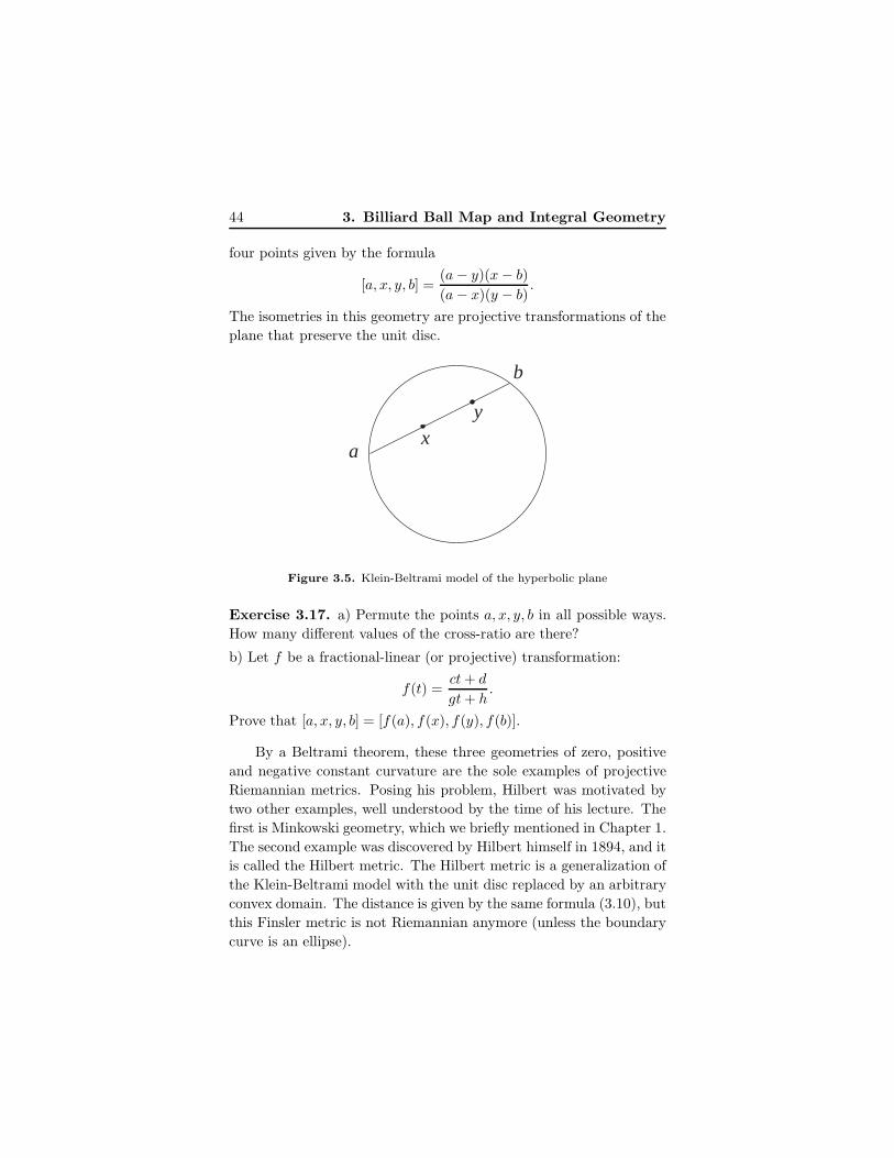
44 3. Billiard Ball Map and Integral Geometry
four points given by the formula
[a, x, y, b] =(a− y)(x− b)
(a− x)(y − b).
The isometries in this geometry are projective transformations of the
plane that preserve the unit disc.
a
b
xy
Figure 3.5. Klein-Beltrami model of the hyperbolic plane
Exercise 3.17. a) Permute the points a, x, y, b in all possible ways.
How many different values of the cross-ratio are there?
b) Let f be a fractional-linear (or projective) transformation:
f(t) =ct+ d
gt+ h.
Prove that [a, x, y, b] = [f(a), f(x), f(y), f(b)].
By a Beltrami theorem, these three geometries of zero, positive
and negative constant curvature are the sole examples of projective
Riemannian metrics. Posing his problem, Hilbert was motivated by
two other examples, well understood by the time of his lecture. The
first is Minkowski geometry, which we briefly mentioned in Chapter 1.
The second example was discovered by Hilbert himself in 1894, and it
is called the Hilbert metric. The Hilbert metric is a generalization of
the Klein-Beltrami model with the unit disc replaced by an arbitrary
convex domain. The distance is given by the same formula (3.10), but
this Finsler metric is not Riemannian anymore (unless the boundary
curve is an ellipse).
3. Billiard Ball Map and Integral Geometry 45
Exercise 3.18. Verify the triangle inequality in the Hilbert metric.
Before we formulate a solution for Hilbert’s fourth problem, let
us make one last preparation. A Finsler metric can be described by a
Lagrangian function L(x, v) on tangent vectors that gives the Finsler
length of a vector v with foot point x. We assume that L is positive for
all v 6= 0 and homogeneous of degree one: L(x, tv) = |t|L(x, v) for all
real t. The indicatrix at point x is the unit level curve of the function
L(x, ·). For example, L(x, v) = |v| describes the Euclidean metric. In
Minkowski geometry, L does not depend on x. For a smooth curve
γ : [a, b] →M , its Finsler length is given by
L(γ) =
∫ b
a
L(γ(t), γ′(t)) dt.
Due to homogeneity of L, this integral does not depend on the pa-
rameterization.
Exercise 3.19. Compute the Lagrangian functions for the projective
metrics of positive and negative constant curvatures in the plane.
The solution for Hilbert’s fourth problem is based on the Crofton
formula (3.3). Let f(p, ϕ) be a positive continuous function on the
space of oriented lines, even with respect to the orientation reversion
of a line: f(−p, ϕ + π) = f(p, ϕ). Then one has a new area form:
Ωf = f(p, ϕ) dϕ ∧ dp.Theorem 3.20. The formula
(3.11) length (γ) =1
4
∫ ∫nγ(ϕ, p)f(p, ϕ) dϕ dp
defines a projective Finsler metric. In other words, one replaces Ω in
the Crofton formula (3.3) with Ωf .
Proof. To prove that the geodesics are straight lines one needs to
check the triangle inequality: the sum of lengths of two sides of a
triangle is greater than the length of the third side. This holds because
every line, intersecting the third side, also intersects the first or the
second.
Applying (3.11) to an infinitesimal segment, one finds the La-
grangian function of the respective Finsler metric. Let (x1, x2) be
46 3. Billiard Ball Map and Integral Geometry
Cartesian coordinates in the plane and (v1, v2) be the coordinates of
the tangent vector. Then
L(x1, x2, v1, v2) =1
4
∫ 2π
0
|v1 cosα+v2 sinα| f(x1 cosα+x2 sinα, α) dα.
Exercise 3.21. Prove this formula.
In fact, every projective Finsler metric is given as in Theorem 3.20.
This means that in each projective Finsler geometry one has a version
of the Crofton formula.
The following exercise describes a result of Hamel, a student of
Hilbert, obtained in 1901, shortly after Hilbert’s ICM talk.
Exercise 3.22. A Lagrangian L(x1, x2, v1, v2) defines a projective
Finsler metric if and only if
∂2L
∂x1∂v2=
∂2L
∂x2∂v1.
Remark 3.23. A “magnetic” version of Hilbert’s fourth problem is
considered in [115], where Finsler metrics in the plane are described
such that their geodesics are circles of a fixed radius. It turns out that
there is an abundance of “exotic” Finsler metrics with this property.
♣
Let us now discuss the phase space of the billiard ball map and
the space of oriented lines in the multi-dimensional setup.
Let Q be a smooth hypersurface in Euclidean space. We identify
the tangent and cotangent vector to Q by the Euclidean structure
and, when convenient, make no distinction between TQ and T ∗Q. A
choice of local coordinates qi in Q provides local coordinates pi = dqiin the covector space TqQ and therefore local coordinates (q, p) in the
cotangent bundle T ∗Q.3 We will use vector notation: if x, y ∈ Rn
then
xy = x1y1 + ...+ xnyn, xdy = x1dy1 + ...+ xndyn,
dx ∧ dy = dx1 ∧ dy1 + ...+ dxn ∧ dyn, etc.
3Covectors p are called momenta in physics.
3. Billiard Ball Map and Integral Geometry 47
The cotangent bundle T ∗Q carries a canonical differential 1-form
λ, called the Liouville or the tautological form. Denote the projection
T ∗Q → Q by π. Let ξ be a tangent vector to T ∗Q at point (q, p).
Then ν := dπ(ξ) is a tangent vector to Q at q, and one defines the
Liouville form by the formula:
(3.12) λ(ξ) = p(ν).
Exercise 3.24. Verify that, in local coordinates, the Liouville form
is given by the formula pdq.
The differential dλ = ω is a differential 2-form on T ∗Q. By
Exercise 3.24, this 2-form is written, in local coordinates, as dp ∧dq and therefore is non-degenerate. A closed and non-degenerate
differential 2-form is called a symplectic form or a symplectic structure.
Thus the cotangent bundle of a smooth manifold carries a canonical
symplectic structure. Note that this structure does not depend on
the metric or any other additional structures on the manifold.
A symplectic structure determines on a smooth manifold a non-
degenerate skew-symmetric bilinear form on each tangent space. Such
a form can exist only on an even-dimensional space. Hence a symplec-
tic manifold is always even-dimensional. A symplectic structure ω on
a manifold M2n gives rise to a volume form ωn. Thus a symplectic
manifold has a canonical volume form and hence a measure.
Consider a domain D ⊂ Rn, a billiard table, with smooth bound-
ary Qn−1. As before, the phase space M of the billiard ball map con-
sists of unit tangent vectors (q, v) with foot point q ∈ Q and inward
direction. Let v be the orthogonal projection of v on the tangent hy-
perplane TqQ. This projection identifies M with the space of tangent
(co)vectors to Q whose magnitude does not exceed 1. Let ω and λ
be the symplectic structure and the Liouville 1-form on T ∗Q, pulled
back to M .
Lemma 3.1 holds without change. The proof follows from the
formula T ∗(λ) − λ = df where f is the free path of the billiard ball,
and this formula is proved similarly to Lemma 3.1. One has an analog
of Corollary 3.8: the mean free path in the billiard table equals
CVol(D)
Area(Q)
48 3. Billiard Ball Map and Integral Geometry
where the constant C depends only on the dimension n and equals
the ratio of the area of the unit sphere Sn−1 and the volume of the
unit ball Bn−1.
The space N of oriented lines in Rn again plays the main role.
As before, a line is characterized by its unit vector q and the perpen-
dicular vector p dropped from the origin to the line. One can think of
q as a point of the unit sphere Sn−1 and p as a tangent (co)vector to
Sn−1 at q. Thus one identifies N with T ∗Sn−1. Let Ω = dp ∧ dq be
the canonical symplectic structure (whose particular case is the area
form on the space of lines in the plane).
Lemma 3.7 also holds without change. Thus, for convex billiard
tables D, the billiard ball map is a symplectic transformation of the
space of oriented lines that intersect D.
We have only scratched the surface of symplectic geometry; see
[3, 7, 15, 67] for an exposition. The following exercise provides
further insight into this important subject.
Exercise 3.25. a) Let (M2n, ω) be a symplectic manifold and L ⊂M a submanifold. Assume that the restriction of ω on L vanishes.
Prove that dimL ≤ n. If dimL = n, then L is called a Lagrangian
submanifold.
b) Let Q be a smooth oriented hypersurface in Rn, and let L be
the set of oriented lines orthogonal to Q. Prove that L ⊂ N is a
Lagrangian submanifold.
3.2. Digression. Symplectic reduction. The construction that
derives the symplectic structure on the space of oriented lines from
the symplectic structure on the cotangent bundle of the ambient space
is called the symplectic reduction. This is a very general and simple
construction, and we describe it here.
Let (M2n, ω) be a symplectic manifold and S ⊂ M a hypersur-
face. Since S is odd-dimensional, the restriction of ω on S cannot be
non-degenerate. This restriction has a 1-dimensional kernel, and S is
foliated by curves having the directions of these kernels. This is the
characteristic foliation of the hypersurface S.
Assume that the space of characteristic curves is itself a smooth
manifold, say, N (locally, this is always the case). The symplectic
3. Billiard Ball Map and Integral Geometry 49
form ω descends from M to N to a new closed 2-form Ω which is
non-degenerate, since the kernel of the restriction of ω to S is factored
out. This is symplectic reduction of ω.
In the case at hand, we start with the cotangent bundle M =
T ∗Rn and its canonical symplectic structure ω. Let (x, y) be coordi-
nates in T ∗Rn (instead of (q, p) which will be used as coordinates in
the space of lines) so that ω = dx ∧ dy. The hypersurface S consists
of unit (co)vectors |y|2 = 1. Hence the 1-form ydy vanishes on S.
Given a unit tangent vector (x, y), the respective rectilinear mo-
tion is described by the vector field y∂x. Let ξ be an arbitrary tangent
test vector to S; then
(dx ∧ dy)(y∂x, ξ) = (ydy)(ξ) = 0
since ydy = 0 on S. Therefore the vector field y∂x has the charac-
teristic direction. We conclude that the characteristic curves on S
consist of unit tangent vectors (x, y) with foot point on a line and
y tangent to this line. Thus the quotient space N is the space of
oriented lines.
To describe the symplectic structure Ω, the result of symplectic
reduction, embed N into M by assigning to a line its closest point to
the origin; in formulas, x = p, y = q. Then the form dx∧ dy becomes
dp ∧ dq, which is just the canonical symplectic form on the space of
oriented lines in Rn.
Symplectic reduction applies, in particular, to projective Finsler
metrics. Given such a metric, one obtains a symplectic form on the
space of oriented lines. In dimension 2, we discussed how to construct
a projective Finsler metric from such a form in Digression 3.1. Sym-
plectic reduction provides a link in the opposite direction and recovers
the area form on the space of lines from the metric.
Example 3.26. The unit sphere gives a good example of the area
form on the space of oriented geodesics. An oriented geodesic on S2 is
a great circle; oriented great circles are in one-to-one correspondence
with points of the sphere: this is the pole-equator correspondence; see
also figure 9.3. Thus the space of oriented geodesics is S2 itself, and
the area form on the space of geodesics is identified with the standard
area form on the unit sphere.
50 3. Billiard Ball Map and Integral Geometry
A similar construction applies to the hyperbolic plane. An ori-
ented geodesic on the hyperboloid z2 − x2 − y2 = 1 is its intersection
with an oriented plane through the origin. The orthogonal comple-
ment to the plane with respect to the Lorentz quadratic form is an
oriented line. The positive half-line intersects the hyperboloid of one
sheet x2 + y2 − z2 = 1 in a unique point. Thus the space of oriented
geodesics on H2 identifies with the hyperboloid of one sheet, and the
area form on the space of geodesics is identified with the standard
area form on this hyperboloid. An industrious reader is invited to
make the computations behind these claims. ♣
Chapter 4
Billiards inside Conicsand Quadrics
The material in this chapter spans about 2,000 years: optical proper-
ties of conics were already known to ancient Greeks, whereas complete
integrability of the geodesic flow on the ellipsoid is a discovery of 19-th
century mathematics (Jacobi for a three-axial ellipsoid).
Recall the geometric definition of an ellipse: it is the locus of
points whose sum of distances to two given points is fixed; these two
points are called the foci. An ellipse can be constructed using a string
whose ends are fixed at the foci – the method that carpenters and
gardeners actually use; see figure 4.1. A hyperbola is defined similarly
with the sum of distances replaced by the absolute value of their
difference, and a parabola is the set of points at equal distances from
a given point (the focus) and a given line (the directrix). Ellipses,
hyperbolas and parabolas all have second order equations in Cartesian
coordinates.
Exercise 4.1. Consider the ellipse with foci at points (−c, 0) and
(c, 0) and the length of the string 2L. Show that its equation is
(4.1)x2
1
L2+
x22
L2 − c2= 1.
An immediate consequence is the following optical property of
conics.
51
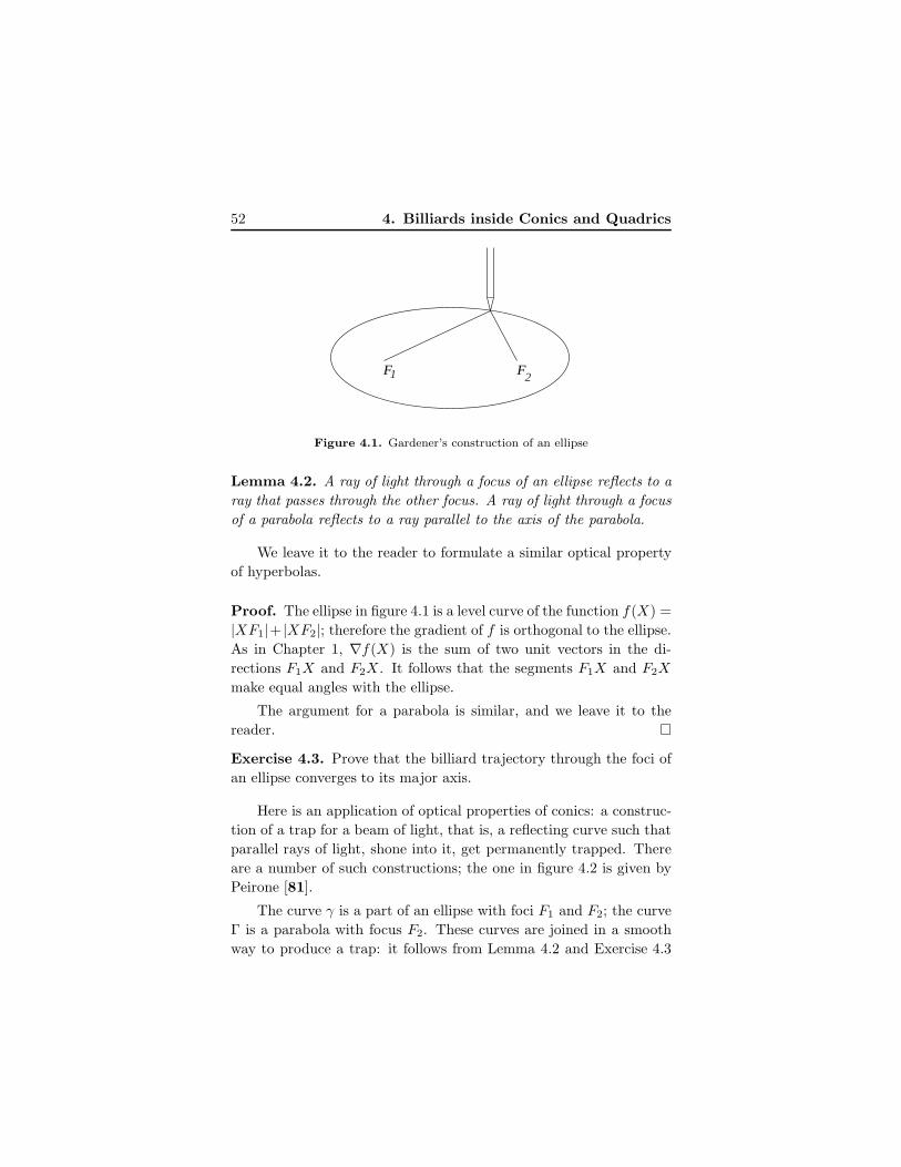
52 4. Billiards inside Conics and Quadrics
F F1 2
Figure 4.1. Gardener’s construction of an ellipse
Lemma 4.2. A ray of light through a focus of an ellipse reflects to a
ray that passes through the other focus. A ray of light through a focus
of a parabola reflects to a ray parallel to the axis of the parabola.
We leave it to the reader to formulate a similar optical property
of hyperbolas.
Proof. The ellipse in figure 4.1 is a level curve of the function f(X) =
|XF1|+ |XF2|; therefore the gradient of f is orthogonal to the ellipse.
As in Chapter 1, ∇f(X) is the sum of two unit vectors in the di-
rections F1X and F2X . It follows that the segments F1X and F2X
make equal angles with the ellipse.
The argument for a parabola is similar, and we leave it to the
reader.
Exercise 4.3. Prove that the billiard trajectory through the foci of
an ellipse converges to its major axis.
Here is an application of optical properties of conics: a construc-
tion of a trap for a beam of light, that is, a reflecting curve such that
parallel rays of light, shone into it, get permanently trapped. There
are a number of such constructions; the one in figure 4.2 is given by
Peirone [81].
The curve γ is a part of an ellipse with foci F1 and F2; the curve
Γ is a parabola with focus F2. These curves are joined in a smooth
way to produce a trap: it follows from Lemma 4.2 and Exercise 4.3
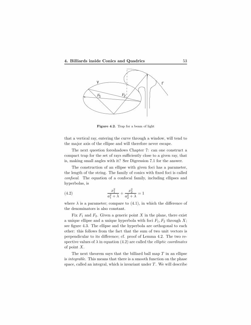
4. Billiards inside Conics and Quadrics 53
2 1 F
Γ γ
F
Figure 4.2. Trap for a beam of light
that a vertical ray, entering the curve through a window, will tend to
the major axis of the ellipse and will therefore never escape.
The next question foreshadows Chapter 7: can one construct a
compact trap for the set of rays sufficiently close to a given ray, that
is, making small angles with it? See Digression 7.1 for the answer.
The construction of an ellipse with given foci has a parameter,
the length of the string. The family of conics with fixed foci is called
confocal. The equation of a confocal family, including ellipses and
hyperbolas, is
(4.2)x2
1
a21 + λ
+x2
2
a22 + λ
= 1
where λ is a parameter; compare to (4.1), in which the difference of
the denominators is also constant.
Fix F1 and F2. Given a generic point X in the plane, there exist
a unique ellipse and a unique hyperbola with foci F1, F2 through X ;
see figure 4.3. The ellipse and the hyperbola are orthogonal to each
other: this follows from the fact that the sum of two unit vectors is
perpendicular to its difference; cf. proof of Lemma 4.2. The two re-
spective values of λ in equation (4.2) are called the elliptic coordinates
of point X .
The next theorem says that the billiard ball map T in an ellipse
is integrable. This means that there is a smooth function on the phase
space, called an integral, which is invariant under T . We will describe
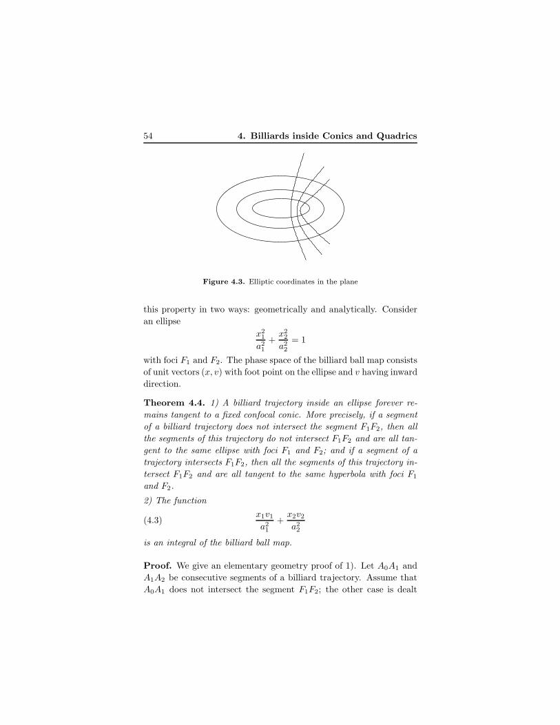
54 4. Billiards inside Conics and Quadrics
Figure 4.3. Elliptic coordinates in the plane
this property in two ways: geometrically and analytically. Consider
an ellipse
x21
a21
+x2
2
a22
= 1
with foci F1 and F2. The phase space of the billiard ball map consists
of unit vectors (x, v) with foot point on the ellipse and v having inward
direction.
Theorem 4.4. 1) A billiard trajectory inside an ellipse forever re-
mains tangent to a fixed confocal conic. More precisely, if a segment
of a billiard trajectory does not intersect the segment F1F2, then all
the segments of this trajectory do not intersect F1F2 and are all tan-
gent to the same ellipse with foci F1 and F2; and if a segment of a
trajectory intersects F1F2, then all the segments of this trajectory in-
tersect F1F2 and are all tangent to the same hyperbola with foci F1
and F2.
2) The function
(4.3)x1v1a21
+x2v2a22
is an integral of the billiard ball map.
Proof. We give an elementary geometry proof of 1). Let A0A1 and
A1A2 be consecutive segments of a billiard trajectory. Assume that
A0A1 does not intersect the segment F1F2; the other case is dealt
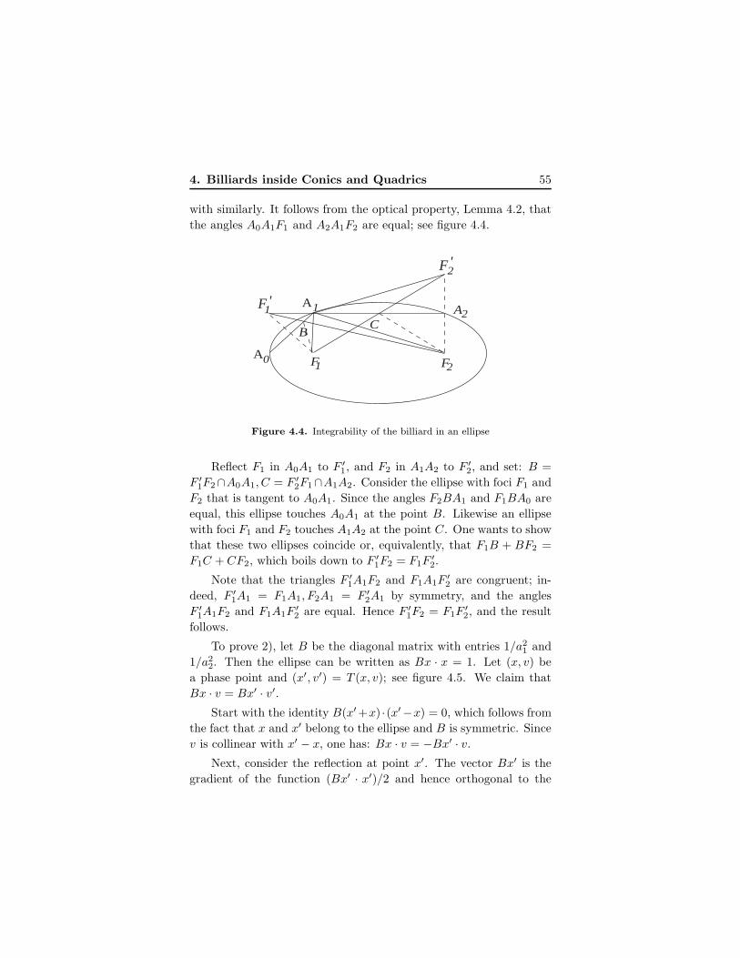
4. Billiards inside Conics and Quadrics 55
with similarly. It follows from the optical property, Lemma 4.2, that
the angles A0A1F1 and A2A1F2 are equal; see figure 4.4.
2
1 21A
0A21
CB
FF
AF '
F '
Figure 4.4. Integrability of the billiard in an ellipse
Reflect F1 in A0A1 to F ′1, and F2 in A1A2 to F ′
2, and set: B =
F ′1F2∩A0A1, C = F ′
2F1∩A1A2. Consider the ellipse with foci F1 and
F2 that is tangent to A0A1. Since the angles F2BA1 and F1BA0 are
equal, this ellipse touches A0A1 at the point B. Likewise an ellipse
with foci F1 and F2 touches A1A2 at the point C. One wants to show
that these two ellipses coincide or, equivalently, that F1B + BF2 =
F1C + CF2, which boils down to F ′1F2 = F1F
′2.
Note that the triangles F ′1A1F2 and F1A1F
′2 are congruent; in-
deed, F ′1A1 = F1A1, F2A1 = F ′
2A1 by symmetry, and the angles
F ′1A1F2 and F1A1F
′2 are equal. Hence F ′
1F2 = F1F′2, and the result
follows.
To prove 2), let B be the diagonal matrix with entries 1/a21 and
1/a22. Then the ellipse can be written as Bx · x = 1. Let (x, v) be
a phase point and (x′, v′) = T (x, v); see figure 4.5. We claim that
Bx · v = Bx′ · v′.Start with the identity B(x′+x) ·(x′−x) = 0, which follows from
the fact that x and x′ belong to the ellipse and B is symmetric. Since
v is collinear with x′ − x, one has: Bx · v = −Bx′ · v.Next, consider the reflection at point x′. The vector Bx′ is the
gradient of the function (Bx′ · x′)/2 and hence orthogonal to the
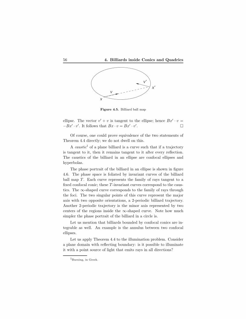
56 4. Billiards inside Conics and Quadrics
x
vx'
v'
Figure 4.5. Billiard ball map
ellipse. The vector v′ + v is tangent to the ellipse; hence Bx′ · v =
−Bx′ · v′. It follows that Bx · v = Bx′ · v′.
Of course, one could prove equivalence of the two statements of
Theorem 4.4 directly; we do not dwell on this.
A caustic1 of a plane billiard is a curve such that if a trajectory
is tangent to it, then it remains tangent to it after every reflection.
The caustics of the billiard in an ellipse are confocal ellipses and
hyperbolas.
The phase portrait of the billiard in an ellipse is shown in figure
4.6. The phase space is foliated by invariant curves of the billiard
ball map T . Each curve represents the family of rays tangent to a
fixed confocal conic; these T -invariant curves correspond to the caus-
tics. The ∞-shaped curve corresponds to the family of rays through
the foci. The two singular points of this curve represent the major
axis with two opposite orientations, a 2-periodic billiard trajectory.
Another 2-periodic trajectory is the minor axis represented by two
centers of the regions inside the ∞-shaped curve. Note how much
simpler the phase portrait of the billiard in a circle is.
Let us mention that billiards bounded by confocal conics are in-
tegrable as well. An example is the annulus between two confocal
ellipses.
Let us apply Theorem 4.4 to the illumination problem. Consider
a plane domain with reflecting boundary: is it possible to illuminate
it with a point source of light that emits rays in all directions?
1Burning, in Greek.
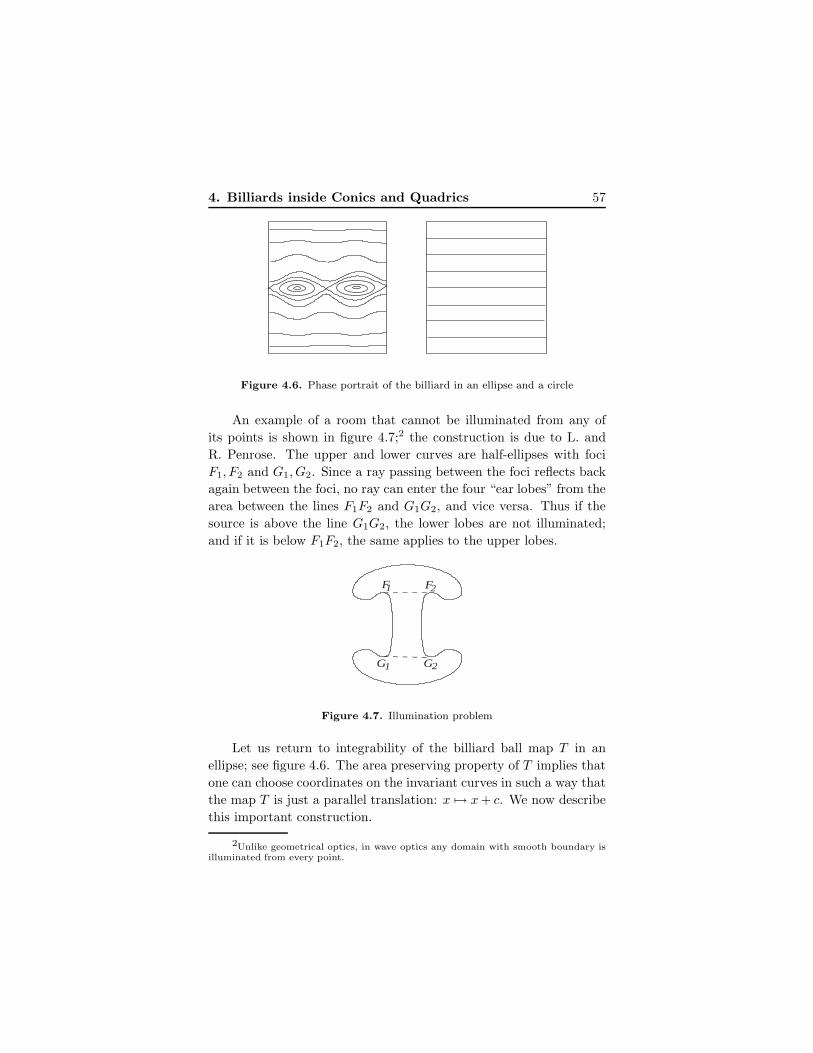
4. Billiards inside Conics and Quadrics 57
Figure 4.6. Phase portrait of the billiard in an ellipse and a circle
An example of a room that cannot be illuminated from any of
its points is shown in figure 4.7;2 the construction is due to L. and
R. Penrose. The upper and lower curves are half-ellipses with foci
F1, F2 and G1, G2. Since a ray passing between the foci reflects back
again between the foci, no ray can enter the four “ear lobes” from the
area between the lines F1F2 and G1G2, and vice versa. Thus if the
source is above the line G1G2, the lower lobes are not illuminated;
and if it is below F1F2, the same applies to the upper lobes.
2G1G
2F1F
Figure 4.7. Illumination problem
Let us return to integrability of the billiard ball map T in an
ellipse; see figure 4.6. The area preserving property of T implies that
one can choose coordinates on the invariant curves in such a way that
the map T is just a parallel translation: x 7→ x+ c. We now describe
this important construction.
2Unlike geometrical optics, in wave optics any domain with smooth boundary isilluminated from every point.
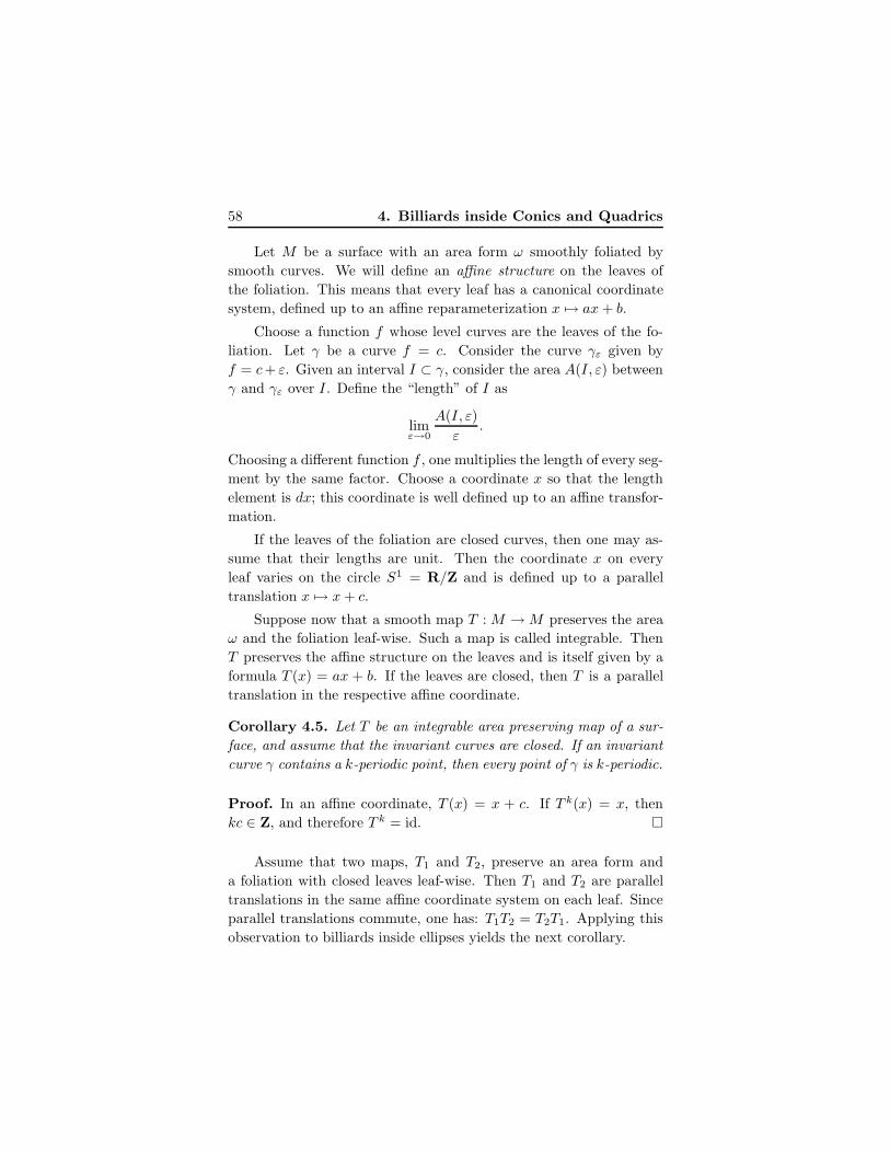
58 4. Billiards inside Conics and Quadrics
Let M be a surface with an area form ω smoothly foliated by
smooth curves. We will define an affine structure on the leaves of
the foliation. This means that every leaf has a canonical coordinate
system, defined up to an affine reparameterization x 7→ ax+ b.
Choose a function f whose level curves are the leaves of the fo-
liation. Let γ be a curve f = c. Consider the curve γε given by
f = c+ ε. Given an interval I ⊂ γ, consider the area A(I, ε) between
γ and γε over I. Define the “length” of I as
limε→0
A(I, ε)
ε.
Choosing a different function f , one multiplies the length of every seg-
ment by the same factor. Choose a coordinate x so that the length
element is dx; this coordinate is well defined up to an affine transfor-
mation.
If the leaves of the foliation are closed curves, then one may as-
sume that their lengths are unit. Then the coordinate x on every
leaf varies on the circle S1 = R/Z and is defined up to a parallel
translation x 7→ x+ c.
Suppose now that a smooth map T : M →M preserves the area
ω and the foliation leaf-wise. Such a map is called integrable. Then
T preserves the affine structure on the leaves and is itself given by a
formula T (x) = ax + b. If the leaves are closed, then T is a parallel
translation in the respective affine coordinate.
Corollary 4.5. Let T be an integrable area preserving map of a sur-
face, and assume that the invariant curves are closed. If an invariant
curve γ contains a k-periodic point, then every point of γ is k-periodic.
Proof. In an affine coordinate, T (x) = x + c. If T k(x) = x, then
kc ∈ Z, and therefore T k = id.
Assume that two maps, T1 and T2, preserve an area form and
a foliation with closed leaves leaf-wise. Then T1 and T2 are parallel
translations in the same affine coordinate system on each leaf. Since
parallel translations commute, one has: T1T2 = T2T1. Applying this
observation to billiards inside ellipses yields the next corollary.
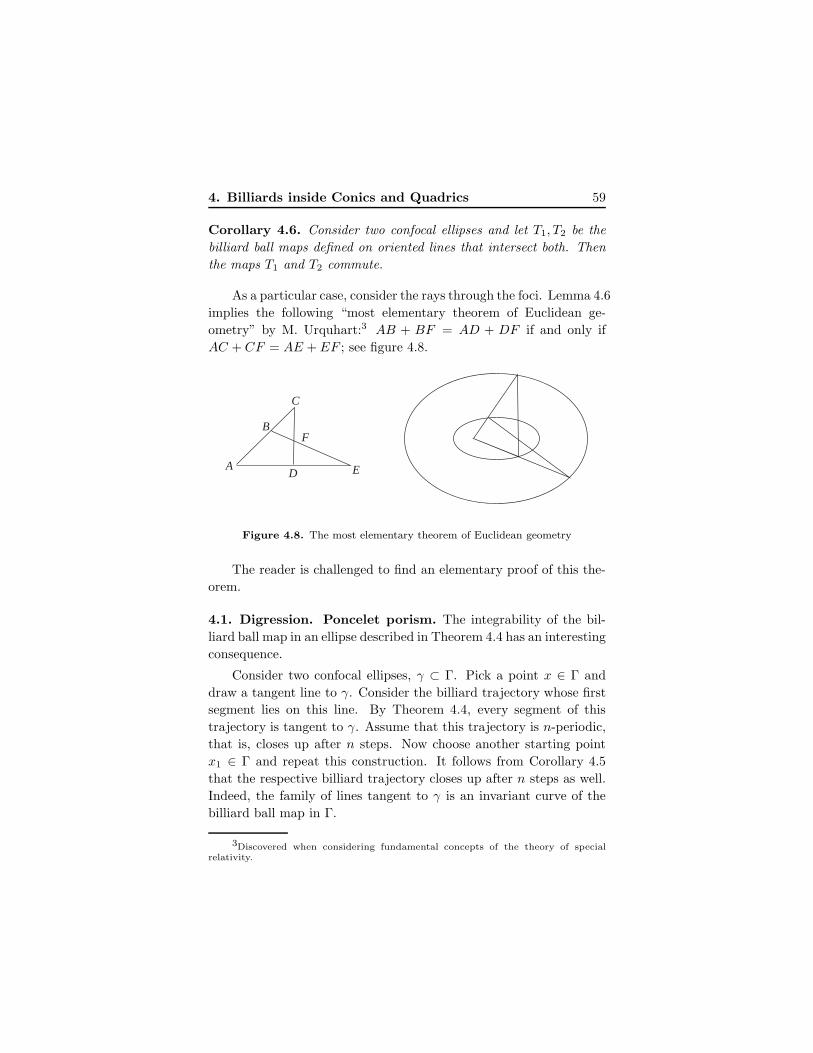
4. Billiards inside Conics and Quadrics 59
Corollary 4.6. Consider two confocal ellipses and let T1, T2 be the
billiard ball maps defined on oriented lines that intersect both. Then
the maps T1 and T2 commute.
As a particular case, consider the rays through the foci. Lemma 4.6
implies the following “most elementary theorem of Euclidean ge-
ometry” by M. Urquhart:3 AB + BF = AD + DF if and only if
AC + CF = AE + EF ; see figure 4.8.
A
B
C
F
D E
Figure 4.8. The most elementary theorem of Euclidean geometry
The reader is challenged to find an elementary proof of this the-
orem.
4.1. Digression. Poncelet porism. The integrability of the bil-
liard ball map in an ellipse described in Theorem 4.4 has an interesting
consequence.
Consider two confocal ellipses, γ ⊂ Γ. Pick a point x ∈ Γ and
draw a tangent line to γ. Consider the billiard trajectory whose first
segment lies on this line. By Theorem 4.4, every segment of this
trajectory is tangent to γ. Assume that this trajectory is n-periodic,
that is, closes up after n steps. Now choose another starting point
x1 ∈ Γ and repeat this construction. It follows from Corollary 4.5
that the respective billiard trajectory closes up after n steps as well.
Indeed, the family of lines tangent to γ is an invariant curve of the
billiard ball map in Γ.
3Discovered when considering fundamental concepts of the theory of specialrelativity.
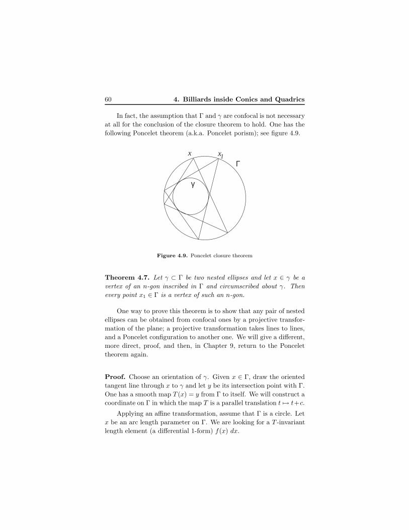
60 4. Billiards inside Conics and Quadrics
In fact, the assumption that Γ and γ are confocal is not necessary
at all for the conclusion of the closure theorem to hold. One has the
following Poncelet theorem (a.k.a. Poncelet porism); see figure 4.9.
Γ
γ
x x1
Figure 4.9. Poncelet closure theorem
Theorem 4.7. Let γ ⊂ Γ be two nested ellipses and let x ∈ γ be a
vertex of an n-gon inscribed in Γ and circumscribed about γ. Then
every point x1 ∈ Γ is a vertex of such an n-gon.
One way to prove this theorem is to show that any pair of nested
ellipses can be obtained from confocal ones by a projective transfor-
mation of the plane; a projective transformation takes lines to lines,
and a Poncelet configuration to another one. We will give a different,
more direct, proof, and then, in Chapter 9, return to the Poncelet
theorem again.
Proof. Choose an orientation of γ. Given x ∈ Γ, draw the oriented
tangent line through x to γ and let y be its intersection point with Γ.
One has a smooth map T (x) = y from Γ to itself. We will construct a
coordinate on Γ in which the map T is a parallel translation t 7→ t+c.
Applying an affine transformation, assume that Γ is a circle. Let
x be an arc length parameter on Γ. We are looking for a T -invariant
length element (a differential 1-form) f(x) dx.
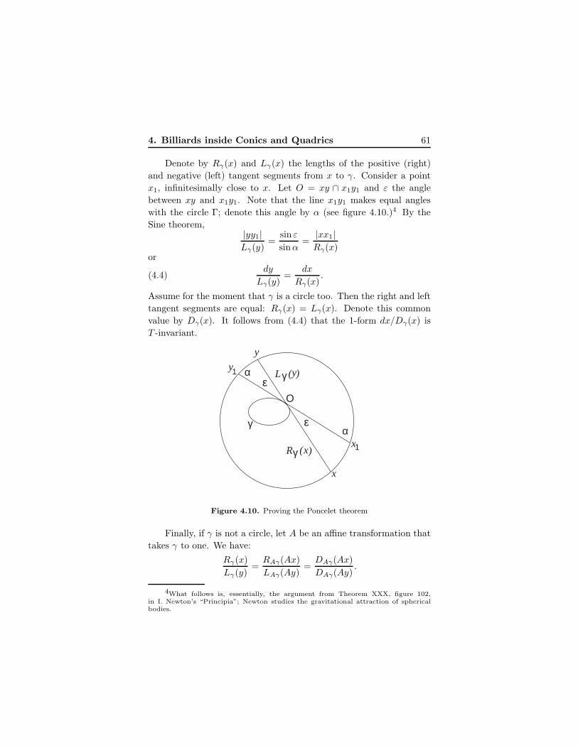
4. Billiards inside Conics and Quadrics 61
Denote by Rγ(x) and Lγ(x) the lengths of the positive (right)
and negative (left) tangent segments from x to γ. Consider a point
x1, infinitesimally close to x. Let O = xy ∩ x1y1 and ε the angle
between xy and x1y1. Note that the line x1y1 makes equal angles
with the circle Γ; denote this angle by α (see figure 4.10.)4 By the
Sine theorem,|yy1|Lγ(y)
=sin ε
sinα=
|xx1|Rγ(x)
or
(4.4)dy
Lγ(y)=
dx
Rγ(x).
Assume for the moment that γ is a circle too. Then the right and left
tangent segments are equal: Rγ(x) = Lγ(x). Denote this common
value by Dγ(x). It follows from (4.4) that the 1-form dx/Dγ(x) is
T -invariant.
)x(γR
)y(γL
γ
α
α
Ο
1y
y
1x
x
ε
ε
Figure 4.10. Proving the Poncelet theorem
Finally, if γ is not a circle, let A be an affine transformation that
takes γ to one. We have:
Rγ(x)
Lγ(y)=RAγ(Ax)
LAγ(Ay)=DAγ(Ax)
DAγ(Ay).
4What follows is, essentially, the argument from Theorem XXX, figure 102,in I. Newton’s “Principia”; Newton studies the gravitational attraction of sphericalbodies.
62 4. Billiards inside Conics and Quadrics
Setting f(x) = 1/DAγ(Ax), one obtains a T -invariant 1-form f(x) dx.
It remains to choose a coordinate t in which f(x) dx = dt. Then
the map T becomes a translation t → t + c, and Poncelet’s theorem
follows.
Exercise 4.8. Let Γ and γ be circles of radii R and r, and let a be
the distance between their centers.
a) Prove that one has a 3-periodic Poncelet configuration if and only
if a2 = R2 − 2rR.
b)* Prove that one has a 4-periodic Poncelet configuration if and only
if (R2 − a2)2 = 2r2(R2 + a2).
Necessary and sufficient conditions, in terms of two conics, for a
Poncelet polygon to close after n steps are due to Cayley; see [12].
Poncelet’s theorem has numerous proofs and generalizations; see
[18] for a thorough discussion. Poncelet discovered this result in 1813-
14, when he was a prisoner of war in the Russian city of Saratov; he
published his theorem in 1822, upon returning to France.
In conclusion of this digression, let us return to billiards in el-
lipses. Let Γ1,Γ2, . . . ,Γn be confocal ellipses and γ another confocal
ellipse inside them all. Let Ti be the billiard map in Γi considered as
a transformation of the space of oriented lines in the plane. Each Ti is
integrable, and these maps share invariant curves that consist of the
lines, tangent to confocal ellipses, such as γ. Hence we can choose an
affine parameter t on this invariant curve so that each Ti is a parallel
translation t 7→ t+ ci. Therefore, in the construction of the Poncelet
polygons, one could choose the first vertex on Γ1, the second on Γ2,
etc., the n-th on Γn: the conclusion of the closure theorem would hold
without change.5 ♣
The rest of this chapter is devoted to two closely related results:
complete integrability of the billiard ball map inside the ellipsoid and
of the geodesic flow on the ellipsoid. As the first step toward this goal
we discuss the notion of polar duality.
5An interesting addition to Poncelet’s theorem was recently made by R. Schwartz;see [92].
4. Billiards inside Conics and Quadrics 63
Let V be a vector space and V ∗ its dual. Every non-zero vector
x ∈ V determines an affine hyperplane Hx ⊂ V ∗ that consists of
covectors p such that p · x = 1 where the dot denotes the pairing
between vectors and covectors. Likewise, a non-zero covector p ∈ V ∗
determines a hyperplane Hp ⊂ V consisting of x ∈ V satisfying the
same equation.
Exercise 4.9. Show that x ∈ Hp if and only if p ∈ Hx.
Let M ⊂ V be a smooth star-shaped hypersurface; this means
that the position vector of every point x ∈ M is transverse to M .
The tangent plane at x is Hp for some p ∈ V ∗. The set of these p is
a hypersurface M∗ ⊂ V ∗ called polar dual to M . The next lemma
justifies the terminology.
Lemma 4.10. The hypersurface dual to M∗ is M .
Proof. Let v be a test tangent vector to M∗ at point p. We want to
show that v ∈ Hx. Since v is tangent to M∗, the covector p + εv is
ε2-close to M∗. Therefore, up to terms second order in ε, the covector
p + εv is dual to a point of M , infinitesimally close to x. Ignoring
terms of higher order in ε, write this point as x + εu where u is a
tangent vector to M at x. Thus one has
(p+ εv) · (x+ εu) = 1
and hence
v · x+ p · u = 0.
Since u ∈ Hp, one has p · u = 0. Hence v · x = 0, and therefore
v ∈ Hx.
The following example will be important for us.
Example 4.11. Let V be Euclidean space, A a self-adjoint linear
operator and M the quadric Ax ·x = 1. The gradient of the quadratic
function Ax ·x at point x is 2Ax; therefore the tangent hyperplane to
M at x is orthogonal to Ax. It follows that TxM = Hp with p = Ax.
The dual hypersurface M∗ is given by A−1p ·p = 1; in particular, M∗
is also a quadric.
64 4. Billiards inside Conics and Quadrics
Consider an ellipsoid M in Rn given by the equation
(4.5)x2
1
a21
+x2
2
a22
+ · · · + x2n
a2n
= 1,
and assume that all semiaxes a1, . . . , an are distinct. Let B be the
diagonal matrix with entries 1/a21, . . . , 1/a
2n, and set A = B−1. The
equation of M is Bx ·x = 1. We define the confocal family of quadrics
Mλ by the equation
(4.6)x2
1
a21 + λ
+x2
2
a22 + λ
+ · · · + x2n
a2n + λ
= 1
where λ is a real parameter. The topological type of Mλ changes as
λ passes the values −a2i . A shorthand formula for the confocal family
is
(A+ λE)−1x · x = 1,
where E is the unit matrix.
The next theorem by Jacobi extends the elliptic coordinates from
the plane to n-dimensional space.
Theorem 4.12. A generic point x ∈ Rn is contained in exactly n
quadrics confocal with the given ellipsoid. These confocal quadrics are
pairwise perpendicular at x.
Proof. We give two proofs, the first based on the notions of polar
duality and an eigenbasis of a quadratic form. The second one is
much more straightforward.
1) A quadric Mλ passes through x if and only if the hyperplane
Hx is tangent to the dual quadric M∗λ . Thus we want to show that
Hx is tangent to n quadric from the dual family M∗λ .
According to Example 4.11, M∗λ is given by equation (A+λE)p ·
p = 1. A normal vector to this hypersurface at point p is (A+ λE)p,
and a normal vector to the hyperplane Hx is x. Thus we are looking
for λ and p such that
(4.7) (A+ λE)p · p = 1, (A+ λE)p = µx.
Consider the quadratic form (1/2)(Ap · p − (p · x)2). This quadratic
form has an eigenbasis p1, . . . , pn with the eigenvalues −λ1, . . . ,−λn
4. Billiards inside Conics and Quadrics 65
such that Api − (pi · x)x = −λipi. Hence
(4.8) (A+ λiE)pi = (pi · x)x.Rescale pi so that pi · x = 1. Then (4.8) implies:
(A+ λiE)pi · pi = x · pi = 1,
and conditions (4.7) are satisfied.
Finally, the eigenvectors p1, . . . , pn are orthogonal, and so are the
hyperplanes Hp1, . . . , Hpn
tangent to the quadrics Mλ1, . . . ,Mλn
.
2) Consider equation (4.6), and assume that a21 < · · · < a2
n. Given
an x, we want to find λ satisfying this equation. This reduces to a
polynomial in λ of degree n, and one wants to show that all its roots
are real.
Consider the segment between a2i and a2
i+1. The left-hand side
F of (4.6) assumes the values −∞ and ∞ at the end point of this
interval; hence it also assumes the value 1. There are n − 1 such
intervals, and in addition, F varies from ∞ to 0 on the infinite interval
(a2n,∞). Hence the equation F = 1 has n roots λ1, . . . , λn, distinct
for a generic x.
Now we need to prove that the quadrics Mλiand Mλj
are or-
thogonal at point x. As in Example 4.11, consider the normal to
Mλi
ni =
(x1
a21 + λi
,x2
a22 + λi
, . . . ,xn
a2n + λi
).
Then
(4.9) ni · nj =x2
1
(a21 + λi)(a2
1 + λj)+ · · · + x2
n
(a2n + λi)(a2
n + λj).
Consider equations (4.6) for λi and λj . The difference of their left-
hand sides is equal to the right-hand side of (4.9) times (λj −λi), and
this right-hand side is zero. Therefore ni · nj = 0, as claimed.
The next theorem is due to Chasles.
Theorem 4.13. A generic line in Rn is tangent to (n− 1) distinct
quadrics from a given confocal family. The tangent hyperplanes to
these quadrics at the points of tangency with the line are pairwise
orthogonal.
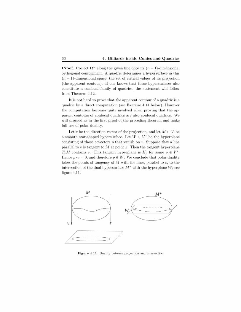
66 4. Billiards inside Conics and Quadrics
Proof. Project Rn along the given line onto its (n− 1)-dimensional
orthogonal complement. A quadric determines a hypersurface in this
(n − 1)-dimensional space, the set of critical values of its projection
(the apparent contour). If one knows that these hypersurfaces also
constitute a confocal family of quadrics, the statement will follow
from Theorem 4.12.
It is not hard to prove that the apparent contour of a quadric is a
quadric by a direct computation (see Exercise 4.14 below). However
the computation becomes quite involved when proving that the ap-
parent contours of confocal quadrics are also confocal quadrics. We
will proceed as in the first proof of the preceding theorem and make
full use of polar duality.
Let v be the direction vector of the projection, and let M ⊂ V be
a smooth star-shaped hypersurface. Let W ⊂ V ∗ be the hyperplane
consisting of those covectors p that vanish on v. Suppose that a line
parallel to v is tangent to M at point x. Then the tangent hyperplane
TxM contains v. This tangent hyperplane is Hp for some p ∈ V ∗.
Hence p ·v = 0, and therefore p ∈W . We conclude that polar duality
takes the points of tangency of M with the lines, parallel to v, to the
intersection of the dual hypersurface M∗ with the hyperplane W ; see
figure 4.11.
v
W
M*M
Figure 4.11. Duality between projection and intersection
4. Billiards inside Conics and Quadrics 67
On the other hand, the hyperplane W is the dual space to the
quotient space V/v (identified with the orthogonal complement to
v). Therefore the apparent contour of M in this quotient space is
polar dual to M∗ ∩ W . Recall Example 4.11: if M belongs to a
confocal family (A+ λE)−1x · x = 1, then M∗ belongs to the family
(A+ λE)p · p = 1. The intersection of the latter with a hyperplane is
a family of the same type, and therefore its polar dual is a confocal
family. This proves that the apparent contours of confocal quadrics
are also confocal quadrics.
Exercise 4.14. Show, by a direct computation, that the apparent
contour of a quadric Ax · x = 1 is a quadric.
Hint: The line y + tv is tangent to the quadric if and only if the
quadratic equation
A(y + tv) · (y + tv) = 1
has a multiple root in t. What is the discriminant of this equation?
Let M be a hypersurface in Rn. A geodesic curve on M is a
curve that locally minimizes the distance between its points. In other
words, a geodesic is a trajectory of light in M or a trajectory of a free
point confined to M . If γ(t) is an arc length parameterized geodesic,
then the acceleration vector γ′′(t) is orthogonal to M (physically, this
means that the only force acting on the point is the normal force that
confines the point to M). For example, a geodesic on the unit sphere
is its great circle. The motion of a free point is described by the
geodesic flow on the tangent bundle TM : given a vector (x, v), the
foot point x moves with the constant speed |v| along the geodesic in
the direction v and the velocity remains tangent to this geodesic.
The geodesic flow on the ellipsoid M ⊂ Rn is completely inte-
grable: it has n − 1 invariant functions. One of them is the energy
|v|2/2, and the other n−2 are described geometrically in the following
theorem.
Theorem 4.15. The tangent lines to a fixed geodesic on M are tan-
gent to (n− 2) other fixed quadrics confocal with M .
Proof. Let ℓ be a tangent line to M at point x. By Theorem 4.13,
ℓ is tangent to (n − 2) confocal quadrics N1, . . . , Nn−2. Consider
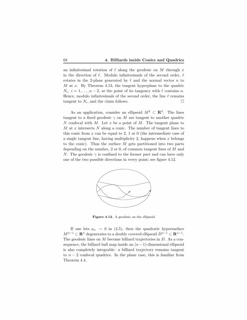
68 4. Billiards inside Conics and Quadrics
an infinitesimal rotation of ℓ along the geodesic on M through x
in the direction of ℓ. Modulo infinitesimals of the second order, ℓ
rotates in the 2-plane generated by ℓ and the normal vector n to
M at x. By Theorem 4.13, the tangent hyperplane to the quadric
Ni, i = 1, . . . , n − 2, at the point of its tangency with ℓ contains n.
Hence, modulo infinitesimals of the second order, the line ℓ remains
tangent to Ni, and the claim follows.
As an application, consider an ellipsoid M2 ⊂ R3. The lines
tangent to a fixed geodesic γ on M are tangent to another quadric
N confocal with M . Let x be a point of M . The tangent plane to
M at x intersects N along a conic. The number of tangent lines to
this conic from x can be equal to 2, 1 or 0 (the intermediate case of
a single tangent line, having multiplicity 2, happens when x belongs
to the conic). Thus the surface M gets partitioned into two parts
depending on the number, 2 or 0, of common tangent lines of M and
N . The geodesic γ is confined to the former part and can have only
one of the two possible directions in every point; see figure 4.12.
Figure 4.12. A geodesic on the ellipsoid
If one lets an → 0 in (4.5), then the quadratic hypersurface
Mn−1 ⊂ Rn degenerates to a doubly covered ellipsoid Dn−1 ⊂ Rn−1.
The geodesic lines on M become billiard trajectories in D. As a con-
sequence, the billiard ball map inside an (n−1)-dimensional ellipsoid
is also completely integrable: a billiard trajectory remains tangent
to n − 2 confocal quadrics. In the plane case, this is familiar from
Theorem 4.4.
4. Billiards inside Conics and Quadrics 69
Explicit formulas for the integrals of the billiard ball map in an
n-dimensional ellipsoid are as follows (cf. Theorem 4.4 for the plane
case). Let the ellipsoid be bounded by the hypersurface (4.5). Let
(x, v) be a phase point, a unit inward tangent vector whose foot point
x lies on the boundary. The following functions are invariant under
the billiard ball map:
Fi (x, v) = v2i +
∑
j 6=i
(vixj − vjxi)2
a2j − a2
i
, i = 1, . . . , n.
These functions are not independent: F1 + · · · + Fn = 1.
Let us add that the billiard ball map inside quadratic hyper-
surfaces is completely integrable in the spherical and hyperbolic ge-
ometries as well. One considers the unit (pseudo)sphere described
in Digression 3.1 and intersects it with a quadratic cone given by an
equation Ax · x = 0. The intersection is, by definition, a quadratic
hypersurface in the respective geometry.
For various approaches to complete integrability of the geodesic
flow on the ellipsoid and the billiard system inside the ellipsoid, see
[73, 72, 74, 112].
4.2. Digression. Complete integrability, Arnold-Liouville the-
orem. Recall that integrability of the billiard ball map inside an
ellipse implies strong restrictions on the behavior of the map: for
example, if an invariant curve contains an n-periodic point, then all
points are n-periodic. This follows from the area preserving property
of the billiard ball map.
Likewise, complete integrability of a symplectic map, such as the
billiard ball map, in multi-dimensional cases imposes severe restric-
tions on its dynamics. To formulate the relevant theorem, we need to
make another excursion to symplectic geometry; see [3, 7, 67].
Let (M,ω) be a symplectic manifold. The symplectic structure
identifies tangent and cotangent vectors: a vector u determines a
linear function v 7→ ω(u, v). Let f be a smooth function on M . The
differential df is a 1-form which therefore corresponds to a vector field
Xf . This field is called a Hamiltonian vector field and the function f a
Hamiltonian function. This resembles a more familiar construction of
70 4. Billiards inside Conics and Quadrics
the gradient of a function f which is a vector field associated with df
by a Euclidean structure (or, more generally, a Riemannian metric),
and Xf is sometimes called the symplectic gradient of f .
One can define a binary operation on smooth functions on a sym-
plectic manifold called the Poisson bracket and denoted by f, g.The Poisson bracket of two functions is the directional derivative of
one of them along the Hamiltonian vector field of the other:
f, g = df(Xg) = ω(Xf , Xg).
Two functions f and g are said to Poisson commute if f, g = 0.
The Poisson bracket satisfies two remarkable identities:
(4.10) f, g = −g, f, f, g, h+g, h, f+h, f, g = 0.
This means that smooth functions on a symplectic manifold constitute
a Lie algebra.
Exercise 4.16. Let ω = dp∧dq and f(q, p), g(q, p), h(q, p) be smooth
functions.
a) Find the formula for Xf .
b) Find the formula for f, g.c) Check identities (4.10).
There are different definitions of complete integrability; the one
we consider is called integrability in the sense of Liouville. A sym-
plectic map T : M2n → M2n is called completely integrable if there
exist T -invariant Poisson commuting smooth functions f1, . . . , fn (in-
tegrals). We assume that these functions are independent almost
everywhere on M ; that is, their differentials (or symplectic gradients)
are linearly independent at almost every point.
Generic level sets of the functions f1, . . . , fn are n-dimensional La-
grangian submanifolds that foliate M . Similarly to the 2-dimensional
case, each of these submanifolds has an affine structure. In this affine
structure, the map T is an affine transformation. If such a level man-
ifold is connected and compact, then it is an n-dimensional torus,
and T is a parallel translation. The statements in this paragraph
constitute the Arnold-Liouville theorem.
4. Billiards inside Conics and Quadrics 71
We discussed torus parallel translations in Chapter 2. In partic-
ular, if a translation has a periodic point, then all points are periodic
with the same period.
The billiard ball map inside an ellipsoid in Rn is completely in-
tegrable. The phase space is a 2(n−1)-dimensional symplectic mani-
fold, and the map has n−1 integrals, one for each confocal quadric to
which a billiard trajectory remains tangent. These integrals Poisson
commute, the fact that we did not prove.
Everything we said about discrete time systems (symplectic maps)
holds for continuous time systems (Hamiltonian vector fields). An im-
portant example of a Hamiltonian vector field is the geodesic flow on a
Riemannian manifold M . The phase space of this flow is T ∗M (iden-
tified with TM via the metric) with its standard symplectic structure,
and the Hamiltonian function is the energy |p|2/2. The geodesic flow
on an ellipsoid is completely integrable in the sense of Liouville. ♣

Chapter 5
Existence andNon-existence ofCaustics
Recall the definition of a caustic: it is a curve inside a plane billiard
table such that if a segment of a billiard trajectory is tangent to this
curve, then so is each reflected segment. For now, we assume that
caustics are smooth and convex.
Let Γ be a billiard curve and γ a caustic. Suppose that one erases
the billiard curve, and only the caustic remains. Can one recover Γ
from γ? The answer is positive and is given by the following string
construction. Wrap a closed non-stretchable string around γ, pull it
tight at a point and move this point around γ to obtain a curve Γ.
Theorem 5.1. The billiard inside Γ has γ as its caustic.
Proof. Pick a reference point y ∈ γ. For a point x ∈ Γ, let f(x) and
g(x) be the distances from x to y by going around γ on the right and
on the left, respectively. Then Γ is a level curve of the function f + g.
We want to prove that the angles made by the segments ax and bx
with Γ are equal; see figure 5.1.
Consider the gradient of f at x.
Lemma 5.2. ∇f(x) is the unit vector in the direction ax.
73
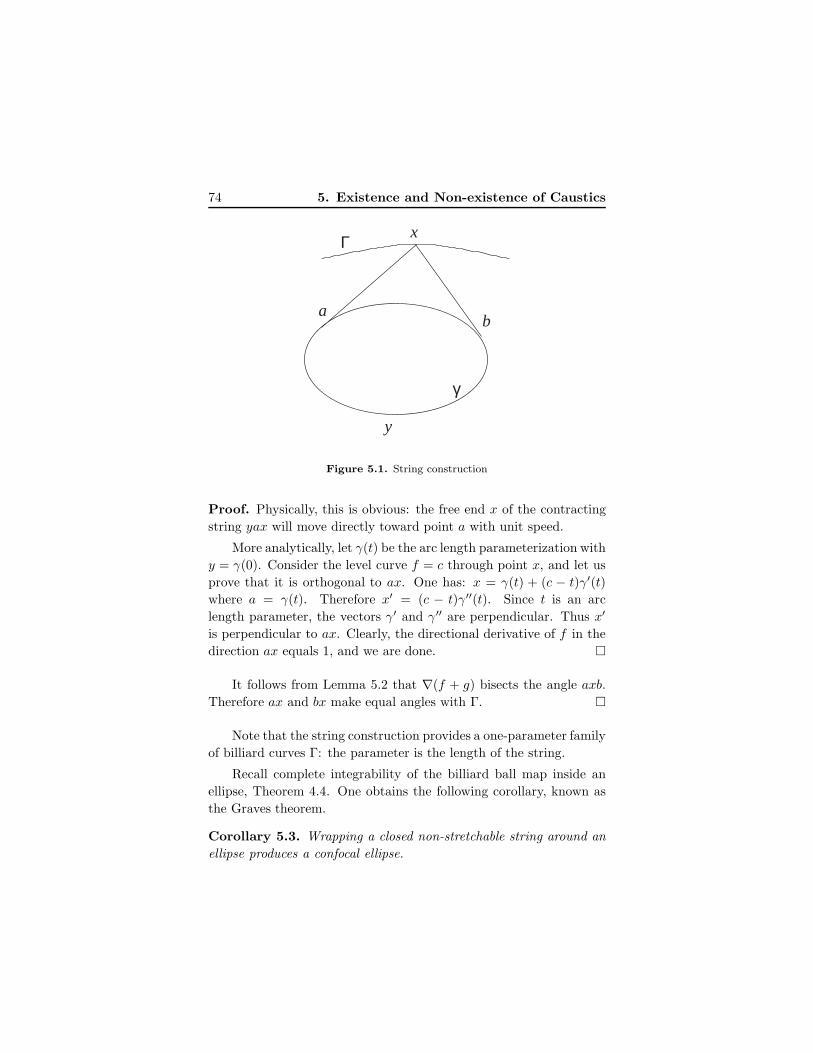
74 5. Existence and Non-existence of Caustics
ab
y
x
γ
Γ
Figure 5.1. String construction
Proof. Physically, this is obvious: the free end x of the contracting
string yax will move directly toward point a with unit speed.
More analytically, let γ(t) be the arc length parameterization with
y = γ(0). Consider the level curve f = c through point x, and let us
prove that it is orthogonal to ax. One has: x = γ(t) + (c − t)γ′(t)
where a = γ(t). Therefore x′ = (c − t)γ′′(t). Since t is an arc
length parameter, the vectors γ′ and γ′′ are perpendicular. Thus x′
is perpendicular to ax. Clearly, the directional derivative of f in the
direction ax equals 1, and we are done.
It follows from Lemma 5.2 that ∇(f + g) bisects the angle axb.
Therefore ax and bx make equal angles with Γ.
Note that the string construction provides a one-parameter family
of billiard curves Γ: the parameter is the length of the string.
Recall complete integrability of the billiard ball map inside an
ellipse, Theorem 4.4. One obtains the following corollary, known as
the Graves theorem.
Corollary 5.3. Wrapping a closed non-stretchable string around an
ellipse produces a confocal ellipse.
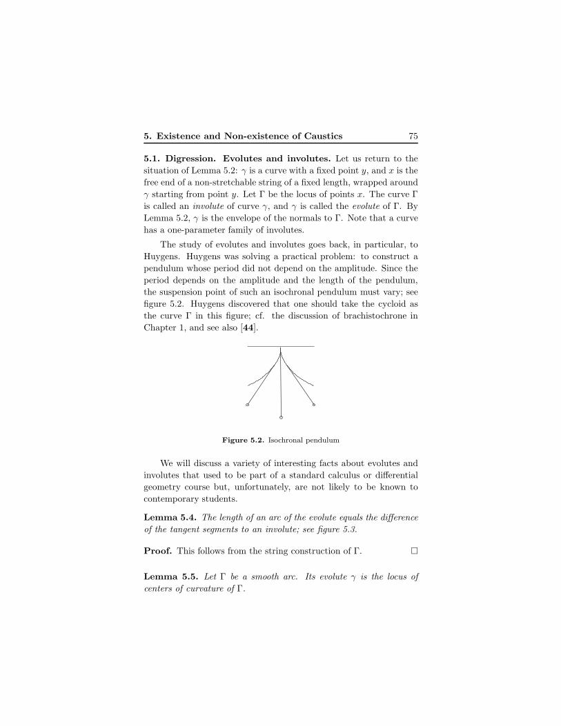
5. Existence and Non-existence of Caustics 75
5.1. Digression. Evolutes and involutes. Let us return to the
situation of Lemma 5.2: γ is a curve with a fixed point y, and x is the
free end of a non-stretchable string of a fixed length, wrapped around
γ starting from point y. Let Γ be the locus of points x. The curve Γ
is called an involute of curve γ, and γ is called the evolute of Γ. By
Lemma 5.2, γ is the envelope of the normals to Γ. Note that a curve
has a one-parameter family of involutes.
The study of evolutes and involutes goes back, in particular, to
Huygens. Huygens was solving a practical problem: to construct a
pendulum whose period did not depend on the amplitude. Since the
period depends on the amplitude and the length of the pendulum,
the suspension point of such an isochronal pendulum must vary; see
figure 5.2. Huygens discovered that one should take the cycloid as
the curve Γ in this figure; cf. the discussion of brachistochrone in
Chapter 1, and see also [44].
Figure 5.2. Isochronal pendulum
We will discuss a variety of interesting facts about evolutes and
involutes that used to be part of a standard calculus or differential
geometry course but, unfortunately, are not likely to be known to
contemporary students.
Lemma 5.4. The length of an arc of the evolute equals the difference
of the tangent segments to an involute; see figure 5.3.
Proof. This follows from the string construction of Γ.
Lemma 5.5. Let Γ be a smooth arc. Its evolute γ is the locus of
centers of curvature of Γ.
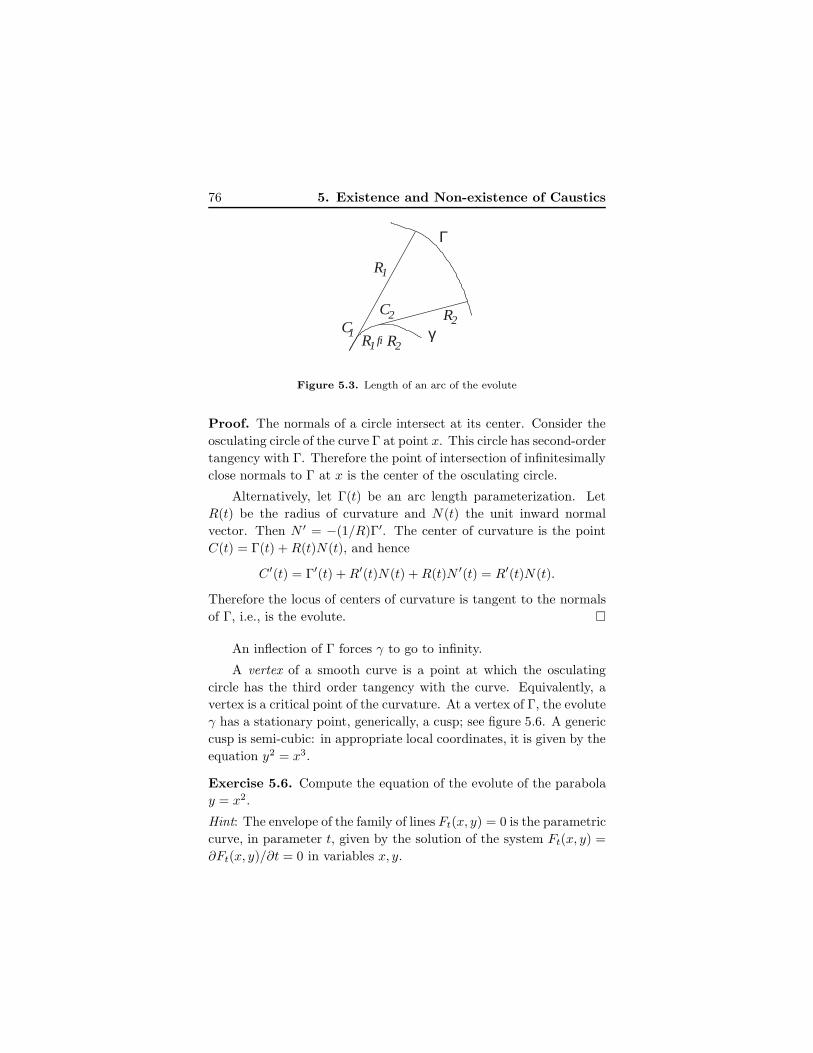
76 5. Existence and Non-existence of Caustics
γ
Γ
1R 2R
2RC2
1R
1C
Figure 5.3. Length of an arc of the evolute
Proof. The normals of a circle intersect at its center. Consider the
osculating circle of the curve Γ at point x. This circle has second-order
tangency with Γ. Therefore the point of intersection of infinitesimally
close normals to Γ at x is the center of the osculating circle.
Alternatively, let Γ(t) be an arc length parameterization. Let
R(t) be the radius of curvature and N(t) the unit inward normal
vector. Then N ′ = −(1/R)Γ′. The center of curvature is the point
C(t) = Γ(t) +R(t)N(t), and hence
C′(t) = Γ′(t) +R′(t)N(t) +R(t)N ′(t) = R′(t)N(t).
Therefore the locus of centers of curvature is tangent to the normals
of Γ, i.e., is the evolute.
An inflection of Γ forces γ to go to infinity.
A vertex of a smooth curve is a point at which the osculating
circle has the third order tangency with the curve. Equivalently, a
vertex is a critical point of the curvature. At a vertex of Γ, the evolute
γ has a stationary point, generically, a cusp; see figure 5.6. A generic
cusp is semi-cubic: in appropriate local coordinates, it is given by the
equation y2 = x3.
Exercise 5.6. Compute the equation of the evolute of the parabola
y = x2.
Hint: The envelope of the family of lines Ft(x, y) = 0 is the parametric
curve, in parameter t, given by the solution of the system Ft(x, y) =
∂Ft(x, y)/∂t = 0 in variables x, y.
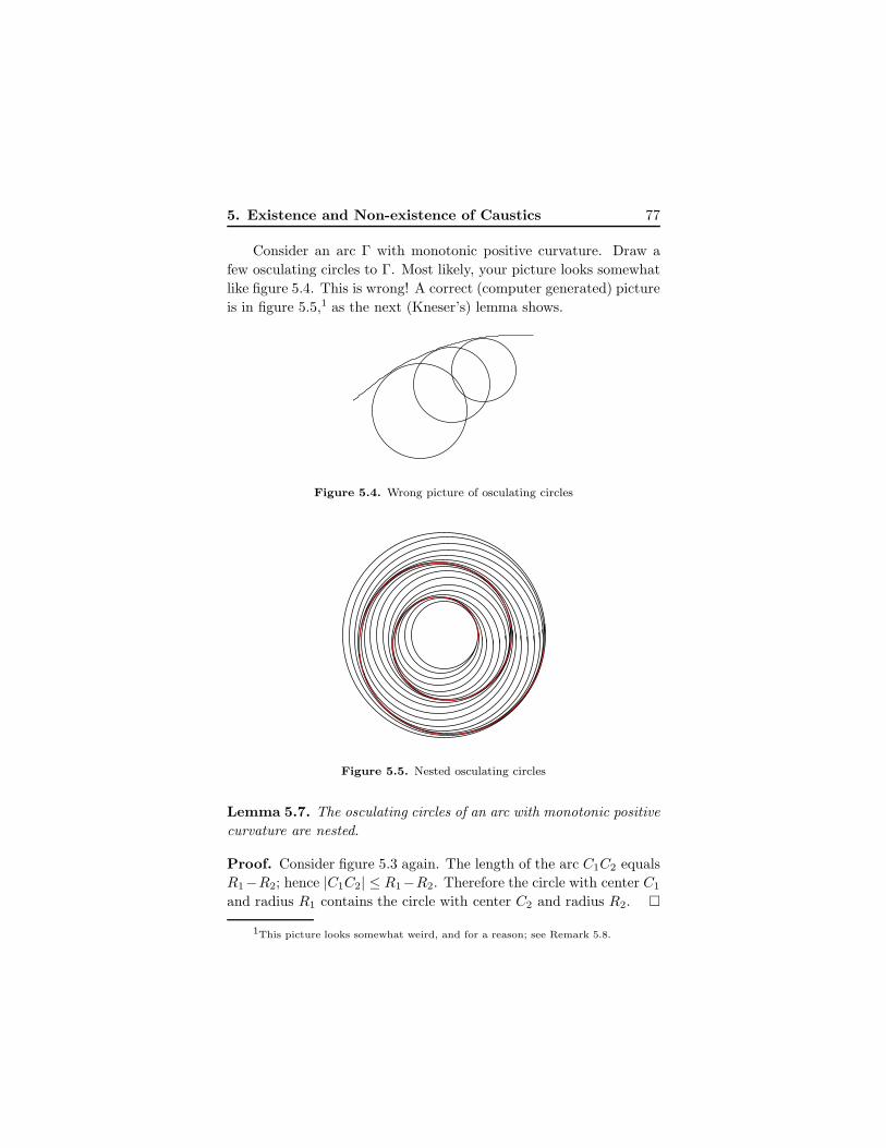
5. Existence and Non-existence of Caustics 77
Consider an arc Γ with monotonic positive curvature. Draw a
few osculating circles to Γ. Most likely, your picture looks somewhat
like figure 5.4. This is wrong! A correct (computer generated) picture
is in figure 5.5,1 as the next (Kneser’s) lemma shows.
Figure 5.4. Wrong picture of osculating circles
Figure 5.5. Nested osculating circles
Lemma 5.7. The osculating circles of an arc with monotonic positive
curvature are nested.
Proof. Consider figure 5.3 again. The length of the arc C1C2 equals
R1−R2; hence |C1C2| ≤ R1−R2. Therefore the circle with center C1
and radius R1 contains the circle with center C2 and radius R2.
1This picture looks somewhat weird, and for a reason; see Remark 5.8.
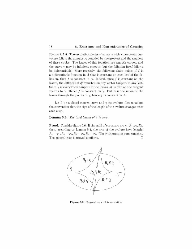
78 5. Existence and Non-existence of Caustics
Remark 5.8. The osculating circles of an arc γ with a monotonic cur-
vature foliate the annulus A bounded by the greatest and the smallest
of these circles. The leaves of this foliation are smooth curves, and
the curve γ may be infinitely smooth, but the foliation itself fails to
be differentiable! More precisely, the following claim holds: if f is
a differentiable function in A that is constant on each leaf of the fo-
liation, then f is constant in A. Indeed, since f is constant on the
leaves, the differential df vanishes on any vector tangent to any leaf.
Since γ is everywhere tangent to the leaves, df is zero on the tangent
vectors to γ. Hence f is constant on γ. But A is the union of the
leaves through the points of γ; hence f is constant in A.
Let Γ be a closed convex curve and γ its evolute. Let us adapt
the convention that the sign of the length of the evolute changes after
each cusp.
Lemma 5.9. The total length of γ is zero.
Proof. Consider figure 5.6. If the radii of curvature are r1, R1, r2, R2,
then, according to Lemma 5.4, the arcs of the evolute have lengths
R1 − r1, R1 − r2, R2 − r2, R2 − r1. Their alternating sum vanishes.
The general case is proved similarly.
1
r1R2
r1
R
r2
r2R1
r2R2
R1 R2
r1
Figure 5.6. Cusps of the evolute at vertices
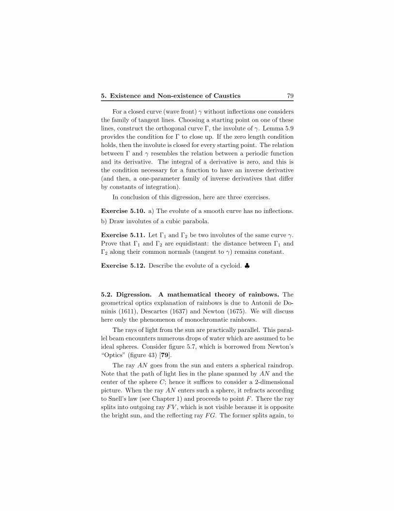
5. Existence and Non-existence of Caustics 79
For a closed curve (wave front) γ without inflections one considers
the family of tangent lines. Choosing a starting point on one of these
lines, construct the orthogonal curve Γ, the involute of γ. Lemma 5.9
provides the condition for Γ to close up. If the zero length condition
holds, then the involute is closed for every starting point. The relation
between Γ and γ resembles the relation between a periodic function
and its derivative. The integral of a derivative is zero, and this is
the condition necessary for a function to have an inverse derivative
(and then, a one-parameter family of inverse derivatives that differ
by constants of integration).
In conclusion of this digression, here are three exercises.
Exercise 5.10. a) The evolute of a smooth curve has no inflections.
b) Draw involutes of a cubic parabola.
Exercise 5.11. Let Γ1 and Γ2 be two involutes of the same curve γ.
Prove that Γ1 and Γ2 are equidistant: the distance between Γ1 and
Γ2 along their common normals (tangent to γ) remains constant.
Exercise 5.12. Describe the evolute of a cycloid. ♣
5.2. Digression. A mathematical theory of rainbows. The
geometrical optics explanation of rainbows is due to Antonii de Do-
minis (1611), Descartes (1637) and Newton (1675). We will discuss
here only the phenomenon of monochromatic rainbows.
The rays of light from the sun are practically parallel. This paral-
lel beam encounters numerous drops of water which are assumed to be
ideal spheres. Consider figure 5.7, which is borrowed from Newton’s
“Optics” (figure 43) [79].
The ray AN goes from the sun and enters a spherical raindrop.
Note that the path of light lies in the plane spanned by AN and the
center of the sphere C; hence it suffices to consider a 2-dimensional
picture. When the ray AN enters such a sphere, it refracts according
to Snell’s law (see Chapter 1) and proceeds to point F . There the ray
splits into outgoing ray FV , which is not visible because it is opposite
the bright sun, and the reflecting ray FG. The former splits again, to
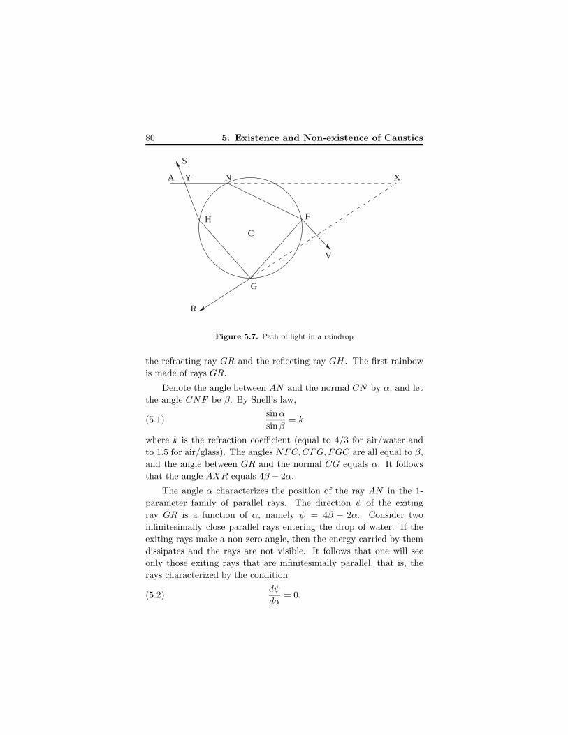
80 5. Existence and Non-existence of Caustics
XY
H
S
C
R
G
V
F
NA
Figure 5.7. Path of light in a raindrop
the refracting ray GR and the reflecting ray GH . The first rainbow
is made of rays GR.
Denote the angle between AN and the normal CN by α, and let
the angle CNF be β. By Snell’s law,
(5.1)sinα
sinβ= k
where k is the refraction coefficient (equal to 4/3 for air/water and
to 1.5 for air/glass). The angles NFC,CFG,FGC are all equal to β,
and the angle between GR and the normal CG equals α. It follows
that the angle AXR equals 4β − 2α.
The angle α characterizes the position of the ray AN in the 1-
parameter family of parallel rays. The direction ψ of the exiting
ray GR is a function of α, namely ψ = 4β − 2α. Consider two
infinitesimally close parallel rays entering the drop of water. If the
exiting rays make a non-zero angle, then the energy carried by them
dissipates and the rays are not visible. It follows that one will see
only those exiting rays that are infinitesimally parallel, that is, the
rays characterized by the condition
(5.2)dψ
dα= 0.
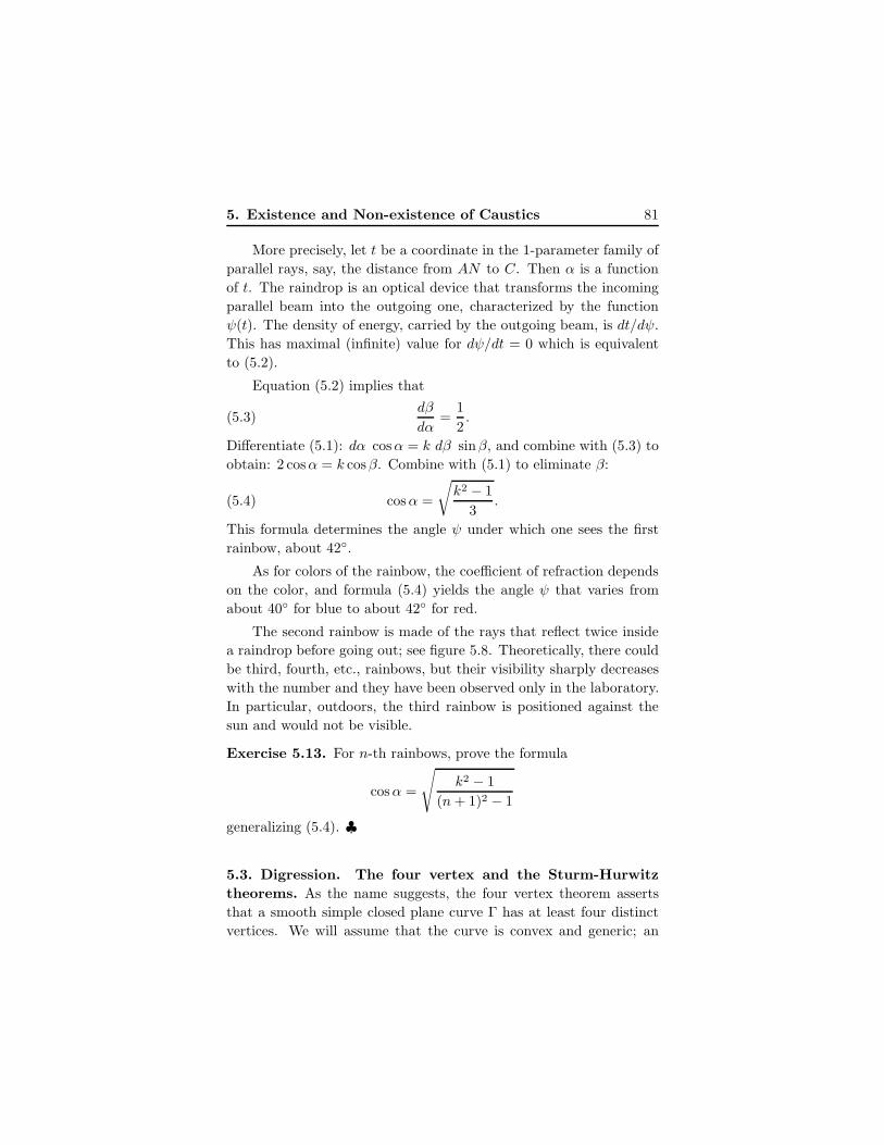
5. Existence and Non-existence of Caustics 81
More precisely, let t be a coordinate in the 1-parameter family of
parallel rays, say, the distance from AN to C. Then α is a function
of t. The raindrop is an optical device that transforms the incoming
parallel beam into the outgoing one, characterized by the function
ψ(t). The density of energy, carried by the outgoing beam, is dt/dψ.
This has maximal (infinite) value for dψ/dt = 0 which is equivalent
to (5.2).
Equation (5.2) implies that
(5.3)dβ
dα=
1
2.
Differentiate (5.1): dα cosα = k dβ sinβ, and combine with (5.3) to
obtain: 2 cosα = k cosβ. Combine with (5.1) to eliminate β:
(5.4) cosα =
√k2 − 1
3.
This formula determines the angle ψ under which one sees the first
rainbow, about 42.
As for colors of the rainbow, the coefficient of refraction depends
on the color, and formula (5.4) yields the angle ψ that varies from
about 40 for blue to about 42 for red.
The second rainbow is made of the rays that reflect twice inside
a raindrop before going out; see figure 5.8. Theoretically, there could
be third, fourth, etc., rainbows, but their visibility sharply decreases
with the number and they have been observed only in the laboratory.
In particular, outdoors, the third rainbow is positioned against the
sun and would not be visible.
Exercise 5.13. For n-th rainbows, prove the formula
cosα =
√k2 − 1
(n+ 1)2 − 1
generalizing (5.4). ♣
5.3. Digression. The four vertex and the Sturm-Hurwitz
theorems. As the name suggests, the four vertex theorem asserts
that a smooth simple closed plane curve Γ has at least four distinct
vertices. We will assume that the curve is convex and generic; an
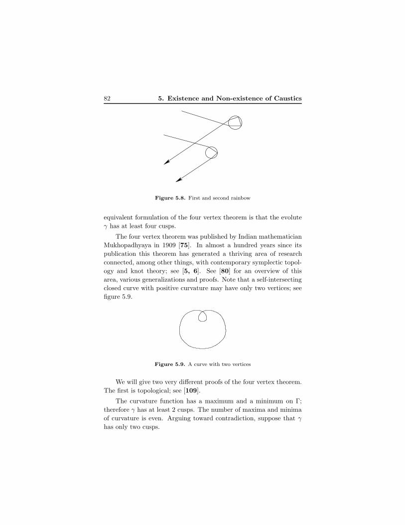
82 5. Existence and Non-existence of Caustics
Figure 5.8. First and second rainbow
equivalent formulation of the four vertex theorem is that the evolute
γ has at least four cusps.
The four vertex theorem was published by Indian mathematician
Mukhopadhyaya in 1909 [75]. In almost a hundred years since its
publication this theorem has generated a thriving area of research
connected, among other things, with contemporary symplectic topol-
ogy and knot theory; see [5, 6]. See [80] for an overview of this
area, various generalizations and proofs. Note that a self-intersecting
closed curve with positive curvature may have only two vertices; see
figure 5.9.
Figure 5.9. A curve with two vertices
We will give two very different proofs of the four vertex theorem.
The first is topological; see [109].
The curvature function has a maximum and a minimum on Γ;
therefore γ has at least 2 cusps. The number of maxima and minima
of curvature is even. Arguing toward contradiction, suppose that γ
has only two cusps.
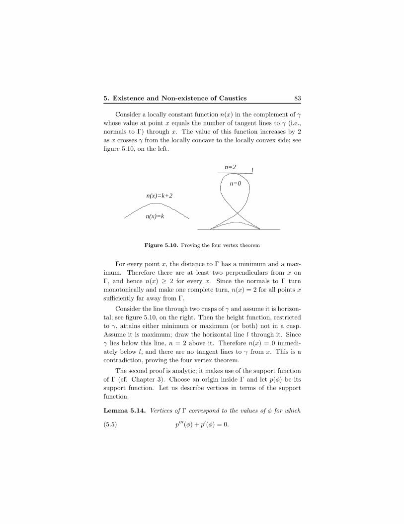
5. Existence and Non-existence of Caustics 83
Consider a locally constant function n(x) in the complement of γ
whose value at point x equals the number of tangent lines to γ (i.e.,
normals to Γ) through x. The value of this function increases by 2
as x crosses γ from the locally concave to the locally convex side; see
figure 5.10, on the left.
ln=2
n=0
n(x)=k+2
n(x)=k
Figure 5.10. Proving the four vertex theorem
For every point x, the distance to Γ has a minimum and a max-
imum. Therefore there are at least two perpendiculars from x on
Γ, and hence n(x) ≥ 2 for every x. Since the normals to Γ turn
monotonically and make one complete turn, n(x) = 2 for all points x
sufficiently far away from Γ.
Consider the line through two cusps of γ and assume it is horizon-
tal; see figure 5.10, on the right. Then the height function, restricted
to γ, attains either minimum or maximum (or both) not in a cusp.
Assume it is maximum; draw the horizontal line l through it. Since
γ lies below this line, n = 2 above it. Therefore n(x) = 0 immedi-
ately below l, and there are no tangent lines to γ from x. This is a
contradiction, proving the four vertex theorem.
The second proof is analytic; it makes use of the support function
of Γ (cf. Chapter 3). Choose an origin inside Γ and let p(φ) be its
support function. Let us describe vertices in terms of the support
function.
Lemma 5.14. Vertices of Γ correspond to the values of φ for which
(5.5) p′′′(φ) + p′(φ) = 0.
84 5. Existence and Non-existence of Caustics
Proof. The claim follows from Exercise 3.14 d). Alternatively, one
may argue as follows.
Support functions of circles are a cosφ+b sinφ+c, where a, b and
c are constants. Indeed, choosing the origin at the center of a circle,
the support function is constant (the radius), and the general case
follows from Exercise 3.4.
Vertices are the points where the curve has a third-order contact
with a circle. In terms of the support functions, it means that p(φ)
coincides with a cosφ + b sinφ + c up to the third derivative. It re-
mains to notice that linear harmonics a cosφ+ b sinφ+ c satisfy (5.5)
identically.
Lemma 5.14 makes it possible to reformulate the four vertex the-
orem as follows.
Theorem 5.15. Let p(φ) be a smooth 2π-periodic function. Then
the equation p′′′(φ) + p′(φ) = 0 has at least 4 distinct roots.
This theorem has a generalization, the following Sturm-Hurwitz
theorem. Recall that a smooth 2π-periodic function has a Fourier
expansion
(5.6) f(φ) =∑
k≥0
(ak cos kφ+ bk sin kφ) .
Theorem 5.16. Assume that the Fourier series (5.6) of function
f starts with n-th harmonics, that is, does not contain terms with
k < n. Then the function f(φ) has at least 2n distinct zeroes on the
circle [0, 2π).
Theorem 5.16 implies Theorem 5.15: the function p′′′(φ) + p′(φ)
does not contain the first harmonics and satisfies the assumption of
Theorem 5.16 with n = 2.
Proof. We will give two proofs; see [80] for other approaches.
1) Denote by Z(f) the number of sign changes of a function f .
The Rolle theorem asserts that Z(f ′) ≥ Z(f). Introduce the operator
D−1, the inverse derivative, on the subspace of functions with zero
5. Existence and Non-existence of Caustics 85
average:
(D−1f)(x) =
∫ x
0
f(t)dt.
The Rolle theorem then reads: Z(f) ≥ Z(D−1f).
Note that
(cos kφ)′′ = −k2 cos kφ, (sin kφ)′′ = −k2 sin kφ,
and hence the operator D−2 multiplies k-th harmonics by −1/k2.
Consider the sequence of functions
fm = (−1)m(nD−1
)2mf,
explicitly,
fm(φ) = (an cosnφ+ bn sinnφ)
+∑
k>n
(nk
)2m
(ak cos kφ+ bk sinkφ) .(5.7)
By the Rolle theorem, for every m, one has: Z(f) ≥ Z(fm).
Since the Fourier series (5.6) converges,∑
k(a2k + b2k) < C for
some constant C. This implies that the second summand in (5.7) is
arbitrarily small for sufficiently large m. It follows that, for large m,
the function fm has as many sign changes as the n-th harmonic, that
is, 2n, and we are done.
2) Let us argue by contradiction. Assume that f has less than
2n sign changes on the circle. The number of sign changes being
even, f has at most 2(n − 1) of them. One can find a trigonometric
polynomial g of degree ≤ n− 1, that is,
g(φ) =
n−1∑
k=0
(ak cos kφ+ bk sin kφ) ,
that changes signs precisely in the same points as f . Then the func-
tion fg has a constant sign on the circle and∫ 2π
0f(φ)g(φ) dφ 6= 0.
On the other hand, for k 6= m,∫ 2π
0
sin kφ sinmφ dφ =
∫ 2π
0
sin kφ cosmφ dϕ
=
∫ 2π
0
cos kφ cosmφ dφ = 0.(5.8)
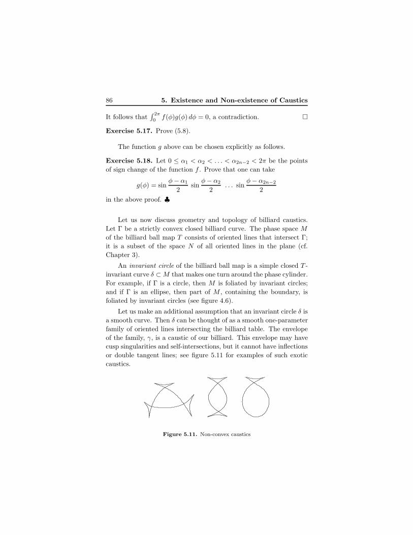
86 5. Existence and Non-existence of Caustics
It follows that∫ 2π
0f(φ)g(φ) dφ = 0, a contradiction.
Exercise 5.17. Prove (5.8).
The function g above can be chosen explicitly as follows.
Exercise 5.18. Let 0 ≤ α1 < α2 < . . . < α2n−2 < 2π be the points
of sign change of the function f . Prove that one can take
g(φ) = sinφ− α1
2sin
φ− α2
2. . . sin
φ− α2n−2
2
in the above proof. ♣
Let us now discuss geometry and topology of billiard caustics.
Let Γ be a strictly convex closed billiard curve. The phase space M
of the billiard ball map T consists of oriented lines that intersect Γ;
it is a subset of the space N of all oriented lines in the plane (cf.
Chapter 3).
An invariant circle of the billiard ball map is a simple closed T -
invariant curve δ ⊂M that makes one turn around the phase cylinder.
For example, if Γ is a circle, then M is foliated by invariant circles;
and if Γ is an ellipse, then part of M , containing the boundary, is
foliated by invariant circles (see figure 4.6).
Let us make an additional assumption that an invariant circle δ is
a smooth curve. Then δ can be thought of as a smooth one-parameter
family of oriented lines intersecting the billiard table. The envelope
of the family, γ, is a caustic of our billiard. This envelope may have
cusp singularities and self-intersections, but it cannot have inflections
or double tangent lines; see figure 5.11 for examples of such exotic
caustics.
Figure 5.11. Non-convex caustics
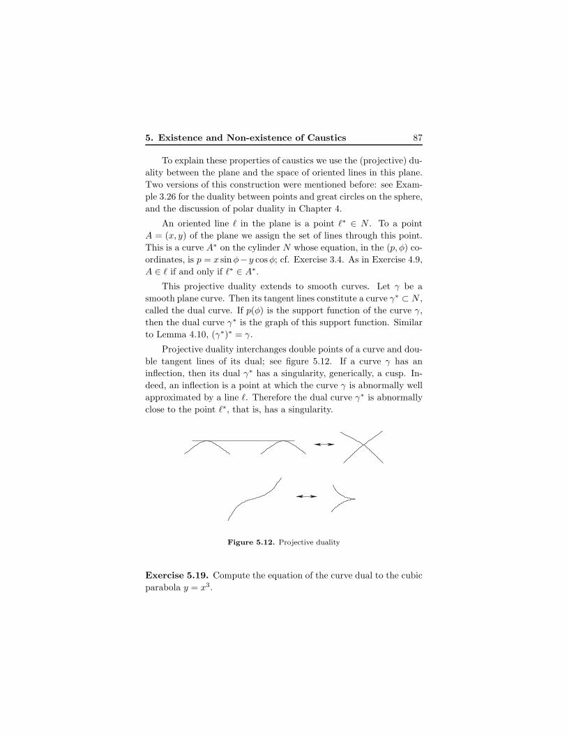
5. Existence and Non-existence of Caustics 87
To explain these properties of caustics we use the (projective) du-
ality between the plane and the space of oriented lines in this plane.
Two versions of this construction were mentioned before: see Exam-
ple 3.26 for the duality between points and great circles on the sphere,
and the discussion of polar duality in Chapter 4.
An oriented line ℓ in the plane is a point ℓ∗ ∈ N . To a point
A = (x, y) of the plane we assign the set of lines through this point.
This is a curve A∗ on the cylinder N whose equation, in the (p, φ) co-
ordinates, is p = x sinφ− y cosφ; cf. Exercise 3.4. As in Exercise 4.9,
A ∈ ℓ if and only if ℓ∗ ∈ A∗.
This projective duality extends to smooth curves. Let γ be a
smooth plane curve. Then its tangent lines constitute a curve γ∗ ⊂ N ,
called the dual curve. If p(φ) is the support function of the curve γ,
then the dual curve γ∗ is the graph of this support function. Similar
to Lemma 4.10, (γ∗)∗ = γ.
Projective duality interchanges double points of a curve and dou-
ble tangent lines of its dual; see figure 5.12. If a curve γ has an
inflection, then its dual γ∗ has a singularity, generically, a cusp. In-
deed, an inflection is a point at which the curve γ is abnormally well
approximated by a line ℓ. Therefore the dual curve γ∗ is abnormally
close to the point ℓ∗, that is, has a singularity.
Figure 5.12. Projective duality
Exercise 5.19. Compute the equation of the curve dual to the cubic
parabola y = x3.
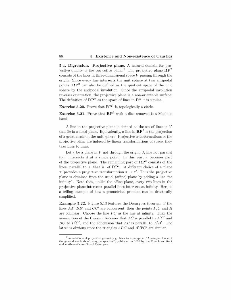
88 5. Existence and Non-existence of Caustics
5.4. Digression. Projective plane. A natural domain for pro-
jective duality is the projective plane.2 The projective plane RP2
consists of the lines in three-dimensional space V passing through the
origin. Since every line intersects the unit sphere at two antipodal
points, RP2 can also be defined as the quotient space of the unit
sphere by the antipodal involution. Since the antipodal involution
reverses orientation, the projective plane is a non-orientable surface.
The definition of RPn as the space of lines in Rn+1 is similar.
Exercise 5.20. Prove that RP1 is topologically a circle.
Exercise 5.21. Prove that RP2 with a disc removed is a Moebius
band.
A line in the projective plane is defined as the set of lines in V
that lie in a fixed plane. Equivalently, a line in RP2 is the projection
of a great circle on the unit sphere. Projective transformations of the
projective plane are induced by linear transformations of space; they
take lines to lines.
Let π be a plane in V not through the origin. A line not parallel
to π intersects it at a single point. In this way, π becomes part
of the projective plane. The remaining part of RP2 consists of the
lines, parallel to π, that is, of RP1. A different choice of a plane
π′ provides a projective transformation π → π′. Thus the projective
plane is obtained from the usual (affine) plane by adding a line “at
infinity”. Note that, unlike the affine plane, every two lines in the
projective plane intersect: parallel lines intersect at infinity. Here is
a telling example of how a geometrical problem can be drastically
simplified.
Example 5.22. Figure 5.13 features the Desargues theorem: if the
lines AA′, BB′ and CC′ are concurrent, then the points P,Q and R
are collinear. Choose the line PQ as the line at infinity. Then the
assumption of the theorem becomes that AC is parallel to A′C′ and
BC to B′C′, and the conclusion that AB is parallel to A′B′. The
latter is obvious since the triangles ABC and A′B′C′ are similar.
2Foundations of projective geometry go back to a pamphlet “A sample of one ofthe general methods of using perspective”, published in 1636 by the French architectand mathematician Girard Desargues.
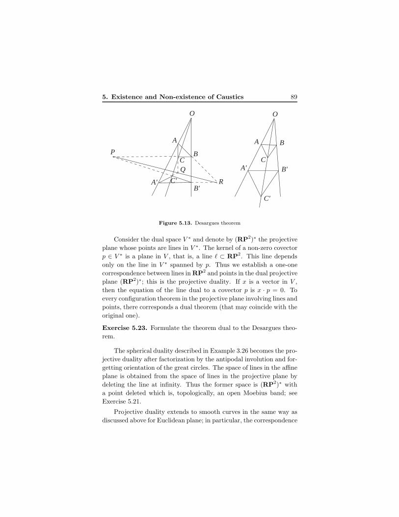
5. Existence and Non-existence of Caustics 89
O
A
BC
A B
CA' B'
C'
A'B'
C'
P
Q
R
O
Figure 5.13. Desargues theorem
Consider the dual space V ∗ and denote by (RP2)∗ the projective
plane whose points are lines in V ∗. The kernel of a non-zero covector
p ∈ V ∗ is a plane in V , that is, a line ℓ ⊂ RP2. This line depends
only on the line in V ∗ spanned by p. Thus we establish a one-one
correspondence between lines in RP2 and points in the dual projective
plane (RP2)∗; this is the projective duality. If x is a vector in V ,
then the equation of the line dual to a covector p is x · p = 0. To
every configuration theorem in the projective plane involving lines and
points, there corresponds a dual theorem (that may coincide with the
original one).
Exercise 5.23. Formulate the theorem dual to the Desargues theo-
rem.
The spherical duality described in Example 3.26 becomes the pro-
jective duality after factorization by the antipodal involution and for-
getting orientation of the great circles. The space of lines in the affine
plane is obtained from the space of lines in the projective plane by
deleting the line at infinity. Thus the former space is (RP2)∗ with
a point deleted which is, topologically, an open Moebius band; see
Exercise 5.21.
Projective duality extends to smooth curves in the same way as
discussed above for Euclidean plane; in particular, the correspondence
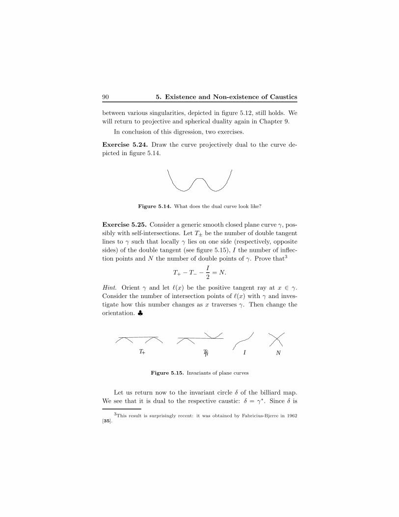
90 5. Existence and Non-existence of Caustics
between various singularities, depicted in figure 5.12, still holds. We
will return to projective and spherical duality again in Chapter 9.
In conclusion of this digression, two exercises.
Exercise 5.24. Draw the curve projectively dual to the curve de-
picted in figure 5.14.
Figure 5.14. What does the dual curve look like?
Exercise 5.25. Consider a generic smooth closed plane curve γ, pos-
sibly with self-intersections. Let T± be the number of double tangent
lines to γ such that locally γ lies on one side (respectively, opposite
sides) of the double tangent (see figure 5.15), I the number of inflec-
tion points and N the number of double points of γ. Prove that3
T+ − T− − I
2= N.
Hint. Orient γ and let ℓ(x) be the positive tangent ray at x ∈ γ.
Consider the number of intersection points of ℓ(x) with γ and inves-
tigate how this number changes as x traverses γ. Then change the
orientation. ♣
T NI+T
Figure 5.15. Invariants of plane curves
Let us return now to the invariant circle δ of the billiard map.
We see that it is dual to the respective caustic: δ = γ∗. Since δ is
3This result is surprisingly recent: it was obtained by Fabricius-Bjerre in 1962[35].
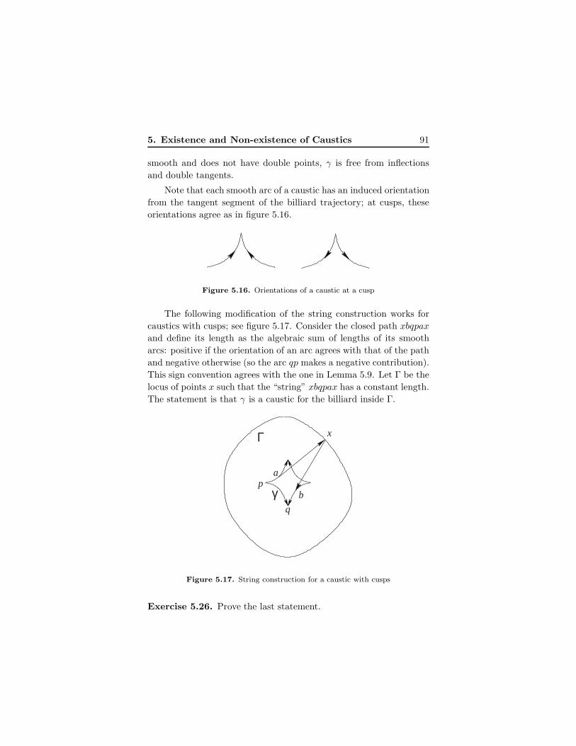
5. Existence and Non-existence of Caustics 91
smooth and does not have double points, γ is free from inflections
and double tangents.
Note that each smooth arc of a caustic has an induced orientation
from the tangent segment of the billiard trajectory; at cusps, these
orientations agree as in figure 5.16.
Figure 5.16. Orientations of a caustic at a cusp
The following modification of the string construction works for
caustics with cusps; see figure 5.17. Consider the closed path xbqpax
and define its length as the algebraic sum of lengths of its smooth
arcs: positive if the orientation of an arc agrees with that of the path
and negative otherwise (so the arc qp makes a negative contribution).
This sign convention agrees with the one in Lemma 5.9. Let Γ be the
locus of points x such that the “string” xbqpax has a constant length.
The statement is that γ is a caustic for the billiard inside Γ.
γ
Γ
b
x
a
q
p
Figure 5.17. String construction for a caustic with cusps
Exercise 5.26. Prove the last statement.
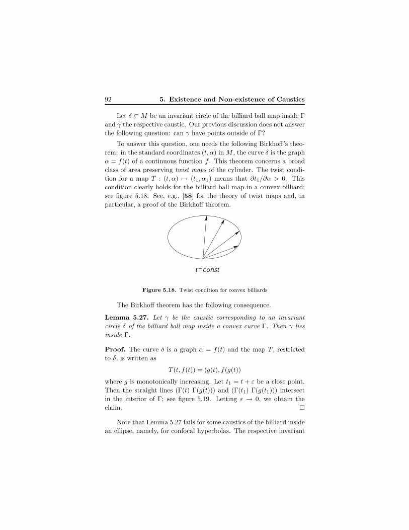
92 5. Existence and Non-existence of Caustics
Let δ ⊂M be an invariant circle of the billiard ball map inside Γ
and γ the respective caustic. Our previous discussion does not answer
the following question: can γ have points outside of Γ?
To answer this question, one needs the following Birkhoff’s theo-
rem: in the standard coordinates (t, α) in M , the curve δ is the graph
α = f(t) of a continuous function f . This theorem concerns a broad
class of area preserving twist maps of the cylinder. The twist condi-
tion for a map T : (t, α) 7→ (t1, α1) means that ∂t1/∂α > 0. This
condition clearly holds for the billiard ball map in a convex billiard;
see figure 5.18. See, e.g., [58] for the theory of twist maps and, in
particular, a proof of the Birkhoff theorem.
t=const
Figure 5.18. Twist condition for convex billiards
The Birkhoff theorem has the following consequence.
Lemma 5.27. Let γ be the caustic corresponding to an invariant
circle δ of the billiard ball map inside a convex curve Γ. Then γ lies
inside Γ.
Proof. The curve δ is a graph α = f(t) and the map T , restricted
to δ, is written as
T (t, f(t)) = (g(t), f(g(t))
where g is monotonically increasing. Let t1 = t + ε be a close point.
Then the straight lines (Γ(t) Γ(g(t))) and (Γ(t1) Γ(g(t1))) intersect
in the interior of Γ; see figure 5.19. Letting ε → 0, we obtain the
claim.
Note that Lemma 5.27 fails for some caustics of the billiard inside
an ellipse, namely, for confocal hyperbolas. The respective invariant
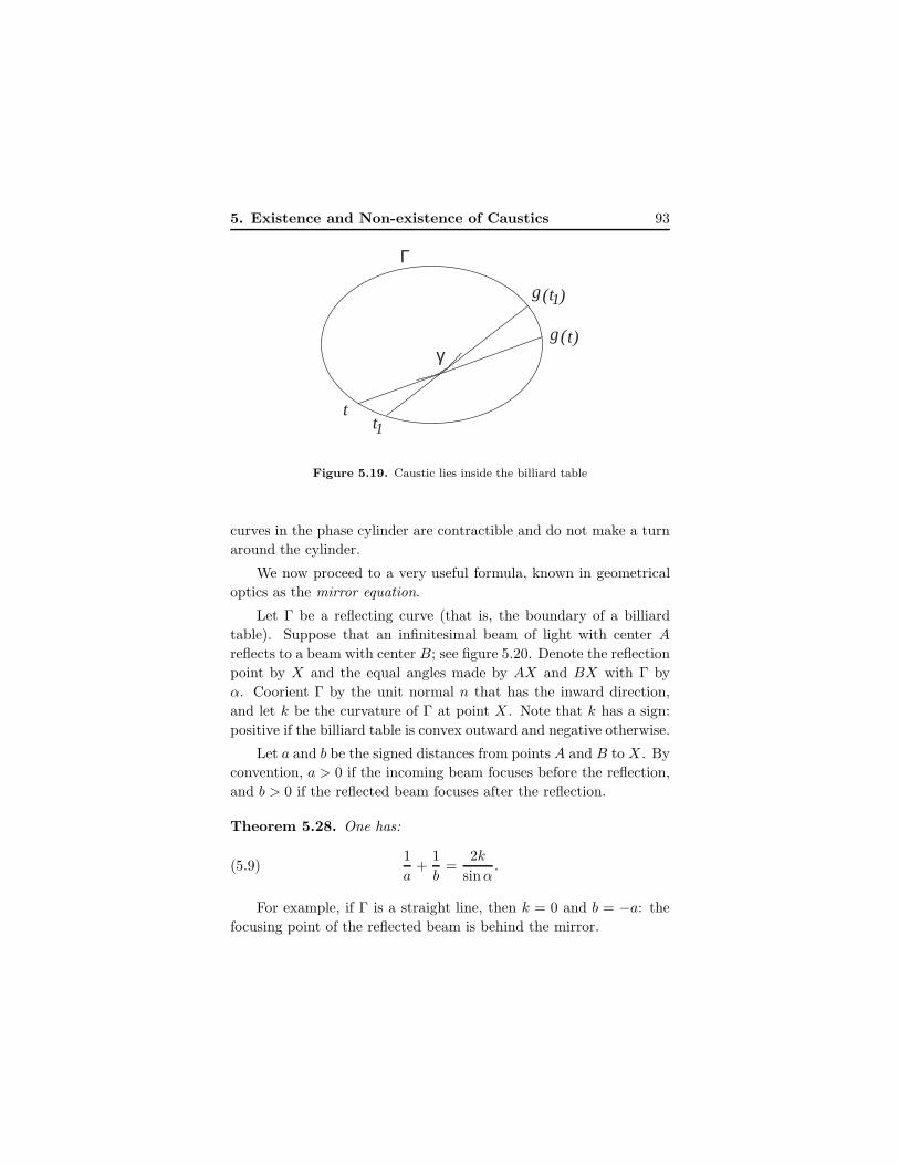
5. Existence and Non-existence of Caustics 93
)1t(g
)t(g
1tt
Γ
γ
Figure 5.19. Caustic lies inside the billiard table
curves in the phase cylinder are contractible and do not make a turn
around the cylinder.
We now proceed to a very useful formula, known in geometrical
optics as the mirror equation.
Let Γ be a reflecting curve (that is, the boundary of a billiard
table). Suppose that an infinitesimal beam of light with center A
reflects to a beam with center B; see figure 5.20. Denote the reflection
point by X and the equal angles made by AX and BX with Γ by
α. Coorient Γ by the unit normal n that has the inward direction,
and let k be the curvature of Γ at point X . Note that k has a sign:
positive if the billiard table is convex outward and negative otherwise.
Let a and b be the signed distances from points A and B to X . By
convention, a > 0 if the incoming beam focuses before the reflection,
and b > 0 if the reflected beam focuses after the reflection.
Theorem 5.28. One has:
(5.9)1
a+
1
b=
2k
sinα.
For example, if Γ is a straight line, then k = 0 and b = −a: the
focusing point of the reflected beam is behind the mirror.
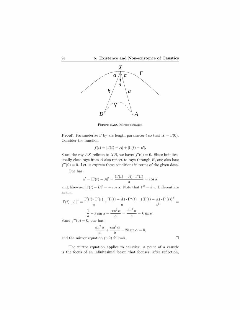
94 5. Existence and Non-existence of Caustics
α α
γ
ΓX
n
B A
b a
Figure 5.20. Mirror equation
Proof. Parameterize Γ by arc length parameter t so that X = Γ(0).
Consider the function
f(t) = |Γ(t) −A| + |Γ(t) −B|.Since the ray AX reflects to XB, we have: f ′(0) = 0. Since infinites-
imally close rays from A also reflect to rays through B, one also has:
f ′′(0) = 0. Let us express these conditions in terms of the given data.
One has:
a′ = |Γ(t) −A|′ =(Γ(t) − A) · Γ′(t)
a= cosα
and, likewise, |Γ(t)−B|′ = − cosα. Note that Γ′′ = kn. Differentiate
again:
|Γ(t)−A|′′ =Γ′(t) · Γ′(t)
a+
(Γ(t) −A) · Γ′′(t)
a− ((Γ(t) −A) · Γ′(t))
2
a3=
1
a− k sinα− cos2 α
a=
sin2 α
a− k sinα.
Since f ′′(0) = 0, one has:
sin2 α
a+
sin2 α
b− 2k sinα = 0,
and the mirror equation (5.9) follows.
The mirror equation applies to caustics: a point of a caustic
is the focus of an infinitesimal beam that focuses, after reflection,

5. Existence and Non-existence of Caustics 95
at another point of this caustic; see figure 5.20. This implies the
following phenomenon discovered by J. Mather [66].
Corollary 5.29. If the curvature of a convex smooth billiard curve
vanishes at some point, then this billiard ball map has no invariant
circles.
Proof. Assume that there is an invariant circle and let γ ⊂ Γ be the
respective caustic. Let X ∈ Γ be a point of zero curvature, and XA
and XB be tangent segment to γ from point X , making equal angles
with Γ. The mirror equation (5.9) implies that b = −a, and therefore
one of the points A or B lies outside the billiard table.
We know that the billiards in ellipses are integrable: the billiard
table is foliated by caustics, the confocal ellipses, and part of the
phase space consists of oriented lines tangent to these caustics (in
figure 4.6, this is the part outside the “eyes”). The billiard in a circle
is even more regular: every phase point is an oriented line, tangent
to a caustic.
How exceptional is this situation? A long-standing conjecture,
attributed to Birkhoff, asserts that if a neighborhood of a smooth
strictly convex billiard curve is foliated by caustics, then the curve is
an ellipse. This conjecture, so far, remains open. The best result in
this direction is a theorem by M. Bialy [17] asserting the uniqueness
of circles. We follow the approach in [119].
Theorem 5.30. If almost every phase point of the billiard ball map
in a strictly convex billiard table belongs to an invariant circle, then
the billiard table is a disc.
Proof. Let (x, v) be a phase point and let
T (x, v) = (x′, v′), T−1(x, v) = (x′′, v′′).
Denote the chord length |xx′| by f(x, v). The line x′′x is tangent
to a caustic γ; denote by a(x, v) the length of its segment from the
tangency point to x; see figure 5.21. Let k(x) be the curvature of the
billiard curve.
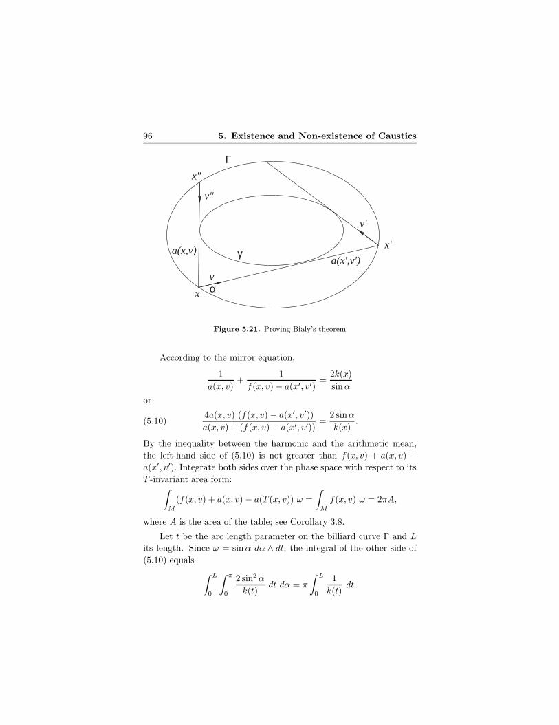
96 5. Existence and Non-existence of Caustics
αv
a(x',v')a(x,v)
v'
v"
x'
x
x"
γ
Γ
Figure 5.21. Proving Bialy’s theorem
According to the mirror equation,
1
a(x, v)+
1
f(x, v) − a(x′, v′)=
2k(x)
sinα
or
(5.10)4a(x, v) (f(x, v) − a(x′, v′))
a(x, v) + (f(x, v) − a(x′, v′))=
2 sinα
k(x).
By the inequality between the harmonic and the arithmetic mean,
the left-hand side of (5.10) is not greater than f(x, v) + a(x, v) −a(x′, v′). Integrate both sides over the phase space with respect to its
T -invariant area form:∫
M
(f(x, v) + a(x, v) − a(T (x, v)) ω =
∫
M
f(x, v) ω = 2πA,
where A is the area of the table; see Corollary 3.8.
Let t be the arc length parameter on the billiard curve Γ and L
its length. Since ω = sinα dα ∧ dt, the integral of the other side of
(5.10) equals
∫ L
0
∫ π
0
2 sin2 α
k(t)dt dα = π
∫ L
0
1
k(t)dt.
5. Existence and Non-existence of Caustics 97
Recall the Cauchy-Schwartz inequality:
∫ L
0
g2(t) dt
∫ L
0
h2(t) dt ≥(∫ L
0
g(t)h(t) dt
)2
.
It follows that ∫ L
0
1
k(t)dt
∫ L
0
k(t) dt ≥ L2.
Since∫ L
0 k(t) dt = 2π, one concludes that 2πA ≥ L2/2. This is op-
posite to the isoperimetric inequality (3.5); hence it is actually an
equality, and the curve Γ is a circle.
Let us finish this chapter with the following question: which plane
convex billiards with smooth boundary have caustics? The answer
is provided by the KAM (Kolmogorov-Arnold-Moser) theory. This
theory concerns small perturbations of integrable systems; see, e.g.,
[3, 58, 70].
Integrable systems are very exceptional, but many important sys-
tems are small perturbations of integrable ones. A classical example
is the solar system. The total mass of the planets is about 0.1% of
the mass of the sun. If one neglects the gravitational forces between
the planets and considers only their attraction to the sun then one
has an integrable (and explicitly solvable) system: every planet moves
along an ellipse with a focus in the sun. Taking into account gravita-
tional attraction between the planets yields a small perturbation of
this integrable system.
To fix ideas, assume that we have a completely integrable area
preserving map T in dimension 2. The phase space is foliated by
invariant circles, and, in appropriate coordinates on these circles, the
map is a parallel translation T : x 7→ x+ c. The constant c depends
on the invariant circle, and we assume that this dependence is non-
degenerate. The map T is perturbed in the class of area preserving
maps.
Consider an invariant circle γ with c = p/q. Then T q = Id on
γ. It is highly exceptional for a map to have a curve consisting of
fixed points, and we should expect the invariant circle γ to disappear
under a small perturbation of the map T .
98 5. Existence and Non-existence of Caustics
However, if c is irrational and, in addition, poorly approximated
by rational numbers, then the invariant circle γ survives a perturba-
tion of the map T and also gets perturbed. The technical condition
on c for this KAM-type result to hold is called Diophantine: there
exist a > 0, b > 1 such that for all non-zero integers p and q one has:
|qc− p| > aq−b.
The KAM theory has numerous applications. For example, it
implies that the geodesics on a surface sufficiently close to a 3-axial
ellipsoid exhibit a behavior similar to that depicted in figure 4.12.
An application to plane convex billiards is due to V. Lazutkin
[64], who proved the following theorem: if the billiard curve is suf-
ficiently smooth and its curvature is everywhere positive, then there
exists a collection of smooth caustics in a vicinity of the billiard curve
whose union has a positive measure. Originally this theorem asked
for 553 continuous derivatives of the billiard curve; later this num-
ber was reduced to 6. Lazutkin found coordinates, suggested by the
string construction, in which the billiard ball map reduces to a simple
form:
x1 = x+ y + f(x, y)y3, y1 = y + g(x, y)y4.
In particular, near the boundary of the phase cylinder y = 0, the map
is a small perturbation of the integrable map (x, y) 7→ (x+ y, y).
In conclusion, let us mention a result by M. Berger [13] on caus-
tics of multi-dimensional billiards. Suppose that a billiard hypersur-
face M has a caustic N , another hypersurface. Then the collection
of rays through a point of M , tangent to N , is a symmetric cone
whose axis is perpendicular to M . Berger proved that this condition,
satisfied near a point of M , implies that M is a part of a quadric and
N is a part of a confocal quadric. Unlike Bialy’s theorem, this is a
local result.
Chapter 6
Periodic Trajectories
Let us start our discussion of periodic billiard trajectories with the
simplest case of period two. Let γ be a smooth strictly convex billiard
curve. A 2-periodic billiard trajectory is a chord of γ which is per-
pendicular to γ at both end points. Such chords are called diameters.
One such diameter is easy to find: consider the longest chord
of γ. Since billiard trajectories are extrema of the perimeter length
function (see Chapter 1), the maximal chord is a 2-periodic trajectory.
Are there others?
The example of an ellipse suggests that, along with the major
axis, there is a second diameter, the minor axis. To construct this
second diameter for an arbitrary γ, consider two parallel support
lines to γ having direction φ; see figure 6.1. Let w(φ) be the distance
between these lines, the width of γ in the direction φ. Then w(φ) is a
smooth (and even) function on the circle. Its maximum corresponds
to the longest chord of γ, and its minimum to another diameter, the
desired second 2-periodic billiard trajectory.
Exercise 6.1. Express w(φ) in terms of p(φ), the support function
of γ. Using Exercise 3.14, formula (3.4), prove that cosα = w′(φ)
in figure 6.1 and conclude that critical points of the width function
correspond to diameters of γ.
99
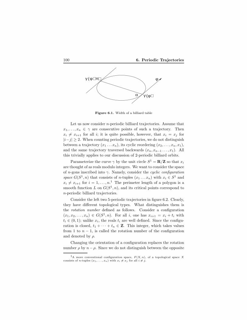
100 6. Periodic Trajectories
α
φ
) φ ( γ
) π + φ ( γ
Figure 6.1. Width of a billiard table
Let us now consider n-periodic billiard trajectories. Assume that
x1, . . . , xn ∈ γ are consecutive points of such a trajectory. Then
xi 6= xi+1 for all i; it is quite possible, however, that xi = xj for
|i−j| ≥ 2. When counting periodic trajectories, we do not distinguish
between a trajectory (x1 . . . xn), its cyclic reordering (x2, . . . , xn, x1),
and the same trajectory traversed backwards (xn, xn−1 . . . , x1). All
this trivially applies to our discussion of 2-periodic billiard orbits.
Parameterize the curve γ by the unit circle S1 = R/Z so that xi
are thought of as reals modulo integers. We want to consider the space
of n-gons inscribed into γ. Namely, consider the cyclic configuration
space G(S1, n) that consists of n-tuples (x1 . . . xn) with xi ∈ S1 and
xi 6= xi+1 for i = 1, . . . , n.1 The perimeter length of a polygon is a
smooth function L on G(S1, n), and its critical points correspond to
n-periodic billiard trajectories.
Consider the left two 5-periodic trajectories in figure 6.2. Clearly,
they have different topological types. What distinguishes them is
the rotation number defined as follows. Consider a configuration
(x1, x2, . . . , xn) ∈ G(S1, n). For all i, one has xi+1 = xi + ti with
ti ∈ (0, 1); unlike xi, the reals ti are well defined. Since the configu-
ration is closed, t1 + · · · + tn ∈ Z. This integer, which takes values
from 1 to n − 1, is called the rotation number of the configuration
and denoted by ρ.
Changing the orientation of a configuration replaces the rotation
number ρ by n− ρ. Since we do not distinguish between the opposite
1A more conventional configuration space, F (X, n), of a topological space Xconsists of n-tuples (x1, . . . , xn) with xi 6= xj for all i 6= j.

6. Periodic Trajectories 101
3
4
52
55 4
4
33
2
2
111 2
3
4
5
1
Figure 6.2. Rotation number of a periodic billiard trajectory
orientations of a configuration, we assume that ρ takes values from 1
to ⌊(n− 1)/2⌋. The left-most 5-periodic trajectory in figure 6.2 has
ρ = 1 and the other three ρ = 2.
The configuration space G(S1, n) is not connected; its connected
components are enumerated by the rotation number. Each compo-
nent is topologically the product of S1 and (n− 1)-dimensional ball.
The next Birkhoff’s theorem asserts that the perimeter length func-
tion has at least two extrema in each connected component.
Theorem 6.2. For every n ≥ 2 and ρ ≤ ⌊(n− 1)/2⌋, coprime with
n, there exist two geometrically distinct n-periodic billiard trajectories
with the rotation number ρ.
If ρ is not coprime with n, then one may obtain an n-periodic
trajectory that is a multiple of a periodic trajectory with a smaller
period.
Proof. (Sketch). Similar to the case n = 2, one periodic trajectory
is relatively easy to find. Fix a connected component M of the cyclic
configuration space corresponding to the given rotation number, and
consider its closure M in space S1 × · · · × S1. This closure contains
degenerate polygons with fewer than n sides.
The perimeter length function L has a maximum in M . We wish
to show that this maximum is attained at an interior point, that is,
not on a k-gon with k < n. Indeed, by the triangle inequality, the
perimeter of a k-gon will increase if one increases the number of sides;
see figure 6.3. Thus we have one n-periodic trajectory (x1, . . . , xn)
corresponding to the maximum of L.
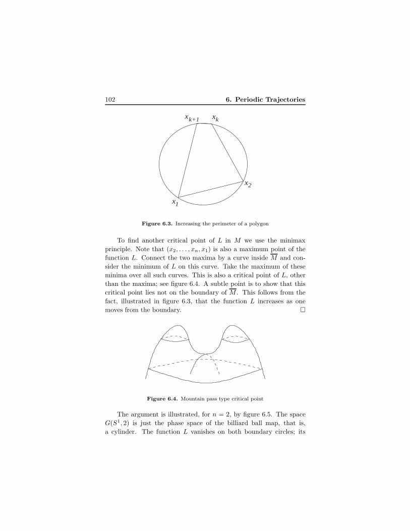
102 6. Periodic Trajectories
xkxk+1
x
x
1
2
Figure 6.3. Increasing the perimeter of a polygon
To find another critical point of L in M we use the minimax
principle. Note that (x2, . . . , xn, x1) is also a maximum point of the
function L. Connect the two maxima by a curve inside M and con-
sider the minimum of L on this curve. Take the maximum of these
minima over all such curves. This is also a critical point of L, other
than the maxima; see figure 6.4. A subtle point is to show that this
critical point lies not on the boundary of M . This follows from the
fact, illustrated in figure 6.3, that the function L increases as one
moves from the boundary.
Figure 6.4. Mountain pass type critical point
The argument is illustrated, for n = 2, by figure 6.5. The space
G(S1, 2) is just the phase space of the billiard ball map, that is,
a cylinder. The function L vanishes on both boundary circles; its
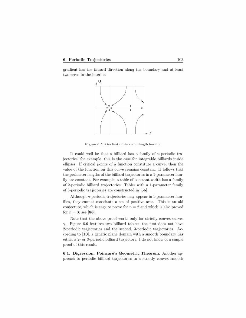
6. Periodic Trajectories 103
gradient has the inward direction along the boundary and at least
two zeros in the interior.
α
t
Figure 6.5. Gradient of the chord length function
It could well be that a billiard has a family of n-periodic tra-
jectories; for example, this is the case for integrable billiards inside
ellipses. If critical points of a function constitute a curve, then the
value of the function on this curve remains constant. It follows that
the perimeter lengths of the billiard trajectories in a 1-parameter fam-
ily are constant. For example, a table of constant width has a family
of 2-periodic billiard trajectories. Tables with a 1-parameter family
of 3-periodic trajectories are constructed in [55].
Although n-periodic trajectories may appear in 1-parameter fam-
ilies, they cannot constitute a set of positive area. This is an old
conjecture, which is easy to prove for n = 2 and which is also proved
for n = 3; see [88].
Note that the above proof works only for strictly convex curves
γ. Figure 6.6 features two billiard tables: the first does not have
2-periodic trajectories and the second, 3-periodic trajectories. Ac-
cording to [10], a generic plane domain with a smooth boundary has
either a 2- or 3-periodic billiard trajectory. I do not know of a simple
proof of this result.
6.1. Digression. Poincare’s Geometric Theorem. Another ap-
proach to periodic billiard trajectories in a strictly convex smooth
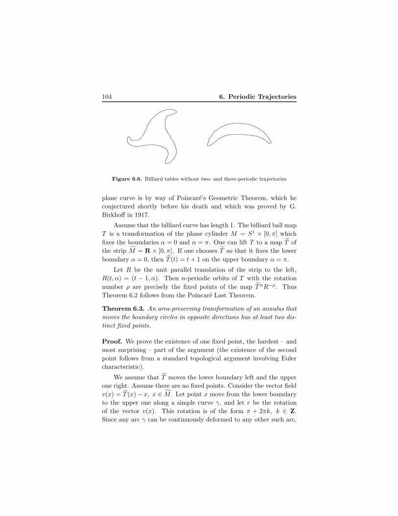
104 6. Periodic Trajectories
Figure 6.6. Billiard tables without two- and three-periodic trajectories
plane curve is by way of Poincare’s Geometric Theorem, which he
conjectured shortly before his death and which was proved by G.
Birkhoff in 1917.
Assume that the billiard curve has length 1. The billiard ball map
T is a transformation of the phase cylinder M = S1 × [0, π] which
fixes the boundaries α = 0 and α = π. One can lift T to a map T of
the strip M = R × [0, π]. If one chooses T so that it fixes the lower
boundary α = 0, then T (t) = t+ 1 on the upper boundary α = π.
Let R be the unit parallel translation of the strip to the left,
R(t, α) = (t − 1, α). Then n-periodic orbits of T with the rotation
number ρ are precisely the fixed points of the map T nR−ρ. Thus
Theorem 6.2 follows from the Poincare Last Theorem.
Theorem 6.3. An area-preserving transformation of an annulus that
moves the boundary circles in opposite directions has at least two dis-
tinct fixed points.
Proof. We prove the existence of one fixed point, the hardest – and
most surprising – part of the argument (the existence of the second
point follows from a standard topological argument involving Euler
characteristic).
We assume that T moves the lower boundary left and the upper
one right. Assume there are no fixed points. Consider the vector field
v(x) = T (x)− x, x ∈ M . Let point x move from the lower boundary
to the upper one along a simple curve γ, and let r be the rotation
of the vector v(x). This rotation is of the form π + 2πk, k ∈ Z.
Since any arc γ can be continuously deformed to any other such arc,
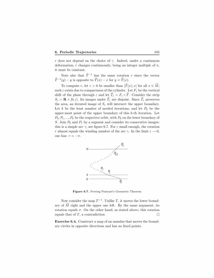
6. Periodic Trajectories 105
r does not depend on the choice of γ. Indeed, under a continuous
deformation, r changes continuously; being an integer multiple of π,
it must be constant.
Note also that T−1 has the same rotation r since the vector
T−1(y) − y is opposite to T (x) − x for y = T (x).
To compute r, let ε > 0 be smaller than |T (x), x| for all x ∈ M ;
such ε exists due to compactness of the cylinder. Let Fε be the vertical
shift of the plane through ε and let Tε = Fε T . Consider the strip
Sε = R × [0, ε]. Its images under Tε are disjoint. Since Tε preserves
the area, an iterated image of Sε will intersect the upper boundary.
Let k be the least number of needed iterations, and let Pk be the
upper-most point of the upper boundary of this k-th iteration. Let
P0, P1, ..., Pk be the respective orbit, with P0 on the lower boundary of
S. Join P0 and P1 by a segment and consider its consecutive images:
this is a simple arc γ; see figure 6.7. For ε small enough, the rotation
r almost equals the winding number of the arc γ. In the limit ε→ 0,
one has: r = −π.
0ε
π
2P1P
0P
k1P
kP
Figure 6.7. Proving Poincare’s Geometric Theorem
Now consider the map T−1. Unlike T , it moves the lower bound-
ary of M right and the upper one left. By the same argument, its
rotation equals π. On the other hand, as stated above, this rotation
equals that of T , a contradiction.
Exercise 6.4. Construct a map of an annulus that moves the bound-
ary circles in opposite directions and has no fixed points.
106 6. Periodic Trajectories
Poincare’s theorem is, probably, the first result of symplectic
topology. By now, this is an extremely active research area with
well-developed techniques; see, e.g, [7, 67]. Let us mention a sample
result, close to Poincare’s theorem: an area preserving smooth trans-
formation of the torus T 2 that fixes the center of mass has at least
3, and generically 4, fixed points (for a symplectic transformation of
T 2n, fixing the center of mass, these numbers are 2n + 1 and 4n,
respectively; this is the celebrated Conley-Zehnder theorem, conjec-
tured by V. Arnold in the 1960s). ♣
6.2. Digression. Birkhoff periodic orbits and Aubry-Mather
theory. Theorem 6.2 extends to area preserving twist maps of the
cylinder. As before, one lifts the cylinder map T to a map T of an
infinite strip M . Assume that the restrictions of T to the lower and
upper boundaries are translations t 7→ t+ c1 and t 7→ t+ c2 (in fact,
it suffices to assume that the restrictions of T to the boundary have
this form in some coordinate on the boundary). The interval (c1, c2)
is called the twist interval of the twist map T ; it is well defined, up
to a shift by an integer.
An extension of Theorem 6.2 asserts that, for every rational num-
ber ρ/n ∈ (c1, c2) given in lowest terms, the twist map has at least
two n-periodic orbits with rotation number ρ. Moreover, one may as-
sume that the first coordinates of the points of the orbit, lifted to M ,
are monotonically increasing. Such periodic orbits are called Birkhoff
orbits.
If α is an irrational number in the twist interval, one may con-
sider its rational approximation ρk/nk → α, k → ∞. The Birkhoff
periodic orbits accumulate to an invariant set S, and T acts on this
set as the rotation through α. This invariant set lies on the graph
of a continuous function; cf. Birkhoff’s theorem that says that an
invariant circle of a twist map is a graph, Chapter 5. The set S can
be an invariant circle, but it can also be a Cantor set. Such sets are
called Aubry-Mather sets. One of the motivations for Aubry-Mather
theory came from solid state physics. ♣
Let us now say a few words about the available multi-dimensional
results. Let Q ⊂ Rm be a smooth strictly convex closed billiard
6. Periodic Trajectories 107
hypersurface. One is interested in the least number of n-periodic
billiard trajectories inside Q. Unlike the planar case m = 2, the
rotation number of a trajectory is not defined.
The case n = 2 is again relatively easy: there are at least m dis-
tinct diameters of a convex hypersurface. This fact is proved similarly
to the planar case. For every direction, one considers the width of Q
in this direction; this gives a smooth function on the projective space
RPm−1. It is known from Morse theory (see Digression 6.3 below)
that a function on RPm−1 has no less than m critical points, and the
result follows.
The case of n ≥ 3 is much harder and was investigated only re-
cently [37, 36]. Here is one result: for a generic Q, the number of n-
periodic billiard trajectories is not less than (n−1)(m−1). The proof
consists of estimating the number of critical points of the perimeter
length function on the cyclic configuration space G(Sm−1, n) and its
quotient space by the dihedral group Dn, the group of symmetries
of the regular n-gon; the main difficulty is in describing the topol-
ogy of these spaces. Note that G(Sm−1, 2) retracts to Sm−1 and
G(Sm−1, 2)/Z2 to RPm−1.
6.3. Digression. Morse theory. Morse theory provides lower bounds
on the number of critical points of a smooth function f on a smooth
manifold M in terms of the topology of M ; see [19, 68].
At a critical point, the Taylor series of a function f(x1, . . . , xn)
starts with a quadratic form. After a coordinate change, this qua-
dratic form can be written as x21 + · · · + x2
p − x2p+1 − · · · − x2
p+q . If
p + q = n, then the critical point is called non-degenerate, and q is
called the Morse index of this critical point.2 A function whose criti-
cal points are all non-degenerate is called a Morse function. A generic
smooth function is Morse.
Let Mn be a smooth compact manifold without boundary, and
let t be a formal variable. One associates a counting function with a
Morse function f : M → R:
Pt(f) = a0 + a1t+ a2t2 + · · · + ant
n
2In the case of two variables, the classification according to Morse index is thefamiliar second derivative test of calculus.
108 6. Periodic Trajectories
where ai is the number of critical points of f with Morse index i.
Exercise 6.5. Consider the function on the unit sphere in Rn given
by the formula
f(x) =
n∑
i=1
λix2i
where λ1 < · · · < λn. Find critical points of this function, determine
their Morse indices and compute Pt(f).
One also associates a counting function with the manifold M :
Pt(M) = b0 + b1t+ b2t2 + · · · + bnt
n
where bi is the i-th Betti number, the rank of i-th homology group of
M . A succinct form of Morse inequalities is as follows:
(6.1) Pt(f) = Pt(M) + (1 + t)Qt
where Qt is a polynomial in t with non-negative coefficients. In par-
ticular, setting t = 1, one finds that the number of critical points of a
Morse function is not less than the sum of Betti numbers of M . For
M = RPn−1, the latter equals n. If M is a surface of genus g, that
is, a sphere with g handles, then the sum of Betti numbers is 2g + 2.
If one sets t = −1 in (6.1), the result is that∑
(−1)iai =∑
(−1)ibi = χ(M),
the Euler characteristic of M .
Exercise 6.6. A Morse function on two-dimensional torus has at
least 4 critical points: maximum, minimum and two saddles. Con-
struct a smooth function on T 2 with only three critical points.
Here is a simple application of Morse inequalities in geometry.
Consider M , a surface of genus g in R3, and let P be a generic point
in space. How many normals from P to M are there? These normals
correspond to critical points of the distance function from P to a
point of M , and therefore there exist at least 2g + 2 such normals.
Likewise, one may consider double normals of a surface M , that
is, its chords, perpendicular to M at both end points (these are gener-
alizations of 2-periodic billiard trajectories). This problem was solved
only recently; see [83]. The result is that if the genus of M is g, then
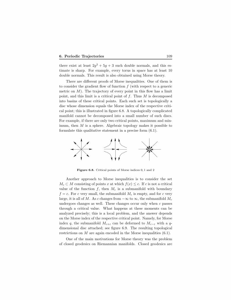
6. Periodic Trajectories 109
there exist at least 2g2 + 5g + 3 such double normals, and this es-
timate is sharp. For example, every torus in space has at least 10
double normals. This result is also obtained using Morse theory.
There are different proofs of Morse inequalities. One of them is
to consider the gradient flow of function f (with respect to a generic
metric on M). The trajectory of every point in this flow has a limit
point, and this limit is a critical point of f . Thus M is decomposed
into basins of these critical points. Each such set is topologically a
disc whose dimension equals the Morse index of the respective criti-
cal point; this is illustrated in figure 6.8. A topologically complicated
manifold cannot be decomposed into a small number of such discs.
For example, if there are only two critical points, maximum and min-
imum, then M is a sphere. Algebraic topology makes it possible to
formulate this qualitative statement in a precise form (6.1).
Figure 6.8. Critical points of Morse indices 0, 1 and 2
Another approach to Morse inequalities is to consider the set
Mc ⊂M consisting of points x at which f(x) ≤ c. If c is not a critical
value of the function f , then Mc is a submanifold with boundary
f = c. For c very small, the submanifold Mc is empty, and for c very
large, it is all of M . As c changes from −∞ to ∞, the submanifold Mc
undergoes changes as well. These changes occur only when c passes
through a critical value. What happens at these moments can be
analyzed precisely; this is a local problem, and the answer depends
on the Morse index of the respective critical point. Namely, for Morse
index q, the submanifold Mc+ε can be deformed to Mc−ε with a q-
dimensional disc attached; see figure 6.9. The resulting topological
restrictions on M are again encoded in the Morse inequalities (6.1).
One of the main motivations for Morse theory was the problem
of closed geodesics on Riemannian manifolds. Closed geodesics are
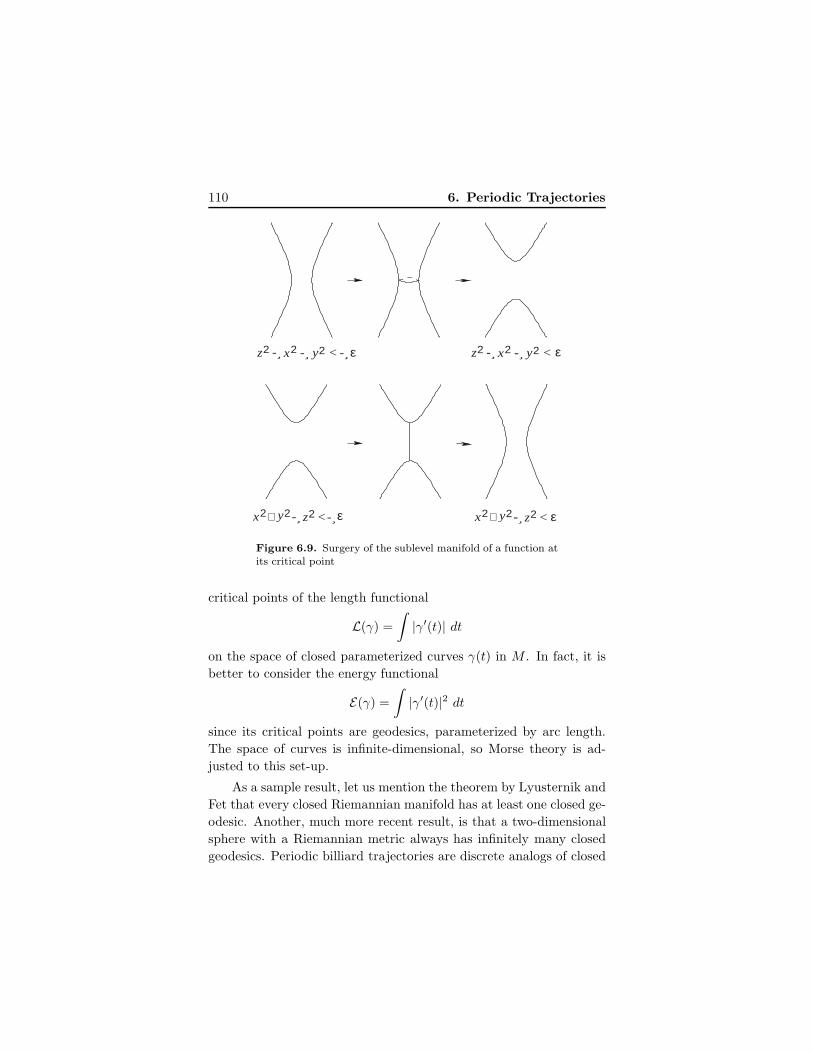
110 6. Periodic Trajectories
2z2y2x2z2y2x ε<-+- ε<-+
-2zε-<2y-2x-2z x ε<2y-2
Figure 6.9. Surgery of the sublevel manifold of a function at
its critical point
critical points of the length functional
L(γ) =
∫|γ′(t)| dt
on the space of closed parameterized curves γ(t) in M . In fact, it is
better to consider the energy functional
E(γ) =
∫|γ′(t)|2 dt
since its critical points are geodesics, parameterized by arc length.
The space of curves is infinite-dimensional, so Morse theory is ad-
justed to this set-up.
As a sample result, let us mention the theorem by Lyusternik and
Fet that every closed Riemannian manifold has at least one closed ge-
odesic. Another, much more recent result, is that a two-dimensional
sphere with a Riemannian metric always has infinitely many closed
geodesics. Periodic billiard trajectories are discrete analogs of closed

6. Periodic Trajectories 111
geodesics, and Morse theory naturally plays a prominent role in their
study. Morse-theoretical methods also play an important role in con-
temporary symplectic topology. ♣

Chapter 7
Billiards in Polygons
To continue with the topic of the last chapter, let us discuss periodic
billiard trajectories in polygons. Start with an acute triangle. The
following elementary geometry construction is called the Fagnano bil-
liard trajectory.
Lemma 7.1. The triangle connecting the base points of the three
altitudes is a 3-periodic billiard trajectory; see figure 7.1.
Proof. The quadrilateral BPOR has two right angles; hence it is
inscribed into a circle. The angles APR and ABQ are supported by
the same arc of this circle; therefore they are equal. Likewise, the
angles APQ and ACR are equal. It remains to show that the angles
ABQ and ACR are equal. Indeed, both complement the angle BAC
to π/2, and the result follows.
Note that the distance between parallel lines does not change after
reflection in a flat mirror. It follows that periodic billiard trajectories
in a polygon are never isolated: an even-periodic trajectory belongs
to a 1-parameter family of parallel periodic trajectories of the same
period and length, and an odd-periodic one is contained in a strip
consisting of trajectories whose period and length is twice as great;
see figure 7.2.
113
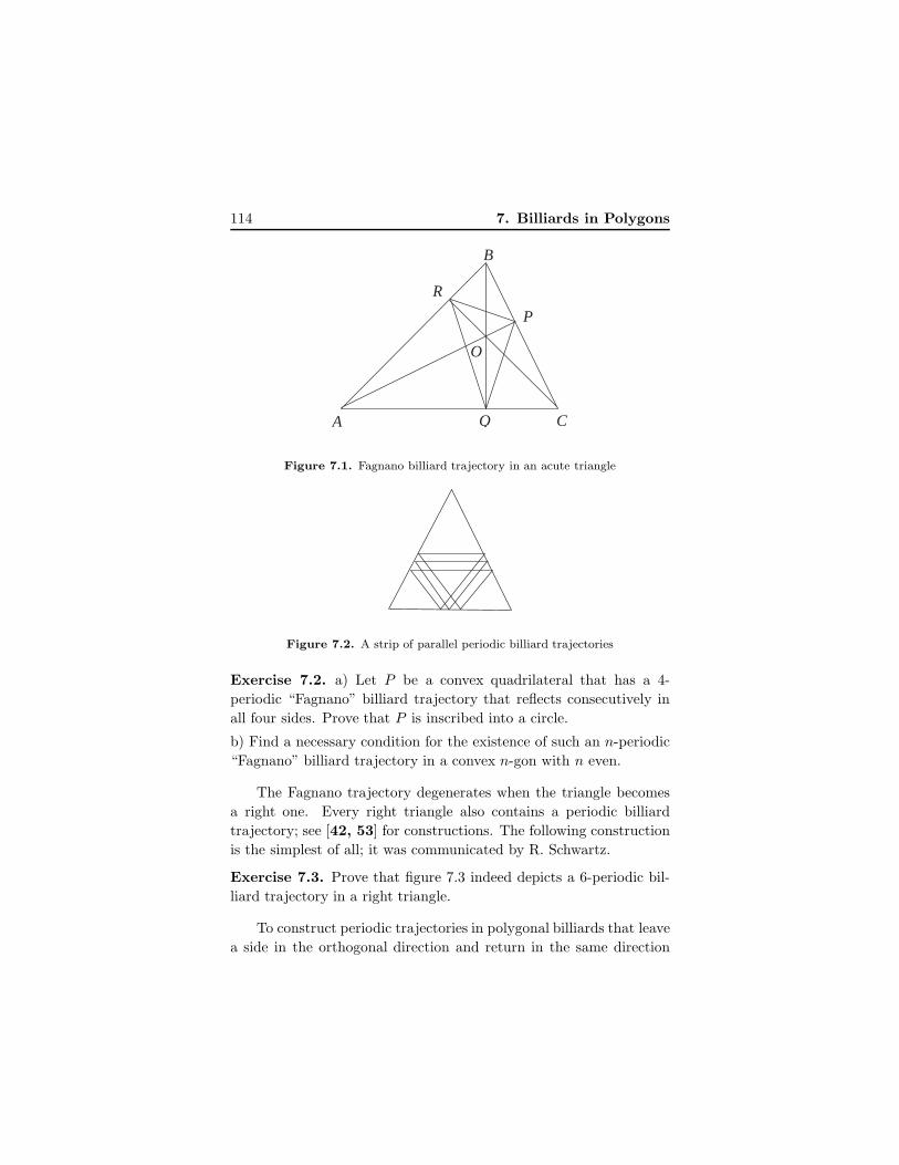
114 7. Billiards in Polygons
B
CA
P
Q
R
O
Figure 7.1. Fagnano billiard trajectory in an acute triangle
Figure 7.2. A strip of parallel periodic billiard trajectories
Exercise 7.2. a) Let P be a convex quadrilateral that has a 4-
periodic “Fagnano” billiard trajectory that reflects consecutively in
all four sides. Prove that P is inscribed into a circle.
b) Find a necessary condition for the existence of such an n-periodic
“Fagnano” billiard trajectory in a convex n-gon with n even.
The Fagnano trajectory degenerates when the triangle becomes
a right one. Every right triangle also contains a periodic billiard
trajectory; see [42, 53] for constructions. The following construction
is the simplest of all; it was communicated by R. Schwartz.
Exercise 7.3. Prove that figure 7.3 indeed depicts a 6-periodic bil-
liard trajectory in a right triangle.
To construct periodic trajectories in polygonal billiards that leave
a side in the orthogonal direction and return in the same direction
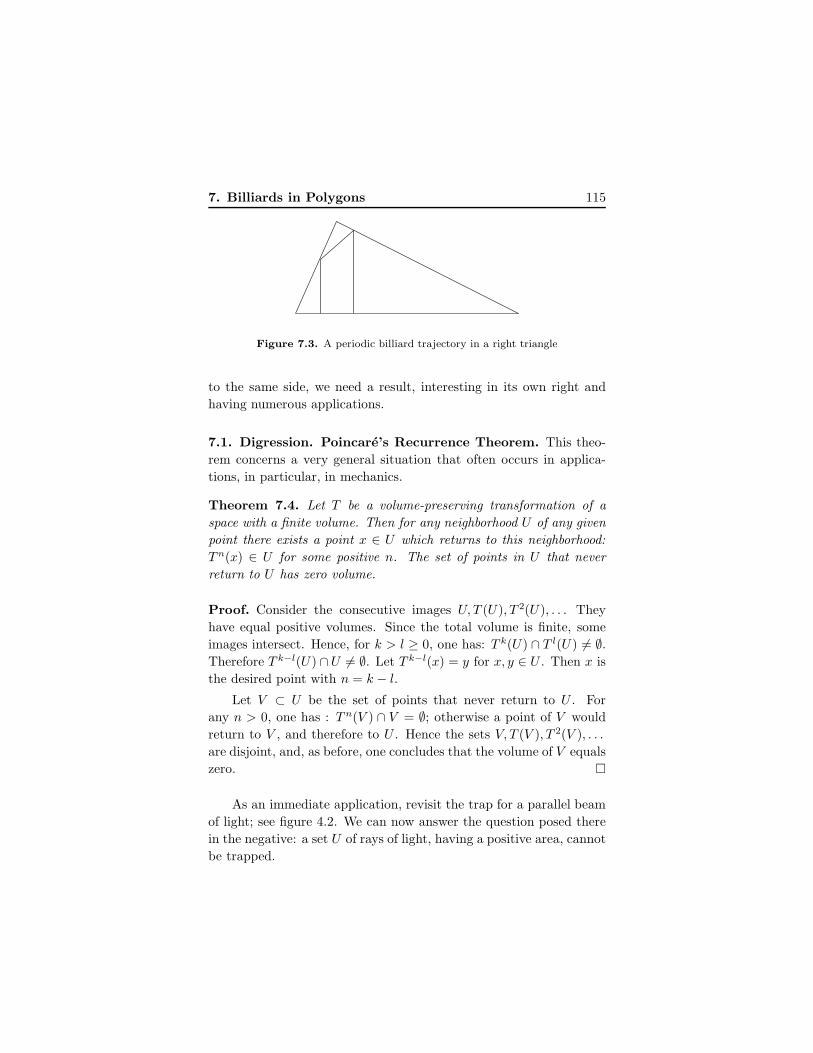
7. Billiards in Polygons 115
Figure 7.3. A periodic billiard trajectory in a right triangle
to the same side, we need a result, interesting in its own right and
having numerous applications.
7.1. Digression. Poincare’s Recurrence Theorem. This theo-
rem concerns a very general situation that often occurs in applica-
tions, in particular, in mechanics.
Theorem 7.4. Let T be a volume-preserving transformation of a
space with a finite volume. Then for any neighborhood U of any given
point there exists a point x ∈ U which returns to this neighborhood:
T n(x) ∈ U for some positive n. The set of points in U that never
return to U has zero volume.
Proof. Consider the consecutive images U, T (U), T 2(U), . . . They
have equal positive volumes. Since the total volume is finite, some
images intersect. Hence, for k > l ≥ 0, one has: T k(U) ∩ T l(U) 6= ∅.Therefore T k−l(U) ∩U 6= ∅. Let T k−l(x) = y for x, y ∈ U . Then x is
the desired point with n = k − l.
Let V ⊂ U be the set of points that never return to U . For
any n > 0, one has : T n(V ) ∩ V = ∅; otherwise a point of V would
return to V , and therefore to U . Hence the sets V, T (V ), T 2(V ), . . .
are disjoint, and, as before, one concludes that the volume of V equals
zero.
As an immediate application, revisit the trap for a parallel beam
of light; see figure 4.2. We can now answer the question posed there
in the negative: a set U of rays of light, having a positive area, cannot
be trapped.
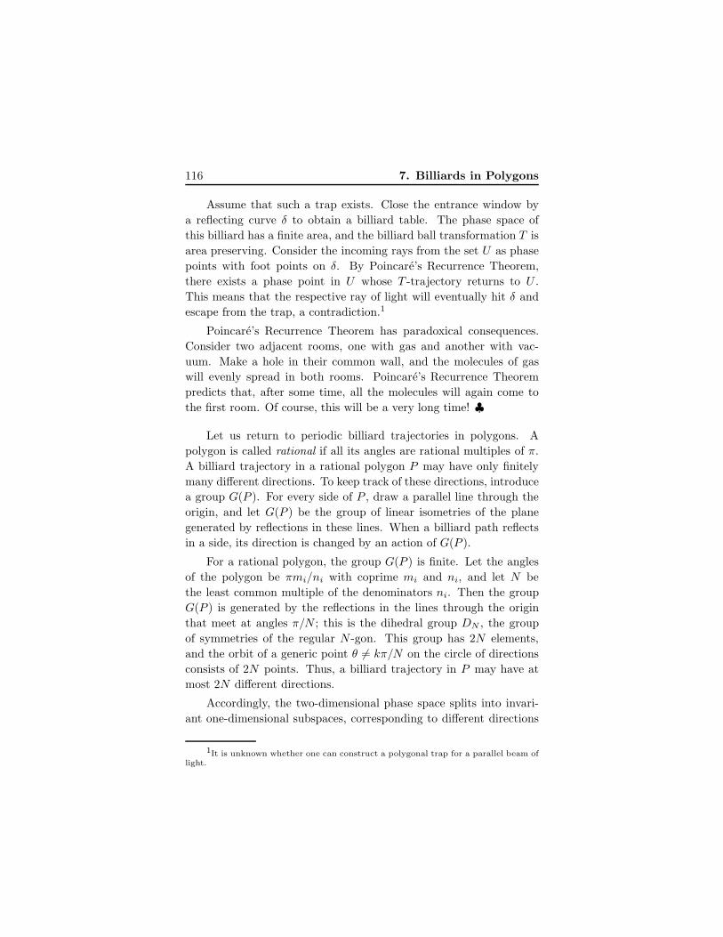
116 7. Billiards in Polygons
Assume that such a trap exists. Close the entrance window by
a reflecting curve δ to obtain a billiard table. The phase space of
this billiard has a finite area, and the billiard ball transformation T is
area preserving. Consider the incoming rays from the set U as phase
points with foot points on δ. By Poincare’s Recurrence Theorem,
there exists a phase point in U whose T -trajectory returns to U .
This means that the respective ray of light will eventually hit δ and
escape from the trap, a contradiction.1
Poincare’s Recurrence Theorem has paradoxical consequences.
Consider two adjacent rooms, one with gas and another with vac-
uum. Make a hole in their common wall, and the molecules of gas
will evenly spread in both rooms. Poincare’s Recurrence Theorem
predicts that, after some time, all the molecules will again come to
the first room. Of course, this will be a very long time! ♣
Let us return to periodic billiard trajectories in polygons. A
polygon is called rational if all its angles are rational multiples of π.
A billiard trajectory in a rational polygon P may have only finitely
many different directions. To keep track of these directions, introduce
a group G(P ). For every side of P , draw a parallel line through the
origin, and let G(P ) be the group of linear isometries of the plane
generated by reflections in these lines. When a billiard path reflects
in a side, its direction is changed by an action of G(P ).
For a rational polygon, the group G(P ) is finite. Let the angles
of the polygon be πmi/ni with coprime mi and ni, and let N be
the least common multiple of the denominators ni. Then the group
G(P ) is generated by the reflections in the lines through the origin
that meet at angles π/N ; this is the dihedral group DN , the group
of symmetries of the regular N -gon. This group has 2N elements,
and the orbit of a generic point θ 6= kπ/N on the circle of directions
consists of 2N points. Thus, a billiard trajectory in P may have at
most 2N different directions.
Accordingly, the two-dimensional phase space splits into invari-
ant one-dimensional subspaces, corresponding to different directions
1It is unknown whether one can construct a polygonal trap for a parallel beam oflight.
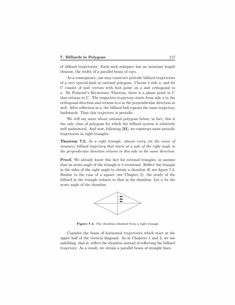
7. Billiards in Polygons 117
of billiard trajectories. Each such subspace has an invariant length
element, the width of a parallel beam of rays.
As a consequence, one may construct periodic billiard trajectories
of a very special kind in rational polygons. Choose a side a, and let
U consist of unit vectors with foot point on a and orthogonal to
a. By Poincare’s Recurrence Theorem, there is a phase point in U
that returns to U . The respective trajectory starts from side a in the
orthogonal direction and returns to a in the perpendicular direction as
well. After reflection in a, the billiard ball repeats the same trajectory
backwards. Thus this trajectory is periodic.
We will say more about rational polygons below; in fact, this is
the only class of polygons for which the billiard system is relatively
well understood. And now, following [31], we construct more periodic
trajectories in right triangles.
Theorem 7.5. In a right triangle, almost every (in the sense of
measure) billiard trajectory that starts at a side of the right angle in
the perpendicular direction returns to this side in the same direction.
Proof. We already know this fact for rational triangles, so assume
that an acute angle of the triangle is π-irrational. Reflect the triangle
in the sides of the right angle to obtain a rhombus R; see figure 7.4.
Similar to the case of a square (see Chapter 2), the study of the
billiard in the triangle reduces to that in the rhombus. Let α be the
acute angle of the rhombus.
Figure 7.4. The rhombus obtained from a right triangle
Consider the beam of horizontal trajectories which start at the
upper half of the vertical diagonal. As in Chapters 1 and 2, we use
unfolding, that is, reflect the rhombus instead of reflecting the billiard
trajectory. As a result, we obtain a parallel beam of straight lines.
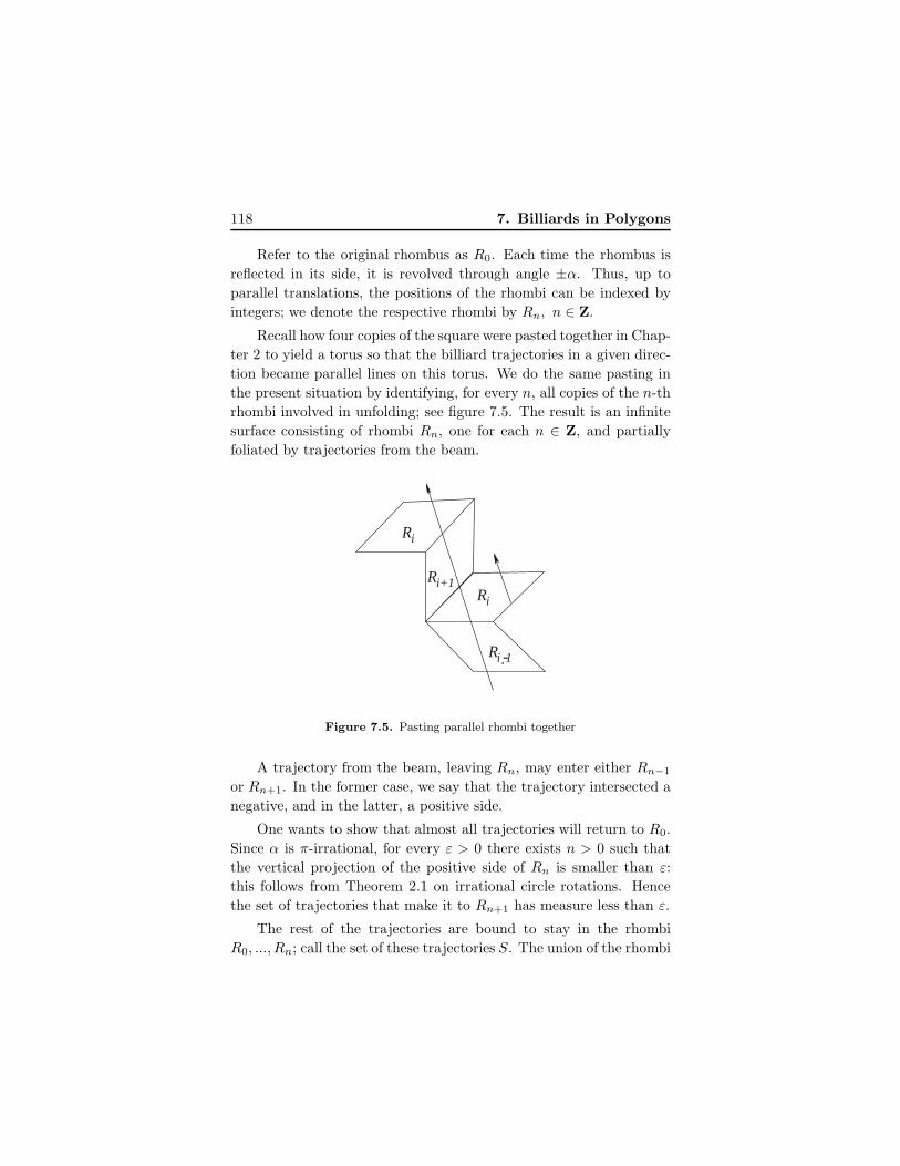
118 7. Billiards in Polygons
Refer to the original rhombus as R0. Each time the rhombus is
reflected in its side, it is revolved through angle ±α. Thus, up to
parallel translations, the positions of the rhombi can be indexed by
integers; we denote the respective rhombi by Rn, n ∈ Z.
Recall how four copies of the square were pasted together in Chap-
ter 2 to yield a torus so that the billiard trajectories in a given direc-
tion became parallel lines on this torus. We do the same pasting in
the present situation by identifying, for every n, all copies of the n-th
rhombi involved in unfolding; see figure 7.5. The result is an infinite
surface consisting of rhombi Rn, one for each n ∈ Z, and partially
foliated by trajectories from the beam.
i+1R
iR
iR
i 1R -
Figure 7.5. Pasting parallel rhombi together
A trajectory from the beam, leaving Rn, may enter either Rn−1
or Rn+1. In the former case, we say that the trajectory intersected a
negative, and in the latter, a positive side.
One wants to show that almost all trajectories will return to R0.
Since α is π-irrational, for every ε > 0 there exists n > 0 such that
the vertical projection of the positive side of Rn is smaller than ε:
this follows from Theorem 2.1 on irrational circle rotations. Hence
the set of trajectories that make it to Rn+1 has measure less than ε.
The rest of the trajectories are bound to stay in the rhombi
R0, ..., Rn; call the set of these trajectories S. The union of the rhombi
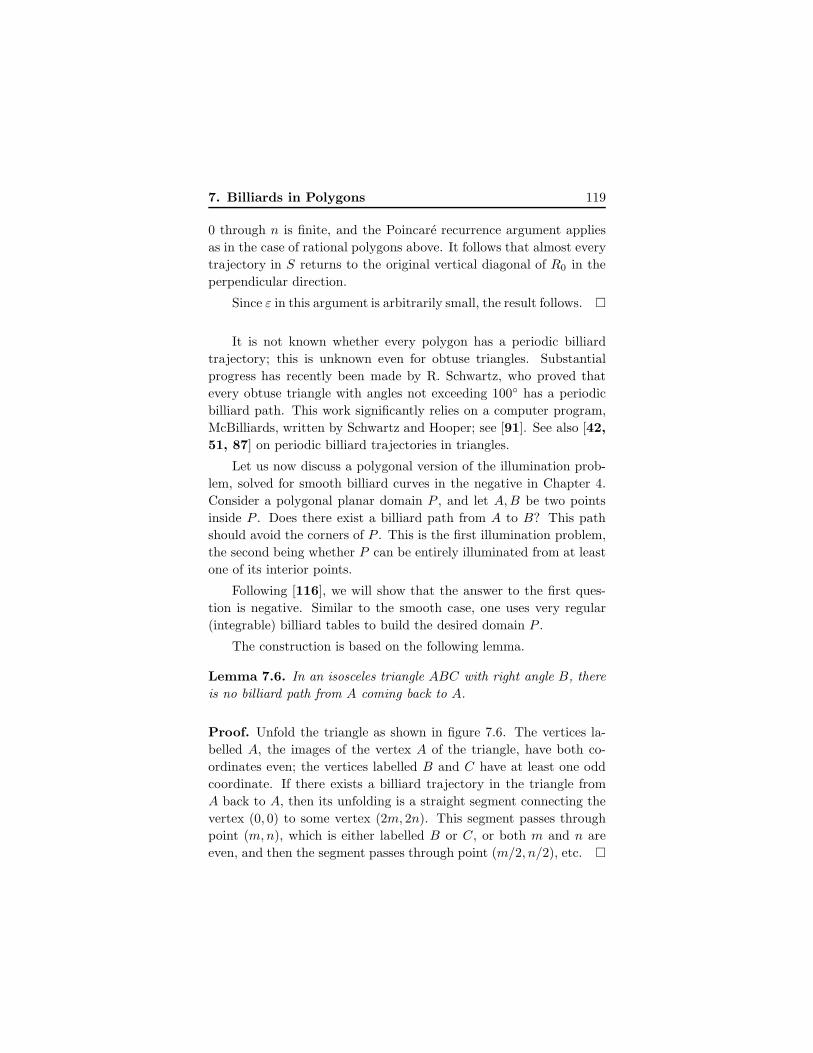
7. Billiards in Polygons 119
0 through n is finite, and the Poincare recurrence argument applies
as in the case of rational polygons above. It follows that almost every
trajectory in S returns to the original vertical diagonal of R0 in the
perpendicular direction.
Since ε in this argument is arbitrarily small, the result follows.
It is not known whether every polygon has a periodic billiard
trajectory; this is unknown even for obtuse triangles. Substantial
progress has recently been made by R. Schwartz, who proved that
every obtuse triangle with angles not exceeding 100 has a periodic
billiard path. This work significantly relies on a computer program,
McBilliards, written by Schwartz and Hooper; see [91]. See also [42,
51, 87] on periodic billiard trajectories in triangles.
Let us now discuss a polygonal version of the illumination prob-
lem, solved for smooth billiard curves in the negative in Chapter 4.
Consider a polygonal planar domain P , and let A,B be two points
inside P . Does there exist a billiard path from A to B? This path
should avoid the corners of P . This is the first illumination problem,
the second being whether P can be entirely illuminated from at least
one of its interior points.
Following [116], we will show that the answer to the first ques-
tion is negative. Similar to the smooth case, one uses very regular
(integrable) billiard tables to build the desired domain P .
The construction is based on the following lemma.
Lemma 7.6. In an isosceles triangle ABC with right angle B, there
is no billiard path from A coming back to A.
Proof. Unfold the triangle as shown in figure 7.6. The vertices la-
belled A, the images of the vertex A of the triangle, have both co-
ordinates even; the vertices labelled B and C have at least one odd
coordinate. If there exists a billiard trajectory in the triangle from
A back to A, then its unfolding is a straight segment connecting the
vertex (0, 0) to some vertex (2m, 2n). This segment passes through
point (m,n), which is either labelled B or C, or both m and n are
even, and then the segment passes through point (m/2, n/2), etc.
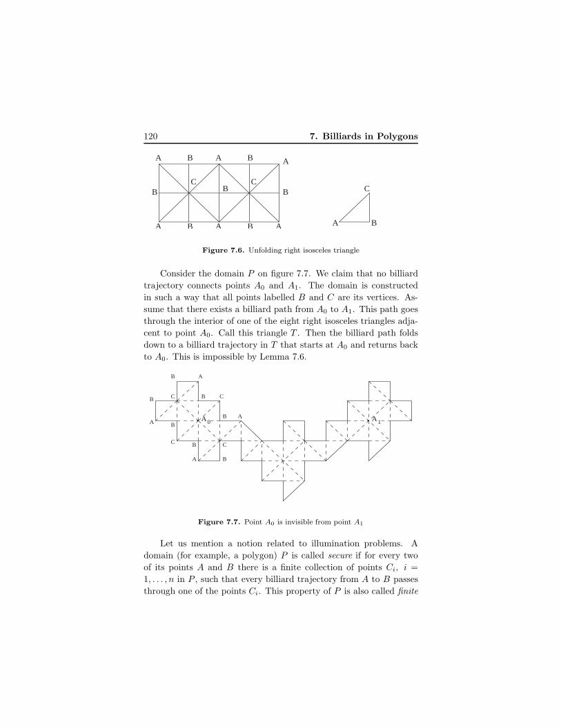
120 7. Billiards in Polygons
B
B
ABABA
BC
BC
A B
C
AA B A
Figure 7.6. Unfolding right isosceles triangle
Consider the domain P on figure 7.7. We claim that no billiard
trajectory connects points A0 and A1. The domain is constructed
in such a way that all points labelled B and C are its vertices. As-
sume that there exists a billiard path from A0 to A1. This path goes
through the interior of one of the eight right isosceles triangles adja-
cent to point A0. Call this triangle T . Then the billiard path folds
down to a billiard trajectory in T that starts at A0 and returns back
to A0. This is impossible by Lemma 7.6.
AA . . 0
C
BA
B
AB
CB
C
B
AB
CB
A 1
Figure 7.7. Point A0 is invisible from point A1
Let us mention a notion related to illumination problems. A
domain (for example, a polygon) P is called secure if for every two
of its points A and B there is a finite collection of points Ci, i =
1, . . . , n in P , such that every billiard trajectory from A to B passes
through one of the points Ci. This property of P is also called finite
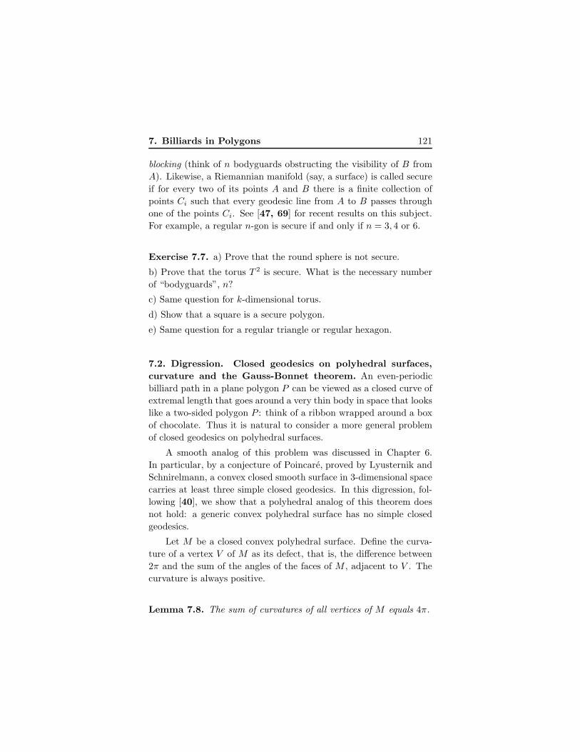
7. Billiards in Polygons 121
blocking (think of n bodyguards obstructing the visibility of B from
A). Likewise, a Riemannian manifold (say, a surface) is called secure
if for every two of its points A and B there is a finite collection of
points Ci such that every geodesic line from A to B passes through
one of the points Ci. See [47, 69] for recent results on this subject.
For example, a regular n-gon is secure if and only if n = 3, 4 or 6.
Exercise 7.7. a) Prove that the round sphere is not secure.
b) Prove that the torus T 2 is secure. What is the necessary number
of “bodyguards”, n?
c) Same question for k-dimensional torus.
d) Show that a square is a secure polygon.
e) Same question for a regular triangle or regular hexagon.
7.2. Digression. Closed geodesics on polyhedral surfaces,
curvature and the Gauss-Bonnet theorem. An even-periodic
billiard path in a plane polygon P can be viewed as a closed curve of
extremal length that goes around a very thin body in space that looks
like a two-sided polygon P : think of a ribbon wrapped around a box
of chocolate. Thus it is natural to consider a more general problem
of closed geodesics on polyhedral surfaces.
A smooth analog of this problem was discussed in Chapter 6.
In particular, by a conjecture of Poincare, proved by Lyusternik and
Schnirelmann, a convex closed smooth surface in 3-dimensional space
carries at least three simple closed geodesics. In this digression, fol-
lowing [40], we show that a polyhedral analog of this theorem does
not hold: a generic convex polyhedral surface has no simple closed
geodesics.
Let M be a closed convex polyhedral surface. Define the curva-
ture of a vertex V of M as its defect, that is, the difference between
2π and the sum of the angles of the faces of M , adjacent to V . The
curvature is always positive.
Lemma 7.8. The sum of curvatures of all vertices of M equals 4π.
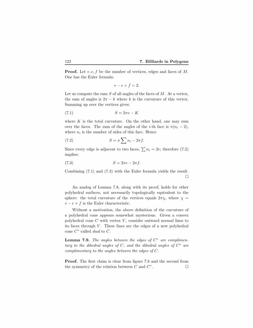
122 7. Billiards in Polygons
Proof. Let v, e, f be the number of vertices, edges and faces of M .
One has the Euler formula:
v − e+ f = 2.
Let us compute the sum S of all angles of the faces of M . At a vertex,
the sum of angles is 2π − k where k is the curvature of this vertex.
Summing up over the vertices gives:
(7.1) S = 2πv −K
where K is the total curvature. On the other hand, one may sum
over the faces. The sum of the angles of the i-th face is π(ni − 2),
where ni is the number of sides of this face. Hence
(7.2) S = π∑
ni − 2πf.
Since every edge is adjacent to two faces,∑ni = 2e; therefore (7.2)
implies:
(7.3) S = 2πe− 2πf.
Combining (7.1) and (7.3) with the Euler formula yields the result.
An analog of Lemma 7.8, along with its proof, holds for other
polyhedral surfaces, not necessarily topologically equivalent to the
sphere: the total curvature of the vertices equals 2πχ, where χ =
v − e+ f is the Euler characteristic.
Without a motivation, the above definition of the curvature of
a polyhedral cone appears somewhat mysterious. Given a convex
polyhedral cone C with vertex V , consider outward normal lines to
its faces through V . These lines are the edges of a new polyhedral
cone C∗ called dual to C.
Lemma 7.9. The angles between the edges of C∗ are complimen-
tary to the dihedral angles of C, and the dihedral angles of C∗ are
complimentary to the angles between the edges of C.
Proof. The first claim is clear from figure 7.8 and the second from
the symmetry of the relation between C and C∗.
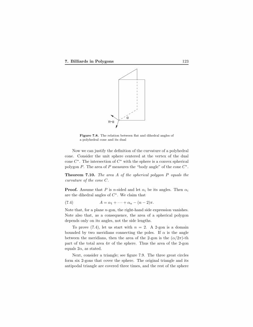
7. Billiards in Polygons 123
α π−α
Figure 7.8. The relation between flat and dihedral angles of
a polyhedral cone and its dual
Now we can justify the definition of the curvature of a polyhedral
cone. Consider the unit sphere centered at the vertex of the dual
cone C∗. The intersection of C∗ with the sphere is a convex spherical
polygon P . The area of P measures the “body angle” of the cone C∗.
Theorem 7.10. The area A of the spherical polygon P equals the
curvature of the cone C.
Proof. Assume that P is n-sided and let αi be its angles. Then αi
are the dihedral angles of C∗. We claim that
(7.4) A = α1 + · · · + αn − (n− 2)π.
Note that, for a plane n-gon, the right-hand side expression vanishes.
Note also that, as a consequence, the area of a spherical polygon
depends only on its angles, not the side lengths.
To prove (7.4), let us start with n = 2. A 2-gon is a domain
bounded by two meridians connecting the poles. If α is the angle
between the meridians, then the area of the 2-gon is the (α/2π)-th
part of the total area 4π of the sphere. Thus the area of the 2-gon
equals 2α, as stated.
Next, consider a triangle; see figure 7.9. The three great circles
form six 2-gons that cover the sphere. The original triangle and its
antipodal triangle are covered three times, and the rest of the sphere
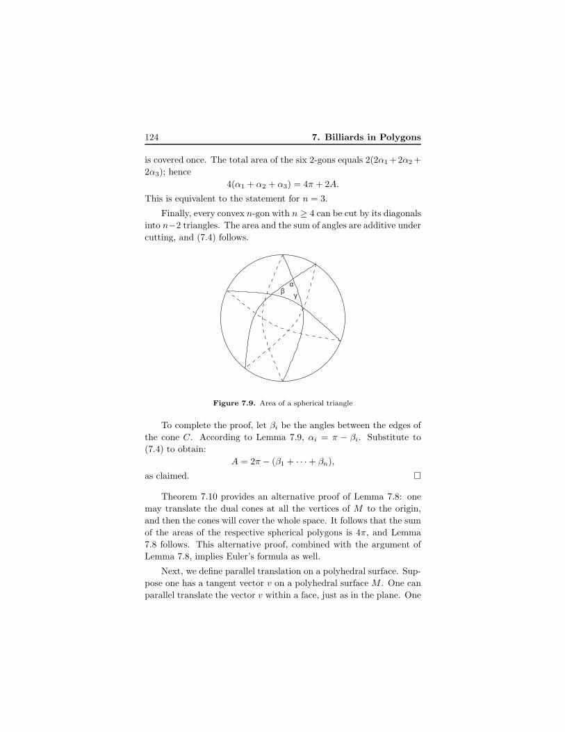
124 7. Billiards in Polygons
is covered once. The total area of the six 2-gons equals 2(2α1 +2α2 +
2α3); hence
4(α1 + α2 + α3) = 4π + 2A.
This is equivalent to the statement for n = 3.
Finally, every convex n-gon with n ≥ 4 can be cut by its diagonals
into n−2 triangles. The area and the sum of angles are additive under
cutting, and (7.4) follows.
αβ γ
Figure 7.9. Area of a spherical triangle
To complete the proof, let βi be the angles between the edges of
the cone C. According to Lemma 7.9, αi = π − βi. Substitute to
(7.4) to obtain:
A = 2π − (β1 + · · · + βn),
as claimed.
Theorem 7.10 provides an alternative proof of Lemma 7.8: one
may translate the dual cones at all the vertices of M to the origin,
and then the cones will cover the whole space. It follows that the sum
of the areas of the respective spherical polygons is 4π, and Lemma
7.8 follows. This alternative proof, combined with the argument of
Lemma 7.8, implies Euler’s formula as well.
Next, we define parallel translation on a polyhedral surface. Sup-
pose one has a tangent vector v on a polyhedral surface M . One can
parallel translate the vector v within a face, just as in the plane. One
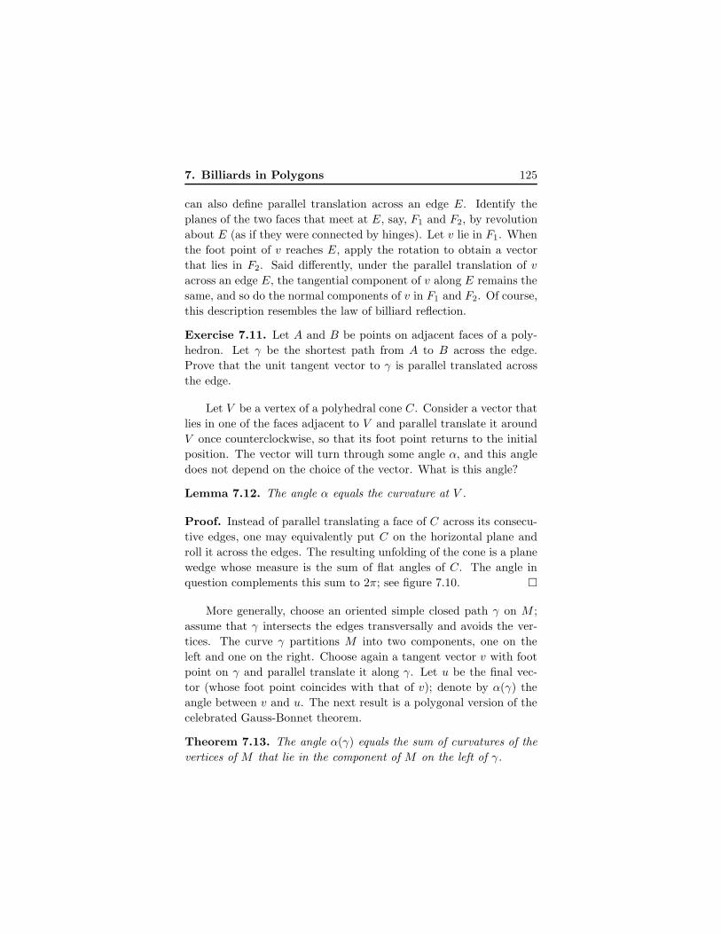
7. Billiards in Polygons 125
can also define parallel translation across an edge E. Identify the
planes of the two faces that meet at E, say, F1 and F2, by revolution
about E (as if they were connected by hinges). Let v lie in F1. When
the foot point of v reaches E, apply the rotation to obtain a vector
that lies in F2. Said differently, under the parallel translation of v
across an edge E, the tangential component of v along E remains the
same, and so do the normal components of v in F1 and F2. Of course,
this description resembles the law of billiard reflection.
Exercise 7.11. Let A and B be points on adjacent faces of a poly-
hedron. Let γ be the shortest path from A to B across the edge.
Prove that the unit tangent vector to γ is parallel translated across
the edge.
Let V be a vertex of a polyhedral cone C. Consider a vector that
lies in one of the faces adjacent to V and parallel translate it around
V once counterclockwise, so that its foot point returns to the initial
position. The vector will turn through some angle α, and this angle
does not depend on the choice of the vector. What is this angle?
Lemma 7.12. The angle α equals the curvature at V .
Proof. Instead of parallel translating a face of C across its consecu-
tive edges, one may equivalently put C on the horizontal plane and
roll it across the edges. The resulting unfolding of the cone is a plane
wedge whose measure is the sum of flat angles of C. The angle in
question complements this sum to 2π; see figure 7.10.
More generally, choose an oriented simple closed path γ on M ;
assume that γ intersects the edges transversally and avoids the ver-
tices. The curve γ partitions M into two components, one on the
left and one on the right. Choose again a tangent vector v with foot
point on γ and parallel translate it along γ. Let u be the final vec-
tor (whose foot point coincides with that of v); denote by α(γ) the
angle between v and u. The next result is a polygonal version of the
celebrated Gauss-Bonnet theorem.
Theorem 7.13. The angle α(γ) equals the sum of curvatures of the
vertices of M that lie in the component of M on the left of γ.

126 7. Billiards in Polygons
3
2
1β β
β 2
1β β
Figure 7.10. Unfolding a polyhedral cone in the plane
Proof. Let us argue inductively in the number n of vertices inside
γ. If n = 1, this is Lemma 7.12. If n > 1, one may cut the domain
bounded by γ by an arc δ into two domains, each with fewer than n
vertices; see figure 7.11. Let γ1 be the curve that follows γ from A
to B and then δ from B to A. Likewise, γ2 is the curve that follows
δ from A to B and then γ from B to A. The concatenation of γ1
and γ2 differs from γ by the arc δ, traversed back and forth. Hence
the contribution of δ cancels: α(γ) = α(γ1) + α(γ2), and the result
follows by induction.
γ
δ
A
B
Figure 7.11. Proving the Gauss-Bonnet theorem
Remark 7.14. A more familiar form of the Gauss-Bonnet theorem
concerns smooth surfaces. To formulate this theorem one needs to
define the Gauss curvature of a smooth surface and the notion of
parallel translation of tangent vectors along curves. This is usually
done in first courses of differential geometry; the reader is challenged
to construct these definitions by analogy with the above discussed
7. Billiards in Polygons 127
polyhedral case. The Gauss-Bonnet theorem states that the parallel
translation of the tangent plane to a smooth surface along a simple
closed curve is the rotation through the angle, equal to the total Gauss
curvature inside the domain bounded by the curve.
Exercise 7.15. Every tennis ball has a clearly visible closed curve
on its surface. Mark a point of this curve and put the ball on the floor
so that it is touching the floor at the marked point. Now roll the ball
without sliding along the curve until it again touches the floor at the
marked point. Comparing the initial and the final positions of the
ball, we see that it has made a certain revolution about the vertical
axis. What is the angle of this revolution?
Finally, consider a generic closed convex polyhedral surface M .
By that we mean that the only linear relation over Q between the
curvatures of the vertices and π is the one given by Lemma 7.8.
Theorem 7.16. There exist no simple closed geodesics on M .
Proof. Assume there is such a geodesic γ. According to Exercise 7.11,
the unit tangent to γ is parallel translated along γ. In particular, this
tangent vector returns, without rotation, to the initial point. On the
other hand, by the Gauss-Bonnet theorem, parallel translation along
γ results in rotation through the angle equal to the sum of curvatures
of the vertices inside γ. This set of vertices is a proper subset of the
set of vertices of M . Since M is generic, the sum of curvatures cannot
be a multiple of 2π, a contradiction.
Note that Theorem 7.16 and its proof do not exclude the existence
of self-intersecting closed geodesics; Theorem 7.16 is somewhat similar
to Exercise 7.2, which implies that a generic convex quadrilateral does
not admit a simple 4-periodic billiard trajectory. ♣
Recall from Chapter 1 that a system of elastic point-masses on the
line or half-line is isomorphic to the billiard inside a polyhedral cone.
Ya. Sinai asked in the 1970s whether the number of reflections in such
a billiard is uniformly bounded above by a constant depending on the
cone but not on the billiard trajectory. This is clearly the case for a
wedge in the plane; see Chapter 1. The next theorem has a number
128 7. Billiards in Polygons
of different proofs given by Ya. Sinai, G. Galperin, M. Sevryuk; we
will follow the exposition in [43].
Theorem 7.17. The number of reflections of any billiard trajectory
inside a convex polyhedral cone in Rn is bounded above by a constant
depending on the cone only.
Proof. (Sketch). Let us argue in the 3-dimensional case. Assume
that the cone is centered at the origin and consider the unit sphere.
The central projection takes the cone to a convex spherical polygon
P , and a billiard trajectory in the cone to a billiard trajectory in P .
Note that the central projection of a line is a great semi-circle. By
unfolding the trajectory in a polyhedral cone to a line, it follows that
the total length of the projection of the billiard trajectory in P is π.
Fix a small ε > 0 and consider ε-neighborhoods of the vertices
of P . We claim that the number of collisions of the billiard ball
inside such a neighborhood is bounded by a constant depending on
the respective angle of P , say, α. Indeed, this is equivalent to a similar
statement about a billiard trajectory in a wedge in space with the
dihedral angle α, which, in turn, is equivalent to the same statement
for a plane wedge; see Chapter 1, where this is proved by unfolding.
Note that a segment from one side of P to another, not within
a single ε-neighborhood of a vertex, has length bounded below by
a constant depending on P and ε. Therefore a billiard trajectory
of total length π can experience a bounded number of reflections
outside of these ε-neighborhoods. It follows that the total number of
reflections is uniformly bounded above.
The proof in arbitrary dimension is similar and uses induction in
dimension.
Exercise 7.18. Consider a cone over a smooth closed plane curve
in 3-dimensional space, and let C be its part inside the unit sphere
centered at the vertex. Prove that a unit speed geodesic on C either
hits the vertex or leaves C after at most time 2.
Exercise 7.19. This problem was communicated by D. Khmelnitskii.
Consider a circular cone whose vertical section is an isosceles triangle
with the vertex angle α. Throw a loop over the cone and pull it down,
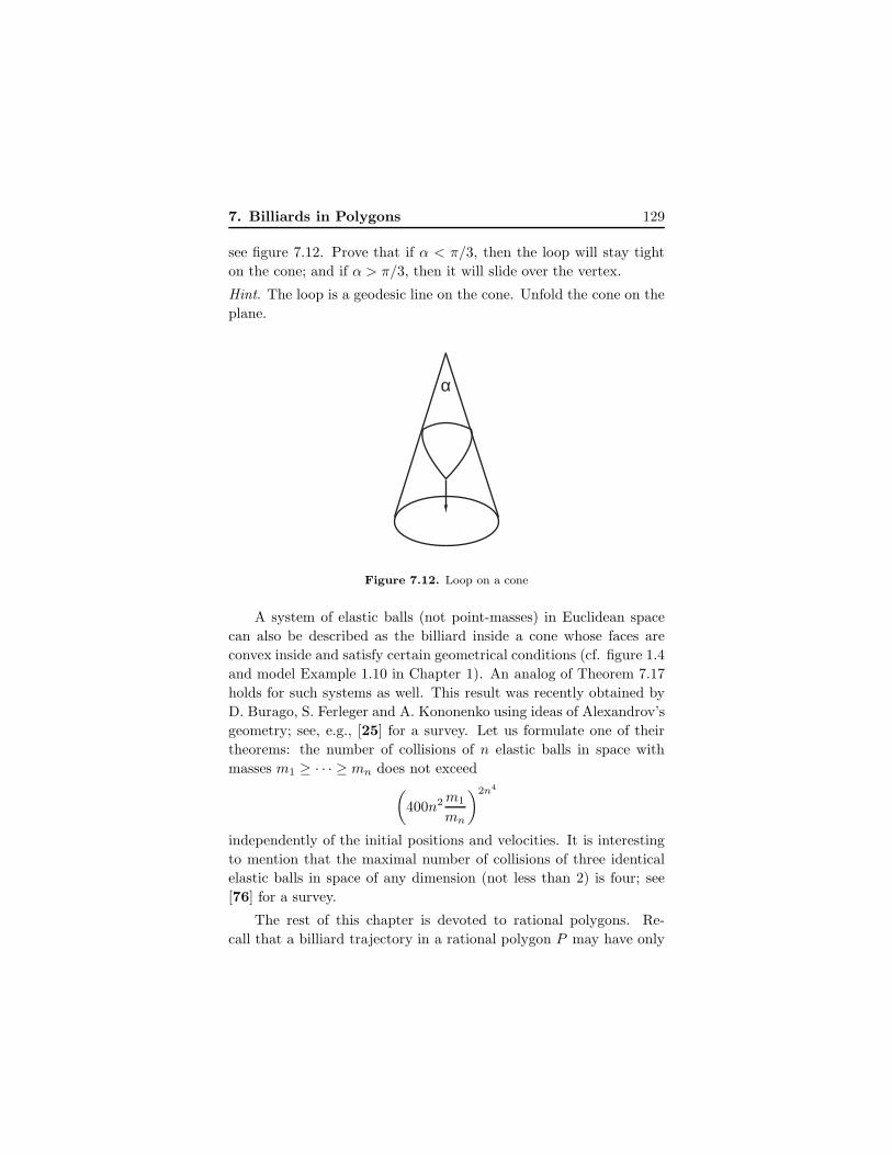
7. Billiards in Polygons 129
see figure 7.12. Prove that if α < π/3, then the loop will stay tight
on the cone; and if α > π/3, then it will slide over the vertex.
Hint. The loop is a geodesic line on the cone. Unfold the cone on the
plane.
α
Figure 7.12. Loop on a cone
A system of elastic balls (not point-masses) in Euclidean space
can also be described as the billiard inside a cone whose faces are
convex inside and satisfy certain geometrical conditions (cf. figure 1.4
and model Example 1.10 in Chapter 1). An analog of Theorem 7.17
holds for such systems as well. This result was recently obtained by
D. Burago, S. Ferleger and A. Kononenko using ideas of Alexandrov’s
geometry; see, e.g., [25] for a survey. Let us formulate one of their
theorems: the number of collisions of n elastic balls in space with
masses m1 ≥ · · · ≥ mn does not exceed(
400n2m1
mn
)2n4
independently of the initial positions and velocities. It is interesting
to mention that the maximal number of collisions of three identical
elastic balls in space of any dimension (not less than 2) is four; see
[76] for a survey.
The rest of this chapter is devoted to rational polygons. Re-
call that a billiard trajectory in a rational polygon P may have only
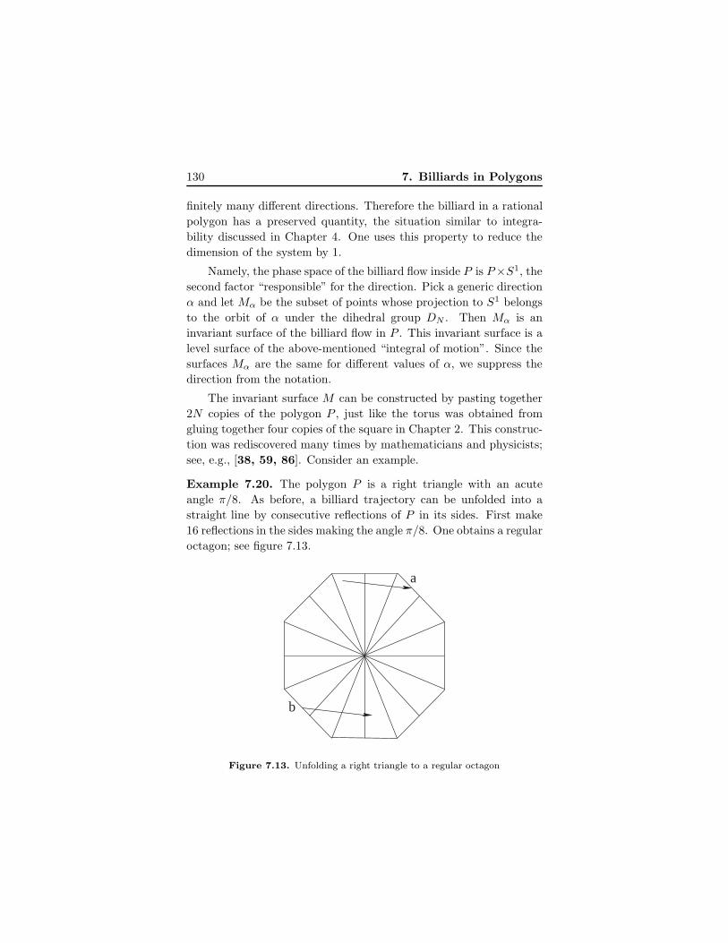
130 7. Billiards in Polygons
finitely many different directions. Therefore the billiard in a rational
polygon has a preserved quantity, the situation similar to integra-
bility discussed in Chapter 4. One uses this property to reduce the
dimension of the system by 1.
Namely, the phase space of the billiard flow inside P is P×S1, the
second factor “responsible” for the direction. Pick a generic direction
α and let Mα be the subset of points whose projection to S1 belongs
to the orbit of α under the dihedral group DN . Then Mα is an
invariant surface of the billiard flow in P . This invariant surface is a
level surface of the above-mentioned “integral of motion”. Since the
surfaces Mα are the same for different values of α, we suppress the
direction from the notation.
The invariant surface M can be constructed by pasting together
2N copies of the polygon P , just like the torus was obtained from
gluing together four copies of the square in Chapter 2. This construc-
tion was rediscovered many times by mathematicians and physicists;
see, e.g., [38, 59, 86]. Consider an example.
Example 7.20. The polygon P is a right triangle with an acute
angle π/8. As before, a billiard trajectory can be unfolded into a
straight line by consecutive reflections of P in its sides. First make
16 reflections in the sides making the angle π/8. One obtains a regular
octagon; see figure 7.13.
a
b
Figure 7.13. Unfolding a right triangle to a regular octagon
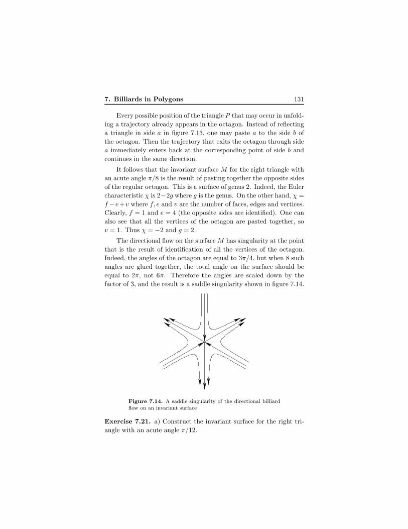
7. Billiards in Polygons 131
Every possible position of the triangle P that may occur in unfold-
ing a trajectory already appears in the octagon. Instead of reflecting
a triangle in side a in figure 7.13, one may paste a to the side b of
the octagon. Then the trajectory that exits the octagon through side
a immediately enters back at the corresponding point of side b and
continues in the same direction.
It follows that the invariant surface M for the right triangle with
an acute angle π/8 is the result of pasting together the opposite sides
of the regular octagon. This is a surface of genus 2. Indeed, the Euler
characteristic χ is 2−2g where g is the genus. On the other hand, χ =
f−e+v where f, e and v are the number of faces, edges and vertices.
Clearly, f = 1 and e = 4 (the opposite sides are identified). One can
also see that all the vertices of the octagon are pasted together, so
v = 1. Thus χ = −2 and g = 2.
The directional flow on the surface M has singularity at the point
that is the result of identification of all the vertices of the octagon.
Indeed, the angles of the octagon are equal to 3π/4, but when 8 such
angles are glued together, the total angle on the surface should be
equal to 2π, not 6π. Therefore the angles are scaled down by the
factor of 3, and the result is a saddle singularity shown in figure 7.14.
Figure 7.14. A saddle singularity of the directional billiard
flow on an invariant surface
Exercise 7.21. a) Construct the invariant surface for the right tri-
angle with an acute angle π/12.
132 7. Billiards in Polygons
b) Same for the right triangle with an acute angle π/5.
c) Same for a square with a hole which is a homothetic square.
The situation with a general rational polygon is similar. Let us
describe the construction of the surface M . Consider 2N disjoint
parallel copies of P in the plane. Call them P1, ..., P2N , and orient
the even ones clockwise and the odd ones counterclockwise. We will
paste their sides together pairwise, according to the action of the
dihedral group DN . Let 0 < θ1 < π/N be some angle, and let θi be
its i-th image under the action of DN . Consider Pi and reflect the
direction θi in one of its sides. The reflected direction is θj for some
j. Paste the chosen side of Pi to the identical side of Pj . After these
pastings are made for all the sides of all the polygons, one obtains
an oriented closed surface M . This surface does not depend on the
choice of the angle θ1.
The topology of the surface M is determined by its genus g de-
scribed in the next theorem.
Theorem 7.22. Let the angles of a (simply connected) billiard k-gon
P be πmi/ni, i = 1, ..., k, where mi and ni are coprime, and let N
be the least common multiple of ni. Then
g = 1 +N
2
(k − 2 −
∑ 1
ni
).
Proof. We need to analyze how the pastings are made around a
vertex of P . Consider the i-th vertex V with the angle πmi/ni. Let
Gi be the group of linear transformations of the plane generated by
the reflections in the sides of P adjacent to V . Then Gi consists of
2ni elements.
According to the construction of M , the number of copies of the
polygons Pj that are glued together at V equals the cardinality of
the orbit of the test angle θ under the group Gi, that is, equals 2ni.
Originally we had 2N copies of the polygon P , and therefore, 2N
copies of the vertex V . After the gluings we have N/ni copies of this
vertex on the surface M .
It follows that the total number of vertices in M is N(∑
1/ni).
The total number of edges is Nk, and the number of faces is 2N .

7. Billiards in Polygons 133
Therefore the Euler characteristic χ(M) equals
N∑ 1
ni−Nk + 2N,
and since χ = 2 − 2g, the result follows.
Similar to Example 7.20, the billiard flow on the surface M will
have saddle singularities at the vertices. The above proof shows that
the i-th vertex of M is the result of gluing 2ni copies of the angle
πmi/ni, which sums up to 2πmi. Thus, unless mi = 1, one has a
saddle point. It is interesting to describe the case when all mi = 1
and the singularities are removable.
Lemma 7.23. If the angles of a k-gon are all of the form π/ni, then
the numbers ni are, up to permutations, as follows:
(3, 3, 3), (2, 4, 4), (2, 3, 6), (2, 2, 2, 2),
and the respective polygons are: an equilateral triangle, an isosceles
right triangle, a right triangle with an acute angle π/6 and a square.
In all these cases the surface M is a torus.
Proof. The sum of angles of a k-gon is π(k − 2). Thus one has the
equation:
(7.5)1
n1+ · · · + 1
nk= k − 2.
Exercise 7.24. Prove that the only solutions of (7.5) are as stated
in the lemma.
The genus of the surface M is computed in Theorem 7.22, and
the result is g = 1. Thus M is a torus.
A common feature of the polygons in Lemma 7.23 is that their
unfoldings tile the plane; see figure 7.7.
Rational polygonal billiards is a very active and fast growing area
of research. Starting with [60], serious progress has been made in un-
derstanding the dynamics of rational polygonal billiards, using meth-
ods of complex analysis; see [65] for a survey of this subject.
We will say just a few words about these results. As we saw, the
billiard in a rational polygon P reduces to a flow in a fixed direction
134 7. Billiards in Polygons
on a surface M . This surface has a flat metric inherited from P ;
this metric has cone singularities with cone angles multiples of 2π.
To understand an individual flat surface, one studies the space of all
such surfaces. The space of flat surfaces has a natural topology and
is acted upon by the group SL(2,R). This group action is crucial for
the study.
To give the reader a taste of the results obtained in this way, we
formulate two theorems. Both statements are familiar in the case of
a square. The first, due to H. Masur, concerns periodic trajectories.
Recall that they come in parallel families. Let N(t) be the number
of strips of periodic trajectories of length not greater than t. Then,
for any rational polygon, there exist constants c and C such that
ct2 < N(t) < Ct2 for sufficiently large t.
Another theorem, due to W. Veech, concerns regular polygons
P (in fact, many more, called Veech polygons; we do not give the
definition). Given a direction θ, the following dichotomy holds: either
every billiard trajectory in the direction θ is infinite and uniformly
distributed in P or every trajectory in this direction is periodic (or
hits a vertex). For a general rational polygon, this dichotomy does
not hold at all!
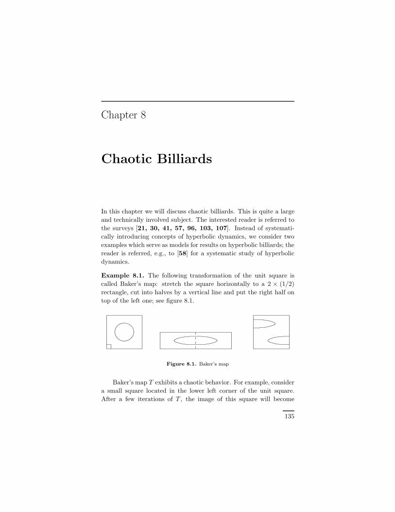
Chapter 8
Chaotic Billiards
In this chapter we will discuss chaotic billiards. This is quite a large
and technically involved subject. The interested reader is referred to
the surveys [21, 30, 41, 57, 96, 103, 107]. Instead of systemati-
cally introducing concepts of hyperbolic dynamics, we consider two
examples which serve as models for results on hyperbolic billiards; the
reader is referred, e.g., to [58] for a systematic study of hyperbolic
dynamics.
Example 8.1. The following transformation of the unit square is
called Baker’s map: stretch the square horizontally to a 2 × (1/2)
rectangle, cut into halves by a vertical line and put the right half on
top of the left one; see figure 8.1.
Figure 8.1. Baker’s map
Baker’s map T exhibits a chaotic behavior. For example, consider
a small square located in the lower left corner of the unit square.
After a few iterations of T , the image of this square will become
135
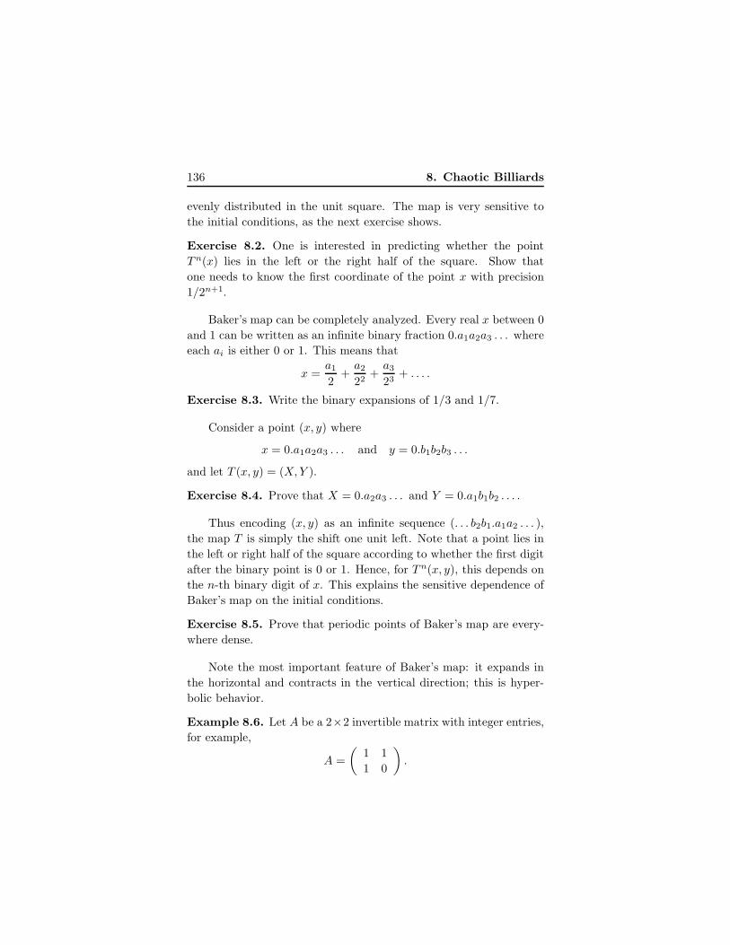
136 8. Chaotic Billiards
evenly distributed in the unit square. The map is very sensitive to
the initial conditions, as the next exercise shows.
Exercise 8.2. One is interested in predicting whether the point
T n(x) lies in the left or the right half of the square. Show that
one needs to know the first coordinate of the point x with precision
1/2n+1.
Baker’s map can be completely analyzed. Every real x between 0
and 1 can be written as an infinite binary fraction 0.a1a2a3 . . . where
each ai is either 0 or 1. This means that
x =a1
2+a2
22+a3
23+ . . . .
Exercise 8.3. Write the binary expansions of 1/3 and 1/7.
Consider a point (x, y) where
x = 0.a1a2a3 . . . and y = 0.b1b2b3 . . .
and let T (x, y) = (X,Y ).
Exercise 8.4. Prove that X = 0.a2a3 . . . and Y = 0.a1b1b2 . . . .
Thus encoding (x, y) as an infinite sequence (. . . b2b1.a1a2 . . . ),
the map T is simply the shift one unit left. Note that a point lies in
the left or right half of the square according to whether the first digit
after the binary point is 0 or 1. Hence, for T n(x, y), this depends on
the n-th binary digit of x. This explains the sensitive dependence of
Baker’s map on the initial conditions.
Exercise 8.5. Prove that periodic points of Baker’s map are every-
where dense.
Note the most important feature of Baker’s map: it expands in
the horizontal and contracts in the vertical direction; this is hyper-
bolic behavior.
Example 8.6. Let A be a 2×2 invertible matrix with integer entries,
for example,
A =
(1 1
1 0
).

8. Chaotic Billiards 137
Then A acts on R2 and preserves the lattice Z2, hence defines a
transformation of the torus T 2 = R2/Z2. Unlike Baker’s maps, this
transformation (which we denote by the same letter) is continuous.
Such transformations are often called cat maps (for continuous auto-
morphisms of a torus).
The matrix A has two real eigenvalues λ1,2 = (1 ±√
5)/2. The
respective eigenspaces have the slopes λ1 − 1 and λ2 − 1; the linear
map A expands in the first and contracts in the second eigendirection.
The projection of a line having either eigendirection is dense on the
torus.
Take a small disc on T 2 and apply the map A to it. After a
few iterations, the disc will become a very long and thin domain, “a
needle”, stretched along the expanding eigendirection. It follows that
the orbit of this disc is dense in the torus; cf. Chapter 2.
Exercise 8.7. a) Prove that every point of the torus with rational
coordinates is periodic under A.
b) Same question for an arbitrary A ∈ SL(2,Z).
A common feature of these examples is the hyperbolic behavior:
the existence of directions in which the map expands and contracts
(unstable and stable directions). As a consequence, one has the prop-
erties usually associated with chaos: sensitivity to initial conditions,
density of periodic orbits, density of the orbit of any open set, etc.1
The first examples of billiards with hyperbolic dynamics were dis-
covered by Ya. Sinai [101]: these billiards are bounded by piecewise
smooth curves whose smooth components are strictly convex inwards
and which intersect transversally. See figure 1.5, a torus or a square
with a convex hole, and figure 8.2. A parallel beam of light, after a
reflection in a convex mirror, becomes dispersing. That is why these
billiards are called dispersing.
Let us analyze this phenomenon in a little more detail. First of
all, the billiard map in a dispersing billiard has discontinuities. There
are two sources of discontinuities: a trajectory may hit a corner and
1The reader should keep in mind another, very important, example of hyperbolicdynamics: the geodesic flow on a negatively curved manifold, such as the hyperbolicplane.

138 8. Chaotic Billiards
Figure 8.2. Sinai’s billiards
a trajectory may be tangent to the boundary of the billiard table.
These discontinuities significantly complicate the analysis of billiard
ball map.
Recall the discussion of projective duality in Chapter 5: to a point
of the plane there corresponds the 1-parameter family of lines through
this point. An infinitesimal one-parameter family of rays consists of
the rays passing through its focusing point (or, in the limiting case, of
parallel rays, for which the focusing point is at infinity). Thus, given
an oriented line x, a direction in the tangent space TxM to the phase
space of the billiard map M is determined by a choice of a focusing
point on x. The magnitude of a tangent vector is characterized by
the angle made by the infinitesimal family of rays through this point.
Let us consider a dispersing infinitesimal family of rays whose
focusing point lies before the point of reflection in the boundary of
the billiard table. A reflection in the boundary convex inward is
described by the mirror equation (5.9). In this equation, k < 0;
therefore b < 0 as well. This means that the focusing point of the
reflected infinitesimal family of rays is outside of the billiard table.
Moreover, 1/|b| > 1/a, which means that the outgoing infinitesimal
family has a greater angle than the incoming one; see figure 8.3. This
is the expansion, characteristic for hyperbolic dynamics. We refer to
[30] for a thorough analysis.
There are numerous results on stochastic properties of dispers-
ing billiards, many obtained by L. Bunimovich, N. Chernov and Ya.
Sinai. For example, a dispersing billiard is ergodic: this means that
the only subsets of the phase space that are invariant under the bil-
liard ball map have zero or full measure. Another result states that

8. Chaotic Billiards 139
b
a
Figure 8.3. Reflection in a dispersing part of the boundary
the number of periodic billiard trajectories with period not greater
than n is bounded below by exp(Cn) for some constant C and all
sufficiently great n. This is, of course, in sharp contrast with the
polygonal case; see Chapter 7.
In the mid-1970s L. Bunimovich discovered a new type of chaotic
billiards, namely, the ones with boundary components convex out-
wards; see figure 8.4 for examples. The first of these billiard tables
is probably the most popular in the mathematical and physical liter-
ature; it is made of two half-circles, connected by common tangents,
and is called “a stadium”. Note that the stadium is a differentiable
curve but its curvature has discontinuities.
Figure 8.4. Bunimovich billiards
Recently Bunimovich [22] introduced a class of billiards called
“mushrooms”; see figure 8.5. These billiards combine integrable and
chaotic behavior. The explanation of the former is given in the next
exercise.
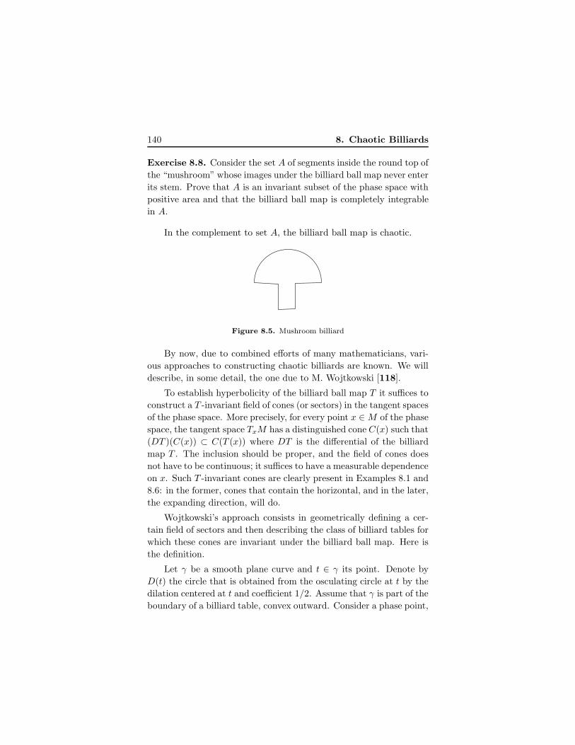
140 8. Chaotic Billiards
Exercise 8.8. Consider the set A of segments inside the round top of
the “mushroom” whose images under the billiard ball map never enter
its stem. Prove that A is an invariant subset of the phase space with
positive area and that the billiard ball map is completely integrable
in A.
In the complement to set A, the billiard ball map is chaotic.
Figure 8.5. Mushroom billiard
By now, due to combined efforts of many mathematicians, vari-
ous approaches to constructing chaotic billiards are known. We will
describe, in some detail, the one due to M. Wojtkowski [118].
To establish hyperbolicity of the billiard ball map T it suffices to
construct a T -invariant field of cones (or sectors) in the tangent spaces
of the phase space. More precisely, for every point x ∈M of the phase
space, the tangent space TxM has a distinguished cone C(x) such that
(DT )(C(x)) ⊂ C(T (x)) where DT is the differential of the billiard
map T . The inclusion should be proper, and the field of cones does
not have to be continuous; it suffices to have a measurable dependence
on x. Such T -invariant cones are clearly present in Examples 8.1 and
8.6: in the former, cones that contain the horizontal, and in the later,
the expanding direction, will do.
Wojtkowski’s approach consists in geometrically defining a cer-
tain field of sectors and then describing the class of billiard tables for
which these cones are invariant under the billiard ball map. Here is
the definition.
Let γ be a smooth plane curve and t ∈ γ its point. Denote by
D(t) the circle that is obtained from the osculating circle at t by the
dilation centered at t and coefficient 1/2. Assume that γ is part of the
boundary of a billiard table, convex outward. Consider a phase point,
8. Chaotic Billiards 141
a unit tangent vector v with the foot point at t, and let ℓ be the line
through t in the direction v. Consider the set of unit vectors with foot
points on γ in a vicinity of t such that the respective lines intersect
ℓ inside the circle D(t). In other words, consider the infinitesimal
families of rays, containing ℓ and focusing inside D(t). This defines
the cone C(x) for x = (t, v).
If γ is a part of the boundary of a billiard table that is convex
outward, then the cone C is defined by the condition that the focus of
the infinitesimal family of rays lies outside of the table. Finally, the
flat parts of the billiard curve are irrelevant, and it does not matter
how one defines the cones therein. This is due to the unfolding trick:
one can reflect the table in a flat component of the boundary and
extend the billiard trajectories through it as straight lines.
The field of cones having been defined, we now need to determine
conditions on the billiard curve ensuring that the billiard ball map
T preserves this field of cones. There are three cases to consider:
when a segment of a billiard trajectory connects two convex inside
(dispersing) curves, one convex outside and one convex inside, and
two convex outside curves. In each case, the relevant formula is the
mirror equation (5.9). Call the curves γ1 and γ2.
In the first case, k < 0 and a > 0. It follows from the mirror
equation that b < 0; that is, the focusing point of the reflected in-
finitesimal beam lies outside the table. This means that T takes the
cones based at γ1 inside the cones based at γ2.
Consider the most interesting third case, that of two curves con-
vex outward; see figure 8.6. Let t1 and t2 be the points of the curves
γ1 and γ2, and set L = |t1t2|. Let v1 be the unit vector from t1 to t2and v2 the reflection of v1 in γ2. Then x1 = (t1, v1) and x2 = (t2, v2).
Let k1 and k2 be the curvatures of the curves at points t1 and t2,
and α1 and α2 the angles made by the segment t1t2 with the curves.
Finally, denote the lengths of the parts of t1t2 inside the circles D(t1)
and D(t2) by d1 and d2.
Lemma 8.9. Assume that L > d1 + d2. Then the billiard map takes
the cone C(x1) strictly inside C(x2).
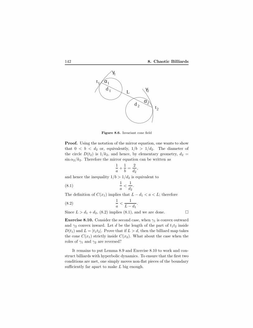
142 8. Chaotic Billiards
22
2
21
1
1
1t
αd
t
γα
Ld
γ
Figure 8.6. Invariant cone field
Proof. Using the notation of the mirror equation, one wants to show
that 0 < b < d2 or, equivalently, 1/b > 1/d2. The diameter of
the circle D(t2) is 1/k2, and hence, by elementary geometry, d2 =
sinα2/k2. Therefore the mirror equation can be written as
1
a+
1
b=
2
d2,
and hence the inequality 1/b > 1/d2 is equivalent to
(8.1)1
a<
1
d2.
The definition of C(x1) implies that L− d1 < a < L; therefore
(8.2)1
a<
1
L− d1.
Since L > d1 + d2, (8.2) implies (8.1), and we are done.
Exercise 8.10. Consider the second case, when γ1 is convex outward
and γ2 convex inward. Let d be the length of the part of t1t2 inside
D(t1) and L = |t1t2|. Prove that if L > d, then the billiard map takes
the cone C(x1) strictly inside C(x2). What about the case when the
roles of γ1 and γ2 are reversed?
It remains to put Lemma 8.9 and Exercise 8.10 to work and con-
struct billiards with hyperbolic dynamics. To ensure that the first two
conditions are met, one simply moves non-flat pieces of the boundary
sufficiently far apart to make L big enough.
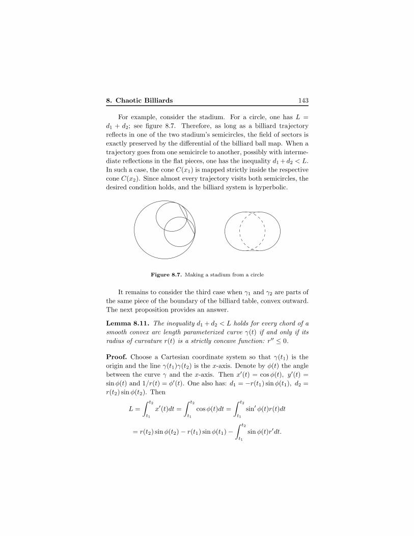
8. Chaotic Billiards 143
For example, consider the stadium. For a circle, one has L =
d1 + d2; see figure 8.7. Therefore, as long as a billiard trajectory
reflects in one of the two stadium’s semicircles, the field of sectors is
exactly preserved by the differential of the billiard ball map. When a
trajectory goes from one semicircle to another, possibly with interme-
diate reflections in the flat pieces, one has the inequality d1 +d2 < L.
In such a case, the cone C(x1) is mapped strictly inside the respective
cone C(x2). Since almost every trajectory visits both semicircles, the
desired condition holds, and the billiard system is hyperbolic.
Figure 8.7. Making a stadium from a circle
It remains to consider the third case when γ1 and γ2 are parts of
the same piece of the boundary of the billiard table, convex outward.
The next proposition provides an answer.
Lemma 8.11. The inequality d1 + d2 < L holds for every chord of a
smooth convex arc length parameterized curve γ(t) if and only if its
radius of curvature r(t) is a strictly concave function: r′′ ≤ 0.
Proof. Choose a Cartesian coordinate system so that γ(t1) is the
origin and the line γ(t1)γ(t2) is the x-axis. Denote by φ(t) the angle
between the curve γ and the x-axis. Then x′(t) = cosφ(t), y′(t) =
sinφ(t) and 1/r(t) = φ′(t). One also has: d1 = −r(t1) sinφ(t1), d2 =
r(t2) sinφ(t2). Then
L =
∫ t2
t1
x′(t)dt =
∫ t2
t1
cosφ(t)dt =
∫ t2
t1
sin′ φ(t)r(t)dt
= r(t2) sinφ(t2) − r(t1) sinφ(t1) −∫ t2
t1
sinφ(t)r′dt.
144 8. Chaotic Billiards
Hence
L− d1 − d2 = −∫ t2
t1
sinφ(t)r′dt = −∫ t2
t1
y′(t)r′dt
= −y(t2)r′(t2) + y(t1)r′(t1) +
∫ t2
t1
y(t)r′′dt =
∫ t2
t1
y(t)r′′dt,
because y(t1) = y(t2) = 0. Since y(t) < 0 for t ∈ [t1, t2], the necessity
follows. If r′′ > 0 at some point t, then, choosing t1 and t2 sufficiently
close to t, one gets L− d1 − d2 < 0.
Here are some examples of the curves satisfying the condition
r′′ ≤ 0: an arc of a circle; an arc of a logarithmic spiral; an arc of a
cycloid; an arc of an ellipse
x2
a2+y2
b2= 1, a < b,
on which |x| ≤ a/√
2. Note that the condition r′′ < 0 is stable under
small perturbations of the curve.
Wojtkowski formulated the following principles for design of hy-
perbolic billiards:
• any convex outward component of the boundary should sat-
isfy the inequality r′′ < 0;
• any convex outward component should be sufficiently far
away from any other such component;
• if two components meet at a vertex, then the internal angle
between them should be greater than π if both components
are convex outward, not less than π if one is convex outward
and another convex inward, and greater than π/2 if one is
convex outward and another flat.
Some examples are shown in figure 8.8: the first curve is the
cardioid, and the second is a unit square with a hole in the shape
of an astroid |x|2/3 + |y|2/3 = a2/3. If a ≤√
2/4, this billiard is
hyperbolic.
Multi-dimensional billiards with hyperbolic dynamics are known
as well. One may use dispersing boundary components, just as in
the plane. It took considerable effort to construct multi-dimensional
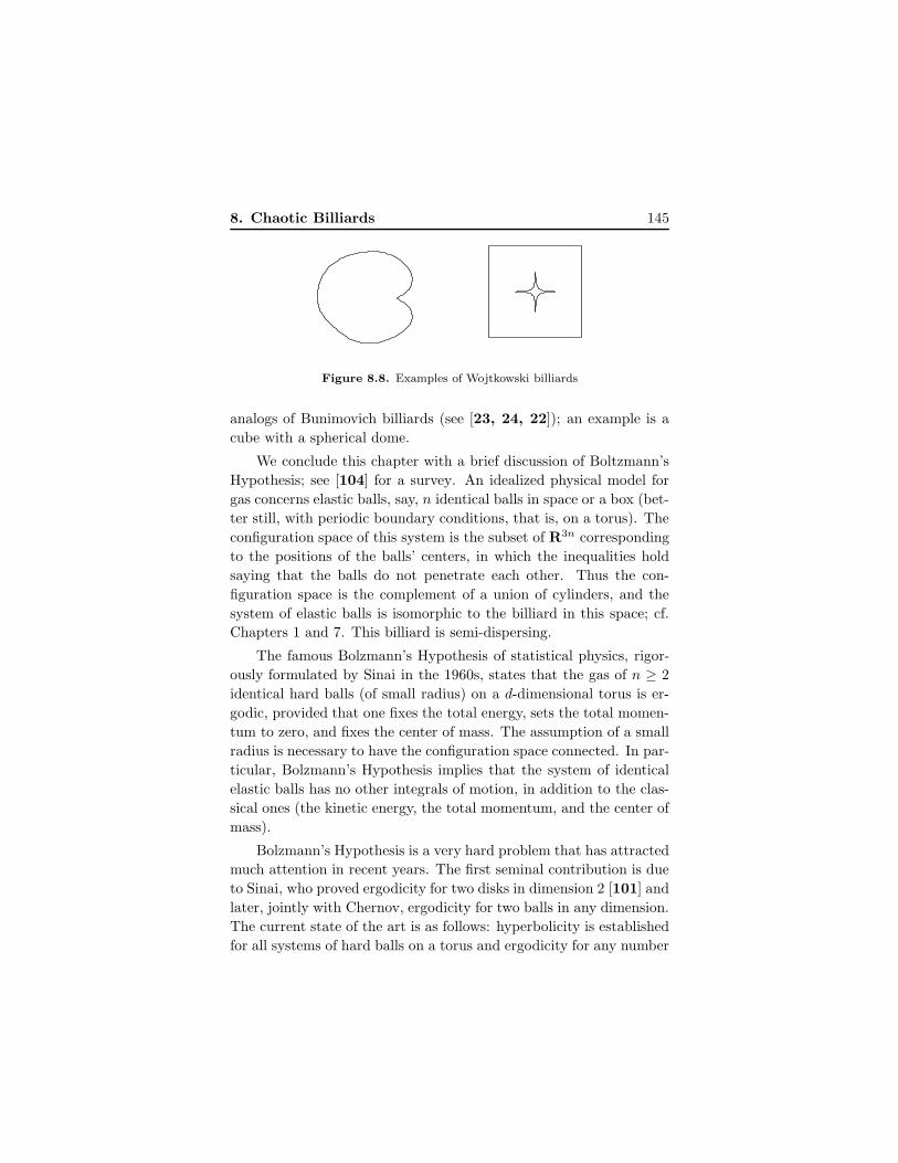
8. Chaotic Billiards 145
Figure 8.8. Examples of Wojtkowski billiards
analogs of Bunimovich billiards (see [23, 24, 22]); an example is a
cube with a spherical dome.
We conclude this chapter with a brief discussion of Boltzmann’s
Hypothesis; see [104] for a survey. An idealized physical model for
gas concerns elastic balls, say, n identical balls in space or a box (bet-
ter still, with periodic boundary conditions, that is, on a torus). The
configuration space of this system is the subset of R3n corresponding
to the positions of the balls’ centers, in which the inequalities hold
saying that the balls do not penetrate each other. Thus the con-
figuration space is the complement of a union of cylinders, and the
system of elastic balls is isomorphic to the billiard in this space; cf.
Chapters 1 and 7. This billiard is semi-dispersing.
The famous Bolzmann’s Hypothesis of statistical physics, rigor-
ously formulated by Sinai in the 1960s, states that the gas of n ≥ 2
identical hard balls (of small radius) on a d-dimensional torus is er-
godic, provided that one fixes the total energy, sets the total momen-
tum to zero, and fixes the center of mass. The assumption of a small
radius is necessary to have the configuration space connected. In par-
ticular, Bolzmann’s Hypothesis implies that the system of identical
elastic balls has no other integrals of motion, in addition to the clas-
sical ones (the kinetic energy, the total momentum, and the center of
mass).
Bolzmann’s Hypothesis is a very hard problem that has attracted
much attention in recent years. The first seminal contribution is due
to Sinai, who proved ergodicity for two disks in dimension 2 [101] and
later, jointly with Chernov, ergodicity for two balls in any dimension.
The current state of the art is as follows: hyperbolicity is established
for all systems of hard balls on a torus and ergodicity for any number
146 8. Chaotic Billiards
of disks of any masses in dimension two; see [97, 98, 99]. A physically
interesting model is the gas of hard balls in a box with flat walls. The
only result so far, due to Simanyi, is ergodicity for two balls [95].
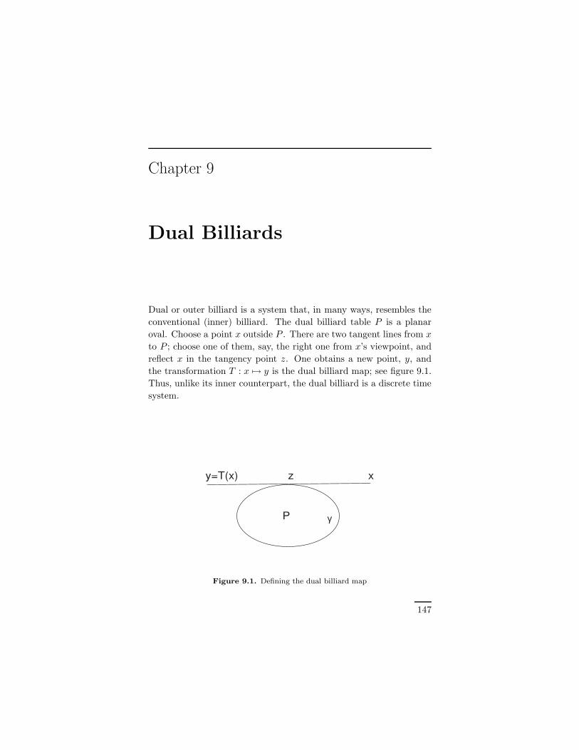
Chapter 9
Dual Billiards
Dual or outer billiard is a system that, in many ways, resembles the
conventional (inner) billiard. The dual billiard table P is a planar
oval. Choose a point x outside P . There are two tangent lines from x
to P ; choose one of them, say, the right one from x’s viewpoint, and
reflect x in the tangency point z. One obtains a new point, y, and
the transformation T : x 7→ y is the dual billiard map; see figure 9.1.
Thus, unlike its inner counterpart, the dual billiard is a discrete time
system.
γ P
x y=T(x) z
Figure 9.1. Defining the dual billiard map
147
148 9. Dual Billiards
The definition of the dual billiard map has a shortcoming: T is
not defined if the tangency point z is not unique. This is the case
if the dual billiard curve γ, the boundary of P , contains a straight
segment, for example, if γ is a polygon. The dual billiard map is not
defined for the points on the extensions of straight segments of γ.
This set is a countable collection of lines and therefore a set of zero
measure, hence one still has ample room to play the game of dual
billiard. The situation resembles the usual, inner billiard: if a billiard
ball hits a corner of the billiard table, then its motion is not defined
beyond this point.
Another useful comment on the definition: the dual billiard map
commutes with affine transformations of the plane. Namely, if A is
such a transformation, γ a dual billiard curve and Tγ the respective
dual billiard map, then
TA(γ) A = A Tγ .
In particular, from the point of view of dual billiards, there is no
difference between a circle and an ellipse.
Dual billiards were probably introduced by B. Neumann in the
late 1950s and popularized by J. Moser in [70, 71]. Moser considered
dual billiard as a toy model for planetary motion: the orbit of a point
around the dual billiard table resembles the orbit of a celestial body.
Like the planetary motions, the dual billiard dynamics is easy to
define but hard to analyze: in particular, it is not at all clear whether
the orbit of a point may escape to infinity or “fall” on the table; this
question was originally asked by B. Neumann.
Many topics that we discussed in these notes have their outer
billiard counterparts. In this last chapter we survey selected results
on dual billiards that were obtained in the last 30 years. See [34,
105, 107] for other surveys of this subject.
Let us start with two motivations. First, in the spirit of Chap-
ter 1, we give an interpretation of the dual billiard system as a me-
chanical system, namely, an impact oscillator. We follow [20]. Con-
sider a harmonic oscillator on the line, that is, a particle whose coor-
dinate, as a function of time, is a linear combination of sin t and
cos t. There is a 2π-periodically moving massive wall to the left
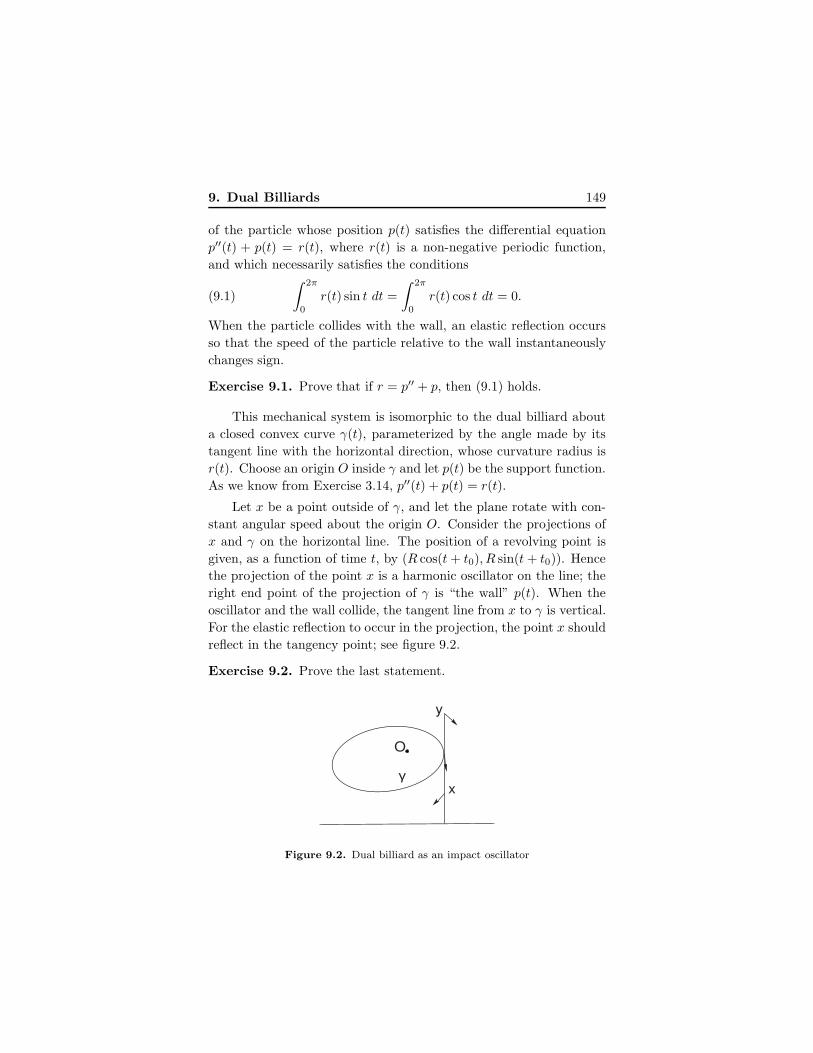
9. Dual Billiards 149
of the particle whose position p(t) satisfies the differential equation
p′′(t) + p(t) = r(t), where r(t) is a non-negative periodic function,
and which necessarily satisfies the conditions
(9.1)
∫ 2π
0
r(t) sin t dt =
∫ 2π
0
r(t) cos t dt = 0.
When the particle collides with the wall, an elastic reflection occurs
so that the speed of the particle relative to the wall instantaneously
changes sign.
Exercise 9.1. Prove that if r = p′′ + p, then (9.1) holds.
This mechanical system is isomorphic to the dual billiard about
a closed convex curve γ(t), parameterized by the angle made by its
tangent line with the horizontal direction, whose curvature radius is
r(t). Choose an origin O inside γ and let p(t) be the support function.
As we know from Exercise 3.14, p′′(t) + p(t) = r(t).
Let x be a point outside of γ, and let the plane rotate with con-
stant angular speed about the origin O. Consider the projections of
x and γ on the horizontal line. The position of a revolving point is
given, as a function of time t, by (R cos(t+ t0), R sin(t+ t0)). Hence
the projection of the point x is a harmonic oscillator on the line; the
right end point of the projection of γ is “the wall” p(t). When the
oscillator and the wall collide, the tangent line from x to γ is vertical.
For the elastic reflection to occur in the projection, the point x should
reflect in the tangency point; see figure 9.2.
Exercise 9.2. Prove the last statement.
γ
y
x
O
Figure 9.2. Dual billiard as an impact oscillator
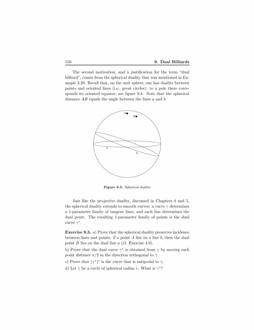
150 9. Dual Billiards
The second motivation, and a justification for the term “dual
billiard”, comes from the spherical duality that was mentioned in Ex-
ample 3.26. Recall that, on the unit sphere, one has duality between
points and oriented lines (i.e., great circles): to a pole there corre-
sponds its oriented equator; see figure 9.3. Note that the spherical
distance AB equals the angle between the lines a and b.
AB
a
b
Figure 9.3. Spherical duality
Just like the projective duality, discussed in Chapters 4 and 5,
the spherical duality extends to smooth curves: a curve γ determines
a 1-parameter family of tangent lines, and each line determines the
dual point. The resulting 1-parameter family of points is the dual
curve γ∗.
Exercise 9.3. a) Prove that the spherical duality preserves incidence
between lines and points: if a point A lies on a line b, then the dual
point B lies on the dual line a (cf. Exercise 4.9).
b) Prove that the dual curve γ∗ is obtained from γ by moving each
point distance π/2 in the direction orthogonal to γ.
c) Prove that (γ∗)∗ is the curve that is antipodal to γ.
d) Let γ be a circle of spherical radius r. What is γ∗?
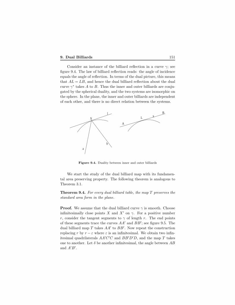
9. Dual Billiards 151
Consider an instance of the billiard reflection in a curve γ; see
figure 9.4. The law of billiard reflection reads: the angle of incidence
equals the angle of reflection. In terms of the dual picture, this means
that AL = LB, and hence the dual billiard reflection about the dual
curve γ∗ takes A to B. Thus the inner and outer billiards are conju-
gated by the spherical duality, and the two systems are isomorphic on
the sphere. In the plane, the inner and outer billiards are independent
of each other, and there is no direct relation between the systems.
X
l
a
b
L
A
Bx
Figure 9.4. Duality between inner and outer billiards
We start the study of the dual billiard map with its fundamen-
tal area preserving property. The following theorem is analogous to
Theorem 3.1.
Theorem 9.4. For every dual billiard table, the map T preserves the
standard area form in the plane.
Proof. We assume that the dual billiard curve γ is smooth. Choose
infinitesimally close points X and X ′ on γ. For a positive number
r, consider the tangent segments to γ of length r. The end points
of these segments trace the curves AA′ and BB′; see figure 9.5. The
dual billiard map T takes AA′ to BB′. Now repeat the construction
replacing r by r − ε where ε is an infinitesimal. We obtain two infin-
itesimal quadrilaterals AA′C′C and BB′D′D, and the map T takes
one to another. Let δ be another infinitesimal, the angle between AB
and A′B′.
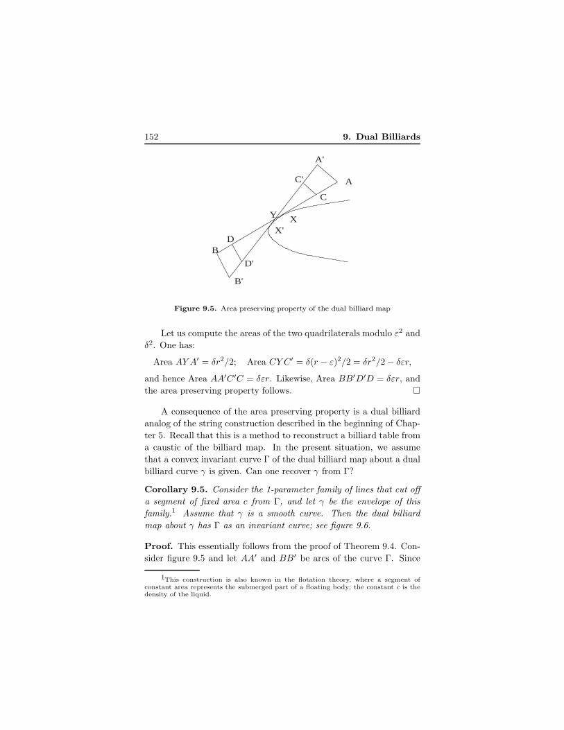
152 9. Dual Billiards
Y XX'
A
A'
B
B'
C
C'
D
D'
Figure 9.5. Area preserving property of the dual billiard map
Let us compute the areas of the two quadrilaterals modulo ε2 and
δ2. One has:
Area AY A′ = δr2/2; Area CY C′ = δ(r − ε)2/2 = δr2/2 − δεr,
and hence Area AA′C′C = δεr. Likewise, Area BB′D′D = δεr, and
the area preserving property follows.
A consequence of the area preserving property is a dual billiard
analog of the string construction described in the beginning of Chap-
ter 5. Recall that this is a method to reconstruct a billiard table from
a caustic of the billiard map. In the present situation, we assume
that a convex invariant curve Γ of the dual billiard map about a dual
billiard curve γ is given. Can one recover γ from Γ?
Corollary 9.5. Consider the 1-parameter family of lines that cut off
a segment of fixed area c from Γ, and let γ be the envelope of this
family.1 Assume that γ is a smooth curve. Then the dual billiard
map about γ has Γ as an invariant curve; see figure 9.6.
Proof. This essentially follows from the proof of Theorem 9.4. Con-
sider figure 9.5 and let AA′ and BB′ be arcs of the curve Γ. Since
1This construction is also known in the flotation theory, where a segment ofconstant area represents the submerged part of a floating body; the constant c is thedensity of the liquid.

9. Dual Billiards 153
AB and A′B′ cut off equal areas from Γ, the areas of infinitesimal
triangles AY A and BY B′ are equal. Hence AY = Y B, up to higher
order infinitesimals, and the result follows as X ′ tends to X .
Γ
γ
Figure 9.6. Area construction
Note that, similar to the string construction, we have a whole 1-
parameter family of dual billiards with a given invariant curve. Note
also that the area construction can easily give a curve γ with singu-
larities; cf. Chapter 5.
Exercise 9.6. a) Let Γ be an ellipse. What is γ?
b) Describe the envelope of the lines that cut off a fixed area from a
given wedge.
c) Let Γ be a triangle of area A. Prove that, for every 0 < c < A/2,
the envelope γ consists of 6 arcs of hyperbolas and has 6 cusps. What
happens when c = A/2?
d) Let Γ be a square. Describe the evolution of the envelope γ as a
function of c.
e) Let c be half of the area bounded by Γ. Prove that γ has an odd
number of cusps.
If the dual billiard table is an ellipse, then its exterior is foliated
by invariant curves that are homothetic ellipses, and the dual billiard
map is integrable. Conjecturally, this is the only integrable case; this
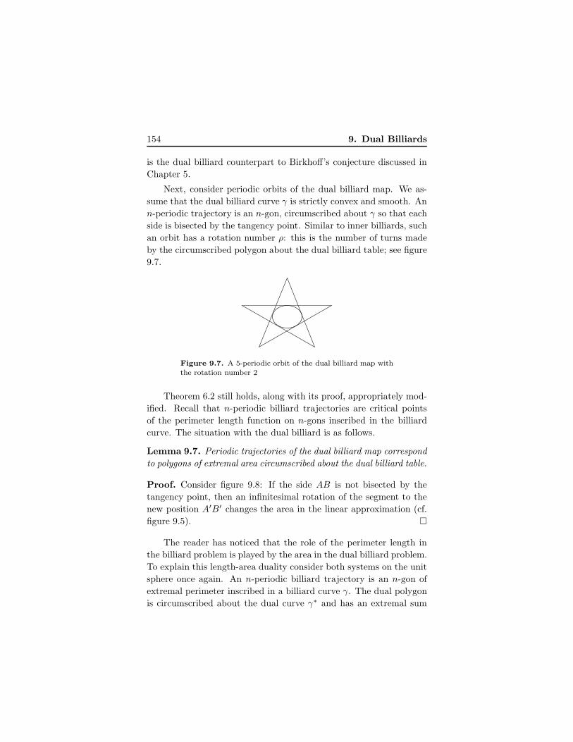
154 9. Dual Billiards
is the dual billiard counterpart to Birkhoff’s conjecture discussed in
Chapter 5.
Next, consider periodic orbits of the dual billiard map. We as-
sume that the dual billiard curve γ is strictly convex and smooth. An
n-periodic trajectory is an n-gon, circumscribed about γ so that each
side is bisected by the tangency point. Similar to inner billiards, such
an orbit has a rotation number ρ: this is the number of turns made
by the circumscribed polygon about the dual billiard table; see figure
9.7.
Figure 9.7. A 5-periodic orbit of the dual billiard map with
the rotation number 2
Theorem 6.2 still holds, along with its proof, appropriately mod-
ified. Recall that n-periodic billiard trajectories are critical points
of the perimeter length function on n-gons inscribed in the billiard
curve. The situation with the dual billiard is as follows.
Lemma 9.7. Periodic trajectories of the dual billiard map correspond
to polygons of extremal area circumscribed about the dual billiard table.
Proof. Consider figure 9.8: If the side AB is not bisected by the
tangency point, then an infinitesimal rotation of the segment to the
new position A′B′ changes the area in the linear approximation (cf.
figure 9.5).
The reader has noticed that the role of the perimeter length in
the billiard problem is played by the area in the dual billiard problem.
To explain this length-area duality consider both systems on the unit
sphere once again. An n-periodic billiard trajectory is an n-gon of
extremal perimeter inscribed in a billiard curve γ. The dual polygon
is circumscribed about the dual curve γ∗ and has an extremal sum
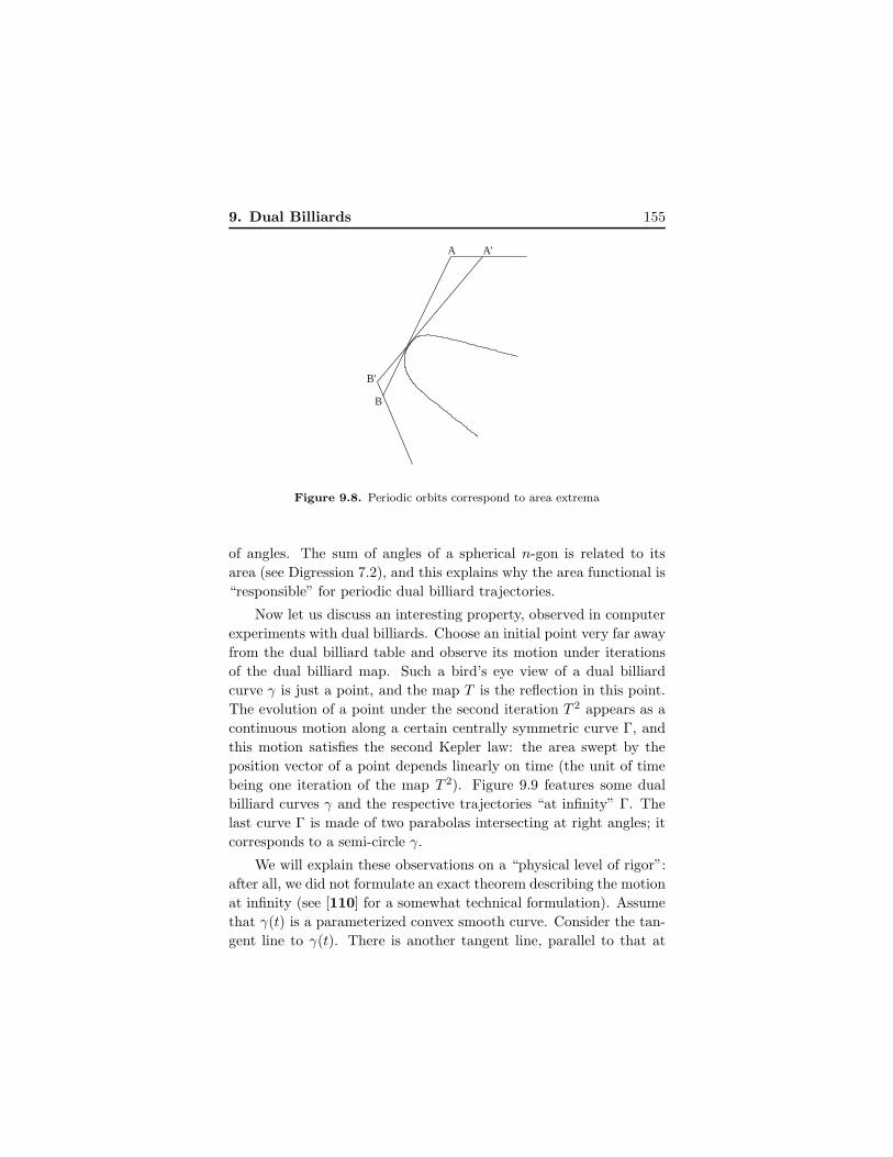
9. Dual Billiards 155
A A'
B'
B
Figure 9.8. Periodic orbits correspond to area extrema
of angles. The sum of angles of a spherical n-gon is related to its
area (see Digression 7.2), and this explains why the area functional is
“responsible” for periodic dual billiard trajectories.
Now let us discuss an interesting property, observed in computer
experiments with dual billiards. Choose an initial point very far away
from the dual billiard table and observe its motion under iterations
of the dual billiard map. Such a bird’s eye view of a dual billiard
curve γ is just a point, and the map T is the reflection in this point.
The evolution of a point under the second iteration T 2 appears as a
continuous motion along a certain centrally symmetric curve Γ, and
this motion satisfies the second Kepler law: the area swept by the
position vector of a point depends linearly on time (the unit of time
being one iteration of the map T 2). Figure 9.9 features some dual
billiard curves γ and the respective trajectories “at infinity” Γ. The
last curve Γ is made of two parabolas intersecting at right angles; it
corresponds to a semi-circle γ.
We will explain these observations on a “physical level of rigor”:
after all, we did not formulate an exact theorem describing the motion
at infinity (see [110] for a somewhat technical formulation). Assume
that γ(t) is a parameterized convex smooth curve. Consider the tan-
gent line to γ(t). There is another tangent line, parallel to that at
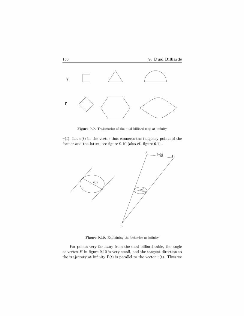
156 9. Dual Billiards
Γ
γ
Figure 9.9. Trajectories of the dual billiard map at infinity
γ(t). Let v(t) be the vector that connects the tangency points of the
former and the latter; see figure 9.10 (also cf. figure 6.1).
v(t)
v(t)
2v(t)A
B
C
Figure 9.10. Explaining the behavior at infinity
For points very far away from the dual billiard table, the angle
at vertex B in figure 9.10 is very small, and the tangent direction to
the trajectory at infinity Γ(t) is parallel to the vector v(t). Thus we
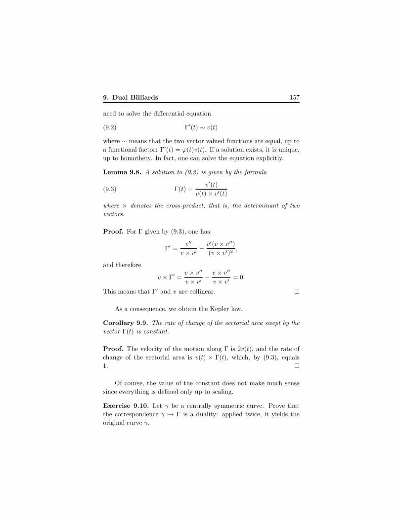
9. Dual Billiards 157
need to solve the differential equation
(9.2) Γ′(t) ∼ v(t)
where ∼ means that the two vector valued functions are equal, up to
a functional factor: Γ′(t) = ϕ(t)v(t). If a solution exists, it is unique,
up to homothety. In fact, one can solve the equation explicitly.
Lemma 9.8. A solution to (9.2) is given by the formula
(9.3) Γ(t) =v′(t)
v(t) × v′(t)
where × denotes the cross-product, that is, the determinant of two
vectors.
Proof. For Γ given by (9.3), one has:
Γ′ =v′′
v × v′− v′(v × v′′)
(v × v′)2,
and therefore
v × Γ′ =v × v′′
v × v′− v × v′′
v × v′= 0.
This means that Γ′ and v are collinear.
As a consequence, we obtain the Kepler law.
Corollary 9.9. The rate of change of the sectorial area swept by the
vector Γ(t) is constant.
Proof. The velocity of the motion along Γ is 2v(t), and the rate of
change of the sectorial area is v(t) × Γ(t), which, by (9.3), equals
1.
Of course, the value of the constant does not make much sense
since everything is defined only up to scaling.
Exercise 9.10. Let γ be a centrally symmetric curve. Prove that
the correspondence γ 7→ Γ is a duality: applied twice, it yields the
original curve γ.
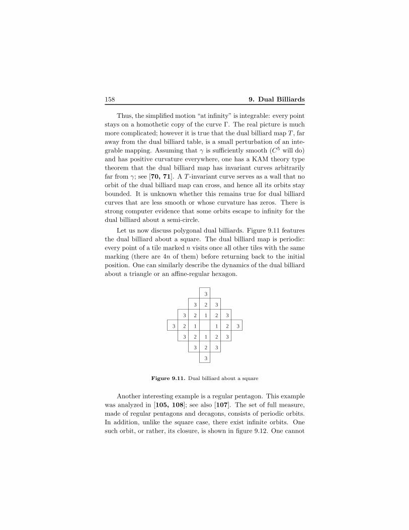
158 9. Dual Billiards
Thus, the simplified motion “at infinity” is integrable: every point
stays on a homothetic copy of the curve Γ. The real picture is much
more complicated; however it is true that the dual billiard map T , far
away from the dual billiard table, is a small perturbation of an inte-
grable mapping. Assuming that γ is sufficiently smooth (C5 will do)
and has positive curvature everywhere, one has a KAM theory type
theorem that the dual billiard map has invariant curves arbitrarily
far from γ; see [70, 71]. A T -invariant curve serves as a wall that no
orbit of the dual billiard map can cross, and hence all its orbits stay
bounded. It is unknown whether this remains true for dual billiard
curves that are less smooth or whose curvature has zeros. There is
strong computer evidence that some orbits escape to infinity for the
dual billiard about a semi-circle.
Let us now discuss polygonal dual billiards. Figure 9.11 features
the dual billiard about a square. The dual billiard map is periodic:
every point of a tile marked n visits once all other tiles with the same
marking (there are 4n of them) before returning back to the initial
position. One can similarly describe the dynamics of the dual billiard
about a triangle or an affine-regular hexagon.
1
1
1
1
2
2
2
2
2
2
2
2
3
3
3
3
3
3
3
3
3
3
3
3
Figure 9.11. Dual billiard about a square
Another interesting example is a regular pentagon. This example
was analyzed in [105, 108]; see also [107]. The set of full measure,
made of regular pentagons and decagons, consists of periodic orbits.
In addition, unlike the square case, there exist infinite orbits. One
such orbit, or rather, its closure, is shown in figure 9.12. One cannot
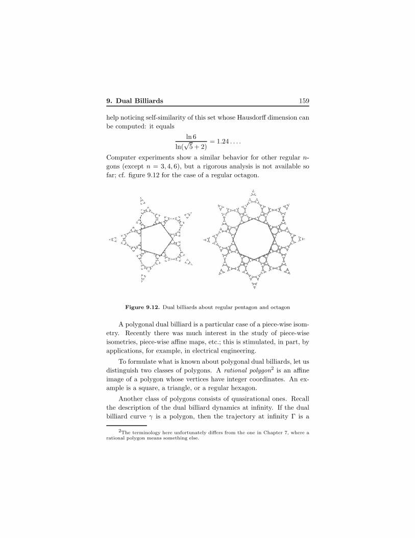
9. Dual Billiards 159
help noticing self-similarity of this set whose Hausdorff dimension can
be computed: it equals
ln 6
ln(√
5 + 2)= 1.24 . . . .
Computer experiments show a similar behavior for other regular n-
gons (except n = 3, 4, 6), but a rigorous analysis is not available so
far; cf. figure 9.12 for the case of a regular octagon.
Figure 9.12. Dual billiards about regular pentagon and octagon
A polygonal dual billiard is a particular case of a piece-wise isom-
etry. Recently there was much interest in the study of piece-wise
isometries, piece-wise affine maps, etc.; this is stimulated, in part, by
applications, for example, in electrical engineering.
To formulate what is known about polygonal dual billiards, let us
distinguish two classes of polygons. A rational polygon2 is an affine
image of a polygon whose vertices have integer coordinates. An ex-
ample is a square, a triangle, or a regular hexagon.
Another class of polygons consists of quasirational ones. Recall
the description of the dual billiard dynamics at infinity. If the dual
billiard curve γ is a polygon, then the trajectory at infinity Γ is a
2The terminology here unfortunately differs from the one in Chapter 7, where arational polygon means something else.
160 9. Dual Billiards
centrally symmetric 2k-gon, and the vectors v are some of the diag-
onals of γ. To every side of Γ there corresponds “time”, the ratio of
the length of this side to the magnitude of the respective vector v.
One obtains a collection of “times” (t1, . . . , tk), well defined up to a
common factor. The polygon is called quasirational if all these num-
bers are rational multiples of each other. For example, every regular
polygon is quasirational: the respective times ti are all equal.
Exercise 9.11. Prove that a rational polygon is quasirational.
The importance of quasirational polygons is due to the following
result; see [48, 61, 94].
Theorem 9.12. All orbits of the dual billiard map about a quasira-
tional polygon are bounded.
The proof is rather involved, and we do not dwell on it: one
has an analog of invariant curves, T -invariant necklaces of polygons
around the dual billiard table connected to each other at their com-
mon vertices.
Theorem 9.12 has the next corollary.
Corollary 9.13. Every orbit of the dual billiard map about a rational
polygon is finite.
Proof. By Exercise 9.11 and Theorem 9.12, the orbits are bounded.
For a rational polygon, the group generated by the reflection in the
vertices is discrete. Hence the orbit of every point is discrete. A
discrete and bounded set is finite.
Let us also mention that, similar to the inner billiard, it was not
known whether the dual billiard about a polygon always has a peri-
odic orbit. For dual billiards, this is a much more accessible problem:
in the summer of 2004, a participant of the Penn State REU program,
C. Culter, proved that for every polygonal dual billiard, periodic or-
bits exist, and, moreover, as far as the measure is concerned, periodic
points constitute a positive proportion of the whole plane.
Let us now say a few words about dual billiards in the hyper-
bolic plane. The definition of the map is exactly the same as in the
9. Dual Billiards 161
Euclidean (or spherical) case: all the notions, such as distance or
area, of course, should be understood in terms of hyperbolic geome-
try. Similar to the plane or spherical cases, the dual billiard map is
area preserving.
It is convenient to use the Klein-Beltrami model of hyperbolic
geometry described in Chapter 3. A new feature of the dual billiard
system is that one has an actual map at infinity t : S1 → S1; this circle
map is continuous even when the dual billiard map is not (namely,
when the dual billiard curve has straight segments). The circle map t
contains all the information about the dual billiard system since the
dual billiard table can be reconstructed as the envelope of the lines
(x t(x)), x ∈ S1. See [33, 111] for some results on dual billiards in
the hyperbolic plane.
Example 9.14. The following example is a generalization of the
square dual billiard in the Euclidean plane. Let the dual billiard
table P be a regular n-gon with right angles (n ≥ 5); that such
polygons exist is a peculiar property of the hyperbolic plane. These
polygons tile the hyperbolic plane; see figure 9.13 in which a different,
Poincare, model of the hyperbolic plane is used (lines are represented
by circles, perpendicular to the circle at infinity, and the Euclidean
angles faithfully represent the hyperbolic ones). Similar to the case
of a square, all orbits of the dual billiard map T are periodic: T
cyclically permutes the tiles that form concentric “necklaces” around
the polygon P .
Let the dual billiard curve γ be an ellipse inside the unit circle.
It turns out that the respective dual billiard map T is integrable, and
this fact provides another proof of the Poncelet porism (this proof
appeared in [106]).
Let γ and Γ be two conics in the plane. These conics deter-
mine a 1-parameter family of conics, called a pencil, consisting of the
conics that pass through the four intersection points of γ and Γ. Al-
gebraically, if φ(x, y) = 0 and Φ(x, y) = 0 are equations of γ and Γ,
then the conics in the pencil have the equations φ + tΦ = 0, t ∈ R.
This equation makes sense and defines the pencil even if the conics γ
and Γ do not intersect (or, more precisely, intersect at four complex
points).
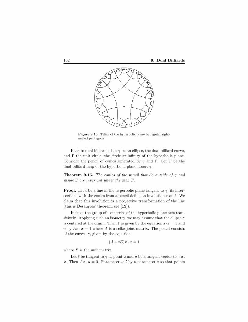
162 9. Dual Billiards
Figure 9.13. Tiling of the hyperbolic plane by regular right-
angled pentagons
Back to dual billiards. Let γ be an ellipse, the dual billiard curve,
and Γ the unit circle, the circle at infinity of the hyperbolic plane.
Consider the pencil of conics generated by γ and Γ. Let T be the
dual billiard map of the hyperbolic plane about γ.
Theorem 9.15. The conics of the pencil that lie outside of γ and
inside Γ are invariant under the map T .
Proof. Let ℓ be a line in the hyperbolic plane tangent to γ; its inter-
sections with the conics from a pencil define an involution τ on ℓ. We
claim that this involution is a projective transformation of the line
(this is Desargues’ theorem; see [12]).
Indeed, the group of isometries of the hyperbolic plane acts tran-
sitively. Applying such an isometry, we may assume that the ellipse γ
is centered at the origin. Then Γ is given by the equation x·x = 1 and
γ by Ax · x = 1 where A is a selfadjoint matrix. The pencil consists
of the curves γt given by the equation
(A+ tE)x · x = 1
where E is the unit matrix.
Let ℓ be tangent to γ at point x and u be a tangent vector to γ at
x. Then Ax · u = 0. Parameterize l by a parameter s so that points
9. Dual Billiards 163
of l are x+ su. The intersection l ∩ γt is given by
(A+ tE)(x + su) · (x+ su) = 1.
Since Ax · x = 1 and Ax · u = 0, the previous equation is rewritten as
s2(A+ tE)u · u+ 2stEx · u+ tx · x = 0.
It follows that1
s1+
1
s2= −2
x · ux · x,
independently of t where s1 and s2 are the two roots of the quadratic
equation. We see that the correspondence τ : s1 7→ s2 is fractional-
linear, that is, projective.
To finish the proof, use Exercise 3.17 b). It follows that the map
τ is a hyperbolic isometry, that is, the dual billiard map T about γ.
Thus the ellipses of the pencil are T -invariant.
Theorem 9.15 implies the Poncelet porism. As was explained in
Chapter 4, the closed invariant curves of an integrable area preserving
transformation carry an affine structure, in which the transformation
is a translation x 7→ x+c where c depends on the curve. In particular,
the map is periodic on a curve if and only if c ∈ Q (independently of
the point x).
We conclude this chapter with a discussion of multi-dimensional
dual billiard; see [105, 108, 107, 113]. One wants to replace the dual
billiard curve by a smooth strictly convex closed hypersurface M in
a vector space and use tangent lines to M to define a dual billiard
map. However one encounters an immediate difficulty: there are too
many tangent lines at a point m ∈M .
This difficulty is resolved as follows. Let the ambient space be
even-dimensional (the plane has an even dimension!), and assume
that one has a linear symplectic structure ω in this space. One may
identify R2n with Cn; let J be the operator of multiplication by√−1.
The relation between the Euclidean and symplectic structure is given
by the formula:
ω(u, v) = Ju · vfor all vectors u and v.
164 9. Dual Billiards
Let M ⊂ Cn be a smooth hypersurface. Then, at every point
m ∈M , one has the characteristic tangent direction to M , the kernel
of the restriction of ω on the tangent space TmM ; cf. Digression
3.2. Let N(m) be the unit normal vector to M at point m; then the
characteristic direction is given by the vector JN(m).
Exercise 9.16. Prove the last statement.
With this definition of the tangent lines to a smooth hypersurface,
we have a (possibly partially defined and multi-valued) dual billiard
map. Let x be a point outside M and assume that it lies on a tangent
characteristic line whose orientation is from x to m. Then the dual
billiard map T reflects x in m, just as in the plane. In fact, one has
a well defined map, as the next theorem asserts.
Theorem 9.17. For every point outside M , there exist exactly two
tangent characteristic lines to M through x, one oriented from M and
one to M .
Proof. (Sketch). Denote the exterior of M by X . Every point of
X lies on a unique outward normal to M ; hence X = M × [0,∞).
Let m ∈ M and N be an outward normal vector to M at point m.
Turn the vector N through π/2 by applying the linear operator J ;
this defines a map f : m+N 7→ m+ JN from X to itself. The claim
is that f is one-to-one and onto.
To prove that f is injective, assume that for two distinct points
m1,m2 ∈ M and normal vectors N1, N2, one has m1 + JN1 = m2 +
JN2. Then
(9.4) m2 −m1 = JN1 − JN2.
Since M is convex, the segment m1m2 has the outward direction at
point m2 and the inward one at m1; that is, (m2 − m1) · N2 > 0
and (m1 − m2) · N1 > 0. It follows, using (9.4) and the fact that
Ju · u = 0 for every vector u, that JN1 ·N2 > 0 and JN2 ·N1 > 0 or
ω(N1, N2) > 0 and ω(N2, N1) > 0. This contradicts skew symmetry
of the symplectic structure.
We only sketch a proof that f is surjective. The argument is
topological. Consider a 1-point compactification of R2n and extend
f to a continuos self map f of this 2n-dimensional sphere: inside M ,
9. Dual Billiards 165
the map is the identity and f preserves the point at infinity. We claim
that f has degree 1; this implies surjectivity. To find the degree of
f , consider this map at a vicinity of infinity where it is approximated
by a linear map, namely, the rotation J . It follows that deg f = 1,
and we are done.
Thus the exterior of a smooth strictly convex closed hypersurface
in linear symplectic space is foliated by the tangent positive char-
acteristic half-lines, just as in the plane case. The area preserving
property of the dual billiard map has a multi-dimensional analog too.
Theorem 9.18. The dual billiard map preserves the symplectic struc-
ture ω.
Proof. According to Theorem 9.17, every point x outside M can be
written as m−JN where m ∈M and N is an outward normal vector
to M at m. Then y := T (x) = m+ JN .
Consider the differential 1-form Ndm =∑Nidmi where Ni and
mi are the components of the vectors N and m; this is a 1-form on
M × [0,∞). Since N is orthogonal to M , the form Ndm vanishes on
the tangent vectors to M . It follows that
(9.5) dN ∧ dm = 0
on M × [0,∞).
For a vector u ∈ Cn, write u = (u1, u2) where u1 ∈ Rn and
u2 ∈ Rn are the real and the imaginary parts. Then Ju = (−u2, u1)
and
ω = du1 ∧ du2 =∑
du1i ∧ du2i, i = 1, . . . , n.
One has:
x = (x1, x2) = (m1+N2,m2−N1), y = (y1, y2) = (m1−N2,m2+N1).
A direct computation, using (9.5) and left to the reader, yields dx1 ∧dx2 = dy1 ∧ dy2; that is, T ∗(ω) = ω. Thus the dual billiard map is a
symplectic mapping.
It is natural to ask about the existence and lower bound on
the number of periodic trajectories of the dual billiard map. Not
much is known about this problem: one can prove that, for every
166 9. Dual Billiards
strictly convex smooth dual billiard hypersurface in R2n and every
odd prime k, there exists a k-periodic orbit of the dual billiard map
[105, 108, 107]. For k = 3, which is the minimal possible period
of the dual billiard map, a better estimate is known [113]: one has
at least 2n such orbits, that is, circumscribed triangles whose sides
are bisected by the tangency points and have characteristic directions
therein. This estimate is sharp. Similar to the case of the inner bil-
liard discussed in Chapter 6, these results are obtained using Morse
theory. The relevant function (for odd k) is defined in terms of the
tangency points mi:
F (m1, . . . ,mk) =∑
1≤i<j≤k
(−1)i+jω(mi,mj).
For k = 3, this is the symplectic area of the triangle.
Let us mention, in conclusion, that a dual billiard table could
be a convex polyhedron as well. This multi-dimensional analog of
polygonal dual billiards has not been studied yet. For example, it
is very intriguing to consider the regular polyhedra in 4-dimensional
space.
Bibliography
[1] J.-C. Alvarez. Hilbert’s fourth problem in two dimensions, MASS Se-lecta, Amer. Math. Soc., Providence, RI, 2003, pp. 165–184.
[2] J.-C. Alvarez, C. Duran. An introduction to Finsler geometry, Publ.Escuela Venezolana de Mat., Caracas, Venezuela, 1998.
[3] V. Arnold. Mathematical methods of classical mechanics, Springer-Verlag, 1989.
[4] V. Arnold. Ordinary differential equations, Springer-Verlag, 1992.
[5] V. Arnold. Topological invariants of plane curves and caustics, Univer-sity Lect. Ser. 5, Amer. Math. Soc., Providence, RI, 1994.
[6] V. Arnold. Topological problems of the theory of wave propagation.Russ. Math. Surv. 51:1 (1996), 1–47.
[7] V. Arnold, A. Givental. Symplectic geometry, Encycl. of Math. Sci.,Dynamical Systems, 4, Springer-Verlag, 1990, pp. 1–136.
[8] D. Bao, S.-S. Chern, Z. Shen. An introduction to Riemann-Finsler ge-ometry, Springer-Verlag, 2000.
[9] Yu. Baryshnikov. Complexity of trajectories in rectangular billiards.Comm. Math. Phys. 174 (1995), 43–56.
[10] V. Benci, F. Giannoni. Periodic bounce trajectories with a low numberof bounce points. Ann. Inst. Poincare, Anal. Non Lineaire 6 (1989),73–93.
[11] F. Benford. The law of anomalous numbers. Proc. Amer. Philos. Soc.78 (1938), 551–572.
[12] M. Berger. Geometry, Springer-Verlag, 1987.
167
168 Bibliography
[13] M. Berger. Seules les quadriques admettent des caustiques. Bull. Soc.Math. France 123 (1995), 107–116.
[14] E. Berlekamp, J. Conway, R. Guy. Winning ways for your mathemat-ical plays, Vol. 2. Games in particular. Academic Press, 1982.
[15] R. Berndt. An introduction to symplectic geometry , Amer. Math. Soc.,Providence, RI, 2001.
[16] M. Berry, M. Robnik. Classical billiards in magnetic fields. J. Phys. A
18 (1985), 1361–1378.
[17] M. Bialy. Convex billiards and a theorem by E. Hopf. Math. Zeit. 214
(1993), 147–154.
[18] H. Bos, C. Kers, F. Oort, D. Raven. Poncelet’s closure theorem. Expos.Math. 5 (1987), 289–364.
[19] R. Bott. Lectures on Morse theory, old and new. Bull. Amer. Math.Soc. 7 (1982), 331–358.
[20] Ph. Boyland. Dual billiards, twist maps and impact oscillators. Non-linearity 9 (1996), 1411–1438.
[21] L. Bunimovich. Systems of hyperbolic type with singularities, Encycl. ofMath. Sci., Dynamical Systems, 2, Springer-Verlag, 1989, pp. 173–203.
[22] L. Bunimovich. Mushrooms and other billiards with divided phasespace. Chaos 11 (2001), 802–808.
[23] L. Bunimovich, J. Rehacek. Nowhere dispersing 3D billiards with non-vanishing Lyapunov exponents. Comm. Math. Phys. 189 (1997), 729–757.
[24] L. Bunimovich, J. Rehacek. How high-dimensional stadia look like.Comm. Math. Phys. 197 (1998), 277–301.
[25] D. Burago, S. Ferleger, A. Kononenko. A geometric approach to semi-dispersing billiards, Hard ball systems and the Lorentz gas. Springer-Verlag, 2000, pp. 9–27.
[26] Yu. Burago, V. Zalgaller. Geometric inequalities, Springer-Verlag,1988.
[27] H. Busemann. Problem IV: Desarguesian spaces, Proc. Symp. PureMath., vol. 28, Amer. Math. Soc., Providence, RI, 1976, pp. 131–141.
[28] J. Cannon, W. Floyd, R. Kenyon, W. Parry. Hyperbolic geometry,Flavors of geometry. Cambridge Univ. Press, 1997, pp. 59–115.
[29] G. Casati, T. Prosen. Mixing property of triangular billiards. Phys.Rev. Lett. 83 (1999), 4729–4732.
[30] N. Chernov, R. Markarian. Theory of chaotic billiards, Amer. Math.Soc., Providence, RI, to appear.
[31] B. Cipra, R. Hanson, A. Kolan. Periodic trajectories in right trianglebilliards. Phys. Rev. E 52 (1995), 2066–2071.
Bibliography 169
[32] H. S. M. Coxeter. The golden section, phyllotaxis, and Wythoff’s game.Scripta Math. 19 (1953), 135–143.
[33] F. Dogru, S. Tabachnikov. On polygonal dual billiard in the hyperbolicplane. Reg. Chaotic Dynamics 8 (2003), 67–82.
[34] F. Dogru, S. Tabachnikov. Dual billiards. Math. Intell. 28 (2005), inprint.
[35] F. Fabricius-Bjerre. On the double tangents of plane curves. Math.Scand. 11 (1962), 113–116.
[36] M. Farber, S. Tabachnikov. Periodic trajectories in 3-dimensional con-vex billiards. Manuscripta Mat. 108 (2002), 431–437.
[37] M. Farber, S. Tabachnikov. Topology of cyclic configuration spaces andperiodic orbits of multi-dimensional billiards. Topology 41 (2002), 553–589.
[38] R. Fox, R. Kershner. Geodesics on a rational polyhedron. Duke Math.J. 2 (1936), 147–150.
[39] G. Galperin. Billiard balls count π, MASS Selecta, Amer. Math. Soc.,Providence, RI, 2003, pp. 197–204.
[40] G. Galperin. Convex polyhedra without simple closed geodesics. Reg.Chaotic Dynamics 8 (2003), 45–58.
[41] G. Galperin, N. Chernov. Billiards and chaos, Math. and Cybernetics,No. 5, 1991 (in Russian).
[42] G. Galperin, A. Stepin, Ya. Vorobets. Periodic billiard trajectories inpolygons: generating mechanisms. Russ. Math. Surv. 47:3 (1992), 5–80.
[43] G. Galperin, A. Zemlyakov. Mathematical billiards. Nauka, Moscow,1990 (in Russian).
[44] H. Geiges. Christiaan Huygens and contact geometry. Nieuw Arch.Wiskd., to appear.
[45] S. Glashow, L. Mittag. Three rods on a ring and the triangular billiard.J. Stat. Phys. 87 (1997), 937–941.
[46] E. Gutkin. Billiard dynamics: a survey with the emphasis on openproblems. Reg. Chaotic Dynamics 8 (2003), 1–13.
[47] E. Gutkin. Blocking of billiard orbits and security for polygons and flatsurfaces. GAFA 15 (2005), 83–105.
[48] E. Gutkin, N. Simanyi. Dual polygonal billiards and necklace dynamics.Comm. Math. Phys. 143 (1991), 431–450.
[49] E. Gutkin, S. Tabachnikov. Billiards in Finsler and Minkowski geome-tries. J. Geom. and Phys. 40 (2002), 277–301.
170 Bibliography
[50] E. Gutkin, S. Tabachnikov. Complexity of piecewise convex transfor-mations in two dimensions, with applications to polygonal billiards.Preprint.
[51] L. Halbeisen, N. Hungerbuhler. On periodic billiard trajectories in ob-tuse triangles. SIAM Rev. 42 (2000), 657–670.
[52] T. Hill. The significant-digit phenomenon. Amer. Math. Monthly 102
(1995), 322–327.
[53] F. Holt. Periodic reflecting paths in right triangles. Geom. Dedicata46 (1993), 73-90.
[54] P. Hubert. Complexite de suites definies par des billards rationnels.Bull. Soc. Math. France 123 (1995), 257–270.
[55] N. Innami. Convex curves whose points are vertices of billiard triangles.Kodai Math. J. 11 (1988), 17–24.
[56] M. Kapovich, J. Millson. Universality theorems for configuration spacesof planar linkages. Topology 41 (2002), 1051–1107.
[57] A. Katok. Billiard table as a mathematician’s playground, Student col-loquium lecture series, v. 2, Moscow MCCME (2001), pp. 8–36 (InRussian.)3
[58] A. Katok, B. Hasselblatt. Introduction to the modern theory of dynam-ical systems, Camb. Univ. Press, 1995.
[59] A. Katok, A. Zemlyakov. Topological transitivity of billiards in poly-gons. Math. Notes 18 (1975), 760–764.
[60] S. Kerckhoff, H. Masur, J. Smillie. Ergodicity of billiard flows andquadratic differentials. Ann. of Math. 124 (1986), 293–311.
[61] R. Kolodziej. The antibilliard outside a polygon. Bull. Pol. Acad. Sci.37 (1989), 163–168.
[62] V. Kozlov, D. Treshchev. Billiards. A genetic introduction to the dy-namics of systems with impacts. Translations of Math. Monographs,98, Amer. Math. Soc., Providence, RI, 1991.
[63] J. Lagarias, T. Richardson. Convexity and the average curvature ofplane curves. Geom. Dedicata 67 (1997), 1–30.
[64] V. Lazutkin. The existence of caustics for a billiard problem in a convexdomain. Math. USSR, Izvestija 7 (1973), 185–214.
[65] H. Masur, S. Tabachnikov. Rational billiards and flat structures, Hand-book of Dynamical Systems, v. 1A, North-Holland, 2002, pp. 1015–1089.
[66] J. Mather. Non-existence of invariant circles. Ergod. Th. Dyn. Syst.4 (1984), 301–309.
3English translation available at A. Katok’s web site.
Bibliography 171
[67] D. McDuff, D. Salamon. Introduction to symplectic topology, ClaredonPress, Oxford, 1995.
[68] J. Milnor. Morse theory, Princeton U. Press, Princeton, 1963.
[69] T. Monteil. On the finite blocking property. Ann. Inst. Fourier, to ap-pear.
[70] J. Moser. Stable and random motions in dynamical systems, Ann. ofMath. Stud., 77, Princeton, 1973.
[71] J. Moser. Is the solar system stable? Math. Intell. 1 (1978), 65–71.
[72] J. Moser. Geometry of quadrics and spectral theory, Chern Symp.,Springer-Verlag, 1980, pp. 147–188.
[73] J. Moser. Various aspects of integrable Hamiltonian systems, Progr. inMath. 8, Birkhauser, 1980, pp. 233–289.
[74] J. Moser, A. Veselov. Discrete versions of some classical integrablesystems and factorization of matrix polynomials. Comm. Math. Phys.139 (1991), 217–243.
[75] S. Mukhopadhyaya. New methods in the geometry of a plane arc. Bull.Calcutta Math. Soc. 1 (1909), 32–47.
[76] T. Murphy, E. Cohen. On the sequences of collisions among hardspheres in infinite space, Hard ball systems and the Lorentz gas.Springer-Verlag, 2000, pp. 29–49.
[77] A. Nazarov, F. Petrov. On S. L. Tabachnikov’s conjecture. Preprint.
[78] S. Newcomb. Note on the frequency of use of the different digits innatural numbers. Amer. J. Math. 4 (1881), 39–40.
[79] I. Newton. Opticks: Or a Treatise of the Reflections, Refractions, In-flections & Colours of Light – Based on the Fourth Edition London,1730, Dover, 1952.
[80] V. Ovsienko, S. Tabachnikov. Projective differential geometry, oldand new: from Schwarzian derivative to cohomology of diffeomorphismgroups, Cambridge Univ. Press, 2005.
[81] R. Peirone. Reflections can be trapped. Amer. Math. Monthly 101
(1994), 259–260.
[82] A. Pogorelov. Hilbert’s fourth problem, J. Wiley & Sons, 1979.
[83] P. Pushkar. Diameters of immersed manifolds and wave fronts. C. R.Acad. Sci. 326 (1998), 201–205.
[84] Ch. Radin. Miles of tiles. Amer. Math. Soc., Providence, RI, 1999.
[85] R. Raimi. The first digit problem. Amer. Math. Monthly 83 (1976),521–538.
[86] R. Richens, M. Berry. Pseudointegrable systems in classical and quan-tum mechanics. Physica D 2 (1981), 495–512.
172 Bibliography
[87] T. Ruijgrok. Periodic orbits in triangular billiards. Acta Phys. Polon.22 (1991), 955–981.
[88] M. Rychlik. Periodic points of the billiard ball map in a convex domain.J. Diff. Geom. 30 (1989), 191–205.
[89] L. Santalo. Integral geometry and geometric probability, Addison-Wesley, 1976.
[90] I. Schoenberg. Mathematical time exposures, MAA, Washington, 1982.
[91] R. Schwartz’s web site at University of Maryland.
[92] R. Schwartz. The Poncelet grid. Preprint.
[93] M. Senechal. Quasicrystals and geometry, Cambridge Univ. Press,1995.
[94] A. Shaidenko, F. Vivaldi. Global stability of a class of discontinuousdual billiards. Comm. Math. Phys. 110 (1987), 625–640.
[95] N. Simanyi. Ergodicity of hard spheres in a box. Ergod. Th. Dyn. Syst.19 (1999), 741–766.
[96] N. Simanyi. Hard ball systems and semi-dispersive billiards: hyper-bolicity and ergodicity, Hard ball systems and the Lorentz gas, Ency-clopaedia Math. Sci., 101, Springer, 2000, pp. 51–88.
[97] N. Simanyi. The complete hyperbolicity of cylindric billiards. Ergod.Th. Dyn. Syst. 22 (2002), 281–302.
[98] N. Simanyi. Proof of the Boltzmann-Sinai ergodic hypothesis for typicalhard disk systems. Invent. Math. 154 (2003), 123–178.
[99] N. Simanyi. The Boltzmann-Sinai ergodic hypothesis in two dimensions(without exceptional models). Preprint.
[100] Ya. Sinai. On the foundations of the ergodic hypothesis for a dynami-cal system of statistical mechanics. Soviet Math. Dokl. 4 (1963), 1818–1822.
[101] Ya. Sinai. Dynamical systems with elastic reflections. Ergodic proper-ties of dispersing billiards. Russ. Math. Surv., 25:2 (1970), 137–189.
[102] Ya. Sinai. Introduction to ergodic theory, Princeton Univ. Press,Princeton, 1976.
[103] Ya. Sinai. Hyperbolic billiards, Proc. ICM, Kyoto 1990, Math. Soc.Japan, Tokyo, 1991, pp. 249–260.
[104] D. Szasz. Boltzmann’s Ergodic Hypothesis, a conjecture for centuries?Hard ball systems and the Lorentz gas. Springer-Verlag, 2000, pp. 421–446.
[105] S. Tabachnikov. Outer billiards. Russ. Math. Surv. 48:6 (1993), 81–109.
Bibliography 173
[106] S. Tabachnikov. Poncelet’s theorem and dual billiards. L’Enseign.Math. 39 (1993), 189–194.
[107] S. Tabachnikov. Billiards, Societe Mathematique de France, “Panora-mas et Syntheses”, No. 1, 1995.
[108] S. Tabachnikov. On the dual billiard problem. Adv. in Math. 115
(1995), 221–249.
[109] S. Tabachnikov. The four vertex theorem revisited – two variationson the old theme. Amer. Math. Monthly 102 (1995), 912–916.
[110] S. Tabachnikov. Asymptotic dynamics of the dual billiard transfor-mation. J. Stat. Phys. 83 (1996), 27–38.
[111] S. Tabachnikov. Dual billiards in the hyperbolic plane. Nonlinearity15 (2002), 1051–1072.
[112] S. Tabachnikov. Ellipsoids, complete integrability and hyperbolic ge-ometry. Moscow Math. J. 2 (2002), 185–198.
[113] S. Tabachnikov. On three-periodic trajectories of multi-dimensionaldual billiards. Alg. Geom. Topology 3 (2003), 993–1004.
[114] S. Tabachnikov. A tale of a geometric inequality, MASS Selecta,Amer. Math. Soc., Providence, RI, 2003, pp. 257–262.
[115] S. Tabachnikov. Remarks on magnetic flows and magnetic billiards,Finsler metrics and a magnetic analog of Hilbert’s fourth problem, Dy-namical systems and related topics, Cambridge Univ. Press, 2004, pp.233–252.
[116] G. Tokarsky. Polygonal rooms not illuminable from every point. Amer.Math. Monthly 102 (1995), 867–879.
[117] S. Troubetzkoy. Complexity lower bounds for polygonal billiards.Chaos 8 (1998), 242–244.
[118] M. Wojtkowski. Principles for the design of billiards with nonvanish-ing Lyapunov exponents. Comm. Math. Phys. 105 (1986), 391–414.
[119] M. Wojtkowski. Two applications of Jacobi fields to the billiard ballproblem. J. Diff. Geom. 40 (1994), 155–164.
[120] B. Yandell. The honors class: Hilbert’s problems and their solvers,A. K. Peters, 2001.


Index
affine structure, 58area construction, 152Arnold-Liouville theorem, 70Aubry-Mather theory, 106average absolute curvature, 41
Baker’s map, 135Benford’s Law, 25billiard ball map, 33Birkhoff conjecture, 95Boltzmann’s Hypothesis, 145brachistochrone, 16Buffon’s needle problem, 38Bunimovich billiards, 139
cat map, 137caustic, 56characteristic foliation, 48complexity function, 29configuration space, 3, 10confocal conics, 53Conley-Zehnder theorem, 106Crofton formula, 37cutting sequence, 27cyclic configuration space, 100
Desargues theorem, 88, 162diameter of a curve, 99dihedral group, 116Diophantine condition, 98DNA geometric inequality, 41
elliptic coordinates, 53equidistribution, 22ergodic map, 138evolute, 75
Fagnano trajectory, 113Fermat principle, 12Fibonacci numbers, 24finite blocking, 121Finsler metric, 14four vertex theorem, 81
Gauss-Bonnet theorem, 125geodesic, 43, 67Graves theorem, 74
Hamiltonian function, 69Hamiltonian vector field, 69Hilbert metric, 44Hilbert’s fourth problem, 42Huygens principle, 14
illumination problem, 56, 119impact oscillator, 148integrable map, 53, 58invariant circle, 86involute, 75isochronal pendulum, 75isoperimetric inequality, 39
KAM theory, 97Klein-Beltrami model, 43Kneser’s lemma, 77
Lagrangian function, 45Lagrangian submanifold, 48Larmor radius, 18length-area duality, 154Lie algebra, 70linkage, 10Liouville form, 47
175
176 Index
Lorentz force, 18
mean free path, 36Minkowski metric, 14mirror equation, 93Morse index, 107Morse theory, 107
pencil of conics, 161phase space of billiard ball map, 46Poincare model, 161Poincare’s Geometric Theorem, 104Poincare’s Recurrence Theorem, 115Poisson bracket, 70polar duality, 62Poncelet porism, 60, 161projective duality, 87, 89projective metric, 43projective plane, 88
quasicrystal, 32quasiperiodic sequence, 27quasirational polygon, 160
rainbow, 79rational polygon, 116rotation number, 21, 100
secure polygon, 120Sinai billiards, 137Snell’s law, 13spherical duality, 150stadium, 139string construction, 73Sturm-Hurwitz theorem, 84Sturmian sequence, 30support function, 38symplectic form, 47symplectic gradient, 70symplectic reduction, 48symplectic structure, 47
twist maps, 92
unfolding, 4uniform distribution, 22
vertex of a curve, 76
Wojtkowski billiards, 144Wythoff’s game, 31


![Introduction to Differential Geometry · 2021. 5. 25. · article [10] with Serge Tabachnikov, titled ‘Fun problems in geometry and beyond’, for further readings along these lines](https://img.pdfslide.net/doc/110x75/6147c8e6a830d0442101a953/introduction-to-differential-geometry-2021-5-25-article-10-with-serge-tabachnikov.jpg)