GGDC RESEARCH MEMORANDUM 174in the Penn World Table (Feenstra et al. 2015), we refer to this measure of real GDP per capita as . This variable is expressed in 2011 US dollars by correcting

university ofgroningen

groningen growth anddevelopment centre

GGDC RESEARCH MEMORANDUM 174

REBASING ‘MADDISON’: NEW INCOME COMPARISONS AND THE SHAPE OF LONG-RUN

ECONOMIC DEVELOPMENT

Jutta Bolt, Robert Inklaar, Herman de Jong and Jan Luiten van Zanden

January 2018

1

REBASING ‘MADDISON’: NEW INCOME COMPARISONS AND

THE SHAPE OF LONG-RUN ECONOMIC DEVELOPMENT 1

Jutta Bolt, Robert Inklaar, Herman de Jong and Jan Luiten van Zanden

January 2018

Abstract

Economists’ understanding of long-run economic development has greatly improved thanks to

the historical statistics compiled by the late Angus Maddison. Yet his method for comparing

income levels across countries and over time has come under increasing criticism. New

estimates of comparative income level often show markedly different outcomes than

Maddison’s projection (or extrapolation) method based on a single, modern-day relative income

benchmark. In this paper, we draw on modern and historical cross-country income comparisons

and incorporate these into a novel measure of real GDP per capita over the very long run. The

resulting new version of the Maddison Project Database thereby does greater justice to

historical insights and provides a fresh impetus for future research. We present applications to

estimating cross-country income convergence and the Balassa-Samuelson effect and

demonstrate that how our new measure of real GDP per capita is a substantial improvement.

(JEL: C43, C82, E01, N10, O47)

1 Bolt: University of Groningen and Lund University, [email protected], Inklaar: University of Groningen,

[email protected], van Zanden: University of Utrecht, [email protected], de Jong: University of Groningen,

[email protected]. We thank Bob Allen, Leticia Arroyo Abad, Luis Bertola, Steve Broadberry, Angus Deaton,

John Devereux, Rob Feenstra, Alan Heston, Andre Hofman, Branko Milanovic, Leandro Prados de la Escosura,

the Maddison Project Board in general, and participants at the World Economic History Congress 2015 in Kyoto,

the Society for Economic Measurement 2016 in Thessaloniki, the International Comparisons Conference 2017 in

Princeton, the Economic History Seminar in Wageningen and the CEPR Meeting in Dublin for helpful comments

and suggestions.

mailto:[email protected]




2

1. Introduction

Angus Maddison has greatly contributed to economists’ understanding of long-run economic

development through his Historical Statistics of the World Economy.2 By judiciously

combining estimates of comparative levels of real GDP per capita in recent periods with long-

term time series of growth of GDP per capita, his database provides the broadest coverage of

comparative income data and is amongst the most widely used sources of economic data in the

world. Especially for the period before 1950, this is the dominant database, providing

systematic and broad cross-country information on comparative income levels.3 Since his

passing, the development of the Maddison Project Database (MPD) has moved to a new

generation of scholars.4 In this paper we introduce a new approach to the measurement of real

GDP per capita over the very long and introduce a new version of the database.

Most importantly, we ‘rebase’ the MPD by incorporating a wealth of historical data on

comparative living standards and economic activity, much of which builds on Maddison’s

pioneering work. The latest series developed by Maddison were based on a single modern-day

cross-country comparison of relative income levels, for the year 1990, projected forwards and

backwards using data on growth of GDP per capita. Yet extended back over many decades and

even centuries, these projections diverged substantially from independent ‘benchmark’

comparisons of relative income or living standards for early periods.5 This is consistent with a

recent literature on how differences in real GDP per capita between benchmarks comparisons

can diverge from GDP growth from national statistics over the same period.6 Changing

economic structures and measurement error and biases in cross-country price comparisons are

important explanations for such differences. But especially over longer time scales, growth

figures also turn unreliable, especially when covering periods of war, rapid inflation or weak-

to-non-existent statistical systems. A consequence is that research results can be sensitive to the

version of a database that is used in a study.7 This has been one reason why versions 8 and 9 of

the Penn World Table (PWT) introduced real GDP series that rely on multiple benchmark

comparisons of prices and income; see Feenstra, Inklaar and Timmer (2015).

2 See Maddison (1995, 2001, 2007). 3 Though Barro and Ursúa (2008) have gone to great lengths to better capture data on economic fluctuations for

42 countries since 1800. 4 See Bolt and van Zanden (2014) for a first new version. 5 Prominent examples are Prados de la Escosura (2000) and Lindert and Williamson (2016). 6 See Deaton (2010), Deaton and Aten (2017) and Inklaar and Rao (2017). 7 See Johnson, Larson, Papageorgiou and Subramanian (2013) and Ciccone and Jarociński (2010).

3

In this paper, we implement a multiple benchmark approach for the MPD based, primarily, on

(i) post-1950 price benchmarks (as also used in PWT) and (ii) pre-1950 real GDP per capita

benchmarks based on a variety of historical studies.8,9 In our new dataset on historical

benchmarks we incorporate relative income levels for 36 out of the 77 countries for which there

are income estimates available prior to 1950. By integrating independent comparative income

estimates for earlier periods, the measurement of long-term relative income developments is

more closely related to research covering this historical period. An important benefit is that

subsequent new, contemporaneous price and income comparisons – such as a new round of the

International Comparison Program (ICP) – can be incorporated into the MPD without these

new numbers rewriting history; only new historical research can rewrite (or affirm) current

estimates. In addition, we incorporate recent estimates of historical national accounts for a range

of countries to provide a new version of the MPD that is state-of-the-art and provides a more

extensive picture of comparative income levels than had been available thus far, with coverage

for over 160 countries and the period from Roman times to the present.

The rest of this paper is organized as follows. In Section 2, we provide a guided tour of the data

in the MPD, highlighting the main variables, briefly discussing their construction and indicating

areas of research where they can be helpful. As in newer versions of PWT, the MPD

distinguishes between a series of real GDP that is useful for comparing income levels across

countries and a series that is useful for comparing growth performance over time. We also use

this section to emphasize that our measurement goal is GDP per capita, i.e. an economy’s

productive, income-generating capacity. While GDP per capita relates to the standard of living

in a country or the broader wellbeing of its population, it is certainly not the same concept; this

should be borne in mind throughout. Section 3 discusses in greater detail the methodology for

comparing income levels, at a point in time, but especially over a (long) period of time. Section

4 discusses the implementation of the multiple-benchmark approach including a discussion of

the different types of information that are developed and used in the different periods. This also

includes a discussion of how our chosen approach compares to other methods, such as indirect

benchmark estimates.10 Section 5 discusses a number of applications, highlighting where the

new database sheds new light on existing questions. We examine the shape of regional

8 With Ward and Devereux (2016) as a major contributor. 9 Given limited estimates available for Africa, we apply an indirect method for estimating comparative income

levels based on real wage comparisons, similar to Allen (2001) or Lindert and Williamson (2016), for the year

1950. See Appendix D for more details. 10 E.g. Prados de la Escosura (2000).

4

economic development, the estimation of cross-country income convergence, extending Barro

(2015), the relationship between relative income and relative prices – the Balassa-Samuelson

effect – in history and the gap between GDP per capita in the United Kingdom and the United

States. We show that our new measure of real GDP per capita based on multiple cross-country

income comparisons yields more reliable estimates of cross-country income convergence and

more plausible estimates of the Balassa-Samuelson effect. In Section 6 we conclude by stressing

that we use this paper and this new version of the MPD not to solidify a ‘true’ account of relative

income levels in history, but rather to provide a state-of-the-art snapshot and a statistical

platform. We see this as an opportunity to acknowledge and emphasize where our current

information is strongest and most reliable and in which places there are important gaps in our

knowledge. This paper is thus also an invitation to other scholars to extend our knowledge and

to bridge those gaps by contributing to the MPD in the future.

2. User guide to the data

The main aim of the MPD is to provide data on GDP per capita for comparisons of relative

income levels across countries. This is often called ‘real GDP per capita’ in the international

comparisons literature, where ‘real’ refers to the series being based on a common set of prices

across countries. In the original work by Maddison (1995, 2001, 2007), such data was compiled

by starting from a modern-day cross-country income comparison – for the year 1990 – and then

using growth rates of GDP per capita from (reconstructed historical) National Accounts to make

comparisons for earlier years. An attractive feature of those data was that the change in real

GDP per capita over time matches the growth rate from those National Accounts. However,

this internal consistency came at the expense of distorted real GDP per capita comparisons in

earlier years; see Section 3 on how, for instance, changing consumption patterns can lead to

such distortions. Limitations to data quality also means that estimating the growth of GDP per

capita over many decades, or even centuries, is a hazardous undertaking that, despite the best

effort of statisticians and researchers, will always be surrounded by a degree of uncertainty. As

a result, earlier estimates of relative income levels diverge substantially from standalone

benchmark comparisons or independent estimates of relative income for those early periods

(e.g. Ward and Devereux, 2018 and Prados de la Escosura, 2000).

In the new version of the MPD, we therefore introduce a new measure of real GDP per capita

based on multiple benchmark comparisons of prices and incomes across countries. The

resulting measure of real GDP per capita can best be understood as based on prices that are

constant across countries but depend on the current year. In keeping with the terminology used

5

in the Penn World Table (Feenstra et al. 2015), we refer to this measure of real GDP per capita

as 𝐶𝐺𝐷𝑃𝑝𝑐. This variable is expressed in 2011 US dollars by correcting for inflation in the

United States to provide magnitudes that are comparable over time, but it is a ‘current’ measure

in the sense that the (implicit) relative prices used for the cross-country comparisons differ over

time. As a result, the relative income levels from this exercise more closely reflect direct

historical income comparisons. We rely on a number of different types of price or income

benchmarks in the construction of the MPD, which will be discussed in more detail in Section

3. We provide labels for all income observations indicating the method used to obtain it.

In addition to the 𝐶𝐺𝐷𝑃𝑝𝑐 series, we provide a measure of growth of GDP per capita that relies

on a single cross-country price comparison, for 2011. This series is also expressed in 2011 US

dollars (and 𝐶𝐺𝐷𝑃𝑝𝑐 = 𝑅𝐺𝐷𝑃𝑁𝐴𝑝𝑐 in 2011), but its defining feature is that it tracks the

growth rate of GDP per capita as given in country National Accounts (or their historical

reconstructions). Following PWT, we refer to this measure of real GDP per capita as

𝑅𝐺𝐷𝑃𝑁𝐴𝑝𝑐. This series is primarily useful for comparing growth rates of GDP per capita over

time. To also allow for a comparison of total GDP, the MPD provides information on

population, with variable 𝑃𝑂𝑃. For the historical (pre-1950) period, data is sometimes available

for only population or only for GDP per capita, due to differences in basic data availability.

In compiling this dataset, we set a number of priorities, in line with the earlier work of

Maddison. First, the primary goal is to provide measures of GDP per capita, i.e. reflecting the

productive capacity of economies. GDP per capita is a measure that easily diverges from more

specific measures of comparative living standards of consumers or laborers,11 or more

comprehensive measures of welfare, that account for differences in health, leisure and

inequality.12 GDP per capita is typically highly correlated with such measures of wellbeing, but

important differences can be seen. For example, in oil-rich countries in the Middle East (e.g.

Qatar or United Arab Emirates), GDP per capita is considerably higher than household

consumption per capita. An important benefit of GDP per capita is that it can be used not only

as an (imperfect) indicator of wellbeing or living standards, but can also serve as the basis for

productivity comparisons, which have the potential to shed more light on the (proximate)

11 As in e.g. Allen (2001) and Lindert and Williamson (2016). 12 See e.g. Jones and Klenow (2016) or Gallardo Albarran (2017).

6

sources of cross-country income differences, such as differences in physical and human capital

and productivity.13

Another important choice is to maximize the coverage of countries and periods, to provide a

broad view on economic development in history. This, again, mirrors the approach of

Maddison, but comes at the cost of a sparser set of concepts covered. For example, PWT

provides an expenditure-level breakdown of GDP, as well as measures of physical and human

capital and productivity for the period since 1950 (Feenstra et al. 2015). In a more historical

context, Barro and Ursúa (2008) provide data on consumption per capita, in addition to GDP

per capita for a smaller set of countries. While cognizant of this trade-off, we hope that by

providing the broadest possible canvas, the MPD can serve as basis for future research to extend

it in other directions.

By presenting two alternative real GDP per capita series, the differences become readily

apparent and these can be quite substantial. For a telling example, Switzerland’s real GDP per

capita in 1872 is either 67 percent of the US level (according to 𝐶𝐺𝐷𝑃𝑝𝑐) or over 150 percent

of the US level (according to 𝑅𝐺𝐷𝑃𝑁𝐴𝑝𝑐). Put differently, 𝐶𝐺𝐷𝑃𝑝𝑐 is only 43 percent as large

as 𝑅𝐺𝐷𝑃𝑁𝐴𝑝𝑐. This is the (perhaps unavoidable) result of having two independent

measurements, one of the relative level (𝐶𝐺𝐷𝑃𝑝𝑐) and one of the growth rate (which implies

𝑅𝐺𝐷𝑃𝑁𝐴𝑝𝑐). Both series aim to capture different concepts, so for the question of the

appropriate level, we would suggest that 𝐶𝐺𝐷𝑃𝑝𝑐 is the most appropriate answer. However,

𝐶𝐺𝐷𝑃𝑝𝑐 should not be used to compute growth rates over time since 𝑅𝐺𝐷𝑃𝑁𝐴𝑝𝑐 is the more

appropriate measure when trying to understand relative growth rates. We discuss conceptual

and practical reasons for divergences between these two series in Section 3.2, but this does not

lead to a reconciliation of the two or an assessment whether measurement errors are larger in

particular GDP growth series or in specific relative level comparisons.

These considerations call for a degree of modesty about the precision of any given real GDP

per capita number; see also the discussion of Deaton and Heston (2010) on uncertainties

surrounding relative price (and thus relative income) measurement. We therefore also provide

a separate set of estimates that follows the basic Maddison approach, linking his 1990

benchmark with the estimates of the growth of GDP per capita according to the official national

accounts and their predecessors in historical national accounting.

13 See e.g. Caselli (2005) or Hsieh and Klenow (2010).

7

3. Measurement of real GDP per capita

3.1 Measurement at a point in time

In any model of the economy that features non-traded as well as traded products, we can only

measure real GDP per capita by measuring and comparing price levels across countries. One

could compare real expenditure on traded products, using exchange rates to express nominal

expenditure in real terms, but only if one is willing to assume that the law-of-one-price (LOP)

holds. However, that is a strong assumption, already in modern times (e.g. Burstein and

Gopinath, 2014), but even more so in historical periods when barriers to trade and limited

market integration held sway (e.g. Irwin, 2005; O’Rourke, 2007). For non-traded products,

there is no mechanism that would push prices towards the LOP and it is amongst the stronger

empirical regularities in international economics that prices of non-traded products are

systematically lower in low-income economies. This is usually explained using the Balassa-

Samuelson hypothesis (Samuelson, 1994), whereby productivity differences between countries

are larger in traded goods than in non-traded goods. As a country develops and its productivity

in the traded sector increases, wages increase across the economy, leading to higher prices of

non-traded products. As a result, differences in income levels would be substantially overstated

if the comparison would be based on exchange-rate converted expenditure.

So rather than relying on exchange rates, the objective should be to estimate real GDP per capita

based on a comparison of prices of traded and non-traded products. Deaton and Heston (2010)

provide an extensive overview of the conceptual (as well as practical) challenges in making

such comparisons. From a conceptual perspective it might be a desirable goal to compare the

cost of living, so that a real expenditure comparison can be interpreted as a comparison of utility

across countries. However, in a world of non-homothetic and (quite possibly) non-identical

preferences, a true cost-of-living comparison faces substantial conceptual and practical

challenges, though see Neary (2004) for an approach of comparing cost-of-living assuming

identical but non-homothetic preferences.

A more achievable goal is to compare a weighted average of relative prices across countries,

drawing on index number theory. Let 𝐩𝑗 be the vector of prices in country 𝑗 and let 𝐪𝑗 be the

vector of products. Nominal GDP in country 𝑗 is then 𝑃𝑗𝑌𝑗 = 𝐩𝑗′ 𝐪𝑗, the sum of spending on

(domestic) products.14 Given these vectors for two countries, we can implement the thought

14 This implies that imported products enter in 𝐪𝑗 with a negative sign.

8

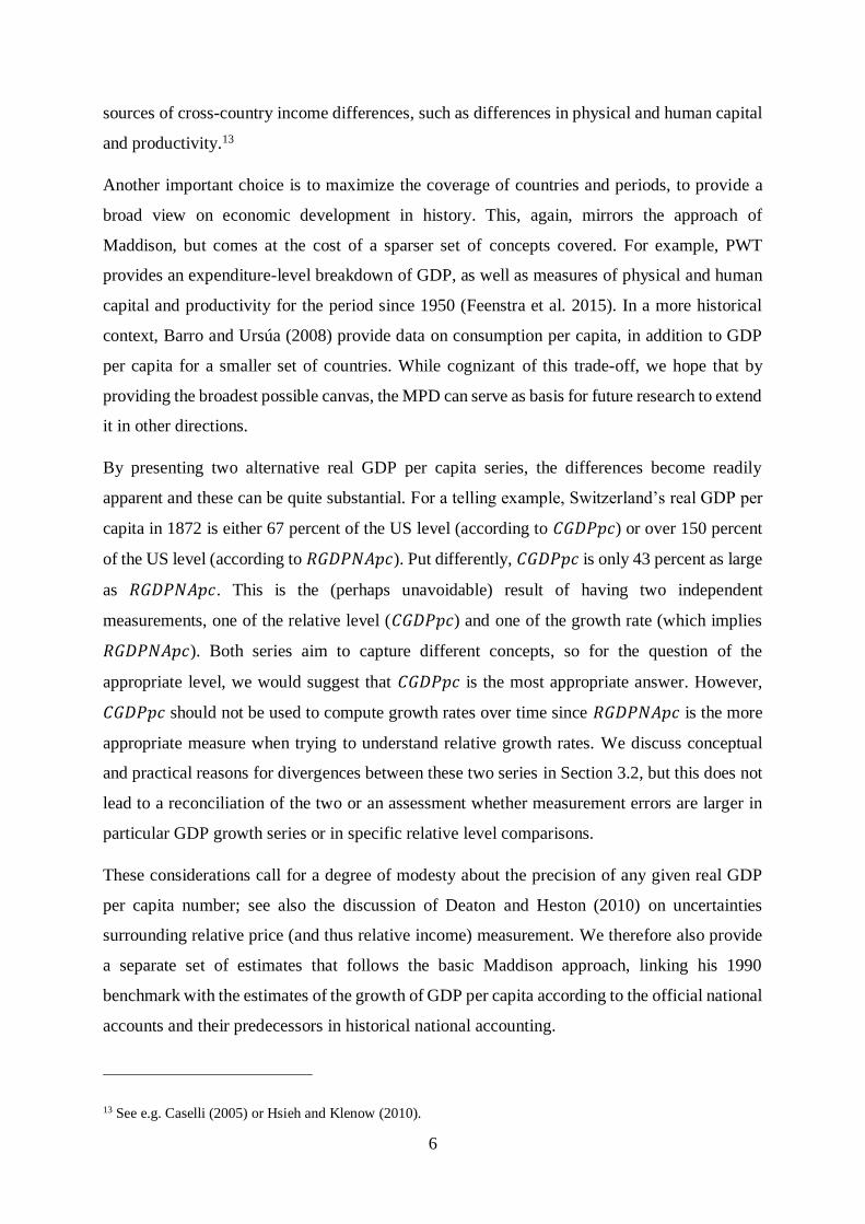
experiment ‘what would a person in country 𝑘 have to spend to purchase the same bundle of

products as a person in country 𝑗’ to arrive at the Laspeyres price index. The Paasche price

index is the outcome of the reverse though experiment, switching the bundle of products to that

of country 𝑘:

𝑃𝑗𝑘𝐿 =

𝐩𝑘′ 𝐪𝑗

𝐩𝑗′ 𝐪𝑗

, 𝑃𝑗𝑘𝑃 =

𝐩𝑘′ 𝐪𝑘

𝐩𝑗′ 𝐪𝑘

(1)

Neither of the these thought experiments is inherently preferable as there is no reason why either

bundle of products should hold a privileged position. Let, therefore, be the Fisher price index

be:

𝑃𝑗𝑘𝐹 = [

𝐩𝑘′ 𝐪𝑗

𝐩𝑗′ 𝐪𝑗

×𝐩𝑘

′ 𝐪𝑘

𝐩𝑗′ 𝐪𝑘

]

12

(2)

The Fisher index has numerous desirable properties, amongst which is that if two countries are

compared where the consumer’s utility function has a homothetic, quadratic functional form,

this index will exactly measure the ratio of utilities 𝑢𝑘 𝑢𝑗⁄ (Diewert, 1976).

In a setting of many countries, a drawback of the Fisher index is that price comparisons are not

transitive, i.e. the results depend on the base country, 𝑗 here. As a result, comparing prices

between 𝑗 and 𝑘 directly will yield a different outcome than via a third country ℎ: 𝑃𝑗𝑘𝐹 ≠

𝑃𝑗ℎ𝐹 × 𝑃ℎ𝑘

𝐹 . To overcome this lack of transitivity we compare prices between 𝑗 and 𝑘 as the

average across all possible indirect comparisons with country ℎ = 1, … , C to arrive at the so-

called GEKS price index:15

𝑃𝑗𝑘𝐺𝐸𝐾𝑆 = ∏(𝑃𝑗ℎ

𝐹 𝑃ℎ𝑘𝐹 )

1𝐶

𝐶

ℎ=1

(3)

The GEKS index is the most widely-used approach for comparing prices across countries, with

it being the main method in the International Comparison Program (ICP) at the World Bank

(2014) for computing global relative prices, or purchasing power parities (PPPs). An especially

desirable property of the GEKS index is that it does not suffer from substitution bias, i.e. the

GEKS index is based on the bundles of products 𝐪𝑗 of all countries rather than relying on some

average bundle. Maddison relied on Geary-Khamis (GK) PPPs for his international

15 After Gini, Elteto, Koves, and Szulc. A modern treatment and references are provided by Balk (2008).

9

comparisons and this index does suffer from substitutions bias. As illustrated by, for instance,

Deaton and Heston (2010), this substitution bias causes the GK PPPs to understate prices in

low-income countries, thereby overstating their real GDP per capita levels and thus understating

the extent of cross-country income differences.

Given a relative price index as defined in equation (3), we can estimate real GDP as:

𝑌𝑘 =𝑃𝑘𝑌𝑘

𝑃𝑗𝑘𝐺𝐸𝐾𝑆 (4)

which allows for comparing GDP or GDP per capita between countries 𝑗 and 𝑘, evaluated at

common prices.

3.2 Measuring real GDP per capita over time

The exposition so far has focused on price and comparisons across countries in a given year.

Yet the main goals of the MPD is to provide data over time. The simplest approach is the so-

called projection or extrapolation approach. In this approach real GDP per capita 𝑦𝑗𝑡 ≡ 𝑌𝑗𝑡/𝑁𝑗𝑡

(with 𝑁𝑗𝑡 as total population in country 𝑗 at time 𝑡) is estimated as:

𝑦𝑗𝑡−1 =𝑦𝑗𝑡

1 + 𝑔𝑗𝑡(5)

where 𝑔𝑗𝑡 is the growth of GDP per capita in constant national prices. An important

consequence of the approach in equation (5) is that the time series of growth in GDP per capita

is the same in national prices and in PPP-converted US dollars. Furthermore, the change in the

PPP implied by equation (5) is:

𝑃𝑗𝑘𝑡−1 = 𝑃𝑗𝑘𝑡𝐺𝐸𝐾𝑆 [

1 + 𝜋𝑗𝑡

1 + 𝜋𝑘𝑡] , (6)⁄

where 𝜋𝑗𝑡 = 𝑃𝑗𝑡 𝑃𝑗𝑡−1⁄ − 1, the rate of inflation of the GDP deflator.

While straightforward, this extrapolation approach has important conceptual and practical

drawbacks. The conceptual argument can be seen by considering the time-series counterpart to

equation 2, so where the change in the GDP deflator (in country 𝑗) is computed between two

time periods:

𝑃𝑗𝑡,𝑡−1𝐹 = [

𝐩𝑗𝑡′ 𝐪𝑗𝑡−1

𝐩𝑗𝑡−1′ 𝐪𝑗𝑡−1

×𝐩𝑡

′ 𝐪𝑡

𝐩𝑡−1′ 𝐪𝑡

]

12

(7)

10

Equation (7) makes clear that a price index for national inflation should be computed using the

bundle of products in the two periods for country 𝑗. Yet as equation (2) makes clear, a good

measure of relative prices should take into account the bundle of products in country 𝑗 and in

country 𝑘. By ignoring country 𝑘’s bundle in the computation of inflation in country 𝑗 (and vice

versa), the implicit relative price index in 𝑡 − 1 is no longer a good measure of relative prices

between countries 𝑗 and 𝑘. Especially if the periods under comparison are far apart, the

extrapolation approach of equations (5) and (6) is likely to be a poor approximation as the

bundle of products will have shifted substantially over time. This is one clear reason why

subsequent benchmark estimates of relative prices are (typically) not consistent with relative

inflation over the intervening period.

This conceptual problem is compounded by practical concerns. It has long been known that

equation (6) does a poor job in predicting changes in PPPs over time,16 but when the results of

the ICP PPP comparison for 2011 were released (World Bank, 2014), the differences with the

previous, ICP 2005, results were very large despite the serious global effort that went into both

sets of PPPs. As detailed in Deaton and Aten (2017) and Inklaar and Rao (2017), part of the

inconsistency was due to biases introduced in the measurement of ICP 2005 PPPs, but even

after correcting for theses biases the differences remained substantial. Furthermore, shifts in the

bundles of products cannot fully account for these differences, leaving ‘measurement error’ of

some sort as the main (though not very informative) explanation.

This view matches that of Maddison, who argued that the difference between observed PPPs in

successive ICP rounds and extrapolations based on relative inflation was more likely due to

errors in the ICP estimates than errors in the national growth measures. Reconciling different

benchmarks with the time series was in his eyes not the preferred method for long-term

comparisons. The basis for this argument was a study by Kravis and Lipsey (1991), who also

suggested that estimates of growth rates should be taken from the national accounts, whereas

estimates of real GDP per capita should be done by benchmark studies (Maddison, 1995, p.

164).

Yet the approach of Maddison has notable limitations. For one, if any given benchmark

comparison of prices and income is imperfect and perturbed by measurement error, relying fully

on a single benchmark comparison would mean that the same error would affect real GDP per

16 See Deaton and Heston (2010) for notable contributions to this discussion.

11

capita estimates through the decades or centuries. Second, while time series of GDP per capita

growth (i.e. 𝑔𝑗𝑡) may be considered reliable in modern times for many countries, periods like

the World Wars, or periods of economic instability such as in much of Latin America in the

1980s diminish the reliability of statistics. The situation is more problematic in countries with

poorly developed statistical systems, such as in many African countries, which can lead to

unreliable growth figures.17

This was illustrated by Prados de la Escosura (2000), who argued that PPPs based on

extrapolations as in equation (6) led to implausible results. His solution was to rely on the

regularity of the price-income relationship to estimate what relative prices (and, as result,

income levels) would have been if we had been able to observe them historically, see also

Klasing and Milionis (2014). Relying heavily on such estimates is less appealing to us, most

importantly because there are still important aspects of the price-income relationship that are

not fully understood. For example, Hassan (2016) argues that the price-income relationship is

non-linear and negative, rather than positive at the lower income levels and Zhang (2017)

argues that mismeasured differences in product quality bias the price-income relationship. That

said, comparing price levels rather than only income levels can serve as a useful check on

relative income estimates derived according to a given methodology, see e.g. Section 5.3 on the

Balassa-Samuelson effect in the MPD. For the MPD more broadly, we implement a multiple-

benchmark approach as detailed in the following section, which is, we argue, the best

approximation of relative levels of GDP per capita over time.

4. Implementation

4.1 The MPD measurement approach

In the new version of MPD, we implement a multiple benchmark approach based on post-1950

ICP benchmarks and historical benchmarks, i.e. independent real GDP per capita benchmarks

from historical studies.18 In keeping with Maddison (2007), we also include several estimates

stretching back even further, but which should be seen as estimates of income relative to a bare-

bones subsistence level rather than explicitly comparing GDP per capita between countries.

17 See e.g. Henderson, Storeygard and Weil (2012), Young (2012) and Jerven (2013). 18 Additionally, we use estimates of PPPs for 1960 from the study of Braithwaite (1968) and for a range of African

countries, we make an indirect income comparison based on real wages and urbanization data, see Appendix D.

There are a few countries that have never participated in an ICP comparison; most importantly Afghanistan and

North Korea. For those countries we use the (econometrically) estimated real GDP per capita level from World

Bank (2014). Cuba also requires also requires special consideration, see Appendix C for details.

12

Using the methodology developed for PWT (Feenstra et al. 2015), we subsequently tie the long-

term income series from the MPD (2013) to the relative income levels, thereby taking into

account relative price changes between the different benchmark years. This means the MPD

estimates for a particular country and year can be based on direct benchmark estimates,

interpolation between benchmarks or extrapolation from the first or last benchmark, following

equation (5). To enable users to distinguish between these different types of observations, we

introduce clear labeling in the MPD. Furthermore, given the differences in the types of

benchmark, we also label which type of benchmark is used to derive a certain estimate.

As discussed in the previous section, problematic estimates in benchmarks or time series can

have substantial consequences over longer periods of time. Given our stated goal of more

closely aligning to our understanding of living standards in history, this requires a degree of

judgement when implementing our multiple benchmark approach. In particular, it can be the

case that a) benchmark relative price estimates diverge substantially from what might be

expected from an estimated price-income relationship using all ICP benchmark PPPs

observations; b) income levels can drop below subsistence for sustained periods of time; or c)

income levels can remain high, in direct contradiction to the historical record. These

observations result in a list of judgmental adjustments, by, for instance, excluding specific ICP

PPP benchmarks or cutting short time series; see Appendix B for details. Category c

observations consist of oil-rich economies whose current high income levels can be understood

from large oil earnings, but where high income levels prior to major oil development or prior

to high oil prices would run counter to the historical understanding of those countries; see

Appendix E.

4.2 Historical benchmarks

Starting with the pioneering work by Rostas (1948) economists and economic historians have

produced benchmarks of the relative income or output levels of economies (or parts of them,

such as the manufacturing sector), including the construction of relevant PPPs to make real

comparisons. Various methods have been used, making use of the output/value added approach,

the income approach, and the expenditure approach. Usually, these studies compare the leading

economy (US, UK) with one or more other economies (Germany, France, or Japan) (Broadberry

1998; Fukao et al. 2007). We collected the available historical economy-wide benchmarks and

used them to re-anchor the historical time series following the PWT methodology described in

the previous section; see Appendix A for a an overview of historical benchmarks and studies

that we rely upon. As there are currently close to no historical benchmarks available for African

13

countries, we have created additional benchmarks for the year 1950 for African countries,

making use of an indirect approach using wages and urbanization rates (see Appendix D).

In addition to the historical benchmarks, we follow Maddison’s approach to also include

estimates of comparative income levels for some of the very earliest (pre-1500) years. As data

for these early economies is increasingly scattered and it is often impossible to estimate

historical trends, economic historians (Pamuk and Schatzmiller 2014, Scheidel and Friesen

2009; Milanovic 2006) used a variety of information to assess to what extent those societies

had income levels notably above the level of subsistence, i.e. was there sufficient surplus

beyond subsistence for development. In particular estimates of real wages were used for this

purpose. We update that approach by updating the subsistence line to $700 (2011 US dollars),

in line with the $1.90/day global poverty line used by the World Bank (Ferreira et al. 2015).19

4.3 Updating historical series

This new version of the MPD includes all new historical estimates of GDP per capita over time

that have become available since the previous update (Bolt and Van Zanden, 2014). Such

updates are necessary as new work on historical national accounts appears regularly and is

important as it provides us new insights in long term global development. This also allows more

recent years, up to 2016, to be covered in the database.

For the recent period the most important new work is Harry Wu’s reconstruction of Chinese

economic growth since 1950, a project inspired by Maddison which produces state of the art

estimates of GDP and its components for this important economy (Wu 2014). Given the large

role China plays in any reconstruction of global inequality, this is a major addition to the dataset.

Moreover, as we will see below, the new results show that the revised estimates of annual

growth are in general lower than the official estimates. Lower growth between 1952 and the

present however substantially increases the estimates of the absolute level of Chinese GDP in

the 1950s (given the fact that the absolute level if determined by a benchmark in 1990 or 2011).

This helps to solve a problem that was encountered when switching from the 1990 to the 2011

benchmark, namely that when using the official growth estimates the estimated levels of GDP

per capita in the early 1950s are substantially below subsistence back until 1890, and therefore

too low. This possible inconsistency in the dataset is therefore ‘solved’ by making use of the

19 An income of $1.90 per person per day implies an annual per capita income of $693.50. To emphasize that these

income estimates are a multiple of subsistence, rather than in observed monetary units, we round the subsistence

level up by 1% to $700.

14

new, much improved set of estimates by Wu (2014). Most of the other additions to the

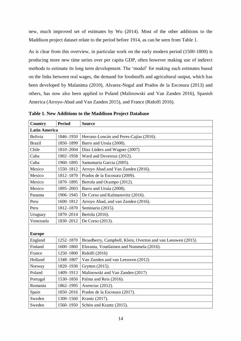
Maddison project dataset relate to the period before 1914, as can be seen from Table 1.

As is clear from this overview, in particular work on the early modern period (1500-1800) is

producing more new time series over per capita GDP, often however making use of indirect

methods to estimate its long term development. The ‘model’ for making such estimates based

on the links between real wages, the demand for foodstuffs and agricultural output, which has

been developed by Malanima (2010), Alvarez-Nogal and Prados de la Escosura (2013) and

others, has now also been applied to Poland (Malinowski and Van Zanden 2016), Spanish

America (Arroyo-Abad and Van Zanden 2015), and France (Ridolfi 2016).

Table 1. New Additions to the Maddison Project Database

Country Period Source

Latin America

Bolivia 1846–1950 Herranz-Loncán and Peres-Cajías (2016).

Brazil 1850–1899 Barro and Ursúa (2008).

Chile 1810–2004 Díaz Lüders and Wagner (2007)

Cuba 1902–1958 Ward and Devereux (2012).

Cuba 1960–1895 Santamaria Garcia (2005).

Mexico 1550–1812 Arroyo Abad and Van Zanden (2016).

Mexico 1812–1870 Prados de la Escosura (2009).

Mexico 1870–1895 Bertola and Ocampo (2012).

Mexico 1895–2003 Barro and Ursúa (2008).

Panama 1906–1945 De Corso and Kalmanovitz (2016).

Peru 1600–1812 Arroyo Abad, and van Zanden (2016).

Peru 1812–1870 Seminario (2015).

Uruguay 1870–2014 Bertola (2016).

Venezuela 1830–2012 De Corso (2013).

Europe

England 1252–1870 Broadberry, Campbell, Klein, Overton and van Leeuwen (2015)

Finland 1600–1860 Eloranta, Voutilainen and Nummela (2016).

France 1250–1800 Ridolfi (2016)

Holland 1348–1807 Van Zanden and van Leeuwen (2012)

Norway 1820–1930 Grytten (2015).

Poland 1409–1913 Malinowski and Van Zanden (2017)

Portugal 1530–1850 Palma and Reis (2016).

Romania 1862–1995 Axenciuc (2012).

Spain 1850–2016 Prados de la Escosura (2017).

Sweden 1300–1560 Krantz (2017).

Sweden 1560–1950 Schön and Krantz (2015).

15

UK 1700–1870 Broadberry, Campbell, Klein, Overton and van Leeuwen (2015)

Asia

China 1952–2008 Wu (2014).

China 1661–1933 Xu, Shi, van Leeuwen, Ni, Zhang, and Ma (2016).

India 1600–1870 Broadberry, Custodis and Gupta (2015).

Turkey Pamuk (2009).

Singapore 1900–1959 Barro and Ursúa (2008).

Middle East

Syria

1820, 1870,

1913, 1950 Pamuk (2006).

Lebanon

Jordan

Egypt

Saudi Arabia

Iraq

Iran

Africa

Cape Colony/

South Africa 1700–1900 Fourie and Van Zanden (2013).

Finally, we have extended the national income estimates for all countries in the database to

include the most recent years, up until 2016, using various sources. The Total Economy

Database (TED) was used to extend the GDP per capita up to 2016 for all countries included in

TED, similar to what has been done for the latest update of the Maddison Project database (Bolt

and van Zanden, 2014). For those countries not present in TED, we have used national accounts

estimates from the UN to extend the GDP per capita series. We have also used the TED and the

US Census Bureau’s International Data Base to extend the population estimates up until 2016.20

Recently, the TED revised their China estimates from 1950 onwards based on Wu (2014). As

discussed above, we also included Wu’s (2014) new estimates in this update. Lastly, we have

extended the series for the former Czechoslovakia, the former Soviet Union and former

Yugoslavia, based on GDP and population data for their successor states.

20 As Palestine is not included in these sources, we used data from the World Development Indicators.

16

5. Applications

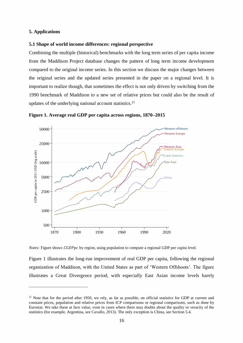
5.1 Shape of world income differences: regional perspective

Combining the multiple (historical) benchmarks with the long term series of per capita income

from the Maddison Project database changes the pattern of long term income development

compared to the original income series. In this section we discuss the major changes between

the original series and the updated series presented in the paper on a regional level. It is

important to realize though, that sometimes the effect is not only driven by switching from the

1990 benchmark of Maddison to a new set of relative prices but could also be the result of

updates of the underlying national account statistics.21

Figure 1. Average real GDP per capita across regions, 1870–2015

Notes: Figure shows 𝐶𝐺𝐷𝑃𝑝𝑐 by region, using population to compute a regional GDP per capita level.

Figure 1 illustrates the long-run improvement of real GDP per capita, following the regional

organization of Maddison, with the United States as part of ‘Western Offshoots’. The figure

illustrates a Great Divergence period, with especially East Asian income levels barely

21 Note that for the period after 1950, we rely, as far as possible, on official statistics for GDP at current and

constant prices, population and relative prices from ICP comparisons or regional comparisons, such as done by

Eurostat. We take these at face value, even in cases where there may doubts about the quality or veracity of the

statistics (for example, Argentina, see Cavallo, 2013). The only exception is China, see Section 5.4.

Western offshoots

Western Europe

East Asia

Eastern Europe

Latin America

Western Asia

Africa

500

1000

2500

5000

10000

25000

50000

GD

P p

er c

apit

a in

20

11

US

D (

log

sca

le)

1870 1900 1930 1960 1990 2020

17

improving relative to the richest regions until 1950. The figure also illustrates that patterns of

rapid improvement alternate with period of relative decline, as in Western Asia in the 1980s,

Eastern Europe in the 1990s and Africa in both the 1980s and 1990s.

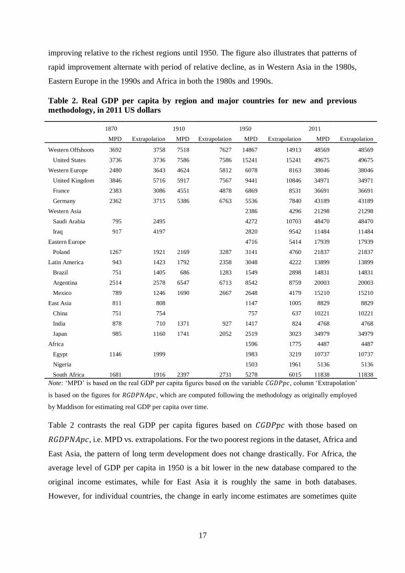
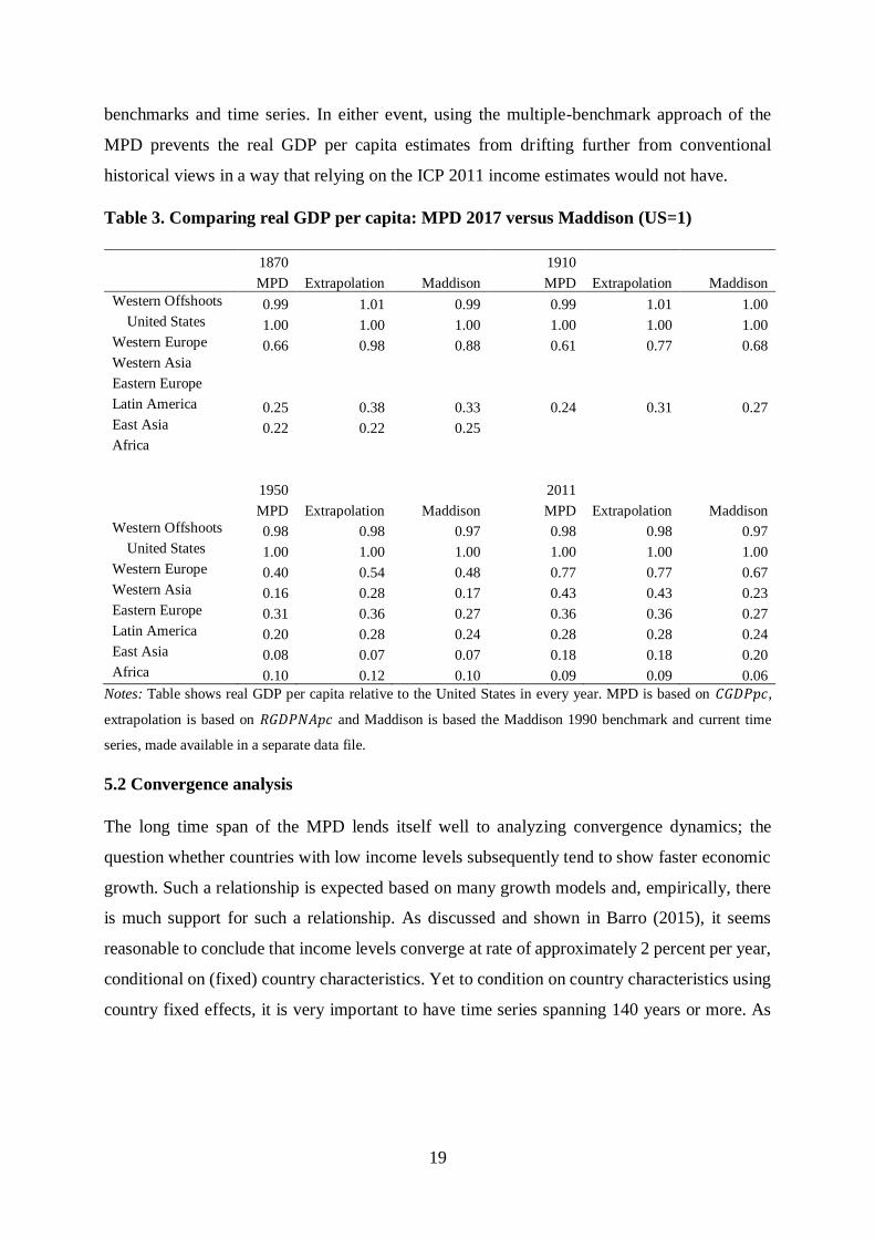
Table 2. Real GDP per capita by region and major countries for new and previous

methodology, in 2011 US dollars

1870 1910 1950 2011

MPD Extrapolation MPD Extrapolation MPD Extrapolation MPD Extrapolation

Western Offshoots 3692 3758 7518 7627 14867 14913 48569 48569

United States 3736 3736 7586 7586 15241 15241 49675 49675

Western Europe 2480 3643 4624 5812 6078 8163 38046 38046

United Kingdom 3846 5716 5917 7567 9441 10846 34971 34971

France 2383 3086 4551 4878 6869 8531 36691 36691

Germany 2362 3715 5386 6763 5536 7840 43189 43189

Western Asia 2386 4296 21298 21298

Saudi Arabia 795 2495 4272 10703 48470 48470

Iraq 917 4197 2820 9542 11484 11484

Eastern Europe 4716 5414 17939 17939

Poland 1267 1921 2169 3287 3141 4760 21837 21837

Latin America 943 1423 1792 2358 3048 4222 13899 13899

Brazil 751 1405 686 1283 1549 2898 14831 14831

Argentina 2514 2578 6547 6713 8542 8759 20003 20003

Mexico 789 1246 1690 2667 2648 4179 15210 15210

East Asia 811 808 1147 1005 8829 8829

China 751 754 757 637 10221 10221

India 878 710 1371 927 1417 824 4768 4768

Japan 985 1160 1741 2052 2519 3023 34979 34979

Africa 1596 1775 4487 4487

Egypt 1146 1999 1983 3219 10737 10737

Nigeria 1503 1961 5136 5136

South Africa 1681 1916 2397 2731 5278 6015 11838 11838

Note: ‘MPD’ is based on the real GDP per capita figures based on the variable 𝐶𝐺𝐷𝑃𝑝𝑐, column ‘Extrapolation’

is based on the figures for 𝑅𝐺𝐷𝑃𝑁𝐴𝑝𝑐, which are computed following the methodology as originally employed

by Maddison for estimating real GDP per capita over time.

Table 2 contrasts the real GDP per capita figures based on 𝐶𝐺𝐷𝑃𝑝𝑐 with those based on

𝑅𝐺𝐷𝑃𝑁𝐴𝑝𝑐, i.e. MPD vs. extrapolations. For the two poorest regions in the dataset, Africa and

East Asia, the pattern of long term development does not change drastically. For Africa, the

average level of GDP per capita in 1950 is a bit lower in the new database compared to the

original income estimates, while for East Asia it is roughly the same in both databases.

However, for individual countries, the change in early income estimates are sometimes quite

18

substantial. For Africa as a whole, the main difference between the two series is the more severe

drop in incomes during the so called ‘lost decades’ of the 1980s and 1990s.

Using multiple benchmarks result in substantially lower relative income levels for Latin

America, most notably for the mid-20th century, where relative average income drops to 23

percent of the US level, down from 32 percent based on the extrapolation method. The new

methodology also clearly affects the pattern of average income development in Western Asia

and Eastern Europe, again particularly after 1910. Incomes for Eastern Europe are now higher

until the mid-1980s, with income levels on par with Western Europe around 1960 (which is

also partly due to lower incomes in Western Europe, see below). In Western Asia the effects of

using more relative income estimates translates mainly in much lower incomes up until the mid-

1990s after which increasing oil prices result in enormous increases in average incomes.22

Western Europe is the region for which most relative income estimates are available.

Incorporating this the new information results in substantially lower income estimates for the

region compared to US incomes. The extrapolated method of Maddison indicates that the US

and Western Europe were about on par around 1870, after which the US forged ahead of Europe

until the end of WW2. Thereafter Europe’s economies expanded rapidly, until average incomes

reached around 73 percent of the US level during the 1970s. After this, relative incomes

remained fairly stable until the present. As a result of integrating the historical benchmarks,

Europe seems behind the US already substantially in the 1870. Growth rates of both the US and

Europe’s economies are then very similar until roughly the Great Depression. Then incomes

initially diverge somewhat until the end of World War 2, but Europe’s incomes grow faster

after 1950s to roughly 77 percent of the level of US incomes in 2011.

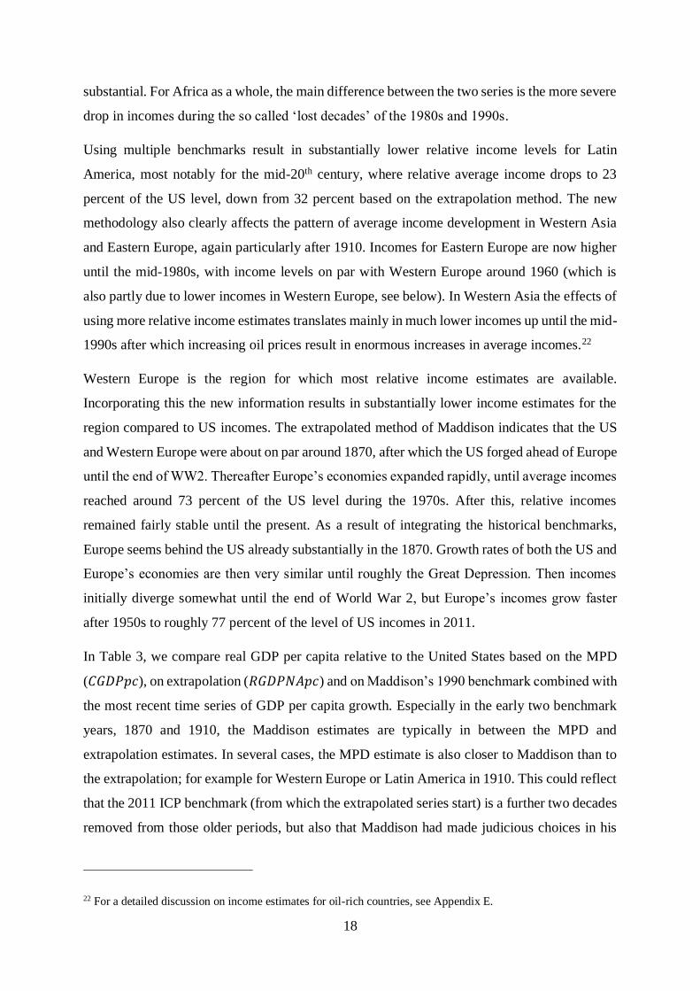
In Table 3, we compare real GDP per capita relative to the United States based on the MPD

(𝐶𝐺𝐷𝑃𝑝𝑐), on extrapolation (𝑅𝐺𝐷𝑃𝑁𝐴𝑝𝑐) and on Maddison’s 1990 benchmark combined with

the most recent time series of GDP per capita growth. Especially in the early two benchmark

years, 1870 and 1910, the Maddison estimates are typically in between the MPD and

extrapolation estimates. In several cases, the MPD estimate is also closer to Maddison than to

the extrapolation; for example for Western Europe or Latin America in 1910. This could reflect

that the 2011 ICP benchmark (from which the extrapolated series start) is a further two decades

removed from those older periods, but also that Maddison had made judicious choices in his

22 For a detailed discussion on income estimates for oil-rich countries, see Appendix E.

19

benchmarks and time series. In either event, using the multiple-benchmark approach of the

MPD prevents the real GDP per capita estimates from drifting further from conventional

historical views in a way that relying on the ICP 2011 income estimates would not have.

Table 3. Comparing real GDP per capita: MPD 2017 versus Maddison (US=1)

1870 1910

MPD Extrapolation Maddison MPD Extrapolation Maddison

Western Offshoots 0.99 1.01 0.99 0.99 1.01 1.00

United States 1.00 1.00 1.00 1.00 1.00 1.00

Western Europe 0.66 0.98 0.88 0.61 0.77 0.68

Western Asia

Eastern Europe

Latin America 0.25 0.38 0.33 0.24 0.31 0.27

East Asia 0.22 0.22 0.25 Africa

1950 2011

MPD Extrapolation Maddison MPD Extrapolation Maddison

Western Offshoots 0.98 0.98 0.97 0.98 0.98 0.97

United States 1.00 1.00 1.00 1.00 1.00 1.00

Western Europe 0.40 0.54 0.48 0.77 0.77 0.67

Western Asia 0.16 0.28 0.17 0.43 0.43 0.23

Eastern Europe 0.31 0.36 0.27 0.36 0.36 0.27

Latin America 0.20 0.28 0.24 0.28 0.28 0.24

East Asia 0.08 0.07 0.07 0.18 0.18 0.20

Africa 0.10 0.12 0.10 0.09 0.09 0.06

Notes: Table shows real GDP per capita relative to the United States in every year. MPD is based on 𝐶𝐺𝐷𝑃𝑝𝑐,

extrapolation is based on 𝑅𝐺𝐷𝑃𝑁𝐴𝑝𝑐 and Maddison is based the Maddison 1990 benchmark and current time

series, made available in a separate data file.

5.2 Convergence analysis

The long time span of the MPD lends itself well to analyzing convergence dynamics; the

question whether countries with low income levels subsequently tend to show faster economic

growth. Such a relationship is expected based on many growth models and, empirically, there

is much support for such a relationship. As discussed and shown in Barro (2015), it seems

reasonable to conclude that income levels converge at rate of approximately 2 percent per year,

conditional on (fixed) country characteristics. Yet to condition on country characteristics using

country fixed effects, it is very important to have time series spanning 140 years or more. As

20

Barro (2015) argues, Hurwicz-Nickell bias23 is sizeable in datasets of only 50 years, with a

downward bias to the convergence coefficient of 0.056 and econometric approaches to

correcting for this bias are found wanting. Once the length of the time series exceeds 140 years,

the bias drops below 0.018, down to 0.010 for 200 years.

The results of Barro (2015) can be usefully re-examined using our new version of the MPD.

Most importantly, the new version of the database allows us to combine the preferred measure

of growth in real GDP per capita, based on 𝑅𝐺𝐷𝑃𝑁𝐴𝑝𝑐, with the preferred measure of the level

of real GDP per capita across countries, 𝐶𝐺𝐷𝑃𝑝𝑐. We would not expect different outcomes

regarding the rate of convergence, but we rather view the results in terms of measurement error

in the independent variable: an improved measure of the level of real GDP per capita (𝐶𝐺𝐷𝑃𝑝𝑐

rather than 𝑅𝐺𝐷𝑃𝑁𝐴𝑝𝑐) should lead to a more accurate estimate of the rate of convergence.

This is helpful in itself, but also for tests of Schumpeterian growth theory, where typically the

interaction between a country’s distance to the (productivity) frontier and a variable of interest

plays a central role; see Aghion, Akcigit and Howitt (2014) for a survey and Madsen (2014) for

an example in a long-term perspective. More reliable measures of the relative position of

countries – i.e. smaller measurement error – will make it easier to establish the information

content of such models.

Another reason to revisit the analysis of Barro (2015) is that we have a more extensive dataset.

Barro (2015) used the dataset of Barro and Ursúa (2008), which covers 28 countries with annual

data since 1896. As discussed in Section 4.3, the new MPD, incorporates data of Barro and

Ursúa (2008) for some countries as well as new source material developed by economic

historians for numerous other countries. This allows us to extend the start of the analysis period

to 1820 and broaden the range of countries to 38, including data for countries such as Indonesia,

India and South Africa – each important for establishing the breadth of a finding of cross-

country income convergence.

We follow Barro (2015) and estimate the following model:

��𝑖,𝑡5 = 𝛼𝑖 + 𝛼𝑡 + 𝛽 log 𝑌𝑖,𝑡−5 + 𝛾𝑘𝑋𝑘,𝑖,𝑡 + 𝜖𝑖 𝑡 (7)

23 This bias stems from including lagged dependent variable alongside fixed effects and forces down the coefficient

on the lagged dependent variable. Since countries with lower income levels are expected to grow faster, the

estimated coefficient is more negative than it should be.

21

The dependent variable is average annual growth of real GDP per capita over a five-year period,

��𝑖,𝑡5 = (

𝑅𝐺𝐷𝑃𝑁𝐴𝑝𝑐𝑖,𝑡

𝑅𝐺𝐷𝑃𝑁𝐴𝑝𝑐𝑖,𝑡−5)

1

5− 1, the equation includes country and year fixed effects and in our

preferred estimation 𝑌𝑖,𝑡−5 = 𝐶𝐺𝐷𝑃𝑝𝑐𝑖,𝑡−5 though we also estimate equation (7) with 𝑌𝑖,𝑡−5 =

𝑅𝐺𝐷𝑃𝑁𝐴𝑝𝑐𝑖,𝑡−5 to compare to earlier studies. Additional control variables 𝑋𝑘 are also

considered, though the scope is limited by the long time span required. The equation is

estimated using data for non-overlapping periods, so 1820–1825, 1825–1830, …, 2010–2015.

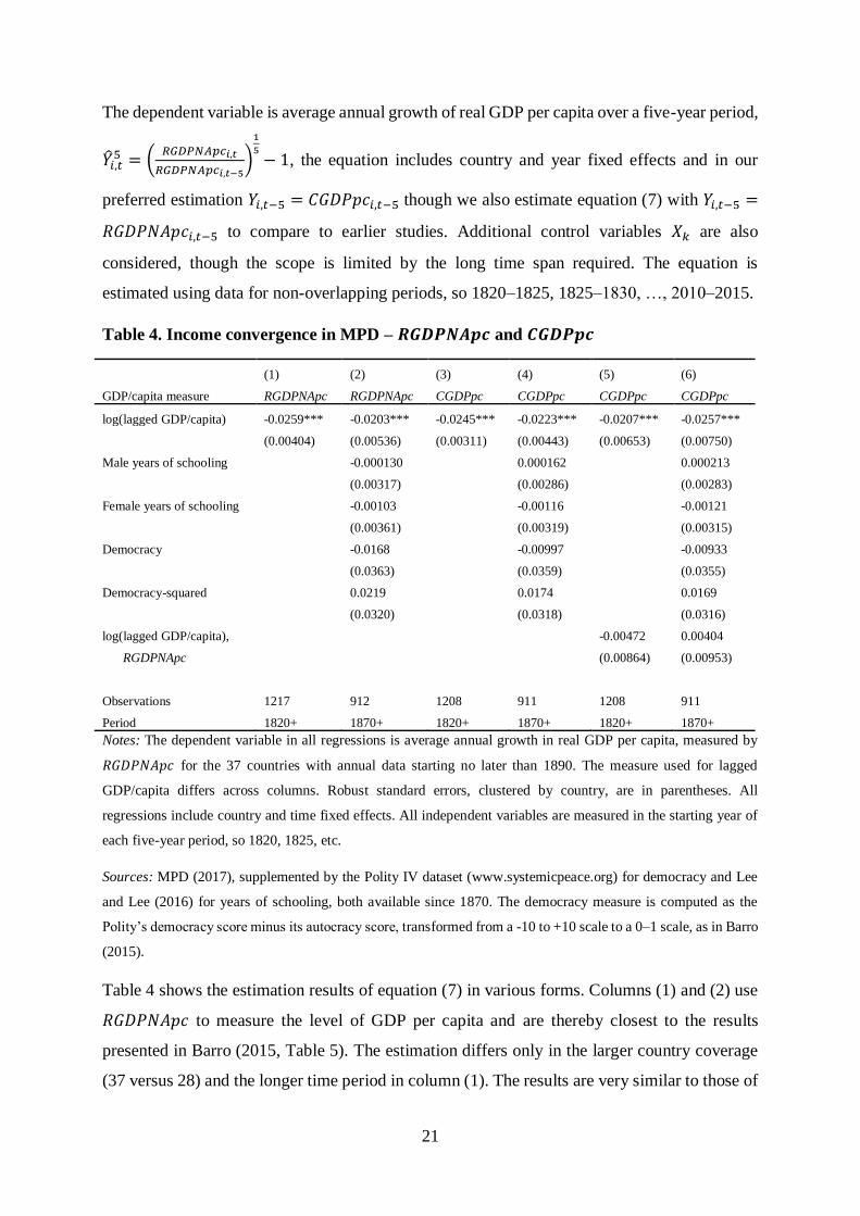
Table 4. Income convergence in MPD – 𝑹𝑮𝑫𝑷𝑵𝑨𝒑𝒄 and 𝑪𝑮𝑫𝑷𝒑𝒄

(1) (2) (3) (4) (5) (6)

GDP/capita measure RGDPNApc RGDPNApc CGDPpc CGDPpc CGDPpc CGDPpc

log(lagged GDP/capita) -0.0259*** -0.0203*** -0.0245*** -0.0223*** -0.0207*** -0.0257***

(0.00404) (0.00536) (0.00311) (0.00443) (0.00653) (0.00750)

Male years of schooling -0.000130 0.000162 0.000213

(0.00317) (0.00286) (0.00283)

Female years of schooling -0.00103 -0.00116 -0.00121

(0.00361) (0.00319) (0.00315)

Democracy -0.0168 -0.00997 -0.00933

(0.0363) (0.0359) (0.0355)

Democracy-squared 0.0219 0.0174 0.0169

(0.0320) (0.0318) (0.0316)

log(lagged GDP/capita),

RGDPNApc

-0.00472 0.00404

(0.00864) (0.00953)

Observations 1217 912 1208 911 1208 911

Period 1820+ 1870+ 1820+ 1870+ 1820+ 1870+

Notes: The dependent variable in all regressions is average annual growth in real GDP per capita, measured by

𝑅𝐺𝐷𝑃𝑁𝐴𝑝𝑐 for the 37 countries with annual data starting no later than 1890. The measure used for lagged

GDP/capita differs across columns. Robust standard errors, clustered by country, are in parentheses. All

regressions include country and time fixed effects. All independent variables are measured in the starting year of

each five-year period, so 1820, 1825, etc.

Sources: MPD (2017), supplemented by the Polity IV dataset (www.systemicpeace.org) for democracy and Lee

and Lee (2016) for years of schooling, both available since 1870. The democracy measure is computed as the

Polity’s democracy score minus its autocracy score, transformed from a -10 to +10 scale to a 0–1 scale, as in Barro

(2015).

Table 4 shows the estimation results of equation (7) in various forms. Columns (1) and (2) use

𝑅𝐺𝐷𝑃𝑁𝐴𝑝𝑐 to measure the level of GDP per capita and are thereby closest to the results

presented in Barro (2015, Table 5). The estimation differs only in the larger country coverage

(37 versus 28) and the longer time period in column (1). The results are very similar to those of

22

Barro (2015), with an estimated convergence rate of close to 2 percent per year. The addition

of control variables, in the form of measures of schooling and democracy, does not substantially

affect the results, though the estimated convergence rate is somewhat reduced.

Columns (3) and (4) show our preferred approach and replace 𝑅𝐺𝐷𝑃𝑁𝐴𝑝𝑐 by 𝐶𝐺𝐷𝑃𝑝𝑐 to

measure the level of GDP per capita, while the growth rate is still computed using 𝑅𝐺𝐷𝑃𝑁𝐴𝑝𝑐.

The estimated convergence rate is quite similar to those in columns (1) and (2), but a notable

result is that the standard error on the coefficient of log(lagged GDP per capita) is 15–20 percent

lower. In columns (5) and (6), we include both measures of the level of GDP per capita at the

same time. The two measures are highly correlated (0.97) but in those columns, too, we find

that it is log(𝐶𝐺𝐷𝑃𝑝𝑐) which remains significant. We take this as further evidence that our

newly introduced measure 𝐶𝐺𝐷𝑃𝑝𝑐 is a more reliable measure of cross-country income

differences, conditional on the belief that there is a process of conditional income convergence.

5.3 The Balassa-Samuelson effect

The Balassa-Samuelson (or Penn) effect states that the price level in a country tends to increase

as it becomes richer and this effect has been a robust feature in the ICP PPP data since that

program’s inception.24 Prados de la Escosura (2000) used the Balassa-Samuelson (BS) effect

to propose alternative historical income estimates, after showing that the extrapolated data of

Maddison implied price levels that differed substantially from what the BS-effect would

predict. In this application, we estimate the BS-effect in three settings, namely based on the ICP

PPP data from 1970 onwards (as in Feenstra et al., 2015), based on the historical income

benchmarks (𝐶𝐺𝐷𝑃𝑝𝑐) and based on the extrapolated income series (𝑅𝐺𝐷𝑃𝑁𝐴𝑝𝑐). In order to

estimate these last two BS-effects, we need information about relative price levels alongside

the relative income estimates. These are either drawn directly from the benchmark comparisons

or computed based on data on nominal GDP per capita, i.e. GDP converted to US dollars using

the nominal exchange rate rather than a PPP.25 We then estimate the following relationship:

ln (𝑃𝑃𝑃𝑖,𝑡

𝑋𝑅𝑖,𝑡) = 𝛽0 + 𝛽1 ln (

𝑁𝐺𝐷𝑃𝑝𝑐𝑖,𝑡

𝑁𝐺𝐷𝑃𝑝𝑐𝑈𝑆𝐴,𝑡) + 𝜖𝑖 𝑡 (8)

24 See e.g. Barro (1991), Samuelson (1994), Rogoff (1996) and Feenstra et al. (2015). 25 We thank Giovanni Federico for providing his most recent work in compiling nominal GDP data.

23

Where 𝑋𝑅𝑖𝑡 is the nominal exchange rate and 𝑁𝐺𝐷𝑃𝑖𝑡 is nominal GDP, for country 𝑖 at time

𝑡.26 Over the full range of relative income levels, Hassan (2016) has shown that a linear

relationship is not appropriate and he argues that a quadratic relationship is not only empirically

superior but also expected based on a model of structural transformation. However, over the

range of relative income levels spanned by the historical income benchmark data, a linear

approximation leads to very similar results as a quadratic model in the case of the ICP PPP data

and if a quadratic model is used to model the historical data this results in a concave, rather than

Hasson’s (2016) convex quadratic relationship. For these reasons, we rely on the simple linear

model of equation (8).

Figure 2 shows the results of the analysis. Of the 68 historical benchmarks (i.e. pre-1950

benchmarks) included in the MPD, we have nominal GDP per capita data for 57 so the two

panels of the figure show 57 country observations of relative prices and (nominal) relative

income levels. In the left-hand panel, we show price-income relationship using the relative

prices implied by the historical benchmarks (i.e. by 𝐶𝐺𝐷𝑃𝑝𝑐) while the right-hand panel shows

the relationship based on extrapolated real GDP series (i.e. by 𝑅𝐺𝐷𝑃𝑁𝐴𝑝𝑐). Also shown in

both panels is the price-income relationship based on ICP PPP data, estimated over the same

income interval as the 57 observations.

Figure 2 shows that relative prices based on extrapolation (𝑅𝐺𝐷𝑃𝑁𝐴𝑝𝑐) tend to be

systematically lower than based on historical benchmarks (𝐶𝐺𝐷𝑃𝑝𝑐), echoing a similar

observation for a more limited sample in Prados de la Escosura (2000). This is most striking in

the case of the three historical benchmarks for Switzerland (1872, 1910 and 1929). The

country’s (nominal) relative income level was between 49 and 67 percent of the US level, while

the extrapolation-based relative prices were between 28 and 31 percent. In ICP 2011, such low

relative prices were seen in countries such as Bangladesh or Yemen, with nominal income

levels of less than 5 percent of the US level. In comparison, the relative prices for Switzerland

based on the historical benchmarks were between 71 and 98 percent of the US. While

Switzerland is an extreme example, there are other countries, such as the UK, Netherlands and

26 Equation 8 can also be estimated using real GDP per capita, but the advantage of this specification is that the

choice of (implied) PPP only affects the dependent variable and not the independent variable. We also express the

relationship in terms of income levels relative to the United States, in parallel with expression of the price level

relative to the United States, to enable estimation of 𝛽1 based on data for multiple years.

24

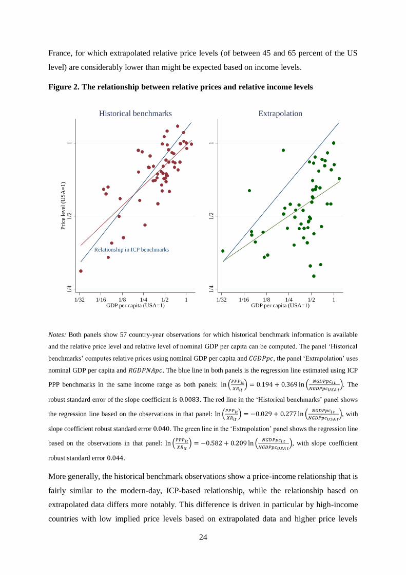
France, for which extrapolated relative price levels (of between 45 and 65 percent of the US

level) are considerably lower than might be expected based on income levels.

Figure 2. The relationship between relative prices and relative income levels

Notes: Both panels show 57 country-year observations for which historical benchmark information is available

and the relative price level and relative level of nominal GDP per capita can be computed. The panel ‘Historical

benchmarks’ computes relative prices using nominal GDP per capita and 𝐶𝐺𝐷𝑃𝑝𝑐, the panel ‘Extrapolation’ uses

nominal GDP per capita and 𝑅𝐺𝐷𝑃𝑁𝐴𝑝𝑐. The blue line in both panels is the regression line estimated using ICP

PPP benchmarks in the same income range as both panels: ln (𝑃𝑃𝑃𝑖𝑡

𝑋𝑅𝑖𝑡) = 0.194 + 0.369 ln (

𝑁𝐺𝐷𝑃𝑝𝑐𝑖 𝑡

𝑁𝐺𝐷𝑃𝑝𝑐𝑈𝑆𝐴 𝑡). The

robust standard error of the slope coefficient is 0.0083. The red line in the ‘Historical benchmarks’ panel shows

the regression line based on the observations in that panel: ln (𝑃𝑃𝑃𝑖𝑡

𝑋𝑅𝑖𝑡) = −0.029 + 0.277 ln (


𝑁𝐺𝐷𝑃𝑝𝑐𝑈𝑆𝐴 𝑡), with

slope coefficient robust standard error 0.040. The green line in the ‘Extrapolation’ panel shows the regression line

based on the observations in that panel: ln (𝑃𝑃𝑃𝑖𝑡

𝑋𝑅𝑖𝑡) = −0.582 + 0.209 ln (


𝑁𝐺𝐷𝑃𝑝𝑐𝑈𝑆𝐴 𝑡), with slope coefficient

robust standard error 0.044.

More generally, the historical benchmark observations show a price-income relationship that is

fairly similar to the modern-day, ICP-based relationship, while the relationship based on

extrapolated data differs more notably. This difference is driven in particular by high-income

countries with low implied price levels based on extrapolated data and higher price levels

Relationship in ICP benchmarks

1/4

1/2

1P

rice

lev

el (

US

A=

1)

1/32 1/16 1/8 1/4 1/2 1GDP per capita (USA=1)

Historical benchmarks

1/4

1/2

1

1/32 1/16 1/8 1/4 1/2 1GDP per capita (USA=1)

Extrapolation

25

implied by the historical benchmarks. Note that these regression lines are meant to be

illustrative rather than an attempt to provide a comprehensive statistical comparison. A

comprehensive analysis would be challenging given the limited number of historical benchmark

observations, but such a more complete model would, for example, also account for the degree

of openness and differences in the monetary regime (Prados de la Escosura, 2000). The figure

does illustrate that reliance on extrapolated time series risks ‘unmooring’ the resulting real GDP

series from underlying economic relationships.

5.4. Poverty and subsistence

An important implication of using different relative price levels is that the poverty level may

change. With the 1990 price levels, the subsistence level income was estimated at between 350

and 400 international dollars per year (Maddison, 2007). The poverty line was equal to around

$1 per day, and was based on the first international poverty line which was set at $1.01 per day

using 1985 PPP’s, which was later updated to $ 1.08 per day using the 1993 PPP’s (Ravallion,

Datt and van de Walle, 1991; Chen and Ravallion, 2001). This made the interpretation of

historical income series very intuitive. By using other relative prices, this subsistence level of

income changes. The price level (in US dollars, the standard used in these calculations)

increased by 59% between 1990 and 2011, bringing the poverty line to 636 dollars of 2011. In

a more extensive re-benchmarking, the World Bank raised the absolute poverty line to 1.90 US

dollars a day, expressed in 2011 prices.

The effects of rebasing the original Maddison estimates has the most notable effects for

countries who experienced substantial price changes relative to the US between the benchmarks

years. China is an interesting case in this perspective. When the 2005 PPPs were released, the

prices for China had increased so much relative to the US, that total GDP per capita came out

around 40% lower than China’s relative income based on earlier price estimates (Deaton and

Heston, 2010: 3; Feenstra et. al, 2015). This led to implausibly low historical income estimates

for China, given that the original estimates were already very close to subsistence around 1950

(Maddison, 2007a). In the years after the release of the 2005 PPP’s consensus arose about the

2005 shortcomings, most of which were corrected for in the 2011 ICP round (see e.g. Deaton

and Aten, 2017). Still, relative prices for China relative to the US were substantially higher in

2011 compared to 1990 which lowers China’s PPP adjusted income per capita in 2011 by 23%.

26

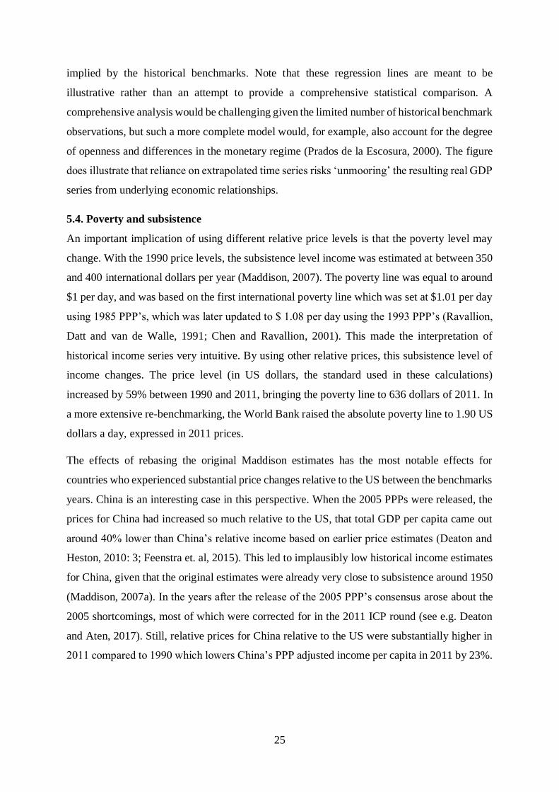
Figure 3. Historical income series China in 2011 US dollars

The case of China is interesting more broadly, as illustrated in Figure 3. The green line shows

GDP per capita as implied by the official National Accounts GDP series from 1952 onwards,

extended backwards with historical growth estimates, tied to the ICP 2011 benchmark. Those

official growth rates imply that before 1979, Chinese GDP per capita was below the $700

subsistence line. This stretches credibility past the breaking point, as this would imply utter

destitution for considerably more than a century. By contrast, the country with the lowest GDP

per capita level in the ICP 2011 comparison was the Democratic Republic of Congo, at $680.

This implication of the official Chinese growth rates had been recognized by Maddison who,

jointly with Harry Wu, developed alternative growth estimates that aimed to correct for the

substantial overestimation of official growth. The most recent work in this line is by Wu (2014),

whose growth series from 1952 onwards is used for the GDP per capita line shown in red in

Figure 3. In blue, we show the new MPD version that relies on multiple benchmarks: the ICP

2011 results, the adjusted ICP 2005 results (Inklaar and Rao, 2017), and the historical

benchmarks for 1935 (Fukao et al. 2007), 1912 (Ye and de Jong, 2017), 1840 (Broadberry,

Guan and Li, 2013) and 1825 (van Zanden and Li, 2012). This blue line implies that, even if

we had not relied on Wu’s (2014) GDP growth series, we would have avoided the extreme

destitution before 1979 that is implied by official GDP statistics because the historical

benchmarks peg China’s income level close to, but still above subsistence level.

Looking more broadly into the subsistence threshold, the original Maddison project dataset

includes 6 countries whose income was below 400 (1990) dollars per year for 10 years or more

Subsistence level

Official GDP series

Wu (2014) GDP series

Multiple benchmark

20

05

00

10

00

200

050

00

10

000

20

11U

S$

, P

PP

-co

nver

ted

1820 1850 1880 1910 1940 1970 2000

27

(Afghanistan, Botswana, Cuba, Democratic Republic of Congo, Malawi and Romania) and an

additional 15 countries, many of these in Africa, with shorter spells. Using the new, multiple

benchmark approach, there are 15 countries with an average income below 700 (2011) dollars

per year, including Brazil, Cambodia, Chile, Democratic Republic of Congo, Ethiopia, Laos,

Lesotho, Liberia, Mali, Mexico, Mozambique, Nepal, Peru, Romania and Rwanda. Most of

these below-subsistence observations are in Africa, especially prior to 1960 or during periods

of civil war. Given that we know still too little about economic development in Africa in earlier

years,27 we would need more information about relative incomes for earlier periods to sensibly

interpret relative development levels. The development of an independent (indirect) 1950

benchmark (Appendix D) represents useful progress in this direction, but this would need to be

extended to cover more formerly French African countries and especially Mozambique and

Angola to provide a more comprehensive picture of the continent.

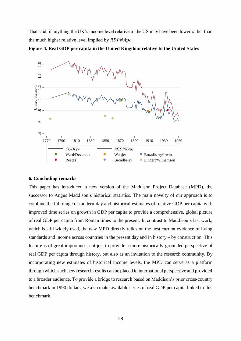
5.5 When did the US overtake the UK?

One of the debates in the study of long term economic growth has focused on the relative

performance of the UK and the USA, and in particular the question when the USA overtook the

UK. Maddison’s approach based on backward projection implied that until the 1870s the UK’s

income level was about 40% higher than that of the USA, and that only after the 1870s the USA

gradually overtook the UK; see Figure 4, the 𝑅𝐺𝐷𝑃𝑁𝐴𝑝𝑐 series. Broadberry (1998, 2003) came

to similar conclusions, based on a benchmark comparison in 1937. These results have, however,

been criticized recently by Ward and Devereux (2003, 2018), who created a set of independent

benchmarks for 1872 and 1910 period, and by Lindert and Williamson (2016) who did similar

research for the 18th century, indicating that the USA was at least on par with the UK at the

time. Our new approach makes use of the new Ward/Devereux benchmarks for the 1872-1910

period, using those as anchors. Figure 4 shows the new results, with series 𝐶𝐺𝐷𝑃𝑝𝑐, showing

the two countries roughly on par until 1870, after which point the US economy gained a

sustained income advantage. The fact that one of the Lindert and Williamson (2016) estimates,

the estimate by Woltjer (2015), by Rostas (1948), and by Broadberry (1998, 2003) are on, or

close to, the 𝐶𝐺𝐷𝑃𝑝𝑐 series is an independent outcome. These independent matches provide a

greater degree of plausibility to this new 𝐶𝐺𝐷𝑃𝑝𝑐 series, in our view, though the fact that three

of the Lindert/Williamson benchmarks deviate substantially suggests a degree of uncertainty.

27 Also the more recent income estimates for many African countries are sometimes of dubious quality (Jerven,

2013; Henderson et al. 2012).

28

That said, if anything the UK’s income level relative to the US may have been lower rather than

the much higher relative level implied by 𝑅𝐷𝑃𝑁𝐴𝑝𝑐.

Figure 4. Real GDP per capita in the United Kingdom relative to the United States

6. Concluding remarks

This paper has introduced a new version of the Maddison Project Database (MPD), the

successor to Angus Maddison’s historical statistics. The main novelty of our approach is to

combine the full range of modern-day and historical estimates of relative GDP per capita with

improved time series on growth in GDP per capita to provide a comprehensive, global picture

of real GDP per capita from Roman times to the present. In contrast to Maddison’s last work,

which is still widely used, the new MPD directly relies on the best current evidence of living

standards and income across countries in the present day and in history – by construction. This

feature is of great importance, not just to provide a more historically-grounded perspective of

real GDP per capita through history, but also as an invitation to the research community. By

incorporating new estimates of historical income levels, the MPD can serve as a platform

through which such new research results can be placed in international perspective and provided

to a broader audience. To provide a bridge to research based on Maddison’s prior cross-country

benchmark in 1990 dollars, we also make available series of real GDP per capita linked to this

benchmark.

.4.6

.81

1.2

1.4

1.6

Unit

ed S

tate

s=1

1770 1790 1810 1830 1850 1870 1890 1910 1930 1950

CGDPpc RGDPNApc

Ward/Devereux Woltjer Broadberry/Irwin

Rostas Broadberry Lindert/Williamson

29

The incorporation of many historical benchmarks has an important effect on our understanding

of long-term income trends. For example, the original Maddison statistics showed that it was

not until the early 20th century that real GDP per capita in the United States overtook the level

of real GDP per capita in the United Kingdom. But as historical evidence has accumulated, it

has become increasingly clear that real GDP per capita in the United States was at comparable

levels as in the United Kingdom already from the mid-19th century onwards. More broadly, we

find that in the 19th century, the United States was farther ahead of countries around the world

with, in particular, lower levels of real GDP per capita in Western Europe and Latin America.

In a broader cross-country setting, we show that our new measure of comparative real GDP per

capita is a more reliable measure for assessing the degree of income convergence and implies

more plausible relative price levels than the Maddison method of extrapolating from a modern-

day income comparison.

These new results do not claim to be the final word on these topics. Despite our inclusion and

estimation of numerous historical benchmarks, our understanding of comparative income levels

becomes based on sparser data as we move back further in time. This is particularly pressing in

regions such as Africa and large parts of Asia, but there also important gaps in 19th century

Latin America. Our hope is that our research contributes a fresh impetus to improving our

understanding of historical income differences as this can only sharpen our understanding of

why a relatively small set of countries managed to become much richer and to what extent those

countries were different. As an example of what such research can achieve, take Broadberry

and Wallis (2017), who find that avoiding a shrinking economy has been much more important

than stimulating growth for reaching higher income levels. More fine-grained information and

more comparative studies are crucial to broadening and deepening such understanding.

Finally, we fully recognize that developing estimates of real GDP per capita is but a first step

to a broader understanding of wellbeing. A fuller picture of well-being would (at least)

distinguish between consumption and investment and, more generally, incorporate additional

dimensions of wellbeing, such as health, leisure and inequality. A better understanding of

differences in income and living standards would require information on the factors of

production – human and physical capital – and productivity. Yet all such subsequent work relies

heavily on reliable and informative data on income per capita and we hope that our new data

serves as a useful starting point and platform for further research.

30

Appendices

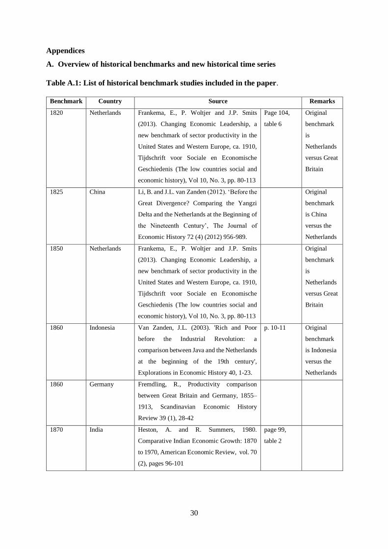
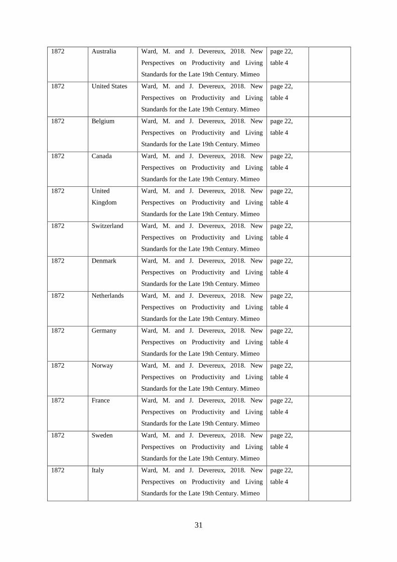
A. Overview of historical benchmarks and new historical time series

Table A.1: List of historical benchmark studies included in the paper.

Benchmark Country Source Remarks

1820 Netherlands Frankema, E., P. Woltjer and J.P. Smits

(2013). Changing Economic Leadership, a

new benchmark of sector productivity in the

United States and Western Europe, ca. 1910,

Tijdschrift voor Sociale en Economische

Geschiedenis (The low countries social and

economic history), Vol 10, No. 3, pp. 80-113

Page 104,

table 6

Original

benchmark

is

Netherlands

versus Great

Britain

1825 China Li, B. and J.L. van Zanden (2012). ‘Before the

Great Divergence? Comparing the Yangzi

Delta and the Netherlands at the Beginning of

the Nineteenth Century’, The Journal of

Economic History 72 (4) (2012) 956-989.

Original

benchmark

is China

versus the

Netherlands

1850 Netherlands Frankema, E., P. Woltjer and J.P. Smits

(2013). Changing Economic Leadership, a

new benchmark of sector productivity in the

United States and Western Europe, ca. 1910,

Tijdschrift voor Sociale en Economische

Geschiedenis (The low countries social and


Original

benchmark

is

Netherlands

versus Great

Britain

1860 Indonesia Van Zanden, J.L. (2003). 'Rich and Poor

before the Industrial Revolution: a

comparison between Java and the Netherlands

at the beginning of the 19th century',

Explorations in Economic History 40, 1-23.

p. 10-11 Original

benchmark

is Indonesia

versus the

Netherlands

1860 Germany Fremdling, R., Productivity comparison

between Great Britain and Germany, 1855–

1913, Scandinavian Economic History

Review 39 (1), 28-42

1870 India Heston, A. and R. Summers, 1980.

Comparative Indian Economic Growth: 1870

to 1970, American Economic Review, vol. 70

(2), pages 96-101

page 99,

table 2

31

1872 Australia Ward, M. and J. Devereux, 2018. New

Perspectives on Productivity and Living

Standards for the Late 19th Century. Mimeo

page 22,

table 4

1872 United States Ward, M. and J. Devereux, 2018. New



page 22,

table 4

1872 Belgium Ward, M. and J. Devereux, 2018. New



page 22,

table 4

1872 Canada Ward, M. and J. Devereux, 2018. New



page 22,

table 4

1872 United

Kingdom

Ward, M. and J. Devereux, 2018. New



page 22,

table 4

1872 Switzerland Ward, M. and J. Devereux, 2018. New



page 22,

table 4

1872 Denmark Ward, M. and J. Devereux, 2018. New



page 22,

table 4

1872 Netherlands Ward, M. and J. Devereux, 2018. New



page 22,

table 4

1872 Germany Ward, M. and J. Devereux, 2018. New



page 22,

table 4

1872 Norway Ward, M. and J. Devereux, 2018. New



page 22,

table 4

1872 France Ward, M. and J. Devereux, 2018. New



page 22,

table 4

1872 Sweden Ward, M. and J. Devereux, 2018. New



page 22,

table 4

1872 Italy Ward, M. and J. Devereux, 2018. New



page 22,

table 4

32

1910 Australia Ward, M. and J. Devereux, 2018. New



page 22,

table 4

1910 United States Ward, M. and J. Devereux, 2018. New



page 22,

table 4

1910 Belgium Ward, M. and J. Devereux, 2018. New



page 22,

table 4

1910 Canada Ward, M. and J. Devereux, 2018. New



page 22,

table 4

1910 United

Kingdom

Ward, M. and J. Devereux, 2018. New



page 22,

table 4

1910 Switzerland Ward, M. and J. Devereux, 2018. New



page 22,

table 4

1910 Denmark Ward, M. and J. Devereux, 2018. New



page 22,

table 4

1910 Netherlands Ward, M. and J. Devereux, 2018. New



page 22,

table 4

1910 Germany Ward, M. and J. Devereux, 2018. New



page 22,

table 4

1910 Norway Ward, M. and J. Devereux, 2018. New



page 22,

table 4

1910 France Ward, M. and J. Devereux, 2018. New



page 22,

table 4

1910 Sweden Ward, M. and J. Devereux, 2018. New



page 22,

table 4

1910 Italy Ward, M. and J. Devereux, 2018. New



page 22,

table 4

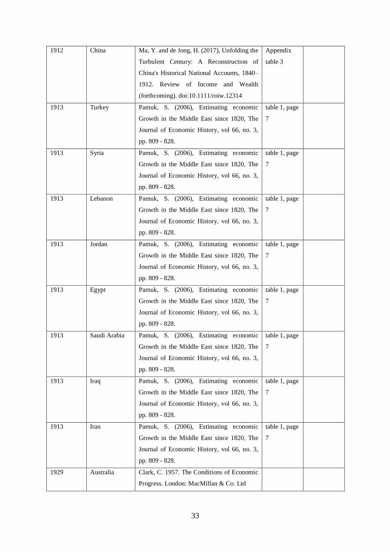
33

1912 China Ma, Y. and de Jong, H. (2017), Unfolding the

Turbulent Century: A Reconstruction of

China's Historical National Accounts, 1840–

1912. Review of Income and Wealth

(forthcoming). doi:10.1111/roiw.12314

Appendix

table 3

1913 Turkey Pamuk, S. (2006), Estimating economic

Growth in the Middle East since 1820, The

Journal of Economic History, vol 66, no. 3,

pp. 809 - 828.

table 1, page

7

1913 Syria Pamuk, S. (2006), Estimating economic



pp. 809 - 828.

table 1, page

7

1913 Lebanon Pamuk, S. (2006), Estimating economic



pp. 809 - 828.

table 1, page

7

1913 Jordan Pamuk, S. (2006), Estimating economic



pp. 809 - 828.

table 1, page

7

1913 Egypt Pamuk, S. (2006), Estimating economic



pp. 809 - 828.

table 1, page

7

1913 Saudi Arabia Pamuk, S. (2006), Estimating economic



pp. 809 - 828.

table 1, page

7

1913 Iraq Pamuk, S. (2006), Estimating economic



pp. 809 - 828.

table 1, page

7

1913 Iran Pamuk, S. (2006), Estimating economic



pp. 809 - 828.

table 1, page

7

1929 Australia Clark, C. 1957. The Conditions of Economic

Progress. London: MacMillan & Co. Ltd

34

1929 Austria Clark, C. 1957. The Conditions of Economic


1929 Belgium Clark, C. 1957. The Conditions of Economic


1929 Canada Clark, C. 1957. The Conditions of Economic


1929 Czechoslovakia Clark, C. 1957. The Conditions of Economic


1929 Denmark Clark, C. 1957. The Conditions of Economic


1929 Finland Clark, C. 1957. The Conditions of Economic


1929 France Clark, C. 1957. The Conditions of Economic


1929 Germany Clark, C. 1957. The Conditions of Economic


1929 Hungary Clark, C. 1957. The Conditions of Economic


1929 Ireland Clark, C. 1957. The Conditions of Economic


1929 Italy Clark, C. 1957. The Conditions of Economic


1929 Netherlands Clark, C. 1957. The Conditions of Economic


1929 New Zealand Clark, C. 1957. The Conditions of Economic


1929 Norway Clark, C. 1957. The Conditions of Economic


1929 Spain Clark, C. 1957. The Conditions of Economic


1929 Sweden Clark, C. 1957. The Conditions of Economic


1929 Switzerland Clark, C. 1957. The Conditions of Economic


1929 Turkey Clark, C. 1957. The Conditions of Economic


1929 Great Brittain Clark, C. 1957. The Conditions of Economic


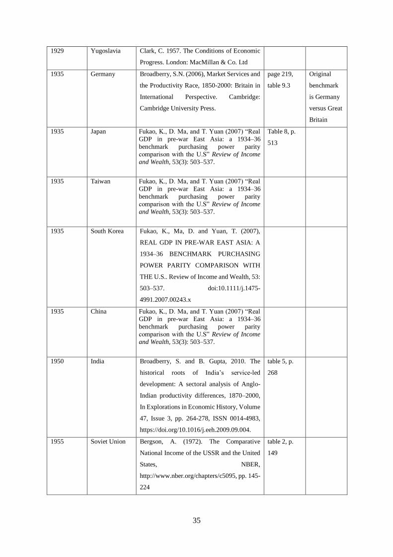
35

1929 Yugoslavia Clark, C. 1957. The Conditions of Economic


1935 Germany Broadberry, S.N. (2006), Market Services and

the Productivity Race, 1850-2000: Britain in

International Perspective. Cambridge:

Cambridge University Press.

page 219,

table 9.3

Original

benchmark

is Germany

versus Great

Britain

1935 Japan Fukao, K., D. Ma, and T. Yuan (2007) “Real

GDP in pre-war East Asia: a 1934–36

benchmark purchasing power parity

comparison with the U.S” Review of Income

and Wealth, 53(3): 503–537.

Table 8, p.

513

1935 Taiwan Fukao, K., D. Ma, and T. Yuan (2007) “Real




and Wealth, 53(3): 503–537.

1935 South Korea Fukao, K., Ma, D. and Yuan, T. (2007),

REAL GDP IN PRE-WAR EAST ASIA: A

1934–36 BENCHMARK PURCHASING

POWER PARITY COMPARISON WITH

THE U.S.. Review of Income and Wealth, 53:

503–537. doi:10.1111/j.1475-

4991.2007.00243.x

1935 China Fukao, K., D. Ma, and T. Yuan (2007) “Real




and Wealth, 53(3): 503–537.

1950 India Broadberry, S. and B. Gupta, 2010. The

historical roots of India’s service-led

development: A sectoral analysis of Anglo-

Indian productivity differences, 1870–2000,

In Explorations in Economic History, Volume

47, Issue 3, pp. 264-278, ISSN 0014-4983,

https://doi.org/10.1016/j.eeh.2009.09.004.

table 5, p.

268

1955 Soviet Union Bergson, A. (1972). The Comparative

National Income of the USSR and the United

States, NBER,

http://www.nber.org/chapters/c5095, pp. 145-

224

table 2, p.

149

36

1958 Thailand Usher, D. (1963). The Thai National Income

at United Kingom Prices. Bulletin of the

Oxford University Institute of Economics &

Statistics, 25: 199–214. doi:10.1111/j.1468-

0084.1963.mp25003003.x

table 1, page

199

Original

benchmark

is Thailand

versus Great

Britain

Time series

This new version of the MPD includes all new historical income estimates that have become

available since the previous update (Bolt and Van Zanden, 2014). For sources of all series not

updated as indicated in the table below, please consult Bolt and Van Zanden (2914).

Table A2: New historical time series included in the paper

Country Period Source

Latin America

Bolivia 1846–1950 Herranz-Loncán, A. and Peres-Cajías (2016). “Bolivian GDP per capita

since the mid-nineteenth century” Cliometrica 10: 99-128

Brazil 1850–1899 Barro, R.J. and J.F. Ursua, 2008. "Macroeconomic Crises since 1870,"

Brookings Papers on Economic Activity, Economic Studies Program, The

Brookings Institution, vol. 39(1 (Spring), pages 255-350

Brazil 1947 onwards National accounts data

Chile 1810–2004

Díaz, J.B. Lüders, R. and Wagner, G. (2007) Economia Chilena 1810 - 2000,

Producto total y sectorial una nueva mirada, Pontificia universidad Catolica

de Chile, Insituto de Economia, Documeno de Trabajo no. 315

Chile 2004 onwards National accounts data

Cuba 1902–1958 Ward, M. and Devereux, J. (2012). The Road Not Taken: Pre-Revolutionary

Cuban Living Standards in Comparative Perspective. The Journal of

Economic History, 72(1), 104-132. doi:10.1017/S0022050711002452

Cuba 1960–1895 Santamaria Garcia, A. (2005). Las Cuentas nacionales de Cuba, 1960 -

2005', mimeo

Mexico 1550–1812

Arroyo Abad, L., & Van Zanden, J. (2016). Growth under Extractive

Institutions? Latin American Per Capita GDP in Colonial Times. The

Journal of Economic History, 76(4), 1182-1215.

doi:10.1017/S0022050716000954

Mexico 1812–1870 Updated data based on Prados de la Escosura, L., ‘Lost decades? Economic

performance in post-independence Latin America’, Journal of Latin

America Studies, 41 (2009), pp. 279–307.

Mexico 1870–1895 Bèrtola, L. and Ocampo, J. A., The economic development of Latin America

since independence (Oxford, 2012).

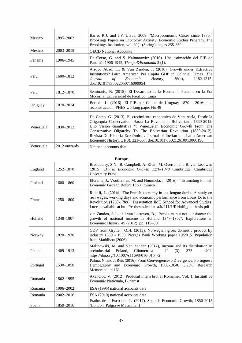
37

Mexico 1895–2003 Barro, R.J. and J.F. Ursua, 2008. "Macroeconomic Crises since 1870,"



Mexico 2003–2015 OECD National Accounts

Panama 1906–1945 De Corso, G. and S. Kalmanovitz (2016). Una estimación del PIB de

Panamá: 1906-1945, Tiempo&Economía 3 (1).

Peru 1600–1812

Arroyo Abad, L., & Van Zanden, J. (2016). Growth under Extractive

Institutions? Latin American Per Capita GDP in Colonial Times. The

Journal of Economic History, 76(4), 1182-1215.

doi:10.1017/S0022050716000954

Peru 1812–1870 Seminario, B. (2015). El Desarrallo de la Economía Peruana en la Era

Moderna, Universidad de Pacifico, Lima

Uruguay 1870–2014 Bertola, L. (2016). El PIB per Capita de Uruguay 1870 - 2016: una

reconstruccion. PHES working paper No 48

Venezuela 1830–2012

De Corso, G. (2013). El crecimiento economico de Venuzuela, Desde la

Oligarquia Conservadora Hasta La Revolucion Bolivariana: 1830-2012.

Uno Vision cuantitativa *: Venezuelan Economic Growth From The

Conservative Oligarchy To The Bolivarian Revolution (1830-2012),

Revista De Historia Económica / Journal of Iberian and Latin American

Economic History, 31(3), 321-357. doi:10.1017/S0212610913000190

Venezuela 2012 onwards National accounts data

Europe

England 1252–1870

Broadberry, S.N., B. Campbell, A. Klein, M. Overton and B. van Leeuwen

(2015), British Economic Growth 1270-1870 Cambridge: Cambridge

University Press.

Finland 1600–1860 Eloranta, J., Voutilainen, M. and Nummela, I. (2016). “Estimating Finnish

Economic Growth Before 1860” mimeo.

France 1250–1800

Ridolfi, L. (2016) “The French economy in the longue durée. A study on

real wages, working days and economic performance from Louis IX to the

Revolution (1250-1789)” Dissertation IMT School for Advanced Studies,

Lucca, available at http://e-theses.imtlucca.it/211/1/Ridolfi_phdthesis.pdf

Holland 1348–1807

van Zanden, J. L. and van Leeuwen, B., ‘Persistent but not consistent: the

growth of national income in Holland 1347–1807’, Explorations in

Economic History, 49 (2012), pp. 119–30.

Norway 1820–1930

GDP from Grytten, O.H. (2015). Norwegian gross domestic product by

industry 1830 - 1930, Norges Bank Working paper 19/2015. Population

from Maddison (2006).

Poland 1409–1913

Malinowski, M. and Van Zanden (2017), Income and its distribution in

preindustrial Poland, Cliometrica 11 (3): 375 - 404.

https://doi.org/10.1007/s11698-016-0154-5

Portugal 1530–1850

Palma, N. and J. Reis (2016). From Convergence to Divergence: Portuguese

Demography and Economic Growth, 1500-1850. GGDC Research

Memorandum 161

Romania 1862–1995 Axenciuc, V. (2012). Produsul intern brut al Romaniei, Vol. 1, Institutl de

Economie Nationala, Bucarest

Romania 1996–2002 ESA (1995) national accounts data

Romania 2002–2016 ESA (2010) national accounts data

Spain 1850–2016

Prados de la Escosura, L. (2017), Spanish Economic Growth, 1850-2015

(London: Palgrave Macmillan)

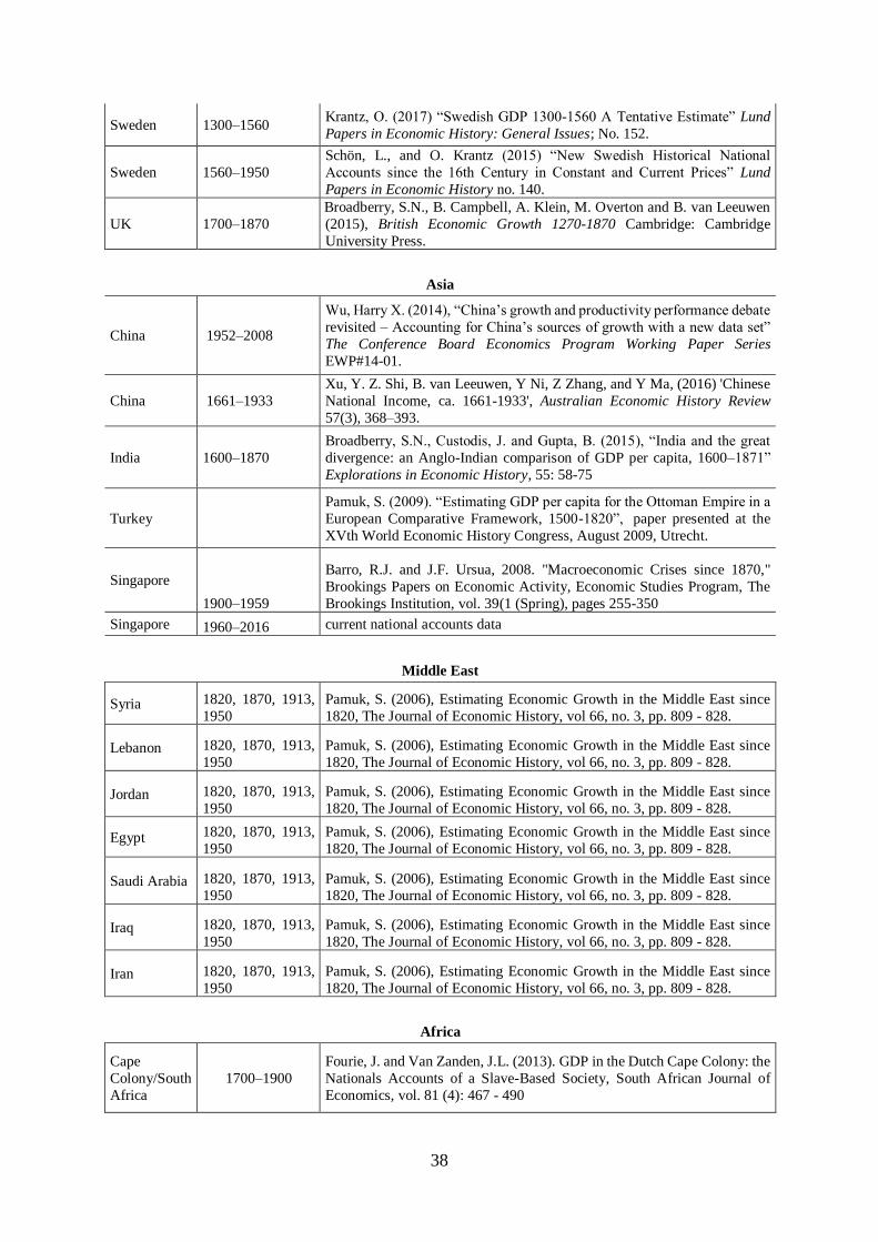
38

Sweden 1300–1560 Krantz, O. (2017) “Swedish GDP 1300-1560 A Tentative Estimate” Lund

Papers in Economic History: General Issues; No. 152.

Sweden 1560–1950

Schön, L., and O. Krantz (2015) “New Swedish Historical National

Accounts since the 16th Century in Constant and Current Prices” Lund

Papers in Economic History no. 140.

UK 1700–1870

Broadberry, S.N., B. Campbell, A. Klein, M. Overton and B. van Leeuwen

(2015), British Economic Growth 1270-1870 Cambridge: Cambridge

University Press.

Asia

China 1952–2008

Wu, Harry X. (2014), “China’s growth and productivity performance debate

revisited – Accounting for China’s sources of growth with a new data set”

The Conference Board Economics Program Working Paper Series

EWP#14-01.

China 1661–1933

Xu, Y. Z. Shi, B. van Leeuwen, Y Ni, Z Zhang, and Y Ma, (2016) 'Chinese

National Income, ca. 1661-1933', Australian Economic History Review

57(3), 368–393.

India 1600–1870

Broadberry, S.N., Custodis, J. and Gupta, B. (2015), “India and the great

divergence: an Anglo-Indian comparison of GDP per capita, 1600–1871”

Explorations in Economic History, 55: 58-75

Turkey

Pamuk, S. (2009). “Estimating GDP per capita for the Ottoman Empire in a

European Comparative Framework, 1500-1820”, paper presented at the

XVth World Economic History Congress, August 2009, Utrecht.

Singapore

1900–1959

Barro, R.J. and J.F. Ursua, 2008. "Macroeconomic Crises since 1870,"



Singapore 1960–2016 current national accounts data

Middle East

Syria 1820, 1870, 1913,

1950

Pamuk, S. (2006), Estimating Economic Growth in the Middle East since

1820, The Journal of Economic History, vol 66, no. 3, pp. 809 - 828.

Lebanon 1820, 1870, 1913,

1950



Jordan 1820, 1870, 1913,

1950



Egypt 1820, 1870, 1913,

1950



Saudi Arabia 1820, 1870, 1913,

1950



Iraq 1820, 1870, 1913,

1950



Iran 1820, 1870, 1913,

1950



Africa

Cape

Colony/South

Africa

1700–1900

Fourie, J. and Van Zanden, J.L. (2013). GDP in the Dutch Cape Colony: the

Nationals Accounts of a Slave-Based Society, South African Journal of

Economics, vol. 81 (4): 467 - 490

39

B. Multiple benchmark implementation

Combining relative income comparisons with very long time series of economic growth can

yield results that are impossible to square with information from other sources. Relying on

multiple benchmark comparison can alleviate such problems, but especially when a comparison

is the first in a time series, it can also be a source of problems. We identified three categories

of problems, related to either problematic benchmark comparisons or time series:

1. Too low: For a long and persistent period of time, income levels drop below the absolute

poverty (or subsistence) level of $1.90 per day (approximately $700/year, in 2011 prices).

While poverty can be widespread – indicating that a substantial fractions of the population

lives on less than $700 per year – it is rare outside periods of severe conflict for the average

income level in a country to be lower than $700. For illustration, in ICP 2011, only the

Democratic Republic of Congo was below this level at $680 and this country had an income

level above $700 before 1996 and since 2012, showing such below-subsistence spells are

mostly temporary rather than persistent.

2. Too high: While it is no rule that the United States should be the highest-income country in

the world, higher incomes are typically only observed in countries with substantial oil

exports (in ICP 2011: Qatar, Norway, Kuwait and United Arab Emirates) or in otherwise

unique and particular circumstances (Luxembourg, Singapore and Switzerland). So if we

find that, for example, oil-exporting countries already had high income levels according to

official growth statistics, before oil exports began or before the 1973 rise in oil prices, these

are reasons for worry.

3. Large swings: Especially before the more thoroughly vetted procedures of ICP 2005 and

ICP 2011, benchmark price comparison differed substantially in quality across countries

and comparisons. For example, there are cases where a particular country in a particular

year relied on the exchange rate as the PPP for a sizeable share of its product categories.

Also, if countries happen to be in unstable macroeconomic conditions around the time of a

benchmark price measurement – such as Zimbabwe in 2005 or some Latin American

countries in 1980 – the resulting benchmark level may be uncertain and distorted. These

may exhibit as large swings in relative income levels between benchmarks.

4. PWT estimation: Problematic time series of real GDP may not only stem from the historical

or ICP benchmarks, but may instead be related to the data and methods used in the Penn

World Table (PWT) for interpolating between benchmarks or extrapolating from the first

(or last) benchmark comparison. While in the MPD, we only have information on GDP

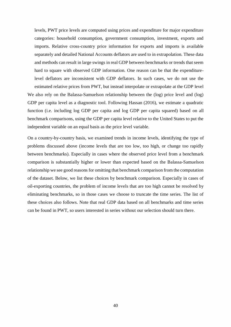
40

levels, PWT price levels are computed using prices and expenditure for major expenditure

categories: household consumption, government consumption, investment, exports and

imports. Relative cross-country price information for exports and imports is available

separately and detailed National Accounts deflators are used to in extrapolation. These data

and methods can result in large swings in real GDP between benchmarks or trends that seem

hard to square with observed GDP information. One reason can be that the expenditure-

level deflators are inconsistent with GDP deflators. In such cases, we do not use the

estimated relative prices from PWT, but instead interpolate or extrapolate at the GDP level

We also rely on the Balassa-Samuelson relationship between the (log) price level and (log)

GDP per capita level as a diagnostic tool. Following Hassan (2016), we estimate a quadratic

function (i.e. including log GDP per capita and log GDP per capita squared) based on all

benchmark comparisons, using the GDP per capita level relative to the United States to put the

independent variable on an equal basis as the price level variable.

On a country-by-country basis, we examined trends in income levels, identifying the type of

problems discussed above (income levels that are too low, too high, or change too rapidly

between benchmarks). Especially in cases where the observed price level from a benchmark

comparison is substantially higher or lower than expected based on the Balassa-Samuelson

relationship we see good reasons for omitting that benchmark comparison from the computation

of the dataset. Below, we list these choices by benchmark comparison. Especially in cases of

oil-exporting countries, the problem of income levels that are too high cannot be resolved by

eliminating benchmarks, so in those cases we choose to truncate the time series. The list of

these choices also follows. Note that real GDP data based on all benchmarks and time series

can be found in PWT, so users interested in series without our selection should turn there.

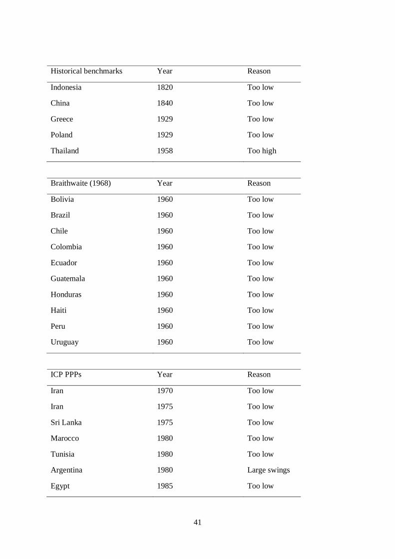
41

Historical benchmarks Year Reason

Indonesia 1820 Too low

China 1840 Too low

Greece 1929 Too low

Poland 1929 Too low

Thailand 1958 Too high

Braithwaite (1968) Year Reason

Bolivia 1960 Too low

Brazil 1960 Too low

Chile 1960 Too low

Colombia 1960 Too low

Ecuador 1960 Too low

Guatemala 1960 Too low

Honduras 1960 Too low

Haiti 1960 Too low

Peru 1960 Too low

Uruguay 1960 Too low

ICP PPPs Year Reason

Iran 1970 Too low

Iran 1975 Too low

Sri Lanka 1975 Too low

Marocco 1980 Too low

Tunisia 1980 Too low

Argentina 1980 Large swings

Egypt 1985 Too low

42

ICP PPPs Year Reason

Iran 1985 Too low

Sierra Leone 1985 Too low

Zimbabwe 1985 Large swings

Equatorial Guinea 1996 Too low

Iran 1996 Too low

Guinea 1996 Too low

Lebanon 1996 Too low

Nigeria 1996 Large swings

Syria 1996 Large swings

Zimbabwe 1996 Too low

Iran 1970 Too low

Iran 1975 Too low

Sri Lanka 1975 Too low

Marocco 1980 Too low

Tunisia 1980 Too low

Argentina 1980 Large swings

Egypt 1985 Too low

Iran 1985 Too low

Sierra Leone 1985 Too low

Zimbabwe 1985 Large swings

Equatorial Guinea 1996 Too low

Iran 1996 Too low

Guinea 1996 Too low

Lebanon 1996 Too low

Nigeria 1996 Large swings

Syria 1996 Large swings

Zimbabwe 1996 Too low

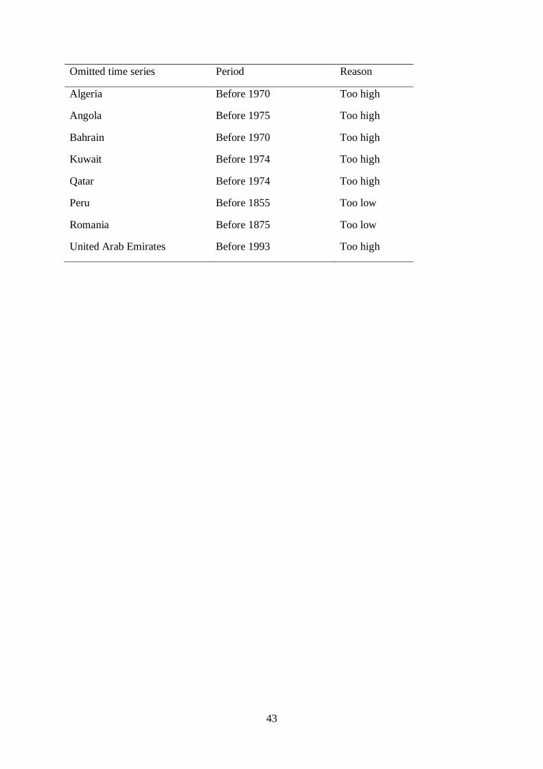
43

Omitted time series Period Reason

Algeria Before 1970 Too high

Angola Before 1975 Too high

Bahrain Before 1970 Too high

Kuwait Before 1974 Too high

Qatar Before 1974 Too high

Peru Before 1855 Too low

Romania Before 1875 Too low

United Arab Emirates Before 1993 Too high

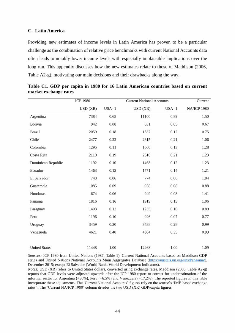
44

C. Latin America

Providing new estimates of income levels in Latin America has proven to be a particular

challenge as the combination of relative price benchmarks with current National Accounts data

often leads to notably lower income levels with especially implausible implications over the

long run. This appendix discusses how the new estimates relate to those of Maddison (2006,

Table A2-g), motivating our main decisions and their drawbacks along the way.

Table C1. GDP per capita in 1980 for 16 Latin American countries based on current

market exchange rates

ICP 1980 Current National Accounts Current

USD (XR) USA=1 USD (XR) USA=1 NA/ICP 1980

Argentina 7384 0.65 11100 0.89 1.50

Bolivia 942 0.08 631 0.05 0.67

Brazil 2059 0.18 1537 0.12 0.75

Chile 2477 0.22 2615 0.21 1.06

Colombia 1295 0.11 1660 0.13 1.28

Costa Rica 2119 0.19 2616 0.21 1.23

Dominican Republic 1192 0.10 1468 0.12 1.23

Ecuador 1463 0.13 1771 0.14 1.21

El Salvador 743 0.06 774 0.06 1.04

Guatemala 1085 0.09 958 0.08 0.88

Honduras 674 0.06 949 0.08 1.41

Panama 1816 0.16 1919 0.15 1.06

Paraguay 1403 0.12 1255 0.10 0.89

Peru 1196 0.10 926 0.07 0.77

Uruguay 3459 0.30 3438 0.28 0.99

Venezuela 4621 0.40 4304 0.35 0.93

United States 11448 1.00 12468 1.00 1.09

Sources: ICP 1980 from United Nations (1987, Table 1), Current National Accounts based on Maddison GDP

series and United Nations National Accounts Main Aggregates Database (https://unstats.un.org/unsd/snaama/),

December 2015; except El Salvador (World Bank, World Development Indicators).

Notes: USD (XR) refers to United States dollars, converted using exchange rates. Maddison (2006, Table A2-g)

reports that GDP levels were adjusted upwards after the ICP 1980 report to correct for underestimation of the

informal sector for Argentina (+36%), Peru (+6.5%) and Venezuela (+17.2%). The reported figures in this table

incorporate these adjustments. The ‘Current National Accounts’ figures rely on the source’s ‘IMF-based exchange

rates’ . The ‘Current NA/ICP 1980’ column divides the two USD (XR) GDP/capita figures.

https://unstats.un.org/unsd/snaama/

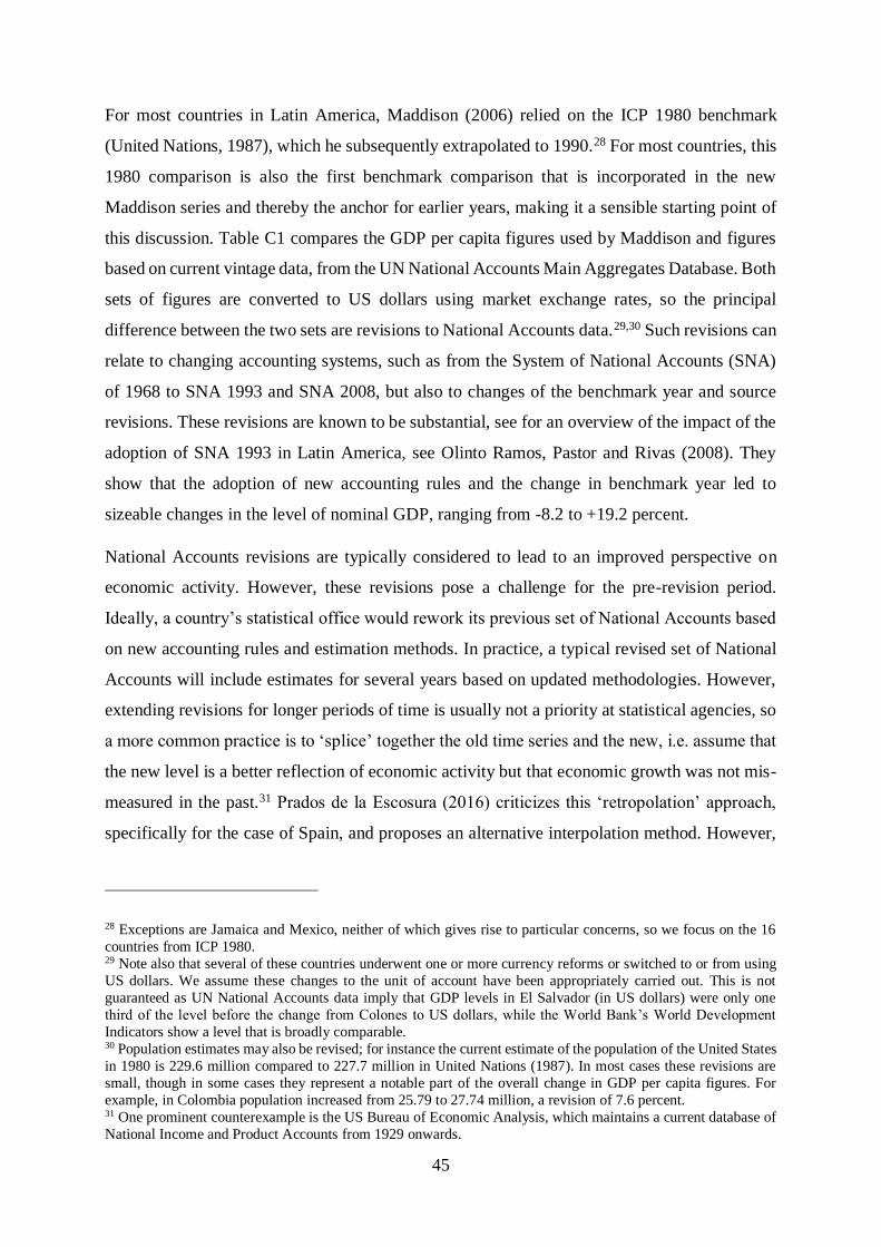
45

For most countries in Latin America, Maddison (2006) relied on the ICP 1980 benchmark

(United Nations, 1987), which he subsequently extrapolated to 1990.28 For most countries, this

1980 comparison is also the first benchmark comparison that is incorporated in the new

Maddison series and thereby the anchor for earlier years, making it a sensible starting point of

this discussion. Table C1 compares the GDP per capita figures used by Maddison and figures

based on current vintage data, from the UN National Accounts Main Aggregates Database. Both

sets of figures are converted to US dollars using market exchange rates, so the principal

difference between the two sets are revisions to National Accounts data.29,30 Such revisions can

relate to changing accounting systems, such as from the System of National Accounts (SNA)

of 1968 to SNA 1993 and SNA 2008, but also to changes of the benchmark year and source

revisions. These revisions are known to be substantial, see for an overview of the impact of the

adoption of SNA 1993 in Latin America, see Olinto Ramos, Pastor and Rivas (2008). They

show that the adoption of new accounting rules and the change in benchmark year led to

sizeable changes in the level of nominal GDP, ranging from -8.2 to +19.2 percent.

National Accounts revisions are typically considered to lead to an improved perspective on

economic activity. However, these revisions pose a challenge for the pre-revision period.

Ideally, a country’s statistical office would rework its previous set of National Accounts based

on new accounting rules and estimation methods. In practice, a typical revised set of National

Accounts will include estimates for several years based on updated methodologies. However,

extending revisions for longer periods of time is usually not a priority at statistical agencies, so

a more common practice is to ‘splice’ together the old time series and the new, i.e. assume that

the new level is a better reflection of economic activity but that economic growth was not mis-

measured in the past.31 Prados de la Escosura (2016) criticizes this ‘retropolation’ approach,

specifically for the case of Spain, and proposes an alternative interpolation method. However,

28 Exceptions are Jamaica and Mexico, neither of which gives rise to particular concerns, so we focus on the 16

countries from ICP 1980. 29 Note also that several of these countries underwent one or more currency reforms or switched to or from using

US dollars. We assume these changes to the unit of account have been appropriately carried out. This is not

guaranteed as UN National Accounts data imply that GDP levels in El Salvador (in US dollars) were only one

third of the level before the change from Colones to US dollars, while the World Bank’s World Development

Indicators show a level that is broadly comparable. 30 Population estimates may also be revised; for instance the current estimate of the population of the United States

in 1980 is 229.6 million compared to 227.7 million in United Nations (1987). In most cases these revisions are

small, though in some cases they represent a notable part of the overall change in GDP per capita figures. For

example, in Colombia population increased from 25.79 to 27.74 million, a revision of 7.6 percent. 31 One prominent counterexample is the US Bureau of Economic Analysis, which maintains a current database of

National Income and Product Accounts from 1929 onwards.

46

to what extent this approach would be generally applicable is hard to assess. Furthermore, the

challenges in the Latin American context are greater because of the numerous episodes of

macroeconomic instability in the twentieth century, with large swings in prices and exchange

rates and currency reforms or dollarization.

Table C2. GDP price level in 1980 for 16 Latin American countries

ICP 1980, GK ICP 1980, GEKS PWT

Argentina 1.42 1.66 1.71

Bolivia 0.59 0.72 0.67

Brazil 0.62 0.70 0.72

Chile 0.68 0.86 0.92

Colombia 0.47 0.54 0.58

Costa Rica 0.68 0.77 0.81

Dominican Republic 0.59 0.69 0.92

Ecuador 0.57 0.69 0.71

El Salvador 0.52 0.61 0.64

Guatemala 0.47 0.60 0.63

Honduras 0.56 0.67 0.71

Panama 0.56 0.76 0.82

Paraguay 0.67 0.80 0.85

Peru 0.45 0.55 0.57

Uruguay 0.83 0.86 0.91

Venezuela 0.73 0.94 0.93

United States 1.00 1.00 1.00

Sources: ICP 1980, GK from United Nations (1987, Table 1); ICP 1980, GEKS computations based on ICP 1980

data; PWT: price level of GDPo (pl_gdpo) from PWT 9.0, normalized to USA=1, see Feenstra, Inklaar and Timmer

(2015).

Notes: GDP price level is the PPP for GDP divided by the exchange rate. GK stands for Geary-Khamis and GEKS

for Gini-Elteto-Kovecs-Szulc as two alternative PPP computation methods, see e.g. Diewert (2013).

Beyond revisions to GDP per capita figures, changes to the computation of purchasing power

parities (PPPs) is another source of differences between Maddison (2006) and current estimates.

Table C2 provides three estimates for the 1980 GDP price level, defined as the PPP for GDP

divided by the market exchange rate. The first column, ‘ICP 1980, GK’, is the main relative

price level as reported in United Nations (1987), computed from detailed price and expenditure

data using the Geary-Khamis method. This method has come under increased criticism in the

period since the ICP 1980 data were released, primarily because the method suffers from

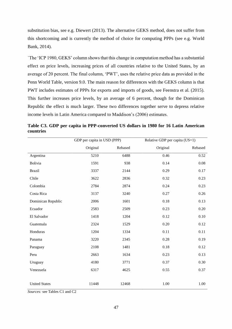
47

substitution bias, see e.g. Diewert (2013). The alternative GEKS method, does not suffer from

this shortcoming and is currently the method of choice for computing PPPs (see e.g. World

Bank, 2014).

`The ‘ICP 1980, GEKS’ column shows that this change in computation method has a substantial

effect on price levels, increasing prices of all countries relative to the United States, by an

average of 20 percent. The final column, ‘PWT’, uses the relative price data as provided in the

Penn World Table, version 9.0. The main reason for differences with the GEKS column is that

PWT includes estimates of PPPs for exports and imports of goods, see Feenstra et al. (2015).

This further increases price levels, by an average of 6 percent, though for the Dominican

Republic the effect is much larger. These two differences together serve to depress relative

income levels in Latin America compared to Maddison’s (2006) estimates.

Table C3. GDP per capita in PPP-converted US dollars in 1980 for 16 Latin American

countries

GDP per capita in USD (PPP) Relative GDP per capita (US=1)

Original Rebased Original Rebased

Argentina 5210 6488 0.46 0.52

Bolivia 1591 938 0.14 0.08

Brazil 3337 2144 0.29 0.17

Chile 3622 2836 0.32 0.23

Colombia 2784 2874 0.24 0.23

Costa Rica 3137 3240 0.27 0.26

Dominican Republic 2006 1601 0.18 0.13

Ecuador 2583 2509 0.23 0.20

El Salvador 1418 1204 0.12 0.10

Guatemala 2324 1529 0.20 0.12

Honduras 1204 1334 0.11 0.11

Panama 3220 2345 0.28 0.19

Paraguay 2108 1481 0.18 0.12

Peru 2663 1634 0.23 0.13

Uruguay 4180 3771 0.37 0.30

Venezuela 6317 4625 0.55 0.37

United States 11448 12468 1.00 1.00

Sources: see Tables C1 and C2

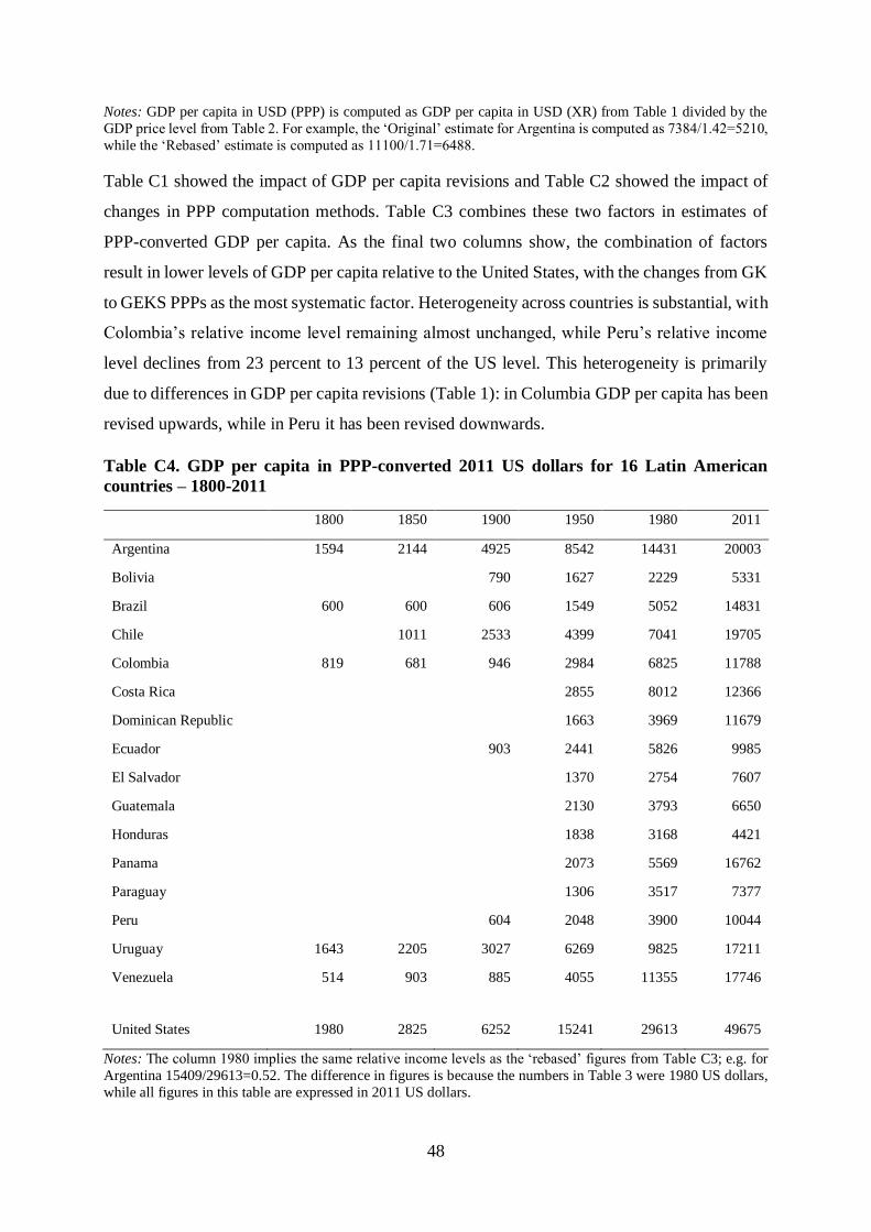
48

Notes: GDP per capita in USD (PPP) is computed as GDP per capita in USD (XR) from Table 1 divided by the

GDP price level from Table 2. For example, the ‘Original’ estimate for Argentina is computed as 7384/1.42=5210,

while the ‘Rebased’ estimate is computed as 11100/1.71=6488.

Table C1 showed the impact of GDP per capita revisions and Table C2 showed the impact of

changes in PPP computation methods. Table C3 combines these two factors in estimates of

PPP-converted GDP per capita. As the final two columns show, the combination of factors

result in lower levels of GDP per capita relative to the United States, with the changes from GK

to GEKS PPPs as the most systematic factor. Heterogeneity across countries is substantial, with

Colombia’s relative income level remaining almost unchanged, while Peru’s relative income

level declines from 23 percent to 13 percent of the US level. This heterogeneity is primarily

due to differences in GDP per capita revisions (Table 1): in Columbia GDP per capita has been

revised upwards, while in Peru it has been revised downwards.

Table C4. GDP per capita in PPP-converted 2011 US dollars for 16 Latin American

countries – 1800-2011

1800 1850 1900 1950 1980 2011

Argentina 1594 2144 4925 8542 14431 20003

Bolivia 790 1627 2229 5331

Brazil 600 600 606 1549 5052 14831

Chile 1011 2533 4399 7041 19705

Colombia 819 681 946 2984 6825 11788

Costa Rica 2855 8012 12366

Dominican Republic 1663 3969 11679

Ecuador 903 2441 5826 9985

El Salvador 1370 2754 7607

Guatemala 2130 3793 6650

Honduras 1838 3168 4421

Panama 2073 5569 16762

Paraguay 1306 3517 7377

Peru 604 2048 3900 10044

Uruguay 1643 2205 3027 6269 9825 17211

Venezuela 514 903 885 4055 11355 17746

United States 1980 2825 6252 15241 29613 49675

Notes: The column 1980 implies the same relative income levels as the ‘rebased’ figures from Table C3; e.g. for

Argentina 15409/29613=0.52. The difference in figures is because the numbers in Table 3 were 1980 US dollars,

while all figures in this table are expressed in 2011 US dollars.

49

As may be expected, these changes to the 1980 benchmark levels have substantial effects on

long-run income levels. Table C4 shows the PPP-converted GDP per capita figures for the 16

Latin American countries since 1800 (or the earliest available year), denominated in 2011 US

dollars. This points to the importance of a more extensive set of benchmark comparisons for

these countries, to establish whether these patterns, implied by the time series of economic

growth and the different benchmarks accords with the historical reality.

The Case of Cuba32

Cuba deserves special attention because it is a country of 11 million that used to be a prosperous,

middle-income country before its Communist revolution (Ward and Devereux, 2012) and has

been on a downward (relative) trajectory since. However, due (at least in part) to its current

political system, it has not actively participated in the ICP before the 2011 round, leading to a

paucity of information that can be used to compare income levels. Moreover, even its

participation in ICP 2011 did not lead to estimates of real GDP per capita that were deemed

reliable enough to publish. The ICP 2011 report only reports Cuba’s relative price level, at 32.2

percent of the US level, but: “The official GDP of Cuba for reference year 2011 is 68,990.15

million in national currency. However, this number and its breakdown into main aggregates are

not shown in the tables because of methodological comparability issues. Therefore, Cuba’s

results are provided only for the PPP and price level index” (World Bank 2014, p. 29). The

reported price level of 32.2 percent of the US level seems low, on a similar level as that of India,

while the official GDP per capita level, valued at current exchange rates, is much higher for

Cuba (12 percent of the US level) than for India (3 percent). The predicted relative price level

at Cuba’s level of GDP per capita is between 52 and 59 percent of the US level, depending on

the Balassa-Samuelson relationship. Similarly, the crowd-sourced price comparison website

Numbeo shows a relative cost-of-living in Havana that is 67 percent of the US level.33

One clear conclusion from this discussion is that combining the ICP 2011 relative price level

for Cuba with official GDP per capita data does not result in plausible real GDP per capita

figures and would substantially overestimate Cuba’s comparative income level. It would thus

be more sensible to treat Cuba as a ‘non-benchmark’ economy, like Afghanistan and North

Korea, and use an econometric estimate of its real GDP per capita level than a direct

32 We would like to thank John Devereux for helpful suggestions and discussions on this topic 33 https://www.numbeo.com/cost-of-living/region_rankings_current.jsp?region=019, consulted on January 4,

2018.

https://www.numbeo.com/cost-of-living/region_rankings_current.jsp?region=019

50

measurement. An estimate by the United Nations for its Human Development Report (2016)

seems plausible, as deemed by Cuba’s statistical office and experts of the region. This puts

Cuba’s real GNI per capita in 2011 at 6821 (in 2011 US dollars). Using the GDP/GNI ratio

from the World Development Indicators, this implies a real GDP per capita level in 2011 for

Cuba of 6928 in 2011 US dollars. Compared to the figures in the final column of Table C4, this

puts Cuba in the lower part of Latin America’s income levels, which seems more plausible than

the $19068 implied by the official GDP per capita data and the ICP 2011 price level, which

would have put Cuba at a similar income level as Chile. We therefore use the $6928 as the

benchmark level for Cuba in 2011.

51

D. Africa

The new methodology for extending income levels back in time appear to have limited

consequences for the income estimates of the far majority of Sub-Saharan African countries.

For a number of African countries the new methodology results in substantially different

income levels compared to those originally published by Maddison (2006). This appendix

discusses how the new estimates and the original estimates relate to each other.

Maddison (2006) relied on the Penn-World tables 5.6 for his estimates of the 1990 benchmark

GDP levels for all African countries except Equatorial Guinea, Sao Tome and Principe, and

five very small countries. For those countries Maddison (2006: 221) assumed that the 1990

GDP per capita was equal to the average of the 50 African countries covered by the PWT. When

using the multiple benchmarks, for 26 out of 47 countries this in effect means using the 2011

and the 2005 PPPs. For the other countries, various earlier benchmarks are available. Kenya is

the first Sub-Saharan African country to participate in an ICP round in 1970, and in 1985

already 15 countries participate in the ICP program. Using the multiple benchmark approach

leads to very similar relative income estimates compared to the original Maddison series for

about half of the African countries. For most other countries the multiple benchmark approach

leads to slightly different but we think still reasonable income estimates. However, for some of

the countries, the earlier income estimates deviate away from previous patterns when using

multiple benchmarks. This leads to a reshuffling in the order of countries compared to the

original series, when we rank them from poor to rich. The best way forward would be to have

benchmarks for 1950 for all African countries, as that would provide the best comparison of

relative income levels in that year allowing us to ‘anchor’ the annual series.

As there currently exists no such anchor, we created benchmarks for African countries for the

year 1950 based on the indirect approach. This indirect approach has been developed in the

context of estimating trends in GDP per capita, within countries, over time, for periods in which

data constraints make it impossible to estimate GDP in the usual way. The method used was

pioneered by Malanima (2010, for Northern Italy 1300-1850), and has now been used for many

country studies (of, amongst others, Germany (Pfister 2003), France (Ridolfi 2016), Spain

(Alvarez-Nogal and Prados de la Escosura 2013), Poland (Malinowski and Van Zanden 2016),

Mexico and Peru (Arroyo-Abad and van Zanden 2015). Here we propose adapting this approach

from a time-series to a cross-country within Africa setting.

52

We first explain the approach, and then present the resulting GDP pc levels for the African

countries for which we could obtain the underlying data. The starting point of the indirect

approach is to assume each country can usefully be represented as a two-sector economy,

consisting of an agricultural sector (𝑎) and a non-agricultural sector (𝑛). Nominal GDP in

country 𝑖 is then defined as:

𝑃𝑖𝑄𝑖 = 𝑃𝑖𝑎𝑄𝑖

𝑎 + 𝑃𝑖𝑛𝑄𝑖

𝑛, (𝐷1)

where 𝑄 denotes the price level and 𝑄 denotes net production. If all variables in equation (D1)

were known, it would be straightforward to compare real GDP between countries 𝑖 and 𝑗. If we

follow Feenstra et al. (2015) and assume an economy-wide translog function that is

homogenous of degree one in factor endowments and has identical second-order parameters on

factor endowments across countries, we can express relative real GDP per capita as the

following Törnqvist index:34

log (𝑄𝑖

𝑄𝑗) =

1

2(

𝑃𝑖𝑎𝑄𝑖

𝑎

𝑃𝑖𝑄𝑖+

𝑃𝑗𝑎𝑄𝑗

𝑎

𝑃𝑗𝑄𝑗) log (

𝑄𝑖𝑎

𝑄𝑗𝑎) +

1

2(

𝑃𝑖𝑛𝑄𝑖

𝑛

𝑃𝑖𝑄𝑖+

𝑃𝑗𝑛𝑄𝑗

𝑛

𝑃𝑗𝑄𝑗) log (

𝑄𝑖𝑛

𝑄𝑗𝑛) (𝐷2)

Yet the absence of sufficient data is what motivates this indirect approach, so we have to impose

more structure and assumptions on the problem to arrive at a method that can be implemented

in practice. First, assume that food production equals food consumption, 𝐹 ≡ 𝑄𝑎 (dropping

country subscripts for conciseness). As discussed in Allen (2000), net food trade accounted for

only 10 percent of food production around 1800 in the Netherlands and United Kingdom, two

of the most open economies at the time, so violations of this assumption are not likely to be

substantial. Second, assume that food consumption per capita is primarily determined by

income per capita 𝑤:

𝐹

𝑁≡ 𝑓 = 𝑤𝛽 (𝐷3),

where 𝑁𝑖 is the population in country 𝑖. The crucial parameter here is 𝛽, the income elasticity

of food demand, whose choice we discuss below.

We approximate income per capita by the real wage level of laborers. This measure, pioneered

by Allen (2001), relates nominal wages of building laborers to the cost of a basket of goods that

34 A Törnqvist index is a superlative index, like the Fisher index (Diewert, 1976) and in many practical situations

the two indexes provide very similar results.

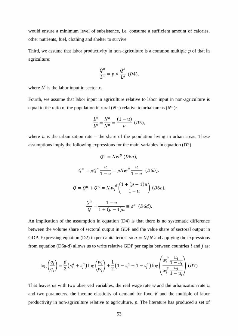
53

would ensure a minimum level of subsistence, i.e. consume a sufficient amount of calories,

other nutrients, fuel, clothing and shelter to survive.

Third, we assume that labor productivity in non-agriculture is a common multiple 𝑝 of that in

agriculture:

𝑄𝑛

𝐿𝑛= 𝑝 ×

𝑄𝑎

𝐿𝑎 (𝐷4),

where 𝐿𝑥 is the labor input in sector 𝑥.

Fourth, we assume that labor input in agriculture relative to labor input in non-agriculture is

equal to the ratio of the population in rural (𝑁𝑎) relative to urban areas (𝑁𝑛):

𝐿𝑎

𝐿𝑛=

𝑁𝑎

𝑁𝑛=

(1 − 𝑢)

𝑢 (𝐷5),

where 𝑢 is the urbanization rate – the share of the population living in urban areas. These

assumptions imply the following expressions for the main variables in equation (D2):

𝑄𝑎 = 𝑁𝑤𝛽 (𝐷6𝑎),

𝑄𝑛 = 𝑝𝑄𝑎𝑢

1 − 𝑢= 𝑝𝑁𝑤𝛽

𝑢

1 − 𝑢 (𝐷6𝑏),

𝑄 = 𝑄𝑎 + 𝑄𝑛 = 𝑁𝑖𝑤𝑖𝛽

(1 + (𝑝 − 1)𝑢

1 − 𝑢) (𝐷6𝑐),

𝑄𝑎

𝑄=

1 − 𝑢

1 + (𝑝 − 1)𝑢≡ 𝑠𝑎 (𝐷6𝑑).

An implication of the assumption in equation (D4) is that there is no systematic difference

between the volume share of sectoral output in GDP and the value share of sectoral output in

GDP. Expressing equation (D2) in per capita terms, so 𝑞 = 𝑄 𝑁⁄ and applying the expressions

from equation (D6a-d) allows us to write relative GDP per capita between countries 𝑖 and 𝑗 as:

log (𝑞𝑖

𝑞𝑗) =

𝛽

2(𝑠𝑖

𝑎 + 𝑠𝑗𝑎) log (

𝑤𝑖

𝑤𝑗) +

1

2(1 − 𝑠𝑖

𝑎 + 1 − 𝑠𝑗𝑎) log (

𝑤𝑖𝛽 𝑢𝑖

1 − 𝑢𝑖

𝑤𝑖𝛽 𝑢𝑗

1 − 𝑢𝑗

) (𝐷7)

That leaves us with two observed variables, the real wage rate 𝑤 and the urbanization rate 𝑢

and two parameters, the income elasticity of demand for food 𝛽 and the multiple of labor

productivity in non-agriculture relative to agriculture, 𝑝. The literature has produced a set of

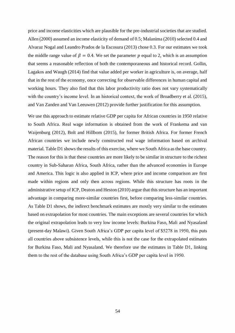
54

price and income elasticities which are plausible for the pre-industrial societies that are studied.

Allen (2000) assumed an income elasticity of demand of 0.5; Malanima (2010) selected 0.4 and

Alvaraz Nogal and Leandro Prados de la Escosura (2013) chose 0.3. For our estimates we took

the middle range value of 𝛽 = 0.4. We set the parameter 𝑝 equal to 2, which is an assumption

that seems a reasonable reflection of both the contemporaneous and historical record. Gollin,

Lagakos and Waugh (2014) find that value added per worker in agriculture is, on average, half

that in the rest of the economy, once correcting for observable differences in human capital and

working hours. They also find that this labor productivity ratio does not vary systematically

with the country’s income level. In an historical context, the work of Broadberry et al. (2015),

and Van Zanden and Van Leeuwen (2012) provide further justification for this assumption.

We use this approach to estimate relative GDP per capita for African countries in 1950 relative

to South Africa. Real wage information is obtained from the work of Frankema and van

Waijenburg (2012), Bolt and Hillbom (2015), for former British Africa. For former French

African countries we include newly constructed real wage information based on archival

material. Table D1 shows the results of this exercise, where we South Africa as the base country.

The reason for this is that these countries are more likely to be similar in structure to the richest

country in Sub-Saharan Africa, South Africa, rather than the advanced economies in Europe

and America. This logic is also applied in ICP, where price and income comparison are first

made within regions and only then across regions. While this structure has roots in the

administrative setup of ICP, Deaton and Heston (2010) argue that this structure has an important

advantage in comparing more-similar countries first, before comparing less-similar countries.

As Table D1 shows, the indirect benchmark estimates are mostly very similar to the estimates

based on extrapolation for most countries. The main exceptions are several countries for which

the original extrapolation leads to very low income levels: Burkina Faso, Mali and Nyasaland

(present-day Malawi). Given South Africa’s GDP per capita level of $5278 in 1950, this puts

all countries above subsistence levels, while this is not the case for the extrapolated estimates

for Burkina Faso, Mali and Nyasaland. We therefore use the estimates in Table D1, linking

them to the rest of the database using South Africa’s GDP per capita level in 1950.

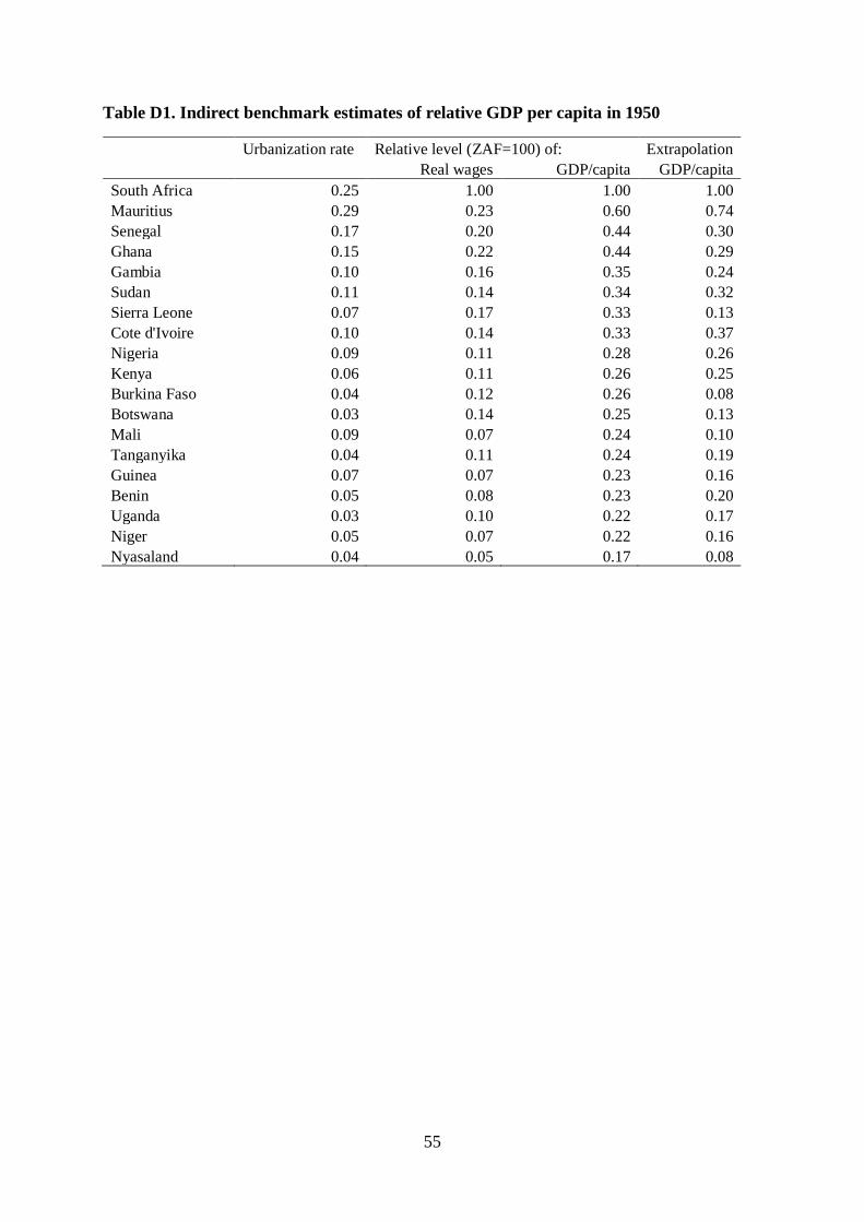
55

Table D1. Indirect benchmark estimates of relative GDP per capita in 1950

Urbanization rate Relative level (ZAF=100) of: Extrapolation

Real wages GDP/capita GDP/capita

South Africa 0.25 1.00 1.00 1.00

Mauritius 0.29 0.23 0.60 0.74

Senegal 0.17 0.20 0.44 0.30

Ghana 0.15 0.22 0.44 0.29

Gambia 0.10 0.16 0.35 0.24

Sudan 0.11 0.14 0.34 0.32

Sierra Leone 0.07 0.17 0.33 0.13

Cote d'Ivoire 0.10 0.14 0.33 0.37

Nigeria 0.09 0.11 0.28 0.26

Kenya 0.06 0.11 0.26 0.25

Burkina Faso 0.04 0.12 0.26 0.08

Botswana 0.03 0.14 0.25 0.13

Mali 0.09 0.07 0.24 0.10

Tanganyika 0.04 0.11 0.24 0.19

Guinea 0.07 0.07 0.23 0.16

Benin 0.05 0.08 0.23 0.20

Uganda 0.03 0.10 0.22 0.17

Niger 0.05 0.07 0.22 0.16

Nyasaland 0.04 0.05 0.17 0.08

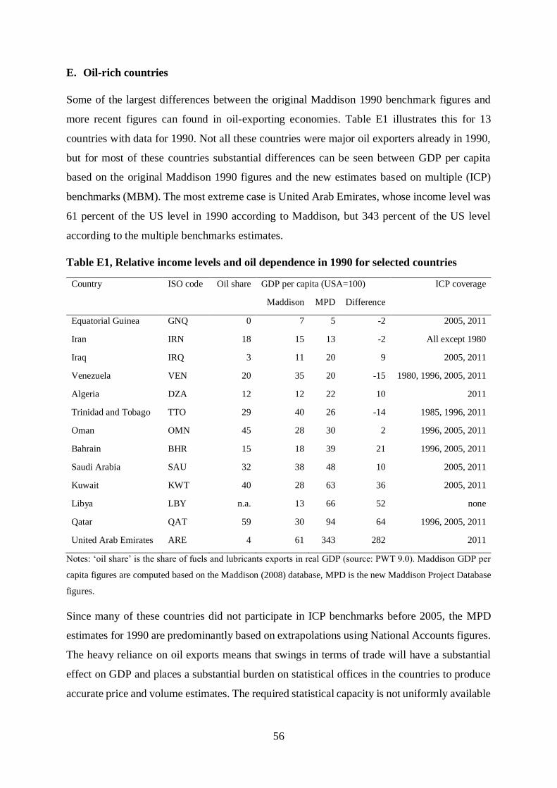
56

E. Oil-rich countries

Some of the largest differences between the original Maddison 1990 benchmark figures and

more recent figures can found in oil-exporting economies. Table E1 illustrates this for 13

countries with data for 1990. Not all these countries were major oil exporters already in 1990,

but for most of these countries substantial differences can be seen between GDP per capita

based on the original Maddison 1990 figures and the new estimates based on multiple (ICP)

benchmarks (MBM). The most extreme case is United Arab Emirates, whose income level was

61 percent of the US level in 1990 according to Maddison, but 343 percent of the US level

according to the multiple benchmarks estimates.

Table E1, Relative income levels and oil dependence in 1990 for selected countries

Country ISO code Oil share GDP per capita (USA=100) ICP coverage

Maddison MPD Difference

Equatorial Guinea GNQ 0 7 5 -2 2005, 2011

Iran IRN 18 15 13 -2 All except 1980

Iraq IRQ 3 11 20 9 2005, 2011

Venezuela VEN 20 35 20 -15 1980, 1996, 2005, 2011

Algeria DZA 12 12 22 10 2011

Trinidad and Tobago TTO 29 40 26 -14 1985, 1996, 2011

Oman OMN 45 28 30 2 1996, 2005, 2011

Bahrain BHR 15 18 39 21 1996, 2005, 2011

Saudi Arabia SAU 32 38 48 10 2005, 2011

Kuwait KWT 40 28 63 36 2005, 2011

Libya LBY n.a. 13 66 52 none

Qatar QAT 59 30 94 64 1996, 2005, 2011

United Arab Emirates ARE 4 61 343 282 2011

Notes: ‘oil share’ is the share of fuels and lubricants exports in real GDP (source: PWT 9.0). Maddison GDP per

capita figures are computed based on the Maddison (2008) database, MPD is the new Maddison Project Database

figures.

Since many of these countries did not participate in ICP benchmarks before 2005, the MPD

estimates for 1990 are predominantly based on extrapolations using National Accounts figures.

The heavy reliance on oil exports means that swings in terms of trade will have a substantial

effect on GDP and places a substantial burden on statistical offices in the countries to produce

accurate price and volume estimates. The required statistical capacity is not uniformly available

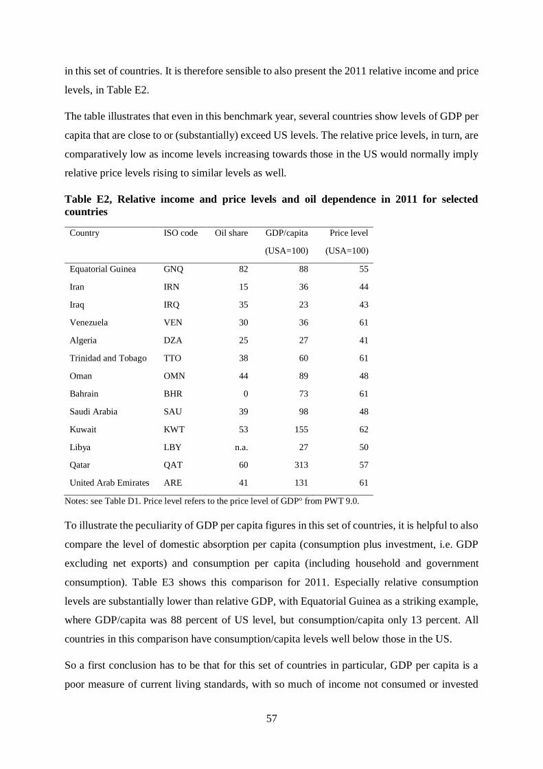
57

in this set of countries. It is therefore sensible to also present the 2011 relative income and price

levels, in Table E2.

The table illustrates that even in this benchmark year, several countries show levels of GDP per

capita that are close to or (substantially) exceed US levels. The relative price levels, in turn, are

comparatively low as income levels increasing towards those in the US would normally imply

relative price levels rising to similar levels as well.

Table E2, Relative income and price levels and oil dependence in 2011 for selected

countries

Country ISO code Oil share GDP/capita Price level

(USA=100) (USA=100)

Equatorial Guinea GNQ 82 88 55

Iran IRN 15 36 44

Iraq IRQ 35 23 43

Venezuela VEN 30 36 61

Algeria DZA 25 27 41

Trinidad and Tobago TTO 38 60 61

Oman OMN 44 89 48

Bahrain BHR 0 73 61

Saudi Arabia SAU 39 98 48

Kuwait KWT 53 155 62

Libya LBY n.a. 27 50

Qatar QAT 60 313 57

United Arab Emirates ARE 41 131 61

Notes: see Table D1. Price level refers to the price level of GDPo from PWT 9.0.

To illustrate the peculiarity of GDP per capita figures in this set of countries, it is helpful to also

compare the level of domestic absorption per capita (consumption plus investment, i.e. GDP

excluding net exports) and consumption per capita (including household and government

consumption). Table E3 shows this comparison for 2011. Especially relative consumption

levels are substantially lower than relative GDP, with Equatorial Guinea as a striking example,

where GDP/capita was 88 percent of US level, but consumption/capita only 13 percent. All

countries in this comparison have consumption/capita levels well below those in the US.

So a first conclusion has to be that for this set of countries in particular, GDP per capita is a

poor measure of current living standards, with so much of income not consumed or invested

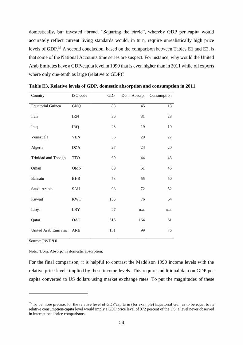
58

domestically, but invested abroad. “Squaring the circle”, whereby GDP per capita would

accurately reflect current living standards would, in turn, require unrealistically high price

levels of GDP.35 A second conclusion, based on the comparison between Tables E1 and E2, is

that some of the National Accounts time series are suspect. For instance, why would the United

Arab Emirates have a GDP/capita level in 1990 that is even higher than in 2011 while oil exports

where only one-tenth as large (relative to GDP)?

Table E3, Relative levels of GDP, domestic absorption and consumption in 2011

Country ISO code GDP Dom. Absorp. Consumption

Equatorial Guinea GNQ 88 45 13

Iran IRN 36 31 28

Iraq IRQ 23 19 19

Venezuela VEN 36 29 27

Algeria DZA 27 23 20

Trinidad and Tobago TTO 60 44 43

Oman OMN 89 61 46

Bahrain BHR 73 55 50

Saudi Arabia SAU 98 72 52

Kuwait KWT 155 76 64

Libya LBY 27 n.a. n.a.

Qatar QAT 313 164 61

United Arab Emirates ARE 131 99 76

Source: PWT 9.0

Note: 'Dom. Absorp.’ is domestic absorption.

For the final comparison, it is helpful to contrast the Maddison 1990 income levels with the

relative price levels implied by these income levels. This requires additional data on GDP per

capita converted to US dollars using market exchange rates. To put the magnitudes of these

35 To be more precise: for the relative level of GDP/capita in (for example) Equatorial Guinea to be equal to its

relative consumption/capita level would imply a GDP price level of 372 percent of the US, a level never observed

in international price comparisons.

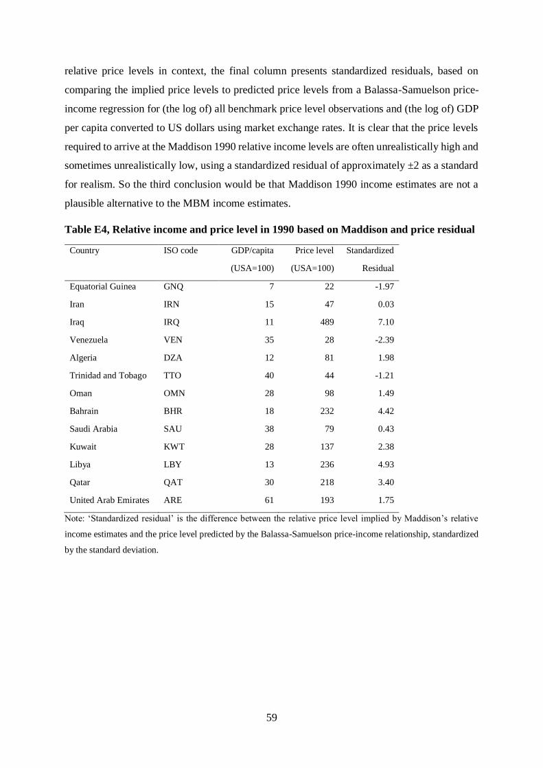
59

relative price levels in context, the final column presents standardized residuals, based on

comparing the implied price levels to predicted price levels from a Balassa-Samuelson price-

income regression for (the log of) all benchmark price level observations and (the log of) GDP

per capita converted to US dollars using market exchange rates. It is clear that the price levels

required to arrive at the Maddison 1990 relative income levels are often unrealistically high and

sometimes unrealistically low, using a standardized residual of approximately ±2 as a standard

for realism. So the third conclusion would be that Maddison 1990 income estimates are not a

plausible alternative to the MBM income estimates.

Table E4, Relative income and price level in 1990 based on Maddison and price residual

Country ISO code GDP/capita Price level Standardized

(USA=100) (USA=100) Residual

Equatorial Guinea GNQ 7 22 -1.97

Iran IRN 15 47 0.03

Iraq IRQ 11 489 7.10

Venezuela VEN 35 28 -2.39

Algeria DZA 12 81 1.98

Trinidad and Tobago TTO 40 44 -1.21

Oman OMN 28 98 1.49

Bahrain BHR 18 232 4.42

Saudi Arabia SAU 38 79 0.43

Kuwait KWT 28 137 2.38

Libya LBY 13 236 4.93

Qatar QAT 30 218 3.40

United Arab Emirates ARE 61 193 1.75

Note: ‘Standardized residual’ is the difference between the relative price level implied by Maddison’s relative

income estimates and the price level predicted by the Balassa-Samuelson price-income relationship, standardized

by the standard deviation.

60

References

Aghion, P., U. Akcigit and P. Howitt (2014), “What do we learn from Schumpeterian growth

theory?” In: Aghion, Philippe, Durlauf, Steven (Eds.), Handbook of Economic Growth,

Vol. 2, 515–563.

Arroyo Abad, L., E. Davies and J. L. van Zanden (2012), “Between conquest and independence:

real wages and demographic changes in Spanish America, 1530–1820” Explorations in

Economic History 49(2): 149–166.

Allen, R.C. (2001), “The great divergence in European wages and prices from the Middle Ages

to the First World War” Explorations in Economic History, 38(4), pp. 411–447.

Allen R.C., J.P. Bassino, D. Ma, C. Moll-Murata and J.L. van Zanden (2011), “Wages, Prices,

and Livings Standards in China, Japan, and Europe, 1738-1925” Economic History

Review 64(1): 8–38.

Arroyo Abad, L. and J.L. van Zanden (2016), “Growth under Extractive Institutions? Latin

American Per Capita GDP in Colonial Times” Journal of Economic History 76(4): 1182–

1215.

Balk, Bert M (2008), Price and Quantity Index Numbers: Models for Measuring Aggregate

Change and Difference Cambridge, UK: Cambridge University Press.

Barro, R.J. and J.F. Ursua, (2008). “Macroeconomic Crises since 1870” Brookings Papers on

Economic Activity, Economic Studies Program, The Brookings Institution, vol. 39(1

(Spring), pages 255-350

Barro, R.J. (2015). “Convergence and modernization” Economic Journal 125: 911–942.

Bergson, A. (1972). The Comparative National Income of the USSR and the United States,

NBER, http://www.nber.org/chapters/c5095, pp. 145-224

Bèrtola, L. and Ocampo, J. A., (2012). The economic development of Latin America since

independence (Oxford: Oxford University Press).

Bertola, L. (2016). El PIB per Capita de Uruguay 1870 - 2016: una reconstruccion. PHES

working paper No 48

Bolt, J. and J. L. van Zanden (2014), ”The Maddison Project: collaborative research on

historical national accounts” Economic History Review, 67 (3): 627–651.

Braithwaite, S.N. (1968), “Real income levels in Latin America” Review of Income and Wealth

14(2): 113–182.

Broadberry, S.N. (1998), “How Did the United States and Germany Overtake Britain? A

Sectoral Analysis of Comparative Productivity Levels, 1870-1990” Journal of Economic

History 58(2): 375-407.

61

Broadberrry, S.N. (2003), “Relative per capita Income Levels in the United Kingdom and the

United States since 1870: Reconciling Time Series Projections and Direct Benchmark

Estimates” Journal of Economic History, 63: 852-863

Broadberry, S.N. (2006), Market Services and the Productivity Race, 1850-2000: Britain in

International Perspective. Cambridge: Cambridge University Press.

Broadberry, S. and B. Gupta, (2010). “The historical roots of India’s service-led development:

A sectoral analysis of Anglo-Indian productivity differences, 1870–2000” Explorations

in Economic History 47(3): 264–278.

Broadberry, S.N., Custodis, J. and Gupta, B. (2015), “India and the great divergence: an Anglo-

Indian comparison of GDP per capita, 1600–1871” Explorations in Economic History,

55: 58-75.

Broadberry, S.N., B. Campbell, A. Klein, M. Overton and B. van Leeuwen (2015), British

Economic Growth 1270-1870 Cambridge: Cambridge University Press.

Broadberry, S.N., H. Guan and D.D. Li (2017), “China, Europe and the great divergence: a

study in historical national accounting, 980–1850” unpublished manuscript.

Broadberry, S.N. and J.J. Wallis (2017), “Growing, shrinking, and long run economic

performance: historical perspectives on economic development” NBER Working Paper,

no. 23343.

Burstein, Ariel and Gita Gopinath (2014), “International prices and exchange rates” In Gita

Gopinath, Elhanan Helpman, and Kenneth Rogoff (eds.), Handbook of International

Economics, Vol. IV, pp. 391–451. Amsterdam: Elsevier.

Caselli, F. (2005), “Accounting for cross-country income differences” in Phillipe Aghion and

Steven N. Durlauf (eds.) Handbook of Economic Growth, Volume 1A, Elsevier: 679-741

Cavallo, A. (2013), “Online and official price indexes: measuring Argentina’s inflation”

Journal of Monetary Economics 60: 152–165.

Ciccone, A. and M. Jarociński (2010), “Determinants of Economic Growth: Will Data Tell?”

American Economic Journal: Macroeconomics 2(4): 226–246.

Chen, S. and M. Ravallion (2001), “How Did the World’s Poor Fare in the 1990s?” Review of

Income and Wealth 47(3): 283–300.

Clark, C. (1957), The Conditions of Economic Progress. London: MacMillan & Co. Ltd

De Corso, G. (2013). El crecimiento economico de Venuzuela, Desde la Oligarquia

Conservadora Hasta La Revolucion Bolivariana: 1830-2012. Uno Vision cuantitativa *:

Venezuelan Economic Growth From The Conservative Oligarchy To The Bolivarian

62

Revolution (1830-2012), Revista De Historia Económica / Journal of Iberian and Latin

American Economic History, 31(3), 321-357. doi:10.1017/S0212610913000190

De Corso, G. and S. Kalmanovitz (2016). Una estimación del PIB de Panamá: 1906-1945,

Tiempo&Economía 3 (1).

Deaton, A. (2010) “Price indexes, inequality, and the measurement of world poverty” American

Economic Review100(1): 5–34.

Deaton, A. and Aten, B. (2017). ‘Trying to Understand the PPPs in ICP 2011: Why Are the

Results So Different?’ American Economic Journal: Macroeconomics 9(1).

Deaton, A. and Heston, A. (2010), ‘Understanding PPPs and PPP-based National Accounts’

American Economic Journal: Macroeconomics, 2: 1–35.

Díaz, J.B. Lüders, R. and Wagner, G. (2007) Economia Chilena 1810 - 2000, Producto total y

sectorial una nueva mirada, Pontificia universidad Catolica de Chile, Insituto de

Economia, Documeno de Trabajo no. 315

Diewert, W.E. (1976) “Exact and Superlative Index Numbers.” Journal of Econometrics 4 (2):

115–45.

Eloranta, J., Voutilainen, M. and Nummela, I. (2016). “Estimating Finnish Economic Growth

Before 1860” mimeo.

Feenstra, R.C., H. Ma, J.P. Neary and D.S.P. Rao (2013) “Who Shrunk China? Puzzles in the

Measurement of Real GDP” Economic Journal 123(573): 1100–1129.

Feenstra, R.C., R. Inklaar and M.P. Timmer, (2015), “The Next Generation of the Penn World

Table” American Economic Review 105(10).

Ferreira, F.H.G., S. Chen, A. Dabalen, Y. Dikhanov, N. Hamadeh, D. Jolliffe, A. Narayan, E.

Beer Prydz, A. Revenga, P. Sangraula, U. Serajuddin and N. Yoshida (2015), “A global

count of the extreme poor in 2012. Data issues, methodology and initial results” World

Bank Policy Research Working Paper, no. 7432.

Fourie, J. and Van Zanden, J.L. (2013). GDP in the Dutch Cape Colony: the Nationals Accounts

of a Slave-Based Society, South African Journal of Economics, vol. 81 (4): 467 – 490

Frankema, E., P. Woltjer and J.P. Smits (2013). Changing Economic Leadership, a new

benchmark of sector productivity in the United States and Western Europe, ca. 1910,

Tijdschrift voor Sociale en Economische Geschiedenis (The low countries social and


Fremdling, R., Productivity comparison between Great Britain and Germany, 1855–1913,

Scandinavian Economic History Review 39 (1), 28-42

63

Fukao, K., D. Ma, and T. Yuan (2007) “Real GDP in pre-war East Asia: a 1934–36 benchmark

purchasing power parity comparison with the U.S” Review of Income and Wealth, 53(3):

503–537.

Gallardo-Albarrán, D. (2017), “Missed opportunities? The development of human welfare in

Western Europe, 1913-1950” GGDC Research Memorandum no. 166.

Grytten, O.H. (2015). “Norwegian Gross Domestic Product by industry 1830 – 1930” Norges

Bank Working paper no. 19.

Hassan, F. (2016), ‘The Price of Development: the Penn-Balassa-Samuelson effect

revisited’ Journal of International Economics, 102: 291–309.

Henderson, J.V., A. Storeygard and D.N. Weil (2012), “Measuring economic growth from outer

space” American Economic Review 102(2): 994–1028.

Herranz-Loncán, A. and Peres-Cajías (2016). “Bolivian GDP per capita since the mid-

nineteenth century” Cliometrica 10: 99-128

Heston, A. (2010), “What can be learned about the Economies of China and India from

Purchasing Power Comparisons”, in Barry Eichengreen, Poonam Gupta and Rajiv

Kumar, eds, Emerging Giants, China and India in the World Economy, Cambridge

University Press, pp. 3-31.

Heston, A. and R. Summers, 1980. Comparative Indian Economic Growth: 1870 to 1970,

American Economic Review, vol. 70 (2), pages 96-101

Hsieh, C.-T. and P.J. Klenow (2010), “Development Accounting” American Economic

Journal: Macroeconomics 2(1): 207–223.

Inklaar, R. and D.S.P. Rao (2017). ‘Cross-Country Income Levels over Time: Did the

Developing World Suddenly Become Much Richer?’ American Economic Journal:

Macroeconomics 9(1): 265–290.

Irwin, Douglas A., (2005) “The Welfare Cost of Autarky: Evidence from the Jeffersonian Trade

Embargo, 1807–09” Review of International Economics 13, 631–645.

Jerven, M. (2013), “Comparability of GDP estimates in Sub-Saharan Africa: the effect of

revisions in sources and methods since structural adjustment” Review of Income and

Wealth 69(S1): S16–S36.

Johnson S., W. Larson, C. Papageorgiou and A. Subramanian (2013), “Is newer better? Penn

World Table Revisions and their impact on growth estimates” Journal of Monetary

Economics 60(2), 255-274.

Jones, C.I. and P.J. Klenow (2016), “Beyond GDP? Welfare across countries and time”

American Economic Review 106(9): 2426–2457.

64

Klasing, M. J. and Milionis, P. (2014). "Quantifying the evolution of world trade, 1870–1949,"

Journal of International Economics 92(1): 185-197.

Krantz, O. (2017) “Swedish GDP 1300-1560 A Tentative Estimate” Lund Papers in Economic

History: General Issues; No. 152.

Kravis, I.B., and R.E. Lipsey (1991) “The International Comparison Program: Current Status

and Problems”, in P.E. Hooper and J.D. Richardson, International Economic

Transactions: Issues in Measurement and Empirical Research, Chicago, University of

Chicago Press.

Kravis, I.B., R. Summers and A. Heston (1982), “Comments on: ‘Selected Problems of the

Intercountry Comparisons on the Basis of the Experience of the EEC.’” Review of Income

and Wealth 28(4): 407-10.

Lee, Jong-Wha and Hanol Lee (2016), “Human Capital in the Long Run,” Journal of

Development Economics, vol. 122, pp. 147-169.

Li, B. and J.L. van Zanden (2012). ‘Before the Great Divergence? Comparing the Yangzi Delta

and the Netherlands at the Beginning of the Nineteenth Century’, The Journal of

Economic History 72 (4) (2012) 956-989.

Lindert, P.H. and J.G. Williamson (2016), Unequal gains. American growth and inequality

since 1700, Princeton University Press: Princeton.

Ma, Y. and H.J. de Jong (2017), “Unfolding the turbulent century: a reconstruction of China’s

historical national accounts, 1840–1912” Review of Income and Wealth forthcoming.

Maddison, A. (1982), Phases of Capitalist Development Oxford, Oxford University Press.

Maddison, A. (1991), Dynamic Forces in Capitalist Development. A Long-Run Comparative

View Oxford: Oxford University Press.

Maddison, A. (1995), Monitoring the World Economy 1820–1992 Paris: Organisation for

Economic Cooperation and Development.

Maddison, A. (2001), The World Economy: a Millennial Perspective Paris: Organisation for


Maddison, A (2006), The World Economy: Historical Statistics Paris: Organisation for


Maddison , A. (2007), Contours of the World Economy, 1-2030 AD Oxford University Press.

Maddison, A. (2007a), Chinese Economic Performance in the Long Run, Second Edition,

Revised and Updated, 960-2030 AD, Paris, OECD Development Center.

Madsen, J.B. (2014), “Human capital and the world technology frontier” Review of Economics

and Statistics 96(4): 676–692.

65

Malanima, P. (2010), “The long decline of a leading economy: GDP in central and northern

Italy, 1300–1913” European Review of Economic History 15: 169–219.

Malinowski, M. and Van Zanden (2015), “National income and its distribution in preindustrial

Poland in a global perspective” EHES working paper no. 76.

Milanovic, Branko (2006), “An estimate of average income and inequality in Byzantium around

year 1000,” Review of Income and Wealth 52(3).

Neary, J.P. (2004), “Rationalizing the Penn World Table: True multilateral indices for

international comparisons of real income” American Economic Review 94(5): 1411–

1428.

O’Rourke, Kevin H. (2007), “War and Welfare: Britain, France and the United States, 1807–

14” Oxford Economic Papers 59: i8–i30.

Olinto Ramos, R., G. Pastor and L. Rivas (2008), “Latin America: Highlights from the

implementation of the System of National Accounts 1993 (1993 SNA)” IMF Working

Paper, no. WP/08/239.

Paige, D. and Bombach, G. (1959) A Comparison of National Output and Productivity of the

United Kingdom and the United States Paris: Organisation for European Economic Co-

operation.

Palma, N. and J. Reis (2016). From Convergence to Divergence: Portuguese Demography and

Economic Growth, 1500-1850. GGDC Research Memorandum 161

Pamuk, S. (2006), “Estimatinge conomic Growth in the Middle East since 1820” Journal of

Economic History, 66(3): 809–828.

Pamuk, S. (2009). “Estimating GDP per capita for the Ottoman Empire in a European

Comparative Framework, 1500-1820”, paper presented at the XVth World Economic

History Congress, August 2009, Utrecht.

Pamuk, Ş, & Shatzmiller, M. (2014). Plagues, Wages, and Economic Change in the Islamic

Middle East, 700–1500. The Journal of Economic History, 74(1), 196-229.

doi:10.1017/S0022050714000072

Pfister, Ulrich (2011). “Economic Growth in Germany 1500-1850” Paper presented at the

conference on quantifying long term economic development. Venice.

Prados de la Escosura, L. (2000), “International Comparisons of Real Product, 1820–1990”

Explorations in Economic History 37: 1–41.

Prados de la Escosura, L. (2016), “Mismeasuring long run growth: the bias from splicing

national accounts – the case of Spain” Cliometrica 10(3): 251–275.

66

Prados de la Escosura, L. (2017), Spanish Economic Growth, 1850-2015 (London: Palgrave

Macmillan)

Ravallion, Datt and van de Walle (1991), “Quantifying absolute poverty in the developing

world” Review of Income and Wealth 37(4).

Ren, R. (1997), China’s Economic Performance in International Perspective Paris:

Organisation for Economic Cooperation and Development.

Ridolfi, L. (2016) “The French economy in the longue durée. A study on real wages, working

days and economic performance from Louis IX to the Revolution (1250-1789)”

Dissertation IMT School for Advanced Studies, Lucca, available at http://e-

theses.imtlucca.it/211/1/Ridolfi_phdthesis.pdf

Rogoff, K. (1996), “The purchasing power parity puzzle” Journal of Economic Literature

34(2): 647–668.

Rostas, L. (1948), Comparative Productivity in British and American Industry Cambridge:

Cambridge University Press.

Samuelson, Paul A. 1994. “Facets of Balassa-Samuelson Thirty Years Later.” Review of

International Economics 2(3): 201–26.

Santamaria Garcia, A. (2005). Las Cuentas nacionales de Cuba, 1960 - 2005', mimeo

Scheidel, Walter, Steven Friesen (2009), “The Size of the Economy and the Distribution of

Income in the Roman Empire,” Journal of Roman Studies, 99, 61-91, 2009.

Schon, L., and O. Krantz (2015) “New Swedish Historical National Accounts since the 16th

Century in Constant and Current Prices” Lund Papers in Economic History no. 140.

Seminario, B. (2015). El Desarrallo de la Economía Peruana en la Era Moderna, Universidad

de Pacifico, Lima.

United Nations (1987), World Comparisons of Purchasing Power and Real Product for 1980.

Phase IV of the International Comparison Project. Part Two: Detailed Results for 60

countries, United Nations: New York.

Usher, D. (1963). The Thai National Income at United Kingom Prices. Bulletin of the Oxford

University Institute of Economics & Statistics, 25: 199–214.

Ward, M. and Devereux, J. (2003), “Measuring British Decline: Direct Versus Long-Span

Income Measures” Journal of Economic History 63: 826-851.

Ward, M. and Devereux, J. (2012), “The Road Not Taken: Pre-Revolutionary Cuban Living

Standards in Comparative Perspective” Journal of Economic History, 72(1): 104–132.

67

Ward, M. and Devereux, J. (2018). New Perspectives on Productivity and Living Standards in

the late 19th century. Maddison Project Working Papers, no. 9. Downloadable at

www.ggdc.net/maddison.

Woltjer, P.J. (2015) “Taking over: a new appraisal of the Anglo-American Productivity gap and

the nature of American economic leadership ca. 1910” Scandinavian Economic History

Review 63(3): 1–22.

World Bank (2014). Purchasing Power Parities and Real Expenditures of World Economies

Summary of Results and Findings of the 2011 International Comparison Program World

Bank: Washington DC.

Wu, Harry X. (2014), “China’s growth and productivity performance debate revisited –

Accounting for China’s sources of growth with a new data set” The Conference Board

Economics Program Working Paper Series EWP#14-01.

Xu, Y. Z. Shi, B. van Leeuwen, Y Ni, Z Zhang, and Y Ma, (2016) 'Chinese National Income,

ca. 1661-1933', Australian Economic History Review 57(3), 368–393.

Young, A. (2012), “The African Growth Miracle” Journal of Political Economy 120(4): 696–

739.

Zhang, Q. (2017), ‘The Balassa–Samuelson relationship: Services, manufacturing and product

quality’ Journal of International Economics 106: 55–82.

Zanden, van, J.L. (2003). 'Rich and Poor before the Industrial Revolution: a comparison

between Java and the Netherlands at the beginning of the 19th century', Explorations in

Economic History 40 (2003), 1-23.

Zanden, Jan Luiten van, and Bas van Leeuwen. “Persistent but not Consistent: The Growth of

National Income in Holland 1347-1807”. Explorations in Economic History 49 (2) (2012)

119-130.

http://www.ggdc.net/maddison

Documents

GGDC RESEARCH MEMORANDUM 174in the Penn World Table (Feenstra et al. 2015), we refer to this measure of real GDP per capita as . This variable is expressed in 2011 US dollars by correcting