Embed Size (px)
Citation preview
Gold-in-calcrete: A continental to profile scale study of regolith carbonates and
their association with gold mineralisation
Robert Charles Dart, B.AppSc (Hons)
Geology and Geophysics School of Earth and Environmental Sciences
The University of Adelaide
Thesis submitted as fulfilment of the requirements for the degree of Doctor of Philosophy in the Faculty of Science,
University of Adelaide
March 2009
1
Chapter 1
Introduction
1.1. Project overview Historically, mineral deposits were located by prospectors and geologists inspecting rock outcrops and recognising signs of visible ore. Today however, with the majority of these “easily” recognised deposits discovered, other methods have to be engaged. The realisation that techniques were required to search for concealed mineralisation beneath a mantle of regolith is not new. Mining and exploration companies had recognised the challenge as far back as the mid 1940s (Hawkes & Webb, 1962; Levinson, 1974). Geochemistry, the study of the distribution and concentration of elements in rocks, minerals, soils, vegetation, water, and atmosphere, is one discipline that has proven useful in locating buried mineral deposits, especially when applied in conjunction with geophysical techniques (e.g. Hawkes & Webb, 1962; Levinson, 1974; Joyce, 1984; Marjoribanks, 1997; Moon, 2006).
Since the early 1990s a new geochemical sampling medium has been implemented in Australia by exploration companies in their search for buried Au mineralisation. This medium is regolith carbonates, especially when in the indurated form commonly referred to as calcrete, a material that is abundant over large areas of semi-arid to arid southern Australia. The discovery of the Challenger Au deposit, South Australia, in 1995 was attributed to calcrete sampling (Bonwick, 1997). This initial success, which was possibly fortuitous due to the presence of near surface, in-situ mineralisation (Lintern & Sheard, 1999b), resulted in calcrete sampling becoming widely adopted by exploration companies (e.g. Ferris, 1998; Lintern, 2001; Chen et al., 2002).
Unfortunately, the rapid adoption of exploration using calcrete resulted in poorly constrained methodology, because of the lack of accepted procedures and underlying scientific processes. It is clear from ongoing sampling programs that the use and understanding of this medium requires refinement. Discussions on the sampling techniques and analysis of regolith carbonates are limited to only a few scientific papers (Anand et al., 1997; Lintern, 1997; Anand et al., 1998; Ferris, 1998; Hill et al., 1998c; Lintern & Butt, 1998b; McQueen et al., 1999; Morris & Flintoft, 1999; Lintern, 2001). The wide variety of regolith carbonate morphologies and more precise descriptions of what constitutes a “calcrete” requires descriptions of the nature of the sampling medium leading to interpretation of its origin. The lack of established sampling procedure and understanding of the sampling medium has resulted in a large analytical dataset of variable quality. This omission is a vital inconsistency between the above papers and is discussed further in Chapter 2.
Beyond these sampling problems there is little understanding as to why Au should be associated with regolith carbonates. Only a limited number of scientific papers discuss the subject (Ypma, 1991; Lintern & Butt, 1993; Gray & Lintern, 1994; Smee, 1998; Okujeni et al., 2005; Lintern et al., 2006).
The exploration industry is therefore spending millions of dollars on sampling and geochemical analyses without an understanding of the actual mechanisms responsible for the results. The industry then uses these data to define exploration targets and undertake
Introduction Chapter 1
2
expensive drilling programs. Not surprisingly the results to date have been equivocal, with several identified Au-in-calcrete anomalies proving to not coincide with underlying Au mineralisation (Lintern, 2002; Van Der Stelt et al., 2006).
The limited scientific research into the association between Au and regolith carbonates, and the high number of anomalous, and largely false, Au-in-calcrete areas being generated, required urgent attention. These requirements were the driving force for the research undertaken and presented in this thesis. The answers to the following questions are the aims of the work:
What methods may be utilised to assist in confirming that a Au-in-calcrete anomaly is representative of underlying mineralisation? Hence, how can a Au-in-calcrete anomaly be interpreted geologically?
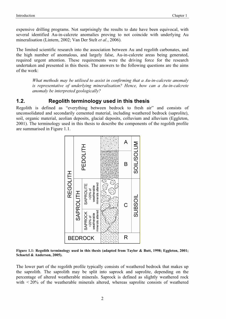
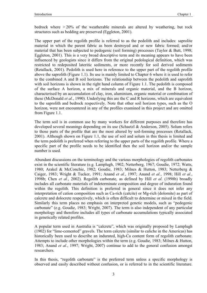
1.2. Regolith terminology used in this thesis Regolith is defined as “everything between bedrock to fresh air” and consists of unconsolidated and secondarily cemented material, including weathered bedrock (saprolite), soil, organic material, aeolian deposits, glacial deposits, colluvium and alluvium (Eggleton, 2001). The terminology used in this thesis to describe the components of the regolith profile are summarised in Figure 1.1.
Figure 1.1: Regolith terminology used in this thesis (adapted from Taylor & Butt, 1998; Eggleton, 2001; Schaetzl & Anderson, 2005).
The lower part of the regolith profile typically consists of weathered bedrock that makes up the saprolith. The saprolith may be split into saprock and saprolite, depending on the percentage of altered weatherable minerals. Saprock is defined as slightly weathered rock with < 20% of the weatherable minerals altered, whereas saprolite consists of weathered
Introduction Chapter 1
3
bedrock where > 20% of the weatherable minerals are altered by weathering, but rock structures such as bedding are preserved (Eggleton, 2001).
The upper part of the regolith profile is referred to as the pedolith and includes: saprolite material in which the parent fabric as been destroyed and or new fabric formed; and/or material that has been subjected to pedogenic (soil forming) processes (Taylor & Butt, 1998; Eggleton, 2001). This is a very broad descriptive term and its meaning appears to have been influenced by geologists since it differs from the original pedological definition, which was restricted to redeposited lateritic sediments, or more recently for soil derived sediments (Retallack, 2001). Pedolith is used here in reference to the upper part of the regolith profile above the saprolith (Figure 1.1). Its use is mainly limited to Chapter 6 where it is used to refer to the combined A and B soil horizons. The relationship between the pedolith and saprolith with soil horizons is shown in the right hand column of Figure 1.1. The pedolith is composed of the surface A horizon, a mix of minerals and organic material, and the B horizon, characterised by an accumulation of clay, iron, aluminium, organic material or combination of these (McDonald et al., 1990). Underlying this are the C and R horizons, which are equivalent to the saprolith and bedrock respectively. Note that other soil horizon types, such as the O horizon, were not encountered in any of the profiles examined in this project and are omitted from Figure 1.1.
The term soil is in common use by many workers for different purposes and therefore has developed several meanings depending on its use (Schaetzl & Anderson, 2005). Solum refers to those parts of the profile that are the most altered by soil-forming processes (Retallack, 2001). Although shown on Figure 1.1, the use of soil and solum in this thesis is limited and the term pedolith is preferred when referring to the upper parts of the regolith profile. Where a specific part of the profile needs to be identified then the soil horizon and/or the sample number is used.
Abundant discussions on the terminology and the various morphologies of regolith carbonates exist in the scientific literature (e.g. Lamplugh, 1902; Netterberg, 1967; Goudie, 1972; Watts, 1980; Arakel & McConchie, 1982; Goudie, 1983; Milnes & Hutton, 1983; Netterberg & Caiger, 1983; Wright & Tucker, 1991; Anand et al., 1997; Anand et al., 1998; Hill et al., 1998b; Chen et al., 2002). Regolith carbonate, as defined by Hill et al. (1998b) broadly includes all carbonate materials of indeterminate composition and degree of induration found within the regolith. This definition is preferred in general since it does not infer any interpretation of cation composition such as Ca-rich (calcite) or Mg-rich (dolomite) as part of calcrete and dolocrete respectively, which is often difficult to determine or mixed in the field. Similarly this term places no emphasis on interpreted genetic models, such as “pedogenic carbonate” (e.g. Goudie, 1983; Wright, 2007). The term is also independent of any particular morphology and therefore includes all types of carbonate accumulations typically associated in genetically related profiles.
A popular term used in Australia is “calcrete”, which was originally proposed by Lamplugh (1902) for “lime-cemented” gravels. The term calcrete (similar to caliche in the Americas) has historically been used to describe an indurated, high-Ca content form of regolith carbonate. Attempts to include other morphologies within the term (e.g. Goudie, 1983; Milnes & Hutton, 1983; Anand et al., 1997; Wright, 2007) continue to add to the general confusion amongst researchers.
In this thesis, “regolith carbonate” is the preferred term unless a specific morphology is observed and easily described without confusion, or is referred to in the scientific literature.
Introduction Chapter 1
4
The term “calcrete” is used in reference only to indurated (hardpan) regolith carbonates dominated by calcium carbonate. Hence calcrete can be considered a type of regolith carbonate, but a regolith carbonate is not synonymous with calcrete.
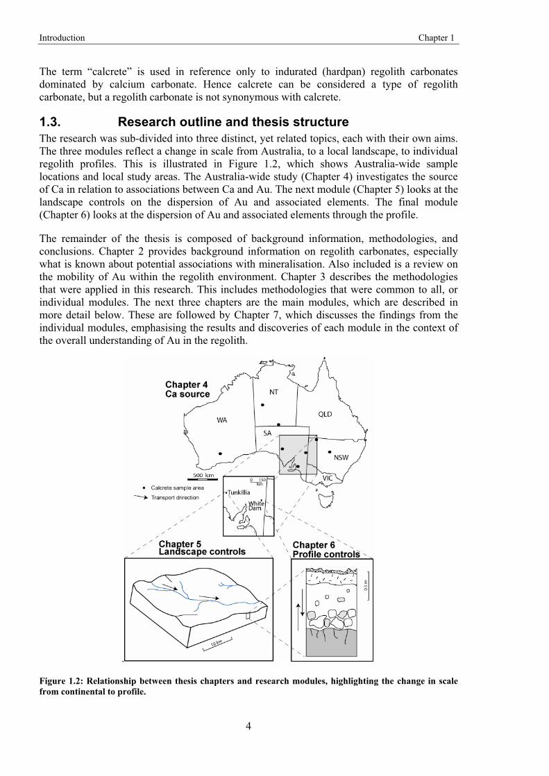
1.3. Research outline and thesis structure The research was sub-divided into three distinct, yet related topics, each with their own aims. The three modules reflect a change in scale from Australia, to a local landscape, to individual regolith profiles. This is illustrated in Figure 1.2, which shows Australia-wide sample locations and local study areas. The Australia-wide study (Chapter 4) investigates the source of Ca in relation to associations between Ca and Au. The next module (Chapter 5) looks at the landscape controls on the dispersion of Au and associated elements. The final module (Chapter 6) looks at the dispersion of Au and associated elements through the profile.
The remainder of the thesis is composed of background information, methodologies, and conclusions. Chapter 2 provides background information on regolith carbonates, especially what is known about potential associations with mineralisation. Also included is a review on the mobility of Au within the regolith environment. Chapter 3 describes the methodologies that were applied in this research. This includes methodologies that were common to all, or individual modules. The next three chapters are the main modules, which are described in more detail below. These are followed by Chapter 7, which discusses the findings from the individual modules, emphasising the results and discoveries of each module in the context of the overall understanding of Au in the regolith.
.
Figure 1.2: Relationship between thesis chapters and research modules, highlighting the change in scale from continental to profile.
Introduction Chapter 1
5
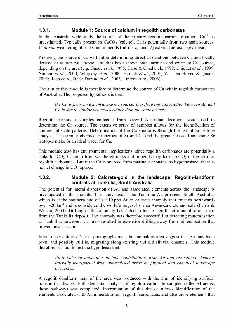
1.3.1. Module 1: Source of calcium in regolith carbonates In this Australia-wide study the source of the primary regolith carbonate cation, Ca2+, is investigated. Typically present as CaCO3 (calcite), Ca is potentially from two main sources: 1) in-situ weathering of rocks and minerals (intrinsic); and, 2) external aerosols (extrinsic).
Knowing the source of Ca will aid in determining direct associations between Ca and locally derived or in-situ Au. Previous studies have shown both intrinsic and extrinsic Ca sources, depending on the area (e.g. Quade et al., 1995; Capo & Chadwick, 1999; Chiquet et al., 1999; Naiman et al., 2000; Whipkey et al., 2000; Hamidi et al., 2001; Van Der Hoven & Quade, 2002; Rech et al., 2003; Durand et al., 2006; Lintern et al., 2006).
The aim of this module is therefore to determine the source of Ca within regolith carbonates of Australia. The proposed hypothesis is that:
the Ca is from an extrinsic marine source; therefore any association between Au and Ca is due to similar processes rather than the same process.
Regolith carbonate samples collected from several Australian locations were used to determine the Ca source. The extensive array of samples allows for the identification of continental-scale patterns. Determination of the Ca source is through the use of Sr isotope analysis. The similar chemical properties of Sr and Ca and the greater ease of analysing Sr isotopes make Sr an ideal tracer for Ca.
This module also has environmental implications, since regolith carbonates are potentially a sinks for CO2. Calcium from weathered rocks and minerals may lock up CO2 in the form of regolith carbonates. But if the Ca is sourced from marine carbonates as hypothesised, there is no net change in CO2 uptake.
1.3.2. Module 2: Calcrete-gold in the landscape: Regolith-landform controls at Tunkillia, South Australia
The potential for lateral dispersion of Au and associated elements across the landscape is investigated in this module. The study area is the Tunkillia Au prospect, South Australia, which is at the southern end of a > 10 ppb Au-in-calcrete anomaly that extends northwards over ~20 km2 and is considered the world’s largest by area Au-in-calcrete anomaly (Ferris & Wilson, 2004). Drilling of this anomaly has failed to locate significant mineralisation apart from the Tunkillia deposit. The anomaly was therefore successful in detecting mineralisation at Tunkillia; however, it as also resulted in extensive drilling away from mineralisation that proved unsuccessful.
Initial observations of aerial photographs over the anomalous area suggest that Au may have been, and possibly still is, migrating along existing and old alluvial channels. This module therefore sets out to test the hypothesis that:
Au-in-calcrete anomalies include contributions from Au and associated elements laterally transported from mineralised areas by physical and chemical landscape processes.
A regolith-landform map of the area was produced with the aim of identifying surficial transport pathways. Full elemental analysis of regolith carbonate samples collected across these pathways was completed. Interpretation of this dataset allows identification of the elements associated with Au mineralisation, regolith carbonates, and also those elements that
Introduction Chapter 1
6
are less mobile within the regolith environment. These elements may then be used to assist in interpreting the significance of other Au-in-calcrete anomalies.
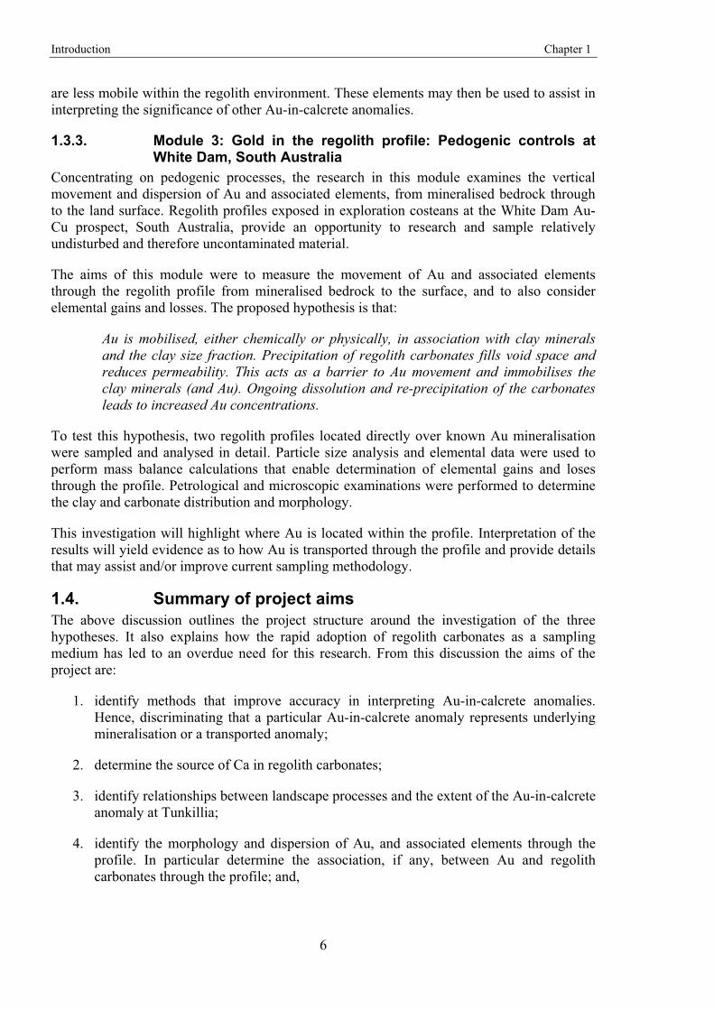
1.3.3. Module 3: Gold in the regolith profile: Pedogenic controls at White Dam, South Australia
Concentrating on pedogenic processes, the research in this module examines the vertical movement and dispersion of Au and associated elements, from mineralised bedrock through to the land surface. Regolith profiles exposed in exploration costeans at the White Dam Au-Cu prospect, South Australia, provide an opportunity to research and sample relatively undisturbed and therefore uncontaminated material.
The aims of this module were to measure the movement of Au and associated elements through the regolith profile from mineralised bedrock to the surface, and to also consider elemental gains and losses. The proposed hypothesis is that:
Au is mobilised, either chemically or physically, in association with clay minerals and the clay size fraction. Precipitation of regolith carbonates fills void space and reduces permeability. This acts as a barrier to Au movement and immobilises the clay minerals (and Au). Ongoing dissolution and re-precipitation of the carbonates leads to increased Au concentrations.
To test this hypothesis, two regolith profiles located directly over known Au mineralisation were sampled and analysed in detail. Particle size analysis and elemental data were used to perform mass balance calculations that enable determination of elemental gains and loses through the profile. Petrological and microscopic examinations were performed to determine the clay and carbonate distribution and morphology.
This investigation will highlight where Au is located within the profile. Interpretation of the results will yield evidence as to how Au is transported through the profile and provide details that may assist and/or improve current sampling methodology.
1.4. Summary of project aims The above discussion outlines the project structure around the investigation of the three hypotheses. It also explains how the rapid adoption of regolith carbonates as a sampling medium has led to an overdue need for this research. From this discussion the aims of the project are:
1. identify methods that improve accuracy in interpreting Au-in-calcrete anomalies. Hence, discriminating that a particular Au-in-calcrete anomaly represents underlying mineralisation or a transported anomaly;
2. determine the source of Ca in regolith carbonates;
3. identify relationships between landscape processes and the extent of the Au-in-calcrete anomaly at Tunkillia;
4. identify the morphology and dispersion of Au, and associated elements through the profile. In particular determine the association, if any, between Au and regolith carbonates through the profile; and,

Introduction Chapter 1
7
5. propose a model that explains how a Au-in-calcrete anomaly can form over mineralised and barren bedrock.

Introduction Chapter 1
8
9
Chapter 2
Regolith carbonates and their use in mineral exploration
2.1. Introduction Regolith carbonates are abundant in arid and semi-arid regions where precipitation is less than evapotranspiration (Goudie, 1983). This extensive coverage of regolith carbonates has resulted in numerous scientific papers and reviews (e.g. Gile et al., 1966; Netterberg, 1967; Goudie, 1972; Watts, 1980; Hutton & Dixon, 1981; Arakel & McConchie, 1982; Goudie, 1983; Milnes & Hutton, 1983; Netterberg & Caiger, 1983; Wright & Tucker, 1991; Anand et al., 1997; Anand et al., 1998; Chen et al., 2002; Wright, 2007). These papers cover aspects of regolith carbonate formation, distribution, and morphology, but more importantly they have been completed by researchers from varied disciplines, including: pedology, geology, geomorphology, biology, and geochemistry (Wright, 2007). This explains the expansive and sometimes contradictory terminology of regolith carbonates, especially in relation to the various morphologies (see Section 1.2).
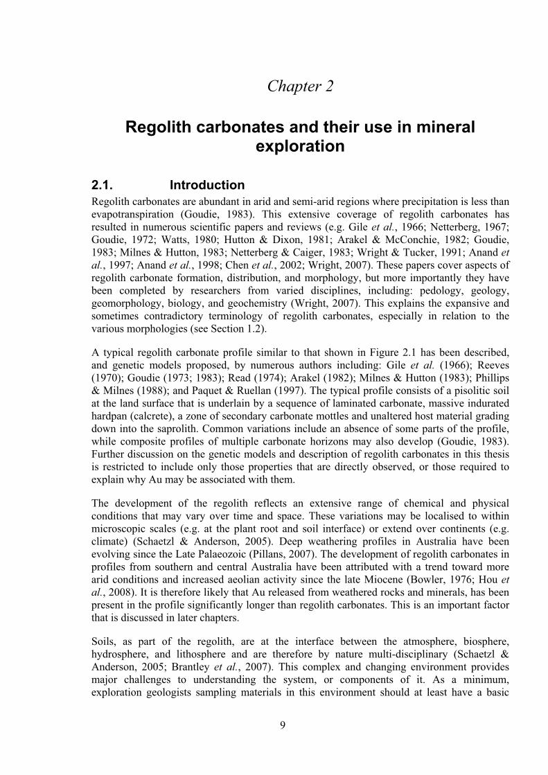
A typical regolith carbonate profile similar to that shown in Figure 2.1 has been described, and genetic models proposed, by numerous authors including: Gile et al. (1966); Reeves (1970); Goudie (1973; 1983); Read (1974); Arakel (1982); Milnes & Hutton (1983); Phillips & Milnes (1988); and Paquet & Ruellan (1997). The typical profile consists of a pisolitic soil at the land surface that is underlain by a sequence of laminated carbonate, massive indurated hardpan (calcrete), a zone of secondary carbonate mottles and unaltered host material grading down into the saprolith. Common variations include an absence of some parts of the profile, while composite profiles of multiple carbonate horizons may also develop (Goudie, 1983). Further discussion on the genetic models and description of regolith carbonates in this thesis is restricted to include only those properties that are directly observed, or those required to explain why Au may be associated with them.
The development of the regolith reflects an extensive range of chemical and physical conditions that may vary over time and space. These variations may be localised to within microscopic scales (e.g. at the plant root and soil interface) or extend over continents (e.g. climate) (Schaetzl & Anderson, 2005). Deep weathering profiles in Australia have been evolving since the Late Palaeozoic (Pillans, 2007). The development of regolith carbonates in profiles from southern and central Australia have been attributed with a trend toward more arid conditions and increased aeolian activity since the late Miocene (Bowler, 1976; Hou et al., 2008). It is therefore likely that Au released from weathered rocks and minerals, has been present in the profile significantly longer than regolith carbonates. This is an important factor that is discussed in later chapters.
Soils, as part of the regolith, are at the interface between the atmosphere, biosphere, hydrosphere, and lithosphere and are therefore by nature multi-disciplinary (Schaetzl & Anderson, 2005; Brantley et al., 2007). This complex and changing environment provides major challenges to understanding the system, or components of it. As a minimum, exploration geologists sampling materials in this environment should at least have a basic
Regolith carbonates in exploration Chapter 2
10
understanding of pedogenic processes, yet surprisingly most geologists know very little about soils (Levinson, 1974). It is a requirement that knowledge of pedogenic processes, as well as geology, are required to fully understand how Au is mobilised within the regolith (including soil) and to identify associations with regolith carbonates. Interactions also exist between biological processes and the regolith that will influence the Au-in-calcrete characteristics. A multidiscipline approach is therefore required. In this chapter, pedogenic, biological, landscape, and geological processes are reviewed in the context of Ca and Au mobility in the regolith.
Figure 2.1: Example of a regolith profile with many of the main regolith carbonate morphologies (roadside cutting near Sedan, South Australia, GDA Zone 54: 34886mE 6173045mN).
Regolith carbonates in exploration Chapter 2
11
In the near surface environment, Au is considered a rare element with an average abundance in soils of 4 ppb and a slight enrichment within the A (humic) horizon compared with other soil horizons (Boyle, 1979). Natural waters also contain measurable Au with a background range of < 0.001 – 0.005 ppb and an elevated anomalous range of 0.01 - 2.8 ppb in mineralised areas (McHugh, 1988). In the Atlantic Ocean, a high variation in Au concentration from 0.004 to 3.4 ppb was reported by Ryabinin et al. (1974). The main source of Au is mineralised bedrock, typically associated with quartz veining and sulphides (Levinson, 1974). Weathering of Au-bearing minerals and rocks releases Au into the regolith environment, which can result in an enriched halo that extends beyond the zone of mineralisation. This is reflected in enriched Au assays in soils from areas of mineralisation (Boyle, 1979). Regolith carbonates in Au mineralisation areas typically have high Au concentrations in Ca enriched soil horizons (Lintern & Butt, 1993; Lintern, 1997; Okujeni et al., 2005; Lintern et al., 2006).
The typically low Au concentration in the regolith is a significant challenge when trying to observe or measure Au geochemical processes. Early research investigating the properties of Au overcame this challenge by using higher Au concentrations in their experiments (Benedetti & Boulegue, 1991; Schoonen et al., 1992). It is possible that these higher Au concentrations affected the outcome of their experiments and led to interpretations that do not represent the natural environment. This problem still persists today, although some recent studies have started to experiment with lower concentrations that are more representative of the natural environment (e.g. Schoonen et al., 1992; Ran et al., 2002).
2.2. Regolith carbonate as a sampling medium Despite the many publications on regolith carbonates, there is a shortage of published research on their relationship with precious metals and exploration applications. The use of caliche (synonymous with calcrete) for exploration was first proposed by the Russians during the late 1950s (McGillis, 1967). McGillis (1967) investigated the presence of Ag in caliche in alluvial fans of the Basin and Range Province, Nevada, and detected anomalously high Ag content in samples from settings near mineralisation. This followed the discovery by Erickson et al. (1964) that caliche, sampled as part of a soil sampling survey of the area, contained high amounts of Ag. Other studies on calcrete in mineral exploration occurred during the 1970s, although these were more concerned about the material being a hindrance, rather than a useful exploration tool (Lintern, 2001). Exceptions are Cox (1975), Garnett et al. (1982) and Tordiffe et al. (1989).
Cox (1975) discussed the dispersion of nickel and copper sulphides in calcrete near Norseman, Western Australia and concluded that the analysis of Ni and Cr in the calcrete horizon can accurately define the boundaries of the underlying ultramafic bodies from the surrounding amphibolites, metasediments and pegmatite dykes. Garnett et al. (1982) investigated the distribution of base metals in calcrete over two sites of mineralisation in South Africa. They suggested that mineralisation could be detected by sampling the top of the calcrete, which returned element values that were equal to or higher than those in the overlying soil. To enhance the technique Garnett et al. (1982) suggested that the carbonate be leached prior to analysis, once again trying to remove the carbonate rather than actually using it. Tordiffe et al. (1989) discussed the distribution of ore-related elements in calcrete and soil above Cu-Ni mineralisation in Northern Cape Province, South Africa. They showed that both soil and calcrete samples geochemically expressed the underlying mineralisation. The calcrete however, had a narrow lateral dispersion pattern and also more elevated anomalous concentrations than the soil.
Regolith carbonates in exploration Chapter 2
12
These positive findings have not been repeated for all metals. Guedria et al. (1989) found that Pb and Zn were depleted within the calcrete horizons over mineralisation at Bou Grine, Tunisia, compared with anomalous geochemical signatures within non-carbonate soils.
Economic U mineralisation exists in association with calcretes in Western Australia (Arakel, 1988). The U is hosted in carnotite and is associated with phreatic (groundwater) calcretes that have formed along underground drainage pathways defined as valley, channel, or deltaic calcrete (Carlisle, 1983; Arakel, 1988).
The association between Au and regolith carbonates was first published by Smith & Keele (1984), who recognised that Au values were highest within the top metre of profiles containing 5 - 30% carbonate material and overlying mineralisation at Norseman, Western Australia. They did not associate this increase with the carbonate however, proposing instead that it was related to the vegetation. Smith & Keele (1984) conclude by saying that samples should be collected from a common in-situ material below the carbonate, further interpreting the calcrete as a hindrance to exploration.
Research into the use of calcrete as a sampling medium was undertaken in Australia by a joint Commonwealth Scientific and Industrial Research Organisation (CSIRO) (later replaced by Cooperative Research Centre for Landscape Environments and Mineral Exploration (CRC LEME)) and Australian Mineral Industries Research Association Ltd. (AMIRA) project based on improving geological, geochemical and geophysical techniques in locating blind or hidden Au deposits (Lintern, 2001). One of the first published references of a recognised Au-carbonate relationship was Lintern (1989). Lintern demonstrated a correlation between Au, CaO and MgO through a series of soil profiles at Mt. Hope, Western Australia (Figure 2.2). Similar Au – Ca correlations have since been reported by Lintern & Butt (1993; 1998b), Lintern (1997), Smee (1998), Lintern & Sheard (1999a), Okujeni et al. (2005), and Lintern et al. (2006). The majority of this research has been based in Australia with few similar accounts published from other countries. Exceptions to this include: Ypma (1991) who investigated Au in calcrete and its significance with Au-U mineralisation in the Eldorado Valley, Nevada, the Yilgarn, Western Australia, and Witwatersrand, South Africa; Smee (1998) who reported on soil Au anomalies from Marigold, Nevada; and, Okujeni et al. (2005) on Au-in-calcrete over Au mineralisation in the Kraaipan greenstone belt, South Africa.
Regolith carbonates cover approximately 21% of the Australian continent with maximum concentrations along a W-E trending broad belt inland from the Great Australian Bight (Figure 2.3) (Chen et al., 2002). It is this extensive coverage and also the ease with which regolith carbonates are identified that makes them such a significant sampling medium.
Figure 2.2: Plots of Ca, Mg and Au concentration v depth (Lintern, 1989).
NOTE: This figure is included on page 12 of the print copy of the thesis held in the University of Adelaide Library.
Regolith carbonates in exploration Chapter 2
13
Figure 2.3: Interpreted distribution of regolith carbonates in Australia, from Chen et al. (2002).
A trial of regolith carbonate sampling was undertaken in the Gawler Craton, South Australia by some Au exploration companies in the early 1990s (Lintern, 1997; Lintern & Butt, 1998b; Lintern, 2001; Chen et al., 2002). The discovery of the Challenger Au deposit, South Australia, was attributed to these trials (Bonwick, 1997). Challenger was initially located by a single anomalous Au-in-calcrete value of 180 ppb from a regional sampling program with 1.6 km sample grid spacing. Repeat sampling at 100 – 200 m spacing confirmed the anomaly, with one calcrete sample returning 620 ppb Au (Bonwick, 1997; Edgecombe, 1997). This now “successful” sampling medium was rapidly adopted amongst Australian exploration companies (Ferris, 1998; Lintern, 2001; Chen et al., 2002).
Understanding the effectiveness of regolith carbonate as a sampling medium is hampered by poor descriptions of morphology and composition. The limited scientific papers on the topic (Lintern, 1997; Ferris, 1998; Morris & Flintoft, 1999; Lintern, 2001) illustrate this. The actual material being sampled in these studies is poorly described and also of variable composition, including “friable, layered, calcareous horizon” (Morris & Flintoft, 1999) to calcareous sand, nodules and hardpan (Lintern, 2001). The papers of Lintern (1997) and Ferris (1998) simply use the term calcrete, which is assumed to be the hardpan variety and highlights the problem in poor terminology and description of regolith carbonates.
An apparent problem is in the collection of regolith carbonate samples. Effervescence from acid addition is generally used to determine if a sample is calcrete; however, the test is an indication that carbonate is present, not the amount or type (Doner & Grossl, 2002). A range of material may effervesce when HCl is added, yet the sample may consist of a lithic
NOTE: This figure is included on page 13 of the print copy of the thesis held in the University of Adelaide Library.
Regolith carbonates in exploration Chapter 2
14
fragment with a thin coating of carbonate material. Close examination of collected samples and also the inclusion of Ca in any elemental analysis can identify and therefore determine if the material is calcrete. An ongoing project by the South Australian Geological Survey (Primary Industries and Resources, South Australia (PIRSA)) to reanalyse donated and acquired calcrete samples has shown that 20% of the samples have < 5% Ca (Fidler, 2007). This potential discrepancy in sample type must be considered when comparing their geochemistry, especially when reviewing historical company data.
2.3. The regolith environment in relation to regolith carbonate and gold
Regolith carbonates used in geochemical sampling are typically collected from the upper parts of profiles. They are equivalent to the Bk soil horizon and have been referred to as “pedogenic carbonates” (e.g. Gile et al., 1966; Goudie, 1983; Dixon, 1998). Their formation is largely by precipitation in a zone of carbonate accumulation (Goudie, 1983), although this is a rather simplistic view. Regolith carbonates are likely to be polygenetic, resulting from various cycles of dissolution and precipitation controlled through a variety of physical, chemical and biological processes.
The soil is a major component of the regolith. It consists of unconsolidated minerals and organic substances that are subjected to and influenced by many physical, chemical, biological and morphological properties (Eggleton, 2001; Schaetzl & Anderson, 2005). Soil forming processes (pedogenesis) may act on materials derived from underlying bedrock or in transported materials (sediments), but the ultimate source materials are weathered rocks and minerals.
Igneous and metamorphic rocks are mostly formed at depth, under higher pressure and temperatures than found near the land surface. Most silicate minerals formed under these conditions are chemically unstable in the surface environment, where through weathering processes they are altered to produce dissolved compounds, and/or ionic species, and new clay minerals and oxides (Nahon, 1991; Blatt & Tracy, 1996; Schaetzl & Anderson, 2005). As weathering of rocks and minerals progresses, Au and other elements are released into the environment. Once released, Au mobility is controlled by physical, chemical and biological processes including: chemical dissolution and reprecipitation; uptake by plants to be redeposited when the plants die or through leaf litter; physical mobilisation by animals in bioturbation processes; and colluvial and alluvial movement.
Climatic conditions, particularly temperature and precipitation, are a major control on weathering rates, although they are not necessarily a prerequisite for specific styles of weathering products (Schaetzl & Anderson, 2005). For example, lateritic profiles have been attributed to seasonal tropical climatic settings (e.g. Freyssinet et al., 1990; Nahon & Tardy, 1992). But laterite may form under a variety of climatic conditions, showing that weathering continues at the surface regardless of climate (e.g. Bourman, 1993a; Taylor & Shirtliff, 2003).
The confusion and misinterpretation of laterites is similar to the problems for regolith carbonate researchers. They are also significant in this review because, supergene Au deposits have developed above and within primary mineralisation of lateritic profiles in Western Australia (Butt, 1987). Hence they are an example of Au-enrichment in the regolith. The use of the term “laterite” is reviewed by Bourman (1993b), Schaetzl & Anderson (2005) and Taylor (2006) who all suggest that the term causes confusion, due to variable and poor usage within the scientific literature. More constrained terms such as “ferricrete”, “lateritic
Regolith carbonates in exploration Chapter 2
15
duricrust” and “ferruginous gravel” have tended to replace the term “laterite”. Taylor (2006) suggests that “laterite” be reserved for profiles that consist of ferruginous or aluminous materials that progressively grade downwards through mottles to pallid and saprolite material. It has also been proposed that the term “laterite” be removed from wide use (Bourman, 1993b). The main point here is that no matter what terminology is used, the context of how the term is being used and what it is referring to must be adequately described to avoid confusion. Specific sample types and their related regolith-landform setting must be recorded to enable accurate geochemical interpretation of samples (Smith & Singh, 2007).
The sorption capabilities of different minerals and complexes on various Au complexes is significant in controlling Au concentration in soils (Schoonen et al., 1992). Different minerals and Au complexes have various sorption capabilities. For instance, a comparison study of the sorption ability of pyrite and goethite on Au – OH – Cl species showed that pyrite is better at scavenging Au (Schoonen et al., 1992). This confirmed the results of Jean & Bancroft (1985), where AuCl4
- was reduced to Au0 instantaneously upon adsorption to sulphides, whereas adsorption onto quartz and hematite was as AuCl2+ and/or AuCl2
+. Schoonen et al. (1992) suggested that the low sorption rate of goethite is possibly why visible Au can occur in laterites, since the sorption of dissolved Au onto already precipitated Au is favoured. Supporting evidence for this comes from Bamba et al. (2002), who describe small (< 5 μm) spherules of Ag-free Au precipitated onto the surface of primary Au particles, on grains at the top of the saprolite. This process can therefore contribute to the formation of a Au-enriched zone at the top of the saprolite.
Phyllosilicate minerals (layer-silicates, including clay minerals) have a major influence on the physical and chemical properties of the soil due to their small particle size, high surface area, and cation exchange properties (Schulze, 1989). The large surface area of clay minerals is negatively charged and needs to be balanced by nearby cations. Clay minerals have been shown to adsorb Au complexes and can be a method of Au accumulation within the regolith (Hong, 2000; Hong et al., 2003).
Biological activity from plants, animals and micro-organisms (biota) can have a major impact and controlling influence on the morphological, chemical and physical properties of the regolith. Most abundant (many million organisms per gram of soil) are the micro-organisms, which include bacteria, fungi, algae and protozoa (Schaetzl & Anderson, 2005). Micro-organisms assist with the decomposition of organic materials derived from animals and plants and produce many inorganic and organic compounds, including those in humus (McKenzie et al., 2004). Larger fauna, including the nematodes, arthropods, earthworms, and the larger mammals, birds and reptiles, tend to act as soil mixers, relocating the materials within the profile (Schaetzl & Anderson, 2005). The biota can both enhance and prevent the development of soil horizons depending on the conditions (Conklin, 2005; Schaetzl & Anderson, 2005). The biota is largely responsible for the development of the regolith and as such, it contributes to the formation of its geochemical characteristics (Gilkes, 1999).
Plants have evolved to survive in a wide range of conditions. Through their evolution they have developed various mechanisms enabling them to take up and host chemicals through their roots and to relocate them into the stems, twigs, foliage, bark, flowers and seeds as they grow (Dunn, 1995b). Since typically the highest density of micro-organisms occurs in the rhizosphere in relation to plant root activity (Gilkes, 1999), it is likely that the adsorption and uptake of Au by plants is from combined processes, rather than only root activity. Dunn (1995b) describes plants as a “sophisticated geochemical sampling device” that we do not yet fully understand.
Regolith carbonates in exploration Chapter 2
16
Organic matter is a minor component of the soil, typically < 5%, yet it has a major influence on its physical and chemical properties (McKenzie et al., 2004). It consists of all natural and biologically derived organic material within the soil, no matter what state it is in or its source (Baldock & Skjemstad, 1999) (Figure 2.4). Along with clay minerals, the surface of organic matter is typically negatively charged and plays an important role in attracting and retaining cations (known as the cation exchange capacity or CEC), the main cations being Ca, Mg, K and Na (McKenzie et al., 2004). Of particular interest are humic substances, which under suitable conditions may have a greater CEC than most clays (McKenzie et al., 2004).
Figure 2.4: Components of the soil organic matter from Baldock & Skjemstad (1999).
The humus consists of complex compounds that are amorphous and resistant to microbial action. Occurring as colloids they have a large surface area with variable charge (McKenzie et al., 2004; Conklin, 2005). Wood (1996) describes a humic substance as a mixture of ligands with numerous binding sites, rather than a single well defined complex.
Humus is released along with CO2, H2O, energy (mainly heat) and inorganic constituents (N, P and S) during the breakdown of fresh organic material (Conklin, 2005). The humus can be separated into fractions based on solubility, which mainly reflects variations in their molecular weight. For instance fulvic acid (FA) has a molecular weight of ~1,000 and is soluble in both acid and alkaline conditions, whereas humic acid (HA) has a molecular weight
NOTE: This figure is included on page 16 of the print copy of the thesis held in the University of Adelaide Library.
Regolith carbonates in exploration Chapter 2
17
> 10,000, is soluble in alkaline conditions and precipitated by acidification. The remaining insoluble and very heavy fraction is known as humin (Vlassopoulos et al., 1990; Wood, 1996; Conklin, 2005). The humus is a major component of the soil, with even minor amounts having an effect on soil CEC. The amount of organic matter in the regolith depends on the soil type and climate, ranging from rudimentary soils and some tropical African soils with less than 0.1% to organic-rich soils that have > 20% (Conklin, 2005).
Many organic complexes formed in the natural environment, including those related to organic soil (humic) and biological processes can form Au compounds. These compounds may be stable under normal conditions and increase the mobility of Au (Lakin et al., 1974; Puddephatt, 1978; Boyle, 1979; Gray et al., 1992; Cotton, 1997).
2.4. Calcium: Chemical, biological, and physical controls in the regolith
In order for a regolith carbonate in the form of calcite to form there has to be a source of Ca, which may be intrinsic and/or extrinsic, including aerosols, rocks, minerals, vegetation, groundwater and surface runoff (Goudie, 1983). Accumulation of Ca tends to be favoured in semi-arid to arid areas where evapotranspiration exceeds precipitation. Where precipitation exceeds evapotranspiration, Ca tends to be leached into solution (Goudie, 1983).
Using Sr isotopes as a tracer for Ca, several authors have shown a predominant external (marine) source for the Ca within regolith carbonates (Quade et al., 1995; Capo & Chadwick, 1999; Chiquet et al., 1999; Hamidi et al., 2001; Van Der Hoven & Quade, 2002; Lintern et al., 2006). Therefore, in these cases, any association between Ca (in regolith carbonates) and Au must to be due to processes that are favourable to the precipitation of both Ca and Au rather than any direct mineral or rock forming process.
The main chemical control on the transportation of Ca is carbonation where CO2 and water form weak H2CO3 (carbonic acid), which readily dissolves CaCO3 to produce Ca2+ and HCO3
– (bicarbonate) ions (Goudie, 1983):
CO2 + H2O � H2CO3 [2.1]
H2CO3 + CaCO3 � Ca2+ + 2HCO3– [2.2]
The formation of H2CO3 occurs in the atmosphere through the mixing of precipitation and atmospheric CO2, but is more prevalent within soil due to the higher concentrations of CO2 derived from soil fauna and plant root respiration (Schaetzl & Anderson, 2005). These weak acids dissolve CaCO3 particles that may have been deposited on the surface, and/or those already present within the profile to create Ca-rich solutions. These solutions transport Ca as they percolate through the profile. Equations 2.1 and 2.2 are reversible, hence environmental changes may result in precipitation of CaCO3 (calcification), or dissolution of CaCO3. Conditions that encourage precipitation are: decreasing water levels through evaporation and/or plant uptake; and/or changes in the availability of CO2 (pCO2 partial pressure); and/or increase in the pH level.
Biological activity has a major influence on the dissolution and precipitation of regolith carbonates. Evidence for this relationship is provided in microstructures that are dominated by biogenic features, classified as beta-type by Wright (1990). Several morphologies have been described and associated with biological activity, including: needle fibre calcite, rhizomorphs, microbial tubes, Microcodium, alveolar septal fabric, and calcified pellets (e.g. Knox, 1977;
Regolith carbonates in exploration Chapter 2
18
Klappa, 1978; 1980; Wright, 1986; Phillips et al., 1987; Phillips & Self, 1987; Jones, 1988; Bruand & Duval, 1999; Loisy et al., 1999). Alternatively, inorganic processes have been suggested for many of these structures (Gile et al., 1966; Solomon & Walkden, 1985).
Vegetation is a major part of the Ca cycle, especially within the rhizosphere (area immediately around the root) where interactions between roots and microbes, including symbiotic relationships, can control both the dissolution and precipitation of Ca. Plants require Ca as it adds strength to cell walls (Glass, 1989; White & Broadley, 2003). Nutrient ions, including Ca, are drawn toward roots through a mass convection system that is driven by evapotranspiration (Drew, 1990). The flow rates generated through this process may supply ions to the roots faster than they can be absorbed, which leads to a build up of excess ions around the roots (Drew, 1990). If Ca is included in the excess ions then it becomes available for calcification. As plants grow they are continually recycling Ca, which is released from decaying leaf litter, and eventually through the total decay of the plant when it dies.
Calcification can result in the creation of protons, which plants may then utilise to extract C from bicarbonate. This creates a 1:1 calcification to photosynthesis reaction that maintains or possibly elevates CO2 concentrations, despite CO2 uptake by the plants (McConnaughey & Whelan, 1997). This process is summarised in the following equations:
Calcification from bicarbonate to produce protons:
Ca2+ + HCO3- � CaCO3 + H+ [2.3]
Photosynthetic use of bicarbonate, which is unavailable without a source of protons, to produce formaldehyde:
H+ + HCO3- � CH2O- + O2 [2.4]
Equation 2.3 and 2.4 combined:
Ca2+ + 2HCO3- � CaCO3 + CH2O- + O2 [2.5]
Additionally, the generation of protons in equation 2.3 increases the acidity of the soil and promotes leaching of nutrients from soil minerals, which are then able to be absorbed by the plants (McConnaughey & Whelan, 1997). Similar photosynthetic reactions are used by cyanobacteria to precipitate CaCO3 at the cell surface and may result in the precipitation of concretions that form around nodules (Ehrlich, 1998).
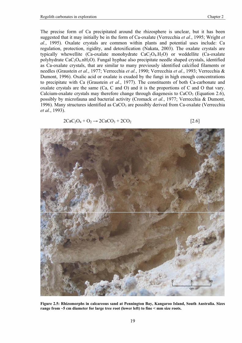
Rhizomorphs, or calcified root structures (Figure 2.5) are among the most prominent features of regolith carbonate accumulations (Jaillard et al., 1991; Wright et al., 1995). They are due to root activity and come in a variety of types that are defined by the amount and location of calcification within and around the root (Klappa, 1980). Calcification may occur within cells while the plant is alive, or prior to cell destruction of dead or dying roots (Wright et al., 1995). Calcified root cells have occasionally been termed Microcodium, but there has been significant debate on whether these microstructures have a root or bacterial origin (Klappa, 1978; Jaillard et al., 1991; Wright et al., 1995; Alonso-Zarza et al., 1998a; Kosir, 2004; Kabanov et al., 2008). External calcification around roots or within voids created after partial or total root decay forms the more typical, vertical tube-shaped, rhizolith structures. Calcification may also occur around root mats forming horizontal structures, possibly including laminar regolith carbonates (Wright et al., 1995; Alonso-Zarza, 1999; Kosir, 2004).
Regolith carbonates in exploration Chapter 2
19
The precise form of Ca precipitated around the rhizosphere is unclear, but it has been suggested that it may initially be in the form of Ca-oxalate (Verrecchia et al., 1995; Wright et al., 1995). Oxalate crystals are common within plants and potential uses include: Ca regulation, protection, rigidity, and detoxification (Nakata, 2003). The oxalate crystals are typically whewellite (Ca-oxalate monohydrate CaC2O4.H2O) or weddellite (Ca-oxalate polyhydrate CaC2O4.nH2O). Fungal hyphae also precipitate needle shaped crystals, identified as Ca-oxalate crystals, that are similar to many previously identified calcified filaments or needles (Graustein et al., 1977; Verrecchia et al., 1990; Verrecchia et al., 1993; Verrecchia & Dumont, 1996). Oxalic acid or oxalate is exuded by the fungi in high enough concentrations to precipitate with Ca (Graustein et al., 1977). The constituents of both Ca-carbonate and oxalate crystals are the same (Ca, C and O) and it is the proportions of C and O that vary. Calcium-oxalate crystals may therefore change through diagenesis to CaCO3 (Equation 2.6), possibly by microfauna and bacterial activity (Cromack et al., 1977; Verrecchia & Dumont, 1996). Many structures identified as CaCO3 are possibly derived from Ca-oxalate (Verrecchia et al., 1993).
2CaC2O4 + O2 � 2CaCO3 + 2CO2 [2.6]
Figure 2.5: Rhizomorphs in calcareous sand at Pennington Bay, Kangaroo Island, South Australia. Sizes range from ~5 cm diameter for large tree root (lower left) to fine < mm size roots.
Regolith carbonates in exploration Chapter 2
20
Microbes can dissolve or precipitate minerals in order to gain energy (Ehrlich, 1996; 1998). Bacteria, for example, have the potential to precipitate significant amounts of CaCO3 in the regolith (Loisy et al., 1999; Burford et al., 2006). They precipitate Ca through a variety of methods depending on whether they are autotrophic or heterotrophic (Castanier et al., 1999). In autotrophs the uptake of CO2 results in its depletion from the surrounding area, which leads to the precipitation of CaCO3. Heterotrophs can precipitate CaCO3 through active or passive processes, which may occur concurrently. Passive precipitation occurs in the surrounding medium due to changes in chemical properties caused by bacterial activity, whereas active precipitation is the result of direct ionic exchanges through the bacterial cell membranes (Castanier et al., 1999; Ledin, 2000).
2.5. Gold: Chemical, biological, and physical controls in the regolith
Within the soil, Au may exist as a native metal or as a minor component, bound to host minerals such as primary minerals, manganese and iron oxides, clays, and organic matter (humus) (Boyle, 1979). As a native metal, Au typically includes around 10% other metals, especially Ag, with which Au will form a complete solution series (Berman et al., 1978; Krupp & Weiser, 1992; Klein & Hurlbut, 1999). Trace amounts of Cu, Fe, Bi, Pb, Sn, Zn, and the platinum metals may also be present with Au (Klein & Hurlbut, 1999).
Despite the general belief that Au is an inert element, significant evidence demonstrates its mobilisation in the regolith, in particular economic deposits such as eluvial and placer deposits, and supergene enrichment (e.g. Puddephatt, 1978; Boyle, 1979; Gray & Lintern, 1998). The release of Au into the regolith is through weathering processes acting on host rocks. Deposits form from the accumulation of the Au, which is either due to its high density, and/or by dissolution and re-precipitation. An example is the supergene or lateritic Au enrichment haloes that are generally well developed within lateritic profiles above primary mineralisation in Western Australia (Butt, 1987; Taylor, 1990). Further evidence of Au mobilisation is in morphological and chemical differences between Au in the primary mineralisation and that in the regolith. This includes: delicate and fragile Au morphologies within high energy sediments; etching of Au grains and crystals; different (generally smaller) grain sizes than those in the underlying deposit; and a lower Ag content including Ag-depleted rims (Gray et al., 1992).
The solubility of Au in soils has been demonstrated through the use of selective extraction techniques. Using an extraction solution of 1 M sodium bicarbonate / 0.1 M potassium iodide, saturated with CO2 and adjusted to a pH of 7.4, Gray et al. (1998) demonstrated the variability in Au solubility for various soil types. They showed that saprolite has low Au solubility, whereas soils with high Fe-oxide content have moderate Au solubility with significant re-adsorption of any dissolved Au; Mn oxide and carbonate soils have high Au solubility; and organic-rich soils have a low Au solubility, possibly due to the re-adsorption of dissolved Au.
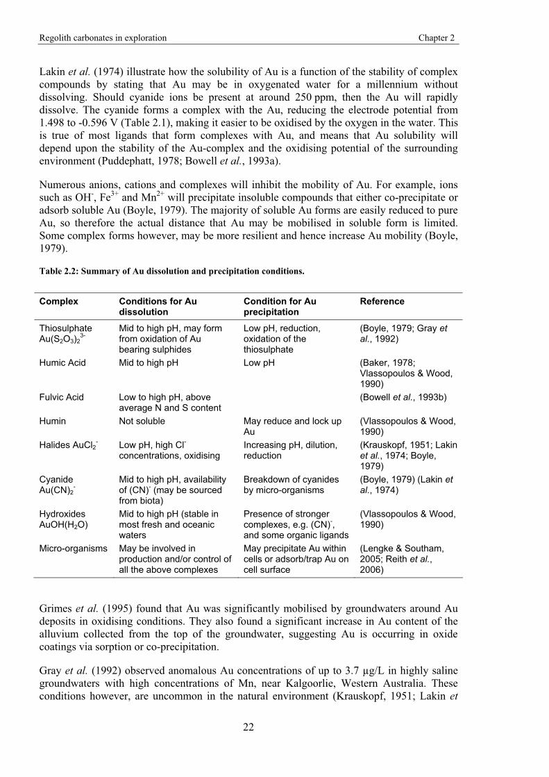
The primary oxidation states of Au are Au+ (aurus) and Au3+ (auric). Both of these states have electrode potentials above the H2 � H+ pair (Table 2.1) and are therefore reduced to pure Au rather than dissolved when in the presence of the H ion. Hence Au is insoluble by ordinary acids alone (Krauskopf, 1951).
In the presence of an oxidising agent and a strong ligand Au can be dissolved by halide or sulphide ions (Figure 2.6) (Puddephatt, 1978). Therefore, the mobility of Au in soil is largely
Regolith carbonates in exploration Chapter 2
21
dependent on the availability of complexing agents such as (S2O3)2-, (CN)- or excess Cl-, which will form soluble complexes of [Au(S2O3)]-, [Au(CN)2]- and [AuCl2]- (Boyle, 1979). In low pH environments, Au is normally more soluble due to the oxidation of sulphides (Boyle, 1979). The formation of AuCl2
- requires highly acidic, high Cl- concentration and oxidising conditions, as found in arid lateritic terrains (Krauskopf, 1951; Lakin et al., 1974; Mann, 1984). A summary of complexes and conditions that will result in the dissolution or precipitation of Au is provided in Table 2.2.
Figure 2.6: Gold interconversion cycle, adapted from Boyle (1979).
Table 2.1: Standard electrode potential of Au and selected compounds at 25�C (Dean 1992; Lide, 2004).
Half reaction Standard potential (V)
Au2+ + e- � Au+ 1.8 Au+ + e- � Au 1.692 Au3+ + 3e- � Au 1.498 Au(OH)3 + 3H+ + 3e- � Au + 3H2O 1.45 Au3+ + 2e- � Au+ 1.401 AuOH2+ + H+ + 2e � Au+ + H2O 1.32 AuCl2- + e- � Au + 2Cl- 1.15 AuCl4- + 3e- � Au + 4Cl- 1.002 AuBr2
- +e- � Au + 2Br- 0.959
AuBr4- + 3e- � Au + 4Br- 0.854
AuI2-+ e- � Au + 2I- 0.576 2H+ + 2e- � H2 0.000 Au(CN)2
- + e- � Au + 2CN- -0.596
NOTE: This figure is included on page 21 of the print copy of the thesis held in the University of Adelaide Library.
Regolith carbonates in exploration Chapter 2
22
Lakin et al. (1974) illustrate how the solubility of Au is a function of the stability of complex compounds by stating that Au may be in oxygenated water for a millennium without dissolving. Should cyanide ions be present at around 250 ppm, then the Au will rapidly dissolve. The cyanide forms a complex with the Au, reducing the electrode potential from 1.498 to -0.596 V (Table 2.1), making it easier to be oxidised by the oxygen in the water. This is true of most ligands that form complexes with Au, and means that Au solubility will depend upon the stability of the Au-complex and the oxidising potential of the surrounding environment (Puddephatt, 1978; Bowell et al., 1993a).
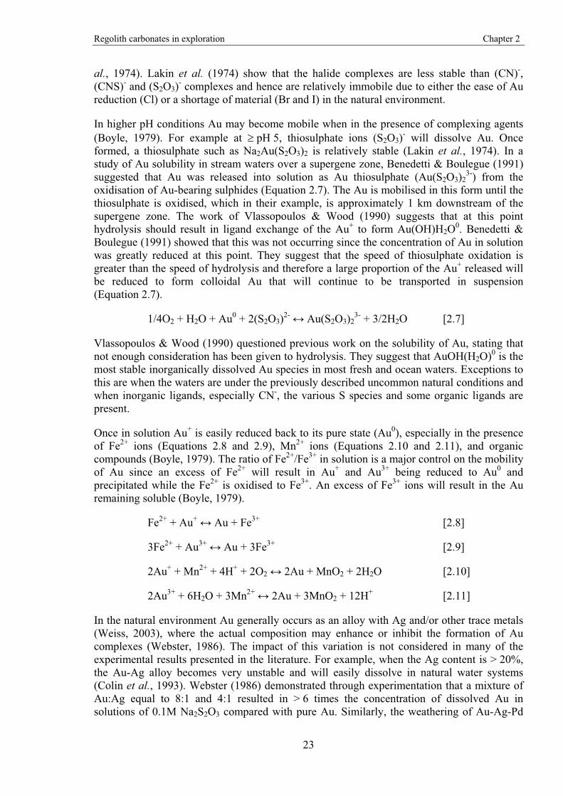
Numerous anions, cations and complexes will inhibit the mobility of Au. For example, ions such as OH-, Fe3+ and Mn2+ will precipitate insoluble compounds that either co-precipitate or adsorb soluble Au (Boyle, 1979). The majority of soluble Au forms are easily reduced to pure Au, so therefore the actual distance that Au may be mobilised in soluble form is limited. Some complex forms however, may be more resilient and hence increase Au mobility (Boyle, 1979).
Table 2.2: Summary of Au dissolution and precipitation conditions.
Complex Conditions for Au dissolution
Condition for Au precipitation
Reference
Thiosulphate Au(S2O3)2
3- Mid to high pH, may form from oxidation of Au bearing sulphides
Low pH, reduction, oxidation of the thiosulphate
(Boyle, 1979; Gray et al., 1992)
Humic Acid Mid to high pH Low pH (Baker, 1978; Vlassopoulos & Wood, 1990)
Fulvic Acid Low to high pH, above average N and S content
(Bowell et al., 1993b)
Humin Not soluble May reduce and lock up Au
(Vlassopoulos & Wood, 1990)
Halides AuCl2- Low pH, high Cl- concentrations, oxidising
Increasing pH, dilution, reduction
(Krauskopf, 1951; Lakin et al., 1974; Boyle, 1979)
Cyanide Au(CN)2
- Mid to high pH, availability of (CN)- (may be sourced from biota)
Breakdown of cyanides by micro-organisms
(Boyle, 1979) (Lakin et al., 1974)
Hydroxides AuOH(H2O)
Mid to high pH (stable in most fresh and oceanic waters
Presence of stronger complexes, e.g. (CN)-, and some organic ligands
(Vlassopoulos & Wood, 1990)
Micro-organisms May be involved in production and/or control of all the above complexes
May precipitate Au within cells or adsorb/trap Au on cell surface
(Lengke & Southam, 2005; Reith et al., 2006)
Grimes et al. (1995) found that Au was significantly mobilised by groundwaters around Au deposits in oxidising conditions. They also found a significant increase in Au content of the alluvium collected from the top of the groundwater, suggesting Au is occurring in oxide coatings via sorption or co-precipitation.
Gray et al. (1992) observed anomalous Au concentrations of up to 3.7 μg/L in highly saline groundwaters with high concentrations of Mn, near Kalgoorlie, Western Australia. These conditions however, are uncommon in the natural environment (Krauskopf, 1951; Lakin et
Regolith carbonates in exploration Chapter 2
23
al., 1974). Lakin et al. (1974) show that the halide complexes are less stable than (CN)-, (CNS)- and (S2O3)- complexes and hence are relatively immobile due to either the ease of Au reduction (Cl) or a shortage of material (Br and I) in the natural environment.
In higher pH conditions Au may become mobile when in the presence of complexing agents (Boyle, 1979). For example at � pH 5, thiosulphate ions (S2O3)- will dissolve Au. Once formed, a thiosulphate such as Na2Au(S2O3)2 is relatively stable (Lakin et al., 1974). In a study of Au solubility in stream waters over a supergene zone, Benedetti & Boulegue (1991) suggested that Au was released into solution as Au thiosulphate (Au(S2O3)2
3-) from the oxidisation of Au-bearing sulphides (Equation 2.7). The Au is mobilised in this form until the thiosulphate is oxidised, which in their example, is approximately 1 km downstream of the supergene zone. The work of Vlassopoulos & Wood (1990) suggests that at this point hydrolysis should result in ligand exchange of the Au+ to form Au(OH)H2O0. Benedetti & Boulegue (1991) showed that this was not occurring since the concentration of Au in solution was greatly reduced at this point. They suggest that the speed of thiosulphate oxidation is greater than the speed of hydrolysis and therefore a large proportion of the Au+ released will be reduced to form colloidal Au that will continue to be transported in suspension (Equation 2.7).
1/4O2 + H2O + Au0 + 2(S2O3)2- � Au(S2O3)23- + 3/2H2O [2.7]
Vlassopoulos & Wood (1990) questioned previous work on the solubility of Au, stating that not enough consideration has been given to hydrolysis. They suggest that AuOH(H2O)0 is the most stable inorganically dissolved Au species in most fresh and ocean waters. Exceptions to this are when the waters are under the previously described uncommon natural conditions and when inorganic ligands, especially CN-, the various S species and some organic ligands are present.
Once in solution Au+ is easily reduced back to its pure state (Au0), especially in the presence of Fe2+ ions (Equations 2.8 and 2.9), Mn2+ ions (Equations 2.10 and 2.11), and organic compounds (Boyle, 1979). The ratio of Fe2+/Fe3+ in solution is a major control on the mobility of Au since an excess of Fe2+ will result in Au+ and Au3+ being reduced to Au0 and precipitated while the Fe2+ is oxidised to Fe3+. An excess of Fe3+ ions will result in the Au remaining soluble (Boyle, 1979).
Fe2+ + Au+ � Au + Fe3+ [2.8]
3Fe2+ + Au3+ � Au + 3Fe3+ [2.9]
2Au+ + Mn2+ + 4H+ + 2O2 � 2Au + MnO2 + 2H2O [2.10]
2Au3+ + 6H2O + 3Mn2+ � 2Au + 3MnO2 + 12H+ [2.11]
In the natural environment Au generally occurs as an alloy with Ag and/or other trace metals (Weiss, 2003), where the actual composition may enhance or inhibit the formation of Au complexes (Webster, 1986). The impact of this variation is not considered in many of the experimental results presented in the literature. For example, when the Ag content is > 20%, the Au-Ag alloy becomes very unstable and will easily dissolve in natural water systems (Colin et al., 1993). Webster (1986) demonstrated through experimentation that a mixture of Au:Ag equal to 8:1 and 4:1 resulted in > 6 times the concentration of dissolved Au in solutions of 0.1M Na2S2O3 compared with pure Au. Similarly, the weathering of Au-Ag-Pd
Regolith carbonates in exploration Chapter 2
24
particles shows a preferential dissolution in the order Pd > Ag > Au (Varajao et al., 2000). The reason for this increased Au solubility is unclear. Webster (1986) suggests a mixed complex such as (Au,Ag)(S2O3)2
3- is possible. Colin & Vieillard (1991) suggest that a trend of higher Au solubility with increasing Ag content is also demonstrated for fulvic acid and AuCl2
- complexes. Once in solution, changes in chemical conditions may result in Au, or Ag, or both being re-precipitated, which allows for preferential leaching of the Au or Ag. Krupp & Weiser (1992) state that under oxidising conditions Ag will react with chloride to form AgCl, which due to its high aqueous solubility, will be leached from the Au.
The Ag content of Au particles over mineralisation at Gabon gradually decreases away from the mineralised zone, highlighting that it is preferentially leached over the Au (Colin & Vieillard, 1991). Along with the loss of Ag, the Au reflects greater weathering away from mineralisation, forming rounded edges and dissolution pits (Colin et al., 1989; Colin & Vieillard, 1991; Santosh & Omana, 1991; Santosh et al., 1992). The loss of Ag occurs progressively from the rims and crosscutting features within the Au particles (Colin & Vieillard, 1991). Similar lower Ag contents and more rounded morphology of Au grains, with distance away from primary mineralisation were reported by Freyssinet et al. (1989b). In a study of elemental distribution above mineralisation at Mborguene, Cameroon, Ag was very mobile and leached away from the system during the earliest stages of weathering, leaving only a small halo directly above mineralisation (Freyssinet et al., 1989a).
The majority of the chemical species described above that permit the mobility of Au (e.g. sulphides, thiosulphate, cyanide and chlorides) may be partly or extensively controlled by biological factors. Micro-organisms, plants and animals, may therefore have a major impact on the mobility of Au (Gray et al., 1992).
Although Au is considered a non-essential element for plants, it may be taken up with nutrient elements by the roots (Gilkes, 1999). Plant roots have the ability to vary the pH to suit their environment and to ensure the availability of essential elements in the surrounding soil (see Section 2.4). Vegetation can therefore be an additional sampling medium for Au exploration (Lakin et al., 1974; Smith & Keele, 1984; Gray et al., 1992; Hill & Hill, 2003).
Plants may take up and amalgamate elements from a large area based on the large spatial extent (laterally and vertically) of their root systems. These elements are later redeposited through leaf litter and plant decay within the soil profile where they can be recycled (Smith & Keele, 1984; Gilkes, 1999). The actual source of the elements in vegetation may exceed the extent of the roots by 1,000s of metres if the plants are tapping into local groundwater systems (Dunn et al., 1991). This potential uptake of Au from a large area by plants means that they have the ability to remove the “nugget effect” that is typically a feature of more traditional sampling media (Busche, 1989). They are also more likely to uptake elements nearer to the bedrock and reflect true anomalous elemental concentrations that may be obscured by overlying transported regolith (Busche, 1989).
Lakin et al. (1974) suggest that Au(CN)2- is the most soluble form of Au in soils due to the
widespread and typically high concentration of available (CN)-. It is the availability of (CN)- that is the limiting factor in the formation of Au(CN)2
-, which is stable over a wide range of
pH/Eh conditions and may accumulate significant amounts of Au (Gray et al., 1992). Many plant species, animals, bacteria and fungi are known to produce cyanogenic glycosides. Hydrolysis of these glycosides results in the formation of HCN which is dispersed into the soil (Lakin et al., 1974). Lakin et al. (1974) assert that enough HCN is formed in the soil to account for the dissolution of Au and its absorption by plants. Shacklette et al. (1970) and
Regolith carbonates in exploration Chapter 2
25
Lakin et al. (1974) suggest that plants are more likely to take up soluble Au in complex form rather than colloids and that Au(CN)2
- is the most readily adsorbed Au complex. For example, in the Yilgarn of Western Australia, there is a symbiotic relationship between the roots of many Acacia species and fungi. These fungi are able to produce CN-, which when complexed with Au may be taken up by the plants (Smith, 1987).
The uptake of Au(CN)2- by plants may be limited by the presence of organisms in the natural
environment that are capable of breaking down the cyanides (Lakin et al., 1974). Not all Au complexes are taken up by plants. Shacklette et al. (1970) found that plants in solutions containing AuCl4
- would reduce Au, which was precipitated on the surfaces of root cell membranes rather than taken up and distributed to its organs.
Decaying plant litter on or near the surface (A horizon) will release Au back into the top soil horizons where it may become concentrated (Smith, 1987). Since both Ca and Au are released by decaying plants into the soil, vegetation may play a role in the formation of Au and regolith carbonate associations, (Lintern, 1989; Lintern et al., 1997; Lintern & Butt, 1998b; Lintern et al., 2006).
The role of organic matter, especially humic substances, in the mobilization of Au is unclear despite numerous studies (Wood, 1996). Several researchers report that Au may be transported by humic substances through the formation of Au complexes (Freise, 1931; Boyle et al., 1975; Baker, 1978; Varshal et al., 1984; 1990; Cook et al., 1992; Varshal et al., 2000), while others suggest that Au may be reduced, leading to its precipitation (Fetzer, 1934; Ong & Swanson, 1969; Gatellier & Disnar, 1990). Wood (1996) proposed a number of factors that may explain these differences, including: variations between the composition and structure of the humic material; the amount of non-humic impurities remaining after treatment, especially amino acids; variations in redox conditions; and the amount of Au being added. This last point is significant since Au will only bind at certain sites within the humic substances. Hence if too much Au is added then once all the binding sites have been filled the remaining Au will most likely be reduced (Wood, 1996).
Variations in the composition of the humus will control whether Au is mobile or fixed. For example, in acid conditions HA is insoluble and Au will be fixed, however with the same conditions FA is soluble and able to bind with Au and allow it to be mobilised (Vlassopoulos et al., 1990). Varshal et al. (1984; 1990) support this, stating that FA will generally form soluble compounds, whilst HA will tend to precipitate and concentrate Au. They showed that the solubility of Au is related to the concentration of FA, such that a doubling of the FA content will result in double the Au concentration.
Schmitt et al. (1993) supported the findings of Vlassopoulos et al. (1990) for Au mobilisation in lake and stream waters from the southern Canadian Shield. They add that in areas of abundant S and humic substances the Au is mobilised by HA complexes and results in a wider Au dispersion pattern. In areas of lesser organic material, the mobilisation is more likely to be controlled by Au-hydroxide species as described by Vlassopoulous et al. (1990). Similarly Bowell et al. (1993b) demonstrated that for any pH, FA with higher S content (4.2%) would dissolve more Au than a FA with a low S content (0.7%).
Baker (1978) showed that oxidation of Au by HA could form complex compounds within the natural environment. These HA compounds have a similar stability to Au(SCN)4
-, and could transport Au in the hydrosphere.
Regolith carbonates in exploration Chapter 2
26
In a discussion on the apparent enrichment of Au within humic soil (A) horizons, Boyle (1979) suggested that organic matter, especially humic substances, may adsorb Au and include it within their structure, making the Au immobile. This enrichment may be the result of bound Au being released from the degradation of humic complexes under oxidising conditions, and then being recaptured by the remaining humic complexes. This process may be repeated many times (Boyle, 1979). Large coordinated humic groups formed during the humification process may also dissociate and form soluble (colloidal) Au and be transported by ground waters, resulting in the removal of the Au (Boyle, 1979). These Au colloids, which are negatively charged, may be mobile within negatively charged soils and precipitate Au when they come into contact with positively charged materials such as Fe-oxides (Gray et al., 1992). Ong & Swanson (1969) suggest that organic acids reduce Au to form colloids, and through the formation of organic coatings around these colloids, render them stable in the natural environment enabling transportation of the Au.
Microbial activity can control the mobility of Au via the alteration of the surrounding soil conditions (Gray et al., 1992), and/or through direct interaction through adsorption or precipitation (Brooks, 1995). Bacteria can accumulate Au on or just inside their cell walls, or accumulate Au passively by bonding with S and P molecules within the cell walls (Mann, 1992; Lengke & Southam, 2005; Reith et al., 2006). In mine waters, bacterial cells may contain concentrations of Au exceeding those in the water by factors of 15-600 (Brooks, 1995).
Indigenous microbiota can mediate the release into solution of up to 80wt% of total Au in soils over mineralisation from areas of differing climate in Australia (Reith & McPhail, 2006; 2007). The suggested mechanism for this is through the dissolution and complexation by free amino acids, which are produced by micro-organisms. Variations in the amount of Au dissolved by indigenous micro-organisms (from 20% in a tropical soil) may be due to a limited availability of N, which will reduce the amount of free amino acids produced by bacteria (Reith & McPhail, 2007). An alternate hypothesis is that the Au may be more tightly bound to organic material and less accessible for solubilisation by micro-organisms (Reith & McPhail, 2007). The Au dissolution rate in these experiments is variable and it appears the Au is in a constant process of dissolution and re-adsorption. Initially Au appears to be liberated from Fe- and Mn-oxides and re-adsorbed to carbonates and clays. Following this the Au is re-adsorbed to the organic matter (Reith & McPhail, 2006). These results are not repeated in soils away from mineralisation following the addition of Au pellets, indicating that specific organisms that are only present in auriferous soils, are responsible for the dissolution of Au (Reith & McPhail, 2006; Reith et al., 2006).
Mineyev (1976) proposes that abundant micro-organisms (e.g. the genus Bacillus) produce high levels of amino acids and proteins that will dissolve Au in alkaline conditions, and therefore micro-organism processes can dissolve, mobilise and accumulate Au. If the ratio of Au to amino acid falls to below 1:10 then Au is reduced to form a colloid that may be transported considerable distances. The colloidal Au may be extracted from solution by the accumulation of microbiological mould micelles such as Aspergillus (Mineyev, 1976). Similarly, Mossman & Dyer (1985) suggest that a major part of the Witwatersrand-type deposits may be the result of prokaryote activity (such as cyanobacteria). They propose that Au is reduced from solution or precipitated by prokaryote communities to become entrapped within algal mats.
The physical properties of Au in soils, including the morphology and distribution have been widely reported (e.g. Wilson, 1983; Mann, 1984; Wilson, 1984; Lecomte & Colin, 1989;
Regolith carbonates in exploration Chapter 2
27
Colin & Vieillard, 1991; Santosh & Omana, 1991; Delaney & Fletcher, 1993; Sibbick & Fletcher, 1993; Lawrance & Griffin, 1994; Colin, 1997; Hough et al., 2006; Smith & Singh, 2007). The distribution of Au within the C horizon above Au mineralisation can have the highest Au concentrations in the < 53 μm size fraction as fine-grained inclusions (Delaney & Fletcher, 1993). An exception occurred in soils developed within glacial till, where free particle Au was more typical and may reflect the original size distribution of the Au deposit. Highest Au concentrations were also in the < 53 μm size fraction of soils and tills from the Nickel Plate Mine, southern British Columbia, Canada (Sibbick & Fletcher, 1993). In a study of Au distribution over mineralisation in lateritic profiles in a tropical rainforest, Gabon, Central Africa, Lecomte & Colin (1989) showed that: i) at sites directly over mineralisation, the Au was enriched in the coarse-grained fraction, suggesting significant influence from weathering and profile collapse; and, ii) the fine grained (< 63 μm) fraction becomes dominant laterally away from the mineralisation, suggesting prevailing influence from chemical processes. An alternative explanation for this distribution is one of lateral sorting with distance away from mineralisation.
In lateritic soils two types of Au particles have been reported: i) residual Au from primary mineralisation with dissolution features and high Ag-content, in some cases with a rim of reduced Ag; and, ii) high fineness Au in the form of Au films (paint gold) dendrites, filaments or octahedral micrometric crystals that is generally associated with Fe or Al oxy-hydroxides (Wilson, 1983; Mann, 1984; Wilson, 1984; Santosh & Omana, 1991; Colin, 1997). Smith & Singh (2007) describe irregular clusters and individual grains of Au (~ 50 μm and 5 – 10 μm respectively), in relic lithic material within lateritic samples. The Au is typically associated with goethite or bauxite nodules (Wilson, 1983; 1984).
2.6. Regolith carbonates and gold: What do we know? Apart from the Au and regolith carbonate associations described above, there is minimal published work on why this association exists. The reason that Au is associated with regolith carbonates, and in particular calcrete, is therefore unclear.
Gray et al. (1990) and Gray & Lintern (1994) showed that the solubility of Au within the carbonate horizon was higher than in the surrounding horizons and therefore it should be depleted rather than enriched. They suggest that the carbonate horizon is an evaporative zone and that solutions carrying mobile elements such as Ca and Mg, will precipitate and add to the carbonate. If the solutions are also enriched in Au, then this will be precipitated within the same horizon. The solubility of Au in regolith carbonates was also demonstrated by Lintern et al. (2006) who recorded high levels of water soluble Au in near surface calcretes over mineralisation at Challenger. They suggest that this implies Au mobilisation is associated with calcrete. Gray & Lintern (1994) stated that calcareous soils adsorb less Au than other soils, meaning that the association must be biological or physical and not chemical. Co-precipitation of Au, Ca and Mg from solutions due to evapotranspiration of the water is suggested by Lintern & Butt (1998b) as the reason for the Au and Ca association. This is preferred to adsorption of Au onto carbonate surfaces by migrating waters since this would result in Au being concentrated at the top or base of the carbonate horizon, which is not observed (Gray et al., 1990; Lintern & Butt, 1993; 1998b).
Lintern et al. (2006) suggest that the association between Au and regolith carbonates is due to hydromorphic processes. These processes and associated environmental factors including rainfall frequency and intensity, evapotranspiration rates and soil type, will result in the dissolution and re-precipitation of Ca and Au within the soil profile (Lintern et al., 2006).
Regolith carbonates in exploration Chapter 2
28
Therefore, the demonstrated high solubility of Au within the carbonate horizon matches the solubility of Ca and therefore they will both dissolve and co-precipitate under similar conditions. The mobility of Ca in soils overlying sulphide mineralisation was discussed by Smee (1998; 1999) who hypothesised that Ca was being mobilised by the upward movement of H+ to the margins of the mineralised zone where it is re-precipitated. He also suggests that Ca controls the distribution of Au, As, Sb and Ba in the regolith.
2.7. Conclusion The increasing use of regolith carbonates in mineral exploration has been mostly driven by the exploration industry. Recent difficulties and uncertainties in the use of regolith carbonates as a sampling medium have created a need to integrate regolith carbonate and Au studies.
The review has demonstrated that significant detail exists about regolith carbonates and how they form. Similarly the mobility of Au in the regolith is reasonably understood. This information is applied to this research to aid in meeting the project aims and to start integrating regolith carbonate and Au mobility research. Specifically, the review has highlighted the following features and issues:
1. descriptions of sampling morphology and landscape setting are poorly constrained;
2. Au is highly mobile in the regolith and its mobility may be controlled by biological, physical, and / or chemical processes;
3. Ca may be sourced from intrinsic or extrinsic sources, if extrinsic, then there can be no direct relationship with Au; and
4. much of the regolith of inland Australian has continued to develop since the Late Palaeozoic, yet regolith carbonates are considered more recent (late Miocene to present).
Point 4 is a significant feature, which to date, has been overlooked. It means that Au has to be in the profile prior to Au-in-calcrete formation, unless in the unlikely scenario, regolith carbonate formation results in Au being released into the regolith from underlying rocks and minerals.
29
Chapter 3
Methodology
3.1. Introduction The analytical procedures adopted were to provide data necessary to improve the understanding of the location and morphology of Au and associated elements within the regolith. The procedures include a variety of chemical and physical, experimental and analytical methods. The methodologies were adapted from scientifically proven methods to maintain validity of the results, and are outlined in this chapter. Where feasible, the facilities at the University of Adelaide were used. These included: mass spectrometry, electron microscopy, and, particle-size analysis. Commercial laboratories were used for determining: elemental concentrations by Inductively Coupled Plasma – Mass Spectrometry (ICP MS), Inductively Coupled Plasma – Optical Emission Spectrometry (ICP OES), X-Ray Fluorescence (XRF) spectrometry and Instrumental Neutron Activation Analysis (INAA); mineralogy by X-Ray Diffraction (XRD); impregnation of undisturbed (in-situ) soil samples with epoxy resin; and preparation of petrology thin sections.
The structure of this chapter follows the modular structure adopted for the thesis. Methodologies used within a single module are described under a subheading of the specific module. Methodologies common to two or all modules are described under their own subheadings. Specialist analytical procedures and sample preparation completed by commercial companies are described under their own section headings. A summary of methodologies and where they were used is provided in Table 3.1.
Geochemists have typically collected soil samples for elemental analysis in their search for mineral deposits, whereas pedologists use soil samples to determine physio-chemical and biological properties as a means of determining pedogenesis. A combination of procedures developed by geologists and pedologists have been utilised here to gain an insight into the mobility of Au within the regolith, particularly the soil environment.
3.2. Sample collection and handling Contamination is a major concern when collecting samples for detailed analysis. Contamination may arise through inadequacies in the sampling methodology or through prior anthropogenic activity in the sample area, such as drilling. Careful site selection away from obvious contamination sources, such as drill spoil, can help to reduce significant contamination. Methods described here were designed to minimise the risk of contamination during collection.
As Au is the major component of interest in the samples, and because natural Au concentrations are very low, care was taken to avoid contamination from external Au sources. Personal jewellery is the largest potential source of Au contamination. Therefore, before samples were collected and experimental processes performed, jewellery was removed and hands washed in clean water. Care was also taken to avoid contamination by sunscreen, by avoiding direct handling of the samples.
Methodology Chapter 3
30
Soil and regolith carbonate samples were collected for detailed description analysis. The various sample media and collection methods are summarised in Table 3.2.
Table 3.1: Summary of the methods used in this research. Module 1: Source of calcium in regolith carbonates, Module 2: Calcrete-gold in the landscape: Regolith-landform controls at Tunkillia, SA, and Module 3: Gold in the regolith profile: Pedogenic controls at White Dam, SA. (* task performed by commercial laboratory).
Process Purpose Applied to Section
Sample collection and handling
Collect samples for analysis that are not, and do not become contaminated
All modules 3.2
Mass spectrometry (Sr isotope determination)
Measure Sr isotope ratios as a tracer for the source of Ca
Module 1 3.3
Regolith landform mapping
Identify and illustrate the regolith landform units and their relationship with Au mobilisation over the landscape
Module 2 3.4
Mass balance analysis Determine elemental gains and losses in the development of the regolith profile
Module 3 3.5.1
Particle-size analysis Separate soil aggregates into individual size components
Module 3 3.5.2
Bulk density measurement
Used in mass balance calculations and to calculate porosity
Module 3 3.5.3
Calcimetry Measure the carbonate content of soil samples Module 3 3.5.4
Density separation Separate the heavy minerals from the fine and medium sand fractions for microscopy examination
Module 3 3.5.5
Electrical conductivity and pH
Measure the acidity of the soil samples and obtain indication of soluble salt content
Module 3 3.5.6
Electron microscopy Identification of the Au morphology and mineralogical associations
Module 3 3.5.7
Thin section preparation*
Petrological and electron microscopy investigation to identify the mineralogy and physical properties of the undisturbed soil samples
Module 3 3.6.2
ICP MS & ICP OES*
Determine elemental concentrations of bulk samples
Module 2 & 3 3.6.3
INAA* Measure the Au concentrations in the different size fractions
Module 3 3.6.4
XRD & XRF* Determine the mineralogy and elemental content of the clay and fine sand fractions
Module 3 3.6.5
3.2.1. Profile sampling Where samples were collected from profiles, the risk of contamination was further reduced by removing exposed surface material by cutting back into the profile with clean tools and brushing away surface material. All tools used for sampling were kept clean and brushed off before each sample was collected. Once the profiles had been prepared for sample collection and a fresh surface was exposed (Figure 3.1), soil horizons were identified, characterised, measured and photographed. At least one sample was collected from each soil horizon.
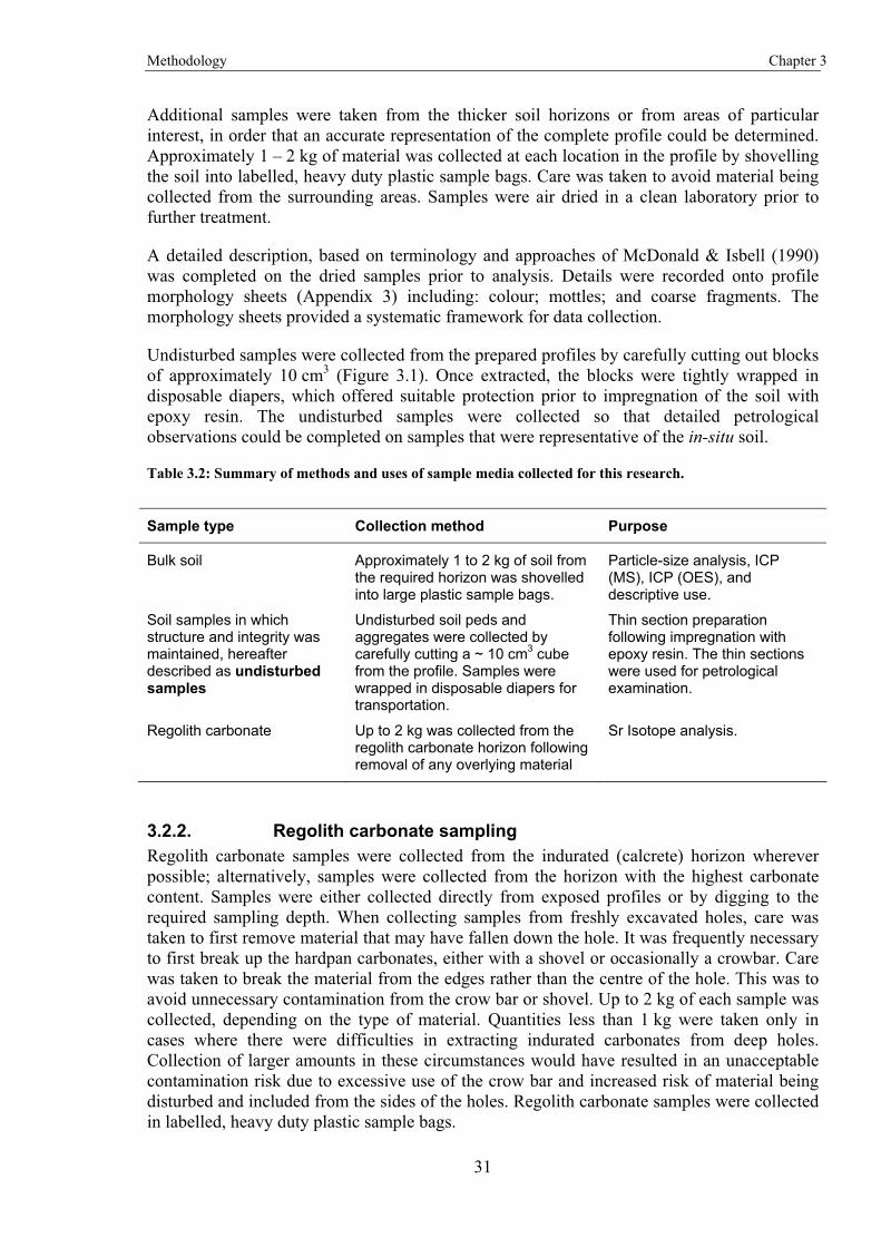
Methodology Chapter 3
31
Additional samples were taken from the thicker soil horizons or from areas of particular interest, in order that an accurate representation of the complete profile could be determined. Approximately 1 – 2 kg of material was collected at each location in the profile by shovelling the soil into labelled, heavy duty plastic sample bags. Care was taken to avoid material being collected from the surrounding areas. Samples were air dried in a clean laboratory prior to further treatment.
A detailed description, based on terminology and approaches of McDonald & Isbell (1990) was completed on the dried samples prior to analysis. Details were recorded onto profile morphology sheets (Appendix 3) including: colour; mottles; and coarse fragments. The morphology sheets provided a systematic framework for data collection.
Undisturbed samples were collected from the prepared profiles by carefully cutting out blocks of approximately 10 cm3 (Figure 3.1). Once extracted, the blocks were tightly wrapped in disposable diapers, which offered suitable protection prior to impregnation of the soil with epoxy resin. The undisturbed samples were collected so that detailed petrological observations could be completed on samples that were representative of the in-situ soil.
Table 3.2: Summary of methods and uses of sample media collected for this research.
Sample type Collection method Purpose
Bulk soil Approximately 1 to 2 kg of soil from the required horizon was shovelled into large plastic sample bags.
Particle-size analysis, ICP (MS), ICP (OES), and descriptive use.
Soil samples in which structure and integrity was maintained, hereafter described as undisturbed samples
Undisturbed soil peds and aggregates were collected by carefully cutting a ~ 10 cm3 cube from the profile. Samples were wrapped in disposable diapers for transportation.
Thin section preparation following impregnation with epoxy resin. The thin sections were used for petrological examination.
Regolith carbonate Up to 2 kg was collected from the regolith carbonate horizon following removal of any overlying material
Sr Isotope analysis.
3.2.2. Regolith carbonate sampling Regolith carbonate samples were collected from the indurated (calcrete) horizon wherever possible; alternatively, samples were collected from the horizon with the highest carbonate content. Samples were either collected directly from exposed profiles or by digging to the required sampling depth. When collecting samples from freshly excavated holes, care was taken to first remove material that may have fallen down the hole. It was frequently necessary to first break up the hardpan carbonates, either with a shovel or occasionally a crowbar. Care was taken to break the material from the edges rather than the centre of the hole. This was to avoid unnecessary contamination from the crow bar or shovel. Up to 2 kg of each sample was collected, depending on the type of material. Quantities less than 1 kg were taken only in cases where there were difficulties in extracting indurated carbonates from deep holes. Collection of larger amounts in these circumstances would have resulted in an unacceptable contamination risk due to excessive use of the crow bar and increased risk of material being disturbed and included from the sides of the holes. Regolith carbonate samples were collected in labelled, heavy duty plastic sample bags.
Methodology Chapter 3
32
Figure 3.1: A prepared profile ready for sampling and undisturbed sample collection, White Dam Profile 1, Curnamona Province, SA (Profile depth ~ 2.3 m, inset scale bar 10 cm).
3.3. Module 1: Source of calcium in regolith carbonates Understanding the source of Ca in regolith carbonates is important for determining possible associations between Au and Ca. There are two potential Ca sources in regolith carbonates: 1) weathering of bedrock (intrinsic); and 2) aeolian deposition (extrinsic). The source of Ca was determined from the analysis of Sr isotopes. The similar chemical properties of Sr and Ca translate to geochemical associations and therefore Sr is an ideal tracer element for Ca.
Strontium has four naturally occurring isotopes: 84Sr; 86Sr; 87Sr; and, 88Sr. Their abundances are approximately: 0.56, 9.87, 7.04, and 82.53 percent respectively. These are stable isotopes; however, 87Sr is the daughter isotope of 87Rb, which has a half life of 48.8 x 10⁹ years (Faure & Mensing, 2005). Conventionally, the Sr isotopic signature of rocks and minerals is represented by the ratio of 87Sr/86Sr. This ratio will vary due to the age and amount of Rb initially present. Over time the 87Sr/86Sr ratio increases due to the decay of 87Rb. Unlike the lighter stable isotopes of H, C or O, which tend to fractionate under various physical and chemical conditions, Rb and Sr appear to remain unfractionated due to their higher atomic mass (Stille & Shields, 1997). Therefore the 87Sr/86Sr ratio in rocks and minerals is purely the result of the Rb and Sr concentration at the time of formation.
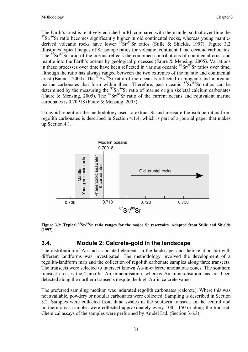
Methodology Chapter 3
33
The Earth’s crust is relatively enriched in Rb compared with the mantle, so that over time the 87Sr/86Sr ratio becomes significantly higher in old continental rocks, whereas young mantle-derived volcanic rocks have lower 87Sr/86Sr ratios (Stille & Shields, 1997). Figure 3.2 illustrates typical ranges of Sr isotope ratios for volcanic, continental and oceanic carbonates. The 87Sr/86Sr ratio of the oceans reflects the combined contributions of continental crust and mantle into the Earth’s oceans by geological processes (Faure & Mensing, 2005). Variations in these processes over time have been reflected in various oceanic 87Sr/86Sr ratios over time, although the ratio has always ranged between the two extremes of the mantle and continental crust (Banner, 2004). The 87Sr/86Sr ratio of the ocean is reflected in biogenic and inorganic marine carbonates that form within them. Therefore, past oceanic 87Sr/86Sr ratios can be determined by the measuring the 87Sr/86Sr ratio of marine origin skeletal calcium carbonates (Faure & Mensing, 2005). The 87Sr/86Sr ratio of the current oceans and equivalent marine carbonates is 0.70918 (Faure & Mensing, 2005).
To avoid repetition the methodology used to extract Sr and measure the isotope ratios from regolith carbonates is described in Section 4.1.4, which is part of a journal paper that makes up Section 4.1.
Figure 3.2: Typical 87Sr/86Sr ratio ranges for the major Sr reservoirs. Adapted from Stille and Shields (1997).
3.4. Module 2: Calcrete-gold in the landscape The distribution of Au and associated elements in the landscape, and their relationship with different landforms was investigated. The methodology involved the development of a regolith-landform map and the collection of regolith carbonate samples along three transects. The transects were selected to intersect known Au-in-calcrete anomalous zones. The southern transect crosses the Tunkillia Au mineralisation, whereas Au mineralisation has not been detected along the northern transects despite the high Au-in calcrete values.
The preferred sampling medium was indurated regolith carbonates (calcrete). Where this was not available, powdery or nodular carbonates were collected. Sampling is described in Section 3.2. Samples were collected from dune swales in the southern transect. In the central and northern areas samples were collected approximately every 100 – 150 m along the transect. Chemical assays of the samples were performed by Amdel Ltd. (Section 3.6.3).
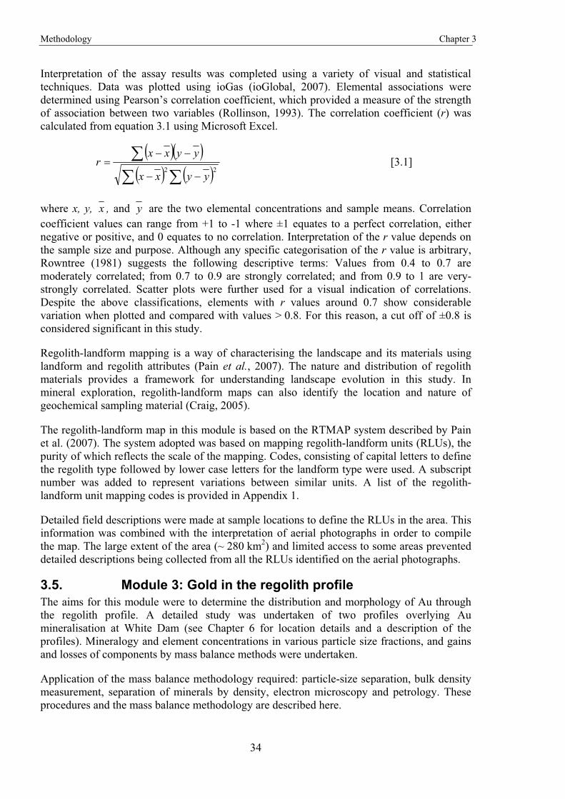
Methodology Chapter 3
34
Interpretation of the assay results was completed using a variety of visual and statistical techniques. Data was plotted using ioGas (ioGlobal, 2007). Elemental associations were determined using Pearson’s correlation coefficient, which provided a measure of the strength of association between two variables (Rollinson, 1993). The correlation coefficient (r) was calculated from equation 3.1 using Microsoft Excel.
� �� �� � � �� ��
��
��
22yyxx
yyxxr [3.1]
where x, y, x , and y are the two elemental concentrations and sample means. Correlation coefficient values can range from +1 to -1 where ±1 equates to a perfect correlation, either negative or positive, and 0 equates to no correlation. Interpretation of the r value depends on the sample size and purpose. Although any specific categorisation of the r value is arbitrary, Rowntree (1981) suggests the following descriptive terms: Values from 0.4 to 0.7 are moderately correlated; from 0.7 to 0.9 are strongly correlated; and from 0.9 to 1 are very-strongly correlated. Scatter plots were further used for a visual indication of correlations. Despite the above classifications, elements with r values around 0.7 show considerable variation when plotted and compared with values > 0.8. For this reason, a cut off of ±0.8 is considered significant in this study.
Regolith-landform mapping is a way of characterising the landscape and its materials using landform and regolith attributes (Pain et al., 2007). The nature and distribution of regolith materials provides a framework for understanding landscape evolution in this study. In mineral exploration, regolith-landform maps can also identify the location and nature of geochemical sampling material (Craig, 2005).
The regolith-landform map in this module is based on the RTMAP system described by Pain et al. (2007). The system adopted was based on mapping regolith-landform units (RLUs), the purity of which reflects the scale of the mapping. Codes, consisting of capital letters to define the regolith type followed by lower case letters for the landform type were used. A subscript number was added to represent variations between similar units. A list of the regolith-landform unit mapping codes is provided in Appendix 1.
Detailed field descriptions were made at sample locations to define the RLUs in the area. This information was combined with the interpretation of aerial photographs in order to compile the map. The large extent of the area (~ 280 km2) and limited access to some areas prevented detailed descriptions being collected from all the RLUs identified on the aerial photographs.
3.5. Module 3: Gold in the regolith profile The aims for this module were to determine the distribution and morphology of Au through the regolith profile. A detailed study was undertaken of two profiles overlying Au mineralisation at White Dam (see Chapter 6 for location details and a description of the profiles). Mineralogy and element concentrations in various particle size fractions, and gains and losses of components by mass balance methods were undertaken.
Application of the mass balance methodology required: particle-size separation, bulk density measurement, separation of minerals by density, electron microscopy and petrology. These procedures and the mass balance methodology are described here.
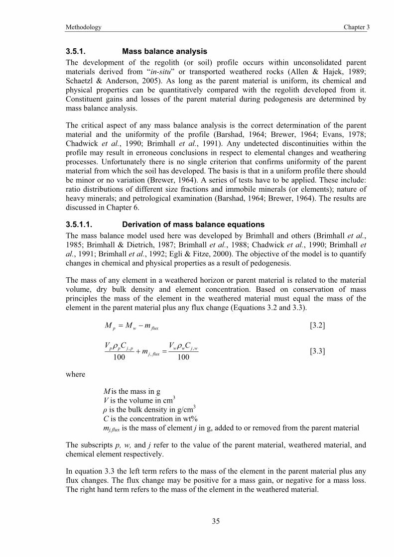
Methodology Chapter 3
35
3.5.1. Mass balance analysis The development of the regolith (or soil) profile occurs within unconsolidated parent materials derived from “in-situ” or transported weathered rocks (Allen & Hajek, 1989; Schaetzl & Anderson, 2005). As long as the parent material is uniform, its chemical and physical properties can be quantitatively compared with the regolith developed from it. Constituent gains and losses of the parent material during pedogenesis are determined by mass balance analysis.
The critical aspect of any mass balance analysis is the correct determination of the parent material and the uniformity of the profile (Barshad, 1964; Brewer, 1964; Evans, 1978; Chadwick et al., 1990; Brimhall et al., 1991). Any undetected discontinuities within the profile may result in erroneous conclusions in respect to elemental changes and weathering processes. Unfortunately there is no single criterion that confirms uniformity of the parent material from which the soil has developed. The basis is that in a uniform profile there should be minor or no variation (Brewer, 1964). A series of tests have to be applied. These include: ratio distributions of different size fractions and immobile minerals (or elements); nature of heavy minerals; and petrological examination (Barshad, 1964; Brewer, 1964). The results are discussed in Chapter 6.
3.5.1.1. Derivation of mass balance equations The mass balance model used here was developed by Brimhall and others (Brimhall et al., 1985; Brimhall & Dietrich, 1987; Brimhall et al., 1988; Chadwick et al., 1990; Brimhall et al., 1991; Brimhall et al., 1992; Egli & Fitze, 2000). The objective of the model is to quantify changes in chemical and physical properties as a result of pedogenesis.
The mass of any element in a weathered horizon or parent material is related to the material volume, dry bulk density and element concentration. Based on conservation of mass principles the mass of the element in the weathered material must equal the mass of the element in the parent material plus any flux change (Equations 3.2 and 3.3).
fluxwp mMM � [3.2]
100100,
,, wjww
fluxjpjpp CV
mCV
� [3.3]
where
M is the mass in g V is the volume in cm3 � is the bulk density in g/cm3 C is the concentration in wt% mj,flux is the mass of element j in g, added to or removed from the parent material
The subscripts p, w, and j refer to the value of the parent material, weathered material, and chemical element respectively.
In equation 3.3 the left term refers to the mass of the element in the parent material plus any flux changes. The flux change may be positive for a mass gain, or negative for a mass loss. The right hand term refers to the mass of the element in the weathered material.
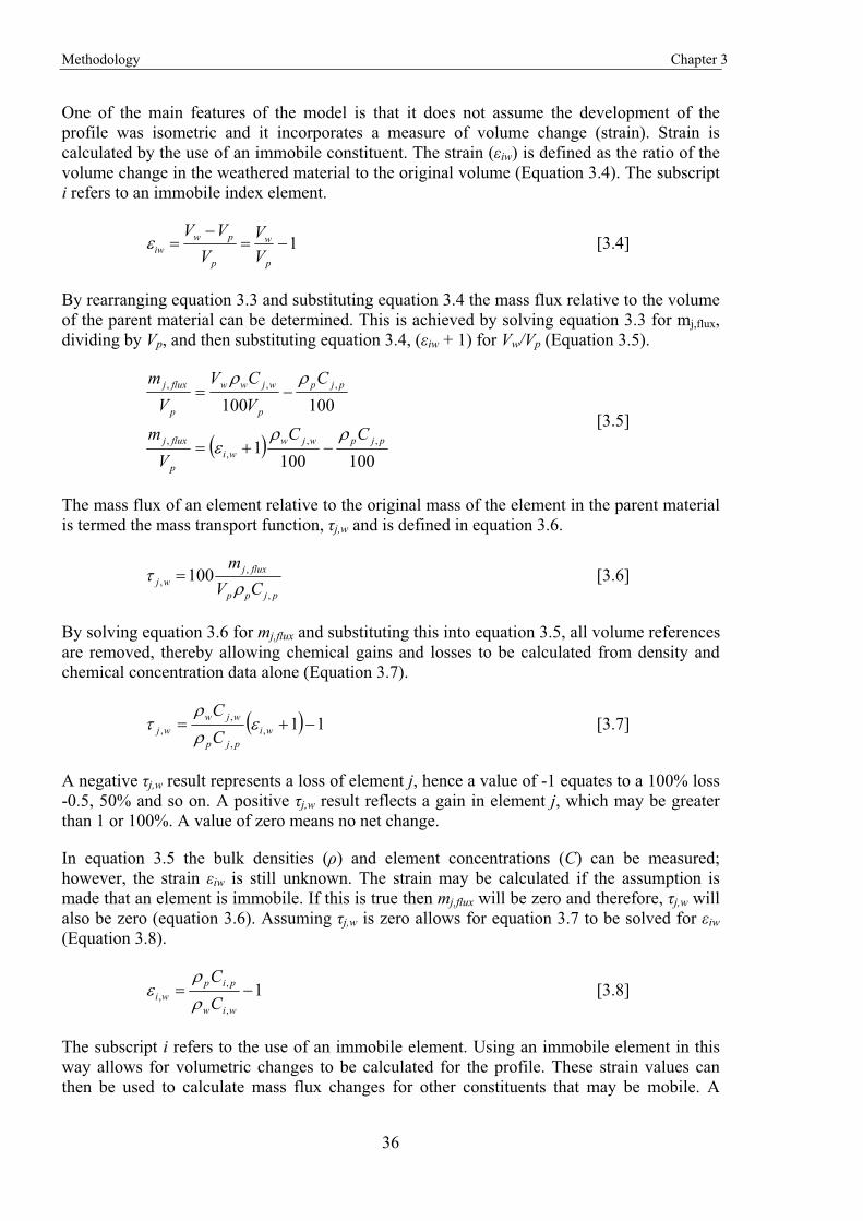
Methodology Chapter 3
36
One of the main features of the model is that it does not assume the development of the profile was isometric and it incorporates a measure of volume change (strain). Strain is calculated by the use of an immobile constituent. The strain (�iw) is defined as the ratio of the volume change in the weathered material to the original volume (Equation 3.4). The subscript i refers to an immobile index element.
1��
p
w
p
pwiw V
VV
VV� [3.4]
By rearranging equation 3.3 and substituting equation 3.4 the mass flux relative to the volume of the parent material can be determined. This is achieved by solving equation 3.3 for mj,flux, dividing by Vp, and then substituting equation 3.4, (�iw + 1) for Vw/Vp (Equation 3.5).
� �100100
1
100100
,,,
,
,,,
pjpwjwwi
p
fluxj
pjp
p
wjww
p
fluxj
CCV
m
CVCV
Vm
�
��
�
[3.5]
The mass flux of an element relative to the original mass of the element in the parent material is termed the mass transport function, �j,w and is defined in equation 3.6.
pjpp
fluxjwj CV
m
,
,, 100
� [3.6]
By solving equation 3.6 for mj,flux and substituting this into equation 3.5, all volume references are removed, thereby allowing chemical gains and losses to be calculated from density and chemical concentration data alone (Equation 3.7).
� � 11,,
,, �� wi
pjp
wjwwj C
C�
� [3.7]
A negative �j,w result represents a loss of element j, hence a value of -1 equates to a 100% loss -0.5, 50% and so on. A positive �j,w result reflects a gain in element j, which may be greater than 1 or 100%. A value of zero means no net change.
In equation 3.5 the bulk densities (�) and element concentrations (C) can be measured; however, the strain �iw is still unknown. The strain may be calculated if the assumption is made that an element is immobile. If this is true then mj,flux will be zero and therefore, �j,w will also be zero (equation 3.6). Assuming �j,w is zero allows for equation 3.7 to be solved for �iw (Equation 3.8).
1,
,, �
wiw
pipwi C
C
� [3.8]
The subscript i refers to the use of an immobile element. Using an immobile element in this way allows for volumetric changes to be calculated for the profile. These strain values can then be used to calculate mass flux changes for other constituents that may be mobile. A
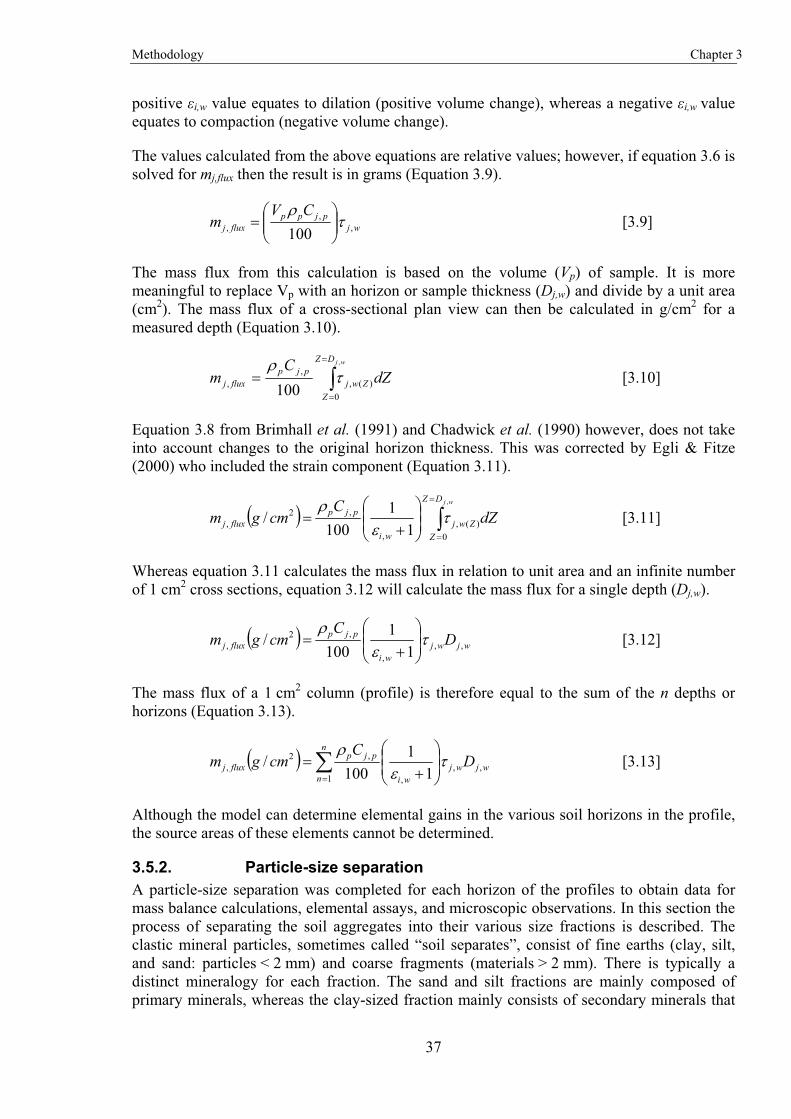
Methodology Chapter 3
37
positive �i,w value equates to dilation (positive volume change), whereas a negative �i,w value equates to compaction (negative volume change).
The values calculated from the above equations are relative values; however, if equation 3.6 is solved for mj,flux then the result is in grams (Equation 3.9).
wjpjpp
fluxj
CVm ,
,, 100
�
�
����
� [3.9]
The mass flux from this calculation is based on the volume (Vp) of sample. It is more meaningful to replace Vp with an horizon or sample thickness (Dj,w) and divide by a unit area (cm2). The mass flux of a cross-sectional plan view can then be calculated in g/cm2 for a measured depth (Equation 3.10).
�
wjDZ
ZZwj
pjpfluxj dZ
Cm
,
0)(,
,, 100
�
[3.10]
Equation 3.8 from Brimhall et al. (1991) and Chadwick et al. (1990) however, does not take into account changes to the original horizon thickness. This was corrected by Egli & Fitze (2000) who included the strain component (Equation 3.11).
� � �
�
����
�
�
wjDZ
ZZwj
wi
pjpfluxj dZ
Ccmgm
,
0)(,
,
,2, 1
1100
/ ��
[3.11]
Whereas equation 3.11 calculates the mass flux in relation to unit area and an infinite number of 1 cm2 cross sections, equation 3.12 will calculate the mass flux for a single depth (Dj,w).
� � wjwjwi
pjpfluxj D
Ccmgm ,,
,
,2, 1
1100
/ ��
�
����
�
� [3.12]
The mass flux of a 1 cm2 column (profile) is therefore equal to the sum of the n depths or horizons (Equation 3.13).
� � �
�
����
�
�
n
nwjwj
wi
pjpfluxj D
Ccmgm
1,,
,
,2, 1
1100
/ ��
[3.13]
Although the model can determine elemental gains in the various soil horizons in the profile, the source areas of these elements cannot be determined.
3.5.2. Particle-size separation A particle-size separation was completed for each horizon of the profiles to obtain data for mass balance calculations, elemental assays, and microscopic observations. In this section the process of separating the soil aggregates into their various size fractions is described. The clastic mineral particles, sometimes called “soil separates”, consist of fine earths (clay, silt, and sand: particles < 2 mm) and coarse fragments (materials > 2 mm). There is typically a distinct mineralogy for each fraction. The sand and silt fractions are mainly composed of primary minerals, whereas the clay-sized fraction mainly consists of secondary minerals that
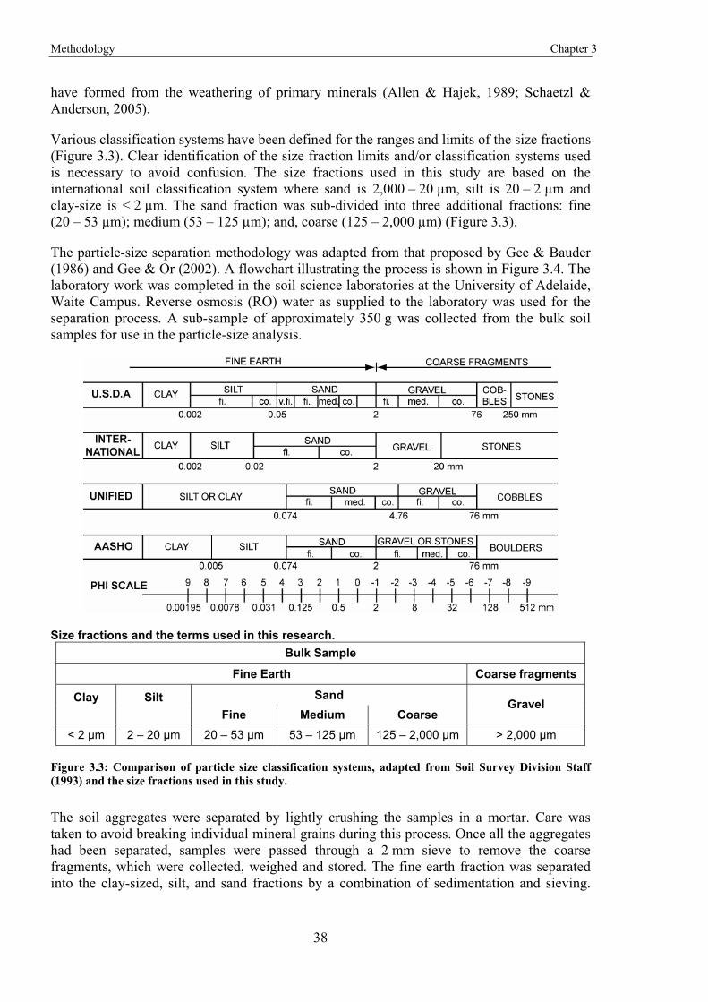
Methodology Chapter 3
38
have formed from the weathering of primary minerals (Allen & Hajek, 1989; Schaetzl & Anderson, 2005).
Various classification systems have been defined for the ranges and limits of the size fractions (Figure 3.3). Clear identification of the size fraction limits and/or classification systems used is necessary to avoid confusion. The size fractions used in this study are based on the international soil classification system where sand is 2,000 – 20 μm, silt is 20 – 2 μm and clay-size is < 2 μm. The sand fraction was sub-divided into three additional fractions: fine (20 – 53 μm); medium (53 – 125 μm); and, coarse (125 – 2,000 μm) (Figure 3.3).
The particle-size separation methodology was adapted from that proposed by Gee & Bauder (1986) and Gee & Or (2002). A flowchart illustrating the process is shown in Figure 3.4. The laboratory work was completed in the soil science laboratories at the University of Adelaide, Waite Campus. Reverse osmosis (RO) water as supplied to the laboratory was used for the separation process. A sub-sample of approximately 350 g was collected from the bulk soil samples for use in the particle-size analysis.
Size fractions and the terms used in this research. Bulk Sample
Fine Earth Coarse fragments
Sand Clay
Silt Fine Medium Coarse
Gravel
< 2 μm 2 – 20 μm 20 – 53 μm 53 – 125 μm 125 – 2,000 μm > 2,000 μm
Figure 3.3: Comparison of particle size classification systems, adapted from Soil Survey Division Staff (1993) and the size fractions used in this study.
The soil aggregates were separated by lightly crushing the samples in a mortar. Care was taken to avoid breaking individual mineral grains during this process. Once all the aggregates had been separated, samples were passed through a 2 mm sieve to remove the coarse fragments, which were collected, weighed and stored. The fine earth fraction was separated into the clay-sized, silt, and sand fractions by a combination of sedimentation and sieving.
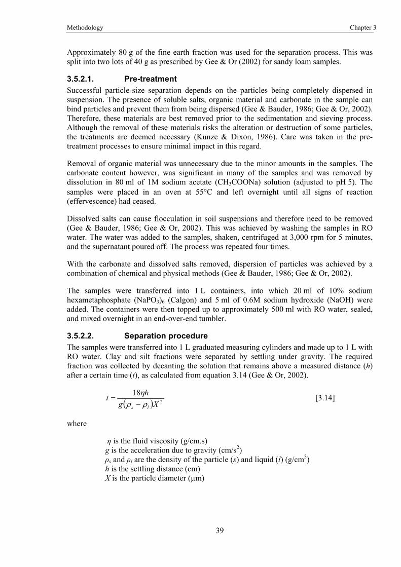
Methodology Chapter 3
39
Approximately 80 g of the fine earth fraction was used for the separation process. This was split into two lots of 40 g as prescribed by Gee & Or (2002) for sandy loam samples.
3.5.2.1. Pre-treatment Successful particle-size separation depends on the particles being completely dispersed in suspension. The presence of soluble salts, organic material and carbonate in the sample can bind particles and prevent them from being dispersed (Gee & Bauder, 1986; Gee & Or, 2002). Therefore, these materials are best removed prior to the sedimentation and sieving process. Although the removal of these materials risks the alteration or destruction of some particles, the treatments are deemed necessary (Kunze & Dixon, 1986). Care was taken in the pre-treatment processes to ensure minimal impact in this regard.
Removal of organic material was unnecessary due to the minor amounts in the samples. The carbonate content however, was significant in many of the samples and was removed by dissolution in 80 ml of 1M sodium acetate (CH3COONa) solution (adjusted to pH 5). The samples were placed in an oven at 55�C and left overnight until all signs of reaction (effervescence) had ceased.
Dissolved salts can cause flocculation in soil suspensions and therefore need to be removed (Gee & Bauder, 1986; Gee & Or, 2002). This was achieved by washing the samples in RO water. The water was added to the samples, shaken, centrifuged at 3,000 rpm for 5 minutes, and the supernatant poured off. The process was repeated four times.
With the carbonate and dissolved salts removed, dispersion of particles was achieved by a combination of chemical and physical methods (Gee & Bauder, 1986; Gee & Or, 2002).
The samples were transferred into 1 L containers, into which 20 ml of 10% sodium hexametaphosphate (NaPO3)6 (Calgon) and 5 ml of 0.6M sodium hydroxide (NaOH) were added. The containers were then topped up to approximately 500 ml with RO water, sealed, and mixed overnight in an end-over-end tumbler.
3.5.2.2. Separation procedure The samples were transferred into 1 L graduated measuring cylinders and made up to 1 L with RO water. Clay and silt fractions were separated by settling under gravity. The required fraction was collected by decanting the solution that remains above a measured distance (h) after a certain time (t), as calculated from equation 3.14 (Gee & Or, 2002).
� � 2
18Xg
htls
��
[3.14]
where
� is the fluid viscosity (g/cm.s) g is the acceleration due to gravity (cm/s2) �s and �l are the density of the particle (s) and liquid (l) (g/cm3) h is the settling distance (cm) X is the particle diameter (μm)
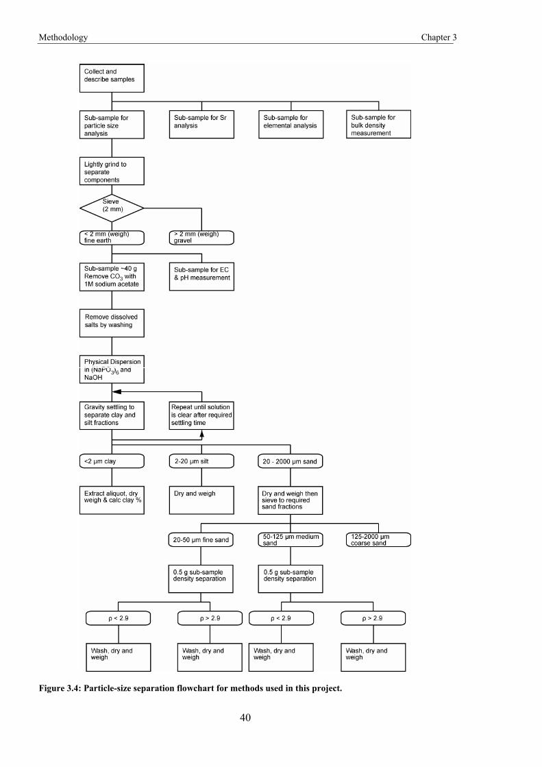
Methodology Chapter 3
40
Figure 3.4: Particle-size separation flowchart for methods used in this project.
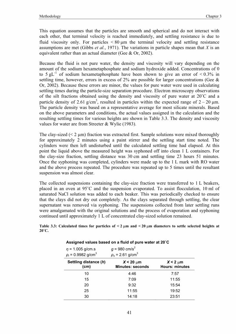
Methodology Chapter 3
41
This equation assumes that the particles are smooth and spherical and do not interact with each other, that terminal velocity is reached immediately, and settling resistance is due to fluid viscosity only. For particles < 80 �m the terminal velocity and settling resistance assumptions are met (Gibbs et al., 1971). The variations in particle shapes mean that X is an equivalent rather than an actual diameter (Gee & Or, 2002).
Because the fluid is not pure water, the density and viscosity will vary depending on the amount of the sodium hexametaphosphate and sodium hydroxide added. Concentrations of 0 to 5 gL-1 of sodium hexametaphosphate have been shown to give an error of < 0.3% in settling time, however, errors in excess of 2% are possible for larger concentrations (Gee & Or, 2002). Because these errors are minor, the values for pure water were used in calculating settling times during the particle-size separation procedure. Electron microscopy observations of the silt fractions obtained using the density and viscosity of pure water at 20�C and a particle density of 2.61 g/cm3, resulted in particles within the expected range of 2 – 20 �m. The particle density was based on a representative average for most silicate minerals. Based on the above parameters and conditions, the actual values assigned in the calculation and the resulting settling times for various heights are shown in Table 3.3. The density and viscosity values for water are from Streeter & Wylie (1983).
The clay-sized (< 2 �m) fraction was extracted first. Sample solutions were mixed thoroughly for approximately 2 minutes using a paint stirrer and the settling start time noted. The cylinders were then left undisturbed until the calculated settling time had elapsed. At this point the liquid above the measured height was syphoned off into clean 1 L containers. For the clay-size fraction, settling distance was 30 cm and settling time 23 hours 51 minutes. Once the syphoning was completed, cylinders were made up to the 1 L mark with RO water and the above process repeated. The procedure was repeated up to 5 times until the resultant suspension was almost clear.
The collected suspensions containing the clay-size fraction were transferred to 1 L beakers, placed in an oven at 95�C and the suspension evaporated. To assist flocculation, 10 ml of saturated NaCl solution was added to each beaker. This was periodically checked to ensure that the clays did not dry out completely. As the clays separated through settling, the clear supernatant was removed via syphoning. The suspensions collected from later settling runs were amalgamated with the original solutions and the process of evaporation and syphoning continued until approximately 1 L of concentrated clay-sized solution remained.
Table 3.3: Calculated times for particles of < 2 �m and < 20 �m diameters to settle selected heights at 20�C.
Assigned values based on a fluid of pure water at 20�C � = 1.005 g/cm.s g = 980 cm/s2 �l = 0.9982 g/cm3 �s = 2.61 g/cm3
Settling distance (h) (cm)
X < 20 �m Minutes: seconds
X < 2 �m Hours: minutes
10 4:46 7:57 15 7:09 11:55 20 9:32 15:54 25 11:55 19:52 30 14:18 23:51
Methodology Chapter 3
42
Once the clay-sized fraction was removed, the silt (2 - 20 �m) fraction was separated. The same process was followed as with the clay-sized fraction. This time however, the suspension was taken from a depth of 25 cm and a settling time, after mixing, of 11 minutes 55 seconds.
Silt fractions from consecutive runs were amalgamated and the excess liquid removed by settling and syphoning. The larger particle size meant that settling was effective without the requirement of evaporation or addition of NaCl.
The dispersing agent, and NaCl in the case of the clay fractions, was removed by washing four times with RO water, centrifuging at 3,000 rpm for 5 minutes and pouring off the supernatant.
The abundance of clay-sized material was measured by taking a 10 ml aliquot of the concentrated suspension. Aliquots were dried and weighed. The remaining clay-sized fractions were stored as liquid slurry in preparation for further analysis. The silt fractions were dried in an oven at 105� C and weighed prior to storage in small vials.
The sand was washed from the cylinders into small containers, dried in an oven at 105� C and weighed prior to further separation into three fractions: fine sand 20 – 53 �m, medium sand 53 – 125 �m, and coarse sand 125 – 2,000 �m (Figure 3.3) by sieving.
Sieving was by hand in brass framed sieves with stainless steel mesh. Sieves were thoroughly cleaned with ethanol and compressed air before each sample to avoid contamination.
Each of the collected size fractions was weighed and stored in small vials for further processing.
3.5.3. Bulk density Bulk density is required for calculation of porosity and void ratios, and in mass balance calculations (Brewer, 1964; Brimhall et al., 1985; Blake & Hartge, 1986; Brimhall & Dietrich, 1987; Brimhall et al., 1988; Chadwick et al., 1990; Brimhall et al., 1991; Brimhall et al., 1992).
Soil ped bulk density was determined by an adaptation of the clod (coarse peds) method described by Blake & Hartge (1986). “Archimedes” principle was employed to determine the volume of the clod. The apparent weight gain of water when a clod is suspended in it, is equivalent to the clod volume.
Representative soil clods, 2 – 5 cm in diameter, were selected. At least two soil clods were used from each horizon and the values averaged. The samples were dried in an oven at 105�C for at least three hours immediately prior to the measuring process in order to remove any moisture from the clods.
A short length of cotton was tied around each clod so that it could hang freely for weighing and suspension in water. The weight of the cotton was deemed negligible and not considered in the bulk density calculation (Blake & Hartge, 1986). Prior to submersion in water the clods were coated in a paraffin wax. The clods were repeatedly dipped into melted paraffin wax until the wax had formed a complete seal. The weight of the clod and paraffin wax coating were determined by weighing the clod before and after the application of the wax.
Methodology Chapter 3
43
The clod volume was measured by recording the apparent weight gain of a beaker of water with the clod suspended within it. The weight gain is equivalent to the volume of the clod, including the wax coating. Therefore the volume of a clod is the apparent gain in water weight, minus the volume of the wax coating.
Once the volume has been measured then the bulk density of the clod was calculated (Equation 3.15).
�
����
��
wax
wax
soilb m
OHm
m
2' [3.15]
where
b is the bulk density msoil is the oven dry weight of the clod m�H2O is the apparent weight increase in water when the clod and wax are submerged mwax is the weight of the paraffin wax coating wax is the density of the paraffin wax
The density of the paraffin wax (wax) was measured by weighing a small sub-sample of wax and dividing its mass by its volume. A value of 0.88 g/cm3 was recorded.
3.5.4. Measuring the carbonate concentration (calcimetry) The carbonate material in the samples had to be removed for the particle-size separation procedure; however, knowing the concentration of carbonate material in each horizon was also required. Hence a small sub-sample from the fine earth material of each horizon was analysed for its carbonate content. The distribution of carbonates in soils is rarely uniform, hence the samples have to be homogenised. This was achieved by finely grinding the samples prior to analysis.
The main carbonate minerals in soils are calcite (CaCO3) and dolomite (MgCO3). These were distinguished by the rapid reaction of calcite with cold acid, whereas dolomite has a slower reaction. Variation in carbonate mineralogy may affect the end results if dolomite is present and significant longer reaction times are not adopted (Allison & Moodie, 1965).
The amount of carbonate in the samples was determined using the volumetric calcimeter method described by Allison & Moodie (1965). In this method a closed system is used to measure the change in volumetric pressure following the release of CO2 when the sample is mixed with HCl. The calcimeter was set up as in Figure 3.5. Variations in air pressure and temperature will affect the volume change in the tubes. If the pressure and temperature are constant during the experiment they can be ignored because the results are calibrated under the same conditions by use of a standard. Air pressure was measured at the start and end of the experiment to ensure that there had not been a major fluctuation. The laboratory temperature was ~ 20� C and maintained by the building air conditioning system. Under these “standard” conditions the relationship between carbonate concentration and the calcimeter volume reading is linear (Allison & Moodie, 1965).
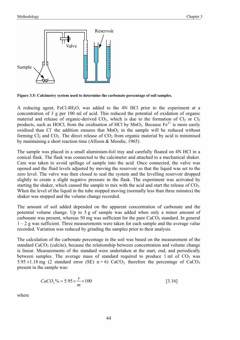
Methodology Chapter 3
44
Figure 3.5: Calcimetry system used to determine the carbonate percentage of soil samples.
A reducing agent, FeCl.4H2O, was added to the 4N HCl prior to the experiment at a concentration of 3 g per 100 ml of acid. This reduced the potential of oxidation of organic material and release of organic-derived CO2, which is due to the formation of Cl2 or Cl2 products, such as HOCl, from the oxidisation of HCl by MnO2. Because Fe2+ is more easily oxidised than Cl- the addition ensures that MnO2 in the sample will be reduced without forming Cl2 and CO2. The direct release of CO2 from organic material by acid is minimised by maintaining a short reaction time (Allison & Moodie, 1965).
The sample was placed in a small aluminium-foil tray and carefully floated on 4N HCl in a conical flask. The flask was connected to the calcimeter and attached to a mechanical shaker. Care was taken to avoid spillage of sample into the acid. Once connected, the valve was opened and the fluid levels adjusted by moving the reservoir so that the liquid was set to the zero level. The valve was then closed to seal the system and the levelling reservoir dropped slightly to create a slight negative pressure in the flask. The experiment was activated by starting the shaker, which caused the sample to mix with the acid and start the release of CO2. When the level of the liquid in the tube stopped moving (normally less than three minutes) the shaker was stopped and the volume change recorded.
The amount of soil added depended on the apparent concentration of carbonate and the potential volume change. Up to 5 g of sample was added when only a minor amount of carbonate was present, whereas 50 mg was sufficient for the pure CaCO3 standard. In general 1 – 2 g was sufficient. Three measurements were taken for each sample and the average value recorded. Variation was reduced by grinding the samples prior to their analysis.
The calculation of the carbonate percentage in the soil was based on the measurement of the standard CaCO3 (calcite), because the relationship between concentration and volume change is linear. Measurements of the standard were undertaken at the start, end, and periodically between samples. The average mass of standard required to produce 1 ml of CO2 was 5.95 ±1.18 mg (2 standard error (SE) n = 6) CaCO3, therefore the percentage of CaCO3 present in the sample was:
10095.5%3 ��myCaCO [3.16]
where
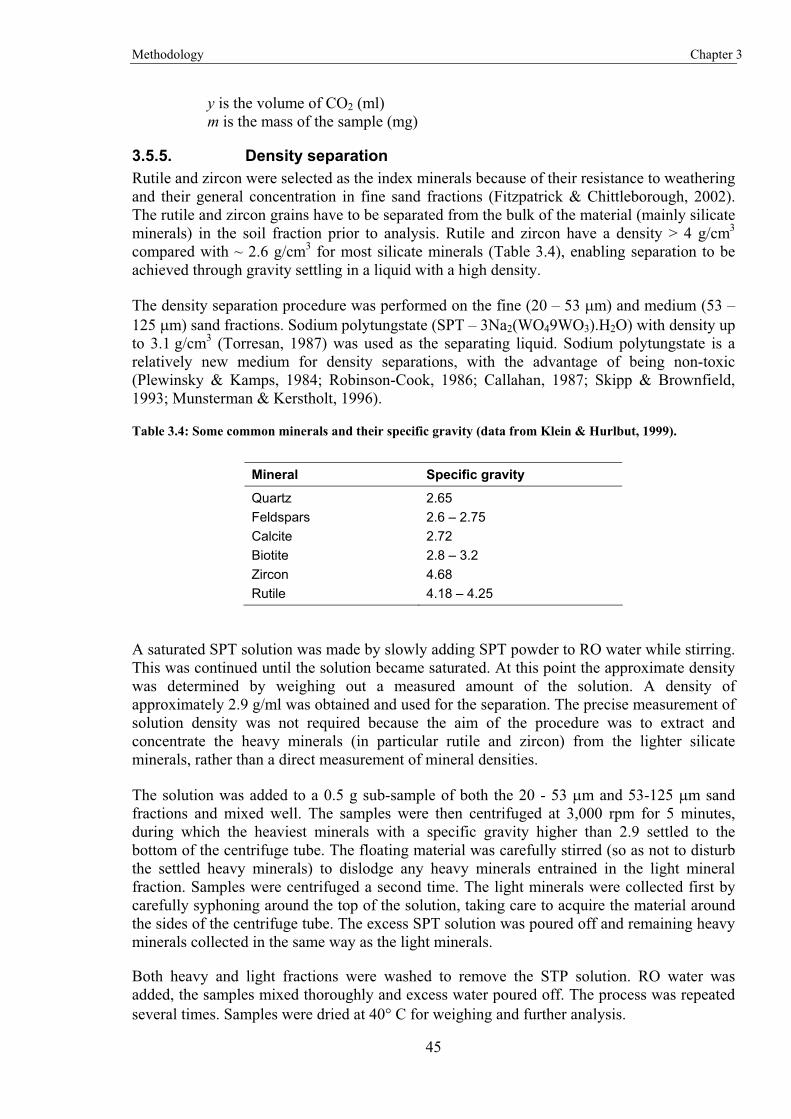
Methodology Chapter 3
45
y is the volume of CO2 (ml) m is the mass of the sample (mg)
3.5.5. Density separation Rutile and zircon were selected as the index minerals because of their resistance to weathering and their general concentration in fine sand fractions (Fitzpatrick & Chittleborough, 2002). The rutile and zircon grains have to be separated from the bulk of the material (mainly silicate minerals) in the soil fraction prior to analysis. Rutile and zircon have a density > 4 g/cm3 compared with ~ 2.6 g/cm3 for most silicate minerals (Table 3.4), enabling separation to be achieved through gravity settling in a liquid with a high density.
The density separation procedure was performed on the fine (20 – 53 �m) and medium (53 – 125 �m) sand fractions. Sodium polytungstate (SPT – 3Na2(WO49WO3).H2O) with density up to 3.1 g/cm3 (Torresan, 1987) was used as the separating liquid. Sodium polytungstate is a relatively new medium for density separations, with the advantage of being non-toxic (Plewinsky & Kamps, 1984; Robinson-Cook, 1986; Callahan, 1987; Skipp & Brownfield, 1993; Munsterman & Kerstholt, 1996).
Table 3.4: Some common minerals and their specific gravity (data from Klein & Hurlbut, 1999).
Mineral Specific gravity
Quartz 2.65 Feldspars 2.6 – 2.75 Calcite 2.72 Biotite 2.8 – 3.2 Zircon 4.68 Rutile 4.18 – 4.25
A saturated SPT solution was made by slowly adding SPT powder to RO water while stirring. This was continued until the solution became saturated. At this point the approximate density was determined by weighing out a measured amount of the solution. A density of approximately 2.9 g/ml was obtained and used for the separation. The precise measurement of solution density was not required because the aim of the procedure was to extract and concentrate the heavy minerals (in particular rutile and zircon) from the lighter silicate minerals, rather than a direct measurement of mineral densities.
The solution was added to a 0.5 g sub-sample of both the 20 - 53 �m and 53-125 �m sand fractions and mixed well. The samples were then centrifuged at 3,000 rpm for 5 minutes, during which the heaviest minerals with a specific gravity higher than 2.9 settled to the bottom of the centrifuge tube. The floating material was carefully stirred (so as not to disturb the settled heavy minerals) to dislodge any heavy minerals entrained in the light mineral fraction. Samples were centrifuged a second time. The light minerals were collected first by carefully syphoning around the top of the solution, taking care to acquire the material around the sides of the centrifuge tube. The excess SPT solution was poured off and remaining heavy minerals collected in the same way as the light minerals.
Both heavy and light fractions were washed to remove the STP solution. RO water was added, the samples mixed thoroughly and excess water poured off. The process was repeated several times. Samples were dried at 40� C for weighing and further analysis.
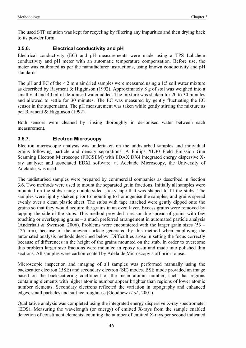
Methodology Chapter 3
46
The used STP solution was kept for recycling by filtering any impurities and then drying back to its powder form.
3.5.6. Electrical conductivity and pH Electrical conductivity (EC) and pH measurements were made using a TPS Labchem conductivity and pH meter with an automatic temperature compensation. Before use, the meter was calibrated as per the manufacturer instructions, using known conductivity and pH standards.
The pH and EC of the < 2 mm air dried samples were measured using a 1:5 soil:water mixture as described by Rayment & Higginson (1992). Approximately 8 g of soil was weighed into a small vial and 40 ml of de-ionised water added. The mixture was shaken for 20 to 30 minutes and allowed to settle for 30 minutes. The EC was measured by gently fluctuating the EC sensor in the supernatant. The pH measurement was taken while gently stirring the mixture as per Rayment & Higginson (1992).
Both sensors were cleaned by rinsing thoroughly in de-ionised water between each measurement.
3.5.7. Electron Microscopy Electron microscopic analysis was undertaken on the undisturbed samples and individual grains following particle and density separations. A Philips XL30 Field Emission Gun Scanning Electron Microscope (FEGSEM) with EDAX DX4 integrated energy dispersive X-ray analyser and associated EDXI software, at Adelaide Microscopy, the University of Adelaide, was used.
The undisturbed samples were prepared by commercial companies as described in Section 3.6. Two methods were used to mount the separated grain fractions. Initially all samples were mounted on the stubs using double-sided sticky tape that was shaped to fit the stubs. The samples were lightly shaken prior to mounting to homogenise the samples, and grains spread evenly over a clean plastic sheet. The stubs with tape attached were gently dipped onto the grains so that they would acquire the grains in an even layer. Excess grains were removed by tapping the side of the stubs. This method provided a reasonable spread of grains with few touching or overlapping grains – a much preferred arrangement in automated particle analysis (Anderhalt & Swenson, 2006). Problems were encountered with the larger grain sizes (53 – 125 μm), because of the uneven surface generated by this method when employing the automated analysis methods described below. Difficulties arose in setting the focus correctly because of differences in the height of the grains mounted on the stub. In order to overcome this problem larger size fractions were mounted in epoxy resin and made into polished thin sections. All samples were carbon-coated by Adelaide Microscopy staff prior to use.
Microscopic inspection and imaging of all samples was performed manually using the backscatter electron (BSE) and secondary electron (SE) modes. BSE mode provided an image based on the backscattering coefficient of the mean atomic number, such that regions containing elements with higher atomic number appear brighter than regions of lower atomic number elements. Secondary electrons reflected the variation in topography and enhanced edges, small particles and surface roughness (Goodhew et al., 2001).
Qualitative analysis was completed using the integrated energy dispersive X-ray spectrometer (EDS). Measuring the wavelength (or energy) of emitted X-rays from the sample enabled detection of constituent elements, counting the number of emitted X-rays per second indicated
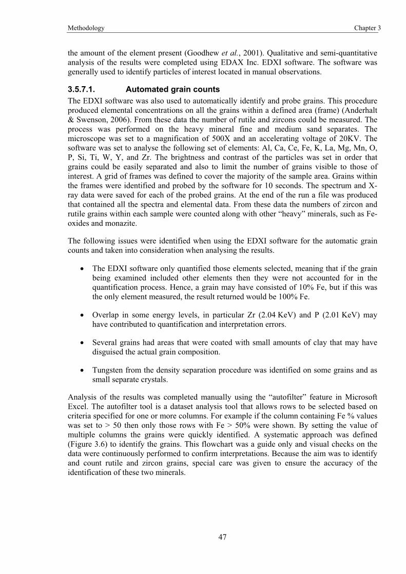
Methodology Chapter 3
47
the amount of the element present (Goodhew et al., 2001). Qualitative and semi-quantitative analysis of the results were completed using EDAX Inc. EDXI software. The software was generally used to identify particles of interest located in manual observations.
3.5.7.1. Automated grain counts The EDXI software was also used to automatically identify and probe grains. This procedure produced elemental concentrations on all the grains within a defined area (frame) (Anderhalt & Swenson, 2006). From these data the number of rutile and zircons could be measured. The process was performed on the heavy mineral fine and medium sand separates. The microscope was set to a magnification of 500X and an accelerating voltage of 20KV. The software was set to analyse the following set of elements: Al, Ca, Ce, Fe, K, La, Mg, Mn, O, P, Si, Ti, W, Y, and Zr. The brightness and contrast of the particles was set in order that grains could be easily separated and also to limit the number of grains visible to those of interest. A grid of frames was defined to cover the majority of the sample area. Grains within the frames were identified and probed by the software for 10 seconds. The spectrum and X-ray data were saved for each of the probed grains. At the end of the run a file was produced that contained all the spectra and elemental data. From these data the numbers of zircon and rutile grains within each sample were counted along with other “heavy” minerals, such as Fe-oxides and monazite.
The following issues were identified when using the EDXI software for the automatic grain counts and taken into consideration when analysing the results.
� The EDXI software only quantified those elements selected, meaning that if the grain being examined included other elements then they were not accounted for in the quantification process. Hence, a grain may have consisted of 10% Fe, but if this was the only element measured, the result returned would be 100% Fe.
� Overlap in some energy levels, in particular Zr (2.04 KeV) and P (2.01 KeV) may have contributed to quantification and interpretation errors.
� Several grains had areas that were coated with small amounts of clay that may have disguised the actual grain composition.
� Tungsten from the density separation procedure was identified on some grains and as small separate crystals.
Analysis of the results was completed manually using the “autofilter” feature in Microsoft Excel. The autofilter tool is a dataset analysis tool that allows rows to be selected based on criteria specified for one or more columns. For example if the column containing Fe % values was set to > 50 then only those rows with Fe > 50% were shown. By setting the value of multiple columns the grains were quickly identified. A systematic approach was defined (Figure 3.6) to identify the grains. This flowchart was a guide only and visual checks on the data were continuously performed to confirm interpretations. Because the aim was to identify and count rutile and zircon grains, special care was given to ensure the accuracy of the identification of these two minerals.
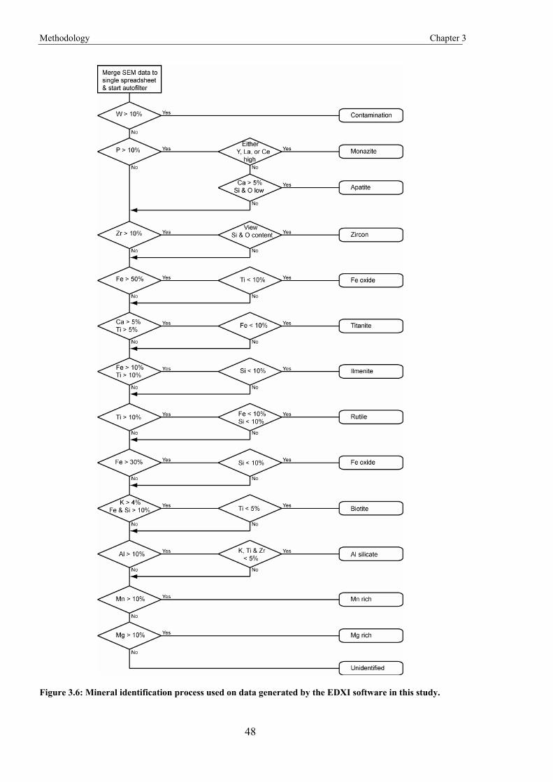
Methodology Chapter 3
48
Figure 3.6: Mineral identification process used on data generated by the EDXI software in this study.
Methodology Chapter 3
49
Results from all the automatic grain count runs were amalgamated and analysed on a single spreadsheet. This meant that interpretation was consistent for all samples. Although the procedure was successful in identifying the majority of grains, several were not easily identified and required personal judgement. Where precise identification was not possible the grains were recorded and not counted in the final tabulation of results. The number of unidentified grains and possible identification errors of some grains were negligible.
3.5.7.2. Gold morphology Assay results of the size fractions revealed that Au was highest within the silt fractions. The highest probability of locating Au particles was therefore within this fraction. The high atomic number of Au means that Au particles occur as bright objects when observed in BSE mode. It was therefore possible to set the brightness and contrast levels of the SEM to show only the “bright” grains. Grains selected by this method were identified and probed to determine their elemental composition. Manual and automatic grain analysis techniques (described above) were used. The automated process was of limited benefit because:
� The higher magnification required (> 10,000X) for the finer grain size (< 20 μm) meant that a high number of frames were required to cover the sample. The time taken was in excess of 24 hours.
� The aim was to view the morphology of the Au, and the sample could not be moved following analysis. Identified grains in the automated procedure could only be located by their relative coordinates as saved with the analytical data.
� The majority of “bright” grains consisted of elements other than Au that also had high atomic weights. These grains were generally monazite ((Ce,La,Y,Th)PO4) or iron oxides.
Because of these issues, it was found that searching manually was more efficient than the automated method. With practice the intensity of the Au brightness became recognisable, and time spent probing monazites or Fe-oxides was reduced.
Although Au may be detected by analytical techniques, it is not always visible, even with an electron microprobe or electron microscope (Wilson, 1984). This so called “invisible Au” is most likely very small, finely disseminated particles. Crystallography studies using electron microscopy have determined the morphology of supergene Au with high fineness from the saprolite. This includes very thin “trigonal” octahedral plates from around 10 μm in diameter (Wilson, 1984; Lawrance & Griffin, 1994; Hough et al., 2006), small octahedral (5 – 12 μm) crystals and polycrystalline aggregates (Lawrance & Griffin, 1994). In some cases however, the octahedral plates are so thin that they appear transparent due to the electron beam passing through the Au-lattice and instead providing information from the underlying material (Wilson, 1984; Hough et al., 2006). Hence, searching for Au on the basis of grain “brightness” meant that Au particles could be overlooked.
3.6. Specialist sample preparation and analysis The methods described in this section were completed by specialist research areas or companies with access to specialised analytical equipment.
Due to economical constraints, the number of samples that could be sent for elemental analysis was restricted. The decision was made to forego the submission of any sample
Methodology Chapter 3
50
duplicates or standards to the assaying companies. The result is a lack of quality control and a reliance on the analytical company controls. It was felt however that this risk was worth taking to ensure all the required samples were analysed.
3.6.1. Impregnation of in-situ samples The undisturbed samples from White Dam were collected for petrographic examination in thin section. Before the samples were made into thin sections they were impregnated with epoxy resin to prevent disintegration during manufacture of the thin sections. Impregnation of the undisturbed clods was performed by CSIRO Land and Water, Canberra.
Twelve samples were impregnated, one from each soil horizon of the two profiles. Samples were impregnated in a vacuum with epoxy resin containing a UV fluorescent dye (UVtex) to highlight pores when viewed under UV light.
3.6.2. Petrological thin section preparation Petrological thin sections were required for standard microscope petrology and also electron microscopy. Both were prepared from samples provided to Pontifex & Associates Pty. Ltd., Adelaide. Petrological microscope slides were 7.5 x 5 cm with cover slides, whereas the electron microscopy slides were 4.7 x 2.5 cm with no cover slide.
Both types of slides were made from the impregnated soil samples. The slides were prepared along cuts that were selected to provide a representative sample and also maximum slide coverage, especially with the larger slides.
Thin sections were also prepared of the 53 – 125 μm heavy mineral separates for automatic grain counts on the FEGSEM. These samples were first set in epoxy resin so that they could be attached to the slide and polished to a flat surface.
3.6.3. Inductively coupled plasma – mass spectrometry (ICP MS)/ optical emission spectrometry (ICP OES) and fire assay / atomic absorption (FAA)
Elemental analyses of the White Dam soil and Tunkillia regolith carbonate samples were completed by Amdel Ltd, Adelaide. A variety of methods were used to measure the concentration of 53 elements (Table 3.5).
The samples were crushed and powdered to form an analytical pulp. Sub-samples of this pulp were used as input to the various analysis methods. For analysis of the trace and rare earth elements (REEs), a 0.2 g sub-sample of the pulp was digested using an HF/multi acid solution and presented to an ICP-MS for the quantification of the elements of interest. The major elements were analysed from a 0.1 g sub-sample of the pulp, which was fused with lithium metaborate followed by dissolution to give a “total solution” for ICP-OES analysis. Gold was analysed by taking a 40 g sub-sample of the pulp that was fused in a lead collection fire assay. The resulting prill was digested in aqua-regia and the Au concentration determined by graphite furnace AAS.
3.6.4. Instrumental neutron activation analysis (INAA) Elemental analysis of the soil separates was completed by INAA because of the small sample masses (~ 1 g for some samples). This work was completed by Becquerel Laboratories, Ontario, Canada. The small sample sizes limited the number of elements that could be analysed and also raised the detection limit of some elements. The following 35 elements
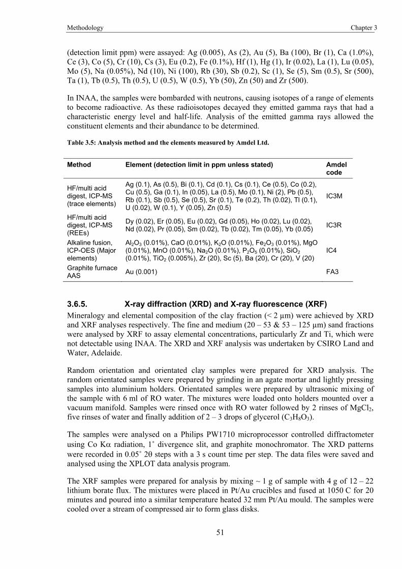
Methodology Chapter 3
51
(detection limit ppm) were assayed: Ag (0.005), As (2), Au (5), Ba (100), Br (1), Ca (1.0%), Ce (3), Co (5), Cr (10), Cs (3), Eu (0.2), Fe (0.1%), Hf (1), Hg (1), Ir (0.02), La (1), Lu (0.05), Mo (5), Na (0.05%), Nd (10), Ni (100), Rb (30), Sb (0.2), Sc (1), Se (5), Sm (0.5), Sr (500), Ta (1), Tb (0.5), Th (0.5), U (0.5), W (0.5), Yb (50), Zn (50) and Zr (500).
In INAA, the samples were bombarded with neutrons, causing isotopes of a range of elements to become radioactive. As these radioisotopes decayed they emitted gamma rays that had a characteristic energy level and half-life. Analysis of the emitted gamma rays allowed the constituent elements and their abundance to be determined.
Table 3.5: Analysis method and the elements measured by Amdel Ltd.
Method Element (detection limit in ppm unless stated) Amdel code
HF/multi acid digest, ICP-MS (trace elements)
Ag (0.1), As (0.5), Bi (0.1), Cd (0.1), Cs (0.1), Ce (0.5), Co (0.2), Cu (0.5), Ga (0.1), In (0.05), La (0.5), Mo (0.1), Ni (2), Pb (0.5), Rb (0.1), Sb (0.5), Se (0.5), Sr (0.1), Te (0.2), Th (0.02), Tl (0.1), U (0.02), W (0.1), Y (0.05), Zn (0.5)
IC3M
HF/multi acid digest, ICP-MS (REEs)
Dy (0.02), Er (0.05), Eu (0.02), Gd (0.05), Ho (0.02), Lu (0.02), Nd (0.02), Pr (0.05), Sm (0.02), Tb (0.02), Tm (0.05), Yb (0.05) IC3R
Alkaline fusion, ICP-OES (Major elements)
Al2O3 (0.01%), CaO (0.01%), K2O (0.01%), Fe2O3 (0.01%), MgO (0.01%), MnO (0.01%), Na2O (0.01%), P2O5 (0.01%), SiO2 (0.01%), TiO2 (0.005%), Zr (20), Sc (5), Ba (20), Cr (20), V (20)
IC4
Graphite furnace AAS Au (0.001) FA3
3.6.5. X-ray diffraction (XRD) and X-ray fluorescence (XRF) Mineralogy and elemental composition of the clay fraction (< 2 μm) were achieved by XRD and XRF analyses respectively. The fine and medium (20 – 53 & 53 – 125 μm) sand fractions were analysed by XRF to assay elemental concentrations, particularly Zr and Ti, which were not detectable using INAA. The XRD and XRF analysis was undertaken by CSIRO Land and Water, Adelaide.
Random orientation and orientated clay samples were prepared for XRD analysis. The random orientated samples were prepared by grinding in an agate mortar and lightly pressing samples into aluminium holders. Orientated samples were prepared by ultrasonic mixing of the sample with 6 ml of RO water. The mixtures were loaded onto holders mounted over a vacuum manifold. Samples were rinsed once with RO water followed by 2 rinses of MgCl2, five rinses of water and finally addition of 2 – 3 drops of glycerol (C3H8O3).
The samples were analysed on a Philips PW1710 microprocessor controlled diffractometer using Co K� radiation, 1� divergence slit, and graphite monochromator. The XRD patterns were recorded in 0.05� 2� steps with a 3 s count time per step. The data files were saved and analysed using the XPLOT data analysis program.
The XRF samples were prepared for analysis by mixing ~ 1 g of sample with 4 g of 12 – 22 lithium borate flux. The mixtures were placed in Pt/Au crucibles and fused at 1050 C for 20 minutes and poured into a similar temperature heated 32 mm Pt/Au mould. The samples were cooled over a stream of compressed air to form glass disks.
Methodology Chapter 3
52
The disks were analysed on a Philips PW1480 wavelength dispersive XRF system using a dual anode Sc/Mo tube. Analysis of the results was completed using algorithms developed by CSIRO. The following oxides (detection limit) were assayed: SiO2 (0.35%), Al2O3 (0.20%), MgO (0.10%), Fe2O3 (0.12%), CaO (0.10%), Na2O (0.08%), K2O (0.05%), TiO (0.03%), P2O5 (0.03%), MnO (0.01%), SO3 (0.02%), ZnO (18 ppm), CuO (12 ppm), SrO (17 ppm), ZrO2 (30 ppm), NiO (16 ppm), Rb2O (14 ppm), BaO (35 ppm), V2O5 (17 ppm), Cr2O3 (17 ppm), La2O3 (20 ppm), CeO2 (20 ppm), PbO (18 ppm), Y2O3 (12 ppm), CoO (12 ppm), Ga2O3 (7 ppm), U3O8 (13 ppm), ThO2 (13 ppm), As2O5 (8 ppm), SnO2 (18 ppm) and Cl (40 ppm).
53
Chapter 4
Source of calcium in regolith carbonates
Section 4.1 is published as: Dart, R. C., Barovich, K. M., Chittleborough, D. J., & Hill, S. M. (2007), Calcium in regolith carbonates of central and southern Australia: Its source and implications for the global carbon cycle. Palaeogeography, Palaeoclimatology, Palaeoecology 249, 322-334.
4.1. Calcium in regolith carbonates of central and southern Australia: Its source and implications for the global carbon cycle
4.1.1. Abstract The widespread regolith carbonates of the Australian continent are a potential sink for CO2. We have used Sr isotopes to investigate the source of the Ca in regolith carbonates that cover approximately 1.6 x 10⁶ km2 of inland Australia. 87Sr/86Sr ratios for nearly all the carbonates were in the range 0.7094 to 0.7211. The results show that only about 10% of the Ca in regolith carbonates is derived from weathered bedrock, with the remaining component being derived from an external marine source. The exceptions are the most northerly samples with a range of 0.7270 to 0.7374, in which bedrock content may be as high as 30%. The likely Ca source areas are sedimentary carbonates located on the continental shelf and calcareous aeolianites that surround much of the southern and western Australian coastline. Winds passing over these carbonates continually rework and transport the material over the Australian continent where it has settled and formed the regolith carbonates we see today. The impact of this process is that, despite the immense area covered, Australian regolith carbonates do not capture any additional CO2; instead the carbonate is simply being remobilised from one pool (marine) to another (terrestrial).
4.1.2. Introduction Regolith carbonates are widespread and abundant in semi-arid to arid climates. They are an important part of the global carbon cycle, which is composed of three major pools: oceanic with approximately 39,000 Pg (Pg = 1015 g), terrestrial with approximately 2,500 Pg and atmospheric with approximately 750 Pg of C. The largest terrestrial pool is in the form of soil organic carbon (SOC) and soil inorganic carbon (SIC) (Eswaran et al., 1999). Although small in relation to the C content of the oceans, C contained in regolith carbonates is a significant proportion of the terrestrial pool, and is on the order of the atmospheric pool. Various estimates of the amount of C contained in modern regolith carbonates have been made by several authors: 780 – 930 Pg (Schlesinger, 1982); 720 Pg (Sombroek et al., 1993); 695 – 748 Pg (Batjes, 1996; Batjes & Sombroek, 1997); and 940 Pg (Eswaran et al., 1999). The large variation in these estimates is mainly a consequence of the varying interpretations of soil profiles and what constitutes a regolith carbonate.
Regolith carbonates cover approximately 21% of Australia (Chen et al., 2002), an area of approximately 1.6 x 10⁶ km2. The distribution of these carbonates is concentrated in the arid
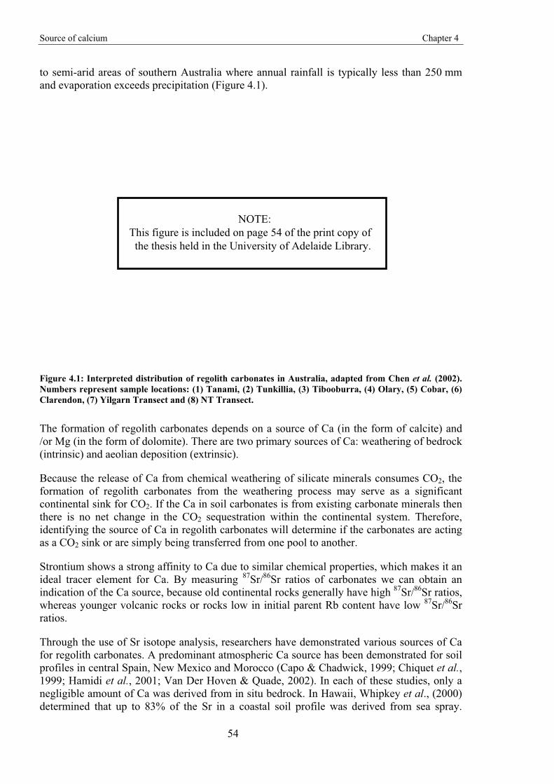
Source of calcium Chapter 4
54
to semi-arid areas of southern Australia where annual rainfall is typically less than 250 mm and evaporation exceeds precipitation (Figure 4.1).
Figure 4.1: Interpreted distribution of regolith carbonates in Australia, adapted from Chen et al. (2002). Numbers represent sample locations: (1) Tanami, (2) Tunkillia, (3) Tibooburra, (4) Olary, (5) Cobar, (6) Clarendon, (7) Yilgarn Transect and (8) NT Transect.
The formation of regolith carbonates depends on a source of Ca (in the form of calcite) and /or Mg (in the form of dolomite). There are two primary sources of Ca: weathering of bedrock (intrinsic) and aeolian deposition (extrinsic).
Because the release of Ca from chemical weathering of silicate minerals consumes CO2, the formation of regolith carbonates from the weathering process may serve as a significant continental sink for CO2. If the Ca in soil carbonates is from existing carbonate minerals then there is no net change in the CO2 sequestration within the continental system. Therefore, identifying the source of Ca in regolith carbonates will determine if the carbonates are acting as a CO2 sink or are simply being transferred from one pool to another.
Strontium shows a strong affinity to Ca due to similar chemical properties, which makes it an ideal tracer element for Ca. By measuring 87Sr/86Sr ratios of carbonates we can obtain an indication of the Ca source, because old continental rocks generally have high 87Sr/86Sr ratios, whereas younger volcanic rocks or rocks low in initial parent Rb content have low 87Sr/86Sr ratios.
Through the use of Sr isotope analysis, researchers have demonstrated various sources of Ca for regolith carbonates. A predominant atmospheric Ca source has been demonstrated for soil profiles in central Spain, New Mexico and Morocco (Capo & Chadwick, 1999; Chiquet et al., 1999; Hamidi et al., 2001; Van Der Hoven & Quade, 2002). In each of these studies, only a negligible amount of Ca was derived from in situ bedrock. In Hawaii, Whipkey et al., (2000) determined that up to 83% of the Sr in a coastal soil profile was derived from sea spray.
NOTE: This figure is included on page 54 of the print copy of the thesis held in the University of Adelaide Library.
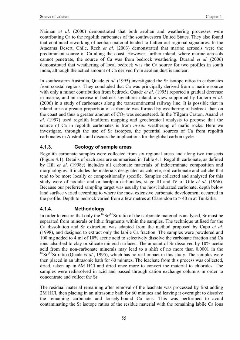
Source of calcium Chapter 4
55
Naiman et al. (2000) demonstrated that both aeolian and weathering processes were contributing Ca to the regolith carbonates of the southwestern United States. They also found that continued reworking of aeolian material tended to flatten out regional signatures. In the Atacama Desert, Chile, Rech et al. (2003) demonstrated that marine aerosols were the predominant source of Ca along the coast. However, further inland, where marine aerosols cannot penetrate, the source of Ca was from bedrock weathering. Durand et al. (2006) demonstrated that weathering of local bedrock was the Ca source for two profiles in south India, although the actual amount of Ca derived from aeolian dust is unclear.
In southeastern Australia, Quade et al. (1995) investigated the Sr isotope ratios in carbonates from coastal regions. They concluded that Ca was principally derived from a marine source with only a minor contribution from bedrock. Quade et al. (1995) reported a gradual decrease in marine, and an increase in bedrock signatures inland, a view supported by Lintern et al. (2006) in a study of carbonates along the transcontinental railway line. It is possible that in inland areas a greater proportion of carbonate was formed by weathering of bedrock than on the coast and thus a greater amount of CO2 was sequestered. In the Yilgarn Craton, Anand et al. (1997) used regolith landform mapping and geochemical analysis to propose that the source of Ca in regolith carbonates is from in-situ weathering of mafic rocks. Here we investigate, through the use of Sr isotopes, the potential sources of Ca from regolith carbonates in Australia and discuss the implications for the global carbon cycle.
4.1.3. Geology of sample areas Regolith carbonate samples were collected from six regional areas and along two transects (Figure 4.1). Details of each area are summarised in Table 4.1. Regolith carbonate, as defined by Hill et al. (1998c) includes all carbonate materials of indeterminate composition and morphologies. It includes the materials designated as calcrete, soil carbonate and caliche that tend to be more locally or compositionally specific. Samples collected and analysed for this study were of nodular and or hardpan carbonates, stage III and IV of Gile et al. (1966). Because our preferred sampling target was usually the most indurated carbonate, depth below land surface varied according to where the most extensive carbonate development occurred in the profile. Depth to bedrock varied from a few metres at Clarendon to > 40 m at Tunkillia.
4.1.4. Methodology In order to ensure that only the 87Sr/86Sr ratio of the carbonate material is analysed, Sr must be separated from minerals or lithic fragments within the samples. The technique utilised for the Ca dissolution and Sr extraction was adapted from the method proposed by Capo et al. (1998), and designed to extract only the labile Ca fraction. The samples were powdered and 100 mg added to 4 ml of 10% acetic acid to selectively dissolve the carbonate fraction and Ca ions adsorbed to clay or silicate mineral surfaces. The amount of Sr dissolved by 10% acetic acid from the non-carbonate minerals may lead to a shift of no more than 0.0001 in the 87Sr/86Sr ratio (Quade et al., 1995), which has no real impact in this study. The samples were then placed in an ultrasonic bath for 60 minutes. The leachate from this process was collected, dried, taken up in 6M HCl and dried once more to convert the material to chlorides. The samples were redissolved in acid and passed through cation exchange columns in order to concentrate and collect the Sr.
The residual material remaining after removal of the leachate was processed by first adding 2M HCl, then placing in an ultrasonic bath for 60 minutes and leaving it overnight to dissolve the remaining carbonate and loosely-bound Ca ions. This was performed to avoid contaminating the Sr isotope ratios of the residue material with the remaining labile Ca ions
Source of calcium Chapter 4
56
that were not removed by the weak acetic acid. The samples were washed several times before total dissolution in a mixture of HNO3, HF and HCl followed by concentration of Sr collection on cation exchange columns in a manner identical with the carbonate leachate.
Measurement of the Sr isotope ratios was performed on a Finnigan MAT262 thermal ionisation mass spectrometer (TIMS) at The University of Adelaide, South Australia. Ratios are measured in 10 blocks of 10 (100 ratios). The results are then normalised using an 88Sr/86Sr ratio of 8.3752.
The average 87Sr/86Sr ratio measured for standard SRM987 during the course of this study was 0.71027 �0.000025 (2SE, 20 runs). Procedural Sr blank values averaged 0.8 ng.
The following simple mixing equation for two end members was used to calculate the percentage of Sr (and Ca) derived from the bedrock:
� �� � � �mixABmix
BmixB SrSrSrSrSrSrSrSr
SrSrSrSrX 8687868786878687
86878687
����
[4.1]
where XB is the proportion of Sr provided by the bedrock, 87Sr/86Srmix is the Sr isotope ratio measured for the sample, 87Sr/86SrA is the Sr isotope ratio for modern oceans and 87Sr/86SrB is the Sr isotope ratio for the bedrock. Bedrock values for each region have been taken, where available, from recent literature (Table 3).
With the majority of Australian continental bedrock Precambrian in age, their 87Sr/86Sr ratios are typically around 0.8 or above. The 87Sr/86Sr ratio of modern oceans is from the mixture of the two input sources (continental and volcanic rocks) derived from weathering processes. The accepted 87Sr/86Sr ratio for modern oceans is 0.70918 (Faure & Mensing, 2005) and is equivalent to the ratio measured in modern marine carbonates.
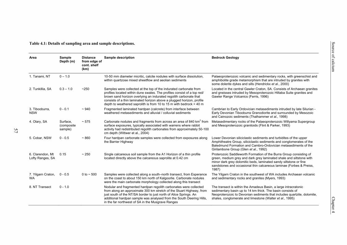
57
Table 4.1: Details of sampling area and sample descriptions.
Area Sample Depth (m)
Distance from edge of cont. shelf (km)
Sample description Bedrock Geology
1. Tanami, NT 0 – 1.0 10-50 mm diameter micritic, calcite nodules with surface dissolution, within quartzose mixed sheetflow and aeolian sediments
Palaeoproterozoic volcanic and sedimentary rocks, with greenschist and amphibolite grade metamorphism that are intruded by granites with some dolerite dykes and sills (Hendrickx et al., 2000)
2. Tunkillia, SA 0.3 – 1.0 ~250 Samples were collected at the top of the indurated carbonate from profiles located within dune swales. The profiles consist of a top red/ brown sand horizon overlying an indurated regolith carbonate that consists of a thin laminated horizon above a plugged horizon, profile depth to weathered saprolith is from 10 to 15 m with bedrock > 40 m
Located in the central Gawler Craton, SA. Consists of Archaean granites and gneisses intruded by Mesoproterozoic Hiltaba Suite granites and Gawler Range Volcanics (Ferris, 1996)
3. Tibooburra, NSW
0 - 0.1 ~ 940 Fragmented laminated hardpan (calcrete) from interface between weathered metasediments and alluvial / colluvial sediments
Cambrian to Early Ordovician metasediments intruded by late Silurian - Early Devonian Tibooburra Granodiorite and surrounded by Mesozoic and Cainozoic sediments (Thalhammer et al., 1998)
4. Olary, SA Surface, (composite sample)
~ 575 Carbonate nodules and fragments from across an area of 840 km2 from surface exposures, typically associated with warrens where rabbit activity had redistributed regolith carbonates from approximately 50-100 cm depth (Wittwer et al., 2004)
Metasedimentary rocks of the Palaeoproterozoic Willyama Supergroup and Mesoproterozoic granitoids (Flint & Parker, 1993)
5. Cobar, NSW 0 - 0.5 ~ 860 Four hardpan carbonate samples were collected from exposures along the Barrier Highway
Lower Devonian siliciclastic sediments and turbidites of the upper Amphitheatre Group, siliciclastic sediments and conglomerates of the Baledmund Formation and Cambro-Ordovician metasediments of the Girilambone Group (Glen et al., 1992)
6. Clarendon, Mt Lofty Ranges, SA
0.15 ~ 250 Single calcareous soil sample from the A1 Horizon of a thin profile located directly above the calcareous saprolite at 0.42 cm
Proterozoic Saddleworth Formation of the Burra Group consisting of green, medium grey and dark grey laminated shale and siltstone with minor dark grey dolomitic beds, laminated sandy siltstone or fine sandstones and occasional thin calcareous laminae (Forbes & Preiss, 1987)
7. Yilgarn Craton, WA
0 - 0.5 0 to ~ 500 Samples were collected along a south–north transect, from Esperance on the coast to about 150 km north of Kalgoorlie. Carbonate nodules were the main carbonate morphology collected along this transect
The Yilgarn Craton in the southwest of WA includes Archaean volcanic and sedimentary rocks and granites (Myers, 1993)
8. NT Transect 0 - 1.0 Nodular and fragmented hardpan regolith carbonates were collected from along an approximate 300 km stretch of the Stuart Highway, from just south of the NT/SA border to just north of Alice Springs. An additional hardpan sample was analysed from the South Deering Hills, in the far northwest of SA in the Musgrave Ranges
The transect is within the Amadeus Basin, a large intracratonic sedimentary basin up to 14 km thick. The basin consists of Neoproterozoic to Devonian sediments that includes quartzite, dolomite, shales, conglomerate and limestone (Walter et al., 1995)
Source of calcium C
hapter 4
57
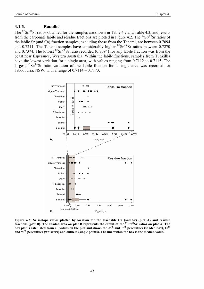
Source of calcium Chapter 4
58
4.1.5. Results The 87Sr/86Sr ratios obtained for the samples are shown in Table 4.2 and Table 4.3, and results from the carbonate labile and residue fractions are plotted in Figure 4.2. The 87Sr/86Sr ratios of the labile Sr (and Ca) fraction samples, excluding those from the Tanami, are between 0.7094 and 0.7211. The Tanami samples have considerably higher 87Sr/86Sr ratios between 0.7270 and 0.7374. The lowest 87Sr/86Sr ratio recorded (0.7094) for any labile fraction was from the coast near Esperance, Western Australia. Within the labile fractions, samples from Tunkillia have the lowest variation for a single area, with values ranging from 0.7112 to 0.7115. The largest 87Sr/86Sr ratio variation of the labile fraction for a single area was recorded for Tibooburra, NSW, with a range of 0.7114 – 0.7173.
Figure 4.2: Sr isotope ratios plotted by location for the leachable Ca (and Sr) (plot A) and residue fractions (plot B). The shaded area on plot B represents the extent of the 87Sr/86Sr ratios on plot A. The box plot is calculated from all values on the plot and shows the 25th and 75th percentiles (shaded box), 10th and 90th percentiles (whiskers) and outliers (single points). The line within the box is the median value.
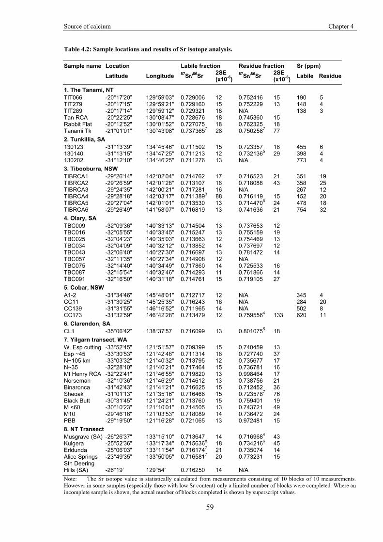
Source of calcium Chapter 4
59
Table 4.2: Sample locations and results of Sr isotope analysis.
Sample name Location Labile fraction Residue fraction Sr (ppm) Latitude Longitude 87Sr/86Sr 2SE
(x10-6) 87Sr/86Sr 2SE
(x10-6) Labile Residue
1. The Tanami, NT TIT066 -20°17'20” 129°59'03" 0.729006 12 0.752416 15 190 5 TIT279 -20°17'15” 129°59'21" 0.729160 15 0.752229 13 148 4 TIT289 -20°17'14” 129°59'12" 0.729321 18 N/A 138 3 Tan RCA -20°22'25" 130°08'47" 0.728676 18 0.745360 15 Rabbit Flat -20°12'52" 130°01'52" 0.727075 18 0.762325 18 Tanami Tk -21°01'01" 130°43'08" 0.7373657 28 0.7502587 77 2. Tunkillia, SA 130123 -31°13'39" 134°45'46" 0.711502 15 0.723357 18 455 6 130140 -31°13'15" 134°47'25" 0.711213 12 0.7321365 29 398 4 130202 -31°12'10" 134°46'25" 0.711276 13 N/A 773 4 3. Tibooburra, NSW TIBRCA1 -29°26'14" 142°02'04" 0.714762 17 0.716523 21 351 19 TIBRCA2 -29°26'59" 142°01'28" 0.713107 16 0.718088 43 358 25 TIBRCA3 -29°24'35" 142°00'21" 0.717281 16 N/A 267 12 TIBRCA4 -29°28'18" 142°03'17" 0.7113893 88 0.716119 15 152 20 TIBRCA5 -29°27'04" 142°01'01" 0.713530 13 0.7144705 24 478 18 TIBRCA6 -29°26'49" 141°58'07" 0.716819 13 0.741636 21 754 32 4. Olary, SA TBC009 -32°09'36" 140°33'13" 0.714504 13 0.737653 12 TBC016 -32°05'55" 140°33'45" 0.715247 13 0.755159 19 TBC025 -32°04'23" 140°35'03" 0.713663 12 0.754469 13 TBC034 -32°04'09" 140°32'12" 0.713852 14 0.737697 12 TBC043 -32°06'40" 140°27'30" 0.716697 13 0.781472 14 TBC057 -32°11'35" 140°27'34" 0.714908 12 N/A TBC075 -32°14'40" 140°34'49" 0.717860 14 0.725533 16 TBC087 -32°15'54" 140°32'46" 0.714293 11 0.761866 14 TBC091 -32°16'50" 140°31'18" 0.714761 15 0.719105 27 5. Cobar, NSW A1-2 -31°34'46" 145°48'01" 0.712717 12 N/A 345 4 CC11 -31°30'25" 145°25'35" 0.716243 16 N/A 284 20 CC139 -31°31'55" 146°16'52" 0.711965 14 N/A 502 8 CC173 -31°32'59" 146°42'28" 0.713479 12 0.7595564 133 620 11 6. Clarendon, SA CL1 -35°06'42” 138°37'57 0.716099 13 0.8010755 18 7. Yilgarn transect, WA W. Esp cutting -33°52'45" 121°51'57" 0.709399 15 0.740459 13 Esp ~45 -33°30'53" 121°42'48" 0.711314 16 0.727740 37 N~105 km -33°03'32" 121°40'32" 0.713795 12 0.735677 17 N~35 -32°28'10" 121°40'21" 0.717464 15 0.736781 16 Mt Henry RCA -32°22'41" 121°46'55" 0.719820 13 0.998464 17 Norseman -32°10'36" 121°46'29" 0.714612 13 0.738756 21 Binaronca -31°42'43" 121°41'21" 0.716625 15 0.712452 36 Sheoak -31°01'13" 121°35'16" 0.716468 15 0.7235787 76 Black Butt -30°31'45" 121°24'21" 0.713760 15 0.759401 19 M <60 -30°10'23" 121°10'01" 0.714505 13 0.743721 49 M10 -29°46'16" 121°03'53" 0.718089 14 0.736472 24 PBB -29°19'50" 121°16'28" 0.721065 13 0.972481 15 8. NT Transect Musgrave (SA) -26°26'37" 133°15'10" 0.713647 14 0.7169684 43 Kulgera -25°52'36" 133°17'34" 0.7156368 18 0.7342166 45 Erldunda -25°06'03" 133°11'54" 0.7161747 21 0.735074 14 Alice Springs -23°49'35" 133°50'05" 0.7165817 20 0.773231 15 Sth Deering Hills (SA) -26°19’ 129°54’ 0.716250 14 N/A Note: The Sr isotope value is statistically calculated from measurements consisting of 10 blocks of 10 measurements. However in some samples (especially those with low Sr content) only a limited number of blocks were completed. Where an incomplete sample is shown, the actual number of blocks completed is shown by superscript values.
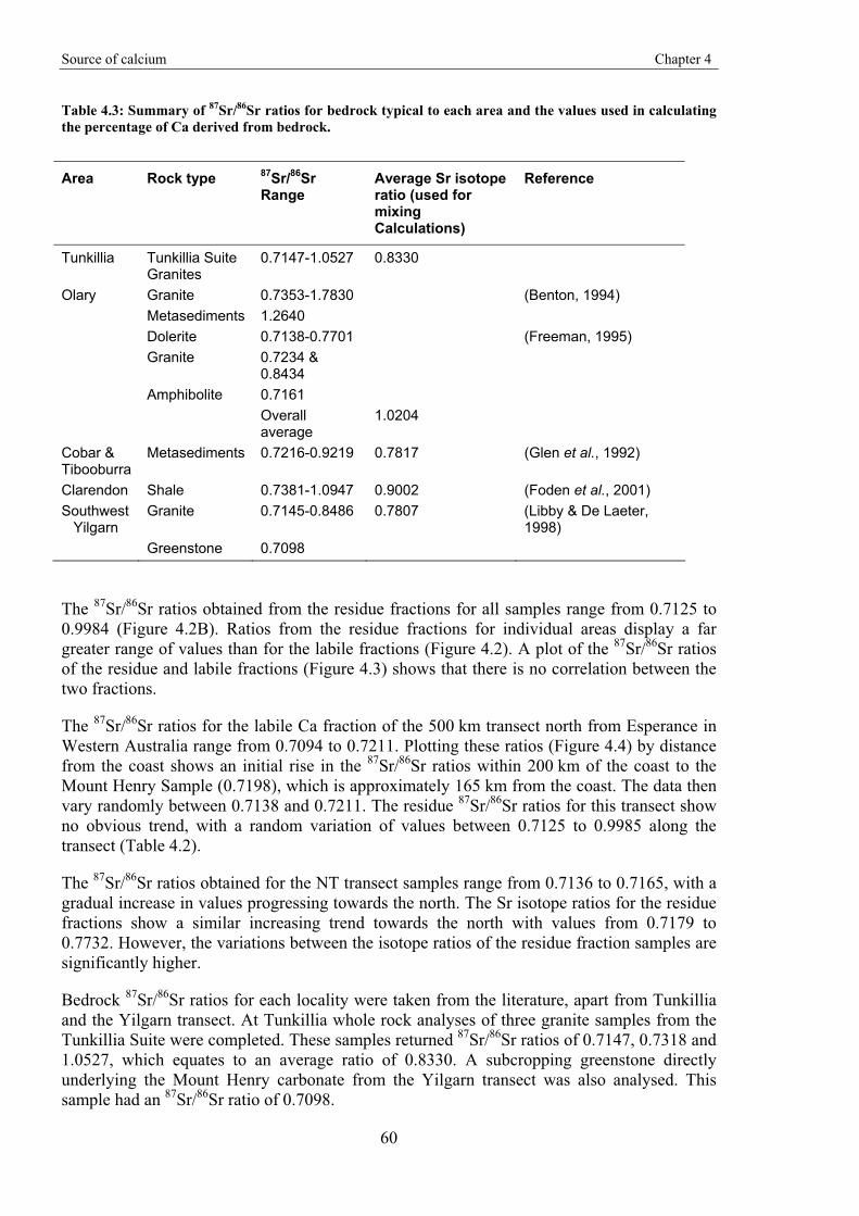
Source of calcium Chapter 4
60
Table 4.3: Summary of 87Sr/86Sr ratios for bedrock typical to each area and the values used in calculating the percentage of Ca derived from bedrock.
Area Rock type 87Sr/86Sr Range
Average Sr isotope ratio (used for mixing Calculations)
Reference
Tunkillia Tunkillia Suite Granites
0.7147-1.0527 0.8330
Olary Granite 0.7353-1.7830 (Benton, 1994) Metasediments 1.2640 Dolerite 0.7138-0.7701 (Freeman, 1995) Granite 0.7234 &
0.8434
Amphibolite 0.7161 Overall
average 1.0204
Cobar & Tibooburra
Metasediments 0.7216-0.9219 0.7817 (Glen et al., 1992)
Clarendon Shale 0.7381-1.0947 0.9002 (Foden et al., 2001) Southwest Yilgarn
Granite 0.7145-0.8486 0.7807 (Libby & De Laeter, 1998)
Greenstone 0.7098
The 87Sr/86Sr ratios obtained from the residue fractions for all samples range from 0.7125 to 0.9984 (Figure 4.2B). Ratios from the residue fractions for individual areas display a far greater range of values than for the labile fractions (Figure 4.2). A plot of the 87Sr/86Sr ratios of the residue and labile fractions (Figure 4.3) shows that there is no correlation between the two fractions.
The 87Sr/86Sr ratios for the labile Ca fraction of the 500 km transect north from Esperance in Western Australia range from 0.7094 to 0.7211. Plotting these ratios (Figure 4.4) by distance from the coast shows an initial rise in the 87Sr/86Sr ratios within 200 km of the coast to the Mount Henry Sample (0.7198), which is approximately 165 km from the coast. The data then vary randomly between 0.7138 and 0.7211. The residue 87Sr/86Sr ratios for this transect show no obvious trend, with a random variation of values between 0.7125 to 0.9985 along the transect (Table 4.2).
The 87Sr/86Sr ratios obtained for the NT transect samples range from 0.7136 to 0.7165, with a gradual increase in values progressing towards the north. The Sr isotope ratios for the residue fractions show a similar increasing trend towards the north with values from 0.7179 to 0.7732. However, the variations between the isotope ratios of the residue fraction samples are significantly higher.
Bedrock 87Sr/86Sr ratios for each locality were taken from the literature, apart from Tunkillia and the Yilgarn transect. At Tunkillia whole rock analyses of three granite samples from the Tunkillia Suite were completed. These samples returned 87Sr/86Sr ratios of 0.7147, 0.7318 and 1.0527, which equates to an average ratio of 0.8330. A subcropping greenstone directly underlying the Mount Henry carbonate from the Yilgarn transect was also analysed. This sample had an 87Sr/86Sr ratio of 0.7098.
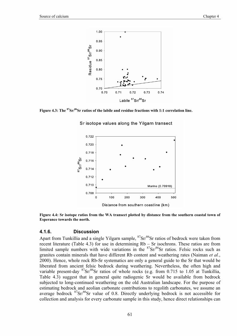
Source of calcium Chapter 4
61
Figure 4.3: The 87Sr/86Sr ratios of the labile and residue fractions with 1:1 correlation line.
Figure 4.4: Sr isotope ratios from the WA transect plotted by distance from the southern coastal town of Esperance towards the north.
4.1.6. Discussion Apart from Tunkillia and a single Yilgarn sample, 87Sr/86Sr ratios of bedrock were taken from recent literature (Table 4.3) for use in determining Rb – Sr isochrons. These ratios are from limited sample numbers with wide variations in the 87Sr/86Sr ratios. Felsic rocks such as granites contain minerals that have different Rb content and weathering rates (Naiman et al., 2000). Hence, whole rock Rb-Sr systematics are only a general guide to the Sr that would be liberated from ancient felsic bedrock during weathering. Nevertheless, the often high and variable present-day 87Sr/86Sr ratios of whole rocks (e.g. from 0.715 to 1.05 at Tunkillia, Table 4.3) suggest that in general quite radiogenic Sr would be available from bedrock subjected to long-continued weathering on the old Australian landscape. For the purpose of estimating bedrock and aeolian carbonate contributions to regolith carbonates, we assume an average bedrock 87Sr/86Sr value of 0.8. Directly underlying bedrock is not accessible for collection and analysis for every carbonate sample in this study, hence direct relationships can
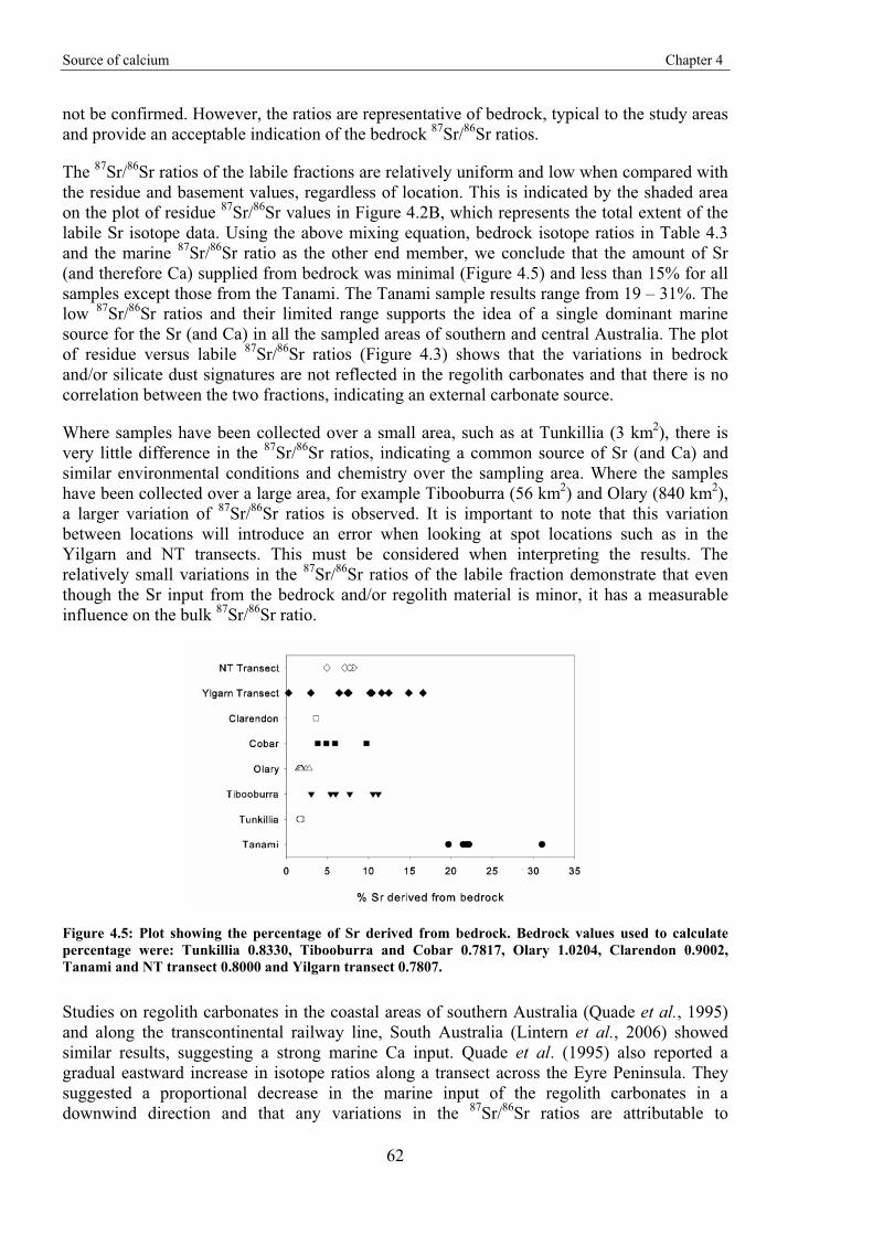
Source of calcium Chapter 4
62
not be confirmed. However, the ratios are representative of bedrock, typical to the study areas and provide an acceptable indication of the bedrock 87Sr/86Sr ratios.
The 87Sr/86Sr ratios of the labile fractions are relatively uniform and low when compared with the residue and basement values, regardless of location. This is indicated by the shaded area on the plot of residue 87Sr/86Sr values in Figure 4.2B, which represents the total extent of the labile Sr isotope data. Using the above mixing equation, bedrock isotope ratios in Table 4.3 and the marine 87Sr/86Sr ratio as the other end member, we conclude that the amount of Sr (and therefore Ca) supplied from bedrock was minimal (Figure 4.5) and less than 15% for all samples except those from the Tanami. The Tanami sample results range from 19 – 31%. The low 87Sr/86Sr ratios and their limited range supports the idea of a single dominant marine source for the Sr (and Ca) in all the sampled areas of southern and central Australia. The plot of residue versus labile 87Sr/86Sr ratios (Figure 4.3) shows that the variations in bedrock and/or silicate dust signatures are not reflected in the regolith carbonates and that there is no correlation between the two fractions, indicating an external carbonate source.
Where samples have been collected over a small area, such as at Tunkillia (3 km2), there is very little difference in the 87Sr/86Sr ratios, indicating a common source of Sr (and Ca) and similar environmental conditions and chemistry over the sampling area. Where the samples have been collected over a large area, for example Tibooburra (56 km2) and Olary (840 km2), a larger variation of 87Sr/86Sr ratios is observed. It is important to note that this variation between locations will introduce an error when looking at spot locations such as in the Yilgarn and NT transects. This must be considered when interpreting the results. The relatively small variations in the 87Sr/86Sr ratios of the labile fraction demonstrate that even though the Sr input from the bedrock and/or regolith material is minor, it has a measurable influence on the bulk 87Sr/86Sr ratio.
Figure 4.5: Plot showing the percentage of Sr derived from bedrock. Bedrock values used to calculate percentage were: Tunkillia 0.8330, Tibooburra and Cobar 0.7817, Olary 1.0204, Clarendon 0.9002, Tanami and NT transect 0.8000 and Yilgarn transect 0.7807.
Studies on regolith carbonates in the coastal areas of southern Australia (Quade et al., 1995) and along the transcontinental railway line, South Australia (Lintern et al., 2006) showed similar results, suggesting a strong marine Ca input. Quade et al. (1995) also reported a gradual eastward increase in isotope ratios along a transect across the Eyre Peninsula. They suggested a proportional decrease in the marine input of the regolith carbonates in a downwind direction and that any variations in the 87Sr/86Sr ratios are attributable to
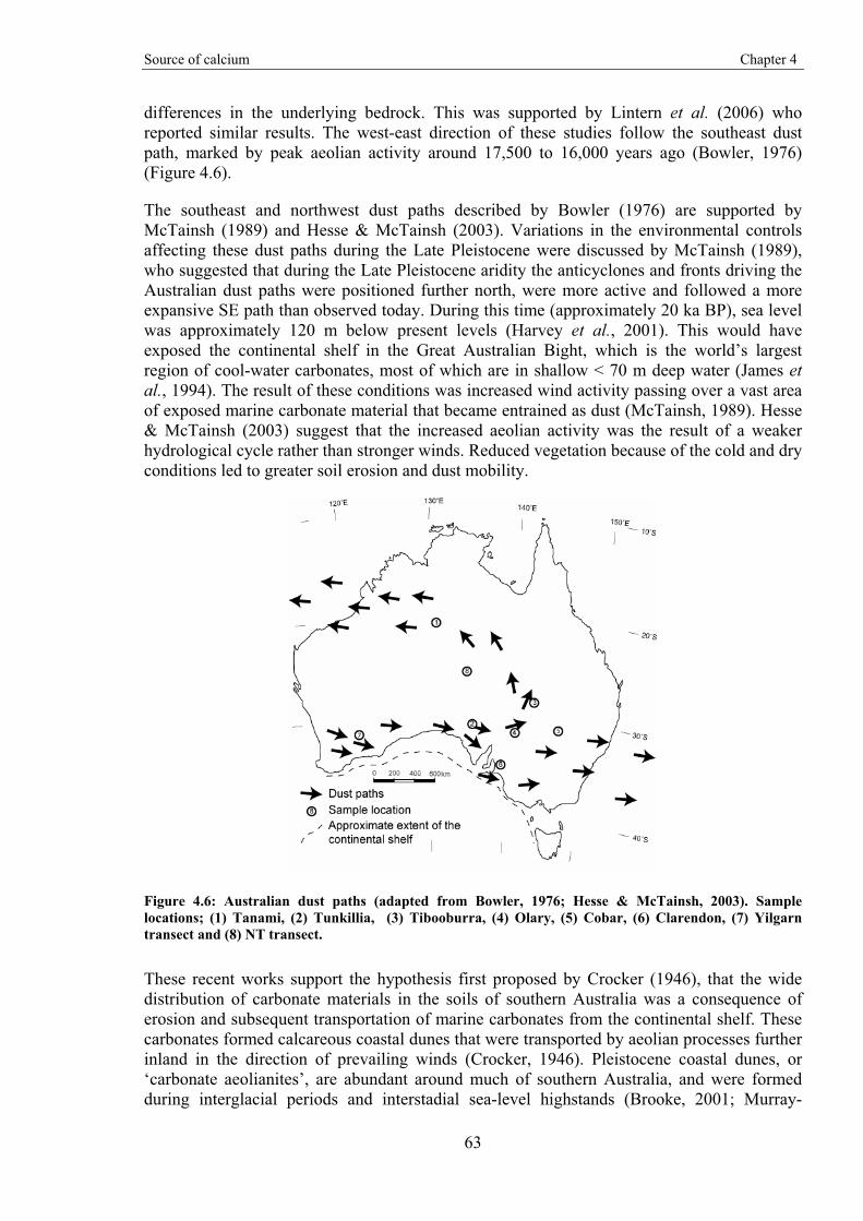
Source of calcium Chapter 4
63
differences in the underlying bedrock. This was supported by Lintern et al. (2006) who reported similar results. The west-east direction of these studies follow the southeast dust path, marked by peak aeolian activity around 17,500 to 16,000 years ago (Bowler, 1976) (Figure 4.6).
The southeast and northwest dust paths described by Bowler (1976) are supported by McTainsh (1989) and Hesse & McTainsh (2003). Variations in the environmental controls affecting these dust paths during the Late Pleistocene were discussed by McTainsh (1989), who suggested that during the Late Pleistocene aridity the anticyclones and fronts driving the Australian dust paths were positioned further north, were more active and followed a more expansive SE path than observed today. During this time (approximately 20 ka BP), sea level was approximately 120 m below present levels (Harvey et al., 2001). This would have exposed the continental shelf in the Great Australian Bight, which is the world’s largest region of cool-water carbonates, most of which are in shallow < 70 m deep water (James et al., 1994). The result of these conditions was increased wind activity passing over a vast area of exposed marine carbonate material that became entrained as dust (McTainsh, 1989). Hesse & McTainsh (2003) suggest that the increased aeolian activity was the result of a weaker hydrological cycle rather than stronger winds. Reduced vegetation because of the cold and dry conditions led to greater soil erosion and dust mobility.
Figure 4.6: Australian dust paths (adapted from Bowler, 1976; Hesse & McTainsh, 2003). Sample locations; (1) Tanami, (2) Tunkillia, (3) Tibooburra, (4) Olary, (5) Cobar, (6) Clarendon, (7) Yilgarn transect and (8) NT transect.
These recent works support the hypothesis first proposed by Crocker (1946), that the wide distribution of carbonate materials in the soils of southern Australia was a consequence of erosion and subsequent transportation of marine carbonates from the continental shelf. These carbonates formed calcareous coastal dunes that were transported by aeolian processes further inland in the direction of prevailing winds (Crocker, 1946). Pleistocene coastal dunes, or ‘carbonate aeolianites’, are abundant around much of southern Australia, and were formed during interglacial periods and interstadial sea-level highstands (Brooke, 2001; Murray-
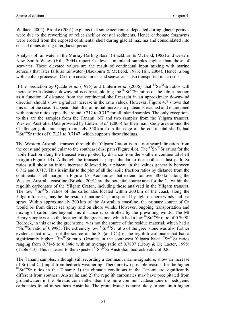
Source of calcium Chapter 4
64
Wallace, 2002). Brooke (2001) explains that some aeolianites deposited during glacial periods were due to the reworking of relict shelf or coastal sediments. Hence carbonate fragments were eroded from the exposed continental shelf during glacial maxima and consolidated into coastal dunes during interglacial periods.
Analysis of rainwater in the Murray-Darling Basin (Blackburn & McLeod, 1983) and western New South Wales (Hill, 2004) report Ca levels in inland samples higher than those of seawater. These elevated values are the result of continental input mixing with marine aerosols that later falls as rainwater (Blackburn & McLeod, 1983; Hill, 2004). Hence, along with aeolian processes, Ca from coastal areas and seawater is also transported in aerosols.
If the prediction by Quade et al. (1995) and Lintern et al. (2006), that 87Sr/86Sr ratios will increase with distance downwind is correct, plotting the 87Sr/86Sr ratios of the labile fraction as a function of distance from the continental shelf margin in an approximate downwind direction should show a gradual increase in the ratio values. However, Figure 4.7 shows that this is not the case. It appears that after an initial increase, a plateau is reached and maintained with isotope ratios typically around 0.712 to 0.717 for all inland samples. The only exceptions to this are the samples from the Tanami, NT and two samples from the Yilgarn transect, Western Australia. Data provided by Lintern et al. (2006) for their main study area around the Challenger gold mine (approximately 350 km from the edge of the continental shelf), had 87Sr/86Sr ratios of 0.7121 to 0.7147, which supports these findings.
The Western Australia transect through the Yilgarn Craton is in a northward direction from the coast and perpendicular to the southeast dust path (Figure 4.6). The 87Sr/86Sr ratios for the labile fraction along the transect were plotted by distance from the southern continental shelf margin (Figure 4.4). Although the transect is perpendicular to the southeast dust path, Sr ratios still show an initial increase followed by a plateau in the values generally between 0.712 and 0.717. This is similar to the plot of all the labile fraction ratios by distance from the continental shelf margin in Figure 4.7. Aeolianites that extend for over 800 km along the Western Australia coastline (Brooke, 2001) are the potential source area for the Ca within the regolith carbonates of the Yilgarn Craton, including those analysed in the Yilgarn transect. The low 87Sr/86Sr ratios of the carbonates located within 200 km of the coast, along the Yilgarn transect, may be the result of marine Ca, transported by light onshore winds and sea spray. Within approximately 200 km of the Australian coastline, the primary source of Ca would be from direct sea spray and on shore winds. However, ongoing transportation and mixing of carbonates beyond this distance is controlled by the prevailing winds. The Mt Henry sample is also the location of the greenstone, which had a low 87Sr/86Sr ratio of 0.7098. Bedrock, in this case the greenstone, was not the source of the residue material, which had a 87Sr/86Sr ratio of 0.9985. The extremely low 87Sr/86Sr ratio of the greenstone was also further evidence that it was not the source of the Sr (and Ca) in the regolith carbonate that had a significantly higher 87Sr/86Sr ratio. Granites in the southwest Yilgarn have 87Sr/86Sr ratios ranging from 0.7145 to 0.8486 with an average ratio of 0.7807 (Libby & De Laeter, 1998) (Table 4.3). This is nearer to the expected 87Sr/86Sr Australian bedrock value of 0.8.
The Tanami samples, although still recording a dominant marine signature, show an increase of Sr (and Ca) input from bedrock weathering. There are two possible reasons for the higher 87Sr/86Sr ratios in the Tanami: 1) the climatic conditions in the Tanami are significantly different from southern Australia; and 2) the regolith carbonates may have precipitated from groundwaters in the phreatic zone rather than the more common vadose zone of pedogenic carbonates found in southern Australia. The groundwater is more likely to contain a higher
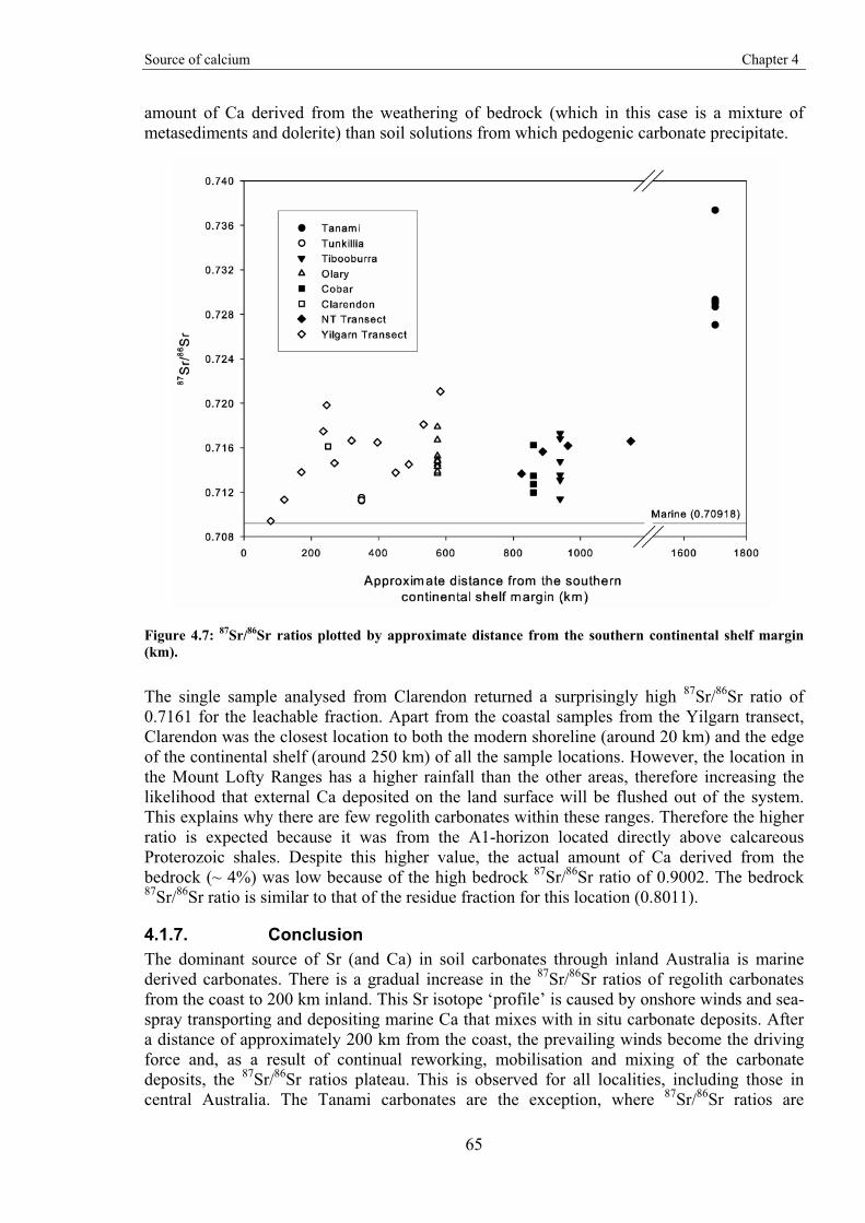
Source of calcium Chapter 4
65
amount of Ca derived from the weathering of bedrock (which in this case is a mixture of metasediments and dolerite) than soil solutions from which pedogenic carbonate precipitate.
Figure 4.7: 87Sr/86Sr ratios plotted by approximate distance from the southern continental shelf margin (km).
The single sample analysed from Clarendon returned a surprisingly high 87Sr/86Sr ratio of 0.7161 for the leachable fraction. Apart from the coastal samples from the Yilgarn transect, Clarendon was the closest location to both the modern shoreline (around 20 km) and the edge of the continental shelf (around 250 km) of all the sample locations. However, the location in the Mount Lofty Ranges has a higher rainfall than the other areas, therefore increasing the likelihood that external Ca deposited on the land surface will be flushed out of the system. This explains why there are few regolith carbonates within these ranges. Therefore the higher ratio is expected because it was from the A1-horizon located directly above calcareous Proterozoic shales. Despite this higher value, the actual amount of Ca derived from the bedrock (~ 4%) was low because of the high bedrock 87Sr/86Sr ratio of 0.9002. The bedrock 87Sr/86Sr ratio is similar to that of the residue fraction for this location (0.8011).
4.1.7. Conclusion The dominant source of Sr (and Ca) in soil carbonates through inland Australia is marine derived carbonates. There is a gradual increase in the 87Sr/86Sr ratios of regolith carbonates from the coast to 200 km inland. This Sr isotope ‘profile’ is caused by onshore winds and sea-spray transporting and depositing marine Ca that mixes with in situ carbonate deposits. After a distance of approximately 200 km from the coast, the prevailing winds become the driving force and, as a result of continual reworking, mobilisation and mixing of the carbonate deposits, the 87Sr/86Sr ratios plateau. This is observed for all localities, including those in central Australia. The Tanami carbonates are the exception, where 87Sr/86Sr ratios are
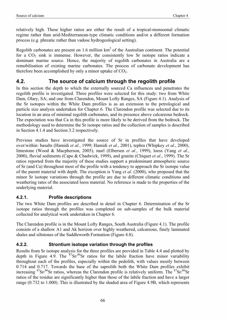
Source of calcium Chapter 4
66
relatively high. These higher ratios are either the result of a tropical-monsoonal climatic regime rather than arid-Mediterranean-type climatic conditions and/or a different formation process (e.g. phreatic rather than vadose hydrogeological setting).
Regolith carbonates are present on 1.6 million km2 of the Australian continent. The potential for a CO2 sink is immense. However, the consistently low Sr isotope ratios indicate a dominant marine source. Hence, the majority of regolith carbonates in Australia are a remobilisation of existing marine carbonates. The process of carbonate development has therefore been accomplished by only a minor uptake of CO2.
4.2. The source of calcium through the regolith profile In this section the depth to which the externally sourced Ca influences and penetrates the regolith profile is investigated. Three profiles were selected for this study: two from White Dam, Olary, SA; and one from Clarendon, Mount Lofty Ranges, SA (Figure 4.1). Analysis of the Sr isotopes within the White Dam profiles is as an extension to the petrological and particle size analysis undertaken for Chapter 6. The Clarendon profile was selected due to its location in an area of minimal regolith carbonates, and its presence above calcareous bedrock. The expectation was that Ca in this profile is more likely to be derived from the bedrock. The methodology used to determine the Sr isotope ratios and the collection of samples is described in Section 4.1.4 and Section 3.2 respectively.
Previous studies have investigated the source of Sr in profiles that have developed over/within: basalts (Hamidi et al., 1999; Hamidi et al., 2001), tephra (Whipkey et al., 2000), limestone (Wood & Macpherson, 2005), marl (Elbersen et al., 1999), loess (Yang et al., 2000), fluvial sediments (Capo & Chadwick, 1999), and granite (Chiquet et al., 1999). The Sr ratios reported from the majority of these studies support a predominant atmospheric source of Sr (and Ca) throughout most of the profile with a tendency to approach the Sr isotope value of the parent material with depth. The exception is Yang et al. (2000), who proposed that the minor Sr isotope variations through the profile are due to different climatic conditions and weathering rates of the associated loess material. No reference is made to the properties of the underlying material.
4.2.1. Profile descriptions The two White Dam profiles are described in detail in Chapter 6. Determination of the Sr isotope ratios through the profiles was completed on sub-samples of the bulk material collected for analytical work undertaken in Chapter 6.
The Clarendon profile is in the Mount Lofty Ranges, South Australia (Figure 4.1). The profile consists of a shallow A1 and Ak horizon over highly weathered, calcareous, finely laminated shales and siltstones of the Saddleworth Formation (Figure 4.8).
4.2.2. Strontium isotope variation through the profiles Results from Sr isotope analysis for the three profiles are provided in Table 4.4 and plotted by depth in Figure 4.9. The 87Sr/86Sr ratios for the labile fraction have minor variability throughout each of the profiles, especially within the pedolith, with values mostly between 0.714 and 0.717. Towards the base of the saprolith both the White Dam profiles exhibit increasing 87Sr/86Sr ratios, whereas the Clarendon profile is relatively uniform. The 87Sr/86Sr ratios of the residue are significantly higher than those of the labile fraction and have a larger range (0.732 to 1.000). This is illustrated by the shaded area of Figure 4.9B, which represents
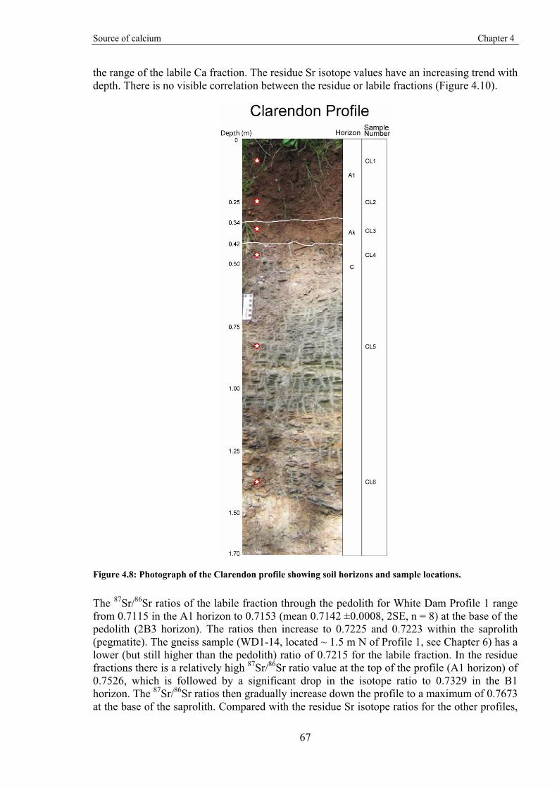
Source of calcium Chapter 4
67
the range of the labile Ca fraction. The residue Sr isotope values have an increasing trend with depth. There is no visible correlation between the residue or labile fractions (Figure 4.10).
Figure 4.8: Photograph of the Clarendon profile showing soil horizons and sample locations.
The 87Sr/86Sr ratios of the labile fraction through the pedolith for White Dam Profile 1 range from 0.7115 in the A1 horizon to 0.7153 (mean 0.7142 ±0.0008, 2SE, n = 8) at the base of the pedolith (2B3 horizon). The ratios then increase to 0.7225 and 0.7223 within the saprolith (pegmatite). The gneiss sample (WD1-14, located ~ 1.5 m N of Profile 1, see Chapter 6) has a lower (but still higher than the pedolith) ratio of 0.7215 for the labile fraction. In the residue fractions there is a relatively high 87Sr/86Sr ratio value at the top of the profile (A1 horizon) of 0.7526, which is followed by a significant drop in the isotope ratio to 0.7329 in the B1 horizon. The 87Sr/86Sr ratios then gradually increase down the profile to a maximum of 0.7673 at the base of the saprolith. Compared with the residue Sr isotope ratios for the other profiles,
Source of calcium Chapter 4
68
the variation through White Dam Profile 1 is minor (mean 0.7512 ±7.0 x 10⁻³ 2SE, n = 12); however, the variation is significantly larger than any of the labile fractions. The residue fraction of the gneiss sample (WD1-14) was the highest of the residues for Profile 1 at 0.7673.
Profile 2 at White Dam has 87Sr/86Sr ratios for the labile fraction about 0.7162 for the A1 and top of B1 horizons, but then drops to values that are similar to Profile 1 through the remainder of the pedolith. The range of 87Sr/86Sr ratios for the pedolith labile fractions are from 0.7139 to 0.7162. The ratios increase from 0.7144 to 0.7436 through the saprolith. The isotope ratios of the residue fraction for Profile 2 (0.7436 to 0.7521) are relatively uniform through the pedolith, but then increase sharply through the saprolith from 0.7668 to 0.8553.
Labile Ca fraction
87Sr/86Sr
0.710 0.712 0.714 0.716 0.718 0.720 0.722 0.724 0.726 0.742 0.744
Dep
th (m
)
0.0
0.5
1.0
1.5
2.0
2.5
3.0
3.5
Marine (0.70918)
White Dam (profile 1)White Dam (profile 2)ClarendonWhite Dam gneiss (profile 1)
Residue Ca fraction
87Sr/86Sr
0.70 0.73 0.76 0.79 0.82 0.85 0.88 0.91 0.94 0.97 1.00
Dep
th (m
)
0.0
0.5
1.0
1.5
2.0
2.5
3.0
3.5
A.
B.
Figure 4.9: Sr isotope ratios plotted by depth for the leachable Ca (and Sr) (plot A) and residue fractions (plot B). The shaded area on plot B represents the extent of the 87Sr/86Sr ratios on plot A.
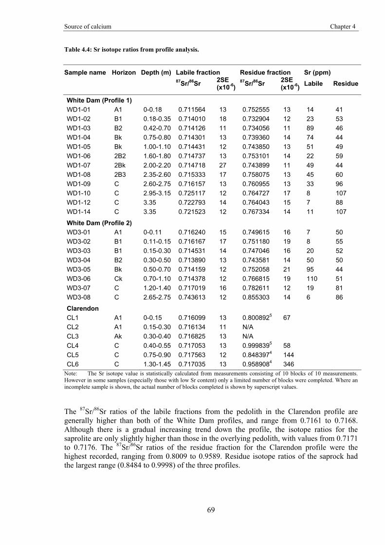
Source of calcium Chapter 4
69
Table 4.4: Sr isotope ratios from profile analysis.
Sample name Horizon Depth (m) Labile fraction Residue fraction Sr (ppm) 87Sr/86Sr 2SE
(x10-6)87Sr/86Sr 2SE
(x10-6) Labile Residue
White Dam (Profile 1) WD1-01 A1 0-0.18 0.711564 13 0.752555 13 14 41 WD1-02 B1 0.18-0.35 0.714010 18 0.732904 12 23 53 WD1-03 B2 0.42-0.70 0.714126 11 0.734056 11 89 46 WD1-04 Bk 0.75-0.80 0.714301 13 0.739360 14 74 44 WD1-05 Bk 1.00-1.10 0.714431 12 0.743850 13 51 49 WD1-06 2B2 1.60-1.80 0.714737 13 0.753101 14 22 59 WD1-07 2Bk 2.00-2.20 0.714718 27 0.743899 11 49 44 WD1-08 2B3 2.35-2.60 0.715333 17 0.758075 13 45 60 WD1-09 C 2.60-2.75 0.716157 13 0.760955 13 33 96 WD1-10 C 2.95-3.15 0.725117 12 0.764727 17 8 107 WD1-12 C 3.35 0.722793 14 0.764043 15 7 88 WD1-14 C 3.35 0.721523 12 0.767334 14 11 107
White Dam (Profile 2) WD3-01 A1 0-0.11 0.716240 15 0.749615 16 7 50 WD3-02 B1 0.11-0.15 0.716167 17 0.751180 19 8 55 WD3-03 B1 0.15-0.30 0.714531 14 0.747046 16 20 52 WD3-04 B2 0.30-0.50 0.713890 13 0.743581 14 50 50 WD3-05 Bk 0.50-0.70 0.714159 12 0.752058 21 95 44 WD3-06 Ck 0.70-1.10 0.714378 12 0.766815 19 110 51 WD3-07 C 1.20-1.40 0.717019 16 0.782611 12 19 81 WD3-08 C 2.65-2.75 0.743613 12 0.855303 14 6 86
Clarendon CL1 A1 0-0.15 0.716099 13 0.8008925 67 CL2 A1 0.15-0.30 0.716134 11 N/A CL3 Ak 0.30-0.40 0.716825 13 N/A CL4 C 0.40-0.55 0.717053 13 0.9998395 58 CL5 C 0.75-0.90 0.717563 12 0.8483974 144 CL6 C 1.30-1.45 0.717035 13 0.9589084 346
Note: The Sr isotope value is statistically calculated from measurements consisting of 10 blocks of 10 measurements. However in some samples (especially those with low Sr content) only a limited number of blocks were completed. Where an incomplete sample is shown, the actual number of blocks completed is shown by superscript values.
The 87Sr/86Sr ratios of the labile fractions from the pedolith in the Clarendon profile are generally higher than both of the White Dam profiles, and range from 0.7161 to 0.7168. Although there is a gradual increasing trend down the profile, the isotope ratios for the saprolite are only slightly higher than those in the overlying pedolith, with values from 0.7171 to 0.7176. The 87Sr/86Sr ratios of the residue fraction for the Clarendon profile were the highest recorded, ranging from 0.8009 to 0.9589. Residue isotope ratios of the saprock had the largest range (0.8484 to 0.9998) of the three profiles.
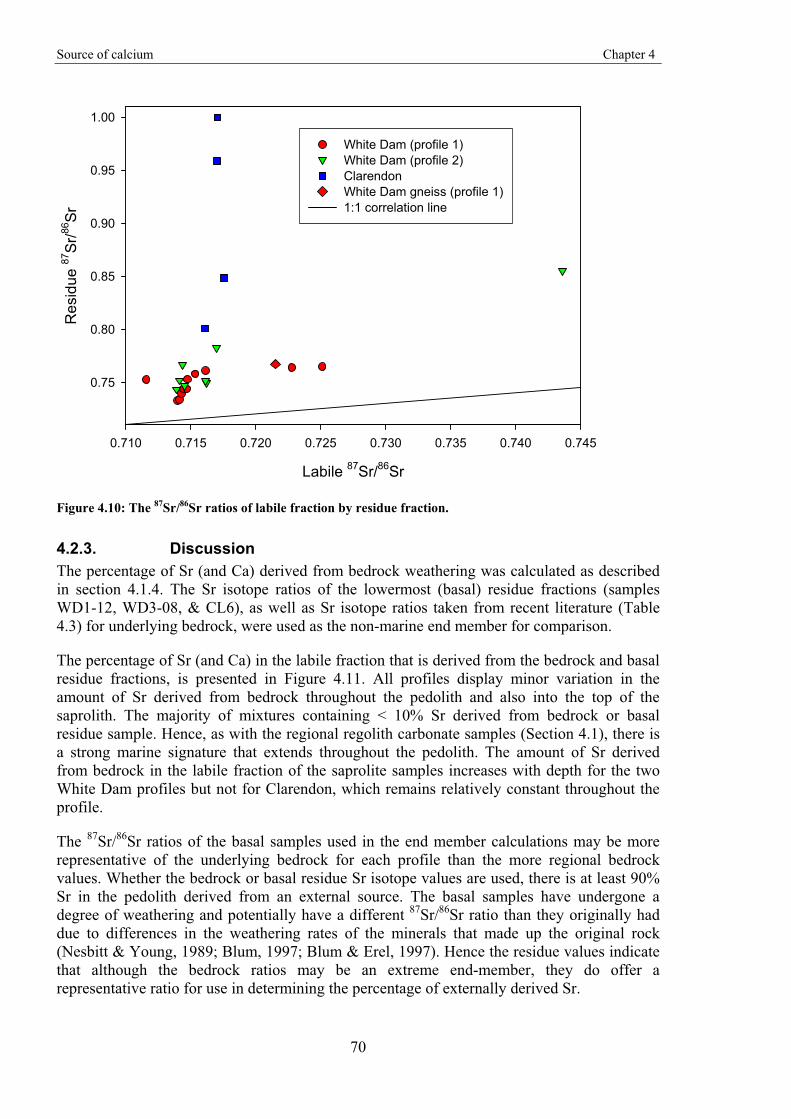
Source of calcium Chapter 4
70
Labile 87Sr/86Sr
0.710 0.715 0.720 0.725 0.730 0.735 0.740 0.745
Res
idue
87Sr
/86Sr
0.75
0.80
0.85
0.90
0.95
1.00
White Dam (profile 1)White Dam (profile 2)ClarendonWhite Dam gneiss (profile 1)1:1 correlation line
Figure 4.10: The 87Sr/86Sr ratios of labile fraction by residue fraction.
4.2.3. Discussion The percentage of Sr (and Ca) derived from bedrock weathering was calculated as described in section 4.1.4. The Sr isotope ratios of the lowermost (basal) residue fractions (samples WD1-12, WD3-08, & CL6), as well as Sr isotope ratios taken from recent literature (Table 4.3) for underlying bedrock, were used as the non-marine end member for comparison.
The percentage of Sr (and Ca) in the labile fraction that is derived from the bedrock and basal residue fractions, is presented in Figure 4.11. All profiles display minor variation in the amount of Sr derived from bedrock throughout the pedolith and also into the top of the saprolith. The majority of mixtures containing < 10% Sr derived from bedrock or basal residue sample. Hence, as with the regional regolith carbonate samples (Section 4.1), there is a strong marine signature that extends throughout the pedolith. The amount of Sr derived from bedrock in the labile fraction of the saprolite samples increases with depth for the two White Dam profiles but not for Clarendon, which remains relatively constant throughout the profile.
The 87Sr/86Sr ratios of the basal samples used in the end member calculations may be more representative of the underlying bedrock for each profile than the more regional bedrock values. Whether the bedrock or basal residue Sr isotope values are used, there is at least 90% Sr in the pedolith derived from an external source. The basal samples have undergone a degree of weathering and potentially have a different 87Sr/86Sr ratio than they originally had due to differences in the weathering rates of the minerals that made up the original rock (Nesbitt & Young, 1989; Blum, 1997; Blum & Erel, 1997). Hence the residue values indicate that although the bedrock ratios may be an extreme end-member, they do offer a representative ratio for use in determining the percentage of externally derived Sr.
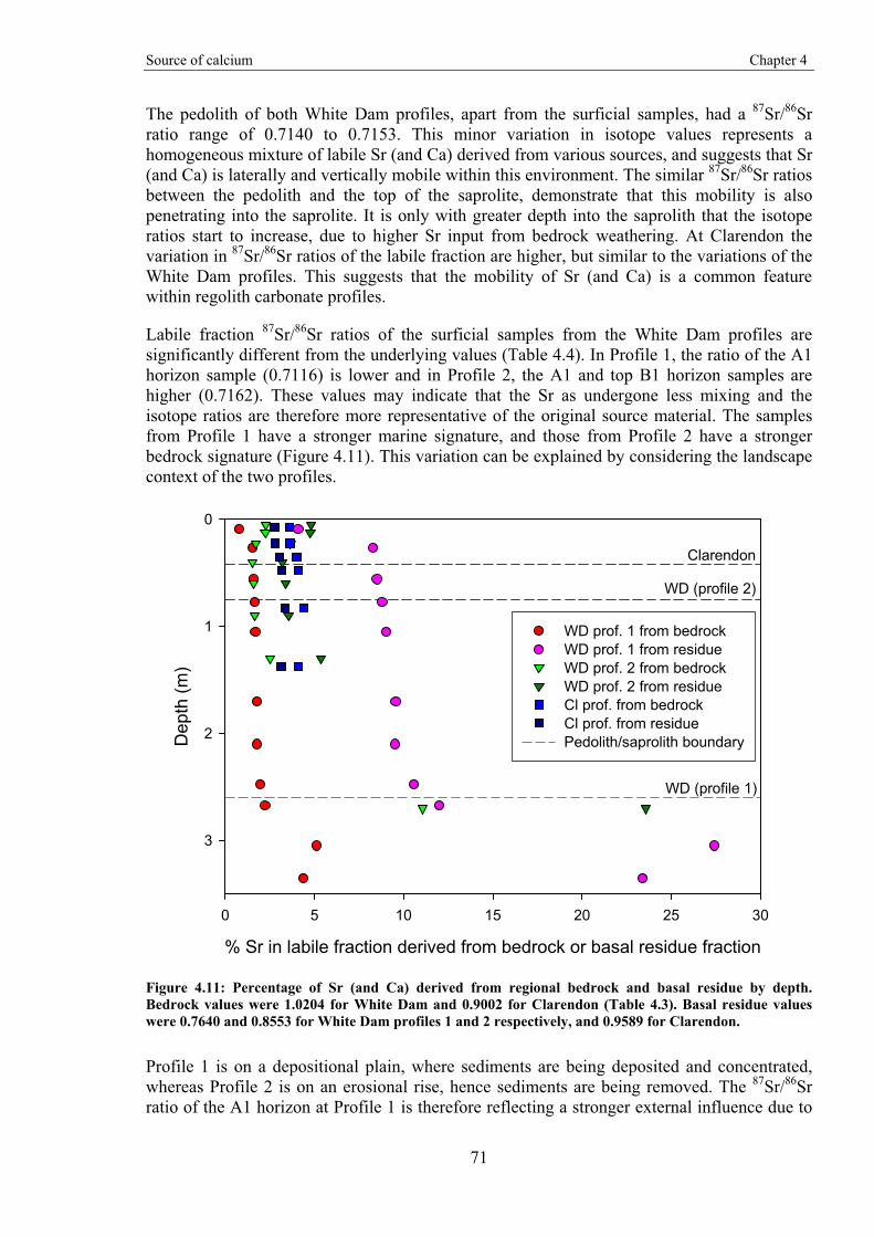
Source of calcium Chapter 4
71
The pedolith of both White Dam profiles, apart from the surficial samples, had a 87Sr/86Sr ratio range of 0.7140 to 0.7153. This minor variation in isotope values represents a homogeneous mixture of labile Sr (and Ca) derived from various sources, and suggests that Sr (and Ca) is laterally and vertically mobile within this environment. The similar 87Sr/86Sr ratios between the pedolith and the top of the saprolite, demonstrate that this mobility is also penetrating into the saprolite. It is only with greater depth into the saprolith that the isotope ratios start to increase, due to higher Sr input from bedrock weathering. At Clarendon the variation in 87Sr/86Sr ratios of the labile fraction are higher, but similar to the variations of the White Dam profiles. This suggests that the mobility of Sr (and Ca) is a common feature within regolith carbonate profiles.
Labile fraction 87Sr/86Sr ratios of the surficial samples from the White Dam profiles are significantly different from the underlying values (Table 4.4). In Profile 1, the ratio of the A1 horizon sample (0.7116) is lower and in Profile 2, the A1 and top B1 horizon samples are higher (0.7162). These values may indicate that the Sr as undergone less mixing and the isotope ratios are therefore more representative of the original source material. The samples from Profile 1 have a stronger marine signature, and those from Profile 2 have a stronger bedrock signature (Figure 4.11). This variation can be explained by considering the landscape context of the two profiles.
% Sr in labile fraction derived from bedrock or basal residue fraction
0 5 10 15 20 25 30
Dep
th (m
)
0
1
2
3
Clarendon
WD (profile 2)
WD (profile 1)
WD prof. 1 from bedrock WD prof. 1 from residueWD prof. 2 from bedrockWD prof. 2 from residueCl prof. from bedrockCl prof. from residuePedolith/saprolith boundary
Figure 4.11: Percentage of Sr (and Ca) derived from regional bedrock and basal residue by depth. Bedrock values were 1.0204 for White Dam and 0.9002 for Clarendon (Table 4.3). Basal residue values were 0.7640 and 0.8553 for White Dam profiles 1 and 2 respectively, and 0.9589 for Clarendon.
Profile 1 is on a depositional plain, where sediments are being deposited and concentrated, whereas Profile 2 is on an erosional rise, hence sediments are being removed. The 87Sr/86Sr ratio of the A1 horizon at Profile 1 is therefore reflecting a stronger external influence due to
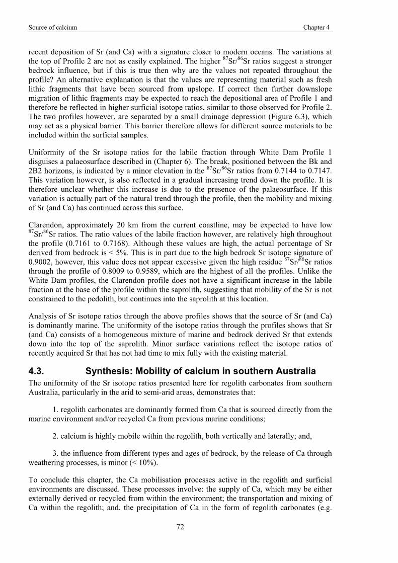
Source of calcium Chapter 4
72
recent deposition of Sr (and Ca) with a signature closer to modern oceans. The variations at the top of Profile 2 are not as easily explained. The higher 87Sr/86Sr ratios suggest a stronger bedrock influence, but if this is true then why are the values not repeated throughout the profile? An alternative explanation is that the values are representing material such as fresh lithic fragments that have been sourced from upslope. If correct then further downslope migration of lithic fragments may be expected to reach the depositional area of Profile 1 and therefore be reflected in higher surficial isotope ratios, similar to those observed for Profile 2. The two profiles however, are separated by a small drainage depression (Figure 6.3), which may act as a physical barrier. This barrier therefore allows for different source materials to be included within the surficial samples.
Uniformity of the Sr isotope ratios for the labile fraction through White Dam Profile 1 disguises a palaeosurface described in (Chapter 6). The break, positioned between the Bk and 2B2 horizons, is indicated by a minor elevation in the 87Sr/86Sr ratios from 0.7144 to 0.7147. This variation however, is also reflected in a gradual increasing trend down the profile. It is therefore unclear whether this increase is due to the presence of the palaeosurface. If this variation is actually part of the natural trend through the profile, then the mobility and mixing of Sr (and Ca) has continued across this surface.
Clarendon, approximately 20 km from the current coastline, may be expected to have low 87Sr/86Sr ratios. The ratio values of the labile fraction however, are relatively high throughout the profile (0.7161 to 0.7168). Although these values are high, the actual percentage of Sr derived from bedrock is < 5%. This is in part due to the high bedrock Sr isotope signature of 0.9002, however, this value does not appear excessive given the high residue 87Sr/86Sr ratios through the profile of 0.8009 to 0.9589, which are the highest of all the profiles. Unlike the White Dam profiles, the Clarendon profile does not have a significant increase in the labile fraction at the base of the profile within the saprolith, suggesting that mobility of the Sr is not constrained to the pedolith, but continues into the saprolith at this location.
Analysis of Sr isotope ratios through the above profiles shows that the source of Sr (and Ca) is dominantly marine. The uniformity of the isotope ratios through the profiles shows that Sr (and Ca) consists of a homogeneous mixture of marine and bedrock derived Sr that extends down into the top of the saprolith. Minor surface variations reflect the isotope ratios of recently acquired Sr that has not had time to mix fully with the existing material.
4.3. Synthesis: Mobility of calcium in southern Australia The uniformity of the Sr isotope ratios presented here for regolith carbonates from southern Australia, particularly in the arid to semi-arid areas, demonstrates that:
1. regolith carbonates are dominantly formed from Ca that is sourced directly from the marine environment and/or recycled Ca from previous marine conditions;
2. calcium is highly mobile within the regolith, both vertically and laterally; and,
3. the influence from different types and ages of bedrock, by the release of Ca through weathering processes, is minor (< 10%).
To conclude this chapter, the Ca mobilisation processes active in the regolith and surficial environments are discussed. These processes involve: the supply of Ca, which may be either externally derived or recycled from within the environment; the transportation and mixing of Ca within the regolith; and, the precipitation of Ca in the form of regolith carbonates (e.g.
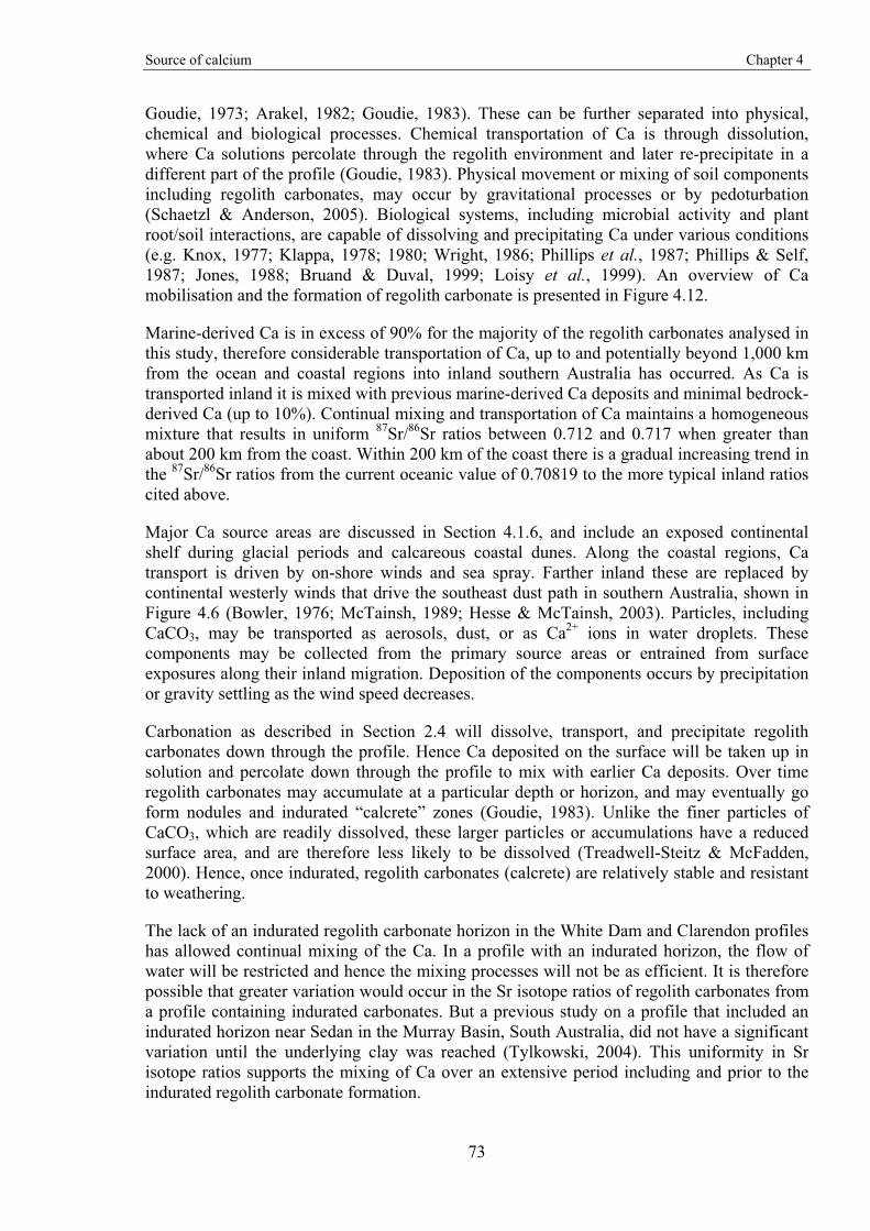
Source of calcium Chapter 4
73
Goudie, 1973; Arakel, 1982; Goudie, 1983). These can be further separated into physical, chemical and biological processes. Chemical transportation of Ca is through dissolution, where Ca solutions percolate through the regolith environment and later re-precipitate in a different part of the profile (Goudie, 1983). Physical movement or mixing of soil components including regolith carbonates, may occur by gravitational processes or by pedoturbation (Schaetzl & Anderson, 2005). Biological systems, including microbial activity and plant root/soil interactions, are capable of dissolving and precipitating Ca under various conditions (e.g. Knox, 1977; Klappa, 1978; 1980; Wright, 1986; Phillips et al., 1987; Phillips & Self, 1987; Jones, 1988; Bruand & Duval, 1999; Loisy et al., 1999). An overview of Ca mobilisation and the formation of regolith carbonate is presented in Figure 4.12.
Marine-derived Ca is in excess of 90% for the majority of the regolith carbonates analysed in this study, therefore considerable transportation of Ca, up to and potentially beyond 1,000 km from the ocean and coastal regions into inland southern Australia has occurred. As Ca is transported inland it is mixed with previous marine-derived Ca deposits and minimal bedrock-derived Ca (up to 10%). Continual mixing and transportation of Ca maintains a homogeneous mixture that results in uniform 87Sr/86Sr ratios between 0.712 and 0.717 when greater than about 200 km from the coast. Within 200 km of the coast there is a gradual increasing trend in the 87Sr/86Sr ratios from the current oceanic value of 0.70819 to the more typical inland ratios cited above.
Major Ca source areas are discussed in Section 4.1.6, and include an exposed continental shelf during glacial periods and calcareous coastal dunes. Along the coastal regions, Ca transport is driven by on-shore winds and sea spray. Farther inland these are replaced by continental westerly winds that drive the southeast dust path in southern Australia, shown in Figure 4.6 (Bowler, 1976; McTainsh, 1989; Hesse & McTainsh, 2003). Particles, including CaCO3, may be transported as aerosols, dust, or as Ca2+ ions in water droplets. These components may be collected from the primary source areas or entrained from surface exposures along their inland migration. Deposition of the components occurs by precipitation or gravity settling as the wind speed decreases.
Carbonation as described in Section 2.4 will dissolve, transport, and precipitate regolith carbonates down through the profile. Hence Ca deposited on the surface will be taken up in solution and percolate down through the profile to mix with earlier Ca deposits. Over time regolith carbonates may accumulate at a particular depth or horizon, and may eventually go form nodules and indurated “calcrete” zones (Goudie, 1983). Unlike the finer particles of CaCO3, which are readily dissolved, these larger particles or accumulations have a reduced surface area, and are therefore less likely to be dissolved (Treadwell-Steitz & McFadden, 2000). Hence, once indurated, regolith carbonates (calcrete) are relatively stable and resistant to weathering.
The lack of an indurated regolith carbonate horizon in the White Dam and Clarendon profiles has allowed continual mixing of the Ca. In a profile with an indurated horizon, the flow of water will be restricted and hence the mixing processes will not be as efficient. It is therefore possible that greater variation would occur in the Sr isotope ratios of regolith carbonates from a profile containing indurated carbonates. But a previous study on a profile that included an indurated horizon near Sedan in the Murray Basin, South Australia, did not have a significant variation until the underlying clay was reached (Tylkowski, 2004). This uniformity in Sr isotope ratios supports the mixing of Ca over an extensive period including and prior to the indurated regolith carbonate formation.
Source of calcium Chapter 4
74
Figure 4.12: Mobility and interactions of Ca in the regolith environment.
It has been suggested that the annual rainfall determines the depth of the regolith carbonate horizon, with areas of higher rainfall producing deeper horizons than areas of low rainfall (Jenny & Leonard, 1934; Yaalon, 1983; Retallack, 2005), although the correlation presented between annual rainfall and depth of carbonate has been questioned (Royer, 1999). Local variations such as drainage, peak rainfall activity (summer or winter), substrate composition, evapotranspiration rates, and soil erosion following carbonate development, all impact on the actual peak regolith carbonate formation depth (Wright, 2007). Regolith carbonate samples collected for this study are from semi-arid to arid conditions with winter rains, apart from the samples from the Tanami which are from a tropical-monsoonal climate. No correlations were
Source of calcium Chapter 4
75
performed on these samples since accurate depth measurements were not available for several of the samples.
Indurated regolith carbonate may form duricrusts that evolve through landscape processes to form cap rocks and ledges on slopes. The duricrust breaks up into calcrete boulders and smaller aggregates as the harder more resilient material is uncovered and the typically softer underlying material removed through weathering processes (Goudie, 1983). The result is surface exposures and a regolith carbonate (calcrete) lag and that extends over the landscape. This material is ultimately broken down and the elements including Ca are released into the regolith environment (Figure 4.12). Alternatively some of the aggregates may be incorporated into new regolith carbonates through cementation, which protects them from further breakdown (Goudie, 1983).
Groundwater movement provides a source of “external” Ca which may accumulate and precipitate in the vadose zone through evaporation at the fringes of capillary action (Goudie, 1983). Precipitation can also occur in the phreatic zone when Ca in solution becomes saturated. This is generally confined to areas where the groundwater is in close proximity to the surface and evaporation is significant, and also where the groundwater gradient is low with only minor flow (Mann & Horwitz, 1979). Regolith carbonates formed in this way are similar in appearance to those formed through pedogenic processes, however, they tend to exist spatially as narrow bands or ribbons, up to 10 km wide that may extend over 100 km in length (Mann & Horwitz, 1979). Carbonates generated in this way are likely to have different Sr isotope ratios due to the increased weathering potential of the groundwaters as they migrate past various bedrock minerals. It is possible that the samples from the Tanami region were derived from groundwater, which explains the higher Sr isotope ratios measured for these samples.
The processes that are recycling Ca and Sr in the regolith environment are also affecting other elements present within the regolith. These relationships and interactions may hide an explanation as to why Au appears to have an association with regolith carbonates. The potential Au-Ca relationship is explored further in the following chapters.

Source of calcium Chapter 4
76
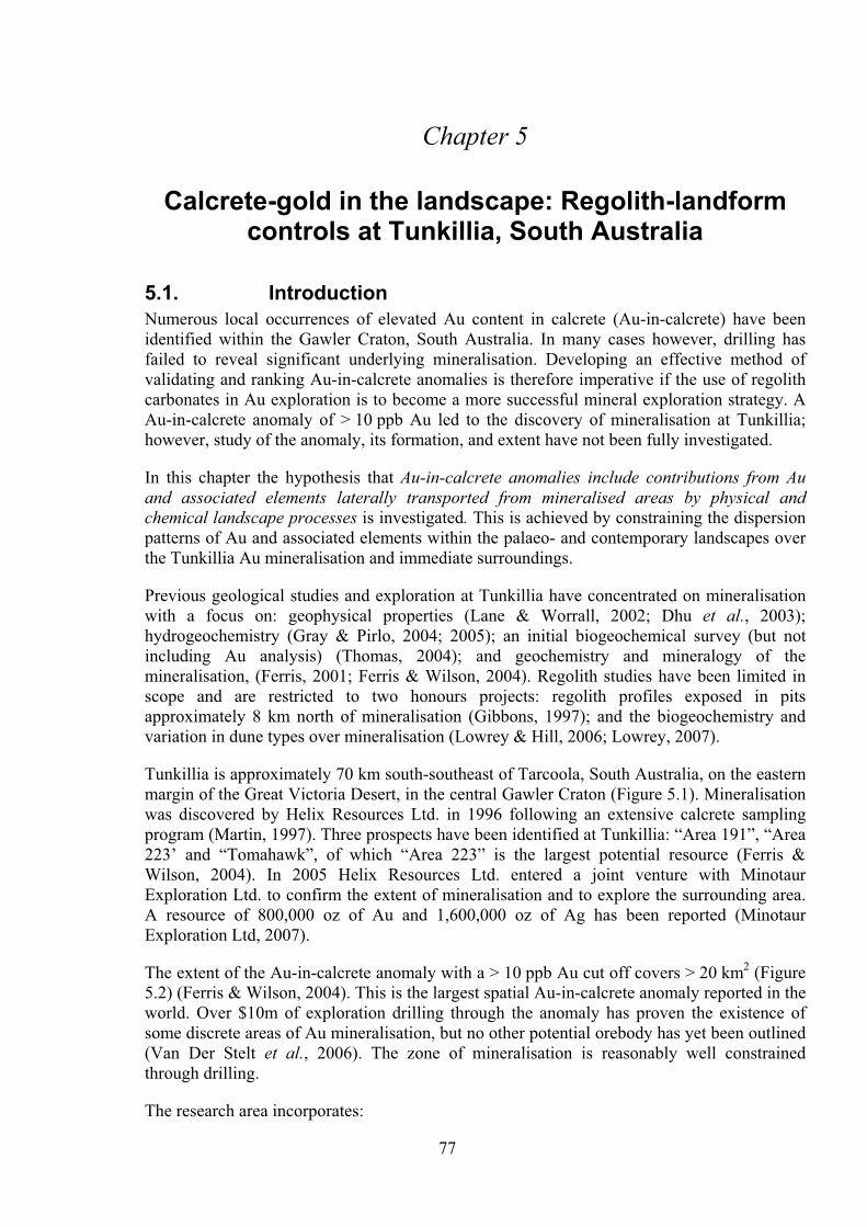
77
Chapter 5
Calcrete-gold in the landscape: Regolith-landform controls at Tunkillia, South Australia
5.1. Introduction Numerous local occurrences of elevated Au content in calcrete (Au-in-calcrete) have been identified within the Gawler Craton, South Australia. In many cases however, drilling has failed to reveal significant underlying mineralisation. Developing an effective method of validating and ranking Au-in-calcrete anomalies is therefore imperative if the use of regolith carbonates in Au exploration is to become a more successful mineral exploration strategy. A Au-in-calcrete anomaly of > 10 ppb Au led to the discovery of mineralisation at Tunkillia; however, study of the anomaly, its formation, and extent have not been fully investigated.
In this chapter the hypothesis that Au-in-calcrete anomalies include contributions from Au and associated elements laterally transported from mineralised areas by physical and chemical landscape processes is investigated. This is achieved by constraining the dispersion patterns of Au and associated elements within the palaeo- and contemporary landscapes over the Tunkillia Au mineralisation and immediate surroundings.
Previous geological studies and exploration at Tunkillia have concentrated on mineralisation with a focus on: geophysical properties (Lane & Worrall, 2002; Dhu et al., 2003); hydrogeochemistry (Gray & Pirlo, 2004; 2005); an initial biogeochemical survey (but not including Au analysis) (Thomas, 2004); and geochemistry and mineralogy of the mineralisation, (Ferris, 2001; Ferris & Wilson, 2004). Regolith studies have been limited in scope and are restricted to two honours projects: regolith profiles exposed in pits approximately 8 km north of mineralisation (Gibbons, 1997); and the biogeochemistry and variation in dune types over mineralisation (Lowrey & Hill, 2006; Lowrey, 2007).
Tunkillia is approximately 70 km south-southeast of Tarcoola, South Australia, on the eastern margin of the Great Victoria Desert, in the central Gawler Craton (Figure 5.1). Mineralisation was discovered by Helix Resources Ltd. in 1996 following an extensive calcrete sampling program (Martin, 1997). Three prospects have been identified at Tunkillia: “Area 191”, “Area 223’ and “Tomahawk”, of which “Area 223” is the largest potential resource (Ferris & Wilson, 2004). In 2005 Helix Resources Ltd. entered a joint venture with Minotaur Exploration Ltd. to confirm the extent of mineralisation and to explore the surrounding area. A resource of 800,000 oz of Au and 1,600,000 oz of Ag has been reported (Minotaur Exploration Ltd, 2007).
The extent of the Au-in-calcrete anomaly with a > 10 ppb Au cut off covers > 20 km2 (Figure 5.2) (Ferris & Wilson, 2004). This is the largest spatial Au-in-calcrete anomaly reported in the world. Over $10m of exploration drilling through the anomaly has proven the existence of some discrete areas of Au mineralisation, but no other potential orebody has yet been outlined (Van Der Stelt et al., 2006). The zone of mineralisation is reasonably well constrained through drilling.
The research area incorporates:
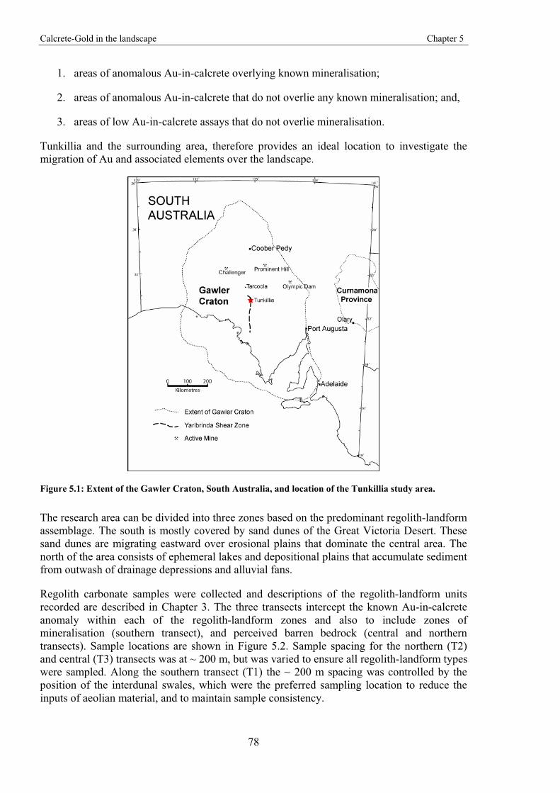
Calcrete-Gold in the landscape Chapter 5
78
1. areas of anomalous Au-in-calcrete overlying known mineralisation;
2. areas of anomalous Au-in-calcrete that do not overlie any known mineralisation; and,
3. areas of low Au-in-calcrete assays that do not overlie mineralisation.
Tunkillia and the surrounding area, therefore provides an ideal location to investigate the migration of Au and associated elements over the landscape.
Figure 5.1: Extent of the Gawler Craton, South Australia, and location of the Tunkillia study area.
The research area can be divided into three zones based on the predominant regolith-landform assemblage. The south is mostly covered by sand dunes of the Great Victoria Desert. These sand dunes are migrating eastward over erosional plains that dominate the central area. The north of the area consists of ephemeral lakes and depositional plains that accumulate sediment from outwash of drainage depressions and alluvial fans.
Regolith carbonate samples were collected and descriptions of the regolith-landform units recorded are described in Chapter 3. The three transects intercept the known Au-in-calcrete anomaly within each of the regolith-landform zones and also to include zones of mineralisation (southern transect), and perceived barren bedrock (central and northern transects). Sample locations are shown in Figure 5.2. Sample spacing for the northern (T2) and central (T3) transects was at ~ 200 m, but was varied to ensure all regolith-landform types were sampled. Along the southern transect (T1) the ~ 200 m spacing was controlled by the position of the interdunal swales, which were the preferred sampling location to reduce the inputs of aeolian material, and to maintain sample consistency.
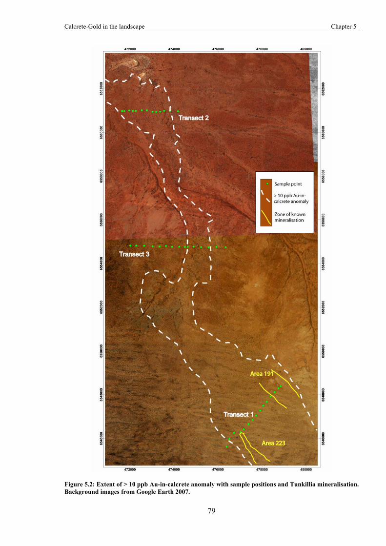
Calcrete-Gold in the landscape Chapter 5
79
Figure 5.2: Extent of > 10 ppb Au-in-calcrete anomaly with sample positions and Tunkillia mineralisation. Background images from Google Earth 2007.
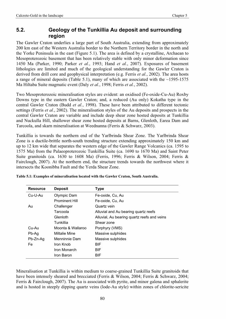
Calcrete-Gold in the landscape Chapter 5
80
5.2. Geology of the Tunkillia Au deposit and surrounding region
The Gawler Craton underlies a large part of South Australia, extending from approximately 200 km east of the Western Australia border to the Northern Territory border in the north and the Yorke Peninsula in the east (Figure 5.1). The area is defined by a crystalline, Archaean to Mesoproterozoic basement that has been relatively stable with only minor deformation since 1450 Ma (Parker, 1990; Parker et al., 1993; Hand et al., 2007). Exposures of basement lithologies are limited and much of the geological understanding for the Gawler Craton is derived from drill core and geophysical interpretation (e.g. Ferris et al., 2002). The area hosts a range of mineral deposits (Table 5.1), many of which are associated with the ~1595-1575 Ma Hiltaba Suite magmatic event (Daly et al., 1998; Ferris et al., 2002).
Two Mesoproterozoic mineralisation styles are evident: an oxidised (Fe-oxide-Cu-Au) Roxby Downs type in the eastern Gawler Craton; and, a reduced (Au only) Kokatha type in the central Gawler Craton (Budd et al., 1998). These have been attributed to different tectonic settings (Ferris et al., 2002). The mineralisation styles of the Au deposits and prospects in the central Gawler Craton are variable and include deep shear zone hosted deposits at Tunkillia and Nuckulla Hill, shallower shear zone hosted deposits at Barns, Glenloth, Earea Dam and Tarcoola, and skarn mineralisation at Weednanna (Ferris & Schwarz, 2003).
Tunkillia is towards the northern end of the Yarlbrinda Shear Zone. The Yarlbrinda Shear Zone is a ductile-brittle north-south trending structure extending approximately 150 km and up to 12 km wide that separates the western edge of the Gawler Range Volcanics (ca. 1595 to 1575 Ma) from the Palaeoproterozoic Tunkillia Suite (ca. 1690 to 1670 Ma) and Saint Peter Suite granitoids (ca. 1630 to 1608 Ma) (Ferris, 1996; Ferris & Wilson, 2004; Ferris & Fairclough, 2007). At the northern end, the structure trends towards the northwest where it intersects the Koonibba Fault and the Yerda Shear Zone.
Table 5.1: Examples of mineralisation located with the Gawler Craton, South Australia.
Resource Deposit Type
Cu-U-Au Olympic Dam Fe-oxide, Cu, Au Prominent Hill Fe-oxide, Cu, Au Au Challenger Quartz vein Tarcoola Alluvial and Au bearing quartz reefs Glenloth Alluvial, Au bearing quartz reefs and veins Tunkillia Shear zone Cu-Au Moonta & Wallaroo Porphyry (VMS) Pb-Ag Miltalie Mine Massive sulphides Pb-Zn-Ag Menninnie Dam Massive sulphides Fe Iron Knob BIF Iron Monarch BIF Iron Baron BIF
Mineralisation at Tunkillia is within medium to coarse-grained Tunkillia Suite granitoids that have been intensely sheared and brecciated (Ferris & Wilson, 2004; Ferris & Schwarz, 2004; Ferris & Fairclough, 2007). The Au is associated with pyrite, and minor galena and sphalerite and is hosted in steeply dipping quartz veins (lode-Au style) within zones of chlorite-sericite
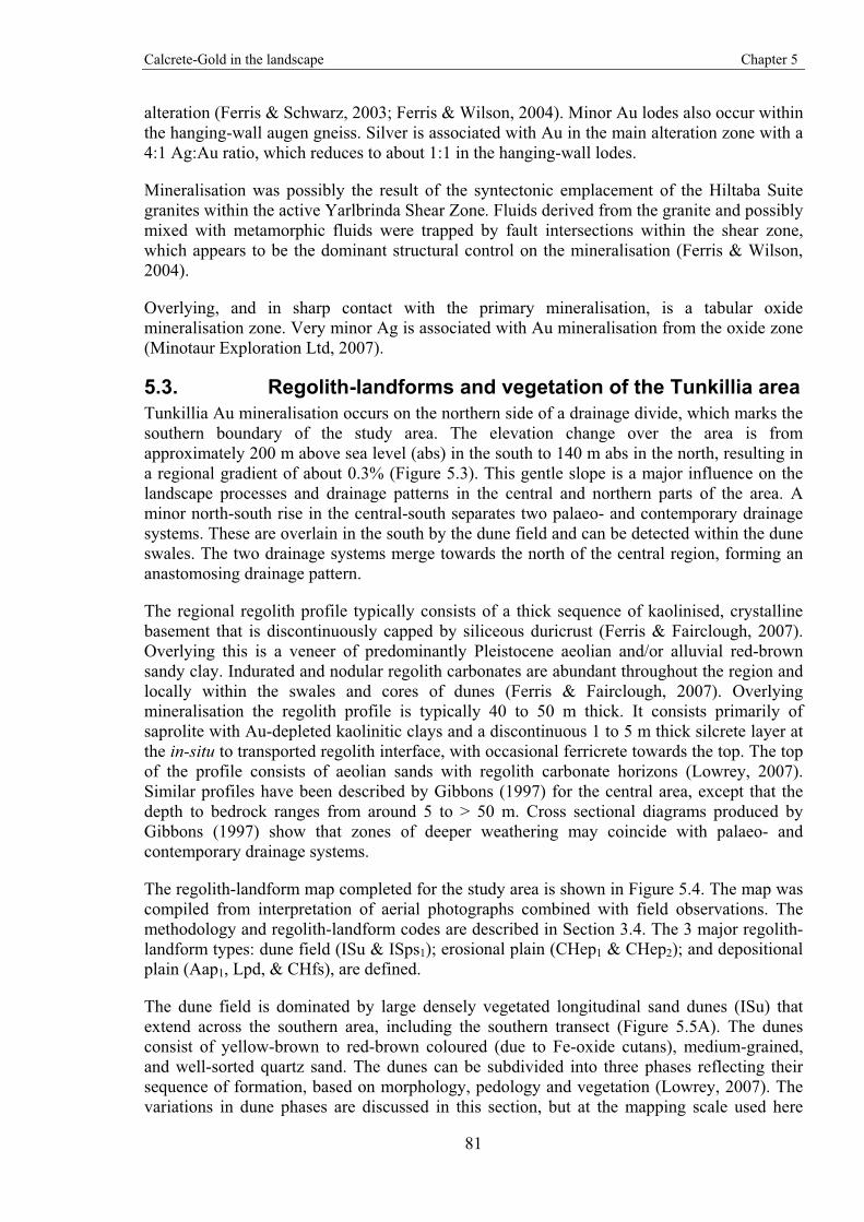
Calcrete-Gold in the landscape Chapter 5
81
alteration (Ferris & Schwarz, 2003; Ferris & Wilson, 2004). Minor Au lodes also occur within the hanging-wall augen gneiss. Silver is associated with Au in the main alteration zone with a 4:1 Ag:Au ratio, which reduces to about 1:1 in the hanging-wall lodes.
Mineralisation was possibly the result of the syntectonic emplacement of the Hiltaba Suite granites within the active Yarlbrinda Shear Zone. Fluids derived from the granite and possibly mixed with metamorphic fluids were trapped by fault intersections within the shear zone, which appears to be the dominant structural control on the mineralisation (Ferris & Wilson, 2004).
Overlying, and in sharp contact with the primary mineralisation, is a tabular oxide mineralisation zone. Very minor Ag is associated with Au mineralisation from the oxide zone (Minotaur Exploration Ltd, 2007).
5.3. Regolith-landforms and vegetation of the Tunkillia area Tunkillia Au mineralisation occurs on the northern side of a drainage divide, which marks the southern boundary of the study area. The elevation change over the area is from approximately 200 m above sea level (abs) in the south to 140 m abs in the north, resulting in a regional gradient of about 0.3% (Figure 5.3). This gentle slope is a major influence on the landscape processes and drainage patterns in the central and northern parts of the area. A minor north-south rise in the central-south separates two palaeo- and contemporary drainage systems. These are overlain in the south by the dune field and can be detected within the dune swales. The two drainage systems merge towards the north of the central region, forming an anastomosing drainage pattern.
The regional regolith profile typically consists of a thick sequence of kaolinised, crystalline basement that is discontinuously capped by siliceous duricrust (Ferris & Fairclough, 2007). Overlying this is a veneer of predominantly Pleistocene aeolian and/or alluvial red-brown sandy clay. Indurated and nodular regolith carbonates are abundant throughout the region and locally within the swales and cores of dunes (Ferris & Fairclough, 2007). Overlying mineralisation the regolith profile is typically 40 to 50 m thick. It consists primarily of saprolite with Au-depleted kaolinitic clays and a discontinuous 1 to 5 m thick silcrete layer at the in-situ to transported regolith interface, with occasional ferricrete towards the top. The top of the profile consists of aeolian sands with regolith carbonate horizons (Lowrey, 2007). Similar profiles have been described by Gibbons (1997) for the central area, except that the depth to bedrock ranges from around 5 to > 50 m. Cross sectional diagrams produced by Gibbons (1997) show that zones of deeper weathering may coincide with palaeo- and contemporary drainage systems.
The regolith-landform map completed for the study area is shown in Figure 5.4. The map was compiled from interpretation of aerial photographs combined with field observations. The methodology and regolith-landform codes are described in Section 3.4. The 3 major regolith-landform types: dune field (ISu & ISps1); erosional plain (CHep1 & CHep2); and depositional plain (Aap1, Lpd, & CHfs), are defined.
The dune field is dominated by large densely vegetated longitudinal sand dunes (ISu) that extend across the southern area, including the southern transect (Figure 5.5A). The dunes consist of yellow-brown to red-brown coloured (due to Fe-oxide cutans), medium-grained, and well-sorted quartz sand. The dunes can be subdivided into three phases reflecting their sequence of formation, based on morphology, pedology and vegetation (Lowrey, 2007). The variations in dune phases are discussed in this section, but at the mapping scale used here
Calcrete-Gold in the landscape Chapter 5
82
(1:62,500) they are not individually defined on the regolith-landform map. The dunes are gradually migrating towards the east, burying older landforms and vegetation that are otherwise characteristic of the interdunal swales (Figure 5.5B).
Vegetation on the older dunes (phase I of Lowrey, 2007) consists of shrublands or woodlands of mulga (Acacia aneura), horse mulga (Acacia ramulosa), and tussock grasses with occasional Walker’s pea (Bossiaea walkeri). A prominent cryptogam mat covers the surface. Younger dunes (phase II of Lowrey, 2007) consist of open woodlands of red mallee (Eucalyptus socialis), occasional Acacia sp. and Walkers pea (Bossiaea walkeri) with a spinifex (Triodia irritans) understorey. The youngest dunes (phase III dunes of Lowrey, 2007) correspond with the landform being buried by the migrating dune and are characterised by minor recently established small shrubs and grasses.
Interdunal swales (ISps1) consist of red-brown, iron-oxide coated, fine- to medium-grained, quartz sands that are moderately to well sorted (Figure 5.5D). Towards the erosional plains, including the north-eastern end of the southern transect, the swales become broader and consist of red-brown, poorly to moderately sorted, sub-rounded, fine- to medium-grained quartz sand with areas of greater clay and silt contents (Figure 5.5F). As the dune swales become broader (ISps2), surface lags become more prevalent with areas of calcrete or silcrete (typically iron-rich) and occasional dolomite sub-rounded to rounded pebbles. These larger plains reveal pre-dune surface features, including palaeo-drainage gravels and depressions (Aap2).
Vegetation within the dune swales is typically open woodland dominated by Victoria Desert mallee (Eucalyptus concinna), horse mulga (Acacia ramulosa) and umbrella wattle (Acacia ligulata) with occasional black oak (Casuarina pauper), pearl bluebush (Maireana sedifolia), bluebush daisy (Cratystylis conocephala) and Walker’s pea (Bossiaea walkeri) (Figure 5.5C). Cryptogams form a thin surface crust in many of the swales, especially in areas of higher silt content, which are generally colonised by mulga (Acacia aneura) thickets with occasional pearl bluebush (Maireana sedifolia). Vegetation over areas with higher regolith carbonate content are characterised by black oak (Casuarina pauper) woodlands with a chenopod understorey of pearl bluebush (Maireana sedifolia), bluebush daisy (Cratystylis conocephala) and dense surficial cryptogam crust (Figure 5.5E).
Extensive, low relief, erosional plains (CHep1 & CHep2) with interspersed alluvial drainage depressions and minor channels (typically < 30 cm deep) are widespread in the central area, including the central transects (Figure 5.6). The main regolith lithology is red-brown coloured, poorly sorted, sub-rounded to sub-angular, fine- to coarse-grained quartz sand, with a surface lag of either sub-angular calcrete, silcrete and quartz gravel or larger, sub-rounded, pebble sized calcrete and minor silcrete (Figure 5.6B). Shallow alluvial channels and depressions (Aed) up to 1 m wide consist of very poorly sorted sands and have greater clay, gravel, and pebble contents than the surrounding areas (Figure 5.6D). Cryptogam surface mats are abundant. Vegetation is predominantly a chenopod shrubland with pearl bluebush (Maireana sedifolia) with occasional mulga (Acacia aneura), black oak (Casuarina pauper) and bluebush daisy (Cratystylis conocephala) (Figure 5.6A). Vegetation surrounding drainage depressions consists of open woodlands with black oak (Casuarina pauper) and mulga (Acacia aneura) (typically with one species dominating and the other interspersed throughout) with an understorey of pearl bluebush (Maireana sedifolia) (Figure 5.6C).
Tunkillia Topographic Map
Figure 5.3: Topographic map of the Tunkillia area showing the extent of the study area, position of the >10 ppb Au-in-calcrete anomaly, and area of known mineralisation (SRTM data sourced from Jarvis et al., 2006)
NOTE: This figure is included on page 83 of the print copy of the thesis held in the University of Adelaide Library.
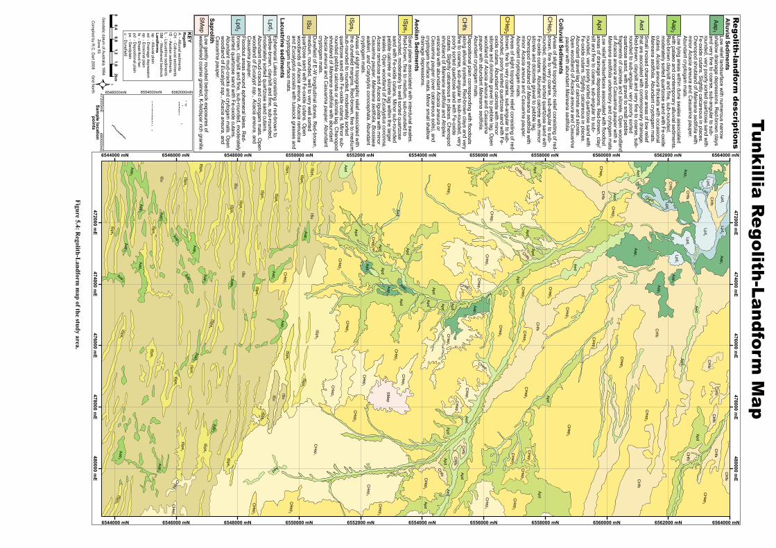
472000 mE
472000 mE
474000 mE
474000 mE
476000 mE
476000 mE
478000 mE
478000 mE
480000 mE
480000 mE
6544000 mN
6544000 mN
6546000 mN
6546000 mN
6548000 mN
6548000 mN
6550000 mN
6550000 mN
6552000 mN
6552000 mN
6554000 mN
6554000 mN
6556000 mN
6556000 mN
6558000 mN
6558000 mN
6560000 mN
6560000 mN
6562000 mN
6562000 mN
6564000 mN
6564000 mN
Tunkillia Regolith-Landform
Map
Regolith-landform
descriptions
Sm
all incised channels over areas of low relief
that are asociated with contem
porary drainage. R
ed-brown, clay/silt and very fine to coarse, sub-
rounded to sub-angular, very poorly sorted quartzose sand, w
ith gravel to small pebble
fragments of calcrete and silcrete. O
pen woodland
of Acacia aneura and Casuarina pauper w
ith a M
aireana sedifolia understory and crytogam m
ats.
Aed
Aap
2
Ephem
eral Lakes consisting of red-brown to
yellow-brow
n, clay/silt and fine, sub-rounded, m
oderately sorted quartzose sand cutans. A
bundant mud-cracks and cryptogam
mats. O
pen w
oodland of Eucalypt ssp., Acacia aneura, and C
asuarina pauper.
Aed
Aed
Aed
Aed
Aed
Aed
CH
fs
Apd
SM
ep
Aed1
Aed
CH
fs
Apd
Apd
Apd
Apd
CH
ep1
CH
ep2
CH
ep2
CH
ep2
CH
ep2
CH
ep2
CH
ep2
CH
ep2
CH
ep2
CH
ep2
CH
ep2
CH
ep2
CH
ep2
CH
ep2
CH
ep2
Aed
CH
ep2
CH
ep2
CH
ep2
CH
ep1
CH
ep1
CH
ep2
CHep1
Apd
Apd
Apd
Apd
Apd
CH
ep2
CH
ep1
CH
ep1
CH
ep1
SM
ep
Apd
Apd A
pd
Apd
Apd
Apd
Apd
Aed
Aap
2IS
u
ISu
ISu
ISu
ISu
Low lying areas w
ithin dune swales associated
with palaeo and contem
porary alluvial sediments.
Red-brow
n clay/silt and fine, sub-rounded,m
oderately sorted quartzose sand with Fe-oxide
cutans. Acacia aneura thickets with occasional
Maireana sedifolia. A
bundant cryptogam m
ats.
Depositional plain corresponding w
ith floodouts along alluvial system
s. Red-brow
n clays and very fine to coarse, sub-angular to sub-rounded, very poorly sorted quartzose sand w
ith Fe-oxide cutans. S
lightly calcareous in places. Chenopod
shrubland of Maireana sedifolia and Atriplex
vesicaria with abundant Acacia aneura or
Casuarina pauper (over calcareous soils), and
cryptogam surface m
ats. Minor sm
all shallow
drainage depressions.
Floodout areas around ephemeral lakes. R
ed-brow
n, clay/silt and fine, sub-rounded, moderately
sorted quartzose sand with Fe-oxide cutans.
Abundant m
ud-cracks and crytogam m
ats. Open
woodland of Eucalypt ssp., Acacia aneura, and
Casuarina pauper.
Low relief landsurface w
ith numerous narrow
shallow
drainage depressions. Red-brow
n clays and very fine to coarse, sub-angular to sub-rounded, very poorly sorted quartzose sand w
ith Fe-oxide cutans. S
lightly calcareous in places. C
henopod shrubland of Maireana sedifolia w
ith m
inor Acacia aneura and Casuarina pauper.
Abundant cryptogam
mats.
Low relief landsurfaces associated w
ith floodout areas of drainage depressions. R
ed-brown, clay/
silt and fine to coarse, sub-angular to sub-rounded, very poorly sorted quartzose sand w
ithFe-oxide cutans. S
lightly calcareous in places. A
bundant gravel lag of calcrete and silcrete.O
pen woodland of Acacia aneura and C
asuarina pauper w
ith abundant Maireana sedifolia.
Areas of slight topographic relief consisting of red-
brown, fine to very coarse, sub-angular to sub-
rounded, moderately sorted quartzose sand w
ith Fe-oxide cutans. A
bundant calcrete with m
inor silcrete and dolom
ite gravel to pebble lag. C
henopod shrubland of Maireana sedifolia w
ith m
inor Acacia aneura and Casuarina pauper.
Abundant cryptogam
mats.
Areas of slight topographic relief consisting of red-
brown, fine to very coarse, sub-angular to sub-
rounded, poorly sorted quartzose sand with Fe-
oxide cutans. Abundant calcrete w
ith minor
silcrete and dolomite gravel to pebble lag. O
pen w
oodland of Acacia aneura and Casuarina
pauper with abundant M
aireana sedifolia. A
bundant cryptogam m
ats.
CH
ep2
CH
ep1
CH
ep1
CH
ep1
Apd
CH
ep1
CH
ep2
CH
ep2
CH
ep2
CH
ep2
CH
ep1
CH
ep1
CH
ep1
CHep1
CH
ep2
Apd
Apd
CH
ep1
CHep1
CH
ep2
Apd
CH
ep2
ISps
2
ISps
1
ISps1
ISps
1
ISps
1
ISuISu
ISps
1
ISps
1
ISps
1
ISps
1
ISps
1
ISps
1
ISps1
ISps
1
ISps1
ISps1
ISps
1
ISps
1
ISps
1
ISps
1
ISps
1
ISps
1
ISps
1
ISps
1
ISps
1
ISps
1
ISps
1
ISps
2
Sand plains associated w
ith interdunal swales.
Red-brow
n, fine to medium
, sub-rounded to rounded, m
oderately to well sorted quartzose
sand with Fe-oxide cutans. M
inor sub-rounded pebble calcrete or silcrete lag w
ithin the larger sw
ales. Open w
oodland of Eucalyptus concinna, Acacia ram
ulosa and Acacia ligulata with m
inorC
asuarina pauper, Maireana sedifolia, Bossiaea
walkeri, and C
ratystylis conocephala. Abundant
cryptogam m
ats.A
reas of slight topographic relief associated with
the dunefield margins. R
ed-brown, fine to m
edium,
sub-rounded to rounded, moderately sorted
quartzose sand with Fe-oxide cutans. M
inor sub-rounded pebble calcrete or silcrete lag. C
henopod shrubland of M
aireana sedifolia with abundant
Acacia aneura and Casuarina pauper. A
bundant cryptogam
mats.
Dunefield of E
-W longitudinal dunes. R
ed-brown,
medium
, rounded, well to very w
ell sorted quartzose sand w
ith Fe-oxide cutans. Open
woodlands of Acacia aneura, Acacia ram
ulosa and Eucalyptus socialis w
ith tussock grasses and cryptogam
surface mats.
Low gently rounded bedrock exposures of
weathered coarse grained, K
-feldspar rich granite.
Alluvial Sedim
ents
Colluvial Sedim
ents
Aeolian Sedim
ents
Saprolith
Lacustrine sediments
Aap
1
Aap
1
Aap
1
Aap
1
Aap
1
Aap
1
Aap
1
Aap
1
Aap1
Aap
1Aap
2
Aap
2
Aap
2
Aap
2
Aap
2
Aap
2
Aap
2
Aap
2
Aap
2
Aap
2
Aap2
Aap2
Aap2
Aap2
Aap
2
Aap
2
Aap
2
Aed
Aed
Lpd1
Lpd2
Lpd1
Lpd1
Lpd1
Lpd1
Lpd2
Lpd2
Lpd2
Lpd1
CH
ep2
CH
ep2
CH
fs
CH
fs
CH
fs
CH
fsC
Hfs
CH
fs
CH
fs
CH
fs CH
fs
CH
fs CH
fs
CHfs
CHfs
CH
fs
CH
fs
CH
fs
CHfs
KEY
Regolith
A - Alluvial sedim
entsC
H - C
olluvial sediments
IS - A
eolian sediments
L - Lacustrine sediments
SM
- Weathered bedrock
ap - Alluvial plain
ed - Drainage depression
ep - Erosional plain
fs - Sheet-flood fan
pd - Depositional plain
ps - Sandplain
u - Dunefield
Landforms
02km
0.40.8
1.21.6
Grid N
orth
Geodatic datum
of Australia 1994
Zone 53C
ompiled by R
.C. D
art 2008Sam
ple location points !(
!(!(
!( !(!( !(
!( !(!(
!( !(!(!(!(!( !(!(!( !(!(
!(!(!(!( !(!( !(
!(!(!(!( !(!(
!(!(!(
!(!(!(
!(
!(
!(
!(!(
!(!(!(
!(!(
!(!(
!(!(
!(!(
!(
!(!(
!(!(
!(!(
!(!(
!(!(!(
!(!(
!(!(
!(!(
!(
6546000mN 6554000mN 6562000mN472000mE
480000mE
Figure 5.4: Regolith-L
andform m
ap of the study area.
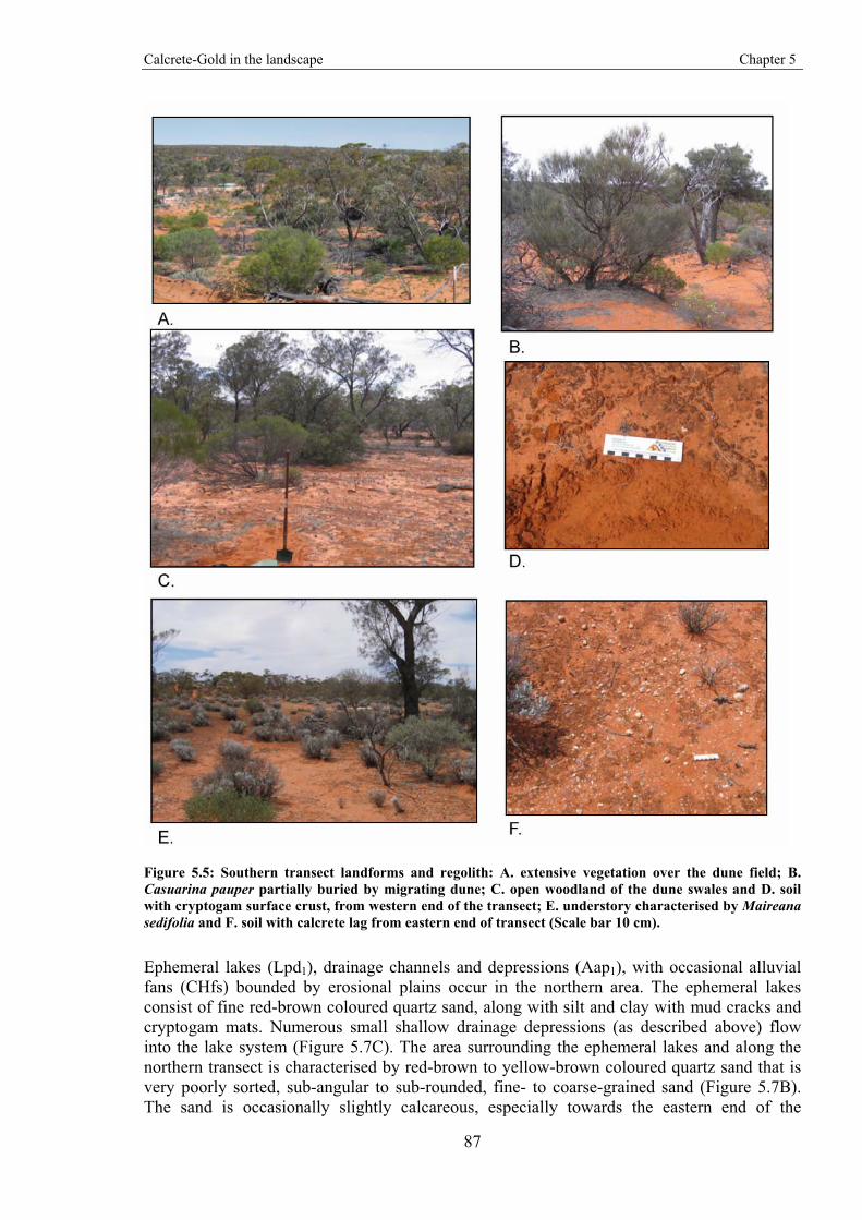
Calcrete-Gold in the landscape Chapter 5
87
Figure 5.5: Southern transect landforms and regolith: A. extensive vegetation over the dune field; B. Casuarina pauper partially buried by migrating dune; C. open woodland of the dune swales and D. soil with cryptogam surface crust, from western end of the transect; E. understory characterised by Maireana sedifolia and F. soil with calcrete lag from eastern end of transect (Scale bar 10 cm).
Ephemeral lakes (Lpd1), drainage channels and depressions (Aap1), with occasional alluvial fans (CHfs) bounded by erosional plains occur in the northern area. The ephemeral lakes consist of fine red-brown coloured quartz sand, along with silt and clay with mud cracks and cryptogam mats. Numerous small shallow drainage depressions (as described above) flow into the lake system (Figure 5.7C). The area surrounding the ephemeral lakes and along the northern transect is characterised by red-brown to yellow-brown coloured quartz sand that is very poorly sorted, sub-angular to sub-rounded, fine- to coarse-grained sand (Figure 5.7B). The sand is occasionally slightly calcareous, especially towards the eastern end of the
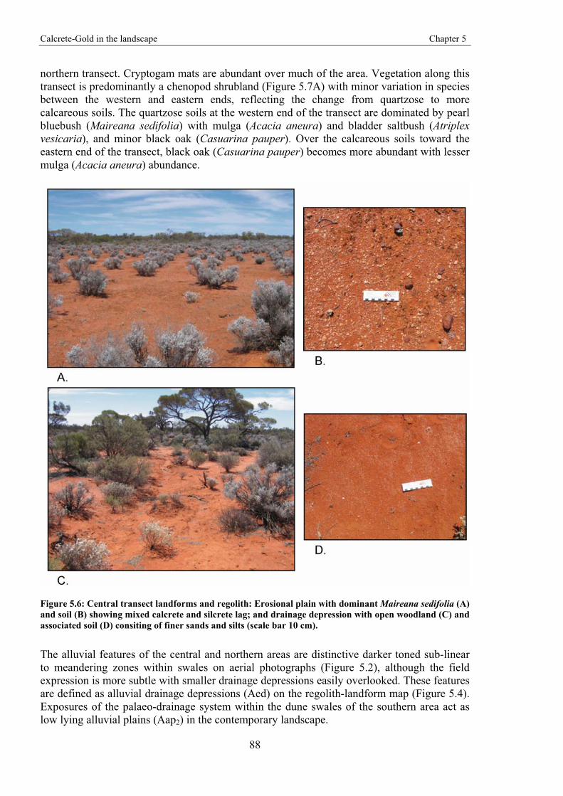
Calcrete-Gold in the landscape Chapter 5
88
northern transect. Cryptogam mats are abundant over much of the area. Vegetation along this transect is predominantly a chenopod shrubland (Figure 5.7A) with minor variation in species between the western and eastern ends, reflecting the change from quartzose to more calcareous soils. The quartzose soils at the western end of the transect are dominated by pearl bluebush (Maireana sedifolia) with mulga (Acacia aneura) and bladder saltbush (Atriplex vesicaria), and minor black oak (Casuarina pauper). Over the calcareous soils toward the eastern end of the transect, black oak (Casuarina pauper) becomes more abundant with lesser mulga (Acacia aneura) abundance.
Figure 5.6: Central transect landforms and regolith: Erosional plain with dominant Maireana sedifolia (A) and soil (B) showing mixed calcrete and silcrete lag; and drainage depression with open woodland (C) and associated soil (D) consiting of finer sands and silts (scale bar 10 cm).
The alluvial features of the central and northern areas are distinctive darker toned sub-linear to meandering zones within swales on aerial photographs (Figure 5.2), although the field expression is more subtle with smaller drainage depressions easily overlooked. These features are defined as alluvial drainage depressions (Aed) on the regolith-landform map (Figure 5.4). Exposures of the palaeo-drainage system within the dune swales of the southern area act as low lying alluvial plains (Aap2) in the contemporary landscape.
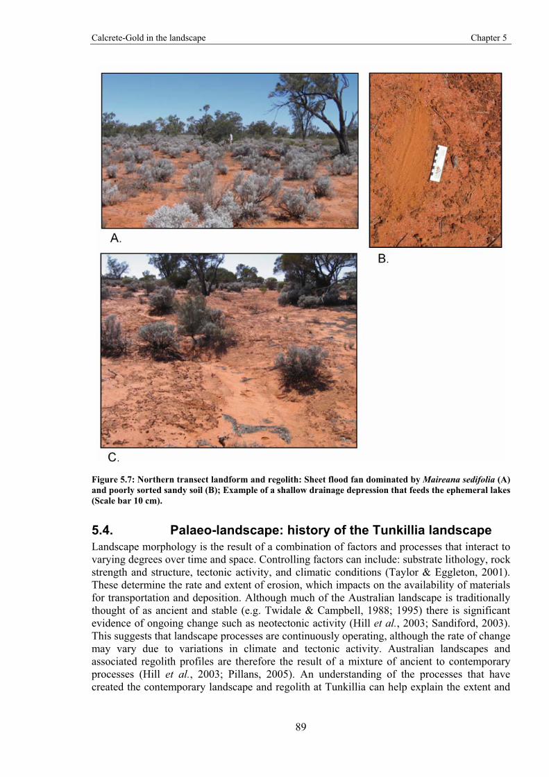
Calcrete-Gold in the landscape Chapter 5
89
Figure 5.7: Northern transect landform and regolith: Sheet flood fan dominated by Maireana sedifolia (A) and poorly sorted sandy soil (B); Example of a shallow drainage depression that feeds the ephemeral lakes (Scale bar 10 cm).
5.4. Palaeo-landscape: history of the Tunkillia landscape Landscape morphology is the result of a combination of factors and processes that interact to varying degrees over time and space. Controlling factors can include: substrate lithology, rock strength and structure, tectonic activity, and climatic conditions (Taylor & Eggleton, 2001). These determine the rate and extent of erosion, which impacts on the availability of materials for transportation and deposition. Although much of the Australian landscape is traditionally thought of as ancient and stable (e.g. Twidale & Campbell, 1988; 1995) there is significant evidence of ongoing change such as neotectonic activity (Hill et al., 2003; Sandiford, 2003). This suggests that landscape processes are continuously operating, although the rate of change may vary due to variations in climate and tectonic activity. Australian landscapes and associated regolith profiles are therefore the result of a mixture of ancient to contemporary processes (Hill et al., 2003; Pillans, 2005). An understanding of the processes that have created the contemporary landscape and regolith at Tunkillia can help explain the extent and
Calcrete-Gold in the landscape Chapter 5
90
dispersion of the Au-in-calcrete anomaly. The knowledge gained from Tunkillia may then be applied to other regions of anomalous Au-in-calcrete in the search for Au mineralisation.
Based on field relationships, the oldest regolith material at Tunkillia is the highly weathered bedrock. Deep weathering profiles, like those observed at Tunkillia, are typical of wet and wet/dry tropical climates, but not all deep weathering profiles are formed under these conditions (Taylor & Eggleton, 2001). Similar profiles may also develop in colder and drier conditions given enough time and limited surface erosion (Paton & Williams, 1972; Bird & Chivas, 1993).
The Precambrian basement of the Gawler Craton is bounded by the Eucla, Warburton, Officer, and Eromanga Basins, and the Adelaide Geosyncline. Deposition of sediments derived from erosion of hinterland areas of these Basins continued through much of the Phanerozoic and up to the end of the Early Cretaceous (Beckmann, 1983). Apart from the marginal areas that were inundated by the basins, the majority of the Gawler Craton surface has been exposed to denudation since the Cambrian. The exception was during Permian glacial activity, when portions of many exposed surface areas of southern Australia were planated (Beckmann, 1983). Many of the Australian landscape features, including deeply oxidised weathering profiles and Permo-Carboniferous glacial landforms, were derived from the Late Palaeozoic (Pillans, 2007).
The deep weathering profiles and low relief landscapes in Australia are the result of denudation that occurred from the Late Palaeozoic to Miocene (Beckmann, 1983; Benbow et al., 1995). Leaching and removal of the soluble components (e.g. cations such as ferrous iron, and silica) over an extended time explains the uniformity within the weathered profiles (Beckmann, 1983). Through the use of oxygen isotopes from regions including the Gawler Craton, Bird & Chivas (1988; 1989; 1993) defined four weathering periods for southern Australia that extend from the late Palaeozoic to the present day (Figure 5.8). These dates are broadly constrained ranges that require correlations with additional methods (Bird & Chivas, 1988; 1989). The formation of these deep profiles is independent of temperature and simply requires periods of high rainfall and efficient leaching (Bird & Chivas, 1988; 1989).
The formation of ferricrete and silcrete duricrusts may be due to extensive periods of continuous and/or repeated episodes of weathering (Stephens, 1971; Bourman, 1993b; Taylor & Shirtliff, 2003; Pillans, 2005). The polygenetic nature of ferricrete makes precise dating difficult (Bourman, 1993b). Conditions favourable to ferricrete formation have occurred over at least three major phases in South Australia: from the early Mesozoic to Middle Eocene; from the late Oligocene to Middle Miocene; and, from the Late Miocene to Pleistocene (Benbow, 1983). A continental wide period of deep oxidation and iron mobilisation has been suggested at about 60 Ma (Pillans, 2005). Silcrete formation appears to have peaked over two main periods: from the Late Eocene to Middle Miocene; and Late Miocene to Pleistocene (Alley, 1977; Benbow, 1983). The later event may also be related to groundwater silicification. These proposed periods may reflect favourable conditions for ferricrete or silcrete formation; however, as discussed above, their formation may also be continuous and ongoing (Figure 5.8), particularly for ferricretes where contemporary reduced groundwaters carry ferrous ions.
Since the late Miocene there has been a progressive trend towards a more arid climate with occasional cycles of wetter conditions in Australia (Bowler, 1976). This increased aridity resulted in the widespread aeolian deposits and the start of regolith carbonate formation in southern and central Australia (Hou et al., 2008). Aeolian activity in southern Australia has
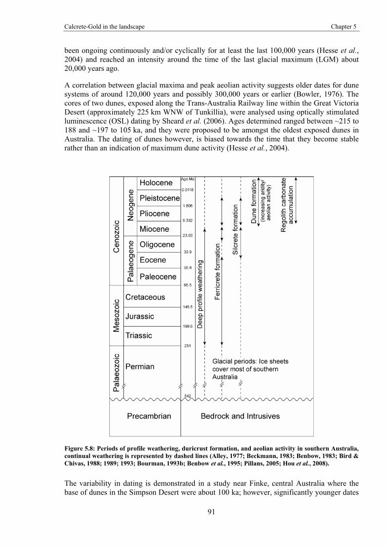
Calcrete-Gold in the landscape Chapter 5
91
been ongoing continuously and/or cyclically for at least the last 100,000 years (Hesse et al., 2004) and reached an intensity around the time of the last glacial maximum (LGM) about 20,000 years ago.
A correlation between glacial maxima and peak aeolian activity suggests older dates for dune systems of around 120,000 years and possibly 300,000 years or earlier (Bowler, 1976). The cores of two dunes, exposed along the Trans-Australia Railway line within the Great Victoria Desert (approximately 225 km WNW of Tunkillia), were analysed using optically stimulated luminescence (OSL) dating by Sheard et al. (2006). Ages determined ranged between ~215 to 188 and ~197 to 105 ka, and they were proposed to be amongst the oldest exposed dunes in Australia. The dating of dunes however, is biased towards the time that they become stable rather than an indication of maximum dune activity (Hesse et al., 2004).
Figure 5.8: Periods of profile weathering, duricrust formation, and aeolian activity in southern Australia, continual weathering is represented by dashed lines (Alley, 1977; Beckmann, 1983; Benbow, 1983; Bird & Chivas, 1988; 1989; 1993; Bourman, 1993b; Benbow et al., 1995; Pillans, 2005; Hou et al., 2008).
The variability in dating is demonstrated in a study near Finke, central Australia where the base of dunes in the Simpson Desert were about 100 ka; however, significantly younger dates
Calcrete-Gold in the landscape Chapter 5
92
were acquired for overlying dunes at around 30 to 17 ka, and even younger on the crests at < 5 ka (Nanson et al., 1995). Similar results have been presented for dunes in the Strezlecki Desert and Murray Mallee (Gardner et al., 1987).
These relatively young dates for sand dunes reflect continual reworking of the dunes, which may have been ongoing since the Pleistocene (Nanson et al., 1995). Evidence of recent dune activity, by the burial of swale vegetation, demonstrates the reworking of the dunes and their continued eastward migration in the margins of the Great Victoria Desert at Tunkillia (Lowrey, 2007). Pedogenesis, especially carbonate accumulation, and vegetation help to stabilise the dunes (Bowler, 1976). Younger dunes forming at the dune field margins are therefore an expansion of the dune field rather than part of an overall movement of dunes within the dune field.
Migrating dunes are burying erosional plains and associated drainage depressions, similar to those in the central area. Remnants of these regolith-landforms are in many of the interdunal swales. The blockage of the palaeo-drainage system by migrating dunes has resulted in a lateral spreading of alluvial sediments between many of the swales.
5.5. Regolith carbonate features in the Tunkillia landscape The morphology, geochemistry and depth of regolith carbonate are shown in Table 5.2 and described below.
At the western end of the southern transect, within the dune-field, indurated carbonates are either absent or occur at a depth > 1 m (which was considered to be the maximum depth that samples could be collected without risk of contamination from hole collapse). These samples were collected from 0.7 to 1.0 m deep and mostly consist of calcareous sand with 0.74 to 4.12% CaO. Within the larger interdunal plains towards the eastern end of the transect, the morphology of the regolith carbonates is mostly nodular and highly indurated. Indurated regolith carbonate samples included T1/11, T1/12, and T1/15, which are from a shallower depth of between 0.2 to 0.7 m. The increasing nodular content in these samples corresponds with an increasing CaO content, with up to 39% CaO in the hardpan calcrete. As well as the regolith carbonate samples from the southern transect, also collected were a non-calcareous, Fe-rich, red silty soil (T1/09), a non-calcareous, friable ferricrete (T1/13), and a red silty soil with silcrete pebbles (possibly a buried palaeosurface with a silcrete lag) (T1/14). The CaO content in these samples is < 1% and assay results from these three samples were significantly different to the regolith carbonates. These samples were not regolith carbonates and were therefore removed from further analysis or discussion.
The regolith carbonate samples from the central transect (T3) generally consisted of shallow (0.1 to 0.3 m) hardpan regolith carbonates with > 30% CaO. The exceptions were a hardpan regolith carbonate at 0.4 m depth that was overlain by a clay/silt rich soil and associated with a Casuarina woodland (T3/07), and three calcareous sand and nodule samples (T3/09, T3/10, and T3/12) from 0.35 to 0.5 m depths that were associated with drainage depressions.
Regolith carbonates of the northern transect (T2) are reasonably uniform with calcareous sand and nodular morphology for all but one sample (T2/02). These samples were collected from approximately 0.6 m deep and contained from 4 to 9% CaO. The exception (T2/02) is a Fe-rich calcareous hardpan from 0.5 m that contained 2.2% CaO.
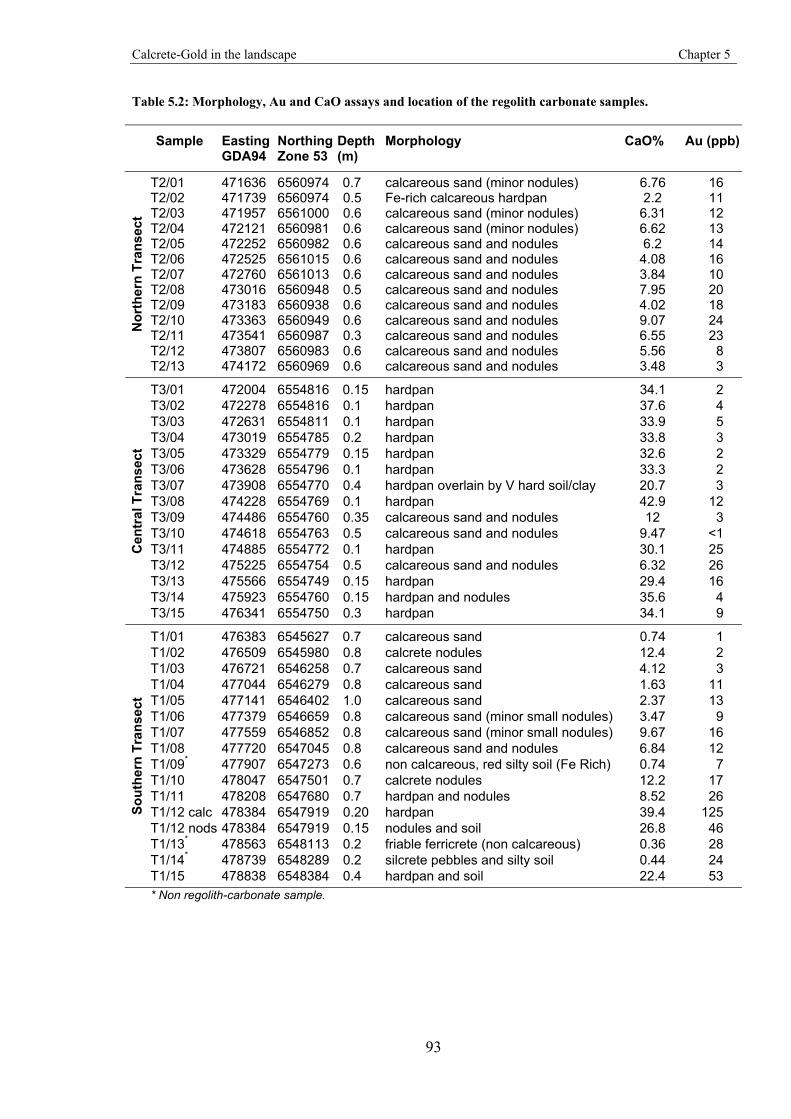
Calcrete-Gold in the landscape Chapter 5
93
Table 5.2: Morphology, Au and CaO assays and location of the regolith carbonate samples.
Sample Easting GDA94
NorthingZone 53
Depth (m)
Morphology CaO% Au (ppb)
T2/01 471636 6560974 0.7 calcareous sand (minor nodules) 6.76 16 T2/02 471739 6560974 0.5 Fe-rich calcareous hardpan 2.2 11 T2/03 471957 6561000 0.6 calcareous sand (minor nodules) 6.31 12 T2/04 472121 6560981 0.6 calcareous sand (minor nodules) 6.62 13 T2/05 472252 6560982 0.6 calcareous sand and nodules 6.2 14 T2/06 472525 6561015 0.6 calcareous sand and nodules 4.08 16 T2/07 472760 6561013 0.6 calcareous sand and nodules 3.84 10 T2/08 473016 6560948 0.5 calcareous sand and nodules 7.95 20 T2/09 473183 6560938 0.6 calcareous sand and nodules 4.02 18 T2/10 473363 6560949 0.6 calcareous sand and nodules 9.07 24 T2/11 473541 6560987 0.3 calcareous sand and nodules 6.55 23 T2/12 473807 6560983 0.6 calcareous sand and nodules 5.56 8
Nor
ther
n Tr
anse
ct
T2/13 474172 6560969 0.6 calcareous sand and nodules 3.48 3
T3/01 472004 6554816 0.15 hardpan 34.1 2 T3/02 472278 6554816 0.1 hardpan 37.6 4 T3/03 472631 6554811 0.1 hardpan 33.9 5 T3/04 473019 6554785 0.2 hardpan 33.8 3 T3/05 473329 6554779 0.15 hardpan 32.6 2 T3/06 473628 6554796 0.1 hardpan 33.3 2 T3/07 473908 6554770 0.4 hardpan overlain by V hard soil/clay 20.7 3 T3/08 474228 6554769 0.1 hardpan 42.9 12 T3/09 474486 6554760 0.35 calcareous sand and nodules 12 3 T3/10 474618 6554763 0.5 calcareous sand and nodules 9.47 <1 T3/11 474885 6554772 0.1 hardpan 30.1 25 T3/12 475225 6554754 0.5 calcareous sand and nodules 6.32 26 T3/13 475566 6554749 0.15 hardpan 29.4 16 T3/14 475923 6554760 0.15 hardpan and nodules 35.6 4
Cen
tral
Tra
nsec
t
T3/15 476341 6554750 0.3 hardpan 34.1 9
T1/01 476383 6545627 0.7 calcareous sand 0.74 1 T1/02 476509 6545980 0.8 calcrete nodules 12.4 2 T1/03 476721 6546258 0.7 calcareous sand 4.12 3 T1/04 477044 6546279 0.8 calcareous sand 1.63 11 T1/05 477141 6546402 1.0 calcareous sand 2.37 13 T1/06 477379 6546659 0.8 calcareous sand (minor small nodules) 3.47 9 T1/07 477559 6546852 0.8 calcareous sand (minor small nodules) 9.67 16 T1/08 477720 6547045 0.8 calcareous sand and nodules 6.84 12 T1/09* 477907 6547273 0.6 non calcareous, red silty soil (Fe Rich) 0.74 7 T1/10 478047 6547501 0.7 calcrete nodules 12.2 17 T1/11 478208 6547680 0.7 hardpan and nodules 8.52 26 T1/12 calc 478384 6547919 0.20 hardpan 39.4 125 T1/12 nods 478384 6547919 0.15 nodules and soil 26.8 46 T1/13* 478563 6548113 0.2 friable ferricrete (non calcareous) 0.36 28 T1/14* 478739 6548289 0.2 silcrete pebbles and silty soil 0.44 24
Sout
hern
Tra
nsec
t
T1/15 478838 6548384 0.4 hardpan and soil 22.4 53 * Non regolith-carbonate sample.
Calcrete-Gold in the landscape Chapter 5
94
5.6. Element dispersion patterns in the Tunkillia area: Results and discussion
Elemental analyses of the regolith carbonate samples were undertaken by Amdel Ltd. Adelaide, for a suite of 53 elements as described in Section 3.6.3. Full spreadsheets of analytical results are included in Appendix 2. A correlation coefficient (r) of ±0.8 was chosen as the value for significance as described in Section 3.4 for discerning elemental associations. Element concentrations close to or below analytical detection for > 20% of the samples were rejected from the following interpretation. Elements meeting this criteria and therefore rejected are: Ag, Bi, Cd, Cr, In, MnO, Sb, Sc, Te, Tl, and V.
To reduce the repetitive descriptions of the REEs due to their similar dispersion patterns and associated correlations, the REEs have been divided into the light REEs (La, Ce, Pr & Nd), mid REEs (Sm, Eu, Gd, Tb, Dy & Ho), and heavy REEs (Er, Tm, Yb & Lu). These have been abbreviated to LREE, MREE and HREE respectively.
5.6.1. Major elements The major components of all samples were CaO and SiO2. In particular, SiO2 was the major constituent of most samples with concentrations > 70% for the northern transect and > 75% for most of the southern transect. The exceptions are the hardpan regolith carbonate samples from the southern and central transects, which had higher CaO contents and corresponding lower SiO2 contents of < 35%. These two components account for > 60% of the material in the majority of samples and up to 90% along the southern transect. The abundance of CaO is inversely proportional to the abundance of SiO2 (Table 5.3) therefore with a very strong negative correlation between CaO and SiO2 (r = -0.99) (Table 5.4 & Figure 5.9). The high SiO2 concentrations along the western end of the southern transect are from samples collected between “Phase I” and “Phase II” dune swales, and correspond with low assay values for the majority of elements.
Elemental correlations with SiO2 are mostly negative (Table 5.4) for the overall dataset, and particularly for the northern and southern transects. These include CaO, Sr, and P2O5, which are closely correlated with each other along all transects, apart from the northern transect where CaO and P2O5 have low correlation coefficient values with SiO2 of -0.75 and 0.10 respectively. The only positive correlations with SiO2 occur along the central transect, which also has the most elements correlated with SiO2.
Similar elemental correlations to SiO2 occur for CaO, except that they are inverted (Table 5.4). Positive correlations with CaO are P2O5 and Sr. The correlation between CaO and P2O5 does not extend to the northern transect and is relatively low along the southern (r = 0.82) and central (r = 0.81) transects. Along the northern transect all P2O5 values except one are < 0.03%, and along the southern transect most values are < 0.02%. The exception is the nodular and indurated carbonate samples of T1/12, which contain 0.05% P2O5. The highest P2O5 concentrations are along the central transect (0.02 to 0.07%).
With concentrations ranging from 2 to 8%, Al2O3 is the next most significant component of the regolith carbonate samples (Table 5.3). The Al2O3 values gradually increase in concentration from the southern to northern transects (Figure 5.10). The Al2O3 concentration ranges from 4.04 to 8.21% along the northern transect, 2.00 to 6.12% along the central transect and 1.89 to 3.91% along the southern transect. The dispersion pattern is relatively uniform along the northern and southern transects, but along the central transect there is an increase in the Al2O3 content for samples within the drainage area. Several elements are
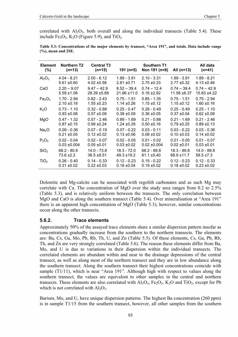
Calcrete-Gold in the landscape Chapter 5
95
correlated with Al2O3, both overall and along the individual transects (Table 5.4). These include Fe2O3, K2O (Figure 5.9), and TiO2.
Table 5.3: Concentrations of the major elements by transect, “Area 191”, and totals. Data include range (%), mean and 2SE.
Northern T2 Central T3 Southern T1 Element (%) (n=13) (n=15) 191 (n=5) Non 191 (n=8) All (n=13)
All data (n=41)
Al2O3 4.04 - 8.21 5.61 ±0.60
2.00 - 6.12 4.02 ±0.58
1.89 - 3.91 2.81 ±0.71
2.10 - 3.31 2.75 ±0.33
1.89 - 3.91 2.77 ±0.32
1.89 - 8.21 4.13 ±0.46
CaO 2.20 – 9.07 5.59 ±1.08
9.47 – 42.9 28.39 ±5.68
8.52 – 39.4 21.86 ±11.0
0.74 – 12.4 5.16 ±2.92
0.74 – 39.4 11.58 ±6.37
0.74 – 42.9 15.83 ±4.22
Fe2O3 1.70 - 2.94 2.10 ±0.18
0.82 - 2.43 1.55 ±0.23
0.75 - 1.51 1.14 ±0.26
0.85 - 1.35 1.15 ±0.12
0.75 - 1.51 1.15 ±0.12
0.75 - 2.94 1.60 ±0.16
K2O 0.73 - 1.10 0.93 ±0.08
0.32 - 0.88 0.57 ±0.09
0.25 - 0.47 0.38 ±0.09
0.28 - 0.49 0.36 ±0.05
0.25 - 0.49 0.37 ±0.04
0.25 - 1.10 0.62 ±0.08
MgO 0.47 - 1.32 0.87 ±0.15
0.57 - 2.46 0.99 ±0.24
0.89 - 1.69 1.24 ±0.29
0.21 - 0.88 0.50 ±0.16
0.21 - 1.69 0.79 ±0.25
0.21 - 2.46 0.89 ±0.13
Na2O 0.09 - 0.36 0.21 ±0.05
0.07 - 0.19 0.12 ±0.02
0.07 - 0.22 0.13 ±0.06
0.03 - 0.11 0.08 ±0.02
0.03 - 0.22 0.10 ±0.03
0.03 - 0.36 0.14 ±0.02
P2O5 0.02 - 0.04 0.03 ±0.004
0.02 - 0.07 0.05 ±0.01
0.02 - 0.05 0.03 ±0.02
0.01 - 0.02 0.02 ±0.004
0.01 - 0.05 0.02 ±0.01
0.01 - 0.07 0.03 ±0.01
SiO2 68.2 - 80.6 73.6 ±2.2
14.0 - 73.8 36.5 ±9.51
18.3 - 72.0 49.3 ±19.2
68.2 - 89.8 81.1 ±5.40
18.3 - 89.8 68.9 ±11.7
14.0 - 89.8 58.5 ±7.3
TiO2 0.26 - 0.40 0.31 ±0.02
0.14 - 0.33 0.22 ±0.03
0.12 - 0.23 0.18 ±0.04
0.15 - 0.22 0.19 ±0.02
0.12 - 0.23 0.18 ±0.02
0.12 - 0.33 0.23 ±0.02
Dolomite and Mg-calcite can be associated with regolith carbonates and as such Mg may correlate with Ca. The concentration of MgO over the study area ranges from 0.2 to 2.5% (Table 5.3), and is relatively uniform between the transects. The only correlation between MgO and CaO is along the southern transect (Table 5.4). Over mineralisation at “Area 191” there is an apparent high concentration of MgO (Table 5.3); however, similar concentrations occur along the other transects.
5.6.2. Trace elements Approximately 50% of the assayed trace elements share a similar dispersion pattern insofar as concentrations gradually increase from the southern to the northern transects. The elements are: Ba, Cs, Ga, Mo, Pb, Rb, Th, U, and Zn (Table 5.5). Of these elements, Cs, Ga, Pb, Rb, Th, and Zn are very strongly correlated (Table 5.6). The reason these elements differ from Ba, Mo, and U is due to variations in their dispersion within the individual transects. The correlated elements are abundant within and near to the drainage depressions of the central transect, as well as along most of the northern transect and they are in low abundance along the southern transect. Along the southern transect their highest concentrations coincide with sample (T1/11), which is near “Area 191”. Although high with respect to values along the southern transect, the values are equivalent to other samples in the central and northern transects. These elements are also correlated with Al2O3, Fe2O3, K2O and TiO2, except for Pb which is not correlated with Al2O3.
Barium, Mo, and U, have unique dispersion patterns. The highest Ba concentration (260 ppm) is in sample T1/15 from the southern transect, however, all other samples from the southern
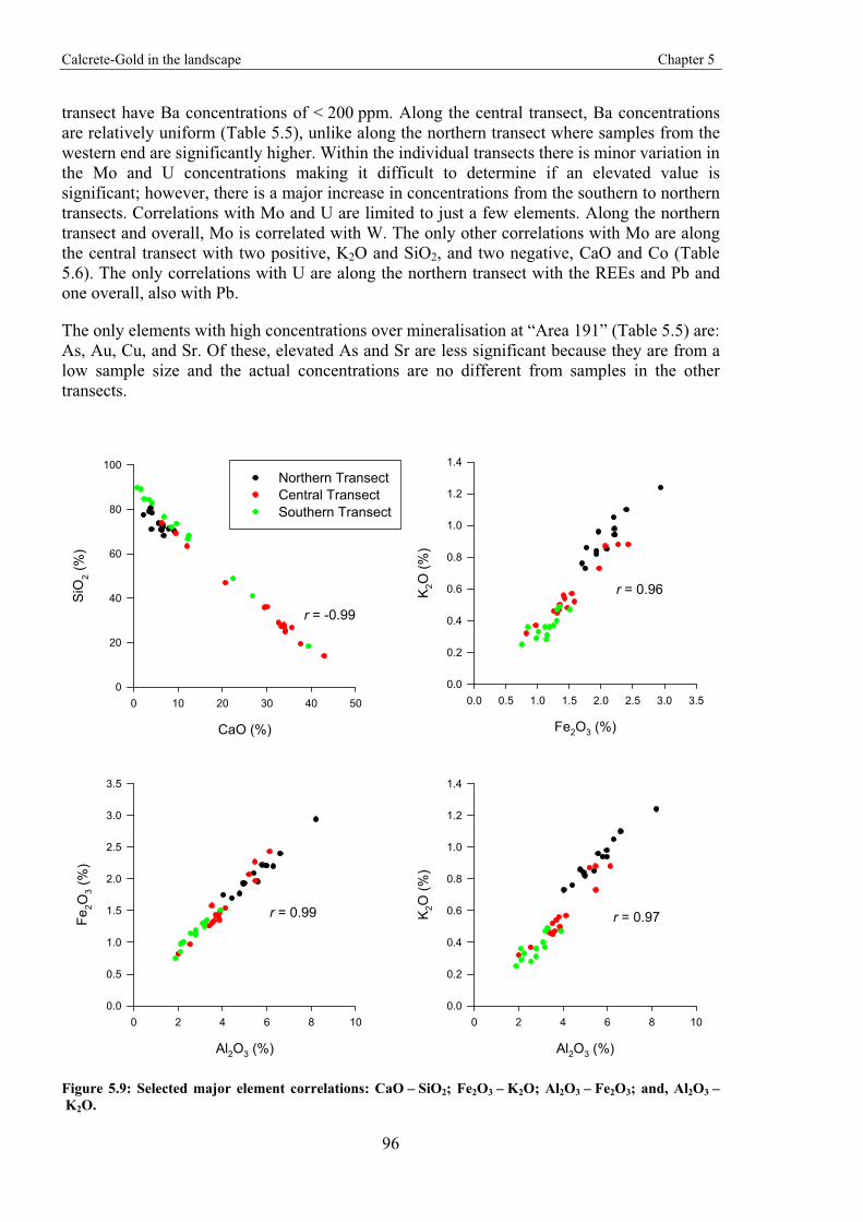
Calcrete-Gold in the landscape Chapter 5
96
transect have Ba concentrations of < 200 ppm. Along the central transect, Ba concentrations are relatively uniform (Table 5.5), unlike along the northern transect where samples from the western end are significantly higher. Within the individual transects there is minor variation in the Mo and U concentrations making it difficult to determine if an elevated value is significant; however, there is a major increase in concentrations from the southern to northern transects. Correlations with Mo and U are limited to just a few elements. Along the northern transect and overall, Mo is correlated with W. The only other correlations with Mo are along the central transect with two positive, K2O and SiO2, and two negative, CaO and Co (Table 5.6). The only correlations with U are along the northern transect with the REEs and Pb and one overall, also with Pb.
The only elements with high concentrations over mineralisation at “Area 191” (Table 5.5) are: As, Au, Cu, and Sr. Of these, elevated As and Sr are less significant because they are from a low sample size and the actual concentrations are no different from samples in the other transects.
CaO (%)
0 10 20 30 40 50
SiO
2 (%
)
0
20
40
60
80
100Northern TransectCentral TransectSouthern Transect
Al2O3 (%)
0 2 4 6 8 10
Fe2O
3 (%
)
0.0
0.5
1.0
1.5
2.0
2.5
3.0
3.5
Al2O3 (%)
0 2 4 6 8 10
K2O
(%)
0.0
0.2
0.4
0.6
0.8
1.0
1.2
1.4
Fe2O3 (%)
0.0 0.5 1.0 1.5 2.0 2.5 3.0 3.5
K2O
(%)
0.0
0.2
0.4
0.6
0.8
1.0
1.2
1.4
r = -0.99
r = 0.96
r = 0.97r = 0.99
Figure 5.9: Selected major element correlations: CaO – SiO2; Fe2O3 – K2O; Al2O3 – Fe2O3; and, Al2O3 – K2O.
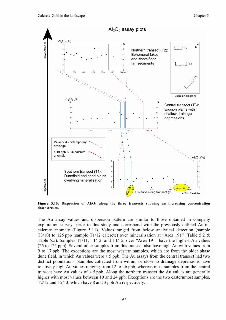
Calcrete-Gold in the landscape Chapter 5
97
Figure 5.10: Dispersion of Al2O3 along the three transects showing an increasing concentration downstream.
The Au assay values and dispersion pattern are similar to those obtained in company exploration surveys prior to this study and correspond with the previously defined Au-in-calcrete anomaly (Figure 5.11). Values ranged from below analytical detection (sample T3/10) to 125 ppb (sample T1/12 calcrete) over mineralisation at “Area 191” (Table 5.2 & Table 5.5). Samples T1/11, T1/12, and T1/15, over “Area 191” have the highest Au values (26 to 125 ppb). Several other samples from this transect also have high Au with values from 9 to 17 ppb. The exceptions are the most western samples, which are from the older phase dune field, in which Au values were < 5 ppb. The Au assays from the central transect had two distinct populations. Samples collected from within, or close to drainage depressions have relatively high Au values ranging from 12 to 26 ppb, whereas most samples from the central transect have Au values of < 5 ppb. Along the northern transect the Au values are generally higher with most values between 10 and 24 ppb. Exceptions are the two easternmost samples, T2/12 and T2/13, which have 8 and 3 ppb Au respectively.
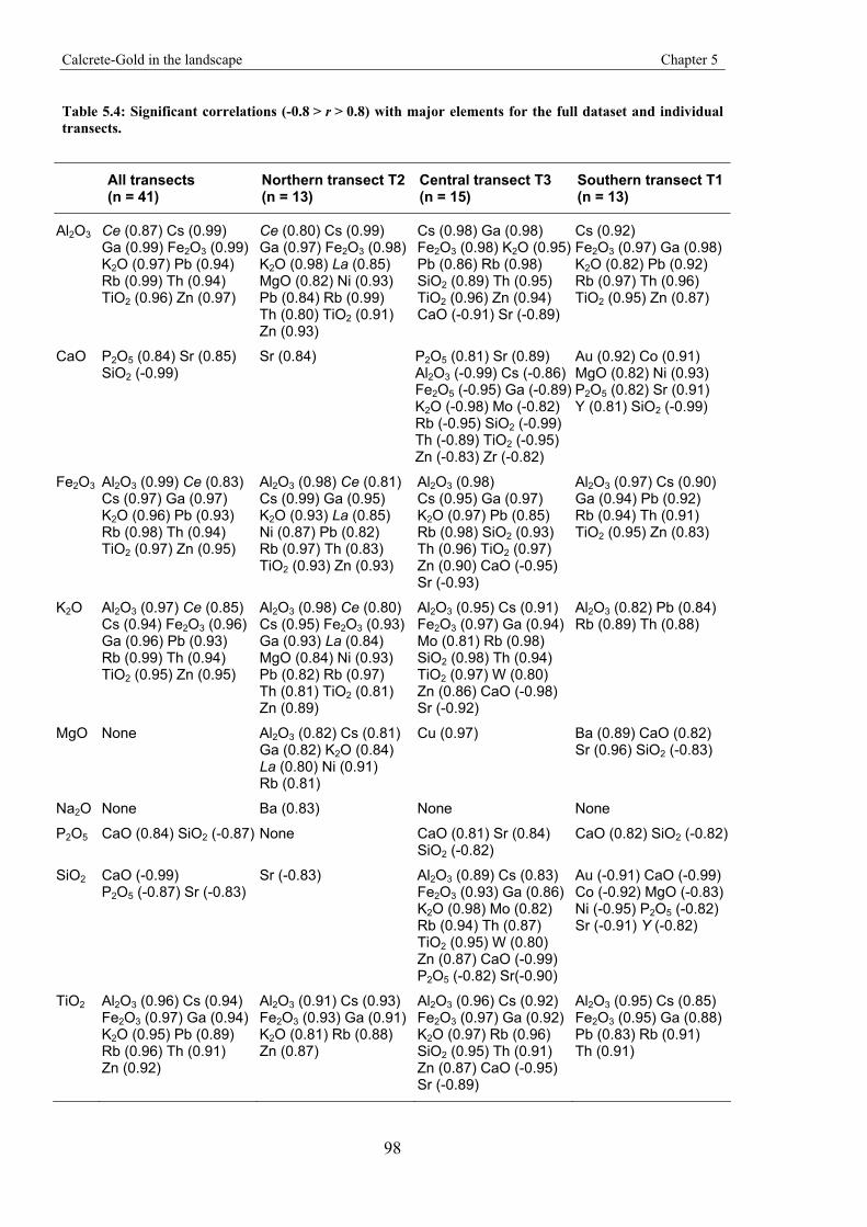
Calcrete-Gold in the landscape Chapter 5
98
Table 5.4: Significant correlations (-0.8 > r > 0.8) with major elements for the full dataset and individual transects.
All transects (n = 41)
Northern transect T2 (n = 13)
Central transect T3 (n = 15)
Southern transect T1(n = 13)
Al2O3 Ce (0.87) Cs (0.99) Ga (0.99) Fe2O3 (0.99) K2O (0.97) Pb (0.94) Rb (0.99) Th (0.94) TiO2 (0.96) Zn (0.97)
Ce (0.80) Cs (0.99) Ga (0.97) Fe2O3 (0.98) K2O (0.98) La (0.85) MgO (0.82) Ni (0.93) Pb (0.84) Rb (0.99) Th (0.80) TiO2 (0.91) Zn (0.93)
Cs (0.98) Ga (0.98) Fe2O3 (0.98) K2O (0.95) Pb (0.86) Rb (0.98) SiO2 (0.89) Th (0.95) TiO2 (0.96) Zn (0.94) CaO (-0.91) Sr (-0.89)
Cs (0.92) Fe2O3 (0.97) Ga (0.98) K2O (0.82) Pb (0.92) Rb (0.97) Th (0.96) TiO2 (0.95) Zn (0.87)
CaO P2O5 (0.84) Sr (0.85) SiO2 (-0.99)
Sr (0.84) P2O5 (0.81) Sr (0.89) Al2O3 (-0.99) Cs (-0.86) Fe2O5 (-0.95) Ga (-0.89) K2O (-0.98) Mo (-0.82) Rb (-0.95) SiO2 (-0.99) Th (-0.89) TiO2 (-0.95) Zn (-0.83) Zr (-0.82)
Au (0.92) Co (0.91) MgO (0.82) Ni (0.93) P2O5 (0.82) Sr (0.91) Y (0.81) SiO2 (-0.99)
Fe2O3 Al2O3 (0.99) Ce (0.83) Cs (0.97) Ga (0.97) K2O (0.96) Pb (0.93) Rb (0.98) Th (0.94) TiO2 (0.97) Zn (0.95)
Al2O3 (0.98) Ce (0.81) Cs (0.99) Ga (0.95) K2O (0.93) La (0.85) Ni (0.87) Pb (0.82) Rb (0.97) Th (0.83) TiO2 (0.93) Zn (0.93)
Al2O3 (0.98) Cs (0.95) Ga (0.97) K2O (0.97) Pb (0.85) Rb (0.98) SiO2 (0.93) Th (0.96) TiO2 (0.97) Zn (0.90) CaO (-0.95) Sr (-0.93)
Al2O3 (0.97) Cs (0.90) Ga (0.94) Pb (0.92) Rb (0.94) Th (0.91) TiO2 (0.95) Zn (0.83)
K2O Al2O3 (0.97) Ce (0.85) Cs (0.94) Fe2O3 (0.96) Ga (0.96) Pb (0.93) Rb (0.99) Th (0.94) TiO2 (0.95) Zn (0.95)
Al2O3 (0.98) Ce (0.80) Cs (0.95) Fe2O3 (0.93) Ga (0.93) La (0.84) MgO (0.84) Ni (0.93) Pb (0.82) Rb (0.97) Th (0.81) TiO2 (0.81) Zn (0.89)
Al2O3 (0.95) Cs (0.91) Fe2O3 (0.97) Ga (0.94) Mo (0.81) Rb (0.98) SiO2 (0.98) Th (0.94) TiO2 (0.97) W (0.80) Zn (0.86) CaO (-0.98) Sr (-0.92)
Al2O3 (0.82) Pb (0.84) Rb (0.89) Th (0.88)
MgO None Al2O3 (0.82) Cs (0.81) Ga (0.82) K2O (0.84) La (0.80) Ni (0.91) Rb (0.81)
Cu (0.97) Ba (0.89) CaO (0.82) Sr (0.96) SiO2 (-0.83)
Na2O None Ba (0.83) None None
P2O5 CaO (0.84) SiO2 (-0.87) None CaO (0.81) Sr (0.84) SiO2 (-0.82)
CaO (0.82) SiO2 (-0.82)
SiO2 CaO (-0.99) P2O5 (-0.87) Sr (-0.83)
Sr (-0.83) Al2O3 (0.89) Cs (0.83) Fe2O3 (0.93) Ga (0.86) K2O (0.98) Mo (0.82) Rb (0.94) Th (0.87) TiO2 (0.95) W (0.80) Zn (0.87) CaO (-0.99) P2O5 (-0.82) Sr(-0.90)
Au (-0.91) CaO (-0.99) Co (-0.92) MgO (-0.83) Ni (-0.95) P2O5 (-0.82) Sr (-0.91) Y (-0.82)
TiO2 Al2O3 (0.96) Cs (0.94) Fe2O3 (0.97) Ga (0.94) K2O (0.95) Pb (0.89) Rb (0.96) Th (0.91) Zn (0.92)
Al2O3 (0.91) Cs (0.93) Fe2O3 (0.93) Ga (0.91) K2O (0.81) Rb (0.88) Zn (0.87)
Al2O3 (0.96) Cs (0.92) Fe2O3 (0.97) Ga (0.92) K2O (0.97) Rb (0.96) SiO2 (0.95) Th (0.91) Zn (0.87) CaO (-0.95) Sr (-0.89)
Al2O3 (0.95) Cs (0.85) Fe2O3 (0.95) Ga (0.88) Pb (0.83) Rb (0.91) Th (0.91)
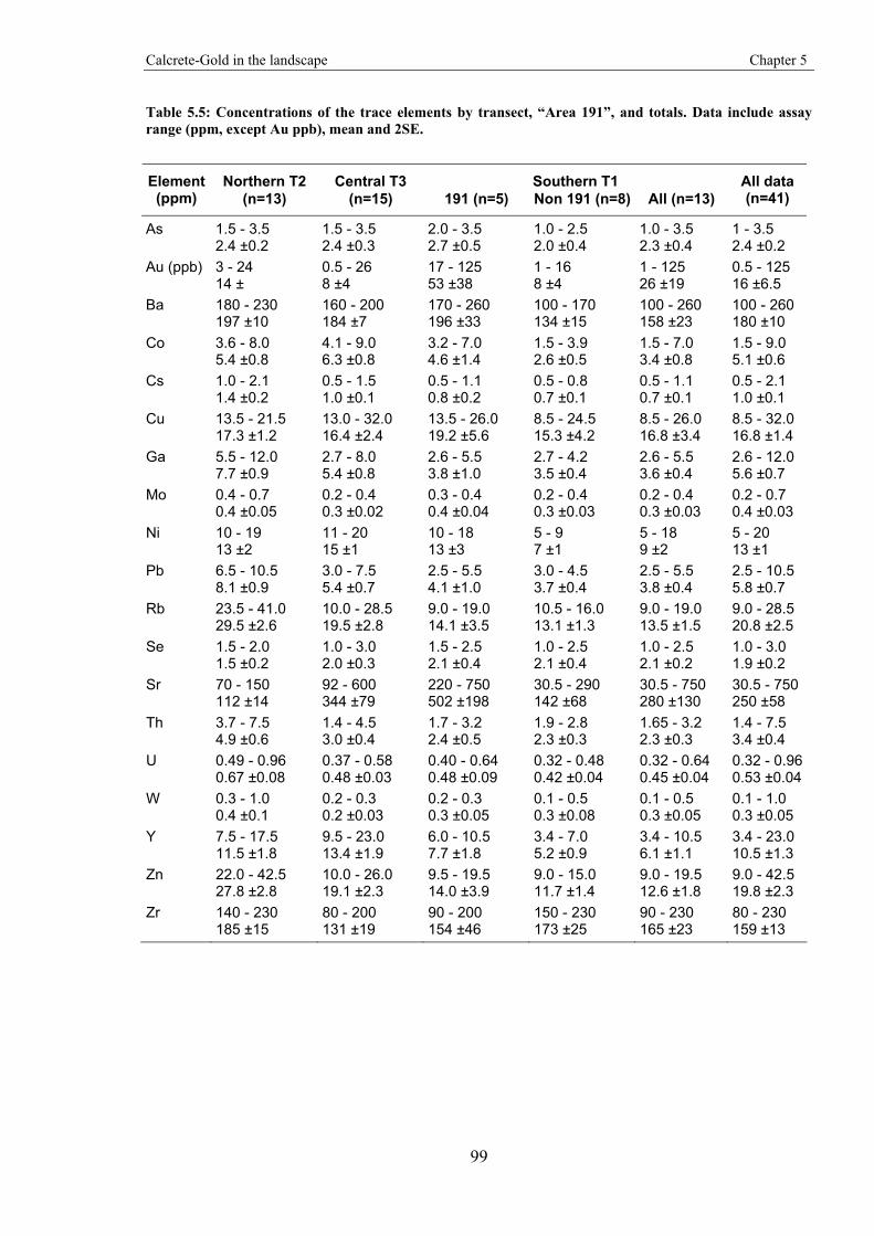
Calcrete-Gold in the landscape Chapter 5
99
Table 5.5: Concentrations of the trace elements by transect, “Area 191”, and totals. Data include assay range (ppm, except Au ppb), mean and 2SE.
Northern T2 Central T3 Southern T1 Element (ppm) (n=13) (n=15) 191 (n=5) Non 191 (n=8) All (n=13)
All data (n=41)
As 1.5 - 3.5 2.4 ±0.2
1.5 - 3.5 2.4 ±0.3
2.0 - 3.5 2.7 ±0.5
1.0 - 2.5 2.0 ±0.4
1.0 - 3.5 2.3 ±0.4
1 - 3.5 2.4 ±0.2
Au (ppb) 3 - 24 14 ±
0.5 - 26 8 ±4
17 - 125 53 ±38
1 - 16 8 ±4
1 - 125 26 ±19
0.5 - 125 16 ±6.5
Ba 180 - 230 197 ±10
160 - 200 184 ±7
170 - 260 196 ±33
100 - 170 134 ±15
100 - 260 158 ±23
100 - 260 180 ±10
Co 3.6 - 8.0 5.4 ±0.8
4.1 - 9.0 6.3 ±0.8
3.2 - 7.0 4.6 ±1.4
1.5 - 3.9 2.6 ±0.5
1.5 - 7.0 3.4 ±0.8
1.5 - 9.0 5.1 ±0.6
Cs 1.0 - 2.1 1.4 ±0.2
0.5 - 1.5 1.0 ±0.1
0.5 - 1.1 0.8 ±0.2
0.5 - 0.8 0.7 ±0.1
0.5 - 1.1 0.7 ±0.1
0.5 - 2.1 1.0 ±0.1
Cu 13.5 - 21.5 17.3 ±1.2
13.0 - 32.0 16.4 ±2.4
13.5 - 26.0 19.2 ±5.6
8.5 - 24.5 15.3 ±4.2
8.5 - 26.0 16.8 ±3.4
8.5 - 32.0 16.8 ±1.4
Ga 5.5 - 12.0 7.7 ±0.9
2.7 - 8.0 5.4 ±0.8
2.6 - 5.5 3.8 ±1.0
2.7 - 4.2 3.5 ±0.4
2.6 - 5.5 3.6 ±0.4
2.6 - 12.0 5.6 ±0.7
Mo 0.4 - 0.7 0.4 ±0.05
0.2 - 0.4 0.3 ±0.02
0.3 - 0.4 0.4 ±0.04
0.2 - 0.4 0.3 ±0.03
0.2 - 0.4 0.3 ±0.03
0.2 - 0.7 0.4 ±0.03
Ni 10 - 19 13 ±2
11 - 20 15 ±1
10 - 18 13 ±3
5 - 9 7 ±1
5 - 18 9 ±2
5 - 20 13 ±1
Pb 6.5 - 10.5 8.1 ±0.9
3.0 - 7.5 5.4 ±0.7
2.5 - 5.5 4.1 ±1.0
3.0 - 4.5 3.7 ±0.4
2.5 - 5.5 3.8 ±0.4
2.5 - 10.5 5.8 ±0.7
Rb 23.5 - 41.0 29.5 ±2.6
10.0 - 28.5 19.5 ±2.8
9.0 - 19.0 14.1 ±3.5
10.5 - 16.0 13.1 ±1.3
9.0 - 19.0 13.5 ±1.5
9.0 - 28.5 20.8 ±2.5
Se 1.5 - 2.0 1.5 ±0.2
1.0 - 3.0 2.0 ±0.3
1.5 - 2.5 2.1 ±0.4
1.0 - 2.5 2.1 ±0.4
1.0 - 2.5 2.1 ±0.2
1.0 - 3.0 1.9 ±0.2
Sr 70 - 150 112 ±14
92 - 600 344 ±79
220 - 750 502 ±198
30.5 - 290 142 ±68
30.5 - 750 280 ±130
30.5 - 750 250 ±58
Th 3.7 - 7.5 4.9 ±0.6
1.4 - 4.5 3.0 ±0.4
1.7 - 3.2 2.4 ±0.5
1.9 - 2.8 2.3 ±0.3
1.65 - 3.2 2.3 ±0.3
1.4 - 7.5 3.4 ±0.4
U 0.49 - 0.96 0.67 ±0.08
0.37 - 0.58 0.48 ±0.03
0.40 - 0.64 0.48 ±0.09
0.32 - 0.48 0.42 ±0.04
0.32 - 0.64 0.45 ±0.04
0.32 - 0.960.53 ±0.04
W 0.3 - 1.0 0.4 ±0.1
0.2 - 0.3 0.2 ±0.03
0.2 - 0.3 0.3 ±0.05
0.1 - 0.5 0.3 ±0.08
0.1 - 0.5 0.3 ±0.05
0.1 - 1.0 0.3 ±0.05
Y 7.5 - 17.5 11.5 ±1.8
9.5 - 23.0 13.4 ±1.9
6.0 - 10.5 7.7 ±1.8
3.4 - 7.0 5.2 ±0.9
3.4 - 10.5 6.1 ±1.1
3.4 - 23.0 10.5 ±1.3
Zn 22.0 - 42.5 27.8 ±2.8
10.0 - 26.0 19.1 ±2.3
9.5 - 19.5 14.0 ±3.9
9.0 - 15.0 11.7 ±1.4
9.0 - 19.5 12.6 ±1.8
9.0 - 42.5 19.8 ±2.3
Zr 140 - 230 185 ±15
80 - 200 131 ±19
90 - 200 154 ±46
150 - 230 173 ±25
90 - 230 165 ±23
80 - 230 159 ±13
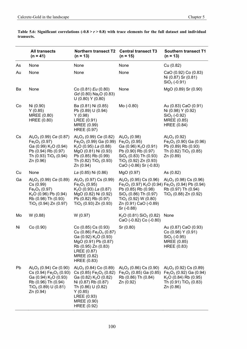
Calcrete-Gold in the landscape Chapter 5
100
Table 5.6: Significant correlations (-0.8 > r > 0.8) with trace elements for the full dataset and individual transects.
All transects (n = 41)
Northern transect T2 (n = 13)
Central transect T3 (n = 15)
Southern transect T1(n = 13)
As None None None Cu (0.82)
Au None None None CaO (0.92) Co (0.83) Ni (0.87) Sr (0.81) SiO2 (-0.91)
Ba None Co (0.81) Eu (0.80) Gd (0.80) Na2O (0.83) U (0.80) Y (0.80)
None MgO (0.89) Sr (0.90)
Co Ni (0.90) Y (0.85) MREE (0.80) HREE (0.80)
Ba (0.81) Ni (0.85) Pb (0.89) U (0.94) Y (0.98) LREE (0.91) MREE (0.99) HREE (0.97)
Mo (-0.80) Au (0.83) CaO (0.91) Ni (0.98) Y (0.92) SiO2 (-0.92) MREE (0.85) HREE (0.84)
Cs Al2O3 (0.99) Ce (0.87) Fe2O3 (0.97) Ga (0.99) K2O (0.94) Pb (0.94) Rb (0.97) Th (0.93) TiO2 (0.94) Zn (0.96)
Al2O3 (0.99) Ce (0.82) Fe2O3 (0.99) Ga (0.99) K2O (0.95) La (0.88) MgO (0.81) Ni (0.93) Pb (0.85) Rb (0.99) Th (0.82) TiO2 (0.93) Zn (0.94)
Al2O3 (0.98) Fe2O3 (0.95) Ga (0.96) K2O (0.91) Pb (0.90) Rb (0.97) SiO2 (0.83) Th (0.93) TiO2 (0.92) Zn (0.93) CaO (-0.86) Sr (-0.83)
Al2O3 (0.92) Fe2O3 (0.90) Ga (0.96) Pb (0.89) Rb (0.93) Th (0.82) TiO2 (0.85) Zn (0.89)
Cu None La (0.85) Ni (0.86) MgO (0.97) As (0.82)
Ga Al2O3 (0.99) Ce (0.89) Cs (0.99) Fe2O3 (0.97) K2O (0.96) Pb (0.94) Rb (0.98) Th (0.93) TiO2 (0.94) Zn (0.97)
Al2O3 (0.97) Cs (0.99) Fe2O3 (0.95) K2O (0.93) La (0.87) MgO (0.82) Ni (0.92) Pb (0.82) Rb (0.97) TiO2 (0.93) Zn (0.93)
Al2O3 (0.95) Cs (0.96) Fe2O3 (0.97) K2O (0.94) Pb (0.85) Rb (0.98) SiO2 (0.86) Th (0.97) TiO2 (0.92) W (0.80) Zn (0.91) CaO (-0.89) Sr (-0.88)
Al2O3 (0.98) Cs (0.96) Fe2O3 (0.94) Pb (0.94) Rb (0.97) Th (0.94) TiO2 (0.88) Zn (0.92)
Mo W (0.88) W (0.97) K2O (0.81) SiO2 (0.82) CaO (-0.82) Co (-0.80)
None
Ni Co (0.90) Co (0.85) Cs (0.93) Cu (0.86) Fe2O3 (0.87) Ga (0.92) K2O (0.93) MgO (0.91) Pb (0.87) Rb (0.95) Zn (0.83) LREE (0.87) MREE (0.82) HREE (0.83)
Sr (0.80) Au (0.87) CaO (0.93) Co (0.98) Y (0.91) SiO2 (-0.95) MREE (0.85) HREE (0.83)
Pb Al2O3 (0.94) Ce (0.90) Cs (0.94) Fe2O3 (0.93) Ga (0.94) K2O (0.93) Rb (0.96) Th (0.94) TiO2 (0.89) U (0.81) Zn (0.94)
Al2O3 (0.84) Co (0.89) Cs (0.85) Fe2O3 (0.82) Ga (0.82) K2O (0.82) Ni (0.87) Rb (0.87) Th (0.86) U (0.82) Y (0.85) LREE (0.93) MREE (0.90) HREE (0.92)
Al2O3 (0.86) Cs (0.90) Fe2O3 (0.85) Ga (0.85) Rb (0.86) Th (0.84) Zn (0.92)
Al2O3 (0.92) Cs (0.89) Fe2O3 (0.92) Ga (0.94) K2O (0.84) Rb (0.95) Th (0.91) TiO2 (0.83) Zn (0.86)
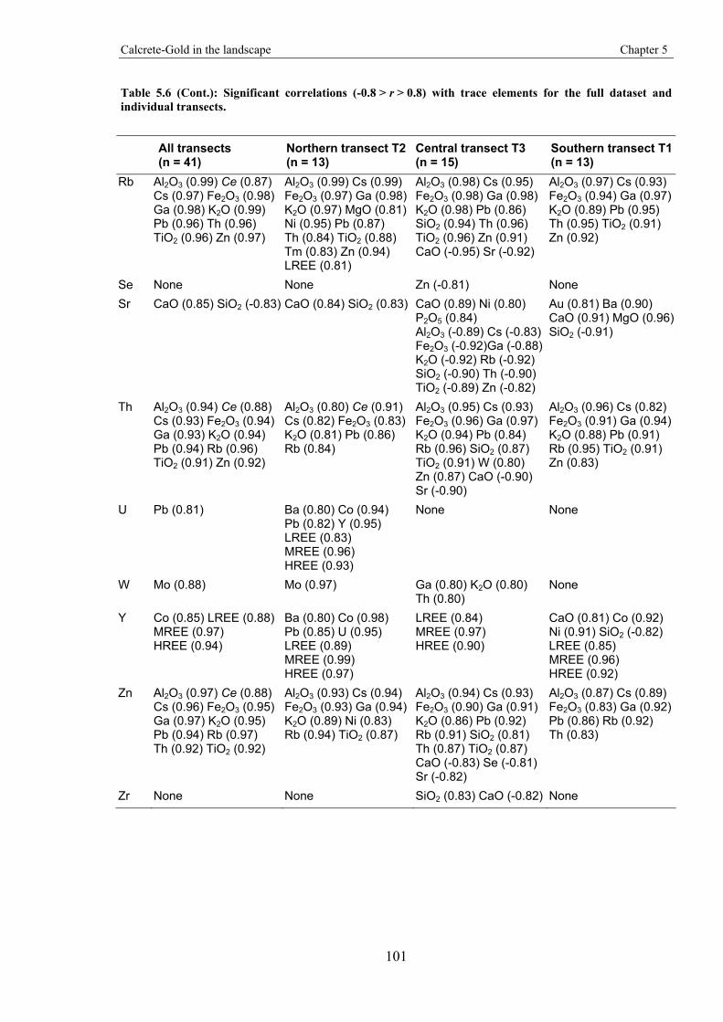
Calcrete-Gold in the landscape Chapter 5
101
Table 5.6 (Cont.): Significant correlations (-0.8 > r > 0.8) with trace elements for the full dataset and individual transects.
All transects (n = 41)
Northern transect T2 (n = 13)
Central transect T3 (n = 15)
Southern transect T1(n = 13)
Rb Al2O3 (0.99) Ce (0.87) Cs (0.97) Fe2O3 (0.98) Ga (0.98) K2O (0.99) Pb (0.96) Th (0.96) TiO2 (0.96) Zn (0.97)
Al2O3 (0.99) Cs (0.99) Fe2O3 (0.97) Ga (0.98) K2O (0.97) MgO (0.81) Ni (0.95) Pb (0.87) Th (0.84) TiO2 (0.88) Tm (0.83) Zn (0.94) LREE (0.81)
Al2O3 (0.98) Cs (0.95) Fe2O3 (0.98) Ga (0.98) K2O (0.98) Pb (0.86) SiO2 (0.94) Th (0.96) TiO2 (0.96) Zn (0.91) CaO (-0.95) Sr (-0.92)
Al2O3 (0.97) Cs (0.93) Fe2O3 (0.94) Ga (0.97) K2O (0.89) Pb (0.95) Th (0.95) TiO2 (0.91) Zn (0.92)
Se None None Zn (-0.81) None Sr CaO (0.85) SiO2 (-0.83) CaO (0.84) SiO2 (0.83) CaO (0.89) Ni (0.80)
P2O5 (0.84) Al2O3 (-0.89) Cs (-0.83) Fe2O3 (-0.92)Ga (-0.88) K2O (-0.92) Rb (-0.92) SiO2 (-0.90) Th (-0.90) TiO2 (-0.89) Zn (-0.82)
Au (0.81) Ba (0.90) CaO (0.91) MgO (0.96)SiO2 (-0.91)
Th Al2O3 (0.94) Ce (0.88) Cs (0.93) Fe2O3 (0.94) Ga (0.93) K2O (0.94) Pb (0.94) Rb (0.96) TiO2 (0.91) Zn (0.92)
Al2O3 (0.80) Ce (0.91) Cs (0.82) Fe2O3 (0.83) K2O (0.81) Pb (0.86) Rb (0.84)
Al2O3 (0.95) Cs (0.93) Fe2O3 (0.96) Ga (0.97) K2O (0.94) Pb (0.84) Rb (0.96) SiO2 (0.87) TiO2 (0.91) W (0.80) Zn (0.87) CaO (-0.90) Sr (-0.90)
Al2O3 (0.96) Cs (0.82) Fe2O3 (0.91) Ga (0.94) K2O (0.88) Pb (0.91) Rb (0.95) TiO2 (0.91) Zn (0.83)
U Pb (0.81) Ba (0.80) Co (0.94) Pb (0.82) Y (0.95) LREE (0.83) MREE (0.96) HREE (0.93)
None None
W Mo (0.88) Mo (0.97) Ga (0.80) K2O (0.80) Th (0.80)
None
Y Co (0.85) LREE (0.88) MREE (0.97) HREE (0.94)
Ba (0.80) Co (0.98) Pb (0.85) U (0.95) LREE (0.89) MREE (0.99) HREE (0.97)
LREE (0.84) MREE (0.97) HREE (0.90)
CaO (0.81) Co (0.92) Ni (0.91) SiO2 (-0.82) LREE (0.85) MREE (0.96) HREE (0.92)
Zn Al2O3 (0.97) Ce (0.88) Cs (0.96) Fe2O3 (0.95) Ga (0.97) K2O (0.95) Pb (0.94) Rb (0.97) Th (0.92) TiO2 (0.92)
Al2O3 (0.93) Cs (0.94) Fe2O3 (0.93) Ga (0.94) K2O (0.89) Ni (0.83) Rb (0.94) TiO2 (0.87)
Al2O3 (0.94) Cs (0.93) Fe2O3 (0.90) Ga (0.91) K2O (0.86) Pb (0.92) Rb (0.91) SiO2 (0.81) Th (0.87) TiO2 (0.87) CaO (-0.83) Se (-0.81) Sr (-0.82)
Al2O3 (0.87) Cs (0.89) Fe2O3 (0.83) Ga (0.92) Pb (0.86) Rb (0.92) Th (0.83)
Zr None None SiO2 (0.83) CaO (-0.82) None
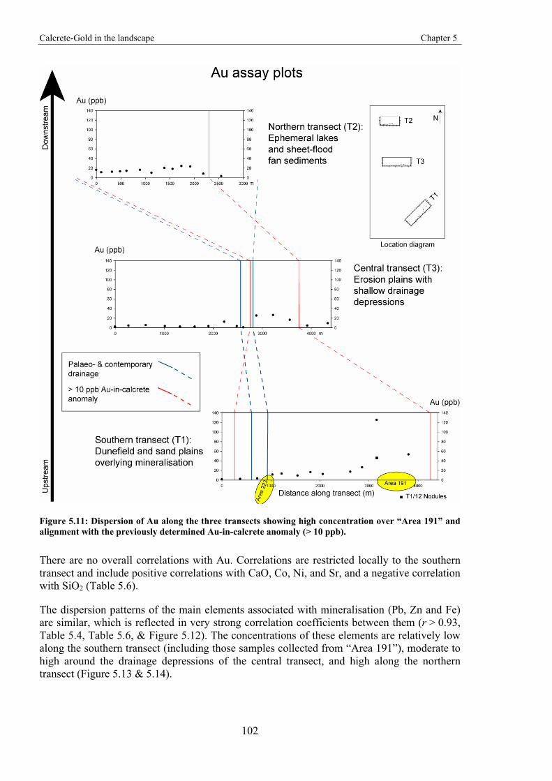
Calcrete-Gold in the landscape Chapter 5
102
Figure 5.11: Dispersion of Au along the three transects showing high concentration over “Area 191” and alignment with the previously determined Au-in-calcrete anomaly (> 10 ppb).
There are no overall correlations with Au. Correlations are restricted locally to the southern transect and include positive correlations with CaO, Co, Ni, and Sr, and a negative correlation with SiO2 (Table 5.6).
The dispersion patterns of the main elements associated with mineralisation (Pb, Zn and Fe) are similar, which is reflected in very strong correlation coefficients between them (r > 0.93, Table 5.4, Table 5.6, & Figure 5.12). The concentrations of these elements are relatively low along the southern transect (including those samples collected from “Area 191”), moderate to high around the drainage depressions of the central transect, and high along the northern transect (Figure 5.13 & 5.14).
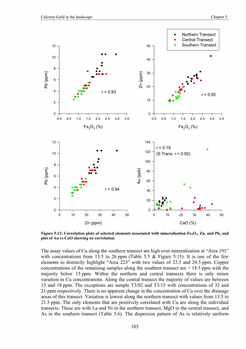
Calcrete-Gold in the landscape Chapter 5
103
Zn (ppm)
0 10 20 30 40 50
Pb
(ppm
)
0
2
4
6
8
10
12
Fe2O3 (%)
0.0 0.5 1.0 1.5 2.0 2.5 3.0 3.5
Zn (p
pm)
0
10
20
30
40
50
Fe2O3 (%)
0.0 0.5 1.0 1.5 2.0 2.5 3.0 3.5
Pb
(ppm
)
0
2
4
6
8
10
12
Northern TransectCentral TransectSouthern Transect
CaO (%)
0 10 20 30 40 50
Au
(ppb
)
0
20
40
60
80
100
120
140
r = 0.93 r = 0.95
r = 0.94
r = 0.19(S Trans. r = 0.92)
Figure 5.12: Correlation plots of selected elements associated with mineralisation Fe2O3, Zn, and Pb, and plot of Au vs CaO showing no correlation.
The assay values of Cu along the southern transect are high over mineralisation at “Area 191” with concentrations from 13.5 to 26 ppm (Table 5.5 & Figure 5.15). It is one of the few elements to distinctly highlight “Area 223” with two values of 22.5 and 24.5 ppm. Copper concentrations of the remaining samples along the southern transect are < 18.5 ppm with the majority below 15 ppm. Within the northern and central transects there is only minor variation in Cu concentrations. Along the central transect the majority of values are between 13 and 18 ppm. The exceptions are sample T3/02 and T3/15 with concentrations of 32 and 21 ppm respectively. There is no apparent change in the concentration of Cu over the drainage areas of this transect. Variation is lowest along the northern transect with values from 13.5 to 21.5 ppm. The only elements that are positively correlated with Cu are along the individual transects. These are with La and Ni in the northern transect, MgO in the central transect, and As in the southern transect (Table 5.6). The dispersion pattern of As is relatively uniform
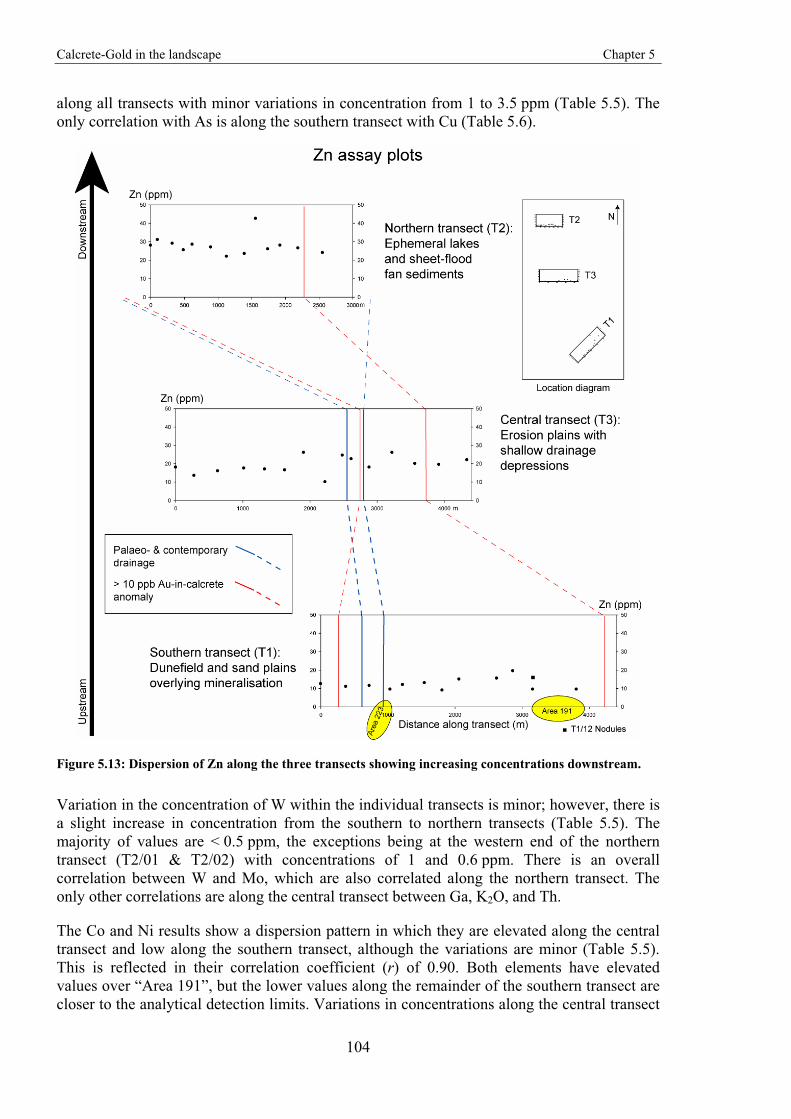
Calcrete-Gold in the landscape Chapter 5
104
along all transects with minor variations in concentration from 1 to 3.5 ppm (Table 5.5). The only correlation with As is along the southern transect with Cu (Table 5.6).
Figure 5.13: Dispersion of Zn along the three transects showing increasing concentrations downstream.
Variation in the concentration of W within the individual transects is minor; however, there is a slight increase in concentration from the southern to northern transects (Table 5.5). The majority of values are < 0.5 ppm, the exceptions being at the western end of the northern transect (T2/01 & T2/02) with concentrations of 1 and 0.6 ppm. There is an overall correlation between W and Mo, which are also correlated along the northern transect. The only other correlations are along the central transect between Ga, K2O, and Th.
The Co and Ni results show a dispersion pattern in which they are elevated along the central transect and low along the southern transect, although the variations are minor (Table 5.5). This is reflected in their correlation coefficient (r) of 0.90. Both elements have elevated values over “Area 191”, but the lower values along the remainder of the southern transect are closer to the analytical detection limits. Variations in concentrations along the central transect
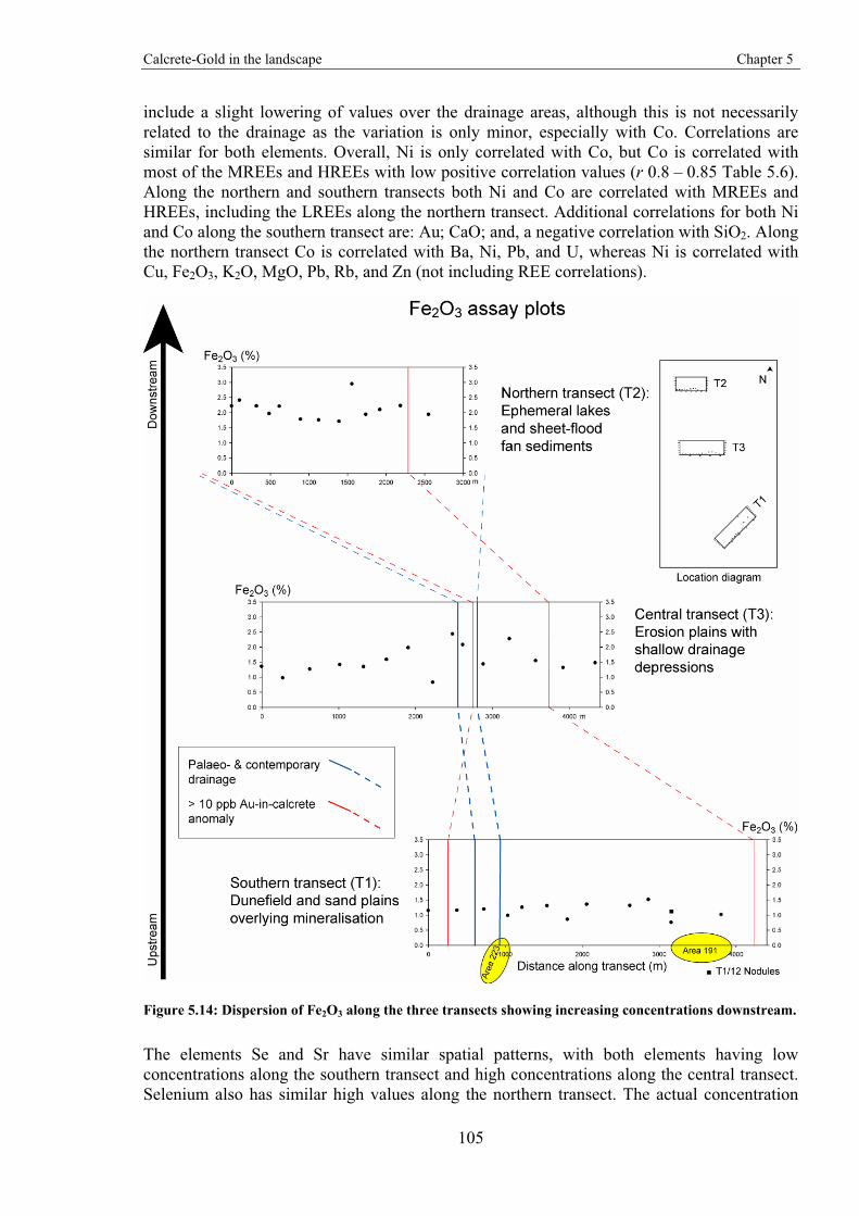
Calcrete-Gold in the landscape Chapter 5
105
include a slight lowering of values over the drainage areas, although this is not necessarily related to the drainage as the variation is only minor, especially with Co. Correlations are similar for both elements. Overall, Ni is only correlated with Co, but Co is correlated with most of the MREEs and HREEs with low positive correlation values (r 0.8 – 0.85 Table 5.6). Along the northern and southern transects both Ni and Co are correlated with MREEs and HREEs, including the LREEs along the northern transect. Additional correlations for both Ni and Co along the southern transect are: Au; CaO; and, a negative correlation with SiO2. Along the northern transect Co is correlated with Ba, Ni, Pb, and U, whereas Ni is correlated with Cu, Fe2O3, K2O, MgO, Pb, Rb, and Zn (not including REE correlations).
Figure 5.14: Dispersion of Fe2O3 along the three transects showing increasing concentrations downstream.
The elements Se and Sr have similar spatial patterns, with both elements having low concentrations along the southern transect and high concentrations along the central transect. Selenium also has similar high values along the northern transect. The actual concentration
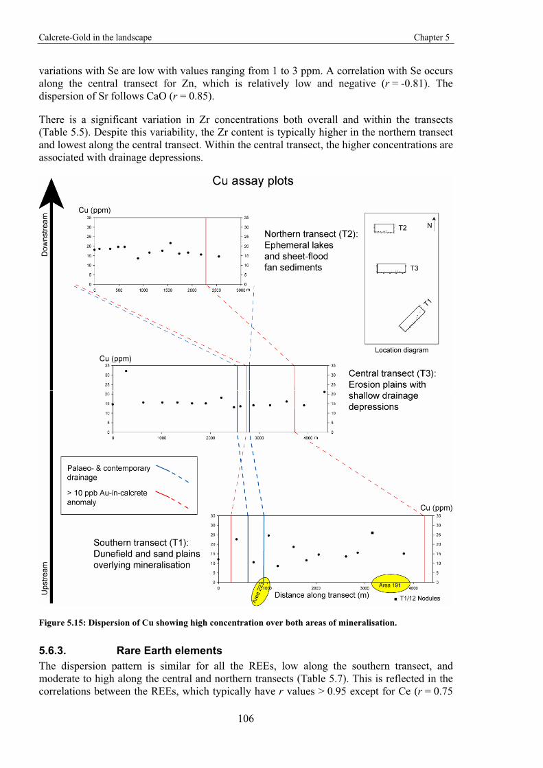
Calcrete-Gold in the landscape Chapter 5
106
variations with Se are low with values ranging from 1 to 3 ppm. A correlation with Se occurs along the central transect for Zn, which is relatively low and negative (r = -0.81). The dispersion of Sr follows CaO (r = 0.85).
There is a significant variation in Zr concentrations both overall and within the transects (Table 5.5). Despite this variability, the Zr content is typically higher in the northern transect and lowest along the central transect. Within the central transect, the higher concentrations are associated with drainage depressions.
Figure 5.15: Dispersion of Cu showing high concentration over both areas of mineralisation.
5.6.3. Rare Earth elements The dispersion pattern is similar for all the REEs, low along the southern transect, and moderate to high along the central and northern transects (Table 5.7). This is reflected in the correlations between the REEs, which typically have r values > 0.95 except for Ce (r = 0.75
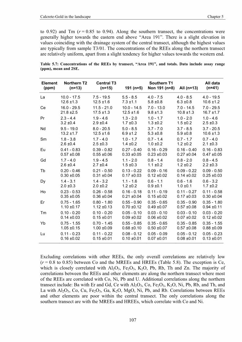
Calcrete-Gold in the landscape Chapter 5
107
to 0.92) and Tm (r = 0.85 to 0.94). Along the southern transect, the concentrations were generally higher towards the eastern end above “Area 191”. There is a slight elevation in values coinciding with the drainage system of the central transect, although the highest values are typically from sample T3/01. The concentrations of the REEs along the northern transect are relatively uniform, apart from a slight tendency for higher values towards the western end.
Table 5.7: Concentrations of the REEs by transect, “Area 191”, and totals. Data include assay range (ppm), mean and 2SE.
Northern T2 Central T3 Southern T1 Element (ppm) (n=13) (n=15) 191 (n=5) Non 191 (n=8) All (n=13)
All data (n=41)
La 10.0 - 17.5 12.6 ±1.3
7.5 - 19.5 12.5 ±1.6
5.5 - 8.5 7.3 ±1.1
4.0 - 7.5 5.8 ±0.8
4.0 - 8.5 6.3 ±0.8
4.0 - 19.5 10.6 ±1.2
Ce 16.0 - 29.5 21.8 ±2.5
11.5 - 21.0 17.5 ±1.3
10.0 - 14.5 12.5 ±1.6
7.0 - 13.0 9.8 ±1.3
7.0 - 14.5 10.8 ±1.3
7.0 - 29.5 16.7 ±1.7
Pr 2.3 - 4.4 3.2 ±0.4
1.9 - 4.6 2.9 ±0.4
1.3 - 2.0 1.7 ±0.3
1.0 - 1.7 1.3 ±0.2
1.0 - 2.0 1.5 ±0.2
1.0 - 4.6 2.5 ±0.3
Nd 9.5 - 19.0 13.2 ±1.7
8.0 - 20.5 12.5 ±1.6
5.0 - 8.5 6.9 ±1.2
3.7 - 7.0 5.3 ±0.8
3.7 - 8.5 5.9 ±0.8
3.7 - 20.5 10.6 ±1.3
Sm 1.8 - 3.8 2.6 ±0.4
1.7 - 4.0 2.5 ±0.3
1.0 - 1.7 1.4 ±0.2
0.7 - 1.4 1.0 ±0.2
0.7 - 1.7 1.2 ±0.2
0.7 - 4.0 2.1 ±0.3
Eu 0.41 - 0.83 0.57 ±0.08
0.39 - 0.82 0.55 ±0.06
0.27 - 0.40 0.33 ±0.05
0.16 - 0.29 0.23 ±0.03
0.16 - 0.40 0.27 ±0.04
0.16 - 0.830.47 ±0.05
Gd 1.7 - 4.0 2.6 ±0.4
1.9 - 4.5 2.7 ±0.4
1.1 - 2.0 1.5 ±0.3
0.8 - 1.4 1.1 ±0.2
0.8 - 2.0 1.2 ±0.2
0.8 - 4.5 2.2 ±0.3
Tb 0.20 - 0.46 0.30 ±0.05
0.21 - 0.50 0.31 ±0.04
0.13 - 0.22 0.17 ±0.03
0.09 - 0.16 0.12 ±0.02
0.09 - 0.22 0.14 ±0.02
0.09 - 0.500.25 ±0.03
Dy 1.4 - 3.1 2.0 ±0.3
1.4 - 3.2 2.0 ±0.2
1.1 - 1.6 1.2 ±0.2
0.6 - 1.1 0.9 ±0.1
0.6 - 1.6 1.0 ±0.1
0.6 - 3.2 1.7 ±0.2
Ho 0.23 - 0.53 0.35 ±0.05
0.26 - 0.58 0.36 ±0.04
0.16 - 0.18 0.21 ±0.04
0.11 - 0.19 0.15 ±0.02
0.11 - 0.27 0.17 ±0.03
0.11 - 0.580.30 ±0.04
Er 0.75 - 1.65 1.10 ±0.17
0.80 - 1.80 1.12 ±0.13
0.55 - 0.90 0.70 ±0.12
0.35 - 0.65 0.49 ±0.07
0.35 - 0.90 0.57 ±0.08
0.35 - 1.800.94 ±0.11
Tm 0.10 - 0.20 0.14 ±0.03
0.10 - 0.20 0.15 ±0.01
0.05 - 0.10 0.09 ±0.02
0.03 - 0.10 0.06 ±0.02
0.03 - 0.10 0.07 ±0.02
0.03 - 0.200.12 ±0.02
Yb 0.75 - 1.55 1.05 ±0.15
0.70 - 1.45 1.00 ±0.09
0.55 - 0.85 0.68 ±0.10
0.35 - 0.65 0.50 ±0.07
0.35 - 0.85 0.57 ±0.08
0.35 - 1.550.88 ±0.09
Lu 0.11 - 0.23 0.16 ±0.02
0.11 - 0.22 0.15 ±0.01
0.08 - 0.12 0.10 ±0.01
0.05 - 0.09 0.07 ±0.01
0.05 - 0.12 0.08 ±0.01
0.05 - 0.230.13 ±0.01
Excluding correlations with other REEs, the only overall correlations are relatively low (r = 0.8 to 0.85) between Co and the MREEs and HREEs (Table 5.8). The exception is Ce, which is closely correlated with Al2O3, Fe2O3, K2O, Pb, Rb, Th and Zn. The majority of correlations between the REEs and other elements are along the northern transect where most of the REEs are correlated with Co, Ni, Pb and U. Additional correlations along the northern transect include: Ba with Er and Gd, Ce with Al2O3, Co, Fe2O3, K2O, Ni, Pb, Rb, and Th, and La with Al2O3, Co, Cu, Fe2O3, Ga, K2O, MgO, Ni, Pb, and Rb. Correlations between REEs and other elements are poor within the central transect. The only correlations along the southern transect are with the MREEs and HREEs, which correlate with Co and Ni.
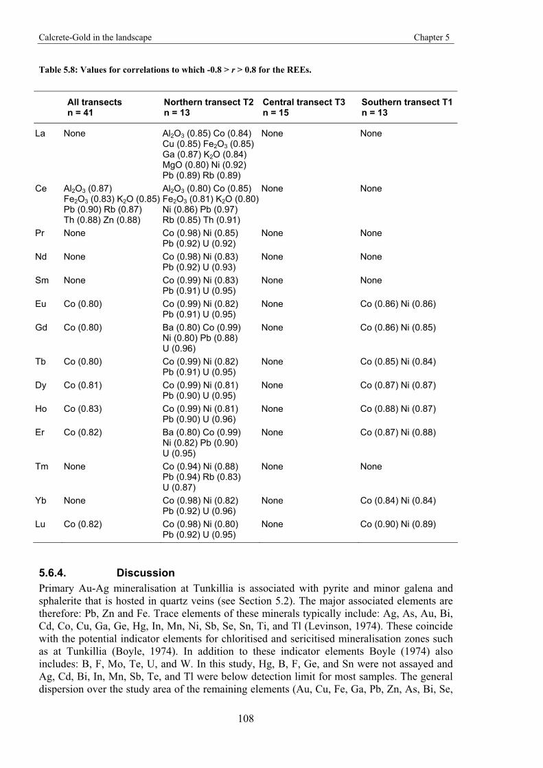
Calcrete-Gold in the landscape Chapter 5
108
Table 5.8: Values for correlations to which -0.8 > r > 0.8 for the REEs.
All transects n = 41
Northern transect T2 n = 13
Central transect T3 n = 15
Southern transect T1n = 13
La None Al2O3 (0.85) Co (0.84) Cu (0.85) Fe2O3 (0.85) Ga (0.87) K2O (0.84) MgO (0.80) Ni (0.92) Pb (0.89) Rb (0.89)
None None
Ce Al2O3 (0.87) Fe2O3 (0.83) K2O (0.85)Pb (0.90) Rb (0.87) Th (0.88) Zn (0.88)
Al2O3 (0.80) Co (0.85) Fe2O3 (0.81) K2O (0.80)Ni (0.86) Pb (0.97) Rb (0.85) Th (0.91)
None None
Pr None Co (0.98) Ni (0.85) Pb (0.92) U (0.92)
None None
Nd None Co (0.98) Ni (0.83) Pb (0.92) U (0.93)
None None
Sm None Co (0.99) Ni (0.83) Pb (0.91) U (0.95)
None None
Eu Co (0.80) Co (0.99) Ni (0.82) Pb (0.91) U (0.95)
None Co (0.86) Ni (0.86)
Gd Co (0.80) Ba (0.80) Co (0.99) Ni (0.80) Pb (0.88) U (0.96)
None Co (0.86) Ni (0.85)
Tb Co (0.80) Co (0.99) Ni (0.82) Pb (0.91) U (0.95)
None Co (0.85) Ni (0.84)
Dy Co (0.81) Co (0.99) Ni (0.81) Pb (0.90) U (0.95)
None Co (0.87) Ni (0.87)
Ho Co (0.83) Co (0.99) Ni (0.81) Pb (0.90) U (0.96)
None Co (0.88) Ni (0.87)
Er Co (0.82) Ba (0.80) Co (0.99) Ni (0.82) Pb (0.90) U (0.95)
None Co (0.87) Ni (0.88)
Tm None Co (0.94) Ni (0.88) Pb (0.94) Rb (0.83) U (0.87)
None None
Yb None Co (0.98) Ni (0.82) Pb (0.92) U (0.96)
None Co (0.84) Ni (0.84)
Lu Co (0.82) Co (0.98) Ni (0.80) Pb (0.92) U (0.95)
None Co (0.90) Ni (0.89)
5.6.4. Discussion Primary Au-Ag mineralisation at Tunkillia is associated with pyrite and minor galena and sphalerite that is hosted in quartz veins (see Section 5.2). The major associated elements are therefore: Pb, Zn and Fe. Trace elements of these minerals typically include: Ag, As, Au, Bi, Cd, Co, Cu, Ga, Ge, Hg, In, Mn, Ni, Sb, Se, Sn, Ti, and Tl (Levinson, 1974). These coincide with the potential indicator elements for chloritised and sericitised mineralisation zones such as at Tunkillia (Boyle, 1974). In addition to these indicator elements Boyle (1974) also includes: B, F, Mo, Te, U, and W. In this study, Hg, B, F, Ge, and Sn were not assayed and Ag, Cd, Bi, In, Mn, Sb, Te, and Tl were below detection limit for most samples. The general dispersion over the study area of the remaining elements (Au, Cu, Fe, Ga, Pb, Zn, As, Bi, Se,
Calcrete-Gold in the landscape Chapter 5
109
Mo, Ti, W, Co, Ni, and U) is presented above. In this section these elements are discussed in relation to mineralisation, landscape controls and mineral associations.
The best indication of mineralisation at Tunkillia is from the samples collected over “Area 191”, particularly with the Au, Ag, and Cu assays. Indication of mineralisation in samples collected over “Area 223” is not as distinct with only Cu and Ag displaying any significant concentrations.
Silver was below analytical detection limit for most of the samples, however, it was detected (at or near detection limit) in samples collected from “Area 191” (T1/09, T1/12 calcrete, T1/13 and T1/14), although samples T1/13 and T1/14 were not classed as regolith carbonates. The only other samples to contain Ag were from the northern transect, all of which were equal to the analytical detection limit of 0.1 ppm. The lack of Ag in the regolith carbonate samples and the secondary mineralised oxide zone is consistent with preferential leaching of Ag from the primary mineralisation.
The Cu abundance is relatively high over mineralisation at “Area 191” and “Area 223”. The highest Cu assay (32 ppm) was from the western end of the central transect (T3/02). The significance of this sample is unclear and appears unrelated to the identified mineralisation. Since Cu is not listed as a major component of mineralisation, the high values suggest that it is has been concentrated within the local environment, particularly over mineralisation, and is therefore relatively immobile. This is supported by the relatively uniform distribution of Cu along the central and northern transects with no apparent variations over the drainage system (Figure 5.15).
Along the southern transect there is a correlation between Cu and As (r = 0.82). The As analyses however, are similar along all transects. A slight elevation in As results above mineralisation is not significant, with similar values occurring along the other transects. The highest As value (5 ppm) was obtained for sample T1/14, which is ferruginous silcrete.
The best indicator of Au mineralisation at “Area 191” appears to be Au with assays of 46, 53 and 125 ppb (Figure 5.11). This is not repeated for samples over “Area 223”, where Au assays are similar to those along the other transects. Possible reasons for the variation in surficial expression of Au and other elements over the two mineralisation areas are discussed further in the next section.
The above elements are the only ones of those analysed to show significant variation over mineralisation. The limited elemental signatures over mineralisation reflect the dispersion of the majority of elements northwards towards the ephemeral lakes via the palaeo- and contemporary drainage systems. This includes the dispersion pattern of the main elements associated with mineralisation (Pb, Zn & Fe), which display no apparent relationship with the mineralised areas. This suggests that these elements are mobile within this environment. It is likely that Pb, which is considered relatively immobile, and Zn, are incorporated within or bound to clay minerals during weathering (Kabata-Pendias & Pendias, 2001). Although Fe can occur in clays, in the regolith it is more prevalent in oxides or hydroxides.
The high sorption properties of clays and Al / Fe-oxides or hydroxides are a major control on the dispersion and residence of many trace elements (Kabata-Pendias & Pendias, 2001). The stability and mobility of these minerals is therefore a strong influence on the dispersion pattern of these elements. This is reflected in the number of elements that are highly
Calcrete-Gold in the landscape Chapter 5
110
correlated with Al2O3 and Fe2O3 (Table 5.4) that are also concentrated in areas with higher clay content.
High correlations between Al2O3, Fe2O3, and K2O (Figure 5.9) suggest that they are present in a single mineral phase, such as an alunite-jarosite mineral or a glauconitic mica. Detailed mineralogy was not undertaken on the Tunkillia samples and precise identification of a single mineral is not possible. Alunite and jarosite are common in acidic environments, especially in acid sulphate soils, their presence around Tunkillia is therefore unlikely (Allen & Hajek, 1989).
The mobility of the clays may also be controlling the dispersion of the REEs at Tunkillia. Within the regolith the REEs are likely to be concentrated within P minerals such as apatite and monazite, and clays (Kabata-Pendias & Pendias, 2001). Overall REE correlations with P2O5 are between 0.2 and 0.5, which are lower than the equivalent correlations with Al2O3 that are between 0.6 and 0.9. This supports an association between the REEs and clay rather than the P minerals, but variations between the transects are not in total support of this. Along the southern transect REE and P2O5 correlations are higher (r = 0.4 to 0.7) and the equivalent REE and Al2O3 are lower (r = 0.2 to 0.6). The reverse is observed along the northern transect with REE and P2O5 correlations between 0.2 and 0.4, and REE and Al2O3 correlations between 0.6 and 0.8. Correlations are low for both P2O5 (r = -0.4 to 0) and Al2O3 (r = 0.1 to 0.4 apart for Ce, 0.6) along the central transect. The REE correlations with Fe2O3 are similar to Al2O3 over all three transects except that the r values are slightly lower for Fe2O3 by about 0.05 (0.15 along the southern transect). This reflects the high correlations between Fe2O3 and Al2O3 (Table 5.4).
Variation of the REE abundances across the landscape is demonstrated between the transects. Chondrite and post Archaean Australian shales (PAAS) normalised REE plots are shown in Figure 5.16 (Taylor & McLennan, 1985; McLennan, 1989). These plots show higher REE concentrations along the central and northern transects, which is most likely due to accumulation of host minerals in depositional areas. There is also variation of the REEs along the northern transect with the western samples (T2/01 to T2/05) and T2/09 enriched over other samples from this transect. These enriched samples also have higher Fe and Al concentration (Figure 5.14).
The REE variation and correlations suggest that in the south the REEs are largely present within P minerals, whereas in the north they have been released from these minerals and are now associated with the clays and Al / Fe-oxides. The spatial distribution of the REEs supports this and also suggests that they are also accumulating in the north. A controlling factor in the adsorption of REEs to clay and Fe-oxide minerals is the pH. In acidic conditions the REEs become soluble and are transported in solution, whereas in normal to alkaline conditions they are adsorbed to clay minerals (Roaldset, 1973; Cullers et al., 1979).
The correlations between Co, Ni and REEs suggest a possible association with clay minerals. Both Co and Ni are considered indicator elements for Au mineralisation and are typically associated with As and S minerals. In the regolith both Co and Ni tend to be associated with clays and Fe or Mn oxides (Kabata-Pendias & Pendias, 2001). Along the southern transect there is a correlation between Au and both Ni and Co, which may be related to mineralisation, however, Co and Ni are also correlated with the MREEs and HREEs along this transect (Table 5.6). Given that MnO is at or below detection for most samples and also that there is a negative correlation with SiO2 for Au, Co and Ni, then the association is more likely to be with the clay or Fe-oxides, since a higher SiO2 content suggests a lower clay content. The
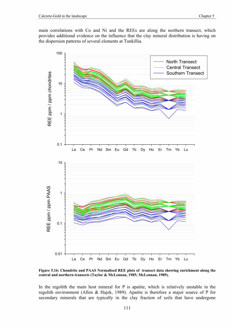
Calcrete-Gold in the landscape Chapter 5
111
main correlations with Co and Ni and the REEs are along the northern transect, which provides additional evidence on the influence that the clay mineral distribution is having on the dispersion patterns of several elements at Tunkillia.
La Ce Pr Nd Sm Eu Gd Tb Dy Ho Er Tm Yb Lu
RE
E p
pm /
ppm
cho
ndrit
es
0.1
1
10
100
North TransectCentral TransectSouthern Transect
La Ce Pr Nd Sm Eu Gd Tb Dy Ho Er Tm Yb Lu
RE
E p
pm /
ppm
PA
AS
0.01
0.1
1
10
Figure 5.16: Chondrite and PAAS Normalised REE plots of transect data showing enrichment along the central and northern transects (Taylor & McLennan, 1985; McLennan, 1989).
In the regolith the main host mineral for P is apatite, which is relatively unstable in the regolith environment (Allen & Hajek, 1989). Apatite is therefore a major source of P for secondary minerals that are typically in the clay fraction of soils that have undergone
Calcrete-Gold in the landscape Chapter 5
112
extensive weathering (Banfield & Eggleton, 1989; Lindsay et al., 1989). Apatite also contains Ca, which may account for the correlation between CaO and P2O5 along the southern and central transects (Table 5.4). In the northern area, the breakdown of apatite releases P into the environment where it is taken up in secondary minerals such as apatite, plumbogummite group and clays (Norrish & Rosser, 1983). Therefore, P no longer has any correlation with CaO (r = -0.3) in the northern area. The low and relatively uniform concentrations of P2O5 (Table 5.3) however, may not be suitable for rigorous correlation interpretation. The analytical detection limit for P2O5 was 0.01% which is equal, or very close, to concentrations in many of the samples.
Previously suggested correlations between Au and Ca through regolith profiles (Lintern, 1989; Lintern & Butt, 1993; Lintern, 1997; Lintern & Butt, 1998b; Smee, 1998; Lintern & Sheard, 1999b; Okujeni et al., 2005; Lintern et al., 2006) are not repeated over the landscape (Figure 5.12), although there is a high correlation between Au and Ca (r = 0.92) along the southern transect.
Besides calcite, regolith carbonates may also be composed of dolomite and Mg-rich calcite and therefore correlation between CaO and MgO may be expected. The distribution of MgO and lack of correlation with CaO, apart from along the southern transect, suggests that if dolomite is present it is not associated with calcite. It is possible that the MgO is hosted within clay minerals rather than dolomite, in which case correlation with Al2O3 may be expected. The only correlation between MgO and Al2O3 however, is along the northern transect. This suggests that MgO is present as both dolomite and clay minerals overall. The low correlations between MgO with CaO (r = 0.82) along the southern transect and Al2O3 (r = 0.82) along the northern transect supports a higher concentration of Mg in dolomite along the southern transect and a higher concentration of Mg in clay along the northern transect.
Gypsum is another source of CaO and if mixed with calcite in high enough concentrations, may alter correlations between CaO and other elements that may exist when the CaO is only from calcite. Gypsum is present around playa lakes in the Central Gawler Craton (Ferris & Fairclough, 2007), but it was not observed while collecting or analysing the regolith carbonate samples from Tunkillia. It is therefore unlikely that gypsum has impacted this study.
The high SiO2 concentrations along the western end of the southern transect are from samples from swales between the “Phase I” and “Phase II” dunes. These high SiO2 concentrations correspond with low assay values for the majority of elements, suggesting that the main component in these samples is clean quartz sand that has possibly been transported from the dunes. Similar high SiO2 concentrations along the northern transect do not correspond with low values in other elements, suggesting that quartz is a minor component and other silicate minerals dominate in this area.
The element dispersion patterns in the Tunkillia area suggest weathering and transportation of material toward the north, particularly along the palaeo- and contemporary drainage. Element dispersion in this area is therefore largely controlled by the landscape.
5.7. Synthesis: Landscape controls on geochemistry The surficial geochemistry for Tunkillia and the surrounding area reflects three main interrelated landscape components:
1. the contemporary landscape; 2. palaeo-landscape; and, 3. the proximity to mineralisation.
Calcrete-Gold in the landscape Chapter 5
113
Variations between components 1 and 2 are reflected in the variations of component 3.
5.7.1. Contemporary landscape The contemporary landscape expresses an extensive history. The dominant contemporary processes are related to the current arid to semi-arid climate and the area’s low relief. The currently active landscape processes include: dune migration over the southern area; ephemeral transport of surface sediments towards the north by colluvial sheetflow and alluvial drainage channels; and, deposition of sediments in ephemeral lakes and alluvial fans towards the north.
Rainfall in arid to semi-arid environments is generally of low frequency and high intensity, with rainfall events typically exceeding the infiltration capacity of the soil, resulting in downslope sediment transport by shallow overland flow (Baird, 1997). Sediments, including surface lag, are transported towards drainage depressions and accumulate in areas of lower energy, such as flood plains, alluvial fans, and lakes. The large erosional plains with scattered surface lag are the result of multiple sheetflow events. The low relief landscape results in the dispersion of alluvial pathways over the surface and within shallow depressions, which have an anastomosing and braided style. The contemporary drainage lies mostly along the western edge of the Au-in-calcrete anomaly through the central area. This slight misalignment of contemporary drainage and Au-in-calcrete anomaly is the result of slight drainage channel migration in the area.
Sand dunes of the Great Victoria Desert are migrating eastwards over much of the southern area and burying erosional plains. Drainage pathways are blocked by the aeolian sand restricting the movement of further alluvial sediments. These typically low-lying areas are mapped as alluvial plains, and because of containment by the dunes, often extend laterally along the swales as shown in Figure 5.4 (Aap2). The relatively recent dune systems, which extend over mineralisation, are therefore modifying the dispersion pathways of elements sourced from the mineralisation area by blocking drainage pathways.
5.7.2. Palaeo-landscape The palaeo-landscape at Tunkillia is partially masked by dune fields, which complicates the contemporary expression of alluvial dispersion in the area. Prior to dune development the landscape here consisted of a series of drainage depressions that flowed northwards from the exposed, east-west drainage divide at the southern margin of the study area. These palaeo-drainage depressions merge with the contemporary drainage system to the north and east beyond the dune-field.
The extent and age of the drainage system are important in determining the dispersion patterns of elements associated with mineralisation. On a regional scale, palaeo-drainage systems possibly initiated during the Cretaceous, have been present throughout the Cenozoic (Hou et al., 2008). At Tunkillia, palaeo-channels identified in an airborne electromagnetic (EM) survey closely follow contemporary drainage pathways (Lane & Worrall, 2002). These two points support a long term (> 65 Ma) existence and relative stability of the drainage system in the study area. The source area of this drainage was located over mineralisation (Figure 5.18) and provides both a physical and chemical dispersion conduit for mineralisation-related elements.
The drainage map produced here (Figure 5.18) was derived from descriptions recorded on the regolith-landform (Figure 5.4) and topographic (Figure 5.3) maps. The map highlights the source and depositional areas of the palaeo- and contemporary drainage systems with the
Calcrete-Gold in the landscape Chapter 5
114
extent of the overlying dune-field. The map illustrates how the “Tunkillia Central” drainage previously extended across “Area 223” and closely follows the Au-in-calcrete anomaly to the north. “Area 191” however, appears to be at the head of the “Tunkillia East” drainage, which does not carry significantly elevated Au-in-calcrete results. The topographic map (Figure 5.3) shows that although “Area 191” appears to be at the head of the “Tunkillia East” drainage, a slight saddle in the minor north-south interfluve ridge could redirect palaeo-flow towards the “Tunkillia Central” drainage, and therefore contribute to the main Au-in-calcrete anomaly to the north.
5.7.3. Proximity to mineralisation The use of surficial samples in mineral exploration is based on the premise that weathering and leaching of the buried mineralisation disperses anomalous concentrations of elements into the regolith, which forms “dispersion halos” around primary mineralisation (Levinson, 1974). This scenario at Tunkillia is complicated by the extensively leached 40 – 50 m thick saprolith, irregular distribution of variably indurated regolith, and the overlying exotic dune sands. Furthermore, the dispersion patterns of most elements reported in this chapter tend to be constrained along drainage pathways and concentrated within the depocentres corresponding with the ephemeral lake system to the north. This suggests that the source of these elements is no longer a major contributor to the surficial environment, including regolith carbonates at this time, and the remaining signature elements are mostly physically dispersed downslope through alluvial and colluvial processes.
Despite the majority of elements assayed from the regolith carbonates having relatively low concentrations directly above mineralisation, Au-in-calcrete concentrations at “Area 191” are relatively high. This surficial expression is the result of Au sourced from any one or combination of the following three possibilities: 1) relict material from a period when mineralisation was close to, or exposed at the surface; 2) upward transport from mineralisation beneath the regolith profile; or, 3) an unidentified nearby mineralisation area (Figure 5.17).
The implication of option 1 is that, prior to burial and weathering, mineralisation was at or near the land surface. Weathering of this material released Au and associated elements into the regolith. Continual reworking of these materials during the erosion of the profile resulted in Au becoming entrained in the surficial environment. The Au may have been recycled many times since its initial release, through chemical, physical and biological processes. The precipitation of regolith carbonates during the Neogene created the latest material to host the Au in the contemporary environment.
Option 2 requires transportation of Au through 40 – 50 m of highly leached clays. This may occur via hydrological processes or through plant root systems. Within the vadose zone (unsaturated zone) movement of water is typically downward or lateral as surface water percolates through the regolith. Dissolution or precipitation of minerals along with the migration of elements as soluble species or colloids can occur within the phreatic zone (groundwater). This is generally a lateral movement, with lesser vertical movement of elements towards the surface. Vertical movement may occur by a range of processes with capillary action favoured in many parts of South Australia (Keeling, 2004). Theoretical rises in excess of 37 m are possible for clays of < 2 μm diameter (Keeling, 2004). Furthermore, in arid environments, several plant species are known to have root systems that penetrate depths > 40 m in their search for water and nutrients (Dunn, 1995a; Canadell et al., 1996; Reid et al., 2008). As the plants uptake nutrients they may also passively take in elements such as Au, which are later deposited onto the surface in leaf litter or decaying material when the plant
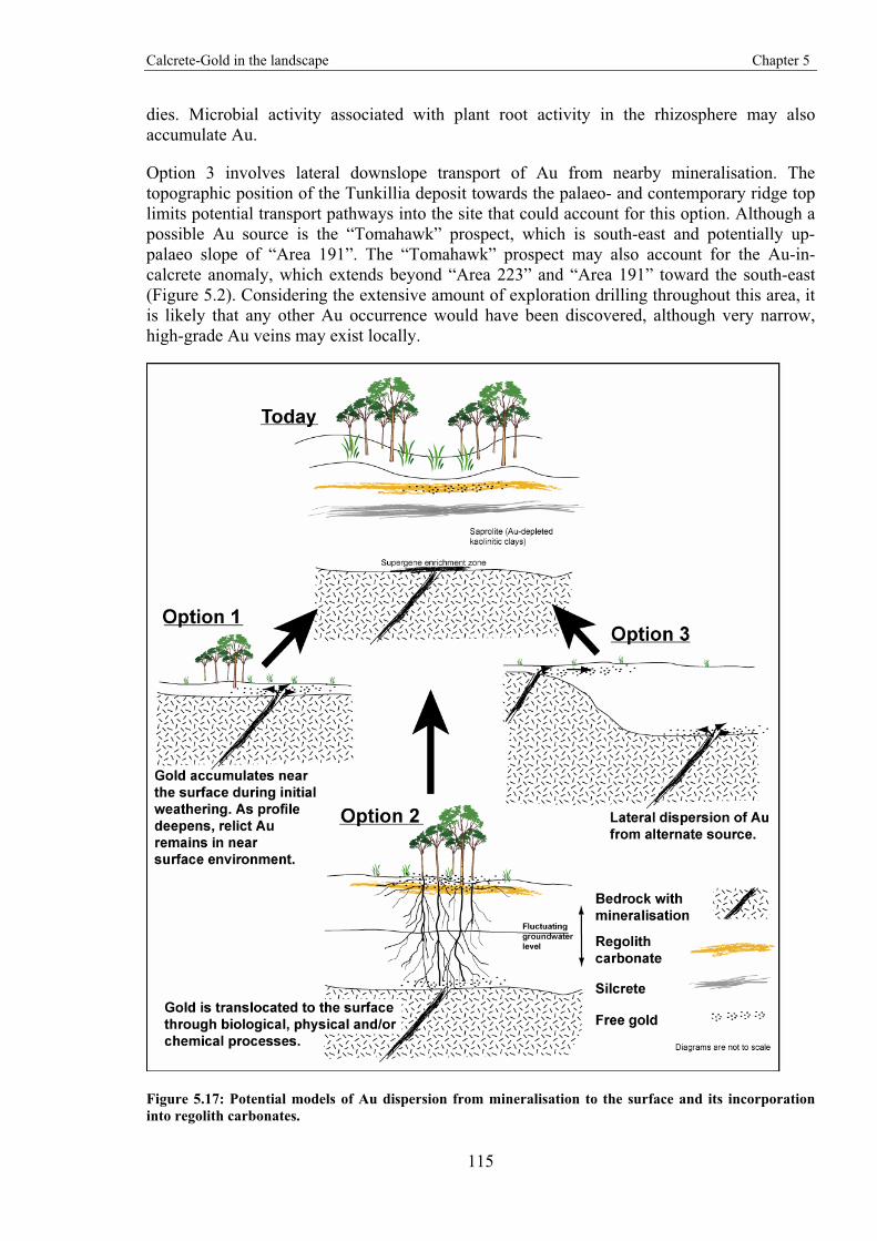
Calcrete-Gold in the landscape Chapter 5
115
dies. Microbial activity associated with plant root activity in the rhizosphere may also accumulate Au.
Option 3 involves lateral downslope transport of Au from nearby mineralisation. The topographic position of the Tunkillia deposit towards the palaeo- and contemporary ridge top limits potential transport pathways into the site that could account for this option. Although a possible Au source is the “Tomahawk” prospect, which is south-east and potentially up-palaeo slope of “Area 191”. The “Tomahawk” prospect may also account for the Au-in-calcrete anomaly, which extends beyond “Area 223” and “Area 191” toward the south-east (Figure 5.2). Considering the extensive amount of exploration drilling throughout this area, it is likely that any other Au occurrence would have been discovered, although very narrow, high-grade Au veins may exist locally.
Figure 5.17: Potential models of Au dispersion from mineralisation to the surface and its incorporation into regolith carbonates.
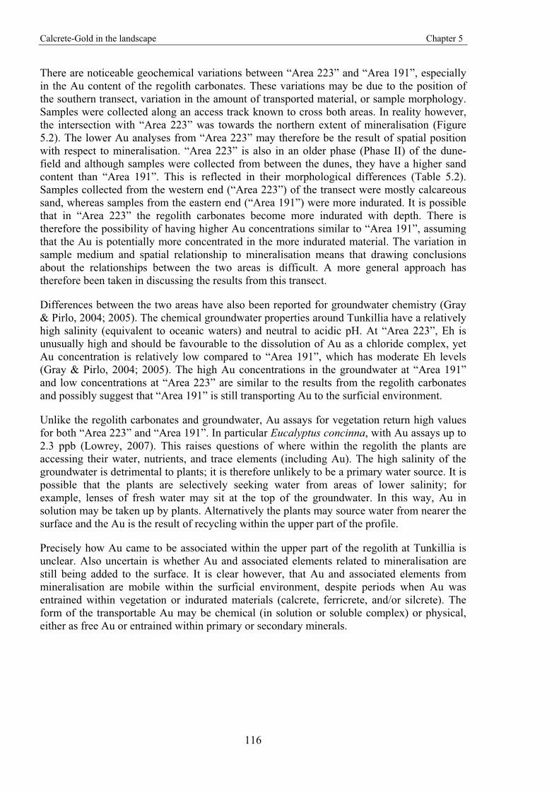
Calcrete-Gold in the landscape Chapter 5
116
There are noticeable geochemical variations between “Area 223” and “Area 191”, especially in the Au content of the regolith carbonates. These variations may be due to the position of the southern transect, variation in the amount of transported material, or sample morphology. Samples were collected along an access track known to cross both areas. In reality however, the intersection with “Area 223” was towards the northern extent of mineralisation (Figure 5.2). The lower Au analyses from “Area 223” may therefore be the result of spatial position with respect to mineralisation. “Area 223” is also in an older phase (Phase II) of the dune-field and although samples were collected from between the dunes, they have a higher sand content than “Area 191”. This is reflected in their morphological differences (Table 5.2). Samples collected from the western end (“Area 223”) of the transect were mostly calcareous sand, whereas samples from the eastern end (“Area 191”) were more indurated. It is possible that in “Area 223” the regolith carbonates become more indurated with depth. There is therefore the possibility of having higher Au concentrations similar to “Area 191”, assuming that the Au is potentially more concentrated in the more indurated material. The variation in sample medium and spatial relationship to mineralisation means that drawing conclusions about the relationships between the two areas is difficult. A more general approach has therefore been taken in discussing the results from this transect.
Differences between the two areas have also been reported for groundwater chemistry (Gray & Pirlo, 2004; 2005). The chemical groundwater properties around Tunkillia have a relatively high salinity (equivalent to oceanic waters) and neutral to acidic pH. At “Area 223”, Eh is unusually high and should be favourable to the dissolution of Au as a chloride complex, yet Au concentration is relatively low compared to “Area 191”, which has moderate Eh levels (Gray & Pirlo, 2004; 2005). The high Au concentrations in the groundwater at “Area 191” and low concentrations at “Area 223” are similar to the results from the regolith carbonates and possibly suggest that “Area 191” is still transporting Au to the surficial environment.
Unlike the regolith carbonates and groundwater, Au assays for vegetation return high values for both “Area 223” and “Area 191”. In particular Eucalyptus concinna, with Au assays up to 2.3 ppb (Lowrey, 2007). This raises questions of where within the regolith the plants are accessing their water, nutrients, and trace elements (including Au). The high salinity of the groundwater is detrimental to plants; it is therefore unlikely to be a primary water source. It is possible that the plants are selectively seeking water from areas of lower salinity; for example, lenses of fresh water may sit at the top of the groundwater. In this way, Au in solution may be taken up by plants. Alternatively the plants may source water from nearer the surface and the Au is the result of recycling within the upper part of the profile.
Precisely how Au came to be associated within the upper part of the regolith at Tunkillia is unclear. Also uncertain is whether Au and associated elements related to mineralisation are still being added to the surface. It is clear however, that Au and associated elements from mineralisation are mobile within the surficial environment, despite periods when Au was entrained within vegetation or indurated materials (calcrete, ferricrete, and/or silcrete). The form of the transportable Au may be chemical (in solution or soluble complex) or physical, either as free Au or entrained within primary or secondary minerals.
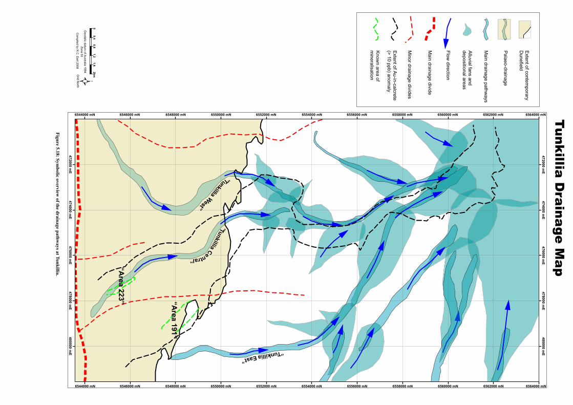
472000 mE
472000 mE
474000 mE
474000 mE
476000 mE
476000 mE
478000 mE
478000 mE
480000 mE
480000 mE
6544000 mN
6544000 mN
6546000 mN
6546000 mN
6548000 mN
6548000 mN
6550000 mN
6550000 mN
6552000 mN
6552000 mN
6554000 mN
6554000 mN
6556000 mN
6556000 mN
6558000 mN
6558000 mN
6560000 mN
6560000 mN
6562000 mN
6562000 mN
6564000 mN
6564000 mN
Tunkillia Drainage M
ap
Extent of contem
porary D
unefield
Main drainage pathw
ays
Alluvial fans and
depositional areas
Main drainage divide
Minor drainage divides
Flow direction
“Tunkillia Central”
“Tunkillia West”
“Tunkillia East”
“Area 223” “A
rea 191”
Extent of A
u-in-calcrete(> 10 ppb) anom
aly
Know
n area ofm
ineralisation
Palaeo-drainage
02km
0.40.8
1.21.6
Grid N
orth
Geodatic datum
of Australia 1994
Zone 53C
ompiled by R
.C. D
art 2008
Figure 5.18: Symbolic overview
of the drainage pathways at Tunkillia.
Calcrete-Gold in the landscape Chapter 5
119
If the southern transect is considered without the assay results from the northern transects, several elements appear to be higher over “Area 191”, including MgO, As, Au, Ba, Co, Cs, Ni, U, and the REEs, (Table 5.3, Table 5.5, and Table 5.7). This highlights a potential problem when using limited datasets, because these apparent highs are equal to or less than many of the assays obtained along the northern transects. The values appear anomalously low along the western end of the southern transect. Care must therefore be taken when investigating data from a single transect and extrapolating trends and interpretations regionally.
5.8. Conclusion For the majority of assayed elements, the highest elemental abundances occur in the northern depositional areas. This includes elements traditionally considered indicators or pathfinders for Au mineralisation and also elements typically thought of as immobile. These elements now appear to be associated with the silt and clay fractions. The contemporary dispersion patterns of these elements are the result of long-term chemical and physical breakdown of primary minerals. Physical, chemical, and biological breakdown of rocks and minerals has released components for transportation through surface processes and/or groundwater flow. During these processes, elements have been released and taken up in new forms, including vegetation and new minerals, to be released and recycled again at a later time. These ongoing cycles have resulted in the removal of many elements from the regolith profiles above mineralisation, as well as transport northwards to settle along drainage depressions and in the lakes.
Regolith-landform mapping provides a framework that helps account for many features of the geochemical signatures in regolith carbonate samples, especially with respect to the extent and spatial pattern of the Au-in-calcrete anomaly. The identification and mapping of palaeochannels within the dune swales linked the contemporary drainage pathways with mineralisation areas. In so doing, a means of Au dispersion from mineralised zones to contemporary drainage was revealed, and with it an explanation of the spatially large Au-in-calcrete anomaly.
This chapter demonstrates that analysing geochemical data without knowledge of landscape controls can provide misleading interpretations. Hence the highest Au-in-calcrete assay may not necessarily be located over mineralisation, but instead have undergone lateral dispersion. The landscape controls on regolith geochemistry should therefore be considered with surficial sampling media.

Calcrete-Gold in the landscape Chapter 5
120