GPS Applications in Atmospheric Research - Accueil … · A priori coordinates of GPS stations Multi-path ... matrice de pondération. G : ... Critère pour effectuer une tomographie

GPS Applications in Atmospheric Research

JoJo ëëll Van Van BaelenBaelen

Laboratoire de Météorologie Physique (LaMP)(UMR-6016 CNRS / UBP)

[email protected]

Tel: 04 73 40 54 26 Bureau 5211 (Bat. 5 / 2ème étage)

2

OVERVIEW

� Atmospheric water vapor

� GPS principles

� GPS integrated water vapor estimation

� Validation of GPS estimates: comparisons with radiosoundings and microwave radiometer measurements

� Case study: The Gard flood event of Sept. 9, 2002

� GPS water vapor tomography

� Use of GPS in operational meteorology

� Other topics

3

I. Atmospheric Water Vapor

� Water vapor plays a major role in many atmospheric

processes concerning physics, thermodynamics and

dynamics

� Particularly important for • Energy budget and radiative transfer

• Clouds formation and composition

• Convective initiation and feeding

• Precipitation processes

• Atmospheric chemistry

� Extremely variable both in time and space

� BUT… it is still a physical parameter difficult to measure

4

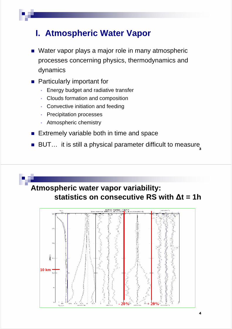
Atmospheric water vapor variability:statistics on consecutive RS with ∆t = 1h

- 20% + 20%

10 km

5

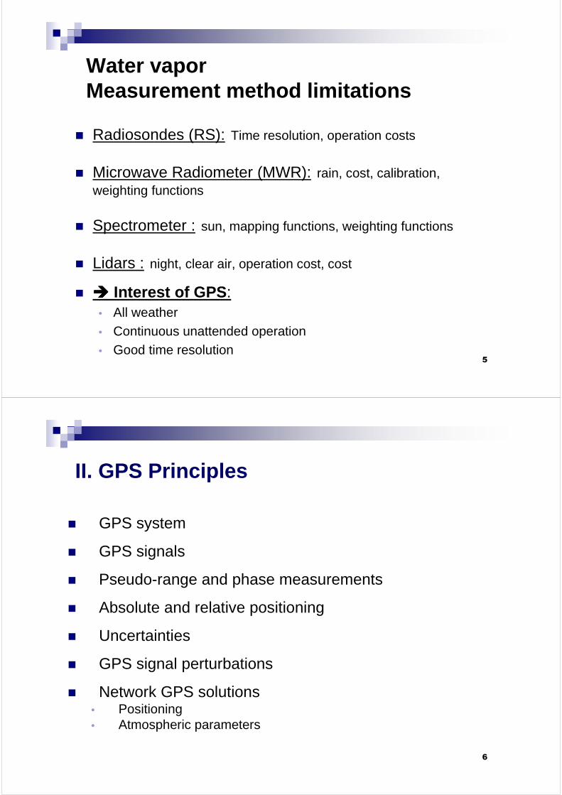
Water vapor Measurement method limitations

� Radiosondes (RS): Time resolution, operation costs

� Microwave Radiometer (MWR): rain, cost, calibration, weighting functions

� Spectrometer : sun, mapping functions, weighting functions

� Lidars : night, clear air, operation cost, cost

� �� Interest of GPS :• All weather• Continuous unattended operation• Good time resolution

6

II. GPS Principles

� GPS system

� GPS signals

� Pseudo-range and phase measurements

� Absolute and relative positioning

� Uncertainties

� GPS signal perturbations

� Network GPS solutions• Positioning• Atmospheric parameters

7

The GPS system

� History:• NAVSTAR-GPS

(NAVigation System by Timing and Ranging / Global Positioning System)

• US military program in the ’70s• 1st satellite in 1978• Operational system completed in 1994 (limited service since 1986)• Full access (non degraded signal) since May 2001

� Three segments:• Space:

24 satellites in operations + 4 reserve satellites

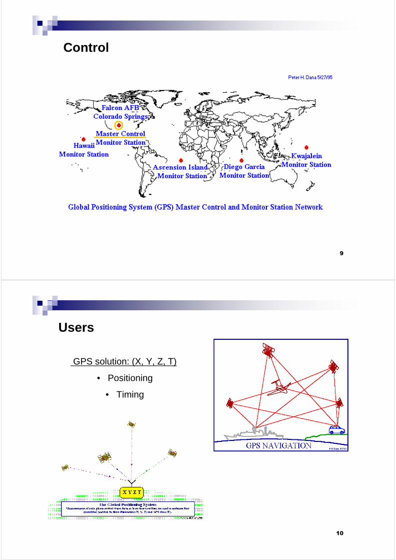
• Control: 5 ground stations for satellites follow-up and command

• Users

8

Space

9

Control

10

Users

GPS solution: (X, Y, Z, T)

• Positioning

• Timing

11

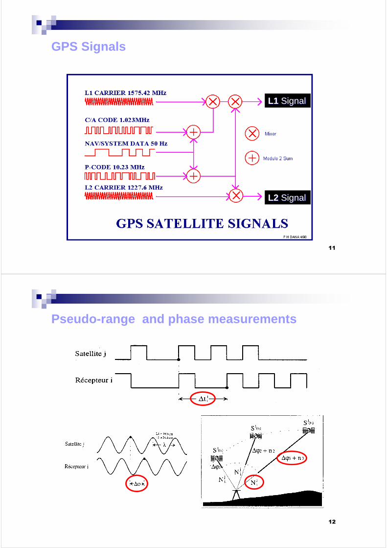
GPS Signals

L1 L1 SignalSignal

L2 L2 SignalSignal

12

Pseudo-range and phase measurements

13

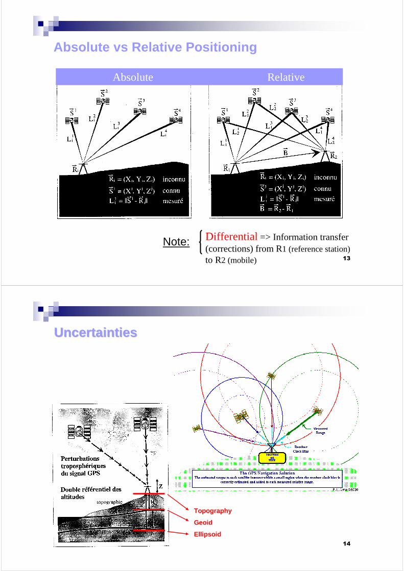
Absolute vs Relative Positioning

Absolute Relative

Differential=> Information transfer (corrections) from R1 (reference station) to R2 (mobile)

Note:

14

UncertaintiesUncertainties

Topography

Geoid

Ellipsoid

15

Signal perturbations

� Satellites orbit and yaw � Satellite and receiver clock drifts� Cycle slips

� A priori coordinates of GPS stations

� Multi-path

� Antenna phase center variations

� Solar and lunar tides

� Ocean and Atmospheric loading

� Ionospheric effect

All these can be addressed with frequency combinati ons, single/double/triple differences, models, and “care ”…

16

ExplExpl : Simple / double / triple differences: Simple / double / triple differences

Effect: suppress satelliteclock drift

Effect: suppress receiverclock drift

Effect: suppress cycle ambiguities

Single Difference Double Difference Triple Difference

17

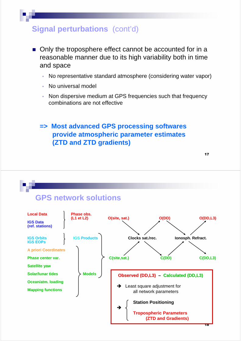
Signal perturbations (cont’d)

� Only the troposphere effect cannot be accounted for in a reasonable manner due to its high variability both in time and space

• No representative standard atmosphere (considering water vapor)

• No universal model

• Non dispersive medium at GPS frequencies such that frequency combinations are not effective

=> Most advanced GPS processing softwaresprovide atmospheric parameter estimates (ZTD and ZTD gradients)

18

GPS network solutions

Local Data Phase obs.(L1 et L2) O(site, sat.) O(DD) O(DD,L3)

IGS Data (ref. stations)

IGS Orbits IGS Products Clocks sat./rec. Ionosph. Refract.IGS EOPs

A priori Coordinates

Phase center var. C(site,sat.) C(DD) C(DD,L3)

Satellite yaw

Solar/lunar tides Models

Ocean/atm. loading

Mapping functions

Observed (DD,L3)Observed (DD,L3) –– Calculated (DD,L3)Calculated (DD,L3)

� Least square adjustment for all network parameters

Station Positioning�

Tropospheric Parameters(ZTD and Gradients)

19

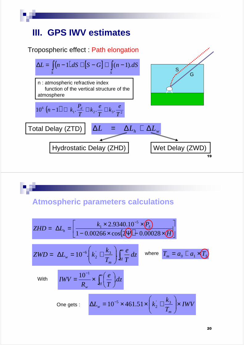
III. GPS IWV estimates

Tropospheric effect : Path elongation

( ) [ ] ∫∫ −≅−+−=∆SS

dSnGSdSnL ).1(.1

( )2321

6 ...110T

ek

T

ek

T

Pkn d ++≅−

wh LLL ∆+∆=∆

n : atmospheric refractive indexfunction of the vertical structure of the

atmosphere

GS

Hydrostatic Delay (ZHD)

Total Delay (ZTD)

Wet Delay (ZWD)

20

Atmospheric parameters calculations

( )

×−Ψ×−××=∆=

−

H

PkLZHD S

h 00028.02cos00266.01

10.9340.2 51

∫∞−

+=∆=

Hm

w dzT

e

T

kkLZWD ..10 3'

26

Sm TaaT ×+= 10where

∫∞−

×=H

w

dzT

e

RIWV .

10 1

With

IWVT

kkL

mw ×

+××=∆ − 3'

25 51.46110One gets :

21

GPS IWV calculation

� GPS observable• ZTD

� GPS station coordinates• Ψ, H : latitude & altitude

� Ground atmospheric parameters• PS and TS (to estimate Tm)

( )( )

×−Ψ×−××−×

+×

=−

H

PkZTD

T

kk

IWV S

m

00028.02cos00266.01

109349.2

51.461

10 15

3'2

5

ZTD = ZHD + ZWD

=> IWV = function

22

ZTD

Slant path

ZTD estimates hypotheses

Cut-off

Isotrope vsGradients

Mapping Functions

23

IV. IWV GPS estimates validation: instrument comparisons

(Van Baelen et al. 2005, JAOT)� Framework of experiment

• Validation campaign for AIRS instrument on board satellite EOS-Aqua (Aug. – Nov. 2002)

� Near real time determination of ZTD• Rapid orbits• Short sessions

� Radiosoundings (RS)• 2 soundings twice a day (1h et 5’ before satellite overpass)• Two daily periods: 0h - 3h TU / 11h - 14h TU

� Microwave radiometer on a nearby site

� Common measurement period: 22 Aug. to 24 Sept.

24

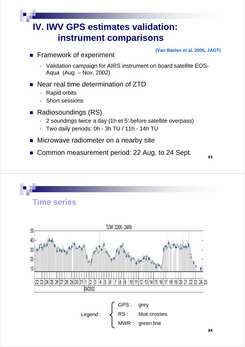
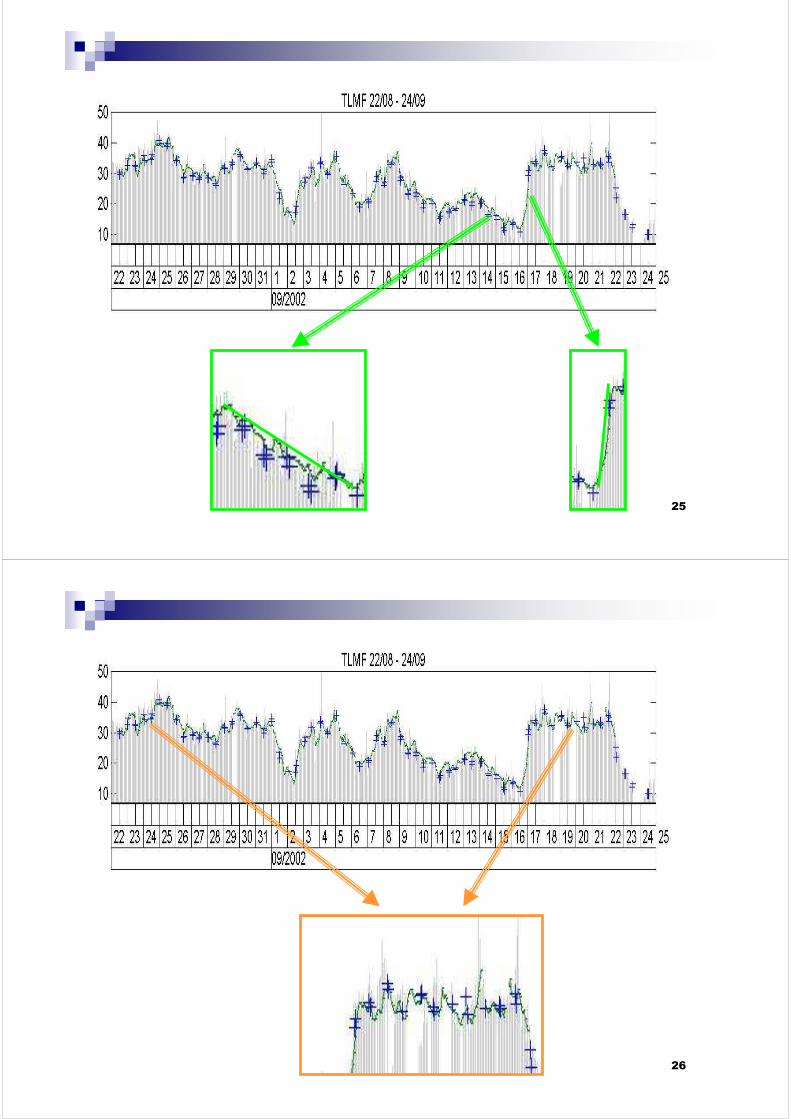
Time series

GPS : grey

RS : blue crosses

MWR : green line

Legend :

25

26

27

28

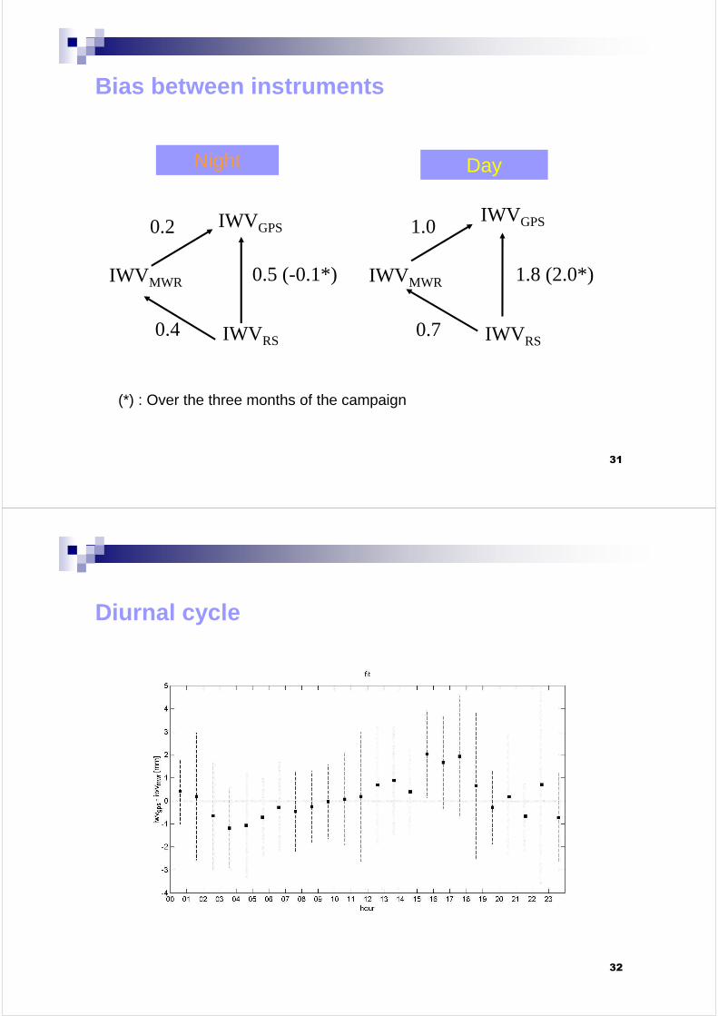
IWVGPS vs IWVRS

∆IWV (GPS-RS) [mm]

∆IWV (GPS-RS) [mm]

Night : m = 0.5 mm, std = 2.3 mm

Day: m = 1.8 mm, std = 2.2 mm

29

IWVMWR vs IWVRS

∆IWV (MWR-RS) [mm]

∆IWV (MWR-RS) [mm]


Day: m = 0.7 mm, std = 1.3 mm

30

IWVGPS vs IWVMWR

∆IWV (GPS-MWR) [mm]

∆IWV (GPS-MWR) [mm]


Day: m = 1.0 mm, std = 2.7 mm

Note : IWVGPS – IWVMWR ~ 0 with all 24 hours of data

31

IWVMWR

IWVGPS

IWVRS

1.0

0.7

1.8 (2.0*)IWVMWR

IWVGPS

IWVRS

0.2

0.4

0.5 (-0.1*)

Bias between instruments

Night Day

(*) : Over the three months of the campaign

32

Diurnal cycle

33

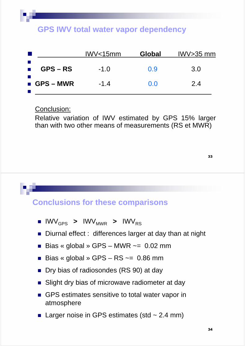
GPS IWV total water vapor dependency

� IWV<15mm Global IWV>35 mm�

� GPS – RS -1.0 0.9 3.0�

� GPS – MWR -1.4 0.0 2.4�

Conclusion:Relative variation of IWV estimated by GPS 15% larger than with two other means of measurements (RS et MWR)

34

Conclusions for these comparisons

� IWVGPS > IWVMWR > IWVRS

� Diurnal effect : differences larger at day than at night

� Bias « global » GPS – MWR ~= 0.02 mm

� Bias « global » GPS – RS ~= 0.86 mm

� Dry bias of radiosondes (RS 90) at day

� Slight dry bias of microwave radiometer at day

� GPS estimates sensitive to total water vapor in atmosphere

� Larger noise in GPS estimates (std ~ 2.4 mm)

35

V. Case study: (Champollion et al., 2005, JGR)

The Gard flooding of September 9, 2002

From 08/09/02 06:00 to 10/09/02 06:00

Total amount of precipitations

mm

Montpellier

36

Synoptic conditions

500 hPa Analysis

09/09/02 12:00 TU

Temperature 2 m

Wind 10 m

09/09/02 00:00 TU

37

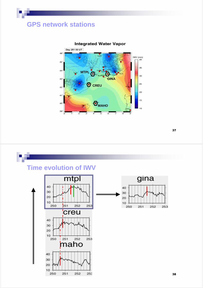
GPS network stations

MAHO

CREU

MTPL

GINA

38

Time evolution of IWV

39

Evolution of relative IWV field

40

Comparison of GPS IWV with Nîmes Precipitation Radar Echoes

41

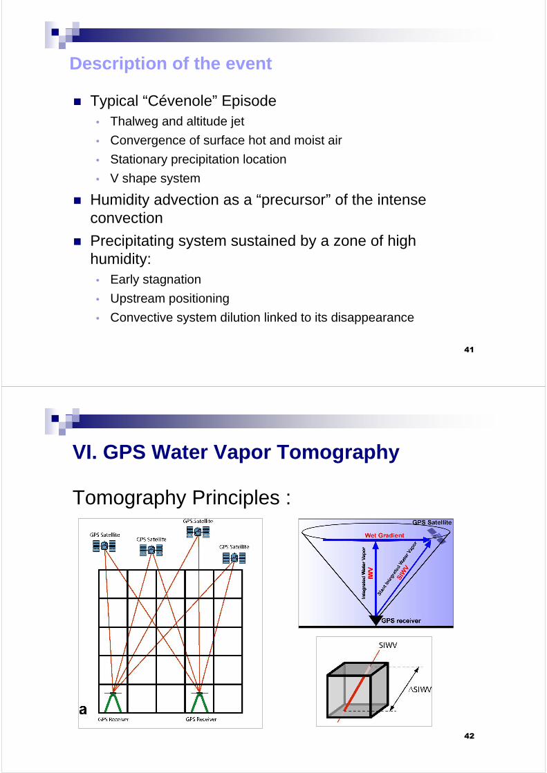
Description of the event

� Typical “Cévenole” Episode• Thalweg and altitude jet

• Convergence of surface hot and moist air

• Stationary precipitation location

• V shape system

� Humidity advection as a “precursor” of the intense convection

� Precipitating system sustained by a zone of high humidity:

• Early stagnation

• Upstream positioning

• Convective system dilution linked to its disappearance

42

VI. GPS Water Vapor Tomography

Tomography Principles :

43

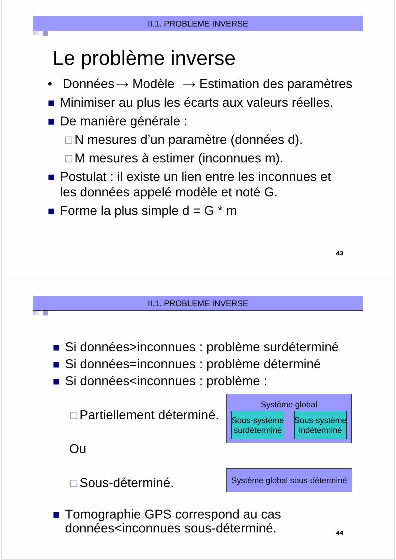
Le problème inverse

� Minimiser au plus les écarts aux valeurs réelles.

� De manière générale :�N mesures d’un paramètre (données d).�M mesures à estimer (inconnues m).

� Postulat : il existe un lien entre les inconnues et les données appelé modèle et noté G.

� Forme la plus simple d = G * m

II.1. PROBLEME INVERSE

• Données→ Modèle → Estimation des paramètres

44

� Si données>inconnues : problème surdéterminé� Si données=inconnues : problème déterminé� Si données<inconnues : problème :

�Partiellement déterminé.

Ou

�Sous-déterminé.

� Tomographie GPS correspond au cas données<inconnues sous-déterminé.


Sous-systèmeindéterminé

Sous-systèmesurdéterminé

Système global

Système global sous-déterminé

45

� Solution du problème inverse via la formule suivante : méthode des moindres carrés pondérés amortis.

( ) ( )0

112110 mGdWGWGGWmm e

tm

tm ×−•×+••••+= −−−− α


α : facteur de pondération.

m : solution recherchée.m0 : valeurs initiales.Wm et We : matrice de pondération.G : modèle → matrice de répartition des données.d : données → SIWV contenu en vapeur d’eau intégrée oblique.

1 23

46

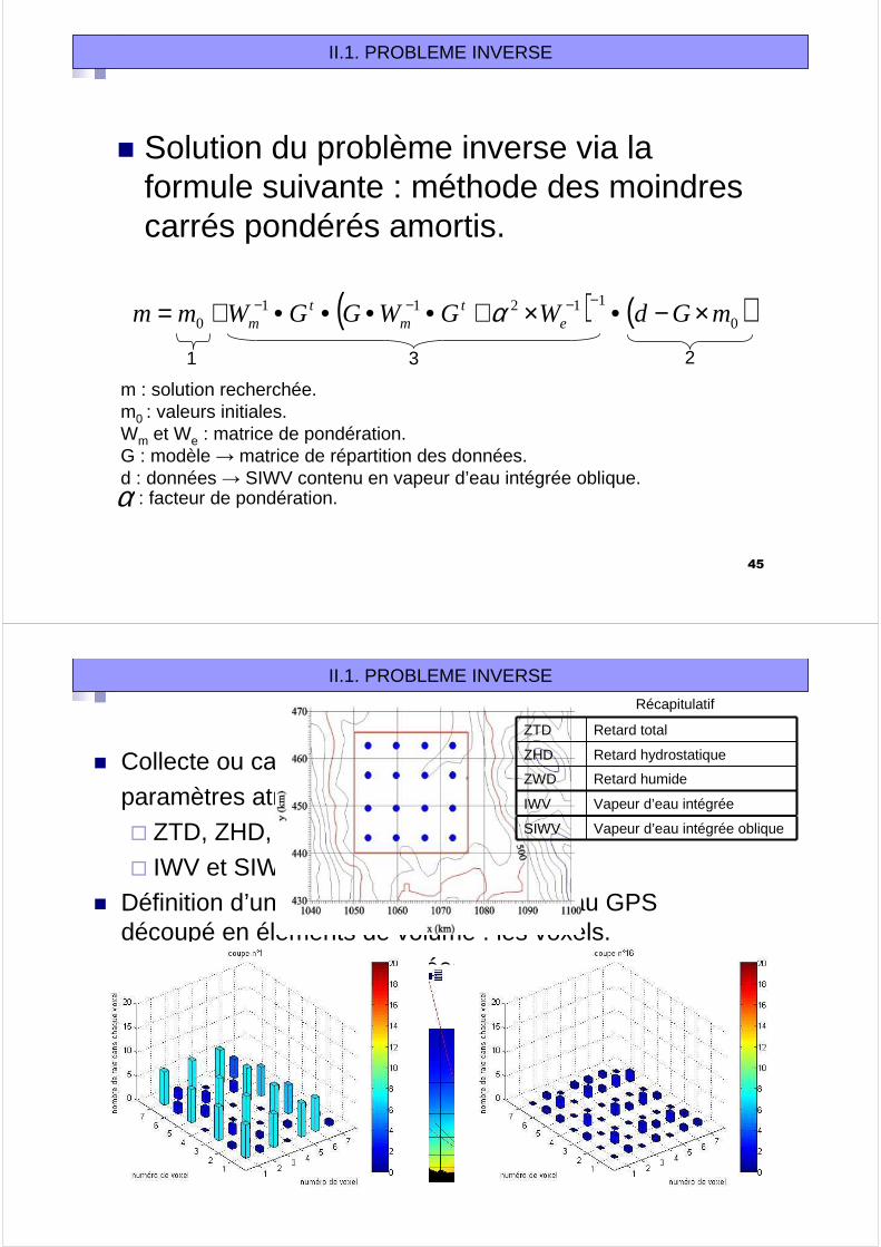
� Collecte ou calcul des paramètres atmosphériques:� ZTD, ZHD, ZWD. � IWV et SIWV.

� Définition d’un volume au-dessus du réseau GPS découpé en éléments de volume : les voxels.

� Répartition des SIWV (données) dans chaque voxel pour former le modèle G.

� Estimation des matrices de pondération et autres paramètres relatifs à l’équation du système inverse.


Retard totalZTD

Retard hydrostatiqueZHD

Retard humideZWD

Vapeur d’eau intégréeIWV

Vapeur d’eau intégrée obliqueSIWV

Récapitulatif

47

� Utilisation d’un modèle atmosphérique non-hydrostatique méso-échelle pour connaître la répartition synthétique de la densité de vapeur d’eau.

� Création de différents réseaux GPS en faisant varier le nombre et la géométrie des stations ainsi que le nombre de voxels.

� Extraction de SIWV synthétiques à travers le modèle atmosphérique.

� Inversion tomographique.� Comparaison de la tomogaphie avec le modèle

atmosphérique.

II.2. TESTS DE SENSIBILITE ET VALIDATION

Méthodologie

48

� Résultat concernant la géométrie du réseau:� 1 réseau composé de 16 stations GPS réparties de

manière optimale.� 1 réseau correspondant à un cas réel.


� Importance de couvrir au mieux le terrain pour:� Eviter les effets de bords. � Diminuer le caractère sous-déterminé du problème.

Tests de sensibilité et validation

Modèle atmosphériqueCoupe horizontale.

Résultat tomographique. Densité de vapeur d’eau en g/m3. Coupe horizontale à 500 m

g/m

3

g/m

3

49

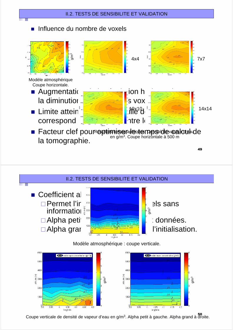
� Influence du nombre de voxels


� Augmentation de la résolution horizontale avec la diminution de la taille des voxels.

� Limite atteinte lorsque la taille des voxels correspond à la distance entre les stations.

� Facteur clef pour optimiser le temps de calcul de la tomographie.

4x4 7x7

10x10 14x14

Modèle atmosphériqueCoupe horizontale.

Résultats tomographiques. Densité de vapeur d’eauen g/m3. Coupe horizontale à 500 m

g/m

3

50

� Coefficient alpha :�Permet l’inversion dans les voxels sans

informations.�Alpha petit → plus de poids aux données.�Alpha grand → plus de poids à l’initialisation.

α


Coupe verticale de densité de vapeur d’eau en g/m3. Alpha petit à gauche. Alpha grand à droite.

Modèle atmosphérique : coupe verticale.

g/m

3

g/m

3

g/m

3

51


� Les tests de validation et de sensibilité ont montré :� Restitution de la densité de vapeur d’eau au

dixième de g/m3. � Différence entre 0% et 20% (effets de bord. 1 g/m3)

par rapport au modèle. � Moyenne de 9%. ( 0.45 g/m3).

� Critère pour effectuer une tomographie :� Nombre minimum de stations GPS :

Superficie(km²) / 100 ou 1000 � Nombre optimum de stations GPS à partir de :

2 * Superficie(km²) / 100 ou 1000

� Nécessité de bien positionner les stations.

52

Campagne OHMCV

� Observatoire hydrométéorologique Méditerranéen Cévennes-Vivarais. � But: étudier et comprendre les phénomènes de pluies intenses conduisant à

des crues éclairs.� En 2002, déploiement d’un réseau dense GPS composé de 16 stations.

Réseau de 26x26 km². Distance entre les stations ~5 km.

III.1. OHMCV

53

� Période du 20 au 22 octobre 2002. � Passage d’un front chaud le 21 octobre 2002 entre 16h

et 20h.

III.1. OHMCV

� Augmentation des IWV avant le front� Déclenchement des précipitations avec le passage du

front chaud (réflectivité et pluviomètres)� Baisse d’IWV pendant l’épisode orageux

54

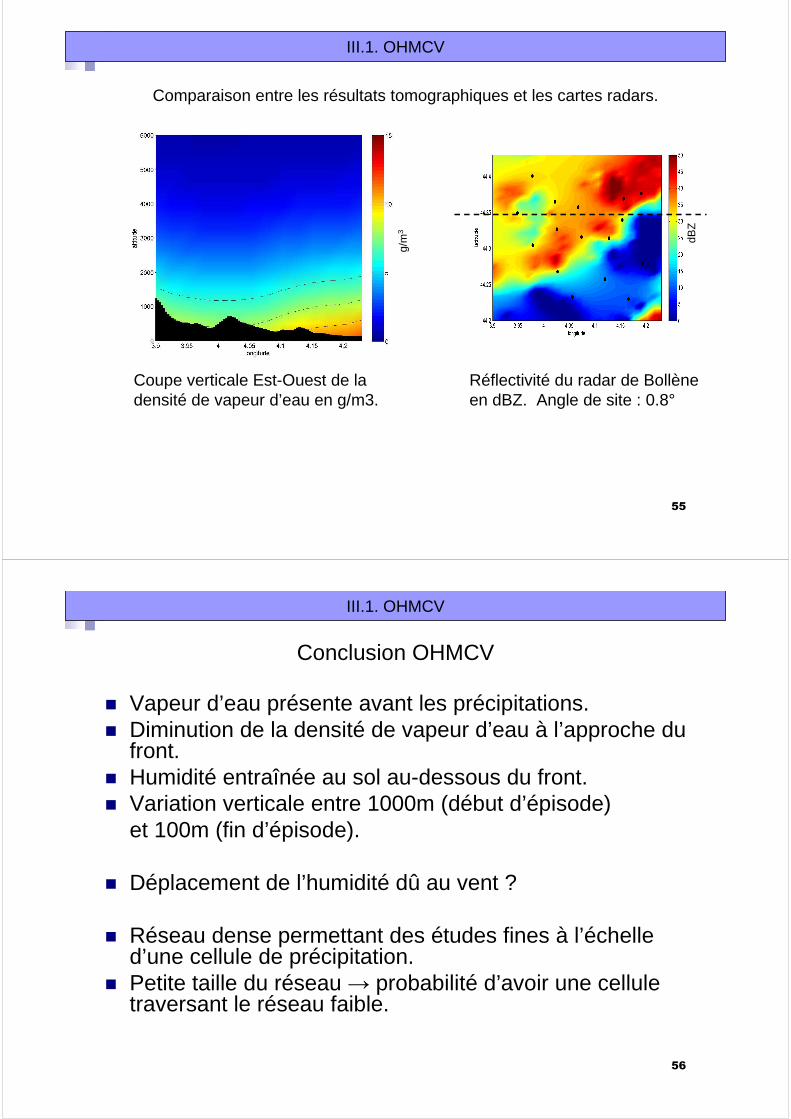
III.1. OHMCV

Densité de vapeur d’eau en g/m3.Coupe horizontale à 500 m d’altitude.

Réflectivité du radar de Bollèneen dBZ. Angle de site : 0.8°

Comparaison entre les résultats tomographiques et les cartes radars.

g/m

3

dBZ

55

III.1. OHMCV

Coupe verticale Est-Ouest de la densité de vapeur d’eau en g/m3.

Réflectivité radar

Réflectivité du radar de Bollèneen dBZ. Angle de site : 0.8°


g/m

3

dBZ

56

III.1. OHMCV

� Vapeur d’eau présente avant les précipitations.� Diminution de la densité de vapeur d’eau à l’approche du

front. � Humidité entraînée au sol au-dessous du front.� Variation verticale entre 1000m (début d’épisode)

et 100m (fin d’épisode).

� Déplacement de l’humidité dû au vent ?

� Réseau dense permettant des études fines à l’échelle d’une cellule de précipitation.

� Petite taille du réseau → probabilité d’avoir une cellule traversant le réseau faible.

Conclusion OHMCV

57

Tomographie IRMB� Environ 70 stations sur l’ensemble du pays.� Distance entre les stations de 20 à 40 km.

III.2. IRMB

� Permet de suivre l’évolution de phénomènes synoptiques.

� Vérifier le comportement du logiciel de tomographie pour de plus grands réseaux.

WideumontWideumont

58

� Cas du 19 Octobre 2005.� Passage d’un front de faible activité pluvieuse

sur le pays entre 0h et 12h.

� Pluie stratiforme, bruine.

III.2. IRMB

� Augmentation des IWV lorsque la perturbation arrive sur le réseau. 4h

� Diminution progressive pendant la traversée du réseau. 4h-8h

� Résidus observés après 8h

59

1 2 8643 5 7

Echelle de temps en heure

0

III.2. IRMB

Précipitation radar en mm/h

1 2 8643 5 7


0


Densité de vapeur d’eau en g/m3.Coupe horizontale à 500 m d’altitude.

60

Précipitation radar en mm/hCoupe verticale Est-Ouest de la densité de vapeur d’eau en g/m3.

III.2. IRMB


1 2 8643 5 7


0

61

III.2. IRMB

� La vapeur d’eau ne précède pas la perturbation, elle arrive en même temps.

� Saturation d’humidité par la bruine de l’atmosphère.� Variation verticale entre 1200m (milieu d’épisode)

et 100m (début et fin d’épisode).

� Petites variations de la série temporelle des IWV correspondant aux passages des bandes pluvieuses ?

� Très bonne couverture quelque soit la zone d’étude.� Mais peu de relief.

Conclusion IRMB

62

Campagne COPS� Convective and Orographically-induced Precipitation Study.� Campagne durant l’été 2007. Déploiement de divers instruments

(radar, GPS, etc…) pour étudier des phénomènes météorologiques. � Réseau GPS d’environ 50 stations avec un espacement d’environ

50 km.� Localisation intéressante pour connaître l’évolution de la vapeur

d’eau dans la vallée du Rhin et pour comprendre les mécanismes liés aux reliefs.

III.3. COPS

63

COPS Network

64

� Cas du 19 juillet entre 8h et 11 h� Augmentation des IWV au début de

l’épisode puis diminution avec les précipitations.

III.3. COPS

(m)

65

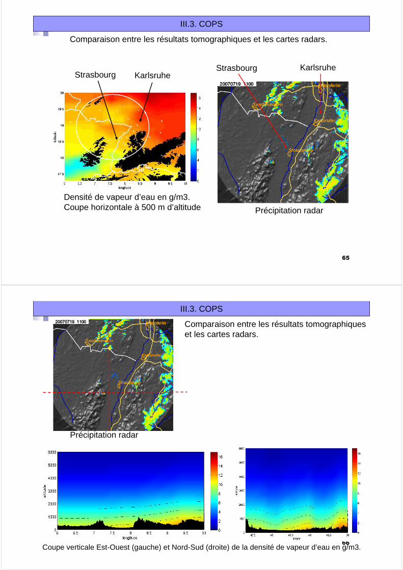
III.3. COPS

Densité de vapeur d’eau en g/m3.Coupe horizontale à 500 m d’altitude Précipitation radar


StrasbourgStrasbourg

KarlsruheKarlsruhe

66

Précipitation radar

III.3. COPS


Coupe verticale Est-Ouest (gauche) et Nord-Sud (droite) de la densité de vapeur d’eau en g/m3.

67

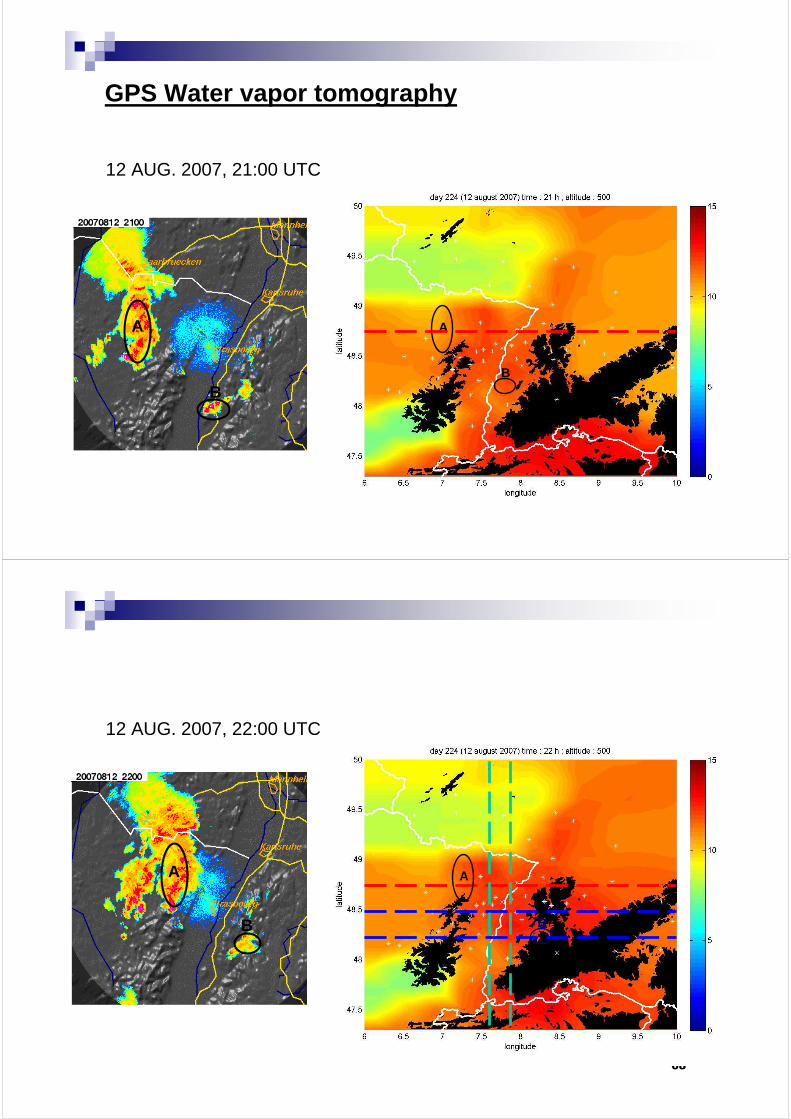
GPS Water vapor tomography

12 AUG. 2007, 21:00 UTC

A

BB

A

68

12 AUG. 2007, 22:00 UTC

A

B

A

B

69

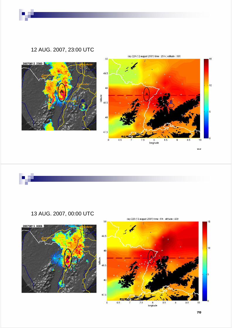
A

B

12 AUG. 2007, 23:00 UTC

A

B

70

A

13 AUG. 2007, 00:00 UTC

A

71

Vertical cut time series

72

12 AUG. 2007, 22:00 UTC

A

B

A

B

73

Vertical cuts

74

� Humidité présente à la verticale du front pluvieux. � Déplacement de la vapeur d’eau avec la bande pluvieuse.� Pas d’humidité entrainée au sol malgré les précipitations

fortes.� Variation verticale entre 1200m (début d’épisode)

et 500m (fin d’épisode).

� Bonne couverture de la zone d’étude mis à part quelques effets de bord.

� Relief important.

III.3. COPS

Conclusion COPS

75

VII. Towards Operational Meteorology

� Large spatial distribution

� Continuous and all-weather operations

� Autonomous and low-cost operations

� Support to radiosoundings

� 4-Dvar models now capable to exploit such data

� Atmospheric humidity parameterization

� Data assimilation periodicity

76

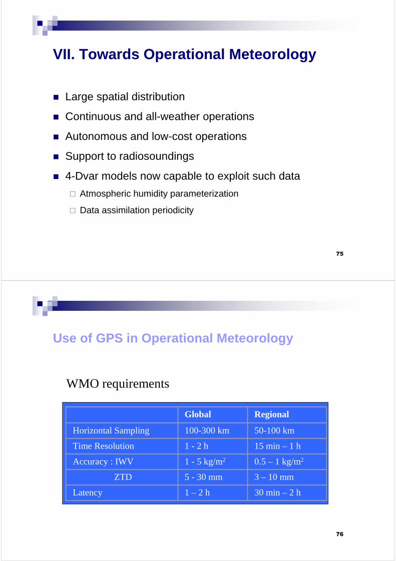
Use of GPS in Operational Meteorology

Global Regional

Horizontal Sampling 100-300 km 50-100 km

Time Resolution 1 - 2 h 15 min – 1 h

Accuracy : IWV 1 - 5 kg/m2 0.5 – 1 kg/m2

ZTD 5 - 30 mm 3 – 10 mm

Latency 1 – 2 h 30 min – 2 h

WMO requirements

77

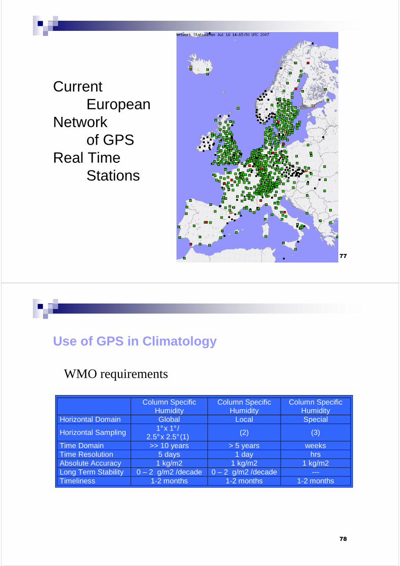
CurrentEuropean

Networkof GPS

Real TimeStations

78

Column Specific Humidity



Horizontal Domain Global Local Special

Horizontal Sampling 1° x 1° / 2.5° x 2.5° (1)

(2) (3)

Time Domain >> 10 years > 5 years weeks Time Resolution 5 days 1 day hrs Absolute Accuracy 1 kg/m2 1 kg/m2 1 kg/m2 Long Term Stability 0 – 2 g/m2 /decade 0 – 2 g/m2 /decade --- Timeliness 1-2 months 1-2 months 1-2 months

Use of GPS in Climatology

WMO requirements

79

Use of GPS data in Numerical Weather Prediction Models

� Experiences have been carried out in the USA (MM5) and in Europe(HIRLAM, LM, ALMo, UKmodel)

� Assimilation of IWV has a generally positive impact upon the restitution of precipitation area and the estimation of precipitation amounts

� Assimilation of IWV provides little impact upon the atmospheric water vapor vertical structure

� Future: assimilation of ZTD (not tributary on P or T), or even assimilation of slant delays

� Experimental: Use of GPS IWV (and wet gradients) to support nowcasting of precipitation and storm development

80

Precipitation forecast effect

Observations

NWP without GPS

NWP with GPS

Vedel et al., MAGIC

81

Now-casting try-outs

82

VIII. Other applications

� Atmospheric studies with GPS Radio Occultation

� Many other campaigns

� Puy de Dôme

� Escompte

� IHOP

� COPS

� Combining GPS and Wind Profiler to retrieve the atmospheric humidity profiles

� Using GPS to correct the atmospheric effect on satellite radar interferometry (volcanology)

83

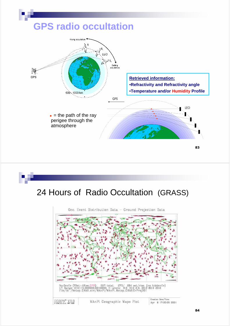
GPS radio occultation

= the path of the ray perigee through the atmosphere

Retrieved information:

•Refractivity and Refractivity angle

•Temperature and/or Humidity Profile

84

24 Hours of Radio Occultation (GRASS)

85

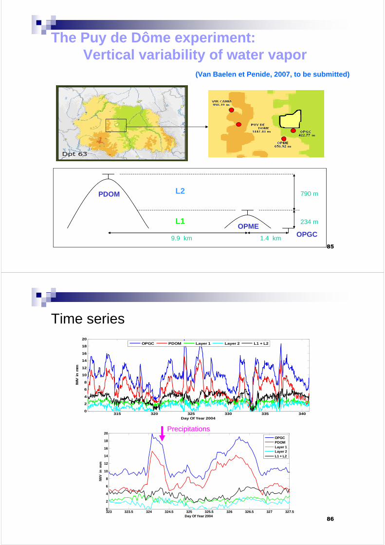
The Puy de Dôme experiment:Vertical variability of water vapor

(Van Baelen et Penide, 2007, to be submitted )

PDOM

OPMEOPGC9.9 km 1.4 km

790 m

234 m

PDOM

OPMEOPGC9.9 km 1.4 km

790 m

234 m

L2

L1

86

Time series

315 320 325 330 335 3400

2

4

6

8

10

12

14

16

18

20

Day Of Year 2004

IWV

in

mm

OPGC PDOM Layer 1 Layer 2 L1 + L2

323 323.5 324 324.5 325 325.5 326 326.5 327 327.50

2

4

6

8

10

12

14

16

18

20

Day Of Year 2004

IWV

in

mm

OPGCPDOMLayer 1Layer 2L1 + L2

Precipitations

87

Vertical Wind / Pressure and Temperature

323 323.5 324 324.5 325 325.5 326 326.5 327 327.50

5

10

15

Day of Year 2004

Tem

p / P

res

323 323.5 324 324.5 325 325.5 326 326.5 327 327.55

10

15

20

IWV

[mm

]

OPGC IWV

88

89

90

* * * * * * * * * * * * * *

Documents

GPS Applications in Atmospheric Research - Accueil … · A priori coordinates of GPS stations Multi-path ... matrice de pondération. G : ... Critère pour effectuer une tomographie