1

Risk taking and excess entry: The roles of confidence and fallible judgment

Daniela Grieco,1 Robin M. Hogarth,2 & Natalia Karelaia3 ∗

Università Bocconi1, Milan, Italy

ICREA & Universitat Pompeu Fabra2, Barcelona, Spain

HEC Université de Lausanne3, Lausanne, Switzerland

daniela.grieco@uni-bocconi.it

robin.hogarth@upf.edu

natalia.karelaia@unil.ch

October 11, 2007

∗ The authors’ names are listed alphabetically. They thank Carlos Trujillo, Julian Rode, and Enric Soria for help in conducting the experiments. They have also benefited from the helpful comments of Michele Bernasconi, Christian Garavaglia, Franco Malerba, Don Moore, Rosemarie Nagel, Rodolfo Prieto, Mercè Roca, and Jack Soll, as well as seminar participants at CESPRI (Università Bocconi), the DRUID 2006 Winter conference, the SAET 2007 conference, the Université de Lausanne, and the Barcelona Economics Decision Group. This research was financed partially by grants from the Spanish Ministerio de Educación y Ciencia (Hogarth) and the Swiss National Science Foundation (Karelaia). For correspondence, please contact Robin M. Hogarth at Universitat Pompeu Fabra, Department of Economics & Business, Ramon Trias Fargas, 25-27, 08005 Barcelona, Spain. Tel: + 34 542 2561.

2

Abstract

Economic explanations for the high failure rate of entrepreneurial ventures suggest “hit and

run” entrants and risk-seeking behavior. A psychological explanation is overconfidence. We

show analytically that excess entry follows inevitably from entrepreneurs relying on imperfect

– but not necessarily overconfident – assessments of their ability, and, by the same token, that

many fail to enter businesses they should have entered. We further investigate the relation

between overconfidence (defined in both absolute and relative terms) and attitudes toward

risk in two experiments designed to mimic entry decisions. Although perhaps not

overconfident, entrepreneurs could gain much by assessing their abilities more accurately.

Keywords: Excess entry; entrepreneurship; overconfidence

JEL classification: C91, L10

3

1. Introduction

The phenomenon of excess entry refers to the observation that “too many” entrepreneurs elect

to enter certain industries and that many subsequently fail. In the U.S., for example, Small

Business Administration datasets suggest that, in any year, 10%-12% of all firms are new

entrants (Dennis, 1997). In Europe, Geroski (1995) documented that up to 100 new firms

enter each of the 87 classifications of British manufacturing industries annually. Individuals

as well as firms create many new enterprises. However, it has been estimated that 75% of new

businesses do not survive more than five years (Bernardo & Welch, 1997). Investigating the

difference between closure and failure, Headd (2003) reports that roughly 50% of firms exit

within their first four years, and about two-thirds of these are unsuccessful at closure (as

defined by their owners). This implies an overall failure rate of 33%.

The causes of this phenomenon have been attributed to both economic and

psychological factors. As to the former, it has been argued that entrepreneurs essentially face

lotteries with highly skewed payoffs. Thus, whereas probabilities of success are low, the

accompanying payoffs are high. It is therefore rational for entrepreneurs to accept gambles

with positive expected utility even though only a minority can succeed.

The psychological explanation has focused on the notion of overconfidence. For

example, Cooper, Woo, and Dunkelberg (1988) found that 81% of a sample of 2,994

entrepreneurs believed that their chances of success were at least 70%, and one-third believed

they were certain to succeed. When asked about others, however, only 39% believed that the

chances of any business like theirs succeeding were 70% or more. Another recent survey

(Koellinger et al., 2007) reports a negative relation between self-report level of

entrepreneurial confidence and the survival chances of new entrepreneurs across countries. In

addition to surveys, the psychological evidence favoring overconfidence is also grounded in

controlled experiments (Camerer & Lovallo, 1999; Moore & Cain, 2007).

4

If overconfidence does lead to excess entry then, of course, much could be gained if

entrepreneurs were to modify their judgments accordingly. Indeed, this is the implicit

recommendation of the psychological evidence just cited. However, if entrepreneurs – as a

population – are not really overconfident, this advice could be counter-productive. In this

paper, we do not question that the judgments of entrepreneurs are imperfect or fallible. But we

also argue that fallibility does not necessarily imply overconfidence. Equating the two can

lead to erroneous implications.

To motivate our argument, imagine a situation where entrepreneurs are considering

entering a market where success can only be achieved by those entrepreneurs whose skill

level, Y, is above a specific threshold, yc. Imagine further that each entrepreneur makes a

judgment or receives a signal, X, about his/her skill level that is imperfectly correlated with Y.

However, there is no systematic bias, that is E[Y] = E[X]. In this case, some entrepreneurs will

believe that their skill level lies above yc when, in fact, it does not, and their decision to enter

the market will lead to excess entry. At the same time, others will believe that their skill level

lies below yc when, in fact, it is greater. But, if the latter take no action (i.e., decide to stay

out), no associated outcomes can be observed. In other words, when entrepreneurs rely on the

imperfect relation between assessed and true skill to take action, we are guaranteed to observe

excess entry but not its converse, missed opportunities.

It is important to note that this scenario captures the essence of many other situations

where individuals accept risk by betting on their skills. Consider, for example, career

decisions, selection of research projects, strategic industrial choices, and so on. Apart from

outcomes being related to skills, these examples also typically involve ambiguity in that

probabilities of outcomes are neither known nor easily quantified. These “entrepreneurial”

decisions differ markedly from situations where risk is unrelated to individual skills and

probabilities of outcomes are well-defined, such as in life insurance or lotteries.

5

In this paper, we first review previous explanations of excess entry and related literature.

Next, we specify the model sketched above in greater detail and illustrate its implications

through some simulations. We specifically note how differential validity of signals that

economic actors receive about their skill levels should affect their actions and the relations

between different types of overconfidence. We subsequently conduct two experiments to test

the relation between overconfidence and risk taking. We conclude by emphasizing

distinctions between different types of overconfidence and the need to understand the role of

judgmental fallibility in producing economic outcomes. As a population, entrepreneurs may

not be overconfident, but much could be gained by increasing the accuracy of their

judgments.

2. Previous explanations and related literature

Explanations of the excess entry phenomenon have been grounded in both economics and

psychology. The standard economic story is that high profits attract entry and entrants bid

away these profits, eventually pushing the industry into long run equilibrium with no excess

returns and a given number of firms. Similarly, whenever profits fall below “normal” levels,

exit occurs and this depopulation of the industry raises profitability for the survivors back to

equilibrium. From this perspective, failures are “hit and run” entrants that have only a small

chance of success in the limited period when the industry exhibits extra profits.

Alternatively, starting a business can be framed as facing a gamble where the probability

of winning is extremely low but the payoff for success is large. This explanation enlarges the

former perspective by accounting for uncertainty, information, and risk attitudes in

determining entry decisions. This can result in excess entry with respect to a limited and

unknown market capacity and consequently individual failures.

6

A further hypothesis is that entrepreneurs are more risk seeking than non-entrepreneurs.

However, the empirical literature provides conflicting results. The general conclusion is that

entrepreneurs do not differ in risk attitudes from the overall population (Brockhaus, 1980;

Master & Meier, 1988; Palich & Bagby, 1995) and may even be more risk averse than non-

entrepreneurs (Miner & Raju, 2004).1 Alternatively, entrepreneurs may simply accept risky

business situations as given (Sarasvathy, Simon, & Lave, 1998) or assess opportunities and

threats differently from non-entrepreneurs (Norton & Moore, 2002).

The explanations grounded in economics assume full rationality on the part of agents.

In contrast, psychological explanations suggest two kinds of “mistakes.” One is the

phenomenon of “competitive blind spots,” that is, agents fail to appreciate how many

competitors they will face. The second is overconfidence, a phenomenon that has been

documented in many contexts (Kahneman, Slovic, & Tversky, 1982; Klayman, Soll,

Gonzalez-Vallejo, & Barlas, 1999). Agents may forecast competition accurately but fail in

evaluating their own chances of success. Specifically, the decision to enter is taken even if

negative industry profits are expected because of a belief in succeeding where others will fail.

Recently, Moore and Healy (2007) clarified conceptual confusion surrounding the

concept of overconfidence by distinguishing three distinct meanings. First, people can be

overconfident in estimating their ability to do something. For example, a person might

overestimate his ability to run a Marathon within a certain time. Moore and Healy call this

overestimation. It is important to note that overestimation is not universal. A robust finding is

that people tend to overestimate their own skill on hard tasks but underestimate it on easy

tasks (Burson, Larrick, & Klayman, 2006; Moore & Cain, 2007). One explanation is that

because most judgments of skill involve error, they are liable to be regressive (Dawes &

Mulford, 1996; Erev, Wallsten, & Budescu, 1994).

1 Parenthetically, this literature relies on biased samples in that studies only include “successful” survivors, i.e., those unsuccessful entrepreneurs who have left the market are excluded.

7

Second, a person might express overconfidence in ability relative to others; for example,

the belief that one can run the Marathon faster than, say, 80% of a specific population. Moore

and Healy call this overplacement. It is also referred to as the “better-than-average” effect

whereby people judge their abilities in familiar domains such as driving as being superior to

that of the “average” person (Svenson, 1981). At the same time, however, there is a tendency

to judge oneself as below average in unfamiliar (and therefore hard) tasks such as juggling

(Kruger, 1999). Also, as Hoelzl and Rustichini (2005) demonstrate, this type of

overconfidence may be moderated when people are required to make incentive-compatible

choices as opposed to expressing opinions.

Third, people can be overconfident when estimating future uncertainty; for example,

when providing confidence intervals for forecasts of, say, sales that subsequently turn out to

be too narrow (see, e.g., Alpert & Raiffa, 1982; Klayman et al., 1999). Moore and Healy call

this overprecision. Interestingly, in an empirical study, Wu and Knott (2006) suggest that,

whereas entrepreneurs might accurately assess market demand (i.e., no overprecision), they

overestimate their ability to manage ventures successfully (i.e., overplacement).

Camerer and Lovallo (1999) tested the overconfidence hypothesis experimentally in a

game designed to mimic entry decisions. Specifically, N participants decide simultaneously

to enter a market with a pre-announced capacity of c participants (N > c) where payoffs

depend on participants’ ranks (i.e., of those choosing to enter, the highest-ranked participant

receives the largest payoff, the lowest-ranked participant, the smallest payoff). Ranks were

established in two ways at the end of the experiment (i.e., after all choices had been made):

one at random, and the other on the basis of relative performance on a test (skill). When

making entry decisions, however, participants knew how ranks would be established, i.e.,

according to relative skill or at random. Camerer and Lovallo tested for overconfidence by

8

comparing entry rates between the random and skill conditions and found significant effects –

greater entry under the skill condition.

Camerer and Lovallo claim that their results are consistent with overconfidence in that,

whereas participants had accurate expectations concerning the number of competitors, the

differential entry rates between the skill and random conditions provided evidence of

overconfidence in their relative skill.2 As we demonstrate below, however, the decision to

act on the basis of an imperfect signal, but not to act in the absence of a signal, does not

necessarily imply overconfidence, either in the sense of overestimation or overplacement.

3. A model of entrepreneurial entry

We assume that an entrepreneur’s success in entering a market depends on her managerial

skill, Y. However, this is not known precisely by the entrepreneur and has to be estimated.

Denote the estimate by X. On any given occasion, therefore, the entrepreneur is overconfident

in her skill (in the sense of overestimation) if x > y and underconfident if x < y.3 However,

assume that, on average, the population of entrepreneurs is neither over- nor underconfident,

i.e., E[Y] = E[X], and that the imperfect relation between Y and X can be captured by the

correlation between them,xyρ , that we label signal validity. For simplicity, we assume that X

and Y are standardized normal variables, N(0,1).

Within this set-up, we define overplacement as occasions when y < E[Y] and x > E[Y].

That is, the entrepreneur is overconfident in the sense of overplacement if her true skill y is

inferior to the average skill in the population and her estimate of own skill x surpasses the

average skill. The proportion of overplacement (i.e., entrepreneurs who erroneously consider

2 Camerer and Lovallo also asked their participants to estimate the number of entrants on each round. For most participants, forecasts were unbiased. 3 We use upper case letters to denote random variables, e.g., Y, and lower case letters to designate specific values, e.g., y. As exceptions to this practice, we use lower case Greek letters to denote random error variables, e.g., ε, as well as parameters, e.g., ρ.

9

themselves to be “better-than-average”) is defined by the joint probability

[ ] [ ]{ }YExYEyP >∩< and is a decreasing function of signal validity,xyρ .

Now imagine further that success or failure depends on whether the level of skill

exceeds a threshold, or cut-off point, yc, located at a specific fractile of the distribution of Y.

This threshold captures market capacity: larger values of yc correspond to more stringent

markets where capacity (and therefore the rate of success) is smaller.

When does market entry take place? What probability of success does an individual

entrepreneur require to enter a market? This question can be reframed by asking what level of

estimated skill, xc, would leave an entrepreneur indifferent between entering or staying out of

the market.

Assume that if the entrepreneur enters the market and loses (i.e., if y < yc), a loss of K,

the initial investment, is incurred. On the other hand, if successful (i.e., y > yc), the

entrepreneur’s payoff is f(y - yc) – K, that is a function of the extent to which y exceeds yc less

the investment, K.

Thus, entrepreneur i will enter the market if her expected payoff is greater than zero (or

the result of staying out). That is, when

[ ] ∫∞

∞−

==Ε dyxyfygxXentry iXYi )()( ≥ 0 (1)

where we assume that the payoff of entry is ( )

<−≥−−

=c

cc

yyK

yyKyyyg

,

,)( ; 4 and the

conditional pdf )(

),()( ,

iX

iYXiXY xf

yxfxyf = is a normal density with mean i

x

yxy xσ

σρ and variance

( ) 221 yxy σρ− .

4 For simplicity we assume that f(y - yc) = (y - yc). Monotonic changes in the form of this function will not alter the qualitative implications of the model.

10

Entrepreneur i is indifferent between entering and not if 0)()( =∫∞

∞−

dyxyfyg iXY .

That is, if

( ) 0)()( =+−−+− ∫∫∞

∞− c

c

y

iXYc

y

iXY dyxyyfKydyxyfK . (2)

The solution of this equation gives ci xx =* , i.e., the entry decision cut-off point. Thus,

if ci xx > , the decision is to enter the market; and if ci xx < , to stay out (all other things being

equal, that is, xyρ , [ ]YΕ , xσ , yσ , cy , and )(yg ). The probability of entry therefore increases

when cx decreases. The location of xc can vary depending on both risk attitudes and the

expected economic consequences of different situations.

Because closed form solutions cannot be found for equation (2), we have simulated

various situations – see Appendix A. Qualitatively, these show that signal validity determines

the number of entrants but that this depends on market capacity. On the one hand, when

market capacity is limited (consider, e.g., the pharmaceutical industry), the number of market

entrants increases as signal validity increases, i.e., with a lot of competition, entrepreneurs

need a more valid signal to enter the market. On the other hand, when market capacity is large

(consider, e.g., the restaurant business), the number of entrants decreases as signal validity

increases. However, when K, the investment needed to enter is high, an increase in signal

validity triggers more entry independently of how tough the competition is.5

As a first implication of our model, consider the experimental set-up of Camerer and

Lovallo (1999) that involved a known, limited market capacity. In this situation, more

entrepreneurs should enter the market as signal validity increases. Thus – contrary to the

assertion of Camerer and Lovallo – the observation of a higher entry rate being associated

5 In our notation, limited market capacity is defined by a large value of cy , the number of entrants is decreasing

in xc, and signal validity is xyρ .

11

with an imperfectly valid as opposed to no signal (i.e., between the skill and random

conditions), does not necessarily imply overconfidence.

Model simulations. As a general statement, our model predicts the observation of

excess entry even if there is no overconfidence in the population of entrepreneurs, i.e., [ ]YΕ

= [ ]XΕ , provided signal validity is imperfect, i.e., xyρ < 1. We now investigate the model to

refine this statement and to illuminate more specific points. 6

First, we examine how different values of signal validity, xyρ affect rates of market

entry and excess entry – that is, { }cxxP > and { }cc xxyyP >< .

Second, whereas much has been said about excess entry, less attention has been paid to

missed opportunities, that is, businesses that would have been successful had entrepreneurs

decided to enter the market instead of staying out of it. How important are these

(i.e., { }cc xxyyP <> )?

Third, we assess the effects of overconfidence in the senses of both overestimation and

overplacement. In particular, what proportion of entrepreneurs overestimates their absolute

skills (i.e., for whom x > y)? What proportion overplaces themselves relative to others (i.e.,

for whom y < E[Y] and x > E[Y])? Does overconfidence differ between those who do and do

not enter the market, and between successful and unsuccessful entrants? On average, do

entrepreneurs in different categories (i.e., entrants, non-entrants, successful entrants, excess

entrants or failures) overestimate or underestimate their skills? (To answer this latter

question, we evaluate, separately for each category, the differences between average

estimated and true skills, i.e., yx − ).

6 In doing so, we now treat xc as exogenous.

12

Finally, we ask what happens when entrepreneurs are, on average, over- and

underconfident. For example, does excess entry occur even in the presence of systematic

underconfidence among entrepreneurs (i.e., when E[X] < E[Y])?

To investigate these issues, we simulated populations of 100 entrepreneurs drawing

estimates of own skill (X) and values of true skill (Y) from correlated normal distributions

with fixed parameters. For each population, we calculated entry rate, excess entry rate,

missed opportunities, the proportions of overestimation within different categories (i.e.,

entrants, non-entrants, successful entrants, and excess entrants), the proportions of

overplacement within the same categories, and the proportions of overplacement among those

entrepreneurs who overestimate their skills in absolute terms. In addition, we calculated the

magnitude of over- or underestimation (i.e., the difference between estimated and true skill)

within each category. We repeated the simulation 1,000 times for each combination of

parameters. Thus, the results correspond to the average of 1,000 populations of entrepreneurs.

-------------------------------------------------- Insert Table 1 about here

--------------------------------------------------

Signal validity and excess entry. Table 1 illustrates the effect of changes in signal

validity, xyρ , when the population of entrepreneurs is well calibrated, i.e., when the means of

estimated and true skill coincide, E[X] = E[Y]. For illustrative purposes, we fixed the entry

cut-off, cx , at 0.5. We provide results for three hypothetical markets (three panels in Table 1)

of different capacity, ranging from large (left panel, 1.0−=cy ) to small (right

panel, 9.0=cy ).

For these parameters, 31% of potential entrepreneurs decide to enter the markets (Table

1, line 1). When signal validity,xyρ , increases from 0.0 (i.e., no signal) to 0.9, excess entry

(the probability of failure given entry – line 2) decreases from 0.46 to 0.02 in the least

stringent market (left panel) and from 0.81 to 0.45 in our most stringent market (right panel).

13

Thus, the imperfect relation between estimated and actual skill ensures excess entry even at

the highest signal validity that we examine (i.e., 0.9).7

As for missed opportunities (line 3), the increase of signal validity from 0.0 to 0.9

decreases the proportion of missed opportunities by about 60% in our least stringent market

(left panel) – from 0.54 to 0.34, by 70% in our moderately stringent market (central panel) –

from 0.31 to 0.09, and by 90% in our most stringent market (right panel) – from 0.18 to 0.02.

Signal validity and overconfidence. The data on proportions of overconfidence in the

sense of overestimation (line 4) reveal several trends. First, these proportions are much greater

among entrepreneurs who enter the market than those who stay out. In particular, more than

50% of entrants overestimate their skill while consistently less than 50% of non-entrants do

so. Second, overestimation is greater among failures (excess entrants) than among successful

entrants. In fact, all failures are overconfident in the sense of overestimation in our least and

moderately stringent markets (left and central panels). Third, there is less overestimation

among successful entrants and excess entrants in the markets with small as opposed to larger

capacity (compare right and left panels).

At one level, it appears that excess entry is due to overconfidence in that a greater

proportion of entrepreneurs who fail are overconfident compared to those that succeed.

However, this observation is entirely consistent with a model in which entrepreneurs’

estimates of their abilities are not systematically biased (i.e., overconfident), simply

imperfect.

Do entrepreneurs, on average, overestimate or underestimate their skills? Line 5

presents the average difference between estimated and true skills ( yx − ) within different

categories and confirms the trend concerning overestimation. There is self-selection in that

7 The value of 0.9 exceeds substantially the correlation between estimated and true own performance that we have observed in several experimental datasets, see below.

14

entrants, on average, overestimate their skills (positive values of the difference, yx − ),

whereas non-entrants underestimate their skills (negative values). As for excess entrants

(failures), they strongly overestimate their skills. In particular, their estimates of own skill are

two standard deviations above their true skill in the largest market when outcomes are close to

random occurrences (left panel, first column). However, this decreases to one standard

deviation when signal validity,xyρ , increases to 0.9 (same panel, last column). The

corresponding inflations of self–estimates in the smallest market (right panel) are lower: 1.5

and 0.4 standard deviations for xyρ of 0.0 and 0.9, respectively. Finally, it is illuminating to

compare the magnitude of average miscalibration among successful entrants in different

markets. While this subgroup of entrepreneurs is overconfident in their skills in the largest

market (left panel), they are underconfident in the smallest (right panel). Importantly, the

magnitude of miscalibration (both in the direction of under- and overestimation) decreases for

all categories when signal validity,xyρ , increases.

The analysis of overplacement (line 6) leads to similar qualitative conclusions as

overestimation. In particular, there are proportionally more individuals who erroneously

believe that they are “better-than-average” among entrants than non-entrants. For the

parameters we consider, less than 15% of non-entrants believe that they are “better-than-

average” when in fact they are not. The proportions of overplacement are also greater for

failures (excess entrants) than for successful entrants. In fact, all failures erroneously believe

that they are “better-than-average” in our largest market (left panel). None of the successful

entrants do so in our moderately and most stringent markets (central and right panels). In the

largest market (left panel), less than 10% of successful entrants believe that they are “better-

than-average” when in fact they are not.

Are the two types of overconfidence (overestimation and overplacement) related? How

often do those who overestimate their skill believe that they are “better-than-average”? We

15

report the probability of overplacement given that individuals overestimate their skill8 on line

7 of Table 1. Overplacement given overestimation is more likely at lower levels of signal

validity, xyρ , and among failures rather than successful entrants. In addition, the probability

of overplacement given overestimation among failures and successful entrants decreases

when one moves from larger to smaller markets (from the left to right panels). Overall,

overestimation does not imply overplacement, especially among successful entrants and not at

all in smaller markets.

The effect of systematic miscalibration in the population. We have examined

populations of, on average, well calibrated individuals. Would our conclusions change with

systematic bias in entrepreneurs’ estimates of their skill? We introduce such bias by shifting

the mean of estimated skill, E[X], away from the mean of true skill, E[Y]. Specifically, we

vary the mean of estimated skill from -0.9 (underconfidence in the sense of underestimation)

to 0.9 (overconfidence in the sense of overestimation). The results for the same three markets

(of low, moderate, and high capacity) are presented in Table 2 (for the entry decision cut-off,

cx , and signal validity, xyρ , of 0.5).

-------------------------------------------------- Insert Table 2 about here

--------------------------------------------------

We comment on several outcomes. First, as the mean level of confidence increases,

more entrepreneurs enter the market (line 1). Second, excess entry (the probability of failure

given entry) occurs even in underconfident populations and increases as E[X] increases (line

2). In particular, when the population presents the most extreme case of underconfidence that

we examine, E[X] – E[Y] = -0.9 (left column within each panel), excess entry amounts to 12%

of entrants in our largest market (left panel), 32% of entrants in our moderately stringent

market (central panel), and 49% of entrants in our smallest market (right panel).

8 Note that from our specification of overestimation and overplacement it follows that overplacement guarantees

16

Interestingly, the proportions of missed opportunities drop significantly as the

population, on average, becomes more overconfident (line 3). In particular, when average

miscalibration changes from extreme underconfidence (i.e., E[X] – E[Y] = -0.9) to extreme

overconfidence (i.e., E[X] – E[Y] = 0.9), missed opportunities decrease by 37% in our largest

market (left panel) – from 0.51 to 0.32, by 54% in our moderately stringent market (central

panel) – from 0.28 to 0.13, and by 63% in our smallest market (right panel) – from 0.16 to

0.06.

The comparisons of the proportions of overestimation and overplacement among

categories (lines 4 and 6) reveal the same trends as in Table 1. In addition, the proportions of

the two types of overconfidence (i.e., overestimation and overplacement) naturally increase in

all categories when miscalibration at the level of the population changes from under- to

overestimation. Moreover, within the cases we examine, the proportion of overestimation

among entrants is always above 50%. That is, the majority of entrants overestimate their skills

independently of the sign and magnitude of the population bias.

As for the average difference between estimated and true skill within different

categories (line 5), the data in Table 2 contain several interesting results. First, the entrants

self-select in that they overestimate their skill even if the population of entrepreneurs

underestimate, on average, their skill (first two columns). Second, successful entrants are

underconfident in their skill in the populations with the negative bias. Failures, however, are

overconfident in their skill even if they come from the underconfident populations, i.e., all

positive values in the “excess entry” category. Failures inflate their skill estimates by, on

average, 0.7 to 1.9 standard deviations, with the size depending on market capacity and the

magnitude and sign of miscalibration in the population.

overestimation. That is, the probability of overestimation given overplacement is one.

17

Overall, the remarkable feature of Table 2 is that excess entry can be observed in the

presence of systematic over- and underconfidence. Moreover, entrants self-select in that, on

average, they are always overconfident in the sense of overestimation. Excess entrants

(failures) present the extreme case of overconfidence both in well calibrated and

underconfident populations.

In short, with or without systematic overconfidence, excess entry simply follows from

people acting on estimates of their skill that are imperfectly related to their true skill.

Moreover, the amount of observable excess entry is a complex function of the different

parameters identified in our model, that is, signal validity ( xyρ ), entry decision cut-off (cx ),

market cut-off ( cy ), and the amount of overconfidence in the population (E[X] – E[Y]), if any.

Thus, in any empirical study, it is difficult to prove or disprove that it is overconfidence that

drives the excess entry phenomenon. In the case of Wu and Knott’s (2006) study of banking,

for example, evidence of overplacement is heavily dependent on observing failures (see Wu

& Knott, 2006, p. 1321). However, this can occur whether or not the population of

entrepreneurs is overconfident. Moreover, surveys that document apparently overconfident

entrepreneurs (e.g., Cooper et al., 1988) suffer from selection bias in that their respondents

typically exclude people who have decided not to take entrepreneurial actions.

4. Experimental evidence

Our analytical model shows that fallible entrepreneurial judgment (either well calibrated or

biased – upwards or downwards) guarantees excess entry. Moreover, more valid signals

should trigger more entry, all other things being equal. Our model also illustrates the

difficulties of demonstrating overconfidence empirically from observed rates of market entry.

We therefore conducted experiments to assess whether people’s risk taking behavior is

18

associated with signal validity or/and their confidence – either over- or underconfidence – in

situations simulating market entry decisions with incentive-compatible rewards.

Overview. In Experiment 1, participants were asked to make a series of choices in a task

where their probabilities of success depended on how well they had performed on a test

relative to other experimental participants. In other words, taking the test provides a signal to

the participants of their chances of success and we examine whether the choices of

experimental participants who are over- and underconfident in the absolute level of their

abilities exhibit different attitudes toward risk (possible effects of overestimation). The level

of confidence was manipulated by administrating easy and hard versions of the test. We also

compare the participants’ responses with those of another group of participants who faced the

same gambles but without any knowledge of the probabilities of success. We refer to the two

groups of participants as the “signal” and “no-signal” groups, respectively. In Experiment 2,

we make a few changes in the experimental paradigm and assess whether over- or under-

confidence in relative ability affects choices (possible effects of overplacement).

Experiment 1

Design. We sought to answer two questions. The first was whether an imperfect signal

would lead to more risk taking than the absence of a signal, and the second was whether over-

or underconfidence induced by a signal leads to more or less risk taking.

To answer the first question, we constituted two groups of participants – the signal and

no-signal groups – who both took tests and then made a series of choices between gambles.

Participants in the signal group were told that the probabilities associated with the gambles

depended on how well they had performed in the test relative to their fellow participants.

(Specifically, the probabilities of gains were determined by their percentile in the distribution

19

of test scores.) In the no-signal group, participants were given no information about the

relevant probabilities.

To answer the second question, we divided the signal group into two sub-groups that

received different versions of the test. One had to choose between two possible answers for

each question (the “easy” condition); the other had to choose between five possible answers

(the “hard” condition). Based on results in the literature (see, e.g., Burson et al., 2006), we

hypothesized that the sub-group in the hard (easy) condition would be overconfident

(underconfident)

Procedure. The experiment was conducted in several phases (see also instructions in

Appendix B). First, participants in the signal group undertook a test involving 20 general

knowledge and logic questions in a multiple choice format. After completing the test,

participants were required to estimate the number of questions they had answered correctly.

(Their remuneration depended on the number of correctly answered questions.)

Second, participants were given the option of leaving the experiment or to continue in a

task that would involve choosing between gambles where they could actually lose money.

They were informed that, at the end of the experiment, their remuneration would depend on

playing out the consequences of one of their chosen gambles selected at random. The non-

signal participants were actually participating in another, unrelated experiment and did not, in

fact, take the same test as the signal participants. For these participants, experimental

instructions presented the choice task as an additional optional activity so that they would not

make any connection between the test and the choice task.

Third, the participants remaining in the experiment faced a series of six choices between

gambles. We describe the gambles below.

20

Fourth, participants faced the consequences of playing out one of their choices that was

determined randomly and were remunerated accordingly.9 For the no-signal group, the

probability of winning was drawn from a uniform distribution. Participants in the signal

group completed a post-experimental questionnaire that inquired, inter alia, about the reasons

for their choices and how they evaluated their scores on the test relative to their fellow

participants.

Choice tasks. Participants were faced with a series of choices between two gambles.

One of these gambles provided a 50% chance of winning money and a 50% chance of losing

money where the expected value was 1€. The other gamble also involved sums to be won or

lost but the probabilities were not specified. Participants in the signal group had been told

that their individual-specific probabilities depended on their relative performance on the test;

no-signal participants were simply informed that the probabilities were unknown.

Each choice could therefore be characterized by a 50/50 gamble to win or lose (w: l)

versus unknown chances to win or lose (w´: l´). Thus, for example, the choice between a

50/50 gamble paying (3€:1€) and an unknown probability gamble paying (3€:1€) can be

described by the notation “3:1 vs. 3:1” (i.e., 50/50 chances on the left, unknown probabilities

on the right). Column headings in Table 3 describe the six choices. As noted above, we

maintained the expected value of all six gambles with known probabilities equal to 1€;

however, we varied the amounts involved (from 3:1 to 5:3) and whether outcomes were

symmetric or asymmetric, e.g., “3:1 vs. 3:1” or “3:1 vs. 5:3”.10

Participants. Participants were recruited through notices on the campus of Universitat

Pompeu Fabra and the experiment was conducted on computers in the Leex laboratory using

9 In fact, participants actually participated in further experimental tasks before the end of the experiment. However, behavior in these latter tasks is not analyzed here. 10 This strategy of asking participants to make several choices to assess attitudes toward risk was guided by considerations in psychometric theory that demonstrate the reliability of constructs measured by multiple indicators (see, e.g., Ghiselli, Campbell & Zedeck, 1981).

21

z-Tree software (Fischbacher, 1999). Participation in the signal condition involved four

groups of fifteen persons where two groups received the easy test and two the hard test. In the

no-signal condition, participation involved six groups varying in size between five and ten

persons. Otherwise, signal and no-signal participants were remunerated in exactly the same

way (performance on test and consequences of randomly selected gambles).

The signal and no-signal groups were homogeneous as to age (means of 20.5 and 20.9

years, respectively, with little variance) with almost as many males as females. As to studies,

the groups could be divided into two categories: business and economics vs. other social

sciences and humanities. The signal and no-signal groups had 65% and 43% in the first

category, respectively. On average, signal (no-signal) participants earned 7.03€ (7.15€) from

the experimental sessions.11

----------------------------------------- Insert Tables 3 and 4 about here

-----------------------------------------

Results. Participants responded strongly to the signal. Table 3 shows, for the six pairs of

gambles, the proportions of participants choosing gambles with unknown probabilities over

the 50/50 gambles. On average, the proportion of such choices by participants in the signal

group was 48% compared to 33% for the no-signal group.

Coding each choice of a gamble with unknown probabilities by a one, we fitted

population-averaged (PA) logistic models to the choices. Such models use generalized

estimating equations (GEE) and correspond to a multivariate repeated-measures approach in

that they simultaneously model all the binary outcomes elicited from an individual. They

therefore account for both within- (i.e., variance in choices across six gamble pairs at the

11 Remuneration consisted of a fixed show-up fee plus a variable component that depended on the number of questions answered correctly on the test and the outcome of playing a randomly selected gamble.

22

individual level) and between-effects (i.e., variance in choices between conditions) (Liang &

Zeger, 1986).12

For example, we used the following model to test for the effect of signal availability on

the probability of selecting gambles with unknown probability over the 50/50 gamble (Table

4, Model 1):

logit(pij) = αj + ß1j Signali, (3)

where pij is the probability that participant i chooses the gamble with unknown probabilities

from a pair j (1, ..., 6); αj is the pair-specific log odds; and ß1j is the log odds ratio associated

with the dummy Signal. (Other subject-level covariates xi can be included in the model by

adding the term xi ß). The regression coefficient ß1j from the population-averaged GEE

model can be interpreted as the average log odds ratio for the jth pair of gambles for

participants in the signal condition relative to participants in the no-signal condition.

The model indicates a significant positive relation between the probability of selecting

gambles with unknown probabilities over the 50/50 gamble and the availability of a signal

related to the participants’ performance.

In the signal group, participants had some idea, i.e., a partially valid signal, as to their

chances of success given their estimates of their test scores. (Recall that prior to making their

six choices, signal participants had been asked to estimate their scores on the test.) The

correlation between estimated and actual scores was positive, 0.25 (n=52), but only

marginally significant (p=0.069).

We next analyze the effect of confidence on risk-taking behavior in the signal group. To

measure absolute levels of over- and underconfidence, we used the difference between

participants’ estimates and actual scores. Participants in the hard condition were, on average,

12 We preferred PA logistic models to subject-specific fixed-effects and random-effects logistic models because our motivation was to examine effects of covariates between groups of subjects (e.g., experimental conditions, gender) while controlling for individual heterogeneity across repeated trials (Diggle et al., 2002). We did not focus on the distinctive characteristics of each individual that could make her behavior vary across choices.

23

overconfident – mean of 2.40 – whereas those in the easy condition were, on average,

underconfident – mean of -1.81. The difference between the means is significant (t (50) =

4.86, p < .001). At the individual level, 68% of participants were overconfident in the hard

condition, while 70% of those in the easy condition were underconfident. 13

Interestingly, Table 3 shows only a small difference between the overall mean risk-

taking exhibited by the hard and easy sub-groups – 0.53 versus 0.44. That is, risk-taking can

occur in populations that, on average, are over- or underconfident. We now examine this

difference in more detail.

Model 2A (Table 4) reports the population-averaged logit regression of choices with

covariates Confidence (i.e., the difference between participants’ estimated and true scores)

and Actual performance. The significant positive log odds ratio associated with Confidence

means that more confident participants were more likely to choose gambles related to their

performance than less confident participants with the same level of test performance. This

result parallels the insight concerning self-selection implied by our analytical model.

Specifically, individuals from more overconfident populations are more likely than

individuals from less confident groups to make risky choices related to their skill (Table 2,

line 1, Proportion entering market).

Between-subject differences in the level of confidence within the easy and hard

conditions were also significant in explaining differences in choice behavior (Model 2B,

Table 4). The result echoes our analytical conclusion that more overconfidence should be

observed among those who take risk related to their skill (i.e., entrants) than among those who

do not (Table 2, line 4, Proportion of overestimation, Entrants vs. Non-entrants).

13 We also analyzed, by condition, the components of confidence, i.e., mean estimated score and mean actual score. Mean actual performance was lower in the hard as compared to easy condition (8.4 vs. 13.5 -- out of 20 -- correct answers, respectively. The difference was significant, t (50) = -9.89, p < 0.001). As to mean estimated performance, there was no difference between the conditions: 10.8 and 11.7 in the hard and easy conditions, respectively, t (50) = -1.16, ns.

24

It is legitimate to question whether our results might have been biased. One possibility

is self-selection by those participants in the signal group who elected not to leave the

experiment. Two other classes of variables are also relevant. One concerns demographic

characteristics, and the second how successful participants had been on the tests.

Our data indicated no effects for age (as noted above the groups were homogeneous on

this dimension) or type of studies. We did, however, find gender effects. First, it was

predominantly women who dropped out of the experiment prior to the choice tasks – all eight

participants in the signal group and nine of 13 in the no-signal group.

Second, there was a gender effect on risk-taking behavior in the signal group.14

Specifically, males chose gambles with unknown probabilities related to their own

performance more often than gambles with known 50/50 chances. The effect, however,

occurred only in the hard condition, where 71% of male choices and only 33% of female

choices favored gambles with unknown probabilities (across the six gambles). In the easy

condition, such decisions amounted to 46% and 44% of male and female choices,

respectively. Unsurprisingly, the interaction of gender and Easy is significant in a PA logistic

model predicting risk-taking behavior (Model 2C, Table 4). In addition, the significant

negative log odds ratio associated with Female means that women were less likely to choose

risky gambles related to their performance than men in the same condition. The effect of

gender, however, is insignificant in a model that controls for the level of confidence and

actual performance (Model 2D, Table 4).

Third, in the easy condition, there was a gender effect on confidence, as defined by the

difference between estimated and true test scores. While both females and males were

14 There was no effect of gender in the no-signal group. Across six gambles, 38% of males and 27% of females chose gambles with unknown probabilities. In a PA logit model predicting the likelihood of choosing gambles with unknown probabilities over gambles with known risks, the coefficient associated with Gender was not significant (0.63, z = 1.35, p > 0.10).

25

underconfident, females were significantly more so – mean confidence of -2.7 and -0.7 for

females (n = 12) and males (n = 13), respectively (t(25) = 2.04, p = 0.05). In the hard

condition, females and males were similarly overconfident, mean confidence of 2.3 (n = 12)

and 2.5 (n = 13), respectively.

------------------------------------------ Insert Table 5 about here

------------------------------------------

Self-selection to the choice tasks in both the signal and no-signal groups was affected

similarly by how well participants had performed in their respective tests (Table 5).

However, precisely because participants with low scores exited the experiment, the mean

probability of winning that signal participants actually faced for the gambles with unknown

probabilities was 0.58. To check the possible effect of this on the differences between the

signal and no-signal groups, we eliminated 8 participants with the largest scores on the test

such that the mean probability for the remaining 44 participants was precisely 0.50. We then

ran again (on the remaining data) a PA logit regression of the choices on the Signal variable.

The regression confirmed a significant positive relation between the probability of selecting

gambles with unknown probabilities over the 50/50 gamble and the availability of a signal

related to the participants’ performance (coefficient of 0.63, z=2.36, p<0.05).

Experiment 2

Rationale. Experiment 1 shows the effect of an available signal on risk taking. In

addition, it shows that more confident individuals are more likely to bet on their skill than the

less confident. In Experiment 1, overconfidence was measured at an absolute level

(overestimation). However, is there an effect on choice between risky alternatives for over-

or underconfidence in ability relative to peers (overplacement)? In the post-experimental

questionnaire from Experiment 1, participants in the signal group were specifically asked to

26

assess their skill in answering the general knowledge questionnaire relative to their peers.

They were given five options from “much worse than others” to “much better than others”

with a mid-point of “similar to others.” A large majority (76%) checked this latter category.

Participants were also asked to estimate in quantitative terms their relative position in the

distribution of scores. Their mean judgment implied an overall probability of success of 0.58

(see also above). Thus, when specifically asked, participants stated that their competence was

similar to their peers.

Self-report data leave room for many doubts. We therefore conducted a further

experiment in which we used choices to assess effects of possible overconfidence

(overplacement) on risky choice.

Design and procedure. We employed the same basic paradigm (gambles and test) faced

by participants in the signal group in Experiment 1 but with two exceptions. First, whereas

the unknown probabilities of half of the participants depended on their percentile scores in the

test (as in Experiment 1), the probabilities for the others depended on the percentile score of a

randomly selected participant. In other words, half of the participants faced the same

situation as the signal participants in Experiment 1 (and were informed as to how the

probabilities had been calculated); the other half was informed that the “unknown”

probabilities were equal to the percentile score of one of their colleagues chosen at random.

If – on average – participants are neither over- nor underconfident in their ability relative to

others, there should be no difference in revealed risk attitudes between those choosing on the

basis of their own scores and those choosing on the basis of randomly selected fellow

participants (i.e., no over- or underplacement). More (less) choice of gambles with unknown

probabilities among those selecting on the basis of their own ability would be evidence for

over (under)placement.

27

Second, to be consistent with the procedure used by Camerer and Lovallo (1999), we

changed the order in which participants made their choices and answered the test

questionnaires. Thus, in Experiment 2, the ordering of activities was as follows: (1)

instructions; (2) participants were offered the chance to leave the experiment if they did not

wish to face the possibility of losses; (3) choices between gambles; (4) test questionnaire; (5)

assessment of own score on test; (6) final questionnaire; (7) payment based on randomly

selected choice.

As in Experiment 1, half of the participants received the hard version of the test

questionnaire and half received the easy version.

In summary, participants in Experiment 2 were assigned at random to four (= 2 x 2)

groups composed of two conditions of uncertain probabilities (based on own ability or that of

a random other) and two levels of test difficulty (hard or easy).

Participants. Similar to Experiment 1, participants were recruited on the campus of

Universitat Pompeu Fabra and the experiment was conducted in the Leex laboratory using the

z-tree software (Fischbacher, 1999). There were 57 participants with an average age of 21.6

years; 40% were male, and 41% were studying business or economics. On average,

participants earned 6.98 €. As in Experiment 1, total remuneration had a fixed “show-up”

component, a variable component that depended on how well participants answered the test,

and the outcome of the randomly selected gamble.

------------------------------------------ Insert Tables 6, 7, & 8 about here

------------------------------------------

Results. The mean proportions of participants who chose gambles with unknown

probabilities over the 50/50 gamble were the same whether results depended on participants’

own ability or the ability of a randomly selected colleague (Table 6). In both conditions, 50%

of participants, across all six gambles, chose gambles with unknown as opposed to 50/50

28

probabilities. PA logit models explaining the choices of gambles with unknown probabilities

show no significant effect of the variable Other (Table 7), when controlling for confidence

(as defined by the difference between estimated and true scores in the test), actual

performance (Model 1), and in addition for task difficulty (Model 2). In other words, these

data provide no support for over- or underconfidence in terms of over- underplacement.

As in Experiment 1, by eliciting participants’ estimates of how well they had done in the

test, we were able to estimate over- or underconfidence at the absolute level (overestimation).

This showed that participants who completed the hard version of the test were overconfident

whereas those who completed the easy version were underconfident (Table 8). The mean

difference between estimated and true score was positive in the hard condition (3.61) –

meaning that participants overestimated their performance – while it was negative (-1.90) in

the easy condition (i.e., underestimation). The difference between the means is significant (t

(55) = 6.72, p < 0.001)15. Similarly to Experiment 1, 86% of participants were overconfident

in the hard condition, and 72% of those who took part in the easy condition were

underconfident.

Was risk-taking behavior related to level of confidence? We analyzed the frequencies

with which participants selected gambles with unknown probabilities in the condition where

results depended on participants’ own ability (n = 31). In the hard condition (n = 15), both

participants who were overconfident about their test results (n = 12) and those who were not

(n = 3) chose gambles related to their performance on average 3 out of 6 times. In the easy

condition (n = 16), overconfident participants (n = 3) chose such gambles more often than and

those who were not overconfident (n = 13): 5 vs. 3 times out of 6. However, the result should

not be used to draw any general conclusions given the low number of participants within

15 The hard/easy difference in overconfidence can be explained by an important difference in mean actual scores (6.5 in the hard condition vs. 14.3 in the easy condition, t(55) = -15.28, p < 0.001), and a less pronounced difference in mean estimated scores (10.0 in the hard condition vs. 12.4 in the easy condition, t(55) = -3.03, p < 0.05).

29

some categories. Indeed, the effect of confidence on risk-taking behavior disappears when we

control for actual performance level (Table 7, Models 2A and 2B). We therefore do not find

any strong evidence of self-selection related to confidence in Experiment 2.

Similar to Experiment 1, participants’ estimates of their own performance and true

performance were positively correlated (0.43, n = 57, p < 0.001), and provides an estimate of

signal validity in this experimental setting.

In short, the data of Experiment 2 provide no evidence of overconfidence in the sense of

overplacement. In addition, while we successfully manipulated confidence in the sense of

overestimation, we do not find strong evidence of self-selection related to this type of

overconfidence. It is clear from Experiment 2 that overconfidence in the sense of

overestimation does not imply overconfidence in the sense of overplacement.

Comparing Experiments 1 and 2, we note that changing the order in which the test and

choices between gambles were made had no effect on the proportion of participants who

chose gambles with unknown probabilities over the 50/50 chance gamble (0.48 vs. 0.50).

Finally, contrary to Experiment 1, no participants elected to leave Experiment 2 in order

to avoid playing gambles where they could lose money. We have no explanation for this

except to note that the order in which tasks were completed differed between the two

experiments. In addition, males were more willing to accept gambles with unknown

probabilities related to their own performance than gambles with known 50/50 chances.

However, this only occurred in the easy condition, where 69% of male choices and 40% of

female choices favored gambles with unknown probabilities. In the hard condition, such

decisions amounted to 48% and 50% of male and female choices, respectively. In a PA

logistic model predicting risk taking behavior, the interaction of gender and Easy is

significant only at the 10% level (Model 2C, Table 7). Similarly to Experiment 1, there is no

30

effect for gender when controlling for level of confidence and actual performance (Model 2D,

Table 7).

Discussion of Experiments 1 and 2

Previous experimental work has conceptualized entry choices as involving multiple-shot

decisions in exogenously determined markets where potential entrants know capacity

limitations (Kahneman, 1988; Rapoport, Seale, Erev & Sundali, 1998; Camerer & Lovallo,

1999; Moore & Cain, 2007). Our experimental paradigm does not make these assumptions

and yet, we replicated one important result. Specifically, participants were more likely to take

risky choices with unknown probabilities of gains and losses when they received a non-

random as opposed to no signal.

Where we differ is in how we interpret this result and in some additional data. As shown

by our analytical model (see Appendix A), the observation of greater market entry rates

following a non-random signal does not imply overconfidence when market capacity is

limited. In addition, even in underconfident (on average) populations there may be a self-

selection process whereby more confident (in the sense of overestimation) individuals are

more inclined to accept risks related to their skills. We show this result in Experiment 1 but

fail to replicate it in Experiment 2. Further research should therefore address the conditions

under which such self-selection occurs. At the same time, we find no evidence for over- or

underplacement (Experiment 2).

It is important to ask how well our experiments simulate the decisions of entrepreneurs.

We propose five arguments. First, there is no evidence that entrepreneurs are fundamentally

different from other people (Shaver, 1995). Also, our experimental participants are as

representative as, for example, those of Camerer and Lovallo (1999).

31

Second, we allowed for self-selection in that participants were not required to engage in

the gambling task. However, in Experiment 1 the participants who dropped out scored less

well on the tests and were largely female (79%). It is unclear whether people with “lesser”

abilities are less likely to become entrepreneurs but women are generally observed to be more

risk averse than men (Beyer & Bowden, 1997; Harris, Jenkins, & Glaser, 2006).

Third, we asked our participants to face several choices thereby increasing reliability of

responses.

Fourth, by having probabilities depend on participants’ relative test performance, we

captured the competitive dimension of market capacity. Unlike participants in Camerer and

Lovallo’s (1999) experiments, our participants did not know the size of market capacity, i.e.,

yc. However, we suspect that most entrepreneurs are also ignorant of this as evidenced, for

example, by the historical failure to predict demand for goods such as computers.

By providing experimental participants “easy” and “hard” versions of the test, it could

be argued that we induced differential overconfidence (Juslin, 1994). Interestingly, although

the harder test was associated with greater risk taking in Experiment 1, this was not the case

in Experiment 2. These findings contradict the results of Moore and Cain (2007) who

amplified Camerer and Lovallo’s (1999) task by having two levels of test difficulty (simple

and difficult) and found greater willingness to enter markets with simple tests.

Moore and Cain (2007) interpret their results in terms of responses to different levels of

task difficulty. However, we believe there is an alternative explanation. In Moore and Cain’s

task, market capacity and payoffs are the same in all conditions. What changes is that

participants receive signals of different validities from taking the simple and difficult tests. In

fact, estimates of these validities are 0.60 and 0.48 (p<0.01 and n=364 for both, the difference

is significant at p<0.05, z = -2.25, Olkin & Finn’s (1995) test), consistent with taking more

32

risk with simpler tests.16 Our interpretation finds additional support in that in Experiment 1

greater risk taking was observed in the condition (hard) for which signal validity was higher.

In addition, in Experiment 2, where there was no difference in risk taking between conditions,

there was also no difference in signal validities.17 Further work is needed to examine this

issue in more detail.

6. Discussion

We have demonstrated that, in the absence of systematic overconfidence in a population of

entrepreneurs and, even in the presence of systematic underconfidence, an imperfect relation

between estimated and true ability is sufficient to produce observable excess entry. We have

also shown that in market entry experiments of the type conducted by Camerer and Lovallo

(1999), it is inappropriate to infer overconfidence from observing higher entry rates in “skill”

as opposed to “random” conditions.

Our analytical results are the consequence of two pervasive phenomena. One is the

presence of irreducible error in judgment and the other the fact that people take actions based

on fallible judgment. What is surprising is that people don’t recognize the joint effects of the

two phenomena. At the individual level, it has been shown that these two factors can induce

people to have unwarranted confidence in their judgments (Einhorn & Hogarth, 1978). At the

same time, ignoring their impact, many studies assert that entrepreneurs are overconfident.

Paradoxically, the very factors that some social scientists have identified as leading people to

be overconfident in their judgments are the same as those that others ignore in asserting that

entrepreneurs are overconfident. (For related phenomena, see Denrell, 2003; 2005).

16 We thank Don Moore for providing these data that were not reported in Moore and Cain (2007). 17 In Experiment 1 (Signal group), correlations for the easy and hard conditions were -0.13 (ns) and 0.40

(p<0.05), the difference is significant at p<0.05 (z = -2.13), Olkin & Finn’s (1995) test. In Experiment 2 (Own

ability group), the correlations were 0.46 (ns) and -0.13 (ns), for the difference: z = -1.84, ns, same test.

33

We have showed analytically that judgmental fallibility produces self-selection in that

entrepreneurs who take risks by acting on beliefs about their own skill are, on average, more

overconfident (both in the sense of overestimation and overplacement) than those who take no

action. At the same time, this occurs even if the population of entrepreneurs is, on average,

underconfident. More research is needed to determine the conditions when such self-selection

does and does not occur.

Our results support the useful distinctions made by Moore and Healy (2007) between

three different types of overconfidence: overestimation, overplacement, and overprecision.

Our analytical model shows that different types of confidence do not necessarily occur

simultaneously. In addition, our experimental participants exhibited both over- and

underestimation (depending on test difficulty) but their choices revealed no overplacement

(Experiment 2). There is growing awareness in the literature of the need to recognize the

different ways in which people can be overconfident (Hilton, in press; Wu & Knott, 2006).

An important issue centers on the costs and benefits of overconfidence. Bonnefon,

Hilton, and Molian (2006) provide an intriguing result that suggests a positive relation

between success as an entrepreneur and being appropriately calibrated when assessing

uncertainty (i.e., lack of overprecision). In a group of entrepreneurs attending a management

course, the more successful entrepreneurs exhibited less overconfidence in an experimental

task. Biais and Weber (2006) have further demonstrated a relation between amount of bias

and performance by investment bankers. The better performing bankers exhibit less bias.

Similarly, Fenton-O’Creevy et al. (2003) gave a test to financial traders designed to measure

susceptibility to the “illusion of control” (Langer, 1975). They found that the less susceptible

earned higher performance-related pay.

34

Our analytical results show that successful entrepreneurs are better calibrated than

failures. As might be expected, success is positively correlated with better judgment. On the

other hand, neither of these results means that excess entry is due to overconfidence. Another

important result is that overconfidence can have two different effects. It reduces both missed

opportunities and the success rate of entrepreneurs who decide to enter the market.

The differences in risk attitudes between signal and no-signal groups in Experiment 1

can be related to other phenomena. For example, people prefer to gamble on their skill in

playing darts as opposed to “equivalent” random events (Cohen & Hansel, 1959). Similarly,

Heath and Tversky (1991) demonstrated that people prefer to gamble on an event related to

their knowledge as opposed to an event of equal probability governed by a random device.

However, if the former concerned events about which they did not feel knowledgeable, they

preferred the random choice. Heath and Tversky (1991) termed this the competence

hypothesis. People prefer uncertain events in the domain of their competence.

Other connections could be made between the findings reported here and the notion of

preference for ambiguity. That is, do people prefer ambiguous prospects when the source of

the uncertainty is related to their own actions and, if so, under what conditions (Einhorn &

Hogarth, 1986)? Much research is needed to distinguish concepts such as competence,

ambiguity seeking, and the like. Competence, for example, has a dynamic dimension that

may not be captured by current models. Indeed, using and developing one’s competences is

highly motivating (White, 1959) and many people choose professions that allow them to

demonstrate competence even if they fail to reach prominence (consider, e.g., the arts,

academia, or professional sports).

It is sometimes said that, whereas overconfidence may be dysfunctional for individual

entrepreneurs, it is functional for society as a whole in that many failures at the individual

level are necessary to achieve success at the societal level. We disagree. Judgmental fallibility

35

plays an important role in why entrepreneurs enter businesses that fail. However, it also

explains why people fail to enter businesses where they could have been successful. There is

little doubt that society would be better off as a whole if entrepreneurs were better able to

calibrate the relation between the abilities they possess and those required to run successful

enterprises. But this is not the same as saying that excess entry is due to overconfidence.

36

References

Alpert, M., & Raiffa, H. (1982). A progress report on the training of probability assessors. In

D. Kahneman, P. Slovic, & A. Tversky, A. (eds), Judgment under uncertainty:

heuristics and biases. Cambridge, UK: Cambridge University Press

Bernardo, A.E., & Welch, I. (2001). On the evolution of overconfidence and entrepreneurs.

Journal of Economics & Management Strategy, 10 (3), 301-330.

Beyer, S. & Bowden E. (1997). Gender differences in self-perceptions: Convergent evidence

from three measures of accuracy and bias. Personality and Social Psychology Bulletin,

23, 157-172.

Biais, B., & Weber, M. (2006). Hindsight bias and investment performance. Unpublished

manuscript, Toulouse University and Mannheim University.

Bonnefon, J.-F., Hilton, D. J., & Molina, D. (2006). A portrait of the unsuccessful

entrepreneur as a miscalibrated thinker: Profit-decreasing ventures are run by

overconfident owners. Unpublished manuscript, CNRS, Toulouse.

Brockhaus, R. H., Sr. (1980). Risk taking propensity of entrepreneurs. The Academy of

Management Journal, 23(3), 509-520.

Burson, K. A., Larrick, R. P., & Klayman, J. (2006). Skilled or unskilled, but still unaware of

it: How perceptions of difficulty drive miscalibration in relative comparisons. Journal of

Personality and Social Psychology, 90(1), 60–77.

Camerer, C. F., & Lovallo, D. (1999). Overconfidence and excess entry: An experimental

approach. American Economic Review, 89(1), 306-318.

Cohen, J., & Hansel, M. (1959). Preferences for different combinations of chance and skill in

gambling. Nature, 183, 841-843.

Cooper, A.C., Woo C.J., & Dunkelberg, W.C. (1988). Entrepreneurs’ perceived chances for

success. Journal of Business Venturing, 2, 97-108.

37

Dawes, R. M., & Mulford, M. (1996). The false consensus effect and overconfidence: Flaws

in judgment, or flaws in how we study judgment? Organizational Behavior and Human

Decision Processes, 65, 201-211.

Dennis, W.J. (1997). More than you think: An inclusive estimate of business entries, Journal

of Business Venturing, 12, 175-196.

Denrell, J. (2003). Vicarious learning, under-sampling of failure, and the myths of

management,” Organization Science, 14 (3), 227-243.

Denrell, J. (2005). Why most people disapprove of me: Experience sampling in impression

formation. Psychological Review, 112 (4), 951-978.

Diggle, P. J., Heagerty, P., Liang, K. Y., & Zeger, S. L. (2002). Analysis of longitudinal data.

Oxford: Oxford University Press.

Einhorn, H. J., & Hogarth, R. M. (1978). Confidence in judgment: Persistence of the illusion

of validity. Psychological Review, 85, 395-416.

Einhorn, H. J., & Hogarth, R. M. (1986). Decision making under ambiguity. Journal of

Business, 59(4), Part 2, S225-S250.

Erev, I., Wallsten, T. S., & Budescu, D. V. (1994). Simultaneous over- and underconfidence:

the role of error in judgment processes. Psychological Review, 101, 519-527.

Fenton-O’Creevy, M., Nicholson, N., Soane, E., & Willman, P. (2003). Trading on illusions:

Unrealistic perceptions of control and trading performance. Journal of Occupational

and Organizational Psychology, 76, 53-68.

Fischbacher, U. (1999). z-Tree 1.1.0.: Experimenter’s manual. University of Zurich, Institute

for Empirical Research in Economics, http://www.iew.unizh.ch/ztree/index.php

Geroski, P. (1995). What do we know about entry? International Journal of Industrial

Organization, 13, 421-440.

38

Ghiselli, E. E., Campbell, J. P., & Zedeck, S. (1981). Measurement theory for the behavioral

sciences. San Francisco, CA: Freeman.

Harris, C. R., Jenkins, M., & Glaser, D. (2006). Gender differences in risk assessment: Why

do women take fewer risks than men? Judgment and Decision Making, 1, 48-63.

Headd, C. (2003). Redefining business success: Distinguishing between closure and failure.

Small Business Economics, 21, 51-61.

Heath, C., & Tversky, A. (1991). Preference and belief: Ambiguity and competence in choice

under uncertainty. Journal of Risk and Uncertainty, 4, 5-28.

Hilton, D. (in press). Overconfidence, trading, and entrepreneurship: Cognitive and cultural

processes in risk-taking. In P. Bourgine, R. Topol, & B. Walliser (Eds.), Cognitive

Economics. Amsterdam: Elsevier Press.

Hoelzl, E, & Rustichini, A. (2005). Overconfident: Do you put your money on it? Economic

Journal, 115 (April), 305-318.

Juslin, P. (1994). The overconfidence phenomenon as a consequence of informal

experimenter-guided selection of almanac items. Organizational Behavior and Human

Decision Processes, 57, 226-246.

Kahneman, D. (1988). Experimental economics: A psychological perspective. In R. Tietz, W.

Albers & R. Selten (eds.), Bounded rational behavior in experimental games and

markets. New York: Springer – Verlag.

Kahneman, D., Slovic, P., & Tversky, A. (eds). (1982). Judgment under uncertainty:

heuristics and biases. Cambridge, UK: Cambridge University Press.

Klayman, J., Soll, J. B., Gonzalez-Vallejo, C., & Barlas, S. (1999). Overconfidence: It

depends on how, what and whom you ask. Organizational Behavior and Human

Decision Processes, 79 (3), 216-247.

39

Koellinger, P., Minniti, M., & Schade, Ch. (2007). “I think I can, I think I can”:

Overconfidence and entrepreneurial behavior. Journal of Economic Psychology, 28,

502–527.

Kruger, J. (1999). Lake Wobegon be gone! The “below-average effect” and the egocentric

nature of comparative ability judgments. Journal of Personality and Social Psychology,

77 (2), 221-232.

Langer, E. J. (1975). The illusion of control. Journal of Personality and Social Psychology

32(2), 311-328.

Liang, K.-Y., & Zeger, S. L. (1986). Longitudinal data analysis using generalized linear

models. Biometrika, 73, 13–22.

Masters, R., & Meier, R. (1988). Sex differences and risk-taking propensity of entrepreneurs.

Journal of Small Business Management, 26(1), 31-35.

Miner, J. B., & Raju, N. S. (2004). Risk propensity differences between managers and

entrepreneurs and between low- and high-growth entrepreneurs: A reply in a more

conservative vein. Journal of Applied Psychology, 89(1), 3–13.

Moore, D. A., & Cain, D. M. (2007). Overconfidence and underconfidence: When and why

people underestimate (and overestimate) the competition. Organizational Behavior and

Human Decision Processes, 103, 197-213.

Moore, D. A., & Healy, P. J. (2007). The trouble with overconfidence. Unpublished

manuscript, Carnegie-Mellon University, Pittsburgh.

Norton, W. I., Jr., & Moore, W. T. (2002). Entrepreneurial risk: Have we been asking the

wrong question? Small Business Economics, 18(4), 281-287.

Olkin, I., & Finn, J. D. (1995). Correlation redux. Psychological Bulletin, 118, 155-164.

Palich, L. E., & Bagby, D. R. (1995). Using cognitive theory to explain entrepreneurial risk-

taking: challenging conventional wisdom. Journal of Business Venturing, 10, 425-438.

40

Rapoport, A., Seale, D.A., Erev I., & Sundali, J.A. (1998). Equilibrium play in large group

market entry games. Management Science, 44, 129-141.

Sarasvathy, D. K., Simon, H., & Lave, L. (1998). Perceiving and managing business risks:

differences between entrepreneurs and bankers. Journal of Economic Behavior &

Organization, 33(2), 207-225.

Shaver, K. G., (1995). The entrepreneurial personality myth, Business and Economic Review,

41, 20-23.

Svenson, O. (1981). Are we all less risky and more skillful than our fellow drivers? Acta

Psychologica, 47, 143-148.

White, R. W. (1959). Motivation reconsidered: The concept of competence. Psychological

Review, 66, 297-333.

Wu, B., & Knott, A. M. (2006). Entrepreneurial risk and market entry. Management Science,

52, 1315-1330.

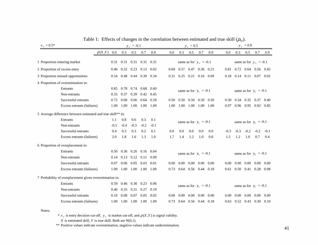
41

x c = 0.5* y c = 0.9

ρ (X ,Y) 0.0 0.3 0.5 0.7 0.9 0.0 0.3 0.5 0.7 0.9 0.0 0.3 0.5 0.7 0.9

1 Proportion entering market 0.31 0.31 0.31 0.31 0.31

2 Proportion of excess entry 0.46 0.32 0.23 0.13 0.02 0.690.57 0.47 0.36 0.21 0.81 0.72 0.64 0.56 0.45

3 Proportion missed opportunities 0.54 0.48 0.44 0.39 0.34 0.31 0.25 0.21 0.16 0.09 0.18 0.14 0.11 0.07 0.02

4 Proportion of overestimation in:

Entrants 0.85 0.78 0.74 0.68 0.60

Non-entrants 0.35 0.37 0.39 0.42 0.45

Successful entrants 0.72 0.68 0.66 0.64 0.59 0.50 0.50 0.500.50 0.50 0.30 0.34 0.35 0.37 0.40

Excess entrants (failures) 1.00 1.00 1.00 1.00 1.00 1.00 1.00 1.00 1.00 1.00 0.97 0.96 0.95 0.92 0.85

5 Average difference between estimated and true skill** in:

Entrants 1.1 0.8 0.6 0.3 0.1

Non-entrants -0.5 -0.4 -0.3 -0.2 -0.1

Successful entrants 0.4 0.3 0.3 0.2 0.1 0.0 0.0 0.0 0.0 0.0 -0.3 -0.3 -0.2 -0.2 -0.1

Excess entrants (failures) 2.0 1.8 1.6 1.3 1.0 1.7 1.4 1.2 1.0 0.6 1.5 1.2 1.0 0.7 0.4

6 Proportion of overplacement in:

Entrants 0.50 0.36 0.26 0.16 0.04

Non-entrants 0.14 0.13 0.12 0.11 0.09

Successful entrants 0.07 0.06 0.05 0.03 0.01 0.00 0.00 0.000.00 0.00 0.00 0.00 0.00 0.00 0.00

Excess entrants (failures) 1.00 1.00 1.00 1.00 1.00 0.73 0.64 0.56 0.44 0.18 0.61 0.50 0.41 0.28 0.08

7 Probability of overplacement given overestimation in:

Entrants 0.59 0.46 0.36 0.23 0.06

Non-entrants 0.40 0.35 0.31 0.27 0.19

Successful entrants 0.10 0.08 0.07 0.05 0.02 0.00 0.00 0.000.00 0.00 0.00 0.00 0.00 0.00 0.00

Excess entrants (failures) 1.00 1.00 1.00 1.00 1.00 0.73 0.64 0.56 0.44 0.18 0.63 0.52 0.43 0.30 0.10

Notes: * x c is entry decision cut-off, y c is market cut-off, and ρ (X ,Y) is signal validity.

X is estimated skill, Y is true skill. Both are N(0,1).** Positive values indicate overestimation, negative values indicate underestimation.

y c = -0.1 y c = 0.5

same as for y c = -0.1 same as for y c = -0.1

same as for yc = -0.1 same as for yc = -0.1

same as for yc = -0.1 same as for yc = -0.1

same as for yc = -0.1 same as for yc = -0.1

same as for yc = -0.1 same as for yc = -0.1

Table 1: Effects of changes in the correlation between estimated and true skill (ρxy).

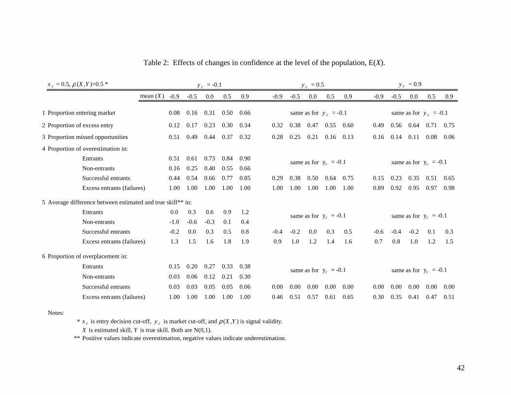
42

x c = 0.5, ρ (X ,Y)=0.5 * y c = 0.9

mean (X ) -0.9 -0.5 0.0 0.5 0.9 -0.9 -0.5 0.0 0.5 0.9 -0.9 -0.5 0.0 0.5 0.9

1 Proportion entering market 0.08 0.16 0.31 0.50 0.66

2 Proportion of excess entry 0.12 0.17 0.23 0.30 0.34 0.320.38 0.47 0.55 0.60 0.49 0.56 0.64 0.71 0.75

3 Proportion missed opportunities 0.51 0.49 0.44 0.37 0.32 0.28 0.25 0.21 0.16 0.13 0.16 0.14 0.11 0.08 0.06

4 Proportion of overestimation in:

Entrants 0.51 0.61 0.73 0.84 0.90

Non-entrants 0.16 0.25 0.40 0.55 0.66

Successful entrants 0.44 0.54 0.66 0.77 0.85 0.29 0.38 0.500.64 0.75 0.15 0.23 0.35 0.51 0.65

Excess entrants (failures) 1.00 1.00 1.00 1.00 1.00 1.00 1.00 1.00 1.00 1.00 0.89 0.92 0.95 0.97 0.98

5 Average difference between estimated and true skill** in:

Entrants 0.0 0.3 0.6 0.9 1.2

Non-entrants -1.0 -0.6 -0.3 0.1 0.4

Successful entrants -0.2 0.0 0.3 0.5 0.8 -0.4 -0.2 0.0 0.3 0.5 -0.6 -0.4 -0.2 0.1 0.3

Excess entrants (failures) 1.3 1.5 1.6 1.8 1.9 0.9 1.0 1.2 1.4 1.6 0.7 0.8 1.0 1.2 1.5

6 Proportion of overplacement in:

Entrants 0.15 0.20 0.27 0.33 0.38

Non-entrants 0.03 0.06 0.12 0.21 0.30

Successful entrants 0.03 0.03 0.05 0.05 0.06 0.00 0.00 0.000.00 0.00 0.00 0.00 0.00 0.00 0.00

Excess entrants (failures) 1.00 1.00 1.00 1.00 1.00 0.46 0.51 0.57 0.61 0.65 0.30 0.35 0.41 0.47 0.51

Notes: * x c is entry decision cut-off, y c is market cut-off, and ρ (X ,Y) is signal validity.

X is estimated skill, Y is true skill. Both are N(0,1).** Positive values indicate overestimation, negative values indicate underestimation.

y c = -0.1 y c = 0.5

same as for y c = -0.1 same as for y c = -0.1

same as for yc = -0.1 same as for yc = -0.1

same as for yc = -0.1 same as for yc = -0.1

same as for yc = -0.1 same as for yc = -0.1

Table 2: Effects of changes in confidence at the level of the population, E(X).

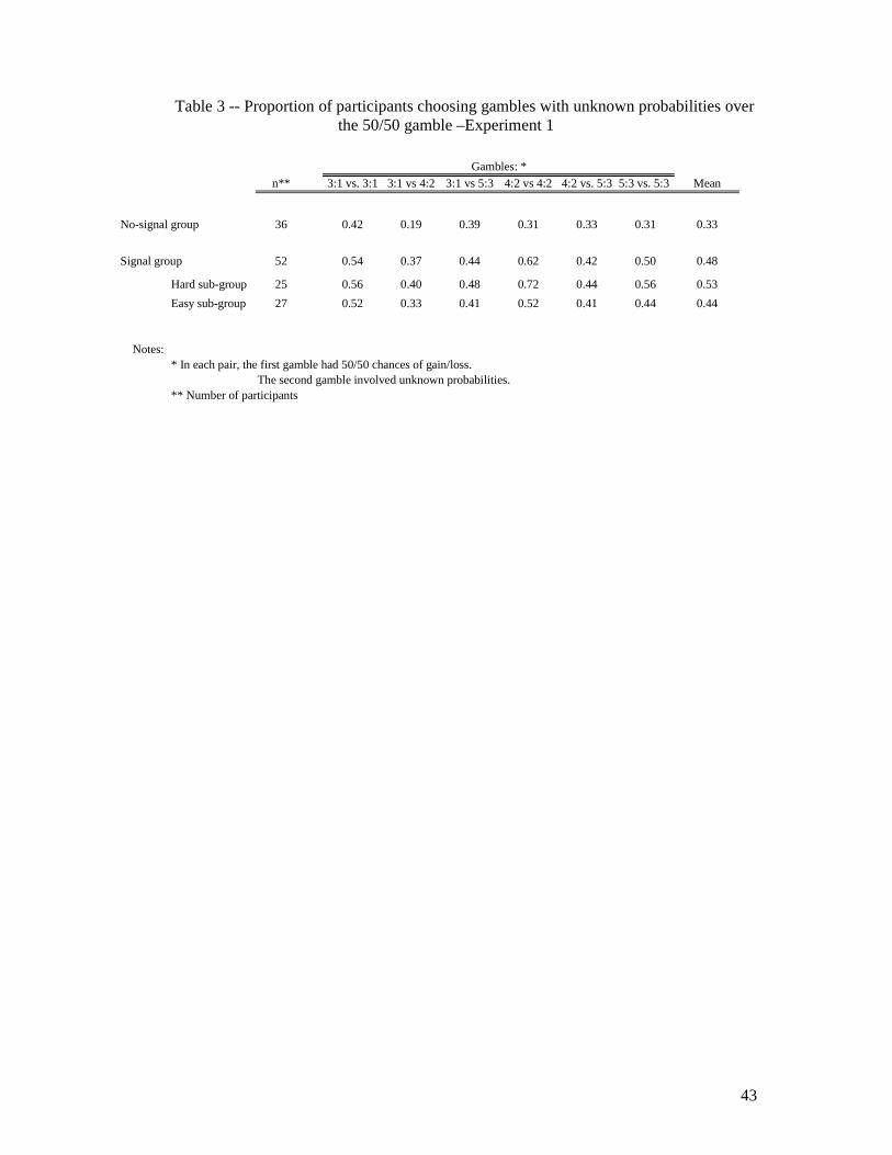
43

n** 3:1 vs. 3:1 3:1 vs 4:2 3:1 vs 5:3 4:2 vs 4:2 4:2 vs. 5:3 5:3 vs. 5:3

36 0.42 0.19 0.39 0.31 0.33 0.31

52 0.54 0.37 0.44 0.62 0.42 0.50

Hard sub-group 25 0.56 0.40 0.48 0.72 0.44 0.56

Easy sub-group 27 0.52 0.33 0.41 0.52 0.41 0.44

Notes: * In each pair, the first gamble had 50/50 chances of gain/loss.

The second gamble involved unknown probabilities. ** Number of participants

Signal group 0.48

0.53

0.44

Mean

No-signal group 0.33

Gambles: *

Table 3 -- Proportion of participants choosing gambles with unknown probabilities over the 50/50 gamble –Experiment 1

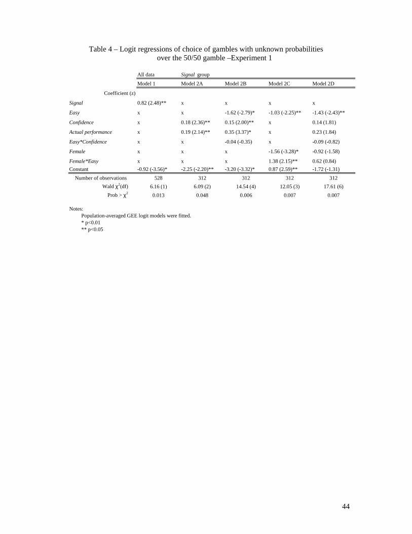
44

All data

Model 1 Model 2A Model 2B Model 2C Model 2D

Coefficient (z)

Signal 0.82 (2.48)** x x x x

Easy x x -1.62 (-2.79)* -1.03 (-2.25)** -1.43 (-2.43)**

Confidence x 0.18 (2.36)** 0.15 (2.00)** x 0.14 (1.81)

Actual performance x 0.19 (2.14)** 0.35 (3.37)* x 0.23 (1.84)

Easy*Confidence x x -0.04 (-0.35) x -0.09 (-0.82)

Female x x x -1.56 (-3.28)* -0.92 (-1.58)

Female*Easy x x x 1.38 (2.15)** 0.62 (0.84)

Constant -0.92 (-3.56)* -2.25 (-2.20)** -3.20 (-3.32)* 0.87 (2.59)** -1.72 (-1.31)

Number of observations 528 312 312 312 312

Wald χ2(df) 6.16 (1) 6.09 (2) 14.54 (4) 12.05 (3) 17.61 (6)

Prob > χ2 0.013 0.048 0.006 0.007 0.007

Notes: Population-averaged GEE logit models were fitted. * p<0.01 ** p<0.05

Signal group

Table 4 – Logit regressions of choice of gambles with unknown probabilities over the 50/50 gamble –Experiment 1

45

Mean % of n correct answers

Chose to continue 52 55Chose not to continue 8 46

Chose to continue 36 39

Chose not to continue 13 27

Note: The differences between choosing and not choosing to continue

are statistically significant in both groups.For signal group, z = 2.106, p = .017.For no-signal group, z = 2.746, p = .003.

No-signal group

Signal group

Table 5 -- Self-selection based on performance in tests – Experiment 1

46

n** 3:1 vs. 3:1 3:1 vs 4:2 3:1 vs 5:3 4:2 vs 4:2 4:2 vs. 5:3 5:3 vs. 5:3

Own ability 31 0.45 0.45 0.61 0.45 0.55 0.48

Hard sub-group 15 0.47 0.40 0.60 0.40 0.47 0.60

Easy sub-group 16 0.44 0.50 0.63 0.50 0.63 0.38

Ability of random other 26 0.50 0.38 0.54 0.46 0.58 0.54

Hard sub-group 13 0.46 0.54 0.69 0.31 0.69 0.62Easy sub-group 13 0.54 0.23 0.38 0.62 0.46 0.46

Notes: * In each pair, the first gamble had 50/50 chances of gain/loss.

The second gamble involved unknown probabilities. ** Number of participants

0.550.45

0.49

0.51

0.50

Result depends on

Gambles: *

Mean

0.50

Table 6 -- Proportion of participants choosing gambles with unknown probabilities over the 50/50 gamble –Experiment 2

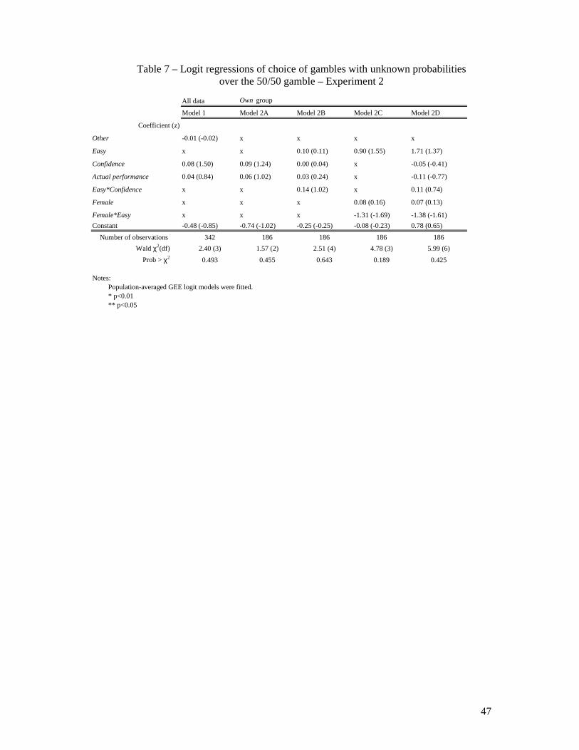
47

All data Own group

Model 1 Model 2A Model 2B Model 2C Model 2D

Coefficient (z)

Other -0.01 (-0.02) x x x x

Easy x x 0.10 (0.11) 0.90 (1.55) 1.71 (1.37)

Confidence 0.08 (1.50) 0.09 (1.24) 0.00 (0.04) x -0.05 (-0.41)

Actual performance 0.04 (0.84) 0.06 (1.02) 0.03 (0.24) x -0.11 (-0.77)

Easy*Confidence x x 0.14 (1.02) x 0.11 (0.74)

Female x x x 0.08 (0.16) 0.07 (0.13)

Female*Easy x x x -1.31 (-1.69) -1.38 (-1.61)

Constant -0.48 (-0.85) -0.74 (-1.02) -0.25 (-0.25) -0.08 (-0.23) 0.78 (0.65)

Number of observations 342 186 186 186 186

Wald χ2(df) 2.40 (3) 1.57 (2) 2.51 (4) 4.78 (3) 5.99 (6)

Prob > χ2 0.493 0.455 0.643 0.189 0.425

Notes: Population-averaged GEE logit models were fitted. * p<0.01 ** p<0.05

Table 7 – Logit regressions of choice of gambles with unknown probabilities over the 50/50 gamble – Experiment 2

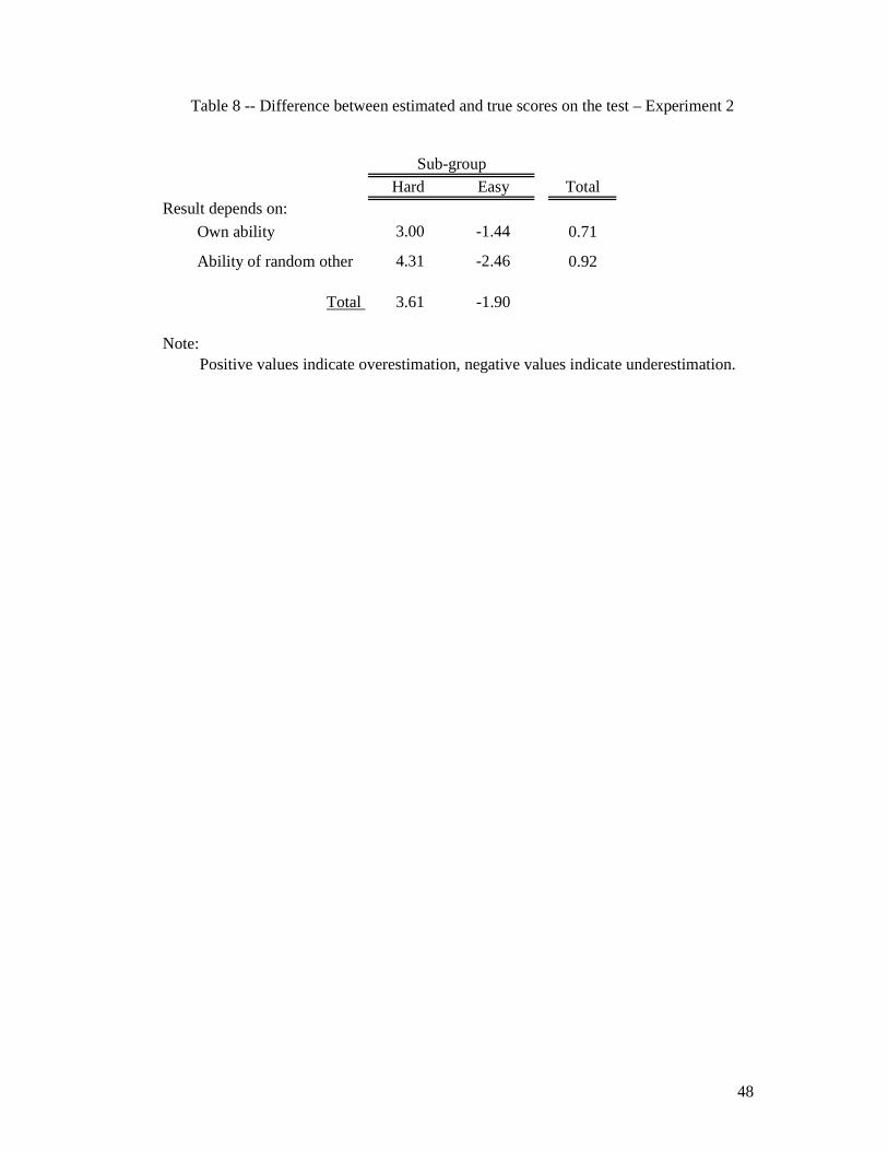
48

Hard Easy Total

Own ability 3.00 -1.44 0.71

Ability of random other 4.31 -2.46 0.92

Total 3.61 -1.90

Note: Positive values indicate overestimation, negative values indicate underestimation.

Result depends on:

Sub-group

Table 8 -- Difference between estimated and true scores on the test – Experiment 2

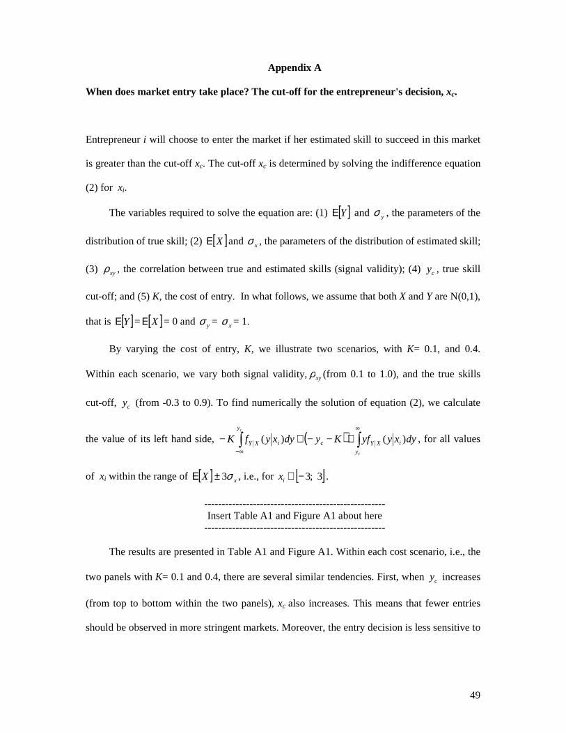
49

Appendix A

When does market entry take place? The cut-off for the entrepreneur's decision, xc.

Entrepreneur i will choose to enter the market if her estimated skill to succeed in this market

is greater than the cut-off xc. The cut-off xc is determined by solving the indifference equation

(2) for xi.

The variables required to solve the equation are: (1) [ ]YΕ and yσ , the parameters of the

distribution of true skill; (2) [ ]XΕ and xσ , the parameters of the distribution of estimated skill;

(3) xyρ , the correlation between true and estimated skills (signal validity); (4) cy , true skill

cut-off; and (5) K, the cost of entry. In what follows, we assume that both X and Y are N(0,1),

that is [ ]YΕ = [ ]XΕ = 0 and yσ = xσ = 1.

By varying the cost of entry, K, we illustrate two scenarios, with K= 0.1, and 0.4.

Within each scenario, we vary both signal validity,xyρ (from 0.1 to 1.0), and the true skills

cut-off, cy (from -0.3 to 0.9). To find numerically the solution of equation (2), we calculate

the value of its left hand side, ( ) ∫∫∞

∞−

+−−+−c

c

y

iXYc

y

iXY dyxyyfKydyxyfK )()( , for all values

of xi within the range of [ ] xX σ3±Ε , i.e., for [ ]3;3−∈ix .

---------------------------------------------------- Insert Table A1 and Figure A1 about here

----------------------------------------------------

The results are presented in Table A1 and Figure A1. Within each cost scenario, i.e., the

two panels with K= 0.1 and 0.4, there are several similar tendencies. First, when cy increases

(from top to bottom within the two panels), xc also increases. This means that fewer entries

should be observed in more stringent markets. Moreover, the entry decision is less sensitive to

50

cy when signal validity, xyρ , is larger (within each panel, compare columns on the right and

left).

Second, when signal validity,xyρ , increases (from left to right within the panels), xc

decreases (i.e., more entry is observed) given that the market is sufficiently “stringent”

(observe the results in bold within each panel, corresponding to larger values of cy ). For less

stringent markets (observe the rest of the table), the effect of xyρ on xc is the opposite. That

is, less entry is observed when xyρ increases. In addition, the critical point of cy at which

the effect of xyρ on xc reverses depends on the cost of entry decision (K). When K = 0.1

(i.e., panel on left), the positive effect of xyρ on xc is observed at lower levels of cy – starting

at cy = 0.3. When the cost of entry, K, increases to 0.4 (i.e., panel on right), the positive effect

of xyρ on xc is observed starting at cy = - 0.1.

Figure A1 illustrates the interaction between cy and the effect of xyρ on xc . The curves

depict the entry cut-off, xc, as a function of xyρ . There is one curve corresponding to each

level of cy . Note that for larger values of cy (i.e., more stringent markets), xc decreases as a

function of xyρ . That is, in these situations increasing signal validity leads to more market

entry.

Finally, the overall effect of a larger cost of entry, K, is to increase the decision cut-off

xc, and, therefore, to decrease entry.

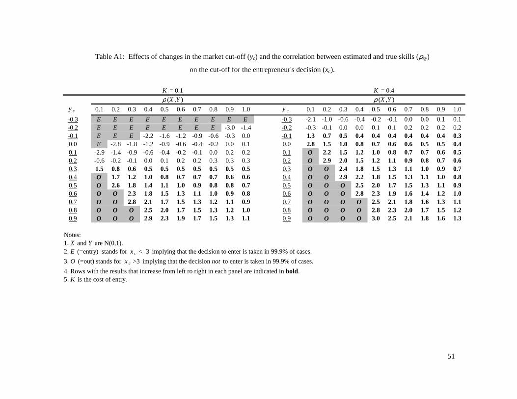
51

y c 0.1 0.2 0.3 0.4 0.5 0.6 0.7 0.8 0.9 1.0 y c 0.1 0.2 0.3 0.4 0.5 0.6 0.7 0.8 0.9 1.0

-0.3 E E E E E E E E E E -0.3 -2.1 -1.0 -0.6 -0.4 -0.2 -0.1 0.0 0.0 0.1 0.1-0.2 E E E E E E E E -3.0 -1.4 -0.2 -0.3 -0.1 0.0 0.0 0.1 0.1 0.2 0.2 0.2 0.2-0.1 E E E -2.2 -1.6 -1.2 -0.9 -0.6 -0.3 0.0 -0.1 1.3 0.7 0.5 0.4 0.4 0.4 0.4 0.4 0.4 0.30.0 E -2.8 -1.8 -1.2 -0.9 -0.6 -0.4 -0.2 0.0 0.1 0.0 2.8 1.5 1.0 0.8 0.7 0.6 0.6 0.5 0.5 0.40.1 -2.9 -1.4 -0.9 -0.6 -0.4 -0.2 -0.1 0.0 0.2 0.2 0.1 O 2.2 1.5 1.2 1.0 0.8 0.7 0.7 0.6 0.50.2 -0.6 -0.2 -0.1 0.0 0.1 0.2 0.2 0.3 0.3 0.3 0.2 O 2.9 2.0 1.5 1.2 1.1 0.9 0.8 0.7 0.60.3 1.5 0.8 0.6 0.5 0.5 0.5 0.5 0.5 0.5 0.5 0.3 O O 2.4 1.8 1.5 1.3 1.1 1.0 0.9 0.70.4 O 1.7 1.2 1.0 0.8 0.7 0.7 0.7 0.6 0.6 0.4 O O 2.9 2.2 1.8 1.5 1.3 1.1 1.0 0.80.5 O 2.6 1.8 1.4 1.1 1.0 0.9 0.8 0.8 0.7 0.5 O O O 2.5 2.0 1.7 1.5 1.3 1.1 0.90.6 O O 2.3 1.8 1.5 1.3 1.1 1.0 0.9 0.8 0.6 O O O 2.8 2.3 1.9 1.6 1.4 1.2 1.00.7 O O 2.8 2.1 1.7 1.5 1.3 1.2 1.1 0.9 0.7 O O O O 2.5 2.1 1.8 1.6 1.3 1.10.8 O O O 2.5 2.0 1.7 1.5 1.3 1.2 1.0 0.8 O O O O 2.8 2.3 2.0 1.7 1.5 1.20.9 O O O 2.9 2.3 1.9 1.7 1.5 1.3 1.1 0.9 O O O O 3.0 2.5 2.1 1.8 1.6 1.3

Notes:1. X and Y are N(0,1).2. E (=entry) stands for x c < -3 implying that the decision to enter is taken in 99.9% of cases.

3. O (=out) stands for x c >3 implying that the decision not to enter is taken in 99.9% of cases.

4. Rows with the results that increase from left ro right in each panel are indicated in bold. 5. K is the cost of entry.

K = 0.1 K = 0.4

ρ (X ,Y) ρ (X ,Y)

Table A1: Effects of changes in the market cut-off (yc) and the correlation between estimated and true skills (ρxy)

on the cut-off for the entrepreneur's decision (xc).

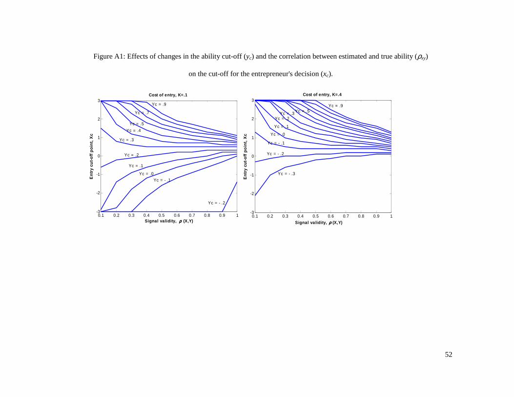
52

0.1 0.2 0.3 0.4 0.5 0.6 0.7 0.8 0.9 1-3

-2

-1

0

1

2

3

Signal validity, (X,Y)

En

try

cut-

off

po

int,

Xc

Cost of entry, K=.1

Yc = - .2

Yc = - .1

Yc = .9

Yc = .0

Yc = .1

Yc = .2

Yc = .3

Yc = .4

Yc = .5

Yc = .7

ρρρρ0.1 0.2 0.3 0.4 0.5 0.6 0.7 0.8 0.9 1

-3

-2

-1

0

1

2

3

En

try

cut-

off

po

int,

Xc

Cost of entry, K=.4

Yc = - .3

Yc = - .1

Yc = .0

Yc = .1

Yc = .2Yc = .3

Yc = .9Yc = .5

Yc = - .2

Signal validity, (X,Y)ρρρρ

Figure A1: Effects of changes in the ability cut-off (yc) and the correlation between estimated and true ability ( ρxy)

on the cut-off for the entrepreneur's decision (xc).

53

Appendix B

Experimental instructions

(Translated from Spanish)

Thank you for participating in this experiment about decision making behavior that is part of

a research project. What you earn will depend on your skill as well as the skill of your peers.

Please follow the instructions carefully. You have the opportunity to gain more than the 3 €

that are already assured by your participation in the experiment. As from now until the end of the

experiment you are not allowed to talk amongst yourselves. Raise your hand if you have a question

and one of the instructors will attend to you. Please, do not ask in a loud voice. Thank you. The

rules are the same for all participants.

Experimental procedure

The experiment consists of 3 phases.

Phase 1 consists of a set of 20 general knowledge questions. Each question is independent of

the others. For each question, you have to decide between A and B.∗ Your earnings at the end of

the experiment depend on the accuracy of your responses. You will earn 0.25 € for each question

that you answer correctly.

Phase 2 is optional. You can

• claim all the money that you have earned up to this point (that is, the initial 3 € and what

you earned from the questionnaire) and go directly to Phase 3 or

• modify your earnings by way of considering 12 pairs of gambles ( 2 groups of 6 pairs) and

for each pair choosing one of two possible options. You have to decide between Option 1 and

Option 2 for the 12 pairs of gambles. The gambles give you the chance to gain or lose certain

sums of money. Each gamble involves different amounts of euros: you can gain between 3 and 5

∗ These are the instructions for the “easy” experimental condition. In the “hard” condition, participants had to choose

one of five possible answers.

54

euros and lose between 1 and 3 euros. The chances of winning or losing in these gambles can be

the same for all the participants or depend on your own skill – compared to the skill of your peers

– in the questionnaire of Phase 1.18

After you have chosen between each pair of gambles, one of the gambles that you have

chosen will be selected and you will face the consequences of that gamble. The money depending

on the outcome of this gamble will be added to (if you win) or subtracted from (if you lose) your

earnings from Phase 1 (that is the initial 3 € plus your earnings from the questionnaire). Thus,

when you choose each gamble, remember that it can be the one that is selected and that your final

earnings can depend on its outcome!

In Phase 3, we ask you to complete a general questionnaire.

Phase 1

This phase consists of 20 multiple-choice questions. For all the questions you have to decide

between A and B. (See last footnote.*) Your earnings depend on the correctness of your responses:

you will receive 0.25 € for each correct answer. You have a maximum of 45 seconds to give each

response: if you indicate no choice between A and B, your answer will be considered wrong.

At the end of this questionnaire, we will ask you to estimate the number of questions you

answered correctly.

Phase 2

This phase is optional. You can decide between:

(a) keeping all the money you have earned up until now (that is the initial 3€ plus your

earnings from the questionnaire) and go directly to Phase 3; or

18 In the present paper, we in fact only analyze the results of the first six choices made. In the actual experiment,

participants were provided feedback on their questionnaire test scores after completing their first six choices.

55

(b) participate in a game where you can influence your own earnings by way of choosing

between two gambles, called Option 1 and Option 2, for 12 pairs of gambles. The gambles give

you the possibility of winning between 3 and 5 euros and losing between 1 and 3 euros. Your

probability of winning or losing in these gambles can be the same as the probabilities for your

peers (Option 1) or can depend on how well you answered the questionnaire in Phase 1 relative to

your peers (Option 2). Your probability of winning will be equal to your percentile. Specifically,

if you were at the 90th percentile of the distribution of points, your probability of winning would be

0.90; if you were at the 50th percentile of the distribution of points, your probability of winning

would be 0.50 (that is at the middle); if you were at the 30th percentile of the distribution of points,

your probability of winning would be 0.30; and so on.

Remember that your percentile indicates the percentage of participants who obtained fewer

points than you!

All the participants have the same opportunity.

If you choose (a), go to Phase 3.

If you choose (b), you have to decide between Option 1 and Option 2 for each pair of

gambles. At the end, one of the gambles that you have chosen will be drawn at random and your

final earnings will depend on the outcome of that gamble.

Phase 3

In the third phase we ask you to complete a general questionnaire. One of the instructors will

give it to you.

When you have completed the general questionnaire of Phase 3, we will give you the sum

that you have earned in Phases 1 and 2 plus the fixed fee of 3€.

Thank you for your participation!