Progress and challenges in short- to medium-range coupled prediction12

GB Brassington1, MJ Martin2, HL Tolman3, S Akella4, M Balmeseda5, CRS Chambers6, JA3Cummings7, Y Drillet8, PAEM Jansen5, P Laloyaux5, D Lea2, A Mehra3, I Mirouze2, H Ritchie9,4G Samson8, PA Sandery1, GC Smith10, M. Suarez4 and R Todling45

61CAWCR, Australian Bureau of Meteorology, Melbourne, Australia72UK Met Office, Exeter, UK83Environmental Modeling Center, NOAA/NCEP, USA94Global Modeling and Assimilation Office, NASA, Maryland, USA105ECMWF, Reading, UK116University of Melbourne, Melbourne, Australia127NRL, Monterey, USA138Mercator-Ocean, Toulouse, France149Environment Canada, Dartmouth, Canada1510Environment Canada, Dorval, Canada16

17Synopsis18

19The availability of GODAE Oceanview-type ocean forecast systems provides the opportunity20to develop high-resolution, short- to medium-range coupled prediction systems. Several21groups have undertaken the first experiments based on relatively unsophisticated22approaches. Progress is being driven at the institutional level targeting a range of applications23that represent their respective national interests with clear overlaps and opportunities for24information exchange and collaboration. These include general circulation, hurricanes, extra-25tropical storms, high-latitude weather and sea-ice forecasting as well as coastal air-sea26interaction. In some cases, research has moved beyond case and sensitivity studies to27controlled experiments to obtain statistically significant metrics.28

29Lead author’s biography30Gary Brassington is a Principal Research Scientist at the Australian Bureau of Meteorology31(ABOM). He leads the research and development team for operational ocean forecasting32within the ABOM. He is Chair of the WMO-IOC Joint Technical Commission for33Oceanography and Marine Meteorology (JCOMM) Expert Team for Operational Ocean34Forecasting and Co-chair of the GODAE OceanView task team on Short- to Medium-Range35Coupled Prediction.36

37Introduction38

39The Global Ocean Data Assimilation Experiment (GODAE)1 (Bell et al., 2010) succeeded in40demonstrating the feasibility of constraining a mesoscale ocean model to perform routine41analyses and forecasts through the data assimilation of the Global Ocean Observing System42(GOOS). Development of ocean forecasting has since been consolidated and extended under43the GODAE OceanView (GOV)2 (Schiller and Dombrowsky, 2014). There are now several44agencies and centres supporting first- or second-generation global and basin-scale pre-45operational and operational ocean prediction systems as described in this special issue.46These systems provide routine estimates of the ocean state for both nowcasts and short-47range forecasts. The performance has been shown to have sufficient skill in the upper ocean48to positively impact a wide range of ocean specific applications (e.g., defence3, search and49rescue4 etc). Unlike waves where there is a very tight relationship between the skill of the50winds and the skill of the waves, the oceans inertia and heat capacity leads to a circulation51that has unique time and space scales that is related more to the integrated (time history) of52surface fluxes of mass, heat and momentum rather than an immediate response to the53atmospheric weather. Important exceptions apply, however, for example over the continental54shelf and in the turbulent surface layer where the time and space scales are a blend between55the atmosphere, waves, sea-ice and ocean systems. These regions also correspond to the56highest biological and human activity and the majority of applications for ocean prediction.57Therefore, minimising errors in the applied stress and fluxes will have a high yield for the58benefit of ocean prediction.59

60

https://ntrs.nasa.gov/search.jsp?R=20150000788 2018-06-24T23:44:06+00:00Z

The availability of GOOS and GOV-type forecast systems provides the opportunity to develop61high-resolution, short- to medium-range coupled prediction systems (SMRCP) for the earth62system. Making progress in this field is a significant challenge due to the added complexity in63all areas of development, coupled frameworks, coupled modelling, coupled initialisation,64observational requirements (including experimental campaigns) and large and more diverse65teams of scientific experts. There have been several vision papers5,6 (Brassington, 2009;66Brunet et al., 2010) and workshops relevant to this area driven predominantly by the needs of67Numerical Weather Prediction (NWP) at ECMWF7 and followed on by the UK Met Office8.68The GOV science team recognised the need to explore the potential benefit to both oceanic69and atmospheric prediction through the use of GOV-type system in coupled prediction70research. The Short- to Medium-Range Coupled Prediction Task Team (SMRCP-TT) was71set-up at the beginning of GOV in 2009 to coordinate an information exchange for the new72developments beginning at some centres in the area of coupled prediction on the medium-73range. The scope and objectives of the TT were defined to focus on issues of direct relevance74to GOV activities and expertise, while recognising that the area of coupled prediction requires75inputs from a number of other disciplines coordinated by other international bodies. The76scope of the TT was therefore defined as covering: SMRCP of the ocean, marine boundary77layer, surface waves and sea-ice; on global and regional scales; to pursue the development78of coupled prediction systems for improving and extending ocean/wave/sea-ice state79estimation and forecast skill; with specific coupling focii: ocean-wave-atmosphere and ocean-80sea-ice-atmosphere. A key achievement of this group was to initiate a linkage with the81Working Group for Numerical Experimentation and to convene a Joint GOV-WGNE workshop82was held March 2013, Washington DC, USA (https://www.godae-83oceanview.org/outreach/meetings-workshops/task-team-meetings/coupled-prediction-84workshop-gov-wgne-2013/).85

86Land surface modelling for atmospheric forecasting has a longer history9,10,11 (de Rasnay et al872014, Ek et al 2003, Pitman 2003) than atmosphere-ocean forecasting and predates the88development of earth modelling frameworks. Land-surface schemes were first introduced as89a sub-model and embedded within the atmospheric model software. As land-surface models90have increased in sophistication these have matured into stand alone models. This91component of the earth system is beyond the scope of this paper.92

93Earth system modelling has evolved through specialist communities for each of the major94components. The requirement to develop coupled earth system models, initially for climate95applications, has seen the development of computational frameworks to permit component96models to be coupled through the synchronous and efficient exchange of fluxes for high97performance computational environments. The US government agencies have adopted the98Earth System Modeling Framework (ESMF; http://www.earthsystemmodeling.org) as the99basic architecture for coupling models. ESMF allows for the passing of variables among the100models in memory and organises horizontal interpolation between the fields in the different101model components via an exchange grid. On top of ESMF, the National Unified Operational102Prediction Capability (NUOPC; http://www.weather.gov/nuopc) standardises ESMF interfaces103further to promote plug-compatability of models in couplers and passes information through104separate flux computation modules. NUOPC is a consortium of the Navy, NOAA, and Air105Force modelers and their research partners. Similar efforts have been undertaken within106Europe such as the Ocean Atmosphere Sea Ice Soil coupler version 4 (OASIS4)12 (Redler et107al., 2010). Achieving all of the requirements for earth system frameworks including platform108independence, interoperability, scalability and others has been elusive but major progress109has been achieved in the past decade of development. Availability of these frameworks has110aided and accelerated research and development for SMR applications.111

112In this paper we summarise some of the progress being made within national/international113centres in section 2, identify a selection of applications that demonstrate the impact of114coupling in section 3; provide a brief overview of some of the known challenges in section 4115and conclude with a discussion on the future outlook for this area.116

117Progress by national programs118

119

Coupling of the ocean, atmosphere and sea-ice has been developed over a number of years120for seasonal and longer-range prediction, but it has been a relatively new area for the121development of SMRCP forecasts. During the past 5 years research programs have emerged122within the leading centres: Bureau of Meteorology, Australia; Met Office, United Kingdom123(UK); National Oceanic and Atmospheric Administration (NOAA)/National Centers for124Environmental Prediction(NCEP), United States of America (USA); European Centre for125Medium-range Weather Forecasting (ECMWF); Naval Research Laboratory, USA;126Environment Canada, Canada; Mercator-Océan/Météo France, France; and NASA, USA. The127present systems being applied to study the impacts of coupling are summarised in Tab 1 and128outlined below in more detail. The modelling systems range from regional to global and are129relatively sophisticated given the availability of earth-system frameworks from the climate130community, an example of which is shown in Fig 1. These systems however use relatively131unsophisticated approaches to data assimilation where the Background error covariances are132uncoupled or weakly coupled and a variety of approaches are adopted to initialise the133coupled model.134

135Bureau of Meteorology, Australia136

137The Australian Bureau of Meteorology has pursued research into the impact of coupling138between the OceanMAPS forecast system and operational NWP systems using a regional139nested framework referred to as CLAM (Coupled Limited Area Model). CLAM is based on the140UK Met Office Unified Model (UM) version 6.413 (Davies et al., 2005), the Ocean Atmosphere141Sea Ice Soil coupler version 4 (OASIS4)12 (Redler et al., 2010) and MOM4p114 (Griffies,1422009). The NWP system known as the Australian Community Climate Earth System143Simulator (ACCESS), comprises a suite of atmospheric model configurations from global to144regional using four-dimensional variational data assimilation (4DVAR), which was developed145for the UM15 by Rawlins et al. (2007). The ocean forecast system is known as the Ocean146Model, Analysis and Prediction System (OceanMAPS; Brassington et al., 2012)16, which uses147an eddy-resolving ocean model and an ensemble optimal interpolation scheme called the148Bluelink Ocean Data Assimilation System (BODAS; Oke et al., 2008)17.149

150The CLAM infrastructure has been used both in Tropical Cyclone (TC) forecasting research18151(Sandery et al., 2010) and in ACCESS-RC (RC stands for the operational regional152atmospheric model (ACCESS-R) coupled to a matching nested regional ocean model), an153application of CLAM designed to study the impact of coupling on regional ocean and weather154prediction. CLAM was recently used to develop an ensemble coupled initialisation method155using cyclic bred vectors19 (Sandery and O’Kane, 2014). Results using ACCESS-RC have156found that ocean-atmosphere coupling offers improvements in the atmospheric model sea157surface temperature (SST) boundary condition in the tropics and in significant to severe158weather events at three day lead time compared to persisting an SST analysis initial159condition. CLAM offered a significant improvement in the forecast of rainfall for the Brisbane160flooding event of 201120 (Barras and Sandery, 2012). Whilst ACCESS-RC is nested inside161data assimilating component systems, until recently it has not explicitly had its own data162assimilation.163

164A collaborative project between the Bureau of Meteorology and the University of Melbourne165funded by the Lloyd’s Register Foundation is examining the impact of coupling on the166prediction of marine extremes. This research makes use of a multiply nested Weather167Research and Forecasting model (WRF)21 with resolution to resolve convective storm168development and ocean surface conditions from OceanMAPS16 and regional/nested ocean169model simulations based on MOM4p1. Initial focus has been on the sensitivity to the170mesoscale SST gradients of storm development22 to justify further research into the coupled171response.172

173Met Office, UK174

175The development of coupled predictions for short-range forecasting at the UK Met Office is176being undertaken through a number of projects, all using versions of the Hadley Centre177Global Environment Model version 3 (HadGEM3). HadGEM3 combines the Met Office Unified178Model (UM) atmosphere23,24 (Walters et al., 2011; Brown et al., 2012) and JULES land179

surface model coupled using the OASIS coupler to the Nucleus for European Modelling of the180Ocean (NEMO)25 (Madec 2008) and the CICE sea-ice model26 (Hunke and Lipscombe 2010).181The assessment of the impact of coupled predictions over atmosphere- and ocean-only182predictions demonstrated a positive impact on 1-15 day atmosphere forecasts from coupling183most notably in the Tropics27. The HadGEM3 model is running operationally on a daily basis184to produce seasonal forecasts in the GloSea5 system28 (MacLachlan et al. 2014). The ocean185component of these operational coupled forecasts have been compared with the operational186Forecast Ocean Assimilation Model (FOAM)29 (Blockley et al. 2014) ocean forecasts for the187first 7-days of the forecast, and shown to be of comparable accuracy. The ocean fields from188these coupled forecasts are now being provided operationally to users through the MyOcean189project (www.myocean.eu.org).190The assessment, development and operational running of the coupled forecasts described191above have all been carried out using initial conditions generated separately for the192atmosphere and land from the Met Office NWP analysis, ocean and sea-ice from the FOAM193analysis. A “weakly” coupled data assimilation (DA) system is being developed in parallel with194the above work in order to provide improved initial conditions for the coupled forecasts (see195Tab 2). For this work, and the work described above, the UM is run at 60km horizontal196resolution on 85 vertical levels, NEMO is at 25km horizontal resolution on 75 vertical model197levels, and CICE is run with 5 thickness categories. The coupled model is corrected using two198separate 6-hour window DA systems: a 4DVAR system for the atmosphere assimilating the199standard set of atmosphere data15 (Rawlins et al. 2007) with associated soil moisture content200nudging and snow analysis schemes on the one hand, and a 3DVAR First Guess at Analysis201Time (FGAT) system NEMOVAR30 (Waters et al 2013) for the ocean and sea-ice (using in202situ SST, temperature and salinity profile, satellite SST, satellite altimeter, and sea ice203concentration data). The background information in the DA systems comes from a previous 6-204hour forecast of the coupled model. Given the short time window the coupling frequency was205increased from the default 3 hours to 1 hour. This also has a particular benefit in improving206the model representation of the diurnal cycle.207

208NOAA/NCEP, USA209

210Whereas coupled modelling has been part of the operational model suite at NCEP (and in a211broader scale within NOAA) for almost a decade, efforts of systematic model coupling have212been taking off only in the last few years.213

214Historically, coupled modelling has been used in tropical cyclone (hurricane in the US)215modelling and in seasonal modelling. In hurricane modelling, the impact of ocean temperature216and heat content on intensification has been long recognised, and operational GFDL and217HWRF models have included an active ocean component for more than a218decade31,32,33,34,35,36,37 (e.g., Bender et al., 1993, 2007, Bender and Ginis, 2000, Yablonsky219and Ginis, 2008, 2009, Tallapragada et al., 2013, Kim et al., 2014). Similar approaches have220been used by the US Navy38 (e.g., Hodur, 1997). Experimental coupled hurricane modelling221has also focused on the air-sea interactions including explicit modelling of wind waves in a222coupled system39,40,41,42 (e.g., Moon et al., 2004, 2007, Fan et al, 2009, and academia (e.g.,223Chen et al. 2007). The wave coupling has not (yet) made its way into operations at NCEP, but224the results of the coupling experiments have contributed to much improved surface flux225parameterisations in the coupled ocean-atmosphere models for hurricanes.226

227Coupled modelling has also been the staple of reanalysis and seasonal forecasting at NCEP.228The most recent reanalysis43 (Saha et al. 2010) and the presently operational Climate229Forecast System (CFS-v2, Saha et al., 2014)44, represents a coupled atmosphere – ocean –230land – ice system, albeit with uncoupled data assimilation efforts for all sub-systems. Land231surface models within atmospheric models, has a fairly long history at NCEP for mesoscale232models10 (e.g., Ek et al., 2003), and is in operations in the global and seasonal models45,46233(e.g., Wei et al., 2012, Meng et al., 2012). Since the underlying land model is a full model that234has been used as a standalone model, this is affectively an example of coupled modelling,235although historically this modelling has not been labeled as such.236

237

Within NOAA, ESMF and the NUOPC layer are used in NOAA's Environmental Modeling238System (NEMS). NEMS now incorporates, and is the model driver for, most weather models239at NCEP. Ocean, ice and wave models such as HYCOM, MOM5, CICE, GFDL ice model240and WAVEWATCH III are now available in NEMS, or will be available in late 2014. This241provides NOAA with a set of well-defined building blocks for coupling in general.242

243ECMWF, Europe244

245Developments of coupled forecasting systems at ECMWF follow three lines: improvement in246the modelling of air-sea interaction processes, use of coupled ocean-wave-seaice-247atmosphere models in forecasts at all time ranges (medium range, monthly and seasonal),248and the development of ocean-atmosphere coupled data assimilation systems.249

250Growing ocean waves play a role in the air-sea momentum and heat transfer while breaking251ocean waves affect the upper ocean mixing. Ocean waves also provide an additional force252on the mean circulation, the so-called Stokes-Coriolis force. Furthermore, the surface stress253felt by the mean circulation is the total surface stress applied by the atmosphere minus the254net stress going into the waves. Finally, momentum transfer and the sea state are affected by255surface currents. These effects have been introduced in the ECMWF coupled forecasting256system, and are currently being assessed. The impact of breaking waves in the upper ocean257mixing has been shown to have a large impact on the prediction of SST. Janssen et al 201347258provide a detailed description on the representation of these effects, and illustrate their impact259on ocean-only simulation and on coupled forecasts.260

261Since the thermodynamical coupling is thought to be important in the modeling of tropical262convection the coupled ocean-atmosphere-wave model, traditionally used only for the263monthly and seasonal forecasts ranges, is also used in the medium range weather prediction,264since November 2013. Results show that the coupled model provides better forecasts of the265tropical atmosphere, improved forecasts of the MJO, and has impacts on the representation266of slow-moving tropical cyclones47 (Janssen et al 2013).267

268ECMWF has implemented a coupled ocean-wave-atmosphere data assimilation system269called CERA (Coupled ECMWF ReAnalysis). This system uses the ECMWF coupled model270with an incremental variational approach to assimilate simultaneously ocean and atmospheric271observations. The ultimate purpose is to generate better and self-consistent coupled states272for atmosphere-ocean reanalysis. The CERA system is based on an incremental variational273approach where the ECMWF coupled system is used to compute the misfits with ocean and274atmospheric observations in the outer loop. The ocean and the atmosphere share a common27524-hour assimilation window but still run separate inner loops. The ocean increment is276computed using a 3DVAR method based only on the first misfit computation, while the277computation of the atmospheric increment is based on a 4DVAR approach with two outer278iterations. An SST nudging scheme has been developed in the ocean model to avoid the279rapidly-growing bias of the coupled model.280

281Naval Research Laboratory, USA282

283The US Navy is actively operating and developing coupled forecasting systems on global and284regional scales. For regional scales the air-ocean version of the Coupled Ocean Atmosphere285Mesoscale Prediction System (COAMPS)48(Holt et al., 2011) was declared operational in2862011. Air-ocean coupled model runs are routinely performed at the Navy operational287production centres. The COAMPS system is being updated to include coupling of a wave288model49 (Allard et al. 2012). Operational implementation of a regional, air-ocean-wave289coupled system is planned for 2015. Fig 1 shows the coupling interfaces for the fully coupled290COAMPS. The various components of the coupled system are integrated through ESMF.291A coupled global ocean/ice model will be operational in 2014. At the present time, the292coupled ocean/ice model is restricted to the Arctic Ocean (Arctic Cap Nowcast Forecast293System). The new global ocean/ice system will produce nowcasts and 120-hour coupled294model forecasts of ice fields from CICE and ocean fields from HYCOM at 1/12 degree295resolution.296

A coupled global atmosphere/ocean/ice/wave/land prediction system providing daily297predictions out to 10-days and weekly predictions out to 30-days is being developed as a298Navy contribution to the Earth System Prediction Capability (ESPC). A schematic of the299system is shown in Fig 2. Initial Operational Capability (IOC) is targeted for 2018. ESPC is a300national partnership among federal agencies and the research community in the U.S. to301develop the future capability to meet the grand challenge of environmental predictions in the302rapidly changing environment. The system will be based on NUOPC and use analysis fields303of each component as initial conditions and make daily forecasts out to 10-days. Throughout304each weekly cycle, predictions out to 30-days will be constructed.305Data assimilation in coupled COAMPS currently consists of independent 3DVar analyses in306the ocean and atmosphere. The first-guess fields (6- or 12-hour forecasts) for each fluid are307obtained from the coupled model state. This assimilation configuration is referred to as308weakly-coupled. A strongly coupled 4DVAR assimilation system for both the ocean and309atmospheric components of COAMPS is under development. In this scheme separate3104DVAR assimilation systems of the atmosphere and ocean models will be linked through the311existing coupling terms and ESMF coupling infrastructure in COAMPS. The tangent linear312and adjoint components of these coupling terms will be developed and used to minimise the313cost function of the coupled system. The state and observation vectors in the assimilation will314be extended to include both ocean and atmosphere variables.315For the global ESPC coupled model a hybrid version of the Navy Coupled Ocean Data316Assimilation (NCODA) 3DVAR50(Cummings and Smedstad, 2013) has been developed. The317hybrid covariances are a weighted average of the static multivariate correlations already in318use and a set of coupled covariances derived from a coupled model ensemble. The coupled319model ensemble is created using the Ensemble Transform (ET) technique in both the ocean320and atmosphere. One idea being explored is to form a combined ocean/atmospheric321innovation vector that is assimilated in independent hybrid 3DVAR-ocean and 4DVAR-322atmosphere assimilation systems using ensemble-based coupled covariances.323An observation operator has been developed for direct assimilation of satellite SST radiances324using radiative transfer modeling51 (Cummings and Peak, 2014). The radiance assimilation325operator has been integrated into NCODA 3DVAR. The operator takes as input prior326estimates of SST from the ocean forecast model and profiles of atmospheric state variables327(specific humidity and air temperature) known to affect satellite SST radiances from the NWP328model. Observed radiances are simulated using a fast radiative transfer model, and329differences between observed and simulated radiances are used to force a SST inverse330model. The inverse model outputs the change in SST that takes into account the variable331temperature and water vapour content of the atmosphere at the time and location of the332satellite radiance measurement. Direct assimilation of satellite SST radiances is an example333of coupled data assimilation. An observation in one fluid (atmospheric radiances) creates an334innovation in a different fluid (ocean surface temperature). The observed radiance variables335depend on both ocean and atmosphere physics. The radiance assimilation operator is ideally336suited for coupled ocean/atmosphere forecasting systems where the atmosphere and ocean337states have evolved consistently over time.338

339Environment Canada340

341The Canadian Operational Network of Coupled Environmental PredicTion Systems342(CONCEPTS) including Mercator-Océan participation (France) is providing a framework for343research and operations on coupled atmosphere-ice-ocean (AIO) prediction. Operational344activity is based on coupling the Canadian atmospheric Global Environmental Multi-scale345(GEM) model with the Mercator system based on the NEMO, together with the CICE sea ice346model. Within CONCEPTS two main systems are under development: a short-range regional347coupled prediction system and a global coupled prediction system for medium- to long-range348applications52 (Smith et al., 2013).349

350A fully coupled AIO forecasting system for the Gulf of St. Lawrence (GSL) has been351developed53 (Faucher et al., 2010) and has been running operationally at the Canadian352Meteorological Centre (CMC) since June 2011. The original ocean-ice component of this353system54 (Saucier et al., 2003) is currently being replaced by NEMO and CICE. This system354

is also the basis for the development of an integrated marine Arctic prediction system in355support of Canadian METAREA monitoring and warnings. Specifically, a multi-component356(atmosphere, land, snow, ice, ocean, wave) regional high resolution marine data assimilation357and forecast system is being developed for short-term predictions of near surface358atmospheric conditions, sea ice (concentration, pressure, drift, ice edge), freezing spray,359waves and ocean conditions (temperature and currents).360

361More recently a coupled global AIO system is under development. The first step was the362development of the Global Ice-Ocean Prediction System (GIOPS)55 Smith et al. (2014).363GIOPS is now producing daily 10-day forecasts in real-time at CMC. A 33km resolution global364version of the GEM model has been interactively coupled with GIOPS. The models are365coupled via a TCP/IP socket server called GOSSIP and exchange fluxes at every timestep.366Fluxes are calculated on the higher resolution ¼° NEMO grid. Coupled and uncoupled367medium-range (16-day) forecasts have been made and evaluated over the summer and368winter of 2011. These forecast trials show statistically significant improvements with the369coupled model.370

371Mercator-Océan/Météo France372

373Mercator Océan is developing and operating global and regional ocean analysis and forecast374systems. In a closer and long term collaboration with Météo France, Mercator Océan provides375ocean initial states for the seasonal forecast systems. More recently, new developments were376conducted to investigate high resolution ocean and atmosphere coupling. Meteo-France La377Réunion is one of the six Tropical Cyclone Regional Specialized Meteorological Centers378handled by the World Meteorological Organization. It is responsible for the issuing advisories379and tracking of tropical cyclones (TC) in the South-West Indian Ocean (SWIO). In order to380provide better guidance to TC forecasters, Meteo-France has developed ALADIN-Reunion56381(Faure et al., 2008), a regional adaptation of ALADIN-France57 (Fischer et al. 2005). This382model has been run operationally since 2006 at 10 km resolution with a specific assimilation383scheme, which provides better TC analysis.384

385Since 2008, Meteo-France has run a new operational limited-area model AROME-France58386(Seity et al., 2011) at 2.5km-resolution. This system is designed for very short range forecast387in order to improve the representation of mesoscale phenomena and extreme weather388events. AROME has its own mesoscale data assimilation system that enable to take benefits389from mesoscale data such as radar data. Meteo-France is planning to operate an SWIO390regional AROME configuration in the near future.391

392Meteo-France and Mercator-Ocean are also exploring the potential benefit of developing an393operational coupled version of AROME with a 1/12 degree regional configuration of the NEMO394ocean model25 (Madec, 2008). This technological demonstrator has been developed in 2013395to explore its feasibility and the impact of air-sea coupling on TC prediction. The ocean396surface can cool by several degrees during the passage of a tropical cyclone (TC) due to the397associated extreme winds. This cooling decreases the ocean-to-atmosphere heat and398moisture supply, which can modulate the TC intensity. Hence, atmospheric models need an399accurate description of the sea surface temperature (SST) under TCs to correctly predict their400intensities. This SST evolution and its feedback on the TC evolution can only be captured by401ocean-atmosphere coupled models.402

403NASA, USA404

In the framework of the Goddard Earth Observing System (GEOS) Data Assimilation405System59 (Rienecker et al., 2011) of the NASA Global Modelling and Assimilation Office,406coupling of the atmosphere-ocean assimilation systems with focus on SST is ready for an407operational atmospheric assimilation system. Full coupling with integrated Ocean DAS408(iODAS)60, Vernieres et al., (2012), is currently being explored. The atmospheric analysis is409carried out by Gridpoint Statistical Interpolation (GSI)61, Kleist et al., (2009), with the GEOS62410(Molod et al., 2012) atmospheric model. The iODAS is based on MOM4-(ocean) and CICE411(sea-ice) and is coupled to GEOS through the ESMF.412

413

Using atmospheric surface fields and fluxes, an atmosphere-ocean interface layer models414diurnal warming63 (Takaya et al., 2010) and cool-skin64 (Fairall et al., 1996) effects upon the415SST boundary condition, the skin SST thus computed is then used by the atmospheric DAS416to directly assimilate (infrared and microwave) radiance observations using the CRTM417(http://www.star.nesdis.noaa.gov/smcd/spb/CRTM/) and GSI. Emphasis is on surface418temperature sensitive channels of the AVHRR (IR), followed by MW instruments such as TMI-419TRMM, AMSR-2, GMI-GPM. In addition, a plan to assimilate in-situ observations within the420interface layer is being considered. Other experiments are in-progress to evaluate the impact421of the two-way feedback of interactive aerosols at 1/4 degree resolution configuration. The422current and near-future plan is to use a simplified version of CICE to provide sea-ice423temperature and WavewatchIII so that wave effects can also be included in the interface424layer.425

426Demonstrated benefits427

428As noted in the introduction, despite the relatively simple approaches to SMRCP there are429many examples that demonstrate quantifiable benefits. At this early stage of research and430development it is important to highlight where these benefits are being realised relative to431applications to identify leading centres, encourage other institutions to undertake similar432research, encourage collaboration between centres for common applications and attract433additional funding. Importantly, the list of applications and the examples described represent434those of the groups participating in the GOV TT-SMRCP and identified through the Joint435GOV-WGNE workshop and represent is not an exhaustive review of all the activities being436undertaken by the international community.437

438General atmospheric circulation439

440An example of the impact of the coupling on the ocean forecast skill from the UK Met Office441system out to 15 days is shown in Fig 3 for the Tropical Pacific region, the area with the442largest positive impact. The coupling clearly benefits ocean forecast skill compared with443running the same ocean model in forced mode, with lower RMS and mean errors throughout444the 15-day forecasts. To assess the benefit of the weakly-coupled data assimilation, one-445month experiments have been carried out, including 1) a full atmosphere/land/ocean/sea-ice446coupled DA run, 2) an atmosphere-only run forced by OSTIA65 (Donlon et al. 2012) SSTs and447sea-ice with atmosphere and land DA, and 3) an ocean-only run forced by atmospheric fields448from run 2 with ocean and sea-ice DA. In addition, 5-day coupled forecast runs, started twice449a day, have been produced from initial conditions generated by either run 1 or a combination450of runs 2 and 3.451

452Fig 4 shows the monthly average surface air temperature increments and sea surface453temperature increments from the Met Office weakly-coupled and un-coupled analysis runs454over December 2011. The ocean and atmosphere increments from the coupled runs are a455little smaller in large parts of the globe suggesting a better balance of the fluxes in these runs.456There are some locations where this is not the case, but this may be useful to suggest457improvements to coupled DA system and also to highlight coupled model biases. In particular,458improvements to the lake assimilation may be needed. There are also clearly some issues at459high latitudes which merit further investigation. Atmospheric forecasts assessments (not460shown) indicate the coupled DA system to be producing improved forecast skill in some461variables and regions near the surface such as temperature and relative humidity in the462tropics. Ocean forecast skill is similar in coupled runs starting from both coupled and un-463coupled analyses at least for the first 5-days, and the impact on longer lead-time forecasts will464be investigated in the future.465THE ECMWF CERA system produces a coupled 10-day forecast where ocean and466atmosphere evolve freely. These coupled forecasts have been compared with the ones467produced by an atmospheric operational-like system using the ECMWF atmospheric model at468the same resolution (T159L91) as the CERA system. The operational-like system is forced by469observed SST during the assimilation and the corresponding atmospheric-only 10-day470forecasts are forced by persisted SST anomalies. Fig 5 shows the root mean square error471

(RMSE) of the SST from the 10-day forecasts in the Tropics for September 2010 with respect472to the OSTIA SST analysis. The CERA system provides an initial SST state that is farther473from the reference than the operational-like system. But, as the RMSE in the operational-like474system increases faster, the CERA system shows better forecast skill for SST by day 4 of the475forecast.476

477Experiments undertaken by NRL have been performed where the local ensemble transform478(ET) analysis perturbation scheme is adapted to generate perturbations to both atmospheric479variables and sea surface temperature (SST). The adapted local ET scheme is used in480conjunction with a prognostic model of SST diurnal variation and the Navy Operational Global481Atmospheric Prediction System (NOGAPS) global spectral model to generate a medium-482range forecast ensemble. When compared to a control ensemble, the new forecast483ensemble with SST variation exhibits notable differences in various physical properties484including the spatial patterns of surface fluxes, outgoing long-wave radiation (OLR), cloud485radiative forcing, near-surface air temperature and wind speed, and 24-hour accumulated486precipitation. The structure of the daily cycle of precipitation also is substantially changed,487generally exhibiting a more realistic midday peak of precipitation. Diagnostics of ensemble488performance indicate that the inclusion of SST variation is very favorable to forecasts in the489Tropics. The forecast ensemble with SST variation outscores the control ensemble in the490Tropics across a broad set of metrics and variables. The SST variation has much less impact491in the Mid-latitudes. Further comparison shows that SST diurnal variation and the SST492analysis perturbations are each individually beneficial to the forecast from an overall493standpoint. The SST analysis perturbations have broader benefit in the tropics than the SST494diurnal variation, and inclusion of the SST analysis perturbations together with the SST495diurnal variation is essential to realise the greatest gains in forecast performance66 (McLay et496al. 2012).497

498The Environment Canada global coupled model based on GIOPS55 (Smith et al., 2014)499shows robust performance in the tropical atmosphere compared to both tropical moored500buoys and analyses produced by the European Centre for Medium Range Weather501Forecasts. Evaluation against CMC ice analyses in the northern hemisphere marginal ice502zone shows the strong impact that a changing ice cover can have on coupled forecasts. In503particular, the coupled system is very sensitive to the ice lead fraction in pack ice and the504formation of coastal polynyas. As the ice model does not explicitly model landfast ice there is505a tendency to overpredict the opening of the ice cover along coastal regions, which has a506strong impact on heat and moisture fluxes to the atmosphere. This sensitivity is under further507investigation.508

509Madden Julian Oscillation510

511The impact of representing the SST in monthly forecasts of the Madden Julian Oscillation512(MJO) has been explored at ECMWF. The ECMWF monthly forecasting system has been513used to conduct sets of monthly hindcasts where the SSTs have been modified in a controlled514manner. The impact of temporal and spatial resolution of SST products has been assessed,515as well as the impact of coupling with an active ocean. It is found that while the temporal516resolution of the SST matters, the temporal coherence between ocean and atmosphere517seems important to simulate tropical convection and propagation of the MJO. By increasing518the temporal resolution from weekly to daily the hindcasts of the MJO do not improve,519probably because in this experimental setting, the high frequency is uncorrelated between520ocean and atmosphere. However, MJO hindcasts improved by coupling to an ocean model521instead of using an uncoupled atmosphere model forced by observed SST. In the past it had522been shown that ocean-atmosphere coupling produced better MJO hindcasts than523prescribing persistence of SST anomalies as lower boundary conditions for the atmosphere.524However, this was the first time that we have obtained results indicating that ocean-525atmosphere coupling produced better MJO forecasts than prescribing observed SST67526Boisseson et al 2012. See also Janssen et al 201347 for the impact of coupling in the medium527range weather forecasts and MJO, using a more recent model version.528

529CFSv2 increased useful prediction skills for MJO from 10-15 days for CFSv1 to around 20530days68 (Wang, W. et al., 2013). This improvement was mostly realized by having better model531

physics and more accurate initializations. But it did not eliminate all biases for weaker532amplitudes and slower propagation of MJO events as compared to observations. While, the533weak amplitude could be due to the slower response of the convection to the large-scale534dynamical fields, the slow eastward movement is related to lower skill in predicting the535propagation across the Maritime Continent, a common problem for several statistical and536dynamical models69,70,71 (Seo et al., 2009; Matsuedo and Endo, 2011; Rashid et al., 2010).537

538Hurricane/Tropical Cyclone prediction539

540In order to evaluate the potential benefit of the ocean atmosphere coupling on TC forecasts in541the South West Indian Ocean, Mercator-Ocean has developed a new coupled regional model542based on the Meteo-France operational atmospheric model AROME and the NEMO ocean543model. As the AROME assimilation system is not available yet for the SWIO region, the544atmospheric model is initialised from ALADIN-Réunion 10km analyses, which are generated545every 6 hours. The TC specific assimilation scheme allows representing accurately the TC546structure, intensity and position in the analysis based on the best estimates provided by TC547forecasters. ALADIN-Réunion is also used for lateral boundary conditions. Experiments have548been conducted with TCs from the last 6-years using NEMO, which is initialised from the549global ¼ degree reanalysis GLORYS72 (Ferry et al., 2012). Because of the resolution550difference between GLORYS and the NEMO regional configuration, an adjustment period is551needed for the model to reach its new equilibrium state. This step is achieved by using a552digital filtering initialisation procedure during a 3-days integration period. During this period,553the ocean model is also forced with 6-hours ALADIN analysis, which allows equilibrating the554ocean surface and mixed layer with the high resolution atmospheric forcing. The coupled555system is then integrated during 96-hours with a coupling frequency of 15-minutes via the556OASIS3 coupler73 (Valcke et al., 2013).557

558The coupled model performances have been evaluated against AROME forecasts forced with559the Meteo-France SST analysis over an ensemble of 23 intensifying TC simulations (5560different TCs from the 2008-2012 seasons). Sea surface temperature (SST) forecast errors561are then calculated by comparing the averaged SST within a 150 km radius centered on the562TC with the SSMI TMI-AMSRE product74 (Gentemann et al., 2003). TC forecasts are563evaluated against TC best-tracks provided by Meteo-France La Réunion. The ensemble564averaged SST and minimum pressure errors are presented in Fig 8 as a function of the565forecast time for the coupled and the forced simulations.566

567Concerning SST (Fig 8a), an important improvement is achieved with the coupled model568when compared to the forced model. Averaged SST forecast error never exceed ±0.4°C in569the coupled model, while it can reach +1.2°C with Meteo-France SST analysis. The initial570SST error (+0.8°C) is mainly due to the lower spatial resolution and the temporal smoothing571of the operational SST analysis. The initial oceanic state generated from GLORYS with the572DFI procedure is really close to the observations. In the forced ensemble, the SST error573slowly increases with the forecast time while it stays close to zero in the coupled ensemble.574Hence, the coupling limits effectively SST error growth during the forecast.575

576The SST improvements lead to a better TC intensity forecast in the coupled ensemble as577shown in Fig 8b. While both coupled and forced ensembles show good skills in predicting TC578intensity during the first 30-hour (error < 10hPa), models behaviours differ quickly at longer579ranges. Coupled forecasts tends to slightly underestimate TC intensity at all forecast times,580but with error < 10hPa even at 96-hour range. In forced simulations, intensity error quickly581increases with time and reaches up to 35hPa at 96-hour range. Consequently, the coupling582with NEMO greatly improves AROME TC intensity forecast for ranges greater than 30 hours583through a more realistic SST representation.584

585These encouraging preliminary results achieved with AROME-NEMO will lead to the586development of a real-time operational version to assist TC forecasters in La Reunion. New587regional configurations will also be developed for the other French overseas territories where588Meteo-France provides weather forecast (South-West Pacific Ocean New Caledonia and589Polynesia, Atlantic Ocean French Guinea and Caribbean). NEMO will also benefit of the new590

operational Mercator-Ocean global 1/12 degree daily forecasts which should improve oceanic591initial and boundary conditions.592

593The NOAA-GFDL coupled hurricane prediction system that has been run operationally for594many years, was designed to account for the effects of upper ocean heat content and the role595of the ocean response on TC forecasts. This system has demonstrated significant596improvements in TC forecasting skill in the Gulf of Mexico32 (Bender et al, 2007).597

598Experiments using a coupled limited area modelling system for tropical cyclones (CLAM-TC)599for a number of cases in the Australian region have shown that the representation of the600ocean cooling response to the passage of a Tropical Cyclone improves in the coupled system601both because surface fluxes are more realistically represented with a high resolution regional602atmospheric model compared to a global model and that the negative feedback provided by603the ocean response tends to limit over-estimates of the storm intensity18 (Sandery et al ,6042010). The ocean component of this system initialises from the data assimilating OceanMAPS605providing an improved representation of sub-surface heat content, which is also an additional606benefit of running such a system. The CLAM-TC system was extended to study coupled607initialisation and in turn an ensemble method was developed that provided further608improvements in forecasting the ocean response to TC-Yasi for both SST and sea-level609anomalies19 (Sandery and O’Kane, 2014). Prediction of SST resulting from the ocean610response to tropical cyclone Yasi in the Coral Sea on the 2nd of February 2012 was improved611using a coupled ocean-atmosphere ensemble initialisation method as shown in Fig 9.612

613Extra-tropical cyclones – East Coast Lows614

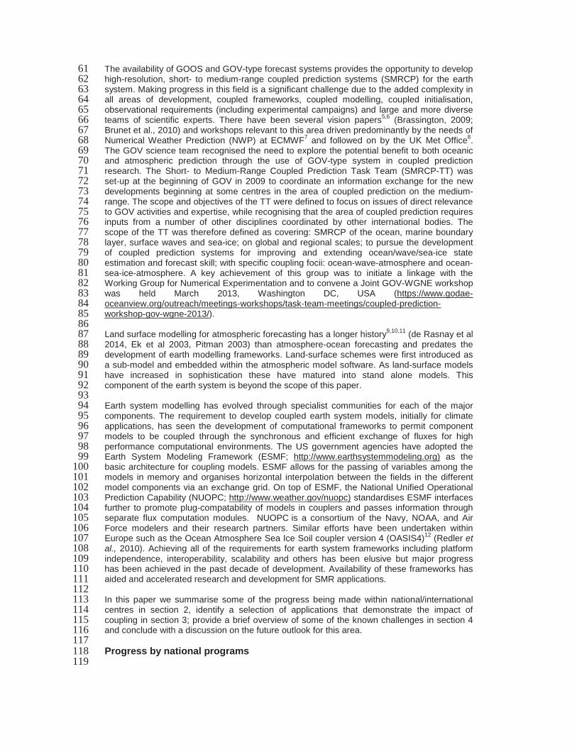
615East Coast Lows are subtropical low pressure weather systems that can rapidly intensify as616they propagate over the marine boundary of Australia’s east coast producing strong localised617convection, lightning and heavy precipitation. Several storms have produced severe impacts618in terms of coastal flooding, damage from hailstones, and in some cases the grounding of619ships and losses of life. Adjacent to the east coast is the so-called East Australian Current, a620western boundary current of the South Pacific sub-tropical gyre transporting warm/fresh621seawater poleward from the Coral Sea to the Tasman Sea. The EAC is frequently unstable622producing several anticyclonic eddies per year from the separation point and along the623northern New South Wales coast which can persist for months75 (Brassington et al., 2010)624providing sources of heat into the Austral winter. A specific case on the 7-9 June 2007 that625occurred off Newcastle, NSW has been studied using downscaled Weather Research and626Forecast model (WRF) simulations. A simulation is initialised with highly resolved SST627(BLUElink) and then compared to a second simulation initialised with coarse resolution (Ctrl)628SST boundary conditions to examine the impact of the gradients in SST arising from the large629scale warm ocean eddies that persist into the Austral winter22 (Chambers et al). Simulations630based on the highly resolved SST produced higher values of 48-hour total precipitation along631an SST front (see Fig 10) resulting in more localised convection consistent with observations632from coastal rain gauges and with lighting strike locations. It is concluded that the SST633gradient along the southern flank of a large warm eddy significantly increased the severity of634the coastal weather impacts that occurred during this storm.635

636High latitude weather and sea-ice forecasting – Gulf St Lawrence637

638Sea-ice acts as a barrier between the atmosphere and the ocean, modulating the fluxes of639heat and moisture across an interface often with temperature differences of greater than64020°C. As such, rapidly evolving changes in the ice cover can have important impacts for polar641weather prediction. This can result from a variety of processes such as ice formation and642break-up, coastal polynyas and leads in pack ice. Differences between coupled and643uncoupled model forecasts after 12-hours from the Canadian Gulf of St. Lawrence coupled644forecasting system are shown in Fig 11. This system has shown the strong impacts that a645dynamic sea-ice cover76 (Smith et al., 2012) can have on 48-hour atmospheric forecasts646leading to large changes in surface air temperature (up to 10°C), low-level cloud cover, and647precipitation. The top panel is for a winter case (Mar. 10, 2012) with sea-ice concentration on648the left and 2m temperature on the right showing that rapid ice changes can cause surface649temperature changes of up to 7-8°C over the open water. Due to the presence of a relatively650

thin seasonal thermocline (~20m) with cold (<0°C) winter surface waters below, upwelling651events in summer can also lead to important impacts on weather predictions. For example,652the bottom panel in Fig 11 shows a summer case (Jul. 10, 2012) with 10m winds on the left653and 2m temperature on the right showing that coastal upwelling in the coupled forecasts can654produce surface temperature changes of several degrees Celcius locally.655

656Nearshore coastal weather – Adriatic Sea657

658A coupled COAMPS48 model was executed in the Adriatic Sea from 25 January to 21659February, 2003. The atmospheric model configuration was triply nested (36, 12, 4 km660horizontal resolution), while the ocean model consisted of two nests (6 and 2 km), with the661inner-most nests of both models centered over the northern Adriatic. Both coupled and662uncoupled model runs were performed. In the coupled model run the winds, wind stresses,663and heat fluxes were interchanged between the atmosphere and ocean (i.e., the ocean feeds664back to the atmosphere and the atmosphere feeds back to the ocean) every 12 minutes using665grid exchange processors based on the Earth System Modeling Framework (ESMF). In the666uncoupled run, wind forcing from the atmospheric model was passed to the ocean model, but667the ocean did not feedback to the atmosphere, i.e., the heat fluxes calculated by the668atmospheric model were computed using daily averaged analysis-quality SST rather than the669time-dependent ocean model forecast SST used in the coupled run. Couple and uncoupled670statistics are presented for the Acqua Alta platform near Venice, Italy in Fig 12. Inspection of671the wind stress time series shows good agreement, with the RMSE slightly larger in the672coupled run (0.112) versus the uncoupled run (0.108). The overall smaller mean stresses in673the COAMPS runs (0.118 coupled, 0.135 uncoupled) compared to the observations (0.151)674are attributed to intensity and positional differences of the Trieste bora jet during the time675period of the experiment. The sensible and latent heat flux comparisons, however, showed a676clear improvement in the coupled model run. These results illustrate how the coupled model677can more accurately predict surface heat fluxes in near-shore regions where a complex SST678field is subject to intense atmospheric events and turbulent heat fluxes have high spatial679inhomogeneity and large gradients.680

681Data assimilation of brightness temperatures682

683The NASA, coupled GEOS-DAS have explored the data assimilation of brightness684temperature using a surface sensitive (10.35 m) channel of the AIRS instrument on AQUA685satellite. The comparison of an experiment that had an active interface-layer with a control686experiment with no interface layer (the SST boundary condition was skin SST) was used to687diagnose the benefit.688

689Preliminary results, at 1 degree resolution, show improved assimilation of all 10-12micron IR690observations and decreased bias in precipitation with respect to GPCP data. Fig 7 shows691three panels with time series of total number of observations assimilated (top panel), global692mean of observation-minus-background (OMB), middle panel, and standard deviation of the693OMB (bottom panel). The use of an improved skin temperature estimate reduced the number694of observations rejected by the analysis quality control, corresponding also to a reduced695standard deviation in OMB. Similar results were obtained for other 10-12 m IR channels of696AIRS-AQUA, IASI-METOP-A, HIRS4-METOP-A, N19 (not shown).697

698Known challenges699

700Based on the current sophistication of the coupled modelling systems and the range of701applications under active investigation many challenges toward coupled prediction have702already been addressed. Sufficient progress has been made in observing, modelling and703initialisation to forecast waves, the ocean state and sea-ice to suggest that coupled modelling704of the marine environment is feasible. The pursuit of seasonal and climate modelling has705introduced several software frameworks that facilitate the coupling of component model706software that is scalable for super-computing environments. In practice there are several707short-comings in their design for GOV-type forecasting and eventual operational applications708which require more frequent restarting and data exchanges. This is not impeding progress in709

basic research but is impacting the efficiency and size of the problems being undertaken and710will require further optimisation in design before implementation into operational applications.711

712The pursuit of coupled modelling specific to applications for hurricanes has yielded several713advances in air-wave-sea coupled parameterisations for high-wind conditions in the tropics.714Significant effort will be required to generalise the coupled parameterisations across all715applications. However, less sophisticated parameterisations from existing models are716demonstrating positive impacts for a wide range of environments.717

718The initialisation of coupled models is currently based on uncoupled or weakly coupled data719assimilation for each component model and an inefficient coupled initialisation procedure to720produce balanced fields in the coupled model. Some promising results are evident from721research focusing on the coupled assimilation of brightness temperatures. Coupled data722assimilation is required to provide the optimum dynamically balanced coupled fields but there723are several challenges to realising this goal.724

7251. Proper handling of different time scales in the ocean and atmosphere. These scales726

may be similar enough in the atmosphere boundary layer and ocean mixed layer to727allow coupled modelling and coupled data assimilation to succeed. This aspect of728the problem needs to be thoroughly studied.729

2. A goal of coupling is to reduce some of the biases in interfacial fluxes that occur in730each component model in their uncoupled form. However, any residual biases in a731coupled model will distribute throughout the coupled model state requiring more732sophisticated analyses to diagnose, attribute and develop bias correction schemes.733

3. It is still a remaining challenge to decide the best way to weight coupled covariances734from ensembles in the hybrid schemes. Similarly, to find appropriate methods for735coupled initialisation and maintaining coupled model ensemble spread given the736disparate temporal and spatial scales of the ocean and atmosphere. It is also737unclear how large an ensemble is needed.738

4. Progress would benefit from community-established benchmarks, test cases, or739metrics to establish beneficial impact of fully coupled analyses740

741In the near-surface ocean, the diurnal cycle imposes time-scales of a few hours64 (Fairall et742al., 1996). Modelling of the diurnal warming layer is important for computation of the skin743temperature. For coupled data assimilation, it is essential to incorporate observational744information directly from satellite brightness temperature observations and near-surface745buoys so that the modeled skin and near-surface temperature profile is estimated accurately,746and thus temporally evolved by the model at the correct time-scale. It is also relevant to note747the different vertical length-scales observed by the observations: IR observations measure748“closest” to the skin or air-sea interface (few microns deep); MW observations penetrate749slightly deeper (to few mm); and further down to centimeter – and meter scale – we have in-750situ measurements e.g., ships and buoys.751

752For coupled prediction in polar environments a significant uncertainty lies in the extent to753which we can accurately predict small scale ice features and the evolution of the ice cover.754Coupled forecasts are strongly sensitive to variations in the ice cover in the marginal ice zone755as well as due to coastal polynya formation and leads in the pack ice. As most sea ice756observational data are of fairly low resolution, the evaluation of small scale features like leads757remains a challenge. The use of ever finer resolution models demands the development of758new sea ice rheologies suitable for resolving kilometre scale features. Currently it is not clear759how significant these errors are for coupled polar prediction and further study is required52760Smith et al., (2013).761

762Notably the majority of the applications presented have focused on atmospheric phenomena763reflecting the maturity of this community and the extensive range of peer-reviewed764benchmarks for uncoupled systems from which the impact of coupling can more readily be765assessed. Coupled prediction is expected to also have a significant impact on several ocean766applications e.g., sonar prediction, search and rescue and hazardous chemical spills. In767addition to the fact that the ocean community is less mature it also reflects the paucity of768

observations available to establish benchmarks for the leading parameters for these769applications such as the sonic layer depth and surface currents.770

771Future/outlook and conclusion772

773All groups contributing to this paper have developed research programs specifically targeting774a subset of applications that represent their national interest. The modelling systems range775from regional to global and the initialisation and data assimilation is uncoupled or weakly776coupled. In many cases the research challenges identified are common across these777programs indicating significant benefit from a community-based approach to share advances778in coupled science and promote international experiments and observation campaigns.779Despite the challenges of achieving skilful forecasts from such complex systems the results to780date using relatively unsophisticated techniques have already yielded positive results. Most781groups are optimistic that coupled prediction will deliver yield further improvements with782continued research and development.783

784The Bureau of Meteorology plan to extend the research into East Coast Lows focusing on785diagnosing the dynamical response of the atmospheric boundary layer and the impact of786coupled modeling. Ensemble Kalman Filter data assimilation has been extensively787investigated for regional ocean prediction and preliminary work is being pursued into their788extension to coupled DA. With the implementation of a near-global 1/10 degree BLUElink789OceanMAPS the impact of these boundary conditions will be assessed for the ACCESS-G790NWP system.791

792Work at the UK Met Office on coupled prediction at short time-scales is targeted at three main793areas: coupled model development; coupled data assimilation development; and UK794environmental prediction. Assessment and development of the coupled model HadGEM3 at795these time-scales is an on-going area of work; current developments include improvements to796the representation of the diurnal cycle of SST, and implementation of a wave model within the797coupled model framework. A higher-resolution version of this global system (12km798atmosphere and 1/12° ocean) is also being developed in order to assess its performance799compared to the uncoupled NWP system. The weakly coupled data assimilation system800described in section 2 is being further assessed and developed, and is planned to be801implemented as a demonstration operational system in the Met Office’s operational suite in8022015. Work to develop a coupled modeling framework around the UK to provide803environmental predictions is also underway.804

805NOAA/NCEP have established a wide range of coupling projects that are underway or806planned using the ESMF - NEMS environment, including: Completing ESMF and NUOPC807versions of all component models mentioned in section 2; Converting the coupled HWRF808hurricane weather model to the NNMB core in NEMS by 2016, transitioning this coupled809model from a custom coupling environment to ESMF – NEMS. In this time frame, the HWRF810model will be coupled to a full HYCOM ocean model, and coupling with the wave model will811begin; A NEMS based prototype for Arctic modelling is intended to be delivered by 2016,812tentatively providing a coupled ocean – sea-ice – atmosphere system, possibly also with a813wind wave component added; global model coupling using an atmosphere – ocean – sea-ice814coupling will be extended for the CFS-v3, and considered for inclusion in the Global815Ensemble System (GEFS) and the deterministic Global Forecast System (GFS); a Nearshore816Wave Prediction System (NWPS) will be rolled out to the NWS field offices in the coming817year77 (Van der Westhuysen et al., 2013). Initially this will consist of a wind wave model with818input from weather, ocean and coastal circulation (inundation) models. In future upgrades,819this model is intended to become a coupled wave-surge model; NOAA has also funded a820project to develop the next generation forecast system for the Great Lakes, consisting of a 3D821unstructured grid circulation model, an ice model and a wave model. In operations, this822coupled lake model is likely to be fully coupled to a regional mesoscale weather model.823

824ECMWF will continue developments on coupled forecasting systems. It is planned to include825a dynamical sea-ice model in the medium-range, monthly and seasonal forecasting systems,826as well as increasing the resolution of the ocean and atmospheric models. For the time827being, the initial conditions for the coupled forecasting system will continue being produced by828

separate atmospheric and ocean/sea-ice assimilation systems. The developments of the829coupled assimilation will continue under the CERA system, targeting a fully coupled830assimilation system. The computation of several outer iterations in the incremental variational831approach of the CERA system has already allowed the observations in one media to impact832the analysis of the other media within the same assimilation cycle. It is expected that the833combination of variational and ensemble data assimilation methods will improve the834formulation of the background error covariances. In the next few years, ECMWF has planned835to produce with the CERA system several extended climate coupled reanalyses spanning the83620th century and the satellite era in the context of the ERA-CLIM2 project funded by the837European Commission.838

839Within CONCEPTS the future activities include research and development to address the840challenges outlined above, particularly for polar prediction. This will include evaluating and841improving the representation of leads, incorporating wave-ice interactions, atmosphere-ice-842ocean momentum transfer, constraining sea-ice thickness and sea-ice forecast verification.843Regional coupled systems will also be further developed and applied to the Great Lakes and844the North Pacific to support high resolution modelling of the Canadian west coast. The845development of global coupled modelling systems will continue for applications of medium-846and long-range forecasts. In this context there will be an expansion to coupled models for847probabilistic forecasting through the Global Ensemble Prediction System at the Canadian848Meteorological Centre.849

850Based on Mercator’s encouraging results, Meteo-France will develop operational systems851covering overseas territories using same modelling tools as described in section 2. The852Global Mercator-Ocean operational system will be used to initialise the coupled forecast and853dedicated ocean configurations could be developed to improve the consistency between the854initialisation phase and the forecast one.855

856NASA plans have some commonalities with the Canadian CONCEPTS in terms of857constraining sea-ice thickness. Along the same lines, they plan to improve near-surface heat858transfer over sea-ice by modelling ice skin temperature using CICE thermodynamics. Plans859have been outlined to couple the GMAO ocean analysis (iODAS) to its atmospheric analysis860system so that the foundation temperature (currently OSTIA SST, used by the atmospheric861analysis) is replaced with the corresponding temperature analyzed in the ocean model.862

863Following the initial concept papers5,6 and early workshops in 20087 and 20098 research and864development in this field has made significant advances in terms of the sophistication of the865modeling systems being implemented as outlined in Tab 1, the rigor of the experiments to866quantify impacts and the range of applications. The GOV science team initiated the SMRCP867task team to promote the use of coupling based on GOV-type ocean prediction systems and868to establish a linkage with the atmospheric community. Outlined in this paper there are many869examples where coupled systems are now being based on GOV-type ocean prediction870systems for short- to medium-range forecasting with demonstrated impacts. The next steps871for the SMRCP-TT are to continue to develop linkages with WGNE and other communities872involved in coupled forecasting and to jointly develop and promote international initiatives to873address the known challenges.874

875Acknowledgements876The authors would like to acknowledge the valuable comments from two anonymous877reviewers and a third reviewer Dr Glenn White, NOAA/NCEP who was a co-convenor of the878Joint GOV-WGNE workshop.879

880References881

8821. Bell MJ, Lefebvre M, Le Traon P-Y, Smith N and Wilmer-Becker K. 2010. GODAE:883

The global ocean data assimilation experiment, Oceanography 22(3): 14-218842. Bell M, Schiller AS and Dombrowsky E, this issue8853. Jacobs GA, Woodham RH, Jourdan D and Braithwaite J. 2009. GODAE applications886

useful to navies throughout the world. Oceanography 22(3): 182-189887

4. Davidson F, Allen A, Brassington GB, Breivik O, Daniel P, Kamachi M, Sato S, King888B, Lefevre F, Sutton M and Kaneko H. 2009. Application of GODAE ocean current889forecasts to search and rescue and ship routing, Oceanography 22(3): 176-181.890

5. Brassington GB. 2009. Ocean prediction issues related to weather and climate891prediction, CAS XV Vision paper (Agenda item 8.5).892

6. Brunet G, Keenan T, Onvlee J, Béland M, Parsons D and Mailhot J 2010. The next893generation of regional prediction systems for weather, water and environmental894applications, CAS XV Vision paper (Agenda item 8.2).895

7. Proceedings of the ECMWF Workshop on Atmosphere-Ocean Interaction, 10-12 Nov8962008, (http://www.ecmwf.int/publications/library/do/references/list/28022009).897

8. Proceeding of the Ocean Atmosphere Workshop, UK Met Office, 1-2 Dec 2009898(http://www.ncof.co.uk/modules/documents/documents/OAsummary.pdf).899

9. De Rosnay P, Balsamo G, Albergel C, Munoz-Sabater J and Isaksen L. 2014.900Initialisation of land surface variables for numerical weather prediction. Surveys in901Geophysics 35: 607-621902

10. Ek M, Mitchell KE, Lin Y, Rogers YE, Grunmann P, Koren V, Gayno G, and Tarpley903JD. 2003. Implementation of Noah land-surface model advances in the NCEP904operational mesoscale Eta model. Journal of Geophysical Research 108(D22): 8851.905doi:10.1029/ 2002JD003296906

11. Pitman AJ. 2003. The evolution of, and revolution in, land surface schemes designed907for climate models. International Journal of Climatolology 23: 479-510908

12. Redler R, Valcke S, Ritzdorf H. 2010. OASIS4 – a coupling software for next909generation earth system modelling. Geoscientific Model Development 3: 87-104910

13. Davies T, Cullen MJP, Malcolm AJ, Mawson MH, Staniforth A, White AA, Wood N.9112005. A new dynamical core for the Met Office’s global and regional modelling of the912atmosphere. Quarterly Journal of the Royal Meteorological Society 131(608): 1759-9131782914

14. Griffies SM. 2009. Elements of mom4p1. GFDL Ocean Group Technical Report. 6: 1-915444916

15. Rawlins F, Ballard SP, Bovis KJ, Clayton AM, Li D, Inverarity GW, Lorenc AC, and917Payne TJ. 2007. The Met Office global four-dimensional variational data assimilation918scheme. Quarterly Journal of the Royal Meteorological Society 133: 347–362919

16. Brassington, GB, Freeman J, Huang X, Pugh T, Oke PR, Sandery PA, Taylor A,920Andreu-Burillo I, Schiller A, Griffin DA, Fiedler R, Mansbridge J, Beggs H and921Spillman CM. 2012. Ocean Model, Analysis and Prediction System (OceanMAPS):922version 2, CAWCR Technical Report 52: 110pp.923

17. Oke PR, Brassington GB, Griffin DA, Schiller A. 2008. The Bluelink ocean data924assimilation system (BODAS). Ocean Modelling 21: 46-70925

18. Sandery PA, Brassington GB, Craig A, Pugh T. 2010. Impacts of Ocean–Atmosphere926Coupling on Tropical Cyclone Intensity Change and Ocean Prediction in the927Australian Region. Monthly Weather Review 138: 2074-2091928

19. Sandery PA and O’Kane TJ. 2014. Coupled initialization in an ocean-atmosphere929tropical cyclone prediction system. Quarterly Journal of the Royal Meteorological930Society, 140: 82-95.931

20. Barras V, Sandery PA. 2012. Forecasting the Brisbane flooding event using932Ensemble Bred Vector SST initialization and ocean coupling in ACCESS NWP.933CAWCR Research Letters 9.934

21. Skamarock WC, Klemp JB, Dudhia J, Gill DO, Barker DM, Wang W and Powers JG.9352005. A description of the Advanced Research WRF Version 2. NCAR Tech Note936468937

22. Chambers CRS, Brassington GB, Simmonds I, Walsh K. 2014. Precipitation changes938due to the introduction of eddy-resolved sea surface temperatures into simulations of939the “Pasha Bulker” east coast low of June 2007, Meteorology and Atmospheric940Physics DOI: 10.1007/s00703-014-0318-4941

23. Walters DN, Best MJ, Bushell AC, Copsey D, Edwards JM, Falloon PD, Harris CM,942Lock AP, Manners JC, Morcrette CJ, Roberts MJ, Stratton RA, Webster S, Wilkinson943JM, Willett MR, Boutle IA, Earnshaw PD, Hill PG, MacLachlan C, Martin GM,944Moufouma-Okia W, Palmer MD, Petch JC, Rooney GG, Scaife AA, Williams KD.9452011. The Met Office Unified Model Global Atmosphere 3.0/3.1 and JULES Global946Land 3.0/3.1 configurations. Geoscientific Model Development 4: 919–941, doi:94710.5194/gmd-4-919-2011948

24. Brown A, Milton S, Cullen M, Golding B, Mitchell J, Shelly A. 2012. Unified modeling949and prediction of weather and climate: A 25-year journey. Bulletin American950Meteorological Society 93: 1865–1877, doi: 10.1175/BAMS-D-12-00018.1951

25. Madec G. 2008. NEMO ocean engine: Notes du Pole de Modélisation 27. Paris:952Institut Pierre-Simon Laplace (IPSL).953

26. Hunke EC, Lipscomb WH. 2010. CICE: The sea ice model documentation and954software user's manual, version 4.1, Technical report LA-CC-06-012. Los Alamos955National Laboratory: Los Alamos, NM.956

27. Johns T, Shelly A, Rodiguez J, Copsey D, Guiavarc’h C, Waters J, Sykes P. 2012.957Report on extensive coupled ocean-atmosphere trials on NWP (1-15 day) timescales.958PWS Key Deliverable Report. Met Office, UK959

28. MacLachlan C, Arribas A, Peterson KA, Maidens A, Fereday D, Scaife AA, Gordon960M, Vellinga M, Williams A., Comer RE, Camp J, Xavier P. and Madec G. 2014.961Global Seasonal forecast system version 5 (GloSea5): a high-resolution seasonal962forecast system. Quarterly Journal of the Royal Meteorological Society doi:96310.1002/qj.2396964

29. Blockley EW, Martin MJ, McLaren AJ, Ryan AG, Waters J, Guiavarc'h C, Lea DJ,965Mirouze I, Peterson KA, Sellar A, Storkey D and While J. 2014. Recent development966of the Met Office operational ocean forecasting system: An overview and assessment967of the new Global FOAM forecasts. Geoscience Model Development Discussion 6:9686219–6278, doi: 10.5194/gmdd-6-6219-2013969

30. Waters J, Lea DJ, Martin MJ, Mirouze I, Weaver A, and While J. 2014. Implementing970a variational data assimilation system in an operational 1/4 degree global ocean971model. Quarterly Journal of the Royal Meteorological Society. doi: 10.1002/qj.2388972

31. Bender MA, Ginis I, and Kurihara Y. 1993. Numerical simulations of tropical cyclone-973ocean interaction with a high-resolution coupled model. Journal of Geophysical974Research 98: 23 245-23 263975

32. Bender MA, Ginis I, Tuleya R, Thomas B, and Marchok T. 2007. The operational976GFDL Coupled Hurricane-Ocean Prediction System and a summary of its977performance. Monthly Weather Review 135: 3965-3989978

33. Bender MA and Ginis I. 2000. Real case simulation of hurricane-ocean interaction979using a high-resolution coupled model: Effects on hurricane intensity. Monthly980Weather Review 128: 917-946981

34. Yablonsky RM and Ginis I. 2008. Improving the ocean initialization of coupled982hurricane-ocean models using feature-based data assimilation. Monthly Weather983Review 136: 2592-2607984

35. Yablonsky RM and Ginis I, 2009: Limitation of one-dimensional ocean models for985coupled hurricane-ocean model forecasts. Monthly Weather Review 137: 4410–4419986

36. Tallapragada V, Bernardet L, Gopalakrishnan S, Kwon Y, Liu Q, Marchok T, Sheinin987D, Tong M, Trahan S, Tuleya R, Yablonsky R, and Zhang X. 2013. Hurricane988Weather Research and Forecasting (HWRF) Model: 2013 scientific documentation.989

Developmental Testbed Center, 99 pp. Available from990http://www.dtcenter.org/HurrWRF/users/docs/.991

37. Kim H-S, Lozano C, Tallapragada V, Iredell D, Sheinin D, Tolman HL, Gerald VM,992and Sims J. 2014. Performance of Ocean Simulations in the Coupled HWRF–993HYCOM Model. Journal of Atmospheric and Oceanic Technology 31: 545-559994

38. Hodur RM. 1997. The Naval Research Laboratory’s Coupled Ocean/Atmosphere995Mesoscale Prediction System (COAMPS). Monthly Weather Review 125: 1414-1430996

39. Moon I-J, Hara T, Ginnis I, Belcher SE and Tolman HL. 2004. Effects of surface997waves on air-sea momentum exchange: I. Effect of mature and growing seas. Journal998of Atmospheric Science 61(19): 2321-2333999

40. Moon I-J, Ginis I, Hara T and Thomas B. 2007. A Physics-Based Parameterization of1000Air–Sea Momentum Flux at High Wind Speeds and Its Impact on Hurricane Intensity1001Predictions. Monthly Weather Review 135: 2,869-2,8781002

41. Fan Y, Ginis I, and Hara T. 2009. The Effect of Wind–Wave–Current Interaction on1003Air–Sea Momentum Fluxes and Ocean Response in Tropical Cyclones. Journal of1004Physical Oceanography 39: 1,019-1,0341005

42. Chen SS, Price JF, Zhao W, Donelan MA and Walsh EJ. 2007. The CBLAST-1006Hurricane Program and the next-generation fully coupled atmosphere-wave-ocean1007models for hurricane research and prediction. Bulletin of the American Meteorological1008Society 88: 311-3171009

43. Saha S, et al., 2010. The NCEP Climate Forecast System Reanalysis, Bulletin of the1010American Meteorological Society 91: 1015-10571011

44. Saha S, Moorthi S, Wu X, Wang J, Nadiga S, Tripp P, Behringer D, Hou Y-T, Chuang1012H-Y, Iredell M, Ek M, Meng J, Yang R, Peña Mendez M, van den Dool H, Zhang Q,1013Wang W, Chen M, and Becker E. 2014. The NCEP Climate Forecast System Version10142. Journal of Climate 27: 2185–22081015

45. Wei H, Xia Y, Mitchell KE, and Ek M. 2012. Improvement of the Noah land surface1016model for warm season processes: evaluation of water and energy flux simulation.1017Hydrological Processes 27(2): 297–303 DOI: 10.1002/hyp.92141018

46. Meng J, Yang R, Wei H, Ek M, Gayno G, Xie P, Mitchell K. 2012. The Land Surface1019Analysis in the NCEP Climate Forecast System Reanalysis. Journal of1020Hydrometeorology 13: 1621–1630. doi: http://dx.doi.org/10.1175/JHM-D-11-090.11021

47. Janssen PAEM, Breivik O, Mogensen K, Vitart F, Balmaseda M, Bidlot J-R, Keeley S,1022Leutbecher M, Magnusson L, Molteni F. 2013. Air-sea interaction and surface waves.1023ECMWF Technical Memorandum 7121024

48. Holt T, Cummings JA, Bishop CH, Doyle JD, Hong X, Chen S and Jin Y. 2011.1025Development and Testing of a Coupled Ocean-Atmosphere Mesoscale Ensemble1026Prediction System. Ocean Dynamics 61(11): 1937-19541027

49. Allard RA, Smith TA, Jensen TG, Chu PY, Rogers E, and Campbell TJ. 2012.1028Validation Test Report for the Coupled Ocean Atmosphere Mesoscale Prediction1029System (COAMPS) Version 5.0: Ocean/Wave Component Validation. Naval1030Research Laboratory Memorandum Report: NRL/MR/7320--12-9423, 91 pp.1031

50. Cummings JA and Smedstad OM. 2013. Variational Data Assimilation for the Global1032Ocean. In,. Park S and Xu L, (eds.) Data Assimilation for Atmospheric, Oceanic &1033Hydrologic Applications (Vol. II), DOI 10.1007/978-3-642-35088-7 13, Springer-1034Verlag, Berlin, Heidelberg.1035

51. Cummings JA and Peak JE. 2014. Variational assimilation of satellite sea surface1036temperature radiances. Naval Research Laboratory Memorandum Report:1037NRL/MR/7320-14-9520, 29 pp.1038

52. Smith GC, Roy F, Belanger J-M, Dupont F, Lemieux J-F, Beaudoin C, Pellerin P, Lu1039Y, Davidson F, Ritchie H. 2013. Small-scale ice-ocean-wave processes and their1040impact on coupled environmental polar prediction, Proceedings of the ECMWF-1041

WWRP/THORPEX Polar Prediction Workshop, 24-27 June 2013, ECMWF Reading,1042UK.1043

53. Faucher M, Roy F, Ritchie H, Desjardins S, Fogarty C, Smith G and Pellerin P. 2010.1044Coupled Atmosphere-Ocean-Ice Forecast System for the Gulf of St-Lawrence,1045Canada. Mercator Ocean Quarterly Newsletter, 38, 23-31.1046

54. Saucier FJ, Roy F, Gilbert D, Pellerin P, Ritchie H. 2003. The formation of water1047masses and sea ice in the Gulf of St. Lawrence. Journal of Geophysical Research1048108(C8): 3269-3289.1049

55. Smith GC, Roy F, Reszka M, Surcel Colan D, He Z, Deacu D, Belanger J-M,1050Skachko S, Liu Y, Dupont F, Lemieux J-F, Beaudoin C, Tranchant B, Drévillon M,1051Garric G, Testut C-E, Lellouche J-M, Pellerin P, Ritchie H, Lu Y, Davidson F,1052Buehner M, Lajoie M and Caya A. 2014. Sea ice Forecast Verification in the1053Canadian Global Ice Ocean Prediction System. Quarterly Journal of the Royal1054Meteorological Society, in press.1055

56. Faure, GG, Westrelin SS and Roy DD. 2008. Un nouveau modèle de prévision à1056Météo-France: ALADIN-Réunion. La Météorologie 8(60) : 29-35 DOI :105710.4267/2042/169421058

57. Fischer C, Montmerle T, Berre L, Auger L and SE. 2005. An overview1059of the variational assimilation in the ALADIN/France numerical weather-prediction1060system. Quarterly Journal of the Royal Meteorological Society 131: 3477–3492. doi:106110.1256/qj.05.1151062

58. Seity Y, Brousseau P, Malardel S, Hello G, Béénard P, Bouttier F, Lac C and Masson1063V. 2011. The AROME-France Convective-Scale Operational Model. Monthly Weather1064Review 139(3): 976-991.1065

59. Rienecker MM, and coauthors, 2011. MERRA - NASA's Modern-Era Retrospective1066Analysis for Research and Applications. Journal of Climate 24: 3624-3648.1067doi:10.1175/JCLI-D-11-00015.1.1068

60. Vernieres G, Rienecker MM, Kovach R and Keppenne CL. 2012. The GEOS-iODAS:1069Description and Evaluation. NASA Technical Report Series on Global Modeling and1070Data Assimilation, NASA/TM-2012-104606, 30: 73 pp.1071

61. Kleist DT et al., 2009. Improving Incremental Balance in the GSI 3DVAR Analysis1072System, Monthly Weather Review, 137, 1046-1060.1073

62. Molod A, Takacs L, Suarez M, Bacmeister J, Song I-S, and Eichmann A. 2012. The1074GEOS-5 Atmospheric general circulation model: Mean climate and development from1075MERRA to Fortuna. NASA Technical Report Series on Global Modeling and Data1076Assimilation, NASA/TM-2012-104606 28: 117 pp.1077

63. Takaya Y, et al., Refinements to a prognostic scheme for skin sea surface1078temperature, Journal of Geophysical Research 115: C06009, 2010.1079

64. Fairall CW et al. 1996. Cool-skin and warm-layer effects on sea surface temperature,1080Journal of Geophysical Research 101: 1295– 13081081

65. Donlon CJ, Martin M, Stark JD, Roberts-Jones J, Fiedler E. 2012. The operational1082sea surface temperature and sea ice analysis (OSTIA) system. Remote Sens.1083Environ. 116: 140–158, doi: 10.1016/j.rse.2010.10.0171084

66. McLay JG, Flatau MK, Reynolds C, Cummings J, Hogan TF, Flatau P. 2012.1085Inclusion of sea-surface temperature variation in the U. S. Navy ensemble-transform1086global ensemble prediction system. Journal of Geophysical Research 117: D19120,1087doi:10.1029/2011JD016937.1088

67. de Boisseson E, Balmaseda MA, Vitart F, and Mogensen K. 2012. Impact of the Sea1089Surface Temperature forcing on hindcasts of Madden-Julian Oscillation events using1090the ECMWF model. Ocean Science, 8, 1071–1084, 2012, doi:10.5194/os-8-1071-10912012.1092

68. Wang W, Hung M-P, Weaver SJ, Kumar A and Fu X. 2013. MJO prediction in the1093NCEP Climate Forecast System version 2. Climate Dynamics 10.1007/s00382-013-10941806-91095

69. Seo K-H, Wang W, Gottschalck J, Zhang Q, Schemm J-KE, Higgins WR, Kumar A.10962009. Evaluation of MJO forecast skill from several statistical and dynamical forecast1097models. Journal of Climate 22: 2372–23881098

70. Matsueda M, Endo H. 2011. Verification of medium-range MJO forecasts with1099TIGGE. Geophysical Research Letters 38: L11801. doi:10.1029/2011GL0474801100

71. Rashid HA, Hendon HH, Wheeler MC, Alves O. 2010. Prediction of the Madden-1101Julian oscillation with the POAMA dynamical prediction system. Climate Dynamics1102doi:10.1007/s00382-010-0754-x1103

72. Ferry N, Parent L, Garric G, Bricaud C, Testut C-E, Le Galloudec O, Lellouche J-M,1104Drevillon M, Greiner E, Barnier B, Molines J-M, Jourdain NC, Guinehut S, Cabanes1105C, Zawadzki L. 2012. GLORYS2V1 global ocean reanalysis of the altimetric era1106(1992-2009) at meso scale. Mercator Quarterly Newsletter 44: 29-391107

73. Valcke S. 2013. The OASIS3 coupler: a European climate modelling community1108software. Geoscientific Model Development, 6(2).1109

74. Gentemann CL, DeMaria M and Wentz FJ. 2003. Near real time global optimum1110interpolated microwave SSTs: applications to hurricane intensity forecasting, Eos1111Trans. AGU, 84(52): Ocean Sci. Meet. Suppl., Abstract OS12C-031112

75. Brassington GB, Summons N and Lumpkin R. 2010. Observed and simulated1113Lagrangian and eddy characteristics of the East Australian Current and Tasman Sea,1114Deep Sea Research Part II, doi:10.1016/j.dsr2.2010.10.001.1115

76. Smith GC, Roy F and B Brasnett B. 2012. Evaluation of an Operational Ice-Ocean1116Analysis and Forecasting System for the Gulf of St. Lawrence, Quarterly Journal of1117the Royal Meteorological Society, DOI:10.1002/qj1982.1118

77. Van der Westhuysen A, Padilla R, Santos P, Gibbs A, Gaer D, Nicolini T, Trjaden S,1119Devaliere E-M and Tolman H. 2013. Development and validation of the Nearshore1120Wave Prediction System. 93rd AMS Annual Meeting, Austin TX, paper 4.5.1121

1122

78.11231124

TABLES112511261127

System Ocean(Model

DA)

Atmos(Model

DA)

Wave(Model

DA)

Sea-ice(Model

DA)

Coupler Interfacialflux

param.

Global/Regional

Target app(s)

BLUElink OFAM(MOM4p1)

BODAS

ACCESS4DVAR

WRF

High-windparam.

roughness,WW3

OASIS4 - Regional TropicalCyclones,Rainfall,

East CoastLows

UK MetOffice

NEMOvn3.4,

NEMOVAR3DVar

UM,Hybrid4DVar

WWIII, noDA

CICE,NEMOVAR

3DVar

OASIS Global,Local

Global forseamless

forecasting:NWP out toseasonal.Local for

environmentalprediction

around UK.

NOAA/NCEP

HYCOM,MOM5

NCEP WW3 CICE, GFDLsea ice

ESMF plusNUOPC

- Global/Regional

NWP, Monthly,Seasonalforecast

Hurricaneprediction

ECWMF NEMO IFS WAM LIM2 SingleExecutabl

e

- Global NWP, Monthly,Seasonal

forecast andclimate

reanalyses

GOFSCOAMPS

HYCOMNCOM

NCODA3DVAR

NCOM4DVAR

NAVGEMCOAMPS

NAVDAS4DVAR

WW3

NCODA2DVAR

CICE

NCODA3DVAR

ESMF plusNUOPCon global

scale

(seeFigure 3)

Global andRegional

High ImpactWeather,ExtendedForecasts

CONCEPTS NEMO GEM WW3 CICE GOSSIP Couplingby GEMfluxes

Global/regional

Global andregional

CanadianNWP,

Operationalmarine supportin ice infested

waters

Mercator NEMO.GLORYS ¼°reanalysis.Forecast :Coupledregional

1/12°configuration

ALADIN10km.

Forecast :AROME2.5km

NO NA OASIS3 ECUME Regional,IndianOcean(46E-

68E/9°S-22°S)

Tropicalcyclonesforecast

GEOS-DAS iODAS(MOM4p1)

GEOS - CICE ESMF - Global TropicalCyclones;Rea

nalysis

Tab 1 Overview of the types of systems being employed to examine the impact of coupled1128modelling together with the type of target applications.1129

1130

1131

Model Observations DA Initialisation

Atmosphere UM

~60km/L85

AIRS, IASI, ATOVS, GPSRO, SSMI, Aircraft, Sondes, Surf-Scat

4D-Var ~120km Direct

Land JULES

~60km/4 layers

3D-Var Screen, ASCAT, NESDIS

Nudging Analysis T/2 Direct

Ocean NEMO

~25km/L75

In situ SST, T/S profiles, AATSR, AVHRR, AMSRE, Jason 1+2, ENVISAT

3D-Var FGAT IAU

Sea Ice CICE

~25km 5 categories

SSMI 3D-Var FGAT IAU

Tab 2 Model, observations, data assimilation and initialisation methods used in the UK Met1132Office’s weakly coupled data assimilation system.1133

1134

1135FIGURES1136

1137

1138Fig 1 ESMF coupling framework for the COAMPS air/ocean/wave system showing the1139variables and exchange parameters passed among the coupled models.1140

11411142

11431144

1145Fig 2 A schematic of the future ESPC coupled system.1146

11471148

1149

1150Fig 3 SST (K) observation-minus-forecast RMS (solid) and mean differences (dotted) for a set1151of coupled forecasts (red) and ocean-only forecasts (green) in the Tropical Pacific region. The1152observations used in this assessment are the drifting buoys.1153

11541155

11561157

1158Fig 4 Monthly average assimilation increments for Dec 2011 for surface air temperature (top1159row) and sea surface temperature (bottom row) for the un-coupled systems (left column) and1160the weakly coupled system (right column).1161

1162

11631164

1165Fig 5 Root mean square error (RMSE) of the SST forecast in the Tropics from the CERA1166system (black) and from the operational-like system (green) for September 2010. The OSTIA1167SST analysis is used as reference. The red curve is the RMSE of the SST climatology used1168to create the SST anomalies persisted in the forecasts from the operational-like system.1169

1170

11711172

1173Fig 6 Evaluation of global coupled forecasts over the tropical Indian Ocean from CMC over1174the winter 2011 period. Mean (dashed) and standard deviation (solid) differences between1175925 hPa temperature forecasts and ECMWF analyses are shown for uncoupled (blue) and1176coupled forecasts (red). The bottom panel indicates the statistical significance of standard1177deviation.1178

1179

1180

1181Fig 7 Improved assimilation of Brightness Temperature from a surface sensitive (10.35 \mu m)1182channel of the AIRS instrument on AQUA satellite. We compare an experiment (exp1) that1183had an active interface-layer with a control (ctl) with no interface layer and hence used SST1184boundary condition as skin SST. The three panels plot time series of total number of1185observations assimilated (top panel), global mean of observation-minus-forecast (OMB),1186middle panel, and standard deviation of the OMB (bottom panel). Notice that the analysis1187quality control accepts more observations in exp1, with lesser standard deviation in OMB.1188Similar results are obtained for other 10-12 \mu m IR channels of AIRS-AQUA, IASI-METOP-1189A, HIRS4-METOP-A, N19 (not shown).1190

11911192

119311941195

1196Fig 8 (a) SST error ensemble mean evolution (K) as a function of forecast time. (b) Central1197Pressure error ensemble mean evolution (hPa) as a function of forecast time. The total1198number of forecasts and the statistical significance of the difference between the forced and1199coupled ensembles are given for each forecast time below the figure.1200

1201120212031204

12051206

1207

Fig 9 Prediction of SST resulting from the ocean response to tropical cyclone Yasi in theCoral Sea on the 2nd of February 2012 was improved using a coupled ocean-atmosphereensemble initialisation method. The colours represent a normalised 2D histogram.

1208

1209Fig 10 48 hour (0000 UTC 7 June to 0000 UTC 9 June, 2007) total rainfall differences1210(colours, mm) (BLUElink - Ctrl). SST differences (°C) between the simulations overlaid as1211contours. In addition the BLUElink simulation average 10 metre wind vectors are overlaid as1212arrows to indicate the surface flow (m s-1, representative vector in bottom right).1213

12141215

12161217

12181219

1220Fig 11 Differences between coupled and uncoupled model forecasts after 12 hours in the1221Canadian Gulf of St. Lawrence forecasting system. Top panel is for a winter case (Mar. 10,12222012) with sea ice concentration on the left and 2m temperature on the right showing that1223rapid ice change can cause surface temperature changes of up to 7-8 °C over the open1224water. The grey colour shows the ice concentration and the colour scale shows the Coupled1225minus uncoupled model differences in ice concentration. The bottom panel shows a summer1226case (Jul. 10, 2012) with 10m winds on the left and 2m temperature on the right showing that1227coupling induced coastal upwelling can produce surface temperature of several degrees C1228locally.1229

12301231

Fig 12 Hourly latent and sensible heat fluxes (W/m2) and wind stress (N/m2) for the fully-1232coupled COAMPS run and observations at Acqua Alta (Venice). From Allard et al. 2010.1233

1234