Embed Size (px)
Citation preview
Guide to RISC Processors
Sivarama P. Dandamudi
Guide to RISC Processors
for Programmers and Engineers
Sivarama P. DandamudiSchool of Computer ScienceCarleton UniversityOttawa, ON K1S [email protected]
Library of Congress Cataloging-in-Publication DataDandamudi, Sivarama P., 1955–
Guide to RISC processors / Sivarama P. Dandamudi.p. cm.
Includes bibliographical references and index.ISBN 0-387-21017-2 (alk. paper)1. Reduced instruction set computers. 2. Computer architecture. 3. Assembler language
(Computer program language) 4. Microprocessors—Programming. I. Title.QA76.5.D2515 2004004.3—dc22 2004051373
ISBN 0-387-21017-2 Printed on acid-free paper.
© 2005 Springer Science+Business Media, Inc.All rights reserved. This work may not be translated or copied in whole or in part without the written permissionof the publisher (Springer Science+Business Media, Inc., 233 Spring Street, New York, NY 10013, USA),except for brief excerpts in connection with reviews or scholarly analysis. Use in connection with any form ofinformation storage and retrieval, electronic adaptation, computer software, or by similar or dissimilar method-ology now known or hereafter developed is forbidden.The use in this publication of trade names, trademarks, service marks, and similar terms, even if they are notidentified as such, is not to be taken as an expression of opinion as to whether or not they are subject toproprietary rights.
Printed in the United States of America. (HAM)
9 8 7 6 5 4 3 2 1 SPIN 10984949
springeronline.com

Tomy parents, Subba Rao and Prameela Rani,
my wife, Sobha,and
my daughter, Veda

Preface
Popular processor designs can be broadly divided into two categories: Complex Instruc-tion Set Computers (CISC) and Reduced Instruction Set Computers (RISC). The dominantprocessor in the PC market, Pentium, belongs to the CISC category. However, the recenttrend is to use the RISC designs. Even Intel has moved from CISC to RISC design fortheir 64-bit processor. The main objective of this book is to provide a guide to the archi-tecture and assembly language of the popular RISC processors. In all, we cover five RISCdesigns in a comprehensive manner.
To explore RISC assembly language, we selected the MIPS processor, which is ped-agogically appealing as it closely adheres to the RISC principles. Furthermore, the avail-ability of the SPIM simulator allows us to use a PC to learn the MIPS assembly language.
Intended UseThis book is intended for computer professionals and university students. Anyone who isinterested in learning about RISC processors will benefit from this book, which has beenstructured so that it can be used for self-study. The reader is assumed to have had someexperience in a structured, high-level language such as C. However, the book does notassume extensive knowledge of any high-level language—only the basics are needed.
Assembly language programming is part of several undergraduate curricula in com-puter science, computer engineering, and electrical engineering departments. This bookcan be used as a companion text in those courses that teach assembly language.
vii
viii Preface
FeaturesHere is a summary of the special features that set this book apart.
• This probably is the only book on the market to cover five popular RISC architec-tures: MIPS, SPARC, PowerPC, Itanium, and ARM.
• There is a methodical organization of chapters for a step-by-step introduction to theMIPS assembly language.
• This book does not use fragments of code in examples. All examples are completein the sense that they can be assembled and run giving a better feeling as to howthese programs work.
• Source code for the MIPS assembly language program examples is available fromthe book’s Web site (www.scs.carleton.ca/˜sivarama/risc_book).
• The book is self-contained and does not assume a background in computer organi-zation. All necessary background material is presented in the book.
• Interchapter dependencies are kept to a minimum to offer maximum flexibility toinstructors in organizing the material. Each chapter provides an overview at thebeginning and a summary at the end.
• An extensive set of programming exercises is provided to reinforce the MIPS as-sembly language concepts discussed in Part III of the book.
Overview and Organization
We divide the book into four parts. Part I presents introductory topics and consists of thefirst three chapters. Chapter 1 provides an introduction to CISC and RISC architectures. Inaddition, it introduces assembly language and gives reasons for programming in assemblylanguage. The next chapter discusses processor design issues including the number ofaddresses used in processor instructions, how flow control is altered by branches andprocedure calls, and other instruction set design issues. Chapter 3 presents the RISCdesign principles.
The second part describes several RISC architectures. In all, we cover five architec-tures: MIPS, PowerPC, SPARC, Itanium, and ARM. For each architecture, we providemany details on its instruction set. Our discussion of MIPS in this part is rather briefbecause we devote the entire Part III to its assembly language.
The third part, which consists of nine chapters, covers the MIPS assembly language.This part allows you to get hands-on experience in writing the MIPS assembly languageprograms. You don’t need a MIPS-based system to do this! You can run these programson your PC using the SPIM simulator. Our thanks go to Professor James Larus for writingthe simulator, for which we provide details on installation and use.
The last part consists of several appendices. These appendices give reference informa-tion on various number systems, character representation, and the MIPS instruction set.In addition, we also give several programming exercises so that you can practice writingMIPS assembly language programs.
Preface ix
Acknowledgments
Several people have contributed, either directly or indirectly, to the writing of this book.First and foremost, I would like to thank Sobha and Veda for their understanding andpatience!
I want to thank Ann Kostant, Executive Editor and Wayne Wheeler, Associate Editor,both at Springer, for their enthusiastic support for the project. I would also like to expressmy appreciation to the staff at the Springer production department for converting mycamera-ready copy into the book in front of you.
I also express my appreciation to the School of Computer Science, Carleton Universityfor providing a great atmosphere to complete this book.
FeedbackWorks of this nature are never error-free, despite the best efforts of the authors, editors, andothers involved in the project. I welcome your comments, suggestions, and corrections byelectronic mail.
Carleton University Sivarama DandamudiOttawa, Canada [email protected] 2004 http://www.scs.carleton.ca/˜sivarama
Contents
Preface vii
PART I: Overview 1
1 Introduction 3Processor Architecture . . . . . . . . . . . . . . . . . . . . . . . . . . . . . 3RISC Versus CISC . . . . . . . . . . . . . . . . . . . . . . . . . . . . . . . 5What Is Assembly Language? . . . . . . . . . . . . . . . . . . . . . . . . . 7Advantages of High-Level Languages . . . . . . . . . . . . . . . . . . . . . 9Why Program in Assembly Language? . . . . . . . . . . . . . . . . . . . . . 10Summary . . . . . . . . . . . . . . . . . . . . . . . . . . . . . . . . . . . . 11
2 Processor Design Issues 13Introduction . . . . . . . . . . . . . . . . . . . . . . . . . . . . . . . . . . . 13Number of Addresses . . . . . . . . . . . . . . . . . . . . . . . . . . . . . . 14The Load/Store Architecture . . . . . . . . . . . . . . . . . . . . . . . . . . 20Processor Registers . . . . . . . . . . . . . . . . . . . . . . . . . . . . . . . 22Flow of Control . . . . . . . . . . . . . . . . . . . . . . . . . . . . . . . . . 22Procedure Calls . . . . . . . . . . . . . . . . . . . . . . . . . . . . . . . . . 26Handling Branches . . . . . . . . . . . . . . . . . . . . . . . . . . . . . . . 28Instruction Set Design Issues . . . . . . . . . . . . . . . . . . . . . . . . . . 32Summary . . . . . . . . . . . . . . . . . . . . . . . . . . . . . . . . . . . . 36
3 RISC Principles 39Introduction . . . . . . . . . . . . . . . . . . . . . . . . . . . . . . . . . . . 39Evolution of CISC Processors . . . . . . . . . . . . . . . . . . . . . . . . . 40Why RISC? . . . . . . . . . . . . . . . . . . . . . . . . . . . . . . . . . . . 41RISC Design Principles . . . . . . . . . . . . . . . . . . . . . . . . . . . . . 43Summary . . . . . . . . . . . . . . . . . . . . . . . . . . . . . . . . . . . . 44
xi
xii Contents
PART II: Architectures 45
4 MIPS Architecture 47Introduction . . . . . . . . . . . . . . . . . . . . . . . . . . . . . . . . . . . 47Registers . . . . . . . . . . . . . . . . . . . . . . . . . . . . . . . . . . . . . 48Register Usage Convention . . . . . . . . . . . . . . . . . . . . . . . . . . . 48Addressing Modes . . . . . . . . . . . . . . . . . . . . . . . . . . . . . . . 50Instruction Format . . . . . . . . . . . . . . . . . . . . . . . . . . . . . . . . 51Memory Usage . . . . . . . . . . . . . . . . . . . . . . . . . . . . . . . . . 52Summary . . . . . . . . . . . . . . . . . . . . . . . . . . . . . . . . . . . . 53
5 SPARC Architecture 55Introduction . . . . . . . . . . . . . . . . . . . . . . . . . . . . . . . . . . . 55Registers . . . . . . . . . . . . . . . . . . . . . . . . . . . . . . . . . . . . . 56Addressing Modes . . . . . . . . . . . . . . . . . . . . . . . . . . . . . . . 58Instruction Format . . . . . . . . . . . . . . . . . . . . . . . . . . . . . . . . 59Instruction Set . . . . . . . . . . . . . . . . . . . . . . . . . . . . . . . . . . 59Procedures and Parameter Passing . . . . . . . . . . . . . . . . . . . . . . . 69Summary . . . . . . . . . . . . . . . . . . . . . . . . . . . . . . . . . . . . 76
6 PowerPC Architecture 79Introduction . . . . . . . . . . . . . . . . . . . . . . . . . . . . . . . . . . . 79Register Set . . . . . . . . . . . . . . . . . . . . . . . . . . . . . . . . . . . 81Addressing Modes . . . . . . . . . . . . . . . . . . . . . . . . . . . . . . . 83Instruction Format . . . . . . . . . . . . . . . . . . . . . . . . . . . . . . . . 84Instruction Set . . . . . . . . . . . . . . . . . . . . . . . . . . . . . . . . . . 86Summary . . . . . . . . . . . . . . . . . . . . . . . . . . . . . . . . . . . . 96
7 Itanium Architecture 97Introduction . . . . . . . . . . . . . . . . . . . . . . . . . . . . . . . . . . . 97Registers . . . . . . . . . . . . . . . . . . . . . . . . . . . . . . . . . . . . . 98Addressing Modes . . . . . . . . . . . . . . . . . . . . . . . . . . . . . . . 100Procedure Calls . . . . . . . . . . . . . . . . . . . . . . . . . . . . . . . . . 101Instruction Format . . . . . . . . . . . . . . . . . . . . . . . . . . . . . . . . 102Instruction-Level Parallelism . . . . . . . . . . . . . . . . . . . . . . . . . . 105Instruction Set . . . . . . . . . . . . . . . . . . . . . . . . . . . . . . . . . . 106Handling Branches . . . . . . . . . . . . . . . . . . . . . . . . . . . . . . . 112Speculative Execution . . . . . . . . . . . . . . . . . . . . . . . . . . . . . . 114Branch Prediction Hints . . . . . . . . . . . . . . . . . . . . . . . . . . . . . 119Summary . . . . . . . . . . . . . . . . . . . . . . . . . . . . . . . . . . . . 119
Contents xiii
8 ARM Architecture 121Introduction . . . . . . . . . . . . . . . . . . . . . . . . . . . . . . . . . . . 121Registers . . . . . . . . . . . . . . . . . . . . . . . . . . . . . . . . . . . . . 123Addressing Modes . . . . . . . . . . . . . . . . . . . . . . . . . . . . . . . 125Instruction Format . . . . . . . . . . . . . . . . . . . . . . . . . . . . . . . . 128Instruction Set . . . . . . . . . . . . . . . . . . . . . . . . . . . . . . . . . . 131Summary . . . . . . . . . . . . . . . . . . . . . . . . . . . . . . . . . . . . 145
PART III: MIPS Assembly Language 147
9 SPIM Simulator and Debugger 149Introduction . . . . . . . . . . . . . . . . . . . . . . . . . . . . . . . . . . . 149Simulator Settings . . . . . . . . . . . . . . . . . . . . . . . . . . . . . . . . 152Running a Program . . . . . . . . . . . . . . . . . . . . . . . . . . . . . . . 153Debugging . . . . . . . . . . . . . . . . . . . . . . . . . . . . . . . . . . . 154Summary . . . . . . . . . . . . . . . . . . . . . . . . . . . . . . . . . . . . 157
10 Assembly Language Overview 159Introduction . . . . . . . . . . . . . . . . . . . . . . . . . . . . . . . . . . . 159Assembly Language Statements . . . . . . . . . . . . . . . . . . . . . . . . 160SPIM System Calls . . . . . . . . . . . . . . . . . . . . . . . . . . . . . . . 161SPIM Assembler Directives . . . . . . . . . . . . . . . . . . . . . . . . . . . 162MIPS Program Template . . . . . . . . . . . . . . . . . . . . . . . . . . . . 165Data Movement Instructions . . . . . . . . . . . . . . . . . . . . . . . . . . 165Load Instructions . . . . . . . . . . . . . . . . . . . . . . . . . . . . . . . . 166Store Instructions . . . . . . . . . . . . . . . . . . . . . . . . . . . . . . . . 167Addressing Modes . . . . . . . . . . . . . . . . . . . . . . . . . . . . . . . 167Sample Instructions . . . . . . . . . . . . . . . . . . . . . . . . . . . . . . . 168Our First Program . . . . . . . . . . . . . . . . . . . . . . . . . . . . . . . . 172Illustrative Examples . . . . . . . . . . . . . . . . . . . . . . . . . . . . . . 174Summary . . . . . . . . . . . . . . . . . . . . . . . . . . . . . . . . . . . . 182
11 Procedures and the Stack 183Introduction . . . . . . . . . . . . . . . . . . . . . . . . . . . . . . . . . . . 183Procedure Invocation . . . . . . . . . . . . . . . . . . . . . . . . . . . . . . 186Returning from a Procedure . . . . . . . . . . . . . . . . . . . . . . . . . . . 188Parameter Passing . . . . . . . . . . . . . . . . . . . . . . . . . . . . . . . 189Our First Program . . . . . . . . . . . . . . . . . . . . . . . . . . . . . . . 189Stack Implementation in MIPS . . . . . . . . . . . . . . . . . . . . . . . . . 192Parameter Passing via the Stack . . . . . . . . . . . . . . . . . . . . . . . . . 196Illustrative Examples . . . . . . . . . . . . . . . . . . . . . . . . . . . . . . 200Passing Variable Number of Parameters . . . . . . . . . . . . . . . . . . . . 207Summary . . . . . . . . . . . . . . . . . . . . . . . . . . . . . . . . . . . . 210
xiv Contents
12 Addressing Modes 211Introduction . . . . . . . . . . . . . . . . . . . . . . . . . . . . . . . . . . . 211Addressing Modes . . . . . . . . . . . . . . . . . . . . . . . . . . . . . . . 212Processing Arrays . . . . . . . . . . . . . . . . . . . . . . . . . . . . . . . . 214Our First Program . . . . . . . . . . . . . . . . . . . . . . . . . . . . . . . . 217Illustrative Examples . . . . . . . . . . . . . . . . . . . . . . . . . . . . . . 219Summary . . . . . . . . . . . . . . . . . . . . . . . . . . . . . . . . . . . . 224
13 Arithmetic Instructions 225Introduction . . . . . . . . . . . . . . . . . . . . . . . . . . . . . . . . . . . 225Addition . . . . . . . . . . . . . . . . . . . . . . . . . . . . . . . . . . . . . 226Subtraction . . . . . . . . . . . . . . . . . . . . . . . . . . . . . . . . . . . 226Multiplication . . . . . . . . . . . . . . . . . . . . . . . . . . . . . . . . . . 228Division . . . . . . . . . . . . . . . . . . . . . . . . . . . . . . . . . . . . . 229Our First Program . . . . . . . . . . . . . . . . . . . . . . . . . . . . . . . . 230Illustrative Examples . . . . . . . . . . . . . . . . . . . . . . . . . . . . . . 232Summary . . . . . . . . . . . . . . . . . . . . . . . . . . . . . . . . . . . . 242
14 Conditional Execution 243Introduction . . . . . . . . . . . . . . . . . . . . . . . . . . . . . . . . . . . 243Comparison Instructions . . . . . . . . . . . . . . . . . . . . . . . . . . . . 244Unconditional Branch Instructions . . . . . . . . . . . . . . . . . . . . . . . 246Conditional Branch Instructions . . . . . . . . . . . . . . . . . . . . . . . . 248Our First Program . . . . . . . . . . . . . . . . . . . . . . . . . . . . . . . . 249Illustrative Examples . . . . . . . . . . . . . . . . . . . . . . . . . . . . . . 252Indirect Jumps . . . . . . . . . . . . . . . . . . . . . . . . . . . . . . . . . . 259Indirect Procedures . . . . . . . . . . . . . . . . . . . . . . . . . . . . . . . 262Summary . . . . . . . . . . . . . . . . . . . . . . . . . . . . . . . . . . . . 267
15 Logical and Shift Operations 269Introduction . . . . . . . . . . . . . . . . . . . . . . . . . . . . . . . . . . . 269Logical Instructions . . . . . . . . . . . . . . . . . . . . . . . . . . . . . . . 270Shift Instructions . . . . . . . . . . . . . . . . . . . . . . . . . . . . . . . . 276Rotate Instructions . . . . . . . . . . . . . . . . . . . . . . . . . . . . . . . 280Our First Program . . . . . . . . . . . . . . . . . . . . . . . . . . . . . . . . 281Illustrative Examples . . . . . . . . . . . . . . . . . . . . . . . . . . . . . . 284Summary . . . . . . . . . . . . . . . . . . . . . . . . . . . . . . . . . . . . 290
16 Recursion 291Introduction . . . . . . . . . . . . . . . . . . . . . . . . . . . . . . . . . . . 291Our First Program . . . . . . . . . . . . . . . . . . . . . . . . . . . . . . . . 292Illustrative Examples . . . . . . . . . . . . . . . . . . . . . . . . . . . . . . 295
Contents xv
Recursion Versus Iteration . . . . . . . . . . . . . . . . . . . . . . . . . . . 303Summary . . . . . . . . . . . . . . . . . . . . . . . . . . . . . . . . . . . . 304
17 Floating-Point Operations 305Introduction . . . . . . . . . . . . . . . . . . . . . . . . . . . . . . . . . . . 305FPU Registers . . . . . . . . . . . . . . . . . . . . . . . . . . . . . . . . . . 306Floating-Point Instructions . . . . . . . . . . . . . . . . . . . . . . . . . . . 307Our First Program . . . . . . . . . . . . . . . . . . . . . . . . . . . . . . . . 312Illustrative Examples . . . . . . . . . . . . . . . . . . . . . . . . . . . . . . 314Summary . . . . . . . . . . . . . . . . . . . . . . . . . . . . . . . . . . . . 322
Appendices 323
A Number Systems 325Positional Number Systems . . . . . . . . . . . . . . . . . . . . . . . . . . 325Conversion to Decimal . . . . . . . . . . . . . . . . . . . . . . . . . . . . . 327Conversion from Decimal . . . . . . . . . . . . . . . . . . . . . . . . . . . 328Binary/Octal/Hexadecimal Conversion . . . . . . . . . . . . . . . . . . . . 329Unsigned Integers . . . . . . . . . . . . . . . . . . . . . . . . . . . . . . . 330Signed Integers . . . . . . . . . . . . . . . . . . . . . . . . . . . . . . . . . 331Floating-Point Representation . . . . . . . . . . . . . . . . . . . . . . . . . 334Summary . . . . . . . . . . . . . . . . . . . . . . . . . . . . . . . . . . . . 336
B Character Representation 339Character Representation . . . . . . . . . . . . . . . . . . . . . . . . . . . . 339ASCII Character Set . . . . . . . . . . . . . . . . . . . . . . . . . . . . . . 340
C MIPS Instruction Set Summary 343
D Programming Exercises 365
Bibliography 375
Index 379

PART I
Overview
1Introduction
We start this chapter with an overview of what this book is about. As programmers weusually write our programs in a high-level language such as Java. However, such lan-guages shield us from the system’s internal details. Because we want to explore the RISCarchitectures, it is best done by knowing the processor’s language. That’s why we look atthe assembly language in the later chapters of the book.
Processor ArchitectureComputers are complex systems. How do we manage complexity of these systems? Wecan get clues by looking at how we manage complex systems in life. Think of how a largecorporation is managed. We use a hierarchical structure to simplify the management:president at the top and workers at the bottom. Each level of management filters outunnecessary details on the lower levels and presents only an abstracted version to thehigher-level management. This is what we refer to as abstraction. We study computersystems by using layers of abstraction.
Different people view computer systems differently depending on the type of theirinteraction. We use the concept of abstraction to look at only the details that are neces-sary from a particular viewpoint. For example, a computer user interacts with the systemthrough an application program. For the user, the application is the computer! Supposeyou are interested in browsing the Internet. Your obvious choice is to interact with the sys-tem through a Web browser such as the Netscape™ Communicator or Internet Explorer.On the other hand, if you are a computer architect, you are interested in the internal de-tails that do not interest a normal user of the system. One can look at computer systemsfrom several different perspectives. Our interest in this book is in looking at processorarchitectural details.
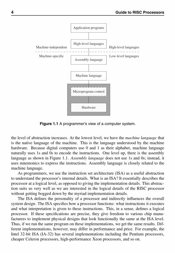
A programmer’s view of a computer system depends on the type and level of languageshe intends to use. From the programmer’s viewpoint, there exists a hierarchy from low-level languages to high-level languages (see Figure 1.1). As we move up in this hierarchy,
3
4 Guide to RISC Processors
Hardware
Microprogram control
Machine language
High-level languages
Application programs
Assembly languageMachine-specific
Machine-independent High-level languages
Low-level languages
Figure 1.1 A programmer’s view of a computer system.
the level of abstraction increases. At the lowest level, we have the machine language thatis the native language of the machine. This is the language understood by the machinehardware. Because digital computers use 0 and 1 as their alphabet, machine languagenaturally uses 1s and 0s to encode the instructions. One level up, there is the assemblylanguage as shown in Figure 1.1. Assembly language does not use 1s and 0s; instead, ituses mnemonics to express the instructions. Assembly language is closely related to themachine language.
As programmers, we use the instruction set architecture (ISA) as a useful abstractionto understand the processor’s internal details. What is an ISA? It essentially describes theprocessor at a logical level, as opposed to giving the implementation details. This abstrac-tion suits us very well as we are interested in the logical details of the RISC processorwithout getting bogged down by the myriad implementation details.
The ISA defines the personality of a processor and indirectly influences the overallsystem design. The ISA specifies how a processor functions: what instructions it executesand what interpretation is given to these instructions. This, in a sense, defines a logicalprocessor. If these specifications are precise, they give freedom to various chip manu-facturers to implement physical designs that look functionally the same at the ISA level.Thus, if we run the same program on these implementations, we get the same results. Dif-ferent implementations, however, may differ in performance and price. For example, theIntel 32-bit ISA (IA-32) has several implementations including the Pentium processors,cheaper Celeron processors, high-performance Xeon processors, and so on.

Chapter 1 • Introduction 5
Two popular examples of ISA specifications are the SPARC and JVM. The rationalebehind having a precise ISA-level specification for the SPARC is to let multiple vendorsdesign their own processors that look the same at the ISA level. The JVM, on the otherhand, takes a different approach. Its ISA-level specification can be used to create a soft-ware layer so that the processor looks like a Java processor. Thus, in this case, we do notuse a set of hardware chips to implement the specifications, but rather use a software layerto simulate the virtual processor. Note, however, that there is nothing stopping us fromimplementing these specifications in hardware (even though this is not usually the case).
Why create the ISA layer? The ISA-level abstraction provides details about the ma-chine that are needed by the programmers. The idea is to have a common platform toexecute programs. If a program is written in C, a compiler translates it into the equivalentmachine language program that can run on the ISA-level logical processor. Similarly, ifyou write your program in FORTRAN, use a FORTRAN compiler to generate code thatcan execute on the ISA-level logical processor. At the ISA level, we can divide the designsinto two categories: RISC and CISC. We discuss these two categories in the next section.
RISC Versus CISCThere are two basic types of processor design philosophies: reduced instruction set com-puters (RISC) and complex instruction set computers (CISC). The Intel IA-32 architecturebelongs to the CISC category. The architectures we describe in the next part are all exam-ples of the RISC category.
Before we dig into the details of these two designs, let us talk about the current trend.In the 1970s and early 1980s, processors predominantly followed the CISC designs. Thecurrent trend is to use the RISC philosophy. To understand this shift from CISC to RISC,we need to look at the motivation for going the CISC way initially. But first we have toexplain what these two types of design philosophies are.
As the name suggests, CISC systems use complex instructions. What is a complexinstruction? For example, adding two integers is considered a simple instruction. But, aninstruction that copies an element from one array to another and automatically updatesboth array subscripts is considered a complex instruction. RISC systems use only simpleinstructions. Furthermore, RISC systems assume that the required operands are in theprocessor’s internal registers, not in the main memory. We discuss processor registers inthe next chapter. For now, think of them as scratchpads inside the processor.
A CISC design does not impose such restrictions. So what? It turns out that char-acteristics like simple instructions and restrictions like register-based operands not onlysimplify the processor design but also result in a processor that provides improved ap-plication performance. We give a detailed list of RISC design characteristics and theiradvantages in Chapter 3.
How come the early designers did not think about the RISC way of designing proces-sors? Several factors contributed to the popularity of CISC in the 1970s. In those days,memory was very expensive and small in capacity. For example, even in the mid-1970s,
6 Guide to RISC Processors
(a) CISC implementation (b) RISC implementation
Hardware
Microprogram control
ISA level
Hardware
ISA level
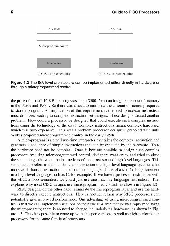
Figure 1.2 The ISA-level architecture can be implemented either directly in hardware orthrough a microprogrammed control.
the price of a small 16 KB memory was about $500. You can imagine the cost of memoryin the 1950s and 1960s. So there was a need to minimize the amount of memory requiredto store a program. An implication of this requirement is that each processor instructionmust do more, leading to complex instruction set designs. These designs caused anotherproblem. How could a processor be designed that could execute such complex instruc-tions using the technology of the day? Complex instructions meant complex hardware,which was also expensive. This was a problem processor designers grappled with untilWilkes proposed microprogrammed control in the early 1950s.
A microprogram is a small run-time interpreter that takes the complex instruction andgenerates a sequence of simple instructions that can be executed by the hardware. Thusthe hardware need not be complex. Once it became possible to design such complexprocessors by using microprogrammed control, designers went crazy and tried to closethe semantic gap between the instructions of the processor and high-level languages. Thissemantic gap refers to the fact that each instruction in a high-level language specifies a lotmore work than an instruction in the machine language. Think of a while loop statementin a high-level language such as C, for example. If we have a processor instruction withthe while loop semantics, we could just use one machine language instruction. Thisexplains why most CISC designs use microprogrammed control, as shown in Figure 1.2.
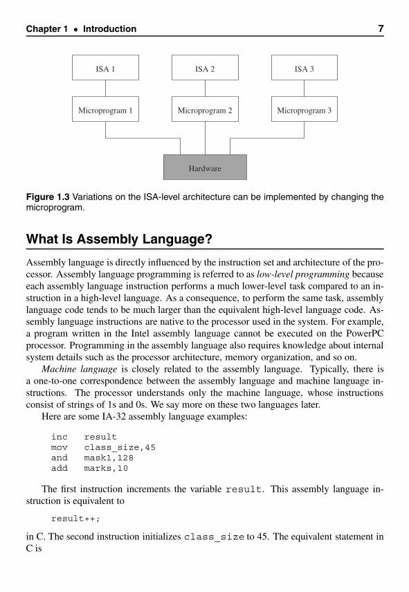
RISC designs, on the other hand, eliminate the microprogram layer and use the hard-ware to directly execute instructions. Here is another reason why RISC processors canpotentially give improved performance. One advantage of using microprogrammed con-trol is that we can implement variations on the basic ISA architecture by simply modifyingthe microprogram; there is no need to change the underlying hardware, as shown in Fig-ure 1.3. Thus it is possible to come up with cheaper versions as well as high-performanceprocessors for the same family of processors.
Chapter 1 • Introduction 7
Microprogram 1
ISA 1
Hardware
Microprogram 2
ISA 2
Microprogram 3
ISA 3
Figure 1.3 Variations on the ISA-level architecture can be implemented by changing themicroprogram.
What Is Assembly Language?
Assembly language is directly influenced by the instruction set and architecture of the pro-cessor. Assembly language programming is referred to as low-level programming becauseeach assembly language instruction performs a much lower-level task compared to an in-struction in a high-level language. As a consequence, to perform the same task, assemblylanguage code tends to be much larger than the equivalent high-level language code. As-sembly language instructions are native to the processor used in the system. For example,a program written in the Intel assembly language cannot be executed on the PowerPCprocessor. Programming in the assembly language also requires knowledge about internalsystem details such as the processor architecture, memory organization, and so on.
Machine language is closely related to the assembly language. Typically, there isa one-to-one correspondence between the assembly language and machine language in-structions. The processor understands only the machine language, whose instructionsconsist of strings of 1s and 0s. We say more on these two languages later.
Here are some IA-32 assembly language examples:
inc resultmov class_size,45and mask1,128add marks,10
The first instruction increments the variable result. This assembly language in-struction is equivalent to
result++;
in C. The second instruction initializes class_size to 45. The equivalent statement inC is
8 Guide to RISC Processors
class_size = 45;
The third instruction performs the bitwise and operation on mask1 and can be expressedin C as
mask1 = mask1 & 128;
The last instruction updates marks by adding 10. In C, this is equivalent to
marks = marks + 10;
As you can see from these examples, most instructions use two addresses. In these in-structions, one operand doubles as a source and destination (for example, class_sizeand marks). In contrast, the MIPS instructions use three addresses as shown below:
andi $t2,$t1,15addu $t3,$t1,$t2move $t2,$t1
The operands of these instructions are in processor registers. The processor registersare identified by $. The andi instruction performs bitwise and of $t1 register contentswith 15 and writes the result in the $t2 register. The second instruction adds the contentsof $t1 and $t2 and stores the result in $t3.
The last instruction copies the $t1 value into $t2. In contrast to our claim that MIPSuses three addresses, this instruction seems to use only two addresses. This is not reallyan instruction supported by the MIPS processor: it is an assembly language instruction.When translated by the MIPS assembler, this instruction is replaced by the followingprocessor instruction.
addu $t2,$0,$t1
The second operand in this instruction is a special register that holds constant zero. Thus,copying the $t1 value is treated as adding zero to it.
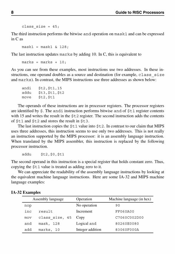
We can appreciate the readability of the assembly language instructions by looking atthe equivalent machine language instructions. Here are some IA-32 and MIPS machinelanguage examples:
IA-32 Examples
Assembly language Operation Machine language (in hex)
nop No operation 90
inc result Increment FF060A00
mov class_size, 45 Copy C7060C002D00
and mask, 128 Logical and 80260E0080
add marks, 10 Integer addition 83060F000A
Chapter 1 • Introduction 9
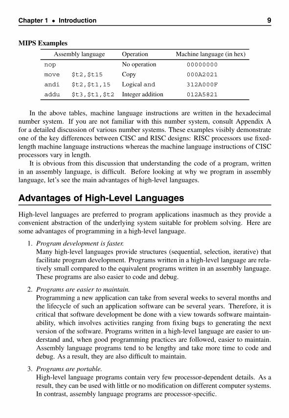
MIPS Examples
Assembly language Operation Machine language (in hex)
nop No operation 00000000
move $t2,$t15 Copy 000A2021
andi $t2,$t1,15 Logical and 312A000F
addu $t3,$t1,$t2 Integer addition 012A5821
In the above tables, machine language instructions are written in the hexadecimalnumber system. If you are not familiar with this number system, consult Appendix Afor a detailed discussion of various number systems. These examples visibly demonstrateone of the key differences between CISC and RISC designs: RISC processors use fixed-length machine language instructions whereas the machine language instructions of CISCprocessors vary in length.
It is obvious from this discussion that understanding the code of a program, writtenin an assembly language, is difficult. Before looking at why we program in assemblylanguage, let’s see the main advantages of high-level languages.
Advantages of High-Level Languages
High-level languages are preferred to program applications inasmuch as they provide aconvenient abstraction of the underlying system suitable for problem solving. Here aresome advantages of programming in a high-level language.
1. Program development is faster.Many high-level languages provide structures (sequential, selection, iterative) thatfacilitate program development. Programs written in a high-level language are rela-tively small compared to the equivalent programs written in an assembly language.These programs are also easier to code and debug.
2. Programs are easier to maintain.Programming a new application can take from several weeks to several months andthe lifecycle of such an application software can be several years. Therefore, it iscritical that software development be done with a view towards software maintain-ability, which involves activities ranging from fixing bugs to generating the nextversion of the software. Programs written in a high-level language are easier to un-derstand and, when good programming practices are followed, easier to maintain.Assembly language programs tend to be lengthy and take more time to code anddebug. As a result, they are also difficult to maintain.
3. Programs are portable.High-level language programs contain very few processor-dependent details. As aresult, they can be used with little or no modification on different computer systems.In contrast, assembly language programs are processor-specific.
10 Guide to RISC Processors
Why Program in Assembly Language?
The previous section gives enough reasons to discourage you from programming in as-sembly language. However, there are two main reasons why programming is still done inassembly language: efficiency and accessibility to system hardware.
Efficiency refers to how “good” a program is in achieving a given objective. Here weconsider two objectives based on space (space-efficiency) and time (time-efficiency).
Space-efficiency refers to the memory requirements of a program (i.e., the size of theexecutable code). Program A is said to be more space-efficient if it takes less memoryspace than program B to perform the same task. Very often, programs written in anassembly language tend to be more compact than those written in a high-level language.
Time-efficiency refers to the time taken to execute a program. Obviously a programthat runs faster is said to be better from the time-efficiency point of view. In general,assembly language programs tend to run faster than their high-level language versions.
The superiority of assembly language in generating compact code is becoming in-creasingly less important for several reasons. First, the savings in space pertain only tothe program code and not to its data space. Thus, depending on the application, the sav-ings in space obtained by converting an application program from some high-level lan-guage to an assembly language may not be substantial. Second, the cost of memory hasbeen decreasing and memory capacity has been increasing. Thus, the size of a programis not a major hurdle anymore. Finally, compilers are becoming “smarter” in generatingcode that is both space- and time-efficient. However, there are systems such as embeddedcontrollers and handheld devices in which space-efficiency is very important.
One of the main reasons for writing programs in assembly language is to generatecode that is time-efficient. The superiority of assembly language programs in producingefficient code is a direct manifestation of specificity. That is, assembly language pro-grams contain only the code that is necessary to perform the given task. Even here, a“smart” compiler can optimize the code that can compete well with its equivalent writtenin an assembly language. Although this gap is narrowing with improvements in compilertechnology, assembly language still retains its advantage for now.
The other main reason for writing assembly language programs is to have direct con-trol over system hardware. High-level languages, on purpose, provide a restricted (ab-stract) view of the underlying hardware. Because of this, it is almost impossible to per-form certain tasks that require access to the system hardware. For example, writing adevice driver to a new scanner on the market almost certainly requires programming inan assembly language. Because assembly language does not impose any restrictions, youcan have direct control over the system hardware. If you are developing system software,you cannot avoid writing assembly language programs.
There is another reason for our interest in the assembly language. It allows us to lookat the internal details of the processors. For the RISC processors discussed in the next partof the book, we present their assembly language instructions. In addition, Part III givesyou hands-on experience in MIPS assembly language programming.

Chapter 1 • Introduction 11
Summary
We identified two major processor designs: CISC and RISC. We discussed the differencesbetween these two design philosophies. The Intel IA-32 architecture follows the CISC de-sign whereas several recent processor families follow the RISC designs. Some examplesbelonging to the RISC category are the MIPS, SPARC, and ARM processor families.
We also introduced assembly language to prepare the ground for Part III of the book.Specifically, we looked at the advantages and problems associated with assembly languagevis-a-vis high-level languages.
2Processor Design Issues
In this chapter we look at some of the basic choices in the processor design space. Westart our discussion with the number of addresses used in processor instructions. Thisis an important characteristic that influences instruction set design. We also look at theload/store architecture used by RISC processors.
Another important aspect that affects performance of the overall system is the flowcontrol. Flow control deals with issues such as branching and procedure calls. We discussthe general principles used to efficiently implement branching and procedure invocationmechanisms. We wrap up the chapter with a discussion of some of the instruction setdesign issues.
IntroductionOne of the characteristics of the instruction set architecture (ISA) that shapes the archi-tecture is the number of addresses used in an instruction. Most operations can be dividedinto binary or unary operations. Binary operations such as addition and multiplication re-quire two input operands whereas the unary operations such as the logical not need onlya single operand. Most operations produce a single result. There are exceptions, however.For example, the division operation produces two outputs: a quotient and a remainder.Because most operations are binary, we need a total of three addresses: two addressesto specify the two input operands and one to specify where the result should go. Typi-cal operations require two operands, therefore we need three addresses: two addresses tospecify the two input operands and the third one to indicate where the result should bestored.
Most processors specify three addresses. We can reduce the number of addresses totwo by using one address to specify a source address as well as the destination address.The Intel IA-32 processors use the two-address format. It is also possible to have in-structions that use only one or even zero address. The one-address machines are called
13
14 Guide to RISC Processors
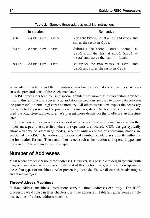
Table 2.1 Sample three-address machine instructions
Instruction Semantics
add dest,src1,src2 Adds the two values at src1 and src2 andstores the result in dest
sub dest,src1,src2 Subtracts the second source operand atsrc2 from the first at src1 (src1 −src2) and stores the result in dest
mult dest,src1,src2 Multiplies the two values at src1 andsrc2 and stores the result in dest
accumulator machines and the zero-address machines are called stack machines. We dis-cuss the pros and cons of these schemes later.
RISC processors tend to use a special architecture known as the load/store architec-ture. In this architecture, special load and store instructions are used to move data betweenthe processor’s internal registers and memory. All other instructions expect the necessaryoperands to be present in the processor internal registers. Vector processors originallyused the load/store architecture. We present more details on the load/store architecturelater.
Instruction set design involves several other issues. The addressing mode is anotherimportant aspect that specifies where the operands are located. CISC designs typicallyallow a variety of addressing modes, whereas only a couple of addressing modes aresupported by RISC. The addressing modes and number of addresses directly influencethe instruction format. These and other issues such as instruction and operand types arediscussed in the remainder of the chapter.
Number of AddressesMost recent processors use three addresses. However, it is possible to design systems withtwo, one, or even zero addresses. In the rest of this section, we give a brief description ofthese four types of machines. After presenting these details, we discuss their advantagesand disadvantages.
Three-Address MachinesIn three-address machines, instructions carry all three addresses explicitly. The RISCprocessors we discuss in later chapters use three addresses. Table 2.1 gives some sampleinstructions of a three-address machine.
Chapter 2 • Processor Design Issues 15
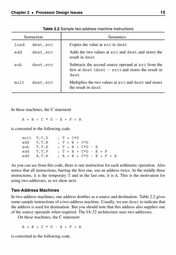
Table 2.2 Sample two-address machine instructions
Instruction Semantics
load dest,src Copies the value at src to dest
add dest,src Adds the two values at src and dest and stores theresult in dest
sub dest,src Subtracts the second source operand at src from thefirst at dest (dest − src) and stores the result indest
mult dest,src Multiplies the two values at src and dest and storesthe result in dest
In these machines, the C statement
A = B + C * D - E + F + A
is converted to the following code.
mult T,C,D ; T = C*Dadd T,T,B ; T = B + C*Dsub T,T,E ; T = B + C*D - Eadd T,T,F ; T = B + C*D - E + Fadd A,T,A ; A = B + C*D - E + F + A
As you can see from this code, there is one instruction for each arithmetic operation. Alsonotice that all instructions, barring the first one, use an address twice. In the middle threeinstructions, it is the temporary T and in the last one, it is A. This is the motivation forusing two addresses, as we show next.
Two-Address MachinesIn two-address machines, one address doubles as a source and destination. Table 2.2 givessome sample instructions of a two-address machine. Usually, we use dest to indicate thatthe address is used for destination. But you should note that this address also supplies oneof the source operands when required. The IA-32 architecture uses two addresses.
On these machines, the C statement
A = B + C * D - E + F + A
is converted to the following code.
16 Guide to RISC Processors
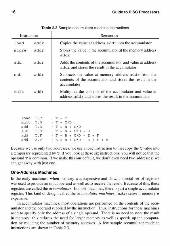
Table 2.3 Sample accumulator machine instructions
Instruction Semantics
load addr Copies the value at address addr into the accumulator
store addr Stores the value in the accumulator at the memory addressaddr
add addr Adds the contents of the accumulator and value at addressaddr and stores the result in the accumulator
sub addr Subtracts the value at memory address addr from thecontents of the accumulator and stores the result in theaccumulator
mult addr Multiplies the contents of the accumulator and value ataddress addr and stores the result in the accumulator
load T,C ; T = Cmult T,D ; T = C*Dadd T,B ; T = B + C*Dsub T,E ; T = B + C*D - Eadd T,F ; T = B + C*D - E + Fadd A,T ; A = B + C*D - E + F + A
Because we use only two addresses, we use a load instruction to first copy the C value intoa temporary represented by T. If you look at these six instructions, you will notice that theoperand T is common. If we make this our default, we don’t even need two addresses: wecan get away with just one.
One-Address MachinesIn the early machines, when memory was expensive and slow, a special set of registerswas used to provide an input operand as well as to receive the result. Because of this, theseregisters are called the accumulators. In most machines, there is just a single accumulatorregister. This kind of design, called the accumulator machines, makes sense if memory isexpensive.
In accumulator machines, most operations are performed on the contents of the accu-mulator and the operand supplied by the instruction. Thus, instructions for these machinesneed to specify only the address of a single operand. There is no need to store the resultin memory: this reduces the need for larger memory as well as speeds up the computa-tion by reducing the number of memory accesses. A few sample accumulator machineinstructions are shown in Table 2.3.
Chapter 2 • Processor Design Issues 17
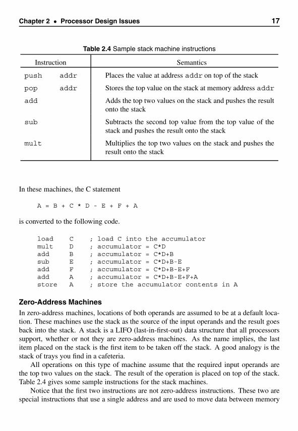
Table 2.4 Sample stack machine instructions
Instruction Semantics
push addr Places the value at address addr on top of the stack
pop addr Stores the top value on the stack at memory address addr
add Adds the top two values on the stack and pushes the resultonto the stack
sub Subtracts the second top value from the top value of thestack and pushes the result onto the stack
mult Multiplies the top two values on the stack and pushes theresult onto the stack
In these machines, the C statement
A = B + C * D - E + F + A
is converted to the following code.
load C ; load C into the accumulatormult D ; accumulator = C*Dadd B ; accumulator = C*D+Bsub E ; accumulator = C*D+B-Eadd F ; accumulator = C*D+B-E+Fadd A ; accumulator = C*D+B-E+F+Astore A ; store the accumulator contents in A
Zero-Address MachinesIn zero-address machines, locations of both operands are assumed to be at a default loca-tion. These machines use the stack as the source of the input operands and the result goesback into the stack. A stack is a LIFO (last-in-first-out) data structure that all processorssupport, whether or not they are zero-address machines. As the name implies, the lastitem placed on the stack is the first item to be taken off the stack. A good analogy is thestack of trays you find in a cafeteria.
All operations on this type of machine assume that the required input operands arethe top two values on the stack. The result of the operation is placed on top of the stack.Table 2.4 gives some sample instructions for the stack machines.
Notice that the first two instructions are not zero-address instructions. These two arespecial instructions that use a single address and are used to move data between memory
18 Guide to RISC Processors
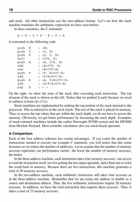
and stack. All other instructions use the zero-address format. Let’s see how the stackmachine translates the arithmetic expression we have seen before.
In these machines, the C statement
A = B + C * D - E + F + A
is converted to the following code.
push E ; <E>push C ; <C, E>push D ; <D, C, E>mult ; <C*D, E>push B ; <B, C*D, E>add ; <B+C*D, E>sub ; <B+C*D-E>push F ; <F, B+D*C-E>add ; <F+B+D*C-E>push A ; <A, F+B+D*C-E>add ; <A+F+B+D*C-E>pop A ; < >
On the right, we show the state of the stack after executing each instruction. The topelement of the stack is shown on the left. Notice that we pushed E early because we needto subtract it from (B+C*D).
Stack machines are implemented by making the top portion of the stack internal to theprocessor. This is referred to as the stack depth. The rest of the stack is placed in memory.Thus, to access the top values that are within the stack depth, we do not have to access thememory. Obviously, we get better performance by increasing the stack depth. Examplesof stack-oriented machines include the earlier Burroughs B5500 system and the HP3000from Hewlett–Packard. Most scientific calculators also use stack-based operands.
A ComparisonEach of the four address schemes has certain advantages. If you count the number ofinstructions needed to execute our example C statement, you will notice that this countincreases as we reduce the number of addresses. Let us assume that the number of memoryaccesses represents our performance metric: the lower the number of memory accesses,the better.
In the three-address machine, each instruction takes four memory accesses: one accessto read the instruction itself, two for getting the two input operands, and a final one to writethe result back in memory. Because there are five instructions, this machine generates atotal of 20 memory accesses.
In the two-address machine, each arithmetic instruction still takes four accesses asin the three-address machine. Remember that we are using one address to double as asource and destination address. Thus, the five arithmetic instructions require 20 memoryaccesses. In addition, we have the load instruction that requires three accesses. Thus, ittakes a total of 23 memory accesses.
Chapter 2 • Processor Design Issues 19
8 bits 5 bits 5 bits
18 bits Opcode Rdest/Rsrc1 Rsrc2
8 bits 5 bits
13 bits Opcode Rdest/Rsrc2
8 bits Opcode
8 bits
2-address format
8 bits 5 bits 5 bits 5 bits
23 bits Opcode Rdest Rsrc2Rsrc1
3-address format
1-address format
0-address format
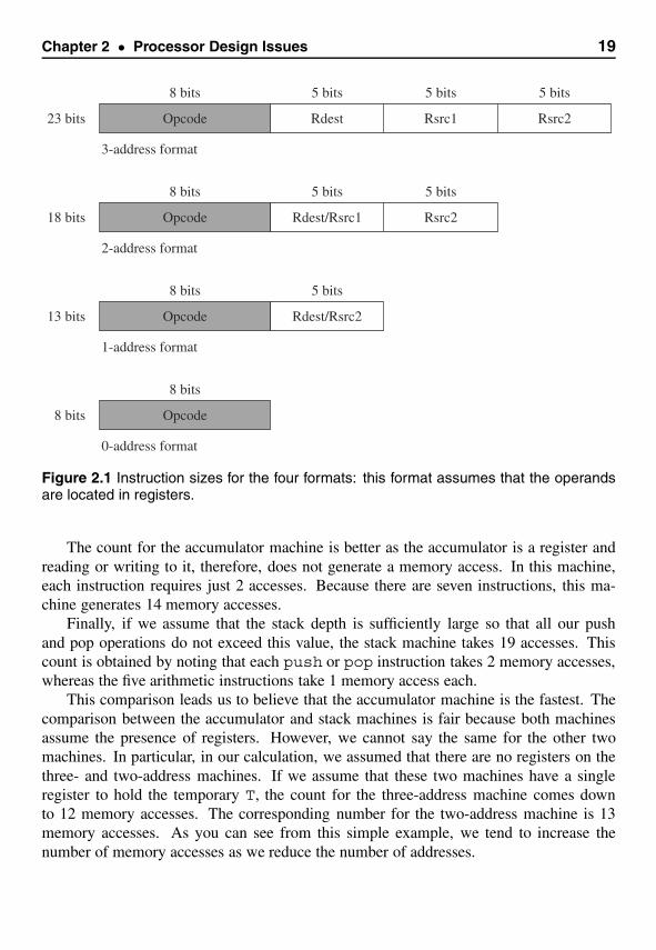
Figure 2.1 Instruction sizes for the four formats: this format assumes that the operandsare located in registers.
The count for the accumulator machine is better as the accumulator is a register andreading or writing to it, therefore, does not generate a memory access. In this machine,each instruction requires just 2 accesses. Because there are seven instructions, this ma-chine generates 14 memory accesses.
Finally, if we assume that the stack depth is sufficiently large so that all our pushand pop operations do not exceed this value, the stack machine takes 19 accesses. Thiscount is obtained by noting that each push or pop instruction takes 2 memory accesses,whereas the five arithmetic instructions take 1 memory access each.
This comparison leads us to believe that the accumulator machine is the fastest. Thecomparison between the accumulator and stack machines is fair because both machinesassume the presence of registers. However, we cannot say the same for the other twomachines. In particular, in our calculation, we assumed that there are no registers on thethree- and two-address machines. If we assume that these two machines have a singleregister to hold the temporary T, the count for the three-address machine comes downto 12 memory accesses. The corresponding number for the two-address machine is 13memory accesses. As you can see from this simple example, we tend to increase thenumber of memory accesses as we reduce the number of addresses.
20 Guide to RISC Processors
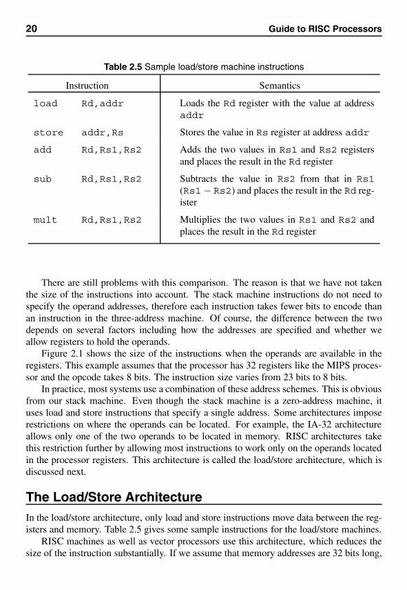
Table 2.5 Sample load/store machine instructions
Instruction Semantics
load Rd,addr Loads the Rd register with the value at addressaddr
store addr,Rs Stores the value in Rs register at address addr
add Rd,Rs1,Rs2 Adds the two values in Rs1 and Rs2 registersand places the result in the Rd register
sub Rd,Rs1,Rs2 Subtracts the value in Rs2 from that in Rs1(Rs1− Rs2) and places the result in the Rd reg-ister
mult Rd,Rs1,Rs2 Multiplies the two values in Rs1 and Rs2 andplaces the result in the Rd register
There are still problems with this comparison. The reason is that we have not takenthe size of the instructions into account. The stack machine instructions do not need tospecify the operand addresses, therefore each instruction takes fewer bits to encode thanan instruction in the three-address machine. Of course, the difference between the twodepends on several factors including how the addresses are specified and whether weallow registers to hold the operands.
Figure 2.1 shows the size of the instructions when the operands are available in theregisters. This example assumes that the processor has 32 registers like the MIPS proces-sor and the opcode takes 8 bits. The instruction size varies from 23 bits to 8 bits.
In practice, most systems use a combination of these address schemes. This is obviousfrom our stack machine. Even though the stack machine is a zero-address machine, ituses load and store instructions that specify a single address. Some architectures imposerestrictions on where the operands can be located. For example, the IA-32 architectureallows only one of the two operands to be located in memory. RISC architectures takethis restriction further by allowing most instructions to work only on the operands locatedin the processor registers. This architecture is called the load/store architecture, which isdiscussed next.
The Load/Store ArchitectureIn the load/store architecture, only load and store instructions move data between the reg-isters and memory. Table 2.5 gives some sample instructions for the load/store machines.
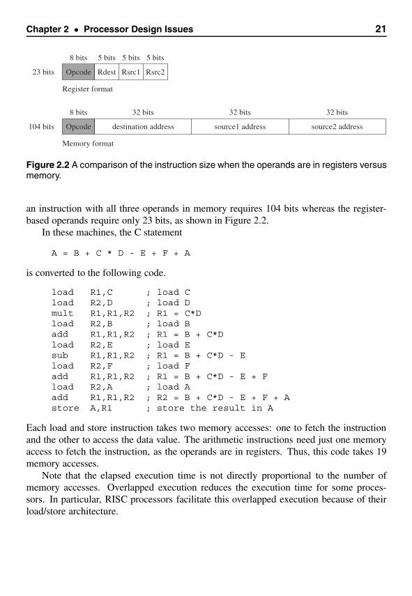
RISC machines as well as vector processors use this architecture, which reduces thesize of the instruction substantially. If we assume that memory addresses are 32 bits long,
Chapter 2 • Processor Design Issues 21
104 bits Opcode destination address
8 bits 32 bits
source1 address source2 address
32 bits 32 bits
23 bits Opcode Rdest
8 bits 5 bits 5 bits 5 bits
Rsrc1 Rsrc2
Register format
Memory format
Figure 2.2 A comparison of the instruction size when the operands are in registers versusmemory.
an instruction with all three operands in memory requires 104 bits whereas the register-based operands require only 23 bits, as shown in Figure 2.2.
In these machines, the C statement
A = B + C * D - E + F + A
is converted to the following code.
load R1,C ; load Cload R2,D ; load Dmult R1,R1,R2 ; R1 = C*Dload R2,B ; load Badd R1,R1,R2 ; R1 = B + C*Dload R2,E ; load Esub R1,R1,R2 ; R1 = B + C*D - Eload R2,F ; load Fadd R1,R1,R2 ; R1 = B + C*D - E + Fload R2,A ; load Aadd R1,R1,R2 ; R2 = B + C*D - E + F + Astore A,R1 ; store the result in A
Each load and store instruction takes two memory accesses: one to fetch the instructionand the other to access the data value. The arithmetic instructions need just one memoryaccess to fetch the instruction, as the operands are in registers. Thus, this code takes 19memory accesses.
Note that the elapsed execution time is not directly proportional to the number ofmemory accesses. Overlapped execution reduces the execution time for some proces-sors. In particular, RISC processors facilitate this overlapped execution because of theirload/store architecture.

22 Guide to RISC Processors
Processor Registers
Processors have a number of registers to hold data, instructions, and state information. Wecan divide the registers into general-purpose or special-purpose registers. Special-purposeregisters can be further divided into those that are accessible to the user programs andthose reserved for system use. The available technology largely determines the structureand function of the register set.
The number of addresses used in instructions partly influences the number of dataregisters and their use. For example, stack machines do not require any data registers.However, as noted, part of the stack is kept internal to the processor. This part of the stackserves the same purpose that registers do. In three- and two-address machines, there isno need for the internal data registers. However, as we have demonstrated before, havingsome internal registers improves performance by cutting down the number of memoryaccesses. The RISC machines typically have a large number of registers.
Some processors maintain a few special-purpose registers. For example, the IA-32uses a couple of registers to implement the processor stack. Processors also have severalregisters reserved for the instruction execution unit. Typically, there is an instructionregister that holds the current instruction and a program counter that points to the nextinstruction to be executed.
Flow of ControlProgram execution, by default, proceeds sequentially. The program counter (PC) registerplays an important role in managing the control flow. At a simple level, the PC can bethought of as pointing to the next instruction. The processor fetches the instruction atthe address pointed to by the PC. When an instruction is fetched, the PC is automaticallyincremented to point to the next instruction. If we assume that each instruction takesexactly four bytes as in MIPS and SPARC processors, the PC is automatically incrementedby four after each instruction fetch. This leads to the default sequential execution pattern.However, sometimes we want to alter this default execution flow. In high-level languages,we use control structures such as if-then-else and while statements to alter theexecution behavior based on some run-time conditions. Similarly, the procedure call isanother way we alter the sequential execution. In this section, we describe how processorssupport flow control. We look at both branch and procedure calls next.
BranchingBranching is implemented by means of a branch instruction. There are two types ofbranches: direct and indirect. The direct branch instruction carries the address of thetarget instruction explicitly. In indirect branch, the target address is specified indirectlyvia either memory or a register. We look at an indirect branch example in Chapter 14(page 259). In the rest of this section, we consider direct branches.
Chapter 2 • Processor Design Issues 23
jump targetinstruction yinstruction z
instruction x
instruction binstruction c
target:instruction a
Figure 2.3 Normal branch execution.
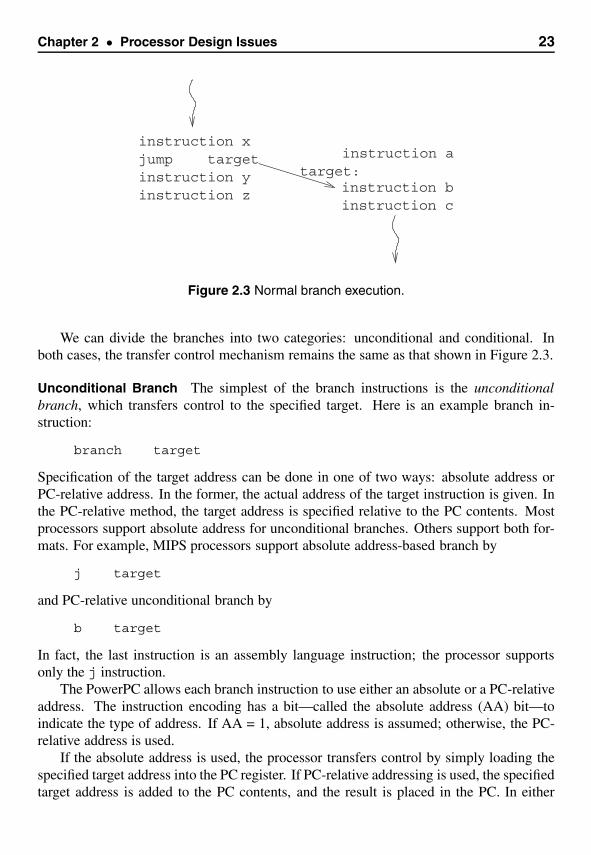
We can divide the branches into two categories: unconditional and conditional. Inboth cases, the transfer control mechanism remains the same as that shown in Figure 2.3.
Unconditional Branch The simplest of the branch instructions is the unconditionalbranch, which transfers control to the specified target. Here is an example branch in-struction:
branch target
Specification of the target address can be done in one of two ways: absolute address orPC-relative address. In the former, the actual address of the target instruction is given. Inthe PC-relative method, the target address is specified relative to the PC contents. Mostprocessors support absolute address for unconditional branches. Others support both for-mats. For example, MIPS processors support absolute address-based branch by
j target
and PC-relative unconditional branch by
b target
In fact, the last instruction is an assembly language instruction; the processor supportsonly the j instruction.
The PowerPC allows each branch instruction to use either an absolute or a PC-relativeaddress. The instruction encoding has a bit—called the absolute address (AA) bit—toindicate the type of address. If AA = 1, absolute address is assumed; otherwise, the PC-relative address is used.
If the absolute address is used, the processor transfers control by simply loading thespecified target address into the PC register. If PC-relative addressing is used, the specifiedtarget address is added to the PC contents, and the result is placed in the PC. In either
24 Guide to RISC Processors
case, because the PC indicates the next instruction address, the processor will fetch theinstruction at the intended target address.
The main advantage of using the PC-relative address is that we can move the codefrom one block of memory to another without changing the target addresses. This type ofcode is called relocatable code. Relocatable code is not possible with absolute addresses.
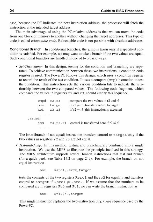
Conditional Branch In conditional branches, the jump is taken only if a specified con-dition is satisfied. For example, we may want to take a branch if the two values are equal.Such conditional branches are handled in one of two basic ways.
• Set-Then-Jump: In this design, testing for the condition and branching are sepa-rated. To achieve communication between these two instructions, a condition coderegister is used. The PowerPC follows this design, which uses a condition registerto record the result of the test condition. It uses a compare (cmp) instruction to testthe condition. This instruction sets the various condition bits to indicate the rela-tionship between the two compared values. The following code fragment, whichcompares the values in registers r2 and r3, should clarify this sequence.
cmpd r2,r3 ; compare the two values in r2 and r3bne target ; if r2 �= r3, transfer control to targetnot r3,r3 ; if r2 = r3, this instruction is executed. . .
target:add r4,r3,r4 ; control is transferred here if r2 �= r3. . .
The bne (branch if not equal) instruction transfers control to target only if thetwo values in registers r2 and r3 are not equal.
• Test-and-Jump: In this method, testing and branching are combined into a singleinstruction. We use the MIPS to illustrate the principle involved in this strategy.The MIPS architecture supports several branch instructions that test and branch(for a quick peek, see Table 14.2 on page 249). For example, the branch on notequal instruction
bne Rsrc1,Rsrc2,target
tests the contents of the two registers Rsrc1 and Rsrc2 for equality and transferscontrol to target if Rsrc1 �= Rsrc2. If we assume that the numbers to becompared are in registers $t0 and $t1, we can write the branch instruction as
bne $t1,$t0,target
This single instruction replaces the two-instruction cmp/bne sequence used by thePowerPC.
Chapter 2 • Processor Design Issues 25
jump targetinstruction yinstruction z
instruction x
instruction binstruction c
target:instruction a
Figure 2.4 Delayed branch execution.
Some processors maintain registers to record the condition of the arithmetic and logi-cal operations. These are called condition code registers. These registers keep a record ofthe status of the last arithmetic/logical operation. For example, when we add two 32-bitintegers, it is possible that the sum might require more than 32 bits. This is the overflowcondition that the system should record. Normally, a bit in the condition code register isset to indicate this overflow condition. The MIPS, for example, does not use a conditionregister. Instead, it uses exceptions to flag the overflow condition. On the other hand, Pow-erPC and SPARC processors use condition registers. In the PowerPC, this information ismaintained by the XER register. SPARC uses a condition code register.
Some instruction sets provide branches based on comparisons to zero. Some examplesthat provide this type of branch instructions include the MIPS and SPARC (see Table 14.3on page 250 for the MIPS instructions).
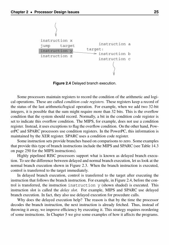
Highly pipelined RISC processors support what is known as delayed branch execu-tion. To see the difference between delayed and normal branch execution, let us look at thenormal branch execution shown in Figure 2.3. When the branch instruction is executed,control is transferred to the target immediately.
In delayed branch execution, control is transferred to the target after executing theinstruction that follows the branch instruction. For example, in Figure 2.4, before the con-trol is transferred, the instruction instruction y (shown shaded) is executed. Thisinstruction slot is called the delay slot. For example, MIPS and SPARC use delayedbranch execution. In fact, they also use delayed execution for procedure calls.
Why does the delayed execution help? The reason is that by the time the processordecodes the branch instruction, the next instruction is already fetched. Thus, instead ofthrowing it away, we improve efficiency by executing it. This strategy requires reorderingof some instructions. In Chapter 5 we give some examples of how it affects the programs.
26 Guide to RISC Processors
instruction xcall procAinstruction yinstruction z
procA:instruction ainstruction b
instruction creturn
Called procedureCalling procedure
. . .
. . .
Figure 2.5 Control flow in procedure calls.
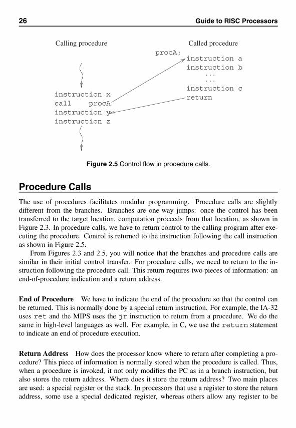
Procedure CallsThe use of procedures facilitates modular programming. Procedure calls are slightlydifferent from the branches. Branches are one-way jumps: once the control has beentransferred to the target location, computation proceeds from that location, as shown inFigure 2.3. In procedure calls, we have to return control to the calling program after exe-cuting the procedure. Control is returned to the instruction following the call instructionas shown in Figure 2.5.
From Figures 2.3 and 2.5, you will notice that the branches and procedure calls aresimilar in their initial control transfer. For procedure calls, we need to return to the in-struction following the procedure call. This return requires two pieces of information: anend-of-procedure indication and a return address.
End of Procedure We have to indicate the end of the procedure so that the control canbe returned. This is normally done by a special return instruction. For example, the IA-32uses ret and the MIPS uses the jr instruction to return from a procedure. We do thesame in high-level languages as well. For example, in C, we use the return statementto indicate an end of procedure execution.
Return Address How does the processor know where to return after completing a pro-cedure? This piece of information is normally stored when the procedure is called. Thus,when a procedure is invoked, it not only modifies the PC as in a branch instruction, butalso stores the return address. Where does it store the return address? Two main placesare used: a special register or the stack. In processors that use a register to store the returnaddress, some use a special dedicated register, whereas others allow any register to be
Chapter 2 • Processor Design Issues 27
instruction xcall procAinstruction yinstruction z
procA:instruction ainstruction b
instruction creturn
Called procedureCalling procedure
. . .
. . .
Figure 2.6 Control flow in delayed procedure calls.
used for this purpose. The actual return address stored depends on the architecture. Forexample, SPARC stores the address of the call instruction itself. Others like MIPS storethe address of the instruction following the call instruction.
The IA-32 uses the stack to store the return address. Thus, each procedure call in-volves pushing the return address onto the stack before control is transferred to the pro-cedure code. The return instruction retrieves this value from the stack to send the controlback to the instruction following the procedure call.
MIPS processors allow any general-purpose register to store the return address. Thereturn statement can specify this register. The format of the return statement is
jr $ra
where ra is the register that contains the return address.The PowerPC has a dedicated register, called the link register (LR), to store the return
address. Both the MIPS and the PowerPC use a modified branch to implement a procedurecall. The advantage of these processors is that simple procedure calls do not have to accessmemory.
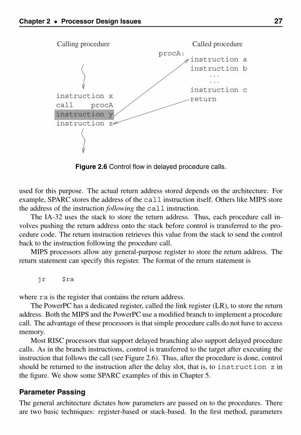
Most RISC processors that support delayed branching also support delayed procedurecalls. As in the branch instructions, control is transferred to the target after executing theinstruction that follows the call (see Figure 2.6). Thus, after the procedure is done, controlshould be returned to the instruction after the delay slot, that is, to instruction z inthe figure. We show some SPARC examples of this in Chapter 5.
Parameter PassingThe general architecture dictates how parameters are passed on to the procedures. Thereare two basic techniques: register-based or stack-based. In the first method, parameters
28 Guide to RISC Processors
are placed in processor registers and the called procedure reads the parameter values fromthese registers. In the stack-based method, parameters are pushed onto the stack and thecalled procedure would have to read them off the stack.
The advantage of the register method is that it is faster than the stack method. How-ever, because of the limited number of registers, it imposes a limit on the number of param-eters. Furthermore, recursive procedures cannot use the simple register-based mechanism.Because RISC processors tend to have more registers, register-based parameter passing isused in RISC processors. The IA-32 tends to use the stack for parameter passing due tothe limited number of processor registers.
Some architectures use a register window mechanism that allows a more flexible pa-rameter passing. The SPARC and Intel Itanium processors use this parameter passingmechanism. We describe this method in detail in later chapters.
Handling Branches
Modern processors are highly pipelined. In such processors, flow-altering instructionssuch as branch require special handling. If the branch is not taken, the instructions in thepipeline are useful. However, for a taken branch, we have to discard all the instructionsthat are in the pipeline at various stages. This causes the processor to do wasteful work,resulting in a branch penalty.
How can we reduce this branch penalty? We have already mentioned one technique:the delayed branch execution, which reduces the branch penalty. When we use this strat-egy, we need to modify our program to put a useful instruction in the delay slot. Someprocessors such as the SPARC and MIPS use delayed execution for both branching andprocedure calls.
We can improve performance further if we can find whether a branch is taken withoutwaiting for the execution of the branch instruction. In the case where the branch is taken,we also need to know the target address so that the pipeline can be filled from the targetaddress. For direct branch instructions, the target address is given as part of the instruc-tion. Because most instructions are direct branches, computation of the target address isrelatively straightforward. But it may not be that easy to predict whether the branch willbe taken. For example, we may have to fetch the operands and compare their values todetermine whether the branch is taken. This means we have to wait until the instructionreaches the execution stage. We can use branch prediction strategies to make an educatedguess. For indirect branches, we have to also guess the target address. Next we discussseveral branch prediction strategies.
Branch PredictionBranch prediction is traditionally used to handle the branch problem. We discuss threebranch prediction strategies: fixed, static, and dynamic.

Chapter 2 • Processor Design Issues 29
Table 2.6 Static branch prediction accuracy
Instruction typeInstruction
distribution (%)Prediction:
Branch taken?Correct prediction
(%)
Unconditional branch 70 × 0.4 = 28 Yes 28Conditional branch 70 × 0.6 = 42 No 42 × 0.6 = 25.2Loop 10 Yes 10 × 0.9 = 9Call/return 20 Yes 20
Overall prediction accuracy = 82.2%
Fixed Branch Prediction In this strategy, prediction is fixed. These strategies are sim-ple to implement and assume that the branch is either never taken or always taken. TheMotorola 68020 and VAX 11/780 use the branch-never-taken approach. The advantageof the never-taken strategy is that the processor can continue to fetch instructions sequen-tially to fill the pipeline. This involves minimum penalty in case the prediction is wrong.If, on the other hand, we use the always-taken approach, the processor would prefetch theinstruction at the branch target address. In a paged environment, this may lead to a pagefault, and a special mechanism is needed to take care of this situation. Furthermore, if theprediction were wrong, we would have done a lot of unnecessary work.
The branch-never-taken approach, however, is not proper for a loop structure. If a loopiterates 200 times, the branch is taken 199 out of 200 times. For loops, the always-takenapproach is better. Similarly, the always-taken approach is preferred for procedure callsand returns.
Static Branch Prediction From our discussion, it is obvious that, rather than follow-ing a fixed strategy, we can improve performance by using a strategy that is dependenton the branch type. This is what the static strategy does. It uses instruction opcode topredict whether the branch is taken. To show why this strategy gives high prediction ac-curacy, we present sample data for commercial environments. In such environments, ofall the branch-type operations, the branches are about 70%, loops are 10%, and the rest areprocedure calls/returns. Of the total branches, 40% are unconditional. If we use a never-taken guess for the conditional branch and always-taken for the rest of the branch-typeoperations, we get a prediction accuracy of about 82% as shown in Table 2.6.
The data in this table assume that conditional branches are not taken about 60% of thetime. Thus, our prediction that a conditional branch is never taken is correct only 60%of the time. This gives us 42 × 0.6 = 25.2% as the prediction accuracy for conditionalbranches. Similarly, loops jump back with 90% probability. Loops appear about 10% ofthe time, therefore the prediction is right 9% of the time. Surprisingly, even this simplestatic prediction strategy gives us about 82% accuracy!
30 Guide to RISC Processors
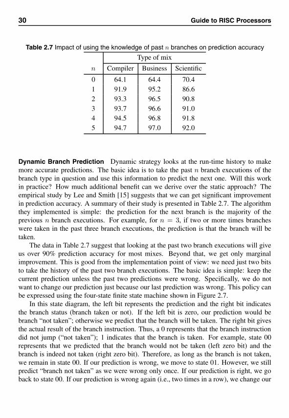
Table 2.7 Impact of using the knowledge of past n branches on prediction accuracy
Type of mix
n Compiler Business Scientific
0 64.1 64.4 70.41 91.9 95.2 86.62 93.3 96.5 90.83 93.7 96.6 91.04 94.5 96.8 91.85 94.7 97.0 92.0
Dynamic Branch Prediction Dynamic strategy looks at the run-time history to makemore accurate predictions. The basic idea is to take the past n branch executions of thebranch type in question and use this information to predict the next one. Will this workin practice? How much additional benefit can we derive over the static approach? Theempirical study by Lee and Smith [15] suggests that we can get significant improvementin prediction accuracy. A summary of their study is presented in Table 2.7. The algorithmthey implemented is simple: the prediction for the next branch is the majority of theprevious n branch executions. For example, for n = 3, if two or more times brancheswere taken in the past three branch executions, the prediction is that the branch will betaken.
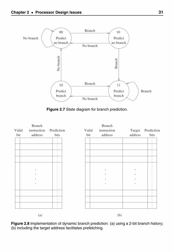
The data in Table 2.7 suggest that looking at the past two branch executions will giveus over 90% prediction accuracy for most mixes. Beyond that, we get only marginalimprovement. This is good from the implementation point of view: we need just two bitsto take the history of the past two branch executions. The basic idea is simple: keep thecurrent prediction unless the past two predictions were wrong. Specifically, we do notwant to change our prediction just because our last prediction was wrong. This policy canbe expressed using the four-state finite state machine shown in Figure 2.7.
In this state diagram, the left bit represents the prediction and the right bit indicatesthe branch status (branch taken or not). If the left bit is zero, our prediction would bebranch “not taken”; otherwise we predict that the branch will be taken. The right bit givesthe actual result of the branch instruction. Thus, a 0 represents that the branch instructiondid not jump (“not taken”); 1 indicates that the branch is taken. For example, state 00represents that we predicted that the branch would not be taken (left zero bit) and thebranch is indeed not taken (right zero bit). Therefore, as long as the branch is not taken,we remain in state 00. If our prediction is wrong, we move to state 01. However, we stillpredict “branch not taken” as we were wrong only once. If our prediction is right, we goback to state 00. If our prediction is wrong again (i.e., two times in a row), we change our
Chapter 2 • Processor Design Issues 31
01
Predictno branch
00
PredictNo branchno branch
Branch
No branch
Bra
nch
No
bran
ch
Branch
No branch
11
Predictbranch
10
Predictbranch
Branch
Figure 2.7 State diagram for branch prediction.
Validbit
Branchinstruction
addressPrediction
bits
.
.
.
.
Validbit
Branchinstruction
address
.
.
.
.
Predictionbits
Targetaddress
.
.
.
.
(a) (b)
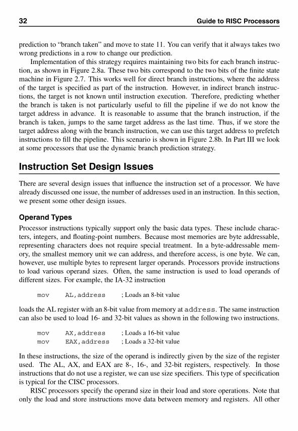
Figure 2.8 Implementation of dynamic branch prediction: (a) using a 2-bit branch history;(b) including the target address facilitates prefetching.
32 Guide to RISC Processors
prediction to “branch taken” and move to state 11. You can verify that it always takes twowrong predictions in a row to change our prediction.
Implementation of this strategy requires maintaining two bits for each branch instruc-tion, as shown in Figure 2.8a. These two bits correspond to the two bits of the finite statemachine in Figure 2.7. This works well for direct branch instructions, where the addressof the target is specified as part of the instruction. However, in indirect branch instruc-tions, the target is not known until instruction execution. Therefore, predicting whetherthe branch is taken is not particularly useful to fill the pipeline if we do not know thetarget address in advance. It is reasonable to assume that the branch instruction, if thebranch is taken, jumps to the same target address as the last time. Thus, if we store thetarget address along with the branch instruction, we can use this target address to prefetchinstructions to fill the pipeline. This scenario is shown in Figure 2.8b. In Part III we lookat some processors that use the dynamic branch prediction strategy.
Instruction Set Design Issues
There are several design issues that influence the instruction set of a processor. We havealready discussed one issue, the number of addresses used in an instruction. In this section,we present some other design issues.
Operand TypesProcessor instructions typically support only the basic data types. These include charac-ters, integers, and floating-point numbers. Because most memories are byte addressable,representing characters does not require special treatment. In a byte-addressable mem-ory, the smallest memory unit we can address, and therefore access, is one byte. We can,however, use multiple bytes to represent larger operands. Processors provide instructionsto load various operand sizes. Often, the same instruction is used to load operands ofdifferent sizes. For example, the IA-32 instruction
mov AL,address ; Loads an 8-bit value
loads the AL register with an 8-bit value from memory at address. The same instructioncan also be used to load 16- and 32-bit values as shown in the following two instructions.
mov AX,address ; Loads a 16-bit valuemov EAX,address ; Loads a 32-bit value
In these instructions, the size of the operand is indirectly given by the size of the registerused. The AL, AX, and EAX are 8-, 16-, and 32-bit registers, respectively. In thoseinstructions that do not use a register, we can use size specifiers. This type of specificationis typical for the CISC processors.
RISC processors specify the operand size in their load and store operations. Note thatonly the load and store instructions move data between memory and registers. All other

Chapter 2 • Processor Design Issues 33
instructions operate on registerwide data. Below we give some examples of the MIPSload instructions:
lb Rdest,address ; Loads a bytelh Rdest,address ; Loads a halfword (16 bits)lw Rdest,address ; Loads a word (32 bits)ld Rdest,address ; Loads a doubleword (64 bits)
The last instruction is available only on 64-bit processors. In general, when the size ofthe data moved is smaller than the destination register, it is sign-extended to the size ofRdest. There are separate instructions to handle unsigned values. For unsigned numbers,we use lbu and lhu instead of lb and lh, respectively.
Similar instructions are available for store operations. In store operations, the size isreduced to fit the target memory size. For example, storing a byte from a 32-bit registercauses only the lower byte to be stored at the specified address. SPARC also uses a similarset of instructions.
So far we have seen operations on operands located either in registers or in memory.In most instructions, we can also use constants. These constants are called immediatevalues because the constants are encoded as part of the instruction. In RISC processors,instructions excluding the load and store use registers only; any nonregister value is treatedas a constant. In most assembly languages, a special notation is used to indicate registers.For example, in MIPS assembly language, the instruction
add $t0,$t0,−32 ; $t0 = $t0 − 32
subtracts 32 from the $t0 register and places the result back in the $t0 register. Noticethe special notation to represent registers. But there is no special notation for constants.Some assemblers, however, use the “#” sign to indicate a constant.
Addressing ModesAddressing mode refers to how the operands are specified. As we have seen in the lastsection, operands can be in one of three places: in a register, in memory, or part of theinstruction as a constant. Specifying a constant as an operand is called the immediateaddressing mode. Similarly, specifying an operand that is in a register is called the registeraddressing mode. All processors support these two addressing modes.
The difference between the RISC and CISC processors is in how they specify theoperands in memory. CISC designs support a large variety of memory addressing modes.RISC designs, on the other hand, support just one or two addressing modes in their loadand store instructions. Most RISC architectures support the following two memory ad-dressing modes.
• The address of the memory operand is computed by adding the contents of a registerand a constant. If this constant is zero, the contents of the register are treated as theoperand address. In this mode, the memory address is computed as
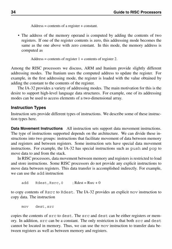
34 Guide to RISC Processors
Address = contents of a register + constant.
• The address of the memory operand is computed by adding the contents of tworegisters. If one of the register contents is zero, this addressing mode becomes thesame as the one above with zero constant. In this mode, the memory address iscomputed as
Address = contents of register 1 + contents of register 2.
Among the RISC processors we discuss, ARM and Itanium provide slightly differentaddressing modes. The Itanium uses the computed address to update the register. Forexample, in the first addressing mode, the register is loaded with the value obtained byadding the constant to the contents of the register.
The IA-32 provides a variety of addressing modes. The main motivation for this is thedesire to support high-level language data structures. For example, one of its addressingmodes can be used to access elements of a two-dimensional array.
Instruction TypesInstruction sets provide different types of instructions. We describe some of these instruc-tion types here.
Data Movement Instructions All instruction sets support data movement instructions.The type of instructions supported depends on the architecture. We can divide these in-structions into two groups: instructions that facilitate movement of data between memoryand registers and between registers. Some instruction sets have special data movementinstructions. For example, the IA-32 has special instructions such as push and pop tomove data to and from the stack.
In RISC processors, data movement between memory and registers is restricted to loadand store instructions. Some RISC processors do not provide any explicit instructions tomove data between registers. This data transfer is accomplished indirectly. For example,we can use the add instruction
add Rdest,Rsrc,0 ; Rdest = Rsrc + 0
to copy contents of Rsrc to Rdest. The IA-32 provides an explicit mov instruction tocopy data. The instruction
mov dest,src
copies the contents of src to dest. The src and dest can be either registers or mem-ory. In addition, src can be a constant. The only restriction is that both src and destcannot be located in memory. Thus, we can use the mov instruction to transfer data be-tween registers as well as between memory and registers.
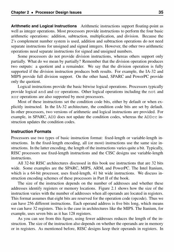
Chapter 2 • Processor Design Issues 35
Arithmetic and Logical Instructions Arithmetic instructions support floating-point aswell as integer operations. Most processors provide instructions to perform the four basicarithmetic operations: addition, subtraction, multiplication, and division. Because the2’s complement number system is used, addition and subtraction operations do not needseparate instructions for unsigned and signed integers. However, the other two arithmeticoperations need separate instructions for signed and unsigned numbers.
Some processors do not provide division instructions, whereas others support onlypartially. What do we mean by partially? Remember that the division operation producestwo outputs: a quotient and a remainder. We say that the division operation is fullysupported if the division instruction produces both results. For example, the IA-32 andMIPS provide full division support. On the other hand, SPARC and PowerPC provideonly the quotient.
Logical instructions provide the basic bitwise logical operations. Processors typicallyprovide logical and and or operations. Other logical operations including the not andxor operations are also supported by most processors.
Most of these instructions set the condition code bits, either by default or when ex-plicitly instructed. In the IA-32 architecture, the condition code bits are set by default.In other processors, two versions of arithmetic and logical instructions are provided. Forexample, in SPARC, ADD does not update the condition codes, whereas the ADDcc in-struction updates the condition codes.
Instruction FormatsProcessors use two types of basic instruction format: fixed-length or variable-length in-structions. In the fixed-length encoding, all (or most) instructions use the same size in-structions. In the latter encoding, the length of the instructions varies quite a bit. Typically,RISC processors use fixed-length instructions and the CISC designs use variable-lengthinstructions.
All 32-bit RISC architectures discussed in this book use instructions that are 32 bitswide. Some examples are the SPARC, MIPS, ARM, and PowerPC. The Intel Itanium,which is a 64-bit processor, uses fixed-length, 41 bit wide instructions. We discuss in-struction encoding schemes of these processors in Part II of the book.
The size of the instruction depends on the number of addresses and whether theseaddresses identify registers or memory locations. Figure 2.1 shows how the size of theinstruction varies with the number of addresses when all operands are located in registers.This format assumes that eight bits are reserved for the operation code (opcode). Thus wecan have 256 different instructions. Each operand address is five bits long, which meanswe can have 32 registers. This is the case in architectures like the MIPS. The Itanium, forexample, uses seven bits as it has 128 registers.
As you can see from this figure, using fewer addresses reduces the length of the in-struction. The size of the instruction also depends on whether the operands are in memoryor in registers. As mentioned before, RISC designs keep their operands in registers. In
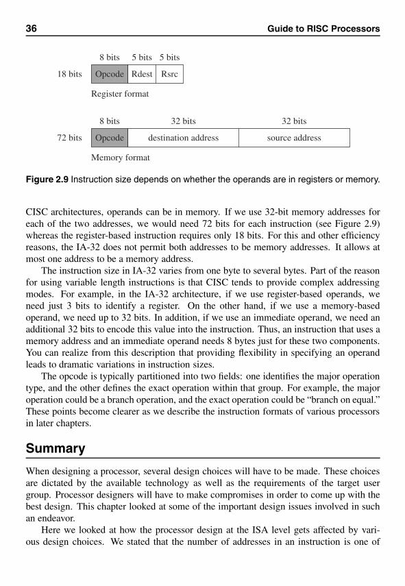
36 Guide to RISC Processors
72 bits Opcode destination address
8 bits 32 bits
source address
32 bits
18 bits Opcode Rdest
8 bits 5 bits 5 bits
Rsrc
Register format
Memory format
Figure 2.9 Instruction size depends on whether the operands are in registers or memory.
CISC architectures, operands can be in memory. If we use 32-bit memory addresses foreach of the two addresses, we would need 72 bits for each instruction (see Figure 2.9)whereas the register-based instruction requires only 18 bits. For this and other efficiencyreasons, the IA-32 does not permit both addresses to be memory addresses. It allows atmost one address to be a memory address.
The instruction size in IA-32 varies from one byte to several bytes. Part of the reasonfor using variable length instructions is that CISC tends to provide complex addressingmodes. For example, in the IA-32 architecture, if we use register-based operands, weneed just 3 bits to identify a register. On the other hand, if we use a memory-basedoperand, we need up to 32 bits. In addition, if we use an immediate operand, we need anadditional 32 bits to encode this value into the instruction. Thus, an instruction that uses amemory address and an immediate operand needs 8 bytes just for these two components.You can realize from this description that providing flexibility in specifying an operandleads to dramatic variations in instruction sizes.
The opcode is typically partitioned into two fields: one identifies the major operationtype, and the other defines the exact operation within that group. For example, the majoroperation could be a branch operation, and the exact operation could be “branch on equal.”These points become clearer as we describe the instruction formats of various processorsin later chapters.
Summary
When designing a processor, several design choices will have to be made. These choicesare dictated by the available technology as well as the requirements of the target usergroup. Processor designers will have to make compromises in order to come up with thebest design. This chapter looked at some of the important design issues involved in suchan endeavor.
Here we looked at how the processor design at the ISA level gets affected by vari-ous design choices. We stated that the number of addresses in an instruction is one of
Chapter 2 • Processor Design Issues 37
the choices that can have an impact on the instruction set design. It is possible to haveinstruction sets with zero, one, two, or three addresses; however, most recent processorsuse the three-address format. The IA-32, on the other hand, uses the two-address format.
The addressing mode is another characteristic that affects the instruction set. RISCdesigns tend to use the load/store architecture and use simple addressing modes. Often,they support just one or two addressing modes. In contrast, CISC architectures provide awide variety of addressing modes.
Both of these choices—the number of addresses and the complexity of addressingmodes—affect the instruction format. RISC architectures use fixed-length instructionsand support simple addressing modes. In contrast, CISC designs use variable-length in-structions to accommodate various complex addressing modes.
3RISC Principles
In the last chapter, we presented many details on the processor design space as well as theCISC and RISC architectures. It is time we consolidated our discussion to give details ofRISC principles. That’s what we do in this chapter. We describe the historical reasonsfor designing CISC processors. Then we identify the reasons for the popularity of RISCdesigns. We end our discussion with a list of the principal characteristics of RISC designs.
IntroductionThe dominant architecture in the PC market, the Intel IA-32, belongs to the ComplexInstruction Set Computer (CISC) design. The obvious reason for this classification is the“complex” nature of its Instruction Set Architecture (ISA). The motivation for designingsuch complex instruction sets is to provide an instruction set that closely supports theoperations and data structures used by Higher-Level Languages (HLLs). However, theside effects of this design effort are far too serious to ignore.
The decision of CISC processor designers to provide a variety of addressing modesleads to variable-length instructions. For example, instruction length increases if anoperand is in memory as opposed to in a register. This is because we have to specifythe memory address as part of instruction encoding, which takes many more bits. Thiscomplicates instruction decoding and scheduling. The side effect of providing a widerange of instruction types is that the number of clocks required to execute instructionsvaries widely. This again leads to problems in instruction scheduling and pipelining.
For these and other reasons, in the early 1980s designers started looking at simpleISAs. Because these ISAs tend to produce instruction sets with far fewer instructions,they coined the term Reduced Instruction Set Computer (RISC). Even though the maingoal was not to reduce the number of instructions, but the complexity, the term has stuck.
There is no precise definition of what constitutes a RISC design. However, we canidentify certain characteristics that are present in most RISC systems. We identify theseRISC design principles after looking at why the designers took the route of CISC in the
39
40 Guide to RISC Processors
first place. Because CISC and RISC have their advantages and disadvantages, modernprocessors take features from both classes. For example, the PowerPC, which follows theRISC philosophy, has quite a few complex instructions.
Evolution of CISC ProcessorsThe evolution of CISC designs can be attributed to the desire of early designers to effi-ciently use two of the most expensive resources, memory and processor, in a computersystem. In the early days of computing, memory was very expensive and small in ca-pacity. This forced the designers to devise high-density code: that is, each instructionshould do more work so that the total program size could be reduced. Because instruc-tions are implemented in hardware, this goal could not be achieved until the late 1950sdue to implementation complexity.
The introduction of microprogramming facilitated cost-effective implementation ofcomplex instructions by using microcode. Microprogramming has not only aided in im-plementing complex instructions, it has also provided some additional advantages. Mi-croprogrammed control units use small fast memories to hold the microcode, thereforethe impact of memory access latency on performance could be reduced. Microprogram-ming also facilitates development of low-cost members of a processor family by simplychanging the microcode.
Another advantage of implementing complex instructions in microcode is that the in-structions can be tailored to high-level language constructs such as while loops. Forexample, the loop instruction of the IA-32 can be used to implement for loops. Simi-larly, memory block copying can be done by using its string instructions. Thus, by usingthese complex instructions, we close the “semantic gap” between HLLs and machine lan-guages.
So far, we have concentrated on the memory resource. In the early days, effectiveprocessor utilization was also important. High code density also helps improve executionefficiency. As an example, consider the VAX-11/780, the ultimate CISC processor. It wasintroduced in 1978 and supported 22 addressing modes as opposed to 11 on the Intel 486that was introduced more than a decade later. The VAX instruction size can range from 2to 57 bytes, as shown in Table 3.1.
To illustrate how code density affects execution efficiency, consider the autoincrementaddressing mode of the VAX processor. In this addressing mode, a single instruction canread data from memory, add contents of a register to it, write back the result to memory,and increment the memory pointer. Actions of this instruction are summarized below:
(R2) = (R2)+ R3; R2 = R2+1
In this example, the R2 register holds the memory pointer. To implement this CISC in-struction, we need four RISC instructions:
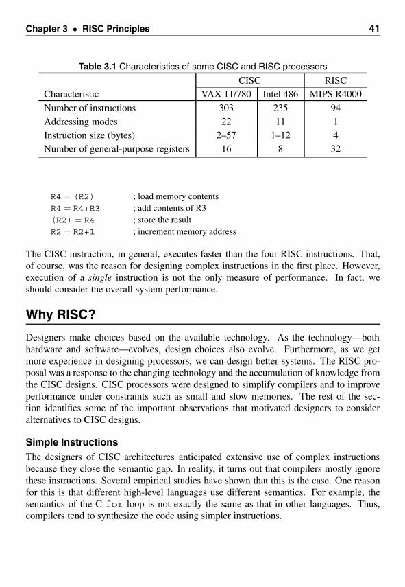
Chapter 3 • RISC Principles 41
Table 3.1 Characteristics of some CISC and RISC processors
CISC RISCCharacteristic VAX 11/780 Intel 486 MIPS R4000
Number of instructions 303 235 94Addressing modes 22 11 1Instruction size (bytes) 2–57 1–12 4Number of general-purpose registers 16 8 32
R4 = (R2) ; load memory contentsR4 = R4+R3 ; add contents of R3(R2) = R4 ; store the resultR2 = R2+1 ; increment memory address
The CISC instruction, in general, executes faster than the four RISC instructions. That,of course, was the reason for designing complex instructions in the first place. However,execution of a single instruction is not the only measure of performance. In fact, weshould consider the overall system performance.
Why RISC?
Designers make choices based on the available technology. As the technology—bothhardware and software—evolves, design choices also evolve. Furthermore, as we getmore experience in designing processors, we can design better systems. The RISC pro-posal was a response to the changing technology and the accumulation of knowledge fromthe CISC designs. CISC processors were designed to simplify compilers and to improveperformance under constraints such as small and slow memories. The rest of the sec-tion identifies some of the important observations that motivated designers to consideralternatives to CISC designs.
Simple InstructionsThe designers of CISC architectures anticipated extensive use of complex instructionsbecause they close the semantic gap. In reality, it turns out that compilers mostly ignorethese instructions. Several empirical studies have shown that this is the case. One reasonfor this is that different high-level languages use different semantics. For example, thesemantics of the C for loop is not exactly the same as that in other languages. Thus,compilers tend to synthesize the code using simpler instructions.

42 Guide to RISC Processors
Few Data TypesCISC ISA tends to support a variety of data structures, from simple data types such asintegers and characters to complex data structures such as records and structures. Empir-ical data suggest that complex data structures are used relatively infrequently. Thus, it isbeneficial to design a system that supports a few simple data types efficiently and fromwhich the missing complex data types can be synthesized.
Simple Addressing ModesCISC designs provide a large number of addressing modes. The main motivations are(i) to support complex data structures and (ii) to provide flexibility to access operands.Although this allows flexibility, it also introduces problems. First, it causes variable in-struction execution times, depending on the location of the operands. Second, it leads tovariable-length instructions. For example, the IA-32 instruction length can range from1 to 12 bytes. Variable instruction lengths lead to inefficient instruction decoding andscheduling.
Large Register SetSeveral researchers have studied the characteristics of procedure calls in HLLs. We quotetwo studies—one by Patterson and Sequin [22] and the other by Tanenbaum [28]. Severalother studies, in fact, support the findings of these two studies.
Patterson and Sequin’s study of C and Pascal programs found that procedure call/returnconstitutes about 12 to 15% of HLL statements. As a percentage of the total machine lan-guage instructions, call/return instructions are about 31 to 33%. More interesting is thefact that call/return generates nearly half (about 45%) of all memory references. Thisis understandable as procedure call/return instructions use memory to store activationrecords. An activation record consists of parameters, local variables, and return values.In the IA-32, for example, the stack is extensively used for these activities. This explainswhy procedure call/return activities account for a large number of memory references.Thus, it is worth providing efficient support for procedure calls and returns.
In another study, Tanenbaum [28] found that only 1.25% of the called procedures hadmore than six arguments. Furthermore, more than 93% of them had less than six localscalar variables. These figures, supported by other studies, suggest that the activationrecord is not large. If we provide a large register set, we can avoid memory references formost procedure calls and returns. In this context, we note that the eight general-purposeregisters available in IA-32 processors are a limiting factor in providing such support. TheItanium, for example, provides a large register set (128 registers), and most procedure callson the Itanium can completely avoid accessing memory.
Chapter 3 • RISC Principles 43
RISC Design Principles
The best way to understand RISC is to treat it as a concept to design processors. Althoughinitial RISC processors had fewer instructions compared to their CISC counterparts, thenew generation of RISC processors has hundreds of instructions, some of which are ascomplex as the CISC instructions. It could be argued that such systems are really hybridsof CISC and RISC. In any case, there are certain principles that most RISC designs follow.We identify the important ones in this section.
Simple OperationsThe objective is to design simple instructions so that each can execute in one cycle. Thisproperty simplifies processor design. Note that a cycle is defined as the time required tofetch two operands from registers, perform an operation, and store the result in a register.The advantage of simple instructions is that there is no need for microcode and operationscan be hardwired. If we design the cache subsystem properly to capture these instructions,the overall execution efficiency can be as good as a microcoded CISC machine.
Register-to-Register OperationsA typical CISC instruction set supports register-to-register operations as well as register-to-memory and memory-to-memory operations. The IA-32, for instance, allows register-to-register as well as register-to-memory operations; it does not allow memory-to-memoryoperations. The VAX 11/780, on the other hand, allows memory-to-memory operationsas well.
RISC processors allow only special load and store operations to access memory.The rest of the operations work on a register-to-register basis. This feature simplifiesinstruction set design as it allows execution of instructions at a one-instruction-per-cyclerate. Restricting operands to registers also simplifies the control unit.
Simple Addressing ModesSimple addressing modes allow fast address computation of operands. Because RISCprocessors employ register-to-register instructions, most instructions use register-basedaddressing. Only the load and store instructions need a memory-addressing mode. RISCdesigns provide very few addressing modes: often just one or two. They provide thebasic register indirect addressing mode, often allowing a small displacement that is eitherrelative or absolute.
Large Register SetRISC processors use register-to-register operations, therefore we need to have a largenumber of registers. A large register set can provide ample opportunities for the com-
44 Guide to RISC Processors
piler to optimize their usage. Another advantage with a large register set is that we canminimize the overhead associated with procedure calls and returns.
To speed up procedure calls, we can use registers to store local variables as well as forpassing arguments. Local variables are accessed only by the procedure in which they aredeclared. These variables come into existence at the time of procedure invocation and diewhen the procedure exits.
Fixed-Length, Simple Instruction FormatRISC designs use fixed-length instructions. Variable-length instructions can cause imple-mentation and execution inefficiencies. For example, we may not know if there is anotherword that needs to be fetched until we decode the first word. Along with fixed-lengthinstruction size, RISC designs also use a simple instruction format. The boundaries ofvarious fields in an instruction such as opcode and source operands are fixed. This allowsfor efficient decoding and scheduling of instructions. For example, both PowerPC andMIPS use six bits for opcode specification.
Summary
We have introduced important characteristics that differentiate RISC designs from theirCISC counterparts. CISC designs provide complex instructions and a large number ofaddressing modes. The rationale for this complexity is the desire to close the semanticgap that exists between high-level languages and machine languages.
In the early days, effective usage of processor and memory resources was important.Complex instructions tend to minimize the memory requirements. Empirical data, how-ever, suggested that compilers do not use these complex instructions; instead, they usesimple instructions to synthesize complex instructions. Such observations led designersto take a fresh look at processor design philosophy. RISC principles, based on empiri-cal studies on CISC processors, have been proposed as an alternative to CISC. Most ofthe current processor designs are based on these RISC principles. The next part looks atseveral RISC architectures.
PART II
Architectures
4MIPS Architecture
In the previous chapter, we discussed the RISC design principles. Starting with this chap-ter, we look at the architecture of several RISC processors. This chapter gives detailsabout the MIPS architecture. However, we do not discuss its instruction set details here.We devote the next part of the book to this purpose.
IntroductionWe have selected to present the MIPS as the first architecture. One of the reasons forthis preference is the simplicity of the MIPS architecture and its faithfulness to the RISCdesign philosophy. Once you read details about the other architectures in the followingchapters, you will see why this is so.
The MIPS architecture primarily grew out of research done at Stanford. Along withthe Berkeley RISC project, these projects influenced processor design towards RISC ori-entation. MIPS is dominant in embedded applications including digital cameras, digitalTVs, Sony PlayStation 2, network routers, and so on.
The MIPS Instruction Set Architecture (ISA) has evolved over time from MIPS Ithrough MIPS V ISAs. In the late 1990s, MIPS formalized their designs around twobasic architectures: MIPS32 for 32-bit architectures and MIPS64 for 64-bit architectures.The MIPS32 architecture is based on the MIPS II ISA with some additional instructionsfrom MIPS III through MIPS V ISAs. The MIPS64 architecture is based on the MIPS VISA.
MIPS first processor implementation R2000 was announced in the mid-1980s. Animproved version R3000 became available three years later. Both these processors were32-bit implementations. The first 64-bit MIPS implementation R4000 was released in theearly 1990s. In the next part, which discusses the MIPS assembly language, we focus onthe MIPS R2000/R3000 processor. The main reason for this selection is that the SPIMsimulator is written for this processor. From a pedagogical perspective, this processor issufficient to explain the MIPS assembly language.
47
48 Guide to RISC Processors
Like the other RISC processors, MIPS is based on the load/store architecture. Asmentioned in Chapter 3, in this architecture most instructions expect their operands to bein registers. Two instructions are used to move data between registers and memory. As weshow in the next part, the MIPS architecture provides several load and store instructionsto transfer data of different sizes: byte, halfword, and so on.
In the rest of the chapter, we give details on the MIPS32 architecture. The instructionset and assembly language programming aspects are covered in the next part. We start ourdiscussion with the registers set.
Registers
The MIPS32 architecture provides 32 general-purpose registers, a Program Counter (PC),and two special-purpose registers. All registers are 32-bits wide as shown in Figure 4.1.In the assembly language, these registers are identified as $0, $1, . . . , $31. Two of thegeneral-purpose registers—the first and the last—are reserved for a specific function:
• Register $0 is hardwired to provide zero. This register is often used as a sourceregister when a zero value is needed. If this register is used as the destinationregister of an instruction, the result is discarded.
• The last register $31 is used as a link register by the jump and link (jal) instruc-tion, which is used to invoke a procedure. Register $31 is used to store the returnaddress of a procedure call. We discuss details about this instruction in Chapter 11.
We discussed the purpose of the PC register in Chapter 2 (see page 22). The twospecial-purpose registers—called HI and LO—are used to hold the results of integer mul-tiply and divide instructions:
• In the integer multiply operation, HI and LO registers hold the 64-bit result, withthe higher-order 32 bits in the HI and the lower-order 32 bits in the LO register.
• In integer divide operations, the 32-bit quotient is stored in the LO and the remain-der in the HI register.
Register Usage Convention
Although there is no requirement from the processor hardware, there is an establishedconvention on how these 30 registers should be used. Table 4.1 shows the suggested useof each register. Because these suggestions are not enforced by the hardware, we can usethe general-purpose registers in an unconventional manner. However, such programs arenot likely to work with other programs.
Registers $v0 and $v1 are used to return results from a procedure. Registers $a0to $a3 are used to pass the first four arguments to procedures. The remaining argumentsare passed via the stack. These registers are not preserved across procedure calls (i.e., thecalled procedure can freely modify the contents of these registers).
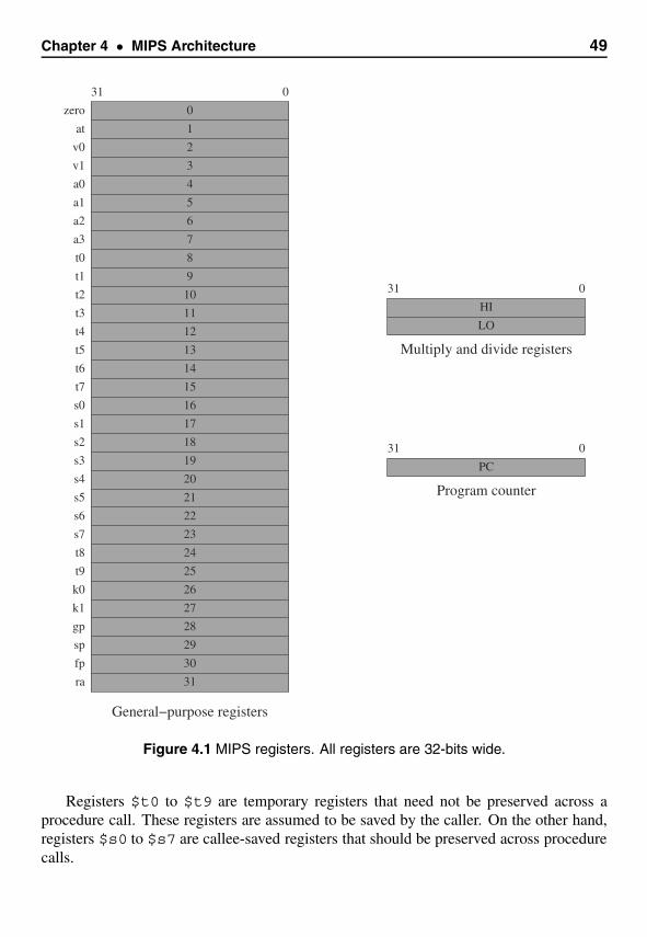
Chapter 4 • MIPS Architecture 49
031
Program counter
PC
031
LO
HI
Multiply and divide registers
zero
at
v0
v1
a1
a0
a2
a3
t0
t1
t2
t3
t4
t5
t6
t7
s0
s1
s2
s3
s4
s5
s6
s7
t8
t9
k0
k1
gp
sp
fp
ra
0
1
2
3
4
5
6
7
8
9
10
11
12
13
14
15
16
17
18
19
20
21
22
23
24
25
26
27
28
29
30
31
31 0
General−purpose registers
Figure 4.1 MIPS registers. All registers are 32-bits wide.
Registers $t0 to $t9 are temporary registers that need not be preserved across aprocedure call. These registers are assumed to be saved by the caller. On the other hand,registers $s0 to $s7 are callee-saved registers that should be preserved across procedurecalls.
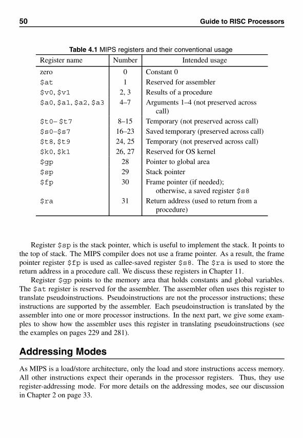
50 Guide to RISC Processors
Table 4.1 MIPS registers and their conventional usage
Register name Number Intended usage
zero 0 Constant 0$at 1 Reserved for assembler$v0, $v1 2, 3 Results of a procedure$a0, $a1, $a2, $a3 4–7 Arguments 1–4 (not preserved across
call)$t0– $t7 8–15 Temporary (not preserved across call)$s0–$s7 16–23 Saved temporary (preserved across call)$t8, $t9 24, 25 Temporary (not preserved across call)$k0, $k1 26, 27 Reserved for OS kernel$gp 28 Pointer to global area$sp 29 Stack pointer$fp 30 Frame pointer (if needed);
otherwise, a saved register $s8$ra 31 Return address (used to return from a
procedure)
Register $sp is the stack pointer, which is useful to implement the stack. It points tothe top of stack. The MIPS compiler does not use a frame pointer. As a result, the framepointer register $fp is used as callee-saved register $s8. The $ra is used to store thereturn address in a procedure call. We discuss these registers in Chapter 11.
Register $gp points to the memory area that holds constants and global variables.The $at register is reserved for the assembler. The assembler often uses this register totranslate pseudoinstructions. Pseudoinstructions are not the processor instructions; theseinstructions are supported by the assembler. Each pseudoinstruction is translated by theassembler into one or more processor instructions. In the next part, we give some exam-ples to show how the assembler uses this register in translating pseudoinstructions (seethe examples on pages 229 and 281).
Addressing Modes
As MIPS is a load/store architecture, only the load and store instructions access memory.All other instructions expect their operands in the processor registers. Thus, they useregister-addressing mode. For more details on the addressing modes, see our discussionin Chapter 2 on page 33.
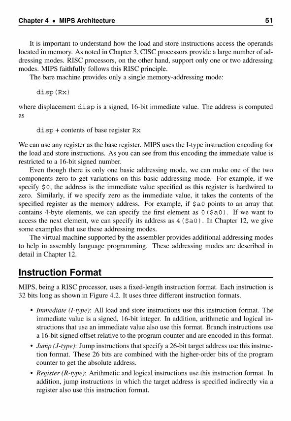
Chapter 4 • MIPS Architecture 51
It is important to understand how the load and store instructions access the operandslocated in memory. As noted in Chapter 3, CISC processors provide a large number of ad-dressing modes. RISC processors, on the other hand, support only one or two addressingmodes. MIPS faithfully follows this RISC principle.
The bare machine provides only a single memory-addressing mode:
disp(Rx)
where displacement disp is a signed, 16-bit immediate value. The address is computedas
disp + contents of base register Rx
We can use any register as the base register. MIPS uses the I-type instruction encoding forthe load and store instructions. As you can see from this encoding the immediate value isrestricted to a 16-bit signed number.
Even though there is only one basic addressing mode, we can make one of the twocomponents zero to get variations on this basic addressing mode. For example, if wespecify $0, the address is the immediate value specified as this register is hardwired tozero. Similarly, if we specify zero as the immediate value, it takes the contents of thespecified register as the memory address. For example, if $a0 points to an array thatcontains 4-byte elements, we can specify the first element as 0($a0). If we want toaccess the next element, we can specify its address as 4($a0). In Chapter 12, we givesome examples that use these addressing modes.
The virtual machine supported by the assembler provides additional addressing modesto help in assembly language programming. These addressing modes are described indetail in Chapter 12.
Instruction FormatMIPS, being a RISC processor, uses a fixed-length instruction format. Each instruction is32 bits long as shown in Figure 4.2. It uses three different instruction formats.
• Immediate (I-type): All load and store instructions use this instruction format. Theimmediate value is a signed, 16-bit integer. In addition, arithmetic and logical in-structions that use an immediate value also use this format. Branch instructions usea 16-bit signed offset relative to the program counter and are encoded in this format.
• Jump (J-type): Jump instructions that specify a 26-bit target address use this instruc-tion format. These 26 bits are combined with the higher-order bits of the programcounter to get the absolute address.
• Register (R-type): Arithmetic and logical instructions use this instruction format. Inaddition, jump instructions in which the target address is specified indirectly via aregister also use this instruction format.
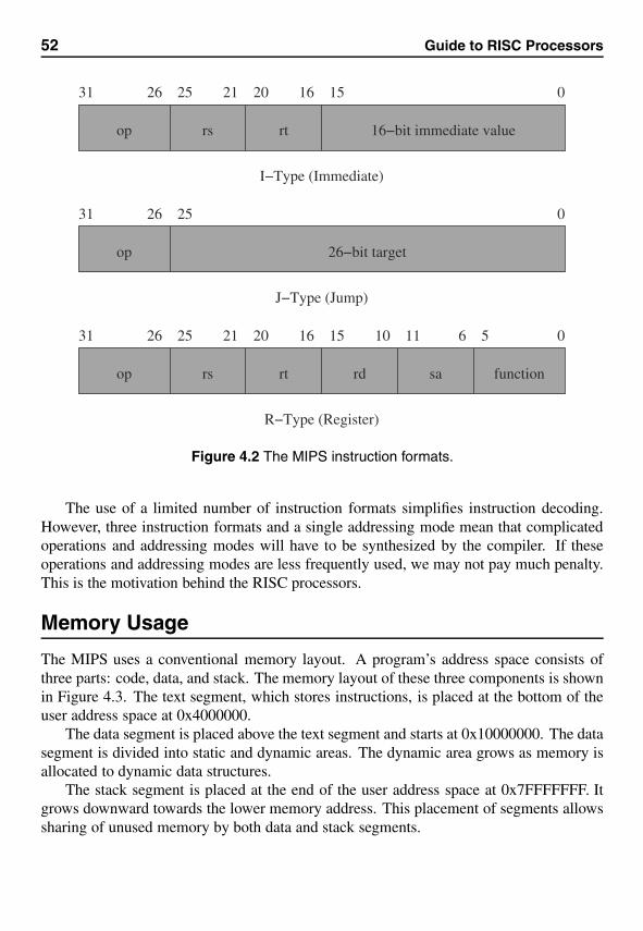
52 Guide to RISC Processors
2031 2526 21 16 0
0
0
31 26 25
31 26 25 21 20 1516 10 11 6 5
op 26−bit target
J−Type (Jump)
op rtrs rd sa function
R−Type (Register)
rt 16−bit immediate valuersop
15
I−Type (Immediate)
Figure 4.2 The MIPS instruction formats.
The use of a limited number of instruction formats simplifies instruction decoding.However, three instruction formats and a single addressing mode mean that complicatedoperations and addressing modes will have to be synthesized by the compiler. If theseoperations and addressing modes are less frequently used, we may not pay much penalty.This is the motivation behind the RISC processors.
Memory Usage
The MIPS uses a conventional memory layout. A program’s address space consists ofthree parts: code, data, and stack. The memory layout of these three components is shownin Figure 4.3. The text segment, which stores instructions, is placed at the bottom of theuser address space at 0x4000000.
The data segment is placed above the text segment and starts at 0x10000000. The datasegment is divided into static and dynamic areas. The dynamic area grows as memory isallocated to dynamic data structures.
The stack segment is placed at the end of the user address space at 0x7FFFFFFF. Itgrows downward towards the lower memory address. This placement of segments allowssharing of unused memory by both data and stack segments.
Chapter 4 • MIPS Architecture 53
Dynamic area
Static area
Reserved
Text segment
0
4000000
10000000
Data segment
Stack segment
7FFFFFFF
Memory addresses(in hex)
Figure 4.3 MIPS memory layout.
Summary
We have presented the basic details of the MIPS architecture. The MIPS32 architec-ture provides 32 general-purpose registers, a program counter register, and two special-purpose registers. Each register is 32 bits long. The two special-purpose registers areused by the multiply and divide instructions. MIPS effectively supports only a singleaddressing mode.
We have not discussed the MIPS instruction set and other details here. We devote thenext part of the book to this purpose. In the remainder of this part, we look at a few otherRISC architectures.
Web ResourcesMIPS32 documentation is available from the MIPS Web site. The MIPS32 Architecturefor Programmers, which consists of three volumes, describes the 32-bit MIPS architec-ture in detail [16, 17, 18]. If you are interested in the 64-bit architecture, it is also de-

54 Guide to RISC Processors
scribed in a three-volume manual MIPS64 Architecture for Programmers [19, 20, 21].These manuals are available from www.mips.com/content/Documentation/MIPSDocumentation.
5SPARC Architecture
This chapter gives details about the SPARC architecture. After a brief introduction, wedescribe the SPARC architecture in depth. We start our discussion with a description of itsregister set. Following this we describe its addressing modes. It supports the two address-ing modes we described in Chapter 2. The SPARC instruction set details are presentednext. The following section describes how procedures are invoked in the SPARC architec-ture. This section also provides information on SPARC’s parameter-passing mechanismand window management. We conclude the chapter with a summary.
IntroductionThe SPARC architecture was initially developed by Sun and is based on the RISC IIdesign from the University of California, Berkeley. SPARC stands for Scalable ProcessorARChitecture. Unlike other companies, Sun was wise to make this an open standardand not to manufacture the processor itself. Sun licensed different chip manufacturers tofabricate the processor. Because SPARC is a specification at the ISA level, manufacturerscan choose to design their version to suit the target price range and to improve efficiency.For example, implementation of the cache is completely transparent at the ISA level.
The initial SPARC specification SPARC Version 7, introduced in 1987, was a 32-bitprocessor. SUN and Fujitsu implemented the first SPARC processor. In the followingyear, SUN introduced the first VME bus-based Sun 4 SPARC workstation. In 1989,SPARC International was set up by SUN and others as the industry body to maintainSPARC as an open architecture, to facilitate distribution of SPARC information and li-censing of technology.
The SPARC Version 8 was published in 1990. This is still a 32-bit architecture. The64-bit SPARC version (Version 9) was introduced in 1993. In 1995, Fujitsu through theirSPARC64 and SUN with their UltraSPARC processor introduced 64-bit workstations. Amore detailed history of SPARC and its implementations is available from several sources,including [26, 13, 27].
55
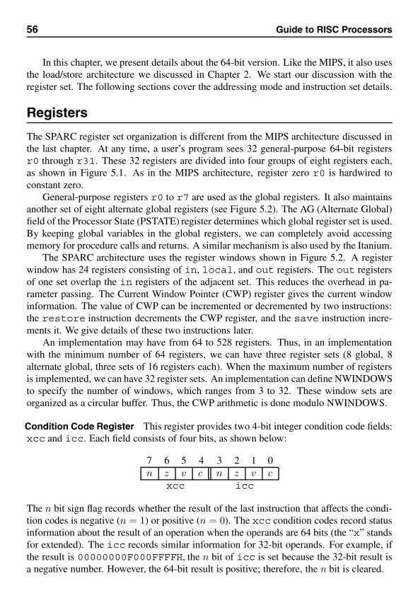
56 Guide to RISC Processors
In this chapter, we present details about the 64-bit version. Like the MIPS, it also usesthe load/store architecture we discussed in Chapter 2. We start our discussion with theregister set. The following sections cover the addressing mode and instruction set details.
Registers
The SPARC register set organization is different from the MIPS architecture discussed inthe last chapter. At any time, a user’s program sees 32 general-purpose 64-bit registersr0 through r31. These 32 registers are divided into four groups of eight registers each,as shown in Figure 5.1. As in the MIPS architecture, register zero r0 is hardwired toconstant zero.
General-purpose registers r0 to r7 are used as the global registers. It also maintainsanother set of eight alternate global registers (see Figure 5.2). The AG (Alternate Global)field of the Processor State (PSTATE) register determines which global register set is used.By keeping global variables in the global registers, we can completely avoid accessingmemory for procedure calls and returns. A similar mechanism is also used by the Itanium.
The SPARC architecture uses the register windows shown in Figure 5.2. A registerwindow has 24 registers consisting of in, local, and out registers. The out registersof one set overlap the in registers of the adjacent set. This reduces the overhead in pa-rameter passing. The Current Window Pointer (CWP) register gives the current windowinformation. The value of CWP can be incremented or decremented by two instructions:the restore instruction decrements the CWP register, and the save instruction incre-ments it. We give details of these two instructions later.
An implementation may have from 64 to 528 registers. Thus, in an implementationwith the minimum number of 64 registers, we can have three register sets (8 global, 8alternate global, three sets of 16 registers each). When the maximum number of registersis implemented, we can have 32 register sets. An implementation can define NWINDOWSto specify the number of windows, which ranges from 3 to 32. These window sets areorganized as a circular buffer. Thus, the CWP arithmetic is done modulo NWINDOWS.
Condition Code Register This register provides two 4-bit integer condition code fields:xcc and icc. Each field consists of four bits, as shown below:
7 6 5 4 3 2 1 0n z v c n z v c
xcc icc
The n bit sign flag records whether the result of the last instruction that affects the condi-tion codes is negative (n = 1) or positive (n = 0). The xcc condition codes record statusinformation about the result of an operation when the operands are 64 bits (the “x” standsfor extended). The icc records similar information for 32-bit operands. For example, ifthe result is 00000000F000FFFFH, the n bit of icc is set because the 32-bit result isa negative number. However, the 64-bit result is positive; therefore, the n bit is cleared.

Chapter 5 • SPARC Architecture 57
0
r31 i763
i0i1i2i3i4i5i6
l0l1l2l3l4l5l6l7
o0o1o2o3o4o5o6o7
r16r17r18r19r20
r8r9
r10r11r12r13r14r15
r0r1r2r3r4r5r6r7
r29r30
r21r22r23r24r25r26r27r28
Hardwired to 0 g0g1g2g3g4g5g6g7
0
CWP
4
xcc icc0347
CCR
063
PC
063
nPC
globalregisters
outregisters
localregisters
inregisters
Figure 5.1 Register set in the SPARC V9 architecture (CWP: Current Window Pointer;CCR: Condition Code Register).
The zero bit indicates if the result is zero: z = 1 if the result is zero; otherwise, z = 0.The overflow bit v indicates whether the result, when treated as a signed number, is withinthe range of 64 bits (xcc) or 32 bits (icc). This bit is useful to detect overflow in signedarithmetic operations. The carry bit c keeps information on whether there was a carry-outfrom bit 63 (xcc) or bit 31 (icc). It is useful to detect overflow in unsigned arithmeticoperations.
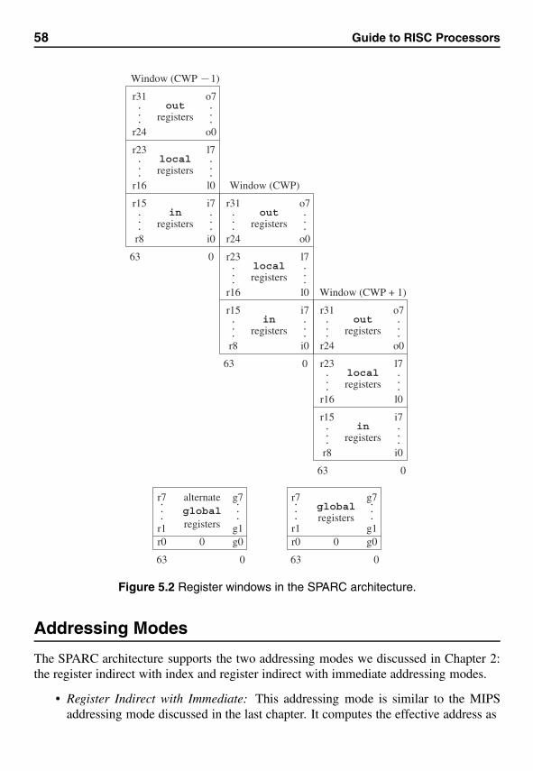
58 Guide to RISC Processors
.
.
....
0 g0
g7
g1r0
r7
r1
globalregisters
063
.
.
.... global
registers
alternate
063
0 g0
g7
g1r0
r7
r1
.
.
.
.
.
....
.
.
....
.
.
.
r8
r15
registersin
i0
i7
l0
l7
r16
r23
r24
r31out
registers
o0
o7
localregisters
.
.
.
.
.
....
.
.
....
.
.
.
r8
r15
registersin
i0
i7
l0
l7
r16
r23
r24
r31out
registers
o0
o7
localregisters
.
.
.
.
.
....
.
.
....
.
.
.
localregisters
63 0
63 0
063
Window (CWP + 1)
Window (CWP)
r8
r15
registersin
i0
i7
l0
l7
r16
r23
r24
r31out
registers
o0
o7
Window (CWP 1)
Figure 5.2 Register windows in the SPARC architecture.
Addressing Modes
The SPARC architecture supports the two addressing modes we discussed in Chapter 2:the register indirect with index and register indirect with immediate addressing modes.
• Register Indirect with Immediate: This addressing mode is similar to the MIPSaddressing mode discussed in the last chapter. It computes the effective address as
Chapter 5 • SPARC Architecture 59
Effective address = contents of Rx + imm13.
The base register Rx can be any general-purpose register. A 13-bit signed con-stant imm13 can be specified as the displacement. This constant is sign-extendedto 64 bits and added to the Rx register (see our discussion on sign extension inAppendix A).
• Register Indirect with Index: This addressing mode computes the effective addressas the sum of two register contents.
Effective address = contents of Rx + contents of Ry.
The base register Rx and the index register Ry can be any general-purpose registers.
There is no register indirect addressing mode in which the contents of a register are takenas the effective address. But we can emulate this addressing mode by making the constantzero in the first addressing mode, or using r0 as the index register in the second addressingmode. Note that r0 is hardwired to read zero.
Instruction FormatAll SPARC instructions are 32 bits long. The instruction format uses two opcode fields:the most significant two bits op (bits 30 and 31) identify a major operation group and thesecond field, op2 or op3, specifies the actual instruction. A sample of the instructionformats is shown in Figure 5.3. The first two formats show how most instructions that usethree addresses are encoded. If an immediate value is used, the second format is used.The i bit specifies whether one of the source operands is in a register (i = 0) or a constant(i = 1).
The next three formats are used for sethi and conditional branch instructions. Thesethi instruction moves a 22-bit constant into a register (see page 62). The SPARCarchitecture supports two types of conditional branch instructions. These branch instruc-tions are also discussed later.
The final format is used for procedure calls. We can specify a 30-bit signed displace-ment value as part of this instruction.
Instruction SetThis section gives details about the SPARC instruction set. Procedure invocation andparameter-passing details are discussed in the next section.
Data Transfer InstructionsBecause the SPARC follows the load/store architecture, only load and store instructionscan move data between a register and memory. The load instruction
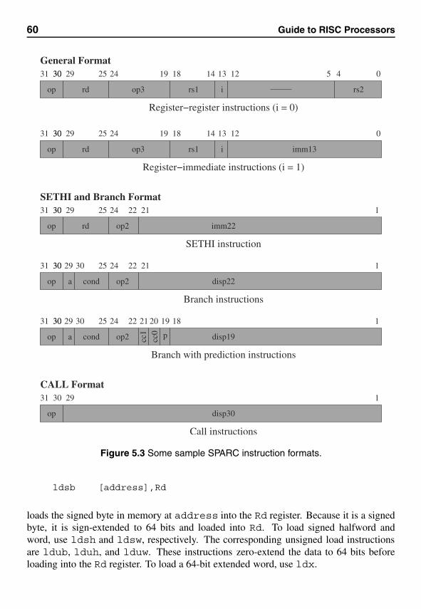
60 Guide to RISC Processors
31 1
disp19op
30
op2
25 24 22 21
conda
30 3029
Branch with prediction instructions
31 1
disp22op
30
op2
25 24 22 21
conda
30 3029
Branch instructions
20 19 18
cc1
cc0 p
General Format
31 0
op
30 25 2430 29
Register−immediate instructions (i = 1)
rd op3
19 18 13 1214
i
31 0
op
30 25 2430 29
Register−register instructions (i = 0)
rd op3
19 18 13 12 5 414
rs1 rs2i
imm13rs1
31 1
imm22op
30
op2
25 24 22 2130 29
SETHI instruction
rd
31 1
disp30op
30 29
CALL Format
Call instructions
SETHI and Branch Format
Figure 5.3 Some sample SPARC instruction formats.
ldsb [address],Rd
loads the signed byte in memory at address into the Rd register. Because it is a signedbyte, it is sign-extended to 64 bits and loaded into Rd. To load signed halfword andword, use ldsh and ldsw, respectively. The corresponding unsigned load instructionsare ldub, lduh, and lduw. These instructions zero-extend the data to 64 bits beforeloading into the Rd register. To load a 64-bit extended word, use ldx.
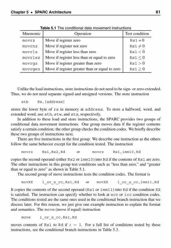
Chapter 5 • SPARC Architecture 61
Table 5.1 The conditional data movement instructions
Mnemonic Operation Test condition
movrz Move if register zero Rs1 = 0movrnz Move if register not zero Rs1 �= 0movrlz Move if register less than zero Rs1 < 0movrlez Move if register less than or equal to zero Rs1 ≤ 0movrgz Move if register greater than zero Rs1 > 0movrgez Move if register greater than or equal to zero Rs1 ≥ 0
Unlike the load instructions, store instructions do not need to be sign- or zero-extended.Thus, we do not need separate signed and unsigned versions. The store instruction
stb Rs,[address]
stores the lower byte of rs in memory at address. To store a halfword, word, andextended word, use sth, stw, and stx, respectively.
In addition to these load and store instructions, the SPARC provides two groups ofconditional data movement instructions. One group moves data if the register contentssatisfy a certain condition; the other group checks the condition codes. We briefly describethese two groups of instructions next.
There are five instructions in the first group. We describe one instruction as the othersfollow the same behavior except for the condition tested. The instruction
movrz Rs1,Rs2,Rd or movrz Rs1,imm10,Rd
copies the second operand (either Rs2 or imm10) into Rd if the contents of Rs1 are zero.The other instructions in this group test conditions such as “less than zero,” and “greaterthan or equal to zero” as shown in Table 5.1.
The second group of move instructions tests the condition codes. The format is
movXX i_or_x_cc,Rs1,Rd or movXX i_or_x_cc,imm11,Rd
It copies the contents of the second operand (Rs1 or imm11) into Rd if the condition XXis satisfied. The instruction can specify whether to look at xcc or icc condition codes.The conditions tested are the same ones used in the conditional branch instruction that wediscuss later. For this reason, we just give one example instruction to explain the formatand semantics. The move (move if equal) instruction
move i_or_x_cc,Rs1,Rd
moves contents of Rs1 to Rd if z = 1. For a full list of conditions tested by theseinstructions, see the conditional branch instructions in Table 5.3.
62 Guide to RISC Processors
Loading ConstantsTo specify constants in registers, the SPARC architecture provides a special instructionsethi (set high). It stores a 22-bit value in the upper 22 bits of the destination register.To facilitate constant manipulation, SPARC assemblers provide several unary operatorsto extract parts of a word or extended word. These operators are as follows.
%uhi Extracts bits 63 to 42 of a 64-bit extended word (i.e., extracts thehigh-order 22 bits of the upper word);
%ulo Extracts bits 41 to 32 of a 64-bit extended word (i.e., extracts thelow-order 10 bits of the upper word);
%hi Extracts bits 31 to 10 of its operand (i.e., extracts the upper 22bits);
%lo Extracts bits 9 to 0 of its operand (i.e., extracts the lower 10 bits).
We are now ready to see how we can use the sethi instruction to load integer con-stants into registers. First, let us look at 32-bit words. The instruction sequence
sethi %hi(value),Rdor Rd,%lo(value),Rd
stores the 32-bit constant value in the Rd register. In fact, SPARC assemblers providethe pseudoinstruction
set value,Rd
to represent this two-instruction code sequence. If the upper 22 bits are zero, set uses
or %g0,value,Rd
On the other hand, if the lower 10 bits are zero, set uses
sethi %hi(value),Rd
The setx is similar to the set instruction except that it allows a 64-bit constant. Thesyntax is
setx value,Rt,Rd
This instruction stores the 64-bit constant value in Rd using Rt as a temporary register.This pseudoinstruction can be translated into a sequence of SPARC processor instructionsby using %uhi, %ulo, %hi, and %lo unary operators along with or, sethi, and sllxinstructions. The or and sllx instructions are discussed in the next section.
Arithmetic InstructionsThe SPARC instruction set supports the basic four arithmetic operations. Most arithmeticoperations have two versions: one version updates the condition codes and the other doesnot. In most instructions, the second operand can be a register or a signed 13-bit immedi-ate imm13.
Chapter 5 • SPARC Architecture 63
Add Instructions The SPARC instruction set provides add instructions with and with-out the carry. The instruction
add Rs1,Rs2,Rd
adds contents of Rs1 and Rs2 and stores the result in the Rd register. The immediateversion of add is
add Rs1,imm13,Rd
The immediate value is sign-extended to 64 bits and added to the contents of Rs1. Thisinstruction does not update the condition codes. If you want the operation to update thecondition codes, use addcc instead of add. It updates the four integer condition codesmentioned before.
If you want to add the carry bit, use addc as shown below:
addc Rs1,Rs2,Rdaddccc Rs1,Rs2,Rd
These instructions add the icc carry bit. As usual, the second operand can be a signed13-bit immediate value. These instructions are useful in multiword addition operations.
Subtract Instructions The SPARC instruction set has four subtract instructions corre-sponding to the four add instructions: sub, subcc, subc, and subccc. The last twosubtract instructions subtract the icc carry bit. The format of these instructions is similarto that of the add instructions. The instruction
sub Rs1,Rs2,Rd
stores the result of Rs1−Rs2 in the destination register Rd.
Multiplication Instructions Unlike the other processors, the SPARC provides a singlemultiplication instruction for both signed and unsigned multiplication. The multiplicationinstruction
mulx Rs1,Rs2,Rd
multiplies two 64-bit values in Rs1 and Rs2 and places the 64-bit result in Rd. Strictlyspeaking, multiplying two 64-bit values can result in a 128-bit result. This instruction,however, provides only a 64-bit result. The input operands, obviously, should be restrictedto get a valid result.
The 32-bit SPARC-V8 has two multiply instructions—one for the signed numbers andthe other for unsigned numbers—as in the other processors we show in this book. Themultiplication instructions do not modify any condition codes.
64 Guide to RISC Processors
Division Instructions Two division instructions are available: udivx for unsignednumbers and sdivx for signed numbers. These instructions divide two 64-bit numbersand produce a 64-bit quotient. The format is
udivx Rs1,Rs2,Rdsdivx Rs1,Rs2,Rd
These instructions place the result of Rs1÷Rs2 in the destination register Rd. As with themultiplication instructions, these instructions do not modify any of the condition codes.However, these instructions generate divide-by-zero exceptions. There is no remaindercomputed. As we show in the next chapter, the PowerPC also does not provide the re-mainder. However, we can easily compute the remainder as shown in the next chapter(page 90).
Logical InstructionsThe three basic logical operations—and, or, and xor—are supported. These performthe bitwise logical operations. The instruction
and Rs1,Rs2,Rd
performs the bitwise AND operation (Rs1 AND Rs2) and stores the result in Rd.The SPARC provides three additional logical operations: andn, orn, and xnor.
The andn and orn operations negate the second operand before applying the specifiedlogical operation. The xnor operation is equivalent to a NOT operation followed by anXOR operation.
If you want to update the condition codes, use the cc versions of these instructions.As before, the second operand can be a 13-bit signed constant.
Shift InstructionsTwo types of shift instructions are provided: 32- and 64-bit versions. The 64-bit versionsuse the suffix “x.” For example, sll is the 32-bit left-shift instruction, whereas sllx isthe 64-bit version. Both left- and right-shift operations are supported. The instruction
sll Rs1,Rs2,Rd
left-shifts the lower 32 bits of Rs1 by the shift count specified by Rs2 and places theresult in Rd. Note that only the least significant 5 bits of Rs2 are taken as the shift count.
The 64-bit version
sllx Rs1,Rs2,Rd
left-shifts the 64 bits of Rs1. The least significant 6 bits of Rs2 are taken as the shiftcount.
For all shift instructions, the second operand can also be a constant specifying the shiftcount. The format is
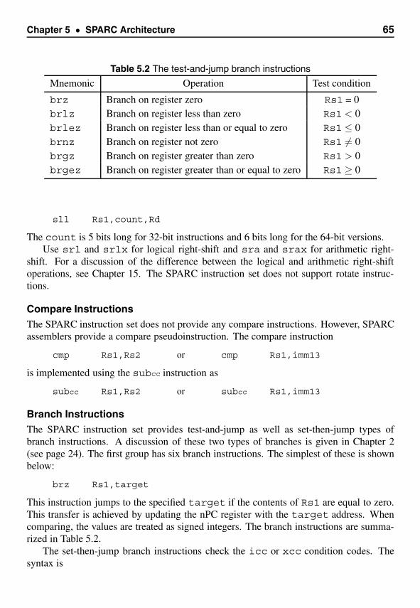
Chapter 5 • SPARC Architecture 65
Table 5.2 The test-and-jump branch instructions
Mnemonic Operation Test condition
brz Branch on register zero Rs1 = 0brlz Branch on register less than zero Rs1 < 0brlez Branch on register less than or equal to zero Rs1 ≤ 0brnz Branch on register not zero Rs1 �= 0brgz Branch on register greater than zero Rs1 > 0brgez Branch on register greater than or equal to zero Rs1 ≥ 0
sll Rs1,count,Rd
The count is 5 bits long for 32-bit instructions and 6 bits long for the 64-bit versions.Use srl and srlx for logical right-shift and sra and srax for arithmetic right-
shift. For a discussion of the difference between the logical and arithmetic right-shiftoperations, see Chapter 15. The SPARC instruction set does not support rotate instruc-tions.
Compare InstructionsThe SPARC instruction set does not provide any compare instructions. However, SPARCassemblers provide a compare pseudoinstruction. The compare instruction
cmp Rs1,Rs2 or cmp Rs1,imm13
is implemented using the subcc instruction as
subcc Rs1,Rs2 or subcc Rs1,imm13
Branch InstructionsThe SPARC instruction set provides test-and-jump as well as set-then-jump types ofbranch instructions. A discussion of these two types of branches is given in Chapter 2(see page 24). The first group has six branch instructions. The simplest of these is shownbelow:
brz Rs1,target
This instruction jumps to the specified target if the contents of Rs1 are equal to zero.This transfer is achieved by updating the nPC register with the target address. Whencomparing, the values are treated as signed integers. The branch instructions are summa-rized in Table 5.2.
The set-then-jump branch instructions check the icc or xcc condition codes. Thesyntax is
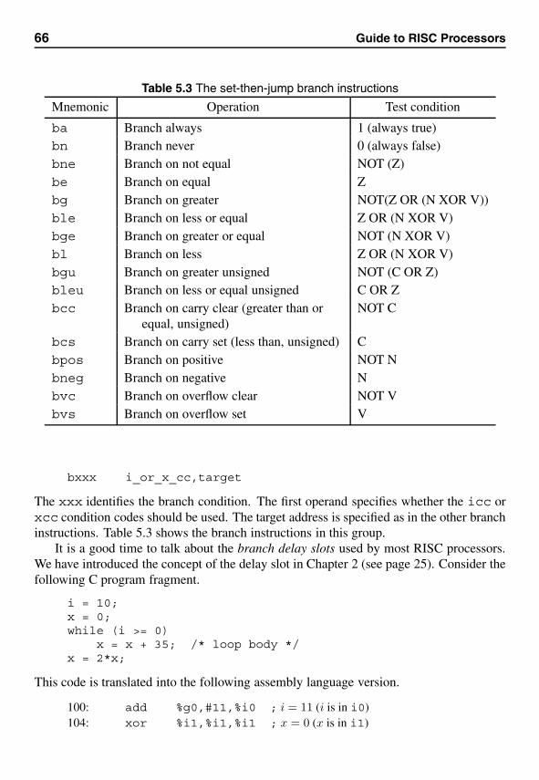
66 Guide to RISC Processors
Table 5.3 The set-then-jump branch instructions
Mnemonic Operation Test condition
ba Branch always 1 (always true)bn Branch never 0 (always false)bne Branch on not equal NOT (Z)be Branch on equal Zbg Branch on greater NOT(Z OR (N XOR V))ble Branch on less or equal Z OR (N XOR V)bge Branch on greater or equal NOT (N XOR V)bl Branch on less Z OR (N XOR V)bgu Branch on greater unsigned NOT (C OR Z)bleu Branch on less or equal unsigned C OR Zbcc Branch on carry clear (greater than or
equal, unsigned)NOT C
bcs Branch on carry set (less than, unsigned) Cbpos Branch on positive NOT Nbneg Branch on negative Nbvc Branch on overflow clear NOT Vbvs Branch on overflow set V
bxxx i_or_x_cc,target
The xxx identifies the branch condition. The first operand specifies whether the icc orxcc condition codes should be used. The target address is specified as in the other branchinstructions. Table 5.3 shows the branch instructions in this group.
It is a good time to talk about the branch delay slots used by most RISC processors.We have introduced the concept of the delay slot in Chapter 2 (see page 25). Consider thefollowing C program fragment.
i = 10;x = 0;while (i >= 0)
x = x + 35; /* loop body */x = 2*x;
This code is translated into the following assembly language version.
100: add %g0,#11,%i0 ; i = 11 (i is in i0)104: xor %i1,%i1,%i1 ; x = 0 (x is in i1)
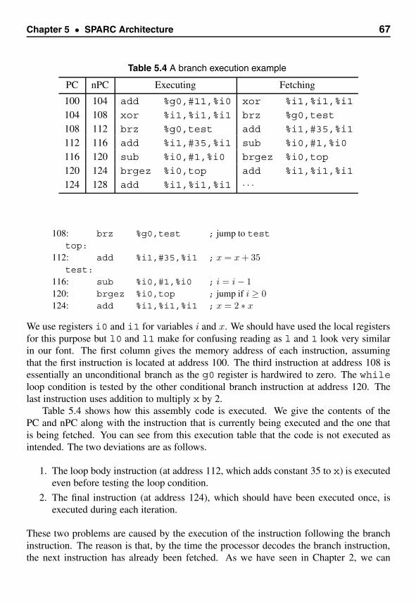
Chapter 5 • SPARC Architecture 67
Table 5.4 A branch execution example
PC nPC Executing Fetching
100 104 add %g0,#11,%i0 xor %i1,%i1,%i1
104 108 xor %i1,%i1,%i1 brz %g0,test
108 112 brz %g0,test add %i1,#35,%i1
112 116 add %i1,#35,%i1 sub %i0,#1,%i0
116 120 sub %i0,#1,%i0 brgez %i0,top
120 124 brgez %i0,top add %i1,%i1,%i1
124 128 add %i1,%i1,%i1 · · ·
108: brz %g0,test ; jump to testtop:
112: add %i1,#35,%i1 ; x = x + 35test:
116: sub %i0,#1,%i0 ; i = i − 1120: brgez %i0,top ; jump if i ≥ 0124: add %i1,%i1,%i1 ; x = 2 ∗ x
We use registers i0 and i1 for variables i and x. We should have used the local registersfor this purpose but l0 and l1 make for confusing reading as l and 1 look very similarin our font. The first column gives the memory address of each instruction, assumingthat the first instruction is located at address 100. The third instruction at address 108 isessentially an unconditional branch as the g0 register is hardwired to zero. The whileloop condition is tested by the other conditional branch instruction at address 120. Thelast instruction uses addition to multiply x by 2.
Table 5.4 shows how this assembly code is executed. We give the contents of thePC and nPC along with the instruction that is currently being executed and the one thatis being fetched. You can see from this execution table that the code is not executed asintended. The two deviations are as follows.
1. The loop body instruction (at address 112, which adds constant 35 to x) is executedeven before testing the loop condition.
2. The final instruction (at address 124), which should have been executed once, isexecuted during each iteration.
These two problems are caused by the execution of the instruction following the branchinstruction. The reason is that, by the time the processor decodes the branch instruction,the next instruction has already been fetched. As we have seen in Chapter 2, we can
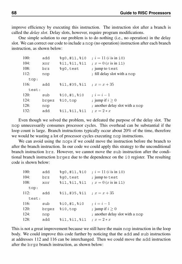
68 Guide to RISC Processors
improve efficiency by executing this instruction. The instruction slot after a branch iscalled the delay slot. Delay slots, however, require program modifications.
One simple solution to our problem is to do nothing (i.e., no operation) in the delayslot. We can correct our code to include a nop (no operation) instruction after each branchinstruction, as shown below:
100: add %g0,#11,%i0 ; i = 11 (i is in i0)104: xor %i1,%i1,%i1 ; x = 0 (x is in i1)108: brz %g0,test ; jump to test112: nop ; fill delay slot with a nop
top:116: add %i1,#35,%i1 ; x = x + 35
test:120: sub %i0,#1,%i0 ; i = i − 1124: brgez %i0,top ; jump if i ≥ 0128: nop ; another delay slot with a nop132: add %i1,%i1,%i1 ; x = 2 ∗ x
Even though we solved the problem, we defeated the purpose of the delay slot. Thenop unnecessarily consumes processor cycles. This overhead can be substantial if theloop count is large. Branch instructions typically occur about 20% of the time, thereforewe would be wasting a lot of processor cycles executing nop instructions.
We can avoid using the nops if we could move the instruction before the branch toafter the branch instruction. In our code we could apply this strategy to the unconditionalbranch instruction brz. However, we cannot move the sub instruction after the condi-tional branch instruction brgez due to the dependence on the i0 register. The resultingcode is shown below:
100: add %g0,#11,%i0 ; i = 11 (i is in i0)104: brz %g0,test ; jump to test108: xor %i1,%i1,%i1 ; x = 0 (x is in i1)
top:112: add %i1,#35,%i1 ; x = x + 35
test:116: sub %i0,#1,%i0 ; i = i − 1120: brgez %i0,top ; jump if i ≥ 0124: nop ; another delay slot with a nop128: add %i1,%i1,%i1 ; x = 2 ∗ x
This is not a great improvement because we still have the main nop instruction in the loopbody. We could improve this code further by noticing that the add and sub instructionsat addresses 112 and 116 can be interchanged. Then we could move the add instructionafter the brgz branch instruction, as shown below:
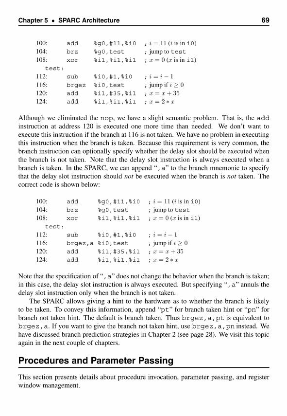
Chapter 5 • SPARC Architecture 69
100: add %g0,#11,%i0 ; i = 11 (i is in i0)104: brz %g0,test ; jump to test108: xor %i1,%i1,%i1 ; x = 0 (x is in i1)
test:112: sub %i0,#1,%i0 ; i = i − 1116: brgez %i0,test ; jump if i ≥ 0120: add %i1,#35,%i1 ; x = x + 35124: add %i1,%i1,%i1 ; x = 2 ∗ x
Although we eliminated the nop, we have a slight semantic problem. That is, the addinstruction at address 120 is executed one more time than needed. We don’t want toexecute this instruction if the branch at 116 is not taken. We have no problem in executingthis instruction when the branch is taken. Because this requirement is very common, thebranch instruction can optionally specify whether the delay slot should be executed whenthe branch is not taken. Note that the delay slot instruction is always executed when abranch is taken. In the SPARC, we can append “,a” to the branch mnemonic to specifythat the delay slot instruction should not be executed when the branch is not taken. Thecorrect code is shown below:
100: add %g0,#11,%i0 ; i = 11 (i is in i0)104: brz %g0,test ; jump to test108: xor %i1,%i1,%i1 ; x = 0 (x is in i1)
test:112: sub %i0,#1,%i0 ; i = i − 1116: brgez,a %i0,test ; jump if i ≥ 0120: add %i1,#35,%i1 ; x = x + 35124: add %i1,%i1,%i1 ; x = 2 ∗ x
Note that the specification of “,a” does not change the behavior when the branch is taken;in this case, the delay slot instruction is always executed. But specifying “,a” annuls thedelay slot instruction only when the branch is not taken.
The SPARC allows giving a hint to the hardware as to whether the branch is likelyto be taken. To convey this information, append “pt” for branch taken hint or “pn” forbranch not taken hint. The default is branch taken. Thus brgez,a,pt is equivalent tobrgez,a. If you want to give the branch not taken hint, use brgez,a,pn instead. Wehave discussed branch prediction strategies in Chapter 2 (see page 28). We visit this topicagain in the next couple of chapters.
Procedures and Parameter Passing
This section presents details about procedure invocation, parameter passing, and registerwindow management.
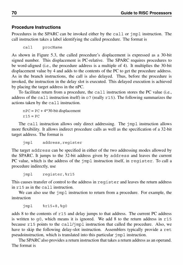
70 Guide to RISC Processors
Procedure InstructionsProcedures in the SPARC can be invoked either by the call or jmpl instruction. Thecall instruction takes a label identifying the called procedure. The format is
call procName
As shown in Figure 5.3, the called procedure’s displacement is expressed as a 30-bitsigned number. This displacement is PC-relative. The SPARC requires procedures tobe word-aligned (i.e., the procedure address is a multiple of 4). It multiplies the 30-bitdisplacement value by 4 and adds to the contents of the PC to get the procedure address.As in the branch instructions, the call is also delayed. Thus, before the procedure isinvoked, the instruction in the delay slot is executed. This delayed execution is achievedby placing the target address in the nPC.
To facilitate return from a procedure, the call instruction stores the PC value (i.e.,address of the call instruction itself) in o7 (really r15). The following summarizes theactions taken by the call instruction.
nPC = PC + 4*30-bit displacementr15 = PC
The call instruction allows only direct addressing. The jmpl instruction allowsmore flexibility. It allows indirect procedure calls as well as the specification of a 32-bittarget address. The format is
jmpl address,register
The target address can be specified in either of the two addressing modes allowed bythe SPARC. It jumps to the 32-bit address given by address and leaves the currentPC value, which is the address of the jmpl instruction itself, in register. To call aprocedure indirectly, use
jmpl register,%r15
This causes transfer of control to the address in register and leaves the return addressin r15 as in the call instruction.
We can also use the jmpl instruction to return from a procedure. For example, theinstruction
jmpl %r15+8,%g0
adds 8 to the contents of r15 and delay jumps to that address. The current PC addressis written to g0, which means it is ignored. We add 8 to the return address in r15because r15 points to the call/jmpl instruction that called the procedure. Also, wehave to skip the following delay-slot instruction. Assemblers typically provide a retpseudoinstruction, which is translated into this particular jmpl instruction.
The SPARC also provides a return instruction that takes a return address as an operand.The format is
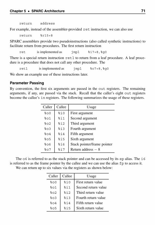
Chapter 5 • SPARC Architecture 71
return address
For example, instead of the assembler-provided ret instruction, we can also use
return %r15+8
SPARC assemblers provide two pseudoinstructions (also called synthetic instructions) tofacilitate return from procedures. The first return instruction
ret is implemented as jmpl %i7+8,%g0
There is a special return instruction retl to return from a leaf procedure. A leaf proce-dure is a procedure that does not call any other procedure. The
retl is implemented as jmpl %o7+8,%g0
We show an example use of these instructions later.
Parameter PassingBy convention, the first six arguments are passed in the out registers. The remainingarguments, if any, are passed via the stack. Recall that the caller’s eight out registersbecome the callee’s in registers. The following summarizes the usage of these registers.
Caller Callee Usage
%o0 %i0 First argument%o1 %i1 Second argument%o2 %i2 Third argument%o3 %i3 Fourth argument%o4 %i4 Fifth argument%o5 %i5 Sixth argument%o6 %i6 Stack pointer/frame pointer%o7 %i7 Return address − 8
The o6 is referred to as the stack pointer and can be accessed by its sp alias. The i6is referred to as the frame pointer by the callee and we can use the alias fp to access it.
We can return up to six values via the registers as shown below:
Caller Callee Usage
%o0 %i0 First return value%o1 %i1 Second return value%o2 %i2 Third return value%o3 %i3 Fourth return value%o4 %i4 Fifth return value%o5 %i5 Sixth return value
72 Guide to RISC Processors
As with the parameter passing, we have to use the stack to return the remaining returnvalues.
Stack ImplementationWe briefly describe the SPARC stack implementation. As in the MIPS architecture, thestack grows downward (i.e., from a higher memory address to a lower address). How-ever, there are no explicit stack push and pop instructions. Instead, these instructions canbe synthesized by manipulating the stack pointer sp. For example, to push or pop thecontents of i0, we can use the following code.
Push operation Pop operationsub %sp,4,%sp add %sp,4,%sp
st %i0,[%sp] ld [%sp],%i0
To allocate an N -byte stack frame, we can use
sub %sp,N,%sp
Window ManagementSPARC processors can have up to 32 register windows. The number of windows availableon a specific implementation is given by NWINDOWS. Note that NWINDOWS can rangefrom 3 to 32. As noted, the Current Window Pointer (CWP) points to the current registerset. These window sets are organized as a circular buffer (see Figure 5.4). Thus, the CWParithmetic can be done modulo NWINDOWS.
With each procedure call, a new register window is assigned. This is done by the saveinstruction. This instruction can also allocate space on the stack for the stack frame. Thesave instruction
save %sp,−N,%sp
slides the register window by incrementing CWP (mod NWINDOWS) and allocates Nbytes of stack space. If no errors occur, save acts as the add instruction does. Thus, byspecifying sp and a negative N value, it allocates N bytes of stack space. As in the addinstruction, the second operand can also be a register.
The restore instruction restores the register window saved by the last save in-struction. Its format is similar to that of the save. It also performs addition on itsoperands as does the save instruction. A trivial restore pseudoinstruction is definedas
restore %g0,%g0,%g0
A typical procedure looks like

Chapter 5 • SPARC Architecture 73
W7
W5
W3
W1
INs
INs
INs
INs
LOCALs
LOCALs
LOCALs
LOCALs
LOCALs OUTs
OUTs
OUTs
OUTs
OUTsINs
INs
INs
INs
LOCALs
OUTs
OUTs
LOCALs
LOCALs
OUTs
CWP = 0
restore
W0
W2
W4
W6
save
Figure 5.4 The register windows are organized as a circular buffer.
proc-name:save %sp,−N,%sp. . .procedure body. . .retrestore
Note that the restore instruction is executed in the delay slot. Because the restoredoes not add N to sp, you might be wondering about how the stack allocation is released.To understand this, we should look at the way the save instruction performs the addoperation on its operands. For this add operation, save uses the old window for thetwo source operands and stores the result in the new window. In our example, it adds−N to the sp value from the previous window and stores the result in the new window’ssp register. Thus, when we restore the previous window, we automatically see theprevious sp value.
A leaf procedure does not use a new register window. It uses the registers from thecaller’s window. A typical leaf procedure looks like
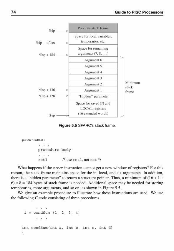
74 Guide to RISC Processors
temporaries, etc.Space for local variables,
Space for remainingarguments (7, 8, . . .)
LOCAL registers(16 extended words)
Space for saved IN and
%sp
%fp
%sp + 128
%sp + 136
%sp + 184
Minimumstackframe
Argument 6
Argument 5
Argument 4
Argument 3
Argument 2
Argument 1
‘‘Hidden’’ parameter
%fp offset
Previous stack frame
Figure 5.5 SPARC’s stack frame.
proc-name:. . .procedure body. . .retl /* use retl, not ret */
What happens if the save instruction cannot get a new window of registers? For thisreason, the stack frame maintains space for the in, local, and six arguments. In addition,there is a “hidden parameter” to return a structure pointer. Thus, a minimum of (16 + 1 +6) * 8 = 184 bytes of stack frame is needed. Additional space may be needed for storingtemporaries, more arguments, and so on, as shown in Figure 5.5.
We give an example procedure to illustrate how these instructions are used. We usethe following C code consisting of three procedures.
. . .i = condSum (1, 2, 3, 4)
. . .
int condSum(int a, int b, int c, int d){
Chapter 5 • SPARC Architecture 75
int t1;
t1 = a;if (a < b)
t1 = b;return(sum(t1,c,d));
}
int sum(int x, int y, int z){
return(x+y+z);}
The corresponding SPARC assembly code is shown in three procedures. In the mainprocedure, the four arguments of condSum are moved to the first four out registers: o0through o3.
. . .mov 1,%o0 ; first argumentmov 2,%o1 ; second argumentmov 3,%o2 ; third argumentcall condSummov 4,%o3 ; fourth argument in delay slot; condSum returns result in %o0. When condSum returns,; the following instruction is executedmov %o0,%l0 ; return result moved to %l0
. . .
Because the call is a delayed instruction, we use the delay slot to move the fourthargument to o3. Note that the condSum call should return to the instruction
mov %o0,%l0
This is the reason for adding 8 to the return address. This procedure returns the sum inthe o0 register. The above mov instruction copies this value to the l0 local register.
The first instruction in the condSum procedure is the save instruction. As we havediscussed, it allocates a new register window by incrementing the CWP. We also allocate184 bytes of stack frame, which is the minimum size. The next four instructions select theminimum of the first two arguments. Note that the out registers of the previous windoware referred to as in registers in the current window. We move the three arguments toout registers to pass them on to the sum procedure. When sum returns the total, thisvalue is moved from o0 to i0 so that the result is available in o0 in the main procedure.
76 Guide to RISC Processors
;*********** condSum procedure **********condSum:
save %sp,-184,%sp; allocate min. stack framemov %i0, %o0cmp %i1, %i0 ; if %i1 is less/equal,ble skip ; skip the following movmov %i1, %o0
skip:mov %i2, %o1 ; second argumentcall summov %i3, %o2 ; third argument in delay slotmov %o0, %i0 ; move the result returned by sum to %o0retrestore ; trivial restore in delay slot of ret
;******* end of condSum procedure *******
The sum procedure is a leaf procedure as it does not call any other procedure. We canoptimize a leaf procedure by not requesting a new window; instead it uses the registersfrom the caller’s window. Thus, there is no need for the save and restore instructions.The only instruction that needs special care is the return: we have to use retl rather thanthe ret instruction.
;*********** sum procedure ***********sum:
add %o0, %o1, %o0 ; first additionretl ; leaf procedure, use retladd %o0, %o2, %o0 ; final add in delay slot; result returned in %o0
;******* end of sum procedure ********
Summary
We have briefly presented the architecture and instruction set of the SPARC. A user pro-gram is provided with 32 general-purpose registers, which are organized into four registersets: in, out, local, and global. It supports a register window mechanism that facilitatesefficient parameter passing in procedure calls. We see a similar mechanism in Chapter 7.
The SPARC architecture supports two basic addressing modes. One is similar to theaddressing mode we have seen in the last chapter. The other computes the effective ad-dress as the sum of the contents of two registers. As does the MIPS architecture, SPARCalso uses 32 bits to encode instructions. After reading details about the other architectures,you will notice that it supports a fairly standard set of instructions.
A notable difference from other processors is that it is a specification at the ISA levelthat is available to chip manufacturers, which means several implementations are possi-ble. For example, an implementation can choose to have a number of register windows be-

Chapter 5 • SPARC Architecture 77
tween 3 and 32. Furthermore, there are also several instructions that have implementation-defined semantics. If you are interested in more details, several reference documents areavailable at the SPARC Web site.
Web ResourcesFull specifications and other reference material on the SPARC architecture are availablefrom www.sparc.org. Sun also maintains information on their SPARC processors atwww.sun.com/microelectronics/sparc.
6PowerPC Architecture
This chapter gives details on the PowerPC architecture. We start the chapter with anoverview and a brief history of the PowerPC architecture. We then give its register setdetails and the addressing modes supported. As does the SPARC, PowerPC supports twoaddressing modes. However, PowerPC also supports update versions of these addressingmodes. The update versions, for example, are useful in providing “regular” access toarrays. Unlike the MIPS architecture, PowerPC supports a variety of instruction formats.The instruction set details are presented next. After reading this section, you will noticethat the PowerPC branch instructions are flexible and can take branch prediction hintsfrom the compiler. We conclude the chapter with a summary.
IntroductionThe PowerPC defines a 64-bit architecture that can operate in two modes: 64-bit and 32-bit mode. It supports dynamic switching between these two modes. In the 32-bit mode, a64-bit PowerPC processor can execute 32-bit application binaries.
Here is a short history of the PowerPC architecture [9]. IBM developed many of theconcepts in 1975 for a prototype system. An unsuccessful commercial version of this pro-totype was introduced around 1986. Four years later, IBM introduced the RS/6000 familyof processors based on their POWER architecture. In early 1991, a group from Motorola,IBM, and Apple began work on the PowerPC architecture using the IBM POWER archi-tecture as the base. The PowerPC includes many of the POWER instructions. PowerPCdropped some of the POWER instructions, but these were not frequently used. The firstimplementation of the PowerPC architecture, the PowerPC 601, implemented all but twoPOWER instructions so that POWER applications run on the PowerPC.
The PowerPC family of processors is available in both 32- and 64-bit implementa-tions. Here we discuss the 64-bit implementation. As are the MIPS and SPARC, thePowerPC architecture is based on the load/store architecture. It satisfies many of theRISC characteristics we mentioned in Chapter 2.
79
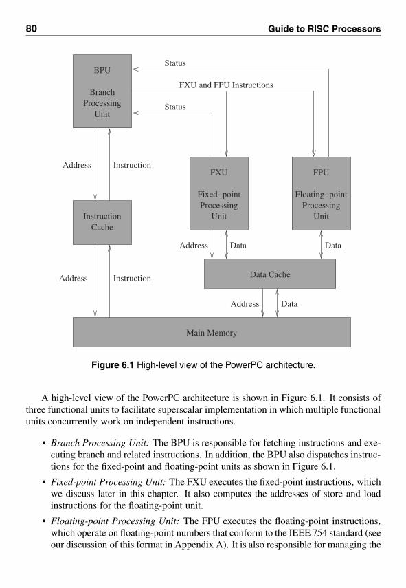
80 Guide to RISC Processors
FXU
Fixed−pointProcessing
Unit
FPU
ProcessingUnit
Floating−point
DataAddress
DataAddress
BPU
BranchProcessing
Unit
InstructionCache
Data Cache
Data
Main Memory
Address Instruction
InstructionAddress
Status
Status
FXU and FPU Instructions
Figure 6.1 High-level view of the PowerPC architecture.
A high-level view of the PowerPC architecture is shown in Figure 6.1. It consists ofthree functional units to facilitate superscalar implementation in which multiple functionalunits concurrently work on independent instructions.
• Branch Processing Unit: The BPU is responsible for fetching instructions and exe-cuting branch and related instructions. In addition, the BPU also dispatches instruc-tions for the fixed-point and floating-point units as shown in Figure 6.1.
• Fixed-point Processing Unit: The FXU executes the fixed-point instructions, whichwe discuss later in this chapter. It also computes the addresses of store and loadinstructions for the floating-point unit.
• Floating-point Processing Unit: The FPU executes the floating-point instructions,which operate on floating-point numbers that conform to the IEEE 754 standard (seeour discussion of this format in Appendix A). It is also responsible for managing the
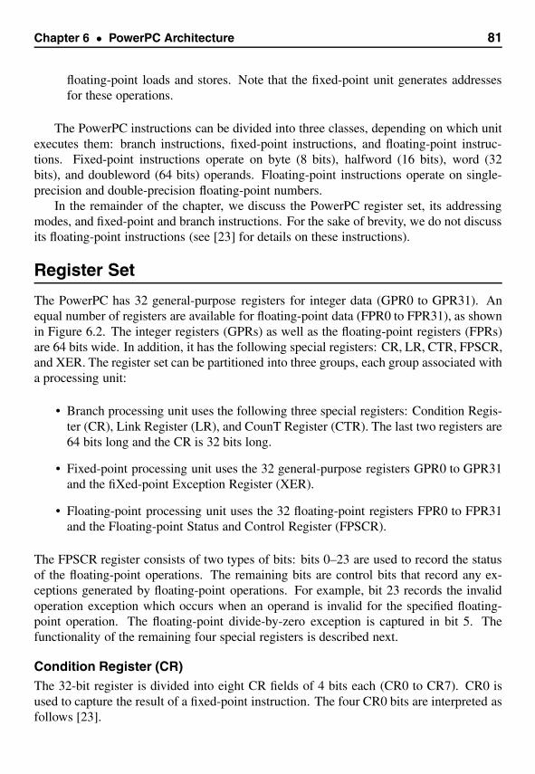
Chapter 6 • PowerPC Architecture 81
floating-point loads and stores. Note that the fixed-point unit generates addressesfor these operations.
The PowerPC instructions can be divided into three classes, depending on which unitexecutes them: branch instructions, fixed-point instructions, and floating-point instruc-tions. Fixed-point instructions operate on byte (8 bits), halfword (16 bits), word (32bits), and doubleword (64 bits) operands. Floating-point instructions operate on single-precision and double-precision floating-point numbers.
In the remainder of the chapter, we discuss the PowerPC register set, its addressingmodes, and fixed-point and branch instructions. For the sake of brevity, we do not discussits floating-point instructions (see [23] for details on these instructions).
Register Set
The PowerPC has 32 general-purpose registers for integer data (GPR0 to GPR31). Anequal number of registers are available for floating-point data (FPR0 to FPR31), as shownin Figure 6.2. The integer registers (GPRs) as well as the floating-point registers (FPRs)are 64 bits wide. In addition, it has the following special registers: CR, LR, CTR, FPSCR,and XER. The register set can be partitioned into three groups, each group associated witha processing unit:
• Branch processing unit uses the following three special registers: Condition Regis-ter (CR), Link Register (LR), and CounT Register (CTR). The last two registers are64 bits long and the CR is 32 bits long.
• Fixed-point processing unit uses the 32 general-purpose registers GPR0 to GPR31and the fiXed-point Exception Register (XER).
• Floating-point processing unit uses the 32 floating-point registers FPR0 to FPR31and the Floating-point Status and Control Register (FPSCR).
The FPSCR register consists of two types of bits: bits 0–23 are used to record the statusof the floating-point operations. The remaining bits are control bits that record any ex-ceptions generated by floating-point operations. For example, bit 23 records the invalidoperation exception which occurs when an operand is invalid for the specified floating-point operation. The floating-point divide-by-zero exception is captured in bit 5. Thefunctionality of the remaining four special registers is described next.
Condition Register (CR)The 32-bit register is divided into eight CR fields of 4 bits each (CR0 to CR7). CR0 isused to capture the result of a fixed-point instruction. The four CR0 bits are interpreted asfollows [23].
82 Guide to RISC Processors
.
.
.
General−purposeregisters
GPR0 (64)
GPR1 (64)
GPR31 (64)
.
.
.
FPR0 (64)
FPR1 (64)
FPR31 (64)
Floating−pointregisters
Floating−point statusand control register
FPSCR (32)
CR (32)
Condition register
XER (64)
XER register
LR (64)
Link register
CTR (64)
Count register
Figure 6.2 PowerPC registers: general-purpose, link, XER, and count registers are 32-bits long in 32-bit implementations and 64-bits long in 64-bit implementations. The otherregisters are of fixed size independent of the implementation.
Bit Description
0 Negative (LT)The result is negative.
1 Positive (GT)The result is positive.
2 Zero (EQ)The result is zero.
3 Summary overflow (SO)This is a copy of the SO bit from XER register (discussed later).
The first bit can be interpreted as representing the “less than” (LT) relationship. Similarly,the second and third bits represent “greater than” (GT) and “equal to” (EQ) relationships,respectively.
The CR1 field is used to capture floating-point exception status. These four bits are acopy of the least significant four bits of the FPSCR register. Because we do not discussthe floating-point unit details here, we skip the interpretation of these four bits (see [23]for details).
The remaining CR fields can be used for either integer or floating-point instructions tocapture integer or floating-point LT, GT, EQ, and SO conditions. Instructions are availableto perform logical operations on individual CR bits. Branch instructions are available totest a specific CR field bit. These instructions can specify the CR field that should be used.
Link Register (LR)The 64-bit link register is used to store the return address in a procedure call. Procedurecalls are implemented by branch (bl/bla) or conditional branch (bc/bca) instructions.For these instructions, the LR register receives the effective address of the instructionfollowing the branch instruction.

Chapter 6 • PowerPC Architecture 83
Count RegisterThe 64-bit CTR register holds the loop count value. Branch instructions can specify avariety of conditions under which branching should take place. For example, a conditionalbranch instruction can decrement CTR and branch only if CTR �= 0 or if CTR = 0. Evenmore complex branch conditions can be tested. More details on the branch instruction arepresented later in this chapter (page 93).
XER RegisterThe XER register serves two distinct purposes. Bits 0, 1, and 2 are used to record Sum-mary Overflow (SO), OVerflow (OV), and CArry (CA). The OV bit records the fact thatan overflow has occurred during the execution of an instruction. The SO bit is different inthe sense that it is set whenever the OV bit is set. However, once set, the SO bit remainsset until a special instruction is executed to clear it. The CA bit is set by add and subtractarithmetic operations and right-shift instructions.
Bits 57 to 63 are used as a 7-bit byte count to specify the number of bytes to be trans-ferred between memory and registers. This field is used by Load String Word Indexed(lswx) and Store String Word Indexed (stswx) instructions. Using just one lswx in-struction we can load 128 contiguous bytes from memory into all 32 general-purposeregisters. Similarly, reverse transfer can be done by stswx instruction.
Addressing Modes
The PowerPC supports two basic addressing modes as does the SPARC. We can specifythree general-purpose registers rA, rB, and rD/rS in load/store instructions. RegistersrA and rB are used to compute the effective address. The third register is treated eitheras the destination register rD in load operations or as the source register rS in storeoperations.
Register Indirect with ImmediateIn this addressing mode, instructions contain a signed immediate value imm. The effectiveaddress is computed by adding this value to the contents of a general-purpose register rAspecified in the instruction. Interestingly, we can specify a 0 in place of rA. In thiscase, the effective address is the immediate value given in the instruction. Thus, it isstraightforward to convert indirect addressing to direct addressing.
Effective address = Contents of rA or 0 + imm
The immediate constant is either 14 or 16 bits depending on the instruction encodingused. We discuss instruction formats in the next section. Also, note that this is the onlyaddressing supported by the MIPS architecture.

84 Guide to RISC Processors
Register Indirect with IndexInstructions using this addressing mode specify two general-purpose registers rA and rB.The effective address is computed as the sum of the contents of these two registers. As inthe other addressing modes, we can specify 0 in place of rA.
Effective address = Contents of rA or 0 + Contents of rB
These addressing modes are also available in the update version. In this version, thecomputed effective address is loaded into the base register rA. We look at these twoversions next.
Register Indirect with Immediate UpdateThis is the update version of the first addressing mode. The semantics are shown below:
Effective address = Contents of rA or 0 + immrA = Effective address
Register Indirect with Index UpdateThe indexed version has the following semantics.
Effective address = Contents of rA or 0 + Contents of rBrA = Effective address
We later show how these update versions are useful in accessing arrays by means of anexample.
In our discussion so far, we assumed 64-bit mode. In 32-bit mode, computation ofthe effective address is the same. However, only the lower-order 32 bits are used as theeffective address to access memory.
Instruction FormatAs with the MIPS and SPARC, all PowerPC instructions are encoded using four bytes.Instructions are assumed to be word-aligned, so that the processor can ignore the leastsignificant two bits of all instruction addresses.
As shown in Figure 6.3, bits 0 to 5 specify the primary opcode. Many instructionsalso have an extended opcode. The remaining bits are used for various fields dependingon the instruction type. Here we discuss some basic instruction formats.
Most instructions use the register format shown in Figure 6.3a. In arithmetic, logical,and other similar instruction types, registers rA and rB specify the source operands andrD specifies the destination register. The OE and rC bits are explained later.
The immediate format shown in Figure 6.3b is used by instructions that specify an

Chapter 6 • PowerPC Architecture 85
Dr rA r B
3130
r C
(a) Register format (XO−form)
opcode
0 5 6
OE
2110 11 15 16 2220
suboperation specification
(b) Immediate format (D−form)
opcode
0 5 6 10 11 15 16 31
rD rA
(d) Load/store format
16−bit signed/unsigned immediate value
Direct conditional branch (B−form)
opcode
0 5 6 10 11 15 16 3029
LKAA14−bit immediate displacementBI
31
Indirect conditional branch (XL−form)
opcode
0 5 6 10 11 15
LKBI count/link register specification
21 30 31
BO
BO
opcode LK
0 5 6 31
AA
29 30
24−bit immediate displacement
Unconditional branch (I−form)
Register indirect mode (D−form)0 5 6 10 11 15 16 31
rD
opcode
0 5 6 10 11 15 16
optionsrD
312120
rA
rA rB
16−bit signed displacementopcode
1816
(c) Branch format
Register indirect with indexing mode (X−form)
HB
Figure 6.3 Sample PowerPC instruction formats.
immediate operand. For example, the addi instruction, described in the next section,uses this format.
The format shown in Figure 6.3c is used by branch instructions. The unconditionalbranch format allows specification of a 24-bit target address. This figure also shows theformat used by direct and indirect conditional branch instructions. The AA bit is used to
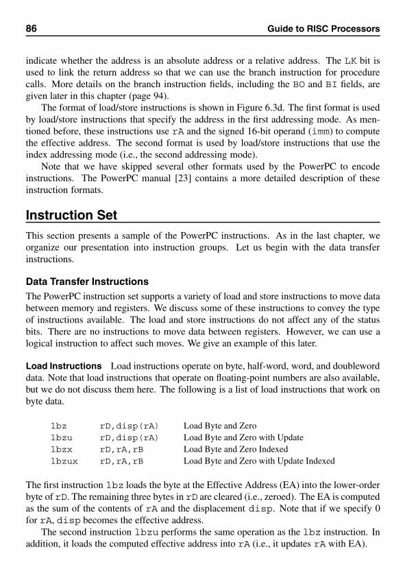
86 Guide to RISC Processors
indicate whether the address is an absolute address or a relative address. The LK bit isused to link the return address so that we can use the branch instruction for procedurecalls. More details on the branch instruction fields, including the BO and BI fields, aregiven later in this chapter (page 94).
The format of load/store instructions is shown in Figure 6.3d. The first format is usedby load/store instructions that specify the address in the first addressing mode. As men-tioned before, these instructions use rA and the signed 16-bit operand (imm) to computethe effective address. The second format is used by load/store instructions that use theindex addressing mode (i.e., the second addressing mode).
Note that we have skipped several other formats used by the PowerPC to encodeinstructions. The PowerPC manual [23] contains a more detailed description of theseinstruction formats.
Instruction SetThis section presents a sample of the PowerPC instructions. As in the last chapter, weorganize our presentation into instruction groups. Let us begin with the data transferinstructions.
Data Transfer InstructionsThe PowerPC instruction set supports a variety of load and store instructions to move databetween memory and registers. We discuss some of these instructions to convey the typeof instructions available. The load and store instructions do not affect any of the statusbits. There are no instructions to move data between registers. However, we can use alogical instruction to affect such moves. We give an example of this later.
Load Instructions Load instructions operate on byte, half-word, word, and doubleworddata. Note that load instructions that operate on floating-point numbers are also available,but we do not discuss them here. The following is a list of load instructions that work onbyte data.
lbz rD,disp(rA) Load Byte and Zerolbzu rD,disp(rA) Load Byte and Zero with Updatelbzx rD,rA,rB Load Byte and Zero Indexedlbzux rD,rA,rB Load Byte and Zero with Update Indexed
The first instruction lbz loads the byte at the Effective Address (EA) into the lower-orderbyte of rD. The remaining three bytes in rD are cleared (i.e., zeroed). The EA is computedas the sum of the contents of rA and the displacement disp. Note that if we specify 0for rA, disp becomes the effective address.
The second instruction lbzu performs the same operation as the lbz instruction. Inaddition, it loads the computed effective address into rA (i.e., it updates rA with EA).
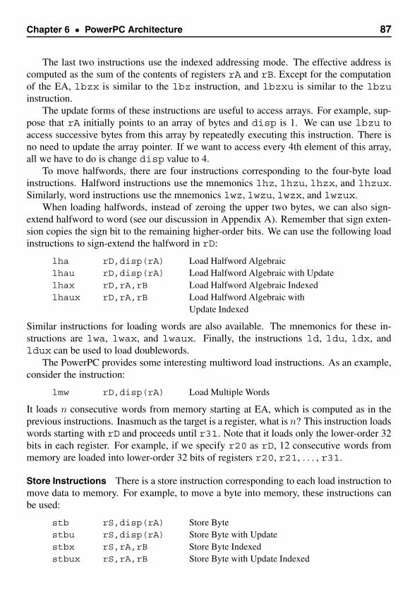
Chapter 6 • PowerPC Architecture 87
The last two instructions use the indexed addressing mode. The effective address iscomputed as the sum of the contents of registers rA and rB. Except for the computationof the EA, lbzx is similar to the lbz instruction, and lbzxu is similar to the lbzuinstruction.
The update forms of these instructions are useful to access arrays. For example, sup-pose that rA initially points to an array of bytes and disp is 1. We can use lbzu toaccess successive bytes from this array by repeatedly executing this instruction. There isno need to update the array pointer. If we want to access every 4th element of this array,all we have to do is change disp value to 4.
To move halfwords, there are four instructions corresponding to the four-byte loadinstructions. Halfword instructions use the mnemonics lhz, lhzu, lhzx, and lhzux.Similarly, word instructions use the mnemonics lwz, lwzu, lwzx, and lwzux.
When loading halfwords, instead of zeroing the upper two bytes, we can also sign-extend halfword to word (see our discussion in Appendix A). Remember that sign exten-sion copies the sign bit to the remaining higher-order bits. We can use the following loadinstructions to sign-extend the halfword in rD:
lha rD,disp(rA) Load Halfword Algebraiclhau rD,disp(rA) Load Halfword Algebraic with Updatelhax rD,rA,rB Load Halfword Algebraic Indexedlhaux rD,rA,rB Load Halfword Algebraic with
Update Indexed
Similar instructions for loading words are also available. The mnemonics for these in-structions are lwa, lwax, and lwaux. Finally, the instructions ld, ldu, ldx, andldux can be used to load doublewords.
The PowerPC provides some interesting multiword load instructions. As an example,consider the instruction:
lmw rD,disp(rA) Load Multiple Words
It loads n consecutive words from memory starting at EA, which is computed as in theprevious instructions. Inasmuch as the target is a register, what is n? This instruction loadswords starting with rD and proceeds until r31. Note that it loads only the lower-order 32bits in each register. For example, if we specify r20 as rD, 12 consecutive words frommemory are loaded into lower-order 32 bits of registers r20, r21, . . . , r31.
Store Instructions There is a store instruction corresponding to each load instruction tomove data to memory. For example, to move a byte into memory, these instructions canbe used:
stb rS,disp(rA) Store Bytestbu rS,disp(rA) Store Byte with Updatestbx rS,rA,rB Store Byte Indexedstbux rS,rA,rB Store Byte with Update Indexed
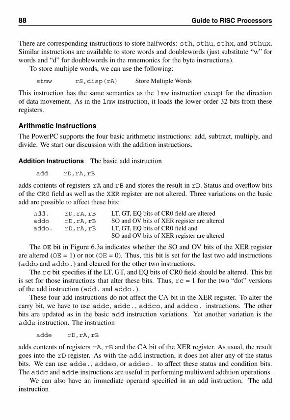
88 Guide to RISC Processors
There are corresponding instructions to store halfwords: sth, sthu, sthx, and sthux.Similar instructions are available to store words and doublewords (just substitute “w” forwords and “d” for doublewords in the mnemonics for the byte instructions).
To store multiple words, we can use the following:
stmw rS,disp(rA) Store Multiple Words
This instruction has the same semantics as the lmw instruction except for the directionof data movement. As in the lmw instruction, it loads the lower-order 32 bits from theseregisters.
Arithmetic InstructionsThe PowerPC supports the four basic arithmetic instructions: add, subtract, multiply, anddivide. We start our discussion with the addition instructions.
Addition Instructions The basic add instruction
add rD,rA,rB
adds contents of registers rA and rB and stores the result in rD. Status and overflow bitsof the CR0 field as well as the XER register are not altered. Three variations on the basicadd are possible to affect these bits:
add. rD,rA,rB LT, GT, EQ bits of CR0 field are alteredaddo rD,rA,rB SO and OV bits of XER register are alteredaddo. rD,rA,rB LT, GT, EQ bits of CR0 field and
SO and OV bits of XER register are altered
The OE bit in Figure 6.3a indicates whether the SO and OV bits of the XER registerare altered (OE = 1) or not (OE = 0). Thus, this bit is set for the last two add instructions(addo and addo.) and cleared for the other two instructions.
The rc bit specifies if the LT, GT, and EQ bits of CR0 field should be altered. This bitis set for those instructions that alter these bits. Thus, rc = 1 for the two “dot” versionsof the add instruction (add. and addo.).
These four add instructions do not affect the CA bit in the XER register. To alter thecarry bit, we have to use addc, addc., addco, and addco. instructions. The otherbits are updated as in the basic add instruction variations. Yet another variation is theadde instruction. The instruction
adde rD,rA,rB
adds contents of registers rA, rB and the CA bit of the XER register. As usual, the resultgoes into the rD register. As with the add instruction, it does not alter any of the statusbits. We can use adde., addeo, or addeo. to affect these status and condition bits.The addc and adde instructions are useful in performing multiword addition operations.
We can also have an immediate operand specified in an add instruction. The addinstruction
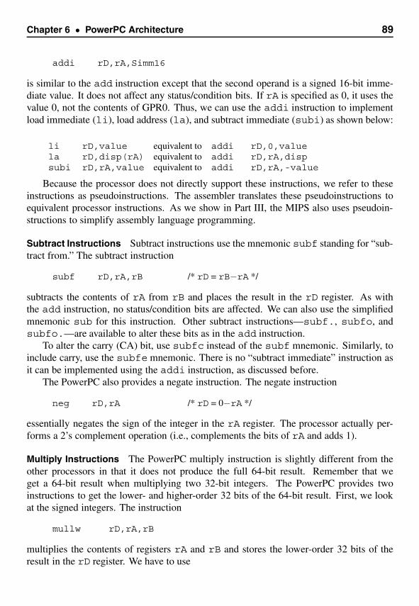
Chapter 6 • PowerPC Architecture 89
addi rD,rA,Simm16
is similar to the add instruction except that the second operand is a signed 16-bit imme-diate value. It does not affect any status/condition bits. If rA is specified as 0, it uses thevalue 0, not the contents of GPR0. Thus, we can use the addi instruction to implementload immediate (li), load address (la), and subtract immediate (subi) as shown below:
li rD,value equivalent to addi rD,0,valuela rD,disp(rA) equivalent to addi rD,rA,dispsubi rD,rA,value equivalent to addi rD,rA,-value
Because the processor does not directly support these instructions, we refer to theseinstructions as pseudoinstructions. The assembler translates these pseudoinstructions toequivalent processor instructions. As we show in Part III, the MIPS also uses pseudoin-structions to simplify assembly language programming.
Subtract Instructions Subtract instructions use the mnemonic subf standing for “sub-tract from.” The subtract instruction
subf rD,rA,rB /* rD = rB−rA */
subtracts the contents of rA from rB and places the result in the rD register. As withthe add instruction, no status/condition bits are affected. We can also use the simplifiedmnemonic sub for this instruction. Other subtract instructions—subf., subfo, andsubfo.—are available to alter these bits as in the add instruction.
To alter the carry (CA) bit, use subfc instead of the subf mnemonic. Similarly, toinclude carry, use the subfe mnemonic. There is no “subtract immediate” instruction asit can be implemented using the addi instruction, as discussed before.
The PowerPC also provides a negate instruction. The negate instruction
neg rD,rA /* rD = 0−rA */
essentially negates the sign of the integer in the rA register. The processor actually per-forms a 2’s complement operation (i.e., complements the bits of rA and adds 1).
Multiply Instructions The PowerPC multiply instruction is slightly different from theother processors in that it does not produce the full 64-bit result. Remember that weget a 64-bit result when multiplying two 32-bit integers. The PowerPC provides twoinstructions to get the lower- and higher-order 32 bits of the 64-bit result. First, we lookat the signed integers. The instruction
mullw rD,rA,rB
multiplies the contents of registers rA and rB and stores the lower-order 32 bits of theresult in the rD register. We have to use
90 Guide to RISC Processors
mulhw rD,rA,rB
to get the higher-order 32 bits of the result.For unsigned numbers, we have to use mulhwu instead of mulhw to get the higher-
order 32 bits of the result. The lower-order 32 bits are given by mullw for both signedand unsigned integers.
There is also a multiply immediate instruction that takes an immediate value. Theformat is
mulli rD,rA,Simm16
The immediate value Simm16 is a 16-bit signed integer. Note that this operation producesa 48-bit result. But the mulli instruction stores only the lower 32 bits of the result.
Divide Instructions Like the multiply operation, two divide instructions—one for signedintegers and the other for unsigned integers—are provided. The instruction
divw rD,rA,rB /* rD = rA/rB */
stores the quotient of rA/rB in rD. The operands are treated as signed integers. The re-mainder is not available. To get both quotient and remainder, we have to use the followingthree-instruction sequence.
divw rD,rA,rB /* quotient in rD */mullw rX,rD,rBsubf rC,rX,rA /* remainder in rC */
For unsigned integers, use the divwu (divide word unsigned) instruction instead.
Logical InstructionsThe PowerPC instruction set has several logical instructions including and, or, nor,nand, equ, and xor instructions. It does not have the not instruction; however, thenot operation can be implemented using the nor instruction. These instructions have asimilar format, therefore we discuss the complete set of and instructions available in thePowerPC instruction set.
and rA,rS,rB and. rA,rS,rBandi. rA,rS,Uimm16 andis. rA,rS,Uimm16andc rA,rS,rB andc. rA,rS,rB
The and instruction performs bitwise AND of rS and rB and places the result in the rAregister. The condition register field CR0 is not affected. The and. instruction is similarto and but updates the LT, GT, and EQ bits of the CR0 field. This is true with all theinstructions ending in a period. The andi takes a 16-bit unsigned integer as one of thesource operands. The andis. instruction is similar to andi. except that the immediate
Chapter 6 • PowerPC Architecture 91
value is left-shifted by 16 bit positions before ANDing. Note that the shifted-out bits onthe right receive zeros. In the andc instruction, the contents of rB are complementedbefore performing the and operation.
The logical or instruction also has six versions as does the and instruction. The onlydifference is that the immediate versions do not update the CR0 field. That is, the imme-diate or instructions are ori and oris with no period. We can use the or instruction tomove register contents as shown below:
mr rA,rS is equivalent to or rA,rS,rS
A no-operation (nop) is implemented as
ori 0,0,0
The NAND instructions (nand and nand.) perform a NOT operation followed by anAND operation. Similarly, NOR instructions (nor and nor.) perform a NOT operationafter an OR operation.
The PowerPC instruction set also includes four xor instructions as shown below:
xor rA,rS,rB xor. rA,rS,rBxori rA,rS,Uimm16 xoris rA,rS,Uimm16
The semantics of these four instructions are similar to the and instructions, except for theactual operation performed.
In addition, the PowerPC provides the eqv (equivalence) logical function. The equiv-alence function is defined as the exclusive-NOR operation (i.e., the output of XOR iscomplemented). Two instructions—eqv and eqv.— are available.
Shift InstructionsThe PowerPC provides four types of shift instructions to shift left or right. Each type ofinstruction is available in two forms: one that does not affect the status bits in CR0 and theother that updates these status bits (i.e., the “dot” version). We first discuss the left-shiftinstruction. The sld (shift left doubleword) instruction
sld rA,rS,rB
left-shifts the contents of rS by the shift count value specified in rB, and the result isplaced in rA. Shifted-out bits on the right receive zeros. For the shift count, only the leastsignificant seven bits are taken from the rB register. If the shift count is between 64 and127, the result is zero. We can use sld. to update the status bits in CR0.
There are two shift right instructions—srd and srd.—that are similar to the twoleft-shift instructions except for the direction of shift. Zeros replace the vacated bits onthe left. These two right-shift instructions perform logical shift operations. In logicalshifts, vacated bits receive zeros. On the other hand, in an arithmetic right-shift operation,vacated bits receive the sign bit. For details on the differences and the need for logical
92 Guide to RISC Processors
and arithmetic shift operations and why we need them only for the right-shifts, see ourdiscussion in Chapter 15.
These shift instructions are also available for word operands. For example, the in-struction
slw rA,rS,rB
left-shifts the lower-order 32 bits of rS by the shift count value specified in rB, and theresult is placed in the lower-order 32 bits of rA. The upper 32 bits are cleared to zero.The shift count is taken from the lower-order six bits of rB. A shift count value between32 and 63 gives a zero result. The dot version of this instruction (slw.) is also available.The instructions are srw and srw. can used to right-shift word operands.
The PowerPC provides two types of arithmetic right-shift operations: one type as-sumes that the shift count is in a register as in the previous shift instructions, and theother type can accept the shift count as an immediate value. The register versions use thefollowing format.
srad rA,rS,rBsard. rA,rS,rB
The instructions sraw and sraw. work on word operands. All these shift instructionsare encoded using the X-form instruction format shown on page 85.
Let us next look at the immediate versions of the arithmetic shift instructions. Theinstructions
sradi rA,rS,countsardi. rA,rS,count
use the 6-bit immediate value count as the shift count. The instructions srawi andsrawi. work on word operands and take a 5-bit immediate value as the shift count. Onedifference between the arithmetic shift instructions and the other shift instructions is thatthe shift arithmetic instructions affect the CA bit in the XER register.
Rotate InstructionsThe PowerPC provides several rotate-left instructions. We describe only one of them tosee an interesting feature of these instructions. The rlwnm (rotate-left word then ANDwith mask) instruction takes five operands as shown below:
rlwnm rA,rS,rB,MB,ME
The contents of rS are rotated left by the count value specified in the lower-order five bitsof rB. A mask value that contains 1s from the MB+32 bit to the ME+32 bit and 0s in allthe other bit positions is generated. The rotated value is ANDed with the mask value andthe result is placed in rA. This instruction is useful to extract and rotate bit fields. It isstraightforward to implement a simple rotate-left instruction as shown below:
rotlw rA,rS,rB is equivalent to rlwnm rA,rS,rB,0,31
Chapter 6 • PowerPC Architecture 93
Comparison InstructionsWe describe two compare instructions: one for comparing signed numbers and the otherfor unsigned numbers. Each of these instructions is available in two formats: registerversion and immediate version. We first look at the signed compare instructions. Thisinstruction compares two numbers and updates the specified CRx field of the CR register.The format is
cmp crfD,L,rA,rB
The L field controls the operand size: 32 bits (L = 0) or 64 bits (L = 1). If the contents ofrA are less than the contents of rB, the LT bit in the crfD is set; if greater, the GT bit isset; otherwise, the EQ bit is set. It also updates the SO field by copying it from the XERregister. The CR0 field is used if no CR field is specified as shown below:
cmpw rA,rB is equivalent to cmp 0,0,rA,rBcmpd cr3,rA,rB is equivalent to cmp 3,1,rA,rB
These instructions use the X-form format shown on page 85. The immediate version ofthis statement
cmpi crfD,L,rA,Simm16
takes an immediate 16-bit signed integer in place of rB. These instructions are encodedusing the D-form instruction format.
To treat the operands as unsigned integers, we can use cmpl (compare logical) andcmpli (compare logical immediate) instructions.
Branch InstructionsThe PowerPC implements branch and procedure invocation operations using more flexiblebranch instructions. As we see in Part III, MIPS also uses a similar mechanism to invokeprocedures. Some of the branch instruction encodings are shown in Figure 6.3 on page 85.
As in the other instructions, the most significant 6 bits are used for op-code. Theremaining 26 bits are used for specifying the target. All instructions take four bytes andare aligned, thus the least significant 2 bits are always zero. These 2 bits are used to makethe branch instruction more flexible. The AA bit is used to indicate whether the addressis the absolute address (AA = 1) or PC-relative address (AA = 0). In the absolute addressmode, the 26-bit value is treated as the branch target address. In the PC-relative mode,this value is used as an offset relative to the contents of the program counter (PC). Thus,the PC-relative mode works as do the Pentium’s jump instructions.
The second bit LK is used to convert the branch instruction into a procedure callinstruction. When the LK bit is set, the return address (i.e., the address of the instructionfollowing the branch) is placed in the Link Register (LR). In this case, LR is loaded witha value equal to the branch instruction address + 4 as each instruction takes four bytes.
There are four unconditional branch variations, depending on the values specified forthe AA and LK bits:
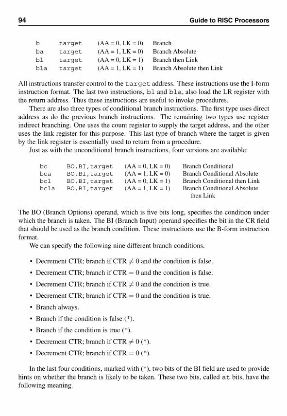
94 Guide to RISC Processors
b target (AA = 0, LK = 0) Branchba target (AA = 1, LK = 0) Branch Absolutebl target (AA = 0, LK = 1) Branch then Linkbla target (AA = 1, LK = 1) Branch Absolute then Link
All instructions transfer control to the target address. These instructions use the I-forminstruction format. The last two instructions, bl and bla, also load the LR register withthe return address. Thus these instructions are useful to invoke procedures.
There are also three types of conditional branch instructions. The first type uses directaddress as do the previous branch instructions. The remaining two types use registerindirect branching. One uses the count register to supply the target address, and the otheruses the link register for this purpose. This last type of branch where the target is givenby the link register is essentially used to return from a procedure.
Just as with the unconditional branch instructions, four versions are available:
bc BO,BI,target (AA = 0, LK = 0) Branch Conditionalbca BO,BI,target (AA = 1, LK = 0) Branch Conditional Absolutebcl BO,BI,target (AA = 0, LK = 1) Branch Conditional then Linkbcla BO,BI,target (AA = 1, LK = 1) Branch Conditional Absolute
then Link
The BO (Branch Options) operand, which is five bits long, specifies the condition underwhich the branch is taken. The BI (Branch Input) operand specifies the bit in the CR fieldthat should be used as the branch condition. These instructions use the B-form instructionformat.
We can specify the following nine different branch conditions.
• Decrement CTR; branch if CTR �= 0 and the condition is false.
• Decrement CTR; branch if CTR = 0 and the condition is false.
• Decrement CTR; branch if CTR �= 0 and the condition is true.
• Decrement CTR; branch if CTR = 0 and the condition is true.
• Branch always.
• Branch if the condition is false (*).
• Branch if the condition is true (*).
• Decrement CTR; branch if CTR �= 0 (*).
• Decrement CTR; branch if CTR = 0 (*).
In the last four conditions, marked with (*), two bits of the BI field are used to providehints on whether the branch is likely to be taken. These two bits, called at bits, have thefollowing meaning.
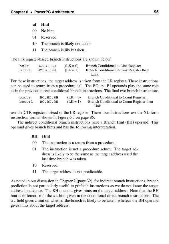
Chapter 6 • PowerPC Architecture 95
at Hint
00 No hint.
01 Reserved.
10 The branch is likely not taken.
11 The branch is likely taken.
The link register-based branch instructions are shown below:
bclr BO,BI,BH (LK = 0) Branch Conditional to Link Registerbclrl BO,BI,BH (LK = 1) Branch Conditional to Link Register then
Link
For these instructions, the target address is taken from the LR register. These instructionscan be used to return from a procedure call. The BO and BI operands play the same roleas in the previous direct conditional branch instructions. The final two branch instructions
bcctr BO,BI,BH (LK = 0) Branch Conditional to Count Registerbcctrl BO,BI,BH (LK = 1) Branch Conditional to Count Register then
Link
use the CTR register instead of the LR register. These four instructions use the XL-forminstruction format shown in Figure 6.3 on page 85.
The indirect conditional branch instructions have a Branch Hint (BH) operand. Thisoperand gives branch hints and has the following interpretation.
BH Hint
00 The instruction is a return from a procedure.
01 The instruction is not a procedure return. The target ad-dress is likely to be the same as the target address used thelast time branch was taken.
10 Reserved.
11 The target address is not predictable.
As noted in our discussion in Chapter 2 (page 32), for indirect branch instructions, branchprediction is not particularly useful to prefetch instructions as we do not know the targetaddress in advance. The BH operand gives hints on the target address. Note that the BHhint is different from the at hint given in the conditional direct branch instructions. Theat field gives a hint on whether the branch is likely to be taken, whereas the BH operandgives hints about the target address.

96 Guide to RISC Processors
Summary
We have presented details on the PowerPC architecture. The PowerPC architecture con-sists of three main functional units: branch processor, fixed-point processor, and floating-point processor. This partitioning facilitates superscalar implementation in which multiplefunctional units can concurrently work on independent instructions.
PowerPC provides two basic addressing modes for the load and store instructions.These modes are similar to the addressing modes in the SPARC. Unlike MIPS, PowerPChas several instruction formats. We have presented only a few instruction formats here.Although most instructions are similar to the SPARC instructions discussed in the lastchapter, there are some instructions that are not simple. In addition, the division operationis supported only partially—it produces only the quotient.
You can see from this description that the PowerPC does not closely adhere to all theprinciples of the RISC philosophy. Although it uses simple addressing modes and fixed-size instructions, some of its instructions are not simple. For example, the lswx andstlwx instructions mentioned earlier are not simple by any stretch of the imagination.This observation also holds for the Itanium that we discuss in the next chapter.
Web ResourcesPowerPC documentation is available from the IBM Web site. The PowerPC ArchitectureBook, which consists of three volumes, describes the PowerPC architecture in detail [23,24, 25]. These three volumes are available from www.ibm.com/developerworks/eserver/articles/archguide.html.

7Itanium Architecture
This chapter describes the Itanium architecture, which is the Intel 64-bit architecture.Unlike their 32-bit architecture, this is a RISC architecture. In addition to the standardRISC features, the Itanium incorporates several advanced architectural features such asinstruction-level parallelism, register stacks, speculative execution, and predication to im-prove instruction reordering. These features are discussed in detail. We conclude thechapter with a summary.
IntroductionIntel has moved from the CISC architecture used in their 32-bit processors to a RISC ori-entation for their 64-bit processors. The Itanium architecture defines their 64-bit processorarchitecture. Implementations of this architecture include the Itanium and Itanium 2 pro-cessors. As do the other processors discussed before, the Itanium architecture also usesthe load/store architecture. Furthermore, the RISC features discussed in Chapter 3 arealso present. In addition, it incorporates several advanced architectural features to im-prove performance. We discuss these features in detail in this chapter. More specifically,we discuss instruction-level parallelism, register stacks, speculative execution, and predi-cation to improve instruction reordering.
The Itanium’s ISA is based on the EPIC (Explicit Parallel Instruction Computing)design philosophy. Of course, it also maintains backward compatibility to the IA-32 ISA.EPIC design features include the following.
• Explicit Parallelism: The ISA provides necessary support for the compiler to con-vey information on the instructions that can be executed in parallel. In traditionalarchitectures, hardware extracts this Instruction-Level Parallelism (ILP) within afairly small window of instructions (or reorder buffer). In contrast, the Itanium al-lows the compiler to do the job. Because ILP extraction is done in software, a moredetailed analysis can be done on a much larger window at compile time.
97
98 Guide to RISC Processors
It also provides hardware support to execute instructions in parallel by reading threeinstructions as a bundle. The compiler packs only instructions that have no depen-dencies into a bundle. Thus, the processor does not have to spend time in analyzingthe instruction stream to extract ILP. We present details on this and other featuresof the Itanium later in this chapter.
• Features to Enhance ILP: The Itanium allows the compiler to detect and extract ILP,therefore we can use more elaborate methods to improve ILP. Two such schemes arespeculative execution and predication. Speculative execution allows high-latencyload instructions to be advanced so that the latency can be masked. Branch handlingis improved by using predication. In some instances, branch instructions can becompletely eliminated. We present details on these two techniques later.
• Resources for Parallel Execution: It is imperative that to successfully exploit theILP detected by the compiler, the processor should provide ample resources to ex-ecute instructions in parallel. The Itanium provides a large number of registers andfunctional units. It has 128 integer registers and an equal number of floating-pointregisters. The large number of registers, for example, can be effectively used tomake procedure calls and returns very efficient. Most procedure calls/returns neednot access memory for parameter values and local and global variables.
To summarize, the Itanium architecture improves performance by
• Increasing instruction-level parallelism by providing large register sets and a three-instruction wide word;
• Hiding memory latency by speculative loads;• Improving branch handling by using predication; and• Providing hardware support for efficient procedure calls and returns.
The Itanium supports both integer and floating-point data types. Integer data typescan be 1, 2, 4, or 8 bytes wide. With a few exceptions, integer operations are done on64-bit data. Furthermore, registers are always written as 64 bits. Thus, 1-, 2-, and 4-byte operands loaded from memory are zero-extended to 64 bits. Floating-point datatypes include IEEE single, double, and double-extended formats. In the remainder of thischapter, we look at the various features of the Itanium architecture.
Registers
The Itanium has 128 general registers, which are labeled gr0 through gr127 as shown inFigure 7.1. Each register is 64 bits wide. In addition, a bit is associated with each registerto indicate whether the register is free or contains something valid. This bit is called NaT,which stands for Not-a-Thing. We explain later how this bit is used in speculative loading.
The general registers are divided into static and stacked registers. Static registersare comprised of the first 32 registers: gr0 through gr31. Of these, gr0 is essentially a
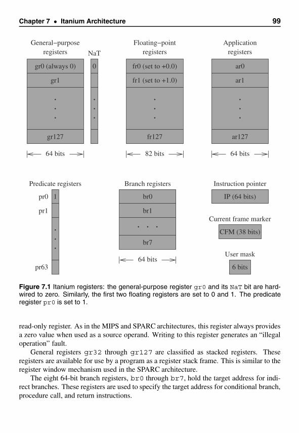
Chapter 7 • Itanium Architecture 99
.
.
.
64 bits
.
.
.
General−purposeregisters
64 bits
.
.
.
.
.
.
64 bits
......
ar0
ar1
ar127
Applicationregisters
Predicate registers
gr0 (always 0)
gr1
gr127
0
NaT
fr0 (set to +0.0)
fr1 (set to +1.0)
fr127
Floating−pointregisters
82 bits
br0
br1
br7
Branch registers
CFM (38 bits)
Current frame marker
User mask
pr63
pr1
pr0 1
6 bits
IP (64 bits)
Instruction pointer
Figure 7.1 Itanium registers: the general-purpose register gr0 and its NaT bit are hard-wired to zero. Similarly, the first two floating registers are set to 0 and 1. The predicateregister pr0 is set to 1.
read-only register. As in the MIPS and SPARC architectures, this register always providesa zero value when used as a source operand. Writing to this register generates an “illegaloperation” fault.
General registers gr32 through gr127 are classified as stacked registers. Theseregisters are available for use by a program as a register stack frame. This is similar to theregister window mechanism used in the SPARC architecture.
The eight 64-bit branch registers, br0 through br7, hold the target address for indi-rect branches. These registers are used to specify the target address for conditional branch,procedure call, and return instructions.
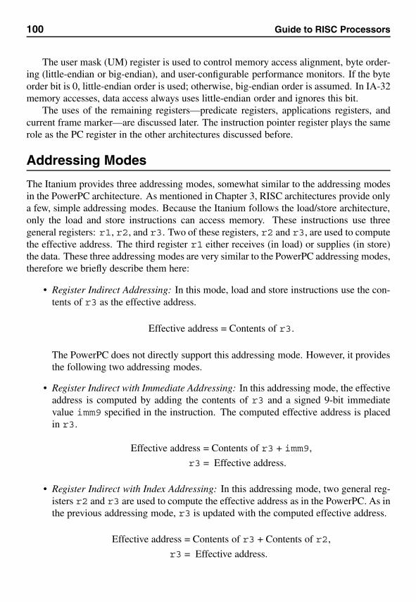
100 Guide to RISC Processors
The user mask (UM) register is used to control memory access alignment, byte order-ing (little-endian or big-endian), and user-configurable performance monitors. If the byteorder bit is 0, little-endian order is used; otherwise, big-endian order is assumed. In IA-32memory accesses, data access always uses little-endian order and ignores this bit.
The uses of the remaining registers—predicate registers, applications registers, andcurrent frame marker—are discussed later. The instruction pointer register plays the samerole as the PC register in the other architectures discussed before.
Addressing Modes
The Itanium provides three addressing modes, somewhat similar to the addressing modesin the PowerPC architecture. As mentioned in Chapter 3, RISC architectures provide onlya few, simple addressing modes. Because the Itanium follows the load/store architecture,only the load and store instructions can access memory. These instructions use threegeneral registers: r1, r2, and r3. Two of these registers, r2 and r3, are used to computethe effective address. The third register r1 either receives (in load) or supplies (in store)the data. These three addressing modes are very similar to the PowerPC addressing modes,therefore we briefly describe them here:
• Register Indirect Addressing: In this mode, load and store instructions use the con-tents of r3 as the effective address.
Effective address = Contents of r3.
The PowerPC does not directly support this addressing mode. However, it providesthe following two addressing modes.
• Register Indirect with Immediate Addressing: In this addressing mode, the effectiveaddress is computed by adding the contents of r3 and a signed 9-bit immediatevalue imm9 specified in the instruction. The computed effective address is placedin r3.
Effective address = Contents of r3 + imm9,
r3 = Effective address.
• Register Indirect with Index Addressing: In this addressing mode, two general reg-isters r2 and r3 are used to compute the effective address as in the PowerPC. As inthe previous addressing mode, r3 is updated with the computed effective address.
Effective address = Contents of r3 + Contents of r2,
r3 = Effective address.
Chapter 7 • Itanium Architecture 101
The last two addressing modes are similar to the update addressing modes supported bythe PowerPC. As discussed in Chapter 6, the update feature of the last two addressingmodes gives more flexibility. For example, we can use the second addressing mode toaccess successive elements of an array by making imm9 equal to the element size.
Procedure CallsThe Itanium provides hardware support for efficient procedure invocation and return. AnItanium procedure call typically does not involve the stack. Instead, it uses a register stackfor passing parameters, local variables, and the like. For this purpose, the 128 generalregister set is divided into two subsets.
• Static Registers: The first 32 registers, gr0 though gr31, are called static regis-ters. These registers are used to store the global variables and are accessible to allprocedures.
• Stacked Registers: The upper 96 registers, gr32 through gr127, are called stackregisters. These registers, instead of the stack, are used for passing parameters,returning results, and storing local variables.
A register stack frame is the set of stacked registers visible to a given procedure. Thisstack frame is partitioned into local area and output area. The size of each area can bespecified by each procedure by using the alloc instruction. The local area consists ofinput area and space for local variables of the procedure. The input area is used to receiveparameters from the caller and the output area is used to pass parameters to the callee.When a procedure is called, the alloc instruction can be used to allocate the requirednumber of registers for the local and output areas. As mentioned, the local area includesthe storage to receive arguments in addition to local variable storage.
The Itanium aligns the caller’s output area with the callee’s local area so that passingof parameters does not involve actual copying of register values (for a similar discussionon SPARC, see Figure 5.2 on page 58). Furthermore, the Itanium uses register renaming.That is, independent of the actual set of registers allocated to a procedure, the allocatedregister set is renamed such that the first register is always labeled as gr32.
The Current Frame Marker (CFM) register maintains information on the current stackframe. It keeps two values: Size of Frame (SOF) and Size of Locals (SOL). As thenames indicate, SOF gives the total stack frame size, and SOL specifies the local areasize. The difference (SOF − SOL) is the output area size. The alloc statement takesthree immediate values that specify the size of inputs, locals, and outputs. The SOF valueis determined by adding these three values; SOL is given by the sum of the first two values(i.e., size of inputs and locals).
Another interesting feature is that a procedure’s stack frame can be up to 90 registers.What happens if some of the registers are allocated to other procedures? Itanium usesa hardware mechanism called a Register Stack Engine (RSE) to transparently manageregisters. When allocation exceeds the available registers on the stack, it moves data
102 Guide to RISC Processors
from the registers to memory. The stored registers are restored when returning from theprocedure. This mechanism is transparent, but the cost is not. If we use RSE to move databetween registers and memory, the overhead is similar to what we see in processors suchas the Pentium that use the stack for activation records.
Instruction FormatA typical Itanium instruction uses a three-operand format. The general syntax is
[(qp)] mnemonic[.comp] dests = srcs
The syntax is quite different from what we have seen before for other architectures. Theoptional qualifying predicate (qp) specifies a predicate register that indicates whetherthe instruction should be executed. Recall that the Itanium has 64 1-bit predicate registers(see Figure 7.1). An instruction is executed only if the specified predicate register has atrue (1) value; otherwise, the instruction is treated as a nop (No OPeration). If a predicateregister is not specified in an instruction, predicate register p0 is used, which is alwaystrue. Note that some instructions cannot be predicated.
The mnemonic field identifies an instruction and is similar to the mnemonic field inother architectures. However, for some instructions, mnemonic identifies only a genericinstruction such as comparison. Such instructions require more information to completelyspecify the operation. For example, in comparison instructions, we have to specify thetype of comparison: equality, greater than, and so on. One or more completers compcan be used for this purpose. Completers indicate optional variations on the basic oper-ation. dests is typically a register to receive the result. Most instructions require twosource operands and srcs specifies these input operands. Some examples of Itaniuminstructions are given below:
Simple instruction add r1 = r2,r3Predicated instruction (p4)add r1 = r2,r3Instruction with an immediate value add r1 = r2,r3,1Instructions with completers cmp.eq p3 = r2,r4
cmp.gt p2,p3 = r3,r4br.cloop.sptk loop_back
Each instruction is encoded using 41 bits as shown in Figure 7.2. This figure showssome sample Itanium instruction formats. In every instruction, the least significant 6bits are used to specify one of the 64 predicate registers. The leftmost 4 bits specify amajor opcode that identifies a major operation group such as comparison, floating-pointoperation, and so on. Opcode extension fields are used to specify subcases of the majoroperations. In the register format, source and destination register specification take atotal of 21 bits. Each register specification needs 7 bits as Itanium has 128 registers (seeFigure 7.2a).
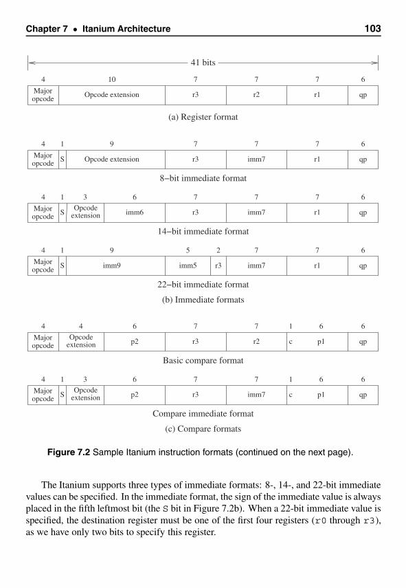
Chapter 7 • Itanium Architecture 103
Majoropcode
Majoropcode
Majoropcode
Opcodeextension
Majoropcode
Majoropcode
Opcodeextension
Majoropcode
Opcodeextension
(b) Immediate formats
(c) Compare formats
Compare immediate format
64 77710
Opcode extension r3 r2 r1 qp
64 7779
Opcode extension r3 imm7 r1 qpS
1
64 777
r3 imm7 r1 qp
1
imm6
63
S
64 779
imm9 imm7 r1 qpS
1
22−bit immediate format
r3imm5
25
64 77
r3 r2 qp
Basic compare format
p2
6
c
1
p1
64
64 77
r3 imm7 qpS
1
p2
63
c
1
p1
6
(a) Register format
41 bits
8−bit immediate format
14−bit immediate format
Figure 7.2 Sample Itanium instruction formats (continued on the next page).
The Itanium supports three types of immediate formats: 8-, 14-, and 22-bit immediatevalues can be specified. In the immediate format, the sign of the immediate value is alwaysplaced in the fifth leftmost bit (the S bit in Figure 7.2b). When a 22-bit immediate value isspecified, the destination register must be one of the first four registers (r0 through r3),as we have only two bits to specify this register.
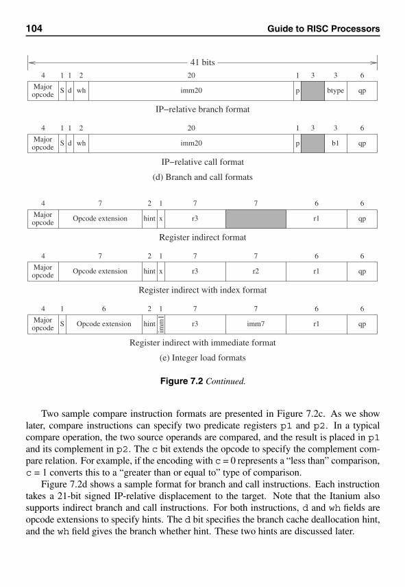
104 Guide to RISC Processors
Majoropcode
Majoropcode
Majoropcode
Majoropcode
Majoropcode
64
qpS
1
IP−relative call format
d wh
1 2
b1p
331
imm20
20
(d) Branch and call formats
(e) Integer load formats
64 77
r3 imm7 qp
Register indirect with immediate format
r1
61
hint
2
imm
1
S Opcode extension
61
64 77
r3 r2 qp
Register indirect with index format
r1
6
x
1
hint
27
Opcode extension
64 77
r3 qp
Register indirect format
r1
6
x
1
hint
27
Opcode extension
64
qpS
1
IP−relative branch format
d wh
1 2
btypep
331
imm20
20
41 bits
Figure 7.2 Continued.
Two sample compare instruction formats are presented in Figure 7.2c. As we showlater, compare instructions can specify two predicate registers p1 and p2. In a typicalcompare operation, the two source operands are compared, and the result is placed in p1and its complement in p2. The c bit extends the opcode to specify the complement com-pare relation. For example, if the encoding with c = 0 represents a “less than” comparison,c = 1 converts this to a “greater than or equal to” type of comparison.
Figure 7.2d shows a sample format for branch and call instructions. Each instructiontakes a 21-bit signed IP-relative displacement to the target. Note that the Itanium alsosupports indirect branch and call instructions. For both instructions, d and wh fields areopcode extensions to specify hints. The d bit specifies the branch cache deallocation hint,and the wh field gives the branch whether hint. These two hints are discussed later.
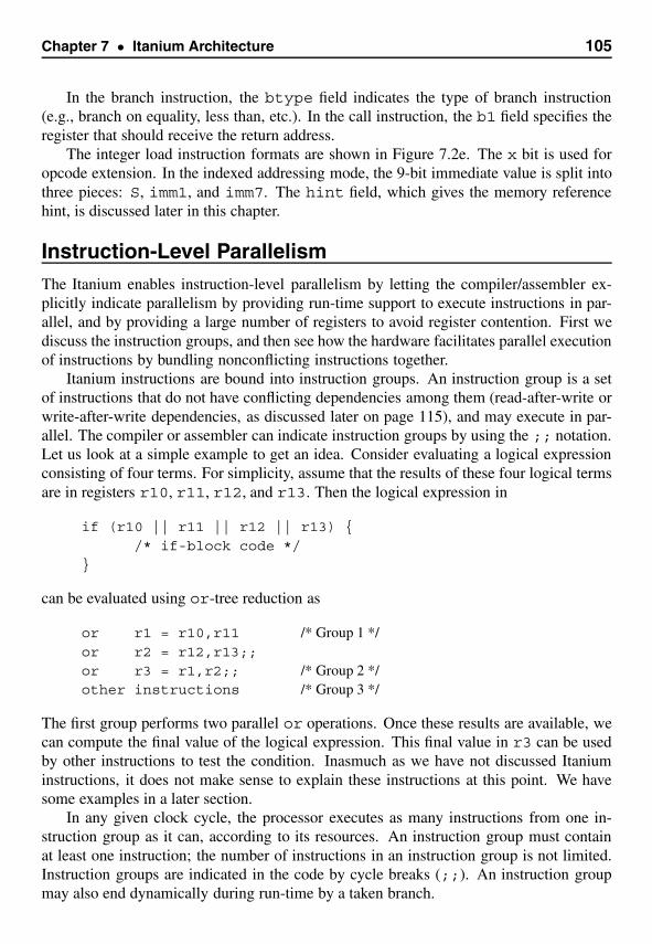
Chapter 7 • Itanium Architecture 105
In the branch instruction, the btype field indicates the type of branch instruction(e.g., branch on equality, less than, etc.). In the call instruction, the b1 field specifies theregister that should receive the return address.
The integer load instruction formats are shown in Figure 7.2e. The x bit is used foropcode extension. In the indexed addressing mode, the 9-bit immediate value is split intothree pieces: S, imm1, and imm7. The hint field, which gives the memory referencehint, is discussed later in this chapter.
Instruction-Level ParallelismThe Itanium enables instruction-level parallelism by letting the compiler/assembler ex-plicitly indicate parallelism by providing run-time support to execute instructions in par-allel, and by providing a large number of registers to avoid register contention. First wediscuss the instruction groups, and then see how the hardware facilitates parallel executionof instructions by bundling nonconflicting instructions together.
Itanium instructions are bound into instruction groups. An instruction group is a setof instructions that do not have conflicting dependencies among them (read-after-write orwrite-after-write dependencies, as discussed later on page 115), and may execute in par-allel. The compiler or assembler can indicate instruction groups by using the ;; notation.Let us look at a simple example to get an idea. Consider evaluating a logical expressionconsisting of four terms. For simplicity, assume that the results of these four logical termsare in registers r10, r11, r12, and r13. Then the logical expression in
if (r10 || r11 || r12 || r13) {/* if-block code */
}
can be evaluated using or-tree reduction as
or r1 = r10,r11 /* Group 1 */or r2 = r12,r13;;or r3 = r1,r2;; /* Group 2 */other instructions /* Group 3 */
The first group performs two parallel or operations. Once these results are available, wecan compute the final value of the logical expression. This final value in r3 can be usedby other instructions to test the condition. Inasmuch as we have not discussed Itaniuminstructions, it does not make sense to explain these instructions at this point. We havesome examples in a later section.
In any given clock cycle, the processor executes as many instructions from one in-struction group as it can, according to its resources. An instruction group must containat least one instruction; the number of instructions in an instruction group is not limited.Instruction groups are indicated in the code by cycle breaks (;;). An instruction groupmay also end dynamically during run-time by a taken branch.
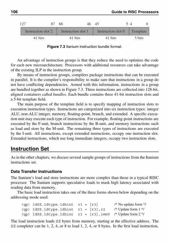
106 Guide to RISC Processors
04687127 86 45 45
Instruction slot 1 Template
41 bits 41 bits 41 bits 5 bits
Instruction slot 2 Instruction slot 0
Figure 7.3 Itanium instruction bundle format.
An advantage of instruction groups is that they reduce the need to optimize the codefor each new microarchitecture. Processors with additional resources can take advantageof the existing ILP in the instruction group.
By means of instruction groups, compilers package instructions that can be executedin parallel. It is the compiler’s responsibility to make sure that instructions in a group donot have conflicting dependencies. Armed with this information, instructions in a groupare bundled together as shown in Figure 7.3. Three instructions are collected into 128-bit,aligned containers called bundles. Each bundle contains three 41-bit instruction slots anda 5-bit template field.
The main purpose of the template field is to specify mapping of instruction slots toexecution instruction types. Instructions are categorized into six instruction types: integerALU, non-ALU integer, memory, floating-point, branch, and extended. A specific execu-tion unit may execute each type of instruction. For example, floating-point instructions areexecuted by the F-unit, branch instructions by the B-unit, and memory instructions suchas load and store by the M-unit. The remaining three types of instructions are executedby the I-unit. All instructions, except extended instructions, occupy one instruction slot.Extended instructions, which use long immediate integers, occupy two instruction slots.
Instruction SetAs in the other chapters, we discuss several sample groups of instructions from the Itaniuminstructions set.
Data Transfer InstructionsThe Itanium’s load and store instructions are more complex than those in a typical RISCprocessor. The Itanium supports speculative loads to mask high latency associated withreading data from memory.
The basic load instruction takes one of the three forms shown below depending on theaddressing mode used:
(qp) ldSZ.ldtype.ldhint r1 = [r3] /* No update form */(qp) ldSZ.ldtype.ldhint r1 = [r3],r2 /* Update form 1 */(qp) ldSZ.ldtype.ldhint r1 = [r3],imm9 /* Update form 2 */
The load instruction loads SZ bytes from memory, starting at the effective address. TheSZ completer can be 1, 2, 4, or 8 to load 1, 2, 4, or 8 bytes. In the first load instruction,
Chapter 7 • Itanium Architecture 107
register r3 provides the address. In the second instruction, contents of r3 and r2 areadded to get the effective address. The third form uses a 9-bit signed immediate value,instead of register r2. In the last two forms, as explained earlier, the computed effectiveaddress is stored in r3.
The ldtype completer can be used to specify special load operations. For normalloads, the completer is not specified. For example, the instruction
ld8 r5 = [r6]
loads eight bytes from the memory starting from the effective address in r6. As mentionedbefore, the Itanium supports speculative loads. Two example instructions are shown be-low:
ld8.a r5 = [r6] /* advanced load */ld8.s r5 = [r6] /* speculative load */
We defer a discussion of these load instruction types to a later section that discusses thespeculative execution model of Itanium.
The ldhint completer specifies the locality of the memory access. It can take oneof the following three values.
ldhint Interpretation
None Temporal locality, level 1nt1 No temporal locality, level 1nta No temporal locality, all levels
A prefetch hint is implied in the two “update” forms of load instructions. The addressin r3 after the update acts as a hint to prefetch the indicated cache line. In the “noupdate” form of load, r3 is not updated and no prefetch hint is implied. Level 1 refersto the cache level. Because we don’t cover temporal locality and cache memory in thisbook, we refer the reader to [6] for details on cache memory. It is sufficient to view theldhint completer as giving a hint to the processor as to whether a prefetch is beneficial.
The store instruction is simpler than the load instruction. There are two types of storeinstructions, corresponding to the two addressing modes, as shown below:
(qp) stSZ.sttype.sthint r1 = [r3] /* No update form */(qp) stSZ.sttype.sthint r1 = [r3],imm9 /* Update form */
The SZ completer can have four values as in the load instruction. The sttype can benone or rel. If the rel value is specified, an ordered store is performed. The sthintgives a prefetch hint as in the load instruction. However, it can be either none or nta.When no value is specified, temporal locality at level 1 is assumed. The nta has the sameinterpretation as in the load instruction.
108 Guide to RISC Processors
The Itanium also has several move instructions to copy data into registers. We describethree of these instructions:
(qp) mov r1 = r3(qp) mov r1 = imm22(qp) movl r1 = imm64
These instructions move the second operand into the r1 register. The first two mov in-structions are actually pseudoinstructions. That is, these instructions are implementedusing other processor instructions. The movl is the only instruction that requires twoinstruction slots within the same bundle.
Arithmetic InstructionsThe Itanium provides only the basic integer arithmetic operations: addition, subtraction,and multiplication. There is no divide instruction, either for integers or floating-pointnumbers. Division is implemented in software. Let’s start our discussion with the addinstructions.
Add Instructions The format of the add instructions is given below:
(qp) add r1 = r2,r3 /* register form */(qp) add r1 = r2,r3,1 /* plus 1 form */(qp) add r1 = imm,r3 /* immediate form */
In the plus 1 form, the constant 1 is added as well. In the immediate form, imm can be a14- or 22-bit signed value. If we use a 22-bit immediate value, r3 can be one of the firstfour general registers GR0 through GR3 (i.e., only 2 bits are used to specify the secondoperand register as shown in Figure 7.2).
The immediate form is a pseudoinstruction that selects one of the two processor im-mediate add instructions,
(qp) add r1 = imm14,r3(qp) add r1 = imm22,r3
depending on the size of the immediate operand size and value of r3.The move instruction
(qp) mov r1 = r3
is implemented as
(qp) add r1 = 0,r3
The move instruction
(qp) mov r1 = imm22
is implemented as
(qp) add r1 = imm22,r0
Remember that r0 is hardwired to value zero.
Chapter 7 • Itanium Architecture 109
Subtract Instructions The subtract instruction sub has the same format as the addinstruction. The contents of register r3 are subtracted from the contents of r2. In theminus 1 form, the constant 1 is also subtracted. In the immediate form, imm is restrictedto an 8-bit value.
The instruction shladd (shift left and add)
(qp) shladd r1 = r2,count,r3
is similar to the add instruction, except that the contents of r2 are left-shifted by countbit positions before adding. The count operand is a 2-bit value, which restricts the shiftto 1-, 2-, 3-, or 4-bit positions.
Multiply Instructions Integer multiply is done using the xmpy and xma instructions.These instructions do not use the general registers; instead, they use the floating-pointregisters.
The xmpy instruction has the following formats.
(qp) xmpy.l f1 = f3,f4(qp) xmpy.lu f1 = f3,f4(qp) xmpy.h f1 = f3,f4(qp) xmpy.hu f1 = f3,f4
The two source operands, floating-point registers f3 and f4, are treated either as signedor unsigned integers. The completer u in the second and fourth instructions specifies thatthe operands are unsigned integers. The other two instructions treat the two integers assigned. The l or h indicate whether the lower or higher 64 bits of the result should bestored in the f1 floating-point register.
The xmpy instruction multiplies the two integers in f3 and f4 and places the lower orupper 64-bit result in the f1 register. Note that we get a 128-bit result when we multiplytwo 64-bit integers.
The xma instruction has four formats as does the xmpy instruction, as shown below:
(qp) xma.l f1 = f3,f4,f2(qp) xma.lu f1 = f3,f4,f2(qp) xma.h f1 = f3,f4,f2(qp) xma.hu f1 = f3,f4,f2
This instruction multiplies the two 64-bit integers in f3 and f4 and adds the zero-extended64-bit value in f2 to the product.
Logical InstructionsLogical operations and, or, and xor are supported by three logical instructions. There isno not instruction. However, the Itanium has an and-complement (andcm) instructionthat complements one of the operands before performing the bitwise-and operation.
All instructions have the same format. We illustrate the format of these instructionsfor the and instruction:
110 Guide to RISC Processors
(qp) and r1 = r2,r3(qp) and r1 = imm8,r3
The other three operations use the mnemonics or, xor, and andcm. The and-comple-ment instruction complements the contents of r3 and ands it with the first operand (con-tents of r2 or immediate value imm8).
Shift InstructionsBoth left- and right-shift instructions are available. The shift instructions
(qp) shl r1 = r2,r3(qp) shl r1 = r2,count
left-shift the contents of r2 by the count value specified by the second operand. Thecount value can be specified in r3 or given as a 6-bit immediate value. If the countvalue in r3 is more than 63, the result is all zeros.
Right-shift instructions use a similar format. Because right-shift can be arithmeti-cal or logical depending on whether the number is signed or unsigned, two versions areavailable. The register versions of the right-shift instructions are shown below:
(qp) shr r1 = r2,r3 (signed right shift)(qp) shr.u r1 = r2,r3 (unsigned right shift)
In the second instruction, the completer u is used to indicate the unsigned shift operation.We can also use a 6-bit immediate value for shift count as in the shl instruction.
Comparison InstructionsThe compare instruction uses two completers as shown below:
(qp) cmp.crel.ctype p1,p2=r2,r3(qp) cmp.crel.ctype p1,p2=imm8,r3
The two source operands are compared and the result is written to the two specified desti-nation predicate registers. The type of comparison is specified by crel. We can specifyone of 10 relations for signed and unsigned numbers. The relations “equal” (eq) and “notequal” (neq) are valid for both signed and unsigned numbers. For signed numbers, thereare 4 relations to test for “<” (lt), “≤” (le), “>” (gt), and “≥” (ge). The correspond-ing relations for testing unsigned numbers are ltu, leu, gtu, and geu. The relation istested as “r2 rel r3”.
The ctype completer specifies how the two predicate registers are to be updated. Thenormal type (default) writes the comparison result in the p1 register and its complementin the p2 register. This would allow us to select one of the two branches (we show anexample on page 113). The ctype completer allows specification of other types such asand and or. If or is specified, both p1 and p2 are set to 1 only if the comparison resultis 1; otherwise, the two predicate registers are not altered. This is useful for implementingor-type simultaneous execution. Similarly, if and is specified, both registers are set to 0if the comparison result is 0 (useful for and-type simultaneous execution).
Chapter 7 • Itanium Architecture 111
Branch InstructionsAs in the other architectures, the Itanium uses branch instruction for traditional jumps aswell as procedure call and return. The generic branch is supplemented by a completerto specify the type of branch. The branch instruction supports both direct and indirectbranching. All direct branches are IP relative (i.e., PC relative). Some sample branchinstruction formats are shown below:
IP Relative Form:(qp) br.btype.bwh.ph.dh target25 (Basic form)(qp) br.btype.bwh.ph.dh b1=target25 (Call form)
br.btype.bwh.ph.dh target25 (Counted loop form)
Indirect Form:(qp) br.btype.bwh.ph.dh b2 (Basic form)(qp) br.btype.bwh.ph.dh b1=b2 (Call form)
As can be seen, branch uses up to four completers. The btype specifies the type ofbranch. The other three completers provide hints and are discussed later.
For the basic branch, btype can be either cond or none. In this case, the branch istaken if the qualifying predicate is 1; otherwise, the branch is not taken. The IP-relativetarget address is given as a label in the assembly language. The assembler translatesthis into a signed 21-bit value that gives the difference between the target bundle and thebundle containing the branch instruction. The target pointer is to a bundle of 128 bits,therefore the value (target25−IP) is shifted right by 4 bit positions to get a 21-bitvalue. Note that the format shown in Figure 7.2d uses a 21-bit displacement value.
To invoke a procedure, we use the second form and specify call for btype. Thisturns the branch instruction into a condition call instruction. The procedure is invokedonly if the qualifying predicate is true. As part of the call, it places the current framemarker and other relevant state information in the previous function state application reg-ister. The return link value is saved in the b1 branch register for use by the return instruc-tion.
There is also an unconditional (no qualifying predicate) counted loop version. Inthis branch instruction (the third one), btype is set to cloop. If the Loop Count (LC)application register ar65 is not zero, it is decremented and the branch is taken.
We can use ret as the branch type to return from a procedure. It should use theindirect form and specify the branch register in which the call has placed the returnpointer. In the indirect form, a branch register specifies the target address. The returnrestores the caller’s stack frame and privilege level.
The last instruction can be used for an indirect procedure call. In this branch instruc-tion, the b2 branch register specifies the target address and the return address is placed inthe b1 branch register.
Let us look at some examples of branch instructions. The instruction
112 Guide to RISC Processors
(p3) br skip or (p3) br.cond skip
transfers control to the instruction labeled skip, if the predicate register p3 is 1.The code sequence
mov lc = 100loop_back:
. . .br.cloop loop_back
executes the loop body 100 times. A procedure call may look like
(p0) br.call br2 = sum
whereas the return from procedure sum uses the indirect form
(p0) br.ret br2
Because we are using predicate register 0, which is hardwired to 1, both the call and returnbecome unconditional.
The bwh (branch whether hint) completer can be used to convey whether the branchis taken (see page 119). The ph (prefetch hint) completer gives a hint about sequentialprefetch. It can take either few or many. If the value is few or none, few lines areprefetched; many lines are prefetched when many is specified. The two levels—few andmany—are system defined. The final completer dh (deallocation hint) specifies whetherthe branch cache should be cleared. The value clr indicates deallocation of branch in-formation.
Handling Branches
Pipelining works best when we have a linear sequence of instructions. Branches causepipeline stalls, leading to performance problems. How do we minimize the adverse effectsof branches? There are three techniques to handle this problem.
• Branch Elimination: The best solution is to avoid the problem in the first place. Thisargument may seem strange as programs contain lots of branch instructions. Al-though we cannot eliminate all branches, we can eliminate certain types of branches.This elimination cannot be done without support at the instruction-set level. Welook at how the Itanium uses predication to eliminate some types of branches.
• Branch Speedup: If we cannot eliminate a branch, at least we can reduce the amountof delay associated with it. This technique involves reordering instructions so thatinstructions that are not dependent on the branch/condition can be executed whilethe branch instruction is processed. Speculative execution can be used to reducebranch delays. We describe the Itanium’s speculative execution strategies later.

Chapter 7 • Itanium Architecture 113
• Branch Prediction: If we can predict whether the branch will be taken, we can loadthe pipeline with the right sequence of instructions. Even if we predict correctly allthe time, it would only convert a conditional branch into an unconditional branch.We still have the problems associated with unconditional branches. We describedthree types of branch prediction strategies in Chapter 2 (see page 28).
Inasmuch as we covered branch prediction in Chapter 2, we discuss the first two tech-niques next.
Predication to Eliminate Branches In the Itanium, branch elimination is achieved bya technique known as predication. The trick is to make execution of each instructionconditional. Thus, unlike the instructions we have seen so far, an instruction is not auto-matically executed when the control is transferred to it. Instead, it will be executed onlyif a condition is true. This requires us to associate a predicate with each instruction. Ifthe associated predicate is true, the instruction is executed; otherwise, it is treated as anop instruction. The Itanium architecture supports full predication to minimize branches.Most of the Itanium’s instructions can be predicated.
To see how predication eliminates branches, let us look at the following example.
if (R1 == R2) cmp r1,r2R3 = R3 + R1; je then_part
else sub r3,r1R3 = R3 - R1; jmp end_if
then_part:add r3,r1
end_if:
The code on the left-hand side, expressed in C, is a simple if-then-else statement. The IA-32 assembly language equivalent is shown on the right. The cmp instruction compares thecontents of the r1 and r2 registers and sets the condition code bits (in the IA-32, theseare called the flag bits). If r1 = r2, the jump equal (je) instruction transfers controlto the then_part. Otherwise, the sub instruction is executed (i.e., the else_part).Then the unconditional jump (jmp) instruction transfers control to end_if. As you cansee from this code, it introduces two branches: unconditional (jmp) and conditional (je).
Using the Itanium’s predication, we can express the same as
cmp.eq p1,p2 = r1,r2(p1) add r3 = r3,r1(p2) sub r3 = r3,r1
The compare instruction sets two predicates after comparing the contents of r1 and r2 forequality. The result of this comparison is placed in p1 and its complement in p2. Thus,if the contents of r1 and r2 are equal, p1 is set to 1 (true) and p2 to 0 (false). Becausethe add instruction is predicated on p1, it is executed only if p1 is true. It should be
114 Guide to RISC Processors
clear that either the add or the sub instruction is executed, depending on the comparisonresult.
To illustrate the efficacy of predicated execution, we look at the following switchstatement in C.
switch (r6){
case 1:r2 = r3 + r4;break;
case 2:r2 = r3 - r4;break;
case 3:r2 = r3 + r5;break;
case 4:r2 = r3 - r5;break;
}
For simplicity, we are using the register names in the switch statement. Translating thisstatement would normally involve a series of compare and branch instructions. Predica-tion avoids this sequence as shown below:
cmp.eq p1,p0 = r6,1cmp.eq p2,p0 = r6,2cmp.eq p3,p0 = r6,3cmp.eq p4,p0 = r6,4 ;;
(p1) add r2 = r3,r4(p2) sub r2 = r3,r4(p3) add r2 = r3,r5(p4) sub r2 = r3,r5
In the first group of instructions, the four compare instructions set p1/p2/p3/p4 if thecorresponding comparison succeeds. If the processor has resources, all four instructionscan be executed concurrently. Because p0 is hardwired to 1, failure conditions are ignoredin the above code. Depending on the compare instruction that succeeds, only one of thefour arithmetic instructions in the second group is executed.
Speculative Execution
Speculative execution refers to the scenario where instructions are executed in the ex-pectation that they will be needed in actual program execution. The main motivation, ofcourse, is to improve performance. There are two main reasons to speculatively execute
Chapter 7 • Itanium Architecture 115
instructions: to keep the pipeline full and to mask memory access latency. We discusstwo types of speculative execution supported by the Itanium: one type handles data de-pendencies, and the other deals with control dependencies. Both techniques are compileroptimizations that allow the compiler to reorder instructions. For example, we can spec-ulatively move high-latency load instructions earlier so that the data are available whenthey are actually needed.
Data SpeculationData speculation allows the compiler to schedule instructions across some types of am-biguous data dependencies. When two instructions access common resources (either reg-isters or memory locations) in a conflicting mode, data dependency exists. A conflictingaccess is one in which one or both instructions alter the data. Depending on the type ofconflicting access, we can define the following dependencies.
• Read-After-Write (RAW): This dependency exists between two instructions if oneinstruction writes into a register or a memory location that is later read by the otherinstruction.
• Write-After-Read (WAR): This dependency exists between two instructions if oneinstruction reads from a register or a memory location that is later written by theother instruction.
• Write-After-Write (WAW): This dependency exists between two instructions if oneinstruction writes into a register or a memory location that is later written by theother instruction.
• Ambiguous: Ambiguous data dependency exists when pointers are used to accessmemory. Typically, in this case, dependencies between load and store instructionsor store and store instructions cannot be resolved statically at compile time becausewe don’t know the pointer values. Handling this type of data dependency requiresrun-time support.
There is no conflict in allowing read-after-read (RAR) access. The first three dependenciesare not ambiguous in the sense that the dependency type can be statically determined atcompile/assembly time. The compiler or programmer should insert stops (;;) so that thedependencies are properly maintained. The example
sub r6=r7,r8 ;;add r9=r10,r6
exhibits a RAW data dependency on r6. The stop after the sub instruction would allowthe add instruction to read the value written by the sub instruction.
If there is no data dependency, the compiler can reorder instructions to optimize thecode. Let us look at the following example:
sub r6=r7,r8 ;; // cycle 1
116 Guide to RISC Processors
sub r9=r10,r6 // cycle 2ld8 r4=[r5] ;;
add r11=r12,r4 // cycle 4
Because there is a two-cycle latency to the first-level data cache, the add instruction isscheduled two cycles after scheduling the ld8 instruction. A straightforward optimiza-tion involves moving the ld8 instruction to cycle 1 as there are no data dependencies toprevent this reordering. By advancing the load instruction, we can schedule the add incycle 3 as shown below:
ld8 r4=[r5] // cycle 1sub r6=r7,r8 ;;
sub r9=r10,r6 ;; // cycle 2
add r11=r12,r4 // cycle 3
However, when there is ambiguous data dependency, as in the following example, instruc-tion reordering may not be possible:
sub r6=r7,r8 ;; // cycle 1
st8 [r9]=r6 // cycle 2ld8 r4=[r5] ;;
add r11=r12,r4 ;; // cycle 4
st8 [r10]=r11 // cycle 5
In this code, ambiguous dependency exists between the first st8 and ld8 because r9and r5 could be pointing to overlapped memory locations. Remember that each of theseinstructions accesses eight contiguous memory locations. This ambiguous dependencywill not allow us to move the load instruction to cycle 1 as in the previous example.
The Itanium provides architectural support to move such load instructions. This isfacilitated by advance load (ld.a) and check load (ld.c). The basic idea is that weinitiate the load early and when it is time to actually execute the load, we will makea check to see if there is a dependency that invalidates our advance load data. If so,we reload; otherwise, we successfully advance the load instruction even when there isambiguous dependency. The previous example with advance and check loads is shownbelow:
1: ld8.a r4=[r5] // cycle 0 or earlier. . .
2: sub r6=r7,r8 ;; // cycle 1
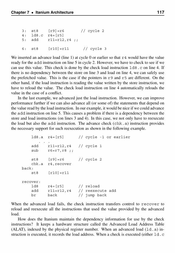
Chapter 7 • Itanium Architecture 117
3: st8 [r9]=r6 // cycle 24: ld8.c r4=[r5]5: add r11=r12,r4 ;;
6: st8 [r10]=r11 // cycle 3
We inserted an advance load (line 1) at cycle 0 or earlier so that r4 would have the valueready for the add instruction on line 5 in cycle 2. However, we have to check to see if wecan use this value. This check is done by the check load instruction ld8.c on line 4. Ifthere is no dependency between the store on line 3 and load on line 4, we can safely usethe prefetched value. This is the case if the pointers in r9 and r5 are different. On theother hand, if the load instruction is reading the value written by the store instruction, wehave to reload the value. The check load instruction on line 4 automatically reloads thevalue in the case of a conflict.
In the last example, we advanced just the load instruction. However, we can improveperformance further if we can also advance all (or some of) the statements that depend onthe value read by the load instruction. In our example, it would be nice if we could advancethe add instruction on line 5. This causes a problem if there is a dependency between thestore and load instructions (on lines 3 and 4). In this case, we not only have to reexecutethe load but also the add instruction. The advance check (chk.a) instruction providesthe necessary support for such reexecution as shown in the following example.
ld8.a r4=[r5] // cycle -1 or earlier. . .
add r11=r12,r4 // cycle 1sub r6=r7,r8 ;;
st8 [r9]=r6 // cycle 2chk.a r4,recover
back:st8 [r10]=r11
recover:ld8 r4=[r5] // reloadadd r11=r12,r4 // reexecute addbr back // jump back
When the advanced load fails, the check instruction transfers control to recover toreload and reexecute all the instructions that used the value provided by the advancedload.
How does the Itanium maintain the dependency information for use by the checkinstructions? It keeps a hardware structure called the Advanced Load Address Table(ALAT), indexed by the physical register number. When an advanced load (ld.a) in-struction is executed, it records the load address. When a check is executed (either ld.c
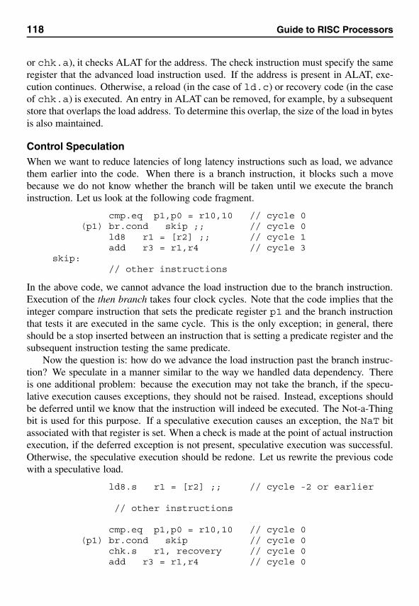
118 Guide to RISC Processors
or chk.a), it checks ALAT for the address. The check instruction must specify the sameregister that the advanced load instruction used. If the address is present in ALAT, exe-cution continues. Otherwise, a reload (in the case of ld.c) or recovery code (in the caseof chk.a) is executed. An entry in ALAT can be removed, for example, by a subsequentstore that overlaps the load address. To determine this overlap, the size of the load in bytesis also maintained.
Control SpeculationWhen we want to reduce latencies of long latency instructions such as load, we advancethem earlier into the code. When there is a branch instruction, it blocks such a movebecause we do not know whether the branch will be taken until we execute the branchinstruction. Let us look at the following code fragment.
cmp.eq p1,p0 = r10,10 // cycle 0(p1) br.cond skip ;; // cycle 0
ld8 r1 = [r2] ;; // cycle 1add r3 = r1,r4 // cycle 3
skip:// other instructions
In the above code, we cannot advance the load instruction due to the branch instruction.Execution of the then branch takes four clock cycles. Note that the code implies that theinteger compare instruction that sets the predicate register p1 and the branch instructionthat tests it are executed in the same cycle. This is the only exception; in general, thereshould be a stop inserted between an instruction that is setting a predicate register and thesubsequent instruction testing the same predicate.
Now the question is: how do we advance the load instruction past the branch instruc-tion? We speculate in a manner similar to the way we handled data dependency. Thereis one additional problem: because the execution may not take the branch, if the specu-lative execution causes exceptions, they should not be raised. Instead, exceptions shouldbe deferred until we know that the instruction will indeed be executed. The Not-a-Thingbit is used for this purpose. If a speculative execution causes an exception, the NaT bitassociated with that register is set. When a check is made at the point of actual instructionexecution, if the deferred exception is not present, speculative execution was successful.Otherwise, the speculative execution should be redone. Let us rewrite the previous codewith a speculative load.
ld8.s r1 = [r2] ;; // cycle -2 or earlier
// other instructions
cmp.eq p1,p0 = r10,10 // cycle 0(p1) br.cond skip // cycle 0
chk.s r1, recovery // cycle 0add r3 = r1,r4 // cycle 0
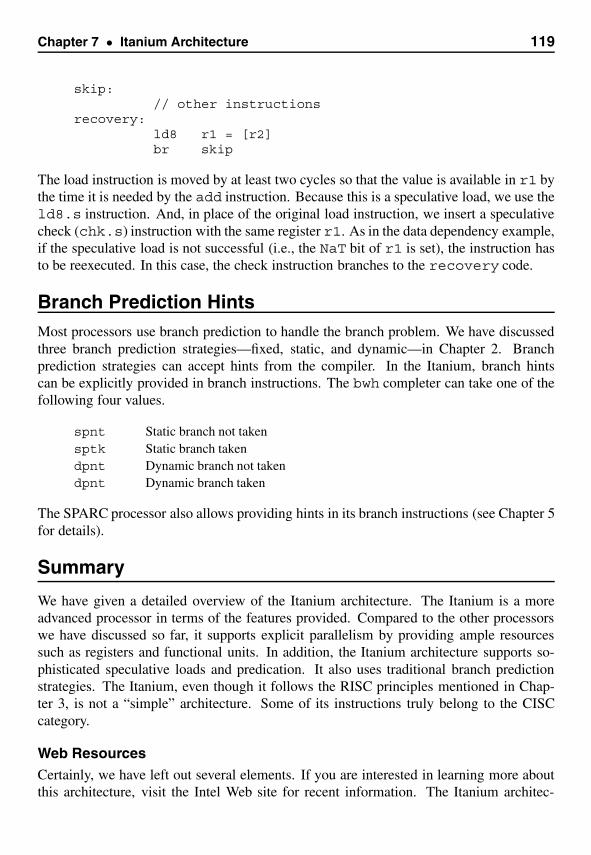
Chapter 7 • Itanium Architecture 119
skip:// other instructions
recovery:ld8 r1 = [r2]br skip
The load instruction is moved by at least two cycles so that the value is available in r1 bythe time it is needed by the add instruction. Because this is a speculative load, we use theld8.s instruction. And, in place of the original load instruction, we insert a speculativecheck (chk.s) instruction with the same register r1. As in the data dependency example,if the speculative load is not successful (i.e., the NaT bit of r1 is set), the instruction hasto be reexecuted. In this case, the check instruction branches to the recovery code.
Branch Prediction HintsMost processors use branch prediction to handle the branch problem. We have discussedthree branch prediction strategies—fixed, static, and dynamic—in Chapter 2. Branchprediction strategies can accept hints from the compiler. In the Itanium, branch hintscan be explicitly provided in branch instructions. The bwh completer can take one of thefollowing four values.
spnt Static branch not takensptk Static branch takendpnt Dynamic branch not takendpnt Dynamic branch taken
The SPARC processor also allows providing hints in its branch instructions (see Chapter 5for details).
Summary
We have given a detailed overview of the Itanium architecture. The Itanium is a moreadvanced processor in terms of the features provided. Compared to the other processorswe have discussed so far, it supports explicit parallelism by providing ample resourcessuch as registers and functional units. In addition, the Itanium architecture supports so-phisticated speculative loads and predication. It also uses traditional branch predictionstrategies. The Itanium, even though it follows the RISC principles mentioned in Chap-ter 3, is not a “simple” architecture. Some of its instructions truly belong to the CISCcategory.
Web ResourcesCertainly, we have left out several elements. If you are interested in learning more aboutthis architecture, visit the Intel Web site for recent information. The Itanium architec-

120 Guide to RISC Processors
ture details and manuals are available from www.intel.com/design/Itanium/manuals/. The architecture is described in three volumes [10, 11, 12].
8ARM Architecture
In this chapter, we take a detailed look at the ARM architecture. Unlike the other architec-tures we have seen so far, ARM provides only 16 general-purpose registers. Even thoughit follows the RISC principles, it provides a large number of addressing modes. Further-more, it has several complex instructions. The format of this chapter is similar to that weused in the last few chapters. We start with a brief background on the ARM architecture.We then present details on its registers and addressing modes. Following this, we givedetails on some sample ARM instructions. We conclude the chapter with a summary.
IntroductionThe ARM architecture was developed in 1985 by Acorn Computer Group in the UnitedKingdom. Acorn introduced the first RISC processor in 1987, targeting low-cost PCs. In1990, Acorn formed Advanced RISC Machines. ARM, which initially stood for AcornRISC Machine but later changed to Advanced RISC Machine, defines a 32-bit RISC ar-chitecture.
ARM’s instruction set architecture has evolved over time. The first two versions hadonly 26-bit address space. Version 3 extended it to 32 bits. This version also introducedseparate program status registers that we discuss in the next section. Version 4, ARMv4,is the oldest version supported today. Some implementations of this version include theARM7™ core family and Intel StrongARM™ processors.
ARM architecture has been extended to support cost-sensitive embedded applicationssuch as cell phones, modems, and pagers by introducing the Thumb instruction set. TheThumb instruction set is a subset of the most commonly used 32-bit ARM instructions.To reduce the memory requirements, the instructions are compressed into 16-bit wideencodings. To execute these 16-bit instructions, they are decompressed transparently tofull 32-bit ARM instructions in real-time. The ARMv4T architecture has added these16-bit Thumb instructions to produce compact code for handheld devices.
121

122 Guide to RISC Processors
SPSR_fiq
SPSR_irq
SPSR_svc
SPSR_abt
SPSR_und
Saved Program Status Registers
CPSR
Current Program Status Registers
R0
R1
R2
R3
R4
R5
R6
R7
R8
R9
R10
R11
R12
R13
R14
PC
R14_fiq
R13_fiq
R12_fiq
R11_fiq
R10_fiq
R9_fiq
R8_fiq
R14_irq
R13_irq R13_svc
R14_svc
General−Purpose Registers
R13_abt
R13_abt
R13_und
R13_und
Program Status Registers
Figure 8.1 ARM register set consists of 31 general-purpose register and six status regis-ters. All registers are 32 bits wide.
In 1999, the ARMv5TE architecture introduced several improvements to the Thumbarchitecture. In addition, several DSP instructions have been added to the ARM ISA. In2000, the ARMv5TEJ architecture added the Jazelle extension to support Java accelera-tion technology for small memory footprint designs. In 2001, the ARMv6 architecturewas introduced. This version provides support for multimedia instructions to execute inSingle Instruction Multiple Data (SIMD) mode.
Like the MIPS, the ARM is dominant in the 32-bit embedded RISC microprocessormarket. ARM is used in several portable and handheld devices including Dell’s AXIMX5, Palm Tungsten T, RIM’s Blackberry, HP iPaq, Nintendo’s Gameboy Advance, andso on [4]. The ARM Web site claims that, by 2002, they shipped over 1 billion of itsmicroprocessor cores [3].
In the remainder of this chapter we look at the ARM architecture in detail. Afterreading this chapter, you will notice that this architecture is somewhat different from theother processors we have seen so far. It shares some features with the Itanium architec-ture discussed in the last chapter. However, you should note that the ARM architecturedevelopment started in 1985.
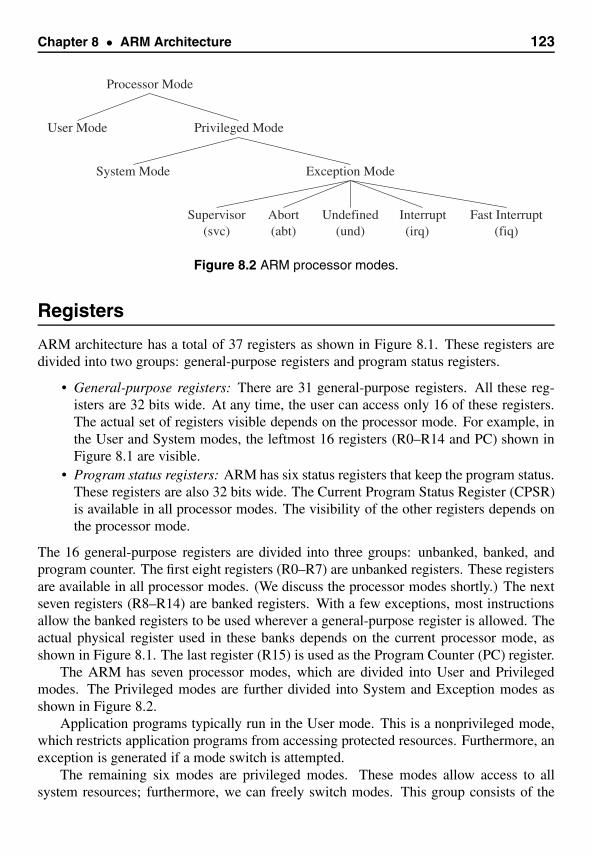
Chapter 8 • ARM Architecture 123
Supervisor Abort Undefined Interrupt Fast Interrupt
Exception ModeSystem Mode
Privileged ModeUser Mode
Processor Mode
(svc) (abt) (und) (irq) (fiq)
Figure 8.2 ARM processor modes.
Registers
ARM architecture has a total of 37 registers as shown in Figure 8.1. These registers aredivided into two groups: general-purpose registers and program status registers.
• General-purpose registers: There are 31 general-purpose registers. All these reg-isters are 32 bits wide. At any time, the user can access only 16 of these registers.The actual set of registers visible depends on the processor mode. For example, inthe User and System modes, the leftmost 16 registers (R0–R14 and PC) shown inFigure 8.1 are visible.
• Program status registers: ARM has six status registers that keep the program status.These registers are also 32 bits wide. The Current Program Status Register (CPSR)is available in all processor modes. The visibility of the other registers depends onthe processor mode.
The 16 general-purpose registers are divided into three groups: unbanked, banked, andprogram counter. The first eight registers (R0–R7) are unbanked registers. These registersare available in all processor modes. (We discuss the processor modes shortly.) The nextseven registers (R8–R14) are banked registers. With a few exceptions, most instructionsallow the banked registers to be used wherever a general-purpose register is allowed. Theactual physical register used in these banks depends on the current processor mode, asshown in Figure 8.1. The last register (R15) is used as the Program Counter (PC) register.
The ARM has seven processor modes, which are divided into User and Privilegedmodes. The Privileged modes are further divided into System and Exception modes asshown in Figure 8.2.
Application programs typically run in the User mode. This is a nonprivileged mode,which restricts application programs from accessing protected resources. Furthermore, anexception is generated if a mode switch is attempted.
The remaining six modes are privileged modes. These modes allow access to allsystem resources; furthermore, we can freely switch modes. This group consists of the
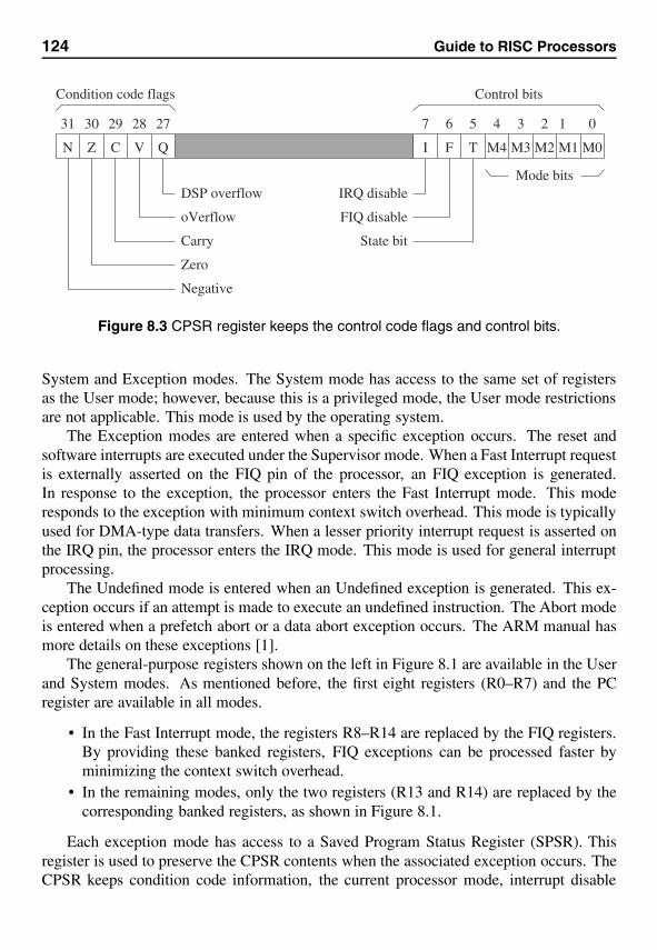
124 Guide to RISC Processors
M0M3M4 M1M2TFI
0134567 2
N Z C V Q
3031 29 28 27
Condition code flags Control bits
Mode bitsIRQ disable
FIQ disable
State bit
DSP overflow
oVerflow
Carry
Zero
Negative
Figure 8.3 CPSR register keeps the control code flags and control bits.
System and Exception modes. The System mode has access to the same set of registersas the User mode; however, because this is a privileged mode, the User mode restrictionsare not applicable. This mode is used by the operating system.
The Exception modes are entered when a specific exception occurs. The reset andsoftware interrupts are executed under the Supervisor mode. When a Fast Interrupt requestis externally asserted on the FIQ pin of the processor, an FIQ exception is generated.In response to the exception, the processor enters the Fast Interrupt mode. This moderesponds to the exception with minimum context switch overhead. This mode is typicallyused for DMA-type data transfers. When a lesser priority interrupt request is asserted onthe IRQ pin, the processor enters the IRQ mode. This mode is used for general interruptprocessing.
The Undefined mode is entered when an Undefined exception is generated. This ex-ception occurs if an attempt is made to execute an undefined instruction. The Abort modeis entered when a prefetch abort or a data abort exception occurs. The ARM manual hasmore details on these exceptions [1].
The general-purpose registers shown on the left in Figure 8.1 are available in the Userand System modes. As mentioned before, the first eight registers (R0–R7) and the PCregister are available in all modes.
• In the Fast Interrupt mode, the registers R8–R14 are replaced by the FIQ registers.By providing these banked registers, FIQ exceptions can be processed faster byminimizing the context switch overhead.
• In the remaining modes, only the two registers (R13 and R14) are replaced by thecorresponding banked registers, as shown in Figure 8.1.
Each exception mode has access to a Saved Program Status Register (SPSR). Thisregister is used to preserve the CPSR contents when the associated exception occurs. TheCPSR keeps condition code information, the current processor mode, interrupt disable
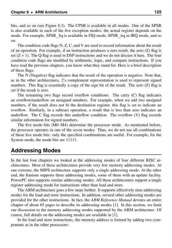
Chapter 8 • ARM Architecture 125
bits, and so on (see Figure 8.3). The CPSR is available in all modes. One of the SPSRis also available in each of the five exception modes; the actual register depends on themode. For example, SPSR_fiq is available in FIQ mode, SPSR_irq in IRQ mode, and soon.
The condition code flags N, Z, C, and V are used to record information about the resultof an operation. For example, if an instruction produces a zero result, the zero (Z) flag isset (Z = 1). The Q flag is used in DSP instructions and we do not discuss it here. The fourcondition code flags are modified by arithmetic, logic, and compare instructions. If youhave read the previous chapters, you know what they stand for. Here is a brief descriptionof these flags.
The N (Negative) flag indicates that the result of the operation is negative. Note that,as in the other architectures, 2’s complement representation is used to represent signednumbers. This flag is essentially a copy of the sign bit of the result. The zero (Z) flag isset if the result is zero.
The remaining two flags record overflow conditions. The carry (C) flag indicatesan overflow/underflow on unsigned numbers. For example, when we add two unsignednumbers, if the result does not fit the destination register, this flag is set to indicate anoverflow. Similarly, in a subtract operation, a result that is less than zero indicates anunderflow. The C flag records this underflow condition. The overflow (V) flag recordssimilar information for signed numbers.
The five mode bits (M0–M4) determine the processor mode. As mentioned before,the processor operates in one of the seven modes. Thus, we do not use all combinationsof these five mode bits: only the specified combinations are useful. For example, for theSystem mode, the mode bits are 11111.
Addressing Modes
In the last four chapters we looked at the addressing modes of four different RISC ar-chitectures. Most of these architectures provide very few memory addressing modes. Atone extreme, the MIPS architecture supports only a single addressing mode. At the otherend, the Itanium supports three addressing modes, some of them with an update facility.PowerPC also supports similar addressing modes. All these architectures support a singleregister addressing mode for instructions other than load and store.
The ARM architecture goes a few steps further. It supports effectively nine addressingmodes for the load and store instructions. In addition, several other addressing modes areprovided for the other instructions. In fact, the ARM Reference Manual devotes an entirechapter of about 65 pages to describe its addressing modes [1]. In this section, we limitour discussion to the memory addressing modes supported by the ARM architecture. Ofcourse, full details on the addressing modes are available in [1].
In the load and store instructions, the memory address is formed by adding two com-ponents as in the other processors:
126 Guide to RISC Processors
Effective address = Contents of the base register + offset.
The base register can be any general-purpose register, including the PC. When thePC is used, it allows us to use PC-relative access. Such an access facilitates position-independent code. So far, it looks as if ARM also supports addressing modes similarto those supported by the processors discussed in the previous chapters. However, theflexibility of the ARM addressing modes is due to (i) how the offset can be specified, and(ii) how the base register and offset are used to form the effective address.
Offset SpecificationThe offset component can be specified in one of three ways: an immediate value, a registervalue, or a scaled register value.
Immediate Value The offset can be an unsigned constant that is either 8 or 12 bitslong. Recall that the other architectures allow this to be a signed number. However, tocompensate for this, ARM allows this number to be either added or subtracted from thecontents of the base register to form the effective address. For the unsigned byte and wordinstructions, the immediate value is a 12-bit number. For the signed byte and halfwordinstructions, it is an 8-bit value. This is similar to the “Register Indirect with ImmediateAddressing” mode of the Itanium and other architectures.
Register Value In this mode, the offset can be in a general-purpose register. The ef-fective address is formed by combining (either adding or subtracting) the contents of thebase register and the offset register. This register is referred to as the index register inthe previous chapters. For the index register, we can specify any general-purpose registerother than the PC register. This is similar to the “Register Indirect with Index Addressing”mode discussed in the last chapter.
Scaled Register Value This addressing mode is similar to the last one except that theindex register contents are shifted before combining the contents of the base and indexregisters. That is, the offset is formed by taking the value from a general-purpose regis-ter and shifting it by a number of positions specified as an immediate value. As in thelast mode, the PC cannot be specified as the index register. We can use any of the shiftoperations that we use on other operands (left-shift, right-shift, and so on). However, theleft-shift operation is commonly used to scale the index register.
This addressing mode is useful to access arrays. For example, assume that the arrayelements are 8-byte doubles and the array index value is in the index register. In this case,we left-shift the array index in the index register by three bit positions (i.e., multiplying itby 8) so that the index value is converted to the corresponding byte displacement. If youare familiar with the Intel IA-32 architecture, you will recognize that this ARM addressingmode is similar to one of the IA-32 addressing modes.
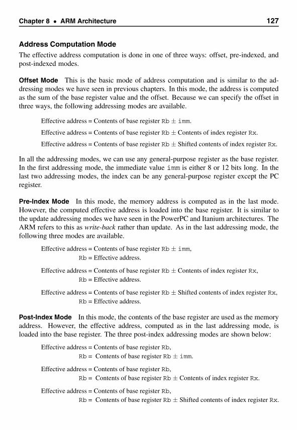
Chapter 8 • ARM Architecture 127
Address Computation ModeThe effective address computation is done in one of three ways: offset, pre-indexed, andpost-indexed modes.
Offset Mode This is the basic mode of address computation and is similar to the ad-dressing modes we have seen in previous chapters. In this mode, the address is computedas the sum of the base register value and the offset. Because we can specify the offset inthree ways, the following addressing modes are available.
Effective address = Contents of base register Rb ± imm.
Effective address = Contents of base register Rb ± Contents of index register Rx.
Effective address = Contents of base register Rb ± Shifted contents of index register Rx.
In all the addressing modes, we can use any general-purpose register as the base register.In the first addressing mode, the immediate value imm is either 8 or 12 bits long. In thelast two addressing modes, the index can be any general-purpose register except the PCregister.
Pre-Index Mode In this mode, the memory address is computed as in the last mode.However, the computed effective address is loaded into the base register. It is similar tothe update addressing modes we have seen in the PowerPC and Itanium architectures. TheARM refers to this as write-back rather than update. As in the last addressing mode, thefollowing three modes are available.
Effective address = Contents of base register Rb ± imm,Rb = Effective address.
Effective address = Contents of base register Rb ± Contents of index register Rx,Rb = Effective address.
Effective address = Contents of base register Rb ± Shifted contents of index register Rx,Rb = Effective address.
Post-Index Mode In this mode, the contents of the base register are used as the memoryaddress. However, the effective address, computed as in the last addressing mode, isloaded into the base register. The three post-index addressing modes are shown below:
Effective address = Contents of base register Rb,Rb = Contents of base register Rb ± imm.
Effective address = Contents of base register Rb,Rb = Contents of base register Rb ± Contents of index register Rx.
Effective address = Contents of base register Rb,Rb = Contents of base register Rb ± Shifted contents of index register Rx.
128 Guide to RISC Processors
The addressing modes we discussed here are available to the load and store instructions.However, ARM architecture provides several addressing modes for other instructions.We mention some of these modes in later sections. The ARM reference manual gives acomplete list of all addressing modes available [1].
Instruction FormatThe ARM instruction execution model is different from the MIPS, PowerPC, and SPARCmodels. It is somewhat similar to that of the Itanium in that most ARM instructionsare conditionally executed. In the Itanium architecture, we used predicate registers todetermine if an instruction should be executed. If the specified predicate register is 1, theinstruction is executed; otherwise, it is treated as a nop (no operation).
The ARM architecture uses a similar scheme. However, ARM uses a 4-bit conditioncode field to express the condition under which the instruction should be executed. Ineach instruction, the most significant four bits (bits 28–31) are reserved for this purpose(see Figure 8.4).
These four bits specify a variety of conditions, as shown in Table 8.1. This table givesthe condition code field value and the mnemonic used in the instructions along with adescription and the condition tested. As shown in this table, the four condition code flagsare used to test for the condition specified in the condition field of the instructions.
The mnemonic given in the second column is appended to the instruction mnemonicto indicate the condition. For example, to branch on equal, we use beq, whereas to branchon the less than condition, we use blt.
Out of the 16 values, two are unconditional. In particular, if the condition field is 1110,the instruction is always executed. This is the default in the sense that if no condition isspecified in the instruction, it is assumed to be AL and the instruction is unconditionallyexecuted. Thus, to branch unconditionally, we can specify either b or bal. We give moreexamples later on.
The last condition is used as “Never” and the instruction is never executed, essen-tially making it a nop. However, recent versions use it for other purposes (e.g., in DSPinstructions) and, therefore, this condition should not be used.
The ARM instruction format is not as simple as that of the MIPS architecture. ARMsupports a wide variety of instruction formats. What we have shown in Figure 8.4 is asmall sample of the formats used by ARM. The A encoding shown in this figure is used bymost arithmetic and logical instructions. The opcode field specifies the operation suchas add and cmp. The Rd field identifies the destination register that receives the result.One of the source operands is in the source register Rn. Because we have 16 general-purpose registers available, each of these fields is 4 bits long. The second source operandis provided by the shifter-operand field. This field takes the least significant 12bits and is used to specify the second source operand. How the second source operand isspecified depends on the addressing mode and whether the operand is to be manipulatedprior to using it. The I bit distinguishes between the immediate and register forms used

Chapter 8 • ARM Architecture 129
31 0
cond
1128
A encoding
31 0
cond
1126
LW encoding
31 0
cond
1126
LH encoding
31 0
cond
28
B encoding
23
0 0 I opcode S Rn Rd shifter_operand
4 2 1 4 1 4 4 12
0 1 I L Rn Rd
4 2 1 1 4 4 12
P U B W address_mode_specific
1 1 1 1
L Rn Rd
4 1 4 4
P U W
1 1 1 1
0 0 0
3
I addr_modeaddr_mode
4 41 1 1 1
4
L1 0 1 Simm24
13 24
Figure 8.4 Selected ARM instruction formats.
to specify the second source operand. We defer a discussion of this topic until the nextsection.
Most ARM instructions can optionally update the condition code flags (N, Z, C, andV). The S bit indicates whether the condition code flags should be updated (S = 1) or not(S = 0) by the instruction.
The branch instructions use the B encoding, which can take a 24-bit signed numberto specify the branch target. The L bit is used to indicate whether to store the returnaddress in the link register. More information is given later when we discuss the branchinstructions.
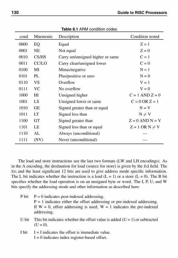
130 Guide to RISC Processors
Table 8.1 ARM condition codes
cond Mnemonic Description Condition tested
0000 EQ Equal Z = 1
0001 NE Not equal Z = 0
0010 CS/HS Carry set/unsigned higher or same C = 1
0011 CC/LO Carry clear/unsigned lower C = 0
0100 MI Minus/negative N = 1
0101 PL Plus/positive or zero N = 0
0110 VS Overflow V = 1
0111 VC No overflow V = 0
1000 HI Unsigned higher C = 1 AND Z = 0
1001 LS Unsigned lower or same C = 0 OR Z = 1
1010 GE Signed greater than or equal N = V
1011 LT Signed less than N �= V
1100 GT Signed greater than Z = 0 AND N = V
1101 LE Signed less than or equal Z = 1 OR N �= V
1110 AL Always (unconditional) —
1111 (NV) Never (unconditional) —
The load and store instructions use the last two formats (LW and LH encodings). Asin the A encoding, the destination for load (source for store) is given by the Rd field. TheRn and the least significant 12 bits are used to give address mode specific information.The L bit indicates whether the instruction is a load (L = 1) or a store (L = 0). The B bitspecifies whether the load operation is on an unsigned byte or word. The I, P, U, and Wbits specify the addressing mode and other information as described here:
P bit P = 0 indicates post-indexed addressing.P = 1 indicates either the offset addressing or pre-indexed addressing.If W = 0, offset addressing is used; W = 1 indicates the pre-indexedaddressing.
U bit This bit indicates whether the offset value is added (U = 1) or subtracted(U = 0).
I bit I = I indicates the offset is immediate value.I = 0 indicates index register-based offset.
Chapter 8 • ARM Architecture 131
Instruction SetThis section presents some sample instructions of the ARM instruction set. If you haveread the previous chapters, you will notice that the ARM instruction semantics are some-what different from the other architectures.
Data Transfer InstructionsWe discuss three types of data transfer instructions: instructions that move data betweenregisters, load instructions, and store instructions.
Move Instructions Two instructions are available to copy data between registers: movand mvn. The mov instruction syntax is
mov{cond}{s} Rd,shifter_operand
It copies the value of shifter_operand into the destination register Rd. It uses the Aencoding format shown in Figure 8.4. The fields shown in curly brackets are optional. Ifs is specified, it makes the S bit a 1. Note that this bit determines whether the conditioncode flags are updated (S = 1) or not (S = 0). The cond field takes any of the two-letter mnemonics given in Table 8.1. Also note that omitting cond implies unconditionalexecution as AL (ALways) is the default. Thus the instruction
mov R1,R2
copies the R2 value to R1 unconditionally. We can also use this instruction to load con-stants, as in the following example.
mov R3,#0
This instruction loads zero into R3. Because the PC register is also a general-purposeregister, we can specify PC as the destination register to cause a branch. The instruction
mov PC,LR
can be used to return from a procedure. Remember that the link register LR (R14) gener-ally keeps the return address.
Now is a good time to unravel the mystery associated with the shifter_operand.This operand can take one of three formats.
Immediate Value: The immediate value is not given directly as in the other architectures.Instead, it takes two numbers: an 8-bit constant and a 4-bit rotate count. The 8-bit constantis rotated by rotate count bit positions to derive the constant. The 4-bit shift count canonly specify 16 bit positions, therefore a zero is appended to it to make it 5 bits long. Forexample, if the 4-bit rotate count is 1001, it is converted to five bits as 10010. Thus, therotate count is always an even number.

132 Guide to RISC Processors
A limitation of this process is that not all constants can be expressed. For example,0xFF00 is a valid constant as we can specify this value with the 8-bit constant taking the0xFF value and using 8 as the rotate count. If we change the rotate count to 28, we get0xF000000F as another valid constant. However, 0x7F8 is not a valid constant as itrequires an odd number of rotations (three in this example). Thus, the move instruction
mov R3,#0xFF00
is a valid one as 0xFF00 is a valid constant.
Register Value: A register can be specified to provide the second operand. This is theformat used in the following instructions.
mov R1,R2mov PC,LR
Shifted Register Value: This is a novel way of expressing the second operand, special tothe ARM architecture. Before the value is used, the operand is shifted/rotated. In thisformat, three components are used to form the final value:
Rm, shift_op SHFT_CNT
The value in Rm is shifted/rotated SHFT_CNT times. The type of shift or rotate operationis specified by shift_op. The shift_op can be any of the following.
lsl Logical Shift Left
lsr Logical Shift Right
asr Arithmetic Shift Right
ror ROtate Right
rrx Rotate Right with eXtend
The lsl specifies a left-shift operation whereas the lsr is used for the right-shiftoperation. The last bit shifted out will be captured in the carry flag as shown here:
012428293031
0
CF
02428293031
0
1
CF
In both cases, the shifted-out bits receive zeros. These are called the logical shifts.
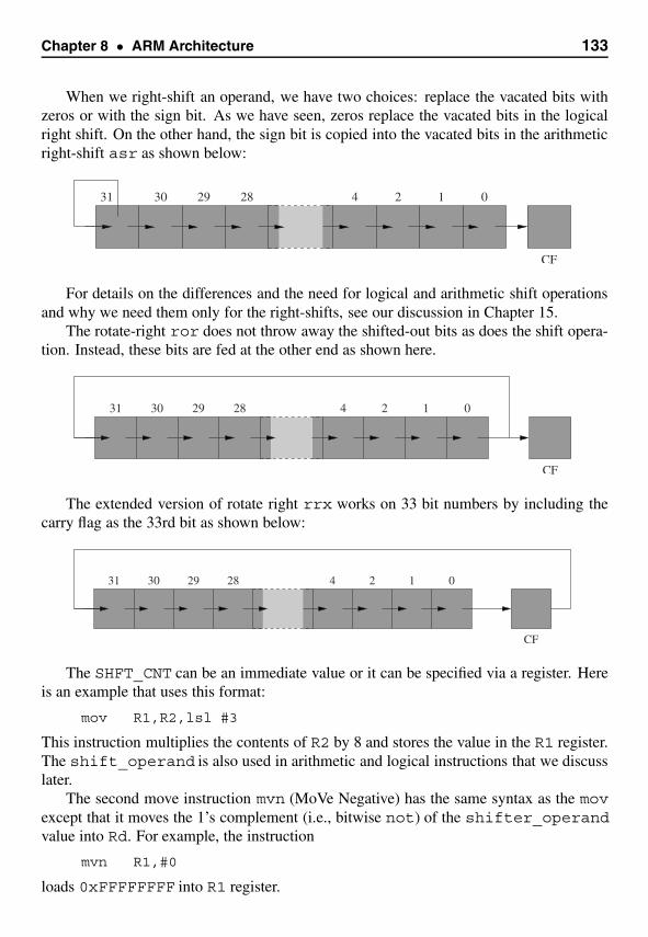
Chapter 8 • ARM Architecture 133
When we right-shift an operand, we have two choices: replace the vacated bits withzeros or with the sign bit. As we have seen, zeros replace the vacated bits in the logicalright shift. On the other hand, the sign bit is copied into the vacated bits in the arithmeticright-shift asr as shown below:
012428293031
CF
For details on the differences and the need for logical and arithmetic shift operationsand why we need them only for the right-shifts, see our discussion in Chapter 15.
The rotate-right ror does not throw away the shifted-out bits as does the shift opera-tion. Instead, these bits are fed at the other end as shown here.
012428293031
CF
The extended version of rotate right rrx works on 33 bit numbers by including thecarry flag as the 33rd bit as shown below:
012428293031
CF
The SHFT_CNT can be an immediate value or it can be specified via a register. Hereis an example that uses this format:
mov R1,R2,lsl #3
This instruction multiplies the contents of R2 by 8 and stores the value in the R1 register.The shift_operand is also used in arithmetic and logical instructions that we discusslater.
The second move instruction mvn (MoVe Negative) has the same syntax as the movexcept that it moves the 1’s complement (i.e., bitwise not) of the shifter_operandvalue into Rd. For example, the instruction
mvn R1,#0
loads 0xFFFFFFFF into R1 register.
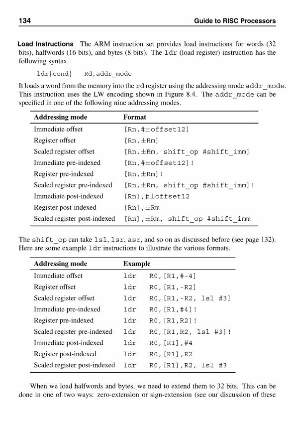
134 Guide to RISC Processors
Load Instructions The ARM instruction set provides load instructions for words (32bits), halfwords (16 bits), and bytes (8 bits). The ldr (load register) instruction has thefollowing syntax.
ldr{cond} Rd,addr_mode
It loads a word from the memory into the rd register using the addressing mode addr_mode.This instruction uses the LW encoding shown in Figure 8.4. The addr_mode can bespecified in one of the following nine addressing modes.
Addressing mode Format
Immediate offset [Rn,#±offset12]Register offset [Rn,±Rm]Scaled register offset [Rn,±Rm, shift_op #shift_imm]
Immediate pre-indexed [Rn,#±offset12]!Register pre-indexed [Rn,±Rm]!Scaled register pre-indexed [Rn,±Rm, shift_op #shift_imm]!
Immediate post-indexed [Rn],#±offset12Register post-indexed [Rn],±RmScaled register post-indexed [Rn],±Rm, shift_op #shift_imm
The shift_op can take lsl, lsr, asr, and so on as discussed before (see page 132).Here are some example ldr instructions to illustrate the various formats.
Addressing mode Example
Immediate offset ldr R0,[R1,#-4]
Register offset ldr R0,[R1,-R2]
Scaled register offset ldr R0,[R1,-R2, lsl #3]
Immediate pre-indexed ldr R0,[R1,#4]!
Register pre-indexed ldr R0,[R1,R2]!
Scaled register pre-indexed ldr R0,[R1,R2, lsl #3]!
Immediate post-indexed ldr R0,[R1],#4
Register post-indexed ldr R0,[R1],R2
Scaled register post-indexed ldr R0,[R1],R2, lsl #3
When we load halfwords and bytes, we need to extend them to 32 bits. This can bedone in one of two ways: zero-extension or sign-extension (see our discussion of these
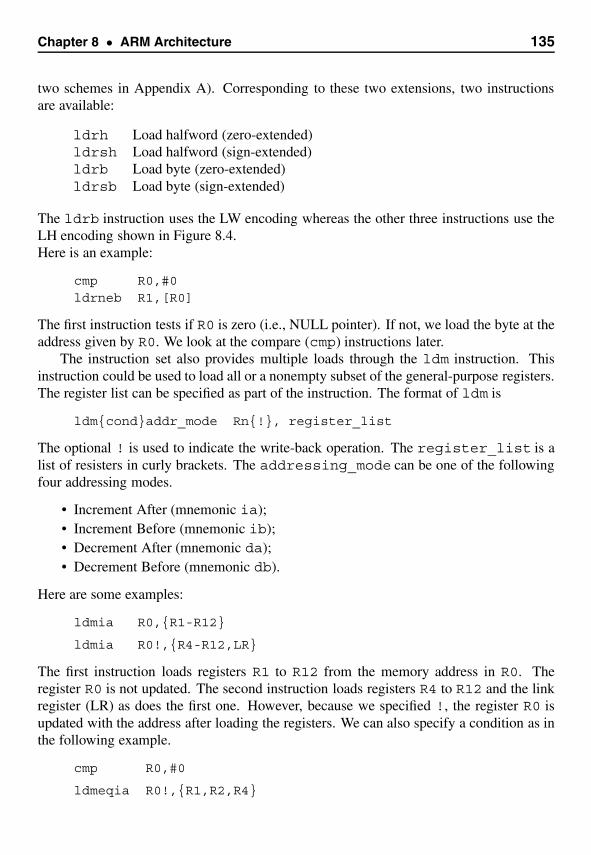
Chapter 8 • ARM Architecture 135
two schemes in Appendix A). Corresponding to these two extensions, two instructionsare available:
ldrh Load halfword (zero-extended)ldrsh Load halfword (sign-extended)ldrb Load byte (zero-extended)ldrsb Load byte (sign-extended)
The ldrb instruction uses the LW encoding whereas the other three instructions use theLH encoding shown in Figure 8.4.Here is an example:
cmp R0,#0ldrneb R1,[R0]
The first instruction tests if R0 is zero (i.e., NULL pointer). If not, we load the byte at theaddress given by R0. We look at the compare (cmp) instructions later.
The instruction set also provides multiple loads through the ldm instruction. Thisinstruction could be used to load all or a nonempty subset of the general-purpose registers.The register list can be specified as part of the instruction. The format of ldm is
ldm{cond}addr_mode Rn{!}, register_list
The optional ! is used to indicate the write-back operation. The register_list is alist of resisters in curly brackets. The addressing_mode can be one of the followingfour addressing modes.
• Increment After (mnemonic ia);• Increment Before (mnemonic ib);• Decrement After (mnemonic da);• Decrement Before (mnemonic db).
Here are some examples:
ldmia R0,{R1-R12}
ldmia R0!,{R4-R12,LR}
The first instruction loads registers R1 to R12 from the memory address in R0. Theregister R0 is not updated. The second instruction loads registers R4 to R12 and the linkregister (LR) as does the first one. However, because we specified !, the register R0 isupdated with the address after loading the registers. We can also specify a condition as inthe following example.
cmp R0,#0
ldmeqia R0!,{R1,R2,R4}
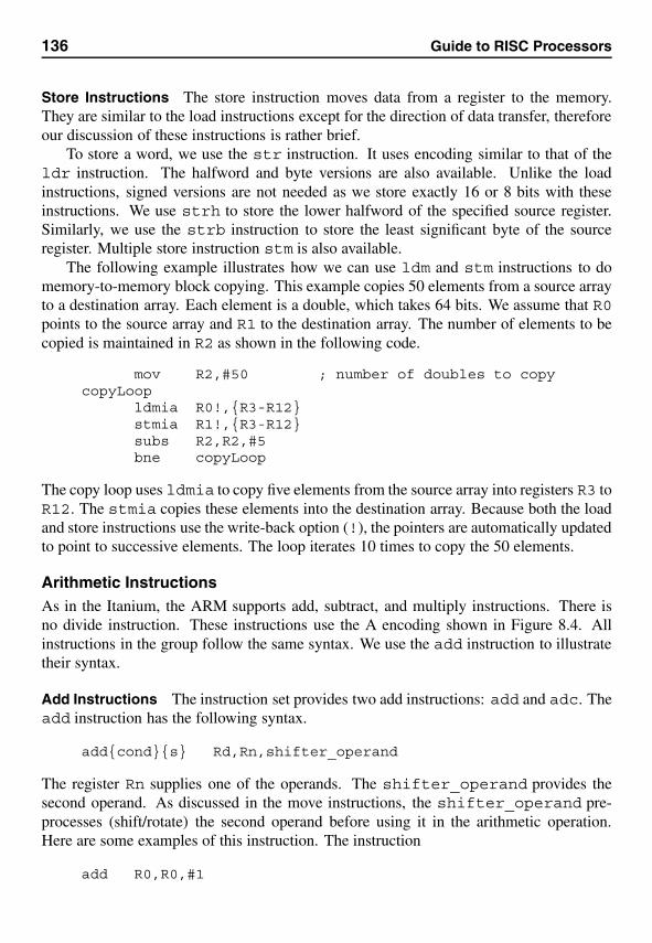
136 Guide to RISC Processors
Store Instructions The store instruction moves data from a register to the memory.They are similar to the load instructions except for the direction of data transfer, thereforeour discussion of these instructions is rather brief.
To store a word, we use the str instruction. It uses encoding similar to that of theldr instruction. The halfword and byte versions are also available. Unlike the loadinstructions, signed versions are not needed as we store exactly 16 or 8 bits with theseinstructions. We use strh to store the lower halfword of the specified source register.Similarly, we use the strb instruction to store the least significant byte of the sourceregister. Multiple store instruction stm is also available.
The following example illustrates how we can use ldm and stm instructions to domemory-to-memory block copying. This example copies 50 elements from a source arrayto a destination array. Each element is a double, which takes 64 bits. We assume that R0points to the source array and R1 to the destination array. The number of elements to becopied is maintained in R2 as shown in the following code.
mov R2,#50 ; number of doubles to copycopyLoop
ldmia R0!,{R3-R12}stmia R1!,{R3-R12}subs R2,R2,#5bne copyLoop
The copy loop uses ldmia to copy five elements from the source array into registers R3 toR12. The stmia copies these elements into the destination array. Because both the loadand store instructions use the write-back option (!), the pointers are automatically updatedto point to successive elements. The loop iterates 10 times to copy the 50 elements.
Arithmetic InstructionsAs in the Itanium, the ARM supports add, subtract, and multiply instructions. There isno divide instruction. These instructions use the A encoding shown in Figure 8.4. Allinstructions in the group follow the same syntax. We use the add instruction to illustratetheir syntax.
Add Instructions The instruction set provides two add instructions: add and adc. Theadd instruction has the following syntax.
add{cond}{s} Rd,Rn,shifter_operand
The register Rn supplies one of the operands. The shifter_operand provides thesecond operand. As discussed in the move instructions, the shifter_operand pre-processes (shift/rotate) the second operand before using it in the arithmetic operation.Here are some examples of this instruction. The instruction
add R0,R0,#1
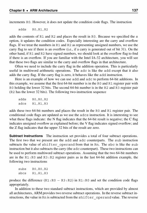
Chapter 8 • ARM Architecture 137
increments R0. However, it does not update the condition code flags. The instruction
adds R0,R1,R2
adds the contents of R1 and R2 and places the result in R0. Because we specified the soption, it updates the condition codes. Especially interesting are the carry and overflowflags. If we treat the numbers in R1 and R2 as representing unsigned numbers, we use thecarry flag to see if there is an overflow (i.e., if a carry is generated out of bit 31). On theother hand, if R1 and R2 have signed numbers, we should look at the overflow flag to findif there is an overflow. If you are familiar with the Intel IA-32 architecture, you will seethat these two flags are similar to the carry and overflow flags in that architecture.
Often we need to include the carry flag in the addition operation. This is particularlyuseful in multiword arithmetic operations. The adc is like the add except that it alsoadds the carry flag. If the carry flag is zero, it behaves like the add instruction.
Here is an example of how we can use add and adc to perform 64-bit additions. Inthis example, we assume that the first 64-bit number is in the R0 and R1 register pair withR0 holding the lower 32 bits. The second 64-bit number is in the R2 and R3 register pair(R2 has the lower 32 bits). The following two-instruction sequence
adds R0,R0,R2adcs R1,R1,R3
adds these two 64-bit numbers and places the result in the R0 and R1 register pair. Theconditional code flags are updated as we use the adcs instruction. It is interesting to seewhat these flags indicate: the N flag indicates that the 64-bit result is negative; the C flagindicates unsigned overflow as explained before; the V flag indicates signed overflow; andthe Z flag indicates that the upper 32 bits of the result are zero.
Subtract Instructions The instruction set provides a total of four subtract operations.The first two that we present are the add and adc counterparts. The sub instructionsubtracts the value of shifter_operand from that in Rn. The sbc is like the subinstruction but it also subtracts the carry (the adc counterpart). These two instructions canbe used to perform multiword subtract operations. Assuming that the two 64-bit numbersare in the R1:R0 and R3:R2 register pairs as in the last 64-bit addition example, thefollowing two instructions
subs R0,R0,R2sbcs R1,R1,R3
produce the difference (R1:R0 − R3:R2) in R1:R0 and set the condition code flagsappropriately.
In addition to these two standard subtract instructions, which are provided by almostall architectures, ARM provides two reverse subtract operations. In the reverse subtract in-structions, the value in Rn is subtracted from the shifter_operandvalue. The reverse
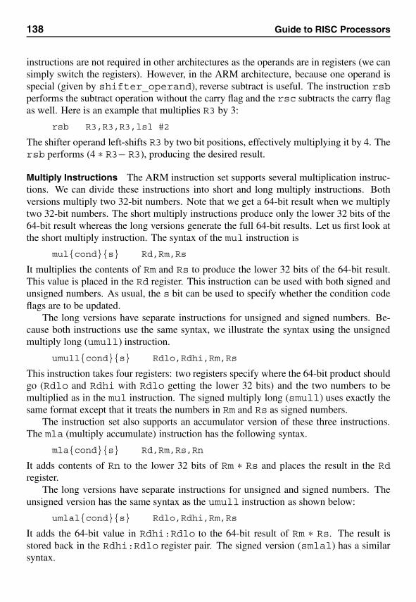
138 Guide to RISC Processors
instructions are not required in other architectures as the operands are in registers (we cansimply switch the registers). However, in the ARM architecture, because one operand isspecial (given by shifter_operand), reverse subtract is useful. The instruction rsbperforms the subtract operation without the carry flag and the rsc subtracts the carry flagas well. Here is an example that multiplies R3 by 3:
rsb R3,R3,R3,lsl #2
The shifter operand left-shifts R3 by two bit positions, effectively multiplying it by 4. Thersb performs (4 * R3− R3), producing the desired result.
Multiply Instructions The ARM instruction set supports several multiplication instruc-tions. We can divide these instructions into short and long multiply instructions. Bothversions multiply two 32-bit numbers. Note that we get a 64-bit result when we multiplytwo 32-bit numbers. The short multiply instructions produce only the lower 32 bits of the64-bit result whereas the long versions generate the full 64-bit results. Let us first look atthe short multiply instruction. The syntax of the mul instruction is
mul{cond}{s} Rd,Rm,Rs
It multiplies the contents of Rm and Rs to produce the lower 32 bits of the 64-bit result.This value is placed in the Rd register. This instruction can be used with both signed andunsigned numbers. As usual, the s bit can be used to specify whether the condition codeflags are to be updated.
The long versions have separate instructions for unsigned and signed numbers. Be-cause both instructions use the same syntax, we illustrate the syntax using the unsignedmultiply long (umull) instruction.
umull{cond}{s} Rdlo,Rdhi,Rm,Rs
This instruction takes four registers: two registers specify where the 64-bit product shouldgo (Rdlo and Rdhi with Rdlo getting the lower 32 bits) and the two numbers to bemultiplied as in the mul instruction. The signed multiply long (smull) uses exactly thesame format except that it treats the numbers in Rm and Rs as signed numbers.
The instruction set also supports an accumulator version of these three instructions.The mla (multiply accumulate) instruction has the following syntax.
mla{cond}{s} Rd,Rm,Rs,Rn
It adds contents of Rn to the lower 32 bits of Rm * Rs and places the result in the Rdregister.
The long versions have separate instructions for unsigned and signed numbers. Theunsigned version has the same syntax as the umull instruction as shown below:
umlal{cond}{s} Rdlo,Rdhi,Rm,Rs
It adds the 64-bit value in Rdhi:Rdlo to the 64-bit result of Rm * Rs. The result isstored back in the Rdhi:Rdlo register pair. The signed version (smlal) has a similarsyntax.
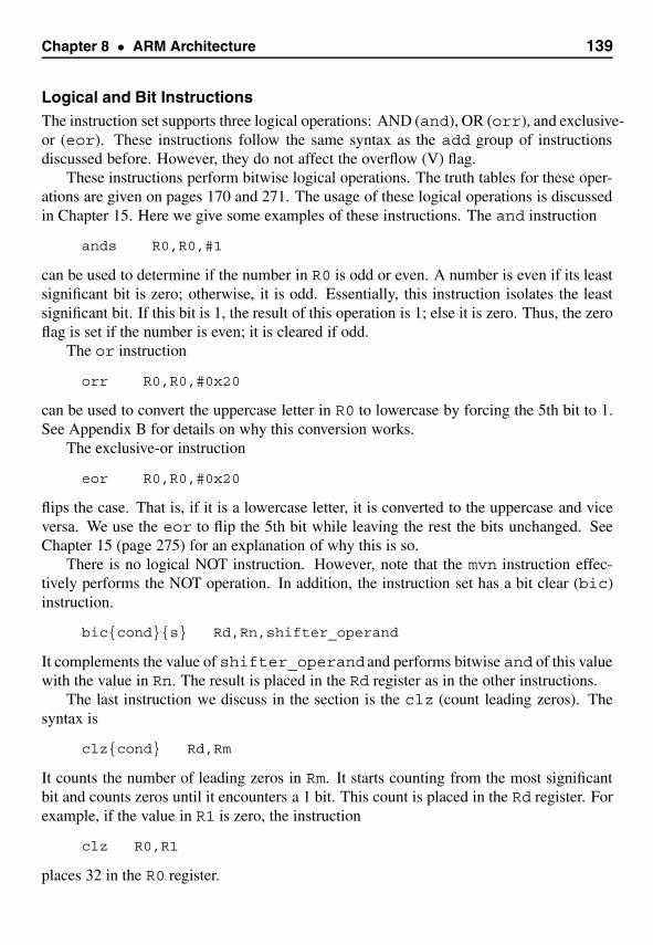
Chapter 8 • ARM Architecture 139
Logical and Bit InstructionsThe instruction set supports three logical operations: AND (and), OR (orr), and exclusive-or (eor). These instructions follow the same syntax as the add group of instructionsdiscussed before. However, they do not affect the overflow (V) flag.
These instructions perform bitwise logical operations. The truth tables for these oper-ations are given on pages 170 and 271. The usage of these logical operations is discussedin Chapter 15. Here we give some examples of these instructions. The and instruction
ands R0,R0,#1
can be used to determine if the number in R0 is odd or even. A number is even if its leastsignificant bit is zero; otherwise, it is odd. Essentially, this instruction isolates the leastsignificant bit. If this bit is 1, the result of this operation is 1; else it is zero. Thus, the zeroflag is set if the number is even; it is cleared if odd.
The or instruction
orr R0,R0,#0x20
can be used to convert the uppercase letter in R0 to lowercase by forcing the 5th bit to 1.See Appendix B for details on why this conversion works.
The exclusive-or instruction
eor R0,R0,#0x20
flips the case. That is, if it is a lowercase letter, it is converted to the uppercase and viceversa. We use the eor to flip the 5th bit while leaving the rest the bits unchanged. SeeChapter 15 (page 275) for an explanation of why this is so.
There is no logical NOT instruction. However, note that the mvn instruction effec-tively performs the NOT operation. In addition, the instruction set has a bit clear (bic)instruction.
bic{cond}{s} Rd,Rn,shifter_operand
It complements the value of shifter_operandand performs bitwise and of this valuewith the value in Rn. The result is placed in the Rd register as in the other instructions.
The last instruction we discuss in the section is the clz (count leading zeros). Thesyntax is
clz{cond} Rd,Rm
It counts the number of leading zeros in Rm. It starts counting from the most significantbit and counts zeros until it encounters a 1 bit. This count is placed in the Rd register. Forexample, if the value in R1 is zero, the instruction
clz R0,R1
places 32 in the R0 register.
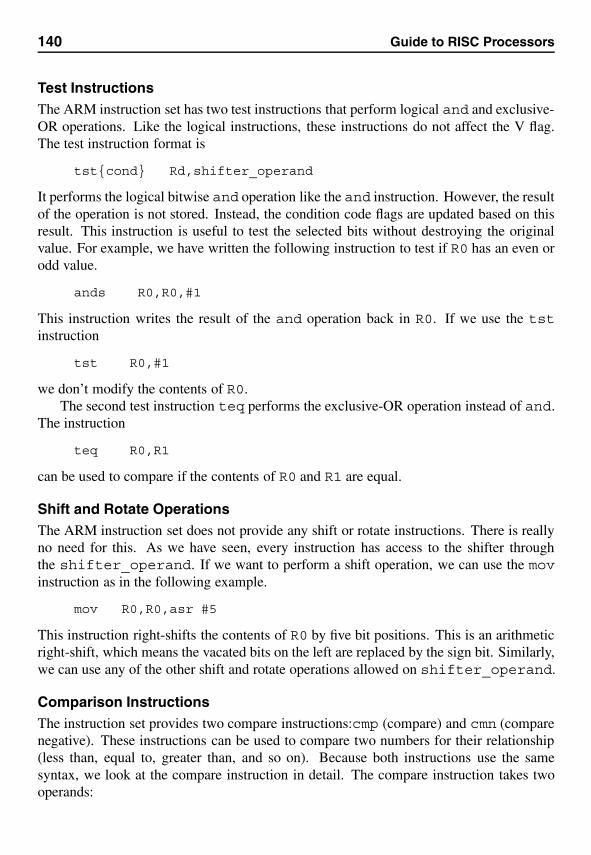
140 Guide to RISC Processors
Test InstructionsThe ARM instruction set has two test instructions that perform logical and and exclusive-OR operations. Like the logical instructions, these instructions do not affect the V flag.The test instruction format is
tst{cond} Rd,shifter_operand
It performs the logical bitwise and operation like the and instruction. However, the resultof the operation is not stored. Instead, the condition code flags are updated based on thisresult. This instruction is useful to test the selected bits without destroying the originalvalue. For example, we have written the following instruction to test if R0 has an even orodd value.
ands R0,R0,#1
This instruction writes the result of the and operation back in R0. If we use the tstinstruction
tst R0,#1
we don’t modify the contents of R0.The second test instruction teq performs the exclusive-OR operation instead of and.
The instruction
teq R0,R1
can be used to compare if the contents of R0 and R1 are equal.
Shift and Rotate OperationsThe ARM instruction set does not provide any shift or rotate instructions. There is reallyno need for this. As we have seen, every instruction has access to the shifter throughthe shifter_operand. If we want to perform a shift operation, we can use the movinstruction as in the following example.
mov R0,R0,asr #5
This instruction right-shifts the contents of R0 by five bit positions. This is an arithmeticright-shift, which means the vacated bits on the left are replaced by the sign bit. Similarly,we can use any of the other shift and rotate operations allowed on shifter_operand.
Comparison InstructionsThe instruction set provides two compare instructions:cmp (compare) and cmn (comparenegative). These instructions can be used to compare two numbers for their relationship(less than, equal to, greater than, and so on). Because both instructions use the samesyntax, we look at the compare instruction in detail. The compare instruction takes twooperands:
Chapter 8 • ARM Architecture 141
cmp{cond} Rn,shifter_operand
It performs Rn− shifter_operand and updates the four condition flags (N, Z, C, andV) based on the result. These flag values can be used to conditionally execute subsequentinstructions. Here is an example.
Suppose we want to find the minimum of two numbers stored in registers R0 and R1.The following statements
cmp R1,R0movlt R0,R1
move the minimum number to R0. The cmp instruction compares the number in R1 withthat in R0. If the number in R1 is greater than or equal to the other number, we do nothing.In this case, because the “less than” condition is not true, the movlt instruction acts as anop. Otherwise, we copy the value from R1 to R0.
This code assumes that the numbers in the two registers are treated as signed numbersas we used “lt” condition. If they are unsigned numbers, we have to use “lo” as in thefollowing code.
cmp R1,R0movlo R0,R1
As a second example, look at the following C code.
if (x > y)x = x + 4*y;
elsey = 3*x;
Assuming that x and y are signed numbers, the following ARM code implements this Ccode.
;x is in R0 and y in R1cmp R0,R1addgt R0,R0,R1,lsl #2addle R1,R1,R1,lsl #1
In the last instruction, we compute 3x as x + 2x with the shifter_operand sup-plying 2x. We can also get 3x as 4x − x, which can be implemented by the followinginstruction.
rsble R0,R0,R0,lsl #2
The cmn instruction updates the flags by adding the shifter_operand value tothe value in the Rn register. In case you are wondering what is “negative” about thisinstruction, think of it as subtracting the negative value of the second operand.
142 Guide to RISC Processors
Branch InstructionsThe branch instructions are used to alter control flow. The branch instruction can also bemodified for procedure invocation. These instructions use the B encoding format shownin Figure 8.4. We first discuss the branch instruction. The syntax is
b{l}{cond} target_address
For now, ignore the l option. We discuss this in the next section. This instruction transferscontrol to target_address if the cond is true. As you can see from Figure 8.4, thetarget address is specified as a 24-bit value. The target instruction address is PC-relativeand is computed as follows.
• The 24-bit target_address is sign-extended to 32 bits.• This value is left-shifted by two bit positions. This is because ARM instructions are
word aligned. The shift operation adds two zeros to the 24-bit target_address.• The value computed in the last step is added to the PC register to form the branch
target. Note that the PC register contains the following address:
PC = branch instruction address + 8
You might have thought that this is due to the delayed branching that many RISCprocessors implement (see our discussion in Chapter 2). Not so! ARM does notimplement delayed branching. The reason for the “plus 8” is the three-stage pipelineused in the ARM cores up to ARM7. If you are not familiar with pipelining, here is abrief explanation of how this three-stage pipeline works. Each instruction that runson this pipeline goes through three stages: fetch, decode, and execute. The pipelineconsists of three units corresponding to these three stages. The pipeline works onthree instructions concurrently, with each unit working on one instruction. Whilethe first instruction is being executed by the execution unit, the next instruction isbeing decoded by the decode unit and a third instruction is being fetched. Thus,the PC points to this third instruction, which is 8 bytes from the first instruction.Even though the ARM9 versions use a five-stage pipeline, the “plus 8” still holdsfor compatibility and other reasons.
If no condition is specified, it becomes an unconditional branch as in the following exam-ple.
b repeat
This is also equivalent to
bal repeat
Here is an example that illustrates how the branch instruction can be used to implement acountdown loop that iterates 50 times.

Chapter 8 • ARM Architecture 143
; loop count is in R0mov R0,#50 ; init loop count to 50
loop. . .. . .
subs R0,R0,#1 ; decrement loop countbne loop ; if R0 != 0, loop back
The last instruction bne can be considered as “branch on not equal to zero” as it branchesto the target if the zero flag is 0.
ProceduresThe branch instruction of the last section can be modified to invoke a procedure. A proce-dure call is like a branch with the provision that it remembers the return address. Thus, ifwe can make the branch instruction store the return address, it can be used as a procedurecall instruction. This is what the l field does:
bl{cond} target_address
This branch and link instruction places the return address in the link register LR, whichis R14, before transferring control to the target. The return address stored is the addressof the instruction following the bl instruction. For example, if we want to invoke thefindMin procedure, we do so by
bl findMin
How do we return from the procedure? It is simple: all we have to do is to copy the returnaddress from the LR to the PC. We can do this by using the following move instruction.
mov PC,LR
Here is an example that shows the structure of an ARM procedure:
; ARM code to find minimum of two signed integers; The two input values are in R0 and R1; The minimum is returned in R2findMin
cmp R1,R0movge R2,R0 ; R1 >= R0? Min = R0movlt R2,R1 ; R1 < R0? Min = R1mov PC,LR ; return
This procedure receives two signed numbers in R0 and R1 and returns the minimum ofthese two values in R2.
144 Guide to RISC Processors
Stack OperationsAs in the MIPS, there is no special stack pointer register in the ARM architecture. Byconvention, register R13 is used as the stack pointer. There is another similarity withMIPS: ARM does not provide any special instructions to manipulate the stack. That is,there are no push and pop instructions. We have to implement these stack operations byusing load and store instructions. This means we have complete freedom as to how thestack should behave. A stack implementation is characterized by two attributes:
• Where the stack pointer points
– Full stack: The stack pointer points to the last full location;
– Empty stack: The stack pointer points to the first empty location.
• How the stack grows
– Descending stack: The stack grows downward (i.e., toward lower memoryaddresses);
– Ascending stack: The stack grows upward (i.e., toward higher memory ad-dresses).
These two attributes define the four types of stacks:
• Full Descending stack (mnemonic fd);
• Full Ascending stack (mnemonic fa);
• Empty Descending stack (mnemonic ed);
• Empty Ascending stack (mnemonic ea).
These mnemonics can be used in ldm and stm instructions to manipulate the stack. Forexample, we can use instructions such as ldmfd, stmfd, and so on. Most implemen-tations, including MIPS and SPARC, prefer descending stacks for reasons discussed inChapter 4 (page 53). Furthermore, the stack pointer points to the last item pushed on tothe stack.
Using the ldmfd and stmfd instructions, we can write procedure entry and exit codeas follows.
procNamestmfd R13!,{R4-R12,LR} ; save registers and
; return address. . .
<procedure body>. . .
ldmfd R13!,{R4-R12,PC} ; restore registers and; return address to PC
Chapter 8 • ARM Architecture 145
This code assumes that we do not have to preserve the first four registers as they are oftenused to pass parameters. Furthermore, we assume that the stack pointer (R13) points to afull descending stack. The stmfd instruction stores registers R4 to R12 and LR on thestack before executing the procedure body. Notice that we use R13! (i.e., the write-backoption) so that the stack pointer is updated to point to the last full location of the stack.Before returning from the procedure, we use the ldmfd instruction to restore the registersand to store the return address in the PC. Because we store the return address in the PCwe do not need a separate return from the procedure.
Summary
The ARM architecture is remarkably different from the other architectures we have seenin this part. It shares some features with the Itanium architecture. One feature of theARM instruction set that sets it apart is that its instructions are executed conditionally. Ifthe specified condition is not true, the instruction acts as a nop. Although Itanium alsouses conditional instruction execution, the ARM uses a 4-bit condition code as opposedto the predicate bits of Itanium. Another interesting feature of ARM is that arithmeticand logical instructions can pre-process (shift/rotate) one of the input operands beforeoperating on it.
At the beginning of this chapter, we mentioned that Thumb instructions are 16 bitslong. To achieve this reduction from the 32-bit ARM instructions, several significantchanges have been made. These include:
• The 4-bit cond field is eliminated. As a result, most Thumb instructions are exe-cuted unconditionally. In contrast, ARM instructions are executed conditionally.
• Most Thumb arithmetic and logical instructions use the 2-address format. In thisformat, as discussed in Chapter 2, the destination register also supplies a sourceoperand.
Even though the ARM is a RISC architecture, it does not strictly follow the RISC prin-ciples as does the MIPS. For example, some of the ARM instructions such as ldm andstm are not simple instructions. In addition, it provides a large number of addressingmodes and uses a somewhat complex instruction format. However, having looked at fivedifferent RISC designs, you will also see a lot of commonality among these architecturesand the RISC principles given in Chapter 3. In the next part, we take a detailed look at theMIPS assembly language.
Web ResourcesMost of the ARM documentation is available from their Web site www.arm.com. TheARM Architecture Reference Manual is published by Addison-Wesley [1]. The referencemanual is also distributed by ARM on their documentation CD. Unfortunately, this infor-mation is not available from their Web site; you have to request this CD from ARM.
PART III
MIPS Assembly Language
9SPIM Simulatorand Debugger
SPIM is a simulator that runs MIPS 2000 programs. SPIM supports various platforms andcan be downloaded from the Web. SPIM also contains a simple debugger. In this chapter,we give details on how you can download and use the SPIM simulator. We start withan introduction to the SPIM simulator. The following section gives details about SPIMsettings. These settings determine how the simulator loads and runs your programs. Wespecify the settings you should use in order to run the example MIPS programs given inlater chapters. Details about loading and running MIPS assembly language programs arediscussed in the next section. This section also presents the debugging facilities providedby SPIM. We conclude the chapter with a summary.
IntroductionThis chapter describes the SPIM simulator, which was developed by Professor JamesLarus when he was at the Computer Science Department of the University of Wisconsin,Madison. This simulator executes the programs written for the MIPS R2000/R3000 pro-cessors. This is a two-in-one product: it contains a simulator to run the MIPS programsas well as a debugger.
SPIM runs on a variety of platforms including UNIX, Linux, Windows, and DOS. Inthis chapter, we provide details on the Windows version of SPIM called PCSpim. TheSPIM simulator can be downloaded from
http://www.cs.wisc.edu/˜larus/spim.html
This page also gives information on SPIM documentation. Although SPIM is available
149
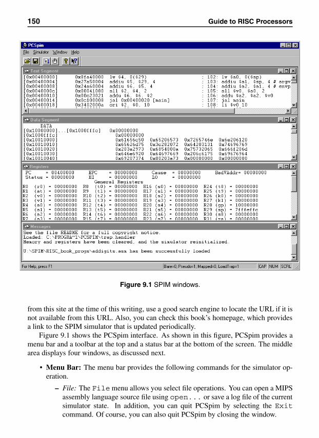
150 Guide to RISC Processors
Figure 9.1 SPIM windows.
from this site at the time of this writing, use a good search engine to locate the URL if it isnot available from this URL. Also, you can check this book’s homepage, which providesa link to the SPIM simulator that is updated periodically.
Figure 9.1 shows the PCSpim interface. As shown in this figure, PCSpim provides amenu bar and a toolbar at the top and a status bar at the bottom of the screen. The middlearea displays four windows, as discussed next.
• Menu Bar: The menu bar provides the following commands for the simulator op-eration.
– File: The File menu allows you select file operations. You can open a MIPSassembly language source file using open... or save a log file of the currentsimulator state. In addition, you can quit PCSpim by selecting the Exitcommand. Of course, you can also quit PCSpim by closing the window.
Chapter 9 • SPIM Simulator and Debugger 151
– Simulator: This menu provides several commands to run and debug a pro-gram. We discuss these commands later in this chapter. This menu also allowsyou to select the simulator settings. When the Settings... command isselected, it opens a setting window to set the simulator settings, which arediscussed in the next section.
– Windows: This menu allows you to control the presentation and navigation ofwindows. For example, in Figure 9.1, we have tiled windows to show the fourwindows: Text Segment, Data Segment, Register, and Messages. In addition,you can also elect to hide or display the toolbar and status bar. The consolewindow pops up when your program needs to read/write data to the terminal.It disappears after the program has terminated. When you want to see yourprogram’s input and output, you can activate this window by selecting theConsole window command.
– Help: This menu allows you to obtain online help on PCSpim.
• Toolbar: The toolbar provides mouse buttons to open and close a MIPS assemblylanguage source file, to run and insert breakpoints, and to get help.
• Window Display Section: This section displays four windows: Data Segment,Text Segment, Messages, and Register.
– Data Segment Window: This window shows the data and stack contents ofyour program. Each line consists of an address (in square brackets) and thecorresponding contents in hexadecimal notation. If a block of memory con-tains the same constant, an address range is specified as shown on the first lineof the Data Segment in Figure 9.1.
– Text Segment Window: This window shows the instructions from your pro-gram as well as the system code loaded by PCSpim. The leftmost hex numberin square brackets is the address of the instruction. The second hex numberis the machine instruction encoding of the instruction. Next to it is the in-struction mnemonic, which is a processor instruction. What you see after thesemicolon is the source code line including any comments you have placed.This display is useful to see how the pseudoinstructions of the assembler aretranslated into the processor instructions. For example, the last line in the TextSegment of Figure 9.1 shows that the pseudoinstruction
li $vi,10
is translated as
ori $2,$0,10
– Registers: This window shows the contents of the general and floating-pointregisters. The contents are displayed in either decimal or hex notation, de-pending on the settings used (discussed in the next section).
– Messages: This window is used by PCSpim to display error messages.
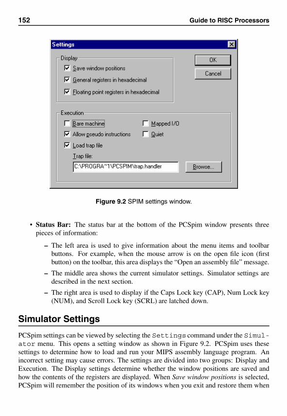
152 Guide to RISC Processors
Figure 9.2 SPIM settings window.
• Status Bar: The status bar at the bottom of the PCSpim window presents threepieces of information:
– The left area is used to give information about the menu items and toolbarbuttons. For example, when the mouse arrow is on the open file icon (firstbutton) on the toolbar, this area displays the “Open an assembly file” message.
– The middle area shows the current simulator settings. Simulator settings aredescribed in the next section.
– The right area is used to display if the Caps Lock key (CAP), Num Lock key(NUM), and Scroll Lock key (SCRL) are latched down.
Simulator Settings
PCSpim settings can be viewed by selecting the Settings command under the Simul-ator menu. This opens a setting window as shown in Figure 9.2. PCSpim uses thesesettings to determine how to load and run your MIPS assembly language program. Anincorrect setting may cause errors. The settings are divided into two groups: Display andExecution. The Display settings determine whether the window positions are saved andhow the contents of the registers are displayed. When Save window positions is selected,PCSpim will remember the position of its windows when you exit and restore them when
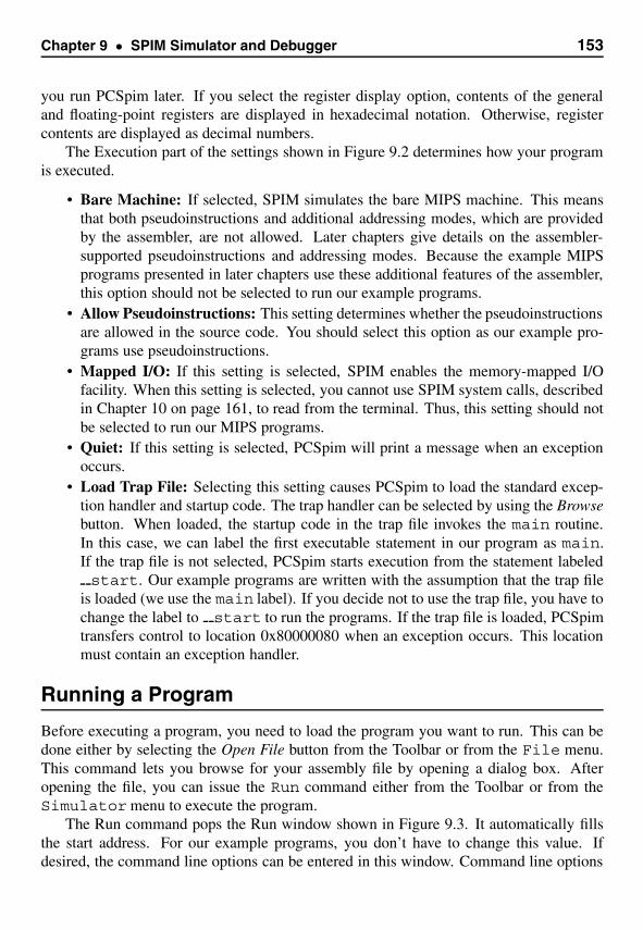
Chapter 9 • SPIM Simulator and Debugger 153
you run PCSpim later. If you select the register display option, contents of the generaland floating-point registers are displayed in hexadecimal notation. Otherwise, registercontents are displayed as decimal numbers.
The Execution part of the settings shown in Figure 9.2 determines how your programis executed.
• Bare Machine: If selected, SPIM simulates the bare MIPS machine. This meansthat both pseudoinstructions and additional addressing modes, which are providedby the assembler, are not allowed. Later chapters give details on the assembler-supported pseudoinstructions and addressing modes. Because the example MIPSprograms presented in later chapters use these additional features of the assembler,this option should not be selected to run our example programs.
• Allow Pseudoinstructions: This setting determines whether the pseudoinstructionsare allowed in the source code. You should select this option as our example pro-grams use pseudoinstructions.
• Mapped I/O: If this setting is selected, SPIM enables the memory-mapped I/Ofacility. When this setting is selected, you cannot use SPIM system calls, describedin Chapter 10 on page 161, to read from the terminal. Thus, this setting should notbe selected to run our MIPS programs.
• Quiet: If this setting is selected, PCSpim will print a message when an exceptionoccurs.
• Load Trap File: Selecting this setting causes PCSpim to load the standard excep-tion handler and startup code. The trap handler can be selected by using the Browsebutton. When loaded, the startup code in the trap file invokes the main routine.In this case, we can label the first executable statement in our program as main.If the trap file is not selected, PCSpim starts execution from the statement labeledstart. Our example programs are written with the assumption that the trap file
is loaded (we use the main label). If you decide not to use the trap file, you have tochange the label to start to run the programs. If the trap file is loaded, PCSpimtransfers control to location 0x80000080 when an exception occurs. This locationmust contain an exception handler.
Running a Program
Before executing a program, you need to load the program you want to run. This can bedone either by selecting the Open File button from the Toolbar or from the File menu.This command lets you browse for your assembly file by opening a dialog box. Afteropening the file, you can issue the Run command either from the Toolbar or from theSimulator menu to execute the program.
The Run command pops the Run window shown in Figure 9.3. It automatically fillsthe start address. For our example programs, you don’t have to change this value. Ifdesired, the command line options can be entered in this window. Command line options
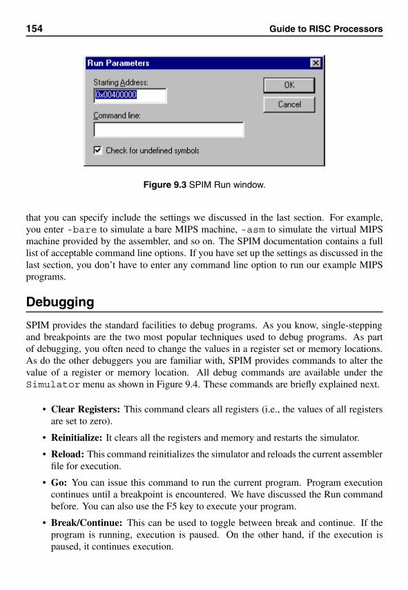
154 Guide to RISC Processors
Figure 9.3 SPIM Run window.
that you can specify include the settings we discussed in the last section. For example,you enter -bare to simulate a bare MIPS machine, -asm to simulate the virtual MIPSmachine provided by the assembler, and so on. The SPIM documentation contains a fulllist of acceptable command line options. If you have set up the settings as discussed in thelast section, you don’t have to enter any command line option to run our example MIPSprograms.
Debugging
SPIM provides the standard facilities to debug programs. As you know, single-steppingand breakpoints are the two most popular techniques used to debug programs. As partof debugging, you often need to change the values in a register set or memory locations.As do the other debuggers you are familiar with, SPIM provides commands to alter thevalue of a register or memory location. All debug commands are available under theSimulatormenu as shown in Figure 9.4. These commands are briefly explained next.
• Clear Registers: This command clears all registers (i.e., the values of all registersare set to zero).
• Reinitialize: It clears all the registers and memory and restarts the simulator.
• Reload: This command reinitializes the simulator and reloads the current assemblerfile for execution.
• Go: You can issue this command to run the current program. Program executioncontinues until a breakpoint is encountered. We have discussed the Run commandbefore. You can also use the F5 key to execute your program.
• Break/Continue: This can be used to toggle between break and continue. If theprogram is running, execution is paused. On the other hand, if the execution ispaused, it continues execution.
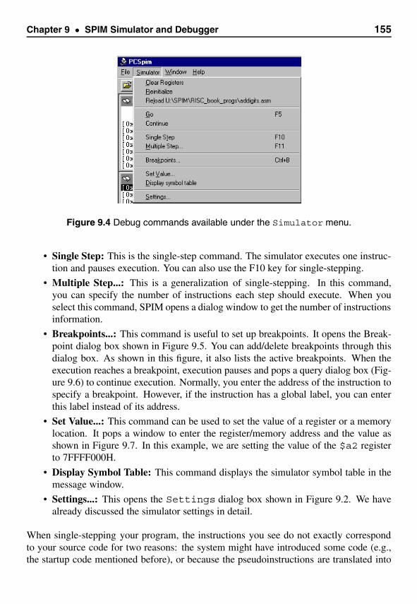
Chapter 9 • SPIM Simulator and Debugger 155
Figure 9.4 Debug commands available under the Simulator menu.
• Single Step: This is the single-step command. The simulator executes one instruc-tion and pauses execution. You can also use the F10 key for single-stepping.
• Multiple Step...: This is a generalization of single-stepping. In this command,you can specify the number of instructions each step should execute. When youselect this command, SPIM opens a dialog window to get the number of instructionsinformation.
• Breakpoints...: This command is useful to set up breakpoints. It opens the Break-point dialog box shown in Figure 9.5. You can add/delete breakpoints through thisdialog box. As shown in this figure, it also lists the active breakpoints. When theexecution reaches a breakpoint, execution pauses and pops a query dialog box (Fig-ure 9.6) to continue execution. Normally, you enter the address of the instruction tospecify a breakpoint. However, if the instruction has a global label, you can enterthis label instead of its address.
• Set Value...: This command can be used to set the value of a register or a memorylocation. It pops a window to enter the register/memory address and the value asshown in Figure 9.7. In this example, we are setting the value of the $a2 registerto 7FFFF000H.
• Display Symbol Table: This command displays the simulator symbol table in themessage window.
• Settings...: This opens the Settings dialog box shown in Figure 9.2. We havealready discussed the simulator settings in detail.
When single-stepping your program, the instructions you see do not exactly correspondto your source code for two reasons: the system might have introduced some code (e.g.,the startup code mentioned before), or because the pseudoinstructions are translated into
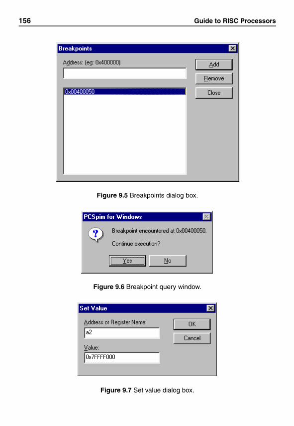
156 Guide to RISC Processors
Figure 9.5 Breakpoints dialog box.
Figure 9.6 Breakpoint query window.
Figure 9.7 Set value dialog box.
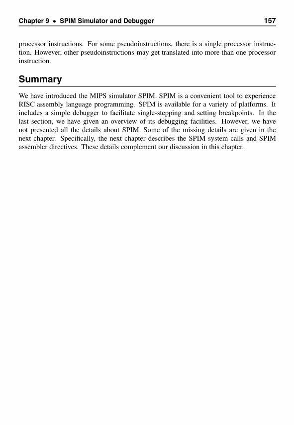
Chapter 9 • SPIM Simulator and Debugger 157
processor instructions. For some pseudoinstructions, there is a single processor instruc-tion. However, other pseudoinstructions may get translated into more than one processorinstruction.
Summary
We have introduced the MIPS simulator SPIM. SPIM is a convenient tool to experienceRISC assembly language programming. SPIM is available for a variety of platforms. Itincludes a simple debugger to facilitate single-stepping and setting breakpoints. In thelast section, we have given an overview of its debugging facilities. However, we havenot presented all the details about SPIM. Some of the missing details are given in thenext chapter. Specifically, the next chapter describes the SPIM system calls and SPIMassembler directives. These details complement our discussion in this chapter.
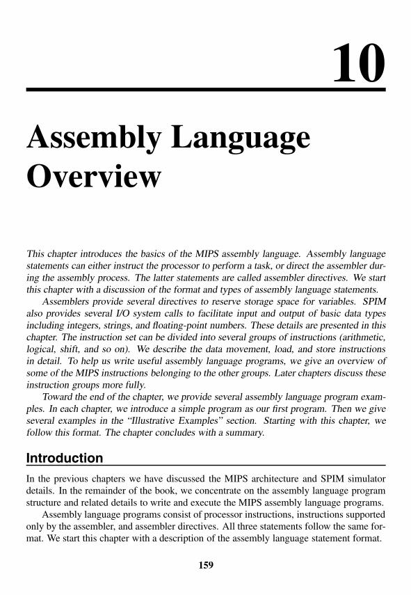
10Assembly LanguageOverview
This chapter introduces the basics of the MIPS assembly language. Assembly languagestatements can either instruct the processor to perform a task, or direct the assembler dur-ing the assembly process. The latter statements are called assembler directives. We startthis chapter with a discussion of the format and types of assembly language statements.
Assemblers provide several directives to reserve storage space for variables. SPIMalso provides several I/O system calls to facilitate input and output of basic data typesincluding integers, strings, and floating-point numbers. These details are presented in thischapter. The instruction set can be divided into several groups of instructions (arithmetic,logical, shift, and so on). We describe the data movement, load, and store instructionsin detail. To help us write useful assembly language programs, we give an overview ofsome of the MIPS instructions belonging to the other groups. Later chapters discuss theseinstruction groups more fully.
Toward the end of the chapter, we provide several assembly language program exam-ples. In each chapter, we introduce a simple program as our first program. Then we giveseveral examples in the “Illustrative Examples” section. Starting with this chapter, wefollow this format. The chapter concludes with a summary.
IntroductionIn the previous chapters we have discussed the MIPS architecture and SPIM simulatordetails. In the remainder of the book, we concentrate on the assembly language programstructure and related details to write and execute the MIPS assembly language programs.
Assembly language programs consist of processor instructions, instructions supportedonly by the assembler, and assembler directives. All three statements follow the same for-mat. We start this chapter with a description of the assembly language statement format.
159
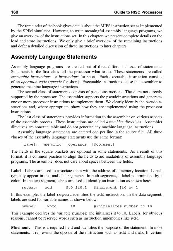
160 Guide to RISC Processors
The remainder of the book gives details about the MIPS instruction set as implementedby the SPIM simulator. However, to write meaningful assembly language programs, wegive an overview of the instructions set. In this chapter, we present complete details on theload and store instructions. We only give a brief overview of the remaining instructionsand defer a detailed discussion of these instructions to later chapters.
Assembly Language Statements
Assembly language programs are created out of three different classes of statements.Statements in the first class tell the processor what to do. These statements are calledexecutable instructions, or instructions for short. Each executable instruction consistsof an operation code (opcode for short). Executable instructions cause the assembler togenerate machine language instructions.
The second class of statements consists of pseudoinstructions. These are not directlysupported by the processor. The assembler supports the pseudoinstructions and generatesone or more processor instructions to implement them. We clearly identify the pseudoin-structions and, where appropriate, show how they are implemented using the processorinstructions.
The last class of statements provides information to the assembler on various aspectsof the assembly process. These instructions are called assembler directives. Assemblerdirectives are nonexecutable and do not generate any machine language instructions.
Assembly language statements are entered one per line in the source file. All threeclasses of the assembly language statements use the same format:
[label:] mnemonic [operands] [#comment]
The fields in the square brackets are optional in some statements. As a result of thisformat, it is common practice to align the fields to aid readability of assembly languageprograms. The assembler does not care about spaces between the fields.
Label Labels are used to associate them with the address of a memory location. Labelstypically appear in text and data segments. In both segments, a label is terminated by acolon. In the text segment, labels are used to identify an instruction as shown here:
repeat: add $t0,$t0,1 #increment $t0 by 1
In this example, the label repeat identifies the add instruction. In the data segment,labels are used for variable names as shown below:
number: .word 10 #initializes number to 10
This example declares the variable number and initializes it to 10. Labels, for obviousreasons, cannot be reserved words such as instruction mnemonics like add.
Mnemonic This is a required field and identifies the purpose of the statement. In moststatements, it represents the opcode of the instruction such as add and sub. In certain

Chapter 10 • Assembly Language Overview 161
statements, this field is not required. Examples include lines consisting of a comment, ora label, or a label and a comment.
Operands Operands specify the data to be manipulated by the statement. The number ofoperands required depends on the specific statement. Most statements have three operandsas shown here:
add $t0,$t1,$t2
However, some instructions and pseudoinstructions have only one or two operands. Hereare some examples:
li $v0,5move $a0,$t2la $t3,numbermflo $t2
Don’t worry about the semantics of these instructions. We give details about these in-structions in the remainder of the book.
Comment This is an optional field and serves the same purpose as that in a high-levellanguage. Comments play a more important role in assembly language, as it is a low-levellanguage. Assembler ignores all comments. Comments begin with a sharp sign (#) andextend until the end of the line. Because the readability of assembly language programsis poor, comments should be generously used to improve readability.
SPIM System Calls
SPIM provides I/O support through the system call (syscall) instruction. Eight ofthese calls facilitate input and output of the four basic data types: string, integer, float,and double. A notable service missing from this list is the character input and output. Forcharacter I/O, we have to use the string system calls.
To invoke a service, the system call service code should be placed in the $v0 register.Any required arguments are placed in the $a0 and $a1 registers (use $f12 for floating-point values). Any value returned by a system call is placed in $v0 ($f0 for floating-pointvalues).
All ten system calls are summarized in Table 10.1. The first three calls are self-explanatory. The print_string system call takes a pointer to a NULL-terminatedstring and prints the string. The read_int, read_float and read_double systemcalls read input up to and including newline. Characters following the number are ignored.The read_string call takes the pointer to a buffer in $a0 and the buffer size n in $a1.The buffer size should be expressed in bytes. It reads at most n − 1 characters into thebuffer and terminates the string by the NULL character. The read_string call has thesame semantics as the fgets function in the C library.
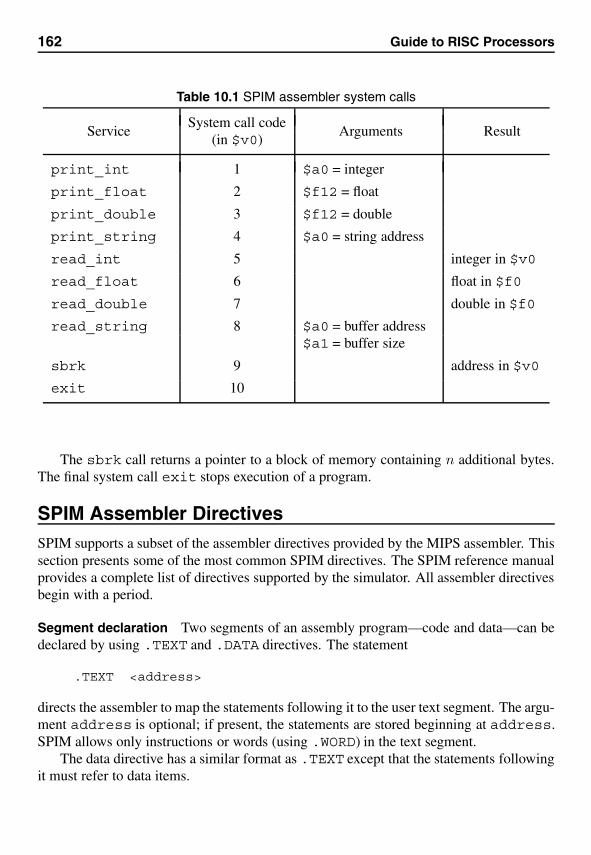
162 Guide to RISC Processors
Table 10.1 SPIM assembler system calls
ServiceSystem call code
Arguments Result(in $v0)
print_int 1 $a0 = integer
print_float 2 $f12 = float
print_double 3 $f12 = double
print_string 4 $a0 = string address
read_int 5 integer in $v0
read_float 6 float in $f0
read_double 7 double in $f0
read_string 8 $a0 = buffer address$a1 = buffer size
sbrk 9 address in $v0
exit 10
The sbrk call returns a pointer to a block of memory containing n additional bytes.The final system call exit stops execution of a program.
SPIM Assembler DirectivesSPIM supports a subset of the assembler directives provided by the MIPS assembler. Thissection presents some of the most common SPIM directives. The SPIM reference manualprovides a complete list of directives supported by the simulator. All assembler directivesbegin with a period.
Segment declaration Two segments of an assembly program—code and data—can bedeclared by using .TEXT and .DATA directives. The statement
.TEXT <address>
directs the assembler to map the statements following it to the user text segment. The argu-ment address is optional; if present, the statements are stored beginning at address.SPIM allows only instructions or words (using .WORD) in the text segment.
The data directive has a similar format as .TEXT except that the statements followingit must refer to data items.
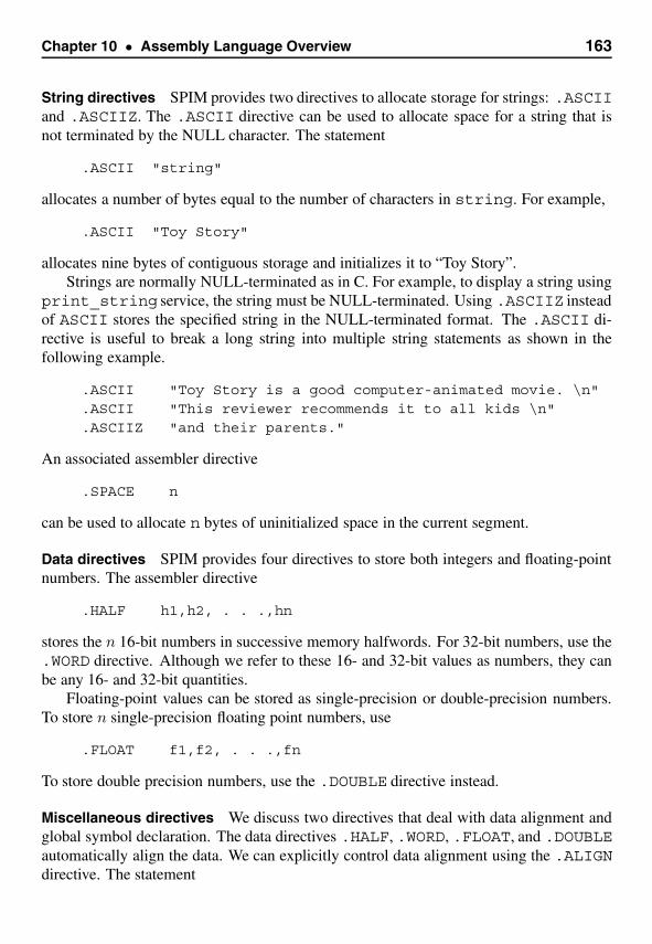
Chapter 10 • Assembly Language Overview 163
String directives SPIM provides two directives to allocate storage for strings: .ASCIIand .ASCIIZ. The .ASCII directive can be used to allocate space for a string that isnot terminated by the NULL character. The statement
.ASCII "string"
allocates a number of bytes equal to the number of characters in string. For example,
.ASCII "Toy Story"
allocates nine bytes of contiguous storage and initializes it to “Toy Story”.Strings are normally NULL-terminated as in C. For example, to display a string using
print_string service, the string must be NULL-terminated. Using .ASCIIZ insteadof ASCII stores the specified string in the NULL-terminated format. The .ASCII di-rective is useful to break a long string into multiple string statements as shown in thefollowing example.
.ASCII "Toy Story is a good computer-animated movie. \n"
.ASCII "This reviewer recommends it to all kids \n"
.ASCIIZ "and their parents."
An associated assembler directive
.SPACE n
can be used to allocate n bytes of uninitialized space in the current segment.
Data directives SPIM provides four directives to store both integers and floating-pointnumbers. The assembler directive
.HALF h1,h2, . . .,hn
stores the n 16-bit numbers in successive memory halfwords. For 32-bit numbers, use the.WORD directive. Although we refer to these 16- and 32-bit values as numbers, they canbe any 16- and 32-bit quantities.
Floating-point values can be stored as single-precision or double-precision numbers.To store n single-precision floating point numbers, use
.FLOAT f1,f2, . . .,fn
To store double precision numbers, use the .DOUBLE directive instead.
Miscellaneous directives We discuss two directives that deal with data alignment andglobal symbol declaration. The data directives .HALF, .WORD, .FLOAT, and .DOUBLEautomatically align the data. We can explicitly control data alignment using the .ALIGNdirective. The statement
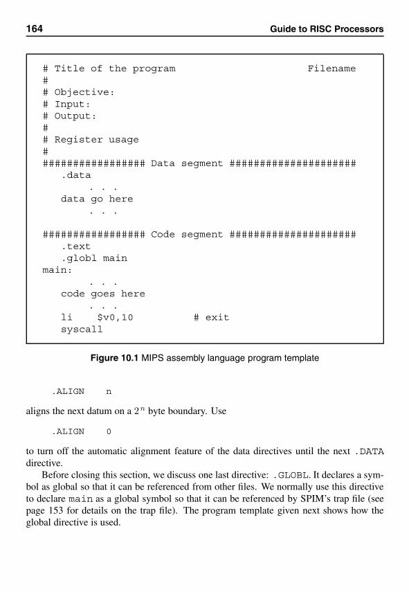
164 Guide to RISC Processors
# Title of the program Filename## Objective:# Input:# Output:## Register usage################## Data segment #####################
.data. . .
data go here. . .
################# Code segment #####################.text.globl main
main:. . .
code goes here. . .
li $v0,10 # exitsyscall
Figure 10.1 MIPS assembly language program template
.ALIGN n
aligns the next datum on a 2n byte boundary. Use
.ALIGN 0
to turn off the automatic alignment feature of the data directives until the next .DATAdirective.
Before closing this section, we discuss one last directive: .GLOBL. It declares a sym-bol as global so that it can be referenced from other files. We normally use this directiveto declare main as a global symbol so that it can be referenced by SPIM’s trap file (seepage 153 for details on the trap file). The program template given next shows how theglobal directive is used.
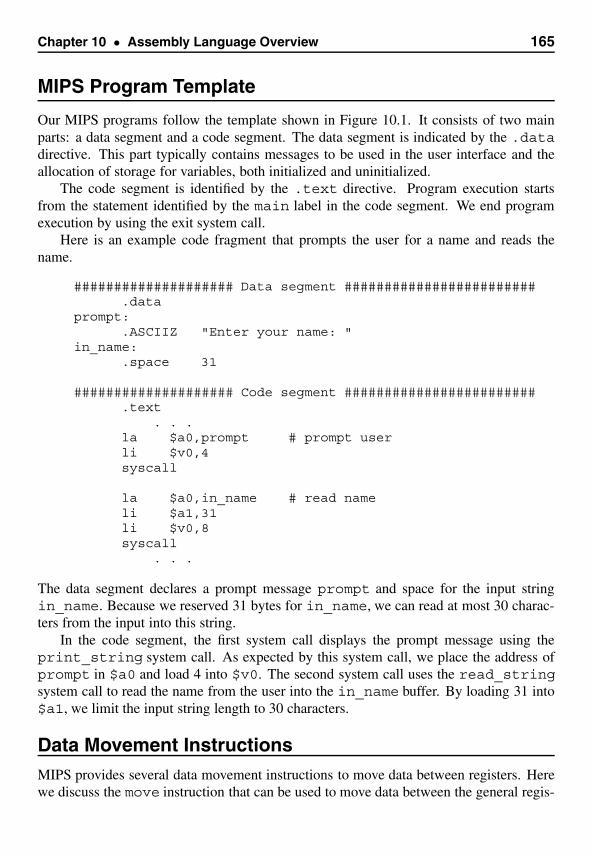
Chapter 10 • Assembly Language Overview 165
MIPS Program Template
Our MIPS programs follow the template shown in Figure 10.1. It consists of two mainparts: a data segment and a code segment. The data segment is indicated by the .datadirective. This part typically contains messages to be used in the user interface and theallocation of storage for variables, both initialized and uninitialized.
The code segment is identified by the .text directive. Program execution startsfrom the statement identified by the main label in the code segment. We end programexecution by using the exit system call.
Here is an example code fragment that prompts the user for a name and reads thename.
#################### Data segment ########################.data
prompt:.ASCIIZ "Enter your name: "
in_name:.space 31
#################### Code segment ########################.text
. . .la $a0,prompt # prompt userli $v0,4syscall
la $a0,in_name # read nameli $a1,31li $v0,8syscall
. . .
The data segment declares a prompt message prompt and space for the input stringin_name. Because we reserved 31 bytes for in_name, we can read at most 30 charac-ters from the input into this string.
In the code segment, the first system call displays the prompt message using theprint_string system call. As expected by this system call, we place the address ofprompt in $a0 and load 4 into $v0. The second system call uses the read_stringsystem call to read the name from the user into the in_name buffer. By loading 31 into$a1, we limit the input string length to 30 characters.
Data Movement InstructionsMIPS provides several data movement instructions to move data between registers. Herewe discuss the move instruction that can be used to move data between the general regis-
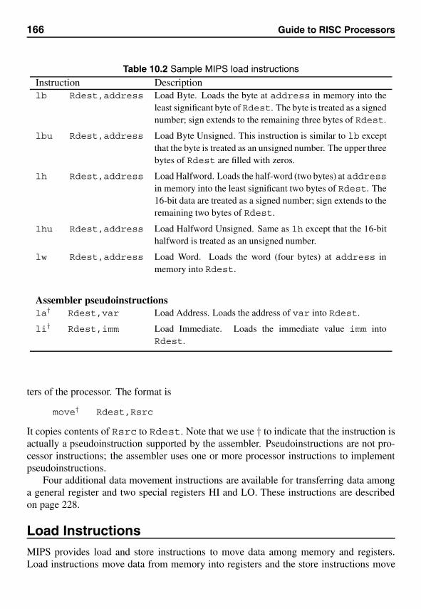
166 Guide to RISC Processors
Table 10.2 Sample MIPS load instructions
Instruction Descriptionlb Rdest,address Load Byte. Loads the byte at address in memory into the
least significant byte of Rdest. The byte is treated as a signednumber; sign extends to the remaining three bytes of Rdest.
lbu Rdest,address Load Byte Unsigned. This instruction is similar to lb exceptthat the byte is treated as an unsigned number. The upper threebytes of Rdest are filled with zeros.
lh Rdest,address Load Halfword. Loads the half-word (two bytes) at addressin memory into the least significant two bytes of Rdest. The16-bit data are treated as a signed number; sign extends to theremaining two bytes of Rdest.
lhu Rdest,address Load Halfword Unsigned. Same as lh except that the 16-bithalfword is treated as an unsigned number.
lw Rdest,address Load Word. Loads the word (four bytes) at address inmemory into Rdest.
Assembler pseudoinstructionsla† Rdest,var Load Address. Loads the address of var into Rdest.
li† Rdest,imm Load Immediate. Loads the immediate value imm intoRdest.
ters of the processor. The format is
move† Rdest,Rsrc
It copies contents of Rsrc to Rdest. Note that we use † to indicate that the instruction isactually a pseudoinstruction supported by the assembler. Pseudoinstructions are not pro-cessor instructions; the assembler uses one or more processor instructions to implementpseudoinstructions.
Four additional data movement instructions are available for transferring data amonga general register and two special registers HI and LO. These instructions are describedon page 228.
Load InstructionsMIPS provides load and store instructions to move data among memory and registers.Load instructions move data from memory into registers and the store instructions move
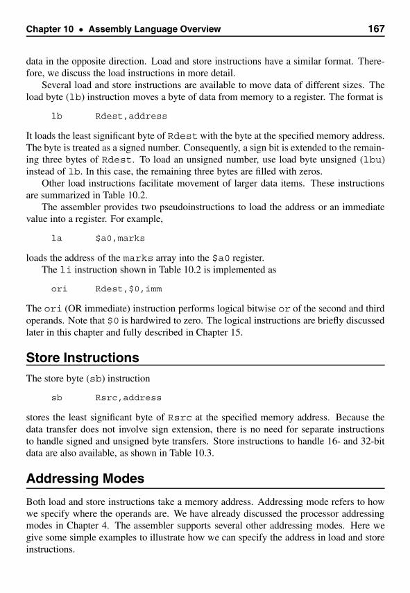
Chapter 10 • Assembly Language Overview 167
data in the opposite direction. Load and store instructions have a similar format. There-fore, we discuss the load instructions in more detail.
Several load and store instructions are available to move data of different sizes. Theload byte (lb) instruction moves a byte of data from memory to a register. The format is
lb Rdest,address
It loads the least significant byte of Rdestwith the byte at the specified memory address.The byte is treated as a signed number. Consequently, a sign bit is extended to the remain-ing three bytes of Rdest. To load an unsigned number, use load byte unsigned (lbu)instead of lb. In this case, the remaining three bytes are filled with zeros.
Other load instructions facilitate movement of larger data items. These instructionsare summarized in Table 10.2.
The assembler provides two pseudoinstructions to load the address or an immediatevalue into a register. For example,
la $a0,marks
loads the address of the marks array into the $a0 register.The li instruction shown in Table 10.2 is implemented as
ori Rdest,$0,imm
The ori (OR immediate) instruction performs logical bitwise or of the second and thirdoperands. Note that $0 is hardwired to zero. The logical instructions are briefly discussedlater in this chapter and fully described in Chapter 15.
Store InstructionsThe store byte (sb) instruction
sb Rsrc,address
stores the least significant byte of Rsrc at the specified memory address. Because thedata transfer does not involve sign extension, there is no need for separate instructionsto handle signed and unsigned byte transfers. Store instructions to handle 16- and 32-bitdata are also available, as shown in Table 10.3.
Addressing Modes
Both load and store instructions take a memory address. Addressing mode refers to howwe specify where the operands are. We have already discussed the processor addressingmodes in Chapter 4. The assembler supports several other addressing modes. Here wegive some simple examples to illustrate how we can specify the address in load and storeinstructions.
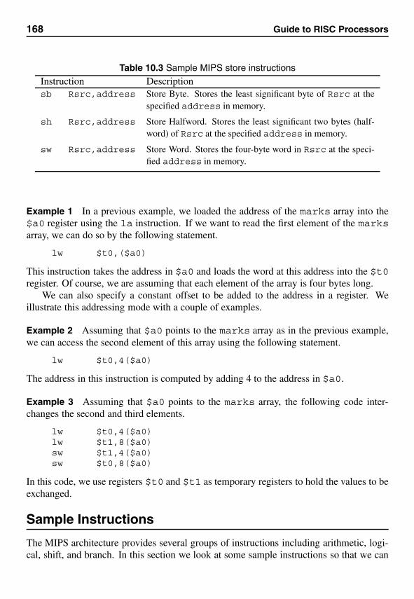
168 Guide to RISC Processors
Table 10.3 Sample MIPS store instructions
Instruction Descriptionsb Rsrc,address Store Byte. Stores the least significant byte of Rsrc at the
specified address in memory.
sh Rsrc,address Store Halfword. Stores the least significant two bytes (half-word) of Rsrc at the specified address in memory.
sw Rsrc,address Store Word. Stores the four-byte word in Rsrc at the speci-fied address in memory.
Example 1 In a previous example, we loaded the address of the marks array into the$a0 register using the la instruction. If we want to read the first element of the marksarray, we can do so by the following statement.
lw $t0,($a0)
This instruction takes the address in $a0 and loads the word at this address into the $t0register. Of course, we are assuming that each element of the array is four bytes long.
We can also specify a constant offset to be added to the address in a register. Weillustrate this addressing mode with a couple of examples.
Example 2 Assuming that $a0 points to the marks array as in the previous example,we can access the second element of this array using the following statement.
lw $t0,4($a0)
The address in this instruction is computed by adding 4 to the address in $a0.
Example 3 Assuming that $a0 points to the marks array, the following code inter-changes the second and third elements.
lw $t0,4($a0)lw $t1,8($a0)sw $t1,4($a0)sw $t0,8($a0)
In this code, we use registers $t0 and $t1 as temporary registers to hold the values to beexchanged.
Sample Instructions
The MIPS architecture provides several groups of instructions including arithmetic, logi-cal, shift, and branch. In this section we look at some sample instructions so that we can
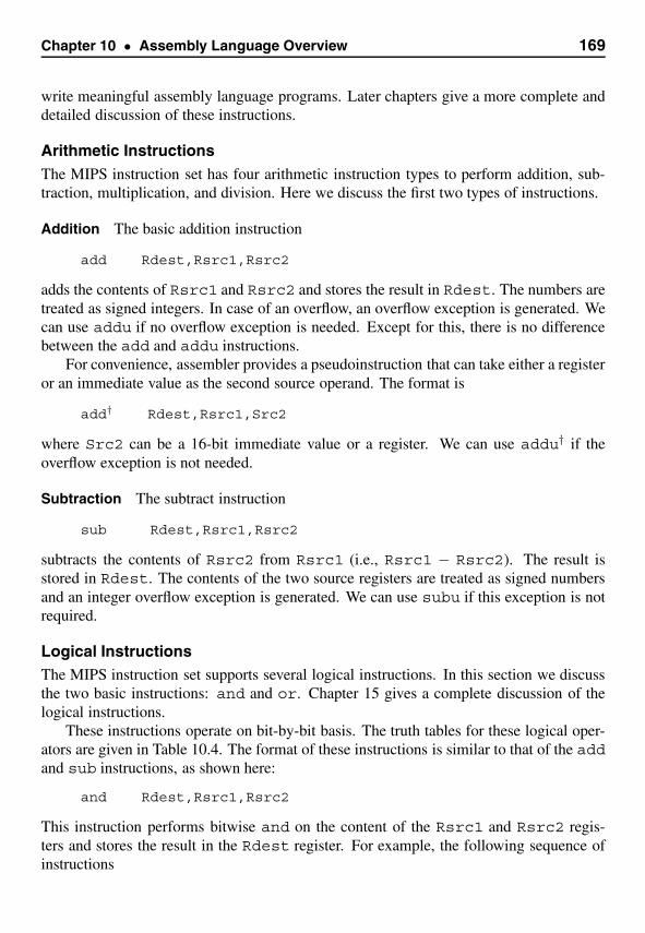
Chapter 10 • Assembly Language Overview 169
write meaningful assembly language programs. Later chapters give a more complete anddetailed discussion of these instructions.
Arithmetic InstructionsThe MIPS instruction set has four arithmetic instruction types to perform addition, sub-traction, multiplication, and division. Here we discuss the first two types of instructions.
Addition The basic addition instruction
add Rdest,Rsrc1,Rsrc2
adds the contents of Rsrc1 and Rsrc2 and stores the result in Rdest. The numbers aretreated as signed integers. In case of an overflow, an overflow exception is generated. Wecan use addu if no overflow exception is needed. Except for this, there is no differencebetween the add and addu instructions.
For convenience, assembler provides a pseudoinstruction that can take either a registeror an immediate value as the second source operand. The format is
add† Rdest,Rsrc1,Src2
where Src2 can be a 16-bit immediate value or a register. We can use addu† if theoverflow exception is not needed.
Subtraction The subtract instruction
sub Rdest,Rsrc1,Rsrc2
subtracts the contents of Rsrc2 from Rsrc1 (i.e., Rsrc1 − Rsrc2). The result isstored in Rdest. The contents of the two source registers are treated as signed numbersand an integer overflow exception is generated. We can use subu if this exception is notrequired.
Logical InstructionsThe MIPS instruction set supports several logical instructions. In this section we discussthe two basic instructions: and and or. Chapter 15 gives a complete discussion of thelogical instructions.
These instructions operate on bit-by-bit basis. The truth tables for these logical oper-ators are given in Table 10.4. The format of these instructions is similar to that of the addand sub instructions, as shown here:
and Rdest,Rsrc1,Rsrc2
This instruction performs bitwise and on the content of the Rsrc1 and Rsrc2 regis-ters and stores the result in the Rdest register. For example, the following sequence ofinstructions
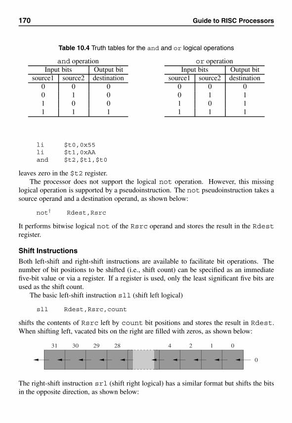
170 Guide to RISC Processors
Table 10.4 Truth tables for the and and or logical operations
and operation or operationInput bits Output bit Input bits Output bit
source1 source2 destination source1 source2 destination0 0 0 0 0 00 1 0 0 1 11 0 0 1 0 11 1 1 1 1 1
li $t0,0x55li $t1,0xAAand $t2,$t1,$t0
leaves zero in the $t2 register.The processor does not support the logical not operation. However, this missing
logical operation is supported by a pseudoinstruction. The not pseudoinstruction takes asource operand and a destination operand, as shown below:
not† Rdest,Rsrc
It performs bitwise logical not of the Rsrc operand and stores the result in the Rdestregister.
Shift InstructionsBoth left-shift and right-shift instructions are available to facilitate bit operations. Thenumber of bit positions to be shifted (i.e., shift count) can be specified as an immediatefive-bit value or via a register. If a register is used, only the least significant five bits areused as the shift count.
The basic left-shift instruction sll (shift left logical)
sll Rdest,Rsrc,count
shifts the contents of Rsrc left by count bit positions and stores the result in Rdest.When shifting left, vacated bits on the right are filled with zeros, as shown below:
012428293031
0
The right-shift instruction srl (shift right logical) has a similar format but shifts the bitsin the opposite direction, as shown below:

Chapter 10 • Assembly Language Overview 171
012428293031
0
As with the sll instruction, the vacated bits are replaced by zeros. These shifts are calledlogical shifts. In Chapter 15 we show another category of shifts called arithmetic shiftswhen dealing with the right-shifts.
Branch InstructionsThe MIPS instruction set provides several instructions to alter flow control. These includeboth unconditional and conditional branch instructions. Here we discuss a few of theseinstructions. The unconditional branch instruction
b† target
transfers control to target unconditionally. As indicated here, this is a pseudoinstruc-tion. Here is an example that illustrates the use of the unconditional branch instruction:
li $t0,50repeat:
add $t1,$t1,1sub $t0,$t0,1b repeat
As written here, it is an infinite loop! We modify this code later to terminate the loop after50 iterations. For this, we need a conditional branch instruction.
There are several conditional branch instructions. Recall from our discussion in Chap-ter 2 (on page 24) that conditional branch can be done in one of two ways: set-then-jumpor test-and-jump. The MIPS instruction set provides several instructions to perform test-and-jump conditional branching. For example, the branch on not equal instruction
bne Rsrc1,Rsrc2,target
tests the contents of the two registers Rsrc1 and Rsrc2 for equality and transfers controlto target if Rsrc1 �= Rsrc2. If we assume that the numbers to be compared are inregisters $t0 and $t1, we can write the branch instruction as
bne $t1,$t0,target
The condition tested can be changed to “equal to”, “less than”, and so on. For example,the conditional branch instruction
blt Rsrc1,Rsrc2,target
compares the contents of Rsrc1 and Rsrc2 and transfers control to target if Rsrc1< Rsrc2. In comparing the contents of these two registers, they are treated as signednumbers. For example, if $t1 = 5 and $t0 = −1, the instruction

172 Guide to RISC Processors
bne $t0,$t1,target
transfers control to target as $t0 < $t1. However, if we treat the contents of theseregisters as unsigned, the condition $t0 < $t1 is not true as $t0 contains all 1 bits(that’s how −1 is stored in 2’s complement notation). If you want to treat the numberas unsigned, simply append the mnemonic with a u as in bltu. For a complete list ofconditional branch instructions, see Table 14.2.
The MIPS instruction set also provides another group of conditional branch instruc-tions that compare the value of a register to zero. For example, consider the beqz in-struction shown below:
bnez Rsrc,target
This instruction transfers control to target if the value of Rsrc is not equal to zero.Using this instruction, we can rewrite the previous infinite loop code fragment as
li $t0,50repeat:
add $t1,$t1,1sub $t0,$t0,1bnez $t0,repeat
to terminate after 50 iterations.We can also use other relationships such as “less then”, “greater than” and so on. A
complete list of these conditional branch instructions is given in Table 14.3 on page 250.
Our First Program
Let us look at our first MIPS assembly language program. The main goal is to showwhat MIPS programs look like. We give several other examples in the next section. Theprogram listing shown in Program 10.1 adds three integers. The program follows thetemplate given in Figure 10.1. The data segment consists of three messages; all three aredeclared as NULL-terminated ASCII strings (see lines 9–14).
Program 10.1 A simple program to add three integers
1: # Find the sum of three numbers SUM3.ASM2: #3: # Objective: Finds the sum of three integers.4: # Input: Requests three numbers.5: # Output: Outputs the sum.6: #7: ################### Data segment ###################8: .data9: prompt:
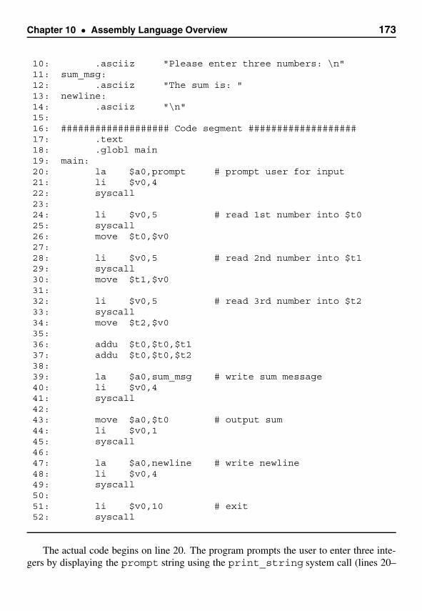
Chapter 10 • Assembly Language Overview 173
10: .asciiz "Please enter three numbers: \n"11: sum_msg:12: .asciiz "The sum is: "13: newline:14: .asciiz "\n"15:16: ################### Code segment ###################17: .text18: .globl main19: main:20: la $a0,prompt # prompt user for input21: li $v0,422: syscall23:24: li $v0,5 # read 1st number into $t025: syscall26: move $t0,$v027:28: li $v0,5 # read 2nd number into $t129: syscall30: move $t1,$v031:32: li $v0,5 # read 3rd number into $t233: syscall34: move $t2,$v035:36: addu $t0,$t0,$t137: addu $t0,$t0,$t238:39: la $a0,sum_msg # write sum message40: li $v0,441: syscall42:43: move $a0,$t0 # output sum44: li $v0,145: syscall46:47: la $a0,newline # write newline48: li $v0,449: syscall50:51: li $v0,10 # exit52: syscall
The actual code begins on line 20. The program prompts the user to enter three inte-gers by displaying the prompt string using the print_string system call (lines 20–
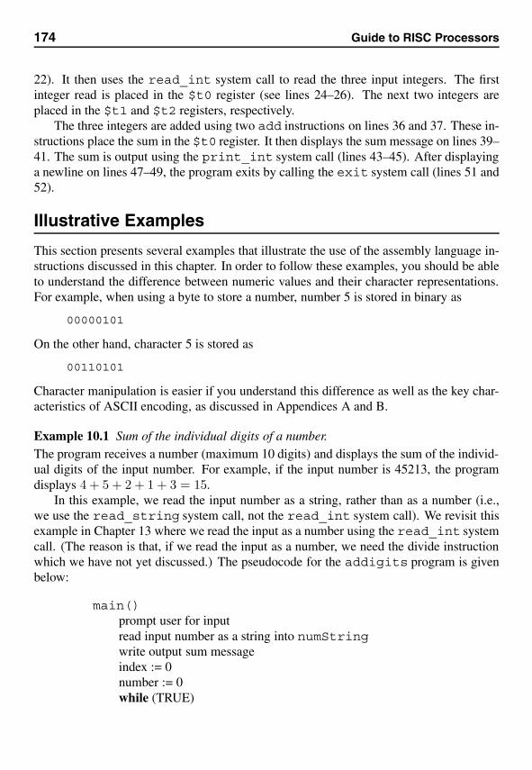
174 Guide to RISC Processors
22). It then uses the read_int system call to read the three input integers. The firstinteger read is placed in the $t0 register (see lines 24–26). The next two integers areplaced in the $t1 and $t2 registers, respectively.
The three integers are added using two add instructions on lines 36 and 37. These in-structions place the sum in the $t0 register. It then displays the sum message on lines 39–41. The sum is output using the print_int system call (lines 43–45). After displayinga newline on lines 47–49, the program exits by calling the exit system call (lines 51 and52).
Illustrative Examples
This section presents several examples that illustrate the use of the assembly language in-structions discussed in this chapter. In order to follow these examples, you should be ableto understand the difference between numeric values and their character representations.For example, when using a byte to store a number, number 5 is stored in binary as
00000101
On the other hand, character 5 is stored as
00110101
Character manipulation is easier if you understand this difference as well as the key char-acteristics of ASCII encoding, as discussed in Appendices A and B.
Example 10.1 Sum of the individual digits of a number.The program receives a number (maximum 10 digits) and displays the sum of the individ-ual digits of the input number. For example, if the input number is 45213, the programdisplays 4 + 5 + 2 + 1 + 3 = 15.
In this example, we read the input number as a string, rather than as a number (i.e.,we use the read_string system call, not the read_int system call). We revisit thisexample in Chapter 13 where we read the input as a number using the read_int systemcall. (The reason is that, if we read the input as a number, we need the divide instructionwhich we have not yet discussed.) The pseudocode for the addigits program is givenbelow:
main()prompt user for inputread input number as a string into numStringwrite output sum messageindex := 0number := 0while (TRUE)
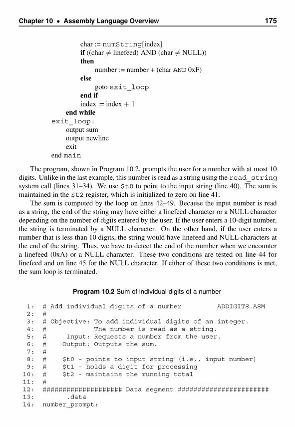
Chapter 10 • Assembly Language Overview 175
char := numString[index]if ((char �= linefeed) AND (char �= NULL))then
number := number + (char AND 0xF)else
goto exit_loopend ifindex := index + 1
end whileexit_loop:
output sumoutput newlineexit
end main
The program, shown in Program 10.2, prompts the user for a number with at most 10digits. Unlike in the last example, this number is read as a string using the read_stringsystem call (lines 31–34). We use $t0 to point to the input string (line 40). The sum ismaintained in the $t2 register, which is initialized to zero on line 41.
The sum is computed by the loop on lines 42–49. Because the input number is readas a string, the end of the string may have either a linefeed character or a NULL characterdepending on the number of digits entered by the user. If the user enters a 10-digit number,the string is terminated by a NULL character. On the other hand, if the user enters anumber that is less than 10 digits, the string would have linefeed and NULL characters atthe end of the string. Thus, we have to detect the end of the number when we encountera linefeed (0xA) or a NULL character. These two conditions are tested on line 44 forlinefeed and on line 45 for the NULL character. If either of these two conditions is met,the sum loop is terminated.
Program 10.2 Sum of individual digits of a number
1: # Add individual digits of a number ADDIGITS.ASM2: #3: # Objective: To add individual digits of an integer.4: # The number is read as a string.5: # Input: Requests a number from the user.6: # Output: Outputs the sum.7: #8: # $t0 - points to input string (i.e., input number)9: # $t1 - holds a digit for processing
10: # $t2 - maintains the running total11: #12: #################### Data segment #######################13: .data14: number_prompt:
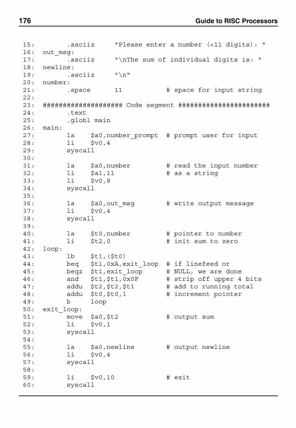
176 Guide to RISC Processors
15: .asciiz "Please enter a number (<11 digits): "16: out_msg:17: .asciiz "\nThe sum of individual digits is: "18: newline:19: .asciiz "\n"20: number:21: .space 11 # space for input string22:23: #################### Code segment #######################24: .text25: .globl main26: main:27: la $a0,number_prompt # prompt user for input28: li $v0,429: syscall30:31: la $a0,number # read the input number32: li $a1,11 # as a string33: li $v0,834: syscall35:36: la $a0,out_msg # write output message37: li $v0,438: syscall39:40: la $t0,number # pointer to number41: li $t2,0 # init sum to zero42: loop:43: lb $t1,($t0)44: beq $t1,0xA,exit_loop # if linefeed or45: beqz $t1,exit_loop # NULL, we are done46: and $t1,$t1,0x0F # strip off upper 4 bits47: addu $t2,$t2,$t1 # add to running total48: addu $t0,$t0,1 # increment pointer49: b loop50: exit_loop:51: move $a0,$t2 # output sum52: li $v0,153: syscall54:55: la $a0,newline # output newline56: li $v0,457: syscall58:59: li $v0,10 # exit60: syscall

Chapter 10 • Assembly Language Overview 177
The loop body to compute the sum follows the pseudocode given before. The inputdigit, which is in character form, must be converted to its numeric equivalent. BecauseASCII assigns a special set of contiguous values to the digit characters, this conversionis straightforward. All we have to do is to mask off the upper half of the byte. Thisconversion is done by
and $t1,$t1,0xF
on line 46. Alternatively, we could also subtract the character code for 0 as
sub $t1,$t1,’0’
instead of masking the upper half-byte. This numeric value is added to the sum (main-tained in $t2) on line 47. The string pointer in $t0 is incremented to point to the nextinput digit (line 48). When the loop is exited, we simply output the sum in the $t2register.
Example 10.2 Conversion of lowercase letters to uppercase.This program demonstrates how character manipulation can be used to convert lowercaseletters to uppercase. The program receives a character string from the user and converts alllowercase letters to uppercase and displays the string. Characters other than the lowercaseletters are not changed in any way. The pseudocode of Program 10.3 is shown below:
main()prompt user for inputread input stringwrite output sum messageindex := 0char := string[index]while (char �= NULL)
if ((char ≥ ’a’) AND (char ≤ ’z’))then
char := char + ’A’ − ’a’end ifindex := index + 1char := string[index]
end whileoutput stringexit
end main
We can see from Program 10.3 that the compound if condition requires two condi-tional branch instructions. The conditional branch instruction blt on line 41 tests if thecharacter is less than a. If so, it is not a lowercase character and conversion is not done.
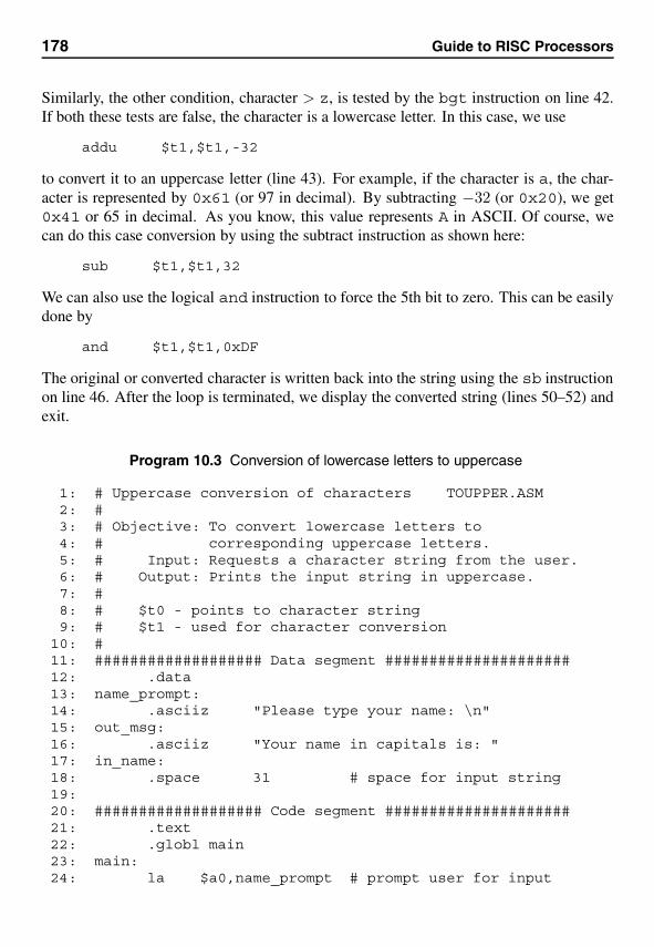
178 Guide to RISC Processors
Similarly, the other condition, character > z, is tested by the bgt instruction on line 42.If both these tests are false, the character is a lowercase letter. In this case, we use
addu $t1,$t1,-32
to convert it to an uppercase letter (line 43). For example, if the character is a, the char-acter is represented by 0x61 (or 97 in decimal). By subtracting −32 (or 0x20), we get0x41 or 65 in decimal. As you know, this value represents A in ASCII. Of course, wecan do this case conversion by using the subtract instruction as shown here:
sub $t1,$t1,32
We can also use the logical and instruction to force the 5th bit to zero. This can be easilydone by
and $t1,$t1,0xDF
The original or converted character is written back into the string using the sb instructionon line 46. After the loop is terminated, we display the converted string (lines 50–52) andexit.
Program 10.3 Conversion of lowercase letters to uppercase
1: # Uppercase conversion of characters TOUPPER.ASM2: #3: # Objective: To convert lowercase letters to4: # corresponding uppercase letters.5: # Input: Requests a character string from the user.6: # Output: Prints the input string in uppercase.7: #8: # $t0 - points to character string9: # $t1 - used for character conversion
10: #11: ################### Data segment #####################12: .data13: name_prompt:14: .asciiz "Please type your name: \n"15: out_msg:16: .asciiz "Your name in capitals is: "17: in_name:18: .space 31 # space for input string19:20: ################### Code segment #####################21: .text22: .globl main23: main:24: la $a0,name_prompt # prompt user for input
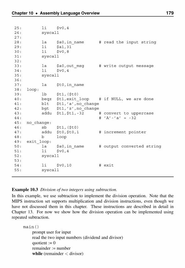
Chapter 10 • Assembly Language Overview 179
25: li $v0,426: syscall27:28: la $a0,in_name # read the input string29: li $a1,3130: li $v0,831: syscall32:33: la $a0,out_msg # write output message34: li $v0,435: syscall36:37: la $t0,in_name38: loop:39: lb $t1,($t0)40: beqz $t1,exit_loop # if NULL, we are done41: blt $t1,’a’,no_change42: bgt $t1,’z’,no_change43: addu $t1,$t1,-32 # convert to uppercase44: # ’A’-’a’ = -3245: no_change:46: sb $t1,($t0)47: addu $t0,$t0,1 # increment pointer48: b loop49: exit_loop:50: la $a0,in_name # output converted string51: li $v0,452: syscall53:54: li $v0,10 # exit55: syscall
Example 10.3 Division of two integers using subtraction.In this example, we use subtraction to implement the division operation. Note that theMIPS instruction set supports multiplication and division instructions, even though wehave not discussed them in this chapter. These instructions are described in detail inChapter 13. For now we show how the division operation can be implemented usingrepeated subtraction.
main()prompt user for inputread the two input numbers (dividend and divisor)quotient := 0remainder := numberwhile (remainder < divisor)
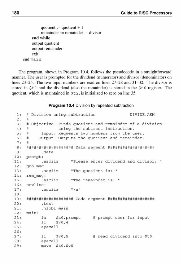
180 Guide to RISC Processors
quotient := quotient + 1remainder := remainder − divisor
end whileoutput quotientoutput remainderexit
end main
The program, shown in Program 10.4, follows the pseudocode in a straightforwardmanner. The user is prompted for the dividend (numerator) and divisor (denominator) onlines 23–25. The two input numbers are read on lines 27–28 and 31–32. The divisor isstored in $t1 and the dividend (also the remainder) is stored in the $t0 register. Thequotient, which is maintained in $t2, is initialized to zero on line 35.
Program 10.4 Division by repeated subtraction
1: # Division using subtraction DIVIDE.ASM2: #3: # Objective: Finds quotient and remainder of a division4: # using the subtract instruction.5: # Input: Requests two numbers from the user.6: # Output: Outputs the quotient and remainder.7: #8: ################### Data segment ###################9: .data
10: prompt:11: .asciiz "Please enter dividend and divisor: "12: quo_msg:13: .asciiz "The quotient is: "14: rem_msg:15: .asciiz "The remainder is: "16: newline:17: .asciiz "\n"18:19: ################### Code segment ###################20: .text21: .globl main22: main:23: la $a0,prompt # prompt user for input24: li $v0,425: syscall26:27: li $v0,5 # read dividend into $t028: syscall29: move $t0,$v0
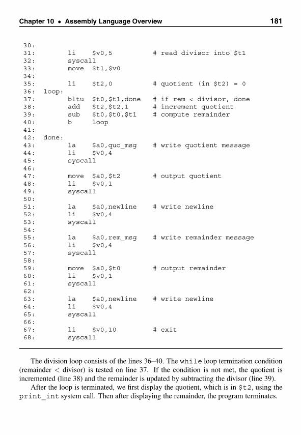
Chapter 10 • Assembly Language Overview 181
30:31: li $v0,5 # read divisor into $t132: syscall33: move $t1,$v034:35: li $t2,0 # quotient (in $t2) = 036: loop:37: bltu $t0,$t1,done # if rem < divisor, done38: add $t2,$t2,1 # increment quotient39: sub $t0,$t0,$t1 # compute remainder40: b loop41:42: done:43: la $a0,quo_msg # write quotient message44: li $v0,445: syscall46:47: move $a0,$t2 # output quotient48: li $v0,149: syscall50:51: la $a0,newline # write newline52: li $v0,453: syscall54:55: la $a0,rem_msg # write remainder message56: li $v0,457: syscall58:59: move $a0,$t0 # output remainder60: li $v0,161: syscall62:63: la $a0,newline # write newline64: li $v0,465: syscall66:67: li $v0,10 # exit68: syscall
The division loop consists of the lines 36–40. The while loop termination condition(remainder < divisor) is tested on line 37. If the condition is not met, the quotient isincremented (line 38) and the remainder is updated by subtracting the divisor (line 39).
After the loop is terminated, we first display the quotient, which is in $t2, using theprint_int system call. Then after displaying the remainder, the program terminates.
182 Guide to RISC Processors
Summary
In this chapter, we presented the basics of the MIPS assembly language programming.We discussed three types of assembly language statements:
1. Executable statements that instruct the processor as to what to do;2. Pseudoinstructions that are supported by the assembler;3. Assembler directives that facilitate the assembly process.
Assembler directives to allocate storage space for data variables and to define numeric andstring constants were discussed in detail. The assembler extends the processor instructionset by providing several pseudoinstructions. It translates these pseudoinstructions to oneor more processor instructions. We have given an example to show how the assemblerdoes this translation. We give more examples in later chapters.
We have given an overview of the MIPS instruction set. Although we discussed in de-tail the load and store instructions, there was only a brief review of the remaining instruc-tions of the MIPS instruction set. A detailed discussion of these instructions is providedin later chapters.
11Procedures and the Stack
We have given an overview of the MIPS assembly language in the last chapter. Thischapter discusses how procedures are written in the MIPS assembly language. Procedureis an important programming construct that facilitates modular programming. Procedurescan be divided into leaf and nonleaf procedures. A leaf procedure does not call otherprocedures. On the other hand, a nonleaf procedure calls other procedures. In the MIPSarchitecture, we can implement simple leaf procedures without using the stack. Nonleafprocedures always need to use the stack, at least to store the return address of the callingprocedure.
In this chapter, we discuss how both leaf and nonleaf procedures are implemented inthe assembly language. Our initial discussion deals with simple leaf procedures that canbe implemented using the registers. Then we look at how the stack is implemented in theMIPS architecture. The details about the stack implementation are useful in understandinghow we can handle nonleaf procedures in the assembly language.
Parameter passing is an important aspect of procedure invocation. As you know, wecan use either the call-by-value or call-by-reference mechanism for parameter passing.Here we give details on how we can implement these two types of parameter-passingmechanisms in the assembly language programs.
IntroductionA procedure is a logically self-contained unit of code designed to perform a specific task.Procedures are sometimes called subprograms and play an important role in modular pro-gram development. In high-level languages, there are two types of subprograms: proce-dures and functions. Each function receives a list of arguments and performs a computa-tion based on the arguments passed onto it and returns a single value.
Procedures also receive a list of arguments just as the functions do. However, pro-cedures, after performing their computation, may return zero or more results back to thecalling procedure. In C language, both these subprogram types are combined into a single
183
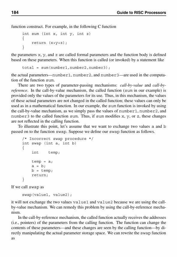
184 Guide to RISC Processors
function construct. For example, in the following C function
int sum (int x, int y, int z){
return (x+y+z);}
the parameters x, y, and z are called formal parameters and the function body is definedbased on these parameters. When this function is called (or invoked) by a statement like
total = sum(number1,number2,number3);
the actual parameters—number1, number2, and number3—are used in the computa-tion of the function sum.
There are two types of parameter-passing mechanisms: call-by-value and call-by-reference. In the call-by-value mechanism, the called function (sum in our example) isprovided only the values of the parameters for its use. Thus, in this mechanism, the valuesof these actual parameters are not changed in the called function; these values can only beused as in a mathematical function. In our example, the sum function is invoked by usingthe call-by-value mechanism, as we simply pass the values of number1, number2, andnumber3 to the called function sum. Thus, if sum modifies x, y, or z, these changesare not reflected in the calling function.
To illustrate this point, let’s assume that we want to exchange two values a and bpassed on to the function swap. Suppose we define our swap function as follows.
/* Incorrect swap procedure */int swap (int a, int b){
int temp;
temp = a;a = b;b = temp;return;
}
If we call swap as
swap(value1, value2);
it will not exchange the two values value1 and value2 because we are using the call-by-value mechanism. We can remedy this problem by using the call-by-reference mecha-nism.
In the call-by-reference mechanism, the called function actually receives the addresses(i.e., pointers) of the parameters from the calling function. The function can change thecontents of these parameters—and these changes are seen by the calling function—by di-rectly manipulating the actual parameter storage space. We can rewrite the swap functionas
Chapter 11 • Procedures and the Stack 185
/* Correct swap procedure */void swap (int *a, int *b){
int temp;
temp = *a;*a = *b;*b = temp;
}
This procedure works fine as it passes the addresses of the two parameters from the callingfunction. Such a function can be invoked as
swap (&data1, &data2);
Often both types of parameter-passing mechanisms are used in the same function. Asan example, consider finding the roots of the quadratic equation
ax2 + bx + c = 0 .
The two roots are defined as
root1 =−b +
√b2 − 4ac
2a,
root2 =−b −√
b2 − 4ac
2a.
The roots are real if b2 ≥ 4ac, and imaginary otherwise.Suppose that we want to write a function that receives a, b, and c and returns the
values of the two roots (if real) and indicates whether the roots are real or imaginary.
int roots (double a, double b, double c,double *root1, double *root2)
{int root_type = 1;if (4*a*c <= b*b){ /* roots are real */
*root1 = (−b + sqrt(b*b − 4*a*c))/(2*a);*root2 = (−b − sqrt(b*b − 4*a*c))/(2*a);
}else /* roots are imaginary */
root_type = 0;return (root_type);
}
The function receives parameters a, b, and c via the call-by-value mechanism, and root1and root2 parameters are passed using the call-by-reference mechanism. A typical in-vocation of roots is
186 Guide to RISC Processors
root_type = roots (a, b, c, &root1, &root2);
In summary, procedures receive a list of parameters, which may be passed either bythe call-by-value or by the call-by-reference mechanism. If more than one result is tobe returned by a called procedure, the call-by-reference parameter-passing mechanismshould be used.
Procedure InvocationMIPS provides two instructions to support procedures: jal and jr. The jal instructionis used for calling a procedure and jr is used to return from a procedure. In this section,we discuss the jal instruction. The jr instruction is discussed in the next section.
The jal (jump and link) instruction
jal proc_name
transfers control to proc_name just as a jump instruction does. Because we need thereturn address to return from the called procedure, it also stores the address of the instruc-tion following the delayed slot instruction in the $ra register. Here are the actions takenin invoking a procedure using the jal instruction:
$ra = PC + 8PC = PC[31:28] || offset<<2
Notice that $ra (i.e., $31) is loaded with PC+8, not PC+4. This is because of the delayedslot instruction (see our discussion on page 25). Thus the control returns to the instructionfollowing the delayed slot instruction.
This instruction uses the J-type instruction encoding shown in Figure 4.2 on page 52.As you can see from this figure, it uses 26 bits to specify the offset. The target address iscomputed as follows. The 26-bit offset specified in the instruction is shifted left by two bitpositions because of the 32-bit alignment. This gives us 28 bits and the remaining 4 bitsare taken from the PC. Before the control is transferred, the delayed branch instruction isexecuted.
SPIM noteBecause SPIM simulates the MIPS R2000 processor, it does notsimulate the delayed branch. Thus, it performs $ra = PC + 4.
An ExampleTo understand the procedure invocation mechanism, let’s look at the program fragment,obtained from SPIM, shown in Figure 11.1. This code consists of three procedures: main,avg, and sum. The first column gives the address of each instruction (the 0x prefix
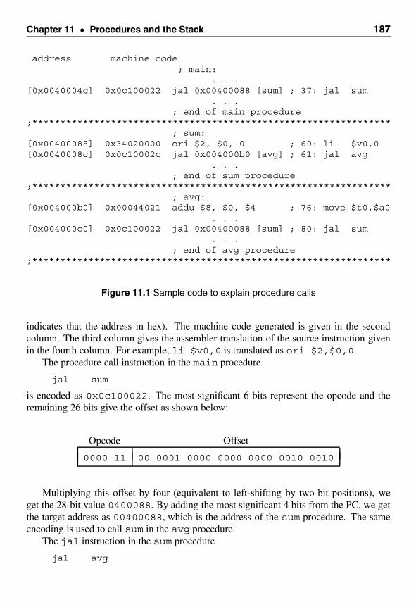
Chapter 11 • Procedures and the Stack 187
address machine code; main:
. . .[0x0040004c] 0x0c100022 jal 0x00400088 [sum] ; 37: jal sum
. . .; end of main procedure
;****************************************************************; sum:
[0x00400088] 0x34020000 ori $2, $0, 0 ; 60: li $v0,0[0x0040008c] 0x0c10002c jal 0x004000b0 [avg] ; 61: jal avg
. . .; end of sum procedure
;****************************************************************; avg:
[0x004000b0] 0x00044021 addu $8, $0, $4 ; 76: move $t0,$a0. . .
[0x004000c0] 0x0c100022 jal 0x00400088 [sum] ; 80: jal sum. . .
; end of avg procedure;****************************************************************
Figure 11.1 Sample code to explain procedure calls
indicates that the address in hex). The machine code generated is given in the secondcolumn. The third column gives the assembler translation of the source instruction givenin the fourth column. For example, li $v0,0 is translated as ori $2,$0,0.
The procedure call instruction in the main procedure
jal sum
is encoded as 0x0c100022. The most significant 6 bits represent the opcode and theremaining 26 bits give the offset as shown below:
Opcode Offset
0000 11 00 0001 0000 0000 0000 0010 0010
Multiplying this offset by four (equivalent to left-shifting by two bit positions), weget the 28-bit value 0400088. By adding the most significant 4 bits from the PC, we getthe target address as 00400088, which is the address of the sum procedure. The sameencoding is used to call sum in the avg procedure.
The jal instruction in the sum procedure
jal avg
188 Guide to RISC Processors
is encoded as 0x0c10002c, which consists of 000011 as the opcode and 0x010002cas the offset value as shown below:
Opcode Offset
0000 11 00 0001 0000 0000 0000 0010 1100
Following the target computation process described before, we get 04000b0 by multi-plying the 26-bit offset 10002c by 4. Adding the 4 most significant PC bits, we get thetarget address of avg as 004000b0.
Returning from a Procedure
To return from a procedure, we use
jr $ra
which reads the return address from the $ra register and transfers control to this address.In the MIPS32 architecture, the instruction following the jr instruction, which is in thebranch delay slot, is executed before transferring control. However, see the followingSPIM note.
SPIM noteBecause the SPIM simulator does not simulate the delayed branch,the control is transferred to the address in the $ra register.
Note that this instruction is a special case of the general jr instruction. In this in-struction, you can specify a register that contains the target address of the jump and hasthe following format.
jr rs
This instruction is encoded as follows.
Opcode Offset
0000 00 rs (5 bits) 00 0000 0000 hint (5 bits) 00 1000
In release 1 of the MIPS architecture, only 0 is defined as the valid hint value. This is thevalue SPIM uses in encoding the jr instruction. For the rs we can substitute the numberof the source register. To return from a procedure, we use $ra, which is r31. Thus,
Chapter 11 • Procedures and the Stack 189
substituting 31 for the rs field, we get the encoding 0x03e00008 for the jr $rainstruction.
Parameter Passing
Parameter passing in assembly language is different and more complicated than that usedin high-level languages. In assembly language, the calling procedure first places all theparameters needed by the called procedure in a mutually accessible storage area (usuallyregisters or memory). Only then can the procedure be invoked.
There are two common methods depending on the type of storage area used to pass pa-rameters: the register method or stack method. As their names imply, the register methoduses general registers to pass parameters, and the stack is used in the other method. Welook at the register method in this section. Stack-based parameter passing is discussedlater.
Recall from our discussion in Chapter 4 that registers $v0 and $v1 are used to returnresults from a procedure. Registers $a0 to $a3 are used to pass the first four parametersto procedures. The remaining parameters are passed via the stack.
We can divide procedures into two major types: leaf procedures and nonleaf pro-cedures. Leaf procedures do not call other procedures whereas nonleaf procedures do.Simple leaf procedures do not have to use the stack if its local variables can fit the caller-save registers $t0 to $t9. If this is not the case, a leaf procedure will have to use thestack. Nonleaf procedures must use the stack, at least to store the return address. We saymore about these procedures later on.
Our First Program
This is a simple program to compute the sum of three integers (see Program 11.1). Ourmain goal is to explain the basics of the procedures in the MIPS assembly language. Themain program requests three integers and passes them to the find_sum procedure. Theprocedure returns the sum. Registers are used for parameter passing as well as to returnthe result. Registers $a0, $a1, and $a2 are used to pass the three integers. The procedurereturns the sum in $v0.
Program 11.1 Our first procedure example
1: # Find the sum of three numbers SUM.ASM2: #3: # Objective: Finds the sum of three integers.4: # To demonstrate register-based5: # parameter passing.6: # Input: Requests three numbers from the user.7: # Output: Outputs the sum.
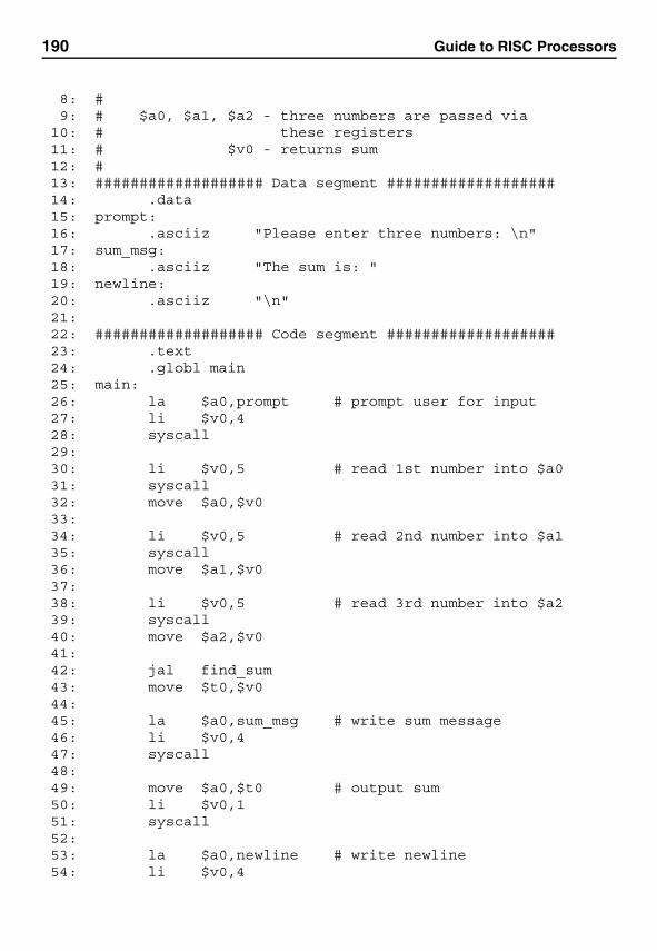
190 Guide to RISC Processors
8: #9: # $a0, $a1, $a2 - three numbers are passed via
10: # these registers11: # $v0 - returns sum12: #13: ################### Data segment ###################14: .data15: prompt:16: .asciiz "Please enter three numbers: \n"17: sum_msg:18: .asciiz "The sum is: "19: newline:20: .asciiz "\n"21:22: ################### Code segment ###################23: .text24: .globl main25: main:26: la $a0,prompt # prompt user for input27: li $v0,428: syscall29:30: li $v0,5 # read 1st number into $a031: syscall32: move $a0,$v033:34: li $v0,5 # read 2nd number into $a135: syscall36: move $a1,$v037:38: li $v0,5 # read 3rd number into $a239: syscall40: move $a2,$v041:42: jal find_sum43: move $t0,$v044:45: la $a0,sum_msg # write sum message46: li $v0,447: syscall48:49: move $a0,$t0 # output sum50: li $v0,151: syscall52:53: la $a0,newline # write newline54: li $v0,4
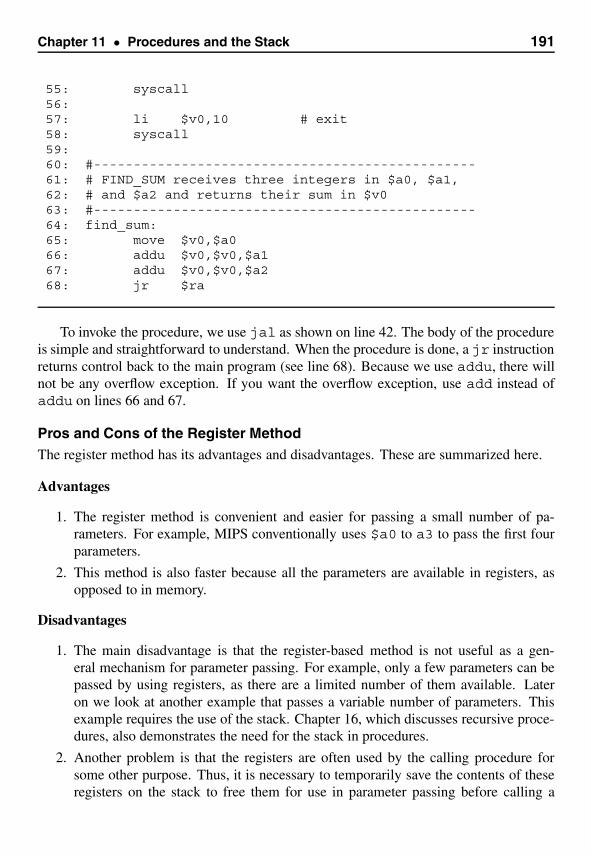
Chapter 11 • Procedures and the Stack 191
55: syscall56:57: li $v0,10 # exit58: syscall59:60: #------------------------------------------------61: # FIND_SUM receives three integers in $a0, $a1,62: # and $a2 and returns their sum in $v063: #------------------------------------------------64: find_sum:65: move $v0,$a066: addu $v0,$v0,$a167: addu $v0,$v0,$a268: jr $ra
To invoke the procedure, we use jal as shown on line 42. The body of the procedureis simple and straightforward to understand. When the procedure is done, a jr instructionreturns control back to the main program (see line 68). Because we use addu, there willnot be any overflow exception. If you want the overflow exception, use add instead ofaddu on lines 66 and 67.
Pros and Cons of the Register MethodThe register method has its advantages and disadvantages. These are summarized here.
Advantages
1. The register method is convenient and easier for passing a small number of pa-rameters. For example, MIPS conventionally uses $a0 to a3 to pass the first fourparameters.
2. This method is also faster because all the parameters are available in registers, asopposed to in memory.
Disadvantages
1. The main disadvantage is that the register-based method is not useful as a gen-eral mechanism for parameter passing. For example, only a few parameters can bepassed by using registers, as there are a limited number of them available. Lateron we look at another example that passes a variable number of parameters. Thisexample requires the use of the stack. Chapter 16, which discusses recursive proce-dures, also demonstrates the need for the stack in procedures.
2. Another problem is that the registers are often used by the calling procedure forsome other purpose. Thus, it is necessary to temporarily save the contents of theseregisters on the stack to free them for use in parameter passing before calling a
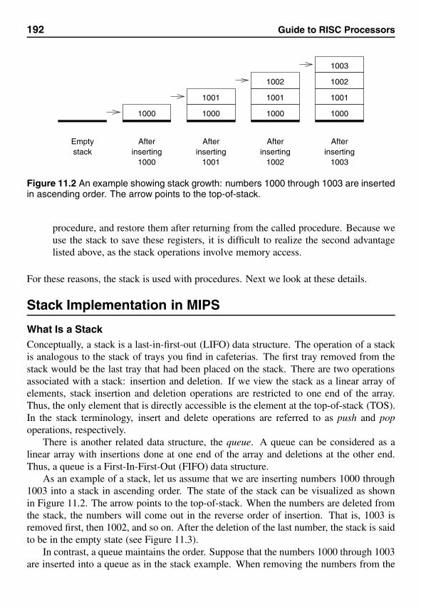
192 Guide to RISC Processors
1000 1000
1001
1000
1001
1002
1000
1001
1002
Emptystack
Afterinserting
1000
Afterinserting
1001
Afterinserting
1002
Afterinserting
1003
1003
Figure 11.2 An example showing stack growth: numbers 1000 through 1003 are insertedin ascending order. The arrow points to the top-of-stack.
procedure, and restore them after returning from the called procedure. Because weuse the stack to save these registers, it is difficult to realize the second advantagelisted above, as the stack operations involve memory access.
For these reasons, the stack is used with procedures. Next we look at these details.
Stack Implementation in MIPS
What Is a StackConceptually, a stack is a last-in-first-out (LIFO) data structure. The operation of a stackis analogous to the stack of trays you find in cafeterias. The first tray removed from thestack would be the last tray that had been placed on the stack. There are two operationsassociated with a stack: insertion and deletion. If we view the stack as a linear array ofelements, stack insertion and deletion operations are restricted to one end of the array.Thus, the only element that is directly accessible is the element at the top-of-stack (TOS).In the stack terminology, insert and delete operations are referred to as push and popoperations, respectively.
There is another related data structure, the queue. A queue can be considered as alinear array with insertions done at one end of the array and deletions at the other end.Thus, a queue is a First-In-First-Out (FIFO) data structure.
As an example of a stack, let us assume that we are inserting numbers 1000 through1003 into a stack in ascending order. The state of the stack can be visualized as shownin Figure 11.2. The arrow points to the top-of-stack. When the numbers are deleted fromthe stack, the numbers will come out in the reverse order of insertion. That is, 1003 isremoved first, then 1002, and so on. After the deletion of the last number, the stack is saidto be in the empty state (see Figure 11.3).
In contrast, a queue maintains the order. Suppose that the numbers 1000 through 1003are inserted into a queue as in the stack example. When removing the numbers from the
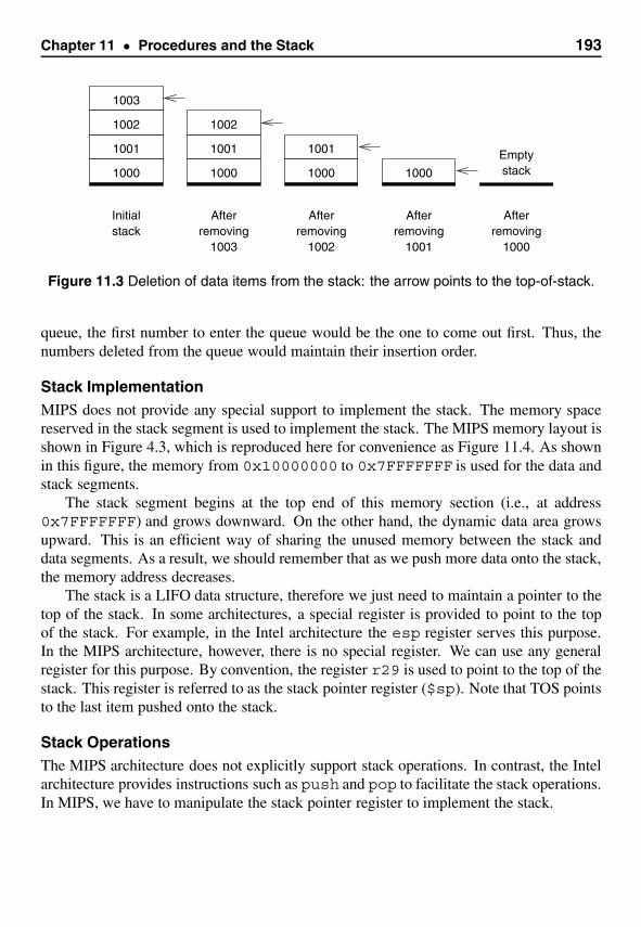
Chapter 11 • Procedures and the Stack 193
1000
1001
1002
1000
1001
1002
1000
1001
1000
Emptystack
Initialstack
After
1003removing
After
1002removing
After
1001removing
After
1000removing
1003
Figure 11.3 Deletion of data items from the stack: the arrow points to the top-of-stack.
queue, the first number to enter the queue would be the one to come out first. Thus, thenumbers deleted from the queue would maintain their insertion order.
Stack ImplementationMIPS does not provide any special support to implement the stack. The memory spacereserved in the stack segment is used to implement the stack. The MIPS memory layout isshown in Figure 4.3, which is reproduced here for convenience as Figure 11.4. As shownin this figure, the memory from 0x10000000 to 0x7FFFFFFF is used for the data andstack segments.
The stack segment begins at the top end of this memory section (i.e., at address0x7FFFFFFF) and grows downward. On the other hand, the dynamic data area growsupward. This is an efficient way of sharing the unused memory between the stack anddata segments. As a result, we should remember that as we push more data onto the stack,the memory address decreases.
The stack is a LIFO data structure, therefore we just need to maintain a pointer to thetop of the stack. In some architectures, a special register is provided to point to the topof the stack. For example, in the Intel architecture the esp register serves this purpose.In the MIPS architecture, however, there is no special register. We can use any generalregister for this purpose. By convention, the register r29 is used to point to the top of thestack. This register is referred to as the stack pointer register ($sp). Note that TOS pointsto the last item pushed onto the stack.
Stack OperationsThe MIPS architecture does not explicitly support stack operations. In contrast, the Intelarchitecture provides instructions such as push and pop to facilitate the stack operations.In MIPS, we have to manipulate the stack pointer register to implement the stack.
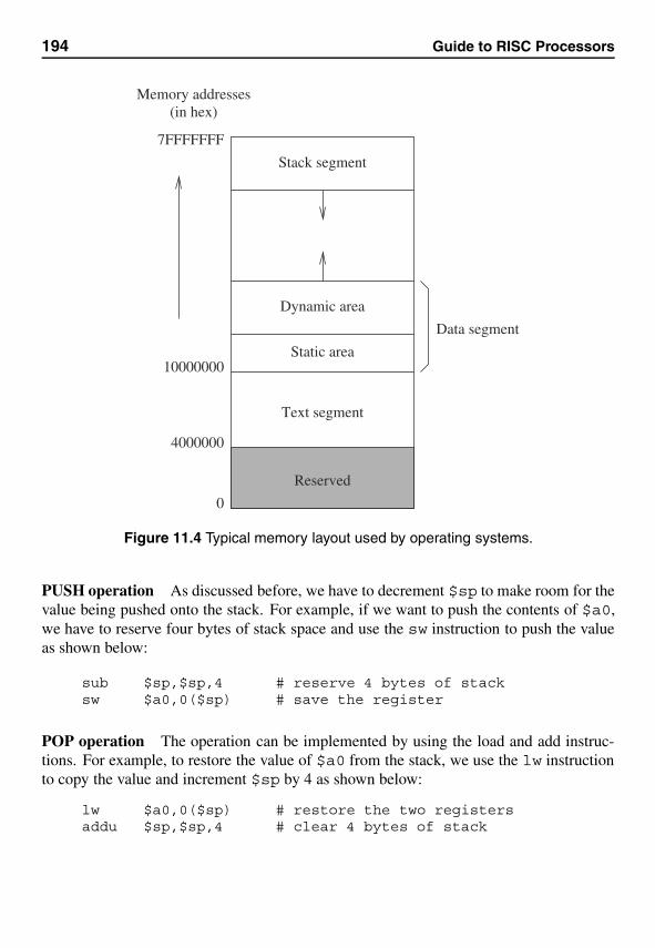
194 Guide to RISC Processors
Dynamic area
Static area
Reserved
Text segment
0
4000000
10000000
Data segment
Stack segment
7FFFFFFF
Memory addresses(in hex)
Figure 11.4 Typical memory layout used by operating systems.
PUSH operation As discussed before, we have to decrement $sp to make room for thevalue being pushed onto the stack. For example, if we want to push the contents of $a0,we have to reserve four bytes of stack space and use the sw instruction to push the valueas shown below:
sub $sp,$sp,4 # reserve 4 bytes of stacksw $a0,0($sp) # save the register
POP operation The operation can be implemented by using the load and add instruc-tions. For example, to restore the value of $a0 from the stack, we use the lw instructionto copy the value and increment $sp by 4 as shown below:
lw $a0,0($sp) # restore the two registersaddu $sp,$sp,4 # clear 4 bytes of stack
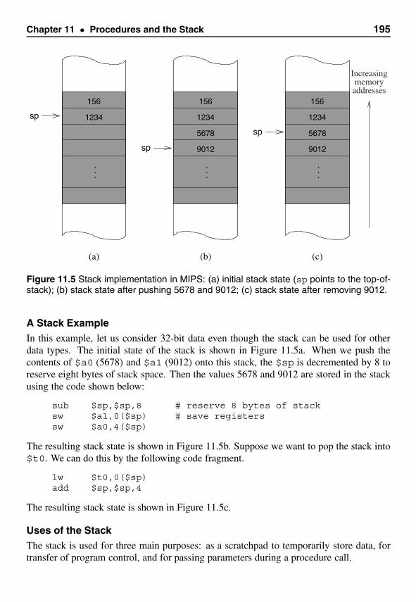
Chapter 11 • Procedures and the Stack 195
Increasingmemoryaddresses
......
...
156
1234
(a)
156
1234
(b)
5678
9012
156
1234
(c)
5678
9012sp
sp
sp
Figure 11.5 Stack implementation in MIPS: (a) initial stack state (sp points to the top-of-stack); (b) stack state after pushing 5678 and 9012; (c) stack state after removing 9012.
A Stack ExampleIn this example, let us consider 32-bit data even though the stack can be used for otherdata types. The initial state of the stack is shown in Figure 11.5a. When we push thecontents of $a0 (5678) and $a1 (9012) onto this stack, the $sp is decremented by 8 toreserve eight bytes of stack space. Then the values 5678 and 9012 are stored in the stackusing the code shown below:
sub $sp,$sp,8 # reserve 8 bytes of stacksw $a1,0($sp) # save registerssw $a0,4($sp)
The resulting stack state is shown in Figure 11.5b. Suppose we want to pop the stack into$t0. We can do this by the following code fragment.
lw $t0,0($sp)add $sp,$sp,4
The resulting stack state is shown in Figure 11.5c.
Uses of the StackThe stack is used for three main purposes: as a scratchpad to temporarily store data, fortransfer of program control, and for passing parameters during a procedure call.
196 Guide to RISC Processors
Temporary Storage of Data The stack can be used as a scratchpad to store data on atemporary basis. For example, suppose that a procedure (say, main) calls another pro-cedure test, which uses some of the callee-save registers (say, $s0, $s1, and $s2).Before using these registers, test must save the contents of these registers so that it canrestore them before returning control to main. The stack can be used for this purpose asshown below:
test:#save $s0, $s1, and $s2 registers on the stacksub $sp,$sp,12 # reserve 12 bytes of stacksw $s0,0($sp) # save registerssw $s1,4($sp)sw $s2,8($sp)# now these three registers can be used
. . .
. . .#restore $s0, $s1, and $s2 registers from the stacklw $s0,0($sp)lw $s1,4($sp)lw $s2,8($sp)add $sp,$sp,12
As demonstrated in this example, the stack is frequently used as a scratchpad to save andrestore registers. The necessity often arises when we need to free up a set of registers sothey can be used by the current code. This is often the case with nonleaf procedures asour later examples show.
Transfer of Control The previous discussion concentrated on how we, as programmers,can use the stack to store data temporarily. The stack is also used to transfer control.In particular, when a nonleaf procedure is called, the return address of the instruction isstored on the stack so that the control can be transferred back to the calling program. Wegive an example of a nonleaf procedure later (see Example 11.2 on page 202). Also seeChapter 16 for a related discussion.
Parameter Passing Another important use of the stack is to act as a medium to passparameters to the called procedure. The stack is extensively used by high-level languagesto pass parameters. This is what we discuss next with an example.
Parameter Passing via the Stack
To demonstrate how we can use the stack to pass parameters, we redo the sum examplediscussed before (see page 189). But this time, we pass the three integers via the stack.The program computes the sum of three integers. The main procedure requests threeintegers from the user and passes them to the find_sum procedure via the stack. As inthe previous sum procedure, it returns the sum in $v0.
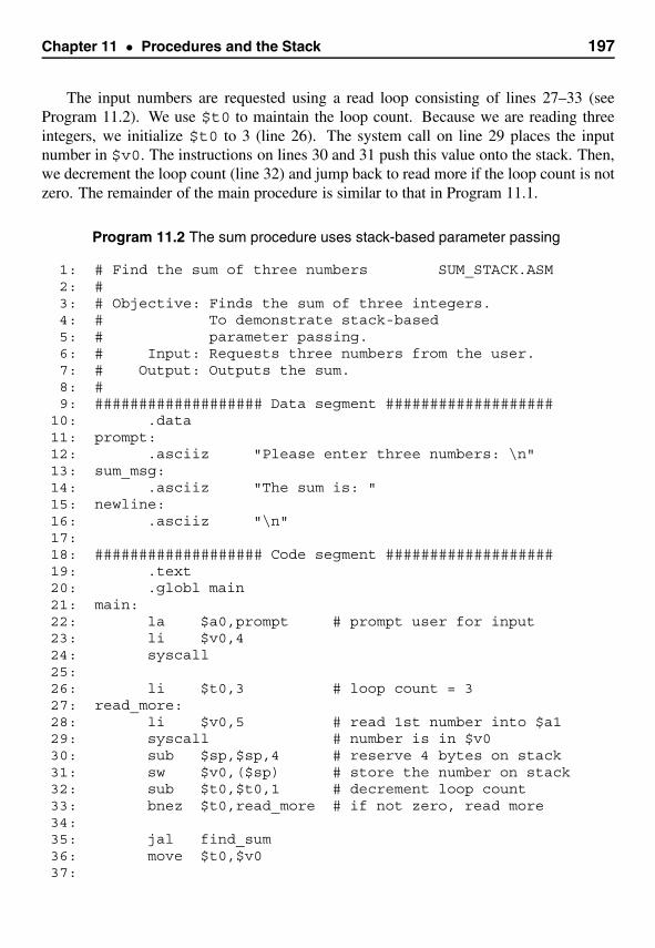
Chapter 11 • Procedures and the Stack 197
The input numbers are requested using a read loop consisting of lines 27–33 (seeProgram 11.2). We use $t0 to maintain the loop count. Because we are reading threeintegers, we initialize $t0 to 3 (line 26). The system call on line 29 places the inputnumber in $v0. The instructions on lines 30 and 31 push this value onto the stack. Then,we decrement the loop count (line 32) and jump back to read more if the loop count is notzero. The remainder of the main procedure is similar to that in Program 11.1.
Program 11.2 The sum procedure uses stack-based parameter passing
1: # Find the sum of three numbers SUM_STACK.ASM2: #3: # Objective: Finds the sum of three integers.4: # To demonstrate stack-based5: # parameter passing.6: # Input: Requests three numbers from the user.7: # Output: Outputs the sum.8: #9: ################### Data segment ###################
10: .data11: prompt:12: .asciiz "Please enter three numbers: \n"13: sum_msg:14: .asciiz "The sum is: "15: newline:16: .asciiz "\n"17:18: ################### Code segment ###################19: .text20: .globl main21: main:22: la $a0,prompt # prompt user for input23: li $v0,424: syscall25:26: li $t0,3 # loop count = 327: read_more:28: li $v0,5 # read 1st number into $a129: syscall # number is in $v030: sub $sp,$sp,4 # reserve 4 bytes on stack31: sw $v0,($sp) # store the number on stack32: sub $t0,$t0,1 # decrement loop count33: bnez $t0,read_more # if not zero, read more34:35: jal find_sum36: move $t0,$v037:
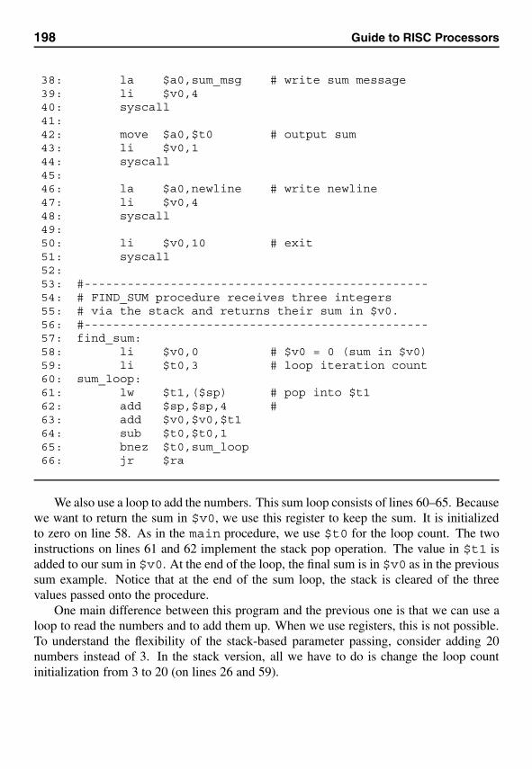
198 Guide to RISC Processors
38: la $a0,sum_msg # write sum message39: li $v0,440: syscall41:42: move $a0,$t0 # output sum43: li $v0,144: syscall45:46: la $a0,newline # write newline47: li $v0,448: syscall49:50: li $v0,10 # exit51: syscall52:53: #------------------------------------------------54: # FIND_SUM procedure receives three integers55: # via the stack and returns their sum in $v0.56: #------------------------------------------------57: find_sum:58: li $v0,0 # $v0 = 0 (sum in $v0)59: li $t0,3 # loop iteration count60: sum_loop:61: lw $t1,($sp) # pop into $t162: add $sp,$sp,4 #63: add $v0,$v0,$t164: sub $t0,$t0,165: bnez $t0,sum_loop66: jr $ra
We also use a loop to add the numbers. This sum loop consists of lines 60–65. Becausewe want to return the sum in $v0, we use this register to keep the sum. It is initializedto zero on line 58. As in the main procedure, we use $t0 for the loop count. The twoinstructions on lines 61 and 62 implement the stack pop operation. The value in $t1 isadded to our sum in $v0. At the end of the loop, the final sum is in $v0 as in the previoussum example. Notice that at the end of the sum loop, the stack is cleared of the threevalues passed onto the procedure.
One main difference between this program and the previous one is that we can use aloop to read the numbers and to add them up. When we use registers, this is not possible.To understand the flexibility of the stack-based parameter passing, consider adding 20numbers instead of 3. In the stack version, all we have to do is change the loop countinitialization from 3 to 20 (on lines 26 and 59).
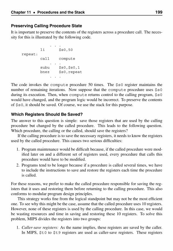
Chapter 11 • Procedures and the Stack 199
Preserving Calling Procedure StateIt is important to preserve the contents of the registers across a procedure call. The neces-sity for this is illustrated by the following code.
. . .li $s0,50
repeat:call compute
. . .subu $s0,$s0,1bnez $s0,repeat
. . .
The code invokes the compute procedure 50 times. The $s0 register maintains thenumber of remaining iterations. Now suppose that the compute procedure uses $s0during its execution. Then, when compute returns control to the calling program, $s0would have changed, and the program logic would be incorrect. To preserve the contentsof $s0, it should be saved. Of course, we use the stack for this purpose.
Which Registers Should Be Saved?The answer to this question is simple: save those registers that are used by the callingprocedure but changed by the called procedure. This leads to the following question.Which procedure, the calling or the called, should save the registers?
If the calling procedure is to save the necessary registers, it needs to know the registersused by the called procedure. This causes two serious difficulties:
1. Program maintenance would be difficult because, if the called procedure were mod-ified later on and a different set of registers used, every procedure that calls thisprocedure would have to be modified.
2. Programs tend to be longer because if a procedure is called several times, we haveto include the instructions to save and restore the registers each time the procedureis called.
For these reasons, we prefer to make the called procedure responsible for saving the reg-isters that it uses and restoring them before returning to the calling procedure. This alsoconforms to modular program design principles.
This strategy works fine from the logical standpoint but may not be the most efficientone. To see why this might be the case, assume that the called procedure uses 10 registers.However, none of these registers is used by the calling procedure. In this case, we wouldbe wasting resources and time in saving and restoring these 10 registers. To solve thisproblem, MIPS divides the registers into two groups:
1. Caller-save registers: As the name implies, these registers are saved by the caller.In MIPS, $t0 to $t9 registers are used as caller-save registers. These registers
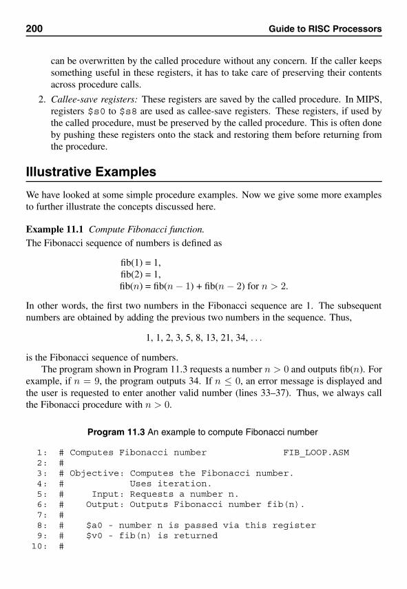
200 Guide to RISC Processors
can be overwritten by the called procedure without any concern. If the caller keepssomething useful in these registers, it has to take care of preserving their contentsacross procedure calls.
2. Callee-save registers: These registers are saved by the called procedure. In MIPS,registers $s0 to $s8 are used as callee-save registers. These registers, if used bythe called procedure, must be preserved by the called procedure. This is often doneby pushing these registers onto the stack and restoring them before returning fromthe procedure.
Illustrative Examples
We have looked at some simple procedure examples. Now we give some more examplesto further illustrate the concepts discussed here.
Example 11.1 Compute Fibonacci function.The Fibonacci sequence of numbers is defined as
fib(1) = 1,fib(2) = 1,fib(n) = fib(n − 1) + fib(n − 2) for n > 2.
In other words, the first two numbers in the Fibonacci sequence are 1. The subsequentnumbers are obtained by adding the previous two numbers in the sequence. Thus,
1, 1, 2, 3, 5, 8, 13, 21, 34, . . .
is the Fibonacci sequence of numbers.The program shown in Program 11.3 requests a number n > 0 and outputs fib(n). For
example, if n = 9, the program outputs 34. If n ≤ 0, an error message is displayed andthe user is requested to enter another valid number (lines 33–37). Thus, we always callthe Fibonacci procedure with n > 0.
Program 11.3 An example to compute Fibonacci number
1: # Computes Fibonacci number FIB_LOOP.ASM2: #3: # Objective: Computes the Fibonacci number.4: # Uses iteration.5: # Input: Requests a number n.6: # Output: Outputs Fibonacci number fib(n).7: #8: # $a0 - number n is passed via this register9: # $v0 - fib(n) is returned
10: #
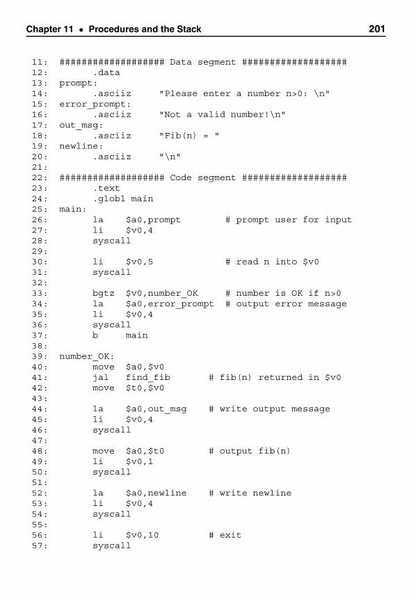
Chapter 11 • Procedures and the Stack 201
11: ################### Data segment ###################12: .data13: prompt:14: .asciiz "Please enter a number n>0: \n"15: error_prompt:16: .asciiz "Not a valid number!\n"17: out_msg:18: .asciiz "Fib(n) = "19: newline:20: .asciiz "\n"21:22: ################### Code segment ###################23: .text24: .globl main25: main:26: la $a0,prompt # prompt user for input27: li $v0,428: syscall29:30: li $v0,5 # read n into $v031: syscall32:33: bgtz $v0,number_OK # number is OK if n>034: la $a0,error_prompt # output error message35: li $v0,436: syscall37: b main38:39: number_OK:40: move $a0,$v041: jal find_fib # fib(n) returned in $v042: move $t0,$v043:44: la $a0,out_msg # write output message45: li $v0,446: syscall47:48: move $a0,$t0 # output fib(n)49: li $v0,150: syscall51:52: la $a0,newline # write newline53: li $v0,454: syscall55:56: li $v0,10 # exit57: syscall
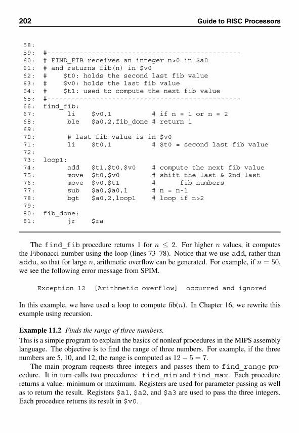
202 Guide to RISC Processors
58:59: #------------------------------------------------60: # FIND_FIB receives an integer n>0 in $a061: # and returns fib(n) in $v062: # $t0: holds the second last fib value63: # $v0: holds the last fib value64: # $t1: used to compute the next fib value65: #------------------------------------------------66: find_fib:67: li $v0,1 # if n = 1 or n = 268: ble $a0,2,fib_done # return 169:70: # last fib value is in $v071: li $t0,1 # $t0 = second last fib value72:73: loop1:74: add $t1,$t0,$v0 # compute the next fib value75: move $t0,$v0 # shift the last & 2nd last76: move $v0,$t1 # fib numbers77: sub $a0,$a0,1 # n = n-178: bgt $a0,2,loop1 # loop if n>279:80: fib_done:81: jr $ra
The find_fib procedure returns 1 for n ≤ 2. For higher n values, it computesthe Fibonacci number using the loop (lines 73–78). Notice that we use add, rather thanaddu, so that for large n, arithmetic overflow can be generated. For example, if n = 50,we see the following error message from SPIM.
Exception 12 [Arithmetic overflow] occurred and ignored
In this example, we have used a loop to compute fib(n). In Chapter 16, we rewrite thisexample using recursion.
Example 11.2 Finds the range of three numbers.This is a simple program to explain the basics of nonleaf procedures in the MIPS assemblylanguage. The objective is to find the range of three numbers. For example, if the threenumbers are 5, 10, and 12, the range is computed as 12 − 5 = 7.
The main program requests three integers and passes them to find_range pro-cedure. It in turn calls two procedures: find_min and find_max. Each procedurereturns a value: minimum or maximum. Registers are used for parameter passing as wellas to return the result. Registers $a1, $a2, and $a3 are used to pass the three integers.Each procedure returns its result in $v0.
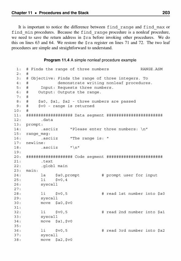
Chapter 11 • Procedures and the Stack 203
It is important to notice the difference between find_range and find_max orfind_min procedures. Because the find_range procedure is a nonleaf procedure,we need to save the return address in $ra before invoking other procedures. We dothis on lines 63 and 64. We restore the $ra register on lines 71 and 72. The two leafprocedures are simple and straightforward to understand.
Program 11.4 A simple nonleaf procedure example
1: # Finds the range of three numbers RANGE.ASM2: #3: # Objective: Finds the range of three integers. To4: # demonstrate writing nonleaf procedures.5: # Input: Requests three numbers.6: # Output: Outputs the range.7: #8: # $a0, $a1, $a2 - three numbers are passed9: # $v0 - range is returned
10: #11: ################### Data segment #######################12: .data13: prompt:14: .asciiz "Please enter three numbers: \n"15: range_msg:16: .asciiz "The range is: "17: newline:18: .asciiz "\n"19:20: ################### Code segment #######################21: .text22: .globl main23: main:24: la $a0,prompt # prompt user for input25: li $v0,426: syscall27:28: li $v0,5 # read 1st number into $a029: syscall30: move $a0,$v031:32: li $v0,5 # read 2nd number into $a133: syscall34: move $a1,$v035:36: li $v0,5 # read 3rd number into $a237: syscall38: move $a2,$v0
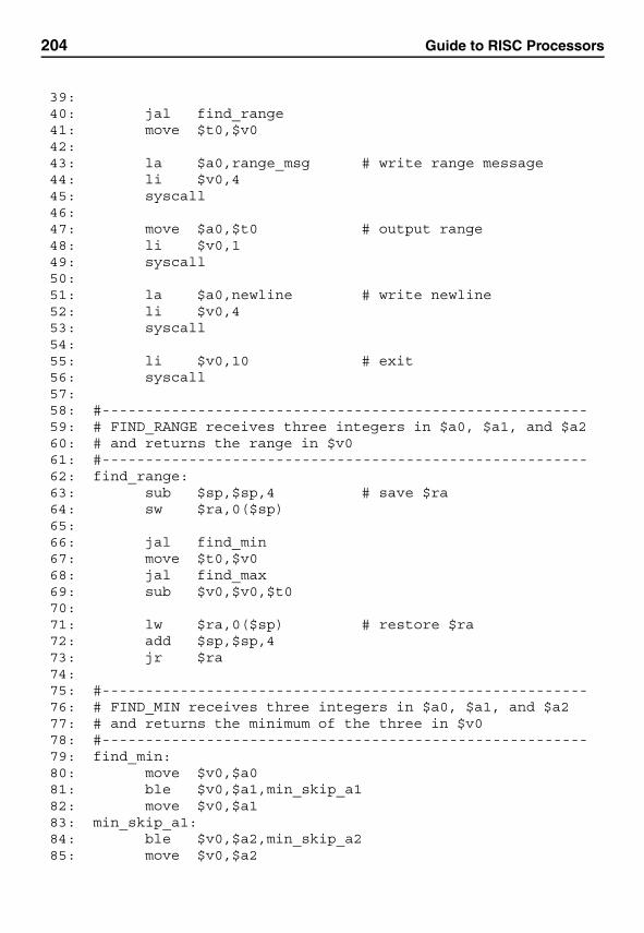
204 Guide to RISC Processors
39:40: jal find_range41: move $t0,$v042:43: la $a0,range_msg # write range message44: li $v0,445: syscall46:47: move $a0,$t0 # output range48: li $v0,149: syscall50:51: la $a0,newline # write newline52: li $v0,453: syscall54:55: li $v0,10 # exit56: syscall57:58: #--------------------------------------------------------59: # FIND_RANGE receives three integers in $a0, $a1, and $a260: # and returns the range in $v061: #--------------------------------------------------------62: find_range:63: sub $sp,$sp,4 # save $ra64: sw $ra,0($sp)65:66: jal find_min67: move $t0,$v068: jal find_max69: sub $v0,$v0,$t070:71: lw $ra,0($sp) # restore $ra72: add $sp,$sp,473: jr $ra74:75: #--------------------------------------------------------76: # FIND_MIN receives three integers in $a0, $a1, and $a277: # and returns the minimum of the three in $v078: #--------------------------------------------------------79: find_min:80: move $v0,$a081: ble $v0,$a1,min_skip_a182: move $v0,$a183: min_skip_a1:84: ble $v0,$a2,min_skip_a285: move $v0,$a2
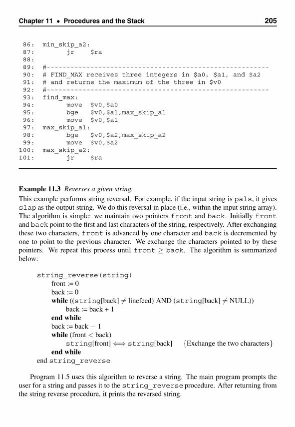
Chapter 11 • Procedures and the Stack 205
86: min_skip_a2:87: jr $ra88:89: #--------------------------------------------------------90: # FIND_MAX receives three integers in $a0, $a1, and $a291: # and returns the maximum of the three in $v092: #--------------------------------------------------------93: find_max:94: move $v0,$a095: bge $v0,$a1,max_skip_a196: move $v0,$a197: max_skip_a1:98: bge $v0,$a2,max_skip_a299: move $v0,$a2
100: max_skip_a2:101: jr $ra
Example 11.3 Reverses a given string.This example performs string reversal. For example, if the input string is pals, it givesslap as the output string. We do this reversal in place (i.e., within the input string array).The algorithm is simple: we maintain two pointers front and back. Initially frontand back point to the first and last characters of the string, respectively. After exchangingthese two characters, front is advanced by one character and back is decremented byone to point to the previous character. We exchange the characters pointed to by thesepointers. We repeat this process until front ≥ back. The algorithm is summarizedbelow:
string_reverse(string)front := 0back := 0while ((string[back] �= linefeed) AND (string[back] �= NULL))
back := back + 1end whileback := back − 1while (front < back)
string[front] ⇐⇒ string[back] {Exchange the two characters}end while
end string_reverse
Program 11.5 uses this algorithm to reverse a string. The main program prompts theuser for a string and passes it to the string_reverse procedure. After returning fromthe string reverse procedure, it prints the reversed string.
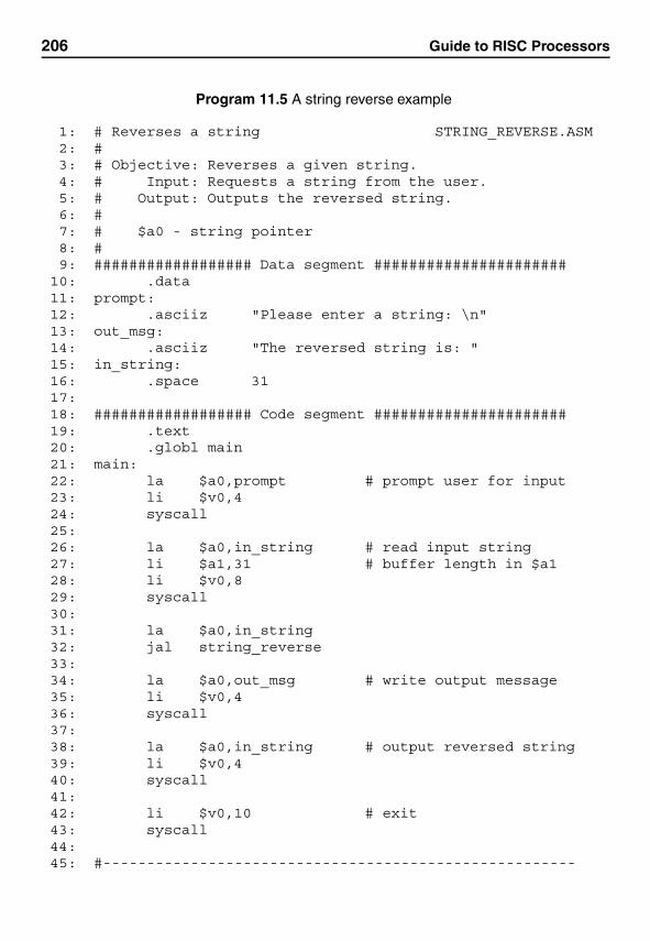
206 Guide to RISC Processors
Program 11.5 A string reverse example
1: # Reverses a string STRING_REVERSE.ASM2: #3: # Objective: Reverses a given string.4: # Input: Requests a string from the user.5: # Output: Outputs the reversed string.6: #7: # $a0 - string pointer8: #9: ################## Data segment ######################
10: .data11: prompt:12: .asciiz "Please enter a string: \n"13: out_msg:14: .asciiz "The reversed string is: "15: in_string:16: .space 3117:18: ################## Code segment ######################19: .text20: .globl main21: main:22: la $a0,prompt # prompt user for input23: li $v0,424: syscall25:26: la $a0,in_string # read input string27: li $a1,31 # buffer length in $a128: li $v0,829: syscall30:31: la $a0,in_string32: jal string_reverse33:34: la $a0,out_msg # write output message35: li $v0,436: syscall37:38: la $a0,in_string # output reversed string39: li $v0,440: syscall41:42: li $v0,10 # exit43: syscall44:45: #------------------------------------------------------
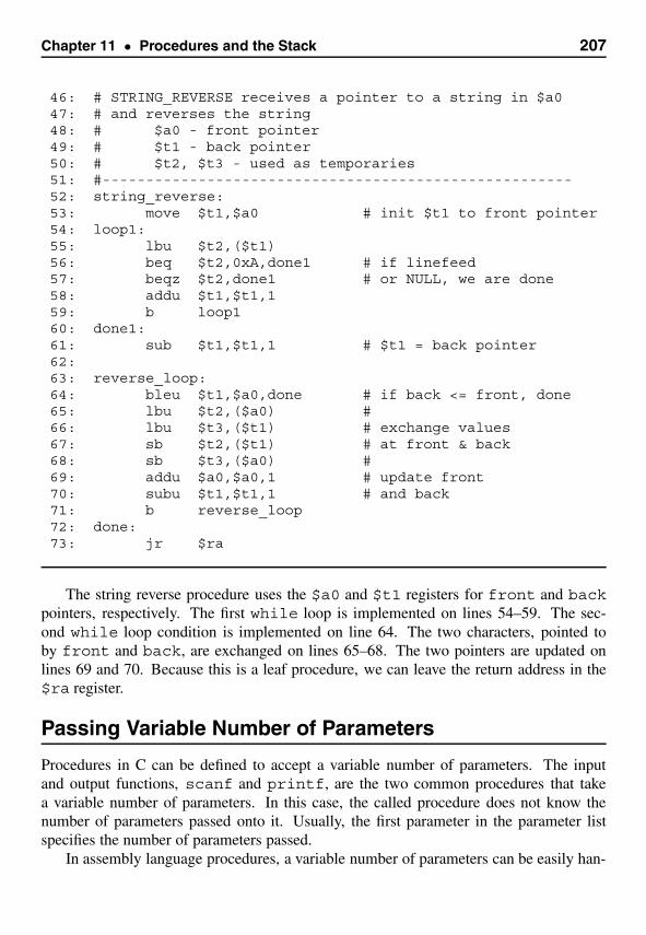
Chapter 11 • Procedures and the Stack 207
46: # STRING_REVERSE receives a pointer to a string in $a047: # and reverses the string48: # $a0 - front pointer49: # $t1 - back pointer50: # $t2, $t3 - used as temporaries51: #------------------------------------------------------52: string_reverse:53: move $t1,$a0 # init $t1 to front pointer54: loop1:55: lbu $t2,($t1)56: beq $t2,0xA,done1 # if linefeed57: beqz $t2,done1 # or NULL, we are done58: addu $t1,$t1,159: b loop160: done1:61: sub $t1,$t1,1 # $t1 = back pointer62:63: reverse_loop:64: bleu $t1,$a0,done # if back <= front, done65: lbu $t2,($a0) #66: lbu $t3,($t1) # exchange values67: sb $t2,($t1) # at front & back68: sb $t3,($a0) #69: addu $a0,$a0,1 # update front70: subu $t1,$t1,1 # and back71: b reverse_loop72: done:73: jr $ra
The string reverse procedure uses the $a0 and $t1 registers for front and backpointers, respectively. The first while loop is implemented on lines 54–59. The sec-ond while loop condition is implemented on line 64. The two characters, pointed toby front and back, are exchanged on lines 65–68. The two pointers are updated onlines 69 and 70. Because this is a leaf procedure, we can leave the return address in the$ra register.
Passing Variable Number of Parameters
Procedures in C can be defined to accept a variable number of parameters. The inputand output functions, scanf and printf, are the two common procedures that takea variable number of parameters. In this case, the called procedure does not know thenumber of parameters passed onto it. Usually, the first parameter in the parameter listspecifies the number of parameters passed.
In assembly language procedures, a variable number of parameters can be easily han-
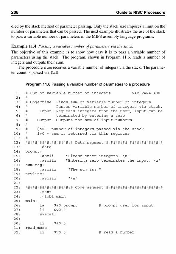
208 Guide to RISC Processors
dled by the stack method of parameter passing. Only the stack size imposes a limit on thenumber of parameters that can be passed. The next example illustrates the use of the stackto pass a variable number of parameters in the MIPS assembly language programs.
Example 11.4 Passing a variable number of parameters via the stack.The objective of this example is to show how easy it is to pass a variable number ofparameters using the stack. The program, shown in Program 11.6, reads a number ofintegers and outputs their sum.
The procedure sum receives a variable number of integers via the stack. The parame-ter count is passed via $a0.
Program 11.6 Passing a variable number of parameters to a procedure
1: # Sum of variable number of integers VAR_PARA.ASM2: #3: # Objective: Finds sum of variable number of integers.4: # Passes variable number of integers via stack.5: # Input: Requests integers from the user; input can be6: # terminated by entering a zero.7: # Output: Outputs the sum of input numbers.8: #9: # $a0 - number of integers passed via the stack
10: # $v0 - sum is returned via this register11: #12: #################### Data segment ########################13: .data14: prompt:15: .ascii "Please enter integers. \n"16: .asciiz "Entering zero terminates the input. \n"17: sum_msg:18: .asciiz "The sum is: "19: newline:20: .asciiz "\n"21:22: #################### Code segment ########################23: .text24: .globl main25: main:26: la $a0,prompt # prompt user for input27: li $v0,428: syscall29:30: li $a0,031: read_more:32: li $v0,5 # read a number
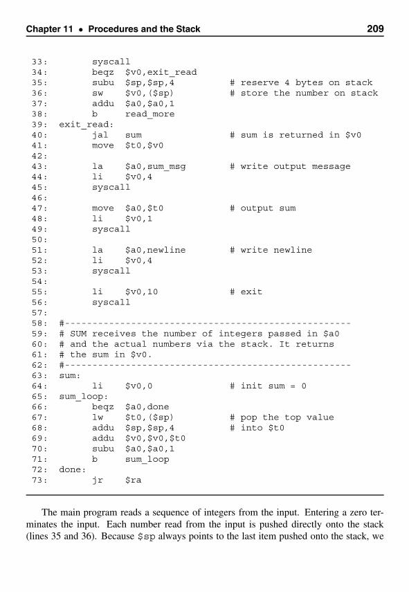
Chapter 11 • Procedures and the Stack 209
33: syscall34: beqz $v0,exit_read35: subu $sp,$sp,4 # reserve 4 bytes on stack36: sw $v0,($sp) # store the number on stack37: addu $a0,$a0,138: b read_more39: exit_read:40: jal sum # sum is returned in $v041: move $t0,$v042:43: la $a0,sum_msg # write output message44: li $v0,445: syscall46:47: move $a0,$t0 # output sum48: li $v0,149: syscall50:51: la $a0,newline # write newline52: li $v0,453: syscall54:55: li $v0,10 # exit56: syscall57:58: #----------------------------------------------------59: # SUM receives the number of integers passed in $a060: # and the actual numbers via the stack. It returns61: # the sum in $v0.62: #----------------------------------------------------63: sum:64: li $v0,0 # init sum = 065: sum_loop:66: beqz $a0,done67: lw $t0,($sp) # pop the top value68: addu $sp,$sp,4 # into $t069: addu $v0,$v0,$t070: subu $a0,$a0,171: b sum_loop72: done:73: jr $ra
The main program reads a sequence of integers from the input. Entering a zero ter-minates the input. Each number read from the input is pushed directly onto the stack(lines 35 and 36). Because $sp always points to the last item pushed onto the stack, we
210 Guide to RISC Processors
can pass this value to the procedure. Thus, a simple procedure call (line 40) is sufficientto pass the parameter count and the actual values.
The procedure sum reads the numbers from the stack. As it reads, it decreases thestack size (i.e., $sp increases). The loop in the sum procedure terminates when $a0 iszero (line 66). When the loop terminates, the stack is also cleared of all the arguments.
Summary
We have introduced procedures and discussed how procedures are implemented in theMIPS assembly language. We can divide procedures into leaf and nonleaf categories.A leaf procedure does not call another procedure whereas a nonleaf procedure invokesanother procedure. In the MIPS architecture, leaf procedures can be written using internalregisters. As part of procedure invocation, the return address is stored in the $ra register.This value is used to transfer control back to the caller after executing the procedure.Nonleaf procedures, however, need to use the stack.
The stack is a last-in-first-out data structure that plays an important role in nonleafprocedure invocation and execution. The stack supports two operations: push and pop.Only the element at the top-of-stack is directly accessible through these operations. The$sp register points to the top of the stack. It is important to note that the stack growsdownward (i.e., towards lower memory addresses). Because the MIPS architecture doesnot explicitly support stack operations, we need to manipulate the stack pointer ($sp)register to implement the stack push and pop operations.
When writing procedures in assembly language, parameter passing has to be explic-itly handled. Parameter passing can be done via registers or the stack. Although theregister method is efficient, the stack-based method is more general and flexible. Also,when the stack is used for parameter passing, passing a variable number of parameters isstraightforward. We have demonstrated this by means of an example.
In this chapter we discussed direct procedure calls in which the target instructionaddress is directly specified. The MIPS architecture also supports indirect procedure calls.In these calls, the target is specified indirectly through a register. Even though we haven’tused this mechanism to invoke a procedure, we have used it to return from a procedure.We discuss indirect procedure calls in Chapter 14.
12Addressing Modes
MIPS supports several ways to specify the location of the operands required by an instruc-tion. These are called addressing modes. Most instructions expect their operands in theregisters. However, load and store instructions are special in the sense that they interfacewith memory. These instructions require a memory address, which can be specified inseveral ways. This chapter gives details on the addressing modes we can use in writingMIPS assembly language programs.
IntroductionAs discussed in Chapter 3, RISC processors use simple addressing modes. In contrast,CISC processors provide complex addressing modes. In this chapter, we look at the MIPSaddressing modes in detail. SPIM simulates the MIPS R2000 processor, therefore ourfocus is on the assembly language of this processor.
As mentioned before, MIPS uses the load/store architecture. In this architecture, onlythe load and store instructions move data between memory and processor registers. Allother instructions expect their operands in registers. Thus, they use the register addressingmode. The load and store instructions, however, need a memory address. A variety ofaddressing modes is available to specify the address of operands located in memory. TheMIPS architecture supports the following addressing modes.
• Register addressing mode
• Immediate addressing mode
• Memory addressing mode
We look at these three addressing modes in the next three sections. Following this de-scription, we give details on accessing and organizing arrays. We consider both one-dimensional and multidimensional arrays. We give several examples to illustrate the usethe addressing modes presented here. We conclude the chapter with a summary.
211
212 Guide to RISC Processors
Addressing Modes
In this section, we briefly look at the three addressing modes. Later sections give examplesthat use these addressing modes.
Register Addressing ModeThis is the commonly used addressing mode. In this addressing mode, the operands arelocated in the registers. For example, in the instruction
add $t2,$t1,$t0
the two source operands are in $t1 and $t0. The result of the operation is also storedin a register ($t2 in this example). Most instructions, excluding the load and store, usethis addressing mode. These instructions are encoded using the R-type format shown inFigure 4.2 on page 52.
Immediate Addressing ModeIn immediate addressing mode, the operand is stored in the instruction itself. This ad-dressing mode is used for constants as shown in the following example.
addi $t0,$t0,4
This instruction is encoded using the I-type instruction format (see Figure 4.2). As youcan see from this format, the immediate value is limited to 16 bits. As a consequence, theconstant is limited to a signed 16-bit value. The advantage of this addressing mode is thatthe immediate operand is fetched along with the instruction; it does not require a separatememory access.
Memory Addressing ModesAs discussed in Chapter 4, the bare machine provides only a single memory addressingmode, disp(Rx), where displacement disp is a signed, 16-bit immediate value. Theaddress is computed by adding disp to the contents of register Rx. The virtual machinesupported by the assembler provides additional addressing modes for load and store in-structions to help in assembly language programming. Table 12.1 shows the addressingmodes supported by the virtual machine. Like the immediate addressing mode, the I-typeinstruction format is used to encode this addressing mode (see Figure 4.2).
Next we look at some examples of the memory addressing modes. The followinginstruction
lw $t0,($t1)
loads the 32-data at the address given by the $t1 register. In the following examples, weassume that the array is declared as
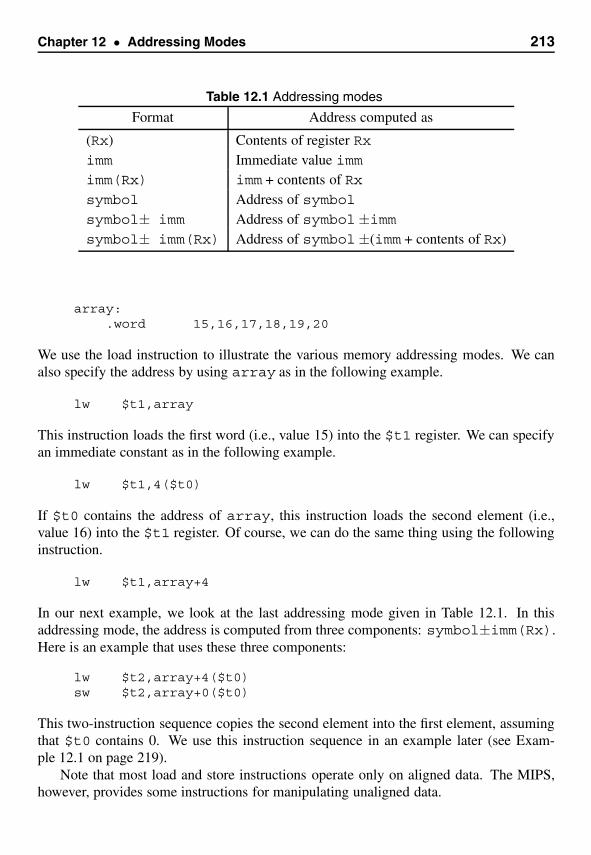
Chapter 12 • Addressing Modes 213
Table 12.1 Addressing modes
Format Address computed as
(Rx) Contents of register Rximm Immediate value immimm(Rx) imm + contents of Rxsymbol Address of symbolsymbol± imm Address of symbol±immsymbol± imm(Rx) Address of symbol±(imm + contents of Rx)
array:.word 15,16,17,18,19,20
We use the load instruction to illustrate the various memory addressing modes. We canalso specify the address by using array as in the following example.
lw $t1,array
This instruction loads the first word (i.e., value 15) into the $t1 register. We can specifyan immediate constant as in the following example.
lw $t1,4($t0)
If $t0 contains the address of array, this instruction loads the second element (i.e.,value 16) into the $t1 register. Of course, we can do the same thing using the followinginstruction.
lw $t1,array+4
In our next example, we look at the last addressing mode given in Table 12.1. In thisaddressing mode, the address is computed from three components: symbol±imm(Rx).Here is an example that uses these three components:
lw $t2,array+4($t0)sw $t2,array+0($t0)
This two-instruction sequence copies the second element into the first element, assumingthat $t0 contains 0. We use this instruction sequence in an example later (see Exam-ple 12.1 on page 219).
Note that most load and store instructions operate only on aligned data. The MIPS,however, provides some instructions for manipulating unaligned data.
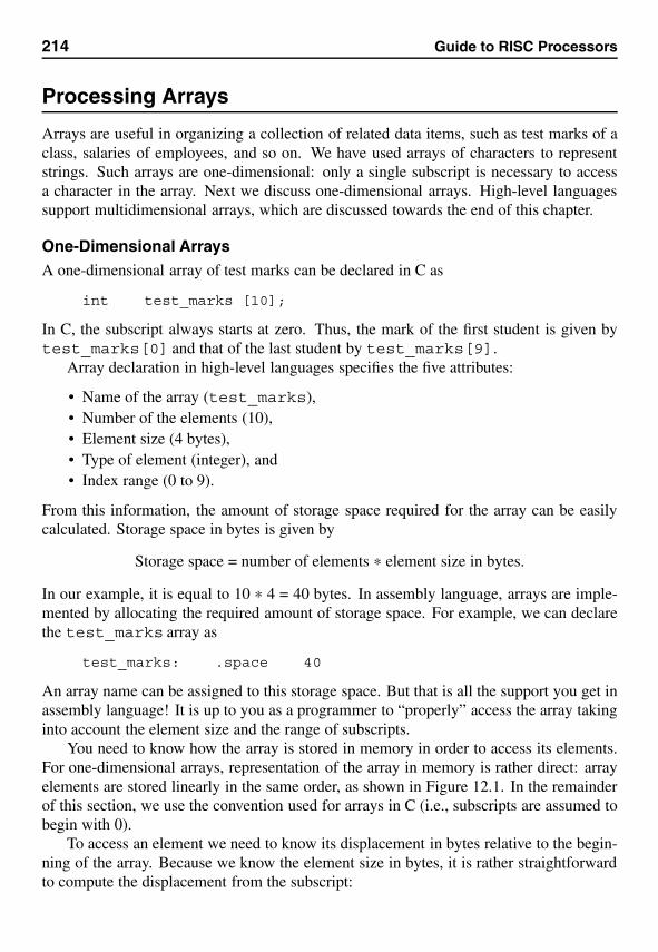
214 Guide to RISC Processors
Processing Arrays
Arrays are useful in organizing a collection of related data items, such as test marks of aclass, salaries of employees, and so on. We have used arrays of characters to representstrings. Such arrays are one-dimensional: only a single subscript is necessary to accessa character in the array. Next we discuss one-dimensional arrays. High-level languagessupport multidimensional arrays, which are discussed towards the end of this chapter.
One-Dimensional ArraysA one-dimensional array of test marks can be declared in C as
int test_marks [10];
In C, the subscript always starts at zero. Thus, the mark of the first student is given bytest_marks[0] and that of the last student by test_marks[9].
Array declaration in high-level languages specifies the five attributes:
• Name of the array (test_marks),• Number of the elements (10),• Element size (4 bytes),• Type of element (integer), and• Index range (0 to 9).
From this information, the amount of storage space required for the array can be easilycalculated. Storage space in bytes is given by
Storage space = number of elements * element size in bytes.
In our example, it is equal to 10 * 4 = 40 bytes. In assembly language, arrays are imple-mented by allocating the required amount of storage space. For example, we can declarethe test_marks array as
test_marks: .space 40
An array name can be assigned to this storage space. But that is all the support you get inassembly language! It is up to you as a programmer to “properly” access the array takinginto account the element size and the range of subscripts.
You need to know how the array is stored in memory in order to access its elements.For one-dimensional arrays, representation of the array in memory is rather direct: arrayelements are stored linearly in the same order, as shown in Figure 12.1. In the remainderof this section, we use the convention used for arrays in C (i.e., subscripts are assumed tobegin with 0).
To access an element we need to know its displacement in bytes relative to the begin-ning of the array. Because we know the element size in bytes, it is rather straightforwardto compute the displacement from the subscript:
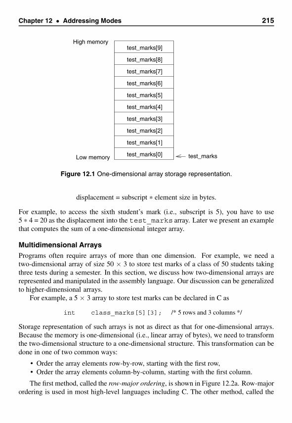
Chapter 12 • Addressing Modes 215
High memory
Low memory
test_marks[9]
test_marks[8]
test_marks[7]
test_marks[6]
test_marks[5]
test_marks[4]
test_marks[3]
test_marks[2]
test_marks[1]
test_marks[0] test_marks
Figure 12.1 One-dimensional array storage representation.
displacement = subscript * element size in bytes.
For example, to access the sixth student’s mark (i.e., subscript is 5), you have to use5 * 4 = 20 as the displacement into the test_marks array. Later we present an examplethat computes the sum of a one-dimensional integer array.
Multidimensional ArraysPrograms often require arrays of more than one dimension. For example, we need atwo-dimensional array of size 50 × 3 to store test marks of a class of 50 students takingthree tests during a semester. In this section, we discuss how two-dimensional arrays arerepresented and manipulated in the assembly language. Our discussion can be generalizedto higher-dimensional arrays.
For example, a 5 × 3 array to store test marks can be declared in C as
int class_marks[5][3]; /* 5 rows and 3 columns */
Storage representation of such arrays is not as direct as that for one-dimensional arrays.Because the memory is one-dimensional (i.e., linear array of bytes), we need to transformthe two-dimensional structure to a one-dimensional structure. This transformation can bedone in one of two common ways:
• Order the array elements row-by-row, starting with the first row,• Order the array elements column-by-column, starting with the first column.
The first method, called the row-major ordering, is shown in Figure 12.2a. Row-majorordering is used in most high-level languages including C. The other method, called the
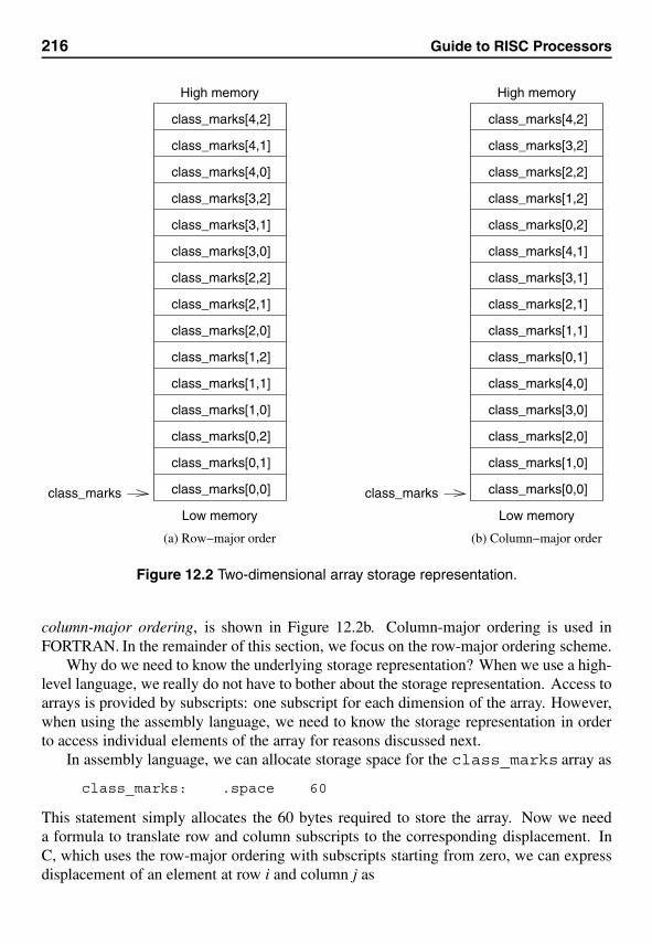
216 Guide to RISC Processors
class_marks[0,0]
High memory
class_marks[0,1]
class_marks[0,2]
class_marks[1,0]
class_marks[1,1]
class_marks[1,2]
class_marks[2,0]
class_marks[2,1]
class_marks[2,2]
class_marks[3,0]
class_marks[3,1]
class_marks[3,2]
class_marks[4,0]
class_marks[4,1]
class_marks[4,2]
class_marks class_marks[0,0]
High memory
class_marks[2,1]
class_marks[4,2]
class_marks[1,0]
class_marks[2,0]
class_marks[3,0]
class_marks[4,0]
class_marks[0,1]
class_marks[1,1]
class_marks[3,1]
class_marks[4,1]
class_marks[0,2]
class_marks[1,2]
class_marks[2,2]
class_marks[3,2]
Low memory
(a) Row−major order (b) Column−major order
Low memory
class_marks
Figure 12.2 Two-dimensional array storage representation.
column-major ordering, is shown in Figure 12.2b. Column-major ordering is used inFORTRAN. In the remainder of this section, we focus on the row-major ordering scheme.
Why do we need to know the underlying storage representation? When we use a high-level language, we really do not have to bother about the storage representation. Access toarrays is provided by subscripts: one subscript for each dimension of the array. However,when using the assembly language, we need to know the storage representation in orderto access individual elements of the array for reasons discussed next.
In assembly language, we can allocate storage space for the class_marks array as
class_marks: .space 60
This statement simply allocates the 60 bytes required to store the array. Now we needa formula to translate row and column subscripts to the corresponding displacement. InC, which uses the row-major ordering with subscripts starting from zero, we can expressdisplacement of an element at row i and column j as
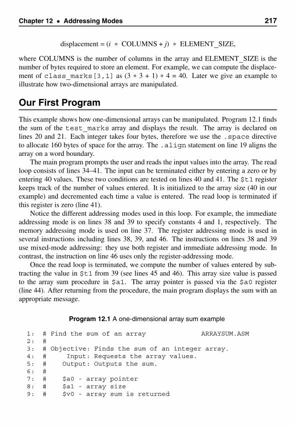
Chapter 12 • Addressing Modes 217
displacement = (i * COLUMNS + j) * ELEMENT_SIZE,
where COLUMNS is the number of columns in the array and ELEMENT_SIZE is thenumber of bytes required to store an element. For example, we can compute the displace-ment of class_marks[3,1] as (3 * 3 + 1) * 4 = 40. Later we give an example toillustrate how two-dimensional arrays are manipulated.
Our First Program
This example shows how one-dimensional arrays can be manipulated. Program 12.1 findsthe sum of the test_marks array and displays the result. The array is declared onlines 20 and 21. Each integer takes four bytes, therefore we use the .space directiveto allocate 160 bytes of space for the array. The .align statement on line 19 aligns thearray on a word boundary.
The main program prompts the user and reads the input values into the array. The readloop consists of lines 34–41. The input can be terminated either by entering a zero or byentering 40 values. These two conditions are tested on lines 40 and 41. The $t1 registerkeeps track of the number of values entered. It is initialized to the array size (40 in ourexample) and decremented each time a value is entered. The read loop is terminated ifthis register is zero (line 41).
Notice the different addressing modes used in this loop. For example, the immediateaddressing mode is on lines 38 and 39 to specify constants 4 and 1, respectively. Thememory addressing mode is used on line 37. The register addressing mode is used inseveral instructions including lines 38, 39, and 46. The instructions on lines 38 and 39use mixed-mode addressing: they use both register and immediate addressing mode. Incontrast, the instruction on line 46 uses only the register-addressing mode.
Once the read loop is terminated, we compute the number of values entered by sub-tracting the value in $t1 from 39 (see lines 45 and 46). This array size value is passedto the array sum procedure in $a1. The array pointer is passed via the $a0 register(line 44). After returning from the procedure, the main program displays the sum with anappropriate message.
Program 12.1 A one-dimensional array sum example
1: # Find the sum of an array ARRAYSUM.ASM2: #3: # Objective: Finds the sum of an integer array.4: # Input: Requests the array values.5: # Output: Outputs the sum.6: #7: # $a0 - array pointer8: # $a1 - array size9: # $v0 - array sum is returned
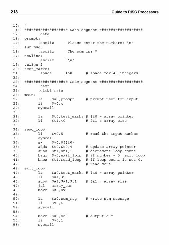
218 Guide to RISC Processors
10: #11: ################### Data segment ###################12: .data13: prompt:14: .asciiz "Please enter the numbers: \n"15: sum_msg:16: .asciiz "The sum is: "17: newline:18: .asciiz "\n"19: .align 220: test_marks:21: .space 160 # space for 40 integers22:23: ################### Code segment ###################24: .text25: .globl main26: main:27: la $a0,prompt # prompt user for input28: li $v0,429: syscall30:31: la $t0,test_marks # $t0 = array pointer32: li $t1,40 # $t1 = array size33:34: read_loop:35: li $v0,5 # read the input number36: syscall37: sw $v0,0($t0)38: addu $t0,$t0,4 # update array pointer39: subu $t1,$t1,1 # decrement loop count40: beqz $v0,exit_loop # if number = 0, exit loop41: bnez $t1,read_loop # if loop count is not 0,42: # read more43: exit_loop:44: la $a0,test_marks # $a0 = array pointer45: li $a1,3946: subu $a1,$a1,$t1 # $a1 = array size47: jal array_sum48: move $s0,$v049:50: la $a0,sum_msg # write sum message51: li $v0,452: syscall53:54: move $a0,$s0 # output sum55: li $v0,156: syscall
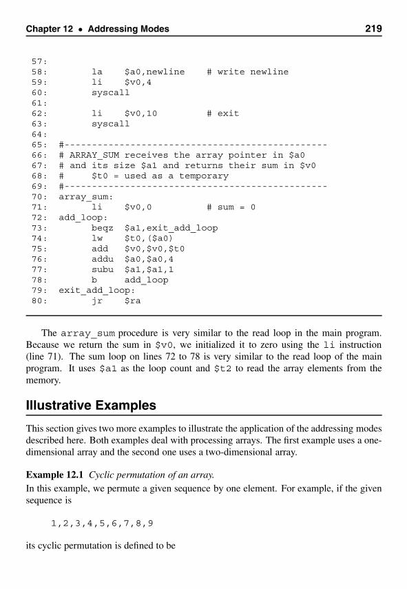
Chapter 12 • Addressing Modes 219
57:58: la $a0,newline # write newline59: li $v0,460: syscall61:62: li $v0,10 # exit63: syscall64:65: #------------------------------------------------66: # ARRAY_SUM receives the array pointer in $a067: # and its size $a1 and returns their sum in $v068: # $t0 = used as a temporary69: #------------------------------------------------70: array_sum:71: li $v0,0 # sum = 072: add_loop:73: beqz $a1,exit_add_loop74: lw $t0,($a0)75: add $v0,$v0,$t076: addu $a0,$a0,477: subu $a1,$a1,178: b add_loop79: exit_add_loop:80: jr $ra
The array_sum procedure is very similar to the read loop in the main program.Because we return the sum in $v0, we initialized it to zero using the li instruction(line 71). The sum loop on lines 72 to 78 is very similar to the read loop of the mainprogram. It uses $a1 as the loop count and $t2 to read the array elements from thememory.
Illustrative Examples
This section gives two more examples to illustrate the application of the addressing modesdescribed here. Both examples deal with processing arrays. The first example uses a one-dimensional array and the second one uses a two-dimensional array.
Example 12.1 Cyclic permutation of an array.In this example, we permute a given sequence by one element. For example, if the givensequence is
1,2,3,4,5,6,7,8,9
its cyclic permutation is defined to be
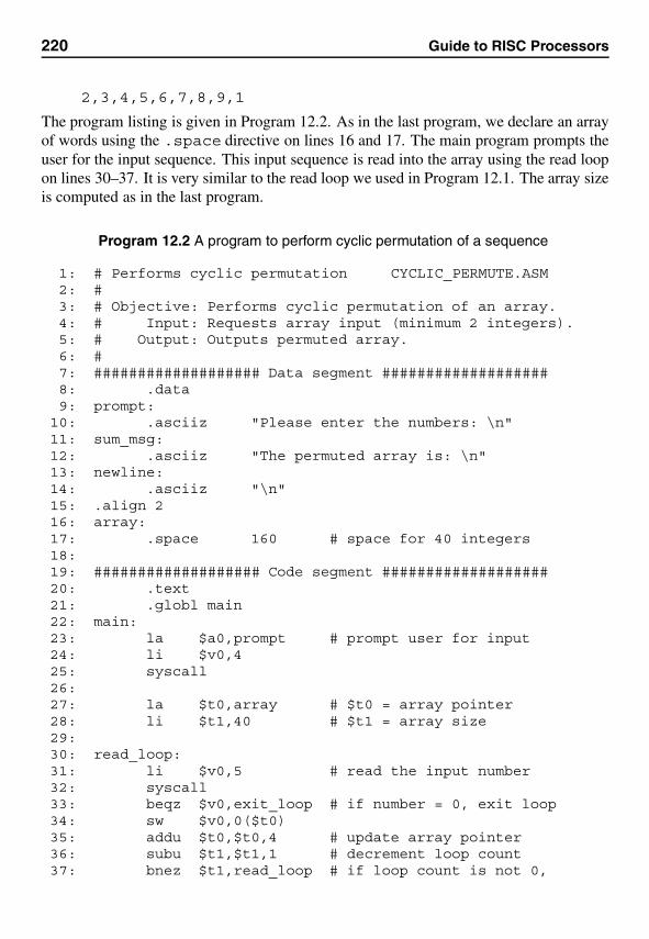
220 Guide to RISC Processors
2,3,4,5,6,7,8,9,1
The program listing is given in Program 12.2. As in the last program, we declare an arrayof words using the .space directive on lines 16 and 17. The main program prompts theuser for the input sequence. This input sequence is read into the array using the read loopon lines 30–37. It is very similar to the read loop we used in Program 12.1. The array sizeis computed as in the last program.
Program 12.2 A program to perform cyclic permutation of a sequence
1: # Performs cyclic permutation CYCLIC_PERMUTE.ASM2: #3: # Objective: Performs cyclic permutation of an array.4: # Input: Requests array input (minimum 2 integers).5: # Output: Outputs permuted array.6: #7: ################### Data segment ###################8: .data9: prompt:
10: .asciiz "Please enter the numbers: \n"11: sum_msg:12: .asciiz "The permuted array is: \n"13: newline:14: .asciiz "\n"15: .align 216: array:17: .space 160 # space for 40 integers18:19: ################### Code segment ###################20: .text21: .globl main22: main:23: la $a0,prompt # prompt user for input24: li $v0,425: syscall26:27: la $t0,array # $t0 = array pointer28: li $t1,40 # $t1 = array size29:30: read_loop:31: li $v0,5 # read the input number32: syscall33: beqz $v0,exit_loop # if number = 0, exit loop34: sw $v0,0($t0)35: addu $t0,$t0,4 # update array pointer36: subu $t1,$t1,1 # decrement loop count37: bnez $t1,read_loop # if loop count is not 0,
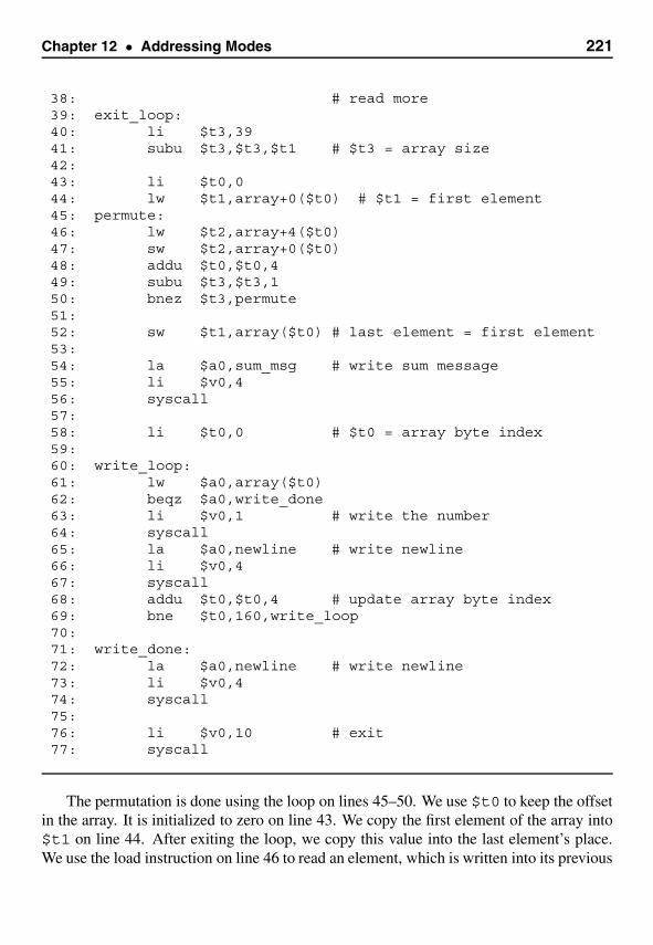
Chapter 12 • Addressing Modes 221
38: # read more39: exit_loop:40: li $t3,3941: subu $t3,$t3,$t1 # $t3 = array size42:43: li $t0,044: lw $t1,array+0($t0) # $t1 = first element45: permute:46: lw $t2,array+4($t0)47: sw $t2,array+0($t0)48: addu $t0,$t0,449: subu $t3,$t3,150: bnez $t3,permute51:52: sw $t1,array($t0) # last element = first element53:54: la $a0,sum_msg # write sum message55: li $v0,456: syscall57:58: li $t0,0 # $t0 = array byte index59:60: write_loop:61: lw $a0,array($t0)62: beqz $a0,write_done63: li $v0,1 # write the number64: syscall65: la $a0,newline # write newline66: li $v0,467: syscall68: addu $t0,$t0,4 # update array byte index69: bne $t0,160,write_loop70:71: write_done:72: la $a0,newline # write newline73: li $v0,474: syscall75:76: li $v0,10 # exit77: syscall
The permutation is done using the loop on lines 45–50. We use $t0 to keep the offsetin the array. It is initialized to zero on line 43. We copy the first element of the array into$t1 on line 44. After exiting the loop, we copy this value into the last element’s place.We use the load instruction on line 46 to read an element, which is written into its previous
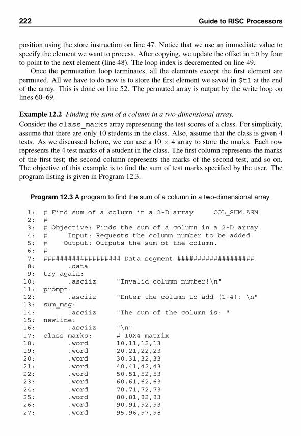
222 Guide to RISC Processors
position using the store instruction on line 47. Notice that we use an immediate value tospecify the element we want to process. After copying, we update the offset in t0 by fourto point to the next element (line 48). The loop index is decremented on line 49.
Once the permutation loop terminates, all the elements except the first element arepermuted. All we have to do now is to store the first element we saved in $t1 at the endof the array. This is done on line 52. The permuted array is output by the write loop onlines 60–69.
Example 12.2 Finding the sum of a column in a two-dimensional array.Consider the class_marks array representing the test scores of a class. For simplicity,assume that there are only 10 students in the class. Also, assume that the class is given 4tests. As we discussed before, we can use a 10 × 4 array to store the marks. Each rowrepresents the 4 test marks of a student in the class. The first column represents the marksof the first test; the second column represents the marks of the second test, and so on.The objective of this example is to find the sum of test marks specified by the user. Theprogram listing is given in Program 12.3.
Program 12.3 A program to find the sum of a column in a two-dimensional array
1: # Find sum of a column in a 2-D array COL_SUM.ASM2: #3: # Objective: Finds the sum of a column in a 2-D array.4: # Input: Requests the column number to be added.5: # Output: Outputs the sum of the column.6: #7: ################### Data segment ###################8: .data9: try_again:
10: .asciiz "Invalid column number!\n"11: prompt:12: .asciiz "Enter the column to add (1-4): \n"13: sum_msg:14: .asciiz "The sum of the column is: "15: newline:16: .asciiz "\n"17: class_marks: # 10X4 matrix18: .word 10,11,12,1319: .word 20,21,22,2320: .word 30,31,32,3321: .word 40,41,42,4322: .word 50,51,52,5323: .word 60,61,62,6324: .word 70,71,72,7325: .word 80,81,82,8326: .word 90,91,92,9327: .word 95,96,97,98
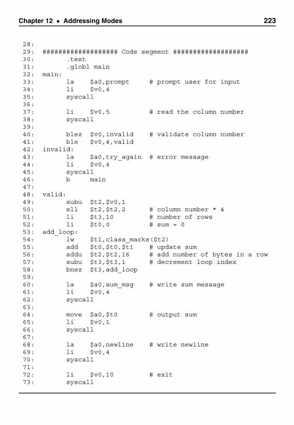
Chapter 12 • Addressing Modes 223
28:29: ################### Code segment ###################30: .text31: .globl main32: main:33: la $a0,prompt # prompt user for input34: li $v0,435: syscall36:37: li $v0,5 # read the column number38: syscall39:40: blez $v0,invalid # validate column number41: ble $v0,4,valid42: invalid:43: la $a0,try_again # error message44: li $v0,445: syscall46: b main47:48: valid:49: subu $t2,$v0,150: sll $t2,$t2,2 # column number * 451: li $t3,10 # number of rows52: li $t0,0 # sum = 053: add_loop:54: lw $t1,class_marks($t2)55: add $t0,$t0,$t1 # update sum56: addu $t2,$t2,16 # add number of bytes in a row57: subu $t3,$t3,1 # decrement loop index58: bnez $t3,add_loop59:60: la $a0,sum_msg # write sum message61: li $v0,462: syscall63:64: move $a0,$t0 # output sum65: li $v0,166: syscall67:68: la $a0,newline # write newline69: li $v0,470: syscall71:72: li $v0,10 # exit73: syscall
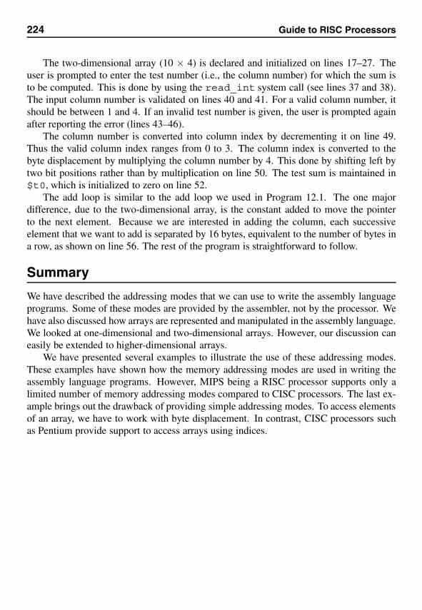
224 Guide to RISC Processors
The two-dimensional array (10 × 4) is declared and initialized on lines 17–27. Theuser is prompted to enter the test number (i.e., the column number) for which the sum isto be computed. This is done by using the read_int system call (see lines 37 and 38).The input column number is validated on lines 40 and 41. For a valid column number, itshould be between 1 and 4. If an invalid test number is given, the user is prompted againafter reporting the error (lines 43–46).
The column number is converted into column index by decrementing it on line 49.Thus the valid column index ranges from 0 to 3. The column index is converted to thebyte displacement by multiplying the column number by 4. This done by shifting left bytwo bit positions rather than by multiplication on line 50. The test sum is maintained in$t0, which is initialized to zero on line 52.
The add loop is similar to the add loop we used in Program 12.1. The one majordifference, due to the two-dimensional array, is the constant added to move the pointerto the next element. Because we are interested in adding the column, each successiveelement that we want to add is separated by 16 bytes, equivalent to the number of bytes ina row, as shown on line 56. The rest of the program is straightforward to follow.
Summary
We have described the addressing modes that we can use to write the assembly languageprograms. Some of these modes are provided by the assembler, not by the processor. Wehave also discussed how arrays are represented and manipulated in the assembly language.We looked at one-dimensional and two-dimensional arrays. However, our discussion caneasily be extended to higher-dimensional arrays.
We have presented several examples to illustrate the use of these addressing modes.These examples have shown how the memory addressing modes are used in writing theassembly language programs. However, MIPS being a RISC processor supports only alimited number of memory addressing modes compared to CISC processors. The last ex-ample brings out the drawback of providing simple addressing modes. To access elementsof an array, we have to work with byte displacement. In contrast, CISC processors suchas Pentium provide support to access arrays using indices.
13Arithmetic Instructions
This chapter describes the arithmetic instructions of the MIPS instruction set in detail.We have introduced some of the basic arithmetic operations such as add and subtract inChapter 10. Here we provide a thorough discussion of the arithmetic instructions, includ-ing the pseudoinstructions supported by the assembler. We then give several examplesto illustrate their use in assembly language programs. We conclude the chapter with asummary.
IntroductionThe MIPS instruction set supports the four basic arithmetic operations: addition, subtrac-tion, multiplication, and division. We have already introduced the basic add and subtractinstructions. These instructions can potentially cause overflow/underflow problems. TheMIPS architecture deals with them by generating an exception.
In addition to the add and subtract instructions, two pseudoinstructions are providedfor signed integers. One computes the absolute value and the other reverses the sign of anumber (i.e., a positive number is converted into a negative number and vice versa).
Multiplication is more complicated than addition or subtraction for these reasons: (i)it produces a result that is double the size of the input operands. For example, multiplyingtwo 32-bit numbers produces a 64-bit result. (ii) We need two separate instructions tooperate signed and unsigned numbers. In contrast, the add instruction can be used withboth signed and unsigned numbers. We give details on how the MIPS instruction sethandles these complications.
The division operation is even more complicated than multiplication for the followingreasons: (i) it produces two results: a quotient and a remainder. For example, dividing200 by 15 results in a quotient of 13 and remainder of 5. (ii) In multiplication, there is nooverflow problem. The result always fits the 64-bit destination. In the division operation,there is a potential overflow problem that needs to be handled. For example, divide byzero leads to such a situation. In fact, it need not be zero; any number that is small enough
225
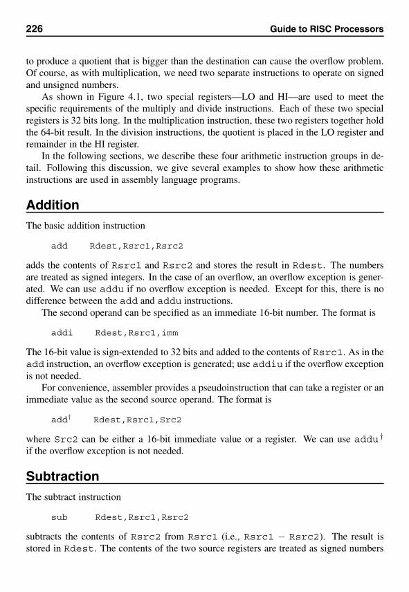
226 Guide to RISC Processors
to produce a quotient that is bigger than the destination can cause the overflow problem.Of course, as with multiplication, we need two separate instructions to operate on signedand unsigned numbers.
As shown in Figure 4.1, two special registers—LO and HI—are used to meet thespecific requirements of the multiply and divide instructions. Each of these two specialregisters is 32 bits long. In the multiplication instruction, these two registers together holdthe 64-bit result. In the division instructions, the quotient is placed in the LO register andremainder in the HI register.
In the following sections, we describe these four arithmetic instruction groups in de-tail. Following this discussion, we give several examples to show how these arithmeticinstructions are used in assembly language programs.
AdditionThe basic addition instruction
add Rdest,Rsrc1,Rsrc2
adds the contents of Rsrc1 and Rsrc2 and stores the result in Rdest. The numbersare treated as signed integers. In the case of an overflow, an overflow exception is gener-ated. We can use addu if no overflow exception is needed. Except for this, there is nodifference between the add and addu instructions.
The second operand can be specified as an immediate 16-bit number. The format is
addi Rdest,Rsrc1,imm
The 16-bit value is sign-extended to 32 bits and added to the contents of Rsrc1. As in theadd instruction, an overflow exception is generated; use addiu if the overflow exceptionis not needed.
For convenience, assembler provides a pseudoinstruction that can take a register or animmediate value as the second source operand. The format is
add† Rdest,Rsrc1,Src2
where Src2 can be either a 16-bit immediate value or a register. We can use addu †if the overflow exception is not needed.
SubtractionThe subtract instruction
sub Rdest,Rsrc1,Rsrc2
subtracts the contents of Rsrc2 from Rsrc1 (i.e., Rsrc1 − Rsrc2). The result isstored in Rdest. The contents of the two source registers are treated as signed numbers
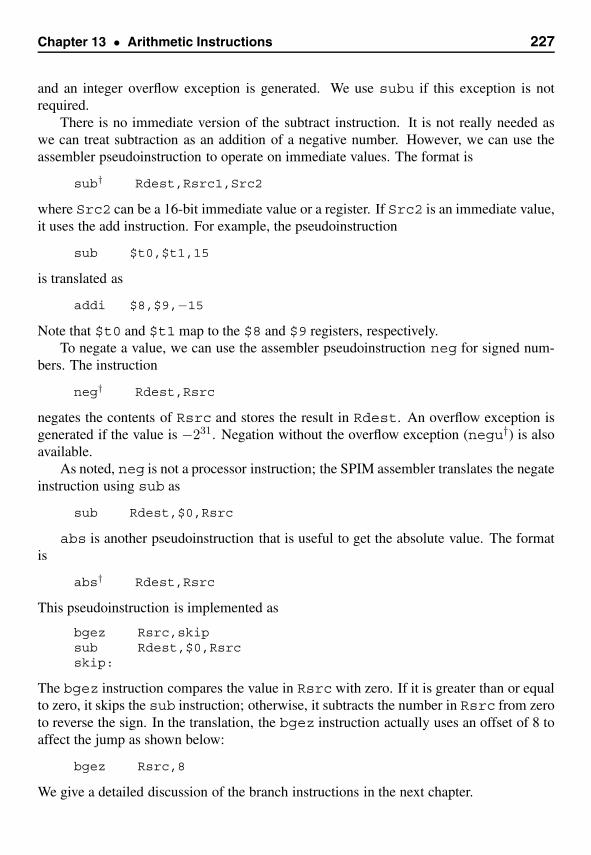
Chapter 13 • Arithmetic Instructions 227
and an integer overflow exception is generated. We use subu if this exception is notrequired.
There is no immediate version of the subtract instruction. It is not really needed aswe can treat subtraction as an addition of a negative number. However, we can use theassembler pseudoinstruction to operate on immediate values. The format is
sub† Rdest,Rsrc1,Src2
where Src2 can be a 16-bit immediate value or a register. If Src2 is an immediate value,it uses the add instruction. For example, the pseudoinstruction
sub $t0,$t1,15
is translated as
addi $8,$9,−15Note that $t0 and $t1 map to the $8 and $9 registers, respectively.
To negate a value, we can use the assembler pseudoinstruction neg for signed num-bers. The instruction
neg† Rdest,Rsrc
negates the contents of Rsrc and stores the result in Rdest. An overflow exception isgenerated if the value is −231. Negation without the overflow exception (negu†) is alsoavailable.
As noted, neg is not a processor instruction; the SPIM assembler translates the negateinstruction using sub as
sub Rdest,$0,Rsrc
abs is another pseudoinstruction that is useful to get the absolute value. The formatis
abs† Rdest,Rsrc
This pseudoinstruction is implemented as
bgez Rsrc,skipsub Rdest,$0,Rsrcskip:
The bgez instruction compares the value in Rsrc with zero. If it is greater than or equalto zero, it skips the sub instruction; otherwise, it subtracts the number in Rsrc from zeroto reverse the sign. In the translation, the bgez instruction actually uses an offset of 8 toaffect the jump as shown below:
bgez Rsrc,8
We give a detailed discussion of the branch instructions in the next chapter.
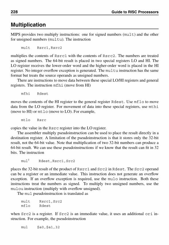
228 Guide to RISC Processors
Multiplication
MIPS provides two multiply instructions: one for signed numbers (mult) and the otherfor unsigned numbers (multu). The instruction
mult Rsrc1,Rsrc2
multiplies the contents of Rsrc1 with the contents of Rsrc2. The numbers are treatedas signed numbers. The 64-bit result is placed in two special registers LO and HI. TheLO register receives the lower-order word and the higher-order word is placed in the HIregister. No integer overflow exception is generated. The multu instruction has the sameformat but treats the source operands as unsigned numbers.
There are instructions to move data between these special LO/HI registers and generalregisters. The instruction mfhi (move from HI)
mfhi Rdest
moves the contents of the HI register to the general register Rdest. Use mflo to movedata from the LO register. For movement of data into these special registers, use mthi(move to HI) or mtlo (move to LO). For example,
mtlo Rsrc
copies the value in the Rsrc register into the LO register.The assembler multiply pseudoinstruction can be used to place the result directly in a
destination register. A limitation of the pseudoinstruction is that it stores only the 32-bitresult, not the 64-bit value. Note that multiplication of two 32-bit numbers can produce a64-bit result. We can use these pseudoinstructions if we know that the result can fit in 32bits. The instruction
mul† Rdest,Rsrc1,Src2
places the 32-bit result of the product of Rsrc1 and Src2 in Rdest. The Src2 operandcan be a register or an immediate value. This instruction does not generate an overflowexception. If an overflow exception is required, use the mulo instruction. Both theseinstructions treat the numbers as signed. To multiply two unsigned numbers, use themulou instruction (multiply with overflow unsigned).
The mul pseudoinstruction is translated as
mult Rsrc1,Src2mflo Rdest
when Src2 is a register. If Src2 is an immediate value, it uses an additional ori in-struction. For example, the pseudoinstruction
mul $a0,$a1,32
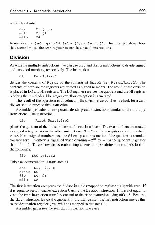
Chapter 13 • Arithmetic Instructions 229
is translated into
ori $1,$0,32mult $5,$1mflo $4
Remember that $a0 maps to $4, $a1 to $5, and $at to $1. This example shows howthe assembler uses the $at register to translate pseudoinstructions.
DivisionAs with the multiply instructions, we can use div and divu instructions to divide signedand unsigned numbers, respectively. The instruction
div Rsrc1,Rsrc2
divides the contents of Rsrc1 by the contents of Rsrc2 (i.e., Rsrc1/Rsrc2). Thecontents of both source registers are treated as signed numbers. The result of the divisionis placed in LO and HI registers. The LO register receives the quotient and the HI registerreceives the remainder. No integer overflow exception is generated.
The result of the operation is undefined if the divisor is zero. Thus, a check for a zerodivisor should precede this instruction.
Assembler provides three-operand divide pseudoinstructions similar to the multiplyinstructions. The instruction
div† Rdest,Rsrc1,Src2
places the quotient of the division Rsrc1/Src2 in Rdest. The two numbers are treatedas signed integers. As in the other instructions, Src2 can be a register or an immediatevalue. For unsigned numbers, use the divu† pseudoinstruction. The quotient is roundedtowards zero. Overflow is signalled when dividing −2 31 by −1 as the quotient is greaterthan 2 31 − 1. To see how the assembler implements this pseudoinstruction, let’s look atthe following.
div $t0,$t1,$t2
This pseudoinstruction is translated as
bne $10, $0, 8break $0div $9, $10mflo $8
The first instruction compares the divisor in $t2 (mapped to register $10) with zero. Ifit is equal to zero, it causes exception 0 using the break instruction. If it is not equal tozero, the bne instruction transfers control to the div instruction using offset 8. Becausethe div instruction leaves the quotient in the LO register, the last instruction moves thisto the destination register $t0, which is mapped to register $8.
Assembler generates the real div instruction if we use
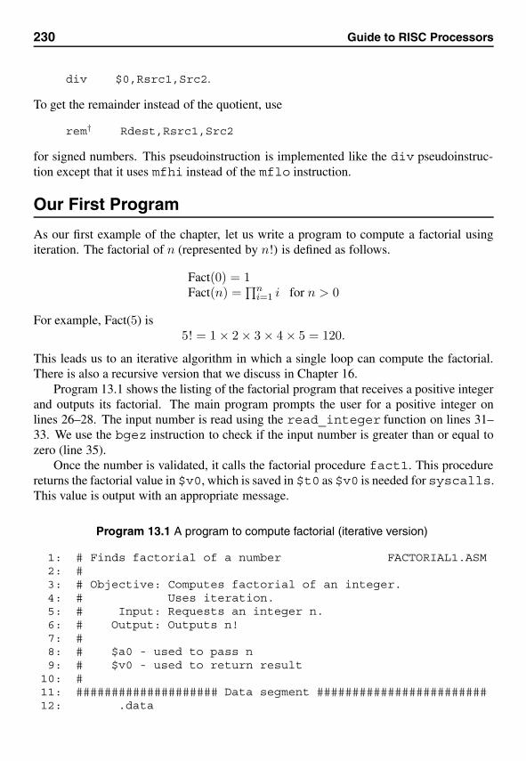
230 Guide to RISC Processors
div $0,Rsrc1,Src2.
To get the remainder instead of the quotient, use
rem† Rdest,Rsrc1,Src2
for signed numbers. This pseudoinstruction is implemented like the div pseudoinstruc-tion except that it uses mfhi instead of the mflo instruction.
Our First Program
As our first example of the chapter, let us write a program to compute a factorial usingiteration. The factorial of n (represented by n!) is defined as follows.
Fact(0) = 1Fact(n) =
∏ni=1 i for n > 0
For example, Fact(5) is5! = 1 × 2 × 3 × 4 × 5 = 120.
This leads us to an iterative algorithm in which a single loop can compute the factorial.There is also a recursive version that we discuss in Chapter 16.
Program 13.1 shows the listing of the factorial program that receives a positive integerand outputs its factorial. The main program prompts the user for a positive integer onlines 26–28. The input number is read using the read_integer function on lines 31–33. We use the bgez instruction to check if the input number is greater than or equal tozero (line 35).
Once the number is validated, it calls the factorial procedure fact1. This procedurereturns the factorial value in $v0, which is saved in $t0 as $v0 is needed for syscalls.This value is output with an appropriate message.
Program 13.1 A program to compute factorial (iterative version)
1: # Finds factorial of a number FACTORIAL1.ASM2: #3: # Objective: Computes factorial of an integer.4: # Uses iteration.5: # Input: Requests an integer n.6: # Output: Outputs n!7: #8: # $a0 - used to pass n9: # $v0 - used to return result
10: #11: #################### Data segment ########################12: .data
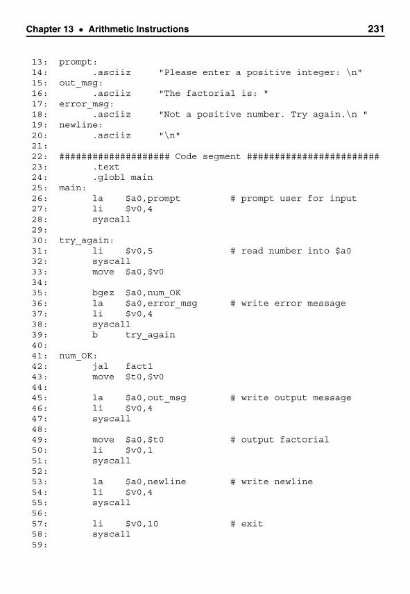
Chapter 13 • Arithmetic Instructions 231
13: prompt:14: .asciiz "Please enter a positive integer: \n"15: out_msg:16: .asciiz "The factorial is: "17: error_msg:18: .asciiz "Not a positive number. Try again.\n "19: newline:20: .asciiz "\n"21:22: #################### Code segment ########################23: .text24: .globl main25: main:26: la $a0,prompt # prompt user for input27: li $v0,428: syscall29:30: try_again:31: li $v0,5 # read number into $a032: syscall33: move $a0,$v034:35: bgez $a0,num_OK36: la $a0,error_msg # write error message37: li $v0,438: syscall39: b try_again40:41: num_OK:42: jal fact143: move $t0,$v044:45: la $a0,out_msg # write output message46: li $v0,447: syscall48:49: move $a0,$t0 # output factorial50: li $v0,151: syscall52:53: la $a0,newline # write newline54: li $v0,455: syscall56:57: li $v0,10 # exit58: syscall59:
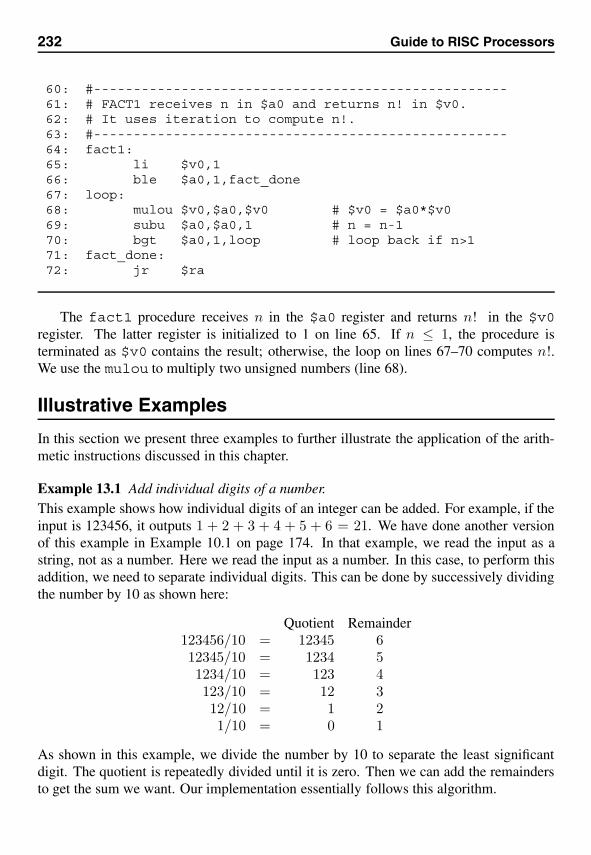
232 Guide to RISC Processors
60: #----------------------------------------------------61: # FACT1 receives n in $a0 and returns n! in $v0.62: # It uses iteration to compute n!.63: #----------------------------------------------------64: fact1:65: li $v0,166: ble $a0,1,fact_done67: loop:68: mulou $v0,$a0,$v0 # $v0 = $a0*$v069: subu $a0,$a0,1 # n = n-170: bgt $a0,1,loop # loop back if n>171: fact_done:72: jr $ra
The fact1 procedure receives n in the $a0 register and returns n! in the $v0register. The latter register is initialized to 1 on line 65. If n ≤ 1, the procedure isterminated as $v0 contains the result; otherwise, the loop on lines 67–70 computes n!.We use the mulou to multiply two unsigned numbers (line 68).
Illustrative Examples
In this section we present three examples to further illustrate the application of the arith-metic instructions discussed in this chapter.
Example 13.1 Add individual digits of a number.This example shows how individual digits of an integer can be added. For example, if theinput is 123456, it outputs 1 + 2 + 3 + 4 + 5 + 6 = 21. We have done another versionof this example in Example 10.1 on page 174. In that example, we read the input as astring, not as a number. Here we read the input as a number. In this case, to perform thisaddition, we need to separate individual digits. This can be done by successively dividingthe number by 10 as shown here:
Quotient Remainder123456/10 = 12345 612345/10 = 1234 51234/10 = 123 4123/10 = 12 312/10 = 1 21/10 = 0 1
As shown in this example, we divide the number by 10 to separate the least significantdigit. The quotient is repeatedly divided until it is zero. Then we can add the remaindersto get the sum we want. Our implementation essentially follows this algorithm.
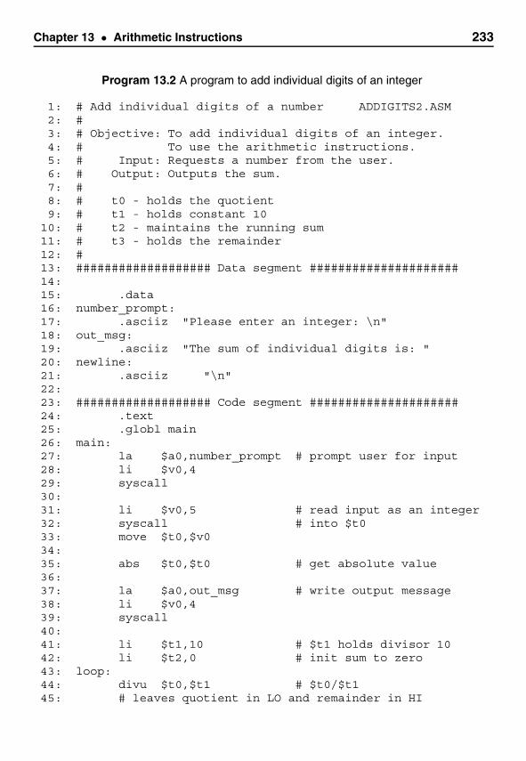
Chapter 13 • Arithmetic Instructions 233
Program 13.2 A program to add individual digits of an integer
1: # Add individual digits of a number ADDIGITS2.ASM2: #3: # Objective: To add individual digits of an integer.4: # To use the arithmetic instructions.5: # Input: Requests a number from the user.6: # Output: Outputs the sum.7: #8: # t0 - holds the quotient9: # t1 - holds constant 10
10: # t2 - maintains the running sum11: # t3 - holds the remainder12: #13: ################### Data segment #####################14:15: .data16: number_prompt:17: .asciiz "Please enter an integer: \n"18: out_msg:19: .asciiz "The sum of individual digits is: "20: newline:21: .asciiz "\n"22:23: ################### Code segment #####################24: .text25: .globl main26: main:27: la $a0,number_prompt # prompt user for input28: li $v0,429: syscall30:31: li $v0,5 # read input as an integer32: syscall # into $t033: move $t0,$v034:35: abs $t0,$t0 # get absolute value36:37: la $a0,out_msg # write output message38: li $v0,439: syscall40:41: li $t1,10 # $t1 holds divisor 1042: li $t2,0 # init sum to zero43: loop:44: divu $t0,$t1 # $t0/$t145: # leaves quotient in LO and remainder in HI
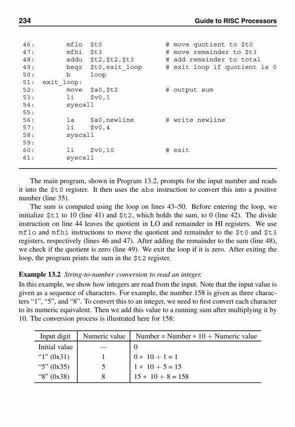
234 Guide to RISC Processors
46: mflo $t0 # move quotient to $t047: mfhi $t3 # move remainder to $t348: addu $t2,$t2,$t3 # add remainder to total49: beqz $t0,exit_loop # exit loop if quotient is 050: b loop51: exit_loop:52: move $a0,$t2 # output sum53: li $v0,154: syscall55:56: la $a0,newline # write newline57: li $v0,458: syscall59:60: li $v0,10 # exit61: syscall
The main program, shown in Program 13.2, prompts for the input number and readsit into the $t0 register. It then uses the abs instruction to convert this into a positivenumber (line 35).
The sum is computed using the loop on lines 43–50. Before entering the loop, weinitialize $t1 to 10 (line 41) and $t2, which holds the sum, to 0 (line 42). The divideinstruction on line 44 leaves the quotient in LO and remainder in HI registers. We usemflo and mfhi instructions to move the quotient and remainder to the $t0 and $t3registers, respectively (lines 46 and 47). After adding the remainder to the sum (line 48),we check if the quotient is zero (line 49). We exit the loop if it is zero. After exiting theloop, the program prints the sum in the $t2 register.
Example 13.2 String-to-number conversion to read an integer.In this example, we show how integers are read from the input. Note that the input value isgiven as a sequence of characters. For example, the number 158 is given as three charac-ters “1”, “5”, and “8”. To convert this to an integer, we need to first convert each characterto its numeric equivalent. Then we add this value to a running sum after multiplying it by10. The conversion process is illustrated here for 158:
Input digit Numeric value Number = Number * 10 + Numeric value
Initial value — 0“1” (0x31) 1 0 * 10 + 1 = 1“5” (0x35) 5 1 * 10 + 5 = 15“8” (0x38) 8 15 * 10 + 8 = 158
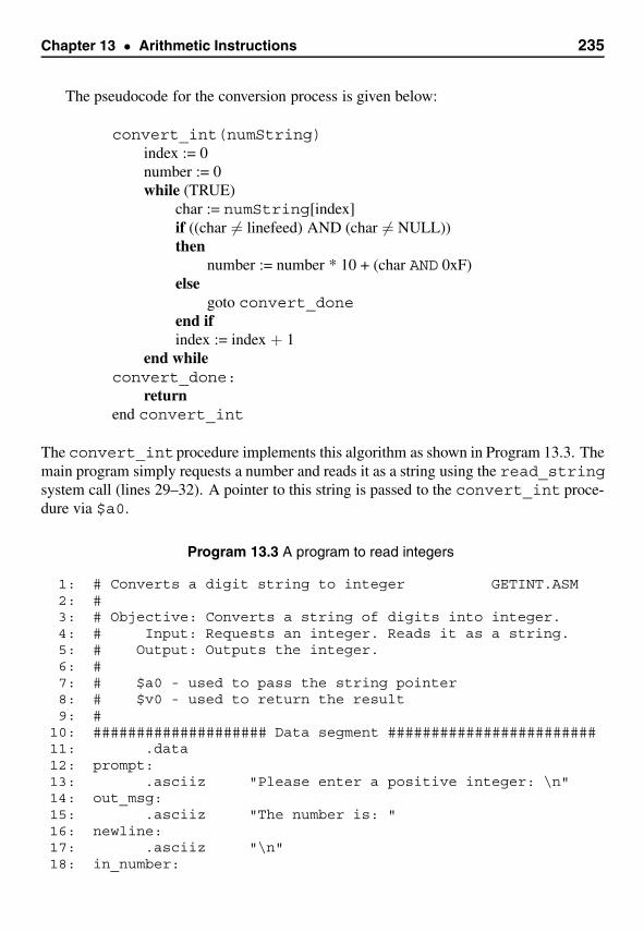
Chapter 13 • Arithmetic Instructions 235
The pseudocode for the conversion process is given below:
convert_int(numString)index := 0number := 0while (TRUE)
char := numString[index]if ((char �= linefeed) AND (char �= NULL))then
number := number * 10 + (char AND 0xF)else
goto convert_doneend ifindex := index + 1
end whileconvert_done:
returnend convert_int
The convert_intprocedure implements this algorithm as shown in Program 13.3. Themain program simply requests a number and reads it as a string using the read_stringsystem call (lines 29–32). A pointer to this string is passed to the convert_int proce-dure via $a0.
Program 13.3 A program to read integers
1: # Converts a digit string to integer GETINT.ASM2: #3: # Objective: Converts a string of digits into integer.4: # Input: Requests an integer. Reads it as a string.5: # Output: Outputs the integer.6: #7: # $a0 - used to pass the string pointer8: # $v0 - used to return the result9: #
10: #################### Data segment ########################11: .data12: prompt:13: .asciiz "Please enter a positive integer: \n"14: out_msg:15: .asciiz "The number is: "16: newline:17: .asciiz "\n"18: in_number:
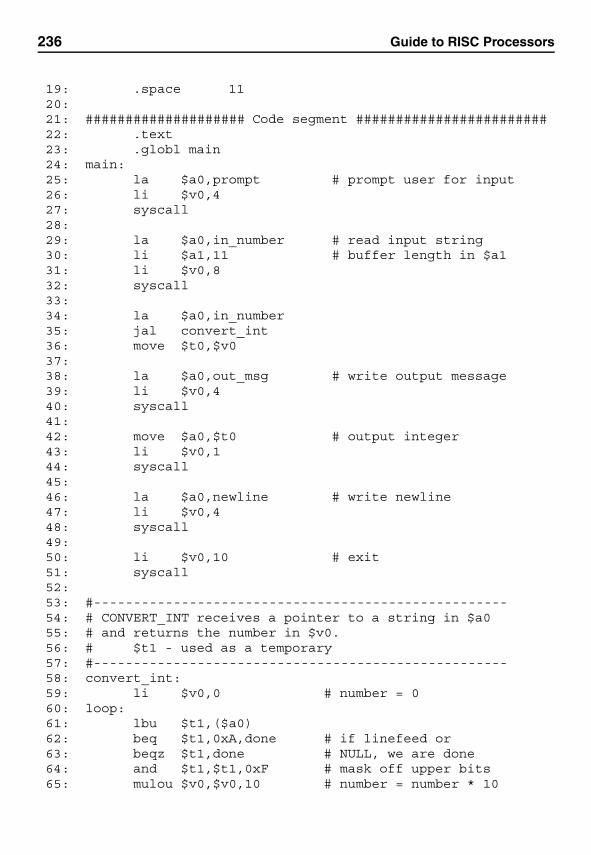
236 Guide to RISC Processors
19: .space 1120:21: #################### Code segment ########################22: .text23: .globl main24: main:25: la $a0,prompt # prompt user for input26: li $v0,427: syscall28:29: la $a0,in_number # read input string30: li $a1,11 # buffer length in $a131: li $v0,832: syscall33:34: la $a0,in_number35: jal convert_int36: move $t0,$v037:38: la $a0,out_msg # write output message39: li $v0,440: syscall41:42: move $a0,$t0 # output integer43: li $v0,144: syscall45:46: la $a0,newline # write newline47: li $v0,448: syscall49:50: li $v0,10 # exit51: syscall52:53: #----------------------------------------------------54: # CONVERT_INT receives a pointer to a string in $a055: # and returns the number in $v0.56: # $t1 - used as a temporary57: #----------------------------------------------------58: convert_int:59: li $v0,0 # number = 060: loop:61: lbu $t1,($a0)62: beq $t1,0xA,done # if linefeed or63: beqz $t1,done # NULL, we are done64: and $t1,$t1,0xF # mask off upper bits65: mulou $v0,$v0,10 # number = number * 10
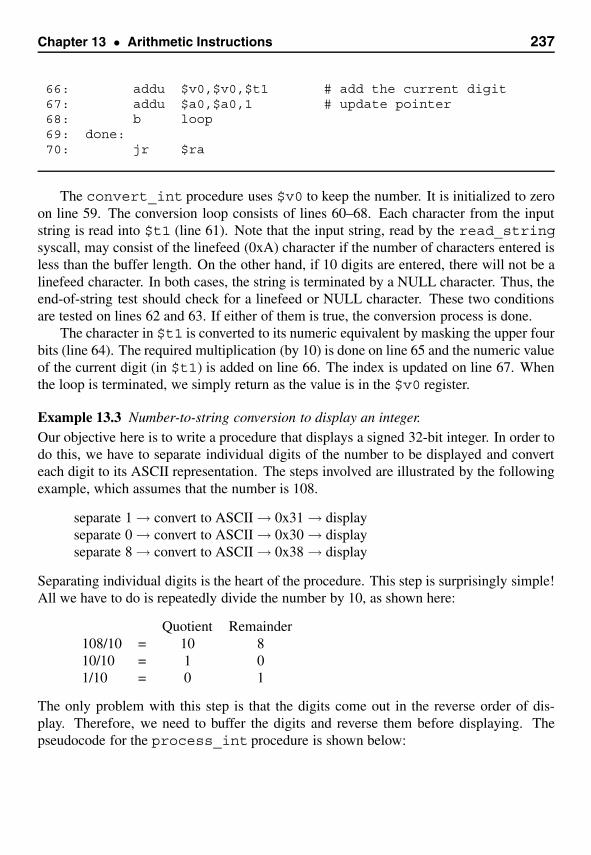
Chapter 13 • Arithmetic Instructions 237
66: addu $v0,$v0,$t1 # add the current digit67: addu $a0,$a0,1 # update pointer68: b loop69: done:70: jr $ra
The convert_int procedure uses $v0 to keep the number. It is initialized to zeroon line 59. The conversion loop consists of lines 60–68. Each character from the inputstring is read into $t1 (line 61). Note that the input string, read by the read_stringsyscall, may consist of the linefeed (0xA) character if the number of characters entered isless than the buffer length. On the other hand, if 10 digits are entered, there will not be alinefeed character. In both cases, the string is terminated by a NULL character. Thus, theend-of-string test should check for a linefeed or NULL character. These two conditionsare tested on lines 62 and 63. If either of them is true, the conversion process is done.
The character in $t1 is converted to its numeric equivalent by masking the upper fourbits (line 64). The required multiplication (by 10) is done on line 65 and the numeric valueof the current digit (in $t1) is added on line 66. The index is updated on line 67. Whenthe loop is terminated, we simply return as the value is in the $v0 register.
Example 13.3 Number-to-string conversion to display an integer.Our objective here is to write a procedure that displays a signed 32-bit integer. In order todo this, we have to separate individual digits of the number to be displayed and converteach digit to its ASCII representation. The steps involved are illustrated by the followingexample, which assumes that the number is 108.
separate 1 → convert to ASCII → 0x31 → displayseparate 0 → convert to ASCII → 0x30 → displayseparate 8 → convert to ASCII → 0x38 → display
Separating individual digits is the heart of the procedure. This step is surprisingly simple!All we have to do is repeatedly divide the number by 10, as shown here:
Quotient Remainder108/10 = 10 810/10 = 1 01/10 = 0 1
The only problem with this step is that the digits come out in the reverse order of dis-play. Therefore, we need to buffer the digits and reverse them before displaying. Thepseudocode for the process_int procedure is shown below:
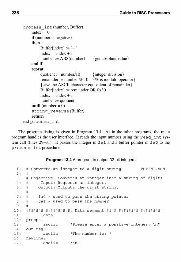
238 Guide to RISC Processors
process_int (number, Buffer)index := 0if (number is negative)then
Buffer[index] := ’−’index := index + 1number := ABS(number) {get absolute value}
end ifrepeat
quotient := number/10 {integer division}remainder := number % 10 {% is modulo operator}{save the ASCII character equivalent of remainder}Buffer[index] := remainder OR 0x30index := index + 1number := quotient
until (number = 0)string_reverse (Buffer)return
end process_int
The program listing is given in Program 13.4. As in the other programs, the mainprogram handles the user interface. It reads the input number using the read_int sys-tem call (lines 29–31). It passes the integer in $a1 and a buffer pointer in $a0 to theprocess_int procedure.
Program 13.4 A program to output 32-bit integers
1: # Converts an integer to a digit string PUTINT.ASM2: #3: # Objective: Converts an integer into a string of digits.4: # Input: Requests an integer.5: # Output: Outputs the digit string.6: #7: # $a0 - used to pass the string pointer8: # $a1 - used to pass the number9: #
10: ################### Data segment #######################11: .data12: prompt:13: .asciiz "Please enter a positive integer: \n"14: out_msg:15: .asciiz "The number is: "16: newline:17: .asciiz "\n"
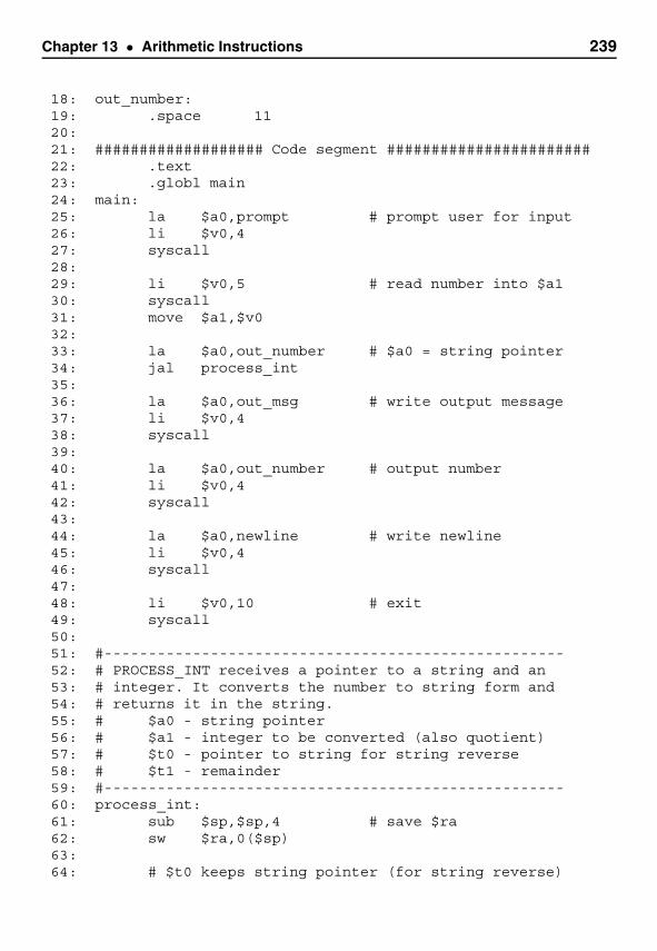
Chapter 13 • Arithmetic Instructions 239
18: out_number:19: .space 1120:21: ################### Code segment #######################22: .text23: .globl main24: main:25: la $a0,prompt # prompt user for input26: li $v0,427: syscall28:29: li $v0,5 # read number into $a130: syscall31: move $a1,$v032:33: la $a0,out_number # $a0 = string pointer34: jal process_int35:36: la $a0,out_msg # write output message37: li $v0,438: syscall39:40: la $a0,out_number # output number41: li $v0,442: syscall43:44: la $a0,newline # write newline45: li $v0,446: syscall47:48: li $v0,10 # exit49: syscall50:51: #----------------------------------------------------52: # PROCESS_INT receives a pointer to a string and an53: # integer. It converts the number to string form and54: # returns it in the string.55: # $a0 - string pointer56: # $a1 - integer to be converted (also quotient)57: # $t0 - pointer to string for string reverse58: # $t1 - remainder59: #----------------------------------------------------60: process_int:61: sub $sp,$sp,4 # save $ra62: sw $ra,0($sp)63:64: # $t0 keeps string pointer (for string reverse)
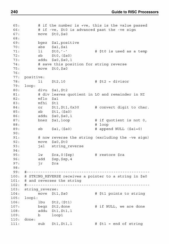
240 Guide to RISC Processors
65: # if the number is +ve, this is the value passed66: # if -ve, $t0 is advanced past the -ve sign67: move $t0,$a068:69: bgez $a1,positive70: abs $a1,$a171: li $t0,’-’ # $t0 is used as a temp72: sb $t0,($a0)73: addu $a0,$a0,174: # save this position for string reverse75: move $t0,$a076:77: positive:78: li $t2,10 # $t2 = divisor79: loop:80: divu $a1,$t281: # div leaves quotient in LO and remainder in HI82: mflo $a183: mfhi $t184: or $t1,$t1,0x30 # convert digit to char.85: sb $t1,($a0)86: addu $a0,$a0,187: bnez $a1,loop # if quotient is not 0,88: # loop89: sb $a1,($a0) # append NULL ($a1=0)90:91: # now reverse the string (excluding the -ve sign)92: move $a0,$t093: jal string_reverse94:95: lw $ra,0($sp) # restore $ra96: add $sp,$sp,497: jr $ra98:99: #------------------------------------------------------
100: # STRING_REVERSE receives a pointer to a string in $a0101: # and reverses the string102: #------------------------------------------------------103: string_reverse:104: move $t1,$a0 # $t1 points to string105: loop1:106: lbu $t2,($t1)107: beqz $t2,done # if NULL, we are done108: addu $t1,$t1,1109: b loop1110: done:111: sub $t1,$t1,1 # $t1 = end of string
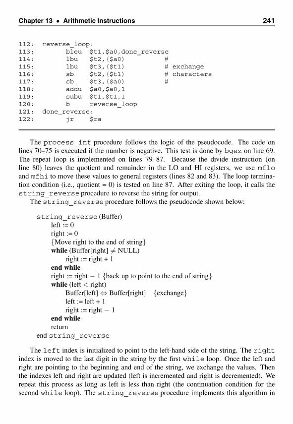
Chapter 13 • Arithmetic Instructions 241
112: reverse_loop:113: bleu $t1,$a0,done_reverse114: lbu $t2,($a0) #115: lbu $t3,($t1) # exchange116: sb $t2,($t1) # characters117: sb $t3,($a0) #118: addu $a0,$a0,1119: subu $t1,$t1,1120: b reverse_loop121: done_reverse:122: jr $ra
The process_int procedure follows the logic of the pseudocode. The code onlines 70–75 is executed if the number is negative. This test is done by bgez on line 69.The repeat loop is implemented on lines 79–87. Because the divide instruction (online 80) leaves the quotient and remainder in the LO and HI registers, we use mfloand mfhi to move these values to general registers (lines 82 and 83). The loop termina-tion condition (i.e., quotient = 0) is tested on line 87. After exiting the loop, it calls thestring_reverse procedure to reverse the string for output.
The string_reverse procedure follows the pseudocode shown below:
string_reverse (Buffer)left := 0right := 0{Move right to the end of string}while (Buffer[right] �= NULL)
right := right + 1end whileright := right − 1 {back up to point to the end of string}while (left < right)
Buffer[left] ⇔ Buffer[right] {exchange}left := left + 1right := right − 1
end whilereturn
end string_reverse
The left index is initialized to point to the left-hand side of the string. The rightindex is moved to the last digit in the string by the first while loop. Once the left andright are pointing to the beginning and end of the string, we exchange the values. Thenthe indexes left and right are updated (left is incremented and right is decremented). Werepeat this process as long as left is less than right (the continuation condition for thesecond while loop). The string_reverse procedure implements this algorithm in
242 Guide to RISC Processors
a straightforward way. The first while loop is implemented on lines 105–109 and thesecond while loop on lines 112–120.
Summary
We have presented details on the arithmetic instructions. The MIPS instruction set sup-ports the basic add, subtract, multiply, and divide operations. The multiply and divideinstructions place the result in special HI and LO registers. The instruction set providesinstructions that move data between these registers and the general registers. Althoughadd and subtract instructions work on both signed and unsigned numbers, multiply anddivide operations have separate instructions to work on signed and unsigned numbers. Wehave used several examples to illustrate the application of these instructions.
14Conditional Execution
Conditional execution is important to alter the control flow from the default sequentialexecution. The MIPS architecture provides several instructions to facilitate conditionalexecution. We have already seen some of these instructions including the unconditionaland conditional branch instructions. In addition, procedure invocation and return also altercontrol flow. We briefly introduced some of these instructions in previous chapters. Thischapter gives a complete discussion of these instructions.
The target address of these flow-altering instructions can be specified either directlyin the instruction or indirectly via a register. In previous chapters, we used direct speci-fication for jumps and procedure calls. However, we used indirect specification to returnfrom a procedure. Most jumps and procedure calls use the direct specification. However,sometimes it is useful to specify the target address indirectly via a register. We discusssuch indirect jumps and procedure calls toward the end of the chapter. We conclude thechapter with a summary.
IntroductionModern high-level languages provide a variety of decision structures. These structuresinclude selection structures such as if-then-else and iterative structures such aswhile and for loops. Assembly language, being a low-level language, does not providethese structures directly. However, assembly language provides several basic instructionsthat could be used to construct these high-level language selection and iteration structures.For example, the following code
li $t2,50loop:
addu $t0,$t0,$t1sub $t2,$t2,1bnez $t2,loop
implements a loop that iterates 50 times.
243
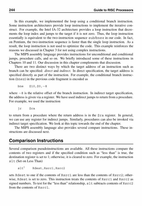
244 Guide to RISC Processors
In this example, we implemented the loop using a conditional branch instruction.Some instruction architectures provide loop instructions to implement the iterative con-struct. For example, the Intel IA-32 architecture provides a loop instruction that decre-ments the loop index and jumps to the target if it is not zero. Thus, the loop instructionessentially is equivalent to the two-instruction sequence sub/bnez in our code. In fact,on Pentium, the two-instruction sequence is faster than the single loop instruction. As aresult, the loop instruction is not used to optimize the code. This example reinforces thereasons we discussed in Chapter 3 for not using complex instructions.
The MIPS assembly language provides instructions for unconditional and conditionaljumps, procedure calls, and so on. We briefly introduced some of these instructions inChapters 10 and 11. Our discussion in this chapter complements that discussion.
There are two distinct ways by which the target address of an instruction such asbranch can be specified: direct and indirect. In direct specification, the target address isspecified directly as part of the instruction. For example, the conditional branch instruc-tion (bnez) in the previous code fragment is encoded as
bne $10,$0,−8
where −8 is the relative offset of the branch instruction. In indirect target specification,the address is given via a register. We have used indirect jumps to return from a procedure.For example, we used the instruction
jr $ra
to return from a procedure where the return address is in the $ra register. In general,we can use any register for indirect jumps. Similarly, procedures can also be invoked viaindirect target specification. We look at this topic towards the end of the chapter.
The MIPS assembly language also provides several compare instructions. These in-structions are discussed next.
Comparison Instructions
Several comparison pseudoinstructions are available. All these instructions compare thecontents of two registers and if the specified condition such as “less than” is true, thedestination register is set to 1; otherwise, it is cleared to zero. For example, the instructionslt (Set on Less Than)
slt† Rdest,Rsrc1,Rsrc2
sets Rdest to one if the contents of Rsrc1 are less than the contents of Rsrc2; other-wise, Rdest is set to zero. This instruction treats the contents of Rsrc1 and Rsrc2 assigned numbers. To test for the “less than” relationship, slt subtracts contents of Rsrc2from the contents of Rsrc1.
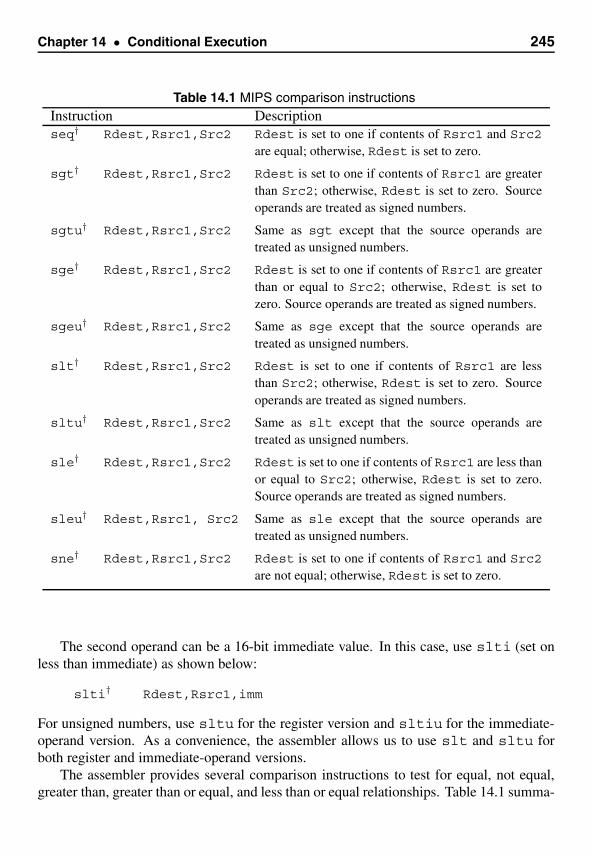
Chapter 14 • Conditional Execution 245
Table 14.1 MIPS comparison instructionsInstruction Descriptionseq† Rdest,Rsrc1,Src2 Rdest is set to one if contents of Rsrc1 and Src2
are equal; otherwise, Rdest is set to zero.
sgt† Rdest,Rsrc1,Src2 Rdest is set to one if contents of Rsrc1 are greaterthan Src2; otherwise, Rdest is set to zero. Sourceoperands are treated as signed numbers.
sgtu† Rdest,Rsrc1,Src2 Same as sgt except that the source operands aretreated as unsigned numbers.
sge† Rdest,Rsrc1,Src2 Rdest is set to one if contents of Rsrc1 are greaterthan or equal to Src2; otherwise, Rdest is set tozero. Source operands are treated as signed numbers.
sgeu† Rdest,Rsrc1,Src2 Same as sge except that the source operands aretreated as unsigned numbers.
slt† Rdest,Rsrc1,Src2 Rdest is set to one if contents of Rsrc1 are lessthan Src2; otherwise, Rdest is set to zero. Sourceoperands are treated as signed numbers.
sltu† Rdest,Rsrc1,Src2 Same as slt except that the source operands aretreated as unsigned numbers.
sle† Rdest,Rsrc1,Src2 Rdest is set to one if contents of Rsrc1 are less thanor equal to Src2; otherwise, Rdest is set to zero.Source operands are treated as signed numbers.
sleu† Rdest,Rsrc1, Src2 Same as sle except that the source operands aretreated as unsigned numbers.
sne† Rdest,Rsrc1,Src2 Rdest is set to one if contents of Rsrc1 and Src2are not equal; otherwise, Rdest is set to zero.
The second operand can be a 16-bit immediate value. In this case, use slti (set onless than immediate) as shown below:
slti† Rdest,Rsrc1,imm
For unsigned numbers, use sltu for the register version and sltiu for the immediate-operand version. As a convenience, the assembler allows us to use slt and sltu forboth register and immediate-operand versions.
The assembler provides several comparison instructions to test for equal, not equal,greater than, greater than or equal, and less than or equal relationships. Table 14.1 summa-
246 Guide to RISC Processors
rizes the comparison instructions provided by the assembler. Notice that all comparisoninstructions in Table 14.1 are pseudoinstructions. For example, the pseudoinstruction
seq $a0,$a1,$a2
is translated as
beq $6,$5,skip1ori $4,$0,0beq $0,$0,skip2
skip1:ori $4,$0,1
skip2:. . .
Note that $a0, $a1, and $a2 represent registers $4, $5, and $6, respectively. Thebranch instructions are discussed next.
Unconditional Branch InstructionsUnconditional transfer of control is implemented by jump and branch instructions. Let usfirst look at the basic jump instruction. The jump instruction
j target
transfers control to the target address. As discussed before, this is a direct jump in-struction in which the target address is given as part of the instruction. In the MIPS32architecture, the control is transferred to target after executing the delay slot instruc-tion. However, see the following SPIM note.
SPIM noteBecause SPIM does not simulate delayed branch, it does not exe-cute the delay slot instruction.
There are other types of jump instructions that are useful as procedure calls. We havealready discussed some of these instructions in Chapter 11. For example, we use the jalinstruction to invoke a procedure. Similarly, the jr instruction is used to return from aprocedure.
Branch instructions provide a more flexible test and jump execution. MIPS supportsseveral branch instructions. We describe some of these instructions in this section.
The unconditional branch instruction
b† target
transfers control to target unconditionally. Semantically, it is very similar to the jumpinstruction. The main difference is that the b instruction uses a 16-bit relative address
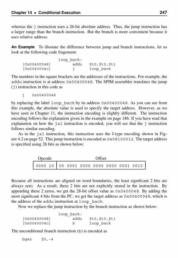
Chapter 14 • Conditional Execution 247
whereas the j instruction uses a 26-bit absolute address. Thus, the jump instruction hasa larger range than the branch instruction. But the branch is more convenient because ituses relative address.
An Example To illustate the difference between jump and branch instructions, let uslook at the following code fragement.
loop_back:[0x00400048] addu $t0,$t0,$t1[0x0040004c] j loop_back
The numbers in the square brackets are the addresses of the instructions. For example, theaddu instruction is at address 0x00400048. The SPIM assembler translates the jump(j) instruction in this code as
j 0x00400048
by replacing the label loop_back by its address 0x00400048. As you can see fromthis example, the absolute value is used to specify the target address. However, as wehave seen in Chapter 11, the instruction encoding is slightly different. The instructionencoding follows the explanation given in the example on page 186. If you have read thatexplanation on how the jal instruction is encoded, you will see that the j instructionfollows similar encoding.
As in the jal instruction, this instruction uses the J-type encoding shown in Fig-ure 4.2 on page 52. This jump instruction is encoded as 0x08100012. The target addressis specified using 26 bits as shown below:
Opcode Offset
0000 10 00 0001 0000 0000 0000 0001 0010
Because all instructions are aligned on word boundaries, the least significant 2 bits arealways zero. As a result, these 2 bits are not explicitly stored in the instruction. Byappending these 2 zeros, we get the 28-bit offset value as 0x0400048. By adding themost significant 4 bits from the PC, we get the target address as 0x00400048, which isthe address of the addu instruction at loop_back.
Now we replace the jump instruction by the branch instruction as shown below:
loop_back:[0x00400048] addu $t0,$t0,$t1[0x0040004c] b loop_back
The unconditional branch instruction (b) is encoded as
bgez $0,-4
248 Guide to RISC Processors
This example gives the following information about the encoding of the b instruction:
• Because the branch instruction is actually a pseudoinstruction, it is encoded usingthe conditional branch instruction bgez. How can this instruction implement anunconditional branch? Well, we compare register $0 to zero and jump to target ifthe register has a value greater than or equal to zero. Register $0 is hardwired tozero, therefore the test is always true, causing the jump to always take place.
• The offset used is a PC-relative value, not the absolute value as in the j instruction.In our example, the relative offset is −4.
Conditional Branch InstructionsNow we look at the conditional branch instructions. These instructions compare the con-tents of two registers and jump to the target if the specified condition is true. For example,the branch instruction
beq Rsrc1,Rsrc2,target
compares the contents of Rsrc1 and Rsrc2 and transfers control to target if they areequal.
Branch instructions to test “less than” and “greater than” are also supported. As anexample, the instruction
bgt Rsrc1,Rsrc2,target
branches to the target location when the contents of Rsrc1 are greater than Rsrc2.When comparing, the contents of Rsrc1 and Rsrc2 are treated as signed numbers. Forunsigned numbers, we have to use the bgtu instruction.
Branch instructions to test combinations such as “greater than or equal to” are alsoavailable. Table 14.2 summarizes some of the branch instructions provided by the MIPSassembler.
Very often, we need to compare a value with zero and transfer control to the targetbased on this comparison. This is often the case in constructing loops. For example,look at the code given at the beginning of this chapter. For this reason, MIPS supportsconditional branch instructions that compare with zero. To illustrate the format of theseinstructions, we use the beqz instruction. The format is
beqz Rsrc,target
This instruction transfers control to target if the value of Rsrc is equal to zero. Ta-ble 14.3 summarizes these instructions.

Chapter 14 • Conditional Execution 249
Table 14.2 MIPS branch instructions (based on register comparison)
Instruction Descriptionb† target Branches unconditionally to target.
beq Rsrc1,Rsrc2,target Branches to target if the contents of Rsrc1 andRsrc2 are equal.
bne Rsrc1,Rsrc2,target Branches to target if the contents of Rsrc1 andRsrc2 are not equal.
blt Rsrc1,Rsrc2,target Branches to target if the value of Rsrc1 is lessthan the value of Rsrc2. The source operands areconsidered as signed numbers.
bltu Rsrc1,Rsrc2,target Same as blt except that the source operands aretreated as unsigned numbers.
bgt Rsrc1,Rsrc2,target Branches to target if the value of Rsrc1 is greaterthan the value of Rsrc2. The source operands aretreated as signed numbers.
bgtu Rsrc1,Rsrc2,target Same as bgt except that the source operands aretreated as unsigned numbers.
ble Rsrc1,Rsrc2,target Branches to target if the value of Rsrc1 is lessthan or equal to the value of Rsrc2. The sourceoperands are treated as signed numbers.
bleu Rsrc1,Rsrc2,target Same as ble except that the source operands aretreated as unsigned numbers.
bge Rsrc1,Rsrc2,target Branches to target if the value of Rsrc1 is greaterthan or equal to the value of Rsrc2. The sourceoperands are treated as signed numbers.
bgeu Rsrc1,Rsrc2,target Same as bge except that the source operands are con-sidered as unsigned numbers.
Our First Program
As our first example of the chapter, we look at counting the number of uppercase lettersin a given string. The program listing is given in Program 14.1. The main programprompts the user for a string and passes it on to the count procedure via the $a0 register.The count procedure returns the uppercase count in $v0. The procedure follows thealgorithm given below:
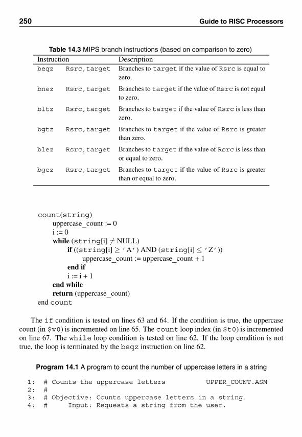
250 Guide to RISC Processors
Table 14.3 MIPS branch instructions (based on comparison to zero)
Instruction Descriptionbeqz Rsrc,target Branches to target if the value of Rsrc is equal to
zero.
bnez Rsrc,target Branches to target if the value of Rsrc is not equalto zero.
bltz Rsrc,target Branches to target if the value of Rsrc is less thanzero.
bgtz Rsrc,target Branches to target if the value of Rsrc is greaterthan zero.
blez Rsrc,target Branches to target if the value of Rsrc is less thanor equal to zero.
bgez Rsrc,target Branches to target if the value of Rsrc is greaterthan or equal to zero.
count(string)uppercase_count := 0i := 0while (string[i] �= NULL)
if ((string[i] ≥ ’A’) AND (string[i] ≤ ’Z’))uppercase_count := uppercase_count + 1
end ifi := i + 1
end whilereturn (uppercase_count)
end count
The if condition is tested on lines 63 and 64. If the condition is true, the uppercasecount (in $v0) is incremented on line 65. The count loop index (in $t0) is incrementedon line 67. The while loop condition is tested on line 62. If the loop condition is nottrue, the loop is terminated by the beqz instruction on line 62.
Program 14.1 A program to count the number of uppercase letters in a string
1: # Counts the uppercase letters UPPER_COUNT.ASM2: #3: # Objective: Counts uppercase letters in a string.4: # Input: Requests a string from the user.
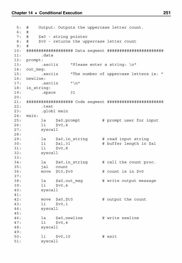
Chapter 14 • Conditional Execution 251
5: # Output: Outputs the uppercase letter count.6: #7: # $a0 - string pointer8: # $v0 - returns the uppercase letter count9: #
10: ################### Data segment #######################11: .data12: prompt:13: .asciiz "Please enter a string: \n"14: out_msg:15: .asciiz "The number of uppercase letters is: "16: newline:17: .asciiz "\n"18: in_string:19: .space 3120:21: ################### Code segment #######################22: .text23: .globl main24: main:25: la $a0,prompt # prompt user for input26: li $v0,427: syscall28:29: la $a0,in_string # read input string30: li $a1,31 # buffer length in $a131: li $v0,832: syscall33:34: la $a0,in_string # call the count proc.35: jal count36: move $t0,$v0 # count is in $v037:38: la $a0,out_msg # write output message39: li $v0,440: syscall41:42: move $a0,$t0 # output the count43: li $v0,144: syscall45:46: la $a0,newline # write newline47: li $v0,448: syscall49:50: li $v0,10 # exit51: syscall
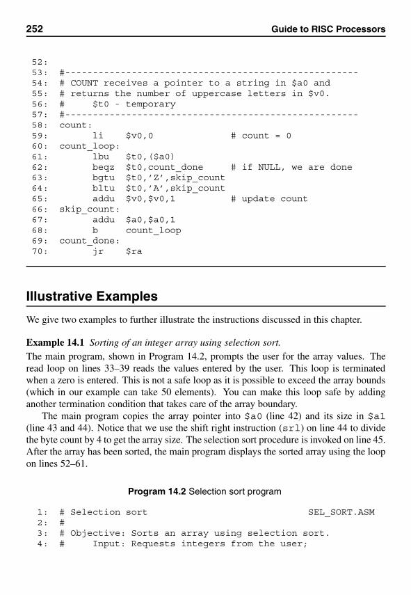
252 Guide to RISC Processors
52:53: #-----------------------------------------------------54: # COUNT receives a pointer to a string in $a0 and55: # returns the number of uppercase letters in $v0.56: # $t0 - temporary57: #-----------------------------------------------------58: count:59: li $v0,0 # count = 060: count_loop:61: lbu $t0,($a0)62: beqz $t0,count_done # if NULL, we are done63: bgtu $t0,’Z’,skip_count64: bltu $t0,’A’,skip_count65: addu $v0,$v0,1 # update count66: skip_count:67: addu $a0,$a0,168: b count_loop69: count_done:70: jr $ra
Illustrative Examples
We give two examples to further illustrate the instructions discussed in this chapter.
Example 14.1 Sorting of an integer array using selection sort.The main program, shown in Program 14.2, prompts the user for the array values. Theread loop on lines 33–39 reads the values entered by the user. This loop is terminatedwhen a zero is entered. This is not a safe loop as it is possible to exceed the array bounds(which in our example can take 50 elements). You can make this loop safe by addinganother termination condition that takes care of the array boundary.
The main program copies the array pointer into $a0 (line 42) and its size in $a1(line 43 and 44). Notice that we use the shift right instruction (srl) on line 44 to dividethe byte count by 4 to get the array size. The selection sort procedure is invoked on line 45.After the array has been sorted, the main program displays the sorted array using the loopon lines 52–61.
Program 14.2 Selection sort program
1: # Selection sort SEL_SORT.ASM2: #3: # Objective: Sorts an array using selection sort.4: # Input: Requests integers from the user;
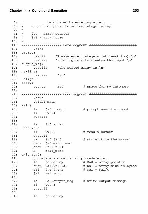
Chapter 14 • Conditional Execution 253
5: # terminated by entering a zero.6: # Output: Outputs the sorted integer array.7: #8: # $a0 - array pointer9: # $a1 - array size
10: #11: #################### Data segment ########################12: .data13: prompt:14: .ascii "Please enter integers (at least two).\n"15: .asciiz "Entering zero terminates the input.\n"16: output_msg:17: .asciiz "The sorted array is:\n"18: newline:19: .asciiz "\n"20: .align 221: array:22: .space 200 # space for 50 integers23:24: #################### Code segment ########################25: .text26: .globl main27: main:28: la $a0,prompt # prompt user for input29: li $v0,430: syscall31:32: la $t0,array33: read_more:34: li $v0,5 # read a number35: syscall36: sw $v0,($t0) # store it in the array37: beqz $v0,exit_read38: addu $t0,$t0,439: b read_more40: exit_read:41: # prepare arguments for procedure call42: la $a0,array # $a0 = array pointer43: subu $a1,$t0,$a0 # $a1 = array size in bytes44: srl $a1,$a1,2 # $a1 = $a1/445: jal sel_sort46:47: la $a0,output_msg # write output message48: li $v0,449: syscall50:51: la $t0,array
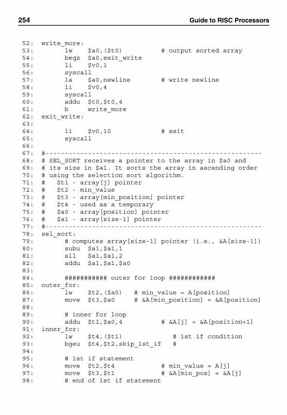
254 Guide to RISC Processors
52: write_more:53: lw $a0,($t0) # output sorted array54: beqz $a0,exit_write55: li $v0,156: syscall57: la $a0,newline # write newline58: li $v0,459: syscall60: addu $t0,$t0,461: b write_more62: exit_write:63:64: li $v0,10 # exit65: syscall66:67: #--------------------------------------------------------68: # SEL_SORT receives a pointer to the array in $a0 and69: # its size in $a1. It sorts the array in ascending order70: # using the selection sort algorithm.71: # $t1 - array[j] pointer72: # $t2 - min_value73: # $t3 - array[min_position] pointer74: # $t4 - used as a temporary75: # $a0 - array[position] pointer76: # $a1 - array[size-1] pointer77: #--------------------------------------------------------78: sel_sort:79: # computes array[size-1] pointer (i.e., &A[size-1])80: subu $a1,$a1,181: sll $a1,$a1,282: addu $a1,$a1,$a083:84: ########### outer for loop ############85: outer_for:86: lw $t2,($a0) # min_value = A[position]87: move $t3,$a0 # &A[min_position] = &A[position]88:89: # inner for loop90: addu $t1,$a0,4 # &A[j] = &A[position+1]91: inner_for:92: lw $t4,($t1) # 1st if condition93: bgeu $t4,$t2,skip_1st_if #94:95: # 1st if statement96: move $t2,$t4 # min_value = A[j]97: move $t3,$t1 # &A[min_pos] = &A[j]98: # end of 1st if statement
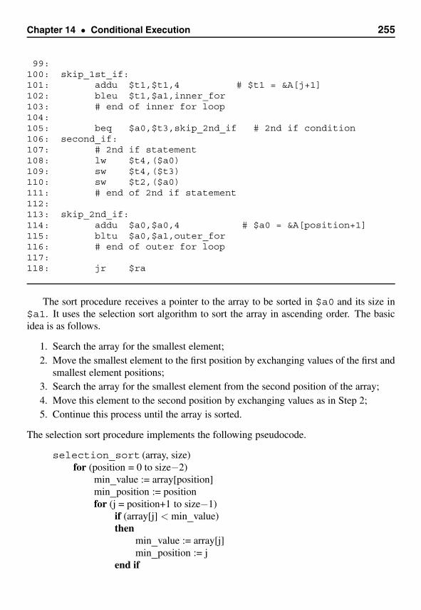
Chapter 14 • Conditional Execution 255
99:100: skip_1st_if:101: addu $t1,$t1,4 # $t1 = &A[j+1]102: bleu $t1,$a1,inner_for103: # end of inner for loop104:105: beq $a0,$t3,skip_2nd_if # 2nd if condition106: second_if:107: # 2nd if statement108: lw $t4,($a0)109: sw $t4,($t3)110: sw $t2,($a0)111: # end of 2nd if statement112:113: skip_2nd_if:114: addu $a0,$a0,4 # $a0 = &A[position+1]115: bltu $a0,$a1,outer_for116: # end of outer for loop117:118: jr $ra
The sort procedure receives a pointer to the array to be sorted in $a0 and its size in$a1. It uses the selection sort algorithm to sort the array in ascending order. The basicidea is as follows.
1. Search the array for the smallest element;2. Move the smallest element to the first position by exchanging values of the first and
smallest element positions;3. Search the array for the smallest element from the second position of the array;4. Move this element to the second position by exchanging values as in Step 2;5. Continue this process until the array is sorted.
The selection sort procedure implements the following pseudocode.
selection_sort (array, size)for (position = 0 to size−2)
min_value := array[position]min_position := positionfor (j = position+1 to size−1)
if (array[j] < min_value)then
min_value := array[j]min_position := j
end if
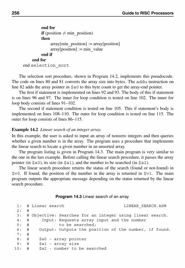
256 Guide to RISC Processors
end forif (position �= min_position)then
array[min_position] := array[position]array[position] := min_value
end ifend for
end selection_sort
The selection sort procedure, shown in Program 14.2, implements this pseudocode.The code on lines 80 and 81 converts the array size into bytes. The addu instruction online 82 adds the array pointer in $a0 to this byte count to get the array-end pointer.
The first if statement is implemented on lines 92 and 93. The body of this if statementis on lines 96 and 97. The inner for loop condition is tested on line 102. The inner forloop body consists of lines 91–102.
The second if statement condition is tested on line 105. This if statement’s body isimplemented on lines 108–110. The outer for loop condition is tested on line 115. Theouter for loop consists of lines 86–115.
Example 14.2 Linear search of an integer array.In this example, the user is asked to input an array of nonzero integers and then querieswhether a given number is in the array. The program uses a procedure that implementsthe linear search to locate a given number in an unsorted array.
The program listing is given in Program 14.3. The main program is very similar tothe one in the last example. Before calling the linear search procedure, it passes the arraypointer (in $a0), its size (in $a1), and the number to be searched (in $a2).
The linear search procedure returns the status of the search (found or not-found) in$v0. If found, the position of the number in the array is returned in $v1. The mainprogram outputs the appropriate message depending on the status returned by the linearsearch procedure.
Program 14.3 Linear search of an array
1: # Linear search LINEAR_SEARCH.ASM2: #3: # Objective: Searches for an integer using linear search.4: # Input: Requests array input and the number5: # to be searched;6: # Output: Outputs the position of the number, if found.7: #8: # $a0 - array pointer9: # $a1 - array size
10: # $a2 - number to be searched
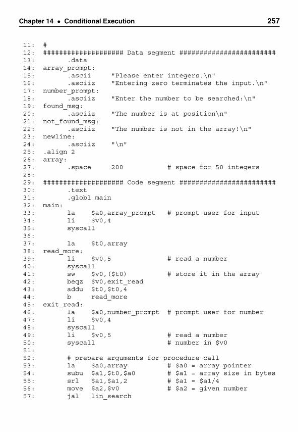
Chapter 14 • Conditional Execution 257
11: #12: #################### Data segment ########################13: .data14: array_prompt:15: .ascii "Please enter integers.\n"16: .asciiz "Entering zero terminates the input.\n"17: number_prompt:18: .asciiz "Enter the number to be searched:\n"19: found_msg:20: .asciiz "The number is at position\n"21: not_found_msg:22: .asciiz "The number is not in the array!\n"23: newline:24: .asciiz "\n"25: .align 226: array:27: .space 200 # space for 50 integers28:29: #################### Code segment ########################30: .text31: .globl main32: main:33: la $a0,array_prompt # prompt user for input34: li $v0,435: syscall36:37: la $t0,array38: read_more:39: li $v0,5 # read a number40: syscall41: sw $v0,($t0) # store it in the array42: beqz $v0,exit_read43: addu $t0,$t0,444: b read_more45: exit_read:46: la $a0,number_prompt # prompt user for number47: li $v0,448: syscall49: li $v0,5 # read a number50: syscall # number in $v051:52: # prepare arguments for procedure call53: la $a0,array # $a0 = array pointer54: subu $a1,$t0,$a0 # $a1 = array size in bytes55: srl $a1,$a1,2 # $a1 = $a1/456: move $a2,$v0 # $a2 = given number57: jal lin_search
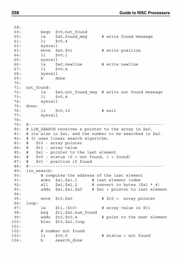
258 Guide to RISC Processors
58:59: beqz $v0,not_found60: la $a0,found_msg # write found message61: li $v0,462: syscall63: move $a0,$v1 # write position64: li $v0,165: syscall66: la $a0,newline # write newline67: li $v0,468: syscall69: b done70:71: not_found:72: la $a0,not_found_msg # write not found message73: li $v0,474: syscall75: done:76: li $v0,10 # exit77: syscall78:79: #-------------------------------------------------------80: # LIN_SEARCH receives a pointer to the array in $a0,81: # its size in $a1, and the number to be searched in $a2.82: # It uses linear search algorithm.83: # $t0 - array pointer84: # $t1 - array value85: # $a1 - pointer to the last element86: # $v0 - status (0 = not found, 1 = found)87: # $v1 - position if found88: #-------------------------------------------------------89: lin_search:90: # computes the address of the last element91: subu $a1,$a1,1 # last element index92: sll $a1,$a1,2 # convert to bytes ($a1 * 4)93: addu $a1,$a1,$a0 # $a1 = pointer to last element94:95: move $t0,$a0 # $t0 = array pointer96: loop:97: lw $t1,($t0) # array value in $t198: beq $t1,$a2,num_found99: addu $t0,$t0,4 # point to the next element
100: bleu $t0,$a1,loop101:102: # number not found103: li $v0,0 # status = not found104: b search_done
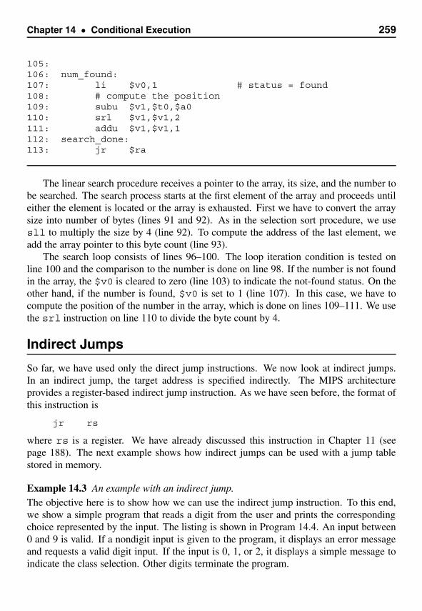
Chapter 14 • Conditional Execution 259
105:106: num_found:107: li $v0,1 # status = found108: # compute the position109: subu $v1,$t0,$a0110: srl $v1,$v1,2111: addu $v1,$v1,1112: search_done:113: jr $ra
The linear search procedure receives a pointer to the array, its size, and the number tobe searched. The search process starts at the first element of the array and proceeds untileither the element is located or the array is exhausted. First we have to convert the arraysize into number of bytes (lines 91 and 92). As in the selection sort procedure, we usesll to multiply the size by 4 (line 92). To compute the address of the last element, weadd the array pointer to this byte count (line 93).
The search loop consists of lines 96–100. The loop iteration condition is tested online 100 and the comparison to the number is done on line 98. If the number is not foundin the array, the $v0 is cleared to zero (line 103) to indicate the not-found status. On theother hand, if the number is found, $v0 is set to 1 (line 107). In this case, we have tocompute the position of the number in the array, which is done on lines 109–111. We usethe srl instruction on line 110 to divide the byte count by 4.
Indirect Jumps
So far, we have used only the direct jump instructions. We now look at indirect jumps.In an indirect jump, the target address is specified indirectly. The MIPS architectureprovides a register-based indirect jump instruction. As we have seen before, the format ofthis instruction is
jr rs
where rs is a register. We have already discussed this instruction in Chapter 11 (seepage 188). The next example shows how indirect jumps can be used with a jump tablestored in memory.
Example 14.3 An example with an indirect jump.The objective here is to show how we can use the indirect jump instruction. To this end,we show a simple program that reads a digit from the user and prints the correspondingchoice represented by the input. The listing is shown in Program 14.4. An input between0 and 9 is valid. If a nondigit input is given to the program, it displays an error messageand requests a valid digit input. If the input is 0, 1, or 2, it displays a simple message toindicate the class selection. Other digits terminate the program.
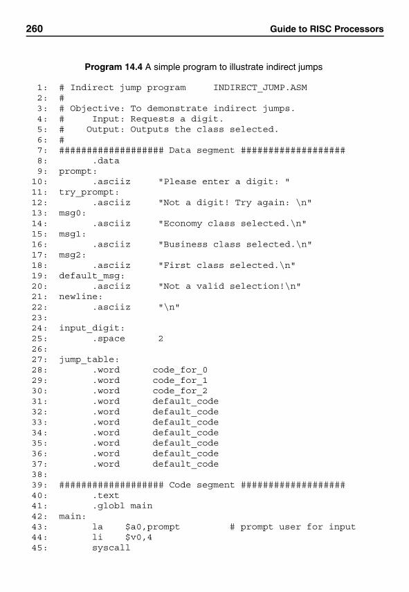
260 Guide to RISC Processors
Program 14.4 A simple program to illustrate indirect jumps
1: # Indirect jump program INDIRECT_JUMP.ASM2: #3: # Objective: To demonstrate indirect jumps.4: # Input: Requests a digit.5: # Output: Outputs the class selected.6: #7: ################### Data segment ###################8: .data9: prompt:
10: .asciiz "Please enter a digit: "11: try_prompt:12: .asciiz "Not a digit! Try again: \n"13: msg0:14: .asciiz "Economy class selected.\n"15: msg1:16: .asciiz "Business class selected.\n"17: msg2:18: .asciiz "First class selected.\n"19: default_msg:20: .asciiz "Not a valid selection!\n"21: newline:22: .asciiz "\n"23:24: input_digit:25: .space 226:27: jump_table:28: .word code_for_029: .word code_for_130: .word code_for_231: .word default_code32: .word default_code33: .word default_code34: .word default_code35: .word default_code36: .word default_code37: .word default_code38:39: ################### Code segment ###################40: .text41: .globl main42: main:43: la $a0,prompt # prompt user for input44: li $v0,445: syscall
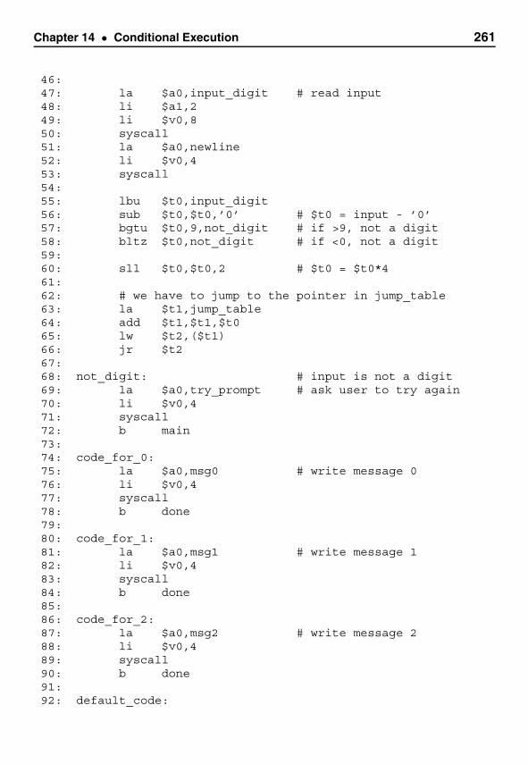
Chapter 14 • Conditional Execution 261
46:47: la $a0,input_digit # read input48: li $a1,249: li $v0,850: syscall51: la $a0,newline52: li $v0,453: syscall54:55: lbu $t0,input_digit56: sub $t0,$t0,’0’ # $t0 = input - ’0’57: bgtu $t0,9,not_digit # if >9, not a digit58: bltz $t0,not_digit # if <0, not a digit59:60: sll $t0,$t0,2 # $t0 = $t0*461:62: # we have to jump to the pointer in jump_table63: la $t1,jump_table64: add $t1,$t1,$t065: lw $t2,($t1)66: jr $t267:68: not_digit: # input is not a digit69: la $a0,try_prompt # ask user to try again70: li $v0,471: syscall72: b main73:74: code_for_0:75: la $a0,msg0 # write message 076: li $v0,477: syscall78: b done79:80: code_for_1:81: la $a0,msg1 # write message 182: li $v0,483: syscall84: b done85:86: code_for_2:87: la $a0,msg2 # write message 288: li $v0,489: syscall90: b done91:92: default_code:
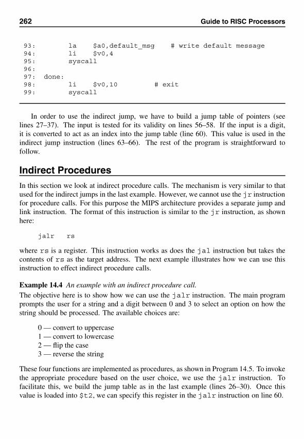
262 Guide to RISC Processors
93: la $a0,default_msg # write default message94: li $v0,495: syscall96:97: done:98: li $v0,10 # exit99: syscall
In order to use the indirect jump, we have to build a jump table of pointers (seelines 27–37). The input is tested for its validity on lines 56–58. If the input is a digit,it is converted to act as an index into the jump table (line 60). This value is used in theindirect jump instruction (lines 63–66). The rest of the program is straightforward tofollow.
Indirect ProceduresIn this section we look at indirect procedure calls. The mechanism is very similar to thatused for the indirect jumps in the last example. However, we cannot use the jr instructionfor procedure calls. For this purpose the MIPS architecture provides a separate jump andlink instruction. The format of this instruction is similar to the jr instruction, as shownhere:
jalr rs
where rs is a register. This instruction works as does the jal instruction but takes thecontents of rs as the target address. The next example illustrates how we can use thisinstruction to effect indirect procedure calls.
Example 14.4 An example with an indirect procedure call.The objective here is to show how we can use the jalr instruction. The main programprompts the user for a string and a digit between 0 and 3 to select an option on how thestring should be processed. The available choices are:
0 — convert to uppercase1 — convert to lowercase2 — flip the case3 — reverse the string
These four functions are implemented as procedures, as shown in Program 14.5. To invokethe appropriate procedure based on the user choice, we use the jalr instruction. Tofacilitate this, we build the jump table as in the last example (lines 26–30). Once thisvalue is loaded into $t2, we can specify this register in the jalr instruction on line 60.
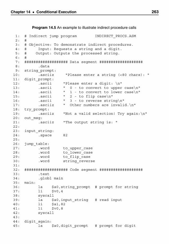
Chapter 14 • Conditional Execution 263
Program 14.5 An example to illustrate indirect procedure calls
1: # Indirect jump program INDIRECT_PROCS.ASM2: #3: # Objective: To demonstrate indirect procedures.4: # Input: Requests a string and a digit.5: # Output: Outputs the processed string.6: #7: ################### Data segment ###################8: .data9: string_prompt:
10: .asciiz "Please enter a string (<80 chars): "11: digit_prompt:12: .ascii "Please enter a digit: \n"13: .ascii " 0 - to convert to upper case\n"14: .ascii " 1 - to convert to lower case\n"15: .ascii " 2 - to flip case\n"16: .ascii " 3 - to reverse string\n"17: .asciiz " Other numbers are invalid.\n"18: try_prompt:19: .asciiz "Not a valid selection! Try again:\n"20: out_msg:21: .asciiz "The output string is: "22:23: input_string:24: .space 8225:26: jump_table:27: .word to_upper_case28: .word to_lower_case29: .word to_flip_case30: .word string_reverse31:32: ################### Code segment ###################33: .text34: .globl main35: main:36: la $a0,string_prompt # prompt for string37: li $v0,438: syscall39: la $a0,input_string # read input40: li $a1,8241: li $v0,842: syscall43:44: digit_again:45: la $a0,digit_prompt # prompt for digit
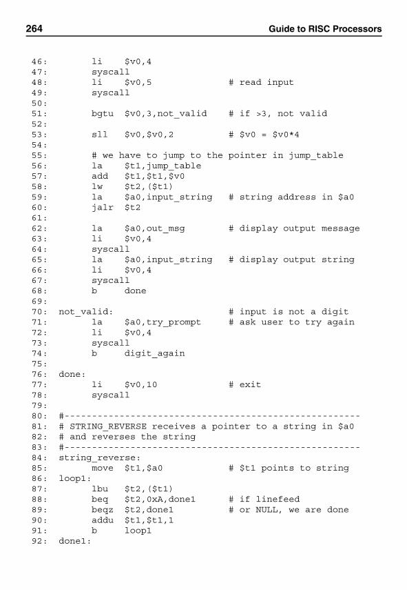
264 Guide to RISC Processors
46: li $v0,447: syscall48: li $v0,5 # read input49: syscall50:51: bgtu $v0,3,not_valid # if >3, not valid52:53: sll $v0,$v0,2 # $v0 = $v0*454:55: # we have to jump to the pointer in jump_table56: la $t1,jump_table57: add $t1,$t1,$v058: lw $t2,($t1)59: la $a0,input_string # string address in $a060: jalr $t261:62: la $a0,out_msg # display output message63: li $v0,464: syscall65: la $a0,input_string # display output string66: li $v0,467: syscall68: b done69:70: not_valid: # input is not a digit71: la $a0,try_prompt # ask user to try again72: li $v0,473: syscall74: b digit_again75:76: done:77: li $v0,10 # exit78: syscall79:80: #------------------------------------------------------81: # STRING_REVERSE receives a pointer to a string in $a082: # and reverses the string83: #------------------------------------------------------84: string_reverse:85: move $t1,$a0 # $t1 points to string86: loop1:87: lbu $t2,($t1)88: beq $t2,0xA,done1 # if linefeed89: beqz $t2,done1 # or NULL, we are done90: addu $t1,$t1,191: b loop192: done1:
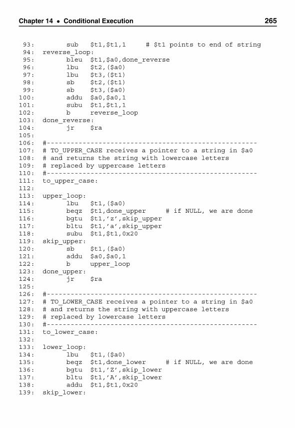
Chapter 14 • Conditional Execution 265
93: sub $t1,$t1,1 # $t1 points to end of string94: reverse_loop:95: bleu $t1,$a0,done_reverse96: lbu $t2,($a0)97: lbu $t3,($t1)98: sb $t2,($t1)99: sb $t3,($a0)
100: addu $a0,$a0,1101: subu $t1,$t1,1102: b reverse_loop103: done_reverse:104: jr $ra105:106: #-----------------------------------------------------107: # TO_UPPER_CASE receives a pointer to a string in $a0108: # and returns the string with lowercase letters109: # replaced by uppercase letters110: #-----------------------------------------------------111: to_upper_case:112:113: upper_loop:114: lbu $t1,($a0)115: beqz $t1,done_upper # if NULL, we are done116: bgtu $t1,’z’,skip_upper117: bltu $t1,’a’,skip_upper118: subu $t1,$t1,0x20119: skip_upper:120: sb $t1,($a0)121: addu $a0,$a0,1122: b upper_loop123: done_upper:124: jr $ra125:126: #-----------------------------------------------------127: # TO_LOWER_CASE receives a pointer to a string in $a0128: # and returns the string with uppercase letters129: # replaced by lowercase letters130: #-----------------------------------------------------131: to_lower_case:132:133: lower_loop:134: lbu $t1,($a0)135: beqz $t1,done_lower # if NULL, we are done136: bgtu $t1,’Z’,skip_lower137: bltu $t1,’A’,skip_lower138: addu $t1,$t1,0x20139: skip_lower:
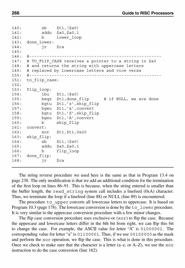
266 Guide to RISC Processors
140: sb $t1,($a0)141: addu $a0,$a0,1142: b lower_loop143: done_lower:144: jr $ra145:146: #-----------------------------------------------------147: # TO_FLIP_CASE receives a pointer to a string in $a0148: # and returns the string with uppercase letters149: # replaced by lowercase letters and vice versa150: #-----------------------------------------------------151: to_flip_case:152:153: flip_loop:154: lbu $t1,($a0)155: beqz $t1,done_flip # if NULL, we are done156: bgtu $t1,’z’,skip_flip157: bgeu $t1,’a’,convert158: bgtu $t1,’Z’,skip_flip159: bgeu $t1,’A’,convert160: b skip_flip161: convert:162: xor $t1,$t1,0x20163: skip_flip:164: sb $t1,($a0)165: addu $a0,$a0,1166: b flip_loop167: done_flip:168: jr $ra
The string reverse procedure we used here is the same as that in Program 13.4 onpage 238. The only modification is that we add an additional condition for the terminationof the first loop on lines 86–91. This is because, when the string entered is smaller thanthe buffer length, the read_string system call includes a linefeed (0xA) character.Thus, we terminate the loop if a linefeed (line 88) or NULL (line 89) is encountered.
The procedure to_upper converts all lowercase letters to uppercase. It is based onProgram 10.3 (page 178). The lowercase conversion is done by the to_lower procedure.It is very similar to the uppercase conversion procedure with a few minor changes.
The flip case conversion procedure uses exclusive-or (xor) to flip the case. Becausethe uppercase and lowercase letters differ in the 6th bit from right, we can flip this bitto change the case. For example, the ASCII value for letter “A” is 01000001. Thecorresponding value for letter “a” is 01100001. Thus, if we use 00100000 as the maskand perform the xor operation, we flip the case. This is what is done in this procedure.Once we check to make sure that the character is a letter (a–z, or A–Z), we use the xorinstruction to do the case conversion (line 162).
Chapter 14 • Conditional Execution 267
Summary
We discussed the unconditional and conditional jump instructions as well as compareinstructions in detail. These assembly language instructions are useful in implement-ing high-level language selection and iteration constructs such as if-then-else andwhile loops. Through detailed examples, we discussed how these high-level decisionstructures are implemented in the assembly language.
In the previous chapters, we extensively used direct jump and procedure call instruc-tions. In this chapter, we introduced the indirect jumps and procedure calls. In the indirectjump and procedure call instructions, the target of the jump is specified indirectly via aregister. By means of examples, we have shown how they are useful in implementingindirect jumps and procedure calls.
15Logical and ShiftOperations
This chapter looks at the logical, shift and rotate instructions provided by MIPS. TheMIPS instruction set provides four logical instructions: and, or, xor, and nor. There isno not instruction. This operation can be synthesized from the nor operation. We haveintroduced some of these instructions in Chapter 10. The logical instructions are usefulto implement high-level language logical expressions. In addition, they can be used forbit manipulation. The shift and rotate instructions are useful in bit shift operations. Wegive several examples to illustrate the use of these instructions. We end the chapter with asummary.
IntroductionAs we have seen in the last chapter, high-level languages provide several conditional andloop constructs. These constructs require Boolean or logical expressions to specify con-ditions. In principle, only a single bit is needed to represent the Boolean data. However,such a representation, although compact, is not convenient, as testing a variable involvesisolating the corresponding bit.
Most high-level languages use a byte to represent the Boolean data. If the byte iszero, it represents false; otherwise, true. Note that any value other than 0 can beused to represent true. In C, which does not provide an explicit Boolean data type, anydata variable can be used in a logical expression to represent Boolean data. The rulesmentioned above apply.
Assembly language provides several logical instructions, which are useful in imple-menting logical expressions of high-level languages. For example, C provides the follow-ing logical operators.
269
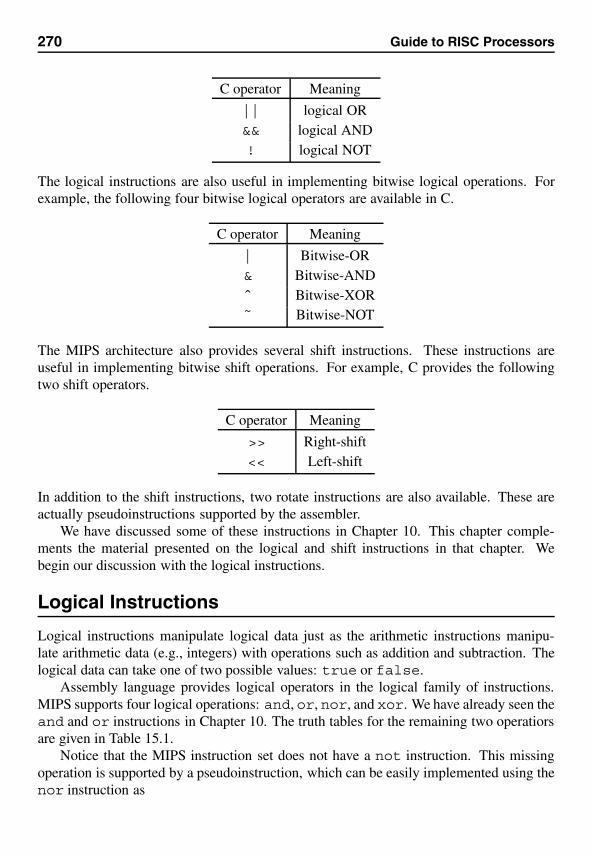
270 Guide to RISC Processors
C operator Meaning
|| logical OR&& logical AND! logical NOT
The logical instructions are also useful in implementing bitwise logical operations. Forexample, the following four bitwise logical operators are available in C.
C operator Meaning
| Bitwise-OR& Bitwise-ANDˆ Bitwise-XOR˜ Bitwise-NOT
The MIPS architecture also provides several shift instructions. These instructions areuseful in implementing bitwise shift operations. For example, C provides the followingtwo shift operators.
C operator Meaning
>> Right-shift<< Left-shift
In addition to the shift instructions, two rotate instructions are also available. These areactually pseudoinstructions supported by the assembler.
We have discussed some of these instructions in Chapter 10. This chapter comple-ments the material presented on the logical and shift instructions in that chapter. Webegin our discussion with the logical instructions.
Logical Instructions
Logical instructions manipulate logical data just as the arithmetic instructions manipu-late arithmetic data (e.g., integers) with operations such as addition and subtraction. Thelogical data can take one of two possible values: true or false.
Assembly language provides logical operators in the logical family of instructions.MIPS supports four logical operations: and, or, nor, and xor. We have already seen theand and or instructions in Chapter 10. The truth tables for the remaining two operatiorsare given in Table 15.1.
Notice that the MIPS instruction set does not have a not instruction. This missingoperation is supported by a pseudoinstruction, which can be easily implemented using thenor instruction as

Chapter 15 • Logical and Shift Operations 271
Table 15.1 Truth tables for the xor and nor logical operations
xor operation nor operationInput bits Output bit Input bits Output bit
source1 source2 destination source1 source2 destination0 0 0 0 0 10 1 1 0 1 01 0 1 1 0 01 1 0 1 1 0
nor Rdest,Rsrc,$0
A summary of these instructions is given in Table 15.2. All operations, except not,take two source operands and a destination operand. The not instruction takes one sourceoperand and one destination operand. As with most instructions, all operands must be inregisters. However, and, or, and xor instructions can take one immediate operand.
Assembler pseudoinstructions use the same mnemonics for the logical operationsand, or, and xor but allow the second source operand to be either a register or a 16-bit immediate value. Next we look at some typical uses for the logical operators.
The and InstructionThe and instruction is useful mainly in these situations:
1. To support compound logical expressions and bitwise and operations of high-levellanguages;
2. To clear one or more bits;
3. To isolate one or more bits.
The use of the and instruction to express compound logical expressions and to im-plement bitwise and operations is discussed later using examples. Here we concentrateon how and can be used to clear or isolate selected bits of an operand.
Clearing Bits If you look at the truth table of the and operation (see Table 10.4 onpage 170), you will notice that source1 acts as a masking bit: if the masking bit is 0, theoutput is 0, no matter what the other input bit is; if the masking bit is 1, the other input bitis passed to the output. Consider the following example.
$t0 = 10010011 00001111 01110010 11010110 ← operand$t1 = 11111111 11111111 11111111 11111100 ← mask$t2 = 10010011 00001111 01110010 11010100
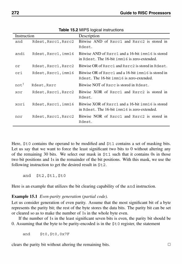
272 Guide to RISC Processors
Table 15.2 MIPS logical instructions
Instruction Descriptionand Rdest,Rsrc1,Rsrc2 Bitwise AND of Rsrc1 and Rsrc2 is stored in
Rdest.
andi Rdest,Rsrc1,imm16 Bitwise AND of Rsrc1 and a 16-bit imm16 is storedin Rdest. The 16-bit imm16 is zero-extended.
or Rdest,Rsrc1,Rsrc2 Bitwise OR of Rsrc1 and Rsrc2 is stored in Rdest.
ori Rdest,Rsrc1,imm16 Bitwise OR of Rsrc1 and a 16-bit imm16 is stored inRdest. The 16-bit imm16 is zero-extended.
not† Rdest,Rsrc Bitwise NOT of Rsrc is stored in Rdest.
xor Rdest,Rsrc1,Rsrc2 Bitwise XOR of Rsrc1 and Rsrc2 is stored inRdest.
xori Rdest,Rsrc1,imm16 Bitwise XOR of Rsrc1 and a 16-bit imm16 is storedin Rdest. The 16-bit imm16 is zero-extended.
nor Rdest,Rsrc1,Rsrc2 Bitwise NOR of Rsrc1 and Rsrc2 is stored inRdest.
Here, $t0 contains the operand to be modified and $t1 contains a set of masking bits.Let us say that we want to force the least significant two bits to 0 without altering anyof the remaining 30 bits. We select our mask in $t1 such that it contains 0s in thosetwo bit positions and 1s in the remainder of the bit positions. With this mask, we use thefollowing instruction to get the desired result in $t2.
and $t2,$t1,$t0
Here is an example that utilizes the bit clearing capability of the and instruction.
Example 15.1 Even-parity generation (partial code).Let us consider generation of even parity. Assume that the most significant bit of a byterepresents the parity bit; the rest of the byte stores the data bits. The parity bit can be setor cleared so as to make the number of 1s in the whole byte even.
If the number of 1s in the least significant seven bits is even, the parity bit should be0. Assuming that the byte to be parity-encoded is in the $t0 register, the statement
and $t0,$t0,0x7F
clears the parity bit without altering the remaining bits. �
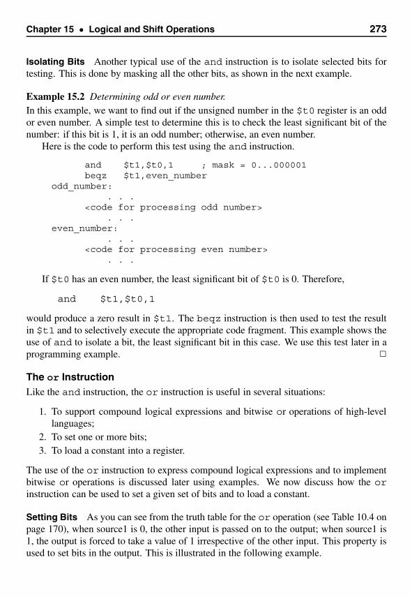
Chapter 15 • Logical and Shift Operations 273
Isolating Bits Another typical use of the and instruction is to isolate selected bits fortesting. This is done by masking all the other bits, as shown in the next example.
Example 15.2 Determining odd or even number.In this example, we want to find out if the unsigned number in the $t0 register is an oddor even number. A simple test to determine this is to check the least significant bit of thenumber: if this bit is 1, it is an odd number; otherwise, an even number.
Here is the code to perform this test using the and instruction.
and $t1,$t0,1 ; mask = 0...000001beqz $t1,even_number
odd_number:. . .
<code for processing odd number>. . .
even_number:. . .
<code for processing even number>. . .
If $t0 has an even number, the least significant bit of $t0 is 0. Therefore,
and $t1,$t0,1
would produce a zero result in $t1. The beqz instruction is then used to test the resultin $t1 and to selectively execute the appropriate code fragment. This example shows theuse of and to isolate a bit, the least significant bit in this case. We use this test later in aprogramming example. �
The or InstructionLike the and instruction, the or instruction is useful in several situations:
1. To support compound logical expressions and bitwise or operations of high-levellanguages;
2. To set one or more bits;3. To load a constant into a register.
The use of the or instruction to express compound logical expressions and to implementbitwise or operations is discussed later using examples. We now discuss how the orinstruction can be used to set a given set of bits and to load a constant.
Setting Bits As you can see from the truth table for the or operation (see Table 10.4 onpage 170), when source1 is 0, the other input is passed on to the output; when source1 is1, the output is forced to take a value of 1 irrespective of the other input. This property isused to set bits in the output. This is illustrated in the following example.
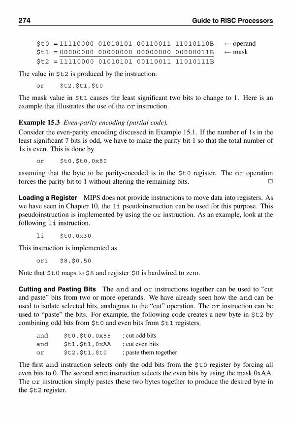
274 Guide to RISC Processors
$t0 = 11110000 01010101 00110011 11010110B ← operand$t1 = 00000000 00000000 00000000 00000011B ← mask$t2 = 11110000 01010101 00110011 11010111B
The value in $t2 is produced by the instruction:
or $t2,$t1,$t0
The mask value in $t1 causes the least significant two bits to change to 1. Here is anexample that illustrates the use of the or instruction.
Example 15.3 Even-parity encoding (partial code).Consider the even-parity encoding discussed in Example 15.1. If the number of 1s in theleast significant 7 bits is odd, we have to make the parity bit 1 so that the total number of1s is even. This is done by
or $t0,$t0,0x80
assuming that the byte to be parity-encoded is in the $t0 register. The or operationforces the parity bit to 1 without altering the remaining bits. �
Loading a Register MIPS does not provide instructions to move data into registers. Aswe have seen in Chapter 10, the li pseudoinstruction can be used for this purpose. Thispseudoinstruction is implemented by using the or instruction. As an example, look at thefollowing li instruction.
li $t0,0x30
This instruction is implemented as
ori $8,$0,50
Note that $t0 maps to $8 and register $0 is hardwired to zero.
Cutting and Pasting Bits The and and or instructions together can be used to “cutand paste” bits from two or more operands. We have already seen how the and can beused to isolate selected bits, analogous to the “cut” operation. The or instruction can beused to “paste” the bits. For example, the following code creates a new byte in $t2 bycombining odd bits from $t0 and even bits from $t1 registers.
and $t0,$t0,0x55 ; cut odd bitsand $t1,$t1,0xAA ; cut even bitsor $t2,$t1,$t0 ; paste them together
The first and instruction selects only the odd bits from the $t0 register by forcing alleven bits to 0. The second and instruction selects the even bits by using the mask 0xAA.The or instruction simply pastes these two bytes together to produce the desired byte inthe $t2 register.
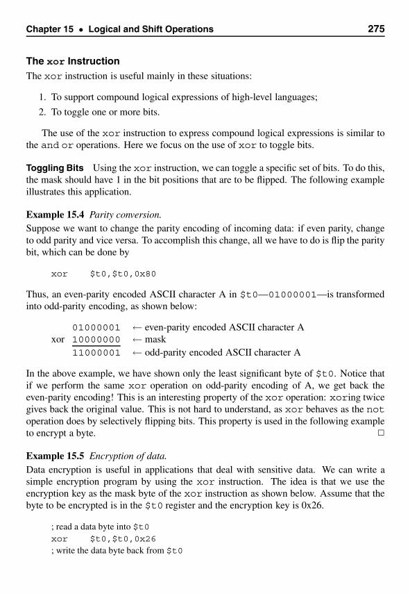
Chapter 15 • Logical and Shift Operations 275
The xor InstructionThe xor instruction is useful mainly in these situations:
1. To support compound logical expressions of high-level languages;
2. To toggle one or more bits.
The use of the xor instruction to express compound logical expressions is similar tothe and or operations. Here we focus on the use of xor to toggle bits.
Toggling Bits Using the xor instruction, we can toggle a specific set of bits. To do this,the mask should have 1 in the bit positions that are to be flipped. The following exampleillustrates this application.
Example 15.4 Parity conversion.Suppose we want to change the parity encoding of incoming data: if even parity, changeto odd parity and vice versa. To accomplish this change, all we have to do is flip the paritybit, which can be done by
xor $t0,$t0,0x80
Thus, an even-parity encoded ASCII character A in $t0—01000001—is transformedinto odd-parity encoding, as shown below:
01000001 ← even-parity encoded ASCII character Axor 10000000 ← mask
11000001 ← odd-parity encoded ASCII character A
In the above example, we have shown only the least significant byte of $t0. Notice thatif we perform the same xor operation on odd-parity encoding of A, we get back theeven-parity encoding! This is an interesting property of the xor operation: xoring twicegives back the original value. This is not hard to understand, as xor behaves as the notoperation does by selectively flipping bits. This property is used in the following exampleto encrypt a byte. �
Example 15.5 Encryption of data.Data encryption is useful in applications that deal with sensitive data. We can write asimple encryption program by using the xor instruction. The idea is that we use theencryption key as the mask byte of the xor instruction as shown below. Assume that thebyte to be encrypted is in the $t0 register and the encryption key is 0x26.
; read a data byte into $t0xor $t0,$t0,0x26; write the data byte back from $t0
276 Guide to RISC Processors
Suppose we have received character B, whose ASCII code is 01000010B. After en-cryption, the character becomes d in ASCII, as shown below.
01000010 ← ASCII character B00100110 ← encryption key (mask)01100100 ← ASCII character d
An encrypted data file can be transformed back into normal form by running the encrypteddata through the same encryption process again. To continue with our example, if theabove encrypted character code 64H (representing d) is passed through the encryptionprocedure, we get 42H, which is the ASCII code for character B. �
The nor InstructionThe nor instruction is needed to implement not, as MIPS does not provide it. Its mainuse is in supporting logical expressions of high-level languages. Furthermore, in lan-guages such as C, it can also be used to implement the bitwise not operation.
Another possible use for the not instruction is to compute negative numbers in the1’s complement representation. Recall that the 1’s complement of a number is simplythe complement of the number. However, most systems use the 2’s complement repre-sentation. The not instruction is not particularly useful for generating 2’s complementrepresentation. A simple example illustrates this point clearly. In the 2’s complementrepresentation, to negate the value in $t0, we have to use
not $t0,$t0add $t0,$t0,1
However, we can do better than this by using a single sub instruction as shown here:
sub $t0,$0,$t0
This is precisely what the neg pseudoinstruction does.
Shift InstructionsAs we have seen in Chapter 10, MIPS supports both left- and right-shift instructions to fa-cilitate bit operations. We have already described the basic shift operations in Chapter 10,therefore we look at the remaining shift instructions in this section.
The number of bit positions to be shifted (i.e., shift count) can be specified as animmediate 5-bit value or via a register. If a register is used, only the least significant fivebits are used as the shift count. In the basic left-shift instruction sll, the shift count isgiven as a 5-bit immediate value (see page 170).
The sllv (shift left logical variable) instruction
sllv Rdest,Rsrc1,Rsrc2
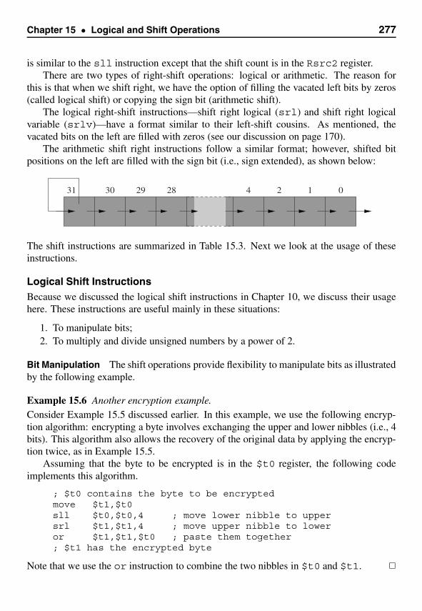
Chapter 15 • Logical and Shift Operations 277
is similar to the sll instruction except that the shift count is in the Rsrc2 register.There are two types of right-shift operations: logical or arithmetic. The reason for
this is that when we shift right, we have the option of filling the vacated left bits by zeros(called logical shift) or copying the sign bit (arithmetic shift).
The logical right-shift instructions—shift right logical (srl) and shift right logicalvariable (srlv)—have a format similar to their left-shift cousins. As mentioned, thevacated bits on the left are filled with zeros (see our discussion on page 170).
The arithmetic shift right instructions follow a similar format; however, shifted bitpositions on the left are filled with the sign bit (i.e., sign extended), as shown below:
012428293031
The shift instructions are summarized in Table 15.3. Next we look at the usage of theseinstructions.
Logical Shift InstructionsBecause we discussed the logical shift instructions in Chapter 10, we discuss their usagehere. These instructions are useful mainly in these situations:
1. To manipulate bits;2. To multiply and divide unsigned numbers by a power of 2.
Bit Manipulation The shift operations provide flexibility to manipulate bits as illustratedby the following example.
Example 15.6 Another encryption example.Consider Example 15.5 discussed earlier. In this example, we use the following encryp-tion algorithm: encrypting a byte involves exchanging the upper and lower nibbles (i.e., 4bits). This algorithm also allows the recovery of the original data by applying the encryp-tion twice, as in Example 15.5.
Assuming that the byte to be encrypted is in the $t0 register, the following codeimplements this algorithm.
; $t0 contains the byte to be encryptedmove $t1,$t0sll $t0,$t0,4 ; move lower nibble to uppersrl $t1,$t1,4 ; move upper nibble to loweror $t1,$t1,$t0 ; paste them together; $t1 has the encrypted byte
Note that we use the or instruction to combine the two nibbles in $t0 and $t1. �
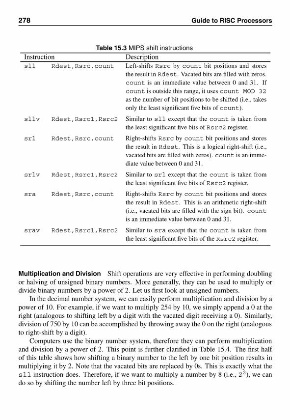
278 Guide to RISC Processors
Table 15.3 MIPS shift instructionsInstruction Descriptionsll Rdest,Rsrc,count Left-shifts Rsrc by count bit positions and stores
the result in Rdest. Vacated bits are filled with zeros.count is an immediate value between 0 and 31. Ifcount is outside this range, it uses count MOD 32as the number of bit positions to be shifted (i.e., takesonly the least significant five bits of count).
sllv Rdest,Rsrc1,Rsrc2 Similar to sll except that the count is taken fromthe least significant five bits of Rsrc2 register.
srl Rdest,Rsrc,count Right-shifts Rsrc by count bit positions and storesthe result in Rdest. This is a logical right-shift (i.e.,vacated bits are filled with zeros). count is an imme-diate value between 0 and 31.
srlv Rdest,Rsrc1,Rsrc2 Similar to srl except that the count is taken fromthe least significant five bits of Rsrc2 register.
sra Rdest,Rsrc,count Right-shifts Rsrc by count bit positions and storesthe result in Rdest. This is an arithmetic right-shift(i.e., vacated bits are filled with the sign bit). countis an immediate value between 0 and 31.
srav Rdest,Rsrc1,Rsrc2 Similar to sra except that the count is taken fromthe least significant five bits of the Rsrc2 register.
Multiplication and Division Shift operations are very effective in performing doublingor halving of unsigned binary numbers. More generally, they can be used to multiply ordivide binary numbers by a power of 2. Let us first look at unsigned numbers.
In the decimal number system, we can easily perform multiplication and division by apower of 10. For example, if we want to multiply 254 by 10, we simply append a 0 at theright (analogous to shifting left by a digit with the vacated digit receiving a 0). Similarly,division of 750 by 10 can be accomplished by throwing away the 0 on the right (analogousto right-shift by a digit).
Computers use the binary number system, therefore they can perform multiplicationand division by a power of 2. This point is further clarified in Table 15.4. The first halfof this table shows how shifting a binary number to the left by one bit position results inmultiplying it by 2. Note that the vacated bits are replaced by 0s. This is exactly what thesll instruction does. Therefore, if we want to multiply a number by 8 (i.e., 2 3), we cando so by shifting the number left by three bit positions.
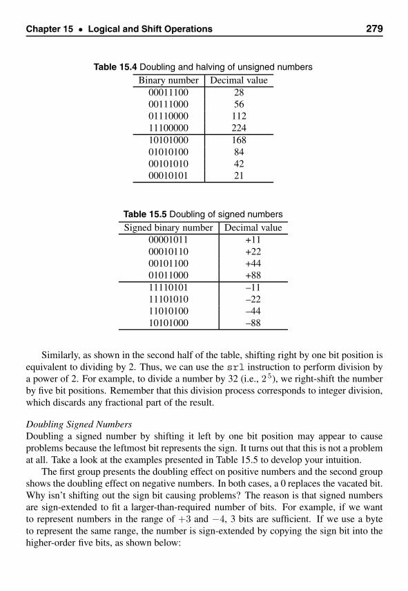
Chapter 15 • Logical and Shift Operations 279
Table 15.4 Doubling and halving of unsigned numbers
Binary number Decimal value00011100 2800111000 5601110000 11211100000 22410101000 16801010100 8400101010 4200010101 21
Table 15.5 Doubling of signed numbers
Signed binary number Decimal value00001011 +1100010110 +2200101100 +4401011000 +8811110101 –1111101010 –2211010100 –4410101000 –88
Similarly, as shown in the second half of the table, shifting right by one bit position isequivalent to dividing by 2. Thus, we can use the srl instruction to perform division bya power of 2. For example, to divide a number by 32 (i.e., 2 5), we right-shift the numberby five bit positions. Remember that this division process corresponds to integer division,which discards any fractional part of the result.
Doubling Signed NumbersDoubling a signed number by shifting it left by one bit position may appear to causeproblems because the leftmost bit represents the sign. It turns out that this is not a problemat all. Take a look at the examples presented in Table 15.5 to develop your intuition.
The first group presents the doubling effect on positive numbers and the second groupshows the doubling effect on negative numbers. In both cases, a 0 replaces the vacated bit.Why isn’t shifting out the sign bit causing problems? The reason is that signed numbersare sign-extended to fit a larger-than-required number of bits. For example, if we wantto represent numbers in the range of +3 and −4, 3 bits are sufficient. If we use a byteto represent the same range, the number is sign-extended by copying the sign bit into thehigher-order five bits, as shown below:
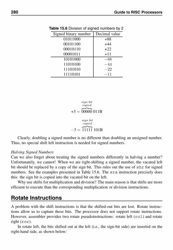
280 Guide to RISC Processors
Table 15.6 Division of signed numbers by 2
Signed binary number Decimal value01011000 +8800101100 +4400010110 +2200001011 +1110101000 −8811010100 −4411101010 −2211110101 −11
+3 =
sign bitcopied︷ ︸︸ ︷00000 011B
−3 =
sign bitcopied︷ ︸︸ ︷11111 101B
Clearly, doubling a signed number is no different than doubling an unsigned number.Thus, no special shift left instruction is needed for signed numbers.
Halving Signed NumbersCan we also forget about treating the signed numbers differently in halving a number?Unfortunately, we cannot! When we are right-shifting a signed number, the vacated leftbit should be replaced by a copy of the sign bit. This rules out the use of shr for signednumbers. See the examples presented in Table 15.6. The sra instruction precisely doesthis: the sign bit is copied into the vacated bit on the left.
Why use shifts for multiplication and division? The main reason is that shifts are moreefficient to execute than the corresponding multiplication or division instructions.
Rotate InstructionsA problem with the shift instructions is that the shifted-out bits are lost. Rotate instruc-tions allow us to capture these bits. The processor does not support rotate instructions.However, assembler provides two rotate pseudoinstructions: rotate left (rol) and rotateright (ror).
In rotate left, the bits shifted out at the left (i.e., the sign-bit side) are inserted on theright-hand side, as shown below:

Chapter 15 • Logical and Shift Operations 281
012428293031
In rotate right, bits falling off the right side are inserted on the sign-bit side, as shownhere:
012428293031
Table 15.7 summarizes the two rotate instructions. As noted, both rotate instructions arepseudoinstructions. For example, the rotate instruction
ror† $t2,$t2,1
is translated as
sll $1,$10,31srl $10,$10,1or $10,$10,$1
Note that $t2 maps to the $10 register. This instruction also demonstrates the use of$at, which is the $1 register. You can see from this translation that the assembler usesthis register as a temporary register to translate the pseudoinstruction.
Our First Program
The goal of this example is to illustrate how the logical and instruction can be used totest a bit. The main program reads a character from the user and passes this character via$a0 to the print_bin procedure, which outputs the character’s ASCII code in binary.
To display the binary value of the input character in $t0, the print_bin proceduretests each bit starting with the most significant (i.e., leftmost) bit. The mask in $t1 isinitialized to 0x80, which tests only the value of the most significant bit of the ASCIIvalue. If this bit is 0, the code
and $t2,$t0,$t1
sets $t2 to zero. In this case, a 0 is displayed by directing the program flow using thebeqz instruction (line 60). Otherwise, a 1 is displayed. The mask is then right-shifted byone bit position (line 69). Thus, we are ready for testing the second most significant bit.
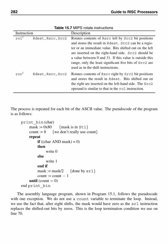
282 Guide to RISC Processors
Table 15.7 MIPS rotate instructionsInstruction Descriptionrol† Rdest,Rsrc,Src2 Rotates contents of Rsrc left by Src2 bit positions
and stores the result in Rdest. Src2 can be a regis-ter or an immediate value. Bits shifted out on the leftare inserted on the right-hand side. Src2 should bea value between 0 and 31. If this value is outside thisrange, only the least significant five bits of Src2 areused as in the shift instructions.
ror† Rdest,Rsrc,Src2 Rotates contents of Rsrc right by Src2 bit positionsand stores the result in Rdest. Bits shifted out onthe right are inserted on the left-hand side. The Src2operand is similar to that in the rol instruction.
The process is repeated for each bit of the ASCII value. The pseudocode of the programis as follows:
print_bin (char)mask := 0x80 {mask is in $t1}count := 8 {we don’t really use count}repeat
if ((char AND mask) = 0)then
write 0else
write 1end ifmask := mask/2 {done by srl}count := count − 1
until (count = 0)end print_bin
The assembly language program, shown in Program 15.1, follows the pseudocodewith one exception. We do not use a count variable to terminate the loop. Instead,we use the fact that, after eight shifts, the mask would have zero as the srl instructionreplaces the shifted-out bits by zeros. This is the loop termination condition we use online 70.
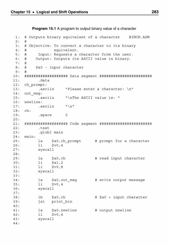
Chapter 15 • Logical and Shift Operations 283
Program 15.1 A program to output binary value of a character
1: # Outputs binary equivalent of a character BINCH.ASM2: #3: # Objective: To convert a character to its binary4: # equivalent.5: # Input: Requests a character from the user.6: # Output: Outputs its ASCII value in binary.7: #8: # $a0 - input character9: #
10: ################### Data segment #######################11: .data12: ch_prompt:13: .asciiz "Please enter a character: \n"14: out_msg:15: .asciiz "\nThe ASCII value is: "16: newline:17: .asciiz "\n"18: ch:19: .space 220:21: ################### Code segment #######################22: .text23: .globl main24: main:25: la $a0,ch_prompt # prompt for a character26: li $v0,427: syscall28:29: la $a0,ch # read input character30: li $a1,231: li $v0,832: syscall33:34: la $a0,out_msg # write output message35: li $v0,436: syscall37:38: lb $a0,ch # $a0 = input character39: jal print_bin40:41: la $a0,newline # output newline42: li $v0,443: syscall44:

284 Guide to RISC Processors
45: li $v0,10 # exit46: syscall47:48: #------------------------------------------------49: # PRINT_BIN receives a character in $a0 and50: # prints its binary value.51: # $t0: holds the character52: # $t1: holds the mask byte53: # $t2: temporary54: #------------------------------------------------55: print_bin:56: move $t0,$a0 # char. in $t057: li $t1,0x80 # mask byte = 0x8058: loop:59: and $t2,$t0,$t160: beqz $t2,zero61: li $a0,1 # print 162: b skip63: zero:64: li $a0,0 # print 065: skip:66: li $v0,167: syscall68:69: srl $t1,$t1,1 # shift mask byte70: bnez $t1,loop # exit loop if mask is 071:72: jr $ra
Illustrative Examples
To further illustrate the application of the logical, shift, and rotate instructions, we givetwo examples.
Example 15.7 Binary to octal conversion.In this example, we convert a number from its binary representation to the octal system.For example, if the number is −1, it is stored as all 1s in the 2’s complement representation(i.e., all 32 bits are 1). Thus, when we express it in the octal number system, we get37777777777.
The main program is straightforward. It requests a number and passes it on to theprint_octal procedure via the $a0 register (lines 35 and 36). This procedure outputsthe octal value. Let us look at the logic of this procedure next.
To convert to the octal equivalent, we start with the most significant octal digit. How-ever, because the number of bits (i.e., 32) is not a multiple of 3, the most significant octal

Chapter 15 • Logical and Shift Operations 285
digit should be derived using the leftmost two bits of the number. Thus, the most signifi-cant digit of the output can be at most 3 as in our example. Once we have converted thesetwo bits, the remaining bits can be processed three bits at a time. The print_octalprocedure follows the pseudocode shown below:
print_octal (number)mask := 0xE0000000 {mask is in $t1}{Handle the leftmost octal digit—special case}temp := numbershift temp right by 1 bit positiontemp := temp AND maskrotate temp left by 3 bit positionswrite temp{Handle the remaining 10 octal digits}count := 10 {count is in $t3}shift number left by 2 bit positionsrepeat
temp := number AND maskrotate temp left by 3 bit positionswrite tempshift number left by 3 bit positionscount := count − 1
until (count = 0)end print_octal
We set the mask such that the most significant three bits are 1 and the remaining bitsare 0. To use the mask, we right-shift the number by one bit position so that the leftmostthree bits can be isolated to output the most significant octal digit. However, to print thevalue of these three bits, we need to move them to the least significant three bit positions.This is done by rotating it three bit positions. To output the remaining 10 octal digits, weuse a loop in which we left-shift the number by three bit positions so that we can isolatethe next three bits. Once isolated, we rotate left by three bit positions to output the valueas explained before.
Program 15.2 A program to convert binary numbers to octal
1: # Integer to octal conversion OCTAL.ASM2: #3: # Objective: To convert a number to its octal4: # equivalent.5: # Input: Requests a number from the user.6: # Output: Outputs its octal value.7: #
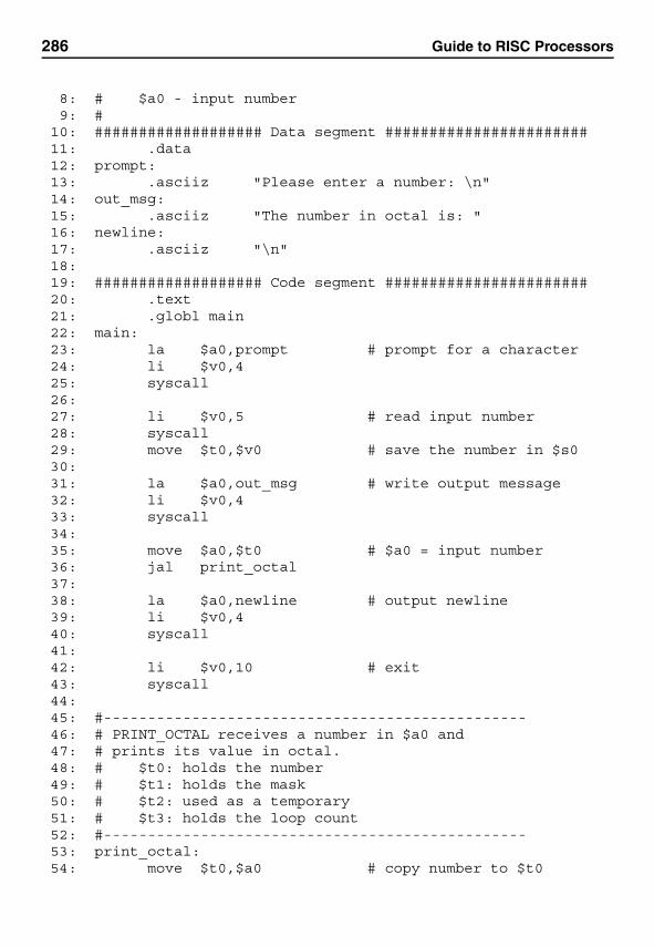
286 Guide to RISC Processors
8: # $a0 - input number9: #
10: ################### Data segment #######################11: .data12: prompt:13: .asciiz "Please enter a number: \n"14: out_msg:15: .asciiz "The number in octal is: "16: newline:17: .asciiz "\n"18:19: ################### Code segment #######################20: .text21: .globl main22: main:23: la $a0,prompt # prompt for a character24: li $v0,425: syscall26:27: li $v0,5 # read input number28: syscall29: move $t0,$v0 # save the number in $s030:31: la $a0,out_msg # write output message32: li $v0,433: syscall34:35: move $a0,$t0 # $a0 = input number36: jal print_octal37:38: la $a0,newline # output newline39: li $v0,440: syscall41:42: li $v0,10 # exit43: syscall44:45: #------------------------------------------------46: # PRINT_OCTAL receives a number in $a0 and47: # prints its value in octal.48: # $t0: holds the number49: # $t1: holds the mask50: # $t2: used as a temporary51: # $t3: holds the loop count52: #------------------------------------------------53: print_octal:54: move $t0,$a0 # copy number to $t0
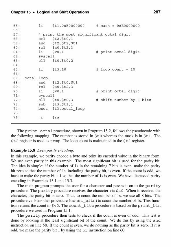
Chapter 15 • Logical and Shift Operations 287
55: li $t1,0xE0000000 # mask = 0xE000000056:57: # print the most significant octal digit58: srl $t2,$t0,159: and $t2,$t2,$t160: rol $a0,$t2,361: li $v0,1 # print octal digit62: syscall63: sll $t0,$t0,264:65: li $t3,10 # loop count = 1066:67: octal_loop:68: and $t2,$t0,$t169: rol $a0,$t2,370: li $v0,1 # print octal digit71: syscall72: sll $t0,$t0,3 # shift number by 3 bits73: sub $t3,$t3,174: bnez $t3,octal_loop75:76: jr $ra
The print_octal procedure, shown in Program 15.2, follows the pseudocode withthe following mapping. The number is stored in $t0 whereas the mask is in $t1. The$t2 register is used as temp. The loop count is maintained in the $t3 register.
Example 15.8 Even parity encoding.In this example, we parity encode a byte and print its encoded value in the binary form.We use even parity in this example. The most significant bit is used for the parity bit.The idea is simple: if the number of 1s in the remaining 7 bits is even, make the paritybit zero so that the number of 1s, including the parity bit, is even. If the count is odd, wehave to make the parity bit a 1 so that the number of 1s is even. We have discussed parityencoding in Examples 15.1 and 15.3.
The main program prompts the user for a character and passes it on to the parityprocedure. The parity procedure receives the character via $a0. When it receives thecharacter, the parity bit is zero. Thus, to count the number of 1s, we use all 8 bits. Theprocedure calls another procedure (count_bits) to count the number of 1s. This func-tion returns the count in $v0. The count_bits procedure is based on the print_binprocedure we used in Program 15.1.
The parity procedure then tests to check if the count is even or odd. This test isdone by looking at the least significant bit of the count. We do this by using the andinstruction on line 58. If the count is even, we do nothing as the parity bit is zero. If it isodd, we make the parity bit 1 by using the or instruction on line 60.
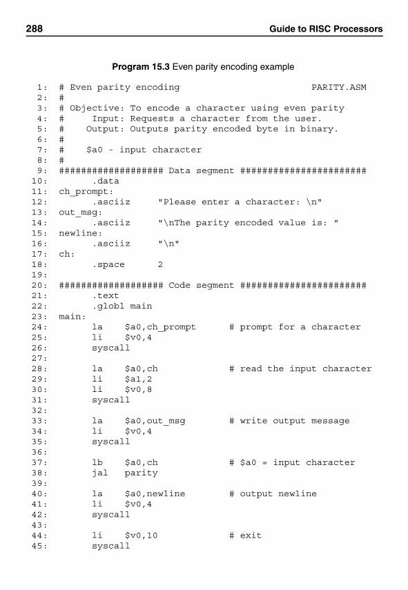
288 Guide to RISC Processors
Program 15.3 Even parity encoding example
1: # Even parity encoding PARITY.ASM2: #3: # Objective: To encode a character using even parity4: # Input: Requests a character from the user.5: # Output: Outputs parity encoded byte in binary.6: #7: # $a0 - input character8: #9: ################### Data segment #######################
10: .data11: ch_prompt:12: .asciiz "Please enter a character: \n"13: out_msg:14: .asciiz "\nThe parity encoded value is: "15: newline:16: .asciiz "\n"17: ch:18: .space 219:20: ################### Code segment #######################21: .text22: .globl main23: main:24: la $a0,ch_prompt # prompt for a character25: li $v0,426: syscall27:28: la $a0,ch # read the input character29: li $a1,230: li $v0,831: syscall32:33: la $a0,out_msg # write output message34: li $v0,435: syscall36:37: lb $a0,ch # $a0 = input character38: jal parity39:40: la $a0,newline # output newline41: li $v0,442: syscall43:44: li $v0,10 # exit45: syscall
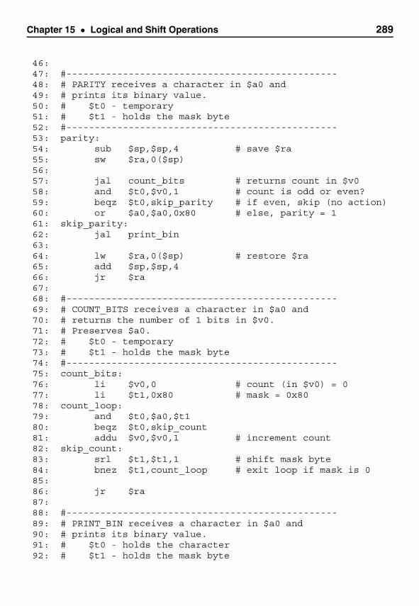
Chapter 15 • Logical and Shift Operations 289
46:47: #------------------------------------------------48: # PARITY receives a character in $a0 and49: # prints its binary value.50: # $t0 - temporary51: # $t1 - holds the mask byte52: #------------------------------------------------53: parity:54: sub $sp,$sp,4 # save $ra55: sw $ra,0($sp)56:57: jal count_bits # returns count in $v058: and $t0,$v0,1 # count is odd or even?59: beqz $t0,skip_parity # if even, skip (no action)60: or $a0,$a0,0x80 # else, parity = 161: skip_parity:62: jal print_bin63:64: lw $ra,0($sp) # restore $ra65: add $sp,$sp,466: jr $ra67:68: #------------------------------------------------69: # COUNT_BITS receives a character in $a0 and70: # returns the number of 1 bits in $v0.71: # Preserves $a0.72: # $t0 - temporary73: # $t1 - holds the mask byte74: #------------------------------------------------75: count_bits:76: li $v0,0 # count (in $v0) = 077: li $t1,0x80 # mask = 0x8078: count_loop:79: and $t0,$a0,$t180: beqz $t0,skip_count81: addu $v0,$v0,1 # increment count82: skip_count:83: srl $t1,$t1,1 # shift mask byte84: bnez $t1,count_loop # exit loop if mask is 085:86: jr $ra87:88: #------------------------------------------------89: # PRINT_BIN receives a character in $a0 and90: # prints its binary value.91: # $t0 - holds the character92: # $t1 - holds the mask byte
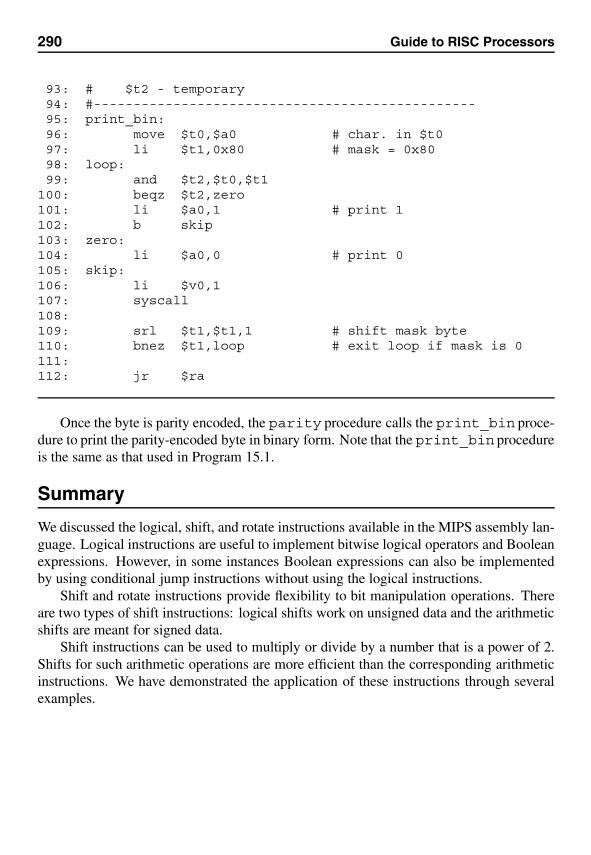
290 Guide to RISC Processors
93: # $t2 - temporary94: #------------------------------------------------95: print_bin:96: move $t0,$a0 # char. in $t097: li $t1,0x80 # mask = 0x8098: loop:99: and $t2,$t0,$t1
100: beqz $t2,zero101: li $a0,1 # print 1102: b skip103: zero:104: li $a0,0 # print 0105: skip:106: li $v0,1107: syscall108:109: srl $t1,$t1,1 # shift mask byte110: bnez $t1,loop # exit loop if mask is 0111:112: jr $ra
Once the byte is parity encoded, the parity procedure calls the print_bin proce-dure to print the parity-encoded byte in binary form. Note that the print_bin procedureis the same as that used in Program 15.1.
Summary
We discussed the logical, shift, and rotate instructions available in the MIPS assembly lan-guage. Logical instructions are useful to implement bitwise logical operators and Booleanexpressions. However, in some instances Boolean expressions can also be implementedby using conditional jump instructions without using the logical instructions.
Shift and rotate instructions provide flexibility to bit manipulation operations. Thereare two types of shift instructions: logical shifts work on unsigned data and the arithmeticshifts are meant for signed data.
Shift instructions can be used to multiply or divide by a number that is a power of 2.Shifts for such arithmetic operations are more efficient than the corresponding arithmeticinstructions. We have demonstrated the application of these instructions through severalexamples.
16Recursion
We can use recursion as an alternative to iteration. Solutions to some problems can benaturally expressed using recursion. We start this chapter with an overview of recursiveprocedures. Next we give some example recursive procedures in the MIPS assemblylanguage. The advantages and pitfalls associated with a recursive solution as opposed toan iterative solution are discussed towards the end of the chapter.
IntroductionA recursive procedure calls itself, either directly or indirectly through another procedure.In direct recursion, a procedure calls itself directly. In indirect recursion, procedure Pmakes a call to procedure Q, which in turn calls procedure P. The sequence of calls couldbe longer before a call is made to procedure P.
Recursion is a powerful tool that allows us to express our solution elegantly. Somesolutions can be naturally expressed using recursion. Computing factorials is a classicexample. Factorial n, denoted n!, is the product of positive integers from 1 to n. Forexample,
5! = 1 × 2 × 3 × 4 × 5.
The factorial function can be formally defined as
factorial(0) = 1factorial(n) = n * factorial(n − 1) for n > 0.
Recursion shows up in this definition as we define factorial(n) in terms of factorial(n−1).Every recursive function should have a termination condition to end the recursion. In thisexample, when n = 0, recursion stops. Some other examples include the binary search,quicksort, and Fibonacci function. Towards the end of this chapter, we give examples ofquicksort and the Fibonacci function.
291
292 Guide to RISC Processors
How do we express such recursive functions in programming languages? Let us firstlook at how this function is written in C:
int fact(int n){
if (n == 0)return(1);
return(n * fact(n-1));}
This is an example of direct recursion. How is this function implemented? At the con-ceptual level, its implementation is not any different from implementing other procedures.Once you understand that each procedure call instance is distinct from the others, the factthat a recursive procedure calls itself does not make a big difference.
Each active procedure maintains an activation record, which is stored on the stack.The activation record, which consists of the parameters, return address, local variables,and a frame pointer, comes into existence when a procedure is invoked and disappearswhen the procedure is terminated. Thus, for each procedure that is not terminated, anactivation record that contains the state of that procedure is stored. A stack is used to keepthese activation records. The number of activation records, and hence the amount of stackspace required to run the program, depend on the depth of recursion.
Figure 16.1 shows the stack activation records for factorial(3). As you can see fromthis figure, each call to the factorial function creates an activation record. In the next twosections we look at some example recursive procedures in the MIPS assembly language.
Our First Program
In MIPS, we can write procedures without using the stack. For simple leaf procedures,we do not have to use the stack. The availability of a large number of registers allows usto use register-based parameter passing. However, when we write recursive procedures,we have to use the stack because recursive procedures are essentially nonleaf procedures(see our discussion of leaf and nonleaf procedures on page 189).
To understand how we can write a recursive procedure, let us look at the factorialfunction. We have defined factorial at the beginning of this chapter. We implement aslightly modified definition of factorial, as implemented in Chapter 13 (see the exampleon page 230 that implements the iterative version).
fact(n) = 1 for n ≤ 1.= n * fact(n − 1) for n ≥ 2.
Program 16.1 requests an integer n from the user and passes this on to the factorial proce-dure (fact) via the $a0 register. After returning from the procedure, it outputs fact(n).
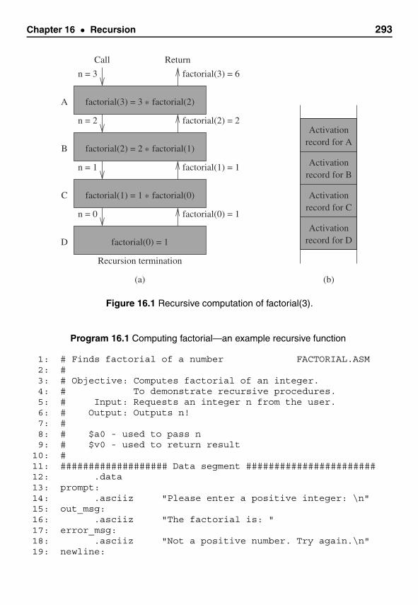
Chapter 16 • Recursion 293
Activationrecord for A
Activationrecord for B
Activationrecord for C
Activationrecord for D
(b)(a)
A
B
C
D
factorial(0) = 1
factorial(1) = 1
factorial(2) = 2
factorial(3) = 6n = 3
n = 1
n = 0
n = 2
Call Return
Recursion termination
factorial(0) = 1
factorial(2) = 2 factorial(1)
*factorial(1) = 1 factorial(0)
*
factorial(3) = 3 factorial(2)*
Figure 16.1 Recursive computation of factorial(3).
Program 16.1 Computing factorial—an example recursive function
1: # Finds factorial of a number FACTORIAL.ASM2: #3: # Objective: Computes factorial of an integer.4: # To demonstrate recursive procedures.5: # Input: Requests an integer n from the user.6: # Output: Outputs n!7: #8: # $a0 - used to pass n9: # $v0 - used to return result
10: #11: ################### Data segment #######################12: .data13: prompt:14: .asciiz "Please enter a positive integer: \n"15: out_msg:16: .asciiz "The factorial is: "17: error_msg:18: .asciiz "Not a positive number. Try again.\n"19: newline:
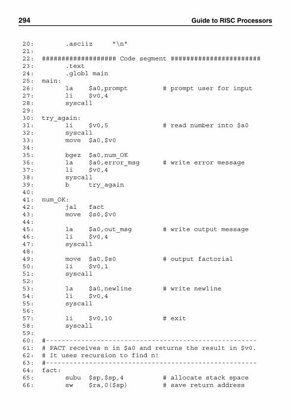
294 Guide to RISC Processors
20: .asciiz "\n"21:22: ################### Code segment #######################23: .text24: .globl main25: main:26: la $a0,prompt # prompt user for input27: li $v0,428: syscall29:30: try_again:31: li $v0,5 # read number into $a032: syscall33: move $a0,$v034:35: bgez $a0,num_OK36: la $a0,error_msg # write error message37: li $v0,438: syscall39: b try_again40:41: num_OK:42: jal fact43: move $s0,$v044:45: la $a0,out_msg # write output message46: li $v0,447: syscall48:49: move $a0,$s0 # output factorial50: li $v0,151: syscall52:53: la $a0,newline # write newline54: li $v0,455: syscall56:57: li $v0,10 # exit58: syscall59:60: #------------------------------------------------------61: # FACT receives n in $a0 and returns the result in $v0.62: # It uses recursion to find n!63: #------------------------------------------------------64: fact:65: subu $sp,$sp,4 # allocate stack space66: sw $ra,0($sp) # save return address
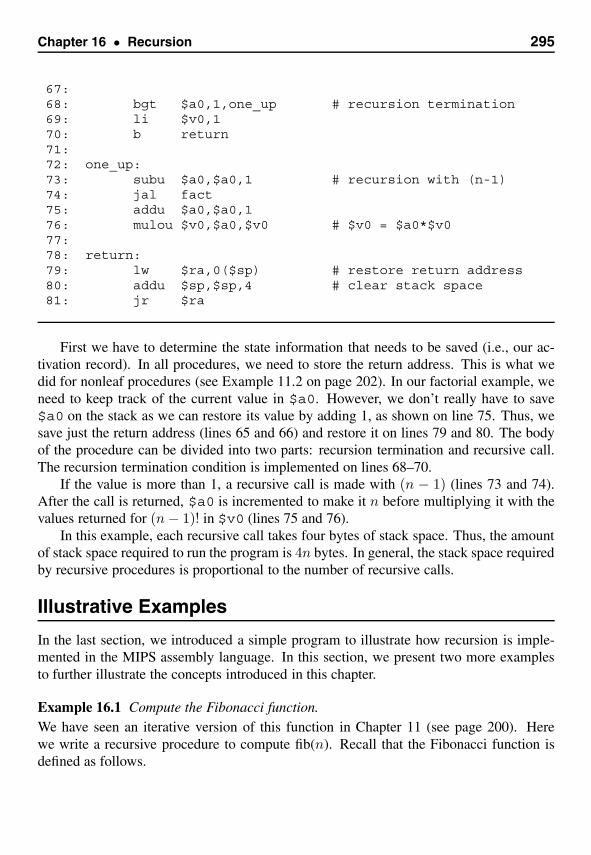
Chapter 16 • Recursion 295
67:68: bgt $a0,1,one_up # recursion termination69: li $v0,170: b return71:72: one_up:73: subu $a0,$a0,1 # recursion with (n-1)74: jal fact75: addu $a0,$a0,176: mulou $v0,$a0,$v0 # $v0 = $a0*$v077:78: return:79: lw $ra,0($sp) # restore return address80: addu $sp,$sp,4 # clear stack space81: jr $ra
First we have to determine the state information that needs to be saved (i.e., our ac-tivation record). In all procedures, we need to store the return address. This is what wedid for nonleaf procedures (see Example 11.2 on page 202). In our factorial example, weneed to keep track of the current value in $a0. However, we don’t really have to save$a0 on the stack as we can restore its value by adding 1, as shown on line 75. Thus, wesave just the return address (lines 65 and 66) and restore it on lines 79 and 80. The bodyof the procedure can be divided into two parts: recursion termination and recursive call.The recursion termination condition is implemented on lines 68–70.
If the value is more than 1, a recursive call is made with (n − 1) (lines 73 and 74).After the call is returned, $a0 is incremented to make it n before multiplying it with thevalues returned for (n − 1)! in $v0 (lines 75 and 76).
In this example, each recursive call takes four bytes of stack space. Thus, the amountof stack space required to run the program is 4n bytes. In general, the stack space requiredby recursive procedures is proportional to the number of recursive calls.
Illustrative Examples
In the last section, we introduced a simple program to illustrate how recursion is imple-mented in the MIPS assembly language. In this section, we present two more examplesto further illustrate the concepts introduced in this chapter.
Example 16.1 Compute the Fibonacci function.We have seen an iterative version of this function in Chapter 11 (see page 200). Herewe write a recursive procedure to compute fib(n). Recall that the Fibonacci function isdefined as follows.

296 Guide to RISC Processors
fib(1) = 1,fib(2) = 1,fib(n) = fib(n − 1) + fib(n − 2) for n > 2.
The main program takes care of the user interface. It requests n and invokes the fibprocedure and outputs the fib(n) value returned by the procedure. It invokes the procedureon line 32 after copying n into the $a0 register.
The fib procedure stores the return address on the stack as in the last example. Inaddition, we need to keep two values on the stack: the last and second to last Fibonaccivalues that are in $v0 and $s0, respectively. Thus, our stack frame consists of threevalues: $ra, $v0, and $s0 (see lines 57–60). These three registers are restored onlines 80–83. The fib procedure is recursively called on lines 69 and 74 to computefib(n − 1) and fib(n − 2), respectively. The rest of the code is straightforward to follow.
Program 16.2 Fibonacci function using recursion
1: # Computes Fibonacci number FIB_RECUR.ASM2: #3: # Objective: Computes the Fibonacci number.4: # Uses recursion.5: # Input: Requests a number n.6: # Output: Outputs Fibonacci number fib(n).7: #8: # $a0 - number n is passed9: # $v0 - fib(n) is returned
10: #11: ################### Data segment ###################12: .data13: prompt:14: .asciiz "Please enter a number n: \n"15: out_msg:16: .asciiz "Fib(n) = "17: newline:18: .asciiz "\n"19:20: ################### Code segment ###################21: .text22: .globl main23: main:24: la $a0,prompt # prompt user for input25: li $v0,426: syscall27:28: li $v0,5 # read number into $a0
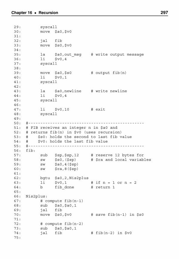
Chapter 16 • Recursion 297
29: syscall30: move $a0,$v031:32: jal fib33: move $s0,$v034:35: la $a0,out_msg # write output message36: li $v0,437: syscall38:39: move $a0,$s0 # output fib(n)40: li $v0,141: syscall42:43: la $a0,newline # write newline44: li $v0,445: syscall46:47: li $v0,10 # exit48: syscall49:50: #------------------------------------------------51: # FIB receives an integer n in $a0 and52: # returns fib(n) in $v0 (uses recursion)53: # $s0: holds the second to last fib value54: # $v0: holds the last fib value55: #------------------------------------------------56: fib:57: sub $sp,$sp,12 # reserve 12 bytes for58: sw $s0,($sp) # $ra and local variables59: sw $a0,4($sp)60: sw $ra,8($sp)61:62: bgtu $a0,2,Nis2plus63: li $v0,1 # if n = 1 or n = 264: b fib_done # return 165:66: Nis2plus:67: # compute fib(n-1)68: sub $a0,$a0,169: jal fib70: move $s0,$v0 # save fib(n-1) in $s071:72: # compute fib(n-2)73: sub $a0,$a0,174: jal fib # fib(n-2) in $v075:
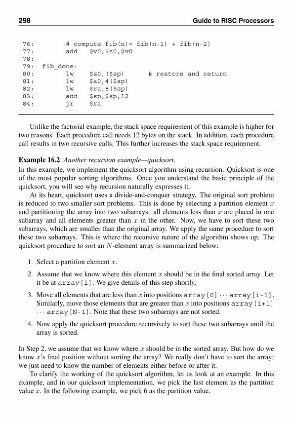
298 Guide to RISC Processors
76: # compute fib(n)= fib(n-1) + fib(n-2)77: add $v0,$s0,$v078:79: fib_done:80: lw $s0,($sp) # restore and return81: lw $a0,4($sp)82: lw $ra,8($sp)83: add $sp,$sp,1284: jr $ra
Unlike the factorial example, the stack space requirement of this example is higher fortwo reasons. Each procedure call needs 12 bytes on the stack. In addition, each procedurecall results in two recursive calls. This further increases the stack space requirement.
Example 16.2 Another recursion example—quicksort.In this example, we implement the quicksort algorithm using recursion. Quicksort is oneof the most popular sorting algorithms. Once you understand the basic principle of thequicksort, you will see why recursion naturally expresses it.
At its heart, quicksort uses a divide-and-conquer strategy. The original sort problemis reduced to two smaller sort problems. This is done by selecting a partition element xand partitioning the array into two subarrays: all elements less than x are placed in onesubarray and all elements greater than x in the other. Now, we have to sort these twosubarrays, which are smaller than the original array. We apply the same procedure to sortthese two subarrays. This is where the recursive nature of the algorithm shows up. Thequicksort procedure to sort an N -element array is summarized below:
1. Select a partition element x.
2. Assume that we know where this element x should be in the final sorted array. Letit be at array[i]. We give details of this step shortly.
3. Move all elements that are less than x into positions array[0] · · · array[i-1].Similarly, move those elements that are greater than x into positions array[i+1]· · · array[N-1]. Note that these two subarrays are not sorted.
4. Now apply the quicksort procedure recursively to sort these two subarrays until thearray is sorted.
In Step 2, we assume that we know where x should be in the sorted array. But how do weknow x’s final position without sorting the array? We really don’t have to sort the array;we just need to know the number of elements either before or after it.
To clarify the working of the quicksort algorithm, let us look at an example. In thisexample, and in our quicksort implementation, we pick the last element as the partitionvalue x. In the following example, we pick 6 as the partition value.
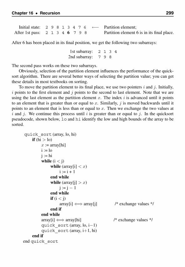
Chapter 16 • Recursion 299
Initial state: 2 9 8 1 3 4 7 6 ←− Partition element;After 1st pass: 2 1 3 4 6 7 9 8 Partition element 6 is in its final place.
After 6 has been placed in its final position, we get the following two subarrays:
1st subarray: 2 1 3 42nd subarray: 7 9 8
The second pass works on these two subarrays.Obviously, selection of the partition element influences the performance of the quick-
sort algorithm. There are several better ways of selecting the partition value; you can getthese details in most textbooks on sorting.
To move the partition element to its final place, we use two pointers i and j. Initially,i points to the first element and j points to the second to last element. Note that we areusing the last element as the partition element x. The index i is advanced until it pointsto an element that is greater than or equal to x. Similarly, j is moved backwards until itpoints to an element that is less than or equal to x. Then we exchange the two values ati and j. We continue this process until i is greater than or equal to j. In the quicksortpseudocode, shown below, lo and hi identify the low and high bounds of the array to besorted.
quick_sort (array, lo, hi)if (hi > lo)
x := array[hi]i := loj := hiwhile (i < j)
while (array[i] < x)i := i + 1
end whilewhile (array[j] > x)
j := j − 1end whileif (i < j)
array[i] ⇐⇒ array[j] /* exchange values */end if
end whilearray[i] ⇐⇒ array[hi] /* exchange values */quick_sort (array, lo, i−1)quick_sort (array, i+1, hi)
end ifend quick_sort
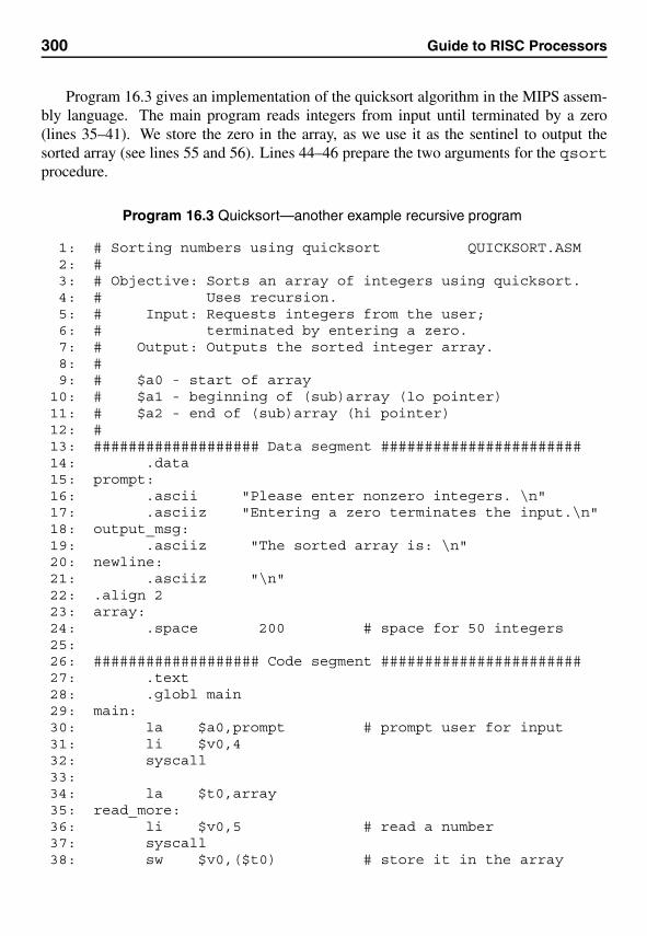
300 Guide to RISC Processors
Program 16.3 gives an implementation of the quicksort algorithm in the MIPS assem-bly language. The main program reads integers from input until terminated by a zero(lines 35–41). We store the zero in the array, as we use it as the sentinel to output thesorted array (see lines 55 and 56). Lines 44–46 prepare the two arguments for the qsortprocedure.
Program 16.3 Quicksort—another example recursive program
1: # Sorting numbers using quicksort QUICKSORT.ASM2: #3: # Objective: Sorts an array of integers using quicksort.4: # Uses recursion.5: # Input: Requests integers from the user;6: # terminated by entering a zero.7: # Output: Outputs the sorted integer array.8: #9: # $a0 - start of array
10: # $a1 - beginning of (sub)array (lo pointer)11: # $a2 - end of (sub)array (hi pointer)12: #13: ################### Data segment #######################14: .data15: prompt:16: .ascii "Please enter nonzero integers. \n"17: .asciiz "Entering a zero terminates the input.\n"18: output_msg:19: .asciiz "The sorted array is: \n"20: newline:21: .asciiz "\n"22: .align 223: array:24: .space 200 # space for 50 integers25:26: ################### Code segment #######################27: .text28: .globl main29: main:30: la $a0,prompt # prompt user for input31: li $v0,432: syscall33:34: la $t0,array35: read_more:36: li $v0,5 # read a number37: syscall38: sw $v0,($t0) # store it in the array
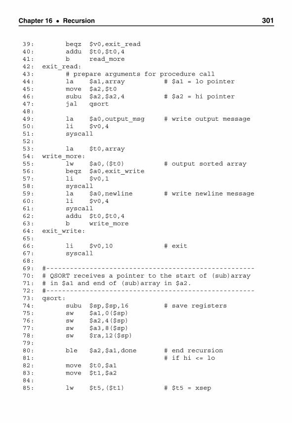
Chapter 16 • Recursion 301
39: beqz $v0,exit_read40: addu $t0,$t0,441: b read_more42: exit_read:43: # prepare arguments for procedure call44: la $a1,array # $a1 = lo pointer45: move $a2,$t046: subu $a2,$a2,4 # $a2 = hi pointer47: jal qsort48:49: la $a0,output_msg # write output message50: li $v0,451: syscall52:53: la $t0,array54: write_more:55: lw $a0,($t0) # output sorted array56: beqz $a0,exit_write57: li $v0,158: syscall59: la $a0,newline # write newline message60: li $v0,461: syscall62: addu $t0,$t0,463: b write_more64: exit_write:65:66: li $v0,10 # exit67: syscall68:69: #-----------------------------------------------------70: # QSORT receives a pointer to the start of (sub)array71: # in $a1 and end of (sub)array in $a2.72: #-----------------------------------------------------73: qsort:74: subu $sp,$sp,16 # save registers75: sw $a1,0($sp)76: sw $a2,4($sp)77: sw $a3,8($sp)78: sw $ra,12($sp)79:80: ble $a2,$a1,done # end recursion81: # if hi <= lo82: move $t0,$a183: move $t1,$a284:85: lw $t5,($t1) # $t5 = xsep
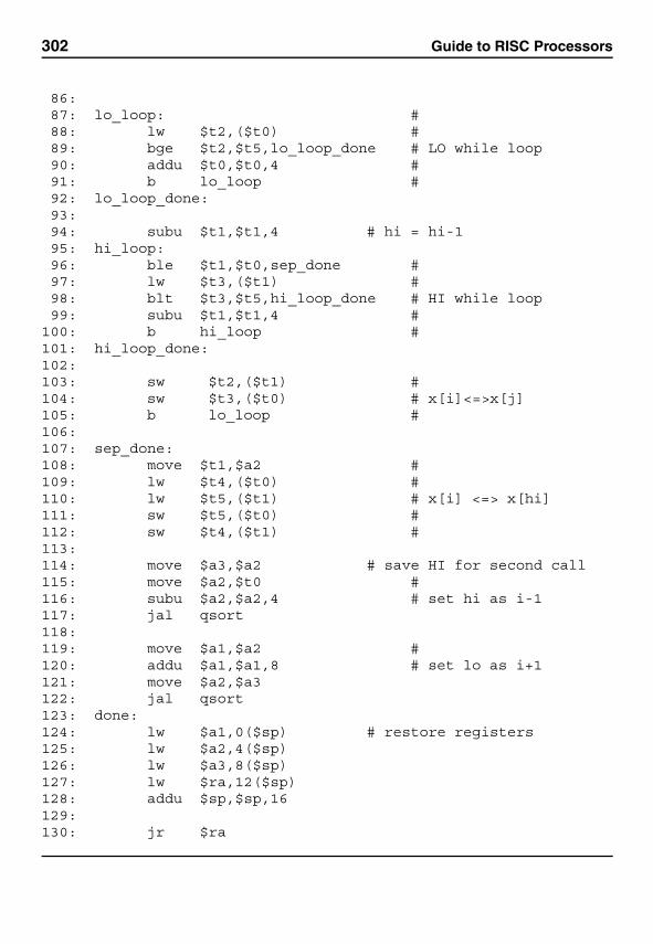
302 Guide to RISC Processors
86:87: lo_loop: #88: lw $t2,($t0) #89: bge $t2,$t5,lo_loop_done # LO while loop90: addu $t0,$t0,4 #91: b lo_loop #92: lo_loop_done:93:94: subu $t1,$t1,4 # hi = hi-195: hi_loop:96: ble $t1,$t0,sep_done #97: lw $t3,($t1) #98: blt $t3,$t5,hi_loop_done # HI while loop99: subu $t1,$t1,4 #
100: b hi_loop #101: hi_loop_done:102:103: sw $t2,($t1) #104: sw $t3,($t0) # x[i]<=>x[j]105: b lo_loop #106:107: sep_done:108: move $t1,$a2 #109: lw $t4,($t0) #110: lw $t5,($t1) # x[i] <=> x[hi]111: sw $t5,($t0) #112: sw $t4,($t1) #113:114: move $a3,$a2 # save HI for second call115: move $a2,$t0 #116: subu $a2,$a2,4 # set hi as i-1117: jal qsort118:119: move $a1,$a2 #120: addu $a1,$a1,8 # set lo as i+1121: move $a2,$a3122: jal qsort123: done:124: lw $a1,0($sp) # restore registers125: lw $a2,4($sp)126: lw $a3,8($sp)127: lw $ra,12($sp)128: addu $sp,$sp,16129:130: jr $ra
Chapter 16 • Recursion 303
The qsort recursive procedure stores $a3 in addition to the $a1, $a2, and $raregisters. This is because we store the end-of-subarray pointer in $a3, which is requiredfor the second recursive call (line 122). Because MIPS does not have an addressing modethat allows access to arrays using the index, we have to use pointers to access individualelements. This means updating the index involves adding or subtracting 4 (see lines 90,94, 99, and 116). The rest of the procedure follows the quicksort algorithm describedearlier.
The stack space requirements of this program are similar to the Fibonacci program inthat each procedure call generates two recursive calls. For each call, it needs 16 bytes ofstack space.
Recursion Versus IterationIn theory, every recursive function has an iterative counterpart. We have seen two exam-ples: factorial and Fibonacci functions. We have looked at the recursive versions of thesetwo functions in this chapter. The iterative versions are given in previous chapters (seeProgram 13.1 on page 230 for the factorial function and Program 11.3 on page 200 for theFibonacci function).
From these examples, it is obvious that the recursive versions reflect the mathemat-ical definition of the functions more directly. Once you get through the initial learningproblems with recursion, recursive code is easier to understand for those functions thatare defined recursively.
This leads us to the question of when to use recursion. To answer this question, weneed to look at the potential problems recursion can cause. There are two main problemswith recursion:
• Inefficiency: In most cases, recursive versions tend to be inefficient. You can seethis point by comparing the recursive and iterative versions of the factorial function.The recursive version induces more overheads to invoke and return from procedurecalls. To compute N !, we need to call the factorial function about N times. In theiterative version, the loop iterates about N times.
Recursion could also introduce duplicate computation. For example, to compute theFibonacci number fib(5) a recursive procedure computes fib(3) two times,fib(2) three times, and so on, as shown in Figure 16.2.
• Increased Memory Requirement: Recursion tends to demand more memory. Thiscan be seen from the simple factorial example. For large N , the demand for stackmemory can be excessive. The other examples (Fibonacci and quicksort) requireeven more stack memory. In some applications, the limit on the available stackmemory may make the recursive version impractical.
On the positive side, however, recursion leads to better understanding of the code for thosenaturally recursive problems. In this case, recursion may be useful as it aids in programmaintenance.
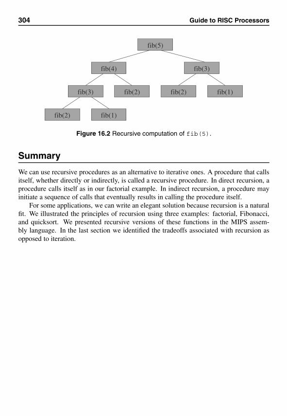
304 Guide to RISC Processors
fib(4)
fib(1)
fib(3)
fib(3) fib(2) fib(2)
fib(2) fib(1)
fib(5)
Figure 16.2 Recursive computation of fib(5).
Summary
We can use recursive procedures as an alternative to iterative ones. A procedure that callsitself, whether directly or indirectly, is called a recursive procedure. In direct recursion, aprocedure calls itself as in our factorial example. In indirect recursion, a procedure mayinitiate a sequence of calls that eventually results in calling the procedure itself.
For some applications, we can write an elegant solution because recursion is a naturalfit. We illustrated the principles of recursion using three examples: factorial, Fibonacci,and quicksort. We presented recursive versions of these functions in the MIPS assem-bly language. In the last section we identified the tradeoffs associated with recursion asopposed to iteration.
17Floating-PointOperations
In this chapter, we look at floating-point instructions. The floating-point unit coprocessorsupports several floating-point instructions. We describe the floating-point registers of thefloating-point unit. The floating-point instructions include the four basic arithmetic op-erations on both single-precision and double-precision floating-point numbers. We giveseveral examples to illustrate the application of these instructions. We conclude the chap-ter with a summary.
IntroductionIn the previous chapters, we have looked at arithmetic operations on integers. Theseoperations are supported by the CPU. In the MIPS architecture, the floating-point oper-ations are supported by a separate Floating-Point Unit (FPU), which is coprocessor 1.There are instructions that move data between the processor registers and the FPU regis-ters. The FPU supports the basic arithmetic operations, including addition, subtraction,multiplication, and division. These operations are available for both single-precision anddouble-precision floating-point numbers.
A single-precision floating-point number takes 32 bits whereas the double-precisionnumber takes 64 bits. These are useful in implementing the floating-point numbers sup-ported by high-level languages. For example, the C float data type corresponds to thesingle-precision number and the double to the double-precision floating-point number.
When we have several formats to represent numbers, we need instructions to convert anumber from one representation to another. The FPU instruction set includes instructionsto do conversions among integers, and single-precision and double-precision floating-point numbers. For example, there are instructions to convert integers to double-precision
305
306 Guide to RISC Processors
floating-point numbers and vice versa. Such conversions are often done in high-levellanguages. Suppose we declared the following variables in C.
double average, sum;int count;
Then the statement
average = sum/count;
computes the average. However, because sum is a double and count is an integer, it pro-motes count to double before the division. As another example, consider the followingdeclaration.
double average;int result;
Then the statement
result = (int *) average;
uses the cast operator to convert average to the integer format before assigning it to theresult variable. Conversions like these can be done using the conversion instructionssupported by the FPU.
Our goal in this chapter is to give an overview of the floating-point instructions. Wedescribe the FPU instruction set along with its registers. For complete details, you shouldconsult the MIPS documentation. We start this chapter with a description of the registersavailable in the FPU.
FPU Registers
The floating-point unit has 32 floating-point registers. These registers are numbered likethe CPU registers. In the floating-point instructions we refer to these registers as $f0,$f1, and so on. Each of these registers is 32 bits wide. Thus, each register can hold onesingle-precision floating-point number. How can we use these registers to store double-precision floating-point numbers? Because these numbers require 64 bits, register pairsare used to store them. This strategy is implemented by storing double-precision numbersin even-numbered registers. For example, when we store a double-precision number in$f2, it is actually stored in registers $f2 and $f3.
As with the CPU registers, the FPU register usage convention has been established tomake programs portable (see Table 17.1). Even though each floating-point register canhold a single-precision number, the numbers are often stored in even registers so that theycan be easily upgraded to double-precision values.
The first four registers are used to return values from a procedure. These registers canbe used to return two double-precision floating-point numbers. The caller-save tempo-raries can be used freely by the called procedure. If the caller needs the values in these
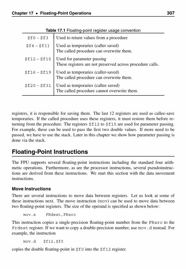
Chapter 17 • Floating-Point Operations 307
Table 17.1 Floating-point register usage convention
$f0 – $f3 Used to return values from a procedure
$f4 – $f11 Used as temporaries (caller saved)The called procedure can overwrite them.
$f12 – $f15 Used for parameter passingThese registers are not preserved across procedure calls.
$f16 – $f19 Used as temporaries (caller-saved)The called procedure can overwrite them.
$f20 – $f31 Used as temporaries (callee saved)The called procedure cannot overwrite them.
registers, it is responsible for saving them. The last 12 registers are used as callee-savetemporaries. If the called procedure uses these registers, it must restore them before re-turning from the procedure. The registers $f12 to $f15 are used for parameter passing.For example, these can be used to pass the first two double values. If more need to bepassed, we have to use the stack. Later in this chapter we show how parameter passing isdone via the stack.
Floating-Point Instructions
The FPU supports several floating-point instructions including the standard four arith-metic operations. Furthermore, as are the processor instructions, several pseudoinstruc-tions are derived from these instructions. We start this section with the data movementinstructions.
Move InstructionsThere are several instructions to move data between registers. Let us look at some ofthese instructions next. The move instruction (mov) can be used to move data betweentwo floating-point registers. The size of the operand is specified as shown below:
mov.s FRdest,FRsrc
This instruction copies a single-precision floating-point number from the FRsrc to theFrdest register. If we want to copy a double-precision number, use mov.d instead. Forexample, the instruction
mov.d $f12,$f0
copies the double floating-point in $f0 into the $f12 register.
308 Guide to RISC Processors
The mov instruction facilitates data transfer between two floating-point registers. How-ever, we also need to move data between the CPU registers and the floating-point registers.This data movement is facilitated by the mtc1 and mfc1 instructions. Note that the 1in these instructions identifies coprocessor 1. There are also instructions to address othercoprocessors (e.g., mtf0 for coprocessor 0, mtf2 for coprocessor 2, and so on) but wefocus here only on the FPU, which is coprocessor 1.
The mfc1 (move from coprocessor 1) instruction
mfc1 Rdest,FRsrc
moves a 32-bit value from the FRsrc floating-point register to the Rdest CPU register.To move the data in the opposite direction, we use the mtc1 (move to coprocessor 1)instruction, which has the following format.
mtc1 FRdest,Rsrc
This instruction moves a 32-bit value from the Rsrc CPU register to the FRdest FPUregister.
These instructions are useful to move single-precision floating-point numbers betweenCPU and FPU registers. However, if we want to move double-precision values, we haveto use two of these instructions. There is a pseudoinstruction that does this job as shownhere:
mfc1.d Rdest,FRsrc
This pseudoinstruction copies the contents of the two floating-point registers (FRsrc andFRsrc+1) to two CPU registers (Rdest and Rdest+1). For example, the pseudoin-struction
mfc1.d $t0,$f2
is translated as
mfc1 $8,$2mfc1 $9,$3
Note that the second register number in these two instructions refers to the floating-pointregister. The first register number refers to a CPU register. As you know, $t0 maps to$8. Thus, we can rewrite this sequence as
mfc1 $t0,$f2mfc1 $t1,$f3
This is more readable than the code generated by SPIM.
Chapter 17 • Floating-Point Operations 309
Load and Store InstructionsThe basic load instruction lwc1 (load a word from memory to an FPU register) has thefollowing format.
lwc1 FRdest,address
Notice that the instruction includes the coprocessor 1 (c1), which is the FPU supportingthese instructions. This instruction loads a 32-bit word from address into the FRdestfloating-point register. The address can be specified as offset(base)where baseis a CPU register containing the base address. For example, the instruction
lwc1 $f0,0($sp)
loads the 32-bit word at the top of stack into the $f0 floating-point register.The corresponding store instruction has the following format.
swc1 FRdest,address
It stores the contents of FRdest in memory at address. For example, if we want tostore the contents of $f0 on the stack, we could do this by the following instruction.
swc1 $f0,0($sp)
Although these load and store instructions take care of the single-precision loads andstores, we have to use two of these instructions to load/store doubles. To simplify loadsand stores, several pseudoinstructions are available. Let us first look at the load pseudoin-structions. The pseudoinstruction
l.s FRdest,address
loads a single-precision floating-point number. For example, the pseudoinstruction
l.s $f2,0($sp)
is translated as
lwc1 $f2,0($29)
Recall that $sp maps to $29. To load a double floating-point number, use l.d as in thefollowing example.
l.d $f2,0($sp)
It is translated as
lwc1 $f2,0($29)lwc1 $f3,4($29)
310 Guide to RISC Processors
We can use s.s to store a single-precision value and s.d for a double-precisionvalue. The s.s pseudoinstruction is translated using a single swc1 instruction. The s.dinstruction requires two instructions as shown in the following example.
s.d $f0,0($sp)
is translated as
swc1 $f0,0($29)swc1 $f1,4($29)
Two additional pseudoinstructions are available to load constants into floating-pointregisters. We illustrate these instructions with two examples. The li.s can be used toload single-precision values into a floating-point register. The pseudoinstruction
li.s $f0,0.0
is translated as
ori $1,$0,0mtc1 $1,$0
We can load a double-precision constant using the li.d pseudoinstruction as shownbelow:
li.d $f2,0.0
is translated as
ori $1,$0,0mtc1 $1,$2ori $1,$0,0mtc1 $1,$3
Arithmetic InstructionsThe FPU supports several arithmetic instructions to perform addition, subtraction, multi-plication, and division on single- as well as double-precision floating-point numbers. Allfour instructions use the same format. We use the sub instruction to illustrate the basicformat.
sub.s FRdest,FRsrc1,FRsrc2 # single-precision subtractsub.d FRdest,FRsrc1,FRsrc2 # double-precision subtract
It places the result of FRsrc1−FRsrc2 in the FRdest register. For addition, useadd.s or add.d as in the following example.
Chapter 17 • Floating-Point Operations 311
add.s $f0,$f0,$f2
This instruction adds the contents of $f0 and $f2 and places the result in the $f0 regis-ter. To divide floating-point numbers, we use div.s or div.d as shown in the examplehere.
div.d $f0,$f2,$f4
This instruction divides the double floating-point value in $f2 and $f3 by that in $f4and $f5 and places the result in the $f0 and $f1 registers. This instruction generatesexceptions to indicate conditions such as divide-by-zero, underflow, and overflow.
For multiplication, we use mul.s or mul.d depending on the precision of the num-bers to be multiplied. Like the div instruction, it also generates exceptions for conditionssuch underflow and overflow.
In addition to these basic four arithmetic operations, the FPU also provides abs andneg instructions. The abs instruction computes the absolute value and has the followingformat.
abs.s FRdest,FRsrc # for single-precision valuesabs.d FRdest,FRsrc # for double-precision values
It computes the absolute value of the number in FRsrc and places the result in theFRdest register. The negate instruction
neg.s FRdest,FRsrc # for single-precision valuesneg.d FRdest,FRsrc # for double-precision values
reverses the sign of the number in FRsrc and places the result in the FRdest register.
Comparison InstructionsThree basic comparison instructions are available to compare floating-point numbers toestablish <, =, and ≤ relationships. All three instructions have the same format. We usethe following to illustrate their format.
c.lt.s FRsrc1,FRsrc2 # for single-precision valuesc.lt.d FRsrc1,FRsrc2 # for double-precision values
It compares the two floating-point values in FRsrc1 and FRsrc2 and sets the floating-point condition flag if FRsrc1< FRsrc2.
To establish the “equal to” relationship, we use c.eq.s or c.eq.d. For the ≤relationship, we use either c.le.s or c.le.d depending on the precision of the valuesbeing compared.
Once the floating-point condition flag is set to reflect the relationship, this flag valuecan be tested by the CPU using bc1t or bc1f instructions. The format of these instruc-tions is the same. For example, the instruction
312 Guide to RISC Processors
bc1t target
transfers control to target if the floating-point condition flag is true. Here is an examplethat compares the values in $f0 and $f2 and transfers control to skip1 if $f0 < $f2.
c.lt.s $f0,$f2 # $f0 < $f2?bc1t skip1 # if yes, jump to skip1
We don’t really need instructions for the missing relationships >, �=, or ≥. For example,the code
c.le.s $f0,$f2 # $f0 ≤ $f2?bc1f skip1 # if not, jump to skip1
transfers control to skip1 if $f0 > $f2.
Conversion InstructionsWhen we have numbers of different types—integers and single-precision and double-precision floating-point values—we often need to convert numbers from one represen-tation to the other. The final group of instructions we discuss here deals with this con-version. These instructions allow us to convert values among the integer and single anddouble floating-point number representations. All these instructions follow the same for-mat. We illustrate the format using the instruction that converts from an integer to doublefloating-point number. The format of this instruction is shown here:
cvt.d.w FRdest,FRsrc
This instruction converts the integer in FRsrc to a double floating-point number andstores it in the FRdest register. Typically, we move the integer to be converted from aCPU register to an FPU register using the mtc1 instruction. The following code demon-strates the use of this conversion.
mtc1 $a1,$f4 # move the integer to $f4cvt.d.w $f4,$f4 # convert the word in $f4 to double
The mtc1 instruction copies the integer in $a1 to the $f4 register. The second in-struction coverts the integer in $f4 to double floating-point format. A summary of theconversion instructions is given in Table 17.2.
Our First Program
In our first floating-point program, shown in Program 17.1, we add three double-precisionfloating-point numbers and output their sum. We read the input values as doubles usingthe read_double system call (see lines 26–27, 30-31, and 34–35). This system callplaces the double in $f0 (i.e., in registers $f0 and $f1). We use the move instruction tocopy this value into another register (see lines 28, 32, and 36).
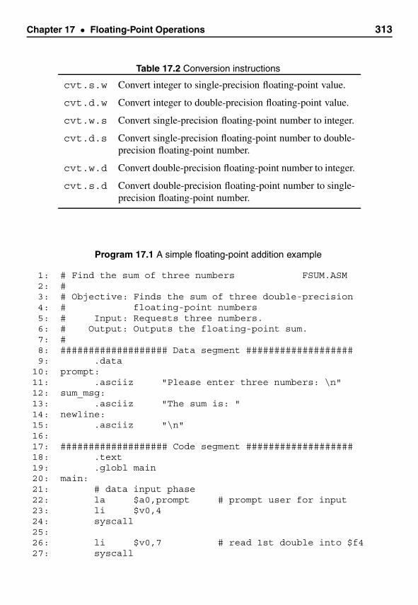
Chapter 17 • Floating-Point Operations 313
Table 17.2 Conversion instructions
cvt.s.w Convert integer to single-precision floating-point value.
cvt.d.w Convert integer to double-precision floating-point value.
cvt.w.s Convert single-precision floating-point number to integer.
cvt.d.s Convert single-precision floating-point number to double-precision floating-point number.
cvt.w.d Convert double-precision floating-point number to integer.
cvt.s.d Convert double-precision floating-point number to single-precision floating-point number.
Program 17.1 A simple floating-point addition example
1: # Find the sum of three numbers FSUM.ASM2: #3: # Objective: Finds the sum of three double-precision4: # floating-point numbers5: # Input: Requests three numbers.6: # Output: Outputs the floating-point sum.7: #8: ################### Data segment ###################9: .data
10: prompt:11: .asciiz "Please enter three numbers: \n"12: sum_msg:13: .asciiz "The sum is: "14: newline:15: .asciiz "\n"16:17: ################### Code segment ###################18: .text19: .globl main20: main:21: # data input phase22: la $a0,prompt # prompt user for input23: li $v0,424: syscall25:26: li $v0,7 # read 1st double into $f427: syscall
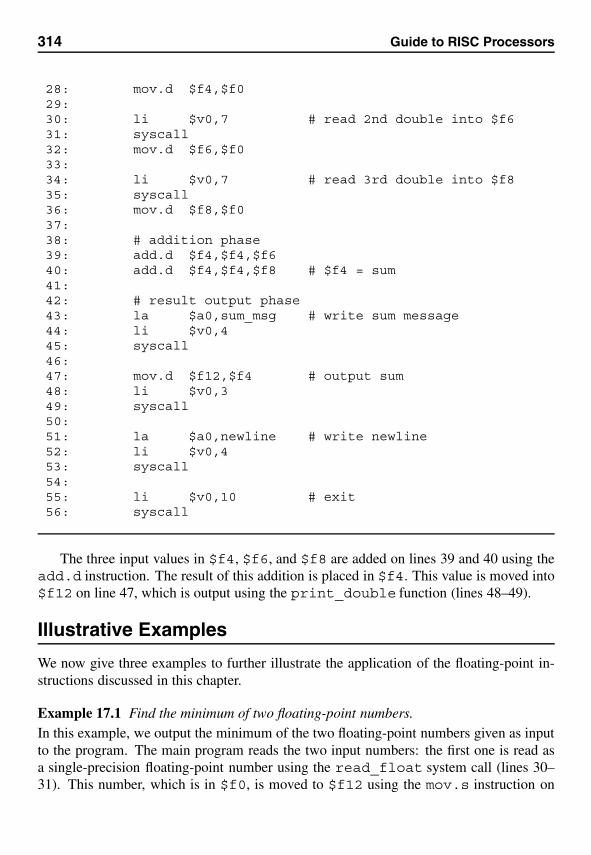
314 Guide to RISC Processors
28: mov.d $f4,$f029:30: li $v0,7 # read 2nd double into $f631: syscall32: mov.d $f6,$f033:34: li $v0,7 # read 3rd double into $f835: syscall36: mov.d $f8,$f037:38: # addition phase39: add.d $f4,$f4,$f640: add.d $f4,$f4,$f8 # $f4 = sum41:42: # result output phase43: la $a0,sum_msg # write sum message44: li $v0,445: syscall46:47: mov.d $f12,$f4 # output sum48: li $v0,349: syscall50:51: la $a0,newline # write newline52: li $v0,453: syscall54:55: li $v0,10 # exit56: syscall
The three input values in $f4, $f6, and $f8 are added on lines 39 and 40 using theadd.d instruction. The result of this addition is placed in $f4. This value is moved into$f12 on line 47, which is output using the print_double function (lines 48–49).
Illustrative Examples
We now give three examples to further illustrate the application of the floating-point in-structions discussed in this chapter.
Example 17.1 Find the minimum of two floating-point numbers.In this example, we output the minimum of the two floating-point numbers given as inputto the program. The main program reads the two input numbers: the first one is read asa single-precision floating-point number using the read_float system call (lines 30–31). This number, which is in $f0, is moved to $f12 using the mov.s instruction on
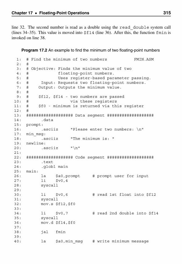
Chapter 17 • Floating-Point Operations 315
line 32. The second number is read as a double using the read_double system call(lines 34–35). This value is moved into $f14 (line 36). After this, the function fmin isinvoked on line 38.
Program 17.2 An example to find the minimum of two floating-point numbers
1: # Find the minimum of two numbers FMIN.ASM2: #3: # Objective: Finds the minimum value of two4: # floating-point numbers.5: # Uses register-based parameter passing.6: # Input: Requests two floating-point numbers.7: # Output: Outputs the minimum value.8: #9: # $f12, $f14 - two numbers are passed
10: # via these registers11: # $f0 - minimum is returned via this register12: #13: ################### Data segment ###################14: .data15: prompt:16: .asciiz "Please enter two numbers: \n"17: min_msg:18: .asciiz "The minimum is: "19: newline:20: .asciiz "\n"21:22: ################### Code segment ###################23: .text24: .globl main25: main:26: la $a0,prompt # prompt user for input27: li $v0,428: syscall29:30: li $v0,6 # read 1st float into $f1231: syscall32: mov.s $f12,$f033:34: li $v0,7 # read 2nd double into $f1435: syscall36: mov.d $f14,$f037:38: jal fmin39:40: la $a0,min_msg # write minimum message
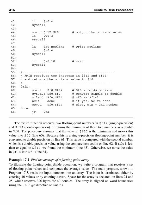
316 Guide to RISC Processors
41: li $v0,442: syscall43:44: mov.d $f12,$f0 # output the minimum value45: li $v0,346: syscall47:48: la $a0,newline # write newline49: li $v0,450: syscall51:52: li $v0,10 # exit53: syscall54:55: #------------------------------------------------56: # FMIN receives two integers in $f12 and $f1457: # and returns the minimum value in $f058: #------------------------------------------------59: fmin:60: mov.s $f0,$f12 # $f0 = holds minimum61: cvt.d.s $f0,$f0 # convert single to double62: c.le.d $f0,$f14 # $f0 <= $f14?63: bc1t done # if yes, we’re done64: mov.d $f0,$f14 # else, min = 2nd number65: done:66: jr $ra
The fmin function receives two floating-point numbers in $f12 (single-precision)and $f14 (double-precision). It returns the minimum of these two numbers as a doublein $f0. The procedure assumes that the value in $f12 is the minimum and moves thisvalue into $f0 (line 60). Because this is a single-precision floating-point number, it isconverted to double precision on line 61. This value is compared with the second number,which is a double-precision value, using the compare instruction on line 62. If $f0 is lessthan or equal to $f14, we found the minimum (line 63). Otherwise, we move the valuein $f14 into $f0 (line 64).
Example 17.2 Find the average of a floating-point array.To illustrate the floating-point divide operation, we write a program that receives a setof floating-point values and computes the average value. The main program, shown inProgram 17.3, reads the input numbers into an array. The input is terminated either byentering 40 values or by entering a zero. Space for the array is declared on lines 24 and25, which reserves 320 bytes for 40 doubles. The array is aligned on word boundariesusing the .align directive on line 23.
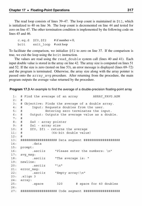
Chapter 17 • Floating-Point Operations 317
The read loop consists of lines 39–47. The loop count is maintained in $t1, whichis initialized to 40 on line 36. The loop count is decremented on line 44 and tested forzero on line 47. The other termination condition is implemented by the following code onlines 45 and 46.
c.eq.d $f0,$f2 # if number = 0,bc1t exit_loop # exit loop
To facilitate the comparison, we initialize $f2 to zero on line 37. If the comparison istrue, we exit the loop using the bc1t instruction.
The values are read using the read_double system call (lines 40 and 41). Eachinput double value is stored in the array on line 42. The array size is computed on lines 51and 52. If the size is zero (tested on line 53), an error message is displayed (lines 69–72)and the program is terminated. Otherwise, the array size along with the array pointer ispassed onto the array_avg procedure. After returning from the procedure, the mainprogram outputs the average value returned by the procedure.
Program 17.3 An example to find the average of a double-precision floating-point array
1: # Find the average of an array ARRAY_FAVG.ASM2: #3: # Objective: Finds the average of a double array.4: # Input: Requests doubles from the user.5: # Entering zero terminates the input.6: # Output: Outputs the average value as a double.7: #8: # $a0 - array pointer9: # $a1 - array size
10: # $f0, $f1 - returns the average11: # (64-bit double value)12: #13: ################### Data segment ###################14: .data15: prompt:16: .asciiz "Please enter the numbers: \n"17: avg_msg:18: .asciiz "The average is: "19: newline:20: .asciiz "\n"21: error_msg:22: .asciiz "Empty array!\n"23: .align 324: array:25: .space 320 # space for 40 doubles26:27: ################### Code segment ###################
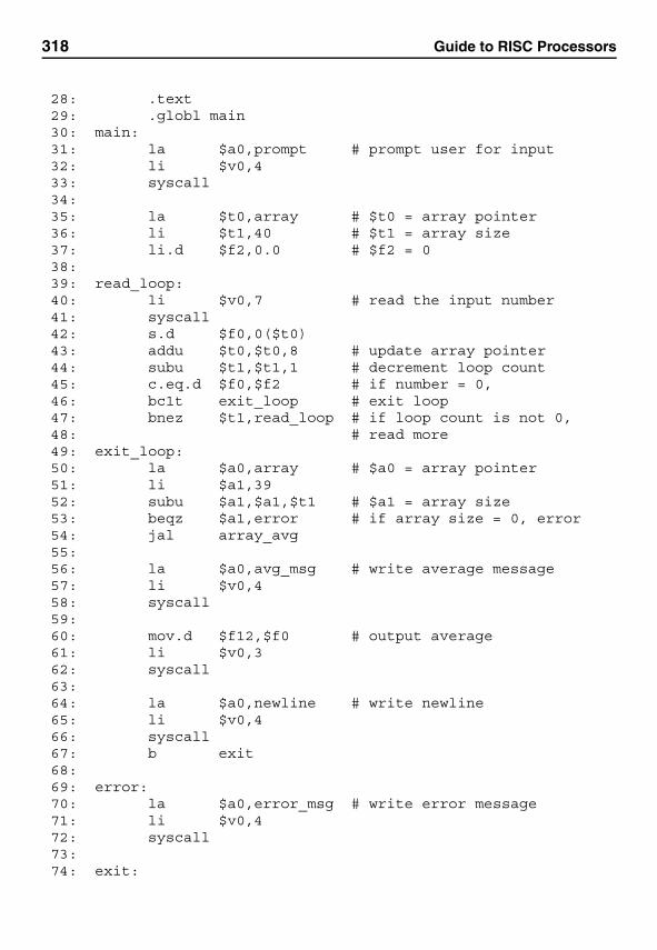
318 Guide to RISC Processors
28: .text29: .globl main30: main:31: la $a0,prompt # prompt user for input32: li $v0,433: syscall34:35: la $t0,array # $t0 = array pointer36: li $t1,40 # $t1 = array size37: li.d $f2,0.0 # $f2 = 038:39: read_loop:40: li $v0,7 # read the input number41: syscall42: s.d $f0,0($t0)43: addu $t0,$t0,8 # update array pointer44: subu $t1,$t1,1 # decrement loop count45: c.eq.d $f0,$f2 # if number = 0,46: bc1t exit_loop # exit loop47: bnez $t1,read_loop # if loop count is not 0,48: # read more49: exit_loop:50: la $a0,array # $a0 = array pointer51: li $a1,3952: subu $a1,$a1,$t1 # $a1 = array size53: beqz $a1,error # if array size = 0, error54: jal array_avg55:56: la $a0,avg_msg # write average message57: li $v0,458: syscall59:60: mov.d $f12,$f0 # output average61: li $v0,362: syscall63:64: la $a0,newline # write newline65: li $v0,466: syscall67: b exit68:69: error:70: la $a0,error_msg # write error message71: li $v0,472: syscall73:74: exit:
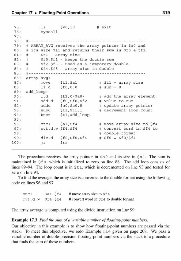
Chapter 17 • Floating-Point Operations 319
75: li $v0,10 # exit76: syscall77:78: #------------------------------------------------79: # ARRAY_AVG receives the array pointer in $a0 and80: # its size $a1 and returns their sum in $f0 & $f1.81: # $t1 - array size82: # $f0,$f1 - keeps the double sum83: # $f2,$f3 - used as a temporary double84: # $f4,$f5 - array size in double85: #------------------------------------------------86: array_avg:87: move $t1,$a1 # $t1 = array size88: li.d $f0,0.0 # sum = 089: add_loop:90: l.d $f2,0($a0) # add the array element91: add.d $f0,$f0,$f2 # value to sum92: addu $a0,$a0,8 # update array pointer93: subu $t1,$t1,1 # decrement loop count94: bnez $t1,add_loop95:96: mtc1 $a1,$f4 # move array size to $f497: cvt.d.w $f4,$f4 # convert word in $f4 to98: # double format99: div.d $f0,$f0,$f4 # $f0 = $f0/$f4
100: jr $ra
The procedure receives the array pointer in $a0 and its size in $a1. The sum ismaintained in $f0, which is initialized to zero on line 88. The add loop consists oflines 89–94. The loop count is in $t1, which is decremented on line 93 and tested forzero on line 94.
To find the average, the array size is converted to the double format using the followingcode on lines 96 and 97.
mtc1 $a1,$f4 # move array size to $f4cvt.d.w $f4,$f4 # convert word in $f4 to double format
The array average is computed using the divide instruction on line 99.
Example 17.3 Find the sum of a variable number of floating-point numbers.Our objective in this example is to show how floating-point numbers are passed via thestack. To meet this objective, we redo Example 11.4 given on page 208. We pass avariable number of double-precision floating-point numbers via the stack to a procedurethat finds the sum of these numbers.

320 Guide to RISC Processors
As in the last example, entering a zero terminates the input. The read loop consists oflines 33–41 and is similar to the read loop of the last example. The main difference is thatthe values are pushed onto the stack as we read them (lines 38 and 39). After exiting theread loop, we can invoke the procedure as the parameter count is in $a0 and the valuesare on the stack.
Program 17.4 An example to illustrate parameter passing of floating-point values via thestack
1: # Find the sum of doubles VAR_FSUM.ASM2: #3: # Objective: Finds the sum of variable number of4: # doubles passed via the stack.5: # To demonstrate stack-based6: # parameter passing.7: # Input: Requests doubles from the user.8: # Entering a zero ends the input.9: # Output: Outputs the sum.
10: #11: # $a0 - number of doubles passed via the stack.12: # $f0 - returns the sum as a double (in $f0,$f1).13: #14: ################### Data segment ###################15: .data16: prompt:17: .asciiz "Please enter the numbers: \n"18: sum_msg:19: .asciiz "The sum is: "20: newline:21: .asciiz "\n"22:23: ################### Code segment ###################24: .text25: .globl main26: main:27: la $a0,prompt # prompt user for input28: li $v0,429: syscall30:31: li.d $f2,0.0 # $f2 = 032: li $a0,0 # parameter count = 033: read_loop:34: li $v0,7 # read the input number35: syscall36: c.eq.d $f0,$f2 # if number = 0, exit loop37: bc1t exit_loop
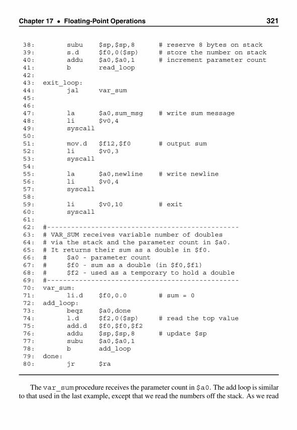
Chapter 17 • Floating-Point Operations 321
38: subu $sp,$sp,8 # reserve 8 bytes on stack39: s.d $f0,0($sp) # store the number on stack40: addu $a0,$a0,1 # increment parameter count41: b read_loop42:43: exit_loop:44: jal var_sum45:46:47: la $a0,sum_msg # write sum message48: li $v0,449: syscall50:51: mov.d $f12,$f0 # output sum52: li $v0,353: syscall54:55: la $a0,newline # write newline56: li $v0,457: syscall58:59: li $v0,10 # exit60: syscall61:62: #------------------------------------------------63: # VAR_SUM receives variable number of doubles64: # via the stack and the parameter count in $a0.65: # It returns their sum as a double in $f0.66: # $a0 - parameter count67: # $f0 - sum as a double (in $f0,$f1)68: # $f2 - used as a temporary to hold a double69: #------------------------------------------------70: var_sum:71: li.d $f0,0.0 # sum = 072: add_loop:73: beqz $a0,done74: l.d $f2,0($sp) # read the top value75: add.d $f0,$f0,$f276: addu $sp,$sp,8 # update $sp77: subu $a0,$a0,178: b add_loop79: done:80: jr $ra
The var_sum procedure receives the parameter count in $a0. The add loop is similarto that used in the last example, except that we read the numbers off the stack. As we read
322 Guide to RISC Processors
the values off the stack, we update the stack pointer by adding 8 (line 76). Recall that thestack grows downward as we push values onto it. Thus, when we take values off, we haveto increment the stack pointer so that, when the loop terminates, the arguments are clearedfrom the stack.
Summary
We presented a brief description of the floating-point unit organization. Specifically, weconcentrated on the registers provided by the FPU. It provides 32 floating-point registersthat can store single-precision floating-point numbers. These registers can be used in pairsto store double-precision floating-point numbers.
The floating-point instructions support the four basic arithmetic operations: add, sub-tract, divide, and multiply. There are also three basic comparison instructions to establish“less than”, “equal to”, or “less than or equal to” relationships between floating-pointnumbers. In addition, several conversion instructions are available. These instructionsallow conversion of values among the integer and single and double floating-point num-ber representations. Finally, we used some examples to illustrate the application of thesefloating-point instructions.

Appendices
ANumber Systems
This appendix introduces background material on various number systems and represen-tations. We start the appendix with a discussion of various number systems, includingthe binary and hexadecimal systems. When we use multiple number systems, we needto convert numbers from one system to another. We present details on how such numberconversions are done. We then give details on integer representations. We cover bothunsigned and signed integer representations. We close the appendix with a discussion ofthe floating-point numbers.
Positional Number Systems
The number systems that we discuss here are based on positional number systems. Thedecimal number system that we are already familiar with is an example of a positionalnumber system. In contrast, the Roman numeral system is not a positional number system.
Every positional number system has a radix or base, and an alphabet. The base is apositive number. For example, the decimal system is a base-10 system. The number ofsymbols in the alphabet is equal to the base of the number system. The alphabet of thedecimal system is 0 through 9, a total of 10 symbols or digits.
In this appendix, we discuss four number systems that are relevant in the context ofcomputer systems and programming. These are the decimal (base-10), binary (base-2),octal (base-8), and hexadecimal (base-16) number systems. Our intention in including thefamiliar decimal system is to use it to explain some fundamental concepts of positionalnumber systems.
Computers internally use the binary system. The remaining two number systems—octal and hexadecimal—are used mainly for convenience to write a binary number eventhough they are number systems on their own. We would have ended up using thesenumber systems if we had 8 or 16 fingers instead of 10.
In a positional number system, a sequence of digits is used to represent a number. Eachdigit in this sequence should be a symbol in the alphabet. There is a weight associated
325

326 Guide to RISC Processors
with each position. If we count position numbers from right to left starting with zero, theweight of position n in a base b number system is bn. For example, the number 579 in thedecimal system is actually interpreted as
5 × (10 2) + 7 × (10 1) + 9 × (10 0) .
(Of course, 10 0 = 1.) In other words, 9 is in unit’s place, 7 in 10’s place, and 5 in 100’splace. More generally, a number in the base b number system is written as
dndn−1 . . . d1d0 ,
where d 0 represents the Least Significant Digit (LSD) and dn represents the Most Signif-icant Digit (MSD). This sequence represents the value
dnbn + dn−1bn−1 + · · · + d1b
1 + d0b0 . (A.1)
Each digit d i in the string can be in the range 0 ≤ di ≤ (b − 1). When we use a numbersystem with b ≤ 10, we use the first b decimal digits. For example, the binary systemuses 0 and 1 as its alphabet. For number systems with b > 10, the initial letters of theEnglish alphabet are used to represent digits greater than 9. For example, the alphabetof the hexadecimal system, whose base is 16, is 0 through 9 and A through F, a total of16 symbols representing the digits of the hexadecimal system. We treat lowercase anduppercase letters used in a number system such as the hexadecimal system as equivalent.
The number of different values that can be represented using n digits in a base bsystem is bn. Consequently, because we start counting from 0, the largest number thatcan be represented using n digits is (bn − 1). This number is written as
(b − 1)(b − 1) . . . (b − 1)(b − 1)︸ ︷︷ ︸total of n digits
.
The minimum number of digits (i.e., the length of a number) required to represent Xdifferent values is given by �logb X�, where � � represents the ceiling function. Note that�m� represents the smallest integer that is greater than or equal to m.
Notation The commonality in the alphabet of several number systems gives rise toconfusion. For example, if we write 100 without specifying the number system in whichit is expressed, different interpretations can lead to assigning different values, as shownbelow:
Number Decimal value
100binary−→ 4
100 decimal−→ 100
100 octal−→ 64
100 hexadecimal−→ 256
Appendix A Number Systems 327
Thus, it is important to specify the number system (i.e., specify the base). One commonnotation is to append a single letter—uppercase or lowercase—to the number to specifythe number system. For example, D is used for decimal, B for binary, Q for octal, and Hfor hexadecimal number systems. Using this notation, 10110111B is a binary number and2BA9H is a hexadecimal number. Some assemblers use the prefix 0x for hexadecimal andthe prefix 0 for octal.
Decimal Number System We use the decimal number system in everyday life. This isa base-10 system presumably because we have 10 fingers and toes to count. The alphabetconsists of 10 symbols, digits 0 through 9.
Binary Number System The binary system is a base-2 number system that is used bycomputers for internal representation. The alphabet consists of two digits, 0 and 1. Eachbinary digit is called a bit (standing for binary digit). Thus, 1021 is not a valid binarynumber. In the binary system, using n bits, we can represent numbers from 0 through(2n − 1) for a total of 2n different values.
Octal Number System This is a base-8 number system with the alphabet consisting ofdigits 0 through 7. Thus, 181 is not a valid octal number. The octal numbers are often usedto express binary numbers in a compact way. For example, we need 8 bits to represent256 different values. The same range of numbers can be represented in the octal systemby using only 3 digits.
For example, the number 230Q is written in the binary system as 10011000B, whichis difficult to read and error prone. In general, we can reduce the length by a factor of 3.As we show later, it is straightforward to go back to the binary equivalent, which is notthe case with the decimal system.
Hexadecimal Number System This is a base-16 number system. The alphabet consistsof digits 0 through 9 and letters A through F. In this text, we use capital letters consistently,even though lowercase and uppercase letters can be used interchangeably. For example,FEED is a valid hexadecimal number, whereas GEFF is not.
The main use of this number system is to conveniently represent long binary numbers.The length of a binary number expressed in the hexadecimal system can be reduced by afactor of 4. Consider the previous example again. The binary number 10011000B can berepresented as 98H. Debuggers, for example, display information—addresses, data, andso on—in hexadecimal representation.
Conversion to DecimalWhen we are dealing with several number systems, there is often a need to convert num-bers from one system to another. Let us first look at how a number expressed in the base-b
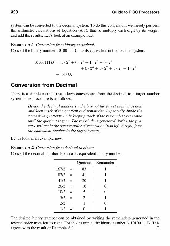
328 Guide to RISC Processors
system can be converted to the decimal system. To do this conversion, we merely performthe arithmetic calculations of Equation (A.1); that is, multiply each digit by its weight,and add the results. Let’s look at an example next.
Example A.1 Conversion from binary to decimal.Convert the binary number 10100111B into its equivalent in the decimal system.
10100111B = 1 · 27 + 0 · 26 + 1 · 25 + 0 · 24
+ 0 · 23 + 1 · 22 + 1 · 21 + 1 · 20
= 167D.
Conversion from DecimalThere is a simple method that allows conversions from the decimal to a target numbersystem. The procedure is as follows.
Divide the decimal number by the base of the target number systemand keep track of the quotient and remainder. Repeatedly divide thesuccessive quotients while keeping track of the remainders generateduntil the quotient is zero. The remainders generated during the pro-cess, written in the reverse order of generation from left to right, formthe equivalent number in the target system.
Let us look at an example now.
Example A.2 Conversion from decimal to binary.Convert the decimal number 167 into its equivalent binary number.
Quotient Remainder
167/2 = 83 183/2 = 41 141/2 = 20 120/2 = 10 010/2 = 5 05/2 = 2 12/2 = 1 01/2 = 0 1
The desired binary number can be obtained by writing the remainders generated in thereverse order from left to right. For this example, the binary number is 10100111B. Thisagrees with the result of Example A.1. �
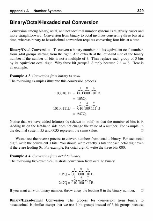
Appendix A Number Systems 329
Binary/Octal/Hexadecimal Conversion
Conversion among binary, octal, and hexadecimal number systems is relatively easier andmore straightforward. Conversion from binary to octal involves converting three bits at atime, whereas binary to hexadecimal conversion requires converting four bits at a time.
Binary/Octal Conversion To convert a binary number into its equivalent octal number,form 3-bit groups starting from the right. Add extra 0s at the left-hand side of the binarynumber if the number of bits is not a multiple of 3. Then replace each group of 3 bitsby its equivalent octal digit. Why three bit groups? Simply because 2 3 = 8. Here isan example.
Example A.3 Conversion from binary to octal.The following examples illustrate this conversion process.
1000101B =1︷︸︸︷
0010︷︸︸︷
0005︷︸︸︷
101 B= 105Q .
10100111B =2︷︸︸︷
0104︷︸︸︷
1007︷︸︸︷
111 B= 247Q .
Notice that we have added leftmost 0s (shown in bold) so that the number of bits is 9.Adding 0s on the left-hand side does not change the value of a number. For example, inthe decimal system, 35 and 0035 represent the same value. �
We can use the reverse process to convert numbers from octal to binary. For each octaldigit, write the equivalent 3 bits. You should write exactly 3 bits for each octal digit evenif there are leading 0s. For example, for octal digit 0, write the three bits 000.
Example A.4 Conversion from octal to binary.The following two examples illustrate conversion from octal to binary.
105Q =
1︷︸︸︷001
0︷︸︸︷000
5︷︸︸︷101B,
247Q =
2︷︸︸︷010
4︷︸︸︷100
7︷︸︸︷111B.
If you want an 8-bit binary number, throw away the leading 0 in the binary number. �
Binary/Hexadecimal Conversion The process for conversion from binary tohexadecimal is similar except that we use 4-bit groups instead of 3-bit groups because
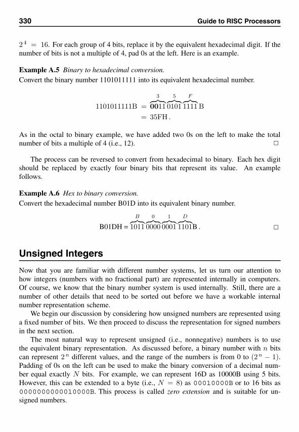
330 Guide to RISC Processors
2 4 = 16. For each group of 4 bits, replace it by the equivalent hexadecimal digit. If thenumber of bits is not a multiple of 4, pad 0s at the left. Here is an example.
Example A.5 Binary to hexadecimal conversion.Convert the binary number 1101011111 into its equivalent hexadecimal number.
1101011111B =3︷ ︸︸ ︷
00115︷ ︸︸ ︷
0101F︷ ︸︸ ︷
1111 B= 35FH .
As in the octal to binary example, we have added two 0s on the left to make the totalnumber of bits a multiple of 4 (i.e., 12). �
The process can be reversed to convert from hexadecimal to binary. Each hex digitshould be replaced by exactly four binary bits that represent its value. An examplefollows.
Example A.6 Hex to binary conversion.Convert the hexadecimal number B01D into its equivalent binary number.
B01DH =
B︷ ︸︸ ︷1011
0︷ ︸︸ ︷0000
1︷ ︸︸ ︷0001
D︷ ︸︸ ︷1101B . �
Unsigned Integers
Now that you are familiar with different number systems, let us turn our attention tohow integers (numbers with no fractional part) are represented internally in computers.Of course, we know that the binary number system is used internally. Still, there are anumber of other details that need to be sorted out before we have a workable internalnumber representation scheme.
We begin our discussion by considering how unsigned numbers are represented usinga fixed number of bits. We then proceed to discuss the representation for signed numbersin the next section.
The most natural way to represent unsigned (i.e., nonnegative) numbers is to usethe equivalent binary representation. As discussed before, a binary number with n bitscan represent 2n different values, and the range of the numbers is from 0 to (2n − 1).Padding of 0s on the left can be used to make the binary conversion of a decimal num-ber equal exactly N bits. For example, we can represent 16D as 10000B using 5 bits.However, this can be extended to a byte (i.e., N = 8) as 00010000B or to 16 bits as0000000000010000B. This process is called zero extension and is suitable for un-signed numbers.
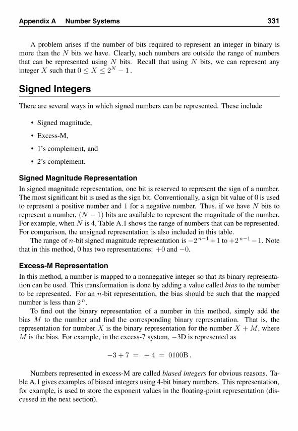
Appendix A Number Systems 331
A problem arises if the number of bits required to represent an integer in binary ismore than the N bits we have. Clearly, such numbers are outside the range of numbersthat can be represented using N bits. Recall that using N bits, we can represent anyinteger X such that 0 ≤ X ≤ 2N − 1 .
Signed Integers
There are several ways in which signed numbers can be represented. These include
• Signed magnitude,
• Excess-M,
• 1’s complement, and
• 2’s complement.
Signed Magnitude RepresentationIn signed magnitude representation, one bit is reserved to represent the sign of a number.The most significant bit is used as the sign bit. Conventionally, a sign bit value of 0 is usedto represent a positive number and 1 for a negative number. Thus, if we have N bits torepresent a number, (N − 1) bits are available to represent the magnitude of the number.For example, when N is 4, Table A.1 shows the range of numbers that can be represented.For comparison, the unsigned representation is also included in this table.
The range of n-bit signed magnitude representation is −2n−1 +1 to +2n−1−1. Notethat in this method, 0 has two representations: +0 and −0.
Excess-M RepresentationIn this method, a number is mapped to a nonnegative integer so that its binary representa-tion can be used. This transformation is done by adding a value called bias to the numberto be represented. For an n-bit representation, the bias should be such that the mappednumber is less than 2n.
To find out the binary representation of a number in this method, simply add thebias M to the number and find the corresponding binary representation. That is, therepresentation for number X is the binary representation for the number X + M , whereM is the bias. For example, in the excess-7 system, −3D is represented as
−3 + 7 = + 4 = 0100B .
Numbers represented in excess-M are called biased integers for obvious reasons. Ta-ble A.1 gives examples of biased integers using 4-bit binary numbers. This representation,for example, is used to store the exponent values in the floating-point representation (dis-cussed in the next section).
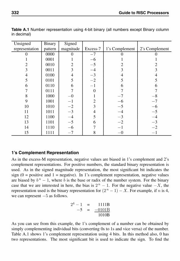
332 Guide to RISC Processors
Table A.1 Number representation using 4-bit binary (all numbers except Binary columnin decimal)
Unsigned Binary Signedrepresentation pattern magnitude Excess-7 1’s Complement 2’s Complement
0 0000 0 −7 0 01 0001 1 −6 1 12 0010 2 −5 2 23 0011 3 −4 3 34 0100 4 −3 4 45 0101 5 −2 5 56 0110 6 −1 6 67 0111 7 0 7 78 1000 −0 1 −7 −89 1001 −1 2 −6 −7
10 1010 −2 3 −5 −611 1011 −3 4 −4 −512 1100 −4 5 −3 −413 1101 −5 6 −2 −314 1110 −6 7 −1 −215 1111 −7 8 −0 −1
1’s Complement RepresentationAs in the excess-M representation, negative values are biased in 1’s complement and 2’scomplement representations. For positive numbers, the standard binary representation isused. As in the signed magnitude representation, the most significant bit indicates thesign (0 = positive and 1 = negative). In 1’s complement representation, negative valuesare biased by bn − 1, where b is the base or radix of the number system. For the binarycase that we are interested in here, the bias is 2n − 1. For the negative value −X, therepresentation used is the binary representation for (2n − 1) −X. For example, if n is 4,we can represent −5 as follows.
24 − 1 = 1111B−5 = −0101B
1010B
As you can see from this example, the 1’s complement of a number can be obtained bysimply complementing individual bits (converting 0s to 1s and vice versa) of the number.Table A.1 shows 1’s complement representation using 4 bits. In this method also, 0 hastwo representations. The most significant bit is used to indicate the sign. To find the
Appendix A Number Systems 333
magnitude of a negative number in this representation, apply the process used to obtainthe 1’s complement (i.e., complement individual bits) again.
Representation of signed numbers in 1’s complement representation allows the use ofsimpler circuits for performing addition and subtraction than the other two representationswe have seen so far (signed magnitude and excess-M). Some older computer systemsused this representation for integers. An irritant with this representation is that 0 has tworepresentations. Furthermore, the carry bit generated out of the sign bit will have to beadded to the result. The 2’s complement representation avoids these pitfalls. As a result,2’s complement representation is the choice of current computer systems.
2’s Complement RepresentationIn 2’s complement representation, positive numbers are represented the same way as in thesigned magnitude and 1’s complement representations. The negative numbers are biasedby 2n, where n is the number of bits used for number representation. Thus, the negativevalue −A is represented by (2n − A) using n bits. Because the bias value is one morethan that in the 1’s complement representation, we have to add 1 after complementing toobtain the 2’s complement representation of a negative number. We can, however, discardany carry generated out of the sign bit. For example, −5 can be represented as follows.
5D = 0101B−→ complement −→1010Badd 1 1B
1011B
Therefore, 1011B represents −5D in 2’s complement representation. Table A.1 showsthe 2’s complement representation of numbers using 4 bits. Notice that there is onlyone representation for 0. The range of an n-bit 2’s complement integer is −2 n−1 to+2n−1 − 1. For example, using 8 bits, the range is −128 to +127.
To find the magnitude of a negative number in the 2’s complement representation, asin the 1’s complement representation, simply reverse the sign of the number. That is, usethe same conversion process: complement and add 1 and discard any carry generated outof the leftmost bit.
Sign ExtensionHow do we extend a signed number? For example, we have shown that −5 can be rep-resented in the 2’s complement representation as 1011B. Suppose we want to save thisas a byte. How do extend these four bits into eight bits? We have seen in Example A.5that, for unsigned integers, we add zeros on the left to extend the number. However, wecannot use this technique for signed numbers because the most significant bit representsthe sign. To extend a signed number, we have to copy the sign bit. In our example, −5 isrepresented using eight bits as
−5D =
sign bit︷ ︸︸ ︷1111 1011.
334 Guide to RISC Processors
We have copied the sign bit to extend the four-bit value to eight bits. Similarly, we canexpress −5 using 16 bits by extending it as follows.
−5D =
sign bit︷ ︸︸ ︷111111111111 1011.
This process is referred to as sign extension.
Floating-Point Representation
Using the decimal system for a moment, we can write very small and very large numbersin scientific notation as follows.
1.2345 × 1045,
9.876543 × 10−37.
Expressing such numbers using the positional number notation is difficult to write andunderstand, error prone, and requires more space. In a similar fashion, binary numberscan be written in scientific notation. For example,
+1101.101 × 2+11001 = 13.625 × 225
= 4.57179 × 10⁸.
As indicated, numbers expressed in this notation have two parts: a mantissa (or signifi-cand) and an exponent. There can be a sign (+ or −) associated with each part.
Numbers expressed in this notation can be written in several equivalent ways, asshown below:
1.2345 × 1045,
123.45 × 1043,
0.00012345 × 1049.
This causes implementation problems in performing arithmetic operations, comparisons,and the like. This problem can be avoided by introducing a standard form called thenormal form. Reverting to the binary case, a normalized binary form has the format
±1.X1X2 · · ·XM−1XM × 2±YN−1YN−2···Y1Y0 ,
where Xi and Yj represent a bit, 1 ≤ i ≤ M , and 0 ≤ j < N . The normalized form of
+1101.101 × 2+11010
is+1.101101 × 2+11101.
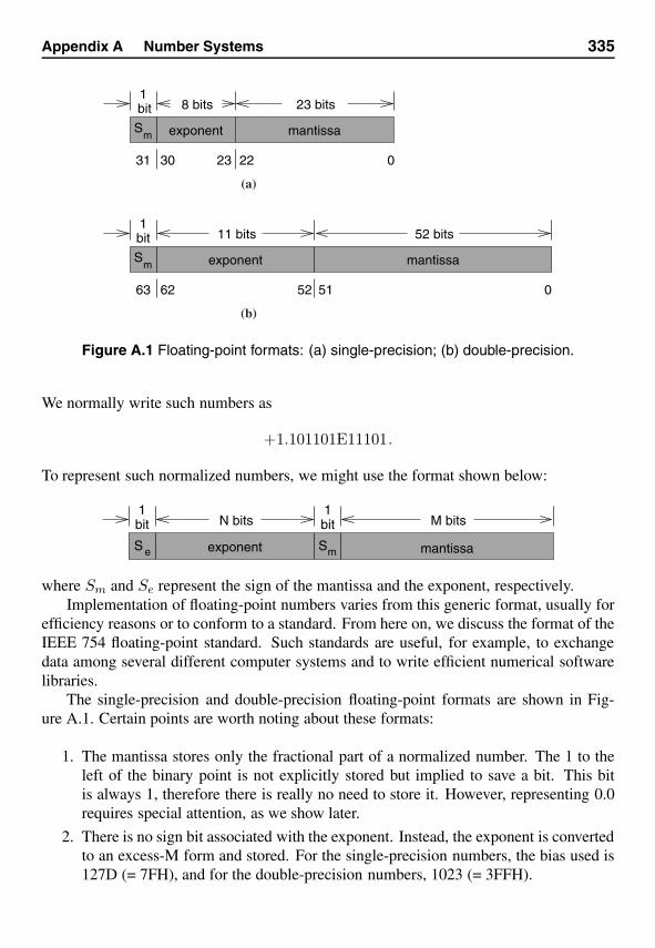
Appendix A Number Systems 335
(b)
(a)
exponent mantissamS
23 bits8 bits
022233031
bit1
bit1
exponent
52 bits
mantissa
11 bits
mS
051526263
Figure A.1 Floating-point formats: (a) single-precision; (b) double-precision.
We normally write such numbers as
+1.101101E11101.
To represent such normalized numbers, we might use the format shown below:
exponent mantissa
N bits M bits
SmeS
1bit bit
1
where Sm and Se represent the sign of the mantissa and the exponent, respectively.Implementation of floating-point numbers varies from this generic format, usually for
efficiency reasons or to conform to a standard. From here on, we discuss the format of theIEEE 754 floating-point standard. Such standards are useful, for example, to exchangedata among several different computer systems and to write efficient numerical softwarelibraries.
The single-precision and double-precision floating-point formats are shown in Fig-ure A.1. Certain points are worth noting about these formats:
1. The mantissa stores only the fractional part of a normalized number. The 1 to theleft of the binary point is not explicitly stored but implied to save a bit. This bitis always 1, therefore there is really no need to store it. However, representing 0.0requires special attention, as we show later.
2. There is no sign bit associated with the exponent. Instead, the exponent is convertedto an excess-M form and stored. For the single-precision numbers, the bias used is127D (= 7FH), and for the double-precision numbers, 1023 (= 3FFH).
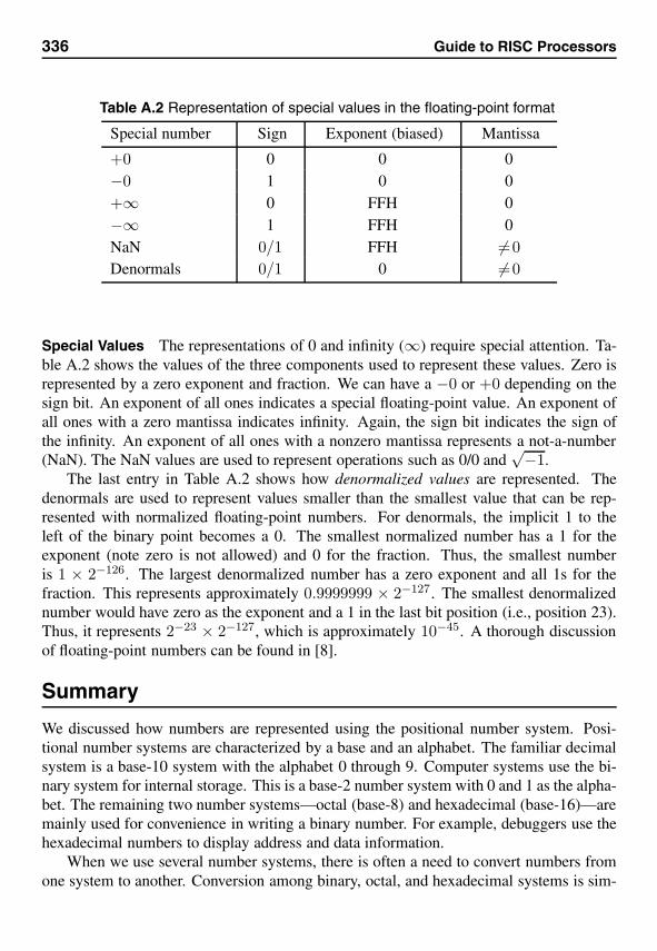
336 Guide to RISC Processors
Table A.2 Representation of special values in the floating-point format
Special number Sign Exponent (biased) Mantissa
+0 0 0 0−0 1 0 0+∞ 0 FFH 0−∞ 1 FFH 0NaN 0/1 FFH �=0Denormals 0/1 0 �=0
Special Values The representations of 0 and infinity (∞) require special attention. Ta-ble A.2 shows the values of the three components used to represent these values. Zero isrepresented by a zero exponent and fraction. We can have a −0 or +0 depending on thesign bit. An exponent of all ones indicates a special floating-point value. An exponent ofall ones with a zero mantissa indicates infinity. Again, the sign bit indicates the sign ofthe infinity. An exponent of all ones with a nonzero mantissa represents a not-a-number(NaN). The NaN values are used to represent operations such as 0/0 and
√−1.The last entry in Table A.2 shows how denormalized values are represented. The
denormals are used to represent values smaller than the smallest value that can be rep-resented with normalized floating-point numbers. For denormals, the implicit 1 to theleft of the binary point becomes a 0. The smallest normalized number has a 1 for theexponent (note zero is not allowed) and 0 for the fraction. Thus, the smallest numberis 1 × 2−126. The largest denormalized number has a zero exponent and all 1s for thefraction. This represents approximately 0.9999999 × 2−127. The smallest denormalizednumber would have zero as the exponent and a 1 in the last bit position (i.e., position 23).Thus, it represents 2−23 × 2−127, which is approximately 10−45. A thorough discussionof floating-point numbers can be found in [8].
Summary
We discussed how numbers are represented using the positional number system. Posi-tional number systems are characterized by a base and an alphabet. The familiar decimalsystem is a base-10 system with the alphabet 0 through 9. Computer systems use the bi-nary system for internal storage. This is a base-2 number system with 0 and 1 as the alpha-bet. The remaining two number systems—octal (base-8) and hexadecimal (base-16)—aremainly used for convenience in writing a binary number. For example, debuggers use thehexadecimal numbers to display address and data information.
When we use several number systems, there is often a need to convert numbers fromone system to another. Conversion among binary, octal, and hexadecimal systems is sim-
Appendix A Number Systems 337
ple and straightforward. We also discussed how numbers are converted from decimal tobinary and vice versa.
The remainder of the chapter was devoted to internal representation of numbers. Rep-resentation of unsigned integers is straightforward and uses binary representation. Thereare, however, several ways of representing signed integers. We discussed four methods torepresent signed integers. Of these four methods, current computer systems use the 2’scomplement representation.
Floating-point representation on most computers follows the IEEE 754 standard. Thereare three components of a floating-point number: mantissa, exponent, and the sign of themantissa. There is no sign associated with the exponent. Instead, the exponent is storedas a biased number.
BCharacterRepresentation
This appendix discusses character representation. We identify some desirable propertiesthat a character-encoding scheme should satisfy in order to facilitate efficient characterprocessing. Our focus is on the ASCII encoding; we don’t discuss other character setssuch as UCS and Unicode. The ASCII encoding, which is used by most computers,satisfies the requirements of an efficient character code.
Character Representation
As computers have the capability to store and understand the alphabet 0 and 1, charactersshould be assigned a sequence over this alphabet; that is, characters should be encodedusing this alphabet. For efficient processing of characters, several guidelines have beendeveloped. Some of these are mentioned here.
1. Assigning a contiguous sequence of numbers (if treated as unsigned binary num-bers) to letters in alphabetical order is desired. Upper- and lowercase letters (Athrough Z and a through z) can be treated separately, but a contiguous sequenceshould be assigned to each case. This facilitates efficient character processing suchas case conversion, identifying lowercase letters, and so on.
2. In a similar fashion, digits should be assigned a contiguous sequence in numeri-cal order. This would be useful in numeric-to-character and character-to-numericconversions.
3. A space character should precede all letters and digits.
These guidelines allow for efficient character processing including sorting by namesor character strings. For example, to test if a given character code corresponds to a lower-case letter, all we have to do is to see if the code of the character is between that of a and
339
340 Guide to RISC Processors
z. These guidelines also aid in applications requiring sorting, for instance, sorting a classlist by last name.
Because computers are rarely used in isolation, exchange of information is an impor-tant concern. This leads to the necessity of having some standard way of representingcharacters. Most computers use the American Standard Code for Information Interchange(ASCII) for character representation. The standard ASCII uses 7 bits to encode a charac-ter. Thus, 2 7 = 128 different characters can be represented. This number is sufficientlylarge to represent uppercase and lowercase characters, digits, special characters such as!,ˆ, and control characters such as CR (carriage return), LF (linefeed), and the like.
We store the bits in units of a power of 2, therefore we end up storing 8 bits for eachcharacter, even though ASCII requires only 7 bits. The eighth bit is put to use for twopurposes.
1. To parity encode for error detection: The eighth bit can be used to represent theparity bit. This bit is made 0 or 1 such that the total number of 1s in a byte is even(for even parity) or odd (for odd parity). This can be used to detect simple errors indata transmission.
2. To represent an additional 128 characters: By using all eight bits we can representa total of 2 8 = 256 different characters. This is referred to as the extended ASCII.These additional codes are used for special graphics symbols, Greek letters, and soon.
The standard ASCII character code is presented in the following two tables. Youwill notice from these tables that ASCII encoding satisfies the three guidelines mentionedearlier. For instance, successive bit patterns are assigned to uppercase letters, lowercaseletters, and digits. This assignment leads to some good properties. For example, the differ-ence between the uppercase and lowercase characters is constant. That is, the differencebetween the character codes of a and A is the same as that between n and N, which is 32.This characteristic can be exploited for efficient case conversion.
Another interesting feature of ASCII is that the character codes are assigned to the 10digits such that the lower-order four bits represent the binary equivalent of the correspond-ing digit. For example, digit 5 is encoded as 0110101. If you take the rightmost four bits(0101), they represent 5 in binary. This feature, again, helps in writing an efficient codefor character-to-numeric conversion. Such a conversion, for example, is required whenyou type a number as a sequence of digit characters.
ASCII Character SetThe following tables give the standard ASCII character set. We divide the character setinto control and printable characters. The control character codes are given next and theprintable ASCII characters follow.

Guide to RISC Processors 341
Control Codes
Hex Decimal Character Meaning00 0 NUL NULL01 1 SOH Start of heading02 2 STX Start of text03 3 ETX End of text04 4 EOT End of transmission05 5 ENQ Enquiry06 6 ACK Acknowledgment07 7 BEL Bell08 8 BS Backspace09 9 HT Horizontal tab0A 10 LF Line feed0B 11 VT Vertical tab0C 12 FF Form feed0D 13 CR Carriage return0E 14 SO Shift out0F 15 SI Shift in10 16 DLE Data link escape11 17 DC1 Device control 112 18 DC2 Device control 213 19 DC3 Device control 314 20 DC4 Device control 415 21 NAK Negative acknowledgment16 22 SYN Synchronous idle17 23 ETB End of transmission block18 24 CAN Cancel19 25 EM End of medium1A 26 SUB Substitute1B 27 ESC Escape1C 28 FS File separator1D 29 GS Group separator1E 30 RS Record separator1F 31 US Unit separator7F 127 DEL Delete
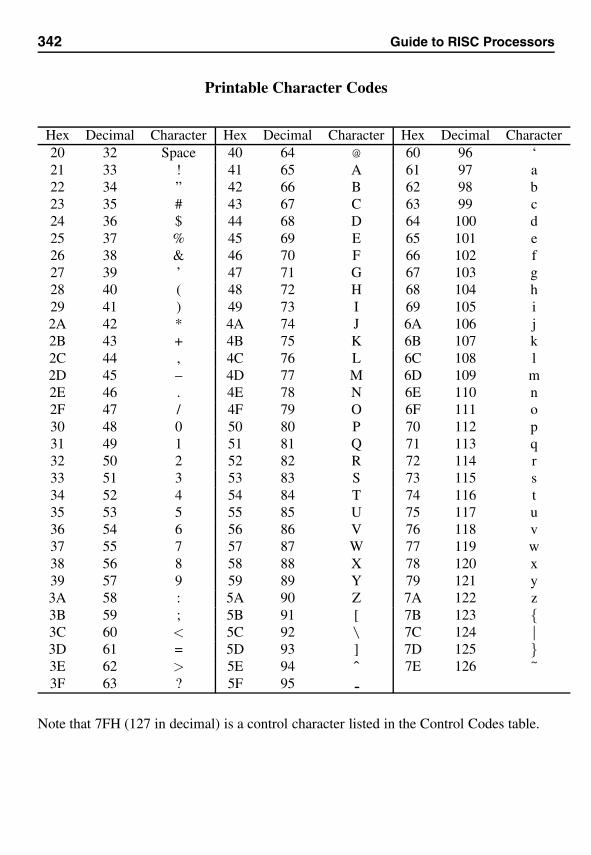
342 Guide to RISC Processors
Printable Character Codes
Hex Decimal Character Hex Decimal Character Hex Decimal Character20 32 Space 40 64 @ 60 96 ‘21 33 ! 41 65 A 61 97 a22 34 ” 42 66 B 62 98 b23 35 # 43 67 C 63 99 c24 36 $ 44 68 D 64 100 d25 37 % 45 69 E 65 101 e26 38 & 46 70 F 66 102 f27 39 ’ 47 71 G 67 103 g28 40 ( 48 72 H 68 104 h29 41 ) 49 73 I 69 105 i2A 42 * 4A 74 J 6A 106 j2B 43 + 4B 75 K 6B 107 k2C 44 , 4C 76 L 6C 108 l2D 45 – 4D 77 M 6D 109 m2E 46 . 4E 78 N 6E 110 n2F 47 / 4F 79 O 6F 111 o30 48 0 50 80 P 70 112 p31 49 1 51 81 Q 71 113 q32 50 2 52 82 R 72 114 r33 51 3 53 83 S 73 115 s34 52 4 54 84 T 74 116 t35 53 5 55 85 U 75 117 u36 54 6 56 86 V 76 118 v37 55 7 57 87 W 77 119 w38 56 8 58 88 X 78 120 x39 57 9 59 89 Y 79 121 y3A 58 : 5A 90 Z 7A 122 z3B 59 ; 5B 91 [ 7B 123 {3C 60 < 5C 92 \ 7C 124 |3D 61 = 5D 93 ] 7D 125 }3E 62 > 5E 94 ˆ 7E 126 ˜3F 63 ? 5F 95
Note that 7FH (127 in decimal) is a control character listed in the Control Codes table.
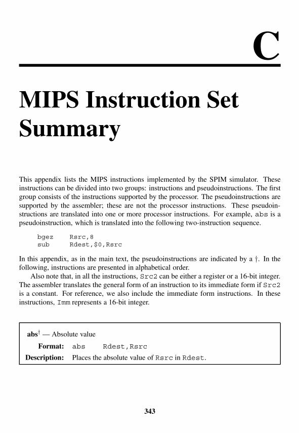
CMIPS Instruction SetSummary
This appendix lists the MIPS instructions implemented by the SPIM simulator. Theseinstructions can be divided into two groups: instructions and pseudoinstructions. The firstgroup consists of the instructions supported by the processor. The pseudoinstructions aresupported by the assembler; these are not the processor instructions. These pseudoin-structions are translated into one or more processor instructions. For example, abs is apseudoinstruction, which is translated into the following two-instruction sequence.
bgez Rsrc,8sub Rdest,$0,Rsrc
In this appendix, as in the main text, the pseudoinstructions are indicated by a †. In thefollowing, instructions are presented in alphabetical order.
Also note that, in all the instructions, Src2 can be either a register or a 16-bit integer.The assembler translates the general form of an instruction to its immediate form if Src2is a constant. For reference, we also include the immediate form instructions. In theseinstructions, Imm represents a 16-bit integer.
abs† — Absolute value
Format: abs Rdest,Rsrc
Description: Places the absolute value of Rsrc in Rdest.
343
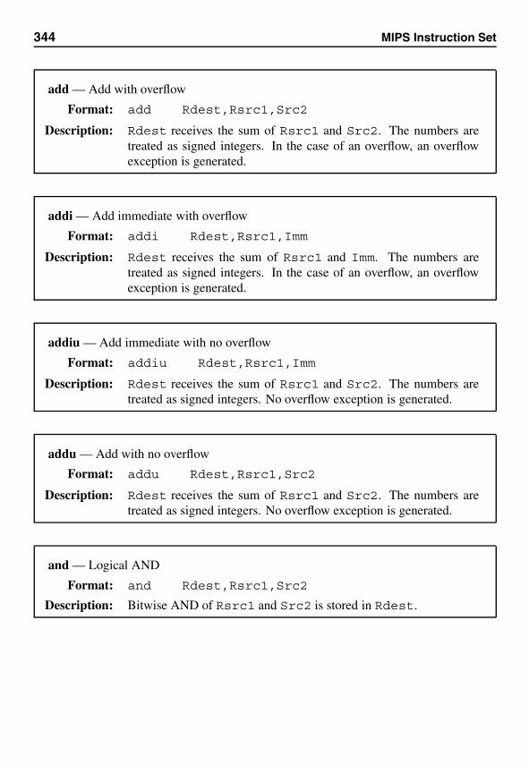
344 MIPS Instruction Set
add — Add with overflow
Format: add Rdest,Rsrc1,Src2
Description: Rdest receives the sum of Rsrc1 and Src2. The numbers aretreated as signed integers. In the case of an overflow, an overflowexception is generated.
addi — Add immediate with overflow
Format: addi Rdest,Rsrc1,Imm
Description: Rdest receives the sum of Rsrc1 and Imm. The numbers aretreated as signed integers. In the case of an overflow, an overflowexception is generated.
addiu — Add immediate with no overflow
Format: addiu Rdest,Rsrc1,Imm
Description: Rdest receives the sum of Rsrc1 and Src2. The numbers aretreated as signed integers. No overflow exception is generated.
addu — Add with no overflow
Format: addu Rdest,Rsrc1,Src2
Description: Rdest receives the sum of Rsrc1 and Src2. The numbers aretreated as signed integers. No overflow exception is generated.
and — Logical AND
Format: and Rdest,Rsrc1,Src2
Description: Bitwise AND of Rsrc1 and Src2 is stored in Rdest.
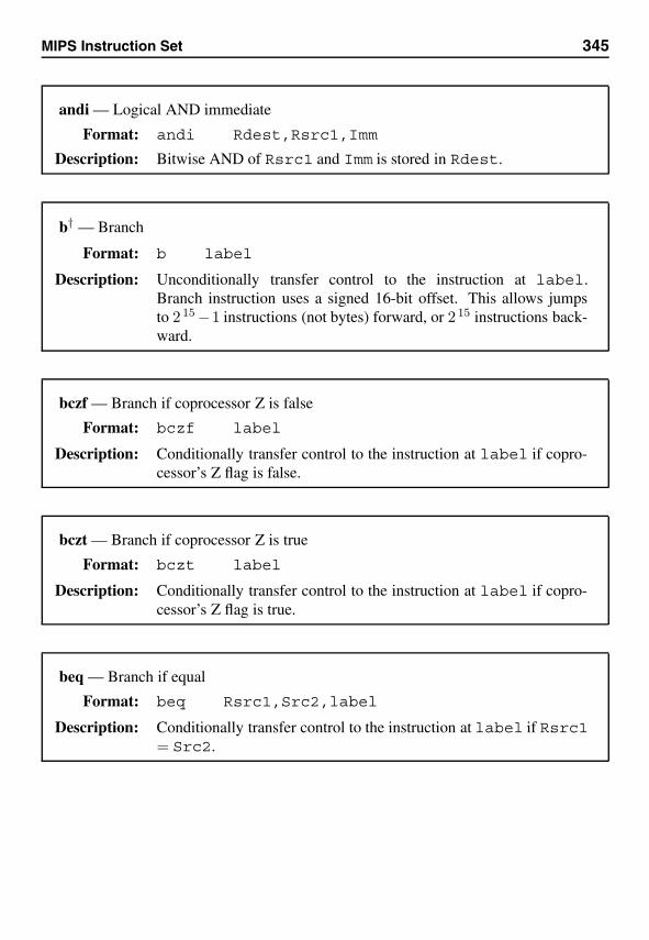
MIPS Instruction Set 345
andi — Logical AND immediate
Format: andi Rdest,Rsrc1,Imm
Description: Bitwise AND of Rsrc1 and Imm is stored in Rdest.
b† — Branch
Format: b label
Description: Unconditionally transfer control to the instruction at label.Branch instruction uses a signed 16-bit offset. This allows jumpsto 2 15−1 instructions (not bytes) forward, or 2 15 instructions back-ward.
bczf — Branch if coprocessor Z is false
Format: bczf label
Description: Conditionally transfer control to the instruction at label if copro-cessor’s Z flag is false.
bczt — Branch if coprocessor Z is true
Format: bczt label
Description: Conditionally transfer control to the instruction at label if copro-cessor’s Z flag is true.
beq — Branch if equal
Format: beq Rsrc1,Src2,label
Description: Conditionally transfer control to the instruction at label if Rsrc1= Src2.
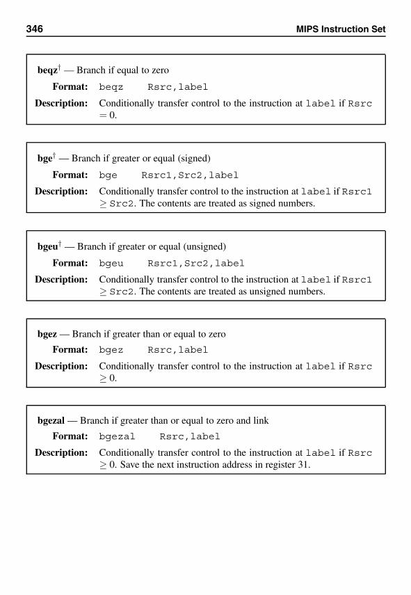
346 MIPS Instruction Set
beqz† — Branch if equal to zero
Format: beqz Rsrc,label
Description: Conditionally transfer control to the instruction at label if Rsrc= 0.
bge† — Branch if greater or equal (signed)
Format: bge Rsrc1,Src2,label
Description: Conditionally transfer control to the instruction at label if Rsrc1≥ Src2. The contents are treated as signed numbers.
bgeu† — Branch if greater or equal (unsigned)
Format: bgeu Rsrc1,Src2,label
Description: Conditionally transfer control to the instruction at label if Rsrc1≥ Src2. The contents are treated as unsigned numbers.
bgez — Branch if greater than or equal to zero
Format: bgez Rsrc,label
Description: Conditionally transfer control to the instruction at label if Rsrc≥ 0.
bgezal — Branch if greater than or equal to zero and link
Format: bgezal Rsrc,label
Description: Conditionally transfer control to the instruction at label if Rsrc≥ 0. Save the next instruction address in register 31.
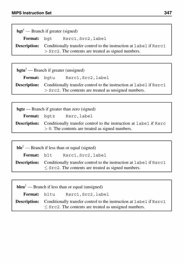
MIPS Instruction Set 347
bgt† — Branch if greater (signed)
Format: bgt Rsrc1,Src2,label
Description: Conditionally transfer control to the instruction at label if Rsrc1> Src2. The contents are treated as signed numbers.
bgtu† — Branch if greater (unsigned)
Format: bgtu Rsrc1,Src2,label
Description: Conditionally transfer control to the instruction at label if Rsrc1> Src2. The contents are treated as unsigned numbers.
bgtz — Branch if greater than zero (signed)
Format: bgtz Rsrc,label
Description: Conditionally transfer control to the instruction at label if Rsrc> 0. The contents are treated as signed numbers.
ble† — Branch if less than or equal (signed)
Format: blt Rsrc1,Src2,label
Description: Conditionally transfer control to the instruction at label if Rsrc1≤ Src2. The contents are treated as signed numbers.
bleu† — Branch if less than or equal (unsigned)
Format: bltu Rsrc1,Src2,label
Description: Conditionally transfer control to the instruction at label if Rsrc1≤ Src2. The contents are treated as unsigned numbers.
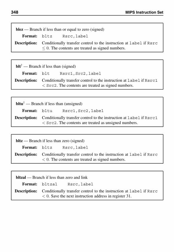
348 MIPS Instruction Set
blez — Branch if less than or equal to zero (signed)
Format: bltz Rsrc,label
Description: Conditionally transfer control to the instruction at label if Rsrc≤ 0. The contents are treated as signed numbers.
blt† — Branch if less than (signed)
Format: blt Rsrc1,Src2,label
Description: Conditionally transfer control to the instruction at label if Rsrc1< Src2. The contents are treated as signed numbers.
bltu† — Branch if less than (unsigned)
Format: bltu Rsrc1,Src2,label
Description: Conditionally transfer control to the instruction at label if Rsrc1< Src2. The contents are treated as unsigned numbers.
bltz — Branch if less than zero (signed)
Format: bltz Rsrc,label
Description: Conditionally transfer control to the instruction at label if Rsrc< 0. The contents are treated as signed numbers.
bltzal — Branch if less than zero and link
Format: bltzal Rsrc,label
Description: Conditionally transfer control to the instruction at label if Rsrc< 0. Save the next instruction address in register 31.
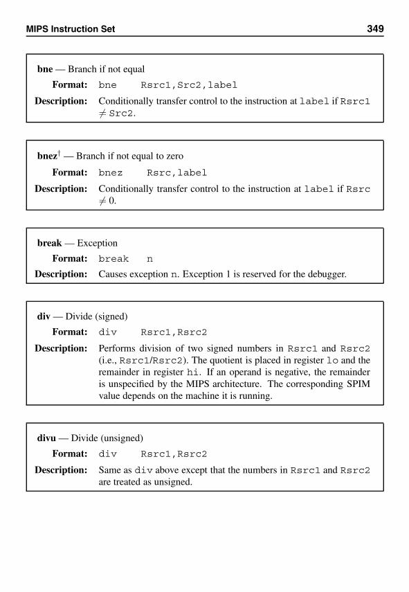
MIPS Instruction Set 349
bne — Branch if not equal
Format: bne Rsrc1,Src2,label
Description: Conditionally transfer control to the instruction at label if Rsrc1�= Src2.
bnez† — Branch if not equal to zero
Format: bnez Rsrc,label
Description: Conditionally transfer control to the instruction at label if Rsrc�= 0.
break — Exception
Format: break n
Description: Causes exception n. Exception 1 is reserved for the debugger.
div — Divide (signed)
Format: div Rsrc1,Rsrc2
Description: Performs division of two signed numbers in Rsrc1 and Rsrc2(i.e., Rsrc1/Rsrc2). The quotient is placed in register lo and theremainder in register hi. If an operand is negative, the remainderis unspecified by the MIPS architecture. The corresponding SPIMvalue depends on the machine it is running.
divu — Divide (unsigned)
Format: div Rsrc1,Rsrc2
Description: Same as div above except that the numbers in Rsrc1 and Rsrc2are treated as unsigned.

350 MIPS Instruction Set
div† — Divide (signed)
Format: div Rdest,Rsrc1,Src2
Description: Performs division of two signed numbers in Rsrc1 and Src2 (i.e.,Rsrc1/Src2). The quotient is placed in register Rdest. Src2can be a register or a 16-bit immediate value.
divu† — Divide (signed)
Format: divu Rdest,Rsrc1,Src2
Description: Same as the last div pseudoinstruction except that the numbers inRsrc1 and Src2 are treated as unsigned.
j — Jump
Format: j label
Description: Unconditionally transfer control to the instruction at label. Jumpinstruction uses a signed 26-bit offset. This allows jumps to 2 25 − 1instructions forward, or 2 25 instructions backward.
jal — Jump and link
Format: jal label
Description: Unconditionally transfer control to the instruction at label. Savethe next instruction address in register 31.
jalr — Jump and link register
Format: jalr Rsrc
Description: Unconditionally transfer control to the instruction whose address isin Rsrc. Save the next instruction address in register 31.
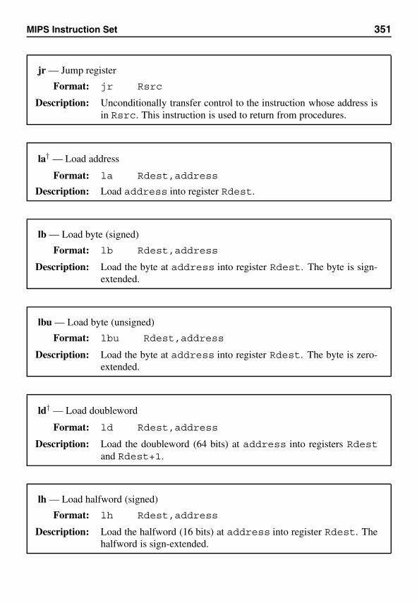
MIPS Instruction Set 351
jr — Jump register
Format: jr Rsrc
Description: Unconditionally transfer control to the instruction whose address isin Rsrc. This instruction is used to return from procedures.
la† — Load address
Format: la Rdest,address
Description: Load address into register Rdest.
lb — Load byte (signed)
Format: lb Rdest,address
Description: Load the byte at address into register Rdest. The byte is sign-extended.
lbu — Load byte (unsigned)
Format: lbu Rdest,address
Description: Load the byte at address into register Rdest. The byte is zero-extended.
ld† — Load doubleword
Format: ld Rdest,address
Description: Load the doubleword (64 bits) at address into registers Rdestand Rdest+1.
lh — Load halfword (signed)
Format: lh Rdest,address
Description: Load the halfword (16 bits) at address into register Rdest. Thehalfword is sign-extended.
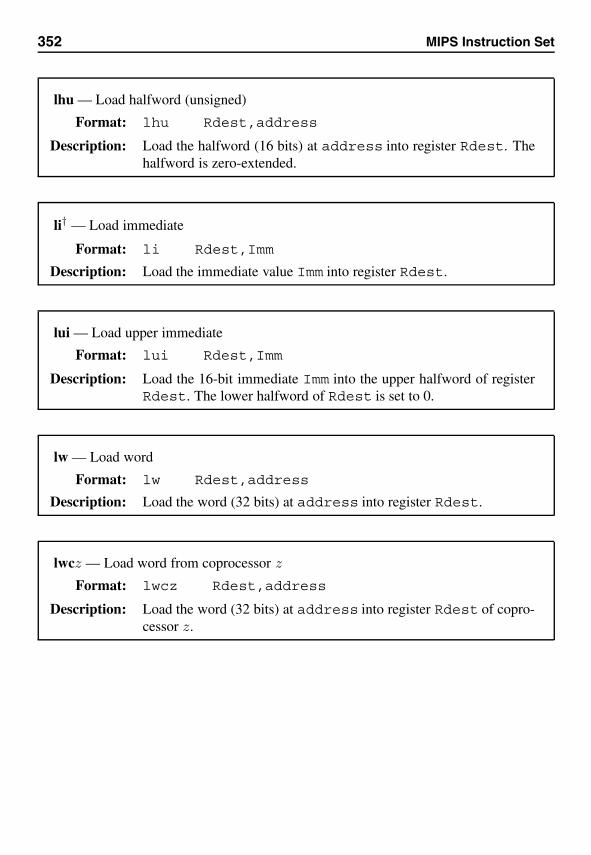
352 MIPS Instruction Set
lhu — Load halfword (unsigned)
Format: lhu Rdest,address
Description: Load the halfword (16 bits) at address into register Rdest. Thehalfword is zero-extended.
li† — Load immediate
Format: li Rdest,Imm
Description: Load the immediate value Imm into register Rdest.
lui — Load upper immediate
Format: lui Rdest,Imm
Description: Load the 16-bit immediate Imm into the upper halfword of registerRdest. The lower halfword of Rdest is set to 0.
lw — Load word
Format: lw Rdest,address
Description: Load the word (32 bits) at address into register Rdest.
lwcz — Load word from coprocessor z
Format: lwcz Rdest,address
Description: Load the word (32 bits) at address into register Rdest of copro-cessor z.
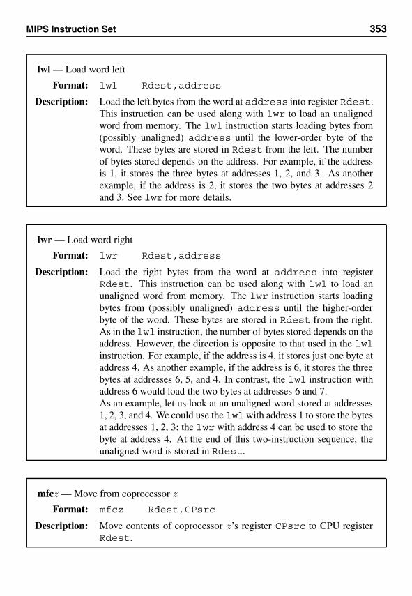
MIPS Instruction Set 353
lwl — Load word left
Format: lwl Rdest,address
Description: Load the left bytes from the word at address into register Rdest.This instruction can be used along with lwr to load an unalignedword from memory. The lwl instruction starts loading bytes from(possibly unaligned) address until the lower-order byte of theword. These bytes are stored in Rdest from the left. The numberof bytes stored depends on the address. For example, if the addressis 1, it stores the three bytes at addresses 1, 2, and 3. As anotherexample, if the address is 2, it stores the two bytes at addresses 2and 3. See lwr for more details.
lwr — Load word right
Format: lwr Rdest,address
Description: Load the right bytes from the word at address into registerRdest. This instruction can be used along with lwl to load anunaligned word from memory. The lwr instruction starts loadingbytes from (possibly unaligned) address until the higher-orderbyte of the word. These bytes are stored in Rdest from the right.As in the lwl instruction, the number of bytes stored depends on theaddress. However, the direction is opposite to that used in the lwlinstruction. For example, if the address is 4, it stores just one byte ataddress 4. As another example, if the address is 6, it stores the threebytes at addresses 6, 5, and 4. In contrast, the lwl instruction withaddress 6 would load the two bytes at addresses 6 and 7.As an example, let us look at an unaligned word stored at addresses1, 2, 3, and 4. We could use the lwlwith address 1 to store the bytesat addresses 1, 2, 3; the lwr with address 4 can be used to store thebyte at address 4. At the end of this two-instruction sequence, theunaligned word is stored in Rdest.
mfcz — Move from coprocessor z
Format: mfcz Rdest,CPsrc
Description: Move contents of coprocessor z’s register CPsrc to CPU registerRdest.

354 MIPS Instruction Set
mfhi — Move from hi
Format: mfhi Rdest
Description: Copy contents of hi register to Rdest.
mflo — Move from lo
Format: mflo Rdest
Description: Copy contents of lo register to Rdest.
move† — Move
Format: move Rdest,Rsrc
Description: Copy contents of Rsrc to Rdest.
mtcz — Move to coprocessor z
Format: mtcz Rsrc,CPdest
Description: Move contents of CPU register Rsrc to coprocessor z’s registerCPdest.
mthi — Move to hi
Format: mfhi Rsrc
Description: Copy contents of Rdest to hi register.
mtlo — Move to lo
Format: mflo Rsrc
Description: Copy contents of Rdest to lo register.
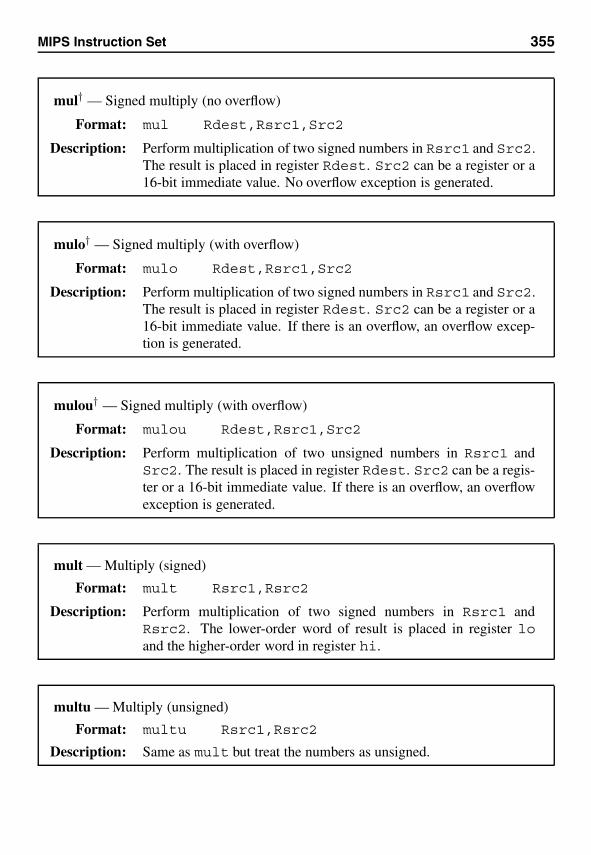
MIPS Instruction Set 355
mul† — Signed multiply (no overflow)
Format: mul Rdest,Rsrc1,Src2
Description: Perform multiplication of two signed numbers in Rsrc1 and Src2.The result is placed in register Rdest. Src2 can be a register or a16-bit immediate value. No overflow exception is generated.
mulo† — Signed multiply (with overflow)
Format: mulo Rdest,Rsrc1,Src2
Description: Perform multiplication of two signed numbers in Rsrc1 and Src2.The result is placed in register Rdest. Src2 can be a register or a16-bit immediate value. If there is an overflow, an overflow excep-tion is generated.
mulou† — Signed multiply (with overflow)
Format: mulou Rdest,Rsrc1,Src2
Description: Perform multiplication of two unsigned numbers in Rsrc1 andSrc2. The result is placed in register Rdest. Src2 can be a regis-ter or a 16-bit immediate value. If there is an overflow, an overflowexception is generated.
mult — Multiply (signed)
Format: mult Rsrc1,Rsrc2
Description: Perform multiplication of two signed numbers in Rsrc1 andRsrc2. The lower-order word of result is placed in register loand the higher-order word in register hi.
multu — Multiply (unsigned)
Format: multu Rsrc1,Rsrc2
Description: Same as mult but treat the numbers as unsigned.
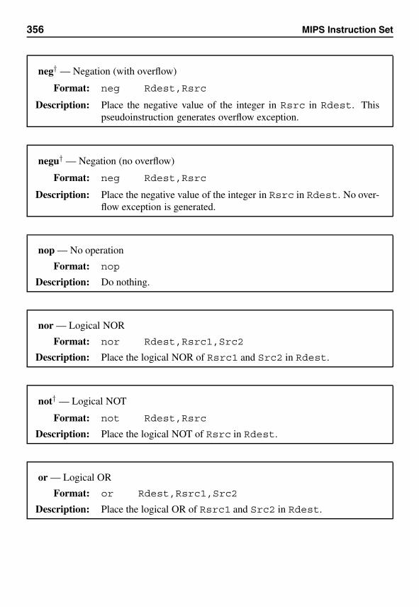
356 MIPS Instruction Set
neg† — Negation (with overflow)
Format: neg Rdest,Rsrc
Description: Place the negative value of the integer in Rsrc in Rdest. Thispseudoinstruction generates overflow exception.
negu† — Negation (no overflow)
Format: neg Rdest,Rsrc
Description: Place the negative value of the integer in Rsrc in Rdest. No over-flow exception is generated.
nop — No operation
Format: nop
Description: Do nothing.
nor — Logical NOR
Format: nor Rdest,Rsrc1,Src2
Description: Place the logical NOR of Rsrc1 and Src2 in Rdest.
not† — Logical NOT
Format: not Rdest,Rsrc
Description: Place the logical NOT of Rsrc in Rdest.
or — Logical OR
Format: or Rdest,Rsrc1,Src2
Description: Place the logical OR of Rsrc1 and Src2 in Rdest.
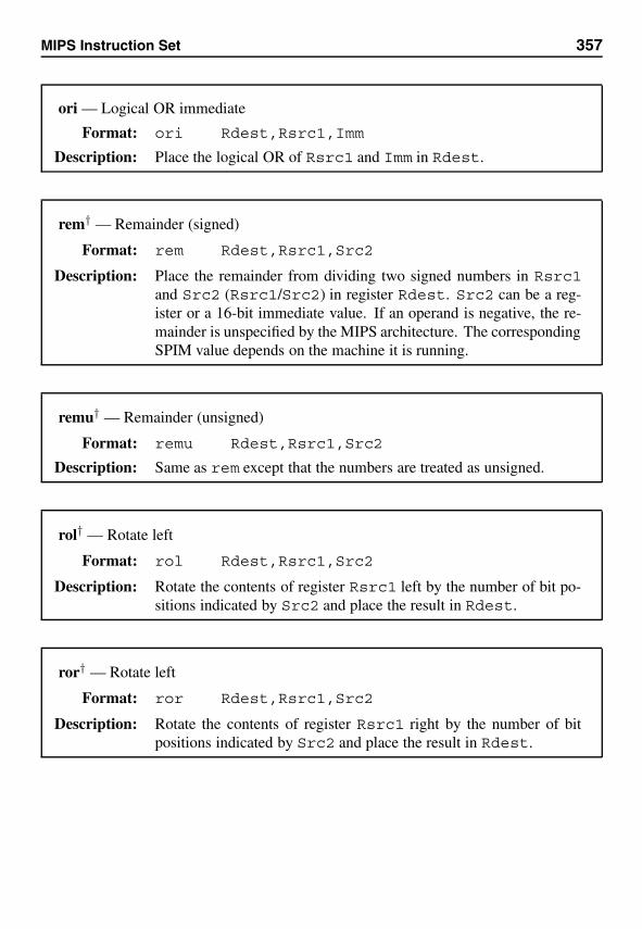
MIPS Instruction Set 357
ori — Logical OR immediate
Format: ori Rdest,Rsrc1,Imm
Description: Place the logical OR of Rsrc1 and Imm in Rdest.
rem† — Remainder (signed)
Format: rem Rdest,Rsrc1,Src2
Description: Place the remainder from dividing two signed numbers in Rsrc1and Src2 (Rsrc1/Src2) in register Rdest. Src2 can be a reg-ister or a 16-bit immediate value. If an operand is negative, the re-mainder is unspecified by the MIPS architecture. The correspondingSPIM value depends on the machine it is running.
remu† — Remainder (unsigned)
Format: remu Rdest,Rsrc1,Src2
Description: Same as rem except that the numbers are treated as unsigned.
rol† — Rotate left
Format: rol Rdest,Rsrc1,Src2
Description: Rotate the contents of register Rsrc1 left by the number of bit po-sitions indicated by Src2 and place the result in Rdest.
ror† — Rotate left
Format: ror Rdest,Rsrc1,Src2
Description: Rotate the contents of register Rsrc1 right by the number of bitpositions indicated by Src2 and place the result in Rdest.
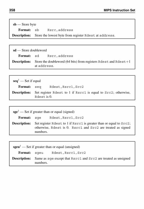
358 MIPS Instruction Set
sb — Store byte
Format: sb Rsrc,address
Description: Store the lowest byte from register Rdest at address.
sd — Store doubleword
Format: sd Rsrc,address
Description: Store the doubleword (64 bits) from registers Rdest and Rdest+1at address.
seq† — Set if equal
Format: seq Rdest,Rsrc1,Src2
Description: Set register Rdest to 1 if Rsrc1 is equal to Src2; otherwise,Rdest is 0.
sge† — Set if greater than or equal (signed)
Format: sge Rdest,Rsrc1,Src2
Description: Set register Rdest to 1 if Rsrc1 is greater than or equal to Src2;otherwise, Rdest is 0. Rsrc1 and Src2 are treated as signednumbers.
sgeu† — Set if greater than or equal (unsigned)
Format: sgeu Rdest,Rsrc1,Src2
Description: Same as sge except that Rsrc1 and Src2 are treated as unsignednumbers.
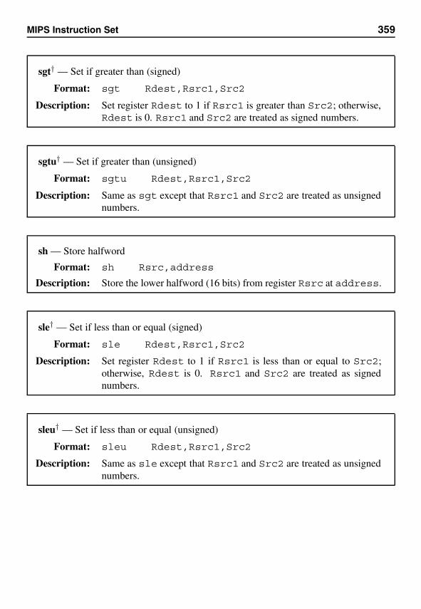
MIPS Instruction Set 359
sgt† — Set if greater than (signed)
Format: sgt Rdest,Rsrc1,Src2
Description: Set register Rdest to 1 if Rsrc1 is greater than Src2; otherwise,Rdest is 0. Rsrc1 and Src2 are treated as signed numbers.
sgtu† — Set if greater than (unsigned)
Format: sgtu Rdest,Rsrc1,Src2
Description: Same as sgt except that Rsrc1 and Src2 are treated as unsignednumbers.
sh — Store halfword
Format: sh Rsrc,address
Description: Store the lower halfword (16 bits) from register Rsrc at address.
sle† — Set if less than or equal (signed)
Format: sle Rdest,Rsrc1,Src2
Description: Set register Rdest to 1 if Rsrc1 is less than or equal to Src2;otherwise, Rdest is 0. Rsrc1 and Src2 are treated as signednumbers.
sleu† — Set if less than or equal (unsigned)
Format: sleu Rdest,Rsrc1,Src2
Description: Same as sle except that Rsrc1 and Src2 are treated as unsignednumbers.
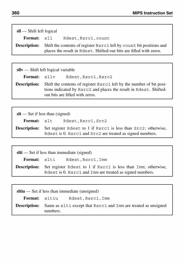
360 MIPS Instruction Set
sll — Shift left logical
Format: sll Rdest,Rsrc1,count
Description: Shift the contents of register Rsrc1 left by count bit positions andplaces the result in Rdest. Shifted-out bits are filled with zeros.
sllv — Shift left logical variable
Format: sllv Rdest,Rsrc1,Rsrc2
Description: Shift the contents of register Rsrc1 left by the number of bit posi-tions indicated by Rsrc2 and places the result in Rdest. Shifted-out bits are filled with zeros.
slt — Set if less than (signed)
Format: slt Rdest,Rsrc1,Src2
Description: Set register Rdest to 1 if Rsrc1 is less than Src2; otherwise,Rdest is 0. Rsrc1 and Src2 are treated as signed numbers.
slti — Set if less than immediate (signed)
Format: slti Rdest,Rsrc1,Imm
Description: Set register Rdest to 1 if Rsrc1 is less than Imm; otherwise,Rdest is 0. Rsrc1 and Imm are treated as signed numbers.
sltiu — Set if less than immediate (unsigned)
Format: sltiu Rdest,Rsrc1,Imm
Description: Same as slti except that Rsrc1 and Imm are treated as unsignednumbers.
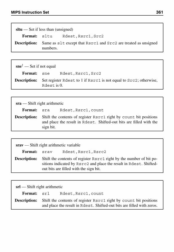
MIPS Instruction Set 361
sltu — Set if less than (unsigned)
Format: sltu Rdest,Rsrc1,Src2
Description: Same as slt except that Rsrc1 and Src2 are treated as unsignednumbers.
sne† — Set if not equal
Format: sne Rdest,Rsrc1,Src2
Description: Set register Rdest to 1 if Rsrc1 is not equal to Src2; otherwise,Rdest is 0.
sra — Shift right arithmetic
Format: sra Rdest,Rsrc1,count
Description: Shift the contents of register Rsrc1 right by count bit positionsand place the result in Rdest. Shifted-out bits are filled with thesign bit.
srav — Shift right arithmetic variable
Format: srav Rdest,Rsrc1,Rsrc2
Description: Shift the contents of register Rsrc1 right by the number of bit po-sitions indicated by Rsrc2 and place the result in Rdest. Shifted-out bits are filled with the sign bit.
srl — Shift right arithmetic
Format: srl Rdest,Rsrc1,count
Description: Shift the contents of register Rsrc1 right by count bit positionsand place the result in Rdest. Shifted-out bits are filled with zeros.
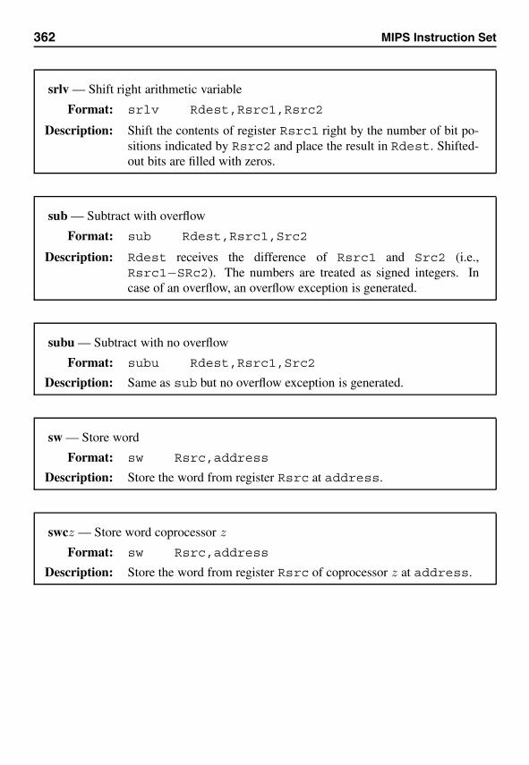
362 MIPS Instruction Set
srlv — Shift right arithmetic variable
Format: srlv Rdest,Rsrc1,Rsrc2
Description: Shift the contents of register Rsrc1 right by the number of bit po-sitions indicated by Rsrc2 and place the result in Rdest. Shifted-out bits are filled with zeros.
sub — Subtract with overflow
Format: sub Rdest,Rsrc1,Src2
Description: Rdest receives the difference of Rsrc1 and Src2 (i.e.,Rsrc1−SRc2). The numbers are treated as signed integers. Incase of an overflow, an overflow exception is generated.
subu — Subtract with no overflow
Format: subu Rdest,Rsrc1,Src2
Description: Same as sub but no overflow exception is generated.
sw — Store word
Format: sw Rsrc,address
Description: Store the word from register Rsrc at address.
swcz — Store word coprocessor z
Format: sw Rsrc,address
Description: Store the word from register Rsrc of coprocessor z at address.
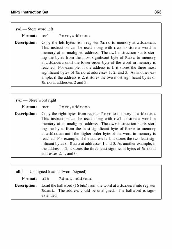
MIPS Instruction Set 363
swl — Store word left
Format: swl Rsrc,address
Description: Copy the left bytes from register Rsrc to memory at address.This instruction can be used along with swr to store a word inmemory at an unaligned address. The swl instruction starts stor-ing the bytes from the most-significant byte of Rsrc to memoryat address until the lower-order byte of the word in memory isreached. For example, if the address is 1, it stores the three mostsignificant bytes of Rsrc at addresses 1, 2, and 3. As another ex-ample, if the address is 2, it stores the two most significant bytes ofRsrc at addresses 2 and 3.
swr — Store word right
Format: swr Rsrc,address
Description: Copy the right bytes from register Rsrc to memory at address.This instruction can be used along with swl to store a word inmemory at an unaligned address. The swr instruction starts stor-ing the bytes from the least-significant byte of Rsrc to memoryat address until the higher-order byte of the word in memory isreached. For example, if the address is 1, it stores the two least sig-nificant bytes of Rsrc at addresses 1 and 0. As another example, ifthe address is 2, it stores the three least significant bytes of Rsrc ataddresses 2, 1, and 0.
ulh† — Unaligned load halfword (signed)
Format: ulh Rdest,address
Description: Load the halfword (16 bits) from the word at address into registerRdest. The address could be unaligned. The halfword is sign-extended.
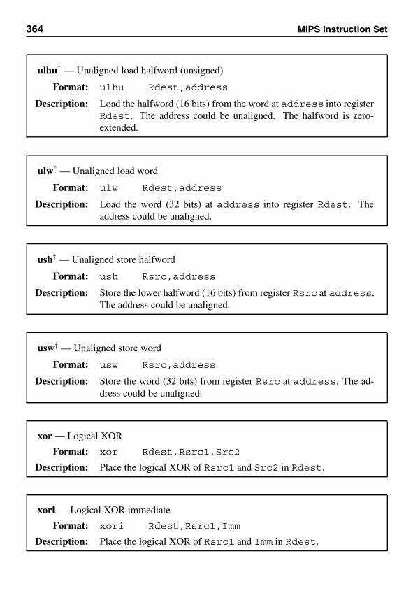
364 MIPS Instruction Set
ulhu† — Unaligned load halfword (unsigned)
Format: ulhu Rdest,address
Description: Load the halfword (16 bits) from the word at address into registerRdest. The address could be unaligned. The halfword is zero-extended.
ulw† — Unaligned load word
Format: ulw Rdest,address
Description: Load the word (32 bits) at address into register Rdest. Theaddress could be unaligned.
ush† — Unaligned store halfword
Format: ush Rsrc,address
Description: Store the lower halfword (16 bits) from register Rsrc at address.The address could be unaligned.
usw† — Unaligned store word
Format: usw Rsrc,address
Description: Store the word (32 bits) from register Rsrc at address. The ad-dress could be unaligned.
xor — Logical XOR
Format: xor Rdest,Rsrc1,Src2
Description: Place the logical XOR of Rsrc1 and Src2 in Rdest.
xori — Logical XOR immediate
Format: xori Rdest,Rsrc1,Imm
Description: Place the logical XOR of Rsrc1 and Imm in Rdest.
DProgramming Exercises
This appendix gives several programming exercises. These exercises can used to practicewriting programs in the MIPS assembly language.
1. Modify the addigits.asm program given in Example 10.1 on page 174 suchthat it accepts a string from the keyboard consisting of digit and nondigit characters.The program should display the sum of the digits present in the input string. Allnondigit characters should be ignored. For example, if the input string is
ABC1?5wy76:˜2
the output of the program should be
sum of individual digits is: 21
2. Write an assembly language program to encrypt digits as shown below:
input digit: 0 1 2 3 4 5 6 7 8 9encrypted digit: 4 6 9 5 0 3 1 8 7 2
Your program should accept a string consisting of digit and nondigit characters. Theencrypted string should be displayed in which only the digits are affected. Then theuser should be queried whether he or she wants to terminate the program. If theresponse is either “y” or “Y” you should terminate the program; otherwise, youshould request another input string from the keyboard.The encryption scheme given here has the property that when you encrypt an al-ready encrypted string, you get back the original string. Use this property to verifyyour program.
3. Write a program to accept a number in the hexadecimal form and display the deci-mal equivalent of the number. A typical interaction of your program is (user inputis shown in bold):
365
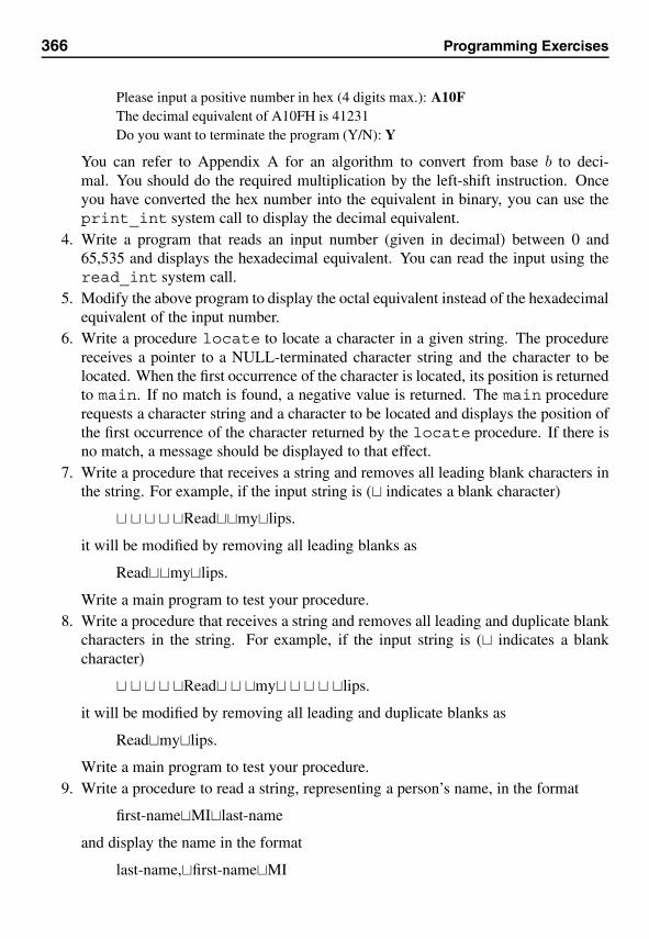
366 Programming Exercises
Please input a positive number in hex (4 digits max.): A10FThe decimal equivalent of A10FH is 41231Do you want to terminate the program (Y/N): Y
You can refer to Appendix A for an algorithm to convert from base b to deci-mal. You should do the required multiplication by the left-shift instruction. Onceyou have converted the hex number into the equivalent in binary, you can use theprint_int system call to display the decimal equivalent.
4. Write a program that reads an input number (given in decimal) between 0 and65,535 and displays the hexadecimal equivalent. You can read the input using theread_int system call.
5. Modify the above program to display the octal equivalent instead of the hexadecimalequivalent of the input number.
6. Write a procedure locate to locate a character in a given string. The procedurereceives a pointer to a NULL-terminated character string and the character to belocated. When the first occurrence of the character is located, its position is returnedto main. If no match is found, a negative value is returned. The main procedurerequests a character string and a character to be located and displays the position ofthe first occurrence of the character returned by the locate procedure. If there isno match, a message should be displayed to that effect.
7. Write a procedure that receives a string and removes all leading blank characters inthe string. For example, if the input string is (� indicates a blank character)
� � � � �Read��my�lips.
it will be modified by removing all leading blanks as
Read��my�lips.
Write a main program to test your procedure.8. Write a procedure that receives a string and removes all leading and duplicate blank
characters in the string. For example, if the input string is (� indicates a blankcharacter)
� � � � �Read� � �my� � � � �lips.
it will be modified by removing all leading and duplicate blanks as
Read�my�lips.
Write a main program to test your procedure.9. Write a procedure to read a string, representing a person’s name, in the format
first-name�MI�last-name
and display the name in the format
last-name,�first-name�MI
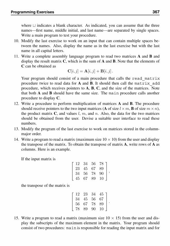
Programming Exercises 367
where � indicates a blank character. As indicated, you can assume that the threenames—first name, middle initial, and last name—are separated by single spaces.Write a main program to test your procedure.
10. Modify the last exercise to work on an input that can contain multiple spaces be-tween the names. Also, display the name as in the last exercise but with the lastname in all capital letters.
11. Write a complete assembly language program to read two matrices A and B anddisplay the result matrix C, which is the sum of A and B. Note that the elements ofC can be obtained as
C[i, j] = A[i, j] + B[i, j] .
Your program should consist of a main procedure that calls the read_matrixprocedure twice to read data for A and B. It should then call the matrix_addprocedure, which receives pointers to A, B, C, and the size of the matrices. Notethat both A and B should have the same size. The main procedure calls anotherprocedure to display C.
12. Write a procedure to perform multiplication of matrices A and B. The procedureshould receive pointers to the two input matrices (A of size l×m, B of size m×n),the product matrix C, and values l, m, and n. Also, the data for the two matricesshould be obtained from the user. Devise a suitable user interface to read thesenumbers.
13. Modify the program of the last exercise to work on matrices stored in the column-major order.
14. Write a program to read a matrix (maximum size 10 × 10) from the user and displaythe transpose of the matrix. To obtain the transpose of matrix A, write rows of A ascolumns. Here is an example.
If the input matrix is ⎡⎢⎢⎣
12 34 56 7823 45 67 8934 56 78 9045 67 89 10
⎤⎥⎥⎦ ,
the transpose of the matrix is
⎡⎢⎢⎣
12 23 34 4534 45 56 6756 67 78 8978 89 90 10
⎤⎥⎥⎦ .
15. Write a program to read a matrix (maximum size 10 × 15) from the user and dis-play the subscripts of the maximum element in the matrix. Your program shouldconsist of two procedures: main is responsible for reading the input matrix and for
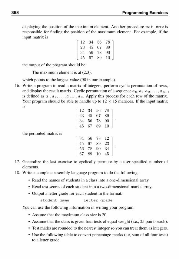
368 Programming Exercises
displaying the position of the maximum element. Another procedure mat_max isresponsible for finding the position of the maximum element. For example, if theinput matrix is ⎡
⎢⎢⎣12 34 56 7823 45 67 8934 56 78 9045 67 89 10
⎤⎥⎥⎦
the output of the program should be
The maximum element is at (2,3),
which points to the largest value (90 in our example).16. Write a program to read a matrix of integers, perform cyclic permutation of rows,
and display the result matrix. Cyclic permutation of a sequence a 0, a1, a 2, . . . , an−1
is defined as a1, a 2, . . . , an−1, a 0. Apply this process for each row of the matrix.Your program should be able to handle up to 12 × 15 matrices. If the input matrixis ⎡
⎢⎢⎣12 34 56 7823 45 67 8934 56 78 9045 67 89 10
⎤⎥⎥⎦ ,
the permuted matrix is ⎡⎢⎢⎣
34 56 78 1245 67 89 2356 78 90 3467 89 10 45
⎤⎥⎥⎦ .
17. Generalize the last exercise to cyclically permute by a user-specified number ofelements.
18. Write a complete assembly language program to do the following.
• Read the names of students in a class into a one-dimensional array.
• Read test scores of each student into a two-dimensional marks array.
• Output a letter grade for each student in the format:
student name letter grade
You can use the following information in writing your program:
• Assume that the maximum class size is 20.
• Assume that the class is given four tests of equal weight (i.e., 25 points each).
• Test marks are rounded to the nearest integer so you can treat them as integers.
• Use the following table to convert percentage marks (i.e, sum of all four tests)to a letter grade.
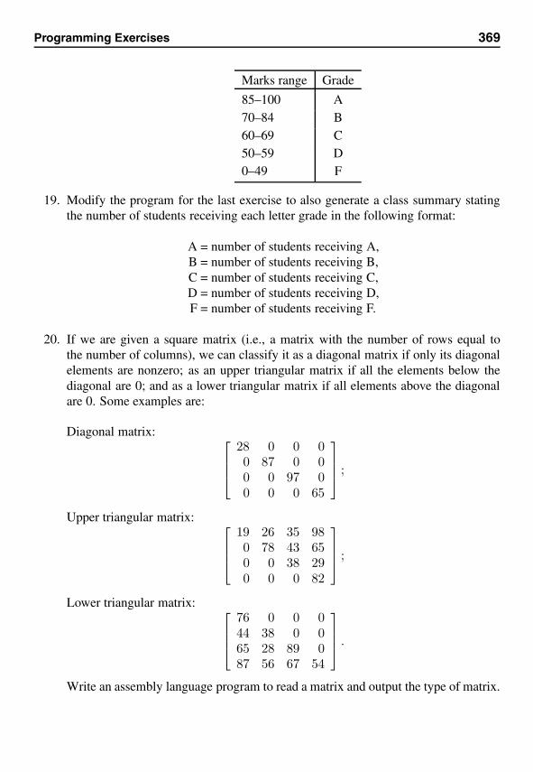
Programming Exercises 369
Marks range Grade
85–100 A70–84 B60–69 C50–59 D0–49 F
19. Modify the program for the last exercise to also generate a class summary statingthe number of students receiving each letter grade in the following format:
A = number of students receiving A,B = number of students receiving B,C = number of students receiving C,D = number of students receiving D,F = number of students receiving F.
20. If we are given a square matrix (i.e., a matrix with the number of rows equal tothe number of columns), we can classify it as a diagonal matrix if only its diagonalelements are nonzero; as an upper triangular matrix if all the elements below thediagonal are 0; and as a lower triangular matrix if all elements above the diagonalare 0. Some examples are:
Diagonal matrix: ⎡⎢⎢⎣
28 0 0 00 87 0 00 0 97 00 0 0 65
⎤⎥⎥⎦ ;
Upper triangular matrix: ⎡⎢⎢⎣
19 26 35 980 78 43 650 0 38 290 0 0 82
⎤⎥⎥⎦ ;
Lower triangular matrix: ⎡⎢⎢⎣
76 0 0 044 38 0 065 28 89 087 56 67 54
⎤⎥⎥⎦ .
Write an assembly language program to read a matrix and output the type of matrix.
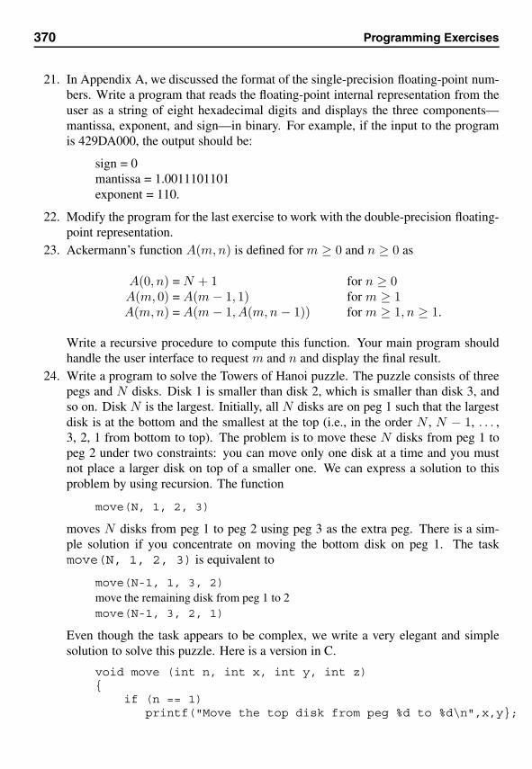
370 Programming Exercises
21. In Appendix A, we discussed the format of the single-precision floating-point num-bers. Write a program that reads the floating-point internal representation from theuser as a string of eight hexadecimal digits and displays the three components—mantissa, exponent, and sign—in binary. For example, if the input to the programis 429DA000, the output should be:
sign = 0mantissa = 1.0011101101exponent = 110.
22. Modify the program for the last exercise to work with the double-precision floating-point representation.
23. Ackermann’s function A(m,n) is defined for m ≥ 0 and n ≥ 0 as
A(0, n) = N + 1 for n ≥ 0A(m, 0) = A(m − 1, 1) for m ≥ 1A(m,n) = A(m − 1, A(m,n − 1)) for m ≥ 1, n ≥ 1.
Write a recursive procedure to compute this function. Your main program shouldhandle the user interface to request m and n and display the final result.
24. Write a program to solve the Towers of Hanoi puzzle. The puzzle consists of threepegs and N disks. Disk 1 is smaller than disk 2, which is smaller than disk 3, andso on. Disk N is the largest. Initially, all N disks are on peg 1 such that the largestdisk is at the bottom and the smallest at the top (i.e., in the order N , N − 1, . . . ,3, 2, 1 from bottom to top). The problem is to move these N disks from peg 1 topeg 2 under two constraints: you can move only one disk at a time and you mustnot place a larger disk on top of a smaller one. We can express a solution to thisproblem by using recursion. The function
move(N, 1, 2, 3)
moves N disks from peg 1 to peg 2 using peg 3 as the extra peg. There is a sim-ple solution if you concentrate on moving the bottom disk on peg 1. The taskmove(N, 1, 2, 3) is equivalent to
move(N-1, 1, 3, 2)move the remaining disk from peg 1 to 2move(N-1, 3, 2, 1)
Even though the task appears to be complex, we write a very elegant and simplesolution to solve this puzzle. Here is a version in C.
void move (int n, int x, int y, int z){
if (n == 1)printf("Move the top disk from peg %d to %d\n",x,y};
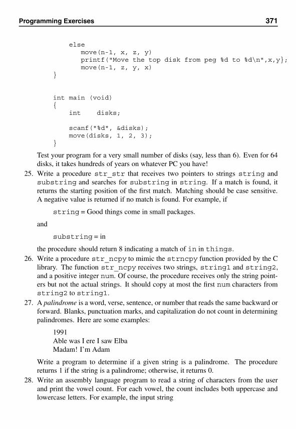
Programming Exercises 371
elsemove(n-1, x, z, y)printf("Move the top disk from peg %d to %d\n",x,y};move(n-1, z, y, x)
}
int main (void){
int disks;
scanf("%d", &disks);move(disks, 1, 2, 3);
}
Test your program for a very small number of disks (say, less than 6). Even for 64disks, it takes hundreds of years on whatever PC you have!
25. Write a procedure str_str that receives two pointers to strings string andsubstring and searches for substring in string. If a match is found, itreturns the starting position of the first match. Matching should be case sensitive.A negative value is returned if no match is found. For example, if
string = Good things come in small packages.
and
substring = in
the procedure should return 8 indicating a match of in in things.26. Write a procedure str_ncpy to mimic the strncpy function provided by the C
library. The function str_ncpy receives two strings, string1 and string2,and a positive integer num. Of course, the procedure receives only the string point-ers but not the actual strings. It should copy at most the first num characters fromstring2 to string1.
27. A palindrome is a word, verse, sentence, or number that reads the same backward orforward. Blanks, punctuation marks, and capitalization do not count in determiningpalindromes. Here are some examples:
1991Able was I ere I saw ElbaMadam! I’m Adam
Write a program to determine if a given string is a palindrome. The procedurereturns 1 if the string is a palindrome; otherwise, it returns 0.
28. Write an assembly language program to read a string of characters from the userand print the vowel count. For each vowel, the count includes both uppercase andlowercase letters. For example, the input string
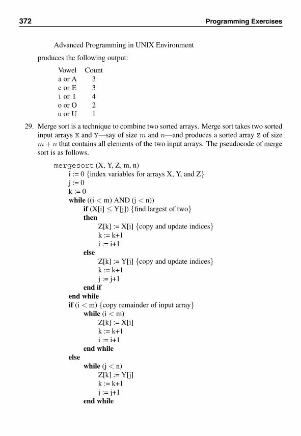
372 Programming Exercises
Advanced Programming in UNIX Environment
produces the following output:
Vowel Counta or A 3e or E 3i or I 4o or O 2u or U 1
29. Merge sort is a technique to combine two sorted arrays. Merge sort takes two sortedinput arrays X and Y—say of size m and n—and produces a sorted array Z of sizem + n that contains all elements of the two input arrays. The pseudocode of mergesort is as follows.
mergesort (X, Y, Z, m, n)i := 0 {index variables for arrays X, Y, and Z}j := 0k := 0while ((i < m) AND (j < n))
if (X[i] ≤ Y[j]) {find largest of two}then
Z[k] := X[i] {copy and update indices}k := k+1i := i+1
elseZ[k] := Y[j] {copy and update indices}k := k+1j := j+1
end ifend whileif (i < m) {copy remainder of input array}
while (i < m)Z[k] := X[i]k := k+1i := i+1
end whileelse
while (j < n)Z[k] := Y[j]k := k+1j := j+1
end while
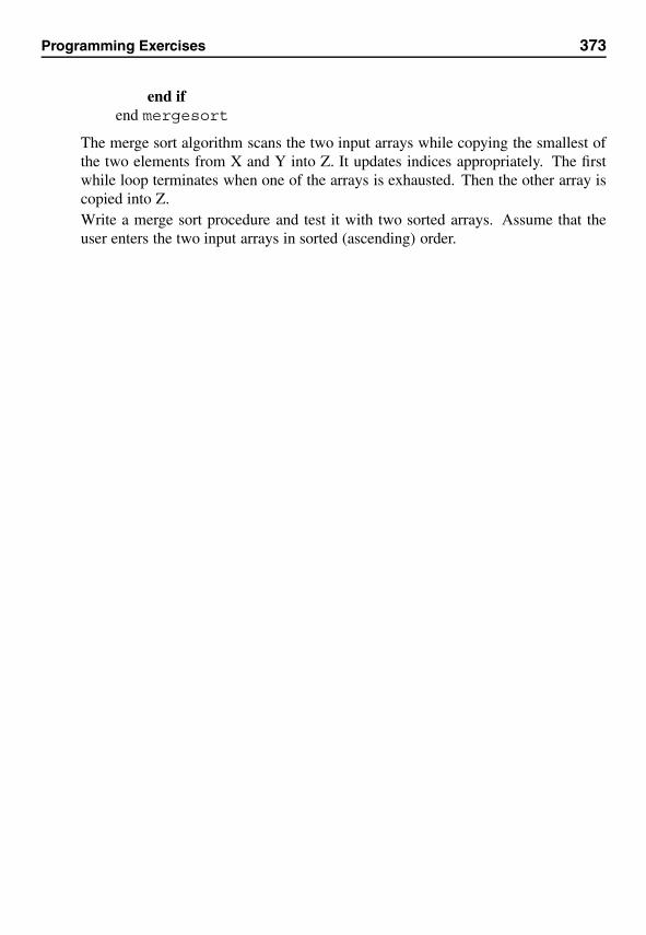
Programming Exercises 373
end ifend mergesort
The merge sort algorithm scans the two input arrays while copying the smallest ofthe two elements from X and Y into Z. It updates indices appropriately. The firstwhile loop terminates when one of the arrays is exhausted. Then the other array iscopied into Z.Write a merge sort procedure and test it with two sorted arrays. Assume that theuser enters the two input arrays in sorted (ascending) order.
Bibliography
[1] ARM, ARM Architecture Reference Manual, Addison-Wesley Professional,2000.
[2] ARM, “ARM Instruction Set Quick Reference Card,” 2003. This document isavailable from www.arm.com.
[3] ARM, “ARM Milestones,” 2003. This document is available from www.arm.com/aboutarm/milestones.html
[4] ARM, “ARM Markets,” 2003. This document is available from www.arm.com/markets/.
[5] ARM, “The Thumb Architecture Extension,” 2003. This document is avail-able from www.arm.com/products/CPUs/archi-thumb.html.
[6] S.P. Dandamudi, Fundamentals of Computer Organization and Design,Springer, New York, 2003.
[7] S.P. Dandamudi, Introduction to Assembly Language Programming, SecondEdition, Springer, New York, 2004.
[8] D. Goldberg, “What Every Computer Scientist Should Know About Floating-Point Arithmetic,” ACM Computing Surveys, Vol. 23, No. 1, March 1991, pp.5–48.
[9] IBM, “PowerPC Architecture: A High-Performance Architecture with a His-tory,” 2003. This document is available from www.ibm.com/servers/eserver/pseries/hardware/whitepapers/power/ppc arch.html.
[10] Intel, Intel Itanium Architecture: Software Developer’s Manual, Volume 1:Application Architecture, 2002. This manual is available from www.intel.com/design/Itanium/manuals/.
[11] Intel, Intel Itanium Architecture: Software Developer’s Manual, Volume 2:System Architecture, 2002. This manual is available from www.intel.com/design/Itanium/manuals/.
[12] Intel, Intel Itanium Architecture: Software Developer’s Manual, Volume 3:Instruction Set Reference, 2002. This manual is available from www.intel.com/design/Itanium/manuals/.
375
376 Bibliography
[13] Z. Kerekes,“History of SPARC Systems,” 2003. This document is availablefrom www.sparcproductdirectory.com/history.html.
[14] J.R. Larus, SPIM S20: A MIPS R2000 Simulator, 1997. This manual isavailable from www.cs.wisc.edu/˜larus/SPIM_manual/spim-manual.html.
[15] J.K. Lee and A.J. Smith, “Branch Prediction Strategies and Branch TargetBuffer Design,” Computer, Vol. 17, No. 1, 1984, pp. 6–22.
[16] MIPS, MIPS32 Architecture for Programmers, Volume I: Introduction tothe MIPS32 Architecture, 2003. It is available from www.mips.com/content/Documentation/MIPSDocumentation.
[17] MIPS, MIPS32 Architecture for Programmers, Volume II: The MIPS32Instruction Set, 2003. This manual is available from www.mips.com/content/Documentation/MIPSDocumentation.
[18] MIPS, MIPS32 Architecture for Programmers, Volume III: The MIPS32Privileged Resource Architecture, 2003. It is available from www.mips.com/content/Documentation/MIPSDocumentation.
[19] MIPS, MIPS64 Architecture for Programmers, Volume I: Introductionto the MIPS64 Architecture, 2003. It is available from www.mips.com/content/Documentation/MIPSDocumentation.
[20] MIPS, MIPS64 Architecture for Programmers, Volume II: The MIPS64Instruction Set, 2003. It is available from www.mips.com/content/Documentation/MIPSDocumentation.
[21] MIPS, MIPS64 Architecture for Programmers, Volume III: The MIPS64Privileged Resource Architecture, 2003. It is available from www.mips.com/content/Documentation/MIPSDocumentation.
[22] D.A. Patterson and C.H. Sequin, “A VLSI RISC,” Computer, Vol. 15, No. 9,1982, pp. 8–21.
[23] PowerPC, PowerPC Architecture Book: PowerPC User Instruction Set Ar-chitecture, Book I, 2003. This document is available from www.ibm.com/developerworks/eserver/articles/archguide.html.
[24] PowerPC, PowerPC Architecture Book: PowerPC Virtual Environment Ar-chitecture, Book II, 2003. This document is available from www.ibm.com/developerworks/eserver/articles/archguide.html.
[25] PowerPC, PowerPC Architecture Book: PowerPC Operating EnvironmentArchitecture, Book III, 2003. This document is available from www.ibm.com/developerworks/eserver/articles/archguide.html.
[26] SPARC, “SPARC History,” 2003. This document is available from www.sparc.com/history.html.
[27] SUN, “SUN History,” 2003. This document is available from www.sun.com/aboutsun/coinfo/history.html.

Bibliography 377
[28] A.S. Tanenbaum, “Implications of Structured Programming for Machine Ar-chitecture,” Communications of the ACM, Vol. 21, No. 3, 1978, pp. 237–246.
IndexSymbols.ALIGN, 164.FLOAT, 163.GLOBL, 164.HALF, 163.SPACE, 1631’s complement, 3321-address machines, 162’s complement, 3332-address machines, 153-address machines, 14
Aabsolute address, 23, 247accumulator machines, 16Ackermann’s function, 370activation record, 42, 292, 295address
absolute, 247PC-relative, 247
addresses0-address machines, 171-address machines, 162-address machines, 153-address machines, 14accumulator machines, 16comparison, 18number of, 14–22stack machines, 17
addressing modes, 33, 50, 58, 83, 100,125, 212
immediate addressing mode, 33, 100
immediate index addressing mode,83
immediate update index addressingmode, 84
in ARM, 125in MIPS, 50, 212in PowerPC, 83in SPARC, 58index addressing mode, 84, 100indirect addressing mode, 100register addressing mode, 33
advanced load, 107architecture
CISC, 5Itanium, 98load/store, 20RISC, 5, 43
arithmetic instructions, 35ARM
addressing modes, 125general-purpose registers, 123instruction set, 131processor modes, 123program status registers, 123registers, 123write-back, 127
ARM instructionsadc, 137add, 136and, 139asr, 132b, 142bic, 139
379
380 Index
bl, 143clz, 139cmp, 141eor, 139ldm, 135ldmfd, 144ldr, 134ldrb, 135ldrh, 135ldrsb, 135ldrsh, 135lsl, 132lsr, 132mla, 138mov, 131mul, 138mvn, 133orr, 139ror, 132rrx, 132rsb, 138rsc, 138sbc, 137smlal, 138smull, 138stm, 136stmfd, 144str, 136sub, 137teq, 140tst, 140umlal, 138umull, 138
arrayscolumn-major order, 216multidimensional, 215one-dimensional, 214row-major order, 215
ASCII string, 163ASCIIZ string, 163assembler directives, 160, 162assembly language, 4, 7–10
advantages, 10what is it, 7–9
Bbinary numbers, 327
conversion, 329bit manipulation, 277
clearing bits, 271cutting and pasting, 274isolating bits, 273toggling, 275
branchabsolute address, 23conditional, 24
set-then-jump, 24test-and-jump, 24
overview, 22PC-relative, 23unconditional, 23
branch elimination, 112, 113branch handling, 112–114branch hints, 112, 119branch prediction, 28–32, 113
dynamic strategy, 30fixed strategy, 28in Itanium, 119static strategy, 29
branch speedup, 112
Ccall-by-reference, 184call-by-value, 184character representation, 339–340
extended ASCII, 340CISC processors
evolution, 40VAX-11/780, 40, 43
column-major order, 216conditional branch, 24control speculation, 118CTR register, 83
Index 381
current frame marker register, 101
Ddata dependency
ambiguous, 115read-after-write, 115write-after-read, 115write-after-write, 115
data movement instructions, 34data speculation, 115delayed procedure call, 27denormalized values, 336dynamic branch prediction strategy, 30
Eend of procedure, 26EPIC design, 97equivalence function, 91even parity, 272, 274excess-M number representation, 331executable instructions, 160explicit parallel instruction computing, see
EPIC design
Ffactorial, 291–295
recursive procedure, 292Fibonacci function, 295, 303
MIPS procedure, 295fixed branch prediction strategy, 28floating-point, 334–336
denormals, 336IEEE 754, 335representation, 334special values, 336∞, 336NaN, 336zero, 336
FPSCR register, 81
Ggeneral-purpose registers, 48, 81
in ARM, 123in Itanium processor, 98in MIPS, 48in PowerPC, 81usage in MIPS, 48
Hhexadecimal numbers, 327
IIEEE 754 floating-point standard, 335immediate addressing mode, 33, 100immediate index addressing mode, 83,
84index addressing mode, 84, 100indirect addressing mode, 100indirect jump, 259instruction format, 35–36, 51, 59instruction set design, 32–36
issues, 32addressing modes, 33instruction types, 34operand types, 32
instruction types, 34arithmetic, 35data movement, 34logical, 35
instruction-level parallelism, 97, 105–106Itanium instructions, 102–112
add, 108advanced load, 107and, 110br, 111branch hints, 112call, 112cmp, 110, 114instruction format, 102ld8, 107ldSZ, 106
382 Index
loop, 112mov, 108movl, 108return, 112shl, 110shladd, 109shr, 110shr.u, 110speculative load, 107stSZ, 107
Itanium processor, 97–119addressing modes, 100architectural features, 98architecture, 98arithmetic instructions, 108branch elimination, 112, 113branch handling, 112–114branch hints, 119branch instructions, 111branch prediction, 119branch speedup, 112comparison instructions, 110data dependency, 115data transfer instructions, 106EPIC design, 97immediate addressing mode, 100index addressing mode, 100indirect addressing mode, 100instruction bundles, 106instruction format, 102instruction-level parallelism, 97, 105–
106logical instructions, 109Not-a-Thing bit, 98predication, 113procedure call, 101register renaming, 101registers, 98shift instructions, 110speculative execution, 114–119
control speculation, 118data speculation, 115
stack frame, 101
Llinear search, 256load instructions, 166load/store architecture, 20, 100logical instructions, 35LR register, 82
Mmachine language, 4, 7masking bit, 271merge sort, 372microprogram, 6MIPS, 47–52
addressing modes, 50architecture, 47–52at register use, 229instruction format, 51memory layout, 52recursion, 292–303
MIPS instructionsabs, 227, 343add, 169, 226, 344addi, 226, 344addiu, 344addu, 169, 226, 344and, 271, 272, 344andi, 272, 345b, 171, 246, 249, 345bczf, 345bczt, 345beq, 171, 248, 249, 345beqz, 172, 248, 250, 346bge, 249, 346bgeu, 249, 346bgez, 227, 250, 346bgezal, 346bgt, 248, 249, 347bgtu, 248, 249, 347bgtz, 250, 347
Index 383
ble, 249, 347bleu, 249, 347blez, 250, 348blt, 249, 348bltu, 249, 348bltz, 250, 348bltzal, 348bne, 249, 349bnez, 250, 349branch instructions, 246break, 229, 349comparison instructions, 244data transfer instructions, 165div, 229, 349, 350divu, 349, 350j, 246, 350jal, 186, 350jalr, 350jr, 188, 351jump instructions, 246la, 166, 351lb, 167, 351lbu, 166, 351ld, 351lh, 166, 351lhu, 166, 352li, 166, 352load instructions, 166logical instructions, 270lui, 352lw, 166, 352lwcz, 352lwl, 353lwr, 353mfcz, 353mfhi, 228, 354mflo, 228, 354move, 166, 354mtcz, 354mthi, 228, 354mtlo, 228, 354mul, 228, 355
mulo, 228, 355mulou, 228, 355mult, 228, 355multu, 355neg, 227, 356negu, 356nop, 356nor, 272, 356not, 272, 276, 356or, 272, 273, 356ori, 167, 272, 357rem, 230, 357remu, 357rol, 282, 357ror, 281, 357rotate instructions, 280sb, 167, 358sd, 358seq, 245, 358sge, 245, 358sgeu, 245, 358sgt, 245, 359sgtu, 245, 359sh, 168, 359shift instructions, 170, 276sle, 245, 359sleu, 245, 359sll, 170, 278, 360sllv, 276, 278, 360slt, 244, 245, 360slti, 245, 360sltiu, 360sltu, 245, 361sne, 245, 361sra, 278, 361srav, 278, 361srl, 278, 361srlv, 278, 362sub, 169, 226, 362subu, 169, 227, 362sw, 168, 362swcz, 362
384 Index
swl, 363swr, 363ulh, 363ulhu, 364ulw, 364ush, 364usw, 364xor, 272, 364xori, 272, 364
MIPS processoraddressing modes, 212
multidimensional arrays, 215
Nnumber of addresses, 14–22number representation
floating-point, 334–336signed integer, 331
1’s complement, 3322’s complement, 333excess-M, 331signed magnitude, 331
unsigned integer, 330number systems, 325
base, 325binary, 325, 327conversion, 327–329decimal, 325, 327floating-point, 334–336hexadecimal, 325, 327notation, 326octal, 325, 327radix, 325
Ooctal numbers, 327one’s complement, 332one-dimensional arrays, 214opcode, 35, 36operand types, 32
Pparameter passing, 27, 71, 184
call-by-reference, 184call-by-value, 184variable number of parameters, 207–
210parity conversion, 275PC-relative, 23PC-relative address, 247Pentium instructions
xor, 275pipelining
branch prediction, 28–32PowerPC, 79–95
addressing modes, 83immediate index addressing mode,
83immediate update index address-
ing mode, 84index addressing mode, 84
instruction set, 86–95instruction format, 84
registers, 81condition register, 81CTR register, 83FPSCR register, 81LR register, 82XER register, 83
PowerPC instructions, 86–95add, 88add., 88adde, 88addi, 89addition instructions, 88addo, 88addo., 88and, 90andc, 90andi., 90arithmetic instructions, 88b, 94ba, 94

Index 385
bc, 94bca, 94bcctr, 95bcctrl, 95bcl, 94bcla, 94bclr, 95bclrl, 95bl, 94bla, 94branch conditions, 94branch hints, 94, 95branch instructions, 93cmp, 93cmpd, 93cmpi, 93comparison instructions, 93data transfer instructions, 86divide instructions, 90divw, 90instruction format, 84la, 89lbz, 86lbzu, 86lbzux, 86lbzx, 86lha, 87lhau, 87lhaux, 87lhax, 87li, 89logical instructions, 90mr, 91mulhw, 90mulli, 90mullw, 89multiply instructions, 89nand, 91nand., 91neg, 89nor, 91nor., 91
ori, 91rlwnm, 92rotate instructions, 91rotlw, 92shift instructions, 91slw, 91, 92sraw, 92sraw., 92srawi, 92srawi., 92stb, 87stbu, 87stbux, 87stbx, 87stmu, 88subf, 89subi, 89subtract instructions, 89xor, 91xori, 91
predicated execution, 113procedure call, 26
delayed call, 27end, 26in Itanium, 101overview, 26parameter passing, 27return address, 26
processor registers, 22, 48program status registers, 123
Qquicksort
algorithm, 299MIPS procedure, 298
Rrecursion, 291–303
activation record, 292factorial, 291, 292Fibonacci function , 295
386 Index
Fibonacci number, 303in MIPS, 292–303
factorial procedure, 292quicksort procedure, 298
quicksort algorithm, 298, 299versus iteration, 303
register addressing mode, 33register renaming, 101registers, 22return address, 26RISC processors, 41–44
characteristics, 41–42design principles, 43–44PowerPC, 79–95
row-major order, 215
Sselection sort, 252sign bit, 331sign extension, 334signed integer, 331
1’s complement, 3322’s complement, 333excess-M, 331signed magnitude representation, 331
signed magnitude representation, 331space-efficiency, 10SPARC, 55–76
addressing modes, 58instruction format, 59instruction set, 59–76parameter passing, 71stack implementation, 72window management, 72
SPARC instructions, 59–76add instructions, 63arithmetic instructions, 62branch instructions, 65compare instructions, 65data transfer instructions, 59division instructions, 64
logical instructions, 64multiplication instructions, 63procedure calls, 69procedure instructions, 70shift instructions, 64subtract instructions, 63
speculative execution, 114–119control speculation, 118data speculation, 115
speculative load, 107SPIM, 149–157
assembler directives, 162data directives, 163debugging, 154loading, 153miscellaneous directives, 163running, 153segments, 162simulator settings, 152string directives, 162system calls, 161
stack, 192–193MIPS implementation, 193SPARC implementation, 72stack frame, 101top-of-stack, 192, 193use, 195what is it, 192
stack depth, 18stack frame, 101stack machines, 17
stack depth, 18static branch prediction strategy, 29string directives, 162system calls, 161
Ttime-efficiency, 10top-of-stack, 192, 193towers of Hanoi, 370two’s complement, 333

Index 387
Uunconditional branch, 23unsigned integer representation, 330
Vvariable number of parameters, 207–210VAX-11/780, 40, 43
Wwindow management, 72
XXER register, 83
Zzero extension, 330