The Geochemist’s Workbench® Release 11

GWB

Essentials Guide

The Geochemist’s Workbench® Release 11

GWB

Essentials Guide

Craig M. Bethke Sharon Yeakel

Aqueous Solutions, LLC

Champaign, Illinois

Printed January 5, 2018

This document © Copyright 2018 by Aqueous Solutions LLC. All rights reserved. Earlier editions copyright 2000–2017. This document may be reproduced freely to support any licensed use of the GWB software package.

Software copyright notice: Programs GSS, Rxn, Act2, Tact, SpecE8, Gtplot, TEdit, React, X1t, X2t, Xtplot, and ChemPlugin © Copyright 1983–2018 by Aqueous Solutions LLC. An unpublished work distributed via trade secrecy license. All rights reserved under the copyright laws.

The Geochemist’s Workbench®, ChemPlugin™, We put bugs in our software™, and The Geochemist’s Spreadsheet™ are a registered trademark and trademarks of Aqueous Solutions LLC; Microsoft®, MS®, Windows XP®, Windows Vista®, Windows 7®, Windows 8®, and Windows 10® are registered trademarks of Microsoft Corporation; PostScript® is a registered trademark of Adobe Systems, Inc. Other products mentioned in this document are identified by the trademarks of their respective companies; the authors disclaim responsibility for specifying which marks are owned by which companies. The software uses zlib © 1995–2005 Jean-Loup Gailly and Mark Adler, and Expat © 1998–2006 Thai Open Source Center Ltd. and Clark Cooper.

The GWB software was originally developed by the students, staff, and faculty of the Hydrogeology Program in the Department of Geology at the University of Illinois Urbana–Champaign. The package is currently developed and maintained by Aqueous Solutions LLC.

Address inquiries to:

Aqueous Solutions LLC 301 North Neil Street, Suite 400 Champaign, IL 61820 USA

Warranty: The Aqueous Solutions LLC warrants only that it has the right to convey license to the GWB software. Aqueous Solutions makes no other warranties, express or implied, with respect to the licensed software and/or associated written documentation. Aqueous Solutions disclaims any express or implied warranties of merchantability, fitness for a particular purpose, and non-infringement. Aqueous Solutions does not warrant, guarantee, or make any representations regarding the use, or the results of the use, of the Licensed Software or documentation in terms of correctness, accuracy, reliability, currentness, or otherwise. Aqueous Solutions shall not be liable for any direct, indirect, consequential, or incidental damages (including damages for loss of profits, business interruption, loss of business information, and the like) arising out of any claim by Licensee or a third party regarding the use of or inability to use Licensed Software. The entire risk as to the results and performance of Licensed Software is assumed by the Licensee. See License Agreement for complete details.

License Agreement: Use of the GWB is subject to the terms of the accompanying License Agreement. Please refer to that Agreement for details.

Cover photo: Salinas de Janubio by Jorg Hackemann

v

Contents

Chapter ListIntroduction ..................................................................................... 3 Configuring the Programs ................................................................ 17 Using GSS ....................................................................................... 31 Using Rxn ....................................................................................... 49 Using Act2 ...................................................................................... 69 Using Tact ...................................................................................... 97 Using SpecE8 ................................................................................ 111 Using Gtplot ................................................................................. 141 Using TEdit ................................................................................... 161 Appendix: Further Reading ............................................................ 177

vi

vii

Detailed Contents

Introduction ..................................................................................... 3

1.1 GWB documentation ............................................................................................... 4 1.2 Online tutorials ........................................................................................................ 4 1.3 GWB dashboard ....................................................................................................... 5 1.4 GWB modeling programs ........................................................................................ 6 1.5 To GUI or not to GUI ................................................................................................ 7 1.6 Saving and reading input files ................................................................................ 8 1.7 Drag and drop feature ............................................................................................. 9 1.8 Helpful features ..................................................................................................... 12 1.9 Exporting results ................................................................................................... 12 1.10 Automatic plot updates ...................................................................................... 14 1.11 Further reading ................................................................................................... 14 1.12 User resources ..................................................................................................... 14

Configuring the Programs ................................................................ 17

2.1 Configuring a calculation ...................................................................................... 17 2.2 Setting and constraining the basis ....................................................................... 18 2.3 Thermodynamic datasets ..................................................................................... 19 2.4 Redox couples ....................................................................................................... 20 2.5 Sorption onto mineral surfaces ............................................................................ 24

2.5.1 Two-layer surface complexation model ..................................................................... 24 2.5.2 Constant capacitance model ...................................................................................... 25 2.5.3 Constant potential model ........................................................................................... 26 2.5.4 Ion exchange ................................................................................................................ 27 2.5.5 Distribution coefficients (Kd) ....................................................................................... 28 2.5.6 Freundlich isotherms ................................................................................................... 29 2.5.7 Langmuir isotherms ..................................................................................................... 29

2.6 Electrical conductivity .......................................................................................... 30 2.7 Environment variables .......................................................................................... 30

Using GSS ....................................................................................... 31

3.1 Your first data sheet .............................................................................................. 31

viii

3.2 Working with a data sheet ..................................................................................... 34

3.2.1 Changing the view ....................................................................................................... 34 3.2.2 Data cells ..................................................................................................................... 34 3.2.3 Changing units ............................................................................................................ 34 3.2.4 Error bars ..................................................................................................................... 35 3.2.5 Calculating analytes ................................................................................................... 35 3.2.6 Sorting ......................................................................................................................... 36 3.2.7 Notes ........................................................................................................................... 37 3.2.8 Undo and redo ............................................................................................................ 37 3.2.9 Saving and exporting data .......................................................................................... 37 3.2.10 Resuming your session ............................................................................................. 37

3.3 Analytes .................................................................................................................. 38

3.3.1 Chemical parameters .................................................................................................. 38 3.3.2 Physical parameters ................................................................................................... 38 3.3.3 Basis species ............................................................................................................... 38 3.3.4 Calculated values ........................................................................................................ 38 3.3.5 User-defined analytes ................................................................................................. 39 3.3.6 Analyte properties....................................................................................................... 40

3.4 Regulations, replicates, standards, and mixing ................................................... 40

3.4.1 Flagging regulatory violations .................................................................................... 40 3.4.2 Replicate analyses ...................................................................................................... 41 3.4.3 Checking standards .................................................................................................... 41 3.4.4 Mixing samples ............................................................................................................ 42

3.5 Launching SpecE8 and React ................................................................................ 44 3.6 Graphing data ........................................................................................................ 46

3.6.1 Series and time series plots ........................................................................................ 46 3.6.2 Cross plots ................................................................................................................... 46 3.6.3 Ternary, Piper, and Durov diagrams .......................................................................... 46 3.6.4 Other diagrams ........................................................................................................... 47 3.6.5 Scatter data ................................................................................................................. 47

Using Rxn ....................................................................................... 49

4.1 Balancing reactions ............................................................................................... 52 4.2 Calculating equilibrium equations ....................................................................... 55 4.3 Determining activity coefficients .......................................................................... 58 4.4 Calculating equilibrium temperatures ................................................................. 60 4.5 Free energy change ............................................................................................... 62 4.6 Sorption reactions ................................................................................................. 63

ix

4.6.1 Surface complexation .................................................................................................. 63 4.6.2 Ion exchange ................................................................................................................ 66 4.6.3 Distribution coefficients (Kd) ....................................................................................... 66 4.6.4 Freundlich isotherms ................................................................................................... 66 4.6.5 Langmuir isotherms ..................................................................................................... 66

4.7 Rxn command line ................................................................................................ 67

Using Act2 ...................................................................................... 69

5.1 Diagram calculation .............................................................................................. 76 5.2 Solubility diagrams ............................................................................................... 84 5.3 Mosaic diagrams.................................................................................................... 87 5.4 Editing plot appearance........................................................................................ 90 5.5 Reaction traces ...................................................................................................... 94 5.6 Scatter data ........................................................................................................... 94 5.7 Act2 command line ............................................................................................... 96

Using Tact ...................................................................................... 97

6.1 Diagram calculation .............................................................................................. 98 6.2 Solubility diagrams ............................................................................................. 104 6.3 Mosaic diagrams.................................................................................................. 107 6.4 Editing plot appearance...................................................................................... 108 6.5 Reaction traces and scatter plots ....................................................................... 108 6.6 Tact command line ............................................................................................. 109

Using SpecE8 ................................................................................ 111

7.1 Example calculation ............................................................................................ 111 7.2 Equilibrium models ............................................................................................. 115 7.3 Redox disequilibrium .......................................................................................... 120 7.4 Activity coefficients ............................................................................................. 123 7.5 Sorption onto mineral surfaces .......................................................................... 127

7.5.1 Surface complexation ................................................................................................ 127 7.5.2 Ion exchange .............................................................................................................. 129 7.5.3 Distribution coefficients (Kd) ..................................................................................... 131 7.5.4 Freundlich isotherms ................................................................................................. 133 7.5.5 Langmuir isotherms ................................................................................................... 133

7.6 Settable variables................................................................................................ 135 7.7 Controlling the printout ...................................................................................... 137 7.8 SpecE8 command line ........................................................................................ 139

Using Gtplot ................................................................................. 141

x

8.1 Plot types ............................................................................................................. 143

8.1.1 Sample selection ....................................................................................................... 148

8.2 Editing plot appearance ...................................................................................... 150 8.3 Scatter data .......................................................................................................... 154 8.4 Loading and saving plot configuration ............................................................... 155 8.5 Exporting the plot ................................................................................................ 156 8.6 Gtplot command line ........................................................................................... 158

Using TEdit ................................................................................... 161

9.1 Getting started with TEdit ................................................................................... 161

9.1.1 Viewing a thermo dataset ......................................................................................... 161 9.1.2 Viewing a surface dataset ......................................................................................... 167 9.1.3 Creating new datasets .............................................................................................. 167 9.1.4 Dataset formats ........................................................................................................ 167 9.1.5 Saving datasets ......................................................................................................... 168

9.2 Working with datasets ......................................................................................... 168

9.2.1 Show .......................................................................................................................... 168 9.2.2 References ................................................................................................................. 169 9.2.3 Add and delete entries .............................................................................................. 169 9.2.4 Completing entries in thermo datasets ................................................................... 169 9.2.5 Completing entries in surface datasets .................................................................... 170

9.2.5.1 Two-layer datasets ............................................................................................ 170 9.2.5.2 Langmuir datasets ............................................................................................. 171 9.2.5.3 Kd and Freundlich datasets ............................................................................... 171 9.2.5.4 Ion exchange ...................................................................................................... 171

9.2.6 Transferring dataset entries ..................................................................................... 171 9.2.7 Basis swapping.......................................................................................................... 172

9.2.8 Exchanging species ........................................................................................... 173

Appendix: Further Reading ............................................................ 177

A.1 Natural waters ..................................................................................................... 177 A.2 Speciation modeling ........................................................................................... 178 A.3 Uniqueness of solutions ...................................................................................... 178 A.4 Stability diagrams................................................................................................ 179 A.5 Activity models for electrolyte solutions ............................................................ 179 A.6 Sorption, ion exchange, and surface complexation .......................................... 179 A.7 Thermodynamic databases ................................................................................ 179 A.8 Electrical conductivity ......................................................................................... 180

1

Origin of the programs The GWB package was originally developed at the Department of Geology of the University of Illinois at Urbana-Champaign over a period of more than twenty years, under the sponsorship of a consortium of companies and government laboratories. The members of the consortium, past and present, include:

Amoco Production Company Arco Oil and Gas Company Chevron Petroleum Technology Corporation ConocoPhillips Company ExxonMobil Upstream Research Company Hewlett Packard, Incorporated Idaho National Engineering Lab Japan National Oil Corporation Lawrence Livermore National Laboratory Marathon Oil Company Mobil Research and Development Corporation Sandia National Laboratories SCKCEN (Belgian nuclear authority) SiliconGraphics Computer Systems Texaco, Incorporated Union Oil Company of California United States Geological Survey The original GWB package was written by Craig Bethke with the assistance of Ming-Kuo

Lee and Jeffrey Biesiadecki of the Hydrogeology Program in the Department of Geology, University of Illinois at Urbana-Champaign. The GWB is currently developed and supported by Aqueous Solutions LLC, located in Champaign, Illinois.

A number of programmers in the Hydrogeology Program, including Rick Hedin, Peter Berger, Tren Haselton, Ester Soriano, David Solt, and Lalita Kalita helped develop the user interface. Brian Healy and Walter Kreiling developed a library used by the programs to produce graphical images on various output devices, and David Solt, Tren Haselton, Changlin Huang, Ester Soriano, Xiang Zhao, and Kevin Gorczowski have updated and eventually replaced this library over the years. J.K. Bohlke, Eric Daniels, and MingKuo

Lee compiled the dataset of isotope fractionation factors; Daniel Saalfeld helped translate thermodynamic datasets to the GWB format; Amy Berger helped develop the surface complexation model; Qusheng Jin helped implement the redox kinetics and microbiological features; and Jungho Park created theGWBSymbol font and helped develop React’s ability to use customrate laws. Peter Berger, RickHedin, Phil Parker, Dan

2 GWB Essentials

Saalfeld, and Sharon Yeakel developed the active graphics facilities and other features of release 7.0; Sharon Yeakel helped prepare documentation for the release. Phil Parker worked on developing the multithreaded versions of X1t and X2t for release 8.0, and Dan Saalfeld, Sharon Yeakel, and Jesse Luehrs developed program GSS and other features of the release. Dan Saalfeld, Sharon Yeakel, and Jesse Luehrs, with the assistance of Brian Farrell, developed release 9.0. Dan Saalfeld, Sharon Yeakel, Brian Farrell, Bryan Plummer, and Steven Canning developed release 10.0. Dan Saalfeld, Sharon Yeakel, Yusheng Hou, Oscar Garcia, Brian Farrell, Katelyn Zatwarnicki, Shelley Goel, and Peter Berger developed the GWB 11 release.

The software authors appreciate the assistance of more people than we can remember who over the years helped with software development and testing. These people include Theresa Beckman, Bill Bourcier, Pat Brady, Tenhung Chu, David Finkelstein, Ted Flynn, Annette Fugl, Oscar Garcia Cabrejo, Man Jae Kwon, Matt Kyrias, Kurt Larson, Meng Lei, Melinda Legg, Gordon Madise, Chuck Norris, Hernán Quinodoz, Derik Strattan, and Melinda Tidrick. We also thank the many students and users who have suggested improvements to the codes and documentation.

3

Introduction

The Geochemist’s Workbench is a set of software tools for manipulating chemical reactions, calculating stability diagrams and the equilibrium states of natural waters, tracing reaction processes, modeling reactive transport, plotting the results of these calculations, and storing the related data. The Workbench, designed for personal computers running MS Windows, is distributed in three packages:

GWB Essentials contains tools for balancing reactions, calculating activity diagrams, computing speciation in aqueous solutions, plotting the results of these calculations, and storing the related data.

GWB Standard contains the tools included in GWB Essentials, as well as a program for modeling reaction processes.

GWB Professional includes all the programs in the Standard release, plus programs for modeling reactive transport in one and two dimensions, and for plotting modeling results.

The GWB Essentials release consists of seven programs: GSS stores analyte and sample data in a spreadsheet specially developed to

work with the GWB set of software tools. Rxn automatically balances chemical reactions, calculates equilibrium

constants and equations, and solves for the temperatures at which reactions are in equilibrium.

Act2 calculates and plots stability diagrams on activity and fugacity axes. It can also project the traces of reaction paths calculated using the React program.

Tact calculates and plots temperature-activity and temperature-fugacity diagrams and projects the traces of reaction paths.

SpecE8 calculates species distributions in aqueous solutions and computes mineral saturations and gas fugacities. SpecE8 can account for sorption of species onto mineral surfaces according to a variety of methods, including surface complexation and ion exchange.

Gtplot graphs SpecE8 results and GSS datasets, including on xy plots, ternary, Piper, Durov, and Stiff diagrams.

TEdit displays, modifies, and creates the thermodynamic and surface reaction datasets used by the various GWB applications.

4 GWB Essentials

The GWB Standard release also includes the program: React, in addition to having the capabilities of SpecE8, traces reaction paths

involving fluids, minerals, and gases. React can also predict the fractionation of stable isotopes during reaction processes. The simulation results can be rendered with Gtplot.

The GWB Professional release contains the additional programs: X1t simulates reactive transport in one-dimensional systems. The program has

all of React’s geochemical modeling capabilities, except isotope fractionation, coupled with groundwater flow and transport.

X2t simulates reactive transport in two-dimensional systems. Xtplot plots in map view and as xy plots the results of reactive transport

simulations made using X1t and X2t.

Each of the programs operates in a similar fashion, so once you learn to use one, you will find the others easy to work with.

1.1 GWB documentation Depending on the package, the GWB comes with a set of User’s Guides accessible as pdf files from the Help pulldown of any of the programs, and also available in printed form:

GWB Essentials Guide—A guide to GSS, Rxn, Act2, Tact, SpecE8, Gtplot, and TEdit (this document).

Reaction Modeling Guide—Information on reaction modeling using React, and using Gtplot to render simulation results.

Reactive Transport Modeling Guide—A guide to reactive transport modeling with X1t, X2t, and Xtplot.

Reference Manual—A comprehensive guide to commands for the GWB programs, the format of the thermodynamic datasets, and so on.

A considerable amount of information, including a large number of fully worked examples, is available in Geochemical and Biogeochemical Reaction Modeling by Craig M. Bethke, available from Cambridge University Press or booksellers such as Amazon.

1.2 Online tutorials The GWB website—www.gwb.com—contains a variety of step-by-step tutorials showing how to use the GWB software package. The website also contains a large number of diagrams and movies showing the results of GWB calculations. By clicking the icons next to each case, you can download the input scripts used to configure the calculation, or start the appropriate GWB application, configured and ready to run.

Introduction 5

The GWB YouTube channel—www.youtube.com/user/GeochemistsWorkbench—contains a number of instructional video clips that will quickly and efficiently help you become expert in using the software.

1.3 GWB dashboard The GWB dashboard is the platform from which you run the GWB programs, access documentation, find online video tutorials, activate and configure the software, and upgrade your software installation.

Start the GWB dashboard from the Start button on your Windows desktop (or the Start charm [Win+Q] in Windows 8). Select The Geochemist’s Workbench 11 in the menu, which brings up the GWB dashboard.

Take a moment to explore each of the tabs along the top of the window. You can launch the various GWB programs from the Apps pane. The Video and Docs panes take you to video tutorials and options for printed documentation, respectively. You can configure the software on the Settings pane, and the Support pane provides tools to activate the software, edit thermo datasets, and obtain user support. The Upgrade pane shows options for upgrading your software license. The dashboard looks like:

6 GWB Essentials

You can start the individual GWB programs in any of several ways: click on the program’s icon in the Apps pane, open (e.g., double-click on) a GWB input file from Windows, or simply drag an input file into the GWB dashboard.

1.4 GWB modeling programs When Rxn, Act2, Tact, SpecE8, React, X1t, and X2t start, they appear as a window containing several panes and a menubar. Rxn’s window, for example, is shown here.

The window contains three panes: The Basis pane, where you can set the most important calculation constraints,

as described below. The Command pane, where you can type Rxn commands. The Results pane, where you view calculation results.

You can detach each pane by dragging the pane title to the desktop with the left mouse button. In this way you can arrange and size the panes individually. The window also contains a menubar, from which you can select a number of options and display a variety of dialog boxes.

When Rxn, Act2, Tact, SpecE8, React, X1t, and X2t start, they assume the working directory from the previous run. The programs write output into this directory and look there for input files. You can change the working directory at any time by selecting File → Working Directory (Ctrl+Shift+W); the current setting is displayed on the window frame.

Introduction 7

Once you have configured a calculation, you generate the calculation results by selecting Run → Go or, on the Results output pane, pressing the Run button (or in Act2 and Tact, the Update Plot button). Once you have viewed the calculation results, you can move to another pane or select options from the menubar to modify the program’s configuration.

Gtplot contains a graphics area and a menubar, but there are no panes to select (as shown below). You configure this program using the mouse (or keyboard shortcuts) to select options from the menubar, or by left-clicking, right-clicking, or double-clicking on aspects of the plot displayed.

1.5 To GUI or not to GUI Some people like to work interactively with a GUI (a GUI is a Graphic User Interface, or “gooey”), whereas others prefer to type commands from the keyboard. In Rxn, Act2, Tact, SpecE8, React, X1t, and X2t, you can work either way, or switch freely from one to the other.

To enter commands, select the Command pane and type your input at the prompt, as shown here.

8 GWB Essentials

Alternatively, each GWB command has a GUI counterpart, which you invoke on a different pane, or by selecting an option or dialog from the program’s menubar.

You can quickly find the GUI equivalents to each command by exploring the program, or by consulting the command reference sections of the GWB Reference Manual. Example calculations in this Guide are most commonly shown as sequences of commands, because the commands can be listed concisely. You can work the examples following either the command listings or their GUI equivalents.

1.6 Saving and reading input files You can save the current settings in Rxn, Act2, Tact, SpecE8, and TEdit for later use. To do so, select File → Save As… (Ctrl+S). Or typing

within Act2, for example, writes the program’s current configuration into a dataset “My_file.ac2”.

Saved datasets contain input commands that can be read later by the program. Select an input dataset using the File → Open → Read script… dialog, or by typing

Alternatively, simply open the file. A list of the most recently opened files can be accessed with File → Recent Files. The number of files in the list can be set in File → Preferences…. The following filename extensions are defined under Windows for the GWB programs: .rxn Rxn .sp8 SpecE8 .x1t X1t .gss GSS .ac2 Act2 .gtp Gtplot .x2t X2t .tdat Thermo data .tac Tact .rea React .xtp Xtplot .sdat Surface data

save My_file.ac2

read My_file.ac2

Introduction 9

Double-clicking on “My_file.ac2”, for example, launches Act2 and executes the commands in the file.

When you exit Rxn, Act2, Tact, SpecE8, and GSS, they automatically save their current configurations to files such as “rxn_resume.rxn” and “act2_resume.ac2” in your profile directory (found by typing %appdata% in the Windows Explorer Address bar, e.g., “c:\Documents and Settings\jones\Application Data\GWB”). Upon reentering the programs, you can restore the previous configuration by choosing File → Resume, or typing

from the command line. Set the File → Resume On Startup option if each time you start one of the programs you would like to resume your previous session automatically.

Gtplot automatically saves the previous plot configuration in a dataset named “gtplot_conf.gtc” when you exit the program with the File → Quit option (Ctrl+Q). When you restart in the same working directory, or when you open a “.gtc” file, the program configuration is restored. You can reset the configuration by choosing File → Reset configuration (Ctrl+R) or use the File → Save As… option (Ctrl+S) to save different configuration files in the same directory (see Using Gtplot).

1.7 Drag and drop feature The drag and drop feature is a convenient way to transfer data within or between GWB programs, or between GWB programs and any other application that supports it.

Drag an input file from your Desktop or Windows Explorer into the GWB dashboard or any GWB application, and the input will be automatically loaded. For example, you could drag a script file (.sp8) or thermo data file (.tdat) into SpecE8, or drag a configuration file (.gtc) into Gtplot.

Left-click, drag onto a GWB app, and release: Input scripts and files Thermo and surface reaction datasets Conductivity data and water standards Plot configuration files Scatter data and reaction traces

You can drag chemical data directly from your spreadsheet or table into any GWB program. Drag data to the Basis pane of SpecE8 or React to analyze an individual sample, to one of the panes in X1t or X2t to constrain the initial, inlet, or injection fluids, or into GSS to transfer your data.

In GSS, right-click on an individual cell or on the sample header (to select an entire sample) and drag. In MS Excel, MS Word, or MS PowerPoint, highlight the cell or column,

resume

10 GWB Essentials

left-click the frame surrounding it, and drag. Release the mouse button over the selected input pane in the GWB program.

If dragging into GSS, bring the pointer to a sample header to fill that sample (as shown below), or to the button to add new samples.

Right-click and drag samples: from one GSS data sheet to another. from GSS into Basis, Initial panes. from GSS into MS Excel.

Left-click and drag: samples from MS Excel into GSS. samples from MS Excel into Basis, Initial panes. in GSS to rearrange samples or analytes.

Right-click and drag any pane title to transfer data within a GWB program, from one GWB program to another, or to another application.

In React, in order to “pick up” the results of a calculation and use these results as the starting point for a new calculation, right-click the Results pane title and drag it onto the Basis pane.

Calculation output can be copied from the Results pane to any other application in the same way. Dragging the Results pane will copy and paste the last step components in the fluid.

Right-click on a dialog title bar and drag to copy the settings of the dialog box from one GWB application to another. For example, if in SpecE8 you have the Alter Log Ks dialog all set up and filled with the values you would like to use in React, right-click the Alter Log Ks dialog title bar and drag it into React. The destination dialog box does not need to be open at the time.

Right-click and drag panes and dialogs to transfer: data from one instance of React, for example, to another. data from one GWB program to another.

Introduction 11

in React, calculation results from the Results pane to the Basis pane. calculation results into GSS. Basis, Initial pane values into GSS. data into MS Excel, MS Word, or MS PowerPoint. text into WordPad to see what the drag/drop actual text is.

You can rearrange the order of the panes by left-clicking and dragging the pane titles. You may also detach each pane by left-clicking on the pane title and dragging it to the desktop. In this way, you can arrange and size the panes individually to view and work with several panes at the same time. For example, you can type commands in the Command pane and immediately see the effect on the Basis, Results, and Plot panes. Re-attach panes with their close buttons. View → Reset Windows resizes, re-attaches, and reorders all of the panes to the default configuration.

You can drag data tables, elements, any type of species, or virial coefficients from one thermo or surface dataset open in TEdit to another. Left-click an entry on the tree structure of the source dataset, drag it to the tree structure or current entry of the target dataset, and release. If the source and target datasets are open in the same TEdit window, you can switch to the target dataset by hovering over its tab while dragging.

Left-click and drag panes: to rearrange the order of the panes. to detach panes and arrange them on the desktop.

Re-attach panes with their close buttons or View → Reset Windows (Alt+S). The User’s Guides provide many examples of how to configure the programs, how to

use the various commands, and how to create input scripts. You can highlight any of these examples in the pdf files, left-click within the selected text, drag with the left mouse, and drop into a GWB program. The commands will be automatically executed in order. Open the Run → History… dialog box to review them, or type history in the Command pane. You might also create an input script by dropping the selected text into an application such as WordPad and saving the file as a plain text document with the appropriate extension (.sp8, .rea, etc.).

*Note: If you are having trouble with Adobe Reader X drag and drop, go to Edit → Preferences → Categories → General and uncheck “Enable Protected Mode at startup”.

Left-click and drag from the pdf User’s Guides: command examples to the GWB programs or other applications. script examples to the GWB programs or other applications.

If you have a spreadsheet that contains the results of a large number of analyses, an alternative to drag and drop is to prepare a short script that performs the operations automatically, reading the analyses one at a time and adding the calculation results to the spreadsheet. For details of this process and a fully worked example, refer to the Multiple Analyses appendix of the GWB Reference Manual.

12 GWB Essentials

1.8 Helpful features The command line interface for the Command pane in Rxn, Act2, Tact, SpecE8, React, X1t, and X2t includes a number of helpful features:

Spelling completion. When you type commands in the Command pane, the programs automatically complete the spelling of a mineral, chemical, or command name (given enough characters to identify the name uniquely)—just press the [tab] key. When the program cannot identify a unique name, it will cycle through the possible completions with subsequent [tab] key presses. You can also show all names beginning with a combination of characters by pressing Ctrl+D.

Command history. The programs maintain a list of previously executed commands, which can be retrieved, modified, and re-executed. Type history or select Run → History… to view the history list.

Special characters. A group of control characters is provided on the Command pane for purposes such as spelling completion and input correction.

Startup files. Users can establish files in their profile directories containing commands for Rxn, Act2, Tact, SpecE8, React, X1t, and X2t to execute at startup. These files should be named with the app name and _startup (e.g., act2_startup.ac2) and placed in your profile directory (found by typing %appdata% in the Windows Explorer Address bar, e.g., “C:\Documents and Settings\jones\Application Data\GWB”).

Calculator. The interface will automatically evaluate any numerical expression typed in the Command pane. This feature facilitates, for example, conversion of numbers to logarithms, or vice versa.

Online documentation. The GWB User’s Guides are available in pdf format online from any of the GWB programs. Select Help on the menubar to access them.

These features are described fully in the User Interface appendix to the GWB Reference Manual.

1.9 Exporting results Programs Act2, Tact, Gtplot, and Xtplot make it convenient to use the plots you create in articles, reports, presentations, and databases. You can copy the current plot to the clipboard and then paste it into a variety of applications, in a format meaningful to the application.

To copy a plot, use Edit → Copy (Ctrl+C). If you paste the plot into MS PowerPoint, it will appear as an EMF (an MS Enhanced Metafile) graphic object. Pasting into Adobe Illustrator places a native AI graphic.

Introduction 13

If you paste a plot from Gtplot or Xtplot into MS Excel or a text editor such as Notepad or MS Word, the numerical values of the data points that make up the lines on the plot will appear in spreadsheet format (as shown below).

In MS Word or MS Excel, use Paste Special… to paste the plot as a picture instead.

You can control the format in which the plot is copied to the clipboard by selecting Edit → Copy As. You can choose to copy the plot as an AI object, an EMF object, or a bitmap, or

“Paste” in Excel or Word inserts numerical values

“Paste Special…” in Excel or Word

inserts a picture

14 GWB Essentials

the data points in the plot as tab delimited or space delimited text. Use the tab delimited option to paste the data into a spreadsheet program like MS Excel. For examining the data in a text file created with an editor like Notepad or MS Word, the space delimited option writes a nicely aligned table.

When importing AI graphics to Adobe Illustrator, the program may prompt you to update the legacy text before you can edit the file. In this case, choose “Update”. You need to release the clipping mask before you attempt to edit individual elements of the plot. Use the “Ungroup” and “Group” functions when repositioning or modifying elements.

The programs can save plots to files in various formats by selecting File → Save Image… from the menubar. The Graphics Output section of the GWB Reference Manual summarizes the options available for saving and using graphical output.

1.10 Automatic plot updates The software is designed so that whenever SpecE8, React, X1t, or X2t completes a simulation, any instances of Act2, Tact, Gtplot, or Xtplot that are displaying the results of that simulation will update their plots automatically.

1.11 Further reading This guide is intended as an introduction to using the programs in The Geochemist’s Workbench Essentials package, and as a reference for the software package. For information about geochemical modeling in general, including a number of examples of how the software can be applied, please refer to the text Geochemical and Biogeochemical Reaction Modeling by Craig M. Bethke, available from Cambridge University Press or booksellers such as Amazon. The Further Reading chapter in this guide gives literature references to this text and a number of other sources that provide starting points for further reading.

1.12 User resources The GWB website holds a set of visual tutorials that show how to use the GWB apps to solve a range of problems in geochemistry. Browse the GWB YouTube channel for a series of narrated video clips showing the GWB in action.

The GWB website also contains galleries of diagrams and movies, along with the input files used to compute them. Finally, the GWB Online Academy is a self-guided course in geochemical and reactive transport modeling that takes you from beginner to expert.

Gwb_users is an independent group of users who share comments and results and answer questions of general interest over the Internet. The group maintains an online

Introduction 15

forum that serves as a bulletin board for posting announcements, bug notices, and other current information about the software.

To subscribe to the forum (there is no charge), unsubscribe, or post a message, select GWB Users’ Group from the Windows Start menu (Start → Programs → Geochemist’s Workbench 11 → GWB Users’ Group), or the Help pulldown in any of the GWB programs. Alternatively, you can visit the group’s home page at forum.gwb.com.

17

Configuring the Programs

2.1 Configuring a calculation Rxn, Act2, Tact, and SpecE8 all work in the same manner. Each program maintains a set of species, known as the basis, with which it writes reactions. Initially, the basis is the set of aqueous species that appears at the beginning of the thermodynamic database (see Table 2.1). This set is known as the “original basis.”

You can alter the basis to reflect the geochemical constraints that you wish to impose in your calculation by substituting (“swapping”) another aqueous species, mineral, or gas for an entry in the original basis. To specify equilibrium with quartz, for example, you swap quartz for the basis species SiO2(aq). Or, to set the CO2 fugacity of your geochemical system, you swap CO2(g) for either the HCO3

– or H+ basis entries. Examples in Chapters 4–7 illustrate the basis swapping technique.

To perform a calculation, follow these steps: 1. Set the basis. First, add or swap the aqueous species, minerals, or gases you wish

to use to constrain your calculation into the basis. The basis should contain any species at known activity, such as H+ if the pH is known, minerals co-existing with the system, or gases at known fugacity. If you are calculating a stability diagram, make sure that the basis also includes the species to appear on the diagram axes.

2. Constrain the basis. Next, specify the temperature for the calculation and assign a value (“constraint”) for total concentration, activity, or fugacity for each entry in the basis.

3. Go. Select Run → Go to initiate the calculation, which might be letting the program balance a reaction, calculate and display a diagram, or trace a reaction path.

4. Revise. When the calculation is completed, you can adjust the basis by adding new components or varying your constraints; then, recalculate the model. You can continue to revise and recalculate until you decide to quit.

18 GWB Essentials

Table 2.1 Basis species in the LLNL thermodynamic database, “thermo.tdat”

H20 Water Li+ Lithium

Ag+ Silver Mg++ Magnesium

Al+++ Aluminum Mn++ Manganese

Am+++ Americium NO3– Nitrogen

As(OH)4– Arsenic Na+ Sodium

Au+ Gold Ni++ Nickel

B(OH)3 Boron Np++++ Neptunium

Ba++ Barium O2(aq) Oxygen

Br– Bromine Pb++ Lead

Ca++ Calcium PuO2++ Plutonium

HCO3– Carbon Ra++ Radium

Cs+ Cesium Rb+ Rubidium

Cl– Chlorine Ru+++ Ruthenium

Co++ Cobalt SeO3– – Selenium

Cr+++ Chromium SiO2(aq) Silicon

Cu+ Copper Sr++ Strontium

Eu+++ Europium SO4– – Sulfur

F- Fluorine TcO4– Technetium

H+ Hydrogen Th++++ Thorium

HPO4– – Phosphorus Sn++++ Tin

Hg++ Mercury U++++ Uranium

I– Iodine V+++ Vanadium

Fe++ Iron Zn++ Zinc

K+ Potassium

2.2 Setting and constraining the basis You set the basis by adding the appropriate entries for the original basis list (Table 2.1) to the calculation. Then, if necessary, you swap another species, mineral, or gas for the original basis entry. If you prefer to type your input, you use the add and swap commands.

Configuring the Programs 19

To configure the basis with the GUI, move to the Basis pane. You will see a list of current basis entries. Click the button (Ctrl+N) to add an entry to the basis. A menu of available entries appears. Navigate the menu with the mouse, the up and down arrow keys, or by typing the entry’s first letter (which is generally uppercase). To swap, click on the entry’s button, and select an aqueous species, mineral, or gas to swap into the basis.

Once you have created a list of basis entries (e.g., as shown in Table 2.1), you can manipulate it in several ways. You constrain an entry by choosing a unit (e.g., the activity of a species or fugacity of a gas) and setting a value in the corresponding box.

You can change the order of the entries by simply dragging them. To delete a basis entry, or several, select the entire entry and press the Delete key or the button. To configure another invocation of the program with these entries, right-click on the pane title, drag it, and release (see Drag and drop).

2.3 Thermodynamic datasets The programs work from one of several versions of a thermodynamic database. Each database contains the properties of aqueous species, minerals, and gases, equilibrium constants for reactions to form these species, and data required to calculate activity coefficients. In most cases, the data span the temperature range 0°C–300°C, at one atm pressure below 100°C, and along the vapor pressure of water at higher temperatures.

You can view, edit, and even create your own thermo datasets in the TEdit graphical editor, which is accessible from the Support pane of the GWB Dashboard (see Using TEdit). Since a thermo dataset is simply an ascii (character) file, you can also alter it using a text editor such as Notepad. The Thermo Datasets appendix to the GWB Reference Manual gives details of the database format.

The most commonly employed dataset is “thermo.tdat”, which supports activity coefficients calculated according to an extended form of the Debye-Hückel equation (the “Bdot” equation; see Activity coefficients under Using SpecE8). The database was compiled by Thomas Wolery, Joan Delany, Ken Jackson, James Johnson, and other members of the geochemical modeling group at Lawrence Livermore National Laboratories (LLNL). The dataset is based in large part on the SUPCRT data compilation (see references in the Further Reading section). Correspondence regarding the dataset may be addressed to James Johnson, L219, LLNL, Livermore, CA 94550.

From time to time, LLNL releases updated and expanded versions of its thermodynamic databases. The dataset “thermo.com.V8.R6+.tdat” is distributed with the GWB. This dataset is the LLNL “combined” dataset, version 8, release 6, in which the redox coupling among organic species has been modified somewhat. You may prefer to use this dataset if you are working extensively with systems containing organic species.

20 GWB Essentials

SpecE8, React, X1t, and X2t can also use virial methods (the “Pitzer equations”) to model species activities in saline fluids. Such calculations require thermo datasets containing the virial coefficients. Dataset “thermo_hmw.tdat”, included with the software release, includes coefficients for the Harvie-Møller-Weare activity model (see Activity coefficients under Using SpecE8). There is no provision in this dataset for calculations at temperatures other than 25°C.

Dataset “thermo_phrqpitz.tdat” is the database used by the USGS program PHRQPITZ. This database is a slightly expanded version of the Harvie-Møller-Weare activity model that contains data for more components than the original, as well as some provision for temperature extrapolation. Before applying this dataset at temperatures other than 25°C, however, you should study the PHRQPITZ documentation (see Further Reading) carefully.

Three other datasets are provided with the GWB release. The datasets “thermo_minteq.tdat”, “thermo_phreeqc.tdat”, and “thermo_wateq4f.tdat” contain data from the MINTEQ, PHREEQC, and WATEQ4F software packages, respectively, which can be downloaded from the Visual Minteq home page (MINTEQ) and the U.S. Geological Survey (PHREEQC and WATEQ4F). When the GWB programs load these datasets, they use the same method as the original program (MINTEQ, and so on) to calculate activity coefficients.

By default, the programs at startup look for a dataset named “thermo.tdat”, but you can specify an alternative default dataset in File → Preferences…. If you set the default file to “mythermo.tdat”, for example, the programs will read the file “mythermo.tdat” as the default thermo dataset.

The programs, at startup, look for the thermodynamic dataset in your working directory and, failing to find it there, in the public “gtdata” directory (by default, “\Program Files\GWB\Gtdata”). You may set an alternative default directory in File → Preferences….

2.4 Redox couples The thermodynamic dataset contains a number of redox coupling reactions that link species of differing oxidation states. There are redox couples between Fe++ and Fe+++, HS– and SO4

– – , CH4(aq) and HCO3– – , and so on. You can enable or disable coupling

reactions interactively. In this way, you control the extent to which the programs honor redox equilibrium in their calculations.

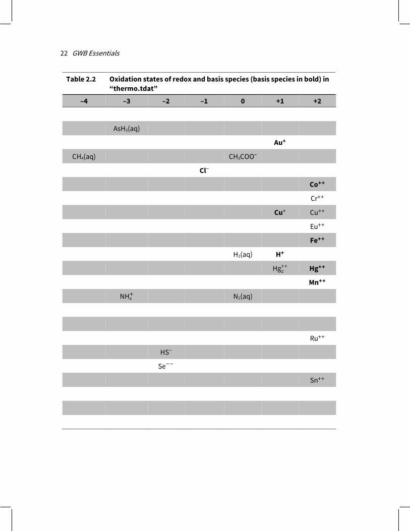
Each of the redox coupling reactions is identified by a redox species, which is a basis species in an alternative oxidation state (Table 2.2). In the examples in the previous paragraph, Fe+++, HS–, and CH4(aq) are the redox species; the corresponding basis species are Fe++, SO4

– – , and HCO3– – . The programs, by default, honor each redox couple

Configuring the Programs 21

and hence assume redox equilibrium. You can disable any number of the couples, however, by selecting Config → Redox Couples…, or invoking the decouple command.

Once a redox couple has been disabled, the redox species in question becomes an entry in the basis list and can be constrained independently of the other basis entries. In an equilibrium calculation, for example, you need only constrain the basis entry Fe++ and the oxidation state to consider ferrous and ferric iron species. By disabling the redox couple between Fe+++ and Fe++, however, ferric and ferrous iron are treated separately. You would need to further constrain Fe+++ to include ferric iron species in the calculation.

Redox reactions in a thermo dataset are set out in a flexible fashion, in terms of a redox pivot, which may be either O2 or H2. Where the pivot is O2, redox reactions may be balanced in terms of the species O2(aq), O2(g), or as half-cells in terms of e–. For the case of H2, reactions are balanced using H2(aq), H2(g), or e–.

22 GWB Essentials

Table 2.2 Oxidation states of redox and basis species (basis species in bold) in “thermo.tdat”

–4 –3 –2 –1 0 +1 +2

AsH3(aq)

Au+

CH4(aq) CH3COO–

Cl–

Co++

Cr++

Cu+ Cu++

Eu++

Fe++

H2(aq) H+

Hg2++ Hg++

Mn++

NH4+ N2(aq)

Ru++

HS–

Se−−

Sn++

Configuring the Programs 23

+3 +4 +5 +6 +7 +8

Am+++ Am++++ AmO2+ AmO2

++

As(OH)4– AsO4

–––

Au+++

HCO3–

ClO4–

Co+++

Cr+++ CrO4––– CrO4

––

Eu+++

Fe+++

MnO4–– MnO4

–

NO2– NO3

–

Np+++ Np++++ NpO2+ NpO2

++

Pu+++ Pu++++ PuO2+ PuO2

++

Ru+++ Ru(OH)2++ RuO4

–– RuO4– RuO4

SO4––

SeO3–– SeO4

––

Sn++++

Tc+++ TcO++ TcO4––– TcO4

–– TcO4–

U+++ U++++ UO2+ UO2

++

V+++ VO++ VO4–––

24 GWB Essentials

2.5 Sorption onto mineral surfaces Rxn, SpecE8, React, X1t, and X2t can account for the sorption of aqueous species onto mineral surfaces by several methods, including the two-layer surface complexation model (including the constant capacitance and constant potential models), ion exchange, distribution coefficients (Kd), and Langmuir isotherms.

In each case, you supply a dataset of surface reactions. You can load into the GWB modeling programs more than one surface dataset, and can mix datasets representing different methods in a single program run. TEdit provides a graphic interface for creating and modifying surface datasets.

2.5.1 Two-layer surface complexation model Rxn, SpecE8, React, X1t, and X2t can account for surface complexation reactions by which species in solution sorb at 25°C onto mineral surfaces. The programs employ the modified two-layer model, as presented by Dzombak and Morel (see Further Reading). By this model, surface complexes form by reaction of aqueous species with sites on a mineral surface.

Dataset “FeOH.sdat” contains reactions for hydrous ferric hydroxide, which sorbs strongly and plays a significant role in many oxidizing environments. Alternative datasets can be prepared in a parallel format for other sorbing minerals. The programs can consider several types of surfaces at a time. Each surface, furthermore, may occur on more than one mineral (e.g., a sorbing silica surface might be distributed across several zeolite minerals) and can contain a number of sorbing sites.

The “FeOH.sdat” dataset considers two types of sites, labeled >(s)FeOH and >(w)FeOH. These sites represent, respectively, strong and weak sorbing positions on the surface. The dataset specifies that the sites occur on the surfaces of three minerals—hematite, Fe(OH)3 precipitate, and goethite—and sets specific surface areas and site densities for each.

The remainder of the dataset contains reactions describing the protonation, deprotonation, and complexation of surface sites. The reactions, each with a specified log K, yield surface species such as >(w)FeOH2

+, >(w)FeO–, and >(w)FeOCa+ +. There is a provision in the dataset for specifying a temperature derivative of the log K

values, but for the current software version these fields should be left with entries of 0. A second dataset supplied with the GWB, “FeOH+.sdat”, is identical to dataset

“FeOH.sdat”, except it contains reactions from the Dzombak and Morel compilation for which log K values have been only estimated. A third dataset, “FeOH_minteq.sdat”, contains the surface complexation data from Visual Minteq release 2.20 for hydrous ferric oxide.

Configuring the Programs 25

2.5.2 Constant capacitance model The constant capacitance is a special case of the two-layer surface complexation model, described above. In the two-layer model, the program calculates surface potential (ψ, in volts) from the electrical charge density (𝜎𝜎, in C/m2) on the sorbing surface according to the well-known result of Debye and Hückel. The capacitance C of the surface is the ratio C = σ/ψ (2.1) where C has units of F/m2.

When treating systems of relatively high ionic strength or low surface charge, or both, the value of C may be taken as constant. This assumption simplifies the calculation since ψ can be calculated directly from 𝜎𝜎. You set a constant capacitance model in Rxn, SpecE8, React, X1t, or X2t by loading a surface complexation dataset in the File → Open → Sorbing Surfaces… dialog and then setting a value for capacitance in F/m2

or with the surface_capacitance command

If you have loaded more than one dataset of surface reactions, you identify the surface in question with its “type”, as shown in the dataset header. For example, for dataset “FeOH.sdat”, you could enter

surface_capacitance = 2

surface_capacitance HFO = 2

26 GWB Essentials

To revert to the default relationship between surface charge and potential, enter

In this case, the program reverts to the standard two-layer model. You may alternatively set a constant value for surface capacitance in the header of a

surface complexation dataset. In this case, the value specified is carried unless the user modifies it with the surface_capacitance command.

2.5.3 Constant potential model The constant potential model is a second special case of the two-layer surface complexation model. In the constant potential model, a single value of the surface potential is assigned, regardless of surface charge. Most commonly, the potential is set to 0, which is equivalent to ignoring electrostatic effects on ion sorption.

You set a constant potential model in Rxn, SpecE8, React, X1t, or X2t in the File → Open → Sorbing surfaces… dialog

or using the surface_potential command

to set a value for electrical potential in mV. The command has the same format as the surface_capacitance command discussed above. You can also specify a constant value for potential in the header of a surface complexation dataset. Note that for a sorbing surface, you can set a constant capacitance or a constant potential model, but not both.

surface_capacitance = ?

surface_potential = 0 surface_potential HFO = 0 surface_potential = ?

Configuring the Programs 27

2.5.4 Ion exchange The GWB programs can model ion exchange reactions on mineral surfaces in two ways. The first and simplest, although less general, method is to swap an activity ratio into the basis and prescribe its value. For example, from the Basis pane select the swap button next to an exchanging ion like Ca++ and select Ratio…. Set “Ca++” for the numerator and “Na+” squared in the denominator with an exponent of “2”.

Then type the desired value for the ratio into the entry box. Or, if for a ratio of 0.2,

This method works in each of the GWB modeling programs (Rxn, Act2, Tact, SpecE8, React, X1t, and X2t).

Using this simple method is equivalent to assuming that the reservoir of exchanging ions on the exchanging surface is sufficiently large that its composition can be taken as invariant. A second, more general method for modeling ion exchange is available in Rxn, SpecE8, React, X1t, and X2t. This method accounts for the number of sites on the exchanging surface.

To invoke the second method, you prepare a small dataset of exchange reactions, using file “IonEx.sdat” as a template. (This file is distributed with the GWB and installed with the thermo datasets, generally in directory “\Program Files\GWB\Gtdata”.) The program TEdit provides a convenient way to create the new dataset (see the chapter Using TEdit in this guide). You can prepare the dataset to honor the Gaines-Thomas, Vanselow, or Gapon convention.

Each exchange reaction is of the form

>X:A+ + B+ ⇆ >X:B+ + A+ (2.2)

swap Ca++/Na+^2 for Ca++ ratio Ca++/Na+^2 = 0.2

28 GWB Essentials

where A+ and B+ are ionic species and >X: represents the exchanging site. For the Gaines-Thomas and Vanselow conventions, the exchange reaction involving a divalent ion takes the form >X:2A++ + 2 B+ ⇆ 2 >X:B+ + A++ (2.3) where A+ + is the doubly charged ion. Such a reaction under the Gapon convention takes the form

>X:A12⁄

++ + B+ ⇆ >X:B+ + 12⁄ A++ (2.4)

A selectivity coefficient serves as the equilibrium constant for the mass action equation

corresponding to each exchange reaction. It is important to note that the GWB carries mass action equations for ion exchange

reactions written in terms of the activities rather than the molalities of the aqueous species. In taking selectivity coefficients from the literature, therefore, you should be careful to check units and convert from total molality to free activity, as necessary.

2.5.5 Distribution coefficients (Kd) You can account for ion sorption in Rxn, SpecE8, React, X1t, and X2t according to the distribution coefficient (Kd) approach. This approach does not carry a mass balance on the sorbing sites, so it is straightforward to implement and hence rather popular. The method’s accuracy, however, can be poor, so the technique should be applied with caution.

According to the distribution coefficient approach, sorption reactions are written

>M++ ⇆ M++ (2.5) where >M+ + and M+ + represent an ion in sorbed and free form. In the GWB, the distribution coefficient Kd represents the ratio of the sorbed mass, in moles per gram of solid phase, to the activity aM++ of the free ion.

Note that in taking Kd values from the literature, you may need to convert the ion’s total molality to free activity. It is also important to remember that, unlike other sorption models, the distribution coefficient approach carries the sorbed concentration in moles per mass solid, rather than liquid phase.

Configuring the Programs 29

To set up a calculation, read one or more datasets containing distribution coefficients for sorption reactions using File → Open → Sorbing Surfaces… or the surface_data command. Prepare the datasets using the file “Kd.sdat” as a template.

2.5.6 Freundlich isotherms Freundlich isotherms are similar to the Kd approach, differing in that the sorbed mass SM>M++ of an ion, in moles per gram of solid phase, is given from the ion’s free activity, the Freundlich coefficient Kf, and an exponent nf, according to SM>M++ = Kf aM++

𝑛𝑛𝑓𝑓 (2.6)

where 0 < nf < 1. For an exponent nf of one, the method reduces to the Kd approach. To invoke Freundlich isotherms, prepare a dataset of surface reactions using the file “Freundlich.sdat” as a template.

2.5.7 Langmuir isotherms In Rxn, SpecE8, React, X1t, and X2t, you can also describe ion sorption in terms of Langmuir isotherms. In this method, ions are taken to sorb according to a reaction >L:A+ ⇆ >L: + A+ (2.7) where >L:A+ is the surface complex, >L: is a sorbing site, and A+ is the sorbing ion.

Each sorbing reaction has a corresponding equilibrium constant, commonly labeled Kads. As with other reactions in the GWB, the equilibrium constants refer to mass action equations for dissociation reactions written in terms of species’ free activity, rather than total molality. You may, therefore, need to correct data for this unit change when extracting data from the literature.

The Langmuir method is in many ways similar to the two-layer surface complexation model. It does not, however, consider electrostatic forces. You set the number of sorbing sites explicitly, instead of having the software calculate this number from the mass of a sorbing mineral.

To invoke a Langmuir model, prepare a reaction dataset containing the sorbing reactions and their equilibrium constants using the format of the file “Langmuir.sdat” as a template.

30 GWB Essentials

2.6 Electrical conductivity Programs SpecE8, React, X1t, and X2t calculate electrical conductivity using one of two approaches: the USGS method, the default, and the older APHA method. The USGS approach, proposed by McCleskey, Nordstrom, Ryan, and Ball (see Further Reading), can be applied to solutions with ionic strengths up to 1 mol/kg, and at temperatures in the range 5°C –95°C. You invoke the USGS method by loading file “conductivity_USGS.dat” from the File → Open → Conductivity Data… dialog, or by dragging the dataset into the app’s window. The dataset contains the coefficients of quadratic equations giving the ionic molal conductivities for various ions, as functions of ionic strength and temperature.

The APHA procedure is outlined in Standard Methods for the Examination of Water and Wastewater, Section “2510A” (see Further Reading), and the equivalent conductances for different ions and their derivatives with respect to temperature are included in the file “conductivity_APHA.dat”. This approach is valid for temperatures between 20°C –30°C and ionic strengths up to 0.5 mol/kg.

Significantly, the GWB programs correctly do not assume complete ionization; they use free species concentrations rather than total concentrations in performing the calculations.

2.7 Environment variables You can specify various default settings for the GWB programs by defining environment variables. In a command line environment, you might, for example, issue the command

which would define “my_thermo.tdat” as the default thermodynamic dataset that loads whenever a GWB app starts. You set environmental variables globally from the Windows Control Panel, under System → Advanced system settings.

You can set the following environment variables: GWB_GTDATA The directory where the apps will look for thermo

datasets, if not found in the working directory.

GWB_THERMODATA The default thermodynamic dataset.

GWB_CONDUCTIVITYDATA The dataset of coefficients for calculating electrical conductivity.

GWB_ISOTOPEDATA The dataset of isotope fractionation factors.

GWB_SURFACEDATA Dataset(s) of surface sorption reactions.

set GWB_THERMODATA=my_thermo.tdat

31

Using GSS

GSS—The Geochemist’s Spreadsheet—is a program developed to hold, manipulate, and graph the results of water chemistry analyses. GSS is a full-featured spreadsheet designed to work with the other software tools in the GWB.

Enter or paste the analyses for all your samples, for each analyte measured, into a GSS data sheet. You can copy your data as a block and paste them in one step, thus creating a data sheet need take only a moment. Once ready, it can do a number of things that would be difficult with an ordinary spreadsheet. It can, for example,

Convert units with a click of the mouse. Use Gtplot to make cross plots and series or time series graphs. Create your favorite plots: triangular, Piper, Durov, Schoeller, Stiff, and so on. Overlay data on a redox-pH or activity diagram created with Act2 or Tact. Compare replicate analyses and check standards. Check results against regulatory limits or remedial objectives. Calculate speciation, mineral saturation, gas fugacity, and so on. Launch SpecE8 or React for any sample.

The next section describes how to set up the data sheet, and later sections explain how to perform calculations and graph results. GSS is designed to be up and running quickly, so there’s no reason to hesitate.

3.1 Your first data sheet To create a data sheet, start GSS or select File → New if it is already running. You will see an empty data sheet containing some common analytes.

32 GWB Essentials

Begin by adding to the data sheet the analytes you need, and deleting those you don’t. Add analytes by clicking on and choosing from various Chemical parameters,

Physical parameters, or any of the Basis species in the thermodynamic dataset. If you don’t see what you need, choose User defined analytes and create your own. Or, you can add the analytes in one step using the Data → Add Analytes… dialog. To delete an analyte, select it and press the Delete key.

If the unit for an analyte doesn’t match your data, right-click on it. To change units for more than one analyte, select a group of analytes by holding down the shift or control key, then right-clicking on the group. Using the “As” pulldown, you can set units as elemental equivalents: “mg/kg SO4-- as S” or “mg/l As(OH)4- as As”. Similarly, you can set units as species equivalents, in terms of protonated or deprotonated forms of the basis or redox species: “mg/kg HPO4-- as PO4---”, “mg/l NH4+ as NH3”, and so on.

Now arrange the analytes to match your data. Simply drag an analyte, or a group of analytes, to the desired point in the list. To arrange the datasheet with the analytes in columns rather than rows, click Edit → Transpose Data Sheet. The data sheet might look like the following example.

Using GSS 33

You are ready to add your data. Click on in your data sheet to create a column (or row) of empty data cells. You can enter values into the cells individually, but it’s easier to copy from a source such as an Excel spreadsheet. Copy a block of values for all of your analytes and samples, then paste it into GSS with Edit → Paste. A completed data sheet is shown below.

34 GWB Essentials

3.2 Working with a data sheet Once you have set up a data sheet containing your data, you can work with it in various ways. Example datasets are installed with the software, under “\Program Files\GWB\Script”. You can open one of these in GSS (File → Open → GSS Spreadsheet…) to experiment with the program.

3.2.1 Changing the view You can change how the data is displayed on the current data sheet with the Edit → Appearance… dialog, and the default appearance for data sheets under File → Preferences…. This allows you to set the font, point size, and number of significant digits shown in the data cells.

Zoom in and out with Edit → Zoom In (Ctrl++) and Zoom Out (Ctrl+-); Zoom 100% (Ctrl+Shift+Z) returns to the font size set in File → Preferences….

To change the width of the data cells, drag the dividing line between columns left or right. Dragging changes the width of all the data cells in the column at once.

If you have too much data to view, you can temporarily hide analytes or samples. Select the rows or columns you wish to hide, then under Data choose Hide Analytes or Hide Samples; restore the display with Show All Analytes or Show All Samples.

3.2.2 Data cells Each cell in a data sheet contains a numerical value, such as the concentration of a species, a character string, or a date or time. If you have no data for a cell, set a character string such as “n/d”, or just leave the cell empty.

Where an analysis falls below the detection limit, enter a value such as “<0.01”. GSS carries this value as it changes units, and will display it with a special “less than” symbol on plots.

You can enter dates in various formats: “Sep 21, 2016”, “9/21/16”, “September 21”, and so on. GSS displays the field in the local format set for your computer. Enter time as a value such as “2:20 PM”, “14:20”, or “2:20:30 PM”.

3.2.3 Changing units To change units on the data sheet, select one or more analytes and right-click on the unit field, or choose Data → Units. Either way, from the As option you can set concentrations in elemental equivalents, such as “mg/kg SO4-- as S”, or in species equivalents, in terms of protonated or deprotonated forms of the basis or redox species, such as “mg/kg HS– as H2S”. When you change units, you can choose to convert the values in the corresponding data cells to the new unit or leave the numbers unchanged.

Using GSS 35

Some unit conversions require knowledge of the fluid’s dissolved solids content (the TDS) or density, or both. If you enter values for these analytes, GSS uses the entries directly. Otherwise, the program estimates values for each sample from the information provided. It is best in that case to enter the complete analysis for a sample before converting units, so GSS can estimate density and TDS as accurately as possible.

The program calculates TDS for each sample by adding the masses of the solutes, and figures density as that of an NaCl solution of the same TDS at the specified temperature, or 25°C if none is set. Converting from concentration units (mg/kg, mmolar, …) to absolute mass (grams, mmoles, ...) requires an entry for solution mass. If a solution mass is not entered, the program calculates it from the concentrations given for the various solutes, assuming a solvent mass of 1 kg.

3.2.4 Error bars Set an error bar for the entry in a data cell as a triplet of values separated by vertical bars. An entry 0.5|2.0|3.5, for example, appears in GSS plots as a data point at 2.0 overlying an error bar extending from 0.5 to 3.5. Entry 0.5| |3.5 appears as an error bar alone with no specified data point.

3.2.5 Calculating analytes You can add a number of calculated values to your data sheet, including

Chemical parameters, such as TDS, electrical conductivity, and hardness. Physical parameters, such as density and fluid volume. Components in fluid. Free concentrations, activities, and activity coefficients of aqueous species. Saturation indices of minerals, such as calcite. Fugacities of gases, such as CO2.

GSS doesn’t do the calculation itself; instead, it sends data from the data sheet to SpecE8, which does the calculations and returns the results to GSS. The SpecE8 program is described in the Using SpecE8 chapter.

Keep in mind that the order of the analytes in the data sheet is important. In its calculations, SpecE8 will use the first constraint it finds for a particular basis component. For example, if both Eh and O2(aq) are present, SpecE8 will use whichever is first in the data sheet. You can easily change the order of the analytes by dragging, or hide analytes you don’t want used in the calculations.

If the data sheet has hidden analytes, “less than” (<0.001) values, or 0 values, you may choose to omit them when generating input for SpecE8 in the Constraints… dialog. You can add additional commands to the SpecE8 input there or in the Analysis → Launch…

36 GWB Essentials

dialog. Header command lines will be inserted near the beginning, just after the thermo data is read. Trailer command lines will be added to the end of the input.

To add calculated analytes to your data sheet, click on → Calculate… or Data → Calculate…. The Calculate Analytes dialog box is shown below.

.

Choose one or more analytes from those listed, then click OK or Apply. The calculated data will appear as a new row (or column) of cells in your data sheet.

3.2.6 Sorting You can sort the analytes or samples in the data sheet numerically, or alphabetically for text entries, with the Data → Sort… dialog shown below.

Using GSS 37

You might sort analytes so the components with the highest concentrations appear at the top of the sheet, and the lowest at the bottom. Or you could sort samples so they are ordered with the most acidic pH values to the left and most alkaline to the right.

Classes of analytes are grouped together in the sorted results. Basis species, then, are grouped, not interspersed with chemical parameters or other analytes. Sort a subset of the data, instead of the entire data sheet, by selecting the data and checking the “Sort selected analytes/samples only” box. You can sequentially undo your sorts with the Revert button.

3.2.7 Notes You can save relevant information—the site’s location, who conducted the sampling, what laboratory analyzed the samples, and so on—along with your data sheet. To do so, select Data → Notes…. Information you type into the text box is saved with your GSS document.

3.2.8 Undo and redo You can reverse one or more recently performed actions in GSS by choosing Edit → Undo (Ctrl+Z). You set the number of levels of undo allowed in the File → Preferences… dialog. To cancel the effects of an undo, select Edit → Redo (Ctrl+Y).

3.2.9 Saving and exporting data Choosing File → Save saves your data sheet as a “.gss” file. Files of this type are in a special format that contains not only the entries in the data cells, but the settings for the program options, the display, the name of the thermo dataset, and so on.

You can export the entries in a GSS data sheet to other programs in several ways. The easiest way is to use GWB’s drag and drop feature (see Drag and drop). In GSS, select a Sample ID with the right mouse button, drag to the other program, and release. Alternatively, you can select the data cells of interest, copy them to the clipboard (Edit → Copy), and paste them in an application such as MS Excel, Notepad, or MS Word.

You can also save the data sheet as a tab-delimited or comma-delimited file (“.txt” or “.csv”) that other applications can read. Select File → Save As… and choose the file type and file name. You can specify on this dialog the data orientation and whether to export hidden analytes or samples.

3.2.10 Resuming your session You can continue working on the data sheet from the last time you had GSS open by choosing File → Resume. To have GSS do this automatically each time you open the program, set File → Resume On Startup.

38 GWB Essentials

3.3 Analytes Analytes are the measurements or sample properties that GSS can store, use, and display. Analytes in GSS fall into five categories:

Chemical parameters Physical parameters Basis species User-defined analytes Calculated values

3.3.1 Chemical parameters A number of commonly used analytes are predefined within GSS. The chemical parameters include temperature, pH, Eh, TDS, and so on.

3.3.2 Physical parameters The physical parameters include fluid density, length, width, X position, and Y position.

3.3.3 Basis species Each of the primary basis species and redox species in the thermodynamic dataset loaded with your session is available as an analyte. The primary basis species might include components such as Na+, Ca+ +, Cl–, SO4

– – , and Fe+ +, whereas Fe+ + +, HS–, and so on might appear in the thermo dataset as redox species.

A number of thermo datasets are installed with the GWB software, and others are available on the GWB.com website. When you create a new data sheet, GSS opens the thermo dataset listed in File → Preferences…, looking for it in the directory shown. You can edit the entries in the thermo dataset or create your own dataset, as described in the Thermo Datasets appendix to the GWB Reference Manual.

To change datasets, use File → Open → Thermo Data…, or File → Recent Files. File → File Properties → Thermo Data… shows information about the thermo dataset currently in use.

3.3.4 Calculated values As described in the previous section, GSS can use SpecE8 to calculate

Chemical parameters, such as TDS, electrical conductivity, and hardness Physical parameters, such as density, porosity, and fluid volume Components in fluid

Using GSS 39

Species’ concentrations, activities, and activity coefficients Mineral saturation indices Gas fugacities

as described in the Using SpecE8 chapter of this guide. Select → Calculate… or Data → Calculate… to add calculated analytes to the data sheet.

You can control the details of how SpecE8 figures calculated values by going to the Data → Constraints… dialog. Here, you tell SpecE8 what to do if it encounters 0 or “less than” values. You can also set commands (see SpecE8 Commands in the GWB Reference Manual) for SpecE8 to execute either before or after defining the chemical system, as it runs for each sample. You might, for example, enter a command such as

to cause the program to force an ionic charge balance.

3.3.5 User-defined analytes If you can’t find the analyte you need, you can quickly define your own. You might, for example, set latitude or longitude as a text field, specify a numerical value for turbidity, and so on. To go directly to the User Defined Analyte dialog, click → User defined analytes → New…. Alternatively, click → User defined analytes → Edit…, or Data → Add Analytes…. This brings up the Add Analytes dialog where, with the “User defined analytes” class selected, you can create a new analyte by clicking New…, or alter an existing one with Edit…. To bring in an analyte from another .gss file, use the Import… button.

balance on SO4--

40 GWB Essentials

GSS keeps a list of your user-defined analytes—those you define and any encountered in data sheets you open—in your computer’s registry, so they are available from one run to the next. To remove an analyte from the registry, select it on the Add Analytes dialog, then hit Delete and Apply.

3.3.6 Analyte properties You can see the properties of each analyte in the data sheet by choosing Data → Analyte Properties and selecting a class. The “Description” and “Source” fields can be set directly from the properties sheet; other fields are set in the thermo data, or from the User Defined Analytes dialog. To return to the data sheet, use the button on the right.

3.4 Regulations, replicates, standards, and mixing GSS can flag analyses violating regulatory limits or remedial objectives, compare replicate analyses, check analytical standards, and mix water samples.

3.4.1 Flagging regulatory violations GSS can flag entries that fall outside the regulatory limits or remedial objectives for an analyte. To flag violations, select the Analysis → Check Regulatory Limits option. Entries below an analyte’s minimum level or above its maximum appear on your data sheet emboldened in red.

GSS reads the regulatory limits from a text file that looks like

You specify the file to read on the File → Preferences… dialog. By default, the program reads a dataset “WaterQualityRegs.dat” installed with the software in “\Program Files\GWB”. You can use this file, based loosely on the US EPA’s drinking water standards, but most commonly you prepare a dataset to meet your own needs.

# Analyte Min Max Unit Notes # ----------------------------------------------- Al+++ -- 0.05 “mg/kg as Al” NSDWR AsO4--- -- 0.01 “mg/kg as As” MCL AsH3(aq) -- 0.01 “mg/kg as As” MCL pH 6.5 8.5 pH NSDWR …

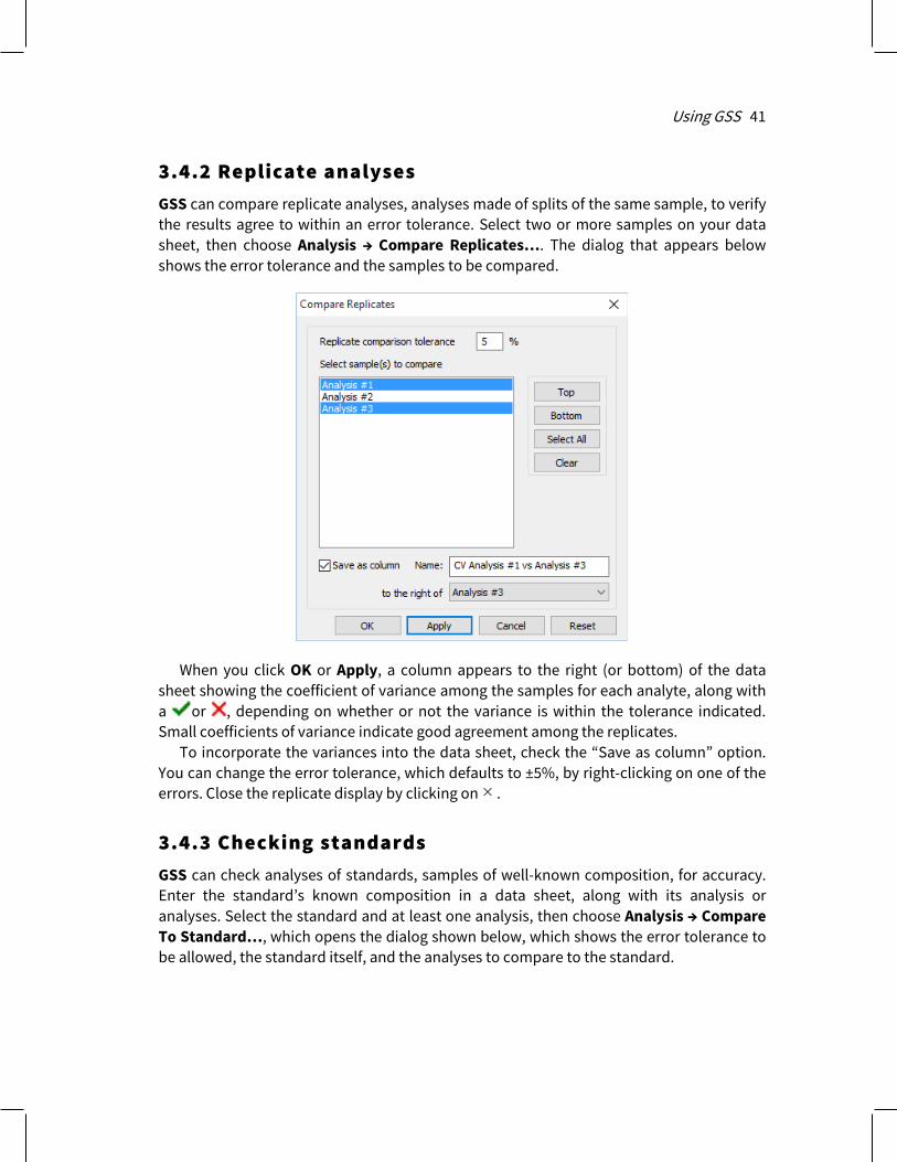
Using GSS 41

3.4.2 Replicate analyses GSS can compare replicate analyses, analyses made of splits of the same sample, to verify the results agree to within an error tolerance. Select two or more samples on your data sheet, then choose Analysis → Compare Replicates…. The dialog that appears below shows the error tolerance and the samples to be compared.

When you click OK or Apply, a column appears to the right (or bottom) of the data sheet showing the coefficient of variance among the samples for each analyte, along with a or , depending on whether or not the variance is within the tolerance indicated. Small coefficients of variance indicate good agreement among the replicates.

To incorporate the variances into the data sheet, check the “Save as column” option. You can change the error tolerance, which defaults to ±5%, by right-clicking on one of the errors. Close the replicate display by clicking on .

3.4.3 Checking standards GSS can check analyses of standards, samples of well-known composition, for accuracy. Enter the standard’s known composition in a data sheet, along with its analysis or analyses. Select the standard and at least one analysis, then choose Analysis → Compare To Standard…, which opens the dialog shown below, which shows the error tolerance to be allowed, the standard itself, and the analyses to compare to the standard.

42 GWB Essentials

When you click OK or Apply, a column appears to the right (or bottom) of the data sheet showing the average deviation, along with a or , depending on whether or not the deviation is within the tolerance indicated.

To incorporate the deviation results into the data sheet, check the “Save as column” option in the dialog box shown above. You can change the error tolerance by right-clicking on the error. Close the error display by clicking on .

3.4.4 Mixing samples GSS can show the results of mixing two or more water samples in any proportion using the values of the total components calculated using SpecE8. Choose Analysis → Mix Samples… to open the Smart Mix wizard, then select the samples to mix and click Next >. A dialog box with settings for the mixing calculations will pop up. These are the same settings you specify in the Data → Constraints dialog. Click OK to move on to the next step.

The wizard will list the Sample ID and the extent of the samples you’ve chosen to mix. GSS will mix samples volumetrically by default, but you can choose instead to mix samples gravimetrically by selecting “mass” from the “Mix by” pulldown. When the “equal proportions” option is checked, each sample will be assigned a value of 1 liter (or 1

Using GSS 43

kilogram of solution, if mixing by mass). By unchecking this option you can set values for samples individually. If you are mixing by mass and your spreadsheet includes values for the chemical parameter “Mass solution”, GSS will use those values. Otherwise, select a sample, set a value in the box, and click the Apply button, then repeat for the remaining samples. The Reset mixing button returns all settings to their defaults. Click Next > to move on to the next step.

GSS will test each sample for convergence and report success or failure before beginning the mixing calculations. You can click More info… to see the SpecE8 input and calculation results for failed samples. Check the “show successful samples” box to show input and results for all samples. If a sample fails to converge, the Next > button to move on to the next step will be disabled. You can click < Back to remove the unsuccessful sample from the mix, or click Close to check the values in the spreadsheet before restarting the Smart Mix wizard.

You can choose how GSS reports the extent of the mixed sample. If samples were mixed volumetrically, you can report the mixture’s total solution volume or scale the results to 1 liter of solution or solvent water. If samples were mixed by mass, you can report the total mass of the mixed fluid or scale the sample to 1 kilogram of solution or solvent water.

The composition of the mixture will appear to the right (or bottom) of the data sheet, showing the results for each analyte in the spreadsheet. Unlike GWB releases 9.0 and earlier, GWB11 will automatically calculate the values of certain parameters that are not conserved during mixing, such as pH. Close the mixture display by clicking on .

44 GWB Essentials

To work with the mixture as if it were a sample, select the “Save as sample” option in the dialog box shown above. The result of the mixing calculation is placed in the data sheet as a new sample to the right of the selected column (or below the selected row).

3.5 Launching SpecE8 and React You can use the chemical analyses in a GSS data sheet to set up and run SpecE8 or React calculations. These programs are described in the Using SpecE8 chapter in this guide and the Using React chapter in the GWB Reaction Modeling Guide.

Select one or more samples on the data sheet, then choose Analysis → Launch…. If a sample has “less than” (<0.001) values, 0 values, or hidden analytes, you can choose to omit them when generating the input.

You can add additional commands to the SpecE8 or React input script created by GSS. Header command lines will be inserted near the beginning, just after the thermo data is read. Trailer command lines will be added at the end of the script.

Using GSS 45

When you hit Apply or OK, GSS writes into the specified directory an input file for each sample you have selected. The input files are named (Root filename) + (Sample ID) + “.sp8” or “.rea”.

Unless you have selected “Save files only”, an instance of SpecE8 or React will be launched configured with the values in the first sample. If you have selected more than one sample, the program will do a batch run, writing the results to an output and plot file for each sample.

46 GWB Essentials

3.6 Graphing data GSS can call on Gtplot to diagram the data in your data sheet in a variety of ways. The Using Gtplot chapter describes in detail the Gtplot program and the types of plots it creates.

3.6.1 Series and time series plots To graph the entries in your data sheet as a series, sample by sample, select the analyte or analytes to plot and click on Graphs → Series Plot. In the Gtplot window that opens, the samples are arrayed along the x axis in the order they appear in your data sheet. To change which analytes are shown, or the axis units or data range, double-click on the y-axis label.

To associate markers or their colors or sizes with samples in the data sheet, rather than analytes, go to Edit → GSS Data…. To control whether the markers are connected by line segments, right-click on a marker and select or deselect “Connect Scatter Points”.

To change the marker representing an analyte or sample, click in GSS on the marker next to the analyte or sample name. Choose a symbol and its color and size, then click on Graphs → Update Graph(s).

To create a time series plot, make sure “Date”, “Time”, or “Time elapsed” appears as an analyte in the data sheet, then choose Graphs → Time Series Plot and proceed as above.

3.6.2 Cross plots To plot one analyte, or several, against another, select the analytes to appear in the diagram, then choose Graphs → XY Plot. To change which analytes appear on the x or y axis, or the units or data range for either, double-click in Gtplot on the axis label. Control the markers and which samples appear in the plot as you would with a series plot.

3.6.3 Ternary, Piper, and Durov diagrams To create a ternary (triangular) diagram, select in the data sheet three analytes to appear on the diagram axes, then choose Graphs → Ternary Diagram. Change the analytes appearing on the diagram axes or the axis units by double-clicking on the axis label.

To plot a Piper or Durov diagram, select Graphs → Piper Diagram or Durov Diagram. Control the markers and which samples appear in the plot as you would with a series plot.

In order to see TDS represented as circles on Piper, ternary, and Durov diagrams, add TDS as an analyte in the data sheet and enter a value for each sample. As described in the Calculating analytes section of this chapter, you may select → Calculate… or Data → Calculate… to add calculated TDS to the data sheet.

Using GSS 47

3.6.4 Other diagrams Create a Schoeller, Stiff, or radial diagram, or a bar or pie chart by selecting the sample you wish to represent and clicking on Graphs → Schoeller Diagram, Stiff Diagram, Radial Plot, Bar Chart, or Pie Chart. Choose to plot another sample by opening the appropriate dialog (Schoeller Diagram…, and so on) in Gtplot under the Plot pulldown.

3.6.5 Scatter data You can overlay the data entries in a GSS data sheet on any plot produced by the GWB applications, including activity diagrams made by Act2 and Tact, and plots of the results of reaction and reactive transport models from Gtplot and Xtplot.

To plot “scatter data,” first save your data sheet as a .gss file. In Act2, Tact, Gtplot, or Xtplot, read the .gss file by selecting File → Open → Scatter Data.... Data points representing each sample will appear on the plot if the .gss file contains analytes corresponding to the plot axes.

For details on plotting scatter data from .gss files, see the Using Act2, Using Tact, and Using Gtplot chapters in this guide, the Using Gtplot chapter in the GWB Reaction Modeling Guide, and the Using Xtplot chapter in the GWB Reactive Transport Modeling Guide.

Table 3.1 Keyboard shortcuts in GSS

Ctrl+A Select all cells in the data sheet

Ctrl+C Copy

Ctrl+D Select all data cells in the data sheet

Ctrl+F Find

F1 GWB Reference Manual

F3 Find next instance

Shift+F3 Find previous instance

Ctrl+L Check regulatory limits toggle

Ctrl+N Create new data sheet

Ctrl+Shift+N Open Notes… dialog

Ctrl+O Open an existing .gss file

Ctrl+P Print

48 GWB Essentials

Ctrl+Q Quit the program

Ctrl+Shift+R Restore the last data sheet configuration

Ctrl+S Save the current spreadsheet to a file

Ctrl+T Open a new thermo dataset

Ctrl+U Update graphs in Gtplot

Ctrl+V Paste

Ctrl+W Open a new water quality regulatory standards file

Ctrl+X Cut

Ctrl+Y Redo

Ctrl+Z Undo

Ctrl++ Zoom in

Ctrl+- Zoom out

Ctrl+Shift+Z Zoom 100%—to font size in Preferences…

49

Using Rxn

Rxn is a program that, among other things, automatically balances chemical reactions among minerals, dissolved species, and gases. The program is easy to use, and quite useful. To show the balanced reaction by which analcime dissolves to form aqueous species, for example, start the program and move to the Basis pane. Clicking on the entry (initially, it is “???”) under “balance reaction for”, select “Analcime” from the list of “Minerals”.

The Rxn window looks like this:

To see the balanced reaction, select Run → Go,

50 GWB Essentials

press the Run button on the Results pane, or type

The program gives the result

The species H+, Na+, etc. are members of the original basis set carried in the thermodynamic database (see Table 2.1).

You can change the basis to generate reactions in alternative forms. To see the reaction balanced in terms of quartz and albite in place of SiO2(aq) and Al+ + +, use the button to swap “Quartz” for “SiO2(aq)”, and “Albite” for “Al+++”.

react Analcime go

Using Rxn 51

Or type

The program gives the result

Rxn will calculate a reaction’s equilibrium constant at a temperature of interest whenever the temperature is given. To find the equilibrium constant for the above reaction at 250°C, set temperature on the Basis pane,

which gives the result log K = 0.3039. To unset the temperature, choose “reset” on the temperature pulldown menu, or type T = ?.

The program can calculate additional information, including a polynomial fit that gives log K as a function of temperature from 0°C to 300°C, the equilibrium equation for the reaction under various conditions, or the temperature at which a reaction is in equilibrium. To calculate additional information, put the program in “long” format by clicking on the button on the Results pane, or by typing the command long. Return to the original “short” format by clicking on the button, or typing short.

swap Quartz for SiO2(aq) swap Albite for Al+++ go

52 GWB Essentials

For example, unsetting temperature and setting long mode generates the response:

You can see that at equilibrium the water activity equals the reaction’s equilibrium constant. The water activity is likely to be 1 or less, but the equilibrium constant is greater than 1 over the temperature range. The minerals albite, quartz, and analcime are unlikely, then, to be in equilibrium between 0°C and 300°C.

If you set the water activity to unity on the Basis pane, or type

the program reports in the Results pane that analcime in the presence of quartz should react to form albite:

4.1 Balancing reactions Using basis swaps, you can balance any primary reaction. As an example of how Rxn balances reactions by basis swapping, consider the dissolution reaction of pyrite. Start on the Basis pane and under “balance reaction for”, select “???” → Mineral… → Pyrite.

(cont’d) a H2O = 1 go

Equilibrium equation: log K = 0 Reaction is not in equilibrium between 0 and 300 C Products favored over this temperature range

Using Rxn 53

The pane should look like this

Alternatively, type

Move to the Results pane and click Run to see the reaction

written in terms of the species in the original basis. Alternatively, you could write the reaction producing hydrogen instead of consuming

dissolved oxygen. Move back to the Basis pane, click on the button next to O2(aq), and select Aqueous… → H2(aq)

react Pyrite go

54 GWB Essentials

or type

which gives the result

Swapping dissolved H2S for the SO4–– ion (and unswapping the H2(aq))

or

gives the reaction written in terms of reduced sulfur

Finally, replacing oxygen in the basis with H2S(aq)

gives a dissolution reaction written in terms of SO4–– and H2S

that involves neither oxygen nor hydrogen.

(cont’d) swap H2(aq) for O2(aq) go

(cont’d) unswap H2(aq) swap H2S(aq) for SO4-- go

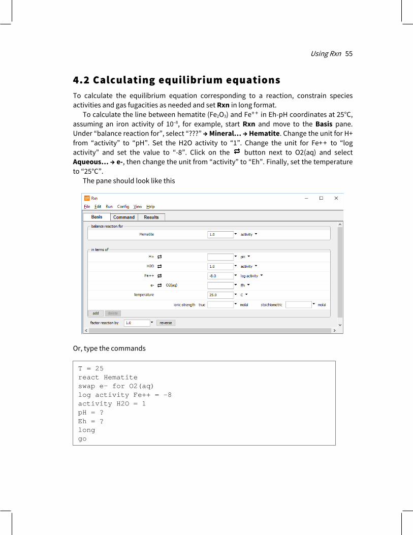
Using Rxn 55

4.2 Calculating equilibrium equations To calculate the equilibrium equation corresponding to a reaction, constrain species activities and gas fugacities as needed and set Rxn in long format.

To calculate the line between hematite (Fe2O3) and Fe+ + in Eh-pH coordinates at 25°C, assuming an iron activity of 10–8, for example, start Rxn and move to the Basis pane. Under “balance reaction for”, select “???” → Mineral… → Hematite. Change the unit for H+ from “activity” to “pH”. Set the H2O activity to “1”. Change the unit for Fe++ to “log activity” and set the value to “-8”. Click on the button next to O2(aq) and select Aqueous… → e-, then change the unit from “activity” to “Eh”. Finally, set the temperature to “25°C”.

The pane should look like this

Or, type the commands

T = 25 react Hematite swap e- for O2(aq) log activity Fe++ = -8 activity H2O = 1 pH = ? Eh = ? long go

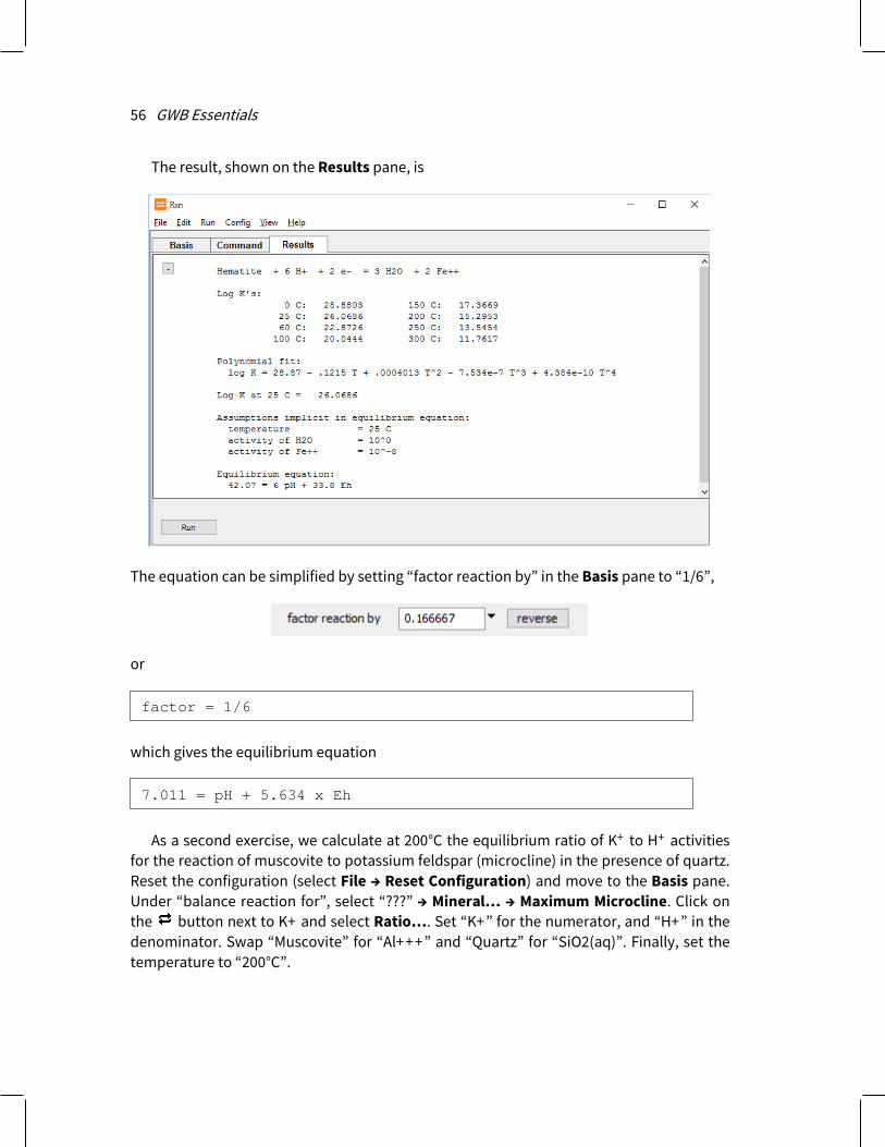
56 GWB Essentials

The result, shown on the Results pane, is

The equation can be simplified by setting “factor reaction by” in the Basis pane to “1/6”,

or

which gives the equilibrium equation

As a second exercise, we calculate at 200°C the equilibrium ratio of K+ to H+ activities for the reaction of muscovite to potassium feldspar (microcline) in the presence of quartz. Reset the configuration (select File → Reset Configuration) and move to the Basis pane. Under “balance reaction for”, select “???” → Mineral… → Maximum Microcline. Click on the button next to K+ and select Ratio…. Set “K+” for the numerator, and “H+” in the denominator. Swap “Muscovite” for “Al+++” and “Quartz” for “SiO2(aq)”. Finally, set the temperature to “200°C”.

factor = 1/6

7.011 = pH + 5.634 x Eh

Using Rxn 57

The pane should look like this

Alternatively, type the commands

T = 200 C react "Maximum Microcline" swap Muscovite for Al+++ swap Quartz for SiO2(aq) swap K+/H+ for K+ long go

58 GWB Essentials

Run the calculation and on the Results pane click for long format results.

Setting “factor reaction by” in the Basis pane to “3/2”

will simplify the result, giving the equilibrium activity ratio directly

at this temperature.

4.3 Determining activity coefficients You can use Rxn to calculate activity coefficients according to the Debye-Hückel theory (see discussion of activity coefficients in Activity coefficients under Using SpecE8). To do so, specify temperature and set solution ionic strength in molal units on the Basis pane, or use the ionic_strength (or I) command. To have Rxn calculate the activity of water, set the solution’s stoichiometric ionic strength on the Basis pane, or with the stoich_IS (or SI) command.

1.5 Maximum Microcline = K+/H+ + .5 Muscovite + 3 Quartz Equilibrium equation: 4.057 = log a[K+/H+]

Using Rxn 59

Start Rxn and move to the Basis pane. Under “balance reaction for”, select “???” → Mineral… → Barite. Set the temperature to “25°C”. Finally, set the ionic strength to “3 molal”. The pane should look like this

Alternatively, type the commands

Running the calculation causes the program to balance the reaction and report activity coefficients (“gammas”) for species Ba+ + and SO4

– – in a solution of 3 molal ionic strength at 25°C. The corresponding values, expressed directly instead of in exponential form, are 0.16 and 0.11.

react Barite T = 25 C I = 3 long go

60 GWB Essentials

On the Results pane, the program gives the equilibrium equation for the reaction.

Here, Rxn has used the calculated values for activity coefficients to simplify the equation, replacing activities with species molalities.

4.4 Calculating equilibrium temperatures Rxn can calculate the temperature (or temperatures) at which a reaction is in equilibrium if the activity of each species and fugacity of each gas in the reaction is known. To calculate the temperature at which gypsum converts to anhydrite, swap the two minerals into the basis and set the water activity.

Start Rxn and move to the Basis pane. Under “balance reaction for”, select “???” → Mineral… → Gypsum. Swap “Anhydrite” in for the “Ca++” and set the water activity to “1”.

Using Rxn 61

The pane should look like this

At unit water activity, the long format result is

To calculate the temperature at lower water activity (which might be appropriate for a brine), set the activity of water to “0.7”. The program gives the result

Rxn’s ability to calculate equilibrium temperatures can be useful for sorting among a mineral’s polymorphs to determine which is stable. For example, selecting Config → Show… and then selecting “Albite”, or typing

produces a list of minerals in the database that have the same chemical formula as albite, which are “Albite high” and “Albite low”.

Gypsum = Anhydrite + 2 H2O Reaction is in equilibrium at 43.7° C Products favored above this temperature

Reaction is in equilibrium at 11.8° C Products favored above this temperature

polymorphs Albite

62 GWB Essentials

The steps

generate the information that high albite is the unstable form from 0°C to 300°C.

4.5 Free energy change When you set a temperature and constrain a reaction sufficiently that either the reactants or reaction products are favored thermodynamically, Rxn will report the corresponding free energy change of reaction.

Set Rxn to balance the reaction for the dismutation of acetate ion at 25°C, assuming bicarbonate is present at mmol/kg, and acetate and methane at 𝜇𝜇mol/kg levels.

Start Rxn and move to the Basis pane. Under “balance reaction for”, select “???” → Aqueous… → CH3COO- and set its log activity to “-6”. Swap “CH4(aq)” for the “O2(aq)” and set its log activity to “-6”. Set the log activity of HCO3- to “-3” and the water activity to “1”. Finally, set the temperature to “25°C”.

The pane should look like this

react Albite swap “Albite high” for Al+++ long go

Using Rxn 63

On the Results pane, the program reports the acetoclastis reaction

along with the result that the reaction has a modest thermodynamic drive to proceed forward.

4.6 Sorption reactions Rxn manipulates the reactions by which ions sorb to a mineral in the same way it handles other types of reactions. Access a dataset of surface reactions by selecting File → Open → Sorbing Surfaces… and then clicking on , or with the surface_data(surf_data) command. Once entered, you can view the surface sites and complexes byselecting Config → Show…, or typing show surfaces.

4.6.1 Surface complexation For the two-layer surface complexation model, read a dataset of complexation reactions, such as “FeOH.sdat” supplied with the GWB. To load the surface dataset, go to File → Open → Sorbing Surfaces…, select , navigate to the FeOH.sdat file, and click Open to load it into Rxn.

Move to the Basis pane. Under “balance reaction for” select “???”→ Surface species… → >(s)FeOPb+. Set the units for “H+” to “pH”.

64 GWB Essentials

The pane should look like this

On the Results pane, Rxn will report the reaction

and its corresponding equilibrium equation

The second term in the equation is the logarithm of the Boltzman factor, which accounts for electrostatic forces between the surface and solution. Here, F is the Faraday constant, PSI is mean surface potential, R is the gas constant, and T is absolute temperature; m represents molal concentration.

Rxn will evaluate the Boltzman factor numerically if you specify temperature and ionic strength (on the Basis pane), and the charge density on the sorbing surface. Provide the latter value on the Sorbing Surfaces… dialog (File → Open → Sorbing Surfaces…) with a constant charge value, or with the surface_charge (or surf_charge) command, in units of 𝜇𝜇C/cm2. Set the temperature to “25°C”, the ionic strength to “0.1”, and the constant charge to “-10.0 𝜇𝜇C/cm2”.

>(s)FeOPb+ + H+ = >(s)FeOH + Pb++

log K + (F PSI[HFO]/2.303 RT) = - log m[>(s)FeOPb+] + log m[>(s)FeOH] + pH + log a[Pb++]

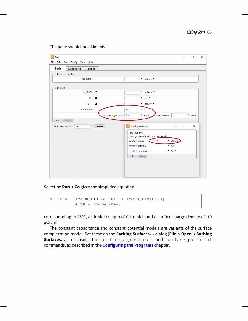
Using Rxn 65

The pane should look like this

Selecting Run → Go gives the simplified equation

corresponding to 25°C, an ionic strength of 0.1 molal, and a surface charge density of -10 𝜇𝜇C/cm2.

The constant capacitance and constant potential models are variants of the surface complexation model. Set these on the Sorbing Surfaces… dialog (File → Open → Sorbing Surfaces…), or using the surface_capacitance and surface_potential commands, as described in the Configuring the Programs chapter.

-5.706 = - log m[>(s)FeOPb+] + log m[>(s)FeOH] + pH + log m[Pb++]

66 GWB Essentials

4.6.2 Ion exchange As described in the Configuring the Programs chapter, you can model ion exchange in two ways. The first method is to swap an activity ratio into the basis. This method is equivalent to assuming that there exists a sufficiently large reservoir of exchanging ions that the composition of the exchanging surface remains invariant.

For a more general treatment, prepare a small dataset of exchange reactions using the file “IonEx.sdat” as a template. Load a dataset of exchange reactions by selecting File → Open → Sorbing Surfaces…, or with the surface_data (or read) command. The exchange reactions in this dataset are now available to your Rxn session.

You can load one or more exchange datasets (containing one or more exchange reactions) at a time, and in a single run combine ion exchange datasets with other types of surface reaction datasets.

4.6.3 Distribution coefficients (Kd) To use distribution coefficients (Kd) to model sorption, prepare one or more datasets containing the sorption reactions and corresponding distribution coefficients using the file “Kd.sdat” as a template (see the Configuring the Programs chapter). As with any sorption model, read the dataset(s) by selecting File → Open → Sorbing Surfaces…, or using the surface_data command. Once the dataset(s) has been read, the sorption reactions they contain are available to your Rxn session.

In the distribution coefficient model, the concentration of a sorbed ion is carried in units of moles per gram solid. If you wish to constrain the sorbed concentration of an ion in Rxn, do so in units of mol/g using the sorbed_mass (rather than the molality) command.

4.6.4 Freundlich isotherms The use of Freundlich isotherms is broadly similar in implementation to the Kd approach, as described in the previous section, except the dataset of surface reactions follows the format of “Freundlich.sdat”, rather than “Kd.sdat”.

4.6.5 Langmuir isotherms To model sorption according to Langmuir isotherms, prepare a dataset containing the sorption reactions in the format of dataset “Langmuir.sdat”.

Enter the dataset into an Rxn run by selecting File → Open → Sorbing Surfaces…, or with the surface_data (or read) command. You can enter one or more Langmuir datasets, and mix Langmuir datasets with datasets for other sorption methods.

Using Rxn 67

4.7 Rxn command line You can start Rxn by clicking the icon under the “Start” menu, opening a “.rxn” file, or entering the command rxn.exe from the Windows “Command Prompt.”

When you start Rxn from the command line (as opposed to clicking on the icon), you can specify a number of arguments. For example, the command

causes Rxn to read input commands from a file “my_script”, and to use “my_thermo.tdat” as the thermodynamic database.

The following options are available from the command line: -cd Change the working directory to the directory containing

the input script specified with the –i option.

-nocd Do not change the working directory.

-i <input_script> Set a file from which to read input commands.

-gtd <gtdata_dir> Set directory to search for thermodynamic datasets.

-d <thermo_data> Set the thermodynamic dataset.

-s <surface_data> Set a dataset of surface sorption reactions.

-append Keep previous results of the “block” command on the clipboard.

-main species Set the species to appear on the left side of the reaction.

-short | -long Set the output to be written in concise or detailed format.

rxn –i my_script –d my_thermo.tdat

69

Using Act2

Act2 is a program that calculates and plots activity-activity diagrams. This class of diagrams shows the stability of minerals and the predominance of aqueous species in chemical systems. A species activity, gas fugacity, activity or fugacity ratio, pH, Eh, or pe may serve as an axis variable.

To diagram the effects of pH and the activity of dissolved oxygen on the speciation of uranium in water, for example, start the program and select “U++++” under “diagram species”. To do so, click on the current setting, initially “???”, to show the choice of basis entries available to diagram (remember that pressing U moves down the list to “U++++”). To the right, change the units by selecting “log activity”, then enter “-10” for the species’ log activity.

In the box below, select “H+” for the x-axis species, and “O2(aq)” for the y axis. Then set “pH” as the unit for the x axis and adjust the y-axis range. The Basis pane should look like this:

70 GWB Essentials

Alternatively, enter the commands

Here we have set a uranium activity of 10–10 and, by default, a temperature of 25°C. Specify axis ranges in terms of the logarithms of activity or fugacity values, and linearly in terms of pH, pe, and Eh. Move to the Plot pane to display the result.

The program produces a file “Act2_output.txt” describing the calculation (select File → View → Act2_output.txt to inspect this dataset) and displays the diagram on the Plot pane. The figure below shows the resulting plot, a redox-pH diagram for uranium plotted against the activity of dissolved oxygen. Dashed lines show stability limits for water at 1 atm pressure. (Note that many of the figures in the User’s Guide have been simplified slightly or relabeled to allow for reduction and printing.)

You can return to the Basis or Command pane to alter the program configuration and produce further diagrams.

diagram U++++ on O2(aq) vs pH log a U++++ = -10 x from 0 to 14; y from -90 to 0 go

Using Act2 71

To plot the fugacity of oxygen gas along the vertical axis on the diagram we just calculated, move to the Basis pane and swap the gas species into the basis by clicking on the next to the y-axis entry and selecting Gas… → O2(g). The pane should look like this

Alternatively, enter the commands

(cont’d) swap O2(g) for O2(aq) y from -90 to 0 go

72 GWB Essentials

Move to the Plot pane to view the diagram. The figure below shows the results, a redox-pH diagram for uranium plotted against the fugacity of oxygen gas.

Swapping the electron into the basis allows you to plot oxidation state in terms of Eh. On the Basis pane, swap Aqueous… → e- for O2(aq), and set units of “Eh”.

Using Act2 73

The pane should look like this

Equivalent commands are

Move to the Plot pane to view the diagram.

(cont’d) swap e- for O2(aq) diagram on Eh y from -.75 to 1.25 go

74 GWB Essentials

The figure below shows the results for the redox-pH diagram plotted against Eh.

The oxidation state can be also represented in terms of the log activity ratio of a redox pair such as ferrous and ferric iron. On the Basis pane, click on next to the y-axis entry and select Ratio…. Set “Fe+++” with a power of “1” as the numerator species, and “Fe++” with the same power in the denominator:

Using Act2 75

To the right of this entry in the Basis pane, set the axis to range from “-25” to “5”. The pane should look like this

Alternate commands are

(cont’d) swap Fe+++/Fe++ for O2(aq) y from -25 to 5 go

76 GWB Essentials

Move to the Plot pane to view the diagram. The figure below shows the results for the redox-pH diagram plotted against the activity ratio of Fe+ + + to Fe+ +.

In calculating a diagram, Act2 balances each reaction possible among the aqueous species and minerals in the system and lists them along with their equilibrium equations in the “Act2_output.txt” dataset.

5.1 Diagram calculation The most familiar class of activity-activity diagram is the redox-pH, but Act2 can calculate diagrams on any activity or fugacity axis, as well as diagrams that account for the presence of minerals, complexing species, and gas buffers.

To evaluate the effect at 60°C of chloride complexing on copper at a CO2 fugacity of 1, for example, you could set the Cl– activity and CO2 fugacity in your input.

Under “diagram species”, click on “???” and select “Cu+”. Change “activity” to “log activity” and set the value to “-6”.

In the box below, select “H+” for the x-axis species, and “O2(aq)” for the y axis. Then select “pH” as the unit for the x axis and set the y-axis range from “-80” to “0”.

Using Act2 77

Under “in the presence of”, click and select “HCO3-”, then click on the button next to it and select Gas… → CO2(g). Set the fugacity to “1”. Next, click and select “Cl-”, then set its value to “.1”. Finally, set temperature to “60°C”.

The Basis pane should look like this:

Or, use the commands

Move to the Plot pane to view the diagram.

T = 60 diagram Cu+ on O2(aq) vs pH x from 0 to 14 y from -80 to 0 swap CO2(g) for HCO3- log a Cu+ = -6 a Cl- = 0.1 f CO2(g) = 1 go

78 GWB Essentials

The figure below shows the activity-activity diagram drawn at 60°C for the copper-CO2-chlorine system at fCO2 = 1 versus oxygen activity and pH at aCl- = .1:

Note the implausibility of maintaining in nature this CO2 fugacity under alkaline conditions.

The effect might be shown better by drawing the diagram at a pH of 6 using the activity of Cl– as an axis. Return to the Basis pane and click on “H+”, then select “Cl-” to take its place as the x-axis species. Set the log activity to range from “-3” to “.5”. Finally, note that “H+” has been automatically shifted to the “in the presence of” section with “pH” units. Set the value to “6”.

Using Act2 79

The pane should look like this

Move to the Plot pane to view the diagram. The figure below shows the activity-activity diagram drawn at 60°C for the copper-CO2-chlorine system at fCO2 = 1 versus oxygen activity and aCl- at pH = 6.

80 GWB Essentials

A number of simple aluminosilicate minerals can be formed from kaolinite by exchanging cations for protons and adding or removing silica. The diagram defined by the following steps shows the stability of potassic and calcic aluminosilicates in the presence of quartz.

Reset the configuration (select File → Reset Configuration) and move to the Basis pane. Under “diagram species”, set “Al+++” and then Mineral… → Kaolinite.

On the x axis, select “Ca++” and then Ratio…. Set “Ca++” for the numerator and “H+” squared in the denominator with an exponent of “2”. Set the range from “12” to “20”. On the y axis, select “K+” and then Ratio…. Set “K+” for the numerator and “H+” in the denominator. Set the range from “2” to “10”.

Under “in the presence of”, click and select “SiO2(aq)”, then Mineral… → Quartz. The Basis pane should look like this

Or configure the diagram by the commands

swap Kaolinite for Al+++ swap Quartz for SiO2(aq) swap K+/H+ for K+ swap Ca++/H+^2 for Ca++ diagram Kaolinite on K+/H+ vs Ca++/H+^2 x 12 20; y 2 10 go

Using Act2 81

Move to the Plot pane to view the diagram. The figure below shows the stability diagram for aluminosilicate minerals at 25°C plotted versus aK+/aH+ and aCa++/aH+

2 in the presence of quartz.

12 13 14 15 16 17 18 19 202

3

4

5

6

7

8

9

10

log a Ca++/H+^2

log

a K+ /H

+

Grossular

KaoliniteLaumontite

Maximum Microcline

Muscovite Prehnite

25°C

82 GWB Essentials

To show the effect of varying the silica activity, replace the x axis with aSiO2 (aq). Return to the Basis pane and next to “Quartz” click Unswap. Next, click on “Ca++/H+^2” on the x axis and select “SiO2(aq)” to take its place. Set the x axis to range from “-5” to “-2”. Next, set the y axis to range from “-5” to “10”. Finally, move to the “in the presence of” section and select “Ca++/H+^2”, then press delete. The pane should look like this

Or use the commands

(cont’d) unswap Quartz diagram vs SiO2(aq) remove Ca++/H+^2 x -5 -2; y -5 10 go

Using Act2 83

Move to the Plot pane to view the diagram. The figure below shows the stability diagram for aluminosilicate minerals at 25°C plotted versus aK+/aH+ and aSiO2 (aq) in the presence of quartz.

–5 –4.5 –4 –3.5 –3 –2.5 –2

–4

–2

0

2

4

6

8

10

log a SiO2(aq)

log

a K+ /H

+

Clinoptil-K

GibbsiteKaolinite

Maximum Microcline

Muscovite

Pyrophyllite

25°C

84 GWB Essentials

5.2 Solubility diagrams Solubility diagrams are similar to the diagrams calculated to this point, except that the activity of the main species, instead of being set to a constant value, appears as an axis variable.

To calculate the solubility of U+ + + + versus pH, for example, move to the Basis pane and under “diagram species”, select “U++++”. Leave the activity blank. Under “on axes”, set “H+” and units of “pH” for x. For the y axis, select “U++++” and set a range from “-16” to “-6”.

The Basis pane should look like this

An alternate method would be

diagram U++++ on U++++ vs pH x from 0 to 14 y from -16 to -6 go

Using Act2 85

Move to the Plot pane to view your diagram. The figure below shows the solubility diagram for uraninite versus pH at 25°C:

You can similarly take steps to draw a diagram showing the solubility of Al+ + + as a function of pH at 60°C in the presence of quartz. Reset the configuration (select File → Reset Configuration) and move to the Basis pane. Under “diagram species”, select “Al+++”. Leave the activity blank. Under “on axes”, set “H+” and units of “pH” for x. Set the range from “3” to “8”. For the y axis, select “Al+++” and set a range from “-8” to “-5”.

0 2 4 6 8 10 12 14–16

–15

–14

–13

–12

–11

–10

–9

–8

–7

–6

pH

log

a U++

++

U++++

U(OH)2++

U(OH)3+

U(OH)4

U(OH)5–

UOH+++

Uraninite

25°C

86 GWB Essentials

Under “in the presence of”, click and select “SiO2(aq)”, then Mineral… → Quartz. Set temperature to “60°C”. The pane should look like this

Move to the Plot pane to view the diagram, which is shown below.

3 3.5 4 4.5 5 5.5 6 6.5 7 7.5 8–8

–7.5

–7

–6.5

–6

–5.5

–5

pH

log

a Al

+++

Al+++

Al(OH)2+

Al(OH)3

Al(OH)4–

AlOH++

Kaolinite

60°C

Using Act2 87

5.3 Mosaic diagrams Calculating diagrams that include complexing ions is complicated in some cases by the speciation of the ions over the diagram axes. For example, while the bicarbonate ion HCO3

– is important at moderate pH values, it reacts under acidic conditions to form CO2(aq), and under alkaline conditions to form CO3

– – . Similarly, the sulfate ion SO4– – occurs in acidic

waters as HSO4– and under reducing conditions as H2S(aq), HS–, and S––; NO3

– is found in the reduced forms HNO2, NO2

– , N2, NH4+, and NH3; and HPO4

– – reacts depending on pH to form H3PO4, H2PO4

– , and PO4– – – .

In such cases, Act2 can calculate mosaic diagrams in which the overall calculation is divided into subdiagrams, in which a single form of a complexing species predominates in each. Assembled, the subdiagrams form the complete diagram. The program allows any number of complexing ions to speciate. Each ion may speciate by reaction with the species on both of the axes, or the x axis or y axis alone.

Set a mosaic diagram by adding a species to the diagram using the button on the Basis pane in the “in the presence of” section. Then, under the corresponding units pulldown, select to speciate that species over x, y, or both x and y. Alternatively, you can use the speciate command.

The following example, using the chemistry of the arsenic-sulfur system, shows the importance of the mosaic diagram. Move to the Basis pane and, under “diagram species”, select “As(OH)4-”. Set the log activity to “-3”. Under “on axes”, set “H+” and units of “pH” for x. For the y axis, select “O2(aq)” and set a range from “-70” to “-40”.

Under “in the presence of”, click and select “SO4--”. Set log activity to “-4”, then click the pulldown next to log activity and select “speciates over x-y”. Set temperature to “100°C”.

88 GWB Essentials

The pane should look like this

Or use the commands

T = 100 C diagram As(OH)4- on O2(aq) vs pH x from 0 to 14 y from -70 to -40 log a As(OH)4- = -3 log a SO4-- = -4 speciate SO4-- go

Using Act2 89

Move to the Plot pane to view the diagram. The figure below shows a diagram predicting the importance of the sulfide minerals orpiment (As2S3) and realgar (AsS) under reducing conditions.

Interior broken lines show mosaic boundaries for sulfur speciation. Subdiagrams in the mosaic, from upper left to lower right, are for the species HSO4

– , SO4– – , H2S(aq), HS–, and

S– –. The basal broken line (black) is the stability limit for water under reducing conditions at 1 atm pressure.

Note that if we had not made a mosaic diagram but had instead assumed that SO4– – or

HS– predominates over the entire diagram, the result would be significantly in error. To test the first variation, click the pulldown next to log activity and select “speciates

over x-y” once again to disable the option. The pane should look like

You could also type

0 2 4 6 8 10 12 14–70

–65

–60

–55

–50

–45

–40

pH

log

a O

2(aq

)

As(OH)4–

AsO4---

As(OH)3

AsO2OH--

H2AsO4–

HAsO4--

Orpiment

Realgar

100°C

(cont’d) unspeciate SO4— go

90 GWB Essentials

To test the second case, click the button next to “SO4--” and choose Aqueous… → HS-, as shown below,

or type

5.4 Editing plot appearance In Act2 you can interactively modify many aspects of the diagram. A right-click on an aspect or area of the plot displays a menu showing the options available. You may choose to reset an axis range or an aspect’s appearance to its default state. A double-click on an aspect brings up a dialog box related to the first item on the pulldown menu, which in most cases is the aspect’s appearance dialog. The dialogs can also be accessed through the Plot menu. To change the font for individual aspects, choose Font from that aspect’s menu. A double-click on the background area will bring up the View… dialog, which lets you select the graphical elements to be shown.

(cont’d) swap HS- for SO4-- go

Right-click on plot background

Right-click on plot interior

Double-click background to show View dialog

Using Act2 91

A left-click on an aspect causes it to be “selected”. An aspect has been selected when its color changes, as in the case of lines, or when it is surrounded by manipulation handles, in the case of text or markers. Change the size of text, markers, and the plot itself

Right-click text to show menu options

Right-click line to show menu options

92 GWB Essentials

by dragging the sizing cursors. Adjust the placement of the plot by clicking within the plot or on either axis and dragging it. The plot title can be moved in the same way.

You can change the range on an axis by clicking and dragging a tick mark, number, or grid line. Dragging a tick within an axis shifts all of the values along the axis, effectively changing the minimum and maximum values at the ends of the axis, but keeping the spacing the same. Dragging the tick at an end of an axis changes the minimum or maximum value. To reset the axis range to span the range of the data being plotted, choose Reset Axis Range from the aspect menu.

Left-click title and drag to reposition Left-click edge and

drag to resize plot

Left-click to select; drag handle to resize

Left-click axis and drag to move plot

Left-click axis and drag to move plot

Drag inner tick, number, or grid line to shift axis range

Drag outer tick, number, or grid line to scale axis range

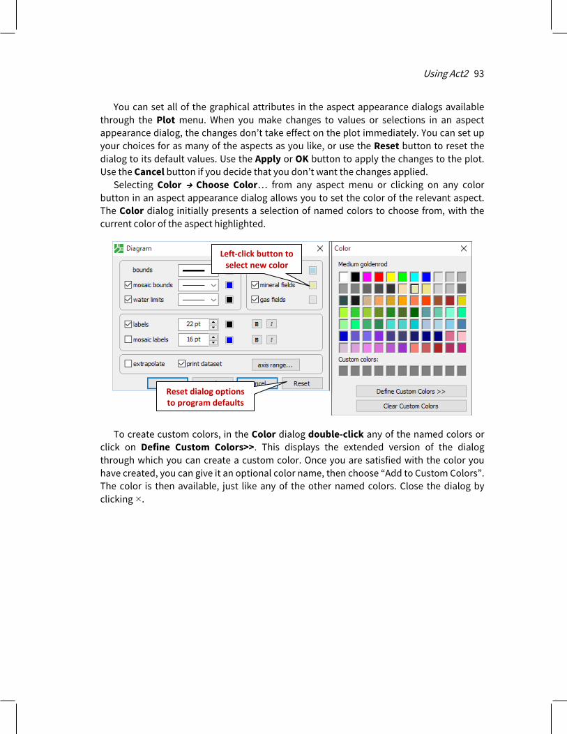
Using Act2 93

You can set all of the graphical attributes in the aspect appearance dialogs available through the Plot menu. When you make changes to values or selections in an aspect appearance dialog, the changes don’t take effect on the plot immediately. You can set up your choices for as many of the aspects as you like, or use the Reset button to reset the dialog to its default values. Use the Apply or OK button to apply the changes to the plot. Use the Cancel button if you decide that you don’t want the changes applied.

Selecting Color → Choose Color… from any aspect menu or clicking on any color button in an aspect appearance dialog allows you to set the color of the relevant aspect. The Color dialog initially presents a selection of named colors to choose from, with the current color of the aspect highlighted.

To create custom colors, in the Color dialog double-click any of the named colors or click on Define Custom Colors>>. This displays the extended version of the dialog through which you can create a custom color. Once you are satisfied with the color you have created, you can give it an optional color name, then choose “Add to Custom Colors”. The color is then available, just like any of the other named colors. Close the dialog by clicking .

Left-click button to select new color

Reset dialog options to program defaults

94 GWB Essentials

5.5 Reaction traces Act2 can overlay onto a diagram the trace of a reaction path calculated with the React program. To project the trace of a reaction, first use React, as described in Using React in the GWB Reaction Modeling Guide, to calculate the reaction path. React produces an output dataset “React_plot.gtp”, which Act2 can read.

Within Act2, select File → Open → Reaction Trace… to select a “.gtp” file produced by a previous React run. To change the default line width, colors, and size (in points) of the markers on the trace, use the Trace… dialog from the Plot pulldown menu.

5.6 Scatter data You can overlay the data points in a GSS data sheet (a .gss file) as “scatter data” on your Act2 diagram. First, check that the .gss file contains the axis variables on your diagram (pH, Eh, pe, species activity, or gas fugacity) or the activities of the original basis entries in the thermo dataset, so Act2 can figure these values. Act2 can figure an activity ratio from the activity of individual species in your .gss file.

Remember that Act2 diagrams are plotted in terms of species’ activities and fugacities, not chemical concentrations. You can quickly add activities and fugacities to your .gss files as “calculated analytes,” as described in the Calculating analytes section of the Using GSS chapter in this guide. Alternatively, you can add user-defined analytes for species’ activities, fugacities, or activity ratios when these values are known. See the User defined analytes section of the Using GSS chapter in this guide for more information. For an activity ratio such as aCa++/aH+

2 , choose the user-defined analyte category “Species

Using Act2 95

activities”, and write the analyte’s name as Ca++/H+^2 to match its appearance on the activity diagram.

Even if your data sheet contains O2(aq) concentration in mg/kg, for example, it would have to also include the activity of O2(aq) in order for the data to appear on a log a O2-pH diagram. Add O2(aq) activity to your data sheet as a calculated analyte, separate from the dissolved oxygen measurements.

An example of a .gss dataset containing Act2 scatter data is

To read a .gss file into Act2, click on File → Open → Scatter Data…. The program will read the data points and project them onto the diagram. Clear scatter data from a diagram on the Open → Scatter Data… dialog, with the OFF button.

The marker representing each sample in the scatter data is set in the .gss file. In GSS, right-click on a sample to change the marker used and its color and size. When you modify a .gss file, you must save it and reload it in Act2, using the Open dialog or scatter command, to see the changes. To add error bars to the scatter points, enter triplets (0.5|2.0|3.5) in the data cells (see Error bars in Using GSS).

You can label each data point with the sample’s “Sample ID”, as set in the .gss file, and display a legend showing the symbols used. In Act2, choose Plot → GSS Data… and under “Labels” select the checkbox for “Sample” to show sample labels, and the “Legend” box to display the legend. Use the Plot → View… dialog to quickly toggle on and off display of the scatter data, data labels, and legend.

96 GWB Essentials

In GWB releases 7.0 and earlier, the program took scatter data from a specially formatted text file, rather than a .gss data sheet. Legacy scatter files are still supported and described in the Scatter Data appendix in the GWB Reference Manual.

5.7 Act2 command line You can start Act2 by clicking the icon under the “Start” menu, opening a “.ac2” file, or entering the command act2.exe in the Windows “Command Prompt.”

When you start Act2 from the command line (as opposed to clicking on the icon), you can specify a number of arguments. For example, the command

causes Act2 to read input commands from a file “my_script”, and to use “my_thermo.tdat” as the thermodynamic database.

The following options are available from the command line: -cd Change the working directory to the directory containing

the input script specified with the –i option.

-nocd Do not change the working directory.

-i <input_script> Set a file from which to read input commands.

-gtd <gtdata_dir> Set directory to search for thermodynamic datasets.

-d <thermo_data> Set the thermodynamic dataset.

act2 –i my_script –d my_thermo.tdat

97

Using Tact

Tact is a program that calculates and plots temperature-activity and temperature-fugacity diagrams. Diagrams of this type show the effect of temperature on the stability of minerals and the predominance of aqueous species in chemical systems. Tact is very similar to Act2, except that the vertical axis represents temperature instead of an activity or fugacity.

To diagram, for example, the thermal stability of phosphate species versus pH, you follow the same steps you would use in Act2, except that you need not specify a variable for the y axis. Under “diagram species” on the Basis pane, click on “???” (or any species already there), select “HPO4--”, and then set the species’ log activity to “-3”. Under “on axes”, click on “???”, choose “H+” and set units to “pH”. The Basis pane should look like this:

Alternatively, enter the commands

diagram HPO4-- vs pH a HPO4-- = 10^-3 x from 0 to 14 go

98 GWB Essentials

on the Command pane. Now move to the Plot pane to display the resulting diagram, which shows the predominance of phosphate species versus temperature and pH.

The program also produces text output in dataset “Tact_output.txt” (click on File → View → Tact_output.txt).

6.1 Diagram calculation Tact, like Act2, can assume any activity or fugacity variable on the x axis and can account for the presence of minerals, complexing species, and gas buffers. You might, for example, calculate the stabilities of aluminosilicate minerals versus SiO2(aq) activity in a system of known ratios aCa++/aH+

2 and aK+/aH+. To start, move to the Basis pane. Under “diagram species”, set “Al+++” and then

Mineral… → Kaolinite. On the x axis, select “SiO2(aq)” and then set the range from “-4.5” to “-1.5”. Set the y-

axis range from “0” to “200”. Under “in the presence of”, click and select “Ca++”, then click on Ratio….

Set “Ca++” for the numerator and “H+” squared in the denominator with an exponent of “2”. Change the unit to “log ratio” and set the value to “10.5”.

Using Tact 99

Next, click and select “K+”, then click on Ratio…. Set “K+” for the numerator and “H+” in the denominator. Change the unit to “log ratio” and set the value to “3.5”.

The Basis pane should look like this

Alternative steps are

swap Kaolinite for Al+++ swap Ca++/H+^2 for Ca++ swap K+/H+ for K+ diagram Kaolinite vs SiO2(aq) log ratio Ca++/H+^2 = 10.5 log ratio K+/H+ = 3.5 x from -4.5 to -1.5 incr 1/2 y from 0 to 200 go

100 GWB Essentials

Move to the Plot pane to view the diagram of the stability of aluminosilicate minerals versus aSiO2 (aq), assuming aK+/aH+ = 103.5 and aCa++/aH+

2 = 1010.5.

To diagram the same system with the SiO2(aq) activity fixed by equilibrium with tridymite, and the aCa++/aH+

2 ratio as the axis variable, return to the Basis pane. Move to the “in the presence of” section and select “Ca++/H+^2”, then press delete. Under “on axes”, click on “SiO2(aq)” and select “Ca++” from the pulldown to take its place, then click

Ratio. Set “Ca++” for the numerator and “H+” squared in the denominator with an exponent of “2”. Set the x axis to range from “8” to “16”.

Using Tact 101

Now that “SiO2(aq)” has been automatically transferred to the “in the presence of” section, select Mineral → Tridymite. The pane should look like this

Or type the commands

(cont’d) diagram vs Ca++/H+^2 swap Tridymite for SiO2(aq) x from 8 to 16

102 GWB Essentials

Move to the Plot pane to view the diagram. The resulting diagram is shown here.

As a second exercise, diagram the equilibrium point of the souring reaction of natural gas

Anhydrite + CH4(g) → Calcite + H2O + H2S(g) (6.1)

in terms of the fugacity ratio of methane to H2S. Reset the configuration (select File → Reset Configuration) and move to the Basis pane. Under “diagram species”, set “Ca++” and then Mineral… → Calcite.

On the x axis, select “SO4--” and then Ratio…. Set “H2S(g)” for the numerator and “CH4(g)” in the denominator. Set the range from “-15” to “10”.

Using Tact 103

The Basis pane should look like this

Or use the commands

swap Calcite for Ca++ swap H2S(g)/CH4(g) for SO4-- diagram Calcite vs H2S(g)/CH4(g) x from -15 to 10 go

104 GWB Essentials

Move to the Plot pane to view the diagram, which shows the equilibrium point of the methane souring reaction, calculated as a function of temperature.

6.2 Solubility diagrams To construct a solubility diagram, specify the main species as the x-axis variable. To plot the solubility of quartz (in terms of SiO2 activity), for example, set “SiO2(aq)” under “diagram species”, and then again under “on axes” as the x-axis variable. Set the log activity to range from “-5” to “-1”.

Using Tact 105

The pane should look like

Alternatively, use the commands

Move to the Plot pane to view the diagram. If you suppress quartz using the Config → Suppress… dialog

diagram SiO2(aq) vs SiO2(aq) x from -5 to -1 go

106 GWB Essentials

or by typing

the resulting diagram shows the solubility of the next most stable polymorph, tridymite (and a small field for chalcedony at high temperature). Continuing this cycle produces plots of the solubilities of each of the silica polymorphs. The figure below shows a composite of five Tact diagrams.

–5 –4.5 –4 –3.5 –3 –2.5 –2 –1.5 –10

50

100

150

200

250

300

log a SiO2(aq)

T (°

C)

Quartz

Tridymite

Chalcedony

Cristobalite

Amorphous silica

(cont’d) suppress Quartz go

Using Tact 107

6.3 Mosaic diagrams Tact, like Act2, can consider complexing ions that speciate over the diagram axes. To calculate the stable forms of uranium versus pH in the presence of dissolved phosphate, for example, Tact must first consider the speciation of the phosphate ion, which has already been calculated (see the example in section 6.1).

Under “diagram species”, set “U++++” and change the unit from “activity” to “log activity”. Set the value to “-10”.

On the x axis, select “H+” and set units to “pH”. Under “in the presence of”, click and select “HPO4-”. Set log activity to “-3”, then click on the pulldown next to log activity and select “speciates over x”. The Basis pane should look like this

The commands are

diagram U++++ vs pH x from 0 to 14 log a U++++ = -10 log a HPO4-- = -3 speciate HPO4-- go

108 GWB Essentials

Move to the Plot pane to view the mosaic diagram of the uranium-phosphate system versus temperature and pH.

Subdiagrams in mosaic, from upper left to lower right, are for H3P2O7– , H2P2O7

– , H2PO4– ,

HPO4– – , and PO4

– – – .

6.4 Editing plot appearance Tact, like Act2, allows you to interactively modify many aspects of the diagram. The details of using active items, aspect menus, and dialogs to edit the plot appearance are given in the Using Act2 section of this guide.

6.5 Reaction traces and scatter plots Tact, like Act2, can project reaction traces and scatter data onto a diagram. These features are especially useful for displaying polythermal reaction paths or datasets. The details of constructing such plots are given in the Using Act2 section of this guide.

Using Tact 109

6.6 Tact command line You can start Tact by clicking the icon under the “Start” menu, opening a “.tac” file, or entering the command tact.exe from the Windows “Command Prompt.”

When you start Tact from the command line (as opposed to clicking on the icon), you can specify a number of arguments. For example, the command

causes Tact to read input commands from a file “my_script”, and to use “my_thermo.tdat” as the thermodynamic database.

The following options are available from the command line: -cd Change the working directory to the directory containing

the input script specified with the –i option.

-nocd Do not change the working directory.

-i <input_script> Set a file from which to read input commands.

-gtd <gtdata_dir> Set directory to search for thermodynamic datasets.

-d <thermo_data> Set the thermodynamic dataset.

tact –i my_script –d my_thermo.tdat

111

Using SpecE8

SpecE8 is a flexible program that models the equilibrium states of geochemical systems that contain an aqueous fluid. The program calculates the equilibrium distribution of aqueous species in a fluid, the fluid’s saturation state with respect to minerals, the sorption of aqueous species onto various types of surfaces, and the fugacities of gases dissolved in the fluid.

7.1 Example calculation The input file “Freshwater.sp8” equilibriates a hypothetical water sample at 25°C. Double-click the file, which can be found in the “Scripts” subfolder of the GWB installation directory, to launch SpecE8, then move to the Basis pane to see the compositional constraints on the hypothetical water.

112 GWB Essentials

If you were starting from scratch, you would click and select each of the components Na+, K+, Ca++, and so on to add them to the basis, then set appropriate constraints and units. You can select from a variety of chemical units using the pulldown for each basis entry.

Alternatively, typing the following commands

configures the same system.

Na+ = 5 mg/kg K+ = 1 mg/kg Ca++ = 15 mg/kg Mg++ = 3 mg/kg Al+++ = 1 ug/kg SiO2(aq) = 3 mg/kg Cl- = 15 mg/kg SO4-- = 35 mg/kg HCO3- = 50 mg/kg pH = 5

Using SpecE8 113

You do not need to type the unit if it is the same as the unit on the previous line, although we will carry units throughout this manual for clarity. The following input is equivalent to that above

You can further set concentrations in elemental equivalents: SO4-- as S, HCO3- as C, As(OH)4- as As, and so on. For example, click on the unit pulldown for SO4-- and select as → S

rather than as → SO4-- to constrain the mass of sulfur, rather than that of the sulfate oxyanion. Set the mass to “12 mg/kg as S”.

Similarly, you can set concentrations in terms of protonated or deprotonated forms of the basis entries: HPO4-- as PO4--, NH4+ as NH3, and so on. Click on the unit pulldown for HCO3 and select as → CO2(aq)

Na+ = 5 mg/kg K+ = 1 Ca++ = 15 Mg++ = 3 Al+++ = 1 ug/kg SiO2(aq) = 3 mg/kg Cl- = 15 SO4-- = 35 HCO3- = 50 pH = 5

114 GWB Essentials

rather than as → HCO3–. Set the mass to “36 mg/kg as CO2(aq)”.

Press the Run button on the Results pane

to calculate the equilibrium species distribution in the fluid. You can alternatively select Run → Go from the menubar or type go in the Command pane.

SpecE8 produces as output a dataset “SpecE8_output.txt” (click on View Results on the Results pane, or File → View → SpecE8_output.txt from the menubar) that shows calculation results in tabular form, and a dataset “SpecE8_plot.gtp” that passes more complete information to the graphics program Gtplot (see the section Using Gtplot in this guide). This shows the results from the calculation above displayed on a Piper diagram with scatter data and TDS circles, as plotted by Gtplot (from the SpecE8 menubar, select Run → Gtplot).

Using SpecE8 115

7.2 Equilibrium models When SpecE8 calculates a model of a system’s equilibrium state, it uses the input constraints you provide to predict the distribution of dissolved species in solution, the fluid’s saturation state with respect to various minerals, the amount of species sorbed onto any sorbing surfaces you specify, and the fugacities of gases dissolved in the fluid.

For example, to calculate the equilibrium state of seawater in contact with the atmosphere, you could assume that the seawater’s oxidation state is controlled by the partial pressure of oxygen in the atmosphere and that pH is set by atmospheric carbon dioxide.

To get started, double-click the “Seawater.sp8” input file to launch SpecE8, then move to the Basis pane.

20%

20%

20%

40%

40%

40%

60%

60%

60%

80%

80%

80%

Mg

++

Ca++

20%20%

20%

40%

40%

40%

60%60%

60%

80%

80%

80%

SO4 --

Cl–

SO4-- +

Cl–

Ca ++ + Mg ++

HCO 3– +

CO 3--

Na + + K +

80%

80%

60%

60%

40%

40%

20%

20%

II

I

JJ

K KL L

TDS (mg/kg)

150

116 GWB Essentials

To set the atmospheric buffer, O2 and CO2 have been swapped into the basis. If we had not done so already, you would click the button next to the basis entry for “O2(aq)” and select Gas… → O2(g), then swap “CO2(g)” for “H+” and set appropriate fugacities for each.

Using SpecE8 117

The commands below prescribe the same model.

By default, the model calculation assumes that the system contains 1 kg of solvent water. Execute the model by pressing the Run button on the Results pane, selecting Run → Go

from the menubar, or typing go in the Command pane. When SpecE8 runs, it reports the imbalance in electrical charge in the system, as

specified by the input constraints you provide. Alternatively, you can have the program adjust the concentration of one component as necessary to achieve an exact ionic charge balance, and report the amount of adjustment. To do so, select “Balance on” under the unit pulldown menu for the desired basis entry. You could, for example, have the program adjust the Cl– concentration. The analytical concentration entered above for Cl– is a starting point for iterating to a solution in this case, not a true constraint on the system’s composition.

When you run the preceding calculation, the “SpecE8_output.txt” dataset contains the calculation results for seawater, including the concentration of a number of aqueous species, the saturation states of various minerals, gas fugacities, and the system’s bulk composition. You can compare the results to the input commands. The O2 and CO2 fugacities agree exactly.

The concentrations of free species such as Na+, however, do not agree with the input constraints. This apparent discrepancy occurs because the input sets the total amounts of all species containing Na+, not just the Na+ ion. The fluid’s bulk composition, toward the bottom of the block, reflects the input.

To calculate a model in which the presence of a mineral buffers the fluid composition, swap the mineral into the basis and specify the mineral’s mass. Continuing in our

swap O2(g) for O2(aq) swap CO2(g) for H+ Na+ = 10760 mg/kg K+ = 399 mg/kg Ca++ = 411 mg/kg Mg++ = 1290 mg/kg SiO2(aq) = 6 mg/kg Cl- = 19350 mg/kg SO4-- = 2710 mg/kg HCO3- = 142 mg/kg f O2(g) = 0.2 log f CO2(g) = -3.5 go

118 GWB Essentials

example, click the button next to the basis entry for “SiO2(aq)” and select Mineral… → Quartz, then set “1” free cm3 in the system.

The Basis pane should look like this

If you are working from the Command pane, continue by typing

In this example, the system contains 1 kg solvent, various solutes, and 1 cm3 of the mineral quartz. The amount of free quartz in the system does not affect the fluid composition, as long as some small amount of the mineral is present.

It is important to understand the difference between bulk and free constraints on the system’s composition. In the previous example, the input constrains components Na+, Mg+ +, and the others to a bulk number of mg/kg. The value for Na+ includes the sodium present in each of the dissolved species: Na+, NaSO4

– , NaCl, NaHCO3, etc. Only by

(cont’d) swap Quartz for SiO2(aq) 1 free cm3 Quartz go

Using SpecE8 119

specifying units of free mg/kg would you constrain the Na+ ion alone. In contrast, pH is a free constraint, since it applies only to the free hydrogen ion, H+. Settings for the O2 and CO2 fugacities similarly serve as free constraints.

The bulk amount of quartz in the system, by the same reasoning, includes the mineral quartz plus the silica dissolved in solution as species such as SiO2(aq). The commands in the example specify 1 cm3 of free quartz (i.e., the silica present as the mineral quartz itself). Mineral buffers generally should be set as free constraints instead of bulk values.

When setting the concentration or activity of species, the mass of minerals, or the fugacity of gases in the Basis pane, it is important to avoid 0 (zero) values, as these will prevent the GWB programs from solving for the distribution of mass. Where the concentration of a particular component is negligible, set a small positive value. Log values, such as log activity, pH, pe, or Eh, however, can be set to 0.

SpecE8 recognizes a number of units for constraining a system’s composition besides those introduced so far. Most of these can be applied either as bulk constraints or as free constraints by preceding the unit name with the word free. Table 7.1 lists the units recognized by the program.

Table 7.1 Units for specifying the composition of the initial system

By mass or volume (free or bulk):

mol mmol umol nmol kg g mg ug ng

eq meq ueq neq

cm3 m3 km3 l

By concentration (free or bulk):

mol/kg mmol/kg umol/kg nmol/kg

molal mmolal umolal nmolal

mol/l mmol/l umol/l nmol/l

g/kg mg/kg ug/kg ng/kg

wt% wt fraction

g/l mg/l ug/l ng/l

eq/kg1 meq/kg1 ueq/kg1 neq/kg1

eq/l meq/l ueq/l neq/l

120 GWB Essentials

By carbonate alkalinity (applied to bicarbonate component):

eq_acid meq_acid ueq_acid neq_acid eq_acid /kg meq_acid /kg ueq_acid /kg neq_acid /kg

eq_acid /l meq_acid /l ueq_acid /l neq_acid /l

g/kg_as_CaCO3 mg/kg_as_CaCO3 ug/kg_as_CaCO3 ng/kg_as_CaCO3

wt%_as_CaCO3

g/l_as_CaCO3 mg/l_as_CaCO3 ug/l_as_CaCO3 ng/l_as_CaCO3

By activity or redox state (free constraints):

activity fugacity ratio

pH V pe

Relative to system bulk volume:

volume% vol. frac. (any unit)/cm3 (any unit)/m3 By ionic charge balance (a bulk constraint):

balance 1Expressed per kg solvent.

7.3 Redox disequilibrium Redox reactions in natural waters, especially at low temperatures, cannot always be assumed to approach thermodynamic equilibrium. For this reason, you may want to calculate a model in which redox reactions are in a state of disequilibrium. You control the extent to which SpecE8 honors redox equilibrium when calculating a chemical model by interactively enabling and disabling redox coupling reactions (see Redox couples in the Configuring the Programs chapter of this guide).

The coupling reactions, when enabled, prescribe redox equilibrium between species of differing oxidation states. You use the Config → Redox couples… dialog (or the decouple and couple commands) to control coupling between a redox species and a basis species. Table 2.2 shows the relationships among redox and basis species.

Using SpecE8 121

As an example, double-click the “Redox.sp8” input file to launch SpecE8, then move to the Basis pane.

The input configures a model of a fluid of a certain pH, Eh, and major ion composition, as shown above.

122 GWB Essentials

Open the Config → Redox couples… dialog

and note the decoupled redox pairs. Disabling the redox couples between ferric and ferrous iron and between trivalent and pentavalent arsenic [i.e., basis species AsO4

– – – and As(OH)4

– ] causes the program to consider that oxidized and reduced iron and arsenic species exist in quantities not related to the value entered for Eh. Other redox couples, such as between HS– and SO4

– – , remain enabled and will reflect the specified Eh. By nature, you need more information to constrain a model of a fluid in redox

disequilibrium than you do for an equilibrium model. As you can see on the Basis pane in the example above, separate constraints are required for the oxidized and reduced forms of iron and arsenic. Analytical values constrain the fluid’s total Fe+ + + +, AsO4

– – – , and As(OH)4

– content, and the amount of ferric iron in the fluid is controlled by equilibrium with hematite.

In the calculation results (in “SpecE8_output.txt”), SpecE8 honors mass balance and mass action among ferric species and among ferrous species, but ferric species do not exist in equilibrium with ferrous species. Similarly, the program honors equilibrium among oxidized and reduced arsenic species, but not between oxidation states.

Whenever there are two or more independent redox couples in a run, SpecE8 reports in “SpecE8_output.txt” the theoretical oxidation state of each couple. In this example, the couples and corresponding Nernst Eh and pe values are:

Eh (volts) pe

e– + 14⁄ O2(aq)+ H+ ⇆ 1

2⁄ H2O 0.400 6.762

2 e– + 4 H+ + AsO4––– ⇆ As(OH)4

– 0.081 1.362

e– + Fe+++ ⇆ Fe++ –0.002 –0.035

Using SpecE8 123

The first line reflects the Eh specified as an input constraint. The second and third lines show the oxidation states calculated from the activities of arsenic and iron species. The differences in oxidation state reflect the extent of redox disequilibrium in the solution.

7.4 Activity coefficients SpecE8 can employ one of two methods to calculate activity coefficients for the aqueous species. Most commonly, the program uses the “B-dot” equation, an extended form of the Debye-Hückel equation described by Helgeson (see Further Reading). This method, which assigns a coefficient to each species in solution, is a general formulation that can be applied to a range of natural waters, including dilute fluids and dominantly Na–Cl solutions with ionic strengths of up to about 3 molal. This method is not especially accurate, however, at ionic strengths greater than about one-half molal.

In this method, species’ activity coefficients are calculated by using the solution’s ionic strength, and the water activity is calculated from the stoichiometric ionic strength. Because coefficients for the method have been correlated to ionic strengths of 3 molal, SpecE8 limits the ionic strength values it uses in calculating activities. For species activities, it uses the value of the actual ionic strength or the value of variable “timax”, whichever is lowest. It calculates the water activity using the lower value of the stoichiometric ionic strength or variable “simax”. Variables “timax” and “simax” are initially set to “3” molal, but you can change them (see Settable variables in this section) on the Config → Iteration… dialog.

SpecE8 can emulate the activity coefficient calculations used in the MINTEQ, PHREEQC, and WATEQ4F software packages. These packages use Debye-Hückel based methods, such as the Davies equation, that are similar but not identical to the B-dot method described above. Consult the MINTEQ, PHREEQC, and WATEQ4F documentation for information about the ranges in temperature and ionic strength over which these calculations can be reliably applied.

Virial methods (the “Pitzer equations”) provide an alternative technique for determining activity coefficients that can be applied to concentrated waters. The technique employs expressions similar to the Debye-Hückel equation, but with extra

124 GWB Essentials

terms that represent interaction among the solution components. The virial coefficients that appear in the extra terms have been determined empirically by statistical regression of a body of experimental data.

SpecE8 makes use of a virial technique known as the Harvie-Møller-Weare (or H-M-W) method (see a reference by these authors in Further Reading). The H-M-W method may be used at very high ionic strength, but extra care should be taken because of the empirical nature of the virial techniques. Virial methods can give misleading results for fluids that differ in composition from those in the experiments used to regress the coefficients.

Projecting the methods to elevated temperatures also requires caution because the model coefficients were derived largely from the results of experiments conducted at low temperature. In addition, the methods treat solutes in bulk without attempting to predict their distribution among the various aqueous species. Virial methods, nonetheless, commonly predict saturation states for concentrated solutions that are considerably more accurate than those calculated by the Debye-Hückel method.

The virial methods require their own databases, two of which—“thermo_hmw.tdat” and “thermo_phrqpitz.tdat”—are included in the software release. Database “thermo_hmw.tdat” contains data from the Harvie-Møller-Weare compilation. This compilation contains data at only 25°C and should not be employed at any other temperature.

The “thermo_phrqpitz.tdat” dataset contains an expanded version of the H-M-W database, as implemented in the PHRQPITZ geochemical model (see Further Reading). This dataset includes more components than the H-M-W version and provides some capability for temperature extrapolation. The data for temperature extrapolation, however, is not complete; it is important to read the PHRQPITZ documentation carefully before working at temperatures other than 25°C. Table 7.2 lists the basis species available in each of the databases.

Using SpecE8 125

Table 7.2 Basis species in the H-M-W and PHRQPITZ databases

Harvie-Møller-Weare

H2O H+ Mg++

Ca++ HCO3- Na+

Cl- K+ SO4-

PHRQPITZ

H2O Fe++ Mn++

B(OH)3 H+ Na+

Ba++ HCO3- SO4-

Br- K+ Sr++

Ca++ Li+

Cl- Mg++ To use the H-M-W method, choose File → Open → Thermo Data… and select database

“thermo_hmw.tdat”, or enter the command

Similarly, selecting “thermo_phrqpitz.tdat” from this dialog, or typing

invokes the PHRQPITZ database; the dataset “thermos.tdat”, which you can invoke with the command

returns the program to the default method for calculating activity coefficients. In the following example, we use the Debye-Hückel and H-M-W methods to calculate

the saturation index of halite in a groundwater sampled from an evaporite bed. Double-click the “HMW.sp8” input file to launch SpecE8. The program moves to the Results pane automatically, as shown below.

h-m-w

phrqpitz

debye-huckel

126 GWB Essentials

The example is set up to perform multiple calculations automatically, so take a look at the results from the first calculation (“SpecE8_output.txt” and “SpecE8_plot.gtp”) before continuing the simulation. These results show the log Q/K of halite for the Debye-Hückel method. To compare with the Harvie-Møller-Weare method, hit Yes to continue the simulation. The program will load “thermo_hmw.tdat”

and repeat the calculation. With your original results still open, double-click on the new results files to compare the calculations side-by-side.

The calculations give the results

log Q/K Debye-Hückel -0.94 Harvie-Møller-Weare 0.02

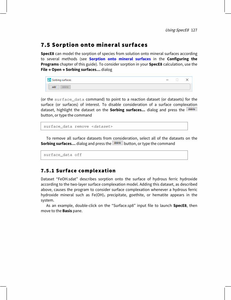
Using SpecE8 127

7.5 Sorption onto mineral surfaces SpecE8 can model the sorption of species from solution onto mineral surfaces according to several methods (see Sorption onto mineral surfaces in the Configuring the Programs chapter of this guide). To consider sorption in your SpecE8 calculation, use the File → Open → Sorbing surfaces… dialog

(or the surface_data command) to point to a reaction dataset (or datasets) for the surface (or surfaces) of interest. To disable consideration of a surface complexation dataset, highlight the dataset on the Sorbing surfaces... dialog and press the button, or type the command

To remove all surface datasets from consideration, select all of the datasets on the Sorbing surfaces… dialog and press the button, or type the command

7.5.1 Surface complexation Dataset “FeOH.sdat” describes sorption onto the surface of hydrous ferric hydroxide according to the two-layer surface complexation model. Adding this dataset, as described above, causes the program to consider surface complexation whenever a hydrous ferric hydroxide mineral such as Fe(OH)3 precipitate, goethite, or hematite appears in the system.

As an example, double-click on the “Surface.sp8” input file to launch SpecE8, then move to the Basis pane.

surface_data remove <dataset>

surface_data off

128 GWB Essentials

This input sets up a model of a dilute fluid coexisting with a ferric hydroxide surface. The program calculates the sorbing surface area from the amount of mineral present (1 g) and the specific surface area given in “FeOH.sdat” (600 m2/g).

The compositional constraints apply to species in the fluid, excluding those sorbed onto the surface, unless you specify otherwise by checking “sorbate” on the Config → Iteration… dialog

or with the sorbate command (see SpecE8 Commands in the GWB Reference Manual). In the example above, the fluid contains 2.4 mg/kg Ca++, 15 mg/kg SO4--, etc.; the mineral surface will be in equilibrium with the fluid and hence contain sites with additional amounts of calcium, sulfate, and so on.

SpecE8 writes the calculated sorbing surface area, surface charge density, mean surface potential, mole numbers of the surface species, and the sorbed fractions of each component into “SpecE8_output.txt”. When you trace reaction paths (see Using React in the GWB Reaction Modeling Guide), these variables are also available for plotting with

Using SpecE8 129

Gtplot. In this example, Ca+ + and Ba+ + are sorbed only weakly, whereas Zn+ + and SO4– –

sorb rather strongly. Several datasets (“FeOH.sdat”, “FeOH+.sdat”, and “FeOH_minteq.sdat”) describing

surface complexation on hydrous ferric oxide are included in the software releases, but you can prepare additional datasets for other surface types. You can also invoke more than one dataset in a single SpecE8 calculation. For example, if you have prepared a dataset “SiOH.sdat” to describe sorption onto silica, adding both “FeOH.sdat” and “SiOH.dat” with the File → Open → Sorbing Surfaces… dialog or the commands

causes SpecE8 to account for sorption onto both ferric and silica surfaces. The constant capacitance and constant potential models are variants of the surface

complexation model. You set these models from the File → Open → Sorbing Surfaces… dialog, or using the surface_capacitance and surface_potential commands (see Constant capacitance model and Constant potential model in the Configuring the Programs chapter of this guide).

7.5.2 Ion exchange As described in the Configuring the Programs chapter of this guide (see the Ion exchange section), you can model ion exchange in two ways. The first method is to swap an activity ratio into the basis. This method is equivalent to assuming that there exists a sufficiently large reservoir of exchanging ions that the composition of the exchanging surface remains invariant.

Once you have swapped the activity ratio into the basis, constrain its value. For example, in the Basis pane, select → Ratio… and set the ratio aCa++/aNa+

2 to “0.2”, or follow the steps

For a more general treatment of ion exchange, prepare a small dataset of the exchange reactions to be considered, using file “IonEx.sdat” as a template. Load the dataset of exchange reactions with the File → Open → Sorbing Surfaces… dialog, or the surface_data (or read) command

surface_data FeOH.sdat surface_data SiOH.sdat

swap Ca++/Na+^2 for Ca++ ratio Ca++/Na+^2 = 0.2

surface_data MyIonEx.sdat

130 GWB Essentials

You can load one or more exchange datasets (containing one or more exchange reactions) at a time, and in a single run combine ion exchange datasets with other types of surface reaction datasets.

SpecE8, in its calculations, maintains a mass balance on the exchanging sites and reports the composition of the exchanging surface. You must, therefore, specify the exchange capacity in the modeled system on the File → Open → Sorbing surfaces… dialog

or using the exchange_capacity command.

You can set the exchange capacity (i.e., the CEC) in terms of either the total number of charge equivalents in the system (eq, meq, and so on), or the number of equivalents per gram of mineral (eq/g, …). In the latter case, the program determines the total mineral mass in the system, including equilibrium, kinetic, and unreactive or inert minerals in the system, to calculate the total exchange capacity. You set inert volume with the inert command, or on the Medium pane; inert minerals are taken to have a density 2.65 g/cm3.

As an example of a SpecE8 calculation accounting for an ion exchange reaction, double-click on the “IonEx.sp8” input file to launch SpecE8. Go to the File → Open → Sorbing surfaces… dialog

to confirm that you’ve loaded IonEx.sdat, a surface dataset of ion exchange reactions, and to see the value assumed for the surface’s exchange capacity.

exchange_capacity = 10 meq/g

Using SpecE8 131

Move to the Basis pane

to see the composition of the fluid. In this example, the amount of Na+ and Ca++ in solution controls the composition of the exchanging surface.

7.5.3 Distribution coefficients (Kd) To set up a calculation considering sorption described by Kd, read one or more datasets containing distribution coefficients for sorption reactions from the File → Open → Sorbing Surfaces… dialog, or using the surface_data command (see Distribution coefficients (Kd) in the Configuring the Programs chapter of this guide). You prepare the datasets using “Kd.sdat” as a template file.

Unlike the other sorption methods, this approach carries the sorbed concentration in moles per mass solid, rather than liquid phase. It is important in configuring a SpecE8 calculation, therefore, to specify carefully the mass of minerals in the system. Minerals include equilibrium and kinetic minerals, as well as the unreactive or inert volume. You specify inert volume (in cm3) with the inert command, or on the Medium pane (the program converts this value to mass, assuming a density of 2.65 g/cm3).

As an example of using the distribution coefficient method to model ion sorption in SpecE8, double-click on the “KD.sp8” input file. When SpecE8 opens, go to the File → Open → Sorbing surfaces… dialog

132 GWB Essentials

to confirm that you’ve loaded the Kd.sdat sorption dataset. Move to the Medium pane

to see the volume of minerals in the system. The Basis pane

describes the fluid. In this case, the program models a system including a fluid containing 10 𝜇𝜇g/kg Pb++ in contact with minerals onto which a considerably greater mass of the ion is predicted to be sorbed.

Using SpecE8 133

7.5.4 Freundlich isotherms To describe sorption in terms of Freundlich isotherms (see Freundlich isotherms in the Configuring the Programs chapter of this guide), prepare a dataset of sorption reactions following the format of file “Freundlich.sdat”. The procedure is otherwise parallel to the Kd approach, as described in the previous section.

Continuing the example above, use File → Open → Sorbing surfaces… to select the “Kd.sdat” file and delete it,

then click and select “Freundlich.sdat” from the Gtdata folder within the GWB installation directory

or use the steps

to implement the Freundlich model in place of the Kd approach. Alternatively, double-click on the “Freundlich.sp8” input file to load the example directly.

7.5.5 Langmuir isotherms To model sorption according to Langmuir isotherms, prepare a reaction dataset containing the sorbing reactions and their equilibrium constants, as described under Langmuir isotherms in the Configuring the Programs chapter of this guide. Prepare the dataset in the format of file “Langmuir.sdat”.

Enter the dataset into a SpecE8 run, as above. You can enter one or more Langmuir datasets, and mix Langmuir datasets with datasets for other sorption methods. As with the ion exchange method, specify the total number of sorbing sites in either absolute

surface_data remove Kd.sdat surface_data Freundlich.sdat go

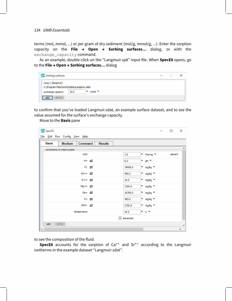
134 GWB Essentials

terms (mol, mmol, ...) or per gram of dry sediment (mol/g, mmol/g, ...). Enter the sorption capacity on the File → Open → Sorbing surfaces… dialog, or with the exchange_capacity command.

As an example, double-click on the “Langmuir.sp8” input file. When SpecE8 opens, go to the File → Open → Sorbing surfaces… dialog

to confirm that you’ve loaded Langmuir.sdat, an example surface dataset, and to see the value assumed for the surface’s exchange capacity.

Move to the Basis pane

to see the composition of the fluid. SpecE8 accounts for the sorption of Ca+ + and Sr+ + according to the Langmuir

isotherms in the example dataset “Langmuir.sdat”.

Using SpecE8 135

7.6 Settable variables SpecE8 allows you to alter the values of certain variables carried in the calculation. Table 7.3 lists these variables and their units and default values. To change a variable, type the new value in the Config → Iteration… dialog box, on the Basis pane (click to expand the “advanced” section), on the Medium pane, or enter as a command the variable name followed by the new value. Examples:

The value given must be in the units carried internally by the program, as listed in Table 7.3. To restore a variable to its default value, enter a blank field in the dialog box, or on the Command pane type its name without a value or followed by a ?:

Current values of the variables can be viewed at any time by looking at the dialog box, the Basis or Medium pane, or using the command show variables.

itmax = 1000 epsilon = 10^-9

itmax itmax = ?

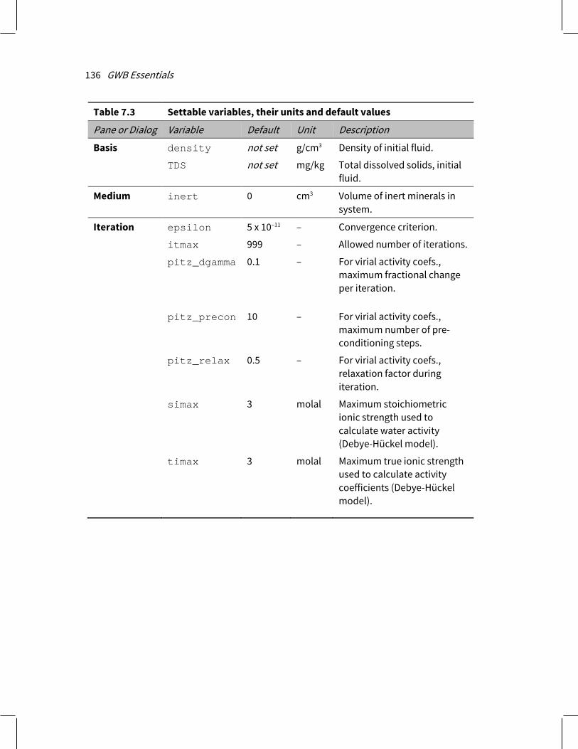
136 GWB Essentials

Table 7.3 Settable variables, their units and default values

Pane or Dialog Variable Default Unit Description

Basis density not set g/cm3 Density of initial fluid.

TDS not set mg/kg Total dissolved solids, initial fluid.

Medium inert 0 cm3 Volume of inert minerals in system.

Iteration epsilon 5 x 10–11 – Convergence criterion.

itmax 999 – Allowed number of iterations.

pitz_dgamma 0.1 – For virial activity coefs., maximum fractional change per iteration.

pitz_precon 10 – For virial activity coefs., maximum number of pre-conditioning steps.

pitz_relax 0.5 – For virial activity coefs., relaxation factor during iteration.

simax 3 molal Maximum stoichiometric ionic strength used to calculate water activity (Debye-Hückel model).

timax 3 molal Maximum true ionic strength used to calculate activity coefficients (Debye-Hückel model).

Using SpecE8 137

7.7 Controlling the printout SpecE8 lets you control the amount of detail presented in the calculation results written to “SpecE8_output.txt”. The dataset is known commonly as the “printout”, although it need never be printed. The printout can contain information about (1) the concentrations and activities of dissolved species, (2) the saturation indices of various minerals, (3) gas fugacities, (4) surface complexes, and (5) the system’s bulk composition in terms of elements of either the current or original basis. The printout can also contain a list of the chemical reactions considered in the calculation.

You can specify that any of these lists be excluded from the printout, or included in a short or long format. To vary the printout, the user can set each aspect in Table 7.4 to “none”, “short”, or “long” on the Config → Output… dialog, or in a command. For example:

The current print settings can be viewed at any time by looking at the three-way check boxes on the Config → Output… dialog. A blank check box indicates exclusion from the printout, a check indicates inclusion in short format, and shading indicates inclusion in long format.

print species = long print basis = short print saturations = none

138 GWB Essentials

Alternatively, type

Table 7.4 Print options and default settings in SpecE8

Default Description

print dataset on to “SpecE8_output.txt”

print alphabetically off Arrange entries in dataset alphabetically

species long Aqueous species

surfaces long Surface complexes

saturations long Mineral saturation states

gases long Gas fugacities

basis none Composition, current basis

orig_basis long Composition, original basis

elements long Elemental composition

reactions none Chemical reactions

stagnant none Composition of stagnant zone

show printout

Using SpecE8 139

7.8 SpecE8 command line You can start SpecE8 by clicking the icon under the “Start” menu, opening a “.sp8” file, or entering the command spece8.exe from the Windows “Command Prompt.” When you start SpecE8 from the command line (as opposed to clicking on the icon), you can specify a number of arguments. For example, the command

causes SpecE8 to read input commands from a file “my_script”, and to use “my_thermo.tdat” as the thermodynamic database.

The following options are available from the command line:

-cd Change the working directory to the directory containing the input script specified with the –i option.

-nocd Do not change the working directory.

-i <input_script> Set a file from which to read input commands.

-gtd <gtdata_dir> Set directory to search for thermodynamic datasets.

-cond <cond_data> Set the dataset for calculating electrical conductivity.

-d <thermo_data> Set the thermodynamic dataset.

-s <surface_data> Set a dataset of surface sorption reactions.

spece8.exe –i my_script –d my_thermo.tdat

141

Using Gtplot

Gtplot is an interactive, mouse-driven program that produces various types of diagrams showing the results of modeling aqueous speciation with SpecE8 or the data stored in a GSS spreadsheet.

After running SpecE8, start Gtplot by clicking on Plot Results on the Results pane, or selecting Run → Gtplot from SpecE8’s menubar. The program will read the calculation results from the “.gtp” file SpecE8 produced and render them on any of a number of types of geochemical diagrams. You can leave Gtplot active when you run further SpecE8 calculations. Each time SpecE8 completes a run, it signals Gtplot, which updates its display to reflect the new results.

After preparing a GSS spreadsheet (“.gss” file, see the Using GSS chapter of this guide), start Gtplot by selecting the analytes you want to plot and making a choice from the Graphs menu. The program will load the data values and render them initially on the chosen type of diagram. You can select which samples to plot within the Samples pane of the dialog for that plot.

You can also start Gtplot by opening any “.gtp” file, clicking on the Gtplot icon under the “Start” menu, or by typing gtplot -i <filename> from the Windows command prompt.

You can take input from a different dataset by choosing File → Open → Data File…. from the menubar and opening a “.gtp” or “.gss” file.

Gtplot opens a window on your computer screen, loads the input data, and renders the data as a two-dimensional plot. The window has three parts: a graphics area, a menubar with pulldown menus, and a frame showing the name of the input dataset and its activity model.

142 GWB Essentials

Gtplot works using information about the fluid modeled, including its bulk composition (i.e., its composition in terms of Na+, Ca++, and so on), pH, TDS, and carbonate speciation. Plots labeled “HCO3 + CO3” show the sum of the concentrations in solution, in terms of electrical equivalents per kg fluid, of the free HCO3

– and CO3– – species.

The program calculates this sum from the fluid’s carbonate alkalinity, as determined by the SpecE8 program. Hence, the value shown for the variable depends not only on carbonate concentration, but the fluid’s pH. In contrast, plots labeled “HCO3” represent the bulk carbonate concentration of the fluid, taking no account of the speciation of carbonate to the CO3

– – , HCO3– , and CO2(aq) species.

When Gtplot starts for the first time in a given directory, it assumes a default configuration. Upon finishing, the program saves for its next run a dataset containing the current configuration of your plots. You can select options from the File menu to specify an alternative configuration (see Loading and saving plot configuration) or reset the entire program configuration.

Using Gtplot 143

8.1 Plot types Use the Plot menu to control the type and configuration of the plot produced.

XY Plot shows a plot of fluid composition, with one component on the x axis and one or more components on the y axis. Use the following to specify the way the variables are plotted:

Variable type to control the type of variables to appear along the plot’s axes. Consider to list, for species or mineral saturation plots, the set of just those that

contain a given basis species. Auto-scale to set the data range for the axis to span the data to be plotted. Minimum, Maximum, and Tick Factor to set the data range for the axis. Reverse axis to reverse the sense of the axis. Units to select alternative units, if any, for the axis. As to plot values as elemental equivalents, or as protonated or deprotonated

species equivalents. Type to set the axis to a linear, log, or delta scale. A delta scale shows change in

a variable’s value from the initial point in the reaction path. First, Previous, Next, Last, and Select all to cycle through the variable choices.

144 GWB Essentials

A Ternary Diagram shows the fluid composition on a tri-linear plot. On the Plot pane, use the following to specify the way the diagram is plotted:

Components to control the three components plotted on the diagram. Units to select alternative units for the axes, which are plotted as fractions. Show TDS as circles to control how circles representing a sample’s dissolved

solids content should be displayed.

A Piper Diagram shows the fluid’s major ion composition. Use: Show TDS as circles to control how circles representing a sample’s dissolved

solids content should be displayed.

Using Gtplot 145

A Durov Diagram represents the fluid’s major ion composition, TDS, and pH. Use: TDS Axis to set the Auto-scale; Minimum, Maximum, and Increment; and Units

for the TDS axis. pH Axis to set the Auto-scale and Minimum, Maximum, and Increment for the

pH axis. Show TDS as circles to control how circles representing a sample’s dissolved

solids content should be displayed.

A Schoeller Diagram shows the pattern of component concentration on a logarithmic scale. Use:

Add, Add All, Remove, Remove All, and Default to choose the components to include in the diagram.

Up, Down to arrange the order of chosen components along the horizontal axis. Auto-scale, Minimum, and Maximum to set the data range for the vertical axis. Units to select alternative units for the vertical axis. Max samples shown to set the number of samples to display together when the

“Block” and “Next Block” buttons on the Samples pane are clicked.

146 GWB Essentials

A Stiff Diagram represents the fluid’s major ion composition as a polygonal shape. Use:

Add, Add All, Remove, Remove All, and Default to choose the components to include in the diagram.

Up, Down to arrange the order of chosen components, with cations plotting on the left and anions on the right.

Auto-scale, Maximum, and Increment to set the data range for the diagram. Max samples shown to set the number of samples to display together when the

“Block” and “Next Block” buttons on the Samples pane are clicked. Labels to control whether the axes and plot labels appear on all samples, only

the first sample, or no samples. Units to select alternative electrical equivalent units. Auto-size and Size to optimize sizing and spacing of multi-sample plots.

A Radial Plot shows the fluid’s composition in a manner similar to a Stiff diagram, but in radial coordinates. Unlike Stiff diagrams, Radial plots can display uncharged components. Use:

Using Gtplot 147

Add, Add All, Remove, Remove All, and Default to choose the components to include in the diagram.

Up, Down to arrange the order of chosen components. Auto-scale and Maximum to set the data range for the diagram. Max samples shown to set the number of samples to display together when the

“Block” and “Next Block” buttons on the Samples pane are clicked. Labels to control whether the axes and plot labels appear on all samples, only

the first sample, or no samples. Units to select alternative units. Auto-size and Size to optimize sizing and spacing of multi-sample plots.

A Bar Chart represents the fluid’s cation–anion balance graphically. Use: Auto-scale, Minimum, Maximum, and Increment to set the data range for the

diagram. Max samples shown to set the number of samples to display together when the

“Block” and “Next Block” buttons on the Samples pane are clicked. Labels to control whether the axes and plot labels appear on all samples, only

the first sample, or no samples. Units to select alternative units for the axis. Common ions to control whether a default set of major ions or all ions in the

sample are plotted. Show all labels to control whether all ions are labeled for a given sample, or

only those that are abundant enough that the label would fit naturally. Auto-size and Size to optimize sizing and spacing of multi-sample plots.

148 GWB Essentials

A Pie Chart is an alternative method for showing cation–anion balance, with the radial direction representing the fluid’s total electrical equivalent content. Use:

Auto-scale and Maximum to set the data range for the radial axis. Max samples shown to set the number of samples to display together when the

“Block” and “Next Block” buttons on the Samples pane are clicked. Labels to control whether the axes and plot labels appear on all samples, only

the first sample, or no samples. Units to select alternative units for the radial axis. Common ions to control whether a default set of major ions or all ions in the

sample are plotted. Show all labels to control whether all ions are labeled for a given sample, or

only those that are abundant enough that the label would fit naturally. Auto-size and Size to optimize sizing and spacing of multi-sample plots.

8.1.1 Sample selection Gtplot can display data for multiple samples (when plotting GSS data) or calculation steps (when plotting results of SpecE8, React, X1t, or X2t models) in all of its plots. For the XY Plot, Ternary Diagram, Piper Diagram, Durov Diagram, and Schoeller Diagram, all selected samples (or steps) are displayed on a single set of axes or in a single diagram. The other plots (Stiff Diagram, Radial Plot, Bar Chart, and Pie Chart) are more suitably displayed side-by-side.

Use the Samples (or Steps) pane of the appropriate Plot Configuration dialog to select samples for plotting. For the XY Plot, Ternary Diagram, Piper Diagram, and Durov Diagram, use the following to specify the way samples are plotted:

Add, Add All, Remove, and Remove All to make samples available or unavailable for plotting.

Up, Down to rearrange the order of samples in the Available list.

Using Gtplot 149

First, Previous, Next, Last, and Select all to cycle through the available samples. Only selected samples in the Available list will plot.

The Samples pane for the Schoeller Diagram, Radial Diagram, Stiff Diagram, Bar chart, and Pie chart is similar to that described above. Instead of a “Select all” button, however, the “Block” button plots a subset of samples together. Use “Next block” to plot the next subset of samples. You control the number of samples displayed in the “block” by setting “Max samples shown” on the Plot pane, as described above.

150 GWB Essentials

8.2 Editing plot appearance In Gtplot, you can interactively modify many aspects of the diagram. A right-click on an aspect or area of the plot displays a menu showing the options available. You may choose to reset an axis range or an aspect’s appearance to its default state. Using Edit → Font will change the font for the entire plot.

To change the font for individual aspects, choose Font from that aspect’s menu. A double-click on an aspect brings up a dialog box related to the first item on the pulldown menu, which in most cases is the plot configuration dialog. These dialogs can also be accessed through the Plot menu.

The aspect appearance dialogs can be accessed through the Edit menu. A double-click on the background area will bring up the View… dialog, which lets you select the graphical elements to be shown.

Right-click on plot background

Double-click background to

show View dialog

Right-click on plot interior

Using Gtplot 151

A left-click on an aspect causes it to be “selected”. An aspect has been selected when its color changes, as in the case of lines, or when it is surrounded by manipulation handles, in the case of text or markers. Change the size of text, markers, and, in the case of the XY Plot, the plot itself by dragging the sizing cursors. Adjust the placement of the plot

Right-click text to show menu

options

Right-click line to show menu options

152 GWB Essentials

by clicking within the plot or on either axis and dragging it. The plot title can be moved in the same way.

When you read new input data and update the plot with the Auto-scale option set, Gtplot automatically adjusts the axis ranges to the new data. Otherwise, Gtplot maintains

Left-click title and drag to reposition

Left-click edge and drag to resize plot

Left-click to select; drag handle to resize Left-click and

hover to view data values

Left-click axis and drag to move plot

Left-click axis and drag to move plot

Drag inner tick, number, or grid line to shift axis range

Drag outer tick, number, or grid line to scale axis range

Using Gtplot 153

the axis ranges you have set for the previous plot. This option lets you quickly adapt the axis ranges to new data.

You can change the range on an axis by clicking and dragging a tick mark, number, or grid line. Dragging a tick within an axis shifts all of the values along the axis, effectively changing the minimum and maximum values at the ends of the axis, but keeping the spacing the same. Dragging the tick at the end of an axis changes the minimum or maximum value. Any tick in a Stiff diagram, radial plot, or pie chart behaves like an end tick because the minimum is always zero and cannot be changed. To reset the axis range to span the range of the data being plotted, choose Auto-scale or Reset Range from the aspect menu, or Plot → Reset Axis Range.

You can set all of the graphical attributes in the aspect appearance dialogs available through the Edit menu. When you make changes to values or selections in an aspect appearance dialog, the changes don’t take effect on the plot immediately. You may set up your choices for as many of the aspects as you like, or use the Reset button to reset the dialog to its default values. Use the Apply or OK button to apply the changes to the plot. Use the Cancel button if you decide that you don’t want the changes applied.

Selecting Color → Choose Color… from any aspect menu or clicking on any color button in an aspect appearance dialog will allow you to set the color of the relevant aspect. The Color dialog initially presents a selection of named colors to choose from, with the current color of the aspect highlighted.

To create custom colors in the Color dialog, double-click any of the named colors or click on Define Custom Colors>>. This displays the extended version of the dialog through which you can create a custom color. Once you are satisfied with the color you have created, you can give it an optional color name, then choose “Add to Custom Colors”. The color is then available, just like any of the other named colors.

Left-click button to select new color

Multicolor automatically

Reset dialog options to program defaults

154 GWB Essentials

8.3 Scatter data Gtplot can plot the data in a GSS data sheet (a .gss file) as “scatter data” in its own diagram, or overlain on a diagram of the results of a SpecE8 or React calculation. You can plot chemical parameters in your data sheet, like pH and TDS, or the measured composition (mg/kg Na+, ...) of the samples in the sheet. Or you can plot “calculated analytes” such as species activity, gas fugacity, and mineral saturation state.

Your .gss file might look like

To read the file into Gtplot, select File → Open → Scatter Data…. If some of the data points lie outside the plot’s axis range, press Ctrl+Z. Clear scatter data from a diagram on the Open → Scatter Data… dialog, with the OFF button.

The marker representing each sample in the scatter data is set in the .gss file. In GSS, right-click on a sample to change the marker used and its color and size. When you modify a .gss file, use Graphs → Update Graph(s) to see the changes.

On xy plots, you can associate the marker for a data point with the analyte (Na+, Ca+ +, ...), rather than the sample (Well #1, Well #2, ...). On the Edit → GSS Data… dialog, you can

Using Gtplot 155

assign the marker, its color, and its size according to the settings in the .gss file for the analytes, or for the samples.

You can label each scatter data point with the sample’s “Sample ID”, as set in the .gss file, and display a legend showing the symbols used. In Gtplot, choose Edit → GSS Data…, and under “Labels” select the checkbox for “Sample” to show sample labels, and the “Legend” box to display the legend. If the “Color from sample” box is checked, the color for each sample label matches that of the sample’s marker. Use the Edit → View… dialog to quickly toggle on and off display of the scatter data, data labels, and legend.

If an analysis falls below detection limit, enter in your GSS data sheet the detection limit preceded by a “<”, for example “< 0.01”. Gtplot will add a downward arrow to the symbol for this entry, signifying it represents the upper limit to concentration. To add error bars to the scatter points, enter triplets (0.5|2.0|3.5) in the data cells in your .gss file (see Error bars in Using GSS).

In plots showing the variable “HCO3 + CO3”, you should enter a value in the scatter dataset for the system parameter “Carbonate alkalinity” so Gtplot can render the variable correctly. If you do not enter a value for alkalinity, the program will render the variable in terms of the reported HCO3 concentration, if available, in which case the diagram produced will not account for the speciation of carbonate.

Certain unit conversions, such as changing mg/l to mmolar, or mg/kg of solute to mg, require knowledge of the fluid’s density and TDS, and the mass of solution in the system. Gtplot first looks for entries “Density”, “TDS”, and “Mass solution” in the .gss file. If it does not find them, it estimates density and TDS, and assumes a solution mass of 1 kg.

In order to see TDS represented as circles on Piper, ternary, and Durov diagrams, you should enter a value for dissolved solids for each sample.

To coordinate the plotting of scatter data versus time on a reaction path, include values for “Time elapsed”, “Time”, and/or “Date”.

In GWB releases 7.0 and earlier, the program took scatter data from a specially formatted text file, rather than a .gss data sheet. Legacy scatter files are still supported and described in the Scatter Data appendix in the GWB Reference Manual.

8.4 Loading and saving plot configuration Gtplot writes into the user’s working directory a file, “gtplot_conf.gtc”, containing the configuration of the current plots. When the program starts again in the same directory, it reads the file and assumes the same configurations.

Choosing File → Reset Configuration or the reset option from the command line (see Gtplot command line) returns the configuration for each plot type to its default state. This option is useful, for example, when you begin to examine results of a SpecE8 simulation unrelated to the previous run.

156 GWB Essentials

You can save plot settings to an alternative configuration file by selecting File → Save As…. Later, double-click on the “.gtc” file to reopen the plot you saved. You may also read the file into Gtplot by selecting File → Open → Configuration…, or simply dragging it into an instance of Gtplot.

Exiting the program by choosing File → Abort (No Save) causes an immediate exit from the program; the plot configuration is lost.

8.5 Exporting the plot Gtplot makes it convenient to use the plots you create in articles, reports, presentations, and databases. You can copy the current plot to the clipboard and then paste it into a variety of applications, in a format meaningful to the application.

To copy a plot, use Edit → Copy (Ctrl+C). If you paste the plot into MS PowerPoint, it will appear as an EMF (an MS Enhanced Metafile) graphic object. Pasting into Adobe Illustrator places a native AI graphic.

If you paste the plot into MS Excel or a text editor such as Notepad or MS Word, the numerical values of the data points that make up the lines on the plot will appear in spreadsheet format.

You can control the format in which the plot is copied to the clipboard by selecting Edit → Copy As. You can choose to copy the plot as an AI object, an EMF object, or a bitmap, or to copy the data points in the plot as tab-delimited or space-delimited text. Use the tab-delimited option to paste the data into a spreadsheet program like MS Excel. For examining the data in a text file created with an editor like Notepad or MS Word, the space-delimited option writes a nicely aligned table.

“Paste” in Excel or Word inserts numerical values

Using Gtplot 157

In MS Word or MS Excel, use Paste Special… to paste the plot as a picture instead.

Use File → Save Image… to copy the plot, in your choice of formats (selected under Save as type:), from the graphics area to a file in the specified directory. The Enhanced Metafile option, for example, saves the plot image in a format that can be read by most art and illustration programs (see Graphics Output in the GWB Reference Manual). The other file formats available are: PNG, JPEG, TIFF, Bitmap, Adobe Illustrator, PDF, Scalable Vector Graphics, Compressed SVG, Encapsulated PostScript, Color PostScript, and B/W PostScript.

When saving a PNG, JPEG, TIFF, or bitmap file, you may specify the quality of the saved image by choosing its resolution: High, Medium, Low, or Custom. Use Custom… to set the pixel width and height of the image, and to choose whether to preserve the aspect ratio of the plot.

Use the Spreadsheet File (Tab delimited) or Text File (Space delimited) option to save the numerical coordinates of the data points on the plot into a table. The spreadsheet table may be read directly into many popular spreadsheet programs.

Certain graphics types support font embedding. PDF files should always display and print properly, regardless of fonts installed on the system. PostScript files should also, if you have used the option to embed fonts.

If you may want to edit the PostScript file, however, you should deselect the option to embed fonts, because programs such as Adobe Illustrator may restrict your ability to edit a document using embedded fonts. To edit these files, be sure that all of the required fonts are installed on your computer (see Font for data markers in the GWB Reference Manual).

“Paste Special…” in Excel or Word

inserts a picture

158 GWB Essentials

When importing AI graphics to Adobe Illustrator, the program may prompt you to update the legacy text before you can edit the file. In this case, choose “Update”. You need to release the clipping mask before you attempt to edit individual elements of the plot. Use the “Ungroup” and “Group” functions when repositioning or modifying elements.

8.6 Gtplot command line To run Gtplot, click on the Gtplot icon on the GWB dashboard, or open a “.gtp” or “.gtc” file. The program can also be initiated from the Windows command prompt by typing gtplot.exe. Starting the program in this way allows you to make use of the command line arguments described below.

Gtplot accepts a number of arguments from the command line. For example, the command

causes Gtplot to read as input the file “SpecE8_plot1.gtp”, and to use the plot configuration stored in “Config1.gtc”.

The following options are available from the command line:

-i <input_data> Set the “SpecE8_plot.gtp” dataset, produced by a SpecE8 run, which contains the data to be plotted. The program, by default, looks for file SpecE8_plot.gtp in the user’s working directory.

-c <config_file> Set the configuration file to be read at startup. By default, the program reads the file gtplot_conf.gtc if it exists in the working directory.

-scat <scatter file> Take scatter data from the named dataset. By default, Gtplot does not plot scatter data.

-graph <plot_type> Set the type of plot displayed at startup. By default, it is set from the configuration file. Choose from: xyplot, ternary, piper, durov, schoeller, stiff, radial, bar, pie, series, and time.

-reset Set the default configuration at startup; do not read gtplot_conf.gtc.

gtplot –i SpecE8_plot1.gtp –c Config1.gtc

Using Gtplot 159

Table 6.1 Keyboard shortcuts in Gtplot

Ctrl+Shift+A Copy plot to the clipboard as an Adobe Illustrator file

Ctrl+Shift+B Copy plot to the clipboard as a bitmap

Ctrl+C Copy plot to the clipboard

Ctrl+Shift+E Copy plot to the clipboard as an Enhanced Metafile

Ctrl+F Refresh display

Ctrl+Shift+G Get scatter data

Ctrl+L Load a configuration file

Ctrl+M Save the graphic image to a file

Ctrl+O Open an input (“React_plot.gtp”) file

Ctrl+P Print the plot

Ctrl+Q Quit Gtplot, save configuration

Ctrl+Shift+Q Abort Gtplot, do not save configuration

Ctrl+R Reset the plot configuration

Ctrl+S Save the current configuration to a file

Ctrl+Shift+S Copy plot to the clipboard as a Spreadsheet (tab delimited)

Ctrl+Shift+T Copy plot to the clipboard as Text (space delimited)

Ctrl+U Update the plot from the current input file

Ctrl+X Reset data range on the x axis

Ctrl+Y Reset data range on the y axis

Ctrl+Z Reset data ranges on the x and y axes

F1 Open online help

160 GWB Essentials

161

Using TEdit

TEdit is a graphical editor that lets you create and modify the thermodynamic and surface reaction datasets used by the GWB programs. You can alternatively use a simple text editor such as Notepad to modify the datasets. If you prefer to use a text editor, details of the datasets’ formats are given in the Thermo Datasets appendix to the GWB Reference Manual.

With TEdit you can view and modify the entries in a dataset, as well as add or delete them. Specifically, you can alter

Header lines, data tables, and dataset information. Elements and species in the dataset, and their properties. Reactions among the species, and log Ks at the principal temperatures. Virial coefficients for pairs or triplets of species.

You can also: Identify entries containing or consisting of specific elements, basis species, or

redox species. Swap basis species as you add reactions for new entries. Copy entries from one dataset to another. Rebalance existing reactions, including altering the coupling of redox reactions. Exchange the locations of basis, redox, and aqueous species.

9.1 Getting started with TEdit

9.1.1 Viewing a thermo dataset To open TEdit, go to the Support pane of the GWB Dashboard and click the “Edit thermo data” button. Then go to File → Open → Thermo Data… and browse to open an existing dataset. You can also double-click any “.tdat” file to open it in TEdit. Or, you can open the thermo dataset currently loaded in any GWB program by going to File → View and selecting the file ending in “.tdat”.

162 GWB Essentials

The dataset might look like this:

On the left side of the window is a tree structure with sections labeled “Header”, “Tables”, “Elements”, “Basis species”, “Redox couples”, “Aqueous species”, “Free electron”, “Minerals”, “Gases”, “Oxides”, and optionally “Virial coefficients”. For detailed descriptions of each section, see the Thermo Datasets appendix in the GWB Reference Manual.

Click “Header” on the tree to view the dataset format, activity model, and bibliographic information. The pane also shows the number of elements, basis species, and so on in the dataset. Click on one of the numbers to navigate to the corresponding section of the dataset.

Using TEdit 163

The next section contains tables showing how various coefficients used by the programs vary with temperature. The eight principal temperatures of the dataset are set in the top line of this section.

The following section contains the list of elements from which species in the dataset can be created. Click the “+” button to expand the list. Each element’s entry contains a name, symbol, and molecular weight. TEdit lists element symbols and species names in alphabetical order.

164 GWB Essentials

The “Basis species” are listed in the next section. Each entry contains a name, charge, ion size parameter in angstroms (plus a second b term for activity coefficients in the phreeqc, minteq, and wateq4f activity models), and mole weight in the labeled text boxes, as well as its elemental composition.

The “Redox couples” are similar to the Basis species, except that redox couples are constructed from existing species, rather than from the elements. The species form a balanced reaction for which equilibrium constants are supplied at each of the principal temperatures.

Using TEdit 165

“Aqueous species”, “Free electron”, “Minerals”, “Gases”, and “Oxide” components are added in a similar manner to redox couples, with a few differences. The name, charge, ion size parameter, and mole weight of the free electron cannot be modified, although you can modify its reaction and log K values, as you would for any other species.

Minerals have fields for entering the mineral’s molar volume, type, and chemical formula. Minerals, gases, and oxide components do not have fields for charge or ion size parameter. The oxide components do not have thermodynamic stabilities, so there is no place to enter log K values.

Datasets that utilize virial (“Pitzer”) equations include coefficients describing the energetic interactions among basis, redox, and aqueous species. In “thermo_hmw.tdat”, for example, the entry for Ca+ + lists interaction terms with anions, cations, neutral species, and triplets of species. TEdit displays the interaction terms for various pair-wise and triplet combinations of species in the “Virial coefficients” section of the tree and under the entry for all involved species.

For example, Ca+ + and Cl– basis species both display the Ca+ + – Cl– cation–anion pair interaction terms, as well as all the triplets involving both species. If, while on the entry for Ca+ +, you apply changes to the Ca+ + – Cl– pair coefficients, the changes will be reflected in the entry for Cl– and in the Ca+ + – Cl– pair’s entry on the tree as well.

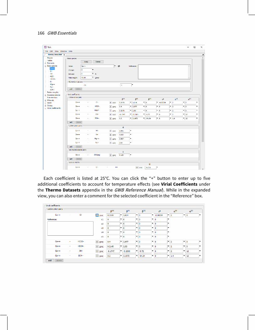
166 GWB Essentials

Each coefficient is listed at 25°C. You can click the “+” button to enter up to five additional coefficients to account for temperature effects (see Virial Coefficients under the Thermo Datasets appendix in the GWB Reference Manual). While in the expanded view, you can also enter a comment for the selected coefficient in the “Reference” box.

Using TEdit 167

9.1.2 Viewing a surface dataset In TEdit, go to File → Open → Sorbing Surfaces… and browse to open an existing surface dataset. You can alternatively open an “.sdat” file in TEdit by double-clicking on it. Or, from one of the GWB modeling programs, choose File → View and select any currently loaded surface dataset.

Surface datasets are organized much like thermo datasets, and can be navigated in TEdit using a similar tree structure.

9.1.3 Creating new datasets To create a new thermo dataset, go to File → New → Thermo Data and select an activity model. TEdit can format GWB datasets that invoke variations of the Debye-Hückel equations or the virial techniques (see Thermodynamic datasets under Configuring the programs, and Activity coefficients under Using SpecE8). Note the format labeled “Pitzer” is outdated and not recognized by TEdit; support for the Pitzer equations has been superceded by the “h-m-w” format.

In the same manner, to create a surface dataset, go to File → New → Sorbing Surfaces and choose one of the surface models (see Sorption onto mineral surfaces under Configuring the Programs). If you choose to create an ion exchange dataset, you will need to also pick an activity convention. You should set a unique “type” in the header section for each surface dataset you create. The “type” identifies the dataset within the GWB modeling programs when more than one surface dataset has been loaded.

9.1.4 Dataset formats Thermo datasets beginning with the GWB 10 release are distributed in the “oct13” format. TEdit can read and write datasets in that format, which is preferred for current installations of the software, or in various legacy formats (see Legacy formats under the Thermo Datasets appendix in the GWB Reference Manual) for use with earlier releases of the software package.

The current format for surface datasets is “jan14”. This format differs from legacy formats in that it identifies a thermo dataset from which the species are drawn to make up surface reactions. The header lines in surface dataset “FeOH_minteq.sdat”, for example, link it to the thermo dataset “thermo_minteq.tdat”. TEdit, then, will look to “thermo_minteq.tdat” to find aqueous species to be used in balancing chemical reactions within “FeOH_minteq.sdat”.

168 GWB Essentials

9.1.5 Saving datasets Click File → Save to save your thermo or surface dataset. TEdit will by default save thermo datasets as “.tdat” files, and surface datasets as “.sdat” files. To save a surface dataset to be used with GWB 9 or earlier releases, choose one of the legacy formats in the “Header” section and set a “.dat” extension in the Save As… dialog.

9.2 Working with datasets

9.2.1 Show When you click on any section (except “Header” and “Tables”) on TEdit’s tree structure, the program will display a pane that allows you to filter the species displayed on the tree. You can choose to show only entries containing specific elements, or those composed of specific basis and redox species.

To filter the species shown in the tree, select either “Elements” or “Basis and redox species” from the pulldown in the upper left of the filter pane. Choose one or more options in the list below, then click on the “Filter” button. To return to showing all the entries, choose “Select all” followed by “Filter”.

Using TEdit 169

9.2.2 References From the “Header” section, you can add comments to appear at either the beginning of a dataset or at the end. Text you type into the “Preamble” appears just below the Header lines at the top of the dataset, whereas the contents of the “Bibliography” appear at the bottom. If you would like to add comments or a reference to an individual species in the dataset, open the species’ data pane, enter text in the “Reference” block, and click Apply.

9.2.3 Add and delete entries To add an element or a species to a dataset, right-click on the appropriate section heading in the tree and choose “Add”. Complete the data template that appears, and click Apply to preserve your changes. The new entry will appear alphabetically within the tree, as well as within the dataset when you save it.

To remove an entry from a dataset, right-click on its label in the tree and choose “Remove”. Alternatively, click on the “Delete” button within the entry’s data pane. If the reactions to form other species in the dataset contain the entry you are deleting, a dialog box will appear listing those species. You may choose “OK” to delete all the species, or “Cancel” to retain them.

9.2.4 Completing entries in thermo datasets When adding an element to a database, you enter a name, symbol, and mole weight. For basis species, fill in the species’ name, charge, ion size parameter, b term, if applicable, and mole weight. Last, click the “add” button to build up the species’ elemental composition.

For the remaining entries, set a balanced chemical reaction. In the “Species in reaction” section, click “add”, choose a type of species (Basis…, Redox…, Aqueous…, Electron…, Mineral…, or Gas…), then select a species. Repeat the procedure for each

170 GWB Essentials

species that appears in the reaction, supplying a reaction coefficient in the space to the right of its name.

Species with a negative reaction coefficient appear on the reaction’s left-hand side; those with a positive coefficient are on the right. As you add species, the reaction is automatically written out. In the fields below the reaction, set a log K for each reaction, as well as its temperature derivative.

For virial datasets (those invoking the “Pitzer equations”), also enter coefficients reflecting pair-wise and triplet interactions among the species. You can specify interaction terms for cation–anion pairs, cation–cation or anion–anion pairs, ion-neutral species pairs, and species triplets on the data pane for any basis, redox, or aqueous species. Click “add” in the appropriate section and select species to form a pair or triplet from the pulldown list. Fill in values for some or all of the coefficients (see Virial Coefficients in the Thermo Datasets appendix to the GWB Reference Manual).

9.2.5 Completing entries in surface datasets

9.2.5.1 Two-layer datasets

Two-layer datasets are arranged much like thermo datasets. You start by adding one or more “Basis surface species”, for which you specify a name, charge, and mole weight. Each basis entry defines a sorbing site. Click “add” to define the site’s elemental composition, drawing from the list of elements in the thermo dataset, which is named in the dataset “Header”.

Second, compile a list of surface complexes under “Surface species”. For each complex, set a reaction written in terms of a basis species in the surface dataset, combined with basis, redox, and aqueous species drawn from the thermo dataset. Set a log equilibrium constant for each reaction (as a log K), as well as the temperature derivative.

Finally, specify one or more minerals to carry the surface. Right-click on “Sorbing minerals” and select “Add”. Each sorbing mineral may host an arbitrary number of sorbing sites, which are the basis species in the dataset. Next to “Name”, click “New Sorbing Mineral” → “Minerals…” and choose a mineral from the thermo dataset. Enter the mineral’s specific surface area, in m2g–1. Under sorption sites, click “add” to pull in the surface’s basis species; for each, set a site density in mol (mol mineral)–1.

You can specify a value for constant capacitance or constant potential, but not both, in the Header section. You may prefer to leave these unset and allow the user to set values as desired from within Rxn, SpecE8, React, X1t, or X2t (see Two-layer surface complexation model under Configuring the Programs).

Using TEdit 171

9.2.5.2 Langmuir datasets

Langmuir datasets contain a single basis entry, which represents the sorbing site. The Langmuir site is uncharged and carries no mass, so you need enter only a name. You can load any number of Langmuir datasets simultaneously into the GWB modeling programs, as long as each has a unique “type” set in the “Header”, and a unique name for the basis entry.

To define the surface complexes, right-click on “Surface species” and choose “Add”. Then, click in the “Species” box and choose a species to complex with the surface site. TEdit will construct a balanced reaction including the Langmuir site and will fill in all the entries, except for the equilibrium constant. Enter values for log K and its temperature derivative.

9.2.5.3 Kd and Freundlich datasets

Kd and Freundlich surface datasets include surface complexes but not basis species. To define a surface complex, right-click on “Surface species” and choose “Add”. Click in the box to the right of “Species:” and choose from the basis, redox, and aqueous species in the thermo dataset. TEdit automatically completes the entry, except for the Kd, or the values of Kf and nf , which you must also enter.

9.2.5.4 Ion exchange

An ion exchange dataset contains a single basis species. To define it, right-click on “Basis species” and choose “Add”. In the box to the right of “Sorbed species”, choose from the list of basis species in the thermo dataset. TEdit will automatically complete the entry.

To define the surface species that exchange with the basis species, right-click on “Surface species” and select “Add”. Click in the box to the right of “Species” and choose from the list of species in the thermo dataset. TEdit will construct a balanced reaction following the activity convention you have chosen, and fill in all entries except for the selectivity coefficient, which you must enter as a linear value.

9.2.6 Transferring dataset entries You can transfer data tables, elements, any type of species, or virial coefficients from one dataset to another. Copy an entry to the clipboard by right-clicking it on the tree structure and selecting “Copy”. Alternatively, select an entry and click on Edit → Copy. Edit → Cut performs a similar function, but removes the entry in question from the source dataset.

To paste, click anywhere on the tree structure of the target dataset and go to Edit → Paste. You do not need to worry about selecting the specific location in a target dataset to paste your entry because TEdit copies this information to the clipboard.

You can also drag entries (see Drag and drop feature under Introduction) from one dataset to another. Left-click an entry on the tree structure of the source dataset, drag it

172 GWB Essentials

to the tree structure or current entry of the target dataset, and release. If the source and target datasets are open in the same TEdit window, switch to the target dataset by hovering over its tab while dragging.

You should use your judgment when transferring thermodynamic data from one dataset to another. TEdit will issue a warning when activity models differ and will not allow you to transfer data in some cases. For example, you cannot transfer virial coefficients to a Debye-Hückel based dataset. Similarly, the program will not allow you to transfer surface species unless both datasets use the same surface model: you cannot transfer a reaction for sorbed Pb+ + from a Kd to a two-layer model dataset.

TEdit will issue a warning if you try to transfer an entry that would be undefined in the target dataset. For example, you would need to add the element Cadmium to “thermo.tdat” before you can paste in the basis species Cd+ +. Similarly, a dataset utilizing the virial equations must include the Ca+ + and Cl– species before you can paste the Ca+ + – Cl– cation–anion pair interaction term.

TEdit will transfer only log Ks corresponding to exact temperature matches when two datasets are compiled at different principal temperatures. If the source and target datasets use different sets of basis and redox species, TEdit will attempt basis swaps to rebalance the reaction, as described below.

9.2.7 Basis swapping The GWB programs require the reactions in a thermo dataset be written in terms of basis species, redox species, the gaseous form of the redox pivot, and the free electron (see Redox couples and later sections under the Thermo Datasets appendix in the GWB Reference Manual).

Reactions you find in the literature may not conform to this convention, but TEdit can quickly convert them by swapping the basis. You might, for example, find a deprotonation reaction written in terms of the hydroxyl ion OH–, even though you are working with a dataset that carries H+ rather than OH– in the basis. When you enter the reaction as written, TEdit replaces OH– in the reaction with H+ and recalculates the reaction’s log Ks. For more information about basis swapping, see Setting and constraining the basis under Configuring the Programs.

Suppose we want to add to dataset “thermo.tdat” the aqueous species FeCl3, given the reaction

FeCl3 ⇆ FeCl2

+ + Cl–, log K = 1.0006 at 25°C (9.1) Right-click on “Aqueous species” and choose “Add”. In the blank pane that opens, type

“FeCl3(aq)” as the species name. Enter the reaction above by clicking

Using TEdit 173

add → Aqueous… → FeCl2+ and add → Basis… → Cl-. Set a reaction coefficient of “1” for each and enter the log K value above.

Note how TEdit automatically swaps out the aqueous species FeCl2+ for the redox species Fe+ + + and recalculates the reaction’s equilibrium constant

FeCl3 ⇆ 3Cl– + Fe+++, log K = -1.1295 at 25°C (9.2)

to reflect the new reaction. Before you click Apply to preserve your changes, your window should look like this:

You can equally employ TEdit’s basis swapping capabilities to rebalance existing reactions. You may wish to convert a redox reaction balanced in terms of O2(aq), for example, to a half-cell reaction. To do so, choose a redox species from the tree and look at the species that appear in its reaction. Click the “swap” button next to “O2(aq)” and select “Electron…”, if the option is available. If it is not, first swap “O2(g)” in for “O2(aq)”, click Apply, then swap in the electron for “O2(g)”. Click Apply to use the rebalanced reaction and updated log K. Whether the rebalancing can be performed in one or two steps depends on whether the reaction for the free electron is written in terms of the aqueous or gaseous form of the redox pivot.

9.2.8 Exchanging species You can use TEdit to exchange the positions of basis, redox, and aqueous species within a thermo dataset. For example, you might replace the basis species “HCO3-” with the

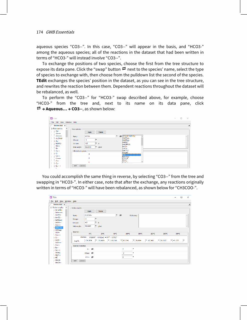
174 GWB Essentials

aqueous species “CO3--”. In this case, “CO3--” will appear in the basis, and “HCO3-” among the aqueous species; all of the reactions in the dataset that had been written in terms of “HCO3-” will instead involve “CO3--”.

To exchange the positions of two species, choose the first from the tree structure to expose its data pane. Click the “swap” button next to the species’ name, select the type of species to exchange with, then choose from the pulldown list the second of the species. TEdit exchanges the species’ position in the dataset, as you can see in the tree structure, and rewrites the reaction between them. Dependent reactions throughout the dataset will be rebalanced, as well.

To perform the “CO3--” for “HCO3-” swap described above, for example, choose “HCO3-” from the tree and, next to its name on its data pane, click

→ Aqueous… → CO3--, as shown below:

You could accomplish the same thing in reverse, by selecting “CO3--” from the tree and swapping in “HCO3-”. In either case, note that after the exchange, any reactions originally written in terms of “HCO3-” will have been rebalanced, as shown below for “CH3COO-”.

Using TEdit 175

The exchange feature provides a quick method for changing the redox pivot of a thermo dataset (see Basis species under the Thermo Datasets appendix in the GWB Reference Manual). In “thermo.tdat”, when you exchange the basis species O2(aq) for the redox species H2(aq), the latter becomes the redox pivot. The reaction for the free electron as well as the redox coupling reactions written in terms of dioxygen will be rebalanced in terms of dihydrogen.

The order in which species are selected for exchange does not matter. If you were to exchange the same two species a second time, the dataset would revert to its original state. H2O is required as an entry in the basis and has therefore been excluded from the exchange feature.

176 GWB Essentials

177

Appendix: Further Reading

The following literature references, from the many hundreds that have been published, provide a starting point for further reading on various aspects of geochemical modeling and its applications. Additional references are available in the GWB Reaction Modeling Guide and the GWB Reactive Transport Modeling Guide.

A.1 Natural waters Anderson, G.M. and D.A. Crerar, 1993, Thermodynamics in Geochemistry, The

Equilibrium Model. Oxford University Press. Appelo, C.A.J. and D. Postma, 1993, Geochemistry, Groundwater, and Pollution.

Balkema, Rotterdam, 536 p. Ball, J.W. and D.K. Nordstrom, 1991, User’s manual for WATEQ4F, with revised

thermodynamic data base and test cases for calculating speciation of major, trace, and redox elements in natural waters. U.S. Geological Survey Open File Report 91–183.

Bethke, C.M., R.A. Sanford, M.F. Kirk, Q. Jin and T.M. Flynn, 2011, The thermodynamic ladder in geomicrobiology. American Journal of Science 311, 183–210.

Chapelle, F.H., 2001, Ground-Water Microbiology and Geochemistry, 2nd ed. Wiley, New York.

Drever, J.I., 1988, The Geochemistry of Natural Waters, 2nd ed. Prentice-Hall, Englewood Cliffs, NJ.

Garrels, R.M. and M.E. Thompson, 1962, A chemical model for sea water at 25°C and one atmosphere total pressure. American Journal of Science 260, 57–66.

Hem, J.D., 1985, Study and interpretation of the chemical characteristics of natural water. U.S. Geological Survey Water-Supply Paper 2254, 263 p.

Kharaka, Y.K. and I. Barnes, 1973, SOLMNEQ: Solution-mineral equilibrium computations. U.S. Geological Survey Computer Contributions Publication 215-899.

Lasaga, A.C., 1998, Kinetic Theory in the Earth Sciences. Princeton, Princeton, New Jersey.

Lindberg, R.D. and D.D. Runnells, 1984, Ground water redox reactions: An analysis of equilibrium state applied to Eh measurements and geochemical modeling. Science 225, 925–927.

178 GWB Essentials

Nordstrom, D.K. and J.L. Munoz, 1994, Geochemical Thermodynamics, 2nd ed. Blackwell, Boston.

Truesdell, A.H. and B.F. Jones, 1974, WATEQ, a computer program for calculating chemical equilibria of natural waters. U.S. Geological Survey Journal of Research 2, 233–248.

Westall, J.C., J.L. Zachary and F.M.M. Morel, 1976, MINEQL, a computer program for the calculation of chemical equilibrium composition of aqueous systems. Hydrodynamics Laboratory Technical Note 18, Massachusetts Institute of Technology, 91 p.

A.2 Speciation modeling Allison, J.D., D.S. Brown and K.J. Novo-Gradac, 1991, MINTEQA2/PRODEFA2, a

geochemical assessment model for environmental systems, version 3.0 user’s manual. US Environmental Protection Agency Report EPA/600/3–91/021.

Bethke, C.M., 2008, Geochemical and Biogeochemical Reaction Modeling. Cambridge University Press, New York, 547 p.

Kharaka, Y.K., W.D. Gunter, P.K. Aggarwal, E.H. Perkins and J.D. DeBraal, 1988, SOLMINEQ.88, a computer program for geochemical modeling of water–rock interactions. US Geological Survey Water Resources Investigation Report 88–4227.

Parkhurst, D.L. and C.A.J. Apello, 1999, User’s guide to PHREEQC (version 2), a computer program for speciation, batch-reaction, one-dimensional transport and inverse geochemical calculations. US Geological Survey Water-Resources Investigations Report 99–4259.

Plummer, L.N., D.L. Parkhurst, G.W. Fleming and S.A. Dunkle, 1988, PHRQPITZ—A computer program incorporating Pitzer’s equations for calculation of geochemical reactions in brines. U.S. Geological Survey Water-Resources Investigations Report 88–4153, 310 p.

Reed, M.H., 1982, Calculation of multicomponent chemical equilibria and reaction processes in systems involving minerals, gases and an aqueous phase. Geochimica et Cosmochimica Acta 46, 513–528.

Wolery, T.J., 1992, EQ3/EQ6, a software package for geochemical modeling of aqueous systems, package overview and installation guide (version 7.0). Lawrence Livermore National Laboratory Report UCRL-MA-110662 (1).

A.3 Uniqueness of solutions Bethke, C.M., 1992, The question of uniqueness in geochemical modeling. Geochimica

et Cosmochimica Acta 56, 4315–4320.

Further Reading 179

A.4 Stability diagrams Bowers, T.S., K.J. Jackson and H.C. Helgeson, 1984, Equilibrium Activity Diagrams.

Springer-Verlag, Berlin, 397 p. Garrels, R.M. and C.L. Christ, 1965, Solutions, Minerals, and Equilibria. Freeman, Cooper

& Co., San Francisco, 450 p.

A.5 Activity models for electrolyte solutions Harvie, C.E, N. Møller and J.H. Weare, 1984, The prediction of mineral solubilities in

natural waters: The Na-K-Mg-Ca-H-Cl-SO4-OH-HCO3-CO3-CO2-H2O system to high ionic strengths at 25°C. Geochimica et Cosmochimica Acta 48, 723–751.

Helgeson, H.C., 1969, Thermodynamics of hydrothermal systems at elevated temperatures and pressures. American Journal of Science 267, 729–804.

Pitzer, K.S., 1987, A thermodynamic model for aqueous solutions of liquid-like density. In Thermodynamic Modeling of Geologic Materials: Minerals, Fluids and Melts, I.S.E. Carmichael and H.P. Eugster (eds.), Reviews in Mineralogy 17, 97–142.

A.6 Sorption, ion exchange, and surface complexation

Appelo, C.A.J. and D. Postma, 1993, Geochemistry, Groundwater, and Pollution. Balkema, Rotterdam, 536 p.

Dzombak, D.A. and F.M.M. Morel, 1990, Surface Complexation Modeling, Hydrous Ferric Oxide. Wiley, New York, 393 p.

Stumm, W., 1992, Chemistry of the Solid-water Interface. Wiley, New York, 428 p. Stumm, W. and J.J. Morgan, 1996, Aquatic Chemistry, 3rd ed. Wiley, New York, 1022 p.

A.7 Thermodynamic databases Delany, J.M. and S.R. Lundeen, 1990, The LLNL thermochemical database. Lawrence

Livermore National Laboratory Report UCRL-21658, 150 p. Helgeson, H.C., J.M. Delany, H.W. Nesbitt and D.K. Bird, 1978, Summary and critique of

the thermodynamic properties of rock-forming minerals. American Journal of Science 278-A, 1–229.

Johnson, J.W., E.H. Oelkers and H.C. Helgeson, 1991, SUPCRT92: A software package for calculating the standard molal thermodynamic properties of minerals, gases, aqueous species, and reactions from 1 to 5000 bars and 0° to 1000°C. Earth Sciences Department, Lawrence Livermore Laboratory, 101 p.

180 GWB Essentials

A.8 Electrical conductivity American Public Health Association, 2012, Standard Methods for the Examination of

Water and Wastewater, Section 2510 A, 2-44–2-48. McCleskey, B., K. Nordstrom, J. Ryan and J. Ball, 2012, A new method of calculating

electrical conductivity with applications to natural waters. Geochimica et Cosmochimica Acta 77, 369–382.