Embed Size (px)
Citation preview

Imperial College London
Department of Computing
Hardware Acceleration of Power SystemSimulation
by
Yumeng Yang(yy1712)
Supervised by Prof. Wayne Luk
Submitted in partial fulfilment of the requirements for the MSc Degree in Advanced Computingof Imperial College London
September 6, 2013
Abstract
Real-time dynamics simulation of large-scale power systems is a computational challenge because ofthe need to solve a large set of stiff, nonlinear differential-algebraic equations. The main bottleneckin these simulations is the solution of the linear system during each nonlinear iteration of Newtonsmethod.The need for faster, and accurate, power system dynamics simulation (or transient stabilityanalysis) has been a primary focus of the power system community in recent years.
FPGAs have become an attractive choice for scientifis computing. This project is about exploringhow the huge computational power and memory optimizations of FPGA based hardware accelera-tors can be used in the dynamic simulation of power systems.
Issues are threefold.
The study begins with the available power system simulation model, which deals with relativelysimple structure and data size (a 4 machines, and 11 buses study system). Firstly,we present anoptimised version of the simulation in a compiled language (C language) and demonstrate perfor-mance gains of approximately 500 times faster than the original run time using SIMULINK as thesimulation environment.
In this paper, we also propose two high performance design for LU decomposition, a key kernelin the power system simulation applications. And a parallelism design for solving the nonlineardifferential-algebraic equations among a number of machines in the power system.
Although the experiments targeting Maxeler systems show that our FPGA-based design can notimprove the time efficiency from the C application of the study system. We builds the relationshipbetween the speedup of simulation and the data size of the power system which indicates that ouracceleration design can give a significant acceleration to larger-scale larger power systems.

Acknowledgements
I would like to express my deepest gratitude to my supervisor, Professor.Wayne Luk, for his con-tinuous guidance, support and enthusiasm throughout the development of this project.
I would also like to thank Dr. Thomas Chua for his valuable ideas and for helping me with all mydifficulties throughout the project.
As well, I would like to thank my beloved family for always believing in me and being by my side,even from far away.
Finally, I would like to thank my professors and my friends at Imperial College, without whom thispast year would not have been half as much enlightening, or fun.
Contents
1 Introduction 4
1.1 Problem Motivation . . . . . . . . . . . . . . . . . . . . . . . . . . . . . . . . . . . . 4
1.2 Problem Specfication . . . . . . . . . . . . . . . . . . . . . . . . . . . . . . . . . . . . 5
1.3 Objectives & Achievements . . . . . . . . . . . . . . . . . . . . . . . . . . . . . . . . 6
1.4 Report Structure . . . . . . . . . . . . . . . . . . . . . . . . . . . . . . . . . . . . . . 7
2 Background 9
2.1 Power System Simulation . . . . . . . . . . . . . . . . . . . . . . . . . . . . . . . . . 9
2.2 Models of Different Components in Power System . . . . . . . . . . . . . . . . . . . . 9
2.2.1 Generators . . . . . . . . . . . . . . . . . . . . . . . . . . . . . . . . . . . . . 10
2.2.2 Excitation systems . . . . . . . . . . . . . . . . . . . . . . . . . . . . . . . . . 11
2.2.3 Network power flow model . . . . . . . . . . . . . . . . . . . . . . . . . . . . . 11
2.2.4 Thyristor conrolled series capacitor (TCSC) . . . . . . . . . . . . . . . . . . . 12
2.3 The Simulation Challenge . . . . . . . . . . . . . . . . . . . . . . . . . . . . . . . . . 12
2.4 The SIMULINK Tool . . . . . . . . . . . . . . . . . . . . . . . . . . . . . . . . . . . 14
2.4.1 What is SIMULINK . . . . . . . . . . . . . . . . . . . . . . . . . . . . . . . . 14
2.4.2 Basic elements of Simulink . . . . . . . . . . . . . . . . . . . . . . . . . . . . 14
2.4.3 Textual Representation of the Model . . . . . . . . . . . . . . . . . . . . . . . 17
2.5 Hardware Acceleration & FPGAs . . . . . . . . . . . . . . . . . . . . . . . . . . . . . 17
2.5.1 Hardware Accelerators . . . . . . . . . . . . . . . . . . . . . . . . . . . . . . . 17
2.5.2 Field-programmable gate array (FPGA) . . . . . . . . . . . . . . . . . . . . . 18
2.5.3 Maxeler Platform . . . . . . . . . . . . . . . . . . . . . . . . . . . . . . . . . . 18
3 Analysing the Power System Simulation 21
3.1 The Study System . . . . . . . . . . . . . . . . . . . . . . . . . . . . . . . . . . . . . 21
3.2 Analysing the SIMULINK Model . . . . . . . . . . . . . . . . . . . . . . . . . . . . . 22
3.2.1 An overview of the simulation process . . . . . . . . . . . . . . . . . . . . . . 22
3.2.2 Subsystems . . . . . . . . . . . . . . . . . . . . . . . . . . . . . . . . . . . . . 23
3.2.3 Data Initialisation . . . . . . . . . . . . . . . . . . . . . . . . . . . . . . . . . 25
3.3 Control Flow (Execution Order of the Blocks, Data Dependency) . . . . . . . . . . . 27
3.4 Dataflow (Block Operations) . . . . . . . . . . . . . . . . . . . . . . . . . . . . . . . 29
3.4.1 Arithmetic operations . . . . . . . . . . . . . . . . . . . . . . . . . . . . . . . 29
3.4.2 Integration . . . . . . . . . . . . . . . . . . . . . . . . . . . . . . . . . . . . . 30
3.4.3 Multiport Switch . . . . . . . . . . . . . . . . . . . . . . . . . . . . . . . . . . 31
3.4.4 Pulse Generator . . . . . . . . . . . . . . . . . . . . . . . . . . . . . . . . . . 32
3.4.5 LU Solver . . . . . . . . . . . . . . . . . . . . . . . . . . . . . . . . . . . . . 33
3.4.6 Real-imag to Complex and Complex to Real-imag . . . . . . . . . . . . . . . 34
3.4.7 Exponential form of complex number . . . . . . . . . . . . . . . . . . . . . . . 35
3.4.8 Others . . . . . . . . . . . . . . . . . . . . . . . . . . . . . . . . . . . . . . . . 35
3.5 Performance Gain . . . . . . . . . . . . . . . . . . . . . . . . . . . . . . . . . . . . . 36
3.6 Summary . . . . . . . . . . . . . . . . . . . . . . . . . . . . . . . . . . . . . . . . . . 36
2
CONTENTS 3
4 Optimised the Power System Simulation 384.1 Simulink Coder & Initial Design . . . . . . . . . . . . . . . . . . . . . . . . . . . . . 384.2 Reimplementation . . . . . . . . . . . . . . . . . . . . . . . . . . . . . . . . . . . . . 40
4.2.1 Data Initialisation . . . . . . . . . . . . . . . . . . . . . . . . . . . . . . . . . 404.2.2 Timing and Update Sequence . . . . . . . . . . . . . . . . . . . . . . . . . . . 414.2.3 Reimplementation of the Multiprt Switch Scheme . . . . . . . . . . . . . . . . 424.2.4 Reimplementation of the Modification of Y bus Data . . . . . . . . . . . . . . 434.2.5 Reimplementation of LU Solver . . . . . . . . . . . . . . . . . . . . . . . . . . 44
4.3 Performance Gains . . . . . . . . . . . . . . . . . . . . . . . . . . . . . . . . . . . . . 454.3.1 Correctness . . . . . . . . . . . . . . . . . . . . . . . . . . . . . . . . . . . . . 454.3.2 Speed . . . . . . . . . . . . . . . . . . . . . . . . . . . . . . . . . . . . . . . . 46
4.4 Summary . . . . . . . . . . . . . . . . . . . . . . . . . . . . . . . . . . . . . . . . . . 47
5 Accelerating the Power System Simulation 485.1 Profiling . . . . . . . . . . . . . . . . . . . . . . . . . . . . . . . . . . . . . . . . . . . 485.2 Pipeline of LU Decomposition . . . . . . . . . . . . . . . . . . . . . . . . . . . . . . . 50
5.2.1 Analysis . . . . . . . . . . . . . . . . . . . . . . . . . . . . . . . . . . . . . . . 505.2.2 Multi-tick Implementation . . . . . . . . . . . . . . . . . . . . . . . . . . . . . 515.2.3 Pipeline Implementation (LU Pipeline 1) . . . . . . . . . . . . . . . . . . . . 545.2.4 Another Pipeline Implementation (LU Pipeline 2) . . . . . . . . . . . . . . . 585.2.5 Machine Parallelism . . . . . . . . . . . . . . . . . . . . . . . . . . . . . . . . 60
5.3 Summary . . . . . . . . . . . . . . . . . . . . . . . . . . . . . . . . . . . . . . . . . . 61
6 Evaluation 626.1 Expected Performance . . . . . . . . . . . . . . . . . . . . . . . . . . . . . . . . . . . 62
6.1.1 LU Pipeline 1 . . . . . . . . . . . . . . . . . . . . . . . . . . . . . . . . . . . . 636.1.2 LU Pipeline 2 . . . . . . . . . . . . . . . . . . . . . . . . . . . . . . . . . . . . 636.1.3 Machine Parallelism . . . . . . . . . . . . . . . . . . . . . . . . . . . . . . . . 63
6.2 Experimental Evaluation . . . . . . . . . . . . . . . . . . . . . . . . . . . . . . . . . . 646.2.1 General Settings . . . . . . . . . . . . . . . . . . . . . . . . . . . . . . . . . . 646.2.2 Test the LU Decomposition Kernel . . . . . . . . . . . . . . . . . . . . . . . . 646.2.3 Machine Parallelism . . . . . . . . . . . . . . . . . . . . . . . . . . . . . . . . 66
6.3 Analysis . . . . . . . . . . . . . . . . . . . . . . . . . . . . . . . . . . . . . . . . . . . 676.3.1 Machine Parallelism . . . . . . . . . . . . . . . . . . . . . . . . . . . . . . . . 70
6.4 Summary . . . . . . . . . . . . . . . . . . . . . . . . . . . . . . . . . . . . . . . . . . 70
7 Conclusion and Future Work 717.1 Future Trial . . . . . . . . . . . . . . . . . . . . . . . . . . . . . . . . . . . . . . . . . 72
7.1.1 A New Design of LU Decomposition . . . . . . . . . . . . . . . . . . . . . . . 727.1.2 System Extension . . . . . . . . . . . . . . . . . . . . . . . . . . . . . . . . . 73
Bibliography 74
Chapter 1
Introduction
1.1 Problem Motivation
The need for power system dynamic analysis has grown significantly in recent years. This is duelargely to the desure to utilize transmission networks for more flexible interchange transactions.[29]
Power system analysis is intensive in computational terms [32]. In fact, the power industry and theassociated academic research are requiring complex developments in high performance computingtools, such as parallel computers, efficient compilers, graphic interfaces and algorithms includingartificial intelligence [10]. Power system dynamic simulation is one of these problems needing aspecial treatment to reduce time and memory requirements. The dynamic simulation is presentin design, planning, operation and control stages of power systems and have been largely used fortesting methods, eigenvalue analysis and optimal control.[23]
In the engineering applications, it is frequently desirable to make many response simulations tocalculate, for example, the effects of different fault locations and types, initial power system oper-ating states and in design studies, different network, machine and control-system characteristics.However, the volume of computation imposes very severe constrain to such studies. For a largesystem, thousands of equations must be solved and each case can take an hour of CPU time on alarge modem computer. Hence, there is always considerable incentive to find superior calculationmethods.[32]
Recent years have seen significant improvements in the application of numerical and computationalmethods to the problem. Also, hardware developments are continuing to reduce the cost of compu-tation spectacularly. Unfortunately, while stability is increasingly a limiting factor in secure systemoperation, the simulation of system dynamic response is grossly overburdening on present-day dig-ital computing resources. It becomes necessary to solve larger systems, with increased detail ofmodeling, over longer response times, more frequently.[32]
The need for faster, and accurate, power system dynamics simulation (or transient stability anal-ysis) has been a primary focus of the power system community in recent years. [1] Therefore, thenext challenge is to accelerate the simulation of such large-scale power systems. To achieve this, theuse of Field-programmable gate array (FPGA) based hardware accelerators is highly commendeddue to the nature of the algorithms involved in the simulation that allow parallel computations.Also, in a practice power grid system, the huge amount of data that are processed can be trans-ferred closer to the processing units, in the FPGAs huge and memories, reducing the latency of thesimulation even more. Previous work has shown that FPGA-based reconfigurable computing ma-chines can achieve order of magnitude speedups compared to microprocessors for many importantcomputing applications [2], [6], [22]. Therefore, this project takes the attempt to discuss how andhow well FPGA based hardware accelerators can be used to speed up the simulation process of apower system.
4
1.2. PROBLEM SPECFICATION 5
1.2 Problem Specfication
At the first stage of the project, we should first focus on a study system for analyzing the dynamicbehavior of different components in the power system provided by Dr Chaudhuri form his bookRobust Control in Power Systems [25]. This is a relatively simple power system simulation withoutthe use of electric springs but using the Multiple-model adaptive control (MMAC) approach forrobust control. This 4-machine, 2 -area study system model is considered as one of the benchmarkmodels for performing studies on inter-area oscillation because of its realistic structure and avail-ability of system parameters [15], [17].
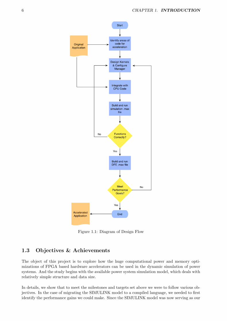
As a block diagram environment for multi-domain simulation and Model-based design, SIMULINKhas been used to analyze and design of power systems. The simulation of 4-machine, 2 -areastudy system is initially in the form of a SIMULINK model based on some standard approaches tomodeling of several power system components in Dr Chaudhuri’s book, and an overview of thesemodels is given as the background knowlegde in Chapter 2. However, although the SIMULINK toolprovides a graphical user interface for building visualized model as block diagrams, It can’t avoidthe restrictions on its simulation performance. For example, large images and complex graphicstake a long time to load and render. As a result, masked blocks that contain images might makeyour model less responsive. [20] In this project we will explore the benefits of accelerating fromusing Field Programming Gate Arrays (FPGAs) to power system simulation. There are many vari-ations of FPGA designs. We will use the hardware and the complier by Maxeler Technologies. Theimplementation can be built using the programming paradigm known as data flow programming.Maxeler’s dataflow system is a hybrid CUP-FPGA system. Therefore, the first step is optimise thesimulation process in a complied language (we use C language) application so that it can run anCPU, and then further accelerate the slow operations by mapping the dataflow to the data flowengines(DFEs) provided by Maxeler. Specially, we should follow the design flow shown in Fig.1.1.
So the task can be divided into steps of progresses:
• Step 1: Study the Maxcompiler system, and dataflow programming technology.
• Step 2: Understanding the SIMULINK model and analyzing the program.
• Step 3: Rewrite the SIMULINK code to C code. Measure how long it takes to run theapplication on CPUs given a set of large datasets.
• Step 4: Identify areas of code for acceleration: a more detailed analysis provides the distri-bution of runtime of various parts of the application using time counter and profiling toolssuch as gprof, oprofile etc.
• Step 5: For the code to be accelerated, create dataflow graph, data layout and representation.
• Step 6: Optimize dataflow, data access and data representation options by the principle:maximizing regularity of computation and minimizing communication between CPU anddataflow engines.
• Step 7: use Maxcompiler to configure application for FPGA and analyze the performance.
6 CHAPTER 1. INTRODUCTION
Figure 1.1: Diagram of Design Flow
1.3 Objectives & Achievements
The object of this project is to explore how the huge computational power and memory opti-mizations of FPGA based hardware accelerators can be used in the dynamic simulation of powersystems. And the study begins with the available power system simulation model, which deals withrelatively simple structure and data size.
In details, we show that to meet the milestones and targets set above we were to follow various ob-jectives. In the case of migrating the SIMULINK model to a compiled language, we needed to firstidentify the performance gains we could make. Since the SIMULINK model was now serving as our
1.4. REPORT STRUCTURE 7
only description of the algorithms, it was in our best interests to rewrite the graphical descriptionsas functions and refactor code which appeared slow or unnecessary. Once the power system simu-lation in SIMULINK was optimised to a complied language, we should check for correctness. Oncewe verified the program’s outputs, we could look at performance gains and consider acceleration.For this, the Field Programmable Gate Array (FPGA) applied by the Maxeler Technologies wasused. We present an evaluation of various design of the Kernels to accelerate the power system,and demonstrate our achievement of acceleration.
The following objectives were key in directing this project to its end and producing our contribu-tions:
• Analyised the simulation model in SIMULINK (chapter 3). Proposed a method to tracethe sorted order of different subsystems and blocks in SIMULINK. This was paramount inproviding a base to begin migrating to a compiled language.
• An optimised version of the simulation in C language (chapter 4). We maximise the perfor-mance gains available without hardware acceleration by 500 times’ faster than SIMULINK.We re-implemented everything from scratch so that have concluded an efficient scheme ofconverting SIMULINK diagrams to C(C++) language.
• An accelerated version of the LU decomposition solver used in the power system simulation.(chapter 5) And implementation of different FPGA kernel designs for pipeline. During thisprocess, we successfully solved the problem of handling complex numbers in maxeler.
• Analysed the performance of the designed kernels(chapter 6). A relationship between thespeedup of simulation and the data size of the power system is built which indicated that ouracceleration design can give a significant acceleration to larger-scale larger power systems.
1.4 Report Structure
In this chapter we looked at an overview of the main motivations, objectives and steps for ourproject. The rest of this report is divided into 7 chapters and organized as follows.
Chapter 2 introduces the background knowledge needed for understanding the project. The firstpart of chapter 2 illustrates the idea of power system simulation and an dynamic simulation modelof the power system is introduced which support the primary mathematical principle underlayingour SIMULINK power system model. The second part of chapter 2 gives an introduction to theSIMULINK tool while the third part presents the principles of FPGAs and Hardware accelerationtechnology and also the FPGA programming platform we used in the project: a programmingmodel based on data-flow programming provided by Maxeler Technologies call MaxCompiler.
Chapter 3 is about how I analysed the given Simulink Model in order to extract the algorithms fora complied language, I will show this from four aspects. 1. An overview of the simulink model, thestructure. 2. What are the inputs and desired outputs of the model and where are they from. 3.How does the operarions linked together: the execution order of the blocks,their dependency. 4.What are the specific operations involved, and how to understand them, the mathematical mean-ing.
Chapter 4 gives a detailed illustration of an optimised application in C language that does the samething with the simulation system. Depending on the analysis in chapter 2, we describe the ideaswe used to re-implement each aspect of the simulation scheme that corresponding to each sectionof chapter 2.
Chapter 5 starts from showing the profiling result of the C application introduced in chapter 4

8 CHAPTER 1. INTRODUCTION
which determined the area of code to be accelerated by FPGA. And then, the design and imple-mentation details using the Maxeler Compiler are represented.
Chapter 6 gives the noteworthy experimental results for both the C application, and the accelerateddesign of FPGA computing blocks. And by comparing them, we analysis the practicability of ourhardware design.
Chapter 7 is the conclusion of the report and lists some further work the author would like to trylater.

Chapter 2
Background
2.1 Power System Simulation
An electric power system is a network of electrical components used to supply, transmit and useelectric power. An example of an electric power system is the network that supplies a region’shomes and industry with power , this power system is known as the power grid and can be broadlydivided into the generators that supply the power, the transmission system that carries thepower from the generating centres to the load centres and the distribution system that feeds thepower to nearby homes and industries. Smaller power systems are also found in industry, hospitals,commercial buildings and homes.
Simulation is historically one the principal tools used in the design of power system controls.Theconventional power-system stability study computes the system response to a sequence of largedisturbances, usually a network short circuit, followed by protective branch-switching operations.The process is a direct simulation in the time domain of duration varying between say 1 s and 20min or m.ore. Different components of the power system have their greatest influences on stabilityat different of the response, and the system modeling (simulation) reflects this fact.
In power systems, the primary sources of electrical energy are the synchronous generators. Theproblem of power system stability is primarily to keep the interconnected synchronous machines insynchronism [17]. The stability is also dependent on several other components such as the speedgovernors, excitation systems of the generators, the loads, the FACTS devices etc. Therefore,an understanding of their characteristics and modeling of their performance are of fundamentalimportance for stability studies and control design. The general approach to modelling of severalpower system components is quite standard, and a quick overview of these models is given in nextsection.
2.2 Models of Different Components in Power System
Accurate modelling of the generators and their excitation systems is of fundamental importancefor studying the dynamic behavior of power systems. Besides generators and excitation systems,other components such as the dynamic loads (e.g. induction motor type), controllable devices (e.g.thyristor controlled series capacitor (TCSC), power system stabilizer (PSS)), prime-movers etc.need to be modelled as well. The dynamic behavior of these devices is generally described througha set of differential equations. The power flow in the network is represented by a set of algebraicequations. This gives rise to a set of differential-algebraic equations (DAE) describing the powersystem behavior. Different types of model have been reported in the literature for each of the powersystem components depending upon their specific application [17], [29]. In this section, the relevantequations governing the dynamic behavior of only the specific types of models used in this projectis described. The IEEE recommended practice regarding d-q axis orientation [5] of a synchronousgenerator is used. This results in a negative d axis component of stator current for an overexcited
9
10 CHAPTER 2. BACKGROUND
generator delivering power to the system.
2.2.1 Generators
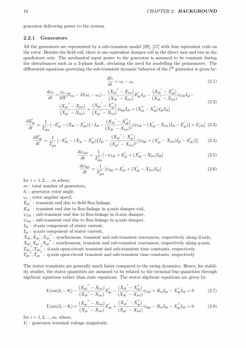
All the generators are represented by a sub-transient model [29], [17] with four equivalent coils onthe rotor. Besides the field coil, there is one equivalent damper coil in the direct axis and two in thequadrature axis. The mechanical input power to the generator is assumed to be constant duringthe disturbances such as a 3-phase fault, obviating the need for modelling the primemover. Thedifferential equations governing the sub-transient dynamic behavior of the ith generator is given by:
dδidt
= ωi − ωs (2.1)
dωi
dt=ωs
2H[Tmi −D(ωi − ωs)−
(Xdi′′ −Xlsi)
(Xdi′ −Xlsi)
E′qiIqi −
(Xdi′ −X ′′
di)
(Xdi′ −Xlsi)
ψ1diIqi−
(Xqi′′ −Xlsi)
(Xqi′ −Xlsi)
+(Xqi
′ −X ′′qi)
(Xqi′ −Xlsi)
ψ2qiIdi + (X′′qi −X
′′di)IqiIdi]
(2.2)
dE′qi
dt=
1
T′doi
[−E′qi− (Xdi−X
′di){−Idi−
(Xdi′ −X ′′
di)
(Xdi′ −Xlsi)2
(ψ1di− (X′di−Xlsi)Idi−E
′qi)}+Efdi] (2.3)
dE′di
dt=
1
T′qoi
[−E′di − (Xqi −X
′qi){Iqi −
(Xqi′ −X ′′
qi)
(Xqi′ −Xlsi)2
(ψ2qi + (X′qi −Xlsi)Iqi − E
′di)}] (2.4)
dψ1di
dt=
1
T′′doi
[−ψ1di + E′qi + (X
′di −Xlsi)Idi] (2.5)
dψ2qi
dt=
1
T′′qoi
[ψ2qi + E′di + (X
′qi −Xlsi)Iqi] (2.6)
for i = 1, 2, ...,m,where,m : total number of generators,δi : generator rotor angle,ωi : rotor angular speed,Eqi
′: transient emf due to field flux-linkage,
Edi′
: transient emf due to flux-linkage in q-axis damper coil,ψ1di : sub-transient emf due to flux-linkage in d-axis damper,ψ1qi : sub-transient emf due to flux-linkage in q-axis damper,Idi : d-axis component of stator current,Iqi : q-axis component of stator current,
Xdi, Xdi′, Xdi
′′: synchronous, transient and sub-transient reactances, respectively along d-axis,
Xqi, Xqi′, Xqi
′′: synchronous, transient and sub-transient reactances, respectively along q-axis,
Tdo′′, Tdo
′′: d-axis open-circuit transient and sub-transient time constants, respectively
Tqo′′, Tqo
′′: q-axis open-circuit transient and sub-transient time constants, respectively
The stator transients are generally much faster compared to the swing dynamics. Hence, for stabil-ity studies, the stator quantities are assumed to be related to the terminal bus quantities throughalgebraic equations rather than state equations. The stator algebraic equations are given by:
Vicos(δi − θi)−(Xdi
′′ −Xlsi)
(Xdi′ −Xlsi)
E′qi −
(Xdi′ −X ′′
di)
(Xdi′ −Xlsi)
ψ1di +RsiIqi −X′′diIdi = 0 (2.7)
Visin(δi − θi) +(Xqi
′′ −Xlsi)
(Xqi′ −Xlsi)
E′di +
(Xqi′ −X ′′
qi)
(Xqi′ −Xlsi)
ψ2qi −RsiIdi −X′′qiIdi = 0 (2.8)
for i = 1, 2, ...,m, where,Vi : generator terminal voltage magnitude,

2.2. MODELS OF DIFFERENT COMPONENTS IN POWER SYSTEM 11
θi : generator terminal voltage angle,Rsi : resistance of the armature,Xlsi : armature leakage reactance.The notation is standard as in [29]. The parameters used for the study system are given in AppendixA.
2.2.2 Excitation systems
The generators are equipped with slow excitation systems (IEEE-DC1A) to ensure adequate damp-ing for its local modes. The rest of the generators are under manual excitation control. The differ-ential equations governing the behavior of an IEEE-DC1A type excitation system are given by:
dVtridt
=1
Tri[−Vtri + Vti] (2.9)
dEfdi
dt= − 1
TEi[KEiEfdi + EfdiAexe
BExEfdi − Vri] (2.10)
dVridt
=1
TAi[KAiKFi
TFiRFi +KAi(Vrefi − Vtri)−
KAiKFi
TFiEfdi − Vri] (2.11)
dRFi
dt=
1
TFi[−RFi + Efdi] (2.12)
where,Efdi : field voltage,Vtri : measured voltage state variable after sensor lag block,and the rest of the notation carries their standard meaning [29].
2.2.3 Network power flow model
The network power balance equation for the ith generator bus is given by:
Vicos(δi − θi)Iqi − Visin(δi − θi)Idi − Spi = 0 (2.13)
−Visin(δi − θi)Iqi − Vicos(δi − θi)Idi − Sqi = 0 (2.14)
where,
Spi =
k=n∑k=1
ViVk[Gikcos(θi − θk) +Biksin(θi − θk)] (2.15)
Sqi =k=n∑k=1
ViVk[Giksin(θi − θk)−Bikcos(θi − θk)] (2.16)
for i = 1, 2, ...,m
Power balance equations for the ith non-generator bus is given by:
PLi(Vi) +
k=n∑k=1
ViVk[Gikcos(θi − θk) +Biksin(θi − θk)] = 0 (2.17)
QLi(Vi) +
k=n∑k=1
ViVk[Giksin(θi − θk)−Bikcos(θi − θk)] = 0 (2.18)
for i = m+ 1, ..., nwhere, n is the total number of buses in the system and Yik = Gik + jBik is the element of the ithrow and kth column of the bus admittance matrix Y .
12 CHAPTER 2. BACKGROUND
2.2.4 Thyristor conrolled series capacitor (TCSC)
A TCSC is a capacitive reactance compensator which consists of a series capacitor bank shuntedby a thyristor controlled reactor (TCR) in order to provide a smooth variation in series capacitivereactance [11], [31].
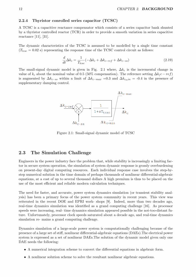
The dynamic characteristics of the TCSC is assumed to be modelled by a single time constant(Ttcsc = 0.02 s) representing the response time of the TCSC control circuit as follows:
d
dt∆kc =
1
Ttcsc(−∆kc + ∆kc−ref + ∆kc−ss) (2.19)
The small-signal dynamic model is given in Fig. 2.1 where, ∆kc is the incremental change invalue of kc about the nominal value of 0.5 (50% compensation). The reference setting ∆k(c− ref)is augmented by ∆kc−ss within a limit of ∆kc−max =0.3 and ∆kcmin = -0.4 in the presence ofsupplementary damping control.
Figure 2.1: Small-signal dynamic model of TCSC
2.3 The Simulation Challenge
Engineers in the power industry face the problem that, while stability is increasingly a limiting fac-tor in secure system operation, the simulation of system dynamic response is grossly overburdeningon present-day digital computing resources. Each individual response case involves the step-by-step numerical solution in the time domain of perhaps thousands of nonlinear differential-algebraicequations, at a cost of up to several thousand dollars A high premium is thus to be placed on theuse of the most efficient and reliable modern calculation techniques.
The need for faster, and accurate, power system dynamics simulation (or transient stability anal-ysis) has been a primary focus of the power system community in recent years. This view wasreiterated in the recent DOE and EPRI work- shops [9]. Indeed, more than two decades ago,real-time dynamics simulation was identified as a grand computing challenge [16]. As processorspeeds were increasing, real- time dynamics simulation appeared possible in the not-too-distant fu-ture. Unfortunately, processor clock speeds saturated about a decade ago, and real-time dynamicssimulation re- mains a grand computing challenge.
Dynamics simulation of a large-scale power system is computationally challenging because of thepresence of a large set of stiff, nonlinear differential-algebraic equations (DAEs).The electrical powersystem is expressed as a set of nonlinear DAEs.The solution of the dynamic model given only oneDAE needs the following:
• A numerical integration scheme to convert the differential equations in algebraic form.
• A nonlinear solution scheme to solve the resultant nonlinear algebraic equations.
2.3. THE SIMULATION CHALLENGE 13
• A linear solver to solve the update step at each iteration of the nonlinear solution.
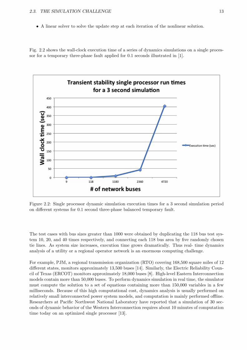
Fig. 2.2 shows the wall-clock execution time of a series of dynamics simulations on a single proces-sor for a temporary three-phase fault applied for 0.1 seconds illustrated in [1].
Figure 2.2: Single processor dynamic simulation execution times for a 3 second simulation periodon different systems for 0.1 second three-phase balanced temporary fault.
The test cases with bus sizes greater than 1000 were obtained by duplicating the 118 bus test sys-tem 10, 20, and 40 times respectively, and connecting each 118 bus area by five randomly chosentie lines. As system size increases, execution time grows dramatically. Thus real- time dynamicsanalysis of a utility or a regional operator network is an enormous computing challenge.
For example, PJM, a regional transmission organization (RTO) covering 168,500 square miles of 12different states, monitors approximately 13,500 buses [14]. Similarly, the Electric Reliability Coun-cil of Texas (ERCOT) monitors approximately 18,000 buses [8]. High-level Eastern Interconnectionmodels contain more than 50,000 buses. To perform dynamics simulation in real time, the simulatormust compute the solution to a set of equations containing more than 150,000 variables in a fewmilliseconds. Because of this high computational cost, dynamics analysis is usually performed onrelatively small interconnected power system models, and computation is mainly performed offline.Researchers at Pacific Northwest National Laboratory have reported that a simulation of 30 sec-onds of dynamic behavior of the Western Interconnection requires about 10 minutes of computationtime today on an optimized single processor [13].
14 CHAPTER 2. BACKGROUND
2.4 The SIMULINK Tool
2.4.1 What is SIMULINK
Simulink [30],[19] developed by The MathWorks, is a software package for modeling, simulating,and analyzing dynamical systems. It supports linear and nonlinear systems, modeled in continuoustime, sampled time, or a hybrid of the two. Systems can also be multirate, such as signal processing,control and communication applications. It can now also be used to analyze and design of powersystems.[24] During last four decades simulation of power systems have gained more importance.Recently published IEEE paper discussing different approaches to modeling protective relays andrelated power system events indicates a variety of possible software tools that may be used for thispurpose [36]. But rather than MATLAB/SIMILINK software it is difficult to add the modelingand simulation features to teach specific protective relaying concepts that go beyond the level ofdetail originally provided by the software.[33]
For modeling, Simulink provides a graphical user interface (GUI) for building models as blockdiagrams, using click-and-drag mouse operations. With this interface, you can draw the modelsjust as you would with pencil and paper (or as most textbooks depict them). Simulink includesa comprehensive block library of sinks, sources, linear and nonlinear components, and connectors.You can also customize and create your own blocks. For information on creating your own blocks,see the separate Writing S-Functions guide.
Models are hierarchical, so you can build models using both top-down and bottom-up approaches.You can view the system at a high level, then double-click on blocks to go down through thelevels to see increasing levels of model detail. This approach provides insight into how a model isorganized and how its parts interact.
After you define a model, you can simulate it, using a choice of integration methods, either fromthe Simulink menus or by entering commands in MATLABs command window. Using scopes andother display blocks, you can see the simulation results while the simulation is running. In addition,the simulation results can be put in the MATLAB workspace for post-processing and visualization.
2.4.2 Basic elements of Simulink
Models in Simulink can be thought of as executable specifications, Simulink’s graphical editor isused for modeling dynamic systems with a block diagram, consisting two major classes of elementsin Simulink: blocks and connections. Blocks are used to generate, modify, combine, output, anddisplay signals. Narrows are used to transfer signals from one block to another.
Blocks
Each block represents a set of equations called block methods, which define a relationship betweenthe blocks input signals, output signals and the state variables. In the Simulink User Guide a blockis characterised by a combination of three functions.
1. A function which computes the output from the state and the input values.
2. A function which computes the next value of the discrete components of the state.
3. A function which yields the rate of change of the continuous components of the state. Blocksare frequently parameterized with constants or arithmetical expressions over constants.
Examples of simulink blocks
2.4. THE SIMULINK TOOL 15
The block is an entity which defines a relation between its inputs and outputs. The block’s func-tionality can vary, depending on the blocks parameters and inputs. It can also be influenced byother blocks. The number of blocks inputs and outputs can vary also. Each input and output hasa dimensionality and it can be a scalar, vector or a matrix signal. We will give a representativeexample for most of these cases.
The Gain block (Fig. 2.3) multiplies the input by a constant value which is specified by the Gainparameter. The Gain can be a scalar or a vector.
Figure 2.3: A Gain block and sample values
The Sum block (Fig. 2.4) performs addition or subtraction on its inputs. This block can addor subtract scalar or vector inputs. If the block has a single input signal, then it collapses itselements into a scalar by summing or subtracting them. The operation of the block is specifiedwith the ”List of signs” parameter, which is a list of Plus (+) and minus (-) signs, and indicatesthe operations to be performed on the inputs. If there are two or more inputs, then the numberof + and characters must equal the number of inputs. For example, ”+-+” requires three inputsand configures the block to subtract the second (middle) input from the first input, and then addthe third input. All non-scalar inputs must have the same dimensions. Scalar inputs are expandedto have the same dimensions as the other inputs.
Figure 2.4: An Add block and sample computations.
The Mux block (Fig. 2.5) combines its inputs into a single vector output. An input can be ascalar or a vector signal. The Mux block’s ”Number of Inputs” parameter allows to specify inputsignal names and sizes as well as the number of inputs.
The Subsystem block. (Fig. 2.6) A subsystem is a set of blocks that have been replaced bya single block called a Subsystem block. As a model increases in size and complexity, it can besimplified by grouping blocks into subsystems. Using subsystems helps to reduce the number ofblocks displayed in the model window, allows to keep functionally-related blocks together, andenables to establish a hierarchical block diagram. The whole Simulink model, composed of blocksand subsystems is placed in a single system block referred to as a root system.
The Outport block. The outport block in a subsystem represents its outputs. A signal arriving
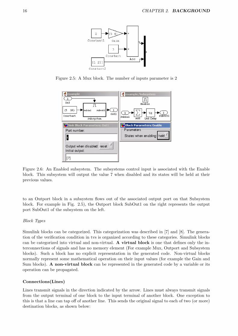
16 CHAPTER 2. BACKGROUND
Figure 2.5: A Mux block. The number of inputs parameter is 2
Figure 2.6: An Enabled subsystem. The subsystems control input is associated with the Enableblock. This subsystem will output the value 7 when disabled and its states will be held at theirprevious values.
to an Outport block in a subsystem flows out of the associated output port on that Subsystemblock. For example in Fig. 2.5), the Outport block SubOut1 on the right represents the outputport SubOut1 of the subsystem on the left.
Block Types
Simulink blocks can be categorized. This categorization was described in [7] and [8]. The genera-tion of the verification condition in tvs is organized according to these categories. Simulink blockscan be categorized into virtual and non-virtual. A virtual block is one that defines only the in-terconnections of signals and has no memory element (For example Mux, Outport and Subsystemblocks). Such a block has no explicit representation in the generated code. Non-virtual blocksnormally represent some mathematical operation on their input values (for example the Gain andSum blocks). A non-virtual block can be represented in the generated code by a variable or itsoperation can be propagated.
Connections(Lines)
Lines transmit signals in the direction indicated by the arrow. Lines must always transmit signalsfrom the output terminal of one block to the input terminal of another block. One exception tothis is that a line can tap off of another line. This sends the original signal to each of two (or more)destination blocks, as shown below:
2.5. HARDWARE ACCELERATION & FPGAS 17
Lines can never inject a signal into another line; lines must be combined through the use of a blocksuch as a summing junction.
Signal
Signals are what kind of information is carried by the connections in a diagram. According to theUsing Simulink manual, a wide range of signal attributes can be specified, including signal name,data type (e.g., 16-bit or 32-bit integer, double, single, uint8, uint16, uint32), numeric type (realor complex), and dimensionality (e.g., one-dimensional or multidimensional array), and introducesthe type Boolean.
2.4.3 Textual Representation of the Model
There are two textual representations of the model:
• The model.mdl file, which is written in a Mathworks propriety markup language. The filecontains the graphical model description and assignments to parameters of template blocks.Simulink allows not specifying blocks parameters that can be derived, i.e., propagated fromother blocks automatically (for example input signals types. Therefore, in the model file notall parameters are contained explicitly for all blocks. Blocks parameters can be defined interms of Matlab workspace variables, but those values are also not included in the model.mdlfile. Thus, the model.mdl file is tightly coupled with the MATLAB environment.
• The model.rtw file, which is derived from model.mdl during code generation. It is an in-termediate representation created by removing graphical information from model.mdl, andevaluating parameters of blocks. Although it contains more information, its format is notdescribed in Mathworks’ documentation and is difficult to understand by reverse engineering.
2.5 Hardware Acceleration & FPGAs
2.5.1 Hardware Accelerators
In computing, hardware acceleration is the use of computer hardware to perform some functionfaster than is possible in software running on the general-purpose CPU. Examples of hardwareacceleration include blitting acceleration functionality in graphics processing units (GPUs) andinstructions for complex operations in CPUs. Many hardware accelerators are built on top of field-programmable gate array chips. Also, machines such as the gaming machine Sony-PlayStation canbe used as hardware accelerators.
Normally, processors are sequential, and instructions are executed one by one. Conventional pro-cessors are hitting the limits of attainable clock frequencies and thus, future significant increases inperformance must come from exploiting parallelism. [26] Various techniques are used to improve

18 CHAPTER 2. BACKGROUND
performance; hardware acceleration is one of them. The main difference between hardware andsoftware is concurrency, allowing hardware to be much faster than software. The hardware thatperforms the acceleration, when in a separate unit from the CPU, is referred to as a hardwareaccelerator. [35]
As shown in [18] The overarching goal of hardware acceleration is to increase the speed at whichdata can be processed by using custom hardware specifically designed to implement a specific rou-tine. By doing so, the software can be sped up in two ways. The first advantage is that the CPU isable to process other data, while the computation necessary for the accelerated routine is offloadedto the coprocessor. This makes the computation appear to be essentially free to the processor.The only time the processor must spend on the computation is the time that it takes to set upthe coprocessor to begin its calculation and the time it takes to receive the results. As long asthe overhead necessary to communicate with coprocessor is less costly than performing the actualcomputation, a speedup is realized.
The second potential gain is realized when the hardware accelerator is structured in such a waythat it is able to calculate the result a faster than the software. In this case, the communicationsoverhead, and the runtime of the hardware accelerator must be less than the time the softwareimplementation of the same algorithm would take. If this condition is met the algorithm will beaccelerated whether or not the processor is processing data in parallel with the coprocessor.
2.5.2 Field-programmable gate array (FPGA)
FPGAs are reconfigurable hardware chips that can be reprogrammed to implement varied combina-tional and sequential logic.For the purpose of this project we will focus on FPGA based accelerationas the significant improvements in FPGA size, speed, and storage capacity have made them ex-cellently potential as hardware accelerators for a wide class of applications. Significant speedupsachieved using FPGAs to accelerate cryptography, sparse matrix-vector multiplication, Viterbi de-coding, and financial computing systems have been reported in recent literature [21],[34],[3]. Asan example, the study described in [34] demonstrated a 2 times speedup for floating-point sparsematrix-vector multiplication (a computational kernel at the heart of many scientific computingapplications) implemented on a Virtex II FPGA compared to the fastest single processor systemat the time and even greater speedups for multi- FPGA systems (compared to multi-processorsystems)[12]. And an FPGA accelerated system can be 31-37 times faster than an equivalentlysized conventional machine, and consume 1/39 of the power. [7]
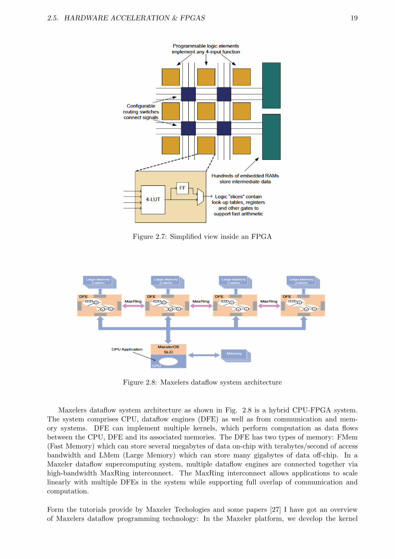
An FPGA is made up of an array of programmable logic blocks (programming cells). These logicblocks are connected by reconfigurable sets of wires as shown in Fig. 2.7, which allow for signalsto be routed according to the definition of the circuit. [18] Modern FPGAs allow the user to re-configure these circuits many times each second, making FPGAs fully programmable and generalpurpose. The price of reconfigurability is a 10x slower dynamic clock frequency compared to todaysstate-of-the-art Pentium and Opteron processors. This slower clock frequency is compensated forby support for massive fine-grained parallelism. [26]
2.5.3 Maxeler Platform
In our project we will use a programming model based on data-flow provided by Maxeler Tech-nologies which is entirely driven by Java. The user specifies kernels, which are statically scheduled,pipelined data-paths, and a manager that controls the routing of streaming data between multiplekernels and off-chip connections. Kernels use arbitrary precision floating/fixed point types and ourcompiler takes care of type conversions. [7]]
2.5. HARDWARE ACCELERATION & FPGAS 19
Figure 2.7: Simplified view inside an FPGA
Figure 2.8: Maxelers dataflow system architecture
Maxelers dataflow system architecture as shown in Fig. 2.8 is a hybrid CPU-FPGA system.The system comprises CPU, dataflow engines (DFE) as well as from communication and mem-ory systems. DFE can implement multiple kernels, which perform computation as data flowsbetween the CPU, DFE and its associated memories. The DFE has two types of memory: FMem(Fast Memory) which can store several megabytes of data on-chip with terabytes/second of accessbandwidth and LMem (Large Memory) which can store many gigabytes of data off-chip. In aMaxeler dataflow supercomputing system, multiple dataflow engines are connected together viahigh-bandwidth MaxRing interconnect. The MaxRing interconnect allows applications to scalelinearly with multiple DFEs in the system while supporting full overlap of communication andcomputation.
Form the tutorials provide by Maxeler Techologies and some papers [27] I have got an overviewof Maxelers dataflow programming technology: In the Maxeler platform, we develop the kernel

20 CHAPTER 2. BACKGROUND
code by the hardware compiler called MaxCompiler. The Maxeler platform utilizes Java as ameta-programing language for implementation. The MaxCompiler IDE isa modified version of theEclipse IDE, with a modified version of Java serving as the descriptive code for the dataflow. Usinga meta-program that describes the structure of dataflow as an input, MaxCompiler generates the.max file which contains the FPGA bitstream. Also, data exchange between a host CPU and adataflow engine is performed using a run-time library API called MaxCompilerRT.
Figure 2.9: Maxeler MaxCompiler Development Flow
In the Maxeler system, data streaming and execution are performed as follows. The dataflowengine is initialized and the .max file generated by MaxCompiler is loaded from the CPU to theengine, configuring the FPGA. After input data are streamed from CPU memory onto the FPGAchip, these are processed by forwarding intermediate results from one functional unit to anotherwhere the results are needed, without ever being written to the off-chip memory until the chain ofprocessing is complete. After all processing on the dataflow engine is completed, the final outputdata are transferred to CPU memory.
Chapter 3
Analysing the Power SystemSimulation
The original power system simulation system (a 4-machine, 2 -area study system) is initially builtas a SIMULINK model. In order to apply the FPGA accelerators to this simulation problem, wetherefore take first steps in converting the Simulink diagram to a software application. Before wecan present our conversions, we must first understand how the power simulation is modeled in theSimulinks grammar and extract the underlying updating algorithms from the diagram representa-tion.
In this chapter we present how we analysed the Power System simulation model to extract thedynamic behavior of the power system from a software optimisations point of view that allow per-formance gains in SIMULINK and a departure from the SIMULINKs graphical user interface to acompiled language.
In detail, we will firstly introduce the power system that the simulation built on, then from theSimulation program we analysed the properties of the program: the requirements of the program,the data flow and the control flow of the program.Section 3.1 describes the power system beingsimulated. Section 3.2 covers an detailed analysis of the power system simulation in the form of aSIMULINK model. And section 3.3 gives a brief illustration of the performance of the SIMULINKmodel from the efficiency prospect.
3.1 The Study System
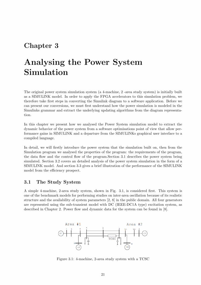
A simple 4-machine, 2-area study system, shown in Fig. 3.1, is considered first. This system isone of the benchmark models for performing studies on inter-area oscillation because of its realisticstructure and the availability of system parameters [2, 8] in the public domain. All four generatorsare represented using the sub-transient model with DC (IEEE-DC1A type) excitation system, asdescribed in Chapter 2. Power flow and dynamic data for the system can be found in [8].
Figure 3.1: 4-machine, 2-area study system with a TCSC
21
22 CHAPTER 3. ANALYSING THE POWER SYSTEM SIMULATION
The system consists of two areas connected by a weak transmission corridor. To enhance thetransfer capability of the corridor, a TCSC is installed in one of the lines connecting buses #8 and#9. From the transfer capacity enhancement point of view, the percentage compensation Kc ofthe TCSC is set to 10%. A maximum and minimum limit of 50% and 1%, respectively, is imposedon the dynamic variation of kc. Under normal operating conditions, the power flow from Area #1to Area # 2 is 400 MW.
3.2 Analysing the SIMULINK Model
As mentioned before, Simulink is a block diagram environment for multi-domain simulation andModel-based design. It supports system-level design, simulation, and continuous test and verifica-tion of embedded systems. It can now also be used to analyze and design of power systems. Theoriginal simulation system is just initially written as a SIMULINK model. The sium4mac.mdl file,containing the graphical model description and assignments to parameters of template blocks, isthe main entry point of our analysis. Form the Model, we can know:
• What is simulation process, the time.
• What are the inputs and desired outputs of the model and where are they from (How arethey initialized and updated).
• How do the operations linked together: the execution order of the blocks, their dependency.
• What are the specific operations involved, and how to understand them: their mathematicalmeaning (control flow)
3.2.1 An overview of the simulation process
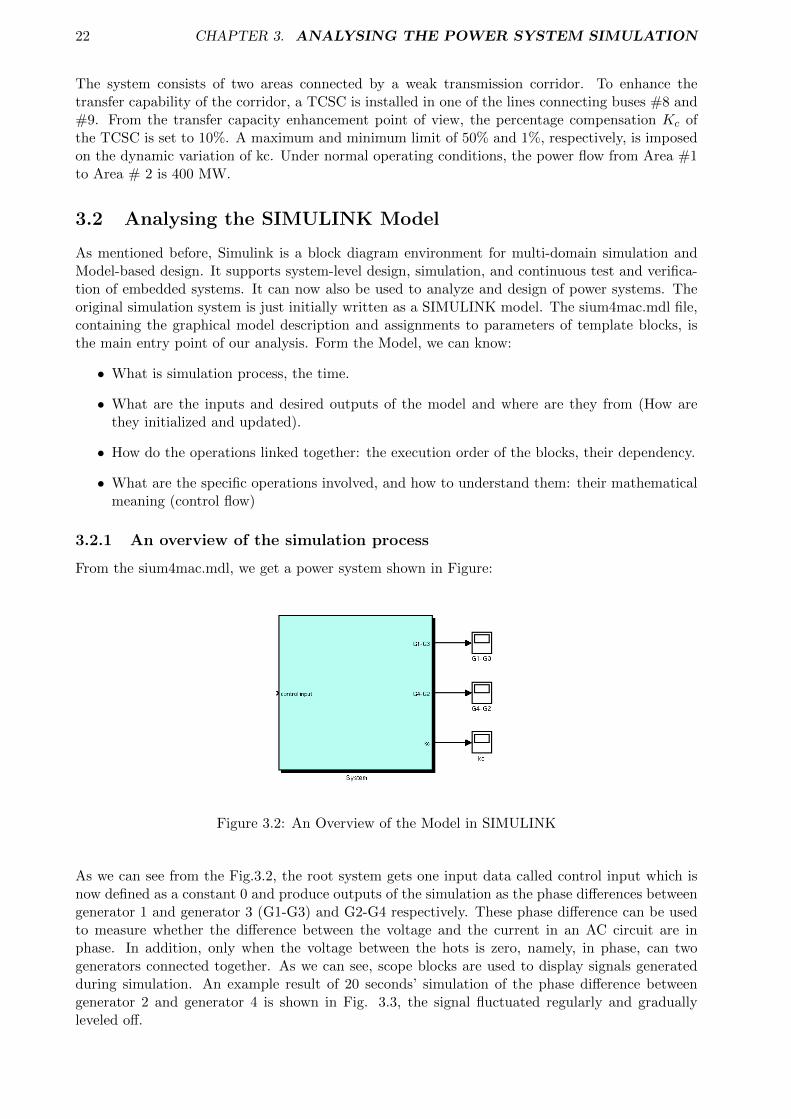
From the sium4mac.mdl, we get a power system shown in Figure:
Figure 3.2: An Overview of the Model in SIMULINK
As we can see from the Fig.3.2, the root system gets one input data called control input which isnow defined as a constant 0 and produce outputs of the simulation as the phase differences betweengenerator 1 and generator 3 (G1-G3) and G2-G4 respectively. These phase difference can be usedto measure whether the difference between the voltage and the current in an AC circuit are inphase. In addition, only when the voltage between the hots is zero, namely, in phase, can twogenerators connected together. As we can see, scope blocks are used to display signals generatedduring simulation. An example result of 20 seconds’ simulation of the phase difference betweengenerator 2 and generator 4 is shown in Fig. 3.3, the signal fluctuated regularly and graduallyleveled off.

3.2. ANALYSING THE SIMULINK MODEL 23
Figure 3.3: The Result of 20s’ simulation of G2-G4
As a simulation system in SIMULINK, the input data streaming through the model, doing oper-ations behind it (more detailed in the subsystems) once each step size and update their states,which will be used in next step. So the total number of iterations is:
Updatetimes =Simulationtime
Stepsize(3.1)
Where step size is set to 1e-3 by default, and Simulation Time is the total length of time thesimulation runs (the period between start time and end time), these values can be set from thesolver pane of the graphical user interface: Simulation →Configure Parameters→Solver.The solver plan specifies not only the simulation start and stop time but also the solver configurationfor the simulation. As we mentioned before, a solver computes a dynamic system’s states atsuccessive time steps over a specified time span, using information provided by the model, whichis the fundamental mechanism of the simulation process.
The Simulink product provides an extensive library of solvers (e.g., the Dormand-Prince method,the Runge-Kutta method, the Bogacki-shampine method, the Heuns method and the Euler method)each of which determines the time of the next simulation step and applies a numerical method tosolve the set of ordinary differential equations (ODEs) that represent the model. In the processof solving this initial value problem, the solver also satisfies the accuracy requirements that wespecify. The default setting is the ode3 solver (Bogacki-shampine).
3.2.2 Subsystems
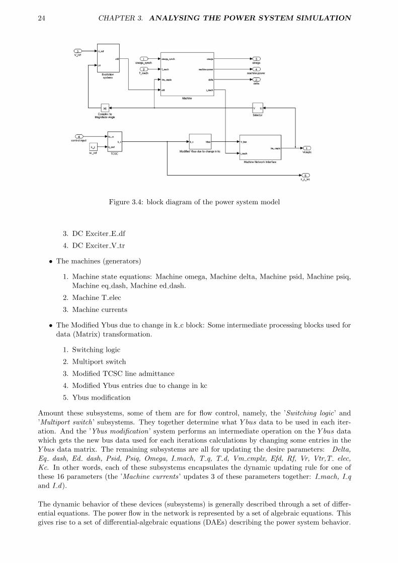
To see how is the power system structured and how is the data updated, we can just trace downhierarchical block diagram level by level.
As shown in Fig. 3.4, the power system is configured by 5 main subsystem blocks, and each ofthese subsystems also contains its own subsystems, totally 19 subsystems:
• TSCS system
• The ’machine network interface’ system
• The excitation system
1. DC Exciter R f
2. DC Exciter V r
24 CHAPTER 3. ANALYSING THE POWER SYSTEM SIMULATION
Figure 3.4: block diagram of the power system model
3. DC Exciter E df
4. DC Exciter V tr
• The machines (generators)
1. Machine state equations: Machine omega, Machine delta, Machine psid, Machine psiq,Machine eq dash, Machine ed dash.
2. Machine T elec
3. Machine currents
• The Modified Ybus due to change in k c block: Some intermediate processing blocks used fordata (Matrix) transformation.
1. Switching logic
2. Multiport switch
3. Modified TCSC line admittance
4. Modified Ybus entries due to change in kc
5. Ybus modification
Amount these subsystems, some of them are for flow control, namely, the ’Switching logic’ and’Multiport switch’ subsystems. They together determine what Y bus data to be used in each iter-ation. And the ’Ybus modification’ system performs an intermediate operation on the Y bus datawhich gets the new bus data used for each iterations calculations by changing some entries in theY bus data matrix. The remaining subsystems are all for updating the desire parameters: Delta,Eq dash, Ed dash, Psid, Psiq, Omega, I mach, T q, T d, Vm cmplx, Efd, Rf, Vr, Vtr,T elec,Kc. In other words, each of these subsystems encapsulates the dynamic updating rule for one ofthese 16 parameters (the ’Machine currents’ updates 3 of these parameters together: I mach, I qand I d).
The dynamic behavior of these devices (subsystems) is generally described through a set of differ-ential equations. The power flow in the network is represented by a set of algebraic equations. Thisgives rise to a set of differential-algebraic equations (DAEs) describing the power system behavior.

3.2. ANALYSING THE SIMULINK MODEL 25
(a) Inside the excitation system (b) Inside the Exciter R f block
Figure 3.5: The Excitation Subsystem
The relevant equations governing the dynamic behavior of only the specific types of models usedin this study system are given in Chapter 2.
By tracing down the subsystems, we can extract the operation blocks and their mathematical repre-sentations to form the algorithms used to simulate the power flow and finally they can be matchedwith the differential-algebraic equations given. For example, the Excitation system and can befurther extended and finally matched the governing equations for the IEEE-DC1A type excitationsystem given by:
dVtridt
=1
Tri[−Vtri + Vti] (3.2)
dEfdi
dt= − 1
TEi[KEiEfdi + EfdiAexe
BExEfdi − Vri] (3.3)
dVridt
=1
TAi[KAiKFi
TFiRFi +KAi(Vrefi − Vtri)−
KAiKFi
TFiEfdi − Vri] (3.4)
dRFi
dt=
1
TFi[−RFi + Efdi] (3.5)
As we can see form Fig. 3.5 below, block DC Exciter R f, DC Exciter V r, DC Exciter E df and DCExciter V tr corresponding to the R Fi,V ri,E fdi,V tri respectively in the formulas. And Figure isextended form the Exciter R f block, it correspongs to the equation (3.2.12) which calculates theRFi by an integration operation.
3.2.3 Data Initialisation
Obviously, the input data of this power system is never only the ’control input ’. However it is onlyone that can be specified by users (it is now set to 0). For each block, the input data stream in andgive rise to outputs after calculations. The input of some blocks depends on the output of someblocks. For each time step, the current states of the input data are used to update the dynamicsystem’s states, which will be used in next step. In this way, the variables in the system keepingchanging their states like a state machine. For example, the DC Exciter V r block of the excitationsystem takes RF ,Vref ,Efd and Vtr as inputs and output the value of Vr which is the input of theDC Exciter E df block. At the same time RF is also the output of Exciter R f block, etc.
Therefore, before the simulation begins, all these parameters in the system should already havetheir initial states. The question is where are from? The answer can be found in the callbacksetting of the model properties. (Fig. 3.6)
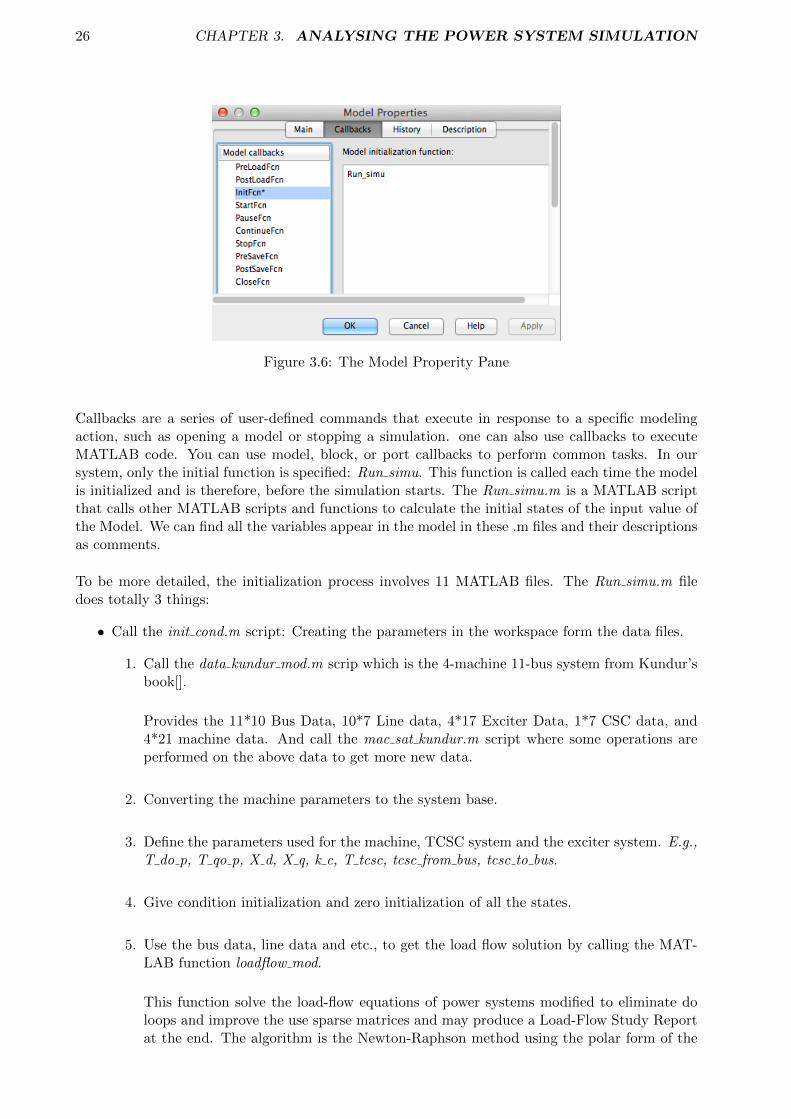
26 CHAPTER 3. ANALYSING THE POWER SYSTEM SIMULATION
Figure 3.6: The Model Properity Pane
Callbacks are a series of user-defined commands that execute in response to a specific modelingaction, such as opening a model or stopping a simulation. one can also use callbacks to executeMATLAB code. You can use model, block, or port callbacks to perform common tasks. In oursystem, only the initial function is specified: Run simu. This function is called each time the modelis initialized and is therefore, before the simulation starts. The Run simu.m is a MATLAB scriptthat calls other MATLAB scripts and functions to calculate the initial states of the input value ofthe Model. We can find all the variables appear in the model in these .m files and their descriptionsas comments.
To be more detailed, the initialization process involves 11 MATLAB files. The Run simu.m filedoes totally 3 things:
• Call the init cond.m script: Creating the parameters in the workspace form the data files.
1. Call the data kundur mod.m scrip which is the 4-machine 11-bus system from Kundur’sbook[].
Provides the 11*10 Bus Data, 10*7 Line data, 4*17 Exciter Data, 1*7 CSC data, and4*21 machine data. And call the mac sat kundur.m script where some operations areperformed on the above data to get more new data.
2. Converting the machine parameters to the system base.
3. Define the parameters used for the machine, TCSC system and the exciter system. E.g.,T do p, T qo p, X d, X q, k c, T tcsc, tcsc from bus, tcsc to bus.
4. Give condition initialization and zero initialization of all the states.
5. Use the bus data, line data and etc., to get the load flow solution by calling the MAT-LAB function loadflow mod.
This function solve the load-flow equations of power systems modified to eliminate doloops and improve the use sparse matrices and may produce a Load-Flow Study Reportat the end. The algorithm is the Newton-Raphson method using the polar form of the

3.3. CONTROL FLOW (EXECUTION ORDER OF THE BLOCKS, DATA DEPENDENCY)27
equations for P (real power) and Q (reactive power). So it calls other MATLAB func-tions: calc, form jac, chq lim, ybus mod.
6. Use the load flow solution to get the initial values of the inputs in the model. E.g.,Theta, Ign, Temp, Delta, Omega, Igm, I q, eq dash, ed dash, psid, psiq, E dc, Efd, K E,Rf, Vtr, Vr, T elec, T mech, I curr.
• Call the init sim.m script: Declarifing the simulation parameters used in the model, such asthe sampling time, pre-fault time, fault duration and the post-fault time.
• Load the bus admittance matrix Y: Ybus data89.mat/ Ybus data79.mat.
As we know that, the data initialization is before the simulation process starts, after we get theinitial states of the data, how to update the states is what we should focus on in order to analysisthe simulation process. We analysis the simulation process from two software aspects: the controlflow and dataflow. The control flow is about how executions of the blocks are sorted accordingto the data dependency. From the data flow perspective we illustrate the specific operations thatdone on the data.
3.3 Control Flow (Execution Order of the Blocks, Data Depen-dency)
From a macroscopical view, we can imagine that the model works like a state machine, data streamin and out with all the blocks are executed in parallel. However, as a software implementation,there must be some kind of sort in the execution of SIMULINK.
During the updating phase of simulation, Simulink determines the order in which to invoke theblock methods during simulation. This block invocation ordering is the sorted order. In order totranslate the simulation process to a C code, we must find out this order. Fortunately, we canview the sorted order in the model window by selecting Display →Blocks →Sorted ExecutionOrder. Simulink displays a notation in the top-right corner of each nonvirtual block and eachnonvirtual subsystem. These numbers indicate the order in which the blocks execute. The firstblock to execute has a sorted order of 0. Here is an example in our system:
However, our system is actually complicated and the data dependency is intricate. If we wantto understand the execution order only from those numbers we must understand how Simulinkdetermines the sorted order. To ensure that the sorted order reflects data dependencies amongblocks, Simulink categorizes block input ports according to the dependency of the block outputs
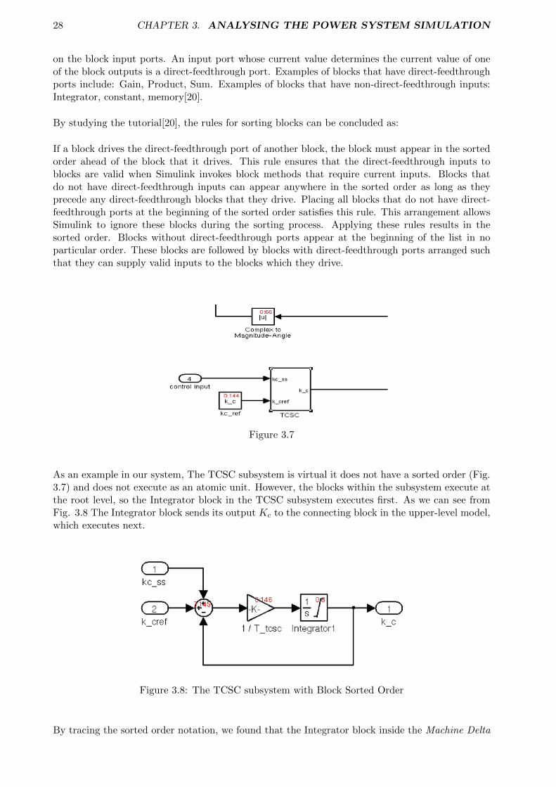
28 CHAPTER 3. ANALYSING THE POWER SYSTEM SIMULATION
on the block input ports. An input port whose current value determines the current value of oneof the block outputs is a direct-feedthrough port. Examples of blocks that have direct-feedthroughports include: Gain, Product, Sum. Examples of blocks that have non-direct-feedthrough inputs:Integrator, constant, memory[20].
By studying the tutorial[20], the rules for sorting blocks can be concluded as:
If a block drives the direct-feedthrough port of another block, the block must appear in the sortedorder ahead of the block that it drives. This rule ensures that the direct-feedthrough inputs toblocks are valid when Simulink invokes block methods that require current inputs. Blocks thatdo not have direct-feedthrough inputs can appear anywhere in the sorted order as long as theyprecede any direct-feedthrough blocks that they drive. Placing all blocks that do not have direct-feedthrough ports at the beginning of the sorted order satisfies this rule. This arrangement allowsSimulink to ignore these blocks during the sorting process. Applying these rules results in thesorted order. Blocks without direct-feedthrough ports appear at the beginning of the list in noparticular order. These blocks are followed by blocks with direct-feedthrough ports arranged suchthat they can supply valid inputs to the blocks which they drive.
Figure 3.7
As an example in our system, The TCSC subsystem is virtual it does not have a sorted order (Fig.3.7) and does not execute as an atomic unit. However, the blocks within the subsystem execute atthe root level, so the Integrator block in the TCSC subsystem executes first. As we can see fromFig. 3.8 The Integrator block sends its output Kc to the connecting block in the upper-level model,which executes next.
Figure 3.8: The TCSC subsystem with Block Sorted Order
By tracing the sorted order notation, we found that the Integrator block inside the Machine Delta
3.4. DATAFLOW (BLOCK OPERATIONS) 29
subsystem has a sorted order of 0:0, indicating that this Integrator block is the first block executedin the context of the entire model. And then is the TCSC subsystem that update the value ofKc with the Integrator block inside the TCSC subsystem has a sorted order of 0:8. In next step,the Machine Eq dash subsystem is invoked etc., the author noticed that it is a good approach tofind the execution order by compare the sorted order notations of the Integrator blocks in eachsubsystems. This is because Integrator block always executes the first in one subsystem.
Finally, the execution order of the subsystems can conclude as:
Machine delta →TSCS system →Modified Y bus due to change in Kc →Machine psid →Machineed dash →Machine psiq →Machine eq dash →Machine currents (I mach) →machine network inter-face →DC Exciter E df →DC Exciter R f →DC Exciter V r →DC Exciter V tr →Machine omega→Machine currents (I q, I d)→Machine T elec
3.4 Dataflow (Block Operations)
Other then other software applications, Simulink provides the graphical user interface that representall the knowledge in a form of a diagram. To convert the model to C code, we should also understandthe operation blocks and extract their mathematical representations form the diagram presentationto see what calculations are performed. As we know, non-virtual blocks normally represent somemathematical operation on their input values. A set of non-virtual blocks connected together maygive rise to an algorithm. Under each of the 19 subsystems, we can find the detailed operations.
In this section, some very important and not common operation blocks used in the simulationprocess are introduced with their underlying mathematical principles discussed.
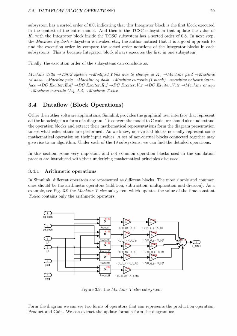
3.4.1 Arithmetic operations
In Simulink, different operators are represented as different blocks. The most simple and commonones should be the arithmetic operators (addition, subtraction, multiplication and division). As aexample, see Fig. 3.9 the Machine T elec subsystem which updates the value of the time constantT elec contains only the arithmetic operators.
Figure 3.9: the Machine T elec subsystem
Form the diagram we can see two forms of operators that can represents the production operation,Product and Gain. We can extract the update formula form the diagram as:
30 CHAPTER 3. ANALYSING THE POWER SYSTEM SIMULATION
Telec = (eq dash ∗ I q ∗ X d dp−X lsX d p−X ls ) + (ed dash ∗ I d ∗ X q dp−X ls
X q p−X ls ) + (psid ∗ I q ∗ X d p−X d dpX d p−X ls ) −
(psiq ∗ I d ∗ X q p−X q dpX q p−X ls )− (I q ∗ I d ∗ (X q dp−X d dp)
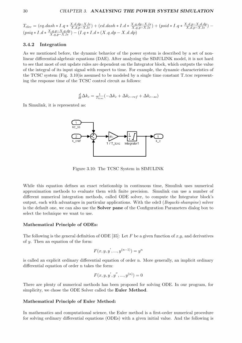
3.4.2 Integration
As we mentioned before, the dynamic behavior of the power system is described by a set of non-linear differential-algebraic equations (DAE). After analyzing the SIMULINK model, it is not hardto see that most of out update rules are dependent on the Integrator block, which outputs the valueof the integral of its input signal with respect to time. For example, the dynamic characteristics ofthe TCSC system (Fig. 3.10)is assumed to be modeled by a single time constant T tcsc represent-ing the response time of the TCSC control circuit as follows:
ddt∆kc = 1
Ttcsc(−∆kc + ∆kc−ref + ∆kc−ss)
In Simulink, it is represented as:
Figure 3.10: The TCSC System in SIMULINK
While this equation defines an exact relationship in continuous time, Simulink uses numericalapproximation methods to evaluate them with finite precision. Simulink can use a number ofdifferent numerical integration methods, called ODE solver, to compute the Integrator block’soutput, each with advantages in particular applications. With the ode3 (Bogacki-shampine) solveris the default one, we can also use the Solver pane of the Configuration Parameters dialog box toselect the technique we want to use.
Mathematical Principle of ODEs:
The following is the general definition of ODE [35]: Let F be a given function of x,y, and derivativesof y. Then an equation of the form:
F (x, y, y′, ..., y(n−1)) = yn
is called an explicit ordinary differential equation of order n. More generally, an implicit ordinarydifferential equation of order n takes the form:
F (x, y, y′, y
′′, ..., y(n)) = 0
There are plenty of numerical methods has been proposed for solving ODE. In our program, forsimplicity, we chose the ODE Solver called the Euler Method.
Mathematical Principle of Euler Method:
In mathematics and computational science, the Euler method is a first-order numerical procedurefor solving ordinary differential equations (ODEs) with a given initial value. And the following is
3.4. DATAFLOW (BLOCK OPERATIONS) 31
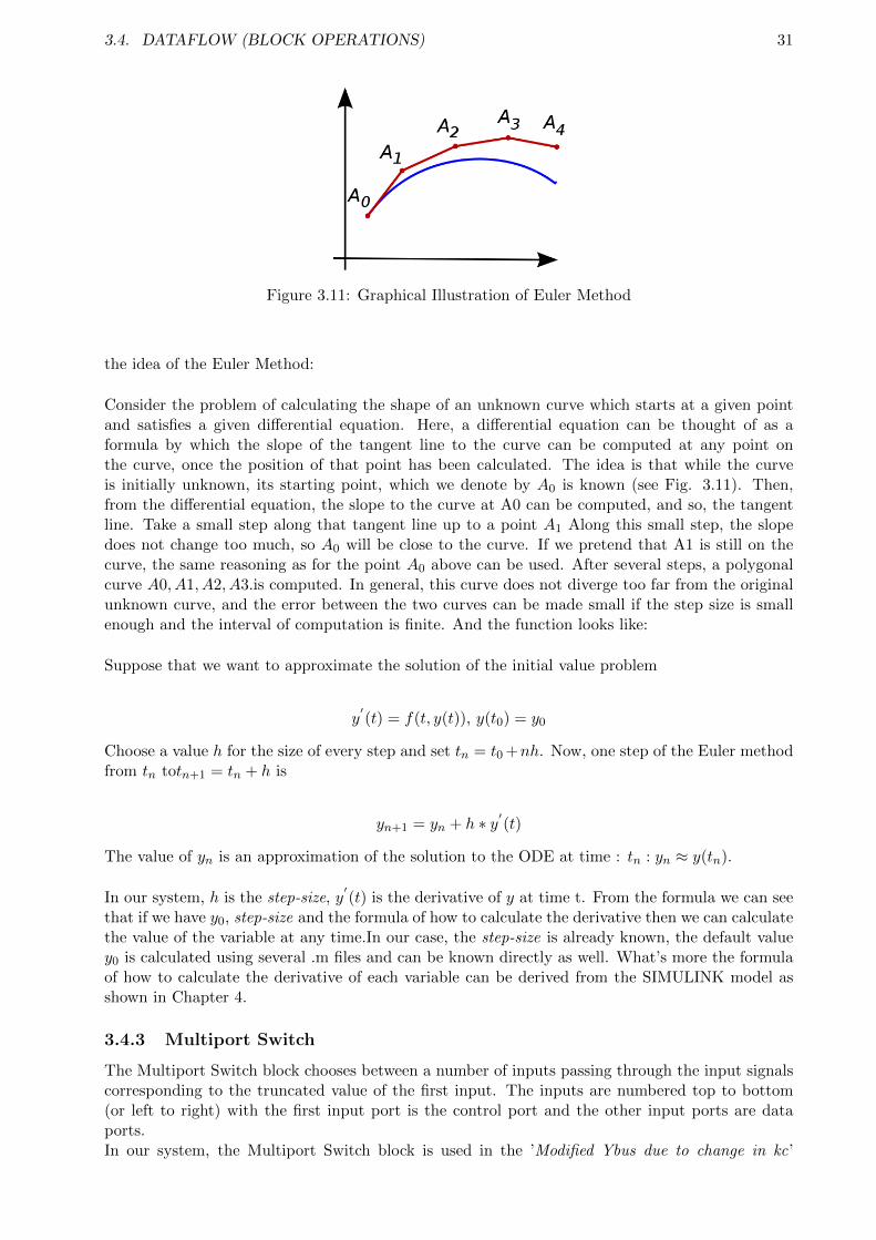
Figure 3.11: Graphical Illustration of Euler Method
the idea of the Euler Method:
Consider the problem of calculating the shape of an unknown curve which starts at a given pointand satisfies a given differential equation. Here, a differential equation can be thought of as aformula by which the slope of the tangent line to the curve can be computed at any point onthe curve, once the position of that point has been calculated. The idea is that while the curveis initially unknown, its starting point, which we denote by A0 is known (see Fig. 3.11). Then,from the differential equation, the slope to the curve at A0 can be computed, and so, the tangentline. Take a small step along that tangent line up to a point A1 Along this small step, the slopedoes not change too much, so A0 will be close to the curve. If we pretend that A1 is still on thecurve, the same reasoning as for the point A0 above can be used. After several steps, a polygonalcurve A0, A1, A2, A3.is computed. In general, this curve does not diverge too far from the originalunknown curve, and the error between the two curves can be made small if the step size is smallenough and the interval of computation is finite. And the function looks like:
Suppose that we want to approximate the solution of the initial value problem
y′(t) = f(t, y(t)), y(t0) = y0
Choose a value h for the size of every step and set tn = t0 +nh. Now, one step of the Euler methodfrom tn totn+1 = tn + h is
yn+1 = yn + h ∗ y′(t)
The value of yn is an approximation of the solution to the ODE at time : tn : yn ≈ y(tn).
In our system, h is the step-size, y′(t) is the derivative of y at time t. From the formula we can see
that if we have y0, step-size and the formula of how to calculate the derivative then we can calculatethe value of the variable at any time.In our case, the step-size is already known, the default valuey0 is calculated using several .m files and can be known directly as well. What’s more the formulaof how to calculate the derivative of each variable can be derived from the SIMULINK model asshown in Chapter 4.
3.4.3 Multiport Switch
The Multiport Switch block chooses between a number of inputs passing through the input signalscorresponding to the truncated value of the first input. The inputs are numbered top to bottom(or left to right) with the first input port is the control port and the other input ports are dataports.In our system, the Multiport Switch block is used in the ’Modified Ybus due to change in kc’

32 CHAPTER 3. ANALYSING THE POWER SYSTEM SIMULATION
Figure 3.12: The Multiport Switch Block
subsystem as shown in Fig. 3.12. Like the usage of switch statement in a programing language,based on the value of Ybus switching timing (1,2 or 3), the system choose different Y bus data fromYbus prf, Ybus psf or Ybus drf to pass to the next operation and if no value matching, the systemwill pass the Ybus drf.
3.4.4 Pulse Generator
From the above section, we know that which Y bus data to use is depending on the value passed tothe ’Switching logic’ block (Fig. 3.13). This block uses two Discrete Pulse Generators each ofwhich generates the value of 1 intermittently. So that, adding up with a constant of 1, it can finallyoutput a value of 1,2 or 3 changing with the simulation time. (This scheme is to simulation anoccur of short-circuit as I observed that after 1.0s the value of Ybus switching timing ’ will alwaysbe 2)
Figure 3.13: The Switching Logic Block
The working principle of a Discrete Pulse Generator block is that it generates a series of pulses atregular intervals. We specify the Amplitude as the amplitude of the pulse; the Pulse width asthe number of sample periods the pulse is high; the Period is the number of sample periods thepulse is high and low and the Phase delay is the number of sample periods before the pulse starts.The Sample time is the length of the one sample period, here is the step size: 0.001 seconds. Forexample, our Pulse Generator 2 as the parameters shown in Fig. 3.14:With prd = prft+psft
Tsmp = 26000, phdelay = prftTsmp = 1000; pulswdth2 = fdtn
Tsmp = 80 predefined in theinit sim.m file. Where Tsmp is sample time = 0.001s. This means that the generator will beginto output value 1 every 26 seconds after 1 seconds simulation and each time lasts for 0.08 seconds.For the remaining time, outputs 0.
3.4. DATAFLOW (BLOCK OPERATIONS) 33
Figure 3.14: Parameters for an Pulse Generator
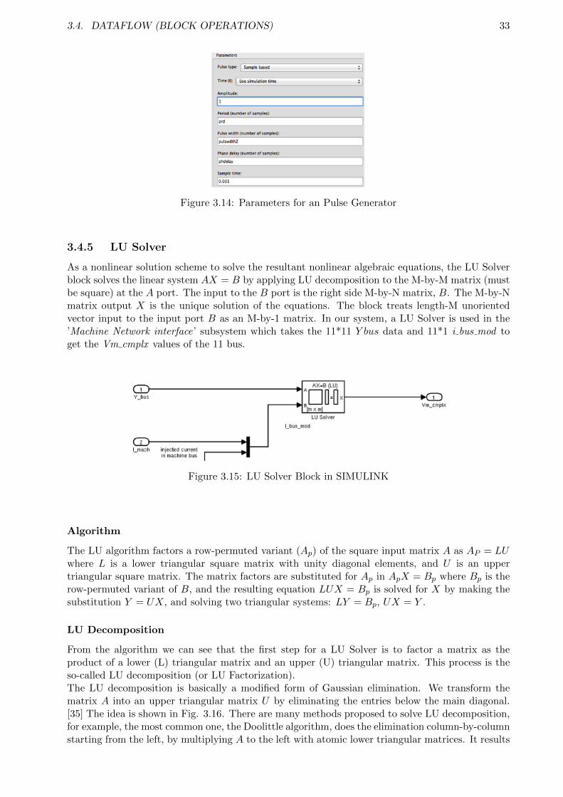
3.4.5 LU Solver
As a nonlinear solution scheme to solve the resultant nonlinear algebraic equations, the LU Solverblock solves the linear system AX = B by applying LU decomposition to the M-by-M matrix (mustbe square) at the A port. The input to the B port is the right side M-by-N matrix, B. The M-by-Nmatrix output X is the unique solution of the equations. The block treats length-M unorientedvector input to the input port B as an M-by-1 matrix. In our system, a LU Solver is used in the’Machine Network interface’ subsystem which takes the 11*11 Y bus data and 11*1 i bus mod toget the Vm cmplx values of the 11 bus.
Figure 3.15: LU Solver Block in SIMULINK
Algorithm
The LU algorithm factors a row-permuted variant (Ap) of the square input matrix A as AP = LUwhere L is a lower triangular square matrix with unity diagonal elements, and U is an uppertriangular square matrix. The matrix factors are substituted for Ap in ApX = Bp where Bp is therow-permuted variant of B, and the resulting equation LUX = Bp is solved for X by making thesubstitution Y = UX, and solving two triangular systems: LY = Bp, UX = Y .
LU Decomposition
From the algorithm we can see that the first step for a LU Solver is to factor a matrix as theproduct of a lower (L) triangular matrix and an upper (U) triangular matrix. This process is theso-called LU decomposition (or LU Factorization).The LU decomposition is basically a modified form of Gaussian elimination. We transform thematrix A into an upper triangular matrix U by eliminating the entries below the main diagonal.[35] The idea is shown in Fig. 3.16. There are many methods proposed to solve LU decomposition,for example, the most common one, the Doolittle algorithm, does the elimination column-by-columnstarting from the left, by multiplying A to the left with atomic lower triangular matrices. It results
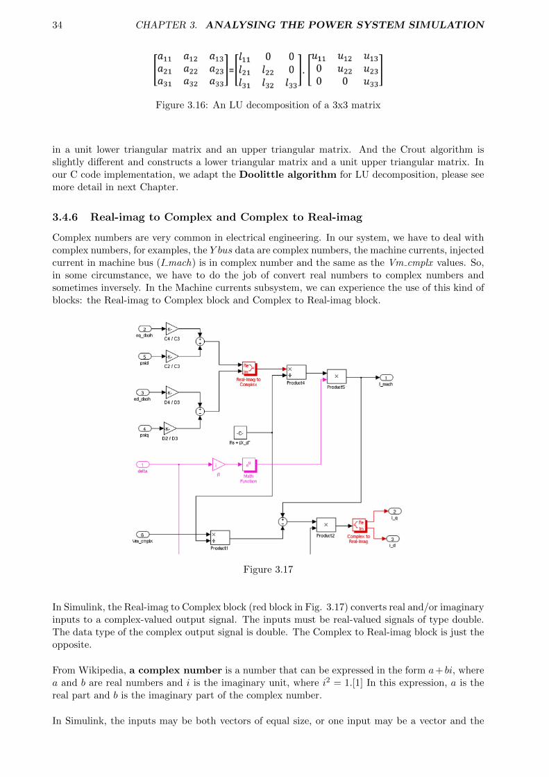
34 CHAPTER 3. ANALYSING THE POWER SYSTEM SIMULATION
Figure 3.16: An LU decomposition of a 3x3 matrix
in a unit lower triangular matrix and an upper triangular matrix. And the Crout algorithm isslightly different and constructs a lower triangular matrix and a unit upper triangular matrix. Inour C code implementation, we adapt the Doolittle algorithm for LU decomposition, please seemore detail in next Chapter.
3.4.6 Real-imag to Complex and Complex to Real-imag
Complex numbers are very common in electrical engineering. In our system, we have to deal withcomplex numbers, for examples, the Y bus data are complex numbers, the machine currents, injectedcurrent in machine bus (I mach) is in complex number and the same as the Vm cmplx values. So,in some circumstance, we have to do the job of convert real numbers to complex numbers andsometimes inversely. In the Machine currents subsystem, we can experience the use of this kind ofblocks: the Real-imag to Complex block and Complex to Real-imag block.
Figure 3.17
In Simulink, the Real-imag to Complex block (red block in Fig. 3.17) converts real and/or imaginaryinputs to a complex-valued output signal. The inputs must be real-valued signals of type double.The data type of the complex output signal is double. The Complex to Real-imag block is just theopposite.
From Wikipedia, a complex number is a number that can be expressed in the form a+ bi, wherea and b are real numbers and i is the imaginary unit, where i2 = 1.[1] In this expression, a is thereal part and b is the imaginary part of the complex number.
In Simulink, the inputs may be both vectors of equal size, or one input may be a vector and the

3.4. DATAFLOW (BLOCK OPERATIONS) 35
other a scalar. If the block has a vector input, the output is a vector of complex signals. Theelements of a real input vector are mapped to real parts of the corresponding complex outputelements. An imaginary input vector is similarly mapped to the imaginary parts of the complexoutput signals. If one input is a scalar, it is mapped to the corresponding component (real orimaginary) of all the complex output signals. For example the Real-imag to Complex block in thediagram does the operation as:
Output = (eq dash ∗ C4/C3 + psid ∗ C2/C3 + (ed dash ∗D4/D3− psiq ∗D2/D3 ∗ I)
3.4.7 Exponential form of complex number
As we can see from the Fig. 3.17 (pink part), It gives an exponential form of complex number asthe output is: ei∗delta, where i ∗ delta is a complex number that equals 0 + i ∗ delta.
Mathematical Principle
We have, so far, considered two ways of representing a complex number: Cartesian form z = a+ ibor polar form z = r(cos + isin) . And since ei = cos + isin, we therefore obtain another way inwhich to denote a complex number: z = a+ ib = r(cos+ isin) = rei
So we get ei∗delta = cos(delta) + I ∗ sin(delta);
3.4.8 Others
(a) Assignment (b) Selector (c) Complex to Mag
Figure 3.18: Other Noteworthing Blocks
Assignment Block (Fig. 3.18(a)): Assign values to specified elements of a multidimensional out-put signal. The index to each element is identified from an input port or this dialog.
Assignment blocks are used after the modified Ybus entries Y (9, 9)Y (8, 8), Y (8, 9) due to the changein the percentage compensation of the TCSC (Kc) are calculated and we have to exchange the oldvalues to the new values.
Selector (Fig. 3.18(b)): Select or reorder specified elements of a multidimensional input signal.The index to each element is identified from an input port or this dialog. In our system, the selectorblock is used when passing the Vm cmplx values, as the Vm cmplx is a 11*1 array, only the first4 units are meaningful values for each of the four machines. So the selector block selectors the 4elements.
Complex to Magnitude-Angle (Fig. 3.18(c)): Compute magnitude and/or radian phase angleof the input.
Consider the complex number z = abi. The complex conjugate of the number z, denoted z∗, isobtained by simply taking every i that you see in the expression for z and replacing it by i. The
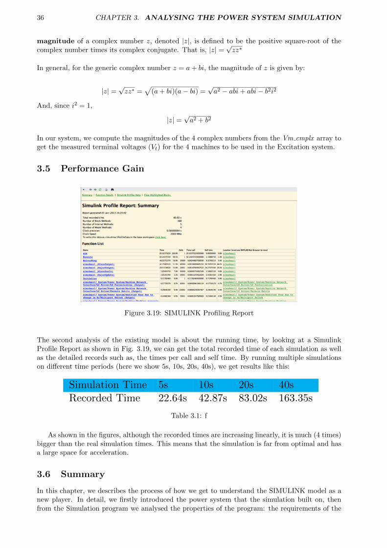
36 CHAPTER 3. ANALYSING THE POWER SYSTEM SIMULATION
magnitude of a complex number z, denoted |z|, is defined to be the positive square-root of thecomplex number times its complex conjugate. That is, |z| =
√zz∗
In general, for the generic complex number z = a+ bi, the magnitude of z is given by:
|z| =√zz∗ =
√(a+ bi)(a− bi) =
√a2 − abi+ abi− b2i2
And, since i2 = 1,
|z| =√a2 + b2
In our system, we compute the magnitudes of the 4 complex numbers from the Vm cmplx array toget the measured terminal voltages (Vt) for the 4 machines to be used in the Excitation system.
3.5 Performance Gain
Figure 3.19: SIMULINK Profiling Report
The second analysis of the existing model is about the running time, by looking at a SimulinkProfile Report as shown in Fig. 3.19, we can get the total recorded time of each simulation as wellas the detailed records such as, the times per call and self time. By running multiple simulationson different time periods (here we show 5s, 10s, 20s, 40s), we get results like this:
Simulation Time 5s 10s 20s 40sRecorded Time 22.64s 42.87s 83.02s 163.35s
Table 3.1: f
As shown in the figures, although the recorded times are increasing linearly, it is much (4 times)bigger than the real simulation times. This means that the simulation is far from optimal and hasa large space for acceleration.
3.6 Summary
In this chapter, we describes the process of how we get to understand the SIMULINK model as anew player. In detail, we firstly introduced the power system that the simulation built on, thenfrom the Simulation program we analysed the properties of the program: the requirements of the

3.6. SUMMARY 37
program, the data flow and the control flow of the program.Section 3.1 described the power systembeing simulated. Section 3.2 covered an detailed analysis of the power system simulation in theform of a SIMULINK model. And section 3.3 gave a brief illustration of the performance of theSIMULINK model from the efficiency prospect.

Chapter 4
Optimised the Power SystemSimulation
4.1 Simulink Coder & Initial Design
The Simulink Coder (formally Real-Time Workshop code generator)[20], is an extension of capa-bilities of Simulink and MATLAB that automatically generates, packages and compiles C or C++source code from Simulink diagrams to create real-time software applications on a variety of sys-tems.
Firstly, we tried to use the Simulink Coder to automatically generate the C code form our Simulinksystem. The Coder generated a folder called simu4mac1 grt rtw which contains 28 files includingheader files, data files, etc. And only the main C file has almost 2500 lines of code with very elu-sive structure. It seems that because of the automaticity, the generated code is not very efficient.Therefore, if we want to use the generated code we have to experience large amount of refactoringand reimplementation work. And it may be time consuming to understand the generated codefirst. According to the above reasons, we decided to write the C code from a scratch.
Drawing lessons from the Simulink Coder [28], we know that in the first phase the Simulink coderconverts the model to an executable form following these steps:
• It evaluates the parameters (given as expressions over constants and Matlab’s workspaceconstants) of the model’s blocks;
• It determines signal attributes, e.g., name, data type, numeric type, dimensionality andsample rate (these are not explicitly specified in the model file) and performs type-checking,i.e., it checks that each block can accept the signals connected to its inputs;
• It flattens the model hierarchy by replacing virtual subsystems with the blocks that theycontain;
• It sorts the blocks according to the execution order.
After this phase, the blocks are executed in a single loop corresponding to a single step of themodel.
As long as we know the sort of execution for each block we are now able to realize exactly whatsimulink does in a time step as follows:
In a specific time i*step time:
For each machine{
38
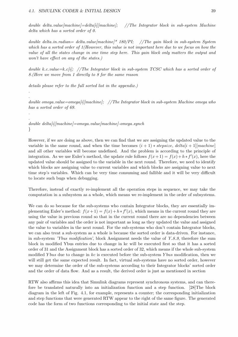
4.1. SIMULINK CODER & INITIAL DESIGN 39
double delta value[machine]=delta[i][machine]; //The Integrator block in sub-system Machinedelta which has a sorted order of 0.
double delta in radian= delta value[machine]* 180/PI; //The gain block in sub-system Systemwhich has a sorted order of 1(However, this value is not important here due to we focus on how thevalue of all the states change in one time step here. This gain block only matters the output andwon’t have effect on any of the states.)
double k c value=k c[i]; //The Integrator block in sub-system TCSC which has a sorted order of8.(Here we move from 1 directly to 8 for the same reason
details please refer to the full sorted list in the appendix.)..double omega value=omega[i][machine]; //The Integrator block in sub-system Machine omega whohas a sorted order of 69...double delta[i][machine]=omega value[machine]-omega synch}
However, if we are doing as above, then we can find that we are assigning the updated value to thevariable in the same round, and when the time becomes (i + 1) ∗ stepsize, delta[i + 1][machine]and all other variables will become undefined. And the problem is according to the principle ofintegration. As we use Euler’s method, the update rule follows f(x+1) = f(x)+h∗f ′(x), here theupdated value should be assigned to the variable in the next round. Therefore, we need to identifywhich blocks are assigning value to current variables and which blocks are assigning value to nexttime step’s variables. Which can be very time consuming and fallible and it will be very difficultto locate such bugs when debugging.
Therefore, instead of exactly re-implement all the operation steps in sequence, we may take thecomputation in a subsystem as a whole, which means we re-implement in the order of subsystems.
We can do so because for the sub-systems who contain Integrator blocks, they are essentially im-plementing Euler’s method: f(x+ 1) = f(x) +h∗f ′(x), which means in the current round they areusing the value in previous round so that in the current round there are no dependencies betweenany pair of variables and the order is not important as long as they updated the value and assignedthe value to variables in the next round. For the sub-systems who don’t contain Integrator blocks,we can also treat a sub-system as a whole is because the sorted order is data-driven. For instance,in sub-system ’Ybus modification’, block Assignment needs the value of Y 8 9, therefore the sumblock in modified Ybus entries due to change in kc will be executed first so that it has a sortedorder of 31 and the Assignment block has a sorted order of 32, which means if the whole sub-systemmodified Y bus due to change in kc is executed before the sub-system Y bus modification, then wewill still get the same expected result. In fact, virtual sub-systems have no sorted order, howeverwe may determine the order of the sub-systems according to their Integrator blocks’ sorted orderand the order of data flow. And as a result, the derived order is just as mentioned in section
RTW also affirms this idea that Simulink diagrams represent synchronous systems, and can there-fore be translated naturally into an initialization function and a step function. [28]The blockdiagram in the left of Fig. 4.1, for example, represents a counter; the corresponding initializationand step functions that were generated RTW appear to the right of the same figure. The generatedcode has the form of two functions corresponding to the initial state and the step.
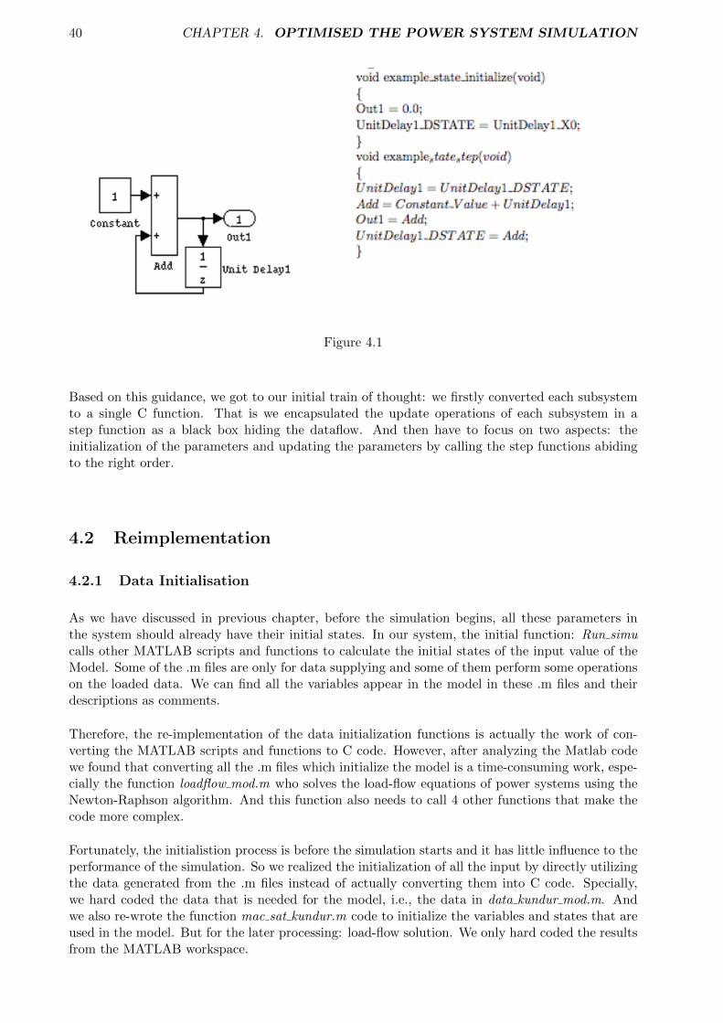
40 CHAPTER 4. OPTIMISED THE POWER SYSTEM SIMULATION
Figure 4.1
Based on this guidance, we got to our initial train of thought: we firstly converted each subsystemto a single C function. That is we encapsulated the update operations of each subsystem in astep function as a black box hiding the dataflow. And then have to focus on two aspects: theinitialization of the parameters and updating the parameters by calling the step functions abidingto the right order.
4.2 Reimplementation
4.2.1 Data Initialisation
As we have discussed in previous chapter, before the simulation begins, all these parameters inthe system should already have their initial states. In our system, the initial function: Run simucalls other MATLAB scripts and functions to calculate the initial states of the input value of theModel. Some of the .m files are only for data supplying and some of them perform some operationson the loaded data. We can find all the variables appear in the model in these .m files and theirdescriptions as comments.
Therefore, the re-implementation of the data initialization functions is actually the work of con-verting the MATLAB scripts and functions to C code. However, after analyzing the Matlab codewe found that converting all the .m files which initialize the model is a time-consuming work, espe-cially the function loadflow mod.m who solves the load-flow equations of power systems using theNewton-Raphson algorithm. And this function also needs to call 4 other functions that make thecode more complex.
Fortunately, the initialistion process is before the simulation starts and it has little influence to theperformance of the simulation. So we realized the initialization of all the input by directly utilizingthe data generated from the .m files instead of actually converting them into C code. Specially,we hard coded the data that is needed for the model, i.e., the data in data kundur mod.m. Andwe also re-wrote the function mac sat kundur.m code to initialize the variables and states that areused in the model. But for the later processing: load-flow solution. We only hard coded the resultsfrom the MATLAB workspace.
4.2. REIMPLEMENTATION 41
4.2.2 Timing and Update Sequence
As we know, in Simulink, the simulation process is time based. A solver computes a dynamicsystem’s states at successive time steps over a specified time span, using information providedby the model. So we should specify the Simulation Time which is the total length of time thesimulation runs (the period between start time and end time) and the Step size which determinesthe update frequency. As for the Euler solver: F (t) = F (t − 1) + h ∗ F ′(t − 1), stepsize = h. Wecan imagine that, the system updates its states every step size. So the total number of iterationsis:
Iterations = Simulationtimestepsize
For example, if the Step size is set to the default value 1e-3, and Simulation Time is the 20s, thetotal number of iterations is: 20000. We can simulate this timing scheme in C code as a single forloop in the main function: for(i = 0; i ∗ stepSize <= simulationtime; i+ +)
In each iteration, we update all the states by calling the step functions of the subsystems in theorder:
Machine delta →TSCS system →Modified Y bus due to change in Kc →Machine psid →Machineed dash →Machine psiq →Machine eq dash →Machine currents (I mach) →machine network inter-face →DC Exciter E df →DC Exciter R f →DC Exciter V r →DC Exciter V tr →Machine omega→Machine currents (I q, I d)→Machine T elec
However, during the implementation phase, we noticed that, keep calling functions outside themain function needs declaration of a large amount of variables which in some extent embarrassedthe algorithm.
As we know, Amount these subsystems, the ’Switching logic’ and ’Multiport switch’ subsystems arefor flow control, and the ’Ybus modification’ system performs an intermediate matrix operations onthe Y bus data which gets the new bus data used for each iterations calculations by changing someentries in the Y bus data matrix. And each of the remaining subsystems encapsulates the dynamicupdating rule for one of these 16 parameters: Delta, Eq dash, Ed dash, Psid, Psiq, Omega, I mach,T q, T d, Vm cmplx, Efd, Rf, Vr, Vtr,T elec, Kc
The dynamic behavior of the some of these subsystems is generally described through a set ofdifferential equations while some them (the power flow in the network) are represented by a set ofalgebraic equations. Therefore, for each of the parameters, we can simplify the step function asa single equation (formula). For example, by the Euler method, the integrator just updates thestates following the formula: F (t) = F (t− 1) +h ∗F ′(t− 1) and F (0) = x0, where F (t) is the valueof a variable at time t, h is the step size, F ′(t) is the derivative at time t. The default value x0 iscalculated using several .m files and can be known directly as well. What’s more the formula of howto calculate the derivative of each variable can be derived from the SIMULINK model. Therefore,we can calculate the value of the variable at any time. And for the algebraic subsystems, we canextract algebraic equations straightforward from the model diagram.
In details, instead of using only one variable to store the current value of state, I created two-dimensional arrays for every variable respectively to store the value of each variable in every round,specifically, the first dimension is the time (iteration) and the second dimension is the machinenumber (totally 4 machines). And we do not need to call any step functions, we just use theformulas to update the parameters in each iteration by the sorted order:
Delta →k c →Psid →Ed dash →Psiq →I mach →Vm cmplx →Efd →Rf →Vr →Vtr →Omega →I q→I d →T elec.

42 CHAPTER 4. OPTIMISED THE POWER SYSTEM SIMULATION
However, a noteworthy thing to mention is that, as the subsystems contain Integrator blocks, theyare essentially implementing Euler’s method: F(t)=F(t-1)+H*F’(t-1) and F(0)=x0, which meansin the current round they are using the value in previous round except the first round. So forupdate of these kind of parameters, we should add a control scheme: if (i >0) before using theupdate formula F(t)=F(t-1)+H*F’(t-1). For the sub-systems who don’t contain Integrator blocks,they use the current values to update in current round. Therefore, based on all the principles wediscussed above, we get the most compact and efficient version of our main function:
i n t main ( i n t argc , char ∗∗ argv ) {f o r ( i = 0 ; i ∗ s t e p S i z e <= 20 ; i++) {
i n i t i a l i z e ( ) ;m o d i f i e d Y b u s e n t r i e s d u e t o c h a n g e i n k c ( ) ;
Ybus modi f i cat ion ( ) ;i n t i t ;f o r ( i t = 0 ; i t <= 3 ; i t ++) {
i f ( i > 0) {// Deltad e l t a [ 1 ] [ i t ] = d e l t a [ 0 ] [ i t ] + ( omega [ 0 ] [ i t ] −
Omega synch )∗ s t e p S i z e ;. . .}
// I machI mach [ 1 ] [ i t ] = ( eq dash [ 1 ] [ i t ] ∗ C4 [ i t ] / C3 [ i t ] + ps id [ 1 ] [ i t ]
∗ C2 [ i t ] / C3 [ i t ] + ( ed dash [ 1 ] [ i t ] ∗ D4 [ i t ]/ D3 [ i t ] − ps iq [ 1 ] [ i t ] ∗ D2 [ i t ] / D3 [ i t ] ) ∗ I )
/ ( R s [ i t ]+ X d dp [ i t ] ∗ I ) ∗ ( cos ( d e l t a [ 1 ] [ i t ] )+ I ∗ s i n ( d e l t a [ 1 ] [ i t ] ) ) ;
. . .}
LUSolver1(&Ybus [ 0 ] [ 0 ] , &b [ 0 ] , 11 , i ) ;
f o r ( i t = 0 ; i t <= 3 ; i t ++) {i f ( i > 0) {
//Efde fd [ 1 ] [ i t ] = ( . . . )
. . .}
// I qI q [ 1 ] [ i t ] = ( . . . )
. . .}
}
4.2.3 Reimplementation of the Multiprt Switch Scheme
We implement the updating of the power system parameters in the way we discussed above. Besidethese subsystems that describe the dynamic behavior of devices in power system, in the simulationmodel, we also have some subsystem for intermediate data handling. Namely, the wholeModifiedYbus due to change in Kc’ system finally outputs the modified bus admittance matrix Y used ineach iteration due to the power injection of the TCSC system represented by the value of percent-age compensation (Kc). However, before the modification, we actually use different original Y bus
4.2. REIMPLEMENTATION 43
data.
The ’Switching logic’ and ’Multiport switch’ subsystems together provide the control scheme forchoosing from 3 different kinds of Y busdata (Ybus prf, Ybus psf, Ybus drf ). As we have detailedlyintroduced these two subsystems in section 3.4.3 and 3.4.4, ’Multiport switch’ chose from the 3options based on the value of ’Ybus switching timing ’ (1,2 or 3) generated by ’Switing logic. Thisscheme can be implemented as a switch statement in C code.
The ’Switing logic’ system determines the value of switching time with the help of two Pulse Gen-erators. The working principle of a Pulse Generator block is that it generates a series of pulsesat regular intervals. We specify the Amplitude as the amplitude of the pulse; the Pulse width asthe number of sample periods the pulse is high; the Period is the number of sample periods thepulse is high and low and the Phase delay is the number of sample periods before the pulse starts.The Sample time is the length of the one sample period, here is the setp size: 0.001 seconds. Forexample, our Pulse Generator 2 as the parameters: With prd = (prft + psft)/Tsmp = 26000,phdelay = prft/Tsmp = 1000; pulswdth2 = fdtn/Tsmp = 80 predefined in the init sim.m file.Where Tsmp is sample time = 0.001s. This means that the generator will begin to output value 1every 26 seconds after 1 seconds simulation and each time lasts for 0.08 seconds. For the remainingtime, outputs 0.
To implement this scheme in our main, we defined 2 variables Pulse1 and Pulse 2. In each iterationi, we should determine whether each of Pulse values is 1 or 0. Lets consider a simple case first,we calculate the value i modulo prd, and if the value is less than pulswdth1 then the amplitude ofthe pulse at time i is 1, otherwise 0. Here in our case, the delay needs to be taken into account,therefore if (i − phdelay) modulo prd is less than pulswdth1, then at time i the amplitude of thepulse is 1. In addition, due to in our case, time should always larger than 0, the first amplitude of1 should appear when (i− phdelay) >= 0. In code, it looks like:
i f ( ( i−( i n t ) phdelay )%( i n t ) prd < pulswdth1 && ( i−( i n t ) phdelay>= 0)) {pul se1 = 1 ;
} e l s e {pul se1 = 0 ;
}
And then, the get Switching time(pulse1, pulse2) function just returns the addition of pulse1,pulse2 and a constant 1 which is 1, 2 or 3. And then, by use a switch statement to implement theMultiple Switch Scheme:switch (getSwitching time(pulse1, pulse2)This statement has 3 cases corresponding to the three kinds of Y bus data and the default case isto use the Y bus drf .
4.2.4 Reimplementation of the Modification of Y bus Data
In the ’Modified Ybus due to change in Kc’ system, we have two subsystems: ’modified Ybus entriesdue to change in kc’ and ’Ybus modification’ who modify the bus admittance matrix Y used ineach iteration due to the change in kc. In our C code implementation, we wrote two functions onefor each of these two subsystems.
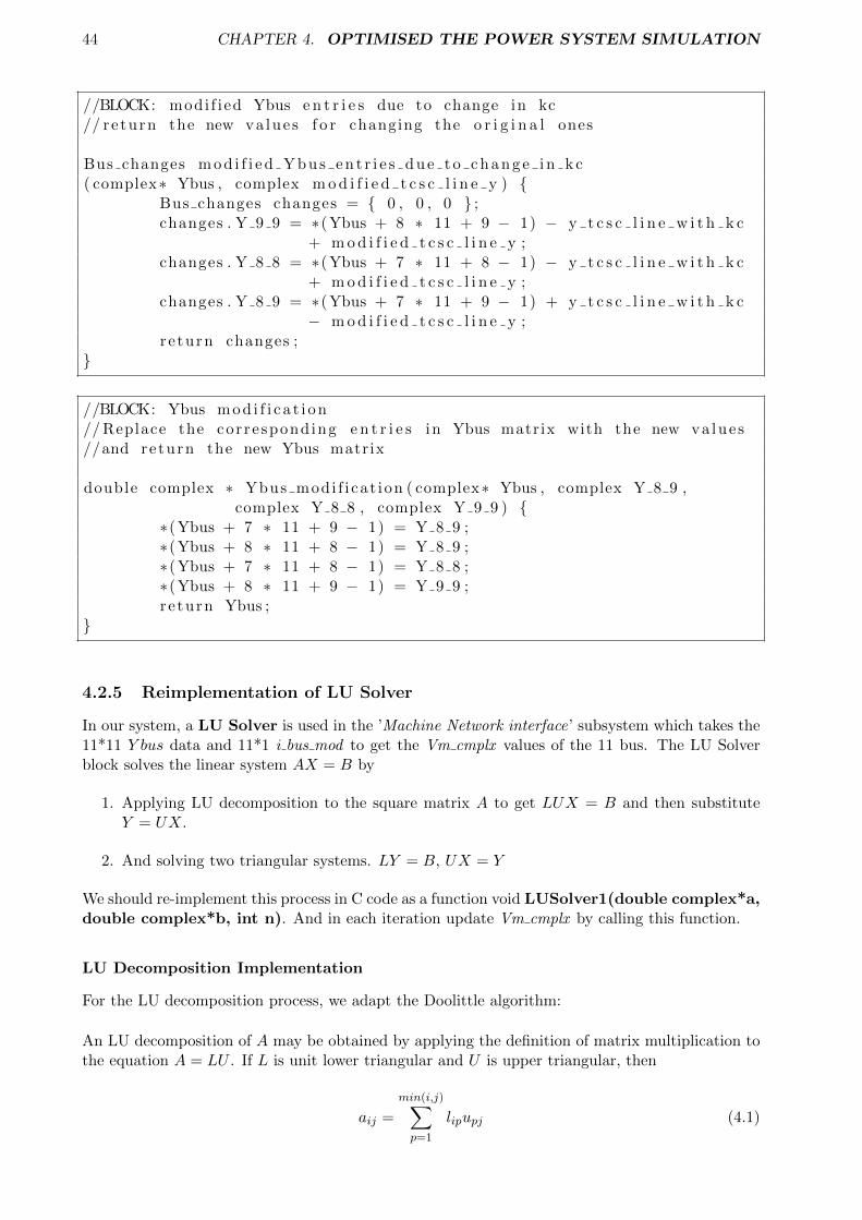
44 CHAPTER 4. OPTIMISED THE POWER SYSTEM SIMULATION
//BLOCK: modi f i ed Ybus e n t r i e s due to change in kc// return the new va lue s f o r changing the o r i g i n a l ones
Bus changes m o d i f i e d Y b u s e n t r i e s d u e t o c h a n g e i n k c( complex∗ Ybus , complex m o d i f i e d t c s c l i n e y ) {
Bus changes changes = { 0 , 0 , 0 } ;changes . Y 9 9 = ∗(Ybus + 8 ∗ 11 + 9 − 1) − y t c s c l i n e w i t h k c
+ m o d i f i e d t c s c l i n e y ;changes . Y 8 8 = ∗(Ybus + 7 ∗ 11 + 8 − 1) − y t c s c l i n e w i t h k c
+ m o d i f i e d t c s c l i n e y ;changes . Y 8 9 = ∗(Ybus + 7 ∗ 11 + 9 − 1) + y t c s c l i n e w i t h k c
− m o d i f i e d t c s c l i n e y ;r e turn changes ;
}
//BLOCK: Ybus mod i f i c a t i on// Replace the cor re spond ing e n t r i e s in Ybus matrix with the new va lues//and return the new Ybus matrix
double complex ∗ Ybus modi f i cat ion ( complex∗ Ybus , complex Y 8 9 ,complex Y 8 8 , complex Y 9 9 ) {
∗(Ybus + 7 ∗ 11 + 9 − 1) = Y 8 9 ;∗(Ybus + 8 ∗ 11 + 8 − 1) = Y 8 9 ;∗(Ybus + 7 ∗ 11 + 8 − 1) = Y 8 8 ;∗(Ybus + 8 ∗ 11 + 9 − 1) = Y 9 9 ;re turn Ybus ;
}
4.2.5 Reimplementation of LU Solver
In our system, a LU Solver is used in the ’Machine Network interface’ subsystem which takes the11*11 Y bus data and 11*1 i bus mod to get the Vm cmplx values of the 11 bus. The LU Solverblock solves the linear system AX = B by
1. Applying LU decomposition to the square matrix A to get LUX = B and then substituteY = UX.
2. And solving two triangular systems. LY = B, UX = Y
We should re-implement this process in C code as a function void LUSolver1(double complex*a,double complex*b, int n). And in each iteration update Vm cmplx by calling this function.
LU Decomposition Implementation
For the LU decomposition process, we adapt the Doolittle algorithm:
An LU decomposition of A may be obtained by applying the definition of matrix multiplication tothe equation A = LU . If L is unit lower triangular and U is upper triangular, then
aij =
min(i,j)∑p=1
lipupj (4.1)
4.3. PERFORMANCE GAINS 45
where 1 <= i and j <= n. Rearranging the terms of Equation 4.1 yields
lij =
aij −j−1∑p=1
lipupj
ujj(4.2)
where i > j, and
uij = aij −i−1∑p=1
lipupj (4.3)
where i < j Jointly Equation 4.2 and Equation 4.3 are referred to as Doolittles method of comput-ing the LU decomposition of A. We implemented the same algorithm as:
\\ LU Decomposition
f o r ( k = 0 ; k < n ; k++) {u [ k ] [ k ] = 1 ;
\\ Find L part us ing Equation 4 .2f o r ( i = k ; i < n ; i++) {
sum = 0 ;f o r (p = 0 ; p <= k − 1 ; p++) {
sum += l [ i ] [ p ] ∗ u [ p ] [ k ] ;}l [ i ] [ k ] = ∗( a + i ∗ n + k ) − sum ;
}\\ Find U part us ing Equation 4 .3
f o r ( j = k + 1 ; j < n ; j++) {sum = 0 ;f o r (p = 0 ; p <= k − 1 ; p++) {
sum += l [ k ] [ p ] ∗ u [ p ] [ j ] ;}u [ k ] [ j ] = (∗ ( a + k ∗ n + j ) − sum) / l [ k ] [ k ] ;
}}
4.3 Performance Gains
4.3.1 Correctness
The program can generate exactly same results as SIMULINK does up to 10 digits after deci-mal point after 20000 times calculations (20s’ simulation). And can give the exact same fluctuatepatterns of the signals as in the SIMULINK model. Take the desired phase differences betweengenerator 1 and generator 3 (G1-G3) of 20’s simulation as an example, the upper diagram (Fig.4.2)is generated by SIMULINK, and the lower one (Fig. 4.3) is generated from the results of ourC code:
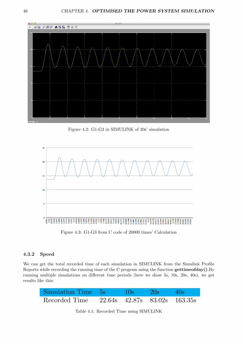
46 CHAPTER 4. OPTIMISED THE POWER SYSTEM SIMULATION
Figure 4.2: G1-G3 in SIMULINK of 20s’ simulation
Figure 4.3: G1-G3 from C code of 20000 times’ Calculation
4.3.2 Speed
We can get the total recorded time of each simulation in SIMULINK from the Simulink ProfileReports while recording the running time of the C program using the function gettimeofday().Byrunning multiple simulations on different time periods (here we show 5s, 10s, 20s, 40s), we getresults like this:
Simulation Time 5s 10s 20s 40sRecorded Time 22.64s 42.87s 83.02s 163.35s
Table 4.1: Recorded Time using SIMULINK
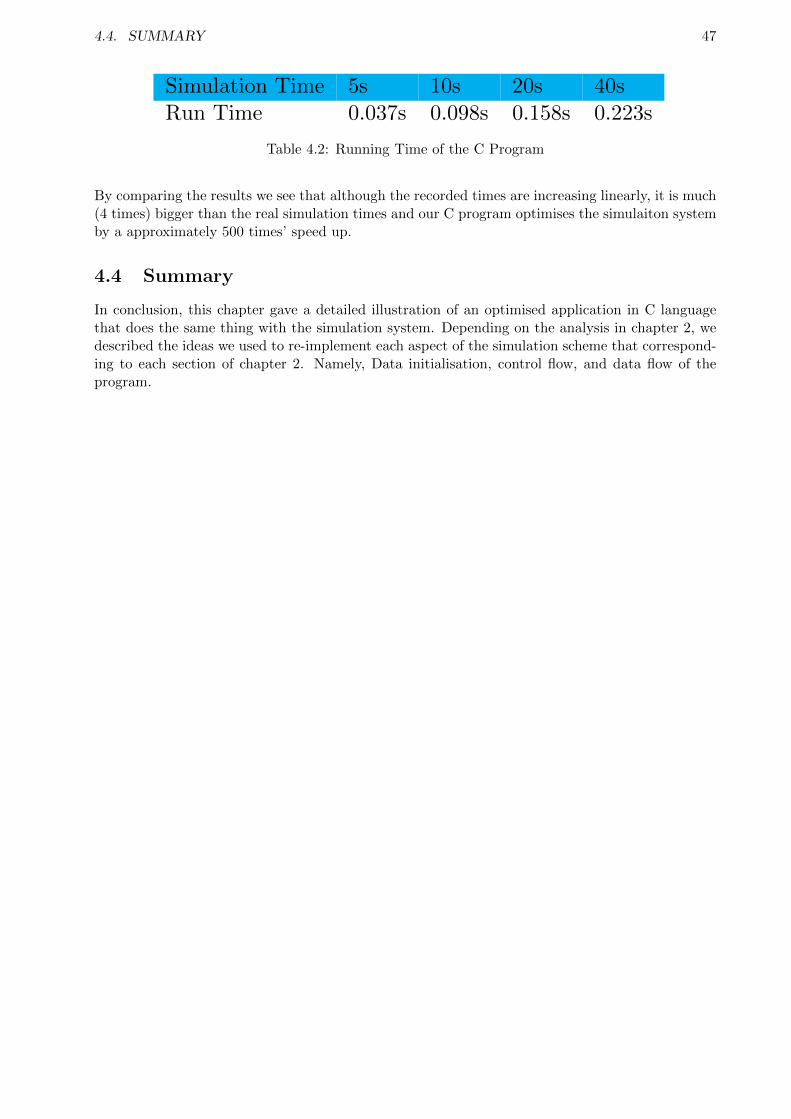
4.4. SUMMARY 47
Simulation Time 5s 10s 20s 40sRun Time 0.037s 0.098s 0.158s 0.223s
Table 4.2: Running Time of the C Program
By comparing the results we see that although the recorded times are increasing linearly, it is much(4 times) bigger than the real simulation times and our C program optimises the simulaiton systemby a approximately 500 times’ speed up.
4.4 Summary
In conclusion, this chapter gave a detailed illustration of an optimised application in C languagethat does the same thing with the simulation system. Depending on the analysis in chapter 2, wedescribed the ideas we used to re-implement each aspect of the simulation scheme that correspond-ing to each section of chapter 2. Namely, Data initialisation, control flow, and data flow of theprogram.

Chapter 5
Accelerating the Power SystemSimulation
In this chapter we present our acceleration solutions to running the Power System simulationand inform the reader of the choices made along the process. Since we identified the most timeconsuming part of the simulation fundamentally as a matrix inversion problem disguised as an LUmatrix decomposition, and since we have optimised the C simulation to what we believe was themaximum possible extent in the timeframe of this project, we look to acceleration by the FPGAtechniques to further speed up our simulation process.
5.1 Profiling
It is important to note that developers using Maxeler technology typically aim to accelerate theslowest portion of the software. To Identify areas of code for acceleration, we did a more detailedanalysis on the distribution of runtime of various parts of the application using both time counterand profiling tool: gprof.
Figure 5.1: Profing Result using Gprof
From the result provided by Gprof (Fig. 5.1) we can see, that is the LUSolver1 function that
48

5.1. PROFILING 49
dominated the most of the running time (75%). It is reasonable as it has nested loops. And itis clear to see, the other part in the main function only occupy 25% of the total running time.However, Gprof tells us that the calling of the function modified Ybus entries due to change in kc,Ybus modification, initialization, getSwitching time do not matter to much to the running speed.that is the something called intel ssse3 rep memcpy in the system that takes this 25% of the time.As we can guess that, that is those parameter update operations which are not defined in functions.
By focusing on the LUSolver1 function, we then use time counters in the program to test the runningtime of different blocks of operations. As in LUSolver1, there are 3 for loops, the first one forLU Decomposition, and the other two for forwarding substitution and finding the X(V m cmplx),respectively. For a 20’s simulation, the first loop takes 122000ms while the other two loops togethertake 46000ms. Therefore, we can get the conclusion that the LU Decomposition process is the mostcomplicated and inefficient part of the code. We should consider if we can accelerate it in Maxeler.
For the second time consuming component, the updating operations, we can also accelerate inMaxeler as these operations are done on 4 machines. As they do the same operations, we canpipeline the 4 machine. Therefore, we get to the initial design of a CUP-FPGA simulation shownin Fig. 5.2.
Figure 5.2: FPGA-based Algorithm Design
50 CHAPTER 5. ACCELERATING THE POWER SYSTEM SIMULATION
5.2 Pipeline of LU Decomposition
The difficulties I’ve met: 1. multiplexer does not support complex numbers which are the datatypes involved in our matrices. 2. For each element of matrix A, the iteration time is different,namely, the behavior is not regular. we show how we solved them in next two sections.
5.2.1 Analysis
As part of the LU Solver function, the LU decomposition process solves the problem of calculatinga lower triangular matrix L and an upper triangular matrix U given matrix A, such that LU = A.The C code implementation can be found in .
Due to every calculation must use the up to date value of elements in L and U , we firslty initializematrix L and U with all the entries on diagonals are one and the others zero. And the Inputs areL, U and A, outputs are new L, new U .
Memory Accessing
DFEs provide two basic kinds of memory: FMem and LMem. FMem (Fast Memory) is on-chipStatic RAM (SRAM) which can hold several MBs of data. Off-chip LMem (Large Memory) isimplemented using DRAM technology and can hold many GBs of data. As we know, the key toefficient dataflow implementations is to choreograph the data movements to maximize the reuse ofdata while it is in the chip and minimize movement of data in and out of the chip.
In our system, A, L, U are 11*11 matrixes and the matrix B is an array of length 11. They areall not of big datasize, so we decided to use the on-chip FMems in Kernels for storing values andcomputation.
For example: L[x ∗ 11 + i] ∗ U [y + i ∗ 11] can be written as: L.read(address)*U.read(address)L[X][Y ] = result can be written as: L.write(address,result,constant.var(true));(Here we mayuse a multiplexer to decide the value of the result to decide whether L or U to be changed)
Complex Numbers in Maxeler
In our system, the LU Solver is used to calculate the Vm cmplx value from the Y bus data andthe ,as we know, they are of the type of complex number. However, multiplexer does not supportcomplex numbers. Therefore in order to use Multiplexer, we need to fisrtly divide the complexernumber into real part and imaginary part which are both DFE variables that Multiplexer supports,and then combine the returned results by Multiplexer into a complexer number again to achievethis. Here is an illustration:
DFEVar d i v i s i o n R e a l=x>=y ? 1 . 0 : stream . o f f s e t ( l . read ( x ∗ 11 + x ) , −128). getReal ( ) . c a s t ( d f eF loa t (11 , 5 3 ) ) ;
DFEVar d iv i s i onImag=x>=y ? 0 . 0 : stream . o f f s e t ( l . read ( x ∗ 11 + x ) , −128). getImaginary ( ) . c a s t ( d f eF loa t (11 , 5 3 ) ) ;
DFEComplex d i v i s i o n = new DFEComplexType( d f eF loa t (11 , 53) ). newInstance ( t h i s ) ;d i v i s i o n . s e tRea l ( d i v i s i o n R e a l ) ;d i v i s i o n . set Imaginary ( d iv i s i onImag ) ;
Data Dependency
The above figure shows in what order the decomposition was executed, and the execution orderwas derived according to data dependency. For example, in the first row all the elements start from
5.2. PIPELINE OF LU DECOMPOSITION 51
the second column need the decomposed result of the first column’s element. This emphasizes thatthe decomposition must be executed in some order to get the correct result. However, if we keepthe algorithm unchanged and then try to rewritten it into Maxeler, then a lot of preparation workare needed. For example:
After that Maxeler can read input and perform the computation in the correct order. However, ifwe do what as what the above illustration shows, then the corresponding computation will change,see below:
f o r ( i = k ; i < n ; i++) {sum = 0 ;f o r (p = 0 ; p <= k − 1 ; p++) {
sum += l [ i ] [ p ] ∗ u [ p ] [ k ] ;}l [ i ] [ k ] = ∗( a + i ∗ n + k ) − sum ;
}
Here i,p,k needs to be changed correspondingly, otherwise the computation will no longer becorrect. And I find that to change them correspondingly is not an easy thing so that I proposed anew algorithm:
f o r each element in A ( read row by row )I t e ra t i on T imes= 11 ( in s t ead o f min ( row number o f the element ,
column number o f the element ) )f o r ( i n t i =0; i<I t e ra t i on T imes ; i ++){
i f ( i < min ( row number o f the element ,column number o f the element ) ){sum+=L [ x∗11+ i ]∗U[ y+i ∗ 1 1 ] ;
}e l s e {
sum+=0;}
}i f ( row number >= column number ){
r e s u l t =(A[ row number ] [ column number]−sum)/L [X ] [ X ] ;}e l s e {
r e s u l t =(A[ row number ] [ column number]−sum ) / 1 ;}i f ( row number o f the element>=column number o f the element ){
L [X ] [ Y]= r e s u l t ;}e l s e {
U[X ] [ Y]= r e s u l t ;}
This algorithm doesn’t break the data dependency as shown in the original algorithm, and makethe behavior regular.
5.2.2 Multi-tick Implementation
After refactoring the code, now the code looks like:
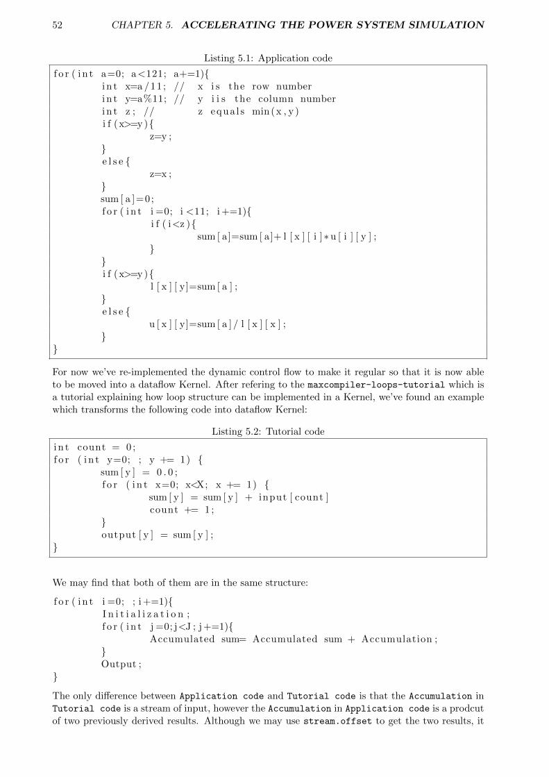
52 CHAPTER 5. ACCELERATING THE POWER SYSTEM SIMULATION
Listing 5.1: Application code
f o r ( i n t a=0; a<121; a+=1){i n t x=a /11 ; // x i s the row numberi n t y=a%11; // y i i s the column numberi n t z ; // z equa l s min (x , y )i f (x>=y ){
z=y ;}e l s e {
z=x ;}sum [ a ]=0;f o r ( i n t i =0; i <11; i +=1){
i f ( i<z ){sum [ a]=sum [ a]+ l [ x ] [ i ]∗ u [ i ] [ y ] ;
}}i f (x>=y ){
l [ x ] [ y]=sum [ a ] ;}e l s e {
u [ x ] [ y]=sum [ a ] / l [ x ] [ x ] ;}
}
For now we’ve re-implemented the dynamic control flow to make it regular so that it is now ableto be moved into a dataflow Kernel. After refering to the maxcompiler-loops-tutorial which isa tutorial explaining how loop structure can be implemented in a Kernel, we’ve found an examplewhich transforms the following code into dataflow Kernel:
Listing 5.2: Tutorial code
i n t count = 0 ;f o r ( i n t y=0; ; y += 1) {
sum [ y ] = 0 . 0 ;f o r ( i n t x=0; x<X; x += 1) {
sum [ y ] = sum [ y ] + input [ count ]count += 1 ;
}output [ y ] = sum [ y ] ;
}
We may find that both of them are in the same structure:
f o r ( i n t i =0; ; i +=1){I n i t i a l i z a t i o n ;f o r ( i n t j =0; j<J ; j +=1){
Accumulated sum= Accumulated sum + Accumulation ;}Output ;
}
The only difference between Application code and Tutorial code is that the Accumulation inTutorial code is a stream of input, however the Accumulation in Application code is a prodcutof two previously derived results. Although we may use stream.offset to get the two results, it
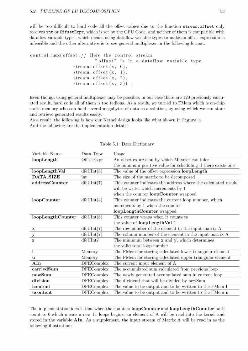
5.2. PIPELINE OF LU DECOMPOSITION 53
will be too difficult to hard code all the offset values due to the function stream.offset onlyreceives int or OffsetExpr, which is set by the CPU Code, and neither of them is compatible withdataflow variable types, which means using dataflow variable types to make an offset expression isinfeasible and the other alternative is to use general multiplexer in the following format:
c o n t r o l .mux( o f f s e t , // Here the c o n t r o l stream” o f f s e t ” i s in a data f low v a r i a b l e type
stream . o f f s e t (x , 0 ) ,stream . o f f s e t (x , 1 ) ,stream . o f f s e t (x , 2 ) ,stream . o f f s e t (x , 3 ) ) ;
Even though using general multiplexer may be possible, in our case there are 120 previously calcu-ated result, hard code all of them is too tedious. As a result, we turned to FMem which is on-chipstatic memory who can hold several megabytes of data as a solution, by using which we can storeand retrieve generated results easily.As a result, the following is how our Kernel design looks like what shown in Figure 1.And the following are the implementation details:
Table 5.1: Data Dictionary
Variable Name Data Type Usage
loopLength OffsetExpr An offset expression by which Maxeler can inferthe minimum positive value for scheduling if there exists one
loopLengthVal dfeUInt(8) The value of the offset expression loopLength
DATA SIZE int The size of the matrix to be decomposed
addressCounter dfeUInt(7) This counter indicates the address where the calculated resultwill be write, which increments by 1when the counter loopCounter wrapped
loopCounter dfeUInt(4) This counter indicates the current loop number, whichincrements by 1 when the counterloopLengthCounter wrapped
loopLengthCounter dfeUInt(8) This counter wraps when it counts tothe value of loopLengthVal-1
x dfeUInt(7) The row number of the element in the input matrix A
y dfeUInt(7) The column number of the element in the input matrix A
z dfeUInt7 The minimum between x and y, which determinesthe valid total loop number
l Memory The FMem for storing calculated lower triangular element
u Memory The FMem for storing calculated upper triangular element
AIn DFEComplex The current input element of A
carriedSum DFEComplex The accumulated sum calculated from previous loop
newSum DFEComplex The newly generated accumulated sum in current loop
division DFEComplex The dividend that will be divided by newSum
lcontent DFEComplex The value to be output and to be written to the FMem l
ucontent DFEComplex The value to be output and to be written to the FMem u
The implementation idea is that when the counters loopCounter and loopLengthCounter bothcount to 0,which means a new 11 loops begins, an element of A will be read into the kernel andstored in the variable AIn. As a supplement, the input stream of Matrix A will be read in as thefollowing illustration:

54 CHAPTER 5. ACCELERATING THE POWER SYSTEM SIMULATION
At the same time, the variable carriedSum is initialized with the 0, and when the loopCounteris smaller then z, the carriedSum is added by l[x][loopCounter] ∗ u[loopCounter][y] , andthis is achieved by reading value from FMem l and u with address x*11+loopCounter andy+loopCounter*11 respectively, otherwise 0, here is the illustration:When the loopCounter equals 10 and loopLengthCounter equals loopLengthVal-1, which
Figure 5.3: x=1,y=1,loopCounter=0
(a) Element to be read (b) Corresponding address
means the totally 11 loops have finished, then we need to decide the result should belong to l oru, and whether the result should be divided by l[x][x], and this can be achieved by comparingx and y, if x>=y, then the result belongs to lower triangle, otherwise the result belongs to up-per triangle and should be firstly divided by l[x][x]. For now, a whole 11 loops is finished, andthen the addressCounter will increments by 1 and a new element in matrix A should be readin and processed. After all the 121 elements have been processed then the decomposition is finished.
As a result, we achieved a total ticks of 121*11*128 for implementing a LU decomposition us-ing a dataflow kernel. Where 121 is the size of the matrix A to be decomposed, 11 is the 11 loopsfor processing each element in A, and 128 is the loopLength, namely, the ticks required for executingone loop.
5.2.3 Pipeline Implementation (LU Pipeline 1)
Although the multi-tick implementation works correctly, it still can be improved a lot. Specifically,it did not make use of the strength of Maxeler which is in a dataflow engine processing pipeline everydataflow core(arithmetic unit)computes simultaneously on neighboring data items in a stream. Itis because for the previous implementation, the computations look like follows:

5.2. PIPELINE OF LU DECOMPOSITION 55
Figure 5.4: Kernel Design
56 CHAPTER 5. ACCELERATING THE POWER SYSTEM SIMULATION
No computations are performed simultaneously. In addition, due to 11 is the minimum loop timesfor all the elements to be processed correctly, for most of the elements the required loop timesare less than 11, which means there are a lot of loops are unnecessary and doing meaning-lesscomputations.In order to make the non-pipelined computations pipelined, a new implementation design was pro-posed, which is to read in and start processing an element of matrix A every 1∗ loopLength insteadof the previously 11∗ loopLength, which means a new element was read in every loop but not every11 loops. The feasibility of this design can be shown from the follows:
Figure 5.5: Feasibility Analysis
(a) Required Loop Number
(b) Dependency Analysis
From Figure 3(a) we can know that the required loop number for processing an element is increas-ing(not strictly increasing) in a row, we always have loop no[x][y] <= loop no[x][y + 1]. Refer toFigure 3(b), this is a diagram showing the dependency during the computation of each element.We use gray squares to denote that the element has been processed, in other words, the elementhas been decomposed, and we use red square to denote that there are dependencies exist duringthe computation for this element. In addition, the horizontal axis is the total loop numbers andthe vertical axis is the index of the element. Take some elements’ computations as examples toshow what are the dependencies, for the 2nd element, a dependency exists during the first loopis due to u[x][y]=sum[a]/l[x][x], where l[x][x] in this case is l[0][0]. Therefore, due to thenon-pipelined algorithm, l[0][0] should have already been generated, which means we can onlyperform this computation when the computation for l[0][0] has been finished. And dependencyalso occurs for another reason, and take the the 13th element as an example, due to its x = 1
and y = 1, its z also equals 1, which means sum accumulation is involved in decomposing the
5.2. PIPELINE OF LU DECOMPOSITION 57
13th element, see sum[a]=sum[a]+l[x][i]*u[i][y]. In this case x = 1, y = 1, i = 0 so thatonly when l[1][0] and u[0][1] have already been calculated by decomposing the original matrix,performing this calculation can get the correct result.After checking Figure 3(b), all the calculations on which the later computations depends finishbefore the later computations, which means if the computations are in performed in the above waythen still correct results can be generated but in a pipelined way.To realise this in Maxeler, we can make modifications on the previous multi-ticks implementation.And in details, we need to change the input behavior from reading in an element from matrix Aevery 11 loops to reading in an element from matrix from A every 1 loop. Using the same data dic-tionary Table 1, this can be achieved by changing the input condition from loopCounter.eq(0)&
loopLengthCounter.eq(loopLengthVal - 1) into loopCounter.eq(loopLengthCounter). Wecan find this works from the following illustration:
Another necessary modification is that, due to this is a pipelined implementation, the results shouldbe written and output once they’ve finished their required computations, and this can be achievedby adding one more variable:
Table 5.2: Data Dictionary
Variable Name Data Type Usage
i dfeUInt(7) This variable is used for determiningwhether the required computations are finished
Once z equals i, the result should be written into the corresponding FMem so that the latercomputation won’t be int.

58 CHAPTER 5. ACCELERATING THE POWER SYSTEM SIMULATION
5.2.4 Another Pipeline Implementation (LU Pipeline 2)
For now we’ve had a pipelined implementation. However, after consideration, the implementationcan be further pipelined.For example, we may group this way, here elements in a same group willbe processed in parallel, see the following illustration:
The procedure is as follows: For each group, start a new loop and all the members will be read induring the loop every tick. Therefore, for the above case, 0 will be read in and processed in loop
1, 1,2,3, ..., 11 will be read in loop 2 and so on.The above procedure works if the first column of the matrix is given. We may conduct the followinganalysis to show this. For group{0}, there is no dependency, for group{1, 2, 3, ..., 10}, as longas element 0’s computation has finished, they can be processed in parallel. For goup{11, 12},element 12 have to wait until element 11’s computation is finished. However, as long as the firstcolumn of the matrix is given so that the decomposed element 11 is known due to there is nocomputation needed for the first column of matrix to be decomposed, then the group{11,12} canbe computed in parallel. Here element 12 may also need element 1’s computation to be finished,and this is true due to grounp{1,2,3, .., 10} start their computation at loop 2, due to they need 0loop to finish the decomposition, when the time comes to loop 3, the group{1, 2, 3, ..., 10} havealready finished decomposition and thus group{11,12} can perform their decompositon withoutwaiting. And if we check exhaustively, we can find this applies to all the other groups.Therefore, in order to achieve this implementation, we need the first column of the matrix andgroup the elements in the above way. The elements should be read in in at the following times:
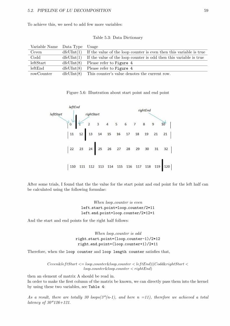
5.2. PIPELINE OF LU DECOMPOSITION 59
To achieve this, we need to add few more variables:
Table 5.3: Data Dictionary
Variable Name Data Type Usage
Ceven dfeUInt(1) If the value of the loop counter is even then this variable is true
Codd dfeUInt(1) If the value of the loop counter is odd then this variable is true
leftStart dfeUInt(8) Please refer to Figure 4
leftEnd dfeUInt(8) Please refer to Figure 4
rowCounter dfeUInt(8) This counter’s value denotes the current row.
Figure 5.6: Illustration about start point and end point
After some trials, I found that the the value for the start point and end point for the left half canbe calculated using the following formulae:
When loop counter is evenleft start point=loop counter/2*11
left end point=loop counter/2*12+1
And the start and end points for the right half follows:
When loop counter is oddright start point=(loop counter-1)/2*12
right end point=(loop counter+1)/2*11
Therefore, when the loop counter and loop length counter satisfies that,
Ceven&leftStart <= loop counter&loop counter < leftEnd)|(Codd&rightStart <loop counter&loop counter < rightEnd)
then an element of matrix A should be read in.In order to make the first column of the matrix be known, we can directly pass them into the kernelby using these two variables, see Table 4:
As a result, there are totally 30 loops(3*(n-1), and here n =11), therefore we achieved a totallatency of 30*126+121.

60 CHAPTER 5. ACCELERATING THE POWER SYSTEM SIMULATION
Table 5.4: Data Dictionary
Variable Name Data Type Usage
firstColumnR Memory The real value of the first column of the matrixis mapped directly to the kernel
firstColumnI Memory The imaginary value of the first column of the matrixis mapped directly to the kernel
5.2.5 Machine Parallelism
There is one more part in our program that needs acceleration. And the code has following struc-ture:
f o r ( i n t i t =0; i t <=3; i t +=1){// Deltad e l t a [ 1 ] [ i t ] = d e l t a [ 0 ] [ i t ]+(omega [ 0 ] [ i t ] − Omega synch )∗ s t e p S i z e ;
// Eq dash
eq dash [ 1 ] [ i t ] = eq dash [ 0 ] [ i t ]+((−1) ∗ eq dash [ 0 ] [ i t ] − ( X d [ i t ] − X d p [ i t ] ) ∗ ((−1) ∗ I d [ 0 ] [ i t ] − ( X d p [ i t ] − X d dp [ i t ] ) /( X d p [ i t ] − X ls [ i t ] ) /
( X d p [ i t ] − X ls [ i t ] ) ∗ (ps id [ 0 ] [ i t ] − ( X d p [ i t ] − X ls [ i t ] ) ∗ I d [ 0 ] [ i t ]− eq dash [ 0 ] [ i t ])
) + e fd [ 0 ] [ i t ]) / T do p [ i t ] ∗ s t e p S i z e ;
// Psid
ps id [ 1 ] [ i t ] = ps id [ 0 ] [ i t ]+((−1) ∗ ps id [ 0 ] [ i t ] + eq dash [ 0 ] [ i t ]+ ( X d p [ i t ] − X ls [ i t ] )∗ I d [ 0 ] [ i t ] ) / T do dp [ i t ] ∗ s t e p S i z e ; // checked
// Ed dash
ed dash [ 1 ] [ i t ] = ed dash [ 0 ] [ i t ]+( ed dash [ 0 ] [ i t ] +( X q [ i t ] − X q p [ i t ] ) ∗(I q [ 0 ] [ i t ] − ( X q p [ i t ] − X q dp [ i t ] ) / ( X q p [ i t ] − X ls [ i t ] ) /
( X q p [ i t ] − X ls [ i t ] ) ∗ ((−1) ∗ ps iq [ 0 ] [ i t ] + I q [ 0 ] [ i t ] ∗ ( X q p [ i t ] − X ls [ i t ] )− ed dash [ 0 ] [ i t ]))
) / (−1) / T qo p [ i t ] ∗ s t e p S i z e ;}
After referring to the maxcompiler-loops tutorial, we found that this part of code has the samestructure as the following code:

5.3. SUMMARY 61
f o r ( i n t count =0; ; count += 1) {B[ count ] = A[ count ] + 1 ;}
The only difference is that the computations are different. Therefore, we may implement this partin the same way. However, there is a restriction that the input stream cannot over 8 streams,but we have totally 28 inputs to be streamed. In order to solve the problem, DFEArrayType wasutilized. And as a reuslt, we just need one string with length of 28. In addition, the code lookslike:
DFEComplexType t=new DFEComplexType( d f eF loa t ( 1 1 , 5 3 ) ) ;DFEArrayType<DFEComplex> at=new
DFEArrayType<DFEComplex>(t , 2 8 ) ;DFEArray<DFEComplex> input=i o . input (” input ” , at ) ;DFEComplex deltaOut=input [ 1 1 ] . getReal ()>0?input [0 ]+( input [1 ] −377)∗0 .001 :input [ 0 ] ;DFEComplex eq dashOut=input [ 1 1 ] . getReal ()>0? input [2 ]+(
(−1) ∗ input [ 2 ] − ( input [ 3 ] − input [ 4 ] ) ∗ ((−1) ∗ input [ 5 ] − ( input [ 4 ] − input [ 6 ] ) /
( input [ 4 ] − input [ 7 ] ) / ( input [ 4 ] − input [ 7 ] ) ∗ (input [ 8 ] − ( input [ 4 ] − input [ 7 ] ) ∗ input [ 5 ]
− input [ 2 ] )) + input [ 9 ]) / input [ 1 0 ] ∗ 0 . 0 0 1 : input [ 2 ] ;
5.3 Summary
In Summary, this chapter firstly show the profiling result which determined the area of code tobe accelerated by FPGA (LU Decomposition and Machine update operations). Next, in order todesign the DFE kernel for LU decomposition, we solved some problems such that, determine Inputand output streams and memory pattern. Most importantly, we solved the problem of representingcomplex numbers in Maxeler. After these, we gave 3 design of LU decomposition and one designfor machines pipeline so that the number of machines can do update operations synchronously.

Chapter 6
Evaluation
6.1 Expected Performance
The first component in estimating performance in dataflow computation is the bandwidth in andout of the dataflow graph. For data in DFE memory, we simply look up the bandwidth of theparticular device and memory storing the data. The second component is the speed at which thedataflow pipeline is moving the data forward. A unit of time in a DFE is called a tick or (a cycle),and the speed of movement through a dataflow pipeline is given in [ticks/second].
Bandwidth can be thought of as the numbers per second that can be read into or written outfrom the DFE chip. The bandwidth of DFEs can be between 200-1000 million numbers per seconddepending on the size of the numbers and the speed of the interconnect (LMEM, PCIe, Infiniband,or MaxRing).The clock frequency is how many ticks per second the kernels can run at. Thefrequency is between 100-300 million ticks per second as determined and displayed during the DFEcompilation process,
In our implementation, We did not use any LMem or MaxRing. We used FMem for storing valuesand computation which provides up to 21TB/s of memory bandwidth within in chip. We shouldalso consider the speed of the interconnection PCIe for transferring data from CPU to FPGA. Wedenote the time of transferring data between the CPU and FPGAs as TPCIE , and the time forreading/writing to FMem as TFMEM . However, this term is usually negligible as accessing to theon-chip FMem is very fast compared to other memory patterns. For the computation time onDFEs TCOMPUTE , we have:
TCOMPUTE =Ticks
Clockfrequncy(6.1)
If TACCEL is the total time used of the accelerated program,
TACCEL = TINIT + TSTREAM (6.2)
where TSTREAM = MAX(TCOMPUTE , TPCIE), and TINIT includes SW time, and also time to setscalar inputs, ROMs, prepare streams etc. Assume the data size of transfer (between CPU andFPGAs) is depend on the number of the buses N .
TPCIE =BY TES INPCIE +BY TES OUTPCIE
BWPCIE(6.3)
Where PCIe bandwidth depends on transfer size that can sustain >2GB/s.
62
6.1. EXPECTED PERFORMANCE 63
6.1.1 LU Pipeline 1
In our first version of pipelining,the Input Data to Kernel is the N*N Matrix A of complex numbers(16 bytes) and a N*N matrix in of double numbers(8 bytes). And the outputs are two N*N matrixesL and U contain complex numbers. So:
TPCIE =(16 + 8)N2 + 2 ∗ 16 ∗N2
BWPCIE
=56N2
BWPCIE
(6.4)
And
Ticks = [(N2 − 1) + (N − 1)] ∗ looplength+N (6.5)
Where looplength is the number of ticks for one loop’s calculation in our kernel.
6.1.2 LU Pipeline 2
In our second version of pipelining,the Input Data to Kernel is not only the N*N Matrix A ofcomplex numbers (16 bytes) and a N*N matrix in of double numbers(8 bytes) but also the firstcolumn of matrix A which is of size N. And the outputs are the same. So:
TPCIE =(16 + 8)N2 + 16 ∗N + 2 ∗ 16 ∗N2
BWPCIE
=56N2 + 16N
BWPCIE
(6.6)
AndTicks = 3(N − 1) ∗ 128 +N2 (6.7)
6.1.3 Machine Parallelism
As we know that, the very important factor of speed is the operation volume within the kernel andthe data transfer time. In the machine parallelism, the input and output streams are dependent onhow many parameters to be updated. Let say, the number of parameters to be imported into thekernel and Din and DOUT for output. And number of the update operations all together is Op. Aswe assume the data type of the parameters are all complex numbers. So,
TPCIE =16 ∗ (Din +Dout)
BWPCIE(6.8)
AndTicks = OP (6.9)

64 CHAPTER 6. EVALUATION
6.2 Experimental Evaluation
6.2.1 General Settings
We use the MPC-C500 reconfigurable accelerator system from Maxeler Technologies for our eval-uation. The system has 4 MAX3434A cards, each of which has a Virtex-6 XC6VSX475T FPGA.The cards are connected to 2 Intel Xeon X5650 CPUs and each card communicates with the CPUsvia a PCI Express gen2 x8 link. The CPUs have 12 physical cores and are clocked at 2.66 GHz. Wedevelop the FPGA kernels using the MaxCompiler which adopts a streaming programming modeland its supports customisable floatingpoint data formats. And the clock frequency is set to 100.
6.2.2 Test the LU Decomposition Kernel
The data we use is from the .m files provided by Dr Chaudhuri, e.g., The matrix size is correspondsto the number of the buses. The name of the matrix is Ybus. For lxample, if we have 11 buses thematrix is 11*11. so N=11.
We firstly tested the running time of the pure C code using on Maxeler Super Computer maxnode2.And of course, we only cut out the time running on LU decomposition process. For 20 seconds’simulation, it only took 0.134s on average to run.
Figure 6.1: Runing time for LU decomposition in C (listed by each iteration)
As we can see from Fig. 6.1, which lists the running time of LU Decomposition in each iteration.So that we can approximate the running time of doing LU Decomposition once in C code (Tc) bytaking an average value:
Tc = 7 microseconds (ms)
As we know, the original LU decomposition algorithm has a time complexity O(N3). To estimatethe speed up. We should know exactly how is the computation time of our C code depends on thesize of N . However, as we do not have data other than the used Y bus data provided, we can not domore experiment. Fortunately we can estimate this relation by derive the relation of the numberof operation steps and the size of N .As shown in the figure above. The LU decomposition algorithm processes the matrix in a sub-matrix by sub-matrix way. That is it will first do calculates on the elements on left-most layer, say,loop 1 in the figure. we denotes the number of operations of the matrix of size N Op(N), we have,
Op(N)−Op(N − 1) = (N − 1) + (N − 1)2 + (N − 1)2
Op(N − 1)−Op(N − 2) = (N − 2) + (N − 2)2 + (N − 2)2
...

6.2. EXPERIMENTAL EVALUATION 65
Op(2)−Op(1) = 3
Where (N − 1) + (N − 1)2 is number of multiplications and (N − 1)2 is for subtraction. So whenwe add them together, we can get Op(N). By the principle of arithmetic progression, and we know12 + 22 + 32...+ n2 = n(n+ 1)(2n+ 1)/6, we can get,
Op(N) = (N−1)22 + (N−1)(N)(2N−1)
3
And then, assuming the one subtraction and one multiplication use the same time in CPU, we canestimation the time of doing each operation, we call it Tunit, by using the experimental result ofour power system. As we has 11 buses, So Op=820. And as the total computation time is 7 ms.We can average it and get Tunit = 0.085ms. Therefore, the computing time for the C program, TCcan be estimated as:
TC = Tunit ∗Op = 0.0085 ∗ (N−1)22 + (N−1)(N)(2N−1)
3
LU Pipeline 1
By only recorded the time speeding on LU decomposition. Our pipelined version of code using thekernel we firstly designed takes average 50s to simulation 20s’ calculation. Compared to the 0.13sused by the pure C code, it is really a very bad result. As it slows down the program by about 500times. However, actually this result is not in-apprehensible and it makes senses:
Firstly,we know the design of my kernel takes [(N2−1)+(N−1)]∗looplength+n ticks, where N=11,looplength=128, so it is TCOMPUTE = 130*128+121/100MHz=16761/100MHz = 0.00016 seconds= 160ms. And for a simulation of 20 seconds which means 20000 times’ calls to the LUSolverfunction, The theoretical computing time on the LU Solver kernel should be: 0.000016*20000=3.2s.
And TPCIE = 56N2
BWPCIE= 3231ms, by taking BWPCIE=2GB/s as the worst case. This value is
much bigger than the TCOMPUTE = 160ms which means that is the Data transfer time dominatesthe computation time. So TSTREAM = TPCIE . Let us take a look at the running time for eachiteration in Fig. 6.2:
It is surprised to see that the first iteration takes much longer time than the remaining itera-tions and is also much(about 10 times) bigger than TSTREAM=3231ms. This is because that forthe fist call of the Kernel, the maxeler system should do some initialization work. And we knowTACCEL=TINIT+TSTREAM , we can only assume TSTREAM dominates for large data volumes. How-ever, the data we use now has too small data size so that the initialisation dominates. And anotherproblem is that, the calculation volume is too small (only 16761 ticks), either. As we can see if theTCOMPUTE = 160ms, the data transfer time TPCIE ≈ 850ms is much bigger.

66 CHAPTER 6. EVALUATION
Figure 6.2: Runing time for LU decomposition in Kernel (listed by each iteration
As we know that in order to use Maxeler kernels to perform calculations, we need to transfer datafrom CPU to kernels and this will cause a big overhead, which means if the scale of the computa-tion on the transferred data is not large enough then the data transfer overhead will become veryobvious and even makes the program slower. Unfortunately, our program is just the case where thescale of computation is not large enough.While FPGAs would speed up the matrix decomposition,they would need to wait for the inputs to be refreshed, and the additional latency over PCIe wouldbecome apparent over a million iterations’ run.
LU Pipeline 2
The second implementation takes average 50s to simulation 20s’ calculation.This design still cannot give any acceleration is because
Firstly,we know the design of my kernel takes 3(N − 1) ∗ looplength + n2 ticks, where N=11,looplength=128, so it is TCOMPUTE = 130*128+121/100MHz=3961/100MHz = 0.00004 seconds= 40ms. The computation volume shrinks as we further pipeline the kernel.
And TPCIE = 56N2+16NBWPCIE
= 3692ms, by taking BWPCIE=2GB/s as the worst case. This value ismuch bigger than the one in the previous implementation since we input an extra column of matrixA to FPGA every time call the LU Solver. That is to say, with the computation volume shrink buteven more Data to transfer. This won’t give any acceleration.
6.2.3 Machine Parallelism
The results for only running the Machine Parallelism kernel is shown below, and the total time onthe kernel for 20 seconds’ simulation is about 22s.
For our system, because the update process is interdicted by the calling of LU Solver function.
we have to pipe line the upper and lower parts of operations separately. For the first part kerneldesign, the input Data to Kernel is an Array Type of Complex numbers with a length of 28. an

6.3. ANALYSIS 67
Array Type of Complex numbers with a length of 6 is the output stream. So:
TPCIE =(28 + 6) ∗ 16
BWPCIE
=544
BWPCIE
(6.10)
if we take BWPCIE= 2GB/s, TPCIE=544/1024/1024/2*1000000=519ms.And as tested from the maxeler system, we know
Ticks = 25 (6.11)
TCOMPUTE = 25/100MHz=0.00000025 seconds = 0.25ms.
It is also clear to see, the time is mostly occupied by the data transfer time.
6.3 Analysis
In conclusion, Maxeler is good at large scale and regular behavior computing, however, in our modelwe only have small scale computations. It seems that the model I have got now is not worth beingput into Maxeler. Fortunately, our objective of this project is not for accelerating this particularpower system simulation, but to explore how FPGAs can be used to accelerate power systems. Inreality, the power system simulation should deal with larger scale of computation (e. g. the SmartGrid with Electric Springs). In this section we will illustrate how can we extent our design to largersystems.
The key to achieving the best performance in FPGA acceleration, while maintaining correctness,is optimization of arithmetic units and data types to suit the range/precision at each point in thecomputation and minimise the data transferred at each compute step as well as perform as manycomputations on the data as possible before moving them back to memory and minimize the num-ber of memory accesses.
Here in our problem, the amount of computations on the data is represented by the value of Ticks,and the amount of data transfer depends on the value of N . We want the former as much aspossible and the latter as less as possible. However, both of them depend on the value of N .When N increases, both of the computation volume and the data transfer volume will increase.We should balance these two volumes, only so the program will be accelerated. and the balancingpoint is when computation volume exceeds the data transfer volume. And we shall estimate thespeedup = T[C]/T[STEAM ] with data size N for the both cases: ignore transfer time or not.
LU Pipeline 1
As we want the Computation time dominates the data transfer time (TCOMPUTE > TPCIE), Thatis:
{[(N2 − 1) + (N − 1)] ∗ looplength+N}/100 > 56N2/1024/1024/BW ∗ 1000, 000
In Fig. 6.3 (a) compares the TCOMPUTE and TPCIE when bandwidth is 2GB/s, and Fig. 6.4 (b)compares the two when bandwidth is 10GB/s. As we know bandwidth has very hauge influence onthe time of data transfer. We can see that, when the bandwidth is the standard 2GB/s (which weconsider), there is no possible for the computation time to exceed data transfer time. We can havea chance to ignore the overhead only if the bandwidth can reach some higher value. For example,
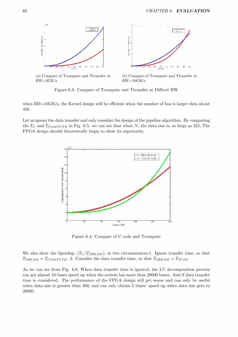
68 CHAPTER 6. EVALUATION
(a) Compare of Tcompute and Ttransfer atBW=2GB/s
(b) Compare of Tcompute and Ttransfer atBW=10GB/s
Figure 6.3: Compare of Tcompute and Ttransfer at Differet BW
when BD=10GB/s, the Kernel design will be efficient when the number of bus is larger then about450.
Let us ignore the data transfer and only consider the design of the pipeline algorithm. By comparingthe TC and TCOMPUTE in Fig. 6.5. we can see that when N , the data size is, as large as 225, TheFPGA design should theoretically begin to show its superiority.
Figure 6.4: Compare of C code and Tcompute
We also show the Speedup, (TC/TSREAM ), in two circumstances:1. Ignore transfer time, so thatTSREAM = TCOMPUTE . 2. Consider the data transfer time, so that TSREAM = TPCIE .
As we can see from Fig. 6.6, When data transfer time is ignored, the LU decomposition processcan get almost 10 times speed up when the system has more than 20000 buses. And if data transfertime is considered. The performance of the FPGA design will get worse and can only be usefulwhen data size is greater than 400, and can only obtain 5 times’ speed up when data size gets to20000.

6.3. ANALYSIS 69
(a) Speed Up When Transfer Time is Ig-nored
(b) Speed Up When Transfer Time is Con-sidered
Figure 6.5: Speed Up with N
LU Pipeline 2
The same with the first design, if we want the Computation time dominates the data transfer time(TCOMPUTE > TPCIE), That is:
{3(N − 1) ∗ looplength+N2}/100 > (56N2 + 16N)/1024/1024/BW ∗ 1000, 000
However, we can not achieve this for our second design. Although it has less computation tickswithin the Kernel, It needs more data to be transferred from CPU to FPGA. And from Fig. 6.7we can see, the TPCIE rapidly increases with the N increases only by 1 and it is alway abovethe TCOMPUTE . Therefore, the data transformation overhead will always slow down our program.Therefore, as a conclusion, our second kernel design for LU Decomposition is not applicative topower system simulation.
Figure 6.6: Compare of Tcompute and Ttransfer at BW=2GB/s
In a similar way, let us first ignore the data transfer and only the design of the pipeline algorithm.The speed up shown in Fig 6.8 (a) show a significant jump of acceleration with the increase of N .And it can get to 950 times speed up when data size is 20000. However, if we consider data transfertime, It can only get a slight shrink in computation time when the band width is 6GB/s and it isnot adaptive to small systems. (Fig. 6.7(b))
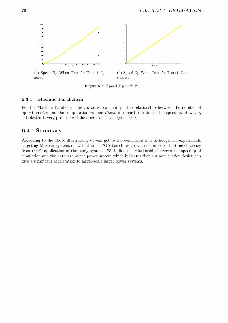
70 CHAPTER 6. EVALUATION
(a) Speed Up When Transfer Time is Ig-nored
(b) Speed Up When Transfer Time is Con-sidered
Figure 6.7: Speed Up with N
6.3.1 Machine Parallelism
For the Machine Parallelism design, as we can not get the relationship between the number ofoperations OP and the computation volume Ticks, it is hard to estimate the speedup. However,this design is very promising if the operations scale gets larger.
6.4 Summary
According to the above illustration, we can get to the conclusion that although the experimentstargeting Maxeler systems show that our FPGA-based design can not improve the time efficiencyfrom the C application of the study system. We builds the relationship between the speedup ofsimulation and the data size of the power system which indicates that our acceleration design cangive a significant acceleration to larger-scale larger power systems.
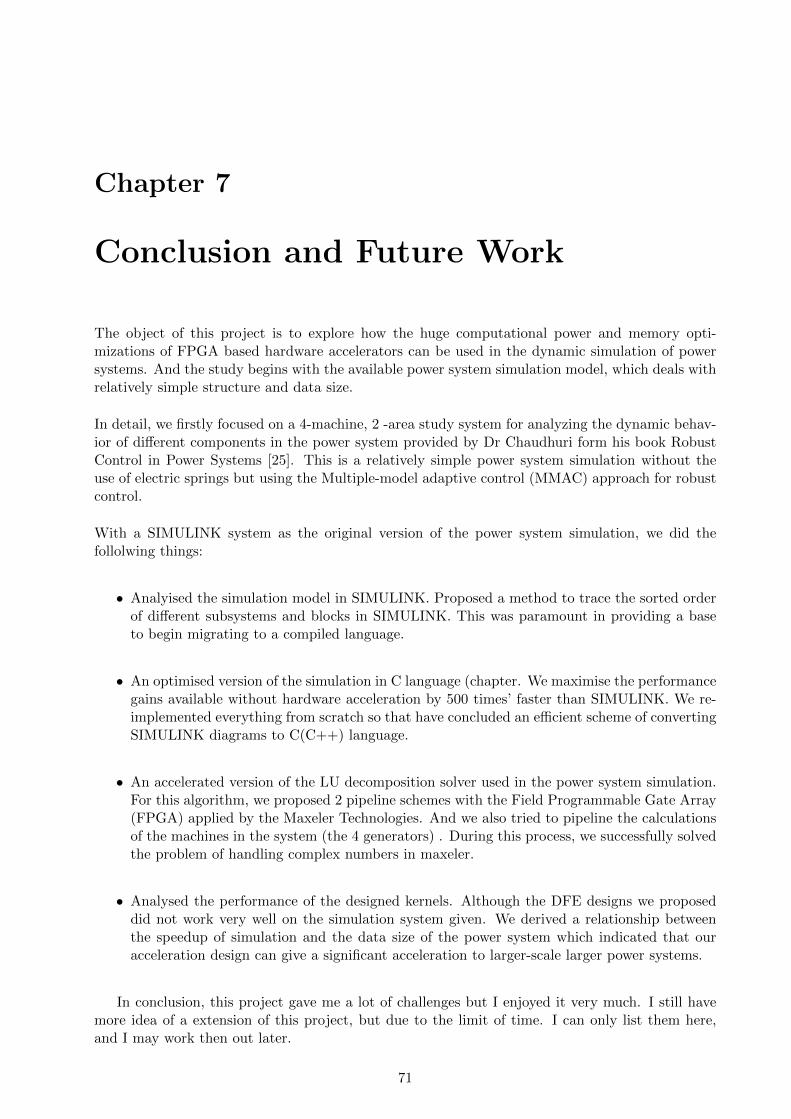
Chapter 7
Conclusion and Future Work
The object of this project is to explore how the huge computational power and memory opti-mizations of FPGA based hardware accelerators can be used in the dynamic simulation of powersystems. And the study begins with the available power system simulation model, which deals withrelatively simple structure and data size.
In detail, we firstly focused on a 4-machine, 2 -area study system for analyzing the dynamic behav-ior of different components in the power system provided by Dr Chaudhuri form his book RobustControl in Power Systems [25]. This is a relatively simple power system simulation without theuse of electric springs but using the Multiple-model adaptive control (MMAC) approach for robustcontrol.
With a SIMULINK system as the original version of the power system simulation, we did thefollolwing things:
• Analyised the simulation model in SIMULINK. Proposed a method to trace the sorted orderof different subsystems and blocks in SIMULINK. This was paramount in providing a baseto begin migrating to a compiled language.
• An optimised version of the simulation in C language (chapter. We maximise the performancegains available without hardware acceleration by 500 times’ faster than SIMULINK. We re-implemented everything from scratch so that have concluded an efficient scheme of convertingSIMULINK diagrams to C(C++) language.
• An accelerated version of the LU decomposition solver used in the power system simulation.For this algorithm, we proposed 2 pipeline schemes with the Field Programmable Gate Array(FPGA) applied by the Maxeler Technologies. And we also tried to pipeline the calculationsof the machines in the system (the 4 generators) . During this process, we successfully solvedthe problem of handling complex numbers in maxeler.
• Analysed the performance of the designed kernels. Although the DFE designs we proposeddid not work very well on the simulation system given. We derived a relationship betweenthe speedup of simulation and the data size of the power system which indicated that ouracceleration design can give a significant acceleration to larger-scale larger power systems.
In conclusion, this project gave me a lot of challenges but I enjoyed it very much. I still havemore idea of a extension of this project, but due to the limit of time. I can only list them here,and I may work then out later.
71
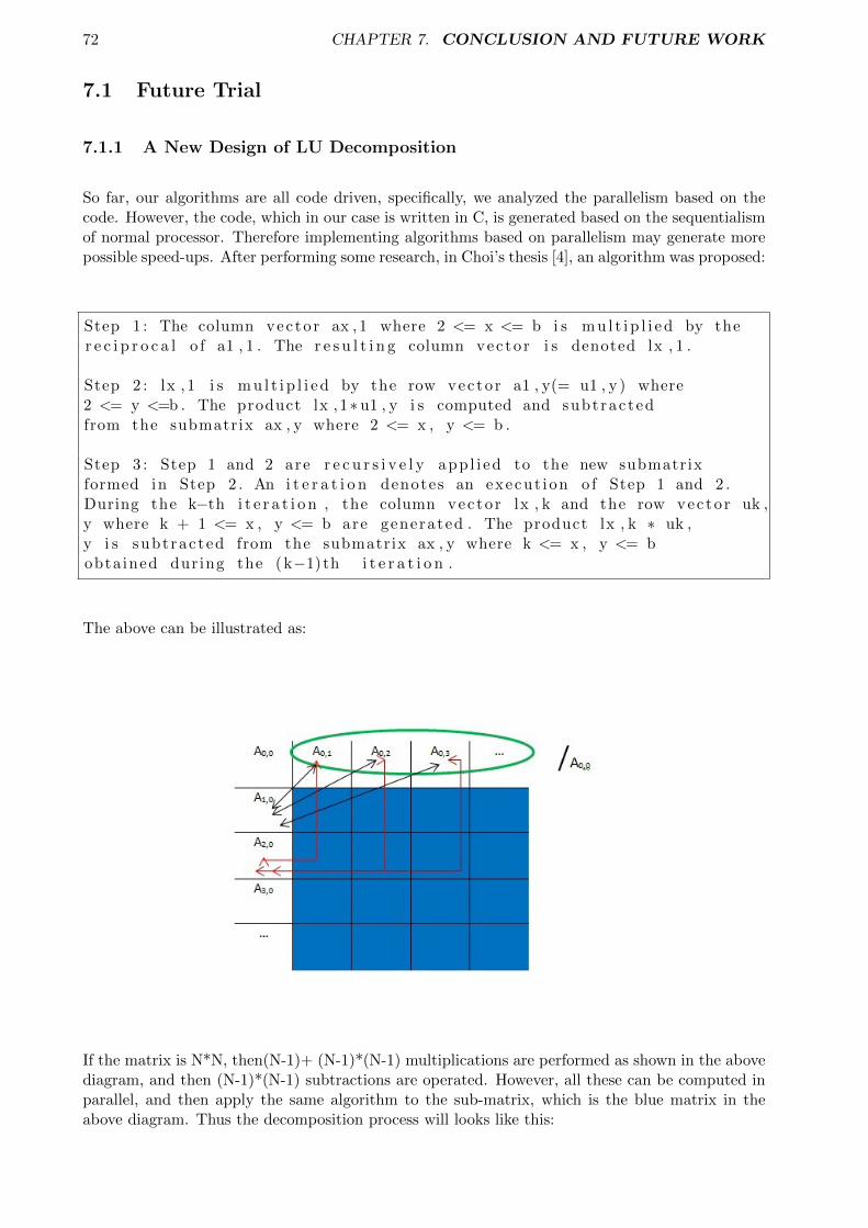
72 CHAPTER 7. CONCLUSION AND FUTURE WORK
7.1 Future Trial
7.1.1 A New Design of LU Decomposition
So far, our algorithms are all code driven, specifically, we analyzed the parallelism based on thecode. However, the code, which in our case is written in C, is generated based on the sequentialismof normal processor. Therefore implementing algorithms based on parallelism may generate morepossible speed-ups. After performing some research, in Choi’s thesis [4], an algorithm was proposed:
Step 1 : The column vecto r ax , 1 where 2 <= x <= b i s m u l t i p l i e d by ther e c i p r o c a l o f a1 , 1 . The r e s u l t i n g column vecto r i s denoted lx , 1 .
Step 2 : lx , 1 i s m u l t i p l i e d by the row vecto r a1 , y(= u1 , y ) where2 <= y <=b . The product lx , 1∗ u1 , y i s computed and subtractedfrom the submatrix ax , y where 2 <= x , y <= b .
Step 3 : Step 1 and 2 are r e c u r s i v e l y app l i ed to the new submatrixformed in Step 2 . An i t e r a t i o n denotes an execut ion o f Step 1 and 2 .During the k−th i t e r a t i o n , the column vecto r lx , k and the row vecto r uk ,y where k + 1 <= x , y <= b are generated . The product lx , k ∗ uk ,y i s subtracted from the submatrix ax , y where k <= x , y <= bobtained during the (k−1)th i t e r a t i o n .
The above can be illustrated as:
If the matrix is N*N, then(N-1)+ (N-1)*(N-1) multiplications are performed as shown in the abovediagram, and then (N-1)*(N-1) subtractions are operated. However, all these can be computed inparallel, and then apply the same algorithm to the sub-matrix, which is the blue matrix in theabove diagram. Thus the decomposition process will looks like this:
7.1. FUTURE TRIAL 73
The implementation is feasible using Maxeler, and possibly further reduce the execution time re-quired. However, due to the time constraints, we regard this as a future trial.
7.1.2 System Extension
• Assuming we need to carry out multiple times of this computation, could we include multiplecopies of your design on chip so that they can support multiple independent computation inparallel? What is the maximum Can the current external memory support this? If not, justassume that the memory is fast enough and see how fast your design would run. As to now,we did not have time to think about it, I do want to explore this later.
• Extension to a more complex power system, e.g., the smart grid with electronic springs.

Bibliography
[1] Shrirang Abhyankar and Alexander J Flueck. Real-time power system dynamics simulationusing a parallel block-jacobi preconditioned newton-gmres scheme. In High Performance Com-puting, Networking, Storage and Analysis (SCC), 2012 SC Companion:, pages 299–305. IEEE,2012.
[2] Jonathan W Babb, Matthew Frank, and Anant Agarwal. Solving graph problems with dynamiccomputation structures. In Photonics East’96, pages 225–236. International Society for Opticsand Photonics, 1996.
[3] Ian Buck, Tim Foley, Daniel Horn, Jeremy Sugerman, Kayvon Fatahalian, Mike Houston, andPat Hanrahan. Brook for gpus: stream computing on graphics hardware. In ACM Transactionson Graphics (TOG), volume 23, pages 777–786. ACM, 2004.
[4] Seonil Choi and Viktor K Prasanna. Time and energy efficient matrix factorization usingfpgas. In Field Programmable Logic and Application, pages 507–519. Springer, 2003.
[5] C Concordia. Ieee committee report on recommended phasor diagram for synchronous ma-chines. IEEE Transactions on Power Apparatus and Systems, 88(11):1593–1610, 1969.
[6] Andreas Dandalis, Alessandro Mei, and Viktor K Prasanna. Domain specific mapping forsolving graph problems on reconfigurable devices. In Parallel and Distributed Processing,pages 652–660. Springer, 1999.
[7] Rob Dimond, Sebastien Racaniere, and Oliver Pell. Accelerating large-scale hpc applicationsusing fpgas. In Computer Arithmetic (ARITH), 2011 20th IEEE Symposium on, pages 191–192. IEEE, 2011.
[8] EROCT. Electrical buses and outage scheduling, 2013. [Online; accessed 5-September-2013].
[9] Joseph H Eto and Robert J Thomas. Computational needs for the next generation electricgrid. Department of Energy, 2011.
[10] Djalma M Falcao. High performance computing in power system applications. In Vector andParallel ProcessingVECPAR’96, pages 1–23. Springer, 1997.
[11] Narain G Hingorani, Laszlo Gyugyi, and Mohamed El-Hawary. Understanding FACTS: con-cepts and technology of flexible AC transmission systems, volume 1. IEEE press New York,2000.
[12] Lee W Howes, Oliver Pell, Oskar Mencer, and Olav Beckmann. Accelerating the developmentof hardware accelerators. In Proc. Workshop on Edge Computing, 2006.
[13] Zhenyu Huang and Jarek Nieplocha. Transforming power grid operations via high perfor-mance computing. In Power and Energy Society General Meeting-Conversion and Delivery ofElectrical Energy in the 21st Century, 2008 IEEE, pages 1–8. IEEE, 2008.
[14] PJM Interconnection. Pjm statistics, 2013. [Online; accessed 5-September-2013].
74
BIBLIOGRAPHY 75
[15] M Klein, GJ Rogers, and P Kundur. A fundamental study of inter-area oscillations in powersystems. Power Systems, IEEE Transactions on, 6(3):914–921, 1991.
[16] David Koester, Sanjay Ranka, and Geoffrey Fox. Power systems transient stability-a grandcomputing challenge. Northeast Parallel Architectures Center, Syracuse, NY, Tech. Rep.SCCS, 549, 1992.
[17] Prabha Kundur. Power system stability and control, volume 12. , 2001.
[18] Aaron Richard Mandle. Fpga based hardware acceleration: A case study in protein identifi-cation, 2013. [Online; accessed 5-Octobet-2013].
[19] T Mathworks. Simulink getting started guide.
[20] MatlabWork. Control and display sorted order, 2013. [Online; accessed 5-September-2013].
[21] Oskar Mencer. Asc: a stream compiler for computing with fpgas. Computer-Aided Design ofIntegrated Circuits and Systems, IEEE Transactions on, 25(9):1603–1617, 2006.
[22] Oskar Mencer, Zhining Huang, and Lorenz Huelsbergen. Hagar: Efficient multi-context graphprocessors. In Field-Programmable Logic and Applications: Reconfigurable Computing Is GoingMainstream, pages 915–924. Springer, 2002.
[23] Felipe Morales, Hugh Rudnick, and Aldo Cipriano. Balanced decomposition for power systemsimulation on parallel computers.
[24] University of Malaga. Simulink basics tutorial, 2013. [Online; accessed 5-Octobet-2013].
[25] Bikash Pal and Balarko Chaudhuri. Robust control in power systems. Springer, 2005.
[26] Oliver Pell, Lee W Howes, Kubilay Atasu, Olav Beckmann, and Oskar Mencer. Acceleratingscientific computations using fpgas. In The Advanced Maui Optical and Space SurveillanceTechnologies Conference, volume 1, page 97, 2006.
[27] Oliver Pell and Oskar Mencer. Surviving the end of frequency scaling with reconfigurabledataflow computing. ACM SIGARCH Computer Architecture News, 39(4):60–65, 2011.
[28] Michael Ryabtsev and Ofer Strichman. Translation validation: from simulink to c. In ComputerAided Verification, pages 696–701. Springer, 2009.
[29] Peter W Sauer and MA Pai. Power system dynamics and stability. Prentice Hall Upper SaddleRiver, NJ, 1998.
[30] User’s Guide Simulink. Version 7. The MathWorks Inc, 2009.
[31] Yong Hua Song and Allan Thomas Johns. Flexible ac transmission systems (FACTS), vol-ume 30. IET, 1999.
[32] Brian Stott. Power system dynamic response calculations. Proceedings of the IEEE, 67(2):219–241, 1979.
[33] Gilbert Sybille, Patrice Brunelle, Hoang Le-Huy, Lo-uis A Dessaint, and Kamal Al-Haddad.Theory and applications of power system blockset, a matlab/simulink-based simulation toolfor power systems. In Power Engineering Society Winter Meeting, 2000. IEEE, volume 1,pages 774–779. IEEE, 2000.
[34] Isa Servan Uzun, Abbes Amira, and Ahmed Bouridane. Fpga implementations of fast fouriertransforms for real-time signal and image processing. In Vision, Image and Signal Processing,IEE Proceedings-, volume 152, pages 283–296. IET, 2005.

76 BIBLIOGRAPHY
[35] Wikipedia. Lu decomposition — wikipedia, the free encyclopedia, 2013. [Online; accessed5-September-2013].
[36] Changyan Zhou and Ratnesh Kumar. Semantic translation of simulink diagrams to input/out-put extended finite automata. Discrete Event Dynamic Systems, 22(2):223–247, 2012.