harshe_m

DESIGN OF ONE DEGREE OF FREEDOM CLOSED LOOP SPATIAL CHAINSUSING NON-CIRCULAR GEARS

By

MANDAR SHRIKANT HARSHE

A THESIS PRESENTED TO THE GRADUATE SCHOOLOF THE UNIVERSITY OF FLORIDA IN PARTIAL FULFILLMENT

OF THE REQUIREMENTS FOR THE DEGREE OFMASTER OF SCIENCE

UNIVERSITY OF FLORIDA

2009

1

c© 2009 Mandar Shrikant Harshe

2

I have to understand the world, you see.

- Richard Feynman, Physicist (1918 - 1988)

3

ACKNOWLEDGMENTS

I am extremely grateful to my supervisory committee chair, Dr. Carl D. Crane III, for

giving me an opportunity to work at CIMAR. His guidance and support throughout the

duration of my study made this work possible and gave direction to my work. I also thank

Dr. David Dooner, of University of Puerto Rico - Mayaguez, with whom we collaborated

on this project. His guidance and support helped me immensely in this work. I would

like to thank Dr. John Schueller and Dr. A. Antonio Arroyo for agreeing to be on my

committee.

I would like to acknowledge the support provided by the Department of Energy via

the University Research Program in Robotics (URPR) through University of Florida grant

number DE-FG04-86NE37967.

I received great support from my friends and colleagues, including Vishesh Vikas,

Sanketh Bhat and Priyank Bagrecha. I am extremely grateful for their words of

encouragement and support. I also thank fellow students at CIMAR. Finally, I am

indebted to my parents and my sister for their love and support; I owe my success and

progress to them.

4

TABLE OF CONTENTS

page

ACKNOWLEDGMENTS . . . . . . . . . . . . . . . . . . . . . . . . . . . . . . . . . 4

LIST OF TABLES . . . . . . . . . . . . . . . . . . . . . . . . . . . . . . . . . . . . . 6

LIST OF FIGURES . . . . . . . . . . . . . . . . . . . . . . . . . . . . . . . . . . . . 7

ABSTRACT . . . . . . . . . . . . . . . . . . . . . . . . . . . . . . . . . . . . . . . . 8

CHAPTER

1 INTRODUCTION . . . . . . . . . . . . . . . . . . . . . . . . . . . . . . . . . . 10

1.1 Motivation . . . . . . . . . . . . . . . . . . . . . . . . . . . . . . . . . . . . 101.2 Related work . . . . . . . . . . . . . . . . . . . . . . . . . . . . . . . . . . 11

2 PROBLEM STATEMENT AND APPROACH . . . . . . . . . . . . . . . . . . . 14

3 DESIGN METHOD . . . . . . . . . . . . . . . . . . . . . . . . . . . . . . . . . 17

3.1 Actual Path Generation . . . . . . . . . . . . . . . . . . . . . . . . . . . . 173.2 Error Measure . . . . . . . . . . . . . . . . . . . . . . . . . . . . . . . . . . 193.3 Weighting Factor . . . . . . . . . . . . . . . . . . . . . . . . . . . . . . . . 223.4 Handling Multiple Solutions . . . . . . . . . . . . . . . . . . . . . . . . . . 23

4 NUMERICAL EXAMPLE . . . . . . . . . . . . . . . . . . . . . . . . . . . . . . 25

5 CONCLUSIONS . . . . . . . . . . . . . . . . . . . . . . . . . . . . . . . . . . . 29

REFERENCES . . . . . . . . . . . . . . . . . . . . . . . . . . . . . . . . . . . . . . . 30

BIOGRAPHICAL SKETCH . . . . . . . . . . . . . . . . . . . . . . . . . . . . . . . . 32

5

LIST OF TABLES

Table page

3-1 Mechanism parameters for A side . . . . . . . . . . . . . . . . . . . . . . . . . . 19

3-2 Mechanism parameters for B side . . . . . . . . . . . . . . . . . . . . . . . . . . 19

3-3 System parameters . . . . . . . . . . . . . . . . . . . . . . . . . . . . . . . . . . 19

4-1 Mechanism parameters for A side . . . . . . . . . . . . . . . . . . . . . . . . . . 25

4-2 Mechanism parameters for B side . . . . . . . . . . . . . . . . . . . . . . . . . . 25

4-3 Desired poses and orientations . . . . . . . . . . . . . . . . . . . . . . . . . . . . 26

4-4 Number of solutions by reverse analysis . . . . . . . . . . . . . . . . . . . . . . . 26

4-5 Solutions selected for min. error criteria . . . . . . . . . . . . . . . . . . . . . . 26

6

LIST OF FIGURES

Figure page

1-1 A 12-link, 1-degree of freedom manipulator . . . . . . . . . . . . . . . . . . . . . 12

2-1 A candidate mechanism . . . . . . . . . . . . . . . . . . . . . . . . . . . . . . . 14

3-1 Case Study :- A-side angles vs input angle . . . . . . . . . . . . . . . . . . . . . 20

3-2 Case Study :- B-side angles vs input angle . . . . . . . . . . . . . . . . . . . . . 20

3-3 Case Study :- Gear ratios (A side) vs step number . . . . . . . . . . . . . . . . . 21

3-4 Start and end configurations . . . . . . . . . . . . . . . . . . . . . . . . . . . . . 21

4-1 Multiple paths arising from different starting configurations . . . . . . . . . . . 27

4-2 Variation of weighting factors . . . . . . . . . . . . . . . . . . . . . . . . . . . . 28

7

Abstract of Thesis Presented to the Graduate Schoolof the University of Florida in Partial Fulfillment of the

Requirements for the Degree of Master of Science

DESIGN OF ONE DEGREE OF FREEDOM CLOSED LOOP SPATIAL CHAINSUSING NON-CIRCULAR GEARS

By

Mandar Shrikant Harshe

May 2009

Chair: Carl D. Crane IIIMajor: Mechanical Engineering

Real world robot manipulators often use open-loop geometry where the motions

governing positioning are independent from those controlling the orientation of the

objects. These types of robot manipulators need expensive hardware and complicated

controllers to manipulate the multiple (generally six) actuators. This research presents

the design of one degree-of-freedom spatial mechanisms that use non-circular gears to

constrain the motion. The geometry of one degree-of-freedom mechanisms and the design

of the non-circular gears that link certain joint axes has already been dealt with. This

research is concerned with the design of mechanism parameters like link lengths, joint

offsets, and twist angles when the gear profiles are known.

In a spatial body-guidance problem, representing the motion by systems of polynomial

equations restricts the number of end-effector positions and orientations (end-effector

poses) that can be used as inputs for mechanism design. An approach has been developed

that takes any number of desired poses as guide points and develops a mechanism that

approximately attains the desired poses over the course of its motion. A problem with

implementing this design strategy is the inherent difficulty in accounting for orientation

and position errors. The approach described here addresses this problem by defining a new

error functional, calculated in the joint space domain. As the mechanisms being dealt with

are single degree-of-freedom closed chains, the starting position is a crucial decision in the

design process. The method outlines the choice of the starting position and details how

8

this error term can be used along with optimization techniques on either the mechanism

parameters or the non-circular gears. Numerical examples are presented.

9

CHAPTER 1INTRODUCTION

1.1 Motivation

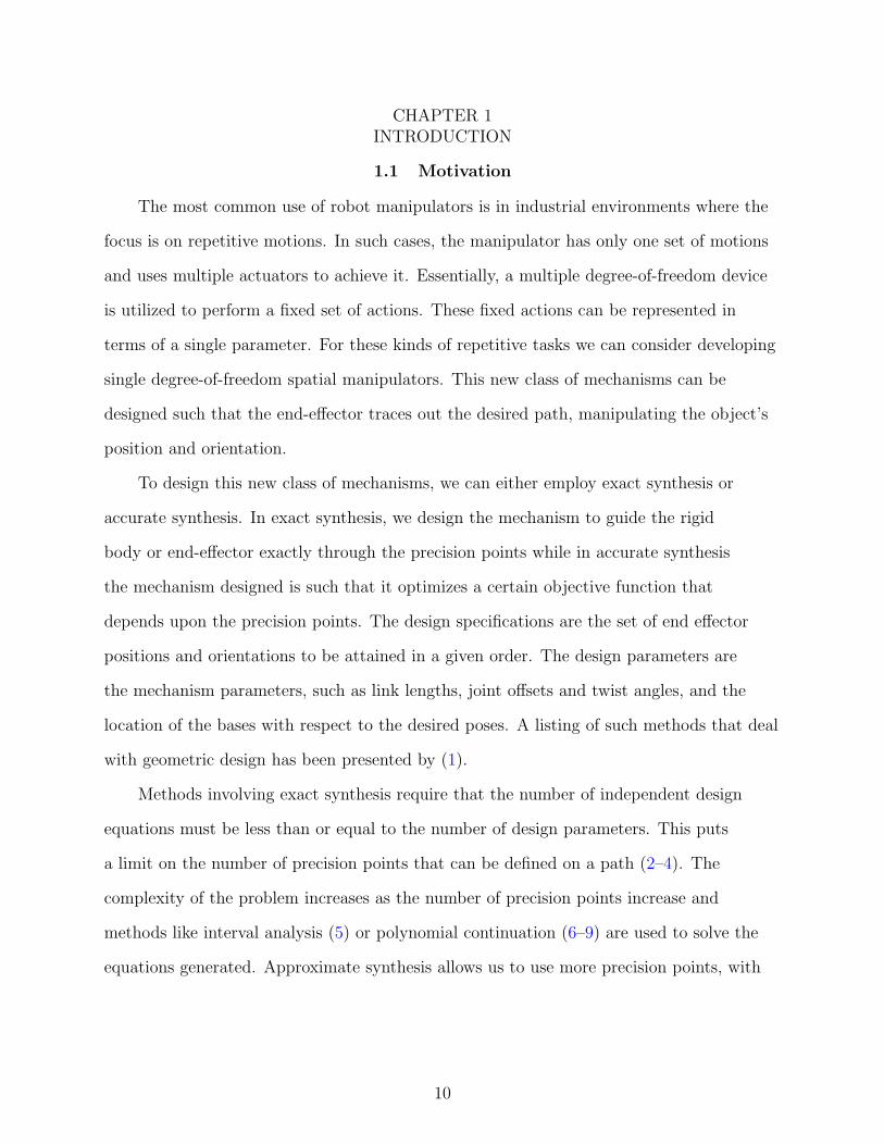
The most common use of robot manipulators is in industrial environments where the

focus is on repetitive motions. In such cases, the manipulator has only one set of motions

and uses multiple actuators to achieve it. Essentially, a multiple degree-of-freedom device

is utilized to perform a fixed set of actions. These fixed actions can be represented in

terms of a single parameter. For these kinds of repetitive tasks we can consider developing

single degree-of-freedom spatial manipulators. This new class of mechanisms can be

designed such that the end-effector traces out the desired path, manipulating the object’s

position and orientation.

To design this new class of mechanisms, we can either employ exact synthesis or

accurate synthesis. In exact synthesis, we design the mechanism to guide the rigid

body or end-effector exactly through the precision points while in accurate synthesis

the mechanism designed is such that it optimizes a certain objective function that

depends upon the precision points. The design specifications are the set of end effector

positions and orientations to be attained in a given order. The design parameters are

the mechanism parameters, such as link lengths, joint offsets and twist angles, and the

location of the bases with respect to the desired poses. A listing of such methods that deal

with geometric design has been presented by (1).

Methods involving exact synthesis require that the number of independent design

equations must be less than or equal to the number of design parameters. This puts

a limit on the number of precision points that can be defined on a path (2–4). The

complexity of the problem increases as the number of precision points increase and

methods like interval analysis (5) or polynomial continuation (6–9) are used to solve the

equations generated. Approximate synthesis allows us to use more precision points, with

10

optimization techniques being used to design the mechanism parameters. This necessitates

a valid objective function to be defined.

In the case of planar mechanism design, methods like approximate synthesis and

accurate synthesis are used. These methods use the position of a point on the coupler

link as the output function and define the objective function as the difference between the

desired and actual positions. (10) shows a method for designing three dimensional links

that also uses only the position of the coupler point to design the four bar linkage. Others,

(11; 12) use the condition number as an objective function to design spatial manipulators.

In this research the focus is on defining an error functional that can be used as an

objective function for optimization techniques. This error functional should include the

errors between the desired and actual position and orientations of the end-effector. The

most common way of doing this is to first calculate the position error. To calculate the

orientation error, the angular differences in the corresponding x,y,z axes of the desired

and actual coordinate systems attached to the end-effectors are converted to length scales.

The choice of this multiplication factor is subjective and essentially decides which of the

position or orientation error must be given priority. This problem is addressed by defining

the error in the joint angle domain space.

1.2 Related work

This work is focused extensively on a class of closed loop serial chains that possess

a special geometry. In order to incorporate gears between specific links, pairs of adjacent

joint axes were set to be parallel. An example which demonstrates this geometry is shown

in Figure 1-1. The work done in (13) focused on the same geometry and demonstrated

a solution to the inverse position analysis of each of the two subchains. For the given

geometry, it was proved that up to 16 real solutions exist for each subchain for a given

pose. Further work was done and (14) dealt with designing non-circular gears for the given

mechanism, that would allow the end-effector to accurately reach each pose. However it is

difficult to ensure that the gear profile remains feasible. In almost all cases, the calculated

11

Figure 1-1. A 12-link, 1-degree of freedom manipulator

gear ratios varied from positive values to negative values. This implied that for certain

sections of the path, internal gears were necessary while for other sections external gears

would be needed. Implementing such solutions is practically not feasible.

Another way of looking at the problem is to treat the gear ratios as fixed, and develop

a scheme that designs the mechanism parameters so that rigid body guidance is possible.

This type of design is dealt in (15), where a design strategy using optimization for open

loop chains is explained. A similar method is employed in (16) where Fourier Analysis

is used to aid the design synthesis. However, in both these approaches, the focus is on

force or energy related design criteria. The optimization approach was used to develop an

open loop chain such that the end-effector best approximates the desired set of poses. For

the purpose of optimization, the paper describes a method that uses the orientation to

parameterize the curves and define a correspondence point that can be used to calculate

the error. The Fourier Analysis approach aims to perform number and dimensional

synthesis.

In this research, the geometry of the mechanism is already known. The dimensional

synthesis is the aim of the design. Also, a purely kinematic approach is taken and any

energy or force considerations are ignored in the design. The path is parameterized in

terms of the input angle but a completely different error functional is developed. The

12

geometry of the chain gives rise to multiple solutions, and a method must be developed

to systematically deal with these and choose the ”best” solution. This kind of scenario

does not arise in other geometries. This method addresses this problem and also attempts

to define an error functional that does not include non-homogeneous terms. The error

measure is also well-defined in the sense that the term calculated has physical significance.

13

CHAPTER 2PROBLEM STATEMENT AND APPROACH

The mechanism to be designed has the geometry as shown in Fig. 2-1. The pairs

of axes that are parallel to each other are ($1, $2), ($3, $4), ($5, $6), ($7, $8), ($9, $10) and

($11, $12), where $i refers to the joint between links i and i + 1. For this type of geometry,

the mechanism parameters are given by the condition:

α12, α34, α56 = 0

α78, α9,10, α11,12 = 0 (2–1)

Figure 2-1. A candidate mechanism

The mechanism can be treated as two 6 link open chains with coincident end-effectors.

The side containing 3 gear pairs is called the A side and the side containing 2 gear pairs

is called the B side. Coordinate systems are attached to the base of the A and B side and

also at the end-effector. The ‘A fixed’coordinate system has the origin on $12). The ‘B

fixed’ coordinate system has the origin fixed on $1 with the z axis along $1/. The ‘tool’

coordinate system is fixed to the end-effector and represents the location and orientation

of the end-effector. The parameters needed for designing the mechanism are:

B fixedA fixedT: Pose of ‘A fixed’ coordinate system with respect to ‘B fixed’ coordinate system

6BtoolT: Pose of ‘tool’ coordinate system with respect to ‘6B’ coordinate system

14

6B6AT: Pose of ‘6A’ coordinate system with respect to ‘6B’ coordinate system

B fixedtool T: Required poses of the tool coordinate system measured with respect to the ‘B

fixed’ coordinate system

A candidate design is evaluated by sweeping the input angle of a candidate

mechanism to reach the given desired poses. Pi is the 4 × 4 matrix that defines the

desired position and orientation of the end effector at the ith pose. A reverse analysis as

outlined by (13) is performed which results in up to 16 real solutions for each pose. We

note that each of the real solutions is valid and could be achieved.

Since this is a rigid body guidance problem, the path is defined by a set of matrices

Pi which must be reached in a particular order. In order to effectively use approximate

synthesis with optimization, the path must be described using a parametric representation.

This parameter will also allow us to define corresponding points on similar paths.

The gears coupling the parallel joint axes result in the mechanism being a single

degree-of-freedom serial chain and hence, the path traced out by the end-effector can

be represented in terms of one parameter. The input angle φ (the first angle on the B

side) is used as this parameter. The focus here is to describe the motion in terms of joint

angles as opposed to in terms of the path coordinates.

If the starting configuration of the candidate mechanism is known, the input angle

can be effectively used to describe the motion of the end-effector, for that starting

configuration. This can be achieved by using a screw theory approach (17; 18) and

iteratively using the velocity equations to find the position of the end-effector corresponding

to each value of the input angle. It is thus noted that each solution in the set of joint

angles Uj1 will give rise to a different behavior of the end-effector, and also a different path.

Thus, we end up with the desired path and sets of actual paths all represented in

terms of the starting configuration and parameterized in terms of the input joint angle.

Points on different paths that are represented by the same value of input angle are defined

to be correspondence points. The error is then defined in terms of the difference in the

15

joint angles obtained to make the end-effector reach the actual pose, and those obtained

as the mechanism traces out its path. The joint angles on the B side are used to calculate

this error. Weighting factors are used since the contribution of each joint is not the same.

Each generated path thus gives us an error value and we can then select the best starting

configuration. This gives an error measure for the mechanism, which can be used as the

optimization objective function. This procedure is detailed in the next chapter.

16

CHAPTER 3DESIGN METHOD

3.1 Actual Path Generation

In order to analyze the motion of the mechanism, it is treated as two 6 link open

chains with coincident end-effectors. The side containing 3 gear pairs is called the A side

and the side containing 2 gear pairs is called the B side. The motion of the mechanism is

represented by the set of joint angles of the A and B sides as the input angle changes from

one value to another value. To calculate these, the screw theory based approach is used

incrementally. A small step size is chosen and the Plucker coordinates of the joint axes

for the current set of joint angles are determined using methods detailed by (13; 19; 20).

Considering the end-effector as a part of the A (or B) side of the mechanism, the velocity

of the end-effector is given by Eqn. (3–1) (21).

0ω1 ·0 $1 +1 ω2 ·1 $2 +2 ω3 ·2 $3 +3 ω4 ·0 $4 +4 ω5 ·4 $5 +5 ω6 ·5 $6 = ω7 · $7 (3–1)

Here, i−1ωi represents the angular velocity of link i + 1 with respect to link i. i−1$i

represents the screw (or the Plucker coordinates) about which link i + 1 moves, with

respect to link i. Since all joints are assumed revolute here, i−1$i represent the joint axes.

$7 represents the screw about which the end-effector moves with respect to ground and ω7

is the corresponding angular velocity.

However, due to the presence of gears, the equations simplify greatly. For the A side,

the three gear pairs reduce the equation to one in the three unknown angular velocities, as

given in Eqn. (3–2). The B side reduces to Eqn. (3–3) in 4 angular velocities, of which one

is the known input angular velocity (0ω1) of the first joint.

0ωA1 · (0$

A1 +1 gA

2 ·1 $A2 ) +2 ω3 · (2$

A3 +3 gA

4 ·3 $A4 ) +4 ω5 · (4$

A5 +5 gA

6 ·5 $A6 ) = ω7 · $7 (3–2)

0ωB1 ·0 $B

1 +1 ωB2 · (1$

B2 +2 gB

3 ·2 $B3 ) +3 ωB

4 · (3$B4 +4 gB

5 ·4 $B5 ) +5 ωB

6 ·5 $B6 = ω7 · $7 (3–3)

17

Equation 3–2 and Eqn. 3–3 gives Eqn. 3–4 which represent 6 scalar equations in 6

unknown angular velocities. These equations are then solved and the B side joint angles

are updated for a small change of the input angle, by using Eqns. 3–5. A forward analysis

of the B side is done to get the updated end effector pose and this is then used to get

the exact joint angles for the A side by inverse analysis. As inverse analysis give rise to

multiple solutions, the new angles that are closest to the previous set of angles are chosen.

0ωA1 · (0$

A1 +1 gA

2 ·1 $A2 ) +2 ω3 · (2$

A3 +3 gA

4 ·3 $A4 ) +4 ω5 · (4$

A5 +5 gA

6 ·5 $A6 ) =

0ωB1 ·0 $B

1 +1 ωB2 · (1$

B2 +2 g3B ·2 $B

3 ) +3 ωB4 · (3$

B4 +2 g3B

4 $B5 ) +5 ωB

6 ·5 $B6

(3–4)

(0ϕ1B)i+1 = (0ϕ1B)i + ∆ϕ

(1θ2B)i+1 = (1θ2B)i + (1ω2

0ω1

)∆ϕ

(2θ3B)i+1 = (2θ3B)i + (2ω3

0ω1

)∆ϕ

(3θ4B)i+1 = (3θ4B)i + (3ω4

0ω1

)∆ϕ

(4θ5B)i+1 = (4θ5B)i + (4ω5

0ω1

)∆ϕ

(5θ6B)i+1 = (5θ6B)i + (5ω6

0ω1

)∆ϕ (3–5)

A case study for this method shows us that this method indeed gives the correct motion

for the closed loop chain as the input angle is swept. This was done by performing the

calculations as given by Equations 3–5 to get new angles. Then using these new angles,

the displacement analyses of the A and B side are performed to get all the screw axes

coordinates. This iterative method using Equations 3–4 and 3–5, gives us the joint angles

for the entire range of motion. The mechanism parameters chosen for this case study are

given in Table 3-1 and Table 3-2 with the other parameters given in Table 3-3.

Figure 3-1 and Fig. 3-2 show the variation of the angles as the input angle sweeps

from its initial value by 0.5 radians. The gears were all chosen to have 1:1 ratios.

Figure 3-3 shows that all calculated gear ratios (by forward difference method) closely

approximate the actual ratios of 1. A smaller value of step size ∆ϕ gives values closer to

18

Table 3-1. Mechanism parameters for A side

Offset distance (in.) Linklengths (in.) Twist angles (deg)S2 = 6 a12 = 3 α12 = 0S3 = 0 a23 = 10 α23 = 90S4 = 6 a34 = 3 α34 = 0S5 = 0 a45 = 10 α45 = 90S6 = 6 a56 = 3 α56 = 0

Table 3-2. Mechanism parameters for B side


1. In Fig. 3-3, the values A12, A34 and A56 denote the three gear ratios for the gear pairs

on the A side. A12 is the gear ratio between joints 1 and 2, A34 between joints 3 and 4,

and A56 between the joints 5 and 6. As seen from the figure, the calculated values of gear

ratios are within 99.5% of the actual values. This is a very good estimate and thus ensures

that the method gives a motion that is accurate to a great extent.

3.2 Error Measure

The first problem addressed was that of defining an error measure, if the actual path

traced by the end-effector of the candidate mechanism was given. Since the input angle

is used as a parameter to define the path, the error is defined in the joint angle space

Table 3-3. System parameters

B fixedA fixedT

1 0 0 −180 0 −1 −50 1 0 120 0 0 1

6BtoolT

1 0 0 40 1 0 −20 0 1 30 0 0 1

6B6AT

−1 0 0 80 0 −1 20 −1 0 40 0 0 1

19

−1.6 −1.5 −1.4 −1.3 −1.2 −1.1 −1 −0.9−2

−1

0

1

2

3

4A angles, delta phi = 0.0001

input angle, radians

angl

es, r

adia

ns

A2A3A4A5A6

Figure 3-1. Case Study :- A-side angles vs input angle

−1.6 −1.5 −1.4 −1.3 −1.2 −1.1 −1 −0.9−4

−3

−2

−1

0

1

2

3B angles, delta phi = 0.0001

input angle, radians

angl

es, r

adia

ns

B2B3B4B5B6

Figure 3-2. Case Study :- B-side angles vs input angle

20

0 1000 2000 3000 4000 50000.993

0.994

0.995

0.996

0.997

0.998

0.999

1

1.001Gear Ratios, delta phi =0.0001

step number

gear

rat

io

A12A34A56

Figure 3-3. Case Study :- Gear ratios (A side) vs step number

A Start: Configurations 1 for A and B Side B End: Input angle sweep = 0.5 radians

Figure 3-4. Start and end configurations

21

domain. The input angle φi required to exactly reach the desired pose Pi,desired can be

calculated by performing the inverse analysis. The problem of choosing the “correct”

solution out of the possible 16 is addressed in the following sections. The actual pose on

the path that is said to correspond with this desired pose is that when the input angle ϕ

equals the φi which was calculated.

Thus, for pose Pi, there exists joint angles θij,desired and θij,actual, where j refers to the

joint number. For each pose, the error can be defined as:

ei =

(6∑

j=2

(wi × |θij,desired − θij,actual|)2

) 12

(3–6)

Here, wi is the weighting factor that is described in the next section. The error for the

entire path, can be defined as:

E =∑

i

ei (3–7)

3.3 Weighting Factor

In calculating the weighting factor, the following observation is made. In a serial

chain manipulator, the error in each joint affects the position and orientation of the

end-effector. However, this contribution is not uniform. Also, assuming that the joints

closer to the base affect the total error more is false. The error in the position of the

end-effector due to a certain joint depends on the perpendicular distance of the end

effector tool point from the joint axis. As a result, the base joint may not necessarily

contribute the largest error. To account for this, a weighting system based on the

configuration of the mechanism is defined.

Let r0 be the location of the end-effector in the given configuration. To calculate the

weight for joint i, the angle θi is varied by a small amount, δθ. Let ri be the new position

of the end-effector if the joint i is varied by δθ. Then, the weight wi is defined as:

wi = |r0 − ri|/δθ (3–8)

22

As the units of the weighting factor are length/angle, the error will have a dimension of

length.

3.4 Handling Multiple Solutions

The major problem that must be handled is the existence of multiple solutions in

the inverse analysis. Each starting configuration will give rise to a different path for the

end-effector. The method implemented involves taking each solution into consideration, in

order to select the best set of solutions. The score of these best solutions is then evaluated

and used as a score for the mechanism.

Let iΩ be the path generated by the solution Ui1. To evaluate the score for the second

pose on this path with respect to the desired second pose, the set of solutions U2 must be

chosen from all Uj2, such that the pose corresponding to U2 lies in iΩ.

Uj21 is checked for all j. If Uj

21 = iΩk1 for some j and k, the two joint angle

sets are said to correspond to the same pose. The iΩk is the joint angle set for the actual

pose while the Uj2 represents the desired second pose. The error ej

2 is then calculated for

this pose. The same calculations are performed for all j, k to get all ej2. The error for the

second pose is then defined as

e2 = minj

ej2 (3–9)

The error for each pose is calculated using the same method, using Eqn. (3–6) to give ejl .

The error for the pose is then defined as

el = minj

ejl (3–10)

Thus, using Eqn. (3–7), the error for the path iΩ is given by Ei. Since each path iΩ

will give rise to a different error, the best path must be chosen to define the mechanism

error. This is done by defining the error E as

E = minl

El (3–11)

23

This error E is used as the measure of the mechanism for following the given path and

can be used as a optimizing cost function for design.

24

CHAPTER 4NUMERICAL EXAMPLE

Table 4-1. Mechanism parameters for A side


Table 4-2. Mechanism parameters for B side

Offset distance (in.) Linklengths (in.) Twist angles (deg)S2 = 3.4947 a12 = 14.238 α12 = 0

S3 = 0 a23 = 0.7411 α23 = 59.2992S4 = 1.3465 a34 = 12.9009 α34 = 0

S5 = 0 a45 = 6.1349 α45 = 76.8924S6 = 6 a56 = 10.3782 α56 = 0

The results of using this method to generate the error measure of a mechanism

on an example set of poses is given below. Table 4-1 and Table 4-2 list the mechanism

parameters for the A and the B side respectively. The six desired poses Pi are listed in

Table 4-3 and the solutions to reverse analysis for each pose for the A side and B side are

calculated. For the given combination of poses and mechanism parameters, the number of

solutions obtained for each side is listed in Table 4-4. For this particular example, the all

gear pairs are assumed to be circular, with gear ratio 1.

Since there are 2 solutions for A side and 14 for the B side for the starting pose,

there are 28 possible starting configurations for the mechanism. The paths taken by the

end-effector in each of the 28 cases are shown in Fig. 4-1. At the first pose, the error is

zero. Each of these configurations gives us a path that the mechanism end-effector follows.

The method described in this paper chooses the solutions given in Table 4-5 for the

starting configuration. The input joint angles for the other 5 poses are also listed. Since

the mechanism is a one degree-of-freedom serial chain, specifying only the input angles for

the successive poses defines the mechanism configuration.

25

Table 4-3. Desired poses and orientations

Pose Transformation matrix (in rad. & in.)

Pose 1

−0.4771 0.4752 0.7393 10.1043−0.5994 0.4393 −0.6691 −7.9145−0.6428 −0.7624 0.07524 0.6524

0 0 0 1

Pose 2

−0.4498 0.4669 0.7614 9.5769−0.5949 0.4792 −0.6453 −8.1136−0.6662 −0.7432 0.06227 0.2199

0 0 0 1

Pose 3

−0.4112 0.4773 0.7766 9.0467−0.5721 0.5281 −0.6276 −8.3770−0.7097 −0.7023 0.0559 −0.0170

0 0 0 1

Pose 4

−0.3575 0.5062 0.7848 8.5276−0.5244 0.5865 −0.6172 −8.8086−0.7728 −0.6322 0.0558 −0.1373

0 0 0 1

Pose 5

−0.2803 0.5514 0.7857 8.023−0.4408 0.6531 −0.6157 −9.4116−0.8527 −0.5190 0.0600 −0.1222

0 0 0 1

Pose 6

−0.1683 0.6034 0.7795 7.5196−0.3040 0.7205 −0.6233 −10.1775−0.9377 −0.3419 0.0621 −0.0159

0 0 0 1

Table 4-4. Number of solutions by reverse analysis

Pose A side B sidePose 1 2 14Pose 2 2 14Pose 3 2 12Pose 4 2 10Pose 5 2 8Pose 6 2 6

Table 4-5. Solutions selected for min. error criteria

Starting joint angles, A side[

0.5885 −0.5885 0.7094 −1.4948 2.8749 −1.3041]

Starting joint angles, B side[

2.1040 0.0805 3.1074 1.6535 −3.1309 1.7276]

Pose 2 Input angle 2.1890Pose 3 Input angle 2.2890Pose 4 Input angle 2.3890Pose 5 Input angle 2.4890Pose 6 Input angle 2.5890

26

Figure 4-1. The different paths traced by end-effector when different startingconfigurations are chosen. All paths start from the same starting pose,highlighted in red.

27

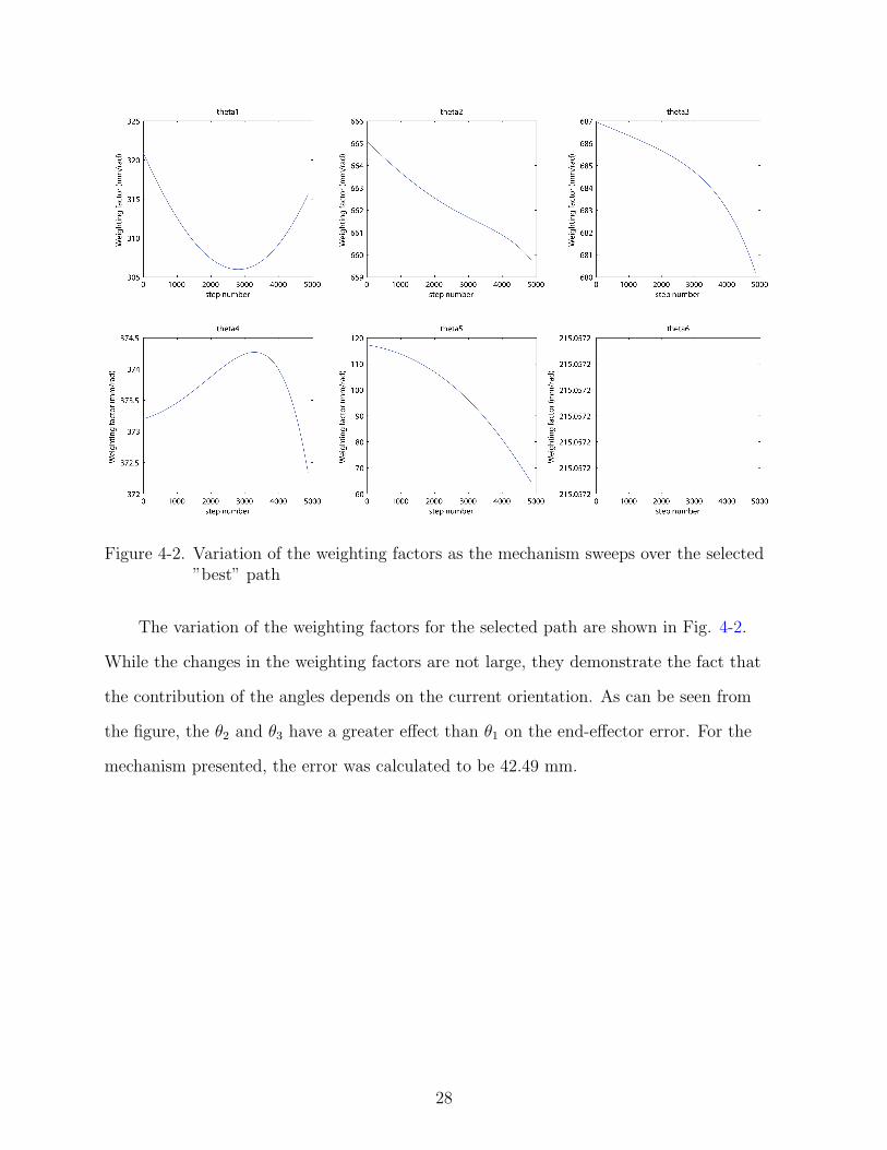
Figure 4-2. Variation of the weighting factors as the mechanism sweeps over the selected”best” path

The variation of the weighting factors for the selected path are shown in Fig. 4-2.

While the changes in the weighting factors are not large, they demonstrate the fact that

the contribution of the angles depends on the current orientation. As can be seen from

the figure, the θ2 and θ3 have a greater effect than θ1 on the end-effector error. For the

mechanism presented, the error was calculated to be 42.49 mm.

28

CHAPTER 5CONCLUSIONS

A method for the design of one degree of freedom, closed loop spatial chains that

utilize planar non-circular gears was presented in this thesis. The method addressed

an important problem of accounting for orientation errors along with position errors

in the rigid body guidance problem. By utilizing the joint space domain, the error

term defined has combined the two errors by avoiding the issue of mixed dimensions or

non-homogeneous terms. The work presented sets up a scheme that could be used to

apply optimization techniques in the design of other closed loop mechanisms.

This method is computationally intensive due to the iterative nature of the algorithm.

The method was implemented using Matlab 7.0 software on a Intel Core2 T5300

(1.73Ghz) processor, with a 2 Gb ram. With parallel processing disabled, a single run

for the code took about 996.32 CPU seconds to calculate the error for the example listed

previously. However, since each path is independent of the other, this method is suited for

parallel architecture and parallel processing will greatly improve the speed.

The geometry of having consecutive axes parallel greatly increases the simplicity of

the gears that are used to couple the joint axes. The problem can be broadened where the

mechanism geometry is changed to simplify the inverse analysis problem and non-planar

non-circular gears are used to couple consecutive axes. The error functional in such a

case would be the same as the one presented in this paper. The problem of extending this

method to mechanisms with a different geometry is being investigated.

29

REFERENCES

[1] M. Bodduluri, J. Ge, M. J. McCarthy, B. Roth, The Synthesis of Spatial Linkages,Modern Kinematics: Developments in the Last Forty Years, J. Wiley and Sons, NewYork, 1993.

[2] B. Roth, Analytic design of open chains, in: O. Faugeras, G. Giralt (Eds.), ThirdInternational Symposium of Robotic Research, MIT Press, 1986.

[3] L. W. Tsai, Design of open loop chains for rigid body guidance, Ph.D. thesis,Stanford University (1972).

[4] C. H. Suh, C. W. Radcliffe, Kinematics and Mechanism Design, Wiley and Sons, NewYork, New York, 1978.

[5] E. Lee, C. Mavroidis, J. P. Merlet, Five precision point synthesis of spatial rrrmanipulators using interval analysis, Journal of Mechanical Design 126 (5) (2004)842–849.

[6] A. P. Morgan, C. W. Wampler, Solving a planar four-bar design problem usingcontinuation, Journal of Mechanical Design 112 (4) (1990) 544–550.

[7] C. W. Wampler, A. P. Morgan, A. J. Sommese, Numerical continuation methodsfor solving polynomial systems arising in kinematics, Journal of Mechanical Design112 (1) (1990) 59–68.

[8] B. Roth, F. Freudenstein, Synthesis of path generating mechanisms, Journal ofEngineering for Industry 85B (1963) 298–306.

[9] C. W. Wampler, A. P. Morgan, A. J. Sommese, Complete solution of the nine-pointpath synthesis problem for four-bar linkages, Journal of Mechanical Design 114 (1)(1992) 153–159.

[10] V. I. Kulyugin, Design of three dimensional four-link mechanisms conforming to thetravel of the driven link and coefficient of increase in velocity of the reverse stroke, in:Analysis and Synthesis of Mechanisms, Amerind Publishing Co. Pvt. Ltd., 1975, pp.152–162.

[11] J. K. Salisbury, J. J. Craig, Articulated hands: Force control and kinematic issues,The International Journal of Robotics Research 1 (1) (1982) 4–17.

[12] L.-W. Tsai, S. Joshi, Kinematics and optimization of a spatial 3-upu parallelmanipulator, Journal of Mechanical Design 122 (4) (2000) 439–446.

[13] J. R. Mckinley, C. Crane, D. Dooner, Reverse kinematic analysis of the spatial sixaxis robotic manipulator with consecutive joint axes parallel, in: International DesignEngineering Technical Conferences & Computers and Information in EngineeringConference, no. DETC2007-34433, ASME, Las Vegas, 2007.

30

[14] J. R. Mckinley, Three-dimensional rigid body guidance using gear connections in arobotic manipulator with parallel consecutive axes, Ph.D. thesis, University of Florida(2007).

[15] V. Krovi, G. K. Ananthasuresh, V. Kumar, Kinematic and kinetostatic synthesis ofplanar coupled serial chain mechanisms, Journal of Mechanical Design 124 (2) (2002)301–312.

[16] Y.-W. Pang, V. Krovi, Kinematic synthesis of coupled serial chain mechanisms forplanar path following tasks using fourier methods, in: ASME Design EngineeringTechnical Conferences, no. DETC2000/MECH-14188, ASME, Baltimore, Maryland,2000.

[17] R. S. Ball, A Treatise on the Theory of Screws, University Press, Cambridge, 1900.

[18] K. H. Hunt, Kinematic Geometry of Mechanisms, Clarendon Press; Oxford UniversityPress, Oxford; New York, 1978.

[19] J. Duffy, C. Crane, A displacement analysis of the general spatial 7-link, 7rmechanism, Mechanism and Machine Theory 15 (3) (1980) 153 – 169.

[20] H.-Y. Lee, C.-G. Liang, Displacement analysis of the general spatial 7-link 7rmechanism, Mechanism and Machine Theory 23 (3) (1988) 219 – 226.

[21] J. M. Rico, J. Gallardo, J. Duffy, Screw theory and higher order kinematic analysisof open serial and closed chains, Mechanism and Machine Theory 34 (4) (1999) 559 –586.

31

BIOGRAPHICAL SKETCH

Mandar Harshe was born in 1985 in Mumbai, India. He did his schooling in E.N.N.S

School, Pune and attended junior college at Fergusson College, Pune. He then attended

M.E.S College of Engineering, affiliated with the University of Pune, and graduated with a

Bachelor of Engineering in mechanical engineering in June 2007. He did his degree project

at Nirmiti Stampings Pvt Ltd, Pune, India where he worked on developing a low cost

robotic arm. In August 2007, he joined the Center for Intelligent Machines and Robotics

(CIMAR) at the University of Florida, and received his Master of Science degree in the

spring of 2009. He plans to pursue to his doctorate in the area of mechanism theory

focusing on kinematics and computational geometry.

32

Documents

harshe_m