Embed Size (px)
Citation preview

Hayden’s
Minitab Guide
for Siegel and Morgan,
Statistics and Data Analysis:
An Introduction
Version 10
Revised for Version 13 of Minitab,
January 2001

The purpose of this guide is to show you how to use the Minitab statistical software to carry out
all the statistical procedures discussed in your textbook. At first you will find that the data we
look at is very simple, and so are the calculations we want to do. You may even feel that it is a
waste of time to learn to use a computer to do such simple things. The idea is to begin with
simple examples so you can learn to use the computer. Once you have learned that, you can
then do more complicated things. For example, you may first learn how to find the average of
five numbers using the computer. Of course, you could do this by hand, and you should do it
by hand, to make sure you understand what it is the computer is doing. Once you have
learned how to average numbers on the computer, however, it is just as easy to average 500
numbers as five. You probably would not like to average 500 by hand.
This guide will teach you (a little bit of) Minitab by example. It is arranged by chapters
corresponding to the chapters in your textbook. Each chapter of the text has a section in this
guide that shows you how to use Minitab to do the things discussed in that chapter . The
examples usually are based on the data in your text to help you coordinate what you are
learning about Minitab with what is in your textbook.
Chapter 1
The first chapter is largely descriptive, and so we begin with

Version 10, last revised January 2001
Chapter 2
In Chapter 2 you will learn how to:
• open a file containing data
• get a table of contents for a data file
• enter your own data into Minitab
• give a name to each column of data
• print your data in the session window and on paper
• save your data
• enter comments into a Minitab session
• make a stem and leaf plot
• split stems in different ways to change the scale of a stem and leaf plot
• make a dotplot
Later you will learn how to start and use Minitab. For now, we will just look at some typical
Minitab sessions. We assume that somehow you have managed to get Minitab running on the
computer of your choice. You can tell that this has happened when you see the Minitab
prompt: MTB >. The prompt means that Minitab is awaiting your command. If you are using
Windows or a Macintosh, this prompt will appear in the upper of two windows on your screen,
called the Session Window. Click on this window with the mouse to enter commands. (If no
prompt apears, pull down the Editor (not Edit ) tab and make sure Enable Commands is
Page 2 We Are Now in Chapter 2

Version 10, last revised January 2001
checked.) In DOS and Unix, the session window is the only window. Commands may be
entered by typing them in or by making choices from the menus. For the most part you should
use whichever system you prefer. Minitab has been around much longer than the Macintosh
or the Windows operating system. In the old days, typing commands was the only way to
enter them, and many old-timers still use Minitab that way. Today a statistician using Minitab
for the first time would probably use the menu system. While other beginners might be more
accustomed to a menu interface, Minitab’s menus assume you already know statistics and
understand all the choices and options. For that reason, they can be puzzling and confusing to
someone just beginning to learn statistics. However you enter commands, it is useful to learn
how to read typed commands. That is because when you use the menus Minitab adds the
equivalent typed commands to your work. This is useful when you look at your work a few
days later and don’t remember what you did. It is also helpful to you and your instructor when
your output is not what you expected.
The examples below show commands and their results. For now, just concentrate on getting a
feel for what a Minitab session is like. Later you will learn to run your own analyses.
In addition to the basic Minitab prompt: MTB > there are two other Minitab prompts you will
see often. The prompt SUBC> means that Minitab is waiting for a subcommand, something
that modifies a command you have already given. The other common prompt is DATA>. As
you might expect, this means that Minitab is waiting for you to type in some data. Below is a
sample run using the data on earthquakes from page 27 of your text. In this and all the
subsequent examples, anything typed on a line following one of the Minitab prompts (MTB >,
SUBC>, or DATA>) was typed by the human. Everything else you see was typed by Minitab. It
will also be helpful to know that Minitab organizes data by columns. Generally, each column
contains data on one variable. Initially, the columns are just named c1, c2, c3, et cetera, but
you can give them more meaningful names of your own. If you are using a Macintosh or
Windows, at least some of the data will be visible in the Data Window at the bottom of the
screen. You can click on this window and type in column names and data.
Try to figure out what is going on in the example below before you read the explanation that
follows it.
We Are Now in Chapter 2 Page 3

Version 10, last revised January 2001
MTB > set into c1 DATA> 5.5 7.7 7.1 7.8 8.1 7.3 DATA> 6.5 7.3 6.8 6.9 DATA> 6.3 6.5 7.7 7.7 6.8 DATA> end MTB > name c1 ’size’ MTB > print c1
size 5.5 7.7 7.1 7.8 8.1 7.3 6.5 7.3 6.8 6.9 6.3 6.5 7.7 7.7 6.8
MTB > save ’mydata’
Worksheet saved into file: mydata.MTW
MTB > stem and leaf c1
Stem-and-leaf of size N = 15 Leaf Unit = 0.10
1 5 52 6 37 6 55889(3) 7 1335 7 77781 8 1
MTB > stop
Let’s see what happened here. The set command allows you to type data into one Minitab
column. In this guide the set command is often used to enter data so you can see what the
data was. (Minitab output does not automatically include the data analyzed, just the commands
and the results of the analysis.) Most of the data you will be using in this course has already
been typed into the computer, but if you want to use Minitab to work with data from another
course, you may have to type it in. If you are using Windows or a Macintosh, you can type the
data directly into the Data Window at the bottom of the screen. Click on it to select it first.
You can put your data in any column you like but if you use the set command, you must tell
Minitab which column you have in mind. The “into” is optional in versions of Minitab prior to
13, and helps make the command line more readable. It is not allowed in Version 13 for
Windows. At the end of the line you must press the key marked ENTER or RETURN . When
you do this, Minitab will respond with the DATA> prompt, and you can type in your data. Use
one or more spaces to separate the numbers. You can type your data in a single column, as it
will appear in Minitab, or all on one line, or break it over two lines, if it will not all fit on one line.
(However, do not split a number in half, so part is on one line, part on another, like
7. 5
Page 4 We Are Now in Chapter 2

Version 10, last revised January 2001
for 7.5.) Typing end tells Minitab that you have reached the end of your data. When you type
end, Minitab responds with the MTB > prompt and awaits your next command.
The (optional) name command attaches a name to a column. You must tell Minitab which
column you have in mind. The name must be in single (not double!) quotes. It should be eight
characters or less in length. If you are using Windows or a Macintosh, you can type the
column names directly into the data window. Click on this window to select it first. However, if
you do this there will be no record in your output of which columns got which names. In this
guide the name command is used so you can see what name goes with what column.
The print command causes Minitab to print the data in the specified column in the session
window. It does not cause the data to be printed on paper immediately, but it will now be part
of the session window when you print that out at the end of your work. Notice that Minitab’s
output labels the data with the name you gave it. If you are using Windows or a Macintosh,
you can see the data and its name directly in the data window at the bottom of the screen, but
this will not automatically be a part of your printout. The print command is also useful if you
want to print all the numbers in a single column when the data window just shows the first few
numbers.
The save command saves the data to disk. You will not need to use this unless you have
actually typed new data into the computer. If you are using the college computers, it is best to
use the menus to save a file to your own floppy or to your oz (email) account. You should
provide a name for this file. Use a legal filename for your particular computer. If in doubt
about this name or any other, keep it to eight characters or less, starting with a letter, and
containing no punctuation marks or spaces. It is a good idea to save your data as soon as you
have entered and named it. Note that all that is saved by the save command is the 15
numbers you typed in and the name “size”. The stem and leaf plots are not saved by this
command. Unless you tell Minitab otherwise, your file will be saved on the hard disk of the
computer you are using, and may not be there the next time you use that computer, and will
certainly be inaccessible if you use another computer. For that reason, you should get in the
habit of saving your work to a floppy disk or to your oz account. On the Macs, your oz account
appears as a folder called FilesHome on the desktop. On the PCs, it usually appears as a
(virtual) disk drive, typically drive E:. If you have any difficulty finding these, ask someone in
the lab where you are working.
We Are Now in Chapter 2 Page 5

Version 10, last revised January 2001
The stem and leaf command is self-explanatory as typed here. In Version 13, you cannot
include “and leaf” as part of the command. The online help for that Version usually highlights
the parts you type, so this example might appear as something like
MTB > stem and leaf c1
In this Guide, text that is optional in older versions of Minitab and forbidden in Version 13 will
be shown in italics
MTB > stem and leaf c1
To make a stem and leaf plot from the menus, pull down Graph and choose Stem and Leaf.
You can type in the name of the column you want, or double-click on it from the list on the left.
Then select OK .
Let’s look at another example session. This one includes getting back the file we saved earlier
by using the retrieve command. This command is not recommended unless you are using
your own copy of Minitab on your own computer. This session shows how you can get Minitab
to split the stems in a stem and leaf plot to show the data on different scales.
MTB > retrieve ’mydata’ WORKSHEET SAVED 2/ 2/1996
Worksheet retrieved from file: mydata.MTW
MTB > info
COLUMN NAME COUNT C1 size 15
CONSTANTS USED: NONE
MTB > stem c1; SUBC> increment 1.
Stem-and-leaf of size N = 15 Leaf Unit = 0.10
1 5 57 6 355889(7) 7 13377781 8 1
Page 6 We Are Now in Chapter 2

Version 10, last revised January 2001
MTB > stem c1;SUBC> increment 0.2.
Stem-and-leaf of size N = 15Leaf Unit = 0.10
1 5 51 51 51 62 6 34 6 554 67 6 889(1) 7 17 7 335 75 7 7772 7 81 8 1
MTB > stem and leaf c1;SUBC> increment 2.
Stem-and-leaf of size N = 15Leaf Unit = 1.0
1 0 5(13) 0 66666677777771 0 8
MTB > stem and leaf c1;SUBC> increment 5.
Stem-and-leaf of size N = 15Leaf Unit = 1.0
(15) 0 566666677777778
In the first Minitab example, we saved a file called “mydata.MTW” to disk. This file contained
the earthquake data entered earlier. (Minitab added the “.MTW” to the filename to mark it as a
Minitab data file. You can ignore the “.MTW” whenever you are inside Minitab.) The
retrieve command gets it back. This will work as shown only if you are running Minitab on
your own computer. On the college computers, it is best to use the menu system to
retrieve files. They are normally in a folder named “stats1a” which should appear when you
select File, Open from the menus. When you first open a file, it is a good idea to type the
info command in the session window to get a table of contents for the data file.
Note that in this example sessions there are some subcommands. If you wish to enter a
subcommand in the Session Window, type a semicolon “;” at the end of the main command,
then hit RETURN or ENTER . Minitab will respond with a SUBC> prompt. Type in your
We Are Now in Chapter 2 Page 7

Version 10, last revised January 2001
subcommand, followed by a period, and hit RETURN or ENTER again. Notice that Minitab is
more like a typewriter than a word processor here; you always have to hit RETURN or ENTER
at the end of every line. From here on out, we’ll assume you know that, and not keep
repeating it over and over. If you use the menus, subcommands usually appear as options in
a dialog box. The dialog box for a stem and leaf plot has a window where you can type in an
increment. If you want to use the menus to plot the same data with several increments as we
did, select Edit, Edit Last Command Dialog to change the increment.
The particular subcommand used above was increment. We specified an increment of 1,
meaning that the distance between the starting points of successive rows of the stem and leaf
is 1. You can see that the rows start at 5.0, 6.0, 7.0, and 8.0, and these numbers are 1 unit
apart. This was done to create a stem and leaf on the same scale as the one in your text
(Display 2.5, p.28). In the original stem-and-leaf (the one without the increment
subcommand that we did in the first example session), the starting points of the rows are 5.5,
6.0, 6.5, 7.0, 7.5, and 8.0. These are 0.5 units apart. (This may be clearer if you try making
the stem-and-leaf yourself by hand.) Minitab automatically selects an increment when no
increment is specified. It doesn’t always pick 0.5; it picks whatever it thinks is best for the data
at hand. Whether you pick it or Minitab does, the increment has to be … 0.01, 0.02, 0.05, 0.1,
0.2, 0.5 , 1, 2, 5, 10, 20, etc. (If you enter an illegal increment, Minitab will use a nearby legal
one, and the result will probably not be what you expected.) Usually Minitab does a good job
of picking increments, so we rarely use the increment subcommand unless we have some
special purpose in mind. For example, you might want to use Minitab to check a stem and leaf
you have done by hand or found in a book. In that case, you would tell Minitab to use the
same scale as the figure you want to reproduce.
Usually you will want to print out a copy of your Minitab session to keep or to turn in to your
instructor. You may also want to print things out during a session to review the work you have
done so far. To print a paper copy of the Session Window, chose File, Print Window while in
the session window. If you only want to print part of the session log, highlight it with the mouse
and then select File, Print Selection. Note that printing the entire session window prints
everything you have done since you started, not just what you can see on the screen.
Now you should be ready to try Minitab yourself. First, you will need to learn how to access
Minitab on whatever computer system you will be using. Your instructor will provide you with
handouts and/or an in-class demonstration on how to use the college’s computers. Some of
you may wish to get a copy of Minitab to use on your own personal computer. If so read the
rest of this paragrah; if not, skip to the boxed information for the PSC computer platform of
Page 8 We Are Now in Chapter 2

Version 10, last revised January 2001
your choice. You can purchase the Student Edition of Minitab at the college bookstore (it costs
about $70 and includes a printed manual). There are (or were?) Student Editions available for
Macintosh, DOS, Windows 3.1 and Windows 95/98, related to the full versions as follows:
• Student Edition for Mac or DOS is based on Version 8
• Student Edition for Windows 3.x is based on Version 9
• Student Edition for Windows 95/98 is based on Version 12
You can also rent the full version for six months for about $30 from http://www.e-
academy.com, or download a free copy of the full version that works for 30 days from
http://www.minitab.com. The download and rental version is 13 for Windows 95/98.
You can also download documentation for it. If you buy or download the software, you can
copy the data files off the server or get them from Dr. Roberts (Versions 8-10.5 for Mac) or Dr.
Hayden (Versions 8-12 for PC). Bring a blank floppy disk to hold the data. How you start
Minitab on the college computers varies with the operating system.
Windows 95/98, Minitab Version 13.1
Select Start, Programs, Applications, Minitab.
You can access existing data from within Minitab with the menu system. (Do not try to
launch files by double clicking on them from outside of Minitab. This works sometimes,
but not always.) Use File and Open Worksheet (not Open Project). On most machines
this brings you to a network drive, in which case you will see several folders for different
courses. You want the stats1a folder. (If instead you find yourself in the DATA directory
of your machine’s hard drive (you’ll see lots of unfamiliar file names!) then click on the
“up one level” icon (a file folder with a bent arrow pointing up) until you get to My
Computer. Then select the Afserv network drive, then data, minitab, stats1a.)
Inside stats1a you should see a folder for each chapter of your textbook. Open the folder
for the chapter you are working on. To find the files you need, pull down the menu for
List Files of Type and select All[*.*]. Scroll if necessary until you can see the_
appropriate file name and double click on it. The data should appear in the data window.
We Are Now in Chapter 2 Page 9

Version 10, last revised January 2001
Macintosh
You will need to set up the data files before you run Minitab. When the computer boots
up, double-click on the Stats Files.smi item on the list that appears. A fake floppy disk
will appear at the right edge of your screen. You will need this later. Now you can start
Minitab by double clicking on the item Minitab 10.5 on the same list. In the window that
opens, double click on the icon labeled Minitab 10.5 Xtra Power.
You can access existing data with the menu system. (Do not try to launch files by double
clicking on them from outside of Minitab. This works sometimes, but not always.) Use
File and Open Worksheet. In the dialog box, click on the Desktop button. Then choose
Stats Files and then the stats1a folder. You should see a folder for each chapter of your
textbook. Open the folder for the chapter you are working on. Scroll if necessary until
you can see the appropriate file name and double click on it. The data should appear in
the data window.
On both platforms, when you open a file through the menus, the command for retrieving a file
is printed in the session window. (It is probably very long and complicated, so we strongly
recommend that you use the menus to work with files!) The echoing of commands to the
session window provides a record (for you and your instructor) of what you did.
Once the file is open, you can click on the session window and type the info command to get
a table of contents for the file. This is most useful for files that contain many variables so you
can only see a few of them in the data window.
Here’s another example using a version of the earthquake data that was already stored on the
computer (in file smt02.07).
MTB > info
COLUMN NAME COUNT A C1 country 15 C2 year 15 C3 size 15 C4 deaths 15
MTB > note Data from page 27 of text.
Page 10 We Are Now in Chapter 2

Version 10, last revised January 2001
MTB > print c1-c4
ROW country year size deaths
1 Columbia 1983 5.5 2502 Japan 1983 7.7 813 Turkey 1983 7.1 13004 Chile 1985 7.8 1465 Mexico 1985 8.1 42006 Ecuador 1987 7.3 40007 India/Nepal 1988 6.5 10008 China/Burma 1988 7.3 10009 Armenia 1988 6.8 5500010 U.S.A. 1989 6.9 6211 Peru 1990 6.3 11412 Romania 1990 6.5 813 Iran 1990 7.7 4000014 Philippines 1990 7.7 162115 Pakistan/Afghanistan 1991 6.8 1200
MTB > stem c2-c4
Stem-and-leaf of year N = 15Leaf Unit = 0.10
3 1983 0003 19845 1985 005 19866 1987 0(3)1988 0006 1989 05 1990 00001 1991 0
Stem-and-leaf of size N = 15Leaf Unit = 0.10
1 5 52 6 37 6 55889(3) 7 1335 7 77781 8 1
Stem-and-leaf of deaths N = 15Leaf Unit = 1000
(13) 0 00000011111442 02 12 12 22 22 32 32 4 01 41 51 5 5
We Are Now in Chapter 2 Page 11

Version 10, last revised January 2001
MTB > dotplot ’year’
. . :: : . : . : .-+---------+---------+---------+---------+---------+-----year
1983.0 1984.5 1986.0 1987.5 1989.0 1990.5
The “A” next to C1 in the output of the info command means that this column contains
alphanumeric data. Such columns contain labeling information.
The note “command” allows you to insert notes into your Minitab printout. These notes may
be reminders to yourself or labels as to which problem this is or what part of an assignment.
Some students type in answers to homework problems with the note “command”. You can
also insert text into the rest of the Session Window. If Minitab won’t let you, you may have to
click on the Editor (not Edit ) tab and select Make Output Editable. (If that option is not
visible, the output is already editable.)
This version of the data set contains four columns of data. Note that if you want to print all four
columns, you can just type the print command followed by c1-c4. This shortcut works with
the histogram and stem and leaf commands, too. Unfortunately, it does not work with all
commands, and may have disastrous effects (usually, erasing part of your data) if used
inappropriately. (If this happens, just reretrieve the data and carry on.) For the stem and leaf,
we abbreviated the command to stem. Minitab only reads the first four letters of a command
anyway. You should compare the displays here to those on page 32 of your text.
At this point, it might be a good idea to pause and reflect on what we’ve learned about data
and about Minitab. From your book, you learned that some kind of simple graphical display,
such as a histogram or stem and leaf diagram, is much more revealing of what is going on in a
batch of numbers than just looking at a listing of the numbers themselves. The stem and leaf
is quicker to do by hand than the traditional barchart type of histogram. It also retains more
detail. About the only advantage of the traditional histogram is that more people are familiar
with it. Whichever kind you use, the usefulness of the display depends on your choice of scale
and increment.
A software package like Minitab can help us in making displays, but the real importance of the
computer is that it allows us to make several different displays and then choose the best. In
the past, someone with a batch of numbers would choose a scale and increment as best they
could, and make one display. It would be too much work to make half a dozen by hand, and
Page 12 We Are Now in Chapter 2

Version 10, last revised January 2001
pick the best, but it is easy to have Minitab do this. (Of course, the “best” display is the display
that tells us the most about the data.)
A more complex data set from Chapter 2 is the golf prize money data discussed on pages
42-44. There we have measurement data on one variable, prize winnings, but there is data for
two different groups, men and women. Thus, we actually have a two variable problem. The
prize monies are a measurement variable and the sex of the golfer is a categorical variable.
We often code categorical variables numerically. For example, we will use 0=male and
1=female. (We could use any two different numbers, but we shall see later that there are
special advantages to using zero and one.) Unfortunately, your textbook does not provide a
listing of the golf prize data. Fortunately, one of the book’s authors provided the data file
“golf91” on disk. We also have data for other years in files “golf79” and “golf90”. (All the golf
files are in the misc folder inside the stats1a folder.) Here we will demonstrate how we
extracted the data for “golf79” from the stem and leaf diagrams below, which appeared in the
first edition of your textbook. The fact that we can extract individual observations from a stem
and leaf is one of its advantages over a conventional histogram.
Men3 33 6644 555555555595 00444444444444456 003367 22
Women1 1121 555555555555555555692 222222233 7
We found it easiest to enter the 35 men’s scores from the stem and leaf at the top, then the 30
women’s scores from the other stem and leaf. While it might seem reasonable to put these in
two columns in Minitab, we put them both in c1, with 0’s and 1’s in c2 to keep track of the two
sexes. There is a lot of repetition in this data (especially in c2!), and Minitab has a shortcut to
make life easier. If you enter data with the set command, you can type in “10(45)” as data
and it will be the same as typing in ten 45’s. (If you want 45 tens, use “45(10)”.) Normally, you
should print out any data you type into the computer and proofread it. Here there is no list to
compare it to to see if it is correct, so we tried to reproduce the stem and leaf diagrams above
We Are Now in Chapter 2 Page 13

Version 10, last revised January 2001
and compare to make sure we entered the data correctly. Here is the Minitab record of how
we entered the 1979 golf prize data.
MTB > set into c1 DATA> 33 36 36 10(45) 49 50 50 13(54) 60 60 63 63 72 72 DATA> 11 11 12 18(15) 16 19 6(22) 37 DATA> end MTB > info
COLUMN NAME COUNT C1 65
CONSTANTS USED: NONE
MTB > name c1 ’Prize-k$’ MTB > set into c2 DATA> 35(0) 30(1) DATA> end MTB > name c2 ’Sex’ MTB > save ’golf79’
Worksheet saved into file: golf79
MTB > stem c1
Stem-and-leaf of Prize-k$ N = 65 Leaf Unit = 1.0
3 1 11223 1 5555555555555555556929 2 22222229 230 3 3(3) 3 66732 432 4 5555555555921 5 0044444444444446 56 6 00332 62 7 22
MTB > stem c1; SUBC>by c2.
Stem-and-leaf of Prize-k$ Sex = 0 N = 35 Leaf Unit = 1.0
1 3 33 3 663 414 4 55555555559(15) 5 0044444444444446 56 6 00332 62 7 22
Page 14 We Are Now in Chapter 2

Version 10, last revised January 2001
Stem-and-leaf of Prize-k$ Sex = 1 N = 30Leaf Unit = 1.0
3 1 112(20) 1 555555555555555555697 2 2222221 21 31 3 7
The second time we used the stem command we also used the by subcommand. This gives
a separate stem and leaf diagram for each value in the column specified after the by
subcommand. Note here that Minitab labeled these displays “Sex = 0” and “Sex = 1”. By
putting all the prize monies in one column and keeping track of sex in another we are able to
look at the prize monies both disregarding sex (first stem and leaf) and divided by sex (second
and third stem and leafs).
New Minitab commands for Chapter 2:
dotplot end increment info
name note print retrieve
save set stem
Minitab Assignment 0
Run Minitab. Do something in Minitab. Print your work. Turn it in.
Minitab Assignment 2-A
With the help of Minitab, do Problem 17 on page 56 of your text. Whenever you do a problem
from your text on Minitab, you should write answers to every part of the problem (Parts a, b, c,
etc.) on your printout and label which answer goes with which part. The data are in file
smp02.17.
We Are Now in Chapter 2 Page 15

Version 10, last revised January 2001
Minitab Assignment 2-B
With the help of Minitab, do Problem 22 on page 58 of your text. Whenever you do a problem
from your text on Minitab, you should write answers to every part of the problem (Parts a, b, c,
etc.) on your printout and label which answer goes with which part. The data are in file
smp02.22.
Minitab Assignment 2-C
You can get the data on growth in food production discussed on pages 45-46 of your textbook
from file sme02.10.
1. Retrieve this data and have Minitab make a stem and leaf diagram with whatever
scale and increment it likes.
2. Try to get Minitab to reproduce the scale of the stem and leaf on page 46.
3. You will find that the shape of your stem and leaf differs from the one in the book.
Describe the differences.
4. The stem-and-leaf plot in the book is wrong. What do you think happened to it?
5. Try some other increments. (Make sure you have at least six different displays.)
6. Pick the increment you think is best and write a paragraph explaining your choice.
Indicate what is good about the one you chose and what is wrong with the others.
Page 16 We Are Now in Chapter 2

Version 10, last revised January 2001
Chapter 3
In Chapter 3 you will learn how to:
• switch between character graphics and high resolution graphics
• sort data
• get basic summary statistics for data
• make a boxplot
• make a traditional histogram
• use tables to summarize categorical data
The next example uses the earthquake data (smt02.07) once again, this time to illustrate
some of the techniques for order statistics discussed in Chapter 3. Order statistics are
statistics based on sorting and counting the data rather than on doing arithmetic with it.
MTB > info
COLUMN NAME COUNTA C1 country 15
C2 year 15C3 size 15C4 deaths 15
CONSTANTS USED: NONE
We Are Now in Chapter 3 Page 17

Version 10, last revised January 2001
MTB > print c3
size 5.5 7.7 7.1 7.8 8.1 7.3 6.5 7.3 6.8 6.9 6.3 6.5 7.7 7.7 6.8
MTB > sort c3 in c5 MTB > print c5
C5 5.5 6.3 6.5 6.5 6.8 6.8 6.9 7.1 7.3 7.3 7.7 7.7 7.7 7.8 8.1
The sort command does what you would expect. In the simplest case it takes two columns − the one where the existing data is (given first) and the one where you want to put the sorted
data (given second). The in is optional except in Version 13 where it is forbidden. What
Minitab actually looks at is
the first four letters on a line, and
any numbers or column numbers you type.
For most commands, anything else you type is ignored by Versions 8-12 of Minitab (and illegal
in Version 13), but may help you to follow what is going on. Sorting is a little more complicated
from the menus. Click on the Manip tab and then choose Sort. Double-click on column you
want sorted. Type in an empty column where the sorted data should be stored in the
worksheet. Then, in the first Sort by column: space double-click again on the column you
want sorted. If you have a problem, use the command line!-)
Sorting the data is the first step in making a boxplot by hand. Of course, if Minitab makes the
boxplot it will do the sorting automatically.
MTB > gstd
MTB > boxplot c3
---------------------------------------------I + I--------
------------------------+---------+---------+---------+---------+---------+----size5.50 6.00 6.50 7.00 7.50 8.00
MTB > dotplot c3
.. . : : . . : : . .
---+---------+---------+---------+---------+---------+---size5.50 6.00 6.50 7.00 7.50 8.00
Page 18 We Are Now in Chapter 3

Version 10, last revised January 2001
The boxplot command is easy to remember. To get it from the menu system, click on the
Graph tab and then choose Character Graphs. (These are graphs made up of typewriter
characters, like I or −-. When you click on Character Graphs you will find a list of them.)
If you want to type commands in the session window, type gstd to enable character graphics.
The command gstd is an abbreviation for standard graphics, the kind of graphics Minitab has
had for decades. The alternative is professional (i.e., high resolution) graphics, which you can
turn on with gpro. For a variety of reasons, standard graphics are more convenient for us, but
you may want to investigate the professional graphics if you want to create some impressive
overheads. Once you turn on a particular type of graphics, that type remains on until you
either select the other type or quit Minitab. In general, the commands in the two systems are
different, so check the online help if you have problems with the high resolution graphics. This
Guide gives mostly the commands for character graphics which work after you type gstd.
These are the only graphics available on DOS and Unix systems, so they do not use the gstd
or gpro commands. To access the standard graphics (other than stem and leaf) from the
menu system, click on the Graph tab and choose Character Graphs. One of the graphs
you can find this was is the dotplot.
The dotplot in the printout above shows the same data on the same scale as the boxplot. You
would use the dotplot when you want this extra detail. A common situation in which you do
not want this detail would be one in which you are comparing several groups at once and do
not want too much detail on any single group. For example, we might want to compare the
prizes for men to the prizes for women in the golf data.
Worksheet retrieved from file: stats1a/misc/golf79.MTW
MTB > info
COLUMN NAME COUNTC1 Prize-k$ 65C2 Sex 65C3 men 35C4 women 30
CONSTANTS USED: NONE
We Are Now in Chapter 3 Page 19

Version 10, last revised January 2001
MTB > boxplot c1; SUBC> by c2.
Sex
--------- 0 ----------I +------- * ---------
----- 1 ---+ I-- O ----- ----+---------+---------+---------+---------+---------+--Prize-k$ 12 24 36 48 60 72
Here the boxplots convey the most noteworthy fact: that the men’s prizes are generally much
larger than the women’s. Additional detail on the individual distributions for men or women
would only detract from communicating this this fact. In this case a short summary is a better
summary. Here the only data points we can read off the display are the adjacent values and
the outliers, and even these can be read only approximately. (A quick boxplot would be an
even shorter summary.) Note that Minitab prints a moderate outlier as an “*” and an extreme
outlier as an “O”. (“Extreme” here means more than 3 IQRs from the box.)
Minitab has a command for getting a variety of basic summary statistics all at once. It can be
confusing in that the Q1 and Q3 it reports are not the same as the quartiles your textbook uses
in making boxplots by hand.
MTB > describe c3
N MEAN MEDIAN TRMEAN STDEV SEMEAN size 15 7.067 7.100 7.108 0.696 0.180
MIN MAX Q1 Q3 size 5.500 8.100 6.500 7.700
The describe command is not one whose name you would have guessed, but it is easy to
remember. In the menu system it lives under the Stat tab. From there, select Basic
Statistics and then Display Descriptive Statistics. The five number summary is
buried in the output. The first and third quartiles are labeled Q1 and Q3. You may notice that
the value for Q does not agree with your text. (They got Q =6.65 on page 79.) Here’s the1 1
story on that. First, there are about a dozen slightly different ways that people calculate
quartiles! What Minitab does is to use the ranks
(n+1)/4 and 3(n+1)/4
Page 20 We Are Now in Chapter 3

Version 10, last revised January 2001
for the first and third quartiles. This is exactly analogous to using the rank (n+1)/2 for the
median, which is what your book does (page 71). Another way to look at Minitab’s take on
quartiles is to note that dividing by 2 is the same thing as multiplying by 0.50, or 50%. Thus
the rank of the median is 0.5(n+1). In this spirit, Minitab takes the rank of the first quartile to be
0.25(n+1) and the rank of the third quartile to be 0.75(n+1). (The first, second, and thirdth th th quartiles are sometimes called the 25 , 50 , and 75 percentiles of the data.) Unfortunately,
Minitab’s formulas sometimes require you to go a quarter or three quarters of the way between
two data values. In developing the boxplot, John Tukey wanted something that could be done
quickly and with minimal arithmetic, so he introduced the idea of taking the top and bottom
halves of the data and finding their medians and using these as approximate quartiles. This is
what your textbook does.
For the earthquake data, everyone agrees that the median is 7.1. In finding the quartiles,
Tukey and Siegel would split the data into two halves. In this case, the rank of the median is a
whole number (8), and so the median is one of the data values (7.1). Which half should it go
in? If you put it in just the top half, then the top “half” has eight numbers and the bottom “half”
has seven numbers. To get around this, Tukey considered the median to be in both halves (in
cases where the median rank is a whole number). This is what Siegel and Morgan do (page
71).
bottom half 5.5 6.3 6.5 6.5 6.8 6.8 6.9 7.1
top half 7.1 7.3 7.3 7.7 7.7 7.7 7.8 8.1
This gives Q =6.65 and Q =7.7, which is what Minitab actually uses in making character1 3
boxplots, even though it is not what is reported by the describe command.
In recent years, some statistics educators have felt it would be more reasonable to put the
median in neither half. This is the method adopted by the Quantitative Literacy materials used
in the schools, by the TI graphing calculators, and by the popular textbooks by David Moore.
These folks would say the top and bottom halves are:
We Are Now in Chapter 3 Page 21

Version 10, last revised January 2001
bottom half 5.5 6.3 6.5 6.5 6.8 6.8 6.9
top half 7.3 7.3 7.7 7.7 7.7 7.8 8.1
and they would get Q =6.5 and Q =7.7 for the quartiles.1 3
In most cases, these different ways of finding quartiles give results that are very close. For the
earthquake data, all three methods we considered gave 7.7 for Q . For Q , all the different3 1
answers are between 6.5 (rank 4) and 6.8 (rank 5). They differ in just where they go between
these numbers.
statistician Q rank 1
Moore et al. 6.50 4.0
Minitab 6.50 4.0
Tukey and Siegel 6.65 4.5
If you would like Minitab to provide the same Q and Q your textbook does (say, to check your1 3
answers to your homework), use the lvals command. This stands for “letter values”. It can
be found under Stat , EDA in the menu system.
MTB > lvals c3
DEPTH LOWER UPPER MID SPREAD N= 15 M 8.0 7.100 7.100 H 4.5 6.650 7.700 7.175 1.050 E 2.5 6.400 7.750 7.075 1.350 D 1.5 5.900 7.950 6.925 2.050 1 5.500 8.100 6.800 2.600
Here the quartiles have been put in boldface. The median is just above them. If you want to
know what the other numbers are, you can use Minitab’s online help. This can be accessed by
pulling down the Help menu (and perhaps by pressing the F1 key). You can also ask for help
with specific commands by typing help on the command line, followed by the name of the
command.
MTB > help lvals
Now let us look at the ski data from pages 73-74. This was not already on the computer so we
had to type it in.
Page 22 We Are Now in Chapter 3

Version 10, last revised January 2001
MTB > set into c1DATA> 450 500 4(475) 550 425 498 450 425 465 475 825 445DATA> 495 400 475 490 460 425 540DATA> endMTB > name c1 ’price’MTB > stem c1
Stem-and-leaf of price N = 22Leaf Unit = 10
5 4 02224(13) 4 55667777779994 5 042 5 51 61 61 71 71 8 2
MTB > sort c1 in c2MTB > print c2
C2400 425 425 425 445 450 450 460 465 475 475475 475 475 475 490 495 498 500 540 550 825
MTB > print c2 c3
ROW C2 C3
1 4002 4253 4254 4255 4456 4507 4508 4609 46510 47511 47512 47513 47514 47515 47516 49017 49518 49819 50020 54021 55022 825
MTB > describe c1
N MEAN MEDIAN TRMEAN STDEV SEMEANprice 22 486.0 475.0 473.4 83.7 17.8
MIN MAX Q1 Q3price 400.0 825.0 448.7 495.8
We Are Now in Chapter 3 Page 23

Version 10, last revised January 2001
MTB > boxplot c1
-------------I + I------- O
---------+---------+---------+---------+---------+---------+----price400 480 560 640 720 800
This example illustrates a little trick. If you ask Minitab to print a single column, it prints it
horizontally across the page. If you ask for more than one column, it prints them as columns.
Here we asked for c2 and c3. There was actually no data in c3, so we tricked Minitab into
printing c2 as a single column. We did this in order to get the ranks printed next to the data
values. The ranks are in the column labeled ROW. They are helpful if we want to use ranks to
compute the median or the quartiles, as your book illustrates on page 72. (Note that your book
sorts things so the largest number is at the top of the list while Minitab sorts things so the
largest number is at the end of the list.) We can also use the ranks to compare the various
ways of finding quartiles that we already discussed. This time everyone agrees on what the
top and bottom halves are:
bottom
400 425 425 425 445 450 450 460 465 475 475
top
475 475 475 475 490 495 498 500 540 550 825
but gets these values for the first quartile:
statistician Q1 rank
Moore et al. 450 6.0Minitab 448.7 5.75Tukey and Siegel 450 6.0
Note that this time Moore’s method agreed with Tukey’s while for the earthquake data it
agreed with Minitab. In most cases, the different methods will give results that are close but
not always identical. You will find that Minitab does not always agree with itself! If you use
character boxplots, quartiles are computed the way Tukey computed them, which disagrees
with the Q1 and Q3 printed by describe. The high resolution boxplots do use the same Q1
and Q3 as describe.
Page 24 We Are Now in Chapter 3
Version 10, last revised January 2001
Your textbook also discusses two measures of variability based on ranks: the range and
interquartile range. Although it does not compute ranges directly, you can use Minitab to help
you find the range by using describe to find the maximum and minimum. Then you can
subtract these numbers to get the range. You can do something similar with the IQR, but
since Minitab does not calculate the quartiles exactly the same way your text does, subtracting
Minitab’s quartiles may give you a slightly different IQR than your book would get.
At this point we have learned a number of ways to summarize and display data. Perhaps we
should pause and devote some attention to the issue of how one chooses from among these
various techniques. Note first that there are two things we do with data: organize and
summarize it. An example of organizing data without summarizing it is simply sorting it. The
displays we use always organize the data; they differ in the extent to which they summarize it.
The dotplot and stem and leaf provide the least amount of summarization. If we do not have to
truncate the data in making a stem and leaf, then we lose no information at all. Similarly, in a
dotplot we can see every single data point, although it may be hard to read accurate values off
the scale. In past examples, we have used small data sets taken from your textbook. These
data sets were small so as to make it reasonably easy for you to learn how to carry out various
computational and graphical procedures by hand. However, artificially small data sets are not
always representative of real life. Let us look at a much larger data set to see something more
realistic. This is a version of the iris data used on pages 99-100 of your text.
Worksheet retrieved from file: stats1a/smp12.15
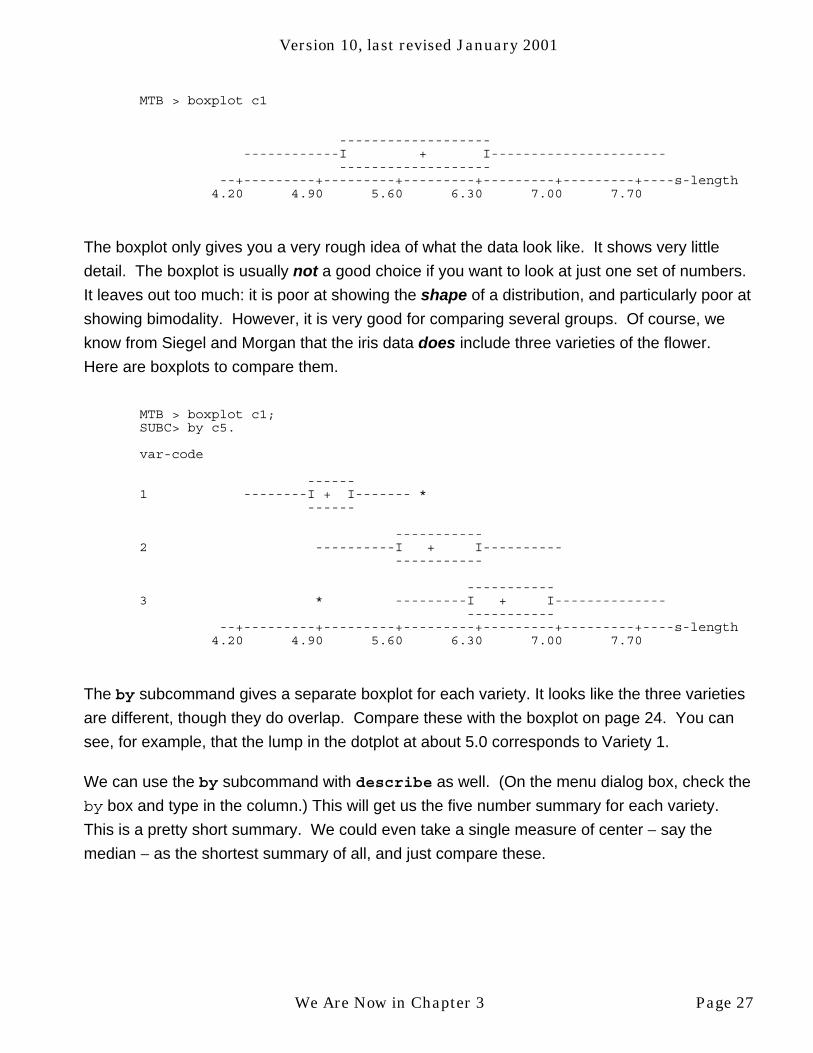
MTB > info
COLUMN NAME COUNTC1 s-length 150C2 s-width 150C3 p-length 150C4 p-width 150C5 var-code 150
A C6 variety 150C7 Setosa 50C8 Versiclr 50C9 Virginic 50
CONSTANTS USED: NONE
We Are Now in Chapter 3 Page 25

Version 10, last revised January 2001
MTB > stem c1
Stem-and-leaf of s-length N = 150 Leaf Unit = 0.10
4 4 344422 4 56666778888899999952 5 000000000011111111122223444444(31) 5 555555566666677777777888888899967 6 0000001111112222333333333444444435 6 555556677777777888999913 7 01222346 7 677779
MTB > histogram c1
Histogram of s-length N = 150
Midpoint Count 4.4 5 ***** 4.8 17 ***************** 5.2 24 ************************ 5.6 27 *************************** 6.0 22 ********************** 6.4 25 ************************* 6.8 17 ***************** 7.2 6 ****** 7.6 6 ****** 8.0 1 *
In the histogram, you can see there are five data points “around” 4.4. (You may need to
enable standard graphics or chose Character Graphs to get this type of histogram. It is under
Graph , Character Graphs in the menus.) In the stem and leaf, you can see they are
actually 4.3, 4.4, 4.4, 4.4, and 4.5. The traditional histogram usually provides a shorter
summary because it almost always involves grouping the data and hiding any differences
among the data points within each group. This may be an advantage with a really huge data
set. Page 53 of your text shows an example where the stem and leaf is too big to fit on a page.
MTB > dotplot c1
: . .: : . : . :. :
.:: : : ::: : :: :: . :. : ::: :: : ::: :. :: ::: : :. : . :
. :. :: ::: :: .: ::: :: :: ::: :: :: :.. :. . .: .-+---------+---------+---------+---------+---------+-----s-length
4.20 4.90 5.60 6.30 7.00 7.70
This dotplot of the iris data is much less smooth than the histogram or stem and leaf. It has a
lumpy look. Is this just random fluctuations, as discussed on pages 46-50 of your text, or is it
the result of more than one type of iris, much as the bimodality of the golf prizes was due to
there being two types of golf tournaments?
Page 26 We Are Now in Chapter 3
Version 10, last revised January 2001
MTB > boxplot c1
-------------------------------I + I----------------------
---------------------+---------+---------+---------+---------+---------+----s-length4.20 4.90 5.60 6.30 7.00 7.70
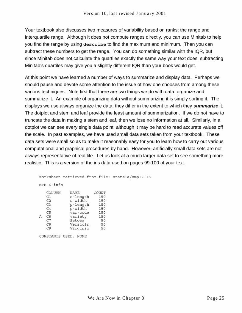
The boxplot only gives you a very rough idea of what the data look like. It shows very little
detail. The boxplot is usually not a good choice if you want to look at just one set of numbers.
It leaves out too much: it is poor at showing the shape of a distribution, and particularly poor at
showing bimodality. However, it is very good for comparing several groups. Of course, we
know from Siegel and Morgan that the iris data does include three varieties of the flower.
Here are boxplots to compare them.
MTB > boxplot c1;SUBC> by c5.
var-code
------1 --------I + I------- *
------
-----------2 ----------I + I----------
-----------
-----------3 * ---------I + I--------------
-------------+---------+---------+---------+---------+---------+----s-length4.20 4.90 5.60 6.30 7.00 7.70
The by subcommand gives a separate boxplot for each variety. It looks like the three varieties
are different, though they do overlap. Compare these with the boxplot on page 24. You can
see, for example, that the lump in the dotplot at about 5.0 corresponds to Variety 1.
We can use the by subcommand with describe as well. (On the menu dialog box, check the
by box and type in the column.) This will get us the five number summary for each variety.
This is a pretty short summary. We could even take a single measure of center − say the
median − as the shortest summary of all, and just compare these.
We Are Now in Chapter 3 Page 27

Version 10, last revised January 2001
MTB > describe c1
N MEAN MEDIAN TRMEAN STDEV SEMEAN s-length 150 5.8433 5.8000 5.8187 0.8281 0.0676
MIN MAX Q1 Q3 s-length 4.3000 7.9000 5.1000 6.4000
MTB > describe c1; SUBC> by c5.
var-code N MEAN MEDIAN TRMEAN STDEV SEMEAN s-length 1 50 5.0060 5.0000 5.0000 0.3525 0.0498 2 50 5.9360 5.9000 5.9364 0.5162 0.0730 3 50 6.5880 6.5000 6.5886 0.6359 0.0899
var-code MIN MAX Q1 Q3 s-length 1 4.3000 5.8000 4.8000 5.2000 2 4.9000 7.0000 5.6000 6.3000 3 4.9000 7.9000 6.2000 6.9500
Looking only at the medians, it looks like Variety 3 is typically about 0.6 units longer than
Variety 2, which is about 0.9 units longer than Variety 1.
Let’s compare what we saw with the iris data to a smaller data set, the bank deposits from
Problem 3.16 (i.e., Problem 16 in Chapter 3).
Worksheet retrieved from file: stats1a/smp03.16
MTB > info
COLUMN NAME COUNT A C1 Banks 10 C2 dollars 10
CONSTANTS USED: NONE
MTB > dotplot c2
.. . . .. . . . .+---------+---------+---------+---------+---------+-------dollars35 70 105 140 175 210
MTB > stem c2
Stem-and-leaf of dollars N = 10 Leaf Unit = 10
2 0 454 0 675 0 95 1 0112 1 31 11 11 11 2 1
Page 28 We Are Now in Chapter 3

Version 10, last revised January 2001
MTB > histogram c2
Histogram of dollars N = 10
Midpoint Count40 1 *60 2 **80 1 *100 2 **120 2 **140 1 *160 0180 0200 0220 1 *
MTB > print c2
dollars217 139 116 110 103 98 76 69 54 49
MTB > stem c2;SUBC> increment 50.
Stem-and-leaf of dollars N = 10Leaf Unit = 10
1 0 45 0 56795 1 01131 11 2 1
Here the dotplot is just a row of dots; it is not a good way to display this data. The histogram
and stem and leaf are better, though with so few observations we might want to compress the
scale.
You have already seen how to retrieve specific files providing you already know the name of
the file. Some filenames are given in your book. For example, the name for the earthquake
data file is given on page 32 of your text. Other files are named according to a systematic
naming system so that you can find any file you want. The last file we used, smp03.16, is an
example. Files of data from the current text start with the letters “sm”, standing for Siegel and
Morgan, the authors. The next letter in the file name tells you whether the data in the file
came from
e an Examplep a Problemt a Tablex an eXercise within a section
We Are Now in Chapter 3 Page 29

Version 10, last revised January 2001
in the Siegel and Morgan text. Then a number tells you which example, problem, table, or
exercise. The part of the number before the decimal point is the chapter number. The part
after the decimal point is the example, problem, table, or exercise number. Both of these are
written as two digit numerals. Thus the file ‘sme02.09’ contains the data for Example 9 in
Chapter 2.
Minitab Assignment 3-A
Do Problem 3.12 on page 101 of your text using Minitab to help you. The problem asks you
about the shape of the distribution. Since boxplots are not particularly good at showing shape,
you should have Minitab make an additional display. Does your added display show anything
that the boxplot does not show?
Minitab Assignment 3-B
Do Problem 3.13 on page 101 of your text using Minitab to help you. The problem asks you
about the shape of the distribution. Since boxplots are not particularly good at showing shape,
you should have Minitab make an additional display. Does your added display show anything
that the boxplot does not show?
Minitab Assignment 3-C
Do Problem 3.14 on page 102 of your text using Minitab to help you. The problem asks you
about the shape of the distribution. Since boxplots are not particularly good at showing shape,
you should have Minitab make an additional display. Does your added display show anything
that the boxplot does not show?
Minitab Assignment 3-D
Problem 2.19 on page 57 of your text involves a data set on boys’ heights that is too large to
analyze without a computer. Use Minitab to get a variety of displays and summary statistics
for this data. Eliminate the ones you do not think are helpful and make a summary report
describing this data. Your summary should be of moderate length − just giving the median
would not be enough, but pages and pages of “summary” would not be appropriate either. If
you find anything interesting going on in this data, be sure it shows in your report! Also
indicate whether you think these are tall boys or short boys.
Page 30 We Are Now in Chapter 3

Version 10, last revised January 2001
Minitab Assignment 3-E
Use Minitab to do Problem 2.24 on pages 59-60 of your text. You should make boxplots of the
yield by variety and also by field to see if you can locate the reason for the lumpy distribution
on page 60. Write a brief summary of your conclusion.
Minitab Assignment 3-F
Use Minitab to analyze the data for Problem 31 on page 64.
1. Does the distribution of oxygen use appear to be bimodal?
2. Do separate displays for the two age groups indicate that oxygen use is about the
same for the two age groups?
3. Does the distribution of fill rate appear to be bimodal?
4. Do separate displays for the two age groups indicate that fill rate is about the same for
the two age groups?
Minitab Assignment 3-G
The bank deposit data from Problems 3.15 and 3.16 on pages 102-103 of your text are
combined in file smp03.17. Use Minitab and this data file to do Problem 3.17 on page 104.
Minitab Assignment 3-H
Use Minitab to check the printout on page 104 of your text. The data is in file smp03.18.
1. Reproduce the two dotplots.
2. You will find that your dotplots differ from the ones in the book. Describe the
differences.
3. The dotplots in your text are incorrect. What do you think happened to them?
We Are Now in Chapter 3 Page 31

Version 10, last revised January 2001
CATEGORICAL DATA
Categorical data is data that places the objects studied into categories. For example, in the
golf prize data, the variable sex placed the golf tournaments into the categories “men’s” and
“women’s”. Other examples might be placing college students into categories based on
whether they are in-state or out-of-state, or by eye color, or class standing (freshperson,
sophomore, junior, senior). Such data is discussed at various points in the early chapters of
your text. The things you need to know about Minitab and categorical data are gathered here.
In using statistical software, it is common to code categories as numbers. On page 69 of your
text there is an example about 29 students and the states they come from. We picked codes
for the states by listing all 50 states and the District of Columbia alphabetically and then
numbering them from 1 to 51.
Worksheet retrieved from file: stats1a/smt03.01 MTB > info
COLUMN NAME COUNT C1 state 29
CONSTANTS USED: NONE
MTB > print c1
state 33 33 33 5 5 33 5 22 5 33 5 5 5 5 38 5 50 50 33 5 22 33 5 22 5 5 5 33 5
MTB > note: Data from page 69. 5=CA 22=MA 33=NY 38=OR 50=WI
MTB > tally c1
state COUNT5 1522 333 838 150 2N= 29
MTB > tally c1; SUBC> percents.
state PERCENT5 51.7222 10.3433 27.5938 3.4550 6.90
Page 32 We Are Now in Chapter 3

Version 10, last revised January 2001
MTB > tally c1;SUBC> counts;SUBC> percents.
state COUNT PERCENT5 15 51.7222 3 10.3433 8 27.5938 1 3.4550 2 6.90N= 29
The tally command gives frequencies (counts) and relative frequencies (proportions or
percents) for categorical data. It can be found under Stat , Tables in the menus. The
category with the most observations is called the modal category. Here it is California.
Sometimes we have measurement data in which only a few distinct values are observed. In
the productivity data from page 82 of your text, there were 24 observations but only 5 different
values: 20, 30, 40, 50, and 70. This data is like categorical data in that we can use these five
values as categories. When the categories are numbers, the number that occurs most often is
called the mode. For the data below, the mode is 30.
Worksheet retrieved from file: stats1a/sme03.08
MTB > info
COLUMN NAME COUNTC1 product 24
CONSTANTS USED: NONE
MTB > note: page 82MTB > histogram c1
Histogram of product N = 24
Midpoint Count20 4 ****25 030 11 ***********35 040 3 ***45 050 5 *****55 060 065 070 1 *
We Are Now in Chapter 3 Page 33

Version 10, last revised January 2001
MTB > stem c1
Stem-and-leaf of product N = 24 Leaf Unit = 1.0
4 2 0000(11) 3 000000000009 4 0006 5 000001 61 7 0
MTB > tally c1
product COUNT 20 4 30 11 40 3 50 5 70 1 N= 24
We can recognize the mode as the category with the largest count in the tally output.
When our categories have an order to them it makes sense to do cumulative counts or
percents. The productivity ratings have an order because they are actually measurement data,
but categories such as “good”, “better” “best” have order as well. here are some of the options
illustrated for the productivity data. The cumulative counts from Minitab match those in Table
3.7 on page 83 of your textbook.
MTB > tally c1; SUBC> cumcounts.
product CUMCNT 20 4 30 15 40 18 50 23 70 24
MTB > tally c1; SUBC> cumpercents.
product CUMPCT 20 16.67 30 62.50 40 75.00 50 95.83 70 100.00
Page 34 We Are Now in Chapter 3

Version 10, last revised January 2001
MTB > tally c1;SUBC> all.
product COUNT CUMCNT PERCENT CUMPCT20 4 4 16.67 16.6730 11 15 45.83 62.5040 3 18 12.50 75.0050 5 23 20.83 95.8370 1 24 4.17 100.00N= 24
From the cumulative columns we can see that 18, or 75%, of the factories had a productivity
score of 40 or less.
Cumulative columns are not so useful for categorical data in which the categories do not have
a natural order. For example, in data on eye color a cumulative count might tell us that 38% of
the eyes were either blue or a color listed before blue in the table − probably not useful
information.
Tables are the usual way to present categorical data. The common displays for a single
categorical variable are the bar chart and the pie chart. Real statisticians don’t do pie charts.
Minitab’s histograms are so crude you cannot tell a histogram from a barchart, so we can do
barcharts with the histogram command, as shown above. You can also see that sometimes
the stem command will also give a crude barchart. However, none of these convey any more
information than a table, and usually they convey less, so we will not use them.
Rounding can often make measurement data look like categorical data. The chest sizes of
Scottish soldiers on page 120 of your text has 5738 measurements but only 16 different values
because the measurements were rounded off to the nearest inch. Here we show part of the
raw data (in file smt04.04). You could get the table on page 120 of your textbook with the
tally command.
MTB > info
COLUMN NAME COUNTC1 chest_sz 5738
CONSTANTS USED: NONE
We Are Now in Chapter 3 Page 35

Version 10, last revised January 2001
MTB > print c1
chest_sz 40 43 41 37 39 39 42 40 42 38 42 40 38 39 37 42 41 41 41 38 39 38 39 41 39 42 39 38 40 40 39 43 38 42 42 40 39 41 40 39 40 39 36 40 39 43 38 42 38 37 41 41 40 42 37 40 39 38 39 40 35 40 38 39 42 42 43 40 38 41 39 38 41 41 41 40 40 40 40 39 40 42 40 40 39 42 40 39 41 43 40 40 43 38 39 38 43 39 40 38 40 37 45 40 38 39 42 40 38 42 39 39 40 40 39 41 36 35 40 38 38 38 40 41 36 37 43 38 39 43 41 40 41 41 39 41 40 42 43 39 39 42 40 38 36 38 39 42 40 37 39 40 41 36 39 36 39 38 42 43 41 39 40 42 36 39 38 42 39 43 40 37 38 43 41 37 41 41 41 41 38 39 39 39 40 40 43 39 41 40 40 38 42 40 41 42 40 40 44 38 40 39 40 43 39 40 41 42 42 41 37 45 42 38 37 37 34 39 43 37 40 36 38 37 38 41 41 40 40 40 38 42 40 39 42 40 45 40 39 39 41 40 43 38 40 35 40 36 41 37 38 38 38 43 39 40 40 43 38 35
(much data omitted to save trees)
MTB > tally c1
chest_sz COUNT 33 3 34 18 35 81 36 185 37 420 38 749 39 1073 40 1079 41 934 42 658 43 370 44 92 45 50 46 21 47 4 48 1
N= 5738
Page 36 We Are Now in Chapter 3

Version 10, last revised January 2001
MTB > stem c1
Stem-and-leaf of chest_sz N = 5738Leaf Unit = 0.10
3 33 00021 34 000000000000000000102 35 00000000000000000000000000000000000000000000000000000000000000000+287 36 00000000000000000000000000000000000000000000000000000000000000000+707 37 00000000000000000000000000000000000000000000000000000000000000000+1456 38 00000000000000000000000000000000000000000000000000000000000000000+2529 39 00000000000000000000000000000000000000000000000000000000000000000+(1079) 40 00000000000000000000000000000000000000000000000000000000000000000+2130 41 00000000000000000000000000000000000000000000000000000000000000000+1196 42 00000000000000000000000000000000000000000000000000000000000000000+538 43 00000000000000000000000000000000000000000000000000000000000000000+168 44 00000000000000000000000000000000000000000000000000000000000000000+76 45 0000000000000000000000000000000000000000000000000026 46 0000000000000000000005 47 00001 48 0
MTB > histogram c1
Histogram of chest_sz N = 5738Each * represents 25 obs.
Midpoint Count33 3 *34 18 *35 81 ****36 185 ********37 420 *****************38 749 ******************************39 1073 *******************************************40 1079 ********************************************41 934 **************************************42 658 ***************************43 370 ***************44 92 ****45 50 **46 21 *47 4 *48 1 *
MTB > describe c1
N MEAN MEDIAN TRMEAN STDEV SEMEANchest_sz 5738 39.832 40.000 39.840 2.050 0.027
MIN MAX Q1 Q3chest_sz 33.000 48.000 38.000 41.000
MTB > boxplot c1
-----------* --------------I + I------------- * * *
---------------+---------+---------+---------+---------+---------+--chest_sz33.0 36.0 39.0 42.0 45.0 48.0
We Are Now in Chapter 3 Page 37

Version 10, last revised January 2001
This is an important example because it is our first experience with a really large data set.
Note that the stem and leaf is too long a summary for such a data set. It tries to show each
individual observation. Since there are so many, the display will not fit on the page. As a
result, it got a crew cut, and we cannot see its true shape very well. The histogram is better
because it can be scaled to fit on the page. Here each * represents 25 observations.
The boxplot shows twenty-nine outliers, although we would not suspect any outliers from the
histogram. These are really false alarms. The main cause is the tiny IQR of 3. Remember that
the (regular) boxplot and Minitab use an arbitrary rule for deciding what is an outlier. You have
to decide for yourself if there is really a problem with outliers. Here there is not.
The simplest kind of categorical data has only two categories, such as male and female. Data
like this is usually coded numerically with 0s and 1s. One example is the rainy day data on
page 127 of your text. If one category is of more interest to us than the other, we code the
interesting category as a 1. Here we let 1 represent a rainy day. Again, the raw data is not
printed in your text, so we reproduce part of it here from file sme04.06.
MTB > info
COLUMN NAME COUNT C1 Rain? 365
CONSTANTS USED: NONE
MTB > print c1
Rain? 1 0 0 0 0 1 1 0 1 1 1 0 0 1 0 1 1 0 0 0 1 0 1 0 1 1 0 0 1 0 0 1 0 0 0 0 0 1 0 1 0 1 0 1 0 1 1 0 0 0 1 0 1 1 0 0 0 0 0 0 0 0 0 0 0 0 0 1 1 0 0 0 0 0 0 0 0 1 0 0 0 0 0 0 0 0 1 0 0 0 1 0 0 1 1 1 1 1 0 1 0 0 0 0 0 0 0 0 0 1 0 0 1 1 0 1 0 0 1 0 1 1 0 0 0 0 1 0 0 0 0 0 0 0 0 1 0 0 0 1 0 1 1 0 0 0 1 0 0 1 0 0 0 1 1 0 0 1 0 0 1 1 1 1 0 0 0 0 1 1 0 1 1 1 0 0 1 1 0 0 1 1 0 0 0 0 0 1 0 1 1 0 0 1 0
(much data omitted to save trees)
This shows that it rained on January first, sixth, seventh, ninth, tenth, eleventh, et cetera.
Page 38 We Are Now in Chapter 3

Version 10, last revised January 2001
MTB > tally c1;SUBC> counts;SUBC> percents.
Rain? COUNT PERCENT0 237 64.931 128 35.07 <-------- Looky here!N= 365 /
/MTB > describe c1 /
/N MEAN MEDIAN TRMEAN STDEV SEMEAN
Rain? 365 0.3507 0.0000 0.3343 0.4778 0.0250
MIN MAX Q1 Q3Rain? 0.0000 1.0000 0.0000 1.0000
MTB > stem c1
Stem-and-leaf of Rain? N = 365Leaf Unit = 0.010
(237) 0 00000000000000000000000000000000000000000000000000000000000000000+128 1128 2128 3128 4128 5128 6128 7128 8128 9128 10 00000000000000000000000000000000000000000000000000000000000000000+
MTB > histogram c1
Histogram of Rain? N = 365Each * represents 5 obs.
Midpoint Count0 237 ************************************************1 128 **************************
MTB > dotplot c1
Each dot represents 16 points
.:::: :: :: :: :+---------+---------+---------+---------+---------+-------Rain?
0.00 0.20 0.40 0.60 0.80 1.00
We Are Now in Chapter 3 Page 39

Version 10, last revised January 2001
With the 0-1 coding, the mean is equal to the proportion of 1s, i.e., the proportion of rainy days.
As a result, we can treat a proportion as a special kind of mean, and the techniques we learn
for working with means will also work for proportions.
You can see that displays for 0-1 data are not very interesting. You can have outliers in 0-1
data if you make a typo, but you can usually spot that with the describe command. (Just
look at the max and min.) The displays could also be useful for spotting a typo like an “0.1”.
New Minitab commands for Chapter 3:
boxplot describe gpro gstd
histogram lvals sort tally
Minitab Assignment 3-I
The data in Table 2.19 on page 61 of your text are also in the file smt02.19. That file also
includes additional information. For the data in the file:
1. Identify each variable as numerical measurements or categorical data.
2. Which measurement variables could reasonably be treated as categorical?
3. There are two columns of coding data in the computer file. Compare the codes to the
table in the book and explain the coding scheme for each column. (For example, in
the data on states students came from, California was coded as “5”.)
4. Give one reasonable summary for each variable. Use a display or a table.
5. Describe (in words) the shape of the distribution of each measurement variable.
6. Could you find any proportions for this data with the describe command? If so, do it
and explain what you found the proportion of.
Page 40 We Are Now in Chapter 3

Version 10, last revised January 2001
Minitab Assignment 3-J
The data in Table 4.10 on page 136 of your text are also in the file smt04.10. That file also
includes additional information. For the data in the file:
1. Identify each variable as numerical measurements or categorical data.
2. Which measurement variables could reasonably be treated as categorical?
3. There is one column of coded data in the computer file. Compare the codes to the
table in the book (page 52) and explain the coding scheme for this column. (For
example, in the data on which states students came from, California was coded as
“5”.)
4. Give one reasonable summary for each variable. Use a display or a table.
5. Describe (in words) the shape of the distribution of each measurement variable.
6. Could you find any proportions for this data with the describe command? If so, do it
and explain what you found the proportion of.
Minitab Assignment 3-K
Rolling a die (singular of “dice”) gave these results:
3,4,1,2,3,2,6,3,4,5,1,2,3,5,2,6,6,4,1,3
Type these 20 numbers into a column in Minitab and find
1. the mode
2. the number of 4’s
3. the percentage of 4’s
4. the number of times we rolled a 4 or less
We Are Now in Chapter 3 Page 41

Version 10, last revised January 2001
Minitab Assignment 3-L
We took candies out of a bag one at a time and recorded the colors:
red, blue, brown, green, brown, blue, red, brown, green, yellow,
brown, blue, red, brown, green, red, blue, brown, green, brown
1. Chose numerical codes for each color.
2. Enter 20 code numbers into a column in Minitab to represent the outcomes above.
3. Use minitab to find
a. the modal category
b. the number of red candies
c. the percentage of brown candies
4. Would it make sense to find cumulative counts or percentages for this data?
Minitab Assignment 3-M
Use Minitab to create a table of cumulative counts and percentages for the data on Scottish
soldiers (in file smt04.04) to answer the following questions:
1. What percent had a chest size of 40?
2. What percent had a chest size less than 40.5?
3. What percent had a chest size more than 40.5?
4. What percent had a chest size between 35.5 and 40.5?
5. What percent had a chest size in the 40s?
Page 42 We Are Now in Chapter 3

Version 10, last revised January 2001
Minitab Assignment 3-N
Make a table for the golf data from 1991 (in file sme02.09) that includes the following
information: the number of men’s tournaments, the number of women’s tournaments, the
percentage of men’s tournaments, and the percentage of women’s tournaments. Label these
numbers with descriptions of what they represent.
Minitab Assignment 3-O
The file sme07.11 contains data on whether job applicants made eye contact during an
interview and whether they were hired. The coding is 0=made eye contact and 1=did not make
eye contact for one variable and 0=hired and 1=not hired for the other.
1. Find the number who made good eye contact.
2. Find the percentage who made good eye contact.
3. Find the number who were hired.
4. Find the percentage who were not hired.
Chapter 4
In Chapter 4 you will learn how to:
• run Minitab macros
• delete outliers from a dataset
• find the average of a column of numbers
We Are Now in Chapter 3 Page 43

Version 10, last revised January 2001
In previous sections of this Guide, you have learned how to use Minitab to get answers. This
is how Minitab is typically used outside of school. (It is used by a majority of the Fortune top
50 companies.) In this section, we will see how Minitab can be programmed to print out many
intermediate steps in a computation. This is helpful to students who are trying to learn how to
do these computations by hand. Although you have answers for most of the problems in your
textbook, these do not tell you where you went wrong if your own answer should disagree. It
would be nice to have a fully worked-out solution to compare to your own calculations.
First, though, let’s look at just getting answers for the mean and standard deviation. We’ll use
the made-up data on page 109 of your text and the orange juice data from page 113 of your
text. The average command will give you the mean (or average) of a column. You can find it
under Calc , Column Statistics in the menus. (Select “mean” from the list.) The
describe command gives both the mean and standard deviation. If you need the variance,
square the standard deviation on your calculator. (Do not take the square root of the
standard deviation!)
MTB > set c1 DATA> 1 8 4 6 8 DATA> end MTB > average c1
MEAN = 5.4000 MTB > note: page 109 MTB > describe c1
N MEAN MEDIAN TRMEAN STDEV SEMEAN C1 5 5.40 6.00 5.40 2.97 1.33
MIN MAX Q1 Q3 C1 1.00 8.00 2.50 8.00
2The variance of the orange juice data is 0.1789 =0.0320. Now let’s suppose that you tried to
calculate the variance and standard deviation of the orange juice data by hand, and you made
a mistake. In fact, let’s suppose you misplaced the decimal point in the variance, just as the
first edition of your textbook did. Though the variance is really 0.0320, they gave 0.32 by
mistake. If you take the square root of 0.32, you will get 0.566, rather than the correct 0.18.
Then you would be wondering what went wrong. Here’s how to get Minitab to print out the
entire calculation, so you can see where the problem is. Since this may look rather
intimidating, it is important to understand that, once you have the data in c1, all of this is typed
by Minitab, not by you.
Page 44 We Are Now in Chapter 4

Version 10, last revised January 2001
MTB > noteMTB > note This macro computes the mean, variance, and standardMTB > note deviation of a set of data. The data must be stored in c1.MTB > note The results of all intermediate steps are printed outMTB > note to aid students in learning to do these computationsMTB > note by hand. The macro will destroy any data stored in c2-c3MTB > note and k1-k7.MTB > note------------------------------------------------------------
ROW OJprice resids. res. sq.
1 2.6 0.200000 0.03999992 2.4 0.000000 0.00000003 2.5 0.100000 0.01000004 2.1 -0.300000 0.09000015 2.3 -0.100000 0.01000006 2.5 0.100000 0.0100000
------------------------------------------------------------
MTB > print k1 The total =K1 14.4000MTB > print k2 number of observations =K2 6.00000MTB > print k3 mean =K3 2.40000MTB > print k4 The sum of the squared residuals =K4 0.160000MTB > print k5 degrees of freedom =K5 5.00000MTB > print k6 variance =K6 0.0320000MTB > print k7 standard deviation =K7 0.178885MTB > end
You should compare the calculations provided by Minitab to those in the table at the top of
page 114 in your textbook.
At first, you might think that all the note and print commands would have to be typed by
you, but actually all of these (and several others) were typed in earlier and stored in the file
called var. If you execute that file, you will cause all the commands stored there to be run in
Minitab just as if you had typed them in one by one. Such a collection of commands is called a
macro. As with opening and saving files, it is recommended that you not try to run macros
from a command line. To execute a macro from the menu system, select File, Other Files,
Run an Exec, Select File. Then you will have to find the macro file just as you do a data file.
At PSC, they are usually in a folder in stats1a called macros. Be sure to read the
documentation provided by all the notes in any macro you use. For example, although
Minitab generally allows you to put things in whatever columns you want, the var macro
requires the data to be in c1.
We Are Now in Chapter 4 Page 45

Version 10, last revised January 2001
The macro shows the correct variance of 0.032. If you had made a mistake there, your results
would agree with those of the macro all the way up to that point (“print k5 variance =”). Then
you would know just where you made your mistake. You can use this macro to check your
answers to homework problems. Unfortunately, the latest version of Minitab inserts a lot of
extra labels in large, boldface letters into the output of this and other macros, making them
hard to follow. Try to ignore these. Comparing your output to the example above should make
it clear what’s been added.
Means, variances, and standard deviations are particularly useful with data that are
(approximately) normally distributed. Your textbook shows one such application in Section 4.3.
Table 4.6 lives inside of Minitab. You can access it as shown below, where we “look up” the
two numbers your textbook looked up in its table.
MTB > note: page 123
MTB > cdf 0.330.3300 0.6293
MTB > cdf -0.25-0.2500 0.4013
Note that Minitab reports its results as proportions rather than percents. In the menu system,
click on Calc and select Probability Distributions. Pick Normal for the type of
distribution and select Cumulative probability and Input Constant. Then type in
your value (0.33 in the first example above) and click OK .
Section 4.5 of your text (on grouped data) shows how you can shorten the calculation of
means and standard deviations when you have measurement data that act like categorical
data, i.e., when certain values are repeated over and over. There is a Minitab macro to do this
calculation. It is called vargroup. Like the var macro, you can use this to check work you
do by hand so you can learn this computation. Here is an example based on the one in your
book on page 130. The macro requires that you put the values in c1 and their frequencies in
c2. Usually you will have to get these from the tally command and type them into c1 and c2
yourself. The read command lets you type in a multicolumn table. In this case, that will erase
whatever used to be in c1 and c2. This will not be a problem if you (or your instructor) has
previously saved the original data on the computer. In the example below, we start off with 24
numbers in c1.
Page 46 We Are Now in Chapter 4

Version 10, last revised January 2001
Worksheet retrieved from file: stats1a/sme04.07
MTB > print c1
product20 70 30 50 40 50 30 30 20 50 30 50 4030 30 30 30 30 20 20 30 40 30 50
MTB > tally c1
product COUNT20 430 1140 350 570 1N= 24
MTB > read c1 c2DATA> 20 4DATA> 30 11DATA> 40 3DATA> 50 5DATA> 70 1DATA> end
5 ROWS READ
Now the numbers that used to be in c1
20 70 30 50 40 50 30 30 20 50 30 50 4030 30 30 30 30 20 20 30 40 30 50
have been replaced with
20 30 40 50 70
Running the macro
We Are Now in Chapter 4 Page 47

Version 10, last revised January 2001
MTB > note This macro computes the mean, variance, and standard MTB > note deviation of grouped data. The data values must be MTB > note stored in c1 and their frequencies in c2. MTB > note The results of all intermediate steps are printed out MTB > note to aid students in learning to do these computations MTB > note by hand. The macro will destroy any data stored in c2-c4, MTB > note k1-k7, and any name given to c1. MTB > note ------------------------------------------------------------
ROW x f xf resids. res.sq. res.sq.f
1 20 4 80 -15.4167 237.67 950.69 2 30 11 330 -5.4167 29.34 322.74 3 40 3 120 4.5833 21.01 63.02 4 50 5 250 14.5833 212.67 1063.37 5 70 1 70 34.5833 1196.01 1196.01
------------------------------------------------------------ MTB > print k1 The total = K1 850.000 MTB > print k2 number of observations = K2 24.0000 MTB > print k3 mean = K3 35.4167 MTB > print k4 The sum of the squared residuals = K4 3595.83 MTB > print k5 degrees of freedom = K5 23.0000 MTB > print k6 variance = K6 156.341 MTB > print k7 standard deviation = K7 12.5036 MTB > end
we get the correct value for the mean of 35.4167. However, if we run describe now
MTB > describe c1
N MEAN MEDIAN TRMEAN STDEV SEMEAN x 5 42.00 40.00 42.00 19.24 8.60
MIN MAX Q1 Q3 x 20.00 70.00 25.00 60.00
the describe command does not give us the correct mean because we replaced the original
24 numbers with our table of five numbers.
MTB > print c1-c2
ROW x f
1 20 4 2 30 11 3 40 3 4 50 5
Page 48 We Are Now in Chapter 4

Version 10, last revised January 2001
We can get the original data back again.
Worksheet retrieved from file: stats1a/sme04.07
MTB > desc c1
N MEAN MEDIAN TRMEAN STDEV SEMEANproduct 24 35.42 30.00 34.55 12.50 2.55
MIN MAX Q1 Q3product 20.00 70.00 30.00 47.50
Now we get the correct mean.
Your text mentions the effect of outliers on data summaries at various points in the earlier
chapters. This is discussed in more detail in Chapter 6. Here is one simple example, based
on the data on per capita GNP from your text.
Worksheet retrieved from file: stats1a/smt02.17
MTB > info
COLUMN NAME COUNTC1 10
CONSTANTS USED: NONE
MTB > note page 59MTB > stem c1
Stem-and-leaf of C1 N = 10Leaf Unit = 100
(9) 0 0001111111 01 01 01 01 1 0
The outlier makes the stem and leaf just about useless − except for spotting the outlier! Your
book suggested that this might be a typo for 106. We will get some summary statistics on the
original data, then change the 1060 to 106 and see what difference it makes.
MTB > desc c1
N MEAN MEDIAN TRMEAN STDEV SEMEANC1 10 201.0 105.0 110.0 302.5 95.7
MIN MAX Q1 Q3C1 70.0 1060.0 90.0 130.0
We Are Now in Chapter 4 Page 49

Version 10, last revised January 2001
MTB > print c1 c2
ROW C1 C2
1 100 2 100 3 70 4 130 5 1060 6 90 7 110 8 130 9 90 10 130
MTB > copy c1 into c2 MTB > let c2(5)=106 MTB > stem c2
Stem-and-leaf of C2 N = 10 Leaf Unit = 1.0
1 7 01 83 9 00(3) 10 0064 11 03 123 13 000
MTB > desc c2
N MEAN MEDIAN TRMEAN STDEV SEMEAN C2 10 105.60 103.00 107.00 20.06 6.34
MIN MAX Q1 Q3 C2 70.00 130.00 90.00 130.00
The copy command does exactly what you might expect. Here we copied the data in c1 into
c2. The let command does arithmetic. Here,
MTB > let c2(5)=106
changes the fifth number in c2 from 1060 to 106. We make the changes on a copy of the
original data in case we need to compare the new version to the old. We know we wanted the
fifth number because we printed out c1 to see in which row the 1060 is. Of course, it is easier
to edit the data in the data window, but copy and let have many other uses.
Notice that changing the outlier decreases the mean by about half and the standard deviation
by more than 90%. This gives you an idea of how far one mistake could throw you off! Also
note that the median and IQR are hardly changed at all.
Page 50 We Are Now in Chapter 4

Version 10, last revised January 2001
Sometimes we have a data point we know is wrong, but we do not know what the right value
is. In that case, all we can do is remove the erroneous data. Here is how you could remove
the 1060 instead of changing it. From the menus, use Manip , Copy Columns.
MTB > copy c2 into c3;SUBC> omit row 5.MTB > print c1-c3
ROW C1 C2 C3
1 100 100 1002 100 100 1003 70 70 704 130 130 1305 1060 106 906 90 90 1107 110 110 1308 130 130 909 90 90 13010 130 130
MTB > stem c3
Stem-and-leaf of C3 N = 9Leaf Unit = 1.0
1 7 01 83 9 00(2) 10 004 11 03 123 13 000
MTB > desc c3
N MEAN MEDIAN TRMEAN STDEV SEMEANC3 9 105.56 100.00 105.56 21.28 7.09
MIN MAX Q1 Q3C3 70.00 130.00 90.00 130.00
This gives results similar to what we got when we guessed that the 1060 really should be a
106. Of course, for this data, we know from the textbook that the 1060 is correct. Thus we
should not throw it out or change it. Instead, we should pick summary statistics that are
appropriate to this kind of data. The mean is inappropriate because there is no data around
201. That is an atypical value. The median does a better job of indicating where the bulk of
the data lie.
We can use the let command for many other purposes. The var and vargroup macros use
it to do their calculations. You could use it to convert the units on the data in a column. In the
example below, we look at the heart data from page 64 of your text. There was a binary
We Are Now in Chapter 4 Page 51
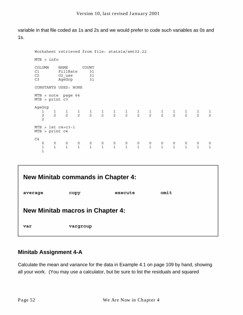
Version 10, last revised January 2001
variable in that file coded as 1s and 2s and we would prefer to code such variables as 0s and
1s.
Worksheet retrieved from file: stats1a/smt02.22
MTB > info
COLUMN NAME COUNT C1 FillRate 31 C2 O2_use 31 C3 AgeGrp 31
CONSTANTS USED: NONE
MTB > note page 64 MTB > print c3
AgeGrp 1 1 1 1 1 1 1 1 1 1 1 1 1 1 1 2 2 2 2 2 2 2 2 2 2 2 2 2 2 2 2
MTB > let c4=c3-1 MTB > print c4
C4 0 0 0 0 0 0 0 0 0 0 0 0 0 0 0 1 1 1 1 1 1 1 1 1 1 1 1 1 1 1 1
New Minitab commands in Chapter 4:
average copy execute omit
New Minitab macros in Chapter 4:
var vargroup
Minitab Assignment 4-A
Calculate the mean and variance for the data in Example 4.1 on page 109 by hand, showing
all your work. (You may use a calculator, but be sure to list the residuals and squared
Page 52 We Are Now in Chapter 4

Version 10, last revised January 2001
residuals.) Then use the var macro to check your work. Note and explain any errors you find.
(You do not have to redo the work you did by hand.)
Minitab Assignment 4-B
Do Problems 2-4 on pages 131-132 by hand, showing all your work. (You may use a
calculator, but be sure to list the residuals and squared residuals.) Then use the var macro to
check your work. Note and explain any errors you find. (You do not have to redo the work you
did by hand.)
Minitab Assignment 4-C
Do Problem 12 on page 134 by hand, showing all your work. (You may use a calculator, but
be sure to list the residuals and squared residuals.) Then use the var macro to check your
work. Note and explain any errors you find. (You do not have to redo the work you did by
hand.)
Minitab Assignment 4-D
Problem 20 on page 137 of your textbook has scores based on rating a student’s singing
voice.
1. The “BEFORE” scores could be summarized in a table as
score frequency
4 3
5 3
Use the vargroup macro to find the mean, variance and standard deviation for this
grouped data.
2. Make a similar table for the “AFTER” data. Use the vargroup macro to find the
mean, variance and standard deviation for this data.
Minitab Assignment 4-E
1. Use describe to find the mean and standard deviation of the data in Exercise 4 on
page 110.
We Are Now in Chapter 4 Page 53
Version 10, last revised January 2001
2. Since many values in this data set are repeated, you can use the method for grouped
data to get the mean and standard deviation. Show how to do this by hand, showing
all your work. (You may use a calculator, but be sure to list the residuals, squared
residuals, etc.)
3. Check the results of Part 2 with the vargroup macro. Also check your answer
against what you got in Part 1.
4. Use describe to find the mean and standard deviation of the data in Exercise 5 on
page 110.
5. Since many values in this data set are repeated, you can use the method for grouped
data to get the mean and standard deviation. Show how to do this by hand, showing
all your work. (You may use a calculator, but be sure to list the residuals, squared
residuals, etc.)
6. Check the results of Part 5 with the vargroup macro. Also check your answer
against what you got in Part 4.
7. What are the differences between the two data sets you just analyzed? Use your
work to write a brief commentary on the effects of outliers on the mean and standard
deviation.
8. Find the median and interquartile range for both data sets and comment on how much
they are affected by outliers.
9. Find the range for both data sets. Is the range sensitive to outliers?
Minitab Assignment 4-F
1. Use describe to find the mean and standard deviation of the number of seats
variable from the data in Table 4.10 on page 136 of your text. (The data in the file
smt04.10 includes data on additional varibles which you can ignore.)
2. Since many values in this varible are repeated, you can use the method for grouped
data to get the mean and standard deviation. Show how to do this by hand, showing
all your work. (You may use a calculator, but be sure to list the residuals, squared
residuals, etc.)
Page 54 We Are Now in Chapter 4
Version 10, last revised January 2001
3. Check the results of Part 2 with the vargroup macro. Also check your answer
against what you got in Part 1.
4. Remove the outlier and repeat Parts 1-3.
5. Which of the statistics generated by the describe command are usually sensitive to
outliers? Were they in this case?
Minitab Assignment 4-G
Investigate the effect of the outlier in the data in Table 4.11 on page 136 of your text. Try
removing it. Also try replacing it with 625. Which would be a better summary for this data, the
mean or the median?
Chapter 5
In Chapter 5 you will learn how to:
• transform data with square roots and logarithms
In Chapter 5 of your text, Siegel takes the Atlantic islands data set (page 149), applies several
transformations to the data, and then makes displays of the results. Because there are 27
data points, this would be a lot of work to do by hand! Let’s see how to get Minitab to help us.
As always, the first step is to look at the data! It’s in sme05.03.
We Are Now in Chapter 4 Page 55

Version 10, last revised January 2001
MTB > print c1
A 3066 34 902 5380 20 785 10 2808 3981 1750 540 4700 7 840000 39769 1396 307 15528 91 108 46 42030 2184 47 1450 18800 40 MTB > histogram c1
Histogram of A N = 27
Midpoint Count 0 26 ************************** 100000 0 200000 0 300000 0 400000 0 500000 0 600000 0 700000 0 800000 1 *
This does not look good! At first we might think that the extreme outlier in our data is an error,
but if you look at a map you will see that Greenland really is a very large island! We will use
Minitab to carry out all the transformations your textbook tried. Between the commands
themselves and the names given to the columns, you should be able to follow this. If it’s too
easy, select Calc , Calculator and enter your formula. (In the list of functions, logarithms to
the base ten are Log 10 while logarithms to the base e are under Natural logarithms.)
MTB > let c2 = sqrt(c1) MTB > let c3 = loge(c1) MTB > let c4 = logten(c1) MTB > name c2 ’sqrt’ c3 ’log e’ c4 ’log 10’
MTB > print c1-c4
ROW A sqrt log e log 10
1 3066 55.371 8.0281 3.486572 34 5.831 3.5264 1.531483 902 30.033 6.8046 2.955214 5380 73.348 8.5904 3.730785 20 4.472 2.9957 1.301036 785 28.018 6.6657 2.894877 10 3.162 2.3026 1.000008 2808 52.991 7.9402 3.448409 3981 63.095 8.2893 3.5999910 1750 41.833 7.4674 3.2430411 540 23.238 6.2916 2.7323912 4700 68.557 8.4553 3.6721013 7 2.646 1.9459 0.8451014 840000 916.515 13.6412 5.9242815 39769 199.422 10.5908 4.5995516 1396 37.363 7.2414 3.1448917 307 17.521 5.7268 2.4871418 15528 124.611 9.6504 4.1911219 91 9.539 4.5109 1.9590420 108 10.392 4.6821 2.03342
Page 56 We Are Now in Chapter 5

Version 10, last revised January 2001
21 46 6.782 3.8286 1.6627622 42030 205.012 10.6461 4.6235623 2184 46.733 7.6889 3.3392524 47 6.856 3.8501 1.6721025 1450 38.079 7.2793 3.1613726 18800 137.113 9.8416 4.2741627 40 6.325 3.6889 1.60206
Whenever you have Minitab fill columns up with numbers, it is a good idea to look and see if
the results are what you intended. If you are using a Mac or Windows, you can see the results
in the data window. (You may need to scroll around.) Otherwise, you can use the print
command. Even with the Mac and Windows, print serves the useful purpose of putting the
results into the session window where they can become part of a record of your work. Another
type of check is to calculate one row of the table by hand, which takes some work, but a lot
less than doing all 27 rows by hand! Once we are sure we have the right numbers, we should
make some sort of display to see the effects of our transformations.
MTB > dotplot c1-c4
:::::::::::: : .+---------+---------+---------+---------+---------+-------A0 150000 300000 450000 600000 750000:: .::::::::. .. : .+---------+---------+---------+---------+---------+-------sqrt0 200 400 600 800 1000
... . .: .. . . : :..:.: : .. .
-------+---------+---------+---------+---------+---------log e2.5 5.0 7.5 10.0 12.5 15.0
. . . ..: : . . ...:....: .. : .---+---------+---------+---------+---------+---------+---log 101.0 2.0 3.0 4.0 5.0 6.0
We Are Now in Chapter 5 Page 57

Version 10, last revised January 2001
Remember that the purposes for transformations in Chapter 5 are to
1. get the data spread out rather than all clumped up at one end,
2. get the data to look more symmetric, and
3. get the data distribution to look more like a normal distribution.
The dotplots show extreme clumping and skewness for A, somewhat less for the square root
of A, and even less for the logarithms of A. We probably have too much detail in this
summary. Let’s try a histogram or stem and leaf. (Note that now we are evaluating the type of
display to use rather than the transformation. We want to make sure we have a good display
of the transformed data before we draw any conclusions about the value of the
transformations.)
MTB > histogram c1-c4
Histogram of A N = 27
Midpoint Count 0 26 ************************** 100000 0 200000 0 300000 0 400000 0 500000 0 600000 0 700000 0 800000 1 *
Histogram of sqrt N = 27
Midpoint Count 0 17 ***************** 100 7 ******* 200 2 ** 300 0 400 0 500 0 600 0 700 0 800 0 900 1 *
Page 58 We Are Now in Chapter 5

Version 10, last revised January 2001
Histogram of log e N = 27
Midpoint Count2 2 **3 1 *4 4 ****5 2 **6 2 **7 5 *****8 5 *****9 1 *10 2 **11 2 **12 013 014 1 *
Histogram of log 10 N = 27
Midpoint Count1.0 2 **1.5 5 *****2.0 2 **2.5 2 **3.0 5 *****3.5 6 ******4.0 1 *4.5 3 ***5.0 05.5 06.0 1 *
MTB > stem c1-c4
Stem-and-leaf of A N = 27Leaf Unit = 10000
(26) 0 000000000000000000000011341 11 21 31 41 51 61 71 8 4
Stem-and-leaf of sqrt N = 27Leaf Unit = 10
(22) 0 00000000112233344556675 1 2392 2 01 31 41 51 61 71 81 9 1
We Are Now in Chapter 5 Page 59

Version 10, last revised January 2001
Stem-and-leaf of log e N = 27 Leaf Unit = 0.10
1 1 93 2 397 3 56889 4 5610 5 713 6 268(5) 7 224699 8 02455 9 683 10 561 111 121 13 6
Stem-and-leaf of log 10 N = 27 Leaf Unit = 0.10
1 0 83 1 038 1 5666910 2 0413 2 789(6) 3 1123448 3 5675 4 123 4 561 51 5 9
Here, the plots of the logs do not look as ragged. In fact, they look pretty good!
Boxplots provide an even briefer summary. Typically, boxplots are used to compare the
centers and variabilities of several groups of numbers. In that situation, we put all the boxplots
on the same scale. Here we are using boxplots to look at the shape of the original data and
the results of each transformation, so we make a separate boxplot for each.
MTB > boxplot c1
-+O O O-+---------+---------+---------+---------+---------+------A0 150000 300000 450000 600000 750000
MTB > boxplot c2
----I +I---- * O----+---------+---------+---------+---------+---------+------sqrt0 200 400 600 800 1000
Page 60 We Are Now in Chapter 5

Version 10, last revised January 2001
MTB > boxplot c3
--------------------------I + I----------------------
-------------------------+---------+---------+---------+---------+--------log e
2.5 5.0 7.5 10.0 12.5MTB > boxplot c4
-----------------------------I + I-----------------------
-----------------------+---------+---------+---------+---------+---------+--log 101.0 2.0 3.0 4.0 5.0 6.0
The shortest summary we could use here is that provided by the describe command.
MTB > describe c1-c4
N MEAN MEDIAN TRMEAN STDEV SEMEANA 27 36510 1396 5831 160965 30978sqrt 27 82.0 37.4 51.8 175.9 33.8log e 27 6.747 7.241 6.663 2.864 0.551log 10 27 2.930 3.145 2.894 1.244 0.239
MIN MAX Q1 Q3A 7 840000 47 4700sqrt 2.6 916.5 6.9 68.6log e 1.946 13.641 3.850 8.455log 10 0.845 5.924 1.672 3.672
One way to use this is to compare means and medians. For a symmetric distribution, they
should be about the same. For the original data, the mean is about 25 times bigger than the
median! For the square roots, it is only about twice as big. For the logs the median is larger,
but only by about 7%. That is about as good as we can expect to get.
Comparing means with medians gives us some idea of how symmetric the distribution is. We
might also look at how variable the different distributions are. The measures of variability we
have studied so far are not appropriate, since the numbers in the six columns to be compared
differ greatly in size. A useful measure of relative variability is the coefficient of variation,
defined as the (absolute value of) the ratio of the standard deviation to the mean. For our
data, the c.v.’s are
A 4.4sqrt 2.1log e 0.4log 10 0.4
We Are Now in Chapter 5 Page 61
Version 10, last revised January 2001
A large c.v. indicates a large amount of variability, possibly due to long, fat tails or to outliers.
For “nice” distributions, the c.v. is considerably less than 1. Here, only the logs appear “nice”.
There are two main lessons to be drawn from our analysis of the island areas data. First, most
indicators suggest that a logarithmic transformation would be appropriate for this data. A more
general lesson has to do with how well the lengths of the various summaries suited the
purpose at hand. The six dotplots showed too much detail for our purpose of comparing the
shapes of the distributions. The stem and leaf and histogram displays showed about the right
amount of detail. The boxplots showed enough detail to enable us to select the logarithm as
the right transformation, but would not show us some other possible problems (such as
bimodality) very well. The one-number summaries were generally too short. Because we are
interested in the shapes of the distributions, it is better to use a display that shows the shape
rather than a single number summary. Here, stem and leaf plots or histograms, each on its
own scale, give the most useful information about shape.
New Minitab commands for Chapter 5:
let
Minitab Assignment 5-A
Use Minitab to do Problem 9 on page 165. Part a does not require a computer, but you should
include an answer (based on reading Chapter 5) on your printout. You only need to use one
kind of logarithm. Pick your favorite.
Minitab Assignment 5-B
Use Minitab to do Problem 10 on page 165.
Minitab Assignment 5-C
Take the major explosions data from page 144 (in file smx05.01) and do the entire analysis
we did for the island data. Comment on the shape of each distribution, pick what you think is
the best transformation for this data, and write a paragraph telling what you learned.
Page 62 We Are Now in Chapter 5

Version 10, last revised January 2001
Chapter 6
There is nothing new to learn about Minitab for Chapter 6. Just apply what you already know.
There is one new fact in the chapter that we could apply to the Atlantic islands data we
transformed in Chapter 5. We could look at the ratio of the IQR to the standard deviation, as
discussed on page 177 of your textbook. Recall that a normal distribution gives a value
around 1.3. Here is what we get for the various versions of the island data.
A 0.029sqrt 0.351log e 1.608log 10 1.608
Once again, the log transformation looks the best. However, don’t jump to conclusions −logarithms are not always the best!
Minitab Assignment 6-A
Use Minitab to do Problem 4 on pages 183-184 in your text. The problem mentions displays
done in earlier chapters. You should do these on Minitab as well.
Minitab Assignment 6-B
Use Minitab to do Problem 5 on pages 184-185 in your text. The problem mentions displays
done in earlier chapters. You should do these on Minitab as well.
Minitab Assignment 6-C
Use Minitab to do Problem 6 on page 185 in your text. The problem mentions displays done in
earlier chapters. You should do these on Minitab as well.
We Are Now in Chapter 6 Page 63

Version 10, last revised January 2001
Minitab Assignment 6-D
Use Minitab to do Problem 7 on pages 185-186 in your text. The problem mentions displays
done in earlier chapters. You should do these on Minitab as well.
Minitab Assignment 6-E
Use Minitab to do Problem 8 on page 186 in your text. The problem mentions displays done in
earlier chapters. You should do these on Minitab as well.
Minitab Assignment 6-F
Use Minitab to do Problem 9 on page 186 in your text.
Minitab Assignment 6-G
Use Minitab to do Problem 10 on pages 186-187 in your text.
Minitab Assignment 6-H
Use Minitab to do Problem 12 on pages 187-188 in your text.
Minitab Assignment 6-I
Use Minitab to do Problem 30 on pages 191-192 in your text. (Hint: What is the title of Chapter
6?)
Minitab Assignment 6-J
Use Minitab to do Problem 31 on pages 193 in your text. (Hint: What is the title of Chapter 6?)
Minitab Assignment 6-K
Use Minitab to do Problem 32 on pages 193 in your text. (Hint: What is the title of Chapter 6?)
Page 64 We Are Now in Chapter 6

Version 10, last revised January 2001
Minitab Assignment 6-L
Take the telephone data from page 184 and do the entire analysis we did for the island data.
Comment on the shape of each distribution, pick what you think is the best transformation for
this data, and write up a paragraph telling what you learned. For the original data and all its
transformed versions, compare the mean to the median and the standard deviation to the IQR.
For each version, pick the most appropriate summary statistics. Which version is most like a
normal distribution?
Minitab Assignment 6-M
Transformations are a tool for dealing with skewness. The tail of a skewed distribution may
show up as a number of outliers on a boxplot. When we cure the skewness, the apparent
outliers disappear. However, transformations are not a cure for outliers when there is no
evidence of skewness.
1. Give an example from Chapter 5 of this Guide where this happened.
2. Enter the numbers 1, 2, 2, 3, 10 into a column in Minitab and make a boxplot of the
data.
3. Take the square roots of the data and make a boxplot. Has the outlier problem been
solved?
4. Take logs of the data and make a boxplot. Has the outlier problem been solved?
5. If you ignore the outlier, does the original data have a skewness problem?
We Are Now in Chapter 6 Page 65

Version 10, last revised January 2001
Chapter 7
In Chapter 7 you will learn how to:
• make tables to show the relationship between categorical variables
• make tables to solve probability problems
Minitab does not include a probability calculator, but fortunately most of the computations in
Chapter 7 are easy to do on a hand calculator. The problem is knowing what to calculate!
Your book mentions empirical probabilities. Minitab is very good at computing empirical
probabilities from data. For example, consider the factory productivity data from Chapter 3
(pages 82-83) of your text.
MTB > tally c1; SUBC>all.
product COUNT CUMCNT PERCENT CUMPCT20 4 4 16.67 16.6730 11 15 45.83 62.5040 3 18 12.50 75.0050 5 23 20.83 95.8370 1 24 4.17 100.00N= 24
The first three columns of this table match Table 3.7 on page 83 of your text. The other two
columns are just the information in the second and third columns expressed as percents.
Consider the experiment of picking one factory at random from among the 24. The probability
that the factory we pick has a productivity score of 20 is 4/24=0.1667=16.67%. This number
appears in the PERCENT column of the tally table. Similarly, the probability that the picked
factory has a productivity score of 40 is 12.5% or 0.125. The probability that it has a
Page 66 We Are Now in Chapter 7

Version 10, last revised January 2001
productivity score of 40 or less is 75%, or 0.75. Appropriate data and the tally command
could have generated the Tables 7.1-7.3 on pages 208 and 209 of your text. These are called
one-way tables because they involve a single variable per table. (For the table above, the
variable was productivity.)
The table on page 215 of your text is an example of a two-way table (or cross-classification)
because it involves two (categorical) variables: whether the students read the textbook and
whether the students read a novel. These are coded as 0 and 1 as discussed in Section 4.4 of
your textbook. Here 0 is used to represent “yes”. (This is the opposite of our usual
convention. We did it this way to make our tables come out looking like the ones in your
textbook.) Siegel does not provide the data on which these probabilities were based, so we
constructed some psuedodata that gives rise to the same results. Let’s look at it. To do this
analysis from the menus, select Stat , Tables, Cross Tabulation.
MTB > info
COLUMN NAME COUNTC1 Student 50C2 Novel 50C3 Text 50
MTB > print c1-c3
ROW Student Novel Text
1 1 1 12 2 1 13 3 0 04 4 1 15 5 1 06 6 1 17 7 0 08 8 1 19 9 0 010 10 0 111 11 0 012 12 0 113 13 0 014 14 1 115 15 0 016 16 1 117 17 1 018 18 1 119 19 1 120 20 1 021 21 1 1
Continue? n
MTB > note 0 means YES!
We Are Now in Chapter 7 Page 67

Version 10, last revised January 2001
MTB > table c3 by c2; SUBC> totpercents.
ROWS: Text COLUMNS: Novel
0 1 ALL
0 30.00 10.00 40.00 1 12.00 48.00 60.00 ALL 42.00 58.00 100.00
CELL CONTENTS --% OF TBL
MTB > note 0 means YES!
The numbers labeled “Student” are just identification numbers. Looking at the data that was
printed out, we can see that Student 5 read the text (Text(5)=0) but did not read a novel
(Novel(5)=1), Student 10 read a novel but did not read the text, Students 3, 7, and 9 did both,
and Students 1, 2, 4, 6, and 8 did neither. The table command, with the totpercents
subcommand, generates the joint probability table on page 215 of your textbook (except that
Minitab prefers percentages to decimal fractions).
We created a similar data set for the job interview example in Section 7.7 of your text.
MTB > info
COLUMN NAME COUNT C1 Aplicant 25 C2 Contact? 25 C3 Hired? 25
MTB > print c1-c3
ROW Aplicant Contact? Hired?
1 1 1 0 2 2 0 0 3 3 1 1 4 4 1 1 5 5 1 1 6 6 0 1 7 7 1 1 8 8 1 0 9 9 1 1 10 10 0 1 11 11 1 1 12 12 0 1 13 13 1 1 14 14 0 1 15 15 1 1 16 16 1 1 17 17 0 0 18 18 0 1 19 19 0 1 20 20 0 1
Page 68 We Are Now in Chapter 7

Version 10, last revised January 2001
21 21 0 022 22 1 123 23 1 124 24 1 125 25 1 1
MTB > table c3 by c2;SUBC>totpercents.
ROWS: Hired? COLUMNS: Contact?
0 1 ALL
0 12.00 8.00 20.001 28.00 52.00 80.00ALL 40.00 60.00 100.00
CELL CONTENTS --% OF TBL
Siegel gives a tree and a Venn diagram for this data, but not a table. Minitab only does tables.
Here’s what the table above might have looked like in Siegel.
If we adopt some standard mathematical notation, we can label Minitab’s tables in general.
We usually write P(X) for the probability of event X. We will use C for the event that eye
contact was made and H for the event the person was hired. The next table gives general
labels for a joint or total percents table. It is best for showing simple probabilities or
probabilities involving and. You can also find probabilities involving or if you work at it. Add
up the probabilities surrounded by the dotted line in the next table to get the probability of H or
C. For the example we have been working with we get
P(H or C) = 0.12+0.08+0.28 = 0.48.
We Are Now in Chapter 7 Page 69

Version 10, last revised January 2001
TOTAL PERCENTS TABLE
To get this kind of table from Minitab we must use the table command. We type table, then
the column containing information on event H (c3), then by (optional), and finally the column
containing information on event C (c2). The first column we mentioned will appear as rows in
the table with labels at the left, while the second column we mention will appear as columns
and be labeled across the top of the table. Of course, we still need the totpercents
subcommand, too.
There are similar tables for conditional probabilities.
MTB > table c3 by c2; SUBC>rowpercents.
ROWS: Hired? COLUMNS: Contact?
0 1 ALL
0 60.00 40.00 100.001 35.00 65.00 100.00
ALL 40.00 60.00 100.00
CELL CONTENTS --% OF ROW
This table is derived from the totpercents table by dividing each row by its total, and changing
the resulting decimal fraction to a percent. Thus the 60.00 in the upper left comes from
12/20=0.6=60%. The usual mathematical symbol for “the probability of X given Y” is P(X|Y).
Using this notation, we can make a table of labels for the probabilities above.
Page 70 We Are Now in Chapter 7

Version 10, last revised January 2001
ROW PERCENTS TABLE
At the bottom of page 224, we were looking for P(H|C). This is not in the table above, and it is
not equal to P(C|H). We need another table.
MTB > table c3 by c2;SUBC>colpercents.
ROWS: Hired? COLUMNS: Contact?
0 1 ALL
0 30.00 13.33 20.001 70.00 86.67 80.00ALL 100.00 100.00 100.00
CELL CONTENTS --% OF COL
The labels for this one are
COLUMN PERCENTS TABLE
We Are Now in Chapter 7 Page 71

Version 10, last revised January 2001
This table is derived from the totpercents table by dividing each column by its total, and
changing the resulting decimal fraction to a percent. Comparing the labels table with the
Minitab output, we can see that P(H|C)=30%=0.3, agreeing with page 225 of your textbook.
All four conditional probabilities from the colpercents table appear in the tree diagram on page
226, where they are printed along the outermost branches of the tree.
There is also data stored for the advertising effectiveness example at the bottom of page 227.
MTB > info
COLUMN NAME COUNT C1 Sucker 200 C2 Heard? 200 C3 Bought? 200
MTB > print c1-c3
ROW Sucker Heard? Bought?
1 1 1 1 2 2 1 1 3 3 0 0 4 4 1 1 5 5 1 1 6 6 1 1 7 7 0 1 8 8 1 1 9 9 1 1 10 10 0 1 11 11 1 1 12 12 1 1 13 13 1 1 14 14 1 1 15 15 1 1 16 16 0 1 17 17 1 1 18 18 1 1 19 19 0 0 20 20 0 0 21 21 1 1 Continue? n
MTB > table c3 by c2; SUBC>totpercents.
ROWS: Bought? COLUMNS: Heard?
0 1 ALL
0 15.00 8.00 23.001 20.00 57.00 77.00
ALL 35.00 65.00 100.00
CELL CONTENTS --% OF TBL
Page 72 We Are Now in Chapter 7

Version 10, last revised January 2001
MTB > table c3 by c2;SUBC>rowpercents.
ROWS: Bought? COLUMNS: Heard?
0 1 ALL
0 65.22 34.78 100.001 25.97 74.03 100.00ALL 35.00 65.00 100.00
CELL CONTENTS --% OF ROW
MTB > table c3 by c2;SUBC>colpercents.
ROWS: Bought? COLUMNS: Heard?
0 1 ALL
0 42.86 12.31 23.001 57.14 87.69 77.00ALL 100.00 100.00 100.00
CELL CONTENTS --% OF COL
The first table command gives all the probabilities calculated on pages 227-228. The last
table command gives 42.86%=0.4286 as the probability of buying the product given that the
advertising was heard. All of the colpercents conditional probabilities appear in the tree on
page 197. Finally, the probability that a person heard the ad given that they bought the
product, calculated on page 229 of your text as 0.65, is given in the rowpercents table as
65.22%. (No, it is not the 65.00% that appears elsewhere in the table. Siegel sometimes
rounds off too much. He divided 0.15 by 0.23, which is 0.652173913 to the nearest billionth,
and rounded his answer to the nearest hundredth.)
The usual question at this point is, “How do I know which subcommand to use with table?”
For unconditional probabilities use totpercents. Rowpercents and colpercents are
used for conditional probabilities. Which you use depends on the order in which you listed the
columns in the table command. If you want a probability concerning the first column given
the second, use colpercents. If you want a probability concerning the second column given
the first, use rowpercents.
The examples in your textbook are mostly 2×2 tables. That’s really a bit too simple. There are
4×3 tables in Example 14.7 on pages 494-495.
We Are Now in Chapter 7 Page 73

Version 10, last revised January 2001
MTB > info
COLUMN NAME COUNT C1 Crime 1822 C2 City 1822
CONSTANTS USED: NONE MTB > print c1 c2
ROW Crime City
1 2 2 2 2 4 3 2 4 4 2 3 5 2 3 6 2 4 7 3 4
(Many pages of printout skipped to save trees.)
1818 2 2 1819 3 4 1820 1 3 1821 3 3 1822 3 4
MTB > table c1 c2
ROWS: Crime COLUMNS: City
1 2 3 4 ALL
1 7 44 63 13 127 2 36 192 294 214 736 3 28 208 209 514 959 ALL 71 444 566 741 1822
CELL CONTENTS --COUNT
Here the table is flipped around compared to Table 14.37 in your textbook. We can straighten
that out by giving the columns to Minitab in the opposite order.
MTB > table c2 c1
ROWS: City COLUMNS: Crime
1 2 3 ALL
1 7 36 28 71 2 44 192 208 444 3 63 294 209 566 4 13 214 514 741 ALL 127 736 959 1822
CELL CONTENTS --COUNT
Page 74 We Are Now in Chapter 7

Version 10, last revised January 2001
MTB > table c2 c1;SUBC> totpercents.
ROWS: City COLUMNS: Crime
1 2 3 ALL
1 0.38 1.98 1.54 3.902 2.41 10.54 11.42 24.373 3.46 16.14 11.47 31.064 0.71 11.75 28.21 40.67ALL 6.97 40.40 52.63 100.00CELL CONTENTS --
% OF TBL
MTB > table c2 c1;SUBC> rowpercents.
ROWS: City COLUMNS: Crime
1 2 3 ALL
1 9.86 50.70 39.44 100.002 9.91 43.24 46.85 100.003 11.13 51.94 36.93 100.004 1.75 28.88 69.37 100.00ALL 6.97 40.40 52.63 100.00
CELL CONTENTS --% OF ROW
These are the tables given in your text on page 495. (Your text rounds the numbers off more
than Minitab does.) From the last table, it is clear that City 4 (San Jose) is an outlier here, with
a very low homicide rate and a very high arson rate. The other three cities are fairly similar to
one another.
The rowpercents table here compared cities. You might be interested in this if you were trying
to decide which city to move to. What if we wanted to compare crimes? This might be of
interest to the California State Police. They would need column percents.
MTB > table c2 c1;SUBC> colpercents.
ROWS: City COLUMNS: Crime
1 2 3 ALL
1 5.51 4.89 2.92 3.902 34.65 26.09 21.69 24.373 49.61 39.95 21.79 31.064 10.24 29.08 53.60 40.67ALL 100.00 100.00 100.00 100.00
CELL CONTENTS --% OF COL
We Are Now in Chapter 7 Page 75

Version 10, last revised January 2001
This tells us, for example, that almost half of the homicides occur in City 3 (San Francisco),
and a majority (53.6%) of the arsons occur in City 4 (San Jose). It tells us there is not enough
crime in City 1 (Berkeley) to worry about. This is something the row percents table does not
tell us. On the other hand, the row percents table tells us that arson is the most common crime
overall, something the column percents table does not tell us. Which table you want depends
on what question you are trying to answer.
New Minitab commands for Chapter 7:
colpercents rowpercents table totpercents
Minitab Assignment 7-A
Data for Problem 28 on page 241 of your text is stored on the PSC computers. The coding is
0=“Yes” and 1=“No”. Use table commands to get as many of the probabilities asked for as
you can. On your printout, label the probabilities printed on Minitab with the part of the
problem they answer, e.g., part a, part b, part c, etc. Note: This is a very large data file. It may
be too large for the Student Edition of Minitab.
Minitab Assignment 7-B
Data for Problem 15 on page 237 of your text is stored on the PSC computers. The coding is
0=“Yes” and 1=“No”. Use table commands to get as many of the probabilities asked for as
you can. On your printout, label the probabilities printed on Minitab with the part of the
problem they answer, e.g., part d, part e, part f, etc.
Page 76 We Are Now in Chapter 7

Version 10, last revised January 2001
Chapter 8
In Chapter 8 you will learn how to:
• find the mean and standard deviation of a probability distribution
• use Minitab to replace the tables in the back of your textbook
On page 248, your textbook shows you how to compute the mean, variance, and standard
deviation of a probability distribution. As you might expect, there is a macro on Minitab to do
this calculation by the basic method. Here is an illustration using the same data used in your
textbook.
We Are Now in Chapter 8 Page 77
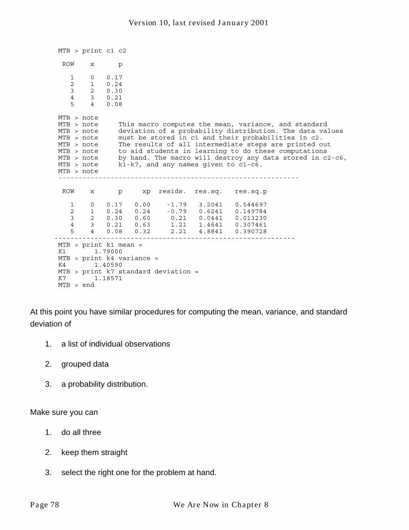
Version 10, last revised January 2001
MTB > print c1 c2
ROW x p
1 0 0.17 2 1 0.24 3 2 0.30 4 3 0.21 5 4 0.08
MTB > note MTB > note This macro computes the mean, variance, and standard MTB > note deviation of a probability distribution. The data values MTB > note must be stored in c1 and their probabilities in c2. MTB > note The results of all intermediate steps are printed out MTB > note to aid students in learning to do these computations MTB > note by hand. The macro will destroy any data stored in c2-c6, MTB > note k1-k7, and any names given to c1-c6. MTB > note ------------------------------------------------------------
ROW x p xp resids. res.sq. res.sq.p
1 0 0.17 0.00 -1.79 3.2041 0.544697 2 1 0.24 0.24 -0.79 0.6241 0.149784 3 2 0.30 0.60 0.21 0.0441 0.013230 4 3 0.21 0.63 1.21 1.4641 0.307461 5 4 0.08 0.32 2.21 4.8841 0.390728 ------------------------------------------------------------ MTB > print k1 mean = K1 1.79000 MTB > print k4 variance = K4 1.40590 MTB > print k7 standard deviation = K7 1.18571 MTB > end
At this point you have similar procedures for computing the mean, variance, and standard
deviation of
1. a list of individual observations
2. grouped data
3. a probability distribution.
Make sure you can
1. do all three
2. keep them straight
3. select the right one for the problem at hand.
Page 78 We Are Now in Chapter 8

Version 10, last revised January 2001
The last of these is not difficult. If you have a list of individual observations, use the first
method you learned. If you have grouped data, use the method for grouped data. If you have
a probability distribution, use the method for probability distributions.
Minitab contains a normal distribution table that can replace the one in your textbook (page
262). On pages 261-262, your textbook calculates the probability that a standard normal
variable is less than 1.5. Here’s how to do that on Minitab.
MTB > cdf 1.51.5000 0.9332
Here are the examples from page 262.
MTB > cdf -0.5-0.5000 0.3085
MTB > cdf 0.29480.2948 0.6159
The example concerning trees on pages 263-264 requires some calculations when done as it
is done in your textbook. Minitab does those automatically if you tell it the mean and standard
deviation (in that order) of the normal distribution you want to work with. (If you don’t tell it
otherwise, it assumes a standard normal distribution, i.e., one with a mean of 0 and a standard
deviation of 1.)
MTB > cdf 25;SUBC>normal distribution with a mean of 20 and std. dev. of 5.
25.0000 0.8413MTB > cdf 25;SUBC>norm 20 5.
25.0000 0.8413
We did that twice, writing everything out the first time, and showing how much things can be
abbreviated the second. In the menu system, click on Calc and select Probability
Distributions. Pick Normal for the type of distribution and type in the mean and standard
deviation in the boxes provided. Select Cumulative probability and Input Constant.
Then type in your value (25 in the example above) and click OK .
Minitab saves you the work of calculating the difference between the given value and the
mean, and then dividing that by the standard deviation. The result of this calculation is called a
We Are Now in Chapter 8 Page 79

Version 10, last revised January 2001
standard score. Standard scores are useful and important, and you should know how to
calculate them even if you use the normal table in Minitab rather than the one in the book.
Note that Minitab does not replace all calculations. If you want probabilities of being more
than some amount (page 264) or between two values (page 265), Minitab can replace the
table, but you will still have to do some minor arithmetic (see your textbook) with the numbers
Minitab provides.
So far we have looked at situations where you are given a value and want the probability that
goes with it. What if you are given a probability and want the value? Your text has a problem
on this (Problem 4 on page 286), but as far as we can see it never tells you how to do this!
Here’s how Minitab can help. This is part a of Problem 4.
MTB > invcdf 0.0010.0010 -3.0902
In the menu system, pick Inverse cumulative probability instead of Cumulative
probability.
New Minitab commands for Chapter 8:
invcdf
New Minitab macros for Chapter 8:
varpd
Minitab Assignment 8-A
Use the Minitab “varpd” macro to find the mean, variance, and standard deviation of the
probability distribution in Problem 6 on page 286.
Page 80 We Are Now in Chapter 8

Version 10, last revised January 2001
Minitab Assignment 8-B
Use the Minitab “varpd” macro to find the mean, variance, and standard deviation of the
probability distribution in Problem 7 on page 286.
Minitab Assignment 8-C
1. Use Minitab’s normal table to do Problem 3 on page 285.
2. Use Minitab’s normal table to do Problem 4 on page 286.
3. Use Minitab’s normal table to do Problem 5 on page 286.
We Are Now in Chapter 8 Page 81

Version 10, last revised January 2001
WHAT HAPPENS WHEN WE TAKE SAMPLES?
Your textbook discusses what happens when we take samples in general terms. This section
of your Minitab Guide gives an extended, concrete example of what happens when we take
samples. Although Minitab is used in developing the example, there is no new material on
Minitab here.
Most people learn better from examples than for theoretical discussions. In order to
understand the sampling process, we will look at a very simple situation where we know both
the population and all the possible samples that might be drawn from it. This is not what
happens in real life, but it does provide us with a simple model to help us understand what
does happen in real life.
As our example, we will take samples from the tiny population:
3, 6, 6, 9, 12, 15.
Clearly no one would need to take a sample if the population were this small, but our example
will serve like a scale model of a house that has not yet been constructed. No one could really
live in such a house, yet study of the model may tell us something about the real house.
Our experiment will consist of taking a sample of three numbers from this population. We will
calculate various statistics to describe our sample and see how they relate to population
parameters. To participate in this experiment, you should take one such sample yourself. The
rules of the game are that it should be a random sample, and that, once an item has been
selected for the sample, it can not be chosen again for the same sample. This is called
sampling without replacement, to distinguish it from sampling with replacement, in which
sampled items are tossed back into the selection pool and may be selected again. Under
sampling without replacement, our sample might contain two 6’s because there are two in the
population, but it could not contain two of any other number.
Once you have your sample, you should compute an assortment of one-number summaries
such as the mean, median, variance, standard deviation, and range. Your instructor may have
Page 82 We Are Now in Chapter 8

Version 10, last revised January 2001
you do this as an in-class activity or quiz. Doing this yourself is much more educational than
reading about it, but for the sake of this printed document we will let Minitab select a sample to
use here.
MTB > set into c1DATA> 3 6 6 9 12 15DATA> endMTB > name c1 ’Pop.’MTB > sample 3 observations from c1 and put them in c2MTB > print c2
C212 9 3
MTB > describe c2
N MEAN MEDIAN TRMEAN STDEV SEMEANC2 3 8.00 9.00 8.00 4.58 2.65
MIN MAX Q1 Q3C2 3.00 12.00 3.00 12.00
Once you have some results for your sample, you can compare them to the results obtained
by others in your class for other samples. Here is a list of all possible samples of three
observations from this population, along with summary statistics for each sample.
Below are all possible samples from the population 3,6,6,9,12,15.
I.D.# X1 X2 X3 Mean Median Variance Std.Dev. Range
1 3 6 6 5 6 3 1.73 32 3 6 9 6 6 9 3 63 3 6 12 7 6 21 4.58 94 3 6 15 8 6 39 6.24 125 3 6 9 6 6 9 3 66 3 6 12 7 6 21 4.58 97 3 6 15 8 6 39 6.24 128 3 9 12 8 9 21 4.58 99 3 9 15 9 9 36 6 1210 3 12 15 10 12 39 6.24 1211 6 6 9 7 6 3 1.73 312 6 6 12 8 6 12 3.46 613 6 6 15 9 6 27 5.2 914 6 9 12 9 9 9 3 615 6 9 15 10 9 21 4.58 916 6 9 12 9 9 9 3 617 6 9 15 10 9 21 4.58 918 6 12 15 11 12 21 4.58 919 6 12 15 11 12 21 4.58 920 9 12 15 12 12 9 3 6
You should use this to check the results for your own sample before going on.
We Are Now in Chapter 8 Page 83

Version 10, last revised January 2001
A common inference technique is to use the sample mean as an estimate of the population
mean. In discussing this we will need to use a notation that distinguishes between these two
means. We will use the traditional X with a bar over it to denote the sample mean and the
Greek letter “mu” µ to denote the population mean. The first thing to notice in our listing of all
possible samples is that the sample mean varies from one sample to the next. In this sense it
is a random variable. Its value depends on the outcome of the random experiment of selecting
a sample. The population mean, on the other hand, is a single number. Let’s see what it is in
this case.
MTB > describe c1
N MEAN MEDIAN TRMEAN STDEV SEMEAN Pop. 6 8.50 7.50 8.50 4.42 1.80
MIN MAX Q1 Q3 Pop. 3.00 15.00 5.25 12.75
How close was your sample mean to the population mean of µ=8.5? For the sample chosen by
Minitab, the sample mean was 8, fairly close to µ=8.5. Looking at the list of all possible
samples we can see how close other sample means came to the population mean. First, note
that no sample had a mean that was exactly equal to the population mean. Our sample mean
of 8 was unusually close. Other samples had means as low as 5 or as high as 12. We can
analyze this even better if we read the results for all 20 samples into Minitab.
MTB > read ’sampleb1.dat’ into c11-c1920 ROWS READ
ROW C11 C12 C13 C14 C15 C16 C17 C18 C19
1 1 3 6 6 5 6 3 1.73 3 2 2 3 6 9 6 6 9 3.00 6 3 3 3 6 12 7 6 21 4.58 9 4 4 3 6 15 8 6 39 6.24 12 . . .
MTB > name c11 ’Number’ c12 ’X1’ c13 ’X2’ c14 ’X3’ c15 ’Mean’ MTB > name c16 ’Median’ MTB > name c17 ’Variance’ c18 ’Std.Dev.’ c19 ’Range’ MTB > print c11-c19
ROW Number X1 X2 X3 Mean Median Variance Std.Dev. Range
1 1 3 6 6 5 6 3 1.73 3 2 2 3 6 9 6 6 9 3.00 6 3 3 3 6 12 7 6 21 4.58 9 4 4 3 6 15 8 6 39 6.24 12 5 5 3 6 9 6 6 9 3.00 6 6 6 3 6 12 7 6 21 4.58 9 7 7 3 6 15 8 6 39 6.24 12 8 8 3 9 12 8 9 21 4.58 9
Page 84 We Are Now in Chapter 8

Version 10, last revised January 2001
9 9 3 9 15 9 9 36 6.00 1210 10 3 12 15 10 12 39 6.24 1211 11 6 6 9 7 6 3 1.73 312 12 6 6 12 8 6 12 3.46 613 13 6 6 15 9 6 27 5.20 914 14 6 9 12 9 9 9 3.00 615 15 6 9 15 10 9 21 4.58 916 16 6 9 12 9 9 9 3.00 617 17 6 9 15 10 9 21 4.58 918 18 6 12 15 11 12 21 4.58 919 19 6 12 15 11 12 21 4.58 920 20 9 12 15 12 12 9 3.00 6
Then we can use the “tally” command to summarize the results on the sample means. (In the
problems at the end of this example you will probably do this tally by hand, so make sure you
understand how Minitab got the table below.)
MTB > tally c15
Mean COUNT5 16 27 38 49 410 311 212 1N= 20
From this we can compute some probabilities that describe how close the sample means are
to the population mean. How likely are we to get a sample mean that is within one unit of the
correct population mean of 8.5? Within one unit of 8.5 means somewhere between 7.5 and
9.5. There are 4 samples with a mean of 8 and four with a mean of 9 for a total of 8 out of 20,
or 40%. Thus we have a 40% chance of getting a sample mean within one unit of the
population mean. What about within two units? That would include the sample means of 7 and
10 as well, for a total of 14 out of 20 or 70%. Within three units of the population mean we find
90% of the sample means, and all the sample means lie within four units of the population
mean. These error bounds and their probabilities provide us with a measure of how accurate
the results of sampling are in this case. Of course, in real life we would have only one sample,
and we would not know the true population mean, so we could not compute error tolerances
and probabilities in quite this way. The amazing thing is that we actually can still compute
them, at least approximately. This possibility is based on a major theorem of statistics called
the Central Limit Theorem. This theorem has several parts which we will investigate in turn.
The first part had to do with the shape of the distribution of sample means. Here are some
We Are Now in Chapter 8 Page 85

Version 10, last revised January 2001
histograms showing the shapes of the population distribution along with the distributions of
some other statistics computed for these samples. We put the population and the two
measures of center on the same scale because they are measures of the same thing. The
measures of variability each get their own scale.
MTB > histogram c1 c15 c16; SUBC>same.
Histogram of C1 N = 6
Midpoint Count 3 1 * 4 0 5 0 6 2 ** 7 0 8 0 9 1 * 10 0 11 0 12 1 * 13 0 14 0 15 1 *
Histogram of Mean N = 20
Midpoint Count 3 0 4 0 5 1 * 6 2 ** 7 3 *** 8 4 **** 9 4 **** 10 3 *** 11 2 ** 12 1 * 13 0 14 0 15 0
Histogram of Median N = 20
Midpoint Count 3 0 4 0 5 0 6 10 ********** 7 0 8 0 9 6 ****** 10 0 11 0 12 4 **** 13 0 14 0 15 0
Page 86 We Are Now in Chapter 8

Version 10, last revised January 2001
MTB > histogram c17 c18 c19
Histogram of Variance N = 20
Midpoint Count5 2 **10 6 ******15 020 7 *******25 1 *30 035 1 *40 3 ***
Histogram of Std.Dev. N = 20
Midpoint Count1.5 2 **2.0 02.5 03.0 5 *****3.5 1 *4.0 04.5 7 *******5.0 1 *5.5 06.0 4 ****
Histogram of Range N = 20
Midpoint Count3 2 **4 05 06 6 ******7 08 09 8 ********10 011 012 4 ****
The population is slightly skewed toward high values. Most of the sample statistics have rather
nondescript distributions, except for the mean, which has the cutest little normal distribution
you ever did see. This is one part of the Central Limit Theorem, which says that, as the size of
the sample increases, the distribution of the sample means approaches a normal distribution.
Since the normal distribution is a well-known distribution whose values are readily available in
printed tables or on Minitab, we can make calculations about the distribution of sample means
even when we actually have only one sample mean and even when we do not know anything
about the population or its distribution. This is why we studied the normal distribution! Another
part of the Central Limit Theorem tells us that, although no particular sample mean may be
equal to the population mean, the sample means as a group equal the population mean on the
average.
We Are Now in Chapter 8 Page 87

Version 10, last revised January 2001
MTB > describe c15
N MEAN MEDIAN TRMEAN STDEV SEMEAN Mean 20 8.500 8.500 8.500 1.850 0.414
MIN MAX Q1 Q3 Mean 5.000 12.000 7.000 10.000
Here we can see that the average of the 20 sample means is equal to 8.5, the population
mean. Does this work out for the other sample statistics? Well, here are some basic
parameters for the population computed by the “describe” command on Minitab.
MTB > describe c1
N MEAN MEDIAN TRMEAN STDEV SEMEAN Pop. 6 8.50 7.50 8.50 4.42 1.80
MIN MAX Q1 Q3 Pop. 3.00 15.00 5.25 12.75
We also need variances. Here is the calculation of the population variance, usually denoted by 2σ , calculated by the var macro.
MTB > execute ’stats1/macros/var’ MTB > note MTB > note This macro computes the mean, variance, and standard MTB > note deviation of a set of data. The data must be stored in c1. MTB > note The results of all intermediate steps are printed out MTB > note to aid students in learning to do these computations MTB > note by hand. The macro will destroy any data stored in c2-c3 MTB > note and k1-k7. MTB > note ------------------------------------------------------------ ROW Pop. resids. res. sq.
1 3 -5.5 30.252 6 -2.5 6.253 6 -2.5 6.254 9 0.5 0.255 12 3.5 12.256 15 6.5 42.25
------------------------------------------------------------ MTB > print k1 The total = K1 51.0000 MTB > print k2 number of observations = K2 6.00000 MTB > print k3 mean = K3 8.50000 MTB > print k4 The sum of the squared residuals = K4 97.5000 MTB > print k5 degrees of freedom = K5 5.00000 MTB > print k6 variance = K6 19.5000 MTB > print k7 standard deviation =
Page 88 We Are Now in Chapter 8

Version 10, last revised January 2001
K7 4.41588MTB > end
By way of review, this is the same algorithm you should have used to compute the mean,
variance, and standard deviation of your sample. For comparison, here are the averages of
the various sample statistics.
MTB > describe c15-c19
N MEAN MEDIAN TRMEAN STDEV SEMEANMean 20 8.500 8.500 8.500 1.850 0.414Median 20 8.100 7.500 8.000 2.404 0.538Variance 20 19.50 21.00 19.33 11.78 2.63Std.Dev. 20 4.195 4.580 4.218 1.408 0.315Range 20 8.100 9.000 8.167 2.770 0.619
Let’s put these into a table for comparison.
average ofpopulation value sample values
mean 8.5 8.5median 7.5 8.1variance 19.5 19.5standard deviation 4.42 4.195range 12 8.1
We see that the sample mean and the sample variance have average values equal to the
corresponding population values. This is not an accident. It happens in any situation in which
we would use the sample mean or variance to estimate the corresponding population
parameters. We call such estimators unbiased. The other statistics in the table (median,
standard deviation, and range) do not have this property and are called biased estimators.
The range is particularly biased, and for this reason we usually do not use the sample range to
estimate the population range.
The third and final part of the Central Limit Theorem tells us something about how close the
sample means are to the population mean. While we generally prefer unbiased estimators to
biased estimators, being unbiased is not enough. Our estimator could be way too high half the
time, way too low the rest of the time, and still average out to be unbiased. We would also like
it to be reasonably close most of the time. We already know that this will be more or less true
for the sample means because they are more or less normally distributed. Thus most of the
observations are close to the center of the mound-shaped distribution, and we already know
We Are Now in Chapter 8 Page 89

Version 10, last revised January 2001
that the center is at the population mean. You can get a visual feel for what this means by
placing the population value on a histogram of the sampling distribution. Here are two extreme
cases, the unbiased mean and the highly biased range.
Histogram of Mean N = 20
Midpoint Count
5 1 *
6 2 **
7 3 ***
8 4 **** Population value falls right here
9 4 ****
10 3 ***
11 2 **
12 1 *
Histogram of Range N = 20
Midpoint Count 3 2 ** 4 0 5 0 6 6 ****** 7 0 8 0 9 8 ******** 10 0 11 0 12 4 **** Population value falls right here
Because the sampling distribution of the mean has a bell shape, and because it is centered on
the population mean, the sample values cluster around the population value. Although the
range has a sampling distribution that is not far from normal in this case, that does not help
much because the population value is not at the center. Instead, it is off at one end, so that
the sample values do not cluster around the population value.
When the sample values do cluster around the population value, we may want to measure how
close they are. Since the sampling distribution of the mean is approximately normal, the
variance and standard deviation are appropriate measures of variability to use. Since the
sampling distribution of any statistic is a probability distribution, we need to divide each
frequency by the total number of possibilities, 20, to get a probability distribution called the
sampling distribution of the mean.
Page 90 We Are Now in Chapter 8

Version 10, last revised January 2001
sample mean probability of getting that mean
5 0.056 0.107 0.158 0.209 0.20
10 0.1511 0.1012 0.05
Computing the mean, variance and standard deviation of such a distribution is similar (but not
identical) to the algorithm for grouped data. There is even a Minitab macro, called varpd, to
do it. As always, it is important to have the correct input. Remember that the correct input for a
simple mean and variance (macro var) is a list of all the data values (in c1). The proper input
for grouped data (macro vargroup) consists of the possible values (in c1) and their
frequencies (in c2). The proper input for calculations on a probability distribution is the
distribution itself, i.e., the values (in c1) and their probabilities (in c2).
MTB > let c2=c2/20MTB > name c2 " ’Prob.’MTB > execute ’stats1/macros/varpd’MTB > noteMTB > note This macro computes the mean, variance, and standardMTB > note deviation of a probability distribution. The data valuesMTB > note must be stored in c1 and their probabilities in c2.MTB > note The results of all intermediate steps are printed outMTB > note to aid students in learning to do these computationsMTB > note by hand. The macro will destroy any data stored in c2-c6,MTB > note k1-k7, and any names given to c1-c6.MTB > note------------------------------------------------------------
ROW x p xp resids. res.sq. res.sq.p1 5 0.05 0.25 -3.5 12.25 0.61252 6 0.10 0.60 -2.5 6.25 0.62503 7 0.15 1.05 -1.5 2.25 0.33754 8 0.20 1.60 -0.5 0.25 0.05005 9 0.20 1.80 0.5 0.25 0.05006 10 0.15 1.50 1.5 2.25 0.33757 11 0.10 1.10 2.5 6.25 0.62508 12 0.05 0.60 3.5 12.25 0.6125
------------------------------------------------------------MTB > print k1 mean =K1 8.50000MTB > print k4 variance =K4 3.25000MTB > print k7 standard deviation =K7 1.80278MTB > end
We Are Now in Chapter 8 Page 91

Version 10, last revised January 2001
Once again, we could not actually do these calculations in real life, because we would have
only one sample. It would be like trying to determine if a coin were fair with just one toss.
However, the third and final part of the Central Limit Theorem tells us the variance of the
sampling distribution of the mean in terms of the population variance.
variance of the sampling distribution of the mean =
2σ n––– × (1 − ––– )
n N
2Here σ is the population variance, n is the sample size, and N is the population size. We took
samples of size n=3 from a population of size N=6.
EXERCISES
1. Look back several pages to find out what the population variance was. Plug that into
the formula above to get the variance of the sampling distribution of the mean. Does
your result agree with the result above?
2. Use the table on page 65 to do the following.
a. Find the sampling distribution of the sample medians.
b. Find the mean, variance, and standard deviation of the distribution in Part a.
c. What is the population median?
d. Is the sample median an unbiased estimator of the population median?
Explain.
3. Use the table on page 65 to do the following.
a. Find the sampling distribution of the sample ranges.
b. Find the mean, variance, and standard deviation of the distribution in Part a.
Page 92 We Are Now in Chapter 8
Version 10, last revised January 2001
c. What is the population range?
d. Is the sample range an unbiased estimator of the population range? Explain.
4. Use the table on page 65 to do the following.
a. Find the sampling distribution of the sample standard deviations.
b. Find the mean, variance, and standard deviation of the distribution in Part a.
c. What is the population standard deviation?
d. Is the sample standard deviation an unbiased estimator of the population
standard deviation? Explain.
5. Use the table on page 65 to do the following.
a. Find the maximum value in each of the 20 possible samples.
b. Find the sampling distribution of the sample maximums.
c. Find the mean, variance, and standard deviation of the distribution in Part b.
d. What is the population maximum?
e. Is the sample maximum an unbiased estimator of the population maximum?
Explain.
6. Use the table on page 65 to do the following.
a. Find the minimum value in each of the 20 possible samples.
b. Find the sampling distribution of the sample minimums.
c. Find the mean, variance, and standard deviation of the distribution in Part b.
d. What is the population minimum?
e. Is the sample minimum an unbiased estimator of the population minimum?
Explain.
We Are Now in Chapter 8 Page 93

Version 10, last revised January 2001
7. Use the table on page 65 to do the following.
a. Find the proportion of 6’s in each of the 20 possible samples.
b. Find the sampling distribution of these proportions.
c. Find the mean, variance, and standard deviation of the distribution in Part b.
d. What is the proportion of 6’s in the population?
e. Is the sample proportion of 6’s an unbiased estimator of the population
proportion of 6’s? Explain.
f. Make a display of the sampling distribution of these proportions and describe
its shape.
8. Why can’t you find the sampling distribution of the mode?
9. Use the table on page 65 to do the following.
a. Find the total of each of the 20 possible samples.
b. Find the sampling distribution of the sample totals.
c. Find the mean, variance, and standard deviation of the distribution in Part b.
d. What is the population total?
e. Is the sample total an unbiased estimator of the population total? Explain.
f. Make a display of the sampling distribution of these totals and describe its
shape.
Page 94 We Are Now in Chapter 8

Version 10, last revised January 2001
10. Use the table on page 65 to do the following.
a. Find the variance value in each of the 20 possible samples.
b. Find the sampling distribution of the sample variances.
c. Find the mean, variance, and standard deviation of the distribution in Part b.
d. What is the population variance?
e. Is the sample variance an unbiased estimator of the population variance?
Explain.
Chapter 9
In Chapter 9 you will learn how to:
• Use Minitab to take a random sample
You know that Minitab has a normal distribution table that can be used in place of the one in
your book. It also has facilities for selecting random samples and generating random numbers
that can replace the table on page 298 of your textbook. At the bottom of that page is an
example of choosing a sample of 10 from a population of 83. The process involves quite a few
rules and calculations as done there. Minitab is much simpler. Just put the numbers from 1 to
83 in a column and use the sample command. You can enter the numbers from 1 to 83 as
1:83. To use the menus to sample, select Calc , Random Data, Sample from columns.
MTB > set into c1DATA> 1:83DATA> end
We Are Now in Chapter 9 Page 95

Version 10, last revised January 2001
MTB > print c1
C1 1 2 3 4 5 6 7 8 9 10 11 12 13 14 15 16 17 18 19 20 21 22 23 24 25 26 27 28 29 30 31 32 33 34 35 36 37 38 39 40 41 42 43 44 45 46 47 48 49 50 51 52 53 54 55 56 57 58 59 60 61 62 63 64 65 66 67 68 69 70 71 72 73 74 75 76 77 78 79 80 81 82 83 MTB > sample 10 values from c1 and put them in c2 MTB > print c2
C2 55 50 82 58 33 41 62 48 39 78
Of course, we don’t get the same sample your book did. If we did, it would not be random!
The second half of Chapter 9 discusses the standard error of a mean and of a proportion. The
standard error of the mean is printed by the Minitab describe command and labeled
SEMEAN. Proportions are handled by coding them as 0-1 variables and then treating the data
as measurement data (see Section 4.4 of your text). For means and proportions, Minitab
assumes that the sample is an insignificant fraction of the population. If this is not the case,
you need to make a correction by hand. (See pages 305-306 of your text.) Here’s the chicken
preference data from pages 320-311.
MTB > print c1
PreferCG 0 1 0 1 1 0 0 0 0 0 1 0 0 0 0 0 0 1 0 1 0 1 0 1 1 0 1 1 0 1 1 0 1 1 1 1 1 0 0 0 0 1 1 0 0 0 1 1 1 1 1 1 1 1 1 1 0 0 1 0 1 0 1 0 0 1 1 1 1 0 1 1 0 1 0 1 1 1 1 1 1 1 0 1 1 0 0 1 1 0 0 1 0 1 0 1 1 0 1 1 1 1 0 0 1 1 0 0 0 0 1 1 0 0 0 0 1 0 1 0 1 1 1 1 0 0 0 0 0 1 0 0 0 0 0 1 0 1 1 0 1 0 1 0 1 0 1 1 1 0 0 0 1 1 0 1 0 0 0 1 1 1 0 1 1 0 1 1 0 0 1 0 1 1 0 1 0 1 1 0 0 1 0 1 1 0 0 1 0 1 0 0 0 1 1 0 1 0 1 0 1 1 0 1 0 0 0 0 0 1 1 1 0 1 1 0 1 1 0 0 1 1 1 0 0 0 0 0 1 1 0 1 1 0 0 0 0 0 1 0 1 0 0 1 0 0 1 1 1 0 1 1 0 0 0 1 1 1 1 0 0 1 1 0 1 0 1 1 0 1 1 1 1 1 0 1 0 1 1 1 1 0 1 0 0 1 0 1 1 1 0 1 1 1 0 1 0 0 1 1 0 1 1 1 1 0 1 0 1 1 1 1 1 1 1 0 0 0 0 1 0 1 0 0 0 0 0 1 0 0
Continue? N
Page 96 We Are Now in Chapter 9

Version 10, last revised January 2001
MTB > describe c1
N MEAN MEDIAN TRMEAN STDEV SEMEANPreferCG 371 0.5310 1.0000 0.5345 0.4997 0.0259
MIN MAX Q1 Q3PreferCG 0.0000 1.0000 0.0000 1.0000
Here we coded people who preferred “Cookin’ Good” as 1’s. The mean of a 0-1 variable is the
proportion of 1’s. Here, 0.5310 = 53.1% prefer “Cookin’ Good”, as on page 311 of your text.
Minitab gives the standard deviation as 0.4997 and the standard error of the mean as 0.0259,
in close agreement with page 311 of your text.
New Minitab commands for Chapter 9:
sample
Minitab Assignment 9-A
Use Minitab to do Problem 8 on pages 316-317. The easy way to do it is to just take a sample
from the NUMBER OF FRANCHISES column. Note that you will have to give Minitab some
assistance with the standard error calculation.
Minitab Assignment 9-B
Use Minitab to do Problems 7-10 on pages 316-317. The easy way to do it is to just take
samples from the NUMBER OF FRANCHISES column. Note that you will have to give Minitab
some assistance with the standard error calculation.
Minitab Assignment 9-C
Use Minitab to do Problem 14 on page 318. What is the population here? How big is it?
We Are Now in Chapter 9 Page 97

Version 10, last revised January 2001
Minitab Assignment 9-D
Use Minitab to find the standard error of the proportion of rainy days in the data from Section
4.4 of your text. Check your answer with a hand calculation. What is the population here? Is
this a random sample?
Minitab Assignment 9-E
Use Minitab to do Exercise Set 9.3 on page 304 of your text. The data are in the file
smx02.15.
Minitab Assignment 9-F
The data for this exercise are in the file smt04.04.
1. Use Minitab to take a sample of 50 of the chest measurements of Scottish soldiers
discussed on pages 120-121 of your text.
2. Find the population mean.
3. Find the sample mean. Is it close to the population mean?
4. Make displays of the population shape and the sample shape and compare them.
Page 98 We Are Now in Chapter 9

Version 10, last revised January 2001
Chapter 10
In Chapter 10 you will learn how to:
• change erroneous data
• find confidence intervals for means
• find confidence intervals for medians
• find confidence intervals for proportions
Minitab contains a table for the t-distribution, but it is actually less convenient than the tables
provided in your textbook. Fortunately, you don’t need either one to do a confidence interval
on Minitab. Here is the example concerning Dr. Robert’s bees from page 325.
MTB > print c1
width2.88 2.83 2.86 2.80 2.91 2.97 2.77 2.88 2.80 2.86 2.942.91 2.83 2.88 2.88 2.80 2.80 2.83 2.86 2.88
MTB > stem c1
Stem-and-leaf of width N = 20Leaf Unit = 0.010
1 27 71 275 28 00008 28 3338 28(3) 28 6669 28 888884 29 112 292 29 41 29 7
We Are Now in Chapter 10 Page 99

Version 10, last revised January 2001
MTB > tinterval 95% c1
N MEAN STDEV SE MEAN 95.0 PERCENT C.I. width 20 2.8585 0.0516 0.0115 ( 2.8343, 2.8827)
From the menus, select Stat , Basic Statistics, 1-Sample t. Of course we should make
some sort of display of the data before doing (or having Minitab do) any calculations with it. All
inference techniques are based on certain “assumptions” that vary from technique to
technique. These are not things you should “assume”, but rather things that you need to
check. If the assumptions are not met, your inferences are likely to be invalid.
Assumptions
For every inference technique studied in this course, we assume that the
data are a random sample from the population of interest.
Minitab cannot check that assumption, you have to look at how the data
were gathered.
Specific techniques have additional assumptions.
For a confidence interval for a mean, another assumption is that the population is more or less
normally distributed. Usually, we cannot actually check the entire population, so we look at the
sample data. Here it looks a little ratty, but not too far from normal.
Note that there is no space between the t and the interval in tinterval.
If we knew that the population standard deviation was 0.06, we would use the zinterval
command (1-Sample z on the menu).
MTB > zinterval 95% pop. std. dev. = 0.06 c1
THE ASSUMED SIGMA =0.0600
N MEAN STDEV SE MEAN 95.0 PERCENT C.I. width 20 2.8585 0.0516 0.0134 ( 2.8322, 2.8848)
Page 100 We Are Now in Chapter 10

Version 10, last revised January 2001
I’m sure you can guess how to get 90% or 99% or 99.44% confidence intervals on the
command line. In the menus, click on the Options button in the dialog box. If you forget to
specify a confidence level, Minitab will do a 95% confidence interval.
For proportions, we use 0-1 coding as described in Section 4.4 of your textbook. Here is the
example from pages 339-340.
Worksheet retrieved from file: stats1a/sme10.06MTB > info
COLUMN NAME COUNTC1 CHANGE? 800
CONSTANTS USED: NONE
MTB > print c1
CHANGE?1 0 0 0 0 1 1 1 1 0 0 0 0 1 00 1 1 1 0 1 0 1 0 0 0 1 1 1 10 1 1 0 1 1 0 1 0 1 1 0 0 0 00 1 0 1 0 0 0 0 0 1 0 0 0 1 10 0 1 0 1 0 1 0 0 0 1 1 0 1 10 0 1 0 0 1 1 0 0 1 0 0 1 1 00 1 1 0 1 0 1 1 1 0 0 0 0 1 00 1 0 1 0 0 1 1 0 1 0 0 0 0 11 1 1 0 1 0 0 0 1 0 1 1 1 0 10 1 0 1 1 0 1 0 0 1 1 1 1 1 11 0 0 0 0 0 0 0 0 0 0 0 1 1 0
Many rows of 0’s an 1’s left out to save trees.
0 1 0 1 0 1 0 0 1 0 0 0 1 1 01 0 0 1 0 1 1 0 1 0 1 0 0 1 01 1 0 1 0
MTB > tinterval c1
N MEAN STDEV SE MEAN 95.0 PERCENT C.I.CHANGE? 800 0.4600 0.4987 0.0176 ( 0.4254, 0.4946)
In this case, the population is obviously not normally distributed.
MTB > histogram c1
Histogram of CHANGE? N = 800Each * represents 10 obs.
Midpoint Count0 432 ********************************************1 368 *************************************
We Are Now in Chapter 10 Page 101

Version 10, last revised January 2001
MTB > stem c1
Stem-and-leaf of CHANGE? N = 800 Leaf Unit = 0.010
(432) 0 0000000000000000000000000000000000000000000000000000000000000000+ 368 1 368 2 368 3 368 4 368 5 368 6 368 7 368 8 368 9 368 10 0000000000000000000000000000000000000000000000000000000000000000+
However, for 0-1 data, if the sample is fairly large, the Central Limit Theorem will make the
sample means normally distributed, and our confidence interval will be valid. How large does
the sample have to be? There are many different rules of thumb. One simple on is this: if your
confidence interval contains any numbers outside the range of 0 to 1, something is wrong!
Here are a couple examples of that.
MTB > set into c1 DATA> 12(1) 3(0) DATA> end MTB > tint c1
N MEAN STDEV SE MEAN 95.0 PERCENT C.I. CHANGE? 15 0.800 0.414 0.107 ( 0.571, 1.029)
MTB > set into c1 DATA> 12(0) 3(1) DATA> end MTB > tint c1
N MEAN STDEV SE MEAN 95.0 PERCENT C.I. CHANGE? 15 0.200 0.414 0.107 ( -0.029, 0.429)
MTB > stem c1
Stem-and-leaf of CHANGE? N = 15 Leaf Unit = 0.010
(12) 0 0000000000003 13 23 33 43 53 63 73 83 93 10 000
Page 102 We Are Now in Chapter 10

Version 10, last revised January 2001
The small sample size combined with the lack of symmetry seen in the stem and leaf plot
combine to create nonsense confidence intervals here.
Minitab can also do the nonparametric confidence interval for the median illustrated below
with the swordfish data on pages 343-344. From the menus, select Stat , Nonparametrics,
1-Sample Sign. You should do a confidence interval for the median in any situation in which
the median would be a better measure of center than the mean. There are no assumptions
for this technique other than a random sample.
MTB > print c1
mercury1.2 2.1 1.6 1.5 0.9 1.1 1.0 1.3 0.3 1.2 0.60.8
MTB > sort c1 in c2
MTB > print c2
C20.3 0.6 0.8 0.9 1.0 1.1 1.2 1.2 1.3 1.5 1.62.1
MTB > stem c2
Stem-and-leaf of C2 N = 12Leaf Unit = 0.10
1 0 31 02 0 64 0 896 1 016 1 2233 1 52 1 61 11 2 1
MTB > sinterval 95% c2
SIGN CONFIDENCE INTERVAL FOR MEDIAN
ACHIEVEDN MEDIAN CONFIDENCE CONFIDENCE INTERVAL POSITION
C2 12 1.150 0.8540 ( 0.900, 1.300) 40.9500 ( 0.826, 1.447) NLI0.9614 ( 0.800, 1.500) 3
This tells you something your book glossed over. If you follow the discussion there, the
authors tell you to sort the data and count in three from each end to get a 95% confidence
interval. Minitab shows this interval (on the last line), but tells you that this is actually a
0.9614=96.14% confidence interval. Two lines above, it tells you that counting in 4 would give
We Are Now in Chapter 10 Page 103

Version 10, last revised January 2001
you an 85.4% confidence interval. Your book’s method always gives you one or the other of
these two intervals, because you can’t get an exact 95.00% confidence interval by counting in
from the ends. Minitab tries to eyeball a 95% confidence interval somewhere between 85.5%
and 96.14% and labels this NLI (for non-linear-interpolation). We can compare this with a 95%
confidence interval for the mean, as your book did on pages 343-344.
MTB > tinterval 95% c2
N MEAN STDEV SE MEAN 95.0 PERCENT C.I. C2 12 1.133 0.475 0.137 ( 0.831, 1.436)
This is pretty close to the NLI interval for the median of 0.826 to 1.447.
Now let’s change the 2.1 in the original data in c1 into an outlier of 5, as your book did on page
344. We use let. You could also edit the Data Window, but this leaves no record in the
Session Window.
MTB > let c1(2)=5 MTB > print c1
mercury 1.2 5.0 1.6 1.5 0.9 1.1 1.0 1.3 0.3 1.2 0.6 0.8
MTB > stem c1
Stem-and-leaf of mercury N = 12 Leaf Unit = 0.10
1 0 34 0 689(5) 1 012233 1 561 21 21 31 31 41 41 5 0
MTB > sinterval 95% c1
SIGN CONFIDENCE INTERVAL FOR MEDIAN
ACHIEVEDN MEDIAN CONFIDENCE CONFIDENCE INTERVAL POSITION
mercury 12 1.150 0.8540 ( 0.900, 1.300) 4 0.9500 ( 0.826, 1.447) NLI 0.9614 ( 0.800, 1.500) 3
Page 104 We Are Now in Chapter 10

Version 10, last revised January 2001
MTB > tinterval 95% c1
N MEAN STDEV SE MEAN 95.0 PERCENT C.I.mercury 12 1.375 1.199 0.346 ( 0.613, 2.137)
ndLet C1(2)=5 tells Minitab to change the 2 number in C1 into a 5. As a result of this
change, the confidence intervals for the median have not changed at all, while that for the
mean has changed quite a bit. You can also see that the outlier has changed the sample
mean a bit and the sample standard deviation a whole lot, more than doubling it. It is the
change in the standard deviation that is responsible for most of the change in the confidence
interval.
New Minitab commands for Chapter 10:
sinterval tinterval zinterval
Minitab Assignment 10-A
Use Minitab to do parts a and c of Problem 5 on page 348. Be sure to make a display of the
data and make sure all assumptions are met.
Minitab Assignment 10-B
Use Minitab to do Problem 8 on page 348.
Minitab Assignment 10-C
Use Minitab to do Problem 9 on page 348.
Minitab Assignment 10-D
Use Minitab to do Problem 15 on page 349. Be sure to make a display of the data and check
whether all assumptions are met for each confidence interval.
We Are Now in Chapter 10 Page 105

Version 10, last revised January 2001
Minitab Assignment 10-E
Use Minitab to do Problem 16 on page 349. Be sure to make a display of the data used for
your confidence interval and check whether all assumptions are met.
Minitab Assignment 10-F
Use Minitab to do Problem 20 on page 350. You need not transform things back again. Be
sure to make a display of the data and check whether all assumptions are met.
Chapter 11
In Chapter 11 you will learn how to:
• test a hypothesis about the mean of a single population
• test a hypothesis about the median of a single population
• test a hypothesis about a proportion for a single population
Chapter 11 of your textbook tells you how to interpret confidence intervals in order to do
hypothesis tests. There are no new Minitab commands for this. You just use the ones from
the previous chapter. For example, here is the candy bar data from page 356.
MTB > info
COLUMN NAME COUNT C1 Weight 6
CONSTANTS USED: NONE
Page 106 We Are Now in Chapter 10

Version 10, last revised January 2001
MTB > dotplot c1
. . . : .-------+---------+---------+---------+---------+---------Weight
0.960 0.975 0.990 1.005 1.020 1.035MTB > tinterval c1
N MEAN STDEV SE MEAN 95.0 PERCENT C.I.Weight 6 0.9917 0.0299 0.0122 ( 0.9602, 1.0231)
The confidence interval of 0.9602 to 1.0231 is in close agreement with your text. Since the
hypothesized weight of 1 oz. is in the interval, we do not reject the null hypothesis that µ=1.
(The Greek letter µ is the usual symbol for the population mean.) To use the jargon, we would
say that the population mean is not significantly different from 1.
The assumptions underlying this test are that we have a random sample from a normally
distributed population. The text says they took a random sample, so that’s OK. The dotplot
looks reasonable for a sample of six observations from a normal distribution. The confidence
interval (and the hypothesis test) are very robust to departures from normality. It does not
matter much whether the population distribution is bell-shaped, as long as it does not have
1. long, fat tails
2. extreme skewness
3. outliers.
These do not seem to be a problem here, though it is hard to tell much with such a small
sample.
On page 360, your text discusses “another way to do a t-test”. Here is an example of that
based on the same candy bar weights discussed above.
MTB > ttest mu=1 c1
TEST OF MU = 1.0000 VS MU N.E. 1.0000
N MEAN STDEV SE MEAN T P VALUEWeight 6 0.9917 0.0299 0.0122 -0.68 0.53
The ttest command requires that you tell Minitab what hypothesis you would like to test.
Here we typed “mu=1”. (Minitab can’t understand Greek, so we could not type “µ=1”, so I
We Are Now in Chapter 11 Page 107

Version 10, last revised January 2001
spelled out “µ”.) The t-statistic, T=−0.68, was calculated by Minitab according to the formula in
your book (p.360) as
t = (sample mean − hypothesized population mean)/est.s.e.(mean)
= (0.9917−1)/0.0122
= −0.68
Your book tells you to compare the absolute value of the t-statistic (here 0.68) to the critical
value from your table (page 323) with n−1=6−1=5 degrees of freedom and α=0.05. The
absolute value of the calculated t (0.68) is less than the critical t=2.571, so you do not reject
the null hypothesis. This is the same conclusion we reached when we did the hypothesis test
by computing and interpreting a confidence interval. You can also reach this conclusion by
comparing Minitab’s p-value of 0.53 to α=0.05. (See page 361 of your text.) The rule is,
If p<α then reject the null hypothesis.
For example, for the candy bar data, p=0.53. Since this is not less than α=0.05, we do not
reject the null hypothesis.
If these methods give the same results, does it matter which way we do it? As your book
points out, the confidence interval provides more information than the results of the ttest
command. The ttest tells us only that the population mean could be 1; the confidence interval
tells us µ is probably somewhere between 0.9602 and 1.0231. This gives us a better idea of
just how close to 1 µ is likely to be. On the other hand, it is unusual to be able to choose
between these different ways of testing hypotheses. For example, when your textbook tests
other hypotheses in later chapters, it does so in a way analogous to what ttest does,
because there is no corresponding confidence interval to interpret. Thus, you need to know
how to do hypothesis tests by comparing a calculated test statistic (like the t-statistic) to a
critical value from a statistical table, or you need to know how to interpret a p-value. In the
menu system, the hypothesis tests are located in the same place as the corresponding
confidence intervals. Just enter a hypothetical value to test.
Here are all three ways of attacking the voting example on page 357.
MTB > info
COLUMN NAME COUNT C1 For 1251
Page 108 We Are Now in Chapter 11

Version 10, last revised January 2001
CONSTANTS USED: NONE
MTB > tinterval c1
N MEAN STDEV SE MEAN 95.0 PERCENT C.I.For 1251 0.6227 0.4849 0.0137 ( 0.5958, 0.6496)
MTB > ttest pi=0.5 c1
TEST OF MU = 0.5000 VS MU N.E. 0.5000
N MEAN STDEV SE MEAN T P VALUEFor 1251 0.6227 0.4849 0.0137 8.95 0.0000
The Greek letter π is used in statistics to signify the population proportion. (This should not
be confused with the constant 3.14159… used in geometry.) We use p for the sample
proportion. It is important to keep these two proportions straight. In practice, p is known (Here
it is 0.6227.), but what we want to know is π. In this case we wanted to know if the population
proportion was one-half or 0.5. Since Minitab doesn’t do Greek, we spelled out π. The
calculated t-statistic of 8.95 far exceeds the critical value of 1.96, so we reject the hypothesis
π=0.5. There is no display of the data because it is 0-1 data, so we are not likely to have
problems with
1. long, fat tails
2. extreme skewness
3. outliers.
It might have been wise to do a describe though, and check the max and min to see if we
made any typos. The Greek letter alpha (α) is used to indicate the significance level of a test.
This is related to the confidence level c by the equation α=1−c because c is the probability of a
randomly chosen confidence interval containing the population value, while α is the probability
of the complementary event that it does not. Thus a 95%=0.95 confidence interval
corresponds to a test with α=5%=0.05. (This relationship is discussed on page 368 of your
text. You can see that α is also the probability of a Type I error.) All of the tests we have done
so far have used α=0.05.
The value of α is also the basis interpreting the p-value. For the voting example, the p-value is
reported as “0.0000”. This is certainly less than α=0.05, so in this case we reject the null
hypothesis. (The “0.0000” does not mean exactly 0, but rather some small probability that
rounds off to 0.0000. It could be 1 in 25000, 1 in a million, or 1 in a trillion.)
We Are Now in Chapter 11 Page 109

Version 10, last revised January 2001
Section 11.8 of your text discusses the s-test that is preferred for data that has
1. long, fat tails
2. extreme skewness
3. or outliers.
Here is the example on changes in net worth of mutual savings banks in Washington (page
373). The data are in smt11.02.
MTB > info
COLUMN NAME COUNT C1 9
CONSTANTS USED: NONE MTB > dotplot c1
:. . . :. .
-+---------+---------+---------+---------+---------+-----C1-24000000 -12000000 0 12000000 24000000 36000000
MTB > tinterval c1
N MEAN STDEV SE MEAN 95.0 PERCENT C.I. C1 9 -231222 14772135 4924045 (-1.2E+07,11126732)
MTB > sinterval c1
SIGN CONFIDENCE INTERVAL FOR MEDIAN
ACHIEVEDN MEDIAN CONFIDENCE CONFIDENCE INTERVAL POSITION
C1 9 -1449000 0.8203 (-4197000, -869000) 30.9500 (-5847735, -387214) NLI0.9609 (-6335000, -245000) 2
MTB > stest population median=0 c1
SIGN TEST OF MEDIAN = 0.00000 VERSUS N.E. 0.00000
N BELOW EQUAL ABOVE P-VALUE MEDIAN C1 9 8 0 1 0.0391 -1449000
Symmetry is not too bad, but we seem to have very long tails or two outliers, which makes the
tinterval for the mean suspect. The median would be a more appropriate measure of
center for this data. The width of the 95% NLI confidence interval for the median is
−387214−(−5847735)=$5460521 or about $5 million. The width of the 95% confidence interval
for the mean is about 11126732−(−12000000)=$23126732 or about $23 million − roughly four
times wider. We can test the hypothesis that the population median is 0 by seeing if 0 is in the
Page 110 We Are Now in Chapter 11

Version 10, last revised January 2001
confidence interval. It is not in the NLI 95% confidence interval nor the 96% confidence
interval computed in your textbook, so we reject the null hypothesis. We can also do this test
by comparing the p-value of 0.0391 computed by Minitab to our α of 0.05. Since p<α, we
reject the hypothesis. Note that stest does not give a test statistic to compare to a critical
value in a table, so we can not test the hypothesis that way. The only assumption to be
checked is that we have a random sample. We do not, and we have a much lower opinion of
these results than Siegel does. However, they do serve the purpose of showing you how to do
an stest. Note from the tinterval output that we cannot reject µ=0. As always, it is
important to select the right procedure.
Let’s close this section with a summary of the pros and cons of the three ways we have seen
for testing hypotheses. Computing a test statistic and comparing it to a critical value from a
table is the oldest and most common method. It provides less information than a confidence
interval, and statisticians (such as Siegel) generally prefer to use a confidence interval
whenever possible. The approach using p-values is the most recent. It is generally preferred
by statisticians in situations where a confidence interval is not possible. To understand why,
you need to know a little bit more about p-values.
The p-value is the smallest α for which we would just barely reject the null hypothesis. Thus,
for the candy bar data, with p=0.53, you would not reject the hypothesis unless α were 0.53 or
more. Since α is the probability of making a Type I error, we definitely would not want it to be
as big as 0.53, as then we would make a Type I error more often than not. In other words, for
the candy bar data we would not reject the null hypothesis for any reasonable α. There is
essentially no support at all in the data for rejecting the null hypothesis. For the voting data,
p=0.0000. This is smaller than any α we have a table for. In other words, in this case we
would reject the null hypothesis for any reasonable α. The data give extremely strong support
for rejecting the null hypothesis. Finally, in the case of the mutual savings banks, p=0.0391.
Thus, we would reject the null hypothesis if α=0.05 or 0.10, but not if α=0.02 or 0.01. Here
whether we reject the null hypothesis depends on the α and the evidence of the sample is less
conclusive.
In general, the p-value is a measure of how consistent the data are with the null hypothesis. In
our examples, we have seen cases where it is quite consistent (candy bars, p=0.53), extremely
inconsistent (voters, p=0.0000), and fairly inconsistent (banks, p=0.0391). The smaller the p-
value, the less support the data give to the null hypothesis. Thus the p-value gives us more
information than just whether to reject or not reject, and this is why it is preferred to the
technique of comparing a calculated value to a critical value. On the other hand, it gives us
We Are Now in Chapter 11 Page 111

Version 10, last revised January 2001
less information than a confidence interval, and it requires a computer, very complex
computations, or very extensive statistical tables in order to be calculated. Here are the
choices in order of preference:
1. confidence interval if possible
2. p-value if available
3. traditional method if all else fails
Note that the assumptions for each procedure are the same no matter how you carry out
the procedure!
New Minitab commands for Chapter 11:
stest ttest ztest
Minitab Assignment 11-A
Use Minitab to do Problems 13-16 on page 378. Be sure to write a complete sentence
indicating whether each drug is effective and to make an appropriate display of the data. State
the assumptions underlying the inference techniques you use, and evaluate each assumption
to see if it is met.
Minitab Assignment 11-B
Use Minitab to do Problem 23 on page 379. Do the hypothesis test by interpreting the
confidence interval.
Minitab Assignment 11-C
Test the hypothesis that it rains more often than not in Seattle using the data from page 127 of
your textbook (file sme04.06) and comparing an appropriate p-value to α=0.05. State the
assumptions underlying your inference, and evaluate each assumption to see if it is met. Use
Page 112 We Are Now in Chapter 11

Version 10, last revised January 2001
the describe command. Explain why you do not need to plot the data. (If you don’t know,
plot it and see!)
Minitab Assignment 11-D
Use Minitab to do #28 in Exercise Set 11.9 on pages 374-375 of your text. Is there anything
about the data that suggests one should use the median rather than the mean? If there is,
what is it?
Minitab Assignment 11-E
Use Minitab to do #29 in Exercise Set 11.9 on pages 374-375 of your text. Is there anything
about the data that suggests one should use the median rather than the mean? If there is,
what is it?
Minitab Assignment 11-F
Use Minitab to do #30 in Exercise Set 11.9 on pages 374-375 of your text. Is there anything
about the data that suggests one should use the median rather than the mean? If there is,
what is it?
Minitab Assignment 11-G
Use Minitab to do #31 in Exercise Set 11.9 on pages 374-375 of your text. Is there anything
about the data that suggests one should use the median rather than the mean? If there is,
what is it?
We Are Now in Chapter 11 Page 113

Version 10, last revised January 2001
Chapter 12
In Chapter 12 you will learn how to:
• find a confidence interval for a difference between two means
• test a hypothesis about a difference between two means
In Chapters 10 and 11 you learned how to do confidence intervals and hypothesis tests for a
single variable. We looked at means and medians for measurement data, and proportions for
categorical data (with two categories). These situations represent the simplest inference
situations, and so we began our studies with them. However, in practice we are much more
likely to be interested in the relationship between two or more variables than in a single
variable alone. Most of the rest of your book is devoted to relationships between two
variables. Chapter 12 and Chapter 13 look at relationships between one categorical and one
measurement variable. Chapter 14 looks at relationships between two categorical variables
(as well as the case of a single categorical variable with more than two categories). Finally,
Chapter 15 looks at the relationship between two measurement variables.
Here we are concerned with Chapter 12, which treats the simple case in which a single
measurement variable depends on a categorical variable with two categories. In this situation,
we generally start by making separate displays or computing separate statistics for each of the
two categories before doing any inference. For that reason, this chapter is divided into
sections on describing data and making inferences.
Description
There are examples involving displays on pages 386-392 of your text. It is very important to
note that we want to get our displays on the same scale. Your book only does a good job__ __ ____ _____ _ _ _
Page 114 We Are Now in Chapter 12

Version 10, last revised January 2001
of this in the display on page 389. The first data set appears on page 393. It involves
comparing the effects of two categories of air filter (CLEAN and DIRTY) on the gas mileage of
automobiles.
Worksheet retrieved from file: stats1a/smt12.01
MTB > info
COLUMN NAME COUNTC1 CLEAN 10C2 DIRTY 10
CONSTANTS USED: NONE
MTB > dotplot c1 c2
. . . . : . . . .-------+---------+---------+---------+---------+---------CLEAN
20.0 22.5 25.0 27.5 30.0 32.5
. . : . . . : .+---------+---------+---------+---------+---------+-------DIRTY
16.0 18.0 20.0 22.0 24.0 26.0
These dotplots do not do a good job of helping us to compare the centers or variabilities of the
two data distributions because they are on different scales. This forces our eyes to try to
separate out the differences due to the different scales from the differences between the two
groups of numbers. We can easily get two (or more) dotplots (or histograms) on the same
scale with the same subcommand.
MTB > dotplot c1 c2;SUBC> same.
. . . .: . . . .+---------+---------+---------+---------+---------+-------CLEAN
. . : . . . : .+---------+---------+---------+---------+---------+-------DIRTY
15.0 18.0 21.0 24.0 27.0 30.0
We Are Now in Chapter 12 Page 115

Version 10, last revised January 2001
MTB > histogram c1 c2
Histogram of CLEAN N = 10
Midpoint Count 19 1 * 20 0 21 0 22 1 * 23 0 24 1 * 25 3 *** 26 2 ** 27 0 28 1 * 29 0 30 0 31 1 *
Histogram of DIRTY N = 10
Midpoint Count 16 1 * 17 0 18 0 19 0 20 1 * 21 2 ** 22 1 * 23 2 ** 24 0 25 2 ** 26 0 27 1 *
MTB > histogram c1 c2; SUBC> same.
Histogram of CLEAN N = 10
Midpoint Count 16 0 18 0 20 1 * 22 1 * 24 2 ** 26 4 **** 28 1 * 30 0 32 1 *
Histogram of DIRTY N = 10
Midpoint Count 16 1 * 18 0 20 1 * 22 4 **** 24 1 * 26 2 ** 28 1 * 30 0 32 0
Page 116 We Are Now in Chapter 12

Version 10, last revised January 2001
In this case the original two histograms are on nearly the same scale, but that will not always
be the case. Unfortunately, the same subcommand does not work with a stem and leaf plot.
MTB > stem c1 c2;SUBC> same.* ERROR * Subcommand in error -- subcommand ignoredSUBC> .
Stem-and-leaf of CLEAN N = 10Leaf Unit = 1.0
1 1 91 22 2 2(5) 2 445553 2 62 2 81 3 1
Stem-and-leaf of DIRTY N = 10Leaf Unit = 1.0
1 1 61 15 2 01115 2 233 2 551 2 7
Stem and leaf displays can be put on the scale of your choice with the increment
subcommand. We will learn more about that later. Even if you use this subcommand, the
displays will not be aligned with one another as dotplots are. If you are very fond of stem and
leaf displays (or histograms), you can have Minitab make them on the same scale, cut them
out, line them up by hand, and paste them in place.
CLEAN DIRTY
Midpoint Count Count16 0 1 *18 0 020 1 * 1 *22 1 * 4 ****24 2 ** 1 *26 4 **** 2 **28 1 * 1 *30 0 032 1 * 0
The dotplots probably make it easiest to see any differences in both center and variability
because the dotplots are plotted on the same scale and lined up one atop the other. However,
they may not be very good for showing the shape of the distribution, especially for small
We Are Now in Chapter 12 Page 117

Version 10, last revised January 2001
samples. Thus, we may want dotplots on the same scale to compare variability and center,
and separate stem and leaf displays or histograms to show the shape.
We can also make two boxplots for this data. These too should be lined up, but getting Minitab
to do this is not so easy. Let’s first make sure we understand why we want them on the same
scale, and then see how to accomplish that. First, here are two separate boxplots for this data,
each on its own scale. Note that your basic boxplot command will only handle one column
of data.
MTB > boxplot c1 c2 * ERROR * Use BY subcommand
MTB > boxplot c1
---------* --------I + I-------- *
-----------------+---------+---------+---------+---------+--------CLEAN
20.0 22.5 25.0 27.5 30.0
MTB > boxplot c2
----------------------------------------------I + I----------
---------------------+---------+---------+---------+---------+---------+------DIRTY
16.0 18.0 20.0 22.0 24.0 26.0
What Minitab has done here is to adjust the scale of each boxplot so that they are each about
5 inches wide. As a result, both boxplots appear to have about the same width (if we include
the outliers) and, since the two distributions are roughly symmetric, they appear to have about
the same center. What Minitab has done here is to hide any real differences in center or
variability in its choice of scale. We need to get two boxplots on the same scale.
Unfortunately, Minitab does not like to do this. To understand the difficulty, you need to give
some thought to how this data is stored in the computer. What we have done with this data is
to put the information for each group into a separate column, much the same way the data was
printed on page 393 of your text. This is one of those things that seems like a good idea at the
time, but really does not work out very well in practice. What we have here are two variables.
One, the gas mileage , is a measurement variable. The other, the condition of the air filter, is a
categorical variable. On Minitab, a column usually represents a variable. However, the way
this data was entered, the data on gas mileage is spread over two columns, while the data on
air filter condition has not been entered into any column. A more orderly arrangement would
Page 118 We Are Now in Chapter 12

Version 10, last revised January 2001
be to put all 20 gas mileage figures in a single column and then fill another column with
numbers representing which type of air filter each car had. We can do this by retyping the
data, but this situation comes up so often that Minitab provides commands for rearranging the
data already typed in. We will print that data out first so you can more easily see what the
commands do.
MTB > print c1-c2
ROW CLEAN DIRTY
1 19.0 16.02 22.0 20.03 24.0 21.04 24.5 21.55 25.0 23.06 25.0 21.07 25.5 22.58 26.0 25.09 28.0 25.010 31.0 27.0
Now we stack the above two columns of data into another column, c3.
MTB > stack c1 and c2 into c3;SUBC> subscripts in c4.MTB > name c3 ’MPG’ C4 ’GROUP’
You will see in a moment what the subscripts command does. Here is the original data, the
stacked data, and the subscripts column all printed out together so you can see what
happened.
We Are Now in Chapter 12 Page 119

Version 10, last revised January 2001
MTB > print c1-c4
ROW CLEAN DIRTY MPG GROUP
1 19.0 16.0 19.0 1 2 22.0 20.0 22.0 1 3 24.0 21.0 24.0 1 4 24.5 21.5 24.5 1 5 25.0 23.0 25.0 1 6 25.0 21.0 25.0 1 7 25.5 22.5 25.5 1 8 26.0 25.0 26.0 1 9 28.0 25.0 28.0 1 10 31.0 27.0 31.0 1 11 16.0 2 12 20.0 2 13 21.0 2 14 21.5 2 15 23.0 2 16 21.0 2 17 22.5 2 18 25.0 2 19 25.0 2 20 27.0 2
The subscripts command creates a column of labels. Data from the first column stacked
(not necessarily c1) is labeled 1, data from the second column stacked is labeled 2, et cetera.
Study the example above and make sure you understand what happened here. Students
often have trouble with stacking, and you want to try to avoid that. Remember, if all else fails,
you can forget the stack command and just retype the data in whatever form you want it to be
in.
Once we have reformatted our data, we can get the boxplots we want.
MTB > boxplot c3; SUBC> by c4.
C4
-------- 1 * -------I + I------ *
--------
-------------- 2 -----------------I + I------- -------------- +---------+---------+---------+---------+---------+------C3 15.0 18.0 21.0 24.0 27.0 30.0
Here we have used the by subcommand (which also works with describe). The column
containing the measurement data must go after the main command while the column
containing the categories must go after the subcommand. Now we can see that the center of
Page 120 We Are Now in Chapter 12

Version 10, last revised January 2001
the first group is actually a good bit higher than that of the second, while the two groups have
similar variability. This is what we were trying to find out.
If two groups we want to compare do not have the same variability, then we can often remedy
that with a transformation. Let’s look at the income data from pages 390-392 of your text.
MTB > info
COLUMN NAME COUNTC1 East 40C2 West 50
MTB > print c1
East7710 10447 8739 32411 8355 9071 7975 11019 293928881 24970 3819 6624 17175 15357 6859 5514 690810802 14398 14794 13124 7062 7207 6819 11087 106469434 2245 18971 8290 4624 9326 6189 7597 400006467 5457 10116 12538
MTB > print c2
West20500 37504 36005 47509 23516 16519 56522 95036 5753929849 25563 23571 17587 25587 87101 38606 56606 1361318662 34679 29682 47695 33704 56713 30725 33736 2877139772 48773 21791 36804 43814 26822 54825 39834 3783834847 33850 28862 49865 9387 38891 25901 25939 5404140951 36971 67472 24979 14986
MTB > stem c1 c2
Stem-and-leaf of East N = 40Leaf Unit = 1000
3 0 234(20) 0 5566666677777888899917 1 00001123447 1 5784 2 43 2 92 3 21 31 4 0
Stem-and-leaf of West N = 50Leaf Unit = 1000
1 0 96 1 3467820 2 01334555568899(15) 3 03334466677889915 4 0377899 5 4466673 6 72 72 8 71 9 5
We Are Now in Chapter 12 Page 121

Version 10, last revised January 2001
The stem-and-leaf for “West” has the same scale as the one in your book, so let’s try to make
the one of “East” match it. Comparing the above displays to the raw data, we can see that the
first row for “East” contains incomes in the range $0-$4999, the second row covers
$5000-$9999, etc. Thus the increment is 5000-0=5000.
MTB > stem c2; SUBC>increment 5000.
Stem-and-leaf of West N = 50 Leaf Unit = 1000
1 0 93 1 346 1 67811 2 0133420 2 555568899(6) 3 03334424 3 66677889915 4 0313 4 77899 5 447 5 66673 63 6 72 72 72 82 8 71 91 9 5
That looks more like it. Now let’s take logarithms like your book did. A little trial and error with
your calculator or a set of log tables will enable you to figure out what base Siegel used for his
logarithms. His smallest income in c1 was $2245.
log (2245)=3.3510
log (2245)=7.72e
The 7.72 matches the smallest number on the stem-and-leaf of the logarithms so they are
probably to base e. This little investigation also tells us where the decimal point goes in the
logarithms.
MTB > let c3=loge(c1) MTB > let c4=loge(c2)
Page 122 We Are Now in Chapter 12

Version 10, last revised January 2001
MTB > stem c3 c4
Stem-and-leaf of C3 N = 40Leaf Unit = 0.10
1 7 71 71 82 8 23 8 48 8 6677716 8 88888999(7) 9 000011117 9 22223311 9 4458 9 6675 9 84 10 13 10 231 10 5
Continue? yStem-and-leaf of C4 N = 50Leaf Unit = 0.10
1 9 11 92 9 55 9 6778 9 89916 10 0011111121 10 22233(14) 10 4444445555555515 10 6677710 10 88999993 11 12 11 31 11 4
This time neither of our displays matches the scale in Siegel. Looking at his first display, it
appears that the first column starts at 7.5 and the second at 8.0. Thus the increment should
be 8.0-7.5=0.5.
MTB > stem c3 c4;SUBC>increment 0.5.
Stem-and-leaf of C3 N = 40Leaf Unit = 0.10
1 7 73 8 2416 8 6677788888999(15) 9 0000111222233449 9 566784 10 1231 10 5
We Are Now in Chapter 12 Page 123

Version 10, last revised January 2001
Stem-and-leaf of C4 N = 50 Leaf Unit = 0.10
1 9 18 9 5677899
(19) 10 001111112223344444423 10 555555556677788999993 11 134
These now look like Siegel’s displays on pages 391 and 392, except for the fact that the two
sixes he has in his low eighties row on page 391 appear in our upper eighties row, as they
should. If you remember how stem-and-leaf displays work, you will realize that there is an error
in Siegel’s and the two sixes belong where Minitab put them.
As you can see, getting stem-and-leaf displays on the same scale is not very convenient in
Minitab. Let’s stack the original data and try boxplots.
MTB > stack c1 and c2 in c5; SUBC>subscripts in c6. MTB > boxplot c5; SUBC>by c6.
C6
---- 1 --I+ I--- * *O O
----
------------ 2 --------I + I---------- * * ------------ +---------+---------+---------+---------+---------+------C5 0 20000 40000 60000 80000 100000
Here we can see that both groups are skewed to the right with a couple of bad outliers in the
first group. The second group has a higher center and more variability. Let’s see if logarithms
can fix any of this. (There is no need to take logs of c1 and c2 and then stack again. We just
take logs of the already stacked c5.)
Page 124 We Are Now in Chapter 12

Version 10, last revised January 2001
MTB > let c7=loge(c5)MTB > boxplot c7;SUBC>by c6.
C6
----------1 * --------I + I------------- *
----------
----------2 * ---------I + I----------
------------+---------+---------+---------+---------+---------+----C77.70 8.40 9.10 9.80 10.50 11.20
This looks charming indeed. Remember that in this chapter we are more concerned with
getting the two groups to have more or less the same variability. We have certainly
accomplished that here. Back in Chapter 5, we were more interested in getting distributions
that were symmetric and approximately normal. In the case at hand, we have accomplished
all of these goals. This concludes the descriptive part of Chapter 12. We next move on to
inference.
Inference
We often want to do a confidence interval or hypothesis test to compare the centers of two
groups. Usually, we want to find out whether two samples come from groups with the same
center, or, if the centers differ, we want an estimate of the size of the difference. This entails
quite a bit of arithmetic if done by hand. It’s much easier on Minitab. The name of the
command comes from the fact we have two groups here, and the t-distribution is the one being
used. (The pooled subcommand forces Minitab to do the same procedure described in your
textbook.) In the menus, choose Stat , Basic Statistics, 2-Sample t. Select the
Samples in two columns option in the dialog box. If you want to use a pooled variance
estimate, check the option that says Assume equal variances. Here is the air filter data again.
MTB > twosamplet 95% c1 c2;SUBC> pooled.
TWOSAMPLE T FOR CLEAN VS DIRTYN MEAN STDEV SE MEAN
CLEAN 10 25.00 3.21 1.0DIRTY 10 22.20 3.09 0.98
95 PCT CI FOR MU CLEAN - MU DIRTY: (-0.2, 5.76)
TTEST MU CLEAN = MU DIRTY (VS NE): T= 1.99 P=0.062 DF= 18
POOLED STDEV = 3.15
We Are Now in Chapter 12 Page 125

Version 10, last revised January 2001
Minitab’s confidence interval of (-0.2,5.76) is close to the result on page 397 of your textbook.
It is just as easy to do 90% confidence intervals, or any other reasonable percent.
As explained on page 394 of your text, the “pooled” technique assumes that the two samples
come from populations with the same variance. This technique is the one most commonly
used when doing such work by hand. However, there is a better technique that does not
require the assumption of equal population variances. Minitab uses this technique if you do
not add the pooled subcommand.
MTB > twosamplet c1 c2
TWOSAMPLE T FOR CLEAN VS DIRTYN MEAN STDEV SE MEAN
CLEAN 10 25.00 3.21 1.0 DIRTY 10 22.20 3.09 0.98
95 PCT CI FOR MU CLEAN - MU DIRTY: (-0.2, 5.77)
TTEST MU CLEAN = MU DIRTY (VS NE): T= 1.99 P=0.063 DF= 17
In this case, the results are very similar, but that is not always the case. We should also check
the assumption that the two populations are reasonably normally distributed. To check shape
we can use stem and leaf displays; they do not need to be on the same scale.
MTB > stem c1 c2
Stem-and-leaf of CLEAN N = 10 Leaf Unit = 1.0
1 1 91 22 2 2(5) 2 445553 2 62 2 81 3 1
Stem-and-leaf of DIRTY N = 10 Leaf Unit = 1.0
1 1 61 15 2 01115 2 233 2 551 2 7
These are about as good as we can expect with such small samples.
Page 126 We Are Now in Chapter 12

Version 10, last revised January 2001
If you prefer to use the pooled subcommand (e.g., so you get the same answers as Siegel),
you should check that the two groups have more or less the same variability. You do this by
plotting both groups on the same scale. We have already done this, and the two groups are
reasonably close in variability, especially considering the small sample size. The pooled
procedure is quite robust to differences in variability between the two populations, particularly if
the sample sizes are about the same, as they are here. You can see in the example above
that the two 95% confidence intervals are very close.
For independent samples, we will sometimes use a transformation on each group of numbers
to try to get our data closer to the assumptions underlying the two sample t-tests. If we want to
use the pooled version, we also need to get the two groups to have similar variabilities. For
either version, we want the data to look more or less normally distributed. Let’s go back to the
income data we have already looked at. If you have been doing transformations and checking
the results with boxplots, you probably have the data stacked. There is an alternate version of
the twosamplet command that works with stacked data. You can type twot on the command
line or select the Samples in one column option in the dialog box. Based on our earlier
displays, we would want to do the test on the logarithms of the data.
MTB > twot c7 by c6
TWOSAMPLE T FOR C7C6 N MEAN STDEV SE MEAN1 40 9.176 0.569 0.0902 50 10.424 0.461 0.065
95 PCT CI FOR MU 1 - MU 2: (-1.469, -1.026)
TTEST MU 1 = MU 2 (VS NE): T= -11.23 P=0.0000 DF= 74MTB > twot c7 by c6;SUBC>pooled.
TWOSAMPLE T FOR C7C6 N MEAN STDEV SE MEAN1 40 9.176 0.569 0.0902 50 10.424 0.461 0.065
95 PCT CI FOR MU 1 - MU 2: (-1.463, -1.032)
TTEST MU 1 = MU 2 (VS NE): T= -11.50 P=0.0000 DF= 88
POOLED STDEV = 0.511
If we do a hypothesis test, it certainly looks like there is a difference in the (population)
incomes for the two sides of the tracks! The confidence intervals for the transformed data are
not as useful because no one is likely to be interested in what the logarithms of the incomes
We Are Now in Chapter 12 Page 127

Version 10, last revised January 2001
might be. We will not discuss ways of getting around this. We can also use twot on the
stacked air filter data.
MTB > twot c3 c4
TWOSAMPLE T FOR C3 C4 N MEAN STDEV SE MEAN 1 10 25.00 3.21 1.0 2 10 22.20 3.09 0.98
95 PCT CI FOR MU 1 - MU 2: (-0.2, 5.77)
TTEST MU 1 = MU 2 (VS NE): T= 1.99 P=0.063 DF= 17
In Section 12.5, we look at comparing proportions for two independent samples. This also
uses the twosamplet command on Minitab if we code each sample as 0’s and 1’s, making
sure that 1 represents the outcome whose proportions we wish to compare. With proportions,
it rarely makes any difference whether we pool or not. Here is the data comparing the
preferences of voters at two different times (page 405).
MTB > info
COLUMN NAME COUNT C1 LastWk 83 C2 Today 91
CONSTANTS USED: NONE MTB > print c1
LastWk 0 1 0 0 1 1 1 1 1 0 1 0 1 1 0 0 0 0 1 0 1 1 0 1 0 0 1 1 0 0 0 0 1 1 0 1 1 1 1 0 1 1 1 1 0 0 0 0 0 0 1 1 0 1 1 1 1 1 1 1 1 1 0 0 1 1 0 0 1 1 1 1 1 1 1 1 1 1 1 1 0 1 0
MTB > print c2
Today 1 1 0 1 0 1 0 0 0 1 1 1 0 0 0 1 0 0 0 0 1 1 0 0 1 1 0 1 1 1 0 0 1 1 1 0 1 0 1 1 0 0 1 0 1 1 1 1 1 1 1 1 0 1 1 0 0 1 1 0 0 1 1 0 1 1 0 1 1 1 1 1 0 0 1 1 1 0 1 0 1 1 1 1 1 0 0 0 0 0 0
Page 128 We Are Now in Chapter 12

Version 10, last revised January 2001
MTB > twosamplet 95% c1 c2;SUBC>pooled.
TWOSAMPLE T FOR LastWk VS TodayN MEAN STDEV SE MEAN
LastWk 83 0.614 0.490 0.054Today 91 0.571 0.498 0.052
95 PCT CI FOR MU LastWk - MU Today: (-0.105, 0.191)
TTEST MU LastWk = MU Today (VS NE): T= 0.57 P=0.57 DF= 172
POOLED STDEV = 0.494
MTB > twosamplet 95% c1 c2
TWOSAMPLE T FOR LastWk VS TodayN MEAN STDEV SE MEAN
LastWk 83 0.614 0.490 0.054Today 91 0.571 0.498 0.052
95 PCT CI FOR MU LastWk - MU Today: (-0.105, 0.191)
TTEST MU LastWk = MU Today (VS NE): T= 0.57 P=0.57 DF= 170
The print command shows us there are no outliers in the data. The principal assumption for
this technique is that the samples are independent, random samples and large enough so that
the Central Limit Theorem tells us the sample proportions are reasonably normally distributed.
Your book says that independent, random samples were selected here. The sample sizes are
also large enough, so the assumptions are met.
Finally, we look at procedures for paired data in Section 12.6. YOU MUST LEARN TO
DISTINGUISH BETWEEN INDEPENDENT SAMPLES AND PAIRED DATA IN ORDER TO
USE THESE TECHNIQUES SUCCESSFULLY! Here is an example of the same study done
both ways. To test the wear characteristics of two tire brands, A and B,
1. Brand A is mounted on 50 cars and Brand B on 50 other cars.
2. On each car, one Brand A tire is mounted on one side in the rear, while a Brand B tire
is mounted on the other side. Which side gets which is determined by flipping a coin.
The same procedure is used on the front.
In the first case, we have independent samples. A tire in Group A does not have a mate in
Group B. In the second case, each tire is paired with the tire on the opposite side of the same
car. Note that paired versus independent is a question of how the data are gathered; you
cannot generally tell from the data whether they are paired or not. Here are some examples
for you to try.
We Are Now in Chapter 12 Page 129

Version 10, last revised January 2001
Independent Samples vs. Paired Samples
Which type of sample do we have in each case?
1. To test the effect of background music on productivity, the workers are observed. For
one month they had no music. For another month they had background music.
2. A random sample of 10 workers in Plant A are to be compared to a sample of 10
workers in Plant B.
3. A new weight reducing diet was tried on ten women. The weight of each woman was
measured before the diet, and again after being on the diet for ten weeks.
4. To compare the average weight gain of pigs fed two different rations, nine pairs of
pigs were used. The pigs in each pair were litter-mates.
5. To test the effects of a new fertilizer, 100 plots are treated with one fertilizer, and 100
plots are treated with the other.
6. A sample of college teachers is taken. We wish to compare the average salaries of
male and female teachers.
7. A new fertilizer is tested on 100 plots. Each plot is divided in half. Fertilizer A is
applied to one half and B to the other.
8. Consumers Union wants to compare two types of calculators. They get 100
volunteers and ask them to carry out a series of 50 routine calculations (such as
figuring discounts, sales tax, totaling a bill, etc.). Each calculation is done on each
type of calculator, and the time required for each calculation is recorded.
On Minitab, you handle paired data by using let to compute the differences, and then using
tinterval or sinterval as you did in Chapter 10. Here is the example from page 408.
Page 130 We Are Now in Chapter 12

Version 10, last revised January 2001
MTB > info
COLUMN NAME COUNTC1 w/nuts 6C2 w/o nuts 6CONSTANTS USED: NONE
MTB > describe c1 c2
N MEAN MEDIAN TRMEAN STDEV SEMEANw/nuts 6 3.667 3.500 3.667 1.211 0.494w/o nuts 6 2.667 2.500 2.667 1.633 0.667
MIN MAX Q1 Q3w/nuts 2.000 5.000 2.750 5.000w/o nuts 1.000 5.000 1.000 4.250
MTB > dotplot c1 c2;SUBC>same.
. : . :+---------+---------+---------+---------+---------+-------w/nuts
: . . . .+---------+---------+---------+---------+---------+-------w/o nuts
0.80 1.60 2.40 3.20 4.00 4.80
MTB > let c3=c1-c2MTB > name c3 ’diff.’MTB > print c1-c3
ROW w/nuts w/o nuts diff.
1 3 2 12 5 4 13 3 1 24 5 5 05 2 1 16 4 3 1
MTB > describe ’diff.’
N MEAN MEDIAN TRMEAN STDEV SEMEANdiff. 6 1.000 1.000 1.000 0.632 0.258
MIN MAX Q1 Q3diff. 0.000 2.000 0.750 1.250
MTB > stem ’diff’* ERROR * Undefined name or improper use of quote* ERROR * 0 is an illegal number of arguments
MTB > stem ’diff.’
Stem-and-leaf of diff. N = 6Leaf Unit = 0.10
1 0 0(4) 1 00001 2 0
We Are Now in Chapter 12 Page 131

Version 10, last revised January 2001
This output illustrates a disadvantage of addressing columns by name rather than by number.
We tried to get a stem and leaf display of the differences, but left out the period. Minitab gave
no display and pelted the user with error messages. If you address columns by name, you
have to type the names exactly the same way every time. If you address the columns by
number, you have to remember what data you put in which column. The choice is up to you.
Since we can remember better than we can type, we usually address columns by number. Of
course, one can always type info to see where things are, assuming things have been given
names!
In the example above, we showed dotplots for each group, and also a single stem and leaf for
the differences. In practice, we would only want the latter for paired data. Assuming the data
really is paired, and that we have a random sample, the principal assumption is that the
differences are more or less normally distributed. That certainly seems to be the case here.
As always, we don’t care too much whether it’s mound-shaped, but we do want to watch for
1. long, fat tails
2. extreme skewness
3. or outliers.
If we see any signs of these, we should use an sinterval or stest rather than a
tinterval or ttest on the differences.
Earlier we warned you that it was absolutely essential that you learn to distinguish between
paired data and independent sample data. Below we have used the twosamplet commands
on this same paired chocolate dessert data, WHICH WOULD NOT BE CORRECT! You can
see that the two versions of twosamplet give results that are fairly close to one another, but
are nowhere near the correct confidence interval given by the tinterval command applied
to the differences.
MTB > tinterval 95% c3
N MEAN STDEV SE MEAN 95.0 PERCENT C.I. diff. 6 1.000 0.632 0.258 ( 0.336, 1.664)
Page 132 We Are Now in Chapter 12

Version 10, last revised January 2001
MTB > twosamplet 95% c1 c2
TWOSAMPLE T FOR w/nuts VS w/o nutsN MEAN STDEV SE MEAN
w/nuts 6 3.67 1.21 0.49w/o nuts 6 2.67 1.63 0.67
95 PCT CI FOR MU w/nuts - MU w/o nuts: (-0.88, 2.88)
TTEST MU w/nuts = MU w/o nuts (VS NE): T= 1.20 P=0.26 DF= 9MTB > twosamplet 95% c1 c2;SUBC>pooled.
TWOSAMPLE T FOR w/nuts VS w/o nutsN MEAN STDEV SE MEAN
w/nuts 6 3.67 1.21 0.49w/o nuts 6 2.67 1.63 0.67
95 PCT CI FOR MU w/nuts - MU w/o nuts: (-0.85, 2.85)
TTEST MU w/nuts = MU w/o nuts (VS NE): T= 1.20 P=0.26 DF= 10
POOLED STDEV = 1.44
Your book analyzes the air filter data as both independent and paired (page 411) data. Here is
how it looks as paired data.
MTB > let c3=c1-c2MTB > name c3 ’DIF’MTB > print c1-c3
ROW CLEAN DIRTY DIF
1 19.0 16.0 32 22.0 20.0 23 24.0 21.0 34 24.5 21.5 35 25.0 23.0 26 25.0 21.0 47 25.5 22.5 38 26.0 25.0 19 28.0 25.0 310 31.0 27.0 4
MTB > tinterval c3
N MEAN STDEV SE MEAN 95.0 PERCENT C.I.DIF 10 2.800 0.919 0.291 ( 2.142, 3.458)
MTB > ttest c3
TEST OF MU = 0.000 VS MU N.E. 0.000
N MEAN STDEV SE MEAN T P VALUEDIF 10 2.800 0.919 0.291 9.64 0.0000
We Are Now in Chapter 12 Page 133

Version 10, last revised January 2001
If you compare this with the analysis for independent samples, you can see that the confidence
intervals, the t-values, and the p-values are all very different.
MTB > twosamplet c1 c2
TWOSAMPLE T FOR CLEAN VS DIRTYN MEAN STDEV SE MEAN
CLEAN 10 25.00 3.21 1.0 DIRTY 10 22.20 3.09 0.98
95 PCT CI FOR MU CLEAN - MU DIRTY: (-0.2, 5.77)
TTEST MU CLEAN = MU DIRTY (VS NE): T= 1.99 P=0.063 DF= 17
You must learn to distinguish between paired data and independent samples!
New Minitab commands:
by pooled same stack
subscripts twosamplet twot
Minitab Assignment 12-A
Use Minitab to do Problem 3 on page 415.
Minitab Assignment 12-B
Use Minitab to do Problem 4 on page 416.
Minitab Assignment 12-C
Use Minitab to do Problem 5 on page 417. Keep in mind that the goal of your transformations
is to get two groups of numbers with comparable variabilities.
Page 134 We Are Now in Chapter 12

Version 10, last revised January 2001
Minitab Assignment 12-D
For each of Problems 3 and 5 on pages 415-417 of your text, decide whether the two groups
are paired or independent. For each paired data set, find the differences and make an
appropriate display of them. Do they look approximately normally distributed? For both data
sets: are the data random samples from some population? Explain.
Minitab Assignment 12-E
Retrieve the income data from Section 12.2 of your text (page 390). Stack the data, do a
square root transformation, and make appropriate boxplots to check the results of the
transformation. Do the square roots look better than the original data? Explain. Do the square
roots look better than the logarithms (shown in your text)? Explain.
Minitab Assignment 12-F
Use Minitab to do Problem 10 on page 418. Use a ttest for Part f. Be sure to make an
appropriate display of the differences.
Minitab Assignment 12-G
Do an stest on the data from Problem 10 on page 418 to see if the population medians
differ. What do you think you should really be comparing here, means or medians? Explain.
Minitab Assignment 12-H
A recent study of the impact of mass media violence on aggression investigated the effect of a
heavyweight championship prize fight on the number of homicides in the United States 3 days
after the fight. One theory is that prize fights may trigger homicides through some type of
modeling of aggression. If so, then prize fights that receive much publicity (such as those
discussed on the network evening news) should be followed by a greater mean increase in the
number of homicides than prize fights that receive less publicity. For all heavyweight
championship fights in the period from 1973 to 1978, the accompanying table records the
observed increase in U.S. homicides from the “norm” 3 days after each fight and whether the
fight was publicized (mentioned on the network evening news). Is there sufficient evidence to
indicate publicized fights yield a different increase in mean number of homicides than
unpublicized fights? Test at α=0.05. You should first decide whether you have independent
samples or paired samples. Then use Minitab to do the problem. State a final conclusion in
We Are Now in Chapter 12 Page 135

Version 10, last revised January 2001
plain English using no statistical jargon. Evaluate whether the assumptions underlying the
procedure you used have been met. The data are in file stats1a/sincich/p10.54
Homicide Homicide Publicized Fights Increase Unpublicized Fights Increase
Foreman/Frazier 12.90 Foreman/Roman -3.43 Ali/Foreman 19.99 Foreman/Norton 0.67 Ali/Wepner -2.78 Ali/Bugner 23.07 Ali/Lyle 6.97 Ali/Coopman 8.98 Ali/Frazier 26.31 Ali/Young -2.62 Ali/Dunn 8.53 Ali/Evangelista -6.11 Ali/Norton 11.43 Ali/Shavers -0.86 Spinks/Ali 10.04 Holmes/Norton 4.03 Ali/Spinks 6.75 Holms/Evangelista 1.76
Minitab Assignment 12-I
A study was conducted in a large metropolitan area to compare the mean supermarket prices
of two leading brands of diet cola. Ten supermarkets in the area were randomly selected and
the price of a six-pack of canned diet cola was recorded for each brand. Do the data listed in
the accompanying table provide sufficient evidence to indicate a difference in the mean prices
of a six-pack for the two brands of diet cola? Test using α=0.02. You should first decide
whether you have independent samples or paired samples. Then use Minitab to do the
problem. State a final conclusion in plain English using no statistical jargon. Evaluate whether
the assumptions underlying the procedure you used have been met. The data are in file
stats1a/sincich/p10.62
SUPERMARKET # PRICEBrand 1 Brand 2
1 $2.25 $2.302 2.47 2.453 2.38 2.444 2.27 2.295 2.15 2.256 2.25 2.257 2.36 2.428 2.37 2.409 2.28 2.3910 2.56 2.50
Minitab Assignment 12-J
To what extent, if any, can we influence local weather conditions? Some Texas farmers have
hired a meteorologist to investigate the effectiveness of cloud seeding in the artificial
Page 136 We Are Now in Chapter 12

Version 10, last revised January 2001
production of rainfall. Two farming areas in Texas with similar past meteorological records
were selected for the experiment. One is seeded regularly throughout the year, while the other
is left unseeded. Data on the monthly precipitation (in inches) at the farms for the first 6
months of the year are recorded in the table below. Using a significance level of α=0.05, test
whether the true mean difference between the monthly precipitation in the seeded and
unseeded farm areas is zero. You should first decide whether you have independent samples
or paired samples. Then use Minitab to do the problem. State a final conclusion in plain
English using no statistical jargon. Evaluate whether the assumptions underlying the
procedure you used have been met. The data are in file stats1a/sincich/p10.84
SEEDED UNSEEDEDMONTH FARM AREA FARM AREA
1 1.75 1.622 2.12 1.833 1.53 1.404 1.10 0.755 1.70 1.716 2.42 2.33
Minitab Assignment 12-K
A state Department of Transportation (DOT) awards road construction contracts to the lowest
bidder. This process works extremely well when the bids are competitive, but it has the
potential to increase the cost of construction to the DOT if bids are noncompetitive or if
collusive practices are present. To investigate the possibility of collusive practices among
bidders on its road construction jobs the DOT recorded the winning bid price and estimated job
cost for each of the last eight jobs awarded. The data (in thousands of dollars) are shown in
the table. Is there sufficient evidence to indicate that the mean winning bid price differs from
the mean DOT estimate for road construction contracts? Test using α=0.05. You should first
decide whether you have independent samples or paired samples. Then use Minitab to do the
problem. State a final conclusion in plain English using no statistical jargon. Evaluate whether
the assumptions underlying the procedure you used have been met. The data are in file
stats1a/sincich/p10.85
We Are Now in Chapter 12 Page 137

Version 10, last revised January 2001
CONTRACT WINNING BID PRICE DOT ESTIMATE
1 3,427 3,2002 1,950 1,6313 844 8424 2,661 2,0355 503 5106 1,028 9677 977 8958 1,320 1,315
Chapter 13
In Chapter 13 you will learn how to:
• test hypotheses about differences among any number of means
Chapter 13 continues the procedures of Chapter 12 for independent samples, except now the
categorical variable may have more than two categories. Conceptually, this is a minor change,
but, as you can see from the contents of the chapter, it is a major change in terms of the
amount of calculation involved. Fortunately for us, it is no harder for Minitab.
Description
Here is the seedling data from page 435. First, the displays are exactly as in Chapter 12. We
just have more of them.
MTB > info
COLUMN NAME COUNT C1 A 6 C2 B 6 C3 C 5 C4 D 6
CONSTANTS USED: NONE
MTB > stack c1-c4 in c5; SUBC>subscripts in c6.
Page 138 We Are Now in Chapter 13

Version 10, last revised January 2001
MTB > name c5 ’Days’ c6 ’Fert.’MTB > print c5 c6
ROW Days Fert.
1 3 12 4 13 4 14 5 15 2 16 2 17 4 28 5 29 5 210 2 211 3 212 4 213 2 314 5 315 3 316 3 317 4 318 5 419 6 420 3 421 5 422 3 423 4 4
MTB > boxplot c5;SUBC>by c6.
Fert.
--------------------------1 I + I-------------
--------------------------
--------------------------2 -------------I + I
--------------------------
-------------3 -------------+ I-------------
-------------
--------------------------4 I + I------------
----------------------------------+---------+---------+---------+---------+--------Days
2.40 3.20 4.00 4.80 5.60
We Are Now in Chapter 13 Page 139

Version 10, last revised January 2001
MTB > describe c5; SUBC>by c6.
Fert. N MEAN MEDIAN TRMEAN STDEV SEMEAN Days 1 6 3.333 3.500 3.333 1.211 0.494 2 6 3.833 4.000 3.833 1.169 0.477 3 5 3.400 3.000 3.400 1.140 0.510 4 6 4.333 4.500 4.333 1.211 0.494
Fert. MIN MAX Q1 Q3 Days 1 2.000 5.000 2.000 4.250 2 2.000 5.000 2.750 5.000 3 2.000 5.000 2.500 4.500 4 3.000 6.000 3.000 5.250
Describe also works as before, and gives the summary statistics at the bottom of the table on
page 435. Comparisons are easiest if the variabilities of the groups are similar. The data
above certainly appear to satisfy this condition. When the data suggest that the variances are
not similar, then a transformation may be in order. Section 13.1 of your text gives one
example of using transformations for this purpose, and Problem 5 in Chapter 12 is another.
The data on reaction times of rats subjected to chemical stimulant from page 441 of your
textbook is a third example. Here is a Minitab analysis of the rats.
MTB > info
COLUMN NAME COUNT C1 ATRO 7 C2 SPI 8 C3 combi 8
CONSTANTS USED: NONE
MTB > print c1-c3
ROW ATRO SPI combi
1 10.5 35.8 16.0 2 0.8 10.5 5.9 3 0.7 10.5 11.5 4 0.7 5.2 4.4 5 0.3 20.9 17.7 6 0.7 44.2 13.5 7 0.3 19.6 60.0 8 20.7 2.3
Let’s make some displays to see what these data look like. Keep in mind that we are looking
for differences in center, but we do not want to see differences in variability. These would
make it harder to compare centers.
Page 140 We Are Now in Chapter 13

Version 10, last revised January 2001
MTB > boxplot c1
----I+I O---
+---------+---------+---------+---------+---------+------ATRO0.0 2.0 4.0 6.0 8.0 10.0
MTB > boxplot c2
------------------------------I + I--------------------
-------------------------------+---------+---------+---------+---------+--------SPI
8.0 16.0 24.0 32.0 40.0
MTB > boxplot c3
-------------I + I- O-----------
+---------+---------+---------+---------+---------+------combi0 12 24 36 48 60
MTB > dotplot c1-c3;SUBC>same.
::: .+---------+---------+---------+---------+---------+-------ATRO
. : .: . .+---------+---------+---------+---------+---------+-------SPI
. .. .. . . .+---------+---------+---------+---------+---------+-------combi0 12 24 36 48 60
These displays give rather different impressions of these three sets of measurements. In the
boxplots, it appears that the outliers in ATRO and combi are more or less at the same level as
one another and as the maximum of the SPI data. In the dotplots, you can see that the ATRO
outlier is actually below most of the data for combi or SPI, while the combi outlier is well above
the SPI data. The reason for these disagreements is that the boxplots are not all on the same
scale! We should go by the dotplots or make boxplots that are on the same scale.
MTB > stack c1-c3 in c4;SUBC>subscripts in c5.MTB > name c4 ’ReacTime’ c5 ’Stimulnt’
We Are Now in Chapter 13 Page 141

Version 10, last revised January 2001
MTB > print c1-c5
ROW ATRO SPI combi ReacTime Stimulnt
1 10.5 35.8 16.0 10.5 1 2 0.8 10.5 5.9 0.8 1 3 0.7 10.5 11.5 0.7 1 4 0.7 5.2 4.4 0.7 1 5 0.3 20.9 17.7 0.3 1 6 0.7 44.2 13.5 0.7 1 7 0.3 19.6 60.0 0.3 1 8 20.7 2.3 35.8 2 9 10.5 2 10 10.5 2 11 5.2 2 12 20.9 2 13 44.2 2 14 19.6 2 15 20.7 2 16 16.0 3 17 5.9 3 18 11.5 3 19 4.4 3 20 17.7 3 21 13.5 3 22 60.0 3 23 2.3 3
MTB > boxplot ’ReacTime’; SUBC>by ’Stimulnt’.
Stimulnt
-- 1 I+ O --
---------------- 2 -----I + I------------- ----------------
----------- 3 --I + I- O ----------- +---------+---------+---------+---------+---------+------ReacTime 0 12 24 36 48 60
These certainly do not seem to have the same variability. ATRO looks especially scrunched
up. Your textbook deals with this by taking logarithms. Note that one advantage of stacking is
that you just have to take logarithms of the single stacked column rather than the original three
columns. Note that you do not have to do anything to the “subscripts” column C5.
Page 142 We Are Now in Chapter 13

Version 10, last revised January 2001
MTB > let c6=loge(c4)MTB > name c6 ’LogTime’MTB > print c6 c5
ROW LogTime Stimulnt
1 2.35138 12 -0.22314 13 -0.35667 14 -0.35667 15 -1.20397 16 -0.35667 17 -1.20397 18 3.57795 29 2.35138 210 2.35138 211 1.64866 212 3.03975 213 3.78872 214 2.97553 215 3.03013 216 2.77259 317 1.77495 318 2.44235 319 1.48160 320 2.87356 321 2.60269 322 4.09434 323 0.83291 3
MTB > boxplot c6;SUBC>by c5.
Stimulnt
------1 ----I +I- O
------
----------2 --------I + I-----
----------
-------------3 --------I + I-------------
-----------------+---------+---------+---------+---------+---------+--LogTime-1.0 0.0 1.0 2.0 3.0 4.0
The transformed data does not look perfect, but it certainly looks better! ATRO is still a bit
scrunched, but at least it looks like a boxplot!
Inference
There is a technique for testing the hypothesis that two or more groups have the same
population mean. This is called analysis of variance or ANOVA. Your textbook gives
complex instructions for carrying out this test without a computer. The calculations are lengthy
and complicated and not very instructive. If we look at the situation in which every group
We Are Now in Chapter 13 Page 143

Version 10, last revised January 2001
contains the same number of observations, the calculations are still a bit lengthy, but each step
is fairly simple and involves things you already know how to do. Thus it provides a good end-
of-course review.
ANOVA Simplified
In your earlier study of statistics, you have learned techniques for comparing the means of two
groups. These techniques are generally based on an analysis of the difference between the
means of the two groups. It is not obvious how these techniques might generalize to more than
two groups. How do you take the difference of three numbers? We could look at all possible
differences, such as Group1-Group2, Group2-Group3, and Group3-Group1, but for sixteen
groups, there are 120 possible intergroup differences that we might want to consider. Beside
the fact that this might be a lot of work, we also run up against The Problem of Multiple
Inference. This names the fact that the alpha and confidence levels we have studied apply to a
single confidence interval or test. If we do 120 95% confidence intervals for the difference of
two means, we would expect 95% of them, or 114, to be correct, and the other 6 to be wrong.
With a single confidence interval, we have a high probability of being correct. With 120, we
have a high probability that several of our intervals are wrong. Similarly, suppose we took 120
pairs of samples, all from the same population, and did 120 tests of no difference between two
means. With an alpha of 0.05, we would expect about 5%, or 6, of the tests to show a
difference even though all of the samples come from the same population (which has only one
mean). The most common route around these problems is a family of techniques collectively
called “analysis of variance.”
We will approach the study of analysis of variance through an example. Although the data is
old (1935), the purpose of the study is still a very current issue: the amount of fat in our diet. In
this study, investigators wanted to know how much fat is absorbed by doughnuts while they
are being fried. In particular, they wished to compare four fats in this regard. Unfortunately we
do not know just what the fats were. You could think of them as corn oil, soybean oil, lard, and
Quaker State. They whipped up a batch of doughnuts, split it into four equal parts, and fried
one part in each oil. The results were as follows:
Page 144 We Are Now in Chapter 13

Version 10, last revised January 2001
Fat 1 164 gramsFat 2 178 gramsFat 3 175 gramsFat 4 155 grams
It appears that Fat 2 is absorbed the most and Fat 4 the least.
Do you see a flaw in the study as described so far? If each fat always is absorbed to exactly
the same degree, and there are no measurement errors, then the data above answers our
question. Unfortunately, it is very likely that the quantity of fat absorbed varies from one batch
to the next, even if we use just one fat. To assess this variability, we need to repeat the
experiment above to see if we get exactly the same results. Our investigators did this, and the
second time around they found
Fat 1 172 gramsFat 2 191 gramsFat 3 193 gramsFat 4 166 grams
These are not the same numbers, and this time Fat 3 was absorbed the most. A repetition of
an experiment that allows us to assess variability is called a replication. Actually, our
investigators made 6 replications. Fats 1, 2, and 3 all absorbed the most fat in at least one
replication; Fats 1 and 4 the least. Now our results are not so clear cut. Let’s look at the
complete data set on Minitab.
Worksheet retrieved from file: donuts.MTWMTB > info
COLUMN NAME COUNTC1 Fat 1 6C2 Fat 2 6C3 Fat 3 6C4 Fat 4 6
CONSTANTS USED: NONE
MTB > print c1-c4
ROW Fat 1 Fat 2 Fat 3 Fat 4
1 164 178 175 1552 172 191 193 1663 168 197 178 1494 177 182 171 1645 156 185 163 1706 195 177 176 168
We Are Now in Chapter 13 Page 145

Version 10, last revised January 2001
We would like to compare the centers of the four sets of data. Let’s stack the data so we can
get four boxplots all to the same scale. Boxplots are the standard tool for comparing the
centers and variabilities of several sets of numbers.
MTB > stack c1-c4 into c5; SUBC> subscripts in c6. MTB > name c6 ’Fat’ MTB > boxplot c5; SUBC> by c6.
Fat
-------------- 1 --------I + I------------------ --------------
-------------- 2 -I + I------ --------------
-------- 3 --------I + I *
--------
-------------- 4 ------I + I--
-------------- ------+---------+---------+---------+---------+---------+C5
150 160 170 180 190 200
It looks like the groups differ, but it looks like there is a lot of overlap as well. What we need
here is some criterion for deciding how different the sample group means have to be before we
will say there is a real difference in the population. In other words, we need some sort of
hypothesis test.
When we compared two means in a hypothesis test, we looked at a calculated t-ratio between
the difference in the sample means and the estimated standard error of that difference. In
analysis of variance, we compute a ratio between a measure of how much the groups differ
and a measure of how much variability there is from replication to replication. As mentioned
earlier, a difference in means won’t do here because we have four groups rather than two. Do
we know of any measures of how different a set of more than two numbers are? We certainly
do! We could use the range, standard deviation, interquartile range, or variance of the group
means as measures of how different the groups are. In fact, with two means, the difference (or
its absolute value) is the range. With more than two means, however, the most common
choice is not the range but the variance. Hence the name, “analysis of variance.”
Page 146 We Are Now in Chapter 13

Version 10, last revised January 2001
The null hypothesis we will want to test is that all four groups have the same population mean.
One of our “assumptions” will be that the four populations do have the same variance. The
previous boxplot can be used to check this. In this case, the variabilities appear to be similar.
The first step in the analysis of variance is to try to estimate this common variance that all the
groups share. Our first estimate is based on the assumption that all groups also have the
same population mean. This is our null hypothesis. As often happens in hypothesis testing, we
do a what if calculation to see what would happen if the null hypothesis were true. Later, we
will estimate the population variance without assuming the null hypothesis. Comparing these
two estimates will give us some evidence for whether the null hypothesis actually is true.
If the null hypothesis were true, we could just treat the 24 observations as one big group. Let’s
have Minitab calculate the overall mean and variance for all 24 observations. Here is the
(slightly edited) output of the var macro. I have inserted some dividing lines to help you keep
the fats separate.
ROW Fat No. Fat wt. resids. res. sq.
1 1 164 -9.75 95.0632 1 172 -1.75 3.0633 1 168 -5.75 33.0624 1 177 3.25 10.5635 1 156 -17.75 315.0626 1 195 21.25 451.563
--------------------------------------------------7 2 178 4.25 18.0628 2 191 17.25 297.5639 2 197 23.25 540.56310 2 182 8.25 68.06211 2 185 11.25 126.56312 2 177 3.25 10.563
--------------------------------------------------13 3 175 1.25 1.56314 3 193 19.25 370.56215 3 178 4.25 18.06216 3 171 -2.75 7.56217 3 163 -10.75 115.56218 3 176 2.25 5.062
--------------------------------------------------19 4 155 -18.75 351.56320 4 166 -7.75 60.06221 4 149 -24.75 612.56222 4 164 -9.75 95.06323 4 170 -3.75 14.06324 4 168 -5.75 33.062
------------------------------------------------------------MTB > print k1 The total =K1 4170.00MTB > print k2 number of observations =K2 24.0000MTB > print k3 mean =K3 173.750MTB > print k4 The sum of the squared residuals =K4 3654.50
We Are Now in Chapter 13 Page 147

Version 10, last revised January 2001
MTB > print k5 degrees of freedom = K5 23.0000 MTB > print k6 variance = K6 158.891 MTB > print k7 standard deviation = K7 12.6052
If the null hypothesis were true, this overall variance of 158.891 would be a good estimator of
the population variance. We can, however, see some signs that the null hypothesis may not be
true. If it were, we would expect the residuals to be randomly positive and negative. What we
actually notice is that all the residuals for Fat 2 are positive while all the residuals for Fat 4 are
negative. This suggests that Fat 2 consistently absorbs an above-average amount of fat, while
Fat 4 consistently absorbs a below-average amount. Let’s see what happens if we compute
separate means and variances for each group. The var macro is used again, but I have
deleted some output that we don’t need.
ROW Fat 1 resids. res. sq.
1 164 -8 642 172 0 03 168 -4 164 177 5 255 156 -16 2566 195 23 529
------------------------------------------------------------ MTB > print k3 mean = K3 172.000 MTB > print k5 degrees of freedom = K5 5.00000 MTB > print k6 variance = K6 178.000 ------------------------------------------------------------
ROW Fat 2 resids. res. sq.
1 178 -7 492 191 6 363 197 12 1444 182 -3 95 185 0 06 177 -8 64
------------------------------------------------------------ MTB > print k3 mean = K3 185.000 MTB > print k5 degrees of freedom = K5 5.00000 MTB > print k6 variance = K6 60.4000 ------------------------------------------------------------
ROW Fat 3 resids. res. sq.
1 175 -1 12 193 17 289
Page 148 We Are Now in Chapter 13

Version 10, last revised January 2001
3 178 2 44 171 -5 255 163 -13 1696 176 0 0
------------------------------------------------------------MTB > print k3 mean =K3 176.000MTB > print k5 degrees of freedom =K5 5.00000MTB > print k6 variance =K6 97.6000------------------------------------------------------------
ROW Fat 4 resids. res. sq.
1 155 -7 492 166 4 163 149 -13 1694 164 2 45 170 8 646 168 6 36
------------------------------------------------------------MTB > print k3 mean =K3 162.000MTB > print k5 degrees of freedom =K5 5.00000MTB > print k6 variance =K6 67.6000
Now the residual patterns are more reasonable. Any one of the four sample variances would
be a reasonable estimator of the population variance. Is there any way we could combine the
four into a single estimator? Yes, you have already studied that as well. A group of numbers
could be represented by its mean, mode, median, or even a trimmed mean. Here we will use
the mean.
MTB > print c3 c1 c2
ROW Fats Means Vars.
1 1 172 178.02 2 185 60.43 3 176 97.64 4 162 67.6
MTB > average c2MEAN = 100.90
The average of the four group variances, 100.90, is another estimator of the amount of
variability in these measurements. It is smaller than the variance of all 24 observations treated
as a single group. That variance, you may recall, was 158.891. The main reason that this
earlier estimate was larger is that it includes both of the sources of variability we are trying to
study: variability from replication to replication, and variability from fat to fat. For this reason,
We Are Now in Chapter 13 Page 149

Version 10, last revised January 2001
we will use the pooled variance estimate of 100.90 as our estimator of just the variability
between replications. What we need next is a measure that includes only variability from fat to
fat. As already mentioned, we will use the variance of the group means.
Fat Means resids. res. sq.
1 172 -1.75 3.0632 185 11.25 126.5633 176 2.25 5.0624 162 -11.75 138.063
------------------------------------------------------------ MTB > print k3 mean = K3 173.750 MTB > print k5 degrees of freedom = K5 3.00000 MTB > print k6 variance = K6 90.9167
This appears to be about the same size. Actually, things are a bit more complicated. The
number 100.90 is an estimator of the population variability between observations. The number
90.9167 is an estimator of the variability between sample means, in this case, means of
samples of size six. These are not the same thing! Can we find a relationship between the
two? By now you may have discovered that the analysis of variance provides a good review of
many topics you have studied earlier. Indeed, you already know a relationship between the two
variances involved. If the null hypothesis is true, we can regard the four groups as four
samples from a single population. The Central Limit Theorem tells us that the variance
between sample means for samples of size n (from a much larger population) is just the
population variance divided by n, the sample size. So, we could divide 100.90 by the sample
size, and compare the result to 90.9167. Then we would be comparing two estimates of the
variance of the sample means. Alternatively, we could multiply 90.9167 by the sample size,
and compare that to 100.90. Then we would be comparing two estimates of the population
variance. We will do the latter.
Calculating 6 × 90.9167 = 545.5, we get a number to compare to 100.90. When we tested a
hypothesis about two means, we calculated a t-ratio in which the numerator was an measure
of how different the groups were and the denominator a measure of variability. We do the
same here, taking the ratio 545.5/100.90 = 5.41. Let’s consider the effect of the truth of the
null hypothesis on this ratio. First, the denominator is a measure of variability between
replications that excludes any variability between fats. Thus, this number should not depend on
whether the null hypothesis is true or false. The numerator, on the other hand, consists entirely
of variability between fats. If the null hypothesis were true, and there were no difference
Page 150 We Are Now in Chapter 13

Version 10, last revised January 2001
between the fats, the numerator would be about the same size as the denominator, and their
ratio about one. On the other hand, if there are differences between the four fats, that would
make the numerator larger than if the null hypothesis were true. How much larger does it have
to be before we will conclude that the fats really differ? In comparing two means, we
compared our calculated test statistic (a t-ratio) to a critical value in a statistical table (t-table)
to find an appropriate cutoff point. We do the same here. The difference is that we use a
different table, the F-table, and so the test statistic is called an F-ratio (in honor of Sir Ronald
Fisher, who developed analysis of variance). Like the t-table, the F-table requires us to know
something about degrees of freedom.
In using the t-table, we needed to use the degrees of freedom involved in computing the
sample variance, which was our estimator of the population variance. The F-ratio involves two
estimates of the population variance, and so there are two degrees-of-freedom numbers. The
degrees-of-freedom number associated with the numerator comes from the calculation of the
variance of the four sample means, and is 4−1 = 3. In general, if k means are being
compared, it is one less than the number of groups, or k−1. The denominator degrees of
freedom is based on the pooled variance estimate, which in turn is the average of the 4 sample
variances. Each sample of size n has a variance based on n−1 degrees of freedom. When we
pool these together, the degrees of freedom add, and we have k(n−1)=nk−k degrees of
freedom. Notice that nk is just the total number of observations, so we can describe the
denominator degrees of freedom as the total number of observations minus the number of
groups. In our example, the numerator and denominator degrees of freedom are 3 and 20
respectively. If we use an alpha of 0.05, we find from an F-table that the critical value of F is
3.10. Note that since F is a ratio of variance estimates, it can never be negative. Also recall
that only large values of calculated F suggest a real difference between fats. Thus the F-test is
a one-tailed test, and we reject the null hypothesis when calculated F is bigger than the critical
F, as it is here: 5.41>3.10. So, our final conclusion is that there really are differences among
these fats.
Having done all this work to reach our conclusion, let us pause and reflect on the process.
Certainly there is a lot of arithmetic involved. Note, however, that except for the final, simple
step of computing the ratio of our two variance estimates, all of the arithmetic is a review of
something you already know how to do: compute the mean and variance of a set of numbers.
We used Minitab to simplify this. Actually, Minitab can simplify things a great deal more: there
is a single command that carries out the entire analysis of variance procedure.
Worksheet retrieved from file: donuts.MTW
We Are Now in Chapter 13 Page 151

Version 10, last revised January 2001
MTB > print c1-c4
ROW Fat 1 Fat 2 Fat 3 Fat 4
1 164 178 175 1552 172 191 193 1663 168 197 178 1494 177 182 171 1645 156 185 163 1706 195 177 176 168
MTB > describe c1-c4
N MEAN MEDIAN TRMEAN STDEV SEMEAN Fat 1 6 172.00 170.00 172.00 13.34 5.45 Fat 2 6 185.00 183.50 185.00 7.77 3.17 Fat 3 6 176.00 175.50 176.00 9.88 4.03 Fat 4 6 162.00 165.00 162.00 8.22 3.36
MIN MAX Q1 Q3 Fat 1 156.00 195.00 162.00 181.50 Fat 2 177.00 197.00 177.75 192.50 Fat 3 163.00 193.00 169.00 181.75 Fat 4 149.00 170.00 153.50 168.50
MTB > aovoneway c1-c4
ANALYSIS OF VARIANCE SOURCE DF SS MS F p FACTOR 3 1637 546 5.41 0.007 ERROR 20 2018 101 TOTAL 23 3654 INDIVIDUAL 95 PCT CI’S FOR MEAN
BASED ON POOLED STDEV LEVEL N MEAN STDEV ---+---------+---------+---------+-- Fat 1 6 172.00 13.34 (------*------) Fat 2 6 185.00 7.77 (------*------) Fat 3 6 176.00 9.88 (------*------) Fat 4 6 162.00 8.22 (------*------)
---+---------+---------+---------+-- POOLED STDEV = 10.04 156 168 180 192
Everything should be familiar except the aovoneway command. Its menu equivalent is Stat ,
ANOVA, One-Way (Unstacked). Let’s figure this out from the bottom up. The pooled
standard deviation of 10.04 is just the square root of our pooled variance estimate of 100.90.
Above this is an abbreviated version of the table the “describe” command gives us. If we
square the four group standard deviations, we will get the four group variances that were2 2averaged together to get the pooled variance: 13.34 =178, 7.77 =6.4, etc. To the right of this
table is a graphic representation of confidence intervals for the four group means. It looks like
Fat 2 definitely is absorbed more than Fat 4. Since the other fats overlap, we can’t say too
much about them.
Above all of this is the so called “analysis of variance table.” Look at the last line in this table. If
you look back to page 3 you will find that 3654 and 23 are just the sum-of-squared-residuals
Page 152 We Are Now in Chapter 13

Version 10, last revised January 2001
and degrees of freedom from calculating the variance of all 24 observations. The next line up
has to do with the pooled variance estimate. Looking back at our earlier calculations, you can
find that the total of the four sample sums-of-squared-residuals was 890+302+488+338 =
2018. The total degrees of freedom was 20, and the ratio of these two numbers, 100.9
(rounded to 101 by Minitab), was the pooled variance estimator. The top row of the analysis of
variance table has to do with the variability between groups. We found that the sum-of-
squared-residuals for that computation was 272.75. You may recall that we divided that by
degrees of freedom (3) to get an estimator of the variability between means, then multiplied by
n to get an estimate of the population variance. The analysis of variance table does this the
other way round. First, the sum of squares (272.75) is multiplied by n (6) to get 1636.5
(rounded to 1637 on Minitab). Then this is divided by degrees of freedom (3) to get the
between-fats variance estimate of 545.5 (rounded to 546 on Minitab). The ratio of the two
estimates gives a calculated F of 5.41. You should learn how to compute a simple analysis of
variance by hand. You can use Minitab to check your results.
The last thing we need to do is to discuss some of the assumptions and limitations of what we
have done. The hand computation methods above only work when the groups are all the
same size. If the groups are not the same size, the computations are a good deal messier, are
not a review of things you learned earlier, and are difficult to interpret as you go along. I
suggest that you let Minitab deal with that situation. All the numbers on the printout will have
exactly the same meaning as above.
The main statistical assumptions of ANOVA are:
1. the sample groups are independently and randomly selected,
2. the size of each group is small compared to the population size
3. the population groups all have the same variance, and
4. the population measurements have normal distributions.
The first of these is up to the person doing the study. Do it right! The second can be checked
by estimating the population size. Analysis of variance is a generalization of the pooled
twosamplet, and like it requires the assumption that all groups come from normally
distributed populations with the same variance (Assumptions 3 and 4). The graphical
techniques described above can be used to check this. A series of boxplots showing the
groups on the same scale is a good tool for comparing the variabilities of the groups, but it
We Are Now in Chapter 13 Page 153

Version 10, last revised January 2001
does not show the shapes of the distributions very well. For that, you may want to do a
histogram or stem and leaf of each group separately. For evaluating shapes, we do not need
the display on the same scale. If either assumption is not met, a transformation may help.
The third and fourth assumptions can also be checked by graphical examination of residuals.
To get the residuals we need, we will use an alternative analysis of variance command that
works with stacked data. Its menu equivalent is Stat , ANOVA, One-Way.
Worksheet retrieved from file: donuts.MTW
MTB > print c1-c4
ROW Fat 1 Fat 2 Fat 3 Fat 4
1 164 178 175 1552 172 191 193 1663 168 197 178 1494 177 182 171 1645 156 185 163 1706 195 177 176 168
MTB > stack c1-c4 in c5; SUBC> subscripts in c6. MTB > name c5 ’Fat wt.’ MTB > name c6 ’Fat No.’ MTB > oneway on c5 levels in c6 resids. in c7 pred. in c8
ANALYSIS OF VARIANCE ON Fat wt. SOURCE DF SS MS F p Fat No. 3 1637 546 5.41 0.007 ERROR 20 2018 101 TOTAL 23 3654 INDIVIDUAL 95 PCT CI’S FOR MEAN
BASED ON POOLED STDEV LEVEL N MEAN STDEV ---+---------+---------+---------+-- 1 6 172.00 13.34 (------*------) 2 6 185.00 7.77 (------*------) 3 6 176.00 9.88 (------*------) 4 6 162.00 8.22 (------*------)
---+---------+---------+---------+-- POOLED STDEV = 10.04 156 168 180 192 MTB > print c5-c8
ROW Fat wt. Fat No. C7 C8
1 164 1 -8 1722 172 1 0 1723 168 1 -4 1724 177 1 5 1725 156 1 -16 1726 195 1 23 1727 178 2 -7 1858 191 2 6 1859 197 2 12 18510 182 2 -3 18511 185 2 0 18512 177 2 -8 18513 175 3 -1 17614 193 3 17 176
Page 154 We Are Now in Chapter 13

Version 10, last revised January 2001
15 178 3 2 17616 171 3 -5 17617 163 3 -13 17618 176 3 0 17619 155 4 -7 16220 166 4 4 16221 149 4 -13 16222 164 4 2 16223 170 4 8 16224 168 4 6 162
You can see that the analysis of variance printout is the same for both the aovoneway and
oneway commands. The latter allows us to store residuals. (These are just the deviations from
the group means that we calculated earlier.) If the populations are normally distributed, the
residuals should be normally distributed. If the populations have the same variance, the
residuals from each group should have that common variance. Finally, the four groups of
residuals all have the same mean, 0. Putting this all together, the 24 residuals should look like
they all come from a single normal distribution. (Note that this is not true of the data unless the
null hypothesis is true. This is why we work with the residuals.) Thus, we can analyze the 24
residuals as a single group. (This is why it is helpful to stack the data.)
Let’s graph those residuals.
MTB > boxplot c7;SUBC> by c6.
Fat No.
-----------------1 ----------I + I-----------------------
-----------------
------------------2 -I + I-------
------------------
----------3 ----------I + I *
----------
------------------4 -------I + I--
----------------------+---------+---------+---------+---------+---------+--C7-16.0 -8.0 0.0 8.0 16.0 24.0
We Are Now in Chapter 13 Page 155

Version 10, last revised January 2001
MTB > histogram c7
Histogram of C7 N = 24
Midpoint Count -15 3 *** -10 2 ** -5 5 ***** 0 6 ****** 5 4 **** 10 2 ** 15 1 * 20 0 25 1 *
All of the graphs produced by Minitab seem to support our assumptions. There are no signs of
differing variabilities, skewness, or severe outliers in any of the plots. If there were problems,
the most common remedy would be a transformation to make the distributions more symmetric
and/or to make the group variances more alike. For example, with the reaction time data from
your textbook, we would do our analysis of variance on the logarithms.
MTB > oneway c6 c5
ANALYSIS OF VARIANCE ON LogTime SOURCE DF SS MS F p Stimulnt 2 38.992 19.496 20.53 0.000 ERROR 20 18.988 0.949 TOTAL 22 57.981 INDIVIDUAL 95 PCT CI’S FOR MEAN
BASED ON POOLED STDEV LEVEL N MEAN STDEV -------+---------+---------+--------- 1 7 -0.1928 1.1972 (----*----) 2 8 2.8454 0.7006 (----*----) 3 8 2.3594 0.9967 (----*----) -------+---------+---------+--------- POOLED STDEV = 0.9744 0.0 1.5 3.0
In Section 13.3 of your text, the seedling data is used as an example of analysis of variance.
We can go back now and do the analysis of variance for this data. We will use the stacked
data. To do a one-way analysis of variance on stacked data, we use the oneway command.
(About all you need to know about what “one-way” analysis of variance is that it is the simplest
kind and the only kind covered in this course, though there are such things as “two-way” or “as
many ways as you can handle”!) The first column mentioned in the command contains the
(dependent) measurement data and the second column contains the (independent) categorical
data.
Page 156 We Are Now in Chapter 13

Version 10, last revised January 2001
MTB > oneway c5 c6
ANALYSIS OF VARIANCE ON DaysSOURCE DF SS MS F pFert. 3 3.73 1.24 0.89 0.466ERROR 19 26.70 1.41TOTAL 22 30.43
INDIVIDUAL 95 PCT CI’S FOR MEANBASED ON POOLED STDEV
LEVEL N MEAN STDEV --------+---------+---------+--------1 6 3.333 1.211 (---------*---------)2 6 3.833 1.169 (---------*---------)3 5 3.400 1.140 (----------*----------)4 6 4.333 1.211 (---------*---------)
--------+---------+---------+--------POOLED STDEV = 1.185 3.0 4.0 5.0
If you look at the middle column in the ANALYSIS OF VARIANCE table, labeled MS, you will
find the average square between groups of 1.24 (calculated on page 437 of your textbook) and
the average square within groups of 1.41 (calculated on page 438 of your text). To the right of
that is the F value (labeled “F”) of 0.89 as calculated on page 437 of your textbook. The first
column in the ANALYSIS OF VARIANCE table gives degrees of freedom (“DF”) of 3 and 19,
as used on page 439 of your textbook to look up the critical F value. Since the calculated F of
0.89 is within plus or minus the critical F of about 3.2. To use the jargon, we would say that
the population means for the four fertilizers are not significantly different. If you don’t like
stacking, you can also do analysis of variance on unstacked data. The analysis of variance
command for unstacked data is aovoneway. The command is followed by a list of columns,
each containing measurement data for a single group.
Please note that analysis of variance situations involve independent samples, as for
twosamplet. In fact, if you run an analysis of variance on just two independent groups, you
will get the same conclusion as if you used twosamplet with the pooled subcommand.
Here is an illustration based on the air filter data from Chapter 12.
We Are Now in Chapter 13 Page 157

Version 10, last revised January 2001
MTB > twosamplet 95% c1 c2; SUBC> pooled.
TWOSAMPLE T FOR CLEAN VS DIRTYN MEAN STDEV SE MEAN
CLEAN 10 25.00 3.21 1.0 DIRTY 10 22.20 3.09 0.98
95 PCT CI FOR MU CLEAN - MU DIRTY: (-0.2, 5.76)
TTEST MU CLEAN = MU DIRTY (VS NE): T= 1.99 P=0.062 DF= 18
POOLED STDEV = 3.15
MTB > aovoneway c1 c2
ANALYSIS OF VARIANCE SOURCE DF SS MS F p FACTOR 1 39.20 39.20 3.95 0.062 ERROR 18 178.60 9.92 TOTAL 19 217.80 INDIVIDUAL 95 PCT CI’S FOR MEAN
BASED ON POOLED STDEV LEVEL N MEAN STDEV ----------+---------+---------+------ CLEAN 10 25.000 3.206 (---------*---------) DIRTY 10 22.200 3.093 (---------*---------)
----------+---------+---------+------ POOLED STDEV = 3.150 22.0 24.0 26.0
Only the p-value and the pooled standard deviation look the same, but remember you can
decide what to do about the null hypothesis just by looking at the p-value, so that is all you
need.
The additional assumptions (see page 434 of your text) for analysis of variance, that the
groups of data are independent samples, randomly selected, cannot be checked by Minitab.
You have to examine the way in which the data were gathered.
New Minitab commands for Chapter 13:
aovoneway oneway
Minitab Assignment 13-A
Use Minitab to do Problem 3 on page 458.
Page 158 We Are Now in Chapter 13

Version 10, last revised January 2001
Minitab Assignment 13-B
Use Minitab to do Problem 3 on page 458. You should also do an analysis of variance on
whatever transformation of the data seems best to meet the assumptions.
Minitab Assignment 13-C
1. Use Minitab to do Parts a,c, d, and e of Problem 2 on pages 457-458. Remember
that your goal is to get the group variances as close as possible.
2. Even after you do the transformations, one of the assumptions of analysis of variance
will still not be met. What is it?
Minitab Assignment 13-D
Use Minitab to do Problem 6 on page 460. You should make appropriate displays of the data.
List the assumptions for any inferences and explain whether and why each is valid for this
data.
Minitab Assignment 13-E
Use Minitab to do Problem 8 on page 460. You should make appropriate displays of the data.
List the assumptions for any inferences and explain whether and why each is valid for this
data.
Minitab Assignment 13-F
Use Minitab to do Problem 13 on page 463. You should make appropriate displays of the
data. List the assumptions for any inferences and explain whether and why each is valid for
this data.
Minitab Assignment 13-G
Use Minitab to do Problem 17 on page 463. You should make appropriate displays of the
data. List the assumptions for any inferences and explain whether and why each is valid for
this data.
We Are Now in Chapter 13 Page 159

Version 10, last revised January 2001
Minitab Assignment 13-H
Use Minitab to do Problem 23 on pages 466-467. You should make appropriate displays of
the data. List the assumptions for any inferences and explain whether and why each is valid
for this data.
Minitab Assignment 13-I
Use Minitab to do Problem 24 on page 468. You should make appropriate displays of the
data. List the assumptions for any inferences and explain whether and why each is valid for
this data.
Chapter 14
In Chapter 14 you will learn how to:
• test hypotheses about categorical data
In Sections 1 and 2 of Chapter 14 we go back to one-variable problems. In this case, we have
one categorical variable with more than two categories. Actually, the techniques work for just
two categories, but that situation is already covered by what we have learned about
proportions.
Minitab does not have a command to do the chi-squared goodness of fit test discussed in your
textbook. There is, however, a macro that does it. The calculations are actually very similar to
the variance calculations done by the other macros you have seen. In every case, we have
columns of residuals and their squares. Other columns vary. As with all Minitab macros, you
must put things in the appropriate column. In this case, that is c1 for the observed values and
c2 for the expected values. Note that you have to figure out the expected values yourself.
How you do this can vary depending on what you expect. (If you don’t have any expectations,
Page 160 We Are Now in Chapter 13

Version 10, last revised January 2001
you probably should not be doing this test!) Usually, the expected values are computed from
the null hypothesis.
Here are the four examples in Section 2 attacked by the ‘goodfit’ macro. See your text for the
background and interpretation of each example. I used the execute command and typed in
the path to the macro file on my own computer. If you are using the college computers, use
the menu sustem to run the macros. Check the index at the back of this Guide if you don’t
remember how to run a macro.
MTB > note page 472MTB > info
COLUMN NAME COUNTC1 6C2 6
CONSTANTS USED: NONE
MTB > print c1 c2
ROW C1 C2
1 5 102 12 103 9 104 9 105 14 106 11 10
MTB > name c1 ’Observed’ c2 ’Expected’
MTB > execute ’stats1a/macros/goodfit’
ROW Observed Expected Residual ResidSqr ResSq/Ex
1 5 10 -5 25 2.52 12 10 2 4 0.43 9 10 -1 1 0.14 9 10 -1 1 0.15 14 10 4 16 1.66 11 10 1 1 0.1
Calculated chi-squared statistic =SUM = 4.8000Degrees of freedom =
K1 5.00000p-value
K4 0.440460
Here the expected values were already stored on the computer. That’s because they were
given and explained in your text. If you were doing a problem, you would expect to have to
figure these out for yourself and type them into Minitab.
We Are Now in Chapter 14 Page 161

Version 10, last revised January 2001
MTB > note page 476 MTB > info
COLUMN NAME COUNT C1 Observed 6 C2 Expected 6
CONSTANTS USED: NONE MTB > execute ’stats1a/macros/goodfit’
ROW Observed Expected Residual ResidSqr ResSq/Ex
1 45 100 -55 3025 30.25 2 116 100 16 256 2.56 3 96 100 -4 16 0.16 4 94 100 -6 36 0.36 5 137 100 37 1369 13.69 6 112 100 12 144 1.44
Calculated chi-squared statistic =SUM = 48.460Degrees of freedom =
K1 5.00000 p-value K4 0
Note that the “goodfit” macro, written, of course, by Mr. Goodfit, provides p-values for testing
the null hypothesis. If we use α=0.05, we would reject this hypothesis in the example above
because p=0<0.05, while in the previous example we would not reject the hypothesis because
p=0.440460 is not less than α.
MTB > note page 477 MTB > info
COLUMN NAME COUNT C1 Observed 6 C2 Expected 6
CONSTANTS USED: NONE
MTB > execute ’stats1a/macros/goodfit’
ROW Observed Expected Residual ResidSqr ResSq/Ex
1 97 100 -3 9 0.09 2 105 100 5 25 0.25 3 113 100 13 169 1.69 4 81 100 -19 361 3.61 5 107 100 7 49 0.49 6 97 100 -3 9 0.09
Calculated chi-squared statistic =SUM = 6.2200Degrees of freedom =
K1 5.00000 p-value K4 0.285075
Page 162 We Are Now in Chapter 14

Version 10, last revised January 2001
MTB > note page 477MTB > execute ’stats1a/macros/goodfit’
ROW Observed Expected Residual ResidSqr ResSq/Ex
1 93 76.38 16.62 276.224 3.616452 15 22.51 -7.51 56.400 2.505563 9 15.87 -6.87 47.197 2.973974 6 8.24 -2.24 5.018 0.60893
Calculated chi-squared statistic =SUM = 9.7049Degrees of freedom =
K1 3.00000p-value
K4 0.0212484
Note from this last example that the expected values do not have to all be the same!
Section 3 of Chapter 14 deals with relationships between two categorical variables.
MTB > info
COLUMN NAME COUNTC1 Object 6C2 Color 6C3 Shape 6
CONSTANTS USED: NONE
MTB > print c1-c3
ROW Object Color Shape
1 1 3 42 2 2 33 3 1 24 4 2 45 5 3 16 6 3 4
This is the data from page 479. The coding is
Color Shape
1. Black 1. Conical
2. Brown 2. Cylindrical
3. White 3. Ellipsoidal
4. Round
We Are Now in Chapter 14 Page 163

Version 10, last revised January 2001
Here we have a common coding system for categorical data in which the categories are listed
in alphabetical order and coded 1, 2, 3, et cetera. Next we have the table from the top of page
480, followed by the other two examples from that page.
MTB > table c3 c2
ROWS: Shape COLUMNS: Color
1 2 3 ALL
1 0 0 1 12 1 0 0 13 0 1 0 14 0 1 2 3
ALL 1 2 3 6
CELL CONTENTS --COUNT
MTB > info
COLUMN NAME COUNT C1 Aplicant 154 C2 Year 154 C3 Sex 154
CONSTANTS USED: K1
MTB > print c1-c3
ROW Aplicant Year Sex
1 1 1984 0 2 2 1985 0 3 3 1985 0 4 4 1985 1 5 5 1984 0 6 6 1984 0 7 7 1985 0 8 8 1985 0 9 9 1984 1 10 10 1985 1 11 11 1984 0 12 12 1984 0 13 13 1984 1 14 14 1984 1 15 15 1985 0 16 16 1984 0 17 17 1985 0 Continue? n
Page 164 We Are Now in Chapter 14

Version 10, last revised January 2001
MTB > table c2 c3
ROWS: Year COLUMNS: Sex
0 1 ALL
1984 64 25 891985 49 16 65ALL 113 41 154
CELL CONTENTS --COUNT
For the artists’ selection and rejection data from page 482, we coded the regions alphabetically
as 1, 2, 3, and 4, and then 0 for “selected” and 1 for “rejected”. Thus the first artist below came
from the South and was selected, the second came from the North Central region and was
also selected, and the third came from the Northeast and was rejected );
MTB > info
COLUMN NAME COUNTC1 Entry 1099C2 Region 1099C3 Reject? 1099MTB > print c1-c3
ROW Entry Region Reject?
1 1 3 02 2 1 03 3 2 14 4 1 15 5 1 16 6 4 17 7 4 18 8 1 19 9 1 110 10 1 011 11 1 112 12 4 113 13 2 114 14 2 115 15 1 116 16 3 117 17 1 1
Continue? n
We Are Now in Chapter 14 Page 165

Version 10, last revised January 2001
MTB > table c2 c3
ROWS: Region COLUMNS: Reject?
0 1 ALL
1 63 299 3622 55 207 2623 44 208 2524 54 169 223
ALL 216 883 1099
CELL CONTENTS --COUNT
Here’s the table on page 484.
MTB > table c2 c3; SUBC>totpercents.
ROWS: Region COLUMNS: Reject?
0 1 ALL
1 5.73 27.21 32.942 5.00 18.84 23.843 4.00 18.93 22.934 4.91 15.38 20.29
ALL 19.65 80.35 100.00
CELL CONTENTS --% OF TBL
Here’s the table on page 485.
MTB > table c2 c3; SUBC>rowpercents.
ROWS: Region COLUMNS: Reject?
0 1 ALL
1 17.40 82.60 100.002 20.99 79.01 100.003 17.46 82.54 100.004 24.22 75.78 100.00
ALL 19.65 80.35 100.00
CELL CONTENTS --% OF ROW
Page 166 We Are Now in Chapter 14
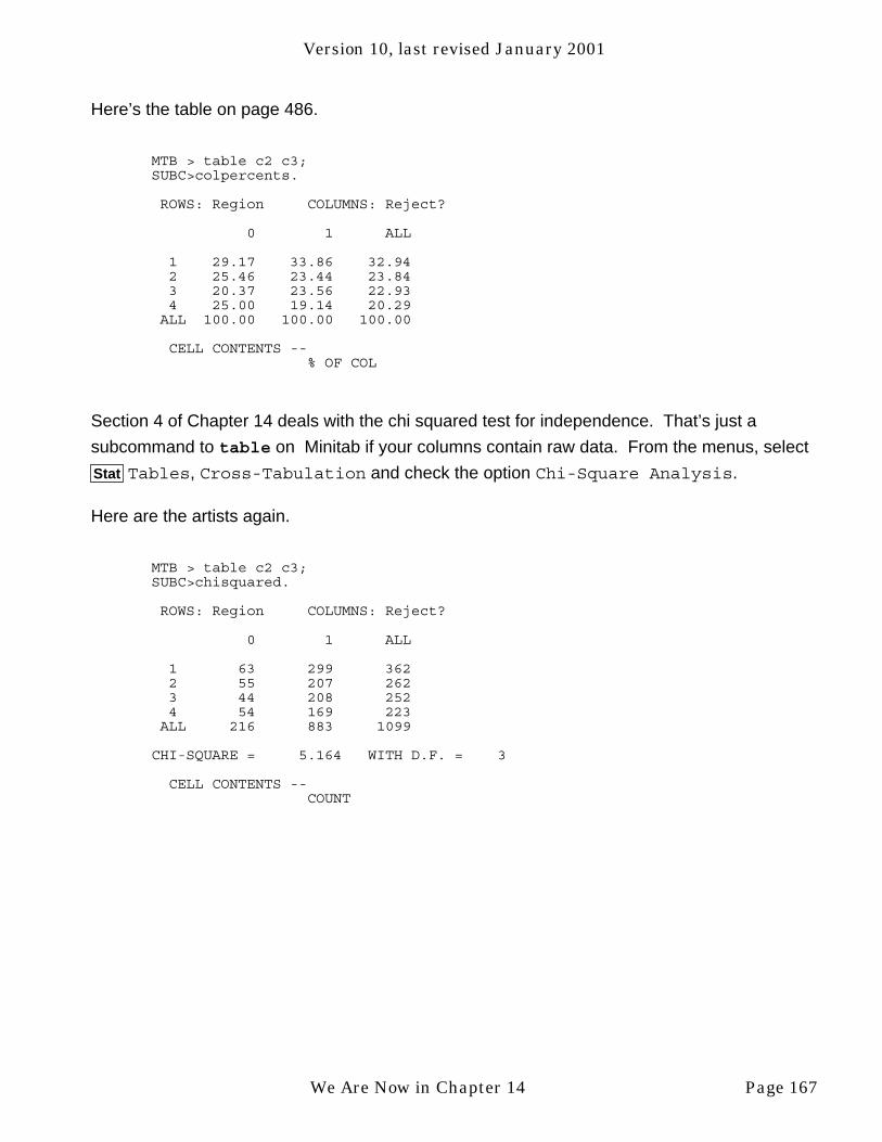
Version 10, last revised January 2001
Here’s the table on page 486.
MTB > table c2 c3;SUBC>colpercents.
ROWS: Region COLUMNS: Reject?
0 1 ALL
1 29.17 33.86 32.942 25.46 23.44 23.843 20.37 23.56 22.934 25.00 19.14 20.29ALL 100.00 100.00 100.00
CELL CONTENTS --% OF COL
Section 4 of Chapter 14 deals with the chi squared test for independence. That’s just a
subcommand to table on Minitab if your columns contain raw data. From the menus, select
Stat Tables, Cross-Tabulation and check the option Chi-Square Analysis.
Here are the artists again.
MTB > table c2 c3;SUBC>chisquared.
ROWS: Region COLUMNS: Reject?
0 1 ALL
1 63 299 3622 55 207 2623 44 208 2524 54 169 223ALL 216 883 1099
CHI-SQUARE = 5.164 WITH D.F. = 3
CELL CONTENTS --COUNT
We Are Now in Chapter 14 Page 167

Version 10, last revised January 2001
MTB > table c2 c3; SUBC>chisquared 2.
ROWS: Region COLUMNS: Reject?
0 1 ALL
1 63 299 36271.15 290.85 362.00
2 55 207 26251.49 210.51 262.00
3 44 208 25249.53 202.47 252.00
4 54 169 22343.83 179.17 223.00
ALL 216 883 1099 216.00 883.00 1099.00 CHI-SQUARE = 5.164 WITH D.F. = 3
CELL CONTENTS --COUNTEXP FREQ
If you put a “2” after the chisquared subcommand, Minitab prints the expected values for
each cell in the table. These are shown on page 489 of your textbook. In the menu dialog box
you can get these by checking the box marked Above and expected count.
In this example, we had all 1099 data points stored in the computer. We used Minitab to get
the summary tables and to do the chi squared test. Sometimes, however, we have the
summary table but not the original data. The table might have come out of a book, or from our
database program, for example. In situations like this, you can just type the table right into
Minitab. Here’s how we would do that with the data on the artists.
MTB > read into c1 c2 DATA> 63 299 DATA> 55 207 DATA> 44 208 DATA> 54 169 DATA> end
4 ROWS READ
Then we would use the chisquared command (not subcommand). (In fact, if you use
table on the table above you will just get garbage. It’s already been tabled so don’t do it
again.) The chisquared command (not subcommand) automatically gives us the eight
numbers from page 494 that were added up to get the calculated chi squared statistic. The
menu way to do this is to select Stat , Tables, Chi-Square Test.
Page 168 We Are Now in Chapter 14

Version 10, last revised January 2001
MTB > chisquared c1 c2
Expected counts are printed below observed counts
C1 C2 Total1 63 299 362
71.15 290.85
2 55 207 26251.49 210.51
3 44 208 25249.53 202.47
4 54 169 22343.83 179.17
Total 216 883 1099
ChiSq = 0.933 + 0.228 +0.239 + 0.058 +0.617 + 0.151 +2.360 + 0.577 = 5.164
df = 3
You can compare this calculated test statistic to a critical value from one of the tables in your
book. For 3 degrees of freedom and α=0.05, the critical value is 7.815. Thus we would not
reject the null hypothesis that these two categorical variables are independent. Unfortunately,
Minitab does not print a p-value for the chi squared test. We can get one in a roundabout way.
MTB > cdf for 5.164;SUBC>chisquared with 3 df.
5.1640 0.8398
This is not the p-value but rather the probability of the complementary event. We need to
calculate p=1−0.8398=0.1602. This is larger than any α normally used in practice, so again we
would not reject the null hypothesis.
We should also look at the residuals. Unfortunately, Minitab does not calculate these.
However, they are not too hard to get from the previous table and a pocket calculator.
Remember that residual=observed−expected. For example, in the upper left hand corner of
the table, the residual is 63−71.15=−8.15. The residuals for the entire table are
Selected Rejected
North Central -8.15 8.15Northeast 3.51 -3.51South -5.53 5.53West 10.17 -10.17
We Are Now in Chapter 14 Page 169

Version 10, last revised January 2001
Note that all eight residuals add up to zero. In addition, the sum of any row or any column is
also zero. This provides a good check on our computation of the expected values. The
interpretation of the residuals is as usual. We see that the largest residuals are in the last row.
This means that the discrepancies from our expectations were greatest in the West. In
particular, about 10 more submissions were selected than we would have expected. The
second greatest departure was in the North Central region, where about 8 fewer submissions
were selected than we would have expected.
As for assumptions, we are in trouble, because this is by no means a random sample. In fact,
it is all the submissions to the art exhibit! On the other hand, none of the cells have expected
counts less than five. The assumptions apply only to the hypothesis test, and there only to the
calculation of the p-value (or the use of the table in the book). In particular, the expected
values are correct and so are the residuals.
New Minitab commands:
chisquared
Note: Where problems involve just a small table of numbers, you may need to type them
in yourself.
Minitab Assignment 14-A
Use the goodfit macro to do Part e of Problem 5 on page 505.
Minitab Assignment 14-B
Use Minitab to do Parts e and f of Problem 6 on pages 505-506. (You will need to calculate
expected counts and then enter these and the observed counts into Minitab.)
Minitab Assignment 14-C
Use Minitab to get row, column, and joint percentages for the cancer data on page 507 of your
text. Note: There are two different versions of this data − this one and the one on page 480.
The numbers on page 480 look more reasonable, so use that data (in file smt14.17).
Page 170 We Are Now in Chapter 14

Version 10, last revised January 2001
Minitab Assignment 14-D
Use Minitab to get row, column, and joint percentages for the data on sex of applicants from
page 480 of your text. Which of your tables would be most useful if you wanted to see if there
was any change in the composition of the applicant pool from one year to the next? Is there?
What is it?
Minitab Assignment 14-E
The data in Problem 17 on page 510 of your text concerns the effectiveness of three
treatments for panic disorder. Make appropriate tables to
1. compare the three treatments as to whether they reduce panic symptoms
2. compare the three treatments as to whether they eliminate panic symptoms
Write a brief interpretation for each table. (NOTE: The label “PANIC FREE?” in Table 14.53
should be “PANIC REDUCED?”)
Minitab Assignment 14-F
Using the data stored on the computer, do Problem 9 on page 507. Do any cells have
expected counts less than five? Is this a random sample?
Minitab Assignment 14-G
Using the data stored on the computer, do Problem 10 on pages 507-508. Do any cells have
expected counts less than five? Is this a random sample? Note: There are two different
versions of this data − this one and the one on page 480. The numbers on page 480 look
more reasonable, so use that data (in file smt14.17).
Minitab Assignment 14-H
Use Minitab to do Problem 11 on page 508. (You’ll have to do some hand calculations in Part
a.) Do any cells have expected counts less than five? Is this a random sample?
We Are Now in Chapter 14 Page 171

Version 10, last revised January 2001
Minitab Assignment 14-I
Use Minitab to do Problem 17 on page 510 of your text. (NOTE: The label “PANIC FREE?” in
Table 14.53 should be “PANIC REDUCED?”)
Minitab Assignment 14-J
The file smp07.22 contains the results of rolling a die (singular of dice) many times. Use
Minitab to get counts and percentages for each outcome.
Minitab Assignment 14-K
The file smp07.22 contains the results of rolling a die (singular of dice) many times. Use
Minitab to test the hypothesis that all six outcomes are equally likely.
Chapter 15
In Chapter 15 you will learn how to:
• plot data on two measurement variables
• find a correlation
• fit a line to bivariate data
Description
Minitab can make bivariate plots like the one at the bottom of page 519. These are often
called “scatter plots”. Don’t let the new name fool you; these are the same kind of x-y plot you
made in Algebra I. From the menus, select Graph , Character Graphs, Scatter Plot.
Page 172 We Are Now in Chapter 14

Version 10, last revised January 2001
Let’s look at the data on the ages and heights of children from page 519 of your text (in file
sm15.03).
MTB > info
COLUMN NAME COUNTC1 age 7C2 height 7
CONSTANTS USED: NONE
MTB > print ’age’ ’height’
ROW age height
1 1.7 722 3.2 883 3.1 854 0.6 635 1.2 776 1.8 847 3.8 100
MTB > plot ’height’ versus ’age’- *-
96+-
height -- *-
84+ * *--- *-
72+ *---- *--+---------+---------+---------+---------+---------+----age0.60 1.20 1.80 2.40 3.00 3.60
In the plot command, the first variable (or column) mentioned will be plotted on the vertical
axis, and so it should be the dependent variable.
The data on questionnaire response from pages 526-527 of your textbook (file smt15.04) is
an interesting application of statistics to statistics. A well designed survey starts with a random
sample, but if everyone surveyed does not reply, the sample of people who did reply is no
longer random. In fact, it’s volunteers! People who do statistical surveys are interested in
finding ways to increase the return rate. Bribes are one method.
We Are Now in Chapter 15 Page 173

Version 10, last revised January 2001
MTB > print c1 c2
ROW Payment RetRate
1 0.0 0.16 2 0.1 0.18 3 0.2 0.22 4 0.5 0.24 5 1.0 0.32 6 2.0 0.30 7 5.0 0.40 8 10.0 0.42 9 20.0 0.50 10 50.0 0.62 MTB > plot c2 c1
*0.60+
- RetRate -
- *-
0.45+- *- *-- *
0.30+ *-- *- *- *
0.15+ *+---------+---------+---------+---------+---------+------Payment0 10 20 30 40 50
This does not look at all linear. A transformation might help, but we will not try one now.
For the data on Neanderthal bones from pages 534-536, the two variables are on the same
footing; we would not consider one to be the independent variable and the other to be the
dependent variable. Thus we could plot them in either order.
The data on professional degrees awarded to women (smt15.13) has a definite independent
and dependent variable, as explained in your book (page 549).
MTB > info
COLUMN NAME COUNT C1 x 8 C2 y 8
CONSTANTS USED: NONE
Page 174 We Are Now in Chapter 15

Version 10, last revised January 2001
MTB > plot c2 c1
- *28.0+ *
-y -
- *-
21.0+---- *
14.0+- * * *---
7.0+ *--------+---------+---------+---------+---------+--------x
2.0 4.0 6.0 8.0 10.0MTB > plot c1 c2
-- * **
10.5+-
x ---
7.0+-- *-- *
3.5+- *- *- *---+---------+---------+---------+---------+---------+----y8.0 12.0 16.0 20.0 24.0 28.0
As you can see, we get quite different graphs depending on the order in which we list the
columns after the plot command. Only the first is correct.
THE METHOD OF LEAST SQUARES
The method of least squares is one way of defining the “best” fit between a set of data and a
model for that data. By a model, we mean some sort of mathematical summary. For example,
we might use a line or curve as a model or summary of the relationship between the variables
we have been plotting. To get a feel for how least squares works, we start with one
measurement variable rather than two. Recall how you found the mean, variance, and
We Are Now in Chapter 15 Page 175

Version 10, last revised January 2001
standard deviation of a set of data. Here is an edited output from the var macro showing this
calculation for the numbers 4, 3, 3, 1, −1.
MTB > note This macro computes the mean, variance, and standard MTB > note deviation of a set of data. The data must be stored in c1. MTB > note The results of all intermediate steps are printed out MTB > note to aid students in learning to do these computations MTB > note by hand. The macro will destroy any data stored in c2-c3 MTB > note and k1-k7. MTB > note ------------------------------------------------------------
ROW y resids. res. sq.
1 4 2 42 3 1 13 3 1 14 1 -1 15 -1 -3 9
------------------------------------------------------------ MTB > print k3 mean = K3 2.00000 MTB > print k4 The sum of the squared residuals = K4 16.0000 MTB > print k5 degrees of freedom = K5 4.00000 MTB > print k6 variance = K6 4.00000 MTB > print k7 standard deviation = K7 2.00000
The mean we have calculated serves as a summary or model for the data. To find the
variance, you first subtract this summary from each observation. This gives the numbers in the
second column, called “residuals” or “deviations”. Note that these add up to zero. Deviations
from the mean always add up to zero. The deviations are then squared to get the numbers in
the third column. These squared deviations are summed (16) and divided by one less than the
number of observations (d.f.=4), giving the variance (4). The square root of the variance is the
standard deviation (2). An important fact about the mean is that it makes the sum of the
squared residuals smaller than any other summary of this data. To understand what this
means, let us carry out the calculations above using the median (3) as a summary rather than
the mean. Now the residuals will be y−median (or y−3) rather than y−mean.
Page 176 We Are Now in Chapter 15

Version 10, last revised January 2001
------------------------------------------------------------
ROW y resids. res. sq.
1 4 1 12 3 0 03 3 0 04 1 -2 45 -1 -4 16
------------------------------------------------------------
Note that, for the median, the sum of the squared deviations is 21, larger than the 16 we got in
using the mean. We call the mean the least squares measure of center because it makes
the sum of the squared deviations as small as it can possibly be. Some people might say that
it is therefore the “best” measure of center, but that would be going too far. You learned in
introductory statistics that the mean is sometimes the best summary measure, but in other
situations the median might be better. We can actually see that here. Suppose that, instead
of trying to make the sum of the squared residuals as small as possible, we tried to make the
sum of the absolute values of the residuals as small as possible. For the mean this sum is 8,
while for the median it is only 7. Thus, by this standard, the median is a better summary.
Which one is really better? There is actually no right answer to that question. Each has its
advantages. If you look at the residuals in both cases you will notice a pattern that is general:
the median gives lots of small deviations at the expense of a few large deviations, while the
mean allows lots of medium size deviations in order to avoid large deviations. Which of these
is better depends of the application. If a miss is as good as a mile, the median might be better.
If moderate deviations are acceptable, but large ones very costly, the mean might be better.
Note that the sum of deviations from the median is not zero − it is −5.
Now let us suppose that we have some additional information about the y-values already
discussed. Suppose that for each y-value, there is a corresponding x-value, and that x and y
are, at least to some degree, related.
MTB > erase c2-c3MTB > set into c2DATA> -2 -1 0 1 2DATA> endMTB > name c2 ’x’
We Are Now in Chapter 15 Page 177

Version 10, last revised January 2001
MTB > print c2 c1
ROW x y
1 -2 4 2 -1 3 3 0 3 4 1 1 5 2 -1
We wish to summarize or model the relationship between x and y with an equation. A plot of
the data will help us choose the type of equation to use.
MTB > plot c1 c2
--
4.0+ *-- * *--
2.0+-- *--
0.0+--- *---------+---------+---------+---------+---------+--------
-1.60 -0.80 0.00 0.80 1.60
From this, we see that a straight line might fit reasonably well, and fooling around with a
straightedge, we find experimentally that the equation M (x)=2−x passes exactly through 3 of1
the 5 points. Note that we use M (x) to represent y-co ̈ rdinates of the line, while we use y too1
represent the y-co ̈ rdinates of the original data. M stands for “model” − the line is a model oro
summary of the relationship between x and y. The “1” indicates that this is the first model we
tried, and the x indicates that y depends on x. Here are what the residuals from Model 1 look
like.
Page 178 We Are Now in Chapter 15

Version 10, last revised January 2001
Deviations of the y-values from M (x)=2−x1
2x y M (x) y−M (x) [y−M (x)]1 1 1
-2 4 4 0 0-1 3 3 0 00 3 2 1 11 1 1 0 02 -1 0 -1 1
Total 10 0 2 Sum of squared deviations
Sum of Abs. Dev. = 2
To find M (x) we just plug the value of x into the equation M (x)=2−x. Notice that the added1 1
information about y provided by knowledge of x has reduced the sum of the squared residuals
from the 16 to 21 range to a mere 2. Is this the best we can do? As a matter of fact, it is not.
However, finding the least sum of squared residuals is not simple. We will let Minitab do the
work.
MTB > regress y in c1 on 1 ind. var. x in c2;SUBC> residuals in c3;SUBC> fits in c4.
The regression equation isy = 2.00 - 1.20 x
This is just a little bit of the output from the regression command you will learn more about
later. In the menu system, it can be found at Stat , Regression, Regression. Like the plot
command, it requires that you give it the column with the dependent variable first. (It’s called
“response” in the dialog boxes. Unlike the plot command, you must also tell Minitab how
many independent variables you have if you enter the regression command on the command
line.
The first subcommand stored the residuals in c3. The second subcommand stored in c4 the
fitted values M (x) for each x in the dataset. These subcommands are behind the Storage2
button in the dialog box. The least squares regression equation turns out to be M (x)=2−1.2x.2
The residuals and fits from Model 2 look like this.
We Are Now in Chapter 15 Page 179
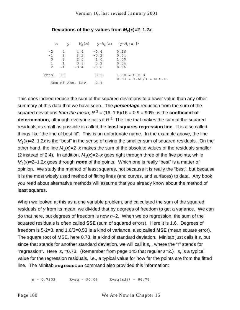
Version 10, last revised January 2001
Deviations of the y-values from M (x)=2−1.2x2
2x y M (x) y−M (x) [y−M (x)]2 2 2
-2 4 4.4 -0.4 0.16-1 3 3.2 -0.2 0.040 3 2.0 1.0 1.001 1 0.8 0.2 0.042 -1 -0.4 -0.6 0.36
Total 10 0.0 1.60 = S.S.E.0.53 = 1.60/3 = M.S.E.
Sum of Abs. Dev. 2.4
This does indeed reduce the sum of the squared deviations to a lower value than any other
summary of this data that we have seen. The percentage reduction from the sum of the2squared deviations from the mean, R = (16−1.6)/16 = 0.9 = 90%, is the coefficient of
2determination, although everyone calls it R . The line that makes the sum of the squared
residuals as small as possible is called the least squares regression line. It is also called
things like “the line of best fit”. This is an unfortunate name. In the example above, the line
M (x)=2−1.2x is the “best” in the sense of giving the smaller sum of squared residuals. On the2
other hand, the line M (x)=2−x makes the sum of the absolute values of the residuals smaller1
(2 instead of 2.4). In addition, M (x)=2−x goes right through three of the five points, while1
M (x)=2−1.2x goes through none of the points. Which one is really “best” is a matter of2
opinion. We study the method of least squares, not because it is really the “best”, but because
it is the most widely used method of fitting lines (and curves, and surfaces) to data. Any book
you read about alternative methods will assume that you already know about the method of
least squares.
When we looked at this as a one variable problem, and calculated the sum of the squared
residuals of y from its mean, we divided that by degrees of freedom to get a variance. We can
do that here, but degrees of freedom is now n−2. When we do regression, the sum of the
squared residuals is often called SSE (sum of squared errors). Here it is 1.6. Degrees of
freedom is 5-2=3, and 1.6/3=0.53 is a kind of variance, also called MSE (mean square error).
The square root of MSE, here 0.73, is a kind of standard deviation. Minitab just calls it s, but
since that stands for another standard deviation, we will call it s , where the “r” stands forr
“regression”. Here s =0.73. (Remember from page 145 that regular s=2.) s is a typicalr r
value for the regression residuals, i.e., a typical value for how far the points are from the fitted
line. The Minitab regression command also provided this information:
s = 0.7303 R-sq = 90.0% R-sq(adj) = 86.7%
Page 180 We Are Now in Chapter 15

Version 10, last revised January 2001
Analysis of Variance
SOURCE DF SS MS F pRegression 1 14.400 14.400 27.00 0.014Error 3 1.600 0.533Total 4 16.000
In the SS column, you can see the sum of the squared residuals from the mean (16) and from2the regression line (1.6), a reduction of 14.4. 14.4/16=90% is R , labeled “R-sq” on Minitab.
You can also find MSE=0.533 and s=0.7303. If you want the correlation, r, take one of the2square roots of R =90%=0.9. The correlation always has the sign of the slope of the
regression line. Here the slope is negative, so r =−0.95. Note that just like any other percent,2R must be changed to a decimal fraction before doing any calculations with it. You can also
use the correlation command on Minitab to find a correlation. Unlike the regression
and plot commands, the order in which you list the columns does not make a difference for
the correlation command.
When you fit a line or curve to data, you should always plot the data with your model to see
how they compare. Because more than one thing is plotted on the graph, Minitab calls this a
multiple plot. On the menus, it’s at Graph , Character Graphs, Multiple Scatter Plot.
MTB > mplot c1 c2 c4 c2
-- B
4.0+ A-- 2 A--
2.0+ B-- A- B-
0.0+- B-- A---------+---------+---------+---------+---------+--------
-1.60 -0.80 0.00 0.80 1.60A = y vs. x B = C4 vs. x
Here the data were in C1 and C2 and the fitted values from Model 2 were in C4. The mplot (multiple plot)
command plots two or more pairs of numbers on the same set of axes. Here the data (C1 and C2) is plotted first
using an A for each data point. Then the second pair of columns (C4 and C2) are plotted using a B for each data
We Are Now in Chapter 15 Page 181
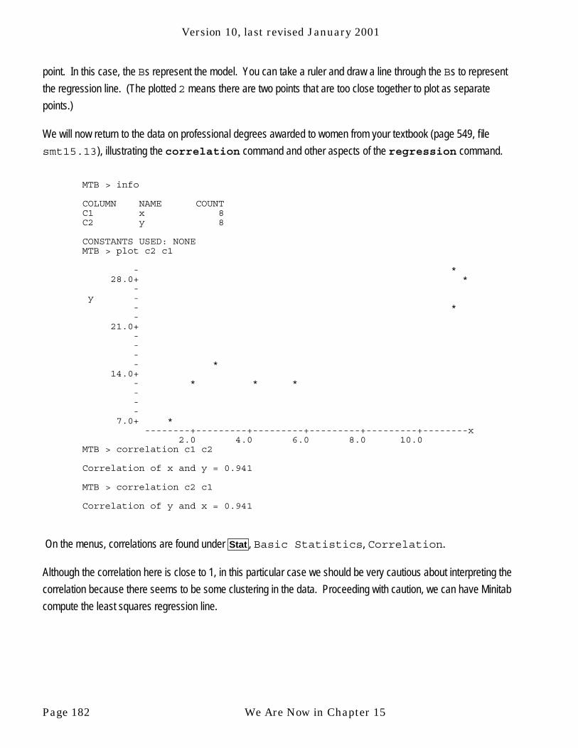
Version 10, last revised January 2001
point. In this case, the Bs represent the model. You can take a ruler and draw a line through the Bs to represent
the regression line. (The plotted 2 means there are two points that are too close together to plot as separate
points.)
We will now return to the data on professional degrees awarded to women from your textbook (page 549, file
smt15.13), illustrating the correlation command and other aspects of the regression command.
MTB > info
COLUMN NAME COUNT C1 x 8 C2 y 8
CONSTANTS USED: NONE MTB > plot c2 c1
- *28.0+ *
- y - - * - 21.0+ - - - - * 14.0+ - * * * - - - 7.0+ * --------+---------+---------+---------+---------+--------x 2.0 4.0 6.0 8.0 10.0 MTB > correlation c1 c2
Correlation of x and y = 0.941
MTB > correlation c2 c1
Correlation of y and x = 0.941
On the menus, correlations are found under Stat , Basic Statistics, Correlation.
Although the correlation here is close to 1, in this particular case we should be very cautious about interpreting the
correlation because there seems to be some clustering in the data. Proceeding with caution, we can have Minitab
compute the least squares regression line.
Page 182 We Are Now in Chapter 15

Version 10, last revised January 2001
MTB > regress ’y’ vs. 1 ind. var. ’x’;SUBC>residuals in c3.
The regression equation isy = 7.01 + 1.72 x
Predictor Coef Stdev t-ratio pConstant 7.007 1.882 3.72 0.010x 1.7241 0.2527 6.82 0.000
s = 2.966 R-sq = 88.6% R-sq(adj) = 86.7%
Analysis of Variance
SOURCE DF SS MS F pRegression 1 409.60 409.60 46.57 0.000Error 6 52.77 8.80Total 7 462.38
MTB > name c3 ’resids’
We can use the stored residuals to make a plot like the one on page 554.
MTB > plot ’resids’ versus ’x’
resids - *--
2.5+ *-- * *--
0.0+-- *- *-
-2.5+- *- *---------+---------+---------+---------+---------+--------x
2.0 4.0 6.0 8.0 10.0
We can also get predicted y-values with the fits subcommand.
We Are Now in Chapter 15 Page 183

Version 10, last revised January 2001
MTB > regress ’y’ vs. 1 ind. var. ’x’; SUBC> residuals in c3; SUBC> fits in c5.
The regression equation is y = 7.01 + 1.72 x
Predictor Coef Stdev t-ratio p Constant 7.007 1.882 3.72 0.010 x 1.7241 0.2527 6.82 0.000
s = 2.966 R-sq = 88.6% R-sq(adj) = 86.7%
Analysis of Variance
SOURCE DF SS MS F p Regression 1 409.60 409.60 46.57 0.000 Error 6 52.77 8.80 Total 7 462.38 MTB > name c3 ’resids’ c5 ’fits’ MTB > print ’x’ ’y’ c5 c3
ROW x y fits resids
1 2.0 11.9 10.4552 1.44485 2 11.5 28.5 26.8345 1.66549 3 11.2 23.1 26.3173 -3.21727 4 4.2 13.0 14.2483 -1.24827 5 2.8 15.7 11.8345 3.86553 6 1.1 7.2 8.9034 -1.70342 7 5.5 13.1 16.4897 -3.38965 8 11.2 28.9 26.3173 2.58273
This table contains all of the information in the table on page 555 of your textbook. It also includes the predicted y-
values in C5. You will note that the residuals only agree with your book to the nearest tenth. That is because
Siegel rounded off the slope and intercept of the regression equation quite a bit. He used y=7+1.72x. Minitab
printed the regression equation as y=7.01+1.72x. However, right below this are more accurate values for the
intercept (7.007) and slope (1.7241). Thus, a more accurate regression equation is y=7.007+1.7241x. In fact,
Minitab maintains an even more accurate equation internally, and uses this to compute the residuals. You should
use the most accurate regression equation available, as the values of the residuals are quite sensitive to the
accuracy of the slope and intercept.
The data on the average heights of girls from pages 554-557 (smt15.16) illustrates why we want to calculate
and plot residuals.
MTB > info
COLUMN NAME COUNT C1 height 10 C2 age 10
Page 184 We Are Now in Chapter 15

Version 10, last revised January 2001
MTB > plot ’height’ versus ’age’
-- *
140+ *-
height - *- *- *
120+- *-- *- *
100+- *-- *-------+---------+---------+---------+---------+---------+age
2.0 4.0 6.0 8.0 10.0 12.0MTB > correlation c1 c2
Correlation of height and age = 0.997
Both the scatter plot and the correlation suggest the data are very close to a straight line.
MTB > regress height in c1 vs. 1 ind. var. age in c2;SUBC>residuals in c3;SUBC>predict height when age = 12.
The regression equation isheight = 76.6 + 6.37 age
Predictor Coef Stdev t-ratio pConstant 76.641 1.188 64.52 0.000age 6.3661 0.1672 38.08 0.000
s = 1.518 R-sq = 99.5% R-sq(adj) = 99.4%
Analysis of Variance
SOURCE DF SS MS F pRegression 1 3343.5 3343.5 1450.45 0.000Error 8 18.4 2.3Total 9 3361.9
Obs. age height Fit Stdev.Fit Residual St.Resid1 2.0 86.500 89.373 0.892 -2.873 -2.34R
R denotes an obs. with a large st. resid.
Fit Stdev.Fit 95% C.I. 95% P.I.153.033 1.037 (150.641,155.426) (148.792,157.275)
We Are Now in Chapter 15 Page 185

Version 10, last revised January 2001
MTB > plot c3 vs c2
-1.5+ *
- * * C3 - * - * - 0.0+ * - * - * - - -1.5+ - * - - - -3.0+ * ------+---------+---------+---------+---------+---------+age 2.0 4.0 6.0 8.0 10.0 12.0
The residual plot shows some curvature that was hidden in the original scatter plot. In general, residual plots
magnify any lack of fit between the data and the model. An ideal residual plot shows no patterns at all − only
random scatter. In this case we could get an even better fit with some sort of curve − a topic studied in Stats.II.
You may have noticed the predict subcommand used with the regress command above. This will provide
a predicted height for a 12-year-old girl. The prediction is 153.033 centimeters, which is printed at the end of the
regression output and labeled Fit. Your book does not say much about predictions, but it asks you to do some in
the problems. To do this one by hand, you would just plug 12 into the regression equation, using the most accurate
slope and intercept available,
y=76.641+6.3661×12=153.0342,
which is very close to Minitab’s 153.033. To do predictions from the menus, you would click on the Options button
in the regression dialog box and then enter the x-value ((it’s 12 here) in the box labeled Prediction
intervals for new observations:.
Inference
The regress command also enables us to do the test of the hypothesis that the population correlation
coefficient is zero, as discussed on pages 541-543 of Siegel. In Minitab, this test is done in conjunction with the
regress command. The numbers along the way do not look like the numbers you get using the hand calculation
method in your textbook, but your conclusion (whether or not to reject the null hypothesis) should be the same.
Page 186 We Are Now in Chapter 15

Version 10, last revised January 2001
Minitab’s method uses the t distribution rather than the table on page 543 of your book. Here’s the regression
printout on degrees awarded to women again (smt15.13).
The regression equation isy = 7.01 + 1.72 x
Predictor Coef Stdev t-ratio pConstant 7.007 1.882 3.72 0.010x 1.7241 0.2527 6.82 0.000
s = 2.966 R-sq = 88.6% R-sq(adj) = 86.7%
Analysis of Variance
SOURCE DF SS MS F pRegression 1 409.60 409.60 46.57 0.000Error 6 52.77 8.80Total 7 462.38
The calculated t is 6.82 in this case, and it is the second number in the column labeled t-ratio on the printout.
In the table below the one where you found 6.82, you will find the appropriate degrees of freedom. This is the
second number in the column labeled DF, and the value is 6. For 6 degrees of freedom and an alpha of 0.05, the
critical t would be 2.447. Since the calculated t-value is not between -2.447 and +2.447, we would reject the null
hypothesis, and conclude that there really is some degree of linear relationship in the population. Alternatively, we
could note that the p-value of 0.000 (printed just to the right of the 6.82) is less than α=0.05 (or any other
reasonable α) and reach the same conclusion. We could also use the jargon and say we found a “significant”
linear relationship.
New Minitab commands for Chapter 15:
correlation fits mplot predict
plot regress residuals
Minitab Assignment 15-A
Use Minitab to do Problem 9 on page 571.
We Are Now in Chapter 15 Page 187

Version 10, last revised January 2001
Minitab Assignment 15-B
Use Minitab to do Part c of Problem 10 on pages 571-572. Write answers to parts a, b and d on your printout.
Minitab Assignment 15-C
Use Minitab to do Problem 7 on page 570. Treat “MARCH” as the dependent variable.
Minitab Assignment 15-D
Use Minitab to do Problem 11 on page 572.
Minitab Assignment 15-E
Use Minitab to do Problem 12 on pages 572-573.
Minitab Assignment 15-F
Use Minitab to do Problem 13 on page 573.
Minitab Assignment 15-G
Use Minitab to do Problem 14 on page 574.
Minitab Assignment 15-H
Use Minitab to do Problem 15 on page 574.
Minitab Assignment 15-I
Use Minitab to explore the relationship between the variables in the voting data on page 416.
Minitab Assignment 15-J
Use Minitab to do Problem 16 on page 574.
Minitab Assignment 15-K
Use Minitab to do Problem 21 on page 575.
Page 188 We Are Now in Chapter 15

Version 10, last revised January 2001
Minitab Assignment 15-L
Use Minitab to do Problem 17 on page 574.
Minitab Assignment 15-M
Use Minitab to do Problem 18 on page 574.
Minitab Assignment 15-N
Use Minitab to do Problem 19 on page 574.
Minitab Assignment 15-O
Explore the data on degrees awarded to women by splitting it into two data sets corresponding to the two clusters
we noted in the various displays of this data. Minitab has some sneaky commands to do this sort of thing, but they
are not worth learning for such a small data set. Just retype the data, one cluster at a time. Do a correlation and a
regression analysis on the data from each cluster. Do you get pretty much the same correlation, slope, and
intercepts for the two clusters? Are they close to the values for the whole data set?
Minitab Assignment 15-P
Use Minitab to do Problem 22 on page 577.
Minitab Assignment 15-Q
Use Minitab to do Problem 23 on page 577.
Minitab Assignment 15-R
Use Minitab to do Problem 24 on page 577.
Minitab Assignment 15-S
Use Minitab to do Problem 25 on page 577.
We Are Now in Chapter 15 Page 189

Version 10, last revised January 2001
Index
0-1 data 13, 38, 39, 67, 96, 97, 100, 102, for a mean 99, 100, 108, 110108, 109, 128 for a median 103, 110
for a proportion 102A confidence intervalabsolute values 177 for a mean 107alpha 109 copy command 50, 51analysis of variance 143, 144, 156 correlation command 181analysis of variance table 152 counts subcommand 33ANOVA 143 cross-classification 67aovoneway command 152, 157
Dassumptions 100, 102, 103, 107, 109,110, 111, 112, 126, 127, 129, 132, Data Window 3, 4, 57153, 157, 158, 170 degrees of freedom 45, 48, 108, 157,
average command 44 169, 187describe command 20, 21, 24, 25, 27,B 40, 41, 44, 61, 109, 120
barchart 35 describe command 96biased estimator 89 dotplot 26, 115bimodal 27 dotplot command 12boxplot command 19, 118 downloading Minitab 9boxplots 60
Ebuying Minitab 9by command 127 end command 5by subcommand 15, 27, 120 execute command 45
C Fc.v. 61 file names for stored data 29categorical data 13, 32, 33, 35, 38, 67, fits subcommand 183
115, 128, 138, 160, 163, 164 fitssubcommand 179cdf command 79, 169 frequencies 33Central Limit Theorem 87, 102, 150 Gchanging outliers 104
goodfit macro 161chisquared command 168, 169gpro 19chisquared subcommand 167, 168grouped data 46coefficient of determination 180gstd 19coefficient of variation 61
colpercents subcommand 73 Hconfidence interval 105, 109, 112, 114,help for Minitab 22132histogram 26for a difference in means 125, 128,histogram command 35129, 134hypothesis test 106, 114for a difference in medians 129
for a correlation 186for a difference in proportions 128,for a difference in means 125, 128,129129, 134
Page 190

Version 10, last revised January 2001
for a difference in medians 129 outliers 20, 38, 40, 49, 50, 56, 61, 104,for a difference in proportions 128, 105, 107, 109, 110, 129, 132129 Pfor a mean 106, 107, 108, 111
p-value 108, 109, 111, 112, 134, 158,for a median 111162, 169, 170, 187for a proportion 108
paired data 129, 132, 133, 134for a regression 186percents 33for independence 167, 169, 170percents subcommand 33
I pie chart 35increment subcommand 8, 117 plot command 173, 174, 175independent samples 129, 132, 133, 134 pooled subcommand 125, 126, 127info command 7, 10, 132 pooled variance estimate 150invcdf command 80 predict subcommand 186
print command 5, 45, 57, 129J proportions 33joint probability table 68 proportions for 0-1 data 39, 97
L Rleast squares measure of center 177 read command 46least squares regression line 180 regress command 182, 183, 186let command 50, 51, 104, 130 regression command 181line of best fit 180 relationships between variables 114lumpy data 26 relative frequencies 33lvals command 22 removing outliers 51
renting Minitab 9M replication 145Macintosh residual plot 183, 186
Minitab Version 10.5 Xtra 10 residuals 45, 48, 78, 160, 169, 184macros 45 residuals subcommand 179, 183measure of center 27, 103, 177 retrieve command 7measure of variability 61, 146 rounding 35measurement data 13, 35, 115 rowpercents subcommand 73Minitab help system 22 running a macro 45Minitab macros 45
SMinitab versions 9modal category 33 same subcommand 115, 117mode 34 sample command 95model 175, 176 sampling distribution 90mplot command 181 sampling distribution of the mean 90multiple inference 144 save command 5
Session Window 2, 10N set command 4, 14name command 5 significant difference 107, 157names of data files 29 sinterval command 103, 110, 130, 132normal distribution 63, 79, 87 sort command 18note command 12, 45 stack command 120, 128
starting Minitab on a Mac 10O starting Minitab on a PC 9omit subcommand 51 stem and leaf 6, 12oneway command 155, 156 stem command 8, 12, 15, 35opening files 9, 10 stest command 110, 132, 135order statistics 17 storing fitted values 179
storing regression residuals 179
Page 191

Version 10, last revised January 2001
Student Editions of Minitab 9 twot command 127, 128subcommand 8 Usubscripts subcommand 120
unbiased estimator 89T
Vtable command 68, 70, 73, 76, 167var macro 44, 88tallyvargroup macro 46counts subcommand 33varpd macro 77percents subcommand 33
tally command 33, 35, 46, 66, 67 Wtinterval command 100, 102, 110, 130,Windows 95/98 9132
totpercents subcommand 68, 70, 73 Ztransformations 55, 127, 154, 156, 174zero-one data 13, 38, 39, 67, 96, 97,ttest command 107, 132, 135
100, 108, 109, 128two-way table 67zinterval command 100twosamplet command 128
Page 192

Contents
Chapter 1 1
Chapter 2 2Minitab Assignment 0 . . . . . . . . . . . . . . . . . . . . . . . . . . . . . . . . . . . . . . . . . . . . . . . . . . . . . 15Minitab Assignment 2-A . . . . . . . . . . . . . . . . . . . . . . . . . . . . . . . . . . . . . . . . . . . . . . . . . . . 15Minitab Assignment 2-B . . . . . . . . . . . . . . . . . . . . . . . . . . . . . . . . . . . . . . . . . . . . . . . . . . . 16Minitab Assignment 2-C . . . . . . . . . . . . . . . . . . . . . . . . . . . . . . . . . . . . . . . . . . . . . . . . . . . 16
Chapter 3 17Minitab Assignment 3-A . . . . . . . . . . . . . . . . . . . . . . . . . . . . . . . . . . . . . . . . . . . . . . . . . . . 30Minitab Assignment 3-B . . . . . . . . . . . . . . . . . . . . . . . . . . . . . . . . . . . . . . . . . . . . . . . . . . . 30Minitab Assignment 3-C . . . . . . . . . . . . . . . . . . . . . . . . . . . . . . . . . . . . . . . . . . . . . . . . . . . 30Minitab Assignment 3-D . . . . . . . . . . . . . . . . . . . . . . . . . . . . . . . . . . . . . . . . . . . . . . . . . . . 30Minitab Assignment 3-E . . . . . . . . . . . . . . . . . . . . . . . . . . . . . . . . . . . . . . . . . . . . . . . . . . . 31Minitab Assignment 3-F . . . . . . . . . . . . . . . . . . . . . . . . . . . . . . . . . . . . . . . . . . . . . . . . . . . 31Minitab Assignment 3-G . . . . . . . . . . . . . . . . . . . . . . . . . . . . . . . . . . . . . . . . . . . . . . . . . . . 31Minitab Assignment 3-H . . . . . . . . . . . . . . . . . . . . . . . . . . . . . . . . . . . . . . . . . . . . . . . . . . . 31CATEGORICAL DATA . . . . . . . . . . . . . . . . . . . . . . . . . . . . . . . . . . . . . . . . . . . . . . . . . . . . 32Minitab Assignment 3-I . . . . . . . . . . . . . . . . . . . . . . . . . . . . . . . . . . . . . . . . . . . . . . . . . . . . 40Minitab Assignment 3-J . . . . . . . . . . . . . . . . . . . . . . . . . . . . . . . . . . . . . . . . . . . . . . . . . . . 41Minitab Assignment 3-K . . . . . . . . . . . . . . . . . . . . . . . . . . . . . . . . . . . . . . . . . . . . . . . . . . . 41Minitab Assignment 3-L . . . . . . . . . . . . . . . . . . . . . . . . . . . . . . . . . . . . . . . . . . . . . . . . . . . 42Minitab Assignment 3-M . . . . . . . . . . . . . . . . . . . . . . . . . . . . . . . . . . . . . . . . . . . . . . . . . . . 42Minitab Assignment 3-N . . . . . . . . . . . . . . . . . . . . . . . . . . . . . . . . . . . . . . . . . . . . . . . . . . . 43Minitab Assignment 3-O . . . . . . . . . . . . . . . . . . . . . . . . . . . . . . . . . . . . . . . . . . . . . . . . . . . 43
Chapter 4 43Minitab Assignment 4-A . . . . . . . . . . . . . . . . . . . . . . . . . . . . . . . . . . . . . . . . . . . . . . . . . . . 52Minitab Assignment 4-B . . . . . . . . . . . . . . . . . . . . . . . . . . . . . . . . . . . . . . . . . . . . . . . . . . . 53Minitab Assignment 4-C . . . . . . . . . . . . . . . . . . . . . . . . . . . . . . . . . . . . . . . . . . . . . . . . . . . 53Minitab Assignment 4-D . . . . . . . . . . . . . . . . . . . . . . . . . . . . . . . . . . . . . . . . . . . . . . . . . . . 53Minitab Assignment 4-E . . . . . . . . . . . . . . . . . . . . . . . . . . . . . . . . . . . . . . . . . . . . . . . . . . . 53Minitab Assignment 4-F . . . . . . . . . . . . . . . . . . . . . . . . . . . . . . . . . . . . . . . . . . . . . . . . . . . 54Minitab Assignment 4-G . . . . . . . . . . . . . . . . . . . . . . . . . . . . . . . . . . . . . . . . . . . . . . . . . . . 55
Chapter 5 55Minitab Assignment 5-A . . . . . . . . . . . . . . . . . . . . . . . . . . . . . . . . . . . . . . . . . . . . . . . . . . . 62Minitab Assignment 5-B . . . . . . . . . . . . . . . . . . . . . . . . . . . . . . . . . . . . . . . . . . . . . . . . . . . 62Minitab Assignment 5-C . . . . . . . . . . . . . . . . . . . . . . . . . . . . . . . . . . . . . . . . . . . . . . . . . . . 62
Chapter 6 63Minitab Assignment 6-A . . . . . . . . . . . . . . . . . . . . . . . . . . . . . . . . . . . . . . . . . . . . . . . . . . . 63Minitab Assignment 6-B . . . . . . . . . . . . . . . . . . . . . . . . . . . . . . . . . . . . . . . . . . . . . . . . . . . 63
i

Minitab Assignment 6-C . . . . . . . . . . . . . . . . . . . . . . . . . . . . . . . . . . . . . . . . . . . . . . . . . . 63Minitab Assignment 6-D . . . . . . . . . . . . . . . . . . . . . . . . . . . . . . . . . . . . . . . . . . . . . . . . . . 64Minitab Assignment 6-E . . . . . . . . . . . . . . . . . . . . . . . . . . . . . . . . . . . . . . . . . . . . . . . . . . 64Minitab Assignment 6-F . . . . . . . . . . . . . . . . . . . . . . . . . . . . . . . . . . . . . . . . . . . . . . . . . . . 64Minitab Assignment 6-G . . . . . . . . . . . . . . . . . . . . . . . . . . . . . . . . . . . . . . . . . . . . . . . . . . 64Minitab Assignment 6-H . . . . . . . . . . . . . . . . . . . . . . . . . . . . . . . . . . . . . . . . . . . . . . . . . . 64Minitab Assignment 6-I . . . . . . . . . . . . . . . . . . . . . . . . . . . . . . . . . . . . . . . . . . . . . . . . . . . 64Minitab Assignment 6-J . . . . . . . . . . . . . . . . . . . . . . . . . . . . . . . . . . . . . . . . . . . . . . . . . . . 64Minitab Assignment 6-K . . . . . . . . . . . . . . . . . . . . . . . . . . . . . . . . . . . . . . . . . . . . . . . . . . 64Minitab Assignment 6-L . . . . . . . . . . . . . . . . . . . . . . . . . . . . . . . . . . . . . . . . . . . . . . . . . . . 65Minitab Assignment 6-M . . . . . . . . . . . . . . . . . . . . . . . . . . . . . . . . . . . . . . . . . . . . . . . . . . 65
Chapter 7 66Minitab Assignment 7-A . . . . . . . . . . . . . . . . . . . . . . . . . . . . . . . . . . . . . . . . . . . . . . . . . . 76Minitab Assignment 7-B . . . . . . . . . . . . . . . . . . . . . . . . . . . . . . . . . . . . . . . . . . . . . . . . . . 76
Chapter 8 77Minitab Assignment 8-A . . . . . . . . . . . . . . . . . . . . . . . . . . . . . . . . . . . . . . . . . . . . . . . . . . 80Minitab Assignment 8-B . . . . . . . . . . . . . . . . . . . . . . . . . . . . . . . . . . . . . . . . . . . . . . . . . . 81Minitab Assignment 8-C . . . . . . . . . . . . . . . . . . . . . . . . . . . . . . . . . . . . . . . . . . . . . . . . . . 81
WHAT HAPPENS WHEN WE TAKE SAMPLES? 82
Chapter 9 95Minitab Assignment 9-A . . . . . . . . . . . . . . . . . . . . . . . . . . . . . . . . . . . . . . . . . . . . . . . . . . 97Minitab Assignment 9-B . . . . . . . . . . . . . . . . . . . . . . . . . . . . . . . . . . . . . . . . . . . . . . . . . . 97Minitab Assignment 9-C . . . . . . . . . . . . . . . . . . . . . . . . . . . . . . . . . . . . . . . . . . . . . . . . . . 97Minitab Assignment 9-D . . . . . . . . . . . . . . . . . . . . . . . . . . . . . . . . . . . . . . . . . . . . . . . . . . 98Minitab Assignment 9-E . . . . . . . . . . . . . . . . . . . . . . . . . . . . . . . . . . . . . . . . . . . . . . . . . . 98Minitab Assignment 9-F . . . . . . . . . . . . . . . . . . . . . . . . . . . . . . . . . . . . . . . . . . . . . . . . . . . 98
Chapter 10 99Minitab Assignment 10-A . . . . . . . . . . . . . . . . . . . . . . . . . . . . . . . . . . . . . . . . . . . . . . . . 105Minitab Assignment 10-B . . . . . . . . . . . . . . . . . . . . . . . . . . . . . . . . . . . . . . . . . . . . . . . . 105Minitab Assignment 10-C . . . . . . . . . . . . . . . . . . . . . . . . . . . . . . . . . . . . . . . . . . . . . . . . 105Minitab Assignment 10-D . . . . . . . . . . . . . . . . . . . . . . . . . . . . . . . . . . . . . . . . . . . . . . . . 105Minitab Assignment 10-E . . . . . . . . . . . . . . . . . . . . . . . . . . . . . . . . . . . . . . . . . . . . . . . . 106Minitab Assignment 10-F . . . . . . . . . . . . . . . . . . . . . . . . . . . . . . . . . . . . . . . . . . . . . . . . . 106
Chapter 11 106Minitab Assignment 11-A . . . . . . . . . . . . . . . . . . . . . . . . . . . . . . . . . . . . . . . . . . . . . . . . 112Minitab Assignment 11-B . . . . . . . . . . . . . . . . . . . . . . . . . . . . . . . . . . . . . . . . . . . . . . . . 112Minitab Assignment 11-C . . . . . . . . . . . . . . . . . . . . . . . . . . . . . . . . . . . . . . . . . . . . . . . . 112Minitab Assignment 11-D . . . . . . . . . . . . . . . . . . . . . . . . . . . . . . . . . . . . . . . . . . . . . . . . 113Minitab Assignment 11-E . . . . . . . . . . . . . . . . . . . . . . . . . . . . . . . . . . . . . . . . . . . . . . . . 113Minitab Assignment 11-F . . . . . . . . . . . . . . . . . . . . . . . . . . . . . . . . . . . . . . . . . . . . . . . . . 113Minitab Assignment 11-G . . . . . . . . . . . . . . . . . . . . . . . . . . . . . . . . . . . . . . . . . . . . . . . . 113
Chapter 12 114Description . . . . . . . . . . . . . . . . . . . . . . . . . . . . . . . . . . . . . . . . . . . . . . . . . . . . . . . . . . . . 114Inference . . . . . . . . . . . . . . . . . . . . . . . . . . . . . . . . . . . . . . . . . . . . . . . . . . . . . . . . . . . . . 125
Independent Samples vs. Paired Samples . . . . . . . . . . . . . . . . . . . . . . . . . . . . . . . . . . . . . . 130Minitab Assignment 12-A . . . . . . . . . . . . . . . . . . . . . . . . . . . . . . . . . . . . . . . . . . . . . . . . 134Minitab Assignment 12-B . . . . . . . . . . . . . . . . . . . . . . . . . . . . . . . . . . . . . . . . . . . . . . . . 134
ii

Minitab Assignment 12-C . . . . . . . . . . . . . . . . . . . . . . . . . . . . . . . . . . . . . . . . . . . . . . . . . 134Minitab Assignment 12-D . . . . . . . . . . . . . . . . . . . . . . . . . . . . . . . . . . . . . . . . . . . . . . . . . 135Minitab Assignment 12-E . . . . . . . . . . . . . . . . . . . . . . . . . . . . . . . . . . . . . . . . . . . . . . . . . 135Minitab Assignment 12-F . . . . . . . . . . . . . . . . . . . . . . . . . . . . . . . . . . . . . . . . . . . . . . . . . 135Minitab Assignment 12-G . . . . . . . . . . . . . . . . . . . . . . . . . . . . . . . . . . . . . . . . . . . . . . . . . 135Minitab Assignment 12-H . . . . . . . . . . . . . . . . . . . . . . . . . . . . . . . . . . . . . . . . . . . . . . . . . 135Minitab Assignment 12-I . . . . . . . . . . . . . . . . . . . . . . . . . . . . . . . . . . . . . . . . . . . . . . . . . . 136Minitab Assignment 12-J . . . . . . . . . . . . . . . . . . . . . . . . . . . . . . . . . . . . . . . . . . . . . . . . . 136Minitab Assignment 12-K . . . . . . . . . . . . . . . . . . . . . . . . . . . . . . . . . . . . . . . . . . . . . . . . . 137
Chapter 13 138Description . . . . . . . . . . . . . . . . . . . . . . . . . . . . . . . . . . . . . . . . . . . . . . . . . . . . . . . . . . . . 138Inference . . . . . . . . . . . . . . . . . . . . . . . . . . . . . . . . . . . . . . . . . . . . . . . . . . . . . . . . . . . . . . 143
ANOVA Simplified . . . . . . . . . . . . . . . . . . . . . . . . . . . . . . . . . . . . . . . . . . . . . . . . . . . . . . . . . . 144Minitab Assignment 13-A . . . . . . . . . . . . . . . . . . . . . . . . . . . . . . . . . . . . . . . . . . . . . . . . . 158Minitab Assignment 13-B . . . . . . . . . . . . . . . . . . . . . . . . . . . . . . . . . . . . . . . . . . . . . . . . . 159Minitab Assignment 13-C . . . . . . . . . . . . . . . . . . . . . . . . . . . . . . . . . . . . . . . . . . . . . . . . . 159Minitab Assignment 13-D . . . . . . . . . . . . . . . . . . . . . . . . . . . . . . . . . . . . . . . . . . . . . . . . . 159Minitab Assignment 13-E . . . . . . . . . . . . . . . . . . . . . . . . . . . . . . . . . . . . . . . . . . . . . . . . . 159Minitab Assignment 13-F . . . . . . . . . . . . . . . . . . . . . . . . . . . . . . . . . . . . . . . . . . . . . . . . . 159Minitab Assignment 13-G . . . . . . . . . . . . . . . . . . . . . . . . . . . . . . . . . . . . . . . . . . . . . . . . . 159Minitab Assignment 13-H . . . . . . . . . . . . . . . . . . . . . . . . . . . . . . . . . . . . . . . . . . . . . . . . . 160Minitab Assignment 13-I . . . . . . . . . . . . . . . . . . . . . . . . . . . . . . . . . . . . . . . . . . . . . . . . . . 160
Chapter 14 160Minitab Assignment 14-A . . . . . . . . . . . . . . . . . . . . . . . . . . . . . . . . . . . . . . . . . . . . . . . . . 170Minitab Assignment 14-B . . . . . . . . . . . . . . . . . . . . . . . . . . . . . . . . . . . . . . . . . . . . . . . . . 170Minitab Assignment 14-C . . . . . . . . . . . . . . . . . . . . . . . . . . . . . . . . . . . . . . . . . . . . . . . . . 170Minitab Assignment 14-D . . . . . . . . . . . . . . . . . . . . . . . . . . . . . . . . . . . . . . . . . . . . . . . . . 171Minitab Assignment 14-E . . . . . . . . . . . . . . . . . . . . . . . . . . . . . . . . . . . . . . . . . . . . . . . . . 171Minitab Assignment 14-F . . . . . . . . . . . . . . . . . . . . . . . . . . . . . . . . . . . . . . . . . . . . . . . . . 171Minitab Assignment 14-G . . . . . . . . . . . . . . . . . . . . . . . . . . . . . . . . . . . . . . . . . . . . . . . . . 171Minitab Assignment 14-H . . . . . . . . . . . . . . . . . . . . . . . . . . . . . . . . . . . . . . . . . . . . . . . . . 171Minitab Assignment 14-I . . . . . . . . . . . . . . . . . . . . . . . . . . . . . . . . . . . . . . . . . . . . . . . . . . 172Minitab Assignment 14-J . . . . . . . . . . . . . . . . . . . . . . . . . . . . . . . . . . . . . . . . . . . . . . . . . 172Minitab Assignment 14-K . . . . . . . . . . . . . . . . . . . . . . . . . . . . . . . . . . . . . . . . . . . . . . . . . 172
Chapter 15 172Description . . . . . . . . . . . . . . . . . . . . . . . . . . . . . . . . . . . . . . . . . . . . . . . . . . . . . . . . . . . . 172THE METHOD OF LEAST SQUARES . . . . . . . . . . . . . . . . . . . . . . . . . . . . . . . . . . . . . . . 175Inference . . . . . . . . . . . . . . . . . . . . . . . . . . . . . . . . . . . . . . . . . . . . . . . . . . . . . . . . . . . . . . 186Minitab Assignment 15-A . . . . . . . . . . . . . . . . . . . . . . . . . . . . . . . . . . . . . . . . . . . . . . . . . 187Minitab Assignment 15-B . . . . . . . . . . . . . . . . . . . . . . . . . . . . . . . . . . . . . . . . . . . . . . . . . 188Minitab Assignment 15-C . . . . . . . . . . . . . . . . . . . . . . . . . . . . . . . . . . . . . . . . . . . . . . . . . 188Minitab Assignment 15-D . . . . . . . . . . . . . . . . . . . . . . . . . . . . . . . . . . . . . . . . . . . . . . . . . 188Minitab Assignment 15-E . . . . . . . . . . . . . . . . . . . . . . . . . . . . . . . . . . . . . . . . . . . . . . . . . 188Minitab Assignment 15-F . . . . . . . . . . . . . . . . . . . . . . . . . . . . . . . . . . . . . . . . . . . . . . . . . 188Minitab Assignment 15-G . . . . . . . . . . . . . . . . . . . . . . . . . . . . . . . . . . . . . . . . . . . . . . . . . 188Minitab Assignment 15-H . . . . . . . . . . . . . . . . . . . . . . . . . . . . . . . . . . . . . . . . . . . . . . . . . 188Minitab Assignment 15-I . . . . . . . . . . . . . . . . . . . . . . . . . . . . . . . . . . . . . . . . . . . . . . . . . . 188Minitab Assignment 15-J . . . . . . . . . . . . . . . . . . . . . . . . . . . . . . . . . . . . . . . . . . . . . . . . . 188Minitab Assignment 15-K . . . . . . . . . . . . . . . . . . . . . . . . . . . . . . . . . . . . . . . . . . . . . . . . . 188Minitab Assignment 15-L . . . . . . . . . . . . . . . . . . . . . . . . . . . . . . . . . . . . . . . . . . . . . . . . . 189Minitab Assignment 15-M . . . . . . . . . . . . . . . . . . . . . . . . . . . . . . . . . . . . . . . . . . . . . . . . . 189
iii

Minitab Assignment 15-N . . . . . . . . . . . . . . . . . . . . . . . . . . . . . . . . . . . . . . . . . . . . . . . . 189Minitab Assignment 15-O . . . . . . . . . . . . . . . . . . . . . . . . . . . . . . . . . . . . . . . . . . . . . . . . 189Minitab Assignment 15-P . . . . . . . . . . . . . . . . . . . . . . . . . . . . . . . . . . . . . . . . . . . . . . . . 189Minitab Assignment 15-Q . . . . . . . . . . . . . . . . . . . . . . . . . . . . . . . . . . . . . . . . . . . . . . . . 189Minitab Assignment 15-R . . . . . . . . . . . . . . . . . . . . . . . . . . . . . . . . . . . . . . . . . . . . . . . . 189Minitab Assignment 15-S . . . . . . . . . . . . . . . . . . . . . . . . . . . . . . . . . . . . . . . . . . . . . . . . 189
Index 190
iv